Dublin Institute of TechnologyARROW@DIT

Articles School of Civil and Building Services Engineering

1998-01-01

Evaluation of Implicit Numerical Methods forBuilding Energy SimulationMichael CrowleyDublin Institute of Technology, michael.crowley@dit.ie

Saleem HashmiDublin City University, saleem.hashmi@dcu.ie

Follow this and additional works at: http://arrow.dit.ie/engschcivartPart of the Heat Transfer, Combustion Commons

This Article is brought to you for free and open access by the School ofCivil and Building Services Engineering at ARROW@DIT. It has beenaccepted for inclusion in Articles by an authorized administrator ofARROW@DIT. For more information, please contactyvonne.desmond@dit.ie, arrow.admin@dit.ie.

Recommended CitationCrowley, M., Hashmi, S.: Evaluation of implict numerical methods for building energy simulation. Proceedings of the Institution ofMechanical Engineers, Part A, Journal of Power and Energy, vol. 212 no. 5 331-342. August 1, 1998. doi: 10.1177/095765099821200502

1

Evaluation of Implicit Numerical Methods for Building Energy Simulation M. E. Crowley, Department of Engineering Technology, Dublin Institute of Technology, Bolton Street, Dublin 1, Ireland and Prof. M. S. J. Hashmi, Head of School of Mechanical and Manufacturing Engineering, Dublin City University, Dublin 9, Ireland Abstract: The stability of numerical methods used for finite-difference thermal modelling of buildings is discussed. A known instability in a commonly used process is described and alternative numerical methods with suitable stability properties are identified. With a view to selecting the optimum numerical method, the building energy simulation problem is characterized mathematically and appropriate implicit solvers are compared on the basis of accuracy and computational effort using a building related test problem prepared for this purpose. A recently developed numerical method with the necessary strong stability is found to possess higher computational efficiency than methods frequently used in this application and it is recommended for inclusion in building energy simulation software. Keywords: dynamic thermal modelling, building energy simulation, numerical methods, finite-difference, stiff systems

NOTATION A Newton iteration matrix b real constant (dimensionless) Bi Biot number, h L kc s1 2 (dimensionless)

Bifd finite-difference form of the Biot number, h h kc s (dimensionless) c specific heat of material represented by a node (J /kg K) Clte local truncation error constant (dimensionless)

f vector of derivative functions

Fo Fourier number, t L1 22 (dimensionless)

Fofd mesh ratio or finite-difference form of the Fourier number, k h2 (dimensionless) g temperature distribution function

h space increment (m) hc convection coefficient (W /m2 K) i space step level or node number I identity matrix j time step level

J Jacobian matrix of Tf ,t

k time increment (s) ks conductivity of slab (W /m K) L slab thickness (m) L1 2 slab half-thickness (m)

2

m mass of material represented by a node (kg) MI number of matrix inversions carried out during a test run n total number of nodes O order of magnitude

q nodal heat gain (W)

r rational function

t time (s) t dimensionless time T nodal temperature (K) Ta air temperature (K) Tin initial slab temperature (K)

T dimensionless temperature T vector of dependent variables w complex number, k x space co-ordinate (m) x dimensionless space co-ordinate ,,z z z successive time derivatives of the variable z Greek symbols thermal diffusivity (m2 /s) weighting factor (dimensionless) mean temperature difference between reference solution and test solution (K) mean absolute temperature difference between reference solution and test

solution (K) maximum absolute temperature difference between reference solution and test

solution (K) round-off error in dependent variable fraction of time step (dimensionless) complex number i eigenvalues of J characteristic time scale of a thermal disturbance (s) min characteristic time scale of the most dynamic thermal disturbance (s)

1 INTRODUCTION A dynamic thermal model of a building must include a means of modelling transient conduction in multi-layered building elements such as walls. The layers are most often treated as plane slabs of a homogeneous material and one dimensional heat flow is assumed. In this case the diffusion equation,

T

t

T

x

2

2 (1)

together with suitable initial and boundary conditions, models the heat conduction process well. The equation and its solution are greatly simplified when presented in non-dimensional form (1). This is done by arranging the relevant variables into suitable groups.

TT T

T T

a

in a

(2)

3

xx

L

1 2

(3)

tt

LFo

1 22

(4)

Equation (2) gives a dimensionless form of the dependent variable which must therefore lie in the range 0 1 T . A dimensionless spatial co-ordinate is defined by dividing x by L1 2 ,

the half-thickness of the slab, and it satisfies 1 1x . A dimensionless time is defined by equation (4) and it is equivalent to the Fourier number. With these changes of variable equation (1) simplifies to

T

t

T

x

2

2 (5)

and the initial and boundary conditions become

10, xT (6)

tTBix

T

x

T

xx

,111

(7)

if the slab temperature is Tin initially and identical convective boundary conditions exist at x L 1 2 and x L 1 2 . It follows that the transient temperature distribution in the slab must

be of the form

BitxgT ,, (8)

where Bi h L k c s1 2 is the Biot number. For a given geometry, then, transient conduction is

characterized by the Fourier and Biot numbers. For most cases of interest the function g in equation (8) cannot be found exactly and

recourse must be made to approximate methods involving spatial, and possibly temporal, discretization. Fundamental studies using electrical analogies have been carried out with a view to optimizing the distribution of a given number of nodes within a wall or roof, and these are summarized in (2). A number of workers considered the application of step and sinusoidal thermal excitations to the surface of a solid building element and equivalent discretized or lumped networks. It was found that the most crucial parameter governing system response was the Fourier-like dimensionless ratio L2 . In the case of a step change was the time since the step was taken and for a sinusoidal excitation was the inverse of its angular frequency. The smaller the value of this ratio the more difficult it was to achieve accurate modelling.

The quantity L2 is a characteristic time for conduction of heat through the thickness of the slab and the results above can be understood in the following way. When a thermal disturbance with a characteristic time scale, , is applied to the surface of a slab with a much larger conduction time scale its effects are, in the short term at least, confined to a small region near the surface. In the model, on the other hand, the disturbance is applied

4

simultaneously to all parts of a high capacity lump and so its short term effects are diluted and unrealistic.

Waters and Wright (2) examined a family of finite-difference schemes

ji

ji

ji

ji

ji

ji

ji

ji TTTTTTFoTT 11

11

111fd

1 212

(9)

which are used in many building thermal models to approximate equation (1). Setting the dimensionless parameter 0, 1 2 and 1 gives the explicit, the Crank–Nicolson and the

implicit schemes respectively. The mesh ratio, Fo k hfd 2 , is a finite-difference form of

the Fourier number. It was concluded that, for a given number of nodes, truncation error is minimized if nodes are distributed in a multi-layer wall in such a way that (a) a node appears on each internal boundary between materials and (b) the mesh ratio is everywhere the same. Since the time step, k , is usually the same throughout, this amounts to selecting the nodal separation, h , within each layer so that the conduction time scale, h2 , is the same for every layer.

In the light of the above, the following strategy for the distribution of nodes in a multi-layer wall or roof would seem logical: 1. Select k to satisfy the relation k b min (10)

where min is the characteristic time scale of the most dynamic thermal excitation of interest. A small value is chosen for the constant, b , when it is required to follow the system response in detail.

2. Place a node on each internal boundary as depicted in (2), and additional nodes within the

layers so that the characteristic conduction time of the slice associated with each node is, as nearly as possible, the same. This time constant should be a small fraction of min for accuracy. The nodal separation or slice thickness, h , should therefore satisfy

h

b k2

min (11)

or

kh (12)

Use of the same constant, b , leads to a corresponding subdivision of space and time. This condition can be written more simply as

Fofd 1 (13)

This strategy merely distributes error evenly over the whole construction. To control the magnitude of the error and to avoid prolonged simulation runs, it is required to change h and k dynamically as the simulation proceeds. Changing the former essentially involves changing the number of equations in the model and is not ordinarily done. An algorithm for changing k is used in the assessment below.

5

2 STABILITY OF NUMERICAL METHODS Much of the earlier work, then, was concerned with local truncation error which results from replacing derivatives by finite-difference approximations. Another error type, round-off error, is inevitably introduced in computer calculations because numerical values are processed using a fixed number of significant digits. Rounding errors can normally be controlled by selective use of double-precision arithmetic unless the numerical method being used is unstable, in which case the error grows exponentially. 2.1 Commonly used methods Crandall (3) has examined the stability and truncation error of the family of schemes represented by equation (9). This work shows that large Fofd values lead to instability or

oscillatory solutions unless 1 2. The temporal truncation error, which is 2kO for

1 2, degrades to kO for any other value of . The spatial truncation error is 2hO for

all . Hensen and Nakhi (4) have applied these results with a view to improving conduction modelling within building energy simulation packages, many of which use the Crank–Nicolson scheme 21 for accuracy. Its performance under various circumstances is

demonstrated in (4) using a test example for which an exact solution is known (5). Homogeneous slabs with thermophysical properties and dimensions as shown in the first three rows of Table 1 are each represented by three nodes. One node is located centrally and represents half of the slab's thermal capacitance. Two surface nodes represent a quarter of the thermal capacitance each. The slab is initially at a temperature of 0C, as are its surroundings. Ambient air temperature is suddenly raised to 20C on both sides. There is no radiant heat exchange, and the convective heat transfer coefficient is assumed to be 3 W /m2 K. [TABLE 1 HERE] [FIGURE 1 HERE] [FIGURE 2 HERE] The Crank–Nicolson predictions (4) for aluminium in Figure 1 show large temperature oscillations because of the magnitude of Fofd . Similar unrealistic temperature behaviour is predicted by the Crank–Nicolson scheme, in Figure 2, for a slab of insulation. In this instance a large value for Bi h h kfd c s , the finite-difference form of the Biot number, was mainly responsible for the instability (6). The predictions for concrete (Fofd 0 35. , Bi fd 0 16. ) were quite stable with a one hour time step. Equation (9) with a higher degree of implicitness, up to 1, is proposed (4) for use with these problematic, but commonly occurring, layers of material. The temporal accuracy of the method is, however, just first-order when 1 2. One of the principal objectives of the present work is to identify numerical methods which are at least as accurate as the Crank–Nicolson scheme, and are stable and free of persistent oscillations in all circumstances.

So far the discussion has centred on partial differential equations (PDE) and the accuracy and stability of finite-difference approximations to them. A PDE such as equation (1) can be decomposed into a set of ordinary differential equations (ODE) by the method of lines (7), in which space is discretized but not time. Equivalently, an ODE can be derived for each capacitive lump or slice using the heat balance method. A typical equation would be

6

1122 iii

i TTThdt

dT (14)

A building thermal model must also include ODEs representing other nodes such as room air masses and plant components. Each of these would have the form

T,tqdt

dTmc i (15)

where the right hand side represents the sum of the thermal driving forces acting on that node. The q are in general non-linear functions of T . A complete building energy model can, therefore, be represented by the vector equation

TfT ,t (16)

If t is included among the dependent variables equation (16) can be written even more succinctly as

TfT (17)

a first-order, autonomous system of non-linear ODEs of dimension n 1 representing n nodes ni ,,2,1 and time 0i .

Numerical methods for ODEs exist which correspond to the finite difference methods previously applied to equation (1). For instance, the Theta method applied to equation (17) gives the difference equation

jjjj k TfTfTT 111 (18)

which is equivalent to equation (9). Setting 0, 1 2 and 1 as before gives Euler's Rule (ER), the Trapezoidal Rule (TR) and the Backward Euler method (BEM) respectively; the ODE equivalents of the explicit, the Crank–Nicolson and the implicit schemes. Table 2 lists these and other abbreviations used for numerical methods. [TABLE 2 HERE]

To examine the stability of a rational numerical method for ODEs, the method is applied to the scalar test equation T T (19) to get

jj TwrT 1 (20)

where r is a rational function of w k . If an error, j , exists at the j th time level it will be processed through equation (20) to give

jjjj TwrT 11 (21)

Subtracting equation (20) from equation (21) gives the error propagation equation

7

jj wr 1 (22)

in which wr is described as the amplification factor. Clearly the condition for error

reduction, and therefore stability, is

1wr (23)

If a rational numerical method is stable when applied to equation (19), it is usually (7) stable also for the general non-linear differential system represented by equation (17).

When the Theta method is used to solve the test equation, T T , it gives

jj T

k

kT

1

111 (24)

Figures 3 and 4 show the amplification factors for the three special cases when 0, 1 2 and 1. ER is stable in the limited interval (-2, 0). TR and BEM are stable for all (negative) values of wRe and, as such, are described as A-stable methods. Equation (17), when representing

a building energy model , is a stiff system. Quoting from (8), ‘The problems called stiff are diverse and it is rather cumbersome to give a mathematically rigorous definition of stiffness.’ ‘The essence of stiffness is that the solution to be computed is slowly varying but that perturbations exist which are rapidly damped.’ The extent of stiffness is given by:

ii

ii

Min

Max

Re

Reratio stiffness (25)

where i ni ,,2,1 are the eigenvalues of J, the Jacobian matrix of Tf ,t . A-stable

methods are considered appropriate for stiff systems because large negative values of Re ,

implied by the definition of stiffness, require small time steps, k, if ER and other methods with restricted stability intervals are to attenuate rather than magnify introduced errors. When

wRe is large, in a negative sense, the amplification factor for TR approaches minus one and

slowly damped oscillations result. These are apparent in Figures 1 and 2. A stronger stability property, namely L-stability, will preclude these long-lived oscillations. A numerical method is L-stable if it is A-stable and, in addition, wr approaches zero as wRe approaches

minus infinity. The first-order BEM alone, of all those emerging from the Theta method, possesses L-stability. All other methods put forward here are both second-order accurate and L-stable. [FIGURE 3 HERE] [FIGURE 4 HERE]

It is worth noting that the stiffness ratio of a system of equations, such as equation (14), representing a plane slab increases as the number of nodes is increased. As a consequence attempts to reduce spatial truncation error by reducing h can result in undesirable oscillations unless the numerical method being used is L-stable. 2.2 More stable alternative methods

8

The Backward Differentiation Formulae (BDF) are among the most widely used numerical methods for stiff systems; one of the best known codes being due to Gear (9). The second-order BDF (BDF2) applied to equation (17), the general non-linear system, gives

111 243 jjjj k TfTTT (26)

and its amplification factors can be shown to be

w

w

23

212

(27)

The larger of these is plotted in Figures 3 and 4. The BDF are not A-stable above second-order. The first-order BDF is just BEM.

A second-order linearly implicit method due to Scraton (SM) (10) is given by

JID k

2

1

uD1 jTf ; v D1 u

(28)

uTT kj

3

2

T Tj j k 1 1

4D1 vTfTf 233 j

It is reported (10) to compare favourably with Gear's method when only moderate accuracy is required. Its amplification factor is given (11) as

3

2

2

11

4

1

2

11

w

ww (29)

Bank et al. (12) developed a composite method, TR-BDF2, for the simulation of circuits

and semiconductor devices which is based on TR and BDF2. It inherits the strong stability of BDF2 without the disadvantage of being multi-step. Each step of length k consists of a fractional step of length k using TR

jjrj k TfTfTT2

1 (30)

followed by a step of length k using the known values of T at time levels j and j in BDF2

121 112 jjjj k TfTTT (31)

The amplification factor for TR-BDF2 is

9

2221

221122

2

ww

w (32)

Choosing 2 2 reduces the Newton iteration matrices for TR and BDF2 to the same form, thereby decreasing the effort required to solve the non-linear difference equations presented at each step. This value of also minimizes the local truncation error and is the one exclusively used below. The success of TR-BDF2 in device simulation has led to further development of the method with a view to including it in general-purpose codes (13).

Figures 1 and 2 show the performance of these methods when applied to demanding test

examples in which Fofd or Bifd , or more generally wRe , is large. Rapid attenuation of

rounding error is evident for all three methods because, as is clear from Figures 3 and 4,

wr is small even when wRe is large. A simple smoothing step (7) can be added to TR

and its effect is seen in Figures 1 and 2. It consists of replacing T j by 42 11 jjj TTT

at the end of each TR step. The device removes slowly damped error but at the cost of some accuracy.

3 CHARACTERIZATION OF PROBLEM The building energy problem is now characterized mathematically so that suitable implicit solvers can be selected for comparison. 3.1 Required accuracy A relative error between 10 1 and 10 6 is frequently requested when testing numerical methods that include automatic interval adjustment (10). A tolerance of 0.1 K, or 10 3 relative to a typical range of solution values of 100 K, may be considered adequate for most building energy simulation work. Hence this is a low to intermediate accuracy problem and the solution is most economically obtained using low to intermediate order numerical methods (9). 3.2 Spectrum The set of eigenvalues i ni ,,2,1 is called the spectrum of J and it has a large

bearing on the character of the problem. The building energy problem is generally over-damped implying negative real eigenvalues. Complex eigenvalues, when they occur, can usually be traced to the plant control system and manifest themselves as oscillating temperatures or energy flows. A larger class of less stable numerical methods, namely A0 -stable methods, offer an unrestricted stability interval if none of the eigenvalues are complex. These methods are not examined here, however, because oscillating solutions, though usually undesirable, can occur in building energy simulation, for instance, when modelling a radiant slab system.

The spectrum for the building ODE system contains a great range of values resulting from the application of the method of lines to plane slabs such as walls, and the widely varying heat capacities of the different component parts of the building. Systems may be considered

marginally stiff if the stiffness ratio is 10O , while ratios of up to 610O are not

uncommon. A building thermal model is moderately stiff. Sample rooms examined in

connection with this work have ratios of 210O for a lightweight room and 310O for a

heavyweight room. It is clear from Section 2.1 that implicit methods with strong stability properties are more efficient for highly-stiff problems or where long time steps are required. However, explicit methods, used with small time increments, may be competitive when low

10

accuracy is adequate and the stiffness ratio is not too large. Only implicit methods have been examined here. 3.3 Non-linearity A set of differential equations used elsewhere to test ODE solvers includes terms up to the twelfth power in the dependent variable. The building energy model may, therefore, be described as moderately non-linear due to the presence of long-wave radiation terms containing the fourth power of temperature. Other mildly non-linear terms appear due to convection and infiltration. Also, the thermal conductivity of some insulating materials has been shown to be marginally dependent on temperature. The problem is often linearized in order to simplify it. Here, the original form of the problem was retained and the search for efficiencies was considered more appropriate to the linear algebra stage of the solution which is discussed next. 3.4 Dimension A single zone requires 50–250 nodes to represent it and a building may contain hundreds of zones. The dimension of this problem is obviously large though not as large as that encountered in the solution of partial differential equations, for example in the field of computational fluid dynamics. In the case of implicit methods, large dimension leads to an equally large set of non-linear difference equations which, with the exception of SM, require iterative solution at each time step. Simple fixed-point iteration, if applied to this set, will fail to converge unless the time increment is restricted to values comparable with explicit methods. The Newton–Raphson method, or some variant of it, is almost always used. The most computationally expensive steps in the process are the evaluation of J and the solution of linear systems involving A , the Newton iteration matrix. Direct linear solvers allow saved triangular (LU) factors of A to be reused within the iteration loop and often for a number consecutive of time steps. When factorizing A , advantage is taken of sparsity or any regular structure that might exist. For very large linear systems, iterative linear solvers may be an attractive choice, and often the only feasible choice if the LU data is too large to store. Sometimes the whole problem can be partitioned into stiff and non-stiff parts which are then processed at different rates.

Dimension obviously affects the amount of computation required but not the choice of ODE solver because each of the numerical methods examined presents just one matrix for processing at each step. SM uses a direct solution method. The same modified Newton–Raphson process was used with each of the other methods.

4 EVALUATION OF NUMERICAL METHODS The three methods outlined in Section 2.2 are appropriate for a problem of this nature in that they are L-stable, of low order and capable of being applied directly to a non-linear system of any dimension. For comparison, TR and BEM are also included in the assessment. A number of other methods were considered and ruled out at an early stage. 4.1 Test problem Analytical tests such as the three-node slab example described in (4) and above are decisive but very limited in scope. Empirical validation using measured data from a real structure, a necessary and appropriate application of the scientific method to whole model validation, is unsuitable here because it is difficult to separate the error due to the numerical method, which is sought, from errors in other parts of the model and in the input data. A mathematical test was used in which the methods were applied to an equation set with the characteristics of the building energy problem. The test equations were generated by considering the heat flows at a cubic space enclosed by five identical plane slabs and one vertical glass sheet. Each three metre square slab was represented by three nodes and exchanged heat by convection with the

11

enclosed air mass, as did the glass sheet which was represented by one node. Internal long-wave radiation was exchanged between opposite faces only. External surfaces were exposed to a sinusoidally varying air temperature with a period of 24 hours, and no other thermal influence. Short-wave radiation, entering through the glass, acted on just one internal surface. This solar term was represented by the positive part of a sinusoid with a 15% ripple superimposed. A casual heat gain to the internal air mass was switched on in the morning and off again in the afternoon. A proportionally controlled convective air-conditioning terminal unit could be activated for the whole of the simulated period.

This test example is small enough to compute quickly and yet detailed enough to capture the essential features of the application. It is a demanding problem which includes step changes and discontinuous derivatives in the thermal driving terms. It consists of 17 differential equations which are, in general, non-linear, and stiffness ratios ranging from

10O to 410O were generated during the testing process.

4.2 Computational procedures In order to solve stiff differential equations efficiently , some form of interval adjustment must be used. This entails varying the time increment until local truncation error (LTE) is within a specified tolerance which was set to 0.1 K per step for this work. A strategy given in (11) was used to decide when to change step length. An estimate of the LTE for a proposed time step, h j , is given by

jj Th 2

2

1 (33)

for BEM, and by

jj ThC 3

lte (34)

for the four second-order methods being assessed. The four error constants lteC are given in

Table 3. It should be noted that the error estimate given in (10) was used here with SM. An LTE of the form (34) was inferred from it so that the error constants could be compared. All of the foregoing pertains to local temporal truncation error. Local spatial truncation error is not controlled here because the space increment is constant throughout each simulation run. However, all methods are affected equally. [TABLE 3 HERE]

Adaptive step size versions of the five numerical methods were programmed, each including a routine to force a small time increment at step changes in the casual load. The Newton iteration matrix, A , was updated and inverted at least once every ten time steps, but not at all within the iteration loop. It was found that just one iteration per time step was generally adequate for the test problem, provided the initial approximation was generated using Newton's divided difference interpolation formula. Though interval adjustment is necessary, results are often presented at fixed intervals. In this work it was necessary to compare a number of test solutions with accurate solutions at identical fixed intervals. Consequently three feasible means of producing approximate solution values at regular intervals were utilized and compared. They were linear interpolation (LI), cubic spline interpolation (CSI) and computation of intermediate values (CIV) using the numerical method under test.

The work was carried out on a personal computer using a general purpose mathematical software package (14). During a typical test run two independent solutions were generated using built-in differential equation solvers and a reference solution was formed by averaging

12

them. Both of these methods, the method of Rosenbrock and the fourth order Runge–Kutta method (14), (15), include adaptive step-size control and the tolerance variable was set to 10 6 in each case. The agreement between these two solutions was excellent (Table 4). The reference solution was subtracted from each of the test solutions in turn at every node and every hour (on the hour) over a four day period following the pre-conditioning period. The statistics presented in Table 4 were extracted from the set of differences for one test run. The cross-correlation coefficient gives a measure of the phase relationship between the reference solution and each of the other solutions. [TABLE 4 HERE] [TABLE 5 HERE]

Each of the five programs was equipped to produce a machine-independent estimate of computational effort by keeping a tally of the most expensive steps in the solution process. These, together with an order of magnitude estimate of the cost in each case, are matrix

DA or inversion { 3nO operations}, matrix by vector multiplication { 2nO

operations}, matrix evaluation { 2nO operations} and derivative function evaluation { nO

operations}. Table 5 lists these measures of computational effort for a single test run. LU

factorization { 33nO operations} is more efficient than matrix inversion but the latter was

more convenient in the chosen environment. The conclusions are unaffected by this substitution. All of the above estimates would reduce to the first power in n if A was sparse. LI and CSI each require nO operations per test run and were not included in the cost

estimate. Test runs were carried out using slabs of the first four materials listed in Table 1, which

between them virtually span the range of thermal diffusivities encountered in building materials. A variety of slab thicknesses was used leading to characteristic conduction times ranging from one second to 26 days and correspondingly large ranges in mesh ratio and stiffness ratio. Discontinuities in the heat gains were expected to lead to the greatest thermal disturbance so tests were carried out with both the step changes and the discontinuous derivatives occurring a fixed amount of time before the assessment points. Time delays (prior to assessment) of between two and eight minutes were used, the shortest time constant for 0.1 m concrete construction being five minutes in the absence of the terminal unit and less than one minute with the unit active. The casual heat gain period was also moved back and then forward by one hour so as to substantially change its time of application relative to other loads. These changes in timing were examined lest fixed relative times favour some numerical methods. In all cases tests were done with the free running cell, and then repeated with the terminal unit active and sized for 120% of the peak thermal load. A 2 K proportional band was used. 4.3 Comparison of methods The performance of a numerical method should be judged not just by the accuracy achieved but also by the computational effort expended because one can usually be traded for the other. The measure of computational efficiency (CE) used here was

CE =100 MI

(35)

where is the maximum absolute temperature difference between the reference solution and

the test solution (Table 4) and MI is the number of matrix inversions for the run (Table 5).

13

The results obtained for the test runs outlined in Section 4.2 are given in Table 6. CE is not a smooth function but the large number of runs undertaken should allow comparison of the performances of the numerical methods. To this end the CE for the most efficient method, TR-BDF2 + CIV, was divided by the CEs of each of the other methods in turn. The geometric mean values of these ratios, calculated for the full set of test runs in each case, are presented in Table 7. [TABLE 6 HERE] [TABLE 7 HERE]

The performance of SM was disappointing considering its very small truncation error constant (Table 3). It was found that the method mistimed the introduction and removal of the casual heat gain. Restarting the integration at these points in time would be expected to remedy the difficulty. This facility was not included here.

TR produced oscillations in air temperature, particularly at discontinuities in the casual heat gain. The eigenvalues of J were real and negative for the whole of the test period. Consequently, oscillations originating in the control system were not expected. The amplitude of the oscillations was limited by the error control routine. They continued for about ten minutes after step changes in the load. Very low amplitude oscillations persisted for many hours in other regions of the solution.

BDF2 is a multi-step method and, as a result, the adaptive step size program for it is complex. TR is nominally single-step but it requires two earlier solution vectors to compute a good initial approximation for the next Newton iteration and also to form an error estimate efficiently. BEM can be applied as a one-step method but it benefits if earlier solution values are extrapolated to provide an initial approximation for the Newton–Raphson process. TR-BDF2 and SM are strictly single-step methods and so do not require the use of another method to initiate integration.

It was observed that the CE was generally not improved by using more than one Newton iteration per time step, provided a low cost divided difference initial estimate of the next solution vector was used. This single iteration approach has also been advocated in (16) for use with BDF. The methods were thus compared as direct rather than iterative methods. Iteration can be included without difficulty if it is found necessary.

Use of CSI sometimes resulted in unrealistic air temperature spikes at step changes in the

casual load, leading to large values for . CSI, therefore, cannot be considered a suitable

interpolation method for this application. Few spikes were generated during the runs with TR + CSI; less than were encountered with TR-BDF2 + CSI. The geometric mean improvement in CE (Table 7) for the former suffered less degradation, therefore, resulting in an excellent mean ratio because CSI generally interpolates accurately and it does not incur the additional cost of computing intermediate values.

TR-BDF2 proved the most effective numerical method for the chosen test example. It offered an improvement of 29% over TR and was 76% more efficient than BEM.

5 CONCLUSIONS It has been stated in (2) and elsewhere that finite-difference schemes such as the Theta method are used in many building thermal models because they are relatively simple and no single scheme is known to be superior to all others. In this work a number of implicit numerical methods that are appropriate to the character of the building energy problem have been identified and their efficiencies in this application quantified. The numerical method being promoted, TR-BDF2, offers superior stability and second-order accuracy with a small truncation error constant. Its computational efficiency was found to be greater than that of

14

commonly used methods for a representative test problem. It is a single-step method and therefore relatively uncomplicated to program. It is recommended for inclusion in new and existing building energy simulation software.

A test problem with the characteristics of the building energy problem has been constructed and it is intended to use it to assess the suitability of further groups of numerical methods for modelling energy flows in buildings.

REFERENCES 1 Incropera, F.P. and DeWitt, D.P. Fundamentals of heat and mass transfer, 3rd

edition, 1990 (John Wiley & Sons, New York). 2 Waters, J.R. and Wright, A.J. Criteria for the distribution of nodes in multi-layer

walls in finite-difference thermal modelling, Bldg. Envir. 1985, 20, 151–162. 3 Crandall, S.H. An optimum implicit recurrence formula for the heat conduction

equation. Q. appl. Math., 1955, 13, 318–320. 4 Hensen, J.L.M. and Nakhi, A.E. Fourier and Biot numbers and the accuracy of

conduction modelling. Proceedings of Building Environmental Performance: Facing the Future, University of York, 1994, pp. 247–256 (BEPAC).

5 Schneider, P.J. Conduction heat transfer, 1955 (Addison–Wesley, Inc., Reading, Massachusetts).

6 Nakhi, A.E. Adaptive construction modelling within whole building dynamic simulation. PhD thesis, University of Strathclyde, Glasgow, 1995.

7 Lambert, J.D. Numerical methods for ordinary differential systems: the initial value problem, 1991 (John Wiley & Sons, Chichester).

8 Dekker, K. and Verwer, J.G. Stability of Runge-Kutta methods for stiff nonlinear differential equations, 1984 (North-Holland, Amsterdam).

9 Gear, C.W. Numerical initial value problems in ordinary differential equations, 1971 (Prentice–Hall, Inc., Englewood Cliffs, New Jersey).

10 Scraton, R.E. Second-order linearly implicit methods for stiff differential equations. Intern. J. Computer Math., 1986, 20, 57–66.

11 Scraton, R.E. Further numerical methods in BASIC, 1987 (Edward Arnold, London). 12 Bank, R.E., Coughran Jr, W.M., Fichtner, W., Grosse, E.H., Rose, D.J. and

Smith, R.K. Transient simulation of silicon devices and circuits. IEEE Trans. Comput.-Aided Design, 1985, 4, 436–451.

13 Hosea, M.E. and Shampine, L.F. Analysis and implementation of TR-BDF2. Appl. Numer. Math., 1996, 20, 21–37

14 User's guide, mathcad PLUS 6.0, 1995 (Mathsoft Inc., Cambridge, Massachusetts). 15 Press, W.H., Flannery, B.P., Teukolsky, S.A. and Vetterling W.T. Numerical recipes

in C, the art of scientific computing, 2nd edition, 1992 (Cambridge University Press, Cambridge).

16 Kazmierski, T.J. and Nichols, K.G. Single iteration approach to backward differentiation formulas. IEE Proceedings, 1985, 132 (G6), 249–254.

32

Table 1 Material properties Thickness

m

Conductivity

W / m K Density

kg / m3

Specific heat

J / kg K

Thermal

diffusivity

m s2 /

Aluminium 0.002 200 2800 880 81 17 10 6. Insulation 0.10 0.045 50 840 1 07 10 6. Concrete 0.20 1.9 2300 840 0 98 10 6. Wood 0.10 0.14 500 2500 0 11 10 6. Glass 0.005 1.05† 2500 750 0 56 10 6. † not utilized

33

Table 2 Abbreviations for numerical methods BDF Backward Differentiation Formulae BDF2 Second-order Backward Differentiation Formula BEM Backward Euler method ER Euler's Rule SM Scraton's method TR Trapezoidal Rule TR-BDF2 Trapezoidal Rule /Backward Differentiation Formula composite method

34

Table 3 Local truncation error constants Numerical method TR BDF2 SM TRBDF2 1

12

2

9

1

24 3 2 4

6

35

Table 4 Accuracy statistics for test run number one Numerical method Temperature difference between reference solution

and other solutions

Cross-correlation at zero time delay (air point node only)

Mean

difference K

Mean absolute

difference K

Maximum absolute

difference

K

Rosenbrock 3 33 10 8. 5 46 10 7. 1 63 10 5. 1.0000 Runge-Kutta 3 33 10 8. 5 46 10 7. 1 63 10 5. 1.0000 TR + CIV 9 00 10 4. 3 44 10 3. 6 05 10 2. 1.0000 TR + LI 6 18 10 3. 9 90 10 3. 8 74 10 2. 1.0000 TR + CSI 4 33 10 3. 5 79 10 3. 5 44 10 2. 1.0000 BEM + CIV 9 67 10 3. 4 47 10 2. 2 08 10 1. 0.9996 BEM + LI 1 23 10 2. 4 88 10 2. 2 42 10 1. 0.9996 BEM + CSI 1 17 10 2. 4 72 10 2. 2 31 10 1. 0.9996 BDF2 + CIV 5 74 10 3. 8 36 10 3. 6 84 10 2. 1.0000 BDF2 + LI 1 30 10 2. 1 78 10 2. 2 15 10 1. 0.9998 BDF2 + CSI 1 01 10 2. 1 29 10 2. 1 61 10 1. 0.9999 SM + CIV 3 57 10 5. 2 27 10 3. 7 35 10 2. 1.0000 SM + LI 6 06 10 4. 1 15 10 2. 3 95 10 1. 0.9994 SM + CSI 1 62 10 3. 1 08 10 2. 4 99 10 1. 0.9996 TR-BDF2 + CIV 1 86 10 4. 1 61 10 3. 2 25 10 2. 1.0000 TR-BDF2 + LI 5 15 10 3. 1 48 10 2. 1 70 10 1. 0.9998 TR-BDF2 + CSI 2 18 10 3. 5 39 10 3. 7 90 10 2. 1.0000

36

Table 5 Measures of computational effort for test run number one Numerical method Matrix

inversions Matrix by vector multiplications

Matrix evaluations

Derivative function evaluations

TR + CIV 263 351 136 791 TR + (LI or CSI) 206 350 118 846 BEM + CIV 216 383 119 637 BEM + (LI or CSI) 165 330 105 565 BDF2 + CIV 277 402 131 862 BDF2 + (LI or CSI) 189 331 110 759 SM + CIV 651 1673 326 682 SM + (LI or CSI) 342 1069 180 478 TR-BDF2 + CIV 271 700 144 1313 TR-BDF2 + (LI or CSI) 136 414 87 858

37

Table 6 Computational efficiency for the test problem Test run ref.

Test space construction

Slab thickness L

m

Characteristic conduction

time L2

s

Average stiffness ratio

Terminal unit status

Time delay

prior to

assessment

s

Displacement

of casual heat

gain

s

Numerical method

TR BEM BDF2

SM TR-BDF2

CIV LI CSI CIV LI CSI CIV LI CSI CIV LI CSI CIV LI CSI 1 Concrete 0.100 1 02 104. 309 On 180 0 6.29 5.56 8.93 2.22 2.50 2.62 5.28 2.47 3.29 2.09 0.74 0.59 16.40 4.33 9.31 2 Concrete 0.100 1 02 104. 49 Off 180 0 2.29 5.68 9.12 1.58 1.96 1.96 0.71 0.96 0.97 0.81 0.56 0.97 0.98 6.67 1.02 3 Insulation 0.100 9 35 103. 57 On 180 0 4.44 2.34 3.41 2.61 6.00 7.89 2.73 2.57 0.76 1.98 2.03 1.03 7.10 3.22 0.86 4 Insulation 0.100 9 35 103. 49 Off 180 0 1.42 0.68 0.88 1.64 1.33 1.32 1.02 1.96 2.46 1.55 1.58 1.55 3.01 2.39 0.55 5 Wood 0.100 9 09 104. 700 On 180 0 4.16 1.55 2.25 2.01 2.92 2.96 2.28 3.38 4.60 1.34 1.23 0.64 7.20 0.92 1.75 6 Wood 0.100 9 09 104. 122 Off 180 0 0.72 3.24 4.82 1.84 2.46 2.50 0.68 0.73 0.73 1.05 0.56 1.01 1.47 2.48 5.47 7 Aluminium 0.100 1 23 102. 1769 On 180 0 9.50 5.96 10.02 2.44 3.08 3.23 6.03 4.31 2.94 6.55 1.68 0.54 13.16 3.64 4.84 8 Aluminium 0.100 1 23 102. 1881 Off 180 0 2.20 4.32 1.44 1.54 1.67 1.64 0.54 1.23 0.39 0.75 0.34 0.80 0.89 2.71 0.98 9 Concrete 0.050 2 55 103. 146 On 180 0 7.54 3.43 0.56 2.69 3.87 4.07 4.95 3.96 5.39 2.64 1.23 0.52 11.84 4.67 2.44 10 Concrete 0.050 2 55 103. 43 Off 180 0 0.87 2.69 3.30 1.83 2.13 2.13 5.31 1.01 1.01 0.73 0.37 0.15 0.99 2.47 0.81 11 Concrete 0.200 4 08 104. 690 On 180 0 6.97 3.31 3.32 2.13 3.02 3.17 3.83 5.09 5.32 4.38 2.67 0.51 9.35 4.29 9.28 12 Concrete 0.200 4 08 104. 120 Off 180 0 2.43 3.74 4.04 1.76 2.36 2.30 1.28 0.94 0.94 0.74 0.44 1.00 1.45 7.71 2.09 13 Concrete 0.100 1 02 104. 309 On 180 -3600 8.52 5.96 11.20 2.36 1.89 2.04 4.88 3.42 5.97 2.08 0.99 0.51 7.98 2.90 8.83 14 Concrete 0.100 1 02 104. 49 Off 180 -3600 0.62 7.72 8.28 1.34 1.00 0.99 0.65 2.73 2.20 0.68 0.60 1.15 3.47 3.20 0.90 15 Concrete 0.100 1 02 104. 310 On 180 +3600 7.72 6.31 8.52 2.22 2.98 3.02 6.29 2.50 3.37 2.48 0.95 0.66 11.93 4.89 2.00 16 Concrete 0.100 1 02 104. 49 Off 180 +3600 2.56 1.49 2.11 1.89 1.80 1.76 1.43 0.93 0.94 0.74 0.56 1.15 1.02 8.90 7.62 17 Concrete 0.100 1 02 104. 309 On 120 0 1.82 2.85 2.85 2.25 2.60 2.43 2.10 2.53 3.38 2.11 0.73 1.11 3.70 4.27 9.17 18 Concrete 0.100 1 02 104. 49 Off 120 0 0.50 5.79 9.10 1.75 2.86 2.95 0.56 0.91 0.91 0.48 0.77 1.04 1.96 6.81 1.18 19 Concrete 0.100 1 02 104. 309 On 240 0 4.62 1.87 3.63 2.18 2.66 2.79 4.31 2.49 3.38 2.08 0.75 0.40 13.68 4.37 9.39 20 Concrete 0.100 1 02 104. 49 Off 240 0 0.77 4.20 9.50 1.42 1.05 1.05 0.55 1.12 1.15 0.76 0.25 0.73 1.34 6.50 0.89 21 Concrete 0.100 1 02 104. 309 On 300 0 2.71 1.85 3.59 2.13 2.50 2.62 6.67 2.49 3.31 2.14 0.76 0.31 10.83 4.25 9.15 22 Concrete 0.100 1 02 104. 49 Off 300 0 2.63 3.58 9.58 0.97 2.78 2.87 2.23 1.26 1.38 1.17 0.20 0.56 1.45 6.46 0.80 23 Concrete 0.100 1 02 104. 309 On 360 0 5.10 1.89 3.58 2.12 2.61 2.34 4.71 2.09 3.15 2.14 0.72 0.26 17.98 4.18 9.00 24 Concrete 0.100 1 02 104. 49 Off 360 0 1.19 4.79 9.63 1.85 2.61 2.69 1.52 1.54 1.72 1.19 0.17 0.41 2.28 6.37 0.72 25 Concrete 0.100 1 02 104. 309 On 420 0 9.72 1.84 3.58 2.30 2.57 2.22 4.85 2.06 3.04 2.14 0.49 0.12 17.39 4.41 9.44 26 Concrete 0.100 1 02 104. 49 Off 420 0 1.92 5.41 9.68 1.65 2.55 2.64 4.13 2.02 2.23 1.57 0.15 0.34 2.41 6.30 0.65 27 Concrete 0.100 1 02 104. 309 On 480 0 10.32 1.82 3.52 2.16 2.59 2.70 5.54 2.11 3.05 2.15 1.94 0.08 13.89 4.40 9.43 28 Concrete 0.100 1 02 104. 49 Off 480 0 1.79 5.47 9.93 1.71 2.87 2.99 1.82 2.85 2.93 1.44 0.15 0.28 3.31 6.23 0.59 29 Wood 0.500 2 27 106. 9311 On 180 0 5.89 1.95 0.25 1.56 1.91 1.91 3.49 3.92 5.03 5.23 0.74 0.46 14.50 3.12 8.05 30 Wood 0.500 2 27 106. 1745 Off 180 0 2.53 2.66 4.23 0.63 1.56 1.56 1.41 1.08 1.09 0.73 0.48 1.10 1.03 2.70 0.23 31 Aluminium 0.010 1 23. 17530 On 180 0 3.93 3.75 6.04 2.67 5.14 6.85 4.92 2.10 2.86 2.51 2.06 0.89 11.74 3.53 0.82 32 Aluminium 0.010 1 23. 19580 Off 180 0 1.07 4.97 5.43 1.35 1.96 1.96 0.51 2.05 1.36 1.12 0.82 1.39 1.36 5.80 0.96

38

Table 7 Geometric mean improvement in computational efficiency provided by TR-BDF2 + CIV over other numerical methods for the test problem Numerical method Method of interpolation

TR BEM BDF2 SM TR-BDF2

CIV 1.50 2.30 1.88 2.76 1.00 LI 1.29 1.76 2.16 6.31 1.01 CSI 1.01 1.72 2.05 7.36 1.86

1 0 1 2 3 4 5 60

5

10

15

20

25

Exact solutionTrapezoidal Rule (Crank-Nicolson scheme)Trapezoidal Rule with smoothingBackward Differentiation Formula (second-order) Scraton's methodTR-BDF2

Figure 1

Time (hours)

Tem

pera

ture

(C

)

Figure 1 Surface temperature predictions for 2 mm aluminium using a one hour time step

65fd

5fd 1017.1Remax;105.1;1092.2

ii kBiFo

1 0 1 2 3 4 5 60

5

10

15

20

25

Exact solutionTrapezoidal Rule (Crank-Nicolson scheme)Trapezoidal Rule with smoothingBackward Differentiation Formula (second-order) Scraton's methodTR-BDF2

Figure 2

Time (hours)

Tem

pera

ture

(C

)

Figure 2 Surface temperature predictions for 100 mm insulation using a one hour time step

2.14Remax;33.3;54.1 fdfd ii kBiFo

4 3 2 1 01

0

1

Euler's RuleTrapezoidal RuleBackward Euler methodBackward Differentiation Formula (second-order)Scraton's methodTR-BDF2

Figure 3

Re(w)

r(w

)

Figure 3 Amplification factors, wr , over a small range of (real) values for w

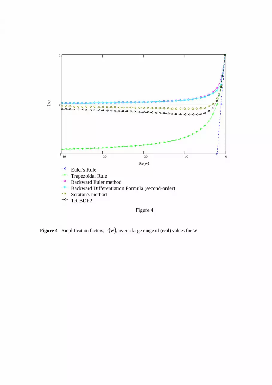
40 30 20 10 01

0

1

Euler's RuleTrapezoidal RuleBackward Euler methodBackward Differentiation Formula (second-order)Scraton's methodTR-BDF2

Figure 4

Re(w)

r(w

)

Figure 4 Amplification factors, wr , over a large range of (real) values for w