error estimates for a semi-implicit numerical scheme solving the landau-lifshitz equation with an...

IMA Journal of Numerical Analysis of 24doi:10.1093/imanum/dri011

Error estimates for a semi-implicit numerical scheme solving theLandau–Lifshitz equation with an exchange field

IVAN CIMRAK†

Department of Mathematical Analysis, Ghent University,Galglaan 2, B-9000 Gent, Belgium

[Received on 5 May 2004; revised on 5 November 2004]

We study the Landau–Lifshitz (LL) equation describing the evolution of spin fields in continuum ferro-magnets. We consider the 3D case when the effective field arising in the LL equation includes exchangeinteraction, the most challenging case. This setting corresponds to the pure isotropic case without a de-magnetizing field. We derive some regularity results for the exact solution to the LL with Neumann-typeboundary conditions. We modify the numerical scheme studied by A. Prohl in two dimensions and weprove error estimates for this scheme in three dimensions.

Keywords: Landau–Lifshitz equation; micromagnetism; ferromagnets.

1. Introduction

We study the Landau–Lifshitz (LL) equation modelling small-scale dynamic processes in ferromagnets

mt = γ m × Heff − αγ m × (m × Heff), m|t=0 = m0, (1.1)

where α is a positive constant called the Gilbert damping constant and γ denotes the gyromagneticfactor. All results mentioned in this paper can be used also in the case when the sign before the termγ m × Heff is negative. After time rescaling where time is measured in units of γ −1, the gyromagneticfactor appears on both sides of the LL equation and can therefore be neglected.

The effective field Heff typically consists of four parts: exchange interaction, crystalline anisotropy,magnetostatic self energy and external magnetic field. The unknown m stands for a spin vector calledmagnetization.

In this work we consider a form of Heff that corresponds to the purely isotropic case without anexternal magnetic field. Then Heff = m and the problem reads as

mt = m × m − αm × (m × m), in R+ × Ω, (1.2)

∇m · ν = 0, on R+ × ∂Ω, (1.3)

m(0, ·) = m0, in Ω. (1.4)

It is obvious that |m| remains constant in time. Therefore, we assume |m| is equal to 1. Then,according to Carbou & Fabrie (2001), (1.2) becomes equivalent to

mt − αm = m × m + α|∇m|2m. (1.5)

The paper of Visintin (1985) contains the first theoretical results concerning the LL equation. Hestudied the system of Maxwell’s equations coupled with the LL equation considering both the exchange

†Email: [email protected]

IMA Journal of Numerical Analysis c© Institute of Mathematics and its Applications 2005; all rights reserved.

IMA Journal of Numerical Analysis Advance Access published February 19, 2005

https://www.researchgate.net/publication/226505361_On_Landau-Lifshitz'_equations_for_ferromagnetism?el=1_x_8&enrichId=rgreq-169729044a5a24674c09c7cdca8b3747-XXX&enrichSource=Y292ZXJQYWdlOzMxMzI2OTkxO0FTOjk5MjA4NjAyMzI0OTk3QDE0MDA2NjQ1ODIxNjE=

2 of 24 I. CIMRAK

field and the anisotropy field. The case without Maxwell’s equations was studied simultaneously byAlouges & Soyeur (1992) and Guo & Hong (1993). They showed the existence of a global weaksolution for the LL equation. Moreover, Alouges and Soyeur give an example, in which the LL equationdoes not have a unique solution. However, the initial condition in this example does not belong toW 2,2(Ω) space. So the question, if the LL equation has a unique solution when we consider smoothinitial conditions, is still open.

Later, Guo & Su (1997) and Guo & Ding (2001) proved the global existence of a weak solutionfor the Landau–Lifshitz–Maxwell equations with Neumann boundary conditions in two or three spacedimensions.

Other types of regularity of weak solutions, a priori gradient estimates for weak solutions and well-posedness of the LL equation, were intensively studied also by Seo (2003) in his Ph.D. thesis.

The question of uniqueness in two space dimensions was discussed by Guo & Hong (1993) and inmore detail by Chen (1996) and Chen & Guo (1996). They proved that any weak solution with finiteenergy is unique and smooth with the exception of at most finitely many points. Chen (2002) devotedthe paper to the study and localization of these singularity points.

All the above authors consider the LL equation with an exchange field.Kruzık & Prohl (2001) and Carstensen & Prohl (2001) deal with the numerical analysis and simu-

lation of micromagnetic phenomena. They propose methods which deal with non-convexity of a min-imizing functional using Young measures. A different approach was used by E & Wang (2000) andWang et al. (2001). They introduced a numerical scheme for LL equations and compared this schemewith other known schemes.

In the papers of Joly et al. (2000), the authors study long-time convergence of solutions to Maxwell–LL equations. Joly & Vacus (1999) and Monk & Vacus (1998) are interested in the numerical modellingof absorbing ferromagnetic materials. They propose a numerical scheme which conserves the magnitudeof magnetization but they do not prove any error estimates in time. A similar problem is studied bySlodicka & Banas (2004) and Slodicka & Cimrak (2003). The authors suggest a new numerical schemeconserving the magnitude of magnetization and they also prove error estimates in time. They considerthe LL equation in a simplified form considering a demagnetizing and anisotropy field but without anexchange field. More results on this scheme were mentioned also by Cimrak & Slodicka (2004) andCimrak & Slodicka (2004).

We mention also a nice numerical analysis study (Monk & Vacus, 2001) considering the fullMaxwell–LL system, where the LL equation is considered with an exchange field. They prove theexistence of a new class of Liapunov functions for the continuous problem, and then also for a vari-ational formulation of the continuous problem. The authors also show a special continuous dependenceresult.

Next, numerical analysis for the 2D LL equation with an exchange field was done by Prohl (2001).The author has proved some new regularity results for an exact solution of the LL equation. We extendthese results to three dimensions. He has also suggested a specific numerical scheme and has provederror estimates in 2D. We change the scheme so that it becomes computationally cheaper and we proveerror estimates in time in three dimensions.

Carbou & Fabrie (2001) proved local existence and uniqueness of regular solutions to the LL equa-tion in 3D. So in three dimensions, solutions to the LL equation can blow up in a finite time. We studythis case, when the theory guarantees the existence and uniqueness of the solutions to the LL equationonly on a finite interval.

The outline of this paper is as follows. In Section 2 we state the results of this paper concerning theregularity of an exact solution to the LL equation in 3D. We provide the proof in Section 5. In Section 3

ERROR ESTIMATES FOR A SEMI-IMPLICIT NUMERICAL SCHEME 3 of 24

we introduce a numerical scheme and we state Theorems 3 and 4 concerning the error estimates in timefor the numerical scheme. We prove these theorems in Sections 6 and 7.

Finally, we confirm the theoretical results with a numerical example in Section 8.

2. Regularity results for the exact solution

In the following text, we use the symbol (·, ·) for the standard L2(Ω) scalar product. The norm in thespace X is denoted by ‖·‖X . The norm in L p(Ω) is denoted by ‖·‖p for ∞ p 1. The scalar productin R3 (Rm , respectively) is denoted by 〈·, ·〉 (〈·, ·〉m , respectively). In the entire text, the letters C and εdenote generic constants, which may change if necessary.

Carbou & Fabrie (2001) have proved the following result for the solution to the LL equation.

THEOREM 1 Suppose m0 ∈ W 2,2(Ω). Then there exists a positive number T0 such that for the solutionm to the problem (1.2)–(1.4) the following estimate is valid:

maxt∈(0,T0)

‖m(t)‖W 2,2(Ω) C. (2.1)

REMARK 1 Using the inequality (4.4) and the fact that the norm of m in W 2,2 is bounded, we have

maxt∈(0,T0)

‖∇m(t)‖4 C. (2.2)

The following theorem is one of the main results in this paper.

THEOREM 2 For the solution m to the problem (1.2)–(1.4) and taking T0 from Theorem 1, the followingestimates are valid:

maxt∈(0,T0)

‖mt‖2 +(∫ T0

0‖∇mt‖2

2 ds

) 12

C, (2.3)

maxt∈(0,T0)

√κ‖∇mt‖2 +

(∫ T0

0κ

‖mt t‖2

2 + ‖mt‖22

ds

) 12

C, (2.4)

∫ T0

0‖mt t‖W−1,2 ds C, (2.5)

where κ is a time weight equal to κ(s) = min1, s.

3. Numerical scheme and error estimates

In the following, any number placed to the upper right of a function represents an index, not a power. Weuse the symbol δf i for the backward Euler approximation of the time derivation, so δf i = 1

τ (f i − f i−1).We provide a standard equidistant discretization of the time interval (0, T0) with J time steps of a

size τ = T0/J and we denote tj = jτ for j = 0, . . . , J. Prohl (2001, Section 4.2) again motivates thestudy of the case of finite time T0. He considers the following semi-implicit scheme and proves errorestimates, all in 2D.

δm j+1 − αm j+1 = α|∇m j |2m j+1 + m j+1 × m j+1, m0 = m0. (3.1)

Note that the previous scheme is non-linear. The term m j+1 × m j+1 makes the scheme quadratic oneach time level.

4 of 24 I. CIMRAK

We change the scheme so that it becomes linear on each time level and we consider the case of 3D:

δm j+1 − αm j+1 = α|∇m j |2m j+1 + m j × m j+1, m0 = m0. (3.2)

The difference is in the torque term. We consider m in this term taken from the previous time level.The existence and uniqueness of m j+1 on every time step is guaranteed by the Lax–Milgram lemma

as soon as we verify the V-ellipticity of the bilinear form

a(u, v) := (u, v) + ατ(∇u, ∇v) − ατ(|∇m j |2u, v) + τ(∇v × m j , ∇u) + τ(v × ∇m j , ∇u).

Let us compute:

a(u, u) ‖u‖22 + ατ‖∇u‖2

2 − ατ |(|∇m j |2u, u)| − τ |(u × ∇m j , ∇u)| ‖u‖2

2 + ατ‖∇u‖22 − ατ‖∇m j‖2

4‖u‖24 − τ‖u‖4‖∇m j‖4‖∇u‖2

‖u‖22 + ατ‖∇u‖2

2 − Cατ‖u‖24 − Cτ‖u‖4‖∇u‖2,

where we have already used Remark 2 below. Now we use inequality (4.3) and the Young inequality tofinish verifying the V-ellipticity of a(u, v):

a(u, u) ‖u‖22 + ατ‖∇u‖2

2 − Cεατ‖u‖24 − ετ‖∇u‖2

2

‖u‖22 + ατ‖∇u‖2

2 − Cεατ‖u‖22 − Cεατ‖u‖

122 ‖∇u‖

322 − ετ‖∇u‖2

2

‖u‖22(1 − Cεατ) + ‖∇u‖2

2(ατ − 2εατ) ατ

2‖u‖2

W 1,2 ,

setting ε = 1/4 and considering τ (2Cεα)−1.To verify the boundedness of a(u, v) in the W 1,2(Ω) norm we simply write

a(u, v) ‖u‖2‖v‖2 + ατ‖∇u‖2‖∇v‖2 + ατ‖∇m j‖24‖u‖4‖v‖4

+ τ‖∇v‖2‖m j‖L∞‖∇u‖2 + τ‖v‖4‖∇m j‖4‖∇u‖2.

Now we use the embedding W 2,2 → W 1,4 → L∞ and Remark 2 below to get

a(u, v) C‖u‖W 1,2‖v‖W 1,2 .

We demonstrate the usefulness of the scheme (3.2) by the following theorem which guarantees theconvergence of the scheme in time. This theorem is the next main result of this paper.

THEOREM 3 Let 0 < tJ < T0(m). Let m j Jj=0 be the solution to (3.2) and let m solve (1.2)–(1.4) for

m0 ∈ W 2,2(Ω), |m0| = 1 on Ω . Let τ τ0 for τ0 sufficiently small. Then we have

max0 jJ

‖m(tj ) − m j‖2 +⎛⎝τ

J∑j=0

‖∇m(tj ) − m j ‖22

⎞⎠

12

Cτ, (3.3)

max0 jJ

‖∇m(tj ) − ∇m j‖2 +⎛⎝τ

J∑j=0

‖m(tj ) − m j ‖22

⎞⎠

12

C√

τ . (3.4)


REMARK 2 As a simple consequence of Theorem 2 and Theorem 3 we have that the solution m j Jj=0

to (3.2) satisfiesmax

0 jJ‖m j‖W 2,2 C.

Notice that we do not enforce |m j | = 1 and moreover the scheme (3.2) does not guarantee thisfeature. However, we are able to prove some kind of convergence of the modulus |m j | to 1 as indicatedby the next theorem.

THEOREM 4 Let the time discretization step τ be the same as in the previous theorem. Then the solutionm j J

j=0 satisfies the following condition

max0 jJ

‖1 − |m j |2‖2 Cτ.

4. Analysis tools

Before we prove the theorems stated in Sections 2 and 3, we mention in Lemmas 1–4 some analyticaltools needed for the proofs.

LEMMA 1 For a, b 0 and 1 s t , we have

(at + bt )s (as + bs)t .

Proof. We follow the idea of ?. For any real x such that 0 x 1, it is clear that xt xs . Then wehave

(1 + xt )s (1 + xs)s .

Since 1 + xs 1, we get (1 + xs)s (1 + xs)t . Therefore, we arrive at

(1 + xt )s (1 + xs)t . (4.1)

Suppose that b a. By substituting x = b/a into (4.1) we obtain

[1 +

(b

a

)t]s

[

1 +(

b

a

)s]t

,

which gives the desired result when multiplied by ats . LEMMA 2 For ai > 0, i = 2, . . . , n ∈ N, and 1 s t we have that(

n∑i=1

ati

)s

(

n∑i=1

asi

)t

.

Proof. We prove this lemma by mathematical induction. The lemma is valid for n = 2, as is the caseof Lemma 1. Suppose this lemma is valid for n = j . We would like to prove that

⎛⎝ j+1∑

i=1

ati

⎞⎠

s

⎛⎝ j+1∑

i=1

asi

⎞⎠

t

.

6 of 24 I. CIMRAK

Let A := (∑ j

i=1 ati )

1t and B := ∑ j

i=1 asi . Then using Lemma 1 with a = A and b = aj+1, we compute

⎛⎝ j+1∑

i=1

ati

⎞⎠

s

= (At + atj+1)

s (As + asj+1)

t . (4.2)

Using the inductive hypothesis we get

As =⎛⎝ j∑

i=1

ati

⎞⎠

st

⎛⎝ j∑

i=1

asi

⎞⎠ = B.

Since the function f (x) = xt is monotonically increasing, we can put B instead of As in the lastexpression of (4.2) keeping the desired inequality, thus

⎛⎝ j+1∑

i=1

ati

⎞⎠

s

(As + asj+1)

t (B + asj+1)

t

⎛⎝ j+1∑

i=1

asi

⎞⎠

t

,

which completes the proof of Lemma 2. LEMMA 3 (SPECIAL CASES OF SOBOLEV INEQUALITIES) Let Ω ∈ R3 be a bounded domain with∂Ω ∈ C1 and let u ∈ W 2,2(Ω) ∩ L2(Ω). Then the following hold:

(i)

‖u‖L4 C‖u‖3/4W 1,2‖u‖1/4

L2 C‖u‖L2 + C‖∇u‖3/4L2 ‖u‖1/4

L2 , (4.3)

(ii)

‖∇u‖L4 C‖∇u‖3/4W 1,2‖∇u‖1/4

L2 C‖∇u‖L2 + C‖u‖3/4L2 ‖∇u‖1/4

L2 , (4.4)

(iii)‖u‖L∞ C‖u‖W 1,4 C‖u‖L4 + C‖∇u‖L4 . (4.5)

We omit the proof of this lemma.

LEMMA 4 Let u, v and m, n be vector-valued functions from L2 (or L4, L∞ if necessary). Then

(〈u, v〉R3 m, n)Ω =∫

Ω〈u, v〉R3〈m, n〉R3 ‖u‖L4‖v‖L4‖m‖L∞‖n‖L2 , (4.6)

(u × v, m)Ω =∫

Ω〈u × v, m〉R3 ‖u‖L4‖v‖L4‖m‖L2 , (4.7)

(u × v, m)Ω =∫

Ω〈u × v, m〉R3 ‖u‖L∞‖v‖L2‖m‖L2 . (4.8)

The proof of this lemma is a straightforward computation using the integral Holder inequality.Therefore, we skip it.


5. Proof of Theorem 2

Proof of inequality (2.3). The time derivation of (1.5) leads to

mt t − αmt = 2α〈∇m, ∇mt 〉R9 m + α|∇m|2mt + mt × m + m × mt . (5.1)

Now, we test this with the function mt to find

1

2∂t‖mt‖2

2 + α‖∇mt‖22 C(A1 + A2 + A3 + A4). (5.2)

The boundary terms always vanish thanks to the homogeneous Neumann boundary conditions.We make use of Theorem 3 to estimate the terms A1, A2, A3 and A4. At the beginning of every

estimate we use some of the inequalities stated in Lemma 4 and then we apply the estimate (2.1) or(2.2). Thus we have

A1 := 2|(〈∇m, ∇mt 〉R9 m, mt )| C‖∇m‖4‖∇mt‖2‖mt‖4‖m‖L∞ C‖mt‖W 1,2‖mt‖4. (5.3)

We apply the inequality (a2 + b2)12 a + b to the first factor. To estimate the L4 norm of mt we use

inequality (4.3) and then we separate the terms by the Young inequality with exponents 4 and 4/3 andappropriate weights ε and Cε :

‖mt‖4 C‖mt‖2 + C‖mt‖142 ‖∇mt‖

342 Cε‖mt‖2 + ε‖∇mt‖2. (5.4)

Together we get

A1 C(‖mt‖2 + ‖∇mt‖2)(Cε‖mt‖2 + ε‖∇mt‖2) Cε‖mt‖22 + ε‖∇mt‖2

2,

where ε is a generic constant which could be changed if needed. To estimate the term ‖mt‖24 in A2 we

again use the same techniques as we have used in (5.4). Then we get

A2 := α(|∇m|2, |mt |2) C‖∇m‖24‖mt‖2

4 C(Cε‖mt‖2 + ε‖∇mt‖2)2 Cε‖mt‖2

2 + ε‖∇mt‖22.

For the term A3, it is simplyA3 := |(mt × m, mt )| = 0.

In the following estimates we perform integration by parts. Because of vanishing Neumann boundaryconditions we can write

A4 := |(m × mt , mt )| = |(∇(m × mt ), ∇mt )| = |(∇m × mt , ∇mt )|.We make use of inequality (4.7) and we arrive at the following:

A4 ‖∇m‖4‖mt‖4‖∇mt‖2 C‖mt‖W 1,2‖mt‖4.

On the right-hand side of the inequality we have the same expression as in (5.3). Therefore, we candirectly end up at

A4 ‖∇m‖4‖mt‖4‖∇mt‖2 Cε‖mt‖22 + ε‖∇mt‖2

2.

8 of 24 I. CIMRAK

Since we have successfully bounded the terms A1, A2, A3 and A4, we can now continue in (5.2)setting 3ε = α/2 to get

1

2∂t‖mt‖2

2 + α‖∇mt‖22

α

2‖∇mt‖2

2 + 3C‖mt‖22,

1

2∂t‖mt‖2

2 + α

2‖∇mt‖2

2 3C‖mt‖22.

Using Gronwall’s lemma in the previous relation we obtain the following result

‖mt‖2 +(∫ T

0‖∇mt‖2

2 ds

) 12

C,

which completes the proof of inequality (2.3). Proof of inequality (2.4). Now we begin the proof starting again with (5.1). We make a formal step bytesting the relation (5.1) with the function −mt . This can be done rigorously by the difference quotientmethod. We make similar steps also further on. Because of vanishing Neumann boundary conditionswe get

1

2∂t‖∇mt‖2

2 + α‖mt‖22 C(B1 + B2 + B3 + B4). (5.5)

We deal with terms B1, B2, B3 and B4 independently. First, we have

B1 := |(〈∇m, ∇mt 〉R9 m, −mt )| ‖∇m‖4‖∇mt‖4‖m‖L∞‖mt‖2

(‖mt‖4 + ‖∇mt‖4)‖mt‖2. (5.6)

To estimate the L4 norms, we apply inequalities (4.3) and (4.4) and then we separate the individual L2

norms by applying the Young inequality with exponents 4 and 4/3 and appropriate weights ε and Cε :

‖mt‖4 + ‖∇mt‖4 C

(‖mt‖2 + ‖mt‖

142 ‖∇mt‖

342 + ‖∇mt‖2 + ‖∇mt‖

142 ‖mt‖

342

) Cε‖mt‖2 + Cε‖∇mt‖2 + ε‖mt‖2. (5.7)

We can now continue in (5.6) twice using the weighted Cauchy inequality to conclude

B1 (Cε‖mt‖2 + Cε‖∇mt‖2 + ε‖mt‖2)‖mt‖2 Cε‖mt‖22 + Cε‖∇mt‖2

2 + ε‖mt‖22.

We proceed with an estimate for B2:

B2 := α|(|∇m|2mt , −mt )| C‖∇m‖24‖mt‖L∞‖mt‖2 C‖mt‖L∞‖mt‖2.

Now we make use of inequality (4.5) to arrive at the same situation as in (5.6):

B2 C(‖mt‖4 + ‖∇mt‖4)‖mt‖2 Cε‖mt‖22 + Cε‖∇mt‖2

2 + ε‖mt‖22.

To estimate B3, we use the same technique as for B2:

B3 := |(mt × m, −mt )| ‖mt‖L∞‖m‖2‖mt‖2 ‖mt‖L∞‖mt‖2

C(‖mt‖4 + ‖∇mt‖4)‖mt‖2 Cε‖mt‖22 + Cε‖∇mt‖2

2 + ε‖mt‖22.


Finally, for B4 we have simply

B4 := |(m × mt , −mt )| = 0.

After applying these estimates, we continue in (5.5) setting 3ε = α/2:

1

2∂t‖∇mt‖2

2 + α‖mt‖22

α

2‖mt‖2

2 + C‖∇mt‖22 + C‖mt‖2

2.

We can get rid of the coefficients 1/2 and α by dividing the equation by min1/2, α. Applying theinequality (2.3) and multiplying by the time weight κ(s) = min(1, s) leads to

κ(s)∂t‖∇mt‖22 + ακ(s)‖mt‖2

2 Cακ(s) + Cακ(s)‖∇mt‖22.

We integrate both sides of the previous equation, integrating by parts in the left term to get

[κ(s)‖∇mt (s)‖22]t

0 − ∫ t0 (κ ′(s))‖∇mt‖2

2 + ∫ t0 κ(s)‖mt‖2

2 Cε

∫ t0 κ(s) + Cε

∫ t0 κ(s)‖∇mt‖2

2,

κ(t)‖∇mt (t)‖22 + ∫ t

0 κ(s)‖mt‖22

∫ t0 ‖∇mt‖2

2 + Cα + Cα

∫ t0 κ(s)‖∇mt‖2

2,

because κ ′(s) 1. Now we use (2.3) and we arrive at the formula

κ(t)‖∇mt (t)‖22 +

∫ t

0κ(s)‖mt‖2

2 Cα + Cα

∫ t

0κ(s)‖∇mt‖2

2.

We are ready to use Gronwall’s lemma to obtain

√κ‖∇mt‖2 +

(∫ T

0κ‖mt‖2

2

) 12

C. (5.8)

Next we take (5.1) and test it with the function mt t to get

‖mt t‖22 + α

2∂t‖∇mt‖2

2 C(D1 + D2 + D3 + D4). (5.9)

The boundary terms vanish. We estimate D1, D2, D3 and D4 as follows. First,

D1 := |(〈∇m, ∇mt 〉R9 m, mt t )| ‖∇m‖4‖∇mt‖4‖m‖L∞‖mt t‖2

C(‖mt‖4 + ‖∇mt‖4)‖mt t‖2. (5.10)

Now we use (5.7) together with the weighted Cauchy inequalities to get

D1 Cε(‖mt‖2 + ‖∇mt‖2 + ‖mt‖2)‖mt t‖2 Cε‖mt‖22 + Cε‖∇mt‖2

2 + Cε‖mt‖22 + ε‖mt t‖2

2.

For the terms D2 and D3 we arrive at these upper bounds using inequality (4.5):

D2 := |(|∇m|2mt , mt t )| ‖∇m‖24‖mt‖L∞‖mt t‖2 (‖mt‖4 + ‖∇mt‖4)‖mt t‖2,

D3 := |(mt × m, mt t )| ‖mt‖L∞‖m‖2‖mt t‖2 (‖mt‖4 + ‖∇mt‖4)‖mt t‖2.

Notice that the expressions at the ends of the previous two inequalities are the same as the expression atthe end of (5.10). Therefore, we use the upper bounds obtained for D1 also for the terms D2 and D3.

10 of 24 I. CIMRAK

For D4 we have the following result using the weighted Cauchy inequality:

D4 := |(m × mt , mt t )| ‖m‖L∞‖mt‖2‖mt t‖2 Cε‖mt‖22 + ε‖mt t‖2.

Now using the previous estimates we can continue in (5.9) setting 4ε = α/4:

‖mt t‖22 + α

2∂t‖∇mt‖2

2 α

4‖mt t‖2

2 + C‖mt‖22 + C‖∇mt‖2

2 + C‖mt‖22.

We can again remove the coefficient α/2 by dividing the equation by min1, α/2. Multiplication byκ(s) followed by time integration now leads to

∫ t

0κ(s)‖mt t‖2

2 + κ(t)‖∇mt‖22 C

∫ t

0κ(s)‖mt‖2

2 + C∫ t

0κ(s)‖∇mt‖2

2 + C∫ t

0κ(s)‖mt‖2

2.

Using (5.8) and (2.3) leads us to the desired result

∫ t

0κ(s)‖mt t‖2 + κ(t)‖∇mt‖2

2 C.

This completes the proof of inequality (2.4).

Proof of inequality (2.5). In order to show (2.5) we employ the previous results. First, we make use of(5.1) and the estimate

∫ T

0‖mt t‖2

W−1,2 = ‖mt t‖2L2(I,W−1,2)

supϕ∈L2(I,W1,2),

‖ϕ‖L2(I,W1,2)

1

∫ T

0|(α∇mt , ∇ϕ) + E1 + · · · + E4| ds. (5.11)

The first term on the right-hand side of (5.11) can be split using the Cauchy inequality:

∫ T

0|(α∇mt , ∇ϕ)| ds C

∫ T

0‖∇mt‖2

2 + ‖∇ϕ‖22 ds C. (5.12)

The boundedness of the first part comes from (2.3). The definition of ϕ in the supremum guarantees theboundedness of the second part.

The terms E1, . . . , E4 can be bounded separately. For the term E1, we write

∣∣∣∣∫ T

0E1

∣∣∣∣ C∫ T

0|(〈∇m, ∇mt 〉R9 m,ϕ)| C

∫ T

0‖∇m‖4‖∇mt‖2‖m‖L∞‖ϕ‖4 C

∫ T

0‖∇mt‖2

2 + ‖ϕ‖2W 1,2 .

We see similar terms as in (5.12). This allows us to use the same arguments to estimate also the term∫ T0 E1.

Applying the embedding W 1,2 → L4, we get the following estimate for E2:

∣∣∣∣∫ T

0E2

∣∣∣∣ C∫ T

0|(|∇m|2mt ,ϕ)| C

∫ T

0‖∇m‖2

4‖mt‖4‖ϕ‖4 C∫ T

0‖mt‖2

2 + ‖∇mt‖22 + ‖ϕ‖2

W 1,2 .

(5.13)


We make use of (2.3) to estimate the first two terms. The last term is bounded from the definition. Thuswe get boundedness of the term | ∫ T

0 E2|. We continue with E3:

∣∣∣∣∫ T

0E3

∣∣∣∣ =∫ T

0|(mt × m,ϕ)| =

∫ T

0|(∇(ϕ× mt ), ∇m)|

∫ T

0‖∇ϕ‖2‖mt‖4‖∇m‖4 +

∫ T

0‖ϕ‖4‖∇mt‖2‖∇m‖4.

We get rid of the term ‖∇m‖4 thanks to (2.2). The embedding W 1,2 → L4 used for the L4 norms inboth terms followed by application of the Cauchy inequality gives us

∣∣∣∣∫ T

0E3

∣∣∣∣ ∫ T

0‖ϕ‖W 1,2‖mt‖W 1,2 +

∫ T

0‖ϕ‖W 1,2‖mt‖W 1,2

∫ T

0‖ϕ‖2

W 1,2 + ‖mt‖22 + ‖∇mt‖2

2,

which is the same upper bound as in (5.13) and confirms the boundedness of the term | ∫ T0 E3|. For the

term E4, we write

∣∣∣∣∫ T

0E4

∣∣∣∣ =∫ T

0|(m × mt ,ϕ)| =

∫ T

0|(∇(ϕ× m), ∇mt )|

∫ T

0‖∇ϕ‖2‖m‖L∞‖∇mt‖2 +

∫ T

0‖ϕ‖4‖∇m‖4‖∇mt‖2.

Now we can do the same tricks as we did above for the term∫ T

0 E3 to get

∣∣∣∣∫ T

0E4

∣∣∣∣ ∫ T

0‖ϕ‖W 1,2‖mt‖W 1,2 +

∫ T

0‖ϕ‖W 1,2‖mt‖W 1,2

∫ T

0‖ϕ‖2

W 1,2 + ‖mt‖22 + ‖∇mt‖2

2 C,

which finally concludes the proof of boundedness of∫ T

0‖mt t‖2W−1,2 and completes the proof of inequality

(2.5).


Let us denote by e j+1 := m(tj+1) − m j+1 the error of the approximation. Consider (3.2) and (1.2) in aweak form. Then for all φ ∈ W 1,2(Ω,R3) we have

(δe j+1,φ) + α(∇e j+1, ∇φ) = (F j+1(m),φ) + α[(|∇m(tj+1)|2m(tj+1),φ) − (|∇m j |2m j+1,φ)

]+ [

(m(tj+1) × m(tj+1),φ) − (m j × m j+1,φ)], (6.1)

where

F j+1(m) := − 1

τ

∫ tj+1

tj(s − tj )mt t (s) ds.

12 of 24 I. CIMRAK

We can easily verify that

τ

J∑j=0

‖F j+1(m)‖22 Cτ, (6.2)

τ

J∑j=0

‖F j+1(m)‖2W−1,2 τ

τ

3

∫ T

0‖mt t (s)‖2

W−1,2 ds Cτ 2. (6.3)

Let us do some technical steps in (6.1). We add and subtract some terms to obtain

(|∇m(tj+1)|2m(tj+1),φ) − (|∇m j |2m j+1,φ)

= (〈∇m(tj+1) − ∇m(tj ), ∇m(tj+1) + ∇m(tj )〉R9 m(tj+1),φ)

+ 2(〈∇m(tj ), ∇e j 〉R9 m(tj+1),φ) − (|∇e j |2m(tj+1),φ)

+ (|∇m(tj )|2e j+1,φ) − 2(〈∇m(tj ), ∇e j 〉R9 e j+1,φ) + (|∇e j |2e j+1,φ).

The last term in (6.1) is

(m(tj+1) × m(tj+1),φ) − (m j × m j+1,φ)

= ([m(tj+1) − m(tj )] × m(tj+1),φ) + (m(tj ) × e j+1,φ)

+ (e j × m(tj+1),φ) − (e j × e j+1,φ).

Thus we have

(δe j+1,φ) + α(∇e j+1, ∇φ)

= (F j+1(m),φ) + (〈∇m(tj+1) − ∇m(tj ), ∇m(tj+1) + ∇m(tj )〉R9m(tj+1),φ)

+ 2(〈∇m(tj ), ∇e j 〉R9 m(tj+1),φ) − (|∇e j |2m(tj+1),φ)

+ (|∇m(tj )|2e j+1,φ) − 2(〈∇m(tj ), ∇e j 〉R9 e j+1,φ) + (|∇e j |2e j+1,φ)

+ ([m(tj+1) − m(tj )] × m(tj+1),φ)

+ (m(tj ) × e j+1,φ) + (e j × m(tj+1),φ) − (e j × e j+1,φ) =: Y, (6.4)

where we have denoted the right-hand side of (6.4) by Y .Now we derive two statements, one by testing (6.4) by φ = e j+1 and the second one by φ =

−e j+1.

STATEMENT 1 Take φ = ei+1 in (6.4). We denote by Y1, . . . ,Y11, the terms arising in Y whenφ = ei+1. Our goal in the following part will be to arrive at the inequality

(δe j+1, e j+1) + α‖∇e j+1‖22 |(F j+1(m), e j+1)| + ε‖∇e j‖2

2 + C‖∇e j‖24‖∇e j‖2

2

+ Cε‖e j+1‖24 + C‖e j+1‖2

4‖∇e j‖24 + C‖∇e j+1‖2‖e j+1‖4[‖∇e j‖4 + 1]

+ C‖∇e j+1‖2‖e j‖4 + ‖m(tj+1) − m(tj )‖22 + ‖∇m(tj+1) − ∇m(tj )‖2

2,

(6.5)


estimating each term in (6.4) separately for φ = ei+1. We leave the term Y1 without any change. Theterm Y2 will be estimated using the inequalities (2.2), (4.6), ‖m‖L∞ = 1 and the Young inequality:

Y2 = (〈∇m(tj+1) − ∇m(tj ), ∇m(tj+1) + ∇m(tj )〉R9m(tj+1), e j+1)

‖∇m(tj+1) − ∇m(tj )‖2‖∇m(tj+1) + ∇m(tj )‖4‖m(tj+1)‖L∞‖e j+1‖4

C‖∇m(tj+1) − ∇m(tj )‖22 + C‖e j+1‖2

4.

In a similar way, also the terms Y3 to Y7 can be bounded:

Y3 = (〈∇e j , ∇m(tj )〉R9 m(tj+1), e j+1) ‖∇e j‖2‖∇m(tj )‖4‖m‖L∞‖e j+1‖4

ε‖∇e j‖22 + Cε‖e j+1‖2

4,

Y4 = (|∇e j |2m(tj+1), e j+1) ‖∇e j‖4‖∇e j‖2‖m‖L∞‖ej+1‖4

C‖∇e j‖24‖∇e j‖2

2 + C‖ej+1‖24,

Y5 = (|∇m(tj )|2e j+1, e j+1) ‖∇m‖24‖ej+1‖2

4 C‖ej+1‖24,

Y6 = (〈∇e j , ∇m(tj )〉R9 , |e j+1|2) ‖∇e j‖4‖∇m(tj+1)‖4‖e j+1‖24

C‖∇e j‖4‖e j+1‖24 C(1 + ‖∇e j‖2

4)‖e j+1‖24,

Y7 = (|∇e j |2, |e j+1|2) ‖∇e j‖24‖e j+1‖2

4.

We estimate the term Y8 using the embedding W 1,2 → L4 and the Cauchy inequality:

Y8 = ([m(tj+1) − m(tj )] × m(tj+1), e j+1) ‖m(tj+1)‖2‖e j+1‖4‖m(tj+1) − m(tj )‖4

C‖e j+1‖4‖m(tj+1) − m(tj )‖2 + C‖e j+1‖4‖∇m(tj+1) − ∇m(tj )‖2

C‖e j+1‖24 + C‖m(tj+1) − m(tj )‖2

2 + C‖∇m(tj+1) − ∇m(tj )‖22.

Next, we use integration by parts to get

Y9 = |(m(tj ) × e j+1, e j+1)| = |(∇(e j+1 × m(tj )), ∇e j+1)| ‖e j+1‖4‖∇m‖4‖∇e j+1‖2 C‖e j+1‖4‖∇e j+1‖2.

We estimate also the terms Y10 and Y11 in a similar way:

Y10 = (e j × m(tj+1), e j+1) |(∇(e j+1 × e j ), ∇m(tj+1))| ‖∇e j+1‖2‖e j‖4‖∇m‖4 + ‖e j+1‖4‖∇e j‖2‖∇m‖4

C‖∇e j+1‖2‖e j‖4 + Cε‖e j+1‖24 + ε‖∇e j‖2

2,

Y11 = (e j × e j+1, e j+1) |∇(e j+1 × e j ), ∇e j+1)| = ‖e j+1‖4‖∇e j+1‖2‖∇e j‖4.

We can now proceed with estimating the right-hand side of (6.5). The letters X1 and X2 denotepositive real numbers. We first do some calculations using (4.3) and then use the Young inequality with

14 of 24 I. CIMRAK

exponents 4/3 and 4:

‖e j+1‖24X1 ‖e j+1‖2

2X1 + ‖e j+1‖122 ‖∇e j+1‖

322X1 CεX1‖e j+1‖2

2 + CεX 41 ‖e j+1‖2

2 + ε‖∇e j+1‖22.

Analogously, using first the Young inequality with exponents 2 and then the Young inequality withexponents 8/7 and 8:

‖∇e j+1‖2‖e j+1‖4X2 X2‖∇e j+1‖2(‖e j+1‖2 + ‖e j+1‖142 ‖∇e j+1‖

342 )

CεX 22 ‖e j+1‖2

2 + CεX 82 ‖e j+1‖2

2 + ε‖∇e j+1‖22.

We apply the previous two inequalities to (6.5). First, we set X1 = Cε then X1 = C‖∇e j‖24. Then we

set X2 = ‖∇e j‖4 and X2 = C. Thus supposing α > ε/2 we can write

(δe j+1, e j+1) + (α − ε)‖∇e j+1‖22

|(F j+1(m), e j+1)| + C‖∇e j‖22‖∇e j‖2

4 + Cε‖∇e j‖24 + ε‖∇e j‖2

2

+ Cε‖e j+1‖22 + Cε‖e j+1‖2

2

(‖∇e j‖24 + ‖∇e j‖4

4 + ‖∇e j‖84

)+ ‖m(tj+1) − m(tj )‖2

2 + ‖∇m(tj+1) − ∇m(tj )‖22. (6.6)

The next step is to sum up (6.6) through j = 0, . . . , l. To get rid of the last two terms in (6.6), weintroduce the following lemma.

LEMMA 5 Keeping all notations from the above discussion the following inequality is valid

l∑j=0

‖m(tj+1) − m(tj )‖22 +

l∑j=0

‖∇m(tj+1) − ∇m(tj )‖22 Cτ.

Proof. From the definition of the L2 norm and using the integral Cauchy inequality with respect to timewe get

l∑j=0

‖∇m(tj+1) − ∇m(tj )‖22 =

j∑j=0

∫Ω

(∫ tj+1

tj〈1, ∇mt (s)〉R9 ds

)2

dx

Cj∑

j=0

∫Ω

τ

∫ tj+1

tj|∇mt (s)|2 ds dx C

j∑j=0

τ

∫ tj+1

tj‖∇mt (s)‖2

2 ds

Cτ

∫ tl+1

0‖∇mt (s)‖2

2 ds Cτ,

where we have used (2.3) at the end. The rest of Lemma 5 can be proved in the same way. To get rid of the first term on the right-hand side of (6.6) we have

|(F j+1(m), e j+1)| =∣∣∣∣∫

ΩF j+1(m) · ei+1

∣∣∣∣ ‖F j+1(m)‖W−1,2‖e j+1‖W 1,2 .


According to (6.3), we get the following estimate for the term (F j+1(m), e j+1) after using the Younginequality:

τ

J∑j=0

|(F j+1(m), e j+1)| τ

J∑j=0

‖F j+1(m)‖W−1,2(‖e j+1‖22 + ‖∇e j+1‖2

2)12

Cετ

J∑j=0

‖F j+1(m)‖2W−1,2 + τε

J∑j=0

(‖∇e j+1‖22 + ‖e j+1‖2

2)

Cετ2 + τε

J∑j=0

(‖∇e j+1‖22 + ‖e j+1‖2

2). (6.7)

We can now continue in (6.6). On the left-hand side we use the inequality

τ

l∑j=0

(δe j+1, e j+1) 1

2‖el+1‖2

2

to find that

‖el+1‖22 + τ

l∑j=0

‖∇e j+1‖22 Cετ

2 + Cετ

l∑j=0

‖∇e j‖24

l∑j=0

‖∇e j‖22

+ ετ

l∑j=0

(‖∇e j‖22 + ‖∇e j+1‖2

2) + Cτ

l∑j=0

‖e j+1‖22

+ Cτ

l∑j=0

(‖∇e j‖24 + ‖∇e j‖4

4 + ‖∇e j‖84)

l∑j=0

‖e j+1‖22,

where for some terms we have already used the inequality

l∑j=0

aj bj l∑

j=0

aj

l∑j=0

bj , (6.8)

which holds for any non-negative aj , bj . Setting ε < 1/4 we can now absorb the term ετ∑l

j=0 ‖∇e j‖22

on the right-hand side into the similar term on the left to get the desired Statement 1:

‖el+1‖2 + τ

l∑j=0

‖∇e j+1‖22 Cτ 2 + Cτ

l∑j=0

‖∇e j‖24

l∑j=0

‖∇e j‖22 + Cτ

l∑j=0

‖e j+1‖22

+ Cτ

l∑j=0

(‖∇e j‖24 + ‖∇e j‖4

4 + ‖∇e j‖84)

l∑j=0

‖e j+1‖22. (6.9)

16 of 24 I. CIMRAK

STATEMENT 2 In this statement we do mostly the same as in Statement 1. We choose φ = −ei+1 in(6.4) and denote by Y ′

1,Y ′2, . . . ,Y ′

11 the terms arising on the right-hand side of (6.4), respectively. Ourgoal will be to arrive at the inequality

(δ∇e j+1, ∇e j+1) + α‖e j+1‖22

Cε‖F j+1(m)‖22 + ε‖e j+1‖2

2 + Cε

(‖∇e j‖24 + C‖e j‖2

4 + ‖∇e j‖44

)+ Cε‖∇e j+1‖2

4 + Cε‖∇e j+1‖24

(‖∇e j‖24 + ‖∇e j‖4

4

)+ Cε‖e j+1‖2

4 + Cε‖e j+1‖24

(‖∇e j‖24 + ‖∇e j‖4

4

)+ Cε‖m(tj+1) − m(tj )‖2

4 + Cε‖∇m(tj+1) − ∇m(tj )‖24. (6.10)

The term Y ′1 causes no trouble. The term Y ′

2 can be estimated using inequalities (2.2) and (4.6), theequality ‖m‖L∞ = 1 and the Young inequality:

Y ′2 = |(〈∇m(tj+1) − ∇m(tj ), ∇m(tj+1) + ∇m(tj )〉R9 m(tj+1),e j+1)| 2‖∇m(tj+1) − ∇m(tj )‖4‖∇m(tj+1)‖4‖m(tj+1)‖L∞‖e j+1‖2

Cε‖∇m(tj+1) − ∇m(tj )‖24 + ε‖e j+1‖2

2.

We handle the terms Y ′3 and Y ′

4 in a similar way:

Y ′3 = |(〈∇e j , ∇m(tj )〉R9m(tj+1),e j+1)| ‖∇e j‖4‖∇m(tj )‖4‖m(tj+1)‖L∞‖e j+1‖2

Cε‖∇e j‖24 + ε‖e j+1‖2

2,

Y ′4 = |(|∇e j |2m(tj+1),e j+1)| ‖∇e j‖2

4‖m(tj+1)‖L∞‖e j+1‖2

Cε‖∇e j‖44 + ε‖e j+1‖2

2.

We estimate the terms Y ′5, Y ′

6 and Y ′7 using (4.5) and the Young inequality:

Y ′5 = |(|∇m(tj )|2e j+1,e j+1)| ‖∇m(tj )‖2

4‖e j+1‖L∞‖e j+1‖2

Cε‖e j+1‖2L∞ + ε‖e j+1‖2

2 Cε(‖e j+1‖24 + ‖∇e j+1‖2

4) + ε‖e j+1‖22,

Y ′6 = |(〈∇e j , ∇m(tj )〉R9 e j+1,e j+1)| ‖∇e j‖4‖∇m(tj )‖4‖e j+1‖L∞‖e j+1‖2

C‖∇e j‖4(‖e j+1‖4 + ‖∇e j+1‖4)‖e j+1‖2

Cε‖∇e j‖24‖e j+1‖2

4 + Cε‖∇e j‖24‖∇e j+1‖2

4 + ε‖e j+1‖22,

Y ′7 = |(〈∇e j , ∇e j 〉R9e j+1,e j+1)| ‖∇e j‖2

4‖e j+1‖L∞‖e j+1‖2

‖∇e j‖24(‖e j+1‖4 + ‖∇e j+1‖4)‖e j+1‖2

Cε‖∇e j‖44‖e j+1‖2

4 + Cε‖∇e j‖44‖∇e j+1‖2

4 + ε‖e j+1‖22.

The term Y8 satisfies

Y ′8 = |([m(tj+1) − m(tj )] × m(tj+1),e j+1)| ‖m(tj+1) − m(tj )‖L∞‖m‖2‖e j+1‖2

(‖m(tj+1) − m(tj )‖4 + ‖∇m(tj+1) − ∇m(tj )‖4)‖e j+1‖2

Cε‖m(tj+1) − m(tj )‖24 + Cε‖∇m(tj+1) − ∇m(tj )‖2

4 + ε‖e j+1‖22.


The terms Y ′9 and Y ′

11 are equal to 0 and the last term Y ′10 can be bounded as follows:

Y ′10 = |(e j × m(tj+1),e j+1)| C‖e j‖L∞‖m‖2‖e j+1‖2

C(‖∇e j‖4 + ‖e j‖4)‖e j+1‖2

Cε‖∇e j‖24 + Cε‖e j‖2

4 + ε‖e j+1‖22.

We can now proceed with estimating the right-hand side of (6.10). We again denote by X1,X2arbitrary positive real numbers. We first do some calculations using the embedding W 1,2 → L4 withthe Young inequality. We get

‖e j+1‖24X1 ‖e j+1‖2

2X1 + ‖∇e j+1‖22X1.

Similarly, using (4.4) and the Young inequality with exponents 4/3 and 4 we arrive at

‖∇e j+1‖24X2 X2(‖∇e j+1‖2

2 + ‖∇e j+1‖122 ‖e j+1‖

322 )

CεX2‖∇e j+1‖22 + CεX 4

2 ‖∇e j+1‖22 + ε‖e j+1‖2

2.

We continue by estimating the right-hand side of (6.10). We use the previous two inequalities for severalvalues of X1 and X2. First take X2 = Cε, second take X2 = ‖∇e j‖2

4 and finally put X2 = ‖∇e j‖44. We

suppose that X1 has the same values as X2. Then supposing α > ε/2, we get

(δ∇e j+1, ∇e j+1) + (α − ε)‖e j+1‖22

Cε‖F j+1(m)‖22 + Cε(‖∇e j‖2

4 + ‖e j‖24 + ‖∇e j‖4

4) + Cε‖e j+1‖22

+ Cε‖e j+1‖22(‖∇e j‖2

4 + ‖∇e j‖44) + Cε‖∇e j+1‖2

2

+ Cε‖∇e j+1‖22(‖∇e j‖2

4 + ‖∇e j‖44 + ‖∇e j‖8

4 + ‖∇e j‖164 )

+ Cε‖m(tj+1) − m(tj )‖24 + Cε‖∇m(tj+1) − ∇m(tj )‖2

4. (6.11)

We would like to follow the strategy of summing up (6.11) for j = 1, . . . , l. First, we introduce aweakened version of Lemma 5.

LEMMA 6 Keeping all notations from the above discussion the following inequality holds:l∑

j=1

‖m(tj+1) − m(tj )‖24 +

l∑j=1

‖∇m(tj+1) − ∇m(tj )‖24 C.

Proof. From the embedding W 1,2 → L4, we have

‖∇m(tj+1) − ∇m(tj )‖24 C‖∇m(tj+1) − ∇m(tj )‖2

2 + C‖m(tj+1) − m(tj )‖22.

From the definition of the L2 norm and using the integral Cauchy inequality with respect to time, weget

l∑j=1

‖m(tj+1) − m(tj )‖22 =

l∑j=1

∫Ω

( ∫ tj+1

tj〈1,mt (s)〉R3 ds

)2

dx

Cl∑

j=1

∫Ω

τ

∫ tj+1

tj|mt (s)|2 ds dx .

18 of 24 I. CIMRAK

Since we sum up from the index j = 1, we have τ κ(s) on the interval (tj , tj+1). Thus,l∑

j=1

‖m(tj+1) − m(tj )‖22 C

l∑j=1

∫Ω

∫ ti+1

tiκ(s) |mt (s)|2 ds dx

Cl∑

j=1

∫ tj+1

tjκ(s)‖mt (s)‖2

2 ds

C∫ tl+1

0κ(s)‖mt (s)‖2

2 ds C,

where we have used (2.4) at the end. The rest of the lemma follows directly from Lemma 5.This completes the proof of Lemma 6. Now we can write the Statement 2 summing up (6.11) for j = 1, . . . , l and applying Lemma 6 and

(6.2). Directly after the summation we use the inequality (6.8) for some terms:

‖∇el+1‖22 + τ

l∑j=1

‖e j+1‖22 Cτ + Cετ

l∑j=1

(‖e j‖24 + ‖∇e j‖2

4 + ‖∇e j‖44) + Cετ

l∑j=1

‖e j+1‖22

+ Cετ

l∑j=1

(‖∇e j‖24 + ‖∇e j‖4

4)

l∑j=1

‖e j+1‖22 + Cετ

l∑j=1

‖∇e j+1‖22

+ Cετ

l∑j=1

(‖∇e j‖24 + ‖∇e j‖4

4 + ‖∇e j‖84 + ‖∇e j‖16

4 )

l∑j=1

‖∇e j+1‖22.

(6.12)

We proceed with the proof of Theorem 3. To prove it, we employ an inductive argument. Thereexists a constant A depending only on ω, α and m such that for a sufficiently small τ0 we have, forevery τ τ0,

‖el+1‖22 + τ

l∑j=0

‖∇e j+1‖22 Aτ 2, (6.13)

‖∇el+1‖22 + τ

l∑j=0

‖e j+1‖22 Aτ. (6.14)

First, these statements are valid for l = 0. To see this, we employ (6.1) for j = 0.Let us prove the statements for l = r assuming that they are valid for l = r − 1. Note that A is

independent of l. At this stage of mathematical induction, the following lemma will be useful.

LEMMA 7 Assuming (6.13) and (6.14) hold true for l = r − 1, the following estimate holds for suffi-ciently small τ :

B :=r∑

j=0

‖∇e j‖24 + ‖∇e j‖4

4 + ‖∇e j‖84 + ‖∇e j‖16

4 1. (6.15)

Proof. For a = 2, 4, 8, 16, it is valid that

(x + y)a a(xa + ya) 16(xa + ya).


Thus, we can use the inequality (4.4) in the form

‖∇u‖a4 C‖∇u‖a

2 + C‖∇u‖a42 ‖u‖

3a4

2 .

We apply the previous inequality for a = 2, 4, 8, 16 and sum it up for j = 0, . . . , r to get

r∑j=0

‖∇e j‖a4

r∑j=0

‖∇e j‖a2 +

r∑j=0

‖∇e j‖a42 ‖e j‖

3a4

2 r∑

j=0

‖∇e j‖a2 +

⎛⎝ r∑

j=0

‖∇e j‖a2

⎞⎠

14⎛⎝ r∑

j=0

‖e j‖a2

⎞⎠

34

.

At the end we have used the discrete Holder inequality with exponents 4 and 4/3. Now we apply Lemma2 on the following terms. Note that 2 a. We have⎛

⎝ r∑j=0

‖∇e j‖a2

⎞⎠

2

⎛⎝ r∑

j=0

‖∇e j‖22

⎞⎠

a

,

⎛⎝ r∑

j=0

‖e j‖a2

⎞⎠

2

⎛⎝ r∑

j=0

‖e j‖22

⎞⎠

a

.

This gives us

r∑j=0

‖∇e j‖a4

⎛⎝ r∑

j=0

‖∇e j‖22

⎞⎠

a2

+⎛⎝ r∑

j=0

‖∇e j‖22

⎞⎠

a8⎛⎝ r∑

j=0

‖e j‖22

⎞⎠

3a8

.

Notice that in the expression of B we have summed up to the index j = r but the indices of the termsare shifted by one when compared with those that appeared in (6.13) and (6.14). Thus, we are able toapply (6.13) and (6.14) for l = r − 1. We combine it with the previous inequality to obtain

B ∑

a = 2,4,8,16

(Aτ)a2 + (Aτ)

a8A 3a

8 .

Since τ appears in every term with exponent at least 1/4, we can guarantee that B remains less than 1by setting τ sufficiently small.

This completes the proof of Lemma 7. If we look at Statement 1, we are able to get rid of some problematic terms by applying the previous

lemma. Thus,

‖el+1‖2 + τ

l∑j=0

‖∇e j+1‖22 Cτ 2 + Cτ

l∑j=0

‖∇e j‖24

l∑j=0

‖∇e j‖22 + 2Cτ

l∑j=0

‖e j+1‖22.

In Lemma 7 we can easily obtain also the estimate B A−1. Then, if we apply the relations (6.13)and (6.14) with l = r − 1 to the term

∑lj=0 ‖∇e j‖2

2 and we apply the estimate B A−1 to the term∑lj=0 ‖∇e j‖2

4, we get

‖el+1‖2 + τ

l∑j=0

‖∇e j+1‖22 Cτ 2 + CτA−1Aτ + 2Cτ

l∑j=0

‖e j+1‖22 2Cτ 2 + 2Cτ

l∑j=0

‖e j+1‖22.

20 of 24 I. CIMRAK

Notice that the previous inequality was obtained independently of the index l. Now we apply Gronwall’sargument to verify (6.13) for l = r.

If we look at Statement 2, we can eliminate some terms by applying Lemma 7. Then we get

‖∇el+1‖22 + τ

l∑j=1

‖e j+1‖22 Cτ + Cετ

l∑j=1

‖e j‖24 + 2Cετ

l∑j=1

‖e j+1‖22 + 2Cετ

l∑j=1

‖∇e j+1‖22.

For the term∑l

j=1 ‖e j‖24, we use the embedding W 1,2 → L4 and (6.13), (6.14) for l = r − 1. For

the term∑l

j=1 ‖e j+1‖22, we use (6.13) for l = r, which has already been proved. Thus,

‖∇el+1‖22 + τ

l∑j=1

‖e j+1‖22 Cτ + 2CετAτ + 2Cετ

l∑j=1

‖∇e j+1‖22 2Cτ + 2Cετ

l∑j=1

‖∇e j+1‖22.

Here we have the sum over the index j starting from 1 and ending with j = r . To make the sum startwith j = 0, we should know that ‖e1‖2

2 C . This is given by the following lemma.

LEMMA 8 Keeping the notations from the above discussion we have

‖e1‖22 C.

Proof. We take (6.4) for j = 0 and set φ = −e1. After considering e0 = 0 and ∇e0 = 0 we get(e1

τ, −e1

)+ α(e1,e1) |(F1(m),e1)|

+ |(〈∇m(t1) − ∇m(t0), ∇m(t1) + ∇m(t0)〉R9 m(t1),e1)|+ |(|∇m(t0)|2e1,e1)| + |([m(t1) − m(t0)] × m(t1),e1)|.

Now we apply some inequalities from Lemma 4, the estimates (2.1) and (2.2) and the Young inequality:

1

τ‖∇e1‖2

2 + α‖e1‖22 C‖F1(m)‖2

2 + ε‖e1‖22 + ‖∇m(t1) − ∇m(t0)‖4‖∇m(t1)

+ ∇m(t0)‖4‖m(t1)‖L∞‖e1‖2 + ‖∇m(t0)‖24‖e1‖L∞‖e1‖2

+ ‖m(t1) − m(t0)‖L∞‖m(t1)‖2‖e1‖2

C‖F1(m)‖22 + ε‖e1‖2

2 + ‖e1‖2L∞ . (6.16)

To estimate the term ‖e1‖2L∞ we use the same techniques as we have already used several times before

with (4.5) and (4.4) and the Young inequality with exponents 4 and 4/3:

‖e1‖L∞ ‖e1‖24 + ‖∇e1‖2

4 Cε‖e1‖22 + Cε‖∇e1‖2

2 + ‖∇e1‖122 ‖e1‖

322

Cε‖e1‖22 + Cε‖∇e1‖2

2 + ε‖e1‖22.

We suppose that α > ε and 1 − Cετ > 0. Then, together with (6.16), since ‖e1‖22 C we have

1 − τCε

τ‖∇e1‖2

2 + (α − ε)‖e1‖22 C‖F1(m)‖2

2 C,

which completes the proof of Lemma 8.


Thus we have arrived at

‖∇el+1‖22 + τ

l∑j=0

‖e j+1‖22 Cτ + 2CτAτ + 2Cτ

l∑j=0

‖∇e j+1‖22

2Cτ + 2Cτ

l∑j=0

‖∇e j+1‖22.

Notice that this inequality was also obtained independently of the index l. We now apply Gronwall’sargument to verify (6.14) for l = r.

This completes the proof of Theorem 3.


The result follows directly from inequality (4.4) and Theorem 3:

‖|m(tj )|2 − |m j |2‖2 = ‖〈e j , e j + 2m(tj )〉R3‖2

2(‖e j‖24 + ‖e j‖2‖m(tj )‖L∞) C

(‖e j‖2

2 + ‖e j‖122 ‖∇e j‖

322 + ‖e j‖2

)

C(τ 2 + τ

12 τ

34 + τ

) Cτ.

8. Numerical tests

In order to verify the theoretical results, we solve the problem (1.2)–(1.4) with an artificial right-handside and with a prescribed solution. Up to now there is no example of such a problem with a knownanalytical solution in the literature. We set

mex(t, x) =

⎧⎪⎪⎪⎨⎪⎪⎪⎩

mex0 =

(1 − ( x0t

2

)2 −(

(x1+x2)t4

)) 12,

mex1 = (x1+x2)t

4 ,

mex2 = x0t

2 ,

in order to ensure that the modulus of mex remains constant equal to 1. Then we solve the followingproblem on a cube Ω = (0, 1)3:

mt = m × m − αm × (m × m) + f, in R+ × Ω,

∇m · ν = ∇f · ν, on R+ × ∂Ω,

m(0, ·) = mex(0, ·), in Ω,

where f = mext −mex ×mex −αmex ×(mex ×mex). For the spatial discretization, we use the standard

W 1,2(Ω)-conforming finite element formulation. We consider a finite-dimensional approximation spaceVh consisting of piecewise linear functions. The symbol h denotes the size of the space discretizationstep. The projection operator Ph associated with the space Vh has the necessary properties needed forfurther analysis of the full discretization in time and space.

22 of 24 I. CIMRAK

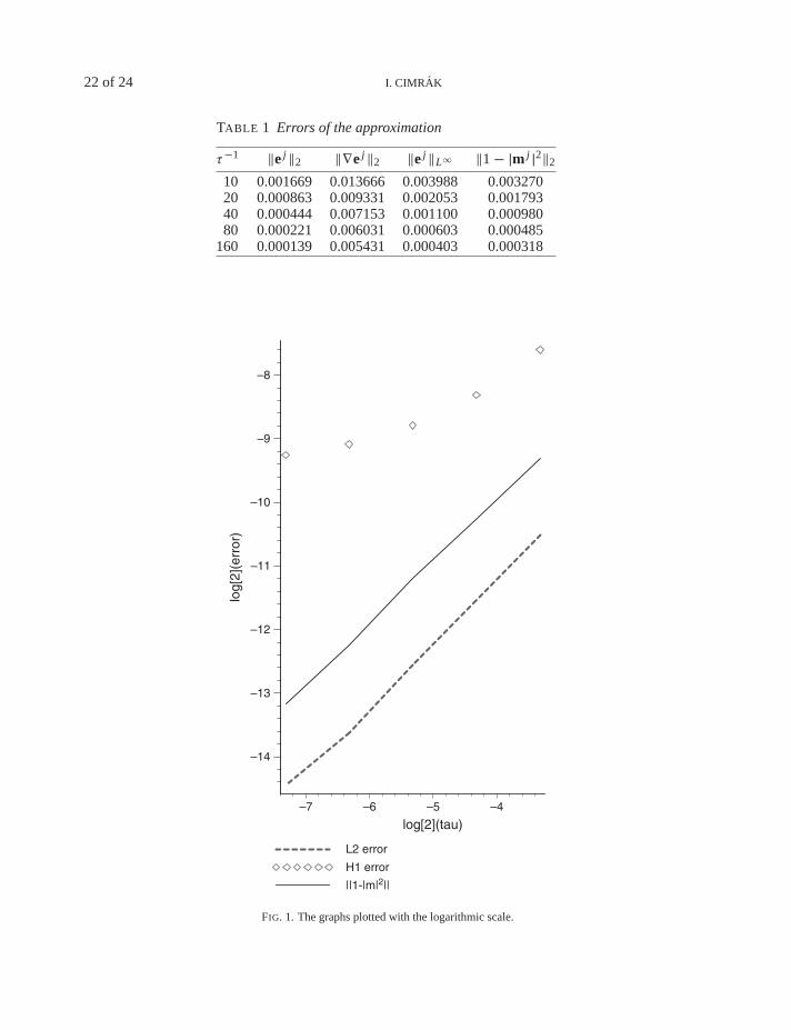
TABLE 1 Errors of the approximation

τ−1 ‖e j‖2 ‖∇e j‖2 ‖e j‖L∞ ‖1 − |m j |2‖2

10 0.001669 0.013666 0.003988 0.00327020 0.000863 0.009331 0.002053 0.00179340 0.000444 0.007153 0.001100 0.00098080 0.000221 0.006031 0.000603 0.000485

160 0.000139 0.005431 0.000403 0.000318

FIG. 1. The graphs plotted with the logarithmic scale.


In order to confirm the theoretical results, we test the rate of convergence of the numericalscheme (3.2). We divide one edge of the cubic domain into 24 elements which gives us 82,944 tetrahedraand 15,625 vertices. The number of vertices determines also the number of degrees of freedom.

Due to the linearity of scheme (3.2), we have to solve only a linear elliptic problem on each timelevel. Compared with (3.1), our scheme is computationally cheaper. To compute the solution on a newtime level in (3.1), it is necessary to solve a non-linear elliptic problem whose solution involves the useof a non-linear solver.

Table 1 shows the results for a time step running from 10−1 to 160−1. The graphs in Fig. 1 are plottedwith a logarithmic scale so that we can easily see that the numerical results confirm the theoreticalones.

Acknowledgements

The work of the author was supported by the IUAP/V-P5/34 project of Ghent University. The authorthanks Roger Van Keer, coordinator of this project, for his stimulation.

REFERENCES

ALOUGES, F. & SOYEUR, A. (1992) On global weak solutions for Landau–Lifshitz equations: existence andnonuniqueness. Nonlinear Anal., 18, 1071–1094.

CARBOU, G. & FABRIE, P. (2001) Regular solutions for Landau–Lifshitz equation in a bounded domain. Diff.Integ. Eqns., 14, 213–229.

CARSTENSEN, C. & PROHL, A. (2001) Numerical analysis of relaxed micromagnetics by penalised finite elements.Numer. Math., 90, 65–99.

CHEN, Y. (1996) A remark on the regularity for Landau–Lifshitz equation. Appl. Anal., 63, 207–221.CHEN, Y. (2002) Existence and singularities for the Dirichlet boundary value problems of Landau–Lifshitz equa-

tions. Nonlinear Anal., 48A, 411–426.CHEN, Y. & GUO, B. (1996) Two dimensional Landau–Lifshitz equation. J. Partial Diff. Eqns., 9, 313–322.CIMRAK, I. & SLODICKA, M. (2004) Optimal convergence rate for Maxwell–Landau–Lifshitz system. Phys. B,

343, 236–240.CIMRAK, I. & SLODICKA, M. (2004) An iterative approximation scheme for the Landau–Lifshitz–Gilbert equa-

tion. J. Comput. Appl. Math., 169, 17–32.E, W. & WANG, X.-P. (2000) Numerical methods for the Landau–Lifshitz equation. SIAM J. Numer. Anal., 38,

1647–1665.GUO, B. & DING, S. (2001) Neumann problem for the Landau–Lifshitz–Maxwell system in two dimensions. Chin.

Ann. Math. Ser. B, 22, 529–540.GUO, B. & HONG, M. (1993) The Landau–Lifshitz equation of the ferromagnetic spin chain and harmonic maps.

Calc. Var., 1, 311–334.GUO, B. & SU, F. (1997) Global weak solution for the Landau–Lifshitz–Maxwell equation in three space dimen-

sions. J. Math. Anal. Appl., 211, 326–346.JOLY, P., KOMECH, A. & VACUS, O. (2000) On transitions to stationary states in a Maxwell–Landau–Lifschitz–

Gilbert system. SIAM J. Math. Anal., 31, 346–374.JOLY, P. & VACUS, O. (1999) Mathematical and numerical studies of non linear ferromagnetic materials. M2AN

Math. Model. Numer. Anal., 33, 593–626.KRUZIK, M. & PROHL, A. (2001) Young measure approximation in micromagnetics. Numer. Math., 90,

291–307.

https://www.researchgate.net/publication/266241232_On_Transitions_to_Stationary_States_in_a_Maxwell--Landau--Lifschitz--Gilbert_System?el=1_x_8&enrichId=rgreq-169729044a5a24674c09c7cdca8b3747-XXX&enrichSource=Y292ZXJQYWdlOzMxMzI2OTkxO0FTOjk5MjA4NjAyMzI0OTk3QDE0MDA2NjQ1ODIxNjE=

https://www.researchgate.net/publication/266241232_On_Transitions_to_Stationary_States_in_a_Maxwell--Landau--Lifschitz--Gilbert_System?el=1_x_8&enrichId=rgreq-169729044a5a24674c09c7cdca8b3747-XXX&enrichSource=Y292ZXJQYWdlOzMxMzI2OTkxO0FTOjk5MjA4NjAyMzI0OTk3QDE0MDA2NjQ1ODIxNjE=

24 of 24 I. CIMRAK

MONK, P. & VACUS, O. (1998) Error estimates for a numerical scheme for ferromagnetic problems. SIAM J.Numer. Anal., 36, 696–718.

MONK, P. & VACUS, O. (2001) Accurate discretization of a nonlinear micromagnetic problem. Comput. Meth.Appl. Mech. Eng., 190, 5243–5269.

PROHL, A. (2001) Computational micromagnetism. Advances in Numerical Mathematics. Stuttgart: B. G. Teubner.SEO, S. (2003) Regularity of Landau–Lifshitz equations. http://www.math.umn.edu/˜sseo/.SLODICKA, M. & BANAS, L. (2004) A numerical scheme for a Maxwell–Landau–Lifshitz–Gilbert system. Appl.

Math. Comput., 158, 79–99.SLODICKA, M. & CIMRAK, I. (2003) Numerical study of nonlinear ferromagnetic materials. Appl. Numer. Math.,

46, 95–111.VISINTIN, A. (1985) On Landau–Lifshitz’s equations for ferromagnetism. Jpn. J. Appl. Math., 2, 69–84.WANG, X.-P., GARCIA-CERVERA, C. & E, W. (2001) A Gauss–Seidel projection method for micromagnetics

simulations. J. Comput. Phys., 171, 357–372.

https://www.researchgate.net/publication/226505361_On_Landau-Lifshitz'_equations_for_ferromagnetism?el=1_x_8&enrichId=rgreq-169729044a5a24674c09c7cdca8b3747-XXX&enrichSource=Y292ZXJQYWdlOzMxMzI2OTkxO0FTOjk5MjA4NjAyMzI0OTk3QDE0MDA2NjQ1ODIxNjE=

error estimates for a semi-implicit numerical scheme solving the landau-lifshitz equation with an...

Documents