evaluation of different vehicle following models under mixed traffic conditions
TRANSCRIPT
Procedia - Social and Behavioral Sciences 104 ( 2013 ) 390 – 401
1877-0428 © 2013 The Authors. Published by Elsevier Ltd.Selection and peer-review under responsibility of International Scientific Committee.doi: 10.1016/j.sbspro.2013.11.132
ScienceDirect
1 Corresponding author Tel.: +91-9444328429 E-mail address: [email protected]
2nd Conference of Transportation Research Group of India (2nd CTRG)
Evaluation of Different Vehicle Following Models under Mixed Traffic Conditions
Venkatesan Kanagaraj1, Gowri Asaithambi, C. H. Naveen Kumar,
Karthik K. Srinivasan, R. Sivanandan * Corresponding Author
Department of Civil Engineering, Indian Institute of Technology Madras, Chennai
Abstract
Car-following models replicate the behavior of a driver following another vehicle. These models are widely used in the development of traffic simulation models. Only fewer studies have been conducted to compare the performance of different car following models under mixed traffic conditions. The present study focuses on the evaluation of different car following models under mixed traffic conditions. Specifically, the following four cars following models were selected: 1. Gipps Model, 2. Intelligent Driver Model (IDM), 3. Krauss Model and 4. Das and Asundi Model. These models were implemented in a microscopic traffic simulation model for a mid block section. Each of these models is then calibrated for three states: non-steady state with constant parameters across classes, steady state parameter and non-steady state with classwise parameters. Then the models are evaluated using the performance measures such as error in hourly stream speeds and classwise speeds, critical parameters and Mean Absolute Percentage Error (MAPE) for speed and density values, obtained at one minute intervals. The main contribution of this paper is calibration of models using different Measure of Effectiveness (MoE) simultaneously. This better replicates field observed conditions compared to calibration based on single MoE. From the analysis, it is observed that non-steady state performs better than steady state. The performance of non-steady state class wise is better compared to non-steady state with constant parameters based on the performance measures. Among the four models, Gipps model is able to replicate the field conditions better than other models in non-steady state. The findings have interesting implications for capacity and PCU estimation and Level of Service (LoS) Analysis. © 2013 The Authors. Published by Elsevier Ltd. Selection and peer-review under responsibility of International Scientific Committee.
Keywords: Mixed Traffic, Traffic Simulation; Car-Following Models
Available online at www.sciencedirect.com
© 2013 The Authors. Published by Elsevier Ltd.Selection and peer-review under responsibility of International Scientific Committee.
391 Venkatesan Kanagaraj et al. / Procedia - Social and Behavioral Sciences 104 ( 2013 ) 390 – 401
1. Introduction
To understand the congestion problem and the occurrence of bottlenecks and to formulate solutions for it, a thorough study of vehicle-to-vehicle interactions is necessary. Car-following behavior refers to how a car following a leading car reacts to the motion of the lead vehicle. Such models can find applications in traffic simulation models and can be used to evaluate traffic flow characteristics, analysis of safety and capacity analysis. Traffic flow conditions in India are mixed in nature. Due to the wide variations in physical dimensions and speeds of these vehicles, it is difficult to impose lane discipline. The vehicles occupy any available lateral position on the road space. Moreover, small sized vehicles (such as two-wheelers) often utilize gaps between larger vehicles in the traffic stream. In mixed traffic conditions, leader-follower vehicle types are not only car-car cases but also there are different combinations of vehicles (e.g., car-two wheeler, two wheeler-auto rickshaw, and heavy vehicle-two wheeler. Hence, under mixed traffic conditions vehicle following describe the following behaviour more appropriately. Here onwards, in this paper vehicle following models are referred as car following models. In addition to this, due to the complex driver behavior and vehicular interactions and manoeuvers it is difficult to model the traffic flow through analytical methods. Hence, such mixed-traffic flows are commonly modeled through simulation techniques. This study was motivated by several considerations. Research studies on mixed traffic are relatively sparse compared with studies on homogeneous traffic in developed countries. Evaluation of microscopic models based on different traffic state assumptions (e.g., steady state and non steady state) and vehicles (constant values across classes or different values for each vehicle class) under mixed traffic conditions have not been addressed adequately in the literature. Moreover, evaluation of calibrated model based on both levels such as aggregate level (one hour data) and disaggregate level (one minute data set) are sparse in the literature. In an attempt to address these gaps in the literature, this study considers the evaluation of different car following models to find the suitability of following models under mixed traffic conditions. The specific objectives are:
1. To study the performance of different car following models by means of a simulation model 2. To compare the different models based on steady state and non- steady state 3. To investigate the class-specific and class-invariant vehicle following parameters for non-steady state
Empirical traffic data collected from an urban midblock section (four lane divided) in Chennai city were used to investigate these objectives. The rest of the paper is structured as follows. In the next section, literature review on different car following models and mixed traffic models are discussed. Third section discusses about the simulation model and its logics. Section 4 provides the calibration details of different car following models for different states such as steady state and non-steady state followed by concluding remarks in Section 5. 2.0 Literature Review 2.1 Car-following Models The Car following behavior describes how a following vehicle reacts to the lead vehicle in the same lane. The General Motors nonlinear model (Gazis et al. 1961) assumes that the following behavior is based on stimulus-response concept. The acceleration of following vehicle depends on the speed of the preceding vehicle, speed difference and the headway between the vehicle pair. The safety distance models (Gipps, 1981; Krauss, 1997; Treiber et al., 2000) assume that the following vehicle will maintain a safe distance with the vehicle in front and will select its speed to ensure that the vehicle can stop safely to avoid a rear-end collision. In the psychophysical models (Leutzbach and Wiedemann, 1986), a driver can be in different driving modes like free driving, approaching, following and braking. The driver switches from one mode to another as soon as he reaches a certain threshold that can be expressed as a function of speed difference, space headway, etc. In optimal velocity models, the following driver accelerates or decelerates based on difference between his/her speed and the optimum speed he/she can attain (Bando et al., 1995). Chakroborty and Kikuchi (1999) developed a fuzzy logic based driver behavior model to capture action of following vehicle based on fuzzy inference rules.
392 Venkatesan Kanagaraj et al. / Procedia - Social and Behavioral Sciences 104 ( 2013 ) 390 – 401
2.2 Mixed traffic models Cho and Wu (2004) developed a longitudinal movement model for motorcycles. This model was derived based on the thrust (desired speed of the follower), space headway and safety margin. Moreover, in this study the staggered following is described based on a weight function by considering the effects of lateral position difference on the longitudinal headway. Lan and Chang (2004) made an attempt to use General Motors model to explain the motorcycle’s following behaviors in two cases: (1) only one leading vehicle in front; (2) two or more leading vehicles in front and neighboring-front (including either left-front, right-front, or both). Arasan and Koshy (2005) described a modeling methodology adopted to simulate the flow of heterogeneous traffic with vehicles of wide ranging static and dynamic characteristics. Lee et al. (2009) developed a model to study the longitudinal behavior of vehicles in mixed traffic conditions. This model consider behavior patterns, such as squeezing through small lateral gaps, moving abreast of other vehicles in the same lane, oblique following and swerving. To capture these behaviors, longitudinal headway model and oblique following model were developed using collision avoidance concept. Mathew and Ravishankar (2011) studied different car following behavior (longitudinal behavior) in mixed traffic conditions. Maurya (2011) developed comprehensive driver behavior model which considers concurrently both longitudinal and lateral interaction with roadway and traffic features. Mallikarjuna et al. (2011) analyzed microscopic data under heterogeneous traffic conditions such as vehicle composition in the traffic stream, lateral distribution of vehicles, lateral gaps and longitudinal gaps. 2.3 Gaps in Literature In mixed traffic conditions, the evaluation of different car following models has received little attention. Moreover, the effect of factors like lead vehicle size, type, traffic composition, volume and headway distributions on longitudinal behaviour has not studied adequately. The calibration details and field data performance however were not reported. Literature on calibration of different car following models based on steady state and non-steady state are not available much. In addition to this, evaluation of models at both aggregate and disaggregate levels are relatively sparse. Some of the factors influencing car following behaviour for mixed traffic which should be studied in more detail include:
1. Studying difference in following behavior and parameters across different car following models 2. Studying difference between different models based on steady state and non-steady state 3. Studying difference in following behavior across different vehicle pairs
3.0 Simulation Model The basic idea in simulation modeling is to build a computer program that mimics the real-world conditions. Once the model is built, a traffic engineer could experiment with different design configurations, control strategies and traffic flow conditions, and determine their impacts on the system. In this study, the simulation model already developed by Gowri et al. (2012) is adapted by incorporating various types of vehicle following models under mixed traffic conditions. Microscopic traffic simulation framework consists of three main modules: Vehicle Generation; Vehicle Placement and Vehicle Movement. At the beginning of a simulation, the road space is empty. Vehicles are generated at the starting point of the simulation road stretch based on time gap distribution. Time gap distributions for different categories based on lead-lag vehicle types are given as input to the simulation model (Venkatesan et al., 2011). Once a vehicle is generated, the type of the vehicle is identified based on the composition of traffic. The generated vehicle is assigned free speed after identifying vehicle type. The generated vehicle is placed at the beginning of the test stretch with a speed which is a function of free flow speed of the class and the acceleration/deceleration characteristics of the vehicles and availability of front clearance. In the vehicle movement logic, two types of vehicular movement are modeled: longitudinal movement and lateral movement as noted below. 3.1 Longitudinal Movement Logic The vehicle following models is used to describe the longitudinal behavior of the vehicle. This model describes the interaction of the follower vehicle with vehicles ahead of them. In mixed traffic, when vehicles are
393 Venkatesan Kanagaraj et al. / Procedia - Social and Behavioral Sciences 104 ( 2013 ) 390 – 401
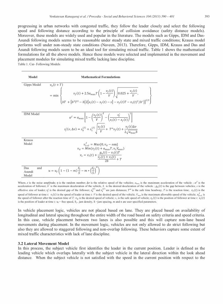
progressing in urban networks with congested traffic, they follow the leader closely and select the following speed and following distance according to the principle of collision avoidance (safety distance models). Moreover, these models are widely used and popular in the literature. The models such as Gipps, IDM and Das-Asundi following models seems to be reasonable under steady state and mixed traffic conditions; Krauss model performs well under non-steady state conditions (Naveen, 2013). Therefore, Gipps, IDM, Krauss and Das and Asundi following models seem to be an ideal tool for simulating mixed traffic. Table 1 shows the mathematical formulations for all the above models. Hence these models were selected and implemented in the movement and placement modules for simulating mixed traffic lacking lane discipline. Table 1. Car- Following Models
Where, is the noise amplitude; is the random number; is the relative speed of the vehicles; amax is the maximum acceleration of the vehicle ; is the acceleration of follower; b* is the maximum deceleration of the vehicle, b is the desired deceleration of the vehicle ; ( ) is the gap between vehicles; s is the effective size of leader; is the desired gap of the follower; ( ) and ( ) are jam distances; is the safe time headway; T is the reaction time; ( ) is the speed of follower at time t; ( ) is the speed of leader at time t; V is the desired speed of the vehicle; Vmax is the maximum allowable speed of the vehicle; is the speed of follower after the reaction time of T; is the desired speed of vehicle; vs is the safe speed of vehicle; ( ) is the position of follower at time t; ( ) is the position of leader at time t; uf = free speed, Sj = jam density, S =jam spacing, m and n are user specified parameters. In vehicle placement logic, vehicles are not placed based on lane. They are placed based on availability of longitudinal and lateral spacing throughout the entire width of the road based on safety criteria and speed criteria. In this case, vehicle placement between two lanes is also possible and this will capture non-lane based movements during placement. In the movement logic, vehicles are not only allowed to do strict following but also they are allowed to staggered following and non-overlap following. These behaviors capture some extent of mixed traffic characteristics with lack of lane discipline.
3.2 Lateral Movement Model In this process, the subject vehicle first identifies the leader in the current position. Leader is defined as the leading vehicle which overlaps laterally with the subject vehicle in the lateral direction within the look ahead distance. When the subject vehicle is not satisfied with the speed in the current position with respect to the
Model
Mathematical Formulations
Gipps Model ( + )= min ( ) + 2.5 1 ( ) 0.025 + ( ) ,+ 2 ( ) ( ) ( ) ( ) / /
IDM Model = 1 ( ) ( ) ( )
( , ) = ( ) + ( ) ( ) + ( ) + ( )2
Krauss Model = [0, ] = ( ( ) + , , ) = ( ) + ( ) ( )( ) + ( )2 +
Das and Asundi Model
= 1 (1 )
394 Venkatesan Kanagaraj et al. / Procedia - Social and Behavioral Sciences 104 ( 2013 ) 390 – 401
leader, subject vehicle will decide to shift laterally in the left or right side. Then, the subject vehicle move laterally to the side of leader (based on direction) with enough clearances between these vehicles. These clearances depend on the speed of both vehicles; clearance of the vehicle varies linearly with speed. The longitudinal distance of the subject vehicle in the tentative target position is calculated based on its acceleration capability. The subject vehicle identifies the leader and follower in the tentative target position. The leader is identified by travelling to the front of vehicle list. If the leading vehicle overlaps with subject vehicle in the tentative target position within look ahead distance, it is defined as the target leader. The target follower is also identified as per the above definition, but travelling from the the back of vehicle list. The safety criteria and gap acceptance criteria are evaluated for target leader at time t (current time step) and for target follower at time t+1 (next time step) in order to maintain conservative behaviour at lateral shift process. The longitudinal position of the target follower at time t+1 is calculated based on its current speed (at time t) and lateral position does not change. The following three conditions have to be satisfied for lateral shift process.
Critical gap (minimum gap required for the subject vehicle to accept the gap) should be less than lead gap for leader in the tentative target position
Critical gap should be less than lag gap for follower in the tentative target position Estimated braking rate in the tentative target position (using car following model) should be less than
comfortable braking rate Estimated speed of the subject vehicle in the tentative target position should be greater than current
speed of the subject vehicle If the above conditions are not satisfied, then subject vehicle continue in the current position in car following mode. If these conditions are satisfied on both directions, lateral shift is invoked in the direction where the estimated speed is higher. To evaluate the calibrated parameters at disaggregate level (time series data of speed and density for one minute interval), the simulation model was modified by matching the input flow for one minute based on field observed data. The outputs from the model are the speed and density values for the corresponding flow for each one minute. Using this, the time trend graph for speed and density is plotted and corresponding MAPEs are also calculated. 4.0 Model Calibration Calibration is the iterative process of comparing the model with real system, and revising the model by making modifications to built parameters if necessary, until a model accurately represents the real system. The models above were calibrated to ensure that the simulation models replicate the field observed traffic conditions for mid-block section of one direction of flow of a four lane divided urban road in Ashoknagar Chennai City, India. Traffic movements were captured using videography during one hour of peak period on a weekday. Irfanview 3.99 software was used to extract data from the video. It extracts video images into frames where 1 sec video data is converted into 25 frames. Flow, speed and area occupancy were extracted for one hour using these frames. Density values were derived from the area occupancy (Arasan and Dhivya, 2009). For the purpose of simulation, a 7.2 m wide and 800 m long road stretch was considered. Calibration of traffic parameters based on optimization procedure is difficult since the objective function does not have closed form. Hence, we use trial and error procedure to carry out to reduce the error between simulation and observed data. The reasonable range of values of model parameters was fixed based on the past literature on mixed traffic studies. The parameters were calibrated by fine tuning within the predefined range of values to fit better with the field data. The models are evaluated in three levels 1. Steady state with class invariant parameters, 2. Non-steady state with class invariant parameters and 3. Non-steady state with classwise parameters. Steady state parameters are obtained by reducing the error between observed and estimated density values. Estimated density values were obtained by steady state
395 Venkatesan Kanagaraj et al. / Procedia - Social and Behavioral Sciences 104 ( 2013 ) 390 – 401
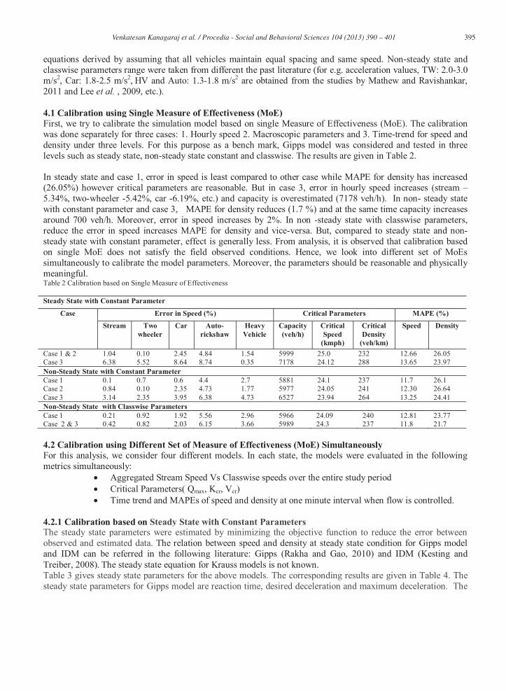
equations derived by assuming that all vehicles maintain equal spacing and same speed. Non-steady state and classwise parameters range were taken from different the past literature (for e.g. acceleration values, TW: 2.0-3.0 m/s2, Car: 1.8-2.5 m/s2, HV and Auto: 1.3-1.8 m/s2 are obtained from the studies by Mathew and Ravishankar, 2011 and Lee et al. , 2009, etc.). 4.1 Calibration using Single Measure of Effectiveness (MoE) First, we try to calibrate the simulation model based on single Measure of Effectiveness (MoE). The calibration was done separately for three cases: 1. Hourly speed 2. Macroscopic parameters and 3. Time-trend for speed and density under three levels. For this purpose as a bench mark, Gipps model was considered and tested in three levels such as steady state, non-steady state constant and classwise. The results are given in Table 2. In steady state and case 1, error in speed is least compared to other case while MAPE for density has increased (26.05%) however critical parameters are reasonable. But in case 3, error in hourly speed increases (stream – 5.34%, two-wheeler -5.42%, car -6.19%, etc.) and capacity is overestimated (7178 veh/h). In non- steady state with constant parameter and case 3, MAPE for density reduces (1.7 %) and at the same time capacity increases around 700 veh/h. Moreover, error in speed increases by 2%. In non -steady state with classwise parameters, reduce the error in speed increases MAPE for density and vice-versa. But, compared to steady state and non-steady state with constant parameter, effect is generally less. From analysis, it is observed that calibration based on single MoE does not satisfy the field observed conditions. Hence, we look into different set of MoEs simultaneously to calibrate the model parameters. Moreover, the parameters should be reasonable and physically meaningful. Table 2 Calibration based on Single Measure of Effectiveness
4.2 Calibration using Different Set of Measure of Effectiveness (MoE) Simultaneously For this analysis, we consider four different models. In each state, the models were evaluated in the following metrics simultaneously:
Aggregated Stream Speed Vs Classwise speeds over the entire study period Critical Parameters( Qmax, Kcr, Vcr) Time trend and MAPEs of speed and density at one minute interval when flow is controlled.
4.2.1 Calibration based on Steady State with Constant Parameters The steady state parameters were estimated by minimizing the objective function to reduce the error between observed and estimated data. The relation between speed and density at steady state condition for Gipps model and IDM can be referred in the following literature: Gipps (Rakha and Gao, 2010) and IDM (Kesting and Treiber, 2008). The steady state equation for Krauss models is not known. Table 3 gives steady state parameters for the above models. The corresponding results are given in Table 4. The steady state parameters for Gipps model are reaction time, desired deceleration and maximum deceleration. The
Steady State with Constant Parameter
Case Error in Speed (%) Critical Parameters MAPE (%)
Stream Two wheeler
Car Auto-rickshaw
Heavy Vehicle
Capacity (veh/h)
Critical Speed
(kmph)
Critical Density
(veh/km)
Speed Density
Case 1 & 2 1.04 0.10 2.45 4.84 1.54 5999 25.0 232 12.66 26.05 Case 3 6.38 5.52 8.64 8.74 0.35 7178 24.12 288 13.65 23.97 Non-Steady State with Constant Parameter Case 1 0.1 0.7 0.6 4.4 2.7 5881 24.1 237 11.7 26.1 Case 2 0.84 0.10 2.35 4.73 1.77 5977 24.05 241 12.30 26.64 Case 3 3.14 2.35 3.95 6.38 4.73 6527 23.94 264 13.25 24.41 Non-Steady State with Classwise Parameters Case 1 0.21 0.92 1.92 5.56 2.96 5966 24.09 240 12.81 23.77 Case 2 & 3 0.42 0.82 2.03 6.15 3.66 5989 24.3 237 11.8 21.7
396 Venkatesan Kanagaraj et al. / Procedia - Social and Behavioral Sciences 104 ( 2013 ) 390 – 401
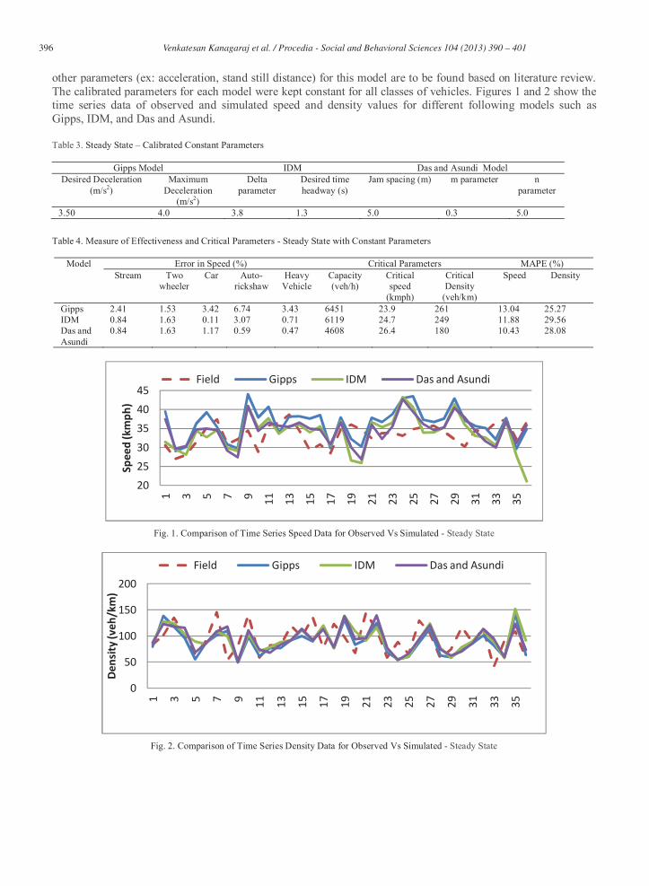
other parameters (ex: acceleration, stand still distance) for this model are to be found based on literature review. The calibrated parameters for each model were kept constant for all classes of vehicles. Figures 1 and 2 show the time series data of observed and simulated speed and density values for different following models such as Gipps, IDM, and Das and Asundi. Table 3. Steady State – Calibrated Constant Parameters
Table 4. Measure of Effectiveness and Critical Parameters - Steady State with Constant Parameters
Fig. 1. Comparison of Time Series Speed Data for Observed Vs Simulated - Steady State
Fig. 2. Comparison of Time Series Density Data for Observed Vs Simulated - Steady State
202530
354045
1 3 5 7 9 11 13 15 17 19 21 23 25 27 29 31 33 35
Spee
d (k
mph
)
Field Gipps IDM Das and Asundi
0
50
100
150
200
1 3 5 7 9 11 13 15 17 19 21 23 25 27 29 31 33 35
Dens
ity (v
eh/k
m)
Field Gipps IDM Das and Asundi
Gipps Model IDM Das and Asundi Model Desired Deceleration
(m/s2) Maximum
Deceleration (m/s2)
Delta parameter
Desired time headway (s)
Jam spacing (m) m parameter n parameter
3.50 4.0 3.8 1.3 5.0 0.3 5.0
Model Error in Speed (%) Critical Parameters MAPE (%) Stream Two
wheeler Car Auto-
rickshaw Heavy
Vehicle Capacity (veh/h)
Critical speed
(kmph)
Critical Density
(veh/km)
Speed Density
Gipps 2.41 1.53 3.42 6.74 3.43 6451 23.9 261 13.04 25.27 IDM 0.84 1.63 0.11 3.07 0.71 6119 24.7 249 11.88 29.56 Das and Asundi
0.84 1.63 1.17 0.59 0.47 4608 26.4 180 10.43 28.08
397 Venkatesan Kanagaraj et al. / Procedia - Social and Behavioral Sciences 104 ( 2013 ) 390 – 401
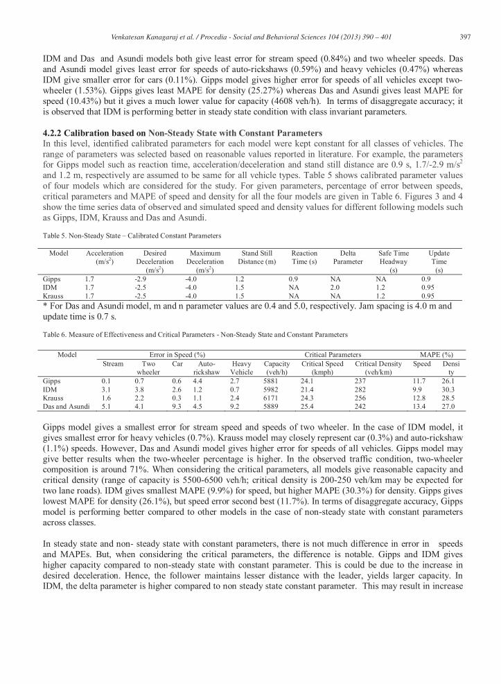
IDM and Das and Asundi models both give least error for stream speed (0.84%) and two wheeler speeds. Das and Asundi model gives least error for speeds of auto-rickshaws (0.59%) and heavy vehicles (0.47%) whereas IDM give smaller error for cars (0.11%). Gipps model gives higher error for speeds of all vehicles except two-wheeler (1.53%). Gipps gives least MAPE for density (25.27%) whereas Das and Asundi gives least MAPE for speed (10.43%) but it gives a much lower value for capacity (4608 veh/h). In terms of disaggregate accuracy; it is observed that IDM is performing better in steady state condition with class invariant parameters. 4.2.2 Calibration based on Non-Steady State with Constant Parameters In this level, identified calibrated parameters for each model were kept constant for all classes of vehicles. The range of parameters was selected based on reasonable values reported in literature. For example, the parameters for Gipps model such as reaction time, acceleration/deceleration and stand still distance are 0.9 s, 1.7/-2.9 m/s2
and 1.2 m, respectively are assumed to be same for all vehicle types. Table 5 shows calibrated parameter values of four models which are considered for the study. For given parameters, percentage of error between speeds, critical parameters and MAPE of speed and density for all the four models are given in Table 6. Figures 3 and 4 show the time series data of observed and simulated speed and density values for different following models such as Gipps, IDM, Krauss and Das and Asundi. Table 5. Non-Steady State – Calibrated Constant Parameters
Model Acceleration (m/s2)
Desired Deceleration
(m/s2)
Maximum Deceleration
(m/s2)
Stand Still Distance (m)
Reaction Time (s)
Delta Parameter
Safe Time Headway
(s)
Update Time
(s) Gipps 1.7 -2.9 -4.0 1.2 0.9 NA NA 0.9 IDM 1.7 -2.5 -4.0 1.5 NA 2.0 1.2 0.95 Krauss 1.7 -2.5 -4.0 1.5 NA NA 1.2 0.95 * For Das and Asundi model, m and n parameter values are 0.4 and 5.0, respectively. Jam spacing is 4.0 m and update time is 0.7 s. Table 6. Measure of Effectiveness and Critical Parameters - Non-Steady State and Constant Parameters
Gipps model gives a smallest error for stream speed and speeds of two wheeler. In the case of IDM model, it gives smallest error for heavy vehicles (0.7%). Krauss model may closely represent car (0.3%) and auto-rickshaw (1.1%) speeds. However, Das and Asundi model gives higher error for speeds of all vehicles. Gipps model may give better results when the two-wheeler percentage is higher. In the observed traffic condition, two-wheeler composition is around 71%. When considering the critical parameters, all models give reasonable capacity and critical density (range of capacity is 5500-6500 veh/h; critical density is 200-250 veh/km may be expected for two lane roads). IDM gives smallest MAPE (9.9%) for speed, but higher MAPE (30.3%) for density. Gipps gives lowest MAPE for density (26.1%), but speed error second best (11.7%). In terms of disaggregate accuracy, Gipps model is performing better compared to other models in the case of non-steady state with constant parameters across classes. In steady state and non- steady state with constant parameters, there is not much difference in error in speeds and MAPEs. But, when considering the critical parameters, the difference is notable. Gipps and IDM gives higher capacity compared to non-steady state with constant parameter. This is could be due to the increase in desired deceleration. Hence, the follower maintains lesser distance with the leader, yields larger capacity. In IDM, the delta parameter is higher compared to non steady state constant parameter. This may result in increase
Model Error in Speed (%) Critical Parameters MAPE (%) Stream Two
wheeler Car Auto-
rickshaw Heavy
Vehicle Capacity (veh/h)
Critical Speed (kmph)
Critical Density (veh/km)
Speed Density
Gipps 0.1 0.7 0.6 4.4 2.7 5881 24.1 237 11.7 26.1 IDM 3.1 3.8 2.6 1.2 0.7 5982 21.4 282 9.9 30.3 Krauss 1.6 2.2 0.3 1.1 2.4 6171 24.3 256 12.8 28.5 Das and Asundi 5.1 4.1 9.3 4.5 9.2 5889 25.4 242 13.4 27.0
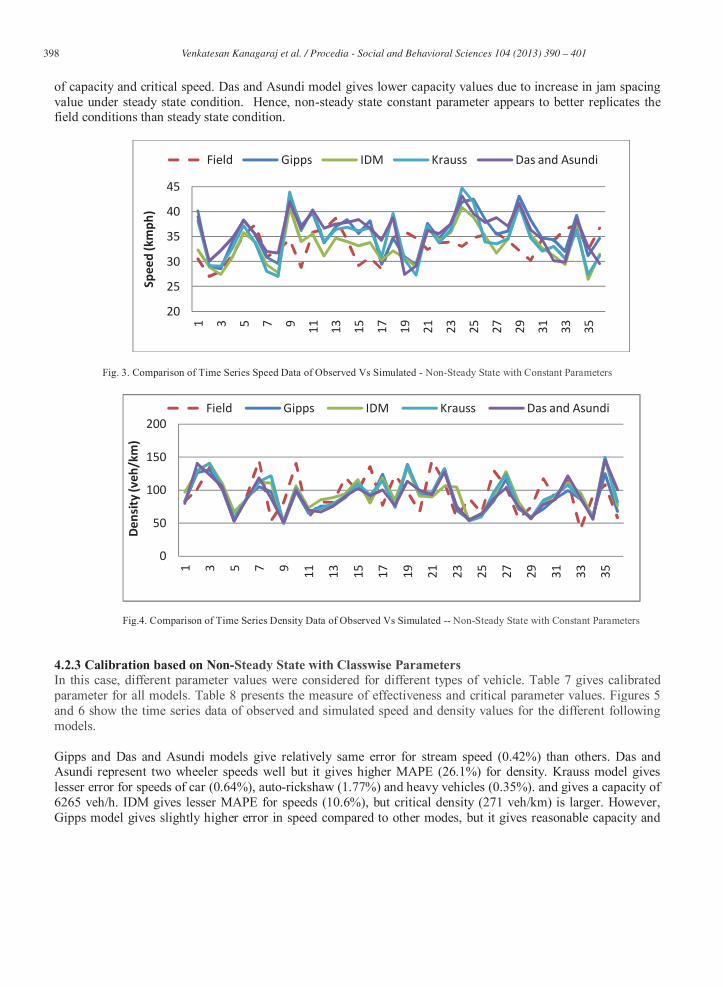
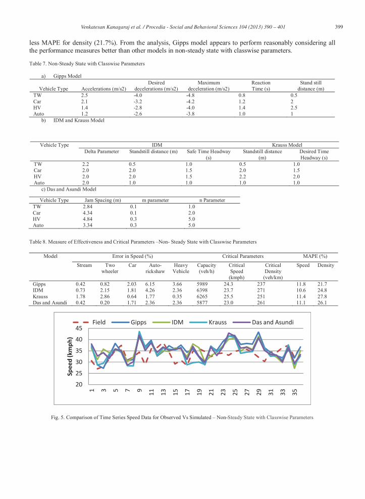
398 Venkatesan Kanagaraj et al. / Procedia - Social and Behavioral Sciences 104 ( 2013 ) 390 – 401
of capacity and critical speed. Das and Asundi model gives lower capacity values due to increase in jam spacing value under steady state condition. Hence, non-steady state constant parameter appears to better replicates the field conditions than steady state condition.
Fig. 3. Comparison of Time Series Speed Data of Observed Vs Simulated - Non-Steady State with Constant Parameters
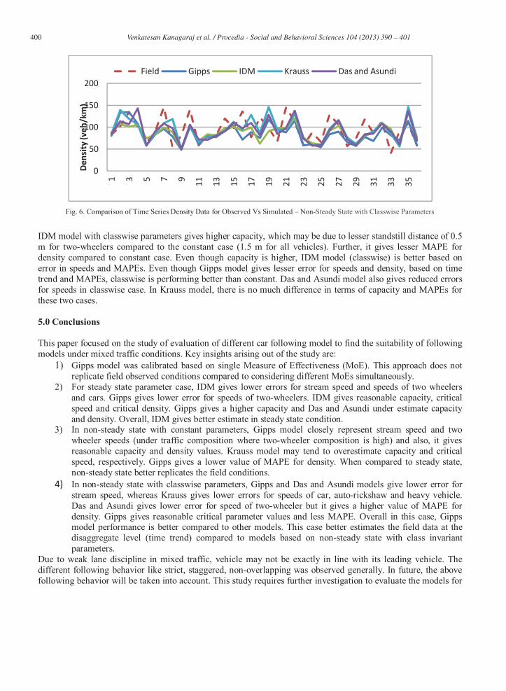
Fig.4. Comparison of Time Series Density Data of Observed Vs Simulated -- Non-Steady State with Constant Parameters 4.2.3 Calibration based on Non-Steady State with Classwise Parameters In this case, different parameter values were considered for different types of vehicle. Table 7 gives calibrated parameter for all models. Table 8 presents the measure of effectiveness and critical parameter values. Figures 5 and 6 show the time series data of observed and simulated speed and density values for the different following models. Gipps and Das and Asundi models give relatively same error for stream speed (0.42%) than others. Das and Asundi represent two wheeler speeds well but it gives higher MAPE (26.1%) for density. Krauss model gives lesser error for speeds of car (0.64%), auto-rickshaw (1.77%) and heavy vehicles (0.35%). and gives a capacity of 6265 veh/h. IDM gives lesser MAPE for speeds (10.6%), but critical density (271 veh/km) is larger. However, Gipps model gives slightly higher error in speed compared to other modes, but it gives reasonable capacity and
20
25
30
35
40
451 3 5 7 9 11 13 15 17 19 21 23 25 27 29 31 33 35
Spee
d (k
mph
)Field Gipps IDM Krauss Das and Asundi
0
50
100
150
200
1 3 5 7 9 11 13 15 17 19 21 23 25 27 29 31 33 35
Dens
ity (v
eh/k
m)
Field Gipps IDM Krauss Das and Asundi
399 Venkatesan Kanagaraj et al. / Procedia - Social and Behavioral Sciences 104 ( 2013 ) 390 – 401
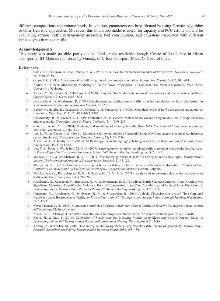
less MAPE for density (21.7%). From the analysis, Gipps model appears to perform reasonably considering all the performance measures better than other models in non-steady state with classwise parameters. Table 7. Non-Steady State with Classwise Parameters
a) Gipps Model
Vehicle Type Accelerations (m/s2) Desired
decelerations (m/s2) Maximum
deceleration (m/s2) Reaction Time (s)
Stand still distance (m)
TW 2.5 -4.0 -4.8 0.8 0.5 Car 2.1 -3.2 -4.2 1.2 2 HV 1.4 -2.8 -4.0 1.4 2.5 Auto 1.2 -2.6 -3.8 1.0 1
b) IDM and Krauss Model
c) Das and Asundi Model
Table 8. Measure of Effectiveness and Critical Parameters –Non- Steady State with Classwise Parameters
Fig. 5. Comparison of Time Series Speed Data for Observed Vs Simulated – Non-Steady State with Classwise Parameters
20
25
30
35
40
45
1 3 5 7 9 11 13 15 17 19 21 23 25 27 29 31 33 35
Spee
d (k
mph
)
Field Gipps IDM Krauss Das and Asundi
Vehicle Type IDM Krauss Model Delta Parameter Standstill distance (m) Safe Time Headway
(s) Standstill distance
(m) Desired Time Headway (s)
TW 2.2 0.5 1.0 0.5 1.0 Car 2.0 2.0 1.5 2.0 1.5 HV 2.0 2.0 1.5 2.2 2.0 Auto 2.0 1.0 1.0 1.0 1.0
Vehicle Type Jam Spacing (m) m parameter n Parameter TW 2.84 0.1 1.0 Car 4.34 0.1 2.0 HV 4.84 0.3 5.0 Auto 3.34 0.3 5.0
Model Error in Speed (%) Critical Parameters MAPE (%)
Stream Two wheeler
Car Auto-rickshaw
Heavy Vehicle
Capacity (veh/h)
Critical Speed
(kmph)
Critical Density
(veh/km)
Speed Density
Gipps 0.42 0.82 2.03 6.15 3.66 5989 24.3 237 11.8 21.7 IDM 0.73 2.15 1.81 4.26 2.36 6398 23.7 271 10.6 24.8 Krauss 1.78 2.86 0.64 1.77 0.35 6265 25.5 251 11.4 27.8 Das and Asundi 0.42 0.20 1.71 2.36 2.36 5877 23.0 261 11.1 26.1
400 Venkatesan Kanagaraj et al. / Procedia - Social and Behavioral Sciences 104 ( 2013 ) 390 – 401
Fig. 6. Comparison of Time Series Density Data for Observed Vs Simulated – Non-Steady State with Classwise Parameters
IDM model with classwise parameters gives higher capacity, which may be due to lesser standstill distance of 0.5 m for two-wheelers compared to the constant case (1.5 m for all vehicles). Further, it gives lesser MAPE for density compared to constant case. Even though capacity is higher, IDM model (classwise) is better based on error in speeds and MAPEs. Even though Gipps model gives lesser error for speeds and density, based on time trend and MAPEs, classwise is performing better than constant. Das and Asundi model also gives reduced errors for speeds in classwise case. In Krauss model, there is no much difference in terms of capacity and MAPEs for these two cases. 5.0 Conclusions This paper focused on the study of evaluation of different car following model to find the suitability of following models under mixed traffic conditions. Key insights arising out of the study are:
1) Gipps model was calibrated based on single Measure of Effectiveness (MoE). This approach does not replicate field observed conditions compared to considering different MoEs simultaneously.
2) For steady state parameter case, IDM gives lower errors for stream speed and speeds of two wheelers and cars. Gipps gives lower error for speeds of two-wheelers. IDM gives reasonable capacity, critical speed and critical density. Gipps gives a higher capacity and Das and Asundi under estimate capacity and density. Overall, IDM gives better estimate in steady state condition.
3) In non-steady state with constant parameters, Gipps model closely represent stream speed and two wheeler speeds (under traffic composition where two-wheeler composition is high) and also, it gives reasonable capacity and density values. Krauss model may tend to overestimate capacity and critical speed, respectively. Gipps gives a lower value of MAPE for density. When compared to steady state, non-steady state better replicates the field conditions.
4) In non-steady state with classwise parameters, Gipps and Das and Asundi models give lower error for stream speed, whereas Krauss gives lower errors for speeds of car, auto-rickshaw and heavy vehicle. Das and Asundi gives lower error for speed of two-wheeler but it gives a higher value of MAPE for density. Gipps gives reasonable critical parameter values and less MAPE. Overall in this case, Gipps model performance is better compared to other models. This case better estimates the field data at the disaggregate level (time trend) compared to models based on non-steady state with class invariant parameters.
Due to weak lane discipline in mixed traffic, vehicle may not be exactly in line with its leading vehicle. The different following behavior like strict, staggered, non-overlapping was observed generally. In future, the above following behavior will be taken into account. This study requires further investigation to evaluate the models for
0
50
100
150
200
1 3 5 7 9 11 13 15 17 19 21 23 25 27 29 31 33 35
Dens
ity (v
eh/k
m)
Field Gipps IDM Krauss Das and Asundi
401 Venkatesan Kanagaraj et al. / Procedia - Social and Behavioral Sciences 104 ( 2013 ) 390 – 401
different compositions and volume levels. In addition, parameters can be calibrated by using Genetic Algorithm or other Heuristic approaches. Moreover, this simulation model is useful for capacity and PCU estimation and for evaluating various traffic management measures, fuel consumption, and emissions associated with different vehicle types in mixed traffic. Acknowledgements This study was made possible partly due to funds made available through Centre of Excellence in Urban Transport at IIT Madras, sponsored by Ministry of Urban Transport (MOUD), Govt. of India. References
1. Gazis, D. C., Herman, R., and Rothery, R. W. (1961). “Nonlinear follow the leader models of traffic flow”. Operations Research, vol. 9, pp.54-567.
2. Gipps, P. G. (1981). A behavioural car following model for computer simulation. Transp. Res. Board, 15-B, 2, 403–414. 3. Krauss, S. (1997). Microscopic Modeling of Traffic Flow: Investigation of Collision Free Vehicle Dynamics. PhD Thesis,
University of Cologne. 4. Treiber, M., Hennecke, A., & Helbing, D. (2000). Congested traffic states in empirical observations and microscopic simulations.
Physical Review E, 62(2), 180S-1824. 5. Leutzbach, W., & Wiedemann, R, (1986). Development and applications of traffic simulation models at the Karlsruhe Institut fur
Verkehrwesen. Traffic Engineering and Control, 270-278. 6. Bando. M., Hasebe. K., Nakayama. A., Shibata, A., & Sugiyama. Y. (1995). Dynamical model of traffic congestion and numerical
simulation. Phys. Rev., E, 51, 2, 1035–1042, 1995. 7. Chakroborty, P., & Kikuchi, S. (1999). Evaluation of the General Motors based car-following models and a proposed fuzzy
inference model. TranspRes., Part C: Emerg. Technol., 7, 4, 209–235. 8. Cho, H. J., & Wu, Y. T., (2004). Modeling and simulation of motorcycle traffic flow. IEEE International Conference on Systems,
Man and Cybernetics, 7, 6262- 6267. 9. Lan, L. W., & Chang, C.W. (2004). Motorcycle-following models of General Motors (GM) and adaptive neuro-fuzzy inference
system (in chinese), Transportation Planning Journal, 33, 3, 511-536. 10. Arasan, V. T., & Koshy, R. Z. (2005). Methodology for modeling highly heterogeneous traffic flow. Journal of Transportation
Engineering, ASCE, 544-551. 11. Lee, T. C., Polak, J. W., & Bell, M. G. H. (2009) A new approach to modeling mixed traffic containing motorcycles in urban area.
In Proceedings of the Transportation Research Board 88thAnnual Meeting, Washington, D.C., USA. 12. Mathew, T. V., & Ravishankar, K. V. R. (2011). Car-following behavior in traffic having mixed vehicle-types. Transportation
Letters: The International Journal of Transportation Research, 3,113-126. 13. Maurya, A. K. (2011) Comprehensive approach for modeling of traffic streams with no lane discipline. 2nd International
Conference on Models and Technologies for Intelligent Transportation Systems, Leuven, Belgium. 14. Mallikarjuna, ch., Ramachandra, R. K., & Seethepalli. N. V. S. K. (2011). Analysis of microscopic data under heterogeneous
traffic conditions. Transport, 25(3), 262-268. 15. Asaithambi, G., Kanagaraj, V., Srinivasan, K.. K., & Sivanandan, R. (2012). Mixed Traffic Characteristics on Urban Arterials with
Significant Motorized Two-Wheeler Volumes: Role of Composition, Intra-Class Variability, and Lack of Lane Discipline. In Proceedings of the Transportation Research Board 91st Annual Meeting, Washington, D.C., USA.
16. Kanagaraj, V., Asaithambi, G., Srinivasan, K. K., & Sivanandan, R. (2011). Vehicle Classwise Analysis of Time Gaps and Headways under Heterogeneous Traffic. In Proceedings of the 90th Transportation Research Board Annual Meeting, Washington, D.C., USA.
17. Naveen Kumar C. H. (2013). Microscopic Analysis of Vehicle Behaviour in Mixed Traffic.M.Tech Project Report, Indian Institute of Technology Madras, Chennai
18. Arasan, V. T. &Dhivya, G. (2009). Concentration of Heterogeneous Road Traffic. Advanced Technologies, In-Teh, Croatia. 19. Rakha, H., & Gao, Y. (2010). Calibration of Steady-state Car-following Models using Macroscopic Loop Detector Data. In
Proceedings of the 89th Transportation Research Board Annual Meeting, Washington D.C. , USA. 20. Kesting, A., & Treiber, M. (2008). Calibrating car-following models using trajectory data: methodological study. Transportation
Research Record: Journal of the Transportation Research Board, 2088, 148- 156.