ethiopian journal of economics
TRANSCRIPT

Ethiopian Journal of Economics
Worku Gebeyehu
Fanaye Tadesse and
Derek Headey
Getnet Alemu
Ibrahim Worku
Clement A.U.
Ighodaro
Causal Links among
Saving, Investment and
Growth and Determinants
of Saving in Sub-Saharan
Africa: Evidence from
Ethiopia
Urbanization and Fertility
Rates in Ethiopia
Poverty Analysis of
Children in Child Headed
Households in Addis Ababa
Road Sector Development
and Economic
Growth in Ethiopia
Infrastructure and
Agricultural Growth in
Nigeria
1
35
73
101
147
Volume XIX Number 2 October 2010

ETHIOPAN ECONOMICS ASSOCIATION
Editorial Board Getnet Alemu (Editor)
Alemayehu Seyoum
Alemu Mekonnen
Eyob Tesfaye
Gezahegn Ayele
Ishak Diwan
Text Layout
Rahel Yilma
Web Postmaster
Mahlet Yohannes
©Ethiopian Economics Association (EEA)
All rights reserved.
No part of this publication can be reproduced, stored in a retrieval system or
transmitted in any form, without a written permission from the Ethiopian Economic
Association.
ISSN 1993-3681
Honorary Advisory Board
Augustin K. Fosu, Economic and Social Policy Division, UNECA Assefa Bekele, African Child Policy Forum, Addis Ababa
Addis Anteneh, formerly International Livestock Centre for Africa Bigisten, A., Gothenburg University, Sweden Collier, P., Director, University of Oxford, U.K.
Diejomach, V.P., ILO/EAMAT Duri Mohammed, formerly Ethiopia’s Ambassador to the UN, New York Elbadawi, I., formerly African Economic Research Consortium, Kenya
Fitz Gerald, E.V.K., Finance and Trade Policy Research Centre, QEH, University of Oxford Fassil G. Kiros, ICIPE, Kenya
Hanson, G., Lund University, Sweden Mukras, M., University of Botswana, Botswana
Mureithi, L.P., formerly African Union, Addis Ababa Pankhurst, R., Addis Ababa University Pichett, J., Stratchyde University, U.K.
Tekaligne Gedamu, Abyssinia Bank, Addis Ababa Teriba, O., UN Economic Commission for Africa, Addis Ababa
Teshome Mulat, Addis Ababa University Wuyts, Marc, Institute of Social Studies, The Netherlands
Vos, Rob, Institute of Social Studies, The Netherlands

3
Ethiopian Journal of Economics
©Ethiopian Economics Association
Volume XIX Number 2 October 2010

A Publication of
THE ETHIOPIAN ECONOMICS ASSOCIATION
(EEA)
ETHIOPIAN JOURNAL OF ECONOMICS
VOLUME XIX NUMBER 2 October 2010
Published: November 2011

1
CAUSAL LINKS AMONG SAVING, INVESTMENT AND GROWTH AND DETERMINANTS OF SAVING IN SUB-SAHARAN AFRICA:
EVIDENCE FROM ETHIOPIA1
Worku Gebeyehu2
Abstract The relationship between saving, investment and GDP still remains an
empirical issue. In their aspiration to catch up the rest of the world, developing
countries provides a special place on this matter. This paper tried to
investigate the main determinants of saving and the connection among
saving, investment and GDP in the case of Ethiopia using a combination of
time series models. The paper finds export, inflation and lag government
expenditure to have a statistically significant short and long term impact on
the saving rate. Growth of income has a positive effect on rate of saving and
the impulse response function shows the relevance of the neoclassical growth
model in explaining the relationship between the saving rate and growth of
income albeit lack of statistically significant causality between saving and
investment in either direction. Although they may not be conclusive, the
results suggest a more conducive policy environment and measures to boost
domestic saving so as to induce growth from inside.
1 The final version of this article was submitted in September 2011. 2 Ph.D Candidate, Department of Economics, Dar es Salaam University and Freelance Consultant. Email: [email protected]
Worku Gebeyehu: Causal links among saving, investment and growth…
2
1. Introduction
The shortest path of development has still remained to be mysterious despite
successes of some countries. Many countries in the developing world are still trying
to search for the root that helps to traverse their population from living in abject state
of life. Although it does not necessarily ensure all-embracing improvements in the life
of every person, economic growth is a necessary condition for eradication of poverty
at a country level. In turn, since economics started emerging as an independent
discipline during the era of mercantilists and Adam smith, accumulation of wealth,
(which is nothing but saving) has been identified as a key variable for growth. Saving,
with the necessary enabling environment is easily converted into investment or
capital and enables labour and other resources to be effectively mobilized for the
growth of overall level of output in an economy.
The pioneer in terms of clearly establishing the link between saving and economic
growth was Harrod (1939), who was later followed by Domar in (1946). The two
pioneer development economists lent for the well-known Harrod and Domar Model.
These two economists, Solow (1956) and Romer (1986) underscored the importance
of saving as it translates itself into investment and stimulates economic growth.
According to the neo-classical school led by Robert Solow, an increase in the saving
rate brings about a shift in a steady state growth path although its effect is transitory
because of diminishing marginal productivity of capital. The endogenous growth
theorists argue that an increase in the rate of saving will have a sustained and
permanent effect on economic growth because of increasing returns to scale.
Regardless of differences in the weight attached to saving by different schools, the
conventional view gives value for saving as a source of financing current investment
or settling debts spent for past investments stemming either from foreign or domestic
sources.
The policies and development activities of various countries have been influenced and
guided by the approach advocated by the last generation development economists
such as Harrod and Domar. The East Asian experience and the World Bank policy
prescription has also been influenced by the same. However, the relationship
between the saving rate and the level of income is somewhat complicated by the
simultaneous operation of several factors. Thus, the relationship between saving and

Ethiopian Journal of Economics, Volume XIX, No. 2, October 2010
3
investment, and thus, the relationship between saving and economic growth (through
the medium of investment) has been an empirical issue.
In the traditional Keynesian theory, the relationship between the saving and the level
of income indicates that saving rate increases with the level of economic
development. The link between domestic saving rate and the investment is based on
the hypothesis that capital does not freely move from one country to the other
because of various imperfections. Economic agents and savers tend to invest their
resources in domestic investment outlets and require premiums to cover the risk
involved in making investment in other countries. This is generally the case provided
that domestic investments opportunities are attractive, and resources are efficiently
allocated for their most productive use.
Athukorala and Sen (2004) also argue against the perception of the globalization of
capital that domestic investment is fundamentally determined by domestic saving and
thus high rate of national saving is a crucial determinant of economic growth. There
is cross-country evidence which supports the hypothesis that long-run growth rate of
income is significantly determined by domestic investment rate and domestic saving
rate (Levine and Renelt, 1992). Bacha (1990), DeGregorio (1992), Otani and Villanueva
(1990) found a similar result. Loayza et. al. (2000) also find a strong and positive
relationship between the national saving rate and the level of income of countries. If
there is causality between the two, the policy implication is that domestic saving
should be increased to finance domestic investment, finance imported capital goods
and thereby achieve sustainable economic growth.
However, the relationship between income level and saving rate in poor countries
might be influenced by considerations of subsistence consumption, which is more
than inter-temporal consumption smoothing (Easterly, 1994 and Ogaki et.al., 1996).
Saving rate and GDP may go in the same direction and this positive association may
not necessarily indicate causality. There could be an omitted variable that commonly
explains both saving and income. The empirical evidence suggests Granger-causality
from economic growth rate to the saving rate instead of the vise versa (Attanasio,
et.al, 2000; Rodrik, 2000). The same result has also been found by the studies of
Jappelli and Pagano (1996), Gavin et al (1997), Sinha and Sinha (1998) and Saltz (1999).

Worku Gebeyehu: Causal links among saving, investment and growth…
4
Besides making an argument based on empirical evidence against the established
view that saving is a necessary prerequisite for growth, Moore (2006) has come in
open to provide a theoretical framework to show that saving cannot be a constraint
for growth. As far as financial markets operate properly and there is a flow of capital
across countries, it is not of a necessity to save for investment.
Even if the argument saving versus investment and economic growth has still been
unsettled, the question of what determines saving is also a source of theoretical and
empirical debate. The life cycle model (LCM), the permanent income hypotheses (PIH)
and the relative income hypothesis (RIH) are widely used as a benchmark to organize
the arguments about the consumption and saving behavior of households. The Life
cycle model (LCM) assumes that economic agents make sequential decisions to
achieve a coherent goal using the currently available information as best they can
(Browning and Crossley, 2001). Utility maximizing agents postpone part of their
current consumption and save it for consumption during retirement in a dynamic and
uncertain environment. The PIH argues that consumption expenditure closely follows
permanent income, instead of current income of economic agents as hypothesized by
Keynesian economists. Modigliani (1986) in his RIH argues that the share of life time
resources that households plan to devote to bequests is an increasing function of their
life time resources relative to others in the same age cohort.
Basing their decisions on the underlying theory that suits the circumstances of their
countries, governments strive to take policy measures that induce mobilization of
saving. Propensity to save and thus the saving rate is relatively low in developing
countries because of low level of income and the necessity to fulfill subsistence
consumption before inter-temporal resource allocation, the relative dominance of
necessities in the household budget and liquidity constraints. Interventions of
governments in controlling interest rate and mobilization of loans and
underdevelopment of financial institutions also contribute for low level of saving.
Empirical evidence with regards to the role financial markets and interest rate in
mobilizing savings has not been impressive in developing countries (Easterly, 1994;
Ogaki et. al, 1996; Rebello, 1991) and this could partly be because of high distortions,
which lead at times to negative real interest rate. One of the policy instruments to
address this problem is financial liberalization. Financial liberalization tends to
improve and nurture the functioning of financial markets and facilitates the flow of

Ethiopian Journal of Economics, Volume XIX, No. 2, October 2010
5
capital across countries. It has become a common knowledge that owing to opening
up of economies and increasing trend of globalization, the flow of capital across
countries has increased over time. However, the mobility of capital is far from being
perfect and supportive of sustainable development in all beneficiary countries.
For instance, Rodrik (2000) claims that countries that have successfully achieved fast
and sustained economic growth are also those that increased and achieved high
domestic saving rate and provided incentives for their citizens to engage in productive
investment and growth promoting activities than otherwise. However, this has not
been the case for counties such as Ethiopia, where a greater share of investment
comes from foreign sources. The domestic saving rate in Ethiopia has been very low.
During 1960-2004, the average domestic saving rate has been only 5.4 percent of GDP.
The rate of saving as a share of GDP not only varied significantly among the three
different policy regimes but also consistently declined: 14 percent during the period
1960/1- 1974/75, about 7% between 1975/76 and 1990/91 and about 4% between
1991/92 to 2004/5. The country has not been able to mobilize the required amount
of saving, which causes for excessive dependence on foreign sources [Worku, 2004].
The main challenge is therefore to identify and explain the factors behind low level of
saving for capital accumulation and establishing the link between saving and
investment as well as the saving and growth in the context of Ethiopia. Having
extensively discussing the theoretical and empirical literatures on saving, Abu (2004)
estimated a saving function for Ethiopia and found that fiscal and monetary policy,
the investment regime and external factors influence the behavior of economic
agents and saving of the country. In addition to this effort, it is worthwhile to
investigate the same with a different dimension with the use of different some sets
of variables which have equality important influence on the saving rate of the country.
This article tries to address these issues. The main objectives of the paper is therefore
to (1) explore the main determinants of domestic saving, (2) assess the causality
between saving and investment and (3) explore the response of economic growth to
a change in saving rate with the intention of confirming or rejecting the validity of
theory of the new classical growth by Robert Solow.
The remaining part of the paper is organized as follows. The next section discusses
model specification, estimation procedures and the nature of the data set. The third

Worku Gebeyehu: Causal links among saving, investment and growth…
6
section deals with the discussion of results and the final section provides a brief
concluding remarks.
2. Model specification and description of the nature of data
2.1. Model specification
On the basis of the above theoretical and empirical literature, the saving function to
be estimated can be specified in general functional form as:
( , , , , , , , , )t t t t tLGDS f LGDP LGC LX LIM LRIM POPGR r INF LUSFC= (1)
where tLGDS is log of gross domestic saving. This variable captures both private and
government saving because of the fact that the private sector economy in Ethiopia is
very fragile and at low stage of development as the country was under a socialist
oriented government over seventeen years. Despite the pressure from World Bank
and IMF, privatization has not gone far and most privatized establishments became
more inefficient after post privatization, thus the public sector has still owned many
large enterprises [Worku, 2005].
The explanatory variables with signs expected from the regression coefficients are
given as follows.
Explanatory variable (Abbreviated)
Descriptions Expected sign
tLGDP
Log values of Gross Domestic Product
+ (saving is a the proportion of income which is not consumed)
tLGC
Government Consumption
- (An increase in government consumption is expected to reduce the amount of saving directly though reduction in government saving and fueling inflation and reducing purchasing power of money kept for consumption).
Explanatory variables continued.

Ethiopian Journal of Economics, Volume XIX, No. 2, October 2010
7
tLX
Log of export proceeds
+ (Export positively contributes to GDP and thus expects to positively affect the level of saving).
tIM
Log of cost of imports
- or + (Imports are expenditures, which suppresses the net worth of the country, thus could reduce saving or high import as sign of spending on capital goods triggering development, implying the need for more saving).
LRIM Log of remittance flow into the country
+ (Remittance contributes fairly high share in the GNP of the country, and thus it is possible that it could positively contribute positively to saving).
POPGR Population growth rate
+ Or – (As the size of population increases, the number of people with capacity to save will increase in absolute size and may positively influence the size of domestic saving. On the other hand, high rate of population growth in the context of a typical developing country such as Ethiopia tend to imply that the dependency ratio tends to increase and thus tends to restrain the amount of saving.
r Nominal interest rate
+ ( Following the classical school, nominal interest rate as opportunity cost of capital is expected to have a positive impact on the level of saving.
INF Inflation rate - (An increase in inflation rate reduces real interest
rate and thus, reduces saving as people tend to diversify risks by spending on real assets than depositing money in the bank).
LUSFC Log of Final Consumption values of the United States of America
- (In line with the relative income hypothesis, the consumption level may tend to follow a similar trend and thus influence the level of saving.

Worku Gebeyehu: Causal links among saving, investment and growth…
8
2.2. Estimation procedures
Determination of a saving function based on country level data on time series requires
following strict estimation procedures including stationarity test so as to have robust
coefficients of parameters.
2.2.1. Unit root test Macroeconomic variables are normally non-stationary and estimating results of non-
stationary series could not provide robust estimates. Thus, unit root tests are done
based on the common ways including graphical analysis, Dickey Fuller (DF) and
Augmented Dickey Fuller (ADF) on both the dependent and explanatory variables3.
2.2.2. Engle Granger - Co-integration test
Once the test for unit root is performed and variables are found to be non-stationary,
the next step is to make a bilateral co-integration test. A saving function will be
3 The common DF test is performed in accordance to the following steps. Assuming that tLGDS is
generated as Autoregressive of Order 1 or AR (1) process of the form:
1 2 1t t tLGDS LGDS u −= + + (i)
Dickey Fuller (DF) test requires estimating
1 2 1t t tLGDS LGDS u − = + + (ii)
where
2~ (0, )tu N , 1( ) 0t tE u u − =
and 2 2(1 ) = −.
The test is carried out under the condition that:
0 2: 0H =, implying unit root, or 2 1 =
,
2: 0AH , implying stationary
ADF Test: Provided that 1( ) 0t tE u u − , the augmented test to correct for this problem is done by
adding differences of lag variables up to the optimal lag length, k.
1 2 1 1
1
k
t t t t
i
LGDS LGDS LGDS u − −
=
= + + + (iii)
In this specification as well, the null and the alternative hypotheses are the same as the DF except in the
case of ADF under 0 2: 0H = , the coefficient follows a -statistic, which has its own critical values
at different levels of degrees of freedom.

Ethiopian Journal of Economics, Volume XIX, No. 2, October 2010
9
estimated based on single explanatory variable each. For instance, we have already
estimated the co-integrating regression.
1 2t t tLGDS LGDP u = + + (2)
The co-integration test is basically a test of the stationarity of the residuals that is
derived from equation 4
1 2t t tu LGDS LGDP = − − (3)
The error term captures the linear combination of the two variables and if it becomes
stationary (0)I , we could say the two variables are integrated. Since, we do not have
the values of the actual error terms; we use the residuals of the estimated results of
equation 4.
1ˆ
t t tu u v − = + (4)
If all or some explanatory variables are co-integrated, the next step will be to estimate
a multivariate saving function, LGDS as a dependent variable and all bilaterally co-
integrated variables with the saving function as explanatory variables. In our case, as
will be discussed in the following section, LGDS, LGC, LX, LUSFC and LREM are co-
integrated with LGDS. Thus, the following function will be estimated and following the
above procedure a unit root test will be made to test overall co-integration of the
variables.
1 2 3 4 5 6t t t t t t t tLGDS LGDP LGC LX LIM LUSFC LREM u = + + + + + + + (5)
2.2.2. Error correction model
Once variables are found to be jointly integrated, the next step is to estimate the
following error correction model.

Worku Gebeyehu: Causal links among saving, investment and growth…
10
0 1 1 2 3 4
1 1 1 1 1
5 6 1 1
1 1
p p p p p
t i t i i i i i
i i i i it i
p p
i i t t
i i
DGDS DGDS DLGDP DLGC DLX DLIM
DLREM DLUSFC POPGR r INF ECT
−
= = = = =−
−
= =
= + + + + + +
+ + + + + +
where1 1 1 1 1 1 2 1 3 4 5 1 6
ˆ ˆ( )t t t t tERT GDS LGDP LGC LX LIM LUSFC LREM − − − − −= − − − − − − −
(6)
p, i, and t optimal lag length, lag length, and time respectively.
2.2.4. Granger causality test
The following VAR model will be employed to test the causality between saving and
investment.
1
1 1
p p
t i t i t i t
i i
lGDS lINV lGDS u − −
= =
= + + (7)
2
1 1
p p
t i t i t i t
i i
lINV lGDS lINV u − −
= =
= + + (8)
After estimating restricted (leaving aside the lag variables of the independent
variables in each equation) and unrestricted model (including all the dependent and
explanatory variables), we construct the F-statistic of the following form:
( ) /
/( )
R UR
UR
RSS RSS mF
RSS T k
−=
− (9)
where RRSS and URRSS are sum of residuals of the restricted and unrestricted
model, T is the number of observation (42 years), m is the number of lagged terms
and k is the number of all estimated parameters.

Ethiopian Journal of Economics, Volume XIX, No. 2, October 2010
11
2.2.5. Impulse response function
To test for the response of LGDP (or output growth, we will estimate a VAR model
only considering LGDS and LGDP and their lags.
2.3. Nature and source of data
The source of data for this study is the World Bank (2007), World Development
Indicators time series data, down loaded from the internet. The series has data for
many socio economic variables. However, figures for most of these variables are
missing for some of the years in the case of Ethiopia, thus limiting the number of key
variables that are likely to have an impact on the dependent variables for this
particular study. For instance, number of branches of commercial banks and bank
density, wealth levels of households and similar other variables could directly or
indirectly influence the level of saving and yet they are not considered in this
particular study. This is one of the serious limitations of the study.
The rate of inflation (INF) is approximated by consumer price index as it directly
influences the amount of expenditure of consumption expenditure of households.
Banks facilitate mobilization of saving through the medium of interest rate and
deposit rate is used to capture the opportunity cost of capital (r). Export proceeds of
goods and services (LX) and cost of imported goods (consumption, intermediate
inputs and capital goods) (LIM) is used to capture expenditure on imports.
Government consumption or expenditure does not include capital goods and military
hard wares. As explained above, an increase in government consumption is likely to
have a negative effect on saving. All values are used in terms of US dollars for purposes
of avoiding heterogeneity of currencies while considering final consumption
expenditure of USA. Gross Domestic Product (LGDP) and remittance (RIM) are treated
in their common usage in the literature. The series covers a period of 42 years (1962
to 2004).

Worku Gebeyehu: Causal links among saving, investment and growth…
12
3. Empirical results
3.1. Pre-estimation analysis of the nature of the series
3.1.1. Stationarity test
The first step is to examine the trend of variables over the study period to have a clue
about the presence of a systematic trend. Because of the relative income hypothesis
of Duesenberry (1949), consumption habits of developing countries could be
influenced by the consumption pattern of industrialized countries. Globalization
further facilitates the trend of cultural transfer. Unlike most other countries, Ethiopia
has never been colonized and thus do not have a special attachment to any particular
developed country. Nonetheless, in order to test for the relevance of demonstration
effects in affecting consumption expenditure of countries transcending across
countries, the consumption expenditure of the US is taken to represent the
consumption pattern of the developed world as it is a giant economy in the globe.
Figure 1 indicates that the trend of consumption of Ethiopia (LC) is slightly upward
trending (with irregularities) while the consumption of USA (LUSFC) shows a smooth
upward trend with a lower linear slop.
The first step is to examine the trend of variables over the study period to have a clue
about the presence of a systematic trend. Because of the relative income hypothesis
of Duesenberry (1949), consumption habits of developing countries could be
influenced by the consumption pattern of industrialized countries.
Globalization further facilitates cultural assimilation in various modes of life. Unlike
most other countries, Ethiopia has never been colonized and thus do not have a
special attachment to any particular developed country. Nonetheless, in order to test
for the relevance of demonstration effects in affecting consumption expenditure of
the consumption expenditure of the US is taken to represent the consumption pattern
of the developed world as it is a giant economy in the globe. Figure 1 in the Appendix
shows that the trend of consumption of Ethiopia (LC) is slightly upward trending (with
irregularities) while the consumption of USA (LUSFC) shows a smooth upward trend
with a lower linear slop.

Ethiopian Journal of Economics, Volume XIX, No. 2, October 2010
13
The saving of Ethiopia (LDGS) and USA (LUSDS) as displayed in Figure 2 in the Appendix
also reflects a similar trend as consumption of the two respective countries. Whereas
the USA consumption and saving functions give a hint that the two variables could be
non-stationary, the saving data for Ethiopia obscure the nature of the series. From the
two figures, one may not be able to deduce that the USA consumption could influence
consumption and thus saving rate of Ethiopia. This will be examined later in the
empirical estimates.
Figures 3, 4 and 7 (in the Appendix), provide a hint that Investment (LINV), domestic
saving (LGDS), import (LIM), export (LX) and remittance are likely to be non-stationary.
On the other hand, Figure 5 and Figure 6 (in the Appendix) do not provide sufficient
evidence on whether or not Gross Domestic Product (LGDP), Population Growth Rate
(POPGR), Nominal Interest Rate (r) and Inflation (INF) are stationary. The summary of
graphical representation of variables in levels (before differenced) is displayed in
Figure 8 below.
A more concrete test of stationarity of variables is conducted using Dickey Fuller (DF) and
Augmented Dickey-Fuller (ADF) and summary of the result is given Table 1 below.
Table 1: Dickey –Fuller and Augmented Dickey Fuller test results4
Variable DF
ADF
Decision Rule Computed
Optimal Lag Length+
LGDP -1.8964 -1.802 4 Non-Stationary LINV -2.8737 -2.2225 4 Non-Stationary
LIM -1.7762 -1.95 4 Non-Stationary
LX -2.9623 -2.4458 4 Non-Stationary
LGC -2.191 -2.1930 4 Non-Stationary
R -0.91974 -1.4678 4 Non-Stationary
LREM -3.2178 -2.1854 4 Non-Stationary
LUSFC -0.49275 -0.43001 4 Non-Stationary
LGDS -2.4423 -2.1820 4 Non-Stationary
POPGR -6.4037** -3.0628 4 Non-Stationary
INF -3.100 -3.058 4 Non-Stationary
Source: Own calculations.
4 Critical Values: DF at 5% = -3.514, DF at 1% = -4.178. ADF at 5% = -3.525 and 1% = -4.202. + Based on the minimum values of AIC and SC.
Worku Gebeyehu: Causal links among saving, investment and growth…
14
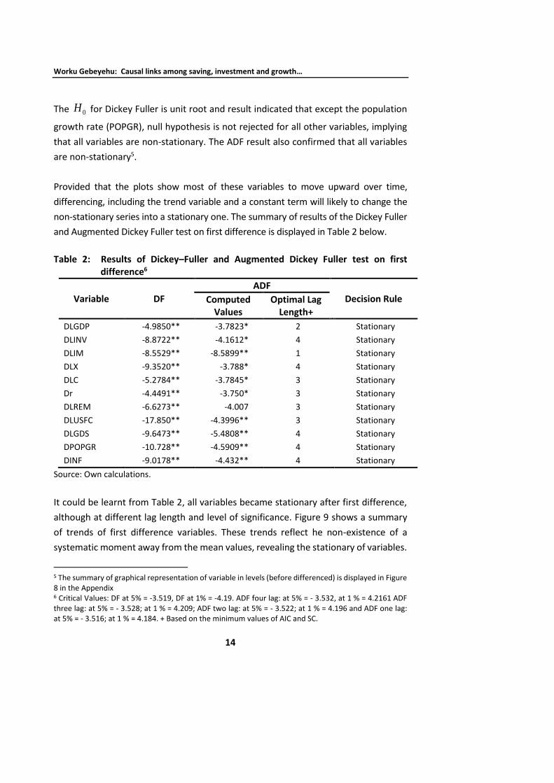
The 0H for Dickey Fuller is unit root and result indicated that except the population
growth rate (POPGR), null hypothesis is not rejected for all other variables, implying
that all variables are non-stationary. The ADF result also confirmed that all variables
are non-stationary5.
Provided that the plots show most of these variables to move upward over time,
differencing, including the trend variable and a constant term will likely to change the
non-stationary series into a stationary one. The summary of results of the Dickey Fuller
and Augmented Dickey Fuller test on first difference is displayed in Table 2 below.
Table 2: Results of Dickey–Fuller and Augmented Dickey Fuller test on first
difference6
Variable DF
ADF
Decision Rule Computed Values
Optimal Lag Length+
DLGDP -4.9850** -3.7823* 2 Stationary
DLINV -8.8722** -4.1612* 4 Stationary
DLIM -8.5529** -8.5899** 1 Stationary
DLX -9.3520** -3.788* 4 Stationary
DLC -5.2784** -3.7845* 3 Stationary
Dr -4.4491** -3.750* 3 Stationary
DLREM -6.6273** -4.007 3 Stationary
DLUSFC -17.850** -4.3996** 3 Stationary
DLGDS -9.6473** -5.4808** 4 Stationary
DPOPGR -10.728** -4.5909** 4 Stationary
DINF -9.0178** -4.432** 4 Stationary
Source: Own calculations.
It could be learnt from Table 2, all variables became stationary after first difference,
although at different lag length and level of significance. Figure 9 shows a summary
of trends of first difference variables. These trends reflect he non-existence of a
systematic moment away from the mean values, revealing the stationary of variables.
5 The summary of graphical representation of variable in levels (before differenced) is displayed in Figure 8 in the Appendix 6 Critical Values: DF at 5% = -3.519, DF at 1% = -4.19. ADF four lag: at 5% = - 3.532, at 1 % = 4.2161 ADF three lag: at 5% = - 3.528; at 1 % = 4.209; ADF two lag: at 5% = - 3.522; at 1 % = 4.196 and ADF one lag: at 5% = - 3.516; at 1 % = 4.184. + Based on the minimum values of AIC and SC.

Ethiopian Journal of Economics, Volume XIX, No. 2, October 2010
15
The test for stationarity for investment variable (DLIV) is done together with the
explanatory variables of the saving function to understand its behaviour as we will
test for causality between saving and investment in the later stage.
3.1.2. Co-integration test
Provided that the variables are non-stationary at levels, the next step is to test for co-
integration at two different levels. First, a bivariate regression of the saving variable
(LGDS) on each of the explanatory variables is made for Engle – Granger and
Augmented Engle Granger test for co-integration on the basis of the error term.
The Engle – Granger Causality test indicated that except interest rate (r), inflation rate
(INF) and population growth parameter (POPGR), residuals of all bivariate estimates
of saving (LGDS) on all other explanatory variables are co-integrated of order 1. The
next step is to estimate a multivariate model on saving (LGDS) on all variables co-
integrated with saving.
Table 3: Test Results of the Engle – Granger Co-integration Test7
Residuals Saved from
(.)GDS F= DF
ADF
Decision Rule Computed values
Optimal Lag Length+
LGDP -4.1871** -3.6459* 2 Co-integrated LIM -8.5529** -4.1404* 4 Co-integrated
LX -4.936** -3.6515* 4 Co-integrated
LGC -4.1210* -3.9770* 3 Co-integrated
R -3.743* -3.743* 0 Not-cointegrated
LREM -4.3904** -3.7975 3 Co-integrated
LUSFC -4.3993** -3.5654* 3 Co-integrated
POPGR -4.9247** -4.9247** 0 Not-cointegrated
INF -4.5233** -4.5233** 0 Not-cointegrated
Residual from multivariate regression
-4.9346** -4.159** 4 Co-integrated
Source: Own calculations.
7 Critical Values for DF: at 5% = -3.514, at 1% = -4.178; ADF: Lag 4: 5% = -3.525; 1% = -4.202; ADF: Lag 3: 5% = -3.522; 1% = -4.196; ADF: Lag 2: 5% = -3.519; 1% = -4.19; + Based on the minimum values of AIC and SC.

Worku Gebeyehu: Causal links among saving, investment and growth…
16
The ADF test on the residual of multivariate co-integrating equation indicated that
individually co-integrated variables with the saving function are jointly co-integrated8.
Before we estimate the final error correction model, the correlation matrix of
independent or predetermined variables is estimated as shown below in Table 4.
Table 4: Correlation Matrix of Independent Variables
REM INF LGC LGDS LUSFC LIM LX POPGR
REM 1.0000 0.060936 0.18038 0.049008 0.0066465 0.030069 -0.0488 -0.0068
INF 0.060936 1.0000 0.53272 0.032368 0.14581 0.17669 0.055952 0.14572
LGC 0.18038 0.53272 1.0000 0.54048 0.59131 0.64347 0.44772 0.16066
LGDS 0.049008 0.032368 0.54048 1.0000 0.77618 0.80285 0.70278 0.29401
LUSFC 0.0066465 0.14581 0.59131 0.77618 1.0000 0.98059 0.88760 0.016970
LIM 0.030069 0.17669 0.64347 0.80285 0.98059 1.0000 0.89553 0.059704
LX -0.0488 0.055952 0.44772 0.70278 0.88760 0.89553 1.0000 -0.10656
POPGR -0.0068 0.14572 0.16066 0.29401 0.016970 0.059704 -0.10656 1.0000
Source: Own computations.
3.2. Error correction model
Most explanatory variables are found to be co-integrated of order 1. Estimating
difference equation of the saving variable (DLGDS) on differences of other variables
would give a robust estimate in econometric sense, but it could only show the short
run or the transitory effect of these variables on saving. Economic policy decision
requires marginal and total effects of predetermined and exogenous variables on the
dependent or target variable. Thus, the error correction model (ECM) is estimated to
capture both transitory and long run effects. The error correction term is captured
from the first lag of the residuals of the multivariate equation. Apparently, we could
observe from Figure 11 of the Appendix that the residual of the multivariate co-
integrating equation is stationary oscillating its zero mean value. The over
parameterization model for estimating the error correction model (8) captures first
8 The trend of co-integrated variables is displayed in Figure 10 below.

Ethiopian Journal of Economics, Volume XIX, No. 2, October 2010
17
differences of co-integrated variables, the non-nonintegrated variables at levels and
the error correction term.
After a series of iteration, the parsimonious estimated ECM with the major diagnostic
test statistics result is summarized in Table 5 below.
Table 5: Error correction model results
Variable Coefficient Std. Error T-value Prob.
Constant -0.0125 0.039625 3.17 0.0
DGDP 0.10581 0.0538 2.1 0.03
DLGC-1 -0.46688 0.2035 -2.29 0.029
DLX 0. 0124 0.02048 2.02 0.024
DLIM 0.346976 0.2751 1.26 0.216
DLRM 0.0818217 0.0557 1.48 0.149
DLUSFC -5.02955 3.303 -1.52 0.138
POPGR 0.15999 0.10628 1.505 0.154
R 0.0096 0.13728 1.43 0.155
INF -0.0530674 0.007328 -3.15 0.001
INF-2 -0.0155380 0.008273 -1.88 0.07
ECT-1 -0.716116 0.2858 -2.51 0.019
Sigma = 0.40893 RSS = 3.01002492 2R = 0.792061, F (30, 12) = 298 [0.009]. Log
likelihood = -4.24527 DW = 2.21 No of Observation = 42. ARCH -2 (1) = 0.05. Reset -
2(1) = 0.061.
Source: Own Calculations.
After a series of experimental estimation, the parsimonious equation estimates reveal
six significant coefficients among eleven parameters (excluding the intercept term).
On the basis of F – test, 2R and the other tests, the model is statistically significant to
describe the short and long run relationships. The stability of the model is also
confirmed through the use of Chow Test. The power of the model to predict the actual
values of the LGDS is also tested using graphical analysis. Both results are displayed in
Figure 12 and 13 in the Appendix. The 1ECT − is the error correction term
demonstrating the long run relationship of variables with the error term and it

Worku Gebeyehu: Causal links among saving, investment and growth…
18
appeared with statistically significant coefficient and expected usual sign. It shows the
process of the long term adjustment towards equilibrium once saving diverges from
equilibrium.
The result confirms the importance of GDP or economic growth in the saving
processes. The level of current income positively and significantly influences the
behavior of aggregate saving rate. This result supports the absolute income
hypothesis in that the level of income is an important determinant of the capacity of
a country to save. However, the aggregate nature of the data does not allow the effect
of distribution of income on saving or the level of saving rates for different income
categories. Lag government consumption (LGC-1) has significant and negative impact
on the level of current saving.
The estimates on the population growth are not statistically significant. This is in line
with our expectation that population growth has a mixed effect on saving. The higher
the rate of growth of population, the larger the number of people joining the active
age group with the capacity to save, which tends to boost the level of saving. However,
because of lopsided population structure towards the dependent age group, the
increasing rate of population may even lead to a more than proportionately increase
in consumption and thus reduction in saving. The insignificant coefficient for the
demographic variable (POPGR) is an indication of the inability of either of the two
effects to outweigh the other. Neither the attempt to change the rate of population
growth with proportion of the people in the active age of group (15 to 64 years)
changes the result.
The coefficient for nominal interest rate (r) is positive as expected but found to be
insignificant. This does not however lead to a conclusion that interest rate does not
have a role to mobilize saving. The rate of interest has been set by the government
and revisions have been made less frequently. Thus, the administratively set rate does
not necessarily reflect the market clearing rate. Particularly before 1992, government
was directly involved in credit rationing and this policy clearly used to distort the
financial market in terms of mobilizing savings. Since 1991/92, the incumbent
government has provided more opening to the financial market and yet the upper and
lower bounds of interest rates are still set by the National Bank of Ethiopia. This has
greatly limited the role of financial markets to link up the demand for loanable funds

Ethiopian Journal of Economics, Volume XIX, No. 2, October 2010
19
with the supply (Authukorala and Worku, 2006). For this reason, interest rate in
Ethiopia does not reflect the opportunity cost of current consumption relative to
future consumption and thus does not provide adequate guide on the basis of which
economic agents adjust their decisions.
Because of the need to capture the effect of the change in real interest rate, inflation
rate (INF) was incorporated in the saving function with the nominal interest rate. As
it is expected, current inflation rate (INF) has a significant negative impact on saving.
This is contrary to the hypothesis and of the result of Athukorala and Sen (2004) that
‘when faced with inflation, consumers attempt to maintain a target real wealth
relative to income by reducing consumption’. The empirical result rather suggests that
in a country where a largest segment of the population live in amidst of poverty, as
risk averse economic agent, consumers tend to utilize their income in the current
period before it looses its value in the coming future. Inflation in this context is a tax
on saving.
Although migration into the developed world has a damaging economic effect as it is
mainly in the form of a brain drain, remittance has now become a significant source
of income into the developing world including Ethiopia. According to the World Bank
(2006), remittance has exceeded US$ 233 billion worldwide by 2005. [Brown, 1994]
indicated that migrants' savings and investment abroad may represent a substantial
or even the major part of their overall transfers. World Bank (2006) attributed this
remittance to an increase in altruistic payments of migrants to their families abroad.
Sinning (2007) indicated that savings in the home country is one of the motives for
remittance. In this study, LRM has shown a positive and yet insignificant value. This
might tends to shade light about the positive impact of remittance on saving.
However, because of the macro nature of the data, it is difficult to capture the saving
behavior of individuals, who benefit out of remittance.
Export proceeds (LX) have shown a positive and statistically significant impact on
saving as it positively influences the trade balance and thus the capacity of the country
to save. On the other side, coefficient for the imports (LIM) is not statistically
significant although shows a theoretically unanticipated positive association with
saving. It could be because of the fact that in the Ethiopian case, imports normally
exceed over and above export revenues and they are largely financed by foreign loan

Worku Gebeyehu: Causal links among saving, investment and growth…
20
and aid. Thus, import revenue may not have a short or a transitory direct effect on
savings.
The theory of the relative income hypothesis suggesting that demonstration effect
has an impact on consumption pattern of households and this effect transcends
across boundaries is not backed by empirical evidence in the case of Ethiopia. Despite
the fact that the level of US consumption is found to be negatively associated with the
Ethiopian domestic saving, it is not found to be statistically significant. This could be
because of various reasons. There is a huge variation in the living standards of the
people of two countries. Owing to Ethiopia’s unique historical background of being
out of cultural domination of any country, associating its consumption pattern and
expenditure on a specific country on the basis of the relative income hypothesis may
not give sound evidence.
3.3. Granger causality between saving and investment
Granger causality test has been undertaken to confirm whether the long-established
view of development economists suggesting that saving is a necessary requisite for
investment and of growth or the recent theoretical literature arguing that saving is
never a constraint on investment. The result is indicated in Table 6 below.
Table 6: Pair-wise Granger causality test: Saving and investment (1962-2004)9
Null Hypothesis Observation
Optimal lag
length for
the test*
Computed
F-Statistic
Decision
Rule
Investment does not Granger cause
saving 42 6 1. 4923** Accepted
Saving does not Granger cause
Investment 42 6 1.2300 Accepted
Source: Own calculations.
The econometric result in this particular study reveals that investment does not
Granger cause saving and saving does not Granger cause investment. This might be
because of the fact that in the Ethiopian case, the role of domestic saving in financing
9 Critical F (28,6): at 1% = 4.02; at 5% = 2.92.

Ethiopian Journal of Economics, Volume XIX, No. 2, October 2010
21
investment is extremely limited. This is clearly observed from the external trade
balance as well as the saving-investment gap of the country. This result seems to go
in line with Moore (2006) hypothesis that ‘Saving is never a constraint on investment’.
Nonetheless, this conclusion does not necessarily imply that countries may not need
to save in order to develop their economies.
Depending heavily on foreign sources for investment is likely to impose high debt
burden and policy interference by lending or foreign capital source countries. In
addition to foreign loan and aid, the other source of external finance is FDI. The
economic impact FDI on sustainable development of countries has remained to be
controversial because of the various motives [Athukorala and Worku, 2003] and
asymmetric information and moral hazard issues. Thus, promoting domestic saving is
not only a more reliable source of sustainable development as it reduces dependence
on foreign sources but also boosts the level of investment of the country, which has
still remained very low.
3.4. Impulse response function: Growth of GDP versus saving
The results of the vector autoregressive (VAR) model for saving and GDP in Table 7
indicates that past growth rate of real per capita income has a strong and robust
prediction power on current saving rate performance.
Table 7: VAR Estimation Results on Saving and GDP Growth for 1962-2004
Variables LGDS (Saving) LGDP (GDP)
saving(-1)
saving (-2)
0.5881***
(0.1703)
0.3417**
(0.16339)
0.0551
(0.3766)
0.0238
(0.3613)
Growth(-1)
Growth (-2)
0.1646**
(0.07439)
0.0021
(0.0779)
0.1939
(0.1645)
-0.507***
(0.1722)
Note: The numbers in parenthesis are standard errors for the corresponding coefficients.
*,**,*** refer to significance levels at 10, 5 and 1 percent, respectively.

Worku Gebeyehu: Causal links among saving, investment and growth…
22
However, GDP growth rate does not seem to be strongly predictable by past domestic
saving performance. The weak, short-run dynamic relationship between past saving
rate and current growth performance, albeit positive, might suggest weaknesses in
allocation of saving to their most productive uses that can sustain and attract further
saving efforts. The short term relation, however, should not be interpreted as if saving
rate does not also have long term effect. A country still finances part of its investment
from external borrowing and grants, this may not however continue in the long term
since the economy would reach unsustainable level of external indebtedness. Rather
failure to improve the saving rate might continue to negatively affect the domestic
capacity of capital formation and thus sustainable development of the economy10.
The empirical result suggests that an increase in the saving rate is likely to boost the
level of GDP and thus creates disequilibrium for a while. Adjustment for the shock
could take up to a period of 20 years. The implication is that a one shot increase in the
saving rate could positively contribute for the growth the economy and yet may not
bring about a sustained increase in the pace of growth of the economy. A continuous
improvement in the level of growth needs continuous rise in the saving rate, which
may not be easy. Thus, in addition to improving the saving rate, it is also worthwhile
to invest on human capital and technical progress to bring about a consistent rise in
the rate of growth of the economy because of their effect in shifting the production
frontier of the country and help to alleviate the problem of diminishing returns to
capital possibly emanating from investing on the prevailing technology through
increasing saving.
4. Conclusion
The article tried to identify the main determinants of domestic saving in Ethiopia. GDP
growth, previous government consumption level, export and inflation have a
statistically significant impact on saving. The error correction term is also found to be
statistically significant indicating the existence of a long run relationship between
these explanatory variables and the saving parameter. Remittance, interest rate and
the US consumption level are found to be statistically insignificant but with the
10 The graphical representation of the impulse response function establishing the relationship between LGDS and LGDP10 is shown in Figure 14 of the Appendix.

Ethiopian Journal of Economics, Volume XIX, No. 2, October 2010
23
expected sign of causality. The Granger causality test indicates that saving does not
cause investment neither does investment cause saving. This is because of the heavy
reliance of the country for investment. The vector auto-regressive model indicates
that there is a positive short and long-run effect of saving on growth, which is not yet
significant. Income growth has been seen to have statistically significant positive
impact on saving. The impulse response function reveals the relevance of the Solow
growth model to explain the relationship between saving rate and growth of GDP in
the Ethiopian context.
The empirical result suggests the need for revisiting the policy environment to induce
growth from inside. Barriers of financial markets including setting interest rate by
government bodies might need to be looked into. The public should be encouraged
to participate in the saving schemes of their choice and invest on various areas of the
economy. Government should also need to look into the possible crowding out effect
of excessive public expenditure and continue its move towards promoting exports.
Although remittances are not found statistically significant impacts on saving, their
importance on reducing foreign dependence should not be under looked. The country
has many people in the Diaspora. Besides the remitting meager resources to the
country, Ethiopians abroad need to be fully engaged into the country’s development
endeavors through mobilization of their savings. For this to come by, it requires
investigating possible hurdles that might have constrained investment flows from this
source in terms of policy, bureaucratic inefficiency, lack of investment promotion
activities or other areas of concern and accordingly making the necessary measures
to create a more accommodative and enabling environment.

Worku Gebeyehu: Causal links among saving, investment and growth…
24
References
Abu Girma Moges. 2004. On the Determinants of Domestic Saving in Ethiopia. Paper prepared for the Second International Conference on the Ethiopian Economy. Ethiopian Economic Association, June 3-5, 2004.
Athukorala, Prema Chandra and Sen Kunal. 2004. Determinant of Private Saving in India,
World Development, Elsevier Ltd., Vol. 32, No. 3, PP. 491 – 503.
Athukorala, Prema Chandra and Worku Gebeyehu. 2006. Trade Performance and
Manufacturing Performance in Ethiopia, in Trade, Growth and Inequality in the
Era of Globalization, eds. Kishore Sharma and Oliver Morrissey, Rutledge Taylor
and Francis Group, London.
Athukorala, Prema Chandra and Worku Gebeyehu. 2003. Foreign Direct Investment and
Trade: Diagnostic Trade Integration Study, Addis Ababa, Unpublished.
Attanasio, Ozario, Lucio Picci and Antonello Scorcu. 2000. Saving, Growth and Investment:
A Macroeconomic Analysis using a Panel of Countries, The Review of Economics
and Statistics, 82(2): 182-211.
Bacha, E. L. 1990. A Three – Gap Model of Foreign Transfers and the GDP Growth Rate in
Developing Countries, Journal of Development Economics, Vol. 32, PP. 279 – 96.
Brown, R. P. C. 1994. Migrants' Remittances, Savings and Investment in the South Pacific,
International Labor Review, 133(3): 347{367.
Browning, Martin and Thomas Crossley. 2001. The Life Cycle Model of Consumption and
Saving, Journal of Economic Perspectives, 15:3, pp 3-22.
DeGregorio J. 1992. Economic Growth in Latin America, Journal of Development
Economics, Vol. 39, PP. 59 - 84.
Domer, E. D. 1946. Capital Expansion, Rate of Growth and Employment’, Econometrica,
Vol. 14, PP 1057 – 72.
Duesenberry, J. 1949. Income, Saving and the Theory of Consumer Behaviour, Cambridge:
Harvard University Press.
Easterly, William. 1994. Economic Stagnation, Fixed Factors, and Policy Thresholds,
Journal of Monetary Economics, 33: 525-557.
Gavin, M. R. Hausmann and E. Talvi. 1997. Saving Behaviour in Latin America: Overview
and Policy Issues, in R. Hausmann and Reisen R. (eds). Promoting Savings in Latin
America, OECD and Inter – America Development Bank, Paris.
Gujarati, D. 2003. Basic Econometrics, 3rd Edition, Mc Graw-Hill, New York.
Jappelli, T. and M. Pagano. 1996. The Determinant of Saving: Lessons from Italy, Paper
Presented at the Inter – America Development Bank Conference on Determinants
of Domestic Saving in Latin America, Bogota, Colombia.

Ethiopian Journal of Economics, Volume XIX, No. 2, October 2010
25
Levine, Ross and David Renelt. 1992. A Sensitivity Analysis of Cross-Country Growth
Regressions, American Economic Review, 82: 942-963.
Harrod, R. 1939. An Essay in Dynamic Theory, Economic Journal, Vol. 49, PP. 14-33.
Loayza, Norman; Klaus Schmidt-Hebble; and Luis Serven. 2000. What Drives Private Saving
around the World? The Review of Economics and Statistics, 82(2): 165-181.
Modigliani, Franco. 1986. Life Cycle, Individual Thrift and the Wealth of Nations, The
American Economic Review, 17(3): 297-313.
Moore, Basil. 2006. Saving is never a Constraint on Investment, South African Journal of
Economics, Vol.74: 1.
Ogaki, Masao, Jonathan Ostry and C.M. Reinhart. 1996. Saving Behavior in Low - and
Middle- Income Countries: A Comparison, IMF Staff Papers, 43(1): 38-71.
Otani, I and D. Villanueva. 1990. Long term Growth in Developing Countries and Its
Determinants: An Empirical Analysis, World Development, Vol. 18, PP. 90 – 98.
Paul R. 1986. Increasing Returns and Long Run Growth, Journal of Political Economy’,
(October 1986), 1002 – 37.
Rebello, Sergio. 1991. Long-Run Policy Analysis and Long-Run Growth, Journal of Political
Economy ,99: 500-521.
Rodrik, Dani. 2000. Saving Transitions, The World Bank Economic Review, 14(3): 481-507.
Romer, Paul M. 1986. Increasing Returns and Long Run Growth. Journal of Political
Economy, 99: 500-521.
Saltz, I. S. 1999. An Examination of the Causal Relationship between Savings and Growth in the
Third World, Journal of Economics and Finance, Vol. 23, PP. 90 – 83.
Sinha, D. 1991 and T. Sinha. 1998. Cart before the Horse? The Saving – Growth Nexus in
Mexico, Economic Letters, Vol. 61, PP. 43 - 47.
Sinning, Mathias. 2007. Determinants of Savings and Remittances Empirical Evidence from
Immigrants to Germany, RWI Essen and IZA Bonn
Solow, R. 1967. A Contribution to the Theory of Economic Growth. Quarterly Journal of
Economics, 70 (February 1956, 65 – 94).
Worku Gebeyehu. 2005. Has Privatization Promoted Efficiency in Ethiopia? A Comparative
Analysis of Privatized Industries vis-à-vis State Owned and Other Private Industrial
Establishments. Ethiopian Journal of Economics, Vol. IX, Number 2, Addis Ababa.
Worku Gebeyehu. 2004. FDI in Ethiopia: Size, Nature and Performance, EEA/Ethiopian
Economic Policy Research Institute, Working Paper No.2/2004, Addis Ababa.
World Bank. 2006. Global Development Finance 2006: The Development Potential of
Surging Capital Flows, World Bank.

Worku Gebeyehu: Causal links among saving, investment and growth…
26
APPENDIX Figure 1: Trend of Ethiopian and US consumption
Figure 2: Trend of Ethiopian and US saving
1960 1965 1970 1975 1980 1985 1990 1995 2000 2005
22
23
24
25
26
27
28
29
30
Domestic Consumption
US Consumption
Years
LC LUSFC
log
USD
Cons
1960 1965 1970 1975 1980 1985 1990 1995 2000 2005 18
20
22
24
26
28
Domestic Saving
US Saving Log
Saving
USD
Years
LGDS LUSDS

Ethiopian Journal of Economics, Volume XIX, No. 2, October 2010
27
Figure 3: Trend of investment and saving
Figure 4: Trend of imports and exports
1960 1965 1970 1975 1980 1985 1990 1995 2000 2005
18.0
18.5
19.0
19.5
20.0
20.5
21.0
Domestic saving
Investment
Year
Log Invest and Saving USD
LINV LGDS
1960 1965 1970 1975 1980 1985 1990 1995 2000 2005
18.5
19.0
19.5
20.0
20.5
21.0
21.5
22.0
Imports
Exports
Year
log Import and Export USD
LIM LX

Worku Gebeyehu: Causal links among saving, investment and growth…
28
Figure 5: Trend of GDP and population growth rate
Figure 6: Trend of interest and inflation
1960 1965 1970 1975 1980 1985 1990 1995 2000 2005
0
10
20
30
Inflation
Interest rate
Fig 6: Trend of interest and inflation
Year
%
r INF
1960 1965 1970 1975 1980 1985 1990 1995 2000 2005
0
5
10
15
20
Population Growth Rate
Log GDP
Year
LGDP POPGR

Ethiopian Journal of Economics, Volume XIX, No. 2, October 2010
29
Figure 7: Trend of remittance
Figure 8: Trends of variable in levels (1960 – 2004)
1960 1980 2000
22.0
22.5
23.0
Fig 8: Trends of Variables in Levels (1960-2004)LGDP
1960 1980 2000
20
21LINV
1960 1980 2000
27
28
29
30LUSFC
1960 1980 2000
26
27
28 LUSDS
1960 1980 2000
18
19
20
21LGDS
1960 1980 2000
19
20
21
22 LIM
1960 1980 2000
19
20
21LX
1960 1980 2000
18
19
20
21LGS
1960 1980 2000
22
23
24LC
1960 1980 2000
15.0
17.5
20.0 LREM
1960 1980 2000
-2.5
0.0
2.5POPGR
1960 1980 2000
0
20
40INF
1960 1965 1970 1975 1980 1985 1990 1995 2000 2005
14
15
16
17
18
19
20
Remittance
Year
Log Remittance in USD
LREM

Worku Gebeyehu: Causal links among saving, investment and growth…
30
Figure 9: Trends of variables in their first difference
Figure 10: Trend of cointegrating variables
1960 1980 2000
15.0
17.5
20.0LREM
1960 1980 2000
-0.25
0.00
0.25
Fig 9: Trends of Variables in their First Difference
DLGDP
1960 1980 2000
0.0
2.5
5.0Dr
1960 1980 2000
-5
0
5DPOPGR
1960 1980 2000
-25
0
25DINF
1960 1980 2000
-0.25
0.00
0.25
0.50DLINV
1960 1980 2000
-0.1
0.0
0.1
0.2DLUSDS
1960 1980 2000
-1
0
1DLGDS
1960 1980 2000
-2.5
0.0
2.5
5.0DLREM
1960 1980 2000
-1
0
1DLC
1960 1980 2000
-0.5
0.0
0.5
1.0DLX
1960 1980 2000
-0.25
0.00
0.25
0.50DLIM
1960 1980 2000
-0.2
-0.1
0.0
0.1DLUSFC
1960 1965 1970 1975 1980 1985 1990 1995 2000 2005
US Consumption
Domestic consumption
GDP
Import
Domestic Saving
Remittance
Export
Year
Log Values
USD
LX LGDS LGDP LC
LIM LUSFC LREM

Ethiopian Journal of Economics, Volume XIX, No. 2, October 2010
31
Figure 11: Error Correction Term from the Cointegrating Equation
Figure 12: Parameter Stability and Chaw Test
1990 2000
-1
0
1
2
Fig 12: Parameter Stability and Chaw TestPOPGR +/-2SE
1990 2000
-1
0
1LX +/-2SE
1990 2000
-2
0LIM +/-2SE
1990 2000
-2
0LGDP +/-2SE
1990 2000
0.0
0.5
1.0LC_1 +/-2SE
1990 2000
-0.1
0.0
0.1
0.2LREM +/-2SE
1990 2000
-10
0
10LUSFC +/-2SE
1990 2000
0
10LUSFC_1 +/-2SE
1990 2000
-0.04
-0.02
0.00INF +/-2SE
1990 2000
-0.025
0.000
0.025INF_2 +/-2SE
1990 2000
0.0
0.5ECT_1 +/-2SE
1990 2000
-0.5
0.0
0.5Res1Step
1990 2000
0.5
1.01up CHOWs 1%
1960 1965 1970 1975 1980 1985 1990 1995 2000 2005
-0.5
0.0
0.5 ECT

Worku Gebeyehu: Causal links among saving, investment and growth…
32
Figure 13: Actual versus fitted residuals
Figure 14: Impulse response function GDP (Growth) caused by change in saving rate
1965 1970 1975 1980 1985 1990 1995 2000 2005
18.5
19.0
19.5
20.0
20.5
21.0
Actual Domestic Saving
Fitted Domestic Saving
LGDS Fitted
0 5 10 15 20 25 30 35 40
0.05
0.10
0.15
0.20
0.25
%
Time
LGDP (LGDS eqn)

Ethiopian Journal of Economics, Volume XIX, No. 2, October 2010
33
Figure 15: Actual GDP versus simulated GDP
1965 1970 1975 1980 1985 1990 1995 2000 2005
22.00
22.25
22.50
22.75
23.00 LGDP Simulated

Worku Gebeyehu: Causal links among saving, investment and growth…
34

35
URBANIZATION AND FERTILITY RATES IN ETHIOPIA1
Fanaye Tadesse2 and Derek Headey2
Abstract
Fertility rates are important determinants of both overall population growth
and demographic transitions from high to low age dependency ratios, which
in turn have important consequences for economic growth, poverty reduction,
and improved health and nutrition outcomes. Ethiopia currently has one of
the highest fertility rates in the world, although there are marked differences
between rural and urban fertility rates. This paper explores the drivers of rural
and urban fertility rates, including systematic tests of differences in key
determinants. This further allows us to project fertility rates into the future
based on alternative urbanization, economic growth, and education
scenarios. Finally, we link these alternative projections with existing estimates
of the benefits of fertility reductions on economic growth, nutrition, and
poverty reduction
1 The final version of this article was submitted in September 2011. 2 Development Strategy and Governance Division, International Food Policy Research Institute – Ethiopia Strategy Support Program II, Ethiopia.

Fanaye and Headey: Urbanization and fertility rates in Ethiopia
36
1. Introduction
Demographic changes have long been recognized as a critical component of economic
development, although there is considerable debate about whether population helps
or hinders development, and whether governments can substantially alter population
growth rates. With regard to the first of these debates, Malthusian arguments that
population growth induces food supply constraints have been viewed with skepticism
by most economists, given the possibility of population-induced technological change
in both agriculture (Boserup 1965) and industry (Henderson 2010), with the latter
capable of financing food imports. More recently, David Bloom and colleagues (Bloom
et al. 2007; Bloom and Williamson 1998) have argued that the change in age
structures matters more than population growth per se, with the transition from low
to high age dependency ratios inducing higher savings rates and greater investments
in education. In successful Asian countries, this demographic “window of
opportunity”—chiefly induced by lower fertility rates—explains 25–40% of the
region’s miraculous economic growth. High population growth has also been
associated with increased poverty (Eastwood and Lipton 2004) and increased
malnutrition (Headey 2011). However, what is not clear is the extent to which direct
population policies substantially influence fertility rates. Economists view fertility
rates as a demand-led factor heavily influenced by income levels, livelihoods, and
education factors. Efforts to directly influence fertility rates (through contraception
family planning or more draconian measures) may therefore be less important than
these indirect factors. Indeed, even in the Chinese context, the effectiveness of the
country’s one-child policy is heavily debated among demographers.3
In Ethiopia these debates are highly relevant. Although the country is undergoing
rapid economic growth (albeit from a low base), Ethiopia has a long history of
Malthusian population dynamics (Pankhurst 1985). In the middle ages, rapid
population growth and the resultant deforestation of the population dense highland
areas contributed to the collapse of the agricultural bases of several early empires,
3 For example, Hasketh, Lu, and Xing (2005) observe: "The policy itself is probably only partially responsible for the reduction in the total fertility rate. The most dramatic decrease in the rate actually occurred before the policy was imposed. Between 1970 and 1979, the largely voluntary "late, long, few" policy, which called for later childbearing, greater spacing between children, and fewer children, had already resulted in a halving of the total fertility rate, from 5.9 to 2.9. After the one-child policy was introduced, there was a more gradual fall in the rate until 1995, and it has more or less stabilized at approximately 1.7 since then."

Ethiopian Journal of Economics, Volume XIX, No. 2, October 2010
37
which eventually led to its downfall. In more recent times Ethiopia has sadly become
notorious for some of the worse famines of the 20th century. And although there are
large tracts of largely uninhabited land in the lowland peripheries of Ethiopia, the
population-dense highlands face shrinking farm sizes and major problems of
deforestation and soil degradation (Ringheim, Teller, and Sines 2009; Yusuf et al.
2005). These problems are clearly related to population growth rates that are too high
relative to the local resource base and to traditional farming practices. Indeed, the
total population is estimated to be growing at 2.6 percent per year, chiefly as a result
of high fertility in rural areas (CSA 2008). Moreover, Demographic Health Survey
(2010) data suggest that Ethiopia not only has one of the largest fertility rates in the
world (at 5.4 children in 2005), the country also has the largest rural-urban fertility
differential in the world: in 2005 an average rural woman can be expected to give
birth to 6 children in her lifetime, relative to just 2.4 children in urban areas.
The federal government of Ethiopia clearly recognizes the importance of reducing
fertility rates. A National Population Policy was initiated in 1993 when the current
government took power, with the general objective of harmonizing the relationship
between population dynamics and other factors that affect the country’s
development. The specific objectives of the policy include raising the contraceptive
prevalence rate among married women from 4 percent in 1990 to 44 percent by 2015,
raising the age of marriage from 15 to 18 years, and reducing the total fertility rate
from 7.1 children in 1990 to 4 children in 2015. However, the most recent DHS data
show achieving these targets is a remote possibility. For example, in 2005 only 15
percent of married women used either a traditional or a modern method of
contraception. And despite a significant decline in mortality rates (from 217 to 123
deaths per 1000 live births between the late 1980s and 2004) the decline in fertility
rates has been gradual, declining to 5.4 children in 2005 (CSA 2005).
Given the critical welfare consequences of reducing the fertility rate, this study
explores the determinants of fertility rates in Ethiopia. However, unlike most previous
studies (reviewed in Section 2) we systematically disaggregate explanations of fertility
rates in rural and urban areas. This is important precisely because Ethiopia has
unusually large rural-urban fertility differentials, but also because Ethiopia is currently
one of the most under-urbanized countries in the world, and is therefore predicted to
urbanize rapidly in coming years. Our approach also allows us to rigorously test

Fanaye and Headey: Urbanization and fertility rates in Ethiopia
38
whether rural and urban fertility have different determinants using the 2005
Ethiopian Demographic and Health Survey (described in Section 3). Specifically, the
econometric tests reported in Section 4 allow us to explore whether the determinants
of rural and urban fertility rates are different, whether these determinants have
statistically different magnitudes, and whether the rural-urban fertility differential is
explained by observed factors (such as rural-urban education or wealth differences)
or unobserved factors (such as the impact of urban living on attitudes). Given the
various interactions between urbanization and fertility differentials—as well as
economic growth and education—a second objective of this paper is to project
fertility rates into the future, based on alternative urbanization and development
scenarios (Section 5). This in turn allows us to re-estimate alternative age dependency
paths for Ethiopia, which have consequences for important welfare objectives, such
as economic growth and poverty reduction. Section 6 concludes by reviewing our
main results and their implications for Ethiopia’s development strategies.
2. A review of existing theories and evidence
As we noted above, the relationship between fertility and economic development has
captured the interests of many economists and is still a controversial subject. In this
section we aim to briefly overview economic theories of fertility, and theories of the
impact of fertility rates on economic growth. The former is clearly relevant for the
specification of our fertility regressions (Section 4), while the latter is pertinent for our
projections of the impact of fertility on economic growth and poverty reduction.
In terms of the underlying socioeconomic determinants of fertility (as opposed to the
proximate health-related determinants), economic theories of fertility have long
focused rigorously separate supply and demand factors, with cultural preference
(related to religion, for example) treated as exogenous. Economic theories also
tended to emphasize demand side factors, as opposed to supply side constraints, such
as access to contraceptives. For example, Becker (1960) introduced a number of
important economic concepts that led to the construction of demand side theories.
One important notion is that children possess both consumption good characteristics
(i.e. they yield utility or happiness to their parents) and investment good

Ethiopian Journal of Economics, Volume XIX, No. 2, October 2010
39
characteristics (e.g. they can provide security for parents in their old age, and provide
labor and income for the household, such as farm labor or remittances).
A second notion is that of quality and quantity tradeoffs, which posits a likely
substitution from quantity to quality as family income increases (Becker and Lewis
1973). A third notion is that of opportunity costs. In other words, while children yield
benefits, they also come with both explicit costs (feeding, education, and so on) and
implicit costs (such as the time required for rearing children, which could be applied
to other activities). This implies that parental demand for children is very much a
function of a variety of individual and social livelihood factors, such as location,
occupation, land-labor ratios, costs and returns to education, female wages, and the
development of formal social security systems. In addition to these economic factors,
infant mortality rates are another demand-side factor deemed to be positively related
to fertility rates, since a greater likelihood of infant death requires a family to have
more births in order to reach its desired number of children. In some cultures there
are also gender preferences that may lead parents to have larger numbers of children
in the hope of satisfying a threshold demand for male children. It has also been noted
that religious factors may influence the demand for children. For example, Muslim
populations tend to have higher fertility rates than non-Muslim populations (both
within and between countries), although this effect may relate more to slower
transitions (Westoff and Frejka 2007).
A wide range of studies have attempted to test these theories with both cross-country
and household level data. One stylized fact consistent with the demand-side view of
fertility decisions is that individual’s desired number of children often closely matches
their actualized number of children, at least in an approximate fashion. Infant
mortality rates and fertility rates are also very closely correlated both across countries
and within them (Ben-Porath 1976; Benefot and Schultz 1996; Murthi, Guio, and
Drèze 1995). Some research has found a negative correlation between family size and
child quality that supports the Becker and Lewis (1973) theory (Rosenzweig and
Wolpin 1980; Li, Zhang, and Yi 2005). Incomes also have a pervasively positive effect
on fertility, especially over the longer run, but there are gender nuances at work,
especially in the short run (Schultz 1997). In cases where the husband’s income
increases fertility rates may increase as the family has an increased ability to support
more children (Freedman and Thornton 1982). On the other hand, an increase in the

Fanaye and Headey: Urbanization and fertility rates in Ethiopia
40
wife’s earning from her participation in the labor force is shown to have a negative
substitution effect by making childbearing a costly activity for the household
(McNown 2003; Engelhardt, Tomas, and Alexia 2004; Foster & Rosenzweig 2006).
Similarly, more women’s education tends to reduce fertility (Jain 1981; Chaudhury
1986; Axinn 1993; Bledsoe and Cohen 1993), partly through female labor force
participation and higher wages (i.e. higher opportunity costs), and partly through
supply side factors such as increased knowledge of contraception, and a later age of
first marriage. However, the level of education that can affect fertility decisions is still
not clear. In most studies it seems only secondary and tertiary education is found to
significantly affect fertility, but some studies have found some significant negative
impact even with primary level education (Dzekedzeke and Nyangu 1994; Garenne
2008). On the other hand, Jain (1981) found that a small amount of education in least
literate societies might initially increase fertility at the early stage of development due
to a positive income effect.
In terms of the effect of urbanization on fertility, it has long since been established
that urban fertility rates are pervasively lower than rural fertility rates, especially in
poor countries (Kuznets 1974). The urban fertility in Sub-Saharan Africa is on average
almost 30 percent lower than the rural fertility (Shapiro and Tambashe 2000; Dudley
and Pillet 1998). Table 1 shows the most recent rural and urban fertility rates based
on Demographic Health Surveys conducted in the last 5 years (DHS 2010). The table
shows that while urban fertility rates are lower than rural rates everywhere, the
differential in Ethiopia (at 3.6 children) is much larger than the African average (2.0
children), and is indeed the highest of any country surveyed by the DHS.

Ethiopian Journal of Economics, Volume XIX, No. 2, October 2010
41
Table 1: Rural and urban fertility differentials in Ethiopia in relative terms
Rural Urban Difference Number of countries
Ethiopia 6.0 2.4 -3.6
Africa 6.1 4.1 -2.0 23
Asia 3.3 2.5 -0.8 8
Central Asia & MENA 2.6 2.2 -0.4 9
Latin America 3.7 2.4 -1.3 10 Source: DHS (2010).
Note: MENA: Middle East and North Africa
What is less clear, however, is how exactly urban living reduced fertility rates. There
are obviously some expected channels. As a stylized fact, mean incomes are
pervasively higher in urban areas (even when adjusted for smaller household size),
women tend to engage more in wage labor, paternal and maternal education levels
are higher, infant mortality rates are lower, and there is generally better access to
contraceptives in urban areas. Moreover, while there is always a rural-urban
differential in fertility, urban fertility rates still vary both across countries and within
countries. For instance, in the case of Addis Ababa, the nation’s capital, the total
fertility rate (TFR) dropped from 3.3 to 1.9 between 1990 and 2000, which is even
below the population replacement rate. However, the contraceptive prevalence rate
was only 34 percent in Addis Ababa in 2000, such that the drop in the TFR occurred in
the absence of any considerable family planning initiatives (Sibanda et al. 2003).
Hence there are many puzzles still unanswered with respect to the precise channels
through which urbanization influences fertility trends.
Existing work has illuminated these questions somewhat. Kirk and Pillet’s (1998) study
of fertility trends in sub-Saharan Africa found a widening rural-urban fertility
differential at early stages of fertility declines (this is also evident in Table 1), and that
this differential was not satisfactorily explained by other rural-urban differences, such
as household wealth or female education. This was in contrast to Asian countries
where the rural-urban fertility differentials were smaller and more easily explained by
differences in education, wealth, and other factors. Hence in the African context in
general, and in Ethiopia in particular, further research is still needed to explain these
much wider rural-urban fertility differentials.

Fanaye and Headey: Urbanization and fertility rates in Ethiopia
42
However, previous work in Ethiopia has not examined this issue in any comprehensive
fashion. Several studies that have been done on fertility under the Ethiopian context
employ the Bongaarts framework to identify the proximate determinants of fertility
such as contraceptives, postpartum insusceptibility, sterility, abortion, and marriage
(Hailemariam and Zewoldi 1994; Population Studies and Training Center 2003;
Sibanda et al. 2003; World Bank 2007; and of course the main descriptive results of
the 2000 and 2005 DHS surveys (Central Statistical Agency [Ethiopia] and ORC Macro
2001, 2006). Others focus on segments of the population to look into the fertility
determinants. For instance, Alemayehu et al. (2010) look into determinants of
adolescent fertility in Ethiopia and a study by Gurmu and Mace (2008) focuses on the
link between fertility and poverty in Addis Ababa.
A 2007 World Bank report is also comprehensive in using both DHS data to explore
both proximate and underlying determinants of fertility, and an economy-wide
macroeconomic simulation model (a computable general equilibrium model) to look
into the impact of demographic change on economic outcomes such as consumption
growth and savings. That analysis showed that two of the proximate determinants of
fertility in Ethiopia are the age at marriage and first birth, and the extremely low use
of contraceptives. Both age at marriage and contraceptive use were found to be much
lower in rural areas, albeit with regional variation. To underlying determinants the
study ran both aggregate and rural and urban regressions on the 2000 Ethiopian
Demographic Health Survey (EDHS) with disaggregations by age groups. However, no
systematic tests were conducted, nor was there any investigation of why urbanization
seemed to reduce fertility, although it did note an association between urban living
and secondary education. Finally, in terms of macroeconomic modeling the study
indicated that fertility will most likely continue to reduce quite quickly if the
government achieves its education targets, and that this fertility reduction will
produce a so called “demographic dividend” in the form of faster growth in per capita
consumption.
Although the World Bank study and others have made impressive contributions to
this literature, to our knowledge there exists no comprehensive study that separately
looks into the social and economic causes of fertility in rural and urban Ethiopia,
particularly with regard to explaining why the rural-urban fertility differential is so
unusually large. Hence, in this study we try to more systematically test for rural urban

Ethiopian Journal of Economics, Volume XIX, No. 2, October 2010
43
differences in fertility determinants through a range of econometric tests described
in the next section.
3. Data and estimation
3.1. Data
The data used for this study is EDHS (Ethiopian Demographic and Health Survey) of
2005. The EDHS is a nationally representative survey of 14,070 women between the
ages of 15 and 49 and 6,033 men with ages between 15 and 59. This survey is
conducted in Ethiopia as part of the worldwide Demographic and Health Surveys
(DHS) project (CSA 2005). The survey contains information on the population and
health situation of the country. Some of the topics covered include family planning,
fertility levels and determinants, fertility preferences, child and maternal mortality,
child health, nutrition, and knowledge of HIV/AIDS. Table 2 provides a list of the
variables used in this study (some of which are constructed by the authors), including
definitions and measurement issues.
The sample for the survey was designed to provide representative estimates for the
variables of interest for Ethiopia as whole, urban and rural areas as separate domains,
and 11 geographic areas with 9 regions and 2 city administrations (CSA 2005). The
sample selection was done in two stages with 250 clusters (145 urban and 395 rural)
selected from the list of enumeration areas4 (EAs) from the 1994 population and
housing census sample frame. The sample was also drawn from the 1994 Census
frame. However, CSA (2005) indicates that there could be some bias in the
representativeness of the regional estimates of Somali and Afar regions since the
census frame excluded some part of these regions which were predominantly
nomadic. Since the selected 540 EAs are not distributed proportionally by region
according to the census population, the sample was weighted to produce national
estimates. On the second stage of sample selection the households were randomly
selected from each previously selected cluster.
4 Enumeration areas are formed by subdividing each woreda into convenient areas and are either total urban or rural.

Fanaye and Headey: Urbanization and fertility rates in Ethiopia
44
In addition to the DHS, Geographic Information Systems (GIS) estimates of travel
times to nearest cities were merged with the DHS data based on the coordinates of
the surveyed clusters. The purpose of adding this variable is to have information on
the effects of isolation on fertility rates, and also because the rural-urban divide is
somewhat arbitrary in locations where rural people have good access to cities (e.g.
peri-urban areas). Information on how travel times are estimated can be sourced in
Schmidt and Mekamu (2009).
Ethiopian Journal of Economics, Volume XIX, No. 2, October 2010
45
Table 2: Variable description and measurement issues
Variable name Definition Measurement Issues
Dependent variables
Children-ever-born Number of children-ever-born by a woman Desired children Number of children a woman desires to have in her life time
Explanatory variables
Women’s age Age Age of woman in years Age2 Square of age of woman in years Woman’s Education
These variables are only a measure of quantity and do not measure quality of education. Also, the variable relate to attendance not completion.
No education Woman has not attended any education
Primary Attended primary education
Secondary Attended secondary education
Higher Attended higher education
Husband’s education No education Husband has not attended any education Primary Attended primary education Secondary Attended secondary education Higher Attended higher education
Religion Muslim Dummy to indicate whether the woman is a Muslim Christian Dummy to indicate whether the woman is a Christian
Other religion Dummy to indicate whether the woman has other religion

Fanaye and Headey: Urbanization and fertility rates in Ethiopia
46
Continued from Table 2 Economic status*
1st wealth quintile Dummy=1 if household’s wealth status is poorest quintile
2nd wealth quintile Dummy=1 if household’s wealth status is poor quintile
3rd wealth quintile Dummy=1 if household’s wealth status is middle quintile
4th wealth quintile Dummy=1 if household’s wealth status is rich quintile
5th wealth quintile Dummy=1 if household’s wealth status is richest quintile
Land ownership Ln land Log of land size in hectares
Ln land2 Log of land size in hectares squared
Women’s occupation
Women who have no labor force participation outside of their homes for the past 12 months are the omitted category
Not working Woman doesn’t participate in any work outside of her home
Professional Participates in professional work outside of her home
Clerical and sales Participates in clerical and sales work outside of her home
Agriculture Participates in agricultural work outside of her home
Others Participates in other works outside of her home
Location Distance to health center Travel time (minutes) to the nearest health center Uses the DHS GPS points
Urban Dummy=1 is residence is urban
Listens to radio Dummy=1 if woman listens to the radio frequently Contraceptive knowledge Percentage of people living in the village who know about contraceptives Child mortality
Treated as endogenous variable.* Child mortality* Number of children born alive but died before age five
Notes: * child mortality is treated as endogenous variables because fertility decisions could also cause mortality outcomes within the household. We therefore use cluster level averages of child mortality rates to proxy for expected child mortality.

Ethiopian Journal of Economics, Volume XIX, No. 2, October 2010
47
3.2. Estimation
Following other empirical studies on fertility, the number of children born by a woman
is used as the measure of fertility (Winklemann and Zimmermann 1994; Schultz and
Zeng 1995), but also the desired number of children. The former might be regarded
as a revealed preference (controlling for age), while the latter is a stated preference.
In such economic contexts where the dependent variable of interest is a nonnegative
integer or count, the response variable is discrete (unlike the classical regression
model), where the distribution places probability mass at nonnegative integer values
only (Wooldridge 2002). Given this discrete and non-negative nature of our
dependent variable, the OLS model is inappropriate and count data models are
therefore used for estimation.
Following the work of Smith, Ruel, and Ndiaye (2004) on child malnutrition in rural and
urban areas (also using DHS), a regression equation that includes an urban dummy
variable (1 if urban and 0 otherwise) and the interaction of all the independent variables
with the urban dummy variable is estimated to see whether the effects of the
socioeconomic determinants differ across urban and rural households. Afterwards,
separate regression equations are run for urban and rural areas and a seemingly
unrelated estimation is obtained along with the Chow-test for coefficient differences
among urban and rural areas. These estimations are done for both the number of
children-ever-born by a woman and the desired number of children.
The national level regression equation is given by:
1 1
( * )k n
i k ik n in i i
k n
y X X u = =
= + + +
where the s are the parameters to be estimated, the sX are the explanatory
variables and the expression ( *inX iu ) are interactions of the explanatory
variables with the urban dummy. The interaction variable obviously tests whether
the effects of the explanatory variables on fertility differ by location. However, we
also separately estimate urban and rural equations and conduct Chow tests to
check for parameter differences among these groups.

Fanaye and Headey: Urbanization and fertility rates in Ethiopia
48
Another complication is that the DHS does not have information on consumption or
income variables. Instead, the DHS measures a wealth index constructed from the
information on asset holdings using principal component analysis. While this wealth index
has been shown to be a good proxy for economic status—such as strong correlations with
education and other non-material welfare indicators (Filmer and Pritchett 2001) - it does
have some limitations. The wealth index has not been shown to be a systematically close
proxy for consumption expenditure in all countries. This is not a bad thing per se
(consumption is also measured with error and is not conceptually the same as wealth),
but it means we have to be careful with interpretation.
Another consideration in the estimation is the possible endogeneity of child mortality
in the household. Since household fertility and mortality rates are likely to respond to
the same determinants (such as access to health services), we use the average child
mortality in the cluster, excluding the household in consideration, as a proxy for the
infant mortality risk that an individual household faces. The use of this variable also
helps to capture the expected child mortality that a household faces since the
formation of such expectations are more likely to be influenced by what happens
within the neighborhood. We note that this type of approach has been previously
used in the development literature, particularly the literature on migration (Trang and
Purnamasari 2011).
4. Results
4.1. Descriptive statistics
We begin our analysis with some basic descriptive statistics on the number of children
born and the desired number of children. Both variables are disaggregated by age
brackets. In the case of the number of children the reasons are obvious (older women
have had more time to have more children), but even for desired number of children
the answers to these questions may be influenced by the number of children already
born, and hence by maternal age. Turning to the results, Table 3 shows that at any
age level there is statistically significant difference between rural and urban levels of
both actual children-ever-born and desired numbers, with rural fertility indicators
invariably exceed urban levels. For example, for women in their 30s there is a huge
difference between rural and urban levels in number of children-ever-born (2.33 to

Ethiopian Journal of Economics, Volume XIX, No. 2, October 2010
49
2.74 more children per rural woman, compared to urban woman). In general there is
less variation between rural and urban women in desired number of children across
age brackets, although the differences are still big (generally, rural women desire 1 to
1.6 more children than urban women). It is also interesting to note that at older ages
the actual number of children-ever-born tends to be higher than the stated
preference for number of children. This suggests that either women have insufficient
decision-making power, insufficient access to contraceptives, or that—because of
infant mortality rates and other health risks—households systematically overshoot
their desired number of children.
In the bottom of Table 3 we also disaggregate by education. While these numbers are
not net of age, they still may be insightful regarding possible interactions between
education and location. We find significant rural–urban fertility differences for
women with no education, and particularly large differences for women with primary
education only. However, for secondary and tertiary education no clear differences
emerge.
Table 3: Average number of children born and desired number of children by age
category, education and place of residence
Number of children-ever-born Desired number of children
Rural Urban Difference Rural Urban Difference
Age
15-19 0.21 0.07 0.14*** 3.46 2.79 0.67***
20-24 1.35 0.53 0.82*** 4.41 3.18 1.23***
25-29 3.15 1.4 1.75*** 4.91 3.57 1.34***
30-34 4.82 2.49 2.33*** 5.4 3.84 1.56***
35-39 6.19 3.45 2.74*** 5.41 4.38 1.03***
40-44 6.99 4.59 2.4*** 5.7 4.32 1.38***
45-49 7.54 5.64 1.9*** 5.99 4.39 1.6***
Education
None 4.09 3.12 0.97*** 5.15 4.16 0.99***
Primary 3.95 1.72 2.23*** 5.06 3.56 1.5**
Secondary 0.92 1 -0.08 3.32 3.28 0.04
Higher 0.44 1.34 -0.9 3.69 3.3 0.39
Source: Authors’ calculations from EDHS (2005). Note: ** significant at 5 percent; *** significant at 1 percent.

Fanaye and Headey: Urbanization and fertility rates in Ethiopia
50
In Table 4 we disaggregate the results by regions. Although we have not controlled
for age, the age structure of women is fairly similar across regions, with the exception
of Addis Ababa. In all regions we again see larger fertility indicators in rural areas. The
levels are statistically different in all regions with the exception of the children-ever-
born variable for the Somali region (where representativeness may explain the
statistically weak result) and for the desired number of children in Addis Ababa. It is
also interesting to note that the differences appear to vary across regions, and that
there are fertility differences across urban areas, and across rural areas. For example,
Addis Ababa appears to have lower fertility rates than urban areas of other regions, and
previous studies have suggested that total fertility rates in Addis Ababa are even below
replacement levels. Although it is not straightforward to explain this result, Addis is by
far the largest city in Ethiopia, with a population of at least 3 million, which is around 6
times the next biggest city, Dire Dawa. Women in Addis also desire less children (3.28
children) than women in other urban centers such as Dire Dawa (4.6 children), while
urban women in the Somali region desire 6.6 children.
Table 4: Children born and desired number of children by region and across rural
and urban areas
Children-ever-born Desired number of children
Rural Urban Difference Rural Urban Difference
Tigray 3.36 1.66 1.7*** 4.93 3.91 1.02***
Afar 3.67 1.55 2.12*** 8.9 3.84 5.06***
Amhara 3.48 1.76 1.72*** 4.25 3.21 1.04***
Oromiya 3.57 1.76 1.81*** 4.44 3.12 1.32***
Somali 3.83 2.8 1.03 10.55 6.64 3.91***
Ben-Gumz 3.47 1.82 1.65*** 5.2 3.31 1.89***
SNNP 3.4 2.44 0.96*** 4.76 3.92 0.84***
Gambela 2.94 2.32 0.62*** 4.92 3.71 1.21***
Harari 3.56 1.31 2.25*** 6.25 3.53 2.72***
Addis Ababa 2.39 1.21 1.18*** 4.19 3.28 0.91
Dire Dawa 3.88 1.75 2.13*** 7.2 4.59 2.61***
Source: Authors’ calculations from EDHS (2005). Note: ** significant at 5 percent; *** significant at 1 percent.

Ethiopian Journal of Economics, Volume XIX, No. 2, October 2010
51
Apart from location determinants, it is obviously of interest to look at other possible
sources of fertility differences. In Table 5 we list our explanatory variables by rural and
urban levels, with p-values for differences. Clearly, urban populations have
substantially greater wealth, female education, health services, access to
contraceptives, and women marry at a slightly older age. Rural areas obviously own
more land, but apart from that obvious exception they are clearly socioeconomically
disadvantaged.
Table 5: Mean of variables by rural and urban areas (mean difference significant at
5 percent for all variables).
Rural Urban Difference
Mother - Age (years) 28.4 26.8 1.6
Mother - No education 75% 25% 50%
Mother - Primary education 22% 25% -3%
Mother - Secondary education 3% 44% -41%
Mother - Higher education 0% 7% -7%
Christian 66% 86% -21%
Other religion 3% 0% 2%
Child mortality 56% 18% 38%
Mother - Listens to radio 34% 80% -45%
Land owned (hectares) 2.2 0.2 2
Mother - Not working 67% 56% 11%
Mother - Professional occupation 0% 6% -6%
Mother - Clerical/sales occupation 8% 27% -19%
Mother - Agriculture occupation 3% 1% 2%
Mother - Other occupations 3% 10% -7%
Husband - no education 70% 23% 47%
Husband - primary education 2% 35% -33%
Husband - secondary education 0% 29% -28%
Husband - higher education 1% 11% -10%
Travel time to health center (hrs) 1.3 0.5 0.8
Source: Authors’ calculations from EDHS (2005).

Fanaye and Headey: Urbanization and fertility rates in Ethiopia
52
In Figure 1 we disaggregate rural and urban fertility outcomes and preferences by
wealth quintiles. There are some interesting patterns. With regard to actual number
of children the poorest women have higher number of children than those in the
richest quintiles. This pattern seems to be consistent for both urban and rural areas.
At the national level the number of children ever born seems to be showing a slight
decline going from the first to the second quintile. A rather sharp decline is especially
observed for those in the richest quintiles. As for desired number of children, the
wealth gradient in urban areas is quite flat, but there is a big difference between the
poor quintile and the rich quintile. At the national level the gradient is quite steep and
linear: moving from one quintile to the next—from poorer to richer—reduces the
number of desired children on average by one child.
Figure 1. Average number of children and desired number of children by economic
status and place of residence
Source: Authors’ calculations from EDHS (2005). Note: 1st quintile is poorest quintile
There is a generally a low contraceptive use among women with only 18 percent of
women using any method. The majority of these women using contraceptives are
living in urban areas. Close to 37 percent of urban dwellers use traditional or modern
contraceptive methods while only 15 percent of women in rural areas use
contraceptive methods. In Figure 2 we look at the reasons for not using contraceptives
across rural and urban areas. Netting out not being married, the main differences are
0
1
2
3
4
5
6
7
rural urban total rural urban total
chldeverborn desiredchildren
1st quintile
2nd quintile
3rd quintile
4th quintile
5th quintile

Ethiopian Journal of Economics, Volume XIX, No. 2, October 2010
53
as follows. First, rural women are frequently ignorant of contraceptive methods (over
10% relative to just over 1% of urban women). A second reason is the desire to have
more children (consistent with Table 5). And finally, small differences include not
knowing any source and opposition on the part of the husband. Interestingly, religious
prohibition is a significant factor in both rural and urban areas, as is lack of fecundity
and health concerns (although it is not clear what those concerns are).
Figure 2: Reasons for not using contraceptives by place of residence
Source: Authors’ calculations from EDHS (2005).
4.2. Regression results
Table 6 reports the results for the national level regression. The results are reported
both for the number of children born and desired number of children; and for both
dependent variables we disaggregate into the ever-married group and the whole
sample. Following Garrett and Ruel (1999) all the explanatory variables are interacted
with the urban dummy to see whether the socioeconomic variables have different
impacts across urban and rural households. Interactions that are not significant were
dropped and are therefore not reported in the results in Table 6.
0
5
10
15
20
25
urban
rural

Fanaye and Headey: Urbanization and fertility rates in Ethiopia
54
Turning the signs and magnitudes of the coefficients, the regressions show fairly
consistent results across dependent variables, although there are some exceptions.
Age consistently has a positive but non-linear effect that is stronger for children-born
relative to the desired number of children (as expected). The positive effect of age on
desired fertility may suggest that younger Ethiopia women desire fewer children, but
since this indicator could be biased by the number of children already born to a
woman, we are hesitant to make strong inferences.

Ethiopian Journal of Economics, Volume XIX, No. 2, October 2010
55
Table 6: National level regression results
Children born Desired number of children Age (years) 0.91*** 0.18*** Age squared -0.01*** -0.01***
Woman - primary education -0.04 -0.37***
Woman - Secondary education -0.70*** -0.47***
Woman - Higher education -0.91*** -0.76**
Husband - primary education 0.15*** -0.06
Husband - Secondary education 0.13 0.04
Husband - Higher education 0.08 -0.52
Christian -0.06 -0.64***
Other religion -0.09 -0.23
Child mortality 0.58*** 0.75***
Listens to radio -0.02 -0.14
2nd wealth quintile 0.09 -0.05
3rd wealth quintile -0.01 -0.08
4th wealth quintile 0.02 0.03
5th wealth quintile 0.18 -0.32
land owned (hectares) 0.26*** -0.18
land, squared -0.03 0.09*
Professional occupation -0.62*** -0.10
Clerical/sales occupation -0.25*** 0.12
Agriculture occupation -0.28*** -0.39***
Other occupations -0.16 -0.10
Travel time to health center (hrs ) 0.02 -0.05
contraceptive knowledge (village level) 0.13 -1.55
Urban -0.46** -2.88***
land*urban 0.01 0.09
land, squared*urban 0.21 0.38
Travel time to health center*urban 0.07 0.22*
Child mortality*urban 2.19*** -2.30***
Christian*urban -0.23 -5.86**
Other religion*urban -1.55** -2.26***
Regions
Oromia 0.32*** -0.62***
Afar -0.02 1.4***
Amhara -0.07 -0.82***
Somali 0.19 2.14***
Benishangul-Gumuz 0.10 -0.82***
SNNP 0.26*** -0.61***
Gambela -0.38*** -0.84***
Harari -0.18 -0.08
Addis Ababa -0.24* -0.26
Dire Dawa -0.09 0.80***
Prob>chi2 0 0 Number of observations 9419 8332
Sources: Authors estimates from EDHS data. Notes: reported coefficients are marginal effects. Asterisks indicate significance a 1 percent (***), 5 percent (**) and 10 percent (*). All variables are dummy variables unless the measurement unit is indicated in parentheses.

Fanaye and Headey: Urbanization and fertility rates in Ethiopia
56
Of considerably more policy relevance is that primary education has no effect on
desired or actual fertility, but secondary and tertiary education have quite sizeable
effects. Relative to no education, secondary education reduces actual or desired
number of children by 0.7 children, while tertiary education has very large effects on
actual number of children (reducing the number by more than two children in the
ever-married sample) but quite modest effects on desired number of children.
Husband’s education seems to have little effect on fertility. Female occupation has
moderately large effects (and may, of course, be correlated with education), with the
largest impact for professional occupation (which reduces observed fertility by around
0.62 children). Impacts of other occupations relative to not working at all are more
modest (around 0.28 children fewer).
Table 7 reports the regression results and test for parameter stability across urban
and rural areas for children born by a woman and desired number of children as a
measure of fertility. According to the results from the regression with children born
as a dependent variable, it is found that fertility is positively related with age while
the negative sign pertaining to the variable age squared implies a quadratic
relationship between age and fertility behavior to reflect the biological factors that
may limit the fertility of women as they grow older. This finding is consistent with the
CSA report (2005) which indicates that fertility is low among adolescents and
increases to a peak of 241 births per 1,000 among women of age 25–29 and declines
thereafter. Although the relationship between age and the dependent variable is
positive and the quadratic relationship is the same for rural and urban areas, the test
for parameter stability suggests a difference in urban and rural areas in the strength
of association between age and fertility with high association witnessed in the rural
areas.
Education has entered the model in level form, rather than by year of schooling. The
reference category for analyzing the results is the variable ‘no education’. Accordingly,
for the two measures of fertility women’s education is a significant determinant for
both rural and urban areas. The test for parameter difference suggests structural
differences across urban and rural areas in the association between education and
number of children born by women. The weak relationship between primary
education and fertility is also an observation worth noting. The regression results

Ethiopian Journal of Economics, Volume XIX, No. 2, October 2010
57
suggest that only education above the primary level plays a significant role in reducing
fertility.
This finding is in line with the argument of Bledsoe and Cohen (1993) which indicates
that throughout the world, formal schooling for women is the single most consistent
variable correlated with their low fertility. Women with no formal education are also
less empowered to make their own decisions in their households. Fertility decisions
may not always necessarily be the choice of the woman and could be imposed by the
husband or other family members. Though the woman may not want to have
additional number of children, the fact that she is dependent on her husband and
other family members for her welfare forces her to adhere to their fertility choices.
Hence, education, by increasing the status of women in a society, empowers women
to make their own choices and decisions regarding their lives and matters in their
households including fertility. Those women with education and their own source of
income tend to be independent in making their own choices and are less likely to be
influenced by others with regards to their fertility choices.
Looking at religious differences, compared to the omitted variable, which is whether
the woman is Muslim or not, Christians and those with other religion are less likely to
have more children. This is especially the case in the urban areas while these variables
are not significant for the rural Ethiopia. The parameter stability test suggests
significance difference in the coefficients across the place of residence. The fact that
Muslim families tend to have more children (and desire more children) than other
religions seems broadly consistent with the cross-country literature, which either
shows higher fertility rates or slow reductions in fertility in Muslim populations
(controlling for other factors).
With regards to village child mortality (a proxy for maternal expectations of mortality),
the number of children who were born alive but died before the age of five affects
fertility decisions for both urban and rural areas across the sample groups. The
coefficient difference is also found to be significantly different across urban and rural
areas. In the presence of expected child mortality the number of children a woman is
likely to have is expected to be higher. For fear of ending up with lower number of
children than desired due to child mortality, it is more likely that women with higher

Fanaye and Headey: Urbanization and fertility rates in Ethiopia
58
expected child mortality will have higher number of children to cope with possible
loss.
The relationship between economic status and the number of children born by a
woman is not found to be significant in both urban and rural areas, while women’s
participation in jobs outside of their homes is negatively related in both urban and
rural areas. The fact that women are engaged in income generating activities makes
the opportunity cost of childrearing activities very high. Allocating a majority of time
at the household could be viewed as a costly activity to the mother leading to a
decision to limit her fertility. The parameter stability test shows no significant
difference between the coefficients among the rural and urban areas. Moreover, the
type of occupations for which the relationship is significant varies across urban and
rural areas. Women engaged in clerical and sales occupations appear to have lower
number of children than those who are not employed, and this holds for both rural
and urban areas. Professional women are also likely to have lower number of children
than those who are not working, all other variables constant, but this relationship is
only significant in the urban areas. This is perhaps not very surprising since the
proportion of women in professional occupations is generally low in rural areas. On
the other hand, in the rural areas women engaged in work in agriculture outside of
their home also have lower number of children than those who are not engaged in
any work outside their home, while the relationship is insignificant for those in the
urban areas.
Distance to the nearest health center and husband’s education are not found to be
significant in affecting fertility in both the urban and rural areas. The result with regard
to husband’s education is not particularly unusual in the literature. The fact that travel
time to health centers has no effect on fertility rates is interesting in that it calls for
further investigation whether availability of contraceptives actually has limited effect
on fertility decisions assuming all health centers provide family planning services, or
whether family planning services do not exist or are not provided sufficiently in the
health centers.
We also observe relatively similar impacts with the desired number of children as the
dependent variable. The direction of relationship between desired number of children
and age, education, religion, and labor force participation (particularly the case of

Ethiopian Journal of Economics, Volume XIX, No. 2, October 2010
59
agriculture for the rural areas) is similar as those observed in the case of actual
children-ever-born by women. However, economic status does not seem to
significantly affect the desired number of children in either urban or rural areas.
Moreover, differences in coefficients across rural and urban areas are only observed
for religion and occupation variables, while there is no statistically significant
difference for the other variables.
One significant difference is that the marginal impact of “listens to radio frequently”
is now significant in rural areas (but not in urban areas), and is predicted to reduce
the desired number of children by 0.17. So while travel time to health centers has no
impact on desired number of children in rural areas, the availability of radios does
have some impact, even after controlling for asset ownership in general. Moreover,
contraceptive knowledge proxied by the number of people in the village who have
information about contraceptive use is found to significantly affect desired number of
children.

Fanaye and Headey: Urbanization and fertility rates in Ethiopia
60
Table 7: Estimation of children born and desired number of children by place of residence Children born Desired children
Urban Rural Significance of
parameter difference
Urban Rural Significance of
parameter difference
Age (years) 0.51*** 0.98*** *** 0.21*** 0.17*** Age squared -0.01*** -0.01*** *** -0.01** -0.01***
Woman - Primary education -0.06 -0.03 -0.39 -0.35***
Woman - Secondary education -0.39** -0.74*** * -0.25 -0.69*** **
Woman - Higher education -0.44** -2.28*** * -0.72** -0.58
husband- Primary education 0.35** 0.14** -0.15 -0.08
husband- Secondary education -0.07 0.11 0.20 0.05
husband- Higher education 0.04 0.17 0.43 -0.64
Christian -0.40** -0.04 *** -1.49*** -0.58***
Other religion -1.39*** -0.08 * -1.99*** -0.17 ***
Child mortality 1.80*** 0.58*** ** 0.93 0.77***
Listens to radio 0.17 -0.04 0.32 -0.17*
2nd wealth quintile -0.04 0.13 -0.63** 0.05
3rd wealth quintile -0.01 0.03 -0.41 0.01
4th wealth quintile 0.25 0.04 -0.39 0.15
5th wealth quintile 0.19 0.73 -0.55 -1.08
Log of land owned (hectares) 0.28 -0.02 0.00 -0.01
Log of land, squared -0.03 0.09*** 0.17 0.05
Professional occupation -0.44** -0.57 -0.05 0.52
Clerical/sales occupation -0.32*** -0.21* 0.00 0.17
Agriculture occupation -0.06 -0.30 ** 2.84 -0.42*** **
Other occupations 0.04 -0.30** -0.07 -0.16
Contraceptive knowledge (village level)
0.44 0.14 0.08 -1.43***
Travel time to health center (hrs) 0.05 0.02 0.13 -0.05*
Oromia -0.14 0.36*** ** -1.17*** -0.50***
Afar -0.86*** 0.03 *** -0.87*** 2.16*** ***
Amhara -0.31* -0.05 *** -1.01*** -0.81*** ***
Somali -0.03 0.23 -0.05 2.78*** ***
Benishangul-gumuz -0.16 0.13 ** -1.52*** -0.67*** **
SNNP 0.36* 0.24*** -0.49** -0.59***
Gambela -0.39** -0.47*** -0.85*** -0.85***
Harari -0.57*** 0.27** *** -0.74*** 0.63
Addis Ababa -0.40*** -0.01 -0.53*** -0.74
Dire Dawa -0.57*** 0.30* *** 0.05 1.02*** ***
Prob>chi2 0.0000 0.0000 0.0000 0.0000
Number of observations 2,157 7,262 1,994 6,338
Note: reported coefficients are marginal effects Asterisks indicate significance a 1 percent (***), 5 percent (**) and 10 percent (*)

Ethiopian Journal of Economics, Volume XIX, No. 2, October 2010
61
5. Implications: Why fertility rates matter and how fertility
reductions can be achieved
In the introduction to this paper we made allusion to some of the important benefits
of reducing fertility relatively quickly, especially in a country like Ethiopia. In this
concluding section we reflect on our findings regarding the causes of fertility rates,
and examine the possible consequences of different fertility rates for Ethiopia’s
economic future based on new demographic projections from the United Nation’s
population division, and existing research on the impact of age dependency rates on
saving rates and economic growth.
5.1. Fertility trends influence the demographic window: when it opens
and how far it opens
To give some idea of the expected impact of getting more women into secondary
education, we combine the results in Table 6 with the UN’s 2010 population revision
forecasts of future demographic trends in Ethiopia based on alternative fertility
scenarios (UN 2011). These new UN projections are a significant improvement on
previous projections because of an improved Bayesian forecast model that
incorporates a broader set of both country-specific and cross-country information on
fertility rates (Raftery et al. 2009). Another advantage of this model is that the only
variation to the entire demographic model is variations in fertility rates, which in turn
influence overall population growth and age dependency rates. Figure 3 shows the
new alternative fertility predictions based on high, low, and medium variants, while
Figure 4 shows the impact of these alternative fertility paths on age dependency
ratios. The alternative fertility paths are purposively set such that by 2020–2025 there
is 0.5 child difference between the medium variant and the high and low variants (and
hence a 1 child difference between high and low variants). Figure 4 shows that these
fertility differences, though seemingly modest, have a sizeable difference on age
dependency ratios. By 2025 the spread of age dependency ratios reaches its
maximum (+/-7 percentage points between medium and high/low variants), and this
is maintained until around the year 2060 when the age dependency ratios reach their
minima. In other words, the speed at which fertility rates fall determines the size of
Ethiopia’s demographic window.

Fanaye and Headey: Urbanization and fertility rates in Ethiopia
62
What about the predicted impacts of reduced fertility rates and age dependency
ratios on economic growth? Long standing theories predict that as the ratio of
working age adults to dependents increases, savings and investment increases (Coale
and Hoover 1958), and human capital accumulation expands as parents opt for quality
over quantity (Becker and Lewis 1973). Cross-country regression analysis has also
showed that growth in the share of the working age population makes a substantial
impact on economic growth, but also that this dividend is increasing in institutional
quality (Bloom et al. 2007). The idea underlying this institutional nexus is fairly simple.
A growing working age share has tremendous potential to increase savings, human
capital, and innovation, but only if the right policies and institutions are in place. The
“right” policies and institutions would generally include a business environment that
is conducive to higher savings and investment—such as secure property rights, a well
developed financial sector, and labor market regulations that encourage job
creation—as well as public investment policies that enhance skills and
competitiveness.
Figure 3: Alternative fertility predictions for 2010 to 2050
Source: 2010 Revision of World Population Prospects (UN 2010).
Notes: The total fertility rate is the average number of children a hypothetical cohort of women would have at the end of their reproductive period if they were subject during their whole lives to the fertility rates of a given period and if they were not subject to mortality. It is expressed as children per woman.
0.00.51.01.52.02.53.03.54.04.55.0
Tota
l fe
rtili
ty r
ate
(ch
ildre
n)
High
Medium
Low

Ethiopian Journal of Economics, Volume XIX, No. 2, October 2010
63
Figure 4. The projected impact of alternative fertility paths on age dependency ratios
Source: 2010 Revision of World Population Prospects (UN 2010).
Using the cross-country regression estimates of Bloom et al. (2007) we can get some
sense of the expected impact of alternative fertility paths on economic growth,
conditional upon institutions. Specifically, we estimate the “demographic dividend”
of each alternative fertility path under two scenarios: constant low institutional
quality path (20%), and a consistently improving path (2 percentage points every five
years). Figure 5 shows the growth impacts that result from the rising working age
population shares from 2010 to 2060, which in turn are a function of the alternative
fertility paths. These predicted growth impacts are additional to whatever baseline
growth rates are obtained by Ethiopia over this period, so we are only presenting an
additional growth impact, not a prediction of Ethiopia’s overall growth rate. Also note
that because the working age population share rises until 2050 and then start to decline
thereafter, the growth dividend does the same (in other words, a declining working age
population share becomes a drag on economic growth after 2050).
Bearing these nuances in mind, the main message in Figure 5 is that the demographic
dividend of lower fertility rates is substantial, but only when institutional quality also
improves. For example, in the low fertility scenarios income per capita in 2050 would
only be 25% higher than in 2010 if institutional quality stayed low, whereas it would
be around 60% if institutional quality doubled between 2010 and 2050. Moreover,
the growth differential between the low and high fertility scenarios is substantial even
3035404550556065707580859095
1001
99
52
00
02
00
52
01
02
01
52
02
02
02
52
03
02
03
52
04
02
04
52
05
02
05
52
06
02
06
52
07
02
07
52
08
02
08
52
09
02
09
52
10
0
Rat
io o
f d
ep
en
de
nts
to
wo
rkin
g ag
e a
du
lts
(%)
Highfertilitypath
Mediumfertilitypath
Lowfertilitypath

Fanaye and Headey: Urbanization and fertility rates in Ethiopia
64
if institutions improve in both cases. In the low fertility–improving institutions
scenario incomes in 2050 would be 60% higher than in 2010, whereas they would be
only 40% in the high fertility–improving institutions scenario. So conditional upon
institutional and policy improvements, it is clear that reducing fertility rates has
important economic benefits.
Figure 5: Ethiopia’s demographic dividend as a function of institutional quality
Source: Author’s calculations based on UN (2010) fertility variants and econometric results
from Bloom et al. (2007). Notes: Under the “poor institutions scenario” Ethiopia’s institutional quality stays constant
at the sub-Saharan average (20%). Under the “improving institutions scenario” institutional quality improves by 1 percentage point every five years from 2010 onwards.
The aforementioned World Bank (2007) study also shows that lower fertility rates
have sizeable economic benefits using a more sophisticated general equilibrium
model. They show that a low fertility–low mortality path results in more rapid growth
in per capita consumption (3.1% per annum) than in a higher fertility–higher mortality
path (2.8% per annum). Numerically their more sophisticated model yields results that
are actually quite similar to those observed in Figure 5,15 although one potential
weakness of their model is that it does not incorporate institutional quality.
15 For example in their low fertility scenario per capita consumption grows by 16.5% from 2005 to 2030, whereas in our low fertility scenario per capita income grows 18.5% between 2010 and 2030.
100%
110%
120%
130%
140%
150%
160%
170%
Ad
dit
ion
al g
row
th f
rom
ris
ing
in
shar
e o
f w
ork
ing
age
po
pu
lati
on
Low fertility;improvinginstitutionsMedium fertility;improvinginstitutionsHigh fertility;improvinginstitutionsLow fertility; poorinstitutions
Medium fertility;poor institutions
High fertility; poorinstitutions

Ethiopian Journal of Economics, Volume XIX, No. 2, October 2010
65
5.2. The best way to reduce fertility rates appears to be via secondary education, particularly for rural women
Our results clearly show that a number of direct and indirect policy related factors can
substantially influence fertility rates. Perhaps foremost among the factors at work is
female education. Controlling for all other factors and relative to no education, some
secondary education reduces fertility rates by 0.63–0.81 children, while some tertiary
education reduces fertility rates by 1.51–2.07 children (see Table 6). The World Bank
(2007) study also finds similarly large effects of secondary education using the 2000
DHS. Like us they also show that secondary and tertiary education levels in Ethiopia
are currently so low that there are potentially huge demographic gains to be reached
by getting more girls into secondary and tertiary institutions. In the 2005 DHS, just
11.9% of women aged 15-49 had secondary or tertiary education, but this masks a
huge rural-urban divide: 51% of urban women had some secondary education against
3.5% of rural women.
Given that rural fertility rates are much higher than urban rates and that we uncover
evidence suggesting that secondary education reduces fertility in rural areas more so
than in urban areas (see Table 6), the most “fertility-effective” education strategy
would therefore be to target secondary education investments towards rural areas.
However, cost considerations are also important. In general, providing secondary
education in rural areas is more expensive than in urban areas (especially after
controlling for quality), and social and economic constraints could also inhibit female
enrollment in rural areas (e.g. gender attitudes, on-farm labor requirements, weak
transport infrastructure). In the medium term it will probably be more cost-effective
to concentrate education infrastructure in population dense rural areas where the
relative returns to female education—and hence potential enrollment—are higher. It
also true that facilitating more rapid urbanization could make a positive contribution
to fertility reduction, especially migration out of isolated areas where infrastructure
investments are less cost-effective.
The emphasis on secondary education and gender equity in enrollment is also
emphasized by the government of Ethiopia in its 5-year growth and transformation
plan (GTP). The plan aims to raise secondary school gross enrollment from 38 percent
in 2010 to 75 percent in 2015. However, while the government has the goal of gender

Fanaye and Headey: Urbanization and fertility rates in Ethiopia
66
parity for primary school enrollment, no such goal exists for secondary school
enrollment, and there are no explicit rural and urban targets either. Another
constraint is that education is almost certainly underfunded. Table 8 shows trends in
the share of federal government expenditures allocated to education and defense in
eight African countries. Despite rapid increases in enrollment rates in the 2000s (and
hence the need for rising expenditure), Ethiopia’s education budget share remains
one of the lowest in Africa (9.2%), with only Nigeria (7.6%) maintaining a lower level.
In the other six countries the education budget grabs 15 to 28% of the total budget.
The result of increased enrollment with such a modest education budget is obviously
relatively low quality, which has been confirmed by very low literacy scores.
Table 8: Trends in federal government budget allocations 2000-2007
Country Agriculture Education Health
Trans/
Comm Social Defense Other
Ethiopia 9.4 9.2 1.9 4.4 9.9 18.3 46.8
Ghana 0.5 15.1 4.7 1.2 0.0 2.1 76.3
Kenya 4.3 27.7 6.0 5.6 5.6 7.8 43.1
Malawi 5.0 18.2 12.2 4.1 7.0 2.6 50.9
Mozambique 5.1 20.1 12.9 15.4 N.A. N.A. 46.2
Nigeria 2.9 7.6 4.6 2.4 2.5 6.2 73.8
Uganda 3.9 18.7 10.7 9.6 2.9 10.0 44.1
Zambia 10.8 16.6 7.9 1.0 0.4 12.4 50.9
Source: Authors’ calculations from IFPRI (2011) data.
5.3. Some persistent knowledge gaps
While our results do not shed much evidence on the role that contraceptive
availability and family planning plays, existing evidence suggests that contraceptive
demand exceeds supply and that family planning services are effective and seemingly
quite cost-effective (World Bank 2007). In some of our results we find that access to
a radio (and hence radio messages on family planning) also had some positive effect
on reducing fertility. We await the new Ethiopia Demographic Health Survey
(forthcoming in 2011) to see what the progress has been made on contraceptive use,
and what impact other family planning interventions, including the relatively new
health extension worker (HEW) program, are having on fertility rates.

Ethiopian Journal of Economics, Volume XIX, No. 2, October 2010
67
In addition to these knowledge gaps we must acknowledge that while some of our
regressions appear to satisfactorily explain the large urban effect on fertility rates (i.e.
in terms of parameter heterogeneity of explanatory variables), there are still some
persistent puzzles regarding Ethiopia’s fertility rates. In particular, there is still
substantial regional variation, with Addis Ababa’s fertility rates seemingly much lower
than other urban centers.

Fanaye and Headey: Urbanization and fertility rates in Ethiopia
68
References
Alemayehu,T., J. Haider and D. Habte. 2010. Determinants of Adolescent Fertility in Ethiopia.
Ethiopian Journal of Health Development 24(1):30-38
Axinn, W. G. 1993. The Effects of Children’s Schooling on Fertility Limitation. Population
Studies 47 (3): 481-493.
Becker, G. S., and H. G. Lewis. 1973. On the Interaction between the Quantity and Quality of
Children. Journal of Political Economy 81 (2): S279-S288.
Becker, G. S. 1960. An Economic Analysis of Fertility. Bureau of Economic Research.
Demographic and Economic Changes in Developed Countries. Princeton, N.J.:
Princeton University Press.
Benefot, K., and P. Shultz. 1996. Fertility and child Mortality in Cote D’Ivoire and Ghana. World
Bank Economic Review 1 (1): 123-158.
Ben-Porath, Y. 1976. Fertility Response to child Mortality: Micro Data from Israel. The Journal
of Political Economy 84 (4): S163-S178.
Bledsoe, C. H., and B. Cohen. 1993. Social Dynamics of Adolescent Fertility in Sub-Saharan
Africa. Panel on Population Dynamics of Sub- Saharan Africa, committee on
Population, National Research Council. Washington, DC: National Academy Press.
Bloom, D. E., and J. G. Williamson. 1998. Demographic Transitions and Economic Miracles in
Emerging Asia. World Bank Economic Review 12 (3): 419-455.
Bloom, D. E., D. Canning, G. Fink, and J. Finlay. 2007. Realizing the Demographic Dividend: Is
Africa any different? PGDA Working Paper 23. Program on the Global Demography of
Aging, Harvard University.
Boserup, E. 1965. The Conditions of Agricultural Growth: The Economics of Agrarian Change
under Population Pressure. Chicago: Aldine. London: Allen & Unwin.
Chaudhury, N., J. Hammer, and A. Pokharel. 2008. First Things First: Infectious Disease, Child
Mortality and the Poor in India 1992-2005. Paper presented at Annual Bank Conference
on Development Economics (ABCDE), Cape Town, South Africa, June 9-11.
Chaudhury, R. H. 1986. Reviewed works: The Influence of Female education, Labor Force
Participation and Age at Marriage on Fertility Behavior in Bangladesh. Studies in
Family Planning 17 (1): 53.
Coale, A. J., and E. M. Hoover. 1958. Population Growth and Economic Development in Low-
Income Countries. Princeton: Princeton University Press.
Central Statistical Agency [Ethiopia] and ORC Macro. 2001. Ethiopia Demographic and Health
Survey 2005.Addis Ababa, Ethiopia and Calverton, Maryland, USA: Central Statistical
Agency and ORC Macro.

Ethiopian Journal of Economics, Volume XIX, No. 2, October 2010
69
Central Statistical Agency [Ethiopia] and ORC Macro. 2006. Ethiopia Demographic and Health
Survey 2005.Addis Ababa, Ethiopia and Calverton, Maryland, USA: Central Statistical
Agency and ORC Macro.
CSA. 2008. Summary and Statistical Report of the 2007 Population and Housing Census. Addis
Ababa.
DHS. 2010. Measure DHS Stat-Compiler. Demographic Health Surveys, Sponsored by USAID.
<http://www.statcompiler.com/>. Accessed November 22.
Dzekedzeke, K. and N. Nyangu. 1994. Fertility Patterns and their Determinants in Zambia:
Findings from the Zambia Demographic and Health Survey. Demographic and Health
Surveys. Macro International Inc. Columbia, Maryland USA
Dudley, K., and B. Pillet. 1998. Fertility Levels, Trends, and Differentials in Sub-Saharan Africa
in the 1980s and 1990s. Studies in Family Planning 29 (1): 1-22.
Eastwood, R., and M. Lipton. 2004. The impact of changes in human fertility on poverty.
Journal of Development Studies 36 (1): 1-30.
Engelhardt, H., K. Tomas, and P. Alexia. 2004. Fertility and Women's Employment
Reconsidered: A Macro-Level Time-Series: Analysis for Developed Countries, 1960-
2000.
<https://dspace.lboro.ac.uk/dspace/bitstream/2134/271/1/Engelhardt%20et%20al.
_PopSt_2004_final%20draft.pdf > Accessed May 12, 2010
Filmer, D., and L. Pritchett. 2001. Estimating wealth effects without expenditure data - or tears:
an application to education enrollment in states of India. Demography 38 (1): 115-
132.
Foster A. D & M. R. Rosenzweig. 2006. Does Economic Growth Reduce Fertility? Rural India
1971-99, India Policy Forum, Global Economy and Development Program, The
Brookings Institution, 3(1): 179-213
Freedman, D. S. and A. Thornton. 1982. Income and Fertility: The Elusive Relationship.
Demography 19 (1): 65-78.
Garenne, M. M. 2008. Fertility Changes in Sub-Saharan Africa. Macro International Inc.
Calverton, Maryland, USA
Garrett, J. L., and M. T. Ruel. 1999. Are determinants of rural and urban food security and
nutritional status different? FCND discussion papers 65. International Food Policy
Research Institute.
Gurmu, E., and R. Mace. 2008. Fertility Decline Driven by Poverty: The Case of Addis Ababa.
Journal of Biosocial Science 40 (3): 339-358.
Hailemariam, H. A., and A. Y. Zewoldi. 1994. Proximate Determinants of Fertility in Ethiopia:
An application of the Bongaarts Model. Demographic training and Research Centre,
Institute of Development Research, Addis Ababa University. Addis Ababa.

Fanaye and Headey: Urbanization and fertility rates in Ethiopia
70
Hasketh, T., L. Lu, and Z. Xing. 2005. The effects of China's One-Child Family Policy after 25
Years. New England Journal of Medicine 353 (11): 1171-1176.
Headey, D. 2011. Turning Economic Growth into Nutrition-Sensitive Growth. Paper presented
at 2020 Conference: Leveraging Agriculture for Improving Nutrition and Health, New
Delhi, India, February 10-12.
Henderson, J. V. 2010. Cities and Development. Journal of Regional Science 50 (1): 515-540.
Jain, A. K. 1981. The Effect of Female Education on Fertility: A Simple Explanation.
Demography 18 (4): 577-595.
Kirk, D. and B. Pillet. 1998. Fertility levels, trends and differentials in sub-Saharan Africa in the
1980’s and 1990’s, Studies in Family Planning 29(1): 1-22.
Kuznets, S. 1974. Rural-Urban Differences in Fertility: An International Comparison.
Proceedings of the American Philosophical Society 118 (1): 1-29.
Li, H., J. Zhang, and Z. Yi. 2005. The Quantity-Quality Tradeoff of Children in a Developing
Country: Identification Using Chinese Twins.
<http://reap.stanford.edu/research/publications/hongbin-quantity-quality-
twins.pdf>. Accessed on July 14, 2011.
McNown, R. 2003. A Cointegration Model of Age- Specific Fertility and Female Labor Supply in
the United States. Southern Economic Journal 70 (2): 344-358.
Murthi, M., A.-C. Guio, and J. Drèze. 1995. Mortality, Fertility and Gender Bias in India – A
District level Analysis. Population and Development Review 21(4): 745-782.
Nguyen,T. and R. Purnamasari. 2011. Impacts of International Migration and Remittances on
Child Outcomes and Labor Supply in Indonesia: How Does Gender Matter? World Bank
Policy Research Working Paper No. 5591. Available at SSRN:
http://ssrn.com/abstract=1792248
Pankhurst, R. 1985. The History of Famine and Epidemics in Ethiopia Prior to the Twentieth
Century. Addis Ababa.
Population Studies and Training Center. 2003. Demographic Training and Research Center
(Addis Ababa University). Proximate determinants of fertility in Amhara region,
Ethiopia: An application of the Bongaarts model. Brown University, USA.
Raftery, A. E., L. Alkema, P. Gerland, Clark, S. J., F. Pelletier, T. Buettner, G. Heilig, N. Li, & H.
Sevcikova .2009. White paper: Probabilistic projections of the total fertility rate for all
countries for the 2010 world population prospects. In United Nations Expert Group
Meeting on Recent and Future Trends in Fertility. United Nations, Department of
Economic and Social Affairs, Population Division. Available at
http://www.un.org/esa/population/meetings/EGM-Fertility2009/egm-
fertility2009.html.

Ethiopian Journal of Economics, Volume XIX, No. 2, October 2010
71
Ringheim, K., C. Teller, and E. Sines. 2009. Ethiopia at a Crossroads: Demography, Gender, and
Development. Population Reference Bureau Policy Brief.
<http://www.prb.org/pdf09/ethiopia.pdf > . Accessed on July 8, 2011
Rosenzweig, M. R., and K. Wolpin. 1980. Testing the Quantity-Quality Fertility Model.
Econometrica 48 (1): 227-240.
Schmidt, E., and M. Kedir. 2009. Urbanization and Spatial Connectivity in Ethiopia: Urban
Growth Analysis Using GIS. ESSP II Discussion Paper 3. International Food Policy
Research institute, Addis Ababa.
http://www.ifpri.org/sites/default/files/publications/esspdp03.pdf
Schultz, T. P., and Y. Zeng. 1995. Fertility of Rural China: Effects of Local Family Planning and
Health Programs. Journal of Population Economics 8 (4): 329-350.
Schultz, T. P. 1997. Demand for Children in Low Income Countries. In Handbook of Population
and Family Economics, edited by M. R. Rosenzweig, and O. Stark. Amsterdam: Elsevier
Science.
Shapiro, D. and B. O. Tambashe. 2000. Fertility Transition in Urban and Rural Areas of Sub-
Saharan Africa. Revised version of paper presented at the Chaire Quetelet Symposium
in Demography, Catholic Univeristy of Louvain, Louvain-la-Neuve, Belgium. University
Park, PA: Department of Economics Working Paper, Pennsylvania State University.
Sibanda, A., Z. Woubalem, D. P. Hogan, and D. P. Lindstrom. 2003. The proximate determinants
of the decline to below-replacement fertility in Addis Ababa, Ethiopia. Studies in
Family Planning 34 (1): 1–7.
Smith, L. C., M. Ruel, and A. Ndiaye. 2004. Why is Child malnutrition lower in urban than rural
areas? FCND Discussion 179. Washington, DC: International Food Policy Research
Institute.
United Nations, Department of Economic and Social Affairs, Population Division. 2011. World
Population Prospects: The 2010 Revision. New York
Westoff, C. F., and T. Frejka. 2007. Religiousness and Fertility among European Muslims.
Population and Development Review 33 (4): 785-809.
Winkelmann R. and K. Zimmermann. 1994. Count data models for demographic data.
Mathematical Population Studies 4(3): 205-221.
Wooldgridge, J. M. 2002. Econometric Analysis of Cross Section and Panel Data. MIT Press.
London
World Bank. 2007. Capturing the Demographic Bonus in Ethiopia: Gender, Development and
Demographic Actions. Report No. 36434-ET.
Yusuf, M., A. Mekonnen, M. Kassie, and J. Pender. 2005. Cost of Land Degradation in Ethiopia:
A Critical Review of Past Studies. Unpublished manuscript.

Fanaye and Headey: Urbanization and fertility rates in Ethiopia
72

73
POVERTY ANALYSIS OF CHILDREN IN CHILD HEADED HOUSEHOLDS IN ADDIS ABABA1
Getnet Alemu2
Abstract
This study attempts to analyse the economic and social situation of children living in
child-headed households using a poverty analysis framework. The study used family
of indexes developed by Foster, Greer and Thorbecke (1984) commonly known as FGT
measures to measure aggregate poverty and micro-econometric method to uncover
the various determinants of poverty status of children in child-headed households.
Quantitative method (Household survey) was used to generate information. From the
descriptive statistics we found out that the average monthly per capita income is
about half of the poverty line and the average level of consumption is also by far
below the poverty line. We found out that about 77.3% of the total CHHs are below
the absolute poverty line. This figure is far below from the national urban average
poverty level, reflecting the miserable living standard of CHHs. The difference in level
of income and consumption between male-headed and female-headed households is
very high. Close to 90% of female CHHs are living below the poverty line while the
percentage for male CHHs is 59%. Gender differential is obvious in CHHs, indicating
that female child headship leads to low level of welfare.
From the regression result we found out that sex, size of household and age are
determinants of child poverty. Male CHHs are less exposed to poverty compared to
females. Household size increases the probability of falling into poverty, while its
square reduced the probability of falling into poverty indicating the presence of
economies of scale at the household level. The age of the head shows that the risk of
poverty increases as age increases but at a decreasing rate as indicated by the
coefficient on its squared variable. Likewise, increase in mean household age
statistically is likely to worsen poverty.
1 The article was submitted in 2009. 2 Institute of Development Studies, Addis Ababa University.

Getnet Alemu: Poverty analysis of children in child headed households in Addis Ababa
74
1. Introduction
Children in Ethiopia constitute about 52% of the Ethiopian population (MoLSA,
2004:6). The figure clearly indicates that the future of the country rests on its children.
Ethiopian children should, thus, be provided with better standards of life in larger
freedom without discrimination of any kind, such as sex, language, religion, social
origin or social and property status. They should also be progressively provided with
access to education and need to have the highest attainable standard of health on the
basis of equal opportunity for all. To this end, the Government of Ethiopia has ratified
a number of conventions, declarations and charters.3 This shows the Government’s
commitment to the welfare of all the children in the country.
Despite this unequivocal commitment of the government to its children, Ethiopian
children have been found to be vulnerable to various problems. While a great number
of them belong to poor families who have no access to education, health, etc. some
others are unattended. They are either abandoned by their parents or separated from
their parents due to various reasons. There are also children who are orphans. In
relation to this, the Ethiopia’s National Plan of Action for Children (ENPAC) document
acknowledges that about 3 million children in the country are, in one form or another,
deprived of their family environment. The Plan for Accelerated and Sustained
Development to End Poverty (PASDEP) document also states ‘out of the total number
of children under age 18, about 12% are found to have lost at least one parent,
comprising 8% that are orphaned of their father, 3% orphaned of their mother, and
1.3 % orphaned by both parents. … the proportion of children orphaned by both
parents is higher in Addis Ababa than other regions’ (MoFED, 2006:30). This makes
the absolute number of children orphaned of both parents to be over 0.5 million.
The public concern given to the grave situation of children abandoned by or separated
from their parents, children without sufficient family support, and children living in
child-headed households (here after, CHHs) is not commensurate o the problem. The
3 The UN Convention on the Rights of the Child (CRC), the African Charter on the Rights and Welfare of the Child (ACRWC), Universal Declaration of Human Rights (UDHR), the International Covenant on Civil and Political Rights (ICCPR), the International Covenant on Economic, Social and Cultural Rights (ICESCR), the Convention on the Elimination of all forms of Discrimination Against Women (CEDAW), the African Charter on Human and Peoples Rights (ACHPR), and two conventions of International Labour Organisation (ILO) (1973 of the Minimum Age Convention and the 1999 Convention on the Worst Forms of Child labour).

Ethiopian Journal of Economics, Volume XIX, No. 2, October 2010
75
need to critically see the social and economic conditions of children living in CHHs is,
therefore, imperative.
The main objective of this study is, thus, to analyse the socio-economic condition of
children living in CHHs. Added to that, the study aims to examine why children are
forced to lead this kind of life.
Studies examining children’s life, survival, and development in an environment where
there is no parental support are practically non-existent. While the emergence of
CHHs has been very apparent, there are disturbingly no dataset on the prevalence of
these households even in Addis Ababa, leave alone in other administrative regions.4
The current study, thus, hopes to advance our knowledge on the socio-economic
conditions of CHHs in Ethiopia and contribute to the debate in the literature.
The rest of this paper is organised as follows. Section 2 looks into methodological
issues. Section 3 gives a descriptive analysis of the survey results in terms of
demographic profile and education and health conditions of children in CHHs. Section
4 provides a synthesis of the analysis and discussion presented in the preceding
sections in terms of poverty profile on the basis of the poverty indices and regression
analysis. Concluding remarks are provided in section 5.
4 This lack of data is in fact rightly captured by the UN Committee on the Rights of the Child, under item 18, in its Concluding Observations of 29 September 2006 on the report submitted to it by the Ethiopian Government in relation to implementation of the CRC. Part of the concluding observation reads, “The Committee notes with concern the lack of data on areas including domestic adoption, street children, children involved in armed conflicts, children without parental care, children involved in the justice system, sexually abused and trafficked children”.

Getnet Alemu: Poverty analysis of children in child headed households in Addis Ababa
76
2. Methodology of the study and methods of data collections
2.1. Methodological issues
The study employs descriptive and analytical methods to analyse poverty profile of
CHHs. While a simple household budget analysis method is employed to discuss the
income and expenditure patterns of CHHs, family of indexes developed by Foster,
Greer and Thorbecke (1984) is employed to measure aggregate poverty which
commonly known as FGT measures. The study also used micro-econometric method
to uncover the various determinants of poverty status of CHHs.
The study used quantitative method to generate the required information. A detailed
and well-structured household level questionnaire that measures the level of
consumption, income, demographic characteristics, and other variables is utilized.
Effort was made to measure consumption and income at an item level so as to capture
a disaggregated level of consumption and income. This approach is believed to be
important to minimize a common problem of measurement errors in survey exercises.
In least developed countries like Ethiopia, measuring income level is very difficult and
researchers usually use consumption expenditure to proxy income. In our study, we
tried to capture the level of income from different sources. These sources include:
salary or wages from formal employment, remittance, friends, income earning assets,
aid, etc.
2.1. Some notes about the processes and challenges of data collection
Consultation with NGOs working on Orphan and Vulnerable Children (OVC) revealed
that there is no dataset on CHH in all the sub-cities of Addis Ababa. Since all the
organisations consulted are found to have the list of children they support irrespective
of vulnerability status, they were approached to identify CHHs from all other children
in their record. All organisations working on OVC were approached for this purpose.
After some taxing exercise, we managed to get a list of about 118 CHHs.
While the survey was being carried out, it was found that some of the children were
not child-headed. A few of them could not be traced. Finally, we managed to get 72

Ethiopian Journal of Economics, Volume XIX, No. 2, October 2010
77
CHHs for the survey. In the process of carrying out the survey, 20 questionnaires were
found to have some technical problems out of which 4 were automatically discarded.
New questionnaires were used to collect data on the rest of the 16 CHHs for the
second time. Still, it was 14 of the new questionnaires which were found to be
useable. Eventually, it was from 66 CHHs that the quantitative primary data on income
and expenditure pattern were generated.
3. Demographic and social situation of children
3.1. Demographic features
The 66 CHHs surveyed in this study consist of 130 household members of which 73
are girls (56.2%) and 57 are boys (43.8%). As can be observed from Table 1, the
average household size is 1.97 ranging from 1 to 6. The second row of the table tells
us an interesting gender differential story. It reveals that there are considerably more
girl CHHs with larger size of households than those headed by boys.
Table 1: Household size and relative incidence of female-headed child households
Sex Frequency
Average
household
size
Minimum Maximum % share of
CHHs
Female-headed 39 2.1 1 6 59.1
Male-headed 27 1.7 1 5 40.9
Total 66 1.97 1 6 100.0
Source: Author’s calculation from survey data.
In terms of ethnicity, the CHH members are composed of 5 different ethnic groups,
the Amhara forming the single most important category (73%) followed by the
Oromo which accounts for 15.4%.
Table 2: Ethnic composition of household members
Frequency Percent

Getnet Alemu: Poverty analysis of children in child headed households in Addis Ababa
78
Amhara 95 73.1
Gurage 5 3.8
Kembata 3 2.3
Oromo 20 15.4
Tigre 7 5.4
Total 130 100.0
Source: Same as Table 1.
With regard to religion, Christianity is the dominant one. While Christianity accounts
for 99.2%, Orthodox Christianity forms the single most important category within this
group (88.4%). There is only one Muslim child who is also the head of single
household.
There are various factors that led children to be heads and members of CHHs. The
survey shows that poverty, child abuse by parents, and being orphan to be the major
reasons for this. The responses given by respondent when asked how they have
become the member of CHHs are summarised in the following table.
Table 3: Reasons why current child became member of CHHs
Reasons Whole sample Male Female
Frequency Percent Frequency Percent Frequency Percent
Orphan 118 90.8 50 87.7 68 93.2
Non-Orphan: left parents
or chased by parents
12 9.2 7 12.3 5 6.8
Total 130 100 57 100 73 100
Source: Same as Table 1.
As may be observed from the table above, 90.8% of the respondents say that they
have become members because they happened to be orphans and this is in
agreement with the stories reported by participants of the nine case studies discussed
in section 4: all nine households said they had their new role for being orphans. Like
the case studies, the survey revealed that there is some kind of transition period
between the death of parents and formation of CHHs. It was found that children are
often cared for initially by a relative and it is usually a death of a care giver that would
eventually lead to establishing to CHHs. Most of these caregivers have been found to
live with the orphaned children for less than a year before their death. CHHs are then

Ethiopian Journal of Economics, Volume XIX, No. 2, October 2010
79
established after death of relatives. On the other hand, the survey results show that
there are instances whereby children (9 children - 6.9% of the total observation) leave
their parents’ houses either expelled by their parents or leaving their parents on their
own accord. A more revealing data, however, is that what we see in the last columns
of the table: there are considerably more female children that are orphan than male
children.
Children were also asked to identify the causes of their parental death. As presented
in Table 4 below, 44 children do not know the causes of the death of their parents.
This is mainly because they lost their parents in their early childhood age. Among
reasons well identified by the respondents HIV/AIDS accounts for 20%. Others types
of disease make up 32.7%. There is, however, every likelihood that a considerable
proportion of other types of diseases could be HIV/AIDS related. Given the stigma and
discrimination particularly in the 1990s, parents might have not disclosed to their
children that they were HIV positive. Nor would their respondents would be
comfortable to reveal this information in a survey questionnaire even if they knew
about it.
Table 4: Causes for the death of parents
Causes Mother Father
Frequency Percent Frequency Percent
HIV/AIDS 22 20.0 22 20.0
Other 36 32.7 36 32.7
Accident 8 7.3 8 7.3
I don't know 44 40.0 44 40.0
Total 110 100 110 100
Source: Same as Table 1.
5.1. Education and health conditions
The access to education and health facilities is one of the reflections of the level of
socio-economic development of a country. CHH members like any other children have
full right for access to education and health care facilities and the government has

Getnet Alemu: Poverty analysis of children in child headed households in Addis Ababa
80
already committed to protect and promote this right. With that in mind, the survey
sought to know the status of the respondents on this regard.
In terms of education the findings of the survey is very encouraging. As can be
observed from the table below, 95.4% of the children are able to read and write. This
percentage is considerably higher than the country average figure. Nearly half of the
children are enrolled in primary school, while 32.4% are enrolled in first cycle
secondary school.
Table 5: Highest grade of schooling of individuals
Frequency Percent
Read and write: Yes 124 95.4
Read and write: No 6 4.6
First cycle primary (1-4) 10 9.3
Second cycle primary (5-8) 42 38.9
First cycle secondary (9-10) 35 32.4
Second cycle secondary (11-12) 13 12.0
Vocational 7 6.5
Other 1 0.9
Total 108 100
Source: Same as Table 1.
Out of the total number of children surveyed, it is only 16.2% who are not attending
school for various reasons.5 According to the respondents, the most prevalent reasons
given for not attending school are: health problems, school expenses, and the need
to work for payment to support other members of the household. More specifically,
among those who do not go to school, while 28.6% say that they have been unable to
get to school because they are not able to afford to pay school expenses, 19.1% of
them ascribe their failure to go to schools to ill health (see Table 6.
Table 6: Reason for not attending school
5 It should be noted that 5 children are less than 7 years old.

Ethiopian Journal of Economics, Volume XIX, No. 2, October 2010
81
Frequency Percent
Cannot afford school expenses 6 28.6
Engaged in other activity to support members of the
household
2 9.5
Because of bad health 4 19.0
Other 9 42.9
Total 21 100
Source: Same as Table 1.
As regards to health, children were asked whether they suffer from illness or injury in
the last four weeks, where they sought treatment, and if they had reasons for not
visiting health facility, if there is any. Their responses are presented in Table 7a-b.
Table 7a: Illness incidence and visits to health facilities
Suffered from
any illness
Visit health
Facilities Places where treatment was sought for
Yes No Yes No Hospital Health centre Clinic Traditional
Frequency 21 109 12 9 3 7 1 1
Percent 16.2 83.8 57.1 42.9 25.0 58.3 8.3 8.3
Table 7b: Reason for not visiting health facility
Reasons Frequency Percent
Illness was not serious 1 11.1
No money 7 77.8
Other 1 11.1
Total 9 100
Source: Same as Table 1.
As can be observed from the tables, 16.2% of the total children (12 female and 9 male)
reported experiencing illness in the reference period. Of those who experienced
illness, only 11 children visit health facilities and whereas 10 of them visited
government owned health facilities, only one of them went to a private health facility.
While nine of the children did not at all visit any kind of health facility, a child reported

Getnet Alemu: Poverty analysis of children in child headed households in Addis Ababa
82
he had visit traditional health facility (holly water, locally known as tsebel). Not
surprisingly, lack of money was given as a major reason for not going to health
facilities.
4. Income, expenditure, and poverty profile of CHHs
4.1. Methodology and tools of analysis
(i) Method of analysis
One of the main reasons of collecting household survey data is the measurement and
understanding of living standard. At the least, such measurement requires data on
consumption, income, household size, and prices (Deaton 1997). In our study, a
detailed and well-structured household level questionnaire that measures the level of
consumption, income, demographic characteristics, and other variables is utilized.
Effort was made to measure consumption and income at an item level so as to capture
a disaggregated level of consumption and income. This approach is believed to be
important to minimize a common problem of measurement errors in survey exercises.
The standard apparatus of welfare economics and welfare measurement concerns the
well being of individuals. Nevertheless, a good deal of our data has to be gathered
from household level.
Another important issue in household budget survey is the choice of a recall period.
When households are asked to report their income or expenditure, a choice has to be
made about the reference or reporting period. Depending on the purpose of the
survey and the variable/s to be measured, the recall period may vary from asking
households to recall expenditures for a day to their last year consumption. Many
budget survey handbooks suggest that the most commonly adopted recall period for
consumption and a frequently purchased item is a period of between a week to a
month since such a duration minimizes measurement errors that may result from
memory tremble. With that in mind, the recall period we used in the present survey
is, thus, one week or seven days.
(ii) Measuring consumption and income

Ethiopian Journal of Economics, Volume XIX, No. 2, October 2010
83
Consumption is an important variable in household level analysis of budget, welfare
or living standards. Total consumption can be measured in different ways. However,
some individual items of expenditure are of interest in their own right because their
consumption is of direct interest - health care, education, food, especially nutrient-
rich foods such as milk, so that the pattern of demand has implications for different
stakeholders. To utilize this feature of disaggregated measure of consumption and
minimizing errors of aggregation, consumption is measured at an item level. The other
concern of measuring consumption is expenditure on consumption and the quantity
consumed. Households have different sources, such as own purchase, in kind gift from
others, aid, etc. However, the amount of consumption is a combination of these
different sources and respondents are asked to report the value of the consumption
items consumed during the last seven days. The value of consumption of a certain
item is aggregated to obtain the total level of consumption at the household level.
The weekly level of consumption can easily be converted into a month or annum for
convenience and comparison.
Another important issue that should be accounted was the problem of seasonality in
consumption pattern. This problem is especially critical if one tries to measure during
abnormal seasons or occasions such as holidays, where consumption patterns are
usually inflated. With an aim of avoiding such possible inflation of consumption, the
present survey was conducted by avoiding those seasons.
Income is often a more sensitive topic than expenditure/consumption is. Accurate
estimates of income also requires knowledge of assets and their returns, a topic that
is always likely to be difficult, and where respondents often have incentive to
understate (Deaton 1997). The same problem is observed in our survey, where the
average level of expenditure/consumption is greater than what the household gets
from any sources. Since our intent is on household budget analysis, we are only
interested to know the reported sources of income, not their level.
4.2 Income and expenditure patterns

Getnet Alemu: Poverty analysis of children in child headed households in Addis Ababa
84
4.2.1. Household budget allocation
(i) Consumption budget pattern
As noted earlier, the primary interest of this study is to understand the consumption
level and the demand pattern of households headed by children. The value of
consumption of each household is measured on a weekly recall basis and Table 8
presents the average consumption per month per capita of our sample.
Table 8: Mean level of consumption per capita (in Birr), food share and non-food
share of total consumption by sex of the head (in %)
Households Mean Consumption
Per capita per month
Median Consumption Per capita per month
Food share
Non-food share
Whole
sample
219.4 172.9 60.0 40.0
Male CHH 240.8 244.7 59.5 40.5
Female CHH 204.5 157.1 60.3 39.7
Source: Same as Table 1.
As can be read from the table, the average level of consumption per capita per month
for the whole sample is about Birr 219. Disaggregated by sex of head of the household,
male-headed households have larger level of nominal consumption, where the mean
consumption per capita per month is Birr 240.8 for male-headed households and Birr
204.5 for the female-headed households. However, unlike the median, mean is very
sensitive for extreme values. In fact the difference in level of consumption between
male-headed and female-headed households is very high when we consider the
median value. In this regard, one can imagine that female child headship leads to low
level of welfare.
When we look at the demand pattern of consumption in the household, on average,
the whole CHHs allocate 60% of their consumption to food items while the rest 40%
is allocated to non-food purchases. Food items constitutes cereals, pulses, spices and
cooking oil, milk, milk products, meat, fish, egg, bread, pasta, macaroni, vegetables,
fruits, soft drinks, and stimulants. Non-food item basket, on the other hand, comprises
education, local transport, water and electric bills, clothes, household consumables
(matches, gasoline, charcoal, etc), health, house rent, etc. Of interest by their own

Ethiopian Journal of Economics, Volume XIX, No. 2, October 2010
85
right, the share of these items in the total household budget is important. It reveals
the demand pattern deemed to be important for policy implication and intervention.
The pattern of expenditure share among the food items is presented in Table 9
Disaggregating the food basket into its various items has important implication not
only for the understanding of demand pattern but also for studying the nutritional
status of children. As shown in the table clearly, the highest share of food budget
(45.3%) goes to the consumption of cereals. This pattern is due to different factors:
household preference, level of prices, seasonality, etc. However, the literature from
least developing countries like Ethiopia attributes such kind of pattern to poverty and
low purchasing power. Studies reveal that poor households purchase less nutritious
foodstuffs and cannot afford to include high nutritious food items like meat, milk, and
the like in their daily menu.
Table 9: Share of food items in total food consumption6
Food items Whole sample Male CHHs Female CHHs
Cereals 0.453 0.457 0.45
Pulses 0.102 0.113 0.096
Spices and cooking oil 0.225 0.228 0.223
Milk and milk products 0.005 0.002 0.007
Meat, egg, fish 0.009 0.013 0.006
Bread, pasta, etc 0.065 0.066 0.064
Vegetables 0.038 0.028 0.044
Fruits 0.009 0.01 0.009
Drinks and stimulants 0.051 0.05 0.052
Total 0.957 0.966 0.951
Source: Same as Table 1.
The evidence from Table 9 implies that malnutrition remains a widespread problem in
CHHs. The implication is far reaching. According to voluminous literature on child
malnutrition, nutrition is an important dimension of child welfare, where the long-term
productivity and growth of the child is determined by early childhood feed.
6 Sum of the share of the different foodstuffs is less than unity for the fact that there are some households who consume prepared food.

Getnet Alemu: Poverty analysis of children in child headed households in Addis Ababa
86
The second more important food basket next to cereals are spices and cooking oil that
serve as food flavours. Pulses, which are relatively nutritious than cereals represent
only around 10% of the food budget of CHHs. Other items, which are known for their
high protein, fat and vitamin contents like milk and milk products, meat, egg, fish,
vegetables constitute only a marginal proportion. In fact, the proportion of all these
items accounts about 5% of food budget. An intervention that aims at buttressing the
calorie intake of CHHs should target at increasing the consumption of these items.
While scrutinizing the pattern of demand for food items at the household level is
important, non-food items are equally vital in studying welfare of the CHHs. Table 4.3
shows the share of non-food items in total value of household consumption. The
share of educational expenditure, which constitutes school fees and other
educational expenses, in total consumption is very small accounting less than 1% of
the total household budget (total consumption) implying the very low share that
education has in CHH. That is the case despite of the fact child education is an
important parcel of human capital. At the same time, it is worth noting the low budget
share of education can partly be attributable to the fact that most public primary
schools have do not charge school fees or most of the educational materials are
covered by NGOs sponsoring children. And that explains as to why that a great
majority (83.1%) of respondents described their primary occupation as “student”.
Table 10: Share of non- food items in total value of consumption
Non-food items Whole sample Male CHHs Female CHHs
Education 0.006 0.012 0.001
Local transport 0.025 0.03 0.02
Water and electric bill 0.069 0.074 0.066
Clothes 0.026 0.01 0.037
Household consumables 0.118 0.122 0.115
Health 0.038 0.024 0.047
House Rent 0.064 0.073 0.057
Non-food 0.40 0.405 0.397
Source: Same as Table 1.

Ethiopian Journal of Economics, Volume XIX, No. 2, October 2010
87
The major basket of non-food consumption item that constitutes 12% of the total
consumption budget is household consumables. These items are things like matches,
batteries, candles, charcoal, firewood, kerosene, soap, etc. Combined, water,
electricity bill and house rent account for about 13% of consumption. The low share
of rent is attributed to the fact that 80.3% of the households have rented from kebele,
where the rent is usually small compared to the private tenancy. Health expenses
account for about 3.7%, 2.4% and 4.7% of the whole sample, male child-headed and
female CHHs, respectively. The observed pattern reflect that female CHHs spend more
of their budget on health care than male CHHs implying that reproductive health and
general medical assistance matters more to female CHHs than to their male
counterparts.
(ii) Income levels and sources
Another important, but difficult to measure, variable in welfare economics is
household income level. In least developed countries like Ethiopia in particular,
measuring income level is very difficult and researchers usually use consumption
expenditure to proxy income. In our study, we tried to capture the level of income
from different sources. These sources include: salary or wages, remittance, income
earning assets, aid, etc. The average monthly per capita income is about Birr 157.5,
while the median is Birr 140. Likewise the level of consumption, the mean and median
level of income per capita of male child-headed is higher than that of female CHHs.
One can also observe the presence of downward bias in income report by comparing
the level of per capita income and per capita consumption, where the former is less
than the latter one (see Table 11).
Table 11: Level of income per capita per month and income shares (%)
Households Mean Median Share from
employment salary
Share form petty trading
Share from other
sources
Whole
sample 157.5 140 19.0 2.9 78.1
Male CHHs 193.2 168 20.2 3.1 76.7
Female CHHs 132.9 129 18.2 2.7 79.1
Source: Same as Table 1.

Getnet Alemu: Poverty analysis of children in child headed households in Addis Ababa
88
We classified the different sources of income into employment income, petty trading
income, and income from other sources (see Table 11). All income from remittance,
friends, and relatives, NGOs, and other sources are categorized under other sources.
Not surprisingly, the share of income from other sources is about 78.1% of the total
household income. Income from employment constitutes only 19% of the total
income. Since most households are headed by children aged ≤18 years and their
primary occupation is student, they cannot generate income through employment or
other activities. They primarily resort to aid from formal sources like NGOs and
informal sources. Further taxonomy of other income sources is made to identify the
major source of income. Parts and participles of other income are shown in Table 12.
The majority of households’ source of income is from NGOs. We can see that, the
majorities are supported by NGOs.
Table 12: Decomposition of other sources of income
Items Frequency Percentage
Non-resident household member 2 2.0
Relatives 14 13.7
Friends 2 2.0
NGOs 78 76.5
Other 6 5.9
Total 102 100.0
Source: Same as Table 1.
4.3. Poverty profile of CHHs
4.3.1. Measurement of poverty7
The important part in most of poverty analysis is identification of the poor, which
necessitate the poverty line to be determined given the appropriate measure of
welfare. Poverty line is understood as a level of standard of living below which a
household is considered as being in poverty. There are a number of approaches to
determine the poverty line (welfare approach and non-welfare approach such as
direct caloric intake, food-energy intake, and cost of basic need methods). In the cost
7 For different definitions, concepts and measurements of poverty see WB (2000), Ravallion and Huppi (1989), Ravallion and Bidani (1994), Ravallion (1994), and Sen (1979, 1983, and 1985).

Ethiopian Journal of Economics, Volume XIX, No. 2, October 2010
89
of basic needs approach, developed by Ravallion and Bidani (1994), for instance, a
basket of goods for which basic food requirements will be met is defined. The cost of
this basket of goods at market price becomes the food poverty line. Then an allowance
for non-food goods is added on the food poverty line to obtain the total poverty line.
However, due to absence of market price to value the basket of consumption
commodities for the determination of the poverty line, we used an internationally
comparable and the most commonly applied absolute poverty line that is sufficient
for an individual to survive. The absolute poverty line is 1USD per day per capita and
this is used as yardstick measuring poverty in the current study. Once the appropriate
poverty line is determined, the next important step is to obtain the aggregate
measures of poverty. The common aggregate measures of poverty indices are
summary measures defined over mean income or consumption, the relevant poverty
line, and the parameters characterizing the underlying income distribution (Bigsten et
al. 1999). The most commonly applied measures, which are adopted for this study,
are the family of indexes developed by Foster, Greer and Thorbecke 1984. These
indices possess desirable properties for poverty comparison and are commonly
known as FGT measures given by;
1
( )1; 0,1,2
q
i
i
z xp
n z
=
− = =
Where ix is income or consumption expenditure of household i, z is the poverty line,
n is size of population and q is the number of poor. 0p measures the incidence of
poverty and tells us only the proportion of the population that are poor. 1p , on the
other hand, measures the depth of poverty, how much on the average the poor fall
below the poverty line. Finally, 2p is a measure of poverty by weighting the situation
of the poor by the square of the shortfall of their income or expenditure from the
poverty line (Mekonnen 1999).
4.3.2. Poverty profile of CHHs

Getnet Alemu: Poverty analysis of children in child headed households in Addis Ababa
90
In this section, we briefly present the poverty profile of CHHs on the basis of the
poverty indices briefly discussed above. Based on our definition of the poverty line,
30USD per month per individual, households who have less than this level of
consumption per capita per month are considered poor.8 As shown in Table 13 (see
the details in Annex 1:1.1-1.3), 95% confidence interval of the head count index is
between 66.89% and 87.65%. The normalized poverty gap index ( 1p ) is 33%. It shows
the percentage of total consumption needed to bring the entire CHHs to the poverty
line. The squared poverty gap or severity of poverty is about 18%.9
Table 13: Summary measures of poverty
Whole sample Male child-headed
Female child-
headed
Head count poverty ( 0p)
77.27% 59.26% 89.74%
Poverty gap ( 1p)
33.11% 25.42% 38.43%
Squared poverty gap ( 2p)
18.28% 15.02% 20.53%
Source: Same as Table 1.
Two important features stand out from the above table. The first feature is that an
overwhelming majority of children are living below the poverty line. Put more
specifically, 77.3% of the total CHHs are below the absolute poverty line. This figure is
far below from the national urban average poverty level, reflecting the miserable
living standard of CHHs.
The second most important feature is that the head count poverty rate is considerably
higher for female CHHs than male CHHs. Close to 90% of female CHHs are living below
the poverty line while the percentage for male CHHs is 59%. Gender differential is
obvious in CHHs, where female-headed households are disadvantageous and live in
absolute poverty.
4.4. Determinants of poverty of CHHs
8 We used 1USD=Birr 10.466 (2009 rate), which gives us a poverty line of Birr 314 per capita per month. 9 This figure should not be compared with the national poverty figure as the poverty line is determined differently.

Ethiopian Journal of Economics, Volume XIX, No. 2, October 2010
91
4.4.1. The model
From the descriptive result, we understand that the majority of the households are
below the absolute poverty line. In the poverty literature there are different ways of
analyzing poverty dynamics, each with their desirable properties and shortcomings.
Using simple regression models, we can uncover the various determinants of poverty
status of the sampled CHHs. The dependent variable is poverty status of the
household, iP , which take the value of 1 if the household is poor and zero otherwise.
The models can be represented by the following equation:
*i i iP x = +
Pr ( 1| ) ( )i i i iob p x F x = = +
Where, *iP is the underlying response variable determining the latent poverty
process, iP is the poverty status of household i, ix is a vector of exogenous
determinants of household poverty status, parameters to be estimated and i is
the error term. F is the probability function, which can take different forms depending
on the assumption on the distribution of the error term. If it is assumed to be normally
distributed, the econometric model will take the probit model or if we assume to be
logistically distributed, the model will be estimated using logit estimation.
The right hand side regressors included into the estimation are size of the of
household and its squared value, sex of the head, age and its squared value of the
head, mean age in the household, occupation of the household head (dummy variable
taking 1 if student and zero otherwise), location dummies where Arada and Yeka are
entered into the regression and all other Kifleketemas are considered as base. Dummy
variables capturing asset status inherited from parents are classified into two:
productive assets and durable assets, taking unit value if there is any
productive/durable assets left by parents and zero, otherwise. Dummy indicating
whether the child is a victim of any abuse, location of residence, occupation and level
of education of parents are included.

Getnet Alemu: Poverty analysis of children in child headed households in Addis Ababa
92
4.4.2. Discussion of results
Regression results from Stata are presented below in Table 14 (a-c) for Probit, Logit
and Linear Probability models, respectively. We have corrected for the common
problem of heteroscedasticity using White-Huber robust regression option. Since the
size and variability of our sample is small, the results could not be claimed to be
representative. As can be shown in Table 14 (a-c), household size increases the
probability of falling into poverty, while its square reduced the probability of falling
into poverty indicating the presence of economies of scale at the household level. The
probability value of z indicates that both coefficients are statistically significant (at 5%
in the probit model). Akin to the descriptive statistics, the regression result shows that
male CHHs are less exposed to poverty compared to females. The coefficient on age
of the head on the other hand shows that the risk of poverty increases as age increases
but at a decreasing rate as indicated by the coefficient on its squared variable.
Likewise, increase in mean household age statistically is likely to worsen poverty.
Moreover, households headed by student child have lower probability of falling into
poverty. This could be due to the fact that these children are sponsored by NGOs who
not only cover their school fees but also some part of their consumption.

Ethiopian Journal of Economics, Volume XIX, No. 2, October 2010
93
Table 14(a): Determinants of poverty of CHH: Probit Model
Probit regression Number of obs = 66 Wald chi2(22) = 28.89 Prob > chi2 = 0.1479
Log pseudolikelihood = -16.077914 Pseudo R2 = 0.5455
poor Coef. Robust Std. Err.
z P>|z| [95% Conf. Interval]
House_size| 21.63504 9.165871 2.36 0.018 3.670265 39.59982 House_sizesqr -2.98878 1.271627 -2.35 0.019 -5.481122 -.4964373 Sex_head -2.081301 1.247242 -1.67 0.095 -4.52585 .3632479 Age_head 74.76863 33.6857 2.22 0.026 8.745874 140.7914 Age_headsqr -2.412891 1.087544 -2.22 0.027 -4.544438 -.2813444 Mean_Age 2.717024 1.148833 2.37 0.018 .4653524 4.968695 Student -8.308363 3.732834 2.23 0.026 15.62458 -.9921419 Arada .6523297 1.635627 0.40 0.690 2.553441 3.8581 Yeka .5409005 .9900807 0.55 0.585 -1.399622 2.481423 Prod’v_asset -6.969231 2.883426 -2.42 0.016 -12.62064 -1.317821 Durable_asset -5.588642 2.349881 -2.38 0.017 -10.19432 -.9829594 Abused -.9651789 1.2143 -0.79 0.427 -3.345163 1.414805 Pvt_tenure 3.354147 1.990801 1.68 0.092 -.547751 7.256045 Mother_uran 2.682058 2.717927 0.99 0.324 2.644981 8.009097 Father_uran -4.023199 2.477605 -1.62 0.104 -8.879215 .8328177 Mother_civil -10.16843 5.01085 -2.03 0.042 -19.98952 -.3473473 Mom_domestic -1.811166 1.469333 -1.23 0.218 -4.691005 1.068673 Mom_housewive -3.885707 2.312063 -1.68 0.093 -8.417267 .6458537 Dad_pvtsector 1.669439 1.364578 1.22 0.221 -1.005085 4.343964 Dad_civil 4.504842 2.796245 1.61 0.107 -.9756985 9.985382 Mom_literate -4.962132 2.501169 -1.98 0.047 -9.864334 -.0599302 Dad_literate 7.416888 3.523204 2.11 0.035 .5115359 14.32224 constant -626.1522 278.9669 -2.24 0.025 -1172.917 -79.3871
Note: Standard errors are corrected using White-Huber robust regression.

Getnet Alemu: Poverty analysis of children in child headed households in Addis Ababa
94
Table 14 (b): Determinants of poverty of CHH: Logit Model
Logistic regression Number of obs = 66 Wald chi2(22) = 23.10 Prob > chi2 = 0.3960
Log pseudolikelihood = -16.194943 Pseudo R2 = 0.5422
poor Coef. Robust Std. Err.
z P>|z| [95% Conf. Interval]
House_size| 36.11661 18.27304 1.98 0.048 .3021083 71.93111 House_sizesqr -5.001603 2.547974 -1.96 0.050 -9.995541 -.0076654 Sex_head -3.559056 2.39344 1.49 0.137 -8.250112 1.132001 Age_head 125.5696 65.58912 1.91 0.056 -2.982717 254.1219 Age_headsqr -4.05187 2.117494 -1.91 0.056 -8.202081 .0983418 Mean_Age 4.531044 2.23092 2.03 0.042 .1585222 8.903566 Student -13.95919 7.219724 -1.93 0.053 -28.10959 .1912058 Arada .9548636 2.762628 0.35 0.730 -4.459788 6.369515 Yeka .8873376 1.594074 0.56 0.578 -2.23699 4.011665 Prod’v_asset -11.60761 5.429525 -2.14 0.033 -22.24928 -.9659349 Durable_asset -9.321564 4.439491 -2.10 0.036 -18.02281 -.6203212 Abused -1.606815 2.625648 -0.61 0.541 -6.75299 3.53936 Pvt_tenure 5.462737 3.43514 1.59 0.112 -1.270014 12.19549 Mother_uran 4.570735 5.166845 0.88 0.376 -5.556095 14.69757 Father_uran -6.811851 5.062083 -1.35 0.178 -16.73335 3.10965 Mother_civil -17.10288 9.97504 -1.71 0.086 -36.6536 2.447837 Mom_domestic -2.948396 2.428379 -1.21 0.225 -7.707932 1.81114 Mom_housewive -6.593315 4.410183 -1.50 0.135 -15.23712 2.050486 Dad_pvtsector 2.898352 2.667357 1.09 0.277 -2.329571 8.126275 Dad_civil 7.601025 5.659151 1.34 0.179 -3.490706 18.69276 Mom_literate -8.227563 5.185874 -1.59 0.113 -18.39169 1.936563 Dad_literate 12.40505 6.828009 1.82 0.069 -.9776042 25.7877 constant -1050.925 545.1096 -1.93 0.054 -2119.32 17.47033

Ethiopian Journal of Economics, Volume XIX, No. 2, October 2010
95
Table 14 (c): - Determinants of poverty of CHH: Linear Probability Model
Linear regression Number of obs = 66 F( 22, 43) = 2.00 Prob > F = 0.0256 R-squared = 0.3737 Root MSE = .41087
poor Coef. Robust Std. Err.
z P>|z| [95% Conf. Interval]
House_size| .3336691 .2284564 1.46 0.151 -.1270573 .7943954
House_sizesqr -.0471003 .0394771 -1.19 0.239 -.1267133 .0325128
Sex_head -.2341293 .1305799 -1.79 0.080 -.4974688 .0292102
Age_head 1.800602 1.3533 1.33 0.190 -.9287308 4.529934
Age_headsqr -.056021 .04176 -1.34 0.187 -.1402447 .0282013
Mean_Age .011566 .0439078 0.26 0.793 -.0769824 .1001144
Student -.0838334 .1502977 -0.56 0.580 -.3869377 .2192709
Arada -.1593349 .1485717 -1.07 0.290 -.4589583 .1402885
Yeka -.0641037 .184436 -0.35 0.730 -.4360543 .307847
Prod’v_asset -.1024818 .2739631 -0.37 0.710 -.654981 .4500175
Durable_asset -.2269859 .1465803 -1.55 0.129 -.5225933 .0686215
Abused -.0544187 .1618102 -0.34 0.738 -.3807401 .2719027
Pvt_tenure .2145039 .1610914 1.33 0.190 -.1103679 .5393757
Mother_uran .2491324 .2841683 0.88 0.386 -.3239476 .8222123
Father_uran .0445522 .2556574 0.17 0.862 -.4710302 .5601345
Mother_civil -.0509466 .2572145 -0.20 0.844 -.5696691 4677759
Mom_domestic -.0458221 .1218886 -0.38 0.709 -.2916338 1999896
Mom_housewive
.0191093 .1570982 0.12 0.904 -.2977095 .3359281
Dad_pvtsector -.0785967 .1405537 -0.56 0.579 -.3620503 .2048569
Dad_civil -.0759313 .1612753 -0.47 0.640 -.4011739 .2493113
Mom_literate -.0113778 1280438 -0.09 0.930 -.2696027 .246847
Dad_literate .1720625 .11174 1.54 0.131 -.0532828 .3974077
constant -14.211 10.83899 -1.31 0.197 -36.0699 .647895
The coefficients on both location variables, where the majority of the sampled
households reside (Arada and Yeka) are positive but not statistically significant in all
the three models. On the other hand, location of resident of parents, especially when
father used to live in urban area seems to lower risk of poverty of CHHs. Education

Getnet Alemu: Poverty analysis of children in child headed households in Addis Ababa
96
level of mother has significant impact in reducing the probability of falling into
poverty.
Owning one or more productive and durable assets from parents has been found to
reduce the probability of falling into poverty, which is indicated by the negative and
statistically significant coefficients on two appropriate models in the table below.
These assets, productive assets like house, livestock, and the like in particular, are
found to be important since they have the capacity of generating income for the
household. Reinforcing the result, households living in rented houses from private
tenure have higher risk of falling into poverty. Reported cases of child abuse have,
however, found to have no relation with the status of poverty of the child.
6. Concluding remarks
The data generated through household survey revealed that more than three-fourth
of the total CHHs live below the absolute poverty line. Gender differential is evident
in CHHs, where female-headed households are at a disadvantage. Gender differential
is evident in CHHs, where female-headed households are at a disadvantage both in
level of income and consumption. Close to 90% of female CHHs are living below the
poverty line while the percentage for male CHHs is only 59%.
The main determinants of child poverty are found to be sex, size of household and
age. Household size increases the probability of falling into poverty, while its square
reduced the probability of falling into poverty indicating the presence of economies
of scale at the household level. The age of the head shows that the risk of poverty
increases as age increases but at a decreasing rate as indicated by the coefficient on
its squared variable. Likewise, increase in mean household age statistically is likely to
worsen poverty.
While the emergence of CHHs is very apparent, there are disturbingly no dataset on
the prevalence of these households even in Addis Ababa, leave alone in other regional
states. Without adequate data nobody knows the degree of the problem and the right
package for intervention. Given the importance of children, both in volume and future
of the country, the government needs to develop a mechanism for developing data
base for orphan and vulnerable children in general and children living in CHHs in
particular.

Ethiopian Journal of Economics, Volume XIX, No. 2, October 2010
97
References
Assefa Admassie. 2003. Investing in Children: The Experience of Sub Saharan African
Countries, unpublished.
Berhanu et al. 2005. Mainstreaming Children: A Child-focused Analysis of Ethiopia’s
Sustainable Poverty Reduction Program’s Poverty Analysis, Policy Goals and
Targets, SCUK: Addis Ababa.
Bigsten A. et. al. 1999. Poverty and Welfare in Ethiopia: Profile and Determinants.
Ethiopian Journal of Economics, vol. 3, no. 1, pp: 21-36.
Central Statistics Authority (CSA). 2002. Ethiopia Child Labour Survey Report 2001,
Statistical Bulletin 262, CSA: Addis Ababa.
Deaton, A. 1997. The Analysis of Household Survey: A Micro-econometric Approach
to Development Policy. Published for The World Bank, The Johns Hopkins
University Press, Baltimore and London.
Foster, J., Greer, J., and Thorbecke, E. 1984. A Class of Decomposable Poverty
Measures. Econometrica, vol. 52, no. 3, pp: 761-766.
Getnet Alemu and Assefa Admassie. 2004. The Impact of Macro Economic Policy
Reforms on the Wellbeing of Children: The Macro-micro Linkage, A Study
Prepared for Save the Children UK Young Lives Project, Addis Ababa, Ethiopia.
National HIV/AIDS Prevention and Control Office (HAPCO) and Ministry of Health
(MoH). 2004. Ethiopian Strategic Plan for Intensifying Multi-sectoral HIV/AIDS
Response, Addis Ababa, Ethiopia.
Richter, L. and Sharmla, R. 2006. Building Resilience: A Right-based Approach to
Children and HIV/AIDS in Africa, Save the Children Sweden
Mekonnen Tadesse. 1999. Determinants of Dynamics of Urban Poverty in Ethiopia”.
Ethiopian Journal of Economics, Special Issue, vol. 3, no. 1, pp: 61-81.
Ministry of Finance and Economic Development. 2006. Plan for Accelerated and
Sustained Development to End Poverty, Volume I, Main Text, Addis Ababa.
_____. 2002. Ethiopia: Sustainable Development and Poverty Reduction Program,
Addis Ababa.
Ministry of Labour and Social Affairs. 2004. Ethiopia’s National Plan of Action for
Children covering the period 2003-2010 and beyond, Addis Ababa.
Ravallion, M. and B. Bidani. 1994. How Robust is a Poverty Profile? The World Bank
Economic Review, vol. 8, no. 1, pp: 75-102.
Ravallion, M. 1994. Poverty comparisons. Chur, Harwood Academic Publishers.

Getnet Alemu: Poverty analysis of children in child headed households in Addis Ababa
98
Ravallion, M. and Huppi. 1989. Poverty and Under-nutrition in Indonesia during the
1980s’. World Bank Policy, Planning and Research, Working Paper No. 286,
World Bank, Washington, Dc.
Sandra Liebenberg. 1999. ‘Socio-Economic Rights’, in Chaskalson, et. al.,
Constitutional Law of South Africa, (3rd Revision Service, 1999), Juta & Co.:
Cape Town.
Save the Children Sweden. 2006. Memory Book: Memory, Grief and Identity: Life
Stories from Orphaned Children, Avant Garde, Nairobi, Kenya.
Sen A. 1979. Personal Utilities and Public Judgments: Or What’s Wrong with Welfare
Economics. The Economic Journal, vol. 89, no. 335, pp: 537-558.
______. 1983. Poor Relatively Speaking. Oxford Economic Papers, vol. 35, pp: 153-
169.
______. 1985. Commodities and Capabilities. Amsterdam, North Holland.
Tilahun Teshome and Getnet Alemu. 2006. Good Governance and Budget Tracking
from a Child Rights Perspective, SCS - Eastern and Central Africa: Addis Ababa
UN-Committee on the Rights of Child. 2006. Consideration of Reports Submitted by
State Parties Under Article 44 of the Convention, Concluding Observations:
Ethiopia, CRC/C/ETH/CO/3.
World Bank. 2004. Ethiopia: Public Expenditures Review The Emerging Challenge,
Volume I, Report No. 29338-ET.
_____. 2000. World Development Report: Attacking Poverty. New York, Oxford
University Press.
_____. 1990. World Development Report, Washington DC: World Bank.
World Health Organization. 1985. Energy and Protein Requirements. WHO Technical
Report Series, no. 724, Geneva.
Yonas Birmeta. no date. Child Rights Duty Bearer’s Hand Book, SCS-Ethiopia and
Federal Supreme Court Juvenile Justice Project Office: Addis Ababa.

Ethiopian Journal of Economics, Volume XIX, No. 2, October 2010
99
Annex 1: Poverty measures
1.1: FGT measures of poverty for the whole sample. Poverty measures for the variable cons_mpc: consumption per capita per month Survey mean estimation pweight: <none> Number of obs = 66 Strata: <one> Number of strata = 1 PSU: <observations> Number of PSUs = 66 Population size = 66 ------------------------------------------------------------------------------ Mean | Estimate Std. Err. [95% Conf. Interval] Deff ---------+-------------------------------------------------------------------- p0 | .7727273 .0519793 .6689175 .876537 1 p1 | .3310922 .0335473 .2640936 .3980908 1 p2 | .1827745 .0245522 .1337403 .2318087 1 1.2: FGT measures of poverty for male CHHs. Survey mean estimation pweight: <none> Number of obs = 27 Strata: <one> Number of strata = 1 PSU: <observations> Number of PSUs = 27 Population size = 27 ------------------------------------------------------------------------------ Mean | Estimate Std. Err. [95% Conf. Interval] Deff ---------+-------------------------------------------------------------------- p0 | .5925926 .096362 .3945176 .7906676 1 p1 | .2542163 .0573786 .1362729 .3721598 1 p2 | .1502259 .0412485 .0654383 .2350135 1 1.3: FGT measures of poverty for female CHHs. Survey mean estimation pweight: <none> Number of obs = 39 Strata: <one> Number of strata = 1 PSU: <observations> Number of PSUs = 39 Population size = 39 ------------------------------------------------------------------------------ Mean | Estimate Std. Err. [95% Conf. Interval] Deff ---------+-------------------------------------------------------------------- p0 | .8974359 .0492161 .797803 .9970688 1 p1 | .3843139 .0389368 .3054904 .4631374 1 p2 | .2053081 .030106 .1443617 .2662546 1 Source: Author’s calculation from survey data using STATA statistical software.

Getnet Alemu: Poverty analysis of children in child headed households in Addis Ababa
100
101
ROAD SECTOR DEVELOPMENT AND ECONOMIC
GROWTH IN ETHIOPIA1
Ibrahim Worku2
Abstract
The study attempts to see the trends, stock of achievements, and impact of road
network on economic growth in Ethiopia. To do so, descriptive and econometric
analyses are utilized. From the descriptive analysis, the findings indicate that the
stock of road network is by now growing at an encouraging pace. The government’s
spending has reached tenfold relative to what it was a decade ago. It also reveals that
donors are not following the footsteps of the government in financing road projects.
The issue of rural accessibility still remains far from the desired target level that the
country needs to have. Regarding community roads, both the management and
accountancy is weak, even to analyze its impact. Thus, the country needs to do a lot
to graduate to middle income country status in terms of road network expansion,
community road management and administration, and improved accessibility. The
econometric analysis is based on time series data extending from 1971-2009.
Augmented Cobb-Douglas production function is used to investigate the impact of
roads on economic growth. The model is estimated using a two-step efficient GMM
estimator. The findings reveal that the total road network has significant growth-
spurring impact. When the network is disaggregated, asphalt road also has a positive
sectoral impact, but gravel roads fail to significantly affect both overall and sectoral
GDP growth, including agricultural GDP. By way of recommendation, donors need to
strengthen their support on road financing, the government needs to expand the road
network with the aim of increasing the current rural accessibility, and more attention
has to be given for community road management and accountancy. Lastly, gravel
road expansion has to be made to meet the target level of the road network and
simultaneously ascertain rural accessibility, thereby improving agricultural
productivity and market access of the poor rural population.
Author Keywords: Road sector development, Stock of achievements, Impact on Overall and
Sectoral Economic Growth, Two-step GMM Estimation, Ethiopia
1 The final version of this article was submitted in October 2011. 2 Ethiopia Support Strategy Program II, International Food Policy Research Institute, Addis Ababa, Ethiopia

Ibrahim Worku: Road sector development and economic growth in Ethiopia
102
1. Introduction
Since 1993/94, the Ethiopian government has been implementing various reforms
that have involved the processes of structural adjustment programs along with
commercialization of agriculture, private sector development, and a number of
related poverty alleviation programs. Successful implementation of the programs
requires an efficient infrastructural system. In particular, road transport is supposed
to create a network over a wide array of infrastructural facilities. In addition, the road
transport sector is essential for developing countries for the reason that provision of
other advanced means of transportation is expensive. For instance, Fan and Rao
(2003), citing numerous studies, indicated that public spending in rural infrastructure
is one of the most powerful instruments that governments can use to promote
economic growth and poverty reduction and among these services road transport
sector is considered as the crucial one.
A well-developed road transport sector in developing countries is assumed to fuel up
the growth process through a variety of activities of the development endeavors of a
nation. Among these, creation of market access opportunities for agricultural
products is the major one. The issue of market access is more relevant for a country
like Ethiopia where rural population accounts for about 85% of the national
population who are engaged in production for both the domestic and international
market. Moreover, road transport facilities play a role in both the production and
consumption decisions of every household in their day-to-day activities. Besides, road
transport facilities are essential for expanding education, health service provision,
trade facilitation – both within the country and the export market, and better public
as well as private service provisions, including banking and insurance services, to the
destitute and marginalized rural dweller. Likewise, roads serve as key infrastructural
units, which provide linkages to other modes of transportation like railways, shipping,
and airways.
In Ethiopia road transport is the dominant mode and accounts for 90 to 95 percent of
motorized inter-urban freight and passenger movements. However, because of its
limited road network, provision of infrastructure has remained one of the formidable
challenges for Ethiopia in its endeavor towards socio-economic development and

Ethiopian Journal of Economics, Volume XIX, No. 2, October 2010
103
poverty reduction (ERA, 2008a).The Ethiopian Road Authority (ERA) investigated the
link between the country’s development plan and the road sector policy (ERA 2008a).
The study generally indicated that there is a well-established nexus between the
development plan of the nation “A Plan for Accelerated and Sustained Development
to End Poverty, Ethiopia’s version of Poverty Reduction Strategy” (PASDEP) and the
road sector policy.
Because of the imperative nature of the sector, it is relevant to undertake critical
investigation of the road transport sector of Ethiopia. Government expenditure
patterns in Ethiopia have changed dramatically over the last few years. Thus, it is also
important to study the trends in the levels and composition of government
expenditures in the road transport sector, and assess the impact of these changes
over time. It is even more important to analyze the contribution of such expenditure
in the overall growth aspiration of the nation. The study will also provide important
information for more efficient targeting and use of limited financial resources of the
country in designing an efficient and effective road transport system and developing
the road transport policy of the nation. Added to this, making such an investigation
contributes to the stock of knowledge regarding the road transport sector.
The aim of the study is to analyze the performance of the road transport sector in
Ethiopia. The study will have the following specific objectives:
• The study will analyze the stock of achievements and the performance of the road
network in Ethiopia;
• The study will review the available reports and policy strategy documents;
• The study will identify and characterize the links that exist between road network
development and overall and sectoral growth; it will also attempt to capture the
impacts of different types of road on the overall and sectoral economic growth;
Based on the findings of the aforementioned analysis, the study will come up with
recommendations for improved performance of the road sector development on the
overall and sector specific economic growth.
To analyze the stock of achievements in the road transport sector of Ethiopia, time
series data are used for the econometric analysis. The major data source regarding
most of road related variables is obtained from the Ethiopian Road Authority (ERA).

Ibrahim Worku: Road sector development and economic growth in Ethiopia
104
Other relevant variables are collected from government authorities such as the
Ministry of Finance and Economic Development (MOFED), and the Central Statistical
Authority (CSA 2008; CSA 1970-2010). In addition, whenever necessary, African
Development Indicators CD-ROMs and other relevant publications are also used in the
data compilation process.
In order to achieve the stated objectives, various empirical methodologies are utilized.
In analyzing the trends in the road transport sector over the last few decades, both
descriptive statistics and econometric methods are employed. Time series analysis is
used to investigate the trends in the road transport sector over the previous years and
its impact on overall and sectoral economic growth. Descriptive analysis is deployed
to capture the link between the road transport sector and performance indicators,
like rural accessibility, road density, road network, road financing, and community
road management. The study also attempts to investigate the stock of road transport
in Ethiopia and its impact on economic growth. To this end, the study reviewed the
scattered knowledge in the area and uses a number of tools in analyzing its impact on
overall and sectoral economic growth.
The limitation of the study is that it is difficult to deal with the socio-economic impact
of the sector. Analyzing the socio-economic impact requires a baseline survey on the
status of the society before and after provision of road infrastructure. This task would
require a significant stock of data, time, and financial resource. It also requires a long-
term plan, which is designed in parallel with a new road project intervention.
Upcoming studies might deal with this issue to see its impact on socio-economic
development.
The study is organized as follows. Section two provides an overview of the road sector
in Ethiopia. Section three presents descriptive analysis of the road sector: road
network, road density, rural and urban road accessibility, community road network,
and financing of the sector. The conceptual framework and econometric model
specification and discussion on data related issues are discussed in section four, as
well as the econometric analysis along with estimation issues and discussion on the
findings. Section five finalizes the study with a brief conclusion and stating plausible
policy recommendations.

Ethiopian Journal of Economics, Volume XIX, No. 2, October 2010
105
2. Overview of road sector policies in Ethiopia
The starting point is the federal government’s vision, which is to transform Ethiopia
from a least developed country into a middle-income country by 2028, by sustaining
the two digit economic growth registered in the recent years (2003–2010/11).
Achieving this Government vision requires sustainable growth of the Ethiopian
economy, which in turn depends on the development of infrastructure in general and
expansion and improvement of the road network of the country in particular (MOFED
2006).
The Ethiopian economy is highly dependent on agriculture, which accounts for around
50 percent of the gross domestic product (GDP). An estimated 85 percent of the
population is directly or indirectly depending on the agricultural sector. More than 90
percent of export earning is generated from the agricultural sector. Second to the
agricultural sector, services account for more than one-third of economic activity. The
composition of service earnings has shifted only slowly in response to economic
liberalization, with recent slight growth in the construction, transport, and tourism
sectors. Contribution of the construction industry to GDP at constant factor cost is
about 6 percent for 2006/07 (Central Statistical Authority 2008). On the other hand,
industry accounts for almost 12 percent of economic activity where most of the
manufacturing firms are concentrated in Addis Ababa. However, these days it is also
common to see manufacturing industries being established in some other cities and
towns. Industrialization of towns outside of Addis Ababa obviously requires more road
infrastructure and efficient transportation operation.
Since its commencement the Ethiopian Roads Authority (ERA) has administered the
road sector. ERA was established in 1967 by proclamation No 256/67 to provide for
the control and regulation of travel and transport on the road. The ERA is responsible
for the use of all roads within Ethiopia, vehicles using these roads, and to all matters
relating to road transport activities of the country. After the downfall of the military
government, ERA restructured its obligations with a vision to ensure the provision of
a modern, integrated, and safe road transport service to meet the needs of all the
communities of a strong and unitary economic and political system in Ethiopia.

Ibrahim Worku: Road sector development and economic growth in Ethiopia
106
When we look at the road network of the country over the past five decades,
compared to the year 1951 the total road network has increased with factor seven to
reach the level in 2009. In 1951 the total stock of road network was only 6400 km; in
2009 that is 46812 km (ERA 2009). The rise in the length of road is due to the emphasis
given to the sector. In particular, the current government, the Federal Democratic
Republic of Ethiopia, has placed increased emphasis on improving the quality and size
of the road infrastructure. To address the constraints in the road sector related to
restricted road network coverage and low standards, the Government originally
formulated a 10-year Road Sector Development Program in 1997 (RSDP 1997-2007).
The first phase of the RSDP (1997-2002) focused on the restoration of the road
network to an acceptable condition. Specifically, the program focused on (1)
rehabilitation of main roads; (2) upgrading of main roads; (3) construction of new
roads; and (4) regular maintenance on the network. Side by side, the program also
considered major policy and institutional reforms.
The program was launched with a very significant donor support to create adequate
capacity in the road sector and to facilitate the economic recovery process through
the restoration of essential road network. The first five year of the program (RSDP I),
1997-2002, was officially launched in September 1997, and has been completed in
June 2002. Accomplishment under RSDP II is rather encouraging. The total
disbursement rate of investment on federal and regional roads for the 5 years of RSDP
II is about 125% and 73%, respectively, whilst the corresponding physical
accomplishment is 134% and 145% of the planned. Within the ten years period of the
program, the total disbursement of projects planned for the execution amount 25.4
billion Birr (US$ 2.9 billion). This would enhance the integration of domestic markets
and the potential growth of exports in terms of volume and international
competitiveness (ERA 2008b). Having looked at policies road sector policies, hereafter
achievements and constraints of the sector are described.
3. Descriptive analysis of relevant factors of the road sector

Ethiopian Journal of Economics, Volume XIX, No. 2, October 2010
107
In this section, attention is given to the road network, road density and accessibility,
financing, construction, and maintenance and betterment costs, as factors are
indicators for the sector’s contribution to a wide range of growth inducing factors.
3.1. Road network
In 1951 the total stock of road network was only 6400 km of which 3400 km was
asphalt and the remaining 3000 km was gravel road. This entire network was found
only in urban areas. When the Imperial regime lost power, the network has reached
to 9160 km in 1973. On average, the network has been growing at a rate of 2.05
percent per annum over the period 1951-1973. During the Derg regime, 1974-1991,
the stock road increased to 19017 km with a growth rate of 6.2 percent per annum.
With the current EPRDF regime, the road network has reached 46812 km in 2009 with
an average annual growth rate of 9.35 percent. Over the period 1991 to 2009, 28731
km of new road network was constructed.
As shown in Figure 1, the red lines depict asphalt roads while the grey ones show the
graveled roads. As it can clearly be seen from the figure, the development of road
network is yet to go far. A large space in the country is networked with only a few
roads. Though the development is good, more construction is important for
connecting the remote areas. Especially, the rural part of Ethiopia is less networked
with roads.
According to World Bank (2010), only 10 percent of the rural population lives within
two kilometers of all weather roads. Thus, the remaining 90 percent of rural people
live at a distance of more than two km from all weather roads. The underdevelopment
of the road network has its implication for the development of the agricultural sector
which is the mainstay of the rural people and the country in general. Visual inspection
indicates that a lot has to be done to put a sufficient network in the country.

Ibrahim Worku: Road sector development and economic growth in Ethiopia
108
Figure 1: Ethiopian road network pictorial representation
Source: World Bank (2010)
Similarly, Table 1 shows the road network length in Ethiopia by type. Though there
was an increase in the length of roads between 1974 and 1989, it was somewhat
constant in the years 1989 to 1991. After, the takeover of EPDRF the government has
invested much in construction of asphalt roads. Especially after 2001 there is a
significant growth in asphalt road length. However, there is a negative growth in
gravel road length. This happened in the recent years like 2003, 2005 and the last two
years.
One possible cause for the negative growth in gravel roads would be the fact that
community roads, which could be considered as part of gravel road, are being
constructed with Productive Safety Net Projects (PSNP). This type of road is not
counted or included as gravel road for the very reason that it fails to meet the
standard set by the Ethiopian Roads Authority (ERA). In addition, either the federal or

Ethiopian Journal of Economics, Volume XIX, No. 2, October 2010
109
regional road authorities do not administer this type of road. Another cause may be
the fall in expenditure for maintenance and reconstruction, mainly over the period
2003 and 2005.
Table 1: Classification of road network (length in km)
Year Asphalt Growth Asphalt
Gravel Growth Gravel
Rural Urban Total Growth
1974 3360 5900 9260 9260
1975 3280 -2.38 6080 3.05 9360 9360 1.08 1976 3200 -2.44 6200 1.97 120 9400 9520 1.709 1977 3126 -2.31 6290 1.45 652 9416 10068 5.756 1978 3051 -2.4 6801 8.12 790 9852 10642 5.701 1979 3115 2.1 7328 7.75 1091 10443 11534 8.382 1980 3285 5.46 7328 0 1595 10613 12208 5.844 1981 3515 7 7430 1.39 1830 10945 12775 4.644 1982 3769 7.23 8532 14.83 2630 12301 14931 16.877 1983 3916 3.9 8532 0 3053 12448 15501 3.818 1984 4000 2.15 8738 2.41 3420 12738 16158 4.238 1985 4042 1.05 8788 0.57 3808 12830 16638 2.971 1986 4050 0.2 8989 2.29 4198 13039 17237 3.6 1987 4062 0.3 8994 0.06 5158 13056 18214 5.668 1988 4109 1.16 9270 3.07 5232 13379 18611 2.18 1989 4109 0 9270 0 5232 13379 18611 0 1990 4109 0 9287 0.18 5550 13396 18946 1.8 1991 4109 0 9298 0.12 5610 13407 19017 0.375
1992 3542 -13.8 8966 -3.57 5573 12508 18081 -4.922 1993 3555 0.37 9011 0.5 5800 12566 18366 1.576 1994 3622 1.88 10100 12.09 7812 13722 21534 17.249 1995 3630 0.22 12000 18.81 8043 15630 23673 9.933 1996 3656 0.72 12133 1.11 9100 15789 24889 5.137 1997 3708 1.42 12162 0.24 10680 15870 26550 6.674 1998 3760 1.4 12240 0.64 11737 16000 27737 4.471 1999 3812 1.38 12250 0.08 12600 16062 28662 3.335 2000 3824 0.31 12250 0 15480 16074 31554 10.09 2001 3924 2.62 12467 1.77 16480 16391 32871 4.174 2002 4053 3.29 12564 0.78 16680 16617 33297 1.296 2003 4362 7.62 12340 -1.78 17154 16702 33856 1.679 2004 4635 6.26 13905 12.68 17956 18540 36496 7.798 2005 4972 7.27 13640 -1.91 18406 18612 37018 1.43 2006 5002 0.6 14311 4.92 20164 19313 39477 6.643 2007 5452 9 14628 2.22 22349 20080 42429 7.478 2008 6066 11.26 14363 -1.81 23930 20429 44359 4.549 2009 6938 14.38 14234 -0.9 25640 21172 46812 5.53
Source: ERA 2009, *the road network in Eritrea is deducted

Ibrahim Worku: Road sector development and economic growth in Ethiopia
110
3.2. Road density
The proper level of road network is assessed by road density, which is measured by
road length per 1000 persons or by road length per 1000 km2. In the three RSDP
periods, there was a plan to increase the road density form 0.43 to 1.5 km per 1000
persons and from 21 to 116 km per 1000 km2, starting 1997 through 2009.
At the end of the first phase the road density has increased achieving the target of the
government. In 2002 the road density was exactly at the aimed level, which is 0.49 km
per 1000 persons whereas the road length per 1000 km2 is more than the target level
by 30.27 km per 1000 km2.
When the second phase of RSDP continued, the government has also targeted for
higher levels, i.e. targeted road density of 0.5 km per 1000 persons and 30 km per
1000 square km. At the end of RSDP II, road density has reached 0.55 km per 1000
persons and 38.6 km per 1000 km2 in the year 2007. The accomplishment of the
second phase was thus a success.
Table 2: Road densities per 1000 persons and per 1000 km2
Year Road Density /1000
person
Road density /1000sq.
km
Total Road
Length
1997 0.46 24.14 26550 1998 0.46 25.22 27737 1999 0.47 26.06 28662 2000 0.5 28.69 31554 2001 0.5 29.88 32871 2002 0.49 30.27 33297 2003 0.49 30.78 33856 2004 0.51 33.18 36496 2005 0.51 33.6 37018 2006 0.53 35.89 39477 2007 0.55 38.6 42429 2008 0.56 40.3 44359 2009 0.57 42.6 46812
Source: ERA (2009)
However, the targeted figures were a bit high for the third phase, which could not be
attained at the end of the period. This phase is the shortest period, which lasted only

Ethiopian Journal of Economics, Volume XIX, No. 2, October 2010
111
for two years. At the expiration of RSDP III, road density of Ethiopia has reached 0.57
km per 1000 persons and 42.6 km per 1000 km2, where 1.5 km per 1000 persons and
116 km per 1000 km2 were the targeted ones. Although road density has increased, it
has not improved that much as planned. At the year 2009, the road density is still
much below the average road density of Africa, that is, 60 km per 1000 km2 (ERA
2008b).
Table 3: Performance of road infrastructure of African regions
Average road length per capita, km/ 1000 persons Regions 1960-1975 1976-1985 1986-1997
Central 6.6 4.6 4.2
Eastern 3.3 2.8 2.2
Northern 3.8 2.9 2.4
Southern 7.1 6.3 5.6
Western 2.8 2.7 2.2
Source: Richaud, C. et al. (1999)
In spite of the successes achieved in improving the road density of Ethiopia, the
current level is much below the different African regions in 1997 (Table 3). Ethiopia’s
road density is even less than the average road density of Eastern Africa. This indicates
that even if there is much investment on construction and maintenance of roads, the
need for further development in the sector remains.
In the calculation of road density, the total road network is used which is a sum of the
good and bad condition ones. For a better indication of the network level, it is good
to investigate also the condition of the roads. Table 4 shows that the total road in
good condition has increased after the implementation of the RSDP programs, while
total road in bad condition has decreased. At completion of the last RSDP program,
the targeted proportion of good condition roads is not yet attained. In the year 2009,
the total good condition road has reached 54% while the planned was 82%.
Table 4: Proportion of different condition of roads in RSDP program
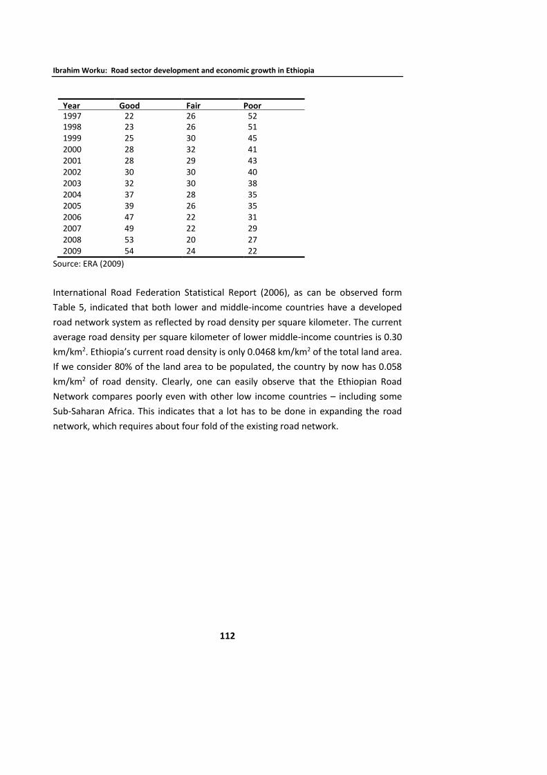
Ibrahim Worku: Road sector development and economic growth in Ethiopia
112
Year Good Fair Poor 1997 22 26 52 1998 23 26 51 1999 25 30 45 2000 28 32 41 2001 28 29 43 2002 30 30 40 2003 32 30 38 2004 37 28 35 2005 39 26 35 2006 47 22 31 2007 49 22 29 2008 53 20 27 2009 54 24 22
Source: ERA (2009)
International Road Federation Statistical Report (2006), as can be observed form
Table 5, indicated that both lower and middle-income countries have a developed
road network system as reflected by road density per square kilometer. The current
average road density per square kilometer of lower middle-income countries is 0.30
km/km2. Ethiopia’s current road density is only 0.0468 km/km2 of the total land area.
If we consider 80% of the land area to be populated, the country by now has 0.058
km/km2 of road density. Clearly, one can easily observe that the Ethiopian Road
Network compares poorly even with other low income countries – including some
Sub-Saharan Africa. This indicates that a lot has to be done in expanding the road
network, which requires about four fold of the existing road network.

Ethiopian Journal of Economics, Volume XIX, No. 2, October 2010
113
Table 5: Road densities of lower middle income countries
Lower Middle Income Countries
Road Density (Km/Sq. Km)
Lower Middle Income Countries
Road Density (Km/Sq. Km)
Algeria 0.05 Indonesia 0.19 Djibouti 0.12 Kiribati 0.92 Egypt 0.09 Micronesia 0.34 Iran 0.11 Philippines 0.67 Iraq 0.10 Samoa 0.82 Jordan 0.08 Thailand 0.11 Morocco 0.13 Tonga 0.91 Tunisia 0.12 Vanuatu 0.09 Bolivia 0.06 Albania 0.63 Brazil 0.20 Armenia 0.27 Colombia 0.10 Azerbaijan 0.68 Cuba 0.55 Belarus 0.45
Dominica Republic 0.26 Bulgaria 0.39 Ecuador 0.15 Georgia 0.29 El Salvador 0.48 Kazakhstan 0.03 Guatemala 0.13 Macedonia 0.34 Guyana 0.04 Moldova 0.39 Honduras 0.12 Serbia 0.16 Jamaica 1.94 Turkmenistan 0.05 Nicaragua 0.14 Ukraine 0.29 Paraguay 0.07 Angola 0.04 Peru 0.06 Cameron 0.11 Suriname 0.03 Cape Verde 0.25 China 0.20 Congo 0.05 Fiji 0.19 Lesotho 0.20 Namibia 0.05 Sri Lanka 1.48
Swaziland 0.21
Average 0.30 Km/Sq. Km
Source: International Road Federation Statistical Report (2006)
3.3. Road accessibility
Access refers to the opportunity to use or the right to or the ability to reach some
destiny. Accessibility is measured as the percentage of population having access to all
weather roads. The benefits of having access to a road network is measured in terms
of reductions in monetary costs or time needed by beneficiaries to access output
markets or key public social services like health and education.

Ibrahim Worku: Road sector development and economic growth in Ethiopia
114
The accepted theory, according to ERA’s (2008b) study, is that accessibility has three
elements: 1) the location of the individual; 2) the location of the supply, service, or
facility to which the individual needs access; 3) the link to bring the two together. The
study used three approaches, namely, the random model approach, the graph theory
approach, and the squire grid approach to cover the country’s network demand. This
demand was estimated as such that all rural population could have access to all
weather roads within a 5 km distance.
According to the ERA study the country is required to construct 200,000 km of
optimum national road network, which is considered as a target road network on the
assumption that it will give reasonably good accessibility. Whereas, for the country to
be competitive enough and enter into middle income category, the targeted road
density which secures the rural population to have access to all weather road is
estimated to be 0.3 km/km2, the average road density of the lower middle countries.
In this case the road transport network has to reach 330,000 km.
The same study defined the concept measured in terms of average distance from the
road network and proportion of area farther than 5 km from all weather roads as lack
of access, which deprives people from the opportunities to improve their lives. Access
is composed of two elements: mobility, reflecting the ease or difficulty in traveling to
a service or facility; and proximity of those services and facilities. The study considered
access to be one key element in providing the opportunity for both social and
economic development, and a key determinant of both poverty itself and
opportunities to escape from the poverty trap.
When we look at the recent trend regarding society’s access to the all weather road
network, we find a slight improvement over the past seven years. However, in 2008
only about 33% of the rural population had access to an all weather road within a
distance of 5 km. Given the fact that around 80 million people are living in rural area,
such a low rate exacerbates the problem of poverty. Improving the current access rate
should be a major concern of the country’s road sector expansion program.
Similarly, African Development Indicators (ADI) (2008/09) data indicates that the
country has made an effort to provide access to all weather roads, though it is not
satisfactory. The graph below depicts that the problem of accessibility is resolved only
very sluggishly. Within a period of seven years (2002 to 2008), an additional seven

Ethiopian Journal of Economics, Volume XIX, No. 2, October 2010
115
percent of the rural population is provided with access to all weather roads (from 26%
to 33% of the rural population). ERA (2008b) study also indicates that with the recent
construction of new roads, the average distance from a road has been reduced from
21km in 1997 to 11.7 km in 2009.
Figure 2. Trends over access to all-season road per percentage of rural population
Source: ADI (2009)
On the other hand, the proportion of area farther than 5 km from all weather roads,
which was 79% in 1997, has been reduced to 65.3% in 2009. Therefore, the issue of
accessibility calls for a kind of ‘big-push’ approach in expanding all weather roads for
the destitute rural poor. The problem of accessibility could also be addressed through
a well-designed planning process coinciding with the parallel trends towards the
decentralization of decision making and the concern to involve the local communities
in the decision making process. The effort made so far towards the improvement of
main roads and rural roads is a necessary but not sufficient measure to enhance rural
accessibility.
However, the future is not unwelcoming. It has been observed that a continuous
support from the government and a serious commitment of the sector offices and
other stakeholders would enable to achieve enhanced access of the rural population.
3.4. Road sector financing
0%
5%
10%
15%
20%
25%
30%
35%
2002 2003 2004 2005 2006 2007 2008
Access to an all-season road (% rural population)

Ibrahim Worku: Road sector development and economic growth in Ethiopia
116
Construction and maintenance of roads is not an easy investment. It requires a huge
amount of expenditure with foreign currency. This huge amount of money is not
affordable only by the government of Ethiopia from internal sources. Hence, the
government of Ethiopia finances road construction and maintenance through loans
and aid from other countries and organizations in addition to domestic finance. In
recent periods, the lion share of finance is the government of Ethiopia followed by
International Development Association. The other following financers are European
Union and African Development Bank.
Looking at the trends in the road sector financing (Figure 3), the pattern shows that
the internal financing in 2008/09 has increased to be more than ten times what it has
been a decade before. The trend also indicates that the total amount of external
financing is also growing but it has only multiplied by a factor five over the same
comparable period. The domestic financial expenditure share in 1997 has been only
twice that of the external source. Whereas, the recent expenditure is about four times
that of the external source in the face of growing financial expenditure over the
sector.
Figure 3: Share of internal and external financing in the road sector
Source: ERA, 2008b and author’s compilation
Additionally, the government of Ethiopia’s financial expenditure in the RSDP programs
had also been consistently rising (see also Table 6).
0.0
1,000.0
2,000.0
3,000.0
4,000.0
5,000.0
6,000.0
7,000.0
8,000.0
9,000.0
Internal
External

Ethiopian Journal of Economics, Volume XIX, No. 2, October 2010
117
All in all, the above discussion reveals that the government is making a relentless
effort towards the development of the road network. In this regard, one key
constraint is the availability of sufficient funding to achieve an adequate road network
comparable with at least the African average of 60km per 1000 km2 (ERA 2008b). The
ERA (2008b) study also indicated that inadequate funding and resource mobilization
are major problems in the road sector. Insufficient public resources lead to under-
funding of road transport infrastructure needs (road network maintenance needs as
well as road network expansion). The problem is found to be worse in expanding the
network in rural areas. The available fund for rural roads development and
maintenance is limited. The possible remedial measure would be to look for an
alternate and sustainable finance.
Table 6: Source of finance by the pursued RSDP programs
Financier Disbursement % of contribution RSDP I
( 5yrs) RSDP II ( 5yrs)
RSDP III (2yrs) (12 yrs)
IDA 1,432.9 3,135.3 1,848.8 6,416.9 14.2
EU 678.1 1,049.7 2,334.7 4,061.9 9.0
ADB 506.4 517.8 275.7 1,299.8 2.9
NDF 14.8 63.9 56.9 135.6 0.3
Japan 164.9 380 274.6 819.5 1.8
Germany 27.7 302.6 54.8 385.0 0.8
Sweden 0.0 5.0 0.0 5.0 0.0
Ireland Aid 2.6 20.9 0.0 24.1 0.1
UK 23.2 135.1 28.2 186.4 0.4
OFID 0.3 293.3 167.9 461.5 1.0
BADEA 0.0 59.9 133.9 193.7 0.4
SDF 0.0 39.3 92.9 132.2 0.3
GOE 3,455.5 8,669.5 11,139.1 23,264.
1
51.3
Road Fund 978.2 2,555.8 3,053.1 6,587.1 14.5
Community 0.0 884.8 469.6 1,354.4 3.0
TOTAL 7,284.6 18,112.
9
19,930.0 45,327.
2
100.0
Source: ERA (2009)
3.5. Few points on community roads

Ibrahim Worku: Road sector development and economic growth in Ethiopia
118
According to the ERA (2008b) study, community roads are being developed in
different woredas. The roads are being constructed as part of the Productive Safety
Net Project (PSNP). Table 7 depicts that 57,000 km of community roads were
constructed in the period 2004-2008 under the “food for work” scheme. Within this
food for work, substantial amounts of community roads are being maintained and
constructed in all the regions.
Table 7: Existing stock of community roads (2007)
Region Existing in 2006
(Km) Constructed in 2007
(Km)
Total Community Road Stock
(km) Tigray 5,803 578 6,381 Afar - - - Amhara 11,980 4,000 15,980 Oromia 13,839 3,489 17,328 Somali 1,273 - 1,273 SNNP 10,754 2,027 12,781 Benishangul-Gumz 2,230 1,001 3,231 Gambella 464 - 464 Total 46,640 11,124 57,438
Source: ERA, 2008b
As per the same study, it shows that community roads are not well accounted and
managed by either the federal or regional road administration. In this regard the study
clearly cites the problem as follows:
However, it’s worth noting that, for these community roads their design standard,
location, condition, ownership and for that matter their existence is not known in the
form of a national database. Further, the issue of how sustainable (in terms of both
financially and administratively) these community roads are with respect to
development and maintenance is unclear – as there is no institution that finances the
maintenance costs of these rural/community roads and nobody is accountable to
them institutionally both at the federal and regional levels. The mileage of community
roads will continue to grow rapidly – and the needed maintenance costs for
rural/community roads alone would become substantial. (ERA, 2008a)
Community road development and its sustained maintenance is a key point in
ensuring the accessibility/mobility of the rural poor and to connect them to the
improved federal and regional road network. Hence, an in-depth assessment of the

Ethiopian Journal of Economics, Volume XIX, No. 2, October 2010
119
status of the community road development program and the future development and
maintenance strategy is recognized as an urgent task.
4. Econometric modeling and the data
In order to analyze the economic impact of the road sector on the growth process of
a country, studies adopted ‘augmented Solow growth model’. Recently, there is a
wide array of literature written towards identifying the relationship between
economic growth and road sector development. However, the focus of previous
studies has been to investigate the link between infrastructure, which is an
aggregated measure, and economic growth.
Previous studies, for instance, Fan et al. (2002), Fan and Chan-Kang (2005), Canning
and Bennathan (2000), Canning and Pedroni (2004) used the standard Cobb-Douglas
type production function to analyze the impact of infrastructure on the overall GDP
growth, which per se is assumed to be a measure of overall economic growth. Dercon
et al. (2008) also used an analogous type of specification to see the impact of road
and agricultural extension on growth and poverty reduction in a panel data set of
selected fifteen Ethiopian villages. Fan and Chan-Kang (2005) indicated that there is
strong link between road development, economic growth, and poverty reduction.
In specifying the production function, we need to take into account different
specifications for paved and gravel roads on the overall productivity. For the reason
cited above, augmented Solow trans-log production function is used to see the impact
of road on GDP growth.
Few of the previous studies consider the issue of diminishing return, which could be
captured by looking to the coefficient of the square of road network. If the coefficient
happens to be negative, the negative sign indicates that road network, used in the
regression, is abided by “neoclassical” paradigm. In case the coefficient happens to be
positive, the sign indicates that road network is a self sustaining input, governed by
an “endogenous growth” paradigm, which is mostly believed to be true for developed
countries.

Ibrahim Worku: Road sector development and economic growth in Ethiopia
120
The possible existence of reverse causality, i.e. the fact that infrastructure
accumulation could be driven by productivity growth, need to be accounted in
analyzing the relationship between infrastructure variables and economic growth. In
this regard, Canning (1999), Canning and Bennthan (2000), Canning and Pedroni
(2004) and Calderon (2009 explicitly stated the need to account for the possible
existence of reverse causality in estimating the growth function which is augmented
with an infrastructure variable, like road network.
The study also looks at the impact of road network on sectoral GDP. For instance,
Dorosh et al. (2009) analyzed the importance of road connectivity to agricultural
productivity in Africa. The findings indicate that lower return from having high density
is exhibited to be low for West Africa. Whereas, longer travel time decreases total
crop production, and reducing travel time significantly increases adoption of high-
input/high-yield technology in East Africa. The findings showed the importance of
increased road connectivity in East Africa.
Following the aforementioned studies, this study utilizes similar specifications to see
the impact of roads on the overall economic growth. The general specification of the
model is an augmented Solow Growth model. Such a model is basically a log
transformation of the Cobb-Douglas production function. The logarithmic form of this
production function of Solow growth model allows including any relevant variable
which affects the growth of GDP. It also allows us to include a dummy variable which
captures the impact of any policy intervention in the analysis period. In addition, Fan
and Chan-Kang (2005) indicated that different types of roads can create different
economic return. Therefore, it is important for us to see the implication of road quality
on the productivity.
4.1. Conceptual framework of the model
Having the theoretical inter-linkage on the relevance of road network to economic
growth from the above discussion, the following section provides the conceptual
framework used in modeling road network. To do so, the starting point is the simplest
production function that has the following specification.
GDP = f (L, K) (1)

Ethiopian Journal of Economics, Volume XIX, No. 2, October 2010
121
Where, GDP is the gross domestic product of the country, L is labor and K denotes
capital. The above general Cobb-Douglas type functional specification will be
augmented with road so as to identify its impact on economic growth. Accordingly,
the above functional specification will be reformulated as
GDP = f (L, K, R) (2)
Where, R is road length and the others are as stated above.
Here again, Fan and Chan-Kang (2005) criticize previous studies for not recognizing
the fact that the return from different types of road on economic growth might be
different. Thus, in this study the road variables will be classified into paved and gravel
road in order to see the impact of the difference on the overall growth. The function,
which takes care of the difference on road type, will be specified as;
GDP = f (L, K, RT) (3)
GDP = f (L, K, Rp, Rg) (4)
Where Rp and Rg represent paved and gravel roads respectively.
We can also specify the production function for agricultural GDP, with the inclusion
of gravel roads as an input. Such specification makes it interesting for the reason that
the agricultural populations rarely have the opportunity to use paved roads for
transportation purposes and thus the impact might be negligible for agricultural GDP
growth. Therefore, we might anticipate at this stage to state the functional
specification on agricultural productivity. The model could now be stated as;
AGDP = f (L, K, RT) (5)
AGDP = f (L, K, Rp, Rg) (6)
Where AGDP denotes the agricultural GDP and Rg is gravel road length and Rp paved
road length, and the rest are as already defined.

Ibrahim Worku: Road sector development and economic growth in Ethiopia
122
In addition to the AGDP, the impact of roads could be seen on non-agricultural sector
GDP growth rates by disaggregating it into industrial GDP (IGDP) and service sector
GDP (SGDP). For this purpose, similar type of production functions will be estimated
with their respective variables. The regression is run on the total road network.
IGDP = f (L, K, RT) .(7)
IGDP = f (L, K, Rp, Rg) .(8)
And the service sector GDP specification will be
SGDP = f (L, K, RT) .(9)
SGDP = f (L, K, Rp, Rg) .(10)
In order to account for other factors, which are missing in the above functional
specification, once again, the model is augmented with policy dummy to see the
impact of any relevant policy intervention in the regression function. At this stage, the
policy dummy is entered in the functional specification on the aggregate production
function. Thus, the specification will be stated as follows:
GDP = f (K, H, Rp, Rg, Dpi) .(11)
Dpi denotes dummy for policy interventions, which are introduced to account for any
policy intervention over the analysis period.
4.2. Specification of the model
Once the variables within the model are clearly defined, the next step is to derive out
the estimable production function. Accordingly, the aggregate Cobb-Douglas
production function along with the road component, which could be estimable, can
be reached through the following procedure,
( ) gtpttttt RRKHGDP .=
(12)
Where: Ht is human capital at time t
Kt is physical capital at time t

Ethiopian Journal of Economics, Volume XIX, No. 2, October 2010
123
Rpt and Rgt is road network for paved and gravel roads, respectively at time t and
whereby the variables are written in per worker terms, and , and are
parameters of interest.
The model is then transformed to the logarithmic form whereby the resulting
equation is set as follows.
tgtptttt khGDP +++++= lnlnlnlnln 21 .(13)
Given the above specification, policy and other structural shift indicator dummies are
introduced in the following specification.
tpgtptttt DkhGDP ++++++= 54321 lnlnlnlnln (14)
Where Dp is policy dummy reflecting the introduction of a new policy which is related
to road provision.
Finally, once the estimable functional form specification is reached in the estimation
procedure, GDP will further be disaggregated to identify the impact of road on
agricultural, manufacturing and service sector productivity. In addition, the model will
also be estimated for the agricultural GDP for a more disaggregated rural road
network to see whether there exists a significant relationship among these variables.
At the end, the marginal return per unit length of different types of road on each of
the three sectors productivity will be computed.
4.3. The data
The objective of the study is to estimate the impact of road infrastructure on the
overall economic growth. A time series data spanning over the period 1971-2009 is
used for the analysis. The aggregate output function is setup with a set of explanatory
variables constituting physical capital, human capital, and road network and policy
intervention dummy variable. The detail on the source and type of each of the
variables is presented below.

Ibrahim Worku: Road sector development and economic growth in Ethiopia
124
Real GDP per worker is obtained from ministry of finance and economic development
(MOFED). The data set from the period 1991 to 2009 is not compatible with prior
year’s data. To deal with this problem, prior year growth rate of GDP is used to
extrapolate and have consistent GDP values with their respective GDP growth rates.
Given the above functional specification, most of the variables could be obtained from
different macroeconomic databases. What is not clearly explained in the above
general specification is as to how the physical capital and human capital variables
could be handled in the model. While the capital variables could be derived from
Kohler’s (1988) capital accumulation function, which is referred as perpetual
inventory method. The procedure for deriving the capital stock is set as follows.
1)1( −−+= ttt kIK (15)
Where Kt is capital stock in period t which could be computed as the sum of It, which
is gross capital formation in year t. is the rate of depreciation of capital. Fan and
Chan-Kang (2005) took the rate of depreciation to be 10%. This study will also adopt
similar assumption to arrive at the stock of capital.
Following Fan and Chan-Kang (2005) and similar other studies, the initial capital stock
is computed using the following mathematical representations.
( )r
Ik t
t+
=
.(16)
Where r is the real interest rate and is rate of depreciation of capital. Using the
above formula, the initial stock of capital is computed for the year 1970. Previous
studies tend to make assumption on the real interest rate and the depreciation rate.
For instance, Kohler (1988) computed the initial capital stock to be 7.4 times gross
capital formation of the beginning year, which is 1978, taking 8 percent depreciation
rate of the stock of capital. In this study too, I assumed 8 percent depreciation rate.
The computed initial capital stock is found to be 5.88 times the gross capital formation
of the year 1970. Then after, the remaining capital stock data are computed using the
above stated capital accumulation function.

Ethiopian Journal of Economics, Volume XIX, No. 2, October 2010
125
As already explained above, the data on physical capital was constructed using the
perpetual inventory method. To implement it, the initial level of the capital stock was
estimated using data on the capital stock and real output from MOFED. The year 1970
is taken as the initial period for which gross capital formation is used. The physical
capital is set up as net of gross capital formation for each period. Since the stock of
road network is used as one variable, it is deducted from the gross capital formation
to avoid double counting.
For human capital, secondary school enrolment rate is used as a proxy. Secondary
school enrolment rate is obtained from Central Statistical Agency annual bulletin. The
best proxy for human capital as indicated by Fan and Chan-Kang (2005) study is
average years of schooling. However, Ethiopian data regarding years of schooling are
not available. With regard to the human capital variable, Calderón (2009) choose
secondary school enrolment to account for human capital in dealing with the impact
of infrastructure and growth in Africa. Not only Calderon (2009), similar other studies,
for instance Cohen and Soto (2001) also used secondary school enrolment as a proxy
for human capital in the growth regression function. So, following the above studies,
taking secondary school enrolment as a proxy for human capital in this study is
justified.
Finally, the labor for converting all inputs in per worker terms is obtained from African
Development Indicators (ADI) (2009) CD-Rom, which is part of World Bank’s World
Development Indicators. Electricity Power generation is also obtained from ADI CD-
Rom.
Road network with a classification of paved urban road, gravel urban road, gravel rural
road and road total network (in kilometers) for the entire period under consideration
is obtained from Ethiopian Road Authority. In the econometric estimate all the
variables are expressed in per worker units.
In addition, a number of ERA publications, ADI, IMF web data set, MOFED and CSA
data are used for the descriptive analysis part.
4.4. Econometric analysis
4.4.1. Test for unit roots

Ibrahim Worku: Road sector development and economic growth in Ethiopia
126
The data set deployed for this study is a time series data. When dealing with time
series data it is important to test the stationary or non-stationary nature of the data
set for the reason that non-stationary variables might lead to spurious regression. In
this regard Harris (1995) stated that:
…models containing non-stationary variables will often lead to a problem of
spurious regression, whereby the results obtained suggest that there is
statistically significant relationship between the variables in the regression
model when in fact all that obtained is evidence of contemporaneous
correlation rather than meaningful causal relation.
Thus, the first step is to test the stationary nature of individual variables that will be
included in the regression. To test the stationary nature of the variables, the
Augmented Dickey-Fuller (ADF), the modified version of the Dickey-Fuller, test is used.
According to the ADF test, null hypothesis is that the variable is assumed to
have/contain a unit root. The time series nature of the data will be tested against the
alternative, where a stationary process generates the variable. Other common unit-
root tests that could alternatively be used to test stationarity include the DF-GLS test
of Elliot, Rothenberg, and Stock (1996) and the Phillips-Perron (1988) test.
Pperron test in stata command performs the Phillips-Perron test that a variable has a
unit root. The null hypothesis is that the variable contains a unit root, and the
alternative is that the variable is generated by a stationary process. Pperron uses
Newey-West standard errors to account for serial correlation, whereas the
augmented Dickey-Fuller test implemented in dfuller uses additional lags of the first-
difference variable. Stata automatically select the appropriate lag length when we use
pperron. So, this study uses both the pperron and ADF tests to check the stationary
nature of the variables.
In testing the unit root, most macroeconomic variables, in practice, are suspected of
showing a time trend. To control for the trending nature of the variables, the graphic
visual inspection test is also conducted. A summary table on test for stationarity of
the variables is reported following the graphic trend test (Annex Figure A.1).

Ethiopian Journal of Economics, Volume XIX, No. 2, October 2010
127
With the exception of agricultural GDP per worker, urban gravel road and urban road,
the other variables exhibit trends. Therefore, unit root tests require a trend term in
both the ADF and pperron tests.
Table 8. Summary table on Phillips-Perron test for unit root Newey-West lags stata
routine lag length selection
Statistic Z(t)
at level a
Statistic Z(t) at level
with trend b *
Statistic Z(t) at
first difference c
lnrgdp_pw -0.926 -0.731 -5.701
lnargdp_pw -2.407 -2.167 -6.193
lnsrgdp_pw 1.209 -0.428 -5.729
lnirgdp_pw -1.189 -1.696 -4.887
lncapnet_pw 1.747 -1.335 -4.260
lnhcap_pw -1.813 -2.283 -4.313
lnelect_pw 0.389 -3.035 -7.596
lnroadtot_pw -0.977 -2.693 -6.457
lnroadtotsq_pw -0.425 -2.560 -5.461
lnaspurb_pw -1.630 -1.194 -5.707
lngrvroad_pw -1.599 -1.553 -5.903
lnrdcapnet_pw 1.429 -1.954 -4.016
Notes: a 1%, 5%, and 10% Critical Values at levels are -3.662, -2.964 and -2.614
b 1%, 5%, and 10% Critical Values at levels with trend are -4.260, -3.548 and -3.209 c 1%, 5%, and 10% Critical Values at difference are -3.668, -2.966 and -2.616
Lag length of three is chosen to be the optimal lag length
* Based on the graphics inspection, de-trending is made for variables showing a trend behavior
As the above table indicates, all of the variables are found to be non-stationary in
levels whereas few of the variables are marginally stationary in the case of ADF test,
only at 10% significant value. The ADF test at times might lead to acceptance of
stationarity even though the variables are not stationary. For this reason, only the
pperron test is chosen. Both tests indicate that all of the variables seem to be
stationary at first difference. In other words, all of the variables are found to be
integrated of order 1, and hence are called I (1) variables. Thus, to be safe the order
of integration for all the variables is considered to be I (1)

Ibrahim Worku: Road sector development and economic growth in Ethiopia
128
Regarding the existence of trend component within a time series data set, Harris
1995 underlined that trend in a data set can lead to spurious correlation that
may imply relationships between the variables in a regression equation, when all
that is present are correlated time trends. The time trend in a trend stationary
variable can either be removed by regressing the variable on time trend (with the
regression forming a new variable which is trend-free and stationary) or nullified
by including a deterministic time trend as one of the regressers in the model.
Harris (1995)
4.4.2. Test for co-integration
Having tested our time-series for stationarity, the next step of time-series analysis is
testing for co-integration, which amounts to checking whether the linear combination
of the variables is also stationary or not. It requires that the variables of interest have
the same order of integration. It is only when the variables are integrated of the same
order that a linear relationship among them can be expected. Variables are said to be
co-integrated if a long run equilibrium relationship exists among them.
Engle and Granger (1987) argue that for such relationships to exist, the error terms of
the model should be stationary. We have applied the Engle-Granger procedure to test
for co-integration. When variable x is said to Granger-cause variable y if, given the
past values of y, past values of x are useful for predicting y. The first stage of the co-
integration test involves estimating model/equation and saving the error terms. In
time series analysis, estimating a relationship between non-stationary variables that
are not co-integrated gives rise to the problem of spurious regression; the error term
in the regression is non-stationary, producing a high degree of "noise" in the
relationship, and inconsistent parameter estimates. In order to test the stationary
nature of the data set both the ADF and pperron tests are applied on the error terms.
If the error terms are found to be stationary, the variables are said to be co-integrated
and this necessitates the estimation of an Error Correction Model (ECM) involving long
run relationships. If, on the other hand, the variables are not co-integrated, then the
regression leads to spurious results. A number of approaches are forwarded to deal
with such kind of problem. Modeling should proceed with the differenced time-series.
Annex Table A.1 reports the test statistics from the unit root tests. As can be seen

Ethiopian Journal of Economics, Volume XIX, No. 2, October 2010
129
from the table, the first and second stage estimation results of the ECM show that
ECM could be applicable to estimate the model.
The Engle-Granger two step estimates indicate that the variables are co-integrating at
10% significant level. The Durbin-Watson test statistic also shows the existence of
serial correlation in both models. Therefore, it is possible for us to estimate the model
using ECM. However the problem with OLS is that it fails to account for the problem
of endogeneity within the model, which is created, in particular, due to the existence
of physical capital as one potential explanatory variable in the model that is
significantly correlated with GDP. In addition, it is also difficult to deal with a model
of variable with a suspect of heteroskedasticity of the error terms.
4.4.3. Method of estimation and pre-estimation requirements
When the above problems are persistent in a time series data set, the best way to
deal with is to opt for generalized method of estimation (GMM) technique for a
number of significant advantages. The recently devised two-step GMM estimator
would be an ideal tool to deal with multiple time series data with endogenous variable
and as well is suspected of having heteroskedasticity. According to Baum et al. (2007),
unlike instrumental variables or two-stage least square estimators, GMM estimator
does not require additional assumption on the error terms. The former estimators are
specific cases of GMM estimation, which require homoskedastic assumption and
independent error terms. Without stating those assumptions one can estimate a
model efficiently and consistently using two-step GMM estimation technique. In
addition, Baum et al. (2007) state that the two-step GMM estimator could also be
applied when the errors are serially correlated, which is a typical nature of time series
data set that we are now dealing with. (See also Bond, Hoeffel, and Temple 2001).
In general, the model that is used to estimate the time series data will have the
following econometric specification.
ttit xy += .(17)
i s’ are the coefficients that are going to be estimated.

Ibrahim Worku: Road sector development and economic growth in Ethiopia
130
Since some of the regressors are endogenous, E( tx t ) 0.
To estimate this model, it requires instruments for endogenous variables in such a way
that the instrumented variable need not be correlated with the error term so that
E(Zt,t) = 0.
Lanne and Saikkonen, (2009) highlight the problem in using the first-differenced GMM
panel data estimator to estimate cross-country growth regressions, which essentially
is similar to time series data set. When the time series are persistent, the first-
differenced GMM estimator can poorly behave, since lagged levels of the series provide
only weak instruments for subsequent first-differences. According to the work of Caselli,
Esquivel and Lefort (1996) this problem may be much more serious in practice. The
authors suggest using a more efficient GMM estimator that exploits stationarity
restrictions, and this approach is shown to give more reasonable results than first-
differenced GMM in our estimation of an empirical growth model. Accordingly, this study
utilized two-step efficient GMM estimator to handle this problem.
To do so, the model is estimated using two-step GMM estimator with the robust
option for the reason that such an estimate is liable for inefficient estimate of
downward biased standard errors. So, the robust two-step estimation procedure is
chosen to estimate the above specified model with an automatic bandwidth selection
with robust standard error.
Another key issue when estimating a model using two-step GMM is that capital is
assumed to be endogenous. In addition, human capital is suspected to be potentially
endogenous. To account for these restrictions, Baum et al. (2007) estimation
technique allows us to instrument the model for the problem of endogeniety and
setup ortogonality condition on the suspect of instrument. Thus these facts are well
taken care of in the estimation procedure with an ivreg2, gmm2s orthog bw( ) stata
installed command.
After conducting Granger causality test, for instance, Rouvinen (2002) also used
lagged levels from the second one onwards as instruments. In this study, to avoid

Ethiopian Journal of Economics, Volume XIX, No. 2, October 2010
131
over-fitting the model, the second and third lags and lagged differences are used as
potential instruments.
Care has to be made over the selection of ideal instrument, when estimating time series
model with endogenous variable. After estimating the model, one has to cautiously look
at test of exogeniety of the instruments before interpreting the result.
4.4.4. Discussion on post-estimation requirements and discussion on the results
Having paid enough attention for all the pre-estimation factors regarding two-step
efficient GMM estimation, the resulting summary table on eight models is presented
below (Table 9). These models are regressions of the growth function, with dependent
variables labeled as total real GDP worker, on agriculture, service and industrial GDP.
lnrgdp_pw = f (lncapnet_pw, lnhcap_pw, lnelect_pw, lnroadtot_pw, lnroadto
tsq_pw, prersdp, rsdp1, rsdp2, rsdp3, year)
lnrgdp_pw = f (lncapnet_pw, lnhcap_pw, lnelect_pw, lnaspurb_pw, lngrvroad_pw,
lnroadtotsq_pw, prersdp, rsdp1, rsdp2, rsdp3, year)
lnargdp_pw = f (lncapnet_pw, lnhcap_pw, lnroadtot_pw, lnroadtotsq_pw,
prersdp, rsdp1, rsdp2, rsdp3, year)
lnargdp_pw = f (lncapnet_pw, lnhcap_pw, lnaspurb_pw, lngrvroad_pw,
lnelect_pw, lnroadtotsq_pw, prersdp, rsdp1, rsdp2, rsdp3, year)
lnirgdp_pw = f (lncapnet_pw, lnhcap_pw, lnroadtot_pw, lnelect_pw,
lnroadtotsq_pw, prersdp, rsdp1, rsdp2, rsdp3, year)
lnsrgdp_pw = f (lncapnet_pw, lnhcap_pw, lnelect_p, lnroadtot_pw,
lnroadtotsq_pw, prersdp, rsdp1, rsdp2, rsdp3, year)
lnsrgdp_pw = f (lncapnet_pw, lnhcap_pw, lnaspurb_pw, lnelect_pw,
lngrvroad_pw, lnroadtotsq_pw, prersdp, rsdp1, rsdp2, rsdp3, year)
Where lnrgdp_pw, lnargdp_pw, lnirgdp_pw and lnsrgdp_pw are logarithm of real GDP
of total, agricultural, industrial, and service GDP in per worker units respectively.
lncapnet_pw is capital stock net of road in per worker units
lnhacap_pw is logarithm of human capital in per worker units
lneclect_pw denotes logarithm of electricity power generation in per worker units
lnroadtot_pw is the logarithm of total road network in per worker
lnaspurban_pw is the logarithm of asphalt urban road network in per worker
lngrvroad_pw is the logarithm of gravel road network in per worker
prersdp is policy dummy for the period 1991-1997 to account for change of regime

Ibrahim Worku: Road sector development and economic growth in Ethiopia
132
rsdp1 is policy dummy for the period 1997-2001 to account for the first RSDP program
rsdp2 is policy dummy for the period 2002-2006
rsdp3 policy dummy for the period 2006-2009
year time dummy included to account for trending nature of the fundamental
components of the model
For all the above alternative models estimation is undertaken. But, before
interpreting the finding of the regression result, the following post-estimation issues
are considered. Otherwise the parameters would not be considered as efficient and
consistent to make a valid statistical inference.
Stata estimate for two-step GMM estimation is produced with a number of statistical
outputs that are indicators of the efficiency of the estimators. For the parameters to
be interpreted, the first task is to check the consistency of these statistical results with
the expected hypothesis that need to be satisfied (Baum et al. 2010). According to
Hayashi (2000), two-step efficient GMM estimator needs to pass test of exogeneity of
instruments, weak identification and overidentifying restrictions. These three
statistics are of our interest that the estimated models need to satisfy.
First, we need to test that the instruments are exogenous with respect to the
instrumented variable. Theoretically, this condition is satisfied when lagged
differences and lag levels are taken as instruments with GMM estimates. In this
regard, Lanne and Saikkonen (2009), for instance, argue that when there is causality,
as causality is already tested using Engle-Granger two-step procedure, within a time
series framework it would be appropriate for one to use lagged variables and lagged
differences as best instruments in GMM estimation. Following this proposition,
capital is instrument by its second and third lagged level and lagged difference. In this
regard, Hayashi (2000) sets the requirement over the null statistics. The C statistic
(also known as a "GMM distance" or "difference-in-Sargan" statistic) allows us to test
exogeneity of one or more instruments. Under the null hypothesis that both the
smaller set of instruments and the additional, suspect instruments are valid, the C
statistic is distributed as chi-squared in the number of instruments tested. Note that
failure to reject the null hypothesis requires that the full set of orthogonality
conditions be valid. Test of exogeneity is reported along with the summary table for
all the models under consideration. The models pass the test of exogeneity.

Ethiopian Journal of Economics, Volume XIX, No. 2, October 2010
133
Second, the instruments should be relatively highly correlated with the instrumented
variable, so that they act as an effective predictor. Weak identification tests are a
category of tests to check for this condition, and the specific version the stata routine
reports Kleibergen-Paap rk Wald F statistics. When the independently and identically
distributed (i.i.d.) assumption is dropped and ivreg2 reports heteroskedastic, AC, HAC
or cluster-robust statistics, the Anderson LM and Cragg-Donald Wald statistics are no
longer valid. In these cases, the LM and Wald versions of the Kleibergen-Paap (2006)
rk statistic, stata output reports also distributed as chi-squared with (L1-K1+1) degrees
of freedom. The rk statistic can be seen as a generalization of these tests to the case
of non-i.i.d. errors. To pass the test, a value of ten or greater is typically required. As
shown in the regression summary table (Table 9), for each model these instruments
pass the test.
Third, the instruments should not influence the dependent variable except via the
instrumented variable. Overidentification tests are a category of tests used to test for
this condition, and the specific version which is presented with the Stata routine
output is called the Hansen J statistic. According to Hayashi (2000), under the
assumption of conditional homoskedasticity, Hansen's J statistic is consistent in the
presence of heteroskedasticity and (for HAC-consistent estimation) autocorrelation,
where a p-value result that is greater than 0.1 is typically considered passing. As
shown in Table 9, the three instruments pass this test. For all the models under
consideration, the Hansen J statistics is greater than 0.4.
Stata output also automatically reports tests of both underidentification and weak
identification. The underidentification test is an LM test of whether the equation is
identified, i.e., the excluded instruments are "relevant", meaning correlated with the
endogenous regressors. Under the null that the equation is underidentified, the
statistic is distributed as chi-squared with degrees of freedom (L1-K1+1). A rejection
of the null indicates that the model is identified. For the models under consideration,
the models pass the underidentification tests (Baum 2006).
In sum, while estimating the models, the estimator is forced to compute estimators
that are heteroskedasticity and autocorrelation consistent (HAC) standard errors. To
do so, while estimating the models automatic bandwidth selection and robust option

Ibrahim Worku: Road sector development and economic growth in Ethiopia
134
are imposed to produce an estimate which accounts for the existence of
heteroskedasticity and autocorrelation in time series data set (HAC). With the HAC
standard errors, various summary statistics are “robustified” as well, in the sense that
the post estimation criteria are satisfied.
Once all the post estimation issues are well handled, it would be safe for us to report
the estimated results. Accordingly, the following section discusses on the findings of
these results.

Ethiopian Journal of Economics, Volume XIX, No. 2, October 2010
135
Table 9: Summary on two-step GMM estimation results of the impact of road network on overall and sectoral GDP Variables| model1 model2 model3 model4 model5 model6 model7 model8 Dependant| RGDP RGDP ARGDP ARGDP SRGDP SRGDP IRGDP IRGDP Explanatory
Phy_capital | .356*** .184* -.0304 -.117* .423*** .43*** .428*** .436*** Hum_capital | .0539*** .0455** .038 .0572* -.0585* -.0644*** .0661*** .0632*** Electricity | .345*** .165 .352 .294 .286* -.00567 .251* -.0209 Road | .575* 1.31*** 1.18*** .568** Road2 | -.401** -.186 -.759*** -.537*** -.126 -.453*** -.122 Pre_RSDP | -.0921*** .0222 .0209 .129* -.378*** -.22*** -.211*** -.0764 RSDP 1 | -.0253 .131* .162*** .256*** -.341*** -.18** -.152*** -.0284 RSDP 2 | .0316 .117 .162* .15 -.253*** -.121 -.0788 .0264 RSDP 3 | .194*** .222* .444*** .27*** -.172* -.112 .0808 .126 Year | -.0182* Asphalt | .582*** .585*** .62*** .426** Gravel | -.0699 -.374*** .214 -.102
Road*Ph_capit| Constant | 45.3*** 10.9*** 17.3*** 9.1*** 11.7*** 10.2*** 8.05*** 7**
r2_a | .808 .786 .623 .609 .856 .873 .928 .933 rmse | .0416 .0438 .0598 .0609 .0583 .0535 .0481 .0454 N | 35 35 35 35 35 35 35 35 K | 20.406 87.309 106.206 42.852 106.206 131.911 106.206 99.961 K P| .5148 0.5166 0.4921 0.3173 0.5201 0.4201 0.6580 0.5863 J | 0.5368 0.4467 0.3280 0.1302 0.2671 0.2073 0.4782 0.4475 C | 0.8396 0.8894 0.4969 0.9401 0.7833 .7036 0.5633 0.4835 F | 2685 978 157 115 2520 696 2378 1828
Notes: * p<0.05; ** p<0.01; *** p<0.001, all the explanatory variables are in log and per-worker units

Ibrahim Worku: Road sector development and economic growth in Ethiopia
136
As can be seen from Table 9, eight models are estimated. The general model, the first
model labeled as model1, is on the impact of roads on aggregate real GDP per worker.
The result indicates that road network per worker is positively related with economic
growth.
In the second model, the study examined the impact of different types of road
(classified as asphalt and gravel road) on economic growth, captured by logarithm of
overall and sectoral real GDP growth. The findings indicate that expansion of asphalt
road has positive influence on overall economic growth. The coefficient for asphalt
road is also statistically significant. Similarly, though it is statistically insignificant,
gravel road has positive impact on growth.
Model3 up to model8 are estimated with the aim of investigating the impact of road
network on sectoral output, i.e. agricultural GDP, industrial GDP and service GDP. All
of them are expressed in per worker terms. In order to see the impact of road quality
on total and sectoral GDP, each sector GDP is estimated on asphalt and gravel road.
Accordingly, model3 and model4 are estimation results on the impact of total and
disaggregated road on agricultural GDP. In both cases, road network has positive
influence on the growth of agricultural GDP. The impact of total road is statistically
highly significant. Nonetheless, the impact of the disaggregated road, asphalt and
gravel, fails to be as such significant. The possible explanations would be that the road
sector is not highly integrated with the agricultural sector in terms of accessibility to
the rural dweller. The other possible explanation would be that disaggregated roads
fail to reach the threshold level, which is required spurring agricultural GDP growth.
Moreover, another plausible explanation ascribed for such unexpected finding might
be the fact that the rural area is not as such networked with asphalt and gravel road
and access to these networks is somehow thin which essentially proves lesser impact
on agricultural GDP growth. Rather, in this area community roads play a more
significant role than these two types of road networks. As already explained in the
descriptive analysis section, community road is not well accounted by the road
authority for it to be in incorporated within the regression equation.
Model5 and model6 are on the impact of road on industrial GDP. In here, again both
total road network and classified roads are found to have positive impact on this
sector GDP growth. Here again, the asphalt road has significant and positive impact

Ethiopian Journal of Economics, Volume XIX, No. 2, October 2010
137
on industrial GDP. Intuitively, this is true for the reason that the asphalt road is
networked where industries are operating, i.e. city areas. This shows that road
network is concentrated around cities. In contrast, gravel network in urban areas are
not prevalent. Thus, their impact on this sector GDP is negligible.
When we look at model7 and model8, we find that the impact of road on service
sector GDP is positive for the total and asphalt road network. The result is concurrent
with the intuitive perception that road quality is essential for the well performing
service sector.
In sum, the findings of all the previous models are consistent with the intuitive and
theoretical explanation. Having this fact in mind, road network is found to have much
more pronounced impact on sectoral GDP than on total GDP. For the road sector to
have significant output on each sector, sector specific objectives regarding road
network expansion is relevant. That is, for the impact of road on agricultural GDP to
be significant, the road network fails to reach the threshold level for it to have
significant impact on this sector. In addition, gravel road expansion is not as such
important for increasing service sector GDP.
In the estimation process, I tried to include other interaction terms, but it resulted in
multicollinearity. When it happened with two-step efficient GMM estimator, the stat
routine command automatically drops those variables. So it is not possible to see the
impact of interaction terms.
Regarding the other inputs used in the models, in all cases the coefficients are found
to be with the theoretical expectation that both human and physical capital have
positive impact on economic growth.
Finally, when we come back to the impact of policy interventions introduced over the
period under study, for all of the models RSDP III, which has been introduced over the
period 2006-2009, has more significant growth spurring impact than the other two.
Here it requires careful interpretation in that, RSDP II also has positive and significant
impact for most of the models. We need to note that policy intervention on
infrastructure would have a pronounced impact in later years than the moment the
policy is introduced. That is, we need to be cognizant of the fact that such kind of

Ibrahim Worku: Road sector development and economic growth in Ethiopia
138
policies, policy on infrastructure, will have impact lag. It would take time for it to spur
growth than having a direct and shorter impact. Such investments will have a very
strong impact over a long time horizon. In all the models the policy dummy for the
period 1991-1997 has a negative influence for the country and fails to have any
growth spurring impact. That period was more a period of political stabilization than
growth. The result is also consistent with this fact.
5. Conclusions
This study investigated achievements in the road sector in Ethiopia and its impact on
both the overall and sectoral economic growth. To do so, the study econometrically
analyzed the impact of roads on economic growth by using a time series data set. To
this end, the study reviewed theoretical and empirical researches related to the road
development over a wide array of perspectives. It also reviewed relevant literature on
the link between road transport and economic growth and certain aspects of road
transport in the context of Ethiopia and some other countries experiences.
Ethiopia has a respectable growth performance in the post-1991 period. In particular,
over the period 2004-2009, the economy averaged 10 percent growth rate of GDP,
which signals the country’s future economic prospects and lays down promising
momentum for further economic growth. Keeping up the growth momentum and
ascertaining its sustainability is a key to boost domestic investment and also attract
foreign investment. In this regard, to sustain the growth performance of the economy,
through creation of a favorable macroeconomic environment, developing vital
infrastructure, ensuring the quality of institutions as well as improving the quality of
human capital, road network development is supposed to play a major catalytic role.
The findings from the descriptive analysis indicate that the government in the recent
decade is making a relentless effort towards expanding the road network of the
country. However, an important key indicator is the issue of accessibility. The
country’s overall accessibility is far below from what is needed to graduate to the club
of lower middle income countries. Accessibility is a good indicator to investigate the
impact of poverty on socioeconomic development. This indicator is linked with rural
population. The issue of access is not a challenge for the urban population. Therefore,

Ethiopian Journal of Economics, Volume XIX, No. 2, October 2010
139
in order to reduce rural poverty or provision of public utilities, expanding the road
network in rural areas would be the best way to reach the rural population.
The recent trend shows that the government is showing strong commitment to
expand and improve the current performance. The analysis also shows that the
government in this decade has made sufficient attention in financing road projects.
By now the government’s expenditure has reached tenfold of what it has been a
decade before. The analysis also reveals that the donor’s share of money spent on the
road network is not increasing as such in the face of the rising road expenditure by
the government and the expansion of the road network.
Community roads should be given sufficient attention both in terms of expansion,
management, and accountancy by either regional or federal road authorities. At this
point, Ethiopian Road Authority should design an easy way to get detailed information
regarding community road networks from regional road authorities. Future
community road expansion need to be an integral part of the road networks as these
might be an easy way to ascertain access to the destitute rural poor. Community roads
are supposed to better reflect the community demand of which roads should be
constructed or upgraded.
When we come to findings of the econometric results according the link between road
length and economic growth, the results indicate that road network per worker is
positively related with economic growth and that expansion of asphalt road has a
positive influence on overall economic growth. Similarly, though statistically
insignificant, gravel road has a positive impact on economic growth.
Finally, at the heart of the above analysis one key question is, are the efforts made so
far sufficient to spur the overall economic growth of the nation and thereby to have
an impact on the livelihood of the rural poor? The impact is seen to be less strong on
the agricultural GDP growth and addressing the issue of accessibility to the rural poor.
The effort is relatively better and has pronounced impact on industrial and service
sector GDP. Nevertheless, for it to have a far-reaching impact on agricultural growth
and poverty reduction, a lot more has to be done.

Ibrahim Worku: Road sector development and economic growth in Ethiopia
140
References
African Development Indicators (ADI). 2009. CD-ROM.
Baum, C. F. 2006. An Introduction to Modern Econometrics Using Stata. College Station,
TX: Stata Press.
Baum, C. F., M. E. Schaffer, and S. Stillman. 2007. Enhanced Routines for Instrumental
Variables/GMM Estimation and Testing. Boston College Economics Working
Paper 667.
Baum, C. F., M. E. Schaffer, and S. Stillman. 2010. IVREG29: Stata module for extended
instrumental variables/2SLS and GMM estimation (v9). Boston College
Department of Economics, Statistical Software Components S4254010.
Bond, S., A. Hoeffler, and J. Temple. 2001. GMM Estimation of Empirical Growth Models.
CEPR discussion paper 3048.
Calderón, C. 2009. Infrastructure and Growth in Africa. Policy Research Working Paper
4914. African Sustainable Development Front Office, World Bank.
Caselli, F., G. Esquivel, and F. Lefort. 1996. Reopening the Convergence Debate: A New
Look at Cross-Country Growth Empirics. Journal of Economic Growth 1 (3): 363-
389.
Canning, D. 1999. Infrastructure’s Contribution to Aggregate Output. Development
Research Group Public Economics, Policy Research Working Paper 2246.
Washington, D.C.: World Bank.
Canning D. and Bennthan. 2000. The Social Rate of Return on Infrastructure Investments.
Development Research Group, Public Economics and Private Sector Development
and Infrastructure Group. World Bank.
Canning, D., and P. Pedroni. 2004. The Effect of Infrastructure on Long Run Economic
Growth. Harvard University, Williams College.
Central Statistical Authority (CSA). 2008. Summary and Statistical Report of the 2007
Population and Housing Census, Population Size by Age and Sex. Addis Ababa:
CSA.
______. 1970-2010. Annual Report, Statistical Abstract. Addis Ababa: CSA.
______. National Abstracts. www.csa.gov.et.
Cohen, D., and M. Soto. 2001. Growth and Human Capital: Good Data, Good Results. OECD
Development Centre Technical Papers 179. Paris: OECD.
Dercon, S., D. O. Gilligan, J. Hoddinott, and T. Woldehanna. 2008. The Impact of
Agricultural Extension and Roads on Poverty and Consumption Growth in Fifteen

Ethiopian Journal of Economics, Volume XIX, No. 2, October 2010
141
Ethiopian Villages, Food Consumption and Nutrition Division, IFPRI Discussion
Paper 00840. Washington, D.C.: International Food Policy Research Institute.
Dorosh, P., H.-G. Wang, L. You, and E. Schmidt. 2009. Crop Production and Road
Connectivity in Sub-Saharan Africa: A Spatial Analysis. Africa Infrastructure
Country Diagnostic (AICD). Washington, D.C.: World Bank.
Engel, R., and C. Granger. 1987. Cointegration and Error Correction: Representation,
estimation and testing. Econometrica 55: 251-276.
Elliott, G., T. J. Rothenberg, and J. H. Stock. 1996. Efficient Tests for an Autoregressive Unit
Root. Econometrica 64: 813-836.
Ethiopian Roads Authority (ERA). 2008a. Rural Transport Infrastructure. Addis Ababa.
______. 2008b. Enhancing Rural Accessibility. Concept Paper. Addis Ababa: Federal
Democratic Republic of Ethiopia, Ministry of Works and Urban Development.
Ethiopian Roads Authority (ERA). 2009. RSDP Performance: Twelve Years Later. Addis
Ababa.
Fan, S., and C. Chan-Kang. 2005. Road Development, Economic Growth, and Poverty
Reduction in Chain. Research Report 138. Washington, D.C.: International Food
Policy Research Institute.
Fan, S., and N. Rao. 2003. Public Spending in Developing Countries: Trend, Determination
and impact. EPTD Discussion Paper 99. Washington, D.C.: International Food
Policy Research Institute.
Fan, S., L. Zhang, and X. Zhang. 2002. Growth, Inequality and Poverty in Rural China, The
Role of Public Investment. Research Report 125. Washington, D.C.: International
Food Policy Research Institute.
Hayashi, F. 2000. Econometrics. Princeton: Princeton University Press.
Harris, R. I. D. 1995. Using Cointegration Analysis in Econometric Modelling. FT Prentice
Hall Publication.
International Monetary Fund. http://www.imf.org/external/data.htm
International Road Federation Statistical Report. 2006. World Road Statistics.
www.irfnet.org.
Kleibergen, F., and R. Paap. 2006. Generalized Reduced Rank Tests Using the Singular
Value Decomposition. Journal of Econometrics 127(1): 97–126.
Kohler, F. D. 1988. The Effect of Defense and Security on Capital Formation in Africa: An
Empirical Investigation. Rand Publication, N-2635-USDP, Santa Monica.
Lanne, P., and M. Saikkonen. 2009. Noncausal Autoregression, Instrumental Variables,
Test of Overidentifying Restrictions. Journal of Economic Literature.

Ibrahim Worku: Road sector development and economic growth in Ethiopia
142
Ministry of Finance and Economic Development (MoFED). 2006. Ethiopia: Building on
Progress, A Plan for Accelerated and Sustained Development to End Poverty
(PASDEP) (2005/06-2009/10). Volume I. Addis Ababa.
______. Macroeconomic Unit, data base.
Phillips, P. C. B., and P. Perron. 1988. Testing for a Unit Root in Time Series Regression.
Biometrika 75: 335-346.
Richaud, C., K. Sekkat, and A. Varoudakis. 1999. Infrastructure and Growth Spillovers: A
Case for Regional Infrastructural Policy in Africa. OECD mimeo
Rouvinen, P. 2002. R&D–Productivity Dynamics: Causality, Lags, and Dry Holes. Journal of
Applied Economics V (1): 123-156.
World Bank. 2010. Ethiopia’s Infrastructure: A Continental Perspective. Africa
Infrastructure Country Diagnostic Country Report, The International Bank for
Reconstruction and Development. Washington, D.C. World Bank.

Ethiopian Journal of Economics, Volume XIX, No. 2, October 2010
143
Annex Table A.1. Error Correction Model
reg lnsrgdp_pw lncapnet_pw lnelect_pw lnhcap_pw lnroadtot_pw rsdp2 rsdp3 year
Source| SS df MS Number of obs = 39
F( 7, 31) = 73.76
Prob > F = 0.0000
R-squared = 0.9434
Adj R-squared = 0.9306
Root MSE = .05627
Model | 1.63507733 7 .233582476 Residual| .098164414 31 .003166594 Total| 1.73324175 38 .045611625
lnsrgdp_pw Coef. Std. Err t P>|t| [95% Conf. Interval] lncapnet_pw .7795128 .1345526 5.79 0.000 .505091 1.053935 lnelect_pw | -.0150187 .1194418 -0.13 0.901 -.2586219 .2285846
lnhcap_pw | .1508255 .0337444 4.47 0.000 .0820033 .2196477
lnroadtot_pw
|
.0550367 .1519828 0.36 0.720 -.2549343 .3650076
rsdp2 | .1385427 .0381224 3.63 0.001 .0607916 .2162937
rsdp3 | .2481983 .0666627 3.72 0.001 .1122389 .3841577
year | -.0448544 .0079673 -5.63 0.000 -.0611038 -.0286051
_cons | 91.0019 14.73099 6.18 0.000 60.95784 121.046
. predict resid
. estat dwatson
Durbin-Watson d-statistic( 8, 39) = 1.22548
. pperron resid, noconstant regress
Phillips-Perron test for unit root Number of obs = 38
Newey-West lags = 3
---------- Interpolated Dickey-Fuller ------------
Test 1% Critical 5% Critical 10% Critical
Statistic Value Value Value
----------------------------------------------------------------------------------------------
Z(rho) 0.148 -12.420 -7.508 -5.404
Z(t) 1.966 -2.639 -1.950 -1.605
----------------------------------------------------------------------------------------------
resid | Coef. Std. Err. t P>|t| [95% Conf. Interval]
-------------+--------------------------------------------------------------------------------
resid |
L1. | 1.003896 .00181 554.63 0.000 1.000229 1.007564
----------------------------------------------------------------------------------------------
. estat dwatson
Durbin-Watson d-statistic( 1, 38) = 1.682735

Ibrahim Worku: Road sector development and economic growth in Ethiopia
144
Annex Table A.2: Stata output on the Engle-granger two-step procedure test of co-integration
. reg lnsrgdp_pw lncapnet_pw lnelect_pw lnhcap_pw lnroadtot_pw rsdp2 rsdp3 year
Source | SS df MS Number of obs = 39
-------------+------------------------------ F( 7, 31) = 73.76
Model | 1.63507733 7 .233582476 Prob > F = 0.0000
Residual .098164414 31 .003166594 R-squared = 0.9434
Adj R-squared = 0.9306
Total | 1.73324175 38 .045611625 Root MSE = .05627
lnsrgdp_pw | Coef. Std. Err. t P>|t| [95% Conf. Interval]
lncapnet_pw| .7795128 .1345526 5.79 0.000 .505091 1.053935
lnelect_pw | .0150187 .1194418 0.13 0.901 .2586219 .2285846
lnhcap_pw | .1508255 .0337444 4.47 0.000 .0820033 .2196477
lnroadtot_pw | .0550367 .1519828 0.36 0.720 .2549343 .3650076
rsdp2 | .1385427 .0381224 3.63 0.001 .0607916 .2162937
rsdp3 | .2481983 .0666627 3.72 0.001 .1122389 .3841577
year | .0448544 .0079673 5.63 0.000 .0611038 .0286051
_cons | 91.0019 14.73099 6.18 0.000 60.95784 121.046
. predict resid
. estat dwatson
Durbin-Watson d-statistic ( 8, 39) = 1.22548
. pperron resid, noconstant regress
Phillips-Perron test for unit root Number of obs = 38
Newey-West lags = 3
Interpolated Dickey-Fuller
Test 1% Critical 5% Critical 10% Critical
Statistic Value Value Value
-----------------------------------------------------------------------------------------------
Z(t) 1.966 -2.639 -1.950 -1.605
-----------------------------------------------------------------------------------------------
resid | Coef. Std. Err. t P>|t| [95% Conf. Interval]
-------------+---------------------------------------------------------------------------------
resid | L1. | 1.003896 .00181 554.63 0.000 1.000229 1.007564

Ethiopian Journal of Economics, Volume XIX, No. 2, October 2010
145
Annex Figure A.1: Graphic visual inspection test on the existence of trend
7.4
7.6
7.8
88.2
lnrg
dp_
pw
1970 1980 1990 2000 2010Year
6.4
6.6
6.8
77.2
lnsrg
dp_
pw
1970 1980 1990 2000 2010Year
6.6
6.8
77.2
7.4
lnarg
dp
_p
w
1970 1980 1990 2000 2010Year
5.6
5.8
66.2
6.4
lnirgd
p_
pw
1970 1980 1990 2000 2010Year

Ibrahim Worku: Road sector development and economic growth in Ethiopia
146
66.5
77.5
88.5
lncap
_p
w
1970 1980 1990 2000 2010Year
-8-7
.9-7
.8-7
.7-7
.6
lngrv
urb
_pw
1970 1980 1990 2000 2010Year
-9-8
.8-8
.6-8
.4
lnasp
urb
_pw
1970 1980 1990 2000 2010Year
-7.6
-7.5
-7.4
-7.3
-7.2
lnurb
roa
d_p
w
1970 1980 1990 2000 2010Year

Ethiopian Journal of Economics, Volume XIX, No. 2, October 2010
147
-12
-11
-10
-9-8
-7
lnru
rgro
ad_p
w
1970 1980 1990 2000 2010Year
-7.8
-7.6
-7.4
-7.2
-7-6
.8
lngrv
road
_pw
1970 1980 1990 2000 2010Year
-7.4
-7.2
-7-6
.8
lnro
adto
t_pw
1970 1980 1990 2000 2010Year
1.5
22.5
33.5
4
lnro
adto
tsq_
pw
1970 1980 1990 2000 2010Year
67
89
10
11
lnro
adth
ca
p_
pw
1970 1980 1990 2000 2010Year
15
16
17
18
19
lnro
adtc
ap
_p
w
1970 1980 1990 2000 2010Year

148
INFRASTRUCTURE AND AGRICULTURAL GROWTH IN NIGERIA1
Clement A.U. Ighodaro2
Abstract
The study considered infrastructure and agricultural growth in Nigeria using a time
series data for over four decades and the Parsimonious Error Correction Model
estimation technique. It was found that various performance indicators with respect
to physical infrastructure used for the study have not been encouraging in Nigeria.
The provision of infrastructure in Nigeria, particularly physical infrastructure is
characterized by the predominance of public enterprises except for
telecommunications sector in recent time. The empirical part of the study revealed
different relative response rates of the different component of infrastructure used in
the study to the growth of the agricultural sector in Nigeria. There was unidirectional
causality between telecommunication facilities and agricultural production. The same
result was found between labour and agricultural production. It was recommended
that the sectoral specific effects of the various forms of infrastructure should be taken
into consideration when designing policy for promoting agricultural growth in Nigeria.
Key Words: Infrastructure, Growth of Agriculture and VAR
JEL: H54, O13
1. Introduction
1 The final version of this article was submitted in October 2011. 2 Ph.D, Department of Economics & Statistics, University of Benin, Benin City, Edo State
Nigeria. E–Mail: [email protected]

Ethiopian Journal of Economics, Volume XIX, No. 2, October 2010
149
The major focus of infrastructure investment has been on irrigation, transportation,
electric power, agricultural markets etc. These not only contribute to agricultural
growth at macro level but also to the wide disparity between different regions with
respect to the growth of agriculture (Venkatachalam, 2003). World Bank (1994) in the
1994 World Development Report defined infrastructure in a narrow way as long lived
engineered structures, equipment and facilities as well as the services they provide
that are used in economic production and by households. The agricultural sector plays
a dominant role in alleviating poverty and overall growth of the economy. In other
words, the level of infrastructure in agricultural sector is one of the major factors that
could explain regional imbalances in the growth of the agricultural sector
(Venkatachalam, 2003). Agricultural related infrastructures are expected to reduce
farmers’ costs and accelerate growth in agriculture (e.g., Antle, 1983).
The growth of agriculture in Nigeria has not been encouraging because of falling
labour input, particularly because of high rural – urban labour force migration.
Another reason is deficient transport infrastructure like road which is a vital
determinant of low technological adoption, cropping choices and of low agricultural
productivity in developing countries (Antle, 1983; Zeller, Diagne and Mataya, 1998).
On the other hand, price policies, with respect to transport pricing might create
distorting signals. For example, Ahmed and Hussein (1990) showed that the fertilizer
use in agriculture sector increases with the improvement in the quality of the roads.
At macro level, the relationship between infrastructure and the growth of agriculture
is still not clear for Nigeria. For example, it is natural to expect that aggregate
agricultural growth is positively related to infrastructure development. However, how
to strengthen such a relationship at the operational level remains debatable. A
conventional approach in this regard is to estimate an aggregate production function
of agriculture as done in (Mundlak et al., 2004; Bravo-Ortega and Lederman, 2004).
This paper therefore aims to empirically determine the impact of infrastructure on
the growth of the agricultural sector in Nigeria using the parsimonious error
correction estimate. Since it is not only infrastructure that may affect agricultural
production, the effect of labour was also tested jointly with the infrastructure
variables in order to test if labour exhibits decreasing returns to scale in agricultural

Ighodaro: Infrastructure and agricultural growth in Nigeria
150
production contrary to previous studies for Nigeria. Section two dwells on literature
review on infrastructure and agricultural growth, section three discussed
infrastructure development in Nigeria while section four considers agricultural sector
in the Nigerian economy. Section five explains the model and results while section six
explains the policy implication of results and conclusion.
2. Literature on infrastructure and agricultural growth
Generally, evidences showed that public investment in infrastructure- specifically, in
the rehabilitation of rural roads, improves local community and market development.
For example, rehabilitation of rural roads raises male agricultural wages and
aggregate crop indices in poor villages of Bangladesh (Khandker et al. 2006). Also, in
Vietnam, the result is an increase in the availability of food and the wages of
agricultural workers (Mu and van de Walle, 2007). Furthermore, other studies found
that access to new and improved roads in rural areas enhance opportunities in non-
agricultural activities in Peru (Escobal and Ponce, 2002) and in non-farm activities
among women in Georgia (Lokshin and Yemtsov, 2005). In Nigeria, Egbetokun (2009)
used infrastructural index on the sampled village level data in Oyo State by summing
the individual cost of access (TCi) to the some eight basic infrastructure elements in
the study area. It was found that provision of infrastructures served as incentives for
increased economic efficiency and productivity of the rural dwellers. The study further
showed that rural infrastructures are very crucial to the growth of agriculture in the
study area. Poor access to infrastructural facilities like health centers, educational
institutions, communication gadget, and water supply all leads to a low agricultural
production.
Jacoby (2000) using data from Nepal showed that there is a negative relationship
between farmland value and its distance to agricultural markets. As indicated by this
author, if farmland behaves like any asset, its price would equal the net present value
of the benefits its cultivation generates and therefore this relationship - between
farmland value and distance to agricultural markets – is an indicator of the capital
gains generated by the improvement of road infrastructure.

Ethiopian Journal of Economics, Volume XIX, No. 2, October 2010
151
As cited by Pinstrup – Andersen and Slimokama (2006), in one of the technical
background documents for the World Food Summit held about a decade ago, it was
concluded that “Roads, electricity supplies, telecommunications and other
infrastructure services are limited in all rural areas, although they are of key
importance to stimulate agricultural investment and growth” (Food and Agriculture
Organization of the United Nations, 1996). The document further put forward that
“Better communications are a key requirement. They reduce transportation cost,
increase competition, reduce marketing margins and in this way can directly improve
farm incomes and private investment opportunities”. This conclusion is supported by
several studies of infrastructure in developing countries like Antle 1984; Binswanger,
Khandker, and Rosenzweig 1993; Fan, Hazell, and Thorat 2000; as well as Fan and
Zhang, 2004). These studies showed that investment in infrastructure is essential to
increase farmers’ access to input and output markets to stimulate the rural non-farm
economy. It also facilitates the integration of less-favoured rural areas into national
and international economies.
Fan, Hazell, and Thorat (2000) found that public investment in rural roads has a large
positive impact on agricultural productivity growth in India. Fan and Zhang (2004)
presented one of the most careful econometric analyses in this area. They controlled
for the reverse causality problem by employing a dynamic GMM method. According
to their estimates, investments in roads and irrigation significantly contribute to
agricultural growth. At the same time, agricultural growth induces a much larger
demand effect on irrigation than on roads. This may be because irrigation is sector-
specific infrastructure and thus its demand is more directly influenced by agricultural
growth while the demand on roads depends on several other factors besides
agricultural growth.
Fan and Chan-Kang (2005) documented that the quality of infrastructure is an
important determinant of agricultural growth and poverty reduction in China. Market
integration over space and time requires good infrastructure and effective market
institutions. Where spatial market integration is poor, favourable local growing
conditions, improved production practices or adoption of modern technologies that
result in increasing marketable surpluses may result in drastic drops in local prices
while other areas may suffer from deficits and rapidly increasing prices. For example,
according to Pinstrup-Andersen (2002), maize prices in Ethiopia tripled from 1997-

Ighodaro: Infrastructure and agricultural growth in Nigeria
152
1998 to 1999- 2000 followed by an 80 % drop from 1999-2000 to 2000-2001. In
Malawi, the price of maize quadrupled between April 2001 and April 2002. The supply
response by small farmers is also seriously affected by the state of infrastructure and
market. Chhibber (1988) found that a one percent increase in output prices would
result in a supply response of 0.3% - 0.5% in areas with poor infrastructure and 0.7%
- 0.9% in areas with good infrastructure.
The farmers’ willingness to adopt productivity-enhancing technology depends very
significantly on the infrastructure and market situation with which they are faced.
Hazarica and Alwang (2003) documented that credit constraint negatively influence
plot size while Groppenstedt, Demeke and Meschi (2003) documented that it
negatively affected fertilizer use. On the other hand, Freeman, Ekhin, and Jabbar
(1998) concluded that it negatively affect total productivity. Binswanger, Khandker
and Rosenzweig (1993) showed that private banks are more likely to be located in
areas with better road infrastructure and marketing systems.
Temel and Maru (2007) assessed infrastructure and use of Information and
Communication Technology (ICT), such as radio, television, printing press, telephony,
fax, computers, and the internet in national agricultural research organizations in
Georgia. It also identified their needs to improve information flow and management.
The study concluded that Georgia has a well-established radio and television
broadcasting network, but its linkage with agricultural development, especially with
extension, is extremely weak. ICT infrastructure in Georgian agricultural organizations
and agricultural research system is extremely poor compared to that of their Western
counterparts. Lalli (2007) study evaluated the importance of infrastructure in
agricultural development in Haryana, the spatial dimensions in its distribution over
time as well as the interlinkages in agricultural facilities available in the state. It was
found that agricultural infrastructure is a necessary but not a sufficient condition for
development in agriculture, implying the role of some other factors in the process of
development. It was found that disparities in the distribution of agricultural
infrastructure tended to result in inequalities in the agricultural productivity.
Furthermore, a decline in disparities in its distribution tended to narrow down
inequalities in agricultural productivity among the districts and delineated
productivity regions.

Ethiopian Journal of Economics, Volume XIX, No. 2, October 2010
153
Limi and Smith (2007) in their study concluded that aggregate agricultural growth is
expected to be accelerated by public infrastructure provision. Though, the potential
infrastructure impact may vary across commodities. The estimation results indicated
that agricultural production could be promoted by different infrastructures,
depending on commodity. For example, according to them, roads and irrigation
facilities could strengthen production efficiency in the coffee and cocoa industries.
Telecommunications infrastructures are also important for branding these
commodities. Conversely, dairy production requires more water in rural areas.
3. Stylized fact on some infrastructure development in Nigeria
The state of infrastructure in Nigeria has remained a matter of concern given its
importance in the growth of agriculture and in the overall economic well being of the
populace. However, various performance indicators with respect to these physical
infrastructure facilities point to the fact that their performance has not been
encouraging. The provision of infrastructure in Nigeria is characterized by the
predominance of public enterprises (Central Bank of Nigeria, 2003).
The Nigeria road system is classified into four broad categories. These are; the Federal
Trunk ‘A’ Roads; these are under federal government ownership and they are
developed and maintained by the federal government. The Federal Trunk ‘F’ Roads
were formerly under state ownership but were taken over by the Federal Government
with a view to upgrading them to federal highway standards. The Trunk ‘B’ Roads are
under the ownership and management of the component states. The Trunk ‘C’ Roads
are under the local government ownership and management. Each tier of government
has the responsibility for planning, construction and maintenance of the network of
roads under its jurisdiction. While the federal government controls 17% of the total
roads network in Nigeria, the state government controls 16% while the local
government authority controls 67% (Central Bank of Nigeria 2003).
Until the early 1980s, the telecommunications sector was viewed as quintessential
public utility. Economies of scale combined with political sensitivity created large
entry barriers and externalities (Jerome, 2003). Beginning from the 1980s however,
policy makers gradually began to recognize that telecommunications system is an
essential infrastructure for the growth of the agriculture and the entire economy. As

Ighodaro: Infrastructure and agricultural growth in Nigeria
154
the economy broadens and becomes critically dependent on vastly expanded flows of
information, telecommunications acquires strategic importance for agricultural
growth hence, overall economic growth and development. Following the
commercialization of Nigeria Telecommunications Limited in 1992 which was quickly
followed by deregulation, the federal government of Nigeria through the
promulgation of Nigerian Communications Commission (NCC) Decree No.75 of 1992
introduced private participation in the provision of telecommunication services in
Nigeria.
According to the Federal Republic of Nigeria (2006), by 2005, the transmission
network consisted of 5000 km of 330 kV lines and 6000 km of 132 kV lines. The 330
kV lines fed 23 substations of 330/132 kV rating with a combined capacity of 6,000
MVA at utilizing factor of 80%. In turn, the 132 kV lines fed 91 sub - stations of 132/133
kV rating with a combined capacity of 7,800 MVA or 5,800 MVA at utilization factor of
75%. The distribution grid consisted of 23,753 km of 33 kV lines and 19,226 km of 11
kV lines. These in turn fed 679 sub – stations of 33/11 kV rating and 20,543 sub
stations of 33/0.415 kV ratings. Also, there were 1,790 distributed transformers and
680 injection transformers.
Federal Republic of Nigeria (2006) further documented that Power Holdings Company
of Nigeria’s business operations are inefficient. The system suffers from chronic under
- investment, poor maintenance, un-recorded connections and under - billing arising
from a preponderance of un-metered connections (this has been presently reduced
as a result of the introduction of pre-paid meter by the federal government of
Nigeria).
4. Agricultural sector in the Nigerian economy
Agricultural sector in Nigeria covers the main fields of primary production in terms of
crops, livestock, forestry, wildlife and fisheries. During the 1980s, the sector employed
on the average, about 80% of the country’s working population. It has constituted a

Ethiopian Journal of Economics, Volume XIX, No. 2, October 2010
155
significant but declining proportion of gross national product. In the 1950s and 1960s
in Nigeria, agriculture was the leading sector in terms of contribution to gross
domestic product. In 1960, the country was still largely an agricultural country with
the sector accounting for approximately 64% of output as well as employing over 73%
of the total labour force. It was the major foreign exchange earner used to pay for
imported capital/ manufactured goods. However, the discovery of crude oil in
commercial quantity brought about reduction in agricultural share of gross domestic
product; from a gross domestic product share of almost 64% in 1960 to about 49% in
1969. Between 1980 and 1989 it fell to an average of 33.4%.
Agriculture’s contribution to gross domestic product between 1990 and 1997
averaged 29.34% (Iyoha, 2003). This clearly shows that agriculture contribution’s to
gross domestic product has been on the downward trend particularly since the early
1970s. Generally, there had been a lack of consistency in the growth performance of
the agricultural sector in the 1981-2000 periods, with some evidence of unstable or
fluctuating trends, probably due to inconsistencies in policies and policy
implementation in the period.
Also, overall food supply has been on the downward trend, probably because of low
productivity. To make up for the shortfall in food supply, Nigeria resorted to massive
importation of some food items. For example, while Nigeria spent about N400.05
million between 1962 and 1970, it spent about N11,288.532 million between 1971
and 1985 on food importation. In 1981, the nation’s food import bill rose to N2,115
million. It decreased to N843.2 million in 1984. The overall consequence of this was
that huge amount of foreign exchange that would have been used for accumulating
capital was used for food importation.
In terms of export earnings, agricultural exports accounted for 86% of total exports in
1955 - 59, 80% in 1960 - 64 and 57% between 1965 - 69. Part of the decline in 1965 -
69 may have been due to destructions in production caused by civil war of 1967 - 70
(Aigbokhan, 2001). Aigbokhan further observed that from 1970, the decline became
very dramatic and this coincided with the evolution of the petroleum sector as the
country’s main export commodity. In the 1970 - 74 periods, agriculture accounted for
26% of total exports, thereafter, it accounted for less than 10%, being 5.7% in 1975 -

Ighodaro: Infrastructure and agricultural growth in Nigeria
156
79, 2.7% and 5.6% in ̀ 1980 - 84 and 1985 - 89 respectively. In 1990, it fell to the lowest
level at 1.8% before some recovery in 1994 - 98 to 8.6%.
5. Agricultural sector in the Nigerian economy
Agricultural sector in Nigeria covers the main fields of primary production in terms of
crops, livestock, forestry, wildlife and fisheries. During the 1980s, the sector employed
on the average, about 80% of the country’s working population. It has constituted a
significant but declining proportion of gross national product. In the 1950s and 1960s
in Nigeria, agriculture was the leading sector in terms of contribution to gross
domestic product. In 1960, the country was still largely an agricultural country with
the sector accounting for approximately 64% of output as well as employing over 73%
of the total labour force. It was the major foreign exchange earner used to pay for
imported capital/ manufactured goods. However, the discovery of crude oil in
commercial quantity brought about reduction in agricultural share of gross domestic
product; from a gross domestic product share of almost 64% in 1960 to about 49% in
1969. Between 1980 and 1989 it fell to an average of 33.4%. Agriculture’s contribution
to gross domestic product between 1990 and 1997 averaged 29.34% (Iyoha, 2003).
This clearly shows that agriculture contribution’s to gross domestic product has been
on the downward trend particularly since the early 1970s. Generally, there had been
a lack of consistency in the growth performance of the agricultural sector in the 1981-
2000 periods, with some evidence of unstable or fluctuating trends, probably due to
inconsistencies in policies and policy implementation in the period. Also, overall food
supply has been on the downward trend, probably because of low productivity. To
make up for the shortfall in food supply, Nigeria resorted to massive importation of
some food items. For example, while Nigeria spent about N400.05 million between
1962 and 1970, it spent about N11,288.532 million between 1971 and 1985 on food
importation. In 1981, the nation’s food import bill rose to N2,115 million. It decreased
to N843.2 million in 1984. The overall consequence of this was that huge amount of
foreign exchange that would have been used for accumulating capital was used for
food importation.

Ethiopian Journal of Economics, Volume XIX, No. 2, October 2010
157
In terms of export earnings, agricultural exports accounted for 86% of total exports in
1955 - 59, 80% in 1960 - 64 and 57% between 1965 69. Part of the decline in 1965 -
69 may have been due to destructions in production caused by civil war of 1967 - 70
(Aigbokhan, 2001). Aigbokhan further observed that from 1970, the decline became
very dramatic and this coincided with the evolution of the petroleum sector as the
country’s main export commodity. In the 1970 - 74 periods, agriculture accounted for
26% of total exports, thereafter, it accounted for less than 10%, being 5.7% in 1975 -
79, 2.7% and 5.6% in ̀ 1980 - 84 and 1985 - 89 respectively. In 1990, it fell to the lowest
level at 1.8% before some recovery in 1994 - 98 to 8.6%.
6. Theoretical framework model estimation, results and analysis
The study adopted the Barro (1990) framework with slight modification by assuming
the production function has the Cobb - Douglas technology form as: 1
t t t t tY AK G L − −= (1)
Where: t is time trend chronologically.
Y = Aggregate output from agricultural sector,
A = Technical progress,
K = Capital stock,
G = Infrastructure,
L = Labour force.
Being constant returns to scale means that capital has to grow along with one type of
infrastructure. From (1), the respective marginal products of G and K are given as;
1 1 0tt t t t
t
YA K G L
G
− − −=
(2)
1 1 0tt t t
t
YA K G L
K
− − −=
(3)
The respective marginal products from (2) and (3) show that K is enhanced by
infrastructure (G), just as the productivity of G is enhanced by capital stock (K). Given
the assumption that infrastructure provision is financed by a flat rate tax on total

Ighodaro: Infrastructure and agricultural growth in Nigeria
158
output (Y) from agricultural sector in (1), the budget constraint can be represented
as:
t tG Y= (4)
Where is tax rate, Gt and Yt are as earlier defined. Equation (4) constraints the
government to run a balanced budget which is not likely to hold for a developing
country like Nigeria. That is the government can neither finance deficits by issuing
debt nor run surpluses by accumulating assets. Theoretically, a proportional tax on
output affects Given the assumption that infrastructure provision is financed by a flat
rate tax on total output (Y) from agricultural sector Let the capital accumulation
identity be specified as:
1(1 )t tK K I −= − + (5)
where represents depreciation of capital and assuming depreciation of capital is
zero, (5) can be re – arranged to get:
1t tk k k I− = − = (6)
For simplicity, assume a constant savings rate and that capital fully depreciates each
period, infrastructure for the next period is a proportion of total savings so that:
1 1t tG Y+ += (7)
Therefore from (7), investment in capital stock is determined by:
1 (1 )t tK sY+ = − (8)
Substituting capital accumulation equations (7) and (8) into equation (1) produces a
difference equation for the evolution of growth rate of output from the agricultural
sector:
1 1 1( ) (1 ) ( ) ( )t t t t t tY A s Y L + + +
+ + += − (9)

Ethiopian Journal of Economics, Volume XIX, No. 2, October 2010
159
Assuming the evolution of technical progress is tA , the share of investment going to
infrastructure is t , and size of labour force is tL and assuming that each of these is
determined by an exogenous stochastic process, total agricultural productivity can be
modeled as:
0t t ta a = + + (10)
where 1t t t −= + for some 0 1 , and t is a stationary random variable with
[ ] 0tW = . Equation (10) implies that total agricultural productivity depends on a
constant 0a , a trend growth rate of growth and a random term that is stationary if
1 and non – stationary if 1 = . While the driving force in the exogenous growth
model is technical process, in the endogenous growth model, there is possibility that
shocks to infrastructure have permanent effect on the level of growth of the
agricultural sector. Furthermore, the sign of this permanent effect may be positive or
negative depending on whether −
has been set above or below the tax rate that
maximizes expected growth from agriculture.
Empirical model
In reality, the relationship between infrastructure and the growth of the agricultural
sector is likely to be more complex than the simple production function modeled. In
line with our theoretical model and the studies of Canning and Pedroni (1999),
Esfahani and Ramirez (2003) as well as Fedderke, Perkins and Luiz (2005), an equation
for the empirical part of the study is specified in error correction form as:
1
M
t o i t i i t i t i t
j
LAGR C LG LLBR ECM − − −
=
= + + + + (11)
Where L before a variable is the log of that variable and sub – script t is time trend in
chronological order and before a variable is the first difference of that variable, M
is the lag length;
AGR = Growth rate of agricultural GDP (Proxy for growth of the agricultural sector)

Ighodaro: Infrastructure and agricultural growth in Nigeria
160
Co = constant term
G = Vector of physical infrastructure variables
LBR = labour force
C = Error correction term
= error term
The data were obtained from, Olayide (1976) and Central Bank of Nigeria Statistical
Bulletin (2004), Vol. 15. Road infrastructures proxied by total length of roads in Nigeria
were obtained from Olayide (1976), Canning David World Infrastructure Data Base
(2005) and World Bank African Data Base (2005).
Stationarity test
The Augmented Dickey Fuller (ADF) [Dickey and Fuller, 1979] test was used to test for
the stationarity of the variables. The ADF test is of the form:
1
n
t t i i i t i t
i
− −
=
= + + (12)
Where: t is our variable of interest; is the difference operator; t is the time trend
and t is the white noise residual of zero mean and constant variance;
1 2 1( , , ,..., )m is a set of parameter to be estimated.

Ethiopian Journal of Economics, Volume XIX, No. 2, October 2010
161
Table 1: ADF test for stationarity
Variable ADF Test-
Statistic
Critical Value 1% Remark
LAGR -2.238356 -4.1837 Non-stationary
LAGR -5.467513 -4.1896 I(1)
LELEC -0.826020 -4.1837 Non-stationary
LELEC -4.836835 -4.1896 I(1)
LLRAD -2.2960613 -4.1837 Non-stationary
LLRAD -4.136460 -3.5189 (5%) I(1)
LTELFAC -1.914396 -3.5889 Non-stationary
LTELFAC -4.537138 -3.5930 I(1)
LLBR -1.958253 -3.5889 Non-stationary
LLBR -4.751795 -4.1896 I(1)
Note: The entire statistic is individually significant at 1% except LLRAD
The ADF result shows that all the variables were not stationary at their levels but
stationary at first difference.
Cointegration test and result
The Johansen and Juselius (1990) multivariate Cointegration test was used by
formulating the VAR model below:
( ) ... ( )t i t i p t p t pL L − − −= + + + (13)
Where t is also our variable of interest; a column vector and ( )i L with 1,...,i p=
is a lag operator; is the white noise residual of zero mean and constant variance.
The order of lag of the model p is determined by Akaike Information Criterion (AIC).
Table 2: Cointegration results

Ighodaro: Infrastructure and agricultural growth in Nigeria
162
Sample: 1960 2004
Included observations: 43
Series: LAGR LELEC LLRAD LTELFAC LLBR
Lags interval: 1 to 1
Likelihood 5 Percent 1 Percent Hypothesized
Eigenvalue Ratio Critical Value Critical Value No. of CE(s)
0.638466 104.3197 87.31 96.58 None **
0.468135 60.57153 62.99 70.05 At most 1
0.274216 33.42278 42.44 48.45 At most 2
0.233523 19.64116 25.32 30.45 At most 3
0.173719 8.205264 12.25 16.26 At most 4
*(**) denotes rejection of the hypothesis at 5%(1%) significance level
L.R. test indicates 1 cointegrating equation(s) at 5% significance level
The result revealed one cointegrating vector. Since it has been ascertained that the
variables are non-stationary at level but stationary after differencing ones, and they
are cointegrated, we can formulate an error correction model. Error correction is
necessary because, it helps to recover the long run information lost by differencing
the variables.
Parsimonious error correction estimation
From Table 3 below, adopting the general to specific framework, an over parametized
error correction model of equation twelve is estimated. Following Hendry’s (1995)
general to specific modeling using four lags for each of the explanatory variable, the
insignificant variables were gradually eliminated from the general form of the ECM
equation. The parsimonious error correction estimation was obtained as below given
this process.

Ethiopian Journal of Economics, Volume XIX, No. 2, October 2010
163
Table 3: Result from the Error Correction Model
Dependent Variable: D(LAGR)
Method: Least Squares
Sample(adjusted): 1965 2004
Included observations: 40 after adjusting endpoints
Variable Coefficient Std. Error t-Statistic Prob.
C 5.886441 2.930324 2.008802 0.0564
D(LELEC(-3)) -0.933139 0.376964 -2.475407 0.0211
LLRAD -0.754374 0.369194 -2.043299 0.0526
D(LLRAD) 0.595613 0.529621 1.124602 0.2724
D(LLRAD(-4)) 1.606691 0.670444 2.396460 0.0251
D(LTELFAC) 0.583900 0.675834 0.863969 0.3965
D(LTELFAC(-1)) -2.982692 0.831854 -3.585595 0.0016
D(LTELFAC(-3)) 2.180013 0.656681 3.319743 0.0030
D(LTELFAC(-4)) 1.861727 0.684435 2.720095 0.0122
LLBR -1.521884 0.906169 -1.679472 0.1066
D(LLBR) -0.318334 0.349126 -0.911803 0.3713
D(LLBR(-1)) 1.611959 0.434370 3.711026 0.0011
D(LLBR(-3)) -1.112958 0.341987 -3.254390 0.0035
D(LLBR(-4)) -0.974677 0.356600 -2.733252 0.0118
LLBR^2 0.176929 0.104696 1.689936 0.1046
LAGR(-1) -0.143913 0.112747 -1.276418 0.2145
ECM(-1) -0.600759 0.141410 -4.248338 0.0003
R-squared 0.736982 Mean dependent var 0.038755
Adjusted R-squared 0.554013 S.D. dependent var 0.135843
S.E. of regression 0.090719 Akaike info criterion -1.665478
Sum squared resid 0.189290 Schwarz criterion -0.947704
Log likelihood 50.30955 F-statistic 4.027903
Durbin-Watson stat 2.095665 Prob(F-statistic) 0.001254
From Table 3, the R-squared value revealed that about 74% variation in agricultural
production is explained infrastructural variables and labour while the F-statistic shows
that the all the variables put together jointly significant at 1% level of significance in
the determination of agricultural output in Nigeria. This implies that components of
infrastructure used for the study have joint effect on the growth of the agricultural
sector in Nigeria. The result further reveals that the error correction coefficient is
statistically significant and it has the expected negative sign. It suggests a high speed

Ighodaro: Infrastructure and agricultural growth in Nigeria
164
of adjustment to long run equilibrium and therefore confirms the validity of long run
equilibrium relationship between agricultural growth and the selected infrastructure
and labour in Nigeria.
Table 4: Granger causality result
Pairwise Granger Causality Tests
Sample: 1960 2004
Null Hypothesis: Obs F-Statistic Probability
LLRAD does not Granger Cause LAGR 44 0.86796 0.35697
LAGR does not Granger Cause LLRAD 1.05124 0.31123
LTELFAC does not Granger Cause LAGR 44 4.56785 0.03859
LAGR does not Granger Cause LTELFAC 0.00886 0.92545
LLBR does not Granger Cause LAGR 44 4.16880 0.04764
LAGR does not Granger Cause LLBR 0.01231 0.91221
LTELFAC does not Granger Cause LLRAD 44 0.03322 0.85627
LLRAD does not Granger Cause LTELFAC 0.64489 0.42658
LLBR does not Granger Cause LLRAD 44 0.05992 0.80784
LLRAD does not Granger Cause LLBR 0.69831 0.40819
LLBR does not Granger Cause LTELFAC 44 0.05928 0.80886
LTELFAC does not Granger Cause LLBR 0.04148 0.83963
Specifically, the lag value of electricity supply though significant had contrary sign. It
shows that it has an inverse relationship with agricultural output. This may result from
non usage of agricultural specific infrastructure for the estimation. As expected,
telecommunication infrastructure has a positive relationship and significant, though
with a delayed effect. The third and fourth lag values of labour are significant with a
delayed effect in the determination of agricultural production, though, with a
negative sign. The one period lag value of agriculture was not significant and also with
a contrary sign. This may imply that the previous year had poor harvest and this would
seriously discourage people from farming in the current period. Surprisingly, the
result further shows that labour is subject to increasing returns to scale rather than
decreasing returns to scale. The recursive residual, Cusum and Cusum of square plots
show that the estimation is stable and can therefore be used for prediction purposes.
The result shows that there is unidirectional causality between telecommunication
facilities and agricultural production with causality from telecommunication facilities

Ethiopian Journal of Economics, Volume XIX, No. 2, October 2010
165
to agricultural production. Causality also runs from labour to agricultural production
but not the other way round.
7. Conclusion and policy implications of results
The result shows different relative response rates of the different infrastructure to
the growth of the agricultural sector in Nigeria. A useful policy implication of the result
is that in designing agricultural sector’s policy, emphasis should be placed on the
provision of roads, and telecommunications facilities; though, both will only impact
on the agricultural sector after some time.
In conclusion, without efficient provision and maintenance of these infrastructures,
the agricultural sector in Nigeria may be unable to contribute significantly to overall
economic growth; a large portion of the population will be relegated to poverty,
hunger and human misery. Even if there has been mixed empirical results on the
relationship between infrastructure and the growth of the agricultural sector, the
usefulness of infrastructure to the growth and development of the agricultural sector
cannot be overemphasized.

Ighodaro: Infrastructure and agricultural growth in Nigeria
166
References
Ahmed, R. and M. Hossain. 1990. Developmental Impact of Rural Infrastructure in
Bangladesh. International Foods Policy Research Institute, IFPRI. Research
Report 83. Washington D.C.
Aigbokhan B. E. 2001. Resuscitating Agricultural Production (Cocoa, Cotton, Ground
nut, Palm oil, Rubber etc) for Export. A Paper Presented at the 10th Annual
Conference of Zonal Research Unit of the Central Bank of Nigeria on the
theme Resource Endowment, Growth and Macro-economic Management,
Owerri June 4th – 8th
Antle, J. M. 1983. Infrastructure and Aggregate Agricultural Productivity: International
Evidence Economic Development and Cultural Change.
Antle, J. M. 1984. Human Capital, Infrastructure and the Productivity of Indian Rice
Farmers. Journal of Development Economics. No. 14. pp 163 – 181.
Barro, R. J. 1990. Government Spending in a Simple Model of Endogenous Growth.
Journal of Political Economy Vol. 98, No.5, pp 5103 - 5125. October.
Bravo-Ortega, C. and D. Lederman. 2004. Agricultural Productivity and its
Determinants: Revisiting International Experiences. Estudios de Economía,
Vol. 31, pp. 133-163.
Binswanger, H. P., S. R. Khandker, M. R. Rosenzweig. 1993. How Infrastructure and
Financial Institutions Affect Agricultural Output and Investment in India.
Journal of Development Economics. No. 41. pp 337- 366.
Calderon, C and L. Serven. 2008. Infrastructure and Economic Development in Sub –
Saharan Africa. World Bank Policy Research Working Paper No. 4712. The
World Bank Development Research Group Macro-economics and Group
Team, September
Canning, D and P. Pedroni. 1999. Infrastructure and Long Run Economic Growth CAER
II Discussion Paper No. 57. Harvard Institute of International Studies.
December
Central Bank of Nigeria. 2003. Highway Maintenance in Nigeria: Lessons from other
Countries. Research Department; Occasional Paper No. 27.
Chhibber, A. 1988. Raising Agricultural Output: Price and Non Price Factors. Finance
and Development. Vol. 25. No. 2. pp 44 – 47.

Ethiopian Journal of Economics, Volume XIX, No. 2, October 2010
167
Dickey, D. A. and W. A. Fuller. 1979. Distribution of the Estimators for Autoregressive
Times Series with a Unit Root. Journal of American Statistical Association Vol.
74, pp 427 – 431.
Egbetokun, O. A. 2009. Provision of Rural Infrastructure Oyo State, Nigeria. Agricultura
– Ştiinţă şi practică nr. 1-2 (69-70]/2009
Escobal, J. and C. Ponce. 2000. The Benefits of Rural Roads: Enhancing Income
Opportunities for the Rural Poor Group of Analysis for Development (GRADE)
Working Paper No. 40, November.
Esfahani, H. and M. T. Ramirez. 2003. Institutions, Infrastructure and Economic
Growth. Journal of Development Economics. No.70 pp 443 – 477.
Fan, S. P., P. Hazell, S. Thorat. 2000. Government Spending, Growth and Poverty in
Rural India. American Journal of Agricultural Economics. Vol. 82, No. 4. pp
1038 – 1051
Fan, S. and X. Zhang. 2004. Infrastructure and Regional Economic Development in
Rural China. China Economic Review. No. 15. pp 203 – 214.
Fan, S. and C. Chan – Kang. 2005. Road Development, Economic Growth and Poverty
Reduction in China. International Food Policy Research Institute Report 138.
Fedderke, J. W., P. Perkins and J. M. Luiz. 2005. Infrastructure Investment in Long –
Run Economic Growth: South Africa: 1875 - 2001. Paper presented at the 10th
African Econometric Society in South Africa. July
Federal Republic of Nigeria. 2000. National Telecommunications Policy.
Federal Republic of Nigeria. 2006. Federal Ministry of Power and Steel: Renewable
Electricity Policy Guidelines www.iccednigeria.org
Food and Agricultural Organization of the United Nations. 1996. Technical Background
Documents 6 – 11, Vol. 2. World Food Summit; FAO, Rome.
Freeman, H. A., S. K. Ekhin, M. A. Jabbar. 1998. Credit Constraints and Smallholder
Daily Production in the East African Highlands: Application of Switching
Regression Model. Agricultural Economics. No. 19. pp 33 – 44.
Groppenstedt, A., M. Demeke, M. M. Meschi. 2003. Technology Adoption in the
Presence of Constraints: The Case of Fertilizer Demand in Ethiopia. Review of
Development Economics. Vol. 7. No. 1: pp 58 – 70.
Hazarica, G. and J. Alwang. 2003. Access to Credit, Plot Size and Cost Efficiency among
Small Holders Tobacco Cultivators in Malawi. Agricultural Economics No. 29:
pp 99 – 109.
Hendry, D. F. 1995. Dynamic Econometrics Oxford University Press, Oxford.

Ighodaro: Infrastructure and agricultural growth in Nigeria
168
Iyoha, M. A. 2003. An Overview of Leading Issues in the Structure and Development
of Nigerian Economy since 1960. In Iyoha, M.A. and G.O. Itsede (ed) Nigerian
Economy, Structure, Growth and Development pp 3 - 28.
Jacoby, H. C. 2000. Access to Markets and the Benefits of Rural Roads, Economic
Journal, No.110, pp. 713 - 737.
Jerome, A. 2003. Public Enterprise Reform in Nigeria Evidence from the
Telecommunications Industry African Economic Research Consortium (AERC)
Research paper 129, AERC, Nairobi, Kenya, March.
Johansen, S. and K. Juselius. 1990. Maximum Likelihood Estimation and Inference on
Cointegration with Application to the Demand for Money. Oxford Bulletin of
Economics and Statistics Vol. 521, pp 169 -210.
Khandker, S. R., Z. Bahkt and G. B. Koowal. 2006. The Poverty Impact of Rural Roads:
Evidence from Bangladesh. World Bank Policy Research Working Paper No
3875, April.
Lalli, S. A. 2007. Infrastructure and Agricultural Development in Haryana--Policy
Implications New Delhi, Research India
Limi, A. and J. W. Smith. 2007. What is missing between Agricultural Growth in
Infrastructure Development? Cases of Dairy in Africa. World Bank Policy
Research Working Paper No. 4411. November.
Lokshin, M. and R. Yemtsov. 2005. Has Rural Infrastructure Rehabilitation in Georgia
Helped the Poor? The World Bank Economic Review No. 19 Vol. 2, pp 311- 333
Mu, R. and D. van de Walle. 2007. Rural Roads and Poor Area Development in
Vietnam. World Bank Policy Research Working Paper No. 4340, August.
Olayide, S. O. 1976. Economic Survey of Nigeria (1960-1975). Aromolaran Publishing
Company Ltd, Ibadan, Nigeria.
Pinstrup – Andersen, P. and S. Shimokawa. 2006. Rural Infrastructure and Agricultural
Development. Paper Prepared for Presentation at the Annual Bank
Conference on Development Economics, Tokyo, Japan. May 29th – 30th.
Pinstrup – Andersen, P. 2002. Food and Agricultural Policy for Globalizing World:
Preparing for the Future. American Journal of Agricultural Economics. Vol. 25,
No. 2. pp 1201 – 1214.
Temel, T. and A. Maru. 2007. Georgia ICT Infrastructure and Use in Agriculture
Agricultural Policy, Research and Education Organizations
http//srn.com/abstract=986496

Ethiopian Journal of Economics, Volume XIX, No. 2, October 2010
169
World Bank. 1994. World Development Report 1994: Infrastructure for Development:
Word Development Indicators Washington D.C. The World Bank.
Zeller, M., A. Diagne and C. Mataya. 1998. Market Access by Small Holder Farmers in
Malawi. Implication for Technological Adoption, Agricultural Productivity and
Crop Income. Agricultural Economics. Special Issue.

Ighodaro: Infrastructure and agricultural growth in Nigeria
170
Appendices
Table A1: Cointegration result
Sample: 1960 2004
Included observations: 43
Series: LAGR LELEC LLRAD LTELFAC LLBR
Lags interval: 1 to 1
Eigenvalue Likelihood 5 Percent 1 Percent Hypothesized
Ratio Critical Value Critical Value No. of CE(s)
0.638466 104.3197 87.31 96.58 None **
0.468135 60.57153 62.99 70.05 At most 1
0.274216 33.42278 42.44 48.45 At most 2
0.233523 19.64116 25.32 30.45 At most 3
0.173719 8.205264 12.25 16.26 At most 4
*(**) denotes rejection of the hypothesis at 5%(1%) significance level L.R. test indicates 1 cointegrating equation(s) at 5% significance level Unnormalized Cointegrating Coefficients:
LAGR LELEC LLRAD LTELFAC LLBR @TREND(61)
-1.325731 -0.596990 -0.223951 3.879140 -1.977223 0.040815
-0.681456 0.368422 1.909520 3.533008 -1.886071 -0.014284
-0.021857 -1.929884 0.703494 4.004075 -2.050792 0.031263
0.436122 -0.240564 2.759573 0.434534 -0.135693 -0.056426
0.005989 -0.036350 -3.094463 -1.404249 0.787033 0.040119
Normalized Cointegrating Coefficients: 1 Cointegrating Equation(s)
LAGR LELEC LLRAD LTELFAC LLBR @TREND(61) C
1.000000 0.450310 0.168927 -2.926039 1.491421 -0.030787 -7.154748
(0.18241) (0.40490) (0.45694) (0.23645) (0.00752)
Log likelihood 264.8527

Ethiopian Journal of Economics, Volume XIX, No. 2, October 2010
171
Normalized Cointegrating Coefficients: 2 Cointegrating Equation(s)
LAGR LELEC LLRAD LTELFAC LLBR @TREND(61) C
1.000000 0.000000 -1.181183 -3.952335 2.071395 -0.007272 -0.001096
(0.96560) (1.06070) (0.56837) (0.01260)
0.000000 1.000000 2.998179 2.279087 -1.287944 -0.052220 -15.88606
(2.09126) (2.29723) (1.23096) (0.02729)
Log likelihood 278.4271
Normalized Cointegrating Coefficients: 3 Cointegrating Equation(s)
LAGR LELEC LLRAD LTELFAC LLBR @TREND(61) C
1.000000 0.000000 0.000000 -2.432676 1.250701 -0.020004 -4.717659
(0.37277) (0.20410) (0.00354)
0.000000 1.000000 0.000000 -1.578240 0.795211 -0.019902 -3.914084
(0.47181) (0.25832) (0.00448)
0.000000 0.000000 1.000000 1.286557 -0.694807 -0.010779 -3.993084
(0.33994) (0.18612) (0.00323)
Log likelihood 285.3179
Normalized Cointegrating Coefficients: 4 Cointegrating Equation(s)
LAGR LELEC LLRAD LTELFAC LLBR @TREND(61) C
1.000000 0.000000 0.000000 0.000000 -0.175724 0.002722 -2.992376
(0.08411) (0.02096)
0.000000 1.000000 0.000000 0.000000 -0.130207 -0.005158 -2.794777
(0.04893) (0.01220)
0.000000 0.000000 1.000000 0.000000 0.059579 -0.022798 -4.905526
(0.03164) (0.00789)
0.000000 0.000000 0.000000 1.000000 -0.586360 0.009342 0.709212
(0.03141) (0.00783)
Log likelihood 291.0359

Ighodaro: Infrastructure and agricultural growth in Nigeria
172
Figure 1: Stability Test Results
-0.3
-0.2
-0.1
0.0
0.1
0.2
0.3
82 84 86 88 90 92 94 96 98 00 02 04
Recursive Residuals ± 2 S.E.
-15
-10
-5
0
5
10
15
82 84 86 88 90 92 94 96 98 00 02 04
CUSUM 5% Significance
-0.4
0.0
0.4
0.8
1.2
1.6
82 84 86 88 90 92 94 96 98 00 02 04
CUSUM of Squares 5% Significance

Ethiopian Journal of Economics, Volume XIX, No. 2, October 2010
173
Table A2: General/Overparameterized Error Correction Model
Dependent Variable: D(LAGR)
Method: Least Squares
Date: 10/17/11 Time: 22:34
Sample(adjusted): 1965 2004
Included observations: 40 after adjusting endpoints
Variable Coefficient Std. Error t-Statistic Prob.
C -1.244826 58891.28 -2.11E-05 1.0000
LELEC 0.596467 12106.89 4.93E-05 1.0000
D(LELEC) 0.006702 12106.89 5.54E-07 1.0000
D(LELEC(-1)) 0.157965 0.474636 0.332813 0.7446
D(LELEC(-2)) 1.980576 0.497840 3.978335 0.0016
D(LELEC(-3)) 0.830102 1.061939 0.781685 0.4484
D(LELEC(-4)) 0.863225 0.694028 1.243790 0.2355
LLRAD -0.129676 48147.46 -2.69E-06 1.0000
D(LLRAD) 0.120773 48147.46 2.51E-06 1.0000
D(LLRAD(-1)) -0.497679 0.635225 -0.783468 0.4474
D(LLRAD(-2)) -0.595286 0.565720 -1.052262 0.3118
D(LLRAD(-3)) -0.831627 0.666779 -1.247230 0.2343
D(LLRAD(-4)) 2.203179 0.676229 3.258038 0.0062
LTELFAC 0.112845 123309.4 9.15E-07 1.0000
D(LTELFAC) -0.036138 123309.4 -2.93E-07 1.0000
D(LTELFAC(-1)) -5.180762 1.386048 -3.737794 0.0025
D(LTELFAC(-2)) -0.779193 1.252347 -0.622186 0.5446
D(LTELFAC(-3)) 2.383619 0.853498 2.792765 0.0152
D(LTELFAC(-4)) 1.652826 0.595307 2.776426 0.0157
LLBR -0.111172 65150.52 -1.71E-06 1.0000
D(LLBR) 0.072707 65150.52 1.12E-06 1.0000
D(LLBR(-1)) 2.883644 0.737651 3.909224 0.0018
D(LLBR(-2)) 0.525279 0.687749 0.763767 0.4586
D(LLBR(-3)) -1.143123 0.448733 -2.547445 0.0243
D(LLBR(-4)) -0.838984 0.305037 -2.750434 0.0165
LAGR(-1) -0.038083 39797.28 -9.57E-07 1.0000
ECM(-1) -0.915925 39797.28 -2.30E-05 1.0000
R-squared 0.917077 Mean dependent var 0.038755
Adjusted R-squared 0.751231 S.D. dependent var 0.135843
S.E. of regression 0.067754 Akaike info criterion -2.319790
Sum squared resid 0.059678 Schwarz criterion -1.179796
Log likelihood 73.39579 F-statistic 5.529699
Durbin-Watson stat 2.423979 Prob(F-statistic) 0.001192

Ighodaro: Infrastructure and agricultural growth in Nigeria
174
Table A3: Data used in Log Form
obs LAGR LELEC LLRAD LTELFAC LLBR
1960 3.153449 2.627067 4.771455 0.000000 1.244277 1961 3.165897 2.743231 4.817565 0.000000 1.255273 1962 3.206718 2.810141 4.820031 0.000000 1.266467 1963 3.224015 2.887210 4.858988 0.000000 1.277838 1964 3.224792 2.962178 4.864547 0.000000 1.289366 1965 3.228349 3.022453 4.900433 0.000000 1.300813 1966 3.251492 3.076560 4.935240 0.000000 1.302114 1967 3.233757 3.114204 4.951129 0.000000 1.313867 1968 3.237192 3.189490 4.964260 0.000000 1.325516 1969 3.241497 3.056306 4.966456 0.000000 1.325516 1970 3.252222 3.125136 4.969574 3.160000 7.354416 1971 3.531402 3.208390 4.972619 3.180000 7.365057 1972 3.553312 3.281013 4.975707 3.230000 7.375755 1973 3.525278 3.365241 4.982416 3.240000 7.386570 1974 3.511415 3.423937 5.009634 3.240000 7.397558 1975 3.527978 3.539515 5.012078 3.240000 7.408732 1976 3.670140 3.613440 5.014508 3.250000 7.419989 1977 3.707288 3.673261 5.021189 3.260000 7.431444 1978 3.645830 3.660780 5.025777 3.340000 7.443122 1979 3.554221 3.794174 5.028876 3.390000 7.455012 1980 3.596017 3.853723 5.033384 3.410000 7.467060 1981 4.388469 3.890779 5.034649 3.450000 7.478855 1982 4.399367 3.931036 5.036749 3.480000 7.490815 1983 4.398100 3.940168 5.036988 3.500000 7.502782 1984 4.376566 3.953450 5.036988 3.510000 7.514534 1985 4.443954 4.009498 5.041314 3.520000 7.525951 1986 4.482252 4.032038 5.042576 3.530000 7.537088 1987 4.468198 4.051747 5.044540 3.550000 7.547996 1988 4.508842 4.066479 5.044540 3.540000 7.558721 1989 4.633198 4.107654 5.046495 3.560000 7.569292 1990 4.547494 4.129139 5.048830 3.560000 7.579784 1991 4.562562 4.151266 5.049761 3.560000 7.592021 1992 4.571393 4.171838 5.050457 3.570000 7.604442 1993 4.577271 4.161506 5.052309 3.560000 7.616948 1994 4.587626 4.191199 5.233681 3.560000 7.629542 1995 4.603197 4.200210 5.286007 3.560000 7.642316 1996 4.620588 4.210661 5.286007 3.490000 7.655167 1997 4.638441 4.207282 5.287018 3.590000 7.667518 1998 4.655657 4.179264 5.287130 3.570000 7.679382 1999 4.676635 4.206521 5.287802 3.580000 7.690754 2000 4.690031 4.168114 5.287802 3.590000 7.701628 2001 4.706389 4.189294 5.287802 3.560000 7.713087 2002 4.729413 4.333326 5.287802 3.570000 7.724571 2003 4.740363 4.304990 5.288987 3.580000 7.736094 2004 4.774984 4.305330 5.288987 3.580000 7.743510