,AO-A 119 AIR FORCE GEOPHYICS LAB HANSCOM AFS MA F/G 4/2TESTS OF SPECTRAL CLOUD CLASSIFICATION USING OMSP FINE MODE SAT--ETC(U)JUN 80 J T BUNTING, R F FOURNIER

UNCLASSIFIED AFG L-TR-80-011 NL

'IE

11111~ 1~ _11.6 _

Iflfl"25 .4lf '*.6

MICROCOPY RESOLUTION TEST CHARTAAl ONAL f01ki At Of ST AN [)ARDIS 14 1A

44

A

4*'

9 fj;e0 4

-#~i' 4

0& '~-AtA4)4's..~~\

A.

'S

'C '

4cm~A~.

~4~t t ~

A

I -- S

A~

"'p5 t4~

A

tA.

-

4$%A A.

-.

A

'A''"v.~A'LY

4

'

'%'.-'~' L ~~ J

4 4 t'~

' ' ~ & * S

A/A.....4A4S4 ~," '4~%"A

444%AA

tiMe

) .4

S A. -'4

-~

IA t'~

'At'4

<A - A~'~ A*

jmnnws.scuatG'1

A

t

_____________________________________________________________

4"S'~'-A& t

14 ~

'*~~ §4~

flu-n 1"'

t

'A4I~

4

ASTOR 1$,,

"" "" At A

IW "1 4*~(s~$'\'"

'"A

A

'~,*A

-.

~

#4~jAA

4~ tA$ relmt - to

..4 .

of& '5; - ---.. '

-0,r~*Arsmay otaA Nf

k~dwcsa worlfia*A

1 t~~~~~~ Z#4.lrjttv-

5*him

-- , -" *44~4 . .

F- - .- *....

UnclassifiedSECURITY CLASSIFICATION OF THIS PAGE (Whern D-1. EflI1d),

REPORT DOCUMENTATION PAGE READ INSTRUCTIONSBEFORE COMPLETING FORM

I. ~ ~ REPOR ACCER_ SSIN NO. 3. RECIPIENT'S CATALOG NUMBER

AFGL-R-8j6l~iS. TYPE OF REPORT 6 PERIOD COVERED

rxLASSIFICATION USING pMSP 'INEDSinii.ItrmODE ATELIT~DAA -6. PERFORMING 01G. REPORT NUMBEW

r. AUTIS. CONTRACT OR GRANT NUMBER(.)

Jam es T. 'BuntingRonald F.Fornie

9. PERFORMING ORGANIXATION NAME AND ADDRESS 10. PROGRAM ELEMENT. PROJECT. TASKAREA& A G& ,NILT NUMBERS

Air Force Geophysics Laboratory (LYU) -

Hanscom AFB --Massachusetts 01731 0 166701)801

11. CONTROLLING OFFICE NAME AND ADDRESS\_1

Air Force Geoph ysics Laboratory (LYU) 2 JNBE OFPAG

Hanscom AFB 1.NME FPGMassachusetts 01731 42 (

14 MONITORING AGENCY NAME & ADORESS(iI dII0'or' fl-0 C..tnfi Oj~,II ce), IS. SECURITY CLASS. 0 lhi e o.TF

~ '..e .~ T.A~ -,~ ~ Unclassified

I.DECLASSIFICATION DOWNGRADING

16. DISTRIBUTION STATEMENT (of this Report) SHDL

Approved for public release; distribution unlimited.

17. DISTRIBUTION STATEMENT (.1 lh. abstract ertt,edin Block 20. iI dilferI from, Report)

IS. SUPPLEMENTARY NOTES

IS KEY WORDS (Coon-on-,.., O.d. it .... y sod ld-nIIII by block .- be,)

Infrared sensors Fourier transformVisible sensors Satellite imagery

Cloud types Satellite data processingCloud categories High resolution imageryWeather satellites

20 ABSTRACT (ConIn.. si . ode If., . y .ndi-d I S by lock no-b.,)

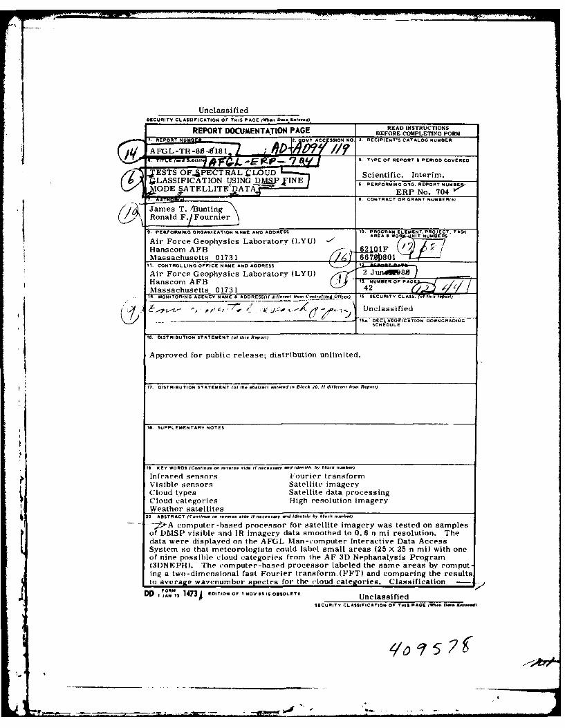
- - -A computer-based processor for satellite imagery was tested on samplesof DMSP visible and IR imagery data smoothed to 0. 6 n mi resolution. Thedata were displayed on the AFGL Man-computer Interactive Data AccessSystem so that meteorologists could label small areas (25 X 25 n mi) with oneof nine possible cloud categories from the AF 3D Nephanalysis Program(31)NEPH). The computer-based processor labeled the same areas by computing a two-dimensional fast Fourier transform.(FFT) and comparing the resultsto average wavenumber spectra for the cloud categories. Classification

DD I FOI 1473 4 EDITION OF INO Mol 61S OBSOLETE Unclassified

SECURITY CLASSIFICATION Of THIS PAGE (BWhen, 0.1 E.P...E

Vi

UnclassifiedSECURITY CLASSIFICATION OF T IS PAGE(Wh, D.i. En.I.-d)

20.- (Cont)

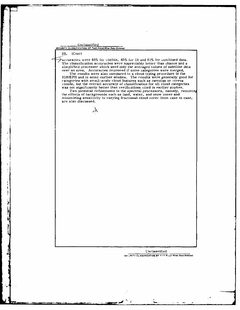
-7accuracies were 65% for visible, 65% for IR and 81% for combined data.The classification accuracies were appreciably better than chance and asimplified processor which used only the averaged values of satellite dataover an area. Accuracies improved if some categories were merged.

The results were also compared to a cloud typing procedure in the3DNEPH and to some earlier studies. The results were generally good forcategories with small-scale cloud features such as cumulus or cirrusclouds, but the overall accuracy of classification for all cloud categorieswas not significantly better than verifications cited in earlier studies.

Two potential refinements to the spectral processors, namely, removinthe effects of backgrounds such as land, water, and snow cover andminimizing sensitivity to varying fractional cloud cover from case to case,are also discussed.

AI

UnclassifiedSEC JR ITY CLASSIFICATION OFT -r P k3,tE'r" l we Ente.d)

.. 1.

Contents

1. INTRODUCTION 5

2. OTHER STUDIES 7

3. DMSP FINE MODE DATA 8

4. SUBJECTIVE CLOUD CLASSIFICATION 11

5. AUTOMATED CLOUD CLASSIFICATION 15

6. RESULTS OF THE STUDY 18

6.1 Mean Spectra of Cloud Types 196.2 Autocorrelation of Picture Elements 226.3 Classification by Mean Values 256.4 Classification for Nine Cloud Types 276.5 Detection of Small-Scale Cloud Features 296.6 Comparison to 3DNEPH 306.7 Multilayered Clouds and Merged Categories 336.8 Adjustments for Varying Backgrounds 346.9 Visible and IR Covariance Consideration 36

7. CONCLUSIONS 36

REFERENCES 39

APPENDIX A: Implications of Changing the Resolution ofSatellite Data 41

3

I, ,

' - -... ... ' " "- "" - ' . . . . . . . .

Illustrations

1. Photograph of the AFGL McIDAS CRT Showing DMSPVisible Data 10

2. Photograph of Same Area Shown in Figure 1 As Viewed by theIR Sensor (8 to 13 Mim) 11

3. DMSP Visible Data at 0. 6 n mi Resolution Over Egypt and theMediterranean Sea (upper right) 12

4. Photograph of Same Area Shown in Figure 3 as Viewed by theIR Sensor 13

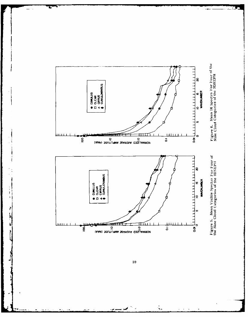
5. Mean Visible Spectra For Four of the Nine Cloud Categories ofthe 3DNEPH 20

6. Mean IR Spectra For Four of the Nine Cloud Categories of the3DNEPH 20

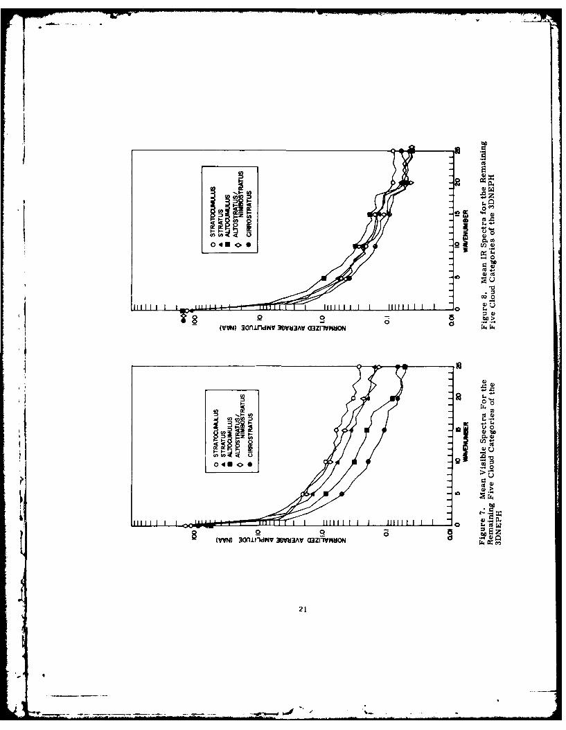
7. Mean Visible Spectra For the Remaining Five Cloud Categoriesof the 3DNEPH 21

8. Mean IR Spectra For the Remaining Five Cloud Categories ofthe 3DNEPH 21

9. The Autocorrelation Function For Three Cases of Visible Data 23

10. The Autocorrelation Function For Three Cases of IR Data 24

11. Mean IR and Visible Values For the Nine Cloud Categories 26

Tables

1. Cloud Type Categories From 3DNEPH 14

2a. Autocorrelation Parameters For Visible Data 24

2b. Autocorrelation Parameters For IR Data 25

3. Classification Accuracy For Two Data Sets 27

4. Classification Accuracy For Nine Categories 28

5. Numerical Values of Probability Terms For Nine CloudTypes in Subset 1 29

6. A Comparison of Observed Cloud Types to AutomatedClassifications 30

7. Classification Accuracy For 3DNEPH Categories 32

8. Cloud Categories Used in Cloud Classification Studies 34

9. Classification Accuracy For Five Categories: (Sc/St/Cu),(Ci/Cs), Cb, Clear 35

4

Tests of SpecTral Cloud Classification UsingDMSP Fine Mode Satellite Data

I. INTRODUCTION

Operational satellite imagers are now capable of ground resolution of less than

I n mi for both visible and IR channels. Photocopy or TV displays of such imagery

reveal a wealth of detail including such features as small-scale cumulus, cirro-

cumulus, or wave clouds. Meteorologists looking at the images can readily identifythese features and use this information to support highly important Air Force

projects. It is also apparent to the meteorologists that the small-scale features

are often not resolved in the currently operational cloud analysis program (3DNEPH) 1 ' 2

that uses satellite data with a ground resolution of approximately 3 n mi. For ex-

ample, when individual cumulus clouds are not resolved in the 3 n mi data, thesatellite data processor might incorrectly classify the cloudy area as either clear

or low overcast depending on the extent of coverage by the cumulus clouds. Either

misclassification could have grave consequences if used to support weapons systems

such as Precision Guided Munitions (PlIMs) since these tend to be sensitive to the

cloud cover at low altitudes. Moreover. cumulus clouds often grow during the day

so a misclassification of clear could also lead to a bad forecast.

(Received for publication 30 May 1980)

1. .ye, F. K. (1978) The AFGWC Automated Cloud Analysis Model. AFGWCTechnical Memorandum 78-002.

2. Coburn. A.R. (197 1) Improved Three-Dimensional Nephanalysis. AFGWCTechnical Memorandum 71-2.

5

--smr WO

Given DoD requirements for cloud analysis, and the limited time and manpower

for human interpretation of photocopy, there has been strong impetus to automate

the processing of very high resolution data. Automation has not been achieved thus

far due to the massive quantities of data involved. Moreover, spacecraft can pre-

sently store and transmit only limited quantities of fine mode imagery so that

coverage is poor on many orbits. Consequently, automated procedures that are

computationally fast and efficient or are suitable for use onboard the satellite are

of particular value.

This report summarizes tests of a computer-based processor to classify cloud

types using fine mode data from the Defense Meteorological Satellite Program

(DMSP). Earlier studies sponsored by the Air Force Geophysics Laboratory (AFGL)

have considered requirements for cloud analysis and developed the procedure tested

here. Pickett and Blackman 3 surveyed processing of satellite imagery at the Air

Force Global Weather Central (AFGWC) to identify automated imagery processing

techniques of potential value. Fourier spectral analysis was identified as the most

promising technique to upgrade automated processing of weather satellite imagery.

Initial demonstrations of spectral analysis using a two-dimensional Fast Fourier

Transform (FFT) over selected cloudy regions were given by Blackman and Pickett 4

and by Fournier. A test of a spectral classifier was described by Pickett and6

Blackman. The test used visible data from DMSP Block 5C satellites with cloud

type verification provided by satellite meteorologists who viewed displays of the

imagery data on a TV screen. While automated classifications using visible data

were found to be appreciably better than chance (46% correct classifications for the

automated program vs 17% for chance), the performance of 46% was less than.

expected. On the other hand, it was observed that many of the misclassifications

were reasonably close to correct, for example, classifying cumulus as strato-

cumulus or cirrostratus as cirrus.

The term fine mode data refers to both visible (0.4- 1. 1 jAm) and IR (8 - 13 rin)measurements by the Operational Linescan System on DMSP Block 5D spacecraft.The nominal resolution of these measurements on the Earth's surface is 0. 3 n mi.

3. Pickett, R.M., and Blackman, E.S. (1976) Automated Processing of SatelliteImagery Data at Air Force Global Weather Central, BBN No. 3Z75, InterimReport. F19628-76-C-0124, Bolt Beranek and Newman Inc.. Cambridge, MA02138.

4. Blackman, E. S., and Pickett. R. Al. (1977) Automated Processing of SatelliteImagery Data at the Air Force Global Weather Central: Demonstrations ofSpectral Analysis, AIGL-TR-77-0080. AD A0399'18.

5. Fournier, R. F. (1977) An Initial Study of Power Spectra for Satellite Imagery,AFGL-TR-77-0295, AD A058483.

6. Pickett, R. M., and Blackman, E. S. (1979) Automated Processing of SatelliteImagery Data: Test of a Spectral Classifier, AFGL-TR-79-0040,A) A 068663.

'd6

A different approach to the same requirements was taken by Hawkins. 7 A bitreduction algorithm was described which is capable of reducing the total number of

bits in a DMSP image by a factor of 6 while maintaining most of the image integrity.

This report extends previous studies since multispectral images of both IRand visible data from a Block 5D satellite are subjected to spectral analysis and

cloud classification using a straightforward extension of the computational procedureand a similar set of cloud cases selected by satellite meteorologists. The following

sections describe related literature, DMSP data, subjective and automatic classifica-

tion of the datak, and our conclusions. Properties of the FFT, classification logic,

and computer applications are described in a separate report by d'Entremont 8 and

will not be repeated here except as needed for clarity. The report does give, how-

ever, a complete discussion of the results of automated classification experiments.

2. OTHER STUDIES

Both before and during the AFGL studies, other investigators have conducted

similar studies. Since these studies are independent of our own by virtue of their

use of different data sets, satellites, cloud truth verification, and computer codes

they serve to substantiate our conclusions on the strengths and weaknesses of auto-

mated cloud classification. In 1963, Leese and Epstein 9 applied two-dimensional

spectral analysis to manually-digitized TIROS photographs. They used the spectralanalysis to quantify patterns of cloud lines and cells with horizontal dimensions in

10the range of 20 to 100 miles. Darling and Joseph applied several decision

algorithms to classify noncumnulus, cumulus with polygonal cells, and cumulus withsolid cells from NIMBUS I cloud pictures. In a comprehensive study, Booth used

both visible and IR NOAA 1 data to classify up to six cloud categories. The spectralenergies at various wavenumbers were included as predictors. The mean spatial

resolution of satellite measurements was given as 6 n mi, so that some considera-tion of the implications of this size difference is necessary before transferring his

results to fine mode satellite data. Sikula 1 2 made the first application of spectralanalysis to DMSP data. Very high resolution (0. 33 n mi) visual data were analyzedby a two-dimensional FFT. He also demonstrated that cumulus and cirrus clouds

had substantially different spectral signatures and that a data compression of about

100 to 1 could be achieved by using sums of spectral coefficients. Parikh1 3 . 14

reported on a comparative study of cloud classification techniques using NOAA 1

data and later did an evaluation of the techniques using data from the geostationary

satellite SMS 1. She considered both four and three categories of cloud conditions.

(Due to the large number of references cited above, they will not be listed here.See References, page 39.)

7

.. . ...... -.

Moreover, instead of using a transform to quantify the variability within arrays of

satellite data she defined other parameters called "textural features". Harris

and Barrett, apparently unaware of the 3DNEPH program, proposed an objective

procedure to distinguish three cloud types using measurements taken from a DMSP

visible transparency which they scanned by microdensitometer. In summary,

although a variety of cloud categories were used by the various authors, accuracies

of classification were moderately good, with higher accuracy when cloud types are

grouped into broader categories.

Aside from applications to cloud classification, a considerable literature exists

for spectral analysis of images of the oceans, earth resources, and so on. It is

beyond the scope of this report to survey this literature. However, a good intro-

duction is provided by Steiner and Salerno in the Manual of Remote Sensing. 16 The

mathematical background is treated in depth by Duda and Hart. 17

3. DMSP FINE MODE DATA

The DMSP Block 5D spacecraft and Operational Linescan System (OLS) sensorshave been described by Nichols et a11 8 and by Spangler. 19 The spacecraft are in

sun-synchronous polar orbits at 450 n mi altitudes. This study used data taken by

Vehicle F-1 that has an ascending node near local nmon. The OLS, which provides

the fine mode imagery, has a visible daytime response from 0.4 to 1. 1 Am and an

IR response from 8 to 13 Itm. The OLS is a scanning optical telescope system. An

approximately constant ground resolution (within a factor of 2) is maintained -by two

special features of the OLS. First, the scanning optics are driven in a sinusoidal

or back and forth motion rather than the conventional circular motion. Since the

scanning velocity slows as the telescope approaches its limit of scan, a nearly

constant sampling rate can be maintained along the scan line. Second, the system

field of view is reduced as the telescope approaches its limit of scan by means of

switching from three detector elements to one. The result is an approximate

15. Harris, R., and Barrett, E. C. (1978) Toward an objective nephanalysis,J. Appl. Meteor. 17:1258-1266.

A"A16. Steiner, D., and Salerno, A. E. (1975) Remote sensor data systems, pro-

cessing and management, Manual of Remote Sensing, Keuffel and Esser Co.,pp 611-803.

17. Duda, R.O., and Hart, P. E. (1973) Pattern Classification and Scene Analysis,John Wiley and Sons.

18. Nichols, D.A. (1975) Block 5D Compilation, Defense Meteorological Satellite

Program, Los Angeles AFS UWCA;99.19. Spangler, M.J. (1974) The DMSP primary data sensor in Proceedings of the

6th Conf. on Aerospace and Aeronautical Meteor. El Paso TX, pp 150-157.

8

0. 3 n mi resolution along scan lines. The frequency of oscillation of the scanning

optics is sized to provide 0.3 n mi resolution across track, that is, between scan

lines.

The approximately constant footprint size and equal spacing of OLS data on the

I earth are great advantages to spectral analysis or any other technique which

extracts information before the data are earth-located. Applications of a two-

dimensional FFT to arbitrary positions along a satellite data swath require

approximately equal spacing of data elements and constant footprint size. The

importance of these requirements can easily be shown by test patterns for the two-

dimensional FFT. Most earlier studies had to restrict coverage or alter the data

so that scale sizes did not depend on location along the scan line. For example,

Pickett and Blackman 6 used only areas reasonably close to the subtrack of the

DMSP 5C satellites while Booth 1 1 repeated scan lines and stretched them near the

limit of scan in order to yield approximately equal intervals between NOAA-I data

elements.

In late February 1978, a series of partial orbits of OLS data were saved by

AFGWC. Both digital magnetic tapes and photocopies were provided to AFGL. The

OLS sample included both fine mode visible (Light Fine, LF) and IR (Thermal Fine,

TF) data. The tapes contained data in a 2 X 2 mode, which means that two adjacent

data elements from two consecutive scan lines of the 0. 3 n mi data were averaged

to yield a nominal ground resolution of 0. 6 n miles. The 2 X 2 averaged mode was

provided since equipment limitations at AFGWC during early usage of the Block 5D

system would not allow digitized data saves at full resolution without undue interrup-

tion of operations. This limitation has subsequently been removed.

* Although our prime motivation was the detection of small-scale cloud elements

in fine mode data, we believe that the 0.6 n mi data are adequate for demonstrating

the feasibility of spectral analysis techniques and estimating the performance of an

automated classifier for cloud types. This confidence is based on the related studies

(discussed in Section 2) that used data from different satellites with various ground

* resolutions. Hence, in the remainder of this report, references to satellite data

will always imply the 0. 6 n mi data unless some other resolution is specified. Some

other implications of substituting 0. 6 for 0. 3 n mi data will be discussed in Appendix A.

The partial orbits were always the R+9 orbit, that is, nine orbits after the

reference orbit of the day. During the sunlit portion of this orbit, the spacecraft

ascends over Africa, the Middle East, and Europe traveling from the southeast to

the northwest. Examples are shown in Figures I and 2 that show part of orbit

7399+9 displayed on the AFGL Man-computer Interactive Data Access System

(McIDAS). Figure I has visible data while Figure 2 has IR data. The McIDAS CRT

i " . .. ...9

shows about 90% of the 1600 n mi swath width of data scans and was generated bydisplaying every fifth element of every fifth scan line. In the clearer areas on thelower part of Figure 1, portions of Libya, Egypt. the Sinai Peninsula, Saudi Arabiaand the Persian Gulf can be seen. The landmarks are not prominent in the IR

channel (Figure 2) due to greater atmospheric attenuation.

,4k,

Figure 1. Photograph of the AFGL McIDAS CRT Showing DMSP Visible Data.The width of the picture shows about 90% of the range of data scans by theOLS instrument. Data were taken on 15 February 1978 by Block 5D vehicleF-I over the Middle East. Africa and the Sinai Peninsula can be seen in thelower left and center of the picture. In this picture, as well as in Figure 2,image quality has been noticeably degraded since only every fifth elementof every fifth scan line is displayed

'I

41

,i-

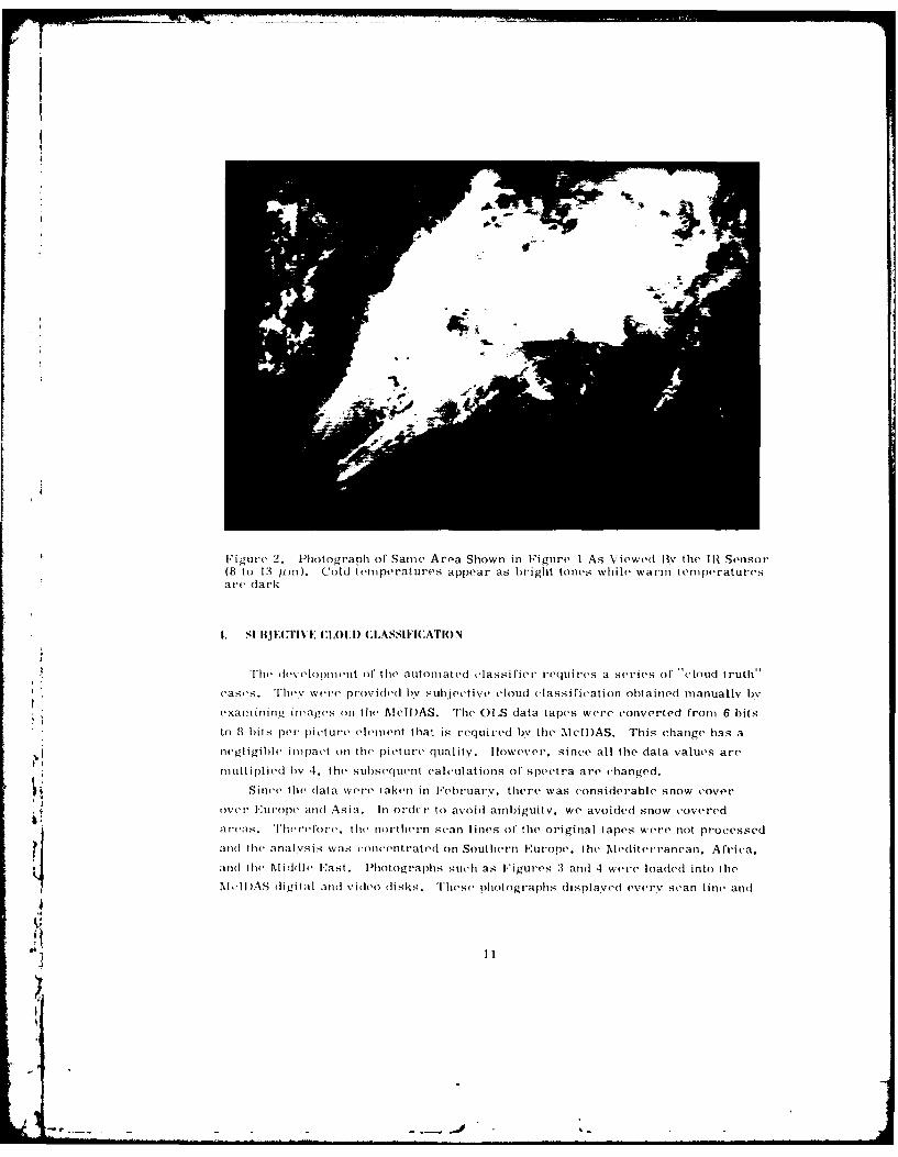
F~igure 2. Photograph of' Same Area Shown in Figure I As Viewed liv the IlI Sensor(8 to 1:3 pin ). Cold temnperatures appear as bright tones while warmi temnperaturesare (dark

L SIBJECT1l% F; CLOUDI CLASSIFICATIO)N

IThe developmei(nt of, the( automated classiftier requires a ser'ies of' "cloud truth"cae.Thev w ere provided liv Sub) e-iy '0( lass i rication ob~tai ned manually by

examining images onl the( fidl HIAS. The 01 S data tapes were ('(nverted fromt 6 hits

to 8t bit s per pi cture eement that is requiried byv the lcI AS. This change has a

n(gl i gible iminpact onirfthe p~ic(ture quality. How ever, since all the data values are

multiplied liv 4, the subsequent calculations of' Spectra are changed.

Si Oi((t Ih( dat a were taken in Febr'uai'v, there was considetrable snow c'over

over Eu roipe and As ia. lni'ul I'dc to avo id anmbigui tv. we avoided snow cove red

arieas. 'Th' rv'fore fit, hn ort herin scan lines of' the original tapes w ere not processed

aid( the analysis was concentrated on Southern Europe. tli' 1\1edite r'tanean, Africa,I 10(1 and I Middile East. liiotograplis such as F~igures 3i anul 4 were loaded into theN~lI )AS digital anid video disks. 'These phiotogr'aphs displayved every scan line and]

.11

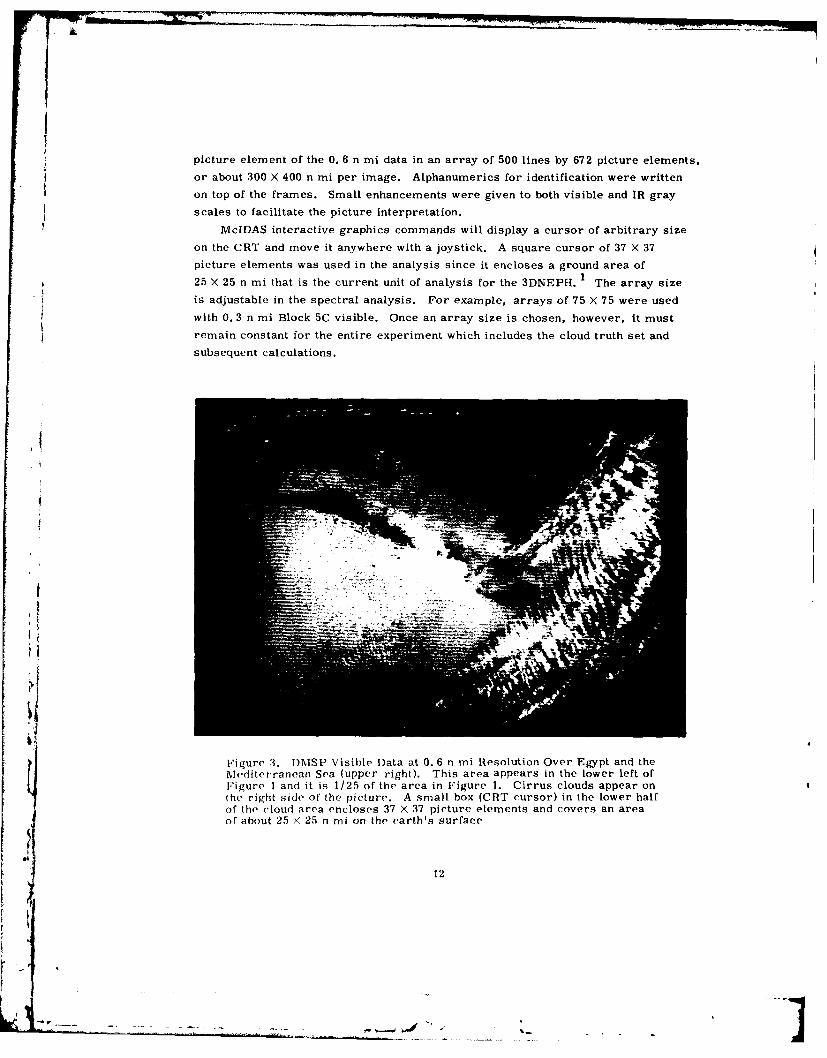
picture element of the 0. 6 n mi data in an array of 500 lines by 672 picture elements,

or about 300 X 400 n mi per image. Alphanumerics for identification were written

on top of the frames. Small enhancements were given to both visible and IR gray

scales to facilitate the picture interpretation.

McIDAS interactive graphics commands will display a cursor of arbitrary size

on the CRT and move it anywhere with a joystick. A square cursor of 37 X 37

picture elements was used in the analysis since it encloses a ground area of

25 X 25 n mi that is the current unit of analysis for the 3DNEPH. I The array size

is adjustable in the spectral analysis. For example, arrays of 75 X 75 were used

with 0. 3 n mi Block 5C visible. Once an array size is chosen, however, it must

remain constant for the entire experiment which includes the cloud truth set and

subsequent calculations.

Figure 3. DM.SP Visible Data at 0. 6 n mi Resolution Over Egypt and theMediterranean Sea (upper right). This area appears in the lower left ofFigure 1 and it is 1/25 of the area in Figure 1. Cirrus clouds appear onthe right side of the picture. A small box (CRT cursor) in the lower halfof the cloud area encloses 37 X 37 picture elements and covers an areaof about 25 X 25 n mi on the earth's surface

12

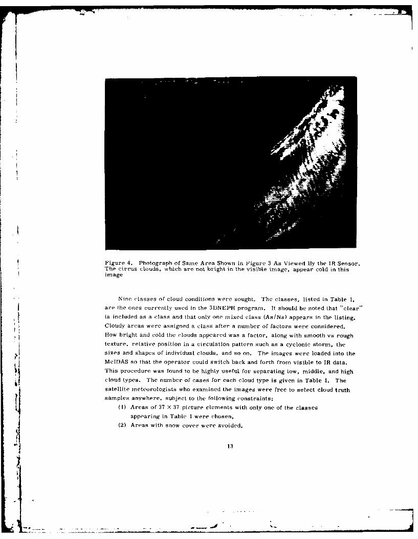
Figure 4. Photograph of Same Area Shown in Figure 3 As Viewed By the JR Sensor.The cirrus clouds. which are not bright in the visible image, appear cold in thisimage

Nine classes of cloud conditions were sought. The classes, listed in Table 1.are the ones currently used in the 3DNEPH program. It should be noted that "clear'

is included as a class and that only one mixed class (As/Ns) appears in the listing.

Cloudy areas were assigned a class after a number of factors were considered.

How bright and cold the clouds appeared was a factor, along with smooth vs rough

texture, relative position in a circulation pattern such as a cyclonic storm, the

sizes and shapes of individual clouds, and so on. The images were loaded into the

McIDAS so that the operator could switch back and forth from visible to IR data.

This procedure was found to be highly useful for separating low, middle, and highcloud types. The number of cases for each cloud type is given in Table 1. Thesatellite meteorologists who examined the images were free to select cloud truth

samples anywhere, subject to the following constraints:

(I) Areas of 37 X 37 picture elements with only one of the classes

appearing in Table I were chosen,

(2) Areas with snow cover were avoided.

13

(3) Areas could have either a land or a water background so

long as no coastline was included,

(4) Areas over a coastline could be chosen if the cloud

cover completely obscured the coastline,

(5) Every effort was made to find some samples for all

cloud categories even if it led to overrepresentation of

the infrequently observed categories such as Ac.

(6) Scan lines that appeared bad were not permitted to

cross a sample area,

(7) Overlapping of sample areas was avoided.

The selection of samples on the McIDAS was greatly aided by the MS command,

which was written specifically for the use of this project. Once a suitable area had

been found and the box-shaped cursor was placed over it, the 37 X 37 arrays of

both visible and IR data could be transferred from the McIDAS digital disk onto a

separate tape. The operator identified the cloud and background types in the MS

command. Bookkeeping information such as the orbit number and line and element

identification of the sample were automatically written on the tape along with the

arrays. When a number of samples had been collected on tape, subjective classifica-

tion was complete and the tape was used as input to the automated classification

program.

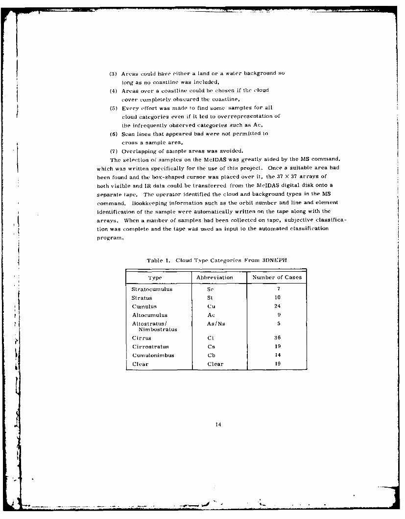
Table 1. Cloud Type Categories From 3DNEPH

Type Abbreviation Number of Cases

Stratocumulus Sc 7

Stratus St 10

Cumulus Cu 24

Altocumulus Ac 9

Altostratus/ As/Ns 5Nimbostratus

Cirrus Ci 36

Cirrostratus Cs 19

Cumulonimbus Cb 14

Clear Clear 19

14

-, I

• , . .. . .. . . . . . . . - , ,= _-. .

5. AUTOMATED CLOUD CLASSIFICATION

The mathematical basis and approximations of automated cloud classification

have been described in past reports by Blackman and Pickett 4 and by Fournier. 5

The extension of the techniques to the III and visible data saves from Block 5D

Vehicle F-I is described in a recent report by d'Entremont. A summary of the

descriptions in these reports is given here to provide a framework for the results

presented in Section 6. The FFT classification program was written for the AFGL

CDC 6600 sYstem due to computational requirements which exceeded the capabilities

of Ill)AS.

The classification program uses the following steps:

(1) An N N array of data is transformed to N X N spectral

coefficients by means of a two-dimensional IFFT.

(2) The N X N spectral coefficients are summedto normalized

average amplitUdes (NAA) for N/l2 wavenumbers. These

two steps are repeated for every case.

(3) The NAA are sorted by cloud type and the average and

standard deviation of NAA are computed for each type for

all N/ -2 wavenumbers.

(4) Probabilities are computed for each cloud type,

(5) Automatic classification is done by simply comparing the

NAA for- each case to the averaged NAA for each cloud type

and selecting the best match. The decision is also weighted

according to the a priori (dependent sample) probabilities

of the cloud types.

Steps 1 through 5 are the same when either visible or IR data are used alone.

\%,hen both are used together, steps I through 4 are run separately but the cloud

type decision in 5 includes both sets of NAA.

The N X N array of data can be represented as a unique linear series of products

of sines and cosines, which is a discrete two-dimensional Fourier transform. The

spectral coefficients in step I are the coefficients of the terms in the series. Since

each term in the series is associated with a particular wavelength, its coefficient

is a measure of how much of the N X N data array is explained by that wavelength.

For example, a data array showing one pure waveform with an integral number of

waves in the array would have one spectral coefficient of unity and the rest would

be zero. All of the variability of that array would be explained by one term of the

Fourier transform.

In digital computer spectral analysis applications, an FFT is generally used

since it reduces computer processing time and storage requirements. Other

15

i

approaches are available, including special purpose hardware and even optical20

devices. In our case. a FORTRAN routine by Brenner was used. In this routine,

all values of N are acceptable as array sizes. In this report, N is 37 corresponding

to ground coverage of about 25 X 25 n miles. In our previous applications we used

8 and 75 as values of N. With N equal to 37. one application of the FFT subroutine

to one cloud case took ,bout 0. 7 sec to run on the AFGL CDC 6600 computer and

this time posed no problem for development purposes. For operational purposes,

a faster and more compact program would probably be preferred. For values of N

which are powers of 2. a special version of the FFT program would take about one-

third as much computer storage as the unrestricted subroutine and would transform

a 32 x 32 array in about 40% of the time required for a 37 X 37 array. Since com-

plex numbers are used for both input and output, the satellite data were read in as

the real parts of complex numbers and the imaginary parts were set to zero.

In step 2 of the classification program, normalized average amplitudes (NAA)

are computed from the spectral coefficients. This step is significant for two12

reasons. First, as discussed by Sikula, the number of spectral measurements

is considerably reduced from N 2 to N8 '-so that subsequent processing is simplified.

Second. the NAA help make the classifier insensitive to the orientation of a given

cloud pattern. Without NAA for example, if a pattern of cloud lines were rotated by

45 degrees, its two-dimensional transform would change cons.derably and an auto-

mated classifier might not assign the same cloud type to the rotated pattern.

The NAA are computed as the sums of spectral coefficients within annular bands

in the frequency plane. Each band is one unit in width. The annular bands are

centered on the zero order term of the [FT. which is the mean of the data array.

The nean itself is the first NAA, and represents wavenumber zero. Wavenumbers

assigned to the bands increase as the radii of the bands increase. The NAA are

computed out to N/2 which is a Nyquist frequency for two dimensions. Aliasing

occurs at wavenumbers higher than N/i2 so that NAA are not computed. For an

tN of 37, N/2-is 26. Two variations in computing the NAA were used in this study.

In one, the coefficients were summed over all quadrants of the frequency plane.

This approach had been followed in earlier reports. Since it was not obvious that

all quadrants were providing independent information, we tried summing the coeffi-

cients only over the first quadrant of the frequency plane. In either case, each

wavenumber amplitude is averaged by dividing the number of terow ,,ntering into the

sum. Results for both cases are given in Section 6.

In step ,. the NAA for all cases in an experiment are sorted by cloud type and

the average and standard deviation of NAA are computed for each type for all

NJ7wavenumbers.

20. Brenner, N. (1967) Special Issue on the FFT. IEEE' Audio Transactions,June 1967.

16

- - Pt-

In step 4. probabilities are computed for each cloud type. These are given by

N.p .i = N 1 (1)1

t

with Ni the number of cases for cloud type i and N the total number of cases. At

the completion of step 4, all the information is at hand for automated classification.

In step 5. the key parameter of the automated classification procedure is given

by

:125 (X - I,'Ei - g 12 - 2- In 7i + lnP.. (2)

n=O (a n I

The index i, used as a subscript and superscript, takes the values of i= 1, 2,3 .... 9

corresponding to the nine cloud types of Table 1. The index n refers to the wave-

numbers of the NAA, X is an observed NAA. g1 is the mean of NAA fo- type i and

wavenumber n, ci is the standard deviation of NAA for type i and wavenumber n.n

l. is the unconditional probability of type i given by Eq. (1) and

I i i ... :V)4~' ii 0 1 2 ~25

A di is calculated for each of the nine cloud types for every area of satellite data

read into the classification program. 'he decision rule selects class k if dk > difor all i k. The first 26 terms of d. measure the distance of the observed spectrum

to the iean spectrum in a least squares sense. If the spectra are similar.

the sum mation over wavenumbers yields a small negative number and d. is likely

to be chosen by the decision rule. It is important to note that the distances

(Xn - 1AtI)2 between the spectra are scaled by the variance (a0 n12. The scaling gives

each wavenumber the same influence when dependent data are used in the classifier

and samples are compared to their correct cloud types since

N.

.; ( ")2 ( i 2 (4)i I n n fl

defines the variance for wavenumber n of type i. The index j is used for summation

over the N i cases of type i in the dependent data sample. The scaling does not insure

that each wavenumber will have the same influence in rejecting a cloud type when

samples are compared to incorrect cloud types. Without the scaling, the term d.

would be dominated by low wavenumbers since they have the highest NAA. This is

discussed in more detail in Section 6.

17l

The last two terms of Eq. (2) depend solely on the cloud type i and not the

sample spectrum. These two terms dominate the decision process in the event that

a sample spectrum is nearly the same distance from two or more mean spectra. A

decision for cloud type i is favored if the next-to-last term has small standard

deviations of NAA for class i. The decision is also favored if the last term repre-

sents a cloud type frequently observed in the dependent data sample.

Equation (2) is derived from a multivariate normal probability function. The

probability function can be used if the class conditional probability densities for the

NAA vectors are assumed as multivariate normal. A further assumption is statis-

tical independence between the spectra of different cloud types. If these assump-

tions are valid, the highest value of di identifies the most probable cloud type.

Two forms of Eq. (2) were used in this study. It was used both with and without

the last two terms in order to test the impact of the class probabilities on classifica-tion accuracy. In the selection of maximum d i. the elimination of the last two terms

is the same as if they were constant for all d.. In other words, it is the same as

assuming that all classes are equally probable.

The same computer programs were used for either visible or IR data when

they were used separately for automated cloud classification. In order to usevisible and IR together, the d i computed in Eq. (2) were arbitrarily added and the

maximum pair of values specified the cloud type. The decision rule selects class k

if

d d dkI > d dI forall iJk. (5)k k i (5

with the superscripts V and I designating visible and IR.

6. RESUITS OF Till. STUDY

A number of topics are addressed in the following section. In Section 6. 1, the

mean spectra for nine cloud types are discussed and used to describe the strengths

and weaknesses of the automated classifier. In Section 6. 2, the autocorrelation of

picture elements at various spatial separations is introduced and related to proper-

ties of the mean spectra. In Section 6. 3, a classification using just the mean

values of cloud areas is introduced as a reference to measure the performance of

the automated classifier using all wavenumbers. In Section 6. 4, the results of

classification for all nine cloud types are presented. The various issues discussed

include a comparison of classifications on two subsets of data. accuracy of classifi-

cation on visible, IR, and combined data, accuracy of classification with and without

JR

.. . ..-. . . . , I- .. . .

a priori probabilities of cloud types, and complete vs partial sums of Fourier

coefficients to define spectra. In Section 6. 5. the results for cumulus and cirrus

clouds are examined in greater detail since these clouds exhibit the small-scale

features which are not resolved in current automated processing. In Section 6. 6.

the nine categories of cloud types are combined into fewer categories so that re-

sults can be compared with the present 3DNEPH. Applications to multilayered

claads made in earlier studies are described in Section 6. 7 and adjustments for

varying backgrounds are discussed in Section 6. 8. A possible expansion of decision

equations is described in Section 6. 9.

6.1 Mean Spetra of Qoud Types

Plots of mean spectra for the nine cloud types are shown in Figures 5 to 8. For

clarity, four cloud types are shown in Figures 5 and 6 and the other five in Figures

7 and 8. In all subsequent discussion, the term "individual spectrum" refers to the

NAA for one case while the term "mean spectra" refers to NAA averaged over all

cases of a cloud type. The mean spectra in Figures 5 to 8 are from one 73-case

subset of the total set of 143 cases. However, they are similar to the mean spectra

for the other subset. In all cases, the spectra are scaled so that the NAA of wave-

number zero is the mean visible or IR value for the cloud type. Since the data were

converted to the McIDAS 8-bit format, a value of 255 would represent the brightest

possible clouds in the visible or the coldest in the IR. The mean values are con-

siderably less than 255 since many of the N '- N areas were only partly cloud covered.

All spectra are similar since the NAA are always highest at wavenumber zero

and no other significant peaks appear at any other wavenumbers. The peaks at low

wavenumbers were first noted by Leese and Epstein9 and explained as the result of

gradual changes of mean cloudiness across the areas studied. In other words, there

was a trend across the area. They minimized the slope of the spectra at low wave-

numbers by fitting a least-squares plane to the initial data. The spectral analysis

was then carried out on the residuals. Such a procedure was not followed in this

study since it would minimize the difference between the means of the various cloud

types and since the means are known to be useful for cloud typing. In particular, itwould lead to confusion between clear areas and cloudy areas since the clear areas

usually have the lowest means. The absence of significant peaks at higher wave-

numbers is due to the fact that the spectra are averages of individual spectra. The

individual spectra appear somewhat rougher than the averages shown here. How-

ever, the shapes and sizes of clouds vary from case to case so that the spectral

peaks at high wavenumbers are more or less randomly distributed and appear

smoothed out in the mean spectra.

19

I.o - " _ . ' . . . -r .:. . . . M '

00 ~0

wI 0

0

w L C15U

) U)

0 S

~1 (VVN) 3ofifldW 3DVU3AV 03Z[IYWNON

02a

4)

jU) C

U)~ -~l-

40

00

T8(VVN) 3anirndwv 30VN3AV O33ZflVIVO 0

(00 0

1 9 1 uj 0OC C

(U

4 Z3 I

211

- Io

-- ------- - ~ -~.--~)~d , .- ba

Despite the fact that the mean spectra appear somewhat similar, they are

different enough for automated classification provided that an individual spectrum

is closer to the mean spectrum of its type than it is to the other mean spectra.

Equation (2) shows that the classifier responds only to differences in the amplitudes

of spectra and is indifferent to their shapes. In Figure 5, for example, all four

visible spectra have similar curvature but the spectrum for clear is low enough that

it is unlikely to be confused with the others. Since all the wavenumbers are used,

the spectra can be distinguished even if they overlap for some wavenumbers. Good

examples of this are the visible spectra for Cu and Cb in Figure 5. They are very

close at wavenumbers 10 to 24 but differ substantially at wavenumbers near zero.

Another interesting feature of Figure 5 is the fact that the mean for Clear is higher

than the mean for Cu since there were more clear cases over land than Cu cases

over land and the land backgrounds appear fairly bright. A classifier using just the

mean visible would miss the Cu while a classifier using higher wavenumbers would

readily distinguish the Cu from the Clear.

Figure 6 has the mean IR spectra for the same four cloud types in Figure 5.

The IR spectra have shapes similar to the visible spectra in Figure 5 but the rela-

Itive position of the cloud types has changed. It was noted previously that the visible

spectra for Cu and Cb were close at high wavenumbers. The IR spectra for Cu are

substantially lower than the Cb spectra over the entire range of wavenumbers. The

IR spectra for Cb and Ci are close at high wavenumbers but the visible spectra are

not. One begins to see how the use of both visible and IR data leads to better classi-

fications since the decision rule requires that an unknown cloudy area have both

visible and IR spectra matching a particular cloud type before that type is chosen.

Two other comments regarding Figures 5 to 8 deserve mention. First, the

rather smooth and featureless appearance of the average spectra suggests consider-

able redundancy in the information they contain. Pickett and Blackman 6 suggested

that the visible spectra they studied had about three independent pieces of informa-

tion, much fewer than the number of wavenumbers used by the classifier. The

second comment is that the logarithmic scale for NAA in Figures 5 to 8 is used to

conveniently plot spectra for all wavenumbers and the reader should remember that

the actual comparisons of spectra are scaled at each wavenumber according to the

variance of NAA for each cloud type.

6.2 Autocorrelation of Picture Elements

In past applications of spectral analysis, considerable attention was given to

the autocorrelation or autocovariance function. The autocorrelation function for a

series of data is computed by simply shifting the series by one lag and computing

the correlation coefficient between the original series and the shifted series. The

22

process is repeated at lags 1, 2, 3 .... n to give the autocorrelation to lag n. While

this information is not provided by the FFT, it can be useful to help interpret thespectra.

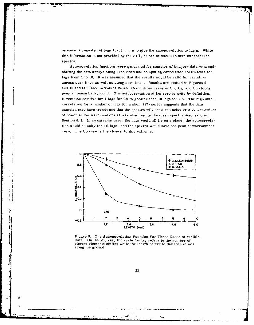
Autocorrelation functions were generated for samples of imagery data by simply

shifting the data arrays along scan lines and computing correlation coefficients for

lags from 1 to 10. It was assumed that the results would be valid for variation

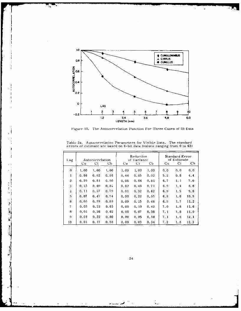
across scan lines as well as along scan lines. Results are plotted in Figures 9

and 10 and tabulated in Tables 2a and 2b for three cases of Cb, Ci, and Cu clouds

over an ocean background. The autocorrelation at lag zero is unity by definition.

It remains positive for 7 lags for Cu to greater than 10 lags for Cb. The high auto-

correlation for a number of lags for a short (37) series suggests that the data

samples may have trends and that the spectra will show red noise or a concentration

of power at low wavenumbers as was observed in the mean spectra discussed in

Section 6. 1. In an extreme case, the data would all lie on a plane, the autocorrela-

tion would be unity for all lags, and the spectra would have one peak at wavenumber

zero. The Cb case is the closest to this extreme.

1.0

OCUMULOIMBUS0.0 a CIRRUS

60.6

4,I* 10.2

0LAG

I 2 3 4 6 7-0.2

8 9 10

1.2 2.4 3.6 4.8 6.0LENGTH (nmi)

Figure 9. The Autocorrelation Function For Three Cases of VisibleData. On the abcissa, the scale for lag refers to the number ofpicture elements shifted while the length refers to distance (n mi)along the ground

23

A ,

C ---

1.00.8A CIRRUS

S0.6

04

904

0.2

0LAG2 3 4 5 6 7 8 9 I0

-0.2 11.2 2.4 3.6 4.8 6.0

LENGTH (nmi)

Figure 10. The Autocorrelation Function For Three Cases of IR Data

Table 2a. Autocorrelation Parameters for Visible Data. The standarderrors of estimate are based on 6-bit data (values ranging from 0 to 63)

Reduction Standard ErrorLag Autocorrelation of Variance of Estimate

Cu Ci Cb Cu Ci Cb Cu Ci Cb

0 1.00 1.00 1.00 1.00 1.00 1.00 0.0 0.0 0.0

1 0.66 0.92 0.96 0.44 0.85 0.92 5.2 0.8 4.4

2 0.29 0.81 0.90 0.08 0.66 0.81 6.7 1.1 7.0

3 0.15 0.69 0.84 0.02 0.48 0.71 6.9 1.4 8.6

4 0.11 0.57 0.79 0.01 0.32 0.62 6.9 1.5 9.6

5 0.07 0.47 0.74 0.00 0.22 0.55 6.9 1.6 10.5

6 0.05 0.39 0.69 0.00 0. 15 0.48 6.9 1.7 11.2

7 0.03 0.32 0.65 0.00 0.10 0.42 7.0 1.8 11.68 0.01 0.26 0.62 0.00 0.07 0.38 7.1 1.8 11.9

4 9 0.01 0.22 0.60 0.00 0.05 0.36 7.1 1.8 12.110 0.01 0.17 0.58 0.00 0.03 0.34 7.2 1.8 12.3

24_

24

Table 2b. Autocorrelation Parameters For IR lOata

Reduction Standard ErrorLag Autocorrelat on of Variance of Estimate

Cu Ci Cb Cu Ci Cb Cu Ci Cb

0 00 1.00 1.00 1.00 1.00 1.00 0.0 0.0 0.0

1 0.79 0.94 0.98 0.62 0.88 0.96 1.3 0.8 2.2

2 0.51 0.85 0.94 0.26 0.72 0.88 1.8 1.3 3.8

3 0.32 0.74 0..89 0. 10 0. 55 0.79 1.9 1. 6 5. 1

4 0.22 0.62 0.84 0.05 0.38 0.71 2.0 1.8 6.2

5 0.14 0.50 0.78 0.02 0.25 0.61 2.0 1.9 7.0

6 0.07 0.40 0.73 0.00 0. 16 0.53 2.0 2. 1 7.7

7 0.02 0.31 0.69 0.00 0.10 0.48 2.1 2.1 8.2

8 -0.01 0.24 0. 65 0.00 0.06 0.42 2. 1 2.2 8.6

9 -0.01 0. 19 0.62 0.00 0.04 0.38 2. 1 2.2 8.9

10 0.01 0.13 0.58 0.00 0.02 0.34 2.1 2.2 9.2

High autocorrelation for a number of lags also suggests that the clouds and

clear areas in the arrays are somewhat homogeneous so that one pixel can be used

to predict the values of its neighbors. A measure of this utility is given by the re-

ductions of variance and standard errors of estimate given in Table 2. This

homogeneity of clouds and clear areas helps to minimize the impact of errors in

the earth location of the data.

6.3 Classification by Mean Valnes

Satellite meteorologists have known for some time that the mean visible bright-

ness or IR temperature of a cloud is useful for determining cloud type. Assuming

the same fractional cloud cover, the brightest clouds tend to be Cb while the least

bright clouds are usually thin Ci. High clouds such as Cs tend to appear colder than

low clouds such as Sc. These properties are currently used for cloud typing in

the 3DNEPH.

The cloud cases used for spectral analysis were also classified by type accord-

ing to their mean visible and IR values. Since the spectral classifier uses the means

as well as higher wavenurobers, it is possible to judge how much the higher wave-

numbers are adding to the accuracy of classification. The mean classifier is equiva-

lent to using only the first term of Eq. (2), that is, choose cloud type i for the

minimurn

di (X 0 (6)

25

for visible or IR data alone. For visible and IR data together, sum the d. for

visible and IR and choose the minimum. This procedure simply finds the nearest

class mean in a two-dimensional space and chooses that type. Figure 11 shows the

relative positions of the computed class means. The classes which are separated

the most in Figure 11 are expected to be distinguished the best by the mean

classifier.

200

Ac Cs CI

150 As/No

A ScC1

St

z4100WLu Cu

CLEAR

50

0

0 DARK 50 100 BRIGHT 150MEAN VISIBLE

Figure 11. Mean IR and Visible Values For the Nine Cloud

Categories

26

6.4 Classification for Nine (Qoud Types

The total data set of 143 cases consists of two parts, subset 1 with 73 cases

and subset 2 with 70 cases. Each subset was classified by a different satellite

meteorologist. The subsets were run separately in the automatic classification

program in order to see how much the program depended on the person defining

the truth set. All nine cloud types were represented in each subset by two or more

cases. For each subset, the classification program was run four times, that is

with and without a priori probabilities of cloud types and for complete and partial

sums of Fourier coefficients.

In the following discussion, it is important to note that the classificationaccuracies are estimated from fairly small samples of dependent data. They are

likely to be less when applied to independent data or else derived from larger data

samples.

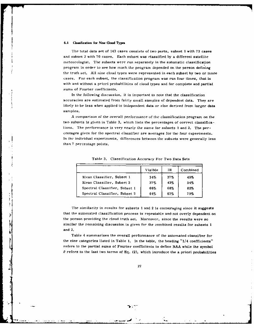
A comparison of the overall performance of the classification program on the

two subsets is given in Table 3, which lists the percentages of correct classifica-

tions. The performance is very nearly the same for subsets 1 and 2. The per-

centages given for the spectral classifier are averages for the four experiments.

In the individual experiments, differences between the subsets were generally less

than 7 percentage points.

Table 3. Classification Accuracy For Two Data Sets

Visible IR Combined

Mean Classifier, Subset 1 34% 37% 49%

Mean Classifier. Subset 2 37% 43% 54%Spectral Classifier. Subset 1 66% 68% 82%

Spectral Classifier, Subset 2 64% 63% 79%

The similarity in results for subsets 1 and 2 is encouraging since it suggeststhat the automated classification process is repeatable and not overly dependent on

the person providing the cloud truth set. Moreover, since the results were so

similar the remaining discussion is given for the combined results for subsets 1

and 2.

Table 4 summarizes the overall performance of the automated classifier for

the nine categories listed in Table 1. In the table, the heading "1/4 coefficients"

refers to the partial sums of Fourier coefficients to define NAA while the symbol

0 refers to the last two terms of Eq. (2), which introduce the a priori probabilities

27

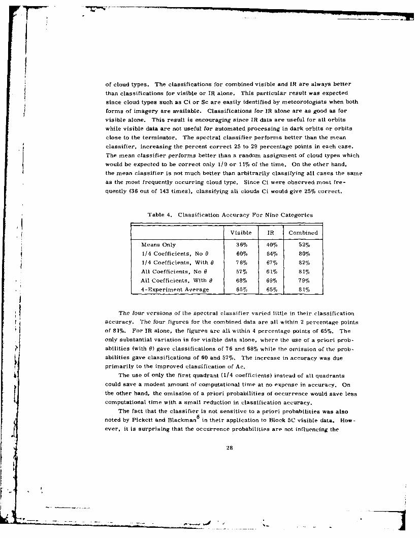
of cloud types. The classifications for combined visible and IR are always better

than classifications for visible or IR alone. This particular result was expected

since cloud types such as Ci or Sc are easily identified by meteorologists when both

forms of imagery are available. Classifications for IR alone are as good as for

visible alone. This result is encouraging since IR data are useful for all orbits

while visible data are not useful for automated processing in dark orbits or orbits

close to the terminator. The spectral classifier performs better than the mean

classifier, increasing the percent correct 25 to 29 percentage points in each case.

The mean classifier performs better than a random assignment of cloud types which

would be expected to be correct only 1/9 or 11% of the time. On the other hand,

the mean classifier is not much better than arbitrarily classifying all cases the same

as the most frequently occurring cloud type. Since Ci were observed most fre-

quently (36 out of 143 times), classifying all clouds Ci would give 25% correct.

Table 4. Classification Accuracy For Nine Categories

Visible IR Combined

Means Only 36% 40% 52%

1/4 Coefficients, No 0 60% 64% 80%

1/4 Coefficients, With 0 76% 67% 82%

All Coefficients, No 0 57% 61% 81%

All Coefficients, With 0 68% 69% 79%

4-Experiment Average 65% 65% 81%

The four versions of the spectral classifier varied little in their classificationaccuracy. The four figures for the combined data are all within 2 percentage points

of 81%. For IR alone, the figures are all within 4 percentage points of 65%. The

only substantial variation is for visible data alone, where the use of a priori prob-

abilities (with 0) gave classifications of 76 and 68% while the omission of the prob-

abilities gave classifications of 60 and 57%. The increase in accuracy was due

primarily to the improved classification of Ac.

The use of only the first quadrant (1/4 coefficients) instead of all quadrants

could save a modest amount of computational time at no expense in accuracy. On

the other hand, the omission of a priori probabilities of occurrence would save less

computational time with a small reduction in classification accuracy.

The fact that the classifier is not sensitive to a priori probabilities was also

noted by Pickett and Blackman6 in their application to Block 5C visible data. How-

ever, it is surprising that the occurrence probabilities are not influencing the

28

. . . . . . . . .

IL_accuracy to a greater extent since they vary by a factor of 7 from the least probable

(As/Ns) to the most probable (Ci) type. This issue was studied by examining the

numerical values of terms in Eq. (2) for a number of classifications. Table 5 lists

the last two terms in Eq. (2), the only terms related to the class probabilities. For

a given classifier, these terms are constants depending only on the cloud type. The

values given in Table 5 are for the 73 case subset with all Fourier coefficients used

to define NAA. The next to last term, -1/2 In I I is always larger in magnitude

than the last term. The next to last term combines the standard deviations of NAA

for all wavenumbers and should serve as a scaling factor for the last term. There

is no obvious explanation of why it dominates unless the statistical assumptions in

the derivation of Eq. (2) are not being met. One possible test which was not tried

was to set the next to last term to zero or else reduce it by an arbitrary factor to

see if classification accuracy would improve.

Earlier studies had suggested that a priori probabilities could be varied with

location on the earth to adapt the classifier to different climates or land vs ocean

influences. The present results suggest that changing the probabilities would not

help the classifier unless Eq. (2) is revised.

Table 5. Numerical Values of Probability Terms for Nine CloudTypes in Subset 1

Visible Infrared

- 1/2 In I In P -1/2 In I ln P.i I i

Sc 22. 843 -2. 904 51. 256 -2. 904

St 38.670 -2.344 69.379 -2.344

Cu 38. 298 -1. 805 65. 169 -1.805

Clear 64.967 -2.344 86.001 -2.344Ac 74.385 -2.904 57.242 -2.904

As/Ns 47. 532 -3. 597 66.743 -3. 597

Ci 34. 182 -1. 199 50.869 -1. 199

Cs 55. 508 -2. 211 60. 288 -2. 211

Cb 32. 404 -2. 344 54. 892 -2. 344

6.5 I)electinii of Smniall-eale Cloud Fealtres

The overall accuracy of classification for nine cloud categories it not the only

measure of merit for automated classification of fine mode data. An equally

important consideration is how well it detects small-scale cloud features that are

29

poorly resolved by smoothed mode data in the current nephanalysis. Among lower

clouds, cumulus clouds tend to have the smallest sizes and at times they are not

detected in smoothed mode data. For high clouds, cirrus tends to have the smallest

or least distinguishable cloud features. Results for Cu are given in Table 6.

Cumulus clouds were correctly chosen 66% of the time, misclassified as another

cumuliform (Cb, Sc or Ac) 21% of the time, and misclassified as hightypes (Cs or

Ci) 12% of the time using visible data. Significantly, in no cases were Cu unde-

tected, that is, misclassified as clear areas. They are either classified correctly

or as some other cloud type. The IR classifier did not do as well (55% to 66%) but

it misLabeled Cu cases as clear only 1% of the time. Regarding cirrus, the IR

classifier was successful 72% of the time and never mislabeled a Ci case as clear.

Visible data were less reliable for cirrus detection (50% compared to 7276). The

combined classifier did well for both Cu (77%) and Ci (76%6) and never misclassified

them as clear.

Table 6. A Comparison of Observed Cloud Types toAutomated Classifications. The numbers tabulatedare percentages of the observed cases. Some columnsdo not sum to 100% due to rounding off to the nearestpercent

Observed Type

Automated Visible IR CombinedClassification Cu Ci Cu Ci Cu Ci

Sc 7 8 19 9 5 6

St 0 6 1 3 2 2

Cu 66 0 55 6 77 3

Ac 5 1 2 0 3 0

As/Ns 0 0 0 0 0 0

Ci 10 50 15 72 2 76

I Cs 2 15 7 3 4 8Cb 9 8 0 7 6 6

Clear 0 13 1 0 0 0

6.6 Comparison lo 31)NEPH

Appendix I of the 3DNEPH report by Fye 1 describes an empirical determina-

tion of cloud types from IR and visual satellite imagery. The 3DNEPH types clouds

using an empirical set of weighted equations and thresholds which are functions of

visual and IR grayshade and variability. The 3DNEPH report does not give an

30

-li I

exact definition of "grayshade" and "variability" as used by the cloud typing routine

nor does the report indicate the extent to which the cloud typing depends on the

visual and IR data processors, which provide considerable information for cloud

detection and estimates of the horizontal and vertical coverage of cloud layers.

Nephanalysis specialists at AFGWC defined G. the visual grayshade, as the average

of visible data over an eighth-mesh box (about 25 X 25 n mi) and the visual vari-

ability as

N

V = N 1 1 Gi- (7)

where G i is a visible datum and N is the total number of data elements. The aver-

age U is the same as the mean value used in the mean classifier and the spectral

classifiers discussed in Sections 6. 3 and 6.4. The variability V. which is some-

times called the mean deviation, is not the same as any of the wavenumbers used

by the spectral classifiers.

The IR grayshades and variabilities used for cloud typing have been defined in

several ways since cloud typing originated in 1976. Early routines used the same

definitions of means and variabilities for both IR and visible data. More recently,

surface temperatures, independent of the satellite IR temperatures, are used as a

reference for the IR grayshade.

When both visible and IR data are available, cloud typing is done for the eight

cloud categories in Table 1. The category clear is not assigned. If only visible

data are available, only Cb clouds are typed. If only IR data are available, low

clouds are excluded and only the middle and high clouds are typed. The four cate-

gories for IR typing are (As/Ns), Ac, (Cs/Cb), and Ci. The two types Cs and Cb

are merged into a supercategory for purposes of comparison with the results of

this report following the advice of AWS technical personnel, who pointed out that

Cs and Cb are difficult to distinguish in the 3DNEPH IR cloud typing.

The accuracy of 3DNEPH cloud typing was found to be 80% in development tests.

A verification program (CLOVER) found surface reports closely timed to satellite

data indicating only one cloud type. The program used IR data to check for cloud

layers which might be hidden from the observers and removed these cases from

the verification.

The results presented in Section 6. 4 were retabulated for comparison to the3DNEPH categories and are given in Table 7. For combined visible and IR data,

the average performance of the spectral classifier dropped from 8176 to 80%. The

clear category, which was purged, had a classification accuracy of 85% so that re-

sults for eight categories are less than for nine categories. For visible data alone.

82%6 of Cb clouds were typed correctly. For IR data alone, 70% of middle and high

31

lo

I 1__ '"

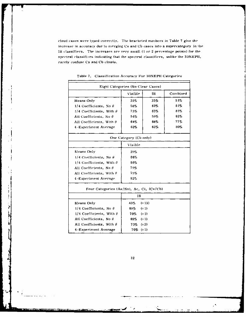
cloud cases were typed correctly. The bracketed numbers in Table 7 give the

increase in accuracy due to merging Cs and Cb cases into a supercategory in the

* IR classifiers. The increases are very small (1 or 2 percentage points) for the

spectral classifi-rs indicating that the spectral classifiers, unlike the 3DNEPH,

rarely confuse Cs and Cb clouds.

Table 7. Classification Accuracy For 3DNEPH Categories

Eight Categories (No Clear Cases)

Visible IR Combined

Means Only 35% 35% 51%

1/4 Coefficients, No 0 58% 62% 81%

1/4 Coefficients. With 0 73/6 63% 81%

All Coefficients, No 0 54% 59% 82%

All Coefficients, With 0 64% 66% 77%

4-Experiment Average 62% 62% 80%

One Category (Cb only)

Visible

Means Only 29%

1/4 Coefficients, No 0 86%

1/4 Coefficients, With 0 86%

All Coefficients, No 0 79%

All Coefficients, With 0 79%

4-Experiment Average 82%

Four Categories (As/Ns), Ac, Ci, (Cs/Cb)

4 JR

Means Only 43% (+13)

1/4 Coefficients, No 0 69%o (+ 1)

1/4 Coefficients, With 0 70% (+ 1)

All Coefficients. No 0 69% (+1)

All Coefficients, With 0 73% (+2)

4-Experiment Average 7076 (+ 1)

32

I *W

The accuracies of the spectral classifier (80% for visible and JR. eight cate-

gories; 82% for visible, one category; 70% for IR, four categories) are about the

same as the 80% figure given for development tests of the 3DNEPH. 1 Since our

study and the 3DNEPli used different data sets and different methods to select cloud

cases to verify the classifiers it is not possible to judge which approach works best.

If both classifiers were used on the same data, we expect the spectral classifier"

would perform as well as or better than the 3DNElPlJ classifier since the spectral

classifier uses the mean and 25 wavenumber parameters while the 3DNEPH uses

the mean and only one other parameter, the variability.

The spectral classifiers were substantially more accurate than the mean

classifiers, for example 70% accuracy was found for four categories in IR data

instead of 43%/ for the mean classifier. The increased accuracy is due to the 25

wavenumber parameters in the spectral classifier. For the 31)NEPH classifier.

we do not know how much of the classification accuracy is due to the means and

how much is due to the variabilities. This information, if known, would be very

helpful for evaluating the utility of wavenumber parameters since it would show how

much classification accuracy was due to the carefully tuned but simply defined

statistic of variability.

6.7 Multilavercd (louds and Merged (Categories

A multilavered category was not included in our study since we used the 3DNEPH

categories given in Table I and concentrated on the categories cumulus and cirrus

which exhibit small-scale features. In a global application, however, multilayered

clouds would be encountered and the spectral classifiers discussed in this report

would assign some single cloud category to these areas. Although we did not test

mixed cases, it is our opinion that a multilayered scene such as Ci over lower cloud

would be assigned a high cloud type such as Ci or Cb by the IR or combined spectral:1 classifiers. It is less clear what the visible classifier would do with multilayered

clouds.

The studies summarized in Table 8 were able to detect multilayereu clouds with

some skill but there was a difference of opinion as to how well it was done. Booth 1 1

and Parikh 1 4 used a multilayered category described as Ci + low. This category

included all cases of cirrus above middle clouds or low clouds. Booth's 1 1 results

show that the Ci + low classification accuracy was about the same as the overall

classification accuracy and he maintained the Ci + low category in all his experi-

ments. Using SMS-1 data, Parikh 1 4 concluded that the multilayer class was not

well separated from the other classes and that classification accuracies could be

improved by removing the multilayered class.

33

'l

Table 8. Cloud Categories Used in Cloud Classification Studies

11 11 14 14 Harris andNumber Booth Booth Parikh Parikh Barrett 1 5

1 Clear Clear Cu/Sc/St Cu/Sc/St Clear

2 Cu Cu/Sc/St Ci + low Ci Stratiform

3 Sc/St Cb Ci Cb Cumuliform

4 Cb Ci Cb Stratocumuliform

5 Ci Ci+ low

6 Ci +l ow

Classification Accuracy

Visible 43-54% 44 -55% 1 72%

IR 57 -60% 63-70% 75%

Combined 63-7 6% 69-81% 81 -89%, 90-96%

All of the studies in Table 8 used fewer categories than we used by merging

categories like Sc and Cu into supercategories such as (Sc/Cu). The use of super-

categories improves the overall classification since misclassifications to closely

related categories are counted as hits rather than misses. The increase in

classification accuracy by the use of supercategories tends to offset the decrease

in accuracy which may occur if a multilayered category is introduced.

The approach to classification followed in this report could he modified to he

similar to the other studies. A condensed version of the categories in Table 1 is

presented in Table 9. All low clouds are merge into one category (St/St/Cu). all

middle clouds are merged into one category (Ac/As!Ns). cirrus is combined with

cirrostratus (Ci/Cs). while cumulonimbus anti clear are kept as separate categories.

Classification accuracies are high (73% for visible. 72% for ll 86% for combined)

and the inclusion of a multilayered (lass might not degrade the classification

accuracies to an unacceptable level.

6.8 Adjustments for Varying larkgproaandsThe variability of backgrounds encountered in a global application of cloud typing

algorithms is of particular concern. Extreme backgrounds may appear so bright

in the visible or so cold in the IR that no technique can detect clouds over these

backgrounds with confidence. For visible data, an example of an extreme back-

ground would be an ice cap or tundra covered by fresh snow. For IR data, in addi-

tion to the very cold temperatures observed near the South Pole there are parts of

Siberia with monthly mean temperatures below -50C.

34

Table 9. Classification Accuracy For Five Categories(Sc/St/Cu), (Ac/As/Ns), (Ci/Cs), Cb, Clear

Visible IR combined

Means Only 44% 48% 59%

1/4 Coefficients, No 0 67% 69% 83%

1/4 Coefficients, With 0 81% 75% 89%

All Coefficients. No 0 66% 670, 84%

All Coefficients, With ft 76% 77% 86%

4-Experiment Average 73% 72% 86%

Between the well-behaved backgrounds, which were generally used in the

studies cited. and the extreme backgrounds, which no one used, there remains a

great range of background conditions encountered while sensing clouds from

satellites. In the 3I)NEPII, the great range of conditions is handled by comparing

the visible data to background brightness fields and the IR data to (clear colunn

temperature fields derived from surface and sounding data or forecast models.

The preparation of background fields probably requires as much data processing

as anv other part of the 31)NE:PH. The experience gained in developing background

fields for the 3)NEPIt suggests that the development of similar background fields

for a spectral class)fier would be a lengthy and ctomputationallYv intensive process.

The 31)NFI'tl approach to background fields could be extended to the spectral

classifiers. For visible data, mean spectra for the category of clear could be

derived for all locations on the earth. The (clear spectra would look different,

depending on whether the background was land, ocean, snow, or some mixture.

"he individual spectrum for an unknown cas(-ould he classified by comparing it

to the location-dependent clear spectrum as well as the mean spectra for cloud

categories. ('loud categories with mean spectra nearly the same as the clear

spectrum could he earmarked as undetectable at that location. Snow covered areas,

which tend to he the brightest backgrounds, would probably be the most difficult

backgrounds for spectral classifiers as they are for the first order statistics in

the 31)NEI'll.

The 31)NFPIt does not handle the background fields for IR data in the same way

that it does for visible data. Since clear column temperatures will vary front day

to dav for a fliven location, a reference field is prepared which is independent of

the satellite data. The reference field, which is a short term forecast based on

surface and sounding temperatures, is rather coarse compared to the satellite data.

)niv a ocean clear column temperature can be derived for a 25 X 25 n mi area.

The higher wavenumbers cannot be directly derived. It may be possible to scale

35

-l . ,.. _. -

the mean spectra for the clear category based on the mean clear column tempera-

ture anticipated at a given location, but some experimentation would be required.

In the absence of special enhancements, it is harder to see surface features in the

IR data due to attenuation of the surface radiation by water vapor and other gases.

Important exceptions are coastlines with a strong temperature gradient from water

to land. The relatively uniform appearance of most c'lear areas in the IR data

suggests that the high wavenumbers of the spectrum will not vary much from case

to case, so that scaled reference spectra based on a mean temperature may be

adequate for the clear category.

6.9 Visible and III CovYariance Consideration

One experiment suggested liv Pickett and Blackman 6has not been done. When

combined visible and Ill data are available, we analyze them separately until the

final step of the cloud tvpinig decision. This mneans that the visible and Ili images

are never compared onl a pixel liv pixel basis. Pickett and Blackman 6suggested

that covariances of visible and I H couild be added to the deci sion equations. Pre -

setitly, we ulse 26 N AA tot- I isi e and 26 for M . Adding the covarianc inuforma -

tion wouild add 26 tc rrs to the decision equations. Adding these termis should help

to (li-t in1'uish (1)b cases fromi C s ,ases :nld A s,) t cases fromt lear cases since

the Ch or, ('ut cases have- hiikl tcorrelate-d visible and 1iH images while the Cs and

clear cases to not. lb., itilprtveriietit I lassi ficat ion accuracies might be small.

hiiio vetr. i spt al classifiers !()t visible and Ill data combined are already

d!.ttii 1.)'oh .1 'I .strtL'uslrni it . as-s, fr'on (Cs and( Cu cases from clear.

\%I. a'. -l *ttiitd'it -.. vall ale lou 1.att,s exemiplifiod In' cumulus or

t-rs loutis a ri.. - ,- ustcjh itrploutss at htl'h wa%,enunibers of the two-

dimnsiotnal Ill." iilil i, tii -1- 1h i-ill. arid IlR triavorv data. The high anipli -

tubds lead ti o i I;)'d L iif, iti,n I. t0w - tra;l I-la.sitier 77.%r, for C'u and 761T

for ti or)I visilb itld Ml hit1.4 ii am . I )I- lassifiation accuracies for the

speiittal las iiti.t ar, - uh.~i cl I ii - 'han i t the tyean classifier. Most of

the. rrutsclassitu1 itiuiu- "ai. . , I-. it, I lahIvpvs -zuch as Sc instead of Cu. It

is partitla-v ietiili atit tho ti hi all -e al oImls. (11 arid( Ci. were not miis-

classified( as lea a i, t. "NJ",t I .I A- Air T r. , ssfollv. detected try, the visible

speetral (~sif, -% .. ? lithI ir~iit .in I ir flard ant (wcean) backgrounds as long

as the ha, kj,!timiths ..pr..ti i -r .- fi nIi Hi oitatin coastlines or snowcover.

Th las,rtiati en111. M tin , I--''I Ill 1-1H1 .AteLvwite5 iliting large as well

as struall lot m toid a i a ti~tk er hietti- than accuracies observed in

16

other studies which used coarser resolution satellite data and (lid not rely on trans-

form statistics. One explanation of why the transform statistics did not do better

is that the two-dimensional FFT is sensitive to the sizes and shapv.s of, louds, but

the sizes and shapes are never quite the same from case to case. The cloud

patterns we observed were like fingerprints, since the images were often similar

but no two cases were identical. The differences in the images lead to substantial

variation from spectrum to spectrum for a given category. Another explanation

for misclassifications by the spectral classifiers is that even if the cloud elements

for a category had the same size and shape for every case, the cloud elements might

not be distributed over the entire area of analysis. For example, if a Cb anvil covers

an entire area, its spectrum will not look the same as the spectrum that would be

found if the area of analysis were shifted so that the Cb anvil covered only a part

of the area. The problem is essentially the variability of horizontal cloud cover

from case to case. It is easy to see how the variability of horizontal cloud cover

limits the mean classifiers. We also believe that changes in cloud cover for a given

category produce changes in all the wavenumbers of the spectrum and are a source

of confusion for the spectral classifiers as well. This problem could be studied

further by classifying specially designed test patterns or else partially overlapping

areas of real data. It might also be possible to improve the spectral classifiers by

introducing estimates of fractional cloud cover. One possibility would be to use an

estimate of fractional cloud cover to scale an individual spectrum to some standard

fractional cover before comparing it to the mean spectra.

The comparison of classification accuracies found in this study to accuracies

observed by the 3DNEPH is complicated by the use of different data samples and

verification procedures. It would be much better to repeat the classifications we

described along with the 3DNEPH analysis in order to see what improvements are

evident when both approaches are followed on the same data sample. The first

order statistics used in the 3DNEPH on smoothed-mode satellite imagery could

also be used on fine mode imagery as a fairer test of the spectral classifiers,

which use fine mode imagery. These comparisons could also consider various

options for spectral classification, such as whether or not to include a priori prob-A' abilities or the use of complete vs partial sums of coefficients to define NAA.

The procedures that we and other investigators have used to label cloud cases

in order to train automated classifiers are somewhat limited. Even with the help

of an interactive system like the McIDAS, it does take time to find an adequate

distribution of cases. Also, meteorologists who label the cloud cases have diffi-

culty finding some cases such as middle clouds or distinguishing between categories

such as Cb and a dense Cs. In other words, the meteorologists experience indeci-sion in a manner similar to the automated classifiers. These limitations suggest

that neither cloud truth sets nor the automated classifiers derived from them will

37

ever approach 1000 accuracy unless the present methods for building cloud truth

sets can be improved. One possibility would be to abandon descriptive cloud cate-

gories such as cumulus or stratocumulus and work with measured quantities such

as the average size of clouds in a predefined area.

The work which has been done can be viewed in perspective if we review thefourteen recommendations for future investigations proposed by Sikula 1 2 in 1974.

Much work has been done and most of his recommendations have been studied by

someone. For examptes, very high resolution infrared radiances have been usedas input to the FFT and grid sizes other than 25 n mi have been used. Two tough

questions remain, however. One question is how to remove the effect of the back-grounds from the computed NAA and the other question is how to best combine

other statistics such as modes from the existing IR processor or estimates of

fractional (,loud amounts with the computed NAA. These questions of backgrounds

and the optimum mix of transform statistics with first order statistics need to be

answtered before applications of FFTs to global satellite data can offer significant

im ,proveceots to (loud analysis.

.18

°I 3

s..

References

1. Fye, F. K. (1978) The A VGMC Automnat ed i Cloud Analysis Model. A, .JWCTechn ical M~emiorandumn 78-00.

2. Coburn, A. R. (197 1) Improved 'Three-Dimensional N ephanaLvs is, AFG;WCTechnical Memorandum 71-2.

:3. Picket t, R. Ml. , and Blackman. E. S. ( 1976) Automated Processing& of Satellitelniagerv Data at Air Force G;lobal Weather, Central. BBN No. 327 5, InterimTHeport. F 19628 -76-C -0 124. Bolt Beranek and Newman Inc. , Cambridge. AA012138.

4. Blackman. E. S. , and P'ickett, R. M. (1977) Automated Procsigo aeltImiagery Dlata at the Air Force Global Weather Central: Dmonstraio -n7-ofSpectral Analysis, AI, l,-'R -77- -080, AD A039918.

5. Fournier, 1H. F. ( 1977) An Initial Study of Power Spectra for Satellite Imagery,A IC 1.-TR -77 -02(95, AD A059483.

6. P'ickett,. ll . . and Blackman, L. S. (1979) Automated Processing of SatelliteImagery lData: lest of' a Spectral Classifier, AGL-T 1-19-UU4U,AT) A068663.

7. lakins, R. 5. (1977) A New Automatic Procesn Tehnique for SatelliteImagery Analysis, ATFGLE-T1-ii-UI74, AD A04 ~350

81. (110?l rernont. H. (1980) Performance of the Discrete Fourier Transform Satel-

,ie mgry Classification Tech-nique, Tech. Rept. Submitted to AFGL-

9. eee..1. A.. and Epstein, L. S. (1963) Application of two-dimensional spectral.4anallysis to the quantification of satellite cloud photographs. J. Appl. Meteor.

2:629 -644.

10. lParling, E, M. , and Joseph, R. 1). (1968) Pattern recognition from satellitealtitudes, IEEE Trans. on System Science and Cybernetics, SSC-4(No. 10:8-47.

11. Booth, A. L. ( 197 3) Objective cloud type classification using visual and infraredsatellite data in Proceedings of the 3rd Conf. on Probability and Statisticsin Atmospheric Science, Amnerican Meteorological Society. Boston, M

4 02108, pp 22U-2727-.

39

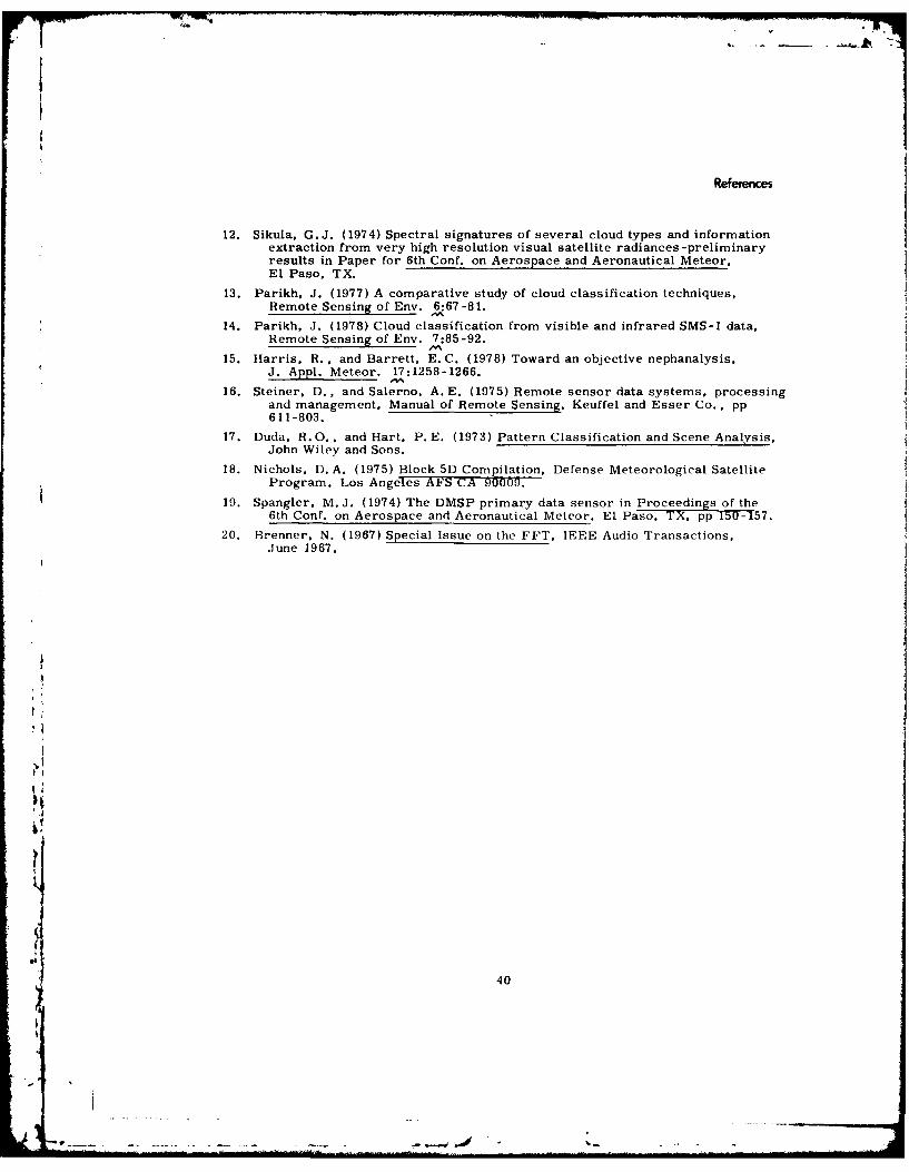
References

12. Sikula, G.J. (1974) Spectral signatures of several cloud types and informationextraction from very high resolution visual satellite radiances -preliminaryresults in Paper for 6th Conf. on Aerospace and Aeronautical Meteor,El Paso, TX.

13. Parikh, J. (1977) A comparative study of cloud classification techniques,Remote Sensing of Env. 6:67-81.

14. Parikh, J. (1978) Cloud classification from visible and infrared SMS-1 data,Remote Sensing of Env. 7:85-92.

15. Harris, R., and Barrett, E. C. (1978) Toward an objective nephanalysis,J. Appl. Meteor. 17:1258-1266.

16. Steiner, D., and Salerno, A. E. (1975) Remote sensor data systems, processingand management, Manual of Remote Sensing. Keuffel and Esser Co., pp611-803.

17. Duda, R.O. , and Hart, P. E. (1973) Pattern Classification and Scene Analysis.John Wiley and Sons.

18. Nichols, D.A. (1975) Block 5D Compilation, Defense Meteorological SatelliteProgram, Los Angeles AFS CA 90009.

19. Spangler, M.J. (1974) The DMSP primary data sensor in Proceedings of the6th Conf. on Aerospace and Aeronautical Meteor. El PasoTX p 150-T57.

20. Brenner, N. (1967) Special Issue on the FFT, IEEE Audio Transactions,June 1967.

.4

1 40

Appendix A

Implications of Changing the Resolution ofSatellite Data

All of the results presented in this report are based on a special data sample

with 0. 6 n mi ground resolution for each data element. This special sample led

to an FFT array size of 37 X 37 to match the 25 X 25 n mi boxes of the 3DNEPH.

In future applications, 0. 3 n mi data could be used and the following options are

available for analysis over the standard areas of 25 X 25 n mi:

(1) Do the same thing. Smooth data to 0.6 n mi

and use an array of 37 X 37 for the FFT,

(2) Apply the same computer program to four 37 X 37

subarrays of 0. 3 n mi data,

(3) Reprogram to a larger array (about 75 X 75 of

0.3 n mi data,

(4) Reprogram to array sizes (such as 32 X 32 or

64 X 64) which are powers of two.

ii Options (1) and (2) have the advantage of requiring no reprogramming effort.

The use of 0.3 n mi data in options (2) and (3) should provide the best detection of

small-scale cloud features. Option (3) would require the most computer time

since the array is large and the dimension is not a power of two. Option (4) would

not exactly cover a 25 X 25 n mi area due to the restriction to powers of two but

it should provide the fastest computer time. Some experimentation would be re-

quired to choose the best option and a development sample considerably larger than

41

".04

our 143 cases should be used to make the decision. The use of four smaller

arrays is equivalent to decreasing the mesh size for cloud typing. This option was

suggested by observations that relatively few wavenumbers contribute independent

information to the spectral classifiers.

42

.... .- .. ~ .,' " . ... ,: .

atom