estimating methodologies for broiler operations
TRANSCRIPT
Development of Emissions-
Estimating Methodologies for Broiler Operations
Draft
U.S. Environmental Protection Agency Office of Air Quality Planning and Standards
Sectors Policies and Programs Division Research Triangle Park, NC 27711
February 2012

2/8/2012
*** Internal Draft – Do Not Quote or Cite *** ii
TABLE OF CONTENTS
Section Page
1.0 INTRODUCTION.......................................................................................................... 1-1 1.1 EPA’s Consent Agreement for Animal Feeding Operations ............................... 1-1 1.2 National Air Emissions Monitoring Study for AFOs .......................................... 1-3 1.2.1 Overview of Emissions and Process Parameters Monitored ................... 1-3 1.2.2 NAEMS Monitoring Sites.................................................................................... 1-5 1.3 Emission Estimating Methodology Development ............................................... 1-6 2.0 OVERVIEW OF BROILER INDUSTRY ................................................................... 2-1 2.1 Industry Overview ............................................................................................... 2-1 2.2 Production Cycle .................................................................................................. 2-2 2.3 Animal Confinement ............................................................................................ 2-2 2.4 Manure Management ........................................................................................... 2-3 2.5 Emissions from Broiler Operations ..................................................................... 2-3 3.0 NAEMS MONITORING SITES .................................................................................. 3-1 3.1 Site Selection ....................................................................................................... 3-1 3.2 Description of Sites Monitored ............................................................................ 3-2 3.2.1 Site CA1B ................................................................................................ 3-3 3.2.2 Sites KY1B-1 and KY1B-2 ..................................................................... 3-6 3.3 Site Monitoring Plans .......................................................................................... 3-8 3.3.1 Site CA1B Monitoring Plan ..................................................................... 3-8 3.3.2 Sites KY1B-1 and KY1B-2 ................................................................... 3-17 4.0 DATA AVAILABLE FOR EEM DEVELOPMENT ................................................. 4-1 4.1 NAEMS Data ....................................................................................................... 4-1 4.1.1 Data Received .......................................................................................... 4-1 4.1.2 Emissions Levels Reported in the NAEMS Final Reports ...................... 4-9 4.2 Other Relevant Data ........................................................................................... 4-10 4.2.1 CFI ......................................................................................................... 4-11 4.2.2 Previous Literature Searches .................................................................. 4-24 5.0 NAEMS DATA PREPARATION ................................................................................ 5-1 5.1 NAEMS Data Assessments.................................................................................. 5-1 5.1.1 QA/QC Procedures .................................................................................. 5-1 5.1.2 Data Validation ........................................................................................ 5-2 5.1.3 Data Completeness................................................................................... 5-3

TABLE OF CONTENTS (continued)
Section Page
*** Internal Draft – Do Not Quote or Cite *** iii
5.2 EPA Assessments................................................................................................. 5-6 5.2.1 Data Processing ........................................................................................ 5-6 5.2.2 Data QA ................................................................................................... 5-6 5.2.3 Data Completeness Assessment ............................................................... 5-7 5.3 Comparison of Broiler Monitoring Sites ............................................................. 5-9 5.3.1 Process-Level Comparison ...................................................................... 5-9 5.3.2 Comparison of Local Meteorological Conditions.................................. 5-12 5.3.3 Emissions-Level Comparison ................................................................ 5-12 6.0 MEASURED EMISSIONS FROM BROILER OPERATIONS ............................... 6-4 6.1 Data Processing .................................................................................................... 6-4 6.1.1 Daily Emissions Graphs ........................................................................... 6-4 6.1.2 Seasonal Emissions Graphs ..................................................................... 6-4 6.2 NH3 Emissions ..................................................................................................... 6-7 6.2.1 General Trends ......................................................................................... 6-7 6.2.2 Seasonal Trends ..................................................................................... 6-10 6.3 H2S Emissions .................................................................................................... 6-14 6.3.1 General Trends ....................................................................................... 6-14 6.3.2 Seasonal Trends ..................................................................................... 6-17 6.4 PM10 Emissions .................................................................................................. 6-21 6.4.1 General Trends ....................................................................................... 6-21 6.4.2 Seasonal Trends ..................................................................................... 6-24 6.5 PM2.5 Emissions ................................................................................................. 6-28 6.5.1 General Trends ....................................................................................... 6-28 6.5.2 Seasonal Trends ..................................................................................... 6-34 6.6 TSP Emissions ................................................................................................... 6-39 6.6.1 General Trends ....................................................................................... 6-39 6.6.2 Seasonal Trends ..................................................................................... 6-43 6.7 VOC Emissions .................................................................................................. 6-47 6.7.1 General Trends ....................................................................................... 6-47 6.7.2 Seasonal Trends ..................................................................................... 6-49 7.0 DEVELOPMENT OF EEMS FOR GROW-OUT PERIODS ................................... 7-1 7.1 Selecting Datasets ................................................................................................ 7-6 7.1.1 Full dataset ............................................................................................... 7-9 7.1.2 Base and Cross-Validation Datasets ........................................................ 7-9 7.2 Choosing the Probability Distribution ............................................................... 7-11 7.3 Developing Candidate Mean Trend Variables ................................................... 7-14

TABLE OF CONTENTS (continued)
Section Page
*** Internal Draft – Do Not Quote or Cite *** iv
7.3.1 Choosing Predictor Variable Functional Forms .................................... 7-14 7.3.2 Creating Mean Trend Variables from Main Effects and Interactions .... 7-30 7.4 Choosing the Covariance Function .................................................................... 7-31 7.4.1 Correlation Function as Subset of Covariance Function ....................... 7-32 7.4.2 Serial Correlation ................................................................................... 7-33 7.4.3 Random Effects ...................................................................................... 7-34 7.4.4 Constant Variance .................................................................................. 7-36 7.5 Selecting Final Mean Trend Variables .............................................................. 7-37 7.5.1 Inventory EEM....................................................................................... 7-38 7.5.2 Inventory and Ambient EEM ................................................................. 7-42 7.5.3 Inventory, Ambient and Confinement EEM .......................................... 7-45 7.5.4 EEM Validation and Modification of Previous Versions ...................... 7-45 7.5.5 Summary of Final Results for the I, IA and IAC EEMs ........................ 7-48 7.6 Producing Point and Interval Predictions .......................................................... 7-50 8.0 RESULTS OF GROW-OUT PERIOD EEM DEVELOPMENT .............................. 8-1 8.1 EEMs for H2S ...................................................................................................... 8-1 8.1.1 Selecting Datasets .................................................................................... 8-1 8.1.2 Choosing the Probability Distribution ..................................................... 8-2 8.1.3 Developing Candidate Mean Trend Variables for H2S ............................ 8-5 8.1.4 Selecting Final Mean Trend Variables for H2S ..................................... 8-14 8.1.5 Summary of Final Results for the I, IA and IAC EEMs for H2S ........... 8-15 8.2 EEMs for PM10 .................................................................................................. 8-17 8.2.1 Selecting Datasets .................................................................................. 8-17 8.2.2 Choosing the Probability Distribution for PM10 .................................... 8-18 8.2.3 Developing Candidate Mean Trend Variables for PM10 ........................ 8-20 8.2.4 Selecting Final Mean Trend Variables for PM10 ................................... 8-28 8.2.5 Summary of Final Results for the I, IA and IAC EEMs for PM10 ......... 8-31 8.3 EEMs for PM2.5 .................................................................................................. 8-34 8.3.1 Selecting Datasets .................................................................................. 8-34 8.3.2 Choosing the Probability Distribution for PM2.5 ................................... 8-35 8.3.3 Developing Candidate Mean Trend Variables for PM2.5 ....................... 8-38 8.3.4 Selecting Final Mean Trend Variables for PM2.5 ................................... 8-46 8.3.5 Summary of Final Results for the I, IA and IAC EEMs for PM2.5 ........ 8-49 8.4 EEMs for TSP .................................................................................................... 8-51 8.4.1 Selecting Datasets .................................................................................. 8-51 8.4.2 Choosing the Probability Distribution for TSP ...................................... 8-52 8.4.3 Developing Candidate Mean Trend Variables for TSP ......................... 8-55

TABLE OF CONTENTS (continued)
Section Page
*** Internal Draft – Do Not Quote or Cite *** v
8.4.4 Selecting Final Mean Trend Variables for TSP ..................................... 8-63 8.4.5 Summary of Final Results for the I, IA and IAC EEMs for TSP .......... 8-65 8.5 EEMs for VOCs ................................................................................................. 8-66 8.5.1 Selecting Datasets .................................................................................. 8-66 8.5.2 Choosing the Probability Distribution for VOCs................................... 8-67 8.5.3 Developing Candidate Mean Trend Variables for VOCs ...................... 8-69 8.5.4 Selecting Final Mean Trend Variables for VOCs .................................. 8-78 8.5.5 Summary of Final Results for the I, IA and IAC EEMs for VOCs ....... 8-82 9.0 DEVELOPMENT OF DECAKING AND FULL LITTER CLEAN-OUT PERIOD EEMS .............................................................................................................. 9-1 9.1 Available Data for Litter Removal Periods ......................................................... 9-1 9.2 EEM Development for Decaking and Full Litter Clean-Out Periods .................. 9-4 10.0 REFERENCES ............................................................................................................. 10-1

2/8/2012
*** Internal Draft – Do Not Quote or Cite *** vi
LIST OF TABLES Table Page
Table 1-1. Process Parameters Monitored at the NAEMS Broiler Sites ........................................... 1-4 Table 1-2. NAEMS Monitoring Sites ................................................................................................ 1-5 Table 3 1. NAEMS Broiler Sites Information ................................................................................... 3-1 Table 3 2. Analyte Sampling Locations at Site CA1B .................................................................... 3-10 Table 3 3. PM Sampling Schedule ................................................................................................... 3-12 Table 3 4. Fan Air Flow Models ...................................................................................................... 3-15 Table 3 5. Analyte Sampling Locations at Sites KY1B-1 and KY1B-2 .......................................... 3-17 Table 3 6. Fan Air Flow Models for KY1B-1 ................................................................................. 3-24 Table 3 7. Fan Air Flow Models for KY1B-2 ................................................................................. 3-25 Table 4-1. Information and Data Submitted ...................................................................................... 4-1 Table 4-2. NAEMS Emissions and Process Parameter Data Received ............................................. 4-3 Table 4-3. Reported Emission Rates for NAEMS Broiler Houses .................................................. 4-10 Table 4-4. Review of Broiler Articles Received in Response to EPA’s CFI .................................. 4-14 Table 4-5. Review of Broiler Articles Obtained by Previous EPA Literature Searches ................. 4-25 Table 5-1. Reported Number of Valid Emissions Days for Required Data from NAEMS Broiler Operations .......................................................................................................................................... 5-4 Table 5-2. Data Completeness for Daily Emissions Data from NAEMS Broiler Operations ........... 5-4 Table 5-3. Particulate Matter Monitoring Schedule for CA1B .......................................................... 5-5 Table 5-4. Number of Valid Emissions Days in the Spring and Summer ......................................... 5-8 Table 5 5. Number of Valid Emissions Days in the Fall and Winter ................................................ 5-8 Table 5-6. NAEMS Data for Broiler Confinement Operations ......................................................... 5-9 Table 5-7. Design and Operating Parameters of the NAEMS Broiler Sites .................................... 5-10 Table 5-8. Duration of Grow-out and Clean-out Periods ................................................................ 5-10 Table 5-9. Summary of Flock and Litter Clean-out Operations ...................................................... 5-11 Table 5-10. Site-Specific Ambient and Confinement Conditions ................................................... 5-12 Table 5-11. Average Daily Emissions for All Periods .................................................................... 5-14 Table 5-12. Average Daily Emissions During Grow-Out Periods (mass per day) .......................... 5-14 Table 5-13. Average Daily Emissions During Grow-Out Periods (mass per day per bird) ............ 5-15 Table 5-14. Average Daily Emissions During Decaking Periods (mass per day) ........................... 5-15 Table 5-15. Average Daily Emissions During Full Litter Clean-Out Periods (mass per day) ........ 5-16 Table 6 1. Average Flock Duration by Site ....................................................................................... 6-5 Table 6 2. Flock Classified by Season ............................................................................................... 6-5
LIST OF TABLES (continued) Table Page
*** Internal Draft – Do Not Quote or Cite *** vii
Table 6 3. Flock Distribution by Season ............................................................................................ 6-6 Table 6-5. Available Daily TSP Emission Values by Site............................................................... 6-40 Table 7 1. Summary of Symbols and Terms Used in Equation 7 1 ................................................... 7-2 Table 7 2. Predictor Variables ........................................................................................................... 7-7 Table 7 3. Data Completeness for NH3 .............................................................................................. 7-8 Table 7 4. Potential Mean Trend Variables to Account for Built-up Litter ..................................... 7-17 Table 7 5. Summary of Main Effect Mean Trend Variables ........................................................... 7-27 Table 7 6. Proportion of Base Dataset Variability Explained by EEMs by Interaction Level ........ 7-31 Table 7 7. Mean NH3 Emissions (kg) After Litter Clean-out .......................................................... 7-35 Table 7 8. Covariance Parameter Estimates .................................................................................... 7-36 Table 7 9. Sample Size, Mean and Standard Deviation for NH3 Bins............................................. 7-36 Table 7 10. Candidate Mean Trend Variables for the I, IA and IAC EEMs ................................... 7-37 Table 7 11. Hypothesis Tests for the I EEM, Runs 0 and 1 ............................................................. 7-39 Table 7 12. Backward Elimination Fit Statistics for the I EEM ...................................................... 7-41 Table 7 13. Backward Elimination Fit Statistics for the IA EEM ................................................... 7-43 Table 7 14. Backward Elimination Fit Statistics (Runs 0 – 11) for IAC EEM................................ 7-46 Table 7 15. Backward Elimination Fit Statistics (Runs 12 – 23) for IAC EEM.............................. 7-47 Table 7 16. Regression Coefficient Estimates for NH3 EEMS ....................................................... 7-49 Table 7 17. Covariance Parameter Estimates for Final NH3 EEMs ................................................ 7-50 Table 7 18. Values of Predictor Variables for the Example Calculation ......................................... 7-51 Table 7 19. Values of Mean Trend Variables for Example Days 15 and 46 ................................... 7-52 Table 8 1. Data Completeness for H2S EEMs ................................................................................... 8-2 Table 8 2. Summary of Main Effect Mean Trend Variables for H2S .............................................. 8-12 Table 8 3. Candidate Mean Trend Variables for the I, IA and IAC H2S EEMs .............................. 8-13 Table 8 4. Centering and Scaling Reference Values for Continuous H2S Predictor Variables ....... 8-13 Table 8 5. Final I, IA and IAC EEM Mean Trend Variables for H2S EEMs .................................. 8-14 Table 8 6. Final I, IA and IAC EEM Fit Statistics for H2S .............................................................. 8-15 Table 8 7. Covariance Parameters for Final H2S EEMs .................................................................. 8-15 Table 8 8. Regression Coefficients for Final H2S EEMs ................................................................. 8-16 Table 8 9. Data Completeness for PM10 EEMs ............................................................................... 8-17 Table 8 10. Summary of Main Effect Mean Trend Variables for PM10 .......................................... 8-26 Table 8 11. Candidate Mean Trend Variables for the I, IA and IAC PM10 EEMs .......................... 8-27 Table 8 12. Centering and Scaling Reference Values for Continuous PM10 Predictor Variables ... 8-28 Table 8 13. Final Candidate I EEM Mean Trend Variables for PM10 ............................................. 8-29

LIST OF TABLES (continued) Table Page
*** Internal Draft – Do Not Quote or Cite *** viii
Table 8 14. Final Candidate I EEM Fit Statistics for PM10 ............................................................. 8-29 Table 8 15. Final Candidate IA EEM Mean Trend Variables for PM10 .......................................... 8-30 Table 8 16. Final Candidate IA EEM Fit Statistics for PM10 .......................................................... 8-30 Table 8 17. Final Candidate IAC EEM Mean Trend Variables for PM10 ........................................ 8-31 Table 8 18. Final Candidate IAC EEM Fit Statistics for PM10 ........................................................ 8-31 Table 8 19. Final EEM Mean Trend Variables for PM10 ................................................................. 8-31 Table 8 20. Covariance Parameter for Final PM10 EEMs ................................................................ 8-32 Table 8 21. Regression Coefficient for Final PM10 EEMs .............................................................. 8-33 Table 8 22. Data Completeness for PM2.5 EEMs ............................................................................. 8-34 Table 8 23. Summary of Main Effect Mean Trend Variables for PM2.5.......................................... 8-44 Table 8 24. Candidate Mean Trend Variables for the I, IA and IAC PM2.5 EEMs ......................... 8-45 Table 8 25. Centering and Scaling Reference Values for Continuous PM2.5 Predictor Variables .. 8-45 Table 8 26. Final Candidate I EEM Mean Trend Variables for PM2.5 ............................................ 8-46 Table 8 27. Final Candidate I EEM Fit Statistics for PM2.5............................................................. 8-47 Table 8 28. Final Candidate IA EEM Mean Trend Variables for PM2.5.......................................... 8-48 Table 8 29. Final Candidate IA EEM Fit Statistics for PM2.5 .......................................................... 8-48 Table 8 30. Final Candidate IAC EEM Mean Trend Variables for PM2.5 ....................................... 8-49 Table 8 31. Final Candidate IAC EEM Fit Statistics for PM2.5 ....................................................... 8-49 Table 8 32. Final EEM Mean Trend Variables for PM2.5 ................................................................ 8-50 Table 8 33. Covariance Parameter for Final PM2.5 EEMs ............................................................... 8-50 Table 8 35. Data Completeness for TSP EEMs ............................................................................... 8-52 Table 8 36. Summary of Main Effect Mean Trend Variables for PM10 .......................................... 8-62 Table 8 37. Candidate Mean Trend Variables for the I, IA and IAC TSP EEMs ............................ 8-63 Table 8 38. Centering and Scaling Reference Values for Continuous TSP Predictor Variables ..... 8-63 Table 8 39. Final I, IA and IAC EEM Mean Trend Variables for TSP EEMs ................................ 8-64 Table 8 40. Final I, IA and IAC EEM Fit Statistics for TSP ........................................................... 8-64 Table 8 41. Covariance Parameter for Final TSP EEMs ................................................................. 8-65 Table 8 42. Regression Coefficient for Final TSP EEMs ................................................................ 8-65 Table 8 43. Data Completeness for VOC EEMs ............................................................................. 8-66 Table 8 44. Summary of Main Effect Mean Trend Variables for VOCs ......................................... 8-76 Table 8 45. Candidate Mean Trend Variables for the I, IA and IAC VOC EEMs .......................... 8-77 Table 8 46. Centering and Scaling Reference Values for Continuous VOC Predictor Variables ... 8-78 Table 8 47. Final Candidate I EEM Mean Trend Variables for VOCs ............................................ 8-79 Table 8 48. Final Candidate I EEM Fit Statistics for VOCs ............................................................ 8-79
LIST OF TABLES (continued) Table Page
*** Internal Draft – Do Not Quote or Cite *** ix
Table 8 49. Final Candidate IA EEM Mean Trend Variables for VOCs ......................................... 8-80 Table 8 50. Final Candidate IA EEM Fit Statistics for VOCs ......................................................... 8-80 Table 8 51. Final Candidate IAC EEM Mean Trend Variables for VOCs ...................................... 8-81 Table 8 52. Final Candidate IAC EEM Fit Statistics for VOCs ...................................................... 8-81 Table 8 53. Final EEM Mean Trend Variables for VOCs ............................................................... 8-82 Table 8 54. Covariance Parameter for Final VOC EEMs ................................................................ 8-82 Table 8 55. Regression Coefficients for Final VOC EEMs ............................................................. 8-83 Table 9-1. Comparison of Litter Removal and Grow-out Period Days ............................................. 9-1 Table 9-2. Comparison of Decaking and Full Litter Clean-out Days ................................................ 9-2 Table 9-3. Duration of Grow-out and Clean-out Periods .................................................................. 9-2 Table 9-4. Number of Valid Non-Negative Daily Emissions Values for Litter Removal Periods .... 9-3 Table 9-5. Range of Emissions for Broiler Litter Removal Periods .................................................. 9-5 Table 9-6. Emissions Factors for Broiler Litter Removal Periods..................................................... 9-7 Table 9-7. Difference in Measured Versus Estimated Emissions ...................................................... 9-8 Table 9-8. Example Flock Characteristics ......................................................................................... 9-9

2/8/2012
*** Internal Draft – Do Not Quote or Cite *** x
LIST OF FIGURES Figure Page
Figure 3 1. California Broiler Site Layout ........................................................................................ 3-4 Figure 3 2. Example House Air Inlet ................................................................................................ 3-5 Figure 3 3. Bank of 122-cm (48-inch) Fans (left, view from inside of house) and (right, view from outside of house) ............................................................................................................................... 3-5 Figure 3 4. Evaporative Cooling Pads .............................................................................................. 3-5 Figure 3 5. Locations of Kentucky Measurement Sites .................................................................... 3-7 Figure 3 6. Aerial Photographs of Kentucky Monitoring Sites ........................................................ 3-7 Figure 3 7. Tunnel Fans and Box Air Inlets...................................................................................... 3-8 Figure 3 8. Overhead View of Sensor and Air Sampling Locations ................................................ 3-9 Figure 3 9. Schematic of KY1B-1 (top) and KY1B-2 (bottom) ..................................................... 3-18 Figure 3 10. Cross-sectional View of Sidewall Sampling Locations ............................................. 3-19 Figure 3 11. Analyte Sampling Locations ...................................................................................... 3-22 Figure 3 12. Schematic of Litter Sampling Locations .................................................................... 3-28 Figure 6-1. NH3 Emission Rates from the CA1B Broiler Houses .................................................... 6-8 Figure 6-2. NH3 Emission Rates from the Kentucky Broiler Houses............................................... 6-9 Figure 6-3. NH3 Emissions by Flock, Color Coded by Season ...................................................... 6-10 Figure 6-4. NH3 Emissions from the Broiler Sites for Spring and Summer ................................... 6-11 Figure 6-5. NH3 Emissions from the Broiler Sites for Summer/Fall and Fall ................................ 6-12 Figure 6-6. NH3 Emissions from the Broiler Sites for Fall/Winter and Winter ............................. 6-13 Figure 6-7. NH3 Emissions from the Broiler Sites for Winter/Spring ............................................ 6-14 Figure 6-8. H2S Emissions from the CA1B Broiler Houses ........................................................... 6-15 Figure 6-9. H2S Emissions from the Kentucky Broiler Sites.......................................................... 6-16 Figure 6-10. H2S Emissions by Flock, Color Coded by Season ..................................................... 6-17 Figure 6-11. H2S Emissions from the Broiler Sites for Spring and Summer ................................. 6-18 Figure 6-12. H2S Emissions from the Broiler Sites for Summer/Fall and Fall............................... 6-19 Figure 6-13. H2S Emissions from the Broiler Sites for Fall/Winter and Winter ............................ 6-20 Figure 6-14. H2S Emissions from the Broiler Sites for Winter/Spring........................................... 6-21 Figure 6-15. PM10 Emissions from the CA1B Broiler Houses ....................................................... 6-22 Figure 6-16. PM10 Emissions from the Kentucky Broiler Houses.................................................. 6-23 Figure 6-17. PM10 Emissions by Flock, Color Coded by Season ................................................... 6-24 Figure 6-18. PM10 Emissions from the Broiler Sites for Spring and Summer ............................... 6-25 Figure 6-19. PM10 Emissions from the Broiler Sites for Fall and Fall/Winter ............................... 6-26

LIST OF FIGURES Figure Page
*** Internal Draft – Do Not Quote or Cite *** xi
Figure 6-20. PM10 Emissions from the Broiler Sites for Fall/Winter and Winter .......................... 6-27 Figure 6-21. PM10 Emissions from the Broiler Sites for Winter/Spring......................................... 6-28 Figure 6-22. PM2.5 Emissions from the CA1B Broiler Houses ...................................................... 6-32 Figure 6-23. PM2.5 Emissions from the Kentucky Broiler Houses ................................................. 6-33 Figure 6-24. PM2.5 Emissions by Flock, Color Coded by Season .................................................. 6-35 Figure 6-25. PM2.5 Emissions from the Broiler Sites for Spring and Summer ............................... 6-36 Figure 6-26. PM2.5 Emissions from the Broiler Sites for Fall and Fall/Winter .............................. 6-37 Figure 6-27. PM2.5 Emissions from the Broiler Sites for Winter and Winter/Spring ..................... 6-38 Figure 6-28. TSP Emissions from the CA1B Broiler Houses ........................................................ 6-41 Figure 6-29. TSP Emissions from the Kentucky Broiler Houses ................................................... 6-42 Figure 6-30. TSP Emissions by Flock, Color Coded by Season .................................................... 6-43 Figure 6-31. TSP Emissions from the Broiler Sites for Spring and Summer ................................. 6-44 Figure 6-32. TSP Emissions from the Broiler Sites for Fall and Fall/Winter................................. 6-45 Figure 6-33. TSP Emissions from the Broiler Sites for Winter and Winter/Spring ....................... 6-46 Figure 6-34. VOC Emissions from the Kentucky Broiler Houses.................................................. 6-48 Figure 6-35. VOC Emissions by Flock, Color Coded by Season ................................................... 6-49 Figure 6-36. VOC Emissions from the Broiler Sites for Spring and Summer ............................... 6-50 Figure 6-37. VOC Emissions from the Broiler Sites for Fall and Fall/Winter ............................... 6-51 Figure 6-38. VOC Emissions from the Broiler Sites for Winter and Winter/Spring ...................... 6-52 Figure 7 1. General Approach for EEM Development ..................................................................... 7-5 Figure 7 2. Example of Constant Late-Period Bird Inventory .......................................................... 7-7 Figure 7 3. Histogram of NH3 Emissions in the Base Dataset........................................................ 7-12 Figure 7 4. Histograms by avem Bins ............................................................................................. 7-13 Figure 7 5. NH3 Emissions vs. Average Live Bird Mass................................................................ 7-15 Figure 7 6. Overlay of buildup on NH3 Emissions vs. Average Live Bird Mass ........................... 7-16 Figure 7 7. Box Plots of NH3 Emissions vs. Candidate Categorical Variables .............................. 7-18 Figure 7 8. NH3 Emissions vs. avem for Individual Flocks at CA1B H10 ..................................... 7-20 Figure 7 9. NH3 Emissions vs. avem for Individual Flocks at CA1B H12 ..................................... 7-21 Figure 7 10. NH3 Emissions vs. avem for Individual Flocks at the Kentucky Sites ....................... 7-22 Figure 7 11. NH3 Emissions vs. Predictor Variables birds and ta .................................................. 7-24 Figure 7 12. NH3 Emissions vs. Predictor Variables ha and pa ..................................................... 7-25 Figure 7 13. NH3 Emissions vs. Predictor Variables tc and hc ....................................................... 7-26 Figure 7 14. NH3 Emissions vs. ha for Six avem Bins ................................................................... 7-28
LIST OF FIGURES Figure Page
*** Internal Draft – Do Not Quote or Cite *** xii
Figure 7 15. Deviations from the Mean Trend Function on Date t vs. Date t-1 ............................. 7-33 Figure 7 16. Illustration of the Relationship Between the Point Estimate and the Prediction Interval ........................................................................................................................................... 7-53 Figure 8 1. Histogram of H2S Emissions in the Base Dataset .......................................................... 8-3 Figure 8 2. Histograms of H2S Emissions by avem* Bins ................................................................ 8-4 Figure 8 3. H2S Emissions vs. Average Bird Mass (Regression Overlays: purple = linear, red = quadratic, green = cubic)................................................................................................................... 8-5 Figure 8 4. H2S Emissions vs. Average Bird Mass, by House ......................................................... 8-6 Figure 8 5. Overlay of buildup on H2S Emissions vs. Average Live Bird Mass .............................. 8-7 Figure 8 6. Box Plots of H2S Emissions vs. Categorical Variables for buildup ............................... 8-8 Figure 8 7. H2S Emissions vs. Predictor Variables birds* and ta* .................................................. 8-9 Figure 8 8. H2S Emissions vs. Predictor Variables ha* and pa* .................................................... 8-10 Figure 8 9. H2S Emissions vs. Predictor Variables tc* and hc* ..................................................... 8-11 Figure 8 10. Histogram of PM10 Emissions in the Base Dataset .................................................... 8-18 Figure 8 11. Histograms of PM10 Emissions by avem* Bins .......................................................... 8-19 Figure 8 12. PM10 Emissions vs. Average Bird Mass (Regression Overlays: purple = linear, red = quadratic, green = cubic)................................................................................................................. 8-20 Figure 8 13. Overlay of buildup on PM10 Emissions vs. Average Live Bird Mass ........................ 8-21 Figure 8 14. PM10 Emissions vs. Average Bird Mass, Color-coded by Site .................................. 8-21 Figure 8 15. Box Plots of PM10 Emissions vs. Categorical Variables for buildup ......................... 8-22 Figure 8 16. PM10 Emissions vs. Predictor Variables birds* and ta*............................................. 8-23 Figure 8 17. PM10 Emissions vs. Predictor Variables ha* and pa* ................................................ 8-24 Figure 8 18. PM10 Emissions vs. Predictor Variables tc* and hc* ................................................. 8-25 Figure 8 19. Histogram of PM2.5 Emissions in the Base Dataset .................................................... 8-36 Figure 8 20. Histograms of PM2.5 Emissions by avem* Bins ......................................................... 8-37 Figure 8 21. PM2.5 Emissions vs. Average Bird Mass (Regression Overlays: purple = linear, red = quadratic, green = cubic)................................................................................................................. 8-38 Figure 8 22. Overlay of buildup on PM2.5 Emissions vs. Average Live Bird Mass ....................... 8-39 Figure 8 23. Box Plots of PM2.5 Emissions vs. Categorical Variables for buildup ........................ 8-40 Figure 8 24. PM2.5 Emissions vs. Predictor Variables birds* and ta* ............................................ 8-41 Figure 8 25. PM2.5 Emissions vs. Predictor Variables ha* and pa* ............................................... 8-42 Figure 8 26. PM2.5 Emissions vs. Predictor Variables tc* and hc*................................................. 8-43 Figure 8 27. Histogram of TSP Emissions in the Base Dataset ...................................................... 8-53 Figure 8 28. Histograms of TSP Emissions by avem* Bins ........................................................... 8-54

LIST OF FIGURES Figure Page
*** Internal Draft – Do Not Quote or Cite *** xiii
Figure 8 29. TSP Emissions vs. Average Bird Mass (Regression Overlays: purple = linear, red = quadratic, green = cubic)................................................................................................................. 8-55 Figure 8 30. Overlay of buildup on TSP Emissions vs. Average Live Bird Mass ......................... 8-56 Figure 8 31. TSP Emissions vs. Average Bird Mass, Color-coded by Site .................................... 8-57 Figure 8 32. Box Plots of TSP Emissions vs. Categorical Variables for buildup........................... 8-58 Figure 8 33. TSP Emissions vs. Predictor Variables birds* and ta* .............................................. 8-59 Figure 8 34. TSP Emissions vs. Predictor Variables ha* and pa* ................................................. 8-60 Figure 8 35. TSP Emissions vs. Predictor Variables tc* and hc* ................................................... 8-61 Figure 8 36. Histogram of VOC Emissions in the Base Dataset .................................................... 8-67 Figure 8 37. Histograms of VOC Emissions by avem* Bins .......................................................... 8-68 Figure 8 38. VOC Emissions vs. Average Bird Mass (Regression Overlays: purple = linear, red = quadratic, green = cubic)................................................................................................................. 8-69 Figure 8 39. VOC Emissions vs. Average Bird Mass, by House (Regression Overlays: purple = linear, red = quadratic, green = cubic) ............................................................................................ 8-70 Figure 8 40. Overlay of buildup on VOC Emissions vs. Average Live Bird Mass ........................ 8-71 Figure 8 41. Box Plots of VOC Emissions vs. Categorical Variables for buildup ......................... 8-72 Figure 8 42. VOC Emissions vs. Predictor Variables birds* and ta*............................................. 8-73 Figure 8 43. VOC Emissions vs. Predictor Variables ha* and pa* ................................................ 8-74 Figure 8 44. VOC Emissions vs. Predictor Variables tc* and hc* ................................................. 8-75
2/8/2012
*** Internal Draft – Do Not Quote or Cite *** xiv
Executive Summary
In 2005, the EPA offered animal feeding operations (AFOs) an opportunity to participate in a voluntary consent agreement referred to as the Air Compliance Agreement (Agreement) (70 FR 4958). Under the Agreement, participating AFOs provided the funding for the National Air Emissions Monitoring Study (NAEMS) – a two-year, nationwide emissions monitoring study of animal confinement structures and manure storage and treatment units in the broiler, egg-layer, swine, and dairy industries. The purpose of this study was to gather baseline uncontrolled emissions data that would be used to develop by the EPA to develop emission estimating methodologies (EEMs). The NAEMS began in the summer of 2007 and consisted of 25 monitoring sites located in 10 states. At the animal confinement sites, the study collected process and emissions data for ammonia (NH3), hydrogen sulfide (H2S), total suspended particulate matter (TSP), particulate matter (PM) with aerodynamic diameters less than 10 micrometers (PM10), PM with aerodynamic diameters less than 2.5 micrometers (PM2.5) and volatile organic compounds (VOCs).
In accordance with the Agreement, the EPA developed EEMs for animal housing structures and manure storage and treatment units using the emissions and process data collected under the NAEMS and other relevant information submitted to the EPA in response to its Call for Information (76 FR 3060). The EEMs will be used by the AFO industry to estimate daily and annual emissions for use in determining their regulatory responsibilities under the Clean Air Act (CAA), the Comprehensive Environmental Response, Compensation, and Liability Act (CERCLA) and the Emergency Planning and Community Right-to-Know Act (EPCRA).
This report presents the background information, data collected, data analyses performed, statistical approach taken and the EEMs developed by the EPA for confinement structures used in the broiler industry. The EEMs provide emissions estimates of the following pollutants for grow-out and decaking/full litter clean-out periods: NH3, H2S, PM10, PM2.5, TSP and VOCs.
The EPA developed the EEMs using emissions and process information collected from one broiler operation in California (site CA1B) and from two broiler operations in Kentucky (sites KY1B- and KY1B-2). At the CA1B site, monitoring was conducted in two houses from 2007 to 2009. At the Kentucky sites, monitoring was conducted in a single house at each location from 2006 to 2007. Monitoring at site CA1B was conducted under the NAEMS while monitoring at the Kentucky sites was sponsored by Tyson Foods. Because the quality assurance project plan (QAPP) and site monitoring plans for the Tyson study were developed to be consistent with the NAEMS, the EPA considered the data collected under the Tyson study to be an integral part of the NAEMS.

2/8/2012
*** Internal Draft – Do Not Quote or Cite *** xv
For broiler grow-out periods, the EPA used the emissions and process parameter data collected at the California and Kentucky sites and SAS statistical software to develop the EEMs. To accommodate varying levels of available input data, the EPA developed three EEMs for grow-out periods: EEMs that uses bird inventory data as input parameters (I EEMs); EEMs that uses bird inventory and ambient parameters (IA EEMs) and EEMs based on bird inventory, ambient and confinement parameters (IAC EEMs). For the I EEMs, the input parameters are total bird inventory in the house and their average weight which are typically recorded manually by growers. For the IA EEMs, the input parameters include the bird inventory parameters and ambient temperature and relative humidity. The ambient data can be obtained by either a monitoring system installed at the farm or from a representative local meteorological station. For the IAC EEMs, the input parameters include the bird inventory, ambient meteorological parameters and confinement parameters (i.e., house temperature and relative humidity). A monitoring system that recorded confinement parameters would have to be installed in the broiler house if the IAC EEM is used to determine emissions.
For litter decaking and clean-out periods, the EPA developed emissions factors that relate pollutant emissions to the mass of birds raised on the litter since the previous decaking or full litter clean-out activity and to the duration of the decaking or clean-out period. The EPA considered using regression analyses to develop separate methods for litter decaking and clean-out periods, but rejected this approach due to the relatively small number of emissions and process parameter data values collected during these periods. Also, applying the regression analyses to litter decaking and clean-out periods was further complicated because the data did not fully represent the manner in which the house doors and openings were managed and the specific activities undertaken during these periods while gas and PM sampling were conducted.

2/8/2012
*** Internal Draft – Do Not Quote or Cite *** 1-1
1.0 INTRODUCTION
There are approximately 1 million livestock and poultry farms in the United States. About one-half of these farms raise animals in confinement, which qualifies them as Animal Feeding Operations (AFOs) (USDA, 2007 Census of Agriculture). AFOs are potential sources of the following emissions: ammonia (NH3), hydrogen sulfide (H2S), total suspended particulate matter (TSP), particulate matter with aerodynamic diameters less than 10 micrometers (PM10), PM with aerodynamic diameters less than 2.5 micrometers (PM2.5) and volatile organic compounds (VOCs).
This report presents emissions-estimating methodologies (EEMs) for determining uncontrolled emissions from a broiler confinement barn. The EEMs were developed based on data collected in the National Air Emissions Monitoring Study (NAEMS) and other relevant information obtained through the EPA’s January 19, 2011, Call for Information (see Section 4.0).
The EPA’s previous effort to quantify potential emissions from this source sector and the evolution of the Air Compliance Agreement, are described in Section 1.1. Section 1.2 outlines the requirement for the NAEMS established by the Air Compliance Agreement. Section 1.3 describes how the data collected during the NAEMS was used to develop the EEMs.
1.1 EPA’s Consent Agreement for Animal Feeding Operations
In August 2001, the EPA published methodologies for estimating farm-level emissions from AFOs in the beef, dairy, swine and poultry (broilers, layers and turkeys) animal sectors (Emissions from Animal Feeding Operations, Draft, August 2001). To develop the methodologies, the EPA: (1) identified the manure management systems typically used by AFOs in each animal sector, (2) developed model farms, (3) conducted literature searches to identify emission factors related to model farm components (e.g., confinement, manure handling and treatment system) and (4) applied the emission factors to the model farms to estimate annual mass emissions.
After publication of the EPA’s 2001 report, the EPA and the United States Department of Agriculture (USDA) jointly requested that the National Academy of Science (NAS) evaluate the current knowledge base and the approaches for estimating air emissions from AFOs. In its 2003 report (Air Emissions From Animal Feeding Operations: Current Knowledge, Future Needs, National Research Council), the NAS concluded the following: reliable emission factors for AFOs were not available at that time; additional data were needed to develop estimating methodologies; current methods for estimating emissions were not appropriate; and the EPA should use a process-based approach to determine emissions from an AFO.
2/8/2012
*** Internal Draft – Do Not Quote or Cite *** 1-2
In January 2005, the EPA announced the voluntary Air Compliance Agreement with the AFO industry. The goals of the Air Compliance Agreement were to reduce air pollution, monitor AFO emissions, promote a national consensus on methodologies for estimating emissions from AFOs and ensure compliance with the requirements of the Clean Air Act (CAA), the Comprehensive Environmental Response, Compensation, and Liability Act (CERCLA) and the Emergency Planning and Community Right-to-Know Act (EPCRA).
To develop the Air Compliance Agreement, the EPA worked with industry representatives, state and local governments, environmental groups and other stakeholders. Approximately 2,600 AFOs, representing nearly 14,000 facilities that included broiler, dairy, egg layer and swine operations, received the EPA’s approval to participate in the Air Compliance Agreement. Participating AFOs paid a civil penalty, ranging from $200 to $100,000, based on the size and number of facilities in their operations. They also contributed approximately a total of $14.6 million to fund the NAEMS.
As part of the Air Compliance Agreement, the EPA agreed not to sue participating AFOs for certain past violations of the CAA, CERCLA and EPCRA, provided that the AFOs comply with the Air Compliance Agreement’s conditions. However, the Air Compliance Agreement does not limit the EPA’s ability to take action in the event of imminent and substantial danger to public health or the environment. The Air Compliance Agreement also preserves state and local authorities’ ability to enforce local odor or nuisance laws. After the EPA publishes the final emissions-estimating methodologies (EEMs) for the broiler, swine, egg layer and dairy sectors, participating AFOs must apply the final methodologies for their respective sectors to determine what actions, if any, they must take to comply with all applicable CAA, CERCLA and EPCRA requirements. If a participating facility does not trigger CAA, CERCLA or EPCRA permitting or release notification requirements based on the data collected, the facility will have 60 days from the publication date of the final EEMs to submit a written certification to EPA confirming compliance with current applicable requirements under these regulations. If a participating facility does trigger CAA, CERCLA or EPCRA permitting or release notification requirements, the facility will have 120 days from the publication date of the final EEMs to apply for any required permits under the CAA, or submit any required release notifications under CERCLA or EPCRA. Finally, AFOs that did not participate in the Air Compliance Agreement can use the appropriate EEMs for their sectors to determine what, if any, measures they must take to comply with applicable CAA, CERCLA and EPCRA requirements.

2/8/2012
*** Internal Draft – Do Not Quote or Cite *** 1-3
1.2 National Air Emissions Monitoring Study for AFOs
1.2.1 Overview of Emissions and Process Parameters Monitored
In the early planning stages of the NAEMS, representatives from the EPA, USDA, AFO industry, state and local air quality agencies and environmental organizations met to discuss and define the parameters that would be collected by the study. The goal was to develop a comprehensive list of parameters that must be monitored to provide a greater understanding and accurate characterization of emissions from AFOs. By monitoring these parameters, the EPA would have the necessary information to develop EEMs for uncontrolled emissions of particulate matter, ammonia, hydrogen sulfide and volatile organic compounds from animal feeding operations.
The Air Compliance Agreement provided guidance on the emissions and process parameters to be monitored under the NAEMS and the specific components that were to be included in the emissions monitoring plans. In addition, the Air Compliance Agreement identified the technologies and measurement methodologies to be used to measure emissions and process parameter data at each of the broiler, dairy, egg layer and swine monitoring sites. The Air Compliance Agreement required that an on-farm instrument shelter (OFIS) for housing monitoring equipment be located at each site and that the following parameters be monitored for 24 months:
• NH3 concentrations using a chemiluminescence or photoacoustic infrared gas analyzer.
• CO2 concentrations using a photoacoustic infrared gas analyzer, or equivalent.
• H2S concentrations using a pulsed fluorescence gas analyzer.
• PM2.5 concentrations using a gravimetric, federal reference method for PM2.5 for at least one month per site.
• PM10 concentrations using a tapered element oscillating microbalance (TEOM).
• TSP concentrations using an isokinetic, multipoint gravimetric method.
• VOC concentrations using a sampling method that captures a significant fraction of the 20 analytes determined by an initial characterization study of confinement VOC emissions to be the greatest contributors to total VOC mass.
• Animal activity, manure handling, feeding and lighting operation.
• Total nitrogen and total sulfur concentrations determined by collecting and analyzing feed, water, and manure samples.
• Environmental parameters (heating and cooling operation, floor and manure temperatures, inside and outside air temperatures and humidity, wind speed and direction and solar radiation).

2/8/2012
*** Internal Draft – Do Not Quote or Cite *** 1-4
• Feed and water consumption, manure production and removal, animal mortalities and production rates.
The Air Compliance Agreement also required that sites estimate the ventilation air flow rate of mechanically ventilated confinement structures by continuously measuring fan operational status and building static pressure and applying field-tested fan performance curves and by directly measuring selected fan air flows using anemometers.
There were some variations in process parameters collected, as not all were applicable to each animal type or site. Additionally, some of the sites may have opted to collect more than required by the Air Compliance Agreement. Table 1-1 lists the process parameters monitored at the NAEMS broiler sites. Section 4.0 discusses the data submitted to EPA, including the amount of data received, in more detail.
Table 1-1. Process Parameters Monitored at the NAEMS Broiler Sites Parameter Units
Confinement conditions
Temperature oC Relative humidity % Activity (personnel and bird) Volts DC Light operation On/off Feeder operation On/off Brood heater operation On/off
Ventilation rate estimation
Fan operationa On/off House differential static pressurea Pascals (Pa)
Meteorological conditions
Ambient temperature oC Ambient relative humidity % Barometric pressure kPa Solar radiation Watts/m2 Wind speed ft/sec Wind direction Degrees
Bird population Bird age Days Bird inventory No. of birds Average bird mass kg
Nitrogen mass balance
Feed consumption rate lb Water consumption gal Feed nitrogen content mg/g Water nitrogen content mg/liter Incoming bedding addition rate lb Incoming bedding nitrogen content mg/g Litter volume ft3 Litter nitrogen content mg/g
a Fan operation, differential static pressure and fan performance curves were used to calculate the ventilation flow rate of the broiler house.
2/8/2012
*** Internal Draft – Do Not Quote or Cite *** 1-5
1.2.2 NAEMS Monitoring Sites
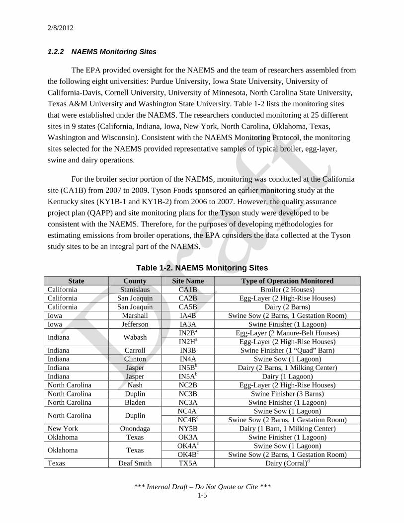
The EPA provided oversight for the NAEMS and the team of researchers assembled from the following eight universities: Purdue University, Iowa State University, University of California-Davis, Cornell University, University of Minnesota, North Carolina State University, Texas A&M University and Washington State University. Table 1-2 lists the monitoring sites that were established under the NAEMS. The researchers conducted monitoring at 25 different sites in 9 states (California, Indiana, Iowa, New York, North Carolina, Oklahoma, Texas, Washington and Wisconsin). Consistent with the NAEMS Monitoring Protocol, the monitoring sites selected for the NAEMS provided representative samples of typical broiler, egg-layer, swine and dairy operations.
For the broiler sector portion of the NAEMS, monitoring was conducted at the California site (CA1B) from 2007 to 2009. Tyson Foods sponsored an earlier monitoring study at the Kentucky sites (KY1B-1 and KY1B-2) from 2006 to 2007. However, the quality assurance project plan (QAPP) and site monitoring plans for the Tyson study were developed to be consistent with the NAEMS. Therefore, for the purposes of developing methodologies for estimating emissions from broiler operations, the EPA considers the data collected at the Tyson study sites to be an integral part of the NAEMS.
Table 1-2. NAEMS Monitoring Sites State County Site Name Type of Operation Monitored
California Stanislaus CA1B Broiler (2 Houses) California San Joaquin CA2B Egg-Layer (2 High-Rise Houses) California San Joaquin CA5B Dairy (2 Barns) Iowa Marshall IA4B Swine Sow (2 Barns, 1 Gestation Room) Iowa Jefferson IA3A Swine Finisher (1 Lagoon)
Indiana Wabash IN2Ba Egg-Layer (2 Manure-Belt Houses) IN2Ha Egg-Layer (2 High-Rise Houses)
Indiana Carroll IN3B Swine Finisher (1 “Quad” Barn) Indiana Clinton IN4A Swine Sow (1 Lagoon) Indiana Jasper IN5Bb Dairy (2 Barns, 1 Milking Center) Indiana Jasper IN5Ab Dairy (1 Lagoon) North Carolina Nash NC2B Egg-Layer (2 High-Rise Houses) North Carolina Duplin NC3B Swine Finisher (3 Barns) North Carolina Bladen NC3A Swine Finisher (1 Lagoon)
North Carolina Duplin NC4Ac Swine Sow (1 Lagoon) NC4Bc Swine Sow (2 Barns, 1 Gestation Room)
New York Onondaga NY5B Dairy (1 Barn, 1 Milking Center) Oklahoma Texas OK3A Swine Finisher (1 Lagoon)
Oklahoma Texas OK4Ac Swine Sow (1 Lagoon) OK4Bc Swine Sow (2 Barns, 1 Gestation Room)
Texas Deaf Smith TX5A Dairy (Corral)d

2/8/2012
*** Internal Draft – Do Not Quote or Cite *** 1-6
Table 1-2. NAEMS Monitoring Sites State County Site Name Type of Operation Monitored
Washington Yakima WA5Ac Dairy (1 Lagoon) WA5Bc Dairy (2 Barns)
Wisconsin Saint Croix WI5Ac Dairy (2 Lagoons)e WI5Bc Dairy (2 Barns)
Kentucky Union KY1B-1 Broiler (1 House) Hopkins KY1B-2 Broiler (1 House)
a Two different types of barns located at the same site were monitored. b Monitoring occurred on two separate dairy farms in Jasper County, IN. c Barns and lagoons were located at the same site. d The reported emission estimates represent the entire corral. e Instrumentation was deployed around two of the lagoons in the three-stage system. The emissions from the two lagoons were reported as a combined value.
1.3 Emission Estimating Methodology Development
Consistent with the Air Compliance Agreement, the EPA developed methodologies for estimating air pollutant emissions from broiler confinement operations using the emissions and process data collected under the NAEMS and other relevant information obtained through the EPA’s January 19, 2011, Call for Information (see Section 4.0). Based on the results of the its analysis of emissions trends (see Section 6.0), the EPA developed separate EEMs for broiler grow-out periods and for periods when litter on the confinement house floor was decaked or fully removed from the house (see Section 2.0 for a description of the broiler industry and production processes).
The EPA developed grow-out and decaking/litter clean-out period EEMs for the following pollutants: NH3, H2S, PM10, PM2.5, TSP and VOCs. Section 7 describes the statistical methodology used to analyze the data and develop the EEMs. Due to issues related to the performance of the gas analyzer at site CA1B and the procedures used to develop speciation profiles for VOC components, the EEM for VOCs is based only on the data from the two Kentucky sites.
For broiler grow-out periods, the EPA used the emissions and process parameter data collected under the NAEMS and SAS statistical software to develop the EEMs. Process data was divided into the following three groups: inventory data (e.g. number of birds and bird weight), ambient data (e.g. ambient temperature, pressure and relative humidity), and confinement data (e.g. building temperature, pressure and relative humidity). All of the process parameters were statistically evaluated to determine if they were predictor variables. In addition, the EPA evaluated whether the predictor variable process data was readily available to the growers, state and local agencies and other interested parties. Based on the results of the EPA’s predictor
2/8/2012
*** Internal Draft – Do Not Quote or Cite *** 1-7
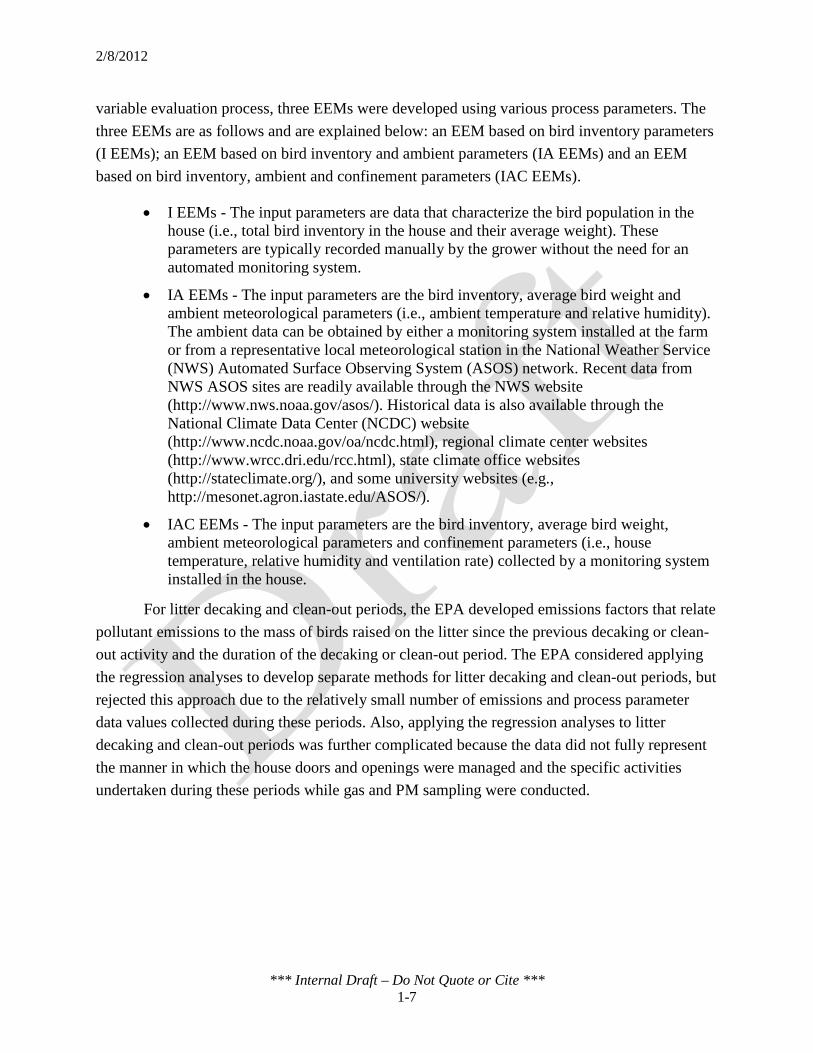
variable evaluation process, three EEMs were developed using various process parameters. The three EEMs are as follows and are explained below: an EEM based on bird inventory parameters (I EEMs); an EEM based on bird inventory and ambient parameters (IA EEMs) and an EEM based on bird inventory, ambient and confinement parameters (IAC EEMs).
• I EEMs - The input parameters are data that characterize the bird population in the house (i.e., total bird inventory in the house and their average weight). These parameters are typically recorded manually by the grower without the need for an automated monitoring system.
• IA EEMs - The input parameters are the bird inventory, average bird weight and ambient meteorological parameters (i.e., ambient temperature and relative humidity). The ambient data can be obtained by either a monitoring system installed at the farm or from a representative local meteorological station in the National Weather Service (NWS) Automated Surface Observing System (ASOS) network. Recent data from NWS ASOS sites are readily available through the NWS website (http://www.nws.noaa.gov/asos/). Historical data is also available through the National Climate Data Center (NCDC) website (http://www.ncdc.noaa.gov/oa/ncdc.html), regional climate center websites (http://www.wrcc.dri.edu/rcc.html), state climate office websites (http://stateclimate.org/), and some university websites (e.g., http://mesonet.agron.iastate.edu/ASOS/).
• IAC EEMs - The input parameters are the bird inventory, average bird weight, ambient meteorological parameters and confinement parameters (i.e., house temperature, relative humidity and ventilation rate) collected by a monitoring system installed in the house.
For litter decaking and clean-out periods, the EPA developed emissions factors that relate pollutant emissions to the mass of birds raised on the litter since the previous decaking or clean-out activity and the duration of the decaking or clean-out period. The EPA considered applying the regression analyses to develop separate methods for litter decaking and clean-out periods, but rejected this approach due to the relatively small number of emissions and process parameter data values collected during these periods. Also, applying the regression analyses to litter decaking and clean-out periods was further complicated because the data did not fully represent the manner in which the house doors and openings were managed and the specific activities undertaken during these periods while gas and PM sampling were conducted.

2/8/2012
*** Internal Draft – Do Not Quote or Cite *** 2-1
2.0 OVERVIEW OF BROILER INDUSTRY
Broiler production is the raising of chickens of either sex for meat. A broiler is a young chicken that is characterized as having tender meat, flexible breastbone cartilage and soft, pliable smooth-textured skin. Section 2.1 describes the typical business structure and the size and scale of broiler operations. Section 2.2 explains the production cycle, outlining the practices of growing hatched chicks to market weight, followed by a description of typical confinement houses in Section 2.3. Section 2.4 describes typical manure management practices. Section 2.5 provides a brief overview of the emissions from broiler production.
2.1 Industry Overview
Broiler production is a highly vertically-integrated industry, wherein a common owner or parent company is involved in several phases of the supply chain. For example, a parent company, or integrator, typically operates or contracts every aspect of the broiler production process (e.g., hatcheries, production houses, slaughterhouses, meat packing plants, feed production facilities and food distributors).
For broiler production operations, the integrator typically provides the birds, feed, medicines, transportation and technical support, under contract, to growers who provide the labor and the production facilities to raise the birds from hatchlings to market weight. The contract grower receives a minimum guaranteed price for the birds moved for market. More than 90 percent of all chickens raised for human consumption in the United States are produced by growers working under contract with integrators (USEPA, 2001). Because of this vertical integration, management strategies at the facility level tend to be more uniform than in other sectors of AFOs.
Based on the information reported in the USDA’s 2007 Census of Agriculture (http://www.agcensus.usda.gov/Publications/2007/Full_Report/usv1.pdf), 27,091 broiler operations produced 8.9 billion birds for market in 2007. Larger operations dominate broiler production, based on the 2007 Census data. In 2007, approximately 76 percent of the total broiler operations had a confinement capacity of 90,900 birds or less. However, operations with confinement capacities greater than 90,900 birds (approximately 24 percent of the total number of broiler operations) accounted for approximately 67 percent of the total annual bird production. The EPA estimated the confinement capacity by dividing the 2007 bird sales by the 5.5 flocks raised per year (this value for the typical flock turnover rate was obtained from the USDA National Agriculture Statistics Service). In addition to being dominated by large producers, the broiler industry is concentrated in several states. Alabama, Arkansas and Georgia are the largest
2/8/2012
*** Internal Draft – Do Not Quote or Cite *** 2-2
broiler producing states followed by Mississippi, North Carolina and Texas. California and Kentucky rank 7th and 14th, respectively, in terms of broiler production.
2.2 Production Cycle
The length of the grow-out period ranges from 28 to 63 days, depending on the size of the bird desired. The grow-out period includes a brooding phase that begins when day-old chicks are placed in a heated section of a broiler house known as the brood chamber. The brood chamber is initially maintained at an elevated temperature (e.g., 85 to 95 °F), which is gradually decreased during the first few weeks of the birds’ growth. As the growing birds need floor space, the remainder of the house is opened and the chicks are grown to market weight.
Broilers are produced to meet specific requirements of customers, which can be retail grocery stores, fast-food chains or institutional buyers. For broilers, the typical grow-out period is 49 days, resulting in an average bird weight of 4.5 to 5.5 pounds. The grow-out period may be as short as about 28 days to produce a 2.25 to 2.5 pound bird, commonly referred to as a Cornish game hen. For producing roasters weighing 6 to 8 pounds, the grow-out period is may take as long as 63 days.
Broiler houses are operated on an “all in-all out” basis and require time between flocks when the house is empty litter removal (either decaking or full litter cleanout), cleaning (e.g., pressure washing fans), and repair and maintenance. For broilers, five to six flocks per house per year is typical. However, the number of flocks raised per year is dependent on final bird weight, so is lower for roasters and higher for Cornish game hens. Female broilers grown to lay eggs for replacement stock are called broiler breeders and are usually raised on separate farms. These farms produce only eggs for broiler replacements. A typical laying cycle for hens is about 1 year, after which the hens are sold for slaughter.
2.3 Animal Confinement
The most common type of housing for broilers, roasters and breeding stock is enclosed housing with a compacted soil floor covered with dry bedding. Dry bedding can be sawdust, wood shavings, rice hulls, chopped straw, peanut hulls or other products, depending on availability and cost. The bedding absorbs moisture from the manure excreted by the birds, which forms litter (mixture of bedding and manure). Mechanical ventilation is typically provided using a negative-pressure system, with exhaust fans drawing air out of the house, and fresh air returning through ducts around the perimeter of the roof. The ventilation system uses exhaust fans to maintain acceptable housing conditions year round. Advanced systems use thermostats and timers to control exhaust fans.

2/8/2012
*** Internal Draft – Do Not Quote or Cite *** 2-3
2.4 Manure Management
Broiler houses are cleaned between flocks to remove some (i.e., decaking) or all of the accumulated litter. In decaking operations, the upper layer of cake (i.e., the compacted mixture of bedding and manure) that typically accumulates on the house floor near waterers and feeders is removed from the house. The litter remaining after decaking may be “top dressed” with an inch or so of new bedding material before the new flock is placed in the house. When the broiler house is completely cleaned out, the litter is typically removed using a front-end loader. After all litter and organic matter (e.g., feathers adhering to building surfaces) is removed, the house is disinfected.
Litter removed from the house is either immediately applied to cropland and/or pastureland or it is stored for later land application. Water quality concerns have led to the increased use of storage structures known as litter sheds, which are typically partially enclosed pole type structures, to store the cake. Water quality concerns also have prompted the recommendation that cake not stored in litter sheds be placed in well-drained areas and covered to prevent contaminated runoff and leaching. Litter sheds generally are sized only to provide capacity for cake storage because of cost. Thus, because of the larger volume of litter involved with a total facility clean-out, litter is often stored in temporary outdoor stockpiles when manure storage containment structures are at capacity, and/or immediate land application is not possible.
Broiler operations may add litter amendments, such as alum or sodium bisulfate, between the flocks to acidify the litter and reduce NH3 levels in the houses. However, amendments were not used on the houses monitored as part of the NAEMS.
2.5 Emissions from Broiler Operations
There are three primary sources of emissions associated with broiler operations: (1) the bird confinement house, (2) manure storage and (3) manure land application site. The NAEMS measured emissions from the confinement house and manure storage facility but did not measure emissions resulting from manure land application.
Gaseous emissions (NH3, H2S and VOC) from broiler confinement houses are predominately generated by microbial decomposition of bird manure and other materials (e.g., bedding, waste feed) that accumulate on the house floor. Ammonia and VOC emissions are generated under aerobic or anaerobic conditions while an anaerobic environment (e.g., around bird watering stations in confinement houses) is necessary to form H2S. Emissions of PM from bird confinement houses are primarily due to the entrainment of dry materials (e.g., feed, litter and feathers) caused by movement of birds and personnel in the confinement house.

2/8/2012
*** Internal Draft – Do Not Quote or Cite *** 3-1
3.0 NAEMS MONITORING SITES
This section describes the broiler operations monitored under the NAEMS. Section 3.1 explains the site selection criteria and an overview of the sites selected for monitoring. Section 3.2 describes the facility design and animal management practices followed at each site. Section 3.3 summarizes the instrumentation, measurement methods and sampling frequency specified in the site monitoring plans (SMPs).
3.1 Site Selection
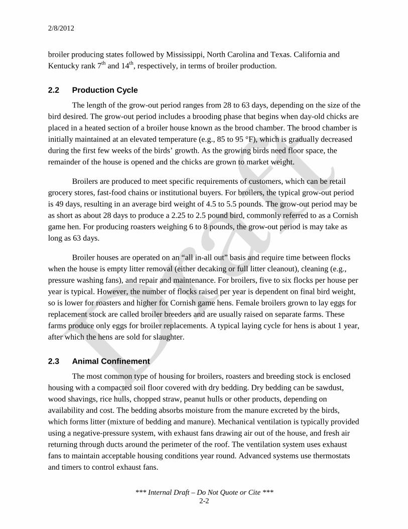
Three broiler farms were selected for the NAEMS based on factors specified in the Agreement. In general, these factors focused on the farm’s location, configuration, relative size, participation in the Agreement and whether it was representative of the broiler industry. Two houses were monitored at the California farm, designated as CA1B, and a single house was monitored at each of the Kentucky sites. Table 3-1 provides an overview of the sites and their characteristics, based on the information contained in the Quality Assurance Project Plans (QAPPs), SMPs, and site final reports. More detailed descriptions of each site are provided in the following sections.
Table 3-1. NAEMS Broiler Sites Information
Parameter Site CA1B H10 CA1B H12 KY1B-1 H5 KY1B-2 H3
Site type Litter on Floor House ventilation type Mechanically ventilated (MV) (tunnel)
House capacity (no. of birds per flock) 21,000a 24,400 (summer)
25,800 (winter) Bird type 60% Cobb, 40% Ross 100% Cobb (mixed sex)
Average animal residence time, days 47 53
Average bird weight 2.63 kg (5.8 lb) 2.75 kg (6.1 lb) Frequency of full litter
clean-out After three flocks Annually
Decaking After each flock After each flock No. of buildings at site 16 8 24 Year of construction 1960s/2002 1992 1991 Ridgeline orientation East-West North-South
House width 12.2 m (40 ft) 13.1 (43 ft) House length 125 m (410 ft) 155.5 m (510 ft) House area 1,524 m2 (16,400 ft2) 2037 m2 (21,930 ft2)
House spacing 12.2 m (40 ft) 18.3 m (60 ft) Ridge height 4.2 m (13.8 ft) 5.2 m (17.2 ft)
Sidewall height 2.3 m (7.5 ft) 2.1 m (7 ft) No. of air inlets 60 sidewall/2 tunnel 52 sidewall
2/8/2012
*** Internal Draft – Do Not Quote or Cite *** 3-2
Table 3-1. NAEMS Broiler Sites Information
Parameter Site CA1B H10 CA1B H12 KY1B-1 H5 KY1B-2 H3
Type of inlet Baffled eave inlet, 0.18 x 1.32 m (0.6 x 4.3 ft)
Box air inlets 0.15 x 0.66 m (0.5 x 2.17 ft)
Inlet control basis Static pressure Automatic (based on air flow rate) No. of ventilation fans 12 14 Largest fan diameter 1.22 m (48 in) 1.22 m (48 in) Smallest fan diameter 0.91 m (36 in) 0.91 m (36 in)
No. of large fans 10 10 No. of small fans 2b 4
Spacing between large fans 0.2 m (8 in) 0.2 m (8 in)
Spacing between small fans 125 m (410 ft)c 36.6 m (120 ft)d
No. of ventilation stages 17 12 13
Fan manufacturer Chore-Time (48 in), Aerotech (36 in) CanArm Euroemme
Controls vendor Chore-Time (48 in), Aerotech (36 in) Chore-Time Rotem
Artificial heating
LP Radiant brooders (14), 12.3 kW (42,000 Btu/h)
Pancake brooders (26), 8.78 kW (30,000 Btu/h)
LP heaters (3), 52.7 kW (180,000 Btu/h)
Space furnaces (3), 65.9 kW (225,000 Btu/h)
Summer cooling Tunnel/evaporative pads Tunnel/evaporative pads Brooding section East half of house South half of house
Monitoring Period Sept. 27, 2007- Oct. 21, 2009 Feb. 14, 2006 – March 14, 2007
Feb. 20, 2006 – March 5, 2007
Length of monitoring (days) 756 394 379
a The NAEMS documentation for site CA1B did not indicate a difference in summer and winter bird placements. b One of the small fans was inactive during the study. c The small fans are located at opposite ends of each house. d The small fans are located along one sidewall of each house.
3.2 Description of Sites Monitored
The NAEMS Monitoring Protocol specified that two broiler sites be monitored as part of the study, one on the west coast and the other in the Southeast to reflect the potential impact of climatic differences and geographical density of broiler production. Furthermore, the NAEMS Monitoring Protocol specified that the houses monitored should be mechanically ventilated with litter-on-the-floor manure handling systems. Final site selection was based on factors outlined in the NAEMS Monitoring Protocol and site-specific factors including facility age, size, design and operation practices and feed and bird genetics.

2/8/2012
*** Internal Draft – Do Not Quote or Cite *** 3-3
Both the California and Kentucky sites are representative of the broiler industry in the following aspects: the confinement house design (mechanically ventilated, tunnel), animal management practices (pancake brooder along with space heaters and half-house brooding), and the litter management and handling practices (decaking of houses between flocks with periodic full litter clean-outs).
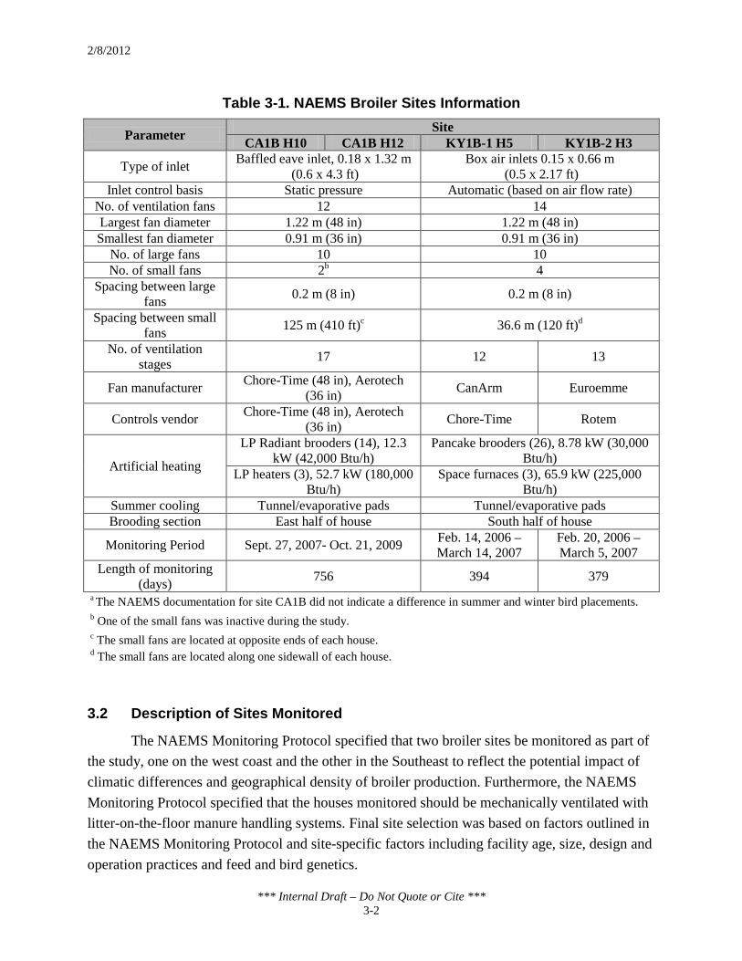
3.2.1 Site CA1B
The California farm (CA1B) is a 16-house broiler ranch in Stanislaus County, California. Figure 3-1 shows the overall layout of the site, with the two monitored houses (Houses 10 and 12) highlighted. The houses are 125 m (410 ft) long x 12.2 m (40 ft) wide arranged in an east-to-west orientation and are spaced 12.2 m (40 ft) apart. The house roofs have a 4:12 slope with sidewall heights of 2.3 m (7.5 ft).
Each house contains 21,000 birds (per flock) for a total farm capacity of 336,000 birds. Six to seven flocks of birds are raised in each house every year, and all houses are operated on the same grow-out and litter clean-out cycles. The birds housed at the facility over the course of the NAEMS were a 60/40 split between Cobb and Ross genetic varieties and were raised from approximately 0.05 to 2.41 kg (1.1 to 5.3 lb) with an average grow-out period of 47 days. The birds were concentrated in the east (front) end of the houses during the first 10 days of each brooding phase of the grow-out period.
Birds were fed a pelleted diet consisting of corn, soybeans, protein, and poultry fat. Four feed rations were used, specially formulated for weeks 1 and 2, weeks 3 and 4, week 5, and week 6. Feed was delivered to the birds by auger and water consumption was recorded by an automatic water meter. The house lights were turned off for several hours each night. A standby generator supplied power for critical systems during power outages.
Ventilation air entered the house through pressure-adjusted, baffled air inlets at the house eaves (Figure 3-2). The building air was withdrawn from the house using 10, 122-cm (48-inch) diameter belted exhaust fans located in banks of five on both the north and south sidewalls (Figure 3-3). The fans within each bank were spaced 20 cm (8 inches) apart. In addition, a single 91-cm (36-inch) diameter belted exhaust fan was located on the west wall at the back of the house. The fan operation in each house was configured into 8 stages to provide temperature control over the grow-out period. Each house was equipped with six sensors to monitor temperature.
During cooler weather, 14 radiant brood heaters [12.3 kW (42,000 Btu/hr) each] heated the front (east) half of the house, while three liquid propane heaters [52.7 kW (180,000 Btu/hr) each] heated the rest of the house. During warmer conditions, evaporative pads located at the
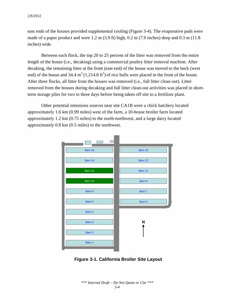
2/8/2012
*** Internal Draft – Do Not Quote or Cite *** 3-4
east ends of the houses provided supplemental cooling (Figure 3-4). The evaporative pads were made of a paper product and were 1.2 m (3.9 ft) high, 0.2 m (7.9 inches) deep and 0.3 m (11.8 inches) wide.
Between each flock, the top 20 to 25 percent of the litter was removed from the entire length of the house (i.e., decaking) using a commercial poultry litter removal machine. After decaking, the remaining litter at the front (east end) of the house was moved to the back (west end) of the house and 34.4 m3 (1,214.8 ft3) of rice hulls were placed in the front of the house. After three flocks, all litter from the houses was removed (i.e., full litter clean-out). Litter removed from the houses during decaking and full litter clean-out activities was placed in short-term storage piles for two to three days before being taken off site to a fertilizer plant.
Other potential emissions sources near site CA1B were a chick hatchery located approximately 1.6 km (0.99 miles) west of the farm, a 10-house broiler farm located approximately 1.2 km (0.75 miles) to the north-northwest, and a large dairy located approximately 0.8 km (0.5 miles) to the northwest.
Barn 16
Barn 14
Barn 12
Barn 10
Barn 8
Barn 6
Barn 13
Barn 4
Barn 3
Barn 2
Barn 11
Barn 9
Barn 7
Barn 15
Barn 5
Barn 1
N
Figure 3-1. California Broiler Site Layout

2/8/2012
*** Internal Draft – Do Not Quote or Cite *** 3-5
Figure 3-2. Example House Air Inlet
Figure 3-3. Bank of 122-cm (48-inch) Fans (left, view from inside of house) and (right, view from outside of house)
Figure 3-4. Evaporative Cooling Pads

2/8/2012
*** Internal Draft – Do Not Quote or Cite *** 3-6
3.2.2 Sites KY1B-1 and KY1B-2
The two broiler farms, designated as KY1B-1 and KY1B-2, are located in western Kentucky. The KY1B-1 farm has 8 broiler houses and has a total maximum winter capacity of 206,400 birds. The KY1B-2 farm has 24 broiler houses and a total maximum winter capacity of 619,200 birds. Figure 3-5 shows the location of the monitored facilities within Kentucky. The aerial photographs in Figure 3-6 show the locations of the monitored houses at each site.
One broiler confinement house at each farm (designated as KY1B-1 House 5 and KY1B-2 House 3) was monitored. Built in the early 1990s, the two houses each measured 13.1 m x 155.5 m (43 ft x 510 ft). The birds housed during the monitoring period were Cobb-Cobb straight-run (mixed sex) broilers. During the winter, the houses were stocked with an initial placement of 25,800 birds. The initial placement during the summer was 24,400 birds. Typically, the birds were grown to 53 days of market age and an average bird weight of 2.75 kg (6.1 lb).
Each house had insulated drop ceilings, 26 box air inlets [15 x 66 cm (6 x 26 inch)] along each sidewall (see Figure 3-7), 26 pancake brood heaters [8.8 kW (30,000 Btu/hr) each], three space furnaces [65.9 kW (225,000 Btu/hr) each], four 91-cm (36-inch) diameter sidewall exhaust fans spaced approximately 36.6 m (120 ft) apart, and 10, 123-cm (48-inch) diameter tunnel fans. A single 91-cm (36-inch) fan (SW1) used for minimum ventilation was located in the brooding end of each house. Two evaporative cooling pads (24-m (80-ft) sections) were located in the opposite end of the houses from the tunnel fans. The houses were also equipped with foggers for additional cooling, if needed. Rice hulls were used as litter bedding in both houses. Each house was decaked and topped off with fresh litter after every flock, with a full litter clean-out occurring once per year.

2/8/2012
*** Internal Draft – Do Not Quote or Cite *** 3-7
Figure 3-5. Locations of Kentucky Measurement Sites
Figure 3-6. Aerial Photographs of Kentucky Monitoring Sites
KY1B - 1
KY1B-2

2/8/2012
*** Internal Draft – Do Not Quote or Cite *** 3-8
Figure 3-7. Tunnel Fans and Box Air Inlets
3.3 Site Monitoring Plans
This section provides a summary of the monitoring conducted at each of the broiler sites. Detailed descriptions of the monitoring program, including monitoring equipment specifications and calibration procedures and frequencies, are provided in Appendix A (QAPPs), Appendix B (SMPs), Appendix C [standard operating procedures (SOPs)], and Appendix D (final site reports).
3.3.1 Site CA1B Monitoring Plan
Figure 3-8 shows the configuration of the house monitoring equipment. Installation and preliminary testing of the monitoring equipment was conducted from May 29, 2007 through September 27, 2007. Monitoring of emissions and process parameters began on September 27, 2007 and was completed on October 21, 2009. Table 3-2 lists the sampling locations by analyte.
The on-farm instrument shelter (OFIS) was positioned between houses 10 and 12 at the far west end houses, with a north/south orientation to minimize interference with vehicle traffic along the driveway west of the houses. The OFIS was positioned somewhat off-center in between the houses to leave enough space on one side for vehicle access.
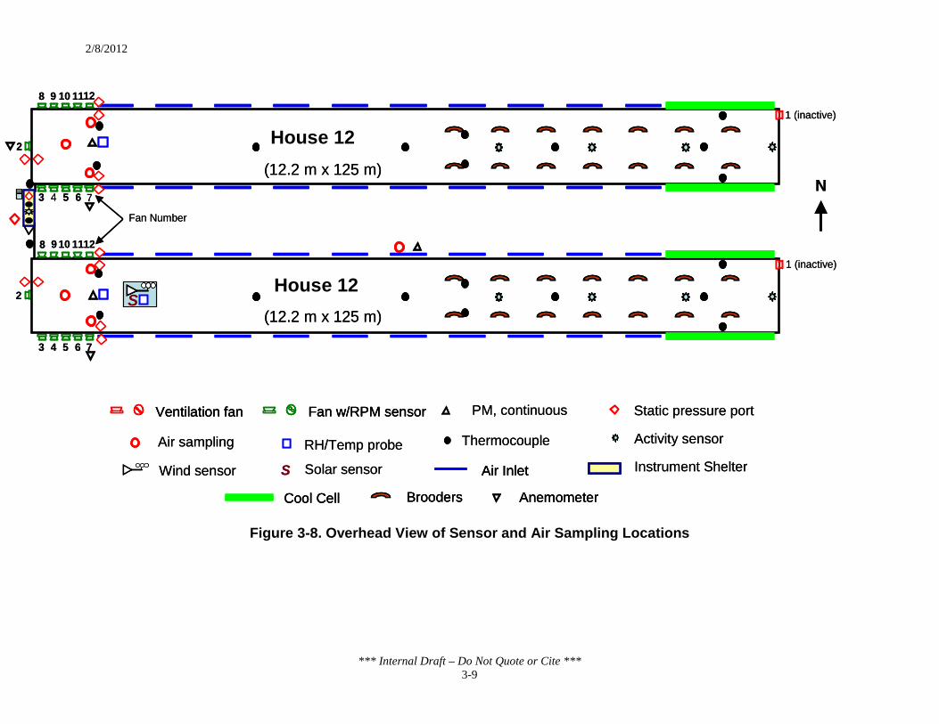
2/8/2012
*** Internal Draft – Do Not Quote or Cite *** 3-9
Figure 3-8. Overhead View of Sensor and Air Sampling Locations
Thermocouple Air sampling RH/Temp probe
Static pressure portPM, continuous
Activity sensor
Instrument ShelterWind sensor Solar sensorS
Cool Cell
Air Inlet
Ventilation fan
Brooders
Fan w/RPM sensor
Anemometer
Thermocouple Air sampling RH/Temp probe
Static pressure portPM, continuous
Activity sensor
Instrument ShelterWind sensor Solar sensorS
Cool CellCool Cell
Air InletAir Inlet
Ventilation fanVentilation fan
BroodersBrooders
Fan w/RPM sensorFan w/RPM sensor
AnemometerAnemometer
1 (inactive)
1 (inactive)
7
9 10 118
3 4 5 6
3 4 5 6 7
9 10 11128
2
SBarn 10(12.2 m x 125 m)
Barn 12(12.2 m x 125 m)
12
N
2
Fan Number
1 (inactive)
1 (inactive)
7
9 10 118
3 4 5 6
3 4 5 6 7
9 10 11128
2
SSBarn 10(12.2 m x 125 m)
Barn 12(12.2 m x 125 m)
12
N
2
Fan Number
House 12
House 12

2/8/2012
*** Internal Draft – Do Not Quote or Cite *** 3-10
Table 3-2. Analyte Sampling Locations at Site CA1B
Analyte Sampling Locationa
Gases (continuous measurements for NH3, H2S and CO2)
GSL-A: Directly in front of the inlet of fan 2, along a line connecting fans 5 and 10 GSL-B: 1 m E of fan 12 and 3 m from N wall GSL-C: 1 m E of fan 7 and 3 m from S wall INLET: In front of the 5th ventilation inlet from the E end of barn 10 on N sidewall
PM (continuous measurements for PM2.5, PM10 and TSP)
TEOM: Located 2 m in front of Fan 7 INLET: Beta-Gage in front of the 5th ventilation inlet from the E end of barn 10 on N sidewall
VOC (grab samples) 1 m E of fan 7 and 3 m from S wall, at fan hub level (GSL-C)
a Gas sampling probes were located at fan hub height, suspended from the ceiling. GSL = Gas sampling location.
3.3.1.1 Gas Sampling
A custom-designed gas sampling system (GSS) collected air samples for continuous gas measurements from multiple gas sampling probes located in and near the monitored houses. Each probe was connected to the GSS with Teflon tubing. Tubular raceways between the OFIS and the monitored houses protected the sampling lines and data signal cables. The sampling lines were wrapped with insulation and heated inside the raceways and at other locations vulnerable to cold air to prevent condensation inside the tubes.
The house exhaust emissions were measured using three gas sampling probes (A, B and C) placed in the west end of each house near the exhaust fans at a height equal to the fan hubs (Figure 3-8). Gas sampling probe A was located in front of the inlet of fan 2 and between fans 5 and 10. Two sampling probes (B and C) were located three meters from each sidewall in a cross-sectional plane approximately 1 meter east of fans 7 and 12. Incoming air for both houses was sampled near the air inlet of House 12 at approximately the midpoint (lengthwise) of the house. Other than the exhaust from other houses, the occasional two- to three-day stockpile of litter just outside the far end of the houses was the only on-farm emissions source that could contribute to the concentrations on the inlet air for Houses 10 and 12.
Each exhaust location was sampled and measured continuously for 10 minutes. The inlet air location was monitored for 20 minutes twice daily. After approximately four months of data collection, the gas concentration data were evaluated at each sampling location to determine whether equilibrium occurred within the sampling periods. A statistical analysis confirmed that 10 minutes was sufficient for the exhaust GSLs, but that 30 minutes was required for the house

2/8/2012
*** Internal Draft – Do Not Quote or Cite *** 3-11
inlet. Consequently, the sampling period for the inlet air was increased from 20 minutes to 30 minutes. Additional detail on the collection method is provided in Appendix A (NAEMS QAPP) and Appendix C (SOP G1). At each sampling location, the gas was analyzed for NH3, H2S, non-methane hydrocarbons (NMHC) and CO2 and the gas analyzer provided concentration readings every second. The average concentration values were recorded every 15 and 60 seconds.
One set of gas analyzers in the OFIS measured gas concentrations as the GSS sequenced through all of the GSLs. A personal computer collected all site monitoring data using a data acquisition and control program (AirDAC). AirDAC averaged the signals (after conversion to engineering units) over 15-second and 60-second intervals and recorded the means into two separate computer files. All real-time data were displayed in tabular and graphic forms for on-site or remote viewing. Measurement alarms, data collection notifications, data files, graphs and statistics of the daily data sets and modified configuration and field note files were automatically emailed to the site investigator and engineer and to the Purdue Agricultural Air Quality Laboratory after midnight each night.
3.3.1.2 PM Sampling
A tapered element oscillating microbalance (TEOM) was placed in each house approximately 6 meters (19.7 ft) in front of fan 7. A Beta Gauge attenuation PM monitor continuously measured the PM concentration of the ambient air. The Beta Gauge was enclosed in a protective outdoor enclosure and was located at the air inlet of House 10. The PM10 size-cut heads on the TEOM and Beta Gauge were replaced with PM2.5 heads for two, two-week periods over the course of the study, and with TSP heads for one week every 8 weeks (beginning with the first week of data collection).
As shown in Table 3-3, PM2.5 emissions were measured in February and July of 2008 and January and September of 2009 continuously for 12 to 18 days each time. The TSP concentrations were measured continuously for six 7- to 14-day periods. Emissions of PM10 were measured continuously at all other times. Additional detail on the collection method is provided in Appendix A (NAEMS QAPP) and Appendix C (SOP P1).

2/8/2012
*** Internal Draft – Do Not Quote or Cite *** 3-12
Table 3-3. PM Sampling Schedule Time and Day (mm/dd/yy) Test Duration (days)
Start Stop PM10 TSP PM2.5 9/28/07 12/10/07 73.6 NS NS
12/10/07 12/19/07 NS 8.9 NS 12/19/07 2/1/08 44.0 NS NS
2/1/08 2/19/08 NS NS 18.1 2/19/08 2/20/08 NS NS 0.3a 2/19/08 2/20/08 0.3b NS NS 2/20/08 5/15/08 85.7 NS NS 5/15/08 5/28/08 NS 12.8 NS 5/28/08 7/9/08 42.0 NS NS 7/9/08 7/25/08 NS NS 16.0
7/25/08 11/17/08 115.1 NS NS 11/17/08 11/24/08 NS 7.1 NS 11/24/08 1/5/09 41.9 NS NS
1/5/09 1/20/09 NS NS 15.0 1/20/09 4/9/09 79.0 NS NS 4/9/09 4/20/09 NS 11.0 NS
4/20/09 6/25/09 66.1 NS NS 6/25/09 7/8/09 NS 12.9 NS 7/8/09 9/26/09 80.1 NS NS
9/26/09 10/7/09 NS NS 10.9 10/7/09 10/21/09 NS 14.1 NS
10/21/09 10/22/09 0.4 NS NS Totals 628.3 66.7 60.3
NS = Not sampled. a For this sampling episode, ambient concentration data were not collected. b For this sampling episode, only ambient concentration data were collected.
3.3.1.3 VOC Sampling
An initial characterization study of VOCs was conducted during the first quarter after site setup at site CA1B. While NMHC were continuously monitored using photoacoustic infrared spectroscopy along with building air-flow rate, periodic grab samples of VOCs were taken at the primary representative exhaust fan location (as defined in the SMPs) of Houses 10 and 12. The purpose of the VOC grab sampling was to obtain data to speciate the NMHC measurements.
During the initial study, three sampling methods were evaluated to determine which method would be used for the remainder of the broiler study: sorbent tubes and Silcosteel canisters for general VOCs, and all-glass bubblers for amines. Each sorbent tube or canister sample was evaluated using gas chromatography – mass spectrometry (GC-MS); amines collected in bubblers were analyzed by ion chromatography (IC). The results of this initial study
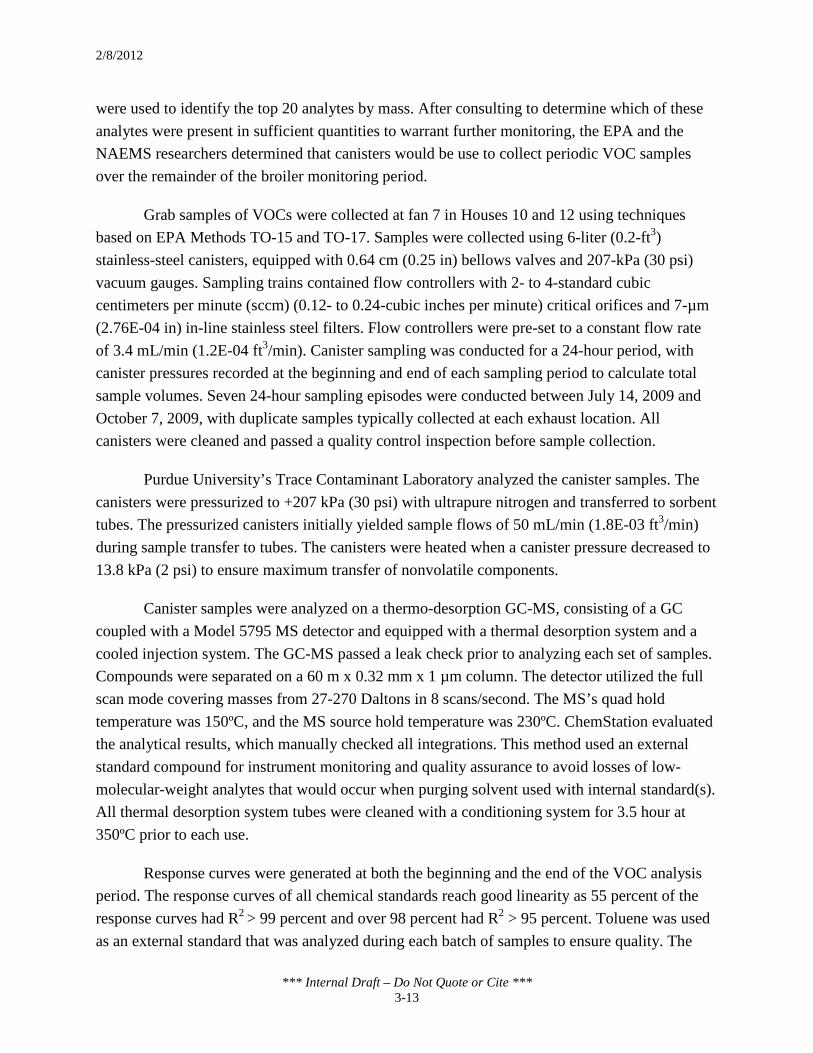
2/8/2012
*** Internal Draft – Do Not Quote or Cite *** 3-13
were used to identify the top 20 analytes by mass. After consulting to determine which of these analytes were present in sufficient quantities to warrant further monitoring, the EPA and the NAEMS researchers determined that canisters would be use to collect periodic VOC samples over the remainder of the broiler monitoring period.
Grab samples of VOCs were collected at fan 7 in Houses 10 and 12 using techniques based on EPA Methods TO-15 and TO-17. Samples were collected using 6-liter (0.2-ft3) stainless-steel canisters, equipped with 0.64 cm (0.25 in) bellows valves and 207-kPa (30 psi) vacuum gauges. Sampling trains contained flow controllers with 2- to 4-standard cubic centimeters per minute (sccm) (0.12- to 0.24-cubic inches per minute) critical orifices and 7-µm (2.76E-04 in) in-line stainless steel filters. Flow controllers were pre-set to a constant flow rate of 3.4 mL/min (1.2E-04 ft3/min). Canister sampling was conducted for a 24-hour period, with canister pressures recorded at the beginning and end of each sampling period to calculate total sample volumes. Seven 24-hour sampling episodes were conducted between July 14, 2009 and October 7, 2009, with duplicate samples typically collected at each exhaust location. All canisters were cleaned and passed a quality control inspection before sample collection.
Purdue University’s Trace Contaminant Laboratory analyzed the canister samples. The canisters were pressurized to +207 kPa (30 psi) with ultrapure nitrogen and transferred to sorbent tubes. The pressurized canisters initially yielded sample flows of 50 mL/min (1.8E-03 ft3/min) during sample transfer to tubes. The canisters were heated when a canister pressure decreased to 13.8 kPa (2 psi) to ensure maximum transfer of nonvolatile components.
Canister samples were analyzed on a thermo-desorption GC-MS, consisting of a GC coupled with a Model 5795 MS detector and equipped with a thermal desorption system and a cooled injection system. The GC-MS passed a leak check prior to analyzing each set of samples. Compounds were separated on a 60 m x 0.32 mm x 1 µm column. The detector utilized the full scan mode covering masses from 27-270 Daltons in 8 scans/second. The MS’s quad hold temperature was 150ºC, and the MS source hold temperature was 230ºC. ChemStation evaluated the analytical results, which manually checked all integrations. This method used an external standard compound for instrument monitoring and quality assurance to avoid losses of low-molecular-weight analytes that would occur when purging solvent used with internal standard(s). All thermal desorption system tubes were cleaned with a conditioning system for 3.5 hour at 350ºC prior to each use.
Response curves were generated at both the beginning and the end of the VOC analysis period. The response curves of all chemical standards reach good linearity as 55 percent of the response curves had R2 > 99 percent and over 98 percent had R2 > 95 percent. Toluene was used as an external standard that was analyzed during each batch of samples to ensure quality. The

2/8/2012
*** Internal Draft – Do Not Quote or Cite *** 3-14
relative bias and standard deviation of 97 toluene checks were -4.3 percent and 18.8 percent, respectively. The uncertainty of the mean of duplicate field samples was calculated as 27 percent, based on the toluene checks.
3.3.1.4 Building Air Flow
The ventilation air flow for each monitored house was calculated as the sum of the volumetric flow rates for all fans operating over a given time interval. The baseline air flow curves of each type of fan were obtained from the Bioenvironmental and Structural Systems (BESS) Laboratory at the University of Illinois, Urbana-Champaign (Appendix C, SOP A1). Each performance record used to develop the fan curves consisted of air flow measurements (Q1) at several static pressure values (P1), and at relatively constant rotational speeds (N1 = 779 and 550 rpm for small and large fans, respectively). For each fan type, the BESS fan curve was adjusted to the mean speed (N2) of the fan tests (530 and 749 rpm for the large and small fans, respectively). The new, speed-indexed baseline curves were derived using the first (Q2 = Q1(N2/N1)) and second (ΔP2 = ΔP1(N2/N1)0.5) fan laws, where Q2 is the speed-adjusted BESS fan curve at speed N2. The speed-corrected air flow prediction model is Q4 = (aΔP4 + b)·(N4/N2)·Q2, where ΔP4 and N4 are measured fan static pressure and speed.
Rotational speed and operational status of the fans installed in each house were monitored using a magnetic Hall-effect sensors (speed sensor) installed on each fan (except for fan 1 which was inactive). The speed sensors were mounted to detect the rotational speed in revolutions per minute (rpm) of either the fan shaft or the fan pulley. The digital signal from the speed sensor was converted into a frequency measurement with a counter module in the data acquisition system. Additionally, impeller anemometers were installed on the outlet of fans 2 and 7 in House 12 and fan 7 in House 10. The differential static pressure was measured across the north, south and west walls of each house using pressure transducers. The outside port was located against the outside wall near the ventilation fans of the north, south and west walls. Additional detail regarding the air flow calculations is provided in Appendix A (NAEMS QAPP) and Appendix C (SOP A4).
The air flow rate of installed fans was measured using a Fan Assessment Numeration System (FANS). The FANS consists of a housing containing five impeller anemometers mounted horizontally. To measure the flow rate of an individual fan, the housing is centered vertically and horizontally on the exhaust side of the fan to be tested and the anemometer readings provide the average air velocity across a known cross-sectional area. Additional detail on the FANS analyzer is provided in Appendix A (NAEMS QAPP) and Appendix C (SOP A2).

2/8/2012
*** Internal Draft – Do Not Quote or Cite *** 3-15
The field data obtained from the FANS were used to develop equations that calculated air flow as a function of differential pressure and fan rotational speed and to assess the uncertainty in air flow predictions. A total of 237 FANS tests with replication were conducted during April and June of 2008 and April, July and September of 2009. Each fan was tested at least once during three or more of the five testing periods. The fan belts had been recently replaced prior to the tests in June 2008. For a given test using the FANS, the model is Q4 = (a·ΔP3 + b)·(N3/N2)·Q2, where ΔP3 and N3 are the measured fan static pressure and speed during the fan test, and the fan degradation factor k = a·ΔP3 + b. The values for the coefficients a and b were those that minimized the sum of square differences between Q4 and Q3 for all the valid fan tests within a speed regime. Table 3-4 shows the resulting fan models.
Table 3-4. Fan Air Flow Models
Fan Type
Reference Speed (N2)
Polynomial Coefficients of Q2=f(ΔP2) at Speed N2 Coefficients of k
a3 a2 a1 a0 b1 b0
Large 530 2.943E-06 -2.304E-04 4.368E-02 9.412 8.213E-04 0.887 Small 749 1.474E-05 5.108E-04 3.908E-02 5.617 4.196E-03 0.697
3.3.1.5 Meteorological and Confinement Data
At site CA1B, the following meteorological data were continuously recorded: ambient temperature, ambient relative humidity, atmospheric pressure, solar radiation, wind direction, and wind speed. The meteorological instruments (i.e., a capacitance-type relative humidity and temperature probe (RH/T), a pyranometer, and a cup anemometer) were mounted on a 1-meter aluminum tower located on the ridge of House 10 near the OFIS.
To measure the building environmental conditions, RH/T sensors were located at the center of the west end of each house. Type-T thermocouples (TCs) were used to measure temperatures at each sampling point not already monitored with a RH/T probe and were also equally spaced along the center of each house. The TCs were attached to the support posts that ran down the center of the house at 3-meter intervals. Two TCs were located next to the two brooders closest to the OFIS, and two were located at the center of the evaporative pads. A TC was added on April 9, 2009, to monitor the manure temperature in House 12 at floor level.
Thermocouples were also located in the heated raceway between the houses and OFIS. Two TCs were located in the OFIS to measure the temperature of the OFIS and the air-conditioning system. One TC monitored the temperature in the ambient PM monitor enclosure. Additional detail on the collection method is provided in Appendix A (NAEMS QAPP) and Appendix C (SOPs E1 and E2).

2/8/2012
*** Internal Draft – Do Not Quote or Cite *** 3-16
3.3.1.6 Animal Husbandry and Building Systems
Infrared motion detectors (activity sensors) were mounted to roof support posts along the center axis of the house to monitor movements of birds and workers. An activity sensor was also used to monitor researcher presence in the OFIS.
The producer recorded data on animal inventory and mortalities manually on a daily basis and provided this information to the NAEMS site personnel. The average mass of the birds between 1 and 47 days old was measured at least weekly during three consecutive cycles of birds. For each measurement period, 25 or 50 birds of each gender (50 or 100 total) were measured in each house and the average mass reported.
The relays that controlled lights, brooders and feeders were monitored in each house using auxiliary contacts in 5V-DC circuits in conjunction with the digital inputs of the data acquisition system.
3.3.1.7 Biomaterials Sampling Methods and Schedule
An independent laboratory, Midwest Laboratories, Omaha, NE, performed all analyses of biomaterials (e.g., litter, bedding). The water provided to the birds in August 2009 was analyzed to evaluate the nitrogen content of the water. Samples of feed and fresh bedding (rice hulls) were collected in duplicate from each house and analyzed for nitrogen and solids. Additional detail regarding the biomaterial sample handling and analyses is provided in Appendix A (NAEMS QAPP) and Appendix C (SOP M1).
On April 15, 2008, the manure mass removed during a full litter clean-out, estimated from the square area and average mass of manure per unit area, was 88,000 kg (97 tons) in House 10 and 79,000 kg (87 tons) in House 12. The total volume of fresh bedding brought into each house on April 18, 2008 after a full litter clean-out was 118 m3, based on measured litter density.
The estimated volume of litter removed by the decaking procedure was 30 to 45 m3
(1,059 to 1589 ft3), based on the volume of manure removed from a house on December 31, 2007, and the average volume of litter removed from multiple houses on January 2, 2008. The amount of bedding used to replenish litter volume after decaking operations was not specified in the final reports submitted to EPA. The density of decaked litter (474 g/m3, 0.03 lb/ft3) was determined from a 15.3-liter (0.54-ft3) sample.
Three types of manure samples were collected: surface litter, decaked litter and litter removed during full clean-out. Surface litter samples were collected over the grow-out period

2/8/2012
*** Internal Draft – Do Not Quote or Cite *** 3-17
from 16 random locations per house, including 8 samples from the front of the house with relatively fresh litter and 8 from the back of the house with the older litter. The two groups were considered representative of the house litter. At each sampling point, all litter within a 0.6-m radius was brought to the center of the sampling location and mixed thoroughly. Composite samples from the mixtures were analyzed for pH, solids and NH3. Decaking and complete litter clean-out samples were collected from the blended litter pile before it was removed from the site. A total of 12 samples were collected for each litter decaking and clean-out event and analyzed for ash (after December 2, 2008), nitrogen and solids content.
3.3.2 Sites KY1B-1 and KY1B-2
Figure 3-9 and Figure 3-10 show the schematics of the monitoring plan for the Kentucky sites, and Table 3-5 lists the locations at which the various samples were collected. Equipment was installed by January 06, 2006, and preliminary testing was completed on February 10, 2006. The monitoring periods ran from February 14, 2006, through March 14, 2007, for KY1B-1, and from February 20, 2006, through March 5, 2007, for KY1B-2.
Each broiler house has its own Mobile Air Emissions Monitoring Unit (MAEMU) that contains the air pollutant and fan flow monitoring systems and provides an environmentally-controlled instrument area. Locations of the MAEMU are noted in Figure 3-9 as the “trailer.” Figure 3-10 shows a cross-section view of monitor placement. Heated raceways connected the MAEMU to each house to avoid condensation in the sampling lines during cold weather.
Table 3-5. Analyte Sampling Locations at Sites KY1B-1 and KY1B-2
Analyte Sampling Location
Gases (continuous measurements for NH3, H2S, NMHC, CO2)
SW1: near the primary minimum ventilation (36-in) sidewall fan (SW1); 1.2 m (4.0 ft) away from the fan in the axial direction, 2.3 m (7.5 ft) in the radial direction, and 1 m (3 ft) above the floor SW3: fourth sidewall (36-in) exhaust fan (SW3) (non-brooding end); 1.2 m (4.0 ft) away from the fan in the axial direction, 2.3 m (7.5 ft) in the radial direction, and 1 m (3 ft) above the floor TE: tunnel end (TE); at the center across the house (for example, 6.6 m or 21.5 ft from each sidewall) and 7.3 m (24.0 ft) from the end wall A: ambient sample location (A) is between the inlet boxes opposite of the sidewall with the exhaust fans
PM (continuous measurements for PM2.5, PM10, TSP)
TEOM: During the brooding period, the TEOMs are placed at SW1 sampling location. When the brood curtain is open, the TEOMs are moved to the TE sampling location.

2/8/2012
*** Internal Draft – Do Not Quote or Cite *** 3-18
Figure 3-9. Schematic of KY1B-1 (top) and KY1B-2 (bottom)
Brood Curtain
Evaporative Coolers
SW1 SW2 SW3 SW4
24’
12’
2 4 6 8 10 1 3 5 7 9
Fan Numbers
Feed Bin
Trailer
Extended gravel lane
KY1B-2 House 3 Drawing not to scale
Control Room
T, RH T, RH
T
120’ 58’
135’ 120’ 83’ 24’-7” 22’-5” 52’
5’
510’ (outside)
80’
235’-6”
Conc Pad
10’
15’
8’ 14’
284’-6”’
Note: Curtain aligns with end of Feed Bin Pad.
RH = Relative Humidity sample point
= Pressure Differential Sampling Point
= Air sampling point = 36” sidewall fan
= 48” fan
T = Temperature sample point = Ambient air sampling point
= TEOM sampling point
T, RH and B
B = Barometric pressure sample point
43’
22’-9” 24’-2”
Brood Curtain Evaporative Coolers
SW1 SW2 SW3 SW4
22’
12’
9 7 5 3 1 10 8 6 4 2
Fan Numbers
Feed Bin Trailer Gravel Pad
KY1B-1 House 5 Drawing not to scale
Ditch
T, RH T, RH
105’ 120’ 98’ 135’ 52’
5’
235’ 15’
Control Room
5’
8’
510’ (outside)
277’
52’
80’
Note: Curtain aligns with end of Feed Bin Pad.
T, RH, B
T
RH = Relative Humidity sample point
= Pressure Differential Sampling Point
= Air sampling point = 36” sidewall fan
= 48” fan
T = Temperature sample point = Ambient air sampling point
= TEOM sampling point B = Barometric pressure sample point
43’

2/8/2012
*** Internal Draft – Do Not Quote or Cite *** 3-19
Figure 3-10. Cross-sectional View of Sidewall Sampling Locations
3.3.2.1 Gas Sampling
Individual air samples for both in-house and background locations were collected using a GSS that was designed to collect samples from four locations on a cyclical basis. Gases and PM were sampled when the house ventilation system was in operation. Gaseous emissions were sampled continuously on a 120-second interval (i.e., samples were continuously collected and analyzed every 30 seconds, with every fourth concentration value used to calculate emissions). A real-time data acquisition (DAQ) system program developed with LabView 7 was used to acquire data, automate sampling location control, display real-time data and deliver data and system operation status.
Air samples moving from the broiler house sampling points (representing the exhaust air streams) to the instrument trailer/analyzers were protected against in-line moisture condensation with insulation and temperature-controlled resistive heating cable. The samples were pumped into the GSS with pumps on its inlet side, making it a positive-pressure system. Using this approach ensured that the integrity of the gas sample was not compromised if a leak developed at any connection point on the GSS.
1.3 m (4.3 ft) 1.2 m (3.8 ft)
2.1m (7.0 ft)
0.9 m (3.0 ft Fan) 1.2 m
(4.0ft Fan)
Floor
Ceiling
= Sampling point
Cross-section View
0.9 m (3.0 ft)
1.2 m (4.0 ft)
0.9 m (3.0 ft)
Top View
2.3 m (7.5 ft) 1.2 m (4.0 ft) Legend

2/8/2012
*** Internal Draft – Do Not Quote or Cite *** 3-20
Three sampling points were located inside each broiler house at two sidewall fans and at the tunnel end. The fourth sampling point was located outside of the broiler house and was used as the ambient measurement point for background concentration determination. Figure 3-9 shows the location of the sampling points in KY1B-1 and KY1B-2. One sampling location was near the primary minimum ventilation sidewall fan (SW1) used for cold weather ventilation (in the brooding half of the house). The second sampling location was near the third sidewall fan (SW3, nonbrooding end). The third location was at the tunnel end (TE). The ambient sample location (A) was between the inlet boxes opposite of the sidewall with the exhaust fans. The mass of pollutant in the background (inlet) air was subtracted from that in the exhaust air when calculating aerial emissions from the house.
Hydrogen sulfide was measured by ultraviolet (UV) pulsed fluorescence analyzer. Concentrations of NMHC were measured with a methane/nonmethane/total hydrocarbon analyzer using column technology to separate methane and nonmethane from total hydrocarbons and a dual flame ionization detector (FID) to measure each component in the air sample. Concentrations of NH3 and CO2 for the ambient (or incoming air) and exhaust air were measured with an advanced photoacoustic multigas analyzer.
Every two hours, air samples from the ambient location were collected and analyzed for 8 minutes. The longer sample analysis time for the ambient point was to account for the longer response time of the instrument when measuring a potentially large step change in gas concentration. The 2-hour interval for the analysis of the ambient concentrations was selected because the ambient conditions remained relatively constant compared to the in-house conditions.
3.3.2.2 PM Sampling
Each of the Kentucky sites was equipped with a TEOM monitor to measure the PM mass concentration of the exhaust air. Three different inlet heads were used on the TEOMs to simultaneously measure TSP, PM10 and PM2.5 continuously over the study period. The TEOM 1400a is a gravimetric instrument that draws ambient air through a filter at a constant flow rate, continuously weighing the filter and calculating near real-time mass concentrations. The mass concentration was recorded at 1-second intervals and the average readings, which were correlated to the INNOVA 1412 sampling interval, were used for the PM emissions calculation provided in the final report for the Kentucky sites.
Due to concerns that the TEOMs might not function properly under high-velocity conditions near the exhaust fan, an in-house evaluation of the TEOM performance was conducted to determine the optimal placement of the instruments. The first phase of testing

2/8/2012
*** Internal Draft – Do Not Quote or Cite *** 3-21
consisted of assessing the TEOM performance in air velocities ranging from 1.3 to 6 m⋅s-1 (250 to 1200 feet per minute) and revealed that the TEOM readings are unaffected by the tested air velocity range. In the second phase of testing, the TEOMs were placed near the center of the house. Comparison of TEOM readings taken near the house center versus near the exhaust location revealed that concentrations near the exhaust were generally lower than concentrations near the center of the house. Because velocity showed no impact on the concentration measurement and the goal of the NAEMS was to quantify the emissions going out of the house, the TEOMs were located near the exhaust fan(s).
During the half-house brooding period, the TEOMs were placed near SW1, 0.6 m (2 ft) from the fan in the axial direction. The individual monitors were located at different distances in the radial direction: the TSP TEOM was located 1.1 m (3.5 ft) to the left of the fan, the PM10
TEOM was 1.1 m (3.5 ft) to the right of the fan, and the PM2.5 TEOM was located 2.2 m (7 ft) to the right of the fan. After the birds were released into the full house (between 10-14 days old), the TEOMs were moved to the tunnel end sampling location: 4.9 m (16 ft) from the tunnel fan in the axial direction. The TSP TEOM was located 11 m (36 ft) from the tunnel end of the house, the PM10 TEOM was located 9.8 m (32 ft) from the tunnel end of the house, and the PM2.5 TEOM was located 8.5 m (28 ft) from the tunnel end of the house. Figure 3-9 shows the TEOM sampling locations. Additionally, the TEOMs were placed outside the broiler houses to measure the ambient background PM concentrations at KY1B-1 from March 22 to April 21, 2007.
3.3.2.3 VOC Sampling
The NAEMS Monitoring Protocol specified using EPA TO-15 to speciate NMHC emitted from these facilities. Stainless steel canisters were used to collect the air samples from the two broiler houses; a GC-MS method was used to speciate the NMHC compounds. A solid sorbent method (TO-17) was used simultaneously to collect the air samples on glass sorbent tubes. Sample collection and speciation trials were conducted on April 19, 2006, at KY1B-2 (empty house) and on February 6, 2007, at KY1B-1 (with birds in house). The air samples were collected from nine different locations throughout the whole house, including each air sampling location (Figure 3-11). The top 25 compounds were speciated with the TO-15 and TO-17 methods.

2/8/2012
*** Internal Draft – Do Not Quote or Cite *** 3-22
Figure 3-11. Analyte Sampling Locations
3.3.2.4 Building Air Flow
The running time of each fan was monitored continuously using an inductive current switch (with analog output) attached to the power supply cord of each fan motor. The voltage signal from induction current switches attached to the fan power cords were sampled every second and recorded every 30 seconds as the average or duty cycle of the time interval.
Static pressure was measured continuously at SW1 and SW3 locations with a differential pressure transducer. These locations provided building static pressure measurements in both brooding and nonbrooding portions of the production houses.
Ventilation rates of the houses were measured using the following procedure. First, all exhaust fans were calibrated in situ, using a FANS unit to obtain the actual ventilation curves (air flow rate versus static pressure). The FANS measured the total air flow rate of a ventilation fan by integrating the intake velocity field obtained from an array of five propeller anemometers used to perform a real-time traverse of the air flow entering ventilation fans of up to 122 cm (48 in) diameter.
At the beginning of the study, all 14 ventilation fans in each house were calibrated by FANS and fan curves were developed. Three to four fans in each house (at least 20 percent of the total fans) were randomly chosen and calibrated at the beginning of each flock for retesting. If differences in the fan flow rate from the previous calibration were greater than 10 percent, all fans were recalibrated.

2/8/2012
*** Internal Draft – Do Not Quote or Cite *** 3-23
Fan ventilation rates (cfm) for each running fan were determined using the building static pressure difference (SP, Pa) and the calibration equation for the fan, as follows:
QFAN = A*(Static pressure, inch)2 + B*(Static pressure, inch) + C
The parameters A, B and C are fan-specific and were obtained from regression of the FANS calibration data (see Table 3-6 and Table 3-7).
Summing air flows from the individual fans during each monitoring cycle or sampling interval produces the overall house ventilation rate, Q’o. When large spatial variations were noted, the building ventilation rate was broken into representative amounts near each sampling location, typically two values in the broiler house (e.g., Q’o1 and Q’o2).

2/8/2012
*** Internal Draft – Do Not Quote or Cite *** 3-24
Table 3-6. Fan Air Flow Models for KY1B-1 Ventilation Rate, cfm = A * (Static Pressure, inch)2 + B * (Static Pressure, inch) + C
Fan ID September 2005 December 1, 2005 February 11, 2006 April 11, 2006
A B C A B C A B C A B C Fan 1 11719 -27449 10948 -125719 239.9 9866.7 -16193 -16591 10708 -16193 -16591 10708 Fan 2 -74375 -12522 10800 -70156 -11629 11127 Not Tested Not Tested Not Tested -52411 -16095 10832 Fan 3 -35469 -21136 9937 43670 -34956 11246 -51604 -13056 10257 -816.07 -20832 9627.9 Fan 4 -53750 -18508 10279 -47062 -14441 10175 Not Tested Not Tested Not Tested 59937 -39618 11259 Fan 5 -73750 -61360 17624 -5010469 11666 16847 -145497 -53723 18821 -191642 -41800 17382 Fan 6 102500 -112015 19647 -109817 -54465 17997 -5190.3 -76587 19018 -65045 -71060 18277 Fan 7 -98750 -81440 19707 Not Tested Not Tested Not Tested Not Tested Not Tested Not Tested -33831 -66266 17584 Fan 8 2578.1 -96907 20675 Not Tested Not Tested Not Tested Not Tested Not Tested Not Tested -561449 10225 16769 Fan 9 48984 -96008 19035 Not Tested Not Tested Not Tested Not Tested Not Tested Not Tested 265002 -112655 18225 Fan 10 215885 -132748 21203 Not Tested Not Tested Not Tested Not Tested Not Tested Not Tested -248939 -26295 17682 Fan 11 -42266 -82438 18652 Not Tested Not Tested Not Tested Not Tested Not Tested Not Tested 96907 -99875 18616 Fan 12 -26562 -83028 20131 Not Tested Not Tested Not Tested Not Tested Not Tested Not Tested -48248 69382 18460 Fan 13 109609 -117881 20425 Not Tested Not Tested Not Tested Not Tested Not Tested Not Tested 306517 -143433 20552 Fan 14 79219 -94836 18649 Not Tested Not Tested Not Tested Not Tested Not Tested Not Tested 212523 -122196 19134
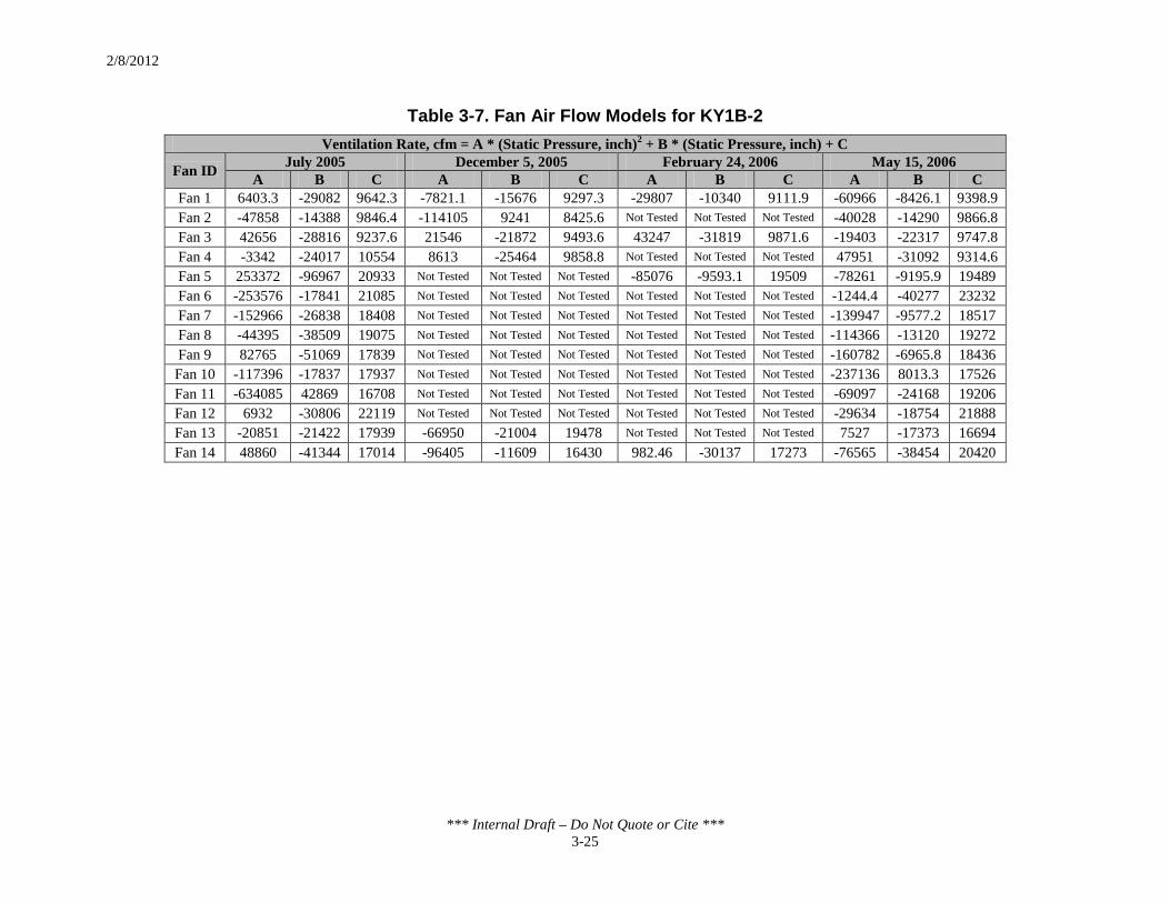
2/8/2012
*** Internal Draft – Do Not Quote or Cite *** 3-25
Table 3-7. Fan Air Flow Models for KY1B-2 Ventilation Rate, cfm = A * (Static Pressure, inch)2 + B * (Static Pressure, inch) + C
Fan ID July 2005 December 5, 2005 February 24, 2006 May 15, 2006 A B C A B C A B C A B C
Fan 1 6403.3 -29082 9642.3 -7821.1 -15676 9297.3 -29807 -10340 9111.9 -60966 -8426.1 9398.9 Fan 2 -47858 -14388 9846.4 -114105 9241 8425.6 Not Tested Not Tested Not Tested -40028 -14290 9866.8 Fan 3 42656 -28816 9237.6 21546 -21872 9493.6 43247 -31819 9871.6 -19403 -22317 9747.8 Fan 4 -3342 -24017 10554 8613 -25464 9858.8 Not Tested Not Tested Not Tested 47951 -31092 9314.6 Fan 5 253372 -96967 20933 Not Tested Not Tested Not Tested -85076 -9593.1 19509 -78261 -9195.9 19489 Fan 6 -253576 -17841 21085 Not Tested Not Tested Not Tested Not Tested Not Tested Not Tested -1244.4 -40277 23232 Fan 7 -152966 -26838 18408 Not Tested Not Tested Not Tested Not Tested Not Tested Not Tested -139947 -9577.2 18517 Fan 8 -44395 -38509 19075 Not Tested Not Tested Not Tested Not Tested Not Tested Not Tested -114366 -13120 19272 Fan 9 82765 -51069 17839 Not Tested Not Tested Not Tested Not Tested Not Tested Not Tested -160782 -6965.8 18436 Fan 10 -117396 -17837 17937 Not Tested Not Tested Not Tested Not Tested Not Tested Not Tested -237136 8013.3 17526 Fan 11 -634085 42869 16708 Not Tested Not Tested Not Tested Not Tested Not Tested Not Tested -69097 -24168 19206 Fan 12 6932 -30806 22119 Not Tested Not Tested Not Tested Not Tested Not Tested Not Tested -29634 -18754 21888 Fan 13 -20851 -21422 17939 -66950 -21004 19478 Not Tested Not Tested Not Tested 7527 -17373 16694 Fan 14 48860 -41344 17014 -96405 -11609 16430 982.46 -30137 17273 -76565 -38454 20420

2/8/2012
*** Internal Draft – Do Not Quote or Cite *** 3-26
Table 3-8. Fan Air Flow Models for KY1B-2 (continued)
Ventilation Rate, cfm = A * (Static Pressure, inch)2 + B * (Static Pressure, inch) + C
Fan ID July 18, 2006 September 28, 2006 December 11, 2006 February 8, 2007 A B C A B C A B C A B C
Fan 1 Not Tested Not Tested Not Tested Not Tested Not Tested Not Tested Not Tested Not Tested Not Tested -56437 -6311.5 9349.2 Fan 2 -145370 5525 8548.6 -5730.9 -21492 9959.2 -41252 -13429 9946.1 34189 -24934 10124 Fan 3 -46087 -11251 8220.3 Not Tested Not Tested Not Tested 2252.3 -23655 9707.6 -43170 -13533 9322.3 Fan 4 Not Tested Not Tested Not Tested -41312 -13038 8456.6 -1771 -23136 9631.9 49357 -30704 9771.2 Fan 5 Not Tested Not Tested Not Tested -18949 -24356 20541 -66110 -7306.8 19526 Not Tested Not Tested Not Tested Fan 6 90002 -63514 23180 Not Tested Not Tested Not Tested -30536 -24754 22502 Not Tested Not Tested Not Tested Fan 7 Not Tested Not Tested Not Tested Not Tested Not Tested Not Tested Not Tested Not Tested Not Tested Not Tested Not Tested Not Tested Fan 8 Not Tested Not Tested Not Tested -118262 -8942.8 17835 Not Tested Not Tested Not Tested Not Tested Not Tested Not Tested Fan 9 3095 -39533 19275 Not Tested Not Tested Not Tested Not Tested Not Tested Not Tested Not Tested Not Tested Not Tested Fan 10 Not Tested Not Tested Not Tested -210356 16026 16108 Not Tested Not Tested Not Tested Not Tested Not Tested Not Tested Fan 11 Not Tested Not Tested Not Tested -86591 -21761 19710 Not Tested Not Tested Not Tested Not Tested Not Tested Not Tested Fan 12 47400 -37407 21819 Not Tested Not Tested Not Tested Not Tested Not Tested Not Tested Not Tested Not Tested Not Tested Fan 13 -120124 -14919 19103 -89008 -18498 19600 Not Tested Not Tested Not Tested Not Tested Not Tested Not Tested Fan 14 Not Tested Not Tested Not Tested Not Tested Not Tested Not Tested -86552 -9773 15676 Not Tested Not Tested Not Tested

2/8/2012
*** Internal Draft – Do Not Quote or Cite *** 3-27
3.3.2.5 Meteorological and Confinement Data
Ambient and confinement temperature and relative humidity were measured type-T TCs and electronic relative humidity transmitters that were connected to the PC-based DAQ. In addition, portable RH/T loggers were used as back-ups. Ambient air samples were taken near the MAEMU (see Figure 3-9). Building temperature and relative humidity probes were placed adjacent to the SW1, SW3 and TE air sampling points (see Figure 3-9).
3.3.2.6 Animal Husbandry and Building Systems
The study conducted at the Kentucky sites did not track animal activity with infrared motion sensors. The only activity information regarding animal movement in and out of the house was recorded by the producer.
Farm personnel at the Kentucky sites manually recorded the daily animal inventories and mortalities and provided the data to the NAEMS site personnel. Similarly, farm personnel were to provide information regarding the operation of the lights and feeders within the monitored houses; however, this information has not yet been submitted to EPA.
3.3.2.7 Biomaterials Sampling Methods and Schedule
Biomaterial sampling for the Kentucky portion of the study was limited to litter sampling. All litter samples were processed by the Agricultural Waste Management Laboratory in the Department of Agricultural and Biosystems Engineering at Iowa State University.
Litter from the production houses was sampled after the removal of each flock and analyzed for pH, moisture content, NH3 and total Kjeldahl nitrogen. Analyzed samples, in conjunction with litter mass removed during clean-out, were used to estimate nongaseous nitrogen movement in and out of the house.
Two types of litter samples were collected: total litter and caked litter. For total litter sampling, the broiler house was divided into nonbrooding and brooding zones. Each zone was then subdivided into three sections: sidewall, waterer and feeder and central. Twenty random samples were collected from each section and pooled together to form one composite sample per section (three composite samples per zone). Figure 3-12 illustrates the zone and section for the house and an example sampling scheme to demonstrate the distribution of samples through the zones. Caked litter samples were also collected by taking shovel samples from each load of removed cake and combining them to form two 20-L samples.

2/8/2012
*** Internal Draft – Do Not Quote or Cite *** 3-28
Figure 3-12. Schematic of Litter Sampling Locations
Brooding (West) Non-brooding (East)
Sidewall area
Waterer and feeders
Central area
Waterer and feeders Sidewall area
Point Sample
N
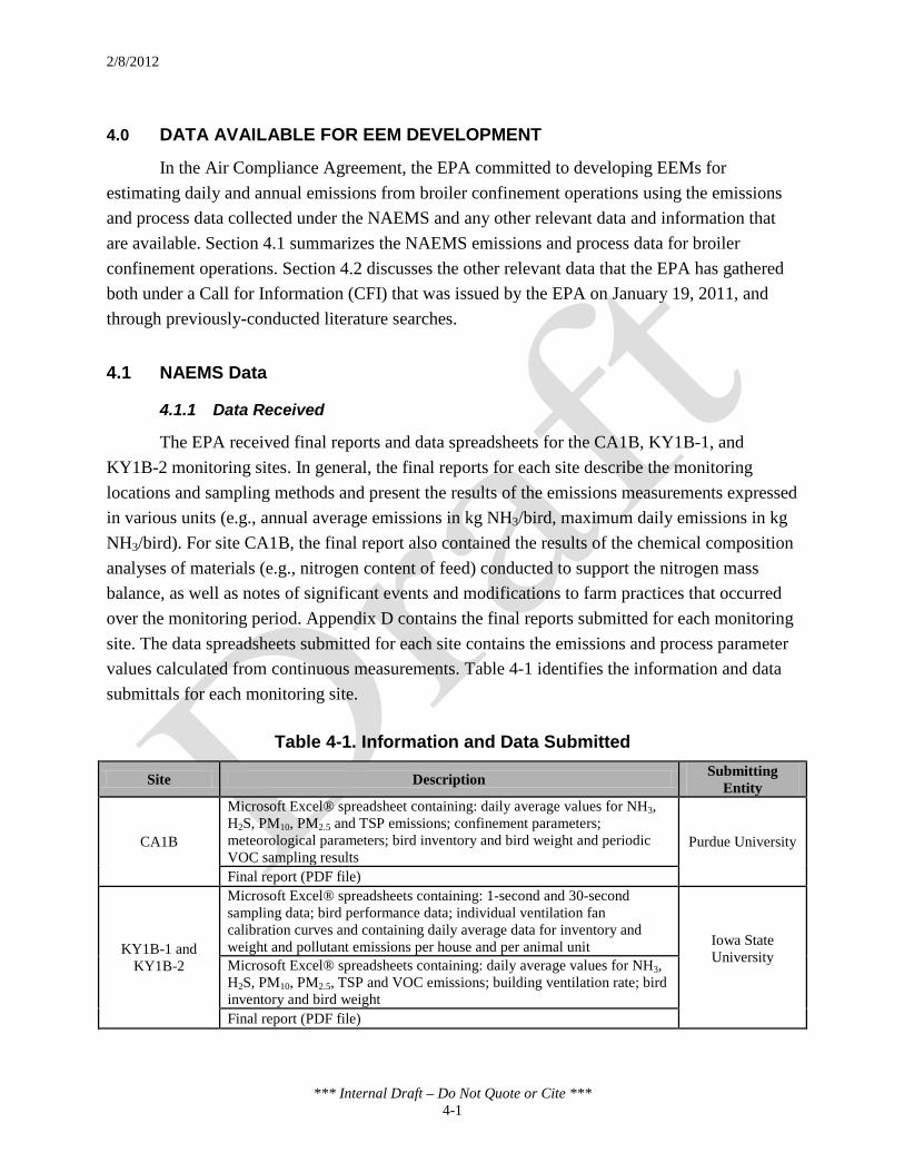
2/8/2012
*** Internal Draft – Do Not Quote or Cite *** 4-1
4.0 DATA AVAILABLE FOR EEM DEVELOPMENT
In the Air Compliance Agreement, the EPA committed to developing EEMs for estimating daily and annual emissions from broiler confinement operations using the emissions and process data collected under the NAEMS and any other relevant data and information that are available. Section 4.1 summarizes the NAEMS emissions and process data for broiler confinement operations. Section 4.2 discusses the other relevant data that the EPA has gathered both under a Call for Information (CFI) that was issued by the EPA on January 19, 2011, and through previously-conducted literature searches.
4.1 NAEMS Data
4.1.1 Data Received
The EPA received final reports and data spreadsheets for the CA1B, KY1B-1, and KY1B-2 monitoring sites. In general, the final reports for each site describe the monitoring locations and sampling methods and present the results of the emissions measurements expressed in various units (e.g., annual average emissions in kg NH3/bird, maximum daily emissions in kg NH3/bird). For site CA1B, the final report also contained the results of the chemical composition analyses of materials (e.g., nitrogen content of feed) conducted to support the nitrogen mass balance, as well as notes of significant events and modifications to farm practices that occurred over the monitoring period. Appendix D contains the final reports submitted for each monitoring site. The data spreadsheets submitted for each site contains the emissions and process parameter values calculated from continuous measurements. Table 4-1 identifies the information and data submittals for each monitoring site.
Table 4-1. Information and Data Submitted
Site Description Submitting Entity
CA1B
Microsoft Excel® spreadsheet containing: daily average values for NH3, H2S, PM10, PM2.5 and TSP emissions; confinement parameters; meteorological parameters; bird inventory and bird weight and periodic VOC sampling results
Purdue University
Final report (PDF file)
KY1B-1 and KY1B-2
Microsoft Excel® spreadsheets containing: 1-second and 30-second sampling data; bird performance data; individual ventilation fan calibration curves and containing daily average data for inventory and weight and pollutant emissions per house and per animal unit Iowa State
University Microsoft Excel® spreadsheets containing: daily average values for NH3, H2S, PM10, PM2.5, TSP and VOC emissions; building ventilation rate; bird inventory and bird weight Final report (PDF file)

2/8/2012
*** Internal Draft – Do Not Quote or Cite *** 4-2
To increase public involvement and maintain transparency throughout the EEMs development process, the EPA has made information and data relating to the NAEMS available at http://www.epa.gov/airquality/agmonitoring/. This website provides links to background information regarding the Air Compliance Agreement, the NAEMS (including information describing the monitoring sites, site-specific data files and final reports), and the CFI. Additionally, the EPA has included all information received pertaining to the NAEMS in the public docket (EPA Docket ID No. EPA-HQ-OAR-2010-0960), which is available at: http://www.regulations.gov.
Table 4-2 summarizes the emissions and process data elements that were required to be monitored by either the NAEMS Monitoring Protocol, the QAPPs, the SMPs or the SOP documents submitted to the EPA. The NAEMS Monitoring Protocol was developed in a collaborative effort by representatives from the EPA, USDA, AFO industry representatives, agricultural researchers, state and local air quality agencies and environmental organizations. The NAEMS Monitoring Protocol identified the parameters to be monitored during the study and, for some parameters, specific measurement methodologies and frequencies. For those parameters for which either or both the measurement methodology and frequency was not specified, the information was provided in the study’s QAPP (Appendix A). Table 4-2 also provides specific information regarding data availability that is based upon the EPA’s review of the final reports and data spreadsheets. During its review of the final reports and data spreadsheets, the EPA identified missing emissions and process data. Section 5 summarizes the issues and discrepancies identified by the EPA’s review.
The EPA’s review of the data spreadsheets also identified negative daily average emissions values for H2S and PM10 for certain days at site CA1B (see Section 5). After discussion with the study’s Science Advisor, it was determined the negative values were a result of instrumentation drift, and are considered to be valid values. To avoid possible complications with EEM development (e.g., the EEM predicting negative emissions), the negative values were withheld from the data sets used for EEM development. The amount of measured negative values is low (less than 1.7 percent) compared to the total number of emissions records for H2S and PM10, which indicates that the steps taken to calibrate and maintain instrumentation and to minimize the influence of other on-site sources on ambient H2S and PM10 emissions were reasonably effective. Because of their relatively small number, excluding the negative values does not compromise the EEM data sets for H2S and PM10.
The EPA’s review of the data spreadsheets also identified daily average emissions and parameter values that were exactly zero. After further review and discussion with the study’s Science Advisor, it was determined the values were valid reported values and were used for EEM development.

2/8/2012
*** Internal Draft – Do Not Quote or Cite *** 4-3
Table 4-2. NAEMS Emissions and Process Parameter Data Received Parameter Information NAEMS Data
Parameter
Required by the
NAEMS Monitoring
Protocol
Measurement Methodology
Measurement Frequency
CA1B (Houses 10 and 12) KY1B – 1 House 5 and KY1B – 2 House 3
Data Description Measurement Methodology
Measurement Frequency Data Description Measurement
Methodology Measurement
Frequency
Emissions
NH3 Yes Chemiluminescence or photoacoustic infrared
24 months with data logged
every 60 seconds
Average measured concentration values
and average calculated emission
rate values
Photoacoustic infrared
Logged every 15 & 60 seconds, for 24 months; daily averages provided
Average measured concentration
values and average calculated
emission rate values
Photoacoustic infrared
Sampled continuously at 120-second intervals
for 12 months; daily averages provided
H2S Yes Pulsed fluorescence
24 months with data logged
every 60 seconds
Average measured concentration values
and average calculated emission
rate values
Pulsed fluorescence Logged every 15 & 60
seconds, for 24 months; daily averages provided
Average calculated emission rate
values
UV Pulsed fluorescence
Sampled continuously at 120-second intervals
for 12 months; daily averages provided
TSP Yes Isokinetic multipoint gravimetric method
24 months with data logged
every 60 seconds
Average measured concentration values
and average calculated emission
rate values
TEOM for representative
exhaust locations in the house, and the
TFS FH62-C-14 Beta Monitor for inlet air
locations
Logged every 15 & 60 seconds, for six 7- to 14-day periods; Daily
average provided
Average calculated emission rate
values
TEOM, Reference Method number EQPM-1090-79
Recorded at 300-second intervals for 12 months; daily averages provided
PM10 Yes
Real-time measurements using the TEOM at
representative exhaust locations in the house
and ambient air
24 months with data logged
every 60 seconds
Average measured concentration values
and average calculated emission
rate values
TEOM for representative
exhaust locations in the house, and the
TFS FH62-C-14 Beta Monitor for inlet air
locations
Logged every 15 & 60 seconds. Daily average
provided.
Average calculated emission rate
values
TEOM, Reference Method number EQPM-1090-79
Recorded at 300-second intervals for 12 months; daily averages provided
PM2.5 Yes Gravimetrically with a
federal reference method for PM2.5
Measured at least for 1
month per site; data logged
every 60 seconds
Average measured concentration values
and average calculated emission
rate values
TEOM for representative
exhaust locations in the house, and the
TFS FH62-C-14 Beta Monitor for inlet air
locations
Logged every 15 & 60 seconds for February and July, 2008, and January and September, 2009 for 12 to 18 days each time; daily averages provided
Average calculated emission rate
values
TEOM, Reference Method number EQPM-1090-79
Recorded at 300-second intervals for 12 months; daily averages provided
CO2 Yes Photoacoustic infrared or equivalent
24 months with data logged
every 60 seconds
Data not availablea Photoacoustic infrared
Logged every 15 & 60 seconds, for 24 months;
Average calculated emission rate
values
Photoacoustic infrared
Sampled continuously at 120-second intervals
for 12 months; daily averages provided

2/8/2012
*** Internal Draft – Do Not Quote or Cite *** 4-4
Table 4-2. NAEMS Emissions and Process Parameter Data Received Parameter Information NAEMS Data
Parameter
Required by the
NAEMS Monitoring
Protocol
Measurement Methodology
Measurement Frequency
CA1B (Houses 10 and 12) KY1B – 1 House 5 and KY1B – 2 House 3
Data Description Measurement Methodology
Measurement Frequency Data Description Measurement
Methodology Measurement
Frequency
Non-methane hydrocarbons
(NMHC) emissions
(continuous)
Yes NMHC – dual channel FID analyzer (Method
25A)
24 months with data logged
every 60 seconds at one
site
Data not availablea Photoacoustic infrared
Logged every 15 & 60 seconds, for 24 months; daily averages provided
Average calculated emission rate
values
Dual-channel flame ionization detector (FID)
Daily for 12 months
VOC (Charac-terization
Study) Yes
Total nonmethane hydrocarbons (NMHC) –
Dual-channel FID analyzer (Method 25A)
VOC - concurrent gas chromatography-mass spectrometry (GC-MS) and GC/FID for TO 15
and other FID-responding compounds
Conducted on 1 day during the first month at the first site
Target VOC compounds for
subsequent continuous
monitoring and speciation
Canisters, sorbent tubes and glass
impingers used to collect VOC samples
One sampling episode using canisters, sorbent
tubes and glass impingers, and one
sampling episode using sorbent tubes
Target VOC compounds for
subsequent continuous
monitoring and speciation
EPA TO-15 EPA TP-17
Two sampling events (9 locations in each house)
VOC (grab samples) Yes
VOC – concurrent GC-MS and GC/FID for TO
15 and other FID-responding compounds.
Continuous for 24 months with
data logged every 60 seconds
Quarterly
samples using selected VOC
sampling method at all
sites
Concentration and emissions for each day that the VOC
samples were taken and the overall
averages
Canisters 24 hour canister samples taken every 3 months Data not collectedb
Confinement Parameters
Bird activity Yes Not specified Data not receivedc Passive infrared detector
Logged every 15 & 60 seconds for 24 months Data not collectedb
Manure handling Yes Not specified Not applicable (litter periodically removed
using manual methods) End of grow-out periods Not applicable (litter periodically removed using manual methods)
End of grow-out periods
Lighting Yes Not specified Data not receivedc Relays for recording on/off status
Logged every 15 & 60 seconds for 24 months Data not receivedc Not specified Not specified
Heating/cooling operation Yes Not specified Data not receivedc Relays for recording
on/off status Logged every 15 & 60 seconds for 24 months Data not collectedb
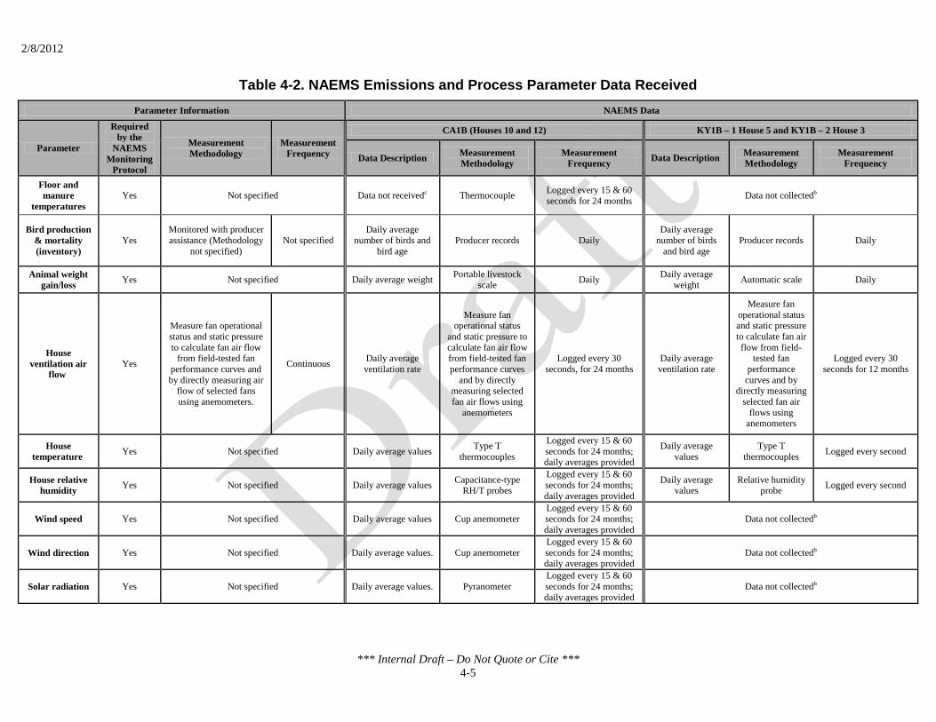
2/8/2012
*** Internal Draft – Do Not Quote or Cite *** 4-5
Table 4-2. NAEMS Emissions and Process Parameter Data Received Parameter Information NAEMS Data
Parameter
Required by the
NAEMS Monitoring
Protocol
Measurement Methodology
Measurement Frequency
CA1B (Houses 10 and 12) KY1B – 1 House 5 and KY1B – 2 House 3
Data Description Measurement Methodology
Measurement Frequency Data Description Measurement
Methodology Measurement
Frequency
Floor and manure
temperatures Yes Not specified Data not receivedc Thermocouple Logged every 15 & 60
seconds for 24 months Data not collectedb
Bird production & mortality (inventory)
Yes Monitored with producer assistance (Methodology
not specified) Not specified
Daily average number of birds and
bird age Producer records Daily
Daily average number of birds
and bird age Producer records Daily
Animal weight gain/loss Yes Not specified Daily average weight Portable livestock
scale Daily Daily average weight Automatic scale Daily
House ventilation air
flow Yes
Measure fan operational status and static pressure to calculate fan air flow
from field-tested fan performance curves and by directly measuring air
flow of selected fans using anemometers.
Continuous Daily average ventilation rate
Measure fan operational status
and static pressure to calculate fan air flow from field-tested fan performance curves
and by directly measuring selected fan air flows using
anemometers
Logged every 30 seconds, for 24 months
Daily average ventilation rate
Measure fan operational status and static pressure to calculate fan air flow from field-
tested fan performance
curves and by directly measuring
selected fan air flows using
anemometers
Logged every 30 seconds for 12 months
House temperature Yes Not specified Daily average values Type T
thermocouples
Logged every 15 & 60 seconds for 24 months; daily averages provided
Daily average values
Type T thermocouples Logged every second
House relative humidity Yes Not specified Daily average values Capacitance-type
RH/T probes
Logged every 15 & 60 seconds for 24 months; daily averages provided
Daily average values
Relative humidity probe Logged every second
Wind speed Yes Not specified Daily average values Cup anemometer Logged every 15 & 60 seconds for 24 months; daily averages provided
Data not collectedb
Wind direction Yes Not specified Daily average values. Cup anemometer Logged every 15 & 60 seconds for 24 months; daily averages provided
Data not collectedb
Solar radiation Yes Not specified Daily average values. Pyranometer Logged every 15 & 60 seconds for 24 months; daily averages provided
Data not collectedb

2/8/2012
*** Internal Draft – Do Not Quote or Cite *** 4-6
Table 4-2. NAEMS Emissions and Process Parameter Data Received Parameter Information NAEMS Data
Parameter
Required by the
NAEMS Monitoring
Protocol
Measurement Methodology
Measurement Frequency
CA1B (Houses 10 and 12) KY1B – 1 House 5 and KY1B – 2 House 3
Data Description Measurement Methodology
Measurement Frequency Data Description Measurement
Methodology Measurement
Frequency
House differential
static pressure Yes Not specified Daily average values. Pressure transducer
Logged every 15 & 60 seconds for 24 months; daily averages provide.
30-second average values
Pressure transducer Logged every second
Ambient temperature at
site Yes Not specified Daily average values
Solar radiation shielded capacitance-
type RH/T probe
Logged every 15 & 60 seconds for 24 months; daily averages provided
Daily average values
Type T thermocouples Logged every second
Ambient relative
humidity at site Yes Not specified Daily average values
Solar radiation shielded capacitance-
type RH/T probe
Logged every 15 & 60 seconds for 24 months
daily averages provided
Daily average values RH probe Logged every second
Nitrogen Mass Balance Water
consumption rate
Yes Monitored with producer assistance (methodology
not specified) Not specified Data not receivedc Automatic water
meter Not specified Daily average values Producer records Daily
Water Total Kjeldahl
Nitrogen (TKN) content
Yes Not specified Data not receivedc Micro-Kjeldahl/ titrimetric Not specified Data not collectedb
Feed consumption
rate Yes
Monitored with producer assistance (methodology
not specified) Not specified Data not receivedc Not specified Daily Data not receivedc Producer records Each flock
Feed TKN content Yes Not specified Data not receivedd Micro-Kjeldahl/
titrimetric Not specified Data not receivedc Producer records Each flock
Feed sulfur content Yes Not specified Data not collectedb Data not collectedb
Incoming bedding
addition rate No Not applicable Volume of litter (m3) Producer estimate Single value Data not receivedc Producer records Each flock
Incoming bedding TKN
content No Not applicable
Two daily average values per house
(wet weight basis, %)
Micro-Kjeldahl/ titrimetric
4 sampling events over course of study
Daily average value (“as is” and dry matter basis, %); Two values
for KY1B-1 and a single value for
KY1B-2.
Titration Taken at least once
during the study period after full litter removal

2/8/2012
*** Internal Draft – Do Not Quote or Cite *** 4-7
Table 4-2. NAEMS Emissions and Process Parameter Data Received Parameter Information NAEMS Data
Parameter
Required by the
NAEMS Monitoring
Protocol
Measurement Methodology
Measurement Frequency
CA1B (Houses 10 and 12) KY1B – 1 House 5 and KY1B – 2 House 3
Data Description Measurement Methodology
Measurement Frequency Data Description Measurement
Methodology Measurement
Frequency
pH of manure and litter (in
house) No Not applicable Data not receivedb Electrochemical pH
meter 6 events/yr
16 values taken over 8 sampling
events distributed over the grow-out
period
Electrochemical pH meter 8 events
Sulfur content of manure and litter (in house)
Yes Not specified 16 daily average values per house
(wet weight basis, %) Not specified 32 sampling events over
course of study Data not collectedb
NH3 content of manure and
litter (in house) Yes Not specified
16 daily average values per house
(wet weight basis, %) Kjeldahl/ titrimetric 6 events/yr
16 values taken over 8 sampling
events distributed over the grow-out
period
Electrochemical pH meter 8 events
Solids content of manure and
litter (in house) No Not applicable
16 daily average values per house
(wet weight basis, %) Gravimetric 6 events/yr
16 values taken over 8 sampling
events distributed over the grow-out
period
Gravimetric 8 events
TKN content of manure and
litter (decaking) Yes Not specified
8 daily average values per house
(wet weight basis, %) Kjeldahl/ titrimetric
3 events over duration of study
6 daily average values per site (“as is” and dry matter
basis, %)
Titration Samples taken after
bird removal and just prior to decaking
activities; Decaking occurred 6 times during
the study period
Solids content of manure and
litter (decaking) No Not applicable
8 daily average values per house
(wet weight basis, %) Gravimetric
6 daily average values per site (“as is” and dry matter
basis, %)
Not specified
pH of manure and litter (de-
caking) No Not applicable Data not receivedc Electrochemical pH
meter 6 daily average values per site
Electrochemical pH meter
TKN content of manure and
litter (cleanout) Yes Not specified
Four daily average values per house
(wet weight basis, %) Kjeldahl/ titrimetric
During each full cleanout (2nd or 3rd
brood); 3 events in the 1st year, 2-3 events in the
2nd year
One daily average value per site Titration
During each full litter removal (occurred once
per year)
pH of manure and litter (cleanout)
No Not applicable Data not receivedc Electrochemical pH meter
One daily average value per site
Electrochemical pH meter
Solids content of manure and
litter (cleanout) No Not applicable
Four daily average values per house
(wet weight basis, %) Gravimetric One daily average
value per site Not specified

2/8/2012
*** Internal Draft – Do Not Quote or Cite *** 4-8
Table 4-2. NAEMS Emissions and Process Parameter Data Received Parameter Information NAEMS Data
Parameter
Required by the
NAEMS Monitoring
Protocol
Measurement Methodology
Measurement Frequency
CA1B (Houses 10 and 12) KY1B – 1 House 5 and KY1B – 2 House 3
Data Description Measurement Methodology
Measurement Frequency Data Description Measurement
Methodology Measurement
Frequency
Manure removed Yes
Monitored with producer assistance (Methodology
not specified) Not Specified Average estimated
mass (metric tons)e Producer estimate Beginning and end of growth period Data not collectedb
Volume of manure
produced Yes
Monitored with producer assistance (Methodology
not specified) Not Specified Average estimated
mass (metric tons)e Producer estimate Beginning and end of growth period Data not collectedb
a Section 3.6 of the final report (p. 12) states that, due to irreconcilable interferences by water vapor and other gases, the CO2 and VOC-related gas emissions measured by the INNOVA are not available. b Data not expected. This parameter is not referenced in the QAPP or final report. c The QAPP mentions this parameter was measured; however, these data are not provided in the final report(s). d Section 4.2 of the final report (p. 23) provides the range of feed nitrogen content but does not provide the test values. Also, the report is unclear if the range is for nitrogen or TKN. e Section 3.4 of the final report (p. 11) states that on 4/15/08, the manure mass removed during a complete load-out, estimated from the square area and average mass of manure per unit area, was 88 metric tons in House 10 and 79 metric tons in House 12.
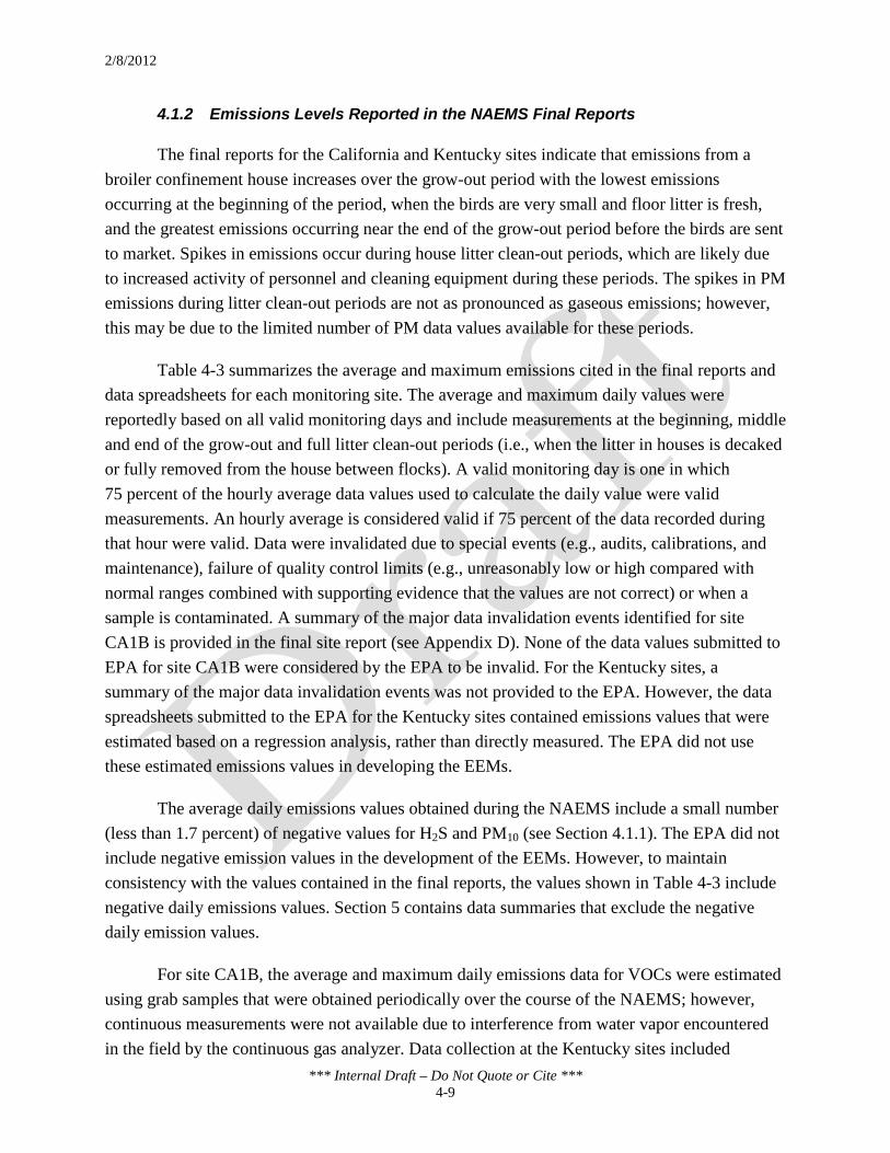
2/8/2012
*** Internal Draft – Do Not Quote or Cite *** 4-9
4.1.2 Emissions Levels Reported in the NAEMS Final Reports
The final reports for the California and Kentucky sites indicate that emissions from a broiler confinement house increases over the grow-out period with the lowest emissions occurring at the beginning of the period, when the birds are very small and floor litter is fresh, and the greatest emissions occurring near the end of the grow-out period before the birds are sent to market. Spikes in emissions occur during house litter clean-out periods, which are likely due to increased activity of personnel and cleaning equipment during these periods. The spikes in PM emissions during litter clean-out periods are not as pronounced as gaseous emissions; however, this may be due to the limited number of PM data values available for these periods.
Table 4-3 summarizes the average and maximum emissions cited in the final reports and data spreadsheets for each monitoring site. The average and maximum daily values were reportedly based on all valid monitoring days and include measurements at the beginning, middle and end of the grow-out and full litter clean-out periods (i.e., when the litter in houses is decaked or fully removed from the house between flocks). A valid monitoring day is one in which 75 percent of the hourly average data values used to calculate the daily value were valid measurements. An hourly average is considered valid if 75 percent of the data recorded during that hour were valid. Data were invalidated due to special events (e.g., audits, calibrations, and maintenance), failure of quality control limits (e.g., unreasonably low or high compared with normal ranges combined with supporting evidence that the values are not correct) or when a sample is contaminated. A summary of the major data invalidation events identified for site CA1B is provided in the final site report (see Appendix D). None of the data values submitted to EPA for site CA1B were considered by the EPA to be invalid. For the Kentucky sites, a summary of the major data invalidation events was not provided to the EPA. However, the data spreadsheets submitted to the EPA for the Kentucky sites contained emissions values that were estimated based on a regression analysis, rather than directly measured. The EPA did not use these estimated emissions values in developing the EEMs.
The average daily emissions values obtained during the NAEMS include a small number (less than 1.7 percent) of negative values for H2S and PM10 (see Section 4.1.1). The EPA did not include negative emission values in the development of the EEMs. However, to maintain consistency with the values contained in the final reports, the values shown in Table 4-3 include negative daily emissions values. Section 5 contains data summaries that exclude the negative daily emission values.
For site CA1B, the average and maximum daily emissions data for VOCs were estimated using grab samples that were obtained periodically over the course of the NAEMS; however, continuous measurements were not available due to interference from water vapor encountered in the field by the continuous gas analyzer. Data collection at the Kentucky sites included
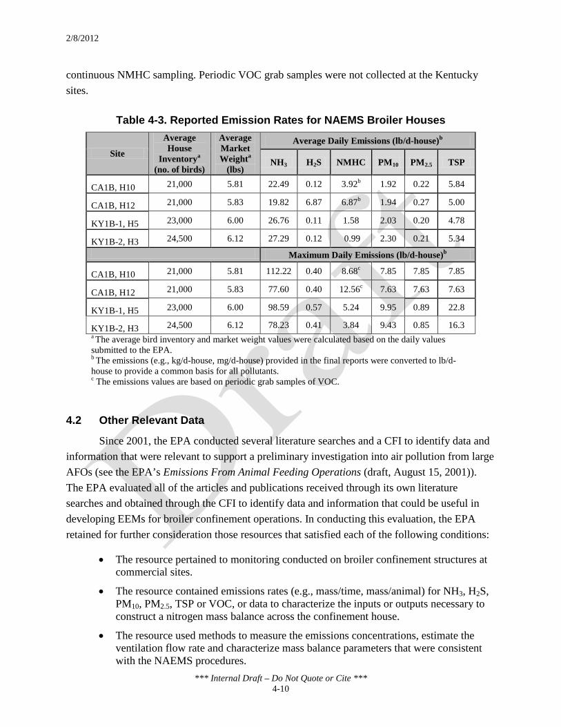
2/8/2012
*** Internal Draft – Do Not Quote or Cite *** 4-10
continuous NMHC sampling. Periodic VOC grab samples were not collected at the Kentucky sites.
Table 4-3. Reported Emission Rates for NAEMS Broiler Houses
Site
Average House
Inventorya (no. of birds)
Average Market Weighta
(lbs)
Average Daily Emissions (lb/d-house)b
NH3 H2S NMHC PM10 PM2.5 TSP
CA1B, H10 21,000 5.81 22.49 0.12 3.92b 1.92 0.22 5.84
CA1B, H12 21,000 5.83 19.82 6.87 6.87b 1.94 0.27 5.00
KY1B-1, H5 23,000 6.00 26.76 0.11 1.58 2.03 0.20 4.78
KY1B-2, H3 24,500 6.12 27.29 0.12 0.99 2.30 0.21 5.34 Maximum Daily Emissions (lb/d-house)b
CA1B, H10 21,000 5.81 112.22 0.40 8.68c 7.85 7.85 7.85
CA1B, H12 21,000 5.83 77.60 0.40 12.56c 7.63 7.63 7.63
KY1B-1, H5 23,000 6.00 98.59 0.57 5.24 9.95 0.89 22.8
KY1B-2, H3 24,500 6.12 78.23 0.41 3.84 9.43 0.85 16.3 a The average bird inventory and market weight values were calculated based on the daily values submitted to the EPA. b The emissions (e.g., kg/d-house, mg/d-house) provided in the final reports were converted to lb/d-house to provide a common basis for all pollutants. c The emissions values are based on periodic grab samples of VOC.
4.2 Other Relevant Data
Since 2001, the EPA conducted several literature searches and a CFI to identify data and information that were relevant to support a preliminary investigation into air pollution from large AFOs (see the EPA’s Emissions From Animal Feeding Operations (draft, August 15, 2001)). The EPA evaluated all of the articles and publications received through its own literature searches and obtained through the CFI to identify data and information that could be useful in developing EEMs for broiler confinement operations. In conducting this evaluation, the EPA retained for further consideration those resources that satisfied each of the following conditions:
• The resource pertained to monitoring conducted on broiler confinement structures at commercial sites.
• The resource contained emissions rates (e.g., mass/time, mass/animal) for NH3, H2S, PM10, PM2.5, TSP or VOC, or data to characterize the inputs or outputs necessary to construct a nitrogen mass balance across the confinement house.
• The resource used methods to measure the emissions concentrations, estimate the ventilation flow rate and characterize mass balance parameters that were consistent with the NAEMS procedures.

2/8/2012
*** Internal Draft – Do Not Quote or Cite *** 4-11
The EPA excluded data that were related to litter storage piles and land application sites because the Air Compliance Agreement does not cover these processes.
The EPA then evaluated the resources that satisfied the EPA’s initial review to determine if the data were appropriate for consideration in either developing the EEMs or assessing the predictive accuracy of the EEMs. Section 4.2.1 summarizes the EPA’s CFI and the review of the resources obtained. Section 4.2.2 summarizes the EPA’s review of the resources obtained by previous EPA literature searches.
4.2.1 CFI
The EPA issued a CFI on January 19, 2011, seeking peer-reviewed, quality-assured emissions and process data relevant to developing EEMs for animal feeding operations. The CFI was designed to help ensure that the EPA would obtain the broadest range of scientific data available. All data and information received by the EPA is contained in the public docket for the Air Compliance Agreement (EPA Docket ID No. EPA-HQ-OAR-2010-0960) and is available online at http://www.regulations.gov.
In the CFI, the EPA requested emissions and process data for AFOs in the broiler, swine, egg-layer, dairy, beef and turkey industries. Although the EPA is interested in all air pollutants emitted from animal confinement, litter storage and treatment and litter land applications sites associated with AFOs, the CFI specifically requested emissions data and related process information for NH3, H2S, PM10, PM2.5, TSP and VOC.
To ensure compatibility with the NAEMS data, the CFI requested that, to the extent possible, the emissions and related process data provided to the EPA be accompanied by documentation that addresses the following parameters:
General information:
• Description of AFO process measured (e.g., animal confinement structure).
• Location of AFO process measured (e.g., physical address, latitude/longitude coordinates of facility).
• Beginning and ending dates of the monitoring period.
Monitoring data:
• Plan for quality assurance and quality control procedures.
• Site-specific monitoring plan.
• Test methods, instrumentation and SOPs used to collect emissions and process data measurements.

2/8/2012
*** Internal Draft – Do Not Quote or Cite *** 4-12
• Results of audits conducted on instruments and procedures.
• Field notes and associated documentation collected during the study.
• Emissions data (unanalyzed or analyzed) and associated process data.
• Meteorological data, including average ambient temperature, relative humidity, pressure, wind speed, wind direction and insolation (solar radiation) for each day that the study was conducted.
• Production data (e.g., number of eggs produced per day or quantity of milk produced per day or number of chickens or swine produced).
• Calculations and assumptions used to convert concentration data (e.g., ppmv) into mass emissions (e.g., lb/hr).
Animal confinement structures:
• Dimensions of structures monitored.
• Designed and permitted animal capacity.
• Type, age, number and weight of animals contained in the confinement structure over the duration of the monitoring period.
• Manure management system (e.g., pull-plug pit, scrape).
• Manure removal activities over the duration of the monitoring period.
• Ventilation method (i.e., natural or mechanical).
• Calculations and assumptions used to estimate the ventilation rate of the monitored confinement structure.
• Calibration procedures for instruments (e.g., flow meters, fan relays) used to collect data for calculating ventilation rate of the monitored confinement structure.
• Nitrogen content of process inputs and outputs (e.g., feed, water, bedding, eggs, milk).
• Nitrogen content of manure excreted.
• Description of any control device or work practice used in the monitored structure to reduce emissions.
Manure storage and treatment processes:
• Type, age, number, and weight of animals contributing manure to the storage and treatment process over the monitoring period.
• Dimensions of storage/treatment unit monitored (e.g., storage pile, tank, lagoon).
• Depth of settled solids in storage/treatment unit.
• Temperature, pH and reduction/oxidation potential of manure contained in the storage/treatment unit.

2/8/2012
*** Internal Draft – Do Not Quote or Cite *** 4-13
• Moisture, total solids, volatile solids, total Kjeldahl nitrogen and ammoniacal nitrogen content and pH of manure entering storage and treatment process over the monitoring period.
Manure land application sites:
• Type, age, number, and weight of animals contributing manure to the land application site.
• Method used to apply manure (e.g., direct injection, broadcast spreading and frequency of application).
• Area (e.g., acres, square feet) used for manure application over the monitoring period.
• Quantity and moisture content of manure applied.
Table 4-4 lists the articles and publications received by the EPA in response to the CFI that pertained to broiler operations and their possible application for the NAEMS. As shown in the table, most of the articles and publications submitted to the EPA did not contain emissions or process data that met the EPA’s initial review criteria (e.g., the measurement methods differed from the NAEMS methods). However, a few resources contained material composition data that could be used to supplement the nitrogen mass balance data collected by the NAEMS.

2/8/2012
*** Internal Draft – Do Not Quote or Cite *** 4-14
Table 4-4. Review of Broiler Articles Received in Response to EPA’s CFI Year Title - Author(s) Brief Description Relevant Data Methodology Possible Application for NAEMS
2000
Atmospheric Transport and Wet Deposition of
Ammonium in North Carolina - Walker, Aneja,
Dickey
This study analyzes transport and deposition of ammonium (NH4
+) by precipitation using regression analysis.
None Not applicable
None. Wet deposition is typically conducted by collecting water and
analyzing anions. Consequently, this article is not applicable to NAEMS.
2001
Ammonia Emissions from Animal Feeding Operations - Arogo, Westerman, Heber,
Robarge, Classen
This article provides a compilation of several studies.
Range of poultry confinement emissions factors: 0.5 – 10 g NH3-
N/hr-animal unit (AU)
Composite poultry emissions factors: 0.18 – 0.24 kg NH3-N/yr-
animal
Not applicable
None. The article presents ranges of NH3 emissions factors for livestock operations but the resource does not
identify the specific types of poultry or process to which the emissions factors
apply.
2002
Ammonia Losses, Evaluations, and Solutions for Poultry Systems - Gates,
Xin, Wheeler
This study describes an ongoing, multistate effort toward
collecting data on emissions rates or emissions factors from
selected U.S. poultry houses and the efficacy of certain
management practices on emissions rates.
Confinement NH3 concentrations (ppmv)
Electrochemical sensors (unspecified vendor and model
no.)
None. Although the electrochemical sensor was compared to EPA
chemiluminescence reference method with good results, the preliminary data
presented in this paper are not useful for developing a emission estimating methodology. Additionally, the
methodology for deploying the FANS unit to estimate total building air flow
was not specified. Ventilation flow rate
Relationship between carbon dioxide (CO2) production and
metabolic rate of the birds, and FANS unit

2/8/2012
*** Internal Draft – Do Not Quote or Cite *** 4-15
Table 4-4. Review of Broiler Articles Received in Response to EPA’s CFI Year Title - Author(s) Brief Description Relevant Data Methodology Possible Application for NAEMS
2002
Emission Factors for Broiler Production Operations: A
Stochastic Modeling Approach - Lacey, Redwine,
Parnell
This article describes development of linear
regressions for NH3 and PM10 from measurement data collected
at a commercial-scale broiler houses at a farm in Texas. The article also compares emissions
factors developed using the regression equations to other published emissions factors.
PM Emissions Factors (mg/hr-500 kg live weight):
Inhalable PM – 5,000; 8,500;
6,218; 4,984; 1,856; and 2,805
Respirable PM – 600, 850, 706, 725, 245, and 394
TSP – 2,214
PM10 – 131.5
NH3 Emissions Factors:
7.4, 8.5, 8.3, 4.2, 2.2, 7.5, 1.9, 6.2, and 8.2 g/hr-500 kg live weight
19.8, 11.2, 8.9, 18.5, and 16.8
mg/hr-bird
0.179, 0.19, 0.2, and 0.02 kg/bird
Confinement NH3 concentrations: electrochemical
sensors (Drager Chip Measurement System)
TSP: Hi-vol sampler
PM10: Beckman Coulter
Multisizer
Building flow rate: vane anemometers on fans, scaled-up
to whole-house flow rate
None. The NH3 concentrations were taken at a single location (center of
house, 1 meter above the litter surface) rather than at the house exhaust
locations. Also, the Coulter particle sizing methodology is not consistent with the federal reference method for
measuring PM10 emissions.
2002
The Scientific Basis for Estimating Emissions from
Animal Feeding Operations - Hagenstein, Flocchini
This interim report from the National Academy of Science provides findings regarding
identification of the scientific criteria needed to ensure that
estimates of air emission rates are accurate, the basis for these
criteria in the scientific literature, and the associated
uncertainties.
None Not applicable
None. The report cites studies that developed emissions factors; however, the report does not contain empirical data that could be used to supplement
the NAEMS data.

2/8/2012
*** Internal Draft – Do Not Quote or Cite *** 4-16
Table 4-4. Review of Broiler Articles Received in Response to EPA’s CFI Year Title - Author(s) Brief Description Relevant Data Methodology Possible Application for NAEMS
2003
Particulate Matter and Ammonia Emission Factors
for Tunnel-Ventilated Broiler Production Houses in the
Southern U.S. - Lacey, Redwine, Parnell
This commercial-scale study measured NH3 and PM10
emission from four tunnel–ventilated broiler production
facilities in central TX. The data were used to develop linear
regression equations.
Confinement NH3 concentrations Electrochemical sensors (Drager Chip Measurement System)
None. Particulate counting by Coulter technique is not equivalent to NAEMS aerodynamic particulate sampling. EPA could not evaluate the comparability of NH3 measurements because the Drager
apparatus used for the study was not specified. Additionally, the daily
emissions and flow rate estimates were not explicitly quantified and several of the houses that participated in the study used litter amendments to suppress NH3
emissions.
Confinement PM10 concentrations Hi-Vol TSP sampler and Beckman Coulter Multisizer
Ventilation flow rate Vane anemometers and FANS unit
2003
Progress Towards the Development of an
Integrated Management System for Broiler Chicken Production - Frost, Parsons, Stacey, Robertson, Welch,
Filmer, Fothergill
The article presents previous research conducted to develop a prototype closed-loop, model-based, real time, system for the
integrated control of broiler growth and pollutant emissions.
Confinement NH3 concentrations
Ammonia concentration in the air was measured by converting the ammonia into nitric oxide
which was fed to a chemiluminescence nitrogen
oxides analyzer.
None. Animal feed was altered in this study when measurements were taken. Because the NAEMS was designed to
focus on baseline or uncontrolled emissions, this study is not relevant for
EEM development.
2004
A Comparison of Ammonia Emission Rates from an
Agricultural Area Source Using Dispersion Modeling: Gaussian Versus Backward-
Lagrangian Stochastic - Price, Lacey, Shaw, Cole, Todd, Capareda, Parnell
This research-scale study compared the emissions rates generated using the Industrial Source Complex (Guassian)
model and the WindTrax (backward Lagrangian
Stochastic)
None Not applicable None. The article does not contain
emissions or process data that could be used to supplement the NAEMS data.
2004 Ammonia Emissions from
Animal Housing Facilities - Gay
This article provides background information regarding NH3
emissions from animal confinement facilities.
NH3 Emissions Factors (g/bird-d): 0.043 (new bedding) 0.61 (reused litter)
NH3 Emissions Factors (g/bird):
0 – 336 (U.S.) 78 – 174 (European)
Not applicable
None. This article summarizes recent research findings regarding
quantification of ammonia emissions from animal confinement in general.
However, there is not sufficient information on the duration of the
studies and/or the specific measurement technologies used to determine how
comparable the results are to the NAEMS data.

2/8/2012
*** Internal Draft – Do Not Quote or Cite *** 4-17
Table 4-4. Review of Broiler Articles Received in Response to EPA’s CFI Year Title - Author(s) Brief Description Relevant Data Methodology Possible Application for NAEMS
2005
CARB Memo: Poultry Emissions VOC Sampling
and Analysis Audit - Goodenow
This memorandum documents an audit of the independent contractor and laboratory
responsible for the collection and analysis of VOC emissions samples from a poultry house in
Livingston, California.
None Not applicable None. The audit does not contain emissions or process data.
2005
Final Report: Quantification of Gaseous Emissions from
California Broiler Production Houses -
Summers, Mattos, Gaffney, FitzGibbon, Duke, Marnatti,
Kim, Stabelfeld, Clutter, Ernst, Humbert
This commercial-scale study measured NH3 and organic compound emissions from a
fabricated duct at tunnel-ventilated broiler house in
California.
Confinement NH3 concentrations (ppmv)
BAAQMD Method ST-1B (impinger train w/0.1 N HCl)
While this study does not use measurement methods that are identical to the NAEMS, the data is still relevant
and may be useful in assessing the EEMs after they have been developed.
Confinement total hydrocarbon (THC) concentrations as propane EPA Method 25A
Stack flow rate (dscfm) CARB Methods 2 and 4
C1, C2 and C4 hydrocarbon concentrations
EPA Method 18 (Tedlar bag samples w/GC FID)
The speciated VOC data may be used to supplement the periodic VOC
measurements taken under the NAEMS. Speciated organic compound
concentrations (ppbv) EPA Method TO-15 (Summa
canisters w/GCMS)
2005
Nitrogen Emissions from Broilers Measured by Mass
Balance Over Eighteen Consecutive Flocks - Coufal,
Chavez, Niemeyer, Carey
This large research-scale evaluated a nitrogen mass balance and partitioning in
broiler houses.
Total nitrogen content of birds, feed and litter
Combustion method using LECO FP-428 Nitrogen
Determinator
The nitrogen content data may be used to supplement NAEMS mass balance
data.
2006
Dietary Modifications to Reduce Air Emissions from Broiler Chickens - Powers, Zamzow, Angel, Applegate
This research-scale study investigated the effects of
changes to diet on NH3 emissions.
Ammonia emissions (mg/kg-day) TEI Model 17C ammonia/NOx chemiluminescence analyzer
Results from the control group in this study may be useful in assessing the
EEMs after they have been developed.
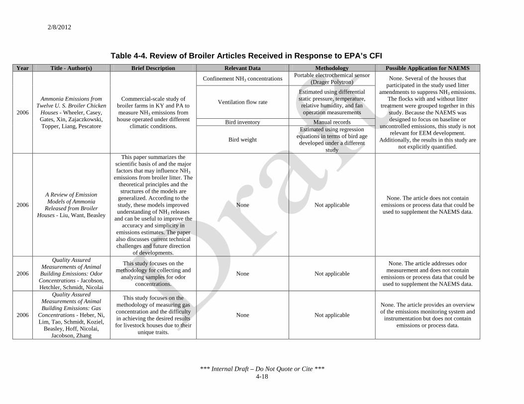
2/8/2012
*** Internal Draft – Do Not Quote or Cite *** 4-18
Table 4-4. Review of Broiler Articles Received in Response to EPA’s CFI Year Title - Author(s) Brief Description Relevant Data Methodology Possible Application for NAEMS
2006
Ammonia Emissions from Twelve U. S. Broiler Chicken
Houses - Wheeler, Casey, Gates, Xin, Zajaczkowski, Topper, Liang, Pescatore
Commercial-scale study of broiler farms in KY and PA to measure NH3 emissions from
house operated under different climatic conditions.
Confinement NH3 concentrations Portable electrochemical sensor (Drager Polytron) None. Several of the houses that
participated in the study used litter amendments to suppress NH3 emissions.
The flocks with and without litter treatment were grouped together in this
study. Because the NAEMS was designed to focus on baseline or
uncontrolled emissions, this study is not relevant for EEM development.
Additionally, the results in this study are not explicitly quantified.
Ventilation flow rate
Estimated using differential static pressure, temperature, relative humidity, and fan operation measurements
Bird inventory Manual records
Bird weight
Estimated using regression equations in terms of bird age developed under a different
study
2006
A Review of Emission Models of Ammonia
Released from Broiler Houses - Liu, Want, Beasley
This paper summarizes the scientific basis of and the major factors that may influence NH3
emissions from broiler litter. The theoretical principles and the structures of the models are
generalized. According to the study, these models improved understanding of NH3 releases
and can be useful to improve the accuracy and simplicity in
emissions estimates. The paper also discusses current technical challenges and future direction
of developments.
None Not applicable None. The article does not contain
emissions or process data that could be used to supplement the NAEMS data.
2006
Quality Assured Measurements of Animal Building Emissions: Odor Concentrations - Jacobson, Hetchler, Schmidt, Nicolai
This study focuses on the methodology for collecting and
analyzing samples for odor concentrations.
None Not applicable
None. The article addresses odor measurement and does not contain
emissions or process data that could be used to supplement the NAEMS data.
2006
Quality Assured Measurements of Animal Building Emissions: Gas
Concentrations - Heber, Ni, Lim, Tao, Schmidt, Koziel,
Beasley, Hoff, Nicolai, Jacobson, Zhang
This study focuses on the methodology of measuring gas concentration and the difficulty in achieving the desired results for livestock houses due to their
unique traits.
None Not applicable
None. The article provides an overview of the emissions monitoring system and
instrumentation but does not contain emissions or process data.

2/8/2012
*** Internal Draft – Do Not Quote or Cite *** 4-19
Table 4-4. Review of Broiler Articles Received in Response to EPA’s CFI Year Title - Author(s) Brief Description Relevant Data Methodology Possible Application for NAEMS
2007
Determination of Ammonia Emission Rates From a
Tunnel Ventilated Chicken House Using Passive
Samplers and a Gaussian Dispersion Model - Siefert,
Scudlark
This study provided NH3 emissions data from tunnel-
ventilated houses.
Mean EF = 0.13 g NH3–N/bird-day
Range of EFs = 0.0053 g NH3–N /s to 0.037 NH3–N g/s
Emissions of NH3 were back-calculated from concentration measurements made using a
sampling array (Ogawa passive samplers) positioned downwind of broiler house and Gaussian
plume model.
None. The use of different sampling methods (passive vs. active) and
modeling limit the applicability of the study for direct comparison or use in the
NAEMS.
2007
Effect of Moisture Content on Ammonia Emissions from Broiler Litter: A Laboratory Study - Liu, Wang, Beasley, Oviedo, Munilla, Baughman,
Williams
The research study evaluated the effect of moisture content on
NH3 emissions from litter samples using dynamic flow-
through chambers.
None
Ammonia emissions from litter samples of varying moisture
content placed in dynamic flow-through chambers were
measured simultaneously using a chemiluminescence analyzer and a boric acid scrubber combined with gas chromatography of the
scrubber solution.
None. Because this study used flux chambers to measure ammonia
emissions, this study is not relevant for EEM development.
2007
Modeling Atmospheric Transport and Fate of
Ammonia in North Carolina—Part I: Evaluation
of Meteorological and Chemical Predictions - Wu,
Krishnan, Zhang, Aneja
This study discusses the application of EPA’s
Community Multiscale Air Quality (CMAQ) modeling
system to study the deposition and fate of NH3 emissions from
activities. Part I of the study describes the model
configurations, evaluation protocols, databases and the operational evaluation for
meteorological and chemical predictions.
None Not applicable None. The article does not contain
emissions or process data that could be used to supplement the NAEMS data.
2007
Modeling Atmospheric Transport and Fate of
Ammonia in North Carolina—Part II: Effect of Ammonia Emissions on Fine
Particulate Matter Formation - Wu, Hu, Zhang,
Aneja
This study discusses the application of EPA’s CMAQ model to study the deposition
and fate of NH3 emissions from agricultural activities. Part II of
the study describes the sensitivity simulations applied to
various emission scenarios.
None Not applicable None. The article does not contain
emissions or process data that could be used to supplement the NAEMS data.

2/8/2012
*** Internal Draft – Do Not Quote or Cite *** 4-20
Table 4-4. Review of Broiler Articles Received in Response to EPA’s CFI Year Title - Author(s) Brief Description Relevant Data Methodology Possible Application for NAEMS
2008
Ammonia Assessment from Agriculture: U.S. Status and
Needs - Aneja, Blunden, James, Schlesinger,
Knighton, Gilliam, Jennings, Niyogi, Cole
This article summarizes recent research on agricultural air quality and describes best management practices for reducing NH3 emissions.
None Not applicable None. The article does not contain
emissions or process data that could be used to supplement the NAEMS data.
2008
Auditing and Assessing Air Quality in Concentrated
Feeding Operations - Cole, Todd, Auvermann, Parker
This paper discusses AFO emissions and the current air
quality regulations and techniques for measuring and
quantifying emissions.
None Not applicable None. The article does not contain
emissions or process data that could be used to supplement the NAEMS data.
2008 Commentary: Farming
Pollution - Aneja, Schlesinger, Erisman
This article provides commentary on the U.S. efforts
to regulate farms. It provides general information related to agricultural emissions and the
state of knowledge of processes and a comparison to of U.S.
regulations to European regulations.
None Not applicable. None. The article does not contain
emissions or process data that could be used to supplement the NAEMS data.
2008
Comparison of Ammonia Emission Rates from Three Types of Broiler Litters -
Atapattu, Senaratna, Belpagodagamage
This research-scale study compared the emissions of NH3
from three kinds of broiler bedding: refused tea, sawdust
and paddy husk.
Confinement NH3 emissions
NH3 emissions volatilized from litter samples in conical flasks
were trapped in 100 mL of 0.32 N H3SO4 solutions. The trap was
titrated with 0.1 N HCl to determine the NH3 emissions.
None. The NH3 concentrations were taken from litter samples analyzed under laboratory conditions. Additionally, data are not available to determine how the
concentration measurements made using the titration method compare to the
measurements made using the NAEMS methodology (i.e., chemiluminescence
analyzer).
2008
Instrumentation for Evaluating Differences in
Ammonia Volatilization from Broiler Litter and Cake -
Miles, Owens, Moore, Rowe
The research-scale study evaluated a chamber acid trap
(CAT) technique for measuring NH3 losses from broiler litter
samples.
None
Ammonia concentrations from litter samples contained in 1-liter containers were measured using
boric acid traps followed by titration with hydrochloric acid.
None. This study specifically looked at emissions from litter samples. Emissions
from litter samples are not directly comparable to emissions from broiler
houses. Additionally, no data was provided to relate the litter samples to a
specific bird inventory.

2/8/2012
*** Internal Draft – Do Not Quote or Cite *** 4-21
Table 4-4. Review of Broiler Articles Received in Response to EPA’s CFI Year Title - Author(s) Brief Description Relevant Data Methodology Possible Application for NAEMS
2008 Modeling Ammonia
Emissions from Broiler Litter at Laboratory Scale - Zifei
Laboratory-scale study to develop an NH3 emissions model using broiler litter samples. Emissions were
measured using a wind tunnel and a flux chamber.
Confinement NH3 concentrations Chemiluminescence gas analyzer
The nitrogen and moisture content and pH of litter may be used to supplement the mass balance data collected under
the NAEMS. Regarding the NH3 concentrations, although the
measurements were made using a chemiluminescence gas analyzer (which
is consistent with the NAEMS), the measurements were taken from litter
samples placed in laboratory flux chambers and a wind tunnel. Also, data
were not provided to relate the NH3 emission to the size of the litter sample
or bird inventory.
Total ammoniacal nitrogen content of broiler litter (manure and wood
shavings) Extraction with 1.25 N K2SO4
Total N and total C content of broiler litter (manure and wood
shavings)
Thermal conductivity detection (Leco C/N 2000 analyzer)
TKN content of broiler litter (manure and wood shavings)
Catalytic digestion (using K2SO4, CuSO4, H2O and
pumice) w/H2SO4 Moisture content of broiler litter
(manure and wood shavings) Gravimetric (before and after
drying) pH of broiler litter (manure and
wood shavings) Not specified
2008
Winter Broiler Litter Gases and Nitrogen Compounds:
Temporal and Spatial Trends - Miles, Rowe, Owens
Commercial-scale study of two broiler houses in Mississippi.
Data specifically relate to spatial/temporal variation in gases emitted from litter at
different locations.
NH3, N2O and CO flux emission rates
Flux chamber w/photoacoustic multigas analyzer (Innova 1312)
None. Because this study used flux chambers to measure emissions, this
study is not relevant for EEM development.
Total NH4, NO3 and TKN content of litter
NH4 and NO3: water extraction (QuikChem 8000)
TKN: block digestion and distillation/titration (2300
Kjeltec Analyzer)
The nitrogen content data may be used to supplement NAEMS mass balance
data.
2009 Ammonia Emissions and
Animal Agriculture - Gay, Knowlton
This article provides general information regarding AFO emissions and the effects of
farming on pollution.
None Not applicable None. The article does not contain
emissions or process data that could be used to supplement the NAEMS data.
2009
Does Animal Feeding Operation Pollution Hurt Public Health? A National
Longitudinal Study of Health Externalities Identified By
Geographic Shifts In Livestock Production -
Sneeringer
This article discusses an epidemiological study that assessed the relationship
between livestock farming and infant mortality.
None Not applicable None. The article does not contain
emissions or process data that could be used to supplement the NAEMS data.

2/8/2012
*** Internal Draft – Do Not Quote or Cite *** 4-22
Table 4-4. Review of Broiler Articles Received in Response to EPA’s CFI Year Title - Author(s) Brief Description Relevant Data Methodology Possible Application for NAEMS
2009
Effects of Agriculture upon the Air Quality and Climate:
Research, Policy, and Regulations - Aneja, Schlesinger, Erisman
This article describes the state of the science and how research can
be improved. None Not applicable
None. The article does not contain emissions or process data that could be used to supplement the NAEMS data.
2009
Efficacy of Urease Inhibitor to Reduce Ammonia
Emission from Poultry Houses - Singh, Casey, King,
Pescatore, Gates, Ford
The study addresses the use of urease inhibitors to reduce NH3
emissions from broiler litter. None
Flux chambers and a photoacoustic infrared gas
analyzer.
None. The litter samples used in the study were subjected to amendments that suppressed NH3 emissions. Also,
because this study used flux chambers to measure emissions, this study is not
relevant for EEM development.
2010
Ammonia Emission Factors from Broiler Litter In
Houses, in Storage, and After Land Application - Moore, Miles, Burns, Pote, Berg,
Choi
Commercial-scale study to measure NH3 emissions from four confinement houses for 1 year and to construct a N mass
across the houses.
Confinement NH3 concentrations Electrochemical sensors (Drager Polytron) These data may be used to supplement
the NAEMS data. Building ventilation rates Anemometers (R.M. Young) located at fan outlets
Bird inventory, final average weight (kg), Final total house bird
weight (kg)
Counts of initial chick placement and birds caught for market
(methods used to determine bird weight not specified).
These data may be used to supplement the NAEMS data.
Nitrogen content of birds, feed, bedding and litter
Feed and litter: total N analysis (method not specified); KCl-
extractable NH4 (Moore et al., 1995)
Bedding: Elementar Variomax N analyzer (combustion w/thermal
conductivity) Birds: Elementar N analyzer
These data may be used to supplement the NAEMS N mass balance data.
NH3, N2O, CH4 and CO flux measurements from litter on floor
Flux chamber and photoacoustic multigas analyzer (Innova 1412)
None. Because this study used flux chambers to measure emissions, this
study is not relevant for EEM development.
NH3, N2O, CH4 and CO flux measurements from litter storage
piles
Flux chamber and photoacoustic multigas analyzer (Innova 1412)
None. The EPA is not assessing emissions from broiler litter storage
piles at this time.
NH3, N2O, CH4 and CO flux measurements from land
application site
Lab-scale wind tunnels, phosphoric acid traps and wire
anemometers
None. The EPA is not assessing emissions from broiler litter land
application sites at this time.

2/8/2012
*** Internal Draft – Do Not Quote or Cite *** 4-23
Table 4-4. Review of Broiler Articles Received in Response to EPA’s CFI Year Title - Author(s) Brief Description Relevant Data Methodology Possible Application for NAEMS
2010
Effect of Atmospheric Ammonia on Growth
Performance and Immunological Response of Broiler Chickens - Wang, Meng, Guo, Wang, Wang,
Yao, Shan
Experimental study to assess the effects of NH3 concentrations on growth and immune response of
broilers.
None Not applicable None. The study subjected birds to
varying levels of NH3 concentrations provided in a controlled environment.
2011
Comparing Ammonia Emissions from Poultry
Barns Using Two Techniques - Flesch, Harper, Wilson
This commercial-scale study compared the NAEMS NH3 emissions rates for CA1B to emissions determined using
backward Lagrangian Stochastics (bLS)
None Not applicable
None. The bLS emissions estimates were determined based on upwind and
downwind NH3 concentrations and inverse dispersion modeling rather than
direct measurement of confinement concentrations and ventilation flow rate.
2011
Spatial Contrasts of Seasonal and Intraflock Broiler Litter Trace Gas Emissions, Physical and
Chemical Properties - Miles, Brooks, Sistani
Commercial-scale study of two broiler houses in Mississippi.
Data showed the litter chemical/physical properties,
and flux values were specific to the litter surface and not
necessarily to the broiler house as a whole.
NH3, N2O and CO litter flux emission rates
Flux chamber w/photoacoustic multigas analyzer (Innova 1312)
None. Because this study used flux chambers to measure emissions, this
study is not relevant for EEM development.
Litter total N, NH4 and total carbon content Max CN analyzer (Elementar)
The litter composition data could be used to supplement the NAEMS N mass
balance data.

2/8/2012
*** Internal Draft – Do Not Quote or Cite *** 4-24
4.2.2 Previous Literature Searches
Beginning in 2001, the EPA conducted several literature searches using the Agricultural Online Access (AGRICOLA) bibliographic database to identify data and information that were relevant to support a preliminary investigation into air pollution from large AFOs (see the EPA’s Emissions From Animal Feeding Operations (draft, August 15, 2001)). The EPA also conducted literature searches to support development of the EPA’s National Emissions Inventory (NEI) for NH3 emissions from animal agricultural operations.
Table 4-5 lists additional articles and publications pertaining to broiler operations that the EPA identified through literature searches it conducted prior to the CFI. Articles that were common to both the CFI and previous literature searches are reported in the Table 4-4 only. As result, articles with a publication date after 2002 are not shown in Table 4-5. As shown in the Table 4-5, none of the articles previously obtained by the EPA to support emissions factor development were applicable for EEM development.

2/8/2012
*** Internal Draft – Do Not Quote or Cite *** 4-25
Table 4-5. Review of Broiler Articles Obtained by Previous EPA Literature Searches
Date Title Author Possible Application for NAEMS
1965 Dust Problems in Poultry Environments Grub, Rollo, Howes
None. This study focuses on collecting dust samples and does not provide particle-sizing data for PM10 or PM2.5.
Consequently, these data were not considered for use in EEM development.
1987 Quantification of Odour Problems Associated
with Liquid and Solid Feedlot and Poultry Wastes
du Toit None. This study focuses on the methodology for collecting
and analyzing samples for odor concentrations. Consequently, these data were not considered for use in EEM development.
1988 Controlling Ammonia Emission from Poultry Manure Composting Plants Bonazzi, et al.
None. This study evaluated emissions of odor and NH3 and litter characteristics from two composting plants in Italy. The EPA is not assessing emissions from broiler litter composting
sites at this time. Consequently, these data were not considered for use in EEM development.
1988 Concentration and Size Distribution of Airborne Particles in a Broiler House
Gupta, Sandhu, Harter-Dennis, Khan
None. This study evaluated PM concentrations inside of a broiler house. However, PM emissions from the house were not quantified. Consequently, these data were not considered
for EEM development.
1988 Ammonia Emission from Poultry Housing Systems Kroodsma, Scholtens, Huis
None. This study presents European farming practices and did not provide data for bird age, weight or inventory.
Consequently, these data were not considered for EEM development.
1988 Ammonia Emissions from Cattle, Pig and Poultry Wastes Applied to Pasture Lockyer, Pain, et al.
None. The EPA is not assessing emissions from broiler litter land application sites at this time. Consequently, these data
were not considered for use in EEM development.
1988 Available Nitrogen in Broiler and Turkey Litter Westerman, et al.
None. This study evaluated nitrogen availability in poultry litter under aerobic and anaerobic conditions. The EPA is not assessing emissions from broiler litter land application sites at this time. Consequently, these data were not considered for use
in EEM development.
1989 Poultry Manure Composting: Design Guidelines for Ammonia Hansen, Keener, Hoitink
None. The EPA is not assessing emissions from composting of broiler litter at this time. Consequently, these data were not
considered for use in EEM development.

2/8/2012
*** Internal Draft – Do Not Quote or Cite *** 4-26
Table 4-5. Review of Broiler Articles Obtained by Previous EPA Literature Searches
Date Title Author Possible Application for NAEMS
1989 Dust and Odour Relationships in Broiler House Air Williams
None. According to the author, the dust emissions measured during the study were likely increased due to a separate study
that was being conducted at the same time that involved catching and weighing the birds. Consequently, these data
were not considered for use in EEM development.
1990 Empirical Models to Determine Ammonia Concentrations from Broiler Chicken Litter Carr, et al. None. The article does not contain emissions or process data
that could be used to supplement the NAEMS data.
1990
Batch Digester Studies on Biogas Production from Cannabis Sativa, Water Hyacinth and Crop Wastes Mixed with Dung and Poultry
Litter
Mallik, et al. None. The EPA is not assessing the performance of anaerobic digestion of broiler litter at this time. Consequently, these data
were not considered for use in EEM development.
1991 Odour Emissions from Broiler Chickens Clarkson, Misselbrook None. This study focuses on the methodology for collecting
and analyzing samples for odor. Consequently, these data were not considered for use in EEM development.
1991 Odor Control from Poultry Manure Composting Plant Using a Soil Filter
Sweeten, Childers, Cochran, Bowler
None. The EPA is not assessing emissions from composting of broiler litter at this time. Consequently, these data were not
considered for use in EEM development.
1992 Effect of Surface-Applied Poultry Waste Source on Infiltration and Runoff Daniel, Edwards
None. The EPA is not assessing emissions from broiler litter land application sites at this time. Consequently, these data
were not considered for use in EEM development.
1992 Gaseous Pollutants Produced by Farm Animal Enterprises Tamminga
None. This resource was used to develop emissions factors for broiler operations for the EPA’s Emissions From Animal
Feeding Operations (draft, August 15, 2001). However, data describing the number, size and weight of the birds associated
with the emissions data were not provided. Consequently, these data were not considered for use in EEM development.
1992 Potential Environmental Effects of Long-Term Land Application of Broiler Litter Kingery, et al.
None. The EPA is not assessing emissions from broiler litter land application sites at this time. Consequently, these data
were not considered for use in EEM development.
1992 Physical and Chemical Characteristics of Pine Shavings Poultry Litter Koon, et al.
None. This study presents the chemical composition and particle size distribution of litter samples collected over four
broiler grow-out periods.

2/8/2012
*** Internal Draft – Do Not Quote or Cite *** 4-27
Table 4-5. Review of Broiler Articles Obtained by Previous EPA Literature Searches
Date Title Author Possible Application for NAEMS
1993 Nitrogen Transformations in Surface-Applied
Poultry Litter: Effect of Litter Physical Characteristics
Cabrera, Chiang, Merka, Thompson, Pancorbo
None. The EPA is not assessing emissions from broiler litter land application sites at this time. Consequently, these data
were not considered for use in EEM development.
1993 Testing of Broiler Litter and its Effect on Land Application Nordstedt
None. The EPA is not assessing emissions from broiler litter land application sites at this time. Consequently, these data
were not considered for use in EEM development.
1993 Mineral Levels of Broiler House Litter and Forages and Soils Fertilized with Litter
Smith, Britton, Enis, Barnes, Lusby
None. The EPA is not currently assessing the mineral concentrations in broiler litter and soils treated with broiler litter, and thus these data were not considered in this study.
1993 Use of Mineral Amendments to Reduce Ammonia Losses from Dairy-Cattle and
Chicken-Manure Slurries Termeer, Warman
None. The EPA is not assessing the performance of litter amendments for broiler litter at this time. Consequently, these
data were not considered for use in EEM development.
1994 Volatile Fatty Acids as Indicators of Process Imbalance In Anaerobic Digestors Ahring, et al.
None. The EPA is not assessing the performance of anaerobic digestion of broiler litter at this time. Consequently, these data
were not considered for use in EEM development.
1994
Chemical and Microbiological Characteristics of Poultry Processing By-Products, Waste and
Poultry Carcasses During Lactic Acid Fermentation
Cai, Pancorbo, Barnhart None. The EPA is not assessing waste composition during
composting at this time. Thus these data were not considered for use in EEM development.
1994 Stabilization of Poultry Processing By-
Products and Waste and Poultry Carcasses Through Lactic Acid Fermentation
Cai, Pancorbo,Merka, Sander, Barnhart
None. The EPA is not assessing emissions from composting of broiler litter at this time. Consequently, these data were not
considered for use in EEM development.
1994 Land Application of Livestock and Poultry Manure Hammond, Segars, Gould
None. The EPA is not assessing emissions from broiler litter land application sites at this time. Consequently, these data
were not considered for use in EEM development.
1994 Impact of Long-Term Land Application of
Broiler Litter on Environmentally Related Soil Properties
Kingery, et al. None. The EPA is not assessing emissions from broiler litter land application sites at this time. Consequently, these data
were not considered for use in EEM development.
1994 Changes in Physical and Chemical
Characteristics of Poultry Litter Due to Rotary Tilling
Koon, et al. None. The EPA is not assessing emissions from broiler litter land application sites at this time. Consequently, these data
were not considered for use in EEM development.
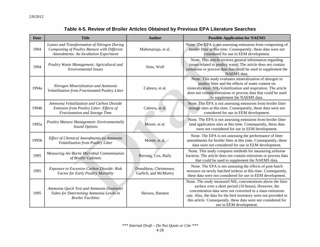
2/8/2012
*** Internal Draft – Do Not Quote or Cite *** 4-28
Table 4-5. Review of Broiler Articles Obtained by Previous EPA Literature Searches
Date Title Author Possible Application for NAEMS
1994 Losses and Transformation of Nitrogen During Composting of Poultry Manure with Different
Amendments: An Incubation Experiment Mahimairaja, et al.
None. The EPA is not assessing emissions from composting of broiler litter at this time. Consequently, these data were not
considered for use in EEM development.
1994 Poultry Waste Management: Agricultural and Environmental Issues Sims, Wolf
None. This article reviews general information regarding issues related to poultry waste. The article does not contain
emissions or process data that could be used to supplement the NAEMS data.
1994a Nitrogen Mineralization and Ammonia Volatilization from Fractionated Poultry Litter Cabrera, et al.
None. This study evaluates mineralization of nitrogen in poultry litter and the effects of water content on
mineralization, NH3 volatilization and respiration. The article does not contain emissions or process data that could be used
to supplement the NAEMS data.
1994b Ammonia Volatilization and Carbon Dioxide
Emission from Poultry Litter: Effects of Fractionation and Storage Time
Cabrera, et al. None. The EPA is not assessing emissions from broiler litter storage sites at this time. Consequently, these data were not
considered for use in EEM development.
1995a Poultry Manure Management: Environmentally Sound Options Moore, et al.
None. The EPA is not assessing emissions from broiler litter land application sites at this time. Consequently, these data
were not considered for use in EEM development.
1995b Effect of Chemical Amendments on Ammonia Volatilization from Poultry Litter Moore, et al.
None. The EPA is not assessing the performance of litter amendments for broiler litter at this time. Consequently, these
data were not considered for use in EEM development.
1995 Measuring Air-Borne Microbial Contamination of Broiler Cabinets Berrang, Cox, Baily
None. This study compares methods for measuring airborne bacteria. The article does not contain emissions or process data
that could be used to supplement the NAEMS data.
1995 Exposure to Excessive Carbon Dioxide: Risk Factor for Early Poultry Mortality
Donaldson, Christensen, Garlich, and McMurtry
None. The EPA is not assessing the effects of post-hatch stressors on newly hatched turkeys at this time. Consequently, these data were not considered for use in EEM development.
1995 Ammonia Quick Test and Ammonia Dosimeter
Tubes for Determining Ammonia Levels in Broiler Facilities
Skewes, Harmon
None. The study measured NH3 concentrations above the litter surface over a short period (10 hours). However, the
concentration data were not converted to a mass emissions rate. Also, the data for the bird inventory were not provided in this article. Consequently, these data were not considered for
use in EEM development.
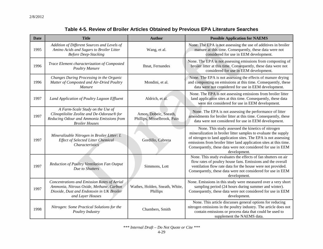
2/8/2012
*** Internal Draft – Do Not Quote or Cite *** 4-29
Table 4-5. Review of Broiler Articles Obtained by Previous EPA Literature Searches
Date Title Author Possible Application for NAEMS
1995 Addition of Different Sources and Levels of Amino Acids and Sugars to Broiler Litter
Before Deep-Stacking Wang, et al.
None. The EPA is not assessing the use of additives in broiler manure at this time. Consequently, these data were not
considered for use in EEM development.
1996 Trace Element characterization of Composted Poultry Manure Ihnat, Fernandes
None. The EPA is not assessing emissions from composting of broiler litter at this time. Consequently, these data were not
considered for use in EEM development.
1996 Changes During Processing in the Organic Matter of Composted and Air-Dried Poultry
Manure Mondini, et al.
None. The EPA is not assessing the effects of manure drying and composting on emissions at this time. Consequently, these
data were not considered for use in EEM development.
1997 Land Application of Poultry Lagoon Effluent Aldrich, et al. None. The EPA is not assessing emissions from broiler litter land application sites at this time. Consequently, these data
were not considered for use in EEM development.
1997
A Farm-Scale Study on the Use of Clinoptilolite Zeolite and De-Odorase® for
Reducing Odour and Ammonia Emissions from Broiler Houses
Amon, Dobeic, Sneath, Phillips, Misselbrook, Pain
None. The EPA is not assessing the performance of litter amendments for broiler litter at this time. Consequently, these
data were not considered for use in EEM development.
1997 Mineralizable Nitrogen in Broiler Litter: I.
Effect of Selected Litter Chemical Characteristics
Gordillo, Cabrera
None. This study assessed the kinetics of nitrogen mineralization in broiler litter samples to evaluate the supply of nitrogen to land application sites. The EPA is not assessing emissions from broiler litter land application sites at this time. Consequently, these data were not considered for use in EEM
development.
1997 Reduction of Poultry Ventilation Fan Output Due to Shutters Simmons, Lott
None. This study evaluates the effects of fan shutters on air flow rates of poultry house fans. Emissions and the overall ventilation flow rate data for the house were not provided.
Consequently, these data were not considered for use in EEM development.
1997
Concentrations and Emission Rates of Aerial Ammonia, Nitrous Oxide, Methane, Carbon Dioxide, Dust and Endotoxin in UK Broiler
and Layer Houses
Wathes, Holden, Sneath, White, Phillips
None. Emissions in this study were measured over a very short sampling period (24 hours during summer and winter).
Consequently, these data were not considered for use in EEM development.
1998 Nitrogen: Some Practical Solutions for the Poultry Industry Chambers, Smith
None. This article discusses general options for reducing nitrogen emissions in the poultry industry. The article does not
contain emissions or process data that could be used to supplement the NAEMS data.

2/8/2012
*** Internal Draft – Do Not Quote or Cite *** 4-30
Table 4-5. Review of Broiler Articles Obtained by Previous EPA Literature Searches
Date Title Author Possible Application for NAEMS
1998 Litter Production and Nutrients from Commercial Broiler Chickens Patterson, Lorenz, Weaver
This study analyzed the moisture, total nitrogen, ammoniacal nitrogen, phosphorous pentoxide and potassium oxide content
of broiler litter samples and the crude protein, total phosphorous, and total potassium content of feed. The nitrogen
content data could be used to supplement NAEMS mass balance data.
1998 Field-Scale Nitrogen and Phosphorus Losses
From Hayfields Receiving Fresh and Composted Broiler Litter
Vervoort, et al. None. The EPA is not assessing emissions from broiler litter land application sites at this time. Consequently, these data
were not considered for use in EEM development.
1998 Aerial Emissions from Poultry Production Wathes
None, This article discusses the potential control mechanisms for pollutants from broiler operations. Emissions values
presented were from other articles and the article does not provide descriptions of monitoring methodologies used to
measure emissions.
1998 Estimating Ammonia Emission Factors in
Europe: Summary of the Work of the UNECE Ammonia Expert Panel
Van der Hoek
None. This resource was used to develop emissions factors for broiler operations for the EPA’s Emissions From Animal
Feeding Operations (draft, August 15, 2001). However, the resource does not provide the underlying data (e.g., daily
values for bird inventory, bird mass, pollutant emissions) for the emissions factors cited. Consequently, these data were not
considered for use in EEM development.
1998 Concentrations and Emissions of Ammonia in Livestock Buildings in Northern Europe
Groot Koerkamp, Metz, Uenk, Phillips, Holden, Sneath, Short,
White, Hartung, Seedorf, Schroder, Linkert, Pederson,
Takai, Johnsen, Wathes
None. This resource was used to develop emissions factors for broiler operations for the EPA’s Emissions From Animal
Feeding Operations (draft, August 15, 2001). However, data describing the number, size and weight of the birds associated
with the emissions data were not provided. Consequently, these data were not considered for use in EEM development.
1999 In Situ Measurement of Ammonia Volatilization
from Broiler Litter Using an Enclosed Air Chamber
Brewer, Costello
None. The study measured NH3 emissions from litter using flux chambers. The article does not contain emissions or
process data that could be used to supplement the NAEMS data.
2002 Efficient Feed Nutrient Utilization to Reduce Pollutants In Poultry and Swine Manure Nahm
None. The EPA is not assessing the effects of dietary changes on emissions at this time, and this study evaluates outcomes
not addressed by the NAEMS (such as odor and manure characteristics).

2/8/2012
*** Internal Draft – Do Not Quote or Cite *** 4-31
Table 4-5. Review of Broiler Articles Obtained by Previous EPA Literature Searches
Date Title Author Possible Application for NAEMS
2002 Continuous Monitoring of Ammonia, Hydrogen Sulfide and Dust Emissions From Swine, Dairy
and Poultry Barns Schmidt, Jacobson, Janni None. This study does not contain broiler data.
NA Ammonia Emissions from Field Applications of Poultry Litter Meisinger, et al.
None. The EPA is not assessing emissions from broiler litter land application sites at this time. Consequently, these data
were not considered for use in EEM development.

2/8/2012
*** Internal Draft – Do Not Quote or Cite *** 5-1
5.0 NAEMS DATA PREPARATION
This section provides an overview of the data assessment procedures followed by the NAEMS in collecting the emissions and process parameter data from the broiler monitoring sites and the procedures followed by the EPA in preparing the data for use in development of EEMs for broiler confinement operations.
Section 5.1 discusses the Quality Assurance/Quality Control (QA/QC) procedures outlined in the NAEMS QAPP and implemented by the researchers to ensure collection of high-quality emissions and process data. Section 5.2 summarizes the steps the EPA followed to process and review the data submitted to the EPA prior to developing the broiler EEMs. Section 5.3 compares the design and operating parameters and reported emissions of each site.
5.1 NAEMS Data Assessments
5.1.1 QA/QC Procedures
The NAEMS followed strict QA/QC procedures throughout the data collection and preliminary data analyses processes of the NAEMS. The investigators developed QAPPs, SOPs for sampling systems and monitoring instruments and site-specific monitoring plans and provided extensive training for on-site operators and producers. Appendix A contains the QAPPs, Appendix B contains the SMPs for each monitoring site and Appendix C contains the SOPs.
Monitoring instruments underwent initial and periodic calibration, bias and precision checks and were corrected if they failed the QC checks. The frequency of each check/calibration event was dependent on the type of instrument and on the site investigator. For example, the NH3 gas analyzer was checked with calibration gases weekly or semi-weekly for the Kentucky sites, while the calibration checks were conducted every two months at site CA1B. The investigators also implemented external system audits conducted by independent personnel and maintained supporting documentation (e.g., field logs, instrument calibration records).
All of the monitoring sites were equipped with data acquisition (DAQ) systems that allowed on-site operators, and other authorized personnel via high-speed Internet connection, to view the measured data and parameter values daily through real-time computer displays. The DAQ systems also generated email notifications for project personnel when monitored parameter values were outside of preset ranges.
The NAEMS also used control charts extensively in QA/QC procedures to assess data quality and measurement variability and to evaluate long-term trends in the

2/8/2012
*** Internal Draft – Do Not Quote or Cite *** 5-2
instrument/equipment performance. The control charts provided a graphical means of determining whether the measured parameters were within acceptable upper and lower control limits. Data values outside the control limits triggered corrective actions by site operators to maintain data quality. The control charts were generated on site using Microsoft ® Excel templates to provide a real-time assessment of the data quality.
Measurement data recorded at each site were uploaded to the respective researchers (Purdue University for site CA1B and Iowa State University for the Kentucky sites) each day for review and evaluation. The researchers used custom-designed software to apply flags to measurement data that were considered invalid or outliers and to calculate emissions rates for the monitored houses. The researchers used the Calculation of Air Pollutant Emissions from Confined Animal Buildings (CAPECAB) program for site CA1B and the Mobile Air Emissions Monitoring Unit (MAEMU v1.2) program for the Kentucky sites.
5.1.2 Data Validation
In general, the researchers invalidated measurement data (e.g., concentration, differential static pressure, temperature) if the data values were:
• Unreasonably low or high when compared to normal ranges if there was supporting evidence that the data value is not correct (e.g., unresponsive relative humidity sensor inside a house producing a reading of less than 10 percent).
• Obtained during system installation, testing or maintenance during which uncorrectable errors might be introduced.
• Obtained when a sensor or instrument was proven to be malfunctioning (e.g., unstable).
• Obtained during calibration or precision check of a sensor or instrument and before the sensor or instrument reached equilibrium after the check.
• Obtained when the data acquisition and control hardware and/or software were not functioning correctly.
Data that the researchers deemed invalid were retained in the preprocessed data sets. However, the EPA did not use the flagged data to calculate pollutant emissions rates.
For averaged data, data were invalidated to avoid errors introduced into calculated mean values due to partial-data days (e.g., only a few hours of valid data) that would result in biased time weights:
• Hourly averages were invalidated if less than 75 percent of the data recorded during that hour were valid.
2/8/2012
*** Internal Draft – Do Not Quote or Cite *** 5-3
• Daily means were invalidated if less than 75 percent of the hourly average data recorded during that day were valid.
• Monthly averages were invalidated if less than 75 percent of the individual days recorded during that month were valid.
• Average daily means (ADM) were invalidated if less than 75 percent of the daily average data recorded during all measurement days were valid.
5.1.3 Data Completeness
Consistent with the EPA’s Guidance for Quality Assurance Project Plans (EPA QA/G-5), data completeness is the measure of the amount of valid data obtained from a measurement system, compared with the amount of data that was expected to be obtained under normal conditions. Data completeness is expressed as the percentage of valid data obtained from the measurement system. For data to be considered valid, they must meet all the acceptance criteria. The researchers calculated data completeness during data processing.
The goal of the NAEMS was to continuously monitor emissions and process parameters over a long period to characterize uncontrolled emissions from broiler confinement houses. The long monitoring period was intended to capture the variations in pollutant emissions due to the bird grow-out and litter clean-out cycles, and diurnal and seasonal variations. Emissions and process parameters were monitored at site CA1B from September 27, 2007, to October 21, 2009, and at site KY1B-1 from February 14, 2006, to March 14, 2007, and at site KY1B-2 from February 20, 2006, to March 5, 2007.
Table 5-1 presents the total number of days that the monitoring instrumentation systems were operational and the number of valid emissions days submitted to EPA for each site. According to the criteria established in the NAEMS QAPPs, a valid day for a pollutant or process parameter was one in which more than 75 percent of the measurement values recorded were valid (i.e., the data passed all QA checks). The NAEMS also established an overall completeness goal of 75 percent for the number of valid days of data that were recorded versus the number of scheduled sampling days. Table 5-2 presents the data completeness percentages for each site by pollutant. In the development of EEMs, the EPA considered all valid data days regardless of whether the NAEMS completeness goal was achieved.

2/8/2012
*** Internal Draft – Do Not Quote or Cite *** 5-4
Table 5-1. Reported Number of Valid Emissions Days for Required Data from NAEMS Broiler Operations
Site Monitoring Period
Total Monitoring Daysa Number of Valid Emissions Daysa NH3 H2S PM10 PM2.5 TSP NMHC NH3 H2S PM10 PM2.5 TSP NMHC
CA1B, H10
9/27/2007 – 10/21/2009 756 756 628 60 67 756 467 592 352 53 37 NAb
CA1B, H12
9/27/2007 – 10/21/2009 756 756 628 60 67 756 466 590 376 43 39 NAb
KY1B-1, H5
2/14/2006 – 3/14/2007 394 394 394 394 394 394 381 342 295 279 304 268
KY1B-2, H3
2/20/2006 – 3/5/2007 379 379 379 379 379 379 337 274 301 299 298 203
a In the final report for the Kentucky sites, the number of total monitoring days and valid emissions days were prorated to represent a monitoring period of 365 days. The values shown in the table are the actual number of days. b Not available. The final report for the CA1B site states that the NMHC data were questionable due to irreconcilable interferences caused by water and other gases.
Table 5-2. Data Completeness for Daily Emissions Data from NAEMS Broiler Operations
Site Data Completeness (%) NH3 H2S PM10 PM2.5 TSP NMHC
CA1B, H10 61.8 78.3 56.1 88.3 55.2 NAa
CA1B, H12 61.6 78.0 59.9 71.7 58.2 NAa
KY1B-1, H5 96.7 86.0 74.9 70.8 77.0 68.5
KY1B-2, H3 88.9 71.2 79.4 78.9 80.8 55.1 a Not available. The final report for the CA1B site states that the NMHC data were questionable due to irreconcilable interferences caused by water and other gases.
At site CA1B, the completeness goal of 75 percent was achieved only for H2S (at Houses
10 and 12) and PM2.5 (only at House 10). The completeness goal was not met for NH3, PM10 and TSP emissions by either house at site CA1B due to delays in receiving monitoring equipment at the beginning of the study and calibration and maintenance issues with the gas analyzer.
At site CA1B, a single instrument (TEOM) and different inlet sampling heads were used to measure PM10, PM2.5 and TSP emissions. Because a single instrument was used, each PM component was sampled on an intermittent schedule. The goal of the NAEMS over the study period was to collect emissions data for seven weeks out of every eight weeks for PM10; two weeks of summertime data and two weeks of wintertime data for PM2.5; and data for one week out of every eight weeks for TSP.

2/8/2012
*** Internal Draft – Do Not Quote or Cite *** 5-5
Table 5-3 shows the operating times for the TEOM instrument and the total number of measurement days at each particle size. The number of valid PM emissions days was limited due to TEOM failures. Emissions of PM2.5 were sampled in periods ranging from 12 to 18 days in February and July 2008 and in January and September 2009, with the goal of obtaining data under both cold (winter) and hot (summer) conditions. For TSP, sampling was conducted during six measurement events, each lasting from 7 to 14 days. Emissions of PM10 were measured at all other times over the course of the monitoring study at site CA1B. The length of the monitoring period for each PM size cut was varied, where possible, to accommodate the completeness requirements. For example, TSP sampling was allowed to run for up to two weeks to meet the 75 percent completeness requirement of 5.25 emissions days. However, if this requirement was not met by the end of the two-week period, the TEOM was reconfigured for the next particle size cut to be monitored.
Table 5-3. Particulate Matter Monitoring Schedule for CA1B Date Test Duration (days)
Start Stop PM10 TSP PM2.5 9/28/07 12/10/07 73.6 NS 12/10/07 12/19/07 NS 8.9 NS 12/19/07 2/1/08 44 NS 2/1/08 2/19/08 NS 18.1 2/19/08 2/20/08 NS 0.3a 2/19/08 2/20/08 0.3b NS 2/20/08 5/15/08 85.7 NS 5/15/08 5/28/08 NS 12.8 NS 5/28/08 7/9/08 42 NS 7/9/08 7/25/08 NS 16 7/25/08 11/17/08 115.1 NS 11/17/08 11/24/08 NS 7.1 11/24/08 1/5/09 41.9 NS 1/5/09 1/20/09 NS 15 1/20/09 4/9/09 79 NS 4/9/09 4/20/09 NS 11 NS 4/20/09 6/25/09 66.1 NS 6/25/09 7/8/09 NS 12.9 NS 7/8/09 9/26/09 80.1 NS 9/26/09 10/7/09 NS 10.9 10/7/09 10/21/09 NS 14.1 NS 10/21/09 10/22/09 0.4 NS
Totals 628.3 66.7 60.3 NS - Not sampled. a Ambient data were not collected during this sampling period. b Only ambient data were collected during this sampling period.

2/8/2012
*** Internal Draft – Do Not Quote or Cite *** 5-6
At the Kentucky sites, the completeness goal of 75 percent was achieved for all pollutants except for H2S (at KY1B-2 H3), PM10 (at KY1B-1 H5) and PM2.5 (at KY1B-1 H5). The final report for the Kentucky sites did not provide explanations for the missing data days.
5.2 EPA Assessments
5.2.1 Data Processing
The data collected under the NAEMS were provided to the EPA in the form of final site reports (pdf format) and Microsoft Excel® spreadsheets that contained the emissions and process data. For site CA1B, separate worksheets were used to present the daily values for each pollutant. In addition, the data within each worksheet were further divided into tables that presented the daily values and summary statistics (i.e., number of data points, averages, standard deviations, minimums and maximums) for each month of the study period.
To facilitate analyses of the emissions and process data for site CA1B, the EPA reformatted and converted the files to a Microsoft Access® database containing all of the data elements provided by the investigators in the summary spreadsheets. To reformat the spreadsheets received, the EPA removed the summary statistics and the blank spaces between data tables that presented the data for each month. Merged cells were removed and the data headers for each month were consolidated and rearranged, as necessary, to create an input file for uploading into Microsoft Access®. The EPA performed QA checks to verify that the conversion from spreadsheets to database tables was performed correctly and that data were not lost or transposed in the conversion. Additionally, the EPA randomly selected three dates during the study period and compared all of the values contained in the database on those dates to the original spreadsheets to ensure the data were properly transferred to the new file format.
The EPA reformatted and converted the spreadsheets submitted for the Kentucky sites to Microsoft Access® data tables. The EPA performed QA checks of the uploaded Kentucky data and then the Kentucky data were combined with the data for site CA1B to create a comprehensive database of the NAEMS broiler data.
5.2.2 Data QA
The EPA developed a comprehensive list of the emissions and confinement operating parameter, meteorological condition and mass balance data that were expected to be submitted to the EPA based on the EPA’s review of the QAPPs, SOPs and SMPs. As the final reports and data spreadsheets were received, the EPA compared the information received to the comprehensive list to identify missing information. After determining whether the data submittals to the EPA were complete and identifying missing data elements, the EPA verified

2/8/2012
*** Internal Draft – Do Not Quote or Cite *** 5-7
that the units of measurement for the emissions and supporting data were consistent between the final reports and spreadsheet data files. In addition, the EPA assessed whether the units of measurement and the magnitude of emissions were consistent across the monitoring sites. The EPA prepared and provided summaries of the missing data elements to the researchers.
The EPA’s review identified that a small number (less than 1.7 percent) of the daily average emissions for H2S and PM10 at site CA1B were reported as negative values. After discussion with the study’s Scientific Advisor, it was determined the negative emission values occurred due to drift in the instrument readings between calibrations. The EPA included the negatives values when graphing the data to visualize emission trends but did not include the negative values when developing EEMs for broiler houses, to avoid possible complications with EEM development (e.g., the EEM predicting negative emissions) the negative values were withheld from the data sets used for EEM development. The EPA’s review also identified a few instances (less than 2 percent) of zero emission values (i.e., instances where the ambient and confinement concentrations were the same). However, because the zero values were not the result of instrument drift, the EPA included the zero emissions values in the data sets used in the development of the EEMs for broiler confinement houses.
As specified in the QAPPs developed for the CA1B and Kentucky sites, the daily emissions values submitted to the EPA did not include measurements that were considered to be outliers by the NAEMS researchers. However, the EPA compared the emissions values calculated for each day of the grow-out, decaking and litter clean-out periods for each flock to the average daily emissions for all flocks to identify anomalies in the reported data. Daily emissions values that were higher or lower than ± two standard deviations and ± twice the average flock emission for that day were noted for further evaluation. For these values, the EPA prepared graphical overlays of the pollutant emissions and the average ambient and confinement parameter values (e.g., air temperature, house temperature, ventilation flow rate) recorded for that day to determine if the anomalous emission value could be attributed to an irregular condition (e.g., an abnormally high ambient temperature or house ventilation flow rate). This analysis identified several anomalies (e.g., spikes in NH3 emissions during litter clean-out periods); however, the analysis suggested that other activities (e.g., high/low ventilation rates) could account for these anomalies. Additionally, the field note summaries in the final reports for the CA1B and Kentucky sites did not suggest abnormal conditions that would warrant excluding the emissions values from EEM development.
5.2.3 Data Completeness Assessment
The EPA assessed the data completeness of the average daily emissions values to verify the completeness calculations presented in the final reports. Based upon its analysis, the EPA
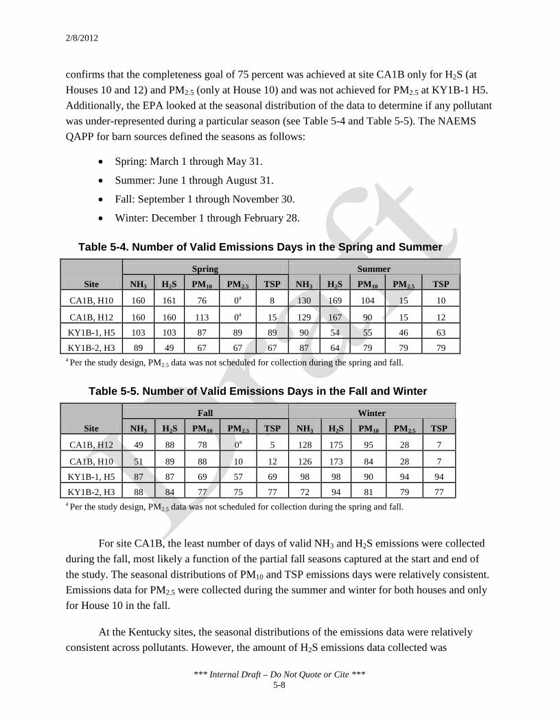
2/8/2012
*** Internal Draft – Do Not Quote or Cite *** 5-8
confirms that the completeness goal of 75 percent was achieved at site CA1B only for H2S (at Houses 10 and 12) and PM2.5 (only at House 10) and was not achieved for PM2.5 at KY1B-1 H5. Additionally, the EPA looked at the seasonal distribution of the data to determine if any pollutant was under-represented during a particular season (see Table 5-4 and Table 5-5). The NAEMS QAPP for barn sources defined the seasons as follows:
• Spring: March 1 through May 31.
• Summer: June 1 through August 31.
• Fall: September 1 through November 30.
• Winter: December 1 through February 28.
Table 5-4. Number of Valid Emissions Days in the Spring and Summer
Site
Spring Summer
NH3 H2S PM10 PM2.5 TSP NH3 H2S PM10 PM2.5 TSP
CA1B, H10 160 161 76 0a 8 130 169 104 15 10
CA1B, H12 160 160 113 0a 15 129 167 90 15 12
KY1B-1, H5 103 103 87 89 89 90 54 55 46 63
KY1B-2, H3 89 49 67 67 67 87 64 79 79 79 a Per the study design, PM2.5 data was not scheduled for collection during the spring and fall.
Table 5-5. Number of Valid Emissions Days in the Fall and Winter
Site
Fall Winter
NH3 H2S PM10 PM2.5 TSP NH3 H2S PM10 PM2.5 TSP
CA1B, H12 49 88 78 0a 5 128 175 95 28 7
CA1B, H10 51 89 88 10 12 126 173 84 28 7
KY1B-1, H5 87 87 69 57 69 98 98 90 94 94
KY1B-2, H3 88 84 77 75 77 72 94 81 79 77 a Per the study design, PM2.5 data was not scheduled for collection during the spring and fall.
For site CA1B, the least number of days of valid NH3 and H2S emissions were collected during the fall, most likely a function of the partial fall seasons captured at the start and end of the study. The seasonal distributions of PM10 and TSP emissions days were relatively consistent. Emissions data for PM2.5 were collected during the summer and winter for both houses and only for House 10 in the fall.
At the Kentucky sites, the seasonal distributions of the emissions data were relatively consistent across pollutants. However, the amount of H2S emissions data collected was
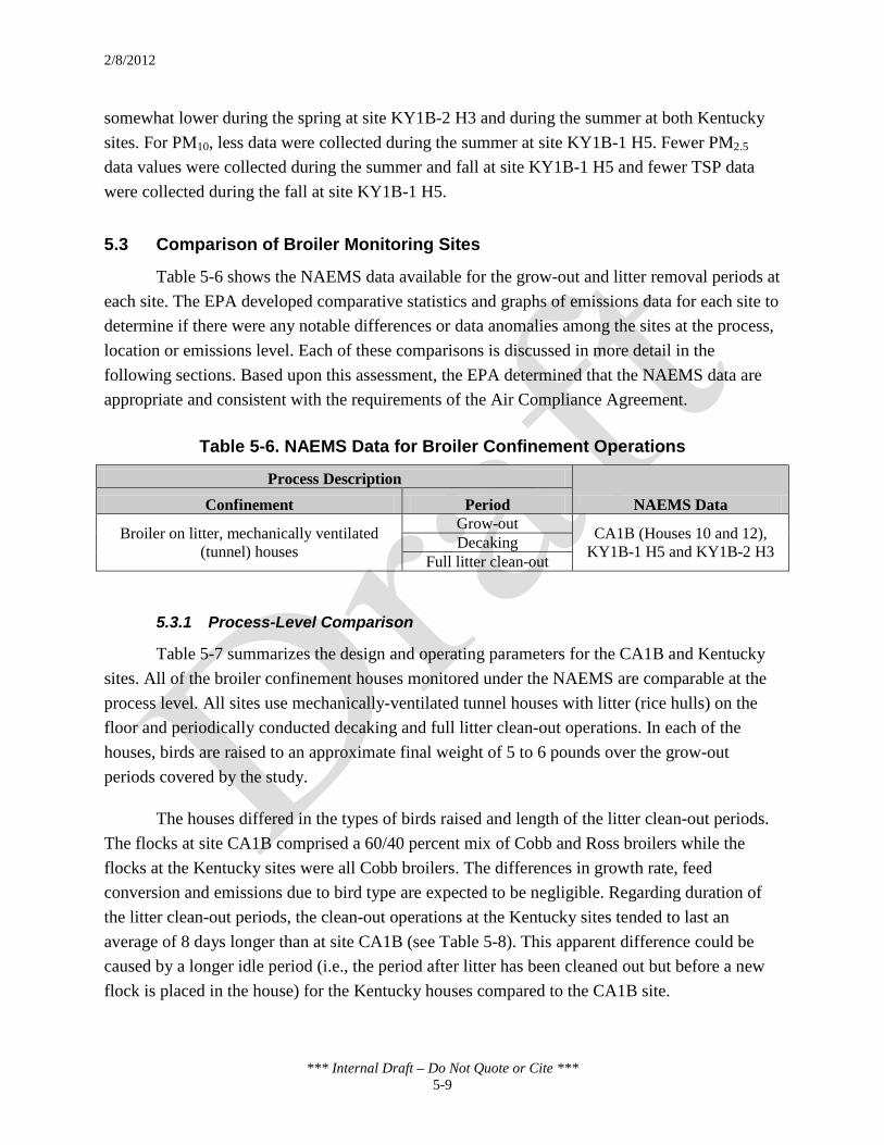
2/8/2012
*** Internal Draft – Do Not Quote or Cite *** 5-9
somewhat lower during the spring at site KY1B-2 H3 and during the summer at both Kentucky sites. For PM10, less data were collected during the summer at site KY1B-1 H5. Fewer PM2.5 data values were collected during the summer and fall at site KY1B-1 H5 and fewer TSP data were collected during the fall at site KY1B-1 H5.
5.3 Comparison of Broiler Monitoring Sites
Table 5-6 shows the NAEMS data available for the grow-out and litter removal periods at each site. The EPA developed comparative statistics and graphs of emissions data for each site to determine if there were any notable differences or data anomalies among the sites at the process, location or emissions level. Each of these comparisons is discussed in more detail in the following sections. Based upon this assessment, the EPA determined that the NAEMS data are appropriate and consistent with the requirements of the Air Compliance Agreement.
Table 5-6. NAEMS Data for Broiler Confinement Operations
Process Description NAEMS Data Confinement Period
Broiler on litter, mechanically ventilated (tunnel) houses
Grow-out CA1B (Houses 10 and 12), KY1B-1 H5 and KY1B-2 H3 Decaking
Full litter clean-out
5.3.1 Process-Level Comparison
Table 5-7 summarizes the design and operating parameters for the CA1B and Kentucky sites. All of the broiler confinement houses monitored under the NAEMS are comparable at the process level. All sites use mechanically-ventilated tunnel houses with litter (rice hulls) on the floor and periodically conducted decaking and full litter clean-out operations. In each of the houses, birds are raised to an approximate final weight of 5 to 6 pounds over the grow-out periods covered by the study.
The houses differed in the types of birds raised and length of the litter clean-out periods. The flocks at site CA1B comprised a 60/40 percent mix of Cobb and Ross broilers while the flocks at the Kentucky sites were all Cobb broilers. The differences in growth rate, feed conversion and emissions due to bird type are expected to be negligible. Regarding duration of the litter clean-out periods, the clean-out operations at the Kentucky sites tended to last an average of 8 days longer than at site CA1B (see Table 5-8). This apparent difference could be caused by a longer idle period (i.e., the period after litter has been cleaned out but before a new flock is placed in the house) for the Kentucky houses compared to the CA1B site.

2/8/2012
*** Internal Draft – Do Not Quote or Cite *** 5-10
Additionally, the Kentucky sites conducted full litter clean-outs once per year, while the CA1B houses cleaned out litter after three consecutive grow-out periods. Table 5-9 specifies the dates of the litter clean-outs for each broiler confinement house during the study and the type of clean-out activity performed.
Table 5-7. Design and Operating Parameters of the NAEMS Broiler Sites
Monitoring Site
House Capacity (no. of birds) Bird Type
Final Bird Weighta (kg) Design Ventilation
Type Average Range
CA1B H10
21,000b
60 percent Cobb, 40 percent
Ross
2.64 2.48 – 2.75
Litter (rice hulls) on
floor
Mechanical (tunnel)
H12 2.65 2.55 – 2.76
KY1B-1 H5 25,800 (summer)
24,400 (winter)
100 percent Cobbc
2.74 2.53 – 2.89
KY1B-2 H3 2.78 2.47 – 2.97 a Bird weight at the end of the grow-out period. b The CA1B site did not vary stocking numbers during the year. c Described in the final report text as “Cobb-Cobb-straight-run (mixed sex).”
Table 5-8. Duration of Grow-out and Clean-out Periods
Monitoring Site
Grow-Out Periods Clean-Out Periods
Decaking Full Litter Clean-Out
Frequency Average (days)
Range (days) Frequency
Average Duration
(days)
Range of Duration
(days) Frequency
Average Duration
(days)
Range of Duration
(days)
CA1B
H10 ~ 7 flocks per year 47 45 -
49 ~ 5 time per year 7.75 6 – 11
Every third flock (~2 times per
year)
12.6 6 – 21
H12 ~ 7 flocks per year 47 45 -
49 ~ 5 time per year 7.25 3 – 11
Every third flock (~2 times per
year)
12.8 6 – 23
KY1B-1 H5 ~ 6 flocks per year 51 50 -
54 ~4 times per year 15.5 12 – 22 Once per
year 25 NAa
KY1B-2 H3 ~ 6 flocks per year 52 50 -
54 ~4 times per year 22 15 – 41 Once per
year 9 NAa a Not applicable. Only one full litter clean-out event was monitored during the study.
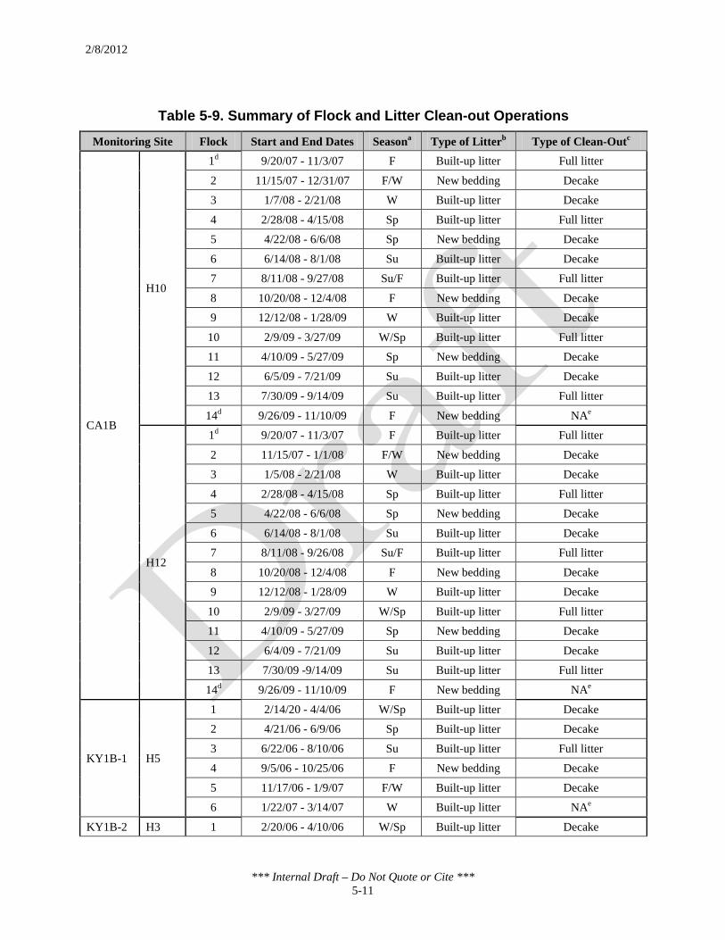
2/8/2012
*** Internal Draft – Do Not Quote or Cite *** 5-11
Table 5-9. Summary of Flock and Litter Clean-out Operations
Monitoring Site Flock Start and End Dates Seasona Type of Litterb Type of Clean-Outc
CA1B
H10
1d 9/20/07 - 11/3/07 F Built-up litter Full litter
2 11/15/07 - 12/31/07 F/W New bedding Decake
3 1/7/08 - 2/21/08 W Built-up litter Decake
4 2/28/08 - 4/15/08 Sp Built-up litter Full litter
5 4/22/08 - 6/6/08 Sp New bedding Decake
6 6/14/08 - 8/1/08 Su Built-up litter Decake
7 8/11/08 - 9/27/08 Su/F Built-up litter Full litter
8 10/20/08 - 12/4/08 F New bedding Decake
9 12/12/08 - 1/28/09 W Built-up litter Decake
10 2/9/09 - 3/27/09 W/Sp Built-up litter Full litter
11 4/10/09 - 5/27/09 Sp New bedding Decake
12 6/5/09 - 7/21/09 Su Built-up litter Decake
13 7/30/09 - 9/14/09 Su Built-up litter Full litter
14d 9/26/09 - 11/10/09 F New bedding NAe
H12
1d 9/20/07 - 11/3/07 F Built-up litter Full litter
2 11/15/07 - 1/1/08 F/W New bedding Decake
3 1/5/08 - 2/21/08 W Built-up litter Decake
4 2/28/08 - 4/15/08 Sp Built-up litter Full litter
5 4/22/08 - 6/6/08 Sp New bedding Decake
6 6/14/08 - 8/1/08 Su Built-up litter Decake
7 8/11/08 - 9/26/08 Su/F Built-up litter Full litter
8 10/20/08 - 12/4/08 F New bedding Decake
9 12/12/08 - 1/28/09 W Built-up litter Decake
10 2/9/09 - 3/27/09 W/Sp Built-up litter Full litter
11 4/10/09 - 5/27/09 Sp New bedding Decake
12 6/4/09 - 7/21/09 Su Built-up litter Decake
13 7/30/09 -9/14/09 Su Built-up litter Full litter
14d 9/26/09 - 11/10/09 F New bedding NAe
KY1B-1 H5
1 2/14/20 - 4/4/06 W/Sp Built-up litter Decake
2 4/21/06 - 6/9/06 Sp Built-up litter Decake
3 6/22/06 - 8/10/06 Su Built-up litter Full litter
4 9/5/06 - 10/25/06 F New bedding Decake
5 11/17/06 - 1/9/07 F/W Built-up litter Decake
6 1/22/07 - 3/14/07 W Built-up litter NAe
KY1B-2 H3 1 2/20/06 - 4/10/06 W/Sp Built-up litter Decake

2/8/2012
*** Internal Draft – Do Not Quote or Cite *** 5-12
Table 5-9. Summary of Flock and Litter Clean-out Operations
Monitoring Site Flock Start and End Dates Seasona Type of Litterb Type of Clean-Outc 2 5/22/06 - 7/11/06 Su Built-up litter Decake
3 7/28/06 - 9/19/06 Su Built-up litter Decake
4 10/5/06 - 11/27/06 F Built-up litter Decake
5 12/14/06 - 2/2/07 W Built-up litter Full litter
6d 2/12/07 - 3/5/07 W New bedding NAe a Season of the year: Su = Summer, Sp = Spring, F = Fall, W = Winter. b Denotes the type of litter on which the flock was raised. Built-up litter is litter that was decaked after removing the previous flock and partially replenished with fresh bedding (typically, 20 – 25 percent of the bedding material is new). New bedding is the complete replenishment of bedding material after full litter clean-out operations. c Clean-out process occurs after the flock has been removed from the confinement house. d Partial data. e Clean-out occurred after study period concluded. No data were collected.
5.3.2 Comparison of Local Meteorological Conditions
Table 5-10 summarizes the site-specific ambient and confinement conditions for each site. Ambient temperature and relative humidity are the same for both CA1B broiler houses because a single sampling point was used to represent the ambient conditions for both houses. The minimum ambient temperature at the Kentucky farms tended to be lower than at the CA1B site, but the average ambient temperatures are very similar to those at CA1B. Ambient relative humidity conditions are very similar for all the broiler sites, as are temperature and relative humidity conditions in the broiler houses.
Table 5-10. Site-Specific Ambient and Confinement Conditions
Monitoring Site
Ambient Confinement
Temperature (oC) Relative Humidity (%) Temperature (oC) Relative Humidity
(%) Average Range Average Range Average Range Average Range
CA1B H10
16.69 3.30 - 31.10 61.53 32.70 -
94.90
24.99 11.40 - 32.60 57.66 35.70 -
89.20
H12 24.99 10.80 - 33.70 55.48 36.60 -
88.10
KY1B-1 H5 13.02 -9.94 - 29.78 71.82 37.44 -
97.46 23.03 10.25 - 30.27 58.24 29.41 -
80.24
KY1B-2 H3 13.37 -6.96 - 29.94 72.97 37.8 -
97.43 24.09 8.04 - 31.92 59.7 33.49 -
83.10
5.3.3 Emissions-Level Comparison
Table 5-11, Table 5-12, Table 5-13, Table 5-14 and Table 5-15 summarize the emissions values from each of the broiler confinement houses monitored during the NAEMS, for each

2/8/2012
*** Internal Draft – Do Not Quote or Cite *** 5-13
phase of production. The data presented in the tables include all non-negative, daily average values.
As shown in Table 5-11, the average and range of daily emissions for all periods (i.e., grow-out, decaking and full litter clean-out) are comparable across the three monitoring sites, although the average NH3 and PM10 emissions tended to be slightly higher for sites KY1B-1 H5 and KY1B-2 H3 than site CA1B.
Table 5-12 presents the emissions for grow-out periods in terms of pollutant mass per day. The average NH3 emissions were somewhat higher at the Kentucky sites. Emissions of H2S and PM10 were also higher at KY1B-2 H3. Table 5-13 presents the emissions for grow-out periods in terms of pollutant mass per day per bird. The average per-bird emissions rates for all pollutants were comparable across the monitoring sites, although PM2.5 emissions at the KY1B-1 H5 were slightly higher than the other sites.
Table 5-14 and Table 5-15 show the emissions for decaking and full litter clean-out periods. For both types of clean-out activities, NH3 emissions tended to be higher at site KY1B-1 H5 than the other broiler houses. Emissions of H2S during decaking periods tended to be higher at site CA1B while H2S during litter clean-out periods were higher at site KY1B-2 H3. The Kentucky sites tended to have higher PM10 emissions during decaking and litter clean-out periods.
The average emissions for gaseous pollutants during the grow-out period are higher than during the decaking or full litter clean-out periods, as fresh manure is constantly deposited by the birds to contribute to the chemical reactions responsible for the emissions. Although PM emissions data during the clean-out periods are limited (the TEOMs at site CA1B were removed to prevent damage by the cleaning operations), the available data show that PM emissions also tend to be higher during grow-out periods. This difference is likely attributable to contributions from bird feathers and dander and the agitation of the litter by the birds.
With the exception of PM10, all pollutant emissions during full litter clean-out periods were lower than during decaking periods. Decaking events are expected to have higher emissions than full litter clean-out events because of litter remaining in the house continues to contribute to gaseous emissions.
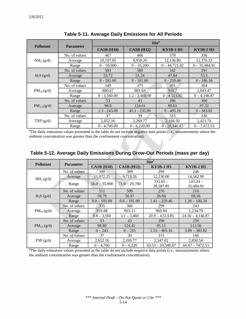
2/8/2012
*** Internal Draft – Do Not Quote or Cite *** 5-14
Table 5-11. Average Daily Emissions for All Periods
Pollutant Parameter Sitea
CA1B (H10) CA1B (H12) KY1B-1 H5 KY1B-2 H3
NH3 (g/d) No. of values 467 466 378 336
Average 10,197.05 8,950.20 12,136.80 12,376.33 Range 0 – 50,900 0 – 35,200 0 – 44,721.02 0 – 35,484.91
H2S (g/d) No. of values 583 580 342 291
Average 53.72 51.24 47.84 53.5 Range 0 - 181.00 0 - 181.00 0 - 259.46 0 - 186.34
PM10 (g/d) No. of values 349 375 301 304
Average 880.67 881.64 919.7 1,043.47 Range 0 - 3,560.00 1.2 - 3,460.00 0 - 4,513.85 0 – 4,146.87
PM2.5 (g/d) No. of values 53 43 286 300
Average 98.8 124.41 89.61 97.32 Range 1.3 - 243.00 45.1 - 235.00 0 - 405.16 0 - 383.82
TSP (g/d) No. of values 37 39 315 330
Average 2,652.16 2,269.77 2,166.50 2,421.74 Range 0 - 4,760.00 0 - 6,220.00 0 - 10,340.87 0 – 7,472.53
aThe daily emissions values presented in the table do not include negative data points (i.e., measurements where the ambient concentration was greater than the confinement concentration).
Table 5-12. Average Daily Emissions During Grow-Out Periods (mass per day)
Pollutant Parameter Sitea CA1B (H10) CA1B (H12) KY1B-1 H5 KY1B-2 H3
NH3 (g/d)
No. of values 390 389 299 246 Average 11,072.25 9,719.26 12,230.00 14,562.90
Range 56.0 – 35,900 71.0 – 29,700 332.65 – 28,587.85
143.24 – 35,484.91
H2S (g/d) No. of values 511 509 276 216
Average 59.79 56.97 56.84 69.56 Range 0.0 – 181.00 0.0 – 181.00 1.41 – 259.46 1.36 – 186.34
PM10 (g/d) No. of values 335 366 299 243
Average 919.88 903.11 969.94 1,234.79 Range 9.8 – 3,560 3.1 – 3,460 20.9 – 4,513.85 24.56 – 4,146.87
PM2.5 (g/d) No. of values 53 43 290 256
Average 98.80 124.41 95.11 113.56 Range 0 – 243 0 – 235 2.55 – 405.16 3.89 – 383.82
TSP (g/d) No. of values 37 39 215 166
Average 2,652.16 2,269.77 2,347.02 2,830.54 Range 0 – 4,760 0 – 6,220 43.53 – 10,340.87 44.47 – 7472.53
aThe daily emissions values presented in the table do not include negative data points (i.e., measurements where the ambient concentration was greater than the confinement concentration).
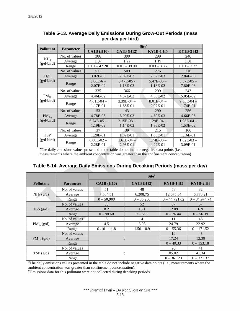
2/8/2012
*** Internal Draft – Do Not Quote or Cite *** 5-15
Table 5-13. Average Daily Emissions During Grow-Out Periods (mass per day per bird)
Pollutant Parameter Sitea CA1B (H10) CA1B (H12) KY1B-1 H5 KY1B-2 H3
NH3 (g/d-bird)
No. of values 386 390 299 246 Average 1.37 1.22 1.19 1.31 Range 0.01 – 42.20 0.01 – 39.90 0.03 – 3.35 0.01 – 3.27
H2S (g/d-bird)
No. of values 511 509 276 216 Average 3.02E-03 2.89E-03 2.52E-03 2.84E-03
Range 3.06E-6 – 2.07E-02
5.47E-05 - 1.18E-02
5.47E-05 – 1.18E-02
5.57E-05 – 7.80E-03
PM10 (g/d-bird)
No. of values 335 366 299 243 Average 4.46E-02 4.37E-02 4.33E-02 5.05E-02
Range 4.61E-04 – 1.17E-01
3.39E-04 – 1.68E-01
8.01E-04 – 2.07E-01
9.83E-04 – 1.74E-01
PM2.5 (g/d-bird)
No. of values 53 43 290 256 Average 4.78E-03 6.00E-03 4.30E-03 4.66E-03
Range 6.74E-05 – 1.19E-02
2.15E-03 – 1.14E-02
1.29E-04 – 1.86E-02
1.08E-04 – 1.53E-02
TSP (g/d-bird)
No. of values 37 39 215 166 Average 1.28E-01 1.09E-01 1.05E-01 1.16E-01
Range 6.80E-02 – 2.28E-01
1.61E-04 – 2.98E-01
1.74E-03 – 4.22E-01
1.82E-03 – 3.09E-01
aThe daily emissions values presented in the table do not include negative data points (i.e., measurements where the ambient concentration was greater than the confinement concentration).
Table 5-14. Average Daily Emissions During Decaking Periods (mass per day)
Pollutant Parameter
Sitea
CA1B (H10) CA1B (H12) KY1B-1 H5 KY1B-2 H3
NH3 (g/d) No. of values 51 48 58 82
Average 7,534.51 6,208.75 12,675.34 6,773.21 Range 0 – 50,900 0 – 35,200 0 – 44,721.02 0 – 34,974.74
H2S (g/d) No. of values 55 52 57 67
Average 18.21 15.1 12.09 6.9 Range 0 – 98.60 0 – 68.0 0 – 76.44 0 – 56.39
PM10 (g/d) No. of values 6 4 11 45
Average 4.5 3.98 24.79 22.92 Range 0 .10 – 11.8 1.50 – 8.9 0 – 55.36 0 – 171.52
PM2.5 (g/d) No. of values
b 19 45
Average 17.24 12.39 Range 0 – 40.33 0 – 153.18
TSP (g/d) No. of values
b 20 41
Average 85.02 41.34 Range 0 – 361.23 0 – 321.37
aThe daily emissions values presented in the table do not include negative data points (i.e., measurements where the ambient concentration was greater than confinement concentration). b Emissions data for this pollutant were not collected during decaking periods.

2/8/2012
*** Internal Draft – Do Not Quote or Cite *** 5-16
Table 5-15. Average Daily Emissions During Full Litter Clean-Out Periods (mass per day)
Pollutant Parameter Sitea
CA1B (H10) CA1B (H12) KY1B-1 H5 KY1B-2 H3
NH3 (g/d) No. of values 30 30 21 8
Average 3,459.60 3,390.07 9,322.43 2,571.25 Range 57.0 – 23,100 17.0 – 24,000 0 – 30,569.63 129.78 – 10,024.84
H2S (g/d) No. of values 23 23 8 8
Average 5.36 7.23 4.62 10.16 Range 0.06 – 31.30 0.05 – 63.50 0.84 – 20.01 1.81 – 30.72
PM10 (g/d) No. of values 9 5 5 3
Average 9.66 12.86 24.86 23.13 Range 0 - 30.50 1.20 – 35.80 0 - 71.29 7.18 – 55.72
PM2.5 (g/d) No. of values
b 1 3
Average 0 6.83 Range 0 0 – 13.76
TSP (g/d) No. of values
b 5 3
Average 21.86 69.97 Range 0 – 61.12 10.83 – 161.71
a The daily emissions values presented in the table do not include negative data points (i.e., measurements where the ambient concentration was greater than the confinement concentration). b Emissions data for this pollutant were not collected during litter clean-out periods.

2/8/2012
*** Internal Draft – Do Not Quote or Cite *** 6-1
6.0 MEASURED EMISSIONS FROM BROILER OPERATIONS
The EPA prepared graphs of the NAEMS daily emissions values to identify general and seasonal trends or cycles in pollutant emissions over the monitoring period. Section 6.1 describes the data processing steps used to prepare the graphs of daily emissions values. Sections 6.2 through 6.6 present the daily and seasonal graphs and discuss any trends seen for NH3, H2S, PM10, PM2.5, TSP and VOC emissions, respectively. For the trend discussions, the EPA related the emissions trends identified for specific process operations based upon its review of the field note summaries in the final reports for the monitoring sites and its general understanding of broiler operations.
In general, the emissions of all pollutants from broiler confinement houses tend to:
• Increase over the grow-out period with the lowest emissions rate occurring at the beginning of the period (when the birds are small and floor bedding is fresh) and the highest emissions rate occurring near the end of the grow-out period before the birds are sent to market.
• Decrease during the decaking and full litter clean-out periods when the houses are empty.
6.1 Data Processing
This section describes the processing steps used by the EPA in preparing the emissions graphs. The graphs prepared by EPA include all of the valid measurements submitted to the EPA.
6.1.1 Daily Emissions Graphs
For the graphs of daily emissions, the emissions values were highlighted to designate whether the emissions values were associated with the grow-out, decaking or full litter clean-out periods. Unshaded values on the daily emissions figures correspond to grow-out periods. Light shading depicts the decaking periods (i.e., partial litter removal and replenishment with fresh bedding) and darker shading indicates full litter clean-out periods (i.e., complete removal of litter).
6.1.2 Seasonal Emissions Graphs
For this analysis, the EPA assigned each of the flocks monitored under the NAEMS a season using the same designations as specified in the NAEMS QAPP:
• Spring - March through May.

2/8/2012
*** Internal Draft – Do Not Quote or Cite *** 6-2
• Summer - June through August.
• Fall - September through November.
• Winter - December through February.
Table 6-1 provides the average duration of the grow-out, decaking and full litter clean-out periods, along with the range of values in brackets. To simplify the seasonal assignments, if the grow-out period of the flock overlapped with another season by less than 15 days, the EPA assigned the flock to the season that had the majority of days. The EPA assigned flocks that overlapped the next season by more than 15 days as mixed-season flocks (e.g., Fall/Winter). Table 6-2 contains the start and end dates for each flock grow-out period and the seasonal designation assigned by EPA.
Table 6-1. Average Flock Duration by Site
Site Average Duration and Range of Period (days) [min, max]
Grow-Out Litter Removal Activity
Total Flock Full Litter Clean-Out Decaking
CA1B H10 47.00 [45, 49] 12.60 [6, 22] 7.75 [6, 11] 56.69 [52, 70] CA1B H12 47.21 [45, 49] 12.80 [6, 23] 7.25 [3, 11] 56.69 [51, 70] KY1B-1 H5 51.17 [50, 54] 25.00 15.50 [12, 22] 72.40 [62, 86] KY1B-2 H3 52.00 [50, 54] 9.00 22.00 [15, 41] 71.40 [60, 91]
Table 6-2. Flock Classified by Season
Site Flock Number of Days Occupied Start Occupied End Season (Occupied)
CA1B H10
1 45 9/20/2007 11/3/2007 Fall 2 47 11/15/2007 12/31/2007 Fall/Winter 3 46 1/7/2008 2/21/2008 Winter 4 48 2/28/2008 4/15/2008 Spring 5 46 4/22/2008 6/6/2008 Spring 6 49 6/14/2008 8/1/2008 Summer 7 48 8/11/2008 9/27/2008 Summer/Fall 8 46 10/20/2008 12/4/2008 Fall 9 48 12/12/2008 1/28/2009 Winter
10 47 2/9/2009 3/27/2009 Winter/Spring 11 48 4/10/2009 5/27/2009 Spring 12 47 6/5/2009 7/21/2009 Summer 13 47 7/30/2009 9/14/2009 Summer 14 46 9/26/2009 11/10/2009 Fall
CA1B H12
1 45 9/20/2007 11/3/2007 Fall 2 48 11/15/2007 1/1/2008 Fall/Winter 3 48 1/5/2008 2/21/2008 Winter

2/8/2012
*** Internal Draft – Do Not Quote or Cite *** 6-3
Table 6-2. Flock Classified by Season
Site Flock Number of Days Occupied Start Occupied End Season (Occupied)
4 48 2/28/2008 4/15/2008 Spring 5 46 4/22/2008 6/6/2008 Spring 6 49 6/14/2008 8/1/2008 Summer 7 47 8/11/2008 9/26/2008 Summer/Fall 8 46 10/20/2008 12/4/2008 Fall 9 48 12/12/2008 1/28/2009 Winter
10 47 2/9/2009 3/27/2009 Winter/Spring 11 48 4/10/2009 5/27/2009 Spring 12 48 6/4/2009 7/21/2009 Summer 13 47 7/30/2009 9/14/2009 Summer 14 46 9/26/2009 11/10/2009 Fall
KY1B-1 H5
1 50 2/14/2006 4/4/2006 Winter/Spring 2 50 4/21/2006 6/9/2006 Spring 3 50 6/22/2006 8/10/2006 Summer 4 51 9/5/2006 10/25/2006 Fall 5 54 11/17/2006 1/9/2007 Fall/Winter 6 52 1/22/2007 3/14/2007 Winter
KY1B-2 H3
1 50 2/20/2006 4/10/2006 Winter/Spring 2 51 5/22/2006 7/11/2006 Summer 3 54 7/28/2006 9/19/2006 Summer 4 54 10/5/2006 11/27/2006 Fall 5 51 12/14/2006 2/2/2007 Winter 6a 22 2/12/2007 3/5/2007 Winter
a Values for flock 6 at KY1B-2 H3 represent a partial flock. The study period concluded before the grow-out period ended.
Table 6-3 summarizes the seasonal distribution of flocks monitored during the course of the NAEMS. The table shows that each discrete season (i.e., spring, summer, fall, and winter) is well represented by the NAEMS data. Although most of the flocks monitored during the NAEMS occurred during a single season, the study also collected data for each transitional period with the exception of spring to summer.
Table 6-3. Flock Distribution by Season Season Number of Flocks Spring 7
Spring/Summer 0 Summer 9
Summer/Fall 2 Fall 8
Fall/Winter 3 Winter 7
Winter/Spring 4

2/8/2012
*** Internal Draft – Do Not Quote or Cite *** 6-4
To derive the values used in the seasonal graphs, the overall average emissions for each
day of each flock was calculated. For example, the EPA determined the data point for the first day of a summer flock by averaging the emissions values for Day 1 for all flocks grown during the summer season.
6.2 NH3 Emissions
6.2.1 General Trends
Figure 6-1and Figure 6-2 present the daily NH3 emission rates calculated over the study period for the CA1B houses and the Kentucky sites, respectively. As reflected in these plots, the daily NH3 emissions rate generally increased over the grow-out period and decreased during the decaking and full litter clean-out periods. These figures also show spikes and dips in emissions during these litter removal periods that are likely due to increased personnel and equipment activity associated with removing litter, disinfecting the house and replenishing or replacing bedding. Low emissions values during litter removal periods reflect the house sitting idle after cleaning before the next flock of birds arrives. The figures also indicate variation in the emissions levels at the beginning of flock placement and the early stages of the grow-out period. The relationship of this variance with litter condition (i.e., fresh bedding versus decaked litter) is discussed in Section 7.
The decrease in NH3 emissions early in the grow-out periods shown in the graphs is likely due to management practices of the confinement space. Typically, the birds are confined to a portion of the house (e.g., using a dividing curtain) for the first few weeks of the grow-out period. As they grow larger, the full house is opened up, allowing emissions to diffuse across a larger volume.
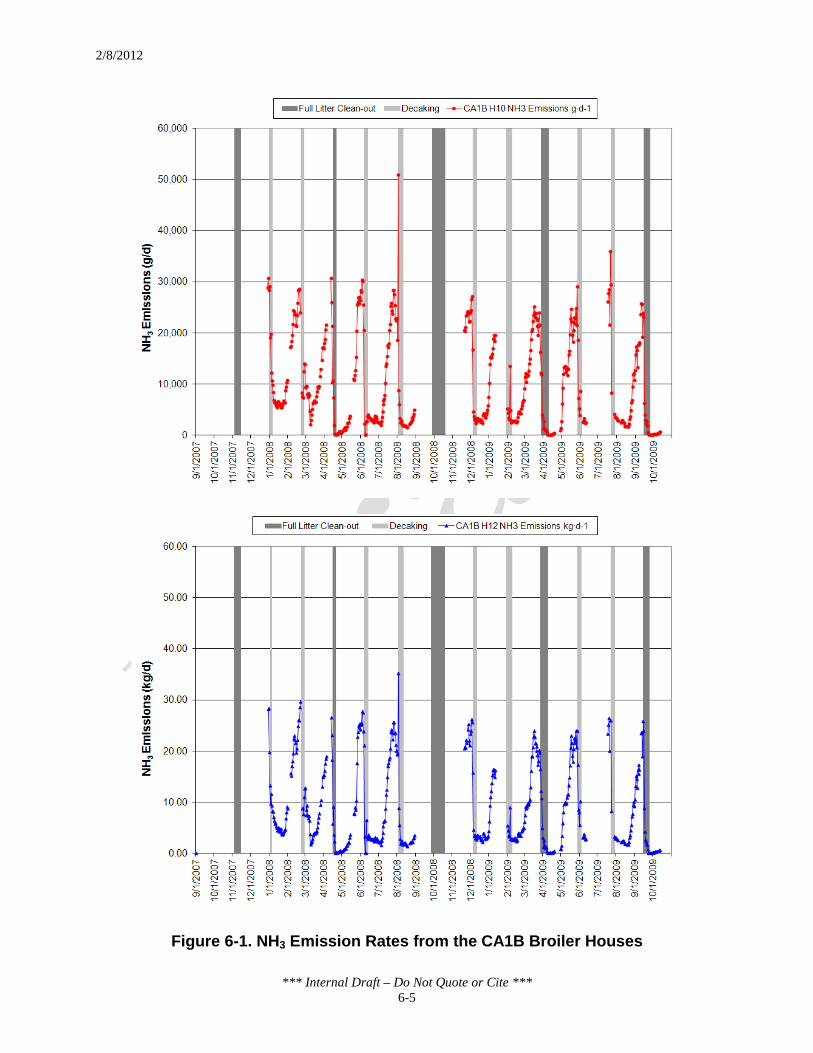
2/8/2012
*** Internal Draft – Do Not Quote or Cite *** 6-5
Figure 6-1. NH3 Emission Rates from the CA1B Broiler Houses

2/8/2012
*** Internal Draft – Do Not Quote or Cite *** 6-6
Figure 6-2. NH3 Emission Rates from the Kentucky Broiler Houses

2/8/2012
*** Internal Draft – Do Not Quote or Cite *** 6-7
6.2.2 Seasonal Trends
Figure 6-3 presents the daily NH3 emissions for the grow-out, decaking and full litter clean-out periods for all flocks monitored under the NAEMS, color coded by season. Figure 6-4, Figure 6-5. Figure 6-6 and Figure 6-7 present the same data shown in Figure 6-3, grouped by season and transitional periods between seasons. The black line on the figures represents the average NH3 emissions for all flocks.
Based on the seasonal plots, NH3 emissions from the grow-out, decaking and full litter clean-out periods tend to be higher than the average during the summer months and lower than average during the winter months. The plots for the seasonal classification (Figure 6-5. and Figure 6-6) also indicate NH3 emissions in the fall season are slightly above average for most of the flock. Furthermore, the average emissions rates for the four seasons suggest that spring is representative of the average emissions rate across all the houses. The graphs show that summer flocks also tended to have the highest NH3 emissions towards the end of the grow-out and litter removal periods. The only exception is the first monitored flock from KY1B-1 H5 that occurred in the transitional period from winter to spring (WI/SP).
Figure 6-3. NH3 Emissions by Flock, Color Coded by Season

2/8/2012
*** Internal Draft – Do Not Quote or Cite *** 6-8
Figure 6-4. NH3 Emissions from the Broiler Sites for Spring and Summer

2/8/2012
*** Internal Draft – Do Not Quote or Cite *** 6-9
Figure 6-5. NH3 Emissions from the Broiler Sites for Summer/Fall and Fall

2/8/2012
*** Internal Draft – Do Not Quote or Cite *** 6-10
Figure 6-6. NH3 Emissions from the Broiler Sites for Fall/Winter and Winter

2/8/2012
*** Internal Draft – Do Not Quote or Cite *** 6-11
Figure 6-7. NH3 Emissions from the Broiler Sites for Winter/Spring
6.3 H2S Emissions
6.3.1 General Trends
Figure 6-8 and Figure 6-9 present the daily H2S emission values calculated over the study period for the CA1B and Kentucky sites. The H2S emissions follow the same general trend as NH3 emissions (i.e., increasing emissions with bird age, with emissions dropping after birds are removed from the house). Figure 6-9 also shows that the H2S emissions rates tended to spike at site KY1B-1 H5.

2/8/2012
*** Internal Draft – Do Not Quote or Cite *** 6-12
Figure 6-8. H2S Emissions from the CA1B Broiler Houses
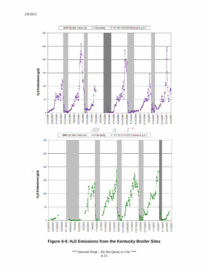
2/8/2012
*** Internal Draft – Do Not Quote or Cite *** 6-13
Figure 6-9. H2S Emissions from the Kentucky Broiler Sites
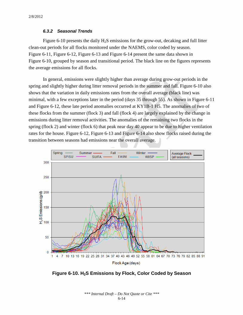
2/8/2012
*** Internal Draft – Do Not Quote or Cite *** 6-14
6.3.2 Seasonal Trends
Figure 6-10 presents the daily H2S emissions for the grow-out, decaking and full litter clean-out periods for all flocks monitored under the NAEMS, color coded by season. Figure 6-11, Figure 6-12, Figure 6-13 and Figure 6-14 present the same data shown in Figure 6-10, grouped by season and transitional period. The black line on the figures represents the average emissions for all flocks.
In general, emissions were slightly higher than average during grow-out periods in the spring and slightly higher during litter removal periods in the summer and fall. Figure 6-10 also shows that the variation in daily emissions rates from the overall average (black line) was minimal, with a few exceptions later in the period (days 35 through 55). As shown in Figure 6-11 and Figure 6-12, these late period anomalies occurred at KY1B-1 H5. The anomalies of two of these flocks from the summer (flock 3) and fall (flock 4) are largely explained by the change in emissions during litter removal activities. The anomalies of the remaining two flocks in the spring (flock 2) and winter (flock 6) that peak near day 40 appear to be due to higher ventilation rates for the house. Figure 6-12, Figure 6-13 and Figure 6-14 also show flocks raised during the transition between seasons had emissions near the overall average.
Figure 6-10. H2S Emissions by Flock, Color Coded by Season

2/8/2012
*** Internal Draft – Do Not Quote or Cite *** 6-15
Figure 6-11. H2S Emissions from the Broiler Sites for Spring and Summer

2/8/2012
*** Internal Draft – Do Not Quote or Cite *** 6-16
Figure 6-12. H2S Emissions from the Broiler Sites for Summer/Fall and Fall
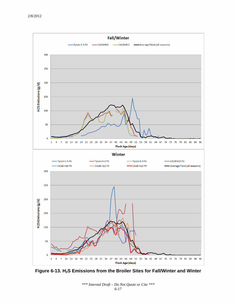
2/8/2012
*** Internal Draft – Do Not Quote or Cite *** 6-17
Figure 6-13. H2S Emissions from the Broiler Sites for Fall/Winter and Winter

2/8/2012
*** Internal Draft – Do Not Quote or Cite *** 6-18
Figure 6-14. H2S Emissions from the Broiler Sites for Winter/Spring
6.4 PM10 Emissions
6.4.1 General Trends
Figure 6-15 and Figure 6-16 present the daily PM10 emissions rates calculated over the study period for the CA1B and Kentucky sites, respectively. The figures show that emissions of PM10 tend to increase with bird age and weight and decrease during decaking and full litter clean-out periods (i.e., the same general trend as the other measured pollutants). However, the steep drop in PM10 emissions during litter removal periods is due to removal of the PM monitors for the first 4 to 9 days of the litter removal period. It is possible that spikes in PM10 emissions, similar to those seen for NH3 and H2S, occurred during these times; however, these spikes were not captured because the monitors were not operating. The PM10 measurements taken during litter removal periods reflect emissions from a clean house that is idle while waiting for the next flock of birds. The PM10 measurements do not reflect periods when the decaking or full litter clean-out activities were being conducted.

2/8/2012
*** Internal Draft – Do Not Quote or Cite *** 6-19
Figure 6-15. PM10 Emissions from the CA1B Broiler Houses

2/8/2012
*** Internal Draft – Do Not Quote or Cite *** 6-20
Figure 6-16. PM10 Emissions from the Kentucky Broiler Houses

2/8/2012
*** Internal Draft – Do Not Quote or Cite *** 6-21
6.4.2 Seasonal Trends
Figure 6-17 presents the daily PM10 emissions for the grow-out, decaking and full litter clean-out periods for all flocks monitored under the NAEMS, color coded by season. Figure 6-18, Figure 6-19, Figure 6-20 and Figure 6-21 present the same data shown in Figure 6-17, grouped by season. The black line on the figures represents the average emissions for all flocks.
These plots show that the PM10 emissions at the beginning of the grow-out period for several flocks were higher than the other flocks and were elevated for several days before returning to levels comparable with the other flocks. For site CA1B, the four flocks that stand out from the mean are flocks 6 and 7 from both Houses 10 and 12 for days 11 through 20 of the grow-out period. In addition, PM10 emissions were elevated from days 21 to 30 of the grow-out period for flock 2 at KY1B-2 H3. The grow-out periods for these five flocks occurred during the summer (see Figure 6-18) or during the transition period from summer to fall (see Figure 6-19). The confinement houses during these periods had above-average ambient temperatures and increased ventilation air flow rates, which could explain the increased PM10 emissions rates.
Emissions of PM10 also show seasonality with flocks. The PM10 emissions are higher than average from most flocks raised during the summer and below average from wintertime flocks. Emissions of PM10 for spring and fall flocks generally fall close to the average daily flock value.
Figure 6-17. PM10 Emissions by Flock, Color Coded by Season
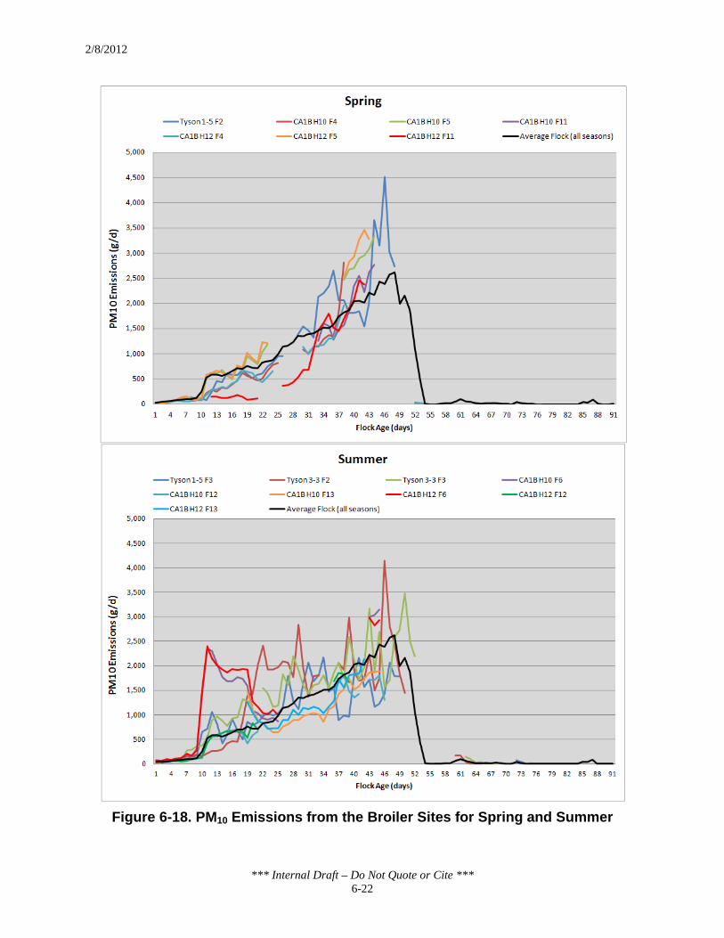
2/8/2012
*** Internal Draft – Do Not Quote or Cite *** 6-22
Figure 6-18. PM10 Emissions from the Broiler Sites for Spring and Summer
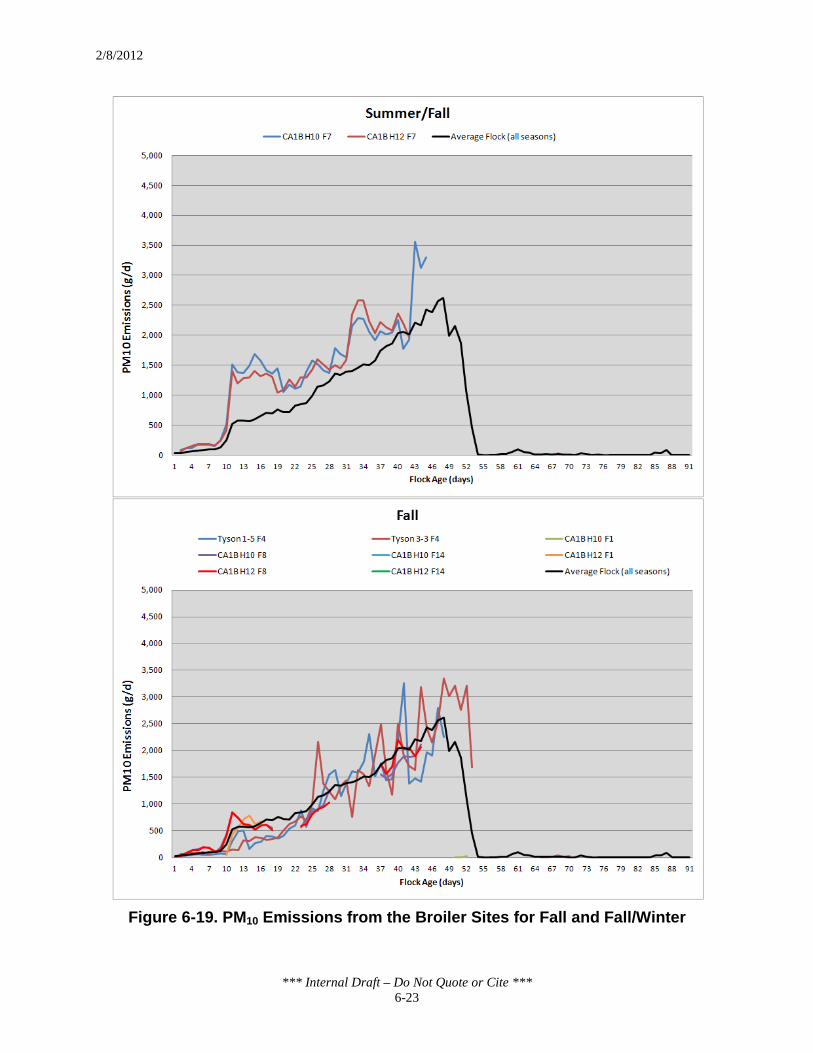
2/8/2012
*** Internal Draft – Do Not Quote or Cite *** 6-23
Figure 6-19. PM10 Emissions from the Broiler Sites for Fall and Fall/Winter

2/8/2012
*** Internal Draft – Do Not Quote or Cite *** 6-24
Figure 6-20. PM10 Emissions from the Broiler Sites for Fall/Winter and Winter
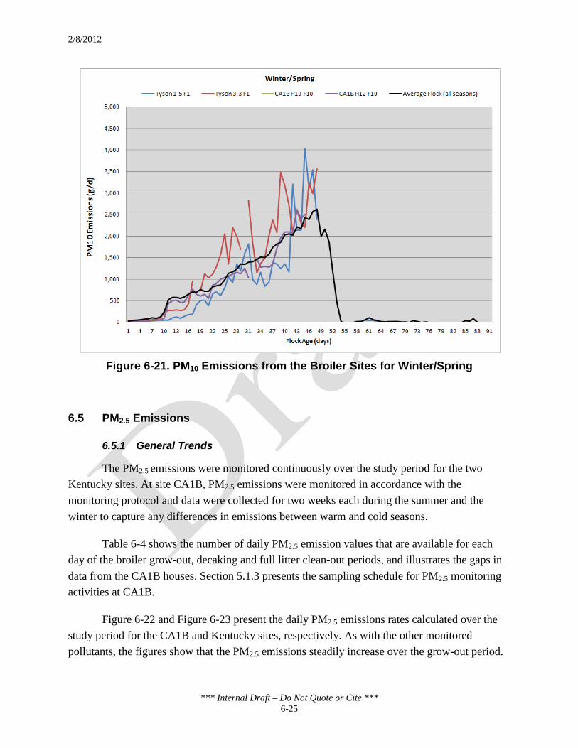
2/8/2012
*** Internal Draft – Do Not Quote or Cite *** 6-25
Figure 6-21. PM10 Emissions from the Broiler Sites for Winter/Spring
6.5 PM2.5 Emissions
6.5.1 General Trends
The PM2.5 emissions were monitored continuously over the study period for the two Kentucky sites. At site CA1B, PM2.5 emissions were monitored in accordance with the monitoring protocol and data were collected for two weeks each during the summer and the winter to capture any differences in emissions between warm and cold seasons.
Table 6-4 shows the number of daily PM2.5 emission values that are available for each day of the broiler grow-out, decaking and full litter clean-out periods, and illustrates the gaps in data from the CA1B houses. Section 5.1.3 presents the sampling schedule for PM2.5 monitoring activities at CA1B.
Figure 6-22 and Figure 6-23 present the daily PM2.5 emissions rates calculated over the study period for the CA1B and Kentucky sites, respectively. As with the other monitored pollutants, the figures show that the PM2.5 emissions steadily increase over the grow-out period.

2/8/2012
*** Internal Draft – Do Not Quote or Cite *** 6-26
Table 6-4. Available PM2.5 Emissions Days by Site
Cycle Day
Number of Available Daily PM2.5 Emissions Values
Cycle Day
Number of Daily PM2.5 Emissions Values
CA1B H10
CA1B H12
KY1B-1 H5
KY1B-2 H3
CA1B H10
CA1B H12
KY1B-1 H5
KY1B-1 H3
1 0 0 6 6 47 0 0 6 5 2 1 0 6 6 48 0 0 6 5 3 1 0 6 6 49 0 0 6 5 4 1 0 6 6 50 0 0 6 5 5 1 0 6 6 51 0 0 6 5 6 1 0 6 6 52 0 0 6 5 7 1 0 6 6 53 0 0 5 5 8 1 0 6 6 54 0 0 5 5 9 1 0 6 6 55 0 0 5 5 10 1 0 6 6 56 0 0 5 5 11 1 0 6 6 57 0 0 5 5 12 0 0 6 6 58 0 0 5 5 13 0 0 6 6 59 0 0 5 5 14 0 0 6 6 60 0 0 5 5 15 0 0 6 6 61 0 0 5 4 16 0 0 6 6 62 0 0 5 4 17 0 0 6 6 63 0 0 4 4 18 0 0 6 6 64 0 0 4 4 19 0 0 6 6 65 0 0 4 4 20 0 0 6 6 66 0 0 4 4 21 0 0 6 6 67 0 0 2 4 22 0 0 6 6 68 0 0 2 3 23 0 0 6 5 69 0 0 2 3 24 0 0 6 5 70 0 0 2 2 25 0 0 6 5 71 0 0 2 1 26 1 1 6 5 72 0 0 2 1 27 2 2 6 5 73 0 0 2 1 28 2 2 6 5 74 0 0 1 1 29 2 2 6 5 75 0 0 1 1 30 3 2 6 5 76 0 0 0 1 31 3 2 6 5 77 0 0 0 1 32 3 3 6 5 78 0 0 0 1 33 3 3 6 5 79 0 0 0 1 34 3 3 6 5 80 0 0 0 1 35 3 3 6 5 81 0 0 0 1 36 3 3 6 5 82 0 0 0 1 37 3 3 6 5 83 0 0 0 1 38 3 3 6 5 84 0 0 0 1 39 3 3 6 5 85 0 0 0 1 40 2 2 6 5 86 0 0 0 1 41 2 2 6 5 87 0 0 0 1 42 1 1 6 5 88 0 0 0 1 43 1 1 6 5 89 0 0 0 1 44 0 1 6 5 90 0 0 0 1 45 0 1 6 5 91 0 0 0 1 46 0 0 6 5 Total 53 43 276 252

2/8/2012
*** Internal Draft – Do Not Quote or Cite *** 6-27
Figure 6-22. PM2.5 Emissions from the CA1B Broiler Houses
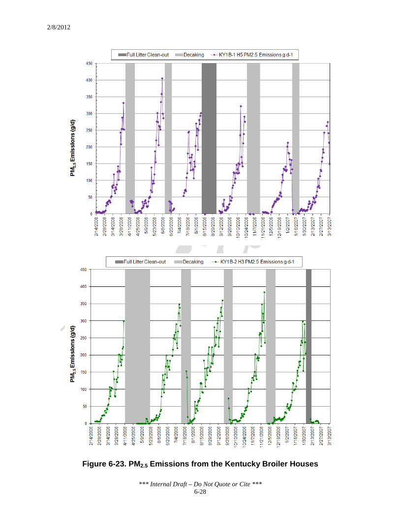
2/8/2012
*** Internal Draft – Do Not Quote or Cite *** 6-28
Figure 6-23. PM2.5 Emissions from the Kentucky Broiler Houses

2/8/2012
*** Internal Draft – Do Not Quote or Cite *** 6-29
Data for PM2.5 emissions were not collected at site CA1B during the decaking and full litter clean-out periods. At the Kentucky sites, the PM monitor was removed during the litter removal periods; monitoring resumed in 9 days, on average. As with PM10 emissions, the PM2.5 emissions values recorded during litter removal periods presented in Figure 6-23 correspond to the time when the house was sitting idle waiting for the next flock to be placed (i.e., PM2.5 emissions data were not collected while decaking and full litter clean-out activities were being conducted).
6.5.2 Seasonal Trends
Figure 6-24 presents daily PM2.5 emissions for the grow-out, decaking and full litter clean-out periods for all flocks monitored under the NAEMS, color coded by season. Figure 6- 25, Figure 6-26 and Figure 6-27 present the same data as Figure 6-24, grouped by season. The black line on the figures represents the average emissions for all flocks.
Because of the small number of PM2.5 emissions values available for site CA1B (see Table 6-4), the comparison of the seasonal trends among the different sites is limited. The average PM2.5 emissions values for the fall from CA1B House 10, flock 14, are for the first 10 days of the grow-out period and do not represent the emissions over the entire period. The data for the winter flocks are from measurements taken late in the grow-out period, when emission rates are peaking (emissions data for days early in the grow-out period or during decaking and full litter clean-out periods are not available). Based on the available data, emissions for summer are typically above average, with winter falling just below average. Fall and spring emissions are close to the overall average, except spring deviates late in the grow-out period.

2/8/2012
*** Internal Draft – Do Not Quote or Cite *** 6-30
Figure 6-24. PM2.5 Emissions by Flock, Color Coded by Season

2/8/2012
*** Internal Draft – Do Not Quote or Cite *** 6-31
Figure 6-25. PM2.5 Emissions from the Broiler Sites for Spring and Summer

2/8/2012
*** Internal Draft – Do Not Quote or Cite *** 6-32
Figure 6-26. PM2.5 Emissions from the Broiler Sites for Fall and Fall/Winter

2/8/2012
*** Internal Draft – Do Not Quote or Cite *** 6-33
Figure 6-27. PM2.5 Emissions from the Broiler Sites for Winter and Winter/Spring
2/8/2012
*** Internal Draft – Do Not Quote or Cite *** 6-34
6.6 TSP Emissions
6.6.1 General Trends
Figure 6-28 and Figure 6-29 present the annual emission plots for TSP for the CA1B and Kentucky sites, respectively. The plots of annual emissions from the CA1B site reflect the abbreviated sampling schedule for those houses. The CA1B study monitored one week out of every 8 weeks; in practice, this yielded 7 weeks of data collection. Table 6-5 shows the number of daily TSP emission values that are available for each day of the broiler grow-out, decaking and full litter clean-out periods, and illustrates the gaps in data from the CA1B houses. Section 5.1.3 presents the sampling schedule for TSP monitoring activities at CA1B. The Kentucky sites monitored TSP emissions continuously over their study period.
In general, the TSP emissions trend was similar to the other particulate sizes in that TSP emissions steadily increase over the grow-out period and decrease over the decaking and full litter clean-out periods. Data for TSP emissions were not collected from either house at the CA1B site during decaking or full litter clean-out periods. At the Kentucky sites, the PM monitor was removed during litter removal activities and reestablished in 7 to 10 days. As with PM10 and PM2.5 emissions, the TSP emissions values for either type of litter removal period reflect emissions from the time when the house was sitting idle waiting for the next flock to be placed. The timing of the monitor removal makes it appear as though there is an abrupt decline in emissions when transitioning from the grow-out period to litter removal period, as opposed to a data gap.

2/8/2012
*** Internal Draft – Do Not Quote or Cite *** 6-35
Table 6-5. Available Daily TSP Emission Values by Site
Cycle Day
Number of Daily TSP Emissions Values Cycle Day
Number of Daily TSP Emissions Values CA1B H10
CA1B H12
KY1B-1 H5
KY1B-2 H3 CA1B
H10 CA1B H12
KY1B-1 H5
KY1B-2 H3
1 0 0 6 6 47 0 0 6 5 2 0 1 6 6 48 0 0 6 5 3 0 1 6 6 49 0 0 6 5 4 0 1 6 6 50 0 0 6 5 5 0 1 6 6 51 0 0 6 5 6 0 1 6 6 52 0 0 6 5 7 0 1 6 6 53 0 0 5 5 8 0 1 6 6 54 0 0 5 5 9 0 1 6 6 55 0 0 5 5 10 0 1 6 6 56 0 0 5 5 11 0 0 6 6 57 0 0 5 5 12 0 0 6 6 58 0 0 5 5 13 1 0 6 6 59 0 0 5 5 14 1 0 6 6 60 0 0 5 5 15 1 0 6 6 61 0 0 5 4 16 1 0 6 6 62 0 0 5 4 17 1 0 6 6 63 0 0 4 4 18 1 0 6 6 64 0 0 4 4 19 0 0 6 6 65 0 0 4 4 20 0 0 6 6 66 0 0 4 4 21 0 0 6 6 67 0 0 2 4 22 1 0 6 6 68 0 0 2 3 23 1 1 6 5 69 0 0 2 3 24 1 1 6 5 70 0 0 2 2 25 1 1 6 5 71 0 0 2 1 26 1 1 6 5 72 0 0 2 1 27 1 1 6 5 73 0 0 2 1 28 2 2 6 5 74 0 0 1 1 29 3 3 6 5 75 0 0 1 1 30 3 3 6 5 76 0 0 0 1 31 3 4 6 5 77 0 0 0 1 32 4 4 6 5 78 0 0 0 1 33 4 4 6 5 79 0 0 0 1 34 3 4 6 5 80 0 0 0 1 35 2 1 6 5 81 0 0 0 1 36 1 0 6 5 82 0 0 0 1 37 0 0 6 5 83 0 0 0 1 38 0 0 6 5 84 0 0 0 1 39 0 0 6 5 85 0 0 0 1 40 0 0 6 5 86 0 0 0 1 41 0 0 6 5 87 0 0 0 1 42 0 0 6 5 88 0 0 0 1 43 0 0 6 5 89 0 0 0 1 44 0 0 6 5 90 0 0 0 1 45 0 0 6 5 91 0 0 0 1 46 0 0 6 5 Total 37 39 276 252
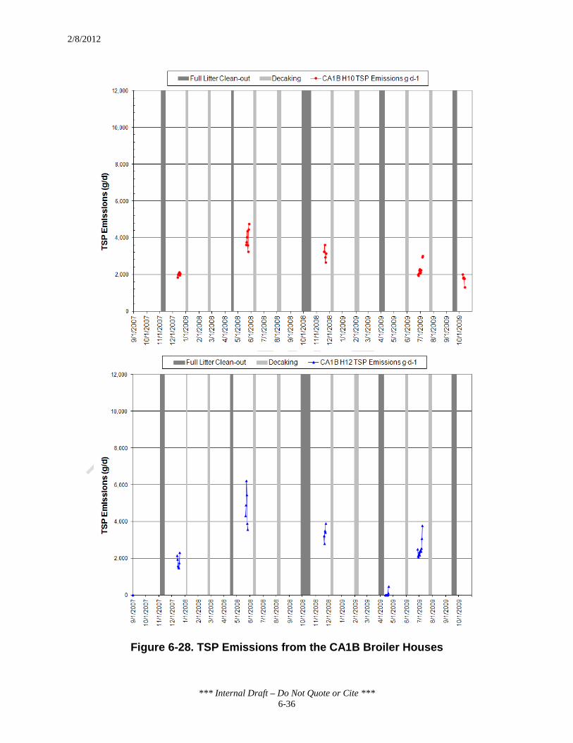
2/8/2012
*** Internal Draft – Do Not Quote or Cite *** 6-36
Figure 6-28. TSP Emissions from the CA1B Broiler Houses

2/8/2012
*** Internal Draft – Do Not Quote or Cite *** 6-37
Figure 6-29. TSP Emissions from the Kentucky Broiler Houses

2/8/2012
*** Internal Draft – Do Not Quote or Cite *** 6-38
6.6.2 Seasonal Trends
Figure 6-30 presents daily TSP emissions for the grow-out, decaking and full litter clean-out periods for all flocks monitored under the NAEMS, color coded by season. The data spans both the grow-out and litter removal periods. The black line represents the average emissions for all flocks.
Comparisons between the TSP emissions for the different houses were limited due to the intermittent sampling periods for the CA1B houses. Available TSP emissions values from the CA1B houses are comparable to the emissions from the Kentucky houses, indicating that the emissions are representative of the housing type. The TSP emissions displayed a seasonal trend with emissions from summertime flocks typically above average and wintertime flocks below average. Figure 6-31, Figure 6-32 and Figure 6-33 present separate plots for each seasonal classification.
Figure 6-30. TSP Emissions by Flock, Color Coded by Season

2/8/2012
*** Internal Draft – Do Not Quote or Cite *** 6-39
Figure 6-31. TSP Emissions from the Broiler Sites for Spring and Summer

2/8/2012
*** Internal Draft – Do Not Quote or Cite *** 6-40
Figure 6-32. TSP Emissions from the Broiler Sites for Fall and Fall/Winter

2/8/2012
*** Internal Draft – Do Not Quote or Cite *** 6-41
Figure 6-33. TSP Emissions from the Broiler Sites for Winter and Winter/Spring

2/8/2012
*** Internal Draft – Do Not Quote or Cite *** 6-42
6.7 VOC Emissions
6.7.1 General Trends
Figure 6-34 presents the annual emission plots for VOCs at the Kentucky broiler houses. The VOC data were collected continuously in the form of NMHC readings at the Kentucky sites. In general, emissions increase with bird age and weight, though the pattern is not as distinct as with the other gaseous species. Emissions of VOC are comparable between the two Kentucky houses.
At site CA1B, grab samples were collected periodically during the course of the study. Seven (7) grab samples were collected at House 10 and six (6) grab samples were collected at House 12. The samples were collected on nonconsecutive days from July 14, 2010 to October 7, 2010. Graphs of the grab sample data were not prepared because the limited number of data values and the short-term sampling period are not sufficient to indicate an emissions trends.
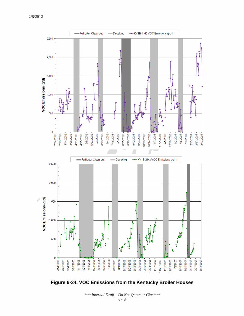
2/8/2012
*** Internal Draft – Do Not Quote or Cite *** 6-43
Figure 6-34. VOC Emissions from the Kentucky Broiler Houses

2/8/2012
*** Internal Draft – Do Not Quote or Cite *** 6-44
6.7.2 Seasonal Trends
Figure 6-35 presents flock VOC emissions for the Kentucky broiler houses, color coded by season. The data spans both the grow-out and litter removal periods. The black line represents average emissions for all flocks.
Based on the limited data (the two Kentucky houses were monitored for only one year each), VOC emissions do not appear to display any seasonality. Flock emissions for the various seasons tend to fluctuate across the average line (see Figure 6-36, Figure 6-37 and Figure 6-38). Emissions of VOC at site KY1B-1 H5 appear slightly higher than KY1B-2 H3 especially during the middle portion of the cycle, approximately days 35 to 50. Both house seem comparable, with KY1B-1 H5 running slightly higher than KY1B-2 H3, especially during the middle portion of the cycle (approximately day 35 to 50).
Figure 6-35. VOC Emissions by Flock, Color Coded by Season
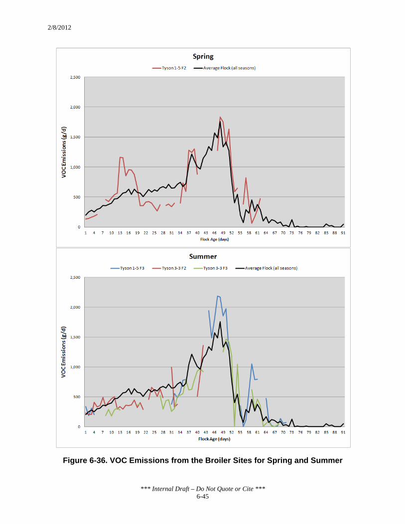
2/8/2012
*** Internal Draft – Do Not Quote or Cite *** 6-45
Figure 6-36. VOC Emissions from the Broiler Sites for Spring and Summer

2/8/2012
*** Internal Draft – Do Not Quote or Cite *** 6-46
Figure 6-37. VOC Emissions from the Broiler Sites for Fall and Fall/Winter

2/8/2012
*** Internal Draft – Do Not Quote or Cite *** 6-47
Figure 6-38. VOC Emissions from the Broiler Sites for Winter and Winter/Spring

2/8/2012
*** Internal Draft – Do Not Quote or Cite *** 7-1
7.0 DEVELOPMENT OF EEMS FOR GROW-OUT PERIODS
This section presents the statistical approach the EPA used to develop the EEMs for the grow-out periods associated with broiler operations using the NAEMS data. This section uses NH3 as the example pollutant to demonstrate the statistical method. The remaining pollutants (H2S, PM10, PM2.5, TSP and VOCs) followed this statistical approach and the resulting EEMs are presented in Section 8.
For each pollutant, the EPA developed an EEM for each of three sets of predictor variables: variables based on animal inventory alone (I), inventory variables supplemented with ambient meteorology (IA), and the combination of these variables with variables describing confinement conditions (IAC). For example, the I EEMs provide emissions estimates based on input data that characterize the bird population in the house (e.g., total bird inventory in the house and their average weight). These data are recorded routinely by growers and would not require additional data collection systems. For the IA EEMs, the input data include the bird inventory, average bird weight and ambient meteorological conditions (e.g., ambient temperature and relative humidity). Under the NAEMS, the ambient data were collected by a monitoring system installed at the participating farm. To apply the EEMs, ambient data gathered by other sources (e.g., National Weather Service stations) that are representative of the applicable site can be used if site-specific data are not available. For the IAC EEMs, the input data include the data used for the I and IA EEMs and data for confinement conditions (e.g., house temperature and relative humidity) that were collected for the NAEMS by a monitoring system installed in each house.
In previous sections, the terms “parameter” and “estimate” were used to describe the data and data collection methods used in the NAEMS. In this section, these terms are used in their formal statistical context. The term “parameter” refers to unknown constants (regression coefficients, the variance, and the auto-correlation coefficient, described below) whose values give the EEMs their shape. The EEM equations given in this section use Greek letters to represent parameters. The term “estimate” refers to the best approximation of a parameter value determined by fitting the EEM to the NAEMS data. The term “predict” refers to obtaining a value of emissions using the EEM, including the use of predictor variables and estimated parameters.
Each EEM produces a point prediction and a 95 percent prediction interval for pollutant emissions. A point prediction is a single value of emissions produced by the mean trend function (described below) for a given set of values of the predictor variables. A 95 percent prediction interval consists of two numbers, a lower and upper bound, on each side of the point prediction that quantify uncertainty about the point prediction due to natural variability in emissions and
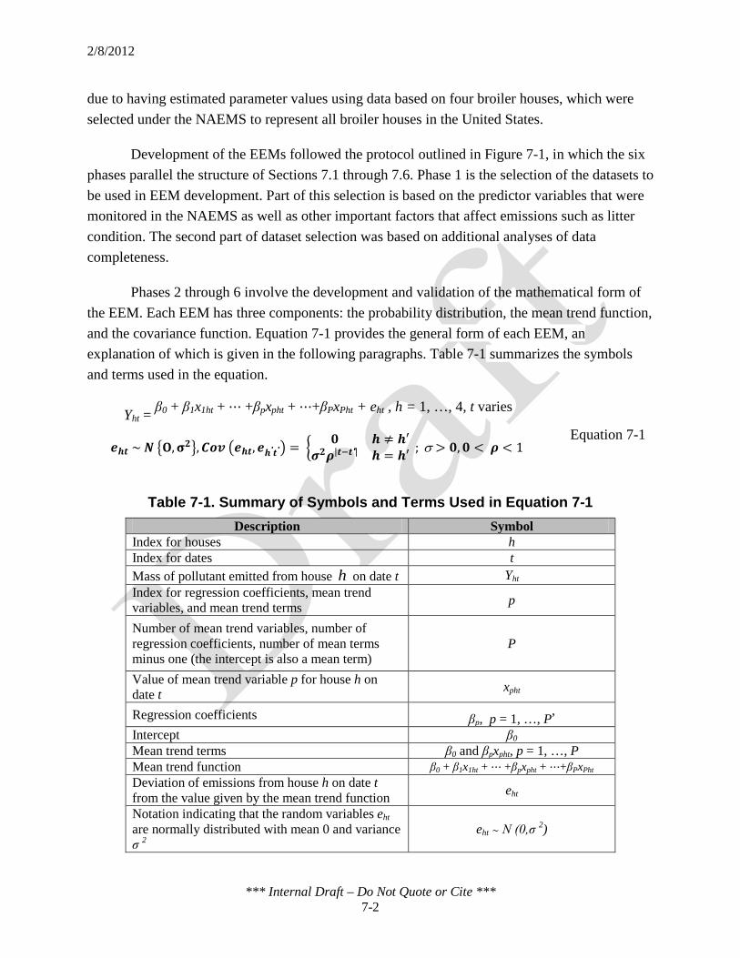
2/8/2012
*** Internal Draft – Do Not Quote or Cite *** 7-2
due to having estimated parameter values using data based on four broiler houses, which were selected under the NAEMS to represent all broiler houses in the United States.
Development of the EEMs followed the protocol outlined in Figure 7-1, in which the six phases parallel the structure of Sections 7.1 through 7.6. Phase 1 is the selection of the datasets to be used in EEM development. Part of this selection is based on the predictor variables that were monitored in the NAEMS as well as other important factors that affect emissions such as litter condition. The second part of dataset selection was based on additional analyses of data completeness.
Phases 2 through 6 involve the development and validation of the mathematical form of the EEM. Each EEM has three components: the probability distribution, the mean trend function, and the covariance function. Equation 7-1 provides the general form of each EEM, an explanation of which is given in the following paragraphs. Table 7-1 summarizes the symbols and terms used in the equation.
Yht = β0 + β1x1ht + ⋯ +βpxpht + ⋯+βPxPht + eht , h = 1, …, 4, t varies
Equation 7-1 𝒆𝒉𝒕 ~ 𝜨 𝐎, 𝛔𝟐, 𝑪𝒐𝒗 𝒆𝒉𝒕, 𝒆𝒉′𝒕′ = 𝟎 𝒉 ≠ 𝒉′
𝝈𝟐𝝆|𝒕−𝒕′| 𝒉 = 𝒉′ ; σ > 𝟎, 𝟎 < 𝝆 < 1
Table 7-1. Summary of Symbols and Terms Used in Equation 7-1 Description Symbol
Index for houses h Index for dates t Mass of pollutant emitted from house h on date t Yht Index for regression coefficients, mean trend variables, and mean trend terms p
Number of mean trend variables, number of regression coefficients, number of mean terms minus one (the intercept is also a mean term)
P
Value of mean trend variable p for house h on date t xpht
Regression coefficients βp, p = 1, …, P,
Intercept β0 Mean trend terms β0 and βpxpht, p = 1, …, P
Mean trend function β0 + β1x1ht + ⋯ +βpxpht + ⋯+βPxPht Deviation of emissions from house h on date t from the value given by the mean trend function eht
Notation indicating that the random variables eht are normally distributed with mean 0 and variance σ 2
eht ∼ N (0,σ 2)

2/8/2012
*** Internal Draft – Do Not Quote or Cite *** 7-3
Table 7-1. Summary of Symbols and Terms Used in Equation 7-1 Description Symbol
Notation indicating the serial correlation between emissions observed day-to-day Cov(eht, eh´t´) Variance of the random deviations eht (a measure of both natural variability and uncertainty)
σ2
The correlation between two deviations from the same house, separated by one day ρ
In the first line of Equation 7-1, Yht represents pollutant emissions from house h on date t,
where the index h takes values 1 through 4, corresponding to monitored houses CA1B H10, CA1B H12, KY1B-1 H5 and KY1B-2 H3, respectively. Values of t are nested within values of h, so that dates for different houses can be the same or different. The values that t takes for each house over the grow-out periods are given in Section 5.3.1. Due to missing data, the dates were not always consecutive.
The expression β0 + β1x1ht + ⋯ +βpxpht + ⋯+βPxPht is the “mean trend function,” and it describes the relationship between the predictor variables and the expected value of pollutant emissions. In the mean trend function, xpht represents the value of the pth mean trend variable for house h on date t, the symbol βp denotes the regression coefficient for that variable and the symbol β0 represents the intercept. The mean trend variables differ from the predictor variables in that they represent the functional form through which the predictor variables enter the mean trend function. This distinction will be discussed in detail in Section 7.3. Lower-case p is an index for regression coefficients βp, mean trend variables xpht, and their products, the non-intercept mean trend terms βpxpht . The index p takes values 1,⋯, P, so that upper-case P is the number of non-intercept mean trend terms.
In the second line of Equation 7-1, the symbol eht represents the deviation of emissions from house h on date t from the value given by the mean trend function. Because the eht are random variables, full EEM specification requires selecting a probability distribution and an appropriate covariance function for them. The notation eht ∼ N (0,σ 2) translated, says that the random variables eht are normally distributed with mean 0 and variance σ 2. The expression for the covariance, Cov(eht, eh´t´), describes the serial correlation between emissions observed day-to-day. Because the eht are random variables, and because the Yht are functions of them, the Yht are also random variables. Although the values of the mean trend variables xpht differ for different values of h and t, for one specific combination of values of h and t, they are fixed (not random), known quantities. All of the parameters in the EEM (the intercept, β0; the regression coefficients, βp; the variance, σ 2; and the auto-correlation coefficient, ρ) were estimated based on the NAEMS data. The estimates of the parameters are written with “hats” on top of them (e.g., 𝛽0).

2/8/2012
*** Internal Draft – Do Not Quote or Cite *** 7-4
The choice of probability distribution, the variables included in the mean trend function, and the form of the covariance function were all based on analyses of a subset of the NAEMS data called the “base” dataset, validated using another subset of the NAEMS data called the “cross-validation” dataset, and then modified and re-validated when necessary. After the final mathematical forms were chosen, the EPA re-estimated the parameters using the “full” dataset (i.e., the combined base and cross-validation datasets).
The following sections describe this process in detail. Section 7.1 describes selection of the full, base, and cross-validation datasets based on data completeness. Section 7.2 shows why the normal distribution was selected as the probability distribution. Section 7.3 details development of candidate mean trend variables from the predictor variables. Section 7.4 lists components considered for the covariance function and tells why some were included and others not. Section 7.5 describes the process through which final mean trend variables were chosen from the candidates. Section 7.6 describes how the EEMs are used to generate point and interval predictions for a single day and for the sum of days. The EEM development and results for H2S, PM10, PM2.5, TSP and VOCs are explained in Section 8.

2/8/2012
*** Internal Draft – Do Not Quote or Cite *** 7-5
Figure 7-1. General Approach for EEM Development

2/8/2012
*** Internal Draft – Do Not Quote or Cite *** 7-6
7.1 Selecting Datasets
The data used to develop the EEMs for NH3 were collected under the NAEMS from four houses at three sites: CA1B H10; CA1B H12; KY1B-1 H5; and KY1B-2 H3. Table 7-2 lists, for each of the three categories [animal inventory (I), ambient meteorology (A) and confinement conditions (C)], available predictor variables, the definitions and units of measure for each. Although ventilation flow rate and differential static pressure were monitored at each of the houses, they were not considered for use as confinement predictor variables for a variety of reasons. Because pollutant emissions are calculated using flow rate, and flow rate is calculated using differential pressure, the validity of using these as predictor variables is questionable. Additionally, the EPA did not consider ventilation flow rate and differential static pressure as predictor variables because these values are not expected to be readily available. For the NAEMS, differential static pressure ports were installed in the monitored houses and the ventilation flow rate values were calculated using continuous measurements of fan operational status (on/off), differential static pressure and fan-specific performance curves. In some cases, the flow rates of selected fans were directly measured using anemometers. The EPA does not expect that these types of monitoring systems and data will be available at typical broiler operations.
As explained in Section 5, the EPA did not use negative emissions to develop EEMs. Additionally, the EPA identified cases late in the grow-out period where bird inventory values remained constant for several consecutive dates. Figure 7-2 shows the number of birds for each date for the first flock monitored at KY1B-1 H5. The red box on the figure highlights the constant inventory values that were removed from the full dataset. This phenomenon occurred for every flock at sites KY1B-1 and KY1B-2, for 5 out of 14 flocks at CA1B H10, and for two flocks at CA1B H12. The EPA contacted the researchers for the California and Kentucky sites and industry representatives to determine whether the constant bird inventory values were valid. These contacts confirmed that the flat inventory values likely did not reflect the number of birds in the house on those dates. According to these contacts, to avoid stressing the birds in the last days of the grow-out period before harvesting, farm personnel did not enter the houses to count mortalities. In these instances, the personnel entered the same number of birds for several consecutive dates.

2/8/2012
*** Internal Draft – Do Not Quote or Cite *** 7-7
Table 7-2. Predictor Variables
Category Predictor Variablea Definition Units
I: Inventory
birds* Number of birds Thousands of birds
avem* Average live bird mass Kilograms (kg)
buildup* Number of flocks since last full litter clean-out in house Number of flocks
A: Ambient meteorology
ta* Temperature outside house o C
ha* Relative humidity outside house % pa* Barometric pressure outside house kilopascals (kPa)
C: Confinement conditions
tc* Temperature inside house o C
hc* Relative humidity inside house % a An asterisk (*) is used to note that these predictor variables are the original values submitted to the EPA before the data were centered and scaled (see Section 7.3.1).
Figure 7-2. Example of Constant Late-Period Bird Inventory

2/8/2012
*** Internal Draft – Do Not Quote or Cite *** 7-8
Because it was unclear whether these constant inventory values represented the number of birds in the house on that date, the EPA excluded from the full dataset observations that satisfied the following criteria. If the number of birds in the house on date t+1 was equal to the number of birds on date t, and these dates occurred at the end of the grow-out period, the observation for date t+1 was excluded. Using this approach, the EPA excluded 44 observations for the grow-out period data for all sites, houses and flocks.
Table 7-3 shows the observations available for each monitoring site after exclusion of negative NH3 emissions and constant late-period inventory values. For example, the total number of grow-out period observations for site CA1B H10 is 642, the number of days for which the NH3 emissions value was available is 382, and the percent available is 60 percent. Although sites KY1B-1 and KY1B-2 conducted monitoring for approximately one year while site CA1B monitored for two years, the greater level of data completeness for KY1B-1 and KY1B-2 caused the number of available observations to be on the order of only 100 days fewer for the houses at each of the Kentucky sites than for the two houses at CA1B.
Table 7-3. Data Completeness for NH3
Season Description
CA1B KY1B-1 KY1B-2
All Houses House 10 House 12 House 5 House 3
All No. of grow-out dates 642 647 288 267 1,844 No. of NH3 days available 382 385 280 232 1,279 Percent complete 60% 60% 97% 87% 69%
Winter
No. of grow-out dates 150 153 87 74 464 No. of NH3 dates available 100 105 80 50 335
Percent complete 66% 69% 92% 68% 72%
Spring
No. of grow-out dates 157 158 83 55 453 No. of NH3 dates available 133 134 82 49 398
Percent complete 85% 85% 99% 89% 88%
Summer
No. of grow-out days 156 157 55 74 442 No. of NH3 dates available 109 108 55 70 342
Percent complete 70% 69% 100% 95% 77%
Fall No. of grow-out dates 179 179 63 64 485 No. of NH3 days available 40 38 63 63 204 Percent complete 22% 21% 100% 98% 42%

2/8/2012
*** Internal Draft – Do Not Quote or Cite *** 7-9
7.1.1 Full dataset
To ensure that the data selected for EEM development were representative of more than one of the monitored sites, the EPA limited the dataset for use in EEM development to those records for which data values were available for all of the inventory, ambient, and confinement predictor variables. To identify this refined dataset, the EPA first evaluated the data records available for the I EEM.
The variables EPA considered for the I EEM were birds* and avem*. All of the 1,279 days with NH3 observations include values for birds*; however, 32 values for avem* were missing. Examination of the sites, houses and dates for which avem* values are missing shows that their absence appeared to be random (i.e., not all missing observations occur when NH3 emissions are high or low). To confirm that the missing data would not bias the development of EEMs, the EPA compared the distribution of emission on the days with the missing values to the distribution of emissions in the full dataset across the quartiles (i.e., minimum, Q1, Q2, Q3, Q4, and maximum). This five-number summary for NH3 emissions for the 32 dates missing avem* is 0.08, 3.2, 9.3, 20 and 36, while the five-number summary over all 1,279 dates is 0.06, 3.3, 9.4, 19 and 36. Because the numbers for each component of the five-number summary are similar in magnitude, the EPA concluded that the distribution of the missing values was random. Excluding the 32 records for which avem* values are not available results in a total of 1,247 observations for use in developing the I EEM for NH3.
The ambient variables considered by EPA for the IA EEM were ta*, ha* and pa*. Of the 1,247 observations in the NH3 dataset, the number of missing values for each of the ambient variables is, respectively, 23, 23 and 9. Not all of the missing data occurred on the same days, thus there was a total of 36 missing observations. Excluding these values leaves 1,211 observations for the NH3 dataset. Although wind speed, wind direction, and solar radiation were recorded at site CA1B, these data were not recorded at sites KY1B-1 and KY1B-2. Consequently, the EPA excluded these data from consideration. Confinement variables considered were tc* and hc*. Of the 1,247 observations for which none of the NH3 emissions or the inventory variables are missing, the number of missing values for tc* and hc* are 0 and 5, respectively. The five observations missing for hc* correspond to missing observations of other variables. Therefore, the EPA chose the data subset containing the 1,211observations for which none of the variables ta*, ha*, pa*, tc* or hc* are missing. Hereafter, the EPA refers to this dataset as the “full” dataset.
7.1.2 Base and Cross-Validation Datasets
As one means of evaluating EEM performance, the EPA randomly selected 217 (approximately 20 percent) of the 1,211 observations in the full dataset to withhold as the “cross-

2/8/2012
*** Internal Draft – Do Not Quote or Cite *** 7-10
validation” dataset. The remaining 994 observations are referred to as the “base” dataset. The EPA made decisions regarding the probability distribution, candidate mean trend variables and the covariance function using the base dataset for exploratory analyses, initial parameter estimation and tests of the significance of covariance parameters.
To select the final mean trend variables, the EPA primarily used p-values calculated on the base dataset to determine whether to keep or eliminate terms in a backward-elimination process. At each step in the backward-elimination process, however, the EPA also compared emissions predicted by the EEM to measured emissions contained in the cross-validation dataset. This practice, described in more detail in Section 7.5.1, ensured that the statistical significance of the estimated regression coefficients captured trends that applied generally, rather than over-fitting the data.
Analysis of cross-validation fit statistics and plots of cross-validation residuals also helped to validate the overall mathematical form of the EEM. The EPA performed multiple iterations of making EEM decisions in Phases 1 through 5, validating the resulting EEMs, modifying decisions, and re-validating. One of the decisions the EPA modified was the means of choosing the cross-validation dataset.
Initially, the EPA constructed the cross-validation dataset by withholding data for entire flocks. Of the 40 flocks in the NAEMS data, the EPA withheld data for six flocks that were chosen so that both the base and cross-validation datasets contained flocks from each season-site combination. A validation analysis later showed that the initial selection of cross-validation dataset resulted in disproportionate representation of different values of buildup in the two datasets. Buildup was not initially included as a predictor variable, and this same validation analysis led to an investigation of the data that revealed its importance.
The EPA attempted to modify selection of the cross-validation flocks to evenly represent site-season-buildup combinations in both the base and cross-validation datasets. However, due to the patterns of missing data, it was not possible to choose entire flocks in this manner without over-representing the Kentucky sites in the cross-validation dataset. On a flock-by-flock basis, the Kentucky flocks had fewer missing values than the flocks at site CA1B.
The EPA therefore chose to randomly select observations to withhold as the cross-validation dataset. To ensure that disproportionate representation of one or more sets of conditions in the cross-validation and base datasets chosen in this manner would not affect results, the EPA created two additional cross-validation datasets with corresponding base datasets and checked the results for the two additional cross-validation datasets for gross aberrations.

2/8/2012
*** Internal Draft – Do Not Quote or Cite *** 7-11
7.2 Choosing the Probability Distribution
Identifying the appropriate probability distribution ensures the validity of the p-values that are used to determine the statistical significance of regression coefficient estimates. The appropriate probability distribution is also needed to produce prediction intervals that quantify the uncertainty regarding the point predictions of NH3 emissions. Many physical phenomena are normally distributed under a fixed set of conditions, and the point predictions and 95 percent prediction intervals generated from the normal distribution are easy for the EEM user to implement and interpret. Therefore, the normal distribution is commonly used unless there is substantial evidence that another distribution is more appropriate.
The EPA plotted the empirical distribution (i.e., histogram) of observed NH3 emissions to determine whether use of the normal distribution could be justified. Figure 7-3 shows that there are many NH3 observations at lower values, with a single peak around 2.5 kg, and the number of observations decreases as emissions increase. In statistical jargon, the empirical distribution is unimodal and skew right. This observation might at first seem to provide evidence against using the symmetric and bell-shaped normal distribution, but the second line of Equation 7-1 does not say that NH3 emissions under all conditions have the same distribution. Instead, the equation says that the distribution of the deviations from the mean trend function, eht, are normally distributed. In other words, if the number of birds was 20,000 and the temperature was 20o C, NH3 emissions would have a symmetric and bell-shaped normal distribution centered at the value given by the mean trend function. For a different number of birds and temperature, the bell-shaped curve would be centered in a different location.

2/8/2012
*** Internal Draft – Do Not Quote or Cite *** 7-12
Figure 7-3. Histogram of NH3 Emissions in the Base Dataset
Because aggregating all conditions into a single histogram masks differences in the distribution for different sets of conditions, the EPA separated the base dataset into bins according to values of average bird mass. Bin 1 contains the observations for which average bird mass takes values (in kg) 0.0 to 0.5; bin 2, 0.5 to 1.0; bin 3, 1.0 to 1.5; bin 4, 1.5 to 2.0; bin 5, 2.0 to 2.5; and bin 6, 2.5 to 3.0. The disaggregated histograms given in Figure 7-4 show that the NH3 distribution for bins 1 and 2 are skew right, those for bins 3 and 5 are symmetric, and those for bins 4 and 6 are skew left. Further disaggregation according to the values of other variables shows a variety of empirical distributions for different sets of conditions, and the skew-right pattern is by no means ubiquitous. There are not enough observations under any specific set of conditions to use the empirical distribution to determine the true distribution. Therefore, in the absence of strong evidence against doing so, the EPA used the normal distribution.

2/8/2012
*** Internal Draft – Do Not Quote or Cite *** 7-13
Figure 7-4. Histograms by avem Bins
2/8/2012
*** Internal Draft – Do Not Quote or Cite *** 7-14
7.3 Developing Candidate Mean Trend Variables
Development of candidate mean trend variables requires first choosing the appropriate functional form to describe the dependence of pollutant emissions on each predictor variable. Section 7.3.1 describes how one or more main effect mean trend variables were created as functions of the predictor variables. Section 7.3.2 explains the importance of including interactions between main effect mean trend variables, and shows how the EPA determined what level of interactions to include as candidate mean trend variables.
7.3.1 Choosing Predictor Variable Functional Forms
The EPA used a variety of exploratory plots, existing knowledge of the chemistry through which NH3 emissions are formed in a broiler confinement house, and results from other studies to discover functional forms describing the relationship between NH3 emissions and the predictor variables listed in Table 7-2. For continuous predictor variables, EPA prepared scatter plots of emissions versus the variable to determine if a relationship exists. If emissions increase (or decrease) as the predictor variable increases, and the rate of increase (or decrease) does not change, then a linear function of the predictor variable is appropriate. If emissions increase (or decrease) as the predictor variable increases, but the slope changes, a variety of functions could be considered, one of which is the exponential function. If emissions increase and then decrease (or decrease and then increase), this single change in direction of the relationship could be represented with a quadratic function. If there were two changes of direction (e.g., if emissions decrease, increase, then decrease or vice versa), a cubic polynomial would be appropriate. For discrete variables such as buildup, the decision is whether to allow each value of the variable (e.g., 0, 1, 2, 3, 4 and 5) to have a different effect on emissions, or whether to consolidate some of the values into a smaller number of categories.
Figure 7-5 displays a scatter plot of NH3 emissions versus average live bird mass aggregated over all sites. The figure shows that, for values of avem* near 0, emissions range from 0 to approximately 15 kg, forming a “tail” on the leftmost side of the graph. The high variability in values decreases before average live bird mass reaches 0.125 kg. The plot slopes upward, with increasing steepness, until approximately 1.5 kg, when the steepness declines.

2/8/2012
*** Internal Draft – Do Not Quote or Cite *** 7-15
Figure 7-5. NH3 Emissions vs. Average Live Bird Mass
To further investigate the relationship between NH3 emissions and avem*, the EPA created the variable buildup to represent the number of flocks introduced into a house since the last full litter clean-out. Although buildup takes values 0 through 5, values of 4 and 5 occurred only for site KY1B-2 H3. Site KY1B-1 H5 had a maximum buildup value of 3, and the CA1B houses had maximum buildup values of 2.
Figure 7-6 shows plots of NH3 emissions disaggregated by house and with the value of buildup as the plot symbol. The curves with red zeros show that the flocks for which buildup = 0 have NH3 emissions near 0 when avem* is near 0. When the value of buildup is greater than zero, NH3 values have greater variability, and the center of the distribution is greater than zero.
To determine how best to use the number of flocks since a full litter clean-out in the mean trend function, the EPA created two additional candidate mean trend variables: build and bld. The indicator variable build is defined as 0 when buildup is 0, and 1 otherwise. The categorical variable bld, takes the value 0 when buildup is zero, 1 when buildup is 1, 2 when buildup is 2, and 3 when buildup is greater than or equal to 3.
Table 7-4 summarizes the three variables that the EPA created to investigate the relationship between NH3 emissions and the number of flocks since a full litter clean-out.
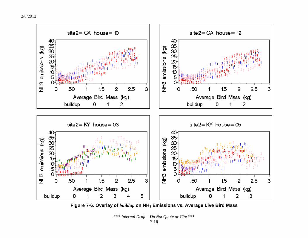
2/8/2012
*** Internal Draft – Do Not Quote or Cite *** 7-16
Figure 7-6. Overlay of buildup on NH3 Emissions vs. Average Live Bird Mass

2/8/2012
*** Internal Draft – Do Not Quote or Cite *** 7-17
Table 7-4. Potential Mean Trend Variables to Account for Built-up Litter
Variable Definition
buildup No. of flocks introduced since last full litter clean-out: 0 ≤ buildup ≤ 5
bld 0 if buildup = 0 1 if buildup = 1 2 if buildup = 2 3 if buildup >3
build 0 if buildup = 0 1 otherwise
Figure 7-7 shows three sets of box plots with NH3 emissions on the vertical axis, and
each of the three built-up litter variables on the horizontal axes. The edges of the boxes represent the first and third quartiles (25th and 75th percentiles) of the distribution of emissions for the value of the variable on the horizontal axis. The line in the middle of the box represents the median or 50th percentile. The “whiskers” extending above and below the box extend to the maximum or minimum value of NH3 emissions, unless there are outliers, which are indicated with dots beyond the edges of the whiskers. An outlier is defined as a value that falls below (or above) the first (or third) quartile by more than 1.5 multiplied by the difference between the third and first quartile. Outliers were analyzed by the NAEMS Science Advisor and were determined to be valid emission values. As such, these values remained in the dataset for EEM development.
In the first set of box plots, when buildup = 0, the minimum and first quartile are indistinguishable, indicating that the first 25 percent of values of NH3 emissions are near 0. Although the box covers all values of NH3 emissions when buildup = 0, the values from the minimum to the first quartile are the values of interest. This range of NH3 emissions occurs when avem* is near 0, when much of the NH3 emissions signal might be attributable to built-up litter. In this same set of box plots, when buildup = 1 or 2, the minima and first quartiles are similar to each other and are both higher than the minimum and first quartile when buildup = 0. When buildup = 3, 4 or 5, the minima and first quartiles are higher again. These last three boxes, however, represent data from the Kentucky sites only, and the total number of observations represented by each box is 95, 42 and 24, respectively, while the number of observations represented by the first three boxes are 266, 383 and 402, respectively. The EPA decided against drawing conclusions regarding the effect of buildup from a small number of data points that do not represent all houses.

2/8/2012
*** Internal Draft – Do Not Quote or Cite *** 7-18
Figure 7-7. Box Plots of NH3 Emissions vs. Candidate Categorical Variables

2/8/2012
*** Internal Draft – Do Not Quote or Cite *** 7-19
In the third set of plots, with bld on the horizontal axis, the first three boxes are the same as the first three boxes in the buildup plots, and the fourth box, where bld = 3, combines the data from the last three boxes in the buildup plots. Notice that the minimum and first quartile for bld = 3 are both higher than the minima and first quartiles for the other values of bld, but, again, all of the data in this box comes from the Kentucky sites. When bld = 1 or 2, there is very little difference in the minima or first quartiles, whether due to noise in the data or to an actual lack of signal, so that the EPA saw no use in distinguishing between these two values. The EPA therefore used the variable build, which simply indicates presence or absence of built-up litter, as the functional form through which the variable buildup enters the mean trend function. The second set of plots show the distinct difference in the minima and first quartiles for the boxes representing build = 0 and build = 1.
In determining the appropriate functional form through which avem enters the mean trend function, the EPA noticed that the slope in Figure 7-5 becomes steeper and then at some point becomes less steep. This change in slope was apparent as a more distinct leveling off or turning down for site KY1B-1 H5 (see Figure 7-6). The EPA further disaggregated the data into plots for individual flocks in Figure 7-8, Figure 7-9 and Figure 7-10. For site CA1B, flocks 1 and 2 were not included in the plots because there were 0 and 2 observations for House 10, and 0 and 3 observations for House 12. These figures show that for all houses, more often than not, NH3 emissions as a function of avem* slopes upward with increasing steepness, then the slope begins to decrease, and then the slope either becomes zero or negative. For a few flocks the curve continued to increase, and for a few flocks, missing data prohibited examination of a pattern.
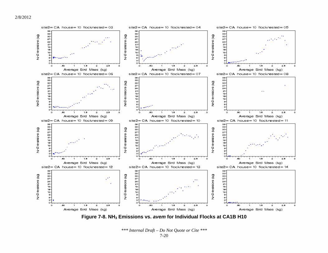
2/8/2012
*** Internal Draft – Do Not Quote or Cite *** 7-20
Figure 7-8. NH3 Emissions vs. avem for Individual Flocks at CA1B H10

2/8/2012
*** Internal Draft – Do Not Quote or Cite *** 7-21
Figure 7-9. NH3 Emissions vs. avem for Individual Flocks at CA1B H12

2/8/2012
*** Internal Draft – Do Not Quote or Cite *** 7-22
Figure 7-10. NH3 Emissions vs. avem for Individual Flocks at the Kentucky Sites
2/8/2012
*** Internal Draft – Do Not Quote or Cite *** 7-23
The decreasing steepness and subsequent leveling-off and/or decrease in slope is apparent in the emissions plots contained in the final report for the Kentucky sites (see Appendix D). In conversations between the EPA, the researchers for the California and Kentucky sites and industry representatives, the hypotheses was raised that the slope may reflect changes in feed protein content that occur at multiple stages of the grow-out period. Protein excreted by the birds is the precursor to NH3 emissions. As birds grow, metabolic changes lead to decreases in protein uptake. Therefore, it is a common practice in the broiler industry to progressively reduce the proportion of protein in the feed during the grow-out period. Reduced protein in the feed reduces protein excreted, thereby reducing the NH3 precursor. To account for this curvature, the EPA chose a cubic polynomial to represent the main effect of average live bird mass on NH3 emissions.
Figure 7-11, Figure 7-12 and Figure 7-13 display scatter plots of NH3 emissions versus the remaining predictor variables. Intuition suggests that emissions of a pollutant will be greater when the number of birds is greater, if all other variables, especially average live bird mass, were held constant. The plot of NH3 emissions versus birds corroborates this intuition. For example, consider a flock made up of 25,000 birds on the date of introduction into the house. On this date, the number of birds for this flock takes its maximum value, while the average live bird mass takes its minimum value. The total live bird mass, and thus the production of manure, is likely at or near its minimum value for this flock on this date. As each day passes, the bird inventory decreases due to mortality, but the average live bird mass increases, and the mortality rate is low enough that the total live bird mass, and thus the quantity of manure, increases as the grow-out period progresses. Thus, for a given flock, pollutant emissions increase as the number of birds decrease, as manifested by the collection of downward-sloping lines, some of which are indistinguishable from one another, in the scatter plot.
Now consider the difference between hypothetical flocks 1 and 2, with 25,000 and 21,000 birds, respectively, on the date of introduction to the house. Because the bird mortality rate is approximately the same for different flocks, if all other variables are held constant, flock 1 should produce more of the pollutant than flock 2. The tops of the downward sloping lines represent maximum NH3 emissions for individual flocks, which occur when the number of birds for each flock is at its minimum. Notice that as the number of birds increases, the values of NH3 emissions at the tops of those lines increase. After the effect of average live bird mass and the interaction between number of birds and average live bird mass were accounted for, the EPA expected the effect of birds to be positive. Figure 7-11 does not indicate that the EPA should use a functional form other than linear in the EEM. Thus, the mean trend variable, birds, represents the main effect of the predictor variable birds*.

2/8/2012
*** Internal Draft – Do Not Quote or Cite *** 7-24
Figure 7-11. NH3 Emissions vs. Predictor Variables birds* and ta*
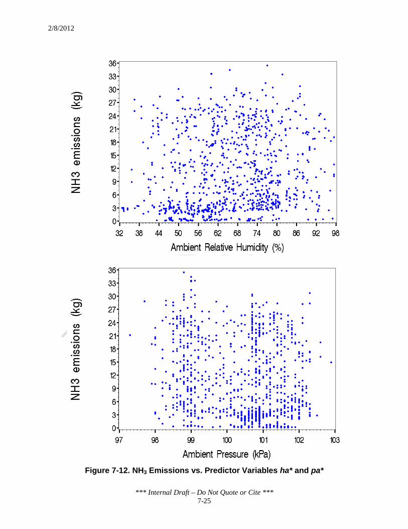
2/8/2012
*** Internal Draft – Do Not Quote or Cite *** 7-25
Figure 7-12. NH3 Emissions vs. Predictor Variables ha* and pa*

2/8/2012
*** Internal Draft – Do Not Quote or Cite *** 7-26
Figure 7-13. NH3 Emissions vs. Predictor Variables tc* and hc*

2/8/2012
*** Internal Draft – Do Not Quote or Cite *** 7-27
The relationships between NH3 emissions and each of the ambient meteorological variables were not apparent in the plots of Figure 7-11 and Figure 7-12, nor were the relationships between NH3 emissions and the confinement variables apparent in Figure 7-13. Such relationships are often hidden in plots aggregated over many different sets of conditions. Consequently, the EPA plotted NH3 emissions versus each variable separately for the six avem* bins.
Figure 7-14 displays example plots of NH3 emissions versus ha*. Excluding bin 1, which has added variability due to differences in buildup, when enough data are available within a bin, the EPA detected a slight increasing trend. For each of these variables, the EPA chose a linear functional form, in the absence of a clear signal or a process-based reason to do otherwise.
Table 7-5 summarizes the functional form chosen by EPA to describe the dependence of NH3 emissions on the original predictor variables. The first column gives the original predictor variable, and the second states the functional form chosen. The last column gives the mean trend variable or variables that represented the main effect of each predictor variable. For the discrete predictor variable buildup, the indicator variable build will be the mean trend variable.
Table 7-5. Summary of Main Effect Mean Trend Variables
Original Predictor Variablea
Functional Form Chosen
Centering Value Scaling Value Main Effect Mean
Trend Variable(s)
buildup* Indicator variable Not applicable Not applicable build
birds* Linear 22 2.5 birds
avem* Cubic polynomial 1.1 0.87 avem, avem2, avem3
ta* Linear 15 8.2 ta
ha* Linear 66 14 ha
pa* Linear 100 1.1 pa
tc* Linear 25 3.8 tc
hc* Linear 58 9.9 hc a An asterisk (*) is used to note that these predictor variables are the original values submitted to the EPA before centering and scaling (see Section 7.3.1).

2/8/2012
*** Internal Draft – Do Not Quote or Cite *** 7-28
Figure 7-14. NH3 Emissions vs. ha* for Six avem Bins

2/8/2012
*** Internal Draft – Do Not Quote or Cite *** 7-29
All of the other predictor variables were continuous variables. Following standard statistical practice, the EPA transformed each predictor variable in Table 7-5 by subtracting the mean value of the original predictor variable and then dividing by the standard deviation. This practice is called centering and scaling the continuous predictor variables. For example, the mean value of birds* in the base dataset, rounded to two significant digits, was 22, and the standard deviation was 2.5 (the unit of measure was thousands of birds.) The EPA created the new variable birds = (birds* - 22)/2.5, and because the functional form chosen for birds is linear, the new variable birds is the mean trend variable that represents the main effect of birds. All of the variables except avem* followed the same pattern as birds, with different centering and scaling values. For avem*, the new variable avem was created by centering and scaling, and then the cubic polynomial functional form chosen for avem was represented by the terms avem, avem2 and avem3.
The reason for centering and scaling the continuous predictor variables prior to creating mean trend variables from them is to prevent collinearity problems. Collinearity occurs when one mean trend variable is equal to, or very nearly equal to, a linear combination of other mean trend variables. In lay terms, it can be thought of as the condition in which two or more mean trend variables in a multiple regression analysis are highly correlated. Collinearity problems can be produced when mean trend terms are created as the squared or cubed value of a predictor variable that takes primarily positive values. They can also be produced when one mean trend variable that takes primarily positive values is multiplied by another that takes primarily positive values to create an interaction between the two. The predictor variables avem, ha, pa, tc and hc have positive values for all 1,211 observations in the NAEMS data, but the centered and scaled versions avem*, ha*, pa*, tc* and hc* have positive values for half the observations, and negative values for the other half.
The potential negative effect of collinearity is that when it is present, small changes in the data could produce very different regression coefficient estimates, but these changes do not produce very different emissions predictions unless the collinearity is quite severe. Because the EPA prevented severe collinearity by centering and scaling the continuous predictor variables, and because the purpose of the EEMs is to produce predictions, collinearity is not a problem for the EEMs developed for broiler houses.
Table 7-5 shows the centering and scaling values used for each continuous predictor variable. The centering value for each variable is the mean value of that variable in the base dataset, and the scaling value is the standard deviation. When using the EEMs, new centering and scaling values are not calculated. The centering and scaling values in Table 7-5 must be used because the EEMs were created using these values.

2/8/2012
*** Internal Draft – Do Not Quote or Cite *** 7-30
7.3.2 Creating Mean Trend Variables from Main Effects and Interactions
After identifying functional forms through which each predictor should enter the mean trend function, the EPA created interaction terms and determined what level of interactions (e.g., two-way, three-way) to include in the set of candidate mean trend variables. An interaction between two mean trend variables occurs when the effect, or slope, of a main effect variable is different for different values of another variable.
A two-way interaction is the product of two main effect variables. For the I EEM, the two-way interaction between build and birds is the product buildbirds. The two-way interaction between build and avem consists of the collection of products buildavem, buildavem2 and buildavem3, and the 2-way interaction between birds and avem consists of the collection of products birdsavem, birdsavem2 and birdsavem3. A three-way interaction is the product of three main effect variables. The three way interactions for the I EEM included buildbirdsavem, buildbirdsavem2 and buildbirdsavem3. Higher order interactions for the I EEM were irrelevant.
Failure to consider interactions among main effect mean trend variables can result in exclusion of important variables from the EEM due to failure to notice their statistical significance. Some variables might affect NH3 emissions only by way of an interaction with another variable. For example, the main effect of a variable such as ta might drop out of the EEM due to an insignificant regression coefficient. However, when its interaction with avem is considered, the regression coefficient for the interaction term might be statistically significant.
Furthermore, even if the main effects of both ta and avem were statistically significant, it might be the case that an interaction between them allows the EEM to explain even more of the variability in NH3 emissions. Failure to consider such an interaction would result in decreased predictive performance in terms of both accuracy (establishing the optimal mean trend function) and precision (minimizing prediction error variance, manifested by the width of the prediction intervals). Including three-way interactions, or n-way interactions for n > 3, particularly when the set of predictor variables is large, might not improve the predictive ability of the EEM, and might lead to extreme collinearity. Therefore, the EPA adopted the following protocol, illustrated with the I EEM, for determining what level of interactions to use as candidate mean trend variables.
The EPA performed an ordinary least squares (OLS) regression of NH3 emissions in the base dataset on main effect inventory variables, then repeated the regression adding two-way interactions, then three-way interactions. With each regression, the EPA examined the value of R2 to determine what percent of variability in NH3 emissions in the base dataset were explained by each set of variables. Using the maximum value of R2 calculated from a regression on the base dataset is not appropriate to determine what mean trend variables should be included in the final EEM because adding variables to the EEM always increases R2, even if some are spurious

2/8/2012
*** Internal Draft – Do Not Quote or Cite *** 7-31
variables or if they explain anomalies in the base dataset as opposed to signals that apply generally. If adding variables increases R2 only slightly, however, those additional variables are not important. Therefore, the EPA decided that only if increasing the level of interactions in the OLS regression from n-way to n + 1 way increased R2 by 0.01 or more would the n + 1 way interactions be included as candidate mean trend variables.
Table 7-6 shows that including only main effects for the I EEM resulted in R2 = 0.8127, and adding two-way interactions resulted in R2 = 0.8457. Because the difference between the R2 values was 0.033, the EPA included the two-way interactions. Because adding 3-way interactions produced R2 = 0.8493, an increase of only 0.0036, the EPA did not include 3-way interactions in the set of candidate mean trend variables.
Table 7-6. Proportion of Base Dataset Variability Explained by EEMs by Interaction Level
EEM Interaction Level P R2
I Main effects 5 0.8127 Add 2-way 12 0.8457 Add 3-way 15 0.8493
IA Main effects 8 0.8365 Add 2-way 33 0.9013
IAC Main effects 10 0.8401 Add 2-way 52 0.9149
Because they contain a superset of the predictor variables in the I EEM, the EPA did not
consider interactions beyond two-way for the IA and IAC EEMs. However, the EPA conducted a test to determine whether adding two-way interactions to the main effect for these two EEMs was necessary. Because the OLS regression of NH3 emissions on main effects for the IA EEM resulted in R2 = 0.8365, and adding two-way interactions produced R2 = 0.9013, the EPA considered two-way interactions for the IA EEM. Because the OLS regression of NH3 emissions on main effects for the IAC EEM resulted in values of R2 = 0.8401, and adding two-way interactions produced R2 = 0.9149, the EPA also considered two-way interactions for the IAC EEM.
7.4 Choosing the Covariance Function Use of OLS regression to determine what mean trend variables are statistically significant
and to obtain prediction intervals requires that the random deviations eht are independent and identically distributed with mean 0 and variance σ2. If they are not independent, the dependence, which is called correlation or covariance, can be accounted for in the EEM using random effects

2/8/2012
*** Internal Draft – Do Not Quote or Cite *** 7-32
and/or a covariance function, via generalized least squares (GLS) regression. If they are not identically distributed, differences in the variance parameter σ2 can be eliminated by transforming the original response variable (NH3 emissions) or by allowing different values of σ2 under different conditions.
Section 7.4.1 explains the meaning of and distinction between correlation and covariance. Sections 7.4.2 and 7.4.3, respectively, describe how the EPA assessed the need to account for serial correlation or correlation due to random effects. Section 7.4.4 explains the EPA’s decision to use the single variance parameter σ2 calculated from all four broiler houses and all three sites in the NAEMS.
7.4.1 Correlation Function as Subset of Covariance Function
The auto-correlation coefficient, ρ, which falls between -1.0 and 1.0, is a measure of the strength and direction of a linear relationship between two random variables. Values closer to 0 indicate little or no relationship, values close to -1.0 indicate a strong negative association, and values close to 1.0 indicate a strong positive association. In the EEM context, the random variables are both the random deviations, eht, from the mean trend function, and the NH3 emissions, Yht, which are functions of the eht.
The covariance between two random variables is the correlation coefficient multiplied by the standard deviation of each: ρσ1σ2. If the two have the same standard deviation (i.e., σ1 = σ2 = σ), then the covariance is simply the product ρ σ2 of the correlation coefficient ρ and the variance σ2. In short, the covariance is a measure of alikeness, for which the units are the squared units of the random variable (kg squared in the case of daily NH3 emissions).
For the EEMs, EPA used the covariance matrix to calculate prediction error. The covariance matrix specifies the joint probability of all types of errors that are possible in the mean trend terms over all dates, houses and sites. For example, the EEM would specify a greater prediction error for mean trend values that are at the extreme values measured in the NAEMS monitoring study than for values that are closer to the central tendency of the measured emissions data.
Because the I EEM has fewer mean trend variables than the other EEMs, the covariance function has to account for more variability in NH3 emissions than it will for the other EEMs. The EPA therefore used only inventory-based mean trend terms to make initial covariance function decisions. However, the EPA continually re-assessed the statistical significance of covariance parameters during the final EEM selection process in case addition of mean trend variables from the ambient and confinement categories explained so much more variability in NH3 emissions that the covariance parameters were no longer needed.

2/8/2012
*** Internal Draft – Do Not Quote or Cite *** 7-33
7.4.2 Serial Correlation
Serial correlation in NH3 emissions, Yht, occurs if the value of emissions at one point in time is related to the value at a nearby point in time. The deviations from the mean trend function, eht, can display serial correlation even when many of the reasons for the similarity between emissions for two consecutive days have been accounted for with the mean trend function. To assess the need to account for serial correlation in the deviations from the mean trend function, the EPA fit an OLS regression model, which does not account for serial correlation or random effects, to the base data and plotted pairs of residuals from the same house, ℎ𝑡, (which are estimates of the deviations) at time t versus those at time t–1, (see Figure 7-15). Because of the strong relationship between the two terms, EPA accounted for serial correlation with the auto-regressive order 1 (AR(1)) covariance function. This function expresses the covariance Cov(eht, eht') between two deviations from the mean trend function within the same house on different dates (t and t') as the product, σ2ρt–t' , of the variance parameter, σ2 , and a power of the auto-correlation coefficient, ρ. Restricting ρ to take values between 0 and 1 ensures that when the distance,t–t', between two dates increases, the correlation ρt–t' between the two deviations decreases.
Figure 7-15. Deviations from the Mean Trend Function on Date t vs. Date t-1

2/8/2012
*** Internal Draft – Do Not Quote or Cite *** 7-34
7.4.3 Random Effects
Random effects must be accounted for if a variable that cannot be used as a predictor might nonetheless affect the value of NH3 emissions. Variables that might affect pollutant emissions from broiler houses include information that was not provided by the NAEMS such as the nitrogen content of feed rations and the timing of changes in feed rations. Such variables might be the same for a given farm or company, but different for different farms or companies. The genetic make-up of the birds might also be the same for a given farm or company, but different for different farms or companies. Other variables that might affect the pollutant emissions measurements, which is different from affecting actual emissions, include the people conducting the measurement activities, the proximity of the house to another emissions source, and the distance separating the outdoor ambient monitor from the house. If, for hypothetical house 1, the distance between the outdoor monitor and the house were less than that of hypothetical house 2, the ambient emissions concentration from house 1 might be more contaminated by emissions from the house, and thus not represent background emissions alone. Then for house 1, the emissions measurement resulting from subtracting the outdoor “background” NH3 concentration from the indoor concentration would not be as representative of true emissions as would the emissions measurement from house 2. To allow for differences in emissions due to such farm-to-farm, company-to-company, or house-to-house differences, known or unknown, the EPA considered random effects of site and house.
The EPA assessed the need to account for random effects first using summary statistics, and then by including each type of random effect in an EEM and testing the statistical significance of the effect. When values of other predictor variables such as buildup, avem* (or avem) and birds* (or birds) are kept constant, a consistent pattern in mean emissions for the different houses or sites would support the need for a random effect. Table 7-7 shows mean NH3 emissions within each house for different ranges of avem* for the subset of the base data for which build = 0. (Note that for the only flock for which KY1B-2 H3 had build = 0, the data beyond the first three weeks were missing.) For avem* bins 1 through 3, KY1B-1 H5 had a higher mean than CA1B H10 and CA1B H12, but the pattern did not continue over bins 4 through 6. Other breakdowns of the data showed a similar lack of consistent pattern. This observation implies that random effects of house or site are not needed.

2/8/2012
*** Internal Draft – Do Not Quote or Cite *** 7-35
Table 7-7. Mean NH3 Emissions (kg) After Litter Clean-out
Site House
𝐀𝐯𝐞𝐫𝐚𝐠𝐞 𝐁𝐢𝐫𝐝 𝐌𝐚𝐬𝐬
0-0.5 kg 0.5-1.0 kg 1.0-1.5 kg 1.5-2.0 kg 2.0-2.5 kg 2.5-3.0 kg
n NH3 n NH3 n NH3 n NH3 n NH3 n NH3
CA1B 10 41 0.42 12 3.97 9 12.4 14 19.1 14 24.7 8 25.2
12 40 0.36 12 2.89 9 9.32 14 17.0 14 23.3 8 24.1
KY1B-1 5 17 1.78 8 11.6 7 18.9 9 19.4 7 17.0 1 13.3
KY1B-2 3 15 0.36 7 2.18 0 a 0 a 0 a 0 a a Site KY1B-2 only had three weeks of data on new bedding.
To formally test the need for a random effect in the EEM, Equation 7-2 presents a
modification of Equation 7-1 that includes a random effect of house, Ah. If there were a consistent pattern in mean NH3 emissions for each house, then the random variables Ah, h = 1,…4, will have variance parameter, σ2
H, significantly different from zero. Note that σ2H
represents a single parameter, whereas the notation σ2h, h = 1,...,4, which will be used in Section
7.4.4, represents four different parameters.
Yht = β0 + β1x1ht + ⋯ +βpxpht + ⋯+βPxPht + Ah + eht , h = 1, …, 4, t varies, p = 1, …, P
Equation 7-2
𝑒ℎ𝑡 ~ 𝛮(O, σ2); 𝐴ℎ~ 𝑁(𝑂, 𝜎𝐻2);
𝐶𝑜𝑣 𝑒ℎ𝑡, 𝑒ℎ′𝑡′ = 𝑂 ℎ ≠ ℎ′𝜎2𝜌|𝑡−𝑡′| ℎ = ℎ′ ; 0 < 𝜌 < 1
The first column of Table 7-8 lists all of the covariance parameters, and the second gives
the estimate for each. The third column gives the p-value of a test of the null hypothesis that the covariance parameter equals zero. The p-value gives the probability (between 0 and 1) that the actual covariance parameter would be as far from zero as the estimate obtained if the null hypothesis were true. Because a small p-value indicates that the estimated value of the parameter is not significantly different from zero, the results provide strong evidence that the random effect of house is not needed in the EEM, but that the auto-correlation coefficient 𝜌 and variance parameter σ 2 are needed. The EPA performed a similar test for the random effect of site instead of house, and in that case the estimated variance component for site 𝜎𝑆
2 was 0.27, and the p-value was 0.40. Consequently, the EPA did not include a random effect of either house or site in the EEMs.

2/8/2012
*** Internal Draft – Do Not Quote or Cite *** 7-36
Table 7-8. Covariance Parameter Estimates
Covariance Parameter Estimate P-value
𝜌 0.9157 <0.0001
𝜎ℎ2 13.7004 <0.0001
𝜎𝑠2 0.2726 0.4028
7.4.4 Constant Variance
Another decision to be made regarding the covariance function was whether to use the same covariance parameters, σ 2andρ, for all houses and conditions. If the variance, σ 2, of the deviations, eht, from the mean trend function increase with the mean, or if they exhibit non-constant variance for some other reason, then a transformation of the response variable, NH3 emissions, would be the most commonly used remedy. Such a transformation, however, would have made both the exploratory plots in Section 7.3, and the regression coefficient estimates, βp, more difficult to interpret.
The EPA did not find evidence supporting an increase in the variance of emissions with increasing values of mean emissions. Table 7-9 shows the mean and standard deviation for six different ranges of values of NH3 emissions for which the first five ranges has enough data to discern patterns. As the mean increases from the first range to the third, the standard deviation does increase, but an increase of 0.1 kg is of no practical significance. Because these are standard deviations of NH3 emissions, Yht, as opposed to the deviations from the mean trend function, eht, the EPA decided that it was not necessary to account for a variance that increases with mean emissions.
Table 7-9. Sample Size, Mean and Standard Deviation for NH3 Bins
Range of NH3 Emissions in kg N
Mean (kg)
Std Dev (kg)
0-6 484 2.7 1.6
6-12 231 8.8 1.7
12-18 172 15 1.8
18-24 209 21 1.8
24-30 104 26 1.6
30-36 11 32 1.9
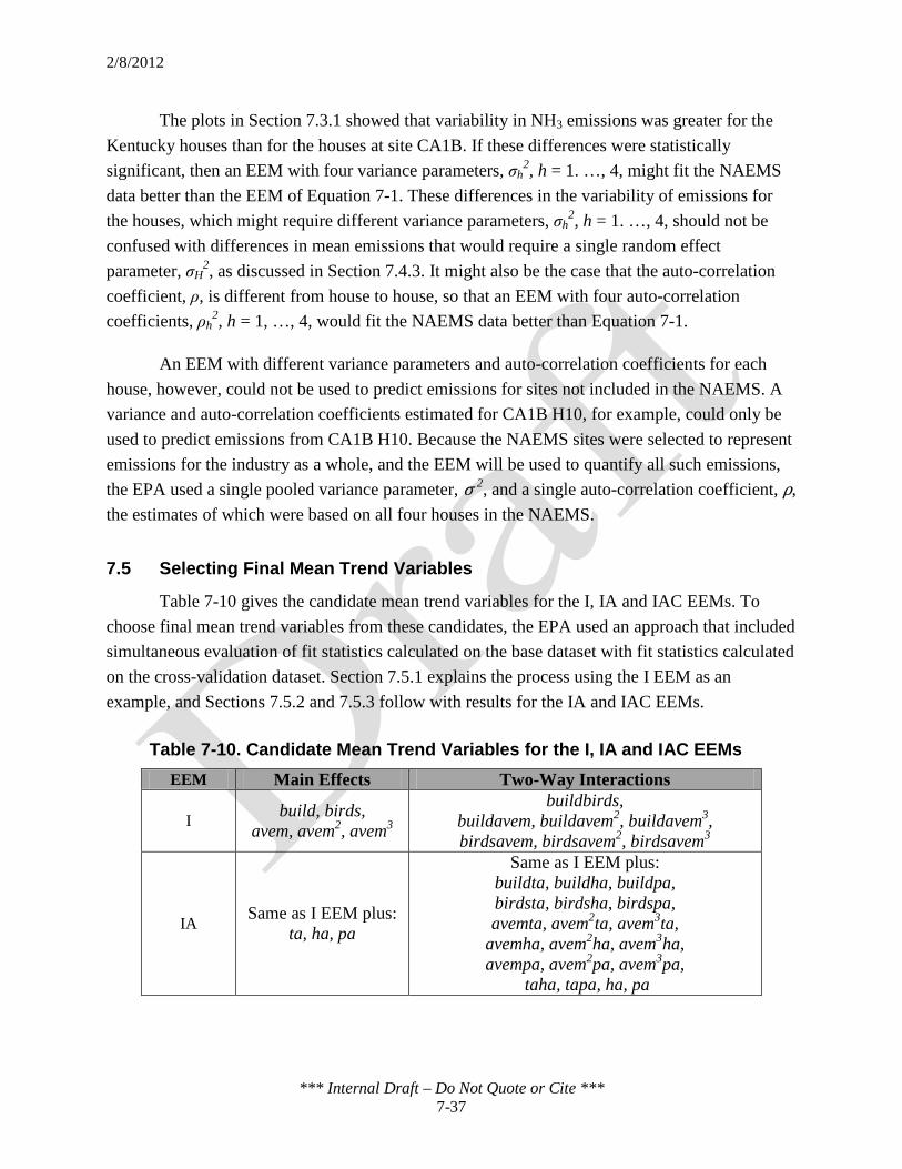
2/8/2012
*** Internal Draft – Do Not Quote or Cite *** 7-37
The plots in Section 7.3.1 showed that variability in NH3 emissions was greater for the Kentucky houses than for the houses at site CA1B. If these differences were statistically significant, then an EEM with four variance parameters, σh
2, h = 1. …, 4, might fit the NAEMS data better than the EEM of Equation 7-1. These differences in the variability of emissions for the houses, which might require different variance parameters, σh
2, h = 1. …, 4, should not be confused with differences in mean emissions that would require a single random effect parameter, σH
2, as discussed in Section 7.4.3. It might also be the case that the auto-correlation coefficient, ρ, is different from house to house, so that an EEM with four auto-correlation coefficients, ρh
2, h = 1, …, 4, would fit the NAEMS data better than Equation 7-1.
An EEM with different variance parameters and auto-correlation coefficients for each house, however, could not be used to predict emissions for sites not included in the NAEMS. A variance and auto-correlation coefficients estimated for CA1B H10, for example, could only be used to predict emissions from CA1B H10. Because the NAEMS sites were selected to represent emissions for the industry as a whole, and the EEM will be used to quantify all such emissions, the EPA used a single pooled variance parameter, σ 2, and a single auto-correlation coefficient, ρ, the estimates of which were based on all four houses in the NAEMS.
7.5 Selecting Final Mean Trend Variables
Table 7-10 gives the candidate mean trend variables for the I, IA and IAC EEMs. To choose final mean trend variables from these candidates, the EPA used an approach that included simultaneous evaluation of fit statistics calculated on the base dataset with fit statistics calculated on the cross-validation dataset. Section 7.5.1 explains the process using the I EEM as an example, and Sections 7.5.2 and 7.5.3 follow with results for the IA and IAC EEMs.
Table 7-10. Candidate Mean Trend Variables for the I, IA and IAC EEMs EEM Main Effects Two-Way Interactions
I build, birds, avem, avem2, avem3
buildbirds, buildavem, buildavem2, buildavem3, birdsavem, birdsavem2, birdsavem3
IA Same as I EEM plus: ta, ha, pa
Same as I EEM plus: buildta, buildha, buildpa, birdsta, birdsha, birdspa, avemta, avem2ta, avem3ta,
avemha, avem2ha, avem3ha, avempa, avem2pa, avem3pa,
taha, tapa, ha, pa
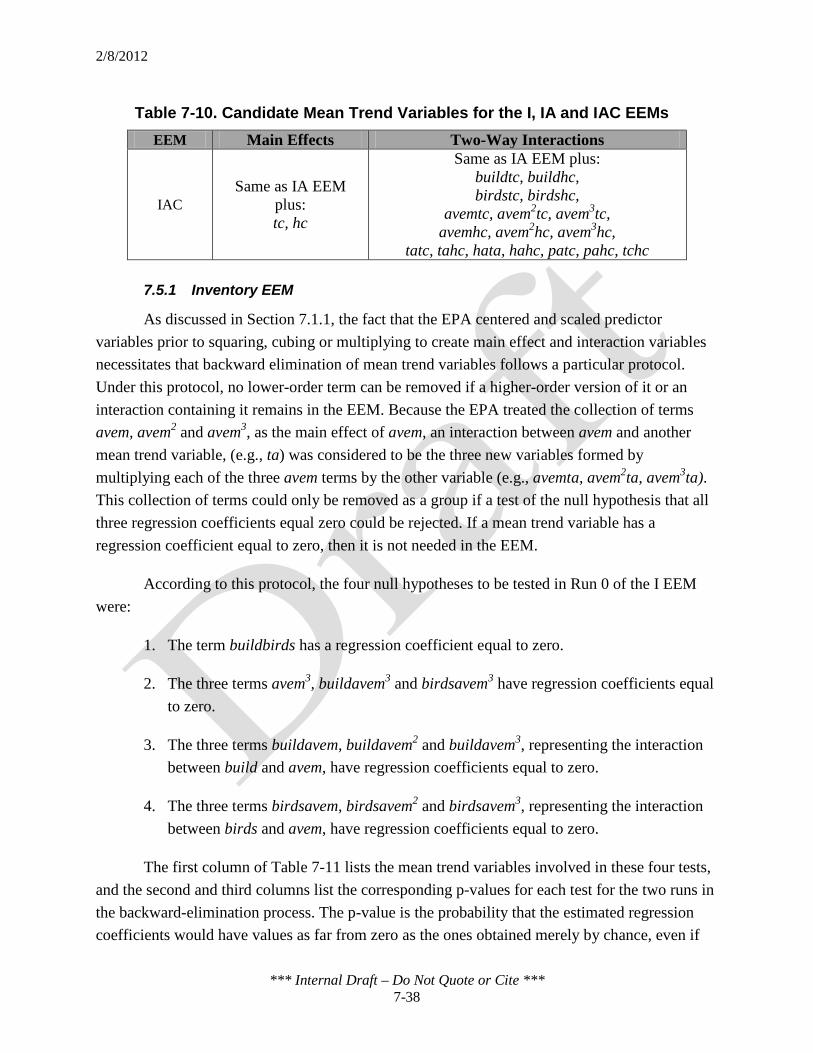
2/8/2012
*** Internal Draft – Do Not Quote or Cite *** 7-38
Table 7-10. Candidate Mean Trend Variables for the I, IA and IAC EEMs EEM Main Effects Two-Way Interactions
IAC Same as IA EEM
plus: tc, hc
Same as IA EEM plus: buildtc, buildhc, birdstc, birdshc,
avemtc, avem2tc, avem3tc, avemhc, avem2hc, avem3hc,
tatc, tahc, hata, hahc, patc, pahc, tchc
7.5.1 Inventory EEM
As discussed in Section 7.1.1, the fact that the EPA centered and scaled predictor variables prior to squaring, cubing or multiplying to create main effect and interaction variables necessitates that backward elimination of mean trend variables follows a particular protocol. Under this protocol, no lower-order term can be removed if a higher-order version of it or an interaction containing it remains in the EEM. Because the EPA treated the collection of terms avem, avem2 and avem3, as the main effect of avem, an interaction between avem and another mean trend variable, (e.g., ta) was considered to be the three new variables formed by multiplying each of the three avem terms by the other variable (e.g., avemta, avem2ta, avem3ta). This collection of terms could only be removed as a group if a test of the null hypothesis that all three regression coefficients equal zero could be rejected. If a mean trend variable has a regression coefficient equal to zero, then it is not needed in the EEM.
According to this protocol, the four null hypotheses to be tested in Run 0 of the I EEM were:
1. The term buildbirds has a regression coefficient equal to zero.
2. The three terms avem3, buildavem3 and birdsavem3 have regression coefficients equal to zero.
3. The three terms buildavem, buildavem2 and buildavem3, representing the interaction between build and avem, have regression coefficients equal to zero.
4. The three terms birdsavem, birdsavem2 and birdsavem3, representing the interaction between birds and avem, have regression coefficients equal to zero.
The first column of Table 7-11 lists the mean trend variables involved in these four tests, and the second and third columns list the corresponding p-values for each test for the two runs in the backward-elimination process. The p-value is the probability that the estimated regression coefficients would have values as far from zero as the ones obtained merely by chance, even if
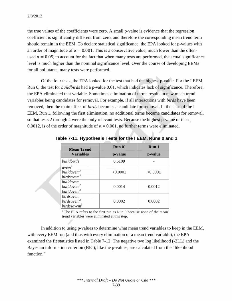
2/8/2012
*** Internal Draft – Do Not Quote or Cite *** 7-39
the true values of the coefficients were zero. A small p-value is evidence that the regression coefficient is significantly different from zero, and therefore the corresponding mean trend term should remain in the EEM. To declare statistical significance, the EPA looked for p-values with an order of magnitude of α = 0.001. This is a conservative value, much lower than the often-used α = 0.05, to account for the fact that when many tests are performed, the actual significance level is much higher than the nominal significance level. Over the course of developing EEMs for all pollutants, many tests were performed.
Of the four tests, the EPA looked for the test that had the highest p-value. For the I EEM, Run 0, the test for buildbirds had a p-value 0.61, which indicates lack of significance. Therefore, the EPA eliminated that variable. Sometimes elimination of terms results in new mean trend variables being candidates for removal. For example, if all interactions with birds have been removed, then the main effect of birds becomes a candidate for removal. In the case of the I EEM, Run 1, following the first elimination, no additional terms became candidates for removal, so that tests 2 through 4 were the only relevant tests. Because the highest p-value of these, 0.0012, is of the order of magnitude of α = 0.001, no further terms were eliminated.
Table 7-11. Hypothesis Tests for the I EEM, Runs 0 and 1
Mean Trend Variables
Run 0a Run 1
p-value p-value
buildbirds 0.6109 - avem3
buildavem3 birdsavem3
<0.0001 <0.0001
buildavem buildavem2 buildavem3
0.0014 0.0012
birdsavem birdsavem2
birdssavem3
0.0002 0.0002
a The EPA refers to the first run as Run 0 because none of the mean trend variables were eliminated at this step.
In addition to using p-values to determine what mean trend variables to keep in the EEM,
with every EEM run (and thus with every elimination of a mean trend variable), the EPA examined the fit statistics listed in Table 7-12. The negative two log likelihood (-2LL) and the Bayesian information criterion (BIC), like the p-values, are calculated from the “likelihood function.”

2/8/2012
*** Internal Draft – Do Not Quote or Cite *** 7-40
The likelihood function of an EEM quantifies the probabilities that different sets of values of the parameters will reproduce NH3 emissions in the NAEMS data. “Fitting the EEM” refers to finding the parameter estimates that maximize the likelihood function, which simply means finding those values of the parameters that result in accounting for the most variability in the data. Minimizing the function that is equal to -2LL is mathematically equivalent to maximizing the likelihood, and the required computations take less time. When comparing the values of -2LL for two different EEMs, the one with the lower -2LL better fits the data.
The BIC statistic is a function of -2LL, with a penalty added for the number of parameters in the EEM for situations in which fewer parameters are desirable. Lower values of the BIC statistic are also better; however there are instances where eliminating a term increases the -2LL while decreasing the BIC. The second column of Table 7-12 shows that elimination of buildbirds from the I EEM resulted in the -2LL increasing from 3,810 for Run 0 to 3,811 for Run 1, but the BIC decreased from 3,819 to 3,815. If both the -2LL and the BIC decrease, there is strong evidence that the resulting EEM is superior, but sometimes when the statistics disagree, other fit statistics must be considered, or it may be the case that the difference between two EEMs has little practical significance.
The remaining fit statistics quantify how well an EEM fits the cross-validation dataset. The EPA fit an EEM of the form given in Equation 7-1 to the base dataset. Using that EEM and the values of the predictor variables corresponding to the 217 values of NH3 emissions in the cross-validation dataset, the EPA then produced point predictions, denoted with Ŷht, and the lower and upper bounds of the 95 percent prediction intervals for the actual emissions, Yht. The fit statistics are different ways of assessing how well the 217 point predictions, Ŷht, compare to the 217 actual values of NH3 emissions, Yht, as well as how well the prediction intervals quantify uncertainty in the point predictions.
The row labeled “% in PI” gives the percent of cross-validation emissions, Yht, that fall inside the 95 percent prediction intervals for them. Values close to 95 indicate that the quantification of uncertainty is on target. For both runs of the I EEM, this value was 94 percent. The width of each prediction interval, in kg of NH3 emissions, quantifies the uncertainty of the point prediction. For a given confidence level, narrower intervals are desirable. A 95 percent prediction interval that says the NH3 emissions for a single date under a given set of conditions will fall between 0 and 36 kg is less useful than a prediction interval that says the emissions will fall between 15 and 30 kg. The width of the interval is a function of the natural variability in the deviations from the mean trend function as well as uncertainty regarding the point estimate due to using sample data. Including more relevant predictor variables, if possible, is one way to obtain narrower intervals, a fact that emphasizes the importance of the collinearity mitigation strategies of Section 7.3.1. The best of a set of candidate EEMs would be one that minimizes

2/8/2012
*** Internal Draft – Do Not Quote or Cite *** 7-41
these widths, while at the same time ensuring that the statistic “% in PI” is close to 95. In other words, the best EEM minimizes uncertainty while at the same time quantifying it accurately. The average width of the prediction intervals produced by the I EEM, Run 0 was 14 kg, and this width did not change upon elimination of the predictor buildbirds.
Table 7-12. Backward Elimination Fit Statistics for the I EEM
Fit Statistic I EEM Runs
0 1 -2LL 3,810 3,811 BIC 3,819 3,815
% in PI 94 - Width (kg) 14 - RMSE (kg) 3.8 -
R2 0.81 - Υ0 (kg) -0.13 -0.14
Υ1 0.99 - Eliminated buildbirds
Note: A dash indicates no change in the fit statistic from the previous EEM. A check mark () indicates that the 95 percent confidence interval (CI) for the intercept (slope) contains zero (one) and the estimate is not significantly different from zero (one). Highlighting emphasizes the EEMs for which a given statistic obtained its optimal value.
To obtain the next four fit statistics, RMSE, R2, Υ0, and Υ1, the EPA performed an OLS
regression of the cross-validation dataset of NH3 emissions, Yht, on the predictions, Ŷht, of the withheld cross-validation data. In other words, the EPA fit the OLS regression given by Equation 7-3, where the values of h and t correspond to those in the cross-validation dataset. In Equation 7-3,Υ0 represents the intercept of the fit line and Υ1 represents the slope.
Yht = Υ0 + Υ1 Ŷht + eht Equation 7-3
The root mean squared error (RMSE), in kg NH3, is defined in Equation 7-4. The RMSE
can be thought of as a measure of the average distance between the point predictions and the actual emissions. Smaller values indicate a better fit. For both runs of I EEM, the RMSE was 3.8 kg.
𝑅𝑀𝑆𝐸 = 1𝑁
𝑌ℎ𝑡 − Ŷℎ𝑡 (2)
𝑛
𝑖=1
Equation 7-4

2/8/2012
*** Internal Draft – Do Not Quote or Cite *** 7-42
The value of R2 is interpreted as the proportion of variability in the cross-validation emissions, Yht, explained by the predictions of them, Ŷht. As mentioned in Section 7.3.2, when R2 is calculated from a regression of the base data emissions on mean trend variables, it is not a good indication of EEM fit because it is a mathematical certainty that R2 will increase when mean trend variables are added. When R2 is calculated based on a regression of the cross-validation dataset, Yht, on the predictions of the cross-validation dataset, Ŷht, from a given EEM, it is not a mathematical certainty that adding mean trend variables to that EEM will increase R2. Thus, values of R2 closer to one indicate better fit of the EEM to the cross-validation data. The proportion of the variability in cross-validation emissions explained by both of the I EEMs is 0.81, or 81 percent.
If the EEM fit the cross-validation data perfectly, the intercept Υ0 of the regression in Equation 7-3 would equal zero, and the slope Υ1
would equal one. If the estimate of the intercept
or slope, Υ0 or Υ1, is significantly different from 0 or 1, respectively, the EEM has systematic bias. A check beside either estimate indicates that the 95 percent confidence interval (CI) for it contains zero or one, and thus the estimate is not significantly different from zero or one. Both runs of I EEM were free from systematic bias.
Because elimination of buildbirds from the I EEM based on the regression coefficient p-value did not have a negative impact on the other fit statistics, the EPA chose the variables from Run 1 as the final mean trend variables for the I EEM.
7.5.2 Inventory and Ambient EEM
The hypotheses to be tested in Run 0 of IA EEM are listed in groups by type:
1. Any of the 7 individual variables that represent an interaction has a regression coefficient equal to zero. These variables are buildbirds, buildta, buildha, buildpa, birdsta, birdsha and birdspa.
2. All 5 variables containing avem3 have regression coefficients equal to zero. These variables are build avem3, birds avem3, avem3 ta, avem3ha and avem3pa.
3. All of the three regression coefficients corresponding to any of the five sets of triplets formed as the product of the terms avem, avem2, avem3 and another variable are equal to zero.
Table 7-13 gives the progression of fit statistics for each backward-elimination step, listing in the bottom row the variable eliminated.

2/8/2012
*** Internal Draft – Do Not Quote or Cite *** 7-43
Table 7-13. Backward Elimination Fit Statistics for the IA EEM
Fit Statistic IA EEM Runs
0 1 2 3 4 5 6 7 8 9 10 -2LL 3,687 3,684 3,681 3,679 3,680 3,678 3,677 - 3,675 3,676 - BIC 3,696 3,692 3,689 3,688 3,689 3,687 3,685 3,686 3,683 3,685 3,684
% in PI 97 - - - 96 - - - 97 - - Width (kg) 13 - - - - - - - - - - RMSE (kg) 3.2 - - - - - 3.3 - - - -
R2 0.86 - - - - - - - - - 0.85
γ0 (kg) -0.24 -0.25 - - -0.26 -0.27 -0.26
-0.24 -0.23 -0.24 -0.23
γ1 0.99 - - - - - - - - - - Eliminated - hapa birdsha buildha buildbirds birdspa birdsta buildta taha buildpa tapa
Note: A dash indicates no change in the fit statistic from the previous EEM. A check mark () indicates that the 95 percent confidence interval (CI) for the intercept (slope) contains zero (one) and the estimate is not significantly different from zero (one). Highlighting emphasizes the EEMs for which a given statistic obtained its optimal value.
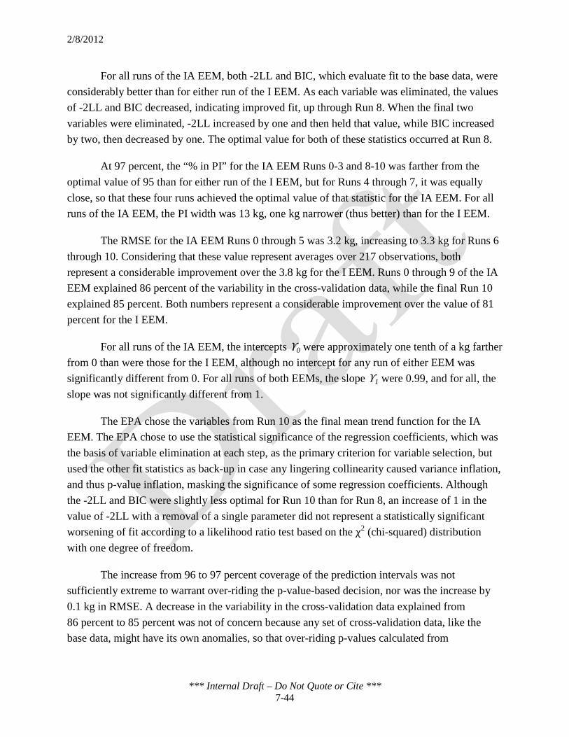
2/8/2012
*** Internal Draft – Do Not Quote or Cite *** 7-44
For all runs of the IA EEM, both -2LL and BIC, which evaluate fit to the base data, were considerably better than for either run of the I EEM. As each variable was eliminated, the values of -2LL and BIC decreased, indicating improved fit, up through Run 8. When the final two variables were eliminated, -2LL increased by one and then held that value, while BIC increased by two, then decreased by one. The optimal value for both of these statistics occurred at Run 8.
At 97 percent, the “% in PI” for the IA EEM Runs 0-3 and 8-10 was farther from the optimal value of 95 than for either run of the I EEM, but for Runs 4 through 7, it was equally close, so that these four runs achieved the optimal value of that statistic for the IA EEM. For all runs of the IA EEM, the PI width was 13 kg, one kg narrower (thus better) than for the I EEM.
The RMSE for the IA EEM Runs 0 through 5 was 3.2 kg, increasing to 3.3 kg for Runs 6 through 10. Considering that these value represent averages over 217 observations, both represent a considerable improvement over the 3.8 kg for the I EEM. Runs 0 through 9 of the IA EEM explained 86 percent of the variability in the cross-validation data, while the final Run 10 explained 85 percent. Both numbers represent a considerable improvement over the value of 81 percent for the I EEM.
For all runs of the IA EEM, the intercepts Υ0 were approximately one tenth of a kg farther from 0 than were those for the I EEM, although no intercept for any run of either EEM was significantly different from 0. For all runs of both EEMs, the slope Υ1 were 0.99, and for all, the slope was not significantly different from 1.
The EPA chose the variables from Run 10 as the final mean trend function for the IA EEM. The EPA chose to use the statistical significance of the regression coefficients, which was the basis of variable elimination at each step, as the primary criterion for variable selection, but used the other fit statistics as back-up in case any lingering collinearity caused variance inflation, and thus p-value inflation, masking the significance of some regression coefficients. Although the -2LL and BIC were slightly less optimal for Run 10 than for Run 8, an increase of 1 in the value of -2LL with a removal of a single parameter did not represent a statistically significant worsening of fit according to a likelihood ratio test based on the χ2 (chi-squared) distribution with one degree of freedom.
The increase from 96 to 97 percent coverage of the prediction intervals was not sufficiently extreme to warrant over-riding the p-value-based decision, nor was the increase by 0.1 kg in RMSE. A decrease in the variability in the cross-validation data explained from 86 percent to 85 percent was not of concern because any set of cross-validation data, like the base data, might have its own anomalies, so that over-riding p-values calculated from

2/8/2012
*** Internal Draft – Do Not Quote or Cite *** 7-45
994 observations in favor of statistics based on 217 would require a more dramatic difference. Finally, for the PI width, intercept Υ0, and slope Υ1, Run 10 had the optimal value.
7.5.3 Inventory, Ambient and Confinement EEM
Table 7-14 and Table 7-15 give the backward-elimination steps for the IAC EEM. The EPA chose variables from the p-value-based optimal Run 23 as the final mean trend function. Although Run 23 had the optimal value of only one fit statistic, the differences between the optimal values and those for Run 23 were not a concern. The EPA performed an additional formal hypothesis test to compare Run 23 with Run 16, which was the most recent run with the optimal value of -2LL. The difference of 18 between 3,504 and 3,522 is the value of a χ2 (chi-squared) statistic for a likelihood ratio test. The null hypothesis is that the 7 eliminated variables had regression coefficients equal to zero, and thus were not needed in the model. The corresponding p-value was 0.01, which was not significant at the α = 0.001 significance level; therefore, the EPA could not reject the hypothesis that those variables were not needed.
7.5.4 EEM Validation and Modification of Previous Versions
An important part of any statistical analysis is validation of results using a variety of techniques. Examination of the fit statistics described in Section 7.5.1 was not only used to validate backward-elimination decisions based on p-values, but also to assess other decisions. The EPA changed three major decisions as a result of validation analyses on previous versions of the EEMs. The first of these changes in decisions was the means of selecting the cross-validation dataset, described in Section 7.1.2. The other two are explained below.
In an earlier version of the EEM, the EPA did not include main effects of birds* and avem*, but instead used total live bird mass, calculated as mass* = (birds*)(avem*). The underlying assumption was that the total live bird mass was the most important factor determining the amount of manure produced. Because a graph of NH3 emissions versus mass* showed curvature similar to that in Figure 7-5, the EPA used a cubic polynomial function of mass (i.e., the centered and scaled version of mass*). When the statistics Υ0 and Υ1 were significantly different from 0 and 1, the EPA considered the variables birds* and avem* separately, producing the plots in Figure 7-5 and Figure 7-11. The EPA realized that cubing mass was equivalent to cubing both birds and avem, but it was only appropriate to cube avem because Figure 7-11 gave no indication that a cubic function of birds* would be appropriate. The result was use of a linear function as the main effect of birds*, a cubic polynomial as the main effect of avem*, and the three terms birdsavem, birdsavem2 and birdsavem3 for the interaction.

2/8/2012
*** Internal Draft – Do Not Quote or Cite *** 7-46
Table 7-14. Backward Elimination Fit Statistics (Runs 0 – 11) for IAC EEM
Fit Statistic IAC EEM Runs
0 1 2 3 4 5 6 7 8 9 10 11
-2LL 3,526 - 3,525 3,522 3,520 3,518 3,516 3,514 - 3,511 3,510 3,508
BIC 3,524 3,535 3,533 3,531 3,528 3,526 3,524 3,522 - 3,520 3,519 3,516
% in PI 96 - - - - - - - - - - -
Width (kg) 13 - - - - - - - - - - -
RMSE (kg) 3.4 - - - - - - - - - - -
R2 0.85 - - - - - - - - - 0.84 -
Υ0 (kg) 0.06 - - 0.07 - - - - 0.06 0.05 0.04 0.05
Υ1 0.97 - - - - - - - - - - -
Eliminated - buildta tapa taha tatc pahc birdspa taha buildtc hatc paavem paavem2
paavem3 patc
Note: A dash indicates no change in the fit statistic from the previous run. A check mark () indicates that the 95 percent confidence interval (CI) for the intercept (slope) contains zero (one) and the estimate is not significantly different from zero (one). Highlighting emphasizes the EEM runs for which a given statistic obtained its optimal value.

2/8/2012
*** Internal Draft – Do Not Quote or Cite *** 7-47
Table 7-15. Backward Elimination Fit Statistics (Runs 12 – 23) for IAC EEM
Fit Statistic IAC EEM Runs
12 13 14 15 16 17 18 19 20 21 22 23
-2LL - 3,506 3,504 3,505 3,504 3,509 3,511 3,513 3,516 3,519 3,520 3,522
BIC - 3,515 3,512 3,514 3,512 3,517 3,520 3,522 3,525 3,528 3,529 3,531
% in PI - - - - - 97 - - - - - -
Width (kg) - - - - - - - - - - - -
RMSE (kg) - - - - - 3.5 - - - - - -
R2 - 0.85 - - 0.84 - - - - 0.83 0.84 -
Υ0 (kg) 0.02 -0.004 -0.009 -0.02 -0.03 -0.11 -0.09 - -0.07 -0.05 -0.03 -0.04
Υ1 - - - - - 0.98 - - - 0.97 - -
Eliminated buildpa hapa pa buildha buildhc buildbirds birdsha birdstc birdsta birdshc hahc tchc
Note: A dash indicates no change in the fit statistic from the previous run. A check mark () indicates that the 95 percent confidence interval (CI) for the intercept (slope) contains zero (one) and the estimate is not significantly different from zero (one). Highlighting emphasizes the EEM runs for which a given statistic obtained its optimal value.
2/8/2012
*** Internal Draft – Do Not Quote or Cite *** 7-48
In another early version of the EEM considered as an alternative to the one in the previous paragraph, instead of using a cubic polynomial as the functional form through which mass* would enter the model, the EPA used a function known as the Gompertz growth curve to capture the curvature in NH3 emissions as a function of mass*. The difference between the Gompertz curve and the cubic polynomial is that the Gompertz curve flattened out as a function of mass*, while the cubic polynomial captured the decrease in NH3 emissions as a function of mass* at the end of the grow-out period. Curvature in plots of cross-validation residuals vs. mass* from the Gompertz EEM led the EPA to further investigate the downturn in emissions at the end of the grow-out period. This investigation, and reaching the conclusions described in the previous paragraph, happened at the same time so that the EPA never considered a Gompertz growth curve as the functional form through which avem* would enter the EEM. Investigation of the downturn in emissions at the end of the grow-out period led to producing the disaggregated plots in Figure 7-8, Figure 7-9 and Figure 7-10. This investigation resulted in use of the cubic polynomial as the functional form through which avem* would enter the EEM.
7.5.5 Summary of Final Results for the I, IA and IAC EEMs
The fit statistics in Table 7-12, Table 7-13, Table 7-14 and Table 7-15 show that adding ambient meteorological predictor variables ta, ha and pa to inventory-based predictors build, birds and avem considerably improved the ability of the EEM to predict NH3 emissions in both the base and cross-validation datasets. Adding confinement-based predictor variables tc and hc improved the ability to predict NH3 emissions in the base dataset, and allowed all terms involving pa, some of which had been significant in the IA EEM, to be eliminated. The IAC EEM had less optimal values of cross-validation statistics RMSE and R2 than did IA EEM, but only by 0.2 kg and 1 percent, respectively. Because the mean trend variables for the final IAC EEM were not a superset of those in the IA EEM, a likelihood ratio test comparing the differences in -2LL was not appropriate.
After selecting final I, IA and IAC EEMs, the EPA refitted each EEM to the full dataset to obtain the final regression coefficient estimates for use in estimating emissions. After selecting the final mean trend variables, the EPA refit the EEM using the full dataset. Re-fitting the final EEM to the full dataset allowed for more accurate estimation of the variance parameter, which quantifies both variability and uncertainty, manifested as prediction interval widths.
Table 7-16 lists the final mean trend variables and the estimated regression coefficients for each EEM, and Table 7-17 lists the final covariance parameter estimates for each EEM.

2/8/2012
*** Internal Draft – Do Not Quote or Cite *** 7-49
Table 7-16. Regression Coefficient Estimates for NH3 EEMS
𝒑 𝒙𝒑 βp
I EEM IA EEM IAC EEM
0 Intercept 10.4845 10.3695 9.9947
1 build 2.3812 2.2340 2.5626
2 birds 3.0668 3.3263 3.0839
3 avem 14.9106 14.4635 16.5926
4 avem2 1.4911 1.1737 2.6695
5 avem3 -3.4083 -3.4425 -4.0508
6 buildavem -4.7227 -4.4761 -5.0093
7 buildavem2 -1.0359 -0.7518 -1.1414
8 buildavem3 1.3166 1.3052 1.4978
9 birdsavem -0.8076 -0.09837 -1.0318
10 birdsavem2 -1.7600 -1.5965 -2.0927
11 birdsavem3 0.8944 0.6744 0.7855
12 ta - 1.6982 1.1261
13 ha - 0.3647 0.3841
14 pa - 0.06279 -
15 avemta - 1.2416 -0.5759
16 avem2ta - 0.1117 -1.0748
17 avem3ta - 0.02461 0.06863
18 avemha - 0.3230 -0.1160
19 avem2ha - 0.1217 -0.3436
20 avem3ha - 0.06174 -0.06470
21 avempa - 0.5491 -
22 avem2pa - 0.4662 -
23 avem3pa - -0.01466 -
24 tc - - 1.9043
25 hc - - 0.02233
26 avemtc - - 2.7732
27 avem2tc - - 0.5435
28 avem3tc - - -0.4688
29 avemhc - - 0.7263

2/8/2012
*** Internal Draft – Do Not Quote or Cite *** 7-50
Table 7-16. Regression Coefficient Estimates for NH3 EEMS
𝒑 𝒙𝒑 βp
I EEM IA EEM IAC EEM
30 avem2hc - - 0.5292
31 avem3hc - - 0.06077 Note: Each main effect variable was centered and scaled prior to creating higher-order terms and interactions.
Table 7-17. Covariance Parameter Estimates for Final NH3 EEMs
Covariance Parameter
Covariance Parameter Estimate
I EEM IA EEM IAC EEM
𝜌 0.9232 0.9306 0.9414
𝜎2 14.6086 13.5434 14.0816
7.6 Producing Point and Interval Predictions
This section uses an example based on the I EEM to show how point (i.e., mean) and interval predictions of NH3 emissions are obtained for a single confinement house on two separate days, using the values of the predictor variables available for each day. These two example days are also used to show how to obtain a point and interval prediction for the sum of two days. For the point prediction of the sum of the two days, the point predictions for each day are simply added. The prediction interval for the sum of the two days is calculated using the variances of each day, as will be demonstrated below. The method used to obtain point and interval predictions of the sum of emissions for an entire year or for multiple houses on the same farm are simply expansions of that used to get the sum of two days.
As an example, suppose that on day 15 of a given flock, the house contains 24,147 birds with average bird mass 0.41 kg, and suppose that on day 46 of the same flock, the house contains 23,795 birds with average bird mass 2.4 kg. Suppose this is the third flock introduced into the house since the last full litter cleanout. Table 7-18 summarizes the values of the predictor variables resulting from this information.

2/8/2012
*** Internal Draft – Do Not Quote or Cite *** 7-51
Table 7-18. Values of Predictor Variables for the Example Calculation
Day buildup *birds *avem
15 3 24.147 0.41
46 3 23.795 2.4
Note: The unit of measure for birds* is thousands of birds and the unit of measure for avem* is kg. The asterisk (*) denotes that these are the centered and scaled values of the original predictor variables.
The values of the mean trend variables can now be obtained from the values of the predictor variables as follows.
• build: The mean trend variable build was chosen to be the functional form that represents the discrete predictor variable buildup. Whenever there is any buildup of litter in the house, the value of build = 1. Otherwise, the value of build = 0. For both days 15 and 46, build = 1.
• birds: The house contained 24,147 birds on day 15 and 23,795 on day 46, but because the EPA used thousands of birds as the unit of measure, birds* = 24.147 and 23.795, respectively. To get the value of birds, this value must be centered and scaled by subtracting from it the “centering value” for birds and dividing by the “scaling value” for birds, both of which are in presented in Table 7-5. The results are 0.859 and 0.718, for days 15 and 46, respectively.
• avem: The values of avem* must also be centered and scaled using the values in Table 7-5. The centered and scaled values for days 15 and 46 are -0.793 and 1.49, respectively.
• avem2: These centered and scaled values are the squares of the values of avem and are equal to 0.629 and 2.23, for days 15 and 46, respectively.
• avem3, etc: The centered and scaled values are the cubic values of avem and are equal to -0.499 and 3.34, for days 15 and 46, respectively. The values above for build, birds and avem can be used to obtain the remaining mean trend variables, the values of which are listed in Table 7-19.
Table 7-19. Values of Mean Trend Variables for Example Days 15 and 46
𝒑 Name of xp Value of xp
βp Day 15 Day 46

2/8/2012
*** Internal Draft – Do Not Quote or Cite *** 7-52
Table 7-19. Values of Mean Trend Variables for Example Days 15 and 46
𝒑 Name of xp Value of xp βp 0 Intercept Not applicable Not applicable 10.4845 1 build 1 1 2.3812 2 birds 0.859 0.718 3.0668 3 avem -0.793 1.49 14.9106 4 avem2 0.629 2.23 1.4911 5 avem3 -0.499 3.31 -3.4083 6 buildavem -0.793 1.49 -4.7227 7 buildavem2 0.629 2.23 -1.0359
8 buildavem3 -0.499 3.34 1.3166
9 birdsavem -0.681 1.07 -0.8076 10 birdsavem2 0.540 1.60 -1.7600
11 birdsavem3 -0.428 2.40 0.8944
To obtain the point estimate for each day, the values of the mean trend variables (xp) and
the estimated regression coefficients from Table 7-16 are inserted into Equation 7-5.
𝑌 = 𝛽0 + 𝛽1 𝑥1 + ⋯ + 𝛽11 𝑥11 + Equation 7-5
For the point prediction (i.e., the mean), the value of is zero. Thus, the point estimates for NH3 emissions for days 15 and 46 are, respectively, 7.97 kg and 22.8 kg. The point estimate for the sum of the two days is simply the sum of the two point estimates (7.97 kg + 22.8 kg = 30.77 kg).
The uncertainty in the predicted emissions values, Ŷ, can be expressed as the 95 percent prediction interval, which is calculated as Ŷ± 1.96 𝑠𝑒(Ŷ). The symbol 𝑠𝑒(Ŷ) represents the “estimated prediction standard error,” which is the square root of the “estimated prediction error variance,” denoted as 𝑉ar (Ŷ). The estimated prediction error variance has two components, as shown in Equation 7-6 and Figure 7-16.
𝑉𝑎𝑟𝑌 = 𝜎2 + 𝒙𝑇 Ω 𝒙 Equation 7-6

2/8/2012
*** Internal Draft – Do Not Quote or Cite *** 7-53
Figure 7-16. Illustration of the Relationship Between the Point Estimate and the
Prediction Interval
The first component 𝜎2, quantifies the uncertainty attributable to the deviation of emissions from the mean trend function. It is the estimated variance 𝜎2, of the eht. The 𝜎2 values for each EEM are presented in Table 7-17. For the I EEM, 𝜎2 = 14.6.
The second component is the product of three terms, xTΩx. This component quantifies the uncertainty attributable to using estimated regression coefficients βp in place of the true values βp. The symbol x represents the 12 × 1 vector (column matrix) that contains the intercept (using 1 as a place holder) and the values of the 11 mean trend variables. The bold print indicates that x is a vector as opposed to a scalar (a single number). For the example of day 46, xT = (1.0, 1.0, 0.72, 1.49, 2.23, 3.34, 1.07 1.60, 2.40). The symbol xT represents the 1 × 12 transpose of this matrix. The matrix Ω is the 12 × 12 covariance matrix for the intercept and regression coefficients, which are random variables. The covariance matrix accounts for the covariance of each mean trend term coefficient with the coefficient of every other mean trend term, and is standard output by software that produces regression coefficient estimates. Unlike the value of

2/8/2012
*** Internal Draft – Do Not Quote or Cite *** 7-54
the first component, 𝜎2 which is constant for a given EEM, the value of the second component varies for combinations of the predictor variables. The uncertainty is related to the number and range of data values available for developing the coefficient for a predictor variable. For example, if the number of NAEMS observations for a house with 20,000 birds is large and the range of emissions values was very narrow, the prediction interval at 20,000 birds will be relatively small. The prediction interval, therefore, will vary for different bird populations and for other mean trend terms (such as temperature if the IA EEM is used). Because the product xT
Ω x includes values of the predictor variables, there also will be differing levels of certainty for different sets of inputs. For example, if the user enters as an input to the EEM an extreme value for birds relative to the mean value of birds in the NAEMS data that were used to develop the EEM, this component of the estimated prediction error variance would be relatively large. Using matrix multiplication, the product xTΩx for days 15 and 46 is respectively, 0.517 and 0.848.
The estimated prediction error variance for the two days can now be calculated as 𝜎 2+ xTΩ x = 14.6 + 0.517 = 15.1 kg2 for day 15, and 14.6 + 0.848 = 15.4 kg2 for day 46, where 𝜎 2is from Table 7-16. The prediction standard errors are calculated as the square root of these values, such that 𝑠𝑒(Ŷ) = 3.89 kg and 3.93 kg, respectively. The 95 percent prediction interval for day 15 is calculated as 7.97 + 1.96(3.89). Thus, the 95 percent confidence interval for NH3 emissions for day 15 falls between 0.34 kg and 15.6 kg. Similarly, for day 46, the formula is 22.8 + 1.96(3.93) and results in a 95 percent confidence interval of between 15.1 kg and 30.5 kg.
The point estimate for the sum of the emissions on days 15 and 46 is obtained by adding the two point estimates, which yields 30.77 kg. To obtain the lower (or upper) bound of the 95 percent prediction interval for the sum of daily emissions, however, it is not appropriate to add the two lower (or upper) bounds. Instead, the estimated prediction error variance of the sum of the two days is calculated as the sum of the prediction error variances for the two days, plus the estimated covariance between the two days. The covariance is calculated from the second line of Equation 7-1 using 𝜎2and 𝜌: Cov𝑌15, 𝑌46 = 𝜎2 𝜌46−15 =14.6(0.9232)31 = 1.23.
Therefore, for the example, the estimated prediction error variance for the sum of day 15 and day 46 is 15.1 + 15.4 + 1.23 = 31.73 kg2. The square root of this value (5.63 kg) is the prediction standard error for the sum of days 15 and 46. The 95 percent prediction interval is calculated as 30.77 + 1.96(5.63). Thus, the 95 percent confidence interval for the sum of NH3 emissions on days 15 and 46 has a lower bound of 19.7 kg and an upper bound of 41.8 kg.

2/8/2012
*** Internal Draft – Do Not Quote or Cite *** 8-1
8.0 RESULTS OF GROW-OUT PERIOD EEM DEVELOPMENT
This section describes the development of the grow-out period EEMs for H2S, PM10, PM2.5, TSP and VOCs. The EEMs for each pollutant were developed using the methodology discussed in Section 7. Sections 8.1 through 8.5 present the development of the EEMs for H2S, PM10, PM2.5, TSP and VOCs, respectively. These sections summarize the decisions regarding the functional forms of the predictor variables, interaction terms included as candidate mean trend variables, selection of final mean trend variables, and the final form of the EEMs. For those components of the EEMs not discussed in detail in this section (e.g., the covariance function), the decision-making process and final decisions regarding the functional form were the same as those presented in Section 7.
8.1 EEMs for H2S
8.1.1 Selecting Datasets
Table 8-1 shows the H2S emissions observations available for each monitoring site after exclusion of the negative emissions and the records where the bird inventory remained constant over consecutive days late in the grow-out period (see Section 7.1). For example, the total number of grow-out period days for site CA1B H10 is 642 and the number of days for which an H2S emissions value is available is 499. Therefore, the H2S data availability is approximately 78 percent.
Of the 1,463 H2S emissions values available, 68 lacked at least one of the inventory, ambient or confinement predictor variables needed for EEM development. After these missing data records were removed, the full dataset available for developing the H2S EEMs consisted of 1,395 observations.
As one means of evaluating EEM performance, the EPA used fit statistics based on a cross-validation dataset (see Section 7.1.2). The EPA ultimately randomly withheld 266 (approximately 19 percent) of the 1,395 observations in the full dataset to serve as the cross-validation dataset.

2/8/2012
*** Internal Draft – Do Not Quote or Cite *** 8-2
Table 8-1. Data Completeness for H2S EEMs
Season Description CA1B KY1B-1 KY1B-2 All
Houses House 10 House 12 House 5 House 3
All seasons
Number of grow-out days 642 647 288 267 1,844
Days H2S data available 499 501 260 203 1,463
Percent complete 78% 77% 90% 76% 79%
Winter
Number of grow-out days 150 153 87 74 464
Days H2S data available 141 146 80 72 439
Percent complete 94% 95% 92% 97% 95%
Spring
Number of grow-out days 157 158 83 55 453
Days H2S data available 134 134 82 19 369
Percent complete 85% 85% 99% 35% 81%
Summer
Number of grow-out days 156 157 55 74 442
Days H2S data available 148 146 35 53 382
Percent complete 95% 93% 64% 72% 86%
Fall
Number of grow-out days 179 179 63 64 485
Days H2S data available 76 75 63 59 273
Percent complete 42% 42% 100% 92% 56%
8.1.2 Choosing the Probability Distribution
The EPA first evaluated the empirical distribution (i.e., histogram) of the observed H2S daily emissions to determine whether using the normal distribution was appropriate (see Section 7.2). The histogram in Figure 8-1 shows that many of the H2S observations correspond to lower emissions values, with a single peak at emissions values less than 15 g. Also, the figure shows that the number of observations decreases as emissions increase. Based on this histogram, the EPA determined that the empirical distribution was unimodal (single-peaked) and skew right.
The EPA separated the base dataset into bins according to values of average bird mass. Figure 8-2, for example, shows histograms of H2S emissions within the following six evenly distributed bins of average bird mass (avem*) values (in kg): 0.0 to 0.5, 0.5 to 1.0, 1.0 to 1.5, 1.5 to 2.0, 2.0 to 2.5 and 2.5 to 3.0. The figure shows that the histograms for bins 1, 2 and 3 are skew right while those for bins 4, 5 and 6 are symmetric. Further disaggregation according to the values of other variables shows a variety of empirical distributions for different sets of conditions, and the skew-right pattern was by no means a consistent pattern. There are not

2/8/2012
*** Internal Draft – Do Not Quote or Cite *** 8-3
enough observations under any specific set of conditions (e.g., bird mass and range of humidity) to use the empirical distribution to determine the true distribution. Therefore, in the absence of strong evidence against doing so, the EPA used the normal distribution.
Figure 8-1. Histogram of H2S Emissions in the Base Dataset
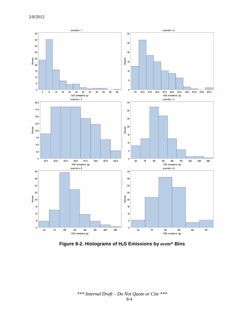
2/8/2012
*** Internal Draft – Do Not Quote or Cite *** 8-4
Figure 8-2. Histograms of H2S Emissions by avem* Bins

2/8/2012
*** Internal Draft – Do Not Quote or Cite *** 8-5
8.1.3 Developing Candidate Mean Trend Variables for H2S
8.1.3.1 Choosing Predictor Variable Functional Forms The plot of H2S emissions for all houses display a flattened “S” shape over the grow-out
period. The plot of H2S emissions versus average mass for all flocks is shown in Figure 8-3. To provide a reference for determining the functional form, the figure also depicts overlays of the linear, quadratic, and cubic regressions. The “S” trend is not as obvious in the aggregated plot due to high variability, especially for higher average bird mass values. However, when the plots are disaggregated by house (Figure 8-4), the trend becomes more apparent, especially in the CA1B houses. It appears that the increased variance in KY1B-1 H5 seen in Figure 8-4 masks the curvature when all house and flocks are plotted together. The trend is further evident in all houses when the H2S emissions are plotted versus average mass by flock (see Appendix F). Due to this curvature, the EPA determined that a cubic form of average mass was appropriate to characterize H2S emissions.
Figure 8-3. H2S Emissions vs. Average Bird Mass (Regression Overlays:
purple = linear, red = quadratic, green = cubic)

2/8/2012
*** Internal Draft – Do Not Quote or Cite *** 8-6
Figure 8-4. H2S Emissions vs. Average Bird Mass, by House
With regard to the effect of accumulated litter (buildup) on H2S emissions (see Section 7.3.1), the EPA did not discern a relationship between H2S emissions and the degree of litter accumulation, based on a visual review of the data. The scatter plot of H2S emissions versus average mass in Figure 8-5 shows very low variability in emissions during periods of low bird mass. The plot also shows that there is very little difference between the levels of litter condition, as the flocks of each buildup level are evenly distributed through the scatter plot. The EPA also created box plots (Figure 8-6) of the buildup variable to determine if the effect of accumulated litter should be included in the candidate mean trend variables for EEM development. The box plots, which depict the emissions for new bedding (build = 0) and any degree of accumulated litter (build = 1), show little difference in H2S emissions when flocks were raised on new bedding or on built-up litter.
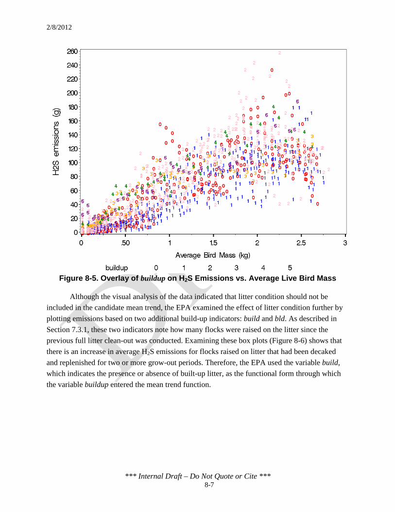
2/8/2012
*** Internal Draft – Do Not Quote or Cite *** 8-7
Figure 8-5. Overlay of buildup on H2S Emissions vs. Average Live Bird Mass
Although the visual analysis of the data indicated that litter condition should not be included in the candidate mean trend, the EPA examined the effect of litter condition further by plotting emissions based on two additional build-up indicators: build and bld. As described in Section 7.3.1, these two indicators note how many flocks were raised on the litter since the previous full litter clean-out was conducted. Examining these box plots (Figure 8-6) shows that there is an increase in average H2S emissions for flocks raised on litter that had been decaked and replenished for two or more grow-out periods. Therefore, the EPA used the variable build, which indicates the presence or absence of built-up litter, as the functional form through which the variable buildup entered the mean trend function.
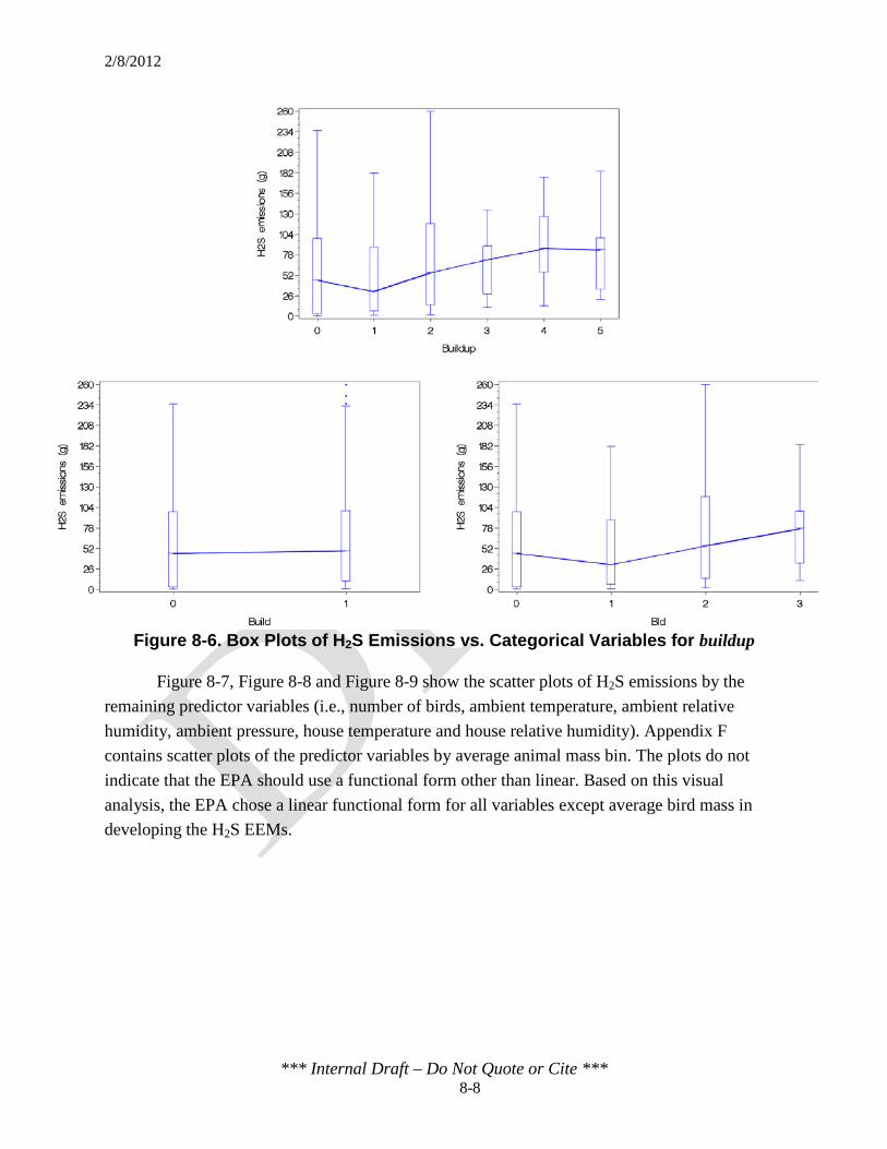
2/8/2012
*** Internal Draft – Do Not Quote or Cite *** 8-8
Figure 8-6. Box Plots of H2S Emissions vs. Categorical Variables for buildup
Figure 8-7, Figure 8-8 and Figure 8-9 show the scatter plots of H2S emissions by the remaining predictor variables (i.e., number of birds, ambient temperature, ambient relative humidity, ambient pressure, house temperature and house relative humidity). Appendix F contains scatter plots of the predictor variables by average animal mass bin. The plots do not indicate that the EPA should use a functional form other than linear. Based on this visual analysis, the EPA chose a linear functional form for all variables except average bird mass in developing the H2S EEMs.

2/8/2012
*** Internal Draft – Do Not Quote or Cite *** 8-9
Figure 8-7. H2S Emissions vs. Predictor Variables birds* and ta*

2/8/2012
*** Internal Draft – Do Not Quote or Cite *** 8-10
Figure 8-8. H2S Emissions vs. Predictor Variables ha* and pa*

2/8/2012
*** Internal Draft – Do Not Quote or Cite *** 8-11
Figure 8-9. H2S Emissions vs. Predictor Variables tc* and hc*

2/8/2012
*** Internal Draft – Do Not Quote or Cite *** 8-12
Table 8-2 summarizes the mean trend variables that describe the dependence of H2S emissions on the original predictor variables. The variables in column two were taken to be the main effect of the original predictors in column one of the table. For all predictors except buildup and avem*, the mean trend variable was the same as the original variable. For buildup, the main effect was the indicator variable build. For avem*, the linear, quadratic and cubic terms were collectively considered the main effect.
Table 8-2. Summary of Main Effect Mean Trend Variables for H2S
Original Predictor Variablea
Main Effect Mean Trend Variable(s)
buildup build
birds* birds
avem* avem, avem2, avem3
ta* ta
ha* ha
pa* pa
tc* tc
hc* hc a An asterisk (*) is used to note that these predictor variables are the original values submitted to the EPA before the data were centered and scaled (see Section 7.3.1).
8.1.3.2 Creating Mean Trend Variables from Main Effects and Interactions
The EPA created interaction terms and determined what level of interactions (e.g., two-way, three-way) to include in the set of candidate mean trend variables of Table 8-2. Initial testing of the R2 of two-way and three-way terms suggested that consideration of two-way interactions was appropriate for development of H2S EEMs. The main effects and interaction terms for the three EEMs tested are presented in Table 8-3.

2/8/2012
*** Internal Draft – Do Not Quote or Cite *** 8-13
Table 8-3. Candidate Mean Trend Variables for the I, IA and IAC H2S EEMs
EEM (Form) Main Effects Two-Way Interaction Terms
I, Cubic (I EEMC)
birds, build, avem, avem2,
avem3
buildbirds, buildavem, buildavem2, buildavem3, birdsavem, birdsavem2, birdsavem3
IA, Cubic (IA EEMC)
Same as I EEMC plus:
ta, ha, pa
Same as I EEMC plus: buildta, buildha, buildpa, birdsta, birdsha, birdspa, avemta,
avem2ta, avem3ta, avemha, avem2ha, avem3ha, avempa, avem2pa, avem3pa, taha, tapa, hapa
IAC, Cubic (IAC EEMC)
Same as IA EEMC plus:
tc, hc
Same as IA EEMC plus: buildtc, buildhc, birdstc, birdshc, avemtc, avem2tc, avem3tc,
avemhc, avem2hc, avem3hc, tatc, tahc, hatc, hahc, patc, pahc, tchc
8.1.3.3 Centering and Scaling Predictors The EPA centered and scaled each continuous predictor variable prior to creating higher
order terms and interaction terms by subtracting the mean of all observations in the base dataset from each value, then dividing by the standard deviation of the base dataset. The centering and scaling factors for the predictor variables for the H2S final EEMs are presented in Table 8-4.
Table 8-4. Centering and Scaling Reference Values for Continuous H2S Predictor Variables
Predictor Variablea Centering
Value Scaling Value birds* 22 2.2 avem* 1.0 0.83
ta* 15 8 ha* 65 14 pa* 101 1.1 tc* 25 3.7 hc* 57 9.5
a An asterisk (*) is used to note that these predictor variables are the original values submitted to the EPA before the data were centered and scaled (see Section 7.3.1). Predictor variables are centered and scaled prior to the creation of higher-order terms (e.g., eavem or avem2) and the creation of interaction terms (e.g., avemta).

2/8/2012
*** Internal Draft – Do Not Quote or Cite *** 8-14
8.1.4 Selecting Final Mean Trend Variables for H2S
Table 8-5 contains the final mean trend variables for the selected form of each EEM after backward elimination of mean trend variables (see Section 7.5). Table 8-6 shows the fit statistics for each EEM. A check mark () in the column for γ0 indicates that the estimate is not significantly different from zero at the α = 0.05 significance level, while an “x” indicates that it is significantly different from zero. Similarly, a check mark or an “x” in the column for γ1 indicates whether the estimate is significantly different from one.
Table 8-5. Final I, IA and IAC EEM Mean Trend Variables for H2S EEMs EEM Main Effects Two-Way Interaction Terms
I build, birds, avem, avem2, avem3
buildbirds, buildavem, buildavem2, buildavem3, birdsavem, birdsavem2, birdsavem3
IA build, birds, avem, avem2, avem3, ta,
ha, pa
buildavem, buildavem2, buildavem3, buildpa, birdsta, birdsha, birdspa, avemta, avem2ta, avem3ta, avemha, avem2ha, avem3ha,
avempa, avem2pa, avem3pa, taha, tapa, hapa
IAC build, birds, avem, avem2, avem3, ta,
ha, pa, tc, hc
buildavem, buildavem2, buildavem3, buildta, buildha, buildpa, buildtc, buildhc, birdspa, birdshc, avemta, avem2ta, avem3ta,
avemtc, avem2tc, avem3tc, avemhc, avem2hc, avem3hc, hapa, tatc, tahc, hatc, tchc
For all EEMs, the intercept, γ0, was significantly different from 0 at the α = 0.05
significance level. For the IA EEM, the slope, γ1, was significantly different from 1. These differences in γ0 and γ1 from 0 and 1 may indicate systematic bias, but the phrase “significantly different” refers to statistical significance, which is not the same as practical significance. The estimates of γ0 and γ1 mean that the relationship between the value of H2S emissions, Yht, in the cross-validation data to the point prediction produced by the EEM, Ŷht, is given by Yht = γ0 + γ1Ŷht. Using the IA EEM as an example, this relationship is Yht = 6.4 + 0.94Ŷht. That means that instead of the H2S emissions being equal to the point prediction, on average, they are equal to 6.4 grams plus 0.94 times the prediction of them. The practical significance of adding 6.4 grams is small, and it is offset by the fact that the multiplier 0.94 is less than 1, which reduces the predicted value of emissions.

2/8/2012
*** Internal Draft – Do Not Quote or Cite *** 8-15
Table 8-6. Final I, IA and IAC EEM Fit Statistics for H2S
EEM
Fit Statistics
-2LL BIC % in
PI Width
(g) RMSE
(g) R2 γ0 (g) γ1
I 9,143 9,152 98 91 23 0.80 4.7 x 1.0
IA 8,945 8,954 97 89 23 0.80 6.4 x 0.94 x
IAC 8,759 8,767 95 85 23 0.80 6.3 x 0.95
Note: A check mark in the column for γ0 indicates that the estimate is not significantly different from zero at the α = 0.05 significance level. A check mark in the column for γ1 indicates that the estimate is not significantly different from one at the α = 0.05 significance level.
8.1.5 Summary of Final Results for the I, IA and IAC EEMs for H2S
The covariance parameters for the final EEMs are listed in Table 8-7. The coefficients for the EEM mean trend variables are listed in Table 8-8. The value of each main effect variable (xp) must be centered and scaled when using these terms in Equation 7-1. The centering and scaling constants for the predictor variables of the H2S EEMs are presented in Table 8-4.
Table 8-7. Covariance Parameters for Final H2S EEMs
Covariance Parameter Estimate
I IA IAC
𝜌 0.8628 0.8683 0.8876
𝜎2 577.84 534.28 522.84
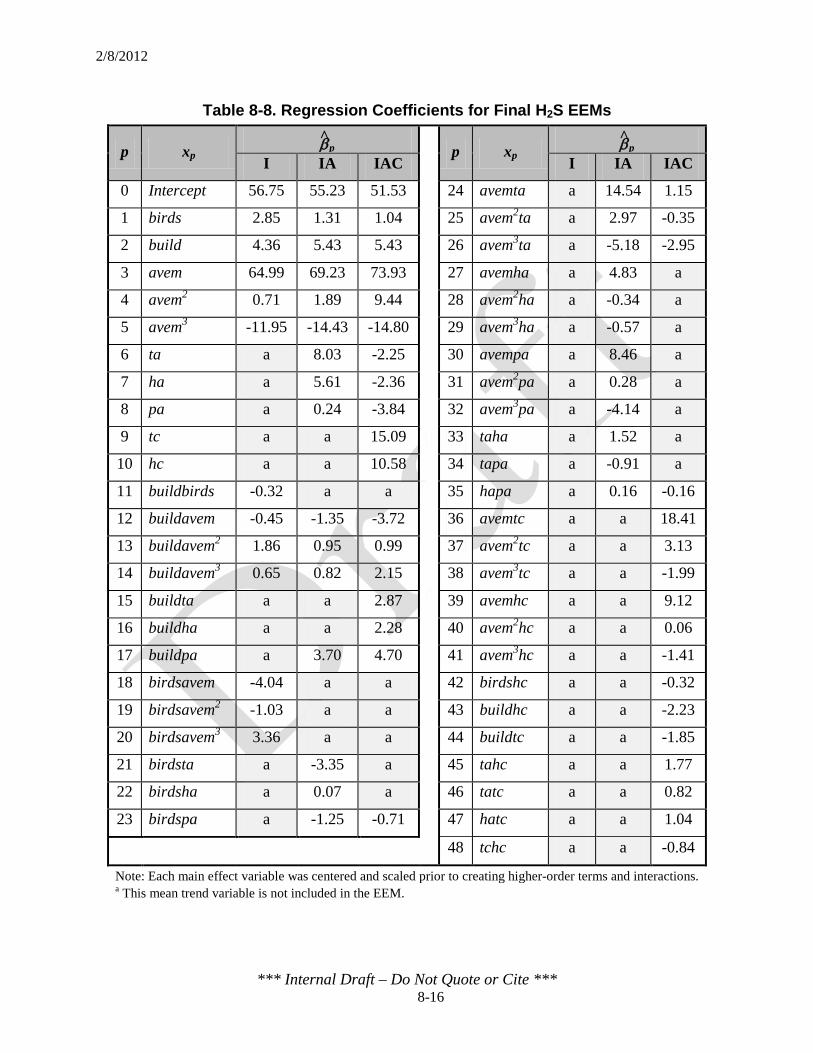
2/8/2012
*** Internal Draft – Do Not Quote or Cite *** 8-16
Table 8-8. Regression Coefficients for Final H2S EEMs
p xp βp p xp βp I IA IAC I IA IAC
0 Intercept 56.75 55.23 51.53 24 avemta a 14.54 1.15
1 birds 2.85 1.31 1.04 25 avem2ta a 2.97 -0.35
2 build 4.36 5.43 5.43 26 avem3ta a -5.18 -2.95
3 avem 64.99 69.23 73.93 27 avemha a 4.83 a
4 avem2 0.71 1.89 9.44 28 avem2ha a -0.34 a
5 avem3 -11.95 -14.43 -14.80 29 avem3ha a -0.57 a
6 ta a 8.03 -2.25 30 avempa a 8.46 a
7 ha a 5.61 -2.36 31 avem2pa a 0.28 a
8 pa a 0.24 -3.84 32 avem3pa a -4.14 a
9 tc a a 15.09 33 taha a 1.52 a
10 hc a a 10.58 34 tapa a -0.91 a
11 buildbirds -0.32 a a 35 hapa a 0.16 -0.16
12 buildavem -0.45 -1.35 -3.72 36 avemtc a a 18.41
13 buildavem2 1.86 0.95 0.99 37 avem2tc a a 3.13
14 buildavem3 0.65 0.82 2.15 38 avem3tc a a -1.99
15 buildta a a 2.87 39 avemhc a a 9.12
16 buildha a a 2.28 40 avem2hc a a 0.06
17 buildpa a 3.70 4.70 41 avem3hc a a -1.41
18 birdsavem -4.04 a a 42 birdshc a a -0.32
19 birdsavem2 -1.03 a a 43 buildhc a a -2.23
20 birdsavem3 3.36 a a 44 buildtc a a -1.85
21 birdsta a -3.35 a 45 tahc a a 1.77
22 birdsha a 0.07 a 46 tatc a a 0.82
23 birdspa a -1.25 -0.71 47 hatc a a 1.04
48 tchc a a -0.84
Note: Each main effect variable was centered and scaled prior to creating higher-order terms and interactions. a This mean trend variable is not included in the EEM.
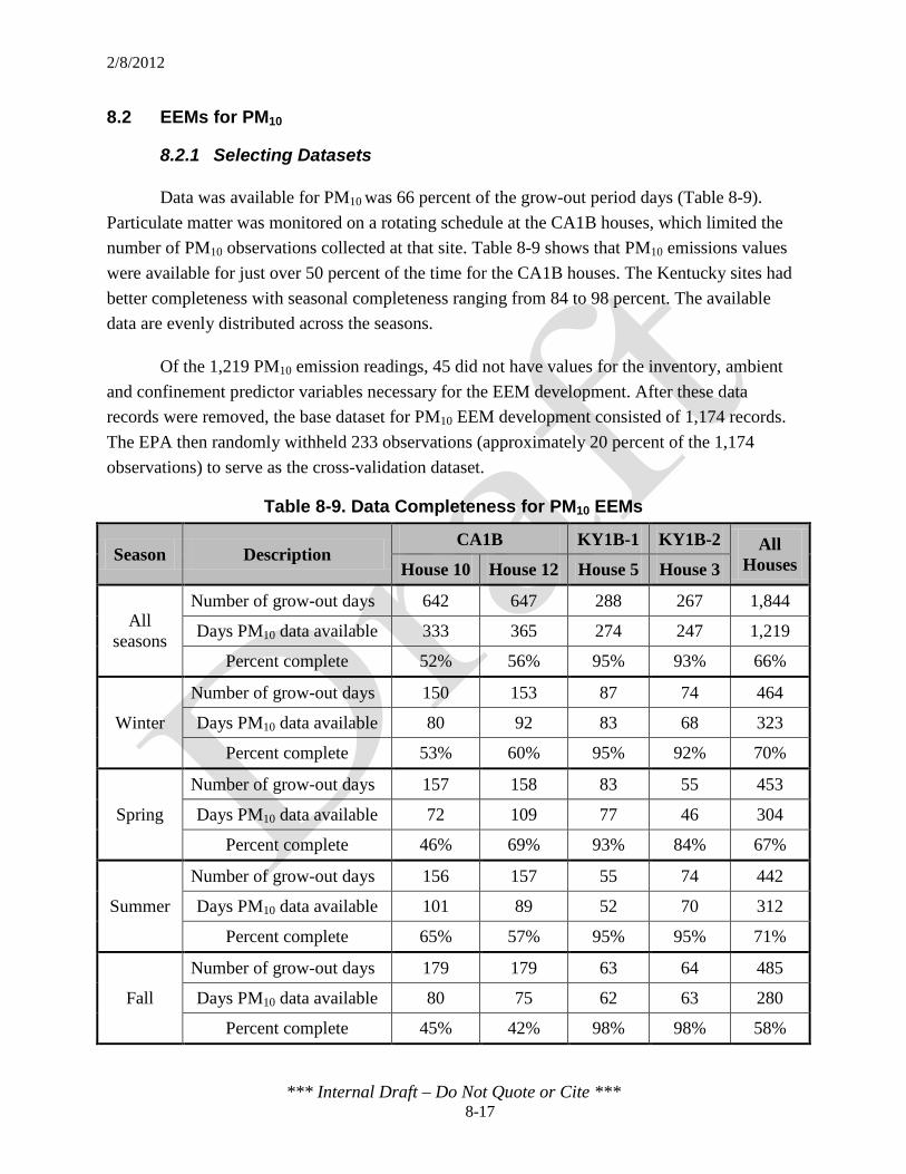
2/8/2012
*** Internal Draft – Do Not Quote or Cite *** 8-17
8.2 EEMs for PM10
8.2.1 Selecting Datasets
Data was available for PM10 was 66 percent of the grow-out period days (Table 8-9). Particulate matter was monitored on a rotating schedule at the CA1B houses, which limited the number of PM10 observations collected at that site. Table 8-9 shows that PM10 emissions values were available for just over 50 percent of the time for the CA1B houses. The Kentucky sites had better completeness with seasonal completeness ranging from 84 to 98 percent. The available data are evenly distributed across the seasons.
Of the 1,219 PM10 emission readings, 45 did not have values for the inventory, ambient and confinement predictor variables necessary for the EEM development. After these data records were removed, the base dataset for PM10 EEM development consisted of 1,174 records. The EPA then randomly withheld 233 observations (approximately 20 percent of the 1,174 observations) to serve as the cross-validation dataset.
Table 8-9. Data Completeness for PM10 EEMs
Season Description CA1B KY1B-1 KY1B-2 All
Houses House 10 House 12 House 5 House 3
All seasons
Number of grow-out days 642 647 288 267 1,844
Days PM10 data available 333 365 274 247 1,219
Percent complete 52% 56% 95% 93% 66%
Winter
Number of grow-out days 150 153 87 74 464
Days PM10 data available 80 92 83 68 323
Percent complete 53% 60% 95% 92% 70%
Spring
Number of grow-out days 157 158 83 55 453
Days PM10 data available 72 109 77 46 304
Percent complete 46% 69% 93% 84% 67%
Summer
Number of grow-out days 156 157 55 74 442
Days PM10 data available 101 89 52 70 312
Percent complete 65% 57% 95% 95% 71%
Fall
Number of grow-out days 179 179 63 64 485
Days PM10 data available 80 75 62 63 280
Percent complete 45% 42% 98% 98% 58%
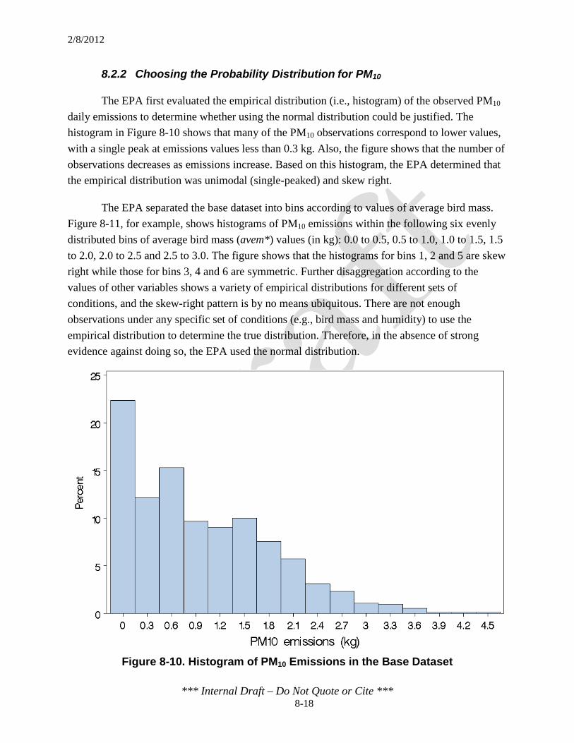
2/8/2012
*** Internal Draft – Do Not Quote or Cite *** 8-18
8.2.2 Choosing the Probability Distribution for PM10
The EPA first evaluated the empirical distribution (i.e., histogram) of the observed PM10 daily emissions to determine whether using the normal distribution could be justified. The histogram in Figure 8-10 shows that many of the PM10 observations correspond to lower values, with a single peak at emissions values less than 0.3 kg. Also, the figure shows that the number of observations decreases as emissions increase. Based on this histogram, the EPA determined that the empirical distribution was unimodal (single-peaked) and skew right.
The EPA separated the base dataset into bins according to values of average bird mass. Figure 8-11, for example, shows histograms of PM10 emissions within the following six evenly distributed bins of average bird mass (avem*) values (in kg): 0.0 to 0.5, 0.5 to 1.0, 1.0 to 1.5, 1.5 to 2.0, 2.0 to 2.5 and 2.5 to 3.0. The figure shows that the histograms for bins 1, 2 and 5 are skew right while those for bins 3, 4 and 6 are symmetric. Further disaggregation according to the values of other variables shows a variety of empirical distributions for different sets of conditions, and the skew-right pattern is by no means ubiquitous. There are not enough observations under any specific set of conditions (e.g., bird mass and humidity) to use the empirical distribution to determine the true distribution. Therefore, in the absence of strong evidence against doing so, the EPA used the normal distribution.
Figure 8-10. Histogram of PM10 Emissions in the Base Dataset
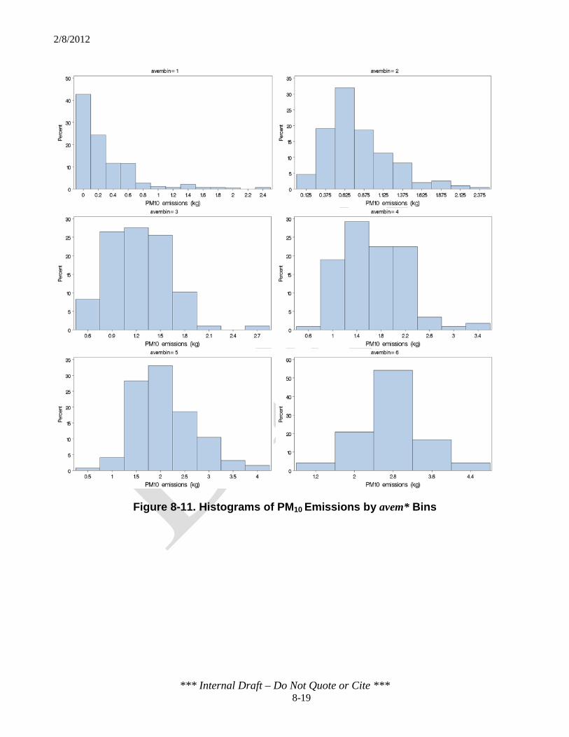
2/8/2012
*** Internal Draft – Do Not Quote or Cite *** 8-19
Figure 8-11. Histograms of PM10 Emissions by avem* Bins

2/8/2012
*** Internal Draft – Do Not Quote or Cite *** 8-20
8.2.3 Developing Candidate Mean Trend Variables for PM10
8.2.3.1 Choosing Predictor Variable Functional Forms for PM10 Plots of PM10 emissions versus average bird mass, for all houses, suggested a positive
relationship, with a slight upward curvature. Figure 8-12 shows a scatter plot of PM10 emissions versus average mass, with overlays of linear, quadratic and cubic regressions. The gradual increasing trend suggested either a quadratic or exponential relationship between PM10 emissions and average bird mass. Accordingly, the EPA tested two forms of the EEMs: an EEM based on a quadratic relationship with average mass (avem and avem2), and an EEM based on an exponential relationship (eavem).
Figure 8-12. PM10 Emissions vs. Average Bird Mass (Regression Overlays:
purple = linear, red = quadratic, green = cubic)
With regard to the effect of accumulated litter (buildup) on PM10 emissions (see Section 7.3.1), the EPA discerned a relationship between PM10 emissions and the degree of litter accumulation, based on the variance in PM10 emissions values for lower bird weights (see Figure 8-13). When PM10 emissions are plotted by average mass and color-coded to indicate the level of buildup, there is some indication that higher emissions correspond to built-up litter at lower animal mass. Further investigations showed that the increased variance was due to two flocks at each of the CA1B houses (Figure 8-14). Both of these flocks (6 and 7) were raised in the summer on built-up litter.

2/8/2012
*** Internal Draft – Do Not Quote or Cite *** 8-21
Figure 8-13. Overlay of buildup on PM10 Emissions vs. Average Live Bird Mass
Figure 8-14. PM10 Emissions vs. Average Bird Mass, Color-coded by Site

2/8/2012
*** Internal Draft – Do Not Quote or Cite *** 8-22
Plots of the build-up indicator parameters (i.e., buildup, build, bld) suggested average PM10 emissions do not increase for flocks raised on built-up litter, because there is little difference in the minimum emissions levels between the litter conditions (Figure 8-15), and only a slight difference in average values. The EPA decided to include build as the functional form through which the variable buildup enters the mean trend function and test its significance using the p-value analysis to determine the final mean trend variables.
Figure 8-15. Box Plots of PM10 Emissions vs. Categorical Variables for buildup
Figure 8-16, Figure 8-17, and Figure 8-18 show the scatter plots of PM10 emissions versus the remaining predictors (i.e., number of birds, ambient temperature, ambient relative humidity, ambient pressure, house temperature and house relative humidity). Appendix F contains scatter plots of the predictor variables by average animal mass bin. The plots do not indicate that the EPA should use a functional form other than linear for all variables other than avem. Based on this visual analysis, and the absence of a process-based reason to do otherwise, the EPA chose a linear functional form for all variables except average bird mass in developing the PM10 EEMs.

2/8/2012
*** Internal Draft – Do Not Quote or Cite *** 8-23
Figure 8-16. PM10 Emissions vs. Predictor Variables birds* and ta*
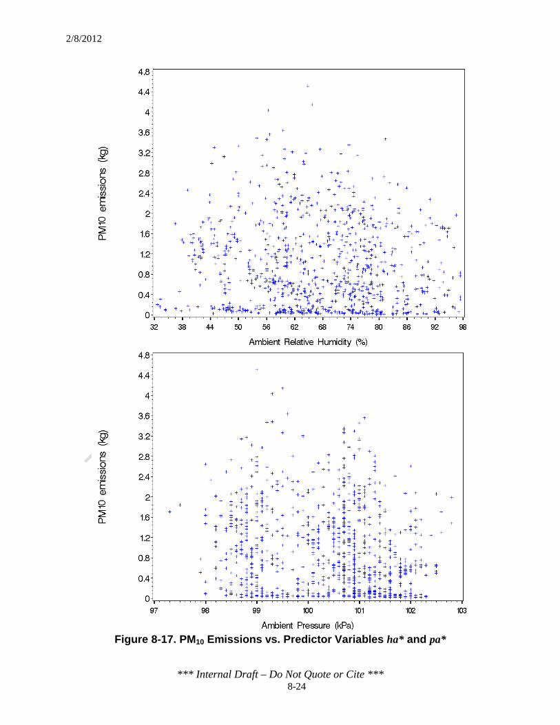
2/8/2012
*** Internal Draft – Do Not Quote or Cite *** 8-24
Figure 8-17. PM10 Emissions vs. Predictor Variables ha* and pa*

2/8/2012
*** Internal Draft – Do Not Quote or Cite *** 8-25
Figure 8-18. PM10 Emissions vs. Predictor Variables tc* and hc*
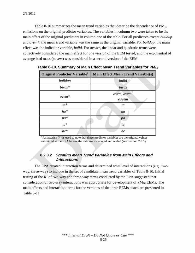
2/8/2012
*** Internal Draft – Do Not Quote or Cite *** 8-26
Table 8-10 summarizes the mean trend variables that describe the dependence of PM10 emissions on the original predictor variables. The variables in column two were taken to be the main effect of the original predictors in column one of the table. For all predictors except buildup and avem*, the mean trend variable was the same as the original variable. For buildup, the main effect was the indicator variable, build. For avem*, the linear and quadratic terms were collectively considered the main effect for one version of the EEM tested, and the exponential of average bird mass (eavem) was considered in a second version of the EEM.
Table 8-10. Summary of Main Effect Mean Trend Variables for PM10
Original Predictor Variablea Main Effect Mean Trend Variable(s)
buildup build
birds* birds
avem* avem, avem2
eavem ta* ta
ha* ha
pa* pa
tc* tc
hc* hc a An asterisk (*) is used to note that these predictor variables are the original values submitted to the EPA before the data were centered and scaled (see Section 7.3.1).
8.2.3.2 Creating Mean Trend Variables from Main Effects and Interactions
The EPA created interaction terms and determined what level of interactions (e.g., two-way, three-way) to include in the set of candidate mean trend variables of Table 8-10. Initial testing of the R2 of two-way and three-way terms conducted by the EPA suggested that consideration of two-way interactions was appropriate for development of PM10 EEMs. The main effects and interaction terms for the versions of the three EEMs tested are presented in Table 8-11.

2/8/2012
*** Internal Draft – Do Not Quote or Cite *** 8-27
Table 8-11. Candidate Mean Trend Variables for the I, IA and IAC PM10 EEMs
EEM Main Effects Two-Way Interaction Terms
I, Quadratic (I EEMQ)
build, birds, avem, avem2
buildbirds, buildavem, buildavem2, birdsavem, birdsavem2
I, Exponential (I EEME)
build, birds, eavem buildbirds, buildeavem, birdseavem
IA, Quadratic (IA EEMQ)
Same as I EEMQ plus:
ta, ha, pa
Same as I EEMQ plus: buildta, buildha, buildpa, birdsta, birdsha, birdspa,
avemta, avem2ta, avemha, avem2ha, avempa, avem2pa, taha, tapa, hapa
IA, Exponential (IA EEME)
Same as I EEME plus:
ta, ha, pa
Same as I EEME plus: buildta, buildha, buildpa, birdsta, birdsha, birdspa,
eavemta, eavemha, eavempa, taha, tapa, hapa
IAC, Quadratic (IAC EEMQ)
Same as IA EEMQ plus: tc, hc
Same as IA EEMQ plus: buildtc, buildhc, birdstc, birdshc, avemtc, avem2tc, avemhc, avem2hc, tatc, tahc, hatc, hahc, patc, pahc,
tchc IAC,
Exponential (IAC EEME)
Same as IA EEME plus: tc, hc
Same as IA EEME plus: buildtc, buildhc, birdstc, birdshc, eavemtc, eavemhc,
tatc, tahc, hatc, hahc, patc, pahc, tchc
8.2.3.3 Centering and Scaling Predictors The EPA centered and scaled each continuous predictor variable prior to creating
interaction terms by subtracting the mean of all observations in the base dataset from each value, then dividing by the standard deviation of the base dataset. The centering and scaling factors for the predictor variable for the PM10 final EEMs are presented in Table 8-12.

2/8/2012
*** Internal Draft – Do Not Quote or Cite *** 8-28
Table 8-12. Centering and Scaling Reference Values for Continuous PM10 Predictor Variables
Predictor Variablea Centering
Value Scaling Value
birds* 22 2.5
avem* 1.1 0.87
ta* 15 8.2
ha* 66 14
pa* 100 1.1
tc* 25 3.8
hc* 58 9.9 a An asterisk (*) is used to note that these predictor variables are the original values submitted to the EPA before the data were centered and scaled (see Section 7.3.1). Predictor variables are centered and scaled prior to the creation of higher-order terms (e.g., eavem or avem2) and the creation of interaction terms (e.g., avemta).
8.2.4 Selecting Final Mean Trend Variables for PM10
8.2.4.1 Inventory EEM The EPA tested two forms of the I EEM; a quadratic and an exponential form
(Table 8-13). Predictions based on the quadratic form of the EEM (I EEMQ) always had systematic bias for the intercept, γ0, regardless of the number of parameters eliminated. Predictions based on the exponential form of the EEM (I EEME) demonstrated systematic bias after initial backward elimination steps.
The selected form of the I EEMQ contains all of the initial interaction terms. This EEM displayed the best fit-statistics against the cross-validation dataset (lowest RMSE and highest R2); however, the EEM still exhibited systematic bias. The best form of the I EEME also included all the initial interaction terms. This version of the I EEME had the best fit-statistics against the cross-validation dataset, as well as the coverage percentage (% in PI) closest to 95 percent, without exhibiting systematic bias. The fit statistics for the selected I EEMQ and I EEME are presented in Table 8-14. A check mark () in the column for γ0 indicates that the estimate is not significantly different from zero at the α = 0.05 significance level, while an “x” indicates that it is significantly different from zero. Similarly, a check mark or an “x” in the column for γ1 indicates whether or not the estimate is significantly different from one.
Because the I EEMQ always exhibited systematic bias, the EPA retested the I EEMQ using different versions of the base and cross-validation datasets to verify that the systematic bias

2/8/2012
*** Internal Draft – Do Not Quote or Cite *** 8-29
was not due to random selection of an improper cross-validation dataset. Examples of an improper cross-validation dataset include a dataset where the values are skewed to one end of the distribution, or a dataset that contains too many extreme values. In these examples, the fit statistics would be biased for the extreme values of the dataset. Based on the results of the retest, the systematic bias for the I EEMQ could not be attributed to improper selection of a cross-validation dataset. Therefore, the EPA selected the I EEME (highlighted in gray) because it did not display systematic bias.
Table 8-13. Final Candidate I EEM Mean Trend Variables for PM10
EEM Main Effects Two-Way Interaction Terms
I EEMQ build, birds, avem, avem2 buildbirds, buildavem, buildavem2, birdsavem, birdsavem2
I EEME build, birds, eavem buildbirds, buildeavem, birdseavem
Table 8-14. Final Candidate I EEM Fit Statistics for PM10
Candidate EEM
Fit Statistics
-2LL BIC % in PI Width (kg) RMSE (kg) R2 γ0 (kg) γ1
I EEMQ 646 654 93 2.1 0.51 0.65 0.16 0.92
I EEME 621 630 91 2.0 0.52 0.63 -0.12 1.1 Note: A check mark in the column for γ0 indicates that the estimate is not significantly different from zero at the α = 0.05 significance level. A check mark in the column for γ1 indicates that the estimate is not significantly different from one at the α = 0.05 significance level.
8.2.4.2 Inventory and Ambient EEM
The selected form of IA EEMQ and IA EEME are presented in Table 8-15. Similar to the I EEM, the quadratic form of the EEM (IA EEMQ) always demonstrated systematic bias for the slope, γ0, regardless of the number of parameters eliminated. The initial eliminations produced minor systematic bias, with the range of estimates for γ0 failing to cover zero by only 0.001. Predictions based on the exponential form of the EEM (IA EEME) demonstrated systematic bias after the third backward elimination steps. The selected version of the IA EEME occurs prior to the development of systematic bias and displays the best fit-statistics against the cross-validation dataset (lowest RMSE and highest R2) and the smallest confidence interval width and best coverage percentage of the backward elimination steps.
Although both selected EEMs had similar fit statistics (Table 8-16), the IA EEMQ had persistent systematic bias. This systematic bias could not be contributed to improper selection of a cross-validation data set. Therefore, the EPA selected the IA EEME (highlighted in gray), which retains the terms listed in Table 8-15.
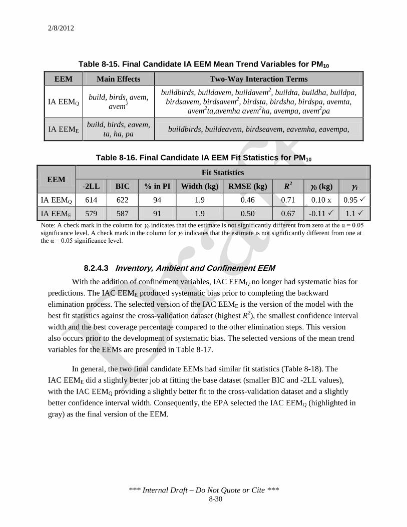
2/8/2012
*** Internal Draft – Do Not Quote or Cite *** 8-30
Table 8-15. Final Candidate IA EEM Mean Trend Variables for PM10
EEM Main Effects Two-Way Interaction Terms
IA EEMQ build, birds, avem, avem2
buildbirds, buildavem, buildavem2, buildta, buildha, buildpa, birdsavem, birdsavem2, birdsta, birdsha, birdspa, avemta,
avem2ta,avemha avem2ha, avempa, avem2pa
IA EEME build, birds, eavem, ta, ha, pa buildbirds, buildeavem, birdseavem, eavemha, eavempa,
Table 8-16. Final Candidate IA EEM Fit Statistics for PM10
EEM Fit Statistics
-2LL BIC % in PI Width (kg) RMSE (kg) R2 γ0 (kg) γ1
IA EEMQ 614 622 94 1.9 0.46 0.71 0.10 x 0.95
IA EEME 579 587 91 1.9 0.50 0.67 -0.11 1.1 Note: A check mark in the column for γ0 indicates that the estimate is not significantly different from zero at the α = 0.05 significance level. A check mark in the column for γ1 indicates that the estimate is not significantly different from one at the α = 0.05 significance level.
8.2.4.3 Inventory, Ambient and Confinement EEM With the addition of confinement variables, IAC EEMQ no longer had systematic bias for
predictions. The IAC EEME produced systematic bias prior to completing the backward elimination process. The selected version of the IAC EEME is the version of the model with the best fit statistics against the cross-validation dataset (highest R2), the smallest confidence interval width and the best coverage percentage compared to the other elimination steps. This version also occurs prior to the development of systematic bias. The selected versions of the mean trend variables for the EEMs are presented in Table 8-17.
In general, the two final candidate EEMs had similar fit statistics (Table 8-18). The IAC EEME did a slightly better job at fitting the base dataset (smaller BIC and -2LL values), with the IAC EEMQ providing a slightly better fit to the cross-validation dataset and a slightly better confidence interval width. Consequently, the EPA selected the IAC EEMQ (highlighted in gray) as the final version of the EEM.

2/8/2012
*** Internal Draft – Do Not Quote or Cite *** 8-31
Table 8-17. Final Candidate IAC EEM Mean Trend Variables for PM10
EEM Main Effects Two-way Interaction Terms
IAC EEMQ
build, birds, avem, avem2, ta, ha, pa, tc,
hc
buildbirds, buildavem, buildavem2, buildta, buildha, buildpa, buildtc, buildhc, birdsavem, birdsavem2, birdsta, birdsha, birdspa, birdstc,
birdshc, avemta, avem2ta, avemha, avem2ha, avempa, avem2pa, avemtc, avem2tc, avemhc, avem2hc, taha, tapa, hapa, tatc, tahc, tchc
IAC EEME build, birds, eavem, ta,
ha, pa, tc, hc
buildbirds, buildeavem, buildta, buildha, buildpa, buildtc, buildhc, birdseavem, eavemta, eavemha, eavempa, eavemtc, eavemhc, taha,
tapa, hapa, tatc, tahc, hatc, hahc, patc, pahc, tchc
Table 8-18. Final Candidate IAC EEM Fit Statistics for PM10
Candidate EEM
Fit Statistics
-2LL BIC % in PI Width (kg) RMSE (kg) R2 γ0 (kg) γ1
IAC EEMQ 519 526 94 1.7 0.40 0.79 0.03 1.0
IAC EEME 507 515 93 1.8 0.45 0.73 -0.09 1.08 Note: A check mark in the column for γ0 indicates that the estimate is not significantly different from zero at the α = 0.05 significance level. A check mark in the column for γ1 indicates that the estimate is not significantly different from one at the α = 0.05 significance level.
8.2.5 Summary of Final Results for the I, IA and IAC EEMs for PM10
A summary of the final mean trend variables for the three EEMs is provided in Table 8-19. The covariance parameters for the final forms of the EEMs are listed in Table 8-20. The coefficients for the EEM mean trend variables are listed in Table 8-21. The value of each main effect variable (xp) must be centered and scaled when using these terms in Equation 7-1. The centering and scaling factors for the predictor variables used in the final PM10 EEMs are presented in Table 8-12.
Table 8-19. Final EEM Mean Trend Variables for PM10
EEM Main Effects Two-Way Interaction Terms
I build, birds, eavem buildbirds, buildeavem, birdseavem
IA build, birds, eavem, ta, ha, pa buildbirds, buildeavem, birdseavem, eavemha, eavempa,
IAC build, birds, avem,
avem2, ta, ha, pa, tc, hc
buildbirds, buildavem, buildavem2, buildta, buildha, buildpa, buildtc, buildhc, birdsavem, birdsavem2, birdsta, birdsha, birdspa, birdstc,
birdshc, avemta, avem2ta, avemha, avem2ha, avempa, avem2pa, avemtc, avem2tc, avemhc, avem2hc, taha, tapa, hapa, tatc, tahc, tchc

2/8/2012
*** Internal Draft – Do Not Quote or Cite *** 8-32
Table 8-20. Covariance Parameter for Final PM10 EEMs
Covariance Parameter
Estimate
I IA IAC
𝜌 0.7486 0.7513 0.6984
𝜎2 0.2131 0.1977 0.1404
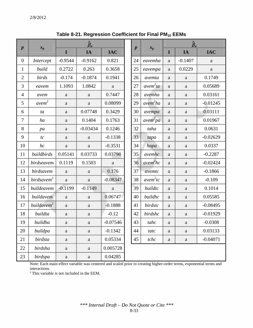
2/8/2012
*** Internal Draft – Do Not Quote or Cite *** 8-33
Table 8-21. Regression Coefficient for Final PM10 EEMs
p xp βp p xp βp I IA IAC I IA IAC
0 Intercept -0.9544 -0.9162 0.821
24 eavemha a -0.1407 a
1 build 0.2722 0.263 0.3658
25 eavempa a 0.0229 a
2 birds -0.174 -0.1874 0.1941
26 avemta a a 0.1749
3 eavem 1.1093 1.0842 a
27 avem2ta a a 0.05689
4 avem a a 0.7447
28 avemha a a 0.03161
5 avem2 a a 0.08099
29 avem2ha a a -0.01245
6 ta a 0.07748 0.3429
30 avempa a a 0.03111
7 ha a 0.1404 0.1763
31 avem2pa a a 0.01967
8 pa a -0.03434 0.1246
32 taha a a 0.0631
9 tc a a -0.1338
33 tapa a a -0.02629
10 hc a a -0.3531
34 hapa a a 0.0337
11 buildbirds 0.05141 0.03733 0.03798
35 avemhc a a -0.2287
12 birdseavem 0.1119 0.1503 a
36 avem2hc a a -0.02424
13 birdsavem a a 0.176
37 avemtc a a -0.1866
14 birdsavem2 a a -0.08347
38 avem2tc a a -0.109
15 buildeavem -0.1199 -0.1149 a
39 buildtc a a 0.1014
16 buildavem a a 0.06747
40 buildhc a a 0.05585
17 buildavem2 a a -0.1888
41 birdstc a a -0.08495
18 buildta a a -0.12
42 birdshc a a -0.01929
19 buildha a a -0.07546
43 tahc a a -0.0308
20 buildpa a a -0.1342
44 tatc a a 0.03133
21 birdsta a a 0.05334
45 tchc a a -0.04071
22 birdsha a a 0.005728
23 birdspa a a 0.04285
Note: Each main effect variable was centered and scaled prior to creating higher-order terms, exponential terms and interactions. a This variable is not included in the EEM.
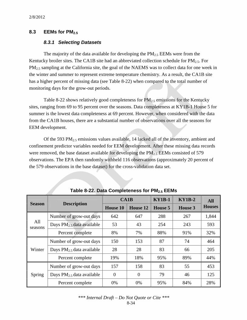
2/8/2012
*** Internal Draft – Do Not Quote or Cite *** 8-34
8.3 EEMs for PM2.5
8.3.1 Selecting Datasets
The majority of the data available for developing the PM2.5 EEMs were from the Kentucky broiler sites. The CA1B site had an abbreviated collection schedule for PM2.5. For PM2.5 sampling at the California site, the goal of the NAEMS was to collect data for one week in the winter and summer to represent extreme temperature chemistry. As a result, the CA1B site has a higher percent of missing data (see Table 8-22) when compared to the total number of monitoring days for the grow-out periods.
Table 8-22 shows relatively good completeness for PM2.5 emissions for the Kentucky sites, ranging from 69 to 95 percent over the seasons. Data completeness at KY1B-1 House 5 for summer is the lowest data completeness at 69 percent. However, when considered with the data from the CA1B houses, there are a substantial number of observations over all the seasons for EEM development.
Of the 593 PM2.5 emissions values available, 14 lacked all of the inventory, ambient and confinement predictor variables needed for EEM development. After these missing data records were removed, the base dataset available for developing the PM2.5 EEMs consisted of 579 observations. The EPA then randomly withheld 116 observations (approximately 20 percent of the 579 observations in the base dataset) for the cross-validation data set.
Table 8-22. Data Completeness for PM2.5 EEMs
Season Description CA1B KY1B-1 KY1B-2 All
Houses House 10 House 12 House 5 House 3
All seasons
Number of grow-out days 642 647 288 267 1,844
Days PM2.5 data available 53 43 254 243 593
Percent complete 8% 7% 88% 91% 32%
Winter
Number of grow-out days 150 153 87 74 464
Days PM2.5 data available 28 28 83 66 205
Percent complete 19% 18% 95% 89% 44%
Spring
Number of grow-out days 157 158 83 55 453
Days PM2.5 data available 0 0 79 46 125
Percent complete 0% 0% 95% 84% 28%

2/8/2012
*** Internal Draft – Do Not Quote or Cite *** 8-35
Table 8-22. Data Completeness for PM2.5 EEMs
Season Description CA1B KY1B-1 KY1B-2 All
Houses House 10 House 12 House 5 House 3
Summer
Number of grow-out days 156 157 55 74 442
Days PM2.5 data available 15 15 38 70 138
Percent complete 10% 10% 69% 95% 31%
Fall
Number of grow-out days 179 179 63 64 485
Days PM2.5 data available 10 0 54 61 125
Percent complete 6% 0% 86% 95% 26%
8.3.2 Choosing the Probability Distribution for PM2.5
The EPA first evaluated the empirical distribution (i.e., histogram) of the observed PM2.5 daily emissions to determine whether using the normal distribution could be justified (see Section 7.2). The histogram in Figure 8-19 shows that many of the PM2.5 observations correspond to lower emissions values, with a single peak at emission values less than 40 g. The figure also shows that the number of observations decreases as emissions increase. Based on this histogram, the EPA determined that the empirical distribution was unimodal (single-peaked) and skew right.
The EPA separated the base dataset into bins according to values of average bird mass. Figure 8-20 shows histograms of PM2.5 emissions within the following six evenly distributed bins of average bird mass (avem*) values (in kg): 0.0 to 0.5, 0.5 to 1.0, 1.0 to 1.5, 1.5 to 2.0, 2.0 to 2.5 and 2.5 to 3.0. The figure shows that the histograms for bins 1, 2, 3, and 4 are skew right, while bin 5 is symmetric and 6 is skew left, though it has fewer data points than the other bins. Further disaggregation according to the values of other variables shows a variety of empirical distributions for different sets of conditions, and the skew patterns were by no means a consistent pattern. There are not enough observations under any specific set of conditions (e.g., bird mass and humidity ranges) to use the empirical distribution to determine the true distribution. Therefore, in the absence of strong evidence against doing so, the EPA used the normal distribution.

2/8/2012
*** Internal Draft – Do Not Quote or Cite *** 8-36
Figure 8-19. Histogram of PM2.5 Emissions in the Base Dataset

2/8/2012
*** Internal Draft – Do Not Quote or Cite *** 8-37
Figure 8-20. Histograms of PM2.5 Emissions by avem* Bins

2/8/2012
*** Internal Draft – Do Not Quote or Cite *** 8-38
8.3.3 Developing Candidate Mean Trend Variables for PM2.5
8.3.3.1 Choosing Predictor Variable Functional Forms for PM2.5 Similar to PM10, plots of PM2.5 emissions versus average bird mass, for all houses
(Figure 8-21), suggested a positive relationship, with a slight upward curvature. The gradual increasing trend suggested either a quadratic or exponential relationship between PM2.5 emissions and the average bird mass. For the PM2.5 analysis, the EPA tested two functional forms of average mass: one form based on a quadratic relationship with average mass (avem and avem2), and the second form based on an exponential relationship (eavem).
Figure 8-21. PM2.5 Emissions vs. Average Bird Mass (Regression Overlays:
purple = linear, red = quadratic, green = cubic)
With regard to the effect of accumulated litter (buildup) on PM2.5 emissions (see Section 7.3.1), the EPA discerned a relationship between PM2.5 emissions and the degree of litter accumulation, based on the variance in PM2.5 emissions values for lower bird weights (see Figure 8-22). Plots of PM2.5 emissions by average mass that are color-coded to indicate the level of buildup (Figure 8-22) suggested built-up litter correspond to higher emissions. However, the EPA was unable to draw a definitive conclusion from the scatter plot because only one full flock was raised on fresh bedding between the California and Kentucky sites due to the design of the study.
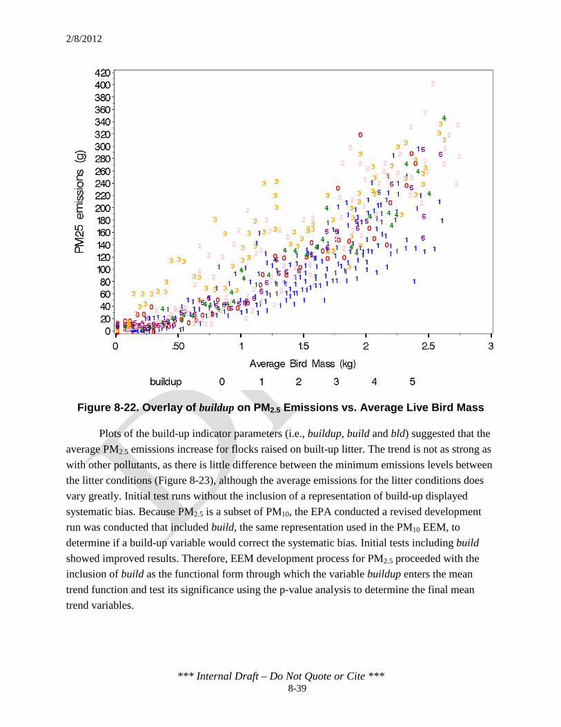
2/8/2012
*** Internal Draft – Do Not Quote or Cite *** 8-39
Figure 8-22. Overlay of buildup on PM2.5 Emissions vs. Average Live Bird Mass
Plots of the build-up indicator parameters (i.e., buildup, build and bld) suggested that the average PM2.5 emissions increase for flocks raised on built-up litter. The trend is not as strong as with other pollutants, as there is little difference between the minimum emissions levels between the litter conditions (Figure 8-23), although the average emissions for the litter conditions does vary greatly. Initial test runs without the inclusion of a representation of build-up displayed systematic bias. Because PM2.5 is a subset of PM10, the EPA conducted a revised development run was conducted that included build, the same representation used in the PM10 EEM, to determine if a build-up variable would correct the systematic bias. Initial tests including build showed improved results. Therefore, EEM development process for PM2.5 proceeded with the inclusion of build as the functional form through which the variable buildup enters the mean trend function and test its significance using the p-value analysis to determine the final mean trend variables.

2/8/2012
*** Internal Draft – Do Not Quote or Cite *** 8-40
Figure 8-23. Box Plots of PM2.5 Emissions vs. Categorical Variables for buildup
Figure 8-24, Figure 8-25 and Figure 8-26 show the scatter plots of PM2.5 emissions by the remaining predictors (i.e., number of birds, ambient temperature, ambient relative humidity, ambient pressure, house temperature and house relative humidity). Appendix F contains scatter plots of the predictor variables by average animal mass bin. The plots do not indicate that the EPA should use a functional form other than linear. Based on this visual analysis, the EPA chose a linear functional form for all variables except average bird mass in developing the PM2.5 EEMs.

2/8/2012
*** Internal Draft – Do Not Quote or Cite *** 8-41
Figure 8-24. PM2.5 Emissions vs. Predictor Variables birds* and ta*

2/8/2012
*** Internal Draft – Do Not Quote or Cite *** 8-42
Figure 8-25. PM2.5 Emissions vs. Predictor Variables ha* and pa*

2/8/2012
*** Internal Draft – Do Not Quote or Cite *** 8-43
Figure 8-26. PM2.5 Emissions vs. Predictor Variables tc* and hc*

2/8/2012
*** Internal Draft – Do Not Quote or Cite *** 8-44
Table 8-23 summarizes the mean trend variables that describe the dependence of PM2.5 emissions on the original predictor variables. The variables in column two were taken to be the main effect of the original predictors in column one of the table. For all predictors except buildup and avem*, the mean trend variable was the same as the original variable. For buildup, the main effect was the indicator variable, build. For avem*, the linear and quadratic terms were collectively considered the main effect for one version of the EEM tested, and the exponential of average bird mass (eavem) was considered in a second version of the EEM.
Table 8-23. Summary of Main Effect Mean Trend Variables for PM2.5
Original Predictor Variablea Main Effect Mean Trend Variable(s) buildup build birds* birds
avem* avem, avem2 eavem
ta* ta ha* ha pa* pa tc* tc hc* hc
a An asterisk (*) is used to note that these predictor variables are the original values submitted to the EPA before the data were centered and scaled (see Section 7.3.1).
8.3.3.2 Creating Mean Trend Variables from Main Effects and Interactions for PM2.5
The EPA created interaction terms and determined what level of interactions (e.g., two-way, three-way) to include in the set of candidate mean trend variables of Table 8-23. Initial testing of the R2 of two-way and three-way terms conducted by the EPA suggested that consideration of two-way interactions was appropriate for development of PM2.5 EEMs. The main effects and interaction terms for the versions of the three EEMs tested are presented in Table 8-24.

2/8/2012
*** Internal Draft – Do Not Quote or Cite *** 8-45
Table 8-24. Candidate Mean Trend Variables for the I, IA and IAC PM2.5 EEMs EEM Main Effects Two-Way Interaction Terms
I, Quadratic (I EEMQ)
build, birds, avem, avem2
buildbirds, buildavem, buildavem2, birdsavem, birdsavem2
I, Exponential (I EEME)
build, birds, eavem buildbirds, buildeavem, birdseavem
IA, Quadratic (IA EEMQ)
Same as I EEMQ plus:
ta, ha, pa
Same as I EEMQ plus: buildta, buildha, buildpa, birdsta, birdsha, birdspa,
avemta, avem2ta, avemha, avem2ha, avempa, avem2pa,taha, tapa, hapa
IA, Exponential (IA EEME)
Same as I EEME plus:
ta, ha, pa
Same as I EEME plus: buildta, buildha, buildpa, birdsta, birdsha, birdspa,
eavemta, eavemha, eavempa, taha, tapa, hapa
IAC, Quadratic (IAC EEMQ)
Same as IA EEMQ plus: tc, hc
Same as IA EEMQ plus: buildtc, buildhc, birdstc, birdshc, avemtc, avem2tc,
avemhc, avem2hc, tatc, tahc, hatc, hahc, patc, pahc, tchc
IAC, Exponential (IAC EEME)
Same as IA EEME plus: tc, hc
Same as IA EEME plus: buildtc, buildhc, birdstc, birdshc, eavemtc, eavemhc, tatc,
tahc, hatc, hahc, patc, pahc, tchc
8.3.3.3 Centering and Scaling Predictors for PM2.5 The EPA centered and scaled each continuous predictor variable prior to creating
interaction terms by subtracting the mean of all observations in the base dataset from each value, then dividing by the standard deviation of the base dataset. The centering and scaling factors for the predictor variable for the PM2.5 final EEMs are presented in Table 8-25.
Table 8-25. Centering and Scaling Reference Values for Continuous PM2.5 Predictor Variables
Predictor Variablea Centering Value Scaling Value birds* 24 2.8 avem* 1.1 0.76
ta* 13 8.8 ha* 72 12 pa* 99 0.73 tc* 27 3.5 hc* 58 9.7
a An asterisk (*) is used to note that these predictor variables are the original values submitted to the EPA before the data were centered and scaled (see Section 7.3.1). Predictor variables are centered and scaled prior to the creation of higher-order terms (e.g., eavem or avem2) and the creation of interaction terms (e.g., avemta).
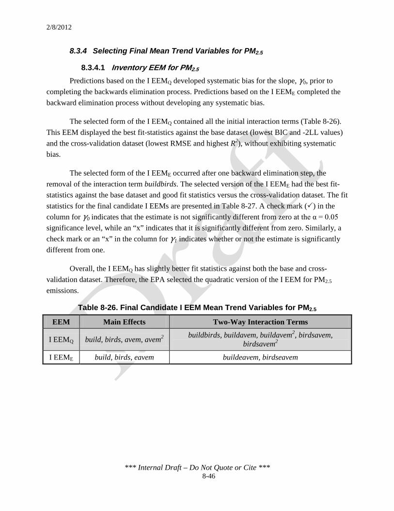
2/8/2012
*** Internal Draft – Do Not Quote or Cite *** 8-46
8.3.4 Selecting Final Mean Trend Variables for PM2.5
8.3.4.1 Inventory EEM for PM2.5 Predictions based on the I EEMQ developed systematic bias for the slope, γ0, prior to
completing the backwards elimination process. Predictions based on the I EEME completed the backward elimination process without developing any systematic bias.
The selected form of the I EEMQ contained all the initial interaction terms (Table 8-26). This EEM displayed the best fit-statistics against the base dataset (lowest BIC and -2LL values) and the cross-validation dataset (lowest RMSE and highest R2), without exhibiting systematic bias.
The selected form of the I EEME occurred after one backward elimination step, the removal of the interaction term buildbirds. The selected version of the I EEME had the best fit-statistics against the base dataset and good fit statistics versus the cross-validation dataset. The fit statistics for the final candidate I EEMs are presented in Table 8-27. A check mark () in the column for γ0 indicates that the estimate is not significantly different from zero at the α = 0.05 significance level, while an “x” indicates that it is significantly different from zero. Similarly, a check mark or an “x” in the column for γ1 indicates whether or not the estimate is significantly different from one.
Overall, the I EEMQ has slightly better fit statistics against both the base and cross-validation dataset. Therefore, the EPA selected the quadratic version of the I EEM for PM2.5 emissions.
Table 8-26. Final Candidate I EEM Mean Trend Variables for PM2.5
EEM Main Effects Two-Way Interaction Terms
I EEMQ build, birds, avem, avem2 buildbirds, buildavem, buildavem2, birdsavem, birdsavem2
I EEME build, birds, eavem buildeavem, birdseavem

2/8/2012
*** Internal Draft – Do Not Quote or Cite *** 8-47
Table 8-27. Final Candidate I EEM Fit Statistics for PM2.5
Candidate EEM
Fit Statistics
-2LL BIC % in PI
Width (g)
RMSE (g) R2 γ0 (g) γ1
I EEMQ 4,320 4,327 97 168 36 0.84 9.6 0.95
I EEME 4,355 4,363 99 201 43 0.77 3.4 0.96 Note: A check mark in the column for γ0 indicates that the estimate is not significantly different from zero at the α = 0.05 significance level. A check mark in the column for γ1 indicates that the estimate is not significantly different from one at the α = 0.05 significance level.
8.3.4.2 Inventory and Ambient EEM for PM2.5 The IA EEMQ developed systematic bias for the slope, γ0, prior to completing the
backwards elimination process, and IA EEME completed the backward elimination process without any systematic bias.
The selected forms of the IA EEMQ and IA EEME are presented in Table 8-28. The best version of the IA EEMQ displayed the best fit-statistics against the cross-validation dataset (lowest RMSE and highest R2) and the smallest confidence interval width and best coverage percentage, without exhibiting systematic bias. The mean trend variables for the selected version of the IA EEME included all the interaction terms. This version of the IA EEME had the best fit-statistics against the base dataset (lowest BIC and -2LL values, and smallest confidence interval width) and the cross-validation dataset (lowest RMSE and highest R2). The fit statistics for the selected IA EEMQ and IA EEME are presented in Table 8-29.
The IA EEMQ generally had better fit statistic than the IA EEME version. The IA EEME version did have slightly better base dataset fit (smaller -2LL and BIC); however, the IA EEMQ version was better with respect to all other fit statistics. Therefore, the EPA selected the quadratic version of the IA EEM for PM2.5 emissions.

2/8/2012
*** Internal Draft – Do Not Quote or Cite *** 8-48
Table 8-28. Final Candidate IA EEM Mean Trend Variables for PM2.5
EEM Main Effects Two-way Interaction Terms
IA EEMQ build, birds, avem, avem2,
ta, ha, pa
buildavem, buildavem2, buildpa, birdsavem, birdsavem2, birdsta, birdspa, avemta, avem2ta, avemha, avem2ha, avempa, avem2pa,
taha, tapa, hapa
IA EEME build, birds,
eavem, ta, ha, pa
buildbirds, buildeavem, buildta, buildha, buildpa, birdseavem, birdsta, birdsha, birdspa, eavemta, eavemha, eavempa, taha, tapa,
hapa
Table 8-29. Final Candidate IA EEM Fit Statistics for PM2.5
Candidate EEM
Fit Statistics
-2LL BIC % in PI
Width (g)
RMSE (g) R2 γ0(g) γ1
IA EEMQ 4,208 4,216 97 144 28 0.90 7.6 0.96
IA EEME 4,210 4,217 99 196 39 0.80 1.4 0.98 Note: A check mark in the column for γ0 indicates that the estimate is not significantly different from zero at the α = 0.05 significance level. A check mark in the column for γ1 indicates that the estimate is not significantly different from one at the α = 0.05 significance level.
8.3.4.3 Inventory, Ambient and Confinement EEM for PM2.5 The IAC EEMQ regularly developed systematic bias for γ0 prior to completing the
backwards elimination process. The IAC EEMQ also developed systematic bias for the intercept, γ1, just prior to completing the backward elimination process. The IAC EEME completed the backward elimination process without any systematic bias.
The mean trend variables for the selected version of the IAC EEMQ and IAC EEME are presented in Table 8-30. The IAC EEMQ displayed the best fit-statistics against the cross-validation dataset (lowest RMSE and highest R2) coupled with a small confidence interval width and approximately 95 percent inclusion in the confidence interval, without displaying systematic bias. The IAC EEME displayed the best fit-statistics against the cross-validation dataset (lowest RMSE and highest R2) coupled with one of the smallest confidence interval widths and approximately 95 percent inclusion in the confidence interval. The fit statistics for both the selected IAC EEMQ and IAC EEME are presented in Table 8-31. Overall, the IAC EEMQ had slightly better fit statistics than the IAC EEME. Therefore, the EPA selected the quadratic version of the IAC EEM for PM2.5 emissions.
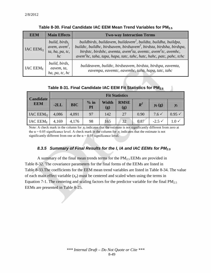
2/8/2012
*** Internal Draft – Do Not Quote or Cite *** 8-49
Table 8-30. Final Candidate IAC EEM Mean Trend Variables for PM2.5
EEM Main Effects Two-way Interaction Terms
IAC EEMQ
build, birds, avem, avem2, ta, ha, pa, tc,
hc
buildbirds, buildavem, buildavem2, buildta, buildha, buildpa, buildtc, buildhc, birdsavem, birdsavem2, birdsta, birdsha, birdspa,
birdstc, birdshc, avemta, avem2ta, avemtc, avem2tc, avemhc, avem2hc, taha, tapa, hapa, tatc, tahc, hatc, hahc, patc, pahc, tchc
IAC EEME build, birds, eavem, ta,
ha, pa, tc, hc
buildeavem, buildtc, birdseavem, birdsta, birdspa, eavemta, eavempa, eavemtc, eavemhc, taha, hapa, tatc, tahc
Table 8-31. Final Candidate IAC EEM Fit Statistics for PM2.5
Candidate EEM
Fit Statistics
-2LL BIC % in PI
Width (g)
RMSE (g) R2 γ0 (g) γ1
IAC EEMQ 4,086 4,091 97 142 27 0.90 7.6 0.95
IAC EEME 4,169 4,176 98 165 32 0.87 -2.5 1.0 Note: A check mark in the column for γ0 indicates that the estimate is not significantly different from zero at the α = 0.05 significance level. A check mark in the column for γ1 indicates that the estimate is not significantly different from one at the α = 0.05 significance level.
8.3.5 Summary of Final Results for the I, IA and IAC EEMs for PM2.5
A summary of the final mean trends terms for the PM2.5 EEMs are provided in Table 8-32. The covariance parameters for the final forms of the EEMs are listed in Table 8-33.The coefficients for the EEM mean trend variables are listed in Table 8-34. The value of each main effect variable (xp) must be centered and scaled when using the terms in Equation 7-1. The centering and scaling factors for the predictor variable for the final PM2.5 EEMs are presented in Table 8-25.

2/8/2012
*** Internal Draft – Do Not Quote or Cite *** 8-50
Table 8-32. Final EEM Mean Trend Variables for PM2.5
EEM Main Effects Two-Way Interaction Terms
I build, birds, avem, avem2 buildbirds, buildavem, buildavem2, birdsavem, birdsavem2
IA build, birds,
avem, avem2, ta, ha, pa
buildavem, buildavem2, buildpa, birdsavem, birdsavem2, birdsta, birdspa, avemta, avem2ta, avemha, avem2ha, avempa, avem2pa,
taha, tapa, hapa
IAC build, birds,
avem, avem2, ta, ha, pa, tc, hc
buildbirds, buildavem, buildavem2, buildta, buildha, buildpa, buildtc, buildhc, birdsavem, birdsavem2, birdsta, birdsha, birdspa,
birdstc, birdshc, avemta, avem2ta, avemtc, avem2tc, avemhc, avem2hc, taha, tapa, hapa, tatc, tahc, hatc, hahc, patc, pahc, tchc
Table 8-33. Covariance Parameter for Final PM2.5 EEMs
Covariance Parameter Estimate
I IA IAC
𝜌 0.7640 0.6833 0.6941
𝜎2 1,504.72 1031.15 981.22
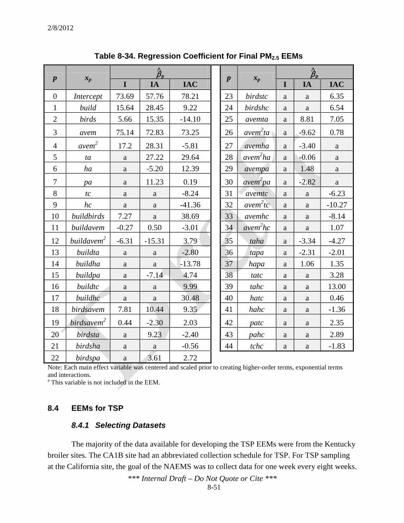
2/8/2012
*** Internal Draft – Do Not Quote or Cite *** 8-51
Table 8-34. Regression Coefficient for Final PM2.5 EEMs
p xp βp p xp βp
I IA IAC I IA IAC 0 Intercept 73.69 57.76 78.21 23 birdstc a a 6.35 1 build 15.64 28.45 9.22 24 birdshc a a 6.54 2 birds 5.66 15.35 -14.10 25 avemta a 8.81 7.05
3 avem 75.14 72.83 73.25 26 avem2ta a -9.62 0.78
4 avem2 17.2 28.31 -5.81 27 avemha a -3.40 a 5 ta a 27.22 29.64 28 avem2ha a -0.06 a 6 ha a -5.20 12.39 29 avempa a 1.48 a
7 pa a 11.23 0.19 30 avem2pa a -2.82 a 8 tc a a -8.24 31 avemtc a a -6.23 9 hc a a -41.36 32 avem2tc a a -10.27 10 buildbirds 7.27 a 38.69 33 avemhc a a -8.14 11 buildavem -0.27 0.50 -3.01 34 avem2hc a a 1.07
12 buildavem2 -6.31 -15.31 3.79 35 taha a -3.34 -4.27 13 buildta a a -2.80 36 tapa a -2.31 -2.01 14 buildha a a -13.78 37 hapa a 1.06 1.35 15 buildpa a -7.14 4.74 38 tatc a a 3.28 16 buildtc a a 9.99 39 tahc a a 13.00 17 buildhc a a 30.48 40 hatc a a 0.46 18 birdsavem 7.81 10.44 9.35 41 hahc a a -1.36
19 birdsavem2 0.44 -2.30 2.03 42 patc a a 2.35 20 birdsta a 9.23 -2.40 43 pahc a a 2.89 21 birdsha a a -0.56
44 tchc a a -1.83
22 birdspa a 3.61 2.72
Note: Each main effect variable was centered and scaled prior to creating higher-order terms, exponential terms and interactions. a This variable is not included in the EEM.
8.4 EEMs for TSP
8.4.1 Selecting Datasets
The majority of the data available for developing the TSP EEMs were from the Kentucky broiler sites. The CA1B site had an abbreviated collection schedule for TSP. For TSP sampling at the California site, the goal of the NAEMS was to collect data for one week every eight weeks.

2/8/2012
*** Internal Draft – Do Not Quote or Cite *** 8-52
As a result, the CA1B site has a higher percent of missing data (see Table 8-35) when compared to the total number of monitoring days for the grow-out periods.
Overall data completeness for TSP was 33 percent of the grow-out period days. Table 8-35 shows that TSP emissions values were available for just over 5 percent of the study period for the CA1B houses. The Kentucky sites had better completeness with seasonal completeness ranging from 84 to 98 percent. The available data are evenly distributed across the seasons.
Of the 601 TSP emission readings, 16 did not have values for the inventory, ambient and confinement predictor variables necessary for the EEM development. After these data records were removed, the base dataset for TSP EEM development consisted of 585 records. The EPA then randomly withheld 107 observations (approximately 18 percent of the 585 observations) to serve as the cross-validation data set.
Table 8-35. Data Completeness for TSP EEMs
Season Description
CA1B KY1B-1 KY1B-2 All Houses House 10 House 12 House 5 House 3
All seasons
Number of grow-out days 642 647 288 267 1,844 Days TSP data available 37 39 278 247 601
Percent complete 6% 6% 97% 93% 33%
Winter Number of grow-out days 150 153 87 74 464
Days TSP data available 7 7 83 68 165 Percent complete 5% 5% 95% 92% 36%
Spring Number of grow-out days 157 158 83 55 453
Days TSP data available 8 15 79 46 148 Percent complete 5% 9% 95% 84% 33%
Summer Number of grow-out days 156 157 55 74 442
Days TSP data available 10 12 54 70 146 Percent complete 6% 8% 98% 95% 33%
Fall Number of grow-out days 179 179 63 64 485
Days TSP data available 12 5 62 63 142 Percent complete 7% 3% 98% 98% 29%
8.4.2 Choosing the Probability Distribution for TSP
The EPA first evaluated the empirical distribution (i.e., histogram) of the observed daily TSP emissions to determine whether using the normal distribution could be justified. The histogram in Figure 8-27 shows that many of the TSP observations correspond to lower values, with a single peak at emissions values less than 0.8 kg. Also, the figure shows that the number of

2/8/2012
*** Internal Draft – Do Not Quote or Cite *** 8-53
observations decreases as emissions increase. Based on this histogram, the EPA determined that the empirical distribution was unimodal (single-peaked) and skew right.
The EPA separated the base dataset into bins according to values of average bird mass. Figure 8-28, for example, shows histograms of TSP emissions within the following six evenly distributed bins of average bird mass (avem*) values (in kg): 0.0 to 0.5, 0.5 to 1.0, 1.0 to 1.5, 1.5 to 2.0, 2.0 to 2.5 and 2.5 to 3.0. The figure shows that the histograms for bins 1 and 2 are skew right while those for bins 3, 4, 5 and 6 are more symmetric. Further disaggregation according to the values of other variables shows a variety of empirical distributions for different sets of conditions, and the skew-right pattern is by no means ubiquitous. There are not enough observations under any specific set of conditions (e.g., bird mass and humidity) to use the empirical distribution to determine the true distribution. Therefore, in the absence of strong evidence against doing so, the EPA used the normal distribution.
Figure 8-27. Histogram of TSP Emissions in the Base Dataset
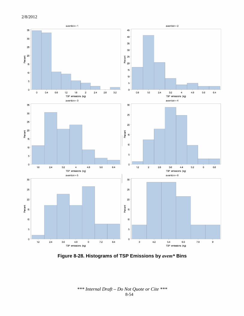
2/8/2012
*** Internal Draft – Do Not Quote or Cite *** 8-54
Figure 8-28. Histograms of TSP Emissions by avem* Bins

2/8/2012
*** Internal Draft – Do Not Quote or Cite *** 8-55
8.4.3 Developing Candidate Mean Trend Variables for TSP
8.4.3.1 Choosing Predictor Variable Functional Forms for TSP
Plots of TSP emissions versus average bird mass, for all houses, suggested a positive relationship, with a slight curvature that levels off at higher average bird masses. Figure 8-29 shows a scatter plot of TSP emissions versus average mass, with overlays of linear, quadratic and cubic regressions. The gradual increasing trend suggested a quadratic relationship between TSP emissions and the average bird mass. Accordingly, the EPA tested one form of the EEM based on a quadratic relationship with average mass (avem and avem2).
Figure 8-29. TSP Emissions vs. Average Bird Mass (Regression Overlays:
purple = linear, red = quadratic, green = cubic)
With regard to the effect of accumulated litter (buildup) on TSP emissions (see Section 7.3.1), the EPA discerned a relationship between TSP emissions and the degree of litter accumulation, based on the variance in TSP emissions values for lower bird weights (see Figure 8-30). When TSP emissions are plotted by average mass and color-coded to indicate the level of buildup, there is some indication that higher emissions correspond to built-up litter at

2/8/2012
*** Internal Draft – Do Not Quote or Cite *** 8-56
any animal mass; however, there is substantial variability in the data. Further investigations showed that the increased variance could not be attributed to differences in sites (Figure 8-31), as all three sites show the same variability across the grow-out period.
Figure 8-30. Overlay of buildup on TSP Emissions vs. Average Live Bird Mass

2/8/2012
*** Internal Draft – Do Not Quote or Cite *** 8-57
Figure 8-31. TSP Emissions vs. Average Bird Mass, Color-coded by Site
Plots of the build-up indicator parameters (i.e., buildup, build, bld) suggested average TSP emissions do not increase for flocks raised on built-up litter, because there is little difference in the minimum emissions levels between the litter conditions (Figure 8-32), and only a slight difference in average values. The EPA decided to include build as the functional form through which the variable buildup entered the mean trend function and test its significance using the p-value analysis to determine the final mean trend variables.
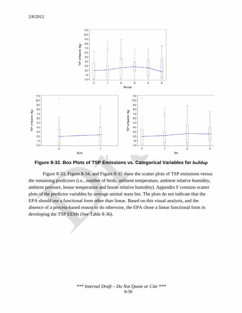
2/8/2012
*** Internal Draft – Do Not Quote or Cite *** 8-58
Figure 8-32. Box Plots of TSP Emissions vs. Categorical Variables for buildup
Figure 8-33, Figure 8-34, and Figure 8-35 show the scatter plots of TSP emissions versus the remaining predictors (i.e., number of birds, ambient temperature, ambient relative humidity, ambient pressure, house temperature and house relative humidity). Appendix F contains scatter plots of the predictor variables by average animal mass bin. The plots do not indicate that the EPA should use a functional form other than linear. Based on this visual analysis, and the absence of a process-based reason to do otherwise, the EPA chose a linear functional form in developing the TSP EEMs (See Table 8-36).

2/8/2012
*** Internal Draft – Do Not Quote or Cite *** 8-59
Figure 8-33. TSP Emissions vs. Predictor Variables birds* and ta*

2/8/2012
*** Internal Draft – Do Not Quote or Cite *** 8-60
Figure 8-34. TSP Emissions vs. Predictor Variables ha* and pa*

2/8/2012
*** Internal Draft – Do Not Quote or Cite *** 8-61
Figure 8-35. TSP Emissions vs. Predictor Variables tc* and hc*
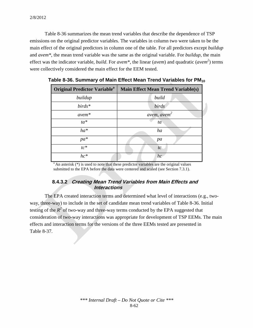
2/8/2012
*** Internal Draft – Do Not Quote or Cite *** 8-62
Table 8-36 summarizes the mean trend variables that describe the dependence of TSP emissions on the original predictor variables. The variables in column two were taken to be the main effect of the original predictors in column one of the table. For all predictors except buildup and avem*, the mean trend variable was the same as the original variable. For buildup, the main effect was the indicator variable, build. For avem*, the linear (avem) and quadratic (avem2) terms were collectively considered the main effect for the EEM tested.
Table 8-36. Summary of Main Effect Mean Trend Variables for PM10
Original Predictor Variablea Main Effect Mean Trend Variable(s)
buildup build
birds* birds
avem* avem, avem2 ta* ta
ha* ha
pa* pa
tc* tc
hc* hc a An asterisk (*) is used to note that these predictor variables are the original values submitted to the EPA before the data were centered and scaled (see Section 7.3.1).
8.4.3.2 Creating Mean Trend Variables from Main Effects and Interactions
The EPA created interaction terms and determined what level of interactions (e.g., two-way, three-way) to include in the set of candidate mean trend variables of Table 8-36. Initial testing of the R2 of two-way and three-way terms conducted by the EPA suggested that consideration of two-way interactions was appropriate for development of TSP EEMs. The main effects and interaction terms for the versions of the three EEMs tested are presented in Table 8-37.

2/8/2012
*** Internal Draft – Do Not Quote or Cite *** 8-63
Table 8-37. Candidate Mean Trend Variables for the I, IA and IAC TSP EEMs
EEM Main Effects Two-Way Interaction Terms
I, Quadratic (I EEMQ)
build, birds, avem, avem2
buildbirds, buildavem, buildavem2, birdsavem, birdsavem2
IA, Quadratic (IA EEMQ)
Same as I EEMQ plus:
ta, ha, pa
Same as I EEMQ plus: buildta, buildha, buildpa, birdsta, birdsha, birdspa,
avemta, avem2ta, avemha, avem2ha, avempa, avem2pa, taha, tapa, hapa
IAC, Quadratic (IAC EEMQ)
Same as IA EEMQ plus: tc, hc
Same as IA EEMQ plus: buildtc, buildhc, birdstc, birdshc, avemtc, avem2tc, avemhc, avem2hc, tatc, tahc, hatc, hahc, patc, pahc,
tchc
8.4.3.3 Centering and Scaling Predictors
The EPA centered and scaled each continuous predictor variable prior to creating interaction terms by subtracting the mean of all observations in the base dataset from each value, then dividing by the standard deviation of the base dataset. The centering and scaling factors for the predictor variable for the TSP final EEMs are presented in Table 8-38.
Table 8-38. Centering and Scaling Reference Values for Continuous TSP Predictor Variables
Predictor Variablea Centering Value Scaling Value
birds* 24 2.6 avem* 1.0 0.77
ta* 14 9.4 ha* 71 13 pa* 100 0.93 tc* 24 4.0 hc* 59 9.6
a An asterisk (*) is used to note that these predictor variables are the original values submitted to the EPA before the data were centered and scaled (see Section 7.3.1). Predictor variables are centered and scaled prior to the creation of higher-order terms (e.g., eavem or avem2) and the creation of interaction terms (e.g., avemta).
8.4.4 Selecting Final Mean Trend Variables for TSP
Only a quadratic version of the I, IA, and IAC EEMs were tested. Table 8-39 contains the final mean trend variables for the selected form of each EEM after backward elimination of
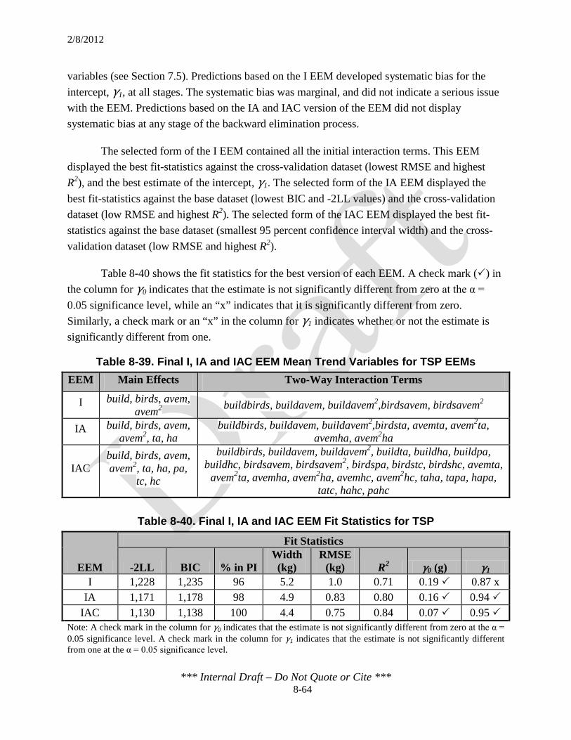
2/8/2012
*** Internal Draft – Do Not Quote or Cite *** 8-64
variables (see Section 7.5). Predictions based on the I EEM developed systematic bias for the intercept, γ1, at all stages. The systematic bias was marginal, and did not indicate a serious issue with the EEM. Predictions based on the IA and IAC version of the EEM did not display systematic bias at any stage of the backward elimination process.
The selected form of the I EEM contained all the initial interaction terms. This EEM displayed the best fit-statistics against the cross-validation dataset (lowest RMSE and highest R2), and the best estimate of the intercept, γ1. The selected form of the IA EEM displayed the best fit-statistics against the base dataset (lowest BIC and -2LL values) and the cross-validation dataset (low RMSE and highest R2). The selected form of the IAC EEM displayed the best fit-statistics against the base dataset (smallest 95 percent confidence interval width) and the cross-validation dataset (low RMSE and highest R2).
Table 8-40 shows the fit statistics for the best version of each EEM. A check mark () in the column for γ0 indicates that the estimate is not significantly different from zero at the α = 0.05 significance level, while an “x” indicates that it is significantly different from zero. Similarly, a check mark or an “x” in the column for γ1 indicates whether or not the estimate is significantly different from one.
Table 8-39. Final I, IA and IAC EEM Mean Trend Variables for TSP EEMs EEM Main Effects Two-Way Interaction Terms
I build, birds, avem, avem2 buildbirds, buildavem, buildavem2,birdsavem, birdsavem2
IA build, birds, avem, avem2, ta, ha
buildbirds, buildavem, buildavem2,birdsta, avemta, avem2ta, avemha, avem2ha
IAC build, birds, avem, avem2, ta, ha, pa,
tc, hc
buildbirds, buildavem, buildavem2, buildta, buildha, buildpa, buildhc, birdsavem, birdsavem2, birdspa, birdstc, birdshc, avemta,
avem2ta, avemha, avem2ha, avemhc, avem2hc, taha, tapa, hapa, tatc, hahc, pahc
Table 8-40. Final I, IA and IAC EEM Fit Statistics for TSP
EEM
Fit Statistics
-2LL BIC % in PI Width (kg)
RMSE (kg) R2 γ0 (g) γ1
I 1,228 1,235 96 5.2 1.0 0.71 0.19 0.87 x IA 1,171 1,178 98 4.9 0.83 0.80 0.16 0.94
IAC 1,130 1,138 100 4.4 0.75 0.84 0.07 0.95 Note: A check mark in the column for γ0 indicates that the estimate is not significantly different from zero at the α = 0.05 significance level. A check mark in the column for γ1 indicates that the estimate is not significantly different from one at the α = 0.05 significance level.
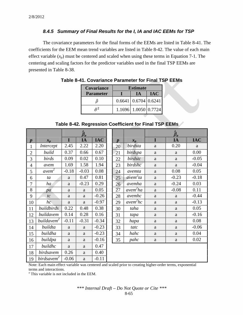
2/8/2012
*** Internal Draft – Do Not Quote or Cite *** 8-65
8.4.5 Summary of Final Results for the I, IA and IAC EEMs for TSP
The covariance parameters for the final forms of the EEMs are listed in Table 8-41. The coefficients for the EEM mean trend variables are listed in Table 8-42. The value of each main effect variable (xp) must be centered and scaled when using these terms in Equation 7-1. The centering and scaling factors for the predictor variables used in the final TSP EEMs are presented in Table 8-38.
Table 8-41. Covariance Parameter for Final TSP EEMs Covariance Parameter
Estimate I IA IAC
𝜌 0.6641 0.6704 0.6241
𝜎2 1.1696 1.0050 0.7724
Table 8-42. Regression Coefficient for Final TSP EEMs
p xp βp
p xp βp
I IA IAC I IA IAC 1 Intercept 2.45 2.22 2.20 20 birdsta a 0.20 a 2 build 0.37 0.66 0.67 21 birdspa a a 0.00 3 birds 0.09 0.02 0.10 22 birdstc a a -0.05 4 avem 1.69 1.58 1.94 23 birdshc a a -0.04 5 avem2 -0.18 -0.03 0.08 24 avemta a 0.08 0.05 6 ta a 0.47 0.81 25 avem2ta a -0.23 -0.18 7 ha a -0.23 0.29 26 avemha a -0.24 0.03 8 pa a a 0.05 27 avem2ha a -0.08 0.11 9 tc a a -0.26 28 avemhc a a -0.44 10 hc a a -0.97 29 avem2hc a a -0.13 11 buildbirds 0.22 0.48 0.38 30 taha a a 0.05 12 buildavem 0.14 0.28 0.16 31 tapa a a -0.16 13 buildavem2 -0.11 -0.31 -0.34 32 hapa a a 0.08 14 buildta a a -0.23 33 tatc a a -0.06 15 buildha a a -0.23 34 hahc a a 0.04 16 buildpa a a -0.16 35 pahc a a 0.02 17 buildhc a a 0.47 18 birdsavem 0.26 a 0.40 19 birdsavem2 -0.06 a -0.11 Note: Each main effect variable was centered and scaled prior to creating higher-order terms, exponential terms and interactions. a This variable is not included in the EEM.

2/8/2012
*** Internal Draft – Do Not Quote or Cite *** 8-66
8.5 EEMs for VOCs
8.5.1 Selecting Datasets
Table 8-43 shows the data completeness for VOC emissions at the California and Kentucky sites. As explained previously in Section 5, issues with the monitoring equipment prevented the collection of continuous data for VOCs at the CA1B houses. Consequently, the EEMs for VOCs were based on data from the Kentucky sites only.
A total of 360 days of VOC emissions measurements were available and were evenly distributed across the seasons. Of the 360 VOC observations available, five lacked the necessary inventory, ambient and confinement predictor variables for EEM development. After these missing data records were removed, the base dataset available for developing the VOC EEMs consisted of 355 observations. The EPA then randomly withheld 78 observations (approximately 22 percent of the 355 observations) to serve as the cross-validation data set.
Table 8-43. Data Completeness for VOC EEMs
Season Description
CA1B KY1B-1 KY1B-2 All Houses House 10 House 12 House 5 House 3
All seasons
Number of grow-out days 642 647 288 267 1,844
Days VOC data available 0 0 200 160 360
Percent complete 0% 0% 69% 60% 20%
Winter
Number of grow-out days 150 153 87 74 464
Days VOC data available 0 0 54 43 97
Percent complete 0% 0% 62% 58% 21%
Spring
Number of grow-out days 157 158 83 55 453
Days VOC data available 0 0 69 32 101
Percent complete 0% 0% 83% 58% 22%
Summer
Number of grow-out days 156 157 55 74 442
Days VOC data available 0 0 18 41 59
Percent complete 0% 0% 33% 55% 13%
Fall
Number of grow-out days 179 179 63 64 485
Days VOC data available 0 0 59 44 103
Percent complete 0% 0% 94% 69% 21%

2/8/2012
*** Internal Draft – Do Not Quote or Cite *** 8-67
8.5.2 Choosing the Probability Distribution for VOCs
The EPA first evaluated the empirical distribution (i.e., histogram) of the observed daily emissions for VOCs in determining whether using the normal distribution could be justified. The histogram in Figure 8-36 shows that many of the observations for VOCs correspond to lower emissions values, with a single peak at values around 0.375 kg. The figure also shows that the number of observations decreases as emissions increase. Based on this histogram, the EPA determined that the empirical distribution was unimodal (single-peaked) and skew right.
The EPA separated the base dataset into bins according to values of average bird mass. Figure 8-37 shows histograms of VOC emissions within the following six evenly distributed bins of average bird mass (avem*) values (in kg): 0.0 to 0.5, 0.5 to 1.0, 1.0 to 1.5, 1.5 to 2.0, 2.0 to 2.5 and 2.5 to 3.0. The figure shows that the histograms for bins 1, 2, 3, and 4 are skew right while those for bins 5 and 6 are symmetric. Further disaggregation according to the values of other variables shows a variety of empirical distributions for different sets of conditions, and the skew right pattern is by no means a consistent pattern. There are not enough observations under any specific set of conditions (e.g., bird mass and humidity ranges) to use the empirical distribution to determine the true distribution. Therefore, in the absence of strong evidence against doing so, the EPA used the normal distribution.
Figure 8-36. Histogram of VOC Emissions in the Base Dataset
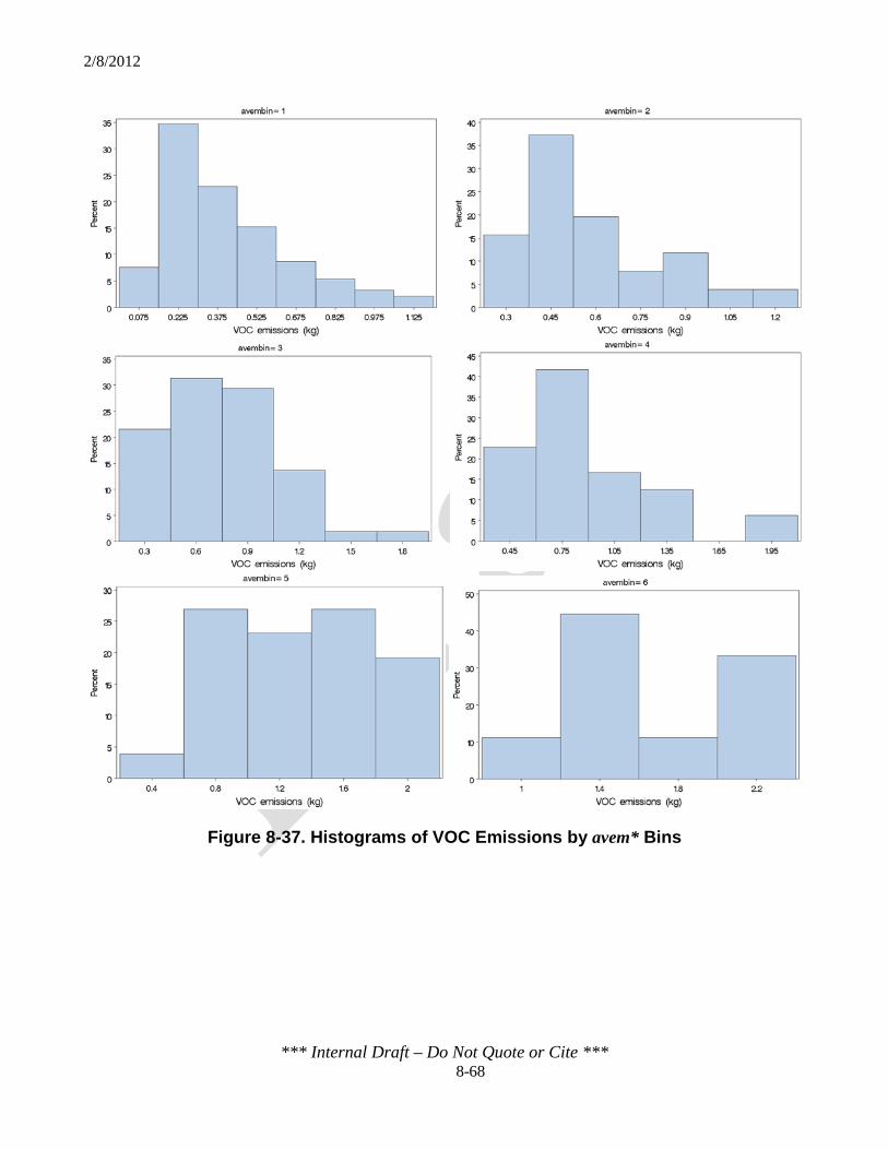
2/8/2012
*** Internal Draft – Do Not Quote or Cite *** 8-68
Figure 8-37. Histograms of VOC Emissions by avem* Bins
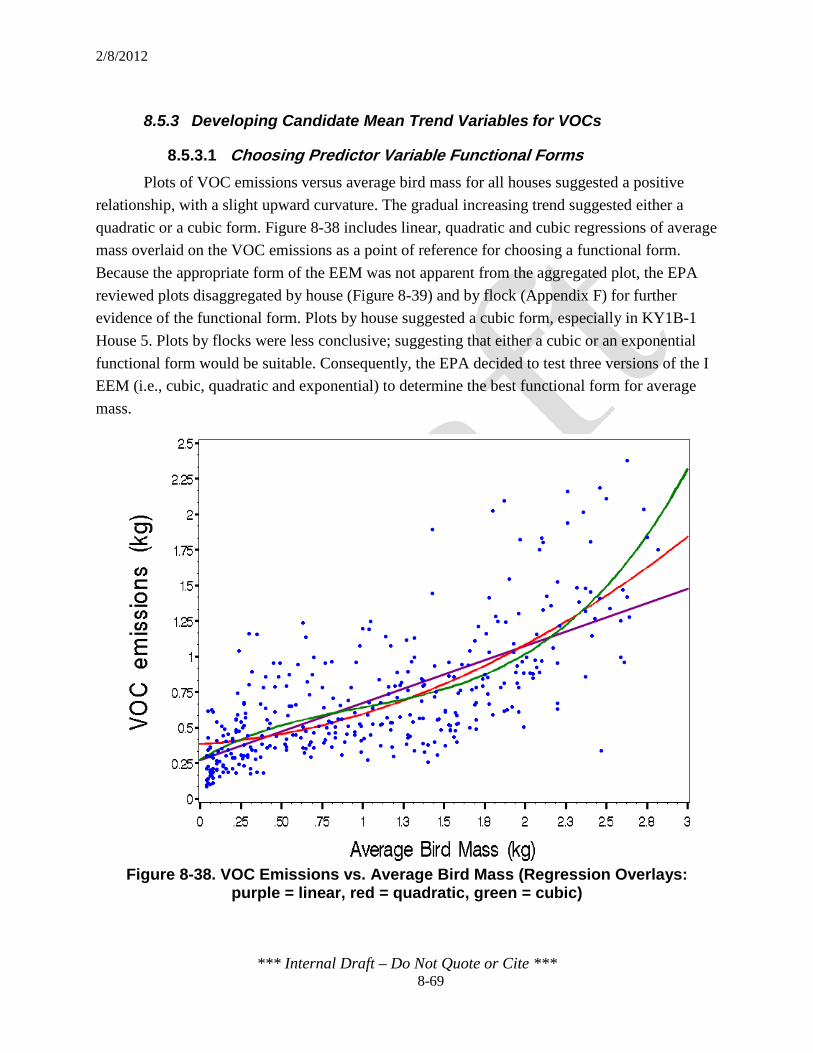
2/8/2012
*** Internal Draft – Do Not Quote or Cite *** 8-69
8.5.3 Developing Candidate Mean Trend Variables for VOCs
8.5.3.1 Choosing Predictor Variable Functional Forms Plots of VOC emissions versus average bird mass for all houses suggested a positive
relationship, with a slight upward curvature. The gradual increasing trend suggested either a quadratic or a cubic form. Figure 8-38 includes linear, quadratic and cubic regressions of average mass overlaid on the VOC emissions as a point of reference for choosing a functional form. Because the appropriate form of the EEM was not apparent from the aggregated plot, the EPA reviewed plots disaggregated by house (Figure 8-39) and by flock (Appendix F) for further evidence of the functional form. Plots by house suggested a cubic form, especially in KY1B-1 House 5. Plots by flocks were less conclusive; suggesting that either a cubic or an exponential functional form would be suitable. Consequently, the EPA decided to test three versions of the I EEM (i.e., cubic, quadratic and exponential) to determine the best functional form for average mass.
Figure 8-38. VOC Emissions vs. Average Bird Mass (Regression Overlays:
purple = linear, red = quadratic, green = cubic)
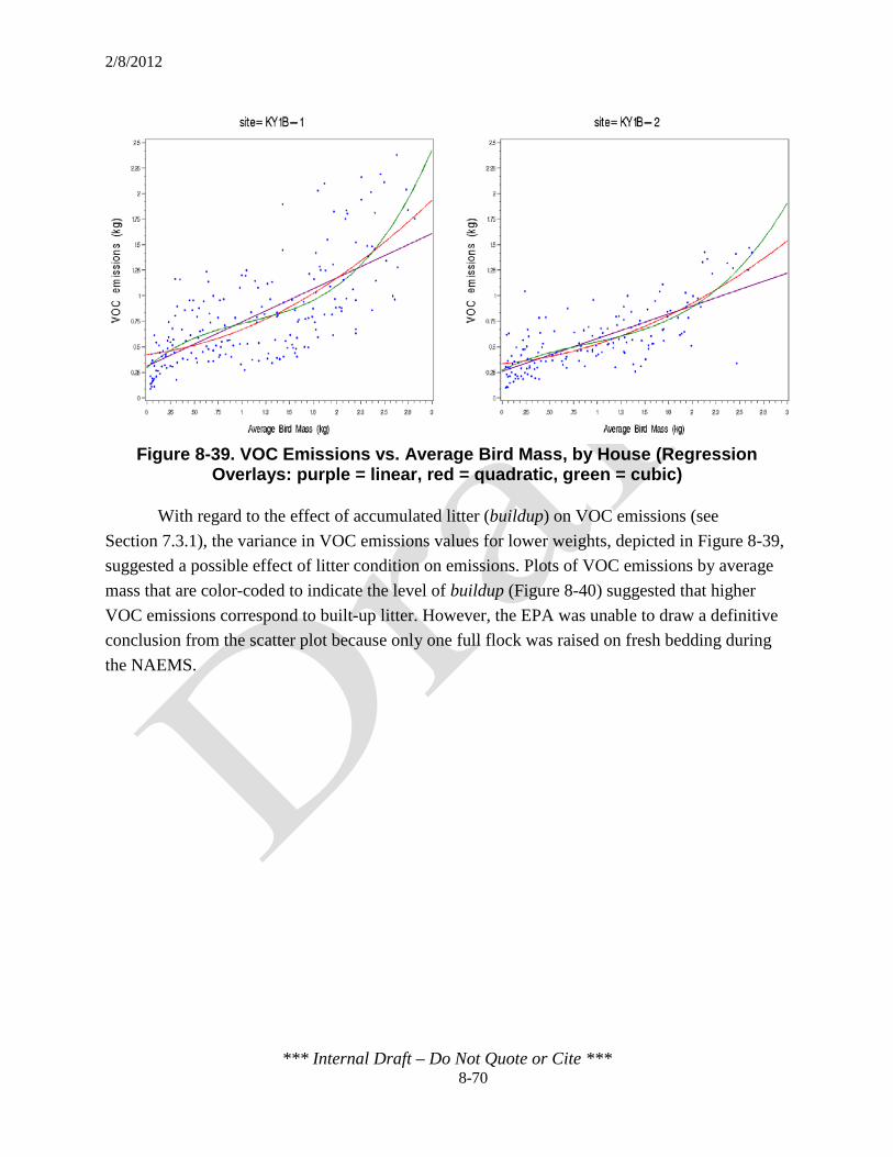
2/8/2012
*** Internal Draft – Do Not Quote or Cite *** 8-70
Figure 8-39. VOC Emissions vs. Average Bird Mass, by House (Regression
Overlays: purple = linear, red = quadratic, green = cubic)
With regard to the effect of accumulated litter (buildup) on VOC emissions (see Section 7.3.1), the variance in VOC emissions values for lower weights, depicted in Figure 8-39, suggested a possible effect of litter condition on emissions. Plots of VOC emissions by average mass that are color-coded to indicate the level of buildup (Figure 8-40) suggested that higher VOC emissions correspond to built-up litter. However, the EPA was unable to draw a definitive conclusion from the scatter plot because only one full flock was raised on fresh bedding during the NAEMS.

2/8/2012
*** Internal Draft – Do Not Quote or Cite *** 8-71
Figure 8-40. Overlay of buildup on VOC Emissions vs. Average Live Bird Mass
Plots of the build-up indicator parameters (i.e., buildup, build, bld) suggested that the average emissions increased for flocks raised on built-up litter. The trend is not as strong as with other pollutants, as there is only a small difference between the minimum emissions levels between the litter conditions (Figure 8-41), although the average emissions for the litter conditions does show a larger difference. To explore the issue, the EPA conducted preliminary tests to determine if a representation of build-up would significantly contribute to the mean trend variables for the VOC EEM. Consistent with the other pollutant EEMs developed, the EPA chose to include build in initial test EEMs, which showed build as a significant mean trend term. Consequently, the EPA decided to include build as the functional form through which the variable buildup enters the mean trend function and continue to test its significance using the p-value analysis to determine the final mean trend variables.

2/8/2012
*** Internal Draft – Do Not Quote or Cite *** 8-72
Figure 8-41. Box Plots of VOC Emissions vs. Categorical Variables for buildup
Figure 8-42, Figure 8-43 and Figure 8-44 show the scatter plots of VOC emissions by the remaining predictors (i.e., number of birds, ambient temperature, ambient relative humidity, ambient pressure, house temperature and house relative humidity). Appendix F contains scatter plots of the predictor variables by average animal mass bin. The plots do not indicate that the EPA should use a functional form other than linear. Based on this visual analysis, and the absence of a process-based reason to do otherwise, the EPA chose a linear functional form in developing the EEMs for VOCs.
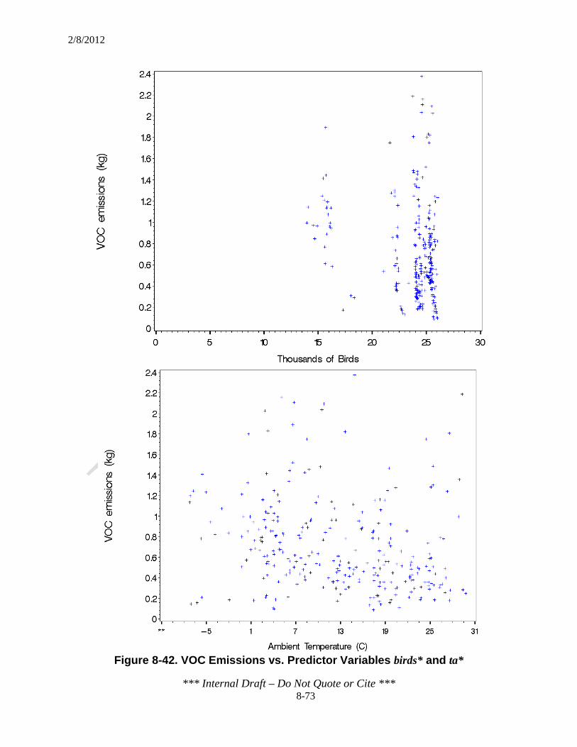
2/8/2012
*** Internal Draft – Do Not Quote or Cite *** 8-73
Figure 8-42. VOC Emissions vs. Predictor Variables birds* and ta*
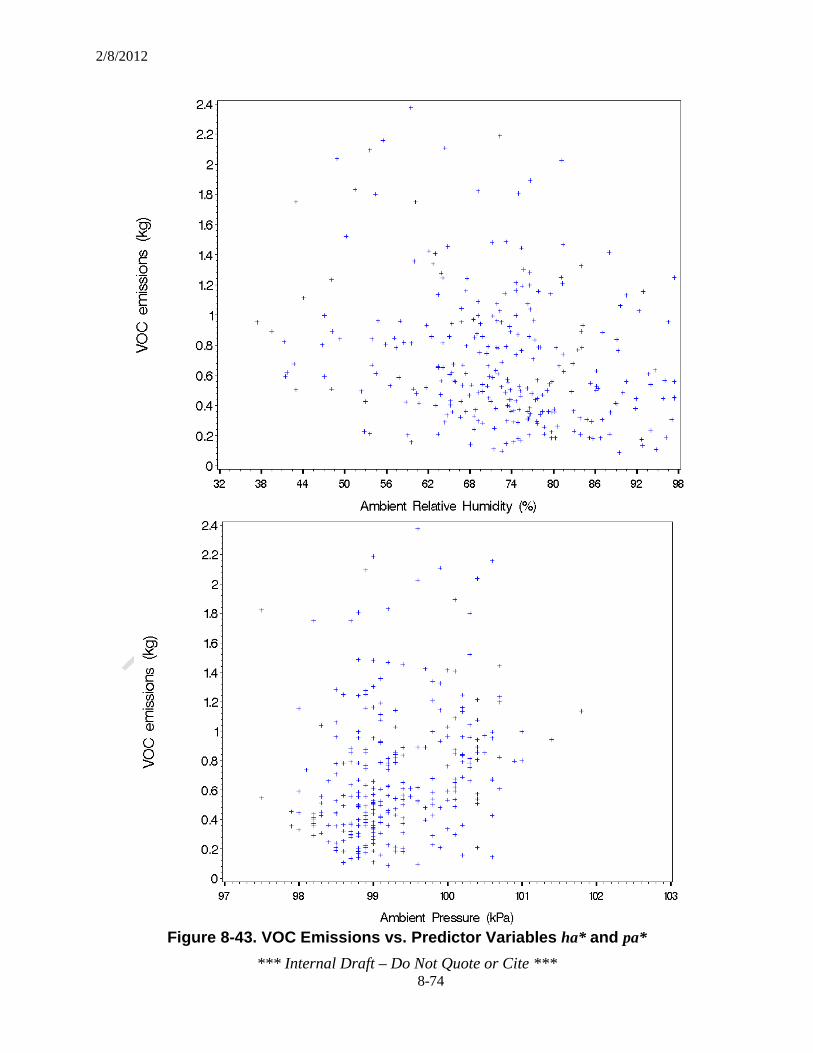
2/8/2012
*** Internal Draft – Do Not Quote or Cite *** 8-74
Figure 8-43. VOC Emissions vs. Predictor Variables ha* and pa*

2/8/2012
*** Internal Draft – Do Not Quote or Cite *** 8-75
Figure 8-44. VOC Emissions vs. Predictor Variables tc* and hc*

2/8/2012
*** Internal Draft – Do Not Quote or Cite *** 8-76
Table 8-44 summarizes the mean trend variables that describe the dependence of VOC emissions on the original predictor variables. The variables in column two were taken to be the main effect of the original predictors in column one of the table. For all predictors except buildup and avem, the mean trend variable was the same as the original variable. For buildup, the main effect was the indicator variable build. Forms of avem* tested separately for EEM development included an exponential (eavem), quadratic (avem and avem2), and cubic (avem, avem2, and avem3) form.
Table 8-44. Summary of Main Effect Mean Trend Variables for VOCs
Original Predictor Variablea Main Effect Mean Trend Variables
buildup build
birds* birds
avem* avem, avem2
avem, avem2, avem3 eavem
ta* ta
ha* ha
pa* pa
tc* tc
hc* hc a An asterisk (*) is used to note that these predictor variables are the original values submitted to the EPA before the data were centered and scaled (see Section 7.3.1).
8.5.3.2 Creating Mean Trend Variables from Main Effects and Interactions
The EPA created interaction terms and determined what level of interactions (e.g., two-way, three-way) to include in the set of candidate mean trend variables of Table 8-2. Initial testing of the R2 of 2-way and 3-way terms conducted by the EPA suggested that consideration of two-way interactions was appropriate for development of VOC EEMs. The main effects and interaction terms for the versions of the three EEMs tested are presented in Table 8-45. Cubic versions of the IA and IAC EEMs are not shown in Table 8-45 because initial testing showed that none of the cubic terms for the EEMs were significant. A discussion of these initial tests for each of these EEMs is provided in Sections 8.5.4.2 and 8.5.4.3.

2/8/2012
*** Internal Draft – Do Not Quote or Cite *** 8-77
Table 8-45. Candidate Mean Trend Variables for the I, IA and IAC VOC EEMs
EEM Main Effects Two-Way Interaction terms
I, Cubic (I EEMC)
build, birds, avem, avem2, avem3
buildbirds, buildavem, buildavem2, buildavem3, birdsavem, birdsavem2, birdsavem3
I, Quadratic (I EEMQ)
build, birds, avem, avem2
buildbirds, buildavem, buildavem2, birdsavem, birdsavem2
I, Exponential (I EEME)
build, birds, eavem buildbirds, buildeavem, birdseavem
IA, Quadratic (IA EEMQ)
Same as I EEMQ plus:
ta, ha, pa
Same as I EEMQ plus: buildta, buildha, buildpa, birdsta, birdsha,
birdspa,avemta, avem2ta, avemha, avem2ha, avempa, avem2pa, taha, tapa, hapa
IA, Exponential (IA EEME)
Same as I EEME plus:
build, birds, eavem, ta, ha, pa
Same as I EEME plus: buildta, buildha, buildpa, birdsta, birdsha, birdspa,
eavemta, eavemha, eavempa, taha, tapa, hapa
IAC, Quadratic
(IAC EEMQ)
Same as IA EEMQ plus:
build, birds, avem, avem2, ta, ha, pa, tc,
hc
Same as IA EEMQ plus: buildtc, buildhc, birdstc, birdshc, avemtc, avem2tc,
avemhc, avem2hc, tatc, tahc, hatc, hahc, patc, pahc, tchc
IAC, Exponential (IAC EEME)
Same as IA EEME plus:
build, birds, eavem, ta, ha, pa, tc, hc
Same as IA EEME plus: buildtc, buildhc, birdstc, birdshc, eavemtc, eavemhctatc,
tahc, hatc, hahc, patc, pahc, tchc
8.5.3.3 Centering and Scaling Predictors The EPA centered and scaled each continuous predictor variable prior to creating
interaction terms by subtracting the mean of all observations in the base dataset from each value, then dividing by the standard deviation of the base dataset. The centering and scaling factors for the predictor variable for the final EEMs for VOCs are presented in Table 8-46.

2/8/2012
*** Internal Draft – Do Not Quote or Cite *** 8-78
Table 8-46. Centering and Scaling Reference Values for Continuous VOC Predictor Variables
Predictor Variablea Centering
Value Scaling Value
birds* 24 2.8 avem* 1.1 0.76
ta* 13 8.8 ha* 72 12 pa* 99 0.73 tc* 27 3.5 hc* 58 9.7
a An asterisk (*) is used to note that these predictor variables are the original values submitted to the EPA before the data were centered and scaled (see Section 7.3.1). Predictor variables are centered and scaled prior to the creation of higher-order terms (e.g., eavem or avem2) and the creation of interaction terms (e.g., avemta).
8.5.4 Selecting Final Mean Trend Variables for VOCs
8.5.4.1 Inventory EEM For the cubic version of the EEM, a full-reduced model F-test of the hypothesis that the
coefficients avem3, birdsavem3, and buildavem3 were simultaneously equal to zero produced a p-value of 0.43 which suggested that these terms should be removed from the EEM. This supported the conclusion that the functional form of avem* is a lower-order polynomial rather than a cubic form. Therefore, the EPA only considered the quadratic and exponential forms (i.e., the cubic form of the EEM was not tested with the IA or IAC versions of the EEM).
Predictions based on the I EEMQ form of the EEM developed systematic bias for γ1 prior to completing the backwards elimination process. Predictions based on the I EEME completed the backward elimination process without any systematic bias.
The best version of the I EEMQ occurred after the elimination of the avem2 interaction terms (Table 8-47). This EEM displayed the best fit-statistics against the base dataset (lowest BIC and -2LL values) and the cross-validation dataset (lowest RMSE and highest R2), without exhibiting systematic bias.
The selected form of the I EEME contains all the initial interaction terms. This version of the I EEME had the best fit-statistics against the test dataset and good fit statistics versus the cross-validation dataset, without systematic bias. The fit statistics for the selected I EEMQ and I EEME are presented in Table 8-48. A check mark () in the column for γ0 indicates that the

2/8/2012
*** Internal Draft – Do Not Quote or Cite *** 8-79
estimate is not significantly different from zero at the α = 0.05 significance level, while an “x” indicates that it is significantly different from zero. Similarly, a check mark or an “x” in the column for γ1 indicates whether or not the estimate is significantly different from one.
Overall, the I EEMQ and I EEME generally have similar fit statistics, with the I EEME having slightly better base dataset fit (smaller -2LL and BIC). The I EEME version was slightly better with respect to the percent of the data that is within the 95 percent prediction interval (% in PI) as this value should be as close to 95 percent as possible. Therefore, the EPA selected the exponential version of the I EEM for VOC emissions.
Table 8-47. Final Candidate I EEM Mean Trend Variables for VOCs
EEM Main Effects Two-Way Interaction terms
I EEMQ build, birds, avem, avem2 buildbirds, buildavem, birdsavem,
I EEME build, birds, eavem buildbirds, buildeavem, birdseavem
Table 8-48. Final Candidate I EEM Fit Statistics for VOCs
Candidate EEM
Fit Parameters
-2LL BIC % in PI
Width (kg)
RMSE (kg) R2 γ0 (kg) γ1
I EEMQ -19.0 -12.7 99 1.3 0.25 0.61 -0.01 0.93
I EEME -29.2 -22.8 97 1.3 0.25 0.59 -0.01 0.92 Note: A check mark in the column for γ0 indicates that the estimate is not significantly different from zero at the α = 0.05 significance level. A check mark in the column for γ1 indicates that the estimate is not significantly different from one at the α = 0.05 significance level.
8.5.4.2 Inventory and Ambient EEM An initial test of the cubic version of the EEM showed a full-reduced model F-test of the
hypothesis that the coefficients avem3, birdsavem3, buildavem3, avem3ta, avem3ha, and avem3pa were simultaneously equal to zero produced a p-value of 0.41, which suggested that these terms should be removed from the EEM. This further supported the conclusion that the functional form of avem* is a lower-order polynomial rather than a cubic form. Therefore, the EPA only considered the quadratic and exponential forms.
The IA EEMQ developed systematic bias for γ1 prior to completing the backwards elimination process, and the IA EEME completed the backward elimination process without any systematic bias.

2/8/2012
*** Internal Draft – Do Not Quote or Cite *** 8-80
The selected form of the IA EEMQ and IA EEME are presented in Table 8-49. The selected IA EEMQ displayed the best fit-statistics against the test dataset (lowest RMSE and highest R2), without exhibiting systematic bias. The selected version of the IA EEME had the best fit-statistics against the base dataset (lowest BIC and -2LL values) and the cross-validation dataset (lowest RMSE and highest R2). The fit statistics for the selected IA EEMQ and IA EEME are presented in Table 8-50.
Overall, the IA EEMQ and IA EEME had similar fit statistics for the test dataset, with the IA EEMQ having a slightly better R2 value. The IA EEME had better base dataset fit (smaller -2LL and BIC), as well as a better representation of the percent of the data that is within the 95 percent prediction interval. Therefore, the EPA selected the exponential version of the IA EEM for VOC emissions.
Table 8-49. Final Candidate IA EEM Mean Trend Variables for VOCs
EEM Main Effects Two-Way Interaction terms
IA EEMQ build, birds,
avem, avem2, ta, ha, pa
buildbirds, buildavem, buildavem2, buildta, buildha, buildpa, birdsavem, birdsavem2, birdsta, birdsha, birdspa, avemta,
avem2ta
IA EEME build, birds, eavem, ta buildbirds, buildeavem, birdsta, eavemta
Table 8-50. Final Candidate IA EEM Fit Statistics for VOCs
Candidate EEM
Fit Parameters
-2LL BIC % in PI
Width (kg)
RMSE (kg) R2 γ0 (kg) γ1
IA EEMQ 1.5 7.8 100 1.3 0.22 0.70 -0.004 0.94
IA EEME -39.5 -33.1 97 1.3 0.24 0.63 -0.01 0.90 Note: An “x” in the columns for γ0 and γ1 indicate systematic bias. A check mark in the column for γ0 indicates that the 95 percent confidence interval for the intercept contains zero and the estimate is not significantly different from zero. A check mark in the column for γ1 indicates the 95 percent confidence interval for the slope contains one and the estimate is not significantly different from one.
8.5.4.3 Inventory, Ambient and Confinement EEM An initial test of the cubic version of the EEM showed a full-reduced model F-test of the
hypothesis that the coefficients avem3, birdsavem3, buildavem3, avem3ta, avem3ha, avem3pa, avem3tc and avem3hc were simultaneously equal to zero produced a p-value of 0.18, which suggested that these terms should be removed from the EEM. This further supported the
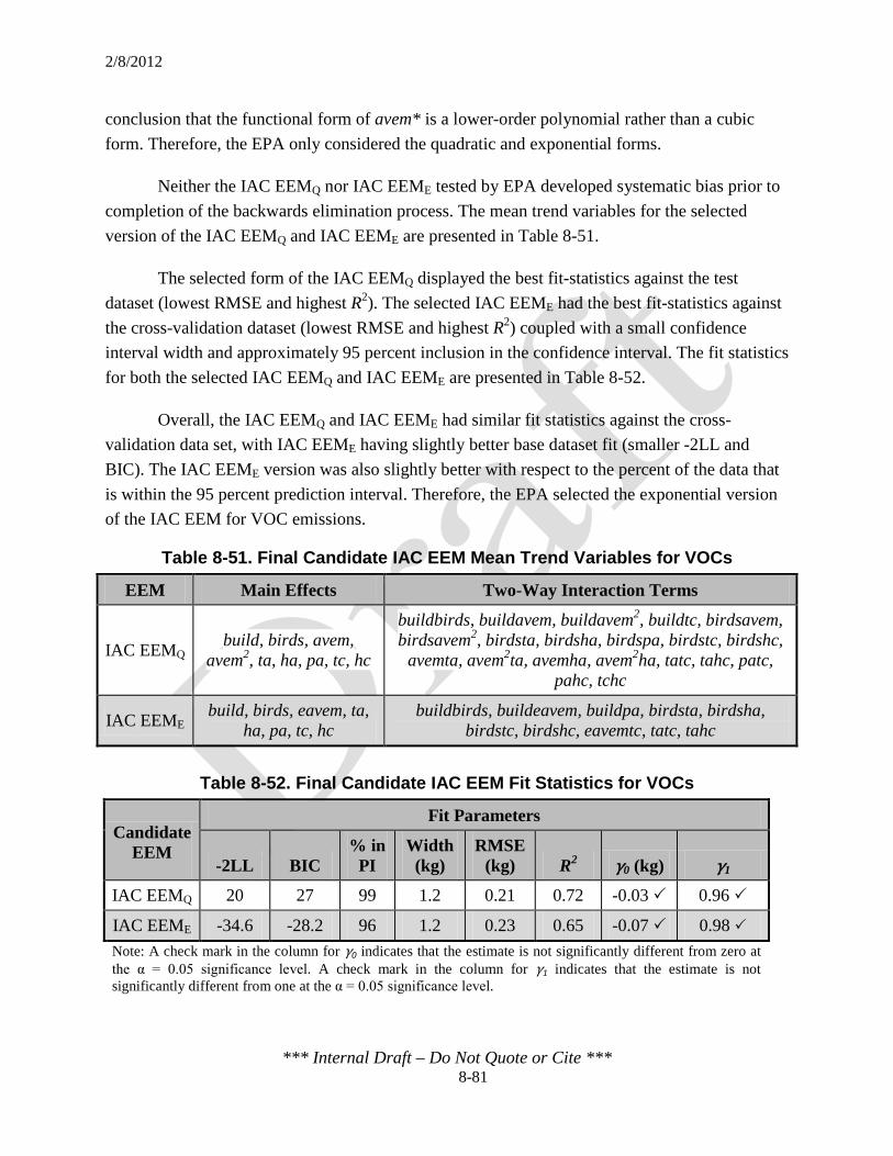
2/8/2012
*** Internal Draft – Do Not Quote or Cite *** 8-81
conclusion that the functional form of avem* is a lower-order polynomial rather than a cubic form. Therefore, the EPA only considered the quadratic and exponential forms.
Neither the IAC EEMQ nor IAC EEME tested by EPA developed systematic bias prior to completion of the backwards elimination process. The mean trend variables for the selected version of the IAC EEMQ and IAC EEME are presented in Table 8-51.
The selected form of the IAC EEMQ displayed the best fit-statistics against the test dataset (lowest RMSE and highest R2). The selected IAC EEME had the best fit-statistics against the cross-validation dataset (lowest RMSE and highest R2) coupled with a small confidence interval width and approximately 95 percent inclusion in the confidence interval. The fit statistics for both the selected IAC EEMQ and IAC EEME are presented in Table 8-52.
Overall, the IAC EEMQ and IAC EEME had similar fit statistics against the cross-validation data set, with IAC EEME having slightly better base dataset fit (smaller -2LL and BIC). The IAC EEME version was also slightly better with respect to the percent of the data that is within the 95 percent prediction interval. Therefore, the EPA selected the exponential version of the IAC EEM for VOC emissions.
Table 8-51. Final Candidate IAC EEM Mean Trend Variables for VOCs
EEM Main Effects Two-Way Interaction Terms
IAC EEMQ build, birds, avem, avem2, ta, ha, pa, tc, hc
buildbirds, buildavem, buildavem2, buildtc, birdsavem, birdsavem2, birdsta, birdsha, birdspa, birdstc, birdshc,
avemta, avem2ta, avemha, avem2ha, tatc, tahc, patc, pahc, tchc
IAC EEME build, birds, eavem, ta, ha, pa, tc, hc
buildbirds, buildeavem, buildpa, birdsta, birdsha, birdstc, birdshc, eavemtc, tatc, tahc
Table 8-52. Final Candidate IAC EEM Fit Statistics for VOCs
Candidate EEM
Fit Parameters
-2LL BIC % in
PI Width
(kg) RMSE
(kg) R2 γ0 (kg) γ1
IAC EEMQ 20 27 99 1.2 0.21 0.72 -0.03 0.96
IAC EEME -34.6 -28.2 96 1.2 0.23 0.65 -0.07 0.98 Note: A check mark in the column for γ0 indicates that the estimate is not significantly different from zero at the α = 0.05 significance level. A check mark in the column for γ1 indicates that the estimate is not significantly different from one at the α = 0.05 significance level.

2/8/2012
*** Internal Draft – Do Not Quote or Cite *** 8-82
8.5.5 Summary of Final Results for the I, IA and IAC EEMs for VOCs
A summary of the final mean trend variables for the VOC EEMs is provided in Table 8-53. The covariance parameters for the final forms of the EEMs are listed in Table 8-53. The coefficients for the EEM mean trend variables are listed in Table 8-53. The value of each main effect variable (xp) must be centered and scaled when using these terms in Equation 7-1. The centering and scaling factors for the predictor variable for the VOC final EEMs are presented in Table 8-46.
Table 8-53. Final EEM Mean Trend Variables for VOCs
EEM Main Effects Two-Way Interaction terms
I build, birds, eavem buildbirds, buildeavem, birdseavem
IA build, birds, eavem, ta buildbirds, buildeavem, birdsta, eavemta
IAC build, birds, eavem, ta, ha, pa, tc, hc
buildbirds, biuildeavem, buildpa, birdsta, birdsha, birdstc, birdshc, eavemtc, tatc, tahc
Table 8-54. Covariance Parameter for Final VOC EEMs
Covariance Parameter Estimate
I IA IAC
𝜌 0.7746 0.7784 0.7770
𝜎2 0.1009 0.09747 0.08368

2/8/2012
*** Internal Draft – Do Not Quote or Cite *** 8-83
Table 8-55. Regression Coefficients for Final VOC EEMs
p xp βp p xp βp I IA IAC I IA IAC
0 Intercept 0.031 0.19 -0.47 10 buildeavem 0.38 0.4 0.21 1 build -0.69 -0.8 -0.65 11 birdseavem 0.13 a a 2 birds -0.82 -0.84 -0.72 12 birdsta a 0.07 -0.07 3 eavem 0.59 0.53 1.12 13 birdsha a a -0.04 4 ta a -0.23 -0.04 14 buildpa a a 0.12 5 ha a a 0.02 15 eavemta a 0.12 a 6 pa a a -0.1 16 birdstc a a 0.06 7 tc a a -0.18 17 birdshc a a 0.11 8 hc a a -0.1 18 eavemtc a a 0.2 9 buildbirds 0.626 0.9 0.88 19 tatc a a 0.04
20 tahc a a 0.04 Note: Each main effect variable was centered and scaled prior to creating higher-order terms, exponential terms and interactions. a This variable is not included in the EEM.

2/8/2012
*** Internal Draft – Do Not Quote or Cite *** 9-1
9.0 DEVELOPMENT OF DECAKING AND FULL LITTER CLEAN-OUT PERIOD EEMS
This section summarizes the analyses used to develop the EEMs for the decaking and full litter clean-out periods of broiler confinement houses. Due to the limited number of data values and lack of supporting information specifying how each house was operated during the period between flocks when the litter removal activities were conducted, the pollutant-specific EEMs developed in this section are emission factors (EFs) rather than predictive equations. The emissions factors provide an estimate of the emissions released over the entire decaking or full litter clean-out period, which begins after the birds have been sent to market and ends when the new chicks are placed in the house. The period covered by the EFs includes when the litter removal activities were conducted and when the house was sitting empty before a new flock was placed in the house.
Section 9.1 discusses the data that are available regarding litter removal periods. Section 9.2 discusses the analyses the EPA performed to develop the EFs for decaking and full litter clean-out periods.
9.1 Available Data for Litter Removal Periods
Compared to grow-out periods, the decaking and full litter clean-out periods account for a relatively small portion of the overall broiler production cycle. While the typical grow-out period lasts approximately 50 days, a typical decaking period lasts 6 to 14 days and a typical full litter clean-out period lasts 12 to 14 days. Because the litter removal periods account for a small number of days over the course of a year, the number of data values collected under the NAEMS for these periods is significantly less than for grow-out periods. Table 9-1 compares the total number of days the NAEMS investigators were on site for litter removal periods to the total number of days on site for the grow-out periods.
Table 9-1. Comparison of Days on Site for Litter Removal and Grow-out Period Days
House Total Monitoring Days on Site
Litter Removal Grow-Out CA1B House 10 125 648 CA1B House 12 122 651 KY1B-1 House 5 87 307 KY1B-2 House 3 97 282
Total 431 1,888
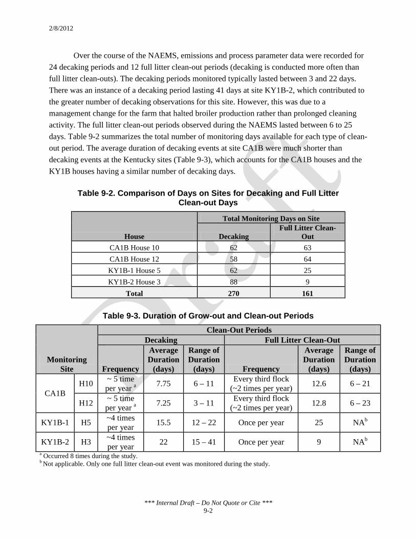
2/8/2012
*** Internal Draft – Do Not Quote or Cite *** 9-2
Over the course of the NAEMS, emissions and process parameter data were recorded for 24 decaking periods and 12 full litter clean-out periods (decaking is conducted more often than full litter clean-outs). The decaking periods monitored typically lasted between 3 and 22 days. There was an instance of a decaking period lasting 41 days at site KY1B-2, which contributed to the greater number of decaking observations for this site. However, this was due to a management change for the farm that halted broiler production rather than prolonged cleaning activity. The full litter clean-out periods observed during the NAEMS lasted between 6 to 25 days. Table 9-2 summarizes the total number of monitoring days available for each type of clean-out period. The average duration of decaking events at site CA1B were much shorter than decaking events at the Kentucky sites (Table 9-3), which accounts for the CA1B houses and the KY1B houses having a similar number of decaking days.
Table 9-2. Comparison of Days on Sites for Decaking and Full Litter Clean-out Days
House
Total Monitoring Days on Site
Decaking Full Litter Clean-
Out CA1B House 10 62 63 CA1B House 12 58 64 KY1B-1 House 5 62 25 KY1B-2 House 3 88 9
Total 270 161
Table 9-3. Duration of Grow-out and Clean-out Periods
Monitoring Site
Clean-Out Periods Decaking Full Litter Clean-Out
Frequency
Average Duration
(days)
Range of Duration
(days) Frequency
Average Duration
(days)
Range of Duration
(days)
CA1B H10 ~ 5 time
per year a 7.75 6 – 11 Every third flock (~2 times per year) 12.6 6 – 21
H12 ~ 5 time per year a 7.25 3 – 11 Every third flock
(~2 times per year) 12.8 6 – 23
KY1B-1 H5 ~4 times per year 15.5 12 – 22 Once per year 25 NAb
KY1B-2 H3 ~4 times per year 22 15 – 41 Once per year 9 NAb
a Occurred 8 times during the study. b Not applicable. Only one full litter clean-out event was monitored during the study.

2/8/2012
*** Internal Draft – Do Not Quote or Cite *** 9-3
As noted in Section 4, the EPA’s review of the NAEMS data identified a small number of negative daily emissions values for H2S, PM10, and VOCs. The number of measured negative values is low (less than 5 percent) compared to the total number of emissions records available for H2S, PM10, and VOC over the litter removal periods. After discussion with the NAEMS Science Advisor, it was determined that the negative values were the result of instrumentation drift, and are valid values. However, to avoid possible complications with EF development (e.g., the EEM predicting negative emissions) the negative values were withheld from the datasets used to develop the EFs for the decaking and full litter clean-out periods.
Table 9-4 summarizes the number of daily emission values that are greater than or equal to zero that are available for EF development by litter removal activity and pollutant. The limited amount of data for decaking and full litter clean-out periods is partially the result of the substantially shorter duration of the litter removal periods compared to the grow-out periods (2 to 20 days for clean-out activities compared to 45 to 54 days for broiler grow-out). Additionally, because the PM monitors had to be removed during litter removal activities to prevent damage to the instruments, fewer valid PM emissions were available during those periods. Consequently, the measurements available for PM10, PM2.5 and TSP emissions are only for periods after the litter removal activities were completed and the house was empty before the next flock of birds was placed. Finally, the intermittent PM sampling schedule at site CA1B did not include measurement of PM2.5 or TSP emissions during decaking and full litter clean-out periods. The EFs developed for PM2.5 or TSP were based only on data collected at the Kentucky sites.
Table 9-4. Number of Valid Non-Negative Daily Emissions Values for Litter Removal Periods
Litter Removal Activity House
Count of Valid Non-negative Daily Emissions Values
NH3 H2S PM10 PM2.5 TSP
Decaking
CA1B House 10 51 55 6 0 0 CA1B House 12 48 52 4 0 0 KY1B-1 House 5 58 57 11 19 20 KY1B-2 House 3 82 67 45 45 41
Total 239 231 66 64 61
Full Litter Clean-Out
CA1B House 10 30 23 9 0 0 CA1B House 12 30 23 5 0 0 KY1B-1 House 5 21 8 5 1 5 KY1B-2 House 3 8 8 3 3 3
Total 89 62 22 4 8

2/8/2012
*** Internal Draft – Do Not Quote or Cite *** 9-4
9.2 EF Development for Decaking and Full Litter Clean-Out Periods
The EPA attempted applying ordinary least squares (OLS) regression analyses to develop predictive equations based EEMs for decaking and full litter clean-out periods. In OLS regression analyses, coefficients of the equation relating emissions to parameters (i.e., predictor variables) are estimated by determining numerical values for the parameters that minimize the sum of the squared deviations between the observed responses and the functional portion of the model. The EPA initially considered this approach because it is a widely accepted method for relating dependent variables (e.g., emissions) to independent variables (e.g., bird mass, house ventilation flow rate). However, the EPA rejected the use of OLS regression analyses for developing predictive equations based EEMs for litter removal periods because of the poor correlation of the resulting regression equations (i.e., R2 values were less than 0.30).
The difficulty in applying the OLS regressions analyses to the litter removal period data was due to several characteristics of the available data. By design of the NAEMS, there are substantially fewer daily emissions values available for the decaking and full litter clean-out periods than for grow-out periods. Additionally, the emissions data that are available vary widely over the clean-out period as shown in Table 9-5. Applying the regression analyses to litter removal periods was further complicated because the data and supporting information do not specify how each house was operated during the period between flocks when the litter removal activities were conducted. For example, the available data do not indicate the date or time that the litter removal activities were initiated or completed, account for the manner in which the house doors and openings were managed, or identify the activities undertaken by farm personnel in the house during these periods. These factors could account for the variability in emissions and would likely improve the ability of a regression analysis to capture the emissions trends of the litter removal periods.
For the EEMs for litter removal periods, the EPA developed pollutant-specific emissions factors for the decaking and full litter clean-out periods. Typically, emissions factors relate pollutant emissions to an activity (e.g., kg of PM10/kg of coal combusted). The EFs developed by the EPA relate pollutant emissions to the total weight of birds raised on the litter and the duration of the litter removal activity.
The emissions released during litter removal periods, which begin after the birds have been sent to market and end when the new flock is placed in the house, are directly related to the manure accumulated on the confinement floor, the amount of manure removed from the house by farm personnel, and the duration of the litter removal event.
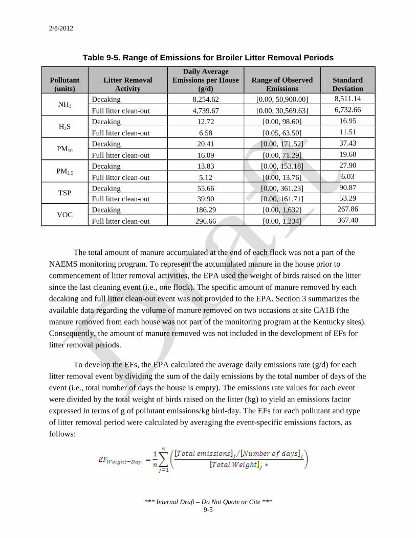
2/8/2012
*** Internal Draft – Do Not Quote or Cite *** 9-5
Table 9-5. Range of Emissions for Broiler Litter Removal Periods
Pollutant (units)
Litter Removal Activity
Daily Average Emissions per House
(g/d) Range of Observed
Emissions Standard Deviation
NH3 Decaking 8,254.62 [0.00, 50,900.00] 8,511.14 Full litter clean-out 4,739.67 [0.00, 30,569.63] 6,732.66
H2S Decaking 12.72 [0.00, 98.60] 16.95 Full litter clean-out 6.58 [0.05, 63.50] 11.51
PM10 Decaking 20.41 [0.00, 171.52] 37.43 Full litter clean-out 16.09 [0.00, 71.29] 19.68
PM2.5 Decaking 13.83 [0.00, 153.18] 27.90 Full litter clean-out 5.12 [0.00, 13.76] 6.03
TSP Decaking 55.66 [0.00, 361.23] 90.87 Full litter clean-out 39.90 [0.00, 161.71] 53.29
VOC Decaking 186.29 [0.00, 1,632] 267.86 Full litter clean-out 296.66 [0.00, 1,234] 367.40
The total amount of manure accumulated at the end of each flock was not a part of the NAEMS monitoring program. To represent the accumulated manure in the house prior to commencement of litter removal activities, the EPA used the weight of birds raised on the litter since the last cleaning event (i.e., one flock). The specific amount of manure removed by each decaking and full litter clean-out event was not provided to the EPA. Section 3 summarizes the available data regarding the volume of manure removed on two occasions at site CA1B (the manure removed from each house was not part of the monitoring program at the Kentucky sites). Consequently, the amount of manure removed was not included in the development of EFs for litter removal periods.
To develop the EFs, the EPA calculated the average daily emissions rate (g/d) for each litter removal event by dividing the sum of the daily emissions by the total number of days of the event (i.e., total number of days the house is empty). The emissions rate values for each event were divided by the total weight of birds raised on the litter (kg) to yield an emissions factor expressed in terms of g of pollutant emissions/kg bird-day. The EFs for each pollutant and type of litter removal period were calculated by averaging the event-specific emissions factors, as follows:

2/8/2012
*** Internal Draft – Do Not Quote or Cite *** 9-6
where j indicates a unique litter removal period and n is the number of litter removal events (24 decaking and 12 full litter clean-out periods).
The EPA evaluated three approaches for calculating the total weight of birds raised on the litter since the previous litter removal period:
Cumulative Weight (CW) = Sum [(Daily bird inventory) * (Avg. daily weight (kg))]
Total Shipped Weight (SW) = (No. of birds shipped to market) * (Max. avg. weight (kg))
Max. Total Weight (MW) = (No. of birds placed) * (Max. avg. weight (kg))
The cumulative weight was considered by the EPA because this value accounts for the actual weight of birds raised on the litter over the grow-out period. However, this approach requires the bird inventory and average weight values for each day of the grow-out period, which might not always be readily available for growers. The total shipped weight and maximum weight approaches require fewer data points to calculate an estimate of bird weight. The total shipped weight, based on the number of birds sent to market, was considered by the EPA because this value accounts for the mortality of the broilers over the course of the grow-out period. A high mortality rate would significantly affect emissions (i.e., fewer birds relates to less deposited manure). The total shipped weight was also considered because the broiler industry typically measures the production of a boiler house in terms of birds marketed. The maximum total weight, based on the number of birds placed in the house at the beginning of the grow-out period, was considered by the EPA because this value represents the highest possible measure of the weight of birds raised on the litter over the grow-out period. This approach to calculating maximum total weight would also account for a severe bird mortality event that occurred near the end of the grow-out period. In other words, the use of total shipped weight would underestimate the total bird weight raised on the litter in the event of a catastrophic loss prior to shipping. Table 9-6 summarizes the EFs developed for the decaking and full litter clean-out periods using the three weight calculation approaches. In general, the emissions factors suggest that decaking events have higher emissions than full litter clean-out events, with the exception of PM10 and VOC. This seems reasonable as the emissions factors take into account the days after the cleaning activity has taken place and the house is idle (i.e., no birds present). After decaking, the idle house will still have some residual biological materials that will continue to produce emissions. After a full litter clean-out, there is minimal residual manure to continue to produce emissions.
PM10 emission estimates for decking events are only slightly higher for one version of the emissions factors tested. This difference could simply be an artifact of the data, since the data

2/8/2012
*** Internal Draft – Do Not Quote or Cite *** 9-7
only represent the period when the house was sitting idle after the cleaning activity. The higher VOC emission estimates for full litter clean-out could possibly be due to cleaning agents used providing an additional source. The NAEMS did not document the cleaning techniques of the broiler houses, so it is difficult to confirm this hypothesis.
To assess the predictive accuracy of the EFs, the EPA compared the measured emissions for litter removal periods to the emissions calculated using each type of EF. Due to the limited data available for litter removal periods, only two decaking events (one from site CA1B and one from a Kentucky site) and one full litter clean-out event (site CA1B) were withheld from the EEM development data set (a single full litter clean-out event was withheld because only two full litter clean-out periods were monitored at the Kentucky sites). Entire clean-out periods were withheld as the emissions factors developed were based on entire clean-out events rather than individual days. Additionally, the EPA’s literature reviews and CFI described in Section 4 did not identify any studies that reported emissions from the litter removal periods.
Table 9-6. Emissions Factors for Broiler Litter Removal Periods
Pollutant Type of Litter Removal
Activity
EF (g pollutant/kg bird-day)
Cumulative Weight
Shipped Weight
Maximum Weight
NH3 Decaking 0.006288 0.1380 0.1285 Full litter clean-out 0.003108 0.0645 0.0629
H2S Decaking 0.000012 0.0003 0.0002 Full litter clean-out 0.000005 0.0001 0.0001
PM10 Decaking 0.000009 0.0002 0.0002 Full litter clean-out 0.000011 0.0002 0.0002
PM2.5 Decaking 0.000010 0.0002 0.0002 Full litter clean-out 0.000003 0.0001 0.0001
TSP Decaking 0.000038 0.0009 0.0008 Full litter clean-out 0.000034 0.0007 0.0007
VOC Decaking 0.000127 0.0026 0.0026 Full litter clean-out 0.000182 0.0038 0.0037
For the assessment, the EPA calculated the three types of bird weight expressions, using the bird inventory data for the flocks, and the durations associated with the litter removal events data withheld for model validation. The measured emissions were compared to the emissions calculated by applying the weight and duration values to the EFs. Table 9-7 summarizes the absolute average difference in the measured and calculated emissions values. Based on this

2/8/2012
*** Internal Draft – Do Not Quote or Cite *** 9-8
assessment, the EPA selected the EFs based on the cumulative bird weight for use in estimating pollutant emissions for litter removal periods.
Table 9-7. Difference in Measured Versus Estimated Emissions
Pollutant Type of Litter Removal
Activity
Absolute Difference in Emissions (g pollutant/kg bird-day)
Cumulative Weight
Shipped Weight
Maximum Weight
NH3 Decaking 13,012.74 26,528.54 28,328.34 Full litter clean-out 1,087.88 1,035.55 1,431.87
H2S Decaking 8.58 17.55 21.03 Full litter clean-out 12.65 16.19 16.85
PM10 Decaking 112.55 118.15 122.32 Full litter clean-out 14.25 10.51 9.81
PM2.5 Decaking 25.60 29.25 45.21 Full litter clean-out a a a
TSP Decaking 214.90 228.66 288.86 Full litter clean-out a a a
VOC Decaking 884.02 355.49 416.56 Full litter clean-out a a a
a No validation data available. CA1B did not have emission measurements of these pollutants for full litter clean-out events.
Using the EFs, the annual emissions for litter removal periods in a confinement house would be determined as the sum of the emissions calculated for each litter removal event that occurred during the year. For example, a farm would determine the cumulative bird weight of each flock raised on the litter in a confinement house between removal events based on daily inventory values and bird weights from site-specific growth curves. The farm also would record the duration of each decaking and full litter clean-out event that occurred in the house over the year. The event-specific emissions would be determined using the EFs and the cumulative bird weight and duration associated with each litter removal event. The farm’s total annual emissions associated with litter removal periods would be the sum of house-specific emissions for each litter removal event that occurred over the year, as follows:
Annual emissionsDecaking = Σ((EFDecaking)*(CW)*(Duration of decaking))
Annual emissionsFull litter clean-out = Σ((EFFull litter clean-out)*(CW)*(Duration of full litter clean-out))

2/8/2012
*** Internal Draft – Do Not Quote or Cite *** 9-9
Total annual emissionsLitter removal periods = Annual emissionsDecaking + Annual emissionsFull litter clean-out
The daily emissions for a given litter removal event at a house would be calculated by multiplying the emissions factor by the cumulative weight only.
Table 9-8 provides an example calculation of the annual and daily emissions values for a confinement house. In this example, the total annual emissions (i.e., the sum of the event-specific emissions) is 656.39 kilograms. The daily emissions (kg/d) for the five flocks are 15.97, 16.59, 16.09, 16.11 and 8.08, respectively.
Table 9-8. Example Flock Characteristics
Flock No.
Cum. Bird Weight
(1,000 kg)
Type of Litter Removal
After Flock Duration
(days)
Emissions Factor (g pollutant/kg
bird-day)
NH3 Emissions
(kg/event) (avg. kg/d) 1 2,540 Decaking 8 0.006288 127.77 15.97
2 2,638 Decaking 10 0.006288 165.88 16.59
3 2,559 Decaking 7 0.006288 112.64 16.09
4 2,562 Decaking 9 0.006288 144.99 16.11
5 2,601 Full litter clean-out 13 0.003108 105.10 8.08
Total annual emissions (kg) = 656.39
2/8/2012
*** Internal Draft – Do Not Quote or Cite *** 10-1
10.0 REFERENCES EPA (U.S. Environmental Protection Agency). 2001. Emissions from Animal Feeding
Operations (Draft). EPA Contract No. 68-D6-0011. Washington, D.C. Available on-line at http://epa.gov/ttn/chief/ap42/ch09/draft/draftanimalfeed.pdf.
National Research Council. 2003. Air Emissions from Animal Feeding Operations: Current Knowledge, Future Needs. National Academy Press, Washington, DC. ISBN: 0-309-08705-8; Available on-line at www.nationalacademies.org.
USDA 2009, 2007 Census of Agriculture, USDA, National Agricultural Statistics Service. Washington, D.C. available on-line at http://www.agcensus.usda.gov/Publications/2007/Full_Report/usv1.pdf.