arX

iv:1

406.

2955

v1 [

mat

h.A

T]

11

Jun

2014

Equivalence of rational links and 2-bridge links revisited

M. M. Toro

Abstract. In this paper we give a simple proof of the equivalence betweenthe rational link associated to the continued fraction [a1, a2, · · · am] , ai ∈

N, and the two bridge link of type p/q, where p/q is the rational given by[a1, a2, · · · am]. The known proof of this equivalence relies on the two fold coverof a link and the classification of the lens spaces. Our proof is elementary andcombinatorial and follows the naive approach of finding a set of movements totransform the rational link given by [a1, a2, · · · am] into the two bridge link oftype p/q.

1. Introduction

The equivalence between the two bridge link of type p/q, introduced and clas-sified by Schubert [10], and the rational links associated to a continued fraction[a1, a2, · · ·am], introduced by Conway [3], is one example of the beautiful relationsbetween knot theory and other mathematical subjects, in this case number the-ory. In an elementary course of knot theory, this relation captures the studentsattention and imagination, but the known proof requires advanced techniques from3-manifold theory that are out of reach at that level. For this reason, we seek anelementary proof, that follows the naive approach of finding an algorithm to changeone of the diagrams into the other.

In this paper we will transform the Conway diagram C of a rational link,associated to a continued fraction [a1, a2, · · · am], with ai ∈ N

+, into a diagram S ofthe two bridge link of type p/q, where p/q is the rational given by the continuedfraction [a1, a2, · · · am]. In this way we give an elementary proof of the equivalencebetween the rational link [a1, a2, · · · aw] and the two bridge link of type p/q. Thisequivalence can be found in [1], but this proof requires to consider the two fold coverof the link and the classification of the lens spaces. Our proof differs completely ofthis approach, and instead, use the direct method of finding a set of moves, thatcan be described in a recursive way as a sequence of steps. In each step of thetransformation process we are able to describe precisely the changes in the diagramand to produce a sequence of integers that keep track of the changes and will allowus to confirm that at the end of the transformation we obtain the diagram of the2-bridge link of the right type. The result of this paper together with the results

2000 Mathematics Subject Classification. Primary 57M25, 57M27 .Key words and phrases. Rational links, 2-bridge links, Conway presentation, continued frac-

tion, 2-tangles, Schubert form, link diagram.Facultad de Ciencias, Universidad Nacional de Colombia.

1

2 M. M. TORO

in [7] and [6], the complete classification of rational links and two bridge links iscompleted, without requiring advanced techniques of three dimensional topology.

The role of knot theory as a didactic tool, not only in undergraduate coursesbut also as a subject to develop mathematical awareness in high school students,requires some effort to present part of the theory in an appropriate level. Thiselementary proof of the equivalence of the two families of links follows this approach.

The technique used in the transformation of a rational diagram into a 2-bridgediagram can be implemented in the transformation of a link diagram given bya 6-plat into a 3-bridge diagram given by the Schubert presentation as a triple(p/n, q/m, s/l), where p, n, q,m, s, l are integers, see [5]. This is a subject of currentresearch.

In section 1 we describe the diagrams of rational links and 2-bridge links and fixsome notation. In section 2 we introduce the transformation process and establishthe main result. Section 3 has a collection of technical results, of combinatorial andcomputational nature, that will be used in Section 4 to prove the main result.

2. Diagrams and notation

Let us consider the continued fraction [a1, a2, · · ·am], with ai a positive integer,1 ≤ i ≤ m. Figure 1 shows the diagrams C = C [a1, a2, · · ·am] of rational linksassociated to a continued fraction [a1, a2, · · · am], where the tangles in even positionsare positive and the ones in odd positions are negative, see Fig. 1 a.

(3,2,2,3)(3,3,2,1,2) (3,2,2,2,1)

dc

positive tangle

negative tangle

a b

Figure 1. Rational links diagrams, with odd and even number of tangles.

The final arcs that close the diagram depend on m. If m is odd, we use the formshown in Fig. 1 b., and if it is even we use the form shown in Fig. 1 c. Usually wealways can consider m odd, by a simple deformation of the diagram, as shown inFig. 1 d., see [7], but in our work we need to consider both diagram types. Notethat our convention for rational links follows [9], [4] and [7] and differs from thestandard one given in [1], [3], [8] and [11], so our rational link C [a1, a2, · · ·am]corresponds to the mirror image of the one in [1].

EQUIVALENCE OF RATIONAL LINKS AND 2-BRIDGE LINKS REVISITED 3

To a rational number p/q, with p and q relatively primes and 0 < q < p, weassociate a two bridge diagram S = S (p/q) as shown in Fig. 2. We call α the bridgeto the left and β the bridge to the right. The integer p represents the number ofsegments in which we divided each one of the bridges, so the number of crossingsunder each bridge is p−1. The integer q represents the position of the first crossingof the bridge α under the bridge β, as shown in Fig. 2 a., counting in a clockwisedirection. See [8] and [10] for a more detailed description of the 2-bridge diagram.

p crossings }position q

a b

Figure 2. Two bridge link diagrams p/q. Particular case withp = 7 and q = 3.

Our 2-bridge link corresponds to the mirror image of the 2-bridge link in [10]and [1]. Usually the standard diagram of a 2-bridge link is symmetric, as shownin Fig. 2 b., but for our purpose we will consider the bridge β as formed by twosegments, so the diagram in Fig. 2 a. is more appropriate.

We will describe a process to transform the diagram C [a1, a2, · · · am] intothe diagram S (p/q), when p/q is the rational given by the continued fraction[a1, a2, · · · , am]. The process will be defined in a recursive way. In each stepn, with 1 ≤ n ≤ m, where m is the length of the continued fraction, we constructa sequence of integers pn and qn and we prove that they satisfy the recurrencerelation of the convergents of the continued fraction [a1, a2, · · · , am], see [2],

(2.1) pn+1 = an+1pn + pn−1, qn+1 = an+1qn + qn−1, n ≥ 1,

with p0 = 1, p1 = a1, q0 = 0, q1 = 1.Notation: In all the paper, each ai will be a positive integer. For a real

number a, ⌈a⌉, the ceiling of a, will be the least integer greater or equal to a, and⌊a⌋, the floor of a, will be the greatest integer less or equal to a. For an integer awe define

(2.2) µa =

{

0 if a is even1 if a is odd.

We will use also the Kronecker delta δlt to indicate 1 if l = t and 0 otherwise.

3. Geometric description of the transformation process

To transform the diagram C of a rational link into a two bridge diagram S, wetake the two bridges as the two superior arcs of diagram C. We call α the bridgeto the left and β the one to the right. From the two bridges emerge 4 strings, thatwave to form the tangles that conforms the rational link. The string to the rightdoes not play any role in the waving, so we will consider only 3 strings and we take

4 M. M. TORO

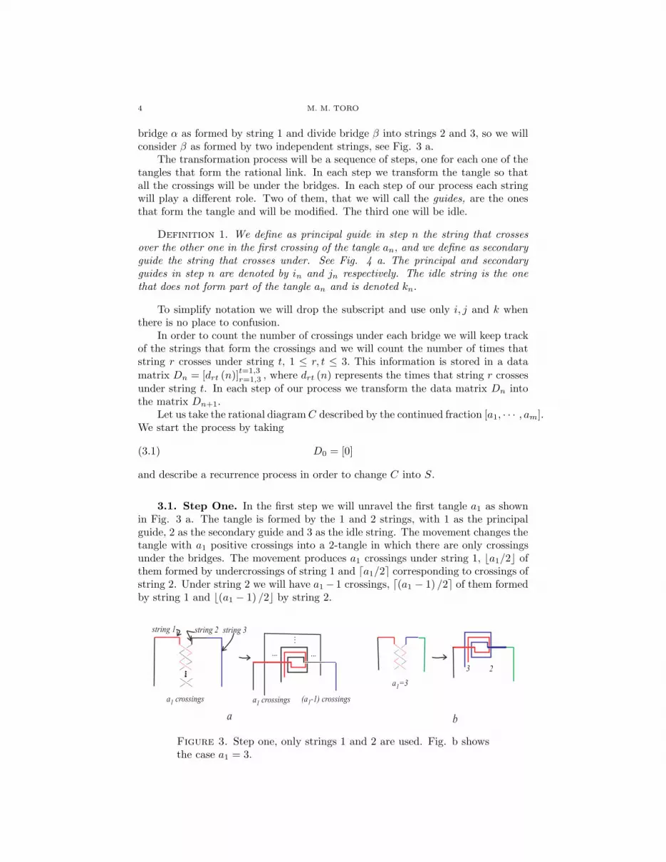
bridge α as formed by string 1 and divide bridge β into strings 2 and 3, so we willconsider β as formed by two independent strings, see Fig. 3 a.

The transformation process will be a sequence of steps, one for each one of thetangles that form the rational link. In each step we transform the tangle so thatall the crossings will be under the bridges. In each step of our process each stringwill play a different role. Two of them, that we will call the guides, are the onesthat form the tangle and will be modified. The third one will be idle.

Definition 1. We define as principal guide in step n the string that crossesover the other one in the first crossing of the tangle an, and we define as secondaryguide the string that crosses under. See Fig. 4 a. The principal and secondaryguides in step n are denoted by in and jn respectively. The idle string is the onethat does not form part of the tangle an and is denoted kn.

To simplify notation we will drop the subscript and use only i, j and k whenthere is no place to confusion.

In order to count the number of crossings under each bridge we will keep trackof the strings that form the crossings and we will count the number of times thatstring r crosses under string t, 1 ≤ r, t ≤ 3. This information is stored in a data

matrix Dn = [drt (n)]t=1,3r=1,3 , where drt (n) represents the times that string r crosses

under string t. In each step of our process we transform the data matrix Dn intothe matrix Dn+1.

Let us take the rational diagramC described by the continued fraction [a1, · · · , am].We start the process by taking

(3.1) D0 = [0]

and describe a recurrence process in order to change C into S.

3.1. Step One. In the first step we will unravel the first tangle a1 as shownin Fig. 3 a. The tangle is formed by the 1 and 2 strings, with 1 as the principalguide, 2 as the secondary guide and 3 as the idle string. The movement changes thetangle with a1 positive crossings into a 2-tangle in which there are only crossingsunder the bridges. The movement produces a1 crossings under string 1, ⌊a1/2⌋ ofthem formed by undercrossings of string 1 and ⌈a1/2⌉ corresponding to crossings ofstring 2. Under string 2 we will have a1 − 1 crossings, ⌈(a1 − 1) /2⌉ of them formedby string 1 and ⌊(a1 − 1) /2⌋ by string 2.

a crossings1 (a -1) crossings1

a =31

a b

3 2

a crossings1

string 1 string 2 string 3

Figure 3. Step one, only strings 1 and 2 are used. Fig. b showsthe case a1 = 3.

EQUIVALENCE OF RATIONAL LINKS AND 2-BRIDGE LINKS REVISITED 5

Therefore, we have the following matrix to describe step one

D1 = [drt (1)]t=1,3r=1,3 =

⌊

a1

2

⌋ ⌈

a1−12

⌉

0⌈

a1

2

⌉ ⌊

a1−12

⌋

0

0 0 0

.

The total number of crossings under string t is given by the sum d1t+d2t+d3t,so these are the numbers that allow us to describe the 2-bridge link produced atthe end of the process.

Definition 2. For t ∈ {1, 2, 3} we define sn,t as the sum of the t column ofmatrix Dn, i.e., sn,t = d1t + d2t + d3t.

3.2. Step n+1. Let us suppose that we have changed the tangles a1, · · · , anand the information is stored in Dn.

In step n + 1 we change the tangle an+1 into a rational tangle, in the sameway as we proceeded in step one. We have an+1 crossings under the principal guideand an+1 − 1 under the secondary guide, see Fig. 4 b. We move all the crossings,forming a parallel set of strings, followings the direction of each of the guides,ending the movement when we reach the initial points of the guides. In this way allthe crossings are under the bridges, see Fig. 4. Figure 6 shows the transformationprocess of C[1, 2, 2]. In Fig. 6b. we made the first step and transform the tangle1. In Fig. 6c. we change the tangle 2 and in Fig. 6d. we move all the crossing,following the guides.

ba c

i=principal guide j=secondary guide

ijj

i

Figure 4. Chages in step n+1.

Now, the important part is to keep track of the number of crossings we haveat the end of step n+ 1 and to find the new guides.

To simplify notation, take a = an+1 and let D = Dn = [drt] and D′ = Dn+1

= [d′rt] defined below. Let us find the values of d′rt in terms of drt and a, for1 ≤ r, t ≤ 3.

Suppose that in step n + 1the guides are i = in+1 and j = jn+1 and the idlestring is k = kn+1. As the string k is idle, the values of dkt, 1 ≤ t ≤ 3, correspondingto undercrossings of string k, do not change, so d′kt = dkt, for 1 ≤ t ≤ 3.

Each time that string i crosses under string t, there are 2a new crossings underthat string, 2 ⌊a/2⌋ of which are formed by string i, or principal guide and 2 ⌈a/2⌉are formed by string j, or secondary guide, see Fig. 4 c.

Each time that string j crosses under string t, there are 2 (a− 1) new crossingsunder string t, 2 ⌈(a− 1) /2⌉ corresponding to crossings of string i and 2 ⌊(a− 1) /2⌋corresponding to crossings of string j. See Fig. 4 c.

6 M. M. TORO

...... ... ......

...

...... ... ......

...

...... ... ......

...

sm ,1 ? 1 sm ,3 + 1

...... ... ......

...

sm,1sm ,3

a

sm ,3sm ,3

sm,1

b c

sm ,1 ? 1

d

Figure 5. Final step. Figure a is for the case m even. Figures b,c and d are for m odd.

Besides these new crossings, when we arrive to the end of string i, we have aadditional crossings, ⌊a/2⌋ corresponding to undercrossings of string i and ⌈a/2⌉corresponding to undercrossings of string j. At the end of string j, there area − 1 additional crossings, ⌈(a− 1) /2⌉ corresponding to string i and ⌊(a− 1) /2⌋corresponding to string j.

So at the end of step n+ 1 we have

d′kt = dkt, for 1 ≤ t ≤ 3,

d′ik =(

1 + 2⌊a

2

⌋)

dik + 2

⌈

a− 1

2

⌉

djk,

d′ij =(

1 + 2⌊a

2

⌋)

dij + 2

⌈

a− 1

2

⌉

djj +

⌈

a− 1

2

⌉

,

d′ii =(

1 + 2⌊a

2

⌋)

dii + 2

⌈

a− 1

2

⌉

dji +⌊a

2

⌋

,

d′jk =

(

1 + 2

⌊

a− 1

2

⌋)

djk + 2⌈a

2

⌉

dik,

d′jj =

(

1 + 2

⌊

a− 1

2

⌋)

djj + 2⌈a

2

⌉

dij +

⌊

a− 1

2

⌋

,

d′ji =

(

1 + 2

⌊

a− 1

2

⌋)

dji + 2⌈a

2

⌉

dii +⌈a

2

⌉

,(3.2)

where {i, j} are the guides and k is the idle string.The process just described can be written as a recurrence relation in terms of

matrices, as we will describe in Theorem 2.For the example C [1, 2, 2] shown in Fig. 6, we have

D1 =

0 0 01 0 00 0 0

,

s1,1s1,2s1,3

=

100

D2 =

0 0 11 0 01 0 1

,

s2,1s2,2s2,3

=

202

3.3. Final step. At the end of step m we have transformed all the tangles andwe have produced a 2-bridge link. When m is even, we reach a reduced 2-bridgediagram but when m is odd, we reach a no reduced diagram with a kink formed bybridge α, that when simplified by a type I Reidemeister move produces a reduced2-bridge diagram, see Fig. 5.

Now we interpret the meaning of the values sm,1 and sm,3 in the description ofthe final diagram.

EQUIVALENCE OF RATIONAL LINKS AND 2-BRIDGE LINKS REVISITED 7

When m is even, see Fig. 5 a., sm,1 is the number of crossings under bridge αand sm,3 is the number of crossings under string 3, so the position of the crossingunder which the bridge α crosses bridge β is sm,3, therefore we obtain the 2-bridgelink of type

(sm,1 + 1) /s3,m.

When m is odd, see Fig. 5 b., there is a kink formed by the bridge α and after thesimplification by type I Reidemeister move, see Fig. 5 c., the number of crossingsunder bridge α decreased by one but the position of the crossing under which thebridge α crosses bridge β increases by one, see Fig. 5 d., and now it is sm,3 + 1, sowe obtain the 2-bridge link

sm,1/ (s3,m + 1) .

In Fig. 6 e. to f. we show the final step in the transformation of C[1, 2, 2]. InFig. 6 e. we change the tangle 2 and in Fig. 6 f. we move all the crossings followingthe guides. In Fig. 6 g. it is clear the kink that is simplified in Fig. 6 h.

e fg

a b c d

i1 k1j1

k2 j2 i2

i3 j3 k3

h

Figure 6. Transformation of C [1, 2, 2] into the 2-bridge knot 7/5.

For the example C [1, 2, 2] we have

D3 =

2 1 14 1 21 0 1

,

s3,1s3,2s3,3

=

724

and after the simplification we get 6 crossings under string 1 and 5 crossings understring 3, so we have the 2-bridge knot 7/5.

3.4. Main result. In order to have the equivalence between the rational linkC [a1, a2, · · · am] and the 2-bridge link p/q, where p/q is the rational given by[a1, a2, · · ·am], we need to prove that the diagram obtained in the final step isin fact the diagram of the 2-bridge link p/q.

Definition 3. Define pn = sn,1 + 1 − µn and qn = sn,3 + µn, where µn wasdefined in (2.2).

8 M. M. TORO

So we need to prove that

pm/qm = p/q,

and we do so by proving the following theorem:

Theorem 1 (Main Result). Given the continued fraction [a1, a2, · · · am] thatrepresents the rational p/q, the integers pn and qn defined above satisfy the recur-rence relations

pn+1 = an+1pn + pn−1, for 1 ≤ n, p0 = 1, p1 = a1,

qn+1 = an+1qn + qn−1, for 1 ≤ n, q0 = 0, q1 = 1.

Therefore pn/qn is the n-convergent of the continued fraction [a1, · · · , am] andso

pm/qm = p/q,

then the rational link C [a1, a2, · · · am] is equivalent to the 2-bridge link p/q.

The proof of this theorem is the content of the following sections.

4. Algorithmic description of the transformation process

In order to describe the transformation process the guides play a fundamentalrole. To each step n we assign a permutation σn ∈ S3 that keep track of the guides.

Definition 4. We define a permutation of {1, 2, 3} by

(4.1) σn (1) = in, σn (2) = jn =, σn (3) = kn,

where in, jn and kn were defined in Definition 1, 1 ≤ n ≤ m.

Lemma 1. The permutation σn satisfies the following recurrence relation

(4.2) σn+1 =

{

σn (1 3) , if an is even,σn (1 3 2) , if an is odd,

for n > 1 and σ1 = Id.

Proof. Just consider the diagrams in Fig. 7.

n evenn odd

an+1Ý1Þ

anÝ1ÞanÝ2ÞanÝ3Þ

anÝ3ÞanÝ2ÞanÝ1Þ

an+1Ý3Þ

an+1Ý1Þ

anÝ1Þ anÝ2Þ anÝ3Þ

an+1Ý2Þ

an+1Ý3Þ

anÝ3ÞanÝ2ÞanÝ1Þ

an+1Ý1Þ

an+1Ý2Þ

an+1Ý3Þ

an+1Ý3Þ

an+1Ý1Þ an+1Ý2Þan+1Ý2Þ

evenan evenanoddan oddan

Figure 7. Changes from permutation σn to permutation σn+1.

�

Corollary 1. For n > 1, in+1 = kn and if an is even then jn+1 = jn andkn+1 = in and if an is odd then jn+1 = in and kn+1 = jn.

EQUIVALENCE OF RATIONAL LINKS AND 2-BRIDGE LINKS REVISITED 9

Definition 5. For each step n, with guides in = i, jn = j and tangle an, wedefine the matrix Mn = M (an, i, j) = [mrt] ∈ M3×3 (N) by

mii = ⌊an/2⌋ , mij = ⌈(an − 1)/2⌉ , mji = ⌈an/2⌉ , mjj = ⌊(an − 1)/2⌋

and zero elsewhere.

The following lemma is clear and give us an alternative way to compute Mn.

Lemma 2. The matrix Mn can be described as

Mn = PσnM (an)P

−1σn

.

where M (an) =

⌊an/2⌋ ⌈(an − 1)/2⌉ 0⌈an/2⌉ ⌊(an − 1)/2⌋ 0

0 0 0

and Pσnis the permutation matrix of

σn.

Theorem 2. The associated matrix Dn of the transformation process of chang-ing the diagram C of the rational link into a 2-bridge diagram satisfies the recurrencerelation

(4.3) Dn+1 = 2Mn+1Dn +Dn +Mn+1, 0 ≤ n ≤ m

where Mn+1 is the changing matrix associated to an+1 and to the permutation σn+1,D0 = [0] and σ1 = Id.

Proof. This is just a new way to write the relations given in (3.2). �

The recurrence described in Theorem 2 is very easy to implement in a computer,in our case we use Mathematica. The following is an example of the calculation totransform the rational diagram C [2, 3, 1, 2, 3].

Example 1. Change the rational C [2, 5, 4, 1] into the 2-bridge 57/26.

Step n an in jn Mn Dn pn qn

1 2 1 2

1 1 01 0 00 0 0

1 1 01 0 00 0 0

2 1

2 5 3 2

0 0 00 2 30 2 2

1 1 05 2 34 2 2

11 5

3 4 1 3

2 0 20 0 02 0 1

23 13 105 2 318 10 7

46 21

4 1 2 3

0 0 00 0 00 1 0

23 13 105 2 328 15 13

57 26

Table 1

4.1. Properties of matrix Dn. As Example 1 shows, there are some inter-esting patterns in the entries of matrix Dn. For instance, the column 1 is ”almost”the sum of columns 2 and 3. In this section we will find relations among the entriesof matrix Dn and among the entries of Dn and Dn+1. The results of this sectionwill be used in the proof of the main result. All the results depend on the guidesin+1, jn+1 and the parity of n and an.

10 M. M. TORO

Proposition 1. Given the rational link C [a1, a2, · · · , am], the sequence of in-tegers sn,t satisfies the recurrence relation

sn+1,t = an+1sn,t + an+1 (dit + djt − dkt + δit + δjt) + (dit − djt + dkt − δjt) ,

1 ≤ n ≤ m, 1 ≤ t ≤ 3,where i = in+1, j = jn+1, k = kn+1 and δrt is the Kroneckerdelta.

Proof. Let Dn = [drt] and D′ = Dn+1 = [d′rt] the data matrices of stepsn and n + 1 in the transformation process; besides let i = in+1, j = jn+1 be theguides, k = kn+1 be the idle string in step n+ 1 and a = an+1. By (3.2) we have,

sn+1,k = d′ik + d′jk + d′kk =(

1 + 2⌊a

2

⌋

+ 2⌈a

2

⌉)

dik+(4.4)(

1 + 2

⌈

a− 1

2

⌉

+ 2

⌊

a− 1

2

⌋)

djk + dkk,

sn+1,i = d′ii + d′ji + d′ki =(

1 + 2⌊a

2

⌋

+ 2⌈a

2

⌉)

dii+(

1 + 2

⌈

a− 1

2

⌉

+ 2

⌊

a− 1

2

⌋)

dji + dki +⌊a

2

⌋

+⌈a

2

⌉

,

sn+1,j = d′ij + d′jj + d′kj =(

1 + 2⌊a

2

⌋

+ 2⌈a

2

⌉)

dij+(

1 + 2

⌈

a− 1

2

⌉

+ 2

⌊

a− 1

2

⌋)

djj + dkj +

⌈

a− 1

2

⌉

+

⌊

a− 1

2

⌋

,

but as 1 + 2⌊a

2

⌋

+ 2⌈a

2

⌉

= 1 + 2a and⌊a

2

⌋

+⌈a

2

⌉

= a we have

(4.5) sn+1,t =

(1 + 2a) dik + (2a− 1) djk + dkk, if t = k,(1 + 2a) dii + (2a− 1)dji + dki + a, if t = i,(1 + 2a) dij + (2a− 1) djj + dkj + a− 1, if t = j,

therefore

sn+1,t = (1 + 2a) dit + (2a− 1) djt + dkt + aδit + (a− 1) δjt

= a (dit + djt + dkt) + a (dit + djt − dkt + δit + δjt) + (dit − djt + dkt − δjt)

= asn,t + a (dit + djt − dkt + δit + δjt) + (dit − djt + dkt − δjt) .

�

Now we need to find expressions for (dit + djt − dkt + δit + δjt) and (dit − djt + dkt − δjt).The following lemmas will take care of finding these expressions that will be usedin proving the main result.

Lemma 3. If i = in+1, j = jn+1, k = kn+1 and a = an+1, then

(4.6) d′it − d′jt = (−1)µa (dit + djt + µaδit + (1− µa) δjt) , for 1 ≤ t ≤ 3,

where µa is given by (2.2).

Proof. Suppose i = in+1, j = jn+1, k = kn+1 and a = an+1. Using therelations given in (3.2) we get

d′ik − d′jk =(

1 + 2⌊a

2

⌋

− 2⌈a

2

⌉)

dik +

(

−1 + 2

⌈

a− 1

2

⌉

− 2

⌊

a− 1

2

⌋)

djk,

EQUIVALENCE OF RATIONAL LINKS AND 2-BRIDGE LINKS REVISITED 11

d′ii − d′ji =(

1 + 2⌊a

2

⌋

− 2⌈a

2

⌉)

dii +

(

−1 + 2

⌈

a− 1

2

⌉

− 2

⌊

a− 1

2

⌋)

dji+

(⌊a

2

⌋

−⌈a

2

⌉)

,

d′ij − d′jj =(

1 + 2⌊a

2

⌋

− 2⌈a

2

⌉)

dij +

(

−1 + 2

⌈

a− 1

2

⌉

− 2

⌊

a− 1

2

⌋)

djj+

(⌈

a− 1

2

⌉

−

⌊

a− 1

2

⌋)

,

but⌊

a2

⌋

−⌈

a2

⌉

= −µa = (−1)µa µa,

⌈

a−12

⌉

−⌊

a−12

⌋

= 1 − µa = (−1)µa (1− µa)

and 1 + 2 ⌊a/2⌋ − 2 ⌈a/2⌉ = −1 + 2⌈

a−12

⌉

− 2⌊

a−12

⌋

= (−1)µa , therefore

d′ik − d′jk = (−1)µa (dik + djk)(4.7)

d′ii − d′ji = (−1)µa (dii + dji)− µa

d′ij − d′jj = (−1)µa (dij + djj) + 1− µa.

Also, as

(−1)µa (µaδit + (1− µa) δjt) =

0, if t = k−µa, if t = i1− µa, if t = j

we get (4.6). �

The following corollary will be used in the proof of Theorem 3. Later, we willconsider only the values of the sum of only two of the columns of Dn, because theother one will give redundant information.

Corollary 2. If i = in+1, j = jn+1, k = kn+1and a = an+1 then

(4.8) sn,t = (−1)µa (d′it − d′jt) + d′kt − µaδit + (µa − 1) δjt, for 1 ≤ t ≤ 3,

where sn,t = d1t + d2t + d3t.

Proof. It is enough to recall that k = kn+1 is the idle string, so d′kt = dkt,therefore from Lemma 3 we get,

(−1)µa

(

d′it − d′jt)

+ d′kt = dit + djt + dkt + µaδit + (1− µa) δjt, for 1 ≤ t ≤ 3.

�

Lemma 4. If i = in+1, j = jn+1 and k = kn+1 then

(4.9) sn−1,t = dit − djt + dkt − δjt

Proof. We apply Corollary 2 to the step n.For an even, µan

= 0 and by Corollary 1, in = kn+1 = k, jn = jn+1 = j andkn = in+1 = i, so we get by (4.8)

sn−1,t = (−1)µan (dkt − djt) + dit − µan

δkt + (µan− 1) δjt = dkt − djt + dit − δjt.

For an odd, µan= 1 and by Corollary 1 in = jn+1 = j, jn = kn+1 = k and

kn = in+1 = i, so by (4.8)

sn−1,t = (−1)µan (djt − dkt) + dit − µan

δjt + (µan− 1) δkt = −djt + dkt + dit − δjt,

therefore, in both cases we get (4.9). �

12 M. M. TORO

This lemma tell us that the values of sn−1,t can be computed using the matrixDn.

Lemma 5. If i = in+1, j = jn+1, k = kn+1 then

(4.10) dkt = dit + djt − δkt + δ3t + (−1)δ3t µn, 1 ≤ t ≤ 3,

where µn = 0 if n is even and µn = 1 if n is odd.

Proof. The proof is by induction on n. Notice that condition (4.10) corre-sponds to the following three conditions:

dk1 = di1 + dj1 − δk1 + µn,

dk2 = di2 + dj2 − δk2 + µn

dk3 = di3 + dj3 − δk3 + 1− µn.

For n = 0, D0 = [0] , and the guides for step one are i = i1 = 1, j = j1 = 2 andthe idle string is k = k1 = 3. Then

d31 = 0 = d11 + d21 − δ31 + µ0,

d32 = 0 = d12 + d22 − δ32 + µ0,

d33 = 0 = d13 + d23 − δ33 + 1− µ0.

For n = 1,

(4.11) D1 =

⌊a12

⌋

⌈

a1 − 1

2

⌉

0

⌈a12

⌉

⌊

a1 − 1

2

⌋

0

0 0 0

.

If a1 is even, by Corollary 1, i = i2 = 3, j = j2 = 2 and k = k2 = 1, then

d11 =⌊a12

⌋

=⌈a12

⌉

= d31 + d21 − δ11 + µ1,

d12 =

⌈

a1 − 1

2

⌉

=

⌊

a1 − 1

2

⌋

+ 1 = d32 + d22 − δ12 + µ1,

d13 = 0 = d33 + d23 − δ13 + 1− µ1.

If a1 is odd, by Corollary 1, i = i2 = 3, j = j2 = 1 and k = k2 = 2 therefore

d21 =⌈a12

⌉

=⌊a12

⌋

+ 1 = d31 + d11 + 1 = d31 + d11 − δ21 + µ1,

d22 =

⌊

a1 − 1

2

⌋

=

⌈

a1 − 1

2

⌉

= d32 + d12 − δ22 + µ1,

d13 = 0 = d33 + d23 − δ23 + 1− µ1.

Suppose that i = in+1, j = jn+1, k = kn+1 and that relations (4.10) hold for stepn. To prove that the results are valid for step n+ 1 we need to find the n+ 2 stepguides, that depend on wether an+1 is even or odd.

If an+1 is even by Corollary 1, in+2 = kn+1 = k, jn+2 = jn+1 = j and kn+2 =in+1 = i and we need to prove that

d′it = d′jt + d′kt − δi1 + δ3t + (−1)δ3t µn+1, for 1 ≤ t ≤ 3.

By Lemma 3 we have

d′it − d′jt = dit + djt + δjt

EQUIVALENCE OF RATIONAL LINKS AND 2-BRIDGE LINKS REVISITED 13

As k is the idle string in the n+ 1 step, we have that d′kt = dkt and for (4.10) weget

(4.12) dit + djt = d′kt + δkt − δ3t − (−1)δ3t µn,

so

d′it = d′jt + (dit + djt) + δjt = d′jt +(

d′kt + δkt − δ3t − (−1)δ3t µn

)

+ δjt,

but δkt + δjt = 1− δit and

(4.13) − δ3t − (−1)δ3t µn = −δ3t − (−1)

δ3t (1− µn+1) = δ3t − 1 + (−1)δ3t µn+1,

so

d′it = d′jt + d′kt + 1− δit − δ3t − (−1)δ3t µn = d′jt + d′kt − δi1 + δ3t + (−1)

δ3t µn+1.

If a = an+1 is odd, by Corollary 1 in+2 = kn+1 = k, jn+2 = in+1 = i and kn+2 =jn+1 = j.

By Lemma 3 we have

d′it − d′jt = −dit − djt − δit

thus, by (4.12) and (4.13) we have

d′jt = d′it + (dit + djt) + δit = d′it + (d′kt + δkt − δ3t − (−1)δ3t µn) + δit

= d′it + d′kt + δkt + δit − 1 + δ3t + (−1)δ3t µn+1

= d′it + d′kt + δjt + δ3t + (−1)δ3t µn+1.

�

Corollary 3. If k = kn+1 then

sn,t = 2dkt + δkt − δ3t − (−1)δ3t µn, 1 ≤ t ≤ 3.

5. Proof of Main Result

Now we use the results of the previous section to prove the main result:

Theorem 3 (Main Result). Given the continued fraction [a1, a2, · · · am] thatrepresents the rational p/q, the integers pn and qn defined in Definition 3 satisfythe recurrence relations

pn+1 = an+1pn + pn−1, for 1 ≤ n, p0 = 1, p1 = a1,

qn+1 = an+1qn + qn−1, for 1 ≤ n, q0 = 0, q1 = 1.

Therefore pn/qn is the n-convergent of the continued fraction [a1, · · · , am] andso

pm/qm = p/q,

therefore the rational link C [a1, a2, · · · am] is equivalent to the 2-brigde link p/q.

Proof. Let [a1, · · · , am] be a continued fraction. For n = 0, D0 = [0] , sop0 = 1 and q0 = 0. From (4.11), s1,1 = a1 and s3,1 = 0, so p1 = a1 and q1 = 1.

By Proposition 1

sn+1,t = an+1sn,t + an+1 (dit + djt − dkt + δit + δjt) + (dit − djt + dkt − δjt)

If i = in+1, j = jn+1, k = kn+1 by Lemma 5

0 = dit + djt − dkt − δkt + δ3t + (−1)δ3t µn,

14 M. M. TORO

but δit + δjt = 1− δkt, so

dit + djt − dkt − δkt = dit + djt − dkt + δit + δjt − 1 = −δ3t − (−1)δ3t µn

and by Lemma 4sn−1,t = dit − djt + dkt − δjt

so

(5.1) sn+1,t = an+1sn,t + an+1

(

1− δ3t − (−1)δ3t µn

)

+ sn−1,t

then, for t = 1, sn,1 = pn − 1 + µn

pn+1 − 1 + µn+1 = an+1 (pn − 1 + µn) + an+1(1− µn) + pn−1 − 1 + µn−1

and µn+1 = µn−1 sopn+1 = an+1pn + pn−1

For t = 3, sn,3 = qn − µn, so (5.1) becomes

qn+1 − µn+1 = an+1 (qn − µn) + an+1(1 − 1 + µn) + qn−1 − µn−1

thereforeqn+1 = an+1qn + qn−1.

�

Acknowledgments

Thanks to Universidad Nacional de Colombia, Sedes Medellın y Manizales.

References

[1] G. Burde and H. Zieschang, Knots, 2 ed, (Walter de Gruyter, New York, NY, 2003).[2] D. Burton. Elementary Number Theory, 7 ed.,( Mcgraw-Hill, 2011).[3] J. Conway, An enumeration of knots and links and some of their related properties, In Com-

putational Problems in Abstract Algebra, Proc. Conf. Oxford (1967), 329-358.[4] H. Gruber, Rational Knots, www2.tcs.ifi.lmu.de/˜gruberh/[5] H. Hilden, J. Montesinos, D. Tejada and M. Toro, On the classification of 3-bridge links,

Revista Colombiana de Matematicas, 46 (2) (2012) 113-144.[6] L. Kauffman and S. Lambropoulou, On the Classification of Rational Tangles, Adv. Appl.

Math. 33(2) (2004), 199-237.[7] L. Kauffman and S. Lambropoulou, On the Classification of Rational Knots, L’ Enseign.

Math., 49(3-4) (2003), 357-410.[8] Kawauchi, A survey of Knot Theory, (Birkhauser, Basel, 1996).[9] K. Murasugi, Knot theory and its applications, (Birkhauser, Boston, 1996).[10] H. Schubert, Knoten mit zwei Brucken, (Math. Z.) 65 (1956), 133-170[11] D. De Wit, The 2-bridge knots of up to 16 crossings, Journal of Knot Theory and Its Rami-

fications, Vol. 16, No. 8 (2007) 997–1019

Current address: Universidad Nacional de Colombia, Sede MedellınE-mail address: mmtoro@unalmed.edu.co