renormalization of rational lagrangians

ANNALS OF PHYSICS: 66, 1-19 (1971)

Renormalization of Rational Lagrangians

R. DELBOURGO, K. KOLLER, AND ABDUS SALAM

Physics Department, Imperial College, London S W7

Received May 2, 1970

We show that rational Lagrangians of the type G@(l + ,kj-yl can be renormalized by introducing a finite class of infinite counter terms providing that the Dyson index v0 - “I < 3. The form of the counter terms is explicitly exhibited. The theories become unrenormalizable when Y 0 - v1 > 3; we discuss, in particular, the case q, - y1 = 4, which resembles a g#” theory for $ --, co, and is nonrenormalizable, contrary to what one may have naively expected.

1. INTRODUCTION

In two earlier papers [l], the problem of infinities associated with nonpolynomial Lagrangians, in general, and rational Lagrangians, in particular, was considered. In this paper, we study the problem of absorbing these infinities into a renormalization of constants in the theory by a small number of counterterms. Our results can be stated for the typical Lagrangian V = G@(l + h~$-~l[~ 2 1, V, integer] and sums thereof:

(i) When V, - + < 1 all S-matrix elements are completely free of infinities and the theory is superrenormalizable.

(ii) When v0 - vr = 2 and 3, there are a finite number of distinct types of infinities in the S-matrix elements which can be absorbed into a finite class of counterterms that serve to renormalize the constants in the theory.

(iii) When v0 - v1 > 4, the theory is nonrenormalizable. This conclusion is especially interesting for the case v,, - v1 = 4; thus, although the polynomial interaction gqS4 is renormalizable by itself, we find that the rational interaction G#‘/(l + hq5) which possesses the same limit when 4 -+ co is not.

Any rational Lagrangian may be decomposed in the general form

1 0 1971 by Academic Press, Inc.

2 DELBOURGO, KOLLER, AND SALAM

and since (1 + A+>-” = (1 + h(a/ah))(l + h&l, etc., it is in practice quite sufficient to study the model

L = G& + Gv-l$"-l + ... + G/(1 + A+)

to gain insight into the infinities one may expect in more complicated examples. We shall call v the Dyson index of the theory, defined by lim,,, L(4) = O(e). Rephrasing our results we can say that when A # 0 the theory is (i) superrenormalizable when v < 1, (ii) renormalizable for v = 2 or 3, but (iii) nonrenormalizable for v 2 4. We prove these results in Sections 3, 4, and 5 after surveying the general techiques for computing S-matrix elements in Section 2. Of special interest are the explicit forms of the counter Lagrangians needed to absorb all infinities of the theory (as exhibited in Eq. (22)). Appendix A discusses various aspects of normally ordered Lagrangians and resulting tadpole terms. Appendix B contains a simplified representation of the momentum space superpropagator for particles of arbitrary mass. Appendix C shows that by taking the limit h2 -+ 0 of the model g+4/(1 + X4) one may recover the conventional infinities of the 4” theory.

2. REPRESENTATIONS OF S-MATRIX ELEMENTS

An exposition (I) of methods for computing S-matrix elements in perturbation theory for nonpolynomial Lagrangians appears in papers I and II. Basically, they can be divided into p-space and x-space methods, both of which we shall use where convenient for isolating the infinities and their renormalization. The p-space methods have the advantage of familiarity, generality, and of giving an idea of possible infinities of subgraphs, in addition to the overall infinity of the graph. The x-space methods are better suited for writing compactly the counterterm Lagrangians. We shall give a brief survey of these methods.

Let us write the interaction Lagrangian as the series

V(+) = G f v, (1) +=Yo .

where G is the major coupling constant to which the perturbation expansion refers. To order GN the conventional Feynman perturbation theory gives the following rules for constructing a graph (see Fig. 1) and its corresponding S-matrix element:

(a) Draw points x1 , x2 ,..., xN to represent the vertices. (b) Attach mi external lines to each point xi and connect each pair of points

RATIONAL LAGRANGIANS 3

m4

FIG. I. An example of a general supergraph.

xi and xj by a cocoon of nij lines which we shall term a superline. Thus, Hi = Cj nif is the total number of internal lines emanating from vertex i.

(c) Sum over all nij with the condition that the total number of lines coming into each vertex, mi + Hi is not less than v,, .

The corresponding S-matrix element is written as

subject to m, + Cj nij 3 vO . Correspondingly there is the more physically relevant momentum space transform

s mlmz...mN(p) = j n d4xj eiBj~jS,,,,,...,,(x). j

Note that in stating how diagrams are to be constructed and calculated, we have not included tadpole lines which emanate from and close onto the same vertex, so have interpreted V(4) in (1) as already normally ordered, each term in the series being considered as : 4” :. If, however, we wish to abandon this assumption of normal ordering and allow for tadpole insertions, we can continue to use (2) but relax the condition that i # j in the summations. We have then to “define” the singular quantity d(U) as the infinite integral J [d4p/(2.rr)4] d(p). Appendix A contains a full treatment of normal ordering and its effect on interaction Lagrangians.

It is possible to obtain a closed form for (2) or (3), interpreted as an asymptotic series, by exploiting Laplace transform methods. Write

V(4) = jy 9’(c) e-‘* d5 (4)


defined by analytic continuation where appropriate. One may then express (2) in the form,

S mlma...m,(~) =

where d, = d(x, - xi) and

From the closed form (5) we note the following identity:

(5)

(6)

(7)

which leads to important results like

&,n&l , 4 = 2 Smo(x1 > x2), N= 2, (8) 12

sooo(xl~ x3 7 x3); N = 3, etc. 13

These relations will prove useful in studying asymptotic behaviors and providing power counting of infinitie9.

An alternative way of obtaining closed expressions and one which is perhaps better suited for obtaining explicitly high energy behaviors is the p-space method

1 The point is that high energy behavior is determined by small x behavior, i.e., the limit as x4 approach one another; this corresponds to taking the limit A ---f co which means, from (5), that the high energy behavior is governed by small 6 behavior of the Laplace transform T(5).

B The momentum space expression corresponding to (5) is

with the interaction-independent kernel

again governed by small 1 as p + 03.


of writing s(p) through a Watson Sommerfeld transformation on (2). This allows one to cast the series as an integral

s ,,...,,(x) = CiGjN r ig j tg r(--zij) u (% + T ZiZ) [-A(& - XN”, (9)

where one can rotate the contours in zii space to lie parallel to the imaginary axes such that mi + Re Ci zij = v0 - E. Denote the Fourier transform of [d(x)]” by A(k, 2) viz.

[A(x)]” E j $$ e-i”” A(k, z). (10)

If we associate the internal momentum kij to each superpropagator (cocoon) joining the point Xi and xj , the space integrations in (3) can be performed to give

~nL’,,l,2...,,(p) = q .n, j 2 T(-zij) einz% (mi + C zil) %>3 ?7 1

. j f!!k A(k,? , zij) . (27~)~ a4 (pi + -$ kit) P94

(11)

an expression which resembles very closely the normal Feynman graph result (where zii = 1 or 0) and which makes it possible to use Dyson power counting techniques. The Fourier transform A(k, z) is welldefined only for 0 < Re z < 2 and is given outside this range by analytical continuation. A convenient approximate form for A(k, z) is given in Appendix B for arbitrary mass p which becomes exact as p --f 0 or k -+ co or z -+ 0, 1 and carries the correct threshold behaviors in momentum space. Because we shall only be interested in the high energy behavior, where k2/p2 + co, it will be sufficient to approximate the superpropagator by the propagator for the massless case

r(2 - z) (167+-= iD(kT ‘1 = r(z) (-k2)2--z: . (12)

In passing, we should note that since the definition of the chronological product (0 I T[Pw, Pm I 0) is ambiguous to the extent of terms like CrLi ~,(a~), a4(x), with a, real and finite, the Fourier transform of (0 ( T[eS1blZ), es2$(0)] 1 0) = erltsD(z) carries an ambiguity of the type Cf, a,(a2)n S4(x), where-to satisfy Jaffe locali- zability for the operator ebd(r)- xz==, a,Zn should be an entire function of order less than $. This ambiguity in the definition of the T-product would carry through for all nonpolynomial theories (whether superrenormalizable or otherwise and whether rational or not) and includes the case of rational Lagrangians through


formula (15). This has been remarked upon (4) by Efimov, Lee, and Zumino and more recently by Lehmann and Pohlmeyer, Mitter, Blomer and Constantinescu. For the particular case of the exponential Lagrangian ec* and for the two-point superpropagator erltzd(s), Lehmann and Pohlmeyer have given a detailed discussion of this ambiguity and show that the ansatz adopted by Volkov, Arbuzov and Fillipov, and Salam and Strathdee (which amounts to setting all the a, = 0) picks out what they call “minimally singular superpropagator”. For the rest of this paper we shall always use the minimal singularity ansatz and neglect the type of ambiguity mentioned, even though the rigorous discussion of Lehmann and Pohlmeyer is so far available only for the two-point superpropagator in an exponential Lagrangian theory. This is because we believe, on the basis of the work in this paper, that all such ambiguous terms are finite renormalization counter Lagrangians which however contain derivatives of field operators of infinitely high order (corresponding to the derivatives occurring in C” a,(a2), a4(x)) and will inevitably give a nonlocal Lagrangian. Thus if we make an ansatz, like we have done in this paper, that if one starts with a local Lagrangian any counter Lagrangians must also be local if the theory is to be renormalizable, we shall be able to discard the ambiguities discussed above.

Returning to the consideration of high energy behavior, as far as high momentum power counts are concerned it is enough to notice that as k2/p2 - co, expression (11) consists of products of factors like J” dz X(z, m)( -k2)z-2 integrated along contours and with kernels .X(z, m) specified by the interaction V($). These kernels exhibit successions of poles at values of z lying to the left of the contour and in the limit k2 ---f -co, it is the nearest pole, at z = z,, say, which dominates and provides the momentum dependence (k2)z,-2 wherefrom one may judge whether or not the integration over internal momenta gives finite results or not. This we shall now investigate.

3. SUPERRENORMALIZABLE MODELS

As a very simple illustration of the more general superrenormalizable case @/(I + h$)Y1 with q, - v1 < 1, take the model theory

and apply the momentum space method for studying the ultraviolet behavior of integrals. In this model, contours lie to the left of Cj zij + mi = 2 and the Taylor coefficients are

v(z) = (-hy2 zyl + z). (14)


Note that because of the positions of the contours on the Re z axes, & zij + CL mi = 2F + m -C 2N, where F = N(N - 1)/2 is the total number of internal super lines joining every pair of supervertices, and m is the total number of external lines.

To estimate the overall asymptotic p-behavior, compute all matrix elements in the Symanzik region of external momenta (pi . pj < 0, etc.). As is well known, one can here perform Wick rotations and employ Euclidean internal momenta (kfj < 0). Also use the massless superpropagator (12) as we are only interested in large k2 contributions. The integral (11) becomes

(15)

The number of independent internal momenta, i.e., the number of loops Z, equals F - N + I for an N-th order graph with F internal lines. (Unlike Feynman diagrams in polynomial theories, F = +N(N - 1) is quadratically dependent on N.) Thus the overall power count of the integral gives:

s ;vv s 17 dz .X(m, z) 1 (&)’ (k2)xi>jZij--2F (16)

w j L7 dz X(m, z) j” (d4k)-N+1 (k2)““‘.

In the limit -k2 = M2 ---t cc the internal integrations provide the ultraviolet3 factor lim,,, M-4N+4+2~;>jZi which describes the overall infinite character of 8 on dimensional grounds. Recalling that the nearest singularity to the left of the z contour governs the high energy behavior so that

Re c zii c 2N - 111, id

(17)

we see that S < M4-m-3N and therefore (m 3 0, N >, 2) there is never any overall infinity in 3. This argument applies to each subintegration and we can therefore conclude that all S-matrix elements are finite in this model theory.

3 The quadratic dependence of F on N necessitates that the superpropagators fall faster than k-2 to guarantee finiteness of the integrals. To get the order of magnitude right, note that 3 w

j- (&)F-N+l(k”yF-2F, where we have very roughly replaced C z by zF. Thus finiteness of s” demands Re z Q 4/N or alternatively stated an average behavior of superpropagators like (k2)--3+4/N rather than (k*)-l is needed.


In more general examples like F/(1 + X$p the z contours lie to the left of Re x1 ziC = v,, - mi and at first sight it would seem that Re xii zij < v,N - m might violate our statement of finiteness since fi < IV~+(“~--~)~-~ could possibly still be infinite. However, a careful analysis reveals that the first singularity in X(m, z) to the left of the contour actually occurs below

Re 1 ziL = v,, - v1 + 1 - m, 1

because of the presence of binomial factors in the expansion of (I + A$)-“1 with v, > 1 and which provide appropriate zeros. Thus, in fact,

Re~z,i<(v,-vv,+l)N-m ij

as regards the high energy behavior of 3 (as one might have expected from the naive consideration of the Dyson index). The correct ultraviolet behavior is given by

3 < ~4+b--v~-3)N-m 9 W9

so the theory is superrenormalizable if v, - vr < 1. Likewise, theories which are linear combinations xi Gi@(l + hi$)+ with vi - ~~ ,( 1 can be shown to be perfectly finite in all their S-matrix elements.

4. RENORMALIZABLE MODELS

We shall now study some simple examples where infinities do arise but can be renormalized by counterterm Lagrangians. We take our prototype superrenormalizable model and add to it a succession of polynomial terms with Dyson indices > 1, viz. G,@ + G3$3 + .‘.. Since G,qY can be simply absorbed into a mass renormalization we shall in this section examine the first nontrivial model

In setting up a perturbation series in G and G’ a term of order GNG’N’ consists of supergraphs from [ V(q%))lN, pure (5” graphs from [V’(+)lN’, and joining terms. We showed that V(4) by itself has no infinities, and one knows that 4” theory by itself has three primitive infinities (see Fig. 2) which can be renormalized by introducing corresponding counterterms.


, - . FIG. 2. The primitive infinities of 4” theory.

More specifically one has

A, w G-c, + Gf4c;, A, m G’3~O’, A, w G’“c, ,

where c,, and c2 are logarithmic and quadratic infinities such as

co = i s

b(x) d4x - log IV, c2 = i s

d3(x) d4x - M2.

For future reference we note that the renormalized Lagrangian of 4” theory, including counterterms, can be compactly expressed as

: v’ + 8~‘: = :[exp G’ (c2 $ + c,, --$- + c,,‘G’ $ f c~G’~ ii<)] b”: - (20)

We now turn to possible infinities which arise when internal lines connect V and v’ interactions. (The V’ infinities by themselves are assumed to be renormalized as above). To lowest order GG’ one has the two infinities shown in Fig. 3 which we can term “vacuum-like” and “self-energy-like”.

:* I+--- FIG. 3. Infinities to order GG’ in ((G$z/l + A#) + G’+a) theory.

Because any number of external lines can emanate from the G-vertex we can call these two graphs primitive since they can be regarded as supervertex modifications of V($). The counterterm

6V = G’ [co -$- +c2$]&


can be added to the Lagrangian to cancel these infinities making every S-matrix element finite to order GG’.

Before we consider further infinite graphs of order GGfN’, there is a basic repetition pattern worth recognizing as shown in Fig. 4.

FIG. 4. Repetitions of lowest order infinities.

These repetition graphs modify the super-vertex and their effect can be elegantly expressed in the compact form:

[exp G’ (c,, $ + cs $)] &a

We need only therefore consider genuine new primitive infinities such as shown in Fig. 5 since further repetitions of them are simply given by modifying the exponential operator above. Although there are an infinite number of such graphs4

(4

04 FIG. 5 (a). Higher order vacuumlike primitive infinities; (b). Higher order self-energylike

primitive infinities in ((GI$~/~ + A+) + G’C3) theory.

* The graphs in Fig. 5 can be obtained from those of Fig. 3 by either drawing new lines out of the supervertex and attaching them through $” vertices to the lines of Fig. 3 or by joining two lines of Fig. 3 by an extra connecting line. The first kind of attachment does not change the ultraviolet behavior; the second kind diminishes it by a factor M2.


(similar to the infinite set of irreducible vertex parts in quantum electro-dynamics) the overall ultraviolet behaviours are still no worse than quadratic. It is this cir- cumstance which permits us to renormalize them along conventional lines by adding further (at most quadratically) infinite counter-terms. In all we get

dl‘f3 f Cr)G”+l~

dc$r+3 + f C;)G’r+l

V($), (21) r=0 T=O

where Cir) denotes a sum of quadratically infinite constants -AR2 (as given by Fig. 5(a)) and C,j7) a sum of Iogarithmically infinite constants -(log M)” (as given by Fig. 5(b)).

We shall now show that with the counterterms SV + SV’ there are no further infinities in any order. Consider first graphs to order G2GfN. Characterize it as a (n, + n2 + m)-point function of 6” theory connected by n, + n2 lines to the superpropagator of V(4) theory having m, + m2 external lines as depicted in Fig. 6.

FIG. 6. A typical graph to order G2G ‘I’ in ((C#+?/l + A+) + G’fP) theory.

We must take n, 3 1 and n2 >, 1 as the case where n, or 1z2 = 0 corresponds to attachments which have already been renormalized. In momentum space we must deal with the integral

where S and S’ refer to elements corresponding to V and V’. It is well known in 4” theory that S,l+,l+,(k) - k4-N-m--nl- na while in the supertheory according to Eq. (7), &I+ml. ,z+m,(4 = (a/Wnl+ml SOIn2+mZ-RI-nll if nl + ml -=c n2 + m2 say; orSnl+~~~l,n2+nl &k) N (k2)--“1+“1 k-2. Therefore the ultraviolet behavior of our integral is given by

~n,+n~-N-m-2-2(n~+m~) < ~-n.~+n~--N--2


But the connectedness properties of our graphs always ensure that N - n2 > -1, so that in every case the integrals converge at least as rapidly as &P.

With more supervertices the situation keeps on improving owing to greater convergence of the internal integrations. Thus all graphs of order G2GN, G3GlN,... are finite. In short the renormalized theory, described by the Lagrangian

&+3 C;)G’r+l - -

d+T+3 + f ,$lG’r+l dr+l

dcjr+l )I (V + V’> (221 7=0

has finite S-matrix elements (including self-mass and self-charge). It is instructive to see what our modifications to the Lagrangian do to the Laplace

transformed interaction P’(?J. Before renormalization the infinities come essentially from 4 + 03 or 5 + 0. The introduction of counterterms to V(4) gives the new interaction

[ ( dZ exp c V + *.* )I V(#) or V-(5> exp[cc2 4 ***I.

Thus, renormalization affects the behavior of the Lagrangian in the limit 5 + 0 so as to eliminate all perturbation infinities.

5. UNRENORMALIZABLE MODELS

If we add to the supernormalizable interaction V(4) the polynomial terms G+J5 + G,# + ... it is obvious that the theory cannot be renormalized since c$~, c#” are already intractable by themselves. However, if we take the model theory

G2 V+V”=l+h+ - + Gn+4,

it looks, on the face of it, capable of renormalization as the Dyson index v of the theory [L(4) -+ #’ as 4 + 031 is 4. We shall now prove that even so the theory cannot be renormalized in the standard way by introducing counterterms. Basically this is because the infinities progressively get worse in higher orders and require counterterms with an increasing number of derivatives. The theory then becomes manifestly nonlocal and no S-matrix is calculable in terms of a few basic parameters.

The demonstration follows the methods of the previous section. To order GN or to order (G”)N there is evidently no problem since in one case the theory is finite or in the other case it is easily renormalized. The difficulties arise from cross terms. Adopting the most optimistic attitude, disregard vacuumlike graphs as in Fig. 7(a)


FIG. 7(a). Vacuumlike graphs to order GG”N in ((G$*/l + A#) + G”#4) theory. (b). Self-energylike graphs to order GG”N in ((G$2/1 + A$) + G”$“) theory.

and their repetitions, since they only contribute multiplicative terms to the supervertex (although the infinities do get worse as the order of G” is increased!). Consider the self energylike graphs of Fig. 7(b) and repetitions thereof. Unlike vacuum graphs, these are momentum dependent and the counterterms needed will necessarily involve derivatives of the field 4. Since their infinities go as M2, M4, M6..., an arbitrarily increasing number of subtraction terms are needed with higher and higher derivatives. This is the typical nonrenormalizable situation. The same difficulty occurs for all other modifications of the supervertex, so that not only are self-energylike modifications of the supervertex infinite but also all the scatteringlike modifications. The same situation holds for more complicated graphs with more than one supervertex.

The problems studied in this paper are a preliminary step to the consideration of the renormalization status of chiral, Yang-Mills and Weak interaction Lagrangians all of which, by suitable field transformations, can be written (3) as a mixture of polynomial and nonpolynomial terms. These more realistic cases are currently under study.

APPENDIX A: NORMAL ORDERING

Suppose we are given an interaction Lagrangian L(4). This can be rewritten as a normally ordered interaction : V(d): for all polynomial L by repeated application of the identity 4” = : q4” : + id,(O). Noting that if the approach to zero is made in the timelike direction, id+(O) = d(O), where d(x) is the causal propagator, let us rewrite the operation as

qP = :[exp (k d(0) $)] +2: .

595/@/r-2


This normal ordering operation actually applies to polynomials # and can thereby be generalized to arbitrary interaction functions. Thus, we have the theorem that

where U(4) = :v#+ 7

V(+) = [exp (!j 40) $)] u(4)

u(4) = [ev (- k 40) $)] Vb). or

One can write an integral representation to compute V(4),

V($) = T2$ 11, e-“““U(+ + uA+(O)) du.

(A.11

(A.3

For example if

u(4) = W’, V(4) = G(--d(O))+ H,[+(--d(O))-+],

H = Hermite polynomial;

(A.3a)

U(4) = Ge-/\*, (A.3b)

Diagrammatically the operation exp[& d(0) d2/dp] has the effect of introducing tadpole loops at every vertex of a Feynman graph and is analogous to the action of exp[+ xiii Aii a2ja@&] which introduces propagators between vertices Xi and xi of the graph. In general, it should be noted that the functional form of V may be very different from U. Only for exponential and polynomial interactions do both functions have the same character.

APPENDIX B: THE SUPERPROPAGATOR

For a massive free particle the causal two-point function can be written as

A is real for x2 < 0 (spacelike) and is cut in the x2 plane from 0 to co, the value on the physical sheet for x2 > 0 (timelike) being obtained from below the cut by


an x2 - ie prescription. In the limit p ---f 0, D(x) = 1/4.rr2(r2 + ic) is the massless propagator. The Fourier transforms are of course given by

J(k) = i(k2 - p + k-1, D(k) = i(k2 + k)-l.

In the text we are interested in the Fourier transform of the superpropagator [d(x)]” for arbitrary complex z,

d(k, z) =: s d*x eiJcz[d(x)lz. (B.2)

In the massless case Gel’fand an Shilov [2] give the result as

iD(k -> = r(2 - z) . (167r”)l-” ,i r(z) (-k’Y

(R-3)

This can be analytically continued outside the range 0 < Re z < 2, where it is originally well-defined. In doing so it is necessary to see the prescription k2 + k2 + ic to obtain the correct distributions at nonpositive integer z values; for example,

ljm% D(k, z) = (27r)* S4(k), etc.

We shall give here an approximate solution to the problem for the massive case which has the virtue of reducing to well-known functions in various limits (z + 0,l; p + 0, p2 ---f co,...) and which also has the correct thresholds and types of discon- tinuities at the branch points in the p2 plane. To this end note that [A( is cut in the x2 plane from 0 to co, and that

as x2 ---f 0,

m 2$ i-i

fz e-“r” as x”+wo.

After Wick rotation, the integration we must perform is (K” = -k2)

iA(k, z) = 7 s”’ dr . r2Jl(u) [ 11>2$tr) ]‘, 0

(R.4)

which cannot be done in general except in very special circumstances (z = 1 or p = 0). Let us therefore replace [Kl(~r)]z by K,(p) multiplied into some simple polynomial of pr‘such that the behaviors as r + 0 (p” --f co) and r -+ co (pz thresholds) are correctly reproduced. This suggests the approximation


or

(B-5)

Hence (B.4) reads

id(k, z) w (8T2)1-z (2k+f1+z) 2Krftd1 + Z>l s co dr . ,,(~-"z'J~(~~)K~(~+~,(~~')

o Carrying out the integration we obtain

i d(k, z) w (167r2)‘-” r(2 - z) r[4(5 - z)] F[;(l + z)]

x (p”z”)“-“F(i(5 - z), 2 - z; 2; k2/p2z2). 03.6)

This superpropagator therefore has a cut in the k2 plane from the threshold p2z2 with discontinuity of (B.6) given by

disc d(k, z) = (1hn2)1-z (p2Z2)$'l+Z' (k2 _ p2z2)+(3Z-5)

r[g(l + z)] F(i[-3 + 3z)l

k2 - F (; (z - l), 2; ; (z - 1); 1 - 7). 03.7)

To take the high energy limit k2/p2 + cc we shall work in the region Re z > -1 and then continue our results to other z values. Thus

,$E_ z&k, 4 - r(2 - z) (167r2)1-z

l-(z) (-k2)2-z F

( 2 - z, 1 + z; f (1 - z); $)

m iD(k, z). (B.8)

Note that the threshold behavior in k2 is corectly obtained at all positive integer z since d(k, z) possesses a square-root branch cut for even z and a logarithmic branch cut for odd z according to (B.7). Lastly, we may check that as z -+ 0 or 1 the correct distributions follow, viz.,

lii d(k, z) = i(k2 - ~3,

ljz d(k, z) = (2~7)~ a4(k).


APPENDIX C: POLYNOMIAL MODELS As LIMITS OF RATIONAL MODELS

As a corollary of our work we shall show that in the lim X2 + 0 of G+3(1 + h+)-l and g+4(1 + h$)-l we recover the conventional renormalization counterterms of G$3 and g@ theory from the counterterms of the rational models.

First, take the simpler case

(C-1)

The counterterms correspond to vacuumlike infinities c,, of 4” theory, and if we follow the same steps as in Section 5, the final renormalized Lagrangian L, free of infinities5 is

L,= v,+sv,=$ + [exp (9 $)I & . (C.2)

Now proceed to the limit h + 0 counting l/h” as a quadratic infinity like c2 = i J .&(x) d4x - M2. Then we get

COG” L, ---f __ - ; co3G4 + ; co2G3+ - ; coG2p + Grj3

x2 .

- 4! (C.3)

which exactly corresponds to the renormalized Lagrangian for G43 theory apart from the linearly divergent terms G3/X + G2$/X. These terms have no counterpart in momentum space integrals and can be eliminated by taking the principal value limit *(lim,,,+ + lim,,,J which averages out the singularity at h + 0.

This next case is more subtle. Begin with the unrenormalised Lagrangian

K.4)

5 Note that the exponential term just corresponds to a mass shift by G/X in the tadpole graphs, viz,

A 0, ma + $) = /P&P - m2 + G/X)-’

= $ d4p(p2 - m2)-l + ; j- &(p” _ ,2)-S + . . .

= d(O, m”) + c,G/X + finite terms.

18 DELBOURGO: KOLLER, AND SALAM

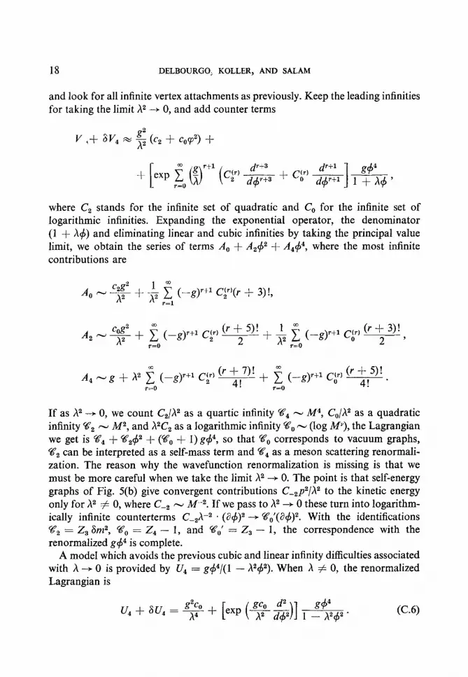
and look for all infinite vertex attachments as previously. Keep the leading infinities for taking the limit h2 -+ 0, and add counter terms

+ [ exp f or+l ((2;) --$& + Cl;) -$&I &,

9-0

where C, stands for the infinite set of quadratic and C,, for the infinite set of logarithmic infinities. Expanding the exponential operator, the denominator (1 + h$) and eliminating linear and cubic infinities by taking the principal value limit, we obtain the series of terms A, + A2$2 + A,p, where the most infinite contributions are

A0 w * + 4 f (-gy+1 qyr + 3)!, r=1

A2 (r + 3)! -zg + f (-g)'+l qe qF + f f (-g)'+l cp, 2'

2-O 7-O

A4 -g+ A2 -f (--S)'+lC~>~+ 2 (-g)?+l+!$F~

T=O 7=0

If as X2 -+ 0, we count C21h2 as a quartic infinity V4 - M4, Co/h2 as a quadratic infinity 45, - M2, and X2C2 as a logarithmic infinity q. - (log My), the Lagrangian we get is g4 + %Y2+2 + (%‘. + 1) gv, so that w. corresponds to vacuum graphs, Q, can be interpreted as a self-mass term and V4 as a meson scattering renormalization. The reason why the wavefunction renormalization is missing is that we must be more careful when we take the limit X2 -+ 0. The point is that self-energy graphs of Fig. 5(b) give convergent contributions C-,p2/h2 to the kinetic energy only for h2 # 0, where C-, - M-2. If we pass to h2 -+ 0 these turn into logarithm- ically infinite counterterms C-2h-2 . (+5)z --+ %?o’(a$)2. With the identifications 92, = 2, 6m2, V. = 2, - 1, and woo’ = 2, - 1, the correspondence with the renormalized g$4 is complete.

A model which avoids the previous cubic and linear infinity difficulties associated with h --f 0 is provided by U, = gfi”/(l - h2qS2). When X # 0, the renormalized Lagrangian is


Now the infinite irreducible set of quartic, quadratic and logarithmic infinities of p theory is exactly recovered by taking the limit X2 + 0, as the reader may easily check from the power series expansion of (C.6).

REFERENCES

I. R. DELBOURGO, ABDUS SALAM, AND J. STRATHDEE, Infinities of nonlinear Lagrangian theories, Phys. Rev. 187 (1969), 1909; ABDUS SALAM AND J. STRATHDEE, “Momentum space behavior of integrals in nonpolynomial Lagrangian theories, Phys. Rev. (to appear). We shall refer to these as papers I and II in the text.

2. I. M. GEL’FAND AND G. E. SHILOV, “Generalized Functions,” Vol. I, Academic Press, New York, 1964.

3. ABDUS SALAM, Nonpolynomial Lagrangian theories, “Proceedings of the Coral Gables Conference on Fundamental Interactions at High Energy, Miami, Gordon & Breach, New York, 1970.

4. G. V. EFIMOV, Nucl. Phys. 74 (1965), 657; B. W. LEE AND B. ZUMINO, Nucl. Phys. B13 (1969), 671; P. K. MITTER, “On an Analytic Approach to the Regularization of Weak Interaction Singularities,” Oxford preprint; H. LEHMANN AND K. POHLMEYER, “On the Superpropagator of Fields with Exponential Coupling,” DESY preprint; R. BLOMER AND F. CONSTANTINSCU, “On the Zero Mass Superpropagator,” Munich preprint.

5. M. K. VOLKOV, Ann. Phys. (New York) 49 (1968), 202; B. A. ARBUZOV AND A. T. FILLIPOV, Soviet Phys. JETP 49 (1965), 990.

renormalization of rational lagrangians

Documents