environmental policy with green consumerism'' - hal inrae
TRANSCRIPT
HAL Id: hal-02945517https://hal.inrae.fr/hal-02945517
Preprint submitted on 22 Sep 2020
HAL is a multi-disciplinary open accessarchive for the deposit and dissemination of sci-entific research documents, whether they are pub-lished or not. The documents may come fromteaching and research institutions in France orabroad, or from public or private research centers.
L’archive ouverte pluridisciplinaire HAL, estdestinée au dépôt et à la diffusion de documentsscientifiques de niveau recherche, publiés ou non,émanant des établissements d’enseignement et derecherche français ou étrangers, des laboratoirespublics ou privés.
”Environmental Policy with Green Consumerism”Stefan Ambec, Philippe de Donder
To cite this version:Stefan Ambec, Philippe de Donder. ”Environmental Policy with Green Consumerism”. 2020. �hal-02945517�
1124
“Environmental Policy with Green Consumerism”
Stefan Ambec and Philippe De Donder
July 2020
Environmental Policy with Green Consumerism
Stefan Ambec∗ and Philippe De Donder†‡
July 2020
Abstract
Is green consumerism beneficial to the environment and the economy? To shed light
on this question, we study the political economy of environmental regulations in a model
with neutral and green consumers where the latter derive some warm glow from buy-
ing a good of higher environmental quality produced by a profit-maximizing monopoly,
while the good bought by neutral consumers is provided by a competitive fringe. Con-
sumers unanimously vote for a standard set at a lower than first-best level, or for a tax
delivering the first-best environmental protection level. Despite its under-provision of
environmental protection, the standard dominates the tax from a welfare perspective
due to its higher productive efficiency, i.e., a smaller gap between the environmental
qualities of the two goods supplied. In stark contrast, voters unanimously prefer a tax
to a standard when the willingness to pay for greener goods is small enough.
Key Words: environmental regulation, corporate social responsibility, green consumerism,
product differentiation, tax, standard, green label, political economy.
JEL codes: D24, D62, Q41, Q42, Q48.
∗Toulouse School of Economics, INRAE, University of Toulouse Capitole, Toulouse, France. Email:[email protected]
†Toulouse School of Economics, CNRS, University of Toulouse Capitole, Toulouse, France. Email:[email protected]
‡We thank participants to seminars and conferences held at EAERE 2019 (Manchester), IAERE 2020(Brescia), CORE (Louvain-la-Neuve), TSE (Toulouse), ANU (Canberra), SCSE (Quebec), and especially M.Dewatripont, J. Hindriks, G. Llobet, M. Price and J. Tirole for their suggestions. This research has beensupported by the TSE Energy and Climate Center and the H2020-MSCA-RISE project GEMCLIME-2020 GANo. 681228. We acknowledge funding from ANR under grant ANR-17-EURE-0010 (Investissements d’Avenirprogram). All errors and shortcomings are ours.
1
1 Introduction
1.1 Green consumerism, corporate social responsibility and envi-
ronmental policies
When firms and customers are only motivated by their self-interest, they tend to ignore their
negative impact on the environment, which leads to excessive pollution and overexploitation
of open-access natural resources such as water and clean air. This in turn calls for public
intervention to fix, or at least mitigate, this market failure. This traditional view is con-
tradicted by the many private initiatives to reduce the negative impacts of human activities
on the environment. For instance, some consumers accept to pay a higher price in order to
purchase more environmentally-friendly products. This phenomenon is sometimes referred to
as ‘green consumerism’. On the supply side, firms often reduce their emissions of pollutants
and their use of natural resources beyond what is mandated by regulations. They engage in
costly eco-labelling of their products and production processes. They endorse the so-called
Corporate Social Responsibility (CSR) policy and code of conduct.
CSR is now very popular among managers and policy makers. It is part of most business
school curricula. There is wide evidence that consumers care about CSR as many of them are
willing to pay more for greener or fair trade products. The positive view of CSR and green
consumerism contrasts with Friedman’s famous criticism published in 1970 in The New York
Times (Friedman, 1970). In an article provocatively entitled ‘The Social Responsibility of
Business is to Increase its Profits’, Milton Friedman criticized CSR for being undemocratic.
He argued that, with CSR, the businessman ‘decides whom to tax by how much and for what
purpose’. In a democratic society, ‘the machinery must be set up to make the assessment of
taxes and to determine through a political process the objectives to be served’.
Our objective is to go beyond Friedman’s criticism and to better understand the interplay
2
between “public” and “private” politics in the context of CSR.1 To this end, we develop a
model encompassing simultaneously social decisions taken democratically (through majority
voting over either an environmental quality standard or an environmental tax), green con-
sumerism (with a fraction of consumers deriving warm glow from buying a greener product)
and CSR. We take Friedman’s criticism on board by reconciling CSR with profit-maximization
(with a single-profit maximizing firm producing the high quality good) in a context where
social decisions are taken democratically.2
We model an economy with a continuum of citizens of two types, dubbed neutral and
green, who all consume one unit of a polluting good. While all consumers suffer in the
same way from aggregate pollution, green consumers derive warm glow from their individual
consumption decision. They value the environmental quality of the products they purchase.
The polluting good is produced under perfect competition except in its green version which is
supplied by only one firm (called the “green firm”). The motive for supplying greener goods is
pure profit-maximization: the green firm pays the cost of higher environmental performance
to move away from perfect competition and to exert some market power on green consumers.
We contrast two forms of public intervention: a standard on environmental performance
and a tax on pollution. In both cases, the timing of decisions is the same: citizens first vote
over the instrument’s level, and then consumers and producers decide what to produce (and
consume) at what price. We first examine the choice of a minimal quality standard. The
green firm might decide to go beyond the standard if charging a price premium for higher
environmental performance is profitable. This decision depends on the green consumers’ taste
1In the words of Benabou and Tirole (2010, p.15), “While the invisible hand of the market and the morevisible one of the state have been the objects of much research, we still know little about the decentralizedcorrection of externalities and inequality.”
2Benabou and Tirole (2010, p15) argue that “there are three possible understandings of corporate socialresponsibility: the adoption of a more long-term perspective, the delegated exercise of philanthropy on behalf ofstakeholders, and insider-initiated corporate philanthropy. The latter two understandings build on individualsocial responsibility.” Our approach is consistent with the second perspective, where “profit maximizationand CRS are consistent.” (Benabou and Tirole, 2010, p.11).
3
(willingness to pay) for environmental quality. When it is low enough, supplying a green
version of the good is not profitable. All firms then produce the same environmental quality
which is set collectively at its first-best level by citizens. When the green consumers’ taste for
environmental quality is high enough, the green firm produces a good whose quality is higher
than the brown one, but not directly affected by the standard. Voters unanimously prefer a
quality standard lower than its first-best level. The intuition for this result is that neutral
voters free ride on the higher quality of the good consumed by green voters, while green
voters have the same political preferences as neutral ones because the green firm captures all
their warm glow with limit pricing. A higher taste for environmental quality increases the
green good’s quality and thus the free-riding effect, resulting in a lower unanimously chosen
value of the standard. For a large enough taste for environmental quality, the average quality
produced may even exceed its first-best level.
Next we consider the choice of an environmental tax. Unlike with a standard, the green
firm always finds it profitable to produce a green version of the good, however small the
willingness to pay for environmental quality is. Hence, two different environmental qualities
are produced, and the tax affects both the brown and green goods’ qualities. Assuming that
tax proceeds are redistributed in a lump sum way to them, consumers are unanimous as to
their most-preferred value of the tax level (for the same reason as with the standard) which
is such that the average quality is set at its first-best level. Yet this outcome is inefficient as
the first-best allocation requires a single environmental quality.
Comparing the standard and the tax, we obtain that the standard dominates the tax from
a welfare perspective. The reason for this result differs according to the intensity of preferences
for environmental quality. When it is low, the standard perfectly decentralizes the first-best
outcome with a single good produced, while the tax entails a wedge between the two qualities
produced (productive inefficiency). When the taste for environmental quality is large enough,
the productive efficiency advantage of the standard over the tax (lower wedge between two
4
goods’ qualities) trumps the standard’s allocative inefficiency disadvantage (inefficient average
quality level).
Looking now at how voters evaluate the standard vs the tax, we obtain a trade-off be-
tween an environmental protection effect and a tax stealing effect. On the one hand, the
environmental protection effect favors the tax, because a higher tax increases both the brown
and green qualities, resulting in a larger impact on average equality, than a higher standard.
On the other hand, the tax stealing effect favors the standard, since there is an extra cost of
increasing environmental quality with the tax as all the fiscal benefit of providing a higher
environmental quality is captured by the green firm and therefore lost by consumers/voters.
We obtain that voters unanimously prefer a tax to a standard when the warm glow effect
is small enough, because the lower quality of the brown good with a standard allows the
neutral voters to free ride on the green ones, and the latter to benefit from a lower priced
good (compared to the standard).
Going back to CRS, we obtain that it is not welfare improving in the presence of con-
sumers/voters enjoying a warm glow from “doing the right thing”, even when firms maximize
profit and when corrective policies are taken by (unanimous) majority voting (to answer
Friedman’s criticism). In our setting, the conjunction of CSR with green consumerism leads
to either a substandard policy, or to productively inefficient taxes.
1.2 Related literature
Our paper builds on the literature on self-regulation and corporate social responsibility (see
Ambec and Lanoie, 2008, and Kitzmueller and Shimshack, 2012, for surveys). Most studies
aim at assessing the profitability of voluntary environmental protection and CSR strategies.
Some previous works have analyzed the interplay between environmental policies and firms’ or
consumers green behavior using different approaches. For instance, Fleckinger and Glachant
(2011) analyze a game between a social-welfare maximizing regulator and a profit-maximizing
5
firm with frictions in the regulation process. They show that self-regulation can be a firm’s
strategy to preempt more stringent future regulations. In the same vein, the Private Politics
approach (Baron 2001, Heyes and Kapur, 2012, Daubanes and Rochet, 2019) assumes that
CSR and environmental policies result from combined pressure from lobbies (firms) and NGOs
(consumers/citizens). We depart from those studies by modeling explicitly the collective
decision process that determines environmental policy. Other papers highlight that CSR
might crowd-out donation and charity (Kotchen, 2006, Besley and Ghatak, 2007), or analyze
price competition and product differentiation with green consumers (Eriksson, 2004, Conrad,
2005). However, they do not endogenize environmental regulations using a political economy
approach. The paper closest to ours is Calveras et al. (2007) which also models green
consumers with warm-glow preferences who vote on environmental regulations. They show
that the presence of green consumers might lead to laxer regulations when a majority of voters
free-ride on their contribution to the environment. We provide a more negative view of green
consumerism when such behavior is used by firms to obtain market power: all consumers
(neutral and green) vote for a laxer minimal quality standard. Moreover, we analyze the
political outcome when an environmental tax is implemented instead of an environmental
standard.
Our paper also contributes to the literature comparing second-best policies, such as a
tax and a standard in the case of environmental externalities (see for instance Weitzman
1974; Bovenberg et al. 2008; Fowlie and Muller 2019; Jacobsen 2013; Carson and LaRiviere
2018). Compared to this literature, we study the welfare dominance of standards even without
behavioral anomalies such as limited attention (Allcott et al. 2012) or temptation (Tsvetanov
and Segerson 2014). Bovenberg et al. (2008) study second-best policies designed to reduce
deadweight loss from externalities and obtain numerically that standards may also be preferred
to taxes, because of higher lump-sum compensation costs with the tax.
The paper closest to ours in this literature is Jacobsen et al. (2017), which demonstrates
6
the possible superiority of standards in a model of public good provision where agents differ
in how much they value the total amount of public good, and where the cost of public good
provision is convex.3 Agents who value more the good provide more of it, creating an inefficient
wedge in the marginal cost of production. They then obtain that, for any amount of public
good, a standard is always more efficient than a uniform price instrument such as the tax.
They also introduce heterogeneity in the cost of provision, which resembles our warm glow
effect, and show how the two types of heterogeneity push in opposite directions on efficiency
of the policies.4 Our analysis goes further, as it endogenizes the amount of the environmental
good offered by explicitly modeling its political determination.
The structure of the paper is straightforward. The next section presents our setting,
with section 3 studying the environmental quality standard, and section 4 the environmental
tax. Section 5 compares the two instruments, and section 6 concludes by focusing on the
robustness of our results to various assumptions. The more convoluted proofs are relegated
to an appendix.
2 The setting
2.1 The model
We consider a good whose production or consumption generates environmental externalities,
typically pollution. We index pollution abatement by the continuous variable x that we call
the good’s environmental quality . A higher value of x reflects, for instance, the use of a cleaner
source of energy to produce electricity, a less polluting car, food grown with less pesticide or
3This heterogeneity, unlike in your paper, drives the private contribution to the public good. Under ourassumption of a continuum of agents, each agent’s consumption decision has an infinitesimal impact on thetotal level of environmental protection and is then unaffected by how much agents care for this aggregatelevel. Our assumption is more in line with global pollution problems such as climate change.
4To be precise, they show that the tax is efficient if agents are homogenous in their valuation of the publicgood but heterogeneous on their cost of providing it like in our model. This result differ from our becausethey do not launder preferences when they measure welfare.
7
water, a manufactured product that can be more easily recycled, etc. Alternatively, one can
see x as a ‘public good’ contribution to society in the corporate social responsibility (CSR)
sense, e.g. better working conditions, transparency, banning of child labor, investment in
education, infrastructure, etc. The cost of supplying one unit of the good with environmental
quality x is denoted c(x) where c(.) is an increasing, twice differentiable and convex function
of x, with c(0) = 0 and c′(0) = 0 (to guarantee interior solutions).
On the demand side, we consider a continuum of mass one of consumers who are divided
into two types, green and neutral, with respective shares α and 1−α. The types are denoted
by subscripts g and n, respectively. All consumers obtain the same private value v from con-
suming one unit of the good, regardless of its environmental quality. Both types of consumers
also enjoy the same benefit b(X) from the average environmental quality X, which is the level
of environmental protection in the economy.5 The function b(.) is strictly increasing, twice
differentiable and strictly concave: b′(x) > 0 and b′′(x) < 0. Neutral consumers rationally
do not care directly about the pollution generated by their own purchase decision: they do
not value the environmental quality of the good they consume, since their own consumption
does not impact the average environmental quality in the economy. Their utility when they
purchase the good at price p is v − p + b(X). By contrast, green consumers enjoy a ‘warm
glow’ from contributing to environmental protection above the minimal environmental quality
standard, that we denote x0.6 Let ω be the green consumers’ willingness to pay for environ-
mental quality when above standard. The parameter ω is hereafter referred to as the level of
green consumerism while α is the share of green consumerism. Green consumers’ utility when
purchasing a good of environmental quality x at price p is v − p + ωx + b(X) when x > x0,
5Note that average and total environmental qualities are equal with a continuum of consumers of mass oneas assumed.
6Assuming rather that green consumers care more about environmental protection X than neutral con-sumers would not induce them to consume higher quality goods than the latter, with a continuum of consumers,unlike with warm glow.
8
and v − p+ b(X) otherwise.7
On the supply side, a competitive industry is supplying the standard (or “brown”) version
of the good with environmental quality x0. Perfect competition drives down profit to zero.
We assume that only one firm (firm 1) can supply higher environmental quality than the
standard, x1 > x0.8 So, firm 1 has a monopoly position on the green version of the good
(called the green good).
We first analyze the socially desirable amount of environmental quality, which will consti-
tute our main benchmark.
2.2 First-best environmental quality
The first-best environmental quality maximizes social welfare defined as the sum of consumers’
utility and firms’ profit. We follow the canonical approach first proposed by Hammond (1988)
and Harsanyi (1995) who advocate to exclude all external preferences, even benevolent ones,
when computing a social welfare function. This means that we “launder” the green consumers’
preferences by assuming away the warm-glow part of their utility.9 We denote the welfare
7The alternative formulation where the warm glow factor is modeled as ω(x−x0) would not affect our results- see the concluding section. This alternative formulation would have the morally unappealing characteristicthat green consumers’ utility would increase when neutral voters consume dirtier goods (i.e., lower x0), otherthings kept equal.
8This assumption can be justified by the ownership of a particular technology or the long-term developmentof a reputation of being greener. For instance, the firm is the only one that can credibly commit to issuea label of better environmental quality. See the concluding section for the robustness of our results to thisassumption.
9See Goodin (1986) for a description of the various grounds for laundering preferences. More specifically,Benabou and Tirole (2010, p.15) write “We saw that prosocial behaviour by investors, consumers and workersis driven by a complex set of motives: intrinsic altruism, material incentives (defined by law and taxes) andsocial- or self-esteem concerns. (...) The pursuit of social- and self-esteem per se is a zero-sum game” whichmay then call for laundering the preferences of these agents. For instance, “The buyer of a hybrid car feelsand looks better, but makes his neighbours (both buyers and non-buyers of hybrid cars) feel and look worse–a‘reputation stealing’ externality” (Benabou and Tirole, 2010, p.6). Finally, observe that our laundering ofpreferences only affects our normative assessment of the equilibrium allocation, as opposed to the descriptionof this equilibrium. See the concluding section for a discussion of the impact of this assumption.
9
level in the economy as
W (x0, x1) = v − (1− α)c(x0)− αc(x1)− b((1− α)x0 + αx1). (1)
Both types of consumers are then characterized by the same welfare function, v+ b(x)− c(x),
so that there is no reason to produce two different quality levels. Maximizing welfare with
respect to x, we obtain the first-best level of environmental quality xFB characterized by the
following first-order condition:
b′(xFB) = c′(xFB), (2)
which equates the marginal benefit and marginal cost of increasing x. Average first-best
environmental quality is XFB = xFB.
We investigate successively two forms of public intervention: an environmental quality
standard and a tax on pollution. In both cases, the timing of decisions runs as follows. First,
consumers vote over the value of the instrument (level of the standard or of the tax). Second,
firms set simultaneously their prices and environmental quality given the policy enacted.
Third, consumers make their purchase decisions.
3 Environmental standard
In this section, we study the setting of an environmental quality standard x0 imposed on all
firms. We solve the model by backward induction. In a first sub-section, we study the firms’
behavior as well as the choice by consumers of which variant of the good to consume.
10
3.1 Firms’ and consumers’ behavior
Competition among producers of the good with minimal quality x0 drives down its equilibrium
price towards its costs, p0 = c(x0). Firm 1 has exclusive capacity to supply greener goods for
technological or legal reasons (e.g. process or product protected by a patent), or because it
acquired a reputation for being green. Firm 1 charges p1 for a good of environmental quality
x1. Green consumers buy green goods whenever10
v − p1 + ωx1 + b(X) ≥ v − p0 + b(X).
We first assume that x1 > x0 and compute the profit-maximizing price for firm 1. We then
check that firm 1 makes a positive profit and that x1 > x0 at that price. If it is not the case,
then firm 1 prefers to offer x1 = x0 for p1 = p0.
The maximum price p1 compatible with green consumers buying quality x1 rather than
x0 is
p1 = c(x0) + ωx1. (3)
Firm 1’s profit is then
π1 = α[p1 − c(x1)]
= α[ωx1 + c(x0)− c(x1)],
where we have used the one-to-one relationship between firm 1’s price and quality defined in
10We make the simplifying assumption that green consumers buy from firm 1 when they are indifferentbetween the offerings of firms 0 and 1.
11
(3). Maximizing π1 with respect to x1, we obtain:
∂π1
∂x1
= α (ω − c′(x1)) ,
so that the profit-maximizing quality level, denoted by xS1 (where the superscript S denotes
the fact that firms are constrained by a standard) is such that11
c′(xS1 ) = ω, (4)
with the corresponding profit-maximizing price given by
pS1 = ωxS1 + c(x0). (5)
Firm 1 uses its monopoly power to capture all the green consumer surplus created by the
warm glow effect of consuming a greener-than-x0 product. Firm 1 then chooses its quality
level to equate the marginal cost of providing a higher quality with the marginal benefit to
the firm (through a larger price), which is equal to the willingness to pay for environmental
quality ω.
To check whether the environmental quality xS1 is profitable for firm 1, first observe that,
if xS1 > x0, firm 1 for sure makes a positive profit as long as consumers buy the green good.
This is due to the fact that the cost function c is convex: since xS1 is set so that its marginal
cost to firm 1 is equal to its marginal benefit (the constant ω), the marginal cost of producing
all inframarginal quality values below xS1 is always strictly smaller than its cost ω, resulting
in a positive profit.
Note from (4) that xS1 does not depend on x0, but increases with ω (since the cost function
is convex). We then obtain the following proposition.
11We concentrate on interior solutions since c′(0) = 0.
12
Proposition 1 With a standard set at x0, firm 1 chooses x1 = xS1 (given by equation (4)) if
x0 < xS1 , and chooses x1 = x0 (and p1 = p0) if x0 > xS
1 .
In words, a lax standard allows firm 1 to exert its market power, sell a green good and
capture the extra surplus from green voters. A standard that is stringent (in the sense that its
marginal cost is larger than ω) results in firm 1 producing the same good as the competitive
fringe, at the same price.
The following definition will prove useful later on.
Definition 1 We denote by ωS1 the unique value of ω such that xS
1 = xFB.
3.2 Collective choice of an environmental standard
We now examine the choice of minimal environmental performance for the product x0 set as
a standard. We first define the utility of both types of consumers as a function of x0, when
firm 1 chooses its price p1 and quality x1. The utility of neutral consumers is
USn (x0) =
!"#
"$
v − c(x0) + b(XS) if x0 < xS1 ,
v − c(x0) + b(x0) if x0 ≥ xS1 ,
(6)
with XS = αxS1 + (1 − α)x0 and xS
1 = c′−1(ω) following equation (4). The utility of green
consumers is given by
USg (x0) =
!"#
"$
v − pS1 + ωxS1 + b(XS) if x0 < xS
1 ,
v − c(x0) + b(x0) if x0 ≥ xS1 .
13
Replacing pS1 by its formulation (5), the utility of green consumers if x0 < xS1 can be simplified
to
USg (x0) = v − ωxS
1 − c(x0) + ωxS1 + b
%XS
&
= v − c(x0) + b%XS
&. (7)
We then obtain that USn (x0) = US
b (x0), but for reasons differing according to whether x0 is
smaller or larger than xS1 . When x0 ≥ xS
1 , the standard is set so high that it is too costly for
firm 1 to differentiate its offering, and all consumers, whether neutral or green buy the brown
good at a price equal to its cost c(x0). When x0 < xS1 , firm 1 does differentiate its offering
and the warm-glow part of the green consumers’ utility is entirely captured by firm 1 through
its pricing.
The unanimity approved standard is the value of x0 maximizing either the first or the
second line in (6). The second line is maximized with first-best environmental quality: x0 =
xFB. It is the preferred standard when a single good is supplied. The first line of (6) peaks
at a standard denoted xSV0 defined by the following first-order condition (FOC):
c′(xSV0 ) = (1− α)b′
%αxS
1 + (1− α)xSV0
&. (8)
The marginal cost of the standard on the left-hand side should be equal to its marginal benefit
on the right-hand side. Compared to the case of the first-best level xFB in (2), the marginal
benefit is deflated by 1−α because, with two environmental qualities xSV0 and xS
1 , increasing
the standard only affects the contribution of neutral consumers to environmental protection
X = αxS1 + (1−α)xSV
0 . The chosen standard is always strictly positive (since xSV0 = 0 would
imply that b′(XSV ) = 0, a contradiction with our assumption that b′(.) > 0). Moreover,
applying the implicit function theorem on (8), we obtain the following proposition.
14
Proposition 2 The unanimity-chosen standard xSV0 is lower than first-best, and is decreasing
with ω and α, with xSV0 > 0.
Both α and ω decrease the marginal benefit from the standard (through a higher environ-
mental quality of the green good for ω, and through a higher proportion of agents consuming
this good for α), and so decrease xSV0 .
Let ω be the unique value of ω that equalizes the neutral consumers’ utility with a unique
good provided with x = xFB, and with a brown good xSV0 and a green good xS
1 as defined
below.
Definition 2 We denote by ω the unique value of ω such that:
b(αxS1 + (1− α)xSV
0 )− c(xSV0 ) = b(xFB)− c(xFB), (9)
with xS1 , x
SV0 and xFB defined by (4), (8) and (2) respectively.
We establish the following proposition, proved in the appendix.
Proposition 3 If ω < ω, the unanimity chosen standard implements the first-best environ-
mental protection level xFB. If ω > ω, green consumerism leads to a suboptimal standard
xSV0 < xFB with green goods. The threshold ω decreases with α.
The citizens’ choice of standard depends on green consumers’ willingness to pay for envi-
ronmental quality. If ω is low, the green version of the good is not supplied. All citizens vote
for the first-best standard. Environmental protection is at the efficient level. All the benefit
from production goes to consumers. When ω is high enough, supplying a green version of
the product becomes profitable. Products are differentiated on environmental quality: one
version with the standard quality x0 = xSV0 and the green version with quality xS
1 > xSV0 . The
green good supplier makes profit by extracting the green consumer’s willingness to pay for
15
environmental quality. All consumers vote for a standard xSV0 which is lower than xFB, but
for different reasons. The green consumers lower the standard from xFB to reduce the price
paid for the green good. The neutral consumers free-ride on the environmental protection
driven by the green consumers’ demand. Overall the standard fails to fix the two market
failures that are the environmental externalities and the market power exerted by the green
firm.
The intuition for the impact of α on ω is that the utility with xSV0 < xS
1 increases with α
(thanks to a better environmental quality for given xSV0 ) while the utility with the first-best
is unaffected, so that voters prefer xSV0 < xS
1 (rather than x0 = xFB) for a lower value of ω
when α increases.
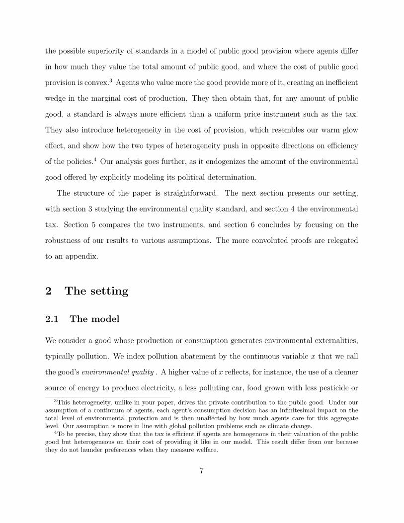
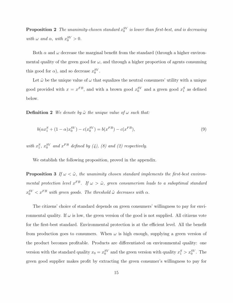
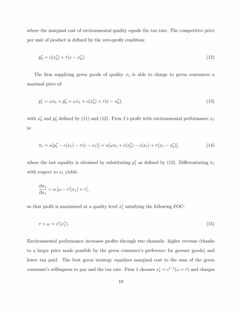
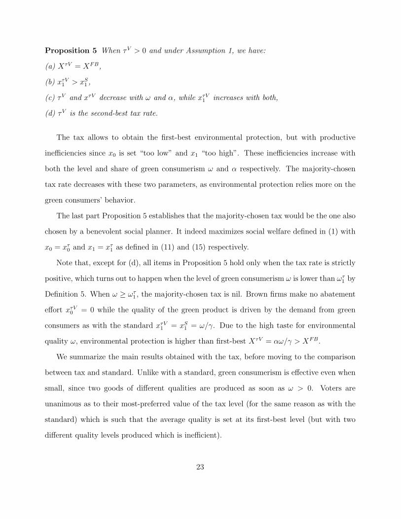
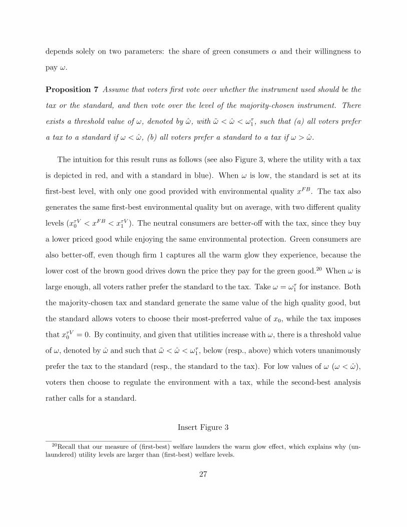
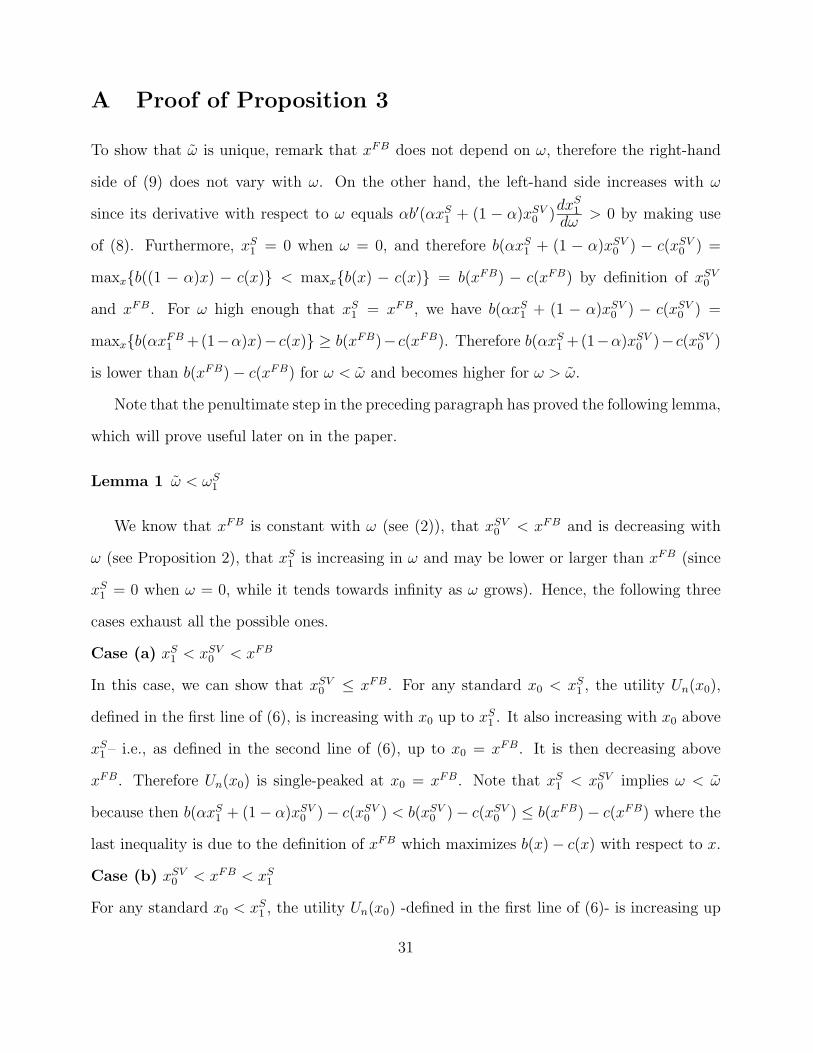
Figure 1 recapitulates the results obtained with a standard, and shows how the first-best
and majority-chosen standard levels and average environmental quality in the economy vary
with the willingness to pay for green products ω.12
Insert Figure 1
The first-best standard and corresponding environmental protection XFB = xFB (black
curve) do not vary with the willingness to pay for environmental quality ω. When ω < ω
the first-best standard is unanimity preferred to any other and a single good is produced
at the voting equilibrium. When ω reaches ω, both a brown (dashed curve) and a green
(full curve) goods are supplied at the voting equilibrium. The economy switches to an equi-
librium with differentiated products and a lower standard xSV0 . Lemma 1 in the proof of
Proposition 3 implies that xS1 < xFB when ω = ω. The switch towards a new majority
voting equilibrium then occurs discontinuously, with a decrease in the environmental quality
of both goods (compared to the unique first-best level) which reduces overall environmental
12All figures are based on c(x) = γx2/2, b(x) = Log(2 + 2x), with γ = 0.8 and α = 0.2.
16
protection XSV = αxS1 + (1− α)xSV
0 (the blue dotted curve in Figure 1). In other words, the
environmental quality decreases discontinuously at the precise point where the green good is
supplied.
As the level of green consumerism ω increases beyond ω, the environmental quality of the
green good xS1 improves while the standard xSV
0 becomes laxer. Environmental protection
XSV improves driven by the demand for environmental quality by green consumers, although
it is still under-provided. It reaches its first-best level when the taste for environmental
quality ω becomes high enough that the green consumer’s demand compensates the lower
standard. In particular, the environmental quality of green goods should exceed the first-best
level xS1 > xFB at that point. Moreover, environmental protection XSV exceeds the first-best
level XFB when ω is large enough.13
It is worth noticing that the collectively-chosen standard xSV0 would not be recommended
by a benevolent social planner when the green good is supplied with a standard xS1 and ω > ω.
Maximizing social welfare defined in (1) with respect to x0 with x1 = xS1 = c′(ω) leads to a
second-best standard xSB0 given by the following first-order condition:
c′(xSB0 ) = b′
%αxS
1 + (1− α)xSB0
&. (10)
Comparing (8) and (10), we obtain that their respective solutions xSV0 and xSB
0 are such that
xSV0 < xSB
0 . A welfare-maximizing social planner would solve the free-riding problem by not
deflating the marginal benefit by (1 − α) in the first-order condition (see (8)). The social
planner then recommends a higher standard of environmental quality and, therefore, a higher
environmental protection XSB = axS1 + (1−α)xSB
0 > XSV , than the one unanimously voted
upon.
We summarize our main results with a standard before moving to a tax. When ω is
13Indeed as ω tends toward infinity, xSV0 tends toward 0 (see (8)), so that XSV tends toward αxS
1 whichtends toward infinity as seen from (4).
17
low enough, green consumerism is not effective in the sense that a single-quality good is
produced, with its majority-chosen level equal to its first-best level. When ω is high enough,
the individuals unanimously prefer a standard lower than its first-best level. Neutral voters
free ride on the higher quality of the good consumed by green voters, and green voters have
the same political preferences as neutral ones because the monopoly firm producing the high
quality good captures all their warm glow through a larger price. The unanimously chosen
value of the standard decreases with the intensity of warm glow ω, while the high quality
good increases with ω. If ω is higher than ωS1 , the average quality in the case the standard
is voted upon may exceed its first-best level thanks to the very large quality bought by green
consumers.
4 Environmental tax
4.1 Firms’ and consumers’ behavior
We now move to another policy instrument to mitigate environmental externalities: a tax on
pollution. We denote by e the pollution emitted in the absence of any pollution abatement
effort by firms, namely when they produce a good of quality x = 0. Environmental quality x
then corresponds to the reduction in polluting emissions from that point. Pollution is taxed
at a linear rate τ . The total cost of supplying one unit of the product with environmental
performance x is c(x) + τ(e − x). The brown good producers choose the value of x that
minimizes their cost given the price of their product p0. The environmental quality they
choose is denoted by xτ0 and satisfies the following FOC:
τ = c′(xτ0), (11)
18
where the marginal cost of environmental quality equals the tax rate. The competitive price
per unit of product is defined by the zero-profit condition:
pτ0 = c(xτ0) + τ(e− xτ
0). (12)
The firm supplying green goods of quality x1 is able to charge to green consumers a
maximal price of:
pτ1 = ωx1 + pτ0 = ωx1 + c(xτ0) + τ(e− xτ
0), (13)
with xτ0 and pτ0 defined by (11) and (12). Firm 1’s profit with environmental performance x1
is:
π1 = α[pτ1 − c(x1)− τ(e− x1)] = α[ωx1 + c(xτ0)− c(x1) + τ(x1 − xτ
0)], (14)
where the last equality is obtained by substituting pτ1 as defined by (13). Differentiating π1
with respect to x1 yields:
∂π1
∂x1
= α [ω − c′(x1) + τ ] ,
so that profit is maximized at a quality level xτ1 satisfying the following FOC:
τ + ω = c′(xτ1). (15)
Environmental performance increases profits through two channels: higher revenue (thanks
to a larger price made possible by the green consumer’s preference for greener goods) and
lower tax paid. The best green strategy equalizes marginal cost to the sum of the green
consumer’s willingness to pay and the tax rate. Firm 1 chooses xτ1 = c′−1(ω + τ) and charges
19
pτ1 = ωxτ1 + c(xτ
0) + τ(e− xτ0). The following proposition, proved in the appendix, shows that
firm 1’s profit is always positive when it chooses x1 = xτ1.
14
Proposition 4 With a tax, we have that π1 > 0 with x1 = xτ1 > xτ
0 for all ω > 0.
As soon as firm 1 produces a good greener than x0, it can increase discontinuously its
price by ωx1, while the other terms in its profit function (the gain in tax bill and the increase
in production costs) are continuous in x1.
A fundamental difference between the environmental tax and the standard is their impact
on environmental performance for the green product. In Section 3, we have shown that the
standard x0 has no direct impact on the level of environmental quality imbedded in the green
good xS1 , see (4). The standard only affects the decision whether to supply a greener good
or not through p1. By contrast, the tax impacts directly the green good’s environmental
performance xτ1 as shown in (15). A higher tax increases both environmental performances
xτ0 and xτ
1 while a higher standard x0 does not change xS1 as long as supplying the green good
is profitable.
It is worth mentioning that, although both environmental qualities xτ0 and xτ
1 depend on
the tax rate, the incremental environmental quality of green goods, xτ1−xτ
0 as well as the incre-
mental marginal cost c′(xτ1)−c′(xτ
0) do not. More precisely, the wedge between marginal costs
of production always equals the green consumers’ willingness to pay for environmental quality
ω at equilibrium, namely c′(xτ1) − c′(xτ
0) = ω. This productive inefficiency of environmental
protection increases with the level of green consumerism ω.
4.2 Collective choice of the environmental tax
To compute the utility of both types of consumers, we need to specify how the revenue
collected by taxing pollution is redistributed. We assume a lump-sum redistribution to all
14Provided of course that consumers’ willingness to pay is high enough to compensate for the tax paid:v ≥ pτ0 and v + ωxτ
1 ≥ pτ1 .
20
consumers as a benchmark.15 After redistributing the revenues from taxing the green firm 1,
ατ(e− xτ1), and the brown good producers, (1− α)τ(e− xτ
0), utilities are:
U τn(τ) = v − pτ0 + b(Xτ ) + τ [α(e− xτ
1) + (1− α)(e− xτ0)],
for neutral consumers, and,
U τg (τ) = v + ωxτ
1 − pτ1 + b(Xτ ) + τ [α(e− xτ1) + (1− α)(e− xτ
0)],
for green consumers. Substituting the prices pτ0 and pτ1 defined in (12) and (13) respectively,
we end up with the following utility for both consumers’ types, i ∈ {n, g}:
U τi (τ) = v − c(xτ
0)− ατ(xτ1 − xτ
0) + b(αxτ1 + (1− α)xτ
0). (16)
As with the environmental standard, we obtain the same utility for both types of consumers,
because the warm-glow effect is fully captured by firm 1’s pricing. By contrast, firm 1’s
profit differs and is higher than with the standard (compare (7) and (16)), by the amount
ατ(xτ1 − xτ
0), which is the amount of tax saved by the firm (and thus lost to consumers).
Majority voting over the tax rate will then result in a unanimous decision. Maximizing
the consumers’ utility defined in (16) with respect to τ , we obtain the FOC
[−c′(xτ0) + τα + (1− α)b′(Xτ )]
dxτ0
dτ− α(xτ
1 − xτ0) + [−τα + αb′(Xτ )]
dxτ1
dτ= 0.
At this stage of our analysis, the following assumption proves useful because it guarantees
that τ has the same impact on both qualities.
Assumption 1 Let c(x) = γ x2
2.
15Other popular ways to recycle tax revenue, and their impact on our results, are discussed in the concludingsection.
21
Under Assumption 1, the FOC for τ simplifies to
c′(xτV0 ) + αγ(xτV
1 − xτV0 ) = b′(XτV ), (17)
whereXτV = αxτV1 +(1−α)xτV
0 and where the superscript τV refers to the allocation obtained
when the tax rate is set at its most-preferred level by consumers–i.e., for τ = τV satisfying
(17). The left-hand term is the marginal cost of increasing environmental quality through
a higher tax while the right-hand term is the marginal benefit. The cost to consumers is
twofold: higher production costs and more tax revenue captured by the green firm.
The comparison of the FOC for the standard in (8) with the one with the tax (17) is
instructive, as we can see that xτV0 differs from xSV
0 for two reasons. First, the tax impacts
both x0 and x1 while the standard has no impact on x1. Consequently, the full marginal
benefit and not only the share 1 − α is considered in the first-order condition (17). Second,
taxing is more costly to voters than using the standard because part of the welfare saved
by improving environmental quality is captured by the green firm. The first effect favors
a higher environmental performance with tax than standard while the second goes in the
opposite direction. Numerical simulations16 indeed show that the comparison between xSV0
and xτV0 can go both ways, with xSV
0 > xτV0 when α is low enough (but strictly positive).
We now introduce the following threshold level for ω.17
Definition 3 The threshold ωτ1 is the unique value of ω such that τV = 0 (if τV > 0 for all
ω, then we set ωτ1 = ∞).
The following proposition, proved in the Appendix, compares the majority-chosen alloca-
tion with a tax and with a standard, and how the former is affected by ω.
16With the same functional forms and parameter values as those reported in footnote 12.17Note that, under Assumption 1, ωτ
1 is such that b′(αωτ1/γ) = αωτ
1 , which exists provided that b(.) isconcave enough, for instance if limx→∞ b′(x) = 0.
22
Proposition 5 When τV > 0 and under Assumption 1, we have:
(a) XτV = XFB,
(b) xτV1 > xS
1 ,
(c) τV and xτV decrease with ω and α, while xτV1 increases with both,
(d) τV is the second-best tax rate.
The tax allows to obtain the first-best environmental protection, but with productive
inefficiencies since x0 is set “too low” and x1 “too high”. These inefficiencies increase with
both the level and share of green consumerism ω and α respectively. The majority-chosen
tax rate decreases with these two parameters, as environmental protection relies more on the
green consumers’ behavior.
The last part Proposition 5 establishes that the majority-chosen tax would be the one also
chosen by a benevolent social planner. It indeed maximizes social welfare defined in (1) with
x0 = xτ0 and x1 = xτ
1 as defined in (11) and (15) respectively.
Note that, except for (d), all items in Proposition 5 hold only when the tax rate is strictly
positive, which turns out to happen when the level of green consumerism ω is lower than ωτ1 by
Definition 5. When ω ≥ ωτ1 , the majority-chosen tax is nil. Brown firms make no abatement
effort xτV0 = 0 while the quality of the green product is driven by the demand from green
consumers as with the standard xτV1 = xS
1 = ω/γ. Due to the high taste for environmental
quality ω, environmental protection is higher than first-best XτV = αω/γ > XFB.
We summarize the main results obtained with the tax, before moving to the comparison
between tax and standard. Unlike with a standard, green consumerism is effective even when
small, since two goods of different qualities are produced as soon as ω > 0. Voters are
unanimous as to their most-preferred value of the tax level (for the same reason as with the
standard) which is such that the average quality is set at its first-best level (but with two
different quality levels produced which is inefficient).
23
5 Comparison of instruments
We consider sequentially two approaches: normative and positive. We first compare the
welfare levels attained with the majority-chosen levels of the standard and of the tax. We
then move to the voting game to figure out which of the two instruments would be collectively
chosen by citizens. We assume that Assumption 1 holds throughout the section.
5.1 Welfare analysis of instrument choice
Following our definition of social welfare in (1), the welfare induced by the majority-chosen
standard xSV0 is:
W%xFB, xFB
&= v − c
%xFB
&+ b
%xFB
&if ω < ω
W%xSV0 , xS
1
&= v − (1− α)c
%xSV0
&− αc
%xS1
&+ b
%XSV
&if ω > ω
The welfare with the majority-chosen tax τV is:
W%xτV0 , xτV
1
&= v − (1− α)c
%xτV0
&− αc
%xτV1
&+ b
%XτV
&if ω < ωτ
1
W%0, xS
1
&= v − αc
%xS1
&+ b
%αxS
1
&if ω > ωτ
1
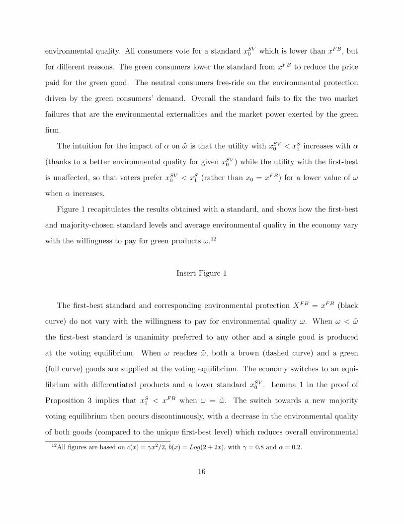
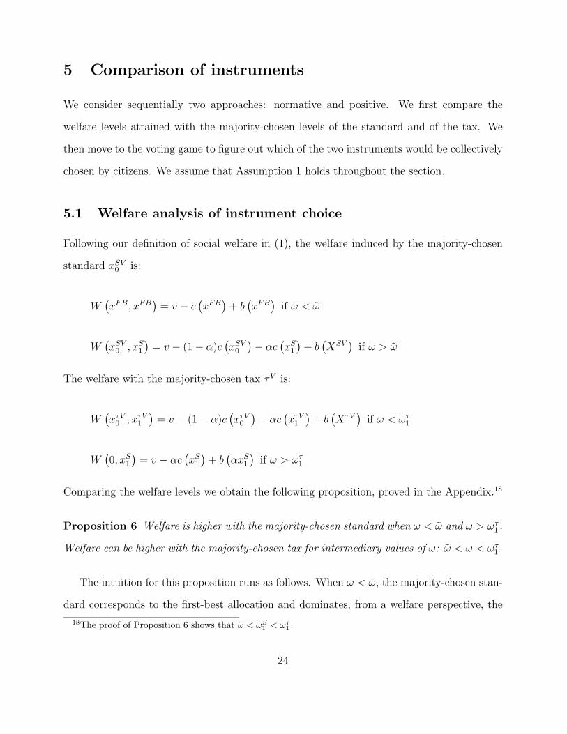
Comparing the welfare levels we obtain the following proposition, proved in the Appendix.18
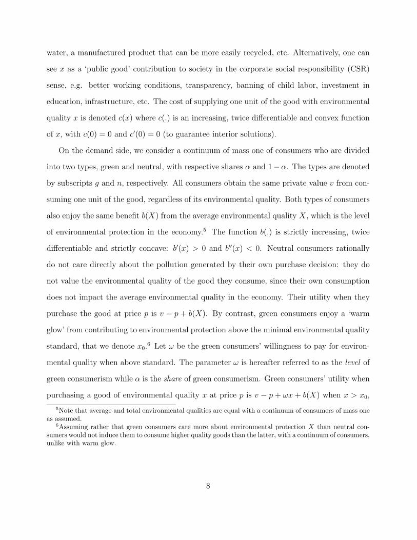
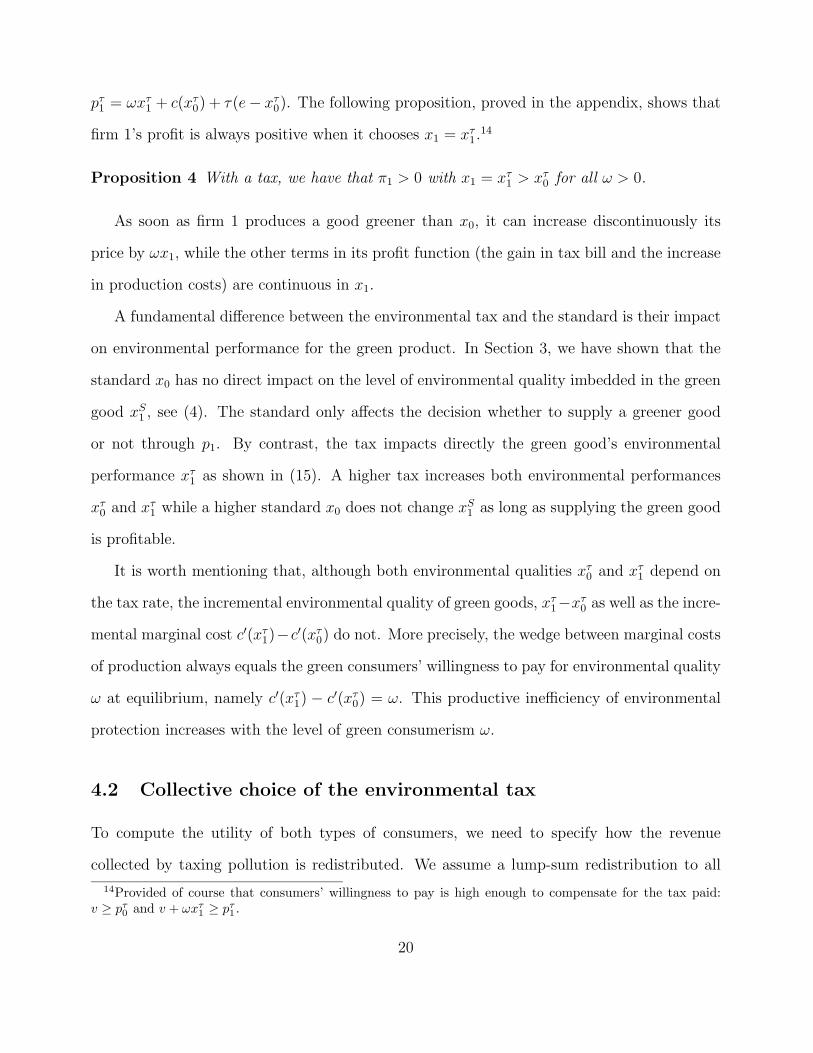
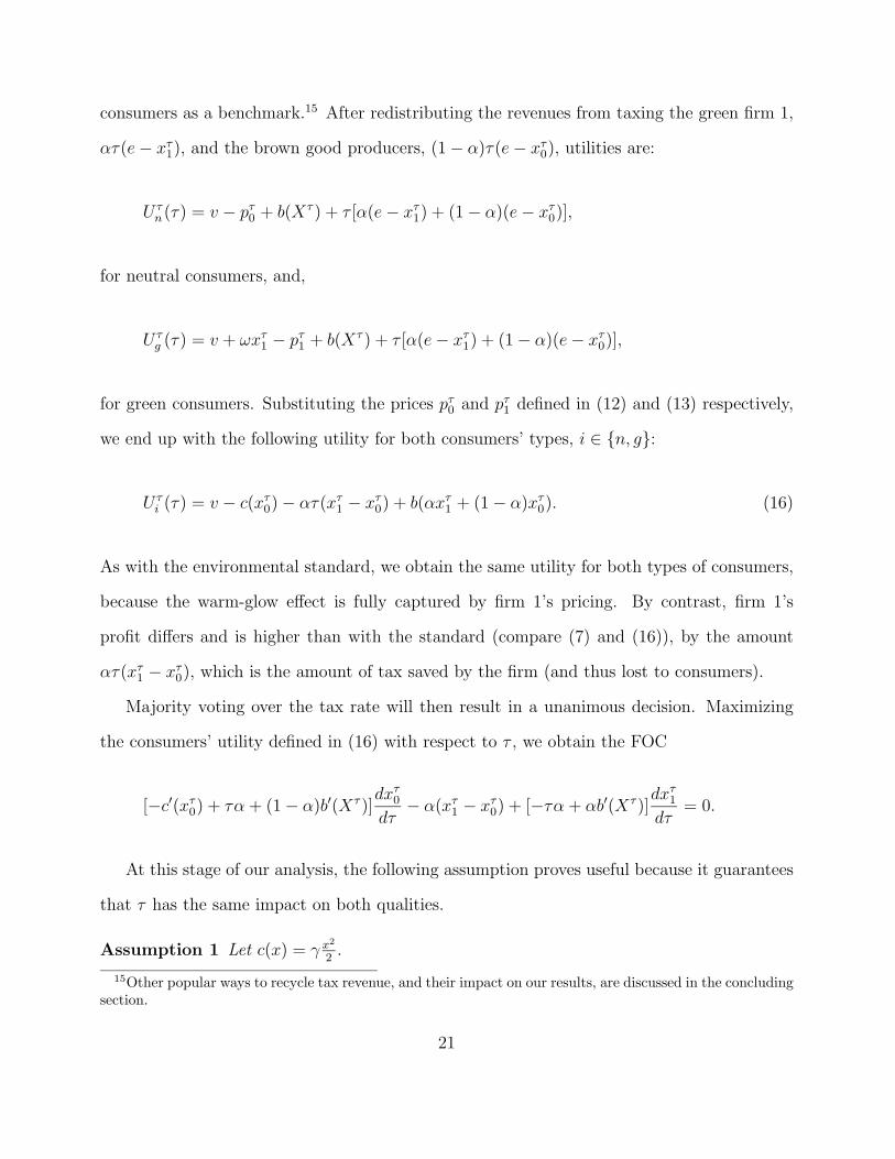
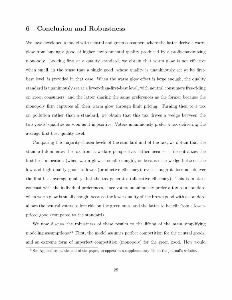
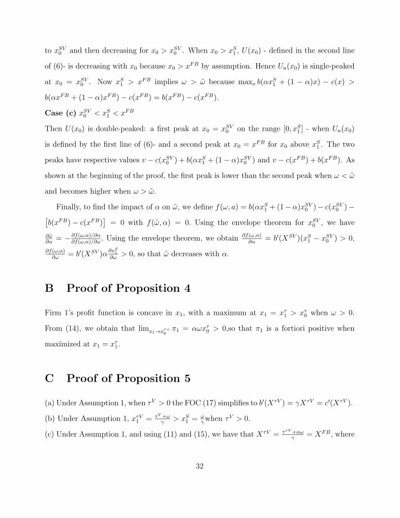
Proposition 6 Welfare is higher with the majority-chosen standard when ω < ω and ω > ωτ1 .
Welfare can be higher with the majority-chosen tax for intermediary values of ω: ω < ω < ωτ1 .
The intuition for this proposition runs as follows. When ω < ω, the majority-chosen stan-
dard corresponds to the first-best allocation and dominates, from a welfare perspective, the
18The proof of Proposition 6 shows that ω < ωS1 < ωτ
1 .
24
majority-chosen tax. Both instruments generate the same overall, first-best, environmental
quality, but the tax does it inefficiently since the environmental quality of the green good
x1 is too high while the brown good’s quality x0 is too low.19 When ω > ωτ1 , the environ-
mental quality of the green good is the same with the two instruments xS1 . The standard
gives more flexibility to choose the environmental quality of the brown good x0 than the tax
which impacts also the green good quality. Indeed a strictly positive tax would induce too
much environmental protection X, therefore, pollution is not taxed and brown firms do not
make any abatement effort while they should. The standard forces them to abate pollution
without impacting the environmental quality of the green good. When ω < ω < ωτ1 , the
environmental qualities with the tax are both more extreme than with the standard, but the
overall environmental protection is first-best with the tax, and too large with a standard.
There is then a trade-off between allocative and productive efficiency, and the comparison of
welfare levels across instruments can go both ways – see Figure 2(a) and 2(b).
Insert Figures 2(a) and 2(b)
To summarize this subsection, the standard dominates the tax when they are set by
majority voting (Proposition 6), except in specific circumstances in the latter case (see Figure
2(b)). We will now see that this ranking is not maintained when we allow voters to choose
their most-preferred instrument.
5.2 Political economy of instrument choice
Assuming that both goods are produced under the standard (i.e., ω > ω so that xS1 > x0),
we can express consumers’ utility as a function of minimal quality x0 as the only endogenous
19This result is reminiscent of Jacobsen et al. (2017), although the “wedge” in the marginal costs of publicgood provision is not driven by differences in the individual valuations of the public good (here b(X)).
25
variable for both instruments. The environmental qualities of both types of goods character-
ized in (4), (11) and (15) boil down to xS1 = ω/γ, xτ
0 = τ/γ and xτ1 = (ω+ τ)/γ. We therefore
obtain a simple relationship between the incremental environmental quality of the green good
with tax, the green consumerism parameter and the green good environmental quality with
a standard:
xτ1 − xτ
0 =ω
γ= xS
1 . (18)
Substituting into the first line of (6) and (16) yields the utility of both types of consumers as
a function of the neutral good quality x0 with standard:
US(x0) = v − c(x0) + b
'αω
γ+ (1− α)x0
(, (19)
and with tax:
U τ (x0) = v − αωx0 − c(x0) + b
'αω
γ+ x0
(. (20)
A closer look at the two functions US and U τ highlights the trade-off in the choice of instru-
ments. On the one hand, the tax has a larger impact on average environmental protection
than the standard because it increases the environmental quality of both types of goods in-
stead of only the brown one. This environmental protection effect shows up into the benefit
functions in (19) and (20) where the minimal environmental quality x0 is impacting fully
environmental protection Xτ = αωγ + x0 with tax in (20) but only a fraction 1−α (the share
of neutral consumers) with standard as XS = αωγ + (1 − α)x0 in (19). On the other hand,
there is an extra cost of increasing environmental quality with the tax as all the fiscal benefit
of providing higher environmental quality is captured by the green firm and therefore lost by
consumers. This tax stealing effect shows up in the welfare through the extra term αωx0. It
26
depends solely on two parameters: the share of green consumers α and their willingness to
pay ω.
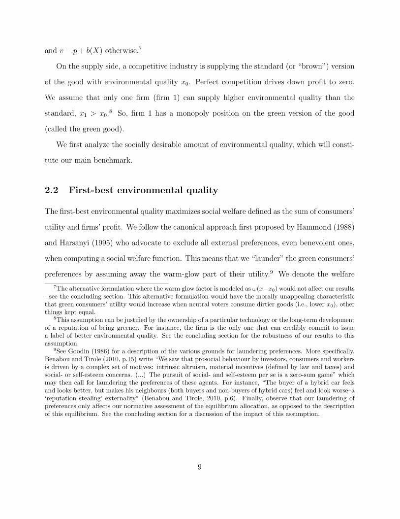
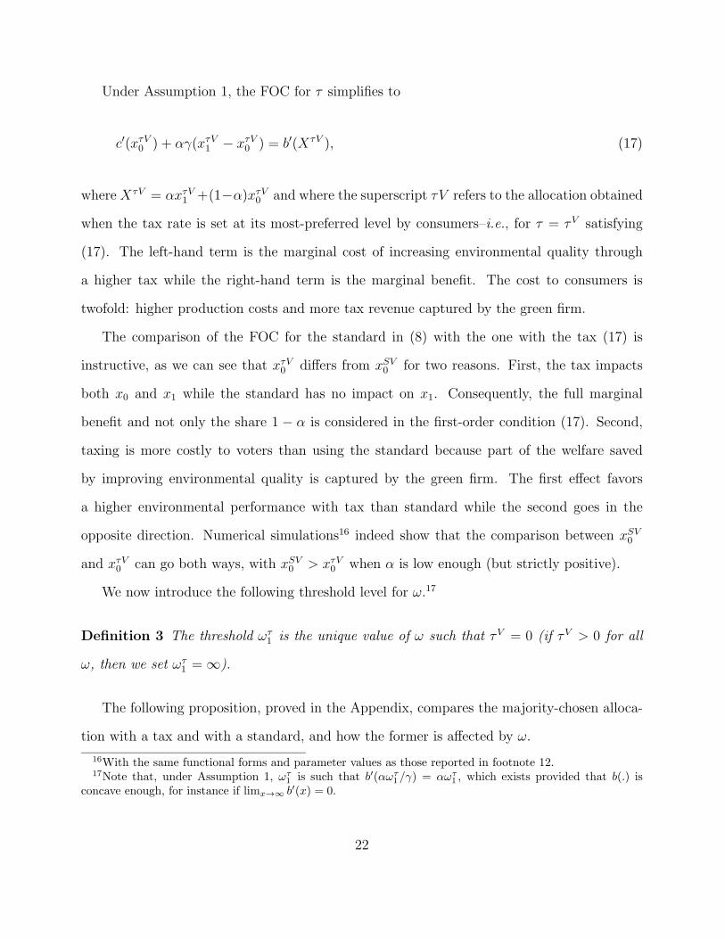
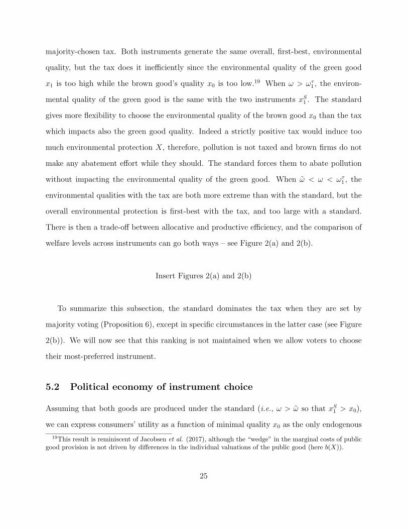
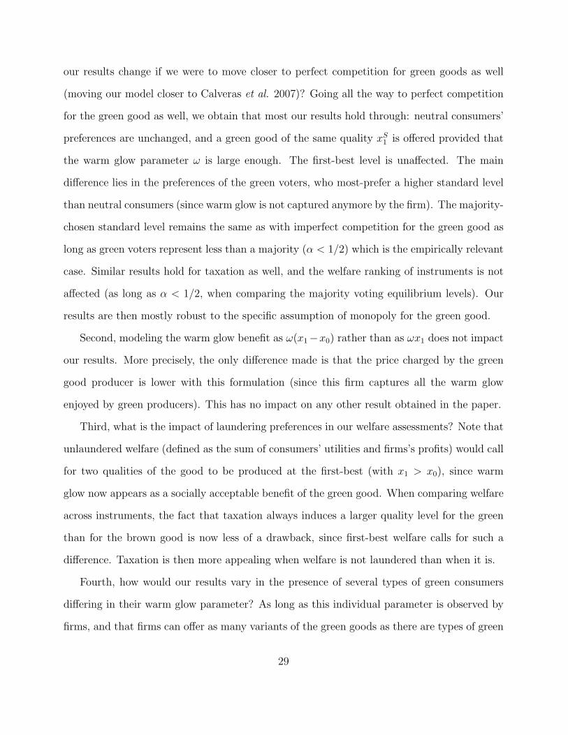
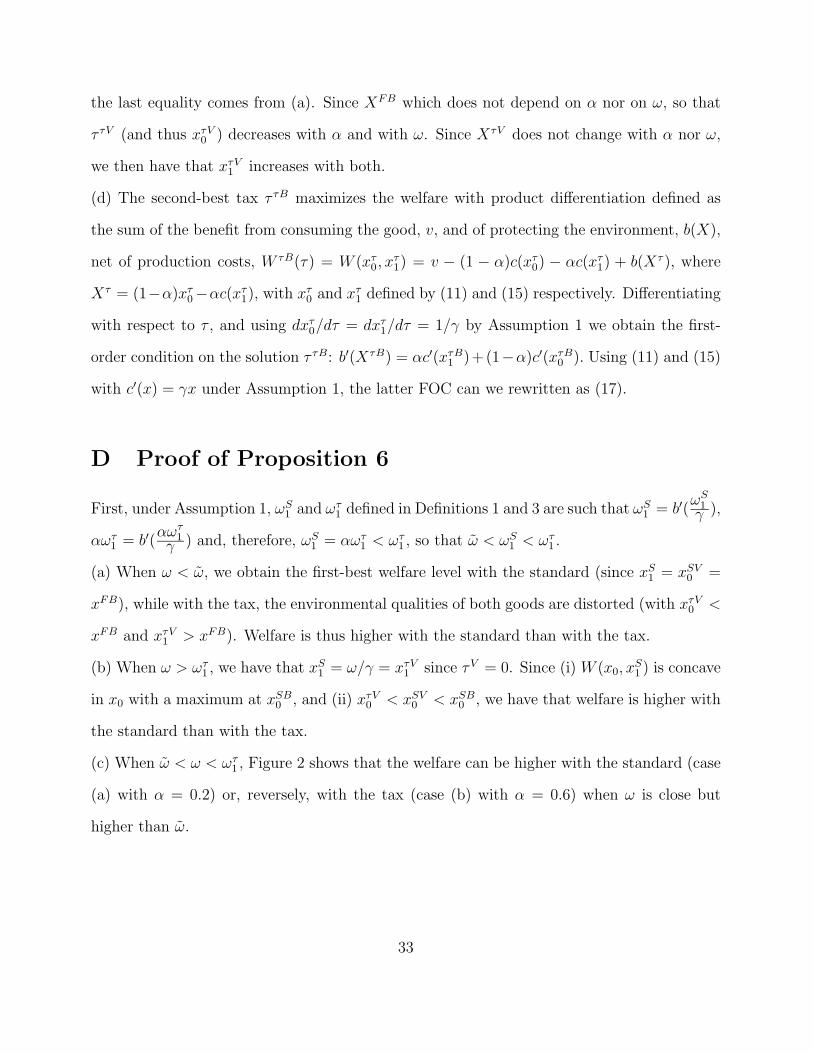
Proposition 7 Assume that voters first vote over whether the instrument used should be the
tax or the standard, and then vote over the level of the majority-chosen instrument. There
exists a threshold value of ω, denoted by ω, with ω < ω < ωτ1 , such that (a) all voters prefer
a tax to a standard if ω < ω, (b) all voters prefer a standard to a tax if ω > ω.
The intuition for this result runs as follows (see also Figure 3, where the utility with a tax
is depicted in red, and with a standard in blue). When ω is low, the standard is set at its
first-best level, with only one good provided with environmental quality xFB. The tax also
generates the same first-best environmental quality but on average, with two different quality
levels (xτV0 < xFB < xτV
1 ). The neutral consumers are better-off with the tax, since they buy
a lower priced good while enjoying the same environmental protection. Green consumers are
also better-off, even though firm 1 captures all the warm glow they experience, because the
lower cost of the brown good drives down the price they pay for the green good.20 When ω is
large enough, all voters rather prefer the standard to the tax. Take ω = ωτ1 for instance. Both
the majority-chosen tax and standard generate the same value of the high quality good, but
the standard allows voters to choose their most-preferred value of x0, while the tax imposes
that xτV0 = 0. By continuity, and given that utilities increase with ω, there is a threshold value
of ω, denoted by ω and such that ω < ω < ωτ1 , below (resp., above) which voters unanimously
prefer the tax to the standard (resp., the standard to the tax). For low values of ω (ω < ω),
voters then choose to regulate the environment with a tax, while the second-best analysis
rather calls for a standard.
Insert Figure 3
20Recall that our measure of (first-best) welfare launders the warm glow effect, which explains why (un-laundered) utility levels are larger than (first-best) welfare levels.
27
6 Conclusion and Robustness
We have developed a model with neutral and green consumers where the latter derive a warm
glow from buying a good of higher environmental quality produced by a profit-maximizing
monopoly. Looking first at a quality standard, we obtain that warm glow is not effective
when small, in the sense that a single good, whose quality is unanimously set at its first-
best level, is provided in that case. When the warm glow effect is large enough, the quality
standard is unanimously set at a lower-than-first-best level, with neutral consumers free-riding
on green consumers, and the latter sharing the same preferences as the former because the
monopoly firm captures all their warm glow through limit pricing. Turning then to a tax
on pollution rather than a standard, we obtain that this tax drives a wedge between the
two goods’ qualities as soon as it is positive. Voters unanimously prefer a tax delivering the
average first-best quality level.
Comparing the majority-chosen levels of the standard and of the tax, we obtain that the
standard dominates the tax from a welfare perspective: either because it decentralizes the
first-best allocation (when warm glow is small enough), or because the wedge between the
low and high quality goods is lower (productive efficiency), even though it does not deliver
the first-best average quality that the tax generates (allocative efficiency). This is in stark
contrast with the individual preferences, since voters unanimously prefer a tax to a standard
when warm glow is small enough, because the lower quality of the brown good with a standard
allows the neutral voters to free ride on the green ones, and the latter to benefit from a lower-
priced good (compared to the standard).
We now discuss the robustness of these results to the lifting of the main simplifying
modeling assumptions.21 First, the model assumes perfect competition for the neutral goods,
and an extreme form of imperfect competition (monopoly) for the green good. How would
21See Appendices at the end of the paper, to appear in a supplementary file on the journal’s website.
28
our results change if we were to move closer to perfect competition for green goods as well
(moving our model closer to Calveras et al. 2007)? Going all the way to perfect competition
for the green good as well, we obtain that most our results hold through: neutral consumers’
preferences are unchanged, and a green good of the same quality xS1 is offered provided that
the warm glow parameter ω is large enough. The first-best level is unaffected. The main
difference lies in the preferences of the green voters, who most-prefer a higher standard level
than neutral consumers (since warm glow is not captured anymore by the firm). The majority-
chosen standard level remains the same as with imperfect competition for the green good as
long as green voters represent less than a majority (α < 1/2) which is the empirically relevant
case. Similar results hold for taxation as well, and the welfare ranking of instruments is not
affected (as long as α < 1/2, when comparing the majority voting equilibrium levels). Our
results are then mostly robust to the specific assumption of monopoly for the green good.
Second, modeling the warm glow benefit as ω(x1−x0) rather than as ωx1 does not impact
our results. More precisely, the only difference made is that the price charged by the green
good producer is lower with this formulation (since this firm captures all the warm glow
enjoyed by green producers). This has no impact on any other result obtained in the paper.
Third, what is the impact of laundering preferences in our welfare assessments? Note that
unlaundered welfare (defined as the sum of consumers’ utilities and firms’s profits) would call
for two qualities of the good to be produced at the first-best (with x1 > x0), since warm
glow now appears as a socially acceptable benefit of the green good. When comparing welfare
across instruments, the fact that taxation always induces a larger quality level for the green
than for the brown good is now less of a drawback, since first-best welfare calls for such a
difference. Taxation is then more appealing when welfare is not laundered than when it is.
Fourth, how would our results vary in the presence of several types of green consumers
differing in their warm glow parameter? As long as this individual parameter is observed by
firms, and that firms can offer as many variants of the green goods as there are types of green
29
consumers, our results would carry through. What about the case where firms offer fewer
variants than types, and where types are individually unobservable? Take for instance the
limit case where there is a single green good and a continuum of types (whose distribution is
known to the monopoly firm). In that case, the firm has to leave some rent to the “greenest”
consumers, and faces an intensive vs extensive margin trade-off, since a higher price generates
more revenue from green buyers, but induces the least green consumers to switch to the brown
version of the good. We surmise that most of our results would still hold in this more complex
setting, but we leave its study to future research.
Finally, how would other ways to redistribute tax proceeds affect our results? An obvious
alternative would be to make transfers to firms rather than to consumers. If these transfers
were made proportional to firms’ market share, they would result in lower prices for both goods
(thanks to competitive pressures on the brown good’s price, which in turn would decrease the
ability of firm 1 to post a high price) but in the same green good quality xτ1 (as the effect
of the higher quality on the rebate exactly cancels out its effect on p1) and also in the same
utility for both types of consumers. In a nutshell, consumers benefit from lower prices, rather
than from government transfers, and all our results carry through to this case. Likewise, a
feebate (which refunds the revenue collected from taxing brown producers with a subsidy per
unit of abatement above a threshold quality level) would not affect our results: both prices
would remain the same as with a lump sum transfer to consumers, and consumers’ utilities
would also remain the same, if the subsidy rate were set for convenience at the same level as
the tax rate.
30
A Proof of Proposition 3
To show that ω is unique, remark that xFB does not depend on ω, therefore the right-hand
side of (9) does not vary with ω. On the other hand, the left-hand side increases with ω
since its derivative with respect to ω equals αb′(αxS1 + (1 − α)xSV
0 )dxS
1dω
> 0 by making use
of (8). Furthermore, xS1 = 0 when ω = 0, and therefore b(αxS
1 + (1 − α)xSV0 ) − c(xSV
0 ) =
maxx{b((1 − α)x) − c(x)} < maxx{b(x) − c(x)} = b(xFB) − c(xFB) by definition of xSV0
and xFB. For ω high enough that xS1 = xFB, we have b(αxS
1 + (1 − α)xSV0 ) − c(xSV
0 ) =
maxx{b(αxFB1 +(1−α)x)− c(x)} ≥ b(xFB)− c(xFB). Therefore b(αxS
1 +(1−α)xSV0 )− c(xSV
0 )
is lower than b(xFB)− c(xFB) for ω < ω and becomes higher for ω > ω.
Note that the penultimate step in the preceding paragraph has proved the following lemma,
which will prove useful later on in the paper.
Lemma 1 ω < ωS1
We know that xFB is constant with ω (see (2)), that xSV0 < xFB and is decreasing with
ω (see Proposition 2), that xS1 is increasing in ω and may be lower or larger than xFB (since
xS1 = 0 when ω = 0, while it tends towards infinity as ω grows). Hence, the following three
cases exhaust all the possible ones.
Case (a) xS1 < xSV
0 < xFB
In this case, we can show that xSV0 ≤ xFB. For any standard x0 < xS
1 , the utility Un(x0),
defined in the first line of (6), is increasing with x0 up to xS1 . It also increasing with x0 above
xS1 – i.e., as defined in the second line of (6), up to x0 = xFB. It is then decreasing above
xFB. Therefore Un(x0) is single-peaked at x0 = xFB. Note that xS1 < xSV
0 implies ω < ω
because then b(αxS1 + (1− α)xSV
0 )− c(xSV0 ) < b(xSV
0 )− c(xSV0 ) ≤ b(xFB)− c(xFB) where the
last inequality is due to the definition of xFB which maximizes b(x)− c(x) with respect to x.
Case (b) xSV0 < xFB < xS
1
For any standard x0 < xS1 , the utility Un(x0) -defined in the first line of (6)- is increasing up
31
to xSV0 and then decreasing for x0 > xSV
0 . When x0 > xS1 , U(x0) - defined in the second line
of (6)- is decreasing with x0 because x0 > xFB by assumption. Hence Un(x0) is single-peaked
at x0 = xSV0 . Now xS
1 > xFB implies ω > ω because maxx b(αxS1 + (1 − α)x) − c(x) >
b(αxFB + (1− α)xFB)− c(xFB) = b(xFB)− c(xFB).
Case (c) xSV0 < xS
1 < xFB
Then U(x0) is double-peaked: a first peak at x0 = xSV0 on the range [0, xS
1 ] - when Un(x0)
is defined by the first line of (6)- and a second peak at x0 = xFB for x0 above xS1 . The two
peaks have respective values v − c(xSV0 ) + b(αxS
1 + (1− α)xSV0 ) and v − c(xFB) + b(xFB). As
shown at the beginning of the proof, the first peak is lower than the second peak when ω < ω
and becomes higher when ω > ω.
Finally, to find the impact of α on ω, we define f(ω, a) = b(αxS1 + (1−α)xSV
0 )− c(xSV0 )−
)b(xFB)− c(xFB)
*= 0 with f(ω,α) = 0. Using the envelope theorem for xSV
0 , we have
∂ω∂α
= −∂f(ω,α)/∂α∂f(ω,α)/∂ω
. Using the envelope theorem, we obtain ∂f(ω,α)∂α
= b′(XSV )(xS1 − xSV
0 ) > 0,
∂f(ω,α)∂ω
= b′(XSV )α∂xS
1
∂ω> 0, so that ω decreases with α.
B Proof of Proposition 4
Firm 1’s profit function is concave in x1, with a maximum at x1 = xτ1 > xτ
0 when ω > 0.
From (14), we obtain that limx1→xτ+0
π1 = αωxτ0 > 0,so that π1 is a fortiori positive when
maximized at x1 = xτ1.
C Proof of Proposition 5
(a) Under Assumption 1, when τV > 0 the FOC (17) simplifies to b′(XτV ) = γXτV = c′(XτV ).
(b) Under Assumption 1, xτV1 = τV +ω
γ> xS
1 = ωγwhen τV > 0.
(c) Under Assumption 1, and using (11) and (15), we have that XτV = ττV +αωγ
= XFB, where
32
the last equality comes from (a). Since XFB which does not depend on α nor on ω, so that
τ τV (and thus xτV0 ) decreases with α and with ω. Since XτV does not change with α nor ω,
we then have that xτV1 increases with both.
(d) The second-best tax τ τB maximizes the welfare with product differentiation defined as
the sum of the benefit from consuming the good, v, and of protecting the environment, b(X),
net of production costs, W τB(τ) = W (xτ0, x
τ1) = v − (1 − α)c(xτ
0) − αc(xτ1) + b(Xτ ), where
Xτ = (1−α)xτ0−αc(xτ
1), with xτ0 and xτ
1 defined by (11) and (15) respectively. Differentiating
with respect to τ , and using dxτ0/dτ = dxτ
1/dτ = 1/γ by Assumption 1 we obtain the first-
order condition on the solution τ τB: b′(XτB) = αc′(xτB1 )+(1−α)c′(xτB
0 ). Using (11) and (15)
with c′(x) = γx under Assumption 1, the latter FOC can we rewritten as (17).
D Proof of Proposition 6
First, under Assumption 1, ωS1 and ωτ
1 defined in Definitions 1 and 3 are such that ωS1 = b′(
ωS1γ ),
αωτ1 = b′(
αωτ1
γ ) and, therefore, ωS1 = αωτ
1 < ωτ1 , so that ω < ωS
1 < ωτ1 .
(a) When ω < ω, we obtain the first-best welfare level with the standard (since xS1 = xSV
0 =
xFB), while with the tax, the environmental qualities of both goods are distorted (with xτV0 <
xFB and xτV1 > xFB). Welfare is thus higher with the standard than with the tax.
(b) When ω > ωτ1 , we have that x
S1 = ω/γ = xτV
1 since τV = 0. Since (i) W (x0, xS1 ) is concave
in x0 with a maximum at xSB0 , and (ii) xτV
0 < xSV0 < xSB
0 , we have that welfare is higher with
the standard than with the tax.
(c) When ω < ω < ωτ1 , Figure 2 shows that the welfare can be higher with the standard (case
(a) with α = 0.2) or, reversely, with the tax (case (b) with α = 0.6) when ω is close but
higher than ω.
33

E Proof of Proposition 7
Recall that all individuals have the same utility function when voting over the instrument. We
then define the utility level attained at the majority voting equilibrium by voters as U τV =
U τ (τV ) with a tax, and USV = US(xSV0 ) with a standard. We now study the comparative
statics of U τV and USV as function of ω, starting with USV .
(i) ω < ω : USV = v + b(xFB)− c(xFB) = W FB.
(ii) ω > ω : We have USV = v + b(XSV )− c(xSV0 ),so that, using the envelope theorem,
dUSV
dω=
α
γb′(XSV ) > 0, (21)
and d2USV
dω2 = αγb′′(XSV )dX
SV
dω< 0, so that USV is increasing and concave over ω > ω. We now
move to the comparative statics of U τV .
(iii) ω < ωτ1 : We have U τV = v+b(XτV )−c(xτV
0 )−ατV ωγso that, using the envelope theorem,
dUτV
dω= α
γ
)b′(XτV )− τV
*= α2ω
γ> 0, where we have made use of the FOC (17) for τV and
(18) to obtain the second line. We then have that d2UτV
dω2 = α2
γ> 0,so that U τV is increasing
and convex over ω < ωτ1 .
(iv) ω > ωτ1 : We have U τV = v + b(αω
γ), so that
dU τV
dω=
α
γb′(
αω
γ) > 0, (22)
andd2UτV
dω2 = α2
γ2 b′′(αω
γ) < 0,so that U τV is increasing and concave. Moreover, we have that
XSV > XτV (since xτV1 = xS
1 > 0 and xSV0 > xτV
0 = 0 for ω > ωτ1 ), so that comparing (21)
and (22), we have that dUSV
dω< dUτV
dω.
We now put all the pieces together. We have that USV = U τV = W FB for ω = 0. For
0 < ω < ω, we have that USV = W FB is invariant with ω while U τV is strictly increasing
with ω so that USV < U τV . We have that limω→∞ U τV = limω→∞USV . USV and U τV are
34

both concave and increasing over ω ∈ [ωτ1 ,∞], with a larger slope for U τV . It then means
that USV > U τV for ω = ωτ1 . Since both U τV and USV are continuously increasing over
ω ∈ [ω,ωτ1 ], there is a unique threshold value of ω , denoted by w, belonging to this interval,
so that voters are better off with a majority-chosen tax if ω < w, and better off with a
majority-chosen standard if ω > w.
35
References
Allcott, Hunt, Mullainathan, Sendhil, and Dmitry Taubinsky. 2012. Externalities, in-
ternalities, and the targeting of energy policy, National Bureau of Economic Research
Working Paper 17977.
Ambec, Stefan, and Paul Lanoie. 2008. Does it pay to be green? A Systematic Overview,
Academy of Management Perspectives, 23: 45-62.
Baron, David. 2001. Private politics, corporate social responsibility, and integrated strat-
egy, Journal of Economics & Management Strategy 10(1): 7-45.
Benabou, Roland, and Jean Tirole. 2010. Individual and corporate social responsibility,
Economica, 77, 1-19.
Besley, Tim, and Maitreesh Ghatak. 2007. Retailing public goods: The economics of
corporate social responsibility, Journal of Public Economics, 91(9): 1645-1663.
Bovenberg, A. Lans, Lawrence H. Goulder, and Mark R. Jacobsen. 2008. Costs of al-
ternative environmental policy instruments in the presence of industry compensation
requirements. Journal of Public Economics 92 (5): 1236–53.
Calveras, Aleix, Juan-Jose Ganuza, and Gerard Llobet. 2007. Regulation, corporate social
responsibility and activism, Journal of Economics and Management Strategy, 16(3): 719-
740.
Carson, Richard T., and Jacob LaRiviere. 2018. Structural uncertainty and pollution con-
trol: Optimal stringency with unknown pollution sources, Environmental and Resource
Economics, 71(2), 337-355.
Conrad, Klaus. 2005. Price competition and product differentiation when consumers care
for the environment, Environmental and Resource Economics, 31: 1-19.
36
Daubanes, Julien, and Jean-Charles Rochet. 2019. The rise of NGO activism, American
Economic Journal: Economic Policy, 11 (4): 183-212.
Eriksson, Clas. 2004. Can green consumerism replace environmental regulation? A
differentiated-products example, Resource and Energy Economics, 26: 281-293.
Fleckinger, Pierre, and Matthieu Glachant. 2011. Negotiating a voluntary agreement
when firms self regulate, Journal of Environmental Economics and Management, 62(1):
41-52.
Fowlie, Meredith, and Nicholas Muller. 2019. Market-based emissions regulation when
damages vary across sources: What are the gains from differentiation? Journal of the
Association of Environmental and Resource Economists, 6(3), 593-632.
Friedman Milton. 1970. The social responsibility of business is to increase its profits, The
New York Times September 13: 32-33.
Goodin, Robert. E. 1986. Laundering preferences. Foundations of social choice theory,
75, 81-86.
Hammond, Peter J. 1988. Altruism, in the New Palgrave: a Dictionary of Economics,
ed. John Eatwell, Murray Milgate, and Peter Newman, London: Macmillan Press.
Harsanyi, John C. 1995. A theory of social values an a rule utilitarian theory of morality,
Social Choice and Welfare, 12: 319-344.
Heyes, Anthony, and Sandeep Kapur. 2012. Community pressure for green behavior,
Journal of Environmental Economics and Management, 64(3): 197-210.
Jacobsen, Mark R. (2013) Evaluating US fuel economy standards in a model with pro-
ducer and household heterogeneity, American Economic Journal: Economic Policy 5 (2):
148–87.
37
Jacobsen Mark R., Jacob LaRiviere and Michael Price. 2017. Public good provision in the
presence of heterogeneous green preferences, Journal of the Association of Environmental
and Resource Economists, 4: 243-280
Kitzmueller, Markus, and Jay Shimshack. 2012. Economic perspectives on corporate
social responsibility, Journal of Economic Literature 50(1): 51-84.
Kotchen, Matthew J. 2006. Green markets and private provision of public goods, Journal
of Political Economy, 114(4): 816-834.
Tsvetanov, Tsvetan, and Kathleen Segerson. 2014. The welfare effects of energy efficiency
standards when choice sets matter Journal of the Association of Environmental and
Resource Economists 1 (1): 233–71.
Weitzman, Martin. 1974. Prices versus quantities Review of Economic Studies 41:477–91.
38
Out[ ]=
0.6 0.7 0.8 0.9 1.0ω
0.6
0.7
0.8
0.9
1.0
xFigure 1: Environmental Standard
ω
ω1S
xFB
x1S
x0SV
XSV
Out[ ]=
0.2 0.4 0.6 0.8 1.0 1.2 1.4ω
0.85
0.90
0.95
1.00
1.05
1.10
WelfareFigure 2(a): Welfare Levels at Majority Voting Equilibrium, α=0.2
ω
Welfare with tax
Welfare with standard
Out[ ]=
0.2 0.4 0.6 0.8 1.0 1.2 1.4ω
0.85
0.90
0.95
1.00
1.05
1.10
WelfareFigure 2(b): Welfare Levels at Majority Voting Equilibrium, α=0.6
ω
Welfare with tax
Welfare with standard
Out[ ]=
0.2 0.4 0.6 0.8 1.0 1.2 1.4ω
1.05
1.10
1.15
1.20
UtilityFigure 3: Utility Levels at Majority Voting Equilibrium
ω
ω
With standard
With tax
|
Online appendices to appear in supplemental file on thejournal’s website
A Perfect competition
To isolate the effect of market power exerted by Firm 1, let’s assume that green consumers can
find green good for all levels of environmental protection at competitive price (as in Calveras
et al. 2007).
A.1 Standard
The good is priced at production cost for all level of environmental qualities: p1 = c(x1)
and p0 = c(x0). The green consumer’s utility when buying the green good x1 > x0 at price
p1 = c(x1) at is v+ωx1−c(x0). Maximizing with respect to x1 yields xS1 defined as c′(xS
1 ) = ω,
i.e. the same than with market power. The market equilibrium is with product differentiation
if xS1 > x0 and v − p1 + ωxS
1 > v − p0, which leads to ωxS1 > c(xS
1 ) − c(x0). It means that
the taste for greener quality ω should be such ω > c′−1(x0) and c(x0) > c(c′−1(ω))−ωc′−1(ω).
Under Assumption 1, the first condition leads to γω > x0 while the second is always met. We
can therefore define the threshold level ωcn(x0) =
x0γ .
Note that the welfare under product differentiation is as before:
W (x0) = v − αc(xS1 )− (1− α)c(x0) + b(αxS
1 + (1− α)x0)
The green consumer’s utility with product differentiation is:
Ug(x0) = v − c(xS1 ) + ωxS
1 + b(αxS1 + (1− α)x0).
Maximizing the above utility yields a corner solution: a green consumer is in favor of the
highest standard that allow enjoying the warm-glow effect which holds as long as xS1 > x0.
The preferred standard is xS1 −ε with ε → 0, which yields approximately Ug(x
S1 ) = v−c(xS
1 )+
ωxS1 + b(xS
1 ).
The neutral consumer’s utility:
Un(x0) = v − c(x0) + b(αxS1 + (1− α)x0).
Since the utility is the same than with market power, the preferred standard is xS1 defined in
1
(9). Under product differentiations, consumers disagree on the standard to implement, the
green ones being in favor of a higher one. The elected standard depends on the relative share
of each population α as in Calveras et al. (2007).
• Neutral consumers majority : α < 1/2.
The elected standard depends on green consumers’ purchase. It is first-best xFB for
low ω such that green consumers do not buy greener goods, that is if ω ≤ ωcn(x
FB).
Otherwise, the elected standard is xS1 and the market equilibrium is with differentiated
product.
• Green consumers majority : α > 1/2.
Under product differentiation, the green consumers prefer the highest standard lower
than their quality choice xS1 which yields them Ug(x
S1 ) = v − c(xS
1 ) + ωxS1 + b(xS
1 ). The
utility with product differentiation is higher if Ug(xS1 ) > v − c(xFB) + b(xFB). That is
with ω higher than a threshold ωcg(x
FB) such that Ug(xS1 ) = v− c(xFB) + b(xFB) which
leads to:
b(xFB)− c(xFB) = b(xS1 )− c(xS
1 ) + ωxS1 .
The elected standard is xFB for ω < ωcg(x
FB) and xS1 − ε if ω > ωc
g(xFB).
A.2 Tax
Equilibrium prices are p1 = c(x1) + τ(e − x1) and p0 = c(x0) + τ(e − x0). Green consumers’
utility is v + ωx1 − c(x1)− τ(e− x1). It is maximized at xτ1 defined as before in (??). Same
for x0 = xτ0 defined in (11).
The consumer’s utilities are:
Ug(τ) = v + ωxτ1 − c(xτ
1) + b(αxτ1 + (1− α)xτ
0) + τ(1− α)(xτ1 − xτ
0)
Un(τ) = v − c(xτ0) + b(αxτ
1 + (1− α)xτ0) + τ(1− α)(xτ
1 − xτ0)
The FOCs characterize the preferred tax. Under Assumption 1, the preferred tax for the
green consumers is such that:
b′(Xτ ) + (1− α)γ(xτ1 − xτ
0) = c′(xτ1),
where (1 − α)(xτ1 − xτ
0) is the marginal benefit of having more revenue assigned to green
consumers from increasing tax. Symmetrically, the tax preferred by neutral consumers is
2
such that:
b′(Xτ ) = c′(xτ0) + αγ(xτ
1 − xτ0),
where α(xτ1 − xτ
0) is the direct marginal cost of a tax increase. Using xτ1 − xτ
0 = ω, we can
rewrite the first-order conditions for the preferred tax respectively:
b′(Xτ ) = c′(xτ1)− (1− α)ω,
and
b′(Xτ ) = c′(xτ1) + αω,
which shows that neutral consumers’ preferred tax rate is lower than the one preferred by
green consumers. Furthermore, by comparing with (17) shows that the neutral consumers’
preferred tax rate is the same with and without market power.
B Unlaundered welfare
The first-best allocation with the alternative definition of welfare as the sum of the unlaundered
consumer’s utilities and firm’s profits calls for x1 > x0, since maximizing
(1− α)(v − c(x0) + b(X)) + α(v − c(x1) + ωx1 + b(X)
= v + b(X)− (1− α)c(x0)− αc(x1) + αωx1
implies that
c′(x0) = b′(X),
c′(x1) = b′(X) + ω.
C Tax Recycling : Earmarked tax to firms
If the tax proceeds
R = τ [α(e− x1)− (1− α)(e− x0)]
3
are redistributed to firms according to their market share, the brown good producers obtain
a transfer equal to
(1− α)[p0 − c(x0)− τ(e− x0) +R] = (1− α)[p0 − c(x0)− ατ(x1 − x0)].
The zero-profit condition leads to a price pτ0 = c(x0) + ατ(x1 − x0). This price is obviously
lower than when revenue is refunded to consumers because the net tax payment of each brown
firm is ατ(x1−x0) which is lower than τ(e−x0) because by definition e > x1 and α < 1. Firm
1 then has to cut the price of its green good to pτ1 = pτ0 + ωx1 = ωx1 + c(x0) + ατ(x1 − x0).
Its profit is thus:
π1 = α(pτ1 − c(x1)− τ(e− x1) +R) = α(p1 − c(x1) + τ(1− α)(x1 − x0)).
With this refunded rule, Firm 1 receives a net transfer. Differentiating with respect to x1, we
obtain
dπ1
dx1
= α[dp1dx1
− c′(x1) + τ(1− α)],
with
dp1dx1
= ω + τα,
which yields the same first-order condition than with a lump sum rebate to consumers,
c′(xτ1) = ω + τ . Substituting prices into the utility functions shows that both types of con-
sumers obtain the same welfare as in (16).
D Tax Recycling : Feebate
A feebate refunds the revenue collected from taxing brown producers with subsidy σ per units
of abatement above a threshold xF . Both σ and xF have to be defined, and are linked to the
tax rate τ by the budget balance condition:
τ(1− α)(xF − x0) = σα(x1 − x),
with xF ∈ [x0, x1]. The brown producers’ profit is the same than with the tax and, therefore,
so are the prices pF0 = c(x0) + τ(xF − x0) and pF1 = ωx1 + p0. The green producer’s profit
4

becomes
π1 = α[pF1 + σ(x1 − xF )− c(x1)] = α[ωx1 + c(x0) + τ(xF − x0) + σ(x1 − xF )− c(x1)].
Environmental performance x1 increases revenue through two channels: a higher price pF1 and
larger subsidies for performance above xF . The first-order condition yields: c′(xσ1 ) = ω + σ.
The subsidy provides similar incentives than the tax. We then set σ = τ so that the above
budget balance condition is satisfied for xF = αx1 + (1− α)x0 = X.
The utility of both types of consumers is:
UFi (σ) = v − c(xτ
0)− τ(xF − xτ0) + b(αxτ + (1− α)xτ
0).
With xF = αx1 − (1− α)x0, we obtain:
UFi (σ) = v − c(xτ
0)− τα(xτ1 − xτ
0) + b(αxτ + (1− α)xτ0).
which is the same utility when the tax is refunded to consumers in (16).
5