engineering design - everyspec

I

AMC PAMPHLET

c~ENGINEERING DESIGN

I -_-"-"-""'-

DEVELOPMENTGUIDE

4 FOR ELIABILITY

MATHEMATICAL JPPENDIX'AND GLOSSARY_

D!STIUBUTIOi4 STA'TEMENT A

.;pmvcd ior public releau -,;"* , ........ :)ution Unlimzit~i I :

HEADQUARTERS, US ARMY MATERIEL COMMAND A'

rI

Downloaded from http://www.everyspec.com

DISCLIMER NOTICE

THIS DOCUMENT IS BEST

QUALITY AVAILABLE. THE COPY

FURNISHED TO DTIC CONTAINEDA SIGNIFICANT NUMBER OF

PAGES WHICH DO NOTREPRODUCE LEGIBLY.


At4CP 706-200J

DEPARTMENT OF THE ARMYHEADQUARTERS UNITED STATES ARMY MATERIEL COMMAND

5001 Eisenhower Ave., Alexandria. VA 22333AMC PAMPHLETNO. 706-20 8 January 1976

ENGINEERING DE §(GN HANDBOOKDEVELOPMENT GUIDE FOP RELIABILITY, PART SIX

MATHEMATICAL APP NDIX AND GLOSSARY

TABLE OI0CONTENTS

Pararaph //Page

LIST OF ILLUSTRATIONS....... ........... viiLIST OF TABLES .................. ixPREFACE................................ xi

CHAPTER 1. GLOSSARY

CHAPTER 2!PROJBABILITY DISI iUBUTIONS,SOME CAUTIONS AND NAMES

2-1 Cautions .. . . . . . . . . . . . ... . . . 2-12-2 Naming Probability Distributlons. .............. 2-2

CHAPTER 1. BINOMIAL DISTRIBUTION

3-0 List of Symbols........................~... 3-13-1 Introduction ............................. 3-13-2 Formulas ................................ 3-23-3 Tables and Curves.......................... 3-2

3-5 Randomized Exact s-Conf idence Intervals .......... 3-4

3-6 Choosing a s-Confidence Level .. ............... 3-123-7 Examples ................................ 3-123-7.1 Example No. 1 .. .................... 3-42

3-7.2 Example No. 2 ........................... 3-24 ----- a. -

References ................................ 3-25 **

CHAPTER 4. POISSON DISTRIBUTION ?A, 6f t I

4-0 List of Symbols ............................ 4-1 ............. ...

4-1 Introduction ............................. 4-1 .......-... . ...4-2 Formulas ................................ 4-24-3 Tables and Curves.......................... 4-2 1OA~~rc.

4--4 Parameter Estimation ........................ 4-2 ~ ;-~

4-5 Ranoomized Exact s-Confidence Intervals ......... 4-6

4-7 Example, Life Test Results....................... AReferences............................... 4-12 {*


AMCP 706.2%

TABLE OF;CONTENTS (Cont'd)

Paragraph J Page

CHAPTER 5. GAUSSIAN (s-NORMAL)DISTRIBUTION'

5-0 List of Symbols ........................... 5-I5-1 Introduction ............................ 5-25-2 Formulas ......... ......................... 5-25-3 Tables and Curves ........................... 5-25-4 Parameter Estimation, Uncensored Samples ........ 5-135-5 Examples .................................... 5- 135-6 Parameter Estimation, Censored Samples ......... 5-14

References ................................. 5-15

CHAPTER 6. PROBABILITY DISTRIBUTIONSDERIVED FROM THE GAUSSIAN

DISTRIBUTION

6-0 List of Symbols ........................... 6-16-1 Tntroduction ............................... 6-26-2 Chi-square (x2) Distribution .................. 6-26-2.1 Formulas ............................... 6-26-2.2 Tables ................................... 6-36-3 Chi-squarefnu (xe /v) Distribution ............... 6-36-3.1 Formulas ................................. 6-36-3.2 Tables ................................ 6-76-4 Student's t-Distribution ....................... 6-76-4.1 Formulas ............................... 6-76-4.2 Tables ................................. 6-76-5 Fisher-Snedecor F Distribotion ................ 6-126-5.1 Formulas ......... /....................... 6-126-5.2 Tables ........ .......................... 6-13

Refetences ................................. 6-22

CHAPTER 7 'EXPONENTIAL DISTRIBUTION

7-0 List of Symbols ............................. 7-17-1 Introduction ............................... 7-17-2 Foimulas ................................... 7-I7-3 Tables ............................ ........ 7-27-4 Paameter Estimation ....................... 7-2

References .............................. 7-8

CHAPTER 8. WEIBULL DISTRIBUTION

8-0 List of Symbols ........................... 8-18-1 Introduction ............................... 8-1

(i

. ....... . . . ...... . .. ' , . ? " : ,


MP 706-200

TABLE OF CONTENTS (Cont'd)

Paragraph Page

8-2 Form ulas ................................... 8-28-3 Tables ..................................... 8-28-4 Parameter Estimation ......................... 8-28-4.1 Graphical Method ............................ 8-78-4.2 Maximum Likelihood Method -.......... 8-78-4.3 Linear Estimation Methods................... 8-108-4.4 Test for Failure Rate: Increasing, Decreasing, or

Constant ................................. 8-108-5 Comparison With Lognormal Distribution ........ 8-10

References ................................. 8-11

CHAPTER 0. LOGNORMAL DISTRIBUTION \

9-,0 list of Symbols ......................... ' 9-19-1 Introduction ............................. .9-19-2 Formulas ................................... 9-29-3 Tables ....................................... 9-49-4 Parameter Estimation ......................... 9-49-4.1 Uncensored Data ......................... 9-69-4.2 Censored Data ............................. 9-10

References ................................. 9-10

CHAPTER 10. BETA DISTRIBUTION,

1O-0 List of Symbols .................. .......... 10--i10-1 introduction ............................... 10 -210-2 Formulas ... ............................... . 10-210-3 Tables . .................................... 10-310-4 Parameter EAtimation ......................... 10-3

References ................................. 10-7

CHAPTER 11. GAMMA DISTRIBUTION '

11-0 List of Symbols ............................. 11-111-1 Introduction .......... .................... 11-111-2 Form ulas ................................... 11-111-3 Tables ..................................... 11-211-4 Parar-,zter Estimation ......................... 11-211-5 Gamn.a Function ........................... 11-4

References...............................11-4

CHAPTER 12. s-CONFIDENCE

12-0 List of Symbols ........... ... ........ .. 12-112-1 Introduction ..... ......................... 12-1

0_.,, , _ .. - . -- .-- . ., : , .... o1, W . - - . , . ',-, .... .. - - - - - -. . .. ,, ...... , r: '


AMCP 706-200

TABLE OF CONTENTS (Cont'd)t

Paragraph Page

12-2 Continuous Randqm Variables ................. 12-312-3 Discrete Random Variables ..................... 12-512-4 Discrete Random *rables, Exact Confidence

Bounds ................. ......... 12-712-5 MoeCopict-9SMore Complicated s-onfidence Situations ......... 12-9References ..... . ............... 12-9

CHAPTER 13. PLOTTING POSITIONS

13-0 List of Symbols ............................. 13-113-1 Introduction ........................... 13-113-2 Sample Cdf ................................. 13-113-3 Percentile Ranges ............................. 13-213-4 Mean ..................................... 13-213-5 Censored Data (Hazard Plotting) ................. 13-5

CHAPTER 14. GOODNESS-OF-FIT TESTS

14-0 List of Symbols ............................. 14-114-1 Introduction ............................... 14-114-2 Chi-square ................................. 14-114-2.1 Discrete Random Variables .................. 14-114-2.2 Continuous Random Variable ................. 14-414-3 Kolmogorov-Smirnoff ........................ 14-5

Reference ................................. 14-8

CHAPTER IS. TESTS FOR MONOTONICFAILURE RATES

Reference ................................. 15-1

CHAPTER 16. BAYESIAN STATISTICS

16-1 Introduction ............................... 16-116-2 Bayes Formula ............................. 16-116-3 Interpretation of Probability ................... 16-116-4 Prior Distribution Is Real and Known ............. 16-416-5 Empirical Bayes ............................. 16-416-6 Bayesian Decision Theory ..................... 16-416-7 Subjective Probability .................... .16-716-8 Recommendations ........................... 16-7

iv j


[

AM;P 70200

TABLE OF CONTENTS (Cont'd)

Pmmraph Page

CHAPTER 17.;SAMPLING PLANS

CHAPTER 18. MISCELLANEOUS DESIGN AIDS.,

References ................................. 18-

INDEX ...................................... I- 1

vlv


NO~

AMCP7O2

LIST OF ILLUSTRATIONS

Figure No. Title page

3-1(A) I1-sided Upper s-Confidence Limit (80%) for p....... 3-93- 1(B) I1-sided Upper s-Confidence Limit (90%) for p....... 3-103-1(C) I -sided Upper s-Confidence Limit (95%) for p....... 3-113-2 Special Case for No Failures in N Trials and C =RL *3-24

4-1 Poisson Cumulative Distribution Function ...... 4-45-1 Curves for Gaussian Distributions...............5-36-1 Chi-squaze Distribution, pdf...................6-4I6-2 Chi-square/Degrees-of-fredom Distribution, pdf ... 6-86-3 Student's t Distribution ...................... 6-107-1 Exponential Distribution ...................... 7 -7-2 -Reliability Nomograph for the Exponential Distribution 7-48_-i Weibull Distributior, pdf ...................... 8-38-2 Weibull Distribution, Failure Rate ............... 8-48-3 Weibull Distribution, Contour Plot ..... ......... 8-59-1 Lognormal Distribution, pdf................. 9-39-2 Lognormal Distribution, Failure Rate ............ 9-59-3 Lognormal Distribution, Contour Plot ............ 9-79-4 Lognormal Failure Rate, Contour Plot ............ 9-89-5 Lognormal Distribution, Failure-rate Mode ......... 9-910-1 Beta Distribution ......... .................. 10-411-1 Gamma D~istribution, pdf ...................... 11-311-2 Gamma Distribution, Contour Plot of pdf .......... 11-5 .12-1 s-Confidence Diagram: Continuous Random Variable

6 (for well-behaved situations) ................. 12-412-2 s-Confidence Diagram: Discrete Random Variable ... 12-614-1 Random Samples of 10 from the Uniform Distribu-j

tion on 10, 1]............................ 14-8

.***'~ ~ .vii/lil


AMCP 705-200

LIST OF TABLES

Table No. Title Page

3-1 Binomiial Distbibution, Examples ............... 3-33-2 1 -sided Upper s-Confiderice Limits for p (The Bi-

nomial Probability)....................... 3-53-3 Sample Page from a Binomial Distribution ......... 3-143-4(A) Neyman-shortest Unbiased 95% s-Confidence Inter-

vals for p.............................. 3-163-4(B) Neyman-shortest Unbiased 99% s-Confidence Inter-I

vals forp ............................... 3-204-1 Poisson Distribution, Examples ................ 4-34-2 Neyman-shortest Unbiased 95% and 99% s-Confidence

Intervals for Ap .......................... 4-95-1 s-Normal Cdf-gauf (z).......................5-55-2 Gaussian (Standard s-Normal) Cdf-gauf W)........ 5-86-1 Percentiles of the Chi-square (X2 ) Distribution...... 6-56-2 Percentiles of the Chi-squarefnu (X /nu) Distribution .6-96-3 Percentiles of the t-Distribution ... ............ 6-116--4(A) F Distribution-fisf= 99%,flsfc - 1%............ 6-14

F6-4(B) F Distribution-flsf =97.5%, flsfc = 2.5%.........6-166-4(C) F Distribution-flsf = 95%, flsfc= 5% ............ 6-186-4(D) F Distribution-flsf =90%,ftMc = 10%........... 6-207-1 Tables of -x ............................. 7-37-2 Ratio of Upper to Lower i-Confidence Limits for the

Exponential Parameter (with equal size tails on eachside) ................................. 7-7

11-1 Gamma Function......................... 11-613-1 Percentile Ranges for Plotting Points ............ 13-314-1 Data for Example No. 2..................... 14-314-2 Critical Values of the Kolmogorov-Smirnoff Test

Statistic............. ................ 14-614-3 Data for Example No. 4 ..................... 14-716-1 Data and Results for Example-Trial No. I1......... 16-516-2 Data and Results for Example-Trial No. 2 ........ 16-516-3 Data and Results for Example-Trial No. 3 ........ 16-6

ixfx


PREFACE

This harxdbuok, Mathematical Appendix and Glossary, is the last in aseries of five on reliability. The series is directed largely toward the workingengineers who have the responsibility for creating and producing equipmentand systems which can be relied upon by the users in the field.

The five handbooks are:

1. Design bo Reliability, AMCP 706-196

2. Reliability Prediction. AMCP 706-197

3. Reliability Measurement, AMCP 706-198

4. Contracting for Reliability, AMCP 706-199

5. Mathematical Appendix and Glossary, AMCP 706-200.

This handbook is directed toward reliability engineers and manegers whoneed to be familiar with or need to have access to statistical tables, curves,and techniques, or to spetial terms used in the reliability discipline.

Rekerences are given to the literatui.e fcr further informaton.

Much of the handbook content was obtained fromu many individuals,reports, journals, books, and other literature. It is impractical here toacknowledge the assistance of everyone who made a contribution.

The original volume was prepared by Tracor Jitco, Inc. The revision wasprepared by Dr. Ralph A. Evans of Eva.ns Associates, Durham, N.C., for theEngineering Handbook Office of the Rems, rch Triangle Institute, primecontractor to the US Army Materiel Command. Technical guidance andcoordination on the original draft were provided by a committee under the

direction of Mr. 0. P. Bruno, Army Materiel System Analysis Agency, USArmy Materiel Command.

The Engineering Design Handbooks fall into two basic categories, thoseapproved for release and sale, and those classified fo security reasons. TheUS Army Materiel Command policy is to release thew. Engineering DesibnHandbooks in accordance with current DOD Directive 7230.7, dated 18September 1973. All unclassified Handbooks can be obtained from theNational Technical Information Service (NTIS). Procedures for acquiringthese Handbooks follow:

id


a. All Department of Army ectivities having need for the Handbooksmust submit their request on an official requisition form (DA Form 17,dated Jan 70) directly to:

CommanderLetterkenny Army DepotATTN: AMXLE-ATDChambersburg, PA 17201

(Requests for classified documents must be submitted, with appropriate"Need to Know" justification, to Letterkeny Army Depot.) DA activitieswill not requisition Handbooks for further free distribution.

b. All other requestors, DOD, Navy, Air Force, Marine Corps, nonmilitaryGovernment agencies, contractors, private industry, individuals, universities,and others must purchase these Handbooks from:

National Technical Information ServiceDepartment of CommerceSpringfield, VA 22151

Classified documents may be released on a "Need to Know" basis verified by

an official Department of Army representative and processed from DefenseDocumentation Center (DDC), ATTN: DDC-TSR, Cameron Station,Alexandria, VA 22314.

Comments and suggestions on this Handbook are welcome and should beaddressed to:

CommanderUS Army Materiel Development and Readiness CommandAlexandria, VA 22333

(DA Forms 2028, Recon..nended (. miges to Publications, which areaviilable through noimal publications supply channels, may be used forcomments/suggestions.)

i,,


AMCP 70S.200

CHAPTER 1

GLOSSARY

LIST OF SYMBOLS

AOQ = average outgoing quality N = population size

AOQL = average outgoing quality limit OC = operating characteristic

AQL = acceptable quality level pdf = probability density function

ASN - average sample number pmf = probability mass furction

ATE = automatic test equipnient QC = quality control

Cd- cumulative distribution factor QPL = qualified products list

E {x) = expected value of x R = reliability

FMECA = failure mode, effects, and criti- rms = square root of arithmetic

cality analysis mean of the squares

g(t) state of system under u RQL = rejectable quality level

conditions Sf = survivor function

G(t) = state of system under unusualconditions s. denotes statistical definition

LTPD = lot tolerance percent defective - time

T = time intervalme a mean square error

x = value of random variable XMTBF fimean time-between-faiksres

= = population mean

MTF = mean time-to-failureX = name of random variable

MTFF = mean time-to-first-failurea = proaucers risk

MTTR = mean time-to-repairconsumers risk

MTX = arithmetic or s-expected valuefor xxxxtime 0 = I/A

t !1-1'


AMCP 706-200

A = failure rate not simple. Conceivably, a set of testconditions which accelerates some failure

A = mean vlue modes could be more benign for otherfailure modes.

o = standard deviationNote 3. Accelerated life tests can be

T(t) = function of time qualitatively useful in finding potentialfailure modes even when they are not

Some words (phrases) have more than one quantitatively useful.definitiun. No relative importance is impliedby the order in which they appear. When See also accelerat.on, truethere is more than one definition of a word(phrase), they are numbered with an initiai acceleration factor. Notation:superscript. r(t) S-the time transformation from

more-severe test conditions toA definition indicated by a * has more the usual test conditions.

complete explanations of the term and fewer The acceleration factor is r(f)/t.ambiguities than other definitions. The 3he differential neeleration factor isdefinitions in this Glossary try to impart .(')/dt.

knowledge. The accompanying notes help toprovide understanding. Knowledge without Note 1 acceleration factor is defined onlyunderstanding can t-, costly. Do not apply for true acceleration. If the acceleration isany of these concepts blindly, not true, the concept is meaningless (see;

2 acceleration, true (Note 3).See Refs. 1-3 for the definitions of many

concepts not listed here. Note 2. It helps, but is not necessary, ifthe acceleration factor is independent of

When the precise statistical definition of a time. In practical situations, it usually isword is iittended, the word has "s-" as a assumed to be independent of time. A goodprefix; e.g., s-norm-d, s-independence, s-reli- reason for so doing is that there is rarelyability, enough statistical evidence to dispute this

simple, convenient hypothesis.A

See also: acceleration, true.accelerated life test. A life test under test

conditions that are more severe than usual lacceleration, true. Acceleration is true ifoperating conditions. It is helpful, but not and only if the system, under thenecessary, thai a relationship between test more-severe test conditions, passes rea-severity and the probability distribution of sonably through equivalent states and inlife be ascertainable, the same order it did at usual conditions.

(Adapted from Ref. 4.)Note 1. The phrase "more severe" isactually defined by the fact that the Cdf of Note 1. Acceleration need not be truc tolife is everywhere greater than the Cdf of b-, useful.life under usual conditions.

Not,! 2. The word "reasonably" is usedNote 2. Where there is more than one because the needs and desires of the peoplefailure mode, the concept of acceleration is inivolved change from time to time. Things

1-2


AMCP 706-200

need only be close enough for the purposes Note 2. Let the time transformation beat hand. r(t), then acceleration factors are defined

as in' acceleration, true (Note 5).Note 3. "System state" describes onlythose characteristics of the system which Note 3. True acceleratior c,,uld be definedare important for the purposes at hand singly for each important failure mode.Oust as is true in thermodynamics).

See also: acceleration factor.Note 4. Two states of a system are"equivalent" if and only if one can be accept/reject test. A-test, the result of whichreversibly tr~ansformed into the other by will be the action to accept or to rejectchanging the test conditions. something, e.g., an hypothesis or a batch of

incoming material.N , , 5. M athe n itc definition.

g(t" state of system under usual The test will have a set of constants whichconditions. are selected before the test, -- d it will have

G(t) equivalent state nf system under an operating characteristic. Frr example, amore-severe test conditions. It is common fixed-san, pierce attribute testnot the state at the more-severe has the constants: ample-size and accep-test conditions, but is the state tance-number; a set of procedures to selectafter being reversibly trans- a random-sample, to test every item forformed to the usual conditions. good/bad (and evaluation criteria therefcr),

r(t) = a function of time. and to stop the test where all items areThere is true acceleration if and only if: tested; and an operating char.cieristic that(a) G(t) = g"[ t I shows the probability of acceptance (or(b) '(t) is strictly monotonically in- rejection) as a function of the true

creasing fraction-bad of the population from which(c) G(0) = g(0) the sample was a random one.(d) "(0) I 0 (this is a logical consequenceof (a) and (c)). Note 1. The data also can be used for

The acceleraion factor is defined as r(t)/t. estimating parameters of the probabilityIncremental acceleration factor is defined distribution of the population. For manyas dr(t)/dt. .kinds of tests, this may be intractable

because the test procedures were chosen toacceleration, true. Acceleration is true if and minimize resources conmumed in the test

only if the probability distribution of life rather than to make parameter estimationfor each important failure mode, under the easy.more-severe test conditions, can be changed(by a time transformation) to the probabil- Note 2. The accept/reject criterion mustity distribution of life for that failure have only I-dimension. That is, even ifmode, under the usual test conditions, and: several characteristics are measured (for

example, major and minor defects) the(a) The time transformation is the same numbers so obtained must be combined infor each such failure mode. some way to get a single number that is(b) The time transformation is strictly then compared against the accept/rejectmonotonically increasing. criterion. The accept/reject criterion can be

complicated, e.g., accept if the average INote . Acceleration need not be true to sample length is between 4.0 and 5.0 in.,be useful. reject otherwise.

1-3


AMCP 706-200

Note 3. This kind of test is used largely for characteristic or group of chaacteristics, hetheoretical hypothesis testing and for indicates to the supplier that his (thequality-control acceptance-sampling. consumer's) acceptance sampling plan will

accept the great majority oi the lots thatSee also: operating characteristic, random the supplier submits, provided that thesample. process average level of percent defective in

these lots is no greater than the designated*acceptable qualitylevel(AQL). A pointon value of AQL. Thus the AQL is a

the quality coordinate of the operating designated value of percent defective (or of-characteristic of an attribute acceptance- defects per hundred units) that thesampling plan which is in the region of consumer indicates will be accepted a greatgood quality and reasonably Inw rejection majority of the time by the acceptanceproba.bility. sampling procedure to be used. The AQL

alone does not describe the protection toNote 1. The rejection probability at the the consumer for individual lots but moreAQL is often called the producer risk a. directly relates to what might be expected

from a series of lots, provided that theNote 2. The conventional definitios (see: steps called for in the reference AQLde',. 2 and 3) tend to endow this point system of procedures are taken. It iswith very special properties which it does necessary to refer to the OC curve of thenot really have. Conventionally this point sampling plan that the consumer will use,(AQL, cv) is one of two that define the or to the AOQL of the plan, to determineacceptance sampling plan and its operating what protection the consumer will have.characteristic. But any 2 points on that (Ref. 3)operating characteristic will generate exact-ly the same acceptance sampling plan. That 3acceptable quality level (AQL). The maxi-is why this modified, more usable defini- mum percent defective (ot the maximumtion is given,.ume number of defects per hundred units) that,

for the purposes of sampling inspection,Note... . A exapleof a AQ is .5%can be considered satisfactory as a processdefective at a rejection probability (pro- an b e n d ssducer risk) of 10%. average. (Refs. I and 7)

Note 4. The term itself can be very ,Iacceptance number. The largest number of

misleading, especially to non-specialists in defects that can occur in an acccptance

Quality Control. Its use ought to be sampling plan and still have the lot

avoided in material written for such people. accepted.

See also: operating characteristic. Note 1. In a I-sample plan, this is astraightforward concept. In an m-sample

2 acceptable quality level (AQL). The maxi- plan (m > I) the concept usually is applied

mum percent defective (or the maximum to each of the samples; so there are mnumber of defects per hundred units) that, acceptance numbers. In a sequential test,for purposes of acceptance sampling, can the acceptance number is the boundary ofbc considered satisfactory as a process the plan which separates "continue testing"average, from "accept": it is a function of the

number tested, total test time, or whateverN~te. When a consumer designates some variable represents the amount of testingspecific value of AQL for a certain done so far.

1-4 A


AMCP 706-200

No . The concept ih limited to those 2 acceptance sampling plan. A specific planplans which have a discrete dependent that states the sample size or sizes to bevariable that can be interpreted as defects. used and the associated acceptance and

rejection criteria. (Ref. 3.)See also: defect.

&Le: A specific acceptance sampling plan2acceptance number. The largest number of may be developed for any acceptance

defectives (or defects) in the sample or situation, but inspection systems usuallysamples under consideration that will include sets of acceptance sampling plans inpermit the acceptance of the inspection lot. which lot sizes, sample sizes, and accep-(Ref., 3.) tance criteria are related.

3 acceptance number. The maximum number 3acceptance sampling plan. A sampling plan

of defects or defective units in the sample indicates the number of units of productthat will permit acceptance of the inspec- from each lot or batch which are to betion lot or batch. (Ref. 1.) inspected (sample size or series of sample

sizes) and the criteria for determining the*1 acceptance sampling plan. An accept/reject acceptability of the lot or batch (accep-

test whose purpose is to accept or reject a tance and rejection numbers). (Definitionlot of items or material. of sampling-plan from Ref. 7.)

Note 1. Rejection may involve 100% *aceptane test. Test to determine con-

inspection or some other scheme rather formance to specifications/requirements

than outright rejection. and which is used to determine if the itemcan be accepted at that point in the

Note 2. These plans often come in sets, so life-cycle.

that the user can pick the best one of the Note I. If the item is accepted, theset for his purposes, life-cycle continues. If the item is not

accepted, continuing with development of

the item is done according to contractand/or agreement of all parties concerned.

Note 3. Each acceptance sampling plan hasan accept/reject (decision) boundary in the Note 2. See also: Acceptance in Ref. 1."number of failures (defects)" vs "amountof sampling" plans. If the "reject line" has 2 acceptance test, (1) .A tesM to demonstratem values it is an m-sample plan. "m = 1" is the degree of compliance of a device withmost common and is referred to as a purchaser's requirements. (2) A con form-single-sample plan. "m = 2" is referred to as ance test (in contrast, is)... withouta double-sample plan. "m > 2" is referred implication of cor.tractual relationsto as a multple-sample plan. "m >> 2" (Ref. 5.)often is refirred to as a trancatedsequential-sarvple plan. active element. A part that converts or

controls energy; e.g., transistor, diode,N.t.4. The data can be used to estimate a electron tube, relay, valve, irotor, hydrau-parameter of the probability distribution, lic pump. (Ref. 6.)but often the sampling chaiacteristics ofsuch an estimator are not easy to calculate. active element group. An active element and

S- 1-5


AMCP 706-200

its associated supporting (passive) parts; by attribu-s can be of two kinds-eithere.g., an amplifier circuit, a relay circuit, a the unit of product is classified simply aspump and its plumbing and fittings. (Ref. defective or nondefective or the number of6.) defects in the unit of product is counted,

with respect to a given requirement or setambient. Used to denote surrounding, en- of requirements. (Adapted frem Ref. 3.)

compassing, or local conditions. Usuallyapplied to environments (e.g., ambient attribute testing. Testing to evaluate whetherteraperature, ambient pressure). or not an item possesses a specified

attribute. See: go/no-go.arithmetic mean. The arithmetic mean of n

numbers is the sum of the n numbers, automatic test equipment (ATE). Test equip-divided by n. ment that contains provisions for automat-

ically performing a series of pre-Note. This is the conventional average. The programmed tests.term is used to distinguish it from otherkinds of mean; e.g., geometric, harmonic. Note. It usually is presumed that the ATE

evaluates the test results in some way.Aassembly. A number of parts or subassem-

blies joined together to perform a specific 'availability. The fraction of time that thefuriction. (Ref. 6.) system is actually capable of performing its

mission. (Ref. 5.)assurance. A qualitative tErm relating to

degree of belief. It often is applied to the 2avaih-ilily., A measure of the degree toachievement of program objectives, which an item is in the operable and

committable state at the start of the*lattribute. A characteristic or property of mission, when the mission is called for at

an item such that the item is presumed an unknown (random) point in time. (Ref.either to have it or not to have it; there is 2.)no middle ground. 3availability (operational readiness). TheNote. The term is used most often in probability that at any point in time thetesting where the attribute is equivalent to system is either operating satisfactorily orgood/bad. ready to be placed in operation on demand

when used under stated conditions.2attiribute. A characteristic or property

which is appraised in terms of whether it 4s-availability. The fraction of time, in thedoes or does not exist (e.g., go or not-go) long run, that an item is up.with respect to a given requirement.(Adaipted from Ref. i.) Note 1. The item is presumed to have only

2 states (up and down) and to cycle3attribute. A term used to designate a between them.

method of measurement whereby units areexamined by noting the presence (or Note 2. The definition of being up can beabsence) of some characteristic or attribute important in a redundant system.in each of the units in the group underconsideration and by counting how many availability, intrinsic. The availability, exceptuuits do (or do not) possiss it. Inspection that the times considered are operating

1-6


AMCP 706.200 ]time and active repair time. (Adapted from Note. In practical cases, different numeri-Ref. 6.) cal values of AOQ may be obtained,

depending on whether or not the defectivesAdded Note: found in samples or in 100% inspection ofNote. This definition does not have wide- rejected lots are replaced by good units.spread use and the term can be misleading.It would be wise to define it wherever it is 3average outgoing quality (AOQ). The averageused. quality of outgoing product including all

accepted lots, plus all rejected lots after theaverage. A general term. It often means rejected lots have been effectively 100

arithmetic mean, but can refer to s-expect- percent inspected and all defectives re-ed value, median, mod., or some other placed by nondefectives. (Refs. I and 7.)measure of the general location of the datavalues. average outgoing quality limit (AOQL). The

maximum AOQ over all possible values of•laverage outgoing quality (AOQ). The ex- incoming product quality, for a given

pected value (for a given acceptance acceptance sampling plan. (Ref. 3.)samplin3 plan) of the outgoing quality of alot, for a fixed incoming quality, when all 2 average outgoing quality limit (AOQL). Therejected lots have been replaced by equal maximum AOQ for all possible incominglots of perfect quality and all accepted lots qualities for a given sampling plan.are unchanged. (Adapted from Ref. 1.)

Note 1. Quality is measured by fraction average sample number (ASN). The average?riive. The terms AOQ and AOQL are number of sample units inspected per lot in

not applicable otherwise, reaching decisions to accept or reject. (Ref.3.)

Note 2. The inspection/sorting/replace-ment process usually is assumed to be Added Notes:perfect. Ngto .The ASN usually is applied only

where te san'ple number (size) is aNote 3. It often is assumed that all bad random variable.parts found during inspection are replacedby good parts. Slight discrepancies in Note 2. It is usually a function ofcalculated AOQ's can occur if this fact is incoming quality.ignored when it is true.

BNote 4. As implied in the definition, theAOQ is a function of incoming quality, bad-as-old. A term which describes repair.

The repaired item is indistinguishable from2average outgoing quality (AOQ). The s-ex- a nonfailed item with the same operating

pected average quality of outgoir.g product history. Its internal clock stays the same asfor a given value of incoming product it was just before failure.quality. The AOQ is computed over allaccepted lots plus all rejected lots after the Note. If the failure rate is constant,latter have becn inspected 100% and the good-as-new and bad-as-old are the same.defective units replaced by good units.(Ref. 3.) basic failure rate. The basic failure rate of an

-7


'

AMCP 706-200

item derived from the catastrophic failure item to achieve mission objectives giver- therate of its parts, before the application of conditions during the mission. (Ref. 2.)use and tolerance factors. The failure ratescontained in MIL-HDBK-217 are "base" 2capabiity. A measure of the ability of anfailure rates. (Adapted from Ref. 6.) item to achieve mission objectives, given

that the item is working properly duringbathtub curve. A plot of failure rate of an the mission.

item (whether repairable or not) vs time.The failure rate initially decreases, then censored. A set of data from a fixed sample isstays reasonably constant, then begins to censored if the data from some of the itemsrise rather rapidly. It has the shape of a are missing.bathtub.

Note 1. In a censored life test, it is knownNote. Not all items have this behavior, only (for censored items that they

survived up to a (.ertain timebias. The difference between the s-expected

value of an estimator and the value of the Note 2. The reason for the censoring in atrue parameter. life test must have nothing to do with the

apparent remaining life of the item.breadboard model. A prcliminary assembly

of parts to test the feasibility of an item or Note 3. Statisticians sometimes give specialprinciple without regard to eventual design names to censoring, depending on whichor form. order statistics are censored.

Note It ustally refers to a small collection checkout. Tests or observations on an item toof electronic parts. determine its condition or status. (Adapted

from Ref. 2.)*lburn-in. The initial operation of an item

for the purpose of rejecting or repairing it Added notes:if it performs unsatisfactorily during thc Note 1. Checkout i., often assumed to beburn-in period. perfect, i.e., to judge properly the condi-

tion of each part and to do no damage toNote 1. The bum-in conditions need not anything. Checkouts are rarely perfect.be the same as operating conditions.

Note 2. It sometimes is implied that anyNote 2. The purpose is to get rid of those nonsatisfactory condition is remedied (per-items that are more likely to fail in use. fectly or otherwise).

Note 3. The method of burn-in and coefficient of variation. The standard devia-dmsciption of desired results need careful tiop divided by the mean.attention. Bum-in can do more harm thangood. Note 1. The term is rarely useful except

for positive random variables. It is not2 burn-in. The operation of an item to defined if the mean is zero, or if the data

stabilize its characteristics. (Ref. 2.) have been coded by anything other than ascale factor.I CNote 2. It is a relative measure of the

'capability. A measure of the ability of an dispersion of a random ,,ariable.

k/


AMCP 706.200

complexity level. A measure of the number Note 3. This refers to the totality of timesof active elements required to perform a the procedure of calculating an s-confi-specific system function. (Ref. 6.) dence statement from a new set of data is

effected.s-confidence. A specialized statistical term. It

refers to the truth of an assertion about the See also: s-confidence, s-confidence inter-value of a parameter of a probability val.distribution.

s-confidence limits. The extremes of an

Note 1. s-confideuce ought always to be s-confidence interval.distinguished from engineering confidence;they are not at all the same thing. One can Note. When only 1 limit is given (alonghave either without the othur. with the modifier "upper" or "lower") the

interval includes the rest of the domain ofNote 2. Incorrect definitions of this and the random variable on the appropriate siderelated terms often are encountered in the of the limit.engineering literature.

s-consi stency. A statistical term relating toNote 3. For more details, consult a the behavior of an estimator as the samplecompetent statistician or competent statis- size becomes very large. An estimator istics book. s-consistent if it stochasticalby converges to

the s-population value as the sample sizes-confidence interval. The interval withini becomes "infinite". It is one of the

which it is asserted that the parameter of a important characteristics of an estimator agprobability distribution lies. far as reliability engineers are concerned.

continuous sampling plan. In acceptanceNote.. The interval is a measure of thestatistical -incertainty in the parameter sampling, a plan, intended for application

to a continuous flow of individual units ofestimate, given that the model is true. product, that (1) involves acceptance andThere might be more important sources of rejection on a unit-by-unit basis and (2)uncertainty involved with the model not uses alternate periods of 100% inspectionbeing true. and sampling, the relative amount of 100%

inspection depending on the quality ofSee also: s-confidence, s-confidence Jim- submitted product. Continuous sampling

plans usually are characterized by requiringthat eact, period of 100% inspection be

s-confidence level. The fraction of times an continued until a specified number ofs-confidence statement is true. consecutively inspected units are found

clear of defects.Note 1. The larger the s-confidence level,the wider the s-confidence interval, for a Note. For single-level continuous samplinggiven rmethod of generating that hiterval. plans, a single sampling rate (e.g., inspect I

unit in say 5 or I unit in 10) is used duringNote 2. Sometimes the asserted level is a sampling. Fo; multilevel continuous sam-lower bound, all that is known is that the pling plans, two or mo-e sampling ratesactual level is above the stated level. This is may be used, the rate at any timeespecially common where the random depending on the quality of submittedvariable is discrete. product. (Adapted from Ref. 3.)

1-9


II

AMCP 706-200 *

controlled part. An item which requires the criticality ranking. A list of items in the ord,'rapplication of specialized manufacturing, of their decreasing criticality.management, and procurement techniques.

eumulative distribution function Cdf. Thecontrolled process. A process which requires probability that the random variable whose

the application of specialized manufactur- name is X takes on any value less than oring, management, and procurement tech- equal to a value x, e.g.,niques.

F(x) =Cdf X) -Pr IX5<x}s-correlation. A form of statistical depen-

dence between 2 variables. Unless other- Note 1. The Cdf need not be continuouswise stated, linear s-correlation is implied. or have a derivative. Its value is 0 below the A

lowest algebraic value of the randomNote. In writing for engineers, it is better variable and is I above the largest algebraicto write the full phrase "linear s-correa- value of the random variable. The Cdf is ation" to avoid ambiguity. nondecreasing function of its argument.

See also: s-correlation coefficient. Note 2. It is possible to have a joint Cdf ofseveral random variables.

s-correlation coefficient. A number between

- 1 and + 1 which provides a normalized Note 3. The concept applies equally wellmeasure of linear s-confelation. to disc'ete and continuous random vari-

ables.Note 1. See Part Three for mathematicalexpressions (for both discrete and contin- See also: pdf, pmf, Sfuous random variables).

Note 2. Values of + l and- 1 represent a Ddeterministic linear relationship. Value of 0implies no linear relationship. 1 debugging. A process of "shakedown opera-

tion" of a finished equipment performed2s-correlation coefficient. A number between prior to placing it in use. During this

- 1 and + I that indicates the degree of period, defective parts and workmanshiplinear relationship between twd sets of errors are cleaned up under test conditionsnumbers. Correlations of - 1 and + I that closely simulate field operation.represent perfect linear agreement betweentwo variables; r = 0 implies no linear N.te. The debugging process is not intend-relationship at all. (Adapted from Ref. 3.) ed to detect gross weaknesses in system

design. These should have been eliminatedcost-effectiveness. A measure of the value in the pr-production stages. (Adapted from

received (effectiveness) for the resources Ref. 6.)expended (cost).

2 debugging. A process to detect and remedycriticality. A measure of the indispensability inadequacies, preferably prior to operation-

of an item or of the function performed by al use. (Ref. 2.)an item.

*ldefect. A deviation of an item from someNote. Criticality is often only coarsely ideal state. The ideal state usually is givenquantified. in a formal specification.

1-10

AMP 706-200

Note . The defect need niot be harmful to hazardous or unsafe conditions for indivi-the item in any way, even when it is readily duals using, maintaining, or dependingdetectable. upon the product; or a defect that

judgment and experience indicate is likelyNote 2. This unmodified word is often to prevent performance of the tacticalmisunderstood, because an ordinary mean- function of major end item such as aning of the word implies "harmful". Thus it circraft, communication system, land vehi-is always wise to be explicit about the kind cle, missile, ship, space vehicle, surveillanceof defect to which reference is being made. system, or major part thereof. (Ref. 1.)

Note 3. Improved nondestructive evalua- 'defective. A unit of product which containstion techniques often (an dtect deviations one or more defects. (Ref. 1.)that are completely unimportant, evenfrom a cosmetic viewpoint. Specifications 2defective. A defective unit; a unit ofought to avoid the phrase "detectable product that contains one or more defectsdefect". with respect to the quality characteristics

under consideration. (Adapted from Ref.

'defect. An instance of failure to meet a 3.)

requirement imposed on a unit of productwith respect to a single quality characteris-tic. dependability., A measure of the item oper-

Note. The term "defect",as used in quality ating condition et one or more points

control, signifies a deviation from some during the mission, including the effects of

standard-a condition "in defect of' strict reliability, maintainability, and survivabil-

conformance to a requirement. The term ity, given the item condition(s) at the starttcorseto a wideqrent. e tpe of the mission. It may be stated as thethus covers a wide range of possible probability that an item will (1) enter orseverity; on the one hand, it may be merely occupy any one of its required operational

a flaw or a detectable deviation from some modes during a specified mission, (2)

minimum or maximum limiting value or, perform the functions associated with

on the other, a fault sufficiently severe to thorm teation s a ted with

cause an untimely product failure. (Ref. 3.) those operational modes. (Adapted fromRef. 2.)

'defect. Any nonconformance of a character- *iderating. The technique of using an item atistic with specified requirements. (Ref. 1.) severity levels below rated values to achieve

defect, critical. A. A defect that could result higher reliability.

in hazardous or unsafe conditions for Note 1. This i the opposite of acceleratedindividuals using, maintaining, or depend- testing.ing upon the item.

Note 2. It is not always obvious how toB. Fo a major system-such as aircraft, derate an item. Considerable knowledgeradar, or tank-a defect that could prevent about the structure and behavior of theperformance of its tactical function. tem often is required.(Adapted from Ref. 6.)

See also: acceletated testing.2 defect, critical. A defect that judgment and

experience indicate is likely to result in 2derating. (1) U, ing an item in such a way

~1-1 1


AMCP 706-200

that applied stresses are oelow rated values, which the item is not in condition toor (2) the lowering of the rating of an item perform its intended function.in one stress field to allew an increase inrating in another stress field. (Ref. 2.) downtime, administrative. That portion of

downtime not included under active repairdesign adequacy. The probability that the sys- time and logistic downtime. (Adapted from

tern will satisfy effectiveness requirements, Ref. 6.)given that the system design satisfies thedesign spcification. (Ref. 6.) downtime, logistic. That portion of down-

time during which repair is delayed solelydiscrimination ratio. A measure of the because of waiting for a replacement part

"distance" between the two points on the or other subdivision of the system.operating characteristic which are used to (Adapted from Ref. 6.)define the acceptance sampling plan.

duty cycle. A specified operating time of anNt tt . It is not an absolute measure of item, followed by a specified time ofthe discriminating ability of an acceptance nonoperation.sampling plan.

Note. This often is expressed as theNote 2. It often is used in place of one of fraction of operating time for the cycle,the measures of quality to drfine the e.g., the duty cycle is 15%.acceptance sampling plan.

ENote 3. It ought always to Ir definedwhen used; although since it is ambiguous 'early failure period. That period of life,and not necessary, its use is wisely avoided, after final assembly, in which failures occur

at an initially high rate because of theNote 4 . A given acceptance sampling plan presence of defective, parts and workman-can have many discrimination ratios de- ship. (Ref. 6.)pending on which 2 points are used todefine it. 2 early failure period. The early period,

beginning at some stated time and duringdistribution. General short name for proba- which the failure rate of some items is

bility distribution, decreasing rapidly.

Not- It is general in that it does not imply Note. This definition applies to the firsta particular descriptive format such as pdf part of the bathtub curve for failure rate.or Cdf. (Adapted from Ref. 5.)

'downtime. The total time during which the effectiveness. The probability that the prod-

system is not in condition to perform its uct will accomplish an assigned missionintended function. successfully whenever required. (Ruf. 6.)

Note. Downtime is subdivided convenient- s-efficiency. k, statistical term relating to thely into active repair time, logistic down- dispersion in values of an estimator. It istime, and administrative downtime. between 0 and 1; and the closer to 1, the(Adapted from Ref. 6.) better. It is one of the important

characteristics of an estimator as far as2downtime. That element of time during reliability engineers are concerned.

1-12


U-"

AMCP 706.200

element. One of the constituent pdrts of 2-parameter ditribution by substitutinganything. An element may be a part, a (- to ) fort everywhere.subassembly, an assemb!y, a unit, a set, etc. F(Adapted from Ref. 6.)

environmet. The aggregate of "all the exter- 'failure. The termination of the ability of annvl conditions and inflences affecting the item to perform its required function.

life and developmrcat of the produ.ct. (Ref. (Refs. 3 and 5.)

6.) Added notes:&.,P- !. It is presumed that the item eitherequipment. A product consisting of one or itspeuedhtteiemihrequimen. Aprouctconsstig o on oris or is not able to perform its requiredmore units and capable of performing at Lo sntal opromisrqiefunction. Partial ability is not considered inleast one specfid function. (Ref. 6.) this definition.

s-expected value. A statistical term. If x is a Note 2. Virtually all failures discussed inrandom variable, and F(x) is its Cdf, then these Handbooks are random failures.E fx - fxdF(x), where the integration isover all x. For continuous random variables 2 failure. The inability of an item to performwith a pdf. this reduces to E { I =within previously specified limits.w x pdf ti d dx.

f failure, catastrophic. A failure that is bothsudden and complete. (Ref. 5.)

For discrete rapdom variables with a prnf,this reduces to E {x} = ,xpmf {xJ 2 failure. catastrophic. A sudden change inwhere the sum is over ail n. the operating characteristics of an item

resulting in a complete ioss of usefulexponential distribution. A I-parameter dis- performance of the item. (Ref. 6.)

tribution (N > 0, t > 0) with:pdf Xexp(-Xt) failure, chance. This is a term that is misusedCdf I - exp(-Xt) so often that it ought to be avoided.Sf it} exp(-Xt) See: failure, random.failure rate X, mean time-to-failure =

I/X. failure, critical. A failure of a component in asystem such that a large portion of the

Note I. This is the constant failure-rate mission will be aborted or such that the

distribution. crew safety is endangered.

Note 2. This has many convenient proper- Note. Criticality is often assumed to haveties, and so is widely used--even when not degrees, as in Failure Modes, Effects, andstrictly applicable, Criticality Analysis.

Note 3. This distribution often is chosen, failure, degradation. A failure that occurs as abecause of its tractability, when there are result of a gradual or partial change in thenot enough data to reject it. operating characteristics of an item.

(Adapted from Ref. 6.)Note 4. Often parameterized with 0 l I/X.

failure, s-dependent. Any failure whose oc-Note 5. It caa be converted to a currence is v-dependent on other failures.

1-13


AMCP 706.200

failure, $-independent. Any failure whose 2 failum mode. The effect by which a failureoccurrence is s-independent of other is observed; e.g., an open- or short. circuitfailures. condition, or a gain change. (Adapted from

Ref. 5.)failure, infant. A failure that occurs during

the very early life of an item. failure mode, effects, aad criticality analysis

Note.. The failure-rate is usually de- (FMECA). An analysis of possible modes

creasing. of failure, their cause, effects, criticalities,s-expected frequency of occurrence, and

t2 It is usually a random failure, means of elimination.

Note 3. It often is usciibed to grossly bad I 1. It often is called FMEA (withoutconditions of manufacture, although that cri.ality).need not be true.

Note 2. The analysis can include morefailure mechanism. The cause in the item of such as (1) estimated cost to eliminate or

the observed failure mode of the item. It is mitigate the failure, (2) listing the items inone level down from the failure mode. ranked order of cost-benefit ratio to fix

them.Note, See. note on I failure mode.

failure, primary. A failure whose occurrence

See also. failure mode. is not caused by other failures. a

'failure mechanism. The physical, chemical, [21. Thjs is sometimes ambiguouslyor other process that results in a failure. called arTndependent failure,(Adapted from Ref. 5.)

'failure, random. Any failure whose occut-

'failure modt. The observable behavior of an rence is unpredictable in an absolute senseitem when it fails; e.g., failure modes of but which is predictable in a probabilisticelectric motor might be classified as bearing sense. (Adapted from Ref. 2.)seizure, winding short, winding open,overheating. Added note.

Note . This term is often improperly usedNote. The distinction between failure to imply "a constant failure rate process"mode and failure mechanism is arbitrary or "some state of maturity of a design".

and depends on the level at whichobservations are made. For example, a Note 2. Virtually all failures discussed infailure mode of a radar is ,ntenna failure, these Handbooks are random failures.the mechanism might be motor failure. Ifthe motor is observed, the failure mode failure, random. Any failure whose causemight be bearing seizure and the failure and/or mechanism make its time ofmechanism might be loss of lubrication. If occurrence unpredictable. (Ref. 5.) (See:the bearing is observed, its failure mode gdded notes in definition 1.)might be loss of lubrication, and the failuremechanism might be seal failure.. If the seal * 'failure rate X, A. The conditional probabil-is observed, ity density that the item will fail just after

time t, given that the item has not failed upSee also: failure mechanism. to time t.

1-1


AMCI' 706-200

Xt) =pdf.t) /Sf!tJ. time points, it can be any time-like discretemeasure of life such as cycles of operalion

The pdf is normalized by the fraction still or events.alive at the time. Note 3B. This is not a common use of theNoie IA. This definition is only for concept. The random variable is virtuallycontinuous random variables whose Sf is always continuous.well-behaved enough for the pdf to be welldefined. Genral note.

Note This concept is directly applicable

Note 2A. In this case (Note 1), only to either:(a) Nonrepairable items, or

N(t) R- n R(t)] (b) Repairable items where repair time isignored and repair is to good-as-new. Each

where R(t)W f I I is the s-reliability, such item is considered to be brand new.For other repairable items, this concept

Note 3A. The variable need not be time, it must be defined further before it can becan be any continuous measure of life such useful.as operating time, calendar %.rme, ordistance. See also: pdf, pmf, Sf.

Note 4A. It has many names such as 'failure rate. The number of failures of anhazard rate, force of mortality (especially item per unit measure of life (cycles, time,for people's lives), instantaneous failure miles, events, etc., as applicable for therate (a poor choice', and conditional failure item). (Ref. 2.)rate

Added nute:Note 5A. It must be distinguished from Note. This may be ambiguous because itthe pdf with which it is occasionally could refer tc the pdf; see: 'failure rate,mistaken in the engineering literature. Note SA. Its use is 1hst avoided unless the

ambiguity can be avoided.Note 6A. Its most popular use is where thefailure rate X is constant. Then Sf ft = 3failure rate. The incremental change in theexp (- Xt). number of failures per associated incremen-

tal change in time. (Adapted from Ref. 5.)B The conditional probability that theitem will fail at the next time point ., Added note:given that the item has not failed beforethat time point t.. Note._. This may be ambiguous because it

could refer to the pdf; see: 'failure rate,

Note 5A. Its use is best avoided unless theambiguity can be avoided.

The pmf is normalized by the fraction still "failure rate. The rate of change of thealive just before t.. number of items that have failed, divided by

the number of items surviving. (Adapted fromNote lB. This definition is only for Ref. 5-definition of instantaneous failurediscrete random variables. rte.)

Note 2B. The variable need not be discrete sfalure rate. The s-expected number of

1-154


AMCP 70W200

failures in a given time interval. (Adapted tion (a > 0) withfrom Ref. 6.)

Added note: pdfx\

Note. This definition is ambiguous and Cdf{x -gauf(x)ought not to be used.

failure, mecondary. A failure caused either Sf x gaufc (x).directly or indirectly by the failure of "mean value of x" = A, "standare deviationnother item. (Adapted from Ref. 5.) of x" = a.

Note. This is sometimes ambiguously Note 1. This has several convenient proper-calle'l a dependent failure. ties, and so is widely used-even when not

strictly applicable.*"failure, wearout. Any failure whose time

of occurrence is governed by a rapidly Note2. This distoibutk,, is sometimesincreasing failure rate. implied by the phia~e "pure random", but

it may refer to other distributions as well.Note 1. Tae failure rate must "becomeinfinite" as time "becomes infinite", Note 3. More commonly this is called the

s-normal distribution.Note 2. The conditional mean remaining-time to failure must go to zero as the geometric mean. The geometric mcn of nconsumed life of the item "becomes numbers is the nth root of their product.infinite".

Note. The term is applicable only toNote 3. An s-normal distribution of life positive numbers.satisfies those requirements and often isused as a typical wearout distribution. go/no-go. This expression implies that only 2

states will be considered: either it "goes"Nte, It may not be possibie to tell, by or it "doesn't go", i.e., is either good orlooking at a failed item what classificativn bad. It is the same as attribute.of failure is involved. Some of theclassifications are for mathematical conven- good-as-new. A term which describes repair.ience only. Tie iepdhic, item is indistinguishabe.- from

a brand new item. Its internal clock hasNot 5. It is usually a random failure, been turned back to zero.

2failure, wearout, Any of the usual failures Note 1. It does not always imply perfec-that occur due to mechanical wear of a tion, especially if the item containspart. redundancy.

Note. This is the prototype for definition Note 2. If the failure rate is constant,1. good-as-new and bad-as-old are the same.

G goodness of fit. A statistial term thatquantifies how likely a sample was to have

Gaussian distribution. A 2-parameter distribu- come from a given probability distribution.

1-16-.'.-f


I

'IAMCP 706.200

H hypothesis, null. An hypothesis that there isno difference between some characteristics

hazard rate. Same as failure rate. of the parent populations of severaldifferent samples, i.e., that the samples

homogeneous. A. The state of being reason- came from similar populations.ably close together with respect to one ormore important properties. Note 1. This is usoally tested by:

(a) Being specific about the characteris-B. Describable by one of the simple, tics of the populationcommon, tract{ble probability distribu- (b) Pooling the sample data in some waytions.

I(c) Seeing how often one would get

Note. This is a qualitative term and samples tnat differ as much as the

suggests that its user is satisfied with his samples at hand.description of the events. It usually isambiguous and ought to be replaced by a Note 2. An alternate hypothesis is oftenmore accurately discriptive phrase. specified or implied. The more narrowly

and specifically the alternate hyputhesis ishuman engineering. The area of human framed, the easier it is to distinguish

factors, which applies scientific knowledge between the null- and alternate-hypotheses.to the d ,sign of items to achieve effectiveman-machine integration and utilization. Note 3. It is easy to reject the null

(Ref. 2.) hypothesis when the occurrence of theobserved sample differences (or worse)

human factors. A body of scientific facts would be very unlikely. One should,

about human characteristics. The term however, be very suspicious when the

covers all biomedical and psychosocial samples are very alike-someone may have

considerations: it includes, but is not taken liberties (perhaps unintentional orlir.ited to, principls and applications in well intentioned) with the date,the areas of human engineering, personnelselection, training, life support, job per- Note 4. In some cases, such as goodness-firmance aids, and human performance of-fit tests, there is only one sample, andevaluation. (Rf. 2.) the null hypothesis is that it came from a

particular family of distributious.

human performance. A measure of man-fuiic- Note 5. Eample. It is hypothesized that 2tions and actions in a specified environ- s - nment. (Ref. 2.) samples came from 2 s-normal populations

that have the same standard deviation and

hypothesis. An assertion that is to be tested the same means. (The null hypothesis hereypomhens of amtiong ad staetstl refers to assuming there is no difference inby means of sampling and statistical the means.) The alternate hypothesis isanalysis. exactly the same, except that the means are

different. This is a quite restrictiveNote. This restricted definition is the way alternate hypothesis and can be testedthe term generally is used in statistical quite sharply.reliability procedures. Other, mcre general,definitions are vali, also. Note 6. The discriminating ability depends

not only on the form of the alternateSee also: hypothesis, null. hypothesis but on the amount of the data.

1-17


It is always possible to have so few data the unit of product is counted, with respect

that one can never reject the null to a given requirement. (Ref. 1.)hypothesis or so many data that one willalways reject the null hypothesis. The See also: attribute.engineering interpretation of the results ofhypothesis testing are often quite different inspection by variables. Inspection whereinfrom the statistical interpretdtion, certain quality characteristics of a sample

are evaluated with respect to a continuousnumerical scale and expressed as precisepoints along this scale. Variable inspections

infant mortality. Premature catastrophic fail- record the degree of conformance orures occurring at a much greater rate than nonconformance of the unit with specifiedduring the period of useful life prior to the requirements for the quality characteristicsonset of substantial wearout. involved. (Ref. 1.)

Note 1. This term is used in analogy to the inspection level. An indication of the reativehuman situation, where the bathtub curve sample size for a given amount of product.holds for the death rate. Infants have a (Ref. 1.)hlgher death rate than do older children.Many infant deaths are due to subnormal Added note:characteristics of the infant. Likewise, earlyfailures in many equipments are due to Note. When the inspection level issubstandard characteristics. changt,:j, the new operating characteristic

will genera!ly cross 'ne old one near the

Note 2. Infant mortality often can be region of "inditfi.rence". This ineans thatreduced by stringent quality control and consumer- and producer-risks will bothdesign efforts. generally rise or fall when the inspection is

reduced or tightened, respectively.inspection. The examination and testing of

supplies and services (including, when inspeCtion lot. A collection of units ofappropriate, raw materials, components, product bearing identification and treatedand intermediate assemblies) to determine as a unique entity from which a sample iswhether they coniorm to specified require- to be drawn and inspected to determinements. (Ref. 1; Source:ASPR 14-001.3.) conformance with the acceptability cri-

teria. (Ref. 1.)inspection. The process of measuring, ex- 2inspection lot. A collection of similar units

amining, testi%~, vgh-g, or otherwirmiseto o.Acllcino iia ntcompring te nitin, ih, o otherpic e or a specific quantity of similar materialcomparing the unit with the applicable offered for inspection and acceptance atrequirements. The unit of product may be one time. (Ref. 3.)a single article, a pair, a set; or a specimen,a length, an area, a volume; or an inspection, normal. Inspection in accordanceoperation, a service, a performance. (Ref. with a sampling plan that is used under3.) ordinary circumstance. (Ref. 3.)

inspection by attributes. Inspection whereby See also: inspection level.either the unit of product or characteristics.hereof, is clasoified simply as defective or inspectiorn, reduced. Inspeciion in accordancenondefective, or the number of defects in with a sampling plan requiring smaller

/

1-18


AMCP 706-200

sample sizes than those used in normal Linspection. Reduced inspection is used insome inspection systems as an economy life test. A test, usually of severai items,measure when the level of submitted made for the purpose of estimating somequality is sufficiently good and other stated characteristic(s) of the probability distribu-conditions apply. (Ref. 3.) tion of life.

Note. The criteria tor determinin, when longevity. Length of useful life of a product,quality is "sufficiently good" must be to its ultimate wearout requiring completedefined in objective terms for any given rehabilitation. This is a term generallyinspection system. applied in the definition of a safe, useful

life for an equipment or system under the

See also: inspection level, conditions of storage and use to which itwill be exposed during its lifetime.

'inspection, tightened. Inspection under a lot. See: inspection lot.sampling plan using the same quality levelas for normal inspection, but requiring lot quality. The true fraction defective in amore stringent acceptance criteria. (Ref. 1.) lot.(Source: MI L. STD- 109A.)

See also: inspection level. Note. This applies to attributes. Otherdefinitions would be needed for variables.

2inspection, tightened. Inspection in accor- *lot tolerance petcent defective (LTPD). A

dance with a sampling plan that has more point on the quality coordinate of thestrict acceptance criteria than those used in operating characteristic of an attributenormal inspection. Tightened inspection is acceptance-sampling-plan which is in theused in some inspection systems as a region of bad quality and reasonably lowprotective measure when the level of acceptance probability.submitted quality is sufficiently poor. It isexpected that the highei rate of rejections Note 1. The rejection probability at thewill lead the supplier to improve the LTPD is often called the consumer risk f.quality of submitted product. (Ref. 3.)

Note 2. The conventional definitionsNote. The criteria for determining when (see: defs. 2 and 3) tend to endow thisquaiicy is "sufficiently poor" must be point with very special properties which itdefined in objective terms for any given doo;s not really have. Conventionally thisinspection system,. point (LTPD, 9) is one of two that define

thf; acceptance sampling plan and itsSee also: inspection level. cperating characteristic. But any 2 points

on that operating characteristic will gener-item. A very general term. It can refer to ate exactly the same acceptance sampling

anything, from very small parts to very plan. That is why this modified, morelarge systems. usable definition is also given.

Note. This term often is used to avoid Note 3. An example of an LTPD is 20%being specific about the size or complexity defective at an acceptance probabilityof the thing to which reference is made. (consumer risk) of 1o.

1-19


I

AMCP 706-200

Note 4. The term itself can be very maintenance ratio. The man-hours of mainte-misleading, especially to non-specialists in nance required to support each hour ofQuality Control. Its use ought to be operation.avoided in material written for such people.

Note. This figure reflects the frequency of2lot tolerance percent defective (LTPD). Ex- failure of the system, the amount of time

pressed in percent defective, the poorest required to locate and replace the faultyquality in an individual lot that 3hould be part, and to some extent the overallaccepted. Also referred to as rejectable efficiency of the maintenance )rganization.quality level (RQL). (Ref. 3.) This method of measurement is valuable

primarily to operating agencies, since,Note. The LTPD is used as a basis for some under a given set of operating conditions, itinspection systems and commonly is provides a figure of merit for use inat-sociated with a small consumer's risk. estimating maintenance manpower require-

M ments. The numerical value for mainte-nance ratio may vary from a very poor

s-maintainability. A charactfristic of design rating of 5 or 10, down to a very goodand installation which is expressed as the rating of 0.25 or less. (Adapted from Ref.probability that an item will be retained in 6.)or restored to a specified condition withina given period of time, when the maintenance time, corrective. See: repairmaintenance is performed in accordance time.with prescribed procedures and resources.(Refs. I and 2.) malfunction. Anything that requires repair. It

i. purposely a general word.maintenance. All actions necessary for retain-

ing an item in or restoring it to a specified Note. It can be anything from a minorcondition. (Ref. 2.) degradation tc a complete system break-

down.

Added note:marginal testing. A test in which itemNote.. Maintenance usually is assumed to environments such as line voltage or >

be perfect, i.e., to restore all parts to e met schage oe rgoodas-ew ad t dono dmag totemperature are changed to worsen (revers-

good-as-new and to do no damage to ibly) the performance. Its purpose is toanything. The assumption is rarely trie. find out how much margin is left in the

maintenance, corrective. This is the same as item for degradation.repair. mean. A. The arithmetic mean; the s-expet-

See also: maintenance. ed value.B. As specifically modified and de-

maintenance, preventive. The maintenance fined, e.g., harmonic mean (recipro-pzerformed in an attempt to retain an item cals), geometric mean (a product),in a specified condition by providing logarithmic mean (logs).systematic inspection, detection and pre-vention of incipient failure. (Adapted from Note. Definition A is implied unlessRef. 2.) otherwise modified. It is wise to be explicit

if there is any possibility of misunderstand-*See also: maintenance (and added note). ing.

1-20.......


AMP 706-200

mean cycles-between-failures. See: mean life- distance, or events. The phrase is ambig-between-failures. uous unless the measure of life is clearly

and explicitly defined.mean cycles-to-failure. See. mean life.

Note 4. When T-. co, the MTF- o formean distance-between-failures. See: mean some s-reliability functions. In that case, it

life-between-failures. is important that T not be allowed to "goto infinity".

mean distance-to-failure. See: mean life.Note 5. For a sample of N, mean life is just

T the usual average life-add the lives of Nmean life. R(t)dt units, and divide by N.0

where Note 6. There are many definitions of thisR(t) the s-reliability of the item concept in the literature, some of which are

T the irlterval over which the misleading and/or ambiguous. Be extremelymean life is desired, usualy the wary of any definition that is notuseful life(longevity). equivalent to the one given here.

Note .The concept is defined only for Note 7. The s-reliability of an item is aitems which are either function of many things, e.g., all the(a) Not repaired, or: mission conditions.(b) Repaired to a good-as-new condition,

and returned to stock, i.e., after repair Note 8. This concept may be modified bythey are treated as brand new items. such terms as estimated, extrapolated, orThe repair process itself is irrelevant to observed. See Ref. 5, pp. 340-341.the concept.

Note 2. T is "ir.linity" in most definitions. See also: s-reliability.Suppose R(t) = exp (- Xt), the often mean life-between-failures. This concept istreated case. Then the same as mean life except that it is for

MTF = [ 1 - exp (- AT)J /X. repaired items, and is the mean up-duration

(a) Suppose T is short compared to I /, of the item. The formula is the same as fori.e., AT << 1. The MTF w T. mean life except that R(t) is interpreted as

(b) Suppose T is long compared to I/X, i.e., the distribution of up-durations.)AT . The MTF; /II. Note 1. The concept is applied, virtually

Thi-. example helps to clear the confusion always, only to items where the up-dura-between I/A (which is often called the tions are exponentially distributed, i.e.,mean-life) and the longevity T. If the R( t)= exp (- At). If it is applied to anylongevity is "infinite", then the mean life other up-duration distribution, there are(for constant failure rate) is 1/A. The mean severe conceptual difficulties and the wholelives in the literature are virtually always repair philosophy must be carefully and1/A, the distinction in this note is very explicitly detailed. With exponentiallyrarely made elsewhere. distributed up-durations (usual case) the

repair process itself is irrelevant to theNote 3. The concept is applicable to any concept.measure of life, sich as calendar time,operating time, cycles of something, Note 2. When up-durations are exponen-

1-21

AMCP 7O6-?W

tially distributed (rate parameter X), the ?se = (bias)2 + variancebad-as-old and good-as-new repair philo-sophies are exactly the same, because the Note. The rse is often a very usefulitem at any point in its up-duration has the concept, more so than variance. But thesame R(t) as at any other point, or as any rse is muca less tractable than varianceother item with the same rate parameter. If and so is less often used.the down-durations are ignored (com-pressed to zero), then the failure events * mean time-between-failures (MTBF). See:form a Poisson process with rate parameter mean life-between-failures.

2 mean time-between-failures (MTBF). For a

Note 3. The concept is only applied when particular interval, the total functioning lifeXT>> 1 so that mean life between failures of a population of an item divided by theis I . (See: mean fi;, Note 2.) If one tries total number of failures within theto apply it in other situations, the population during the measuremen inter-definition must be extended to include the val. The definition holds for time, cycles,entire maintenance philosophy. miles, events, or other measure of life units.

(Ref. 2.)Note 4. The concept is applicable to anymeasure of life, such as calendar time, mean time-to-failure (MTF). See: mean life.operating time, cycles of something,distance, or events, mean time-to-first-failure (MTFF). Same ar

mean life, but can apply to repairableNote 5. For a sample of N, mean equipment (Plthough behavior subsequentup-duration is just the usual average to the first failure is irrelevant unless theup-duration-add the up-durations of N item is restored to good-as-new and isunits, and divide by N. treated as any other brand new item).

Note 6. There are many definitions of this mean time-to-repair (MTTR). Similar toconcept in the literature, some of which are mean life except that repair time is usedmisleading and/or ambiguous. Be extremely instead of life.wary of any definition that is not 1:r

equivalent to the one given here. MTTR (t) dt

0Note 7. The up-duration of an item is a wherefunction of many things, e.g., all the G(t) Cdf of repair timemission conditions. G(t) I - G(t)

T maximum allowed repair time,Note 8. This concept may be modified by i.e., item is treated as nonrepair-such terms as estimated, extrapolated, or able at this echelon and isobserved. See: Ref. 5, pp. 340-341. discarded or sent to a higher

echelon for repair.See also: mean life, s-reliability.

Note 1. The value of T can be importantmean square error (mse). A property of a for distributions with very long tails, e.g.,

statistical estimator. It is similar to variance lognormal.except that it is referred to the truepopulation mean instead of its own mean. Note 2. Suppose the repair rate,

1-22


AMCP 706.200

[-en Z(t)], is constant, then Note 2. The mission can consist ofsub-missions (phases) each of which is?(t) = exp (- t) and defined as a mission in itself. TheMTTR = [1 -exp (- T)]/p sub-missions can be time sequential or

occur at the game time (e.g., maltipleIf T is long compared to 1/p, the usual missions).case, then MTTR ; lip. This suppositionof constant repair rate is not considered to module. An item which is packaged for easebe realistic although it is often made. of maintenance of the next higher level ofConventional wisdom suggests a lognormal assembly. (Adapted from Ref. 6.)distribution.

NNote 3. See: notes on mean life.

s-normal distribution. See: Gaussian distribu-2 mn time-to-repair (MTTR). The total cor- tion.

rective maintenance time divided by thetotal number of corrective maintenance 0actions during a given period of time. (Ref.2.) operating characteristic (OC). A. For an

accept/reject test: the relationship betweenmean time-to-xxxx (MTX). This is simply the probability of accepting an hypothesis and

arithmetic mean (for a sample) or the the tr.: value of a parameter in thats-expected value (for a population) of the hypothesis.xxxxtime.

MTX (t)dt B. For acceptance sampling: the relation-fo ship between probability of accepting a lot

where and the true quality (usually measured byxxxx any event fraction defective) of the lot.

T the maximiun considered Note 1. Probability of acceptance is thexxxxtime same as longrun fraction of lots accepted.

(t) 2M Sf of xxxxtime Note 2. The OC is most usually presentedas a curve and referred to as the OC curve.

See also: mean life.* 1.,perating characteristic curve (OC

mission. The objective or task, together with curve). The curve which shows the rela-purpose, which clearly indicates the action tiomships of the operating characteristic.to be talen (Ref. 2.)

See also: operating characteristic.Added notes:Note I. In reliability it is presumed th.at 2operating characteristic curve. The curve ofthe mission description includes conditions a sampling plan whicb shows the percent-under which the performance is to be age of lots or batches which may beobtained, the time duration (where appro- expected to be accepted under thepriate), and the definition of failure/suc- specified sampling plan for a given processcers. quality. (Ref. 1.) "

-234 ' ,


I

AMCP 706-200

3operating characteristic curve. A. A curve through one item does not flow throughshowing, for a given sampling plan, the another.probability of accepting a lot, as a functionof the lot quality. Note. The term is often ambiguous be-

cause it can refer to a logic diagram as wellB. A curve showing, for a given sampling as a physical diagram, and the two do notplan, the probability of accepting a lot, as a always agree. It is wise to modify the termfunction of the quality of the process from explicitly to be clear.which the lots come. Also, as used for sometypes of plans-such as chain sampling part. An item that will not be disassembledplans and continuous sampling plans-a for maintenance.curve showing the percentage nf lots, orproduct units, that may be expucted to be Note. It is a loose term, and applies to theaccepted as a function o7 the process purposes at hand.quality. (Ref. 3.)

passive element. An element that is notNote. For sampling plans, the terms OC active.curve, consumer's risk, producer's risk, andthe'like, are used in two senses, referred to See also: active element.a; type A and type B, depending onwhether interest centers on (A) probabili- population. The totality of the set of items,ties associated with sampling from a lot of units, elements, measurements, and thestated quality or on (B) probabilities like, real or conceptual, that is underassociated with sampling the output (series consideration. (Adapted from Ref. 3.)of lots, units, etc.) from a process of statedquality. For sampling from a lot, the values Added notes:of probabilities, risks, and the like, are Note 1. A synonym is universe.based on sampling from a finite population,

and for sampling from a process, they are Note 2. In practice, where the sampling isbased on sampling from an infinite actual, rather than hypothtical, thepopulation. population is likely to be defimed (by

working backwards) as that group fromoperational. Of, or pertaimng to, the state of which the sample was actually a random

actual usage (being up, being in operation). sample. This working backwards may arrive(Adapted from Ref. 2.) at a rather different population than

originally was intended. The actual v.overtress. A condition wherein the severity "hoped-for" population has been at the

levels of operation (use, etc.) are more than root of many statistical errors.usual or more than the specification.

precision. Degree of mutual agreementNote. ' Often the term is applied where the among individual measurements. Relativestress is increased slowly (perhaps in steps) to a method of test, precision is the degreeuntil failure occurs or until an adequate of mutual agreement among individualability to resist the stress is demonstrated. measurements made under prescribed like

conditions. (Ref. 3.)P

predicted. That which is expected at someparallel. Items that are connected so that the future date, postulated on analvss of past

total flow is through all, and what flows experience. (Adapted from Ref, 2.)

1-24 ---


AMCP 706-200

probability density function pdf. The deriva- stated in the applicable specification,tive of the Cdf with respect to the random including appropriate product identifica-variable. tion and test reference with the name and

plant address of the manufacturer orNote 1. For continuous random variables distributor, as applicable. (Source: DSMonly. 4120.3-M.) (Ref. 1.)

Note 2. The Cdf must be well behaved 'quality. The totality of features and char-enough for the operation to be performed. acteristics of a product or service that bearOtherwise the pdf will not be defined at on its ability to satisfy a given need. (Ref.the ill behaved places. 3.)

See also: Cdf, pmf 2 quality. The composite of all the attributesor characteristics, including performance,

probability distribution. A general term that of an item or product. (Source: DOD-D-

refers to the way a random variable is 4155. 1.) (Ref. p.)

distributed. It is often used in association

with a name such as Gamma, Gaussian, 'quali'y assurance. A system of activitiesexpo.,ential, or Weibull. The probability whose purpose is to provide assurance thatdistrioution has quantitative properties the overall quality-control job is in factsuch as a Cdf and Sf. If the random variableis cntiuou andwel beavedenoghbeing done effectively, The system involvesis continuous and well behaved enough,there will be a pdf. If the random variable a continuing evaluation of the adequacy

is discrete, there will be a prof. and effectiveness of the overall quality-con-trol program with a view to havingcorrective measures initiated where neces-

problity assigunto achale mout sary. For a specific product or service, thisof prob.wlity assigned to each value of the involves verifications, audits, vad therandom variable, evaluation of the quality factors that affect

the specification, production, inspection,Note. .For disrete random variables only. and use of the product or service. (Adapted

See also: Cdf pdf. from Ref. 3.)

Q See also: I quality control.

qualification. The entire prozess by which 2quality assurance. A planned and systematicproducts are obtained from manufacturers pattern of all actions necessary to provideor distributors, examined and tested, and adequate confidence that the item or

then identified on a Qualified Products product conforms to established technicallist. (Source: DSM 4120.3-M.) (Ref. 1.) requirements. (Source: DOD-D-4155.11.)

(Ref. 1.)qualified product. A product that has been

examined and tested and listed on or quality characteristics. Those properties of anqualified for inclusion on the applicable item or process which can be m~asured,Qualified Products List. (Source: DSM reviewed, or observed, and which are4120.3-M.) (Ref. 1.) identified in the drawings, specifications, or

ccntractual requiements. Reliability be-qualified product list (QPL). A list of comes a quality characteristic when so

products, qualified under the requirements defined. (Ref. 6.)

1 ..

1-25i


ACP 76200

tquality control (QC). The overall system of necessary is that the probability ofactivities whose purpose is to provide a selection be ascertainable. The statedquality of product or service which meets properties of published sampling tables,the needs of users; r.iso, the use of such a however, are based on the assumption ofsystem. random sampling with equal probabilities.

An acceptable method of random selectionThe aim of quality control is to provide with equal probabilities is the use of a tablequality that is satisf-ctory, adequate, of pseudorandom numbers in a standarddependable, and economic. The overall manner.system involves integrating the qualityaspects of several related steps, including (The definition of "sampting at random"the proper specification of what is wanted; adapted from Ref. 3.)production to meet the full intent of thespecification: inspection to determine See also: population.whether the resulting product or service isin accordance with the specification; and 2 random sample. A sample selected in such areview of usage to provide for revision of way that each unit of the population has anspecification. equal chance of being selected. (Ref. 1.)

The term "qu-lity control" often is applied See also: population.to specific phases in the overall system ofactivities, as, for example "process quality *Iredund-ncy. The existence of more thancontrol". one means for accomplishing a given

function.Note. Broadly, quality control has to dowith making quality what it should be, and Note 1. Each means of accomplishing thequality assurance has tc do with making function need not be identical. (Adaptedsure that quality control is what it should from Ref. 2.)be. In some industries, quality assurance isused as an all-inclusive term combining Further notes:both functions. (Ref. 3.) Note 2. In the qualified definitions of

2quality control. A management function redundancy in the Glossary, the collectionquality control Af qan t ofuncion of all means for accomplishing the givenwhereby control of quality of raw or

produced material is exercised for the function is called a group.

purpose of preventing production of Note 3. The changeover (switching) oftendefective material. (Ref, 1.) is presumed to be perfect, i.e., no

information or product is lost, theR changeover takes negligible time, the

system performance never "knows" that1random sample. As commonly used in the failure occurred. Perfection rarely is

acceptance sampling theory, the process of observed in practice. Loss of information inselecting sample units in such a manner computer ystems is especially important.,that all units under consideration have thtesame probability of being selected. Note 4. Some action is often necessary to

disconnect a failed item and possibly toNote: Actually, equal probabilities are not connect a 4ood item. If much action isnecessary for random sampling; what is necessary, it is often called maintenance.

1t

. . . 1 -2 6 2'


AMCP 706-200

The distinction between maintenance and Note 2. Some action is usually necessaryredundancy is one of degree of effort to to connect the new item into the system.effect the changeover.

Note 3. The failure behavior of the2redundancy. The introduction of auxiliary standby items is not always cleai when thiselements and components to a system to term is used. Often cold standby is implied,perform the same functions as other but warm- or hot-standby might ,ctually beelements in the system for the purpose of occurring. It is wise always to be explicitimproving reliability and s,fety., (Ref. 5.) about the failure behavior of standbys-it

may even be worse thin for operatingJredundancy, active. A type of redundancy items.

wherein all items in the group are operatingsimultaneously. See also: redundancy.

Note 1. A failed item might need to be 2redundancy, standby. That redundancydisconnected from the system; e.g., centri- wherein the alternate means of performing

fugal pumps physically in parallel, might the function is inoperative until needed andhave a check valve physically in series with is switched on upon failure of the primaryeach pump. means of performing the function.

Note 2. The failure behavior of each (Adapted from Refs. 2 and 5.)

operating item in the group usually is *1reliability. The ability of an item topresumed to be the same, although thatbehavior might be a function of the complete its mission successfully.number of operating units. 2 reliability. The ability of an item to perform

Note 3. This often is presumed to be the a required function under stated conditionssame.,mathematically, as hot standby. for a stated period of time. (Adapted from

Ref. 5.)

Note 4. This often is presumed to be theopposite of pa sive redundancy and stand- 3reliability. A general term donoting someby redundancy. measure of the failure characteristics of an

item.See also: redundancy.

*ls-reliability. The probability that the item2redundancy, active. That redundancy successfully completes its mission, given

wherein all redundant items are operating that the item was in proper condition atsimultaneously rather than being switched on the mission beginning.when needed. (Refs. 2 and 5.) wne d( s) 1The characteristics of the mission,

redundancy, passive. This usually is standby such as length, environments, and theredundancy. definition of failure must be defined

clearly.*I redundancy, standby. A type of redundan-

cy wherein some items in the group are not Note 2. The method for assuring "properoperating, i.e., are on standby. condition at the beginning of the mission"

must be defined clearly. This is importantNote 1. A failed item might need to be when the item contains any nominaldisconnected from the system. redundancy.

1 -2 7


AMCP "7-200

Note 3. The mission can be either i-sl"t will perform its function over the specified(such as an explosive bolt) or over a length time shoild be equal to or greater than theof time, such as a radar. reliability.

(Adapted from Ref. 5.)Note 4. The mission must oe reasonablysimple, otherwise other concepts will be reliability, achieved. The reliability actuallymore appropriate, e.g., system effective- demonstrated (with appropriate statisticalness. considerations) by hardware tests, at a

given calendar time.Note S. The concept can be modified bysuch words as assessed, estimated, pre- reliability apportionment. The assignment of

dicted, extrapolated, or operational. reliability goals to subitems (e.g., fromsystem to its subsystems) in such a way

Note 6. Sometimes a long range reliability that:

implicitly is being considered, and mission (a) The item will have the required

reliability is to be calculated for a short reliability.

mission during that time. Such a concept (b) The resources consumed in meeting therequires careful delineation of the concep- goals will be minimized.tual model and its implications. See Ref. 5,pp. 488-489. reliability growth. Any design is incomplete,

inadequate, and wrong in places. TheNote 7. If repair is to be allowed, the failure rate of initially produced items

assumptions concerning repair must be often will be 10 times the hoped-for value.stated clearly and explicitly. See notes Reliability growth is the effort, theunder mean life and mean life-between-fail- resource commitment, in improving design,ures. purchasing, production, inspection proced-

ures to improve the reliability.2s-reliability. The probability that an item

will perform its intended fur.ction for a Note. Reliability growth is one of th- main

specified interval under stat-!d conditions. reasons that inherent reliability is a pooi(Refs. I and 2.) phrase to use.

At'ed notc: s-reliability, inherent. This is a poor term tous.; it is very ambiguous and subject to

Note. This is the conventional definition. gross misuse. It can cause much misunder-

It lacks some of the important features of standing. Very often it means s-reliability's-reliability, e.g., "1-shot missions", ind calculated using only those failures that an"condition at mission beginning". imaginative, aggressive, intelligent designer

cannot blame on someone else. ThisIs-reliability. The probability that a de.ice cuncept violates the very foundtion of

will function without failure over a reliability growth.specified time period or amount of usage. reliability measure. A general term denotingNote 1. This is used most commonly in the s-reliability, s-unreliability or someengineerirg applications. In any case where function thereof.confusion may arise, specify the definitionbeing uswd. Note. This term is iused most often when

the constant failure rate assumption isNcte 2. The probability that the system made. The measures usually being consid-

1-28


I

I

I

AMCP 706-200

ered are then s-reliability, s-,Jnreliability, *'risk, consumer P. A point on the accep-failure rate, mean lif', mean life-between- tance-probability axis of the operatingfailures, characteristic of an attribute acceptance-

sampling-plan which is in di.. region of badSee also 3reliability. quality and reasonably low acceptance

probability.s-relibility, mission. See: Is-reliability, Note6. Note I. The bad quality corresponding to

P is often called the lot tolerance percentreliability, operational. This !s a vague term. defective (LTPD).

It usually refers to a method of calculatingreliability using handbook failure rates and Note 2. The conventional defiition (see:

severity factors. Its use is best avoided def. 2) tends to endow this point with veryunless its meaning is clearly explained, special properties which it does not really

have. Conventionally this point (LTPD, P)reliability, predicted. The reliability of an is one of two that define the acceptance

equipment computed from its design sampling plan anc, its operating characteris-considerations and from the reliability of tic. But any 2 points on that operatingits parts in the intended conditions of use. characteristic will generate exactly the(Ref. 5.) same acceptance sampling plan. That is

why this modified, more usable definitionAdded note: is also given.

Note. The prediction does not sa',, what See also: lot tolerance percent defective,the reliability will be, but what the operating characteristic.reliability can be if there is a reasonablereliability growth program. 2 risk, consumer A. For a given sampling plan,

the probability of acceptance for aSee also: reliability. designated numerical value of relatively

poor submitted quality.reliability-with-repair. The reliability that can

be achieved when maintenance is allowed Note. The exact risk depends on whetherunder circumstances such that the system is "submitted quality" relates to lot qualitynever officially down (i.e., any downtime is or process quality.,not charged against reliability).

Note. When using this concept, th1 circum- (Adapted from Ref. 3.)

stances of allowable maintenance and *risk, producer a. A point on the rejection-definition of system states must be defined probability curve of the operating charac-c -refully and explicitly. teristic of an attribute acceptance-sampling

repair. The maintenance perlormea, as a plan which is in the region of good quality

result of failure, to restore an item to a and reasonably low rejection-probability.

specified condition. (Adapted from Ref. 2.) liot. I. The good quality corresponding to

risk. The protability of making a poor a is often called the acceptable quality leveldecision. (AQL).

See al'so: risk, consumer; risk, producer. Note 2. The conventiond definition (see: I

___ - ~~'-.z,1-29 -i


AMCP 706.200

def. 2) tends to endow this point with very ;nspection of the first sample leads to aspecial properties which it does not really decision to accept, to reject, or to take ahave.. Conventionally thU point (AQL, ot) is second sample. The inspection of a secondone of two that define the acceptance sample, when required, then leads to arampling plan and its operating characteris- decision to accept or reject. (Source:tic. But any 2 points on that operuting MIL-STD-105) (Adapted from Ref. 1.)characteristic will generate exactly thesame acceptance sampling plan. That is 2sampling plan, double. Sampling inspectionwhy this modified, more usable definition in which the inspection of the first sampleis also given, leads to a decision to accept a lot, to reject

it, or to take a second sample; and theSee also: acceptable quality level, operat- inspection of a second sample, whening characteristic, required, tnen leads to a decision to accept

or to reject the lot. (Ref. 3.)2risk, producer a. For a given sampling plan,

the probability of rejection for a designated 'sampling plan, multiple. A specific type ofnumerical value of reLtively good sub- attribute sampling plan in which a decisionmitted quality. to accept or reject an irsrection lot may be

reached after one or more samples fromNo'te. The exact risk depends on whether that inspection lot have been inspected,"submitted quality" relates to lot quality and always %ill be reached after not moreor pi-ocess quality, than a designated number of samples have

been inspected. (Source- MIL-STD-105)(Adapted from Ref. 3.) (Adapted from Ref. 1.)

root mean square (rms). The square root of 2sampling plan, multiple. Sampling insdec- Ithe arithmetic mean of the squeres. tion in which, after each sample is

inspected, the iecision is made to accept alot, to reject it, or to !ake another sample; I

S but in which there is a prescribedmaximum numter of samples, after which

s statistic. See: standard deviation, a decision to accept or to deject the lotmust be reached.

safety. The conservation of human life and

its effectiveness, and the prevention of Note. Multiple sampling as defined heredamage to items, consistent with mission .ometimes has been called "'sequentialrequirements. (Ref. 2.) sampling" or "truncated sequential sam-

pling". The term "multiple sampling" issafety factor. A general term relating to the recommended.

ability of the item to withstand more thanthe nominal "stresses". (The definition of "multiple sampling"

from Ref. 3.)Note. Whenever this is used in a specifnsense, it must be clearly defined. sampling plan, sequenti. A specific type

of sampling plan in which the sample unitssampling plan. See: acceptance sampling are selected one at a time. After epch unit

plan. is inspected, the decision is ma le to accept.reject, or continue inspection until the

'sampling plan, double, A specific type of acceptance or rejection criteria are met.

attribute sarrpling plan in which the Sampling terminates when tCe inspection

1-30


/JI

AMCP 706-200

results of the sample units determine that greater than can be explained by randomthe acceptance or reje>:tion decision can be variation or chance alone, are calledmade. The sample size ig not fixed in statistically significant. (Tie definition ofadvance, but depends on acruai >-spection "statistical significance, statistically signifi-results. (Source: Handbook H53.) (Ref. I.) cant" from Ref. 3.)

Added note: ,Is-significance level. The probability that, ifthe hypothesis uilder test were true, a

Note. In practice most such plans are sample test statistic' would be as bad ortruncated and then become like multiple worse than the observed test statistic.sampling plans. The term multiple is ",sedmost often when there are only a few Note 1. The operating characteristic (prob-decision points, say up to 5, whereas the ability of rejection) gives the s-significanceterm sequential is used most often where level for any given test.there are many. say more than 5, decisionpoints. Note 2. In many situations, there is a

numerical relationship between s-confi-See also: multiple sampling plan. dence and s-significance.

series. Items which are connected so that 2s-significance level. The probability (risk) of Iwhat flows through one item flows throughanother o rejecting an hypothesis that is true. This is

also referred to as producer risk in sampling

Note. The term is often ambiguous be- inspection (acceptance sampling). (Adaptedcause it can refer to a logic diagram as well from Ref. 3.)as a physical diagram, and the two do notalways agree. It is wise to modify the term standard deviation. h",e root mean squareexplicitly to be clear. deviation from the mean. It is a measure of

dispersion of a random variable or of data.severity level. A general term implying the Four cases are important:

degree to which an environment will causedamage and/or short-:, life. (1) For a continuous rando- 7anable x,

*s-significance. A statistical term that relates o2 = )al f(XM2 pdf{X~dxio the probability that an observed teststatistic would be as bad (or worse) than itwas, if the hypothesis under test were true. where

Nua population standard deviationNote 1. One must distinguish between p population mean -fxpdf JxJ dxs-significance and engineering significance; and the probability distribution is wellchere can be one without the other. behaved enough for the expressions

to have meapingNote 2. It would be wise to obtain the and the integratioas are over all values ofservices of a competent statistician if x (the domain of x)s-significance tests are to be used.

(2) For a discrete random variable x,,,2s-significance. Results that show deviationsbetween an hypothesis and the observa- 2tions used as a test of the hypothesis, (X,- p)2 pm! XJJ)

1-31


AMCP 706-200

where a sample i; the rms deviation from the

mean, nor that it is the maximuma = population standard deviation likelihood estimator for the populationp = population mean - 2 xnPmf Xn standard deviation of an s-normal distribu-

the probability distribution is well tion. There is likewise no question that s2

behaved enough for the expressions is the unbiased estimate of the populationto have meaning variance (although s is a biased estimate ofthe sum is over all values of x. (the the population standard deviation) anddomain of x) that, for s-normal distributions, the s- and

s2 -:tatistics an, extremely useful. But the(3) For a finite population of size N with utility -i s ante s2 for s-normal distributionsrandom variable x, does not make s the rms deviation from the

mean, nor is unbiasedness very importantN for s2 as an estimator for the population

N (x -:)2 variance (rarely, if ever, does one wish to

estimate the population variance for its

where own sake). When the probability distribu-

a = population standard deviation tion is s-normol, zne is virtually alwaysinterested in the s-statistic, not the

population mean E Osampl because s is used in calculating aN pStudent's t statistic, a X2 IV statistic, an

F-statistic, and for s-confidence or s-signifi-(4) For a sample of size N (from cance statements."Infinite" population) with data x,

N standby. A reserve item, often considered to

N1 F be part of redundancy.

Note. Nothing is implied about its failurebehavior, either absolutely or relative to

Nv operating equipment. Often cold standby is-N- (xn -i) 2 implied, but the term is ambiguous.

wbere See also: redundancy.

ample =sample standarddeviatior, standby, cold. A standby which is notdegrading in any way and which cannot

S = s-statistic fail. Its failure rate is zero and is

goo -as-new when put in service.N '

standby, hot. A standby whose failure andn- 1 degradation behavior is exactly that of a

like operating item.There is considerable controversy, confu-sion, and insunderstanding in the literature Note. Hot standbys are usually indistin-concerning whether o,, m p or i is the guishable from active redundancy.sample standard deviation. The -impleanswer is that it all depends on what you standby, warm. A standby whose failure and 'want to get. There is no question that degradation behavior is not specified. It

1-32


AMCP 700-200

often is presumed to be between hot- and Note 3. The concept applies equally wellcold-standby, but (for mathematical con- to discrete and continuous random vari-venience) often is presumed to include ables. For continuous random variablesboth. with continuous Sf (and thus continuous

Cd), Sf + Cdf = 1; otherwise the identityNote. It is implied that the failure and does not hold.degradation behavior is never worse thanhot standby. Note 4. Since the identity in Note 3 holds

so often, sometimes the Sf is defined thatstress. A general and ambiguous term used as way. (Where there is no chance of

an extension of its meaning in mechanics as misunderstanding, it may appear that waythat which could cause failure. It does not in some Parts of this Handbook series.)distinguish between those things whichcause permanent damage (deterioration) system. A combination of complete oper-and those things which do not (in the ating equipments, assemblies, components,absence of failure). parts, or accessories interconnected to

perform a specific operational function.See also." severity level.

subassembly. A. A general term implying alower level than ani assembly, i.e., anassembly is made up of subassemblies. T

B. Two or more parts which form a portion test category. Category I: A test in which USof an assembly, or form a unit replaceable Army Test and Evaluation Commandas i whole, but having a part or parts which (TECOM) is responsible for establishing theare r.eplaceable as individuals. (Ref. 6.) test objective, preparation, and approval of

the plan of test, and the processing andSee also: assembly. distribution of the report of test. The

results of this category of tzsts may lead tosubsystem. A major subdivision of a system type classification of the materiel undergo-

which performs a specified function in the ing tt.:ts.overall operation of a system. (Ref. 6.)

Category II: A test in which TECOM isSurvivor function Sf. The probability that the performing a service for the requesting

random variable whose name is X takes on agency and in which the test objectives,

any value great( t:nan or equal to a value x, plan of test, and the processing ande.g., distribution of the report of test are the

responsibilities of the requestor.(x) = Sf(x}= r{X _ x}.

test severity. The severity level at which aNote I. The Sf need not be continuous nor tst is run. If there is more than one failurehave a derivative. Its value is I below the mode, the concept might be ambiguouslowest algebraic value of the random unless only overall failure rate is cansid-variable and is 0 above the highest algebraic ered.value of the random variable. The Sf is anonincreasing function of its argument. tolerance failure. A drift- or degradation

failure.No9.... It is permissible to have a joint Sfof several random variables. See also: failure, degradation.

1-33


AMCP 706-200

tractable. Easy to work with mathematically configurations other than those applicableand statistically, to grcund based systems. (Ad.apted from

Ref. 6.)truncation. A. Deletion of portions of the

domain of a random variable greater-thanand/or less-than specified value(s). V

B. (For a sequential test) closing the variable. (in testing) The opposit. of attrib-decision boundary so that a decision always ute; i.e., the characteristic under exarinu-is made within a reasonable amount of tion can have many (or a continuum of)testing. values.

U variance. The square of the standard devia-tion. The term often is used in theoretical

use factor. I. factor for adjusting base failure statistics because it avoids taking the squarerate, as determined from MIL-HDBK-217, root of a calcu;ation. Variarit is theto specific use environments and packaging second central moment.

REFERENCES

1. MIL-STD-109, Quality Assurance Terms 4. R. A. Evans, Literature Review Study onand Definitions. (All reproduced material Accelerated Testing of Electronics Parts,was taken from 109B, 4 April 1969. Some April 1968, Research Triangle Institute,references therein to MIL-STD-105 are N68-36621.obsolete, i.e., the latest version does notcontain the exact definition.) 5. IEEE Std. 100-1972, IEEE Dictionary of

Electrical and Electronics Terms, John2. MIL-STD-721, Definitions of Effectiveness Wiley & Sons, March 1972.

Terms for Reliability, Maintainability,Human Factors, and Safety. (All repro-duced material was taken from 721B, 25 6. NA'WEPS 00-65-502, Reliability En-August 1966, revised 10 March 1970.) gineering Handbook, Bureau of Naval

Weapons, 1 June 64.

3. Glossary and Tables for Statistical QualityControl, 1973 American Society for 7. MIL-STD-05, Sampling Procedures andQuality Corlroi, 161 W. Wisconsin Ave., Tables for Inspection by Attributes. (AllMilwaukee, WI 53203. (All reproduced reproduced material was taken from 105D,material has copyright permission.) 29 April 1963, revised 20 March 1964.)

1I

*-1-34


I

AMCP 706-200

CHAPTER 2

PROBABILITY DISTRIBUTIONS, SOME CAUTIONS AND NAMES

2-1 CAUTIONS some sense) to the sample data. If that is theonly reason for choosing a family of PrD's, itis not a good enough reason. It is especially

The common tractable PrD's (probability bad practic, when the desired results dependdistributions) have no magic power to heavily on the shape of the PrD outside thetransform sample data into absolute knowl- region of the data.edge, but many people act as if they did.Some important cautions are listed: The reason for all the cautions to the

amateur analyst (and even some professional(1) Avoid assuming that the selected PD analysts) is not that he will violate some

represents the physical data outside the range purist theory, but that he will outsmartof the sample data, merely because the sample himself. After having outsmarted and fooleddata might reasonably (statistically) have himself, he will proceed to mislead others.come from it. Gross extrapolation beyond the Ohne of the main functions of statistics inrange of the data is very misleading. reliability engineering is to tell the engineer

what he does NOT know fiom the data.(2) Do not use Ioint estimates of the

parameters of the PrD without calculating The main purpose of fitting a PrD to thesome measure of their uncertainty such as data is for a summary. Once the data ares-confidence* limits or a standard deviation, presumed to be a random sample from a PrD,

there is no need to save the data.(3) Avoid fitting sam,|ple data too ciosely

by brute force, possibly by using a multi- It is always possible to have so few dataparameter PrD for each of several segments of that they could ieasonably have come fromthe random variable. If one wishes a very almost any family of PrD's. It is also alwaysclose fit, there are several old fashioned possible to have so much data that they couldmethods such as power series which do not not have 2ome from any given family ofclothe brute force in a co:aely cloak. In PrD's.samples of less than 10 or -,i, there can betremendous scatter in the shape of a sample When the purpose of fitting a PrD to thepdf, all from the same PrD. data is to estimate some characteristic of the

PrD--e.g., mean, standard deviation, or(4) Avoid f;tting a PrD to the data merely median-then using the corresponding sample

because it ,in be done. characteristic directly always ought to beconsidered. That way no delusion of increased

(5) Avoid extensive calculations that select accuracy is generated by the extra mathemati,the family of PrD's which gives the best fit (in cal manipulations. If this can't be done

because extrapolation is ,'--.,,sary, then theunceitainties osight to be faced directly,

*The prefix "s-" indicate; tl'e word is being used in the without the delusion of mathematical vreci-statistical sen . sion.

2-1_


AMCP 706.200

Always ask yourself why you want to do a (3) csn = chi-square/nu (X2 /v)particular statistical calculation, and will itreally help you, or will it just let you f,)ol (4) ,is = f-hersnedecor (F)yourself into thinking you know more aboutyour data than you really do. (5) exp = e.onential

(6) wei = weibull

2-2 NAMING PROBABILITY DISTRIBU- (7) lgn = lonormalTIONS

(8) gain = Mmma

Engineers and statisticians generally ap-proach statistics from different points of (9) bet = betaview. It is very convenient for an engineer tohave a name for each function he uses; (10) poi = oijssonstatisticians seem not to mind the lack ofnames for many PrD's. The suffix f implies the Cdf, the suffix

fc implies the Sf. For continuous Cdfs, the SfThis handbook has adopted the convention is the complement of the Cdf, from which

of giving a base name to each PrD, and then name (complement) the c is derived for theadding a suffix to imply a particular function. suffix fc. The suffix hr implies the failure rateThe base name consists of 3 letters which are (hazard rate). The hazard rate for a PrDreasonably mnemonic. generally is defined for a loLation parameter

Df zero and a scale parameter of one.(1) gau = gassianI

When each Cdf and Sf have a short name, it

(2) csq = chi-_uare (X2) is much easier to write equations.

-2-

I


AMCP 706-200

CHAPTER 3

BINOMIAL DISTRIBUTION

I3.0 LIST OF SYMBOLS p, N - parameters

bin base name for binomial ditri- pdf - probability density function Ibution pmf = probability mass function

binf Cdf for binomial distribution Pr { Probability

binfc = Sf for binomial distribution PrD = probability distribution

C = s-Confidence r = discrete random variable

Cdf = Cumulative distribution func- R = s-Reliabilitytion

S- = denotes statistical definitionC, L, U = subscripts that imply a s-con-

fidence; C is general, L is Sf = Survivor functionlower, U is upper.

StDv } standard deviatiosiCM, [ } = ith central moment

Conf { } = s-Confidence level Var = variance

1= a uniformly distributed ran.csqfc = Sf for the chi-square distribu- dom variable

tionCV c fe= the complement, e.g., 4T- I -,

CV { coefficient of variation: wher. 0 is any probabilityStDv{ }/E({ }

s-Expected value 1;}' ( ;) = the fixed parameters are listeato the right of the semicolon,the random variable is listed tof, x = notation used in linear inter- the left of the semicolon

polption (often with sub-qcript-.) = estimate

lp = incomplete beta function 3-1 INTRODUCTION

M, { ith moment about the origin The binomial distribution arises when re-peated trials have only 2 outcomes. Each triai

NCM{ = normalized Ith central me- is under the ame conditions as all themoment; CMIf IStDv } repeated trials. One of the outcomes is

3-1


+/

AMCP 706-200

labeled, and the number of times it occurs is It is easier to temember the pmf in thecounted. The probability parameter refer.' to form of Eq. 3-4.the labeled outcome. The other outcome isnot considered further. pm f(rl, r2 ;P I P2, N) =r, ! r2'-. P P2

The base name bin is given to t&e binomial P2 +P2 =distribution (for binomial). The suffix fimplies the Cdf, and the suffix fc implies the r, + r2 = N (3-4)Sf The Cdf and Sf are not complementarybecause the random variable is discrete. Eq., 3-4 is also easy to extend to the

multinomial form, e.g., for 4 possible3-2 FORMULAS outcomes:

N= number of trials, fixed in advance. N pmf{rj, r2 , r3 , r4 ;p 1 , P2 ,P 3 , P4 , N)is a paiameter of the distribution butis always known-never estimated =\r !r2 !r3 !r4!1.p p 2 r2 p 3r P 4from the data.

P) +P, +P? +P4p = probability parameter. It turns out to

be the long run relative frequency of rl + r 2 + r 3 + r4 = N

the labeled outcome.E(, p, N) = Np

r iandom variable, r= 0, 1, 2, N..N

= I-p cv; p, N) =( / pN)112

pmf{r;p, N ) p r pmj -N - r; f. N) CM3{r;p, NJ" Np3(i' -p)

(3-1)NCM3{r; p, N) = (p - p)(Npp) 1'2

3-3 TABLES AND CURVESr

Cdf~r; p, N} = bnf (r;p, N) = o0PipN4 Sit.ce there are 2 parameters, the distribu-0-o- tion is tedious and awkward to tabulate. The

binfc(N - r; p, N) (3-2) pmf is so easily calculated, it rarely istabulated. One of the most extensive tables isRef. 1. Refs. 2 and 5 have modest tables. Ref.,3 is reasonably extensive.

Sf(r; p, N) = binfc(r; p. N) =- (N jp -i The identity in Eq. 3-5 can provide other.. ,/t = r sources of tables.

= binf(N - r; P, IV) (3-3) sV E _(Nl '=,(,-+1 C-5

Table 3-1 shows a few examples of thebinomial pmf Some of the symmetries in the where IP is the Beta Distribution (Incompletebinomial distribution are shown in Eqs. 3-1 Beta Function), Ref. 4 (Sec. 26.5), andthrough 3-3. Chapter 10.

3-2


AMCP 706-200

TABLE 3-1

BINOMIAL DISTRIBUTION, EXAMPLES

N ,. 5 Thebodyofthetablegivesthebinomialpmf{r;p, N1

r p 0.1 p - 0.2 p - 0.5 p 0.8 p 0.9

0 0.59 0.33 0.0031 0.00032 0.0000101 0.33 0.41 0.16 0.0064 0.000452 0.073 0.20 0.31 0.061 0.00813 0.0081 0.=61 0,31 0.20 0.0734 0.00045 0.0064 0.16 0.41 0.335 0.000010 0.0o32 0.0031 0.33 0.56

E tr;p, N} 0.50 1.00 2.50 4.00 4.50StOD 1 r; p, N) 0.67 0.89 1.12 089 0.67CV1r;P,N1 1.34 0.89 0.AS 0.22 0.15Cs { r; , N 0.36 0.48 0 -0.48 -0.36NCMW3 r;p, N} 1.19 0.67 0 -0.67 -1.19

Note: All pmf terms have been rounded to 2 significanu Hires; that is why the terms do not sum to 1.

The Poisson approximation is useful in limit is used in place of the point estimate,ordinary reliability work. If p is taken as the usually corresponding to about 50% s-confi-failure prnbability, it will be reasonably small dence level.(if not, very few people are interested in its Iexact value). The approximtion is s-Confidence statements arm more difficult

e3for discrete iidom variables than for_ 6) continuous random variables. Chapter 12

(N)p 9 r-, r!N i discusses the matter thoroughly.

Eq. 3-6 reduces the number of parametersfrom 2 (p, N) to 1 (pN); it is reasonably good The usual s-confidence statements for p areas long as r << N and the right hand side of the formssums close to I for r = 0, ... , N, viz, csqfc(21, 2N + 2) v 1 (see Chapter 4). For Conf{p s } p <CL (3-8a).contractual situations the exact formulasoutt to be used. Conf(p Pu) > CU (3-8b)

3-4 PARAMETER ESTIMATION Conf{PL -- CU - CL (3-8c)

The parameter N is known. The parameterp is estimated from the data. The estimate where PL and Pu are defined by

p- rIN (3-7) CL = binfc(r; PL, N), or

is unbiased and miximum likelihood. If r = 0 CL = btnfcN.- [r- 1]; P , N)or r = N, Eq. 3-7 is eithetically displeasing tomany people, although it is still quite true.Very often (whc , t = 0, N) a s-confidence Cu = I - binf(r: pu, N) =blnfc(r + 1; pu, N)

3-3

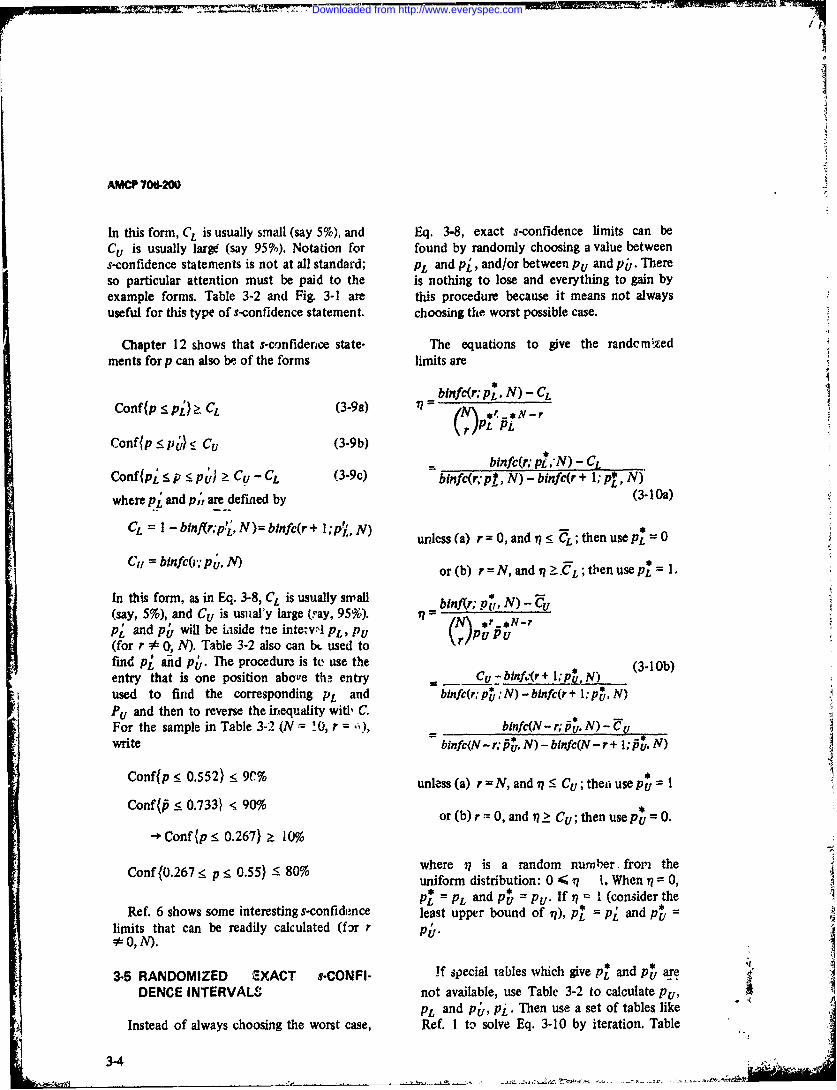
.V"P 706.200

In this form, CL is usually small (say 5%), and Eq. 3-8, exact s-confidence limits can beCu is usually largd (say 95%). Notation for found by randomly choosing a value betweens-confidence statements is not at all standard; PL and pi, and/or between Pu and p&. Thereso particular attention must be paid to the is nothing to lose and everything to gain byexample forms. Table 3-2 and Fig. 3-1 are this procedure because it means not alwaysuseful for this type of s-confidence statement. choosing the worst possible case.

Chapter 12 shows that s-confidence state- The equations to give the randomizedments for p can also be of the forms limits are

binfc(r. p, N) - C,Conf(p :_ pi) 2- C, (3-9a) I

rPL Pj

Conf{p <--p p). CU (3-9b)blnfc(r; p*,'N) - CL

Conf{pj Cu - CL (3-9c) binfc(r. p1, N) - binfc(r + 1; pI, N)

where P; and p, , are defied by (3-1 Oa)

CL = 1 -binfl(r;p', N)= blnfc(r + I; p' , N)IL unless (a) r = 0, and i?< : ?L ; then use pL* = 0

C, = btnfcO;Pi, N) or (b) r = N, and i >.-L ;then usep= 1.

In this form, as in Eq. 3-8, CL is usually small binf(r; p*,, N) - Z I(say, 5%), and Cu is usuary large (ay, 95%). t? ....pj and pu will be idside tMe inte-v.'l PL, Pu ()Pu Pu(for r * 0, N). Table 3-2 also can bL. used tofind p1 and pW" The procedur is te use the (3-1Ob)entry that is one position above th? entry f Cu-blnf jr+ 1;pUN)used to find the corresponding PL and binfc(r;p,N) -blnfc(r+ l; p, N)Pu and then to reverse the inequality witl, C.For the sample in Table 3-2 (N 1_0, r = binfc(N-r; , N)- U.write binfc(N- r; rfi, N) - bfnfc(N- r + l; Piu. N)

Conf{p 0.552) < 9C.% unless (a) r N, and tj < Cu; thei usePtr 1

Conf{(P < 0.733) e. 90% ,or (b) r= 0, and 1 2_ Cu; then use pu = 0.

Conf{p < 0.267) a 10%onf27 p 0.55) 80% where q is a random number. frop the-o- -7uniform distribution: 0 < q I. When i = 0,

p* = pL and p, = Pu. If q= I (consider theRef. 6 shows some interesting s-confidence least upper bound of q), pZ p and Pt,

limits that can be readily calculated (f:or r pt.0, N).

3-5 RANDOMIZED EXACT s-CONFI- if special tables which give p* and pt, 1DENCE INTERVALS not available, use Table 3-2 to calculate Pu,

PL and p&, pL. Then use a set of tables likeInstead of always choosing the worst case, Ref. I to solve Eq. 3-10 by iteration. Table

3-4

AMCP 706-200

TABLE 3-2

1-SIDED UPPER s-CONFIDENCE LIMITS FORp (THE BINOMIAL PROBABILITY) (ADAPTED FROM Ref. 7)

The body of the table gives pc, a 1-sided upper s-confidence (90%, 95%, 99%) limit for p, for the formConf (P P} > C.

p - probab;lity of occurrence of labeled eventr - number of such events in N trials, the random variableN - number ot trials in which r events occurred, fixedC a s-conidence (minirv um valu?)

Example: For N - 10, r - 4., Ccnf p < 0.646) > 90%(lieerot 1)- - Con o T O.812 } >90% - Conf {p }4O018 10%

Conf 0i.88 <p < O.M6 80%

C 90% 95% 99% r C -90% 95 r ' 0 95% 99%N = N=3 N=4

0 .684 .776 .900 0 .536 .632 185- 0 .438 .527 .6841 .949 .975- .99. 1 .804 .865. .941 1 so .751 .859

2 .965, .983 .997 2 .857 .902 .9583 .974 ."7 .997

N-5 N=6 N=70 .369 .451 .602 0 .319 .393 .536 0 .280 .348 .4821 .584 .657 .778 1 .510 .582 .706 1 .453 .521 .6432 .753 .811 .894 2 .667 .729 .827 2 .596 .659 .7643 48;: .9?4 .967 3 .799 .847 .915+ 3 .721 .175- .8584 .9" .)90 .998 4 .907 .937 .973 4 .330 .871 .929

5 .93 .991 .998 .921 .947 .9 76 .985+ .993 .999

N=8 N=9 N=10

0 .250 .312 .438 0 .226 .283 .401 0 .206 .259 .36f1 .406 .471 .590 1 .368 .429 .544 1 .337 .39 5042 .538 .600 .707 2 .490 .550 .656 2 .450 .507 .6123 .655+ .711 .802 3 .599 .655+ .750 3 .552 .607 .7034 .760 .807 .879 4 .699 .749 .829 4 .646 .696 7825 .853 .889 .939 5 .790 .831 .895- 5 .733 .778 .850

0 .931 .954 .980 6 .871 .902 .947 6 .812 .850 .9077 .987 .9r14 .999 7 .939 ..)59 .983 7 .884 913 .952

8 .98 .994 .99 8 .945+ .963 .9849 .990 .995- .999

N=11 N=12 N- 13

0 .189 .238 .342 0 .175- .221 .319 0 .162 .206 .291 .310 .364 .470 1 .287 .339 .440 1 .260 .316 .4132 .415+ .470 .572 2 .386 .438 .537 2 360 .410 .5063 .511 .564 .660 .475,1 .527 .622 3 .444 .495- .5884 .599 .650 .738 4 .559 .609 .698 4 .* 3 .573 .6615 .682 .729 ."06 5 .638 .685- .765+ 5 .598 .645+ .727

6 .759 .800 .866 6 .712 .755- .825+ 6 .669 .713 .7877 .831 .865- .916 7 .781 .819 .879 7 .736 .776 .8418 .895+ .921 .957 8 .846 .877 .924 8 .799 .834 .889

10 .990 .995+ .999 10 .955- .970 .987 10 .912 .934 .964

11 .991 .996 .999 11 .958 .972 .9812 .992 .996 .V9

Notes:1. If a 1-sided lower s-confidence limit is desired, use N-r instead of rp instead of p and C mstema of C, and -

switch the inequality. See the example.2. The +, - after a 5 indicates which way the number can be rounded to fewer decimal placns.

3-5

AMCP 7 200

TABLE ?-2 (Continued)

N-14 N- 15 N- 160 .152 .193 .280 0 .142 .181 .264 0 .134 .171 .2501 .251 .297 .389 1 .236 .279 .368 1 .222 .264 .3492 .331 .3854 .478 2 .317 .363 .453 2 .300 .344 .4303 .417 .466 .557 3 .393 .440 .529 3 .371 .417 .5034 .492 .540 .627 4 .164 .511 .F47 4 .439 .484 .5695 .563 .61 n .692 s .32 .577 .660 5 .504 .548 .6306 .631 .675- .751 6 .596 .640 .718 6 .565+ .609 .6877 .695+ .736 .805+ 7 .658 .700 .771 7 .625- .667 .7398 .757 .794 .854 8 .718 .756 .821 8 .682 .721 .7889 .815- .847 .898 9 .774 .809 .865+ , .737 .773 .83410 .869 .896 .936 10 .828 .858 .906 10 .790 .822 .875.

11 .919 .939 .967 11 .878 .903 .941 11 .839 .868 .91212 .961 .974 .989 12 .924 .943 .969 12 .886 .910 .945-13 .993 .996 .999 13 .964 .976 .990 13 .929 .Q47 .971

14 .993 .997 .999 14 .966 .977 .99015 .993 .997 .999

N 17 N=18 N=190 .127 .162 .237 0 .120 .154 .226 0 .114 .146 .215+1 .210 .250 .332 1 .199 .238 .316 1 .190 .226 .3022 .284 .326 .410 2 .269 .310 .391 2 .257 .296 .3743 .352 .396 .480 3 .334 .377 .458 3 .319 .359 .4394 .416 .461 .543 4 .396 .439 .520 4 .378 .419 .4985 .471 .522 .603 5 .455+ .498 .577 5 .434 .476 .5546 .537 .580 .658 6 .512 .554 .631 6 .489 .530 .6067 .594 .636 .709 7 .567 .608 .681 7 541 .582 .655+8 .650 .689 .758 8 .620 .659 .729 8 .592 .632 .7029 .703 .740 .803 9 .671 .709 .774 9 .642 .680 .746

10 .754 .788 .845- 10 .721 .756 .816 10 .690 .726 .788

II .803 .834 .883 11 .769 .801 .855- 11 .737 .770 .82712 .819 .876 .918 12 .815- .844 .890 12 .782 .812 .86313 .893 .915+ .948 1 .858 .tN84 .923 13 825. .8%3 .89714 .933 .950 .973 14 .899 .920 .951 14 .k466 .890 .92715 .968 .979 .991 15 .937 .953 .975- 15 .905- .925- .95416 .994 .997 .999 16 .970 .980 .992 16 .941 .956 .:76

17 .994 .997 .Q99 17 .972 .981 .99218 .994 .997 .9,

N 20 N=21 N=22

0) .109 .139 .206 0 .104 .133 .197 0 .099 .127 .1891 .181 .216 .289 1 .173 .207 .277 1 .166 .198 2662 .245- .283 .358 2 .234 .271 .344 2 .224 .259 .3303 .304 .344 .421 3 .291 .329 .404 3 .279 .316 .3894 .361 .401 .478 4 .345+ .384 .460 4 .331 .369 w4435 .415- .456 .532 5 .397 .437 .512 5 .381 .420 .4936 .467 .508 .583 6 .448 .487 .561 6 .430 .468 .5417 .518 .558 .631 7 .497 .536 .608 7 .477 .515+ .5878 .567 .606 .677 8 .544 .583 .653 8 . 23 .561 .6309 .615+ .653 .720 9 .590 .628 .695+ 9 .568 .605- .672

10 S,62 .698 .761 10 .636 .672 .736 10 .611 .647 .712

11 .7(7 .741 .800 11 .679 .714 .774 11 .654 .689 .75012 .751 .783 .937 12 .722 .755- .811 12 .695+ .729 .78613 .793 .823 .871 13 .764 .794 .645- 13 .736 .767 .82114 .834 .860 .902 14 .804 .832 .818 14 .775+ .804 .85315 .873 .696 .931 15 .842 .868 .908 15 .813 .840 .88416 .910 .929 .956 16 .879 .901 .935- 16 .850 .874 .91217 .944 .958 .977 17 .914 .932 .959 17 .885+ .906 .93818 .973 .982 .992 18 946 .960 .978 18 .918 .935+ .96119 .995- ,997 .999 19 .974 .983 .993 19 .949 .962 .979

20 .995- .998 1.000 20 .976 .984 .993 ..

21 .995+ .998 1.000

3 -


2

AMCP 706-2.

TABLE 3-2 (Continued)

90% 95% 99% r 90% 95% 99% r 90% 95% 99%

N'23 _____N-24 -- N 25

0 .0954 .122 .181 0 .091 .117 .175- 0 .088 J 33 .1681 ,159 .190 .256 1 .153 .183 246 1 .147 .1'6 .2372 .215+ .249 .318 2 .207 .240 .307 2 .199 .23. .2963 .26b .304 .374 3 .258 .292 .361 3 .248 .282 .3494 .318 .355- .427 4 .306 .342 .412 4 .295- .330 .3985 .36e .404 .476 5 .352 .389 .460 5 .340 .375-. .444

6 .413 .451 .522 6 .398 .43S. .305- 6 .383 .420 .4887 .459 .496 .567 7 .442 .479 .548 7 .426 .462 .5318 .503 .540 .609 8 .484 .521 .590 8 .467 .504 .5719 .546 .583 .650 4 .526 .563 .630 9 .508 .544 .610

10 .589 .625- .689 10 .567 .603 .668 10 .548 .583 .648

11 .630 .665- .727 I1 608 .642 .705- 11 .5e7 .621 .68412 .670 .704 .763 12 .647 .681 .740 12 .625- .659 .71913 .710 .742 .797 13 '1854- .718 .774 14 .662 .695- .75214 .748 .778 .829 14 ,723 .754 .806 14 .699 .730 .78415 .786 .814 .860 1 .759 .788 .837 15 .735- .764 .8is+

16 .822 .848 .889 16 .795+ .822 .867 16 .770 .798 845+17 .8' .880 .916 17 .830 .854 .894 17 .804 .930 .87318 .890 .910 .941 18 .863 .885+ .920 18 .837 .861 .89919 .922 .938 .962 19 .b95+ .914 .943 19 .860 .890 .9232n .911 .963 .980 20 .925+ .941 .964 20 .899 .918 .946

21 .97 t .984 .993 21 .953 .965+ .981 21 .928 .943 .96622 .99!; 1 .998 1.000 22 .978 .985. .994 22 .955+ .966 .982

23 .996 .998 1.000 23 .979 .986 .99424 .9 .998 1.000

N=26 N=27 N=28

0 .085- .109 .162 0 .082 .105+ .157 0 .079 .101 .1521 .142 .170 .229 1 .137 .164 .222 1 .132 .159 .2152 .192 .223 .286 2 .185+ .215+ .277 2 .179 .208 .2683 .239 .272 .337 3 .231 .263 .326 3 .223 .254 .3164 .284 .318 .385- 4 .275. .308 .373 4 .265+ .298 .Z615 .328 .363 .430 5 .317 .351 .417 5 .306 .339 .4(%4

6 .370 .405+ .473 6 .358 .392 .458 6 .346 .380 .445-7 .411 .447 .514 7 .397 .492 .498 7 .385- .419 .4848 .451 .487 55 8 .436 .471 .537 8 .422 .157 .5219 .491 .526 .592 9 .475- .509 .574 9 .4 9 .494 .558

10 .529 .564 .628 10 .512 .547 .610 10 .496 .530 .593

11 .567 .602 .664 11 .549 .583 .645+ 11 .532 .565+ .627 "112 .604 .638 .698 12 .585- .618 .679 12 .5r .600 .66013 .641 .673 .731 13 .620 .653 .711 13 .601 .634 .69214 .676 .708 .763 ! s .655+ .687 .743 14 .635+ .667 .72315 .711 .742 .794 is 689 .720 .773 15 .669 .699 .753

16 .746 .774 .823 16 .723 .752 .802 16 .701 .731 .78217 .779 .806 .851 17 .756 .783 .831 17 .733 .762 .81018 .812 .837 .878 18 .788 .814 .857 18 .765- .792 .83719 .843 .866 .903 19 .X19 .843 .383 19 .796 .821 .86320 .874 .894 .927 2f9 .840 .871 .907 20 .826 .849 .888

21 .903 .921 .948 21 .879 .899 .930 21 .855+ .876 .91122 .931 .946 .967 22 .907 .924 .950 22 .883 .902 .03223 .957 .968 .983 23 .924 .948 .968 23 .911 .927 .952

24 .979 .n86 .994 24 .9.18 .969 .983 24 .936 .950 .96925 .996 .998 1.000 25 .980 .987 .994 25 .960 .970 .984

26 .996 .998 1.000 26 .981 .987 .995-27 .996 .998 1.000

3-7


AMCP 702t'0


90% 95% 99% r 90 5 9, ~N=29 N-30 I

0 .076 .098 .147 0 .074 .095 * .1421 .128 .153 .208 1 .124 .149 .2022 .173 .202 .260 2 .168 .195 - .2523 .216 .246 .307 3 .209 .239 .2984 .257 .288 .350 4 .249 .280 .3405 .297 .329 .392 S .287 .319 .3816 .335- .368 .432 6 .325- .357 .4207 .372 .406 .470 1 .361 .S94 .4578 .409 .443 .707 8 .307 .430 .4939 .445 .479 .543 9 .432 .465+ .527

10 .481 .514 .57 10 .466 .499 .7??

18 .515+ .549 .610 11 .500 .533 .59412 .574 .83 .643 12 .533 .566 .62613 .583 .828 .684 20 ..266 .'78 .84714 .8 64327 .75 14 .S9Q9 .630 66722 .649 .8 .734 15 .830 .66) .716

16 .8 .7016 .73 1 23 .662 .692 .7025 .938 .951 .70 17 .692 .721 .'7212 .912 .741 .918 18 .93 .750 .7219 .774 800 2843 19 .72 .779 82420 .803 .828 .86 20 .7 2 .807 .849

21 .832 .855- .!:92 21 .81 . .934 .87'22 .860 ,881 .914 22 .838 JMbO .80623 .888 .906 .935- 23 .865 5 ' .124 .914 .930 954 24 .891 ." (", .'?3725 .938 .951 .970 25 .917 .932 .9t55 +

26 .961 .971 .985- 26 .941 .Q53 .o2

27 .982 .988 .995- 27 .963 .972 ,985+28 .)96 ,.998 1.000 28 .982 .988 .995-29 .996 .99R 1.000

3-3 is a copy of pages 30, 579, & 580, Ref. 1, Use the example in Table 3--': N 10, rand is used to illustrate the procedure of 4, Cu = 90%, C-L =01 It is shown in Tablefinding pi and p,. 3 2 that pu = .. 646, Pt = 0.188. It is shown

just followLnr' Eq. 3-9c that P'u = 0.552, pL0.267. Suprose !he random number is 17

A handy random number generator is a = 0.28125 (same as in the example in thecoin, flipped several times. Decide whether paragraph immediately above) Linear inter-heads is to be 0 or 1 ; tails is the reverw. Then polation kapplied several times) will be usedmultiply the result of the first flip by 0.5, the to solve Eq. 3-10. The forms cf Eq. 3- 10 usingsecopd flip by 0.25, the third by 0.125, etc. the rightmost expressions are most suitable(the numbers are 2-flip), as fine as desired. for using Table 3-3. They are written asThen add the numbers. Usually 5 or 6 flipsgive a sufficiently continuous random vari-able. (For examph., heads is 0, tails is 1; thesequence is H, T, H, H, T, H. Add 0.25 uvn'c(r..,,-C 0

+ 0.03125 - 0.28125; truncate to 0.261 for , . 'i,- - ' 1N

convenience.) (3-1I a) ,

U3


AMCP 706-200

.28

4I

I11 Y 1-4-

.26

.24 1,

0 1 .0:0:.6 .6 1 1 .4 .: 1 2

(Etiat ot I) a

0

p prbailt of ocurne flble vn

r ume of su • evnt inN ralh rndmvaial

...... ...... .

.106 -M

= rIf

swthteieul. See theexmpe n abe *2

O 0 z0 .0_0 0 10 .12 .f16 .8 2

sI a e I I I

If i-

Not. I a -s~ed owe s-on ineh tisdsrdusN- intaof,/intdofC ntedoCnd'sw~~~~~~tch~~~~~ thinqaiy dSeteeape nTbe32

.08 if


AMCP 706-200

.304 44

.244

M -----. 4 .44444 -** 4 **I Tl~-

i3 TaI

o.200 0 .6 .0 .2 .1 1 1 2

(Etmaeofp4Fiue3 1.1-sddUprsC1iec ii 9% o aatdfo e.7

Th gap gve te -sde upe scofiene imt or:wer

p =prba~iy o ocureceof able.eenr = nmberof sch vnsi Lras h admvral

3-1010


AMCP 706-200

.36

0.D

.26 J1.26 4

( E ti a t o f-- ---

Figur E 1C.7sddUprsCniec ii 9% o aatdfo e.i

The graphgives th 1 2dupr0 cnienelmtfr hr

.1-3

p~~~~~~C .16,,biyofocrec f aee vn-~ n mbe 'Msuc! es0rgs i N tgal, te radomvarablIC

N~~~~~~ .14n~ t asir h~ vns curd ie.12.1 4/N

Noe fa1sddloe -ofdneliiAsdsrd s -nta fr ised- ,Cinta fC nswich he neualty.Se th exmpl i Tale -2

.06 t-3-1U

.02 *


AMCP 706-200

ft. (X") a binfc(N - r xL). X._+ -X+f.b nfc(IN -, .xv N) -blne( w-,T + 1 .0 X r w f f.(3- 2)

(3-1ib)

The solution to Eq. 3-I la is XL p7. The where x- and x+ are the smaller and largersolution to Eq. 3-11 b is xU = FU*. values of x, respectively; and f+ f(x+) and

The formula for linear interpolation is f_ -flx_.

3-12 '1


I

AMCP 706-200

Procedure Example

1. Solve Eq. 3-11 a first. Usex PL andx+ 1. CL =0.10= Pj. The values of f are known from thedefinition of PL , Pi. Use Eq. 3-12 to find x Jx ,ew, round off to 2 decimal places. Solve 0.188 --0.281 = (--)Eq. 3-1 Ia using x = 0.21. 0.267 +0.719 = (1)

0.2100.21 +0.113 (new)

2. Make a new chart, discarding the old pair 2. x f(0.267, 0.719) with the same sign as 0.188 -0.281Repeat the linear interpolation and round 0.21 +0.113off. 0.204 - -

0.20 -0.044 (new)

3. x is now isolated to be between 2 con- 3. X fsecutive entries in the table. Repeat the 0.20 -0.044linear interpolation but do not round off. 0.21 +0.113The answer ispZ = 0.203. 0.203

4. Solve Fq. 3-11 b next. Usex PUIX.. 4. CU =0.10= p. Proceed asin Step 1. N-r 10-4=6. x f

0.354 -0.281 = (-q)0.478 +0.719 = (l-7)0.3890.39 +0.208 (new)

5. lake new chart and repeat Step 1. 5. x _ _ f0.354 I -0.2810.39 +0.2080.37470.37 -0.0394 (new)

6. Make new chart and repeat Step . Round 6. X f"up", to bracket the true value. 0.37 -0.0394

0.39 +0.2080.373 - -

0.38 +0.09 10 (new)

7. Repeat Step 3. The answer isU = 0.373; 7. x f"p* = 0.627. 0.37 -0.0394

0.38 +0.09100.373

8. Make the final s-confidence statement. 8. Conf { 0.203 <p < 0.627 1 = 80%

3-'

A ~' ----- -- ~--3-13 ,

AMCP 716200

TABLE 3-3

SAMPLE PAGE FROM A BINOMIAL DISTRIBUTION (Ref. 1)

binfc(c, p, tD (N P

i-c N'1O

.0± .03 .03 .04 .03 .04 .07 .03

1 .0936179 .109373 .3437~59 .3314674 .4013631 .4;13849 .S160177 .8411S.004443 .0141774 .034504 .058153 .0841364 .11759;0 .1517299 .19705

3 .0001139 .0009439 .0037449 .0042137 .0%11038 .010(378 .1U341 .04007564 .0000030 .000030 .0001471 .0004430 .0010326 .0t90393 .0035741 .000013

S.000007 .0000084 .000016 .0000437 .0001317 .0003139 .00053

4 .0000001 .0000001 .0000038 ,0000079 .0000193 .000041. 0000001 .0000003 ,0000000 .0000030,0.0100001 :

.09 .10 .11 .18 .13 .14 .1 s14

1 .4105839 .5313314 .401±131 .7314990 .7315?6 ,7764934 .803118 .33509303 .3354411 .3839011 ,3037V9©0 .3417350 ,3800493 .4 1.400 .48570003 *491953

3 .0140400 .0701908 .0304435 #10611 .130764 .1545498 .17900S .0o4054 03 .0137*9 .0177973 .1039 .10304M .10399:42 .049:94 .0813577

.0010096 '.0014349 .0023170 .0037161 .0053907 .0073343 .0096741 .0130101

,00001110 .0001449 .0003307 .0004019 .000313 .000130 .001303 .0019593

1 .0000048 .0000091 .0000173 .0000301000000315 .0000634000001346 .0000818 .000000 .0000004 .000000800000 .000001 .00000a7 .00001!21 .0000001 .0000003 .0000003 .0000004

.17 .I .19 .20 .11 .33 .33 .14

1 .:4403914 .8;1520 .fl?433 .9360*1 .3053173 .9;14142 .9367338 2 9357111

S .5370413 .510341 .593435 .4241904 .4534289 ,6b1304 . 104 :33,11934

3 .8341305 .1431010 .39*1104 .3333OOS .35255.4 .331197 .4137173 .4441949

4 .0741472 .0663411 .109341 .1200179 .139141 .1501731 .1794034 .401:4:7.,01a8038 .015 .0337930 ,03 34 .047:297 .0549194 .049190

4 00 7098 .003 494 .004 37 7 .00 3 84 .00 1 3 5 0 1393 8 0130 14 014111 4

7 .0003042 .0004 .00.0004339 .000644 .001173 .001604 .000 .00373

..00003 .000380 .000016 .0000719 .000117 .0001399 .0033 .0003040

9 .0000010 .0000017 .0000037 .000004 .00064 .0000097 .0000143 .000030710 .0000001 .0000001 .00000 .0000003 4 000000

,35 .36 .37 .38 .39 .30 .31 *33

1 .9436315 .950701 .9370237 .942409 .94471 .#973$S .975381 .97334013 .7589740 .7771850 .797005 .014964 .1344369 .306917 .7563366 .07,9313 .474A073 .5047200 .53;5113 .5491710 .5901015 .4173172 .643444S ,46073134 .241 349 *3479349 .3735?61 1979405 .3 39164 .3503893 .3773433 .4043434S .0731249 .0903543 .1036l431 .119t171 .1336%03 .1302483 .1679478 .1344554

4 .0197277 .0R39148 .0387224 .0341994 .0403932 0.073490 .0831097 .04T71497 .0035057 .0044410 .0054101 .0070039 .0054507 .0105921 .01:6437 .0155039

.0004180 .00054 .0007380 .000905 .0012430 .0013904 .0030179 .00353049 .000089 .09000M1 .00005T7 .0000791 .0001072 .0001437 .0001904 .000380810 .0000010 .0000014 .0001 .0000030 .0000042 .00000S9 .000008 .0000113

.33 .34 .3b .36 .37 IS$ .39 .40

1 .981771: .914410 . 5373 .980470 .901507 .9916070 .99306 34 .9995343 .0919901 .9039235 .9140456 .9238190 .9333056 .9401441 .9472594 .95344163.69994 .7163304 .7303926 .7594437 774242 .792387 .0140483 .8337105

4 ,43163P0 .459060 .4361730 .5133284 .5400038 .564030 .893331 .4177945 .053~04 .2549060 .2405045 .370415 .2939377 .317670 .34085 .36418947

6 .073:'005 .08979 ,649341 .1073304 .130504 ,1344$01 .11000:6 .14433647 .0105489 .030042 ,0240243 .0305374 .0354052 .041301 .0470949 .0547619a .001173 .0039319 .0048213 .00508l4 .0071403 .006079 .0103143 .01399469 . 2003845 .0004314 .0005399 .0004045 .0006448 .0010071 .0013S44 .0014777

10 .000o 0153 .0000306 .0000276 .000036 .0000401 .0000600 .0000014 .010049

.41 .42 .43 .44 .45 .44 .47 .40

1 .994098• ,9954910 .9943797 .9949449 .9974470 .'9976917 .993511 .99'8442.9593709 .0444950 .949004 .973135 .9747439 .9799319 .9637433 .9353109

3 .843007 .6431039 .. 7'383 0 .6 07 .9004403 .911069 .9308530 .9378394 4472 .4665312 .6399401 .7111307 .7339431 ,75469 .7744905 .7933480

.3,921723 .4177749 ,443494 .449513 495954 .5315571 .5473730 .5731931

4 .1034452 .8014093 .2207058 .3407033 .3815437 .3333315 .3034773 .3369305

4!1:

1 ,0•7:2 .407171843 .00$1 .010817 :219,49: ,!*0If* 111S,40

$ ?0471 0711 .020.696 .02 $S83 .0.7318 .0311705 .0315S.0 .0419713

9 .002001Sol.0 .00 0009 S0: 001 .0034040 .0044S74 .0il19 .0001149 .0001100: ,030011 :00'09'2;1 .00*093.0 .000410 .:000110 .:010140

.49 .50

1 .9980094 .99902342 .97372 . 1970

.93792:1 .94523134 .8113340 .0301350S . 908047 .4230449

S.35260!P .37675317 .1S9 7 .171 780 *8 ,0400003 .05446171

9 .0091028 .010743310 .0007979 .0009?74

3-14


AMCP 706-200

Table 3-4 lists randomized 2-sided s-confi- low, or a very low s-confidence that thedence limits which have special statistical s-relihbility is very high. A reasonableproperties. They are not equal-tailed s-confi- compromise is to choose a s-confidence leveldence limits; they cannot be used separately which is approximately the fraction of successfor upper and lower s-confidence imits. See in the sample (unless that fract'on is 100%).Ref. 8 for a more complete discussion. Ingeneral, the s-confidence limits in Table 3-4 If 'there are no failures, one can reasonablywill be different from those calculated using choose the s-confidence level equal to thethe methods in this chapter. It is difficuit to minimum [-sided lower s-confidence limit onsay that one set s bea r than the other s-reliability. Fig. 3-2 shows the graph for this itexcept in the narrow statistical sense stated situation. One could also use the Poissonfor Table 3-4. approximation for this case.

3-6 CHOOSING A s--CONFIDENCE LEVEL 3-7 EXAMPLES

Choosing an appropriate s-confidence 3-7.1 EXAMPLE NO. 1level is always troublesome. Suppose thelabeled events are failures; so p is the Ten tests were run with 1 failure. Find theprobability of failure and is the s-reliability. 5% and 95% I-sided s-confidence limits on theThere is obviously little point in having a very failure probability p; combine them for ahigh s-confidence that the s-reliability is very 2-sided s-confidence statement.

4

3-15


AMCP 7W6-20O

Procedure Example

1. The labeled events are failures. State N, r, 1. N = 10, r = 1Cu , CL., and = rP!. (by Eq. 3-7). Cu = 95%, CL =5%

2. Use Table 3-2 to find puand PL. Then make 2. Pu = 0.394the s-confidence statements. PL = 1 - 0.995 = 0.005

Conf J p 0.394 > 95%Confi p < 0.005 < 5%Conf 0.005 5%Conf 1 0.037 < p < 0.259 1 90%

4. Again choose a random number by the 4. Result is H, H, T, T, T, H (unusual, but true)coin flipping method. Take heads = 0, - 0.125 + 0.0625 + 0.03125 = 0.21875 - 0.219tails = 1. Use linear interpolation in Ref. 1 =to find the exact randomized s-confidence p* lies between 0.006 and 0.007;interval. Use Table 3-3. p* = 0.0066.

p lies between 0.37 and 0.38;p . = 0.378.

5. Make the exact s-confidence statements. 5. Conf p < 0.0066) = 5%Conf p '0.378 95ro

Conf 0.0066 <p < 0.3 78 I 90%

3-163-16

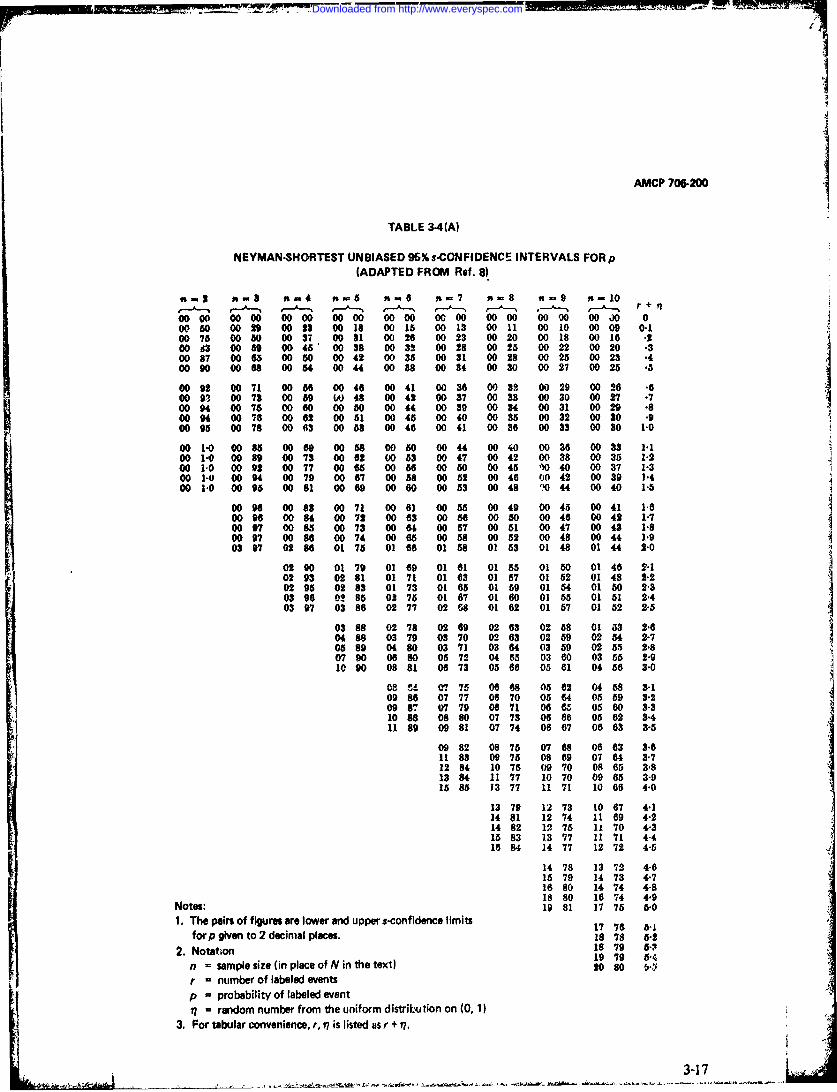
AMCP 706-200

TABLE 3-4(A)

NEYMAN-SHORTEST UNBIASED 96% s-CONFIDENCE INTERVALS FOR p(ADAPTED FROM Ref. 8)

1-- 3-- ,=4 #--5 6 7 "" 8 u'9 to-l0

00 00 00 00 00 00 00 00 00 00 00 00 00 00 00 00 00 J0 000 50 00 0 2 0 3 00 18 00 15 00 13 00 11 00 10 00 09 0-10 75 00 50 00 37 00 81 00 26 00 23 00 20 00 18 00 16 .2

00 d3 00 69 O0 45 00 38 00 32 00 28 00 25 00 22 00 20 .300 87 00 63 00 50 00 42 00 35 00 31 O0 28 00 25 00 23 -400 90 00 68 0054 0 44 00 38 00 34 00 30 00 27 00 26 .5

00 92 00 71 00 56 00 46 00 41 00 36 00 3P 00 29 00 26 .600 93 00 73 00 59 W 48 00 42 00 37 00 33 00 30 00 27 -700 0 0 75 00 60 00 60 00 44 00 390 0 34 00 31 00 29 .8

00 94 00 76 00 062 0 51 00 45 00 40 00 35 00 32 00 80 .900 95 00 78 0 063 0058 O0 46 00 41 00 36 00 33 00 30 1-0

00 1-0 0 85 00 69 00 58 00 50 00 44 00 40 00 36 00 33 1-100 1-0 00 89 00 73 00 62 00 53 00 47 00 42 00 38 00 35 1-200 1'0 00 92 00 77 00 65 0 56 00 50 00 45 1 40 00 37 1-300 1-0 00 00 79 00 67 00 58 0 052 00 46 00 42 00 39 1-400 1'0 1 0 95 O0 81 00 69 00 60 00 53 00 48 0 44 00 40 1-5

0 9 0 800 0 71 00 61 00 55 00 49 00 45 00 41 1-600 96 0084 00 72 00 63 00 56 00 50 00 46 00 42 1-700 97 00 85 00 73 0064 O0 57 00 61 00 47 00 43 1-800 97 00 86 00 74 0 065 00 58 00 52 00 48 0 44 1-903 97 02 86 01 75 01 66 01 58 01 53 01 48 01 44 2.0

02 90 01 79 01 69 01 61 01 55 01 50 01 46 2-102 93 02 81 01 71 01 63 01 57 01 52 01 48 2-202 95 02 83 017 3 01 65 01 59 0154 01 50 2-303 96 02 85 027 5 01 67 01 60 01 55 01 51 2.403 97 03 86 02 77 02 68 01 62 01 57 01 52 2-5

03 88 02 78 02 69 02 63 02 58 01 53 2-604 88 03 79 03 70 02 63 02 59 02 54 2-705 89 04 80 03 71 03 64 03 59 02 55 2-807 90 06 80 05 72 04 85 03 60 03 55 2-910 90 08 81 06 73 05 66 05 61 04 56 3-0

. *A 07 75 06 68 05 62 04 58 3-1

09 86 07 77 06 70 05 64 05 59 3-209 87 07 79 06 71 06 65 05 60 3-310 88 08 80 07 73 06 66 05 62 3-411 89 09 81 07 74 06 67 06 63 3-5

09 82 08 75 07 68 06 63 3-611 83 09 75 08 69 07 64 3-712 84 10 76 09 70 08 65 3-813 84 11 77 10 70 09 65 3-915 85 13 77 11 71 10 06 4-0

13 79 12 73 10 67 4-114 81 12 74 11 69 4-214 82 12 75 I 70 4-315 83 13 77 11 71 4-4

16 84 14 77 12 72 4-5

14 78 13 72 4-615 79 14 73 4-716 80 14 74 4-818 80 16 74 4-9

Notes: 19 81 17 75 5-0

1. The pairs of figures are lower and upper s-confidence limits 17 76 64

forp given to 2 decimal places. 18 78 5-2

2. Notation 18 79 5-719 79 5-4

n = sample size (in place of N in the text) 20 s0 5-r = number of labeled eventsp = probability of labeled event

-- random number from the uniform distribution on (0, 1)3. For tabular convenience, r, Yj is listed as r + 17.

3-17


AMCP 706-200

TABLE 34(A) (Continued)

n-I n 12 ..=13 ut=14 n 15 f- 16 n 17 n.18 ,,19

00 00 O0 0 00 00 0) 00 00 00 00 00 00 00 0001 00 0 000 08 0008 00 07 00 07 0008 00 0 00 05 00 05 00 05 0.100 15 00 14 00 13 00 12 00 11 0 10 00 10 O0 09 00 09 .200 19 00 17 00 16 00 15 00 14 00 13 00 It 00 12 0011 .300 21 00 19 00 18 00 17 00 16 00 15 00 14 00 13 00 13 .400 23 00 21 00 19 00 18 00 17 00 16 00 16 . 0 14 00 14 .5

.O 24 O0 22 00 21 00 19 0018 0 17 00 16 00 15 00 15 600 25 00 23 00 22 00 20 00 10 00 18 00 17 00 16 00 15 "700 26 00 24 00 23 00 21 00 20 00 19 00 18 00 17 0016 "800 27 (0 25 00 23 00 22 00 2 00 19 00 18 00 17 00 17 .900 28 00 26 00 24 00 22 00 21 00 20 00 19 00 18 00 17 1.0

00 32 00 30 00 28 00 26 00 35 00 23 00 22 00 21 00 20 1"200 36 00 33 00 31 00 29 00 27 00 26 00 24 00 23 00 22 1.400 38 00 35 00 33 00 31 00 29 00 27 00 26 00 25 0 23 1'600 40 00 37 00 34 00 32 00 30 00 29 00 27 00 26 00 25 1.801 41 00 38 00 36 00 34 00 32 00 30 00 28 00 27 00 26 2.0

01 45 01 41 01 39 00 36 00 34 00 32 00 31 00 019 0028 2 .201 47 01 44 01 41 01 39 01 36 01 34 01 32 W 31 00 29 2"401 49 01 46 01 43 01 40 01 38 01 36 01 34 01 32 01 31 2.602 51 02 47 02 44 02 42 01 0 01 37 01 35 0134 01 32 2-8045 2 03 49 03 45 03 43 03 40 02 38 02 36 2 34 02 33 3"0

04 55 04 51 03 48 03 45 03 43 03 40 03 38 02' 36 02 35 3.205 57 04 53 04 50 04 47 03 44 03 42 03 40 03 38 03 36 3.406 59 05 55 05 52 04 49 04 46 04 44 03 41 03 39 03 38 3-607 60 06 56 06 53 05 50 05 47 04 45 04 42 04 40 04 39 3.809 61 08 58 07 54 07 51 06 48 06 46 05 43 Oo 41 0 39 4.009 64 08 60 08 56 07 53 07 50 06 48 06 45 05 43 05 41 4-210 66 09 62 08 58 08 55 07 52 07 49 06 47 0 45 06 43 4.411 68 10 63 09 60 09 56 08 53 07 51 07 4 06 16 06 44 4.613 69 12 65 11 61 10 57 09 54 08 52 08 49 07 47 07 45 4.815 70 14 66 12 62 11 58 10 55 10 A3 09 50 08 43 08 46 5.0

16 72 14 68 13 64 1260 11 57 10 54 10 52 09 43 08 47 5-217 74 15 70 14 66 13 62 12 59 11 56 10 53 10 5] 09 48 5.41 76 16 71 15 67 14 63 13 60 12 57 11 54 10 5. 10 50 5.620 77 18 72 18 '8 15 64 14 61 13 58 12 55 11 53 11 50 5.8227 8 20 73 18 69 17 5 r5 62 14 59 13 56 12 54 12 51 6'0

31 75 19 71 17 67 16 84 15 61 14 K8 13 55 12 53 6.222 77 21 73 18 69 17 65 16 62 14 59 14 56 13 54 6'423 78 21 74 19 70 18 86 16 63 15 60 14 t8 14 55 6.6

23 75 21 71 19 67 18 ,34 16 61 15 14 56 F ^

24 76 22 72 21 68 19 65 18 62 11 59 16 57 7.9

23 74 21 70 20 67 18 63 17 61 16 58 7'224 75 2 71 it 68 19 65 18 62 17 59 7.425 76 23 72 21 69 20 66 19 63 18 60 7.6

24 73 23 70 21 67 20 64 18 61 7.326 74 24 71 22 68 21 65 20 62 8'0

25 72 23 69 21 66 20 63 8.226 73 24 70 22 67 21 64 8"427 74 25 71 23 68 22 65 8.6

28 72 24 69 23 66 8.827 73 26 70 24 67 9.0

26 71 25 68 9'227 72 23 89 9428 73 26 70 940

27 71 9'828 72 10"0

13-18


AMCP 706.200

TABLE 3.4(A) (Continued)

• 20 n-21 ,t-22 n 23 n=24 ,sa26 n -28 5,, 0 n=32

D0 0 0000 00 D 00 00 0000 00 00 00 )0 00 00 00 00 000 05 00 04 00 04 0004 0004 00 04 00 03 00 03 D 03 0-I0 00 08 00 08 00 07 00 07 00 07 O0 6 00 06 O0 05 *20011 0 10 O0 10 00 00 00 0 0008 00 08 0 07 00 07 -300 02 O0 I 1 0 011 00 10 00 10 O0 09 0009 00 08 00 08 .400 13 00 12 00 12 00 011 0011 0 10 00 09 00 09 O0 0 .5

00 14 o013 0 13 00 12 00 12 00 11 00 10 00 09 00 09 .600 15 00 14 00 13 00 13 00 12 00 11 00 11 00 10 00 09 -700 15 00 15 00 14 00 13 00 13 00 12 00 11 00 10 00 1) .80016 0015 00 14 00 14 0 13 00 12 00 12 00 0 1 D 10 .900 16 00 16 00 15 00 14 00 14 00 13 00 12 00 11 00) 10 1-0

00 10 00 18 00 17 00 17 00 16 00 15 00 14 00 lb 00 12 1.200 21 00 20 00 19 00 18 00 18 00 16 0 15 00 14 O 01 1.4002 002 1 00 r 0 20 00 19 00 18 00 16 0 15 00 14 1-6WA 24 09 3 00 22 00 21 0020 00 19 00 17 0016 0 15 1.800 24 00 23 00 22 00 22 00 21 00 19 O0 08 00 17 00 10 2.0

00 27 00 25 00 24 00 23 00 22 0 21 00 20 0 18 00 17 2-2D 28 D 27 00 26 00 25 00 24 00 22 00 21 00 19 D 18 2-40129 01 28 01 27 01 26 01 25 00 23 00 22 00 20 00 19 2.601 31 01 29 01 28 01 27 01 26 01 24 01 23 01 21 01 20 2-802 31 02 30 02 29 02 28 02 27 01 25 01 23 01 22 01 20 3-0

02 33 02 32 02 31 02 29 02 28 0226 01 25 01 23 01 22 3-2023 5 02 33 02 3 02 31 02 29 02 27 Ot 26 02 24 GI 23 3.403 36 03 34 03 33 02 32 02 31 02 28 02 27 02 25 02 23 3-603 37 03 85 03 34 03 33 03 31 03 20 02 27 02 26 02 24 8-804 38 04 36 04 35 04 33 04 32 03 30 03 28 03 26 03 25 4.0

05 39 05 38 04 36 04 35 04 34 04 31 03 P9 03 27 03 26 4-205 41 )5 39 05 37 04 36 04 35 04 32 04 30 03 28 03 27 4-406 42 05 40 05 39 05 37 05 36 04 33 04 31 04 29 03 28 4-607 43 06 41 06 39 06 58 05 86 05 34 05 S2 018 0 04 28 4-808 44 07 42 07 40 06 39 06 37 06 35 05 32 05 31 05 29 5-0

08 45 08 43 07 42 07 40 07 39 06 36 06 34 05 82 05 30 6-208 46 08 45 08 43 07 41 07 40 06 37 06 35 05 33 05 31 5-409 47 09 46 08 44 08 42 07 41 07 38 06 35 06 33 05 31 ,5-610 48 09 46 09 45 09 43 08 41 07 39 07 36 06 34 06 32 5-811 49 10 47 10 45 09 44 09 42 08 39 08 37 07 35 07 33 U-0

12 52 12 50 11 48 11 46 10 45 09 42 09 39 08 37 07 35 6-51554 14 b2 13 50 13 48 12 47 11 44 10 41 09 38 09 36 7-016 57 15 55 15 53 14 51 13 49 12 46 11 43 10 41 10 38 7-518 59 17 57 17 55 16 53 15 51 14 48 13 45 12 42 11 40 8,020 62 19 60 18 58 17 56 16 54 15 50 14 47 13 44 12 42 8-5

23 64 :1 62 20 60 19 57 18 65 17 62 15 49 14 46 13 43 9-024 67 23 64 22 62 21 60 20 58 18 54 17 Q. 15 48 14 45 9-527 69 5 66 24 64 23 62 22 60 20 56 18 52 17 49 16 47 10-028 72 27 69 25 668 24 64 23 62 21 58 19 55 185 1 17 49 10-5

29 71 28 68 26 66 25 64 23 60 21 56 20 53 18 50 11-0

2f; 71 28 68 27 66 24 62 22 68 21 55 19 52 11-530 70 29 67 26 63 24 60 22 56 21 53 12-0

30 70 28 65 25 62 23 58 22 55 12-533 71 30 67 27 63 25 60 23 56 13-0

31 69 29 65 26 61 25 58 13-5

33 70 30 66 28 63 26 59 14-032 68 29 05 27 61 14-534 70 31 66 29 03 15

34 69 32 65 1635 68 17

3-19


AMCP 706-200

TABLE 3-4(A) (Continued)

n-34 - 36 n 38 n-40 n-42 n-44 ,t-46 is 48 -S50

0000 0000 0 00 00 O0 o0 00 00 00 00 00 00 00 0 00 000 05 00 05 00 05 00 04 00 04 0 04 00 04 00 04 00 03 0-200 07 00 07 00 06 00 00 00 06 00 06 00 05 00 05 00 05 *400 08 00 08 00 08 00 07 00 07 00 07 00 06 00 06 00 06 .600 09 00 09 00 08 00 08 00 08 00 07 00 07 00 07 00 06 1.00 10 00 09 00 09 00 08 00 08 00 08 00 07 00 07 00 07 1-0

00 12 00 11 O0 10 O0 10 0 09 O0 09 00 09 00 08 00 08 1.200 13 00 12 00 11 0 11 00 10 00 10 0 10 00 09 0 09 1"400 14 00 13 00 12 00 12 00 11 00 11 00 10 0 10 00 09 1'600 14 00 14 00 13 00 12 00 12 0 11 O0 11 00 10 00 10 1-00 15 00 14 00 13 00 13 00 12 00 12 O0 11 00 11 O0 10 2"0

00 18 00 17 00 16 00 15 00 15 00 14 00 13 00 13 00 12 2'501 19 01 18 01 17 01 17 Ol 16 01 15 01 15 01 14 O 13 !'001 22 01 21 01 20 01 19 01 18 01 17 01 16 01 16 01 15 3'503 23 02 22 02 21 02 20 02 19 02 18 02 18 02 17 (6 16 4-003 6 03 24 03 23 03 22 02 21 02 20 02 19 02 19 02 18 4'5

04 27 04 20 04 25 04 23 03 22 0 21 03 21 03 20 03 19 5-005 29 05 28 04 27 04 25 04 24 04 23 04 22 03 21 03 21 6'506 31 06 29 05 28 05 27 052 5 05 24 04 23 04 22 04 22 6'007 33 07 31 06 30 06 28 06 27 05 26 05 25 05 24 05 23 6'508 34 08 33 07 31 07 30 07 28 06 27 06 26 06 25 05 24 7-0

09 36 09 35 O 33 08 31 07 30 07 29 07 28 06 27 06 26 7.510 38 10 36 M 34 09 33 08 31 08 30 06 29 07 23 07 27 8-011 40 10 38 10 36 09 34 09 33 08 31 08 30 08 29 07 28 8'512 41 12 39 11 37 10 36 10 34 09 33 09 31 09 30 08 2V 9-013 43 13 41 12 39 11 37 11 36 10 34 10 33 09 31 09 30 95

15 44 14 42 13 40 12 38 12 37 11 35 11 34 10 33 10 31 10016 40 15 44 14 42 13 40 12 38 12 37 11 35 11 34 10 33 10'417 47 16 45 15 43 14 41 14 39 13 38 12 36 12 35 11 34 11"018 49 17 47 16 45 15 43 14 41 14 Z9 13 38 12 30 12 35 11"519 51 18 48 17 46 16 44 15 42 15 40 14 39 13 '7 13 36 12'0

20 52 19 50 18 47 17 45 16 43 15 42 15 40 14 39 13 37 12'522 54 21 51 19 49 18 47 17 45 16 43 16 41 15 40 14 38 13'023 .55 22 53 20 50 19 48 18 46 17 44 16 42 16 41 15 39 13'524 57 3 54 22 51 2v 19 19 47 18 45 18 43 17 42 16 40 14'0'255 8 24 55 22 53 21 51 20 43 19 47 18 45 17 43 17 42 14'5

27 59 25 57 24 54 22 52 21 50 20 48 19 46 18 44 18 42 15028 61 26 58 25 56 23 53 22 61 21 49 20 47 19 45 1844 15"530 62 28 59 26 57 25 6, 23 52 22 50 1 48 20 46 19 45 16-031 4 29 61 27 58 26 5d 24 63 23 51 22 49 1 47 20 46 16.532 65 30 62 28 59 27 57 25 54 24 52 23 50 $2 48 1 47 17'0

33 67 31 64 29 31 28 58 26 56 2S5* 24 52 23 50 22 48 17'535 68 83 65 31 62 2969 28 57 26 35 25 52 24 51 23 49 18'0

34 68 32 63 30 61 2858 27 56 26 54 26 52 23 50 18535 07 33 64 31 62 30 59 29 57 27 55 26 53 24 51 19'0

34 66 32 63 31 60 29 68 28 56 $6 54 25 52 19'5

36 67 34 64 32 61 30 59 29 57 27 65 26 53 20"A35 65 33 63 31 00 30 58 28 56 27 54 20.536 66 34 64 32 6! 31 59 29 57 8 55 21'0

35 65 33 62 32 60 30 58 29 56 21'536 66 34 63 33 61 31 59 30 57 22'0

36 65 34 62 32 60 81 58 22'537 66 35 63 33 61 32 59 23

37 65 35 63 34 61 2437 65 35 63 25

37 65 26

3-20


AMCP 706-200

TABLE 3-4(B)

NEYMAM-SHORTEST UNBIASED 99%s-CONFiDENCE INTERVALS FOR p(ADAPTED FROM Ref. 8)

S-2 *,-3 n-c5 A-S ti n=7 n-8 ,,9 n, 1Or --

- '

- ..-

, --- '..-- e-- + 1 7- r

00 00 00 00 0000 0000 000 0 0000 00 00 00 00 O00 000 90 00 68 0054 0044 0 37 00 3 009 0 0 6 0 24 0-100 95 007 8 00 63 00 53 00 45 00 40 00 36 00 32 00 30 .200 97 00 82 00 68 00 87 00 49 00 44 00 39 00 360 0033 .300 18 00 84 00 71 060 o00 52 00 46 00 42 00 38 00 35 -400 D8 00 86 00 73 (0 62 00 54 00 48 00 43 00 39 00 36 .5

00 98 00 87 00 74 (0 64 00 56 00 49 00 45 00 41 00 38 .600 99 00 88 00 76 00 , 00 0 7 00 51 00 46 00 42 O0 39 '700 99 0089 00 77 (Q 67 00 56 00 52 00 47 00 43 00 39 .80099 00 89 00 78 W 68 00 59 00 53 00 48 0044 0 40 900 99 00 90 O0 78 60 68 00 60 00 54 00 49 00 44 00 41 1-0

1.0 0095 084 0, 74 00 65 00 58 00 52 00 48 0044 1.100 10 00 98 00 88 00 77 00 68 00 61 00 55 00 51 00 47 1-200 -0 0 0 98 00 90 00 79 00 71 00 63 00 57 00 52 00 48 1'300 10 00 99 00 91 00 81 00 72 0065 00 59 005 4 00 50 1-400 1-0 00 99 00 92 00 82 00 74 00 0 6 O0 60 O0 55 00 51 1-5

00 99 00 92 00 83 00 76 00 67 00 81 00 56 00 52 1-600 99 00 93 00 84 00 76 00 68 00 62 00 57 00 53 1-700 99 00 93 00 85 00 77 00 69 00 63 00 58 00 54 1-800 99 00 94 00 85 00 77 00 70 0 4 00 58 00 54 1-901 99 00 94 0 86 00 78 00 71 00 64 00 54 00 55 2-0

00 97 00 89 00 81 00 74 00 67 00 62 00 57 2-100 98 00 91 00 83 00 76 00 69 00 64 00 59 X-20099 00 93 00 85 00 77 00 71 00 65 00 60 2-301 99 00 93 00 86 00 79 00 72 00 66 00 61 2.40199 01 94 00 87 00 80 00 73 00 67 00 62 2-5

01 95 00 88 00 80 00 74 00 68 00 63 2"801 95 01 88 01 81 00 75 00 69 00 64 2-701 95 01 89 01 82 01 75 01 70 01 65 2-802 96 02 89 01 82 0) 76 01 70 01 65 2-904 96 03 89 03 83 02 76 02 71 02 66 3-0

03 92 03 85 02 79 02 73 02 68 3-104 9S 03 87 03 80 02 74 02 69 3-2

904 9 03 98 03 81 02 70 (2 70 3-304 95 03 89 03 82 03 77 02 71 3-405 95 04 89 03 83 03 77 02 72 3,3

04 90 04 84 03 78 03 73 3-605 90 04 84 0 79 03 74 $.705 91 05 85 04 79 04 74 3-807 91 06 85 05 80 04 75 3"9 .

08 92 07 8C 06 8C 05 75 4-0

07 St 06 82 06 77 4-108 89 07 83 05 78 4-208 90 07 84 C 1 79 4-308 91 07 A5 06 80 4-409 91 08 86 07 81 4-5

08 86 07 81 4-603 87 08 82 4-710 87 08 62 4-811 88 09 83 4-912 88 11 83 5-0

Notes: 11 84 5-1 ,11. The pairs of figures are lWer and upper s-confidence lirmits for p, 11 85 5.2

I'1 86 5-3given to 2 decimal places. 12 87 5-4

2. Notation 12 88 5-5n= sample size (in place of N in the text)r - number of labeled eventsp = probability of labeled event. = random number from the uniform distribution on [0, 1)

. For tabular convenience, r, r is listed as r + 17.

3-21


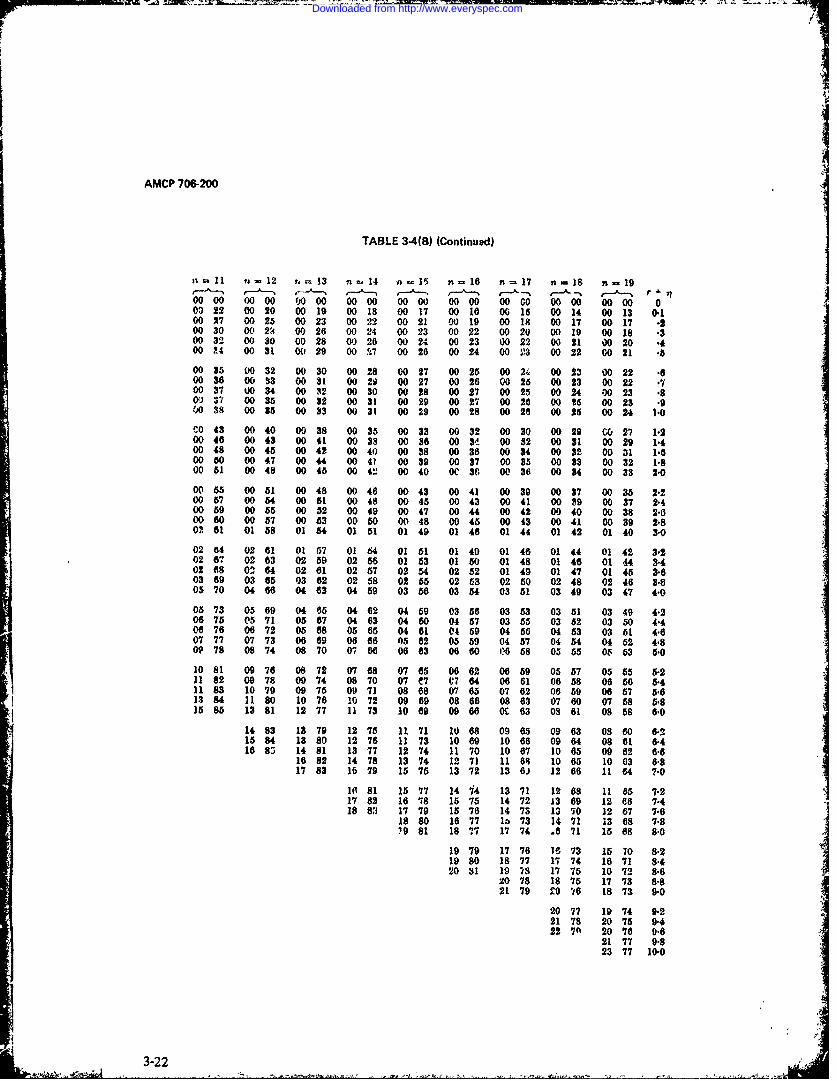
|I

AMCP 706-200

TABLE 3-4( 0) (Continuad)

n 11 ta= 12 1,=13 ,i= 14 a= 15 nf16 n=17 n-18 ,i 19

0000 0 00 (00 0 00 00 00 00 00 00 00 00 00 00 00 00 00D 22 00 20 00 19 00 IS 00 17 0010 0 015 00 14 00 13 0.100 27 00 25 00 23 00 22 00 21 00 19 0018 00 17 00 17 "200 30 00 23 00 26 00 24 O0 23 00 22 00 20 00 19 00 18 .300 32 00 30 00 28 00 26 00 24 00 23 00 22 00 21 00 20 .400 24 00 31 00 29 00 !7 00 26 00 24 00 23 00 22 00 21 .5

00 0 5 00 32 00 30 00 28 O0 27 00 25 00 24 00 23 00 22 .600 36 00 0 3 0031 0 20 00 27 O0 26 00 25 00 23 00 22 .700 37 00 34 00 S2 00 30 00 28 00 27 00 25 00 24 00 23 .80 37 00 35 00 32 00 31 00 29 00 27 00 20 00 25 00 23 .900 38 00 35 00 33 00 31 00 29 00 28 00 2 00 25 00 24 1-0

C0 43 00 40 00 38 00 35 00 33 00 32 00 30 00 29 C0 27 1.200 46 00 43 00 41 00 38 00 36 00 3,4 0 2 00 31 00 29 1.400 48 00 45 O0 42 00 40 00 38 00 36 0034 O0 32 00 31 1.600 60 00 47 0044 0 41 00 39 00 37 00 35 00 33 00 32 1.800 51 00 48 00 45 00 4,-, 00 40 OC 36 00 36 00 34 00 33 2.0

00 55 00 51 00 48 00 46 00 43 00 41 00 39 00 37 00 35 2.200 57 00 54 00 51 00 48 00 45 00 43 00 41 00 0 9 00 37 2.4O0 59 00 55 00 52 00 49 00 47 00 44 00 42 00 40 00 38 2-0O0 60 00 57 O0 53 00 50 00 48 00 45 0 03 00 41 00 39 2-802 61 01 58 01 4 01 51 01 49 01 48 01 44 01 42 01 40 3-0

02 64 02 61 01 57 01 64 01 51 01 49 01 46 0144 01 42 3-202 67 02 63 02 59 02 56 015 3 015 0 01 48 01 46 01 44 3-402 68 02 64 02 61 02 57 02 54 02 52 01 49 01 47 01 45 3-603 69 03 65 03 62 02 58 02 55 02 53 02 50 02 48 02 46 3-805 70 04 66 04 63 04 59 03 56 03 54 03 51 03 49 03 47 4-0

05 73 05 69 04 65 04 62 04 59 03 56 03 53 03 51 03 49 4.206 75 05 71 05 67 04 63 04 60 04 57 03 55 03 52 03 50 4-406 76 06 72 05 68 05 65 04 61 04 59 04 56 04 53 03 51 4-607 77 07 73 06 69 08 66 05 62 05 59 04 57 04 54 04 52 4-8OP 78 08 74 08 70 07 66 06 63 06 60 06 68 05 55 06 53 5-010 81 09 76 08 72 07 68 07 65 06 62 06 59 05 57 05 55 5-211 82 09 78 09 74 08 70 07 7 C7 64 06 61 06 58 06 56 5.411 83 10 79 09 75 09 71 08 68 07 65 07 62 06 59 06 57 5-613 84 11 80 10 76 10 72 09 69 08 66 08 63 07 60 07 58 5.815 85 13 81 12 77 11 73 10 69 09 66 O 63 08 61 08 58 6.0

14 83 13 79 12 75 11 71 10 68 09 65 09 63 08 60 6.215 84 13 80 12 76 11 73 10 69 10 66 09 64 08 61 6-416 85 14 81 13 77 12 74 11 70 10 67 10 85 09 62 6.6

16 82 14 78 13 74 12 71 11 88 10 65 10 63 6-817 83 16 79 15 75 13 72 13 6J 12 66 11 64 7-0

1A 81 15 77 14 74 13 71 12 68 11 65 7-217 82 16 18 16 75 14 72 13 69 12 FO 7.418 83 17 79 15 76 14 73 13 70 12 67 7-6

18 80 16 77 1* 73 14 71 13 68 7-8i9 81 18 77 17 74 .6 71 15 68 8.0

19 79 17 76 1 73 15 70 8-219 80 18 77 17 74 16 71 8-420 31 19 is 17 75 10 72 8.6

20 78 18 75 17 73 8-821 79 209 '16 18 73 9.0

20 77 19 74 9.221 78 20 75 9-422 7A 20 76 9.6

21 77 9-823 77 10-0

3-22


AMCP 706:200

TABLE 34(8) (Continued)

-20 A-It t ,22 A- 23 n- 24 Aim26 n-28 i,30 A-32

O0 00 O0 00 00 00 00 00 O0 00 00 00 00 00 00 00 00 00 00013 012 0 12 00 11 00 11 O0 10 O0 09 O0 09 00 08 0.100 16 00 15 00 14 00 14 00 13 00 12 00 12 00 11 00 10 .200 18 00 17 00 16 00 16 00 15 00 14 00 13 00 12 00 11 .300 19 00 18 00 17 00 17 00 16 00 15 00 14 00 13 00 12 .400 20 00 19 00 18 00 17 00 17 00 16 00 15 00 14 00 13 .5

00 21 00 20 00 19 0018 0 17 00 16 00 15 00 14 00 13 .600 21 00 20 00 20 00 19 0018 0 17 00 16 00 15 00 14 .700 22 00 21 00 20 00 19 00 19 00 17 00 16 00 15 00 14 .800 22 00 21 00 21 00 20 00 19 00 18 00 16 00 15 00 15 '600 23 00 22 00 21 00 20 00 19 00 18 00 1', 00 16 00 15 1.0

002 6 00 25 00 24 00 23 00 22 00 21 00 19 00 18 00 17 1.200 28 00 27 O0 26 00 25 00 24 00 22 00 21 00 20 00 18 1.400 29 00 2S 00 27 00 26 00 25 00 23 00 22 00 21 00 19 1.600 31 00 29 00 28 00 27 00 26 50 24 00 23 00 21 00 20 1.800 31 00 30 00 29 00 28 00 27 00 25 00 23 00 22 00 21 2.0

O0 34 00 32 00 31 00 30 00 29 00 27 00 25 00 24 0022 2.2O0 36 0) 34 00 33 00 32 00 30 00 28 00 27 00 25 00 24 2.400 37 00 35 O034 O0 33 00 31 00 29 00 27 O0 26 00 24 2.60038 0 36 00 35 00 34 00 32 00 30 00. 28 00 27 O0 25 2"801 39 01 37 01 36 01 34 01 33 01 31 01 29 01 27 00 26 3"0

01 41 01 39 01 37 01 _5 01 35 01 32 0130 o 0129 01 27 3'201 42 01 40 01 39 01 37 01 36 01 34 01 32 01 30 01 28 3-401 43 01 42 01 40 01 38 01 37 01 35 01 32 01 31 01 29 a602 44 02 42 01 41 01 39 013 8 01 35 013 3 01 31 013 0 3'802 45 02 43 02 42 02 40 02 3C 02 36 02 34 02 32 01 30 4-0

03 47 02 45 02 43 02 42 02 40 02 38 02 35 02 33 02 31 4'203 48 03 46 03 44 02 43 02 41 02 39 02 36 02 34 02 32 4'403 49 03 47 03 46 0344 03 42 02 40 02 37 02 35 02 33 4'604 51 04 48 03 46 03 45 03 43 03 40 03 38 02 36 02 34 4,805 51 .04 49 Ot 47 04 45 0444 03 41 03 38 03 46 03 34 5"0

05 52 05 50 04 49 04 47 04 45 04 42 03 40 03 37 03 35 5"205 54 05 52 05 50 04 48 04 46 04 43 04 41 03 38 03 36 6"406 85 05 63 05 51 05 49 05 47 0444 04 41 04 39 03 37 5-606 55 06 53 r6 51 05 50 05 48 05 45 04 42 04 40 04 38 5,807 56 07 54 07 52 06 50 06 49 05 45 05 43 05 40 04 38 6,0

08 659 08 57 07 55 07 53 07 51 06 48 06 45 05 43 05 40 6,510 81 10 59 09 57 09 55 08 53 08 50 07 47 07 44 06 42 7"011 64 11 62 10 60 10 58 09 56 08 52 08 49 07 47 07 44 7"514 66 13 64 12 61 12 59 11 57 10 54 09 51 09 48 08 45 8"015 69 14 65 13 64 13 62 12 60 11 56 10 53 09 50 09 48 8"5

17 70 16 68 15 66 15 64 14 62 13 58 12 65 11 52 10 49 9'019 73 18 71 17 68 16 66 15 64 14 60 13 57 12 54 11 51 9'521 75 20 72 19 70 18 68 17 66 16 62 14 58 13 55 12 52 10"023 77 21 75 20 72 19 70 18 68 17 64 15 60 14 57 13 54 105

2 76 22 74 21 72 20 69 18 65 17 62 16 58 15 56 11-0

24 76 23 74 21 72 19 68 18 64 17 60 15 57 11"525 75 24 73 21 69 20 65 18 62 17 59 12"0

25 75 23 71 21 67 19 64 18 61 12.527 76 25 72 22 68 2) 65 19 62 13'0

26 74 24 70 22 67 20 4 13"S

28 75 25 72 23 68 22 65 14.027 73 24 70 23 66 14.528 75 26 71 24 68 15

29 74 27 70 1630 73 17

,


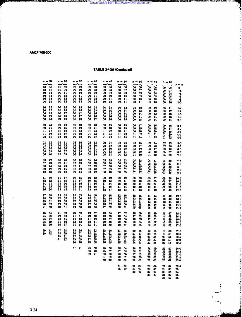
AMCP 706-200

TABLE 34(B) (Continued)

n-34 ,-36 -38 t.40 R..42 ,,-44 ,t-46 #-48 n--50

O0 00 00 00 00 00 00 00 00 00 00 00 00 00 00 00 00 00 00010 o0 09 00 09 00 08 00 08 00 07 00 0? 00 07 00 07 .200 12 00 11 00 10 00 10 O0 09 00 09 00 09 00 08 OG 08 .400 13 00 12 00 11 00 11 00 10 00 10 00 09 00 09 00 O .6C013 00 13 00 12 00 12 00 11, 00 11 00 10 00 10 00 09 *800 14 00 13 00 13 00 12 00 12 00 11 00 11 00 10 00 10 1.0

00 16 00 15 00 15 00 14 00 13 00 13 00 12 00 12 00 11 1-200 17 00 16 00 16 00 15 00 14 00 14 00 13 00 13 00 12 1.40018 0 17 00 1" 00 16 00 15 00 14 O0 14 00 13 00 13 1-600 19 00 18 00 17 00 16 00 16 00 15 O0 14 00 14 00 13 1-800 20 00 19 00 18 00 17 00 16 00 15 00 15 00 14 00 14 2-0

00 23 00 22 00 20 00 20 00 19 00 18 00 17 00 16 00 16 2'500 24 00 25 00 22 00 21 0020 00 19 00 18 00 18 00 17 3-001 27 01 26 01 24 01 23 01 22 00 21 00 20 00 20 00 19 3.501 29 01 27 01 26 01 25 01 24 01 23 01 .2 01 21 01 20 4-002 31 02 29 01 28 01 27 01 26 01 25 01 2* 01 23 01 22 4'5

03 32 02 31 02 29 02 28 02 27 02 26 02 25 02 24 02 23 5-003 35 03 33 03 32 03 30 02 29 02 28 02 27 02 26 02 25 5.504 36 04 34 04 33 03 31 03 30 03 29 03 2f% 03 27 03 26 6"005 38 04 37 04 35 04 33 04 32 03 31 03 29 03 28 03 27 6.506 40 05 38 06 36 05 35 05 33 04 32 04 30 04 29 04 28 7-0

06 42 06 40 06 38 06 36 05 35 05 33 05 32 04 31 04 30 7-507 43 07 41 07 39 06 38 06 36 06 35 05 33 05 32 05 31 8.008 45 08 43 07 41 07 39 07 38 06 36 06 35 06 33 05 32 809 47 09 44 08 42 08 40 07 39 07 37 07 36 06 34 06 33 9-b10 48 10 46 0944 08 42 08 40 08 39 07 37 07 36 07 35 9-5

11 50 11 47 10 45 10 43 09 42 09 40 08 38 08 37 08 36 10.012 52 11 49 11 47 10 45 10 43 09 41 09 40 08 38 08 37 10-514 53 13 50 12 48 11 46 1144 10 42 10 41 09 39 09 38 11.014 55 14 52 13 50 12 48 11 46 11 44 10 42 10 41 09 39 11-516 56 15 53 1t 51 13 49 12 47 12 45 11 43 11 42 10 40 12-0

17 58 15 55 15 53 14 50 13 48 12 46 12 45 11 43 11 42 12-518 59 17 56 16 54 15 51 14 49 13 47 13 46 12 44 12 43 13-019 61 18 58 17 55 16 53 15 51 14 49 13 47 13 45 12 44 13-520 62 19 59 18 56 17 54 16 52 15 50 14 48 14 46 13 45 14-021 63 20 61 19 58 18 56 17 53 16 61 15 49 14 48 14 46 14-5

23 64 21 62 20 59 19 57 1854 17 52 16 50 15 49 15 47 15.24 66 22 63 21 61 20 58 19 56 18 54 17 62 16 50 15 48 15.525 67 23 64 22 62 21 59 20 57 19 55 18 53 17 61 16 49 16-026 69 24 66 23 63 22 61 20 58 19 56 18 54 15 52 17 50 16-528 70 26 67 24 64 23 61 22 59 20 57 19 55 19 53 18 51 17-0

29 71 27 68 25 66 24 63 22 60 21 58 20 56 19 54 185 2 17-530 72 28 69 26 67 25 64 24 61 22 59 21 57 20 55 19 5,' 18.0

29 71 27 68 26 65 24 63 23 60 22 58 21 56 20 54 18.531 72 29 69 27 66 26 64 24 61 23 9 22 57 21 55 19.0

30 70 28 68 26 65 25 63 24 6t 23 58 22 66 19-5

31 71 20 68 28 66 26 64 25 61 24 59 23 57 20-030 70 26 67 27 65 26 62 24 60 23 58 20-532 71 30 68 28 66 27 63 26 61 24 59 21-0

31 69 29 67 28 65 26 62 25 60 21-532 70 30 68 29 65 27 63 20 61 22-0

31 69 29 67 28 64 27 62 22-532 70 31 67 29 65 2A 63 23

33 69 31 67 30 65 2433 69 31 67 25

33 66 26

3-24


AMCP 706-200

C -a-confidence level -

R - one-sided e-conf'dence level ona-r~liabilit

"4

t4510 20___ 50 20 50

Figure 3-2. Special Case for No Failures in N Trials and C = RL

All the s-confidence intervals are discouraging- 3-7.2 EXAMPLE NO. 2ly broad. Statistics shows us how little weknow from the experimenit. Thirty tests were run, there were no

failures. Find the low&r I-sided s-confidencelimit C on the s-reliability R such that C = R.

If N is too large for Table 3-2, use Fig. 3-1 A = 30/30 =1.or use the Poisson appro.dmation. Ref. 1 canbe used to find the inside and outside limits Enter Fig. 3-2 with N = 30; thenby setting i? 1 and 0 and solving for the I -C= 1 -R =0.08 = 1 -0.92;appropriate value of p. Cenf I R >' 0.921 > 92%.

- 345


AM"P 706.20

REFERENCES

1. AMCP 706-109, Engineering Desigt Hand- 5. W. J. Conover, Practical Nonparametricbook, Tables of the Cumulative Binomial Statistics, John Wiley & Sons, New York,Probabilities. 1973.

Probability and 6. N. R. Mann, "Approximately OptimalSat. Miller and . E. Freund, Pili, n Confidence Bounds on Series- and Parallel-Statistics for Engineers, Prentice-Hall, N.J., System Reliability for Systems with1965. Binomial Subsystem Data", IEEE Trans.

Reliability. Vol. R23-5, Dec. 1974.

3. Harvard Computation Laboratory, Tables

of the Cumdative Binomial Probability 7. Handbook of Reliabitlty Engineering,Distribution, Harvard Univ. Press, 1955. NAVWFPS 00-65-502, Bureau of Naval

Weapons, I June 1964.

4. Abramowitz and Stegun, Eds., Handbook t. C. Blyth and D. Hutchinson, "Table ofof Mathematical Functon., AMS55, NBS, Neyman-shortest Unbiased ConfidenceUSGPO, June 1964 with subsequent Intervals for the Binomial Parameter",corrected printings. Biometrika, Vol. 47, pp. 381-391 (1960).

.. 3-26 i


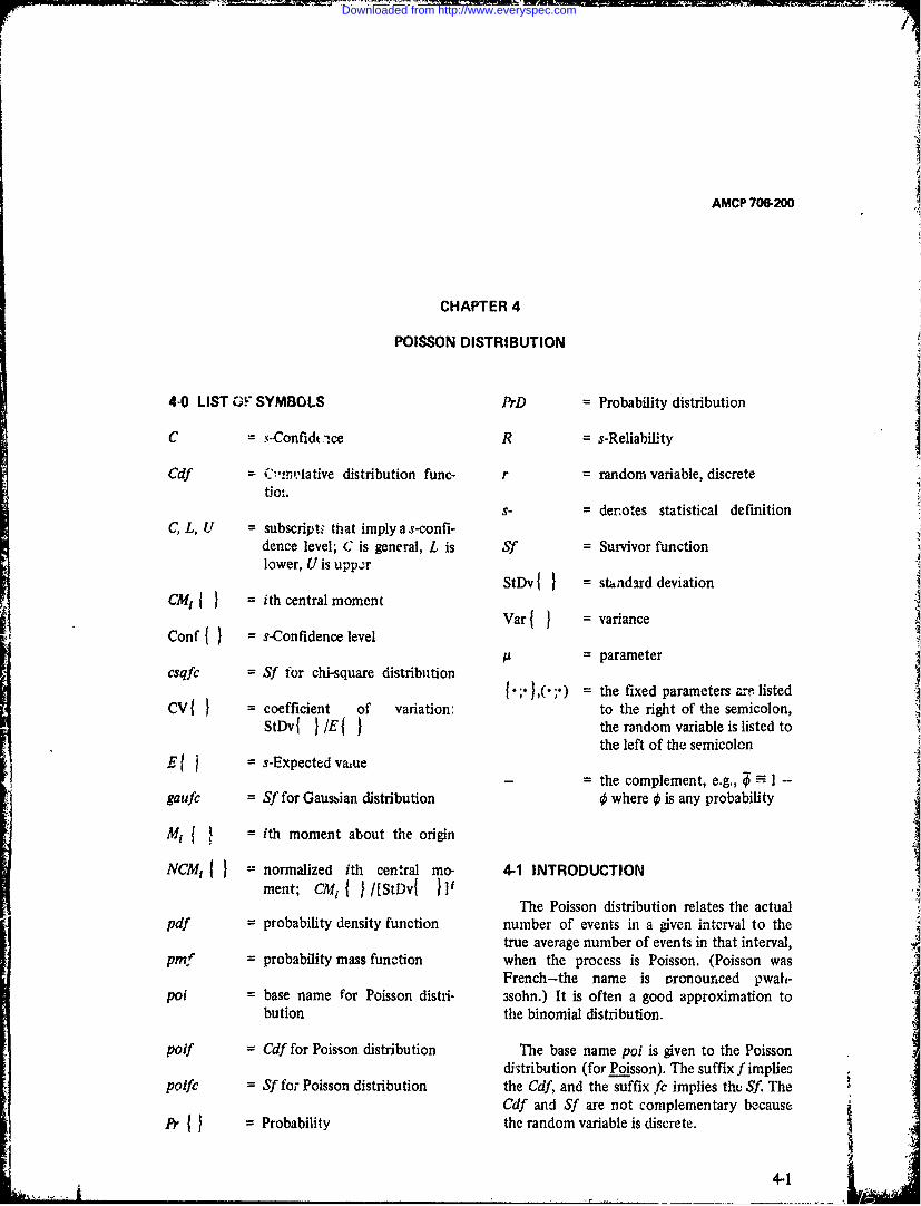
AMCP 706-200

CHAPTER 4

POISSON DISTRIBUTION

4-0 LIST GF SYMBOLS PrD = Probability distribution

C = s-Confidt 'ce R = s-Reliability

Cdf = ( .'tlative distribution func- r = random variable, discretetior.

s- = derotes statistical definitionC, L, U subscript- that imply a s-confi-

dence level; C is general, L is Sf = Survivor functionlower, U is upp. r

StDv } = standard deviationCM } = ith central moment

Var{ varianceConf { s-Confidence level

pt = parametercsqfc = Sf for chi-square distribution

; },(;.) = the fixed parameters arf listedCV{ - coefficient of variation: to the right of the semicolon,

StDv{ J/E{ I the random variable is listed tothe left of the semicolon

Ef = s-Expected vaue- the complement, e.g., 1 -

gaufc = Sf for Gaussian distribution 4 where is any probability

M, { = ith moment about the origin

NCM } = normalized ith central mo- 4-1 INTRODUCTIONment; CM, /[StDv{ Ili

The Poisson distribution relates the actualpdf = probability density function number of events in a given interval to the

true average number of events in that interval,pmf = probability mass function when the process is Poisson. (Poisson was

French-the name is pronounced pwah-poi = base name for Poisson distri- 3sohn.) It is often a good approximation to

bution the binomial distribution. Ipoif = Cdf for Poisson distribution The base name poi is given to the Poisson

ditribution (for Poisson). The suffix fimpliespotfc = Sf for Poisson distribution the Cdf, and the suffix fc implies thtu Sf. The

Cd! and Sf are not complementary becausePr = Probability the random variable is discrete.

.... 4-1


AMCP 706.200

4-2 FORMULAS Eq. 4-5 relates the Poisson and chi-squaredistributions.

I = Poisson parameter (true average nun-ber of events in the interval) p t poifgr; p) = csqfc[2p; 2(r + 1) (4-5a)

r = random variable, r = 0. 1, 2, ... poifc(r; A) = csqf(2pu, 2r) (4-5b)

(actual number of events in theinterval) For reasonably large ' (say v > 5), Eq. &-a is

sufficiently accurate.

pmf {r; I A) = exp( - pA)prfr! (4-I) 2

p 2Q +A\9p/ \9v')/2] (4-6)

Cdf {r;p) = poif(r;tp) A exp(-u)pii! where=0

(4-2) csqfc(xQ; v) =

Sf{r; 14 = poifc(r; IA) = exp( -p)uili!ifr

(4-3) gaufc(zQ) Q

E{r,;p} = Figure 4-1 is a graph of the poif from Eq. 4-2.

StDp{r, A) = A112 4-4 PARAMETER ESTIMATION

CV{r,t} = -1/2 The estimator

CM 3 {r, IA} = A _= r (4-7)

NCM3(r, 1) -1/2 is unbiased and maximum likelihood. Ifr = 0,it is esthetically displeasing, although still

Table 4-1 shows a few examples of the quite true. Very often (when r = 0) aPoisson pm. If a Poisson process has a rate X s-confidence limit is used in place of A usually(events per unit measure of r). then corresponding to about 50% s-confidence

I=(level. If pA = Xr, and X is to be estimated,= (4-4) mert.ly divide all estimates and s-confidence

limits for p by r.4-3 TABLES AND CURVES

s-Confidence statements are more difficultThe pmf is easily calculated and so is rarely for discrete random variables than for

tabulated; Ref. I (Table 39 and Sec. 21) gives continuous random variables. Chapter 12some tables of individual terms. The Cdf is discusses the matter thoroughly. The usualavailable in tables such as Ref, 1 (Table 7 and s-confidence intervals for p are of the formsSec. 3), Ref. 2 (Table V and p. 24), Ref. 3(Table 26.7), Ref. 4, and almost any Conf(p < AL) 5 CL (4-8a)statistics!probability/quality control text-book. Conf (A < p }U -CU (4-8b)

4-2

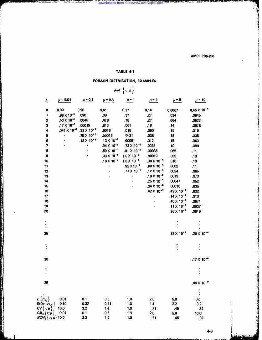
AMCP 706-200

TABLE 4-1

POISSON DISTRIBUTION, EXAMPLES

pmf {r;,p

r ,..0.01 p 0.1 p - 0-5 p=2 105 A 110

0 0.99 0.90 0.61 0.37 0.14 0.0067 0.45 X 10 - 4

X .99 x 10"1 .090 .30 .37 .27 .034 .00452 .50 X 10 4 .0045 .)76 .18 .27 .084 .00233 .17 X 10"6 .00015 .013 .061 .18 .14 .00764 .541X 10- .38X 10-' .0016 .015 .090 .18 .0195 .75 X 10- 7 .00016 1vt31 .036 .18 .0386 .13 X 10-8 13 X 10 "4 .00051 .012 .15 .0637 . .94 X 10- .73 X i0 - .0034 .10 .0908 .59 X 10- 7 .91 X 10- 1 .00086 .065 .119 .33X 10- 8 1.0X 10- 6 .00019 .036 .13

10 .16X 10- 9 1.0X 10- 7 .38X 10- 4 .018 .1311 .92 X 10-5 .69X 10- 5 .0082 .1112 .77 X 10 "9 .12X 10 5s .0034 .09513 • .18X 10"6 .0013 .07314 .25 X 10- 7 .00047 .05215 • .34X 10- 8 .00016 .03516 42 X 10 - .49 X 10- 4 .02217 • .14 X 10- 4 .01318 * .40 X 10- 1 .007119 * .11 X 10"1 .003720 .26 X 10- 6 .0019

25 .13 X 10- 9 .29 X 10- 4

30 .17 X 10'

35 .44 X 10- 9

E{r;/} 0.01 0.1 0.5 1.0 2.0 5.0 10.0StDv { r;/} 0.10 0.32 0.71 1.0 1.4 2.2 3.2CV r;/4 10.0 3.2 1.4 1.0 .71 .45 .32CM3 {r; , 0.01 0.1 0.5 1 0 2.0 5.0 10.0NCM 3 I ;,A 10.0 3.2 1.4 1.0 .71 .45 .32

4-3


AMCP 706-200

00

00

000.

"ooLO~

00,

00/0

4-44-~~

4w -"4~~

-_________________vi I__ 1 1


AMCP 70-200

Conf ( -L 5 <- PuS >: CU - CL (4-8c) Conf(pi < p <4 5 CU - CL (4-9c)

where /L and Pu are defined by where pi and p& are defined by

Cu = I - poif(r; Pu) = csqf(2pU; 2r + 2) Cu = poifc (r; I) = csqf(2pi,; 2r), r * 0.

CL = poifc(r; UL )csqf(2pUL ; 20, r * 0 ju, = 0, r = 0.

gl = 0, r = 0. CL = 1 - poif(r; p)= cqf(2, ; 2r + 2)

In this torm, CL is usually small (say 5%) and In this form, as in Eq. 4-8, CL is usually small

Cu is usually large (say 955). Notation for (say 5%), and CU is usually large (say 95%).s-confidence statements is nut at all standard; AL and pi will be inside the interval (uL, Mu)

so particular attention must be paid to the (for r * 0). Table 6-1 and Fig. 4-1 are usefulexample forms, Table 6-1 and Fig. 4-1 are for this type of s-confidence statement also.useful for this type ofs-confidence statement.

Example. In a 1000-hr life test, there are 3Chapter 12 shows that s-confidence state- failures. Find the 5% and 95% 1-sided

ments for p can also be of the forms s-confidence limits on the true mean (for the

Conf{fL: <j ) a CL (4-9a) 1000 hr) p; also make the associated 2-sideds-confidence statement. Find the correspond-

Conf{ p: <I CU (4-9b) ing limits on the failure rate X(X = p1!000-hr).

Procedure Example

1. Find yu,pt from Eq. 4-8 and Table 6-1. 1. csqf(15.5;8)=0.95PUv = 7.75

csqf(1.64;6) = 0.05

PL = 0.82

2. FindPt,,Mj from Eq. 4-9 and Table 6-1. 2. csqf(12.6;6) 0.95p =6.3csqj (2.73;8) 0.05

1.37

3. Make the s-confidence statements from 3. Conf p 4 0.82 < 5%

Steps I and 2. Conf M < 7.75 > 95%Conf 0.82 <pt 7. 7 5 Y90%Conf p<1.37} >5%Conf Ag:6.3 }<95%Conf 1.37'<p<6.3 ) < 90%

4. Make the corresponding s-confidence 4. Conf X < 0.82/1000-hr } ' 5%statements about X. Conf , -7.8/1000-hr I < 95%

Conf 0.82/1000-hr < X < 7.8/1000-hr } 90%Conf X < 1.37/1000-hr} 5%Coif X < 6.3/1000-hr I <95%Conf 1.37/1000-hi < X <6.3/1000-hr} <90%

~*4- 4

AMCP 706-200

The statements about X, and p are dic,'our- where 7? is a random number from theagingly wide. This is due to the small number uniform distribution 0 4 n < 1. When i? = 0,of failures. JAL= 1L and 4 = pjU. If 17= I (consider the

!east upper bound of i7), AL = sj and IAV tr -4-5 RANDOMIZED EXACT s-CONFI-

DENCE INTERVALS If ,cial tables are not available for p7 andju use Eqs. 3-8 and 3-9 with Table 6-1 to

Traditionally, the s-confience statement find puq L and pt,, pi. Then use Eq. 3-10 to(Eq. 4-8)-worst case-is made to be on the find , ,* by an iterative process.safe side. Instead of always choosing thisworst case, one can get exact s-confidence A handy random number generator is alimits by randomly choosing a value between coin, flipped several times. Decide whetherPiL and pi, or between uu and pt. There is heads is to be 0 or 1; tails is the reverse. Thennothing to lose and everything to gain by this multiply the resu't of the first flip by 0.5, theprocedure because it means not always second flip by 0.25, the third flip by 0.125,choosing the wor-t.possible case. etc. (the numbers are 2"fliP), as fine as

desired. Then add the numbers. Usually 5 or 6The equations to give the randomized flips give a sufficiently continuous random

limits are variable. (For example, heads is 0, tails is 1,the sequence is H, T, H, H, T, H. Add 0.25 +

poifcr;p)-CL 0.03125 = 0.28125; truncate to 0.281 for

exp(- "t)('4Y /r! convenience.)Example. Use the data and solution from

poifc(r; P7) - CL the example in par. 4-4. Find the randomited___poifcr;/_)_- ____exact 5% and 95% s-confidence limits.

poifc(r; p7) - poifc(r + I; p7) Suppose q = 0.281 (the random number inthe paragraph immediately above). Since r = 3

- L - poif(r - 1; pt) is not very large, direct calculation of

poif(r; p)- poif(r - 1; pf)poif (r; p) will be used. (This is reasonable onthe electronic calculators with eiigineeringfunctions. An HP-45 was used for this

(unless r = 0, and q7 _ L; example.)

then use p7 = 0) (4-1Oa) The forms of Eq. 4-10 suitable for direct

calculation with interpolation are

p oiftr;,4 )ju fL- poif(r - 1; Lx ?)poif~r; IS) -u h (XL) -j p-xr -r =

=exp(-t)(p)r! exp(.- -XL Lr

C - poifc(r + 1; At) (unless r = 0, and 17< ,?

poifc(r; p) -poifc(r + 1; P) then use a7 = 0) (4-11 a)

poff(r; p)) - pof(r; xu) - Cupoif(r; pt) - poif(r - 1; p.A ) fU(xU) exp( x )x =r!

(unless r 0, and 17 CU, (unless r =0, and 17 Cu;

thenusePit = O) (4-10b) then use pl = 0). 1 lb)

4-6 - i .. a. v. .

AMCP 706200

The solution to Eq. 4-11 a is XL = u. The where x and x+ are the smaller and largersolution to Eq. 4-1l b is xu = &A?. values of x, respectively; and f -f (x_) and

f+ =f(x).The formula for linear interpolation is

x.f+ - x+f. (4-12)f- f-


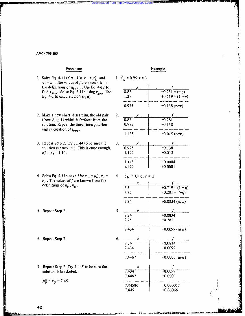
AMCP 706-200

Procedure Example

1. SolveEq. 4-11a firs(. Usex =.,and . C. 0.95,r 3X+ = ML. The values off are known fromthe definitions of pj, gL .Use Eq. 4-12 to x .ffind xnew , Solve Eq. 3-11 a using Xnew . Use 0.82 -0 281 = (-r)E4. 4-2 to calculate poi'(r; p). 1.37 +0.719 = (1 - 7?)

0.975 -0.138 (new)

2. Make a new chart, discarding the old pair 2. x f_ , _

(from Step 1) which is farthest from the 0.82 -0.281solution. Repeat the linear interpo;.tion 0.975 -O.138and calculation of fnew. - - - - -

1.125 -0.015 (new)

3. Repeat Step 2. Try 1. 144 to be sure the 3. x f_ _

solution is bracketed. This is close enough, 0.975 -0.138a* =x = 1. 14, 1.125 I --0.015

1.143 - -0.0004

1.144 I +0.0001

4. Solve Eq. 4-11 b next. Use x - ib, x+= 4. eu = 0.05, r = 3/AU. The values of f are known from the fdefinitions of pb, Pt. 6.3 +0.719 (1 -r?)

7.75 -0.281 = (--q)

7.31 7 +0.0834 (new)

5. Repeat Step 2. 5. x ___

7.34 +0.08347.75 -0.281

7.434 +0.0099 (new)

6. Repeat Step 2. 6. xf__J7.34 +9.08347.434 +0.0099

7.4467 -0.0007 (new)

7. Repeat Step 2. Try 7.445 to be sure the x fsolution is bracketed. 7.434 +0.0099

7.4467 -0.000"U.U =xU 7.45. 7.44586 -0.000057

7.445 0.00066

S4-8


AIMCP 706-200

The randomized exact s-confidence statements excep, in the narrow statistical sense statdare for Table 4-2.

Conf p .l.14 5%Conf p 7.45 = 95% 4-8 CHOOSING As-CONFIDENCE LEVELConf 1.14<p<7.45I =90%

Choosing an appropriate s-confidence level"The corresponding statements for X are is always troublesome. Thiere is obviously

little point in having a very high s-confidenceConf { X < 1.14/1 000-hr' = 5% that the s-reliability is very low, or a very lowConf ) < 7.45/A000-hr 95% s-confidence that the s-reliability is very high.Conf 1.14/1000-hr< ),< 7.45/i000-hr} A reasonaLle compromise is to choose a

= 90%. s-confidence level that is approximately thepo.nt estimate of the s-reliability; for r = 0 the

Table 4-2 lists randomized 2-sided s-confi- s-confidence level can be chosen to be equaldence limits that have special statistical to the lower s-confidence limit 09 s-reliability.properties. They are not equal-tailed -confi-dence limits; they cannot be tsed separatelyfor upper and lower s-confide,.cc limits. See 4-7 iXAMPLE, LIFE TEST RESULTSRef. 6 for a more completv :ussio .. Ingeneral, the s-confidence iim ts n Table 4-2 On a life test there were no failures. Findwill be different from those calculated using 1%, 99%, ]-sided s-confidence intervals for p,the methocs in this chapt.r. It is difficult to and then fnd the associated 2-sided s-confi-say that one set is better than the other dence inte-'al.

IiI2

I

AMCP 706.200

TABLE 4-2

NEYMAN-SHORTEST UNBIASED 95% AND 9% s-CONFIDENCE INTERVALS FOR p(ADAPTED FROM Ref. 6)

9, + ; 99% + 99';95% 9%95

not 0 3 0 36 05 1 O 13$ ,.1 40 1!, 1.9 4.2 31 0 1) 9 37 h 62 3311t 102 4019 30366

113 0 U 311 1 4 3 1,; 13 41 133 3'0 itI3 11 II iI 37 1!I . I 1117 it4 41 162 3.1 161.

01 V 0 0 13 Il 40 8 86 .4 )I1 V9. 41. I33 3,1 11

006 0 03 0 21 41 08 8 5 08 43 185 32 18-4." 1 0 1 23 42 0 ,5 3 i7 443 60.1 3.3314

0 1 4 I 214 43 1 335 11 09 4 3. 13396

03 0 2 00 46 330 063 30 , 7 60It 8 I 5 4 .0 13 5 11i, 9 45 1018 3.4 1-7

III 0 ,3 ,7 45 30 9, 5 11 101 46 19 '8 5 1

012 0 I3t 0 2 4 6 I 1 96 06 I 102 41171 1 06.1S 1.3 o 3 47 I 1 07 1!, 104 4817. 3 :1, 0It, 0 1 5 0 3 2 48 1 2 9A4 12 L' t0 5 1 173 3-1 US8

1', 0 16 n '33 49 13 o 0 ,7 123 10.8 5-t S160 4'o 210•20 0 137 0 3.4 50 3 4 I311. I 12-4 3110 53 18. 4.1 21.2

025 0 2'0 0 36 51 1 4 10,3 08 326 I1.2 6.4 165 421 21'630 0 36 5,2 1.4 114 . 129 334 50 18,1 43 21.35 0 24 0 40 63 35 Io6 '13 30 16 97 133 4 4 223 441) 0 29 c 4 A 4 15 0 -9 132 118 56 13 .6 22-445 Q 2.0 0 43 55 1.6 109 0 134 120 60 19 46 22-4

060 0 2.8 0 44 A,6 13 330 30 3-5 322 6-190 49 22655 0 29 0 4. t, 7 3 112 I.11 33 124 63 20I .0 3-f0 0 3.0 0 40 .56 36 333 31 3 3.5 1 0-4 20.3 51 21165 0 30 0 47 so IV 114 12 3139 31 206 5.2 3•10 0 331 0 4'7 60 20 11.5 13 141) 130 068 06 84 24-0

0-75 0 33. 0 4'6 03-1 2-0 117 13 142 112 6.0 21.1 55 34.3.90 0 3.3 0 4. 62 21 33! ,13 144 134 70 21.4 56 24-4as 0 3.3 0 4.1) 82 2.1 1.0 ,14 ,140 136 7.L1 21. 57 149 .

90 0 34 0 I0 64 22 122 14 147 1338 7.3 2135 5*.9 15.1Iit 0 36 0 5.1 05 22 323 1.4 149 I 1.O 76 22.1 60 253

3 0 1.: 0 .6 66 23 1".4 3'5 390 342 76 224 6"! 26"32 0 41 0 A0 67 24 12.6 3651 I4.4 77 22 0 326-0

13 0 43 0 03 68 24 12.7 1.6 153 14.0 7.9 22 9 0.4 26214 0 465 0 6 4 639 25 126 17 154 ;4 8,0 231 65 26-415 0 47 0 06 70 26 32 t 8 55 353 82 23.3 6.7 26-7

16 4-9 0 6.7 7.1 27 131 18 157 152 9.3 238 6-8 27'017 50 0 (19 7'2 27 13,2 19 1. , 154 69 23-9 09 273

;; 52 0 70 73 28 13'4 139 3310 350 66 243 73 2739 3 93 0 71 74 28 135 19 1612 139 6'6 24.4 72 T7.420 0 54 0 72 75 29 137 20 161.4 I00 10 24.0 7.4 1"

23 0 96 5 ) 716 76 29 138 20 135 162 931 24.0 7"5 28"22 .59.9 0 76 77 30 130 231 3 3014 932 21 7'6 26623 'I I1 0 63 76 33 340 22 311 16C 94 254 7.7 2624 1 0 2 11 831 7.9 92 141 22 168 36 9-5 25.6 79 9.3

. 64 0 34 60 3-3 14,3 23 17,1 L70 97 2. 63 29 3

26 0.1 65 0 86 8.1 3.3 14.4 24 132 172 9.3 26.1 A2 11427 .2 81 0 #1 62 34 14.0 24 17.3 174 100 20'4 63 29.628 .2 G6 0 88 63 34 147 2-4 17r 170 102 20.0 34 30-320 .9 09 01 00 84 3, 141 25 177 17.8 103 20.6 66 0430 4 7.3 1 9 1 6 6 30 0 25 178 363 105 71 88 30 64

31 04 73 02 0.4 8'6 36 15'1 A3 17.9 1R'2 10.6 27.3 6 89 206l32 4 75 2 036 7 37 73 27 16. 364 306 276 90 33.333 4 7fl -2 q8 88 38 54 27 132 3 303 27, 921 3.534 .5 78 .2 100 80 38 15.5 28 1111 18'8 31.1 281 93 31.735 .9 so -2 102 3o 3.9 135n 20 364 10.0 131.3 2$3 9.5 36-

Notes:1. The pairs of figures under each s-confidence heading are lower and upper s-confidence limits for p.2. Notation:

P = Poisson pararriete,"r - number of events observed in cample17 - random number from the uniform distribution on (0, 1),.4

3. For tabular zonvenience, r, ? is listed as r + i7.

4-10


iI

AMCP 706-200


95% 99% 95% 99% 95% 99%r + ?I ..A_ r + v? -*-- r + 11 r-%

66 69 105 64 112 141 119 165 112 173 196 169 224 162 23487 70 106 65 113 142 119 166 113 174 197 170 225 163 23588 70 107 60 114 343 120 167 114 176 198 171 226 IJ3 23689 71 108 66 115 144 121 168 115 177 199 172 227 164 23790 72 109 67 116 145 122 169 116 178 200 173 228 165 238

91 73 110 68 117 146 123 170 117 179 201 174 230 160 23992 74 112 60 118 147 124 172 117 180 202 175 231 167 24093 75 113 70 120 148 125 173 118 181 203 176 232 168 24194 76 114 71 121 149 126 174 119 182 204 177 233 169 24295 77 115 72 122 180 127 175 120 183 205 178 234 170 244

96 78 1136 2 123 181 128 176 121 184 206 179 235 171 24507 78 117 73 124 162 129 177 122 185 207 180 236 172 24698 7) 118 74 25 153 130 178 ;23 187 208 181 237 173 24799 80 119 75 126 154 130 179 124 188 209 181 238 173 248100 81 120 76 127 155 131 190 125 169 210 182 239 174 249

101 82 121 77 129 156 132 181 126 190 211 183 240 175 250102 83 123 78 130 157 133 182 126 191 212 184 241 176 251103 84 124 79 131 158 )34 183 127 192 213 185 242 177 252104 85 125 o9 132 159 135 184 128 193 214 186 243 178 253105 80 126 80 133 160 136 186 129 194 215 187 245 179 254

106 87 127 81 134 101 137 187 130 195 2:5 188 246 180 256107 88 128 S2 135 162 13b 188 131 196 217 189 247 181 257108 88 129 63 136 163 139 189 132 198 218 190 248 182 258109 89 130 84 138 164 140 190 133 399 219 Vi 249 163 252110 90 131 85 139 165 141 191 134 200 220 192 250 84 260

111 91 132 86 140 166 142 192 135 201 221 193 251 184 261112 92 134 86 141 167 142 193 135 202 222 194 252 185 262111 03 135 87 142 168 143 194 136 203 223 195 253 I86 263114 94 136 88 143 169 144 195 137 204 224 195 284 187 264115 95 337 89 144 170 145 106 138 205 225 196 256 188 265

116 96 138 90 145 171 146 197 139 206 226 197 256 189 266117 97 139 91 147 172 147 198 140 207 227 198 257 190 268118 98 140 92 148 173 148 200 141 209 228 199 258 191 269119 98 141 93 149 174 149 201 142 210 229 200 259 192 270120 99 142 93 150 175 160 202 143 211 230 201 260 193 271

121 100 143 91 151 176 151 203 144 212 231 202 262 194 272122 101 144 95 152 177 152 204 144 213 232 203 263 194 273123 102 146 96 153 178 153 205 145 214 233 204 204 195 274124 103 147 97 154 179 154 206 143 215 334 205 265 196 275125 104 148 98 150 180 154 207 14 216 235 206 266 197 276

126 105 349 99 157 181 155 108 148 217 236 207 207 198 277127 100 150 100 158 182 156 209 149 218 237 208 208 199 278128 107 111 101 159 183 157 210 150 220 238 209 269 200 279129 108 12 1 10 10 134 158 211 151 212 239 209 270 201 281130 108 153 102 161 185 159 212 :52 222 240 210 211 202 282

131 109 154 103 162 386 60 213 153 223 241 211 272 203 283132 110 155 104 103 137 J1 215 153 225 242 212 213 204 284133 111 156 105 164 188 162 216 154 225 243 213 274 205 288134 112 157 100 16 189 163 217 155 226 244 214 275 205 286135 113 159 107 167 190 164 218 156 227 245 215 276 206 287

136 114 1GO 108 In8 191 105 219 157 228 246 216 278 207 288137 11' 101 109 l09 192 106 220 158 229 247 217 279 208 280138 036 162 109 170 193 167 221 159 230 248 218 280 209 290'39 117 103 110 171 194 "7 222 160 232 249 219 281 210 291

140 118 164 111 172 19b 1bb 223 381 233 2a0 220 282 211 292

4-11


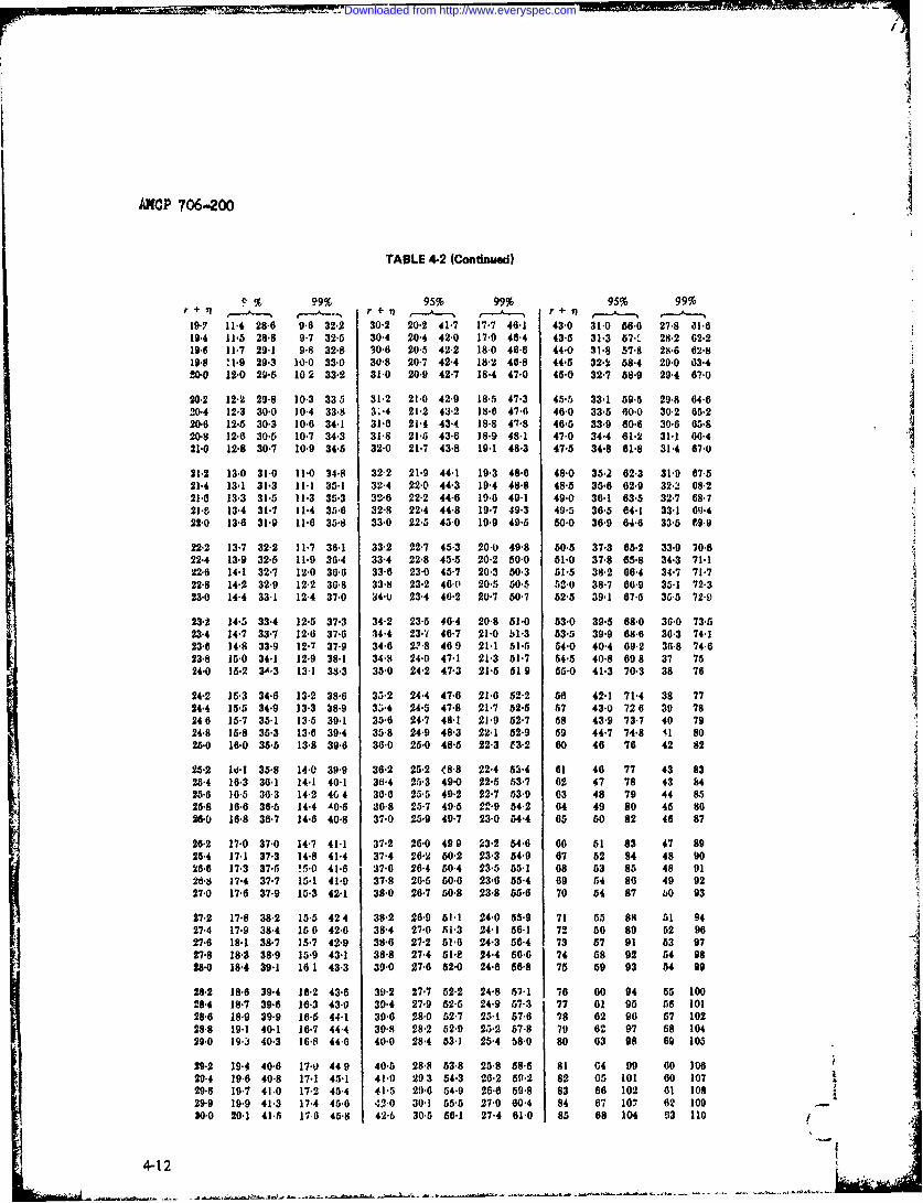
ANWP 706-200


% 99% 95% 99% 9s% 99%r + l r- * r + ia r-, r+ n

19 P 11,4 28-6 9.6 32,2 30-2 20.2 41.7 17.7 46-1 43.0 31.0 566 27,8 ali619.4 11-5 28-8 9,7 325 30-4 20-4 42-0 17-9 46-4 43.5 31-3 57- 28-2 62-219.6 11-7 29.1 9,8 32.8 30.6 20,5 42-2 18.0 46-6 44-0 31.8 57-8 28-6 62-819.8 11.9 29.3 10-0 33-0 30.8 20.7 42-4 18-2 46.8 44-5 32-2 58-4 29-0 03-420.0 12-0 29-5 10 2 33.2 31.0 20-9 42-7 18-4 47-0 45,0 32-7 88-9 29-4 7-0

20.2 12-2 29-8 10.3 335 31-2 21-0 42-9 18,5 47-3 45,5 33-1 59-5 29-8 04-620-4 12-3 30-0 10.4 33-8 3;.4 21-2 43-2 18-60 47.6 46-0 33-5 600 30-2 65-220.6 12-5 30-3 10-6 34.1 31-0 21-4 43-4 18-8 47-8 46-5 33-9 60-6 30-6 65-820-8 12-6 30-5 10-7 34-3 31-8 21- 43-6 18.9 48-1 47-0 34-4 61-2 31-1 66-421-0 12-8 30-7 10-9 34-5 32-0 21-7 43-8 19-1 48-3 47.5 34-8 61-8 31-4 67-0

21-2 13-0 31-0 11-0 34-8 32,2 21-9 44-1 19.3 48-6 48-0 35-2 62-3 31.9 67.521-4 13-1 31-3 11-1 35-1 32-4 22-0 44-3 19-4 48-8 48-0 35-6 62-9 32- 08-221-0 13-3 31-5 11-3 35-3 32-6 22-2 44-6 19-6 49-1 49-0 36-1 63-5 32-7 68-721-8 13-4 31-7 11-4 35-0 32-8 22-4 44-8 19-7 49-3 49-5 36-5 e4-1 33-1 69-422-0 13-6 31-9 11-0 35-8 33-0 22-5 45-0 19-9 49.5 50-0 36-9 64-6 33-5 69-9

22-2 13-7 32-2 11-7 36-1 33-2 22-7 45-3 20-0 49-8 50-5 37-3 65-2 33-9 70-622-4 13-9 32-5 11-9 30-4 33-4 22-8 45-5 20-2 50-0 51-0 37-8 65-8 34.3 71-122-6 14-1 32-7 12-0 30-0 33-6 23-0 45-7 20-3 50-3 51-5 38-2 06-4 34-7 71-722-8 14-2 32-9 12-2 30-8 33-8 23-2 46.0( 20-5 50- 52-0 38-7 60.9 35-1 72-323-0 14-4 33-1 12-4 37-0 34-0 23.4 40-2 20-7 50-7 62-5 39-1 67-5 35.5 72-0

23-2 14-5 33-4 12-5 37-3 34-2 23-5 46-4 20-8 51-0 53-0 39-5 68.0 36.0 73-523-4 14-7 33-7 12-6 37-0 34-4 23-/ 46-7 21-0 h1-3 83-5 39-9 68-6 36-3 74-123-6 14-8 33-9 12.7 37-9 34.6 2?-8 469 21-1 51-5 64-0 40-4 69-2 36.8 74-623-8 15-0 34-1 12-9 38-1 34-8 24-0 47-1 21-3 61-7 64-5 40-8 698 37 7524-0 15-2 32A3 13-1 38-3 35-0 24-2 47-3 21-5 61 9 55-0 41-3 70-3 38 76

24-2 15-3 34-6 13-2 38-0 35-2 24-4 47-6 21.0 52-2 66 42-1 71-4 38 7724-4 15-5 34-9 13-3 38-9 35-4 24-5 47-8 21-7 52-5 57 43-0 72 6 39 78246 15-7 35-1 13-5 39-1 35-6 24-7 48-1 21-9 52-7 58 43-9 73.7 40 7924.8 15-8 35-3 13-6 39-4 35-8 24-9 48-3 22-1 52-9 59 44-7 74-8 ,1 8025-0 16-0 35-5 13-8 39-6 36-0 25-0 48-5 22-3 f3-2 60 48 76 42 82

25-2 14-I 35-8 14-0 39-9 36-2 25-2 t8-8 22-4 53-4 61 46 77 43 8325-4 16-3 36-1 14-1 40-1 36-4 25-3 49-0 22.5 53-7 02 47 78 43 8425.6 16.5 36.3 14-2 404 36-0 25-5 49-2 22-7 53-9 63 48 79 44 8525-8 16-6 36-5 14-4 AO.6 36.8 25-7 49.5 22-9 54-2 64 49 80 45 802-0 16-8 36-7 14-6 40-8 37-0 25-9 49.7 23-0 54-4 65 50 82 46 87

26-2 17-0 37-0 14-7 41-1 37-2 26-0 499 23-2 54-6 66 51 83 47 8926-4 17-1 37-3 14-8 41-4 37-4 26-2 50-2 23-3 54-9 67 52 94 48 90266 17-3 37-5 !5.0 41-6 37-0 26-4 50-4 23-5 55-1 68 53 85 48 9126-8 17-4 37-7 15-1 41-9 37-8 20-5 50.6 23-6 55-4 69 5-4 86 49 9227-0 17-6 37-9 15-3 42-1 38-0 26-7 50-8 23-8 55-6 70 54 87 bO 93

27-2 17-8 38-2 15-5 424 38-2 26-9 51-1 24-0 55-9 71 55 88 51 9427-4 17-9 38-4 150 42-6 38-4 27.0 A1-3 24-1 56-1 72 506 9 52 9627-6 18-1 38-7 15-7 42-9 38-6 27-2 61-6 24-3 50-4 73 57 91 53 9727-8 18-3 38-9 15-9 43-1 38-8 27-4 51-8 24-4 566 74 68 92 54 98U8-0 18-4 39-1 16 1 43-3 39-0 27-8 52-0 24-6 56-8 75 59 93 54 99

28-2 18-6 39-4 16-2 43-6 39-2 27-7 52-2 24-8 57-1 76 60 94 55 10028-4 18-7 39-6 16-3 43-0 39-4 27-9 52"5 24-9 57-3 77 61 95 58 10128-8 18-9 39-9 16- 44-1 39-6 28-0 52-7 25-1 57-6 78 62 90 57 10228-8 19-1 40-1 16.7 44-4 39-8 28-2 52-9 25-2 57-8 79 62 97 58 10429.0 19-3 40-3 16-8 44-6 40-0 28-4 53-1 25-4 68-0 80 63 98 609 105

29.2 19-4 40-6 17-0 449 40-5 28-8 53-8 25-8 58-6 81 64 99 60 10629-4 19-6 40-8 17-1 45-1 41-0 293 54-3 20-2 59-2 82 05 101 60 10729.6 19-7 41.0 17-2 45-4 41-5 20-6 54-9 26'6 59-8 83 66 102 01 10829-9 19-9 41-3 17-4 4566 42-0 30.1 85-5 27-0 60-4 84 67 107 62 10930-0 20.1 41-5 17,0 45-8 42-b 30-5 56-1 27-4 61-0 85 68 104 63 110 (

4-12 I i i


AMCP 706-200

Procedure Example

1. Use Eqs. 4-8 and 4-9 along with Table 6-1. 1. r= 0, CL = 1%, Cu = 99%csqf(9.21;2) = 99%

csqf(O.0201 ;2) = 1%

1AU = 4.&1

= - 0.0101MAu =JUL =0

2. Make the feasible s-confidence statements. 2. Conf u < 4.61 1 > 99%Conf < 0.0101 } > 1%

3. Find the randomized exact s-confidence 3. The coin flipping sequence is T, H, T, T, H, Tlimits. Use the method near the end of which gives the number 0.703125. 1 = 0.703par. 4-5 to find the random number (Let (truncated)heads--+ 0, tails -- 1I).

4. Solve Eq. 4-11 a. Since r = 0, check the 4. =0.703, .=.99condition "ni CL '"- < CLO ; SO = 0

5. Solve Eq. 4-1 lb. Since r = 0, check the 5. = 0 .70 3, CU 0.99 Icondition "7 > C1,". Since r = 0, Eq. 7 <C U; s *0.4-11 b becomes 4 = £n(j/C ) * - 3.39

The randomized exact s-confidence statement is Conf j 0 <,up < 3.39 = 98%.

REFERENCES

1. E. S. Pearson and H. 0. Hartley, 4. E. C. Molina, Tables of Poisson's Exponen-Biometrikr Tables for Statisticians, Vol. 1, tial Limit, D. 'an Nostrand Co., NY,Cambridge Univ. Press, 1956. 1945.

2. A. Hald, Statistical Tables and Formulas, 5. Jlandbook of Reliability Engineering,John Wiley & Sons, 1952. NAVWEPS 00-65-502, Bureau of Naval

Weanons, 1 June 1964.

3. Abramowitz and Stegun, Eds., Handbook 6. C. ',. Blyt" and D. W. Hutchinson, "Tableof Mathematical Functions, AM555, NBS, of Neyman-shortest Unbiased ConfidenceUSGPO, June 1964 with subsequent cor- Intervals for the Poisson Parameter", Bio-rected printings. metrika, VvI. 48, pp. 191-194 (1961).

4-ISA-14

AMCP 706200

CHAPTER 5

GAUSSIAN (s-NORMAL) DISTRIBUTION

5-0 LIST OF SYMBOLS NCM, normalized ith central mo-ment: CM )I(StDvI I

C s-Confidencepdf =probability density function

Cdf =Cumulative distribution func-tion pmf, = probability mass function

C, L, U = subscripts that imply a s-con- h~( = Probabilityfidence level; C is g.-neral, L islower, U is upper PrD =Probability distribution

CM, ith central moment R =s-Reliability

Conf =s-Confidence level 8 s statistic

csn =base name for chi-square/nu S- = devotes statistical definitiondistribution

t =t statisticCV coefficient of variation: Suvorfntn

StDvj )E If =Iuvvrfnto

=j s-Expected value StDv = standard deviation

gau base name for Gaussian (s-nor- Stu = base name for Student's f-dis-mal) distribution tribution

g~iud O pf for Gaussian s-normal dis- Var =variancetributior

x = random variablegauf Cdf for Gaussian s-normal dis-

tribution xT sample mean

gaufc = Sf for Gaussian s-normal disti- Z, Z = (X - AIbution

A location parametergauhr =hazard ate (failure rate) for

Gaussian s-normal distribution V = Ugrees of freedom

M i =ith moment about the origin a = scale parameter

N sample size k2/p = (x2/P) statistic


AMCP 706-200

I .;. ,;) =the fixed parameters are listed E {x; p,o} = E(z }0to th* right of the semicolon,the random variable is listed to StDv(x, u, o} = a StDv(z }Ithe left of the semicolon

CV{x;tw, } = / , forp> 0

the complement, e.g., 1 -I -

0 where 0 is any probability CM3 (x;Mu, o} = 0 CM3 (z} 0

5.1 INTRODUCTION NCM{x; A, } 0 NCM3{z} = 0

The Gaussian distribution is a good approxi- NCM4 { x; p, )= 3 NCM4 (z ) = 3mation to the central portion of many distri-butions, and often is used to describe the mode {x;it, o) =;L mode {z} = 0random behavior of product performance.The base name gau is given to the Gaussian median {; u, a) =A median {z} = 0standard (s-normal) distribution (for Figure 5-1 shows some curves of the pdf1!Mssian). The suffix f implies the Cdf, the and failure rate. The random variable x always

sui ican be scaled to z so that curves for all valuesCdf), the suffix hr implies the failure rao ) become the same. The PrD for Z is(jazard rate), called the Ga'lssian or standards-normal distri-

5-2 FORMULAS bution.

location parameter The s-normal distribution often is appliedto characteristics whirh ar-. inherently non.negative such as length, weight, strength, and

o scale parameter, >OX time-to-fadure. In order that there be norandom variable, it may take any conceptual difficulties, the coefficient of vari-

value ation ought to be at least 3; then the negative

fraction is quite negligible. Truncated (on thez = (x - W/o. standard s-normal variate left) s-normal distributions can be used (the

theory is straightforward) but the extra com-2 plication is rarely justified. Where the trnca-

pdf (x;i, o) = (l/2o7 exp- (x e- /21 tion would be necessary, one often tries a. 0 /I .! Weibull or lognormal distribution instead.

= (I/a)gaud[(x - ji)/o] (5 1) 5-3 TABLES AND CURVES

The pdf is calculated readily, not oftenCdf(x, p, o = gaujft(x - I)1o] (5-2) needed, and tabulated in many places; so it is

not given here. See Ref. i (Table 1 and Sec.1) and Ref. 2 (Table 1). The Cdf is given in

Sf {x; A, a) = gaufc[(x - p)/o] (5-3) Tables 5-1 and 5-2. It also is given in virtuallyevery probability/statistics/quality ,ontrolbook and set of matheinaticalfstatistical

failure rate (x; t, u) = (l/o)gauhr[(x -,tq)/] tables. The failure rate is given in Table 5-3Formulas for calculating these and related

(5-4) functions are given in Ref. 3 (See. 26.2).

5-2


AMCP 7'*200

1.051

0.901 a 0.66

0.75-

A= 2.5 -.55 8 50.60-

0.45-

0.30-

I . ,I

------ ' '

0 1 2 3 4 5 6 7 8 9 10 11x

(A) GAUSSIAN pdf WITH A STANDARD DEVIATION a BUT DIFFERENT MEANS u

1.051 -0.40

0.901

0.75-

j,- 5.5S0.4' /

0.30-

5 6 7 13 9 10 11x

() GAUSSIAN pdf WITH SAME MEPN IA BUT LIFFERENT STANDARD DEVIATIONS a

Figure 5-1. Curles for Gaussian Distributions


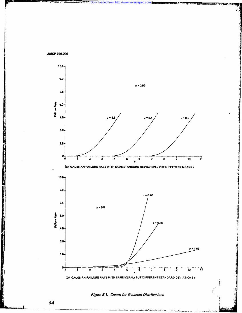
AMCP 706200i 10.5-

9.0-

a- 0.66

7.5,

6.0.fIA

Il34 U 2 .5 / 55y/

3.0.

1.5. __ _ _ _ _ _

Is-

(C) GAUSSIAN FAILURE RATE WITH SAME STANDARD DEVIATION u PUT DIFFERENT MEANS

10.51

9.0-

91-0.40

.0 - 0.66

4.

3A

a 1.66

0 1 2 3 io II

(D) GAUSSIAN FAILURE RATE WITH SAME MIANu BUT DIFFERENTSTANDARD DEVIATIONS a

FiCure 51. Curves for Gaussian Distrib ,t ns

5-4


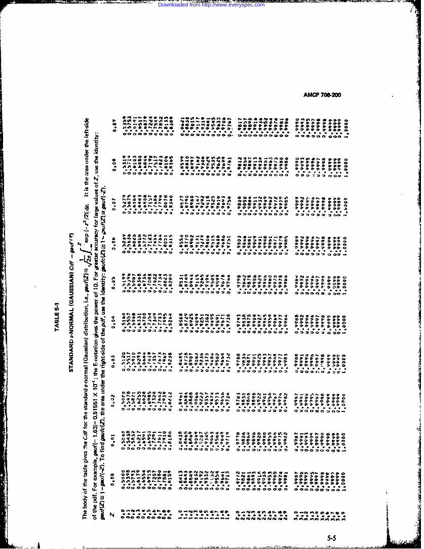
AMCP 706-200

;-01 Ina * N was & -. 4. 0 & lp p 4. 0- tWo, 0 a. &* CP .@a0-C.&a

D, a 040 .00 0 0.0 000; 0007 0. 00000000 0 0 D0 0 000 0 0 -a

00 a. a Q* a 0

.. a T 0 "W, . w =P i, 0*o 0.....000 *00& a.&Ji-l It~ It I It . . . .~030~ .00'0200* .

N0

Na 0J 3P -VJaMLA . d-'U W A 4.j P- C 40 0 a& && && . 00*0aAn aa40 . oe AP.0 -iJWA40p3. a . a- . &0. *0, 0 *00 0, &00o a

IL1t1 4tI? cc. o c~l ONc~c C;#.; ; 0 0.o 2 Zo0 D 0 0.*0U-.P0 ~0 * *,

J% On .0 a O* N'M0. 00 0.0 '1e.V0~' *0)..nU. . ftp.U0' fu I a 0 2 ON*O'O,.0. O ,4 nt," .4U' .. I0 u .0 QNIt.U .* fu -na A JCI *&& OP.&V 0. '*&*o0, O L 0~w %A 4P., _M ve &o., -CO a.'0N.uU . ala. l0.0-0 go0 02.0.0. C. 9.0,a

cc .2 a .a a

0- 4j o~~*.-A. 4) " Z 4 U 0 'A -0o * a. 'IN 0 "- I0, N . 0*0 1 ' I1 121? !V% . flJ40 m 4 &N C0. N -It P. a n I- ,co 0. 0. . &0v 0.0. S 1 . 0..00

4 * .flU'U0O0 a c .0 04 00**.* 0...*0*I. *0'*.to~

S- WI nWk -N - 0V I f44 A00O A 0( c&0CC so aN.a. O0N miP~Jn 4 # 4e0AJ*U'O , 0 0 0&.*o.,o oe3-.4 & * CF Pa ,0 F o. *. 2 C, .a il 0 ,00.0.****o I

CD 00 .1 a0 a0 0 0 0 00 .OOO o oo 0 0 * 4 0 c 00 0C 00c: .0 L

r) r

oo

c: . N ~ 0 0 0 0 ~ ~ - N N ~ E~EJ N W ' g I u p ~ ~ e~ec a l M 0) 0 - 1 a 1 0 1 D O , a t ~ c 0 0 D ll 0 - D -2


AMCP 7064200

.00C c00000O *0e0 00000s 0 ooOO CC a a o C C a C a

1 t'*9**u. 0:;o'-,s !O V*rseo0I43O P*F SuV t. j d

. .00 00 G . .. . .. c;0 C O o 0 0.2 0 0C000a0 0 00C

0 0 c . . . a Ca d a A ~ ..0J i . J. J J * M C3 & J.44 & 0 1 C l .J0 0 a0 s I~~~ a C a, e. # 0Qtt'c,.0 %30

10 OCaa % 0 A 1 0 00000000-0. o ooooo&oo v :1c o

0000 @00000-c a0lo C00 C;4N Nd" ' C C n I ; 0<1QC0Ca00 00 0 C, 0 a 0 :0 990;000 00 0 08 0 0 0 0000

C COO0* n~ll C .0*'.AOO:o 0' te CO CO 041C0C* 0 0 0 a C4

4 0 . -1 1a. v 0 a -% V

pot00000a 00fm0 0 ruE a N 0co a-C 0 0s!N 1*0000000000 0 0040 a00,0 0 00 0 0 00 000000O00

0 0D I ~ 0 0J0-~ C..*..t~ a 0~~b

.. MO a.. 0 mo C. 0 a .A0 .- 700 05

1 C O CC O 00 - - - - EJIga0J. v 0 41 46,0 10

00 0 00 0 s 00 000, 000 0 0 0A h. J AW A IJIA IV&.A 0P G 4VJ* .aJ

0 0.. . . ~ . -d .Q~ P.11 .*- .'J- . CO .... 4..

4 aaJ9. . 0 N 0s 10 1 0 0N CO Z ;; uN sNNfuN r 4 %I . lPIc ~ ~ ~ ~ ~ Q9o1A 0,[email protected]@tN 0 -,a0 C .0c p, * CCocb 0 , 0 Q C

sf.o 0 V;AN NO * CP .a# I I . %I ='Nl~l ' 10 '--

~~~.0@V1'~~oVV N.U ~llt . .,P'.

*OaCO CONO #000Z on I 00C-M~N 0 0A on a

000000000 000 0 0 0 00 0 0 00 0 00 0

0000 0 0 0 CO 000 02 00000 1000 0000000000I

iv. a I *. . ..-I V. ...... av ..... ...

c0002 0 00a0a 0 00- --- --- lOtNEcEJ 0 aC 00 C0

0000 0000 00000000 00 0 0 0 0 0 O.0000000

0 00. A.0 a N ".*-' af

to 0,C " f I. PO N

C 0 000a C 0 0 0 - - - - - - --,l fl A~ ll 0 ~ P b wga 0 toI Q .0

,; ~ Ja~i~~Jh WW.JW WW~W111 WW11LaJIJWJhWWILi.ZiIj!A

4440 A 4 r D 1t-aV * 0A v 4 0 a No '.'lo .0P.0N W, .0 0 l@.

000 I000000 0.0. .'. . -. NNA. % 1 i

co 000 00 000 000 ma 0C OIUN o0 00 0 c 0 0 00 0 C. C0 0 C0 ,

07 *S**s**ww w5"5£WW 1 .L 3.i* er ga^4 &0,t 0. v f" 2 N a Y%; 0s i a O 'VAW 04 - 0V4,3 *ovagi ,9 0*

Is ~ w..s 0,ip~.~. on.o- o..s fu WPg.4ne

0 0 Cy, a a 0 0 CSAA.5 0 CPOdU u.'tA fW..Q0ybl fu .9*VyFA-A"IA ft-ft0

0 020 0 0 00 00 000 004 o.c 0C00o0 000 00O0000000.

N... *** .* "A4 *. W~ W* a** WM *iWu "W im u AWWA tAa a. " v dWukW W,* a. . .V000 WA 00 a -F- Cp- - - 0 *N N N on 0 0

-,1 cor.t ". . . . . . . .-It

AMCP 7064200

0 001C) 0 0 C 0 0 00a ~~ O0 0 C

0 Nam 04g , smu 0.ns SSBS AC g lI S N, N 'AoD 0C U0N0 C . Cov 'P~ol G NS ).-.l A 0 1SA 21 , -n

a, O3aiN~- 0-J 0- 0, * i '.3v 0'zM&* n0- : , n at

o~1 a0 0, a Q a aaa 0 0 0 0 a0 0 C2 00 C.C 0 0 0 0 0-0 > 10 I=C 0 0 0 10

;Iz nI ,f 0 4' aDooo o oa ao 0 W 40 a,*- !tf

0 CP 00.CNa 0 0 (1 , 0-2 o0fl jo 005 0C 0. i D.

al G,~- 5 03.05- en. py 1.,i~I~ 4t . O NPg- N 4v 1(p C. 5f'.7 AU. QO U-T Pg..

44 41 444 44 4 44 4 4444444444 I44*N44 4-A

oo a 0C.o Oo 300000 O 0 C0 .COoc 20 I I

a3 ZFPJ nJ1J 0 10 . 4 f-- - 0 C 00 ~ 0 00 - .OD3 C f

0 4444444444 rue 044~ .J4 4 4 44 4 p-44. 4 n4ma 0 IN c5=On ,- .sNC-.os sg -l0C. - 40 0, P-s.P-U N .

6 ~ J w.D Q'.~ 'A ". *'j% 0 - A~5.l z

. .0 o0 .S0 t-.%to1

0eo 01>0 0 00 000aC00 00v0 00 o cao c ao eoecc 4 0 coc S

v444 %44 4)44 4 44 4 4 4 4 4 44 4 4 4 4 4 4

0 O cc c4o Mooc I0c a 10 00 ee0' 49- oa aeo Q

iii~ ~~ ~ 0 a 0Q0 a 00 0 00000 0e 00------------------------------------

0 "'-Pi~Od 00O-'~'0 Oor0~ O 0 000 0 000000'JD*P-0 0 a 0 o CI 0 3 oC 0 0 *1 00.-0 0 .l 0 , 01 P

o e4e2 o V o gne oo o coco eeo 0 0 0& AeceoNcocQ~N 0 n.ISWvO v5NC @MaO=2--- 01 n ' 0 a -, -

o , c, o ac C o0c, 0 0C.0c00c00 o a--.. c.O O O o 00

a4 rL nknI 4 4,Q4 -oCfa.J N j Pf F0- ODc IPC CPOo0' % N l N ILUo C' 00*0 Oo.. Cj3J. C3a.l"~

OloacoP 0 g Qo o N -C C 3 -0 U' oN - O - c i-C3 *1N..1 .AD

0 s 1 1 71 1 t

O00 Cc 00 oc oo cc c C,0 cC 0C zc ec ccC- 4D'%wofO O _ t ~ o ~ -----*III ***t 0 * ~ *I B A. Pt* * X 'oII

~.0 .5= . t% 0tN . . .l. >5.C% P.IPN % .

0 OC000=0 0000 o 0 0 co 000 000COCC -00 0 C0 10 0 0 aC C

Z 3 I&~" , I U C0C *0 4 '-- P-' CCC 0e 3 cc0 0PNg.f$* 3

0 C,00. 0 C300 0 0 a 0eo0 o 0coo a (.0 0O0 tU P'7 C U'csPN0:Cr 5J %OUO3~ a 0P 73JI03

w* i js 0n w-.o r- J, P InW, *-C06 f 0 N* 4F C.- . 0'. a to & c P" m

=NNN aO-~0U P- AD m z4. v=35JP.~= 0 -M m 0 '

0000000000 00 0'00 00 00,,0 . 00 C 0 00 0 0:1 0 0 aUi~~ 0 Cg- <1 P-2C , a 0~0 a - C - ~ ~ 0

0, (p, Z7 SU' NQ Ui34.OO O 0 3N.NC- oo,4 V 0 1-~l

No & , A 0,'o 4 Ao~~i~-O-. vc~ -U 3~ *0 .QO Iv0o;;c 00 clOOo COVOC 000000 05C 000 o 0Coa 0 c 0 000 41 . 0

CoC0 c C'46aC0 D 0. 0 0 0 S-0 C a0~ * 'P* o.flSf.5=

N i u . L 1 L. 1 , -IW ILI 111 14.,C . 1 ~ . - -W :lu u A

AMCP -200

TABLE 5-2

GAUSSIAN (STANDARD *-NORMAL) Cdf - puf (z)

Body of the tale is z. the standarda-normal variate, corresponding toPuf (z).

.00 0.01 0.02 0.03 0.04 0.05 '0.06 _ 0.07 0.0 0.00

.00 - -2.33 -206 -1.88 -1.75 -1.64 -1.65 -1.48 -1.41 -1.34

.10 -128 -123 -1.18 -1.13 -1.06 -1.04 -0.99 -0.96 -0.92 -0.88

.20 -0.84 -0.81 -0.77 -0.74 -0.71 -0.67 -0.64 -0.61 -0.58 -0.55

.30 -0.52 -0.50 -0A7 -0.44 -0.41 --0.39 -0.36 -0.33 -0.31 -0.28

.40 -025 -4123 -020 -0.18 -0.15 -0.13 -0.10 -6.08 -0.05 -0.03

.50 0.00 -1.03 0.05 0.08 0.13 0.13 0.15 0.18 0.20 0.23

.00 0.25 0.2b 0.31 0.33 0.36 0.39 0.41 0.44 0A7 0.50

.70 0.52 0.55 0.58 0.61 0.64 0.67 0.71 0.74 0.77 0.81

.80 0.84 0.88 0.92 0.95 0.99 1.04 1.08 1.13 1.18 1.23

.90 1.28 1.34 1.41 1.48 1.56 1.64 1.75 1.88 2.06 2.33

Special Values

o) 0.091 0.006 0.010 0.075 0.050 Q.1C

z -3.000 -2.578 -2.326 -1.960 -1.645 -1.282

0f9z) O.0.9 0.90 0.975 0.90 0.90

z 3.090 2.576 2.326 1.960 1.645 1.282

A*1l,


4p in' A-. 0 'i

LL 0. 0* OW p.04 NoA * 4C nA-t

0;:. .2kf.0 4r- OJ'U OAl. InP~f~ d ly~ O'*D :Z F N Z..,ftft-

NJ 0 . .. . . . .S I


AMCP 706-2010

&* in@~~ge9 ae~' w CE 0 f aa^Za in~AA4V 0.4 41 a- A M~P* 0 M

o cr A A a.** e ow.* 30 '01PA-, "

*V*W VVIA I9~W~~9AJ~%44 4*b*4**-P. 9rn.9r..9.- ID

0.6 j VV 0E A IZO A9~J A 0 .A,.I A 4 0 00 , 4 4;4; .4; A0-9 t-es I- 9- Z ( 99

* fO*N*W*A44 PA A CWE99 A 4; 404 0CCC0

i 42 -0 .11. M M

I* o 41w ; ;'AJ AA i W, ,A A A.C a a9 . C A.C,9 a aC a

0 0%P-*A a 0I m aP WP. 0. o-AFlifl Mft. mO O 42 r.- n w No a a ,. . A * N ~ aC P

a mL 44* *C .J i l vkIa W -1 - f., 40440 X4.09.-9 9 1- t'. l C3.

I~~9 " .0A~ * 9 0 ' -fJ. . .0V . . .O- .Q .a .O.-.C.

a *A ~ S * '(v *SP a D41 C4

fli#- " M: - O u # ~ol@ 8 @ I.,W N- #- ~ w U W4 ~ ~ ~ A a Ai9CA4-CO i.W& 49-. .. iA 49..EC0 V9E1fl-AA

- ~ ~ e .. v .* J f -A~ 0 P40 4 - 9-I a L-9-%9UOa2. M A -C

A ~~ ~ ~ ~ F4A Jotwi.nWFid s,..~4 PCtd#- l Z U..WE 49-- 40ge~U@ O

0 0 44N P9 4 ## 0 a 0, O N#. a 44 4 4 4 9 w. - 4 -9in-9-C

CC ** .* . % 0.. ... .1~ . e .~ . . . . C. . . . L

4 *WEV# *VJ wI ,IflJAAAJA.I4 4 44 8 09 999--

z

C: &&a~ - t- P. -00 4D **4 S* In 0 z m9-^01

WW#*# Vo',I W 0I.A A 44 44 44 9 r a -

a t .4Vt lt. PV .C Titw~#-W l!C I9t'9 W ~.104@*wi A4w eee *0 *An 9nW. "n4@ * a a a a* S041' : F f9 0.AN*- W @EW

a* ' "AVe W 9l"dS0@ C fCt NWI -0- 0 b f 9& a 10-0404 A~ ~ V@ V 0& 1 N P n0 C 1a f'0W .je *0 : 0 'on 49i, 00i-C9 -9Wm 4-* 0 mm f"NN N O f

o0z ' "W a&... . ** 5 ASe~ *"l * * ...g*=.01

**V* @*~i A~9 %W 4 44 44 4 9- 9--to-.

**** *SS* 100 14 o 0 nS.** * 6.* S S * , . 5

5-10


AMCP 706-200

0. 000 00 0 .J 0 000 000000 O ,0oCoaoo ,ao 0 ;01 00 a0 00o0o a0 C

aOO O~cOa MNNa

~00000000800 00000 00 0000a0 0 c000 00000000o0

N N a A Apt!*

C.000000000 0 0 C,0 00 -- ;g ir N Uf A- A fO0000000000 a000000000OOOOOoO

4 )0N-Z -0 !10~ii~ihJ.Sh g0iW4~&ihJ~ ihMnz:aMiwisIiA w- 0i0 Siii(hVaU In0 1 00. A.IVflJ0 0 .. il A IV A 4 - * .-ihpeflr .ha

Z, ~C000ON 00 0 0 00 0000 000 000 0 0 0

4m 000 C 00 0000 0 - -- l 00 vI i4 A l U A J a~ NE 4:2fu 000 00 00 000 00 00 0000000000 0 0 000 0

0000000000O 0000000000 0000000000o 0000000000

1*O000000000 000000eoh -NNNlhi N o%. .

4 0 0 0 0 i f 0 p 11.00. 0 0 0 0 0 afla 0 a Oi

.~ 0000 coo40O4 0 00000 000000000v 4 0 000080 000000

eat ~ ~ ~ I Wsi i i i ilt SI~

-0- IO *4-.. 0U 0-C0 .i S ~ NNPI~i~ VA 0 Q00 oO 03 1", 10 01, 0 C~.l~ 0 - 0 00 A 0

* 0 II0 'Ag S~i 00 V :j0g.e.

QO ca) *.5 * *a .

*a J.&I 4)AtAsW w! W u WW USJW WW W t. & W AWuh.0 ttW U W W W W W W

o -0 00 N & 47- n In o 2 0 0 - V 0- 0 0 0 r. 0 0 00 00000 0

0 - 0 - 0 0 0 0 0 0 0 0 0 0 - - - - - - - - -. f l a.

0co-oc 000000000 0000o0 000000000000 , -20 aI U SS I 0 IS0 0 . 0oIIgZI;g; WS;g ,OS= C

*~~l W.ia~SIWWh WI&LWW~W Waii..JiII~ W~~istooleho *P~W4&lE%4~OV''fltI4Vl *111MPI-L- 00.409,,g

10 a 0 N N0 ) P a *W NnO t C- a 4 fltN A tJV &. IP k

a. a. . . .. . . .. . .a 4t.. 0-.mA .. a iV 00 00 0000 000 o o oo o 000V P 0 10 coo 000

O.WflS iNt OaW~~II. o. v wm P . 04) WMy 4T

cc COCC;4O.4CCOOO OaC CO Z j.*o coo ~a a * .. * * ae. *

Q C C C I o 00 0 C 0 C0 I UlI NSI IV OV I*fSNA*,SSPf 1

CQ~oao5o11


Im__ !!Lrw 'W-

AMCP 706-200

CPC .0a 0 A f 1a c-0 C 0 4.-Pp-. ,.f 0- 0O-.

-W00 000 00010040 wwD00 wI 00 i0 I0.4 It -- 44 . U..0 n ;I- n . ac . mo 00 * 0. 'n %A on t IV -n 0 SSI agPggIn tfl

Ild & 2 a IA,4 A0.44.0fl A0 . a 1C 0 " -±P.t# 1 N 1 40,1 f 0 ow in5 ol.4 -4. M. 5 0* 3 0P- v .J 0A Nl -

IsV~umJ 0 4CT4 l n 44-P.C 4 0000 00 *1 C, 10 1a 000 0 0 0 Cm000000000 0 C ,C 1 a C ' 0 , In.~

0 a IL ISI & g s a, . sm e se .I I I, aseIqIIZaI- e-- WA W -a . .1. .0 J11 . L 1 .&1hJ14Js. hiii.11 . ~J. L atMJ whhhiiala

0 4 4 Wlftt 4f a A : .Q0 Q i - l N 4 MfU *IJQ04 ,.Q;: n M Mt oV' l'..4* ~ ~ ~ r a.4 4* 4 r0C)J 49-A0W3N 00 S Q 4 00 .03.04'

N 11 n 4 %: A .4fl. C> 4n-A M *4 Q .fu0 0 M4 J4..AZ'. 4 . O N003 ' '. 0 O l--4 0 4

00 00 >c o0 0 C 0 0CQ0 00 400c0c0 0 oo Qoo ooo c

-0 * V 'IA.14%A n 4 ~p4 4aL 000 4-AlW'v'moI.4P.cc 0000000000C 000 00 00 n000n.4n44.

0t- 0.015V - Z v2. , vA -'4l030-A1 3 30 0 .4 a'-0 An S--

~C. 0 a0 0 o 000 I0 0 0 000 00 0000 001 ; ;jC;C c 0 ao Q o'c C 0000

WlW W% 0 U# WN 0 A A A 4 41P. 20- :0 o0,00 00

cc a a W00 00 0 O000 I, -4I -- 4-17:2o--I -- *;a Sl C o.ill a. . as,-. ,ga.su*ge*s

CI* ;'4 l4; a * 0 aits.40 C4.. '..O3'.04 c0 310 QJILO -jf.0 -0 0 '

0 A 000000000 00000000oo00 0.0Q0C I .I I 18 11 *aiI i g IB S , i a Igr 10 . .

&W a". w WMiiiiit w w a wwwwJ! sa )wi aLL.?~i&u.h t!.JJIJ. W 4Al W Ah.i. A.. j.J.ihP, *l 0, N 0 MW. 0 Mn4 N .'.. MfA100C3. 0 = 0 0 3154C"

16 c ea oCl eo a0oo oo oc0o c c >1 occ cooocc oc o C C;ooc

A 00 0 00 0 0000000 00 Oooa o 0 0 c 0 0 " -..-.n.n0~ a~S~l~ a,,~g m 1.s ., a 3 d I a0 1 ,

LL w. c o ,0.cc _ t m o- oa n -A.40 v r- FP.c .3.0 a 0' a.a. 1,cWM0 N- Vl34.4 " a .InAA.-J A A a 1303-"),A - 9 Ja_ o37*0

0?514 mmLz C iJ0 f.54 50O".. M .&1& 43l I000'.. z 04*30N.-.

:f P..4A0 A Al "A4 4 a-- A Al. 4A-f . zC r

0 0 M -. 0 Ctail.aa, i ,, Nim M ~ ,.., 4 eZSZgIifS c ;M

W'0 4 N *03fl3A000A 043M4.3003 0V- 0-f 0 ' -4 CC.4 230.4

0 c000 000 0 0 000 00 00000000000 0SCccc 0cc0 C.

z -* * o n 44@ 31uJu 1f..4 Pt-t-t-t-g. 00 00 00 0 woolelJW.4cc'MNl o00 00000 00000000 .a 00 0 c000-0' o IOS a111 SI UI S @ I SOIII S I SIS .IS C IS I

it .4 4C 0 O . 0e ~ , o o- -. .0 4 0V - ... 4OW.00A10"1MN P A.4 .l0N. W0 A ' LO wN 'l4 WI00" -4 ofA.,' V m po & M ... 1 .

M V N a i'At Ln . 40 CA-.P .40M'a- -n 4Al Vz - M3 -0I'. U 2al3 -C

4 c c 00 0 0 0 0 00c 00 0 00 0 00 0 0000000000co oc ac oc c-

*W.W WWW WWJ IWWLIA k LWL L.Jl.~J.lJLJ LUIL..UilwIJ

WCePn 0Cf.3... ,W -. 00 0 M o'.~f~l50ftU'4iA-T nf t-%INc4zM P 4 -I0 Q. * N..Q"A 4.t A I 0- 7OWD

ID N N P_ N M C Lm V .0.4mU 4.- 4a.Alof;P4o M.0 P.,3f1

0lc 0004 0000 000 000 0 .0-Q C'c0 0 0 000 0.0 0 "C0c00000C

a V0 4IS @VLnAU i U n L414 oaPt N-P t CC m0. 0 0 0 m--l. flI..0 00 00000 000000000a 4 0C'C 0b Q00 O0.- -- ..

loiNa AV to -o 43, kp-W3 p-.. :A. P o0..4 . V q VVrI- V 7.v00.A O.in 0-ma. CI4 t .q W flP. 1 4D t.Cp.0 N0 04MI., I.lt4c A sApn % MM. t- so15 V nC 14 V V, - .. 00 - '- C,.4 Al. CO4. mO o4) W4 AA

Wt 5j0 vv51- M 0.Al.#VtC 0411. r! .%-! C0 0.4IU14It~- _: I

N in.:: : 0SW m 0 0 m .6 44 4 4.0a04 . -ttpt.tI. -I. .9P.I.-(

512


-1,

AMCP 706-200

5-4 PARAMETER ESTIMATION, UNCEN- Conf{p < g - ts/r} =stufc(t;N- 1)SORED SAMPLES (.5b)

Estimation for uncensored (complete) sam-pies is very easy and straightforward, if the (X2/v)fs 2 /o2 (5L6a)samples are censored, more complicated tech- has the chi-square/nu (x2 Iv) distribution with v-niques must be used. = N - I degrees of freedom. This fact can be,

Conventional wisdom uses the estimators used to set s-confidence limits on a:

(for a sample of size N): Conf_( 2 < s2/(X2/p)) "= csnfc[(X2/Iv);

= sample mean=" (N - 1)]. (5-6b)

a = (sample standard deviation) The subscripts L, U are used to denoteLower and Upper s-confidence limits, respec-

X/s---I =statistic. tively.

Sis unbiased and'maximum likelihood. s2 is Joint s-confidence limits on p and a are notan unbiasedestimator for a2 but s is a biased feasible. The cases where either / or a (butestimator for a. not both) is known are simpler to treat but

are rarely met in practice.The maximum likelihood estimator for a is

5-5 EXAMPLES!ML = sample standard-deviation.

The following data on strengths of a plastic-Other useful estimators are the sample median bar were taken from 1, lot of bars. They arefor p and various measures involving the listed in order of occurrence. All have thesample range for a. These other estimators same units, which are ignored here. Assumewill not be discussed further here but can be s-normality and estimate-,A and a, along withfound in most textbooks on statistical quality suitable s-confidence limits.control or in-Ref. 1.

-a 89.0 85.8(5-5a) 105.2 93.3;

105.2 87.5has the Student's t-distribution with v = N - 107.7 92.31 degrees of freedom. This fact can be used to 99.5 95.6set s-confidence limits on-A: N= 10

SI"

_________ ____ ____________

Procedure Example

1. Calculate the sample mean i', the s statis- 1. 3F = 96.11tic, and the degrees of freedom for s. s = 7.92

v = 10-1=9

2. Estimate ! and o. 2. A =96.11= 7.92

3. Calculate s-cbnfidence limits on p; Use 3. For C = 5%, 95%, and v 9'Eq. 5-5b. t9, 5% =-1.833, tg. 95 - + 1.833.

s-confidence level = 95% -5% = 90%,uL = 9 1.5 2,iU = 100.70Conf { 91.5'<A< 100.7 } =90%

4. Calculate s-confidence limits on s. Use 4. For C = 5%, 95% and V = 9"Eq. 5-6b. (x2 /v) 95% = 0.3694,

(X2 /v) 9,95% = l.8799.s-confidence level = 95% - 5% = 90%oL = 5.78, o, = i3.03Conf {5.8 < U < 13.0 90%

There are no data outside the range of 85.8 to us an idea anyway. .However, we don't really107.7. Therefore, it is difficult to guess what know that the distribution- is s-normal downthe population is like out there. that low, there might be 7% defectives -down

at about,30 for all weknow. If that x1 % valueThe true mean is not known too well, is important to know, we have to get more

S-,thin about 9% (at 90% s-confidence),and knowledge from somewhere, or admit thatthe true standard deviation is- only known we're just guessing.within a factor of about 2 (at 90% s-confi-dence). Any estimates more certain than The detail in this (iscussion has been tothose must come from other knowledge-they show-that making the calculations is straight-cannot come from the data. Be very careful forward, but getting some understanding -isnot to us. the point estimates and blithely difficult.fqrget all the uncertainty. For example, sup-pose someone wants to know the value of x In this example, the data were ,selectedsuch that only 1% of the population lies randomly from a s-normal distribution withbelow it. One way to get an idea about an mean 100 and standard deviation 10; theanswer is to take the 2 worst cases, "pu = u lowerf 1% point was 76.7.and a = au", and "14 = uu and a = aL andsee what the two 1% values come (,ut to be if 5-6 PARAMETER ESTIMATION, CEN-the distribution were s-normal. The number SORED SAMPLESof standard deviations corresponding to thelower 1% point is- 2.33. Therefore x1%,L = Analytic estimation of the parameters is.61.2, "xl% u = ,87.2. We don't know any difficult when the sampies aie censored. Thes-confidenc. level for this range, but it gives method of maximum likelihood often is used,

V!

AMCP 706-00

in such cases, but the equations are very is a reasonably good method and can givecomplicated, especially for the covariance some idea of the uncertainty.matrix of the estimators. Analytic techniquesthat do not provide a measure of the uncer-tainty can be very misleading because the A stitistician ought to be consulted foruncertainties are usually much greater than anilytic techniques arid the mearing of theirfor uncensored samples. Graphical estimation results. Ref. 4 might be ef some help.

REFERENCES

1. E. S. Pearson and H. 0. Hartley, Blo- of Mathematical Functions, AM555, NBS,metrika Tables for Statisticians, VoL I, USGPO, June 1964 with subsequent print-Cambridge Univ. Press, 1956. inn.

2. A. Hald, Statistical Tables and Formulas,John Wiley & Sons, 1952. 4. Sarhan. and Greenberg, Contributions to

Order Statistics, John Wiley & Sons, NY,3. Abramowitz and Stegun, Eds., Handbook 1962.

_ )


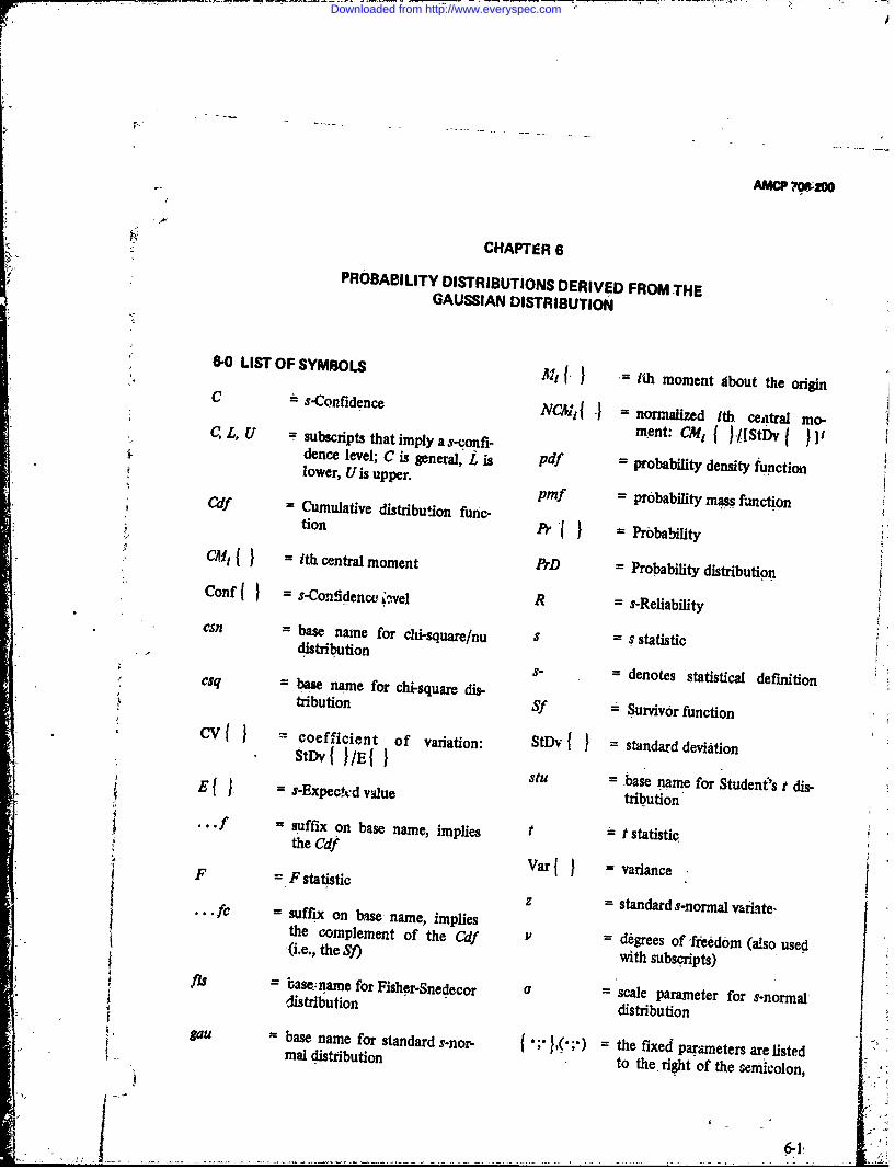
A"C ?W0o0

CHAPTER 6

PROBABI LITY DISTR IBUTIONS DERIVED FROM THEGAUSIANDISTRIBUTION

6-0 LIST OF SYMBOLSM1 (J =hhmmn lotherin

C = s C~ nfi enceN C M, { -J norm alized ith central M o-c , =sbscripts that imply a s-confi- CMj ~~tv(JJdence level; C is general, L is pdf = Probability density functionlower, U is upper.M

pmf = probability mass functionCdf -Cumulative distribution funfc-tion ft = Probability

CMf, J =ith central moment PrD = Probability distribution

Conff I =s-Confidence;'.vel R = s-Refiabilitycsn =base name for chi-square/nu S =s statistic

distributionS_- denotes qtatistical definitioncsq =bane name for chi-square dis-

tribution Sf =Survivor functionCV({ coefficient of variation: StDv {J standard deviation

StDv{ /E{EStu -base name for Studenf's t dis-£ (), sEXPectvd value tribution

suffix on base name, implies t t tstatisticthe Cdf

F =F statistic Var{ =Variance

I*l = suffix On base-'name, implies z tnarI.oalraethe complement of the- ccift v deigrees of 'freedom,(also used,(i.e., the SIt) with subscrits)

.tZ, basename for Fisher-Snedecor al ='scale Parameter for s-normal-

gau base name for standard s-nor- {;*}(;)=the fixed Parameters are listedmal distribution to the, right of the semicolon,

(5


AMCKM06200

the random variable is listed to c 2 P [r(/2)J-1

the left of the semicolon

the complement, e.g., .1 - Cdf x2 ; P' = qsrf( P) (6-2)

where # is any. probability Sf (xe; 0) = csqfc(x2 ; V) (6-3)

6-1 INTRODUCTION E{x 2 ; Y,) = v

These PYD's are .rarely if ever fitted to StDv(x 2 ; V) =experimental data. They are useful becausesome estimators for other -PrDS have these CV (x 2 ; V) = V

PrD's. The X2 and xe/v distributions arerelated to the Poisson and exponential distri- CM3 ( X2; a) w 8,butions, in addition-to the-Gaussian distribu-tion. Failure rates 'are virtually never used NCM3 Ix; P) =witi these distributions; so they are not given.They could be readily (although tediously)calculated. (, -2, for a > 2mode MX P)

For many reliability purposes, the Xe/ /0, otherwisedistribution is more useful than the xa disti-bution. median {x ; P) P-. 0.6

6-2 CHI-SQUARE (Xe) DISTRIBUTIONFig 6-1 shows some curves of the pdf.

The base name _csq is given to the Xdistribution (for chi-square). The suffix f It is convenient occasionally to defineimplies the Cdf, and the suffix fc implies the the Cdf and Sf for a' 0.3f (complement of the Cdf).

The -sum of the squares of v s-independent csqf(x2 ;0)-.l, for X2 > 0 (6-4a)standard s-normal variates is a x2 variate withv degrees of freedom. In reliability work, the x2 csqfc (X2 ;0)- O;.for X 2 -0 (6-4b)distribution itself is rarely needed; it is virtually'always the X2 / distribution t',at is desired. csqf(0; 0) = 0, csqfc(0; 0) m I (6-4c)

6.2.1 FORMULASP = degrees of freedom, P > 0 Some approximations for X; In terms of the

standard s-normal variate z are

random variable, X2 > 0

pdf(x2 ;) C(x ,.exp( x/2) for ,,-*o, 2a ~ (4 ,,- )/.'r"j (6-5)

(6-1) for 0 > 100, za, P -- I

6V


AMCP 706)06

for Pv> 20, z Q P /P)1/3 6-3 CHI-SQUARE/NU (X2/v) DISTRIBU-TION

- - The base name csn is given to the x2 /I

distribution (for dhi-square/nu). The suffix f(6-7) implies the Cdf, and the suffix fc implies the

where gaufL(zQ) = Q, crqfr (4, v; v) = Q Sf (complement of the Cdf).62.2 "IABLE$ The average thne-to-failure in a samplewith

Calculating the pdf is straightforward buat r failures from the exponential distributiontedious. It is rarely used and rarely tabulated. has the x2 /v distribf~on' with v = 2r; seeThe pdf is shown ir. Fig. 6-1. Table 6-1 gives Chapter 7. The sum of the pmfs (rth term to

)from a Poisen distribution has a Xe/p

the percentiles of the chi-square Cdf. Othergood references for the Cdf are Ref. 1 (Tables distribution with v = 2r; see Chapter 4. The

7, 8, and Chap. 3) and Ref. 2 (Tables 26.7, ratio s2 /a2 has a x. /v distribution; see Chap-

26.8, and Sec. 26.4). Many statistical/quality- ter 5.

control texts give partial tables of the chi-square distribution.

P = degrees of freedom, v > 0

Eq. 6-8 is quite good, even-for small valuesof ; it is the inverse of Eq. 6-7. X2Iv = random variable,, (X2/a) >D

bdfDQv3 ((2 P;y12f 00-ixp-E(e/~to9 Y-4 c E ( Pl 2 ) / [ r ( Pl ) 1- ( 64"

(6-8) X/p) (2ppCdf~x21v;v) =csnf(x2 /v;v) (6-9)

where Sf /v; v) = c /nfc(x2 I'; v) (6-10)

gaufc(z_)=Q, csqfc(x , ""=Q

Eqs. 6-7 and 6-8 reproduce the{Cdf X2;v}

quite well for values-bf the Cdf as low as 1/v2 . V (X2 J; p) =

Very roughly, the relative error of a tail areaof I/v 2 is less than 1/v0. For v = 5, Eq. -8give the following results: CV (X /P; P} = "

relative error CM,{x2 /v;v)} =8/A

Q csqfc(x ), in tail area

0.001 0.00092 -0.08 NCM (xv; I} V=.i

0.01 -0.00990 -0.01 1 - 2/v, forlv>

S1-0.1 1-6.1000 0.0 mdeX/v;otheise

1 - 0.05 1 - 0.0487 -0.0'26 median~x/v; v) ,I - 0.6/v

1 - 0.01 1- 0.008 -0.20 -

[;1


AMCP 7O6*2O

0.7-

2

0.4-

* 0.13

0.100

20

0.100

P,-100

0.030-

0.015-

0-10 15s 3 45 80 75 90 106 120 135 150

REISxU(B) FOR DEGREES-OF-FREEDOM v-10, 20,30,50, 100 (FOR LARGE a', THEpOf IS, REASONABLY

SYMMETRICAL ABOUT x' - a-2.)

figure 6- 1. C/il-square Distribution, Wd

6-4


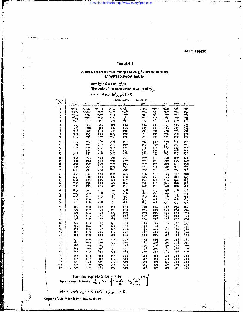
TABLE 6-1

PERCENTILES OF THE CHI-SQUARE (x2 ) DISTRIBUTIflN(ADAPTED FROM Ref. 3)

j Qcsqf (?;,v)a Cdf ;f' The body of the table gives the values of X,

such that crqf 1.2p, 6 ) 3 8.

PR9ABIIT 3Ma Pi-CEN

"i 0.05 O-1 .5 1.0 2,1 580 10.0 20.0 300 40"o! z 0'39/3 '0"157 '0'393 '01157 o°,982 .o1393 .o158' .o642 -148 '275

J i 1 o -0 o okx .o ,2 o o .0 10 0 .o2 0 1 o 5 o 6 .1 3 2 1 1 4 4 6 '7 1 3 1 -0 2

3 'o353 '243 770 17 3.36 "33'584 00 14 1-87. !4 ¢,39 .o'y .207 "297 -484 v71 xo6 z-65 2-t19 2'7

2-i -P639 3025) 394 7

5 .'58 210 .412 3054 .832 15 5.6 234 3-00 3666 .299 .3841 "676 .872 1.24 1.64 2.20 3'07 3-83 4-57

"475 59 .989 24 35 69 2"17 2"-3 382 4"67 5"491 710 857 '34 1465 211 2"73 349 459 5"53 6-429 972 1 31 173 2-9 21 3'33 417 5-38 639 736

16 126 394 2.16 -z56 335 3'94 4-87 6.12 7.26 8-30it V,59 1.-83 2.60 3'05 3.82 4'57 5.58 6.99 8.15 9.241' 2 1-93 2.21 3.07 3'57 4"40 5"23 6.30 7-81 9'03 10.213 V,31 2.62 3'57 4.11 5.01 S,89 7-04 8'63 9-93 11-1

, '14 "o 3'04 4"07 4'66 '6 '57 7179 9"47 10.8 z.115 3 11 3- 1

8 4-60 5 23 6.26 T A2 8 55 10 3 1 7 13 .O

16 3'54 3'94 5'14 5"81 6.9xv 7'96 9"31 11.2 12-6 14.o

17 3'98 442 5"70 6-41 7.56 8'67 10.1 12.0 13'5 14'918 4'44 490 6-26 7-01 8-23 9'39 1(.9 12-9 14"4 15"9

.19 4'91 5141 6,8| 7-63 8-9' 20,1 11.7 137 15"4 '169"0 5'40 5'91 7'43 8.26 9'59 20-9 12.4 14.6 16'3 17-821 5.9O 6-45 8-03 8-go 10-3 1t.6 13.2- 15.4 17.2 18-822 6-40 6-98 8-64 9'54 11,) 12.3 14.0 j6-3 18-1 19.723 6.92 7"53 9

.26 10.2 11.7 13.1 14.8 17.2 19'0 20"7

24 7",45 808 9.89 10-9 12-4 ;3"8 15"7 18.1 9'9 21-725 7-99 8-65 10-5 '1-5 131 14'6 16'5 i8-9 20'9 "22-6

26 8.34 9"22 11V2 12-2 13-8 15"4 17'3 .19.8 21-8 23'627 9o9 9-8o 1 1-8 12'9 14-6 16,2 18.1 20-7 22-7 24'528 966 10.4 12'5 13, 15'3 169 18.9 21-6 2.36 25'529 10.2 1!0 13-1 14'3 16.0 17.7 19'8 2,- 24'6 26-530 1o'8 ti-6 13'8 150 x6-8 18"5 206 23.4 25"5 27"4

31 11.4 12-2 14*5 157 17-5 19"3 21-., 24-3 26-4 28"4-3 32 12'0 12'8 "5-1 16'4 18-3 20-1 22-3 25-1 274 29'4

33 12-6 MA.4 15.8 17.1 19-0 20"9 23.1 26-0 28-3 30'334 13"2 14'1 6-5 17-8 19'8 21-7 24.0 26'9 29-2 31-335 - 13"8 14.7 17-2 8.5 20'6 22-5 24-8 27.8 302 32.3

36 144 15'3 17'9 19'2 21'3 23-3 25'6 287 31-1 33337 15-0 t6-o 18- 200 22-1 24-1 26'5 29'6 32-1 34'238 15.6 x6.6 19-3 20-7, 22-9 24'9 27"3 30'5 33"i 35"239 26"3 173 20-0 21-4 23'7 257 282 31'4 33-9 36-240 26-9 17-9 20-7 22-2 24.4 26-5 29". 32-3 34"9 37"1

41 17" 18-6 214 22-9 25-2 27-3 29'9 33.3 35-8 38"142 18.2 19"2 22,1 23"7 26'0 28"I- 30'8 34'2 36' '8 39-143 18.8 1919 22-9 24"4 26-8 29'0 31,6 35" 37"7 40'0

44 19.5 2o6 23-6 251 27-6 29-8 32'5 36o 38-6 41.0,* 45 20.1 21. 3 '24 " 25"9 .28.4 30-6 33"1 36-9 49'6 42-0

46 zo.8 21 9 25.0 26.7 29-2 31"*4 34'2 37"F ,40-5 43-047 21.5 22.6 25.8 27'4 300 32"3 35'1 38', 41"5 43'948 22"1 23"3 -6"5 28-2 30'8 33" 35'9 396 42.4 44-9

* 9 22-N 24.0 27-2 28-9 31-6 33'9 36-8 40*5 43-i 45-950so -. 23'5 24'7 28.0 29-7 324 34"8 377 41"4 44-3 46'9

Exampe csqf (4.4C; 12) . 2.5% 2/

Approximate formula: X22 L+ZQ (,2

where: gauc(Zio) =Q_;csqfC (X2 1 V) =0

Co tesyofJohn Wiley & Sons, Inc., publishers+ ....... . 6


AMCP 706-200


P'ROBAVILATY IN1 rKR CINT I p500 600 70V 8oo 9oo 95"0 97'5 99-0 995 99'9 99'95

'455 '708 1"07 1.64 2'71 384 5.02 663 7.88 2o' 12.1 11"39 1'83 2.41 3.22 401 5'99 7'38 9"21 1O6 13.8 15-2 22"37 2-9% 3.67 4'64 (0'25 7-81 9-35 11-3- 128 16-3 17.7 33 36 4-04 4 8$ 5 99 7 78 9 49 11 .1 13 3 14 9 18.5 2o C 44 "Z5 5 13 6-66 7 29 9.24 11.1 12 8 15-1 16-7 20 5 22 1 5

5"35 6.21 723 b'56 20.6 12-6 14"4 16.8 18.5 21.5 24"I 6

6-35 7'28 8'38 9-80 2.0 14.x 16-o 185 20.3 24.3 26-0 77"34 8'35 9'52 11,0 134 15'5 17'5 20.1 22-0 26.1 27'9 88.34 9'41 1o37 12-2 14.7 16'9 29.° 21-7 23.6 27'9 297 99"34 10.5 11-8 13-4 t6.o 18.3 20.5 23'2 25.2 29.6 31.4 to

10'3 115 129 14.6

173 19.7 21"9 *47 268 31.3 33'1 1111.3 12'6 14.0 15'8 18-5 21"0 23.3 26"2 28"3 32-9 34"8 1212.3 1.136 15.1 77.0 19.8 2-4 24'7 27' 29.8 34"5 36.5 1313'3 14'7 1.. 18.2 21.1 23,7 2t.1 29.1 31"3 36.1 38.1 14

S143 157 17'3 19.3 22.3 25.0 27.5 3 6 32.8 377 39.7 15

15'3 168 18-4 235 23.5 26.3 28,8 32.0 34.3 39"3 41"3 1616"3 17-8 19.3 :.1.6 248 27"6 302 33"4 35"7 408 42.9 717'3 18'9 2336 22,8 2(0 28-9 31'5 34'8 37.2 42.3 44'4 1818.3 19'9 21-7 23'9 27.2 30't 32.9 36.2 38'6 43'8 46.0 1919.3 21.o 22.8 25.0 28.4 34 34.2 3j-6 40'0 45-3 47'5 20

20.3 220 23.9 26,2 29.6 32.7 35-5 36'"9 41.4 46.8 49'0 21

22.3 23-0 24.9 27.3 .308 33-9 368 403 42.8 483 50'5 22

22'3 24" 26.o 2$'4 32'0 35.2 38"1 41.6 44:2 49'7 52"0 2323'3 25.1 27.1 290 33'2 35-4 39.4 43"0 456 5t'2 53'5 24* 24'3 26.1 28.2 307 34'4 37"7 411-

6 j4-3 46-9 52"6 54'9 25

25'3 27-2 29.2 31'8 .5'() 38'9 41.9 45'6 48'3 54"I 56-4 26

26'3 28.2 30'3 32.9 36.7 40.1 43'2 41'0 49' 55"5 57'9 "2727"3 29'2 31-4 34"3 37'9 41'3 44'5 48-3 51.0 56-9 59'3 2828-3 30.3 31'5 35'1 391 42'6 "45-7 49

.6 52"3 58-3 60-7 29

29"3 31'3 33-5 36'3 40.3 43.8 47-0 50'9 53*7 597 62-2 30

30"3 32.3 34-6 37'4 414 45-0 48"2 5.'2 55"o 61.1 63.6 3131'3 334 35"7 38-5 42-6 46.2 49'5 53'5 5(6'3 62.5 65.0 3232.3 34.4 3(-7 39-6 43.7 47.4 50"7 54.8 57.6 63-9 66.4 3333.3 354 37

8 40-7 449 486 52.0 56.1 59-0 65.2 678 34

34.3 36.5 38-9 41.(t 46-1 49'8 53.2 57.3 60,3 66.6 69.2 3535.3 37'5 39'9 42'9 47*2 51.0 54"4 586 6t.6 68.o 70' 36

36'3 38"5 41.0 440 48"4 52.2 5.'7 59.9 62.9 69"3 72.0 3737'3 396 42.0 45, 49'5 5.1"4 56'9 61.2 64.2 70.7 .73'4 3838.3 40.6 431 46.2 50.7 54"6 58. 62-4 65'5 72.2 747 3939"3 41"6 44"2 47.3 5.8 5 59"3 63"7 66,8 73.4 7.1 40

403 42.7 45.2 48'4 52.9 56.9 6o.6 65-o 68.1 74"7 77'5 4141'3 437 46"3 495 54' 58' 61.8 66.2 693 76.1 78.8 4242'3 44'7 473 505 552 59'3 63.0 675 706 774 8o., 43

43"3 45'7 48.4 5'-6 56'4 60"5 041 6.7 71-9 78-7 31.5 4444'3 46.8 49-5 52.7 57.5 61'7 65.4 70-0 73.' 801. 32"9 4545.3 47'8 50'5 53.8 58'6 62'8 66 6 71.2 74"4 81"4 84.2 46

46"3 48'8 5z.6 54-9 59.8

64"o 67'8 724 75.7 82.7 85-6 47473 498 52.6 56.0 609 65.2, 69.0 73.7 77'0 840 869 4848"3 50.9 5 ' 7 57.1 620o 66.3 7d

;'2 7.'9 ,78.2 85"4 88.2 49 *

49-3 51.9 '54'7 58'2 63.2, \ 67'5 71-4 76'2 7911 86"7 89"6 5d

I

I t : , .


AMCP 706.200

Fig. 6-2 shows some curns of the pdf. 6-4.1 FORMULAS

,-3.2 TABLES P = degees of freedom, P > 0

Calculating the pdf is strgightforward but t = random variable, it can take any va:ue.tedious. It is rarely used and almost nevertabulated. It is shown in Fig, 6-2. pdf(t; s'} = c(l + t2 /p" (v + 1)/2

.Table 6-2 gives some pirmentiles of the x2 / c o [ff r(v/2 + l/2)r(v/2)] -

Cdf. Tables of the y=/P distribution arehandy, but uncommon. .= 2,, [w r(v) - (6-12)

An approximation for k2 /P, in terms of thestandard s-normal variate z is Cdf (t; V) S tuf 0; V) (6-13)

For P > 20, z (x2,5,)1I3 Sf(t; =stufc(t; P) (6-14)

-(I - / (6-7)

Eq. 6-11 is the inverse of Eq. 6-7 and is quite Sti1{t; ) = {vI/v2' for s> 2good. See Eq. 6-8 et seq.(t; P) otherwise

-1 /2 1n.' CM3 ( t; V) 09P (#[- CM3(t; ) =

where NCM{t;v)=0

gaufc(zQ) Q, csnfc((X2IV)Q ,.; V) = Q {3+6/(v-4)forP>4,- 00 otherwise

-6-4 STUDENT'S t-DISTRIB TION median {t: 3} = C

The base name stu is given to the tdistribution (for student). The suffix f implies mode {t; a} = 0the Cdlf, and the suffix fc implies the Sf Fig. 6-3 shows some curves of the pdf. Theyicomplement of'the Cdf). are quite similar to the Gaussian pdf. For

ai - oo, the t-distribution becomes theThe ratio of a standard s-normal variate to Gaussian distributior.

:he square-root of a chi-square/nu variate has:he t distribution. It occurs most frequently 6-4.2 TABLES

,.ith the Y-nonmal distribudon where both-themean and stand1ard deviation of a s-normal The- pdf r-rely is used and almost never

-istrioution are to be estimated from the tabulated. If needed, it can be calculated,ample data- Student was-used as a penname (tediously) from Eq. 6-12. Table 6-3 gives the

* ]i~ li y W. S. (oset-" in 1908 to publish his prcentiles of the t-distribution. Tables forterivation of the t distribution. See Chapter 5 thet-distribution are quite common;-see, for

examples of the t distribution. The distri- -,xample Ref. 1 (Tables 9, 10, 12, and ChapterSition is symmetrical about the origin. 5).

-w Z-7


"AMC~? 706-200

V-1~

1.0. 2 '0

0.8

35

0.6r

0.4.

0.2-

0 0.40 0.80 1.2 1.6 2. 2A 2.3 3.2 3.6 40

CHISQUARE/NU, xIV

(A) FOR DEGREES4)F-FREEDOM v - 1,2,3,5,10 (FOR LARGE ,'THEpdf- AS X2/O+'.)

3.5

3.0-a, 100

2.0

1.5

1.0 -1

0.5

0 0.20 040 0.60 0.80 1.0 1,2- 1. 1.61 1.8 2.0

CHISQUAREINU, x [

.{S, C." DEC-9EES-OF-FREEDOM v j, 20, 30, 50, 100 (FOR LARGE v, THE pdo'IS REASONABLY

SYMMETRI(AL ABOUT X2/a% 1-2/I.)"

7 Figure 6-2 Chi-square/Degrees-o f-freedom Distribution, pdf6-8 /


AMCP 706.2_10

TABLE 6.2

PERCENTILES OF THE CHI-SQUARE/NU (x2 I) DISTRIBUTION(ADAPTED FROM Ref. 3)

cwf ( 2/ V; A') Cdf {X2/V;v}The body_ of the table gives the value of()? ,,sfuch that nf [(X2/v)p,,W] -P.

PROBABIITY IN'PXI3 OVA PROBABILITY IN PXt CIST

0'05 0.1 0.5 10 -2'5 5'0 95.0 97'5 99"0 905 99'9 99'95

I 0000 *0000 0000 0002 .0010 '0039 3.8410 50240 6.35$o 7.8790 1O08280 xz.zz6o2 ,oo5 o0010 '0050 '0100 '0253 '0515 29955 3.6890 4"6050 5.2985 6'9USo 7'6o10

3 '0s1 I o81 '0239 "0383 .0720 "1173 2-605 3-1160 378t7, 4"2793 5.4220 5-91-o

4 '016o '0217 '05t1 '0742 '120 '1778 2.3720 2.7858 3.3192 3-7150 4'6168 4'9995

5 'o316 '0420 0824 .1138 162 .2290 2.2140 25061 30172 33500 4o1030 4-4210

6 '0499 . 135 '1127 '1453 .2062 .2725 2.o 9C7 2.4082 2.8020 3.0913 3-7430 4-0172

7 '0693 '0854 '1413 '1770 '2414 "3096 2oo96 2'2876 2"6393 S.8969 3.4746 3.71698 'U888 .1071 .z8o 2058 -2725 '3416 19384 21919 25112 2'7444 3.2656 3-4835

9 .1o8o .1281 '1928 '2320 "3000 "3694 I'8799 2"1137 2"4073 2.6m)o 3.0974 3.2962

10 .165 '1479 .2156 "2558 '3247 '3940 1.8307 2"0403 2-3209 2-5188 2"9588 3"1419

11 '1443 '1667 "2306 '2775 "3469 '4159 1.7886 1"9927 2"2477 2.4325 2-8422 3"0124

12 .1612 '1845 "2562 .2976 "3670 '4355 1.7522 1.9447 2.1848 2.3583 2-7421 2"9018

13 .1773 -2013 2742 3159 '3853 4532 V72C2 1-9028 2-1298 22938 26560 2.80o60

14 '1926 .2172 2911 .3329 '4021 .4694 I'6918 '8056 20815 2.2371 2.5802 27221

15 .2072 .2322 "3')67 '34) '4175 '4841 1.6664 1.8325 2-0385 2"1867 2"5131 2.6479

16 '2210 '2464 "3214 .3632 "4318 '4976 z'6435 1.8028 210000 2'1417 2"4532 2"5818

17 "2341 '2598 .3351 .3769 '4449 5(31 16228 17759 1.9652 2201I 2-3994 2.5223

18 '2466, .2725 '3481 '3897 '4573 '5217 1 'o8 1"7514 '1'9336 2"(("42 2-3507 2-4686

19 '2585 .2846 '302 '4017 '468 "5325 z"5865 1-7291 I"9048 2"0306 2-3063 2.4196

20 '2699 '2961 .3717 '4130 '4796 '5420 1.5705 1-7085 1"8783 I'4M8 2"2658 23749-

21 '2308 '3070 '3826 "4437 '4897 "5520 -1.5558 1-6,95 1-8539 1"9715 2.2284 i"333822 '2911 .3174 '3929 '4337 '4992 '5608 15420 1.6719 1'8313 1'9453 2'1940 2.29(V

23 '3010 '3273 '4026 '4433 '5082 '569 1.5292 1,-6.j5 I81o3 1.9209 2.1621- 22609

24 '3105 '33(9 '4119 '4523 '5167 '5770 1'5173 1.-89992 18I89 2"1325 2"2283

25 '3196 "346 '4203 '4610 '5248 '5844 15061 1"6258 1'7726 1-8771 2"1048 2.1979

26 '3284 '3547 '4292 '4692 '5325 '5915 1'4956 1"6124 1-7555 1"8573 2'0789 2.z695

27 '3368 '3(631 '4373 '4770 '5397 '5982 1-4857 1-5908 1V7394 1-8387 20547 2"1429

28 '3449 '3711 '-1453 .4845 '5467- '046 1,4763 1'5879 1.7242 1.8212 2.0319 2'1179

29 '3527 '3788 '4524 "4 9b '5533 -6106 1'4(175 1'57( g) 1'7099 181)47 20104 2-0943

30 '3(01 '363 "459() '4984 '5597 .6161 1.459t 1,566(3 'V('964 1.7 89 1'99) 2"0720

31 "3674 '3934 '44134 '5053 '5658 '6220 1'4511 1'5559 ')936 1'7743 1-9709 2"0510

32 '3743 "4X)3 '4729 '5113 '5716 '6272 1'4436 1"541J 1'6714 1' 77

-l 1V9527 2"0311

33 '3811 '4070 '4792 '5174" '5772 "6323 1-4364 1-537t I.6599 1'74639 1'9355 2-0122

.34 '3876 '4134 '4853 .5232 .5825 '6372 1-4295 1'5284 1-6489 I"7342 1'9t90 1'9942

35 '3939 '4197 '4912 '5288 '5877 '6*19 1-4229 1"520t 1"()383 1-722t I'93)34 1-9771

16 '4000 '4257 '4909 '6342 '5927 q64 I'4166 t'5121 t6283 171116 18885 19608 1

37 '4059 '4315 '5023 "5395 "5975 '6507 1.4106 1'5045 1-6187 1"95 1'8742 1-9452

38 '4117 '4371 '5076 "5445 .6021 '6548 1'4048 1'4972 1'6OX95 1'2 ) ~810 1'9303

39 '4t73 '4426 '5127 '5494 '665 '6588 1'3993 I'493 '607 1.0789 1.8476 z'91(.,)

40 '4226 '4479 '5177 '5541 .6tO8 -(,627 1.3940 14831) 1.5923 IV6g 1,8350 1'9014

41 '4279 '453) '5225 '5587 "6150 "6665 I'38M 1'4771 1.5841 1'6598 1,8230 1'8$92

42 4330 '4580 '5271 '5631 -6190 '6701 1.3839 1.4709 1.5763 x.6509 1.8115 1.8767

,43 .4380 '4629 '5316 '5674 '6229 '6736 1-3792 X.4149 1-5688 1-6422 I'8oo4 1.8646

44 '4428 '4676 '5360 '5715 .6267 '6770 1-3746 I'459t z.566 1-6339 1"7F98 1"8529.

45 '4475 '4722 '5402 '5756 .6304 '6803 1.3701 1'4536 1-:546 1)259 1-7795 1-8417-

46 '4520 '4767 '5444 '795 "6339 '6835 1-3659 1-4482 1-5478 I.6182 1.769z f"8309

47 '4565 '4811 '5484 .5833 .6374 '6866 1'3617 1'4430 1.54t3 1.6to7 1.76 oo 1.82o4

48 '4609 '4853 '5523 .5870 '64o7 4,495 1'3577 1'4-80 I'5351 1'635 1.7508 v.81o4

'59 '4651 '4894 556: .5906 64/0 '6924 1'3539 14331 15290 15966 1.748 x8oo6

50 '4692 '4935 '5598 '5941 "6471 '6953 1'3501 1"4784 1.523t 1'58 9 1-7332 1-7912

Example: csnf (0.3670;12) - 2.5% 2) 112 ] 3

Approximate'formula: (e"I Ad [1 - ( ) + 3

were: gau (z) - 0; cantc (X/V), 7 0 and z0 can be, ~ ~~clcularted from Eq. 67. .

- CourLay of John We '& Som, Inc., publishers

6"9


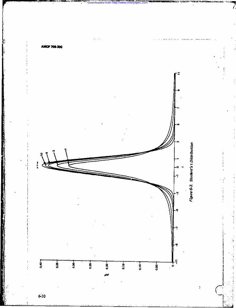
-MC 70620

CIO0

I4

I

Fl

640I


r

AMCP 700-200"'

TABLE 6-3

PERCENTILES OF THE t DISTRIBUTION(ADAPTED FROM Ref. 3)

The body of the table gives the value of tp, ,such that

Cdf {tp,,; V stuf (tp, ; A) P.

tj.p o- , 0

PD PROAuU1ITk I aXR CENT~ I60 70 80 90 95 975 99 99'5 99"9 99"95.

S'325 727 1'376 3'078 6314 1271 3182 6366 318-3 636.6

2 .289 '617 1-o61 t886 2'920 4'303 6.965 9,925 22"33 360,

3 '77 584 978 r638 2.353 3-182 4'54, 5-841 1O22 194

4 *271 '569 941 1'533 2.132 2776 3-747 4604 7"273 8.6%o

5 267 '559 920 1476 2.015 2-571 3'365 4032 893 6859

6 265 553 .906 1.440 1'943 2'447 3143 3707 5.208 5.959

7 263 '549 896 1415 1895 2'65 '998 3.499 4-785 5405

8 .262 546. '889 V397 VW860 2'306 2-896 3'355 4501 5'041

9 261 '543 -883 1'383 1'833 2-262 2'821 3.250 4'297 4-781

10 ,260 '542 879 1-37; V81z 2228 2-764 3"069 4.144 4587

xz .26) '540 "876 1363 I'796 '2o 2718 3'0 4d25 4.437

12 .259 539 873 1356 1-782 12179 2 681 3'055 3;9,0 4'318

13 '259 '538 .87o 1'350 1-771 2.-60 2.650 3"012 3-852 4221

14- 258 '537 .868 1345 1'761 2-145 2.624 2977 3787 4"140,

15 '258 '536 .W '-34' 1753 2-13L, 2602 2947, 3.733 4,073

%6 258 '535 .865 1'337 1.746 2 '120 2'583 2-92t 3686 4015

17 '257 '534 .863 i'333 1740 2'110 2'567 2898 466 3-965

28 '257 534 86z 1'330 '734 2o101 2'552 2'878 36n 3.922

19 257 '533 -86t 1328 1.729 2-093 2-'539 2 861 3.579 3-"3

20 257 .533. -860o 1'325 "725 2.o86 -r',l 2'845 3.552 3850

21 .257 ,532 859 1.323 1721 2-6O0 i-518 2'83" 3'527 3.819

22 '256 .532 .858 1321 1717 2074 2-'508 2-'819 3'505 3,792

23 '256 532 .858 1'319 1714 2o69 q 25oo 2807 3485 3,767

24 .256 '531 '857 1'318 1711 264 '2.492 '2'797 3-467 3-745

z5 .256 .531 .856 1-36 1'708 z'o6o .485 2-787 3"45q 3725

26 .256 '53i .856 1.315 1.7o6 2-056 2-'479 2-'779 3-435 3"707

27 '256 '531 "855 1'314 '793 2"052 2'473 '!71 3.421 34:90

28 .256 '530 "855 1.313 1'701 2'048 2-'467 1-703 3-408 3'674,

29 256 '530 '854 1'1;- t 1'699 204c Z-462 -2756 3396 3"

30 '256 '530 "854 1'310 1-697 2'042 2'457 2'750 3'385 3446

40 '255 '529 851 1'303 1-684 Z021 2'423 2-704 3"307 3.55t

50 255 .528 '849 1.298 z-676 2-.0; 2*403 2'678 3'62 3-495

60 '254 '527 '843 1.296 x.671 2'. 2'39o 2.66o 3'232 3'460

so .254 527 ,846 1.292 1664 19Po 2'374 2'639 3195 3415

100 '254 '526 845 1 .290 x'66o 1984 2'365 2-26 3-174 3.389200 2 54 !525 '843 1286 -653 I'972' z'345 26o 3.131 3'339,

500 '?53 '525 .. 965 334 2-5M6 3,9 .. 3o'253 '524 .842 1.282 1.645 1.96o 2.326 276 34- 3-291

1' 2(1-P)I 8o 8 o 40 20 20 5 2 1 02 0.

ftuf(2.086; 20) - 97.5%

Courtesy of John Wiley &Sons, Inc., publishen

6- 1'


AMCP706.200

Ref. 2 (Form.26.7.8) gives the following F =random variable; F > 0approximation fL.. large P (it is not very goodpf(;v, 2 cFll-even for moderate P): pf(;PsP)-cF /

(6-17)

4P) X (V2 +vP1 F) + vF)- (PI + V 2)/2

ZP 2'V/ (Zp has the sign of tp)

(6-15)

where gaujzp) = P and stuf(tp,,; P) =P. Eq. Cdf (F; v1, P2 ) =ffF; v1,'Y 2 ) (6-18)6-15 can bc inverted to give

S{fV;v 1I)v2 ) =fts~fi(F V), P2 ) (6-19)

tp~[( :~ 2~1I ~The first parameter is the degrees-of-free-tphas the sign of zp) (6-16) dom of the x 2 /v variate in the nunterator; the

(tp ~second -,parameter is the degrees-offreedomn of

the X2 /V variate in the denominator.As an example -of the accuracy of Eqs. 6-15and 6-16, for v =10,4l%, 10 'Zi 1%. The F distribution has some symmetry in

its parameters w~hich. is often used to shorten6-5 FISHER-SNEDECOR r: DISTRIBUTION tables of the 1' distribution.

The base name fis is given to the F .fisfF; Pi, M.0 =fisfc(IIF; v2, v1) (6-20)distribution (for Fisher-Snedecor). The suffixf implies the Cdf, and the suffix fc implies the P,*(v2 -2) fr~v2 > 2Sf (complement of the Cdf). E(,F; vi, v,- 2 2 oews

The ratio of the squares of 2 s-independent*~ statistics from the same s-nornial, distribution

has the F distribution. It is the ratio of any V2 f2(v + v2 -2)1/2 rV2>4tw xlv, variates. Fisher's original distribu- S~(;uv)= 2Lv ~ frvtion used-a different function-of F. Snedecor *- 00, otherwiseintroduced the F variable and named it afterFisher. Many authors, since then have givenboth men credit. 2pv+P2';21 1 2

I, (v2v 2The. symbol F is not used universally for CV{F; v1, v2 = V(V-4the random variable, butit is,'by far the most +0,otherwisecommon symlol.

6-5.1 FORMULAS

v1 , v2 =parameters, degrees of freedom, I(v.u) ['21[II2 4 )4;3Jv 6Pi ,P2 >0 oteris

6-12


AMCP 706-200

v (vI -2) wheremode(F; vv 2 ) =v(v 2 +2) - ifc(zQ)= Q

mdaFrI -21(9v, )i3 fisfc(FQ,,;v,, 2)Q (6-24)med;an(F; V1, P2 } 1 - 2/(9 v2).

cj -2/(9j ) << l, for t= 1, 2.

The-F distribution is related to other distribu- Eq. 6-24 is reasonably- good even -for smallertions (adapted from Ref. 2). values-of v, v2 , at least in the region-where it

is usudly used (right-hand tail area). TypicalflSfc(t 2 ;1, v)=2stufc(t;v),fort>O (6-21) results are

relative er-flsfc(F; vj, i 2 ) = l(vj/2, a'1 /2) (6-22) ,or in tail

/ + V 2 Q, % Q(z*), % area, %x 1) R/V2 + Pt F)

5 10 1.00 1.028 2.8where is the Beta distribution (Chapter 10), 10 5 1.00 1.18 18also called Incomplete Beta Function, Ref. 2 - 3 5 5.00 5.09 1.8(Sec. 26.5).

'Eq. 6-24 can be inverted to give Eq. 6-25.fisf (F, P, )= csnf (F, v) (6-23a)

flsf(F;*; v) fcsnfc(IIF; v) (6-23b).r7.cl) 1+1Z 1 O)/ 3

6-5.2 TABLES L\1-e 2 t,2 C2 UZQ

( 3The pdf is neither tabulated nor of engi- ) -, z, =0 (Q = 50%)

neering interest. Table 6-4 gives percentiles of c2

the F distribution (right-hand tal area only).- 1 -cA\ U"Because there are 2 parameters, the F distri- X Ll-cz) 1+(1 T U _U2)1/2J' 0

bution is difficult to tabulate extensively.Other tables are in Ref. I (Tables 18,19 and (6-25)Sec. 9) and Ref. 3 (Table VII, called the v2 where

distribution). Abbreviated tables are in moststatistics and quality control books.. c- 2/(9'v) <<-1

An approximation is &ien in Ref. 2 (For- U1, 1 - C1c (1 - c1)2 " 0mula 26.6.15)

*F FJ The approximations Eqs. 6-24 and 6-25 .re-z ,q - .F ".3 (1-Z( Z c (+ p , / -)1JI duce to those for X2/v as shown in Eq. 6-23

Qv and par. 6-3.

6-13

AMCP 706-200

TABLE 64A1

F DISTRIBUTIONS (ADAPTED FROM Rof. 4)

fisf (F; 01, 2) = 9%, fisfe (F; Pv, v2)

= 1%

fisf (1/F; v2,v) = 1%,fisfc 1/F; v2,v1 ) = 99%Body of the table gives the value of F.

Degrees of Freedom J- Numerator v

S3 4 5 6 7 8 9

1 4052.2 4999.5 5403.3 5624.6 5163,7 5859.0 5928.3 5981.6 6022.5

2 98.503 99.000 99.166 99.249 99.299 99.332 99.356 99.374 99.38C

3- 34.116 30.817 29.457 28.710 28.237 27.9)1 27i672 97.489 s7.'t45

4 21.)98 18.000 16.694 15.977 15.522 15.207 14.976 14.799 V-.659

5 16.258 , 13.274 12.060 11.392 10.967 10.672 10.45( 1 10- s 10.158

6 13.745 10.925 9.7-95 9,1483 8.7459 8.4661 8.-2600 1 8,o16 7.9761

7 12.246 9.5466 8.4513 7,8467 7.4604 7.1914 6,9928 6,84O1 6.718

8 11.259 8.6491 7.5910 7.0060 6.6318 6.3707 6.1776 6.0289 5.9106

9 10.551 8.0215 6.9919 6.4221 6.0569 5.8038 5.6129 5.4671 5.1511

0 10.044 7.5594 6.5523 5.9943 5.6363 5.3858 5.2001 5.0567 4.9424

11 9.6460 7.2057 6.2167 5.6683 5.3160 5.0692 4.8861 4.7445 4.63151

0 12 9.3302 6.9266 5.9526 5.411' 5.0643 4.8206 4.6395 4.4994 4.3875

0 - 13 9.0738 6.7010 5.7394 5.2053 4.866 4.6204 4.44i0 4.3021 4.1911

14 8.8616 6.5149- 5.5639 5.0354 4.695o 4,4558 4.2779 4.1399 4.0297

r 15- 8.6831 &.3589 5.4170 4.8932 4.5556 4.3183 4.1415 4.oo45 3.8948

! 16 8.5310 6.2262 5.2922 4.7726 4.4374 4.2016 4.0259 3.8896 3.7b04

.! 17 8.3997 6.1121 5.1850 4.6690 4.3359 4.1015 3.9267 , 3.7910 3.6822

18 8.2854 6.0129 ,5.0919 4.5790 4.2479 4.0146, 3;84o6- 3.7054 3.5971

19 8.1850 5.9259 5.0103 4.5003 4.1708 3.9386 3.7653 3.6305 3.5225,

20 8.0960 5.8489 4.9382 -4.4307 4.1027 3.87-14 3.6987 _ 3.5644 3.4567

o 21 -8.o166 - 5.7804- 4,8740 4.3688 4.0421 3.8117 3.6396 3.5056 3.396100 22 7.9454 5.7190 4.8166 4.3134 3.9880 3.7583. 3.5867 3.4530 3.3458

23 7.8811- 5.6637 4.7649 4,.2635 3.9392, 3.7102 3.5290 3,4057 3.28624 7.8229 5.6136 4.7181 4.2184 3.8951 3.6667 3.4959 3.3629 3.2560

25 7.7698 5.5680 4.6755 4.1774 3.8550 3.6272 3.4568 3.3239 3,2172

26 7.7213 5.5263 4.6366 4.1400 3.8183 3.591', 3.4216 3.2884 3,1818S2/ 7.677 5.4881 4.0009 4.1056 3.7848 3.5580 3.3882 3.2558 3.1494

28 7.6356 5.4529 4.5681 4.0740 3.7539' 3.5276 3.3581- 3.2259 3.1195

29 7.5976 5.4205 4.5378 4.0449 3.7254 3.4995 3.3302 3.1981 3.0920

30 7.5625 5.3904 4.5097 4.0179 3.6990 3.4735 3.3045 3.1726 3.0665

40 7.341l- 5.1785 4.3126 3;8283 3.5138- 3.2910 3.1238 2,9930- 2.8876

60 7.0771 4 i9774 4;1259 3.6491 3.3389 3.1187 2.9530 2.8233 2.7185

120 6.8510 4, 7865 3.9493 3.4-96 3.1735 2,9559 2.7918 2.6629 2.5586

L 6.6349 ,t.6052, 3.7816 3.3192 3.0173 2.8020 2.6303 2.5113 2.4073.

6-14


AMCP 706-200

TABLE 6-4(A) (Coitinued)

F DISTRIBUTIONS (ADAPTED FROM Hef. 4)

fisf(F;v,,v1 = cj3%,fisfc(F; vi,v 2 ) = 1%

fisf (llF;V2 ,v1 ) = 1%,fisfc (1/F; v2 ,) = 99%Body of the table gives the value of F.

Degreea of Freedom In Num6rator v1

10 12 15 20 24 30 40 60 120 _

1 6055.8 6106.3 6157.3 -6208.7 6234.6 -6260.7 6286.8 6313,0 6339.4 6366.02 99.399 99.416 99.432 99.449 .99.458- 99.1166 99.474 99.483 99.491 99.501

27.052 26.872 26.690 26.598 26.505 26.411 26.316 26.221 26.125

4 14.546 14.374 14.158 14.020 13.929 13.838 13.745 13.652 13.558 13.463

5 10.051 9.8863 9.7222 9.5527 9.4665 9.793 9.2912 9.2020 9.1118 9.0204

6 7.8741 7.7183 7.5590 7.3958 7.3127 7.2285 7.L432 7.0568 6.9690 6.88o

7 6,6201 6.4691 6.31,'3 6.1554 6.0743 5.9921 5.9084 5.8326 5.7572 5.6495

8 5.8143 5.6668 5.5151 5.3591 5.2793j 5.1981 5.1156 5.0316 4.9460 4.85889 5.2565 5.1114 4.96,1 4.80301 4.7290 4.6486 4.5667 -4.4831 4.3978 4.3105

10 4.8492 4.7059 4.5582 -4.4054 4,3269 4.2469 4.1653 4.0819 3.9965 3.9090-

11 4.5393 4.3974 4.2509 4.0990 4.0209 3..9411 3.8596 3.7761 3.6904 3.6025

0 12 4.2961- 4.1553 4.0096 3.8584 3.7805 3.7008- 3.6192 3.5355 3.4494 3.360813' 4.1003' 3.9603 3.8154 3.6646 3.5868 3.5070 3.4253 3.3413 3.2548 3.1654.

14 3.9394 3.8001 3.6557 3.5052 3.4274 3.3476 3.2656 3.1813 3.0942 3.0040

15 3.8049. 3.6662 3.5222 3.3719 3.2946 3.2141 3.1319 3.o471 2.9595 2.8684

16 3.6909 3.5527 3.4089 3.2588 3.1808 3.1007 3.0182 2.9330 2.8447 2.7528

17 3.5931 3.4552 3.3117 3,1615 3.0835- 3.0032 2.9205 ?.8348 2.7459 12.653018 3.5082 3.3706 3.2273 3.0771 2.9990 2.9185 2.8354 2.7493 2.6597 -.566o-19 3.4338 3.2965 3.1533 3.0031 2.9249 2.8442 2.7608 2.6742 2.5839 ?.489320 5,3682 3.2311 3.0880 2;9377 2.8594 2.7785 2.6947 -2.6077 2.5168 q.4212,

21 3.3098 3.1729 3.0299 '2.8796 2.8011 2.,7200 2.6359 2.5484 '2.4568 2.3603'0 -22 3.2576 3.1209 2.9780 2.8274 2.7488 2.6675 2.5831 2.4951 2.4029 2.3055

' 23 3;2106 3.0740 2.9311 2.7805 *2.-7017, 2.6202 2.5355 2.4471 2.3542 2.2559'

24 3.1681 3.0316 2.8887 2.7380 2.6591 2.577-3 2.4923 2.4035 2.3099 2.2107

25. 3.1294 2.9931 2.8502 2.6993 2.6203 2.5383 2.4536' 2.3637 2.2695 '.1694

26 3.0941 2.9579 2.8150 2.6640 2.5848 2.5026 2.4170 2.3273 2.2 25 2.131527 3.0618 2.9256 2.7827 2.6316 2.5522 2.4699 2.3840 2.2938 2.1984 2.0965

28 3.0320 2.8959 2.7530 2.6o17 2.5223 2.4397 2.3535 2.2629 2.1670 2.0642

29 3.0045 2.8685 2.7256 2.5742 2.4946 2.:,118 2.3253 2.2344 2.1378 2.0342

30 2.9791 2.8431 2.7002 2.5487 -.4689 2.3860 2.2992 2.2079 2.1107 2.006.,

40 2.8005 2.6648 2.5216 2.3689 2.2880 2.2034 2.1142 2.0194 1.9172 i.8047-

60 2.6318 2.4961 2.3523 2.1978 2.1154 2.0285 1.9360 1.8363 1.7263 1.6006120 2.4721 2.3363 2.915 2.0346 1.9500 ?.8600 1.7628, 1.6557 1.5330'1.3805 -

I - 2.3209 2.1848 2.0385. 1.8783 1.790 1.6964 1.5923 1.4730 i.3246 1.000

____________-15


AMCP 704-200

TABLE 6.4(B)

F DISTRIBUTION (ADAPTED FROM Ref. 4)

fisf (F; V1, v2 ) = 97.5%, fisfc (F; V1 , v2) - 2.5%fkf (I/F;, 2,vi) = 2.5%,fisfc (1/F; v2 ,v) = 97.5%Body of tho tahle givss the value of F.

Degrees of Freedom in Numerator V1

- 1 2 3 4 5 6 7 8 9

1 647.79 799.50 864.16 899.58 921.85 937.11 948.22 956.66 963.28

2 38.506 39.000 39.165 39.248 39.298 39.331 39.355 39.373 39.387

3 17.443 16.044 15.439 15.101 14.885 14.735 14,624 14.540 14.473

4 12.218 1O.649 9.9792 9.6o45 9.3645 9.1973 9.0741 8.796 8.9047

5 1.-007 8.4336 7.7636 7.3879 7..1464 6.9777 6.831 6.7572 6.681o

6 8.8131, 7.2598 6.5988 6.2272 5.9876 5.8197 5.6955 5.5996 5.523k

7 8.0727 6.5415 5.8898 5.5226 5.2852 5.1286 4.9949 4.8994 4.8232

8 7,5709 6.0595 5.4160 5.0526 4.8173 4.6517 4.5286 4.4332 4.3572

9 7.2093 5.7147 5,0781 4.7181 4.4844 4.3197 4.1971 4.1020 4.0260

10 6.9367 5.4564 4.8256 4.4683 4.2361 4.0721 3.9498 3.8549 3.7790

11 6.7241 5.2559 4.6300 4.2751 4.0440 3.8807 3.7586 3.6638 3.5079

12 6.5538 5.0959 4.4742 4.1212 3.8911 3.7283 3.6065 3.5118 3.4358

13 6.4143 4.9653 4.3472 3.9959 3.766 3.6043 3.4827 3.3880 3.3120

14 6.2979 4.8567 4.2417 3.8919 3.6634 3.5014 3.3799 3.2853 3.2093

15 6.1995 4.7650 4.1528 3.043 3.5764 3.4147 3.2934 3.1987 3.1227-

16 6.1151 4.6867 4.0768 37294 3.5U21 3.3406 3.2194 3.1248 3.0' 88

1.7 6.oZ"' 4.6189 4.0112 3.6648 3.4379 3.2767 3.1556 3.0610 2.9849

18 5.9781 4.5597 3.9539 3.608 3.3820 3.2209 3.0999 3.0053 2.9291

i9 5.9216 4.5075 3.9034 3.5587 3.3327 3.1718 3.0509 2.9563 2.8800

20 5.8715 4;4613 3.8581 3.5147 3.2891 3.1283 3.0074 2i912P 2.8365

21 5.8266 4.4199 3.8188 3.475 3.250i 3.0895 2.9686 2.8740 2.7977

22 5.7863 4.3828 3.7829 3.44Ol 3.2151 3.0546 2.9338 2.8392 2.7628

23 5.7498 4.3492 3.7505 3.4083, 3.1835 3.0232 2.9024 2.8077 2.7313

24 5.7167 4.3187 3.7211 3.3794 3.1548 2.9946 2.8738 2.7791 2.7027

25 5.6864 4.2909 3.6943 3.3530 3.1287 2.9685 2.8478 2.7531 2.766

26 5.6586 4.2655 3,6697 3.3289 3.1048 2.9'47 2.820 2.7293 2.6528

27 5.6331 4.2421 3.6R72 3,3067 3.0828 2.9228 1 8021 L;7074 2.6309

28 5.6096 4.2P05 3.6264 3.2863 3.0625 2.9027 2.782b 2.6872 2.6106

29 5.5878 4.2006 3.6072 3.2674 3.0438 2.8840 2.7633 2.6686 2.5919

-30 5.5675 4.1821 3.5894 3.2499 3.0265 2.8667 2.7460 2.6513 2.5746

40 5.4239 4.0510 3.4633 3.1263. 2.9037 2.7444 2.6238 2.5289 2.4519

0 5.2857 3.9253 3.3425 3.0077 2-.7863 2.6274 2.5068 2:4117 2.3344

120 5.1524- 3.8046 3.2270 2.8943 2.6740 2.5154 2.3948 2.2994 2.2217*6 M.239 3.6889 3.161 27858 2.5665 2.4082 227 .98 213

- , - -' A


AMCP 706-200

TABLE 6-4(B) (Contlr ud)


fisf (F; v,V 2) = 97.5%,fisfc (F;v 1 ,v2) = 2.5%fisf (1/F; 2 ,v,) = 2.5%,fisfc (1/F;v 2 , V) =-97.5%Body of the table gives the value of F.

Decrees ofreedomn in Numeratorv

10 i2 15 20 24 30 4o0 60 120

1 968.63 976.71 984.87 993.10 997,25 1001.4 1005.6 1009.8 1014.0 1018.32 39.398 39.415 39.431 39.448 39.456 39.465 39.473 39.481 39.090 39.A98

3 14.419 14.337- 14.253, 14.167 14.124 14.081 14.037 13.992 13.947 13.9024 8.8439 8.7512 8.6565 8.5599- 8.5109 8.4613 84111 8.36p4 8.3092 8.25735 6.6192 6.5246 6.4277 6.3285 6.2780 6.2269 6.175i 6.1225- 6.0693 6.0153

6 5.4613 5.3662 5.2687 5.1684 5.1172 5.0652 5.0125 4.95a9 4.9o45 4.81s917 4.7611 4,.6658 4.5678 4,4667 4.450 4.3624 4. 3089 b.25,4 4,1919 4,,4,3

8 4.2951 4.1997 4.1012 3.9995 3.9472 3.8940 3.8398 3.7844 3.7279 3.6702

9 3.9639 3.8682 3.7694 3.6669 3.6142 3.560) 3.5055 3.4493 3.3918 3.3329

10 ..168 3.6209 3.5217 3.4186 3.3654 3.3110 3.2554 3.1984 3.1399 3.0796> 11 3.5257 3.4296 3.3299 3.2261 3.1725 3.1176 3.0613 3.0035 2.9441 2.8828

, 12 3.3736 3.2773 3.1770 3.0728 3.0187 2 9633 2.9063 2.8478 2.7874 2.7249

4 13 3.2497 3.1532 3.0527 2.9477 2.8932 2.8373 2.77,17 2.720 2.6590 2.595514 3.1469 3.0501 2,9493, 2.8437 2.7888 2.7324 2.,6742 2.6142 2.5519 2.487

15 3.0602 2.9633 2.8621 2.7559 2.7006 2.6437 2.5850 2;5242 2.4611 2.3953

16 2.9862 2.8890 2.7875 2.6808 2.6252 2.5678 2.5085 2.4471 2.3831 2.316?

17 P.9222 e.8249 2.7230 2.6158 2.5598 2;5021 2.422 2.3801 2.3153 2.2474

18 2.8664 2.7689 2.6667 2.5590 2.5027 2.4445 2.3842 2.3214 2.2558 2.1869

19 2.8173 2.7196 2.6171 2.5089 2.4523 2.3937 2.3329 2.2695 2.2032 2.1333

? 20 2.7737 2-.6758 2.5731 2.4645 2.4076 2.3486 2.2873 2.2234 2.1562 2.0853

21 '2.7348 2.6368 2.5338 2.424-7 2.3675 2.3082 2.2465 2.1819 2.1141 2-.0422o 22 2.6998 2.6017 2.4984 2.3890 2.3315 2.2118 ,2.2097 2.1446 2.0760 2.0032

23 2.6682 2.5699 2.4665 2.3567 2.2989 2.2389 2.1763 2,1107 2.0415 1.9677

24 2.6196 2.5412 2.4374 2.3273. 2.2693 2.2090 2.1460 2.0799 2.0099 1.9353

25 2.6135 2.5149 2.4110 2.3005 2.2422 2.1616 2.1183 2.0517 1.9811 1.9055

26 2.5895 2.4909 2.3867 2.2759 2.2174 2.1565 2.0928 2.0257 1.9545 1.8781

27 2.5676 2.4688 2.364 2.2,33 2.1946 2.1334 2.0693 2.0018 1.9299 1.8527

28 2.5413 2.4484 2.3438 2.23?4 2.1735 2.1121 2.0477 1.9796 1.9072 1.0291

29 2.5286 2.4295 2.3248 2.213i 2.1540 2.0923 2.0276 1.9591 1.8861 1.8072

30 2.5112 2.4120 2.3072 -.1952 2.1359 2.0739 2.0089 1.9400 1.8664 1.7867

40 2.3832 2.2882 2.1819 2.0677 2.0069 1.9429 1.8752 1:8028 1.7242 1.6371

60 2.2702 2.1692 2.0613 1.445 1.8817 1.8152 1.74';0 1.6668 1.5810, 1.4822

120 2.1570 2.0548 1.9450 1.8249 1.7597 1.6899 1.6141 1.5299 i.4327 1. 3104

2.0483 1,9447 1.8326 1.7085, 1.6402 1.5660 1.4835 1 i.3883 1.2684 1.0300,

_6-17,


AMCP 706-200

TABLE 6-4 (C)

F DISTRIBUTION (ADAPTED FROM Rof. 4)

fisf (F; vi, V2 ) = 95%,fisfc-(F;vj,V2) = 5%

fif (1/F; v2 , P,) = 5%, fisfc (1F; V1, V) =95%

Body of the table gives the value of F.

Degreca of Freedom in Numerator, Y1

2 3 4 5 6 7 8 9

1 161.45 199.50 215.71 224.58 230.!,6 233.99 236.77 238.8b 240. ,54

2 18.513 19.000 19.164- 19.247 19.296 19.330 19.353 19.371 19.385

3 10.128 9.5-21 9.2766, 9.1172 9.0135 8.9466 8.8868 8.8452 8.8123

4 7.7086 6.9443 6.5914 6.3883 6.2560 6.1631 6.092 6.0410 5.9988

5 6.6079 5.786! 5.4095 5.1922 5.0503 '4.9503 4.8759 4.8183 4.7725

6 5.9871; 5.1433 4.7571 4.5337 4.3874 4.2839 4.2066 4.1463 4.0990

7 5.5914 4.7374 4.3468 4.120- 3.9715 3.866o 3.7870 3.7257 3. 6767

8 5.317y 4.459o 4.c662 3.8378 3-6875 3.5806 3.5005 3.4381 3.3881

9 5-.174 4.2565 3.8626 3.6331 3.4817 3.3738 3.2927 3.2296 3.1789

10 4.9646 4.1028 3.7083 3.4780 3.3258 3.217? 3.1355 3.0717 3.0204

> 11 4.8443 3.9823 3.5874 3.3507 3,2039 3.0946 3.0123 P.9480 2.8962

12 4.7472 3.8853 3.4903 3.2592 3.1059 2.9961 2.9134" 2.8486 2.7964

13 4 .6672 3.8056 3.4105 3.1791 3.0254 2.9153 2.8321 2.7669 2.7144

14 4.6001 3.7-389 3,3439 3.1122 2.9582 I 2.8477 2.7642 2.6987 2.6458

13 4.5431 3.6823 3.2874 3.0556 2.9013 2,7905 2.7066 2.6408 2.5876

16 11.4940 3.6337 3.2389 3.0069 2.8524 2.7413 2.6572 2.5911 2.5377

17 4.4513 3.5915 3.1968 2,9647 2. 87 2.613 2.5480 2.4943

18 4.4139 3.5546 3.1599 2.9277 2.7729 2.6613 2.5767 2.5102 2.4563

19 4.3803 3.5219 3.1274 2.8951 2.7401 2.6283 2.5435 2.4768 2.4227

10 20 4 351 4928 3.0984 2.8661 2.709 2.5990 2.514C 2.44'71 243928,

04 1 2/48 3.4668 3.0725 2.84o1 2.6848 2.5727 2.4876 2.4205 2.3661

- 22a 4.3009 3,4434 3.0491 2.8187 2.6613 2.5491 2.4638 2.3965 2.3419

23 .2793 3.4221 3.0286 2.7955 2.6400 2.5277 2,4422 2.3748 2.3201

24 4.2597 3.4028 3.0088 2.7763 2.6207 2.5082 2.4226 2.3551 2.3002

25 4.2417 3.3852 2.9912 2.7587 2.6030 ".4904 2.4047 2.3371 2.2821

* 26 4.2252 3,3690 2.9751 2.7426 2.5868 2.4741 2.3883 2.3205 2.:655

27 4.2100 3.3541 P.9604 2.7273 2.5719 2.4591 2.3732 2.3053 2.2501

28 4.1960 3.3404 2.9467 2.7141 2.5581 2.4453 ,.3593 2.2913 2.2360

29 4.1830 3.3277 2.9340 2.7014 2.5454 2.4324 2.3463 2.2782 2.2229

30 4.1709 .3158 2.9223 ,.689,6 2.5336 i 2.4205 2.3343 2.2662 2.21U7

40 4.0848 3.2311r 2.8387 2.6060 2.4495 2.3359 2.29490 2.1802 2.1240

60 4.0012 3.1504 2.7581 2.5252 2.3683 2.2540 2.1665 2.0970 2.0401

20 3.9201 3.0718 2.6802 .4472 2.2900 2.1750 2.0867 2.0164 1.9588

3.8415 Z.9957 2.6049 2.3719 2.2141 2.0986 P.6096 1.93804 1.8799

- -- A- - - -


AMCP 706-200. .3

TABLE 6-4(C) (Continued)


fisf (F; vk, v) 95%, fisf (F; P1, v2 ) = 5%fisf(F2v,v) = 5%,fisfc (11F;v 2 ,,) = 95%Body of the table gives the velue of F.

Iegrees of Freedom in Numeato, v

10 12 15 20 24 30 4o 60 12o

1. 241.88 '243.91 245.95 248.01 249.05 250.09 051.14 252.20 253.25 254.32

2 19-396 19.413, 19.429, 19.446 19.454 19.462 19.471 19.479 19.487 19.4963 8.7855 8.7446' 6.7029 8.6602 8.6365 :8.6166 8.5941, 8.5720 8.5494 8.52654 5.9644 5.9117 5.8578 5.8025 5.7744 5.7459 5.7,170- 5.6678 5.6581 5.62815 4.7351 4.6777 4.6188 4.5581 4.5272 4.4957- 4.4638 4.4314, 4.3984 4.36506 4.0600 3.9999 3.9381 3.8742 3.8415 3.8082 3.7743 3.7398 3.7o47, 3.66887 3.6365 3.5747 3.5108 3.4445 3.4105 3.3758 3.34G4 3.3043 3.2674 3.22988 3.3472 3.2840 3.2184 3.1503 3.1152 3.0794 3.0428 3.0053 2.9669 2.9276

9 3.1373 3.0729 3.0061 2.9365 2.9005 2.8637 2.8259 2.7872 2.7473 2.706710 2.9782 2.9130 2.8450 -2.7740 2.7372 2.6996 -2.6609 2,6211 2.5801 2.537911 2.8536 2.7876 2.7186 2.6464 2.6090 2.5705 2.5309- 2.4901 2.4480 2.404512 2,7534 2.6866 2.6169 2.543612.5055 2.4663 2.4259<2.384 2.3P10 2.2962

13 2.6710 2,6037 2.5331 2.4589 "2.4202 2.3803 '2.3392 2,2966 2.2524- 2.206414 2.6021 2.5342 2.4630 2.3879 2.3487 2.3082 2.2664 2-2230 2.1778 '2.130715 2.5437 2.4753 2.4035 2.3275 4.2878 2.2468 2.2043: '2.1601 2.114.1 2.065816 2.4935 2.4247 2.3522 2.2756 2.2354 '2.1938 2.1507 2.1058 2.0589 2.009617 2.4499 2.3807 2.3077 2.2304 2.1898 2.1477 2.104 2.0584 2.0107 1.960418 2.4117 2.3421 2.2686 2.1906 2.1497 2.1071 2.0629 2.0156 1.9681 1.916819 2.377 2.3080 -2.2341 2.1555 2.141 ,2.0712 2.0264 1.9796, 1.9302 1.878020 2.3479 2.277M6 2.2033 2.1L,42 2.0825 2.0591, 1.9938 1.9464 1.8963 1.8432

o 21' 2.3210 2.2504 2.1757 2.0960 2.0540' 2.0102 1.9645T 1.9165- 1.8657 1.8117q2 2.2967 2.2258 2.1508 2.0707 2.0283 1.9842 1.9380 1;8895 1.8386 1.783123 2.2747 2.2036 2.3282 2.0476 2.00,50 1.9605 1.9190 1.8649 1.8128 1.757024 2.2547 2.1834 2.1077 2.0267 1.9838 1.9390 1.8920 1.8424 1.7897 1.733125 2.2365 2.1649 -2.0889 2.0075 1.9643 1.9192 1.8718 1.8217 1.7684 1.71.1026 2.2197' 2.1479 2.0,16 1.9898 1.9464 1.9010 1.853a 1.8027 1.7488 1.690627 -2.2043 .2.1323 2-.0558 :.9736 1.9299 1.8842 1.8361 1.7851 1.7307 1.671728] 2.1900 2.1179 2.0411 1.9586 1.9147 1.8687 1.8203 1.7689, 1.7138' 1.6541

• I 29 2.1768 2 1045 2.0275 1.9446 .1.9005 1.85A3, 1.80 5 1.7537 1.698i' 1.637730 2.13646, 2.0921 2.0148 1.93171 1.8874, 3-.8409- 1.7918 1.73.6 1.6335 1.4223

'40 2.0772' 2.0035 1.9245 1.8389 1.7929 1.7444 -1.'6928 -1L.6373 1.5766 ,.5089-60 1.9926 1.9174 1.8364 1.7480' 1.7001 1.6491 1.5943 1.5343 1.4673 1.3893-120 1.9105 1.833 7 1.-7505 1.6587 1.6084 1.5543 1.4952 1.4290 i.3519 1.2539

. o 1.8307 1.752L 1.6664 1.5705 1.5173 1.4591 1.39401..3180 1.2214 1.00o0

77t

AMCP 706200

TABLE 64MD)


fisf (F; v, v2) '. 90%, fskfc (F; vY, v2) = 10%fisf (I/F; v2 ,v1) -l0%,fisfc (IIF; P2,s) - 90%B'dy of the table gives values of F.

Degrees or Freedom-In orator V

1 2 3 J 5 6 T 8

1 39.864 49.500 53-.593 55.833 57,241 58.204 58.906 59.439 59.8582 8.5263 9.0000 9.i618 9.2434 9.2926 -9.3255 9.3491 9.3668 9.3805

3 5.5383 5.4624 5.3908 5.3427 5.3092 5.2847 5.2662 5.2517 5.24004 4.5448 4.3246 4.1908 4.1073 4.0506 4.0098 3.9790 3.9549 3.9357

5 4.0604 3.7797 3.6195 3.520e 3.4.130 3.4045 3.3679 3.3393 3.31636 3,7760 3.4633 3.2888 3.1808 3.1075 3.0546 3.0145 2.9830 2.§577

7 3.5894 3.2574 3.0741 2.9605 2.8833 2.8274 2.7849 2.7516 2.72478 3.4579 3.1131 2.9238 2.8064 2.7265 2.6683 2.6241 2.58q3 2.56129 3.3603 3.0065 2.8129 2.6927 2.6106 2.5509 2.5053 2.4694 2.4403

10 3.2B50 2.Q245 2.7277 2.6053 2.5216 2.4606 2.414o 2.3772 "'.3473

11 3.2252 2.8595 2.6602 2.5362 2.4512 2.3891 2.3416 2.3040 2;273512 3.1765 2.8068 2.6055 2.4801 2.39k0 2.3310 2.2828 2.2446 2.213513 3.1362 2.7632' 2.5603 2.4337 2.3467 2.2830 2.i341 2.1953 2.1638

14 3.1022 2.7265 2.5222 2.3947 2.3069 2.2426 2.1931 2.1539 2.122015 3.0732 2.6952 2.4898 2.3614 2.2730 2.2081 2.1582 2.1183 2.086216 3.0481 2.668R 2,4618 2.3327 2.243B 2.1783, 2.1280 2.086Z 2.055317 ".0262 2.6446 2.4374 2.3077 2.2183 2.1524 2.1017 2.o613 2.0284.18 3.0010 2.6239 2.4160 2.2858 2.1958 2.1296' 2.0785 2.A379 2.0o47'

19 2.9899 2.6056 2,3970 2.2663 2.1760 2.1094 2,0580 2.0171 1,9836

0 20 2.9747 2.5893 2.3801 2.2489 2.1582 2.0913 2.039, 1.9985 1,964921 2.9609 2.5746 2.3649 2.2333 2.1423 2.0751 2.0232 1,9819 1.9480

22 2.9486 2.5613 2.3512 2.2193 2.1!79 2,0605 2.0084 1.9668 1.932723 2.9374 2.5493 2.3387 2.20(3 2.1149. 2.o472 1.9949 1.9531 1.9189

24 2.927 2.53b3 2 3274 2.1949 2.1030 2.0351 1.9826 1.9407 1.9o63

25 2.9177 2.5283 2.3170 2.1843 2.0922 2.0241 1,9714 1.9292 1.894726 2.9091 2.5191 2.3075 2.1745 2.0822 2.0139 1.961o i.9188 1.8841.

27 2.9n12 2;5106 2-2987 2.655 2.0730 2.6045 1.9515 1.9091 3.874328 2.8939 2.5028 2.2906 2.1571' 2.0045 1.9959 1.9427 1.9001 1.8652

29 2.8871 2.4955 2.2831 2.1494 2 0566 1.9878 1.9345 1.8918 1.8568

30 2.8807 2.4887 2.2761 2.1422 C.0492 1.9803 1.9269 1.8841 , 1.84o90

.40 2.8354 2.4404 2.2261 2.0909 1.9968 1.9269 1.8725 1.8289 1.7929

60 2.7914 2.3932 2.1774 2.0410 1,9457 1.8747 1.8194 1.7748 1.7380

120 2.7478 2.j473- 2.1300 1.9923 1.8959 -1.8238 1.7675 .1.7220 1.68432.7055 2.3026 -.. 0838 1.9449 1.8413 1.7741-, 1.7167- 1.67b2 1.6315,

;A&20


AMCP 706-200

TABLE 6-4(D) (Continued)


fisf (F -P1 ." 2 ) 90%, isfc (F; v1, P2) = 10%fisf (1/F; 12,v) lO%,fisfc(1/F;v2,z) = 90%Body of the table gives values of F.

Degreet" Freedom In NWzer.or v-

10 12 15 20 2I 30 40 60 12060.195 60.705 61.220 61,743 - 2.002 62,265 62.529 62.794 63.061 63.328

9.3§16 9.4081 9.4247 9.4413 9.4496 94579 9.4663 9.4746 9.4829 9.4913

3 5.2304 5.2156 5.2003 5.1845 r.1764 5,1681 5.1597 5.1512 5.1425 5.1337

4 3.9199 3.8955 3.8689 3,8443 3.8310 3.8174 3.8036 3.7896 3.7753 3.7607

5 3.2974 3.2682 3.2380 3.2067 3.1905 3.71 3,1573 3.1A402 3.1228 3.1050

6 2.9369 2.9047 2.8712 2.863 2.8.83 2.8000 2.7812 2.7620 2.7423 2.7222

7 2.7025 2.6681 2.6322 2.5947 2.5753 2.5555 2.5351 2.5142 2.492e 2.4708

8 2.5380 2.5020 2.4642 2.4246 2.4041 2.3830 2.3614 2-3391 2.3162 2.292f

9 2.4163 2.3789 2.3396 2.2983 2.2768 2.25k7 2.2320 2.2085 2.1843 2.159'e

10 2.3226 2.2841 2.2435 2.2007 2.1784 2.1554 2.1317 2.1072 2.0818 &.o554

11 2.2482 2.2117 P.1671 2.1230 2.100C- 2.0762 2.0516 2.C,61 1.9997 1.9721,

L 12 2.1878 2.14,4 2.1049 2.0597 2.0360 2.0115 1.'861 1.9597 1.9323 1.9036

13 2.1376 2.0966 2.,0532 2.0070 1.9827 1.9576 1.9315 1.9043 1.8759 1.8462

- 14 2.0954 2.0537 2 .0095 1.9625 1.9377 1.9119 1.8352 1.8572 1.8280 1.7973

15 2.0593 2.0171 1.9722 1.9243 1.8990 1.8728 1.8454 1.8168 1.7867 1.7551

8 11 2.0281 1.9854 1.9399 1.8913 1.8656 1.8388 1.8108 1.781b 1.7507 1.7182

4 '7 2.00C9 1.9577 1.9117 1.8624 1.8362 1.8090 1.7809 1,7506 1.7191 1.656

F 18 1.9770 1.9333 1.8868 1.8368 1.8103 1.7827 1.7537 1.7232 1.6910 1.6567

19 1.9557 1.9117 1.8647 1.8142 1.7873 1.7592 1.7298 1.6988 1.6659 1.6308

20 1.9367 1.8924 1.8449 1.7938 1.7667 1.7382 1.7083 1.6768 1.6433 i.6074

21 1.9197 1.8750 1.8272 1.7756 1.7481 1.7193 1.(890 1.6569 1.62-5 1.5862

22 1.9043 1.8593 1.8111 1.7590 1.7312 1.7021 1.6714 1.6389 1.6042 1.5668

23 1.39(" 1.8450 1.7964 1.7439 1.7159 1.6864 1.6554 1.6224 1.5871 1.5490

t 24 1.8775 1.835 9 1.7831 1,7302 1.7019 1.6721 1.6407 1.6073 1.5715 1.327

25 1.8658 1.8200 1.7708 1.7175 i1.6890 1.6589 1.6272 1.5934 1 5570 1.5176

26 1.8550 1.8090 1.7596 -.7059 i6771 1.6468 1.6147 1.5805 1.5437 1.5036

27 1.8451 1.7989 !.7492 1.6951 1.6662 1.6356 1.6032 1.5686 1.5313 1.496

28 1.3359 1.7895 1.7395 1.6852 1.6560 1.6252 1.5925 1.5575 1.5198 1.4784

29 1.8274 1.7808 1.7306 1.6759 1.6465 1.6155 1.5825 1.5472 1.5090 1.4670

30 1.8195 1.7727 1.7223 1.6673 1.6377 1.6065 1.5732 1 5376 1.4989 1.456440 1.727 1.7146 1.6624 1,6052 1.5741 1.5411 1.5056 1.4672 1.4248 1.3769

60 1.707C 1.6574, 1.6034, 1.54,05 1.5107 1.4755 1.4373 1.3952 1.3476 1.2915

120 1.6524 1.6012 1.5450 1.4821 1.4472 1.4094 1.3676 1.3203 1.c646 1.1926

1.5987 1.54;8 1.4871 1.4206 1.3832 1.3419 1.29:)1 1.2400 1.1686 1.0000

.1 1


REFERENCES

1. E. S. Pearson and H. 0. Hartley, Bio- 3. A. Hati, Statisticad Tables and Formulas,metrlka Tables for Statisticians, Vai. I, John Wiley & Sons, 1952.Cambridge Univ. Press, 1956.,

2. Abramowitz and Stgun, Eds., Handbook 4. Reliability and Maintainability Handbookof Mathematical Functions, AM555, NBS, for the U.S. Weather Bureau, Publ.USGPO, June 1964 with subsequent cor- 530.01!1-762, ARINC Research, Corp;,rected printings., Annapolis, MD, April 1967.

II

7- a

I .!

a g 'IN


AMCP 7000

CHAPTER,7

EXPONENTIAL DISTaIBUTION

7-0 LIST OF SYMBOLS R = s-Reliability

C~~~5 = -ofdne~ denotes statistical definition

Cdf =Cumulative. distributicn func- Sf =Survivor fuinctiontion

C, L, U =subscripts -that imply a s-confi- S v = tnad eito

dence level; C is general, L is Var {I = variancelower, U is upper

8 = scale parameterCorf f } = a-Confidence level

X rate-parameter- CM = Ith central moment

V degrees of freedomCV1 I coefficient of variation:

StDv { )Ef random variable

EfI s-Expected value {;, ') =the fixed' parameters are listedto the right of the semicolon,

exp -base name for exponential dis- the random variable is listed totribution the left of the semicolon

expf = Cdf for exponential distri- -= the complement,, e.g.,- -1-bution 0 where 0 is any probability

expfc =Sf for exponential distribution 7.1 INTRODUCTION

Mil I = Ith moment about the origin This, Is -the mc-fl commonly used PrD f.or* life-eg., flime to failure). It is closely related

*NCMi = normalized ith central mo- to the-Poisson process. The'base-name exp, is'ment; CM, j If /Stm{ I ji given to the exponenitial- disrribution (for

Wpntatial). The suffix f -implies the Cdf,pdf = probability density function and the suffix fc implies the Sf (complement

of the Cd!).pint - probability mass function

7-2 FORMULASPr I =Probability

PrD =Probability distribution =rate parameter, X> 0, (N 1 /0)

7-1J


AMCP,706-200

0 = scale parameter, 0 > 0, (0 I/X) 7-3 TABLES

" random variable, t L 0 In the 1950's several tables were generatedfor the exponential distribution in reliability,

pdf {r; X) =X exp( - Xr) (7-1a) e.g., Ref. 2. Since the exponential functionhas been common in mathematics for hun-

pdf(r; 0) = (1/0) exp( - r/0) (7-Ib) dreds of years, several extensive tables exist intheir own right, e.g., Ref. 1 (Tables 4.4 and4.5). The electronic calculator with engineer-

Cdf( (r; X) = expf(Xr) = 1 - exp( - Xr) ing functions often contains the exp and Rn(7-2a) functions, thus tables are virtually unneces-

Cdf{ r; 0) =exp(r0) = 1 - exp( -T,/0) sary.(7-2b)

Table 7-1 is an abbreviated set of tables. Ituses the fact that exp(xl + .+ .x) =

Sf {vr;X) = expfc(X7) = exp(- )X) (7-3a) exp(x 1) ... exp(xs).

Sf(r; 0} = expfc(r/0) = exp( - r/0) (7-3b) In reliability work, more accuracy usuallyis required for small values of the argument

failure rate{ 'r; X,) = X (7-4a) than for-large ones, because very low reliabili-ty (large values of the argument) is bad

feilure rate (r;0.= 1/0 (Q-4b) anyway and 'the degree of badness need notbe known to many significant figures. Eq. 7-5

E(; 0) = 0 is good for all values of the argument, but iseasiest to use for small values. The error is

StDv{ r; 0) = 0 always less than the next unused term. (It is:the usual power series: xn/n!.)

CV (r;0) = 1

exp x)l e-X x

NCM3 {r; -- 2 (7-5)

moder ; 0) = 0 For example, expf(0.1) = i -0.10.1(1 - 0.0500 + 0.00.17) = 0.09517'

median({r;.0) = 0In2.z 0.70Figure 7-2 is a nomugraph for estimating R

Fig. 7-1 shows some curves of the pdf. The =exp(- X) = exp(- t/0).failure rate X is constant; so, no graphs of itare shown. 7.4 PARAMETER ESTIMATION

It is possible to substitute (T - ro) for r, An s-sufficient statistic for estimating thewhere r. often is called the "guarantee parameter of the- exponential distribution- isperiod". Ref. 6 (Chapter 5) discusses this case total-test-time, i.e., the total time to acquirethoroughly. the specified number of failures.

U""

Ie


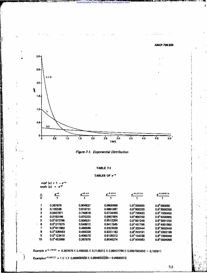
AMCP-706-200

3.0-

2.5-

2.0

1.5-

0 0.5 1.0 1.5 2.0 .5 3.i .0 4.5 56.0,TIME

Figure 7-1. Exponential Distribution

TABLE 7-1

TABLES OF e-1

*xpfc (K) e,

o 1- -. IX-'0 X- 1 0 1 1

1 0.367879 0.904837, 0.99004 98 0.95,000500 0.9 00005C2 0.135335 0.818731 0.9801987 0.92800200 0.93,800M203 0.0497871 0.740818 0.9704455 0.927053~g 0054 0.0183164 0.670320 0.960784 0.92600799 0.93600M805 0.02673795 0.6065 '31, 0.9512294 0.92501248 0.93 50012506 0.02 2. 7875 0.548812 0.9417645 0.92 4017'96 0.§34001800

7 002182 0.496585 0.9323i938 0.202 .93 3004498 0.03335463 0.449329 0.9231163, 0.P203191 092003199

9 0.03123410 0.A066706 0.9139312 6,9210408 0.93 100404910 0.0 46399 0.367879 0.9048374, 0.92 004983 0.930004998

Example e-~ 96 0.367879 X 0.49655 X 0.?139312 X 0.9941796 X 0.997000450 =0.165911

) Examplee-0 .0 01 2 '. 1 X 1 X 0.99900050X 0.§§g00200.99880072

7-3 I 2,


AMCP 70&200

Mean Time Hourly Operating.Between Failure Time,Failure, I at hr

hr iReliabilityR t

10,00 .0001- 9999.0

51000.999995 .02

.99999.3

1 =00 .001 .. 999 .1

500 .9995 .2.999 .3

.005 .5.995

100 .01.9

50 23.90 4

.05 5

10 .1 10

5 20e R t30

S 50

1- 1.0 $ . j100200

Given equipment mean time to 30failure or hourly failure rate Soo-and: operating time, solve forreliability. Connect 118' and'It" values with straight line.Read 1?"I.

R "mexpfc(Xt) -exp(-Xt;)

- -expfc(-t/e) -exp(-t/e)

Figure 7-2. Reliability Nomograh for the Exponential Distribution

/-,to<----7-4-

AMC,.7.0P-200

Notation: Conf{XW j X2/v) =csnf[(x2/v);2r]" (7-8aT)

T = total test time for all ,nits; T > 0. Conf{ < 0/(x 2Iv)} =csnfc[x 2 1v);2r](7"8b)This is the random variable.

r = number of failures; r > 0. This is not a Table 7-2 shows the ratio dfthe upper andrandom variable; in principle, it is lower symmetrical s-confidence limits as afixed at the beginning of the test. function of the number of failures; the ratio is

not a function of anything else. This ratio isThe items can be tested in afiy order, at any very large for any reasonable number oftime, and with or without replacement. The failures; e.g., for 5 failures and only 80%only restriction is that items be removed from s-confidence, the-ratio-is 3.3 (from 'able 7-2).test (e.g., end of test) only upon the failure of That means that the true value is uncertain tosome item. If this restriction is not fulfilled, a factor of over 3. To get an.uncertainty ofthen the Poisson distribution in Chapter 4 10% (a ratio of' 1.10) at a 95% s-confidencemust be used. level requires about 1700 failures (from Table

7-2).The usual point estimates for 8 and X are

Example. Ten items are put on test. TheTr (7-6a) failure/c~nsoring times are as listed in the

table. All times are in huurs and are ordered.r' rT (7-6b)

1. 1420 is unbiased and maximum likelihood -(in 2. 205

fact, it has virtually all the desirable proper- 3. 249ties). 1 is maximum likelihood (but is biased). 4. 448 (3 unfailed items were also

removed)0/0 has the X2Iv distribution with v = 2r, viz., 5. 1351

6. 2947 (the last item was also removed).CdIf{ 0/0 ; r-) = csnf(O/O ; 2r) (7-7a)Make estimates for 0, X, assuming that the

?,/ has the x2/v distributiopwith v = 2r, i. 'e., times-to-failure are exponentially distributed.All censoring, was done at a failure; so 'this

Cdf(/X; r)} = csnf(,X/X 2r) (7-7b) section Ppplies; i.e., the number of failures isnot a random variable, the total-test-time is a

s-Confidence limits can be set by Eq. 7-8. random viriable.

* ' 4

1'7-5

I

AMCP 706-200

Procedure Example

1. Calculate total-test-time T. 1. T = 142 + 205 + 249 + 4, X 448 + 135 1

+ 2 X 2947 = 9633

2. State the number of failures r. 2. r = 6

3. Calculate I -and 0 from Eq. 7-6. 3. = 0.6229/1000-hro = 1605.5 hr

4. Calculate the 5% and 95% s-confidence 4. (X2/,) , 12 = 0.4355limits using Eq. 7-8 and Table 6-2. (X2 /v) 95%. 12 = 1.7522(Subscripts L, U imply Lower and Upper XL = (0.6229/1000-hr) X 0.4355s-confidence limits.) = 0.2713/1000-hr

0 U = (1605.5 hr)/0.4355= 3687 hr

Xu = (0.6229/1000-hr) X 1.7522= 1.091/1000-hr

0L = (1605.5 hr)/1.7522 = 916 hr

5. Make the s-confidence statements. 5. s-Confidence level= 95%- 5% = 90%.Conf 0.2713/1000-hr < l < 1.091/1000-hr)

90%Conf{ 916hr<0 <3687 hr =90%

6. Calculate the ratio of upper to lowers-confidence limits. (See also Table 7-2). 6. ratio - 4.0

Note how misleading the point estimates are have been generated; e.g., Refs. 2, 4, and 5.with all of their apparent precision. The X2 /v (or j2 ) tables are just as easy to use,

and one doesn't get lost in someone else'sThe test did not give as much information partially explained mathematics.

about the parameter as wc would have liked.This paradox is well known and has led to Often it is desirable to test whether or notseveral suggestions to avoid it; e.g., use the data might reasonably have come from anBayesian methods, or use smaller s-confidence exponential distribution. For general alter-

levels, natives, see Chapter 14.

Foi the specific alternative of a WeibullThe data in this test were generated using a distributi, se Chapter 8 A scndc I] set of 10 pseudorandom numbers with 0 = Inevluu- , : " \"',' ,"""."

set f 1 psudoando nuber wih 0interval usually is generated on the shape1000 1r (X = 1.0/1 000-hr). The data are quite parameter. If that interval includes unity, the:] ~~unevenly distributed which again shows the exnat;';nh ''t ~';'~dexponential hypothesis need not be rejected.

wide variability in samples which are not In most practical situations there are so few

aedata that the exponential hypothesis is notrejected; indeed, it would be difficult to reject ,T

Special tables for making these inferences many other hypotheses as well.

7 6

AMCP 706200

TAI3LE 7-2

RATIO OF UPPER TO LOWER s-CONFIDENCE LIMITS FOR THE EXPONENTIALPARAMETER (WITH EQUAL SIZE TAILS ON EACH SIDE)

Body of table gives the ratio

s-Confidence Level

number of 602 80% 90% 95% 98% §9%failures r (20%, 80%) (10%, 90%) (5%, 95%) (2 %, 97 W) (1%, 99%) ( %, 99 Z)

1 7.2 22 58 150 460 l10i2 3.6 7.3 13 23 45 723 2.8 4.8 7.7 12 19 '274 2.4 3.8 5.7 8.0 12, 165 2.2 3.3 4.6 6.3 9.1 126 2.0 2.9, 4.0 5.3 7;3 9.27 1.92 2.7 3.6 4.6 6.2 7.78 1.83 2.5 3.3 4.2 5.5 6.79 1.77 2.4 3.1 3.8 5.0 5.9

10 ..71 2.3 2.9 3.6 4.6 5.4

12 1.64 2.1 2.6 3.2 3.9 4.614 1.57 2.0 2.4 2.9 3.6 4.116 1.53 1.91 2.3 2.7 3.3 3.718 1.49 1.84 2.2 2.6 3.1 3.420 1.46 1.78 2.1 2.4 2.9 3.2

25 1.41 1.68 1.94 2.2 2.6 2.830 1.36 1.60 1.83 2.1 '2.4 2.635 1.33 1.55 1.75 1.95 2.2 2.440 1.31 1.50- 1.69 1.86 2.1 2.345 1.29 1.47 1.64 1.80 2.0 2.250 1.27 1.44 1.60 1.75 1.94 2.1

60 1.24 1.39 1.53 1.66 1.83 1.9570 1.22 1.36 1.48 1.60 1.75 1.8680 1.21 1.33 1.45 1.55 1.69 1.890 1.19 1.31 1,42 1.51 1.64 1.72-100 1.18 1.29 1.39 1.48 1.59 1.68

150 1.15 1.23 1.31 1.38 1.46 1.53200 1.13 1.20 1.26 1.32 1.39 1.44250 1.11 1.18 1.23 1.28 1.34 1.39300 1.10 1.16 1.21 1.25 1.31 1.35400 1.088 1.14 1.18 1,22' 1.26 1.29500 1.078 1.12 1.16 1.19 1.23 1.261 1000 1.055 1.084 1.11 1.13 1.16 1.18

! 1500 1.044 1.068 1.089 1.11 1.13 1.14t 2000 1.038 1.059 1.076 1.092 1.l1 1.12

2500 1.034 1.053 1.068 1.082 1.097 i.113000 1.031 1.048 1.062 1.074 1.089 1.0994000 1.027 1.041 1.053 1.064 1.076 1.085-

1 5000 1.024 1.037 1.048 1.057 1.068 1.076'

10000 1.017 1.026 1.033 1.040 1,053

+(1.7/yr) 1+(2.6/r). 1+(3.31~r) I+(3.9/,r) 1+(4,7/i) 1 (5.2/7r) F


AMCP 706-200,

REFERENCES

1. Abramowitz and Stegun, Eds., Handbook 4. Dior, (impe6, Thomas, Exponential Red!-of Mathematical Functions, A.M555, NBS, absility Tables, 1 May 63, SD 261,GeneralUSGPO, June 1964 with subscquent cor- 'ElectricCo., Missile and Space Div., N63-rected printings. 20169.

2. Fritz, Sternberg, Weir, Yciiicheff, Reliabil- 5. A. H1. Cronshagen, Lower Confldin'o? Li ti-ity Tables, 15 April 6$ (originally printed Its for Mean Life When Lifetimes Areby GE Co., April '1962, R62SD1 35), Exponentially Distributed, RCS6O; Aero-NAVWEPS OD 306 68. jet-Azusa, 9 May 1960, AD 287-360.

3. Handbook of Reliability Engineering, 6. Mann, Schafer, -Singpurwalla, Methads forNAVWEPS 00-65-502, Bureau of Naval Statistical Analysis of Reliability and-LifeWeapons, I June 1964. Data, John Wiley & Sons, 1974.


AMCP 706-200:

CHAPTER 8

WEIBULL DISTRIBUTION

8- LIST OF SYMBOLS s- = denotes statistical' defiution

ACv{ estimated asymptotic covari. Sf = Survivor functionance

StDvj I = standard deviationAVar{ = estimated asymptotic variance

Var } varanceC f s-Confidence

wet base name for Weibuli distri-Cdf = Cumulative distribution func- bution

tionweif = Cdf for Weibul! distribution

C, L, U = subscripts that imply a s-confi-

dence level; C is general, L is welfc = Sf for Weibull distributionlower, U is upper

ct = scale parameterCM, { = ith central moment

= shape parameterConf f s-Confidene level

T = random variableCV{ } = coefficient of variation:

StDv {' }/E{ I i =

Ej } = s-Expected value f';'}, (';') = the fixed parameters are listedto the right of thesemidolon,

M,{ } = ith moment about the origin the i-andom variable is listed tothe left-of the semicolon

NCM,{} = normalized ith central mo-ment; CM, f 1/[StDv{ I]' = the complement, e.g., I -10

where 0 is any probabilitynf number of failures°: 8-1 INTRODUCTION

pdf -probability density functionThis is a-very commonly used PrD for life

pmf = probabilitymass function (e.g., time-to-failure). It is a rather tractablePrD and is reasonably rich in being able to fit

N Probability various sets of data. I.n,= base name wei isgiven to the Weibuli distribution (for Wei-

PrD = .Probability distribution bal.,). The suffix f implies the aCdf, and thesuffix fc implies the Sf (complement of the

R = s-Reliability Cdf).

... ...._8__ _ _ _4_


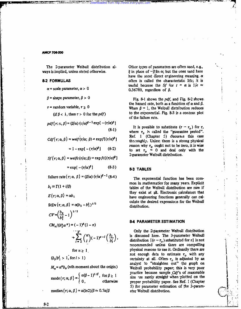
AMCFP 706.200

The 2-parameter Weibull distribution al- Other types of parameters are often used, e.g.,ways is implied, unless stated otherwise. t in place of -3 kn a; but the ones used here

have the most direct ergineering meaning. a8-2 FORMULAS often is called the characteristic life; .t is

useful because the Sf for t = a is I lea = scale parameter, a > 0 0.36788, regardless of P3.

P = shape parameter, P > 0 Fig. 8-1 shows the pdf, and Fig. 8-2 shows

the hazard rate, both as a function of a and 13.-= random variable, r >_ 0 When P- 1, the Weibull distribution reduces

(if P < 1, then , > 0 for the pdf) to the exponential. Fig. 8-3 is a contoui plotof the failure rate.

pdf(7 r.t, p)} = (6/a)( - 1 exp - (rla)cP ]It is possible to substitute (r - r) for T,

(8-1) where r, is called the "guaratee period".Ref. I (Chapter 5) disctws.ss this case

Cdf{r; a, 13) = weif(T/a; 13)= expf[(/aY5 ] thoyoughly. Unesr_ there is a strong physicalreason why r,, ought not to be zero, it is wise

=l-exp[-(r/ltr ] (8-2) to set r4, = 0 and deal only with the2-parameter WeibulU distribution.

Sff;a, 13) = weifc(T/aq 13) expfc[(rcx)P]

= exp[ -(/a) 5 ] (8-3) 8.3 TABLES

failure rate{r; a,13) = (3/a) (r/ay - 1 (8-4,) The. exponential function has been com-

mon in mathematics-for many years. Explicitbi =-( + i/o) tables of the Weibull distribution are rire if

they exist at all. Electronic calculators that{r;a, ) =abt have engineering functions generally can cal-

culate the desired expressions for the WeibullStDv T; a, 13) = C02 - b Idistribution.

C,(b2 _ 11/2CV I

84 PARAMETER ESTIMATION

Only the 2-parameter Weibull distribution(n)(_ l, b is discussed here. The 3-parameter Weibull

1'2 1 distribution [(r- )substituted-forr] is notrecommended unless there are compelling

for n .> I physical reasons to use it. Ordinarily there arenot enough data to estimate r. With any

(b,/bl > lfori> 1) certainty at all. Often. %" is, adjusted by ananalyst to "straighten out" -the graph on

in= aeb, (nth moment about the origin) Weibull probability paper; this is very poorpractice because sample Cdf's of reasonable

mode(r; a,-3) c -1)", for P> 1 size ire rarely straighi when -plotted on the0, otherwise proper probability paper. See Ref. I (Chapter 2

5) for parameter estimation of the 3-param-median {r; ot, P1,) a(n2)/3 , 0.7a/[3 eter Weibull distribution.

etrWibl itrbton 2, ' :

AMCP7(*200

3.6

,-0.3 FOR ALL CURVES

3.0-

2.4-

a-3

1.2-

LL

0.6

0 0.50 1.0 1.5 2.0 2.5 3.0 3.5 4.0 4.5 5.0TIME

(A) FOR SHAPE PARAMETER p - 0.3. THIS SET OF CURVES IS TYPICAL-FOR 0 1. (FOR 1 < P < 2, THE pdf-SLOPE - ,S TIME - EV'.)!]:'. i 'F/gure 8. 1. Weibull Distribution, pdf

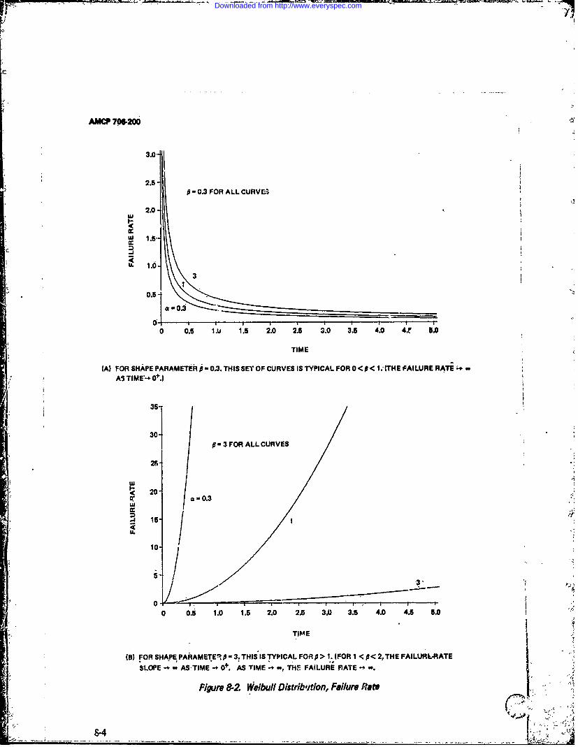
AMCP 7060

3.0--

2.50.3 FOR ALL CURVF.0

2.0-

330.-

0 0.5 1I 1.5 2.0 2.5 3.0 3.5 4.0 4t 5.0

TIME

(A) FOR SHAPE PARAMETER " 0.3. THIS SET OF CURVES IS TYPICAL FOR 0 1. (FOR 1 < P< 2, THE FAILURL-RATESLOPE - AS TIME-. 0+. AS TIME-*, THE FAILURE RATE -.

Figure 8.2. We/bull Distrib'ition, Failure Rate

-~, 8-4

3iLvu 3uiivd aQIMMW4ON

4C

W-4-P

x A IM 0.j ax- <

~~flU. -J C J Lo

wu1111 wj

I w C;

QXFJ cc c

ullZ:) x I'>l5w

I!V'w J lC a

Ii _________________ 7

______________________J

- ~0 J

85

AMCP 706-200

JPdC3ZflTVUON

z 1 0

Ut 00

LL-

4c 0 UJ

LL. ui0UJI V j

l4-,J3

10- .5

04

z5

05

U. L:i

LU-

0 OXii:1

8-6 1


l'I

AMCP 706.200

84.1 GRAPHICAL METHOD "

~ fa allGraphical estimation is 21asible using spe- -

cial Weibull probability paper. One ought (8-5)always to try to get some idea of theuncertainty ivolved in the estimates, no The yj (03) must be calculated each time thematter how roughly the uncertainty is guessed value of 0 is changed. There is only oneat. positive value of ( which satisfies the equa-

tion; so Newton's method, linear inter-8-4.2 MAXIMUM LIKELIHOOD METHOD polation, or any standard method works quite

well. If the data are first graphed on WeibullThe method of maxinmum likelihood,(ML) pLobability paper, the graphical value of-( can

is virtually the only analytic technique that is be used to begin the iteration. Otherwise,used. Unfortunately, one of the 2 ML equa- begin with I = 1 (it's about as good as anytions cannot be solved explicitly, and iterative other).techniques must be used. The ML method issuitable for any kind of censoring, and always The equation for & iscan be used. Even though it is somewhattedious, it is recommended here because the &et . x (8-6)%amateur analyst "can't" go wrong with it. \f all /

Estimating the uncertainty in the ML esti- The elements of the asymptotic covariancemates is difficult because one knows only the matrix are estimated by the following expres-asymptotic (large sample) behavior. The esti- sions:mates are asymptotically s-normal; this fact is _ 1 Iused in makings-confidence statements. AVar = In - - - (87)

Notation:1 A~ar (9-8)nf = number of failures a ( .T- (8

x = falre or censoring time for item i ACov T, -

(if more than 1 item i censored at - f l

the same time, each is given the (8-9)value x) where

= sum only over all failed items

sum over all times (failed and cen-Id, sorod)

+/all :

"The equation to be solved iteratively is -TPal _ ..ln, L

8-7


AMCP 706.200

AVar =estimated asymptotic variance AVar fQ .} = (4,2/4) Avar )

ACov estimated asymptotic covariance + A~ar{Rnal - (W4,P)

Ap =estimated asymptotic correlation X ACov fg Al .(8'-l 3)1coefficient

AStDv =estimated asymptotic standard devi Appromimate s-confidence, limfits 'are set byationassumixig that the parameters are s-normially

AStDv (. [ AVar (.]1/2 (8-40a) distributed With mean givenby the maximumlikelihood value and standard deviation 'givenby the square root oi the asymptotic variance.

Ap{(Ino&1 P ACov (lnci, P3 *FPorsmall samples, the answers are~veiy rough,[AVar (Ina^)AVar{^) 112 but they do serve the purpose of showing the

uncertainty.

Eq.8-4canbe ewrtte as(8-1)Example. Ten items were put on test. The/~ (3lnrfailure/censoring times are as listed in the

where table.- All times are in hours and are ordered.

I, n( - nR). 1. 142

The two =~al problems are to estimate 42.205(and thus R) given r, and to estimate r, given 3. 249R (and thus 4'). Since the variances are, not 4. r48(3ovaed ies er asalways small, it is wise to consider Rnr and rmvdRnct instead of Trand .o. The AVar's of Rnr and 5. 1351

4are 6. 2947 (the last item was also removed)

AVar{, (In [1-16 ])2AVar(i3)A~ar{ln&)Estimate otj P assuming that the times to

+ a3 Ia^ failure have the Weibull distribution. (The-2P3Qn[,rI&1)ACovhiC^4 1'f follow"ng calcui tions were all performed on

an IHP-45 electronic calculator-a computer is(8-12)Y not necessary if there aren't too many data.)


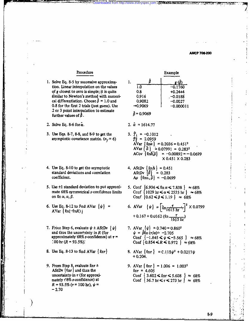
AMCP 706-200

Procedure Example

1. Solve Eq. 8-5 by successive approxima- 1. g(tion. linear interpolation on the values 1.0 -0.1760of g closest to zero is simple; it is quite 0.8 +0.2444iimilar to Newton's method with numeri- 0.916 .-0.01,88cal differentiation. Choose 1 = 1.0 and 0.9082 -0.00270.8 for the first 2 trials (just guess). Use -*0.9069 -0.000011.2 or 3 point interpolation-to estimatefurther values of . =0.9069

2. Solve Eq. 8-6 forct. 2. & 1614.77

3. Use Eqs. 8-7, 8-8, and 8-9 to get the 3. T, = -0.1012asymptotic covariance matrix. (n1 6) t = 2.0959

AVar 12n&) =0.2036=0.4512AVar . 3 - 0.07991 = 0.2832ACov 12n&,} -0.00892 =-0.0699

X 0.451 X 0.283

4. Use Eq. 8-10 to get the asymptotic 4. AStDv t{nA& = 0.451standard deviations and correlation AStDv jij = 0.283coefficient. Ap {2n,,} -0.0699

5. Use +I standard deviation to put approxi- 5. Conf {6.936 < Rn a < 7.838 ) n 68%mate 68% symmetrical s-confidence limits Conf { 1029 hr < < 2535 hr 68%onn a, a,. Conf {0.62 < 1. 19 } 68%

6. Use Eq. 8-12tofndAVar {4} = 6. AVar =[in 2 X0.0799AVar { gn(--RnR) i L"

+0.167+0.0162(n T" )1,615 hr

7. F:0ra Step 6, evaluate 4±AStDv {4} 7. AVar (4} = 0.740= 0.8602and thus the uncertainty in R (for 0 = P3n (r/)- -2.705approximately 68% s-confidence) at T = Conf 1-1.845 - 4 <-3.565 ) m 68%:00 hr (R = 93.5%): Conf 1.0.854 <R <0.972 } - 68%

8. Use Eq. 8-13 to find AVar {Qn'r} 8. AVar {2nr} C.1,8 2 + 0.02174+ 0.204.

9. From Step 8 evaluate 2nr ± 9. AVar { Rnr} = 1.006 = 1.0032AStDv ({nr } and thus the Rnr = 4.605uncertainty-in r (for approxi- Conf { 3.602 < Rnr < 5.608 1 68%niately (.8% s-confidence) at Conf 36.7 hr.< r < 273 hr ) 68%R = 93.5% (r 1O0 hr), 4=-2.70

8-9

AMCPi06.200

The point of going ii.to the analysis in hypothesis were true), then you ordinarilydetail is to show that the calculation of the accept the alternate hypothesis. But veryuncertainties is by far the most important often the data do not force you to reject yourcontribution.of statirtics. Without those cal- hypothesis-your data arez quite :reasonable ifculations of uncertainty, a dangerous delusion the hypothesis. is true. Then-what,.you, reallyof accuracy would prevail. These data are the ought to say is "This is a~reasonablehypothe-san'e as in the example in Chapter 7. They are sis; there may also be many other reasonablefrom an exponential distribution with param- hypotheses."eter 0 1000 hr., i.e., a Weibull distributionwith 3 = 1, a = 1000 hr. For the example in par 8-4.2, ; : 0.91, and

&0 - 0.28 (60 =- StDv {(3j ). If Ptrue = 1,8-4.3 LINEAR ESTIMATION METHODS you'd get a P as low as (or lower than) 0.91 at

least gauf[(0.91 - 1.00)/0.28] = 37% of theThere are many linear estimation tech- time. The data do not forc; you to reject the

niques in the literdiure. None are given here hypothesis that P = 1.because they require extensive tabulations.The tabulations are usually only for specific Now if (truc = 0.8, you'd get a as high assample sizes. Ref. 1 (Chapter 5) discusses (or higher than) 0.91 at least gaufc[(0.91many of these and gives the references. Ref. 2 - 0.80)/0.281 = 35% of the time. The data do(Chapter 3) collects several of the tables. It is net force you to reject that hypothesis.usually wise to go back to the original paper ifthe explanation of the use of'any reproduced Now if 3true = 1.2, you'd get a 'P as low astable is not clear and explicit. For example, (or lower than) 0.91 at least gauf[(0.91some techniques are designed for uncensored - l.2)/0:281 = 15% of the time. The data dosamples, others can be used only if all not really force you to reject that hypothesis.censoring is at the end of the test. Many ofthe methods are very good whenthey apply; Often it is desirable to make as simple anit is wise to consult a statistician about using assumption as the data will allow. Thatthem and about the methods for estimating usually means to assume ( = I (exponentialuncertainty (e.g., s-confidence intervals). disti lbution) if the data will allow it.

8-4.4 TEST FOR FAILURE RATE: IN-CREASING;, DECREASING, ON CON- 8-5 COMPARISON WITH LOGNORMALSTANT DISTRIBUTION

The literature contains tables for testing For 10 failures o: less (or perhaps even 20the hypothesis about whether P .> I (in- failures or less) data sets from a Weibull and acreasing failure rate), ( = 1 (constant failure lognormal distribution are virtually indistin-rate), ( < I (decreasing failure rate). Some guishable from each other. It is not wise totables are not valid if there is any kind of use - goodness-of-fit test to find which is thecensoring. better fit because neither onu ought to fit the

sample data very well;-there is just too muchYou must remember what such a test really scatter in sinall to medium size samples. This

does. It says, "Do the test data wirtually force is an illustration of why it is not wise tome to reject my hypothesis?" If they do force extrapolate very far from the sample data.you to reject the hypothesis (i.e., data as bad These 2 distributions voll gnerally have quiteas yours rarely would be obtained if the different behavior in the right tail region.

8-10

AMCP70-

REFERENCES

1. Mann, Schafer, Singpurwalla, Methods for 2. W. Yurkowisky, Nonelectronic ReliabilityStatistical Analysis of Reliability and Life Notebook, March 1970, RADC-TR-69-Data, Johi. Wiley & Sons. 1974. 458, AD.868 372.


AMCP 706-200

CHAPTER 9

LOGNORMAL DISTRIBUTION

9-0 LIST OF SYMBOLS M1{ } = ith moment about the origin

pdf = probability density functionC = s-Confidence

pmf = probability mass functionCdf = Cumulative distribution func-

tion Pr{ } = Probability

C, L, U = subscripts that imply a s-confi- PrD = Probability distributiondence leiel; C is general, L islower, U is upper R = s-Reliability

CM1 f = ith central moment s- = denotes statistical definition

Conf{ } = s-Confidence level Sf = Survivor function

CV } = coefficient of variation: StDv{ = standard deviationStDv{ )/E{ )

V.r{ } = varianceE { } = s-Expected value

x - sample mean.. f = suffix for base name, implies

the Cdf = scale parameter

... fc = suffix for base name, implies f3 shape parameterthe Sfbr erandom variable

gau =base name for Gaussian distri-bution { " ,(") the fixed. parameters are listed

to the right of the semicolon,gaud = pdf for Gaussian distribution the random variable is listed to

the left of the semicolongauhr = hazard rate (failure rate) for

Gaussian distributikn = the complement, e.g., - 1 -0 where is any probability

lgn = base name for lognormal dis-tribution 9-1 INTRODUCTION

!NCM = normaiized ith central mo- This distiibution is used occasionally forNC'M, ment;CM1 { }/[StDv{ }1] the life of semiconductors a'd mechanical

K ;.


V0

AMCP 706-200

parts. Part of *ts popularity is traceable to "is Sf (r: a, P) = lgnfc('r/a; j) (9-3a)relation to the s-norma! distribution, andpart is traceable to the non-negative character lnr - lna\of the random variable. The basic name Ign is = taufc\ 1 /- 3 )given to the lognormal distribution (!brloiormal). The suffix f implies the Cdf, and = gaufc ( ln i-ithe suffix fc implies the Sf (complement of L \CJthe Cd).

The 2-parameter lognornal distribution is =gaufc (9-3b)

always implied unless otherwise stated.

9-2 FORMULAS failure rate {r; a,1} = pdf(r; a,})/

Sf { r; a,1} (9-4q)

a scale parameter, a > 0 , gauhr

, = shape parameter, P > 0 != 3gauhr [In 1

r = random variable, r > 0 (- .(9-4)

where gauhr is the Gaussian hazard ratepdf(r;u, ,) J - exp[ - l/2[ln(r/a)P ]2 (failure rate); see par. 5.2.

(9-1a)

S (1)/ B - exp[/(2P2 )] > 1

!n-lna) E{r; a, P) = aB > aXexp[-1/2 " I'nr - JnIe { 1/StDv(r; a, P) = otB(B 2

- 1)1/2

(9-1b)

CV{r; a,)" (B 2 - 1)!/2

= (1/T)saud~1n-J] (9-Ic) CM3 { 1; 1, A) = a3 B3 (B2 - 1)i(B 2 + 2)

where gaud is the Gaus.ian pdf; see Par. 5-1. = -I~ n.- + t

Cdf {r; a, 1) = IgaAn(T/; P) (9-2a)mode {r; a, 3) :a/B2 < a,

Alnt - inot"=gaul1ii ) median (r; a, 3) = a

=gauf' Fn( )Y Mode of failure rate occurs at (alB2 )ef. 7u n(0 < y < 1) is given in Fig. 9-5. The failure

rate is zero for r = 0, then rises to a singlel maximum, and finally decreases toward zero.

=gauf~lny) (9-2b) Fig. 9-I shows the pdf, and Fig. 9-2 shows the

C"

AMCP 706.200

2.5-13

2.0

1.5 -1

1.0

0.5

1' 3

0 4- ~ * j-__-.

O 0.8 t'.6 2.4 3.2 4.0 4.8 66.4 7:2 8.0'TIME"

(A) FOR SHAPE PARAMETER P3 - 1

-0.3

4-

3-

2-

0 1 10 -

0 0.8 1.6 2.4 3,2 4.0 4.8 5.6 6.4 7.2 8.0

TIME(B) FOR SHAPE PARAMETER P- 3

Figure 9-1, Lognormal Distribution, pdf

I9 3


AMP 70640

failure rate, for several values of at, j3. Figs. 9-3 to set r, = 0 and deal only with the "N'and 9-4 are contour plots of the pdf and 2-parameter lognonaal distribution.failure rate.

9-3 TABLESThere are several ways of putting the

parameters into the lognormal distribution, Tables of the lognormal distribution arebut the common ones in the literature which virtually nonexistent. The Cdf and Sf areuse the symbols p and o are confusing because calculated easily using gauf and gaufc tablesps and a do not stand for the mean and (standard s-distribution), see Eqs.. 9-2 and 9-3.standard deviation of r, but for knr. The pdf can be calculated directly, or from

the s-normal pdf using Eq. 9-1.If a change of variable is made from r to'nr, then Rnr has the s-normal distribution. 9-4 PARAMETER ESTIMATION

See Chapter S.Only the 2-parameter lognormal- distribi-

It is possible to substitute (,r - r,) for r, tion is discussed here. The 3-parameter log-where r. is called the "guarantee period", normal distribution [(r - tr) substituted forRef. I (Chapter 5) discusses this case r"] is not recommended unless there arethoroughly. Unless there is a strong physical' compelling physical reasons-to use it. Ordinar-reason why r ought not to- be zero, it is wise ily, there re not enough data to estimate r,

14" 0.3

12"p-10

10

8"

6'

4-

2-

3

0 0.0 1.6 2.4 3.2 4.0 4.8 5.6 6.4 7.2 8.0

TIME(C) FOR SHAPE PARAMETER d - 10 -:

Figure 9.1. Lognormal Distribution, pdf

9-4


-, 'a "7 ""?- 7-

AMCP 10620

3* ~.o~s

0 0.5 1.6 2.4 3.2 4.01 4.8 56 6.4 cis

(Al FOR SHAPE PARAMETER 0 TIME

e.0.312

4-

cc

4U.

0 0.8 1.6 2.4 3.2 4.0 4.8 5.6 6.4 7.2 8.0

(9) FOR SHAPE 17ARAMETERt P 3 TIME,

Figure 9-2. Lognorm DistrI n Failure Rate

9-51.


/

AMCP 700-200

with any certainty at alL Often -r, is adjusted 1 =/i (9-5b)by an analyst to "straighten out" the graphon lognormal probability paper; this is very where p and a are tht mean and standardpoor practice because sample Cdis of reason- deviations of x, respectively, s-confidenceable size are rarely straight when plotted on statements about A and a will hold for thethe proper probability paper. See Ref. 1 corresponding and,8.(Chapter 5) for parameter estimation of the3-parameter loguormal distribution. Example. The following failure tines were

observed (all times are in hours). Assume a9-4.1 UNCENSORED DATA lognormal distribution. 'Estimate the param-

eters.By far the most satisfactry procedure is to

use x- £ni. Then % is for a Gaussian 566 2171distribution; see par. 5-3 for parameter 625 2226estimation. 1000 2638

1073 2-773a -z ell (9-5a) 1240 3781

70-

FOR a - 0.3, PEAK VALUE (ABOUT a-03

100) OCCURS ATTIME 0.8. 13 10

a00.3

40-

30-

20-

a-;310/

0 0.8 1.6 2.4 3.2 4.0 .4.8 5.6 6.4 7.2 8.0

(C) FOR SHAPE PARAMETER 3 = 10 TIME

* j Figure --2. Lognormal Distribution,, Failuro Rate

!9-6


AMCP 706-200

;pd O3ZflVIVUON

LL

A.~

'Ij _ _ _ [1I~~ ~ Hi _I3 c

IL 0 0LL z 0

0 LU < I 0

w 2 it xLLUJX.7

AMCP 706-200

El313MiVAi 3d.VHS

9 L o

Ilk-

0'0

U. 0% atZjII "

1"1

M;R0 .4 4

jILL W ,WZ : Dx w 2 N~ >r

Wozowm *E404Iomc

9-8 -


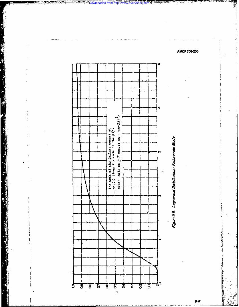
AMCP 706M200

o I I

I I11

1 - 0

41 0

0 4nzo,

X. 0

lei

d 4 Uld c d

-959


AMC 7 2o.PO

Procedure Example

1. Calculate the logs (natural) of the failure 1. i= 7.322times (any base will give correct answers if it s = 0.656it is used consistently) and find the sample N= 10mean x and s statibtic. State sam.le size V = 9and degrees of freedom.

2. Calculate point estimates from Eq. 9-5 2. & 1513 hr= 1.525

1/6 = 1/s

3. Calculate 90% symmetrical s-confidence 3. t.os, 9 =-1.833limits for ot. Calculate then for A first. Use t.95 ,9- = + 1.833Eq. 5-5b. uL = 7.322 - 0.380 = 6.942

if = 7.322 + 0.380 = 7.702t, = 1034 hr

atf= 2213 hrConf { 1030 hr < a < 2210 hr = 90%

4. Calculate 90% symmetrical s-confidence 4. (X2 /V) o . S, 9 = 0.3694 = 0.60782limits for#. Calculate them for a first. (X2/V)o.gs, 9 = 1.8799 = 1.37112Use. Eq. 5-6b. on = 0.656/0.6078 = 4.0792

oL = 0.656/1.3711 0.4784PH = 2.099L =0.927Conf { 0.93 ,3< 2.1 J = 90%

The uncertainty in ot is more than a factor 9-4.2 CENSORED DATAof 2, and in: ( is more than a factor of 2. Thusthe statistical analysis has shown how little we Maximum likelihood is complicated be-know about the distribution after taking this cause 2 simultaneous equations must besample of 10. The actual data were a random selved iteratively just as for the s-normalsample from a lognormal distribution with a = distribution. Rof. 2 shows how order statistics1000 hr'and 4 = 2. can be used. Ref. 1 also discusses this situa-

tion. A statistician oug'. to be consulted.

REFERENCES

1. Mann, Schafer, Singpurwalla, Methods for 2. Sarhan and Greenberg, Contributions toStatistical Analysis of Reliability and Life Order Statistics, John Wiley & Sons, NY,Data, John Wiley & Sons, 1974. 1962.

91

AMCP7O&20

CHAPTER 10

BETA. DISTRIBUTION

100 LIST OF SYMBOLS NCM, (1 = normalized ith central mo-

ment;CMtf I /[StDvf i'B beta function pdf = probability density functionbet = base-name for beta distribu- pmf probability mass function

tion ir{J Probabitybef = Cdf for beta distribution Pr Probability

PrD = Probability distributionbefc = Sf for beta distribution R = s-ReliabilityC

= s-Confidencer, n =ParametersCdf =Cumulative distribution func-tion s- = denotes statistical definition

C, L, U subscripts that imply a s-cc.nfi- Sf = Survivor functiondence level;. C is general, L is StDv{ } standard deviationlower, U is upperI =

C~t{ } = ih central moment stufc Sf of theoStudent's t-distribu.Conf = s-Confidence level ain

esVar{S V= variancecsqfc = Sf for the chi-square distribu-tion x =random variableCV{ = coefficient of vaiation: Parameters

S S-ted v lue Pi, V2 = degrees of freedom:1t u dsr o { ; ( = the fixed parameters are listedflsfc Sf of the Fisher-Snedecor F to the right of the semicolon,

distribution the random variable is listed tothe left of the semicolong a uf = C df fo r G au ssian d istri b u tio n-= t e c o p c e n , e ., ' - ! -ftecompleffent, e~g., 1-1p = incomplete beta function 0 where 0 is any probability

.M,{ } = ith moment about the origin * implies use of the,(r, n) param.eter set K-


AMCP 706-200

"9-1 INTRODUCTION pdf* (x; r,n) =xr-"(1-x)n-rf'),This is sometimes used as a PrD for forr> I (lO-Ib)

s-reliability since the random variable has therange 0 - 1. It also finds some use, in prin- pmf* 10; 0, n, =ciple, as a prior PrD for Bayesian analysisof the binomial parameter. The base name bet pdf* {x; 0, n) =0 for x 0 0is given to the beta distribution (for beta).The suffix f implies the-Cdf, and the suffix fc Cdf {x; c, ) Ix (a, () = 1 -1 -x (3, 0)implies the Sf (complement of the Cdf). Most (I 0-2a)of the formulas were obtained from Refs. 1, Cdf* {x; r, n) = Ix (r,-n - r + -1)2, and 3 (many formulas appear all 3 places).The beta distibution is also called the incom- = 1-11 x(n -r + 1, r)plete beta funbtion. = betf*(x;r, n) (10-2b),

10-2 FORMULAS Sf(x;CX, 3)= I --IX(,P\)=11_ x,)

c,3= parameiers, ca > 0, P > 0 (. 6-3a)'5, sf(X;r, n) = -Ix(r, n - r+ 0)

x randomvariable, 0 < x < .1 (for somevalues.of ce, P the pdfis not defined =Zi - x(n - r + 1, r)at the end points)

r, n alternate parametes, 0:< r e= n ( therestriction on n is more stringent than E{x;x, ( = r/(c +(3)mathematically necessary)

E*{x;r, n) =r/(n + 1)r -z n =x +'P - l(r and n are usually 1 1/2

restricted to non-negative StDv (x; c, ) = -- P I +integers) 01 L++

Srn+1-rjl 1/

n sometimes is called a "scale" parameter StDv* {x; r, n) = n-+.. "rn+-r 2

and r a shape parameter n+ I n+ 2

B(ct, P) r(o+(3) is called the beta function. CV(x;a,3} = )T/2

pdf{x; a, ) -xj" /B(a,3) rn +l-rl1 /2

fora, P-k0 (10-1a) CV{x rl (n 2 )J

Pmf{O;O, } - 1 }for*O 0pdf.(x; 0, P 0 , for x =kO CM3 (X; 01, f

(a + p)3 (a +p + l)(a+ (+ 2)pmf (I; o,O-" ro 0pfo1;xr0 o = 2r(n + 1 - r)(n + 1 - 2r)

ncu'(x ot, 0 or x 0 1 3M (x; r,n)(n + 1)3 (n + 2)(n + 3)

pmf{0; 0,O} 0)pmf{1; 0,O} = 1/2 "2((-a). _++1__

pdf{x;.O,0}=0, forx.O NCM3 (x;c04'0}= (a'C- +j+2) [cx"

10-2 -

AMCP 706.200

2(n + 1 - 2r) Ref. 2 has tables, a chart, and a discussion of3xn + 3 the distribution.

,[, n + 2 iRef. 1 (formulas 26.5.20 and 26.5.21) has'

r(n+ -r) two approximations for calculating Ix,.

mode {x; ct, a =(- 1)/(a + - 2) For (0e + P - 1)(1 - x) < 0.8,'

mode* (x;r, n} = (r- l)/(n - 1) IX(a, p) = csqfc(×2 ; 23) + e

median (x; ot, P) - (a - 0.3)1(oz+ P- 0.6) 1 el < 0.005, ifot+ P> 6

median* { x; r, n) -- 1,(r - 0. 3)/(n + 0.4) X, (a + P - 1 ) (1 - x) (3 -x !-x

(10-7).The beta distribution is related to other Ix (a, 3) = gauf(y) + c

distributions as follows:

n lel< 0.005ifct+P> 6pl~nl=Ir~n-+ I)3[w,( I . y(l I)

= betf*(x; r, n) (10-4) 907 .- 9w -24 2 11/2

Istufc(t; u)l' Ixtv/2, 12), x = l(P+ t1) " ot+

(1-)wj =-PX)'Ii , W2 -[Cel-X)] t 15 . (10-8)

flSfC(F, P1 V) 40v 2f2, v/2), Eq. 10-8 is related to Eq. 6-24. No tables are

X V1 (10-6) included in this Handbook series. Eq. 10-6V2 + v1 F and Tzblc 6-4 can be used.

Fig. 10-1 shows some graphs of Eq. 10-1a. 10-4 PARAMETER ESTIMATIONFig. 10-2 shows some graphs of Eq. 10-lb.

There are no simple good estimation proce-10-3 TABLES dures. The method of moments is reasonably

straightforward but does not readily allow anRef. 4 is an extensive set of tables of Eq. estimpion of the uncertainties in the param-

10-4. Other tables are given ;n Refs. 5 and 6. eter estimates.

_r__ _ it0r

AMCP MO200

3.0

2.0- pdf x;c,p} xt: a:p1 1 ]

~ 0.9

0D.5- P- 0.

2.0 1.0

0 0.1 0.2 0.3 04 0.5 0.6 0.7 0.8 0.94 X

(A) -a' 0.1; P0.1, 0.9, 1, 2

6L.

4.0" pd r (at+p)

r la) r(p)~3.0

0.5 2I 50%. 0.1 0.2 0.3 05 0.5 0.6 0.7 0. 9 10

.(a) 1, P - 0.5.1, 2, 5

Figure l0.7. Beta Distribution

I 10Y4


MCP 706420

5.0- a-

p-tof

~3.0-r ri_ x

2.0-

1.0.

0*0 0.1 0.2 0.3 0.4 0.5 0.6 0.7 0.8 0.9 1.0

(C) a 2;p 0.1, 1,5, 10

4.0- rd~~zi. ( ) [r- 1xff1

3.0-

2.0

.0

0 0.1 0.2 O.s 0.4 0.5 0.6 0.7 0.8 0.9 1.00* x

Figure 10-1. 6eta Distribution (Continued)


6.0n-

5.0-

r- r Pd.xn W} - --- " ii ix~'~r Wr r (n r LI

4.0-

3.0-

0 0.1 0.2 0.3 0.4 0.5 0.6 0.7 0.8 0.9 1.0x(A) n7;r..1,2,3, 5

6.0- n-il

r (n) r(nr)

4.0-

0 0.2 0 .3 0.4 0.5 0.6 0.7 0.8 0.9 1.0()n 11, 1, 2,3,5

Figure 10-2. Beta Distribution (alternate parameters)

10-6


"57

AMCP 706-200

REFERENCES

1. Abramowitz and Stegun, Eds., Handbook 4. AMCP 706-109, Engineering Design Hand-of Mathematical Functions, AM555, NBS, book, Tables of the Cumulative BinomialUSGPO,'June 1964 with subp~quent cor-. Probabilities.rected printings.

S. K. Pearson, Table.- of the Incomplete Beta2. E S. earon ad H 0. artey, lo-Function, Univeysity Press, Cambridge2. E S. earon ad H 0. artey, lo-(England), 1968 (first ed.,' 1934).metrika Tables for Statisticians, Vol. 1,

Cambidg Unv. res, 156.6. H. L. Harter, New Tables of the Incom-plete Gamma Function Ratio and of Per-

3. W. G. Ireson, Ed., Reliability Handbook, centage Points of the C/a-square and BetaMcGraw-Hill, NY, 1966. Distributions, USGPO, 1964.


AMCP 706-200

CHAPTER 11

GAMMA DISTRIBUTION

11-0 LIST OF SYMBOLS R = s-Reliability

C = s-Confidence s- = denotes statistical definition

Cdf = Cumulative distribution func- Sf = Survivor functiontion- StDv { I = standard deviation

C, L, U = subscripts that imply a s-confi-dence level; C is general, L is Var ) = variancelower, U is upper

a= scale parameterConf{ j = s-Confidence level

(3 = shape parameterCM{ } = ith central moment

r" = gamma functioncsqf = Cdf for chi-square distribution

CV { } coefficient of variation: " = random variableStDv{ I/E{ ) = the fixed parameters are listed

E {I = s-Expected value to the right of the semicolon,the random variable is listed to

gain = base name for gamma distribu- the left of the semicolontion

= the complement, e.g., 1 -gamf = Cdf for gamma distribution 4 where 0 is any probability

gamfc = Sf for gamma distribution 11-1 INTRODUCTION

gaufc = Sf for Gaussian distribution This is the distribution actually used insome of the exponential distribution exam-

M {} = ith moment about the origin ples when there is more than 1 failure. It isrelated closely to the chi-square distribution.

NCM{ = normalized ith central mo- The base name gain is given to the gammament; CM,{ } /[StDv{ }]t distribution (for apma). The suffix f implies

the Cdf, and the suffix fc implies the Sfpdf = probability densiy function (complement of the Cdf). The gamma distri-

bution is also called the incomplete gammapmf = probability mass function function.

Pr{ ) = Probability 11-2 FORMULAS

PrD = Probability distribution = scale parameter, c > 0

_. - ,J . ... ....... ..... ..... ... 11-1 . .. . ,


AMCP 706-200

1 = shape parameter, 0 > 0 gamf(x' /2; v/2) csqf(x2 ; P)~for P a positive integerr randoin variable, r_ 0 (if( < 1, p i ier

then r > 0 for the pdf

pdf(,r;ct,3) =(1/)e-(Tt)(Tc)-/(3) Larnf{ p;r} = (e-P) ,

(11-1) for r a noni-negative integer

Cdf (r; o, 0)' = gainf('r1; 3) (11-2) (11-6)

Sf {r;a, P) =-gamfc&/o ,3) (11 -3) Fig. 11-1 shows a few values of the pdf.

Fig. 11-2 is a contour plot of the pdf. Many=a of the formulas in this chapter are' adapted

StDv {r;,) =from Ref. 1.

cV fr; a, 3) =.,..rp 11-3 TABLES

Tables of the gamma distribution are notvery common. Refs. 2 and 3 are two of thefew extensive tables available. Of course,

NCM3 (r;a, P) = 2/v" chi-square tables can be used when 3 isa multi-

ple or / (see Eq. 11-5). No tables are included

E&r:a,0) in this volume.

[E(r;,} =) In Eq. 11-7 and its inverse are useful forx(1 + &- -),~l approximating the gamma distributionX! I" +- I,

- ), > I: (11-7)e a1 } -" 0, ,otherwise where

gaufc(zQ) = Qmedian {r; t, 1)s a(0 - 0.3) fu )ga7mfcu0, 0; P) Q

Miscellaneous formulas are 11-4 PARAMETER ESTIMATION

gamf('rfr;-P + 1)= gamf(rcic; 3) Rarely does one wish to estimate both, parameters of the gamma distribution. If 1 is+ xt~e-xI r( + I] known, the estimation is straightforward-see

(11-4) the exponential distribution (Chapter 7).

° ~~11-2 . . .

AMCP 706-200;

5.0-

p 0.34.0-

0i.3

2.0-

3

1.0-

40 0.2 0.4 0.6 0.8 1.0 1.2 1 A 1.6 1. 20x

(A) SHAPE PARAMETER P 0.3. TYPICAL OF ALL p <i1. (ASx - 0+, THEpffs-00),

P-1

3.0~f\(SAME AS EXPONENTIAL DISTRIBUTION, WHERE 1/h l

a-0.3

2.0-

0.5-

0 0.5 1 0 1.5 2.0 .2:5 3.0 3.5 4.6 4.5 51

B) SHAPE PARAMETER A 1. THIS IS THE EXPONENTIAL DISTRIBUTION; SEE FIG. 7-1.50

Figvre I11. Gamma Distribution, pdf

11-3 L

AMCP 708-200

a0.3.I0-3

0.8 -

.L 0.6-

0A.

0.2-

3

0 2 4 6 8 10 12 14 16 18 20x

(C) SHAPE PARAMETER ,, 3. TYPICAL FOR A.L j > 1.

Figure 11-1. Gamma Distribution, pdf (Continued)

If both parameters must be estimated, rconsult a statistician. Be sure to estimate the C(J3) J e-'u-I du (11-8)uncertainties in the parameter estimates.

11-5 GAMMA FUNCTION See Ref. 1 (Chapter 6) for many characteri-stics and tables of this and related functions.

The gamma function appears many places. 'Fable 11-1 can be used to find r1).

REFERENCES

1. Abramowitz and Stegun, Eds., Handbook centage Points of the Chi-square and Betaof Mathematical Functions, AM555, NBS, Distributions, USGPO, 1964.USGI , June 1964 with subsequent cor-rected pr;ntings.

3. K. Pearson, Tables of the Incomplete2. H. L. Harter, New Tables of the Incom- Gamma Function, University Press, Cam-

plete Gamma Function Ratio and of Per- bridge (England), 1922.

-4


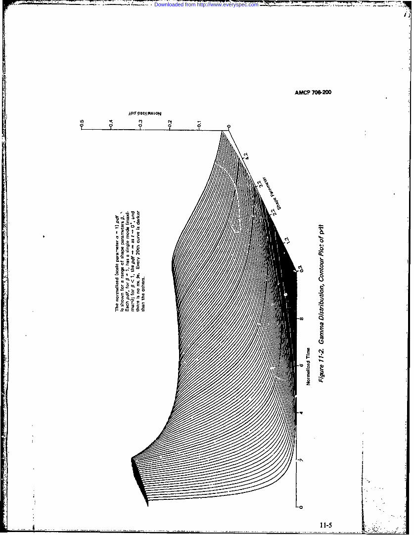
AMCP 706-200

JPd POGLftON

C4-

CCA

LUj

V - 1-


TABLE 11-1

GAMMAI FUNCTION

rn - r (n + 1), fo n an l ftaI"a(o + I) " r i.. ~~(s (J+n- 1) (d+ +-2) ... p r" (p),

1.00 1.00000 1.25 o.90640 1.50 O.8C623 1,75 0 919061.Q0 10.99433 1.26 0.90440 1,51 0,88659 1.76 0.921371.02 0.98884 1.27 0.90250 1.52 0.88704 1.77 0.923761.03 0.98355 1.28 0.90072 1.53 0.88757 1.78 0.9t1623.Lo4 0.97844 1.29 0.89904 1.54 0.88813 1.79 0.92877

1.05 0,97-350 1.30 0.89747 1.55 0.88887 1.80 0.931381.06 0.96874 1.31 0.8u600 1.56 0.88964 1.81 0.934081.07 0.96516 1.32 0.89464 1.,7 0.89049 1.82 0.9?5851.08 0.95973 1.33 0.89338 1.58 0.89142 1.83 0.939691.09 0.95546 1.34 0.89222 1.59 0.89243 1.84 0.94261

1.10 0.95135 1.35 0.89115 1.60 0.89352 1.85 0.945611.11 0.94739 1.36 0,89018 1.61 0.89468 1.86" 0.948691.12 0.94359 1.37 0.8803i 1.62 0.89592 1.87 0.9518141.13 0.9399A 1.38 0.88854 1.63 0.89721 1.88 0.955071.14 0.93642 1.39 0.88785 1.64 0.89864 1.89 0.95838

i.15 0.93304 1.40 0.88726 : ,65 0.90012 1.90 0.961771.16 0.92980 1.41 0.88676 1.66 0.90167 1.91 0.965231.17 0.92670 1.42 0.88636 1.67 0.90330 1.92 0.968781.18 0.92373 1.43 0.88604 1.68 0.90500 19 0.9724o1.19 0.2088 1.44 0.88580 1.69 0.90678 1,94 0.97610

1.20 0.91817 1.45 0.80565 1.70 0.9C864 1.95 0.979881.21 0.91558 1.46 0.88560 1.71 0.91.057 1.96 0.983741. 2 0.91311 1.47 0.88563 1.72 0.91258 1.97 0.987681.23 0.,91075 1.48 0.83575 1.73 0.91466 1.98 0.991711.24 0.90852 1.49 0.88595 1.74 0,91683 1.99 0.99581

2.00 1.00000

i i


AMCP.706.200

CHAPTER 12

s-CONFIDENCE

12-0 LIStr OF SYMBOLS 11 = random variable from uniformdistribution

C = s-Confiden-,e level; or sub-script that iinplies such a level 1" = 1 -

= 1-C 0 0,p = parameters about which as-confidence statement is to be

Cdf = Cumulative distribution func- madetion

P = degrees of freedomConf } s-Confidence level

x2 1V chi-square/nu statisticglb greatest lower bound

implies a point estimate of aLCL = lower s-confidence limit parameter

L, U = subscripts implying lower and 12-1 INTRODUCTIONupper s-confidence levels andlimits s-Confidence is one of the first difficult

statistical concepts an engineer needs to grasp.lub = least upper bound s-Confidence is to statistics as entropy is to

physics. s-Confidence and entropy are bauicN = sample size concepts that must become familiar in their

own right; it is almost impossible to under-pdf = probability density function stand them in terms of more-basic concepts.

pmf = probability mass Function This chapter applies to the common situa-tion where the parameters in a PrD are not,

PrD = probability distribution random variables themselves; rather they arefixed, usually-unknown quantities. If ,the

r = integer random variable parameters are random variables (irrespectiveof the meaning attached to piobability), the

s-= denotes statistical definition situation is handled by a Bayesian techniquc(see Chapter 15).

Sf = Survivor functionSP r a statistic fixed nonrandom quantities. Probability state-

ments that- contain a parameter cannot implyUCL = upper s-confidence limit that the parameter itself is a random variable.

1' 12-1


AMCP7M6200

A s-confidence statement is generated by an can be used to generate useful s-confidencealgorithm (computational procedure) which statements.is specified, in advance of the experiment.Examples of such procedures are given in the r = c, (12-2)parag-aphs that follow. It is presumed that allfunctions and PrD's are well-behaved enough where r is the number of f'.ilures observed in afor the concept of s-confidence to be easily sample from a Poisson distribution withand unambiguously applied. Such is the case parameter p, and c. has the Poisson distribu-for the PrD's usually used in reliability work. tion with parameter p.

Eq. 12-1 shows one kind of expression The remainder of this chapter is limited towhich can be used to generate useful s-confi- those cases for which:dence statements.

(1) There is only 1 unknown parameter.

Q - A)/s = t. (12-1a) (2) There is a single s-sufficient statistic.

2'l' = Wx /0 (12-1 b) (Examples of s-sufficient statistics are thenumber of failures in N tries for a binomialdistribution, the number of events for a

where i and s are the sample-mean and s Poisson distribution, and total-test-time tostatistic, respectively, of a fixed-size sample achieve r, failures for the exponential distri-from a s-normal distribiAtion with mean A and bution.)standard deviation o;

(3) The situation is well-behaved enough0/0 = (x2/), (1 2-1c) that no difficulties are involved in making

s-confidence statements.where 0 is the sample mean-life of a

fixed-size (fixed number of failures) sample The cases considered here have a simplefrom an exponential distribution with scale geonetric and analytic interpretation. Consultparameter (mean life) 0. a competent statistician or a good reference,

e.g., Ref. 2 (Chapter 20), for a discussion ofEach expression in Eq. 12-1 contains on othercases.

the left:Suppose the single parameter in a PrD is 0

(1) Only I unknown parameter from the and an estimate of 0, from a sample, is $.PrD, and Examples are

(2) Sample statistics, i.e., quantities calcu- (I) Exponential distribution: parameter =

lated from the sample data. scale parameter 0; estimate, = Tro where Tis total-test-time for r, failures.

Each quantity on the right in Eq. 12-1 is astatistic whose PrD can be determined with- (2) Poisson distribution: parameter = meanout regard to the PrD parameters or to the number of events, j; estimate, A = r where r israndom data although it may depend on such the observed number of events.things as the fixed sample size. Both t andX2 / have well-known PrD's (see Chapter 6) (3) Binomial distribution: parameter =w, d depend on the sample size through P. probability of an event p; etimate, =rN

where r is the observed number of events in NEq. 12-2 is another kind of expression that trials.

_6j


.w

AMCP 706-200

is a random variable because it depends means that if a 0 is found, and C is given, theon the sample data. The procedure for making statement 0 4 0c(O,C) will be a true fraction Ca s-confidence statement is as follows: of the time, regardless of the true value of 0.

The reason this can be so is that 0c is selected(1) Take the random sample and calculate so that the statement "00 4 0 c (0, 09" is truefrom the data. a fraction C of the time for any particular 00

and C, for all random samples from the PrD(2) Use the algorithm to generate another with that parameter 0.. Since it is true for

statistic 0C which will be a s-confidence limit, any particular 0o, it is true regardless of the0C is a random variable; it is calculated from value of 0.the sample data.

When the PrD is discrete, the s-confidence(3) Make a s-confidence statement. It will statements are usually of the forms

use Conf {' I rather than Pr ( I to denote Cof (0 < 0C + 6) 0 > (I 24b)probability. The Conf I I implies that the - -parameter is unknown and that a value of the Conf ( 0c-($, C)) C. (12-4c)random variable 0c has been calculated from - Cthe data. Conf ( I is interpreted as the frac- This situation is discussed further in Par. 12-3.tion of times such a statement will be true whenthese 3 steps are followed. In statistical papers, the concept of s-confi-Conf (0 < 0C C. dence often is modified slightly so that Eq.

12-4b is written Conf { < 0c+ (, c) } = C.The procedure often is extended by calcu- This is confusing to nonengineers. This hand-

lating 2 values of 0c (OL and CU) such that book series always makes the inexact s-confi-the s-confidence statements are dence statements in the form of Eqs. 12-4b

Conf (0: OU) CU (12-3a) and 12-4c.

Conf _0}:. L=CL (12-3b) 12-2 CONTINUOUS RANDOM VARI-

ABLESConf{! < < (0=1(7;•(1-c

,n~ 0 'u) = CU CL . (12-3c) Fig. 12-1 graphically shows how v-confi-CL is usually small (say 5%) and Cu is usually dence limits are derived.large (say 95%). Notation for s-confidencestatements is not at all standard; so particular s-Confidence statements need not have theattention must be paid to the example forms inequality as in Eq. 12-3a, b. They can be of(Eq. 12-3). the form in Eq. 12-5. But the form in Eq.

12-5 is not used in 1-sided s-confid-nceSuppose one is estimating the exponential statements in this chapter because it would

parameter 0 by means of a continuous ran- further complicate an already complicateddom variable T/r. (T is the total notation.

operating time to the predetermined fixednumber of failures r0 .) Suppose a s-confi- Conf { 0 > 0c(O, C) } = 1 - C (12-5)dence limit 0c is calculated at a s-confidence

level C. 0c = Oc(O, C); then, 0c is a function Fig. 12-1 is a contour plot of Sf{0 ; 3of 0 and C.The statement contours are shown, Sf = 10%, Sf = C, Sf =

90%. The algorithm for finaing 0 (9, C) is to"Conf(0 <_ Oc(O, C)) = C" (12-4a) choose Oc(d , C) such that Sf{6 ;0c } = C.

12-3

AMCP,706.200

Conf {Q 4-S 4Q}~

0, (0j,

0

r-igpure-12-1. s-Confidence Dlagram: Continuous RandomVariable 0 (for well-behaved situations)


AMCP -/06-200

That is,. pick 0¢ equal to th,. 0 that corres- Poisson distribittion (parameter It) is a goodponds to 0 on the Sf = C contour. example of a discrete random variable, and is

the basis for the explanation in this para-0 c is a random variable; it is calculated graph. The discussion is valid for other dis-

anew each time a 0 is estimated. crete distributions, e.g., the binomial di3tribu-tion.

The algorithm can be checked in thefoowing way from Fig. 12-1. Suppose 0 is Fig. 12-2(A) shows contour plots of thefixed at 00 and that many samples are Cdf and Sf. The PrD is defined only for thedrawo -- each sample yields a 0. If 0 < 0, say discrete values of r. The dashed lines serve

=0. the statement "0o <0c" will be false only to guide the eye from one point to abecause 0c¢ = 01 < 00. If 0, say 0 = 02, related point. The spacing between consecu-the statement "00 4 Oc" will be true because tive r's is irrelevant, as is the shape of the0c = 0 > 0o. By the nature of the dashed lines. No Sf contour (other thanconstructiov "0 I > 0"is true a fraction C of 100%) is defined at the left boundary, and nothe time, i.e., .3f/0 ;0c1 = C. Since the Cdf contour (other than 100%) is defined at3-confidence stat'ment is true for any 0., no the right boundary. The Poisson variable r hasmatter what its value. it is true for any 0. no right boundary; the binomial variable r hasThus the s-confidence statement is: a right boundary at r = N. N will be used to

denote maximum value of r; for the PoissonConf10 <0c (0, C)) = C (12-4) distribution, N - o. ueax will be used to

denote maximum value of IA.where Oc(O, C) is a random variable. Acon.molt misunderstanding is to assume that For a given p and C, i¢. is defined such0c is not a random variable and to vant the thatstatements to hold tnte, assuming some sortof distribution of 0. (1) Ctf(rcm; A} > C, (12-7a)

s-Confidence is a difficult .concept. It anddoesn't really answer an engineer's question,"How much engineerting~confidence do I have (2) Sf~rcj,; p)} >_ C. (12-7b)

in the answer?", but it does respond to aquestion the statistician can answer.

It helps to visualize rcA from Fig. 12-2(A).Suppose there are 2 s-confidence limits, Ou Just find the value of r for which It lies

and 0 L such that 0U > OL ; then between the 2 contours. If rC, is a boundary,one of the 2 contours will not be defined

Conf { OL(O, CL) ' 0 < 0U (0, Cu) there; but Eq. 12-7 will be satisfied since atCU -CL (12-6) the right boundary the Cdf {r, 141 = 1 forif any (r, u); and 4at the left boundary the Sf I r,

This can be seen either graphically by the nI for any r, t.construction in Fig. 12-1 or analytically. Define Ac+ -S lub (At; rcA)( (2"-8a)

12-3 DISCRETE RANDOM VARIABLESPc- Eglb(p; rc,,) (12-8b)

s-Confidence statements (and their deriva-tions) are more difficult for discrete random where lub means "least upper bound 'and gibvariables than for continuous ones. The nians "greatest lower bound".

12-5

AI*P'706.200

I--- - ~-

I 1 0

I . -•

(A) Definition' of rA u

.0,

''-C

--- 1A A -

1 -62

/6. c) ,/- /

, -5C . , -' A:

(B) a-Confidence

Figuire 12.2. s-Confidence Diagrm: Discrete Random Variable i


AMCP 706200

On Fig. 12-2(A), Eq. 12-8 means to move p Eq. 12-11 a is favored by statisticians becauseup until it intersects the "Cdf= Ccontour" the s-confidence is at least the desired(for Mc+) and then down until it intersects the quantity. It is the -one given in virtually all"Sf= C contour" (for Ac-). reliability texts and articles.

It can readily be shown that pc_ and c+ Eq. 12-9 shows that when the Cdf and Sf

are defined, for each r, by are complementary, the s-confidence bounds(+ and -) come together as in ?ar. 12-2.Cdf (r, pc+) , for r * N 012-9a)

12-4 DISCRETE RANDOM VARIABLES,

Ac+ = A for r = N EXACT CONFIDENCE BOUNDS

It appears to be foolish to use the worstSf (r;PcC} , forr:* 0 (124,b) case s-confidence bounds always, because

,_ = 0, forr= obviously they are always further apart thanjuc_ need be. A method, generally attributed to

where each r is interpreted as the rcm in Fig. Ref. I, is available for generating a s-confi-12-2(A). dence interval that is exact. The basic idea is

to generate a random variablE and then,Fig. 12-2(B) shows how the Ac _ and pc+ according to its value, choose a Mc between

look for several values of r. The pc- for one j- and gc+ such that the s-confidencevalue of r is the AC+ for the previous value, r statement is exact.- , except at the endpoints.

For a given ;t (and rcl, * 0, N) theBy the nature of the construction of Fig. statement A < .c (for ac- < I.c <;&c+) will

12-2, the following s-confidence statements be true for r = 1, ... , rcm - I and sometimesare appropriat, for r = rcp, as shown in Fig. 12-2(A). Suppose

for a fixed pA we calculate the number €ic,.Conf(IA <_ pc+(r, C)) >_ C (I2..10a) between 0 and 1 such that

Conf{p <__ pc_(r, C)) _ C (12-10b) "=pmf(O; g) +pmf(l;I) +p'nf{2;p )

Thus the + on Mc+ shows an excess of +...+pmf{rcUl;p)+ cuPmf{rcM)4 s-confidence the - on Ac-,shows a deficit

of s-confidence.=pMf{0; A) + + pmf(rC,; J)

Suppose there are 2 s-confidence levels, Cuand CL such that CU > CL., Then the levels can -(1 -nc)Pmf{rc,; A)be combined as follows:

Conf{ j_(r, CL) <_ I <u+(r, Cu)) Cdfrc';M) -(1c)pmf~rc,;M),

>CU-CL (12-11a) forr*:0,N; (I2-12a)

Conf (t+(r, CL) .< juA u(r, Cu)) C= Sf{rc,; JA} - ?Cpp f(rc,,; A),

< CU - CL (12-11b) forr*0,N. (12-12b)

12-7

AMCP 706200

It is easy to solve for tlc,. For r 0, N; Eq. 12-15a becomes

Cdf I rc ; A ) -V 7 for t7 a_- ')I7Cu pmfirc';P) for rcl #O,N PmfO;PcJ f _r forr=0;

(12-13a) Pc 0 , for< (12-15b)

pf{rc;P},,for rc ON --

.m -rc A; for 1 fr5

(12-13b) - forr N.AC=mx for 1?> C

(12715,c)To use this for a s-confidence intervalstatement, choose an t7 from the uniform Equations corresponding to Eq. 12-1 5b anddistribution on [0, 1). Then use Eq. 12-14 or 12-5c follow from Eq. 12-14a.15 to calculate a PC (r, C, ?7).

To show thatthe lie (r, C,.i?) from Eq. I2-15satisfies the proper s-confidence statement,

Cdff r; e dP C e we calculate Conf { A rcu ] orforr 00, N (12-14a)

[r=rc,] and [nl_ 2tco ]" (12-16)Sf.r; p ()-CdefinesP)fo 0N7 = (pfr; Pc ( s Pc), forr*0, N Confp < PC) = [Sf {ro, ;P) -pmf(rCM;p } I

(12-15a) + s . -{cj

The reason either Eq. 12-14a or 15a can be =Sf{rcm;p ) -Pmf{rc";P)x Cdf (nco)used is. that the pdf of tj and 1 - tj are thesame. = Sf(rc,; p) - pmf (rc,,; p) x n7c,

For rcA= 0,N; Eqs. 12-12 and 12-13 become (because r has the uniform distribution)= C (from Eqs. 12-126 and 12-13).

C=nTcgPmf(O;P), forflc -; "=fforr 0; (12-17)

1A-= 0, for nc,. < If r = 0, N: Conf I J < JA}C C followsdirectly from Eqs. 12-12c, 12-12d, 12-15b,and12-15c.

C= ffcA bmf(N;)P for <c,, C4 Unfortunately Eqs. 12-14 or 15 are notforr=N.

S=Pmax, for ?c > ) simple to solve. Thus special tables must begenerated for this method to be useful. Such

(I 2-12d) tables have been generated for 2-sided

12-8

AMCP 706.200

s-confidence intervals for the binomial param- for more complicated situations such as Eqs.eter p, and the Poisson parameter A. 12-1 a and 12-1 b because it is easy to generate

the appropriate random variable.The traditional literature that explas this

concept tends to use (r + icm) as the variable. Joint s-confidence statements for severalThis renders the understanding more difficult. parameters in a PrD are very complicated, andAlthough if p is plotted vs (r + icp), a are virtually impossible to make in anycontinuous curve results which resembles Fig. practical situation.12-1.

It is fairly easy to find pathological12-5 MORE COMPLICATED s-CONFI- situations where the explanation of s-confi-

DENCE SITUATIONS dence given in this chapter does not apply.Those situations rarely, if ever, xise in

Easy s-confidence statements are feasible reliability engineering.

REFERENCES

1. W. L. Stevens, "Fiducial Limits of the 2. Kendall and Stuart, The Advanced TheoryParameter of a Discontinuous Random of 'Statistics, Vol. 2, Inference and

Variable", Bionetrika, Vol. 37, pp. Relationship 3rd ed., Hafner Publishing117-124, 1950. Co., NY, 1973.

1 1: ~12-9/12-10 :


AMCP 706200

CHAPTER 13

PLOTTING POSITIONS

13-0 LIST OF SYMBOLS necessarily bad, but they must be recognized.For example, if greatly different answers are

Cdf = 'Cumulative distribution func- obtained from each of the popular plotting-tion position methods; then the data analysis is in

trouble regardless of the plotting-positionConf {") = s-Confidence level of {" method. Generally speaking, the uncertainties

due to small sample size swamp out theH = cumulative hazard uncertainties due to the various plotting

positions.I . = ordered failure number, i = 1,

.,N Plotting positions that use only point esti-mates ought to be avoided, since a most

I = reverse order statistic, I = N, important use of statistics is to estimate the1 uncertainty in an answer. The two methods

(mentioned here) which encourage estimatesK-S = Kolmogorov-Smirnoff of the uncertainty are the sample Cdf (with

K-S limits) and the percentile ranges.N = sample size

When sample distributions are plotted it isPrD = Probability distribution often convenient to use one of the special

probability papers such as s-normal ors. = denotes statistical definition Weibuil. Even if the theoretical PrD will not

be a straight line on the paper, the specialSf = survivor function paper usually makes the theoretical PrD

straighter than it would have beep on linear13-1 INTRODUCTION paper.

Any graphical method of analyzing sample 13-2 SAMPLE Cdfdata requires a *plotting position for eachsample point, i.e., the probability to be Notation:associated with each data point must bedetermined. There is no "right" method. N = number of items put on testSome are more convenient than others; someshow the uncertainties in the data better; and i = the ith order statisticsome have been shown to have special statisti-cal properties. d = Kolmogorov-Smirnoff statistic

Giaphical methods are not precise; they Failure i is plotted at a probability oft/N.contaih, a great deal of subjectivity and For example, if N = 10, the second failure (i=nonrepeatability. These characteristic- are not 2) is plotted At 20%.

_13-1


AMCP 706.200

The uncertainty in plotting position is The sample Cdf with K-S limits is always aintroduced by means of the K-S statistic. See very sobering method for plotting probabilitypar. 14-3 for an explanation of this statistic data. See Part Three for more detail.and tables for its use. In Chapter 13 theplotting position is considered to lie between 13-3 PERCENTILE RANGES"(i/N) + d" and "(i/N) - d". If N = 10, andthe desired s-confidence level is 90%, then d = The PrD of order statistics is well known0.368. Thus failure #4 would be plotted in (see Chapter 10). It is useful to use percentilesthe range "0.400 - 0.368 = 0.032" and of this PrD for plotting positions. Table 13-1"0.400 + 0.368 = 0.768". The following gives these plotting positions for the 5th,s-cohfidence statement is true for all i, irre- 50th, 95th percentiles. It covers many valuesspective of the actual PrD. of n. These percentiles refer to the s-confi-

dence that any one true vah'e will fall withinConf - N Cdf (XI) the range. They ate not joint s-cofifidence

levels.

- + dC, N f C These bands of uncertainty, are discourag-

ingly wide. They illustrate.1how little is knownwhere from a sample and how important it is to

make interval estimates. This method requiresxi = ith order statistic large tables; so, often the sample Cdf with K-S

limits (see par. 13-2) is preferred.

C = s-confidence level The median. (50%) plotting position often

is used by itself when quick plotting must bedC, N = K - S statistic for sample size N and done. For example, one may wish to get a

starting value for an iterative analytic solu-s-confidence C tion. The median plotting position is given

Because i/N -dc, and i/N + dc N often can approximately by Eq. 13-3.

lie outside the interval [0, 1 ], the limits oftenare written as PPso% (i -0.3)/(N + 0.4) (13-3)

lower limit = max 0 -- dc,N} (13-2a) where

N = sample size

upper imitmin )1,-N+C, N4 (13-2b) i = ordered failure number

As shown in the example in this paragraph,~Eq. 13-3 is much more accurate than (i -for N = 10, i = 4, the 90% s-confidence limits 0.5)/N which is occasionally used.are 0.032 and 0.768. They are discouragingly

wide. They show why it doesn't pay to fool M~13-4 MEANaround trying to get the best fit to the sampledata-the sample data rarely fall on the trueTi PrD very well at all. The PrD of the ith order statistic (men-

tioned in Par. 13-3) has a very simple mean

Statisticians occasionally recommend not that often is used as the plotting positionusing this test bccause it is so broad and is when quick results are dsired (usually to beespecially discouraging in the tail,region. But followed by a more precise complete analytictheir alternatives assume that muTh more is solution). The mean plotting position is given1 - known about the data than is usually the case. by Eq. 13-4.


AMCP 70&.200

'1~~~0 c rNg t ' I A C Z-

co Im C', LntI r- 0C4i

- - -

r- r.% a -iC-4c o oc, ) w(

w U.) r- 0 c)

C4 w 0is -n mu0. P' U., -M 6 - -.' -~ --

c;~ir --. ..-- N v dN, C

00

0) V-0

le U, 0o (WR

__"t - - to F -'-I Z -4C4

c; C v a N N OC .N

IIq- . -. - -

r.I N w% 01D 0~c N toC)

0 0-

_____cc________ 13-3z


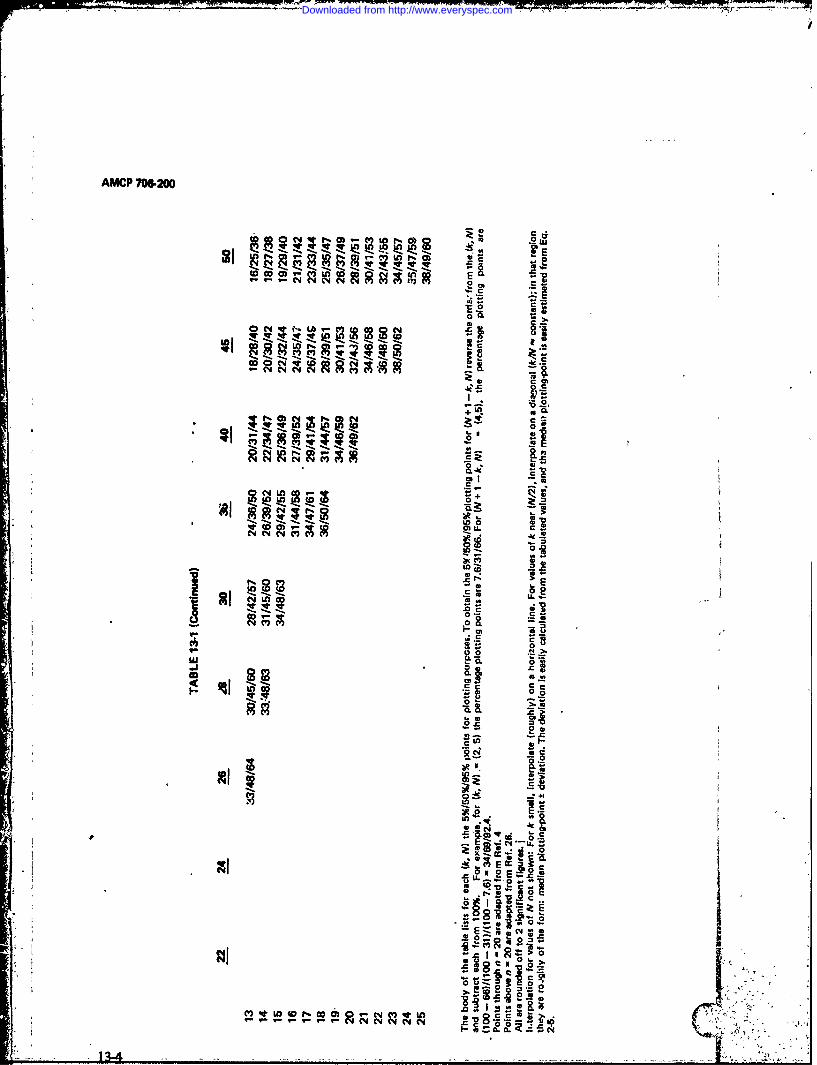
AMCP 7M62oo

2o(c

v~ :e

~I c4

al - a0* s-

.26

0.0ZK !Q

W. go

l'u 0

I--

CC C

td -

o >.A7

e

-o 8.E-1S

13-4On.


I

AMCP 706-200

PPmean =i(N+ 1) (13-4) the observed hazard rate 1/1. The cumulativeS, haza,'d HI is calculated for each failure by

summing the 1/i (for failures only) up to and13-5 CENSORED DATA (HAZARD PLOT- including the failure. The'plotting position is

TING) then

If the data are simply censored by stopping Cdf= I - exp(- HI), S = exp(-I). (13-5) ithe test, then Pars. 13-2, 13-3, or 13-4 can be

used for plotting positions. If the censoringoccurs among the failures, then it is extremely Special probability paper can be printed thatdifficult to find the PrD of failure times. is labeled with H instead of Cdf (or S). It is

di'ficult to aqsign an uncertainty to theHazard plotting was developed for this plotting position, but H ± Vf somutimes is

situation (credit is usually given to Wayne used because of the relationship of H to tfieNelson). The items are listed in order of their Poisson and exponential distributions.censoring and/or failure times (intermingled).They are given the reverre order statistics/ An example of this plotting method is(from N to I). Each failure is then assigned given in Part Three.

t

1351!

:1

I

t 13-5/13-6 '


AMCP 706.200

CHAPTER 14

GOODNESS-OF-FIT TESTS

14-0 LIST OF SYMBOLS (2) Take so many data that any hypothesiswill be rejected.

Cdf = Cumulative distribution func-tion Generally it is considered unwise to use

goodness-of-fit tests as Jnything more thani acsqf = Cdf of the chi-square distribu- very crude means to decide which PrD family

tion to use. Samples are so varied, even from thesame PrD, that one can look very foolish by

k = number of cells trying to get more information from a samplethan is there.

K-S = Kolmogorov-SmirnoffThe two goodness-of-fit tests discussed in

ni = actual nuin.. in cell i tids chapter calculate a statistic from the dataand compare it with the PrD of that statistic.

AT = sample size Usual procedure is to see if the sample2 statistic is too large; if it is too large, the fit is

X2 = statistic calculated from the regarded as inadequate. It is very worthwhilhdata checking to see if the fit is "too good". If the

fit is fortuitously very good (sample statistics- = denotes statistical definition is very small), there is a reasonable possibility

that the sampling procedure was not asPt = mean number in cell i random as was planned. For example, some-

one may have massaged the data to makev = degrees of freedom them look better.

2X V, = value of chi-square such that 14-2 CHI-SQUARE

csqf(X2,., p; v) = PThe data are put into cells. The actual

14-1 INTRODUCTION number in each cell is conpared with thes-expected number for that cell. The numbers

Stat'-ticians are divided on the utility of are combined into a statistic which has, :4

goodness-cf-fit tests, although there is no asymptotically, a chi-square distribution.qLestio aboilt their statistical validity. Thequestion is on their utility. In almost any 14-2.1 DISCRETE RANDOM VARIABLESsampling situation, two extremes are possible:

The data fall naturally into cells-the dis-1) Take so few data that no hypothesis crete values of the random variable. For a

will be rejected. large sample, the number in cell i, ni, can

- 14-1


AKCP 706200

reasonably be represented as a Poisson situa- usually is reduced by the number of param-tion with mean jpj for cell i. The standard eters so estimated.deviation of n1 is VI. If it, is large, ni has as-normal distributi)n with mean p, and stan- Conventional wisdom suggests that p, > 5dard deviation VA. The n. is converted to a for all cells, ol'erwise cells ought to bestandard s-itormal variate by the transforma- combined. Simulation has shown that this istion too strict. If fewer than 1/5 of the p1 are less

than 5 and none are less than 1, reasonableV -/results will be obtained.

The sum of squares of P s-independent stan- The previous heuristic description of thedard, s-normal variables has a chi-square dis- source of the statistic is not rigorous, but ittribution with P degrees of freedom. Suppose helps in remembering how to calculate thethere are k cells (values of the discrete statistic and what its limitations are.random variable), e.g., for the usual pair ofdice, there are 11 cells: the numbers 2, 3. 4, X2 in Eq. 14-2 is compared with X2V'p

S11, 12. If sample size is fixed and known, where- csqf(x2 ,,p; P) = P, and P is someonly (k - 1) of the zi are s-independent, reasonably large percentage, e.g., 95%. If X 2

becpuse if the first k - 1 are known, the kth > 2 v, p, the fit is regarded as too poor. ,

can be calculated from the data. Therefore P = also is compared with a X2 ,, p where P is ak - 1, and the statistic reasonably small percentage, e.g., 5%. If X 2 <

X2 , , the fit is regarded as suspiciously goodk k and the source uf the data is investigated.

A12 Z' (n 1 - p) 2/ 1A '(14-2). 1 gt='I Example No. 1. A single coin was flipped

10 times; the results were 2 heads, 8 tails. Washas a chi-square distribution with v (k - 1) the combination of coin and flipping-methoddegrees of freedom. If any of the PrD a fair one; i.e., is this result reasonable whenparameters are estimated from the data, P the expectation is 50%-50%?

14-2

AMCP,706-200

Procedure Example

1. Calculate number in each cell. State 1. n. 2degrees of freedom. nT= 8

v -=2-1 1

2. Calculate X 2 from Eq. 14-2. 2. n A (n - p) 2 /p

H 2 5 1.8

Total 10 10 3.6

3. In Table 6-1, find X21,5% and X2 1 3. )?1;95 = 3.85X21,s% = .0039

4. State a conclusion. 4. The data are not "too good"; so there is nodifficulty there. The data are poor, but theyare that poor over 5% of the time. So onemight be suspicious of the fairness of theprocedure, but that is all.

(The data actually were acquired with a nominally fair coin and method of flipping.)

Example No. 2. A pair of dice were rolled 72 rolling- method fair; i.e., is this a reasonabletimes; the results are given in column 1 of result if the expected values are as shown inTable 14-1. Is th,! combination of dice and column 2 of the table?

TABLE 14-1

DATA FOR EXAMPLE NO. 2

#1 #2 #3 #1 #2 #3"

all n1 p (ni -.p) 2 IAJ all n,-1(iJNA- - - I - - - -

2 2 2 0.00 8 10 10 0.003 5 4 0.25 9 5 8 1.13

4 8 6 0.67 10 7 6 0.17

5 8 8 0.00 11 5 4 0.25

6 12 10 0.40 I 12 1 2 0.50

7 9 12 0.75 Total 72 72 4.12

S=411-i=10

. ....... . .. t14-3


AMCP 606.200

Procedure Example

1. Put the data and s-expected values in a 1. See Table 14-1, columns 1 and 2. The usualtable. assumptions about dice were made. v = 11 -

]=10

2. Calculate the individual terms in Eq. 14-2; 2. See column 3.then find X2. X2 = 4.12

3. In Table 6-1, find X2 o1 ,95% and X210 ,5 %. 3. X2

10 ,95% = 18.3X' 3.94

4. State a conclusion. 4. Since ,the X 2 'is so low, th data are almo3tsuspiciously good. Certainly, X2 is not toolarge

(The data actually were acquired with a nominally fair pair of dice and rolling method.)

14-2.2 CONTINUOUS RANDOM VARI- choose k = 10 (jk = 4.3) because 10 is such anABLE easy number to work with.

The basic theory is similar to that for a If the cqual probability method is used, Eq.discrete random variable in par. 14-2.1,except 14-2 becomesthat artificial cells must be set up. In the k -..

absence of an otherwise obvious method, the X 2 = k4 xi2 - N (14-3)equal probability method has much to recom- N .I

mend it. The cell intervals are adjusted so thata random observation is equally likely to fall Eq. 14-2 can also be used if it is morein any cell. With this method, the 1A cani be convenient.less than 5.0, perhaps even as low as 1.0 or2.0. An adequate policy is to choose the Example No; 3. A table in the literature isnumber of cells (which must be an integer) so asserted to 'be random standard s-normalthat #1 is just less than 5; e.g., if there are 43 deviates. Pick the first 50 numbers and checkdata, calculate 43/5 = 8.6 and round upwards that assertion with a chi-squae test .forto 9 cells. In this example, it wouldn't hurt to goodness-of-fit.

(i


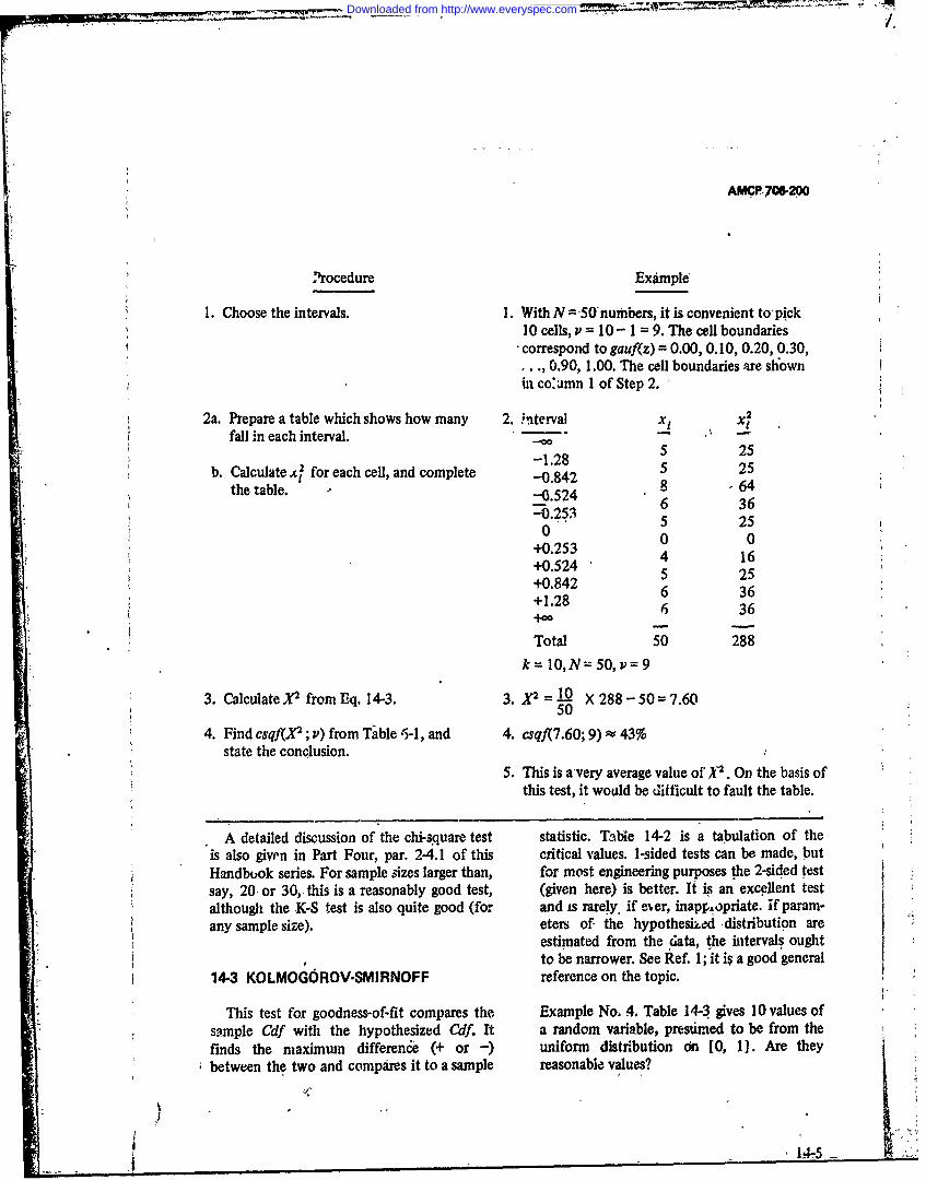
AMCP 706-200

rocedure Example

1. Choose the intervals. 1. With N =SOnumbers, it is convenient to' pickl0 cells, P = 10 - 1 = 9. The cell boundariescorrespond to gauf(z) = 0.00, 0.10, 0.20, 0.30,

*.., 0.90, 1.00. The cell boundaries are shownui co'umn 1 of Step 2.

2a. Prepare a table which shows how many 2. hiterval x x2

fall in each interval. - "-

-1.28 25b. Calculatex. for each cell, and complete -0.842 25

the table. --0.524 6 36

-0.253 5 250 0 0

+0.253 4 16+0.524 5 25+0.842+1.28 6 36. 6 36

Total 50 288

k= 10,N 50, v=9

3. Calculate X2 from Eq. 14-3. 3. X 2 =10 X 288-50= 7.6050

4. Find csqf(X2 ; v) from Table '-I, and 4. csqf(7.60; 9) w 43%state the conclusion.

5. This is avery average value of *2. On the basis ofthis test, it would be difficult to fault the table.

A detailed discussion of the chi-square test statistic. Tbile 14-2 is a tabulation of theis also given in Part Four, par. 2-4.1 of this critical values. 1-sided tests can be made, butHandbook series. For sample sizes larger than, for most engineering purposes the 2-sided testalthough the K-S test is also quite good (for and is rarely, if ever, inappaopriate. if param-

any sample size). eters of- the hypothesiked distribution areestimated from the data, the intervals ought

* to be narrower. See Ref. 1; it is a good general14-3 KOLMOGOROV-SMIRNOFF reference on the topic.

This test for goodness-of-fit compares the Example No. 4. Table 14-3 gives 10 values ofsample Cdf with the hypothesized Cdf. It a random variable, prestimed to be from thefinds the maximun difference (+ or -) uniform distribution di [0, 11. Are theybetween the two and compares it to a sample reasonable values?

1l4-5A€,I _


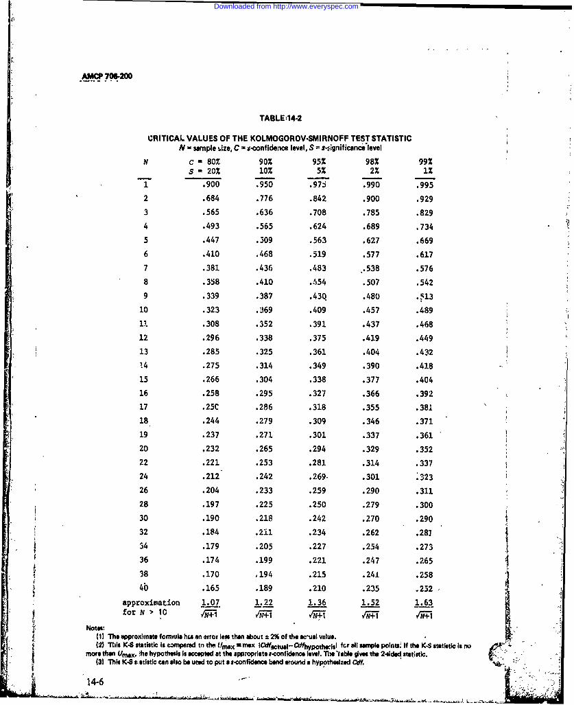
AMCP 706-200

TABLE,14-2

CRITICAL VALUES OF THE KOLMOGOROV.SMIRNOFF TEST STATISTICN - sample size, C = s-confldence level, S = s ignificance level

N c -80% 90% 95% 98% 99%s -20% 10% 5% 2% 1%

.900 .950 .97S .990 .9

2 .684 .776 .842 .900 .929

3 .565 .636 .708 .785 .829

4 .493 .565 .624 .689 .734

5 .447 .309 .563 .627 .669

6 .410 .468 .519 .577 .617

7 .381 .436 .483 ..538 .576

8 .358 .410 .454 .507 .542

9 .339 .387 .43Q .480 .513

10 .323 .369 .409 .457 .489

1i .308 .352 .391 .437 .468

12 .296 .338 .375 .419 .449

13 .285 .325 .361 .404 .432

14 .275 .314 .349 .390 .418

15 .266 .304 .338 .377 .404

16 .258 .295 .327 .366 .392

17 .25C .286 .318 .355 .381

18 .244 .279 .309 .346 .371

19 .237 .271 .301 .337 .361

20 ,232 .265 .294 .329 .352

22 .221 .253 .281 .314 .337

24 .212 .242 .269. .301 .323

26 .204 .233 .259 .290 .311

28 .197 .225 .250 .279 .300

30 .190 .218 .242 .270 .290

32 .184 .211 .234 .262 .281 434 .179 .205 .227 .254 .273

36 .174 .199 .221 .247 .265

38 .170 ,194 .215 .241 .258

4b .165 .189 .210 .235 .232

approximation 1.07 1.22 1.36 1.52 1.63for N > 10 M +1 AT

Notes:(1) The approxlnate fomuiul h an error lea than about 1 2% of the acual value.(2) T is K-S statistic is compared tn the Umax a Mx [email protected] i1 for all sample points! If the K-S statistic Is no ' "

more then Umax, he hypothesis Is accepted at the appropriate s-conf idence level. The *(able gves the 2sided statstle.(3) This K- s; aistic can also be uted to put a s-confidence bnd around a hypothesized W..

14-6 -°m~~~~~i . " " Jl

-NI


AMCP 706-200

Procedure Example

1. Prepare the data in a table. 1. See Table. 14-3. Cols. 1 and 2.

2. Calculate the sample Cdf, and the differ- 2. See Table 14-3, Cols. 3 and 4.ence of the CoIl 2 and 3.

3. Find the max I klifference, 1 3. max. diff. 0. 1708

4. From Tiible 14-2, find the K-S statistic 4. s-Confidence level for N 10-for several s-confidence levels. 80% 0.323

90%1 0.36995% 0.409

5. Draw a conclusion. 5. The maximum deviation is well within bounds.

TABLE 14-3

DATA FOR EXAMPLE NO. 4

Omer random sample

number number Cdf difference

1 0.1080 0.1000 0.00802 0.3153 0.2000 0. 115W43 0.4708 0.3000 0.17084 0.4885 0.4000 0.08855 0.6018 0.5000 0.10186 0.6795 0.800 0.07957 0.7548 0.7000 0.0L'4M8 0.8791 0.8000 0.07919 0.9032 0.9000 0.0032

10 0.9961 1.0000 0.0039

Note: For the uniform distribution, Cdf X }X; socolumn 2is both x nd Cdf X) .


AMCP 7W6200

Example No. 5. Pick 8 random samples of 10 points each from the uniform distribution and plottheir actual Cdf vs uniform Cdf. Draw the 90% K-S lines on the graph. See Fig. 14-1. Of the 8samples, none crossed the 90% K-S lines, although on the average, I out of 10 samples will gooutside the limits. The best linear fit to any of the lines is probably not one going through the originwith 45 deg slope (the population line). Certainly, all of the lines are quite crooked. Choosing acurved line to go through a set of points would be most inappropriate.

See also the example in Part Four, par. 2-2.6.

l.eC

0 .0 0.4 0.6 0.8 I 0. 02 Q4 Q6 0.8 1.0Sample Cdf Sample Cdf

Figure 14-1. Random Sampies of 10 from the Uniform Distribution on [0, 1]

REFERENCE

1. L. H. Miller, "Table of Percentage Points Amer. Statistical Assoc., Vol. 51, pp.of Kolmogorov Statistics", Journal of 111-121 (1956).

I0 14.8 0. . . 1 . A Q . .


AMCP 706-00

CHAPTER 15

TESTS FOR MONOTONIC FAILURE RATES

If it is known that a PrD has an increasing (2) The alternate hypotheses involve onlyfailure rate (IFR) or has a decreasing failure monotonic failure rates. Failure rates thatrate (DFR), then various other characteristics increase then decrease 'e.g., a lognormalof these distributions can be proved. This is a distribution), or vice versa, are not con-field of current-research. sidered.

Tests for IFR and DFR, and further refer- (3) It is not clear why a reliability engineerences are given in Ref. 1 (Sec. 3.4.6). Thu would really want to know this information.arithmetic in applying these tests is tedious Even if he were sure, for example, that a PrDbut straightforward. There are difficulties in had an IFR, he wouldn't know how fast itinterpritation: was increasing. Most of the theorems in the

literature are more interesting to the reliabil-(1) The conclusion applies only to the ity theorist than to reliability engineers.

time interval within which data are taken.There is no guarantee that the conclusion Before iing a test for monotonic failureapplies to the PrD for very long times, but it rates, a statistician ought to be consulted tois at very long times that the conclusion is of be sure that the test is not blindly applied andmost interest. interpreted.

REFERENCE

1. W. Yurkowsky, Nonelectronic ReliabilityNotebook, March 1970, RADC-TR-69-458, AD-868 372.

II

_ 1/15-1/15-2-Z -A,


AMCP 70200

CHAPTER 16

BAYESIAN STATISTICS

161 INTRODUCTION Pr (A IB) cPr(BIIA,}pr{A, (16-1)

This chapter discusses the various Bayesian where c is a normalizing constant such thattechniques and their caveats and controver-sies; it does not give detailed information ontheir use. A statistician ought to be consulted.. Pr(A ) IB1), = 1

There is never any quarrel with the Bayesformula (also called Bayes theorem). It isstrongly associated with the very definition of implies the sun. over all i.conditional probability.

If the set of possible values for the param-There are 4 main categories of Bayesian oter is the con tinuous random variable x,

activity (the categories are not necessarily then Bayes formula ismutuallI exclusive): pdf~x IBI)" = cPr(B! Ix) pdf{x) (16-2)

(1) Prior distribution is real and known(no controversy), where c is a normalizing constant such that

f pdf {x2B } dx = 1, Jx implies the integral(2) Empirical Bayes. Prior distribution is over all x.

real, but unknown.If the possible outcomes of the experiment

(3) Subjective Probability. Probability is are the continuous random varial'le y,. thenused as a measure of degree-of-beiief (d-of-b); Baye. fornula isthe prior distribution is one of d-of-b before aparticular test is run. This is quite controver- pdf{x Iy) = c pdf{y I x) pdf(x) (16-3)sial.

where c is a normalizing constant such that(4) Bayesian Decision Theory. This is very

diffiult ito use in practice; so it rarely is used fxin anything but simple examples in textbooks fxand articles. If it were used often, it would b,,

* very controversial. There is nothirg coritroversial iabout any ofthese formulas, they are straightforward,well-known applications of probability

16-2 BAYES FORMULA theory. It is in their use that controversyK! arises.

Suppose the set of possible values for aparameter is discr&'" and f'mite: 16-3 INTERPRETATION OF PROBABILITY

~~A t, 1 1, .. ,.Suppose the possible .outcomes of an experiment are the set

B/=l,...,b. Then Bayes formula is Probability is a mathemnatical concept and

16-1 -


AMCP 706-200

as such can be applied to anything that fits In many complicated situations it is verythe constraints of the theory. The two main difficult to know one's d-of-b. One may eveninterpretations are believe mutually contradictory things, espe-

cially when the contradiction is not apparent.(1) Relative frequency

Many engineers view the results of their(2) Degree-of-belief. own labors very optimistically. In order for

them to use d-of-b fluitfully, they mustRelative frequency is a straightforward con- impose a discipline upon themselves. Other-cept and is the classical statistical approach. wise, they will commit the sins that op-Degree-of-belief often is associated with ponents of d-of-b like to talk about. Degree-Bayesian theory and is a controversial ap- of-belief is useful but unless one activelyproach. The controversy stems about its practices the necessary discipline, d-of-b mustsubjective nature. A prudent person (by deft- be avoided.nition) will adjust his d-of-b to correspond torelative frequency where the relative fre- The discipline has the -following steps:quency is known. For example, a person whois concerned about the outcomes of honest (1) Write down the prior d-of-b.throws of honest dice would be wise to havehis d-of-b the same as the woll-known relative (2) Run many hypothetical experiments.frequency for dice. Calculate the new d-of-b after each hypo-

thetical experiment.. The proponents of d-of-b argue further that

there are many situations where relative fre- (3) Analyze whether or not each newquency is not appropriate since it will never d-of-b seems x-asonable in view of the hypo-be known. For example, it is d-of-b that one thetical data.has concerning whether a pair- of dice ishonest or not. It is d-of-b that can be refined (4) (a) If it does, repeat Steps 2 and 3by actually throwing the dice and observing until virtually all possible outcomes have beenthe outcomes. hypothesized.

Degree-of-belief before any tests are run (b) If it does not, revise the pror d-of-b("prior" d-of-b) is subjective and not repro- and go back to Step 2.ducible from person to person or even time totime for the same person. To opponents this Example. Suppose an equipment is beingis a disadvantage; to proponents it is an designed and an engineer describes his pfioradvantage because it recognizes a fact of.life. d-of-b about its failure rate in a 1000-hr test.

16-2 K -


AMCP 706-200

Procedure Example

1. Step 1, state the prior d-of-b. 1. See Table 16-1 rows 1 and 2 For row 1 wepresume that the engineer has decided it isreasonable to distinguish between these threefailure rates. lit practice, one would probablyuse more;e.g., 10- 1, 10-, 10-3, 10- , 10-S.For row 2 we presume that'the engineer is ratheroptimistic about his handiwork, i.e., he is justpositive it is almost perfect-a very commonstate of affairs, unfortunately.

2. Step 2, try several hypothetical experi- 2. Suppose 5 samples are put on test. Hypothesizemenits. Use Eq. 16-1 for calculations. 0 failures

1 failure2 failhres.

See rows 3, 4, and 5 of Table 16-1 for the cal-culations. We have presumed that the tects areof the pass-fail type. Thus the terms in thebinomial distribution give the probability ofthe observed results for row 3.

3. Analyze the results (Step 3). 3. For the 0 failure case, the new d-of-b's arereasonable. For the 1 failurm case, it is notlikely that anyone would still have a 13% d-of-bthat the failure-rate wNas 10-s For the 2 failurecase, the results are reasonable; all the d-of-b hasshifted to !he worst failure rate.

4. Steo 4b; try again. 4. See Table 16-2, rows land 2. This time, forrow 2 the engipeer is less blindly enthusiasticabout his work, because he has seen the badlogical consequences Qfl his former (Table .16-1),allocation of a-of-b about the failure rates.

S. Repeat Step 2 of this procedure. 5. 5 samples are put on test. Hypothesize0 failure1 failure2 failures

See rows 3, 4, and 5 of Table 16-2 for thecalculations.

6. Analyze tyi- results. 6. Fcr 0 failures, the new d-of-b's are reasonable.For 1 failure, the new d-of-b in a 10-3 failurerate is lower than before, but still seems toohigh.

'-.4 16.


AMC*70w~-52"

7. Try again. 7. See Table 16-3, rows 1 and 2. This time, forrow 2 the engineer is downright humble abouthis work, again because he has seen the badlogical consequences of his former (Tables 16-1and 16-.2) allocations of d-of-b about the failurerates.

8. Repeat Step 2 of this procedure. 8. See Table 16-3, rows 3 and 4.

9. Analyze the results. 9. For 0 failures, the ne d-of-b's are reasonable.For I failure, the new d-of-b's are more reason-able than they were. Perhaps one could livewith them. These methods are the way a rational(in the Bayesian sense) person converts priord-of-b and the test results into a new d-of-b. Onecannot go back and change the prior d-of-bafter seeing the real actual data. That is Y'hyextensive simulation is so necessary. The exactsame prior d-of-b that is used to convert thegood test results also m:ist be used to convertthe bad ones. Anyone who suggests differentlyis, at best, ill informed. Unfortunately, theBayesian reliability literature abounds withthose bad suggestions about changing the priord-of-b after seeing the actual data.

The example will not be pursued further, 16-5 EMPIRICAL BAYESbut in practice, the simulation ought to bemuch rore extensive. If one is~not prepared The prior distribution is presumed to beto perform extensive simulatioi on his prior real, but unknown. As sanples are taken, theydegree-of-belief, he ought to avoid subjective are presumed to illustrate that real priorBayesian analysis altogether. distribution. Since the real Cdf of the prior

distribution is only coarsely definud by the16-4 PRIOR DISTRIBUTION IS REAL AND data (i.e., by the sample Cdf) a smoothing

KNOWN function is employed to estimate the realprior Cdf. Once this real prior Cdf has been

"tits case presents no difficulties, it often is estimated, it is usei with the sample data inused as an example in textbooks to demon- the same way as a real, known Cdf would be.strate apparent paradoxes about probabilities.It is probabl rare tLt ihe prior distribution A statistician ought to be consulted. Theis known, although some work has been done choico of a smoothing function is an art, not aon the PrD qf actual reliability vs predicted science. One may wish to test the'hypothesisreliability for; some militaiy systems. In these that the samples do come- from PrD's withapplications the validity of the prior dictribu- diffeient parameters. A great deal of engineer-tion can be questioned as far as its future ing and statistical judgment is necessary, andutility is concerned; but this is no different it ought to be made Ps expF.dit as possible.than in many applications of probability. Astatistician ought to be consulted. The blind 16-6 BAYESIAN DECISION THEORYapplication of formulas can be very mislead- T ie t v ul win4g. The baic tenet Lt. that eventually one want16-4 :


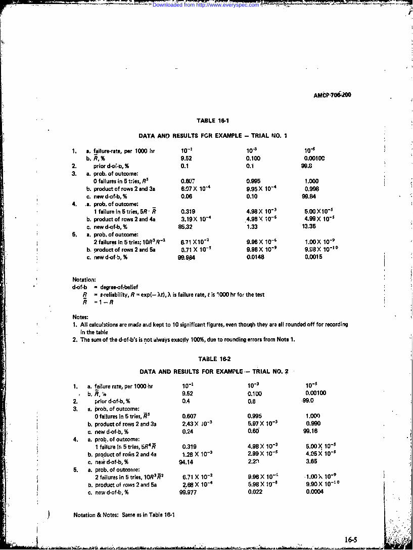
w

AMCP706200

TABLE 16-1

DATA AND RESULTS FOR EXAMPLE - TRIAL NO. 1

1. a. failure-rate, per 1000 hr 10" 10-3 10"6

b. R,% 9.52 0.100 0.0010102. prior d-oi b, % 0.1 0.1 99.83. a. prob. of outcome:

0 failures in 5 tries, R s 0.607 0.995 1.000b. product of rows 2 and 3& 6.07 X 10-4 9.95 X 10- 4 0.998c. new d-of-b, % 0.06 0.10 99.84

4. ,a. prob. of outcome:I failure In 5 tries, 5R- R 0.319 4.98 X 0 3 5.00X10 "s

b. product of rows 2 and 4a 3.19X 10- 4 4.98 X 10-.6 4.99 X 10-s

c. new d-of-b, % 85.32 1.33 13.355. a. prob. of outcome:

2failures in 5 trie3; IOR3 R -2 6.71 X10 " 9.96 X 10-6 1.00X 10"

b. product of rows 2 and 5a 8.71 X 10-' 9.96X 10-9 9X8X 10-10c. new d-of-b, % 99,984 0.0148 0.0015

Notation:d-of-b - degree-of-belief

R = s-reliability, R = exp(- Xt), X is failure rate, t is ,000 hr for the testR=1-R

Notes:

1. All calcul3tions are made and kept to 10 significant figures, even thouqh they are all rounded off for recording

in the table2. The sum of the d.of-b's is not a!ways exactly 100%, due to rounding errors from Note 1.

TABLE 16-2

DATA AND RESULTS FOR EXAMPLE.- TRIAL NO.2

1. a. failure rate, per 1000 hr 10"1 10- 3 10-1b. R, % 9.52 0.100 0.00100

2. prior d-of-b, % 0.4 0.6 99.03. a. prob. of outcome:

0 failures in 5 tries, R5 0.607 0.995 1.00'b. product of rows 2 and 3a 2.43 X i0- 3 5.97 X 10- 3 0.990c. new d-of-b, % 0.24 0.60 99.16

4. a. prob. of outcome:1 failure In 5 tries, 5RR 0.319 4.98 X 10- 5.00 X 10-s

b. product of roars 2 and 4a 1.28 X 10-3 2.99 X 10"s 4.95 X 10"s

c. nev, d-of-b, % 94.14 2.2.1 3.655, a. prob. of outcome:

2 failures in 5 tries, 10R3 fRi 2 6.71 X 10 -2 9.96 X 10 "' -1.00 X 10-9

b. product of rows 2 and 5a 2.68 X 10-4 5.98 X 10- ' 9.90X 10- o

c. new d-of-b, % 99.977 0.022 0.0004

Notation & Notes: Same as in Table 16-1

16:5'-


AMCP 706200

TABLE 16-3

DATA AND RESULTS FOR EXAMPLE- TRIAL NO. 3

1. a. failure rate; per 1000 hr 10-1 10- 3 10"S

b. R,% 9.52 0.100 0.001002. prior d-of-b, % 1 1 '983. a. prob. of outcome:

0 failures ip 5 tries, Rs 0.607 0.995 1.000b. product of rows 2 and 3a 6.07 X 10- 3 9.95 X 10- 3 0,180c. new d-of.b,% 0.61 1.00 98.39

4. a. prob. of outcome:1 failure ir1 5 tries, 5R4,# 0.319 4.98 X 10- 3 5.00 X 10- 5

b. product of, rows 2 and 4a 3.19 X 10- 3 4.98X 10- s 4.90 X 10- 5c. new d-of.b, % 97.00 1.51 1.49

5. a. prob. of ofitcome:2 failures in 5 tries, 10R3R2 671 X 1002 .96 X 10-6 1.00 X 10- 9

b. product of rows 2 and 5a 6.71 X 10 - 4 9.96 X 10- 8 9.80 X i0 - ' °

c. new d-of-b, % 99.985 0.0148 0.00016

Notation & Notes: Same as in Table 16-1

01


AM706=0

to make a decision that is based on the variable about which degree-of-belief state-experimental results. Those results tire not of ments are to be made.interest in themselves; so why analyze them indetail. The procedure is to list the possible (2) Use the conjugate prior distributionstates of nature (e.g., the 3 failure rates -in (continuous). It transforms the simpler situa-Table 16-1). Then the loss or gain involved in tions into very straightforward, calculations.choosing each state when some state is true is For example, fo; the constant failure rateestimated. Then a criterion for good decisions case, choosing a -prior distribution is equiva-is hypothdeized (e.g., minimize the worst lent to choosing a prior test time and priorpossible loss, or maximize the s-expected number of failures. The pair of sample datavalue) and the decision i chosen (given the (failures, test time) are appropriately added toexperimental data) according to the criterion the prior pair to give the new pair, which willfor a good decision. represent the new degree-of-belief...TXhe bino-

mial situation, is similar, except that total-The argument against this whole process is number-tested replaces test-time.

that there are too many arbitrary assumptionsthat get lost in the shuffle. The final result The conjugate failure distribution methodappears quite emphatic, but the arbitrariness ought to be used with caution. The family ofis hidden from view (perhaps unintentionally) prior distributions is quite rich, but it isand there is no measure of the uncertainties difficult for an engineer to quantify hisinvolved. It is argued that except for the most information in the necessary way. As men-simple-minded situations of the kind used ja tioned in par. 16-3, extensive simulation oftexibook examples, applying Bayesian dc-1 experimental outcomes is necessary. It is

sion theory is impossible. quite easy, if no simulation is performed, tomake seemingly realistic assumptions about

The arguments for Bayesian decision one's prior beliefs, which turn out to betheory are that it gets all the assLmptions out grossly misleading.where they can be viewed. The value of moreinformation can be calculated, and a variation The discrete prior distribution is moreanalysis can be performed to find the critical straightforward, although tedious to calculate.variables in the decision. Far from hiding It has many advantages in terms of thethings, it makes everything explicit. The visibility of the results. In cases where therecomplications merely reflect reality. are double peaks in the new d-of-b distribu-

tion, the engineer is alerted to the fact thatOne certainly ought not to attempt to use choosing a single number for his "best" belief

Bayesian decision theory without the services might be misleading.of a very competent statistician (who under-stands it) and a very competent engineer (who If either of these approaches is used, aunderstands it). The odds against its being statistician ought to be consulted. The arith-really productive, rather than pointless or metic is easy enough to do (although some-misleading are quite high. So unless there are times tedious) but the results may be difficultlots of resources, leave it alone, to interpret. Merely because the calculations

can be made does not mean they ought to be16-7 SUBJECTIVE PROBABILITY made.

The 2 main approaches are: 16-8 RECOMMENDATIONS

(1) Use a discrete PrD for the random Engineers have a great deal of prior

- - -'-----16-7'


-i

knowledge. If they did not, no production conditions, and with help from competentline would ever work. But engineers do not statisticians, one of the Bayesian techniquesdesign, predict, or produce perfectly. A large might be- fruitful. This is .'in area of research,part of their training is in the directions to try not an area for blind calculations.for improvement. Prediction techniques thatsomehow use an engineer's prior knowledge, Cookbook formulas and procedures havewithout being overly optimistic (or even been omitted from this chapter on purpose.blindly optimistic), are needed. Under some They are too easy to misuse.

I

|[

I C


A"CP 706-200

CHAPTER 17

SAMPLING PLANS

MIL-STD-781 and MIL-STD-105 contain the MIL-STD's.sampling plans that are useful in reliabilityand quality control. They are not repeatedhere. Before any sampling plan is used, its op- There is rarely a need to invent new

erating characteristics ought to be investigated sampling plans. . One doesn't really know

rather thoroughly. If the sample size is not exactly what operating characteristic he is

fixed, then the average sample-size and maxi- willing to settle for, and a great deal of

mum sample-size characterestics ought to be arbitrariness exists-enough so that it will

investigated. Much of this is already done in usually encompass an already analyzed plan.

1

4

11-1/17-2 i" :. .


AMCP 706=O

CHAPTER 18

MISC'ELLANEOUS DESIGN AIDS

* Several references have collected many tion. Some of the aids become obsolete asreliability-mathematics design-aids. They are the techniques and materiel to which theynot reprint.d ,here since each requires exten- refer are replaced by newer technologies andsive explanation of its procedures and limita- analyses. Refs. 1. 2, and 3 are good sources of

these aids.

REFERENCES

1. Handbook of Reliability Engineering, 530-01-1-762, ARINC Research Corp.,NAVWEPS 00-65-502, Bureau of Naval Annapolis, MD, April 1967.Weapons, 1 June 1964. 3. NAVSHIPS 94501. BuShips Reliability

Design Handbook, Fleet Electronics Ef-2. Reliability and Maintainability Handboor. fectiveness Branch, BuShips, 28 February

for the US Weather Bureau, Publ. 19 .


AMCP 706-200

B Incomplete. gamma function, 11-1

Bayesian statistics, 16-1 KBeta distribution, 10-1, 13-2Binomial distribution, 3-1, 13-2 Kolmogorov-Smirnov test, 13-1, 14-5

C L

Chi-square distribution, 6-2, 6-3, 14-1 Lognormal distribution, 9-1Chi-square/nu distribution, 6-3s~confidence, 12-1

continuous variable, 12-3 Ndiscrete variable, 12-5, 12-7See also: Under each probability distribu- Names (probability distributions)tion See: Under each name of a probability

distribution, 2-2D s-normal distribution, 5-1

Decision theory, 16-4 PDefinitions

See: The desired word in Chapter 1, for Plotting positions, 13-1probability distributions. See: The name Poisson distribution, 4-1, 7-2of the probability distribution Probability distribution,

Discrete probability distributions, 3-1, 4-1 See: Under the name of the probabilitydistribution

ER

Empirical Bayes, 16-4Exponential distribution, 7-1 Randomized s-confidence intervals, 12-7

F

F-distibution, 6-12 s-statistic, 5-1Fisher-Snedecor F-distribution, 6-12 Student's t-distribution, 6-7

GT

Gamma distribution, 11-1Gaussian distribution, 5-1 t-distribution, 6-7Glossary, 1-1 Tables,Goodness-of-fit tests, 14-1 See: Under each probability distribution

W

Incomplete beta function, 10-1 Weibull distribution, 8-1 L


(AMCRD-TV) AMCP 706-200

FOR THE COMMANDEP:

ROBERT L. KIRWANOFFICIAL, Brigadier General, USA

Chief of StaffJ HAROLD

. LTC, GS

Adjutant General

DISTRIBUTION:Special

* US. GOVERNMENT PRINTING OFFICE: IW6-60-770/ 310

t

1'1

tI


ENGINEERING DESIGN HANDBOOKSArsb~ to 30 Poes, Intoo Ito. poottith Ce t 11 NS -,,l Ch. p ....P 722 I 2 "I ~ o t.and *t0.b"'71"" Vor'tAo o 1.000 1,. .teo fnl 1.tock2 tfifunit.. Sorote. topertao-t of Cospres. OpIosti.ld. VA 22ill.11. hi.1.. gor Ne.ther deceit$ 0.4 UK Potl" To"0or4 r.q.-toot.4 of CI0..'f2.d d"opOsts.

1 .tiCodot .rrd4b~r ZI)s 12.1.4 Sypo. Ad Coe ..et&1A No. o1...rI low rr'wit..

100 91-...' of Ar....,?l Instr.*,Ioa. Port 0... 211(C) I .oo. Proottr. g1.otricalPrSo()0...,.. of tooruy 212(s) 7:-.4, Prost.t. C2.,trt0 IP:?r"t T'_ I'm

to, alienitof Ars.onist la2.oer1., Pitt Too. I,,(,) Pt:a. t.2.ty, zt.ctrol. Fort 11cr. (t)

go Illoli.. 210( Po.. Frotelt, ttrit. IPart Vc (to204 sle~.t of Aconit fakimoarlai. Fort The.., 220(0 Pa..,. r .I.1,. otrric V Par:t Five(0

$Ittoo " and.. . Coostto I2I2) A*r., tg Weapon tyst... Against IF 304:21I1 ?abl.ofa tOoo totlr.1 Stintol 127 6 strto Va#~ Pa . .

lit moaptal.t. $factor( 0. tactics 1. "sit, 239 #:Z1 Ar. loop.. SysoinC'r"to &A0 Analyips of 1900.ro...2o lots 240(C) Criss. (0)

III later1.t.1 tot twico. soctito 2. Analyst.a 242 Do.'o Iso Control of PoulII flight foot-of fewor.ct. 0. 4olo .att r sets attorlta ~o(Ropli. .20

.. 4 Amo~l oCw~rto In prooo Cra. .12. t . .1 Cotoo C"tary.122 0olootal s1tttics "A020 4.S1ro.4 .lfo ar.?.Pie. 245(C) .to. otla2 .t.oraool

214 tap~trloo. Otati.%t,., $felt"o 5. 102.. W.".g (U)i20 Iot I..lSr... Part 04. I ltc 140 *5o1tim. s#1le is Pol I torent"o

Coolop.sotI Coo:pto ?lit Chorat.rllat (satiated ty .202121 ~ ~ ~ To &-tu..o ot..'r I. ~ r.) 21 4.lto 0% b. go for Peni. I-t~

to~~lr..o~rIt Potrl0 Aotoom. otie w . S MpoW10 A~pt oIII sp.ot otl 20,2.. Port Thc..., Indced Art "I",y Ase, titko to.A

'to..ot~ P0 61 2(9 A-ctt is. Ste. 6. ll0.,acto of Metallti2s toloo. triprt.. pact Poor. Lifo Cycle Coopooats of Artillery A-tone

12t 1..2r...otal ;*t.. Part five. 02,..ory 22 ,tlPol.ef tevressot. Tell. 212 so-0.k. 0

120 Crig's2 for I o'II.otoO Cootr, of 223 -It..%h 90.'oo. Deals.P.., ;, is,.. 201 S r Ir~ doorsrt rtotca of l..r.2. fl.sh

122 Puasooto sea Poct loamorlt 2 i. Ao't.t I U.aPoso

22 ~roc2 2 OI ol a 2701 i Prevails01 Atoolod Povitt.12C 101,1ol.. Sttr I.t..t 2180 Design of Arodynamicaolly Stohloltard Fret

If, Ifrro 1. ltr 1r~m Pat. 202(2102 v. %yet- if.2 .ett.2oo (W212110) Sf c M.4 t2o, O:,m Pot Too (0 222 OP.oP.1 .l. aid trop.21.t. (Replaced 07 -26)

1: o.fr Ate Transport &.A Atrdrop of 24 trtc.

Flatoo2.0 t af.r4 Ice ~ qro (Ott)P .,91 o.t-Alr 4164t3@8. part 04..w *Poo1$4 144t.to.blltr ekoic. r~ D0~on d 202.tItgot

Prot4r litle17 .Tho) 292(C Otorfoattto-Air Missile.. part Fia. Po

*ad 318ool Can trtro 2$5(C) 4torfao..to-Atr Missiles. Port five, Cvetor234~~ *1r..loo.. Soits. 3. .oplfioclo .ooooro. to)

)9 0tsurooticoot.o 04220, 4: t-wer staist. Its 4orfo.t-AIT H1.411.6. part SIU. ItfoCtucroo

barPol for Projoct t .6 prbl. (ic) ie::.?:104 ttor 2o221ttc. of An. 1 ort esta'.Is$24 pm 7o.o1o.t 00211,. tU..t ryoo.2r.. 112 Rotatio-ol Noing a1 PI Po .data

lert 0O 3) Short ?floor Plsotic less Cooppottoo,209(2) Tvadmo..20 of 3oI101(tc Depart 07.0.02.. 127 Pir Control sysa.-G'Oetral

Poot I. fil) 129 'I r Cootra oewi Co.2s yst.o0(C) statute. of Tarotool go Iltalic, Port One. 131 C..os. V141..c

a 22 el~ohoi .4r !,apoI-hwt, (0) 12110 00..k. 9-4toopera Now2.or 510.2. spaniel (Dowf.1110 11-.of. Intelsat Sol.tatte .or Top. 70200. 1. MUoittooo and IOoOpOR 170cm to

coI2.ctto. and Analysis if Polo Concorn- 334(00) "14.X Waomen, 10.? low affct* Hassel (tcUMl.togO tart 0 vopo It. tlect-ol Systeas ad Login'tico1

1201b) S2t.Vof .r.1oa 00112.210. Port T1cr., i47oto (0)kpltt04ift to Iltootll And Sp: ac. rget. (2)l 337(15O) 004.100f Inflators' Macloar Ufocto Mante1 (bDll)

163($) 000.22 Tarm. Volooobillly (0) Polav ttI. fhoclear Ultraioe (0o240 LIq.Id-FtIo4 Prlatest 1l esg ... I403) obo.-Iol. s . WicIoor I11042. Havant (lU9t)l2V0(S Am~r aid Its Apptctfott. (i7) Vo1os 2?. Shoetoor Uifct$ to)2 70 solid Prao22sto. Parr 0" 340 Crrflags. 004 00.Oqt-CrW4170 40224 Pro.21oats. Port 100 31 Cr042..1T7 Pro"ofile$ of S.P1.olv.o of M1.t.ry 142 SReo12 syst.o

tolerant 343 Top Coreb05..270 ,"At.o02. of taploolv#. of ilitary 34 f too, Croflogo.

lo _r.c motlo. 2 ("oplad by -277) 340 b4-ti10roo279 wp~o. 1,0. 344 boeo Koohol..

1'g0 Pr'sle~lt of Zoplolo somooir 347 Torivueta Machinists20 Liplosoao. to Air. Pft On. 124 000.1.4 Np0lht.

22(2 loo.o Is Air. Part To. o )30) Th. At-ittv. A.02100 .' Si IF P ?olrc2,. t 0.0. Theory a.4 324 Alrol"'o Oo1 o..o116 milit2ary PyooecloPrt Tw.o safety. 34 Military Yabolol tloctrtcol systo

Pro4 eedr 0.4 Closoory U41 I. Mlitary Vehicle por Plo1ot Coog113 NOitr P Fotr olo rt Thr... Proprtion 420 *tletro..qcct "' Copr 412 C.2 tls Used to Pyr tetoic 0Coelotop 411(s) eolcc2.rsh(litp fCicorto.2.tol100 Ilittty Pyrotechncs. part yeor. Pool. of 1l tticrp2 l0 2.o. (bctopt woid missile$o)

Ae.cltIo for Pyrartuhol 0f1.cl. to gloclttoc Warfare. Part 00.. totrw to.J2e109 ,,,lttzrytyyrot o2.cl Part ties, l1bI1o.V4ph7 sod Coastal icpprooo tc g1.ctroa(r P~tto-.200 -Ar.Y S..P.. - o Aoa1t ol. Oolcr.01 11ity (o)2021 SlotdA 4.lyto aid Cstforti.2ot... 412(c) 91ulorotllty of Casowecocatlos,b.ceros1, A"4192 Coso"Cor Aid"4.4Wig. of Mechaniclco lytma, Z2.ctro-Otlri systaem (Incept Cm1404 Miles~o)

Port One to t2.ctro.1c warfare. port Ti., l1rtroolc Porforo103 C.0.oto Aided Deals. of Me.chanical Syt...,. Vo200rattlilly of Tactical Coin,cctlOm (t)

PO" Tw 421(1) "~.s 201112p of &ad~to-lcto~ .2s$ O~. I Coor 0ol. far I.I

10

01lltjF Part Dole. Y1ctro-0pti1l1 2702000 (Cecor, G find Mit".)

lt r-r .%. . .Otka .. .4 and lanin to e2.ctrmlc lIttloe. Part Three, Iltrooltfor A"o "oo~lboImuo~ w~rfoj a oloarstillly of Cr0,04-bases0. ko osm

1294 0_.fspasoe Cjdo for 0100111ty. Part Tsn. Scoro.Ilooo 4-4 lTto At 18114nn U5or 02

0_01. for P-1illilty 414(5) T.Iftoralllty of Cmoato.oer o d.it? Ccopej.ot Cold. (or 1@o1t*0111ty. Part Thre. R.1ttro-0p21ro1 syst toOcopt 0444 Misfit"~)

sa1(solotpt Prodtlo.f to Electronic Parfaore. Port Pour. slotpoO(I2TW U0o.on o... 0 for Reliability, Fort Por ittefr# Vl..rohlty of Av.1eflro (U)

oIlability Main r....t 010() o"..ro02111ty of Cm cot.lctopic 824I"9 *O.liphle, ,1do for 3.110011(27., Fort viv.. tloctro-Opticol system, (tocept Guide4M.4 '1.Igo.)

Cantrestl*I for 3.)2ald21ty to totrotc Vettr*r. Port PHe.. Optlol/gloetrmilDeviool=p.. 0.14. for As011.0ty. Pat Sit. Welrfare Vulnerability of Ilutro-Optc Systme (9)

les200.01(0.1e Appondix 0.04 Otiosity 41'(6) iru2orrobillt o1 Cpospeltolisoo2loclro.Ic loo4201 lalieaptor toel...rt., Pert 04.. Pro1lory zlecto-2021c0 s7stop (00e"p2 Co~d 111.011..)

Poesg to ElecOtronic Parforo. tort $.. to04trosic tIotlae242 ola.Icopter Bsowin01g. tast Iv.. 041021osafr Soolo01orailfltv of S02e22i20 com~tc~tf to 0203 lielicipt o htmsrtma, Fort th'004. QoAtAbtf.o44 . tooocson ,W10.1

sinousrac 70 "lerft Conversion 0.140 f or Military Applictoo204 sal1tepteryuPouoc tll

-06 0602120-..? avalle


engineering design - everyspec

Documents