ENDOGENOUS PRODUCTDIFFERENTIATION IN CREDIT MARKETS:

WHAT DO BORROWERS PAY FOR?∗

Moshe Kim† Eirik Gaard Kristiansen‡ Bent Vale§

May 14, 2001

Abstract

This paper studies strategies pursued by banks in order to differentiatetheir services from those of their rivals. In that way the level of competitionin the industry is reduced. More specifically we analyze whether the bank size,a bank’s ability at avoiding losses, or its capital ratio can be used as strategicvariables to make banks different and increase the interest rates banks cancharge their borrowers in equilibrium. Using a panel of data covering Norwe-gian banks between 1993 and 1998 we find empirical support for the the abilityat avoiding losses measured by the ratio of loss provisions as such a variable.Borrowers in the market for credit line loans may discipline banks into avoid-ing losses. We also find evidence that banks pass on parts of increases in theiroperating costs to credit line borrowers. However, we do not find any strongevidence for the use of high capital ratio as a strategic variable that borrowersare willing to pay for. This implies that strategic competition does not leadbanks to hold more capital than their cost minimizing level. Thus, our papergives support to the rationale for imposing capital requirements on all banks.

JEL code: G21 L15

Preliminary version

∗Views and conclusions expressed are the the responsibility of the authors alone and cannot beattributed to Norges Bank.

†University of Haifa, Department of Economics, Haifa 31905 Israel, and Humboldt University,Berlin. Fax: +972 4 824 0059, e-mail: kim@econ.haifa.ac.il

‡Norges Bank (The central bank of Norway). Adress: Norges Bank, C51, Box 1179, Sentrum,N-0107 Oslo Norway. Fax: +47 22 42 40 62, e-mail: eirik.kristiansen@norges-bank.no

§Norges Bank (The central bank of Norway) and Norwegian School of Management. Adress:Norges Bank, C51, Box 1179, Sentrum, N-0107 Oslo Norway. Fax: +47 22 42 40 62, e-mail:bent.vale@norges-bank.no

1. Introduction

There exists a vast literature investigating the nature of competition in markets

with differentiated products. In this paper we focus on endogenous differentiation

among banks. More precisely, how banks strategically choose different “quality”

characteristics (equity ratios, monitoring capacities, screening efforts, size etc.) in

order to differentiate themselves from competing banks given that customers exhibit

different characteristics, and thereby soften competition. This focus enables the

analysis of why banks become different and not why different borrowers choose

different contracts, which is extensively analyzed in the literature.

Different groups of borrowers have different characteristics or needs. For in-

stance, some borrowers face large lock-in effects due to the fact that their current

bank has an informational advantage compared to competing banks (see Sharpe

(1990)). These borrowers are inclined to choose banks that they anticipate are able

to extend credit lines or provide new loans in future periods (switching to another

bank is costly). Hence, they may be willing to pay for loans which originate from

a bank that is well diversified and therefore has a small probability of experiencing

future losses and be less able to serve their customers in the future.1 Usually di-

versification will increase with the number of bank loans, and hence the size of the

bank (see for instance Diamond (1984)). On the other hand large banks may face

larger principal agent problems in their organizations than small banks do, and thus

perform monitoring and screening of less quality than smaller banks. For instance,

Williamson (1967) and Qian (1994) discuss theories that may explain why agency

costs may increase with the size of a hierarchical firm. Cerasi and Daltung (????)

provides an interesting combination of these principal agency theories and the theory

of diversification a la Diamond (1984) to arrive at a theory of the optimal size of the

banking firm. Borrowers for whom tight monitoring and screening is important may

hence be willing to pay for being served by a smaller bank. For borrowers willing to

accept low quality of monitoring and screening functions, it may turn out to be the

opposite. This example of bank size as a quality characteristic of the lender illus-

trates that theory alone cannot provide a definite answer as to what characteristics1Peek and Rosengren (1997) provide empirical evidence for a negative relation between loan

losses at banks and their concurrent supply of loans.

2

borrowers are willing pay for; this is an empirical issue, which we explore in this

paper. We also consider other quality characteristics of banks in addition to size.

The fact that borrowers are different opens up an opportunity for banks to

differentiate their quality characteristics (provide different services) in order to soften

competition.

The majority of the literature dealing with debt structure analyzes the decision

made by firms of whether to utilize arm’s length (publicly traded) versus bank (pri-

vately held) debt. A comprehensive review of the issue is given in Boot (2000). An

interesting recent paper by Cantillo and Wright (2000) investigates the character-

istics determining which companies finance themselves through intermediaries and

which borrow directly from arm’s length investors. In the present paper however, we

focus on and restrict our attention to debt taken from the banking sector only, and

analyze why and how banks choose different characteristics to differentiate them-

selves in order to soften competition. The reasons for focusing our analysis to debt

taken from the banking sector alone are two-fold. First, in most European countries

markets for arm’s length debt (bonds and certificates) are still relatively thin.2 Sec-

ond, since the major reasons for firms choice between arm’s length and bank debt

are quite well known (see e.g., James (1987) about value enhancing bank-originated

debt), it would be of much interest to further analyze and investigate the type of

banks and their characteristics that borrowers are willing to pay for once they have

decided to raise bank debt.

Before conducting the empirical analysis, we provide a simple theoretical model

which can shed some light on ways banks can utilize borrower-heterogeneity in order

to differentiate themselves. In the empirical part, we use data from the Norwegian

banking industry to show along which dimensions banks find it most profitable to

differentiate and soften competition.

The paper is organized in the following way: section 2 presents the theoretical

model; section 3 describes the data used and variables calculations, and the empirical

model is presented; section 4 presents empirical results and discussion. Section 5

concludes the paper.2OECD statistics show that bond and certificates as of 1995 comprized only around 4.0%-5.0%

of total funding for the private non-financial firms in Europe.

3

2. A theoretical model

A two-stage model is introduced to illustrate how banks can differentiate their ser-

vices in order to attract borrowers with different financial needs. In general, banks

can pursue two kinds of differentiation strategies. A bank can differ from the other

banks in a way that all borrowers consider as better than its competitors (e.g. bet-

ter services). In the literature this kind of differentiation is denoted vertical product

differentiation which is the kind of product differentiation we consider here. In

contrast, horizontal product differentiation does not imply that all borrowers agree

about whether or not a bank offers better services than its competitors. For exam-

ple, a bank may move a branch from one city to another. We will briefly discuss

horizontal product differentiation in the section containing our empirical results.

In the theoretical model we are deliberately vague about exactly which strategic

variable banks use in their vertical product differentiation strategy. In the empir-

ical part we analyze different potential ”quality” variables that banks can use to

differentiate.

For simplicity, we study the case with two banks, bank A and bank B. At stage

1, the banks choose their quality variables, qi, i = A,B and, at stage 2, the banks

choose interest rates, ri, i = A,B (Bertrand competition). This two-stage structure

captures that some characteristics are strategic variables that are more costly or

difficult to alter than interest rates. Figure 1 presents a schematic diagram of the

two-stage game

Stage 1

Banks choose quality variables, qA and qB, simultaneously.

Stage 2

Banks choose interest rates, rA and rB, simultaneously.

Borrowers accept an offer from one of the banks.

Figure 1: Competition in a two-stage game

There are numerous potential ways a bank can distinguish itself from its com-

petitors. If bank relationships are important, borrowers may be concerned about the

4

capabilities or characteristics of their main bank. Let us here briefly point out some

potential quality variables in banking. Which quality variables that are important

is an empirical question examined in the following empirical part of the paper.

• Monitoring/screening: Some banks may be well-known for having high-qualitystaff that is experienced evaluators of investment projects. A low level of losses

on loans may indicate high monitoring/screening capabilities. A borrower that

faces switching costs may favor such a bank since it increases the probability

of correct evaluation of future loan applications (profitable projects obtain

loans). This idea has been explored in Chemmanur and Fulghieri (1994).

• Signalling: Bank loans may signal the quality of the borrowing firm to stock

owners, buyers, suppliers and other creditors.3 A loan commitment from a

high-quality bank may provide a more favorable signal than a similar loan

commitment from low-quality banks. This is so because high-quality banks

provide a more thorough screening and monitoring of its borrowers. Further-

more, some banks have a reputation for being more risk averse than others.

Consequently, a loan commitment from a bank with a reputation for being

highly risk averse can signal that its borrowers have low-risk for going bank-

rupt. In this way, a bank loan can be used to levitate the asymmetric informa-

tion problems a firm may face in negotiations with for example suppliers and

buyers. Signalling quality of a bank can for instance be negatively associated

with the extent to which the bank has suffered losses on its loan portfolio.

• Bank solvency (equity or profitability): Empirical literature has shown thatborrowers may suffer if their main bank is forced to restrict its lending capacity

(see Slovin, Sushka, and Polonchek (1993)). Consequently, a borrower may be

concerned about their main bank’s solvency or, more precisely, how likely it is

that their bank may face difficulties in providing loans in the future.

• Size: Large banks tend to have a taller hierarchical structure than small banks.Generally, Qian (1994) shows that this may lead to weak incentives for workers

3The empirical study of Billett et al. (1995) show loans from high-quality lenders are associatedwith more positive stock price reactions than loans from low-quality lenders.

5

in the lowest hierarchical tiers. Consequently, in large organization workers are

frequently guided by rules rather than a more flexible incentives system. Along

these lines, Cerasi and Daltung (1994) focus on how diversification benefits in

banking may be countervailed by losses due to weaker incentives in the lowest

tiers in large banks. Incentive problems may lead to restriction on local branch

managers’ authority to provide loans and to the use of inflexible rules.4 Some

borrowers may fear that future loan applications may be turned down in rules

oriented banks.5 Hence, some borrowers may prefer to use small and more

flexible banks.

Our very simple model structure is able to capture all these potentially important

bank characteristics.

In the first period borrowers are assumed to have access to an investment project

with present value, V (not including financing costs).

In the following analysis we take into account that there are many different

qualities of a bank that borrowers may consider when they choose their main bank.

For simplicity, we denote borrower f ’s value of a bank relationship with a bank of

quality q,

q ·Rfwhere Rf represents borrower f ’s need for a long term bank relationship and q

represents the (current and expected) quality of the bank. For example, a borrower

which does not need additional funding in the future has a low Rf (possibly 0). In

contrast, a borrower that is locked into a relationship with a particular bank (high

switching cost) and need high quality service today as well as in the future, would

have a high Rf .6 Note that Rf cannot be observed by the bank and hence a bank

must charge the same interest rate from all its borrowers. On the other side, banks

may also differ in many ways. A well capitalized bank will very unlikely be forced

to introduce credit restrictions. Furthermore, borrowers can be ensured that banks

that have suffered low losses in the past due to high-quality monitoring and screening4For example, the local manager may face rules regarding borrowers equity or cash flow.5Besides, weak incentives may lead to less thorough evaluation of loan applications.6See for example Sharpe (1990) for a discussion of switching costs due to information asymme-

tries between lenders.

6

of loan applicants are able to do skillful evaluation of a new projects in the future.

A high-quality bank is characterized by a high q. In the theory model, we do not

allow the banks to differentiate along many dimensions at the same time. However,

our simple framework suffices to show that heterogenous borrowers enable the banks

to pursue differentiation strategies and thereby reduce the level of competition.

We make three simplifying assumptions:

Assumption 1. Rf is uniformly distributed on [0, 1] .

Assumption 2. Total market demand is normalized to 1.

Assumption 3. Let the costs related to deviation from a banks’ cost minimizing

quality level, qo,be quadratic

e(qi) = β (qi − qo)2 i = A,B

Note that the cost minimizing quality level, qo, can be interpreted as the quality

level that would have been chosen in the absence of strategic interactions among the

banks. The banks deviate from this level in order to ease the level of competition

in interest rates in period 2 (with identical banks, qo = qA = qB competition would

be fierce and there would be no profit).

To find the sub-game perfect Nash equilibrium in the two-stage game we start

with stage 2.

2.1. Competition at stage 2

First, let us examine the demand for loan given qA, qB, rA, and rB. Without loss of

generality assume qA ≥ qB, which implies that rA ≥ rB (otherwise bank B’s offerdominates bank A’s offer). Borrower f compares the net benefits from using bank

A and bank B:7

Bank A: V − rA + qA ·Rf7For simplicity we have assumed that the project has a certain outcome. However, we could

have assumed that there is a probability p < 1 for success. In case of failure the project is worthless.Then, the expected value of the project would have been: p [V − ri + qiRi]. The choice betweenthe two banks would not change.

7

Bank B: V − rB + qB ·RfA borrower of type bR, is indifferent between using bank A and bank B.

V − rA + qA · bR = V − rB + qB · bRbR =rA − rBqA − qB

Consequently, bank A and bank B face demand DA(rA, rB) and DB(rA, rB), respec-

tively

DA(rA, rB) = 1− bRDB(rA, rB) = bR

and the banks’ profit levels are

πA(rA, rB) = (rA − r0)DA(rA, rB) (2.1)

πB(rA, rB) = (rB − r0)DB(rA, rB)

where r0 is the banks’ cost of funding. From the two banks’ profit maximizing choice

of interest rates, we get the Nash equilibrium at stage 2.

rA = (qA − qB)23+ r0 (2.2)

rB = (qA − qB)13+ r0

From, equation (2.1) and (2.2) we have

πA(qA, qB) =4

9(qA − qB)

πB(qA, qB) =1

9(qA − qB)

2.2. Competition at stage 1

At stage 1 the banks decide their strategic variables (qA and qB) taking as given the

profit maximization behavior at stage 2.

8

Seen from stage 1 the banks’ profit maximization problems are:

Bank A: MaxqA

{πA(qA, qB)− e(qA)}

Bank B: MaxqB

{πB(qA, qB)− e(qB)}

From the first order conditions we get

q∗A = qo +2

9

1

β

q∗B = qo − 1

18

1

β

Proposition 1 sums up our predictions from the theoretical model

Proposition 1.

i) If the banks become more differentiated, their interest rates and profitability

increasedri

d (q∗A − q∗B)> 0, i = A,B,

dπid (q∗A − q∗B)

> 0, i = A,B, .

ii) The bank with the highest level of the strategic quality variable is most profitable.

Since q∗A > q∗B, πA > πB.

Proposition 1 ii) implies that both banks would prefer to be the high quality

bank but i) implies that both would loose if both become high quality banks (i.e.

qA − qB is small).8

3. Empirical model

In this section we present the empirical model that can facilitate a test of the pre-

diction of Proposition 1 i); as banks are more dispersed in terms of a certain bank

quality variable that borrowers appreciate and hence may be willing to pay for, com-

petition is softened and banks are able to charge borrowers higher interest rates.

More specifically we want to find out empirically what characteristics of a bank8In this model as in all other models with ex ante symmetric agents and ex post asymmetric

profit levels, there is a potential coordination problem.

9

borrowers are willing to pay for, and hence along what characteristics banks can

distinguish themselves from each other in order to soften competition.

The general structure of our empirical model is:

si,r,t = f(si,r,t−1, v (q)i,r,t−h, g (q)r,t−h,xi,t−h,fr,t−h, zt−h, ²i,r,t) , (3.1)

where si,r,t is the spread over the period t money market interest rate on loans from

bank i in market r in period t. v (q)i,r,t−h is a vector representing the difference

between the value of bank i’s quality variables and the cross-sectional median of the

corresponding bank quality variables in market r in period t − h. h ∈ [0, T ] is theappropriate lag length for the various explanatory variables. g (q)r,t−h is a vector

containing for each bank quality variable a measure of the inequality in that variable

across banks in market r in period t− h. xi,t−h is a vector of other bank and periodspecific variables that can influence the interest rate spread si,r,t (e.g., the riskiness

of a bank’s loan portfolio). fr,t−h is a vector of variables specific to market r. zt−h

is a vector of macro economic variables. ²i,r,t is the error term.

The type of interest rates we consider are the interest rates banks charge on

credit lines to firms. Hence si,r,t is the spread of interest rates on credit lines over

the money market rate. Credit lines are usually considered as the most information

intensive type of loans, see Berger and Udell (1995)9. Thus problems of lock-in and

high switching costs are likely to be more profound in markets for credit lines than

in other loan markets. Therefore the quality of a bank should be more important

for credit line customers than for other loan customers. We therefore apply and test

the hypothesis that credit line borrowers are willing to pay extra for borrowing from

a bank of high quality.

The theory model in section 2.1 predicts that the better bank i is compared to

its competitors in terms of a certain quality variable, the higher equilibrium interest

rate it will be able to charge its borrowers. That is the motivation for specifying

the variables contained in v (q)i,r,t−h as differences from the cross-sectional median

of the corresponding bank quality variables in the market in which bank i operates.

I.e. these variables represent what in the IO literature is referred to as vertical9Mester (1992) estimates a cost function based on information-theoretic considerations, realizing

the different costs entailed in the provision of different information-intensive outputs.

10

differentiation. However, when more than two banks are competing in the same

market it is not just how much better or worse bank i is, that matters for its

competitive position, i.e. how much it is able to charge its borrowers. The overall

differentiation of all competitors in terms of the quality variable will also matter.

A larger dispersion will soften the overall competition in the market and enable

all banks to charge their borrowers a higher margin. That is the motivation for

including g (q)r,t−h that represents the cross-sectional inequality or dispersion of

the quality variables in each market. As will be shown below, the inequalities are

measured by Gini coefficients.

Markets are defined by geography, and the country is divided into 18 regions, as

is explained in more details in subsection 3.1.

3.1. Data

We use a panel of Norwegian bank data covering the years 1993 to 1998. This is

the period immediately following the banking crisis in Norway. In the crisis three

of the four largest banks failed and were recapitalized by the government subject

to trimming of the banks’ balances and operating costs. Smaller banks that failed

were acquired by sounder banks by the help of guarantees from the deposit insurance

funds. Only one small bank was forced to close. Thus, all other problem banks were

allowed to continue their operations but, as mentioned, on certain conditions. It can

therefore be assumed that in the years covered by our data both banks and their

borrowers had learnt about possible consequences of a bank running into solvency

problems.

The data are annual and include banks from small local savings banks to large

nationwide banks. This large variety in the data ensures a relatively large dispersion

of various characteristics of the banks. The data consists both of balance items,

items from the banks’ result account and average interest rates by the end of the

year on some specific loan aggregates. The number of banks in the sample used

varies between a maximum of 98 in 1997 and 71 in 1993.10 Norway is divided into

19 counties. Loans outstanding for each bank are also reported by county.

Markets are defined by geography, and the country is divided into 19 counties.10Only banks reporting the necessary data are included in the sample.

11

We define each county as one market. The capital Oslo, which itself is a county, and

the county surrounding it, Akershus, are defined as one market, leaving us with a

total of 18 markets. The majority of Norwegian banks only operate in one or two

counties. Only the three largest banks are represented in all of the 18 loan markets

defined here in the whole period covered. The fourth largest bank is represented in

all 18 markets in three of six years.11

As the data on interest rates charged by the banks are not specified by county

we have to maintain the hypothesis that there is no systematic variation in the

interest rates on credit lines across counties, thus any variation is random and is

captured by the error term of the model. However, we have data on total loans

by all banks by county, which allows us to define what banks operate in what

county. Characteristics of the banks other than loans are not specified by county.

However, most of the characteristics of a banking firm that matters to the borrowers

(its solvency, capital ratio, overall size, its overall ability to screen and monitor etc.)

would be constant across counties. Hence for our purpose this can not be considered

a severe limitation of the data.

3.2. Specification of the empirical model

We estimate the following log-linear version of 3.112:

si,t = α0 + α1si,t−1 + v (q)i,r,t−hβ + g (q)r,t−hγ + xi,r,t−hδ + f r,t−hµ+ zt−hθ + ²i,r,t

(3.2)

where h ∈ [0, 1].The model is not specified as a fixed effects model, as is common in many analysis

of panel data. Fixed effects would capture influence on the LHS variable that are

specific to each bank but stays constant over time. In the present context where

the LHS variable is the spread of the interest rate on loans, such factors would

typically arise from the composition of the bank’s loan portfolio. It is well known11In cases where a bank has less than 0.1 pct. of the loan market in a county, it is considered not

represented in that county, and that particular combination of bank and county is not included inthe data set. If this was not done, small banks, having a few borrowers that physically have movedto another county and maintained their loans in the original bank, would have been considered asactively competing for loans in that county. This also implies that a few very small banks are notincluded in the sample nor as competing banks to those in the sample.12A linear version of the same model did not pass the RESET test for functional form.

12

from other empirical work that the composition of a bank’s borrowers changes over

time but only slowly (see for instance Ongena and Smith (1998), Degryse and van

Cayseele (2000) and Kim, Kliger, and Vale (1999)). The influence on si,t from this

sluggishness in the bank’s loan portfolio is therefore better captured by allowing a

lagged value of si,t among the RHS variables than just using a set of fixed effects.

We specify a log-linear version of 3.2 with the following RHS variables:

Variable Descriptionsi,t−1 Lag of the spread of interest rate on credit lines

Bank quality v (q)i,r,t−h:v(assets)i,r,t−1 Total assets of bank i end of year t− 1v(cap88)i,r,t−1 Capital ratio(Basel 88) of bank i end of year t− 1v(loss)i,r,t−1 Ratio of accumulated loss provisions for bank i end of year t− 1

Gini coefficients of quality g (q)i,r,t−h:g(assets)r,t−1g(cap88)r,t−1g(loss)r,t−1

Controls (xi,t−h; zt−h; fr,t):costrati,t Ratio of materials- and wagecost to loans outstanding

for bank i in year tcl_lossrati,t Ratio of accumulated loss provisions on credit line loans to

credit line loans outstanding for bank i in year trealratet 3 month money market interest rate annual average

minus annual growth in CPI in year therfinr,t Herfindahl index of the bank to business credit

market in county r in year tv(q)i,r,t−h is a vector representing the difference between the value of bank i’s qualityvariables and the cross-sectional median of the corresponding bank quality variables inmarket r in period t−h. h ∈ [0, T ] is the appropriate lag length for the various explanatoryvariables. g(q)r,t−h is a vector containing for each bank quality variable a measure of theinequality in that variable across banks in market r in period t− h.All lagged stock variables are aggregated backwards, i.e. the bank structure of year t isforced upon the variable in year t− 1.

The variables listed under the heading ‘bank quality variables’ are variables that

borrowers are likely to take into account as signals by banks when choosing a bank.

The operator v represents the cross-sectional difference of a quality variable q in the

13

following way:

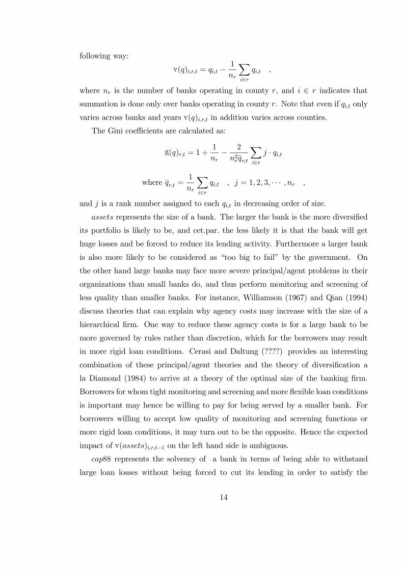
v(q)i,r,t = qi,t − 1

nr

Xi∈rqi,t ,

where nr is the number of banks operating in county r, and i ∈ r indicates thatsummation is done only over banks operating in county r. Note that even if qi,t only

varies across banks and years v(q)i,r,t in addition varies across counties.

The Gini coefficients are calculated as:

g(q)r,t = 1 +1

nr− 2

n2rqr,t

Xi∈rj · qi,t

where qr,t =1

nr

Xi∈rqi,t , j = 1, 2, 3, · · · , nr ,

and j is a rank number assigned to each qi,t in decreasing order of size.

assets represents the size of a bank. The larger the bank is the more diversified

its portfolio is likely to be, and cet.par. the less likely it is that the bank will get

huge losses and be forced to reduce its lending activity. Furthermore a larger bank

is also more likely to be considered as “too big to fail” by the government. On

the other hand large banks may face more severe principal/agent problems in their

organizations than small banks do, and thus perform monitoring and screening of

less quality than smaller banks. For instance, Williamson (1967) and Qian (1994)

discuss theories that can explain why agency costs may increase with the size of a

hierarchical firm. One way to reduce these agency costs is for a large bank to be

more governed by rules rather than discretion, which for the borrowers may result

in more rigid loan conditions. Cerasi and Daltung (????) provides an interesting

combination of these principal/agent theories and the theory of diversification a

la Diamond (1984) to arrive at a theory of the optimal size of the banking firm.

Borrowers for whom tight monitoring and screening andmore flexible loan conditions

is important may hence be willing to pay for being served by a smaller bank. For

borrowers willing to accept low quality of monitoring and screening functions or

more rigid loan conditions, it may turn out to be the opposite. Hence the expected

impact of v(assets)i,r,t−1 on the left hand side is ambiguous.

cap88 represents the solvency of a bank in terms of being able to withstand

large loan losses without being forced to cut its lending in order to satisfy the

14

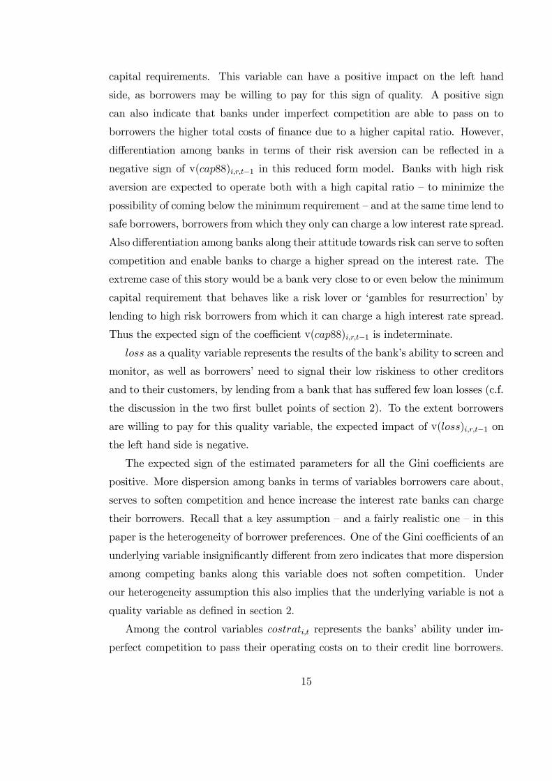
capital requirements. This variable can have a positive impact on the left hand

side, as borrowers may be willing to pay for this sign of quality. A positive sign

can also indicate that banks under imperfect competition are able to pass on to

borrowers the higher total costs of finance due to a higher capital ratio. However,

differentiation among banks in terms of their risk aversion can be reflected in a

negative sign of v(cap88)i,r,t−1 in this reduced form model. Banks with high risk

aversion are expected to operate both with a high capital ratio — to minimize the

possibility of coming below the minimum requirement — and at the same time lend to

safe borrowers, borrowers from which they only can charge a low interest rate spread.

Also differentiation among banks along their attitude towards risk can serve to soften

competition and enable banks to charge a higher spread on the interest rate. The

extreme case of this story would be a bank very close to or even below the minimum

capital requirement that behaves like a risk lover or ‘gambles for resurrection’ by

lending to high risk borrowers from which it can charge a high interest rate spread.

Thus the expected sign of the coefficient v(cap88)i,r,t−1 is indeterminate.

loss as a quality variable represents the results of the bank’s ability to screen and

monitor, as well as borrowers’ need to signal their low riskiness to other creditors

and to their customers, by lending from a bank that has suffered few loan losses (c.f.

the discussion in the two first bullet points of section 2). To the extent borrowers

are willing to pay for this quality variable, the expected impact of v(loss)i,r,t−1 on

the left hand side is negative.

The expected sign of the estimated parameters for all the Gini coefficients are

positive. More dispersion among banks in terms of variables borrowers care about,

serves to soften competition and hence increase the interest rate banks can charge

their borrowers. Recall that a key assumption — and a fairly realistic one — in this

paper is the heterogeneity of borrower preferences. One of the Gini coefficients of an

underlying variable insignificantly different from zero indicates that more dispersion

among competing banks along this variable does not soften competition. Under

our heterogeneity assumption this also implies that the underlying variable is not a

quality variable as defined in section 2.

Among the control variables costrati,t represents the banks’ ability under im-

perfect competition to pass their operating costs on to their credit line borrowers.

15

cl_lossrati,t represents the idiosyncratic part of the credit risk in the bank’s portfolio

of credit line loans. realratet, the real interest rate, represents the macroeconomic

part of the banks’ credit risk. This variable passes a Dickey-Fuller test and hence is

a stationoray macro variable. A higher real interest rate is associated with higher

credit risk due to an expected slowdown in the overall economic activity. Hence the

expected sign on the coefficient of this variable is positive.

The regional Herfindahl index herfinr,t controls for the competitive environ-

ment, as measured by market concentration, in which a bank operates. The more

concentrated the market is the higher is the value of the Herfindahl index. A more

concentrated market is usually considered a less competitive market, and banks

should be able to charge a higher interest rate. Hence the expected sign of this

variable should be positive. However, as problems of asymmetric information and

adverse selection are expected to be more severe in the market for lines of credit,

the ‘winner’s curse’ problem may be considerable in this market: The more banks

that operate in the market, and borrowers shop around, the more likely it is that

the lowest quality borrowers mistakenly are assumed to be good borrowers by some

banks. Broecker (1990) and Shaffer (1998) study the theory of winner’s curse in

banking. Moreover Shaffer (1998) also finds empirical support for the hypothesis

that banks operating in less concentrated markets have higher loan losses. The bank

competing most aggressively for borrowers in such a market by offering low interest

rates (the ‘winner’) will almost certainly capture a larger fraction of the low quality

borrowers. Banks being aware that the winner’s curse problem is more severe in a

less concentrated market will compete less aggressively. Thus, banks may charge

higher interest rates the less concentrated is the market, if the winner’s curse prob-

lem is large.1314 All in all the sign of herfinr,t can be both positive and negative, a

negative sign indicating the presence of a large winner’s curse problem in the market

for credit lines.13Bulow and Klemperer (1999) construct a theory model of auctions where fewer bidders actually

raises the price when bidders are asymmetric. This is exactly so because the winner’s curse effectis shown to dominate the traditional effect of less competition. In our setting this will correspondto fewer banks bidding for borrowers leading to lower interest rate.14Furthermore, to the extent the variables controlling for the riskiness of the banks’ loan portfolio

only do so incompletely, the effect on loan losses identified by Shaffer (1998) may show up as higherineterest rate margin in our model. This effect will also imply a positive sign on herfinr,t.

16

We use a lag of one year for all the quality variables. Borrowers have to base

their evaluation of the bank on the values published in the bank’s annual report and

financial statements for the last year. These are usually more comprehensive and

more scrupulously audited statements than the quarterly statements made during

the year.

4. Empirical results

The model in 3.2 is estimated using two-stage least square. Both costrati,t and

cl_lossrati,t are endogenous, they may be partially determined by the LHS variable

si,t. They are instrumented using their own one year lags, not aggregated backwards

and aggregated backwards respectively15. The correlation between ln costrati,t and

its lag is 0.91, and between ln cl_lossrati,t and its lag is 0.74.

We start by estimating the general model including all the RHS variables listed

in section 3.2, a model that satisfies certain misspecification tests regarding lack of

serial correlation in the residuals and functional form. The results are presented in

Table 4.1 column (a).

Model (a) passes the misspecification tests for functional form and for no pos-

itive serial correlation in the residuals. However inclusion of the size as a quality

variable does not pass a test of complying with economic theory as the coefficient

of ln g(assets)r,t−1 is negative and the coefficient of ln v(assets)i,r,t−1 is insignificant.

Hence we find no evidence of size as a quality variable.16 Thus we proceed by speci-

fying a model without size as quality variable, model (b). Model (b) also passes the

misspecification tests for functional form and for no positive serial correlation in the

residuals. Furthermore exclusion of the two insignificant variables ln realratet and

lnherfinr,t from model (b) is statistically valid and we get the parsimonious model

(c) which also passes the tests for functional form and for no positive serial correla-

tion in the residuals. Note that due to the log-linear specification all coefficients of

the model can be interpreted as elasticities.

The negative and significant coefficient of ln v(loss)i,r,t−1 and the positive and15Backward aggregation of a variable means that the bank structure of year t is forced upon the

variable in year t− 1.16The same qualitative results regarding size as quality variable apeared also when total loans,

number of employees or number of branches were used as measures of size.

17

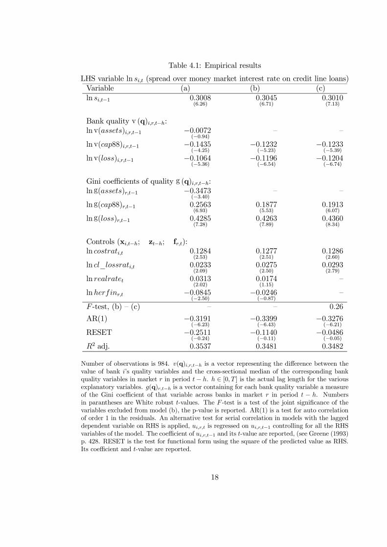
Table 4.1: Empirical results

LHS variable ln si,t (spread over money market interest rate on credit line loans)Variable (a) (b) (c)ln si,t−1 0.3008

(6.26)0.3045(6.71)

0.3010(7.13)

Bank quality v (q)i,r,t−h:ln v(assets)i,r,t−1 −0.0072

(−0.94)— —

ln v(cap88)i,r,t−1 −0.1435(−4.25)

−0.1232(−5.23)

−0.1233(−5.39)

ln v(loss)i,r,t−1 −0.1064(−5.36)

−0.1196(−6.54)

−0.1204(−6.74)

Gini coefficients of quality g (q)i,r,t−h:ln g(assets)r,t−1 −0.3473

(−3.40)— —

ln g(cap88)r,t−1 0.2563(6.93)

0.1877(5.53)

0.1913(6.07)

ln g(loss)r,t−1 0.4285(7.28)

0.4263(7.89)

0.4360(8.34)

Controls (xi,t−h; zt−h; fr,t):ln costrati,t 0.1284

(2.53)0.1277(2.51)

0.1286(2.60)

ln cl_lossrati,t 0.0233(2.09)

0.0275(2.50)

0.0293(2.79)

ln realratet 0.0313(2.02)

0.0174(1.15)

—

lnherfinr,t −0.0845(−2.50)

−0.0246(−0.87)

—

F -test, (b) — (c) — — 0.26

AR(1) −0.3191(−6.23)

−0.3399(−6.43)

−0.3276(−6.21)

RESET −0.2511(−0.24)

−0.1140(−0.11)

−0.0486(−0.05)

R2 adj. 0.3537 0.3481 0.3482

Number of observations is 984. v(q)i,r,t−h is a vector representing the difference between thevalue of bank i’s quality variables and the cross-sectional median of the corresponding bankquality variables in market r in period t− h. h ∈ [0, T ] is the actual lag length for the variousexplanatory variables. g(q)r,t−h is a vector containing for each bank quality variable a measureof the Gini coefficient of that variable across banks in market r in period t − h. Numbersin parantheses are White robust t-values. The F -test is a test of the joint significance of thevariables excluded from model (b), the p-value is reported. AR(1) is a test for auto correlationof order 1 in the residuals. An alternative test for serial correlation in models with the laggeddependent variable on RHS is applied, ui,r,t is regressed on ui,r,t−1 controlling for all the RHSvariables of the model. The coefficient of ui,r,t−1 and its t-value are reported, (see Greene (1993)p. 428. RESET is the test for functional form using the square of the predicted value as RHS.Its coefficient and t-value are reported.

18

significant coefficient of the corresponding ln g(loss)r,t−1 supports the hypothesis

that borrowers are willing to pay for the ability of a bank at avoiding losses (c.f.

the two first bullet points in section 2). In addition, when banks to a different

degree specialize in being low loss banks, they soften the competition by dividing

the market as borrowers have different needs for banks with low losses. A bank at

sample mean with an interest rate spread on its credit line loans of 4.85 pct. will be

‘punished’ by appro. 0.5 pct. points on its spread if its loss provisions relative to its

competitors double. This indicates that there may be a market discipline effect at

work not only in the money market, but also in the market for credit line loans, for

banks reporting higher loan loss provisions.

The negative sign for ln v(cap88)i,r,t−1 supports the claim that banks with high

risk aversion tend to both have high capital ratio and lend to safe borrowers imply-

ing a low interest rate spread. The positive and significant sign of the corresponding

Gini coefficient indicates that as banks differ in their capital ratio they soften com-

petition. This latter effect may be due both to capital ratio being a quality variable

along which banks can differentiate themselves, and to banks’ risk aversion being

a parameter along which they differentiate themselves provided more risk averse

banks have higher capital ratio. The negative sign of ln v(cap88)i,r,t−1 combined

with a positive sign for the Gini coefficient implies that we cannot rule out a high

capital ratio as a quality variable by itself that borrowers are willing to pay for.

However, if there is such an effect it is too weak not to be dominated by the high

bank risk aversion and high capital ratio effect.

Among the control variables note that the elasticity of the costrati,t is positive

and significant. Thus banks operating under imperfect competition in the market

for credit line loans are able to pass some of their operating costs over to these

borrowers. The estimated elasticity implies that a bank at sample mean with NOK

mill. 540 in operating costs and credit line loans of NOK mill. 2160 facing a ten pct.

increase n its operating costs would be able to pass appro. NOK mill. 1.3 of the cost

increase of NOK mill. 54 on to its credit line borrowers.

As the Herfindahl index does not get a significant coefficient we can neither give

support to the traditional view of more concentrated credit markets leading to higher

interest rates nor to the theories of winner’s curse.

19

All in all our empirical results give support to the hypothesis that there are

certain characteristics of banks that borrowers evaluate and hence are willing to pay

for. If banks differentiate themselves along these characteristics, banks are able to

soften competition and make borrowers pay them a higher interest rate.

5. Concluding remarks

In this paper we have studied strategies pursued by banks in order to differentiate

their services from those of their rivals. In that way the level of competition in

the industry can be reduced. More specifically we have analyzed whether the bank

size, a bank’s ability at avoiding losses, or its capital ratio can be used as strategic

variables to make banks different and increase the interest rates banks can charge

their borrowers in equilibrium. Using a panel of data covering Norwegian banks

between 1993 and 1998 we found empirical support for the ability at avoiding losses

measured by the ratio of loss provisions as such a variable. In fact borrowers in

the market for credit line loans may discipline banks into avoiding losses. We also

found evidence that banks pass on parts of increases in their operating costs to

credit line borrowers. However, we did not find any strong evidence for the use of

high capital ratio as a strategic variable that borrowers are willing to pay for. This

implies that strategic competition does not lead banks to hold more capital than

their cost minimizing level. This level is normally below the socially optimal level

due to explicit and implicit deposit insurance. Only the more risk averse among

banks would hold capital well in excess of their cost minimizing level. Thus, our

paper gives support to the rationale for imposing capital requirements on all banks.

20

References

Berger, A. N., and G. F. Udell (1995): “Relationship lending and lines of credit insmall firm finance,” Journal of Business, 68, 351—381.

Boot, A. W. (2000): “Relationship banking: What do we know?,” Journal of Fi-nancial Intermediation, 9, 7—25.

Broecker, T. (1990): “Credit-worthiness tests and interbank competition,” Econo-metrica, 58, 429—452.

Bulow, J., and P. Klemperer (1999): “Prices and winner’s curse,” Working paper,http://www.nuff.ox.ac.uk/users/klemperer/papers.html.

Cantillo, M., and J. Wright (2000): “How Do Firms Choose Their Lenders? AnEmpirical Investigation,” The Review of Financial Studies, 13, 155—189.

Cerasi, V., and S. Daltung (????): “The optimal size of a bank: costs and benefitsof diversification,” Discussion paper 231, LSE, Financial Markets Group.

(1994): “The optimal size of a bank: costs and benefits of diversification,”FMG discussion paper, London School of Economics.

Chemmanur, T. J., and P. Fulghieri (1994): “Reputation, renegotiation and thechoice between bank loans and publicly traded debt,” Review of Financial Studies,7, 475—506.

Degryse, H., and P. van Cayseele (2000): “Relationship lending within a bank basedsystem: evidence from European small business data,” Journal of Financial In-termedioation, 9, 90—109.

Diamond, D. (1984): “Financial Intermediation and Delegated Monitoring,” Reviewof Economic Studies, 51, 393—414.

Greene, W. H. (1993): Econometric Analysis. Macmillan, New York.

James, C. (1987): “Some evidence on the uniqueness of bank loans,” Journal ofFinancial Economics, 19, 217—235.

Kim, M., D. Kliger, and B. Vale (1999): “Estimating switching costs and oligopolisticbehavior,” Arbeidsnotat 1999/4, Norges Bank, Oslo.

Mester, L. J. (1992): “Traditional and nontraditional banking: An information-theoretic approach,” Journal of Banking and Finance, 16, 545—566.

21

Ongena, S., and D. C. Smith (1998): “Quality and duration of banking relation-ships,” in Global Cash Management in Europe, ed. by D. Birks. MacMillan Press,London.

Peek, J., and E. S. Rosengren (1997): “The international transmission of financialshocks: the case of Japan,” American Economic Review, 87, 495—505.

Qian, Y. (1994): “Incentives and loss of control in an optimal hierarchy,” Review ofEconomic Studies, 61, 527—544.

Shaffer, S. (1998): “The winner’s curse in banking,” Journal of Financial Interme-diation, 7, 359—392.

Sharpe, S. A. (1990): “Asymmetric information, bank lending, and implicit con-tracts: A stylized model of customer relationships,” Journal of Finance, 45, 1069—1087.

Slovin, M. B., M. E. Sushka, and J. A. Polonchek (1993): “The Value of bankdurability: Borrowers as Bank Stakeholders.,” Journal of Finance, 48, 247—266.

Williamson, O. (1967): “Hierarchial control and optimal firm size,” Journal of Po-litical Economy, 75, 123—138.

22