END-TO-END CONGESTION DETECTION ANDAVOIDANCE IN WIDE AREA NETWORKSbyLawrence Sivert BrakmoCopyright c Lawrence Sivert Brakmo 1996A Dissertation Submitted to the Faculty of theDEPARTMENT OF COMPUTER SCIENCEIn Partial Ful�llment of the RequirementsFor the Degree ofDOCTOR OF PHILOSOPHYIn the Graduate CollegeTHE UNIVERSITY OF ARIZONA1 9 9 6

END-TO-END CONGESTION DETECTION ANDAVOIDANCE IN WIDE AREA NETWORKSLawrence Sivert Brakmo, Ph.D.The University of Arizona, 1996Director: Larry L. PetersonAs human dependence on wide area networks like the Internet increases, so doescontention for the network's resources. This contention has noticeably a�ected theperformance of these networks, reducing their usability. This dissertation addressesthis problem in two ways.First, it describes TCP Vegas, a new implementation of TCP that is distin-guished from current TCP implementations by containing a new congestion detec-tion and avoidance mechanism. This mechanism was designed to work in currentlyavailable wide area networks and achieves between 37% and 71% better throughputon the Internet, with one-�fth to one-half the losses, as compared to the currentimplementation of TCP.Second, it describes x-Sim, a network simulator based on the x-kernel, that isable to simulate the topologies and tra�c patterns of large scale networks. Theusefulness of the simulator to analyze and debug network components is illustratedthroughout this dissertation.

3STATEMENT BY AUTHORThis dissertation has been submitted in partial ful�llment of the requirements foran advanced degree at The University of Arizona and is deposited in the UniversityLibrary to be made available to borrowers under rules of the Library.Brief quotations from this dissertation are allowable without special permission,provided that accurate acknowledgment of the source is made. Requests for permis-sion for extended quotation from or reproduction of this manuscript in whole or inpart may be granted by the copyright holder.SIGNED:

4ACKNOWLEDGMENTSI would like to express my gratitude to my advisor, Larry Peterson. He has beenthe ideal advisor, one whose experience and knowledge provided me with the haventhat allowed me the freedom to explore my own ideas. I have been very fortunateto have both his guidance and friendship during this journey.I am also grateful to the other members of my committee, Pete Downey andJohn Hartman, for their comments and suggestions on my work. I am thankful toUdi Manber for our many enjoyable discussions. I would like to thank the minormembers of my committee, Ted Laetsch, and specially William Velez, who has beena great counselor and friend for many years.I also want to thank everyone in the Computer Science department at Arizonafor making my stay here so pleasurable. Special thanks to Cara Wallace, MargaretNewman, Wendy Swartz, John Cropper, Cli� Hathaway and John Luiten.Finally, I would like to thank my fellow graduate students, Vince Freeh, DavidMosberger, Peter Drushel, Mark Abbot, David Lowenthal, Nina Bhatti, and MuditaJain for their friendship.This work was supported by the National Science Fundation under Grant IRI-9015407 and by ARPA under Contract DABT63-91-C-0030.

5DEDICATIONTo my parents, for always supporting my quest for knowledge, even when thejourney strayed from the direct path. For raising me in an environment that en-couraged the pursuit of knowledge. For always giving of themselves. And mostimportantly, for teaching me the meaning of love, caring, and sel essness throughtheir example.

6TABLE OF CONTENTSLIST OF FIGURES : : : : : : : : : : : : : : : : : : : : : : : : : : : : : : : : 9ABSTRACT : : : : : : : : : : : : : : : : : : : : : : : : : : : : : : : : : : : : 11CHAPTER 1: Introduction : : : : : : : : : : : : : : : : : : : : : : : : : : : : 121.1 Computer Networks : : : : : : : : : : : : : : : : : : : : : : : : : : : : 121.2 Congestion : : : : : : : : : : : : : : : : : : : : : : : : : : : : : : : : : 151.3 Protocols : : : : : : : : : : : : : : : : : : : : : : : : : : : : : : : : : 171.4 Dissertation Outline : : : : : : : : : : : : : : : : : : : : : : : : : : : 18CHAPTER 2: Simulator and Visualization Tools : : : : : : : : : : : : : : : : 202.1 The x-Kernel : : : : : : : : : : : : : : : : : : : : : : : : : : : : : : : 202.1.1 Protocol Objects : : : : : : : : : : : : : : : : : : : : : : : : 222.1.2 Session Objects : : : : : : : : : : : : : : : : : : : : : : : : : 232.1.3 Message Objects : : : : : : : : : : : : : : : : : : : : : : : : : 242.1.4 Support Routines : : : : : : : : : : : : : : : : : : : : : : : : 242.1.5 x-Kernel Modi�cations to Support the Simulator : : : : : : : 252.2 Simulator : : : : : : : : : : : : : : : : : : : : : : : : : : : : : : : : : 272.2.1 Links : : : : : : : : : : : : : : : : : : : : : : : : : : : : : : : 292.2.2 Nodes : : : : : : : : : : : : : : : : : : : : : : : : : : : : : : 302.2.3 Load : : : : : : : : : : : : : : : : : : : : : : : : : : : : : : : 312.2.4 Related Work : : : : : : : : : : : : : : : : : : : : : : : : : : 322.3 Visualization Tools : : : : : : : : : : : : : : : : : : : : : : : : : : : : 342.3.1 Coarse Grained Tools : : : : : : : : : : : : : : : : : : : : : : 342.3.2 Fine Grained Tools : : : : : : : : : : : : : : : : : : : : : : : 37

7CHAPTER 3: Transmission Control Protocol : : : : : : : : : : : : : : : : : : 403.1 Background : : : : : : : : : : : : : : : : : : : : : : : : : : : : : : : : 413.2 Reliability : : : : : : : : : : : : : : : : : : : : : : : : : : : : : : : : : 433.3 Flow Control : : : : : : : : : : : : : : : : : : : : : : : : : : : : : : : 443.4 Congestion Control : : : : : : : : : : : : : : : : : : : : : : : : : : : : 473.4.1 Jacobson's Original Proposal : : : : : : : : : : : : : : : : : : 473.4.2 Fast Retransmit and Fast Recovery Mechanisms : : : : : : : 513.5 General Graph Description : : : : : : : : : : : : : : : : : : : : : : : : 553.6 Detailed Graph Description : : : : : : : : : : : : : : : : : : : : : : : 58CHAPTER 4: New Approach to Congestion Detection and Avoidance : : : : 614.1 Analysis of TCP's Congestion Control Mechanism : : : : : : : : : : : 614.2 Previous Congestion Avoidance Mechanisms : : : : : : : : : : : : : : 634.3 Congestion Avoidance in Vegas : : : : : : : : : : : : : : : : : : : : : 654.4 Congestion Avoidance During Slow-Start : : : : : : : : : : : : : : : : 724.5 Other Mechanisms in TCP Vegas : : : : : : : : : : : : : : : : : : : : 75CHAPTER 5: Experimental Results : : : : : : : : : : : : : : : : : : : : : : : 795.1 Internet Results : : : : : : : : : : : : : : : : : : : : : : : : : : : : : : 795.2 Simulation Results : : : : : : : : : : : : : : : : : : : : : : : : : : : : 825.2.1 One-on-One Experiments : : : : : : : : : : : : : : : : : : : : 825.2.2 Background Tra�c : : : : : : : : : : : : : : : : : : : : : : : 845.2.3 Other Experiments : : : : : : : : : : : : : : : : : : : : : : : 855.3 Other Evaluation Criteria : : : : : : : : : : : : : : : : : : : : : : : : 865.3.1 Fairness : : : : : : : : : : : : : : : : : : : : : : : : : : : : : 865.3.2 Stability : : : : : : : : : : : : : : : : : : : : : : : : : : : : : 875.3.3 Delay : : : : : : : : : : : : : : : : : : : : : : : : : : : : : : : 895.4 Discussion : : : : : : : : : : : : : : : : : : : : : : : : : : : : : : : : : 895.4.1 BSD Variations : : : : : : : : : : : : : : : : : : : : : : : : : 895.4.2 Alternative Approaches : : : : : : : : : : : : : : : : : : : : : 905.4.3 Independent Validation : : : : : : : : : : : : : : : : : : : : : 91

8CHAPTER 6: Experiences with x-Sim : : : : : : : : : : : : : : : : : : : : : : 926.1 Analysis of BSD4.4-Lite TCP : : : : : : : : : : : : : : : : : : : : : : 926.1.1 Network Con�guration : : : : : : : : : : : : : : : : : : : : : 936.1.2 Error in Header Prediction Code : : : : : : : : : : : : : : : : 956.1.3 Suboptimal Retransmit Timeout Estimates : : : : : : : : : : 986.1.4 Options and ACKing Frequency : : : : : : : : : : : : : : : : 1036.1.5 Linear Increase of the Congestion Window and ACKing Fre-quency : : : : : : : : : : : : : : : : : : : : : : : : : : : : : : 1056.1.6 Handling Big ACKs : : : : : : : : : : : : : : : : : : : : : : : 1076.1.7 Final Details : : : : : : : : : : : : : : : : : : : : : : : : : : : 1086.1.8 Comparing the Di�erent Versions of TCP Lite : : : : : : : : 1086.2 Guidelines for Network Simulation : : : : : : : : : : : : : : : : : : : 1106.2.1 Sensitivity to Network Parameters : : : : : : : : : : : : : : : 1116.2.2 Analyzing Results : : : : : : : : : : : : : : : : : : : : : : : : 1126.2.3 Realistic Tra�c Sources : : : : : : : : : : : : : : : : : : : : : 1156.2.4 Insider Knowledge : : : : : : : : : : : : : : : : : : : : : : : : 1186.2.5 Byte versus Time Transfers : : : : : : : : : : : : : : : : : : : 1206.2.6 Unwanted Synchronicity : : : : : : : : : : : : : : : : : : : : 121CHAPTER 7: Conclusion : : : : : : : : : : : : : : : : : : : : : : : : : : : : : 1247.1 Summary : : : : : : : : : : : : : : : : : : : : : : : : : : : : : : : : : 1247.2 Contributions and Limitations : : : : : : : : : : : : : : : : : : : : : : 1267.3 Future Directions : : : : : : : : : : : : : : : : : : : : : : : : : : : : : 127REFERENCES : : : : : : : : : : : : : : : : : : : : : : : : : : : : : : : : : : : 129

9LIST OF FIGURES1.1 Switch network. : : : : : : : : : : : : : : : : : : : : : : : : : : : : : : 131.2 Interconnection of networks. : : : : : : : : : : : : : : : : : : : : : : : 141.3 Small congested network. : : : : : : : : : : : : : : : : : : : : : : : : : 152.1 Example x-Kernel con�guration. : : : : : : : : : : : : : : : : : : : : : 222.2 Time di�erence between current time and time of next event. : : : : : 262.3 Example network and corresponding protocol graph. : : : : : : : : : 282.4 Database output comparing TCP implementations. : : : : : : : : : : 352.5 Database output comparing TCP implementations. : : : : : : : : : : 362.6 Database output comparing TCP implementations. : : : : : : : : : : 372.7 Graph showing router's queue size. : : : : : : : : : : : : : : : : : : : 382.8 Graph showing router's average output bandwidth for a speci�ed link. 383.1 Block Protocols maintain block boundaries. : : : : : : : : : : : : : : 403.2 Stream Protocols do not maintain block boundaries. : : : : : : : : : : 413.3 Window ow control. : : : : : : : : : : : : : : : : : : : : : : : : : : : 453.4 Window ow control. : : : : : : : : : : : : : : : : : : : : : : : : : : : 463.5 Timeline of Slow-start. : : : : : : : : : : : : : : : : : : : : : : : : : : 483.6 Packets spaced by slow link. : : : : : : : : : : : : : : : : : : : : : : : 493.7 Slow-start: Congestion window size versus time. : : : : : : : : : : : : 503.8 TCP trace: Congestion window size versus time. : : : : : : : : : : : : 513.9 Example time-line of Fast Retransmit mechanism. : : : : : : : : : : : 523.10 Behavior of TCP without Fast Retransmit. : : : : : : : : : : : : : : : 523.11 Network con�guration for simulations. : : : : : : : : : : : : : : : : : 533.12 Behavior of TCP with Fast Retransmit. : : : : : : : : : : : : : : : : : 543.13 Behavior of TCP with Fast Retransmit and Fast Recovery. : : : : : : 553.14 Common elements in TCP trace graphs. : : : : : : : : : : : : : : : : 56

103.15 TCP windows graph. : : : : : : : : : : : : : : : : : : : : : : : : : : : 574.1 TCP Reno with no other tra�c (throughput: 123 KB/s) : : : : : : : 624.2 Network con�guration for simulations. : : : : : : : : : : : : : : : : : 634.3 TCP Vegas with no other tra�c (throughput: 169 KB/s). : : : : : : 674.4 Congestion detection and avoidance in Vegas. : : : : : : : : : : : : : 694.5 TCP Vegas with tcplib-generated background tra�c. : : : : : : : : : 704.6 TCP Reno with tcplib-generated background tra�c. : : : : : : : : : : 714.7 TCP Vegas on the left, experimental on the right. : : : : : : : : : : : 744.8 Example of retransmit mechanism. : : : : : : : : : : : : : : : : : : : 765.1 Network con�guration for simulations. : : : : : : : : : : : : : : : : : 815.2 Complex simulation network. : : : : : : : : : : : : : : : : : : : : : : 886.1 Network con�guration for simulations. : : : : : : : : : : : : : : : : : 936.2 TCP Lite with No Other Tra�c (Throughput: 70 KB/s). : : : : : : : 946.3 TCP Reno with No Other Tra�c (Throughput: 123 KB/s). : : : : : 956.4 TCP Lite.1 with No Other Tra�c (Throughput: 99 KB/s). : : : : : : 976.5 RTT and RTO examples. : : : : : : : : : : : : : : : : : : : : : : : : : 1016.6 TCP Lite.3 with No Other Tra�c (Throughput: 117 KB/s). : : : : : 1046.7 Simple Simulation Network. : : : : : : : : : : : : : : : : : : : : : : : 1106.8 Complex Simulation Network. : : : : : : : : : : : : : : : : : : : : : : 1116.9 Graph of queue size showing information lost due to averaging. : : : : 1136.10 Graph of queue size at bottleneck including min-max bars. : : : : : : 1146.11 Queue behavior during four large TCP transfers. : : : : : : : : : : : : 1156.12 Queue behavior during two large TCP transfers and tcplib tra�c. : : 1166.13 Throughput vs. Send Bu�er Size. : : : : : : : : : : : : : : : : : : : : 1186.14 Throughput vs. Send Bu�er Size. : : : : : : : : : : : : : : : : : : : : 1196.15 Graphs showing arti�cial periodic e�ects in simulation. : : : : : : : : 123

11ABSTRACTAs human dependence on wide area networks like the Internet increases, so doescontention for the network's resources. This contention has noticeably a�ected theperformance of these networks, reducing their usability. This dissertation addressesthis problem in two ways.First, it describes TCP Vegas, a new implementation of TCP that is distin-guished from current TCP implementations by containing a new congestion detec-tion and avoidance mechanism. This mechanism was designed to work in currentlyavailable wide area networks and achieves between 37% and 71% better throughputon the Internet, with one-�fth to one-half the losses, as compared to the currentimplementation of TCP.Second, it describes x-Sim, a network simulator based on the x-kernel, that isable to simulate the topologies and tra�c patterns of large scale networks. Theusefulness of the simulator to analyze and debug network components is illustratedthroughout this dissertation.

12CHAPTER 1IntroductionOur society's dependence on computer networks and computer communicationhas been increasing during the last two decades, a trend that is likely to continue inthe foreseeable future. The importance of computer networks in our daily life canbe attested by the exponential growth of the Internet, a global computer networkconsisting of thousands of connected heterogeneous networks. When traced back toits origins, the number of hosts connected to the Internet has been doubling in sizeevery year since 1981.This growth has been fueled by applications that have enabled new levels of com-munication and information sharing between people in di�erent cities or countries.Graphical World WideWeb (WWW) browsers, like Mosaic and Netscape, have beenresponsible for most of the Internet's growth in the last two years by simplifying thechore of making information publicly available and easy to �nd on the Internet.A downside to this growth has been an increase in contention for Internet re-sources. This contention has noticeably a�ected the performance of distributedapplications like Mosaic, at the same time that our dependence on such applicationsis increasing. This dissertation addresses this problem in two ways. First, it pro-poses a new technique to manage this contention, and second, it describes a set oftools to analyze the performance and behavior of such mechanisms.1.1 Computer NetworksComputer communication is made possible by the connectivity provided by com-puter networks [24]. At the lowest level, computers are directly connected with eachother through a physical medium, such as a cable. We call such a physical mediuma link, and refer to the computers it connects as nodes, to underscore the fact that

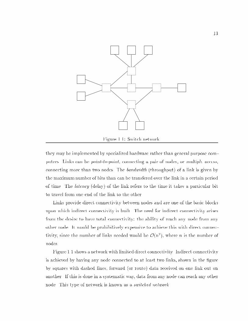
13Figure 1.1: Switch network.they may be implemented by specialized hardware rather than general purpose com-puters. Links can be point-to-point, connecting a pair of nodes, or multiple access,connecting more than two nodes. The bandwidth (throughput) of a link is given bythe maximumnumber of bits than can be transfered over the link in a certain periodof time. The latency (delay) of the link refers to the time it takes a particular bitto travel from one end of the link to the other.Links provide direct connectivity between nodes and are one of the basic blocksupon which indirect connectivity is built. The need for indirect connectivity arisesfrom the desire to have total connectivity: the ability of reach any node from anyother node. It would be prohibitively expensive to achieve this with direct connec-tivity, since the number of links needed would be O(n2), where n is the number ofnodes.Figure 1.1 shows a network with limited direct connectivity. Indirect connectivityis achieved by having any node connected to at least two links, shown in the �gureby squares with dashed lines, forward (or route) data received on one link out onanother. If this is done in a systematic way, data from any node can reach any othernode. This type of network is known as a switched network.

14

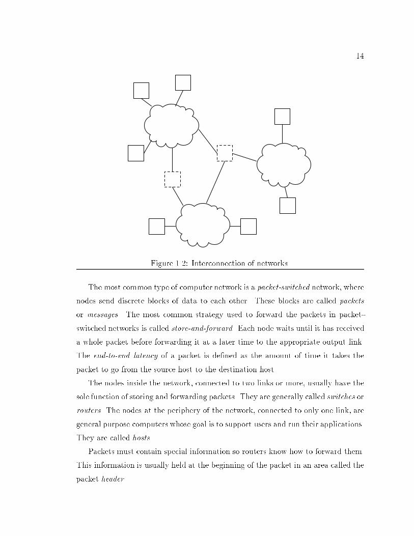
Figure 1.2: Interconnection of networks.The most common type of computer network is a packet-switched network, wherenodes send discrete blocks of data to each other. These blocks are called packetsor messages. The most common strategy used to forward the packets in packet-switched networks is called store-and-forward. Each node waits until it has receiveda whole packet before forwarding it at a later time to the appropriate output link.The end-to-end latency of a packet is de�ned as the amount of time it takes thepacket to go from the source host to the destination host.The nodes inside the network, connected to two links or more, usually have thesole function of storing and forwarding packets. They are generally called switches orrouters. The nodes at the periphery of the network, connected to only one link, aregeneral purpose computers whose goal is to support users and run their applications.They are called hosts.Packets must contain special information so routers know how to forward them.This information is usually held at the beginning of the packet in an area called thepacket header.

15Router

Source 1

Source 2

Dest

10 Mbps

15 Mbps

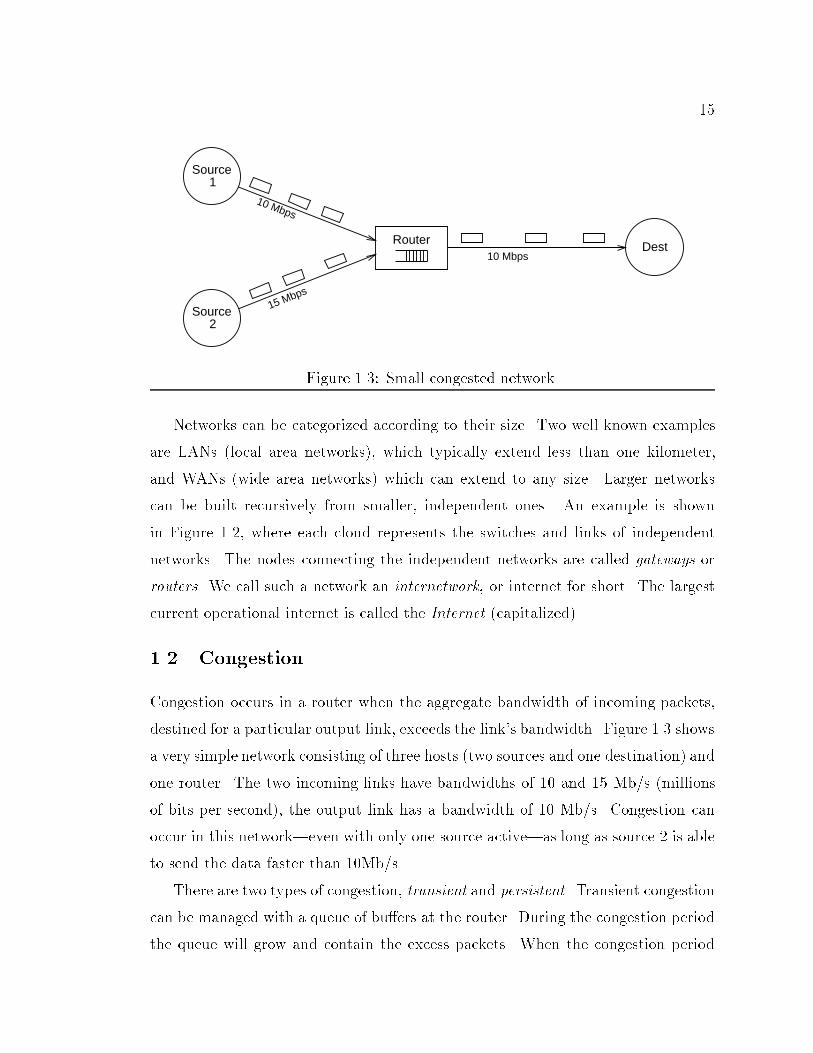
10 MbpsFigure 1.3: Small congested network.Networks can be categorized according to their size. Two well known examplesare LANs (local area networks), which typically extend less than one kilometer,and WANs (wide area networks) which can extend to any size. Larger networkscan be built recursively from smaller, independent ones. An example is shownin Figure 1.2, where each cloud represents the switches and links of independentnetworks. The nodes connecting the independent networks are called gateways orrouters. We call such a network an internetwork, or internet for short. The largestcurrent operational internet is called the Internet (capitalized).1.2 CongestionCongestion occurs in a router when the aggregate bandwidth of incoming packets,destined for a particular output link, exceeds the link's bandwidth. Figure 1.3 showsa very simple network consisting of three hosts (two sources and one destination) andone router. The two incoming links have bandwidths of 10 and 15 Mb/s (millionsof bits per second), the output link has a bandwidth of 10 Mb/s. Congestion canoccur in this network|even with only one source active|as long as source 2 is ableto send the data faster than 10Mb/s.There are two types of congestion, transient and persistent. Transient congestioncan be managed with a queue of bu�ers at the router. During the congestion periodthe queue will grow and contain the excess packets. When the congestion period

16ends, the packets in the queue are sent through the output link and the queueshrinks. All current routers contain some bu�er space to handle transient congestion.It is worthwhile to note that a non-empty queue increases packet latency.Persistent congestion occurs when the congestion period is long enough thatthe queue over ows (packets are removed from the network by the router). In thisdissertation we interpret the term congestion, when used by itself, to mean persistentcongestion.Strategies to handle congestion can be divided into two categories. Insider strate-gies are those in which the routers are actively involved. For example, the routerscan detect when their queues become non-empty and send a special message to thesources asking them to slow their sending rate. Such a strategy, whose goal is toprevent queue over ow, is called congestion avoidance.End-to-end strategies are those in which the routers are not actively involved,and the hosts must use indirect methods to detect the congestion. For example, thedestination can inform the source when a packet has been lost, at which time thesource can slow its sending rate, under the assumption that all losses are caused bycongestion. This type of strategy, whose goal is to control congestion once it occurs,is called congestion control.Insider strategies have the advantage of being able to detect congestion in itsearliest stages. Their main disadvantage is that they require a certain amount ofprocessing be done at the routers, increasing their cost and complexity.In principle, routers can use the Internet Control Message Protocol (ICMP) toinform sources that they should decrease their sending rate (source quench request).This is not done for two reasons. First, there is no accepted mechanism for decidinghow to pick which sources should be informed and when they should be informed.Second, there is no accepted general mechanism for decreasing the sending rate ofthe sources when the source quench requests are received.End-to-end strategies have the advantage of being implemented in general pur-pose computers, so they are easier to implement and modify. Routers, on the otherhand, are sometimes implemented with specialized hardware, so modifying their

17programming is much harder. Another advantage of end-to-end strategies is thatthey make few (or no) assumptions about the routers in the network, so they canwork in any network. Their disadvantage, as mentioned earlier, is that they mustdepend in less accurate indirect methods to detect congestion.Routers have historically been designed to be as simple as possible. As a result,there is no widespread insider congestion strategy in use at this time on the Internet.The only congestion control mechanisms in use today are end-to-end.As a �nal comment, when developing a new congestion strategy, an end-to-endstrategy has the added advantage of being easily tested in real networks. All thatis required is the right software at a few of the hosts. On the other hand, testing aninsider strategy on a real network requires changes to the routers in the network.This implies that it would be nearly impossible to test an insider mechanism onlarge networks like the Internet.1.3 ProtocolsA protocol is a communication standard. It describes a set of rules that allowdi�erent machines to communicatewith each other without ambiguity. In particular,it speci�es how to pass messages, details the message format, and describes how tohandle error conditions.The task of writing protocols is simpli�ed by following a layered approach, wherelower level protocols provide some of the functionality upon which higher level pro-tocols are successively build. For example, the lowest layer may provide host-to-hostconnectivity, the next highest layer may provide reliability, and so on.Two of the most important protocols are the Internet Protocol (IP) and theTransmission Control Protocol (TCP). The main goal of IP is the delivery of pack-ets in heterogeneous connected networks. It forms the infrastructure that allows the\seamless" integration of heterogeneous networks. IP follows a best e�ort approachto the delivery of packets; there are no guarantees that the packets will be success-fully delivered to their �nal destination. IP is a connection-less protocol, meaningthat it maintains no state information about successive packets. Each packet is

18handled independently from all other packets.TCP is layered on top of IP and provides such services as reliability and end-to-end congestion control. It is responsible for most of the Internet's tra�c. Inparticular, tra�c traces collected at one of the main Internet access points (FIX-West) show that TCP is responsible for more than 80% of the bytes and 70% of thepackets seen in the traces. The most widely used implementations of TCP|Tahoeand Reno|are named after the Berkeley Software Distributions (BSD) of Unix theywere a part of.1.4 Dissertation OutlineThe goal of this dissertation is to addresses the problem of increased contentionfor the resources on the Internet. It does so in two ways. First, it proposes a newend-to-end congestion avoidance strategy. Second, it presents a new architecture fornetwork simulation, together with a set of analysis tools.The rest of this dissertation is organized as follows. Chapter 2 presents anddescribes the architecture of x-Sim, a realistic network simulator that is able tosimulate the topologies and tra�c patterns of large scale networks. This chapteralso describes a set of tools whose purpose is to aid in the analysis of networkbehavior and performance.The simulator and its tools are then used to do a detailed analysis of TCP inChapter 3. This analysis shows the weaknesses in TCP's congestion control mech-anism and provides the insight needed for developing a new congestion avoidancemechanism. This new mechanism is implemented in TCP by modifying TCP's ex-isting congestion control mechanism. This new congestion avoidance mechanism isdescribed in detail in Chapter 4 in the context of its TCP implementation.Chapter 5 examines the performance of both the existing and new implemen-tations of TCP through experiments, in both real and simulated networks. Theperformance of the new congestion avoidance mechanism is gauged by comparing itto the performance of the current TCP implementation.Chapter 6 presents some of our experiences with x-Sim, including a study of

19a new implementation of TCP. This study uncovers a series of problems with thisimplementation, proposes solutions to these problems, implements the changes, andmeasures the performance of the �xed implementation. It also gives a set of guide-lines for network simulation.Finally, Chapter 7 summarizes the major contributions of this dissertation anddiscusses possible future directions.

20CHAPTER 2Simulator and Visualization ToolsSimulation is a critical tool for the development, analysis, testing and evaluationof network components. This is specially true in the case of wide area networks(WANs) where we are unlikely to have access to more than a few of the system'scomponents. Access to the other components of a WAN is particularly importantwhen comparing congestion detection, control and recovery mechanisms. It is notsu�cient to show that one particular connection with the new mechanism performsbetter than one with the old mechanism; it is important to measure the e�ectsthat the new mechanism has on the other tra�c in the network. For example,it is inadvisable to employ a mechanism that results in unfair sharing of networkresources, or in low utilization of these resources.This chapter describes x-Sim, a new network simulator we have implementedto aid with network research, as well as a set of tools developed to aid in theanalysis of the simulations. It starts with a discussion of the x-kernel|a protocolimplementation environment [11]|which is the framework on which the simulator isbuilt. It also describes the minor modi�cations to the x-kernel that were necessaryto support the simulator. Next, there is a description of the simulator itself, startingwith the overall design and ending with the major individual components. This isfollowed by a comparison of x-Sim with existing network simulators, as well as withother alternative approaches such as network emulation. The chapter concludeswith a description of the analysis tools.2.1 The x-KernelThe x-kernel speci�es an architecture and provides mechanisms for the e�cientimplementation of network protocols. It is an object-oriented architecture whose

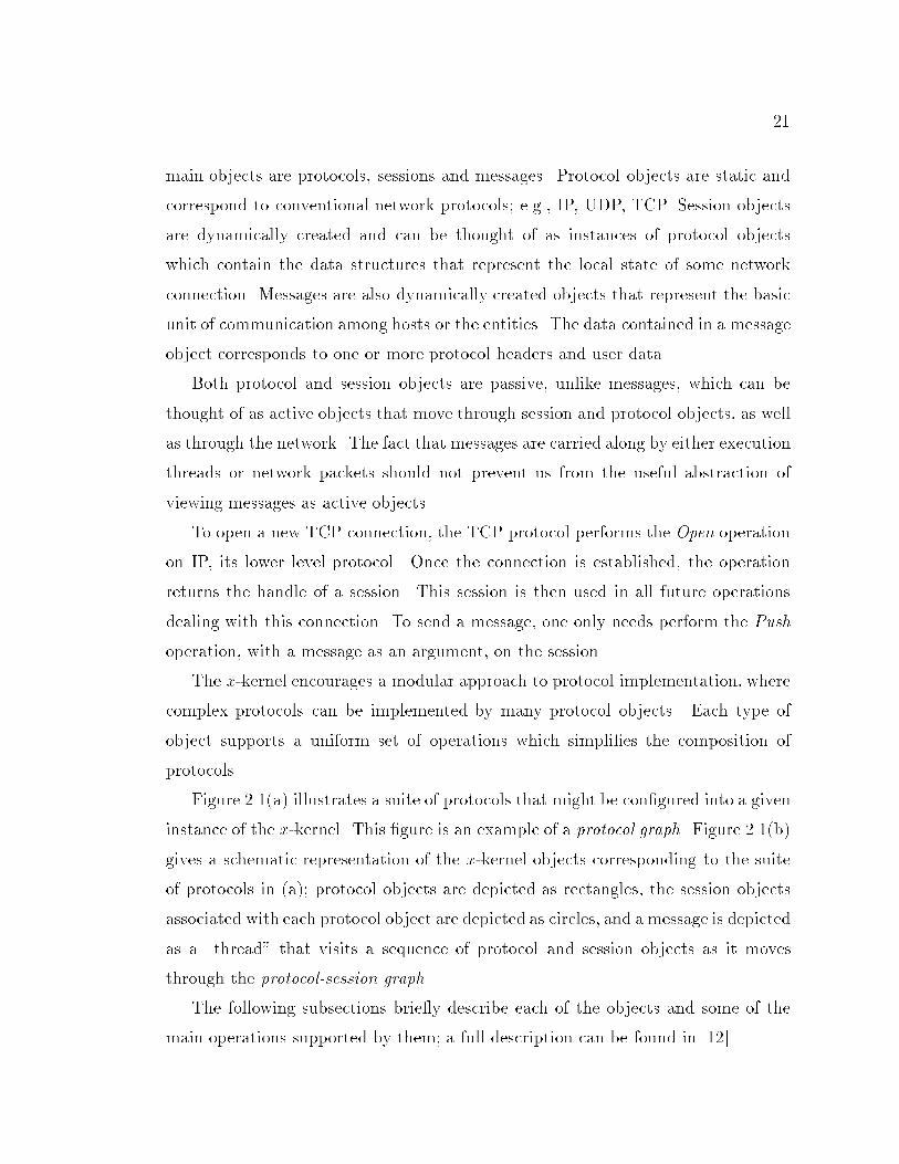
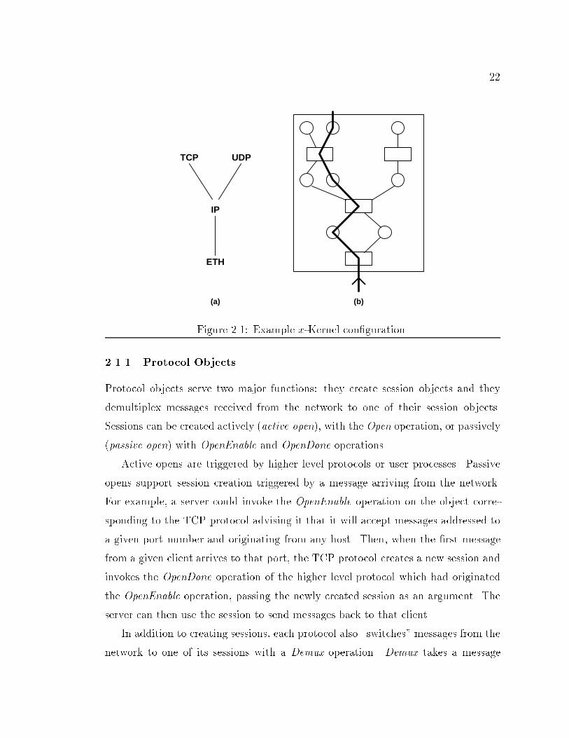
21main objects are protocols, sessions and messages. Protocol objects are static andcorrespond to conventional network protocols; e.g., IP, UDP, TCP. Session objectsare dynamically created and can be thought of as instances of protocol objectswhich contain the data structures that represent the local state of some networkconnection. Messages are also dynamically created objects that represent the basicunit of communication among hosts or the entities. The data contained in a messageobject corresponds to one or more protocol headers and user data.Both protocol and session objects are passive, unlike messages, which can bethought of as active objects that move through session and protocol objects, as wellas through the network. The fact that messages are carried along by either executionthreads or network packets should not prevent us from the useful abstraction ofviewing messages as active objects.To open a new TCP connection, the TCP protocol performs the Open operationon IP, its lower level protocol. Once the connection is established, the operationreturns the handle of a session. This session is then used in all future operationsdealing with this connection. To send a message, one only needs perform the Pushoperation, with a message as an argument, on the session.The x-kernel encourages a modular approach to protocol implementation, wherecomplex protocols can be implemented by many protocol objects. Each type ofobject supports a uniform set of operations which simpli�es the composition ofprotocols.Figure 2.1(a) illustrates a suite of protocols that might be con�gured into a giveninstance of the x-kernel. This �gure is an example of a protocol graph. Figure 2.1(b)gives a schematic representation of the x-kernel objects corresponding to the suiteof protocols in (a); protocol objects are depicted as rectangles, the session objectsassociated with each protocol object are depicted as circles, and a message is depictedas a \thread" that visits a sequence of protocol and session objects as it movesthrough the protocol-session graph.The following subsections brie y describe each of the objects and some of themain operations supported by them; a full description can be found in [12].

22TCP

IP

ETH

UDP

(a) (b)Figure 2.1: Example x-Kernel con�guration.2.1.1 Protocol ObjectsProtocol objects serve two major functions: they create session objects and theydemultiplex messages received from the network to one of their session objects.Sessions can be created actively (active open), with the Open operation, or passively(passive open) with OpenEnable and OpenDone operations.Active opens are triggered by higher level protocols or user processes. Passiveopens support session creation triggered by a message arriving from the network.For example, a server could invoke the OpenEnable operation on the object corre-sponding to the TCP protocol advising it that it will accept messages addressed toa given port number and originating from any host. Then, when the �rst messagefrom a given client arrives to that port, the TCP protocol creates a new session andinvokes the OpenDone operation of the higher level protocol which had originatedthe OpenEnable operation, passing the newly created session as an argument. Theserver can then use the session to send messages back to that client.In addition to creating sessions, each protocol also \switches" messages from thenetwork to one of its sessions with a Demux operation. Demux takes a message

23as its argument, and either passes the message to one of its sessions, or creates anew session|using the OpenDone operation|and then passes the message to it. Inthe case of a protocol like IP, Demux may also \route" the message to some otherlower-level session.Each protocol object's Demux operation makes the decision as to which sessionshould receive the message by �rst extracting the appropriate external id(s) from themessage's header. It then uses a map routine|part of the x-kernel's framework|totranslate the external id(s) into either an internal id for one of its sessions (in whichcase Demux passes the message to that session) or into an internal id for some high-level protocol (in which case Demux invokes that protocol's OpenDone operationand passes the message to the resulting session).2.1.2 Session ObjectsA session is an instance of a protocol created at runtime as a result of an Openor OpenDone operation. Intuitively, a session corresponds to the end-point of anetwork connection; i.e., it interprets messages and maintains state informationassociated with a connection. For example, TCP session objects implement thesliding window algorithm (among other tasks), IP session objects fragment andreassemble datagrams, UDP sessions only add and strip UDP headers.The meaning of a connection is, of course, protocol dependent. For example,an IP session object is associated with a unique f protocol id, remote ip addr g id,whereas a TCP session object is associated with a unique f local port, remote port,remote ip addr g id. Hence, one IP session will handle all TCP connections to agiven host, whereas each TCP connection will have its own TCP session object.Sessions support two primary operations. The Push operation is invoked bya high level session to pass a message down to some low-level session. The Popoperation is invoked by the Demux operation of a protocol to pass a message up toone of its sessions.For example, once a connection has been established, a session wishing to senda message out invokes the Push operation of the corresponding lower-level session.

24Only session objects, and no protocol objects, are involved in the path of the messageas it works its way down. Note however, that a message's journey through the sessionobjects is not necessarily continuous, as it may temporarily block if, for example, aprotocol enforces congestion or ow control.On the other hand, as a message works its way up a protocol-session graph, alower-level session invokes the Demux operation on the corresponding higher-levelprotocol, which in turn �nds the session associated with that connection and passesit the message by invoking its Pop operation.2.1.3 Message ObjectsConceptually, messages are active objects. They either arrive at the bottom of thex-kernel (i.e., a device) and ow upwards, or they originate from a user process orhigher level protocol and ow downward to a device. While owing downward, amessage visits a series of sessions via their Push operations. While owing upward,a message alternatively visits a protocol via its Demux operation and then a sessionin that protocol's class via its Pop operation.As a message visits a session on its way down, headers are added, the messagemay fragment into multiple message objects, the message may suspend itself whilewaiting for a reply message, and so on. As a message visits a session on the way up,headers are stripped and the message may suspend itself while waiting to reassembleinto a larger message.The data portion of a message is manipulated|e.g., headers attached or stripped,fragments created or reassembled|using the bu�er management routines describedin the next subsection.2.1.4 Support RoutinesA bu�er manager is used to allocate space, concatenate two bu�ers, break a bu�erinto two separate bu�ers and truncate the left or right end of a bu�er. The bu�ermanager is implemented in a way that allows multiple references to arbitrary piecesof a given bu�er without incurring any data copying. The bu�er manager is used

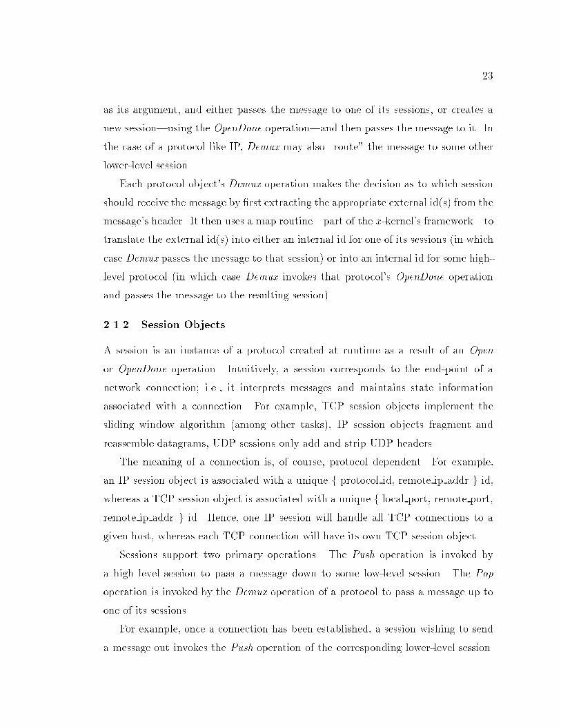
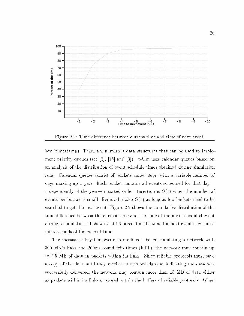
25to implement and manipulate messages; i.e., add and strip headers, fragment andreassemble messages.A map manager is used to manage a set of bindings of one identi�er to another.The map manager supports the addition of new bindings to the set, removal ofbindings from the set, and the mapping one identi�er into another relative to a setof bindings. Protocol implementations use the map manager to translate identi�ersextracted from message headers|e.g., addresses, port numbers|into capabilitiesfor x-kernel objects.An event manager is used to create and manage threads, as well as timer events.The event manager lets a protocol specify a timer event as a procedure that is tobe called at some future time. By registering a procedure with the event manager,protocols are able to timeout and act on messages that have not been acknowledged.2.1.5 x-Kernel Modi�cations to Support the SimulatorOnly minimal modi�cations to the x-kernel were necessary in order to use it asthe infrastructure for the simulator. No modi�cations were done to the x-kernelinterfaces, and only some of the routines implementing the interfaces were changed.This means that protocols can be moved between the simulator and the x-kernelwithout modi�cations.The event manager was modi�ed to support a global virtual time. The simulatorkeeps track of a simulated global time, and when there are no more threads readyto run at this time|all of the threads are either blocked or scheduled to run at afuture time|the event manager picks the thread that is scheduled to run nearest inthe future, increments the global time to that thread's scheduled time, and �nally,the simulator starts executing the thread.Since event calendar processing can consume as much as 40 percent of simula-tion time ([6], [21]) it is important to choose the right data structure to manageevent lists. Events lists are represented by priority queues, which are abstract datatypes supporting the following two operations: (1) insertion of an element (event)with a key (timestamp), and (2) removal of the element (event) with the smallest

26<1 <2 <3 <4 <5 <6 <7 <8 <9 <10

Time to next event in us

10

20

30

40

50

60

70

80

90

100

Per

cen

t o

f th

e ti

me

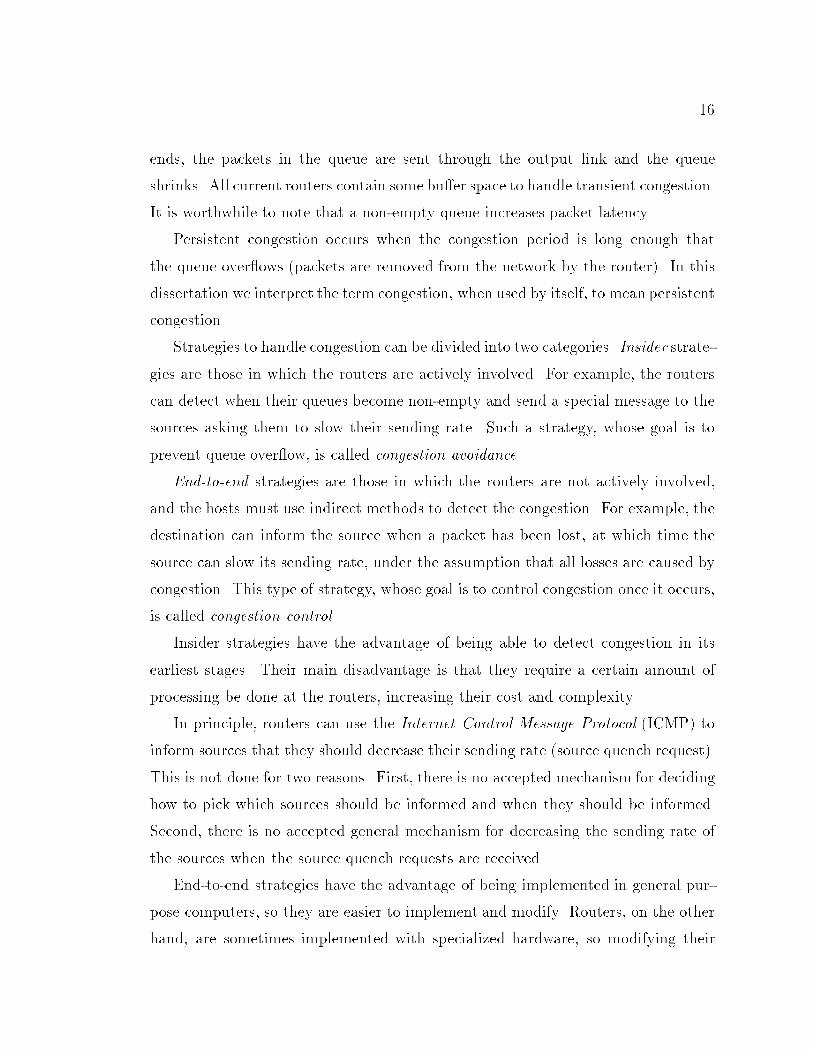
Figure 2.2: Time di�erence between current time and time of next event.key (timestamp). There are numerous data structures that can be used to imple-ment priority queues (see [5], [18] and [3]). x-Sim uses calendar queues based onan analysis of the distribution of event schedule times obtained during simulationruns. Calendar queues consist of buckets called days, with a variable number ofdays making up a year. Each bucket contains all events scheduled for that day|independently of the year|in sorted order. Insertion is O(1) when the number ofevents per bucket is small. Removal is also O(1) as long as few buckets need to besearched to get the next event. Figure 2.2 shows the cumulative distribution of thetime di�erence between the current time and the time of the next scheduled eventduring a simulation. It shows that 96 percent of the time the next event is within 5microseconds of the current time.The message subsystem was also modi�ed. When simulating a network with300 Mb/s links and 200ms round trip times (RTT), the network may contain upto 7.5 MB of data in packets within its links. Since reliable protocols must savea copy of the data until they receive an acknowledgment indicating the data wassuccessfully delivered, the network may contain more than 15 MB of data eitheras packets within its links or stored within the bu�ers of reliable protocols. When

27doing simulations, one normally does not care about the contents of most of the datain the messages. Only the beginning of the message, which contains the protocolheader information, is important. The message subsystem was modi�ed so messagescarry only about 200 bytes of non-zero data.In the standard x-kernel, the protocol graph is static and it is speci�ed at compiletime. In contrast, x-Sim uses enhanced versions of the routines dealing with thecreation of the protocol graph, and as a consequence, the protocol graph can bespeci�ed at runtime. The simulator reads a �le specifying the network topology:number and type of networks, number of hosts and routers, how the networks,hosts and routers are connected, the protocol graph for each host, and con�gurationparameters for all of the elements in the simulation scenario. These con�gurationparameters specify the addresses of each host and network, the speed and delay ofeach point-to-point link and network, whether Ethernet networks should simulatecollisions, and so on.Finally, the simulator augments the x-kernel interface with a few new functions.For example, the x-kernel's event manager has a resolution of 1 microsecond; this isperfectly adequate for events scheduled by protocols but not for a network simulatorwhich may need to simulate a 600 Mb/s ATM link that only takes 0.71 microsecondsto consume each packet (ATM packets are 53 bytes long). The simulator allows eventscheduling with nanosecond accuracy through a new event scheduling function.2.2 Simulatorx-Sim is a network simulator based on the x-kernel. It provides a framework for de-veloping, analyzing, and testing network protocols; for evaluating congestion controlmechanisms; and for studying network dynamics.x-Sim is tightly integrated with the x-kernel architecture; it runs x-kernel pro-tocols and protocols can be moved between the simulator and any x-kernel imple-mentations without any change in the protocol code. This allows us to experimentwith protocol implementations both in the controlled environment of the simulatoras well as in real networks like the Internet.

28SIM

MEGTEST TRAFFIC TRAFFIC MEGTEST

ETH

IP

TCP

ETH

IP

TCP

ETH

IP

TCP

ETH

IP

TCP

link

routers

Ethernets

point-to-pointho

sts

hosts

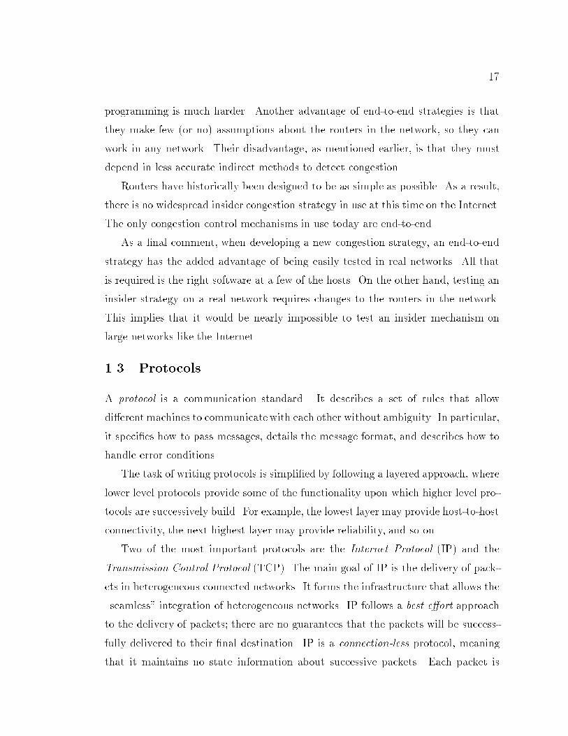
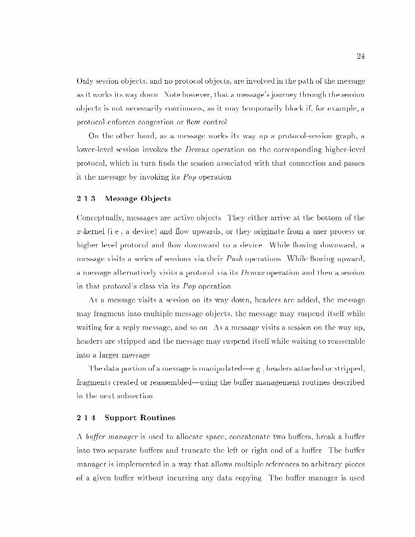
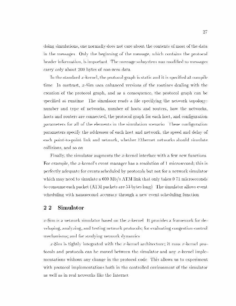
(a) (b)Figure 2.3: Example network and corresponding protocol graph.When designing a network simulator, one must balance accuracy and simulationspeed. In general, higher accuracy results in slower simulations. As computingpower continues to increase, the cost of the simulations becomes less signi�cant, butit is never irrelevant. Our approach was to �rst create a simulator that is as accurateas we could make it, and then, when simulation speed becomes an issue, to introduceoptional mechanisms that decrease the accuracy and increase the simulation speed.This approach, of going from more accurate to less accurate simulations, allows usto gauge the e�ect that the lower accuracy has on the simulations; only then canwe decide if the resulting less accurate simulations are good enough to be useful.The modular nature of the x-kernel lends itself to packaging the code simulatingan underlying network as a protocol (SIM) which lies at the bottom of the proto-col graph. Hosts are represented by protocol subgraphs lying on top of the SIMprotocol. Routers are represented either by protocol subgraphs or by SIM mod-ules. Protocol subgraphs are used for implementing complex routers, such as thosecontaining complete implementations of IP. Simpler routers are easier to implementas SIM modules. Figure 2.3 shows a network on the left and the correspondingx-kernel protocol graph on the right, with routers implemented as SIM modules. Inthis model, passing a message to the SIM protocol is equivalent to putting it into anetwork's physical wire. The SIM protocol then simulates its journey through themodeled network until it reaches a protocol subgraph representing the �nal desti-nation or an intermediate router, at which point SIM passes the message up to theprotocol subgraph.

29The following describes the structure of the SIM protocol in terms of three fun-damental components|links, nodes, and load. We then compare x-Sim to existingsimulators and emulators, presenting the relative strengths and weaknesses of eachapproach.2.2.1 LinksPhysical links can usually be simulated in software very accurately, at least to thelevel of the written speci�cation. Simulating a link's real behavior accurately mayentail some analysis of real implementations to �nd, among other things, the likeli-hood of losses due to noise. For example, accurately simulating an ethernet shouldinclude the ability to simulate collisions and the exponential backo� strategy. As an-other example, simulating ATM networks implies the use of small packets, increasingthe complexity level|and execution time|of a simulation.The architecture of x-Sim closely models the interactions between a link and thehost/network adapter. The lowest software layer in each node (driver) is tightlycoupled to the type of link (network) to which it is connected; together they modelthe interactions that occur in a real computer between the network, the adapter,and the device driver.The three main operations of the driver/network interface in the simulator are:(1) queries to the network, for example to check if it is busy; (2) transmissions ofpackets, and (3) callbacks from the network, which are used to model interrupts.For example, a node connected to an Ethernet �rst queries the network to see if itis busy. If it is not, it sends the packet. Otherwise, the node registers a callbackto be noti�ed when the network is not busy. Once the packet has been transmittedsuccessfully, the driver gets a callback notifying it of this fact so it can delete itscopy of that packet. However, since Ethernets allow collisions, the interactions canbecome more complicated. For example, a query may return that the network isnot busy, including a transmission right after another host has started transmitting,this will result in a collision of packets. In this case, both hosts get a callback atsome later time indicating that the transmission failed. Each host then schedules a

30retransmission at a later time based on an exponential backo� mechanism.The simulator currently supports point-to-point links, Ethernet links (with andwithout collisions), and a multiple access link that is a generalization of an Ethernetlink. The �rst and last type of links (networks) allow the user to specify severalparameters, including the bandwidth, delay, byte overhead per packet, a minimumand maximum packet size, and a loss or corruption probability. The second linktype exactly models an Ethernet.2.2.2 NodesPhysical links are used to connect network nodes, which are usually either routersor hosts. To capture their behavior, we need to consider the characteristics of boththe processor and the software, thereby simulating the delays introduced by boththe nodes, and the algorithms that they run.In x-Sim, the software running on a node is represented in one of two ways: (1)by an x-kernel style protocol graph or (2) by a program that implements an abstractspeci�cation of the node. When using a protocol graph, each protocol in the graph isgiven by the actual C code that implements the complete protocol. In other words,the �rst case can be viewed as supporting a direct execution simulation. The lattercase is commonly used to implement a simpli�ed (less accurate) model of a node.For example, a router can be simulated with an actual implementation of IP (plusthe necessary lower level protocols) by using existing x-kernel protocol modules, orby implementing a simpli�ed speci�cation that models some queuing discipline, suchas FIFO. Note that when a protocol is given as a module in the protocol graph, thenthis is exactly the same implementation that runs in the x-kernel. This makes itpossible to move a protocol back-and-forth between a simulated network and a realnetwork.Note that even though the goal is accurate simulation, there are times whenpractical realities force us to make small deviations from the real code. An illustra-tive example is the length of the TIME WAIT state in TCP, which is one minute inthe latest BSD implementation. When doing complex WAN simulations, with more

31than one thousand connections starting and ending during every simulated second,it is not feasible to keep the connection state (after the connection has been closed)around for the full simulated minute as this ties up too much memory. Our solutionis to reduce this delay. We can do this because we know our particular simulationdoes not require the full one minute delay for correctness.To simulate the processor accurately, one needs to account for the delays result-ing from the execution of the code invoked to handle each packet. For an even moreaccurate simulation, one needs to also add some variance to these delays to modelinteractions between di�erent subsystems. Simulating the delays and variance withtotal accuracy is probably not practical, as the variance may be due to cache andTLB e�ects. Even if one could simulate all of these details, it may not be the bestthing to do as it ties the results of the simulation to a speci�c model of hardware.x-Sim allows the protocol code to introduce delays by specifying periods of timeduring which the node does no other processing; incoming packets cannot be pro-cessed during such a delay. These delays might be based on measurements of thecode running on an actual processor and can be speci�ed by a uniform or normaldistribution.2.2.3 LoadNetwork load is usually the result of many applications executing on numeroushosts. In the case where one is interested in studying the behavior under realisticload, realistic tra�c sources are of the utmost importance. For example, tra�ccreated by multiple bulk TCP transfers is radically di�erent from tra�c generatedby multiple FTP, Telnet, SMTP and NNTP connections.1The �rst step in the creation of realistic tra�c is to use a common implementationof the underlying protocols|x-Sim gets this from the protocol graph. Next, we needa way to model the tra�c. Here, x-Sim contains a protocol that simulates Internettra�c based on tcplib [7]. Tcplib is a library that models Internet tra�c sources1The File Transfer Protocol (FTP) is used to transfer �les between computers, Telnet is used toconnect (login) to remote computer systems, SMTP is the protocol used for email delivery, NNTPis used to deliver Usenet news.

32based on empirical data collected at di�erent Internet gateways, and it has beenshown to produce realistic tra�c patterns [23]. This tra�c model is realized as aprotocol called TRAFFIC, which sits at the top of the protocol graph generatingwork.The tra�c simulation protocol (TRAFFIC) starts conversations with inter-arrivaltimes given by an exponential distribution. Each conversation can be of type Tel-net, FTP, NNTP or SMTP; type-speci�c parameters are also speci�ed. For example,FTP conversations are parameterized by the number of items to transmit, controlsegment sizes, and the individual item sizes. All of these parameters are obtainedfrom tcplib and are based on probability distributions obtained from real tra�ctraces. Each of these conversations runs on top of its own TCP connection, so eachconversation adapts to the network conditions by way of TCP's congestion controlmechanisms.One last feature of the tra�c simulation protocol is that it is instrumented insuch a way that the major tra�c characteristics are independent of the underlyingprotocols and router congestion mechanisms|the detailed tra�c itself is of coursea�ected by these di�erences. What we mean by major tra�c characteristics are thestart times of each conversation, the type of conversation, and the parameters forthat conversation. This feature allows us to compare the e�ects that changes|e.g.,to the TCP implementation|have on the tra�c. For example, it allows us to answerquestions of the form \what are the e�ects on the routers and bottleneck utilizationwhen we go from the one implementation of TCP to another?"Finally, there are other protocols (everything is a protocol in the x-kernel) thatmodel other types of transfers; for example, the MEGTEST protocol models TCPbulk transfers.2.2.4 Related WorkSome of best known freely available network simulators are REAL [19], Netsim [10]and the recently released ns from LBL's Network Research Group. None of thesesimulators support common implementations of protocols, that is, direct execution.

33Instead there is code to simulate the major characteristics of the protocol. Oneproblem with this approach is that it misses some of the behavior present in thecommon protocol implementations. In particular, it is our experience that in eval-uating the di�erent BSD implementations of TCP, running the actual TCP code ispreferred to running an abstract speci�cation of the protocol; the latter approach ismostly useful for rapid experimentation.For example, we have found the actual behavior of timers in the BSD imple-mentations of TCP to be quite important. Speci�cally, the round-trip time (RTT)measurements are done with a clock that ticks every half a second, resulting invery coarse estimates of the RTT. This a�ects the real time behavior of the proto-col because retransmit timeouts tend to be much longer than the real RTT. Manyexisting simulators use more accurate RTT measurements, resulting in retransmis-sion timeouts that are much smaller than those that normally occur in BSD TCP.As a consequence, packet losses that result in timeouts have a lesser e�ect on thethroughput in the simulator than they do in the BSD implementation.It turns out that it would be very hard, if not impossible, to do a full implemen-tation of TCP under either Netsim or REAL due to architectural constraints. Asa result, neither simulator could be used to study the exact behavior of one of thecommon implementation of TCP (like the BSD implementations) to see if there areany problems with it.Another important feature is that x-Sim protocols are just x-kernel protocols.One can use the simulator while implementing and debugging a new protocol, andwhen done, just move it to any x-kernel based system.An alternative to simulation is emulation [1], a technique that uses workstationsconnected by a real network, with modi�cations to the operating system to simulateslower links and larger propagation delays. Under this framework, simulated timeand real time are the same. Some of the advantages of emulation are that it runs realprotocols, actual behavior like processing overheads need not be simulated, and atwo minute simulation only takes two minutes to run. There are some disadvantages,however, such as the cost of the necessary hardware (to emulate a network with �ve

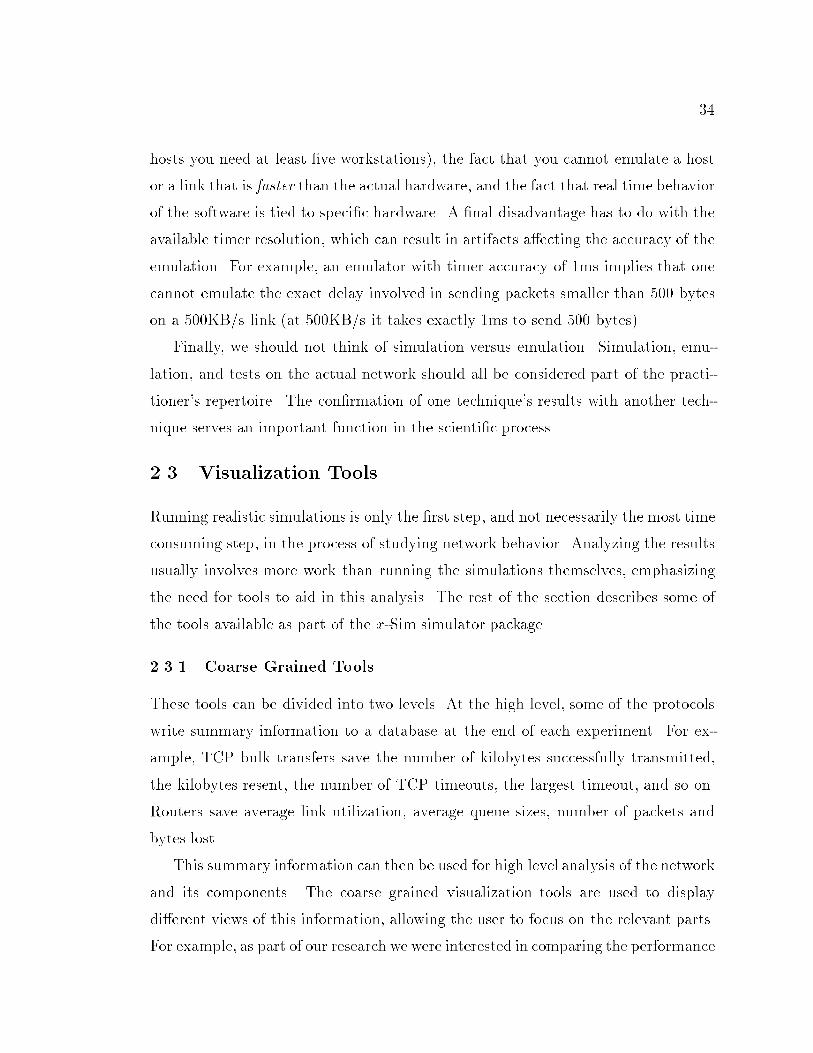
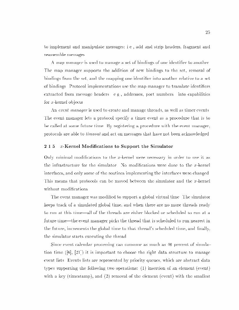
34hosts you need at least �ve workstations), the fact that you cannot emulate a hostor a link that is faster than the actual hardware, and the fact that real time behaviorof the software is tied to speci�c hardware. A �nal disadvantage has to do with theavailable timer resolution, which can result in artifacts a�ecting the accuracy of theemulation. For example, an emulator with timer accuracy of 1ms implies that onecannot emulate the exact delay involved in sending packets smaller than 500 byteson a 500KB/s link (at 500KB/s it takes exactly 1ms to send 500 bytes).Finally, we should not think of simulation versus emulation. Simulation, emu-lation, and tests on the actual network should all be considered part of the practi-tioner's repertoire. The con�rmation of one technique's results with another tech-nique serves an important function in the scienti�c process.2.3 Visualization ToolsRunning realistic simulations is only the �rst step, and not necessarily the most timeconsuming step, in the process of studying network behavior. Analyzing the resultsusually involves more work than running the simulations themselves, emphasizingthe need for tools to aid in this analysis. The rest of the section describes some ofthe tools available as part of the x-Sim simulator package.2.3.1 Coarse Grained ToolsThese tools can be divided into two levels. At the high level, some of the protocolswrite summary information to a database at the end of each experiment. For ex-ample, TCP bulk transfers save the number of kilobytes successfully transmitted,the kilobytes resent, the number of TCP timeouts, the largest timeout, and so on.Routers save average link utilization, average queue sizes, number of packets andbytes lost.This summary information can then be used for high level analysis of the networkand its components. The coarse grained visualization tools are used to displaydi�erent views of this information, allowing the user to focus on the relevant parts.For example, as part of our research we were interested in comparing the performance

35Comparison of different implementations of TCP

TCP-1 traffic TCP-2 traffic TCP-3 trafficKB/S

KB sent

KB resent

% resent

Telnet delay

delay < 1000

count

78.9 61.8 48.3

2339.7 3344.7 1854.2 3285.2 1449.1 3292.4

40.3 88.4 78.8 88.8 55.0 54.0

1.7 2.6 4.2 2.7 3.8 1.6

145.3 160.2 150.9

99.4 98.5 98.5

20 20 20 20 20 20 Figure 2.4: Database output comparing TCP implementations.of three implementations of TCP which we will refer to as TCP-1, TCP-2 andTCP-3. The simulation topology used is that on Figure 2.3. Two hosts, one oneach ethernet, run the TRAFFIC protocol to simulate background tra�c while theother two hosts run the MEGTEST protocol which does a TCP bulk transfer fromone host to the other. The point-to-point link connecting the two ethernets has amaximum bandwidth of 200KB/s and it is the bottleneck since it is slower than the1.25MB/s bandwidth of the ethernet networks.Each simulation was uniquely speci�ed by choosing one of the three TCP im-plementations and by a seed that was used to create a speci�c tra�c pattern. Eachsimulation lasted 30 (simulated) seconds during which a bulk transfer shared thebottleneck link with background tra�c. Sixty simulations were run, twenty witheach TCP implementation using di�erent tra�c patterns. The twenty tra�c pat-terns were the same for each TCP implementation.Figure 2.4 shows the average of some of the information saved in the database�les. Each pair of columns correspond to one of the TCP implementations: the �rsttwo are for TCP-1, the next two for TCP-2 and the �nal two for TCP-3. In eachpair of columns, the left one|with the TCP implementation name as a heading|shows the averages corresponding to the bulk transfer, and the right one showsthe averages for the background tra�c. Hence, the bulk transfer in the TCP-1implementation achieved an average throughput of 78.9 KB/s, and during the 30

36Percent Link Utilization

TCP-1 TCP-2 TCP-30-5 sec5-10 sec10-15 sec15-20 sec20-25 sec25-30 secaverage

90.6% 74.3% 64.1%

93.2% 82.4% 78.1%

92.3% 82.9% 76.5%

91.4% 83.8% 75.8%

91.8% 85.7% 79.2%

88.6% 80.8% 81.2%

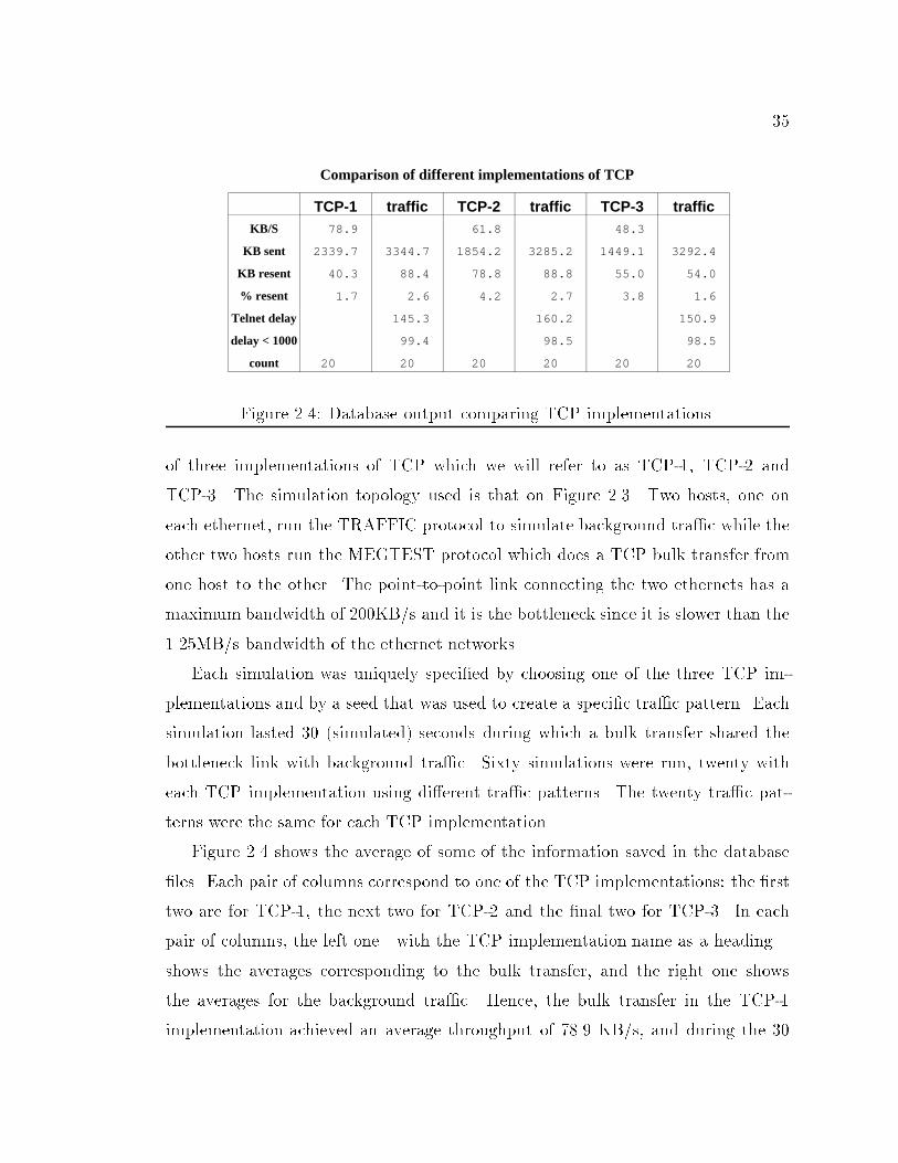
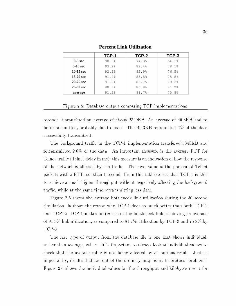
91.3% 81.7% 75.8%Figure 2.5: Database output comparing TCP implementations.seconds it transfered an average of about 2340KB. An average of 40.3KB had tobe retransmitted, probably due to losses. This 40.3KB represents 1.7% of the datasuccessfully transmitted.The background tra�c in the TCP-1 implementation transfered 3345KB andretransmitted 2.6% of the data. An important measure is the average RTT forTelnet tra�c (Telnet delay in ms); this measure is an indication of how the responseof the network is a�ected by the tra�c. The next value is the percent of Telnetpackets with a RTT less than 1 second. From this table we see that TCP-1 is ableto achieve a much higher throughput without negatively a�ecting the backgroundtra�c, while at the same time retransmitting less data.Figure 2.5 shows the average bottleneck link utilization during the 30 secondsimulation. It shows the reason why TCP-1 does so much better than both TCP-2and TCP-3: TCP-1 makes better use of the bottleneck link, achieving an averageof 91.3% link utilization, as compared to 81.7% utilization by TCP-2 and 75.8% byTCP-3The last type of output from the database �le is one that shows individual,rather than average, values. It is important to always look at individual values tocheck that the average value is not being a�ected by a spurious result. Just asimportantly, results that are out of the ordinary may point to protocol problems.Figure 2.6 shows the individual values for the throughput and kilobytes resent for

375 10 15 20

id

20406080

100120140160

KB

/STCP-3TCP-2TCP-1TCP Throughput for 1-Meg

5 10 15 20id

20

40

60

80

100

KB

res

ent

TCP-3TCP-2TCP-1TCP KBytes Resent for 1-Meg

Figure 2.6: Database output comparing TCP implementations.the bulk transfers.2.3.2 Fine Grained ToolsThe database �les contain coarse information about the simulations. Often it isuseful to be able to do detailed examination of particular network components.For this purpose, some protocols and routers can save detailed information intotracing �les. These traces are analyzed and displayed using a set of common toolswhich are part of the x-Sim package. The most detailed traces are obtained fromthe more complex protocols, and they have proven invaluable in the analysis andunderstanding of these protocols. For example, the x-kernel/x-Sim versions of thedi�erent TCP implementations have been augmented with calls to trace all therelevant state of the protocol, such as the size of the di�erent windows and bu�ers,

380.5 1.0 1.5 2.0 2.5 3.0 3.5 4.0 4.5 5.0 5.5 6.0 6.5 7.0 7.5 8.0 8.5 9.0 9.5 10.0

Time in seconds

5

10Q

ueue

siz

e in

rou

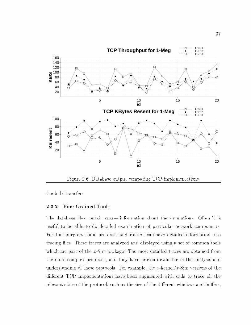
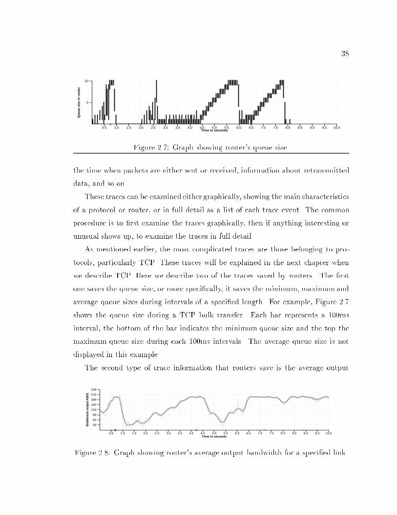
ter Figure 2.7: Graph showing router's queue size.the time when packets are either sent or received, information about retransmitteddata, and so on.These traces can be examined either graphically, showing the main characteristicsof a protocol or router, or in full detail as a list of each trace event. The commonprocedure is to �rst examine the traces graphically, then if anything interesting orunusual shows up, to examine the traces in full detail.As mentioned earlier, the most complicated traces are those belonging to pro-tocols, particularly TCP. These traces will be explained in the next chapter whenwe describe TCP. Here we describe two of the traces saved by routers. The �rstone saves the queue size, or more speci�cally, it saves the minimum, maximum andaverage queue sizes during intervals of a speci�ed length. For example, Figure 2.7shows the queue size during a TCP bulk transfer. Each bar represents a 100msinterval, the bottom of the bar indicates the minimum queue size and the top themaximum queue size during each 100ms intervals. The average queue size is notdisplayed in this example.The second type of trace information that routers save is the average output

0.5 1.0 1.5 2.0 2.5 3.0 3.5 4.0 4.5 5.0 5.5 6.0 6.5 7.0 7.5 8.0 8.5 9.0 9.5 10.0Time in seconds

30

60

90

120

150

180

210

240

Bot

tlene

ck o

utpu

t KB

/SFigure 2.8: Graph showing router's average output bandwidth for a speci�ed link.

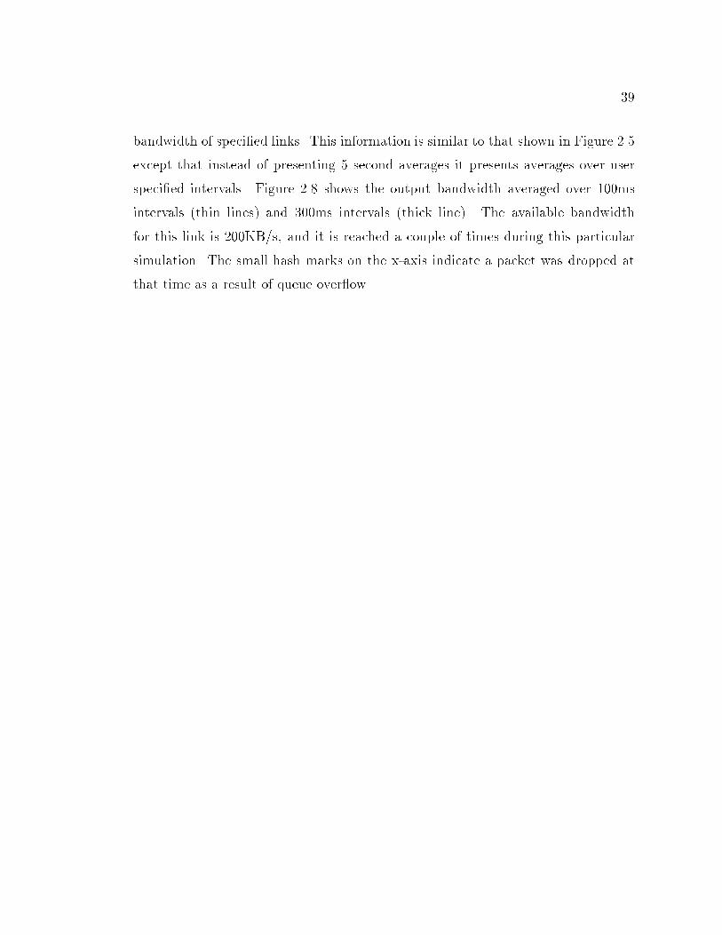
39bandwidth of speci�ed links. This information is similar to that shown in Figure 2.5except that instead of presenting 5 second averages it presents averages over userspeci�ed intervals. Figure 2.8 shows the output bandwidth averaged over 100msintervals (thin lines) and 300ms intervals (thick line). The available bandwidthfor this link is 200KB/s, and it is reached a couple of times during this particularsimulation. The small hash marks on the x-axis indicate a packet was dropped atthat time as a result of queue over ow.

40CHAPTER 3Transmission Control ProtocolWe know from experience that internets with no congestion control behave badlyunder high loads [13]. Since most of the tra�c over the Internet comes from TCPconnections, TCP's congestion control mechanisms play a pivotal role in maintainingthe health of the Internet. This chapter outlines the main characteristics of TCP,describes its congestion control mechanisms, and provides an insight into its generalbehavior.This chapter is organized as follows. First, we give a brief description of some ofthe early applications that were the catalysis for the invention of computer networks.It is easy to understand TCP's main characteristics in this context. Second, wedescribe some of the most important mechanisms in TCP, focusing in those dealingwith reliability and congestion control. Third, we provide some insight into TCP'scongestion control mechanisms by analyzing graphs depicting some of the mostimportant internal state of TCP.Protocol

Block

Protocol

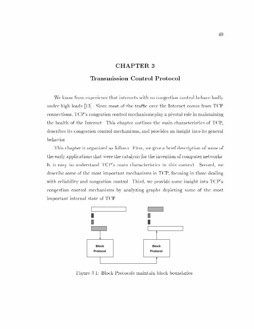
BlockFigure 3.1: Block Protocols maintain block boundaries.

41Stream

Protocol

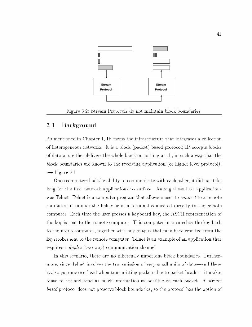
Stream

ProtocolFigure 3.2: Stream Protocols do not maintain block boundaries.3.1 BackgroundAs mentioned in Chapter 1, IP forms the infrastructure that integrates a collectionof heterogeneous networks. It is a block (packet) based protocol; IP accepts blocksof data and either delivers the whole block or nothing at all, in such a way that theblock boundaries are known to the receiving application (or higher level protocol);see Figure 3.1.Once computers had the ability to communicate with each other, it did not takelong for the �rst network applications to surface. Among these �rst applicationswas Telnet. Telnet is a computer program that allows a user to connect to a remotecomputer; it mimics the behavior of a terminal connected directly to the remotecomputer. Each time the user presses a keyboard key, the ASCII representation ofthe key is sent to the remote computer. This computer in turn echos the key backto the user's computer, together with any output that may have resulted from thekeystrokes sent to the remote computer. Telnet is an example of an application thatrequires a duplex (two way) communication channel.In this scenario, there are no inherently important block boundaries. Further-more, since Telnet involves the transmission of very small units of data|and thereis always some overhead when transmitting packets due to packet header|it makessense to try and send as much information as possible on each packet. A streambased protocol does not preserve block boundaries, so the protocol has the option of

42aggregating blocks of data before sending them (see Figure 3.2). The term segmentis used to refer to a block of data passed by a stream protocol to a lower protocol.A common requirement for most types of communications is reliability. Forexample, one expects email to arrive at the destination without any missing parts.As previously mentioned, IP is not a reliable protocol. It makes perfect sense notto burden a protocol whose primary purpose is the integration of heterogeneousnetworks with reliability. There are high costs associated with reliability both interms of code complexity and storage|a reliable protocol must keep a copy of thedata it sends until the protocol knows the data has been successfully received, incase the protocol needs to send the data again.Stream based protocols also need to be ordered since there is no way for thereceiving higher level protocol (or application) to know the position of a block ofdata just received. The usual way of communicating the position of a block is bywriting this information at the beginning of the block|in the header. Since a streambased protocol may break a block into smaller components, it is possible to receiveparts of the block without the block header.Another important issue to consider when dealing with computer communica-tions is how to deal with sources that are able to send at a higher rate than thedestination can deal with. This mismatch can be due to: (1) the source may be amore powerful (higher instruction execution rate) computer than the destination,or, (2) the destination may have to perform some time consuming task|such asin client-server computing. Flow control is the term used to denote some sort ofsynchronization between the source and destination, so that the source does notoverrun the destination.It is important to distinguish the di�erences between ow and congestion control.Flow control mechanisms prevent the source from overrunning the receiver. Theyare usually simple to design since there are only two entities involved. Congestion,on the other hand, occurs at intermediate nodes (the routers) and may involvemultiple sources. As a result, congestion control mechanisms are more complex andharder to design.

43A useful analogy is to think of a connection's path as a water pipe. Using all ofthe bandwidth available to the connection is equivalent to keeping the pipe full.TCP is a protocol designed to provide the communication paradigms just de-scribed. It is a connection based protocol that provides an ordered, stream based,reliable duplex communication channel with ow and congestion control. It runs ontop of IP, so it has at its disposal the full set of network services provided by IP.The next subsections present more detailed descriptions of how reliability, ow andcongestion control are implemented in TCP.3.2 ReliabilityHaving reliability as a goal implies the possibility of having to retransmit some ofthe data already sent. Thus data needs to be bu�ered until it is known to have beensuccessfully received on the other end. Successful reception implies not only that adatagram arrived, but also that it arrived uncorrupted. Hence there is a need formechanisms that insure that the data was not corrupted and that it was successfullyreceived. A checksum is used to validate both the TCP header and data.Two possible mechanisms for informing the source that data arrived successfullyare: (1) having the receiver send a positive acknowledgment (ACK) announcing thata block of data arrived safely, or (2) having the receiver send a negative acknowl-edgment (NACK) announcing that a block of data is missing.To specify that a block of data has been received or that it is missing, one musthave a naming scheme. The usual approach used in block based protocols is tonumber each block of data in the order in which it was passed to the source. Thisapproach can be expanded to cover stream based protocols by thinking of each unitof data|bytes in this case|as a block. TCP uses a sequence number to uniquelyname each byte sent over the communication channel. These sequence numbers areused by the receiver to correctly order segments that may be received out of orderand to eliminate duplicates.TCP uses positive rather than negative acknowledgments. Furthermore, to con-serve packet space and for reliability reasons, TCP's designers decided on cumulative

44acknowledgments. Acknowledging a block of data requires two numbers to code thesequence numbers of the beginning and end of the block. A cumulative ACK ac-knowledges all data up to a given sequence number, so only one number is neededto acknowledge a block of data|assuming all previous blocks have been received. Afurther advantage of cumulative ACKs is the reliability of this approach; the loss ofan ACK is not very damaging in the common case when later ACKs will be received,as the information on the lost ACK will be contained in succeeding ACKs.Cumulative acknowledgments inform the source that segments were successfullyreceived; an additional mechanism is still needed to determine when segments arelost. TCP uses a timeout mechanism to detect and then retransmit lost segments.If an ACK is not received by the source within a timeout interval, the data isretransmitted.The original protocol speci�cation does not require any particular mechanism(algorithm) for determining the timeout interval. However, it gives an exampleretransmission timeout procedure based on the measured round trip time (RTT)|the elapsed time between sending the segment and the reception of the ACK. Theretransmit timeout procedure in use today is based on both round trip time andvariance estimates computed by sampling the time between when a segment is sentand an ACK arrives [13].3.3 Flow ControlFlow control is the mechanism used to prevent a faster host from overruning a slowerhost. TCP uses a window based ow control mechanism by which the receiving TCPallows the source to send only as much data as the receiver can bu�er. The receivercontrols the ow of data by advertising the amount of free space in its receive bu�er.This space decreases as new packets arrive and increases as the application readsmore data. Each acknowledgment the receiver transmits to the source contains thetotal number of free bytes in its bu�er space; it is known as the advertised window.A convenient way to visualize the dynamics of the advertised window as seenby the source is shown in Figure 3.3. The thick gray line represents the advertised

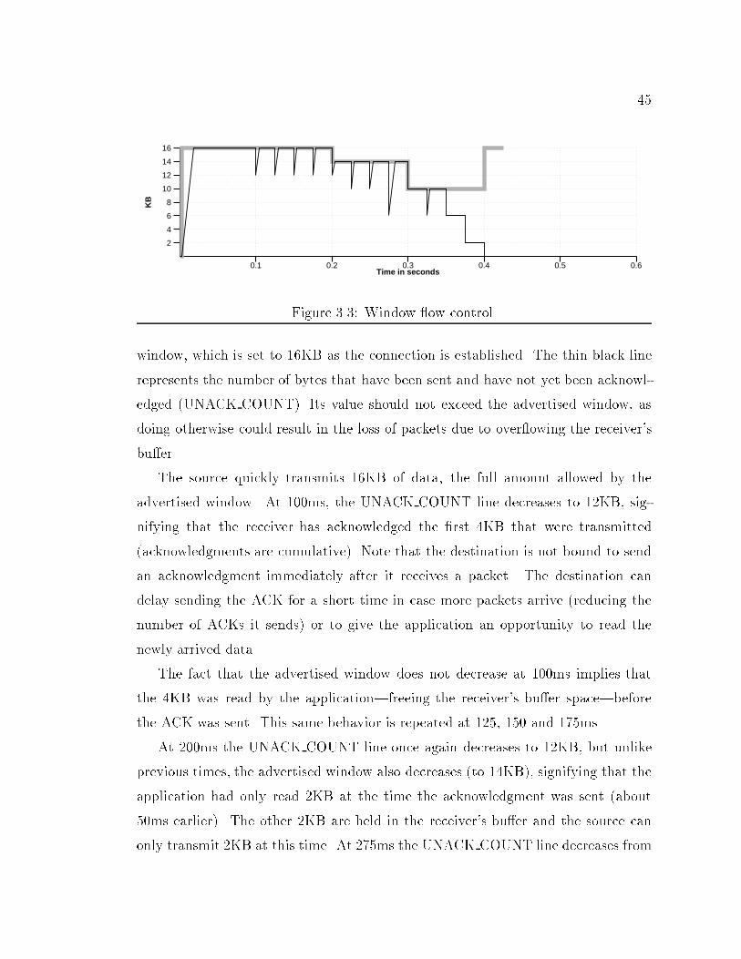
450.1 0.2 0.3 0.4 0.5 0.6

Time in seconds

2

4

6

8

10

12

14

16K

B Figure 3.3: Window ow control.window, which is set to 16KB as the connection is established. The thin black linerepresents the number of bytes that have been sent and have not yet been acknowl-edged (UNACK COUNT). Its value should not exceed the advertised window, asdoing otherwise could result in the loss of packets due to over owing the receiver'sbu�er.The source quickly transmits 16KB of data, the full amount allowed by theadvertised window. At 100ms, the UNACK COUNT line decreases to 12KB, sig-nifying that the receiver has acknowledged the �rst 4KB that were transmitted(acknowledgments are cumulative). Note that the destination is not bound to sendan acknowledgment immediately after it receives a packet. The destination candelay sending the ACK for a short time in case more packets arrive (reducing thenumber of ACKs it sends) or to give the application an opportunity to read thenewly arrived data.The fact that the advertised window does not decrease at 100ms implies thatthe 4KB was read by the application|freeing the receiver's bu�er space|beforethe ACK was sent. This same behavior is repeated at 125, 150 and 175ms.At 200ms the UNACK COUNT line once again decreases to 12KB, but unlikeprevious times, the advertised window also decreases (to 14KB), signifying that theapplication had only read 2KB at the time the acknowledgment was sent (about50ms earlier). The other 2KB are held in the receiver's bu�er and the source canonly transmit 2KB at this time. At 275ms the UNACK COUNT line decreases from

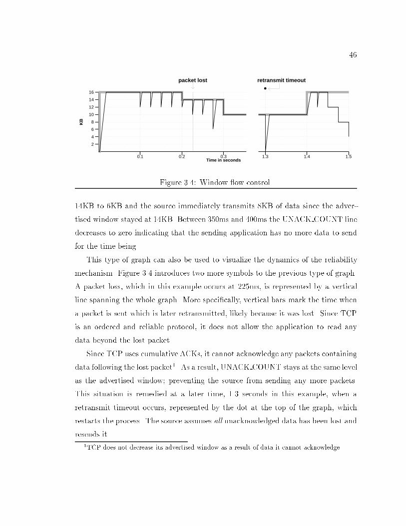
460.1 0.2 0.3 1.3 1.4 1.5

Time in seconds

2

4

6

8

10

12

14

16

KB

packet lost retransmit timeout

Figure 3.4: Window ow control.14KB to 6KB and the source immediately transmits 8KB of data since the adver-tised window stayed at 14KB. Between 350ms and 400ms the UNACK COUNT linedecreases to zero indicating that the sending application has no more data to sendfor the time being.This type of graph can also be used to visualize the dynamics of the reliabilitymechanism. Figure 3.4 introduces two more symbols to the previous type of graph.A packet loss, which in this example occurs at 225ms, is represented by a verticalline spanning the whole graph. More speci�cally, vertical bars mark the time whena packet is sent which is later retransmitted, likely because it was lost. Since TCPis an ordered and reliable protocol, it does not allow the application to read anydata beyond the lost packet.Since TCP uses cumulative ACKs, it cannot acknowledge any packets containingdata following the lost packet1. As a result, UNACK COUNT stays at the same levelas the advertised window; preventing the source from sending any more packets.This situation is remedied at a later time, 1.3 seconds in this example, when aretransmit timeout occurs, represented by the dot at the top of the graph, whichrestarts the process. The source assumes all unacknowledged data has been lost andresends it.1TCP does not decrease its advertised window as a result of data it cannot acknowledge.

473.4 Congestion ControlThe original version of TCP did not contain any congestion control mechanisms.Congestion is only mentioned in the reliability section of the protocol speci�cationas a possible cause of packet losses. This lack of congestion control eventuallyresulted in what is called congestion collapses as a result of the increasing tra�c onthe Internet. The term is used to indicate a persistent state of congestion, wherethe actual throughput of the connections involved is almost zero.The dynamics of congestion collapse can be deduced from Figure 3.4. Once alink becomes congested, a few of the connections whose path contains the congestedlink are likely to lose one or more packets. This congestion can occur by increasingthe number of connections going through the link. All connections that lose packetstimeout and start retransmitting at around the same time (the delay before theretransmit timer �res is a function of the connection's RTT). Figure 3.4 shows thatwhen the retransmit timeout occurs, the connection resends all the data it hadpreviously sent but not gotten an acknowledgment for. The link becomes even morecongested as a result of one or more connections quickly sending so much data onan already congested link. It is not hard to imagine how the process could continueinde�nitely once it got started.3.4.1 Jacobson's Original ProposalIn 1988, Van Jacobson published a paper [13] in which he describes mechanisms toprevent congestion collapse by detecting and controlling congestion. During periodswhen there is no congestion|and therefore no losses|there is a directly proportionalrelationship between UNACK COUNT and throughput:Throughput = UNACK COUNTRTTAs UNACK COUNT increases, the throughput should also increase. When UN-ACK COUNT decreases, so should the throughput. Jacobson introduced the con-gestion window as a way of dynamically controlling UNACK COUNT. The amount

48Source Destination

Time

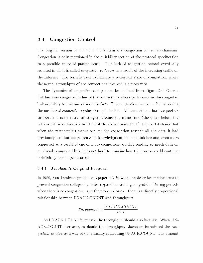
Figure 3.5: Timeline of Slow-start.of UNACK COUNT that is allowed is now bounded by both the advertised win-dow and by the congestion window. The congestion window is allowed to changedynamically with the purpose of controlling congestion. He described two mech-anisms to control the the size of the congestion window: (1) slow-start and (2)linear-increase/multiplicative-decrease.Slow-start is used to control the rate by which UNACK COUNT increases atthe beginning of the connection, or after a retransmit timeout. When executingthe slow-start mechanism, the congestion window is initially set to the size of thelargest packet TCP is allowed to send (max-packet). Each time an acknowledgmentis received, the congestion window is increased by max-packet. If the receiver isacknowledging each packet, then the congestion window will double in size duringeach RTT, resulting in exponential growth of the congestion window.Figure 3.5 shows the dynamics of slow-start. The source starts by sending onepacket to the destination, which sends an acknowledgment in return. When thesource gets the acknowledgment, it immediately sends two packets. The destinationonce again sends an acknowledgment immediately after receiving each packet. Eachof these two ACKs results in two packets sent by the source, and so on.

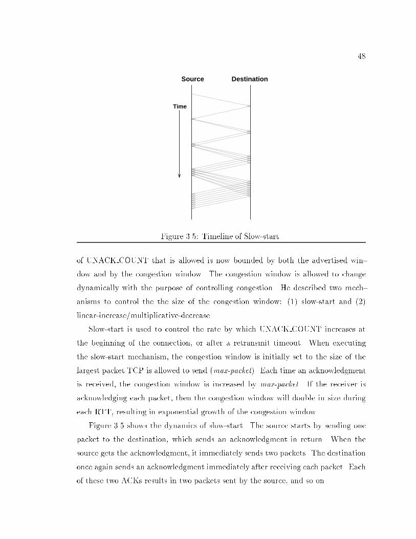
49Bottleneck

Link DestinationSource

Time

Figure 3.6: Packets spaced by slow link.Even though the source sent two packets back-to-back, they are spaced out whenthey arrive at the destination. The reason for this is shown graphically in Figure 3.6.In this �gure, the thickness of a line is inversely proportional to the speed of the linkit traverses|the thickness of the line represents the time needed to insert the packetinto the link. Initially, two packets leave the source close together, on a fast link.When they get to the bottleneck link it takes longer to insert each packet into thelink, either because it is a slower link or because other packets are waiting in a queueto be sent over this link. For this discussion it is assumed that the bottleneck linkis slower, so it takes longer to put each packet into the link, and the time betweeneach packet increases. When the packets leave the slower link and go into a fasterlink, the time di�erence between the packets is preserved. If an acknowledgment issent immediately after each packet arrives, the acknowledgments will carry the timedi�erence back to the source (assuming there are no queues at the routers). If thesource now sends one packet as it receives each acknowledgment, they will be sentat the rate of the bottleneck link.The exponential growth of the congestion window during slow-start continuesuntil one of three things happens: (1) it reaches the size of the advertised window,(2) it reaches a pre-established value (threshold window), or losses are detected.Consider the second case in more detail: at the beginning of the connection, thethreshold window is usually set to 64KB. However, when slow-start is used after a

500.5

Time in seconds

0102030405060

KBFigure 3.7: Slow-start: Congestion window size versus time.retransmit timeout, the connection has an idea of the available bandwidth and thethreshold window is set in such a way so as to stop the exponential growth rightbefore the available bandwidth is reached.Figure 3.7 shows the dynamics of slow-start by plotting the congestion windowas a function of time. The tick marks at the top of the graph are used to indicatethe time when a packet is sent. Notice how the congestion window increases expo-nentially and how the tick marks seem to be nicely spaced. However, since packetsare sent back-to-back in pairs, each tick mark is really two overlapping tick marks.After slow-start terminates, the linear-increase and multiplicative-decreasemech-anism comes into play. This mechanism increases the congestion window by onemax-packet on each RTT (a linear increase) and decreases the congestion windowby half (a multiplicative decrease) whenever congestion is detected. TCP interpretsany loss as a sign of congestion. The coarse behavior|without the slow-starts|ofthe linear-increase and multiplicative-decrease mechanism is shown in Figure 3.8.The exact mechanism is as follows. When congestion is detected, the thresholdwindow is set to half the size of the congestion window. Next, the congestion windowis set to one. All unacknowledged packets are assumed lost, and slow-start is usedto increase the size of the congestion window exponentially until it reaches the sizeof the threshold window.A mechanism is e�cient if it results in a full utilization of the available band-

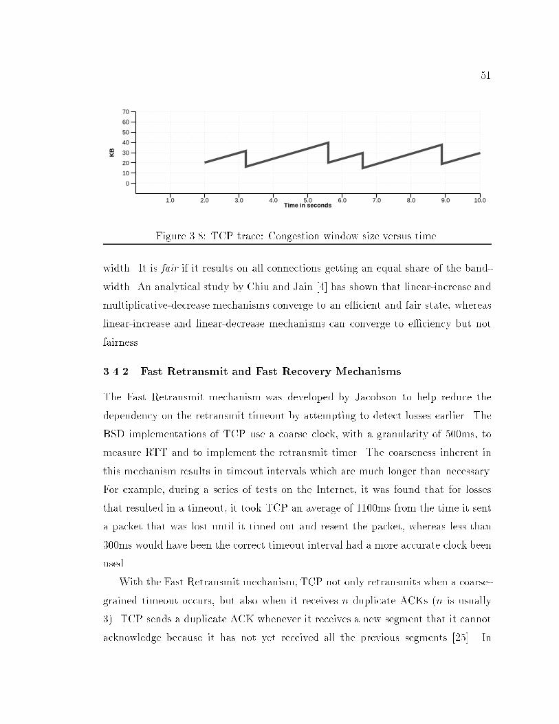
511.0 2.0 3.0 4.0 5.0 6.0 7.0 8.0 9.0 10.0

Time in seconds

0

10

20

30

40

50

60

70K

B Figure 3.8: TCP trace: Congestion window size versus time.width. It is fair if it results on all connections getting an equal share of the band-width. An analytical study by Chiu and Jain [4] has shown that linear-increase andmultiplicative-decrease mechanisms converge to an e�cient and fair state, whereaslinear-increase and linear-decrease mechanisms can converge to e�ciency but notfairness.3.4.2 Fast Retransmit and Fast Recovery MechanismsThe Fast Retransmit mechanism was developed by Jacobson to help reduce thedependency on the retransmit timeout by attempting to detect losses earlier. TheBSD implementations of TCP use a coarse clock, with a granularity of 500ms, tomeasure RTT and to implement the retransmit timer. The coarseness inherent inthis mechanism results in timeout intervals which are much longer than necessary.For example, during a series of tests on the Internet, it was found that for lossesthat resulted in a timeout, it took TCP an average of 1100ms from the time it senta packet that was lost until it timed out and resent the packet, whereas less than300ms would have been the correct timeout interval had a more accurate clock beenused.With the Fast Retransmit mechanism, TCP not only retransmits when a coarse-grained timeout occurs, but also when it receives n duplicate ACKs (n is usually3). TCP sends a duplicate ACK whenever it receives a new segment that it cannotacknowledge because it has not yet received all the previous segments [25]. In

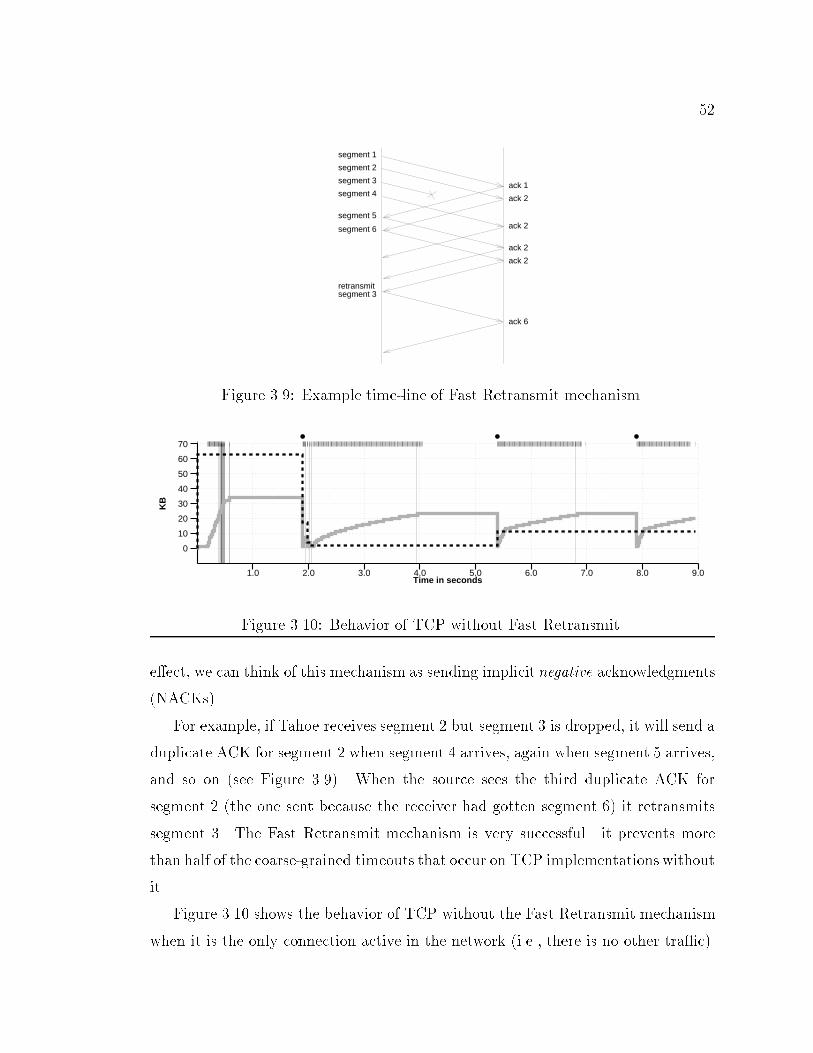
52segment 1

segment 2

segment 3

segment 4

segment 5

segment 6

retransmitsegment 3

ack 1

ack 2

ack 2

ack 2

ack 2

ack 6Figure 3.9: Example time-line of Fast Retransmit mechanism.1.0 2.0 3.0 4.0 5.0 6.0 7.0 8.0 9.0

Time in seconds

0

10

20

30

40

50

60

70

KB Figure 3.10: Behavior of TCP without Fast Retransmit.e�ect, we can think of this mechanism as sending implicit negative acknowledgments(NACKs).For example, if Tahoe receives segment 2 but segment 3 is dropped, it will send aduplicate ACK for segment 2 when segment 4 arrives, again when segment 5 arrives,and so on (see Figure 3.9). When the source sees the third duplicate ACK forsegment 2 (the one sent because the receiver had gotten segment 6) it retransmitssegment 3. The Fast Retransmit mechanism is very successful|it prevents morethan half of the coarse-grained timeouts that occur on TCP implementations withoutit. Figure 3.10 shows the behavior of TCP without the Fast Retransmit mechanismwhen it is the only connection active in the network (i.e., there is no other tra�c).

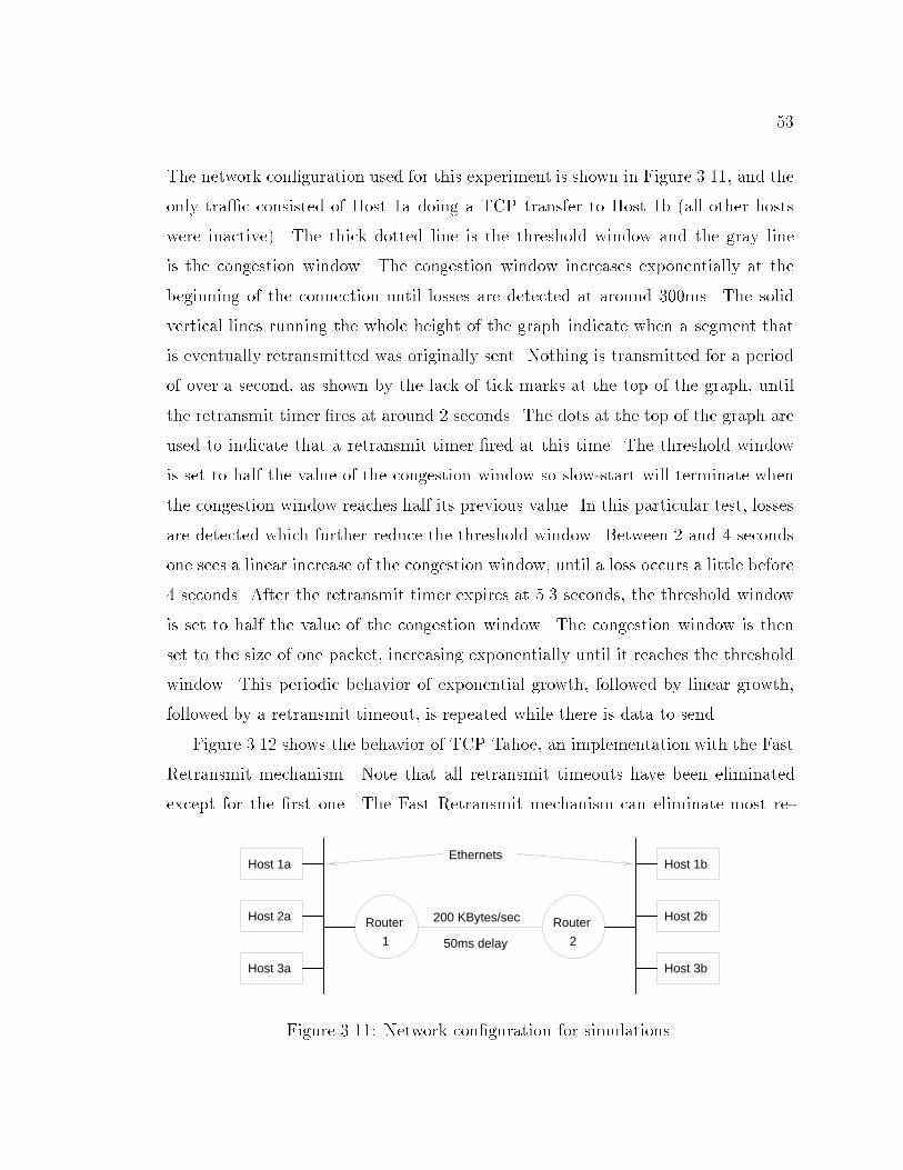
53The network con�guration used for this experiment is shown in Figure 3.11, and theonly tra�c consisted of Host 1a doing a TCP transfer to Host 1b (all other hostswere inactive). The thick dotted line is the threshold window and the gray lineis the congestion window. The congestion window increases exponentially at thebeginning of the connection until losses are detected at around 300ms. The solidvertical lines running the whole height of the graph indicate when a segment thatis eventually retransmitted was originally sent. Nothing is transmitted for a periodof over a second, as shown by the lack of tick marks at the top of the graph, untilthe retransmit timer �res at around 2 seconds. The dots at the top of the graph areused to indicate that a retransmit timer �red at this time. The threshold windowis set to half the value of the congestion window so slow-start will terminate whenthe congestion window reaches half its previous value. In this particular test, lossesare detected which further reduce the threshold window. Between 2 and 4 secondsone sees a linear increase of the congestion window, until a loss occurs a little before4 seconds. After the retransmit timer expires at 5.3 seconds, the threshold windowis set to half the value of the congestion window. The congestion window is thenset to the size of one packet, increasing exponentially until it reaches the thresholdwindow. This periodic behavior of exponential growth, followed by linear growth,followed by a retransmit timeout, is repeated while there is data to send.Figure 3.12 shows the behavior of TCP Tahoe, an implementation with the FastRetransmit mechanism. Note that all retransmit timeouts have been eliminatedexcept for the �rst one. The Fast Retransmit mechanism can eliminate most re-Router

2

Router

1

Host 1a

Host 2a

Host 3a Host 3b

Host 2b

Host 1b

50ms delay

200 KBytes/sec

EthernetsFigure 3.11: Network con�guration for simulations.

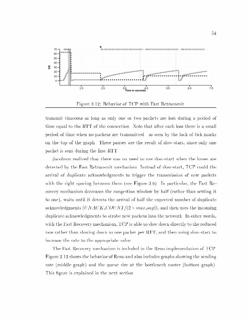
541.0 2.0 3.0 4.0 5.0 6.0 7.0

Time in seconds

0

10

20

30

40

50

60

70K

B Figure 3.12: Behavior of TCP with Fast Retransmit.transmit timeouts as long as only one or two packets are lost during a period oftime equal to the RTT of the connection. Note that after each loss there is a smallperiod of time when no packets are transmitted|as seen by the lack of tick markson the top of the graph. These pauses are the result of slow-start, since only onepacket is sent during the �rst RTT.Jacobson realized that there was no need to use slow-start when the losses aredetected by the Fast Retransmit mechanism. Instead of slow-start, TCP could thearrival of duplicate acknowledgments to trigger the transmission of new packetswith the right spacing between them (see Figure 3.6). In particular, the Fast Re-covery mechanism decreases the congestion window by half (rather than setting itto one), waits until it detects the arrival of half the expected number of duplicateacknowledgments (UNACK COUNT=(2�max seg)), and then uses the incomingduplicate acknowledgments to strobe new packets into the network. In other words,with the Fast Recovery mechanism, TCP is able to slow down directly to the reducedrate rather than slowing down to one packet per RTT, and then using slow-start toincrease the rate to the appropriate value.The Fast Recovery mechanism is included in the Reno implementation of TCP.Figure 3.13 shows the behavior of Reno and also includes graphs showing the sendingrate (middle graph) and the queue size at the bottleneck router (bottom graph).This �gure is explained in the next section.

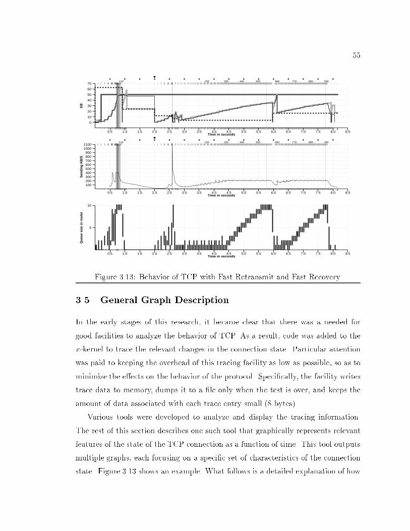
550.5 1.0 1.5 2.0 2.5 3.0 3.5 4.0 4.5 5.0 5.5 6.0 6.5 7.0 7.5 8.0 8.5

Time in seconds

0

10

20

30

40

50

60

70K

B110 220 330 440 550 660 770 880 990

0.5 1.0 1.5 2.0 2.5 3.0 3.5 4.0 4.5 5.0 5.5 6.0 6.5 7.0 7.5 8.0 8.5Time in seconds

100200300400500600700800900

10001100

Sen

ding

KB

/S

110 220 330 440 550 660 770 880 990

0.5 1.0 1.5 2.0 2.5 3.0 3.5 4.0 4.5 5.0 5.5 6.0 6.5 7.0 7.5 8.0 8.5Time in seconds

5

10

Que

ue s

ize

in r

oute

r Figure 3.13: Behavior of TCP with Fast Retransmit and Fast Recovery.3.5 General Graph DescriptionIn the early stages of this research, it became clear that there was a needed forgood facilities to analyze the behavior of TCP. As a result, code was added to thex-kernel to trace the relevant changes in the connection state. Particular attentionwas paid to keeping the overhead of this tracing facility as low as possible, so as tominimize the e�ects on the behavior of the protocol. Speci�cally, the facility writestrace data to memory, dumps it to a �le only when the test is over, and keeps theamount of data associated with each trace entry small (8 bytes).Various tools were developed to analyze and display the tracing information.The rest of this section describes one such tool that graphically represents relevantfeatures of the state of the TCP connection as a function of time. This tool outputsmultiple graphs, each focusing on a speci�c set of characteristics of the connectionstate. Figure 3.13 shows an example. What follows is a detailed explanation of how

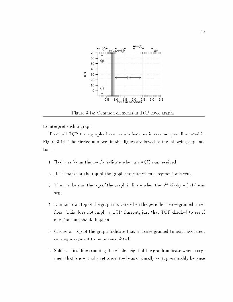
560.5 1.0 1.5 2.0 2.5 3.0 3.5

Time in seconds

0

10

20

30

40

50

60

70

KB

60 120 180

1

2

34

5

6Figure 3.14: Common elements in TCP trace graphs.to interpret such a graph.First, all TCP trace graphs have certain features in common, as illustrated inFigure 3.14. The circled numbers in this �gure are keyed to the following explana-tions:1. Hash marks on the x-axis indicate when an ACK was received.2. Hash marks at the top of the graph indicate when a segment was sent.3. The numbers on the top of the graph indicate when the nth kilobyte (KB) wassent.4. Diamonds on top of the graph indicate when the periodic coarse-grained timer�res. This does not imply a TCP timeout, just that TCP checked to see ifany timeouts should happen.5. Circles on top of the graph indicate that a coarse-grained timeout occurred,causing a segment to be retransmitted.6. Solid vertical lines running the whole height of the graph indicate when a seg-ment that is eventually retransmitted was originally sent, presumably because

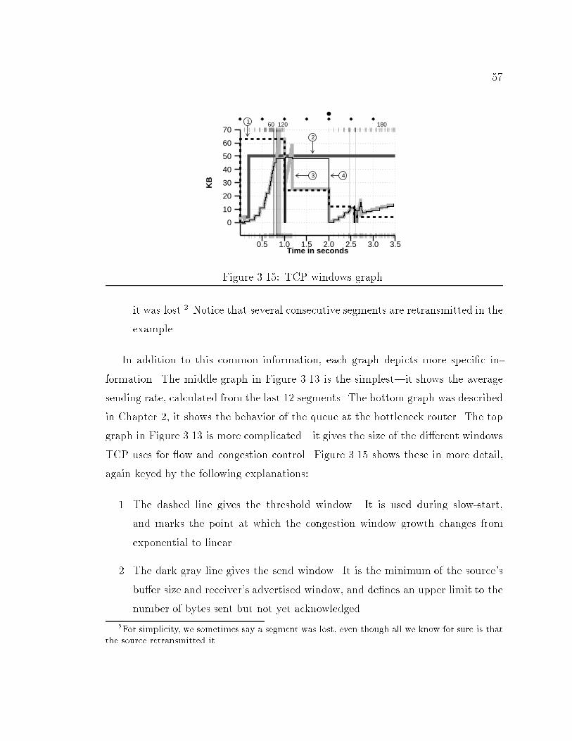
570.5 1.0 1.5 2.0 2.5 3.0 3.5

Time in seconds

0

10

20

30

40

50

60

70

KB

60 120 1801

2

3 4Figure 3.15: TCP windows graph.it was lost.2 Notice that several consecutive segments are retransmitted in theexample.In addition to this common information, each graph depicts more speci�c in-formation. The middle graph in Figure 3.13 is the simplest|it shows the averagesending rate, calculated from the last 12 segments. The bottom graph was describedin Chapter 2, it shows the behavior of the queue at the bottleneck router. The topgraph in Figure 3.13 is more complicated|it gives the size of the di�erent windowsTCP uses for ow and congestion control. Figure 3.15 shows these in more detail,again keyed by the following explanations:1. The dashed line gives the threshold window. It is used during slow-start,and marks the point at which the congestion window growth changes fromexponential to linear.2. The dark gray line gives the send window. It is the minimum of the source'sbu�er size and receiver's advertised window, and de�nes an upper limit to thenumber of bytes sent but not yet acknowledged.2For simplicity, we sometimes say a segment was lost, even though all we know for sure is thatthe source retransmitted it.

583. The light gray line gives the congestion window. It is used for congestioncontrol, and limits the number of bytes sent but not yet acknowledged (UN-ACK COUNT). More speci�cally, a packet will not be sent if the resultingUNACK COUNT is larger than the congestion window.4. The thin line gives the actual number of bytes in transit; that is, those sentbut not yet acknowledged (UNACK COUNT).The graphs just described are obtained from tracing information saved by theprotocol, and are thus available whether the protocol is running in the simulator orover a real network.3.6 Detailed Graph DescriptionTo assist the reader to develop a better understanding of the graphs used throughoutthis paper, and to gain a better insight of Reno's behavior, this section contains adetailed description of one of these graphs. Figure 3.15 is a trace of Reno when thereis other tra�c through the bottleneck router. The numbers in parenthesis refer tothe type of line in the graph.In general, output is allowed while the UNACK COUNT (4) is less than thecongestion window (3) and less than the send window (2). The purpose of thecongestion window is to control congestion. The send window is used for owcontrol; it prevents data from being sent when there is no bu�er space availableat the receiver.The threshold window (1) is set to some maximumvalue|e.g. 64KB| at the be-ginning of the connection. Soon after the connection is started, both sides exchangethe size of their receive bu�ers, and the send window (2) is set to the minimum ofthe source's send bu�er size and the receiver's advertised window size.The congestion window (3) increases exponentially while it is less than the thresh-old window (1). At 0.75 seconds, losses start to occur, as indicated by the tall verticallines. More precisely, the vertical lines represent segments that are later retransmit-ted, usually because they were lost. At around 1.0 second, a loss is detected after

59receiving 3 duplicate ACKs and Reno's Fast Retransmit and Fast Recovery mech-anisms go into action. The purpose of these mechanisms is to detect losses beforea retransmit timeout occurs, and to continue transmitting|although at a reducedrate|while recovering from these losses.The congestion window (3) is set to the maximal allowed segment size for thisconnection and the UNACK COUNT is set to zero momentarily, allowing the lostsegment to be retransmitted. The threshold window (1) is set to half the value thatthe congestion window had before the losses. TCP assumes that this is a safe level,and that losses will not occur at this window size.The congestion window (3) is also set to this value after retransmitting thelost segment, but it increases with each duplicate ACK. Since the receiver sends aduplicate ACK when it receives a segment that it cannot acknowledge because ithas not received all previous data, the reception of a duplicate ACK implies that apacket has left the network.This implies that the congestion window (3) will reach the UNACK COUNT (4)when half the data in transit has been received at the other end. From this point on,the reception of any duplicate ACKs will allow a segment to be sent. This preventsthe \pipe" from becoming empty, and allows TCP to continue sending at half itsprevious rate.Since losses occurred at the previous value, it is assumed that the availablebandwidth is now only half its previous value. Earlier versions of TCP immediatelybegin the slow-start mechanism when losses are detected. This resulted in the\pipe" becoming almost empty and then �lling up again. Reno's mechanism allowsthe \pipe" to stay full.At around 1.2 seconds, a non-duplicate ACK is received, and the congestionwindow (3) is set to the value of the threshold window (1). The congestion windowwas temporarily in ated when duplicate ACKs were received as a mechanism tokeep the pipe full. When a non-duplicate ACK is received, the congestion windowis reset to half the value it had when losses occurred.Since the congestion window (3) is below the UNACK COUNT (4), no more data

60can be sent. At 2 seconds, a retransmit timeout occurs|see black circle on top|anddata starts to ow again. The congestion window (3) increases exponentially whileit is below the threshold window (1). A little before 2.5 seconds, a segment is sentthat will later be retransmitted. Skipping to 3 seconds, one can see the congestionwindow (3) increasing linearly since it is above the threshold window (1).

61CHAPTER 4New Approach to Congestion Detection and AvoidanceThe congestion detection and control mechanisms in TCP Reno|and all othercurrent implementations of TCP|use the loss of segments as a signal that there iscongestion in the network. These implementations have no mechanisms to detect theincipient stages of congestion|before losses occur|so that no attempt is made toprevent loss. These mechanisms are reactive, rather than proactive, in this respect.A preferable mechanism is one that detects the early stages of congestion, suchas increased queue sizes at the bottleneck routers, so that it can slow down thesource and avoid the losses associated with the later stages of congestion. Such amechanism is described in this chapter.The chapter starts by providing an analysis of the behavior of Reno's congestioncontrol mechanism. This is followed by a description of previously proposed con-gestion avoidance mechanisms. Next, it describes a new congestion detection andavoidance mechanism which forms the cornerstone of a new TCP implementation.We call this new implementation TCP Vegas, thereby continuing the practice startedby the BSD distributions of Unix of naming the releases after cities in Nevada. Thechapter concludes by describing other performance improving mechanisms which arealso part of the Vegas implementation.4.1 Analysis of TCP's Congestion Control MechanismAs a consequence of using a reactive congestion control mechanism, Reno needs tocreate losses to �nd that it is exceeding the bandwidth of the connection. This canbe seen in Figure 4.1, which shows the trace of a Reno connection sending 1MB ofdata over the network con�guration seen in Figure 4.2, with no other tra�c sources;i.e., only Host1a sending to Host1b. In this case, the router queue size is 10, each

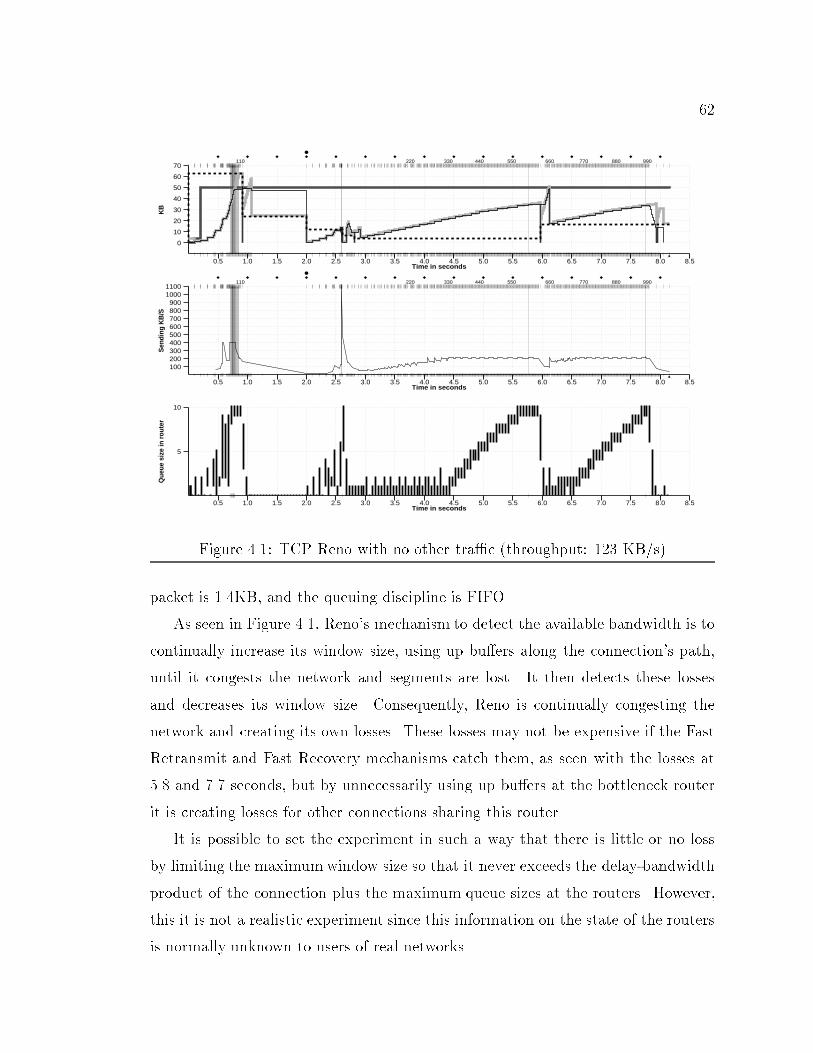
620.5 1.0 1.5 2.0 2.5 3.0 3.5 4.0 4.5 5.0 5.5 6.0 6.5 7.0 7.5 8.0 8.5

Time in seconds

0

10

20

30

40

50

60

70K

B110 220 330 440 550 660 770 880 990

0.5 1.0 1.5 2.0 2.5 3.0 3.5 4.0 4.5 5.0 5.5 6.0 6.5 7.0 7.5 8.0 8.5Time in seconds

100200300400500600700800900

10001100

Sen

ding

KB

/S

110 220 330 440 550 660 770 880 990

0.5 1.0 1.5 2.0 2.5 3.0 3.5 4.0 4.5 5.0 5.5 6.0 6.5 7.0 7.5 8.0 8.5Time in seconds

5

10

Que

ue s

ize

in r

oute

r Figure 4.1: TCP Reno with no other tra�c (throughput: 123 KB/s)packet is 1.4KB, and the queuing discipline is FIFO.As seen in Figure 4.1, Reno's mechanism to detect the available bandwidth is tocontinually increase its window size, using up bu�ers along the connection's path,until it congests the network and segments are lost. It then detects these lossesand decreases its window size. Consequently, Reno is continually congesting thenetwork and creating its own losses. These losses may not be expensive if the FastRetransmit and Fast Recovery mechanisms catch them, as seen with the losses at5.8 and 7.7 seconds, but by unnecessarily using up bu�ers at the bottleneck routerit is creating losses for other connections sharing this router.It is possible to set the experiment in such a way that there is little or no lossby limiting the maximumwindow size so that it never exceeds the delay-bandwidthproduct of the connection plus the maximum queue sizes at the routers. However,this it is not a realistic experiment since this information on the state of the routersis normally unknown to users of real networks.

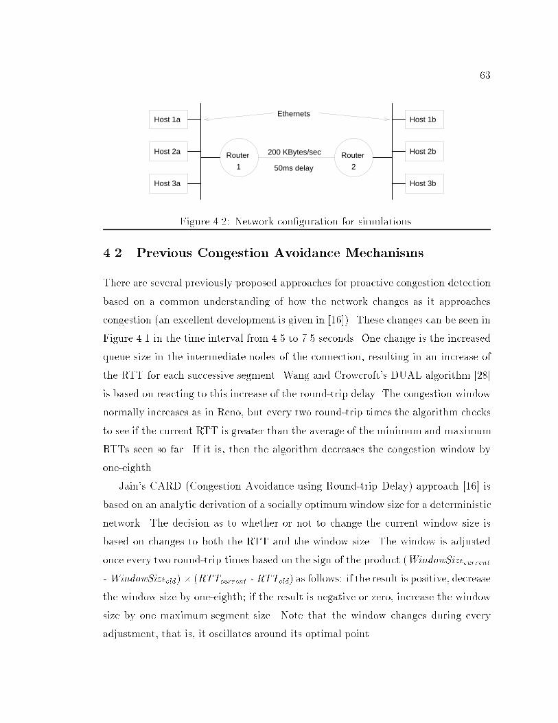
63Router

2

Router

1

Host 1a

Host 2a

Host 3a Host 3b

Host 2b

Host 1b

50ms delay

200 KBytes/sec

EthernetsFigure 4.2: Network con�guration for simulations.4.2 Previous Congestion Avoidance MechanismsThere are several previously proposed approaches for proactive congestion detectionbased on a common understanding of how the network changes as it approachescongestion (an excellent development is given in [16]). These changes can be seen inFigure 4.1 in the time interval from 4.5 to 7.5 seconds. One change is the increasedqueue size in the intermediate nodes of the connection, resulting in an increase ofthe RTT for each successive segment. Wang and Crowcroft's DUAL algorithm [28]is based on reacting to this increase of the round-trip delay. The congestion windownormally increases as in Reno, but every two round-trip times the algorithm checksto see if the current RTT is greater than the average of the minimum and maximumRTTs seen so far. If it is, then the algorithm decreases the congestion window byone-eighth.Jain's CARD (Congestion Avoidance using Round-trip Delay) approach [16] isbased on an analytic derivation of a socially optimumwindow size for a deterministicnetwork. The decision as to whether or not to change the current window size isbased on changes to both the RTT and the window size. The window is adjustedonce every two round-trip times based on the sign of the product (WindowSizecurrent- WindowSizeold)� (RTTcurrent - RTTold) as follows: if the result is positive, decreasethe window size by one-eighth; if the result is negative or zero, increase the windowsize by one maximum segment size. Note that the window changes during everyadjustment, that is, it oscillates around its optimal point.

64Another change seen as the network approaches congestion is the attening ofthe sending rate. Wang and Crowcroft's Tri-S scheme [27] takes advantage of thisfact. Every RTT, they increase the window size by one segment and compare thethroughput achieved to the throughput when the window was one segment smaller.If the di�erence is less than one-half the throughput achieved when only one segmentwas in transit|as was the case at the beginning of the connection|they decreasethe window by one segment. Tri-S calculates the throughput by dividing the numberof bytes outstanding in the network (UNACK COUNT) by the RTT.A �nal congestion avoidance mechanism is Keshav's Packet Pair mechanism [20].As the name implies, this mechanism sends a pair of packets, one immediately afterthe other, and uses the spacing of the acknowledgments to determine the availablebandwidth; see Figure 3.6.As described in the original papers, these mechanisms have weaknesses whichmake them unsuitable for current networks. As a matter of fact, none of thesemechanisms was ever tested on a real network. DUAL uses individual measurementsof the RTT to determine if the congestion window should increase or decrease. Thismechanism works well in the simple queueing networks in which it was tested, butbreaks down in real networks where the RTT is highly variable.CARD continually changes the window size and measures the e�ect this has onthe RTT. Based on this e�ect the window will be either increased or decreased.For example, a window size increase (WindowSizecurrent - WindowSizeold > 0) whichdoes not increase the RTT results in a further increase of the window. CARD su�ersfrom the same weakness described in the previous paragraph|it uses individualmeasurements of the RTT.As long as no losses are detected, Tri-S can either increase its window size, orleave it unchanged by decreasing it right after it was increased. As a result, Tri-Scannot adapt to decreases in the available bandwidth unless the decrease is so largethat it results in packet losses. That is, Tri-S cannot avoid congestion created byincreasing background tra�c levels.The spacing of acknowledgments in Packet Pair can be easily lost when there is

65tra�c in the network. For example, the �rst acknowledgment may be delayed in arouter by encountering a large queue at that router. If the second acknowledgmentis not delayed by a similar amount, the spacing between them cannot be used todetermine the available bandwidth. As a result, Packet Pair can only be used innetworks where all routers use queueing disciplines that preserve the spacing|suchas Fair Queueing [8].4.3 Congestion Avoidance in VegasVegas's approach is most similar to Tri-S in that it looks at changes in the through-put rate, or more speci�cally, changes in the sending rate. However, it di�ers fromTri-S in the way it calculates throughput and instead of looking for a change inthe throughput slope, it compares the measured throughput rate with an expectedthroughput rate. The basis for this idea can be seen in Figure 4.1 in the region be-tween 3.0 and 5.5 seconds. As the window size increases one expects the throughput(or sending rate) to also increase. But the throughput cannot increase beyond theavailable bandwidth; beyond this point, any increase in the window size only resultsin the segments taking up bu�er space at the bottleneck router.Vegas uses this idea to measure and control the amount of extra data this con-nection has in transit; that is, data that would not have been sent if the bandwidthused by the connection exactly matched the available bandwidth of the network.The goal of Vegas is to maintain the \right" amount of extra data in the network.Obviously, if a connection is sending too much extra data, it will end up distributedover system bu�ers and cause congestion. Less obviously, if a connection is sendingtoo little extra data, it cannot respond rapidly enough to transient increases in theavailable network bandwidth. Vegas's congestion avoidance actions are based onchanges in the estimated amount of extra data in the network, and not only ondropped segments.We now describe the algorithm in detail. Note that the algorithm is not in e�ectduring slow-start. Vegas's behavior during slow-start is described in Section 4.4.First, de�ne a given connection's BaseRTT to be the RTT of a segment when

66the connection is not congested. In practice, Vegas sets BaseRTT to the minimumof all measured round trip times; it is commonly the RTT of the �rst segmentsent by the connection, before the router queues increase due to tra�c generatedby this connection. Although we do not know the exact value for the BaseRTT,our experience suggests our algorithm is not sensitive to errors in the BaseRTT.Assuming the connection is not over owing the link, the expected throughput isgiven by: Expected = WindowSize / BaseRTTwhereWindowSize is the size of the current congestion window, assumed to be equalto the number of bytes in transit.Second, Vegas calculates the current Actual sending rate. This is done by record-ing the sending time for a distinguished segment, recording how many bytes aretransmitted between the time that segment is sent and its acknowledgment is re-ceived, computing the RTT for the distinguished segment when its acknowledgmentarrives, and dividing the number of bytes transmitted by this RTT. This calculationis done once per round-trip time.Third, Vegas compares Actual to Expected, and adjusts the window accordingly.Let Di� = Expected - Actual. Note that Di� is positive or zero by de�nition, sinceActual > Expected implies the need to change BaseRTT to the latest sampled RTT.Also de�ne two thresholds, � < � roughly corresponding to having too little andtoo much extra data in the network, respectively. When Di� � �, Vegas increasesthe congestion window linearly during the next RTT, and when Di� � �, Vegasdecreases the congestion window linearly during the next RTT. Vegas leaves thecongestion window unchanged when � < Di� < �.Intuitively, the farther away the actual throughput gets from the expectedthroughput, the more congestion there is in the network, which implies that thesending rate should be reduced. The � threshold triggers this decrease. On theother hand, if the bottleneck router queue is empty (no congestion), any transient|lasting less than one RTT|increase in the available bandwidth will be wasted since

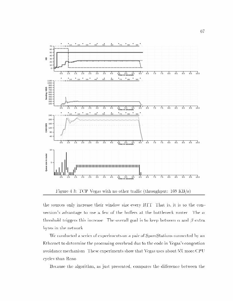
670.5 1.0 1.5 2.0 2.5 3.0 3.5 4.0 4.5 5.0 5.5 6.0 6.5 7.0 7.5 8.0 8.5 9.0 9.5 10.0

Time in seconds

0

10

20

30

40

50

60

70K

B110 220 330 440 550 660 770 880 990

0.5 1.0 1.5 2.0 2.5 3.0 3.5 4.0 4.5 5.0 5.5 6.0 6.5 7.0 7.5 8.0 8.5 9.0 9.5 10.0Time in seconds

100200300400500600700800900

10001100

Sen

ding

KB

/S

110 220 330 440 550 660 770 880 990

0.5 1.0 1.5 2.0 2.5 3.0 3.5 4.0 4.5 5.0 5.5 6.0 6.5 7.0 7.5 8.0 8.5 9.0 9.5 10.0Time in seconds

40

80

120

160

200

240

CA

M K

B/S

110 220 330 440 550 660 770 880 990

0.5 1.0 1.5 2.0 2.5 3.0 3.5 4.0 4.5 5.0 5.5 6.0 6.5 7.0 7.5 8.0 8.5 9.0 9.5 10.0Time in seconds

5

10

Que

ue s

ize

in r

oute

r Figure 4.3: TCP Vegas with no other tra�c (throughput: 169 KB/s).the sources only increase their window size every RTT. That is, it is to the con-nection's advantage to use a few of the bu�ers at the bottleneck router. The �threshold triggers this increase. The overall goal is to keep between � and � extrabytes in the network.We conducted a series of experiments on a pair of SparcStations connected by anEthernet to determine the processing overhead due to the code in Vegas's congestionavoidance mechanism. These experiments show that Vegas uses about 5%more CPUcycles than Reno.Because the algorithm, as just presented, compares the di�erence between the

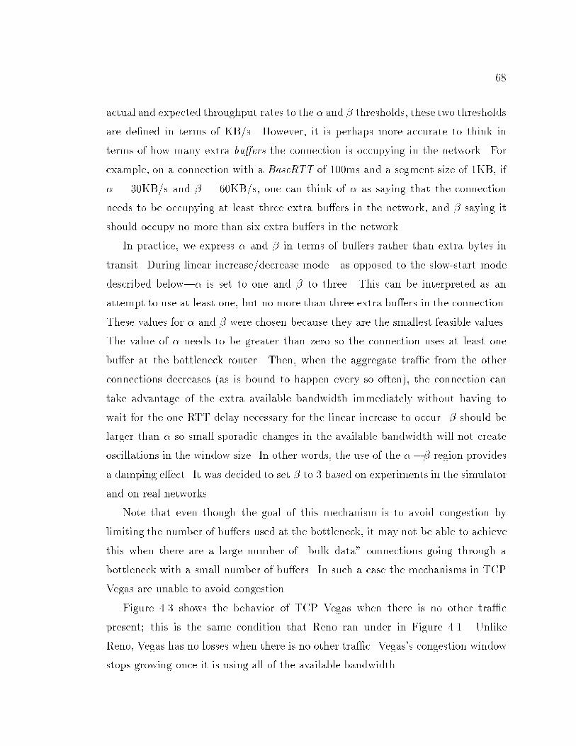
68actual and expected throughput rates to the � and � thresholds, these two thresholdsare de�ned in terms of KB/s. However, it is perhaps more accurate to think interms of how many extra bu�ers the connection is occupying in the network. Forexample, on a connection with a BaseRTT of 100ms and a segment size of 1KB, if� = 30KB/s and � = 60KB/s, one can think of � as saying that the connectionneeds to be occupying at least three extra bu�ers in the network, and � saying itshould occupy no more than six extra bu�ers in the network.In practice, we express � and � in terms of bu�ers rather than extra bytes intransit. During linear increase/decrease mode|as opposed to the slow-start modedescribed below|� is set to one and � to three. This can be interpreted as anattempt to use at least one, but no more than three extra bu�ers in the connection.These values for � and � were chosen because they are the smallest feasible values.The value of � needs to be greater than zero so the connection uses at least onebu�er at the bottleneck router. Then, when the aggregate tra�c from the otherconnections decreases (as is bound to happen every so often), the connection cantake advantage of the extra available bandwidth immediately without having towait for the one RTT delay necessary for the linear increase to occur. � should belarger than � so small sporadic changes in the available bandwidth will not createoscillations in the window size. In other words, the use of the ��� region providesa damping e�ect. It was decided to set � to 3 based on experiments in the simulatorand on real networks.Note that even though the goal of this mechanism is to avoid congestion bylimiting the number of bu�ers used at the bottleneck, it may not be able to achievethis when there are a large number of \bulk data" connections going through abottleneck with a small number of bu�ers. In such a case the mechanisms in TCPVegas are unable to avoid congestion.Figure 4.3 shows the behavior of TCP Vegas when there is no other tra�cpresent; this is the same condition that Reno ran under in Figure 4.1. UnlikeReno, Vegas has no losses when there is no other tra�c. Vegas's congestion windowstops growing once it is using all of the available bandwidth.

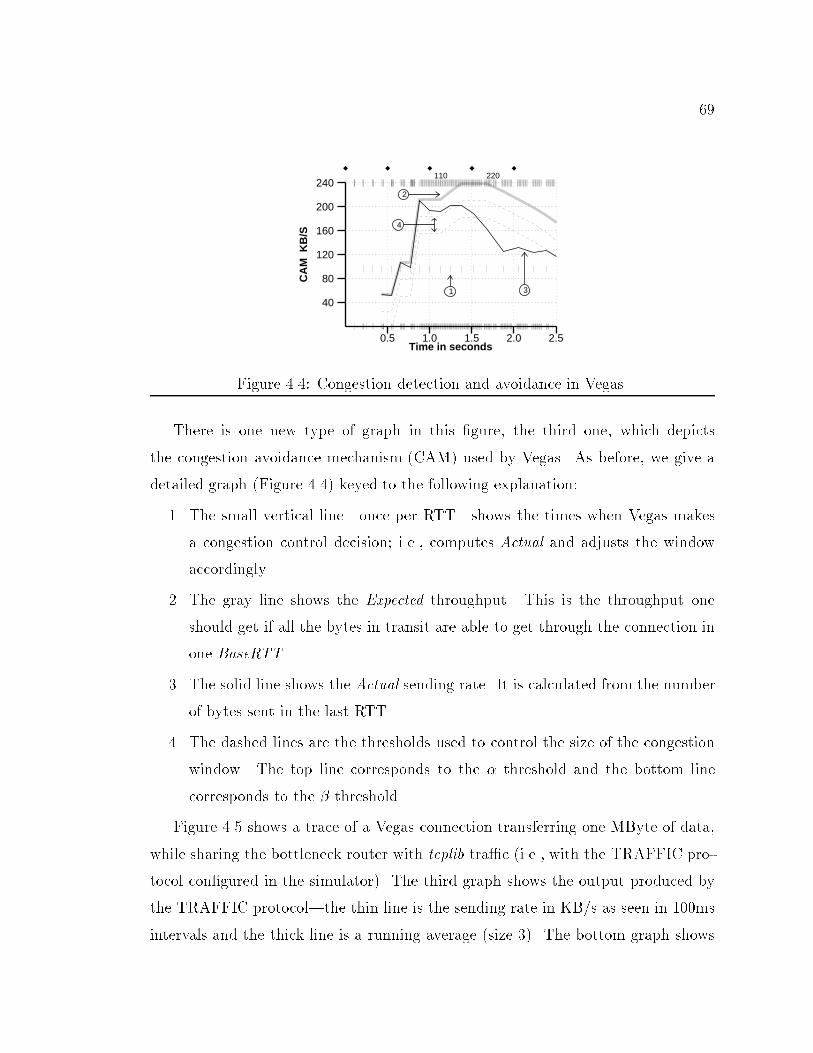
690.5 1.0 1.5 2.0 2.5

Time in seconds

40

80

120

160

200

240

CA

M K

B/S

110 220

1

2

3

4

Figure 4.4: Congestion detection and avoidance in Vegas.There is one new type of graph in this �gure, the third one, which depictsthe congestion avoidance mechanism (CAM) used by Vegas. As before, we give adetailed graph (Figure 4.4) keyed to the following explanation:1. The small vertical line|once per RTT|shows the times when Vegas makesa congestion control decision; i.e., computes Actual and adjusts the windowaccordingly.2. The gray line shows the Expected throughput. This is the throughput oneshould get if all the bytes in transit are able to get through the connection inone BaseRTT.3. The solid line shows the Actual sending rate. It is calculated from the numberof bytes sent in the last RTT.4. The dashed lines are the thresholds used to control the size of the congestionwindow. The top line corresponds to the � threshold and the bottom linecorresponds to the � threshold.Figure 4.5 shows a trace of a Vegas connection transferring one MByte of data,while sharing the bottleneck router with tcplib tra�c (i.e., with the TRAFFIC pro-tocol con�gured in the simulator). The third graph shows the output produced bythe TRAFFIC protocol|the thin line is the sending rate in KB/s as seen in 100msintervals and the thick line is a running average (size 3). The bottom graph shows

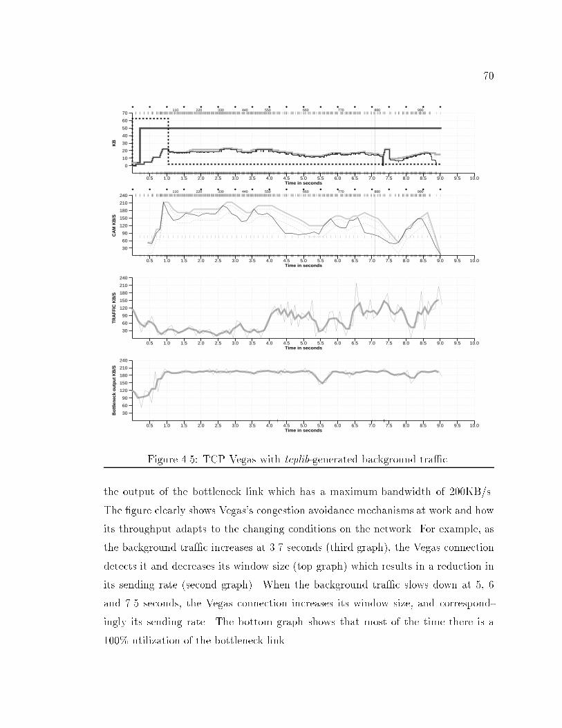
700.5 1.0 1.5 2.0 2.5 3.0 3.5 4.0 4.5 5.0 5.5 6.0 6.5 7.0 7.5 8.0 8.5 9.0 9.5 10.0

Time in seconds

0

10

20

30

40

50

60

70K

B110 220 330 440 550 660 770 880 990

0.5 1.0 1.5 2.0 2.5 3.0 3.5 4.0 4.5 5.0 5.5 6.0 6.5 7.0 7.5 8.0 8.5 9.0 9.5 10.0Time in seconds

30

60

90

120

150

180

210

240

CA

M K

B/S

110 220 330 440 550 660 770 880 990

0.5 1.0 1.5 2.0 2.5 3.0 3.5 4.0 4.5 5.0 5.5 6.0 6.5 7.0 7.5 8.0 8.5 9.0 9.5 10.0Time in seconds

30

60

90

120

150

180

210

240

TRA

FFIC

KB

/S

0.5 1.0 1.5 2.0 2.5 3.0 3.5 4.0 4.5 5.0 5.5 6.0 6.5 7.0 7.5 8.0 8.5 9.0 9.5 10.0Time in seconds

30

60

90

120

150

180

210

240

Bot

tlene

ck o

utpu

t KB

/S Figure 4.5: TCP Vegas with tcplib-generated background tra�c.the output of the bottleneck link which has a maximum bandwidth of 200KB/s.The �gure clearly shows Vegas's congestion avoidance mechanisms at work and howits throughput adapts to the changing conditions on the network. For example, asthe background tra�c increases at 3.7 seconds (third graph), the Vegas connectiondetects it and decreases its window size (top graph) which results in a reduction inits sending rate (second graph). When the background tra�c slows down at 5, 6and 7.5 seconds, the Vegas connection increases its window size, and correspond-ingly its sending rate. The bottom graph shows that most of the time there is a100% utilization of the bottleneck link.

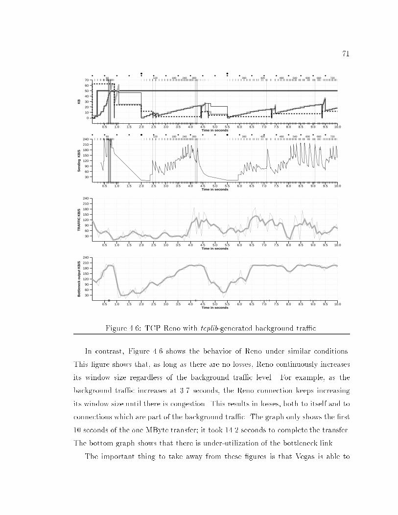
710.5 1.0 1.5 2.0 2.5 3.0 3.5 4.0 4.5 5.0 5.5 6.0 6.5 7.0 7.5 8.0 8.5 9.0 9.5 10.0

Time in seconds

0

10

20

30

40

50

60

70K

B60 120 180 240 300 360 420 480 540 600 660 720

0.5 1.0 1.5 2.0 2.5 3.0 3.5 4.0 4.5 5.0 5.5 6.0 6.5 7.0 7.5 8.0 8.5 9.0 9.5 10.0Time in seconds

30

60

90

120

150

180

210

240

Sen

ding

KB

/S

60 120 180 240 300 360 420 480 540 600 660 720

0.5 1.0 1.5 2.0 2.5 3.0 3.5 4.0 4.5 5.0 5.5 6.0 6.5 7.0 7.5 8.0 8.5 9.0 9.5 10.0Time in seconds

30

60

90

120

150

180

210

240

TRA

FFIC

KB

/S

0.5 1.0 1.5 2.0 2.5 3.0 3.5 4.0 4.5 5.0 5.5 6.0 6.5 7.0 7.5 8.0 8.5 9.0 9.5 10.0Time in seconds

30

60

90

120

150

180

210

240

Bot

tlene

ck o

utpu

t KB

/S Figure 4.6: TCP Reno with tcplib-generated background tra�c.In contrast, Figure 4.6 shows the behavior of Reno under similar conditions.This �gure shows that, as long as there are no losses, Reno continuously increasesits window size regardless of the background tra�c level. For example, as thebackground tra�c increases at 3.7 seconds, the Reno connection keeps increasingits window size until there is congestion. This results in losses, both to itself and toconnections which are part of the background tra�c. The graph only shows the �rst10 seconds of the one MByte transfer; it took 14.2 seconds to complete the transfer.The bottom graph shows that there is under-utilization of the bottleneck link.The important thing to take away from these �gures is that Vegas is able to

72make better utilization of the bottleneck link than Reno. In other words, and thisis discussed further in Section 6.4, Vegas's increased throughput is not a resultof its taking bandwidth away from Reno connections, but due to a more e�cientutilization of the bottleneck link. In fact, Reno connections do slightly better whenthe background tra�c is running on top of Vegas as compared to when the tra�cis running on top of Reno1.4.4 Congestion Avoidance During Slow-StartAs mentioned in the previous chapter, the slow-start mechanism in TCP will con-tinue until the window reaches a preset maximum or when losses occur. Since thereis usually not enough information to determine the right preset maximum duringthe initial slow-start, slow-start continues the exponential growth of the congestionwindow until it results in large packet losses|see Figure 4.1. Later occurrences ofslow-start have enough information to set the maximum: they set it to half the sizethe congestion window had when losses occurred.What is needed is a way to �nd a connection's available bandwidth which doesnot incur these losses. Towards this end, the congestion avoidance mechanism wasincorporated into slow-start with only minor modi�cations. To be able to detect andavoid congestion during slow-start, Vegas allows exponential growth only every otherRTT. In between, the congestion window stays �xed so that a valid comparison ofthe expected and actual rates can be made. When the actual rate falls below theexpected rate by the equivalent of one router bu�er, Vegas changes from slow-startmode to the linear increase/decrease mode|described in the previous section|toprevent packet losses.The behavior of the Vegas's slow-start mechanism can be seen in Figure 4.3and Figure 4.5. Vegas's slow-start mechanism is highly successful at preventing thelosses incurred during Reno's initial slow-start period (see Chapter 5).Two problems remain during any slow-start period. First, segments are sent at1Remember that the background tra�c is generated by a protocol (TRAFFIC) that runs ontop of TCP.

73a rate higher than the available bandwidth|up to twice the available bandwidth,depending on the ACKing frequency (e.g., every segment or every two segments).This causes the bottleneck router to bu�er up to half of the data sent on each RTT,thereby increasing the likelihood of losses during the slow-start period. Moreover,as network speeds increase, so does the amount of bu�ering needed. Second, whileVegas's congestion avoidance mechanism during the initial slow-start period is quitee�ective, it can still overshoot the available bandwidth, and depends on enoughbu�ering at the bottleneck router to prevent losses until realizing it needs to slowdown. Speci�cally, if the connection can handle a particular window size, then Vegaswill double that window size|and as a consequence, double the sending rate|onthe next RTT. At some point the available bandwidth will be exceeded.We have experimented with a solution to both problems. To simplify the fol-lowing discussion, we refer to the alternative version of Vegas with an experimentalslow-start mechanism as Vegas*. Vegas* is based on using the spacing of the ac-knowledgments to gauge the available bandwidth. The idea is similar to Keshav'sPacket-Pair probing mechanism [20], except that it uses the average spacing be-tween four segments sent during the slow-start period rather than the spacing fromtwo segments. Looking at four segments results in a more robust algorithm thanlooking at two because we can use the average of three values rather than justone value. This available bandwidth estimate is used to set the threshold windowwith an appropriate value, which makes Vegas* less likely to overshoot the availablebandwidth.Speci�cally, as each ACK is received, Vegas* schedules an event at a certain pointin the future, based on its available bandwidth estimate, to increase the congestionwindow by one maximum segment size. This is in contrast to increasing the windowimmediately upon receiving the ACK. For example, assume the RTT is 100ms,the maximum segment size is 1 KByte, and the available bandwidth estimate iscurrently 200 KB/s. During the slow-start period, time is divided into intervalsof length equal to one RTT. If 4 ACKs are expected to arrive during the currentRTT interval, Vegas* uses the bandwidth estimate (200KB/s) to guess the spacing

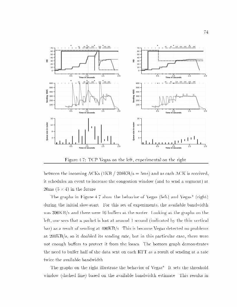
740.5 1.0 1.5 2.0

Time in seconds

0

10

20

30

40

50

60

70K

B40 80 120 160 200 240 280

0.5 1.0 1.5 2.0Time in seconds

100

200

300

400

500

600

Sen

ding

KB

/S

40 80 120 160 200 240 280

0.5 1.0 1.5 2.0Time in seconds

4

8

12

16

Que

ue s

ize

in r

oute

r

0.5 1.0 1.5 2.0Time in seconds

0

10

20

30

40

50

60

70

KB

40 80 120 160 200 240 280

0.5 1.0 1.5 2.0Time in seconds

100

200

300

400

500

600

Sen

ding

KB

/S

40 80 120 160 200 240 280

0.5 1.0 1.5 2.0Time in seconds

4

8

12

16

Que

ue s

ize

in r

oute

rFigure 4.7: TCP Vegas on the left, experimental on the right.between the incoming ACKs (1KB / 200KB/s = 5ms) and as each ACK is received,it schedules an event to increase the congestion window (and to send a segment) at20ms (5� 4) in the future.The graphs in Figure 4.7 show the behavior of Vegas (left) and Vegas* (right)during the initial slow-start. For this set of experiments, the available bandwidthwas 300KB/s and there were 16 bu�ers at the router. Looking at the graphs on theleft, one sees that a packet is lost at around 1 second (indicated by the thin verticalbar) as a result of sending at 400KB/s. This is because Vegas detected no problemsat 200KB/s, so it doubled its sending rate, but in this particular case, there werenot enough bu�ers to protect it from the losses. The bottom graph demonstratesthe need to bu�er half of the data sent on each RTT as a result of sending at a ratetwice the available bandwidth.The graphs on the right illustrate the behavior of Vegas*. It sets the thresholdwindow (dashed line) based on the available bandwidth estimate. This results in

75the congestion window halting its exponential growth at the right time|when thesending rate equals the available bandwidth and preventing the losses. The middlegraph shows that the sending rate never exceeds the available bandwidth (300KB/s)bymuch. Finally, the bottom graph shows that Vegas* does not need as many bu�ersas Vegas.Notice that while the available bandwidth estimate could be used to jump im-mediately to the available bandwidth by using rate control during one RTT interval,congestion can result if more than one connection does this at the same time. Eventhough it is possible to congest the network if more than one connection does slow-start at the same time, there is an upper bound on the number of bytes sent duringthe RTT when congestion occurs regardless of the number of connections simulta-neously doing slow-start|about twice the number of bytes that can be handled bythe connection. There is no such limit if more than one connection tries to usethe available bandwidth at once. Hence, we strongly recommend against doing thisunless it is known a priori that there are no other connections sharing the path, orif there are, that they will not increase their sending rate at the same time.Although these traces illustrate how Vegas*'s experimental slow-start mechanismdoes in fact address the two problems with Vegas outlined above, simulation dataindicates that the new mechanismdoes not have a measurable impact on throughput,and only marginally improves the loss rate. While additional simulations mightexpose situations where Vegas* is more bene�cial, we have decided to not includethese modi�cations in Vegas. The results presented in Chapter 5 are for Vegas, notVegas*.4.5 Other Mechanisms in TCP VegasAs mentioned earlier, Reno uses two mechanisms to detect and then retransmitlost segments. The �rst mechanism is the retransmit timeout. It determines atimeout interval based on round trip time (RTT) and variance estimates computedby sampling the time between when a segment is sent and an ACK arrives. If asegment is not acknowledged within the timeout interval, it is presumed lost and is

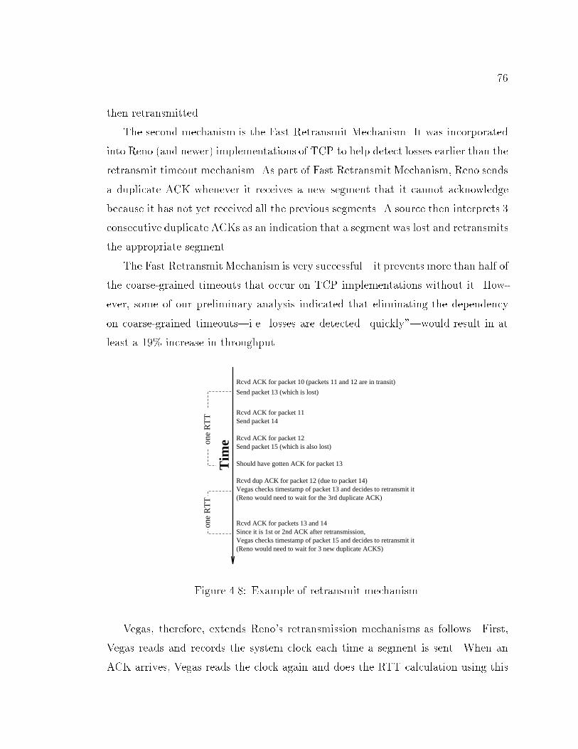
76then retransmitted.The second mechanism is the Fast Retransmit Mechanism. It was incorporatedinto Reno (and newer) implementations of TCP to help detect losses earlier than theretransmit timeout mechanism. As part of Fast Retransmit Mechanism, Reno sendsa duplicate ACK whenever it receives a new segment that it cannot acknowledgebecause it has not yet received all the previous segments. A source then interprets 3consecutive duplicate ACKs as an indication that a segment was lost and retransmitsthe appropriate segment.The Fast Retransmit Mechanism is very successful|it prevents more than half ofthe coarse-grained timeouts that occur on TCP implementations without it. How-ever, some of our preliminary analysis indicated that eliminating the dependencyon coarse-grained timeouts|i.e. losses are detected \quickly"|would result in atleast a 19% increase in throughput.T

imeon

e R

TT

one

RT

T

Rcvd ACK for packet 10 (packets 11 and 12 are in transit)

Send packet 13 (which is lost)

Rcvd ACK for packet 11Send packet 14

Rcvd ACK for packet 12Send packet 15 (which is also lost)

Should have gotten ACK for packet 13

Rcvd dup ACK for packet 12 (due to packet 14)Vegas checks timestamp of packet 13 and decides to retransmit it(Reno would need to wait for the 3rd duplicate ACK)

Rcvd ACK for packets 13 and 14Since it is 1st or 2nd ACK after retransmission,Vegas checks timestamp of packet 15 and decides to retransmit it(Reno would need to wait for 3 new duplicate ACKS)Figure 4.8: Example of retransmit mechanism.Vegas, therefore, extends Reno's retransmission mechanisms as follows. First,Vegas reads and records the system clock each time a segment is sent. When anACK arrives, Vegas reads the clock again and does the RTT calculation using this

77time and the timestamp recorded for the relevant segment. Vegas then uses thismore accurate RTT estimate to decide to retransmit in the following two situations(a simple example is given in Figure 4.8).� When a duplicate ACK is received, Vegas checks to see if the di�erence be-tween the current time and the timestamp recorded for the relevant segmentis greater than the timeout value. If it is, then Vegas retransmits the segmentwithout having to wait for n (3) duplicate ACKs. In many cases, losses areeither so great or the window so small that the source will never receive threeduplicate ACKs, and therefore, Reno has to rely on the coarse-grained timeoutmentioned above.� When a non-duplicate ACK is received, if it is the �rst or second one after aretransmission, Vegas again checks to see if the time interval since the segmentwas sent is larger than the timeout value. If it is, then Vegas retransmits thesegment. This will catch any other segment that may have been lost prior tothe retransmission without having to wait for a duplicate ACK.In other words, Vegas treats the receipt of certain ACKs as a hint to check ifa timeout should occur. Since it only checks for timeouts in rare occasions, theoverhead is small. Notice that even though one could reduce the number of duplicateACKs used to trigger the Fast Retransmit from 3 duplicate ACKs to either 2 or 1,it is not recommended as it could result in many unnecessary retransmissions andbecause it makes assumptions about the likelihood that packets will be deliveredout of order.The goal of the new retransmission mechanism is not just to reduce the time todetect lost packets from the third duplicate ACK to the �rst or second duplicateACK|a small savings|but to detect lost packets in cases where there is no secondor third duplicate ACK. The new mechanism is very successful at achieving thisgoal, as it further reduces the number of coarse-grained timeouts in Reno by morethan half. Note that Vegas contains Reno's coarse-grained timeout code in case thenew mechanisms fail to recognize a lost segment.

78Related to making timeouts more timely, notice that the congestion windowshould only be reduced due to losses that happened at the current sending rate, andnot due to losses that happened at an earlier, higher rate. In Reno, it is possibleto decrease the congestion window more than once for losses that occurred duringone RTT interval[9]. In contrast, Vegas decreases the congestion window only ifthe retransmitted segment was previously sent after the last decrease. Any lossesthat happened before the last window decrease do not imply that the network iscongested for the current congestion window size, and therefore, do not imply thatit should be decreased again. This change is needed because Vegas detects lossesmuch sooner than Reno.

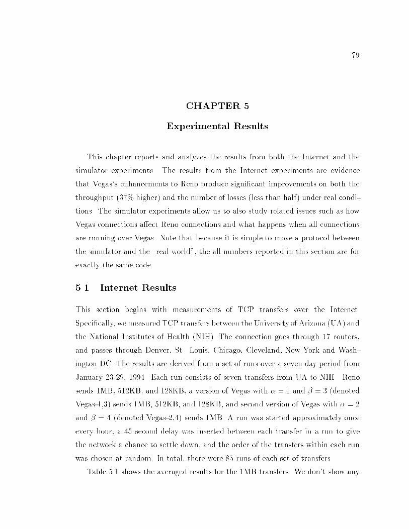
79CHAPTER 5Experimental ResultsThis chapter reports and analyzes the results from both the Internet and thesimulator experiments. The results from the Internet experiments are evidencethat Vegas's enhancements to Reno produce signi�cant improvements on both thethroughput (37% higher) and the number of losses (less than half) under real condi-tions. The simulator experiments allow us to also study related issues such as howVegas connections a�ect Reno connections and what happens when all connectionsare running over Vegas. Note that because it is simple to move a protocol betweenthe simulator and the \real world", the all numbers reported in this section are forexactly the same code.5.1 Internet ResultsThis section begins with measurements of TCP transfers over the Internet.Speci�cally, we measured TCP transfers between the University of Arizona (UA) andthe National Institutes of Health (NIH). The connection goes through 17 routers,and passes through Denver, St. Louis, Chicago, Cleveland, New York and Wash-ington DC. The results are derived from a set of runs over a seven day period fromJanuary 23-29, 1994. Each run consists of seven transfers from UA to NIH|Renosends 1MB, 512KB, and 128KB, a version of Vegas with � = 1 and � = 3 (denotedVegas-1,3) sends 1MB, 512KB, and 128KB, and second version of Vegas with � = 2and � = 4 (denoted Vegas-2,4) sends 1MB. A run was started approximately onceevery hour, a 45 second delay was inserted between each transfer in a run to givethe network a chance to settle down, and the order of the transfers within each runwas chosen at random. In total, there were 85 runs of each set of transfers.Table 5.1 shows the averaged results for the 1MB transfers. We don't show any

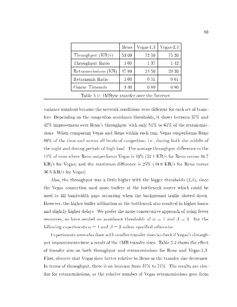
80Reno Vegas-1,3 Vegas-2,4Throughput (KB/s) 53.00 72.50 75.30Throughput Ratio 1.00 1.37 1.42Retransmissions (KB) 47.80 24.50 29.30Retransmit Ratio 1.00 0.51 0.61Coarse Timeouts 3.30 0.80 0.90Table 5.1: 1MByte transfer over the Internet.variance numbers because the network conditions were di�erent for each set of trans-fers. Depending on the congestion avoidance thresholds, it shows between 37% and42% improvement over Reno's throughput with only 51% to 61% of the retransmis-sions. When comparing Vegas and Reno within each run, Vegas outperforms Reno89% of the time and across all levels of congestion; i.e., during both the middle ofthe night and during periods of high load. The average throughput di�erence in the11% of runs where Reno outperforms Vegas is 10% (52.1 KB/s for Reno versus 46.7KB/s for Vegas) and the maximum di�erence is 25% (49.0 KB/s for Reno versus36.5 KB/s for Vegas).Also, the throughput was a little higher with the bigger thresholds (2,4), sincethe Vegas connection used more bu�ers at the bottleneck router which could beused to �ll bandwidth gaps occurring when the background tra�c slowed down.However, the higher bu�er utilization at the bottleneck also resulted in higher lossesand slightly higher delays. We prefer the more conservative approach of using fewerresources, so have settled on avoidance thresholds of � = 1 and � = 3. For thefollowing experiments � = 1 and � = 3 unless speci�ed otherwise.Experiments were also done with smaller transfer sizes to check if Vegas's through-put improvements were a result of the 1MB transfer sizes. Table 5.2 shows the e�ectof transfer size on both throughput and retransmissions for Reno and Vegas-1,3.First, observe that Vegas does better relative to Reno as the transfer size decreases.In terms of throughput, there is an increase from 37% to 71%. The results are sim-ilar for retransmissions, as the relative number of Vegas retransmissions goes from

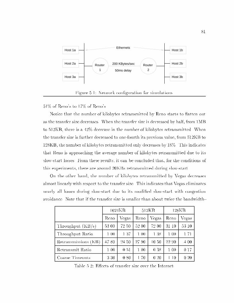
81Router

2

Router

1

Host 1a

Host 2a

Host 3a Host 3b

Host 2b

Host 1b

50ms delay

200 KBytes/sec

EthernetsFigure 5.1: Network con�guration for simulations.51% of Reno's to 17% of Reno's.Notice that the number of kilobytes retransmitted by Reno starts to atten outas the transfer size decreases. When the transfer size is decreased by half, from 1MBto 512KB, there is a 42% decrease in the number of kilobytes retransmitted. Whenthe transfer size is further decreased to one-fourth its previous value, from 512KB to128KB, the number of kilobytes retransmitted only decreases by 18%. This indicatesthat Reno is approaching the average number of kilobytes retransmitted due to itsslow-start losses. From these results, it can be concluded that, for the conditions ofthis experiments, there are around 20KBs retransmitted during slow-start.On the other hand, the number of kilobytes retransmitted by Vegas decreasesalmost linearly with respect to the transfer size. This indicates that Vegas eliminatesnearly all losses during slow-start due to its modi�ed slow-start with congestionavoidance. Note that if the transfer size is smaller than about twice the bandwidth-1024KB 512KB 128KBReno Vegas Reno Vegas Reno VegasThroughput (KB/s) 53.00 72.50 52.00 72.00 31.10 53.10Throughput Ratio 1.00 1.37 1.00 1.38 1.00 1.71Retransmissions (KB) 47.80 24.50 27.90 10.50 22.90 4.00Retransmit Ratio 1.00 0.51 1.00 0.38 1.00 0.17Coarse Timeouts 3.30 0.80 1.70 0.20 1.10 0.20Table 5.2: E�ects of transfer size over the Internet.

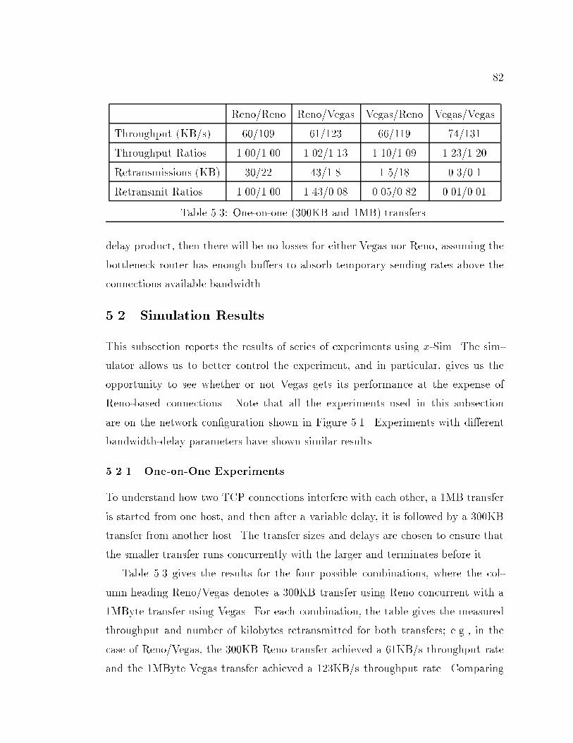
82Reno/Reno Reno/Vegas Vegas/Reno Vegas/VegasThroughput (KB/s) 60/109 61/123 66/119 74/131Throughput Ratios 1.00/1.00 1.02/1.13 1.10/1.09 1.23/1.20Retransmissions (KB) 30/22 43/1.8 1.5/18 0.3/0.1Retransmit Ratios 1.00/1.00 1.43/0.08 0.05/0.82 0.01/0.01Table 5.3: One-on-one (300KB and 1MB) transfers.delay product, then there will be no losses for either Vegas nor Reno, assuming thebottleneck router has enough bu�ers to absorb temporary sending rates above theconnections available bandwidth.5.2 Simulation ResultsThis subsection reports the results of series of experiments using x-Sim. The sim-ulator allows us to better control the experiment, and in particular, gives us theopportunity to see whether or not Vegas gets its performance at the expense ofReno-based connections. Note that all the experiments used in this subsectionare on the network con�guration shown in Figure 5.1. Experiments with di�erentbandwidth-delay parameters have shown similar results.5.2.1 One-on-One ExperimentsTo understand how two TCP connections interfere with each other, a 1MB transferis started from one host, and then after a variable delay, it is followed by a 300KBtransfer from another host. The transfer sizes and delays are chosen to ensure thatthe smaller transfer runs concurrently with the larger and terminates before it.Table 5.3 gives the results for the four possible combinations, where the col-umn heading Reno/Vegas denotes a 300KB transfer using Reno concurrent with a1MByte transfer using Vegas. For each combination, the table gives the measuredthroughput and number of kilobytes retransmitted for both transfers; e.g., in thecase of Reno/Vegas, the 300KB Reno transfer achieved a 61KB/s throughput rateand the 1MByte Vegas transfer achieved a 123KB/s throughput rate. Comparing

83the small transfer to the large transfer in any given column is not meaningful becausethe large transfer was able to run by itself during most of the test. Small transfersshould only be compared to other small transfers (similarly with large transfers).The ratios for both throughput rate and kilobytes retransmitted are relative to theReno/Reno column. The values in the table are averages from 12 runs, using 15and 20 bu�ers in the routers, and with the delay before starting the smaller transferranging between 0 and 2.5 seconds.The main thing to take away from these numbers is that Vegas does not ad-versely a�ect Reno's throughput. Reno's throughput changes very little when it iscompeting with Vegas rather than itself|the ratios for Reno are 1.02 and 1.09 forReno/Vegas and Vegas/Reno, respectively. Also, when Reno competes with Vegasrather than itself, the combined number of kilobytes retransmitted for the pair ofcompeting connections drops signi�cantly. The combined Reno/Reno retransmitsare 52KB compared with 45KB for Reno/Vegas and 19KB for Vegas/Reno. Fi-nally, note that the combined Vegas/Vegas retransmits are less than 1KB on theaverage|an indication that the congestion avoidance mechanism is working.The 43% increase in the losses of Reno for the Reno/Vegas case is explained asfollows. The Vegas connection starts �rst, and is using the full bandwidth (200KB/s)by the time the Reno connection starts. When Vegas detects that the network isstarting to get congested, it decreases its sending rate to between 80 and 100KB/s.The losses incurred by Reno (about 48KB), are approximately the losses Reno ex-periences when it is running by itself on a network with 100 to 120KB/s of availablebandwidth and around 15 available bu�ers at the bottleneck router. The reason thelosses where smaller for the 300KB transfer in the Reno/Reno experiment is that bythe time the 300KB transfer starts, the 1MB connection has stopped transmittingdue to the losses in its slow-start, and it will not start sending again until it timesout at around 2 seconds. A Reno connection sending 300KB when there is 200KB/sof available bandwidth and 20 bu�ers at the bottleneck router only losses about3KB.This type of behavior is characteristic of Reno: by slightly changing the param-

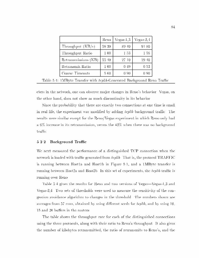
84Reno Vegas-1,3 Vegas-2,4Throughput (KB/s) 58.30 89.40 91.80Throughput Ratio 1.00 1.53 1.58Retransmissions (KB) 55.40 27.10 29.40Retransmit Ratio 1.00 0.49 0.53Coarse Timeouts 5.60 0.90 0.90Table 5.4: 1MByte Transfer with tcplib-Generated Background Reno Tra�c.eters in the network, one can observe major changes in Reno's behavior. Vegas, onthe other hand, does not show as much discontinuity in its behavior.Since the probability that there are exactly two connections at one time is smallin real life, the experiment was modi�ed by adding tcplib background tra�c. Theresults were similar except for the Reno/Vegas experiment in which Reno only hada 6% increase in its retransmission, versus the 43% when there was no backgroundtra�c.5.2.2 Background Tra�cWe next measured the performance of a distinguished TCP connection when thenetwork is loaded with tra�c generated from tcplib. That is, the protocol TRAFFICis running between Host1a and Host1b in Figure 5.1, and a 1MByte transfer isrunning between Host2a and Host2b. In this set of experiments, the tcplib tra�c isrunning over Reno.Table 5.4 gives the results for Reno and two versions of Vegas|Vegas-1,3 andVegas-2,4. Two sets of thresholds were used to measure the sensitivity of the con-gestion avoidance algorithm to changes in the threshold. The numbers shown areaverages from 57 runs, obtained by using di�erent seeds for tcplib, and by using 10,15 and 20 bu�ers in the routers.The table shows the throughput rate for each of the distinguished connectionsusing the three protocols, along with their ratio to Reno's throughput. It also givesthe number of kilobytes retransmitted, the ratio of retransmits to Reno's, and the

85average number of coarse-grained timeouts per transfer. For example, Vegas-1,3 had53% better throughput than Reno, with only 49% of the losses. Again note thatthere is little di�erence between Vegas-1,3 and Vegas-2,4.These simulations tell us the expected improvement of Vegas over Reno: morethan 50% improvement on throughput, and only half the losses. The results fromthe one-on-one experiments indicate that the gains of Vegas are not made at theexpense of Reno; this belief is further supported by the fact that the backgroundtra�c's throughput is mostly una�ected by the type of connection doing the 1Mbytetransfer.The tests were rerun using Vegas for the background tra�c instead of Reno.These experiments simulate the situation where the whole world uses Vegas. Thethroughput and the kilobytes retransmitted by the 1MByte transfers (Reno andVegas) did not change signi�cantly (less than 4%) as compared to the previousexperiment.5.2.3 Other ExperimentsVariations of the previous experiments showed similar results, except when TCP'ssend-bu�er size was changed. Below is a summary of these experiments and theirresults.There have been reports of change in TCP's behavior when the backgroundtra�c is two-way rather than one-way [30], so tcplib tra�c was added from Host3bto Host3a. The throughput ratio stayed the same, but the loss ratio was muchbetter: 0.29. Reno resent more data and Vegas remained about the same. The factthat there was little change is probably due to the fact that tcplib already createssome 2-way tra�c|Telnet connections send one byte and get one or more bytesback, and FTP connections send and get control packets before doing a transfer.For all the experiments reported so far, TCP's send-bu�er size was set to 50KB.Experiments were also done with send-bu�er sizes between 50KB and 5KB. Vegas'sthroughput and losses stayed unchanged between 50KB and 20KB; from that pointon, as the bu�er decreased, so did the throughput. This was due to the protocol

86not being able to keep the pipe full.Reno's throughput initially increased as the bu�ers got smaller, and then itdecreased. It always remained under the throughput measured for Vegas. We havepreviously seen this type of behavior while running Reno on the Internet. Figure 4.1shows that as Reno increases its congestion window, it uses more and more bu�ersin the router until it loses packets by overruning the queue. Limiting the congestionwindow by reducing the size of the send-bu�er may prevent it from overrunning therouter's queue.5.3 Other Evaluation CriteriaThroughput and losses are not the only metrics by which a transport protocol isevaluated. This section discusses several other issues that must be addressed.5.3.1 FairnessIf there is more than one connection sharing a bottleneck link, one would like foreach connection to receive an equal share of the bandwidth. Unfortunately, given thelimited amount of information currently available at the connection endpoints, thisis unlikely to happen without some help from the routers. Given that no protocol islikely to be perfectly fair, one needs a way to decide whether its level of fairness isacceptable or not. Given that so far the Internet community has found Reno's levelof fairness acceptable, it was decided to compare Vegas's fairness levels to Reno'sand judge it in those terms.Jain's fairness index [17] is used as the metric. It is de�ned as follows: given aset of throughputs (x1; x2; : : : ; xn) the following function assigns a fairness index tothe set: f(x1; x2; : : : ; xn) = (Pni=1 xi)2nPni=1 x2i = (E[X])2E[X2] !For all nonnegative numbers, it follows by Jensen's Inequality (E[X2] � (E[X])2)that the fairness index always results in numbers between 0 and 1. If all throughputsare the same, the fairness index is 1. If only k of the n users receive equal throughput

87and the remaining n � k users receive zero throughput, the fairness index is k=n(large dispersion implies small index).We ran simulations with 2, 4 and 16 connections sharing a bottleneck link,where all the connections either had the same propagation delay, or where one halfof the connections had twice the propagation delay of the other half. Many di�erentpropagation delays were used, and the results averaged.In the case of 2 and 4 connections, with each connection transferring 8 MB, Renowas slightly more fair than Vegas when all connections had the same propagationdelay (0.993 vs. 0.989), but Vegas was slightly more fair than Reno when thepropagation delay was larger for half of the connections (0.962 vs. 0.953). In theexperiments with 16 connections, with each connection transferring 2MB, Vegas wasmore fair than Reno in all experiments regardless of whether the propagation delayswere the same or not (0.972 vs. 0.921).To study the e�ect that Reno connections have on Vegas connections (and viceversa) we ran 8 connections, each sending 2 MB of data. The experiment consistedof running all the connections on top of Reno, all the connections on top of Vegas,or one half on top on Reno and the other half on top of Vegas. There was littledi�erence between the fairness index of the eight connections running a particularTCP implementation (Vegas or Reno) and the fairness index of the four connectionsrunning the same TCP implementation and sharing the bottleneck with the fourconnections running the other TCP implementation. Similarly, there was littledi�erence in the average size of the bottleneck queue.In another experiment, four connections ran over background tra�c. For thisexperiment, Vegas was always more fair than Reno. Overall, we conclude that Vegasis no less fair than Reno.5.3.2 StabilityA second concern is stability|it is undesirable for a protocol to cause the Internetto collapse as the number of connections increases. In other words, as the loadincreases, each connection must recognize that it should decrease its sending rate.

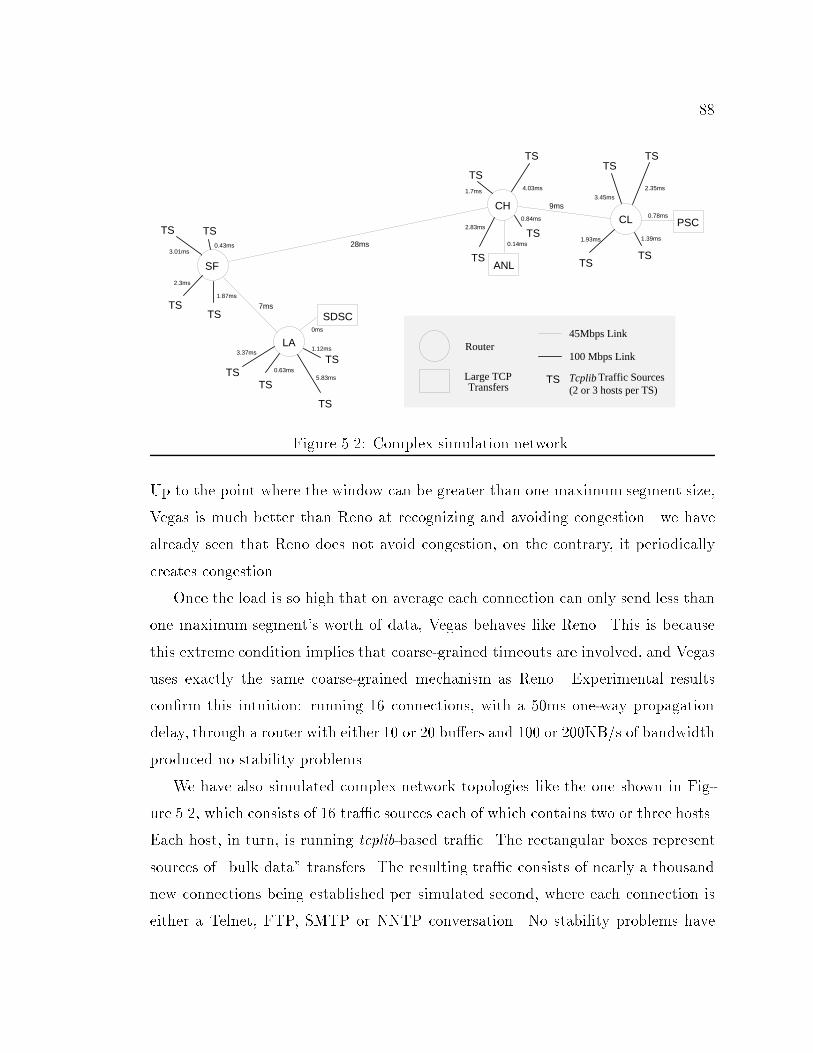
88Router

Large TCP Transfers

TS

100 Mbps Link

45Mbps Link

Tcplib Traffic Sources(2 or 3 hosts per TS)

28ms

9ms

7ms

5.83ms

1.12ms

0ms

0.63ms

3.37ms

3.01ms0.43ms

2.3ms

1.87ms

4.03ms

2.83ms

1.7ms

1.93ms

3.45ms

2.35ms

1.39ms

0.78ms0.84ms

0.14ms

TS

TSTS

TS

TSTS

TS TS

TS

TS

TS

TSTS

TSTS

TS

SDSC

ANL

PSC

LA

SF

CHCL

Figure 5.2: Complex simulation network.Up to the point where the window can be greater than one maximum segment size,Vegas is much better than Reno at recognizing and avoiding congestion|we havealready seen that Reno does not avoid congestion, on the contrary, it periodicallycreates congestion.Once the load is so high that on average each connection can only send less thanone maximum segment's worth of data, Vegas behaves like Reno. This is becausethis extreme condition implies that coarse-grained timeouts are involved, and Vegasuses exactly the same coarse-grained mechanism as Reno. Experimental resultscon�rm this intuition: running 16 connections, with a 50ms one-way propagationdelay, through a router with either 10 or 20 bu�ers and 100 or 200KB/s of bandwidthproduced no stability problems.We have also simulated complex network topologies like the one shown in Fig-ure 5.2, which consists of 16 tra�c sources each of which contains two or three hosts.Each host, in turn, is running tcplib-based tra�c. The rectangular boxes representsources of \bulk data" transfers. The resulting tra�c consists of nearly a thousandnew connections being established per simulated second, where each connection iseither a Telnet, FTP, SMTP or NNTP conversation. No stability problems have

89occurred in any of our simulations when all of the connections are running Vegas.Intuitively, there is no reason to expect Vegas to lead to network collapse. Onereason for this is that most of Vegas's mechanisms are conservative in nature|itscongestion window never increases faster than Reno's (one maximum segment perRTT), the purpose of the congestion avoidance mechanism is to decrease the conges-tion window before losses occur, and during slow-start, Vegas stops the exponentialgrowth of its congestion window before Reno would under the same conditions.5.3.3 DelayGiven that Vegas purposely tries to occupy between one and three extra bu�ersalong the path for each connection, it seems possible that persistent queues couldform at the bottleneck router if the whole world ran Vegas. These persistent queueswould, in turn, add to the latency of all connections that crossed that router.Since the analytical tools currently available are not good enough to realisticallymodel and analyze the behavior of either Reno or Vegas, we must rely on simula-tions to answer this issue. Our simulations show that average queue sizes underReno and Vegas are approximately the same. However, they also show that Telnetconnections in tcplib experience between 18 and 40% less delay, on average, when allthe connections are Vegas instead of Reno. This seems to suggest that if the wholeworld ran Vegas, Internet delay would not be adversely a�ected.5.4 DiscussionWe conclude this chapter with a discussion of issues that are relevant to the processof evaluating the practical value of TCP Vegas. It also comments on the relation-ship between this work and other e�orts to improve end-to-end performance on theInternet.5.4.1 BSD VariationsTCP has been a rather uid protocol over the last several years, especially in itscongestion control mechanism. Although the general form the original mechanism

90described in [13] has remained unchanged in all BSD-based implementations (e.g.,Tahoe, Reno, BNR2, BSD 4.4), many of the \constants" have changed. For example,some implementations ACK every segment and some ACK every other segment;some increase the window during linear growth by one segment per RTT and someincrease by half a segment per RTT plus 1/8th the maximum segment size per ACKreceived during that RTT; and �nally, some use the timestamp option and some donot.We have experimented with most of these variations and have found the com-bination used in the x-kernel implementation of TCP Reno to be the among themost e�ective. For example, the latest version of TCP, that found in BSD 4.4-lite,achieves 14% worse throughput than the x-kernel's implementation of TCP Renoduring Internet type simulations (see Chapter 6).5.4.2 Alternative ApproachesIn addition to improving TCP's congestion control mechanism, there is a large bodyof research addressing the general question of how to fairly and e�ectively allocateresources in the Internet.One example gaining much attention is the question of how to guarantee band-width to real-time connections. The basic approach requires that a more intelligentbu�er manager be placed in the Internet routers [2]. One might question the rele-vance of TCP Vegas in light of such mechanisms. We believe end-to-end congestioncontrol will remain very important for two reasons. First, a signi�cant fraction ofthe data that will ow over the Internet will not be of a real-time nature; it will bebulk-transfer applications (e.g., image transfer) that want as much bandwidth as iscurrently available. These transfers will be able to use Vegas to compete againsteach other for the available bandwidth. Second, even for a real-time connection, itwould not be unreasonable for an application to request (and pay for) a minimallyacceptable bandwidth guarantee, and then use a Vegas-like end-to-end mechanismto acquire as much additional bandwidth as the current load allows.As another example, selective ACKs [14, 15] (as opposed to cumulative ACKs)

91have been proposed as a way to decrease the number of unnecessarily retransmittedpackets and to provide information for a better retransmit mechanism than theone in Reno. Although the selective ACK mechanism is not yet well de�ned, wemake the following observations about how it compares to Vegas. First, it onlyrelates to Vegas's retransmission mechanism; selective ACKs by themselves a�ectneither the congestion nor the the slow-start mechanisms. Second, there is littlereason to believe that selective ACKs can signi�cantly improve on Vegas in terms ofunnecessary retransmissions, as there were only 6KB per MB (0.6%)unnecessarilyretransmitted by Vegas in the Internet experiments. Third, selective ACKs havethe potential to retransmit lost data sooner on future networks with large delay-bandwidth products. It would be interesting to see how Vegas and the selectiveACK mechanism work in tandem on such networks. Finally, we note that selectiveACKs require a change to the TCP standard, whereas the Vegas modi�cations arean implementation change that is isolated to the sender.5.4.3 Independent ValidationAn important part of experimental science is the validation of results by independentparties. Peter Danzig's group at the University of Southern California published apaper [1] con�rming that TCP Vegas yields higher network throughput and transfersbytes more e�ciently than TCP Reno. Their Internet experiments showed thatVegas achieved between 20 and 300% higher throughput depending on the TCPversion implemented on the receiving host. With Reno receivers, Vegas sourcesaveraged 20% higher throughput than Reno sources; with Tahoe receivers, Vegassources averaged 300% higher throughput than Reno sources. This is a signi�cantresult, as Danzig points out that most receivers in the Internet are running Tahoeimplementations of TCP. Their experiments also show that with 90% con�denceVegas retransmits fewer segments|1/5th as many retransmissions|and lowers RTTaverage and variance.

92CHAPTER 6Experiences with x-SimThe simulator and its tools are an important contribution of this work. Theability of x-Sim to run real protocol code allows us to analyze existing protocolimplementations under realistic conditions. This is an important feature of the sim-ulator, as newer implementations of protocols not only include desirable features butalso sometimes introduce performance bugs. The �rst half of this chapter documentsour experiences analyzing the latest BSD implementation of TCP. This analysis un-covered serious performance problems with this implementation of TCP and led tosolutions, which when implemented, increased its performance by more than 20%.Although there are excellent books on simulation providing good general guide-lines, it is not clear how to map these guidelines to the area of network simulation.Furthermore, just as important as the guidelines is being able to quantify the ef-fect of ignoring them. The second half of this chapter provides a set of guidelinesfor network simulation and provides examples that help to quantify the result ofignoring them.6.1 Analysis of BSD4.4-Lite TCPThis section presents a case study illustrating how to do performance debugging withx-Sim. While the work with TCP Vegas was underway, a new BSD implementationof TCP|TCP Lite|was released. We ported this release to the x-kernel with thegoal of comparing its performance to that of x-kernel's implementation of TCPReno and TCP Vegas. Early simulation results showed that TCP Lite performedsigni�cantly worse than TCP Reno, the TCP implementation used to measure thebene�ts of using TCP Vegas. In one simple simulation scenario|when no othertra�c is present|TCP Reno sends one MByte of data in 8.2 seconds (123 KB/s)

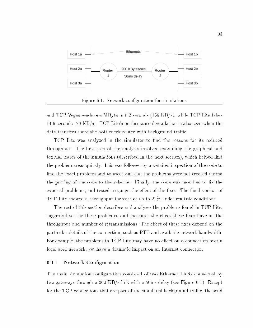
93Router

2

Router

1

Host 1a

Host 2a

Host 3a Host 3b

Host 2b

Host 1b

50ms delay

200 KBytes/sec

EthernetsFigure 6.1: Network con�guration for simulations.and TCP Vegas sends one MByte in 6.2 seconds (166 KB/s), while TCP Lite takes14.6 seconds (70 KB/s). TCP Lite's performance degradation is also seen when thedata transfers share the bottleneck router with background tra�c.TCP Lite was analyzed in the simulator to �nd the reasons for its reducedthroughput. The �rst step of the analysis involved examining the graphical andtextual traces of the simulations (described in the next section), which helped �ndthe problem areas quickly. This was followed by a detailed inspection of the code to�nd the exact problems and to ascertain that the problems were not created duringthe porting of the code to the x-kernel. Finally, the code was modi�ed to �x theexposed problems, and tested to gauge the e�ect of the �xes. The �xed version ofTCP Lite showed a throughput increase of up to 21% under realistic conditions.The rest of this section describes and analyses the problems found in TCP Lite,suggests �xes for these problems, and measures the e�ect these �xes have on thethroughput and number of retransmissions. The e�ect of these �xes depend on theparticular details of the connection, such as RTT and available network bandwidth.For example, the problems in TCP Lite may have no e�ect on a connection over alocal area network, yet have a dramatic impact on an Internet connection.6.1.1 Network Con�gurationThe main simulation con�guration consisted of two Ethernet LANs connected bytwo gateways through a 200 KB/s link with a 50ms delay (see Figure 6.1). Exceptfor the TCP connections that are part of the simulated background tra�c, the send

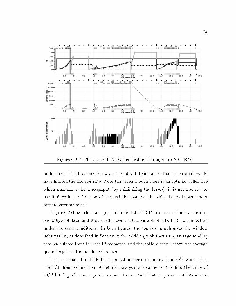
941.0 2.0 3.0 4.0 5.0 6.0 7.0 8.0 9.0 10.0 11.0 12.0 13.0 14.0 15.0

Time in seconds

0

20

40

60

80

100K

B110 220 330 440 550 660 770 880 990

1.0 2.0 3.0 4.0 5.0 6.0 7.0 8.0 9.0 10.0 11.0 12.0 13.0 14.0 15.0Time in seconds

250

500

750

1000

1250

1500

Sen

ding

KB

/S

110 220 330 440 550 660 770 880 990

1.0 2.0 3.0 4.0 5.0 6.0 7.0 8.0 9.0 10.0 11.0 12.0 13.0 14.0 15.0Time in seconds

5

10

Que

ue s

ize

in r

oute

r Figure 6.2: TCP Lite with No Other Tra�c (Throughput: 70 KB/s).bu�er in each TCP connection was set to 50KB. Using a size that is too small wouldhave limited the transfer rate. Note that even though there is an optimal bu�er sizewhich maximizes the throughput (by minimizing the losses), it is not realistic touse it since it is a function of the available bandwidth, which is not known undernormal circumstances.Figure 6.2 shows the trace graph of an isolated TCP Lite connection transferringone Mbyte of data, and Figure 6.3 shows the trace graph of a TCP Reno connectionunder the same conditions. In both �gures, the topmost graph gives the windowinformation, as described in Section 2; the middle graph shows the average sendingrate, calculated from the last 12 segments; and the bottom graph shows the averagequeue length at the bottleneck router.In these tests, the TCP Lite connection performs more than 70% worse thanthe TCP Reno connection. A detailed analysis was carried out to �nd the cause ofTCP Lite's performance problems, and to ascertain that they were not introduced

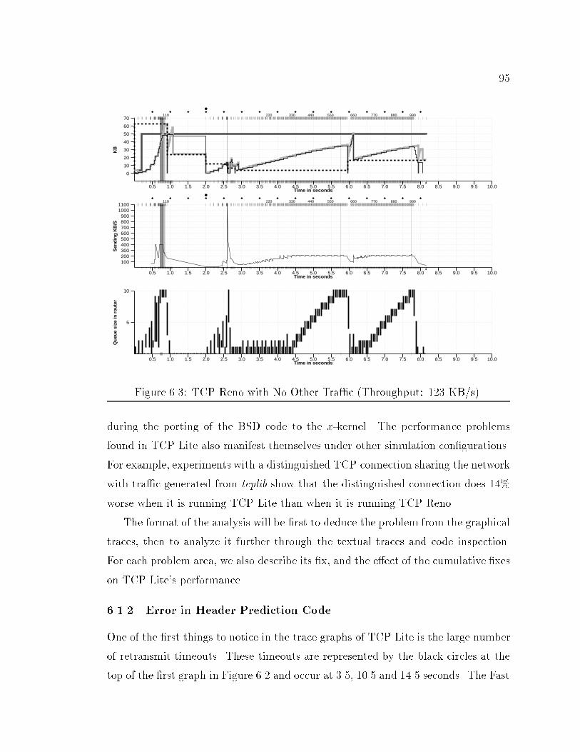
950.5 1.0 1.5 2.0 2.5 3.0 3.5 4.0 4.5 5.0 5.5 6.0 6.5 7.0 7.5 8.0 8.5 9.0 9.5 10.0

Time in seconds

0

10

20

30

40

50

60

70K

B110 220 330 440 550 660 770 880 990

0.5 1.0 1.5 2.0 2.5 3.0 3.5 4.0 4.5 5.0 5.5 6.0 6.5 7.0 7.5 8.0 8.5 9.0 9.5 10.0Time in seconds

100200300400500600700800900

10001100

Sen

ding

KB

/S

110 220 330 440 550 660 770 880 990

0.5 1.0 1.5 2.0 2.5 3.0 3.5 4.0 4.5 5.0 5.5 6.0 6.5 7.0 7.5 8.0 8.5 9.0 9.5 10.0Time in seconds

5

10

Que

ue s

ize

in r

oute

r Figure 6.3: TCP Reno with No Other Tra�c (Throughput: 123 KB/s).during the porting of the BSD code to the x-kernel. The performance problemsfound in TCP Lite also manifest themselves under other simulation con�gurations.For example, experiments with a distinguished TCP connection sharing the networkwith tra�c generated from tcplib show that the distinguished connection does 14%worse when it is running TCP Lite than when it is running TCP Reno.The format of the analysis will be �rst to deduce the problem from the graphicaltraces, then to analyze it further through the textual traces and code inspection.For each problem area, we also describe its �x, and the e�ect of the cumulative �xeson TCP Lite's performance.6.1.2 Error in Header Prediction CodeOne of the �rst things to notice in the trace graphs of TCP Lite is the large numberof retransmit timeouts. These timeouts are represented by the black circles at thetop of the �rst graph in Figure 6.2 and occur at 3.5, 10.5 and 14.5 seconds. The Fast

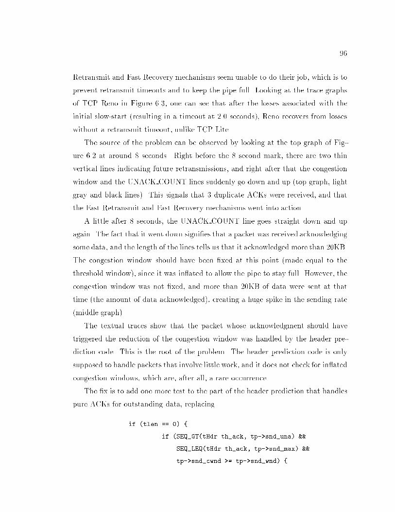
96Retransmit and Fast Recovery mechanisms seem unable to do their job, which is toprevent retransmit timeouts and to keep the pipe full. Looking at the trace graphsof TCP Reno in Figure 6.3, one can see that after the losses associated with theinitial slow-start (resulting in a timeout at 2.0 seconds), Reno recovers from losseswithout a retransmit timeout, unlike TCP Lite.The source of the problem can be observed by looking at the top graph of Fig-ure 6.2 at around 8 seconds. Right before the 8 second mark, there are two thinvertical lines indicating future retransmissions, and right after that the congestionwindow and the UNACK COUNT lines suddenly go down and up (top graph, lightgray and black lines). This signals that 3 duplicate ACKs were received, and thatthe Fast Retransmit and Fast Recovery mechanisms went into action.A little after 8 seconds, the UNACK COUNT line goes straight down and upagain. The fact that it went down signi�es that a packet was received acknowledgingsome data, and the length of the lines tells us that it acknowledged more than 20KB.The congestion window should have been �xed at this point (made equal to thethreshold window), since it was in ated to allow the pipe to stay full. However, thecongestion window was not �xed, and more than 20KB of data were sent at thattime (the amount of data acknowledged), creating a huge spike in the sending rate(middle graph).The textual traces show that the packet whose acknowledgment should havetriggered the reduction of the congestion window was handled by the header pre-diction code. This is the root of the problem. The header prediction code is onlysupposed to handle packets that involve little work, and it does not check for in atedcongestion windows, which are, after all, a rare occurrence.The �x is to add one more test to the part of the header prediction that handlespure ACKs for outstanding data, replacingif (tlen == 0) {if (SEQ_GT(tHdr.th_ack, tp->snd_una) &&SEQ_LEQ(tHdr.th_ack, tp->snd_max) &&tp->snd_cwnd >= tp->snd_wnd) {

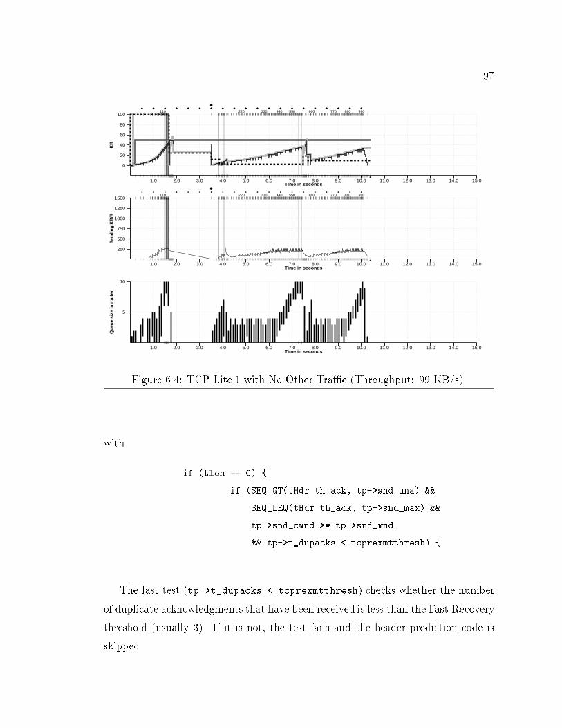
971.0 2.0 3.0 4.0 5.0 6.0 7.0 8.0 9.0 10.0 11.0 12.0 13.0 14.0 15.0

Time in seconds

0

20

40

60

80

100K

B110 220 330 440 550 660 770 880 990

1.0 2.0 3.0 4.0 5.0 6.0 7.0 8.0 9.0 10.0 11.0 12.0 13.0 14.0 15.0Time in seconds

250

500

750

1000

1250

1500

Sen

ding

KB

/S

110 220 330 440 550 660 770 880 990

1.0 2.0 3.0 4.0 5.0 6.0 7.0 8.0 9.0 10.0 11.0 12.0 13.0 14.0 15.0Time in seconds

5

10

Que

ue s

ize

in r

oute

r Figure 6.4: TCP Lite.1 with No Other Tra�c (Throughput: 99 KB/s).with if (tlen == 0) {if (SEQ_GT(tHdr.th_ack, tp->snd_una) &&SEQ_LEQ(tHdr.th_ack, tp->snd_max) &&tp->snd_cwnd >= tp->snd_wnd&& tp->t_dupacks < tcprexmtthresh) {The last test (tp->t_dupacks < tcprexmtthresh) checks whether the numberof duplicate acknowledgments that have been received is less than the Fast Recoverythreshold (usually 3). If it is not, the test fails and the header prediction code isskipped.

98The behavior of TCP Lite with this �x (Lite.1) is shown in Figure 6.4. Eventhough the performance increases considerably for this speci�c simulation, whereTCP is running by itself (no background tra�c), there is an average 2% decreasein throughput|as compared to the original implementation of TCP Lite| on themore complex simulations which also include tcplib tra�c. The reason why Lite.0(the original version) performs better than Lite.1 when there is background tra�cis as follows. The e�ect of the problem|not �xing the congestion window size afterlosses|is proportional to the window size when the losses occur. When TCP Liteis running by itself, it has a large window when the losses occur, and the problemcauses a congestion window that is large enough to result in losses and a timeout.When TCP Lite is sharing the bandwidth with background tra�c, its window sizeis much smaller, and the problem causes a congestion window that is not largeenough to result in losses. Furthermore, it turns out that the larger congestionwindow size can partially neutralize the problem described in Section 4.5: undersome circumstances, TCP decreases its congestion window more than necessary.These results help to illustrate just how complex and nonintuitive TCP behaviorcan be.6.1.3 Suboptimal Retransmit Timeout EstimatesThe retransmission timeout value (RTO) calculation in TCP Lite closely followsthe code described in the updated version of Jacobson's '88 paper[13]. The RTO isbased on a, an average round-trip time (RTT) estimator, and d, a mean deviationestimator of the RTT, as follows: rto a+ 4dGiven m, a new RTT measurement, the estimators are updated as follows:Err � m� aa a+ g0Errd d + g1(jErrj � d)

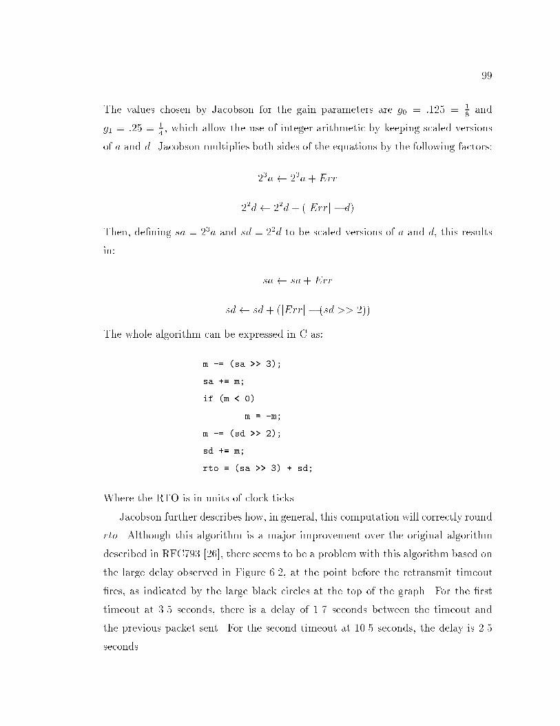
99The values chosen by Jacobson for the gain parameters are g0 = :125 = 18 andg1 = :25 = 14 , which allow the use of integer arithmetic by keeping scaled versionsof a and d. Jacobson multiplies both sides of the equations by the following factors:23a 23a+ Err22d 22d+ (jErrj � d)Then, de�ning sa = 23a and sd = 22d to be scaled versions of a and d, this resultsin: sa sa+ Errsd sd + (jErrj � (sd >> 2))The whole algorithm can be expressed in C as:m -= (sa >> 3);sa += m;if (m < 0)m = -m;m -= (sd >> 2);sd += m;rto = (sa >> 3) + sd;Where the RTO is in units of clock ticks.Jacobson further describes how, in general, this computation will correctly roundrto. Although this algorithm is a major improvement over the original algorithmdescribed in RFC793 [26], there seems to be a problem with this algorithm based onthe large delay observed in Figure 6.2, at the point before the retransmit timeout�res, as indicated by the large black circles at the top of the graph. For the �rsttimeout at 3.5 seconds, there is a delay of 1.7 seconds between the timeout andthe previous packet sent. For the second timeout at 10.5 seconds, the delay is 2.5seconds.

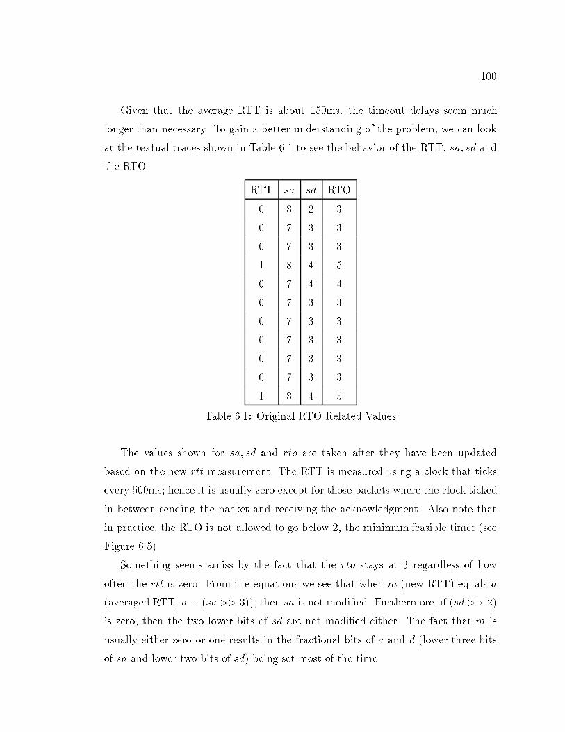
100Given that the average RTT is about 150ms, the timeout delays seem muchlonger than necessary. To gain a better understanding of the problem, we can lookat the textual traces shown in Table 6.1 to see the behavior of the RTT, sa; sd andthe RTO. RTT sa sd RTO0 8 2 30 7 3 30 7 3 31 8 4 50 7 4 40 7 3 30 7 3 30 7 3 30 7 3 30 7 3 31 8 4 5Table 6.1: Original RTO Related ValuesThe values shown for sa; sd and rto are taken after they have been updatedbased on the new rtt measurement. The RTT is measured using a clock that ticksevery 500ms; hence it is usually zero except for those packets where the clock tickedin between sending the packet and receiving the acknowledgment. Also note thatin practice, the RTO is not allowed to go below 2, the minimum feasible timer (seeFigure 6.5).Something seems amiss by the fact that the rto stays at 3 regardless of howoften the rtt is zero. From the equations we see that when m (new RTT) equals a(averaged RTT, a � (sa >> 3)), then sa is not modi�ed. Furthermore, if (sd >> 2)is zero, then the two lower bits of sd are not modi�ed either. The fact that m isusually either zero or one results in the fractional bits of a and d (lower three bitsof sa and lower two bits of sd) being set most of the time.

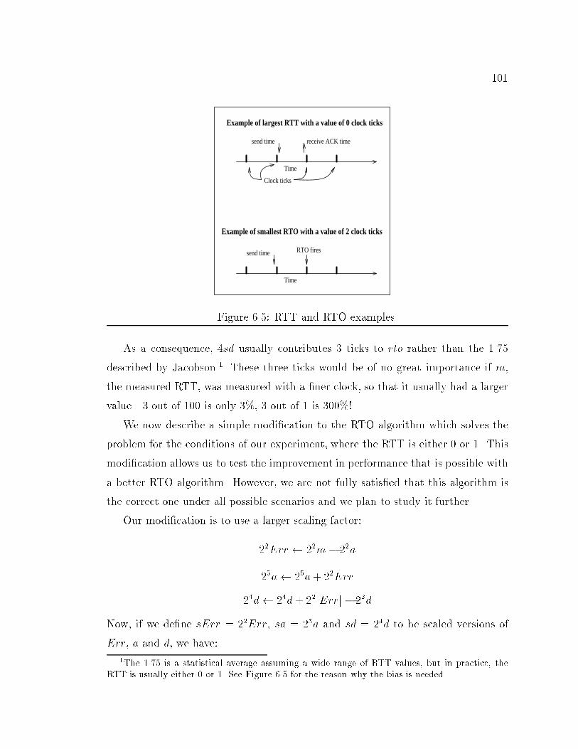
101Time

Time

send time receive ACK time

send time

Clock ticks

Example of largest RTT with a value of 0 clock ticks

Example of smallest RTO with a value of 2 clock ticks

RTO firesFigure 6.5: RTT and RTO examples.As a consequence, 4sd usually contributes 3 ticks to rto rather than the 1.75described by Jacobson.1 These three ticks would be of no great importance if m,the measured RTT, was measured with a �ner clock, so that it usually had a largervalue|3 out of 100 is only 3%, 3 out of 1 is 300%!We now describe a simple modi�cation to the RTO algorithm which solves theproblem for the conditions of our experiment, where the RTT is either 0 or 1. Thismodi�cation allows us to test the improvement in performance that is possible witha better RTO algorithm. However, we are not fully satis�ed that this algorithm isthe correct one under all possible scenarios and we plan to study it further.Our modi�cation is to use a larger scaling factor:22Err 22m� 22a25a 25a+ 22Err24d 24d+ 22jErrj � 22dNow, if we de�ne sErr = 22Err, sa = 25a and sd = 24d to be scaled versions ofErr, a and d, we have:1The 1.75 is a statistical average assuming a wide range of RTT values, but in practice, theRTT is usually either 0 or 1. See Figure 6.5 for the reason why the bias is needed.

102sErr (m << 2) � (sa >> 3)sa sa+ sErrsd sd+ (jsErrj � (sd >> 2))Then the low order bits that are not modi�ed (and usually end up set) after m hasthe same value repeatedly do not a�ect the RTO calculation.Since we want to be conservative when setting the RTO, and by conservative wemean that we never want to retransmit as a result of choosing too small an RTO,this implies that the RTO should always be at least two larger than the RTT. Forexample, the largest possible RTT with a value of x ticks has a real time length ofjust less than x+1 clock ticks (see Figure 6.5), but the smallest possible RTO withvalue x+2 has real time length of just greater than x+1 ticks (again see Figure 6.5).Note that if there is access to a more accurate clock, as in TCP Vegas, then thecoarse RTO can be made more accurate since one does not have to worry aboutthe extreme cases described in the previous paragraph. For example, if the moreaccurate RTO is less than 200ms, then as long as the segment is sent within the �rst300ms after the coarse-grained clock ticked, the coarse rto can be set to 1 (insteadof at least 2). A more accurate clock will also eliminate the large jumps in the sizeof the RTO which come from the RTT jumping between 0 and 1.The whole algorithm can be expressed in C as:sdelta = (m << 2) - (sa >> 3);sa += sdelta;if (sdelta < 0)sdelta = -sdelta;sdelta -= (sd >> 2);sd += sdelta;rto = max( m + 2, ((sa >> 3) + sd) >> 2 );

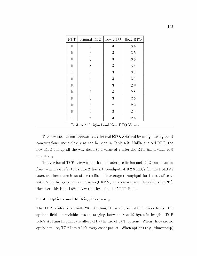
103RTT original RTO new RTO oat RTO0 3 3 3.40 3 3 3.50 3 3 3.50 3 3 3.41 5 3 3.10 4 3 3.10 3 3 2.90 3 3 2.80 3 3 2.50 3 2 2.30 3 2 2.11 5 3 2.5Table 6.2: Original and New RTO ValuesThe new mechanismapproximates the real RTO, obtained by using oating pointcomputations, more closely as can be seen in Table 6.2. Unlike the old RTO, thenew RTO can go all the way down to a value of 2 after the RTT has a value of 0repeatedly.The version of TCP Lite with both the header prediction and RTO computation�xes, which we refer to as Lite.2, has a throughput of 102.8 KB/s for the 1 MBytetransfer when there is no other tra�c. The average throughput for the set of testswith tcplib background tra�c is 55.9 KB/s, an increase over the original of 9%.However, this is still 6% below the throughput of TCP Reno.6.1.4 Options and ACKing FrequencyThe TCP header is normally 20 bytes long. However, one of the header �elds|theoptions �eld|is variable in size, ranging between 0 to 40 bytes in length. TCPLite's ACKing frequency is a�ected by the use of TCP options. When there are nooptions in use, TCP Lite ACKs every other packet. When options (e.g., timestamp)

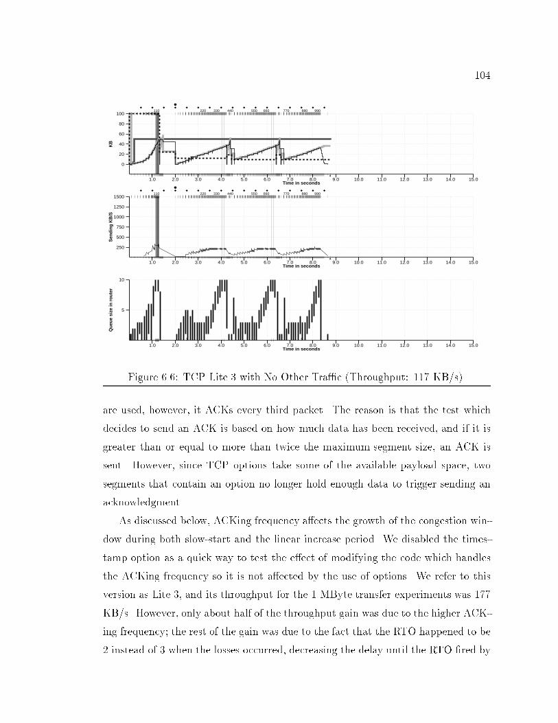
1041.0 2.0 3.0 4.0 5.0 6.0 7.0 8.0 9.0 10.0 11.0 12.0 13.0 14.0 15.0

Time in seconds

0

20

40

60

80

100K

B110 220 330 440 550 660 770 880 990

1.0 2.0 3.0 4.0 5.0 6.0 7.0 8.0 9.0 10.0 11.0 12.0 13.0 14.0 15.0Time in seconds

250

500

750

1000

1250

1500

Sen

ding

KB

/S

110 220 330 440 550 660 770 880 990

1.0 2.0 3.0 4.0 5.0 6.0 7.0 8.0 9.0 10.0 11.0 12.0 13.0 14.0 15.0Time in seconds

5

10

Que

ue s

ize

in r

oute

r

3 3Figure 6.6: TCP Lite.3 with No Other Tra�c (Throughput: 117 KB/s).are used, however, it ACKs every third packet. The reason is that the test whichdecides to send an ACK is based on how much data has been received, and if it isgreater than or equal to more than twice the maximum segment size, an ACK issent. However, since TCP options take some of the available payload space, twosegments that contain an option no longer hold enough data to trigger sending anacknowledgment.As discussed below, ACKing frequency a�ects the growth of the congestion win-dow during both slow-start and the linear increase period. We disabled the times-tamp option as a quick way to test the e�ect of modifying the code which handlesthe ACKing frequency so it is not a�ected by the use of options. We refer to thisversion as Lite.3, and its throughput for the 1 MByte transfer experiments was 177KB/s. However, only about half of the throughput gain was due to the higher ACK-ing frequency; the rest of the gain was due to the fact that the RTO happened to be2 instead of 3 when the losses occurred, decreasing the delay until the RTO �red by

105half a second. In the experiment when there is also background tra�c, the averagethroughput increased by 5%, but the losses increased by 28% when compared toTCP Lite.2.Figure 6.6 shows the graphical traces of Lite.3 when transferring 1 MByte. Theimportant thing to notice is how the losses are paired when they occur around 4and 6 seconds, resulting in decreasing the congestion window twice. The reason thelosses are paired is that the congestion window is increasing too rapidly|by morethan one maximum segment per RTT. Before the �rst loss is detected, TCP Liteincreases the congestion window, again resulting in an extra lost packet.The reason the congestion window is increasing so fast is the extra 1=8th of amaximum segment being added to it:if (cw > tp->snd_ssthresh)incr = incr * incr / cw + incr / 8;By removing this 1=8th increase:if (cw > tp->snd_ssthresh)incr = incr * incr / cw;the losses are not paired any more, so the congestion window is decreased only once.In the experiments with background tra�c, running TCP Lite.4, which includesthe four previous modi�cations (header prediction �x, RTO �x, no timestamps, andeliminating the extra 1=8th increase) results in an average throughput of 62.3 KB/s.This represents a 21% increase over the original TCP Lite, and a 6% increase overLite.3 .6.1.5 Linear Increase of the Congestion Window and ACKing FrequencyTCP should perform a multiplicative decrease of the congestion window when lossesare detected, and a linear increase while there are no losses detected. Due to thebugs described above, TCP Lite follows no speci�c guidelines on how fast to increasethe congestion window. If there are options, the acking frequency is reduced and the

106window increases more slowly. By adding the extra 1=8th of a maximum segmentsize to the congestion window, the rate of increase is now a function of the windowsize (which means the increase is exponential).It is easy to specify what should be the upper bound to the rate of increase for thecongestion window during the linear increase mode: the congestion window shouldnot be increased by more than one maximum segment size per RTT. Increasing thecongestion window at a faster rate will result in the loss of two or more segments perRTT when the queue at the bottleneck router is full. This may result in a timeoutsince the fast retransmit and fast recovery mechanisms in TCP Lite cannot alwaysrecover from the loss of two segments when the losses occur during a one RTT timeinterval.ACKing frequency can be seen as a tradeo� between higher congestion and lowerlatency. As shown here, it also a�ects the rate of the linear growth of the congestionwindow in TCP Lite|this is due to the implementation, and it could be changed.However, it is not clear that ACKing every two or three packets puts less stress in thenetwork than acking every packet. On the one hand, lower ACKing frequencies implyfewer packets on the network, but on the other hand, lower ACKing frequenciesresult in more packets being sent at one time. For example, if the receiver ACKsafter receiving three packets, then the source will transmit 3 or 4 packets at onetime, the fourth one if the congestion window linear increase allows one more packetto go out. If two or more connections do this at the same time, then the likelihoodof losses increases. Another example resulting in increased stress to the network isa server that does not reply to requests immediately. As a consequence, all of thedelayed acknowledgments are sent at the same time when a TCP timer forces theirtransmission every 200ms.We modi�ed the code, creating Lite.5, so that it ACKs after every packet ratherthan after every two packets. The e�ect on the tests with tra�c was a slight increasein the throughput (3%) but a much larger increase in the losses (48%). The increasein the losses may be due to the simulation scenario|e.g., number of bu�ers at therouter. We are planning to look into this issue in more detail, since we do not believe

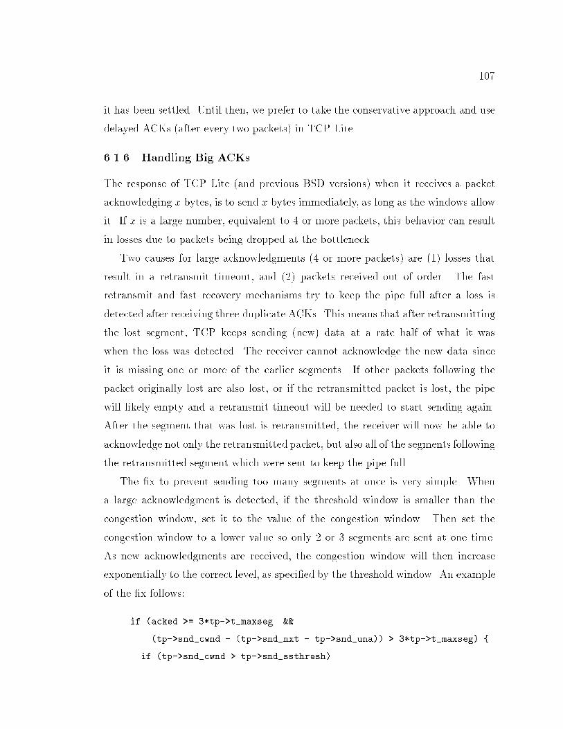
107it has been settled. Until then, we prefer to take the conservative approach and usedelayed ACKs (after every two packets) in TCP Lite.6.1.6 Handling Big ACKsThe response of TCP Lite (and previous BSD versions) when it receives a packetacknowledging x bytes, is to send x bytes immediately, as long as the windows allowit. If x is a large number, equivalent to 4 or more packets, this behavior can resultin losses due to packets being dropped at the bottleneck.Two causes for large acknowledgments (4 or more packets) are (1) losses thatresult in a retransmit timeout, and (2) packets received out of order. The fastretransmit and fast recovery mechanisms try to keep the pipe full after a loss isdetected after receiving three duplicate ACKs. This means that after retransmittingthe lost segment, TCP keeps sending (new) data at a rate half of what it waswhen the loss was detected. The receiver cannot acknowledge the new data sinceit is missing one or more of the earlier segments. If other packets following thepacket originally lost are also lost, or if the retransmitted packet is lost, the pipewill likely empty and a retransmit timeout will be needed to start sending again.After the segment that was lost is retransmitted, the receiver will now be able toacknowledge not only the retransmitted packet, but also all of the segments followingthe retransmitted segment which were sent to keep the pipe full.The �x to prevent sending too many segments at once is very simple. Whena large acknowledgment is detected, if the threshold window is smaller than thecongestion window, set it to the value of the congestion window. Then set thecongestion window to a lower value so only 2 or 3 segments are sent at one time.As new acknowledgments are received, the congestion window will then increaseexponentially to the correct level, as speci�ed by the threshold window. An exampleof the �x follows:if (acked >= 3*tp->t_maxseg &&(tp->snd_cwnd - (tp->snd_nxt - tp->snd_una)) > 3*tp->t_maxseg) {if (tp->snd_cwnd > tp->snd_ssthresh)

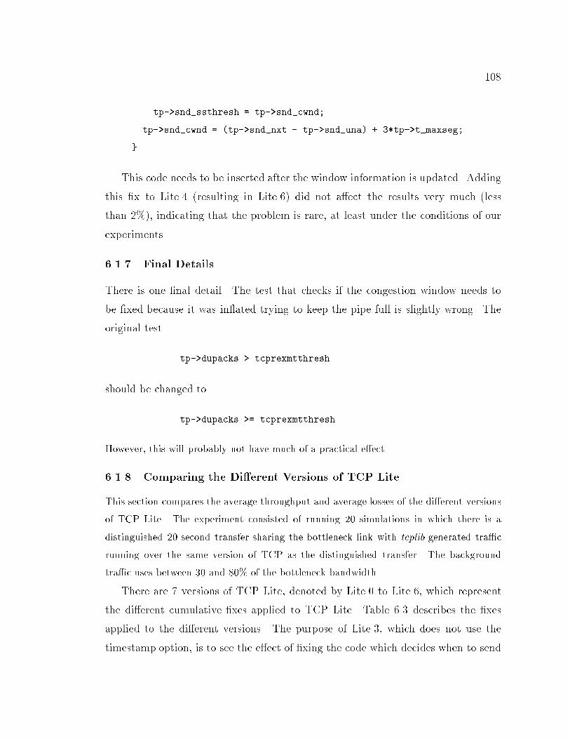
108tp->snd_ssthresh = tp->snd_cwnd;tp->snd_cwnd = (tp->snd_nxt - tp->snd_una) + 3*tp->t_maxseg;}This code needs to be inserted after the window information is updated. Addingthis �x to Lite.4 (resulting in Lite.6) did not a�ect the results very much (lessthan 2%), indicating that the problem is rare, at least under the conditions of ourexperiments.6.1.7 Final DetailsThere is one �nal detail. The test that checks if the congestion window needs tobe �xed because it was in ated trying to keep the pipe full is slightly wrong. Theoriginal test tp->dupacks > tcprexmtthreshshould be changed totp->dupacks >= tcprexmtthreshHowever, this will probably not have much of a practical e�ect.6.1.8 Comparing the Di�erent Versions of TCP LiteThis section compares the average throughput and average losses of the di�erent versionsof TCP Lite. The experiment consisted of running 20 simulations in which there is adistinguished 20 second transfer sharing the bottleneck link with tcplib generated tra�crunning over the same version of TCP as the distinguished transfer. The backgroundtra�c uses between 30 and 80% of the bottleneck bandwidth.There are 7 versions of TCP Lite, denoted by Lite.0 to Lite.6, which representthe di�erent cumulative �xes applied to TCP Lite. Table 6.3 describes the �xesapplied to the di�erent versions. The purpose of Lite.3, which does not use thetimestamp option, is to see the e�ect of �xing the code which decides when to send

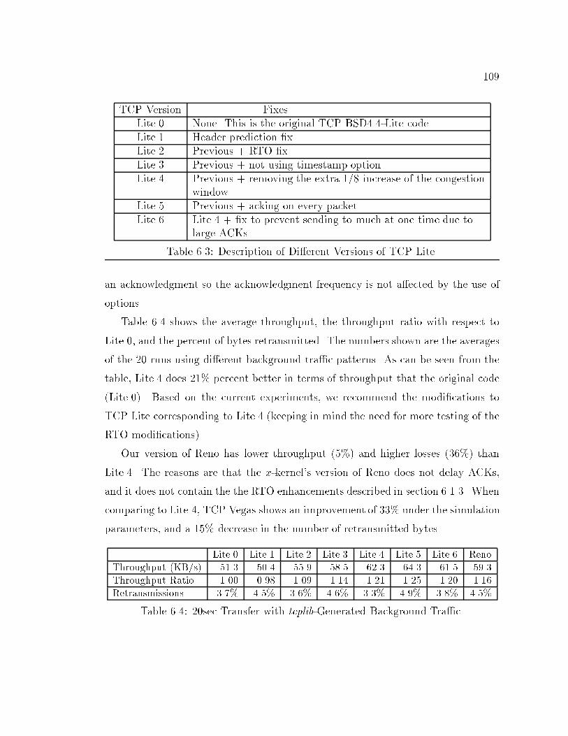
109TCP Version FixesLite.0 None. This is the original TCP BSD4.4-Lite codeLite.1 Header prediction �xLite.2 Previous + RTO �xLite.3 Previous + not using timestamp optionLite.4 Previous + removing the extra 1/8 increase of the congestionwindowLite.5 Previous + acking on every packetLite.6 Lite.4 + �x to prevent sending to much at one time due tolarge ACKsTable 6.3: Description of Di�erent Versions of TCP Lite.an acknowledgment so the acknowledgment frequency is not a�ected by the use ofoptions.Table 6.4 shows the average throughput, the throughput ratio with respect toLite.0, and the percent of bytes retransmitted. The numbers shown are the averagesof the 20 runs using di�erent background tra�c patterns. As can be seen from thetable, Lite.4 does 21% percent better in terms of throughput that the original code(Lite.0). Based on the current experiments, we recommend the modi�cations toTCP Lite corresponding to Lite.4 (keeping in mind the need for more testing of theRTO modi�cations).Our version of Reno has lower throughput (5%) and higher losses (36%) thanLite.4. The reasons are that the x-kernel's version of Reno does not delay ACKs,and it does not contain the the RTO enhancements described in section 6.1.3. Whencomparing to Lite.4, TCP Vegas shows an improvement of 33% under the simulationparameters, and a 15% decrease in the number of retransmitted bytes.Lite.0 Lite.1 Lite.2 Lite.3 Lite.4 Lite.5 Lite.6 RenoThroughput (KB/s) 51.3 50.4 55.9 58.5 62.3 64.3 61.5 59.3Throughput Ratio 1.00 0.98 1.09 1.14 1.21 1.25 1.20 1.16Retransmissions 3.7% 4.5% 3.6% 4.6% 3.3% 4.9% 3.8% 4.5%Table 6.4: 20sec Transfer with tcplib-Generated Background Tra�c.

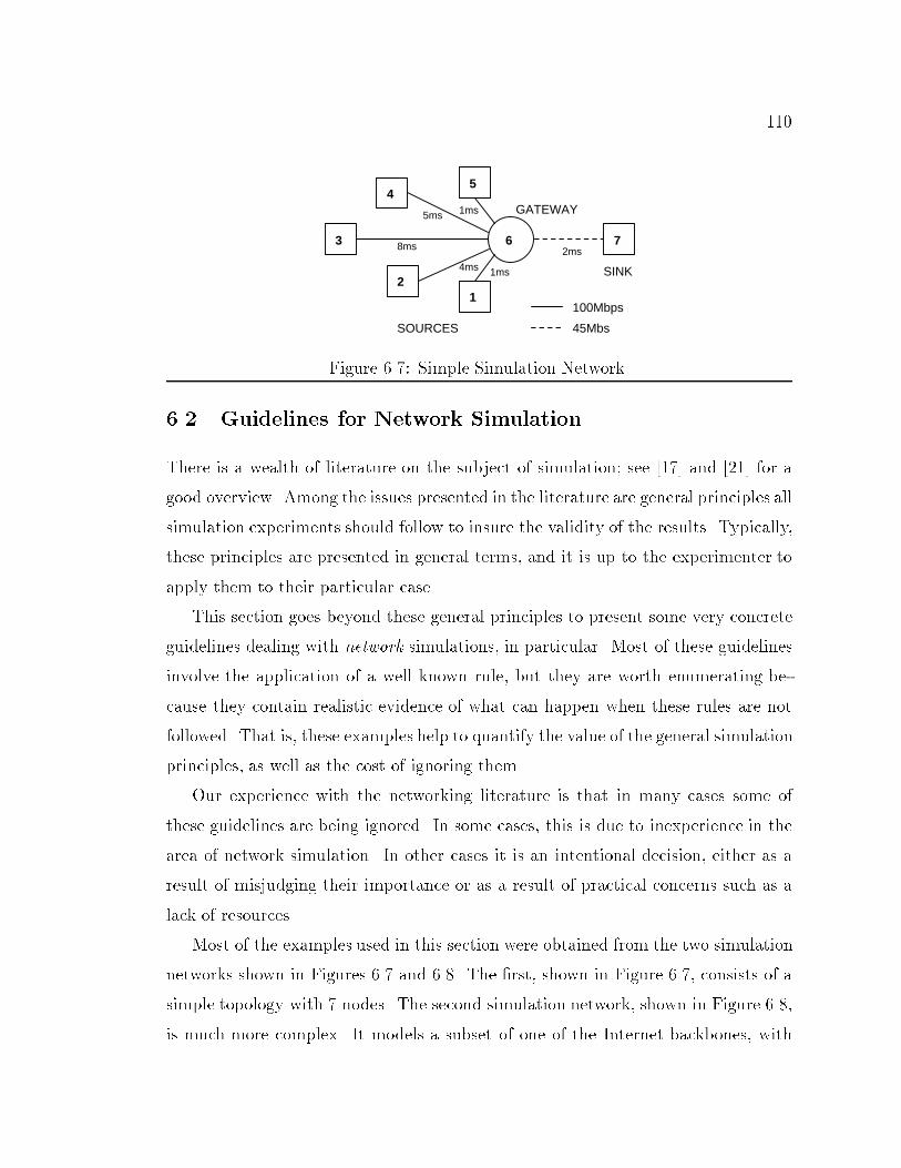
110GATEWAY

SINK

SOURCES

2ms

1ms4ms

8ms

5ms 1ms

2

45

1

3 6 7

45Mbs

100MbpsFigure 6.7: Simple Simulation Network.6.2 Guidelines for Network SimulationThere is a wealth of literature on the subject of simulation; see [17] and [21] for agood overview. Among the issues presented in the literature are general principles allsimulation experiments should follow to insure the validity of the results. Typically,these principles are presented in general terms, and it is up to the experimenter toapply them to their particular case.This section goes beyond these general principles to present some very concreteguidelines dealing with network simulations, in particular. Most of these guidelinesinvolve the application of a well known rule, but they are worth enumerating be-cause they contain realistic evidence of what can happen when these rules are notfollowed. That is, these examples help to quantify the value of the general simulationprinciples, as well as the cost of ignoring them.Our experience with the networking literature is that in many cases some ofthese guidelines are being ignored. In some cases, this is due to inexperience in thearea of network simulation. In other cases it is an intentional decision, either as aresult of misjudging their importance or as a result of practical concerns such as alack of resources.Most of the examples used in this section were obtained from the two simulationnetworks shown in Figures 6.7 and 6.8. The �rst, shown in Figure 6.7, consists of asimple topology with 7 nodes. The second simulation network, shown in Figure 6.8,is much more complex. It models a subset of one of the Internet backbones, with

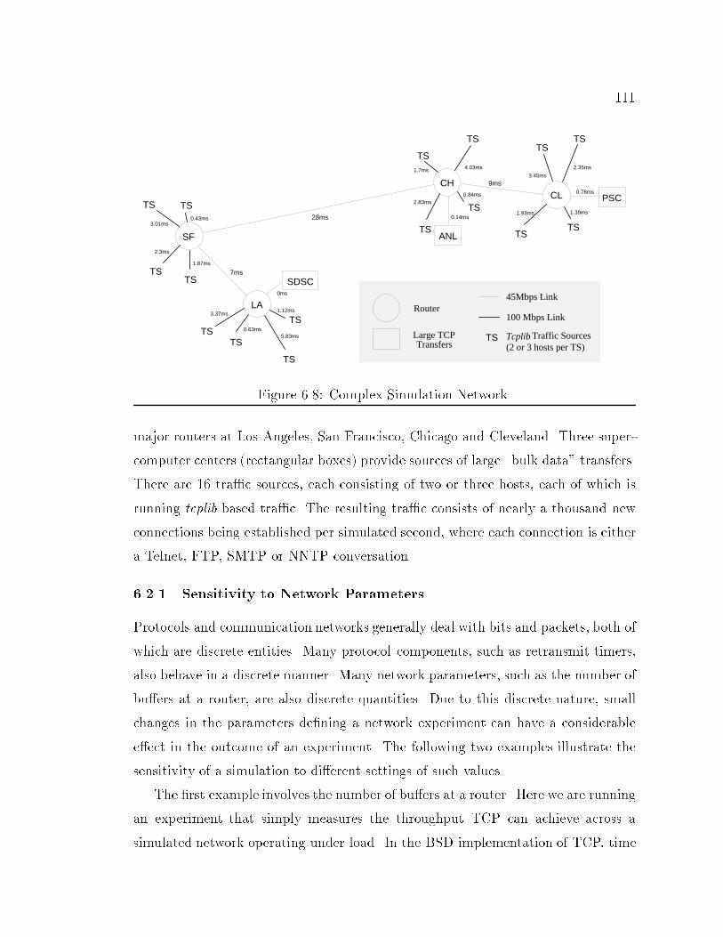
111Router

Large TCP Transfers

TS

100 Mbps Link

45Mbps Link

Tcplib Traffic Sources(2 or 3 hosts per TS)

28ms

9ms

7ms

5.83ms

1.12ms

0ms

0.63ms

3.37ms

3.01ms0.43ms

2.3ms

1.87ms

4.03ms

2.83ms

1.7ms

1.93ms

3.45ms

2.35ms

1.39ms

0.78ms0.84ms

0.14ms

TS

TSTS

TS

TSTS

TS TS

TS

TS

TS

TSTS

TSTS

TS

SDSC

ANL

PSC

LA

SF

CHCL

Figure 6.8: Complex Simulation Network.major routers at Los Angeles, San Francisco, Chicago and Cleveland. Three super-computer centers (rectangular boxes) provide sources of large \bulk data" transfers.There are 16 tra�c sources, each consisting of two or three hosts, each of which isrunning tcplib based tra�c. The resulting tra�c consists of nearly a thousand newconnections being established per simulated second, where each connection is eithera Telnet, FTP, SMTP or NNTP conversation.6.2.1 Sensitivity to Network ParametersProtocols and communication networks generally deal with bits and packets, both ofwhich are discrete entities. Many protocol components, such as retransmit timers,also behave in a discrete manner. Many network parameters, such as the number ofbu�ers at a router, are also discrete quantities. Due to this discrete nature, smallchanges in the parameters de�ning a network experiment can have a considerablee�ect in the outcome of an experiment. The following two examples illustrate thesensitivity of a simulation to di�erent settings of such values.The �rst example involves the number of bu�ers at a router. Here we are runningan experiment that simply measures the throughput TCP can achieve across asimulated network operating under load. In the BSD implementation of TCP, time

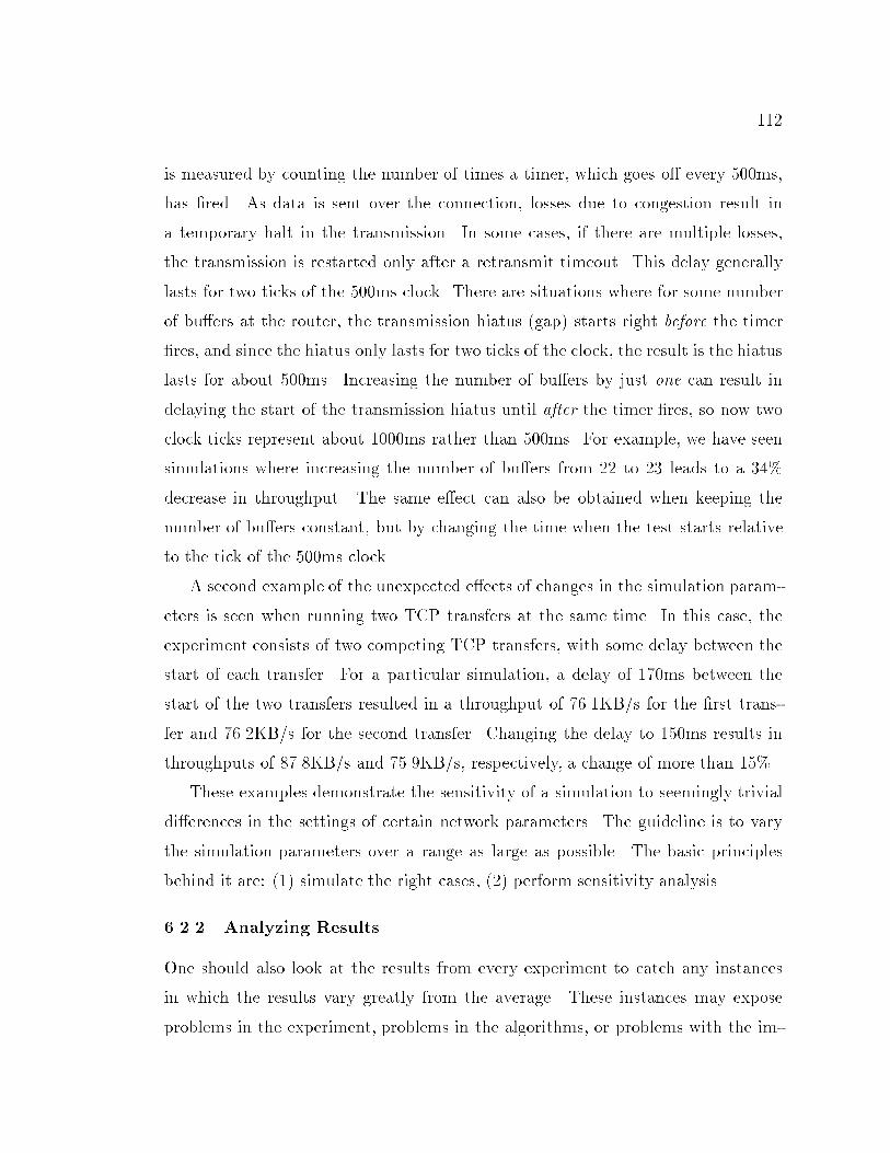
112is measured by counting the number of times a timer, which goes o� every 500ms,has �red. As data is sent over the connection, losses due to congestion result ina temporary halt in the transmission. In some cases, if there are multiple losses,the transmission is restarted only after a retransmit timeout. This delay generallylasts for two ticks of the 500ms clock. There are situations where for some numberof bu�ers at the router, the transmission hiatus (gap) starts right before the timer�res, and since the hiatus only lasts for two ticks of the clock, the result is the hiatuslasts for about 500ms. Increasing the number of bu�ers by just one can result indelaying the start of the transmission hiatus until after the timer �res, so now twoclock ticks represent about 1000ms rather than 500ms. For example, we have seensimulations where increasing the number of bu�ers from 22 to 23 leads to a 34%decrease in throughput. The same e�ect can also be obtained when keeping thenumber of bu�ers constant, but by changing the time when the test starts relativeto the tick of the 500ms clock.A second example of the unexpected e�ects of changes in the simulation param-eters is seen when running two TCP transfers at the same time. In this case, theexperiment consists of two competing TCP transfers, with some delay between thestart of each transfer. For a particular simulation, a delay of 170ms between thestart of the two transfers resulted in a throughput of 76.1KB/s for the �rst trans-fer and 76.2KB/s for the second transfer. Changing the delay to 150ms results inthroughputs of 87.8KB/s and 75.9KB/s, respectively, a change of more than 15%.These examples demonstrate the sensitivity of a simulation to seemingly trivialdi�erences in the settings of certain network parameters. The guideline is to varythe simulation parameters over a range as large as possible. The basic principlesbehind it are: (1) simulate the right cases, (2) perform sensitivity analysis.6.2.2 Analyzing ResultsOne should also look at the results from every experiment to catch any instancesin which the results vary greatly from the average. These instances may exposeproblems in the experiment, problems in the algorithms, or problems with the im-

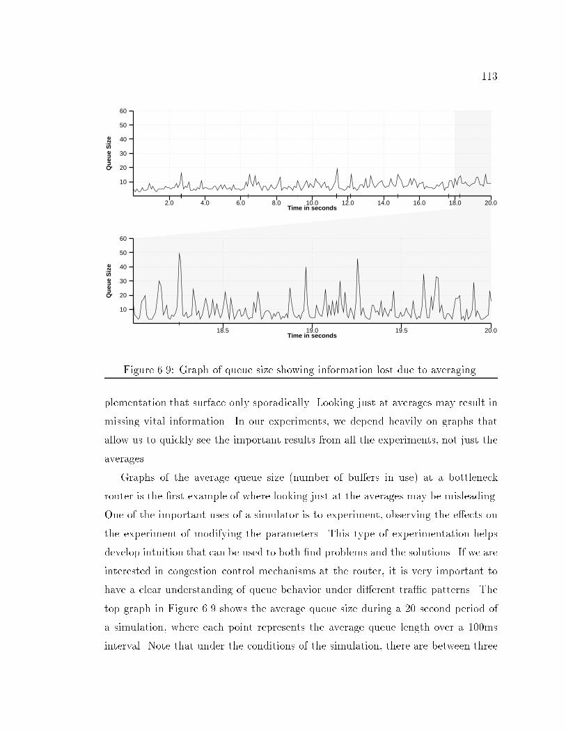
1132.0 4.0 6.0 8.0 10.0 12.0 14.0 16.0 18.0 20.0

Time in seconds

10

20

30

40

50

60Q

ueu

e S

ize

18.5 19.0 19.5 20.0Time in seconds

10

20

30

40

50

60

Qu

eue

Siz

e Figure 6.9: Graph of queue size showing information lost due to averaging.plementation that surface only sporadically. Looking just at averages may result inmissing vital information. In our experiments, we depend heavily on graphs thatallow us to quickly see the important results from all the experiments, not just theaverages.Graphs of the average queue size (number of bu�ers in use) at a bottleneckrouter is the �rst example of where looking just at the averages may be misleading.One of the important uses of a simulator is to experiment, observing the e�ects onthe experiment of modifying the parameters. This type of experimentation helpsdevelop intuition that can be used to both �nd problems and the solutions. If we areinterested in congestion control mechanisms at the router, it is very important tohave a clear understanding of queue behavior under di�erent tra�c patterns. Thetop graph in Figure 6.9 shows the average queue size during a 20 second period ofa simulation, where each point represents the average queue length over a 100msinterval. Note that under the conditions of the simulation, there are between three

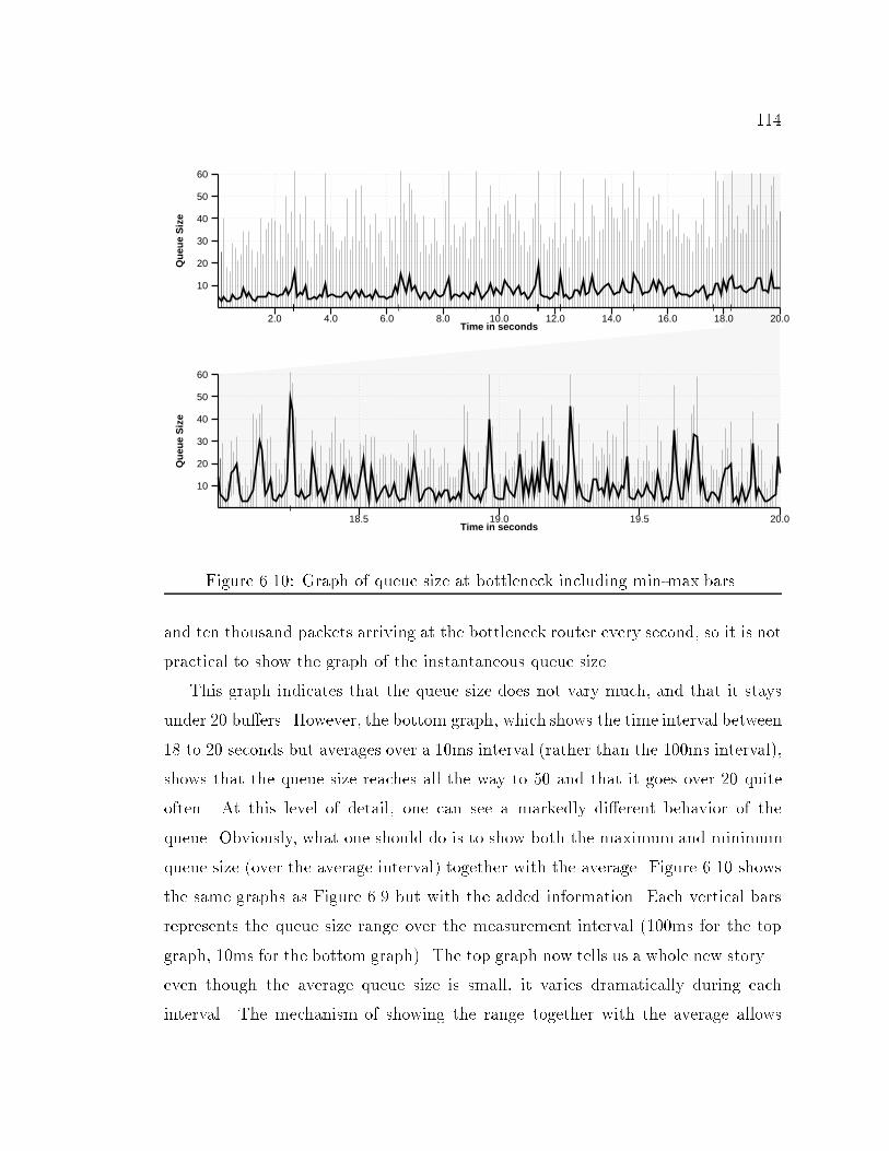
1142.0 4.0 6.0 8.0 10.0 12.0 14.0 16.0 18.0 20.0

Time in seconds

10

20

30

40

50

60Q

ueu

e S

ize

18.5 19.0 19.5 20.0Time in seconds

10

20

30

40

50

60

Qu

eue

Siz

e Figure 6.10: Graph of queue size at bottleneck including min-max bars.and ten thousand packets arriving at the bottleneck router every second, so it is notpractical to show the graph of the instantaneous queue size.This graph indicates that the queue size does not vary much, and that it staysunder 20 bu�ers. However, the bottom graph, which shows the time interval between18 to 20 seconds but averages over a 10ms interval (rather than the 100ms interval),shows that the queue size reaches all the way to 50 and that it goes over 20 quiteoften. At this level of detail, one can see a markedly di�erent behavior of thequeue. Obviously, what one should do is to show both the maximum and minimumqueue size (over the average interval) together with the average. Figure 6.10 showsthe same graphs as Figure 6.9 but with the added information. Each vertical barsrepresents the queue size range over the measurement interval (100ms for the topgraph, 10ms for the bottom graph). The top graph now tells us a whole new story|even though the average queue size is small, it varies dramatically during eachinterval. The mechanism of showing the range together with the average allows

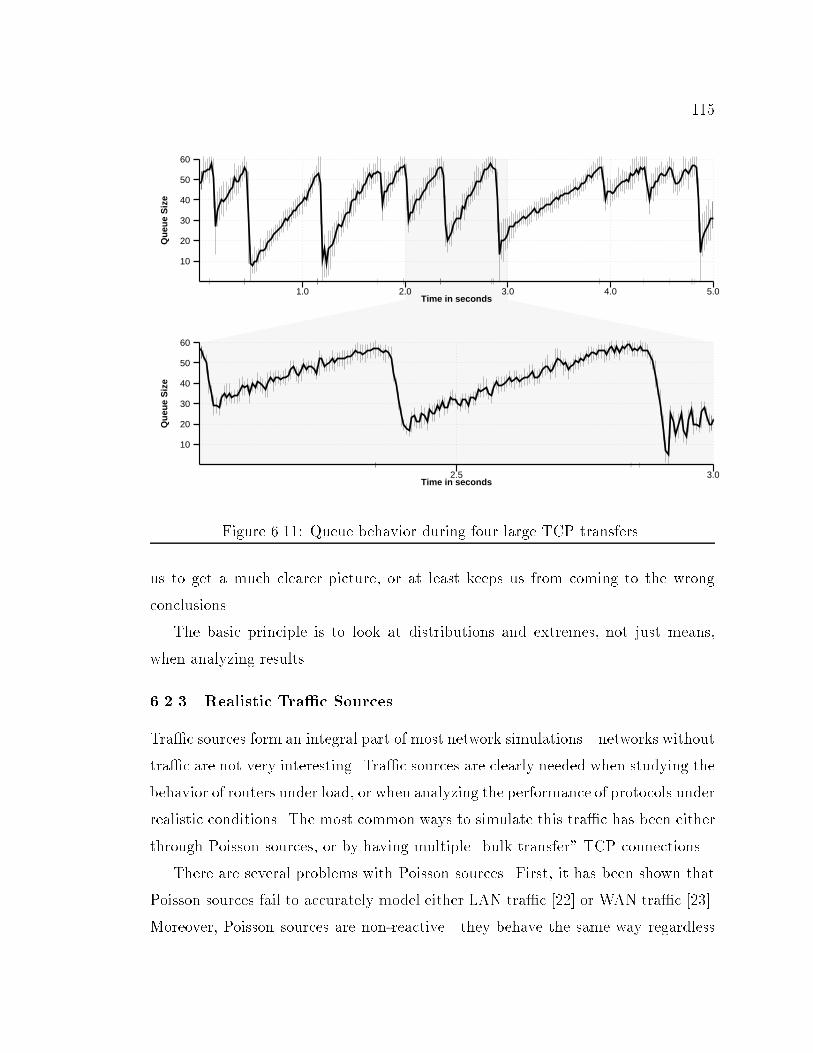
1151.0 2.0 3.0 4.0 5.0

Time in seconds

10

20

30

40

50

60Q

ueu

e S

ize

2.5 3.0Time in seconds

10

20

30

40

50

60

Qu

eue

Siz

e Figure 6.11: Queue behavior during four large TCP transfers.us to get a much clearer picture, or at least keeps us from coming to the wrongconclusions.The basic principle is to look at distributions and extremes, not just means,when analyzing results.6.2.3 Realistic Tra�c SourcesTra�c sources form an integral part of most network simulations|networks withouttra�c are not very interesting. Tra�c sources are clearly needed when studying thebehavior of routers under load, or when analyzing the performance of protocols underrealistic conditions. The most common ways to simulate this tra�c has been eitherthrough Poisson sources, or by having multiple \bulk transfer" TCP connections.There are several problems with Poisson sources. First, it has been shown thatPoisson sources fail to accurately model either LAN tra�c [22] or WAN tra�c [23].Moreover, Poisson sources are non-reactive|they behave the same way regardless

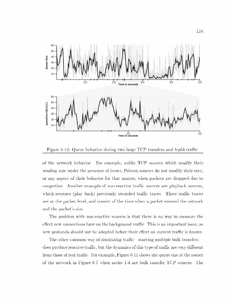
1161.0 2.0 3.0 4.0 5.0

Time in seconds

10

20

30

40

50

60Q

ueu

e S

ize

2.5 3.0Time in seconds

10

20

30

40

50

60

qu

eueC

nt-

192.

0.2.

1

Figure 6.12: Queue behavior during two large TCP transfers and tcplib tra�c.of the network behavior. For example, unlike TCP sources which modify theirsending rate under the presence of losses, Poisson sources do not modify their rate,or any aspect of their behavior for that matter, when packets are dropped due tocongestion. Another example of non-reactive tra�c sources are playback sources,which recreate (play back) previously recorded tra�c traces. These tra�c tracesare at the packet level, and consist of the time when a packet entered the networkand the packet's size.The problem with non-reactive sources is that there is no way to measure thee�ect new connections have on the background tra�c. This is an important issue, asnew protocols should not be adopted before their e�ect on current tra�c is known.The other common way of simulating tra�c|starting multiple bulk transfers|does produce reactive tra�c, but the dynamics of this type of tra�c are very di�erentfrom those of real tra�c. For example, Figure 6.11 shows the queue size at the routerof the network in Figure 6.7 when nodes 1-4 are bulk transfer TCP sources. The

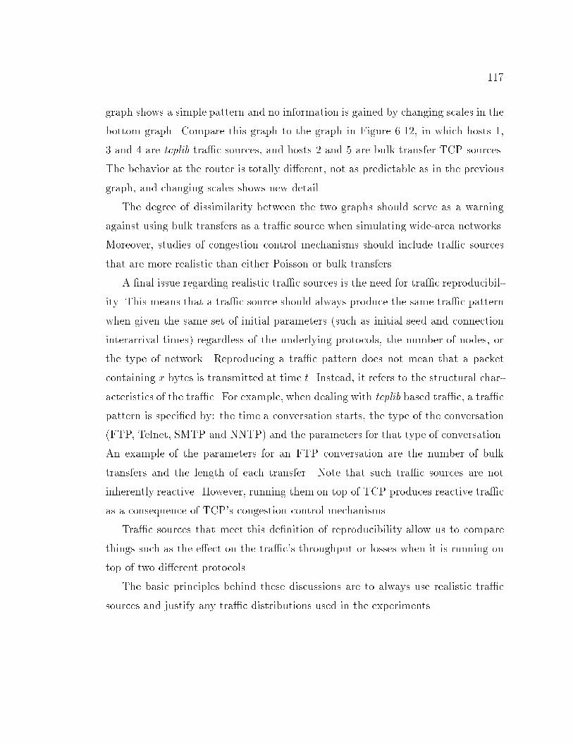
117graph shows a simple pattern and no information is gained by changing scales in thebottom graph. Compare this graph to the graph in Figure 6.12, in which hosts 1,3 and 4 are tcplib tra�c sources, and hosts 2 and 5 are bulk transfer TCP sources.The behavior at the router is totally di�erent, not as predictable as in the previousgraph, and changing scales shows new detail.The degree of dissimilarity between the two graphs should serve as a warningagainst using bulk transfers as a tra�c source when simulating wide-area networks.Moreover, studies of congestion control mechanisms should include tra�c sourcesthat are more realistic than either Poisson or bulk transfers.A �nal issue regarding realistic tra�c sources is the need for tra�c reproducibil-ity. This means that a tra�c source should always produce the same tra�c patternwhen given the same set of initial parameters (such as initial seed and connectioninterarrival times) regardless of the underlying protocols, the number of nodes, orthe type of network. Reproducing a tra�c pattern does not mean that a packetcontaining x bytes is transmitted at time t. Instead, it refers to the structural char-acteristics of the tra�c. For example, when dealing with tcplib based tra�c, a tra�cpattern is speci�ed by: the time a conversation starts, the type of the conversation(FTP, Telnet, SMTP and NNTP) and the parameters for that type of conversation.An example of the parameters for an FTP conversation are the number of bulktransfers and the length of each transfer. Note that such tra�c sources are notinherently reactive. However, running them on top of TCP produces reactive tra�cas a consequence of TCP's congestion control mechanisms.Tra�c sources that meet this de�nition of reproducibility allow us to comparethings such as the e�ect on the tra�c's throughput or losses when it is running ontop of two di�erent protocols.The basic principles behind these discussions are to always use realistic tra�csources and justify any tra�c distributions used in the experiments.

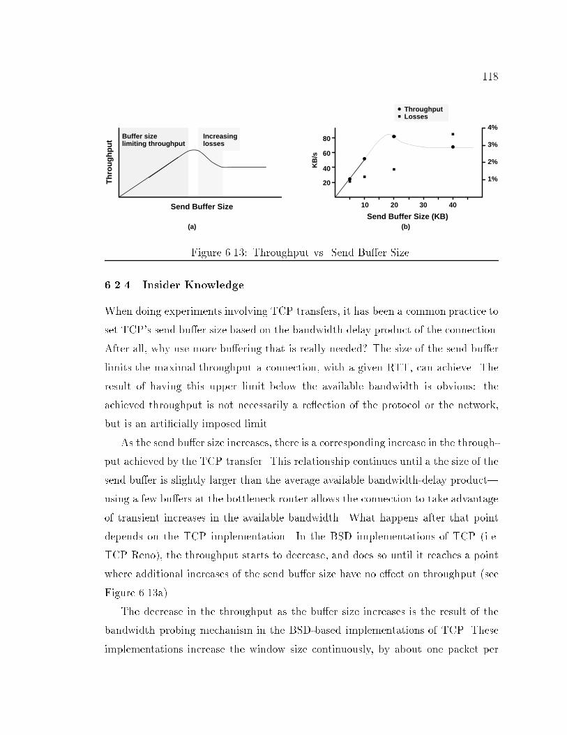
1181%

2%

3%

4%

ThroughputLosses

Buffer sizelimiting throughput

Increasinglosses

Th

rou

gh

pu

t

Send Buffer SizeSend Buffer Size (KB)

10 20 30 40

20

40

60

80

KB

/s

(a) (b)Figure 6.13: Throughput vs. Send Bu�er Size.6.2.4 Insider KnowledgeWhen doing experiments involving TCP transfers, it has been a common practice toset TCP's send bu�er size based on the bandwidth delay product of the connection.After all, why use more bu�ering that is really needed? The size of the send bu�erlimits the maximal throughput a connection, with a given RTT, can achieve. Theresult of having this upper limit below the available bandwidth is obvious: theachieved throughput is not necessarily a re ection of the protocol or the network,but is an arti�cially imposed limit.As the send bu�er size increases, there is a corresponding increase in the through-put achieved by the TCP transfer. This relationship continues until a the size of thesend bu�er is slightly larger than the average available bandwidth-delay product|using a few bu�ers at the bottleneck router allows the connection to take advantageof transient increases in the available bandwidth. What happens after that pointdepends on the TCP implementation. In the BSD implementations of TCP (i.e.TCP Reno), the throughput starts to decrease, and does so until it reaches a pointwhere additional increases of the send bu�er size have no e�ect on throughput (seeFigure 6.13a).The decrease in the throughput as the bu�er size increases is the result of thebandwidth probing mechanism in the BSD-based implementations of TCP. Theseimplementations increase the window size continuously, by about one packet per

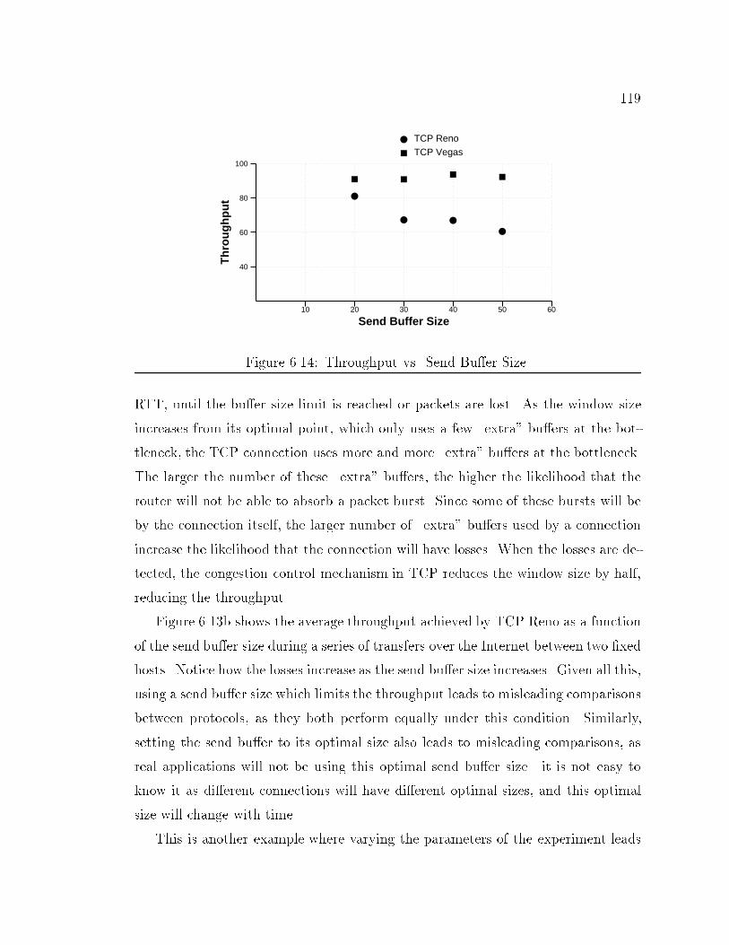
11910 20 30 40 50 60

Send Buffer Size

40

60

80

100

Th

rou

gh

pu

t

TCP VegasTCP Reno

Figure 6.14: Throughput vs. Send Bu�er Size.RTT, until the bu�er size limit is reached or packets are lost. As the window sizeincreases from its optimal point, which only uses a few \extra" bu�ers at the bot-tleneck, the TCP connection uses more and more \extra" bu�ers at the bottleneck.The larger the number of these \extra" bu�ers, the higher the likelihood that therouter will not be able to absorb a packet burst. Since some of these bursts will beby the connection itself, the larger number of \extra" bu�ers used by a connectionincrease the likelihood that the connection will have losses. When the losses are de-tected, the congestion control mechanism in TCP reduces the window size by half,reducing the throughput.Figure 6.13b shows the average throughput achieved by TCP Reno as a functionof the send bu�er size during a series of transfers over the Internet between two �xedhosts. Notice how the losses increase as the send bu�er size increases. Given all this,using a send bu�er size which limits the throughput leads to misleading comparisonsbetween protocols, as they both perform equally under this condition. Similarly,setting the send bu�er to its optimal size also leads to misleading comparisons, asreal applications will not be using this optimal send bu�er size|it is not easy toknow it as di�erent connections will have di�erent optimal sizes, and this optimalsize will change with time.This is another example where varying the parameters of the experiment leads

120to useful insights and comparisons. For example, a set of experiments comparingTCP Reno with TCP Vegas (see Section 5.2.3) showed that TCP Vegas was notsensitive to the send bu�er size|as long as it is big enough so that it is not thelimiting factor. Figure 6.14 shows the average throughput for a set of simulationswith di�erent send bu�er sizes. Note that TCP Vegas was not a�ected by the bu�ersize, whereas TCP Reno's throughput decreases by more than 30%.The basic principle to remember is that simulation results are constrained bythe values of the input parameters. Any bias in the choice of these parameters willa�ect the results.6.2.5 Byte versus Time TransfersThroughput is generally measured by recording the time required to send a spe-ci�c amount of data; e.g., if it takes 10 seconds to send 1 MByte of data, thenthe throughput is 100 KBytes/sec. When measuring the di�erence in throughputbetween two protocols, one of which is generally faster than the other, there is thepossibility of erroneous measurements in some cases.For example, if the experiment includes background tra�c, there may be a sys-tematic tendency for the level of tra�c to either increase or decrease during theduration of the transfer we are timing. If the level increases during the transfer,then the slower protocol will be unfairly penalized because it had to compete withhigher levels of tra�c at the end of the test, whereas the faster protocol did not.Alternatively, if the level of the background tra�c tends to decrease during the du-ration of the test, then the slower protocol will be measured as being faster|relativeto the faster protocol|than it really is.Instead, another way of measuring the throughput is to transfer as much dataas possible for a certain amount of time. This way both protocols will encounterthe same background tra�c for the duration of the transfer. The di�erences in themeasured throughput between the two methods can be considerable, depending onthe characteristics of the tra�c. For example, in one series of experiments resultedin a 56% di�erence in the throughput between two protocols when sending 1 MByte

121of data but only a 28% di�erence when sending for 30 seconds. Clearly, the preferredmethod should be to use timed transfers rather than length transfers.6.2.6 Unwanted SynchronicityIt is very easy for simulations to lose a lot of the variability (randomness) that isinherent in the real world. This can be either a design aw with the simulator orthe result of badly chosen simulation parameters. An example of synchronicity ina simulation is starting all transfers at the same time. This is very easy to do in asimulator, but it would generally be an uncommon occurrence outside of a simulator.Another example of lack of variability can occur with protocols, like the BSDimplementation of TCP, where coarse timers are used to perform special processing.In this implementation of TCP, two coarse timers are used, one �ring every 200msand the other every 500ms. Most of the implementations of TCP delay ACKs,which means that when they receive a packet they do not send an acknowledgmentimmediately, but instead wait for more packets to arrive so they can acknowledgemore than one packet at a time. The BSD implementations of TCP wait for onemore packet, thereby acknowledging two packets at a time. However, since anotherpacket may not arrive, TCP uses the 200ms timer to send any acknowledgments thatwere delayed. The 500ms timer is used to check if packets need to be retransmittedbecause they were lost.If one is not careful in the implementation, it is easy to have these timers �re atthe same time on all hosts in the simulated network. This results in periodic burstsof data as all hosts send the delayed acknowledgments or start retransmitting lostpackets at the same time. Since the retransmissions occurring as a result of the500ms timers involve the slow-start mechanism, which is a restart of the connectioninvolving exponential growth of the sending rate, the e�ect is equivalent to startingmultiple transfers at the same time.A similar burstiness can occur even when the timers for each node do not all�re at the same time. The problem happens when using realistic tra�c sourcesinvolving multiple TCP connections, but having only a few tra�c sources, each of

122which is responsible for a large percent of the tra�c. Then, when one of the timers�res at one of the sources, a large number of connections may send delayed ACKsor restart their transmissions. The results are similar to having a large number oftra�c sources, with a group of sources �ring their timers at the same time.A tool that is very useful at �nding unwanted uniform behavior is Fourier analy-sis [29]. This type of analysis uncovers periodic behavior which may point to possibleproblems and to the cause of these problems. Figure 6.15(a) shows the queue sizeat the router in Figure 6.7 when the only source of tcplib tra�c is node 4. It isclear from the graph that there is periodic behavior which occurs 5 times per second(every 200ms). The fact that the spikes occur every 200ms points to the fast timerin TCP as the cause of these spikes. Note that this behavior does not appear in thegraph of the average queue size, it only appears in the maximum queue size graph.One way to eliminate these bursts is to have more tra�c sources so the burstswill be distributed more evenly|assuming the tra�c sources do not �re their timersat the same time. Figure 6.15(b) shows the queue behavior when there are threetra�c sources. Periodic behavior is not as evident in this case, although Fourieranalysis shows that it still exists. This periodicity can be decreased even further byincreasing the number of sources.Another way to eliminate some of the periodicity is to introduce node processingdelays. Figure 6.15(c) shows the queue behavior when a delay, with a uniformdistribution between 0 and 50�s, is introduced before a packet is sent by the node.The periodicity is not as evident as in the top graph, but it still exists and withvery high peaks in some instances.The basic principle is to put a distribution on everything that needs it. Theproblem is that when dealing with complex simulators, it is not always clear whatthings need to have distributions in them.

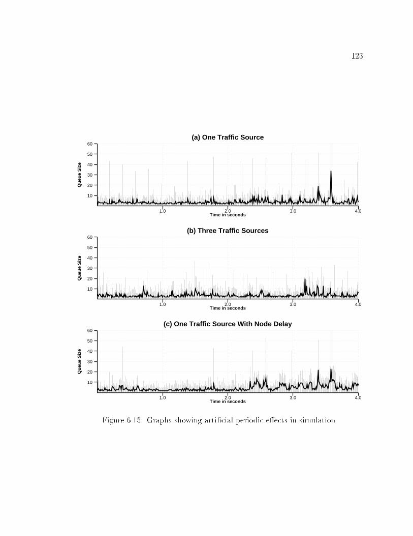
1231.0 2.0 3.0 4.0

Time in seconds

10

20

30

40

50

60

Qu

eue

Siz

e

(a) One Traffic Source

1.0 2.0 3.0 4.0Time in seconds

10

20

30

40

50

60

Qu

eue

Siz

e

(b) Three Traffic Sources

1.0 2.0 3.0 4.0Time in seconds

10

20

30

40

50

60

Qu

eue

Siz

e

(c) One Traffic Source With Node Delay

Figure 6.15: Graphs showing arti�cial periodic e�ects in simulation.

124CHAPTER 7Conclusion7.1 SummaryThis dissertation has presented the design and implementation of both a new con-gestion avoidance mechanism for wide area networks and a wide area network simu-lator. The primary objective of the congestion avoidance mechanism was to increaseperformance in currently available wide area networks by making better utilizationof network resources. The network simulator (x-Sim) was developed to aid in theanalysis and testing of this congestion avoidance mechanism. A description of x-Simwas given in Chapter 2. Its main goals were to: (1) be a realistic network simulator,(2) run x-kernel protocols without modi�cation, (3) include good analysis tools.The reasons for the �rst and third point are obvious. The reason for the sec-ond point, the requirement that x-Sim run x-kernel protocols, is that it allowed usto test the same protocol implementation in both the simulator and the Internet.This eliminates the danger associated with having two implementations of the sameprotocol, one for the simulator and another for the Internet|the danger that thetwo implementations would not exhibit the same exact behavior, leading to faultyresults. The consequences of this requirement are twofold. First, any protocols al-ready implemented in the x-kernel can be used, saving valuable development time.Second, x-Sim is closer to its goal of being a realistic network simulator as a resultof using common protocol implementations.One major weakness of earlier work with end-to-end congestion avoidance mech-anisms is that the mechanisms are never tested in either realistic simulations or realwide area networks. The examination of some of these earlier mechanisms indicatesthat they fail under realistic network conditions. Since one of the goals of this workwas that it result in measurable bene�ts when used over the Internet, and since

125TCP is the most widely used protocol, it was decided that the congestion avoid-ance mechanism should be introduced into TCP. This was done by modifying TCPReno, the most common implementation of TCP in use today, without requiring anychanges to the TCP speci�cation. As a result, this new implementation of TCP,named TCP Vegas, interoperates with any other valid implementation of TCP|infact, all the changes are con�ned to the sending side. TCP and its congestion controlmechanisms were described in Chapter 3.Chapter 4 examined the behavior of TCP Reno's congestion control mechanisms,provided some insights into congestion avoidance, examined previous congestioncontrol mechanisms, and described the congestion avoidance mechanisms in TCPVegas. The main mechanism consists of two fundamental ideas. First, congestioncan be avoided by limiting the number of extra bu�ers used by each connectionin the network. Second, the number of bu�ers used by a connection can be esti-mated by comparing its actual throughput to an expected optimal throughput|thethroughput if there were no congestion in the network.The behavior and performance of TCP Vegas was examined in Chapter 5 throughexperiments on both real and simulated networks. Experiments on the Internetallowed us to measure the performance of TCP Vegas by comparing the throughput,number of retransmissions and network response times achieved by TCP Vegas andTCP Reno. Although important, performance is not the only issue that needs to beconsidered when measuring the value of a new network mechanism. Other relevantissues are the mechanism's e�ects on existing tra�c, its fairness, and its stability.These and other issues were explored through simulations with x-Sim.The value of x-Sim is further demonstrated in Chapter 6 were it is used to analyzeTCP Lite, the TCP implementation in the latest release of the Berkeley SoftwareDistribution (BSD) of Unix. This analysis uncovered a number of problems inTCP Lite which seriously a�ected its performance. The causes of these problemswere determined through the simulator's analysis tools. Finally, solutions to theseproblems are implemented and tested with the simulator. Chapter 6 concludes witha set of guidelines for network simulation.

1267.2 Contributions and LimitationsThis dissertation provides two major contributions to the area of computer net-working. The �rst contribution consists of TCP Vegas and its congestion avoidancemechanisms. Experiments on real and simulated networks show that TCP Vegasachieves between 37 and 71% higher throughput on the Internet, with one-�fth toone-half the losses, as compared to TCP Reno. Moreover, this improvement inthroughput is not achieved by an aggressive strategy that steals bandwidth awayfrom TCP connections that use the current algorithms. Rather, it is achieved by amore e�cient use of the available bandwidth. Further experiments with simulatednetworks also show that TCP Vegas is stable and at least as fair as TCP Reno.Independent experiments by Peter Danzig at USC con�rm that TCP Vegas yieldshigher network throughput and transfers bytes more e�ciently than TCP Reno [1].Although TCP Vegas has been shown to decrease congestion in the network, thefact that it is an end-to-end mechanism imposes certain limitations. For example,its view of the network state is delayed by one round trip time. Therefore it can notalways react quickly enough to avoid congestion; congestion and losses may havealready happened by the time it gets enough information to detect the early stagesof congestion.Insider mechanisms|those in which routers are actively involved|could be moree�ective at avoiding congestion than end-to-end mechanisms since they have moreinformation available to them. This does not necessarily imply that they wouldalways be able to prevent losses; that would depend on the particular details of eachmechanism.One of the reasons why insider mechanisms have not been deployed over theInternet is the high cost of modifying or replacing the routers. Another reason isthe lack of universal agreement on what is the best insider mechanism, and just asimportant, whether the current best is good enough to justify the costs involved.Insider mechanisms will likely be used in the future, the only question is how muchtime their deployment will take.

127Whether end-to-end congestion avoidance mechanisms have a place in the fu-ture of the Internet will depend on the details of the chosen insider mechanism, ormechanisms.The second contribution of this dissertation consists of x-Sim and its analysistools, together with a set of guidelines for doing network simulation. x-Sim wasdesigned to be more realistic than existing network simulators. It achieves this goalthrough two techniques: by executing real protocol code|from the commonly usedimplementations of the protocol|and by producing realistic network tra�c. Theusefulness of x-Sim can be seen throughout this dissertation. It appears �rst in thework dealing with TCP Vegas, and then in the work analyzing TCP Lite. Throughthe simulator and its tools we were able not only discover the existence of perfor-mance problems, but more importantly, to uncover the causes of these problemsand to test solutions to these problems. These solutions resulted in throughputimprovements of more than 20%.The realism of x-Sim comes at a cost: detailed and accurate simulations can takea long time to execute and can use a large number of resources such as memory.Both of this factors limit the complexity and length of network simulations that canbe executed in x-Sim.7.3 Future DirectionsThere are a number of related areas we plan to explore in the future. For example,we plan to enhance the simulator and investigate congestion avoidance techniquesthat require new mechanisms in the routers. As mentioned earlier, the realism ofthe simulator can limit the complexity of the simulations it can run. We plan tosolve this problem by having more than one implementation of the major modulesof the simulator. Each implementation of a module will simulate the behavior of aparticular network component at a di�erent level of realism.This approach has two advantages. First, it allows us to quantify the e�ect onthe simulation of using a lower realism module by comparing the behavior of thesimulator to a version of the simulator that contains the highest realism modules.

128This contrasts the current practice of simplifying simulators during their design: asa result, it is hard to quantify the e�ect the simpli�cations have on the simulations.The second advantage is that we can increase execution speed of the simulator byusing the lowest realism modules which are acceptable for the level of detail we areinterested in.There have been some proposed techniques to avoid network congestion throughnew router mechanisms. A weakness of these works has been the limited realism ofthe simulations used to measure the e�ectiveness of each approach. Analyzing thesemechanisms with x-Sim should either uncover weaknesses or increase the con�dencelevel in these mechanisms.

129REFERENCES[1] J.-S. Ahn, P. B. Danzig, Z. Liu, and L. Yan. Experience with TCP Vegas:Emulation and Experiment. In Proceedings of the SIGCOMM '95 Symposium,pages 185{195, Aug. 1995.[2] R. Braden, D. Clark, and S. Shenker. Integrated Services in the InternetArchitecture: an Overview. Request for Comments 1633, Sept. 1994.[3] R. Brown. Calendar Queues: A Fast O(1) Priority Queue Implementa-tion for the Simulation Event Set Problem. Communications of the ACM,31(10):1220{1227, Oct. 1988.[4] D. Chiu and R. Jain. Analysis of the Increase and Decrease Algorithms forCongestion Avoidance in Computer Networks. Computer Networks and ISDNSystems, 17:1{14, 1989.[5] K. Chung, J. Sang, and V. Rego. A Performance Comparison of Event Calen-dar Algorithms: an Empirical Approach. Software|Practice and Experience,23(10):1107{1138, Oct. 1993.[6] J. C. Comfort. The Simulation of a Microprocessor Based Event Set Processor.14th Annual Simulation Symposium, pages 17{34, 1981.[7] P. Danzig and S. Jamin. tcplib: A Library of TCP Internetwork Tra�c Char-acteristics. Technical Report CS-SYS-91-495, Computer Science Department,USC, 1991.[8] A. Demers, S. Keshav, and S. Shenker. Analysis and Simulation of a FairQueueing Algorithm. In Proceedings of the SIGCOMM '89 Symposium, pages1{12, Sept. 1989.[9] S. Floyd. TCP and Successive Fast Retransmits. Technical report,Lawrence Berkeley Laboratory, 1994. Available from anonymous ftp fromftp.ee.lbl.gov:papers/fastretrans.ps.[10] A. Heybey. The network simulator. Technical report, MIT, Sept. 1990.[11] N. C. Hutchinson and L. L. Peterson. The x-kernel: An architecture for im-plementing network protocols. IEEE Transactions on Software Engineering,17(1):64{76, Jan. 1991.

130[12] N. C. Hutchinson, L. L. Peterson, and S. W. O`Malley. x-Kernel program-mer's manual: Version 3.0. Technical Report 89-29, Department of ComputerScience, University of Arizona, Nov. 1989.[13] V. Jacobson. Congestion Avoidance and Control. In Proceedings of the SIG-COMM '88 Symposium, pages 314{32, Aug. 1988.[14] V. Jacobson and R. Braden. TCP Extensions for Long-Delay Paths. Requestfor Comments 1072, Oct. 1988.[15] V. Jacobson, R. Braden, and D. Borman. TCP Extensions for High Perfor-mance. Request for Comments 1323, May 1992.[16] R. Jain. A Delay-Based Approach for Congestion Avoidance in InterconnectedHeterogeneous Computer Networks. ACM Computer Communication Review,19(5):56{71, Oct. 1989.[17] R. Jain. The Art of Computer Systems Performance Analysis: Techniquesfor ExperimentalDesign, Measurement, Simulation and Modeling. John Wileyand Sons, Inc., New York, 1991.[18] D. W. Jones. An Empirical Comparison of Priority-Queue and Event-SetImplementations. Communications of the ACM, 29(4):300{311, Apr. 1986.[19] S. Keshav. REAL: A Network Simulator. Technical Report 88/472, Depart-ment of Computer Science, UC Berkeley, 1988.[20] S. Keshav. A Control-Theoretic Approach to Flow Control. In Proceedingsof the SIGCOMM '91 Symposium, pages 3{15, Sept. 1991.[21] A. M. Law and W. D. Kelton. Simulation Modelling and Analysis. McGraw-Hill, New York, 1990.[22] W. Leland, M. Taqqu, W. Willinger, and D. Wilson. On the Self-SimilarNature of Ethernet Tra�c. In Proceedings of the SIGCOMM '93 Conference,pages 183{193, Oct. 1993.[23] V. Paxson and S. Floyd. Wide-Area Tra�c: The Failure of Poisson Modeling.In Proceedings of the SIGCOMM '94 Conference, pages 257{268, Aug. 1994.[24] L. L. Peterson and B. S. Davie. Computer Networks: A Systems Approach.Morgan Kaufmann Publishers, Inc., San Fransisco, California, 1996.[25] W. R. Stevens. TCP/IP Illustrated, Volume 1: The Protocols. Addison-Wesley Publishing Co., New York, 1994.

131[26] USC. Transmission control protocol. Request for Comments 793, USC In-formation Sciences Institute, Marina del Ray, Calif., Sept. 1981.[27] Z. Wang and J. Crowcroft. A New Congestion Control Scheme: Slow Startand Search (Tri-S). ACM Computer Communication Review, 21(1):32{43,Jan. 1991.[28] Z. Wang and J. Crowcroft. Eliminating Periodic Packet Losses in 4.3-TahoeBSD TCP Congestion Control Algorithm. ACM Computer CommunicationReview, 22(2):9{16, Apr. 1992.[29] H. J. Weaver. Applications of Discrete and Continuous Fourier Analysis.John Wiley and Sons, Inc., New York, 1983.[30] L. Zhang, S. Shenker, and D. D. Clark. Observations on the Dynamics of aCongestion Control Algorithm: The E�ects of Two-Way Tra�c. In Proceed-ings of the SIGCOMM '91 Symposium, pages 133{147, Sept. 1991.