enamel insulated copper wire in electric motors - core
TRANSCRIPT
University of WindsorScholarship at UWindsor
Electronic Theses and Dissertations
2014
Enamel Insulated Copper Wire in Electric Motors:Sliding Behavior and Possible DamageMechanisms During Die BendingAlbion DemiriUniversity of Windsor
Follow this and additional works at: http://scholar.uwindsor.ca/etd
Part of the Mechanical Engineering Commons
This online database contains the full-text of PhD dissertations and Masters’ theses of University of Windsor students from 1954 forward. Thesedocuments are made available for personal study and research purposes only, in accordance with the Canadian Copyright Act and the CreativeCommons license—CC BY-NC-ND (Attribution, Non-Commercial, No Derivative Works). Under this license, works must always be attributed to thecopyright holder (original author), cannot be used for any commercial purposes, and may not be altered. Any other use would require the permission ofthe copyright holder. Students may inquire about withdrawing their dissertation and/or thesis from this database. For additional inquiries, pleasecontact the repository administrator via email ([email protected]) or by telephone at 519-253-3000ext. 3208.
Recommended CitationDemiri, Albion, "Enamel Insulated Copper Wire in Electric Motors: Sliding Behavior and Possible Damage Mechanisms During DieBending" (2014). Electronic Theses and Dissertations. Paper 5063.
Enamel Insulated Copper Wire in Electric Motors:
Sliding Behavior and Possible Damage Mechanisms During Die Bending
By
Albion Demiri
A Thesis
Submitted to the Faculty of Graduate Studies through the
Department of Mechanical Automotive and Materials Engineering in
Partial Fulfillment of the Requirements for the
Degree of Master of Applied Science at the
University of Windsor
Windsor, Ontario, Canada
2014
© 2014 Albion Demiri
Enamel Insulated Copper Wire in Electric Motors:
Sliding Behavior and Possible Damage Mechanisms During Die Bending
by
Albion Demiri
APPROVED BY:
______________________________________________
Dr. A. Fartaj
Department of Mechanical, Automotive and Materials Engineering
______________________________________________
Dr. A. Alpas
Department of Mechanical, Automotive and Materials Engineering
______________________________________________
Dr. A. Edrisy, Advisor
Department of Mechanical, Automotive and Materials Engineering
22 January 2014
iii
Declaration of Co- Authorship
I hereby declare that this thesis incorporates material that is the outcome of a joint
research undertaken in collaboration with Dr. P. Foss and Dr. T. Perry from the Materials
and Processes Laboratory of General Motors Research and Development Center under
the supervision of Professor A. Edrisy. The collaboration is covered in Chapters 3, 4, and
5 of the thesis. In addition appendix A was written in collaboration with Sama Hussein
and Chris Imeson.
I am aware of the University of Windsor Senate Policy on Authorship and I
certify that I have properly acknowledged the contribution of other researchers to my
thesis, and have obtained written permission from each of the co-author(s) to include the
above material(s) in my thesis.
I certify that, with the above qualification, this thesis, and the research to which it
refers, is the product of my own work.
I declare that, to the best of my knowledge, my thesis does not infringe upon
anyone’s copyright nor violate any proprietary rights and that any ideas, techniques,
quotations, or any other material from the work of other people included in my thesis,
published or otherwise, are fully acknowledged in accordance with the standard
referencing practices. Furthermore, to the extent that I have included copyrighted
material that surpasses the bounds of fair dealing within the meaning of the Canada
Copyright Act, I certify that I have obtained a written permission from the copyright
owner(s) to include such material(s) in my thesis.
I declare that this is a true copy of my thesis, including any final revisions, as
approved by my thesis committee and the Graduate Studies office, and that this thesis has
not been submitted for a higher degree to any other University or Institution.
iv
ABSTRACT
This study investigates the sliding friction and the forming behaviour of enamel insulated
copper wire during the die-forming process. It also aims to determine potential damage
mechanisms to the wire during bending process for electric motor coils. In this investigation a
wire-bending machine was designed and built in order to simulate the wire forming process in a
laboratory scale. Bending angle of the wire and the bending radii were used to control the strain
on the wire surface. The effect of speed on COF was investigated for different speeds of of 1, 5,
10, 15, and 20mm/s. A positive correlation was observed between the COF and the testing
speed. Additionally, the effect of strain on COF was studied for 2% and 23% to determine its
influence on the COF. A general trend was observed of decreased COF with increased strain in
wires. Finally, the ability of the enamel coating to resist external damage and wire strain was
investigated by tensile testing of pre-scratched magnet wire. The results showed that wire
enamel can withstand significant surface damage prior to breach and failure. The insulating
polymer coating failed under the scratch tests at 20N load using a Rockwell indenter and at 5N
load using a 90° conical steel indenter. Additional tests, such as tensile testing, scratch testing
and reciprocating friction testing, were used to characterize the mechanical and tribological
properties of the enamel insulated copper wire.

v
DEDICATION
To my parents Shkëlzen & Anila
For instilling in me the importance of
education

vi
ACKNOWLEDGEMENTS
First I would like to offer my sincere thanks to my advisor Dr. Afsaneh Edrisy for her
guidance and supervision throughout the course of my research. It is though her enthusiasm for
the field that she inspires her students to do grate work.
I would also like to thank the members of my committee Dr. A. Alpas and Dr. A. Fartaj
for their time and commitment attending my presentation and reviewing my thesis. Their input
and feedback was invaluable in the ensuring the quality of my work
Further acknowledgements and thanks our corporate partners at GM R&D Dr. T.Perry
and Dr. P.Foss, for their time and help.
Funding from General Motors is gratefully acknowledged.
Additionally special thanks to technologist Andy Jenner for his help and dedication to
the success of my research.
Finally I would like to thank both my parents for their love and support throughout my
schooling. Thanks my friends and fellow students for all their constant and enthusiastic help.
vii
Table of Contents
Declaration of Co- Authorship ......................................................................................................... iii
ABSTRACT ......................................................................................................................................... iv
DEDICATION ......................................................................................................................................v
ACKNOWLEDGEMENTS .................................................................................................................... vi
List of figures ..................................................................................................................................... x
List of tables ................................................................................................................................. xviii
Nomenclature ................................................................................................................................ xix
List of abbreviations ................................................................................................................... xix
List of symbols ............................................................................................................................. xx
1: Introduction ................................................................................................................................. 1
1.1 Organization of thesis ............................................................................................................ 3
2: Literature survey .......................................................................................................................... 4
2.1 General introduction .............................................................................................................. 4
2.1.1Principle of operation of electric DC motors ................................................................... 4
2.1.2Main operating components ........................................................................................... 6
2.2 Characteristics of the bar wound stator motor ..................................................................... 8
2.3 Enamel used in magnet wire application for electric motors ................................................ 9
2.3.1 Base layer of the enamel or inner most coating ............................................................. 9
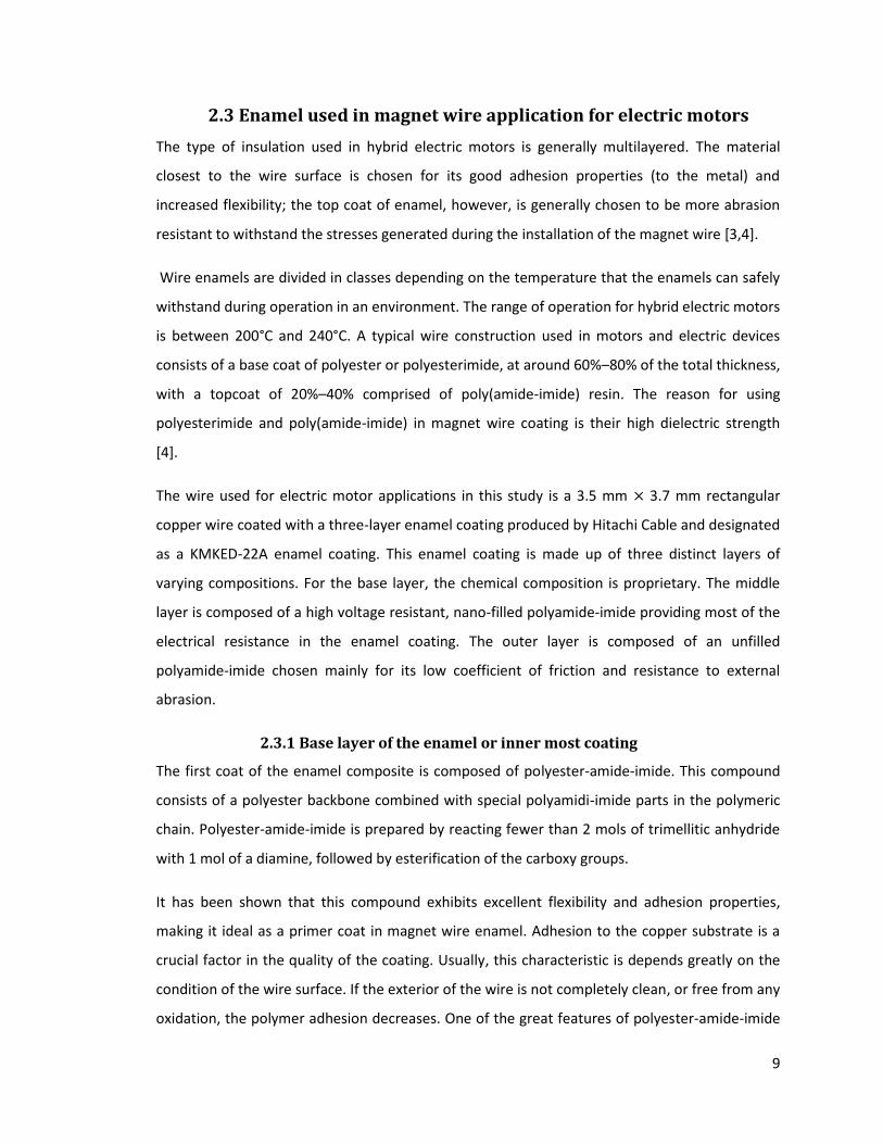
2.3.2 Middle layer of the enamel coating .............................................................................. 10
2.3.3 Third or outer layer of the enamel coating ................................................................... 10
2.4 Magnet wire enamels and required properties ................................................................... 14
2.4.1 Thermal properties ....................................................................................................... 14
2.4.2 Electrical properties ...................................................................................................... 14
2.4.3 Chemical properties ...................................................................................................... 15
2.4.4 Physical properties ........................................................................................................ 15
2.4.5 Windability .................................................................................................................... 15
2.5 Manufacturing of magnet wire ............................................................................................ 23
2.6 Failure modes in wire used in an electric motor ................................................................. 25
2.6.1 Aging of enamel wire .................................................................................................... 26
2.6.2 Defects in magnet wire manufacturing ........................................................................ 28
viii
2.7 Testing methods of magnet wire enamel ............................................................................ 35
2.7.1 Dynamic coefficient of friction test............................................................................... 35
2.7.2 Scratch test for enamel coated magnet wire................................................................ 37
2.7.3 Repeated scrape test .................................................................................................... 44
2.7.4 Unilateral scrape test .................................................................................................... 45
2.7.5 Nano indentation .......................................................................................................... 45
2.8 Isolated contact stress deformations of polymers .............................................................. 47
2.8.1 Influence of contact strain in enamel surface reaction ................................................ 47
2.8.2 Influence of normal load on enamel surface reaction .................................................. 48
2.8.3 Scratch map of polymers .............................................................................................. 49
2.9 Work objectives ................................................................................................................... 58
3: Material and experimental methods ......................................................................................... 59
3.1 Magnet wire sample used .................................................................................................... 60
3.1.1 Cross-sectional preparation and micro-structural observation of magnet wire samples 60
3.1.2 Enamel coating layers composition .............................................................................. 64
3.2 Wire enamel characterization testing procedure ................................................................ 66
3.2.1 Micro-indentation testing ............................................................................................. 66
3.2.2 Scratch testing............................................................................................................... 67
3.2.3 Reciprocating COF measurement procedure................................................................ 68
3.3 Die-forming friction measuring method .............................................................................. 72
3.3.1 Design and fabrication considerations of wire-forming simulator ............................... 72
3.3.2 Die-forming procedure ................................................................................................. 82
3.3.3 Wire-forming simulator machine testing procedure .................................................... 84
3.4 Wire tensile testing procedure ............................................................................................ 86
3.5 Pre-scratch enamel response to tensile testing procedures ............................................... 87
4: Results ........................................................................................................................................ 90
4.1 Wire enamel characterization testing results ...................................................................... 90
4.1.1 Micro-indentation testing results ................................................................................. 90
4.1.2Constant load scratch testing ........................................................................................ 92
4.1.3. Varying load scratch testing ......................................................................................... 97
4.2 Reciprocating COF measurement results .......................................................................... 100
4.3 Wire-on-wire reciprocating friction tests results ............................................................... 116
ix
4.4 Wire bedding simulator machine preliminary calibration testing results ......................... 118
4.4.1 Sample surface ............................................................................................................ 126
4.5 Diamond-like coating (DLC) counterface friction testing................................................... 136
4.6 Friction testing of uniformly strained samples .................................................................. 139
4.7 Effect of bending angle and bending radius friction results .............................................. 142
4.8 Friction testing of magnet wire samples at various speeds and surface strains ............... 148
4.9 Tensile testing of enamelled magnet wires ....................................................................... 155
4.9.1 Tensile test results ...................................................................................................... 155
4.9.3 Tensile testing sample observations ........................................................................... 157
4.10 Pre-scratch enamel response to tensile testing .............................................................. 166
4.10.1 Experimental results, scratch testing observations .................................................. 167
4.10.2 Experimental results, tensile testing observations ................................................... 176
5: Discussion ................................................................................................................................ 188
5.1 Magnet wire friction coefficient fluctuation at reciprocating friction test........................ 188
5.2 Sample Tension, Strain Control and Calculation ................................................................ 189
5.3 Effect of counterface on coefficient of friction .................................................................. 190
5.4 Effect of speed on coefficient of friction ........................................................................... 191
5.5 Effect of surface strain on coefficient of friction ............................................................... 192
5.6 Enamel coating damage threshold in magnet wire ........................................................... 193
6: Summary and Conclusions ....................................................................................................... 195
6.1 Suggestions for future research ......................................................................................... 198
References ................................................................................................................................... 199
Appendix A: Wire Bending Machine Operating Manual .............................................................. 202
VITA AUCTORIS ............................................................................................................................ 252
x
List of figures
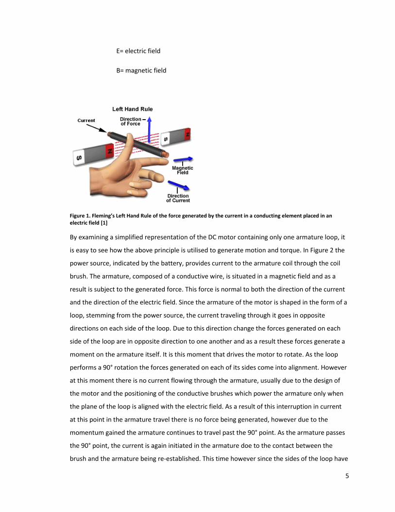
Figure 1. Fleming’s Left Hand Rule of the force generated by the current in a conducting element
placed in an electric field [1] ............................................................................................................ 5
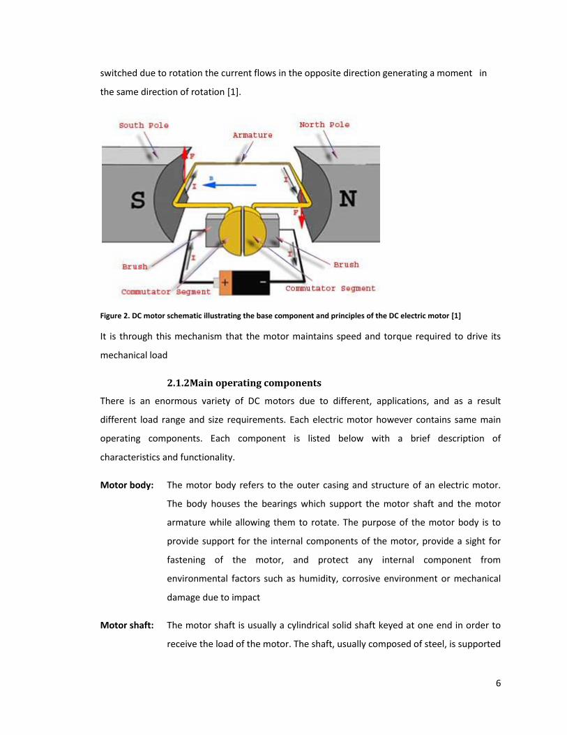
Figure 2. DC motor schematic illustrating the base component and principles of the DC electric
motor [1] .......................................................................................................................................... 6
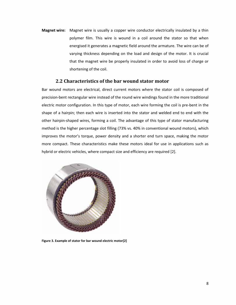
Figure 3. Example of stator for bar wound electric motor[2] .......................................................... 8
Figure 4. silicon particle dispersion in ester-imide base of mid layer (corona resistant nano-filled
polyamide-imide) [7]...................................................................................................................... 10
Figure 5. Adhesion: New enamels for hevy and flat wires. Adhesion tested through the twist peel
method. .......................................................................................................................................... 11
Figure 6. Temperature index for new flat wire enamels Components tested: E3537=usual THEIC-
esterimide, E3525=polihydration, E3537HHT=modified Poly-THEIC-Esermide high tenperature
stability, E3960=modified Poly-THEIC-Esermide low tenperature stability, E3940=modified
Polyester-amide-imide, E3566= modified Polyamide-imide [4-5] ................................................. 12
Figure 7. constitution unit of a polyamide-imide resin can be both thermosetting or
thermoplastic amorphous polymer [6] .......................................................................................... 12
Figure 8. wire insulation properties [3,5] ...................................................................................... 13
Figure 9. Characteristics of PAI Film [4] ......................................................................................... 13
Figure 10. Circulating pump-felt principle. Dosage by level, felt application [12] ........................ 18
Figure 11. Principle of roller dosage, roller polishing [12] ............................................................. 18
Figure 12. principle of yarn lubrication [12] .................................................................................. 19
Figure 13. Application from the vapor phase by condensation [12] ............................................. 19
Figure 14. Peel-twist test results [3] .............................................................................................. 22
Figure 15. Measurement results of adhesion force between conductor and film. Adhesion
pressure is measured against compresion ratio of the enamel wire showing a drop in adhesion
force at 30% [3] .............................................................................................................................. 22
Figure 16. illustration of wire rolling from round to rectangular profile [15] ............................... 23
Figure 17. Summary of data from thermal aging of elongated enameled wire samples.
Experimental enamels A, B, C, and control enamel D, chosen for its good heat resistance but
poor aging performance [17] ......................................................................................................... 25
Figure 18. Polyimide deterioration mechanism. Top: normal repeat unit. Middle: incomplete
imidized defect site. Bottom: scission of defect site by water reaction [19]. ............................... 26
Figure 19. Optical micrographs showing sliver from rod [15] ....................................................... 29
Figure 20. longitudinal cracks in wire caused during rolling [15] .................................................. 29
Figure 21. Wire drawing surface damage [15] ............................................................................... 30
Figure 22. Copper fines in enamel base coat [15] ......................................................................... 31
Figure 23. SEM micrograph showing cavitation defect on surface of film [15] ............................. 31
Figure 24. scratches in enamel caused by mechanical damage [15] ............................................. 32
Figure 25. tracking defects in enamel film [15] ............................................................................. 32
Figure 26. optical micrograph showing airborne contaminants collected near oven [15]............ 33
xi
Figure 27. optical micrograph showing foreign contaminants [15] ............................................... 33
Figure 28. SEM micrograph showing gel particles [15] .................................................................. 34
Figure 29. Photographs showing faults due to voids in base coat [15] ......................................... 34
Figure 30. SEM photograph of pinhole in enamel film [15] ........................................................... 34
Figure 31. test loads for coefficient of friction testing [28] ........................................................... 35
Figure 32. drawing of friction head assembly [22] ........................................................................ 36
Figure 33. load contact surface - Sapphire (Synthetic) [22]........................................................... 37
Figure 34. residual scratch parameters of interest for (a) 3-response model concerning
deformation response analysis, and (b) interpretation of measured test quantities [25]. .......... 39
Figure 35. materials used in scratch testing study [26] ................................................................. 40
Figure 36. critical normal and tangential forces [26] ..................................................................... 40
Figure 37. Type I scratches: deformation fringes are convex with respect to the scratching
direction (75µm radius stylus). (a) PET at 120g normal load; (b) pure gelatin at 50% RH at 30g
normal load; (c)polypropylene at a normal load f 50g. [26] .......................................................... 41
Figure 38. Type II scratches: deformation fringes are concave with respect to the scratching
direction (75 gm radius stylus). (a) Acetate at normal load of 100 g; (b) gelatin at 5% RH at
normal load of i30 g; (c) glass at a normal load of 1000 g [26] ..................................................... 42
Figure 39. Type III scratches: removal of the overcoat (75 gm radius stylus) [26] ........................ 43
Figure 40. Type IV scratches: clear track (75 gm radius stylus). (a) PET/PDMS at normal load of
120 g; (b) acetate/PDMS at normal load of 100 g; (c) glass at a normal load of 500 g [26] .......... 44
Figure 41. magnet wire candidates under investigation for nanoindentation [27] ...................... 46
Figure 42. Young’s modulus of elasticity (GPa) for the individual layers of wire enamel tested
[27] ................................................................................................................................................. 46
Figure 43. Hardnes (GPa) measurement of the 8 wire enamels tested [27] ................................. 46
Figure 44. The influence of cone angle a, upon the types of damage produced in scratching. This
type of response is typical for polymers . For clarity of presentation the pictorial view does not
show the variation in attack angle α [28] ...................................................................................... 48
Figure 45. Deformation map for a poly (carbonate) resin. The diagram shows results from
scratching performed at room temperature for a range of cone angles and normal loads and at a
scratching velocity of 0.0026 mm/s [28] ....................................................................................... 49
Figure 46. Ductile ploughing. SEM (×200)of a scratch on a PMMA. The scratch was produced
under the following contact conditions: cone angle, 120°: normal load, 1.2 N; scratching velocity,
0.2 mm/s; T= 20 °C; no lubricant. [23] ........................................................................................... 51
Figure 47. Regular crank formation. SEM (X 200) of a scratch on a UHMWP. The scratch was
produced under the following contact conditions; cone angle, 90°; normal load, 2 N; scratching
velocity, 0.2 mm/s; T = 20 °C; no lubricant [23] ............................................................................. 52
Figure 48. Machining and clip forming. SEM (x200) of a scratch on a HDPC. The scratch was
performed under the following contact conditions: cone angle, 30°; normal load, 2,5N;
scratching velocity, 0.002mm/s; T= 20 °C; no lubricant [23] ......................................................... 53
Figure 49. Ironing. SEM ( × 100) of a scratch on a UHMWPE. The scratch was produced under the
following contact conditions: cone angle, 120°; normal load, 0.5 N; scratching velocity 0.2mm/s;
T = 20°C; no lubricant [23] ............................................................................................................. 54
xii
Figure 50. Scratching mode map for PMMA. The diagram shows the dependence office observed
scratching deformation mode upon the nominal contact strain and the applied normal load. The
scratches were produced at a constant scratching velocity of 0.004mm/s, at ambient
temperature (20 °C) and under un-lubricated contact conditions [23]......................................... 55
Figure 51. Scratching mode map for PMMA. The diagram shows the dependence of the
observed scratching deformation mode upon the nominal contact strain and the bulk
temperature. The scratches were produced at a constant scratching velocity of 0.004 mm/s,
under a constant applied load of l N and un-lubricated contact conditions [23] .......................... 56
Figure 52. Friction map for PMMA, PTFE and UHMWPE. The coefficient of friction is plotted as a
function of (E/Y)tan θ or (E/Y)(r/R). The scratches were produced using a range of spheres and
cones of various dimensions at room temperature and under un-lubricated conditions. The plot
shows that the friction coefficient is fairly constant when the ironing deformation regime is
observed ((E/Y)tan θ <3 for PTFE and (E/Y)tan θ <5 for PMMA and UHMWPE). For higher values
of (E/Y)tan θ, the friction coefficient data display along a slope (ductile ploughing) until brittle
fracture is produced ((E/Y)tan θ >30 for PMMA). [23] .................................................................. 57
Figure 53. Schematic of a typical bar wound permanent magnet electric motor [30]. ................ 59
Figure 54. General dimensions of rectangular wire samples. ....................................................... 60
Figure 55. View of the polished polymer coating cross-section observed through SEM at 400x
magnification showing mounting material the enamel coating and the copper wire cross-section.
....................................................................................................................................................... 61
Figure 56. Polymer coating cross-section observed through SEM at 3000x magnification .......... 62
Figure 57. Polymer coating cross-section at enamel wire corner observed through SEM at 800x
magnification ................................................................................................................................. 64
Figure 58. EDS scans of the enamel coating, a) color-coded illustration of each scan on the SEM
image of the wire enamel cross-section, b) EDS scan of the inner most layer (primer) of the
enamel coating, c) EDS scan of the middle layer (nano-filled isolative layer) of the enamel
coating, d) EDS scan of the outer most layer of the enamel coating. ........................................... 66
Figure 59. Loading curve for micro-indentation. ........................................................................... 67
Figure 60. Movement direction of the wire-on-wire reciprocating friction test. .......................... 69
Figure 61. Sample holder setup for wire-on-wire reciprocating friction test. ............................... 70
Figure 62. Setup for the wire-on-wire reciprocating friction test in the universal testing machine.
....................................................................................................................................................... 71
Figure 63. Photograph of wire forming simulator machine. ......................................................... 73
Figure 64. Illustration of wire forming simulator machine. ........................................................... 74
Figure 65. Friction arm and roller assembly. ................................................................................. 75
Figure 66. Photograph friction arm and roller assembly. .............................................................. 75
Figure 67. Friction arm and load cell assembly. ............................................................................. 76
Figure 68. Calibration chart for total load range with cubic trend line ......................................... 77
Figure 69. Calibration chart for the lower section of the load range with cubic trend line .......... 78
Figure 70. Calibration chart for middle section of the load range 2lb-10lb with cubic trend line 78
Figure 71. Calibration chart for upper section of the load range 10lb-16lb with cubic trend line 79
Figure 72. Wire tension load cell in assembly................................................................................ 80
xiii
Figure 73. Section view of friction arm and roller assembly ......................................................... 81
Figure 74. Actuator arm assembly ................................................................................................. 82
Figure 75. Progressive stages of XY dies based wire forming [30]. ............................................... 84
Figure 76. Clamp modeled after tensile testing clamp, US patent #3528283 ............................... 87
Figure 77. Illustration of the wire tensile sample with gage length and grip sections highlighted in
white and blue, respectively. ......................................................................................................... 88
Figure 78. Averaged depth vs. applied force graph for 0.5N micro-indentation test. .................. 91
Figure 79. SEM image of micro-indentation site on the sample surface observed at 800x
magnification. ................................................................................................................................ 92
Figure 80. Friction coefficient vs. distance travelled in a 1N load scratch test. ............................ 93
Figure 81. Friction coefficient vs. distance travelled in a 2N load scratch test. ............................ 93
Figure 82. Friction coefficient vs. distance travelled in a 3N load scratch test. ............................ 93
Figure 83. SEM image of 1N scratch-test site observed at an inclination of 50° and 400x
magnification. ................................................................................................................................ 94
Figure 84. Optical microscope image of 1N scratch track. ............................................................ 95
Figure 85. SEM image of 2N scratch test site observed at an inclination of 50° and 200x
magnification. ................................................................................................................................ 95
Figure 86. Optical microscope image of 2N scratch track. ............................................................ 96
Figure 87. SEM image of 3N scratch test site observed at an inclination of 50° and 200x
magnification. ................................................................................................................................ 96
Figure 88. Optical microscope image of 3N scratch track. ............................................................ 97
Figure 89. Friction coefficient (COF), normal load (Fn) and tangential load (Ft) measurements for
the 0.03N-3.7N load scratch test. .................................................................................................. 98
Figure 90. The 0.03N-3.7N load scratch test track observed through optical microscope and used
to measure the track width during the scratch test. ..................................................................... 98
Figure 91. The 0.03N-3.7N load scratch test track observed through SEM................................... 98
Figure 92. Surface scratch hardness calculation according to the standard test method for the
Evaluation of Scratch Resistance of Polymeric Coatings and Plastics (ASTM Standard D7027 –
05). ................................................................................................................................................. 99
Figure 93. Friction coefficient (COF), normal load (Fn) and tangential load (Ft) measurements for
the 0.03N-1N load scratch test. ..................................................................................................... 99
Figure 94. COF and friction force results for the entirety of the 5N normal load 5mm/s speed
test. a) initial testing results (0-150 seconds). b) mid section results (150-300 seconds) . c) final
section results (250 to 400 seconds) ........................................................................................... 101
Figure 95. Tangential force and COF for the first passes of the 5N 5mm/s test. ........................ 103
Figure 96. COF for the first passes of the 5N test. ....................................................................... 103
Figure 97. Static COF for the 5N test. .......................................................................................... 104
Figure 98. Tangential force and COF for the last passes of the 5N test. ..................................... 104
Figure 99. COF for the last passes of the 5N test with a recorded value of 0.053-0.058. ........... 105
Figure 100. Depth of sphere tip along the surface for the first, second, and last sample pass for
the 5N test. .................................................................................................................................. 105
Figure 101. 100x magnification of 5N test wear track. ................................................................ 106
xiv
Figure 102. SEM image of 5N test wear track observed at 45° inclination, carbon coated and
observed at low vacuum. ............................................................................................................. 106
Figure 103. COF results vs. time for 10N test. Figures a-f shows the progression of COF and
friction force with time. ............................................................................................................... 110
Figure 104. Tangential force and COF for the first passes of the 10N test. ................................. 111
Figure 105. Forward direction COF for the first passes of the 10N test [recorded value 0.056-
0.047]. .......................................................................................................................................... 112
Figure 106. Forward direction COF for the last passes of the 10N test [recorded value 0.0598].
..................................................................................................................................................... 112
Figure 107. Tangential force and COF for the last passes of the 10N test. ................................. 113
Figure 108. COF for the last passes of the 10N test [recorded value 0.1-0.092]. ........................ 113
Figure 109. 100x magnification of 10N test wear track. .............................................................. 114
Figure 110. SEM observations of 10N wear track. ....................................................................... 115
Figure 111. Depth of sphere tip along the surface for the first, second and last sample pass for
the 10N test. ................................................................................................................................ 115
Figure 112. COF and tangential force observed in 2N normal load wire-on-wire reciprocating
friction test. .................................................................................................................................. 116
Figure 113. COF and tangential force observed in 4N normal load wire-on-wire reciprocating
friction test. .................................................................................................................................. 116
Figure 114. COF and tangential force observed in 6N normal load wire-on-wire reciprocating
friction test. .................................................................................................................................. 116
Figure 115. COF and tangential force observed in 8N normal load wire-on-wire reciprocating
friction test. .................................................................................................................................. 117
Figure 116. COF and tangential force recorded in 10N normal load wire-on-wire reciprocating
friction test. .................................................................................................................................. 117
Figure 117. COF and Normal load using 6mm ball bearing diameter counterface tested at 5mm/s
speed ............................................................................................................................................ 121
Figure 118. COF and Normal load using 3mm ball bearing diameter counterface tested at 5mm/s
speed ............................................................................................................................................ 121
Figure 119. COF and Normal load using 6mm ball bearing diameter counterface tested at
10mm/s speed ............................................................................................................................. 122
Figure 120. COF and Normal load using 3mm ball bearing diameter counterface tested at
10mm/s speed ............................................................................................................................. 122
Figure 121. COF and Normal load using polished 4140 steel, counterface 20mm/s speed 40lb
normal load 60° bend 3mm cylinder radius ................................................................................ 123
Figure 122. COF and Normal load using polished 4140 steel counterface, 20mm/s speed 40lb
normal load 60° bend 24mm cylinder radius .............................................................................. 123
Figure 123. COF and Normal load using polished 4140 steel counterface, 20mm/s speed, 60lb
normal load .................................................................................................................................. 124
Figure 124. COF and Normal load using polished 4140 steel counterface, 20mm/s speed, 40lb
normal load .................................................................................................................................. 124
xv
Figure 125. Coefficient of friction (with standard deviations) obtained through calibration testing
at various conditions. ................................................................................................................... 125
Figure 126. Optical microscope image of sample surface for friction test using Counterface
diameter: 6mm at sliding speed: 5mm/s ..................................................................................... 127
Figure 127. Optical microscope image of sample surface for friction test using Counterface
diameter: 6mm at sliding speed: 10mm/s ................................................................................... 127
Figure 128. Optical microscope image of sample surface for friction test using Counterface
diameter: 3mm at sliding speed: 5mm/s ..................................................................................... 128
Figure 129. Optical microscope image of sample surface for friction test using Counterface
diameter: 3mm at sliding speed: 10mm/s ................................................................................... 128
Figure 130. Optical microscope image of sample surface for friction test using 4140 flat on flat
counterface at 40lb normal load. ................................................................................................ 129
Figure 131. Optical microscope image of 4140 counterface surface after testing...................... 130
Figure 132. Zygo image of 6mm diameter ball counter face at 5mm/s speed ............................ 132
Figure 133. Zygo image of 6mm diameter ball counter face at 10mm/s speed .......................... 133
Figure 134. Zygo image of 3mm diameter ball counter face at 5mm/s speed ............................ 134
Figure 135. Zygo image of 3mm diameter ball counter face at 10mm/s speed .......................... 135
Figure 136. Summary of DLC average friction testing results and standard deviation ............... 138
Figure 137. Average friction results and standard deviation for elongated samples .................. 141
Figure 138. Summary of clean wire and bent wire sample friction test for 24mm radius roller.
Average friction testing results and standard deviation.............................................................. 145
Figure 139. The average coefficient of friction and standard deviation for tests performed at
various degrees of forming using 3mm radius roller. .................................................................. 145
Figure 140. Average COF results and standard deviation. COF results at varying roller radius and
forming angle. .............................................................................................................................. 146
Figure 141. Individual sample COF results as a function of the maximum predicted strain applied
to the wire. ................................................................................................................................... 147
Figure 142. Coefficient of friction plot along the sample length for the 2% surface strain sample
at varying sample speed .............................................................................................................. 149
Figure 143. Coefficient of friction plot along the sample length for the 5% surface strain sample
at varying sample speed .............................................................................................................. 149
Figure 144. Coefficient of friction plot along the sample length for the 10% surface strain sample
at varying sample speed .............................................................................................................. 149
Figure 145. Coefficient of friction plot along the sample length for the 15% surface strain sample
at varying sample speed .............................................................................................................. 150
Figure 146. Coefficient of friction plot along the sample length for the 20% surface strain sample
at varying sample speed .............................................................................................................. 150
Figure 147. Average coefficient of friction and standard deviation values at varying surface
strain. Each line representing sample testing speed. .................................................................. 151
Figure 148. Average coefficient of friction and standard deviation values at varying sample
testing speed. Each line representing surface strain. .................................................................. 151
xvi
Figure 149. Surface plot of the average coefficient of friction vs. sample surface strain vs. friction
testing speed, a) tilted surface plot, b) normal view of surface plot. .......................................... 152
Figure 150. 3D column plot of the average coefficient of friction vs. sample surface strain vs.
friction testing speed ................................................................................................................... 153
Figure 151. 3D column plot of the average coefficient of friction showing standard deviation vs.
sample surface strain vs. friction testing speed .......................................................................... 154
Figure 152. engineering stress and strain curves for tensile tested magnet wire ....................... 156
Figure 153. examination of magnet wire enamel failure sites .................................................... 157
Figure 154. Side view of cup and cone fracture .......................................................................... 158
Figure 155. Top view of cup and cone fracture ........................................................................... 159
Figure 156. 200X magnification wire surface at fracture Heavily deformed wire necking region
..................................................................................................................................................... 160
Figure 157. 400x Magnification fracture surface transition from side of the sample to shear
failure section .............................................................................................................................. 161
Figure 158. Tensile failure section 200x Magnification Uniform dimple pattern observed
throughout the fracture surface .................................................................................................. 162
Figure 159. Tensile failure section 800x Magnified side view of failure pattern in fracture surface
..................................................................................................................................................... 163
Figure 160. Tensile test fracture surface 400x Magnified top view of interior failure pattern ... 164
Figure 161. Tensile test fracture surface 1500x Magnified top view of interior failure pattern . 165
Figure 162. Tensile test fracture surface 3000x Magnified top view of interior failure pattern . 166
Figure 163. optical image of the scratch path on the enamel coating at 5N load....................... 168
Figure 164. SEM images from enamel cross-section prior to tensile test with scratches at normal
loads of 5N (Rockwell indenter) ................................................................................................... 168
Figure 165. optical image of the scratch path on the enamel coating at 10N load..................... 169
Figure 166. SEM images from enamel cross-section prior to tensile test with scratches at normal
loads of 10N (Rockwell indenter)................................................................................................. 169
Figure 167. optical image of the scratch path on the enamel coating at 15N load..................... 170
Figure 168. SEM images from enamel cross-section prior to tensile test with scratches at normal
loads of 15N (Rockwell indenter)................................................................................................. 170
Figure 169. optical image of the scratch path on the enamel coating at 20N load..................... 171
Figure 170. SEM images from enamel cross-section prior to tensile test with scratches at normal
loads of 20N (Rockwell indenter)................................................................................................. 171
Figure 171 optical image of the scratch path on the enamel coating at 25N load ..................... 172
Figure 172. SEM images from enamel cross-section prior to tensile test with scratches at normal
loads of 25N (Rockwell indenter)................................................................................................. 173
Figure 173. SEM images from enamel cross-section prior to tensile test with scratches at normal
loads of 20N (conical indenter) .................................................................................................... 173
Figure 174. optical image of the scratch path on the enamel coating at 20N load (90° cone steel
indenter) ...................................................................................................................................... 174
Figure 175. Variation of the scratch width on the enamel coating at different loads ................ 175
Figure 176. Variation of the scratch depth at different loads on the enamel wires .................. 175
xvii
Figure 177. (a, b) - SEM images from enamel surfaces undergone 20% strain by tensile test with
per-existing scratches at normal loads of 25N (rockwell indenter) and 20N (90° cone tip)
respectively. ................................................................................................................................. 178
Figure 178. (a, b) - SEM images from enamel surfaces undergone 25% strain by tensile test with
per-existing scratches at normal loads of 25N (rockwell indenter) and 20N (90° cone tip)
respectively. ................................................................................................................................. 179
Figure 179. (a, b) - SEM images from enamel surfaces undergone 30% strain by tensile test with
per-existing scratches at normal loads of 25N (rockwell indenter) and 20N (90° cone tip)
respectively. ................................................................................................................................. 180
Figure 180. (a, b) - SEM images from enamel surfaces undergone 35% strain by tensile test with
per-existing scratches at normal loads of 25N (rockwell indenter) and 20N (90° cone tip)
respectively. ................................................................................................................................. 181
Figure 181. (a, b) - SEM images from enamel surfaces undergone 40% strain by tensile test with
per-existing scratches at normal loads of 25N (rockwell indenter) and 20N (90° cone tip)
respectively. ................................................................................................................................. 182
Figure 182. (a, b,c) - SEM images from enamel surfaces undergone 45% strain by tensile test
with per-existing scratches at normal loads of 20N (rockwell indenter), 25N (rockwell indenter),
and 20N (90° cone tip) respectively. ........................................................................................... 183
Figure 183. (a, b,c) - SEM images from enamel surfaces undergone 50% strain by tensile test
with per-existing scratches at normal loads of 20N (rockwell indenter), 25N (rockwell indenter),
and 20N (90° cone tip) respectively. ........................................................................................... 184
Figure 184. The increase in the scratch width (using rockwell indenter) of enamel coating after
tensile tests at various strain percentage .................................................................................... 185
Figure 185. Scratch width versus applied normal load (Rocwell indenter) after tensile tests at
different strain range ................................................................................................................... 186
Figure 186. Scratch width versus applied normal load (90° conica indenter) after tensile tests at
different strain range ................................................................................................................... 186
Figure 187. Digital images of the outer enamel surfaces before and after the tensile test shows
an increase in the roughness ....................................................................................................... 187
xviii
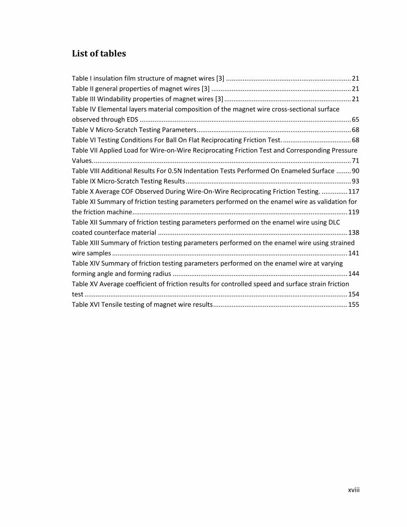
List of tables
Table I insulation film structure of magnet wires [3] .................................................................... 21
Table II general properties of magnet wires [3] ............................................................................ 21
Table III Windability properties of magnet wires [3] ..................................................................... 21
Table IV Elemental layers material composition of the magnet wire cross-sectional surface
observed through EDS ................................................................................................................... 65
Table V Micro-Scratch Testing Parameters .................................................................................... 68
Table VI Testing Conditions For Ball On Flat Reciprocating Friction Test. ..................................... 68
Table VII Applied Load for Wire-on-Wire Reciprocating Friction Test and Corresponding Pressure
Values. ............................................................................................................................................ 71
Table VIII Additional Results For 0.5N Indentation Tests Performed On Enameled Surface ........ 90
Table IX Micro-Scratch Testing Results .......................................................................................... 93
Table X Average COF Observed During Wire-On-Wire Reciprocating Friction Testing. .............. 117
Table XI Summary of friction testing parameters performed on the enamel wire as validation for
the friction machine ..................................................................................................................... 119
Table XII Summary of friction testing parameters performed on the enamel wire using DLC
coated counterface material ....................................................................................................... 138
Table XIII Summary of friction testing parameters performed on the enamel wire using strained
wire samples ................................................................................................................................ 141
Table XIV Summary of friction testing parameters performed on the enamel wire at varying
forming angle and forming radius ............................................................................................... 144
Table XV Average coefficient of friction results for controlled speed and surface strain friction
test ............................................................................................................................................... 154
Table XVI Tensile testing of magnet wire results ......................................................................... 155
xix
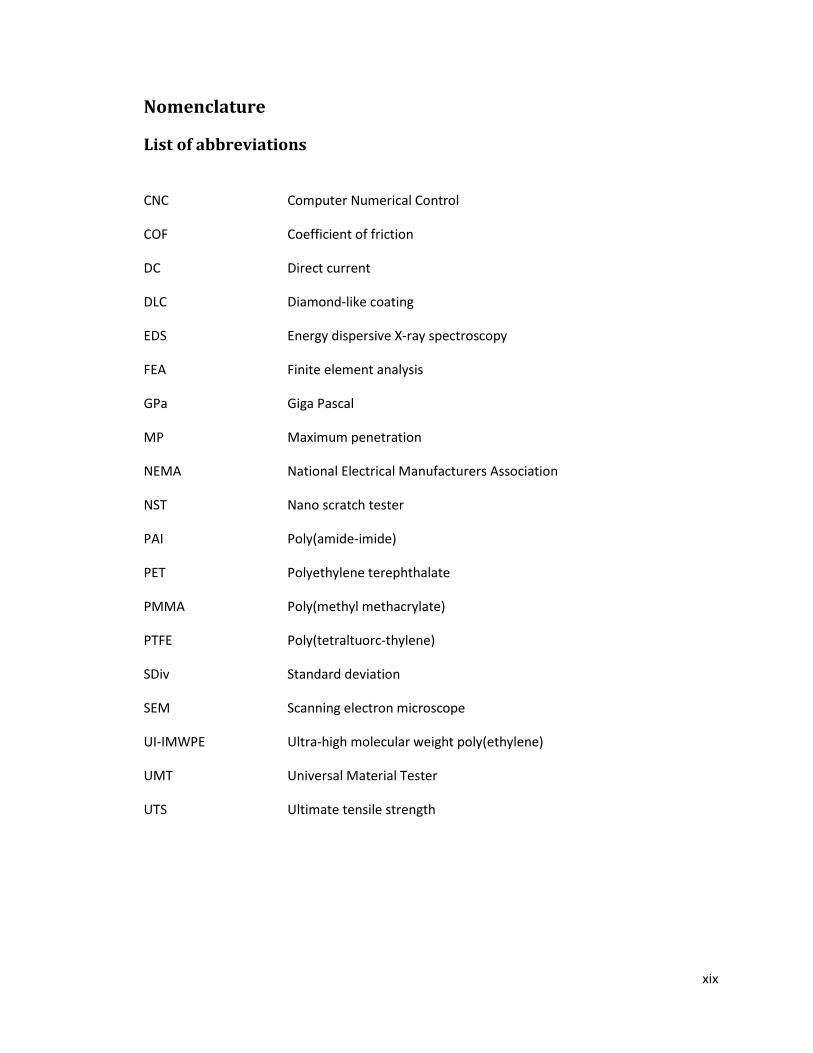
Nomenclature
List of abbreviations
CNC Computer Numerical Control
COF Coefficient of friction
DC Direct current
DLC Diamond-like coating
EDS Energy dispersive X-ray spectroscopy
FEA Finite element analysis
GPa Giga Pascal
MP Maximum penetration
NEMA National Electrical Manufacturers Association
NST Nano scratch tester
PAI Poly(amide-imide)
PET Polyethylene terephthalate
PMMA Poly(methyl methacrylate)
PTFE Poly(tetraltuorc-thylene)
SDiv Standard deviation
SEM Scanning electron microscope
UI-IMWPE Ultra-high molecular weight poly(ethylene)
UMT Universal Material Tester
UTS Ultimate tensile strength
xx
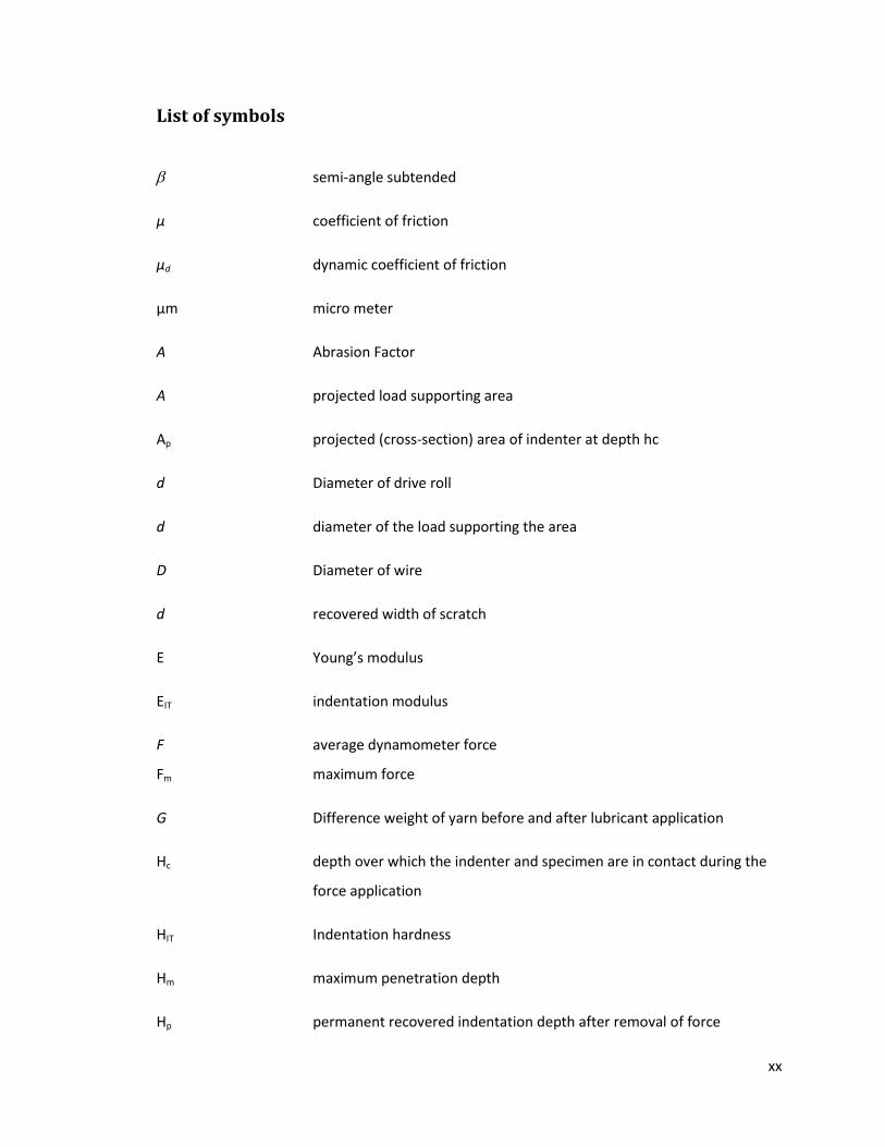
List of symbols
semi-angle subtended
µ coefficient of friction
µd dynamic coefficient of friction
µm micro meter
A Abrasion Factor
A projected load supporting area
Ap projected (cross-section) area of indenter at depth hc
d Diameter of drive roll
d diameter of the load supporting the area
D Diameter of wire
d recovered width of scratch
E Young’s modulus
EIT indentation modulus
F average dynamometer force
Fm maximum force
G Difference weight of yarn before and after lubricant application
Hc depth over which the indenter and specimen are in contact during the
force application
HIT Indentation hardness
Hm maximum penetration depth
Hp permanent recovered indentation depth after removal of force
xxi
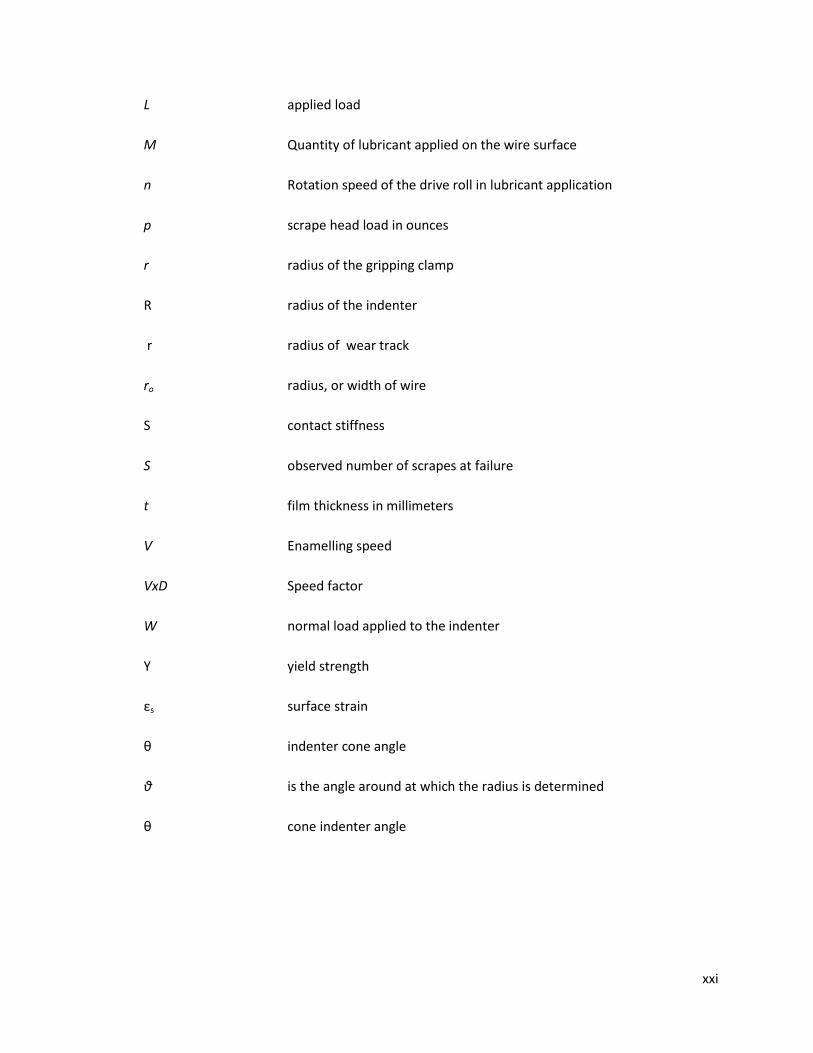
L applied load
M Quantity of lubricant applied on the wire surface
n Rotation speed of the drive roll in lubricant application
p scrape head load in ounces
r radius of the gripping clamp
R radius of the indenter
r radius of wear track
ro radius, or width of wire
S contact stiffness
S observed number of scrapes at failure
t film thickness in millimeters
V Enamelling speed
VxD Speed factor
W normal load applied to the indenter
Y yield strength
εs surface strain
θ indenter cone angle
θ is the angle around at which the radius is determined
θ cone indenter angle
1
1: Introduction Numerous electric devices that are used every day, such as motors, transformers and
electromagnets, rely on electrical coils for their operation. These long segments of insulated
conductive material, in most instances copper wire, are tightly wound and must not allow
conduction between adjacent wires. In electric motors, the coil wires are referred to as magnet
wires because the magnetization of the coil provides the force for the rotation of the rotor.
Closely packing the wire into the stator is essential to manufacturing the electrical coil, because
this action increases the power density of the motor. As a result of this requirement, the goal is
to make magnet wire insulation that electrically insulates the coil loops from one another even
thinner so there would be more space in the stator enclosure for the copper wire. The thinness
and transparent nature of the insulating material have caused it to be described as wire enamel
coating, even though the material is a multilayer polymer coating and not a ceramic coating, as
the term “enamel” would imply. The enamel coating generally consists of a multi-layer polymer
coating of a thickness in the order of 50 µm. Its flexibility and its resistance to external damage
during winding play a critical role in the longevity of the coil and the correct operation of the
motor. The properties of ideal magnet wire enamel must balance the thinness of the coating
with the ability to insulate the magnet wire and to withstand the coil-winding process.
Apart from enamel thickness, other factors, such as wire shape and thickness, can be
used to increase the space that can be filled of a motor stator. For the bar wound eclectic motor
(which will be addressed in this thesis), a rectangular gauge wire, for example is used to more
fully fill the stator space. Because of the size of the motor, the rectangular profile wires
comprising the coil are of significant size, at 3.75 mm by 4 mm. The manufacturing process of
this type of coil makes it impractical to make this coil by using the full length of the wire. As a
result, 610mm-long segments are bent one at a time. The wire segments are bent in a rough “U”
shape using either a steel die or a computer-controlled bending machine, giving the segments
their final shape. The “U” sections are then positioned in the stator, where the ends of each wire
are stripped from the enamel coating and soldered together to form a continuous coil. Through
this method of fabrication, the bar wound electric motor can achieve a high power density and
very effectively fill a high percentage of the stator space with copper.
2
The bar wound electric motor method of coil fabrication, however, presents several
challenges if the motor is to be reliable and the coil free of defects. Chief among these
challenges is the die-bending process of the magnet wire segments. During this process, when
the magnet wire is bent into its initial shape, the wire experiences significant plastic
deformation. Because the bent wire is already insulated, it must be guaranteed that no damage
happens to the enamel coating during this process. In addition, a thorough understanding of the
damage threshold of the enamel coating would be required to achieve this goal as well as a
good understanding of the bending and friction stresses of the wire when a die is formed. A
good estimate can be made of the bending stresses during the die-forming process by using the
finite element analysis (FEA) model. This model would be invaluable in optimizing bending the
die shape without having to build a prototype die for each case. To be effective, however, an
FEA model needs to reflect the interaction between the magnet wire and bending die very
accurately. As the coefficient of friction of the two materials changes significantly with the range
contact factors such as normal load, material strain and testing speed, these must be studied in
a controlled setting.
As a result, this study investigates the contact mechanics of the rectangular, profiled
magnet wire used in bar wound electric motors. This goal is achieved by friction testing of the
magnet wire at varying strains, speeds and normal loads. In addition, tensile testing is
performed to determine the threshold of damage to the enamel coating which causes the
enamel to fail. Understanding the contact mechanics during wire bending process of bar wound
electric motors is crucial in facilitating the design and manufacture of these coils, as well as
avoiding any defects in the coil fabrication process that can lead to shortening the motor.
3
1.1 Organization of thesis
CH1 – Introduction to the basic background of the research along with the overall organization
of the thesis.
CH2 – literature survey introducing the tribological basics for friction mechanisms typically
observed between polymers and metals. The focus then turns to the friction mechanisms
between steel (die material) and the enamel coating of the magnet wire studied. Additionally,
the chapter outlines previous studies done in characterizing the damage mechanisms of the
enamel coating. The chapter then outlines the properties of the materials used in both the wire
sample and friction counterface.
CH3 – An outline of the materials and experimental procedures used to characterize the
behaviour and coefficient of the friction of enamelled copper conductors. The design
parameters of the bending simulator machine and its features are explained in details. The
chapter elaborates on the different types of counterfaces, wire enamel coating properties,
different tests and characterization techniques used in this study.
CH4 – Outlines in detail the results obtained by the friction testing and characterization testing
of the enamel wire coatings. The chapter also includes observations obtained as a result of the
characterization testing done with optical microscopy, scanning electron microscopy and Wyko.
CH5 – Discussion of the friction mechanisms in the bending procedure of enamelled magnet
wire. The chapter also describes the effects of strain, speed and different counterface material
on friction coefficient and damage mechanisms.
CH6 – Summarizes in point form the conclusions obtained in this study as well as
recommendations for future study.
4
2: Literature survey
Literature survey introduces the tribological basics for friction mechanisms typically observed
between polymers and metals. The focus then turns to the friction mechanisms between steel
(die material) and the enamel coating of the magnet wire studied. Additionally, the chapter
outlines previous studies done in characterizing the damage mechanisms of the enamel coating.
The chapter then outlines the properties of the materials used in both the wire sample and
friction counterface.
2.1 General introduction
This section outlines the general operating principle of direct current electric motor
concentrating in particular components of motors used in hybrid cars.
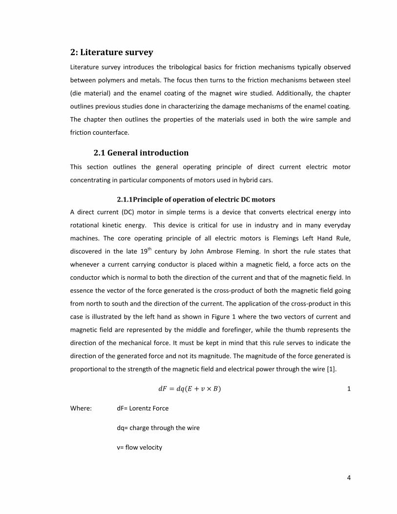
2.1.1Principle of operation of electric DC motors
A direct current (DC) motor in simple terms is a device that converts electrical energy into
rotational kinetic energy. This device is critical for use in industry and in many everyday
machines. The core operating principle of all electric motors is Flemings Left Hand Rule,
discovered in the late 19th century by John Ambrose Fleming. In short the rule states that
whenever a current carrying conductor is placed within a magnetic field, a force acts on the
conductor which is normal to both the direction of the current and that of the magnetic field. In
essence the vector of the force generated is the cross-product of both the magnetic field going
from north to south and the direction of the current. The application of the cross-product in this
case is illustrated by the left hand as shown in Figure 1 where the two vectors of current and
magnetic field are represented by the middle and forefinger, while the thumb represents the
direction of the mechanical force. It must be kept in mind that this rule serves to indicate the
direction of the generated force and not its magnitude. The magnitude of the force generated is
proportional to the strength of the magnetic field and electrical power through the wire [1].
1
Where: dF= Lorentz Force
dq= charge through the wire
v= flow velocity
5
E= electric field
B= magnetic field
Figure 1. Fleming’s Left Hand Rule of the force generated by the current in a conducting element placed in an electric field [1]
By examining a simplified representation of the DC motor containing only one armature loop, it
is easy to see how the above principle is utilised to generate motion and torque. In Figure 2 the
power source, indicated by the battery, provides current to the armature coil through the coil
brush. The armature, composed of a conductive wire, is situated in a magnetic field and as a
result is subject to the generated force. This force is normal to both the direction of the current
and the direction of the electric field. Since the armature of the motor is shaped in the form of a
loop, stemming from the power source, the current traveling through it goes in opposite
directions on each side of the loop. Due to this direction change the forces generated on each
side of the loop are in opposite direction to one another and as a result these forces generate a
moment on the armature itself. It is this moment that drives the motor to rotate. As the loop
performs a 90° rotation the forces generated on each of its sides come into alignment. However
at this moment there is no current flowing through the armature, usually due to the design of
the motor and the positioning of the conductive brushes which power the armature only when
the plane of the loop is aligned with the electric field. As a result of this interruption in current
at this point in the armature travel there is no force being generated, however due to the
momentum gained the armature continues to travel past the 90° point. As the armature passes
the 90° point, the current is again initiated in the armature doe to the contact between the
brush and the armature being re-established. This time however since the sides of the loop have
6
switched due to rotation the current flows in the opposite direction generating a moment in
the same direction of rotation [1].
Figure 2. DC motor schematic illustrating the base component and principles of the DC electric motor [1]
It is through this mechanism that the motor maintains speed and torque required to drive its
mechanical load
2.1.2Main operating components
There is an enormous variety of DC motors due to different, applications, and as a result
different load range and size requirements. Each electric motor however contains same main
operating components. Each component is listed below with a brief description of
characteristics and functionality.
Motor body: The motor body refers to the outer casing and structure of an electric motor.
The body houses the bearings which support the motor shaft and the motor
armature while allowing them to rotate. The purpose of the motor body is to
provide support for the internal components of the motor, provide a sight for
fastening of the motor, and protect any internal component from
environmental factors such as humidity, corrosive environment or mechanical
damage due to impact
Motor shaft: The motor shaft is usually a cylindrical solid shaft keyed at one end in order to
receive the load of the motor. The shaft, usually composed of steel, is supported
7
at two points by the motor bearing which are impeded in the motor body. The
shaft is attached to the armature which provides it with the driving torque. The
purpose of the motor shaft is the transfer of toque generated at the armature
to the load of the motor. The motor shaft and armature are the only two
moving parts of an electric motor, making the machine very reliable and not
prone to mechanical or friction damage.
Armature: The armature of an electric motor is composed of a bobbin, wire winding or coil
in the form of a ball, cylinder or elongated oval. These coils are the one powered
by the power source which generates the torque required to drive the motor.
An armature is usually composed a number of coils depending on the design of
the motor. Each coil is in turn powered by the power source when in the correct
position in order to generate the maximum torque. The coils are each insulated
from one another in order to avoid shorting (or jumping of the charge between
them) and malfunctioning of the motor. Additionally the armature consists of a
steel frame which serves to hold the coils in place and attach them to the motor
shaft.
Stator: The stator in an electric motor refers to the component within the motor that is
responsible for generating the magnetic field required for the motor operation.
Since the magnetic field is static the stator itself is stationary and attached to
the motor body. The stator surrounds the armature in order to provide it with a
uniform and constant magnetic field. In some cases the magnetic field is
generated through the use of rare earth magnets which provide a constant field
without the need for additional power. These magnets however are sometimes
cost prohibitive for application on large scale and are susceptible to
demagnetisation at high heats which limit their operating temperature range.
As a result many stator designs rely on electromagnets through the use of
magnet wire, which is aligned in coils around the stator. Apart from the magnet
wire coil, or rare earth magnets providing the magnetic field, the stator is
composed of steel or aluminum bracket holding the coil in place and fixing it to
the motor frame.
8
Magnet wire: Magnet wire is usually a copper wire conductor electrically insulated by a thin
polymer film. This wire is wound in a coil around the stator so that when
energised it generates a magnetic field around the armature. The wire can be of
varying thickness depending on the load and design of the motor. It is crucial
that the magnet wire be properly insulated in order to avoid loss of charge or
shortening of the coil.
2.2 Characteristics of the bar wound stator motor
Bar wound motors are electrical, direct current motors where the stator coil is composed of
precision-bent rectangular wire instead of the round wire windings found in the more traditional
electric motor configuration. In this type of motor, each wire forming the coil is pre-bent in the
shape of a hairpin; then each wire is inserted into the stator and welded end to end with the
other hairpin-shaped wires, forming a coil. The advantage of this type of stator manufacturing
method is the higher percentage slot filling (73% vs. 40% in conventional wound motors), which
improves the motor’s torque, power density and a shorter end turn space, making the motor
more compact. These characteristics make these motors ideal for use in applications such as
hybrid or electric vehicles, where compact size and efficiency are required [2].
Figure 3. Example of stator for bar wound electric motor[2]
9
2.3 Enamel used in magnet wire application for electric motors
The type of insulation used in hybrid electric motors is generally multilayered. The material
closest to the wire surface is chosen for its good adhesion properties (to the metal) and
increased flexibility; the top coat of enamel, however, is generally chosen to be more abrasion
resistant to withstand the stresses generated during the installation of the magnet wire [3,4].
Wire enamels are divided in classes depending on the temperature that the enamels can safely
withstand during operation in an environment. The range of operation for hybrid electric motors
is between 200°C and 240°C. A typical wire construction used in motors and electric devices
consists of a base coat of polyester or polyesterimide, at around 60%–80% of the total thickness,
with a topcoat of 20%–40% comprised of poly(amide-imide) resin. The reason for using
polyesterimide and poly(amide-imide) in magnet wire coating is their high dielectric strength
[4].
The wire used for electric motor applications in this study is a 3.5 mm 3.7 mm rectangular
copper wire coated with a three-layer enamel coating produced by Hitachi Cable and designated
as a KMKED-22A enamel coating. This enamel coating is made up of three distinct layers of
varying compositions. For the base layer, the chemical composition is proprietary. The middle
layer is composed of a high voltage resistant, nano-filled polyamide-imide providing most of the
electrical resistance in the enamel coating. The outer layer is composed of an unfilled
polyamide-imide chosen mainly for its low coefficient of friction and resistance to external
abrasion.
2.3.1 Base layer of the enamel or inner most coating
The first coat of the enamel composite is composed of polyester-amide-imide. This compound
consists of a polyester backbone combined with special polyamidi-imide parts in the polymeric
chain. Polyester-amide-imide is prepared by reacting fewer than 2 mols of trimellitic anhydride
with 1 mol of a diamine, followed by esterification of the carboxy groups.
It has been shown that this compound exhibits excellent flexibility and adhesion properties,
making it ideal as a primer coat in magnet wire enamel. Adhesion to the copper substrate is a
crucial factor in the quality of the coating. Usually, this characteristic is depends greatly on the
condition of the wire surface. If the exterior of the wire is not completely clean, or free from any
oxidation, the polymer adhesion decreases. One of the great features of polyester-amide-imide
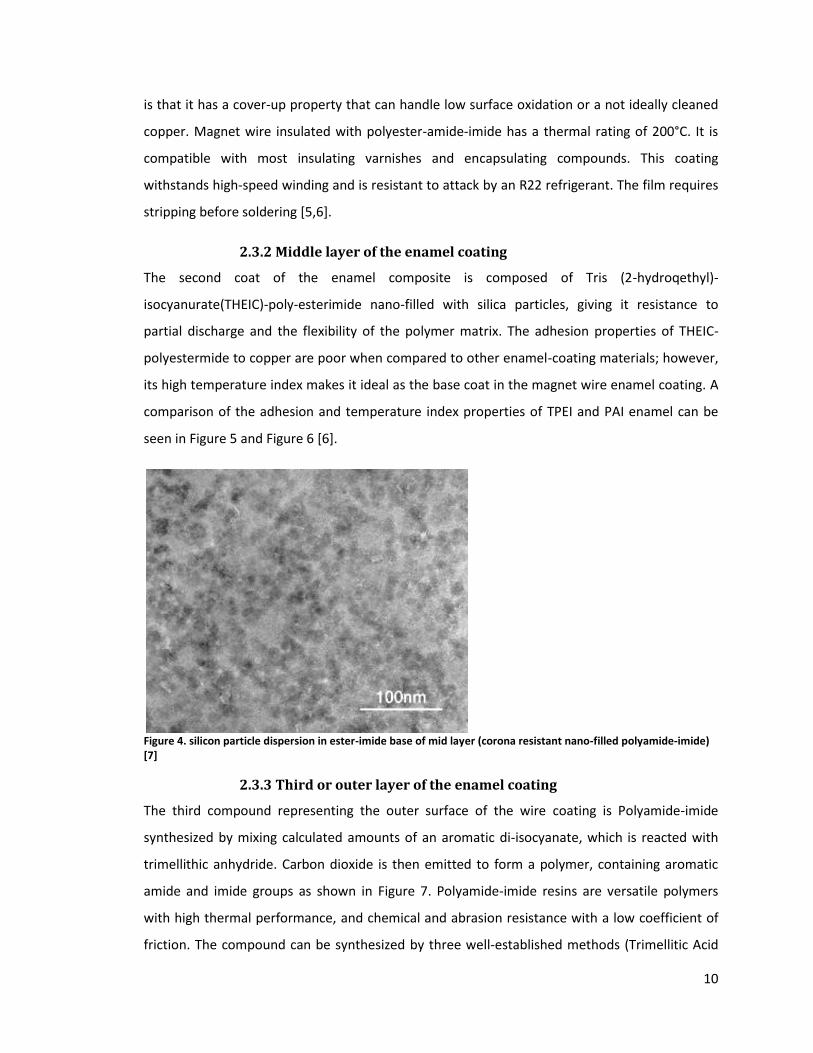
10
is that it has a cover-up property that can handle low surface oxidation or a not ideally cleaned
copper. Magnet wire insulated with polyester-amide-imide has a thermal rating of 200°C. It is
compatible with most insulating varnishes and encapsulating compounds. This coating
withstands high-speed winding and is resistant to attack by an R22 refrigerant. The film requires
stripping before soldering [5,6].
2.3.2 Middle layer of the enamel coating
The second coat of the enamel composite is composed of Tris (2-hydroqethyl)-
isocyanurate(THEIC)-poly-esterimide nano-filled with silica particles, giving it resistance to
partial discharge and the flexibility of the polymer matrix. The adhesion properties of THEIC-
polyestermide to copper are poor when compared to other enamel-coating materials; however,
its high temperature index makes it ideal as the base coat in the magnet wire enamel coating. A
comparison of the adhesion and temperature index properties of TPEI and PAI enamel can be
seen in Figure 5 and Figure 6 [6].
Figure 4. silicon particle dispersion in ester-imide base of mid layer (corona resistant nano-filled polyamide-imide) [7]
2.3.3 Third or outer layer of the enamel coating
The third compound representing the outer surface of the wire coating is Polyamide-imide
synthesized by mixing calculated amounts of an aromatic di-isocyanate, which is reacted with
trimellithic anhydride. Carbon dioxide is then emitted to form a polymer, containing aromatic
amide and imide groups as shown in Figure 7. Polyamide-imide resins are versatile polymers
with high thermal performance, and chemical and abrasion resistance with a low coefficient of
friction. The compound can be synthesized by three well-established methods (Trimellitic Acid
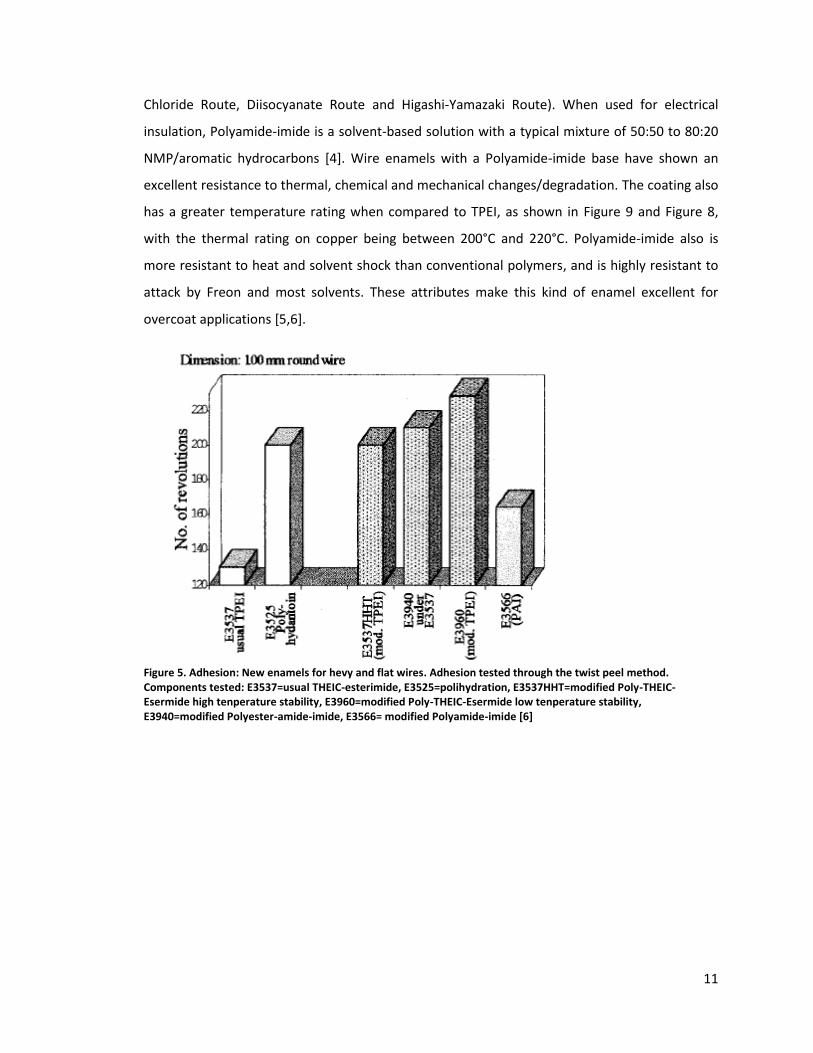
11
Chloride Route, Diisocyanate Route and Higashi-Yamazaki Route). When used for electrical
insulation, Polyamide-imide is a solvent-based solution with a typical mixture of 50:50 to 80:20
NMP/aromatic hydrocarbons [4]. Wire enamels with a Polyamide-imide base have shown an
excellent resistance to thermal, chemical and mechanical changes/degradation. The coating also
has a greater temperature rating when compared to TPEI, as shown in Figure 9 and Figure 8,
with the thermal rating on copper being between 200°C and 220°C. Polyamide-imide also is
more resistant to heat and solvent shock than conventional polymers, and is highly resistant to
attack by Freon and most solvents. These attributes make this kind of enamel excellent for
overcoat applications [5,6].
Figure 5. Adhesion: New enamels for hevy and flat wires. Adhesion tested through the twist peel method. Components tested: E3537=usual THEIC-esterimide, E3525=polihydration, E3537HHT=modified Poly-THEIC-Esermide high tenperature stability, E3960=modified Poly-THEIC-Esermide low tenperature stability, E3940=modified Polyester-amide-imide, E3566= modified Polyamide-imide [6]
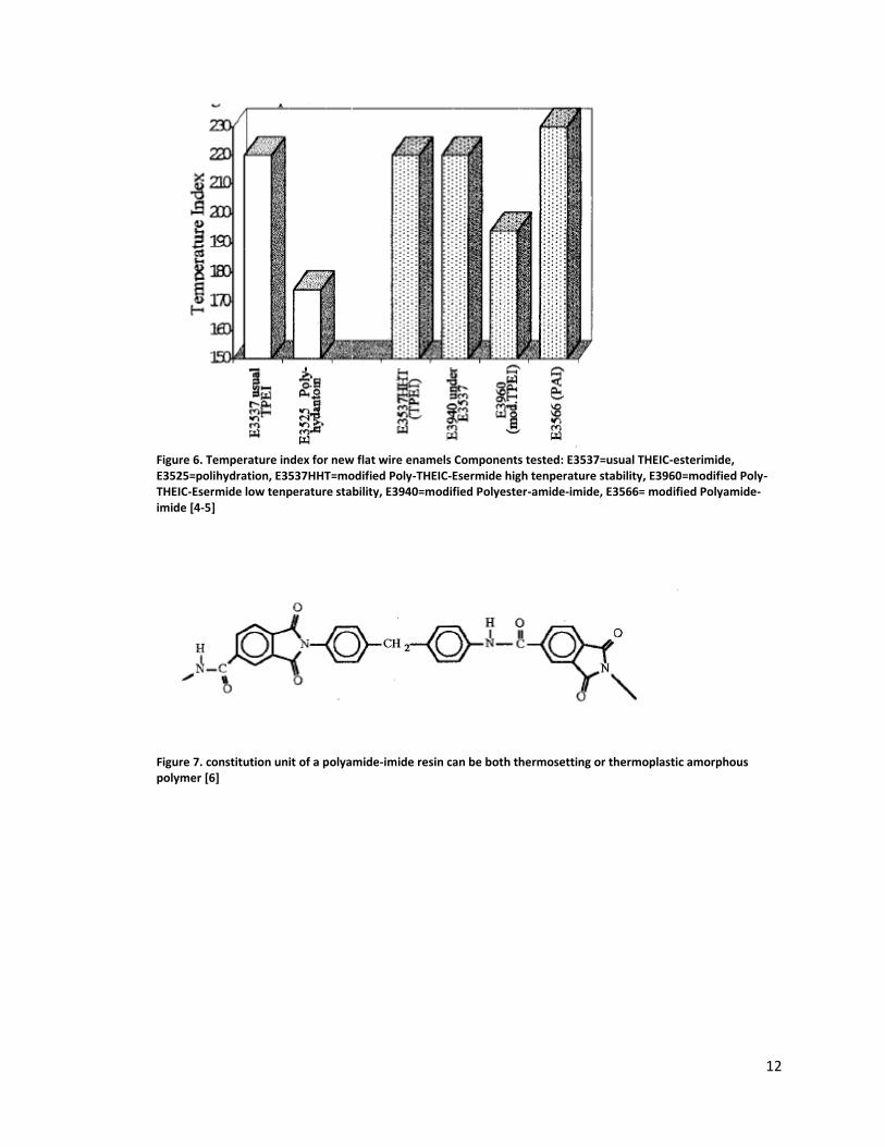
12
Figure 6. Temperature index for new flat wire enamels Components tested: E3537=usual THEIC-esterimide, E3525=polihydration, E3537HHT=modified Poly-THEIC-Esermide high tenperature stability, E3960=modified Poly-THEIC-Esermide low tenperature stability, E3940=modified Polyester-amide-imide, E3566= modified Polyamide-imide [4-5]
Figure 7. constitution unit of a polyamide-imide resin can be both thermosetting or thermoplastic amorphous polymer [6]
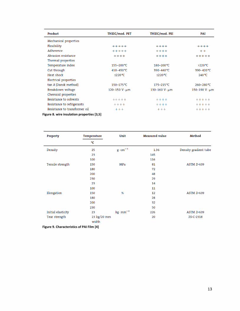
13
Figure 8. wire insulation properties [3,5]
Figure 9. Characteristics of PAI Film [4]
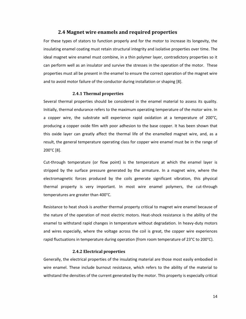
14
2.4 Magnet wire enamels and required properties
For these types of stators to function properly and for the motor to increase its longevity, the
insulating enamel coating must retain structural integrity and isolative properties over time. The
ideal magnet wire enamel must combine, in a thin polymer layer, contradictory properties so it
can perform well as an insulator and survive the stresses in the operation of the motor. These
properties must all be present in the enamel to ensure the correct operation of the magnet wire
and to avoid motor failure of the conductor during installation or shaping [8].
2.4.1 Thermal properties
Several thermal properties should be considered in the enamel material to assess its quality.
Initially, thermal endurance refers to the maximum operating temperature of the motor wire. In
a copper wire, the substrate will experience rapid oxidation at a temperature of 200°C,
producing a copper oxide film with poor adhesion to the base copper. It has been shown that
this oxide layer can greatly affect the thermal life of the enamelled magnet wire, and, as a
result, the general temperature operating class for copper wire enamel must be in the range of
200°C [8].
Cut-through temperature (or flow point) is the temperature at which the enamel layer is
stripped by the surface pressure generated by the armature. In a magnet wire, where the
electromagnetic forces produced by the coils generate significant vibration, this physical
thermal property is very important. In most wire enamel polymers, the cut-through
temperatures are greater than 400°C.
Resistance to heat shock is another thermal property critical to magnet wire enamel because of
the nature of the operation of most electric motors. Heat-shock resistance is the ability of the
enamel to withstand rapid changes in temperature without degradation. In heavy-duty motors
and wires especially, where the voltage across the coil is great, the copper wire experiences
rapid fluctuations in temperature during operation (from room temperature of 23°C to 200°C).
2.4.2 Electrical properties
Generally, the electrical properties of the insulating material are those most easily embodied in
wire enamel. These include burnout resistance, which refers to the ability of the material to
withstand the densities of the current generated by the motor. This property is especially critical
15
during the starting phase of the motor, which can be in the range of 40,000 to 60,000
amperes/sq. in [8].
Dielectric strength is another critical electrical property, referring to the maximum electric field
strength that can be withstood intrinsically without the material breaking down. The dielectric
strength of the enamel coating must be sufficient to withstand the maximum voltage strength
arising during the switching operation. The dielectric strength of a material can be influenced by
moisture and extremes of temperature in the wire enamel [8,9].
2.4.3 Chemical properties
The chemical characteristics needed in wire enamel depend most on the environment where
the final product, such as the motor, will be operated. In general, these characteristics include
resistance to oxidation, compatibility with any solvents present during operation and resistance
to environmental damage. The chemical reaction caused by external contaminants generally
takes the form of the breakdown of the polymer chains in the enamel coating. These chemical
changes can be grouped in the aging characteristic of the wire enamel, which will be discussed
in a subsequent section [8,9].
2.4.4 Physical properties
The physical properties of the magnet wire enamel are those that most strongly determine the
success of an enamel coating during operation. The physical resistance of the enamel is
important due to the great amount of stress and abrasion that the magnet wire is subject to,
especially during motor assembly. The required physical properties of the magnet wire enamel
are abrasion resistance, a low coefficient of friction, flexibility and good adhesion to the metallic
substrate [8,9].
2.4.5 Windability
When the magnet wire coils used in electric motor stators are considered, it is important that
manufacturers improve two major factors: the preservation of the insulating enamel surface
during assembly, and the maximization of the amount of slot fill possible to increase the
efficiency of the motor. The ability of the wire to withstand the winding or deformation process
needed to generate a tight coil without damage to the insulating enamel is defined as
windability. Three parameters determine the windability of a particular magnet wire. They are
the improvement of abrasion resistance of the enamel surface, the improvement of the surface
16
condition or lubricity of the enamel, and the improvement of the adhesion between the wire
subsurface and the enamel [3].
The standard test used to determine the windability of wire are the National Electrical
Manufacturers Association (NEMA) windability test. This test consists of winding the wire
around a mandrel with a certain amount of tension and then moving the wire back and forth
lengthwise. This motion generates an uneven stretch in the enamel of the wire in the
circumferential direction and the conducting substrate. This result leads to the generation of
defects, such as cracks in the parts of the abnormally stretched film [9].
2.4.5.1 Abrasion Resistance
High abrasion resistance is a critical property in enamel coating, because any breach in the
enamel coating can lead to short-circuiting the motor coil. One of the principal ways of
improving the coating’s abrasion resistance would an increase of the toughness of the insulating
film. By making the outer surface of the magnet wire stronger, it is less likely that the wire will
be damaged by friction or wear during installation of the coil. The toughness of the outer
enamel layer combined with the slickness of the outer surface serve as abrasion resistance for
the wire isolative coating. Tests like the repeated scrape test can be performed on enamel wire
samples to test the resistance of a certain coating to abrasion. The repeated scrape test consists
of using either a needle or a piano wire as contact counterfaces in a pendulum that applies a
certain load (depending on the gauge and thickness of the tested magnet wire) pushing against
the enamel surface. The number of swings of the pendulum that the enamel surface can
withstand without being peeled back and exposing the conductor is a measure of the wire’s
abrasion resistance. It has been shown that introducing toughening agents, such as polyamide-
imide and THEIC-based polyester-polyamide-imide, to wire enamel materials improves the
performance of the wire under a repeated scrape test two fold [3,10].
2.4.5.1.1 Testing for abrasion resistance
The repeated scrape abrasion test is the principal testing procedure for determining the
abrasion resistance of enamel wire. The test is performed on 6-inch wire samples stretched at
2% to 3%. The samples are secured in a V-shaped, grooved anvil and scraped using a scraping
head generally composed of a music wire needle. The enamel is considered to have failed when
the resistance measured between the wire and the scraping head drops. The test can be
repeated up to six times in each round wire (every 60° around the perimeter of each wire),
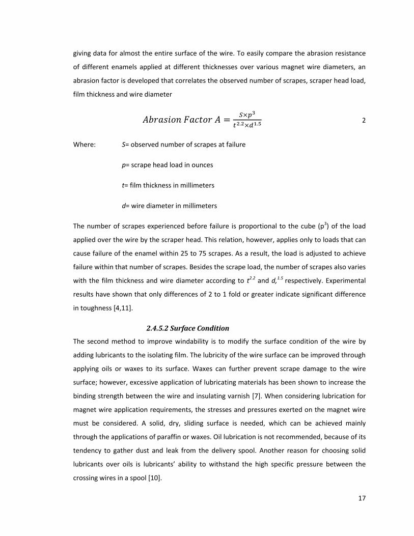
17
giving data for almost the entire surface of the wire. To easily compare the abrasion resistance
of different enamels applied at different thicknesses over various magnet wire diameters, an
abrasion factor is developed that correlates the observed number of scrapes, scraper head load,
film thickness and wire diameter
2
Where: S= observed number of scrapes at failure
p= scrape head load in ounces
t= film thickness in millimeters
d= wire diameter in millimeters
The number of scrapes experienced before failure is proportional to the cube (p3) of the load
applied over the wire by the scraper head. This relation, however, applies only to loads that can
cause failure of the enamel within 25 to 75 scrapes. As a result, the load is adjusted to achieve
failure within that number of scrapes. Besides the scrape load, the number of scrapes also varies
with the film thickness and wire diameter according to t2.2 and d,1.5 respectively. Experimental
results have shown that only differences of 2 to 1 fold or greater indicate significant difference
in toughness [4,11].
2.4.5.2 Surface Condition
The second method to improve windability is to modify the surface condition of the wire by
adding lubricants to the isolating film. The lubricity of the wire surface can be improved through
applying oils or waxes to its surface. Waxes can further prevent scrape damage to the wire
surface; however, excessive application of lubricating materials has been shown to increase the
binding strength between the wire and insulating varnish [7]. When considering lubrication for
magnet wire application requirements, the stresses and pressures exerted on the magnet wire
must be considered. A solid, dry, sliding surface is needed, which can be achieved mainly
through the applications of paraffin or waxes. Oil lubrication is not recommended, because of its
tendency to gather dust and leak from the delivery spool. Another reason for choosing solid
lubricants over oils is lubricants’ ability to withstand the high specific pressure between the
crossing wires in a spool [10].
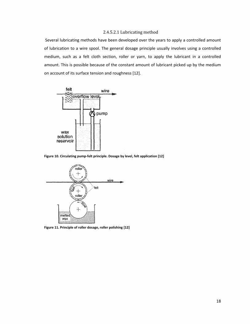
18
2.4.5.2.1 Lubricating method
Several lubricating methods have been developed over the years to apply a controlled amount
of lubrication to a wire spool. The general dosage principle usually involves using a controlled
medium, such as a felt cloth section, roller or yarn, to apply the lubricant in a controlled
amount. This is possible because of the constant amount of lubricant picked up by the medium
on account of its surface tension and roughness [12].
Figure 10. Circulating pump-felt principle. Dosage by level, felt application [12]
Figure 11. Principle of roller dosage, roller polishing [12]
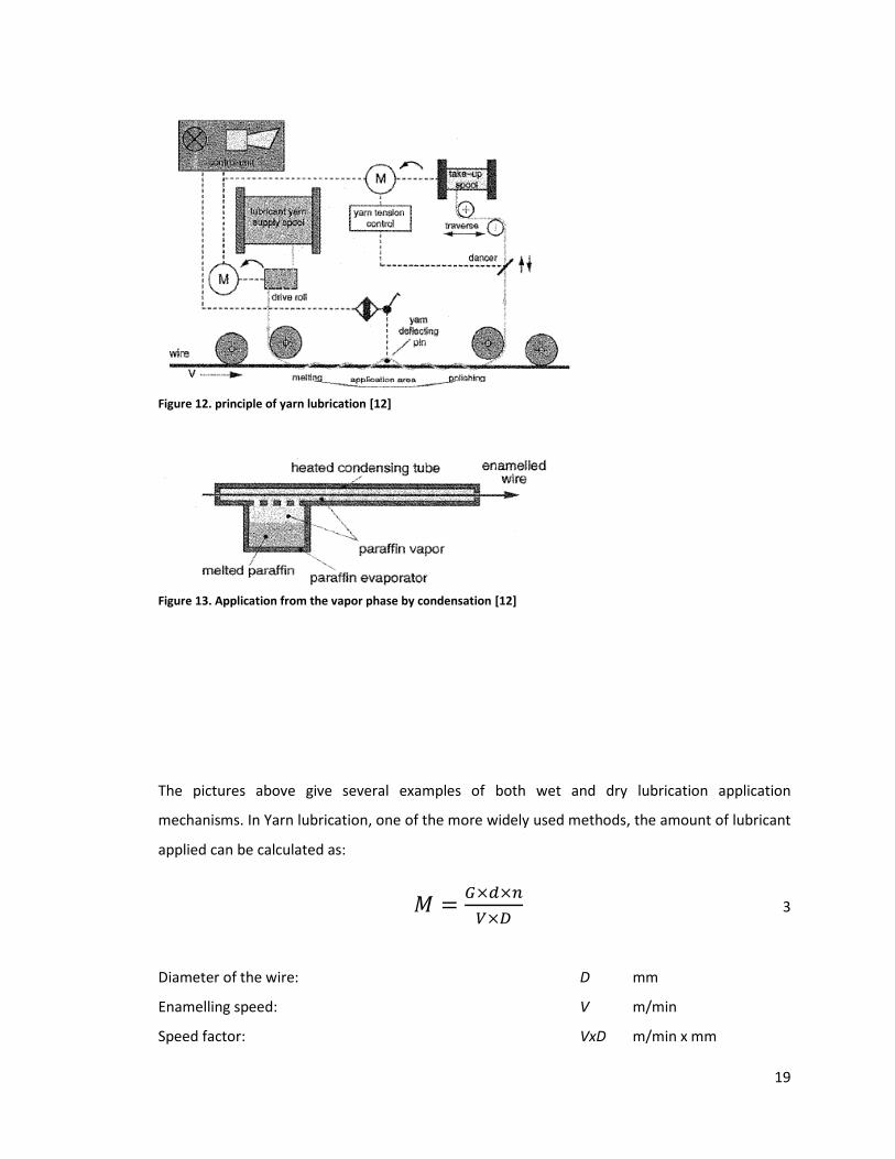
19
Figure 12. principle of yarn lubrication [12]
Figure 13. Application from the vapor phase by condensation [12]
The pictures above give several examples of both wet and dry lubrication application
mechanisms. In Yarn lubrication, one of the more widely used methods, the amount of lubricant
applied can be calculated as:
3
Diameter of the wire: D mm
Enamelling speed: V m/min
Speed factor: VxD m/min x mm
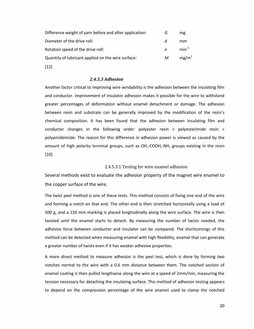
20
Difference weight of yarn before and after application: G mg
Diameter of the drive roll: d mm
Rotation speed of the drive roll: n min-1
Quantity of lubricant applied on the wire surface: M mg/m2
[12]
2.4.5.3 Adhesion
Another factor critical to improving wire windability is the adhesion between the insulating film
and conductor. Improvement of insulator adhesion makes it possible for the wire to withstand
greater percentages of deformation without enamel detachment or damage. The adhesion
between resin and substrate can be generally improved by the modification of the resin’s
chemical composition. It has been found that the adhesion between insulating film and
conductor changes in the following order: polyester resin > polyesterimide resin >
polyamideimide. The reason for this difference in adhesion power is viewed as caused by the
amount of high polarity terminal groups, such as OH,-COOH,-NH, groups existing in the resin
[10].
2.4.5.3.1 Testing for wire enamel adhesion
Several methods exist to evaluate the adhesion property of the magnet wire enamel to
the copper surface of the wire.
The twist peel method is one of these tests. This method consists of fixing one end of the wire
and forming a notch on that end. The other end is then stretched horizontally using a load of
500 g, and a 150 mm marking is placed longitudinally along the wire surface. The wire is then
twisted until the enamel starts to detach. By measuring the number of twists needed, the
adhesive force between conductor and insulator can be compared. The shortcomings of this
method can be detected when measuring enamel with high flexibility, enamel that can generate
a greater number of twists even if it has weaker adhesive properties.
A more direct method to measure adhesion is the peel test, which is done by forming two
notches normal to the wire with a 0.6 mm distance between them. The notched section of
enamel coating is then pulled lengthwise along the wire at a speed of 2mm/min, measuring the
tension necessary for detaching the insulating surface. This method of adhesion testing appears
to depend on the compression percentage of the wire enamel used to clamp the notched
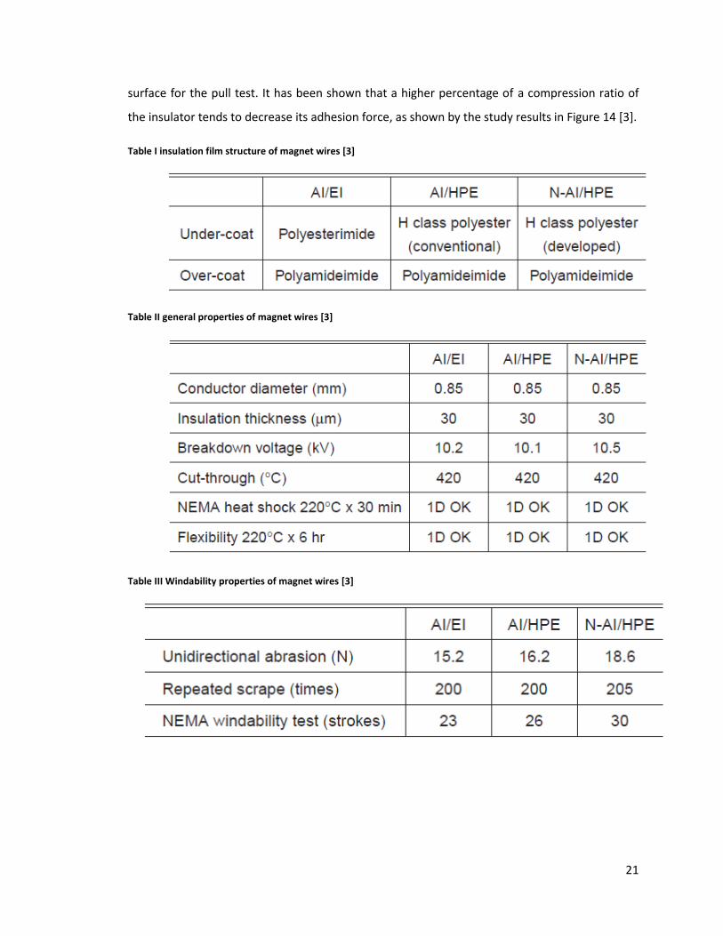
21
surface for the pull test. It has been shown that a higher percentage of a compression ratio of
the insulator tends to decrease its adhesion force, as shown by the study results in Figure 14 [3].
Table I insulation film structure of magnet wires [3]
Table II general properties of magnet wires [3]
Table III Windability properties of magnet wires [3]
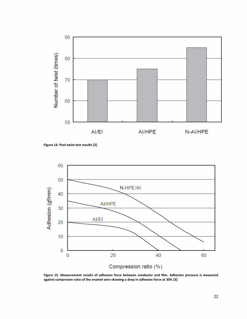
22
Figure 14. Peel-twist test results [3]
Figure 15. Measurement results of adhesion force between conductor and film. Adhesion pressure is measured against compresion ratio of the enamel wire showing a drop in adhesion force at 30% [3]
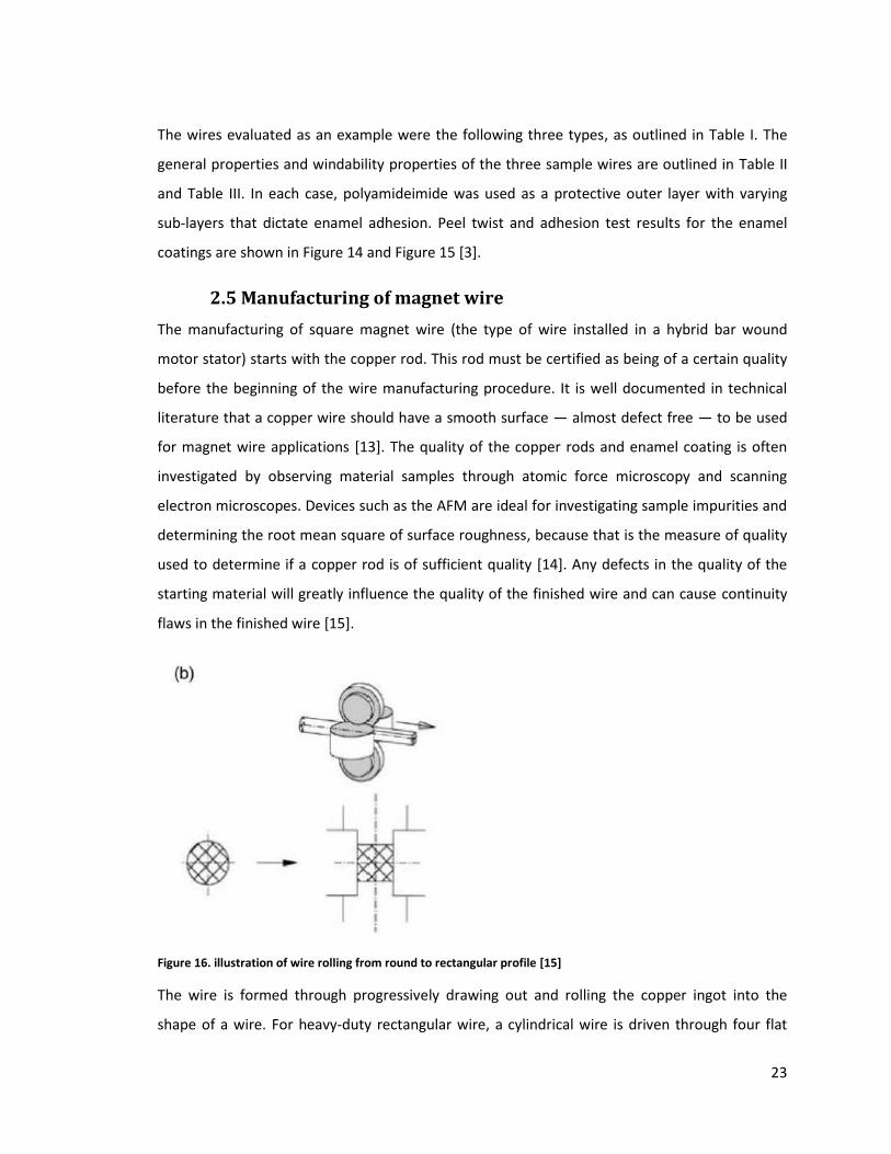
23
The wires evaluated as an example were the following three types, as outlined in Table I. The
general properties and windability properties of the three sample wires are outlined in Table II
and Table III. In each case, polyamideimide was used as a protective outer layer with varying
sub-layers that dictate enamel adhesion. Peel twist and adhesion test results for the enamel
coatings are shown in Figure 14 and Figure 15 [3].
2.5 Manufacturing of magnet wire
The manufacturing of square magnet wire (the type of wire installed in a hybrid bar wound
motor stator) starts with the copper rod. This rod must be certified as being of a certain quality
before the beginning of the wire manufacturing procedure. It is well documented in technical
literature that a copper wire should have a smooth surface — almost defect free — to be used
for magnet wire applications [13]. The quality of the copper rods and enamel coating is often
investigated by observing material samples through atomic force microscopy and scanning
electron microscopes. Devices such as the AFM are ideal for investigating sample impurities and
determining the root mean square of surface roughness, because that is the measure of quality
used to determine if a copper rod is of sufficient quality [14]. Any defects in the quality of the
starting material will greatly influence the quality of the finished wire and can cause continuity
flaws in the finished wire [15].
Figure 16. illustration of wire rolling from round to rectangular profile [15]
The wire is formed through progressively drawing out and rolling the copper ingot into the
shape of a wire. For heavy-duty rectangular wire, a cylindrical wire is driven through four flat
24
rollers to create the desired rectangular shape, as illustrated in Figure 16. During these
processes of thinning and shaping the copper wire, it is preferable to use driven rolling machines
where the wire is driven through the rollers by the motion of the rollers themselves rather than
the wire being drawn out. This method reduces the amount of stress in the wire and, as a result,
minimizes any faults in the magnet wire [13].
After the wire substrate has been brought to the proper dimensions required by the
manufacturer, the enamel coating is applied. The most common way to apply wire enamel is by
submerging the wire in a solution of the enamel polymer and an organic solvent. The organic
solvent is usually a mixture of cresol isomers, as a solvent, and aromatic hydrocarbons (solvent
naphtha), as a diluent [16]. The wire is then cured by passing through an oven at a controlled
temperature, which evaporates the solvent and cures the polymer coating. The process is
repeated several times for each layer of enamel to build the necessary thickness of insulation on
the wire. By controlling the percentage of polymer enamel coating dispersed in the solvent, the
manufacturer can control the thickness of enamel applied in each coating. The percentage of
polymer in the solvent solution can vary depending on the enamel used. One of the largest
areas of development in the field of magnet wire production is the effort to reduce or eliminate
the amount of organic solvent during the manufacturing process. These methods of enamel
application have not had significant success and have not been able to replace the current
application method. These methods included using enamel solutions of up to 55%–70% solid
content to reduce the volume of evaporated solvent, using hot melt enamels to directly coat the
magnet wire and applying a powder coating using ionized air. These methods can reduce the
environmental impact of the solvents, but the methods produce uneven coatings and, in the
case of the powder coating, coatings of poor resistance [5].

25
2.6 Failure modes in wire used in an electric motor
The main failure modes in an electric motor are the result of the loss of insulation in the magnet
wire. This insulation loss can be a result of the gradual degradation of the enamel over time (as
enamel ages) or can be caused by defects introduced to the wire surface during the installation
of the wire in the motor.
As the magnet wire is exposed to thermal, mechanical and electrical stresses throughout its
operating life, the insulating enamel starts to degrade and peel. This degradation, especially in
rectangular wire, can be influenced by the percent deformation of the wire [17]. During the
thermal aging of wire samples, the time before the development of faults in the insulator
enamel decreased as the wire samples’ deformation increased. In a deformed or bent wire
sample, it has been shown that the degradation of the enamel layer can be mostly observed on
the outer surfaces of wire’s bends, places that suffer the greatest amount of stress during wire
formation. The effect of elongation was studied using four various wire enamel compositions at
0%, 10% and 25% elongation of the enamel. These samples were then heat socked and varnish
shocked until the enamel failed to determine the life of the enamel. A summary of the results is
outlined in Figure 17.
Figure 17. Summary of data from thermal aging of elongated enameled wire samples. Experimental enamels A, B, C, and control enamel D, chosen for its good heat resistance but poor aging performance [17]
Aside from the constant exposure of the magnet wire to the operating stresses of the motor,
manufacturing defects in either the copper wire or in the enamel coating can cause premature
failure of the magnet wire.
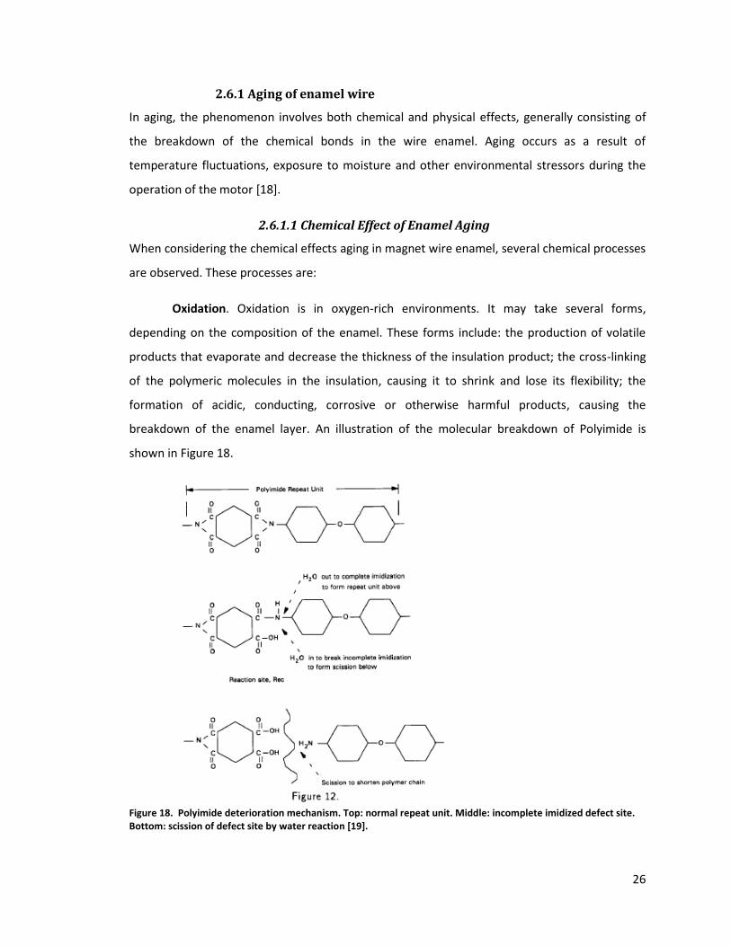
26
2.6.1 Aging of enamel wire
In aging, the phenomenon involves both chemical and physical effects, generally consisting of
the breakdown of the chemical bonds in the wire enamel. Aging occurs as a result of
temperature fluctuations, exposure to moisture and other environmental stressors during the
operation of the motor [18].
2.6.1.1 Chemical Effect of Enamel Aging
When considering the chemical effects aging in magnet wire enamel, several chemical processes
are observed. These processes are:
Oxidation. Oxidation is in oxygen-rich environments. It may take several forms,
depending on the composition of the enamel. These forms include: the production of volatile
products that evaporate and decrease the thickness of the insulation product; the cross-linking
of the polymeric molecules in the insulation, causing it to shrink and lose its flexibility; the
formation of acidic, conducting, corrosive or otherwise harmful products, causing the
breakdown of the enamel layer. An illustration of the molecular breakdown of Polyimide is
shown in Figure 18.
Figure 18. Polyimide deterioration mechanism. Top: normal repeat unit. Middle: incomplete imidized defect site. Bottom: scission of defect site by water reaction [19].
27
Depolymerization. Depolymerization consists of the breakdown of the polymer bonds in
the enamel and can occur even in the absence of oxygen. It causes a reduction in tensile
strength in the enamel material, evaporation of the coating and even changes the shape of the
polymer [18].
Hydrolysis. Hydrolysis is the chemical reaction of the insulation to water. The main
effect of hydrolysis is a form of depolymerization, occurring mainly in sealed systems.
2.6.1.2 Physical Effects of Wire Enamel Aging
The physical effects of wire enamel’s aging depends mainly on the operating environment of the
motor itself. These effects include:
Melting. Melting of the wire enamel is a reversible process, if the enamel is not exposed
to any external stresses. Softening occurs as a result of exposure to temperatures beyond the
glass transition point. Melting can occur at a particular temperature or, as in thermoplastics,
gradually over a range of temperatures [18].
Volatilization. Volatilization is a slow process that requires ventilation to remove the
volatile products or an effective cold trap in the cold system. It can also rapidly occur when the
enamel coating is operated close to its boiling point.
Hardening. Hardening of the enamel is mainly caused by the cross-linking of the
polymer chains. Hardening is the most common physical effect of aging in varnishes and resin
coatings. It can be caused by the evaporation of the plasticizer in the resin and is the main cause
of the enamel’s cracking. Differential expansion of the resin and of inorganic or metallic
materials to which the resin is bonded often contributes to the production of cracks as well.
2.6.1.3 Testing Aging in Magnet Wire Enamel
The standard procedure for testing wire enamel aging is through the twist, motorette and motor
tests [20,21]. In each case, the magnet wire is subjected to fluctuating voltage for prolonged
periods at elevated temperatures in air-circulating ovens.
The twist test consists of subjecting twisted pairs of a magnet wire sample to aging at different
temperatures. The samples are dipped in impregnating varnish and periodically subjected to
voltage stress until a breakdown in the enamel coating is detected.
28
In the motor test, the magnet wire is mounted in a DC motor operated at 200°C for 7,000 hrs at
100% humidity. Normally, insulation resistance decreases rapidly during the first 24 hours and
then levels out to a more or less stable low value.
Stress generated in the enamel film because bending the magnet wire has been shown to have a
detrimental effect on the mechanical, chemical and thermal properties of enamel wire. It has
been shown that highly stressed areas exhibited a faster deterioration of the insulating enamel
film during heat shock and the aging process than unstressed wire samples [17].
2.6.2 Defects in magnet wire manufacturing
The defects introduced during manufacturing a typical magnet wire can be detected by
performing high-voltage continuity testing on large samples of magnet wire. By using visual
examination, metallographic evaluation of cross sections, scanning electron microscope (SEM)
examination of the bare wire surfaces and elemental analysis of foreign contaminants, the type
of continuity faults are determined and organized into six major classifications. The continuity
test involves the continuous application of current, either AC or DC, across a grounded moving
conductor. A fault in the conductor is considered to be any section in the wire that shows
reduced resistance of the insulating material.
2.6.2.1 Copper wire and substrate defects
The condition of the wire substrate can significantly influence the performance of an enamel
coating. By providing an uneven base for the enamel layer during the application of the coating,
the wire substrate can form sections of decreased enamel thickness that provide reduced
resistivity and are more likely to fail under stress. The presence of corrosion on the substrate
surface would also decrease enamel adhesion, causing poor flexibility of the coating on the
magnet wire.
2.6.2.1.1 Copper Rod Defects
Copper rod defects are most often generated during hot rolling, casting or melting operations
and subsequently become aggravated during the drawing and annealing processes that follow.
These types of defects are linked to brittle copper oxide particles formed after hot-cracking, by
fold over of overfills, or are pressed into the surface during hot-rolling. They appear as
longitudinal cracks or slivers in the copper wire, and when they are exposed to the enamelling
solution, they are filled with the liquid polymer and prevent the solvent in the solution from

29
vaporizing. Hindering solvent vaporization creates beads close to the surface’s opening.
Examples of these types of copper rod defects are shown in Figure 19 and Figure 20 [15].
Figure 19. Optical micrographs showing sliver from rod [15]
Figure 20. longitudinal cracks in wire caused during rolling [15]
2.6.2.1.2 Wire Drawing Damage
Most wire drawing damage observed in copper wires can be attributed to inadequate
lubrication, worn or defective dies, or non-axial entry of the moving conductor into the bearing.
Copper fines always form during wire drawing and can cause severe damage to the bare wire
surface. These fines can become compacted in the throat of the draw die, thereby causing
starvation of the drawing lubricant and an increase in the coefficient of friction. It is, however,
very difficult to determine simply by visual inspection if slivers are generated during hot-rolling
or by wire drawing. Most continuity faults caused by wire drawing are shown as continuous
scraping and scratching as shown in Figure 21 [15].
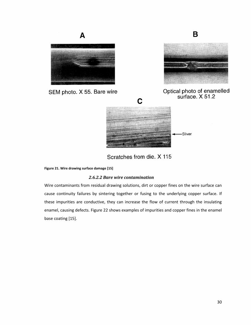
30
Figure 21. Wire drawing surface damage [15]
2.6.2.2 Bare wire contamination
Wire contaminants from residual drawing solutions, dirt or copper fines on the wire surface can
cause continuity failures by sintering together or fusing to the underlying copper surface. If
these impurities are conductive, they can increase the flow of current through the insulating
enamel, causing defects. Figure 22 shows examples of impurities and copper fines in the enamel
base coating [15].
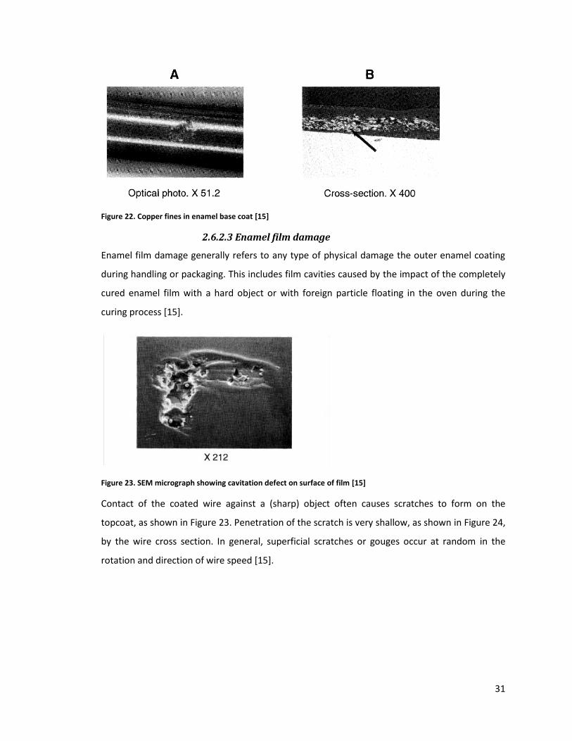
31
Figure 22. Copper fines in enamel base coat [15]
2.6.2.3 Enamel film damage
Enamel film damage generally refers to any type of physical damage the outer enamel coating
during handling or packaging. This includes film cavities caused by the impact of the completely
cured enamel film with a hard object or with foreign particle floating in the oven during the
curing process [15].
Figure 23. SEM micrograph showing cavitation defect on surface of film [15]
Contact of the coated wire against a (sharp) object often causes scratches to form on the
topcoat, as shown in Figure 23. Penetration of the scratch is very shallow, as shown in Figure 24,
by the wire cross section. In general, superficial scratches or gouges occur at random in the
rotation and direction of wire speed [15].
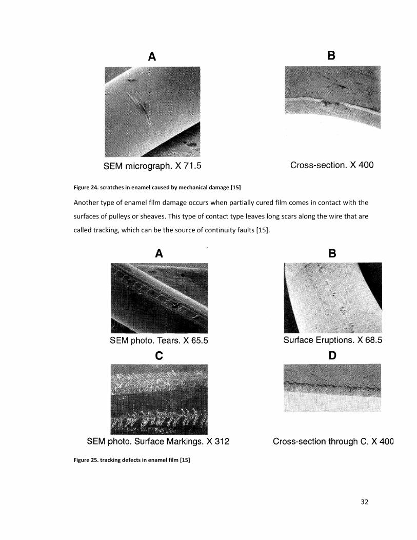
32
Figure 24. scratches in enamel caused by mechanical damage [15]
Another type of enamel film damage occurs when partially cured film comes in contact with the
surfaces of pulleys or sheaves. This type of contact type leaves long scars along the wire that are
called tracking, which can be the source of continuity faults [15].
Figure 25. tracking defects in enamel film [15]
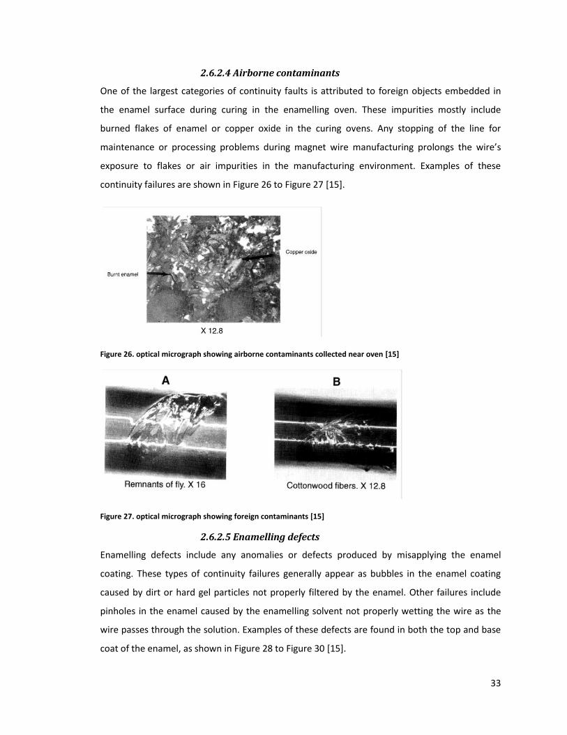
33
2.6.2.4 Airborne contaminants
One of the largest categories of continuity faults is attributed to foreign objects embedded in
the enamel surface during curing in the enamelling oven. These impurities mostly include
burned flakes of enamel or copper oxide in the curing ovens. Any stopping of the line for
maintenance or processing problems during magnet wire manufacturing prolongs the wire’s
exposure to flakes or air impurities in the manufacturing environment. Examples of these
continuity failures are shown in Figure 26 to Figure 27 [15].
Figure 26. optical micrograph showing airborne contaminants collected near oven [15]
Figure 27. optical micrograph showing foreign contaminants [15]
2.6.2.5 Enamelling defects
Enamelling defects include any anomalies or defects produced by misapplying the enamel
coating. These types of continuity failures generally appear as bubbles in the enamel coating
caused by dirt or hard gel particles not properly filtered by the enamel. Other failures include
pinholes in the enamel caused by the enamelling solvent not properly wetting the wire as the
wire passes through the solution. Examples of these defects are found in both the top and base
coat of the enamel, as shown in Figure 28 to Figure 30 [15].
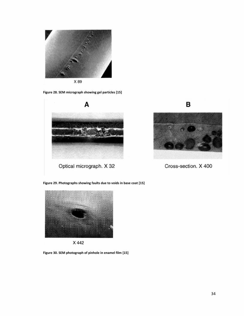
34
Figure 28. SEM micrograph showing gel particles [15]
Figure 29. Photographs showing faults due to voids in base coat [15]
Figure 30. SEM photograph of pinhole in enamel film [15]
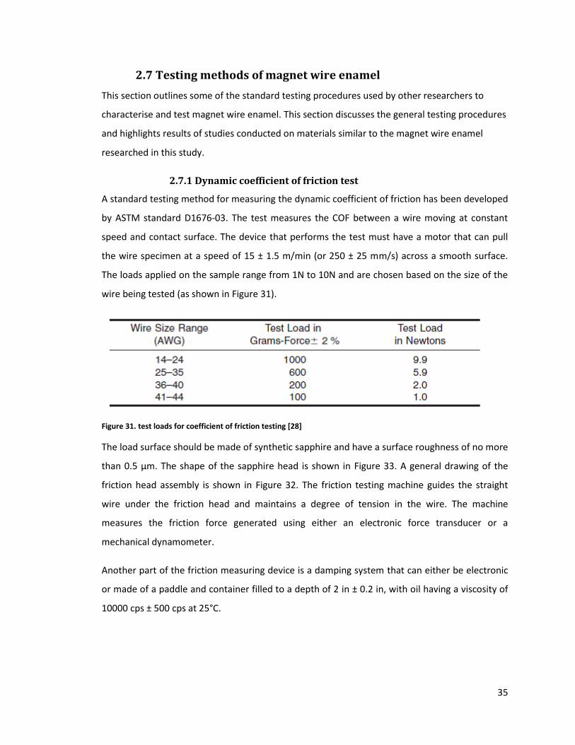
35
2.7 Testing methods of magnet wire enamel
This section outlines some of the standard testing procedures used by other researchers to
characterise and test magnet wire enamel. This section discusses the general testing procedures
and highlights results of studies conducted on materials similar to the magnet wire enamel
researched in this study.
2.7.1 Dynamic coefficient of friction test
A standard testing method for measuring the dynamic coefficient of friction has been developed
by ASTM standard D1676-03. The test measures the COF between a wire moving at constant
speed and contact surface. The device that performs the test must have a motor that can pull
the wire specimen at a speed of 15 ± 1.5 m/min (or 250 ± 25 mm/s) across a smooth surface.
The loads applied on the sample range from 1N to 10N and are chosen based on the size of the
wire being tested (as shown in Figure 31).
Figure 31. test loads for coefficient of friction testing [28]
The load surface should be made of synthetic sapphire and have a surface roughness of no more
than 0.5 µm. The shape of the sapphire head is shown in Figure 33. A general drawing of the
friction head assembly is shown in Figure 32. The friction testing machine guides the straight
wire under the friction head and maintains a degree of tension in the wire. The machine
measures the friction force generated using either an electronic force transducer or a
mechanical dynamometer.
Another part of the friction measuring device is a damping system that can either be electronic
or made of a paddle and container filled to a depth of 2 in ± 0.2 in, with oil having a viscosity of
10000 cps ± 500 cps at 25°C.
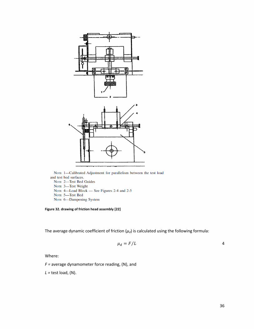
36
Figure 32. drawing of friction head assembly [22]
The average dynamic coefficient of friction (µd) is calculated using the following formula:
4
Where:
F = average dynamometer force reading, (N), and
L = test load, (N).
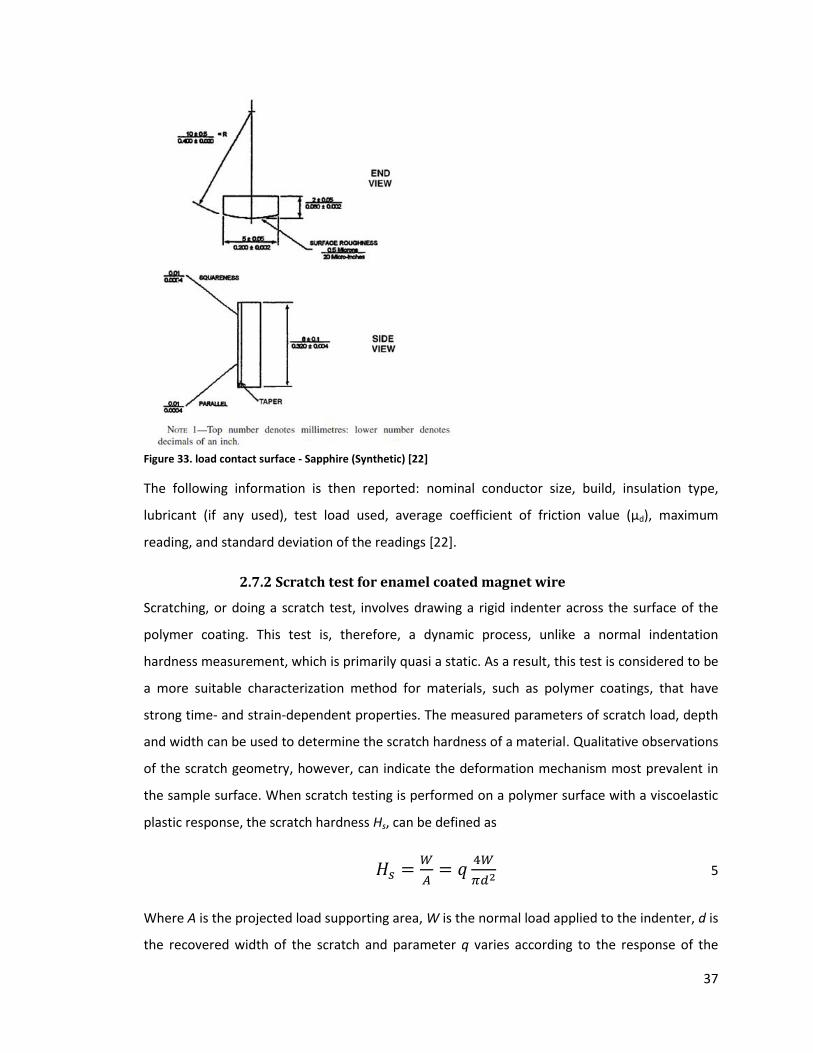
37
Figure 33. load contact surface - Sapphire (Synthetic) [22]
The following information is then reported: nominal conductor size, build, insulation type,
lubricant (if any used), test load used, average coefficient of friction value (μd), maximum
reading, and standard deviation of the readings [22].
2.7.2 Scratch test for enamel coated magnet wire
Scratching, or doing a scratch test, involves drawing a rigid indenter across the surface of the
polymer coating. This test is, therefore, a dynamic process, unlike a normal indentation
hardness measurement, which is primarily quasi a static. As a result, this test is considered to be
a more suitable characterization method for materials, such as polymer coatings, that have
strong time- and strain-dependent properties. The measured parameters of scratch load, depth
and width can be used to determine the scratch hardness of a material. Qualitative observations
of the scratch geometry, however, can indicate the deformation mechanism most prevalent in
the sample surface. When scratch testing is performed on a polymer surface with a viscoelastic
plastic response, the scratch hardness Hs, can be defined as
5
Where A is the projected load supporting area, W is the normal load applied to the indenter, d is
the recovered width of the scratch and parameter q varies according to the response of the
38
material and how the material supports the indenter. The value of q transitions from q=2 for
rigid plastic materials to q>1 for viscoelastic plastic materials.
The measurement of the friction coefficient throughout scratch testing will also be useful in
characterizing the nature of energy dissipation involved during dynamic contact. The coefficient
of friction, however, has been found to depend strongly on the contact geometry and the strain
applied on the sample. For perfectly ductile material that undergoes “ploughing” under a
spherical indenter, a simple geometric model was developed by Tabor for the friction coefficient
[18].
6
Where R is the radius of the sphere, d is the diameter of the load supporting the area, and is
the semi-angle subtended by the track [23].
2.7.2.1 Nano Scratch Test
Nano scratch testing can be used to characterize the elasticity, hardness, adhesion and
mechanical integrity in a coated system, such as an enamelled magnet wire where film thickness
is less than 1 mm. Instruments such as the Nano scratch tester can be used in this case to
overcome the limitations of both the classic stylus scratch test (limited range of normal force
applied) and the atomic force microscope technique (short sliding distance), allowing a scratch
length of up to 10 mm. The Nano scratch tester (NST) exploits the normal force range from 10
mN to 1 N. The normal and tangential loads generated by the diamond tip indenter are
constantly monitored during the test and can provide the coefficient of friction between the
diamond tip and the various materials. Nano-indentation can be extremely useful in
characterizing the thin enamel coating layers because of the small size of the indenter head,
each individual layer of a coating can be examined without affecting or being affected by the
adjacent layers [24].
2.7.2.2 Nano Scratch Test Analysis
The procedure for determining the shape of the scratch indentation on ductile polymer coatings
involves using a scanning electron microscope in combination with the Nano scratch tester.
Before making the indentation, the indenter profiles the surface of the scratch path using a very
small load of 0.05 mN. By first recording this profile, a computer program can then subtract it
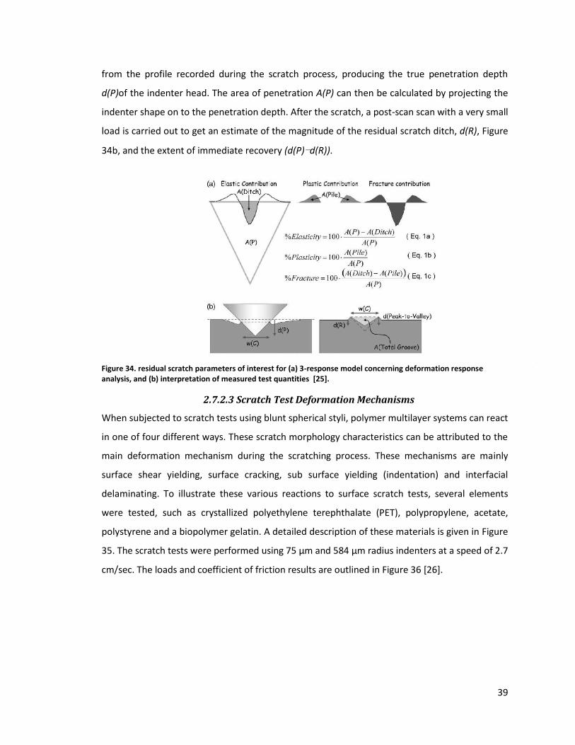
39
from the profile recorded during the scratch process, producing the true penetration depth
d(P)of the indenter head. The area of penetration A(P) can then be calculated by projecting the
indenter shape on to the penetration depth. After the scratch, a post-scan scan with a very small
load is carried out to get an estimate of the magnitude of the residual scratch ditch, d(R), Figure
34b, and the extent of immediate recovery (d(P)−d(R)).
Figure 34. residual scratch parameters of interest for (a) 3-response model concerning deformation response analysis, and (b) interpretation of measured test quantities [25].
2.7.2.3 Scratch Test Deformation Mechanisms
When subjected to scratch tests using blunt spherical styli, polymer multilayer systems can react
in one of four different ways. These scratch morphology characteristics can be attributed to the
main deformation mechanism during the scratching process. These mechanisms are mainly
surface shear yielding, surface cracking, sub surface yielding (indentation) and interfacial
delaminating. To illustrate these various reactions to surface scratch tests, several elements
were tested, such as crystallized polyethylene terephthalate (PET), polypropylene, acetate,
polystyrene and a biopolymer gelatin. A detailed description of these materials is given in Figure
35. The scratch tests were performed using 75 µm and 584 µm radius indenters at a speed of 2.7
cm/sec. The loads and coefficient of friction results are outlined in Figure 36 [26].
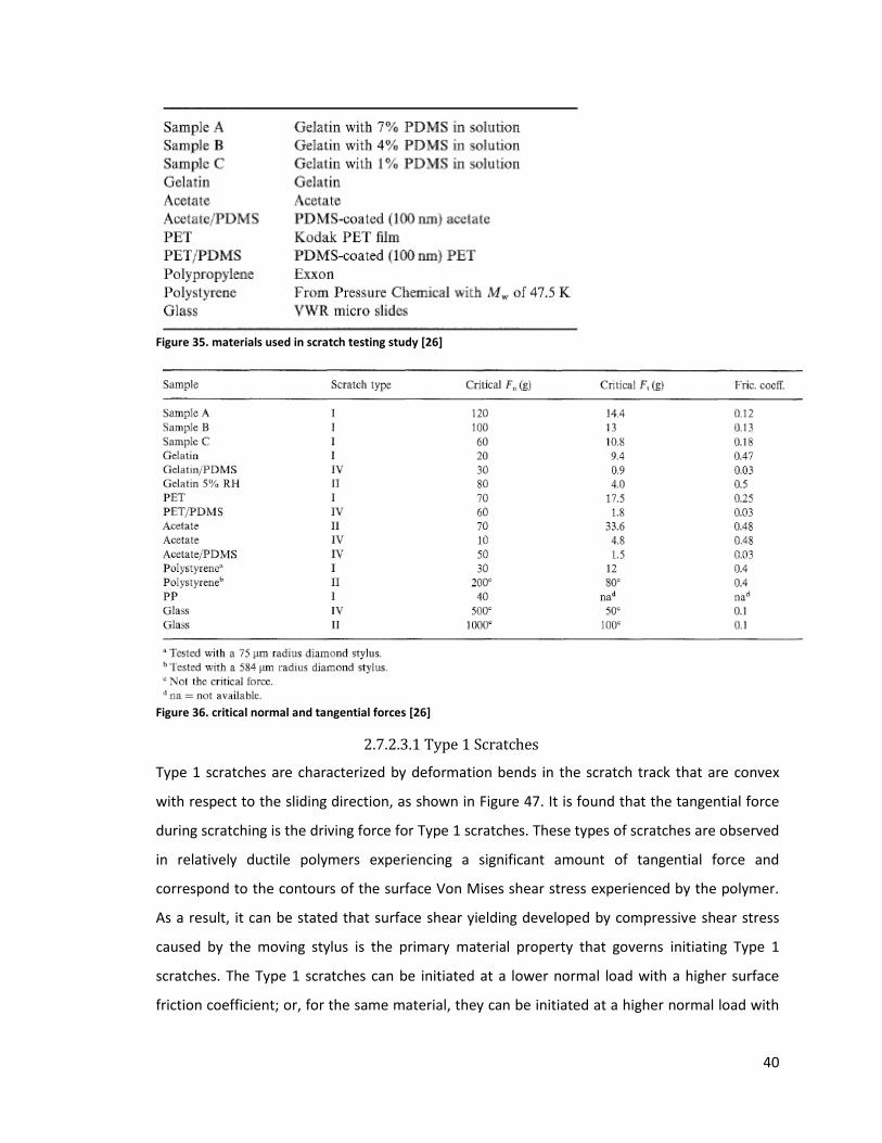
40
Figure 35. materials used in scratch testing study [26]
Figure 36. critical normal and tangential forces [26]
2.7.2.3.1 Type 1 Scratches
Type 1 scratches are characterized by deformation bends in the scratch track that are convex
with respect to the sliding direction, as shown in Figure 47. It is found that the tangential force
during scratching is the driving force for Type 1 scratches. These types of scratches are observed
in relatively ductile polymers experiencing a significant amount of tangential force and
correspond to the contours of the surface Von Mises shear stress experienced by the polymer.
As a result, it can be stated that surface shear yielding developed by compressive shear stress
caused by the moving stylus is the primary material property that governs initiating Type 1
scratches. The Type 1 scratches can be initiated at a lower normal load with a higher surface
friction coefficient; or, for the same material, they can be initiated at a higher normal load with
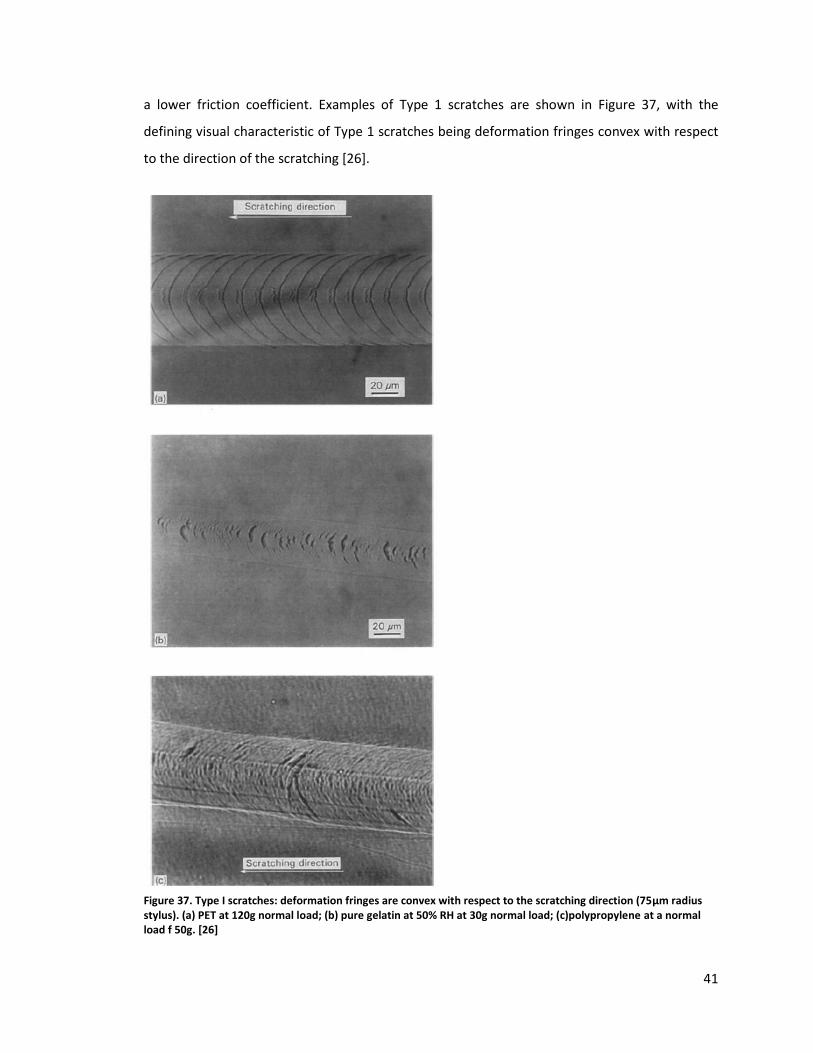
41
a lower friction coefficient. Examples of Type 1 scratches are shown in Figure 37, with the
defining visual characteristic of Type 1 scratches being deformation fringes convex with respect
to the direction of the scratching [26].
Figure 37. Type I scratches: deformation fringes are convex with respect to the scratching direction (75µm radius stylus). (a) PET at 120g normal load; (b) pure gelatin at 50% RH at 30g normal load; (c)polypropylene at a normal load f 50g. [26]
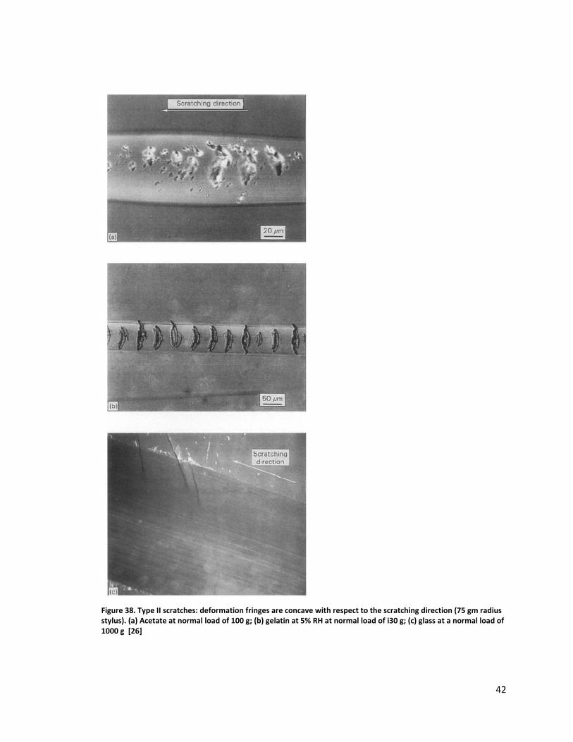
42
Figure 38. Type II scratches: deformation fringes are concave with respect to the scratching direction (75 gm radius stylus). (a) Acetate at normal load of 100 g; (b) gelatin at 5% RH at normal load of i30 g; (c) glass at a normal load of 1000 g [26]
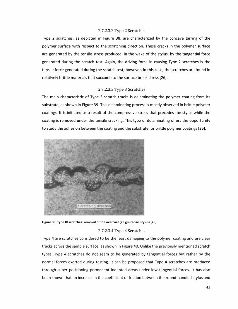
43
2.7.2.3.2 Type 2 Scratches
Type 2 scratches, as depicted in Figure 38, are characterized by the concave tarring of the
polymer surface with respect to the scratching direction. These cracks in the polymer surface
are generated by the tensile stress produced, in the wake of the stylus, by the tangential force
generated during the scratch test. Again, the driving force in causing Type 2 scratches is the
tensile force generated during the scratch test; however, in this case, the scratches are found in
relatively brittle materials that succumb to the surface break stress [26].
2.7.2.3.3 Type 3 Scratches
The main characteristic of Type 3 scratch tracks is delaminating the polymer coating from its
substrate, as shown in Figure 39. This delaminating process is mostly observed in brittle polymer
coatings. It is initiated as a result of the compressive stress that precedes the stylus while the
coating is removed under the tensile cracking. This type of delaminating offers the opportunity
to study the adhesion between the coating and the substrate for brittle polymer coatings [26].
Figure 39. Type III scratches: removal of the overcoat (75 gm radius stylus) [26]
2.7.2.3.4 Type 4 Scratches
Type 4 are scratches considered to be the least damaging to the polymer coating and are clear
tracks across the sample surface, as shown in Figure 40. Unlike the previously mentioned scratch
types, Type 4 scratches do not seem to be generated by tangential forces but rather by the
normal forces exerted during testing. It can be proposed that Type 4 scratches are produced
through super positioning permanent indented areas under low tangential forces. It has also
been shown that an increase in the coefficient of friction between the round-handled stylus and
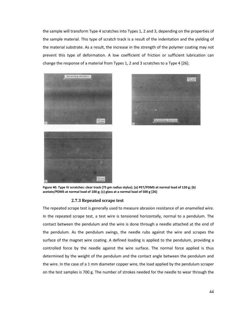
44
the sample will transform Type 4 scratches into Types 1, 2 and 3, depending on the properties of
the sample material. This type of scratch track is a result of the indentation and the yielding of
the material substrate. As a result, the increase in the strength of the polymer coating may not
prevent this type of deformation. A low coefficient of friction or sufficient lubrication can
change the response of a material from Types 1, 2 and 3 scratches to a Type 4 [26].
Figure 40. Type IV scratches: clear track (75 gm radius stylus). (a) PET/PDMS at normal load of 120 g; (b) acetate/PDMS at normal load of 100 g; (c) glass at a normal load of 500 g [26]
2.7.3 Repeated scrape test
The repeated scrape test is generally used to measure abrasion resistance of an enamelled wire.
In the repeated scrape test, a test wire is tensioned horizontally, normal to a pendulum. The
contact between the pendulum and the wire is done through a needle attached at the end of
the pendulum. As the pendulum swings, the needle rubs against the wire and scrapes the
surface of the magnet wire coating. A defined loading is applied to the pendulum, providing a
controlled force by the needle against the wire surface. The normal force applied is thus
determined by the weight of the pendulum and the contact angle between the pendulum and
the wire. In the case of a 1 mm diameter copper wire, the load applied by the pendulum scraper
on the test samples is 700 g. The number of strokes needed for the needle to wear through the
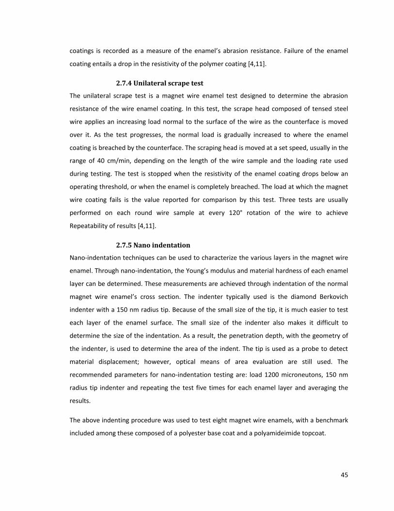
45
coatings is recorded as a measure of the enamel’s abrasion resistance. Failure of the enamel
coating entails a drop in the resistivity of the polymer coating [4,11].
2.7.4 Unilateral scrape test
The unilateral scrape test is a magnet wire enamel test designed to determine the abrasion
resistance of the wire enamel coating. In this test, the scrape head composed of tensed steel
wire applies an increasing load normal to the surface of the wire as the counterface is moved
over it. As the test progresses, the normal load is gradually increased to where the enamel
coating is breached by the counterface. The scraping head is moved at a set speed, usually in the
range of 40 cm/min, depending on the length of the wire sample and the loading rate used
during testing. The test is stopped when the resistivity of the enamel coating drops below an
operating threshold, or when the enamel is completely breached. The load at which the magnet
wire coating fails is the value reported for comparison by this test. Three tests are usually
performed on each round wire sample at every 120° rotation of the wire to achieve
Repeatability of results [4,11].
2.7.5 Nano indentation
Nano-indentation techniques can be used to characterize the various layers in the magnet wire
enamel. Through nano-indentation, the Young’s modulus and material hardness of each enamel
layer can be determined. These measurements are achieved through indentation of the normal
magnet wire enamel’s cross section. The indenter typically used is the diamond Berkovich
indenter with a 150 nm radius tip. Because of the small size of the tip, it is much easier to test
each layer of the enamel surface. The small size of the indenter also makes it difficult to
determine the size of the indentation. As a result, the penetration depth, with the geometry of
the indenter, is used to determine the area of the indent. The tip is used as a probe to detect
material displacement; however, optical means of area evaluation are still used. The
recommended parameters for nano-indentation testing are: load 1200 microneutons, 150 nm
radius tip indenter and repeating the test five times for each enamel layer and averaging the
results.
The above indenting procedure was used to test eight magnet wire enamels, with a benchmark
included among these composed of a polyester base coat and a polyamideimide topcoat.
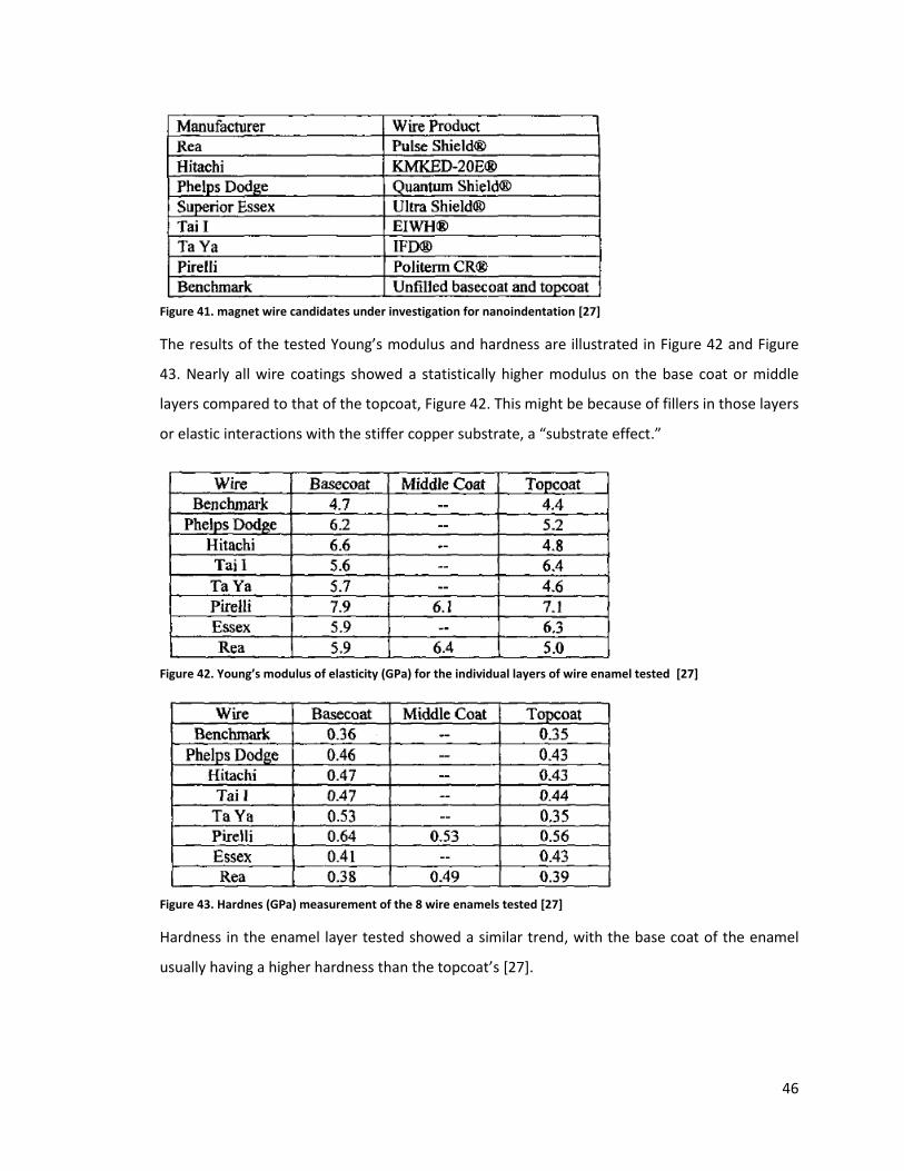
46
Figure 41. magnet wire candidates under investigation for nanoindentation [27]
The results of the tested Young’s modulus and hardness are illustrated in Figure 42 and Figure
43. Nearly all wire coatings showed a statistically higher modulus on the base coat or middle
layers compared to that of the topcoat, Figure 42. This might be because of fillers in those layers
or elastic interactions with the stiffer copper substrate, a “substrate effect.”
Figure 42. Young’s modulus of elasticity (GPa) for the individual layers of wire enamel tested [27]
Figure 43. Hardnes (GPa) measurement of the 8 wire enamels tested [27]
Hardness in the enamel layer tested showed a similar trend, with the base coat of the enamel
usually having a higher hardness than the topcoat’s [27].
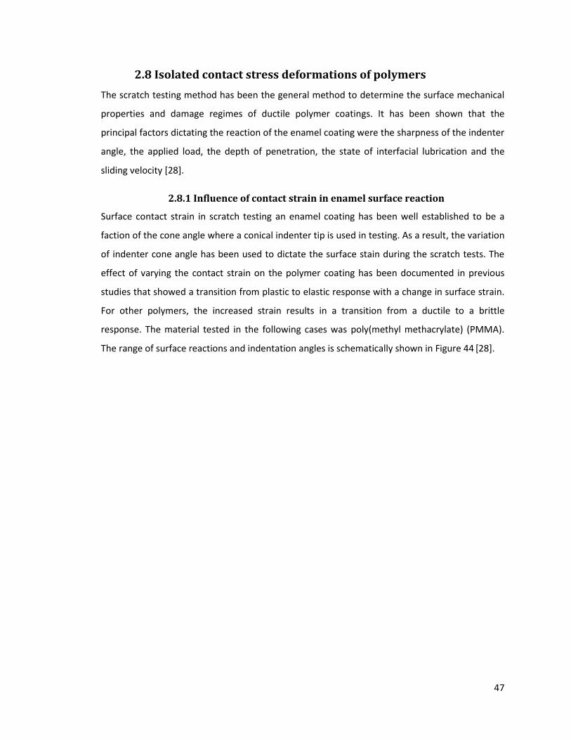
47
2.8 Isolated contact stress deformations of polymers
The scratch testing method has been the general method to determine the surface mechanical
properties and damage regimes of ductile polymer coatings. It has been shown that the
principal factors dictating the reaction of the enamel coating were the sharpness of the indenter
angle, the applied load, the depth of penetration, the state of interfacial lubrication and the
sliding velocity [28].
2.8.1 Influence of contact strain in enamel surface reaction
Surface contact strain in scratch testing an enamel coating has been well established to be a
faction of the cone angle where a conical indenter tip is used in testing. As a result, the variation
of indenter cone angle has been used to dictate the surface stain during the scratch tests. The
effect of varying the contact strain on the polymer coating has been documented in previous
studies that showed a transition from plastic to elastic response with a change in surface strain.
For other polymers, the increased strain results in a transition from a ductile to a brittle
response. The material tested in the following cases was poly(methyl methacrylate) (PMMA).
The range of surface reactions and indentation angles is schematically shown in Figure 44 [28].
48
Figure 44. The influence of cone angle a, upon the types of damage produced in scratching. This type of response is typical for polymers . For clarity of presentation the pictorial view does not show the variation in attack angle α [28]
A critical angle was observed where, when testing at a varying applied load, the deformation
changed from the adhesion to the ploughing mode of friction.
2.8.2 Influence of normal load on enamel surface reaction
When considering the change in enamel surface behaviour during scratch testing using a conical
tip, it is apparent that load and tip penetration plays an important role in the polymer surface
reaction. Deformation maps showing dependence of the deformation mechanism on both
normal load and surface strain have been developed and are shown in Figure 45 [28]. In this
figure, it can be seen that the increased applied load — and, as a result, increased surface
penetration — causes a transition of the surface deformation from ductile to brittle machining.

49
This reaction is observed only at cone angles below 45°. At blunt cone angles (above 120°), the
surface reaction moves from fully elastic to the ironing of the polymer coating.
Figure 45. Deformation map for a poly (carbonate) resin. The diagram shows results from scratching performed at room temperature for a range of cone angles and normal loads and at a scratching velocity of 0.0026 mm/s [28]
2.8.3 Scratch map of polymers
By using both conical and spherical indenters, scratch tests were performed to evaluate the
relative scratch resistance of the polymer coatings. The results were then used to develop
scratch deformation maps based on surface strain, evaluated by the shape of the indenter tip
and the applied load. To further determine the abrasion resistance properties of the polymer
coatings, the influence of temperature was also studied. Deformation maps based on surface
temperature were compiled to summarize the results. The effect of deformation patterns on the
coefficient of friction was also observed. The materials tested in this study were
poly(methylmethacrylate) (PMMA), a poly(tetraltuorc-thylene) (PTFE) and an ultra-high
molecular weight poly(ethylene) (UI-IMWPE) [23].
2.8.3.1 Determining Surface Strain
To depict the stress distribution under the loaded indent, two types of indenter models were
considered in this study. The first type, consisting of shapes such as a wedge or cone indenter,
imposed a fixed strain on the specimen proportional to the tangent of the cone angle θ, with
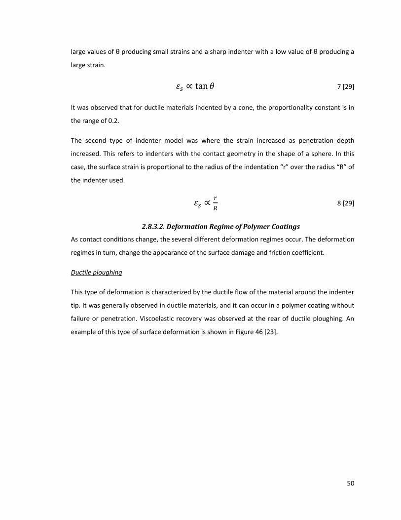
50
large values of θ producing small strains and a sharp indenter with a low value of θ producing a
large strain.
7 [29]
It was observed that for ductile materials indented by a cone, the proportionality constant is in
the range of 0.2.
The second type of indenter model was where the strain increased as penetration depth
increased. This refers to indenters with the contact geometry in the shape of a sphere. In this
case, the surface strain is proportional to the radius of the indentation “r” over the radius “R” of
the indenter used.
8 [29]
2.8.3.2. Deformation Regime of Polymer Coatings
As contact conditions change, the several different deformation regimes occur. The deformation
regimes in turn, change the appearance of the surface damage and friction coefficient.
Ductile ploughing
This type of deformation is characterized by the ductile flow of the material around the indenter
tip. It was generally observed in ductile materials, and it can occur in a polymer coating without
failure or penetration. Viscoelastic recovery was observed at the rear of ductile ploughing. An
example of this type of surface deformation is shown in Figure 46 [23].
51
Figure 46. Ductile ploughing. SEM (×200)of a scratch on a PMMA. The scratch was produced under the following contact conditions: cone angle, 120°: normal load, 1.2 N; scratching velocity, 0.2 mm/s; T= 20 °C; no lubricant. [23]
Regular crack formation
With the increase of applied load or surface strain, cracks in the polymer coatings start to form
either on the edges of the scratch track or in the scratches themselves. This type of deformation
was especially observed in amorphous material. For semi-crystalline polymers, the cracks show
more regularly in the groove, caused by the material accumulating in front of the indenter, until
the elastic limit of the polymer is reached. An example of this type of deformation is shown in
Figure 47 [23].
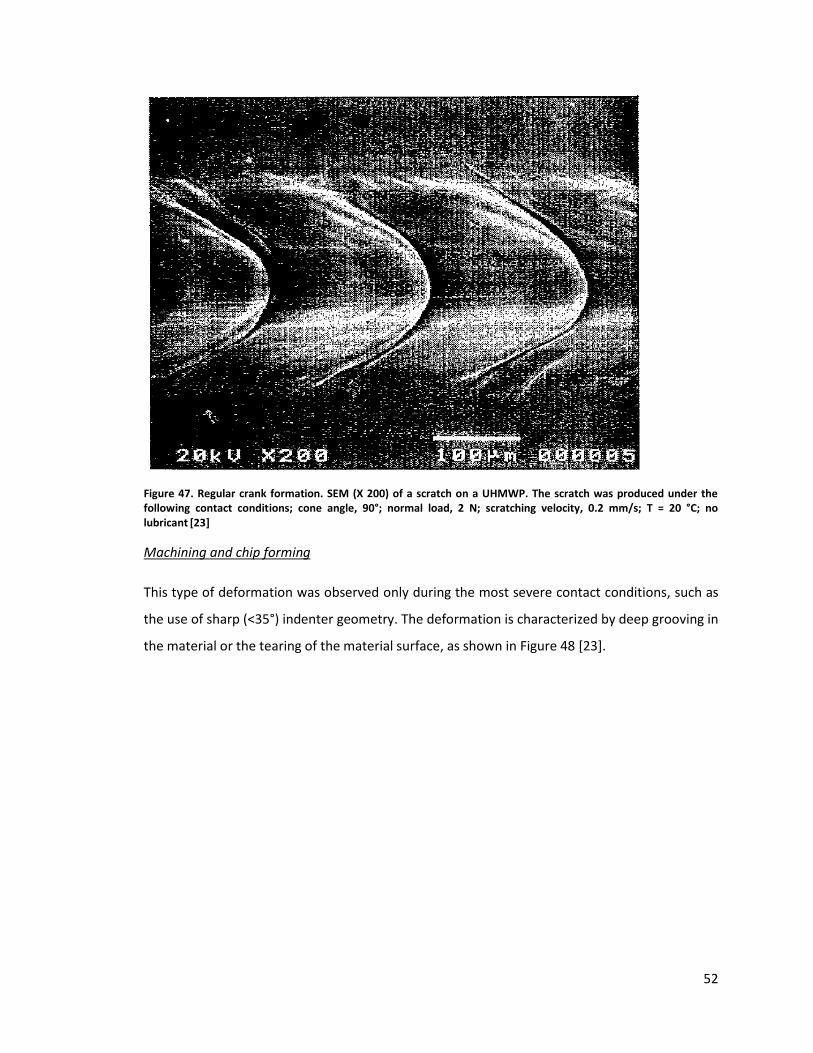
52
Figure 47. Regular crank formation. SEM (X 200) of a scratch on a UHMWP. The scratch was produced under the following contact conditions; cone angle, 90°; normal load, 2 N; scratching velocity, 0.2 mm/s; T = 20 °C; no lubricant [23]
Machining and chip forming
This type of deformation was observed only during the most severe contact conditions, such as
the use of sharp (<35°) indenter geometry. The deformation is characterized by deep grooving in
the material or the tearing of the material surface, as shown in Figure 48 [23].
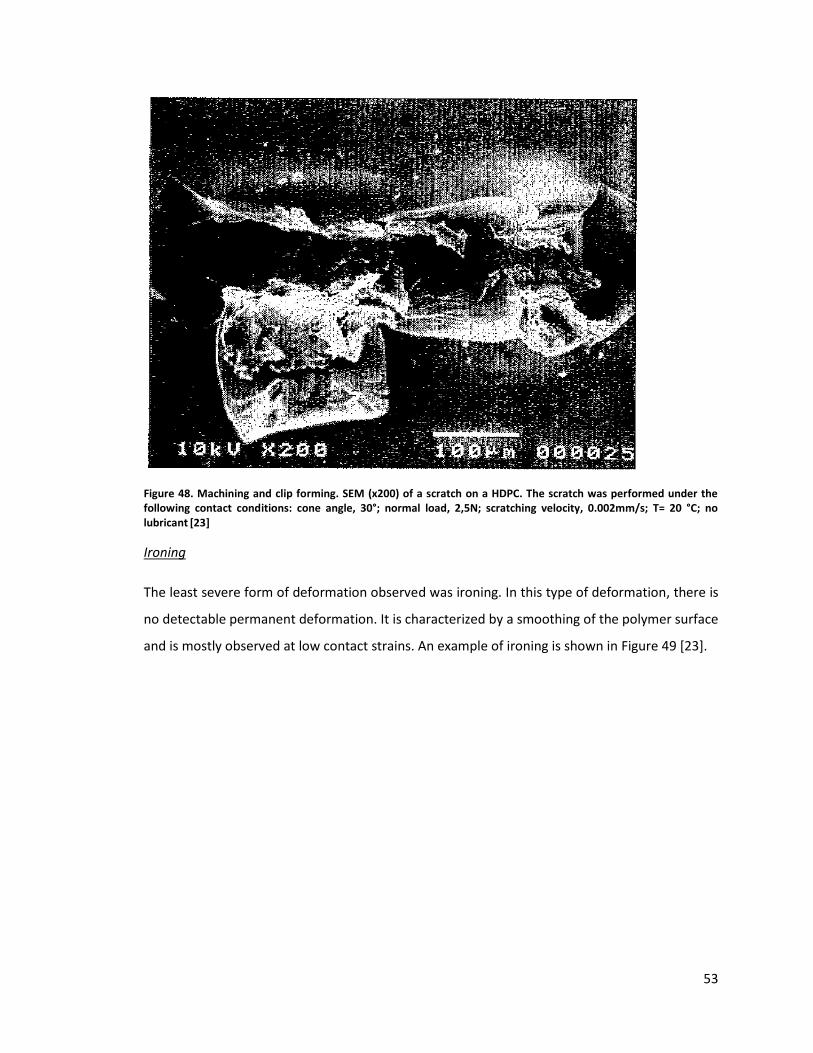
53
Figure 48. Machining and clip forming. SEM (x200) of a scratch on a HDPC. The scratch was performed under the following contact conditions: cone angle, 30°; normal load, 2,5N; scratching velocity, 0.002mm/s; T= 20 °C; no lubricant [23]
Ironing
The least severe form of deformation observed was ironing. In this type of deformation, there is
no detectable permanent deformation. It is characterized by a smoothing of the polymer surface
and is mostly observed at low contact strains. An example of ironing is shown in Figure 49 [23].
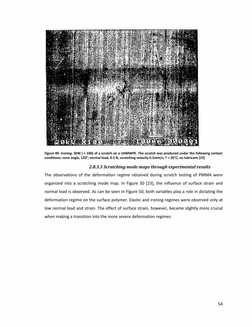
54
Figure 49. Ironing. SEM ( × 100) of a scratch on a UHMWPE. The scratch was produced under the following contact conditions: cone angle, 120°; normal load, 0.5 N; scratching velocity 0.2mm/s; T = 20°C; no lubricant [23]
2.8.3.3 Scratching mode maps through experimental results
The observations of the deformation regime obtained during scratch testing of PMMA were
organized into a scratching mode map. In Figure 50 [23], the influence of surface strain and
normal load is observed. As can be seen in Figure 50, both variables play a role in dictating the
deformation regime on the surface polymer. Elastic and ironing regimes were observed only at
low normal load and strain. The effect of surface strain, however, became slightly more crucial
when making a transition into the more severe deformation regimes.
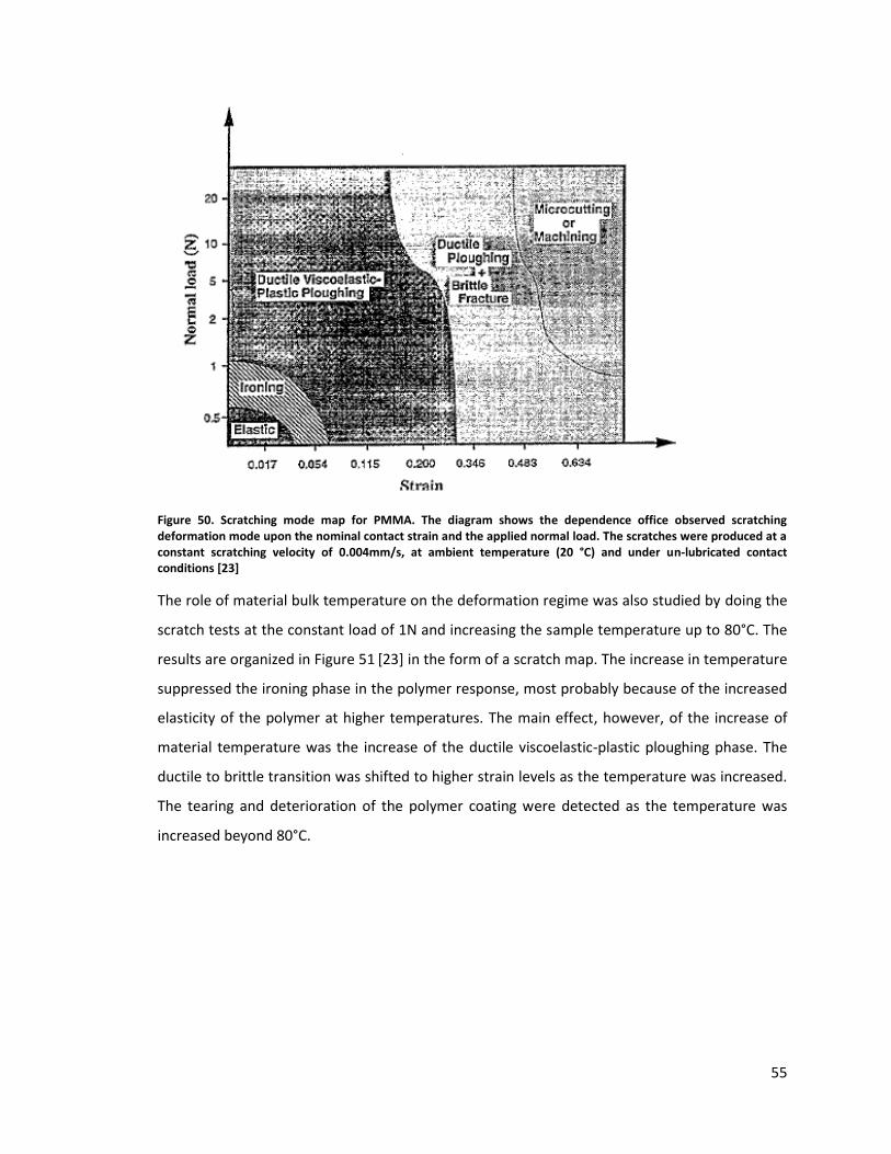
55
Figure 50. Scratching mode map for PMMA. The diagram shows the dependence office observed scratching deformation mode upon the nominal contact strain and the applied normal load. The scratches were produced at a constant scratching velocity of 0.004mm/s, at ambient temperature (20 °C) and under un-lubricated contact conditions [23]
The role of material bulk temperature on the deformation regime was also studied by doing the
scratch tests at the constant load of 1N and increasing the sample temperature up to 80°C. The
results are organized in Figure 51 [23] in the form of a scratch map. The increase in temperature
suppressed the ironing phase in the polymer response, most probably because of the increased
elasticity of the polymer at higher temperatures. The main effect, however, of the increase of
material temperature was the increase of the ductile viscoelastic-plastic ploughing phase. The
ductile to brittle transition was shifted to higher strain levels as the temperature was increased.
The tearing and deterioration of the polymer coating were detected as the temperature was
increased beyond 80°C.
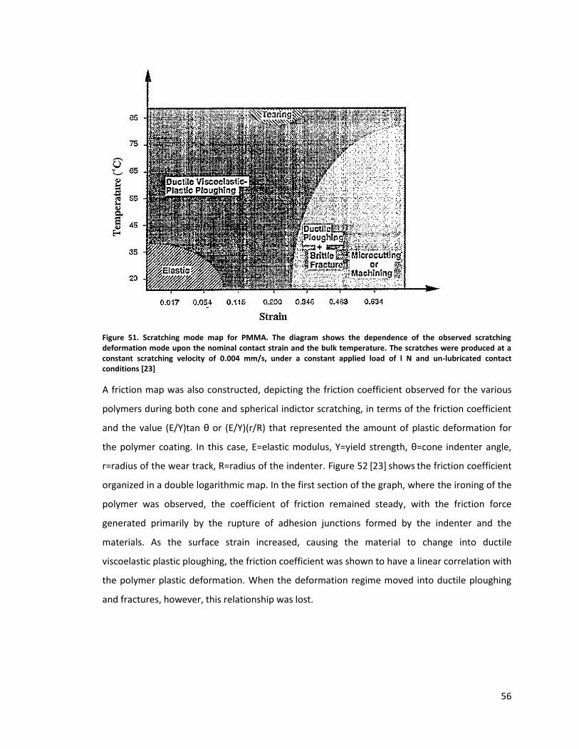
56
Figure 51. Scratching mode map for PMMA. The diagram shows the dependence of the observed scratching deformation mode upon the nominal contact strain and the bulk temperature. The scratches were produced at a constant scratching velocity of 0.004 mm/s, under a constant applied load of l N and un-lubricated contact conditions [23]
A friction map was also constructed, depicting the friction coefficient observed for the various
polymers during both cone and spherical indictor scratching, in terms of the friction coefficient
and the value (E/Y)tan θ or (E/Y)(r/R) that represented the amount of plastic deformation for
the polymer coating. In this case, E=elastic modulus, Y=yield strength, θ=cone indenter angle,
r=radius of the wear track, R=radius of the indenter. Figure 52 [23] shows the friction coefficient
organized in a double logarithmic map. In the first section of the graph, where the ironing of the
polymer was observed, the coefficient of friction remained steady, with the friction force
generated primarily by the rupture of adhesion junctions formed by the indenter and the
materials. As the surface strain increased, causing the material to change into ductile
viscoelastic plastic ploughing, the friction coefficient was shown to have a linear correlation with
the polymer plastic deformation. When the deformation regime moved into ductile ploughing
and fractures, however, this relationship was lost.
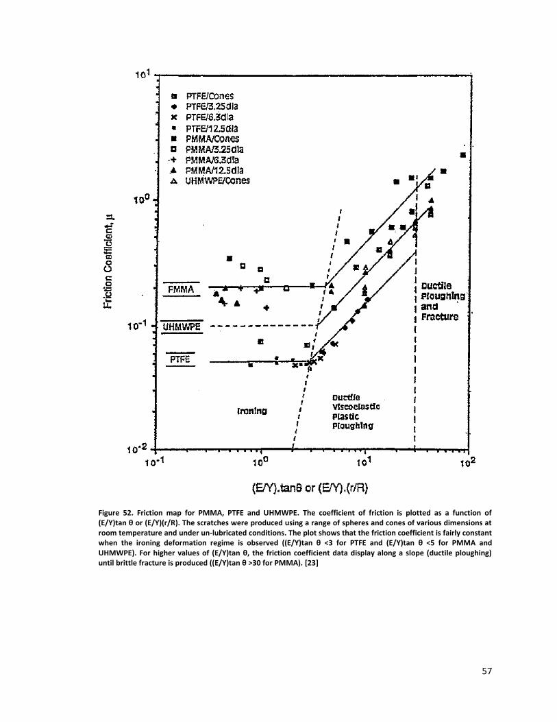
57
Figure 52. Friction map for PMMA, PTFE and UHMWPE. The coefficient of friction is plotted as a function of (E/Y)tan θ or (E/Y)(r/R). The scratches were produced using a range of spheres and cones of various dimensions at room temperature and under un-lubricated conditions. The plot shows that the friction coefficient is fairly constant when the ironing deformation regime is observed ((E/Y)tan θ <3 for PTFE and (E/Y)tan θ <5 for PMMA and UHMWPE). For higher values of (E/Y)tan θ, the friction coefficient data display along a slope (ductile ploughing) until brittle fracture is produced ((E/Y)tan θ >30 for PMMA). [23]
58
2.9 Work objectives
It has been shown that the physical damage of the enamel coating is the principal factor in
failure of enamel wire. This is due to the fact that even minute surface damage can be a factor in
shortening magnet wire operating life. Die forming of the magnet wire during the motor
fabrication processes is the most likely to cause damage of the enamel coating. As a result it is
difficult to fabricate a die of appropriate shape, and optimization of the die forming procedure
in such a way as to minimize enamel damage during die bending. This procedure requires both a
thorough understanding of the interaction between die steel and the wire surface, along with
the material properties of the enamel coating.
As a result my research objective was to optimize the fabrication of magnet wire coils by
minimizing physical damage of enamel coating during die bending process. This will be achieved
through Characterization of enamel polymer coatings, Investigation of COF between magnet
wire surface and die material, and studying the effect of die bending parameters e.g. speed and
strain on COF between magnet wire surface and die material. Understanding the contact
mechanics during wire bending process of bar wound electric motors is crucial in facilitating the
design and manufacture of these coils, as well as avoiding any defects in the coil fabrication
process that can lead to shortening the motor.
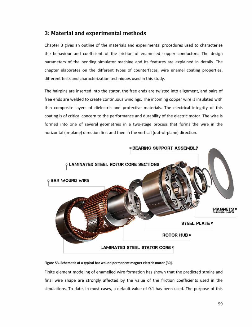
59
3: Material and experimental methods
Chapter 3 gives an outline of the materials and experimental procedures used to characterize
the behaviour and coefficient of the friction of enamelled copper conductors. The design
parameters of the bending simulator machine and its features are explained in details. The
chapter elaborates on the different types of counterfaces, wire enamel coating properties,
different tests and characterization techniques used in this study.
The hairpins are inserted into the stator, the free ends are twisted into alignment, and pairs of
free ends are welded to create continuous windings. The incoming copper wire is insulated with
thin composite layers of dielectric and protective materials. The electrical integrity of this
coating is of critical concern to the performance and durability of the electric motor. The wire is
formed into one of several geometries in a two-stage process that forms the wire in the
horizontal (in-plane) direction first and then in the vertical (out-of-plane) direction.
Figure 53. Schematic of a typical bar wound permanent magnet electric motor [30].
Finite element modeling of enamelled wire formation has shown that the predicted strains and
final wire shape are strongly affected by the value of the friction coefficients used in the
simulations. To date, in most cases, a default value of 0.1 has been used. The purpose of this
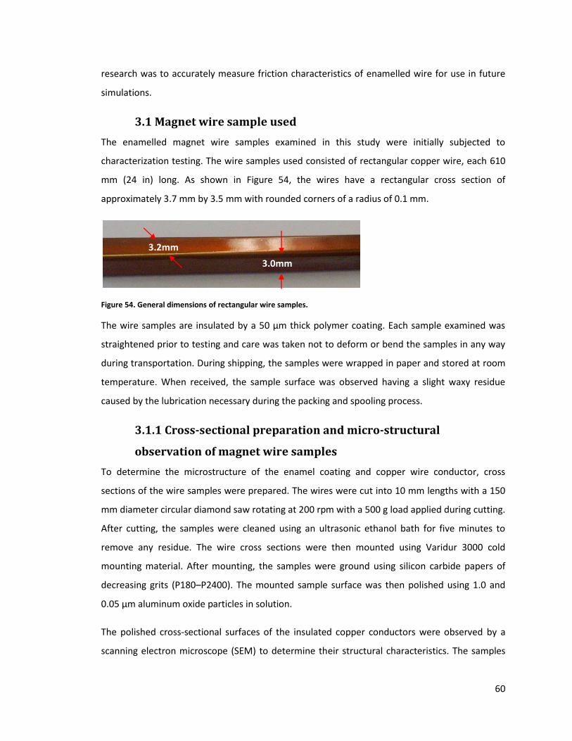
60
research was to accurately measure friction characteristics of enamelled wire for use in future
simulations.
3.1 Magnet wire sample used
The enamelled magnet wire samples examined in this study were initially subjected to
characterization testing. The wire samples used consisted of rectangular copper wire, each 610
mm (24 in) long. As shown in Figure 54, the wires have a rectangular cross section of
approximately 3.7 mm by 3.5 mm with rounded corners of a radius of 0.1 mm.
Figure 54. General dimensions of rectangular wire samples.
The wire samples are insulated by a 50 μm thick polymer coating. Each sample examined was
straightened prior to testing and care was taken not to deform or bend the samples in any way
during transportation. During shipping, the samples were wrapped in paper and stored at room
temperature. When received, the sample surface was observed having a slight waxy residue
caused by the lubrication necessary during the packing and spooling process.
3.1.1 Cross-sectional preparation and micro-structural
observation of magnet wire samples
To determine the microstructure of the enamel coating and copper wire conductor, cross
sections of the wire samples were prepared. The wires were cut into 10 mm lengths with a 150
mm diameter circular diamond saw rotating at 200 rpm with a 500 g load applied during cutting.
After cutting, the samples were cleaned using an ultrasonic ethanol bath for five minutes to
remove any residue. The wire cross sections were then mounted using Varidur 3000 cold
mounting material. After mounting, the samples were ground using silicon carbide papers of
decreasing grits (P180–P2400). The mounted sample surface was then polished using 1.0 and
0.05 μm aluminum oxide particles in solution.
The polished cross-sectional surfaces of the insulated copper conductors were observed by a
scanning electron microscope (SEM) to determine their structural characteristics. The samples
3.2mm
3.0mm
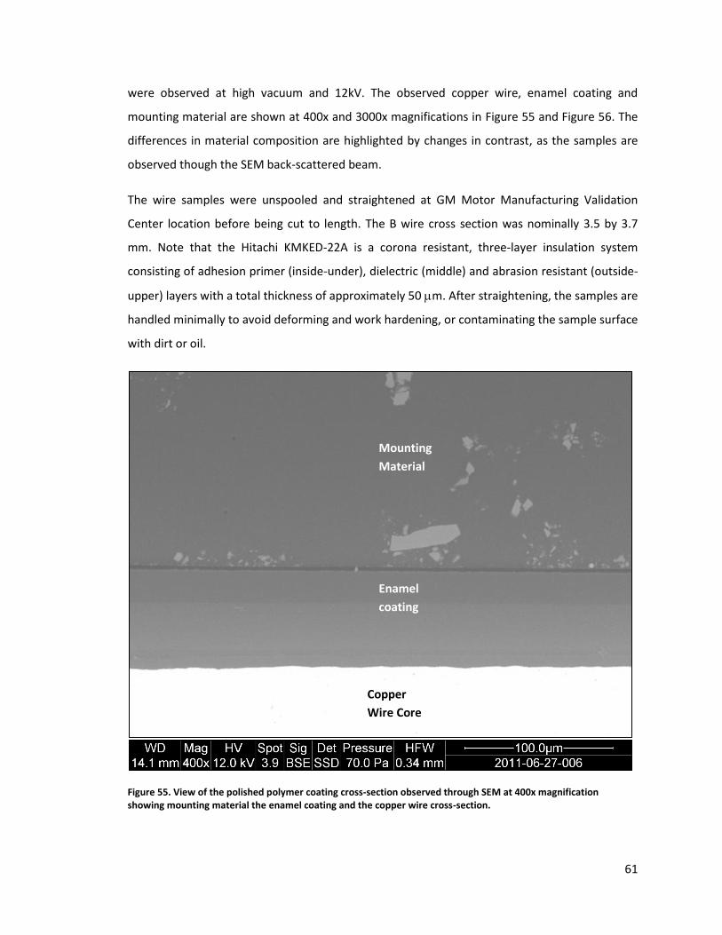
61
were observed at high vacuum and 12kV. The observed copper wire, enamel coating and
mounting material are shown at 400x and 3000x magnifications in Figure 55 and Figure 56. The
differences in material composition are highlighted by changes in contrast, as the samples are
observed though the SEM back-scattered beam.
The wire samples were unspooled and straightened at GM Motor Manufacturing Validation
Center location before being cut to length. The B wire cross section was nominally 3.5 by 3.7
mm. Note that the Hitachi KMKED-22A is a corona resistant, three-layer insulation system
consisting of adhesion primer (inside-under), dielectric (middle) and abrasion resistant (outside-
upper) layers with a total thickness of approximately 50 m. After straightening, the samples are
handled minimally to avoid deforming and work hardening, or contaminating the sample surface
with dirt or oil.
Figure 55. View of the polished polymer coating cross-section observed through SEM at 400x magnification showing mounting material the enamel coating and the copper wire cross-section.
Enamel
coating
Mounting
Material
Copper
Wire Core
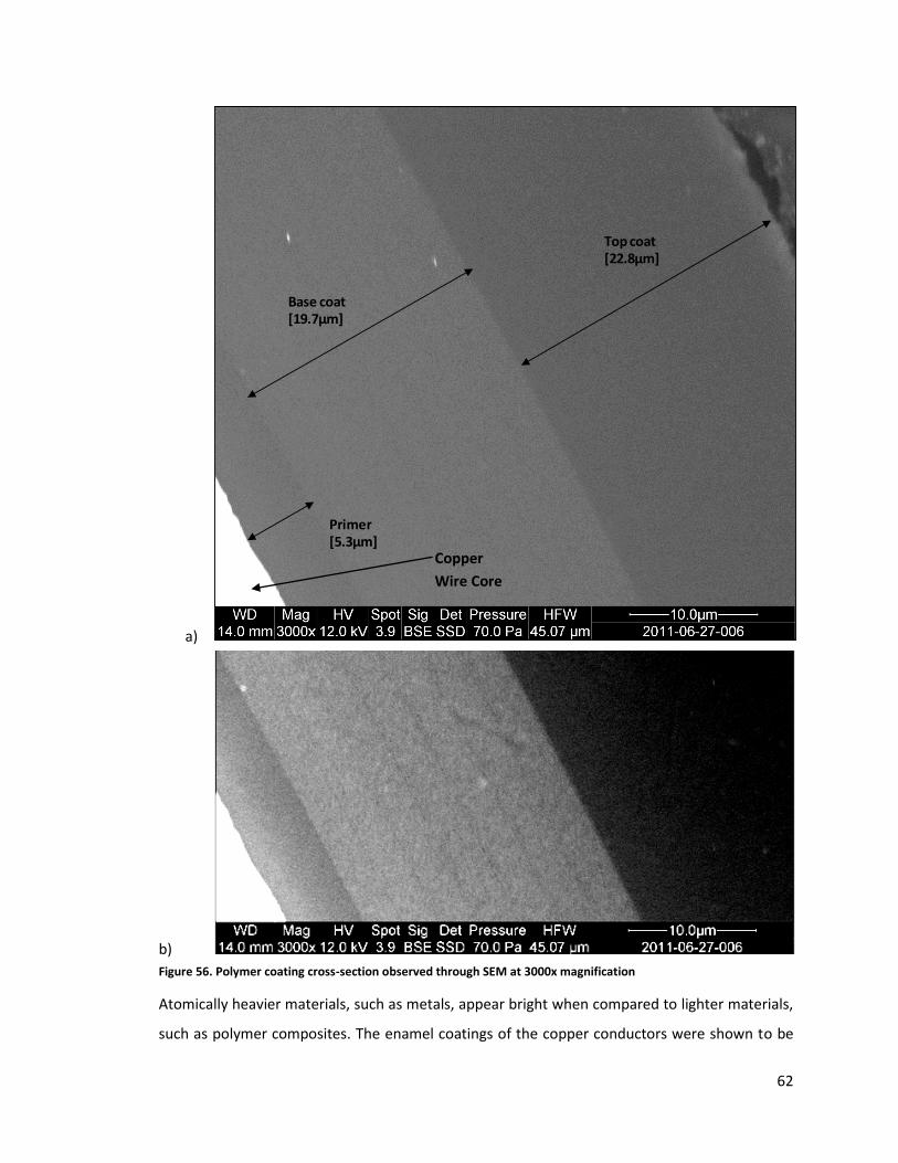
62
a)
b)
Figure 56. Polymer coating cross-section observed through SEM at 3000x magnification
Atomically heavier materials, such as metals, appear bright when compared to lighter materials,
such as polymer composites. The enamel coatings of the copper conductors were shown to be
Primer [5.3µm]
Base coat [19.7µm]
Top coat [22.8µm]
Copper
Wire Core
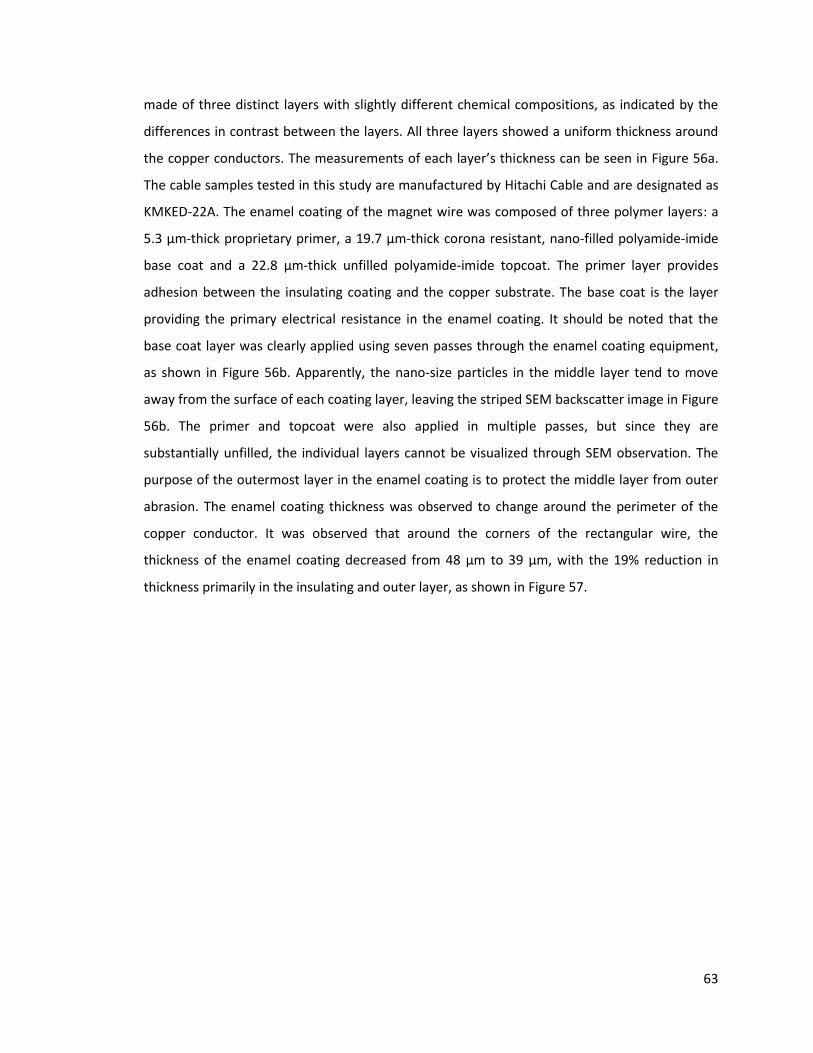
63
made of three distinct layers with slightly different chemical compositions, as indicated by the
differences in contrast between the layers. All three layers showed a uniform thickness around
the copper conductors. The measurements of each layer’s thickness can be seen in Figure 56a.
The cable samples tested in this study are manufactured by Hitachi Cable and are designated as
KMKED-22A. The enamel coating of the magnet wire was composed of three polymer layers: a
5.3 μm-thick proprietary primer, a 19.7 μm-thick corona resistant, nano-filled polyamide-imide
base coat and a 22.8 μm-thick unfilled polyamide-imide topcoat. The primer layer provides
adhesion between the insulating coating and the copper substrate. The base coat is the layer
providing the primary electrical resistance in the enamel coating. It should be noted that the
base coat layer was clearly applied using seven passes through the enamel coating equipment,
as shown in Figure 56b. Apparently, the nano-size particles in the middle layer tend to move
away from the surface of each coating layer, leaving the striped SEM backscatter image in Figure
56b. The primer and topcoat were also applied in multiple passes, but since they are
substantially unfilled, the individual layers cannot be visualized through SEM observation. The
purpose of the outermost layer in the enamel coating is to protect the middle layer from outer
abrasion. The enamel coating thickness was observed to change around the perimeter of the
copper conductor. It was observed that around the corners of the rectangular wire, the
thickness of the enamel coating decreased from 48 µm to 39 µm, with the 19% reduction in
thickness primarily in the insulating and outer layer, as shown in Figure 57.
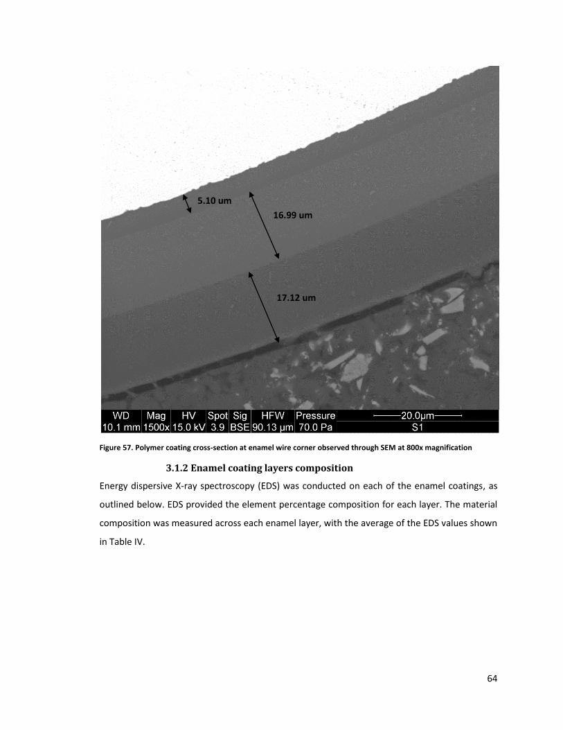
64
Figure 57. Polymer coating cross-section at enamel wire corner observed through SEM at 800x magnification
3.1.2 Enamel coating layers composition
Energy dispersive X-ray spectroscopy (EDS) was conducted on each of the enamel coatings, as
outlined below. EDS provided the element percentage composition for each layer. The material
composition was measured across each enamel layer, with the average of the EDS values shown
in Table IV.
5.10 um
16.99 um
17.12 um
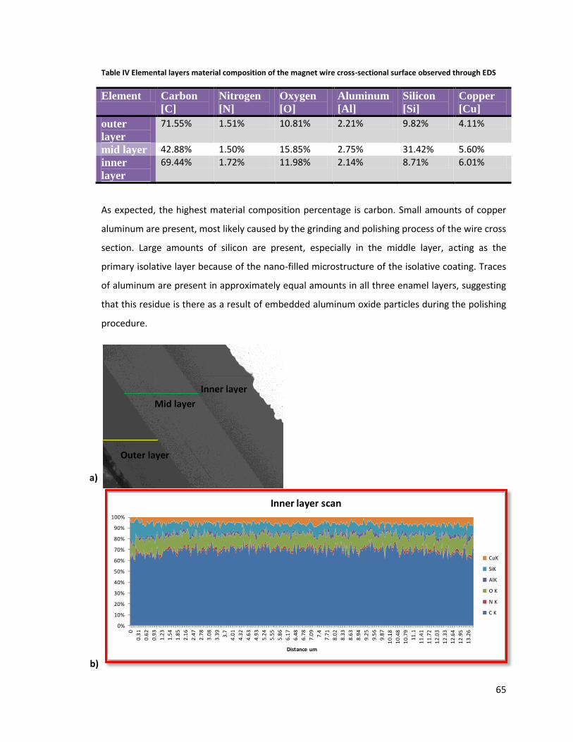
65
Table IV Elemental layers material composition of the magnet wire cross-sectional surface observed through EDS
Element Carbon
[C]
Nitrogen
[N]
Oxygen
[O]
Aluminum
[Al]
Silicon
[Si]
Copper
[Cu]
outer
layer
71.55% 1.51% 10.81% 2.21% 9.82% 4.11%
mid layer 42.88% 1.50% 15.85% 2.75% 31.42% 5.60%
inner
layer
69.44% 1.72% 11.98% 2.14% 8.71% 6.01%
As expected, the highest material composition percentage is carbon. Small amounts of copper
aluminum are present, most likely caused by the grinding and polishing process of the wire cross
section. Large amounts of silicon are present, especially in the middle layer, acting as the
primary isolative layer because of the nano-filled microstructure of the isolative coating. Traces
of aluminum are present in approximately equal amounts in all three enamel layers, suggesting
that this residue is there as a result of embedded aluminum oxide particles during the polishing
procedure.
0%
10%
20%
30%
40%
50%
60%
70%
80%
90%
100%
0
0.3
1
0.6
2
0.9
3
1.2
3
1.5
4
1.8
5
2.1
6
2.4
7
2.7
8
3.0
8
3.3
9
3.7
4.0
1
4.3
2
4.6
3
4.9
3
5.2
4
5.5
5
5.8
6
6.1
7
6.4
8
6.7
8
7.0
9
7.4
7.7
1
8.0
2
8.3
3
8.6
3
8.9
4
9.2
5
9.5
6
9.8
7
10
.18
10
.48
10
.79
11
.1
11
.41
11
.72
12
.03
12
.33
12
.64
12
.95
13
.26
Distance um
Inner layer scan
CuK
SiK
AlK
O K
N K
C K
Inner layer
Mid layer
Outer layer
a)
b)
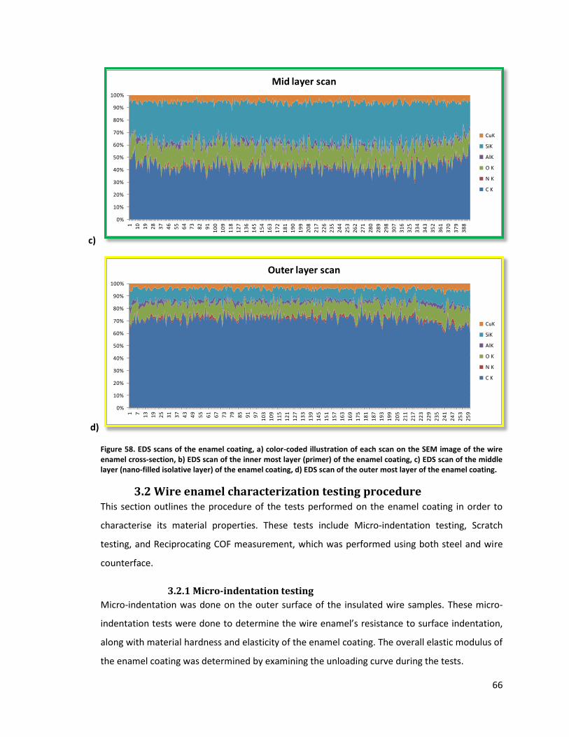
66
Figure 58. EDS scans of the enamel coating, a) color-coded illustration of each scan on the SEM image of the wire enamel cross-section, b) EDS scan of the inner most layer (primer) of the enamel coating, c) EDS scan of the middle layer (nano-filled isolative layer) of the enamel coating, d) EDS scan of the outer most layer of the enamel coating.
3.2 Wire enamel characterization testing procedure This section outlines the procedure of the tests performed on the enamel coating in order to
characterise its material properties. These tests include Micro-indentation testing, Scratch
testing, and Reciprocating COF measurement, which was performed using both steel and wire
counterface.
3.2.1 Micro-indentation testing
Micro-indentation was done on the outer surface of the insulated wire samples. These micro-
indentation tests were done to determine the wire enamel’s resistance to surface indentation,
along with material hardness and elasticity of the enamel coating. The overall elastic modulus of
the enamel coating was determined by examining the unloading curve during the tests.
0%
10%
20%
30%
40%
50%
60%
70%
80%
90%
100%
1 10
19
28
37
46
55
64
73
82
91
10
0
10
9
11
8
12
7
13
6
14
5
15
4
16
3
17
2
18
1
19
0
19
9
20
8
21
7
22
6
23
5
24
4
25
3
26
2
27
1
28
0
28
9
29
8
30
7
31
6
32
5
33
4
34
3
35
2
36
1
37
0
37
9
38
8
Mid layer scan
CuK
SiK
AlK
O K
N K
C K
0%
10%
20%
30%
40%
50%
60%
70%
80%
90%
100%
1 7 13
19
25
31
37
43
49
55
61
67
73
79
85
91
97
10
3
10
9
11
5
12
1
12
7
13
3
13
9
14
5
15
1
15
7
16
3
16
9
17
5
18
1
18
7
19
3
19
9
20
5
21
1
21
7
22
3
22
9
23
5
24
1
24
7
25
3
25
9
Outer layer scan
CuK
SiK
AlK
O K
N K
C K
c)
d)
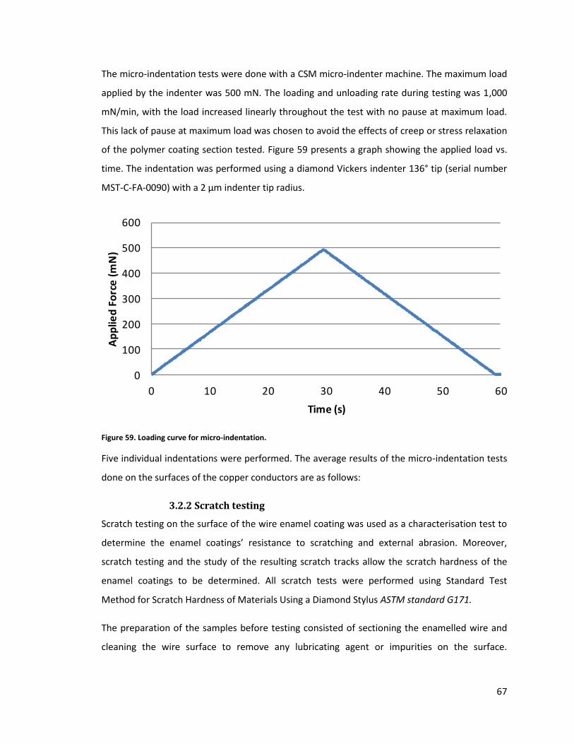
67
The micro-indentation tests were done with a CSM micro-indenter machine. The maximum load
applied by the indenter was 500 mN. The loading and unloading rate during testing was 1,000
mN/min, with the load increased linearly throughout the test with no pause at maximum load.
This lack of pause at maximum load was chosen to avoid the effects of creep or stress relaxation
of the polymer coating section tested. Figure 59 presents a graph showing the applied load vs.
time. The indentation was performed using a diamond Vickers indenter 136° tip (serial number
MST-C-FA-0090) with a 2 μm indenter tip radius.
Figure 59. Loading curve for micro-indentation.
Five individual indentations were performed. The average results of the micro-indentation tests
done on the surfaces of the copper conductors are as follows:
3.2.2 Scratch testing
Scratch testing on the surface of the wire enamel coating was used as a characterisation test to
determine the enamel coatings’ resistance to scratching and external abrasion. Moreover,
scratch testing and the study of the resulting scratch tracks allow the scratch hardness of the
enamel coatings to be determined. All scratch tests were performed using Standard Test
Method for Scratch Hardness of Materials Using a Diamond Stylus ASTM standard G171.
The preparation of the samples before testing consisted of sectioning the enamelled wire and
cleaning the wire surface to remove any lubricating agent or impurities on the surface.
0
100
200
300
400
500
600
0 10 20 30 40 50 60
Ap
plie
d F
orc
e (
mN
)
Time (s)
Force VS Time
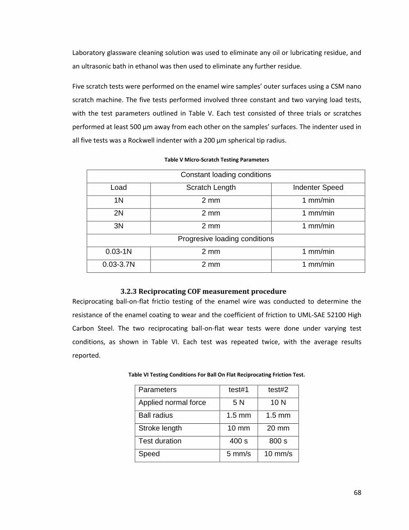
68
Laboratory glassware cleaning solution was used to eliminate any oil or lubricating residue, and
an ultrasonic bath in ethanol was then used to eliminate any further residue.
Five scratch tests were performed on the enamel wire samples’ outer surfaces using a CSM nano
scratch machine. The five tests performed involved three constant and two varying load tests,
with the test parameters outlined in Table V. Each test consisted of three trials or scratches
performed at least 500 μm away from each other on the samples’ surfaces. The indenter used in
all five tests was a Rockwell indenter with a 200 μm spherical tip radius.
Table V Micro-Scratch Testing Parameters
Constant loading conditions
Load Scratch Length Indenter Speed
1N 2 mm 1 mm/min
2N 2 mm 1 mm/min
3N 2 mm 1 mm/min
Progresive loading conditions
0.03-1N 2 mm 1 mm/min
0.03-3.7N 2 mm 1 mm/min
3.2.3 Reciprocating COF measurement procedure
Reciprocating ball-on-flat frictio testing of the enamel wire was conducted to determine the
resistance of the enamel coating to wear and the coefficient of friction to UML-SAE 52100 High
Carbon Steel. The two reciprocating ball-on-flat wear tests were done under varying test
conditions, as shown in Table VI. Each test was repeated twice, with the average results
reported.
Table VI Testing Conditions For Ball On Flat Reciprocating Friction Test.
Parameters test#1 test#2
Applied normal force 5 N 10 N
Ball radius 1.5 mm 1.5 mm
Stroke length 10 mm 20 mm
Test duration 400 s 800 s
Speed 5 mm/s 10 mm/s
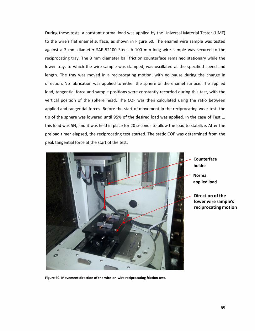
69
During these tests, a constant normal load was applied by the Universal Material Tester (UMT)
to the wire’s flat enamel surface, as shown in Figure 60. The enamel wire sample was tested
against a 3 mm diameter SAE 52100 Steel. A 100 mm long wire sample was secured to the
reciprocating tray. The 3 mm diameter ball friction counterface remained stationary while the
lower tray, to which the wire sample was clamped, was oscillated at the specified speed and
length. The tray was moved in a reciprocating motion, with no pause during the change in
direction. No lubrication was applied to either the sphere or the enamel surface. The applied
load, tangential force and sample positions were constantly recorded during this test, with the
vertical position of the sphere head. The COF was then calculated using the ratio between
applied and tangential forces. Before the start of movement in the reciprocating wear test, the
tip of the sphere was lowered until 95% of the desired load was applied. In the case of Test 1,
this load was 5N, and it was held in place for 20 seconds to allow the load to stabilize. After the
preload timer elapsed, the reciprocating test started. The static COF was determined from the
peak tangential force at the start of the test.
Figure 60. Movement direction of the wire-on-wire reciprocating friction test.
Direction of the lower wire sample’s reciprocating motion
Counterface
holder
Normal
applied load
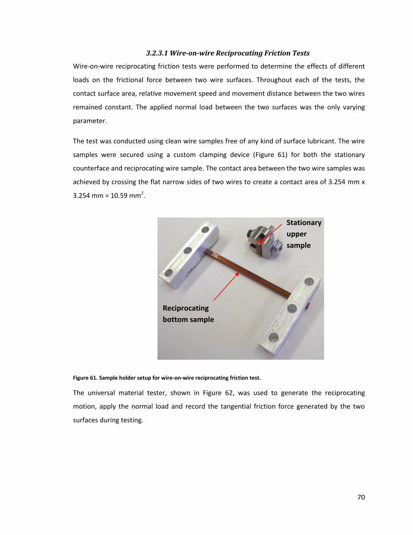
70
3.2.3.1 Wire-on-wire Reciprocating Friction Tests
Wire-on-wire reciprocating friction tests were performed to determine the effects of different
loads on the frictional force between two wire surfaces. Throughout each of the tests, the
contact surface area, relative movement speed and movement distance between the two wires
remained constant. The applied normal load between the two surfaces was the only varying
parameter.
The test was conducted using clean wire samples free of any kind of surface lubricant. The wire
samples were secured using a custom clamping device (Figure 61) for both the stationary
counterface and reciprocating wire sample. The contact area between the two wire samples was
achieved by crossing the flat narrow sides of two wires to create a contact area of 3.254 mm x
3.254 mm = 10.59 mm2.
Figure 61. Sample holder setup for wire-on-wire reciprocating friction test.
The universal material tester, shown in Figure 62, was used to generate the reciprocating
motion, apply the normal load and record the tangential friction force generated by the two
surfaces during testing.
Stationary
upper
sample
Reciprocating
bottom sample
71
Figure 62. Setup for the wire-on-wire reciprocating friction test in the universal testing machine.
A 10mm/s movement speed was chosen with a 20 mm stroke length and a 150-second (37
reciprocating strokes) test duration. The applied normal load was varied between 2N and 10N,
as outlined in Table VII, with the applied normal pressure. The applied pressure in the wire-on-
wire friction tests was significantly lower compared to that used in the reciprocating ball-on-flat
tests. This result is because of the greater contact area between the two samples and the
limitations in the maximum applied load for the universal material-testing machine used.
Table VII Applied Load for Wire-on-Wire Reciprocating Friction Test and Corresponding Pressure Values.
Load [N] Pressure [MPa]
2 0.1888
4 0.3777
6 0.5666
8 0.7554
10 0.9443
20N capacity
load sensor
Steel leaf
spring
Stationary upper
wire sample
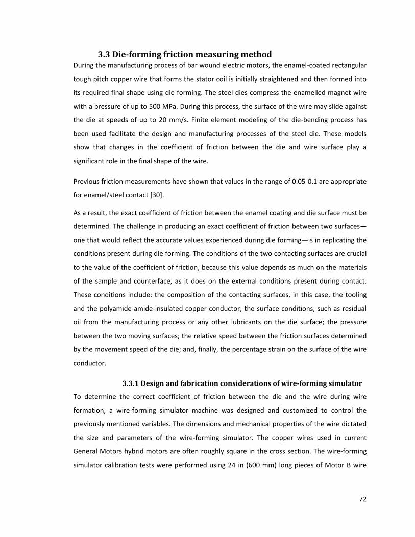
72
3.3 Die-forming friction measuring method During the manufacturing process of bar wound electric motors, the enamel-coated rectangular
tough pitch copper wire that forms the stator coil is initially straightened and then formed into
its required final shape using die forming. The steel dies compress the enamelled magnet wire
with a pressure of up to 500 MPa. During this process, the surface of the wire may slide against
the die at speeds of up to 20 mm/s. Finite element modeling of the die-bending process has
been used facilitate the design and manufacturing processes of the steel die. These models
show that changes in the coefficient of friction between the die and wire surface play a
significant role in the final shape of the wire.
Previous friction measurements have shown that values in the range of 0.05-0.1 are appropriate
for enamel/steel contact [30].
As a result, the exact coefficient of friction between the enamel coating and die surface must be
determined. The challenge in producing an exact coefficient of friction between two surfaces—
one that would reflect the accurate values experienced during die forming—is in replicating the
conditions present during die forming. The conditions of the two contacting surfaces are crucial
to the value of the coefficient of friction, because this value depends as much on the materials
of the sample and counterface, as it does on the external conditions present during contact.
These conditions include: the composition of the contacting surfaces, in this case, the tooling
and the polyamide-amide-insulated copper conductor; the surface conditions, such as residual
oil from the manufacturing process or any other lubricants on the die surface; the pressure
between the two moving surfaces; the relative speed between the friction surfaces determined
by the movement speed of the die; and, finally, the percentage strain on the surface of the wire
conductor.
3.3.1 Design and fabrication considerations of wire-forming simulator
To determine the correct coefficient of friction between the die and the wire during wire
formation, a wire-forming simulator machine was designed and customized to control the
previously mentioned variables. The dimensions and mechanical properties of the wire dictated
the size and parameters of the wire-forming simulator. The copper wires used in current
General Motors hybrid motors are often roughly square in the cross section. The wire-forming
simulator calibration tests were performed using 24 in (600 mm) long pieces of Motor B wire
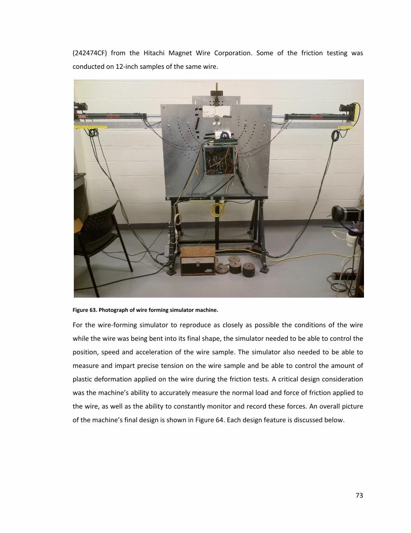
73
(242474CF) from the Hitachi Magnet Wire Corporation. Some of the friction testing was
conducted on 12-inch samples of the same wire.
Figure 63. Photograph of wire forming simulator machine.
For the wire-forming simulator to reproduce as closely as possible the conditions of the wire
while the wire was being bent into its final shape, the simulator needed to be able to control the
position, speed and acceleration of the wire sample. The simulator also needed to be able to
measure and impart precise tension on the wire sample and be able to control the amount of
plastic deformation applied on the wire during the friction tests. A critical design consideration
was the machine’s ability to accurately measure the normal load and force of friction applied to
the wire, as well as the ability to constantly monitor and record these forces. An overall picture
of the machine’s final design is shown in Figure 64. Each design feature is discussed below.
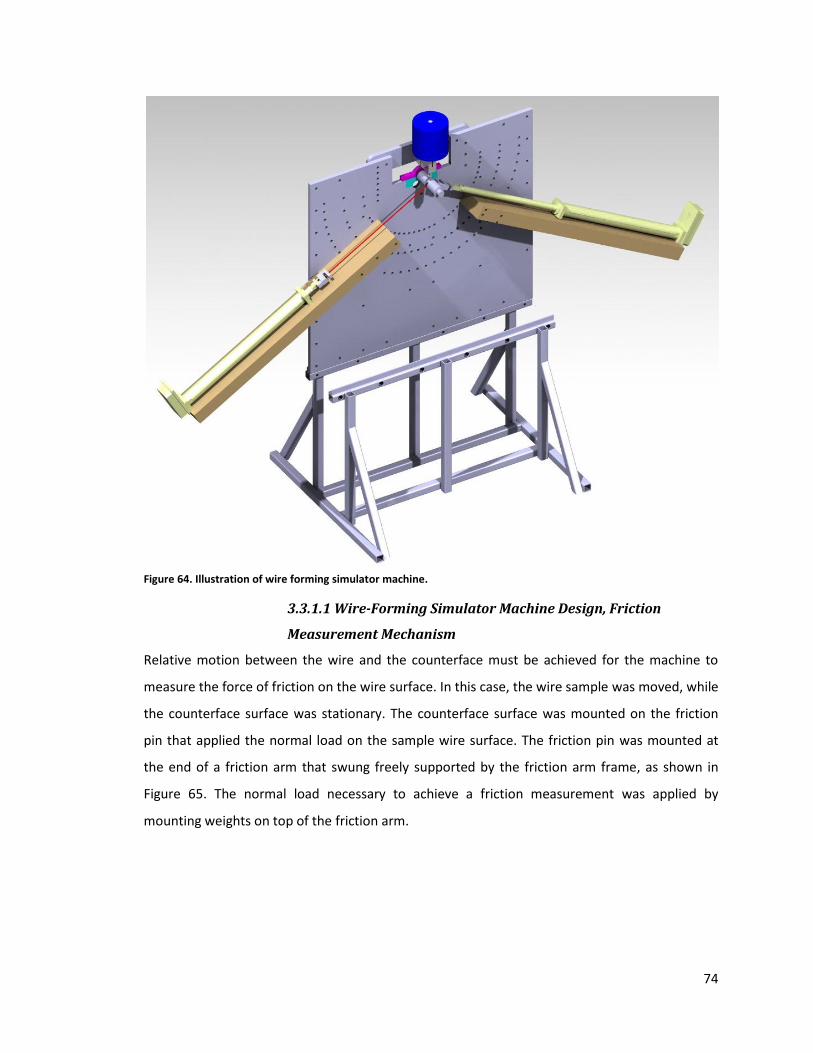
74
Figure 64. Illustration of wire forming simulator machine.
3.3.1.1 Wire-Forming Simulator Machine Design, Friction
Measurement Mechanism
Relative motion between the wire and the counterface must be achieved for the machine to
measure the force of friction on the wire surface. In this case, the wire sample was moved, while
the counterface surface was stationary. The counterface surface was mounted on the friction
pin that applied the normal load on the sample wire surface. The friction pin was mounted at
the end of a friction arm that swung freely supported by the friction arm frame, as shown in
Figure 65. The normal load necessary to achieve a friction measurement was applied by
mounting weights on top of the friction arm.
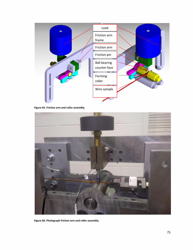
75
Figure 65. Friction arm and roller assembly.
Figure 66. Photograph friction arm and roller assembly.
Friction pin
Friction arm
frame
Friction arm
Ball bearing
counter face
Load
Forming
roller
Wire sample
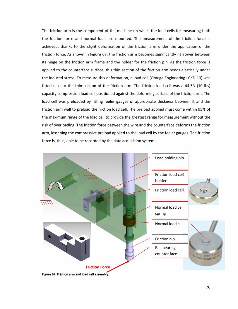
76
The friction arm is the component of the machine on which the load cells for measuring both
the friction force and normal load are mounted. The measurement of the friction force is
achieved, thanks to the slight deformation of the friction arm under the application of the
friction force. As shown in Figure 67, the friction arm becomes significantly narrower between
its hinge on the friction arm frame and the holder for the friction pin. As the friction force is
applied to the counterface surface, this thin section of the friction arm bends elastically under
the induced stress. To measure this deformation, a load cell (Omega Engineering LCKD-10) was
fitted next to the thin section of the friction arm. The friction load cell was a 44.5N (10 lbs)
capacity compression load cell positioned against the deforming surface of the friction arm. The
load cell was preloaded by fitting feeler gauges of appropriate thickness between it and the
friction arm wall to preload the friction load cell. The preload applied must come within 95% of
the maximum range of the load cell to provide the greatest range for measurement without the
risk of overloading. The friction force between the wire and the counterface deforms the friction
arm, lessening the compressive preload applied to the load cell by the feeler gauges. The friction
force is, thus, able to be recorded by the data acquisition system.
Figure 67. Friction arm and load cell assembly.
Load holding pin
Friction load cell
holder
Friction load cell
Normal load cell
spring
Normal load cell
Friction pin
Ball bearing
counter face
Friction Force
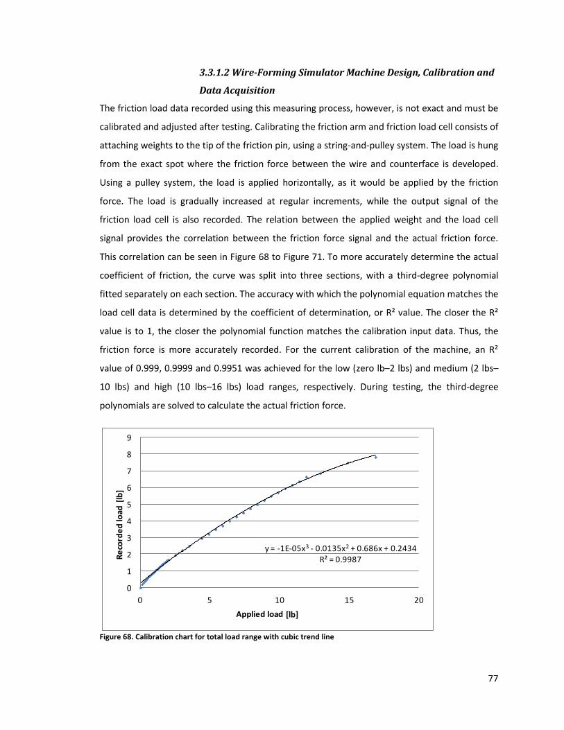
77
3.3.1.2 Wire-Forming Simulator Machine Design, Calibration and
Data Acquisition
The friction load data recorded using this measuring process, however, is not exact and must be
calibrated and adjusted after testing. Calibrating the friction arm and friction load cell consists of
attaching weights to the tip of the friction pin, using a string-and-pulley system. The load is hung
from the exact spot where the friction force between the wire and counterface is developed.
Using a pulley system, the load is applied horizontally, as it would be applied by the friction
force. The load is gradually increased at regular increments, while the output signal of the
friction load cell is also recorded. The relation between the applied weight and the load cell
signal provides the correlation between the friction force signal and the actual friction force.
This correlation can be seen in Figure 68 to Figure 71. To more accurately determine the actual
coefficient of friction, the curve was split into three sections, with a third-degree polynomial
fitted separately on each section. The accuracy with which the polynomial equation matches the
load cell data is determined by the coefficient of determination, or R² value. The closer the R²
value is to 1, the closer the polynomial function matches the calibration input data. Thus, the
friction force is more accurately recorded. For the current calibration of the machine, an R²
value of 0.999, 0.9999 and 0.9951 was achieved for the low (zero lb–2 lbs) and medium (2 lbs–
10 lbs) and high (10 lbs–16 lbs) load ranges, respectively. During testing, the third-degree
polynomials are solved to calculate the actual friction force.
Figure 68. Calibration chart for total load range with cubic trend line
y = -1E-05x3 - 0.0135x2 + 0.686x + 0.2434R² = 0.9987
0
1
2
3
4
5
6
7
8
9
0 5 10 15 20
Re
cord
ed
load
sig
nal
[lb
]
Applied load signal [lb]
y = -1E-05x3 - 0.0135x2 + 0.686x + 0.2434R² = 0.9987
0
1
2
3
4
5
6
7
8
9
0 5 10 15 20
Re
cord
ed
load
sig
nal
[lb
]
Applied load signal [lb]
y = -1E-05x3 - 0.0135x2 + 0.686x + 0.2434R² = 0.9987
0
1
2
3
4
5
6
7
8
9
0 5 10 15 20
Re
cord
ed
load
sig
nal
[lb
]
Applied load signal [lb]
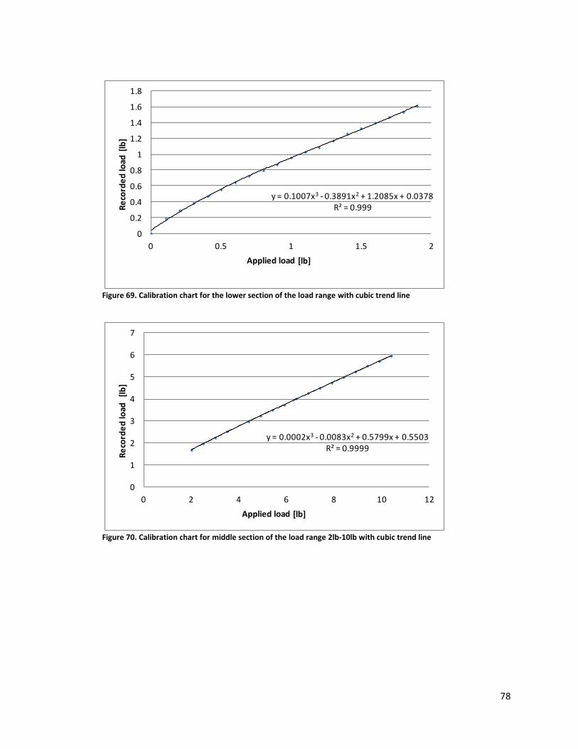
78
Figure 69. Calibration chart for the lower section of the load range with cubic trend line
Figure 70. Calibration chart for middle section of the load range 2lb-10lb with cubic trend line
y = 0.1007x3 - 0.3891x2 + 1.2085x + 0.0378R² = 0.999
0
0.2
0.4
0.6
0.8
1
1.2
1.4
1.6
1.8
0 0.5 1 1.5 2
Re
cord
ed
load
sig
nal
[lb
]
Applied load signal [lb]
y = 0.0002x3 - 0.0083x2 + 0.5799x + 0.5503R² = 0.9999
0
1
2
3
4
5
6
7
0 2 4 6 8 10 12
Re
cord
ed
load
sig
nal
[lb
]
Applied load signal [lb]
y = -1E-05x3 - 0.0135x2 + 0.686x + 0.2434R² = 0.9987
0
1
2
3
4
5
6
7
8
9
0 5 10 15 20
Re
cord
ed
load
sig
nal
[lb
]
Applied load signal [lb]
y = -1E-05x3 - 0.0135x2 + 0.686x + 0.2434R² = 0.9987
0
1
2
3
4
5
6
7
8
9
0 5 10 15 20
Re
cord
ed
load
sig
nal
[lb
]
Applied load signal [lb]
y = -1E-05x3 - 0.0135x2 + 0.686x + 0.2434R² = 0.9987
0
1
2
3
4
5
6
7
8
9
0 5 10 15 20
Re
cord
ed
load
sig
nal
[lb
]
Applied load signal [lb]
y = -1E-05x3 - 0.0135x2 + 0.686x + 0.2434R² = 0.9987
0
1
2
3
4
5
6
7
8
9
0 5 10 15 20
Re
cord
ed
load
sig
nal
[lb
]
Applied load signal [lb]
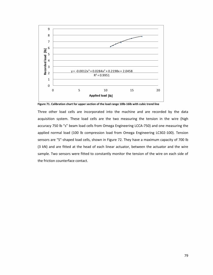
79
Figure 71. Calibration chart for upper section of the load range 10lb-16lb with cubic trend line
Three other load cells are incorporated into the machine and are recorded by the data
acquisition system. These load cells are the two measuring the tension in the wire (high
accuracy 750 lb “s” beam load cells from Omega Engineering LCCA-750) and one measuring the
applied normal load (100 lb compression load from Omega Engineering LC302-100). Tension
sensors are “S”-shaped load cells, shown in Figure 72. They have a maximum capacity of 700 lb
(3 kN) and are fitted at the head of each linear actuator, between the actuator and the wire
sample. Two sensors were fitted to constantly monitor the tension of the wire on each side of
the friction counterface contact.
y = -0.0012x3 + 0.0284x2 + 0.2198x + 2.0458R² = 0.9951
0
1
2
3
4
5
6
7
8
9
0 5 10 15 20
Re
cord
ed
load
sig
nal
[lb
]
Applied load signal [lb]
y = -1E-05x3 - 0.0135x2 + 0.686x + 0.2434R² = 0.9987
0
1
2
3
4
5
6
7
8
9
0 5 10 15 20
Re
cord
ed
load
sig
nal
[lb
]
Applied load signal [lb]
y = -1E-05x3 - 0.0135x2 + 0.686x + 0.2434R² = 0.9987
0
1
2
3
4
5
6
7
8
9
0 5 10 15 20
Re
cord
ed
load
sig
nal
[lb
]
Applied load signal [lb]
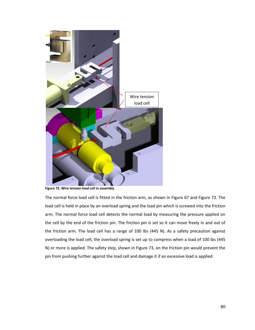
80
Figure 72. Wire tension load cell in assembly
The normal force load cell is fitted in the friction arm, as shown in Figure 67 and Figure 73. The
load cell is held in place by an overload spring and the load pin which is screwed into the friction
arm. The normal force load cell detects the normal load by measuring the pressure applied on
the cell by the end of the friction pin. The friction pin is set so it can move freely in and out of
the friction arm. The load cell has a range of 100 lbs (445 N). As a safety precaution against
overloading the load cell, the overload spring is set up to compress when a load of 100 lbs (445
N) or more is applied. The safety step, shown in Figure 73, on the friction pin would prevent the
pin from pushing further against the load cell and damage it if an excessive load is applied.
Wire tension
load cell
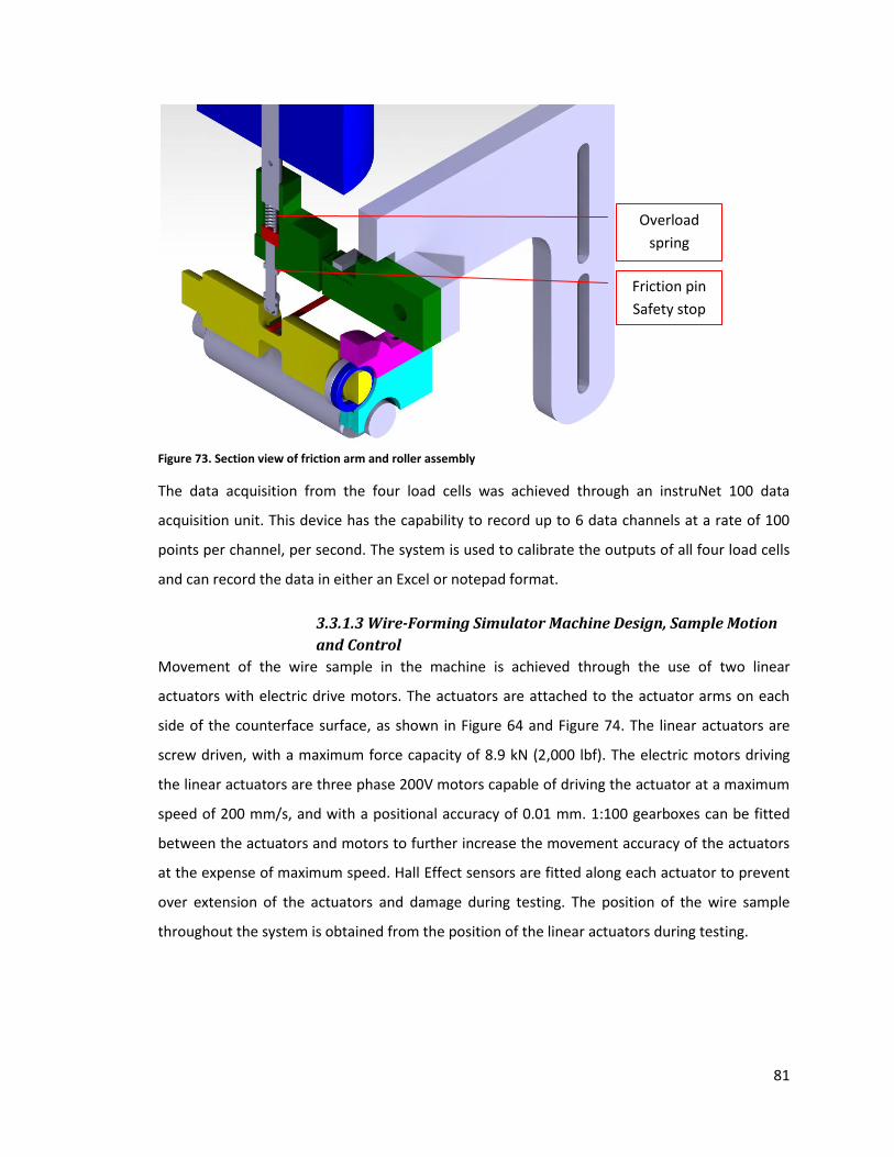
81
Figure 73. Section view of friction arm and roller assembly
The data acquisition from the four load cells was achieved through an instruNet 100 data
acquisition unit. This device has the capability to record up to 6 data channels at a rate of 100
points per channel, per second. The system is used to calibrate the outputs of all four load cells
and can record the data in either an Excel or notepad format.
3.3.1.3 Wire-Forming Simulator Machine Design, Sample Motion
and Control
Movement of the wire sample in the machine is achieved through the use of two linear
actuators with electric drive motors. The actuators are attached to the actuator arms on each
side of the counterface surface, as shown in Figure 64 and Figure 74. The linear actuators are
screw driven, with a maximum force capacity of 8.9 kN (2,000 lbf). The electric motors driving
the linear actuators are three phase 200V motors capable of driving the actuator at a maximum
speed of 200 mm/s, and with a positional accuracy of 0.01 mm. 1:100 gearboxes can be fitted
between the actuators and motors to further increase the movement accuracy of the actuators
at the expense of maximum speed. Hall Effect sensors are fitted along each actuator to prevent
over extension of the actuators and damage during testing. The position of the wire sample
throughout the system is obtained from the position of the linear actuators during testing.
Friction pin
Safety stop
Overload
spring
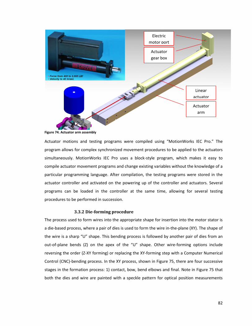
82
Figure 74. Actuator arm assembly
Actuator motions and testing programs were compiled using “MotionWorks IEC Pro.” The
program allows for complex synchronized movement procedures to be applied to the actuators
simultaneously. MotionWorks IEC Pro uses a block-style program, which makes it easy to
compile actuator movement programs and change existing variables without the knowledge of a
particular programming language. After compilation, the testing programs were stored in the
actuator controller and activated on the powering up of the controller and actuators. Several
programs can be loaded in the controller at the same time, allowing for several testing
procedures to be performed in succession.
3.3.2 Die-forming procedure
The process used to form wires into the appropriate shape for insertion into the motor stator is
a die-based process, where a pair of dies is used to form the wire in-the-plane (XY). The shape of
the wire is a sharp “U” shape. This bending process is followed by another pair of dies from an
out-of-plane bends (Z) on the apex of the “U” shape. Other wire-forming options include
reversing the order (Z-XY forming) or replacing the XY-forming step with a Computer Numerical
Control (CNC)-bending process. In the XY process, shown in Figure 75, there are four successive
stages in the formation process: 1) contact, bow, bend elbows and final. Note in Figure 75 that
both the dies and wire are painted with a speckle pattern for optical position measurements
Actuator
arm
Linear
actuator
Electric
motor port
actuator Actuator
gear box
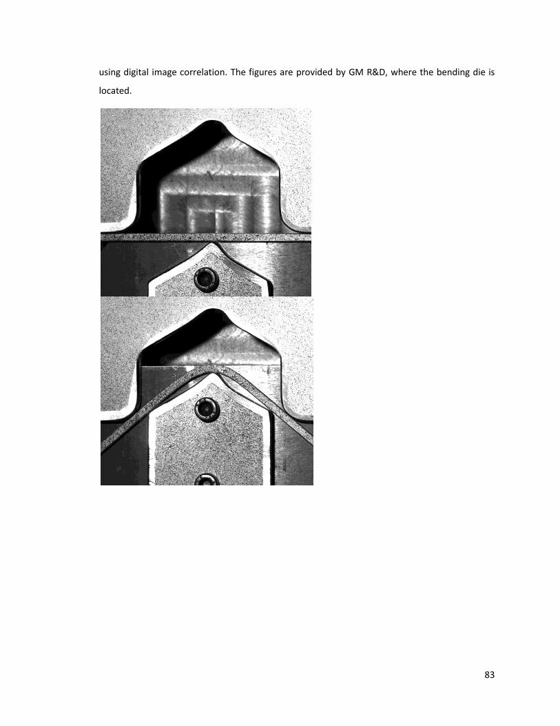
83
using digital image correlation. The figures are provided by GM R&D, where the bending die is
located.
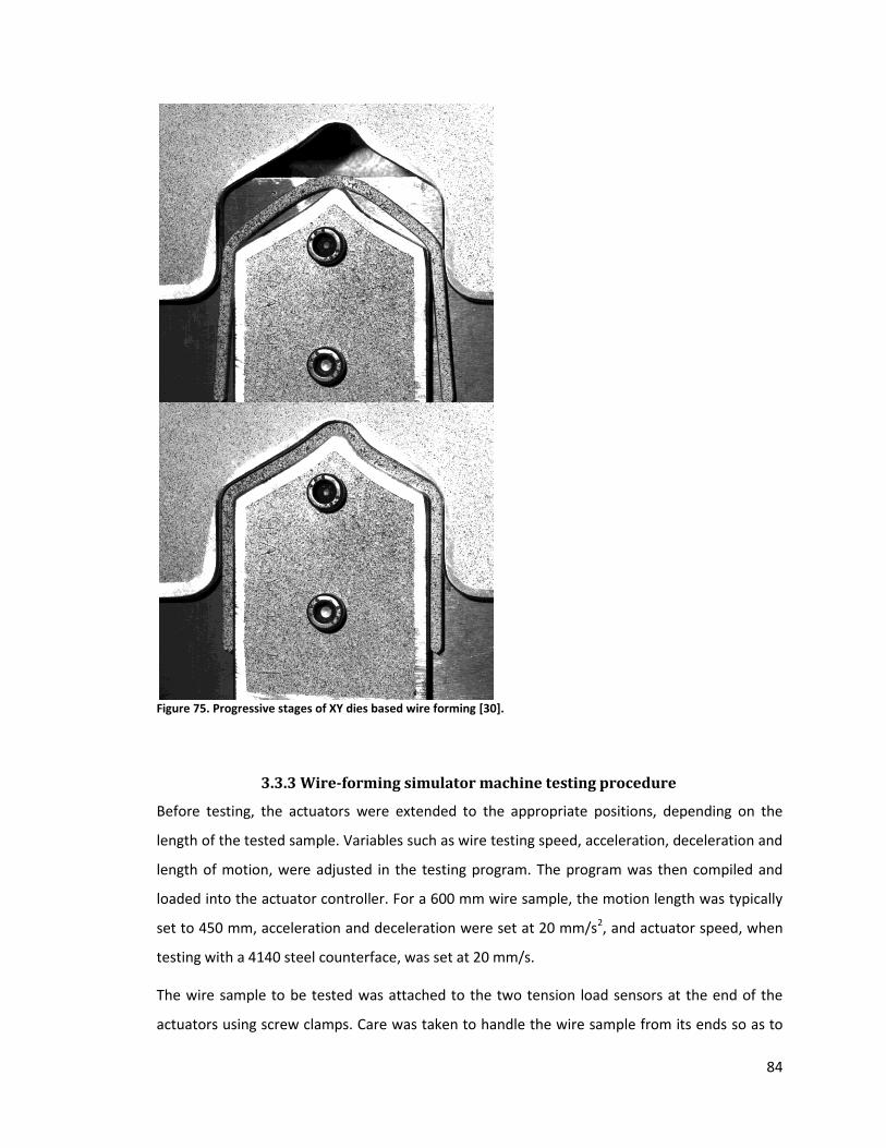
84
Figure 75. Progressive stages of XY dies based wire forming [30].
3.3.3 Wire-forming simulator machine testing procedure
Before testing, the actuators were extended to the appropriate positions, depending on the
length of the tested sample. Variables such as wire testing speed, acceleration, deceleration and
length of motion, were adjusted in the testing program. The program was then compiled and
loaded into the actuator controller. For a 600 mm wire sample, the motion length was typically
set to 450 mm, acceleration and deceleration were set at 20 mm/s2, and actuator speed, when
testing with a 4140 steel counterface, was set at 20 mm/s.
The wire sample to be tested was attached to the two tension load sensors at the end of the
actuators using screw clamps. Care was taken to handle the wire sample from its ends so as to
85
not contaminate the sample surface with additional impurities, such as skin oil, that might alter
the friction results.
The wire friction testing program was divided into the preload section and the friction testing
section. In the former, the controller was programmed to pull the wire samples from both
actuators continuously at a speed of 0.002mm/s on the command of the operator. The preload
motion was run until the desired wire tension was achieved. Prior to friction testing the enamel
wire, the data acquisition software InstruNet-World was used to zero the force and normal force
load cells. The recording of the load cell signals started before testing to provide feedback to the
operator during the preloading phase. Tension was applied until a load of 90.7N (200 lbs) was
reached.
After tensioning, the friction pin was installed in the friction arm. The friction arm frame height
had been previously adjusted to ensure that the friction arm remained perfectly horizontal
when the steel counterface surface rested on the enamelled wire surface. The load was then
applied through weights on the load pin. A normal load of 178 N (40 lbs) was applied for most
tests. This value was chosen because it generated pressures on the wire surface comparable to
those predicted by simulations of the actual formation process (500 MPa).
The normal load and friction pin assembly was left to stabilize for 10 to 20 seconds before the
motion of the sample was started to give the friction load cell time to zero itself. The data
collected by the friction load cell during this period was later used to normalize the friction force
signal. As the friction testing program was executed, the two actuators moved simultaneously,
pulling the wire sample under the counterface surface while keeping the wire length constant.
After the sample came to a stop, the load and friction pin were removed from the fiction arm,
data acquisition was stopped, data from the sensors was saved and the wire sample was
removed from the machine. In flat-on-flat contact between the counterface and the sample,
care was taken not to touch or disturb the steel counterface surface after testing. The surface
was observed after each test to determine the contact area between it and the sample. The
contact area was indicated by scratches and impurities collected on the polished surface of the
counterface. After observation and before further testing, the counterface was polished and
cleaned using ethanol.
86
The data recorded by the data acquisition program was subsequently analyzed to determine the
coefficient of friction along the length of the wire sample. There was no feedback system to
determine the position of the actuators during testing. The position of the sample was derived
during the post-test data analysis based on the predetermined actuator motion distance, speed
and acceleration. The starting point of the test was detected by the increase in friction force,
and then the position of the sample was deduced based on the elapsed time after each data
point and on the known values of acceleration and sample speed. The value for the average
coefficient of friction and standard deviation were obtained from the constant speed section of
the tests. The initial acceleration and last deceleration section of data were discarded.
3.4 Wire tensile testing procedure
The tensile testing of the magnet wire samples was conducted using an Instrum tensile testing
machine. The strain of the magnet wire sample was tracked by displacing the tensile testing
machine grips. Unlike conventional tensile testing of metal samples or other material, where the
samples can be machined to conform to tensile testing standards for tensile samples, enamelled
wire samples can not be modified before testing. As a result, in tensile testing of the magnet
wire, provisions must be made to ensure that the wire will fail within the gauge length of the
tensile test sample. Because the wire sample tested is of a constant cross-section, any stress
concentraton on the wire surface caused by the grips of the tensile testing machine provides an
initiation spot for sample failure under tension. A solution to this problem was using a custom
gripping clamp that distributed the clamping pressure along a significant length of the magnet
wire. An illustration of the custom wire clamp is seen in Figure 76, with a picture showing its
application during tensile testing. The wire clamp design was obtained from U.S. patent
#3528283. The shape of the clamp was based on the COF between the clamp and the wire
surface. For its design, friction values obtained from the clean wire sample and 4140
counterface were used. The size and shape of the clamp design are dictated by the dimensions
of the wire and the COF between the wire surface and the clamp material. The outer radius of
clamp was calculated based on the following formula:
9
Where:
r- is the radius of the gripping clamp
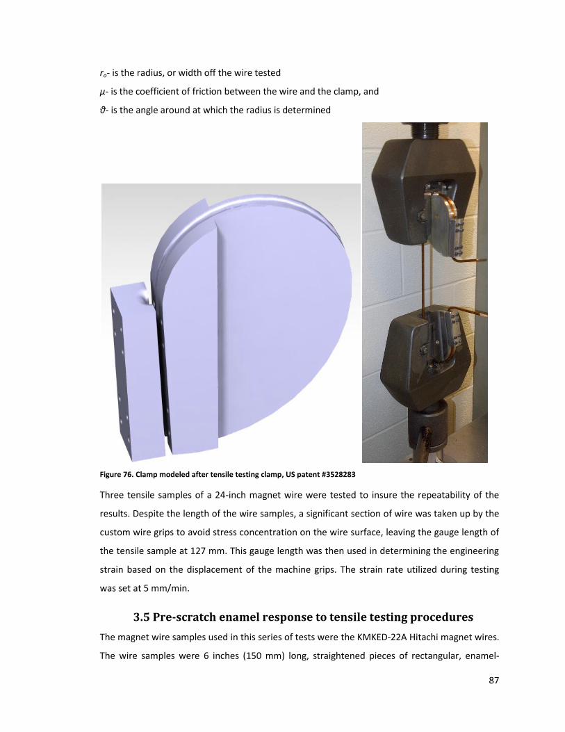
87
ro- is the radius, or width off the wire tested
µ- is the coefficient of friction between the wire and the clamp, and
θ- is the angle around at which the radius is determined
Figure 76. Clamp modeled after tensile testing clamp, US patent #3528283
Three tensile samples of a 24-inch magnet wire were tested to insure the repeatability of the
results. Despite the length of the wire samples, a significant section of wire was taken up by the
custom wire grips to avoid stress concentration on the wire surface, leaving the gauge length of
the tensile sample at 127 mm. This gauge length was then used in determining the engineering
strain based on the displacement of the machine grips. The strain rate utilized during testing
was set at 5 mm/min.
3.5 Pre-scratch enamel response to tensile testing procedures
The magnet wire samples used in this series of tests were the KMKED-22A Hitachi magnet wires.
The wire samples were 6 inches (150 mm) long, straightened pieces of rectangular, enamel-
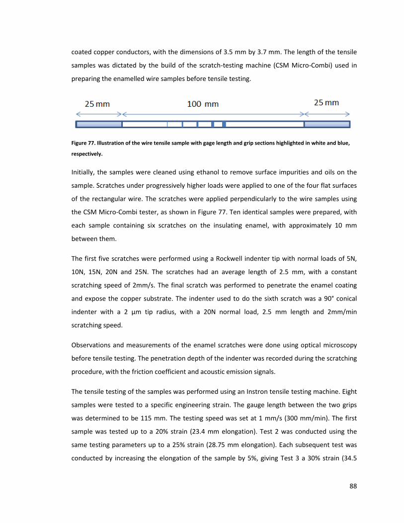
88
coated copper conductors, with the dimensions of 3.5 mm by 3.7 mm. The length of the tensile
samples was dictated by the build of the scratch-testing machine (CSM Micro-Combi) used in
preparing the enamelled wire samples before tensile testing.
Figure 77. Illustration of the wire tensile sample with gage length and grip sections highlighted in white and blue,
respectively.
Initially, the samples were cleaned using ethanol to remove surface impurities and oils on the
sample. Scratches under progressively higher loads were applied to one of the four flat surfaces
of the rectangular wire. The scratches were applied perpendicularly to the wire samples using
the CSM Micro-Combi tester, as shown in Figure 77. Ten identical samples were prepared, with
each sample containing six scratches on the insulating enamel, with approximately 10 mm
between them.
The first five scratches were performed using a Rockwell indenter tip with normal loads of 5N,
10N, 15N, 20N and 25N. The scratches had an average length of 2.5 mm, with a constant
scratching speed of 2mm/s. The final scratch was performed to penetrate the enamel coating
and expose the copper substrate. The indenter used to do the sixth scratch was a 90° conical
indenter with a 2 µm tip radius, with a 20N normal load, 2.5 mm length and 2mm/min
scratching speed.
Observations and measurements of the enamel scratches were done using optical microscopy
before tensile testing. The penetration depth of the indenter was recorded during the scratching
procedure, with the friction coefficient and acoustic emission signals.
The tensile testing of the samples was performed using an Instron tensile testing machine. Eight
samples were tested to a specific engineering strain. The gauge length between the two grips
was determined to be 115 mm. The testing speed was set at 1 mm/s (300 mm/min). The first
sample was tested up to a 20% strain (23.4 mm elongation). Test 2 was conducted using the
same testing parameters up to a 25% strain (28.75 mm elongation). Each subsequent test was
conducted by increasing the elongation of the sample by 5%, giving Test 3 a 30% strain (34.5
89
mm elongation), Test 4 a 35% strain (40.25 mm elongation), Test 5 a 40% strain (46 mm
elongation), Test 6 a 45% strain (51.75 mm elongation) and Test 7 a 50% strain (57.5 mm
elongation). The ultimate tensile strength of the enamel copper wire samples was achieved at a
47% engineering strain; therefore, Test 7 resulted in the failure of the sample. Test 8 was a
repetition of Test 7, because the failure of the Test 7 sample occurred at the sample grips.
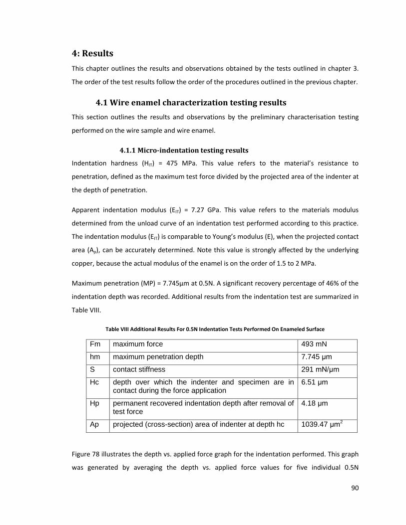
90
4: Results
This chapter outlines the results and observations obtained by the tests outlined in chapter 3.
The order of the test results follow the order of the procedures outlined in the previous chapter.
4.1 Wire enamel characterization testing results
This section outlines the results and observations by the preliminary characterisation testing
performed on the wire sample and wire enamel.
4.1.1 Micro-indentation testing results
Indentation hardness (HIT) = 475 MPa. This value refers to the material’s resistance to
penetration, defined as the maximum test force divided by the projected area of the indenter at
the depth of penetration.
Apparent indentation modulus (EIT) = 7.27 GPa. This value refers to the materials modulus
determined from the unload curve of an indentation test performed according to this practice.
The indentation modulus (EIT) is comparable to Young’s modulus (E), when the projected contact
area (Ap), can be accurately determined. Note this value is strongly affected by the underlying
copper, because the actual modulus of the enamel is on the order of 1.5 to 2 MPa.
Maximum penetration (MP) = 7.745μm at 0.5N. A significant recovery percentage of 46% of the
indentation depth was recorded. Additional results from the indentation test are summarized in
Table VIII.
Table VIII Additional Results For 0.5N Indentation Tests Performed On Enameled Surface
Fm maximum force 493 mN
hm maximum penetration depth 7.745 μm
S contact stiffness 291 mN/μm
Hc depth over which the indenter and specimen are in contact during the force application
6.51 μm
Hp permanent recovered indentation depth after removal of test force
4.18 μm
Ap projected (cross-section) area of indenter at depth hc 1039.47 μm2
Figure 78 illustrates the depth vs. applied force graph for the indentation performed. This graph
was generated by averaging the depth vs. applied force values for five individual 0.5N
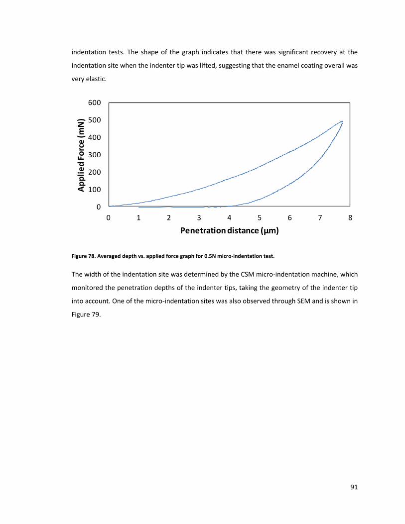
91
indentation tests. The shape of the graph indicates that there was significant recovery at the
indentation site when the indenter tip was lifted, suggesting that the enamel coating overall was
very elastic.
Figure 78. Averaged depth vs. applied force graph for 0.5N micro-indentation test.
The width of the indentation site was determined by the CSM micro-indentation machine, which
monitored the penetration depths of the indenter tips, taking the geometry of the indenter tip
into account. One of the micro-indentation sites was also observed through SEM and is shown in
Figure 79.
0
100
200
300
400
500
600
0 1 2 3 4 5 6 7 8
Ap
pli
ed
Fo
rce
(mN
)
Penetration distance (µm)
Depth VS Applied Force Average
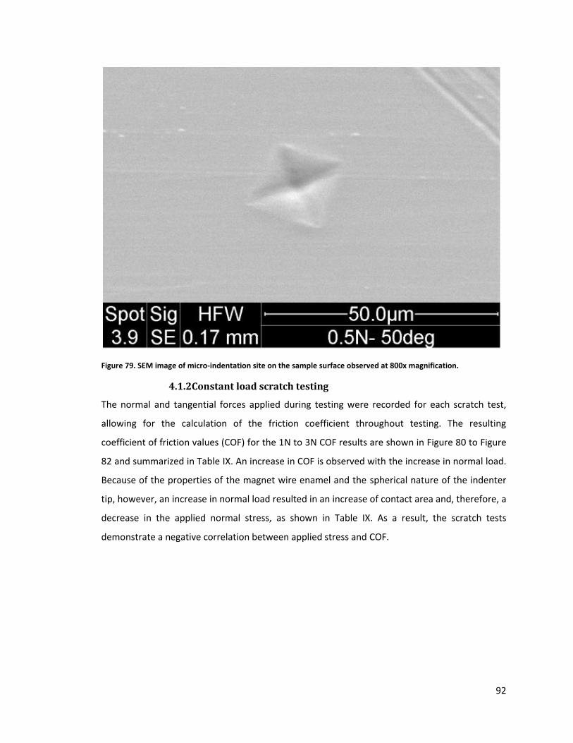
92
Figure 79. SEM image of micro-indentation site on the sample surface observed at 800x magnification.
4.1.2Constant load scratch testing
The normal and tangential forces applied during testing were recorded for each scratch test,
allowing for the calculation of the friction coefficient throughout testing. The resulting
coefficient of friction values (COF) for the 1N to 3N COF results are shown in Figure 80 to Figure
82 and summarized in Table IX. An increase in COF is observed with the increase in normal load.
Because of the properties of the magnet wire enamel and the spherical nature of the indenter
tip, however, an increase in normal load resulted in an increase of contact area and, therefore, a
decrease in the applied normal stress, as shown in Table IX. As a result, the scratch tests
demonstrate a negative correlation between applied stress and COF.
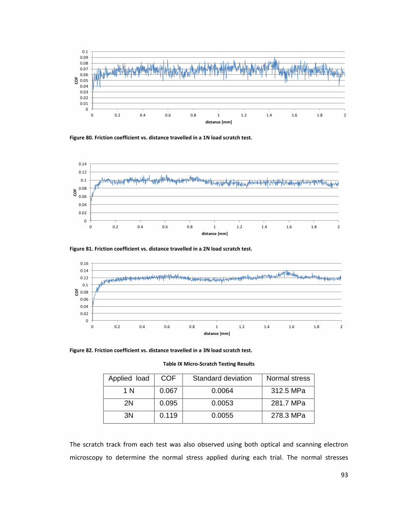
93
Figure 80. Friction coefficient vs. distance travelled in a 1N load scratch test.
Figure 81. Friction coefficient vs. distance travelled in a 2N load scratch test.
Figure 82. Friction coefficient vs. distance travelled in a 3N load scratch test.
Table IX Micro-Scratch Testing Results
Applied load COF Standard deviation Normal stress
1 N 0.067 0.0064 312.5 MPa
2N 0.095 0.0053 281.7 MPa
3N 0.119 0.0055 278.3 MPa
The scratch track from each test was also observed using both optical and scanning electron
microscopy to determine the normal stress applied during each trial. The normal stresses
0
0.01
0.02
0.03
0.04
0.05
0.06
0.07
0.08
0.09
0.1
0 0.2 0.4 0.6 0.8 1 1.2 1.4 1.6 1.8 2
CO
F
distance [mm]
Coefficient of Friction for 1N load Scratch Test
COF
0
0.02
0.04
0.06
0.08
0.1
0.12
0.14
0 0.2 0.4 0.6 0.8 1 1.2 1.4 1.6 1.8 2
CO
F
distance [mm]
Coefficient of Friction for 2N load Scratch Test
COF
0
0.02
0.04
0.06
0.08
0.1
0.12
0.14
0.16
0 0.2 0.4 0.6 0.8 1 1.2 1.4 1.6 1.8 2
CO
F
distance [mm]
Coefficient of Friction for 3N load Scratch Test
COF
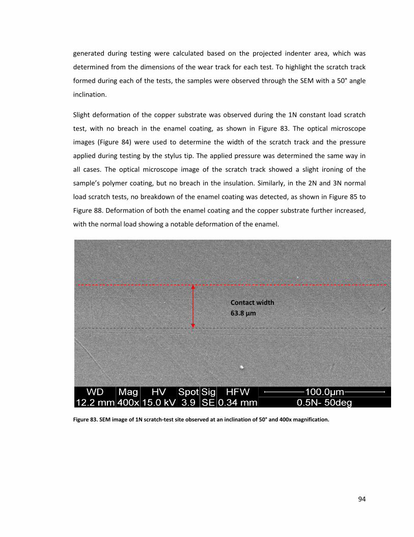
94
generated during testing were calculated based on the projected indenter area, which was
determined from the dimensions of the wear track for each test. To highlight the scratch track
formed during each of the tests, the samples were observed through the SEM with a 50° angle
inclination.
Slight deformation of the copper substrate was observed during the 1N constant load scratch
test, with no breach in the enamel coating, as shown in Figure 83. The optical microscope
images (Figure 84) were used to determine the width of the scratch track and the pressure
applied during testing by the stylus tip. The applied pressure was determined the same way in
all cases. The optical microscope image of the scratch track showed a slight ironing of the
sample’s polymer coating, but no breach in the insulation. Similarly, in the 2N and 3N normal
load scratch tests, no breakdown of the enamel coating was detected, as shown in Figure 85 to
Figure 88. Deformation of both the enamel coating and the copper substrate further increased,
with the normal load showing a notable deformation of the enamel.
Figure 83. SEM image of 1N scratch-test site observed at an inclination of 50° and 400x magnification.
Contact width
63.8 µm
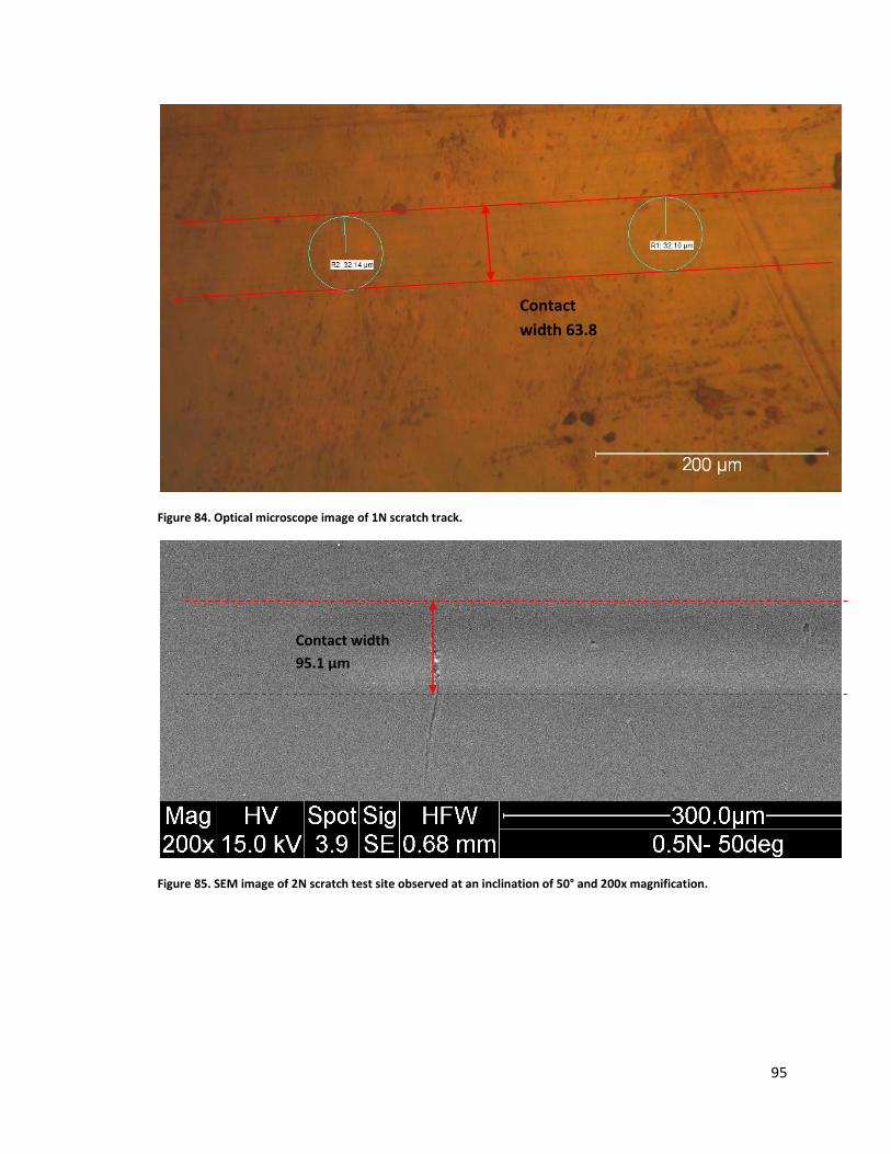
95
Figure 84. Optical microscope image of 1N scratch track.
Figure 85. SEM image of 2N scratch test site observed at an inclination of 50° and 200x magnification.
Contact
width 63.8
µm
Contact width
95.1 µm
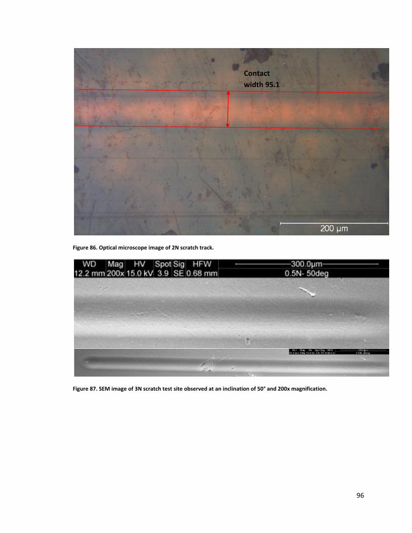
96
Figure 86. Optical microscope image of 2N scratch track.
Figure 87. SEM image of 3N scratch test site observed at an inclination of 50° and 200x magnification.
Contact
width 95.1
µm
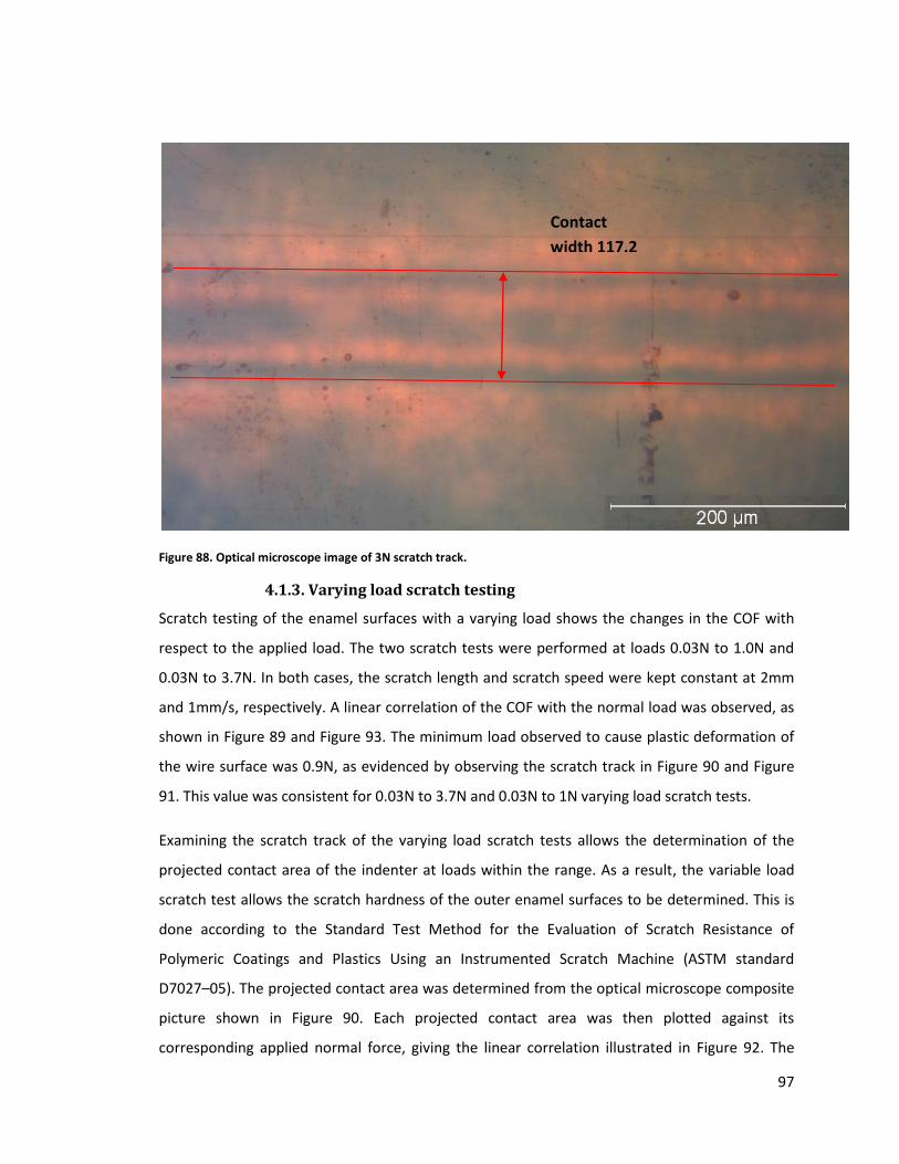
97
Figure 88. Optical microscope image of 3N scratch track.
4.1.3. Varying load scratch testing
Scratch testing of the enamel surfaces with a varying load shows the changes in the COF with
respect to the applied load. The two scratch tests were performed at loads 0.03N to 1.0N and
0.03N to 3.7N. In both cases, the scratch length and scratch speed were kept constant at 2mm
and 1mm/s, respectively. A linear correlation of the COF with the normal load was observed, as
shown in Figure 89 and Figure 93. The minimum load observed to cause plastic deformation of
the wire surface was 0.9N, as evidenced by observing the scratch track in Figure 90 and Figure
91. This value was consistent for 0.03N to 3.7N and 0.03N to 1N varying load scratch tests.
Examining the scratch track of the varying load scratch tests allows the determination of the
projected contact area of the indenter at loads within the range. As a result, the variable load
scratch test allows the scratch hardness of the outer enamel surfaces to be determined. This is
done according to the Standard Test Method for the Evaluation of Scratch Resistance of
Polymeric Coatings and Plastics Using an Instrumented Scratch Machine (ASTM standard
D7027–05). The projected contact area was determined from the optical microscope composite
picture shown in Figure 90. Each projected contact area was then plotted against its
corresponding applied normal force, giving the linear correlation illustrated in Figure 92. The
Contact
width 117.2
µm
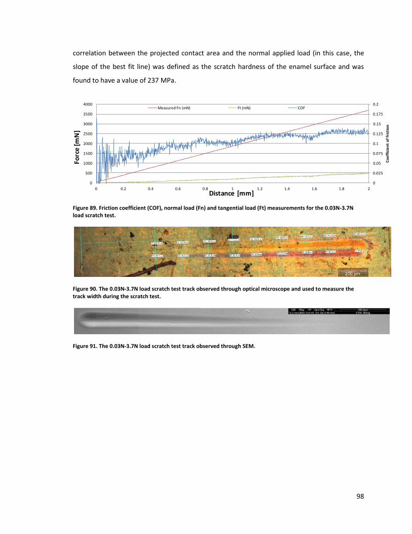
98
correlation between the projected contact area and the normal applied load (in this case, the
slope of the best fit line) was defined as the scratch hardness of the enamel surface and was
found to have a value of 237 MPa.
Figure 89. Friction coefficient (COF), normal load (Fn) and tangential load (Ft) measurements for the 0.03N-3.7N load scratch test.
Figure 90. The 0.03N-3.7N load scratch test track observed through optical microscope and used to measure the track width during the scratch test.
Figure 91. The 0.03N-3.7N load scratch test track observed through SEM.
0
0.025
0.05
0.075
0.1
0.125
0.15
0.175
0.2
0
500
1000
1500
2000
2500
3000
3500
4000
0 0.2 0.4 0.6 0.8 1 1.2 1.4 1.6 1.8 2
Co
eff
icie
nt
of
fric
tio
n
Forc
e [m
N]
Distance [mm]
Coefficient of Friction for 0.03N-3.7N load Scratch Test
Measured Fn (mN) Ft (mN) COF
0
0.025
0.05
0.075
0.1
0.125
0.15
0.175
0.2
0
500
1000
1500
2000
2500
3000
3500
4000
0 0.2 0.4 0.6 0.8 1 1.2 1.4 1.6 1.8 2
Co
eff
icie
nt
of
fric
tio
n
Forc
e [m
N]
Distance [mm]
Coefficient of Friction for 0.03N-3.7N load Scratch Test
Measured Fn (mN) Ft (mN) COF
0
0.025
0.05
0.075
0.1
0.125
0.15
0.175
0.2
0
500
1000
1500
2000
2500
3000
3500
4000
0 0.2 0.4 0.6 0.8 1 1.2 1.4 1.6 1.8 2
Co
eff
icie
nt
of
fric
tio
n
Forc
e [m
N]
Distance [mm]
Coefficient of Friction for 0.03N-3.7N load Scratch Test
Measured Fn (mN) Ft (mN) COF
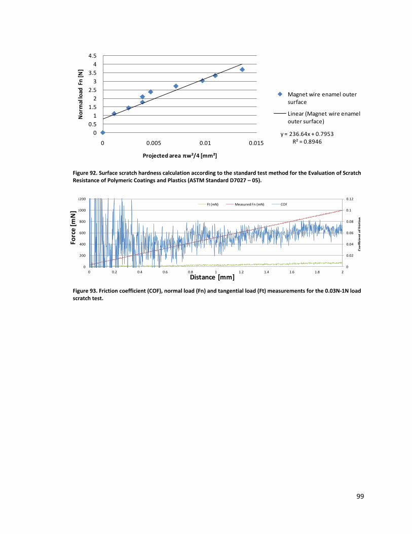
99
Figure 92. Surface scratch hardness calculation according to the standard test method for the Evaluation of Scratch Resistance of Polymeric Coatings and Plastics (ASTM Standard D7027 – 05).
Figure 93. Friction coefficient (COF), normal load (Fn) and tangential load (Ft) measurements for the 0.03N-1N load scratch test.
y = 236.64x + 0.7953R² = 0.8946
0
0.5
1
1.5
2
2.5
3
3.5
4
4.5
0 0.005 0.01 0.015
No
rmal
load
Fn
[N
]
Projected area πw²/4 [mm²]
Magnet wire enamel outer surface
Magnet wire enamel outer surface
Linear (Magnet wire enamel outer surface)
0
0.02
0.04
0.06
0.08
0.1
0.12
0
200
400
600
800
1000
1200
0 0.2 0.4 0.6 0.8 1 1.2 1.4 1.6 1.8 2
Co
eff
icie
nt
of
fric
tio
n
Forc
e [m
N]
Distance [mm]
Coefficient of Friction for 0.03N-1N load Scratch Test
Ft (mN) Measured Fn (mN) COF
0
0.025
0.05
0.075
0.1
0.125
0.15
0.175
0.2
0
500
1000
1500
2000
2500
3000
3500
4000
0 0.2 0.4 0.6 0.8 1 1.2 1.4 1.6 1.8 2
Co
eff
icie
nt
of
fric
tio
n
Forc
e [m
N]
Distance [mm]
Coefficient of Friction for 0.03N-3.7N load Scratch Test
Measured Fn (mN) Ft (mN) COF
0
0.025
0.05
0.075
0.1
0.125
0.15
0.175
0.2
0
500
1000
1500
2000
2500
3000
3500
4000
0 0.2 0.4 0.6 0.8 1 1.2 1.4 1.6 1.8 2
Co
eff
icie
nt
of
fric
tio
n
Forc
e [m
N]
Distance [mm]
Coefficient of Friction for 0.03N-3.7N load Scratch Test
Measured Fn (mN) Ft (mN) COF
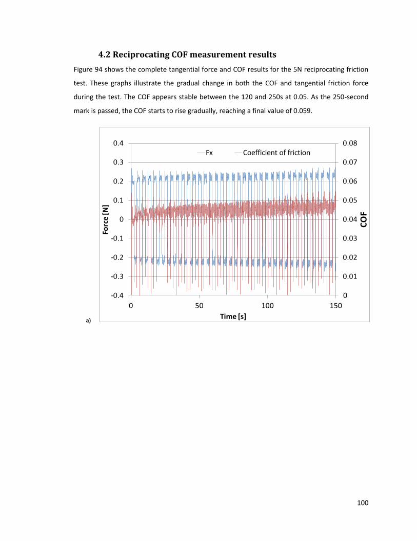
100
4.2 Reciprocating COF measurement results
Figure 94 shows the complete tangential force and COF results for the 5N reciprocating friction
test. These graphs illustrate the gradual change in both the COF and tangential friction force
during the test. The COF appears stable between the 120 and 250s at 0.05. As the 250-second
mark is passed, the COF starts to rise gradually, reaching a final value of 0.059.
a)
0
0.01
0.02
0.03
0.04
0.05
0.06
0.07
0.08
-0.4
-0.3
-0.2
-0.1
0
0.1
0.2
0.3
0.4
0 50 100 150
CO
F
Forc
e [N
]
Time [s]
Fx Coefficient of friction
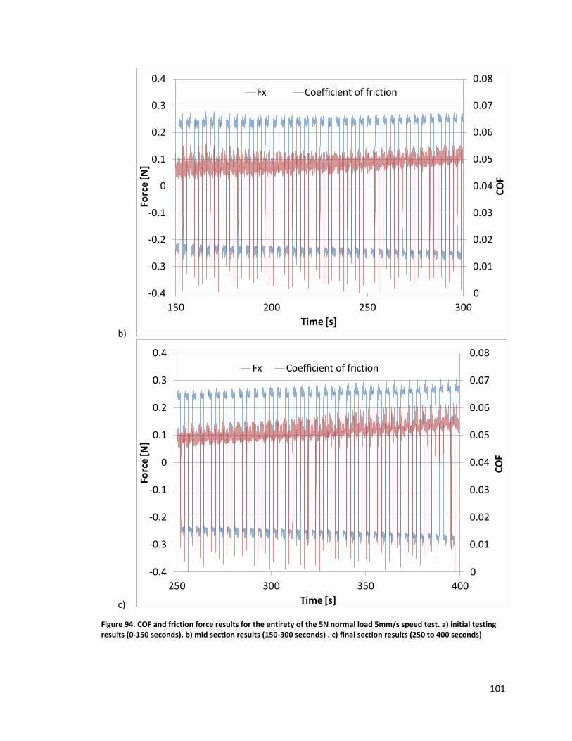
101
b)
c)
Figure 94. COF and friction force results for the entirety of the 5N normal load 5mm/s speed test. a) initial testing results (0-150 seconds). b) mid section results (150-300 seconds) . c) final section results (250 to 400 seconds)
0
0.01
0.02
0.03
0.04
0.05
0.06
0.07
0.08
-0.4
-0.3
-0.2
-0.1
0
0.1
0.2
0.3
0.4
150 200 250 300
CO
F
Forc
e [N
]
time [s]
Fx Coefficient of friction
0
0.01
0.02
0.03
0.04
0.05
0.06
0.07
0.08
-0.4
-0.3
-0.2
-0.1
0
0.1
0.2
0.3
0.4
250 300 350 400
CO
F
Forc
e [N
]
time [s]
Fx Coefficient of friction
0
0.01
0.02
0.03
0.04
0.05
0.06
0.07
0.08
-0.4
-0.3
-0.2
-0.1
0
0.1
0.2
0.3
0.4
0 50 100 150
CO
F
Forc
e [N
]
Time [s]
Fx Coefficient of friction
0
0.01
0.02
0.03
0.04
0.05
0.06
0.07
0.08
-0.4
-0.3
-0.2
-0.1
0
0.1
0.2
0.3
0.4
0 50 100 150
CO
F
Forc
e [N
]
Time [s]
Fx Coefficient of friction
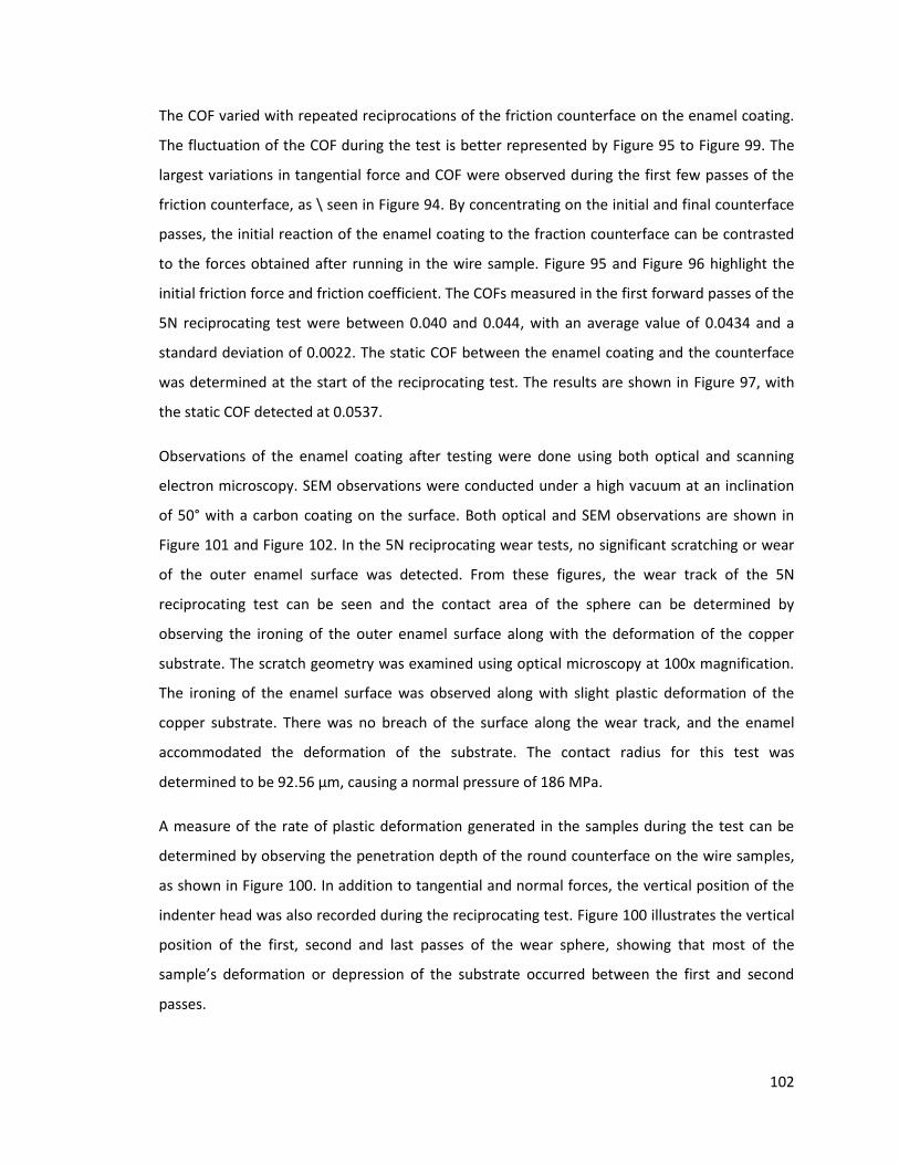
102
The COF varied with repeated reciprocations of the friction counterface on the enamel coating.
The fluctuation of the COF during the test is better represented by Figure 95 to Figure 99. The
largest variations in tangential force and COF were observed during the first few passes of the
friction counterface, as \ seen in Figure 94. By concentrating on the initial and final counterface
passes, the initial reaction of the enamel coating to the fraction counterface can be contrasted
to the forces obtained after running in the wire sample. Figure 95 and Figure 96 highlight the
initial friction force and friction coefficient. The COFs measured in the first forward passes of the
5N reciprocating test were between 0.040 and 0.044, with an average value of 0.0434 and a
standard deviation of 0.0022. The static COF between the enamel coating and the counterface
was determined at the start of the reciprocating test. The results are shown in Figure 97, with
the static COF detected at 0.0537.
Observations of the enamel coating after testing were done using both optical and scanning
electron microscopy. SEM observations were conducted under a high vacuum at an inclination
of 50° with a carbon coating on the surface. Both optical and SEM observations are shown in
Figure 101 and Figure 102. In the 5N reciprocating wear tests, no significant scratching or wear
of the outer enamel surface was detected. From these figures, the wear track of the 5N
reciprocating test can be seen and the contact area of the sphere can be determined by
observing the ironing of the outer enamel surface along with the deformation of the copper
substrate. The scratch geometry was examined using optical microscopy at 100x magnification.
The ironing of the enamel surface was observed along with slight plastic deformation of the
copper substrate. There was no breach of the surface along the wear track, and the enamel
accommodated the deformation of the substrate. The contact radius for this test was
determined to be 92.56 μm, causing a normal pressure of 186 MPa.
A measure of the rate of plastic deformation generated in the samples during the test can be
determined by observing the penetration depth of the round counterface on the wire samples,
as shown in Figure 100. In addition to tangential and normal forces, the vertical position of the
indenter head was also recorded during the reciprocating test. Figure 100 illustrates the vertical
position of the first, second and last passes of the wear sphere, showing that most of the
sample’s deformation or depression of the substrate occurred between the first and second
passes.
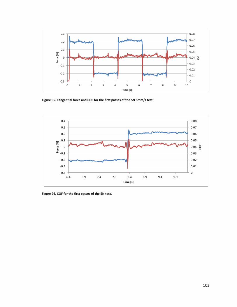
103
Figure 95. Tangential force and COF for the first passes of the 5N 5mm/s test.
Figure 96. COF for the first passes of the 5N test.
0
0.01
0.02
0.03
0.04
0.05
0.06
0.07
0.08
-0.3
-0.2
-0.1
0
0.1
0.2
0.3
0 1 2 3 4 5 6 7 8 9 10
CO
F
Forc
e [N
]
Time [s]
0
0.01
0.02
0.03
0.04
0.05
0.06
0.07
0.08
-0.4
-0.3
-0.2
-0.1
0
0.1
0.2
0.3
0.4
6.4 6.9 7.4 7.9 8.4 8.9 9.4 9.9
CO
F
Forc
e [N
]
Time [s]
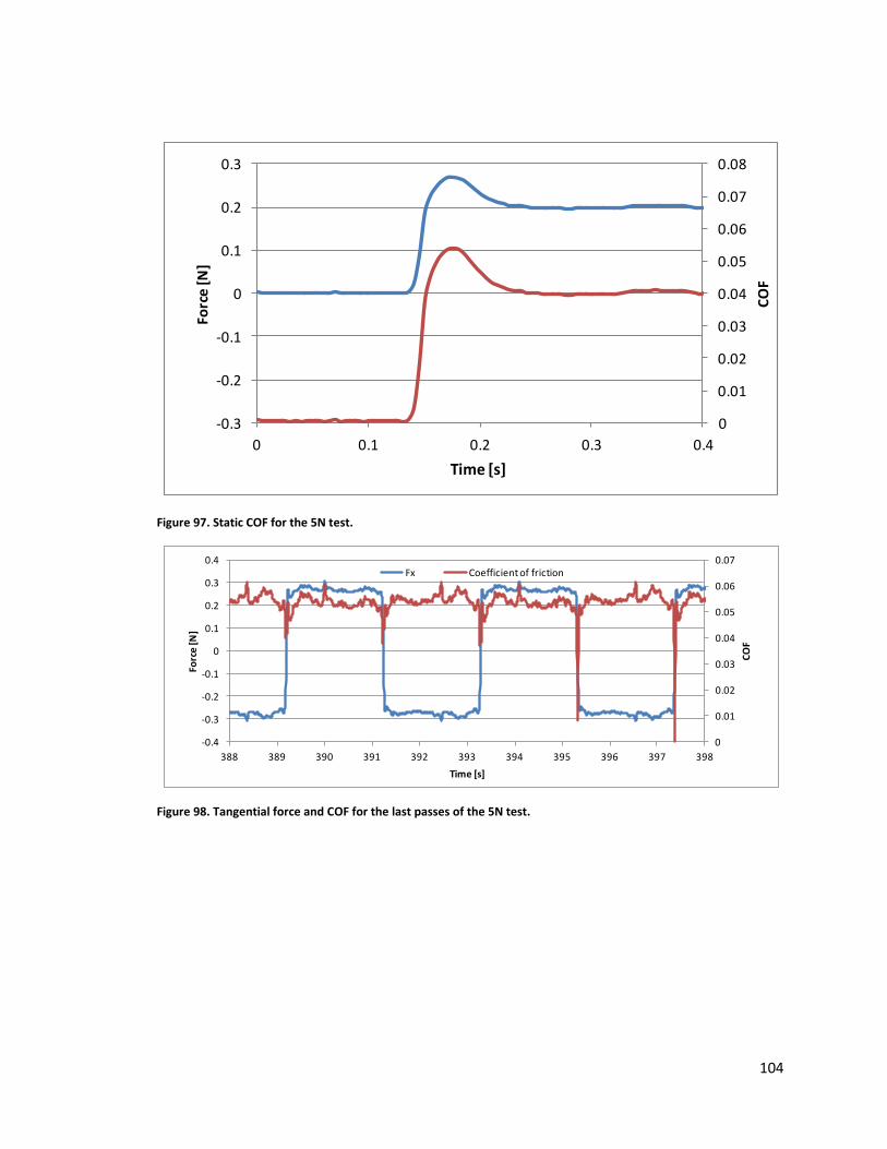
104
Figure 97. Static COF for the 5N test.
Figure 98. Tangential force and COF for the last passes of the 5N test.
0
0.01
0.02
0.03
0.04
0.05
0.06
0.07
0.08
-0.3
-0.2
-0.1
0
0.1
0.2
0.3
0 0.1 0.2 0.3 0.4
CO
F
Forc
e [N
]
time [s]
0
0.01
0.02
0.03
0.04
0.05
0.06
0.07
-0.4
-0.3
-0.2
-0.1
0
0.1
0.2
0.3
0.4
388 389 390 391 392 393 394 395 396 397 398C
OF
Forc
e [N
]
Time [s]
Fx Coefficient of friction
0
0.01
0.02
0.03
0.04
0.05
0.06
0.07
0.08
-0.4
-0.3
-0.2
-0.1
0
0.1
0.2
0.3
0.4
0 50 100 150
CO
F
Forc
e [N
]
Time [s]
Fx Coefficient of friction
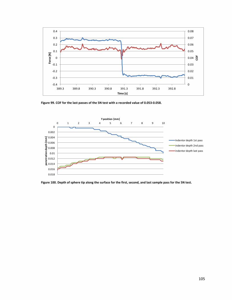
105
Figure 99. COF for the last passes of the 5N test with a recorded value of 0.053-0.058.
Figure 100. Depth of sphere tip along the surface for the first, second, and last sample pass for the 5N test.
0
0.01
0.02
0.03
0.04
0.05
0.06
0.07
0.08
-0.4
-0.3
-0.2
-0.1
0
0.1
0.2
0.3
0.4
389.3 389.8 390.3 390.8 391.3 391.8 392.3 392.8
CO
F
Forc
e [N
]
Time [s]
0
0.002
0.004
0.006
0.008
0.01
0.012
0.014
0.016
0.018
0 1 2 3 4 5 6 7 8 9 10
pe
ne
trat
ion
de
pth
[m
m]
Y position [mm]
Depth Vs position
Indentor depth 1st pass
indentor depth 2nd pass
indentor depth last pass
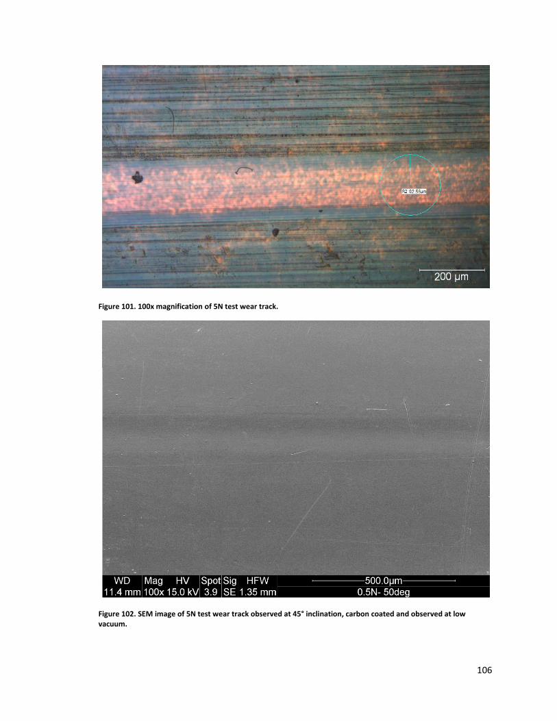
106
Figure 101. 100x magnification of 5N test wear track.
Figure 102. SEM image of 5N test wear track observed at 45° inclination, carbon coated and observed at low vacuum.
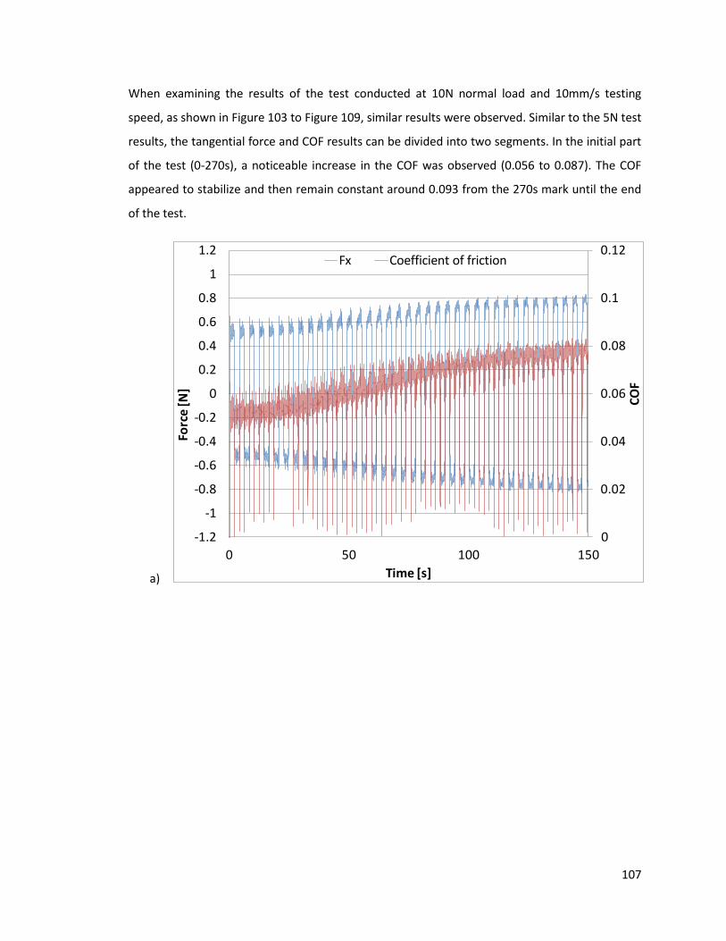
107
When examining the results of the test conducted at 10N normal load and 10mm/s testing
speed, as shown in Figure 103 to Figure 109, similar results were observed. Similar to the 5N test
results, the tangential force and COF results can be divided into two segments. In the initial part
of the test (0-270s), a noticeable increase in the COF was observed (0.056 to 0.087). The COF
appeared to stabilize and then remain constant around 0.093 from the 270s mark until the end
of the test.
a)
0
0.02
0.04
0.06
0.08
0.1
0.12
-1.2
-1
-0.8
-0.6
-0.4
-0.2
0
0.2
0.4
0.6
0.8
1
1.2
0 50 100 150
CO
F
Forc
e [N
]
Time [s]
Fx Coefficient of friction
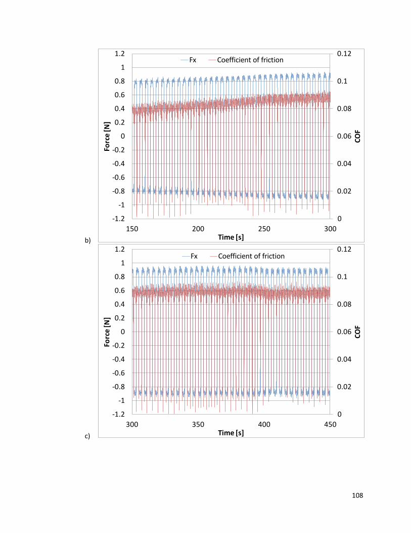
108
b)
c)
0
0.02
0.04
0.06
0.08
0.1
0.12
-1.2
-1
-0.8
-0.6
-0.4
-0.2
0
0.2
0.4
0.6
0.8
1
1.2
150 200 250 300
CO
F
Forc
e [N
]
Time [s]
Fx Coefficient of friction
0
0.02
0.04
0.06
0.08
0.1
0.12
-1.2
-1
-0.8
-0.6
-0.4
-0.2
0
0.2
0.4
0.6
0.8
1
1.2
300 350 400 450
CO
F
Forc
e [N
]
Time [s]
Fx Coefficient of friction
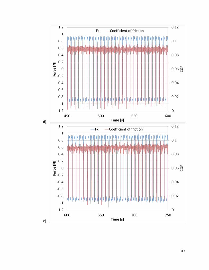
109
d)
e)
0
0.02
0.04
0.06
0.08
0.1
0.12
-1.2
-1
-0.8
-0.6
-0.4
-0.2
0
0.2
0.4
0.6
0.8
1
1.2
450 500 550 600
CO
F
Forc
e [N
]
Time [s]
Fx Coefficient of friction
0
0.02
0.04
0.06
0.08
0.1
0.12
-1.2
-1
-0.8
-0.6
-0.4
-0.2
0
0.2
0.4
0.6
0.8
1
1.2
600 650 700 750
CO
F
Forc
e [N
]
Time [s]
Fx Coefficient of friction
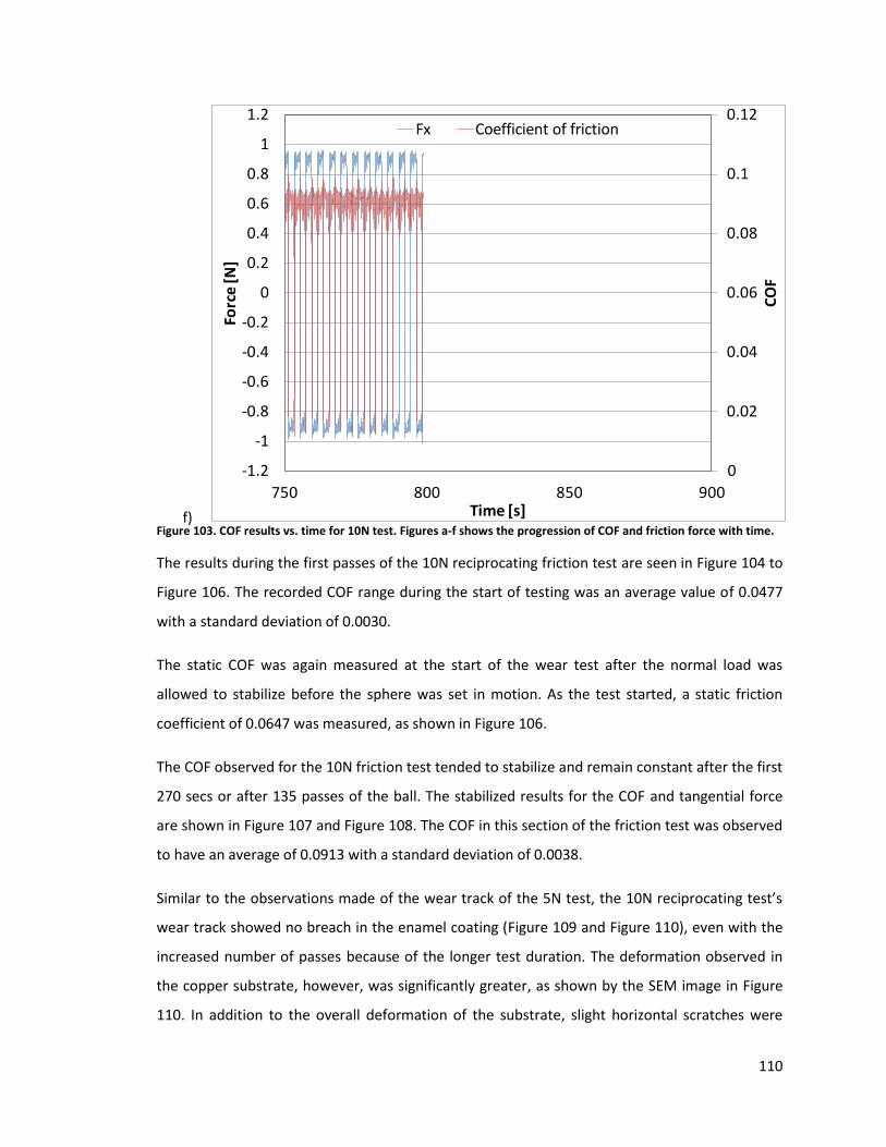
110
f) Figure 103. COF results vs. time for 10N test. Figures a-f shows the progression of COF and friction force with time.
The results during the first passes of the 10N reciprocating friction test are seen in Figure 104 to
Figure 106. The recorded COF range during the start of testing was an average value of 0.0477
with a standard deviation of 0.0030.
The static COF was again measured at the start of the wear test after the normal load was
allowed to stabilize before the sphere was set in motion. As the test started, a static friction
coefficient of 0.0647 was measured, as shown in Figure 106.
The COF observed for the 10N friction test tended to stabilize and remain constant after the first
270 secs or after 135 passes of the ball. The stabilized results for the COF and tangential force
are shown in Figure 107 and Figure 108. The COF in this section of the friction test was observed
to have an average of 0.0913 with a standard deviation of 0.0038.
Similar to the observations made of the wear track of the 5N test, the 10N reciprocating test’s
wear track showed no breach in the enamel coating (Figure 109 and Figure 110), even with the
increased number of passes because of the longer test duration. The deformation observed in
the copper substrate, however, was significantly greater, as shown by the SEM image in Figure
110. In addition to the overall deformation of the substrate, slight horizontal scratches were
0
0.02
0.04
0.06
0.08
0.1
0.12
-1.2
-1
-0.8
-0.6
-0.4
-0.2
0
0.2
0.4
0.6
0.8
1
1.2
750 800 850 900
CO
F
Forc
e [N
]
Time [s]
Fx Coefficient of friction
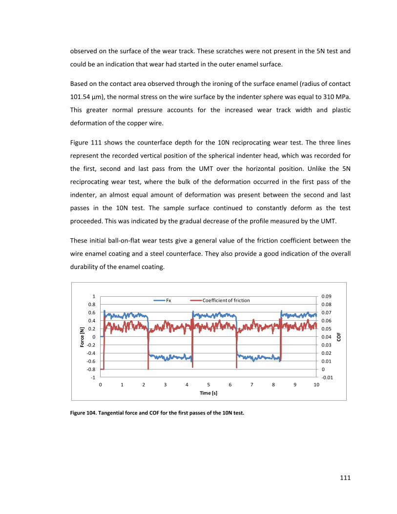
111
observed on the surface of the wear track. These scratches were not present in the 5N test and
could be an indication that wear had started in the outer enamel surface.
Based on the contact area observed through the ironing of the surface enamel (radius of contact
101.54 μm), the normal stress on the wire surface by the indenter sphere was equal to 310 MPa.
This greater normal pressure accounts for the increased wear track width and plastic
deformation of the copper wire.
Figure 111 shows the counterface depth for the 10N reciprocating wear test. The three lines
represent the recorded vertical position of the spherical indenter head, which was recorded for
the first, second and last pass from the UMT over the horizontal position. Unlike the 5N
reciprocating wear test, where the bulk of the deformation occurred in the first pass of the
indenter, an almost equal amount of deformation was present between the second and last
passes in the 10N test. The sample surface continued to constantly deform as the test
proceeded. This was indicated by the gradual decrease of the profile measured by the UMT.
These initial ball-on-flat wear tests give a general value of the friction coefficient between the
wire enamel coating and a steel counterface. They also provide a good indication of the overall
durability of the enamel coating.
Figure 104. Tangential force and COF for the first passes of the 10N test.
-0.01
0
0.01
0.02
0.03
0.04
0.05
0.06
0.07
0.08
0.09
-1
-0.8
-0.6
-0.4
-0.2
0
0.2
0.4
0.6
0.8
1
0 1 2 3 4 5 6 7 8 9 10
CO
F
Forc
e [N
]
Time [s]
Fx Coefficient of friction
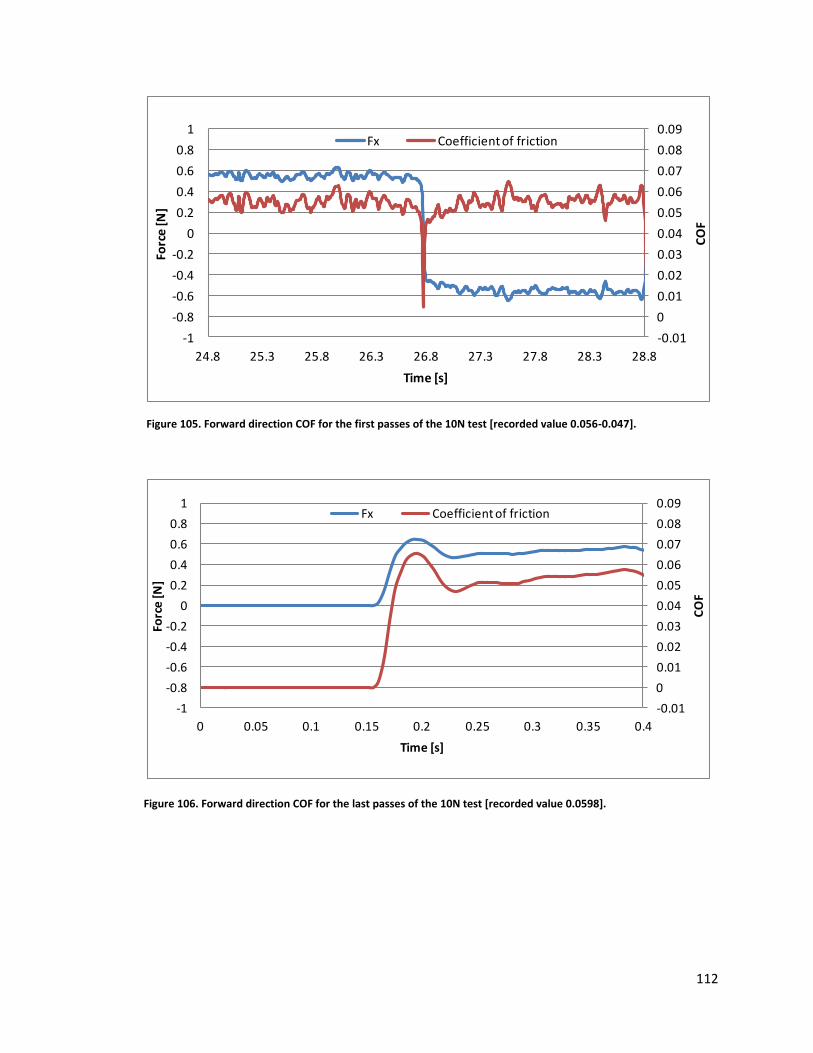
112
Figure 105. Forward direction COF for the first passes of the 10N test [recorded value 0.056-0.047].
Figure 106. Forward direction COF for the last passes of the 10N test [recorded value 0.0598].
-0.01
0
0.01
0.02
0.03
0.04
0.05
0.06
0.07
0.08
0.09
-1
-0.8
-0.6
-0.4
-0.2
0
0.2
0.4
0.6
0.8
1
24.8 25.3 25.8 26.3 26.8 27.3 27.8 28.3 28.8
CO
F
Forc
e [N
]
Time [s]
Fx Coefficient of friction
-0.01
0
0.01
0.02
0.03
0.04
0.05
0.06
0.07
0.08
0.09
-1
-0.8
-0.6
-0.4
-0.2
0
0.2
0.4
0.6
0.8
1
0 0.05 0.1 0.15 0.2 0.25 0.3 0.35 0.4
CO
F
Forc
e [N
]
Time [s]
Fx Coefficient of friction
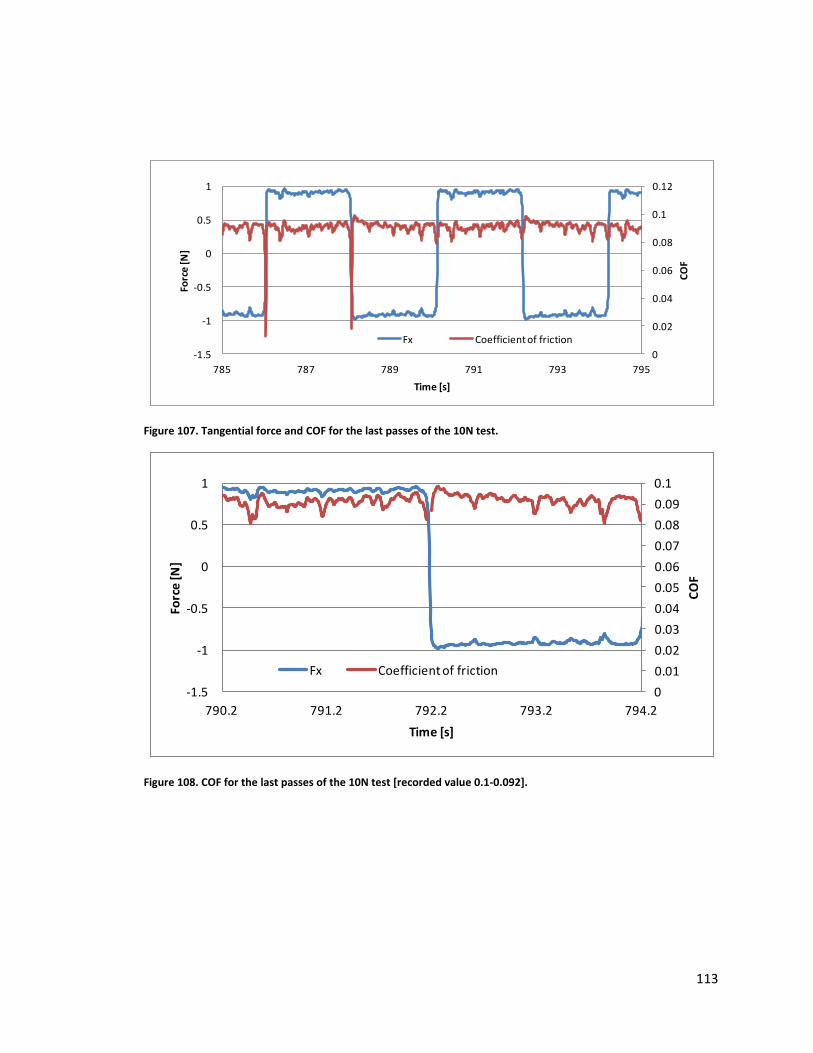
113
Figure 107. Tangential force and COF for the last passes of the 10N test.
Figure 108. COF for the last passes of the 10N test [recorded value 0.1-0.092].
0
0.02
0.04
0.06
0.08
0.1
0.12
-1.5
-1
-0.5
0
0.5
1
785 787 789 791 793 795
CO
F
Forc
e [N
]
Time [s]
Fx Coefficient of friction
0
0.01
0.02
0.03
0.04
0.05
0.06
0.07
0.08
0.09
0.1
-1.5
-1
-0.5
0
0.5
1
790.2 791.2 792.2 793.2 794.2
CO
F
Forc
e [N
]
Time [s]
Fx Coefficient of friction
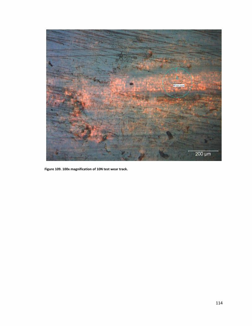
114
Figure 109. 100x magnification of 10N test wear track.
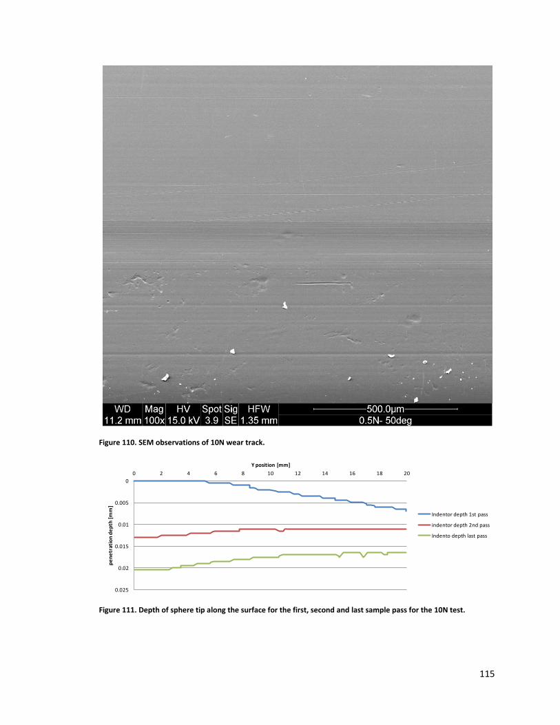
115
Figure 110. SEM observations of 10N wear track.
Figure 111. Depth of sphere tip along the surface for the first, second and last sample pass for the 10N test.
0
0.005
0.01
0.015
0.02
0.025
0 2 4 6 8 10 12 14 16 18 20
pe
ne
trat
ion
de
pth
[m
m]
Y position [mm]
Depth Vs position
Indentor depth 1st pass
indentor depth 2nd pass
Indento depth last pass
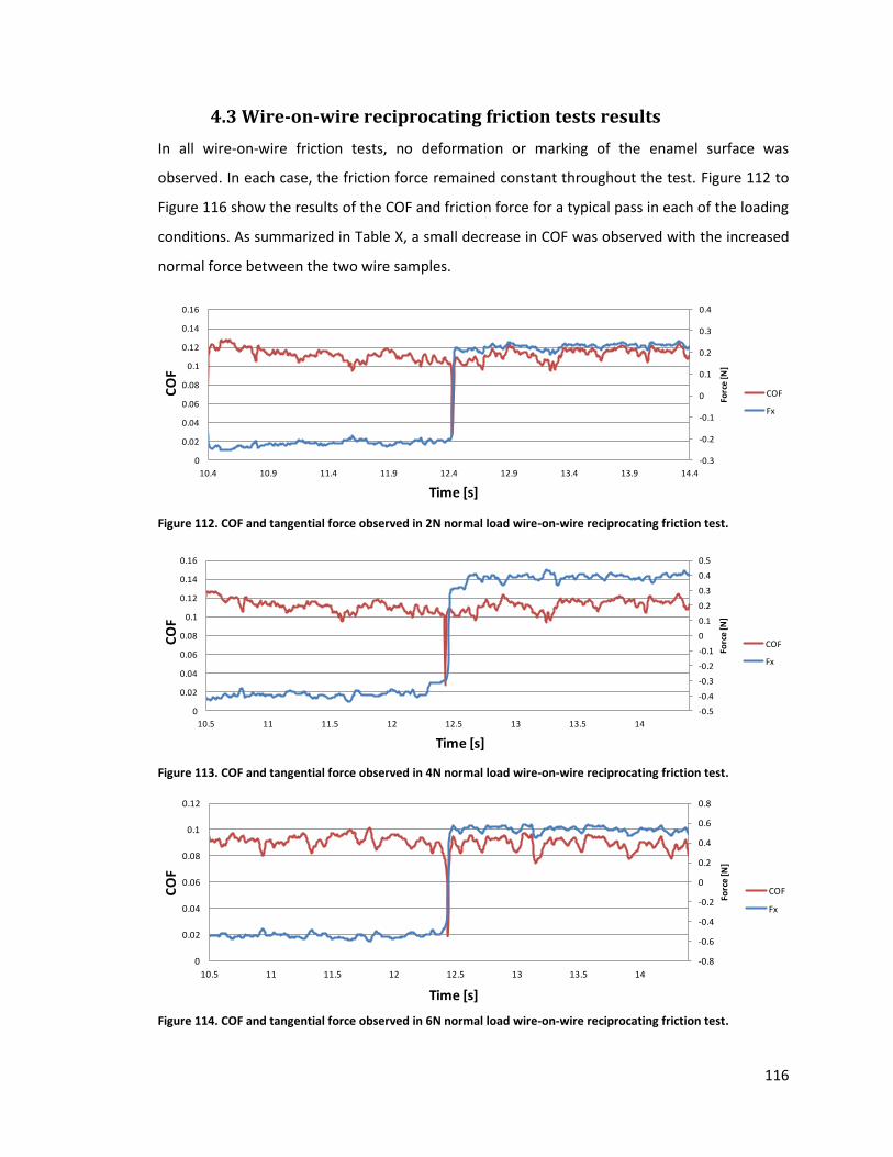
116
4.3 Wire-on-wire reciprocating friction tests results
In all wire-on-wire friction tests, no deformation or marking of the enamel surface was
observed. In each case, the friction force remained constant throughout the test. Figure 112 to
Figure 116 show the results of the COF and friction force for a typical pass in each of the loading
conditions. As summarized in Table X, a small decrease in COF was observed with the increased
normal force between the two wire samples.
Figure 112. COF and tangential force observed in 2N normal load wire-on-wire reciprocating friction test.
Figure 113. COF and tangential force observed in 4N normal load wire-on-wire reciprocating friction test.
Figure 114. COF and tangential force observed in 6N normal load wire-on-wire reciprocating friction test.
-0.3
-0.2
-0.1
0
0.1
0.2
0.3
0.4
0
0.02
0.04
0.06
0.08
0.1
0.12
0.14
0.16
10.4 10.9 11.4 11.9 12.4 12.9 13.4 13.9 14.4
Forc
e [N
]
Co
f
Time
2N
COF
Fx
-0.5
-0.4
-0.3
-0.2
-0.1
0
0.1
0.2
0.3
0.4
0.5
0
0.02
0.04
0.06
0.08
0.1
0.12
0.14
0.16
10.5 11 11.5 12 12.5 13 13.5 14Fo
rce
[N]
Co
f
Time
4N
COF
Fx
-0.8
-0.6
-0.4
-0.2
0
0.2
0.4
0.6
0.8
0
0.02
0.04
0.06
0.08
0.1
0.12
10.5 11 11.5 12 12.5 13 13.5 14
Forc
e [N
]
Co
f
Time
6N
COF
Fx
0
0.01
0.02
0.03
0.04
0.05
0.06
0.07
0.08
0.09
0.1
-1.5
-1
-0.5
0
0.5
1
790.2 791.2 792.2 793.2 794.2
CO
F
Forc
e [N
]
Time [s]
Fx Coefficient of friction
0
0.01
0.02
0.03
0.04
0.05
0.06
0.07
0.08
0.09
0.1
-1.5
-1
-0.5
0
0.5
1
790.2 791.2 792.2 793.2 794.2
CO
F
Forc
e [N
]
Time [s]
Fx Coefficient of friction
0
0.01
0.02
0.03
0.04
0.05
0.06
0.07
0.08
0.09
0.1
-1.5
-1
-0.5
0
0.5
1
790.2 791.2 792.2 793.2 794.2
CO
F
Forc
e [N
]
Time [s]
Fx Coefficient of friction
0
0.01
0.02
0.03
0.04
0.05
0.06
0.07
0.08
0.09
0.1
-1.5
-1
-0.5
0
0.5
1
790.2 791.2 792.2 793.2 794.2
CO
F
Forc
e [N
]
Time [s]
Fx Coefficient of friction
0
0.01
0.02
0.03
0.04
0.05
0.06
0.07
0.08
0.09
0.1
-1.5
-1
-0.5
0
0.5
1
790.2 791.2 792.2 793.2 794.2
CO
F
Forc
e [N
]
Time [s]
Fx Coefficient of friction
0
0.01
0.02
0.03
0.04
0.05
0.06
0.07
0.08
0.09
0.1
-1.5
-1
-0.5
0
0.5
1
790.2 791.2 792.2 793.2 794.2
CO
F
Forc
e [N
]
Time [s]
Fx Coefficient of friction
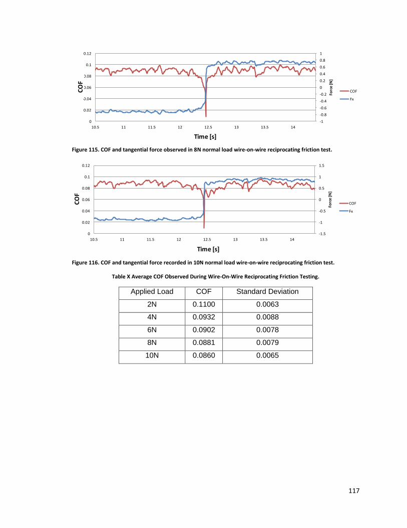
117
Figure 115. COF and tangential force observed in 8N normal load wire-on-wire reciprocating friction test.
Figure 116. COF and tangential force recorded in 10N normal load wire-on-wire reciprocating friction test.
Table X Average COF Observed During Wire-On-Wire Reciprocating Friction Testing.
Applied Load COF Standard Deviation
2N 0.1100 0.0063
4N 0.0932 0.0088
6N 0.0902 0.0078
8N 0.0881 0.0079
10N 0.0860 0.0065
-1
-0.8
-0.6
-0.4
-0.2
0
0.2
0.4
0.6
0.8
1
0
0.02
0.04
0.06
0.08
0.1
0.12
10.5 11 11.5 12 12.5 13 13.5 14
Forc
e [N
]
Co
f
Time
8N
COF
Fx
-1.5
-1
-0.5
0
0.5
1
1.5
0
0.02
0.04
0.06
0.08
0.1
0.12
10.5 11 11.5 12 12.5 13 13.5 14
Forc
e [N
]
Co
f
Time
10N
COF
Fx
0
0.01
0.02
0.03
0.04
0.05
0.06
0.07
0.08
0.09
0.1
-1.5
-1
-0.5
0
0.5
1
790.2 791.2 792.2 793.2 794.2
CO
F
Forc
e [N
]
Time [s]
Fx Coefficient of friction
0
0.01
0.02
0.03
0.04
0.05
0.06
0.07
0.08
0.09
0.1
-1.5
-1
-0.5
0
0.5
1
790.2 791.2 792.2 793.2 794.2
CO
F
Forc
e [N
]
Time [s]
Fx Coefficient of friction
0
0.01
0.02
0.03
0.04
0.05
0.06
0.07
0.08
0.09
0.1
-1.5
-1
-0.5
0
0.5
1
790.2 791.2 792.2 793.2 794.2
CO
F
Forc
e [N
]
Time [s]
Fx Coefficient of friction
0
0.01
0.02
0.03
0.04
0.05
0.06
0.07
0.08
0.09
0.1
-1.5
-1
-0.5
0
0.5
1
790.2 791.2 792.2 793.2 794.2
CO
F
Forc
e [N
]
Time [s]
Fx Coefficient of friction
118
4.4 Wire bedding simulator machine preliminary calibration
testing results
Initial friction testing conducted on the wire bending simulation machine tested the accuracy
and repeatability of the friction measuring system. This series of tests exercise all features of the
wire bending simulator machine. The first series of tests conducted concentrated on
determining the coefficient of friction in the enamel wire surface using conventional friction
counterface material. In this case, 6mm and 3mm diameter UML-SAE 52100 steel high carbon
anti-friction ball bearings were used with a sample speed of 5 and 10mm/s. These counterface
and movement speeds were chosen to match those in the preliminary testing of the enamel-
coated wire to be able to compare the effect of increased applied pressure on the friction
coefficient. Friction tests conducted using a ball-bearing counterface were conducted at a zero
bending angle, and the wire was simply rolled on top of the roller instead of being wrapped
around it. The normal applied load in these series of tests was kept constant at 40 lbs, which
amounted to a normal pressure in the range of 500 MPa. The complete summary of the testing
conditions is shown in Table XI Tests 1–4, and the remainder of the calibration testing (Table XI
Tests 5–8) was conducted using a flat-on-flat configuration and a finely polished 4140 steel
counterface. The counterface material and condition of the surface were chosen to replicate the
surface of the forming die composed of the same material. In these tests, the sample speed was
kept at 20 mm/s to mimic the movement speed of the forming die itself. Apart from the straight
runs with zero deformation, the forming angle tested was 60°, which was achieved by setting
each of the actuator arms at 30°, as shown in Figure 64. This positioning of the linear actuators
allowed measuring the friction coefficient in the section where the sample experienced the
maximum amount of deformation. In the forming rollers, both 24 mm and 3 mm radius rollers
were tested, because these values represented the maximum and minimum radius fittings for
the wire-forming simulator. The COF and normal load were recorded for each test. Each test was
performed three times using identical testing conditions to ensure repeatability and determine
an average of the friction coefficient along with the standard deviation for each test. The
resulting COF recorded and the normal load applied for each test run can be shown as they
varied along the length of the wire sample.
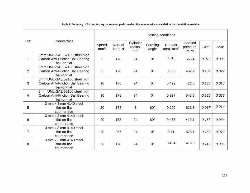
119
Table XI Summary of friction testing parameters performed on the enamel wire as validation for the friction machine
Test Counterface
Testing conditions
Speed, mm/s
Normal load, N
Cylinder radius,
mm
Forming angle
Contact area, mm2
Applied pressure,
MPa COF SDiv
1 6mm UML-SAE 52100 steel high Carbon Anti-Friction Ball Bearing
ball-on-flat 5 178 24 0° 0.315 565.4 0.073 0.006
2 3mm UML-SAE 52100 steel high Carbon Anti-Friction Ball Bearing
ball-on-flat 5 178 24 0° 0.385 462.2 0.137 0.022
3 6mm UML-SAE 52100 steel high Carbon Anti-Friction Ball Bearing
ball-on-flat 10 178 24 0° 0.422 421.6 0.136 0.018
4 3mm UML-SAE 52100 steel high Carbon Anti-Friction Ball Bearing
ball-on-flat 10 178 24 0° 0.327 543.3 0.186 0.023
5 3 mm x 3 mm 4140 steel
flat-on-flat counterface
20 178 3 60° 0.290 613.8 0.067 0.014
6 3 mm x 3 mm 4140 steel
flat-on-flat counterface
20 178 24 60° 0.433 411.1 0.163 0.034
7 3 mm x 3 mm 4140 steel
flat-on-flat counterface
20 267 24 0° 0.71 376.1 0.163 0.012
8 3 mm x 3 mm 4140 steel
flat-on-flat counterface
20 178 24 0° 0.424 419.6 0.142 0.036

120
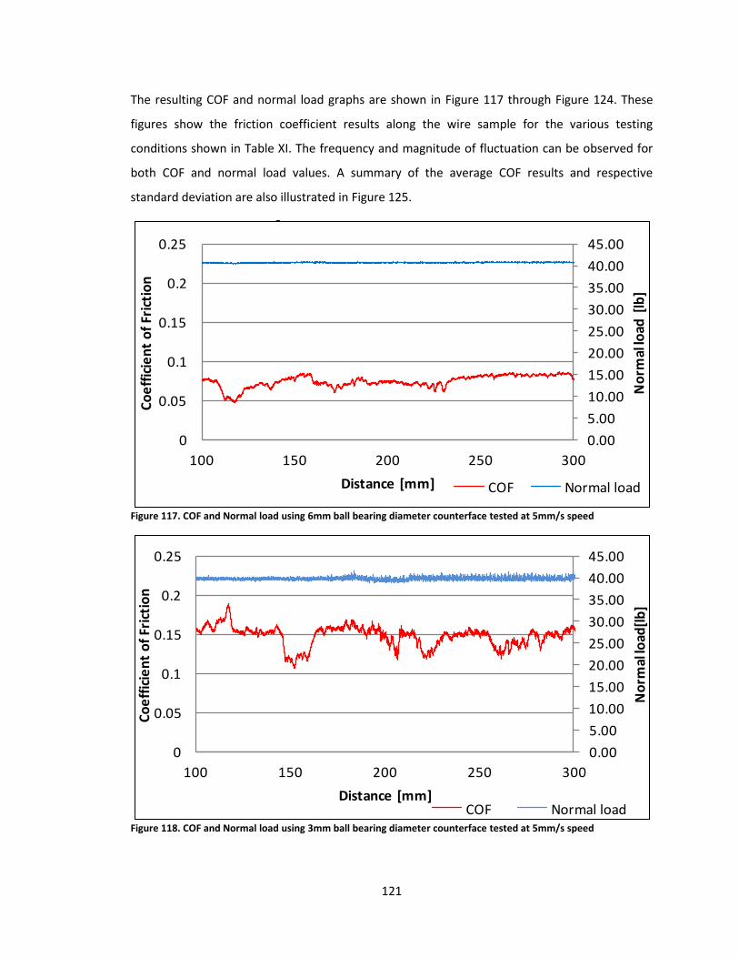
121
The resulting COF and normal load graphs are shown in Figure 117 through Figure 124. These
figures show the friction coefficient results along the wire sample for the various testing
conditions shown in Table XI. The frequency and magnitude of fluctuation can be observed for
both COF and normal load values. A summary of the average COF results and respective
standard deviation are also illustrated in Figure 125.
Figure 117. COF and Normal load using 6mm ball bearing diameter counterface tested at 5mm/s speed
Figure 118. COF and Normal load using 3mm ball bearing diameter counterface tested at 5mm/s speed
0.00
5.00
10.00
15.00
20.00
25.00
30.00
35.00
40.00
45.00
0
0.05
0.1
0.15
0.2
0.25
100 150 200 250 300
No
rmal
load
[lb
]
Co
eff
icie
nt
of
Fric
tio
n
Distance [mm]
5mm/s 40lb friction test result
COF Normal load
0.00
5.00
10.00
15.00
20.00
25.00
30.00
35.00
40.00
45.00
0
0.05
0.1
0.15
0.2
0.25
100 150 200 250 300
No
rmal
load
[lb
]
Co
eff
icie
nt
of
Fric
tio
n
Distance [mm]
5mm/s 40lb friction test result
COF Normal load
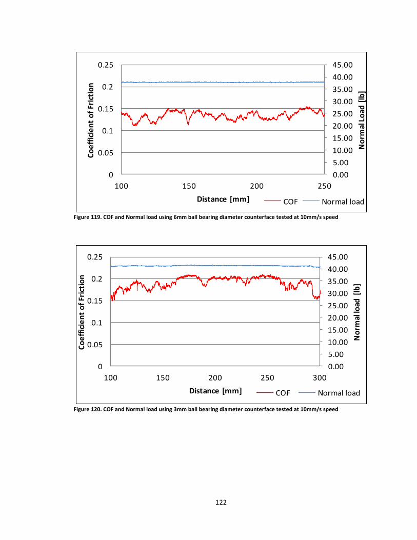
122
Figure 119. COF and Normal load using 6mm ball bearing diameter counterface tested at 10mm/s speed
Figure 120. COF and Normal load using 3mm ball bearing diameter counterface tested at 10mm/s speed
0.00
5.00
10.00
15.00
20.00
25.00
30.00
35.00
40.00
45.00
0
0.05
0.1
0.15
0.2
0.25
100 150 200 250
No
rmal
Lo
ad [
lb]
Co
eff
icie
nt
of
Fric
tio
n
Distance [mm]
10mm/s 40lb friction test result
COF Normal load
0.00
5.00
10.00
15.00
20.00
25.00
30.00
35.00
40.00
45.00
0
0.05
0.1
0.15
0.2
0.25
100 150 200 250 300
No
rmal
load
[lb
]
Co
eff
icie
nt
of
Fric
tio
n
Distance [mm]
10mm/s 40lb friction test result
COF Normal load
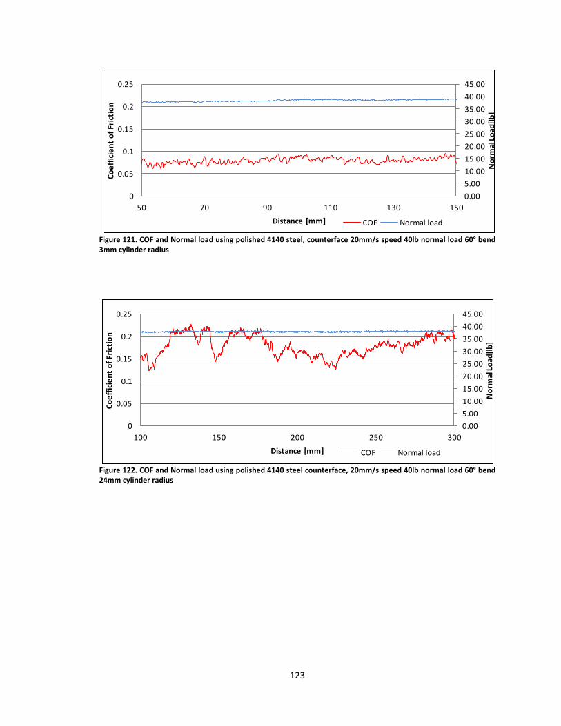
123
Figure 121. COF and Normal load using polished 4140 steel, counterface 20mm/s speed 40lb normal load 60° bend 3mm cylinder radius
Figure 122. COF and Normal load using polished 4140 steel counterface, 20mm/s speed 40lb normal load 60° bend 24mm cylinder radius
0.00
5.00
10.00
15.00
20.00
25.00
30.00
35.00
40.00
45.00
0
0.05
0.1
0.15
0.2
0.25
50 70 90 110 130 150
No
rmal
Lo
ad[l
b]
Co
eff
icie
nt
of
Fric
tio
n
Distance [mm]
4140 counterface friction results
COF Normal load
0.00
5.00
10.00
15.00
20.00
25.00
30.00
35.00
40.00
45.00
0
0.05
0.1
0.15
0.2
0.25
100 150 200 250 300
No
rmal
Lo
ad[l
b]
Co
eff
icie
nt
of
Fric
tio
n
Distance [mm]
4140 counterface friction results
COF Normal load
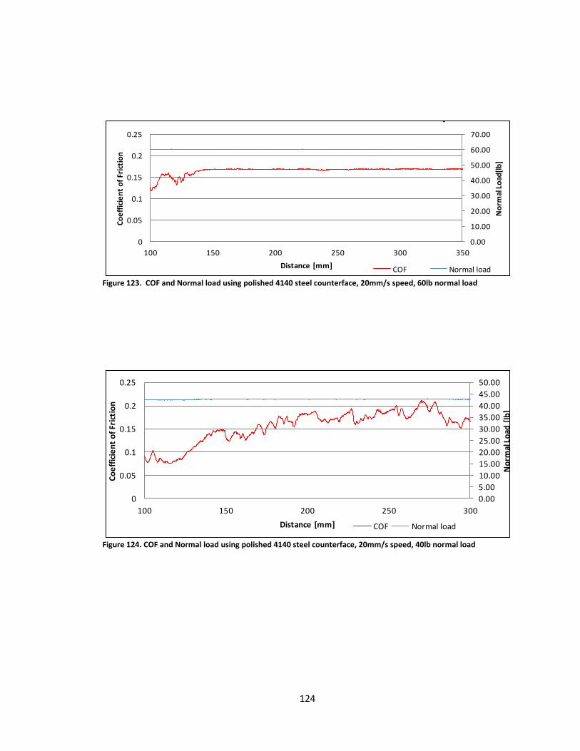
124
Figure 123. COF and Normal load using polished 4140 steel counterface, 20mm/s speed, 60lb normal load
Figure 124. COF and Normal load using polished 4140 steel counterface, 20mm/s speed, 40lb normal load
0.00
10.00
20.00
30.00
40.00
50.00
60.00
70.00
0
0.05
0.1
0.15
0.2
0.25
100 150 200 250 300 350
No
rmal
Lo
ad[l
b]
Co
eff
icie
nt
of
Fric
tio
n
Distance [mm]
4140 counterface friction results 60lb 20mm/s
COF Normal load
0.00
5.00
10.00
15.00
20.00
25.00
30.00
35.00
40.00
45.00
50.00
0
0.05
0.1
0.15
0.2
0.25
100 150 200 250 300N
orm
al L
oad
[lb
]
Co
eff
icie
nt
of
Fric
tio
n
Distance [mm]
4140 counterface friction results
COF Normal load
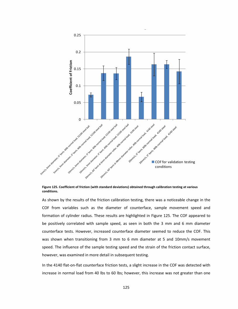
125
Figure 125. Coefficient of friction (with standard deviations) obtained through calibration testing at various conditions.
As shown by the results of the friction calibration testing, there was a noticeable change in the
COF from variables such as the diameter of counterface, sample movement speed and
formation of cylinder radius. These results are highlighted in Figure 125. The COF appeared to
be positively correlated with sample speed, as seen in both the 3 mm and 6 mm diameter
counterface tests. However, increased counterface diameter seemed to reduce the COF. This
was shown when transitioning from 3 mm to 6 mm diameter at 5 and 10mm/s movement
speed. The influence of the sample testing speed and the strain of the friction contact surface,
however, was examined in more detail in subsequent testing.
In the 4140 flat-on-flat counterface friction tests, a slight increase in the COF was detected with
increase in normal load from 40 lbs to 60 lbs; however, this increase was not greater than one
0
0.05
0.1
0.15
0.2
0.25
Co
eff
icie
nt
of
Fric
tio
n
COF for validation testing conditions
COF for validation testing conditions
5mm
/s, 6
mm
dia
mete
r, 0° b
ent, 40lb
norm
al lo
ad, 52100 st
eel bal
l
5mm
/s, 3
mm
dia
mete
r, 0° b
ent, 40lb
norm
al lo
ad, 52100 st
eel bal
l
10mm
/s, 6
mm
dia
mete
r, 0° b
ent, 40lb
norm
al load
, 52100 st
eel ball
10mm
/s, 3
mm
dia
mete
r, 0° b
ent, 40lb
norm
al load
, 52100 st
eel ball
20mm
/s, 6
0° bent a
t 6m
m d
iam
eter r
oller,
40lb n
ormal
load
, 4140 st
eel
20mm
/s, 6
0° bent a
t 48m
m d
iamete
r rolle
r, 40lb
norm
al lo
ad, 4140 st
eel
20mm
/s, 0
° bent,
60lb n
ormal
load
, 4140 st
eel
20mm
/s, 0
° bent,
40lb n
ormal l
oad,
4140 steel
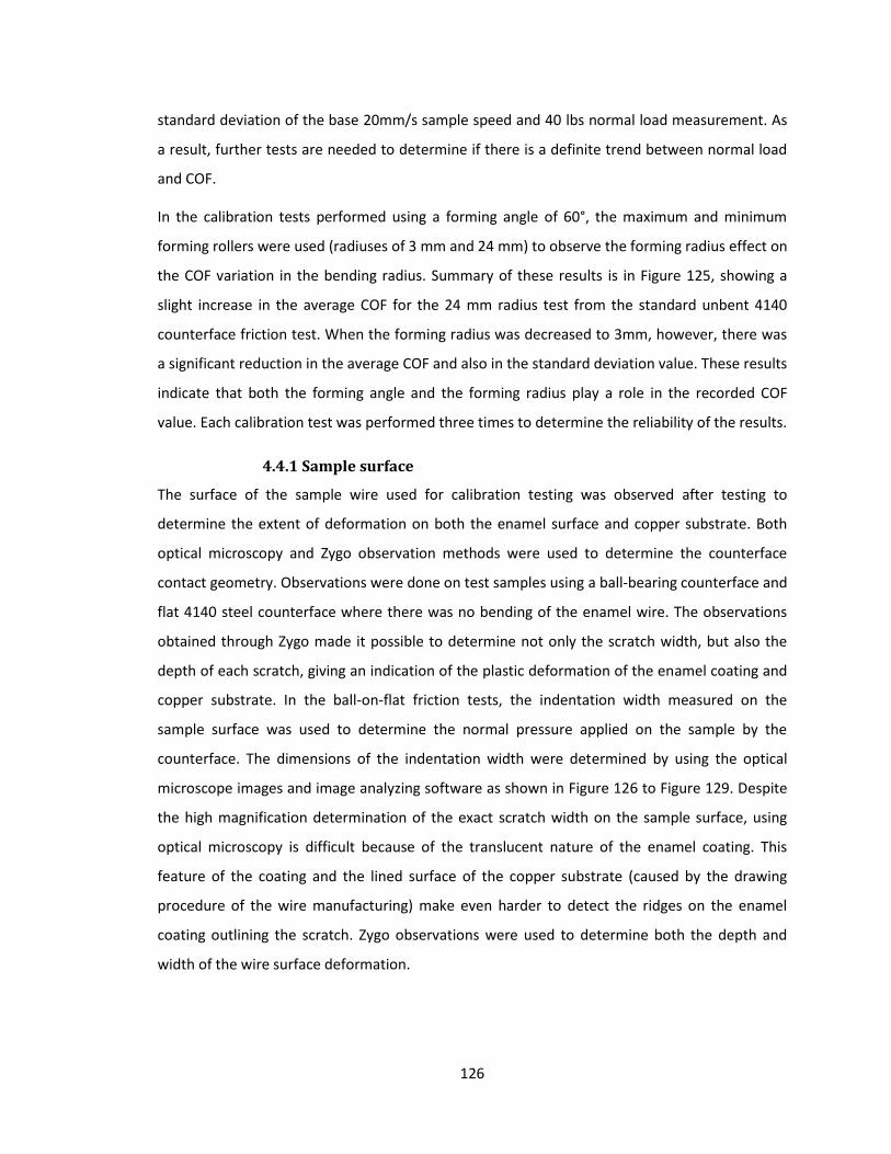
126
standard deviation of the base 20mm/s sample speed and 40 lbs normal load measurement. As
a result, further tests are needed to determine if there is a definite trend between normal load
and COF.
In the calibration tests performed using a forming angle of 60°, the maximum and minimum
forming rollers were used (radiuses of 3 mm and 24 mm) to observe the forming radius effect on
the COF variation in the bending radius. Summary of these results is in Figure 125, showing a
slight increase in the average COF for the 24 mm radius test from the standard unbent 4140
counterface friction test. When the forming radius was decreased to 3mm, however, there was
a significant reduction in the average COF and also in the standard deviation value. These results
indicate that both the forming angle and the forming radius play a role in the recorded COF
value. Each calibration test was performed three times to determine the reliability of the results.
4.4.1 Sample surface
The surface of the sample wire used for calibration testing was observed after testing to
determine the extent of deformation on both the enamel surface and copper substrate. Both
optical microscopy and Zygo observation methods were used to determine the counterface
contact geometry. Observations were done on test samples using a ball-bearing counterface and
flat 4140 steel counterface where there was no bending of the enamel wire. The observations
obtained through Zygo made it possible to determine not only the scratch width, but also the
depth of each scratch, giving an indication of the plastic deformation of the enamel coating and
copper substrate. In the ball-on-flat friction tests, the indentation width measured on the
sample surface was used to determine the normal pressure applied on the sample by the
counterface. The dimensions of the indentation width were determined by using the optical
microscope images and image analyzing software as shown in Figure 126 to Figure 129. Despite
the high magnification determination of the exact scratch width on the sample surface, using
optical microscopy is difficult because of the translucent nature of the enamel coating. This
feature of the coating and the lined surface of the copper substrate (caused by the drawing
procedure of the wire manufacturing) make even harder to detect the ridges on the enamel
coating outlining the scratch. Zygo observations were used to determine both the depth and
width of the wire surface deformation.
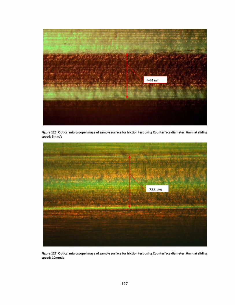
127
Figure 126. Optical microscope image of sample surface for friction test using Counterface diameter: 6mm at sliding speed: 5mm/s
Figure 127. Optical microscope image of sample surface for friction test using Counterface diameter: 6mm at sliding speed: 10mm/s
633 um
733 um
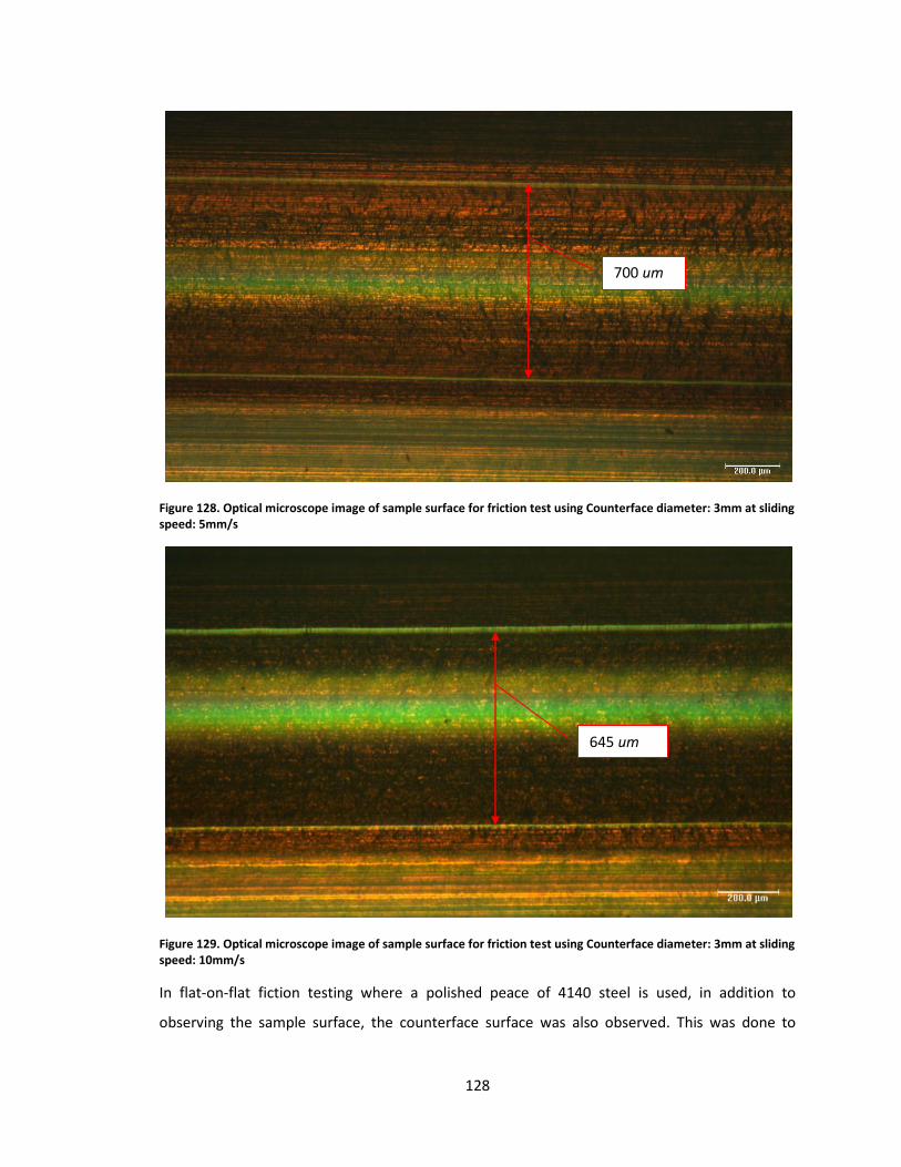
128
Figure 128. Optical microscope image of sample surface for friction test using Counterface diameter: 3mm at sliding speed: 5mm/s
Figure 129. Optical microscope image of sample surface for friction test using Counterface diameter: 3mm at sliding speed: 10mm/s
In flat-on-flat fiction testing where a polished peace of 4140 steel is used, in addition to
observing the sample surface, the counterface surface was also observed. This was done to
700 um
645 um
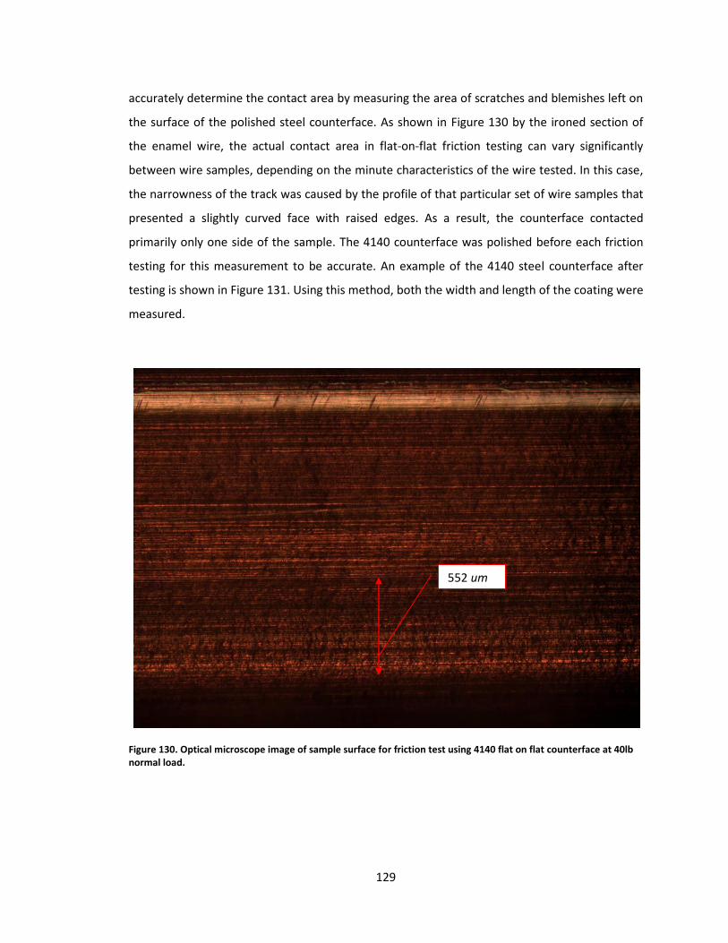
129
accurately determine the contact area by measuring the area of scratches and blemishes left on
the surface of the polished steel counterface. As shown in Figure 130 by the ironed section of
the enamel wire, the actual contact area in flat-on-flat friction testing can vary significantly
between wire samples, depending on the minute characteristics of the wire tested. In this case,
the narrowness of the track was caused by the profile of that particular set of wire samples that
presented a slightly curved face with raised edges. As a result, the counterface contacted
primarily only one side of the sample. The 4140 counterface was polished before each friction
testing for this measurement to be accurate. An example of the 4140 steel counterface after
testing is shown in Figure 131. Using this method, both the width and length of the coating were
measured.
Figure 130. Optical microscope image of sample surface for friction test using 4140 flat on flat counterface at 40lb normal load.
552 um
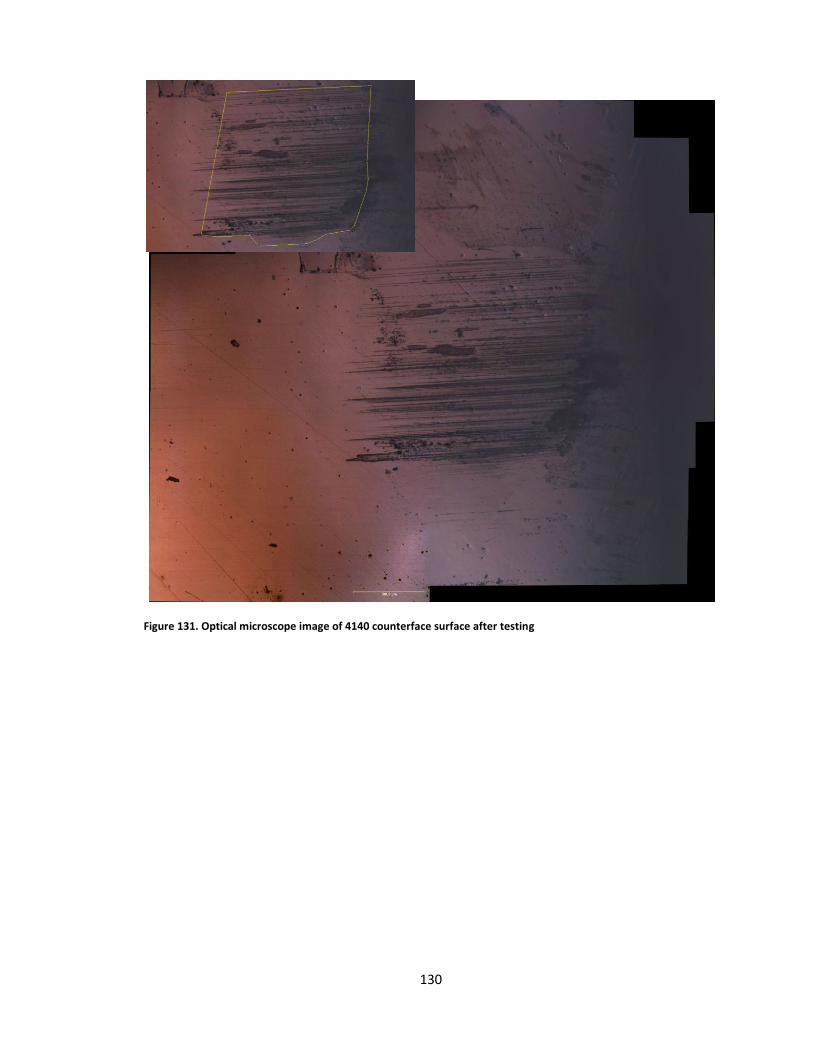
130
Figure 131. Optical microscope image of 4140 counterface surface after testing
131
3-D images of the observed sample surface, along with measurements of the enamel scratch
width and depth, were obtained through Zygo scans of the scratched surface, as shown in Figure
132 to Figure 135. As can be seen in these figures, there was significant increase in penetration
depth when the friction counterface was switched from 6 mm to 3 mm diameter ball. The depth
of the friction test track ranged from 13 µm for the 6 mm ball counterface to 30 µm and 40 µm
for the 3 mm ball. This increase in deformation was expected when considering the increase in
sharpness in the two counterfaces. The increase in deformation of the enamel surface would
account for the increase in the friction coefficient observed between the 6 mm and 3 mm
diameter counterface friction tests. This trend was observed for both the 5 mm/s and 10 mm/s
test cases. The widths of the track did not show as great a degree of variation as observed on
the track depth, with the width varying between 729 µm and 651 µm.
808.5µm 808.5µm
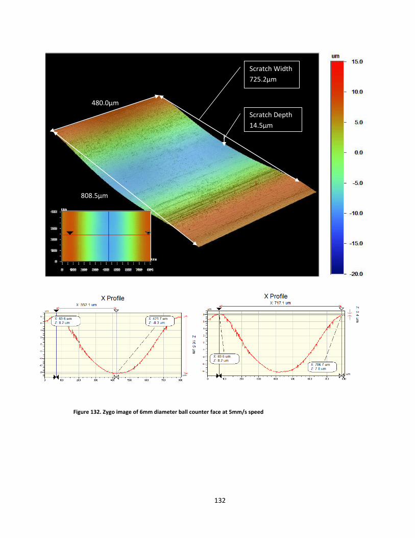
132
Figure 132. Zygo image of 6mm diameter ball counter face at 5mm/s speed
Scratch Width
725.2µm
Scratch Depth
14.5µm
480.0µm
808.5µm
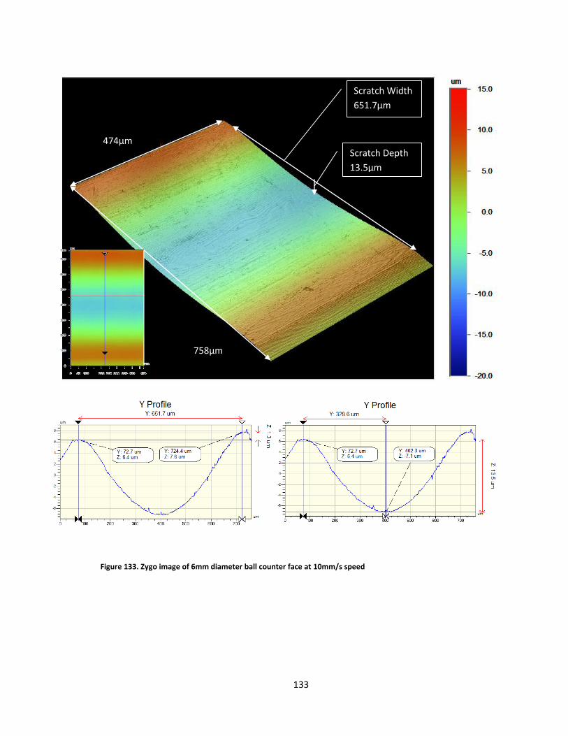
133
Figure 133. Zygo image of 6mm diameter ball counter face at 10mm/s speed
Scratch Width
651.7µm
Scratch Depth
13.5µm
474µm
758µm
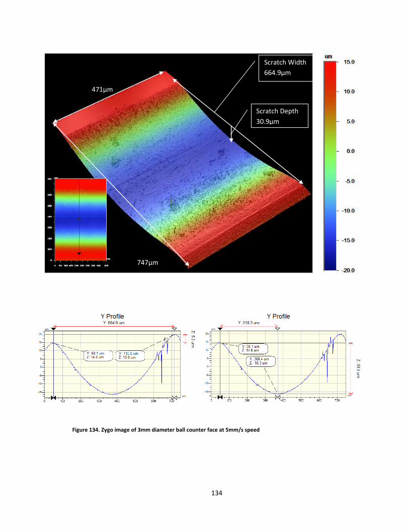
134
Figure 134. Zygo image of 3mm diameter ball counter face at 5mm/s speed
Scratch Width
664.9µm
Scratch Depth
30.9µm
471µm
747µm
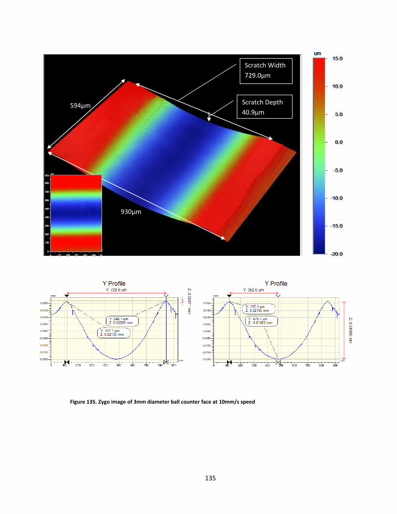
135
Figure 135. Zygo image of 3mm diameter ball counter face at 10mm/s speed
Scratch Width
729.0µm
Scratch Depth
40.9µm 594µm
930µm
136
4.5 Diamond-like coating (DLC) counterface friction testing
The COF between the insulated copper conductors was also tested using a diamond-like carbon
(DLC) coated counterface. This was done to establish the influence of the DLC surface treatment
of the coefficient on the friction coefficient between the two surfaces. The influence of DLC on
the COF was determined by using DLC-coated 6 mm diameter ball bearings as counterface
material during friction tests. Friction tests using uncoated 52100 Steel High Carbon Anti-Friction
ball bearings were used as control runs in this series of tests. Identical testing parameters were
then used for all friction tests dealing with a DLC counterface.
These parameters included: A normal applied load of 40 lbs,
A draw length of 260 mm,
Acceleration/deceleration speeds of 20 mm/s²,
A sample movement speed of 20 mm/s,
A sample pre-tensioned to 200 lbs of force.
The DLC coatings studied in these friction trials were DLC Tribobond TB40 and TB41. These DLC
coatings are some of the most common physical vapor deposition and plasma-assisted chemical
vapor deposition coatings used in the automotive industry, with TB41 being mainly applied to
reduce friction in mechanical components.
Before testing, all bearings used as a friction counterface were cleaned using a glassware
cleaning solution and a 5-min ultrasonic bath in ethanol. The wire samples used in the testing
procedure were tested as received, with no additional cleaning or handling before testing.
Before testing, the wire samples were individually stored in straight polymer tubes. The samples
were straightened, and care was taken not to deform the wire samples before testing.
The results of the DLC counterface friction tests are listed in Table XII and shown in Figure 136.
Two friction tests were performed on each wire, each one using an adjacent side of the wire in
contact with the counterface. The average and standard deviation of the COF was calculated
based on these two runs. The average COF recorded using the 6 mm diameter steel bearing was
0.164, with a standard deviation of 0.016. Both DLC coatings exhibited slightly higher average
COFs, with TB40 at 0.179 and TB41 at 0.168. As expected from its description, TB41 did show a

137
lower COF, when compared to DLC TB40. The COF results obtained using TB41 were very close
to those of the uncoated sample, with the difference between the runs well within the standard
deviation of both values.
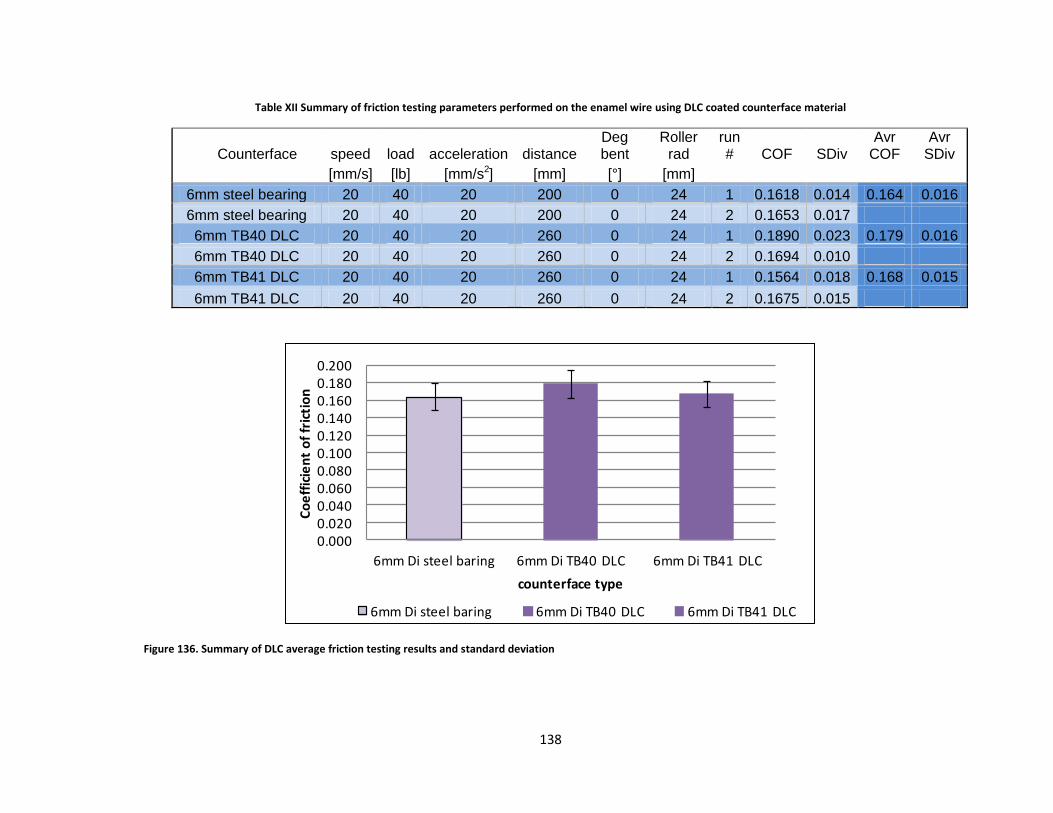
138
Table XII Summary of friction testing parameters performed on the enamel wire using DLC coated counterface material
Counterface speed load acceleration distance Deg bent
Roller rad
run # COF SDiv
Avr COF
Avr SDiv
[mm/s] [lb] [mm/s2] [mm] [°] [mm]
6mm steel bearing 20 40 20 200 0 24 1 0.1618 0.014 0.164 0.016
6mm steel bearing 20 40 20 200 0 24 2 0.1653 0.017
6mm TB40 DLC 20 40 20 260 0 24 1 0.1890 0.023 0.179 0.016
6mm TB40 DLC 20 40 20 260 0 24 2 0.1694 0.010
6mm TB41 DLC 20 40 20 260 0 24 1 0.1564 0.018 0.168 0.015
6mm TB41 DLC 20 40 20 260 0 24 2 0.1675 0.015
Figure 136. Summary of DLC average friction testing results and standard deviation
0.0000.0200.0400.0600.0800.1000.1200.1400.1600.1800.200
6mm Di steel baring 6mm Di TB40 DLC 6mm Di TB41 DLC
Co
eff
icie
nt
of
fric
tio
n
counterface type
COF for DLC counterface
6mm Di steel baring 6mm Di TB40 DLC 6mm Di TB41 DLC
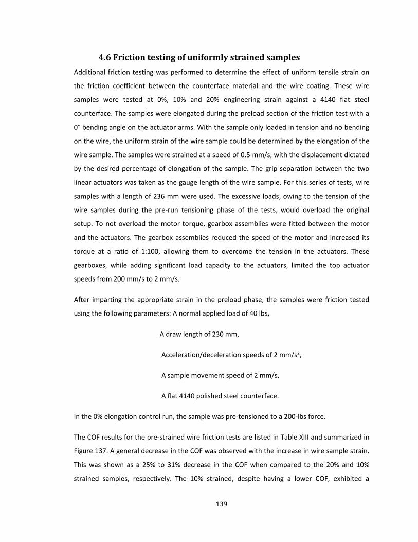
139
4.6 Friction testing of uniformly strained samples
Additional friction testing was performed to determine the effect of uniform tensile strain on
the friction coefficient between the counterface material and the wire coating. These wire
samples were tested at 0%, 10% and 20% engineering strain against a 4140 flat steel
counterface. The samples were elongated during the preload section of the friction test with a
0° bending angle on the actuator arms. With the sample only loaded in tension and no bending
on the wire, the uniform strain of the wire sample could be determined by the elongation of the
wire sample. The samples were strained at a speed of 0.5 mm/s, with the displacement dictated
by the desired percentage of elongation of the sample. The grip separation between the two
linear actuators was taken as the gauge length of the wire sample. For this series of tests, wire
samples with a length of 236 mm were used. The excessive loads, owing to the tension of the
wire samples during the pre-run tensioning phase of the tests, would overload the original
setup. To not overload the motor torque, gearbox assemblies were fitted between the motor
and the actuators. The gearbox assemblies reduced the speed of the motor and increased its
torque at a ratio of 1:100, allowing them to overcome the tension in the actuators. These
gearboxes, while adding significant load capacity to the actuators, limited the top actuator
speeds from 200 mm/s to 2 mm/s.
After imparting the appropriate strain in the preload phase, the samples were friction tested
using the following parameters: A normal applied load of 40 lbs,
A draw length of 230 mm,
Acceleration/deceleration speeds of 2 mm/s²,
A sample movement speed of 2 mm/s,
A flat 4140 polished steel counterface.
In the 0% elongation control run, the sample was pre-tensioned to a 200-lbs force.
The COF results for the pre-strained wire friction tests are listed in Table XIII and summarized in
Figure 137. A general decrease in the COF was observed with the increase in wire sample strain.
This was shown as a 25% to 31% decrease in the COF when compared to the 20% and 10%
strained samples, respectively. The 10% strained, despite having a lower COF, exhibited a
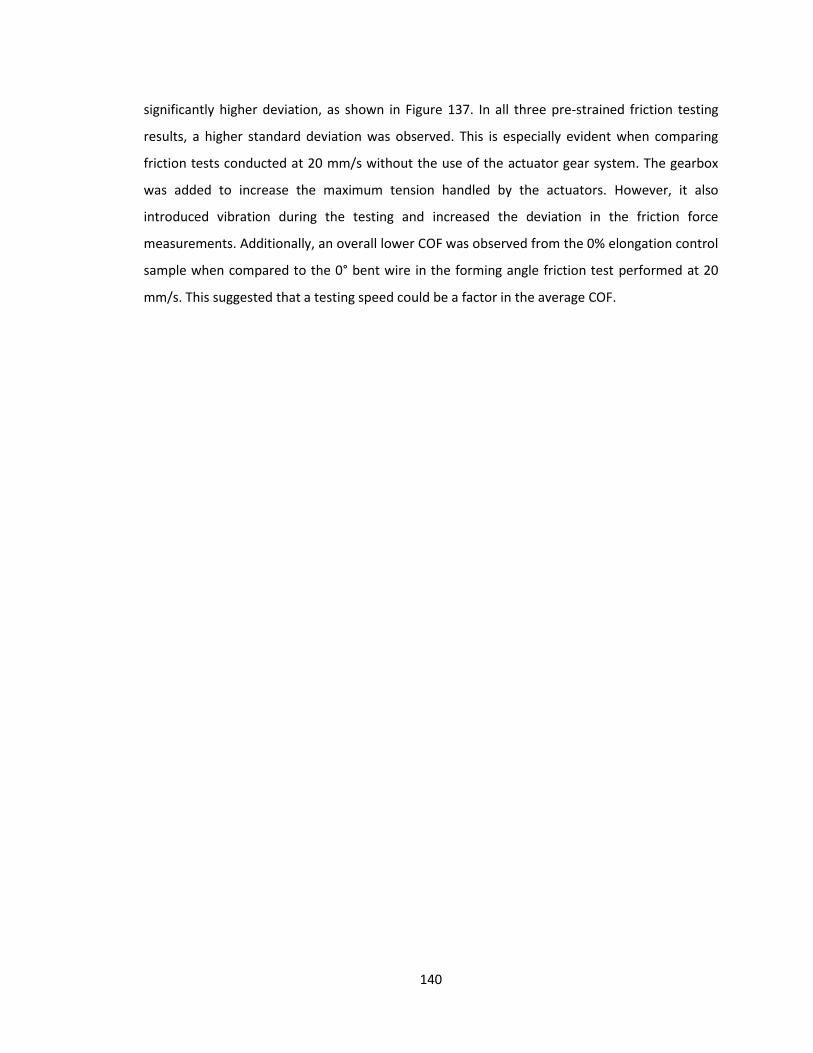
140
significantly higher deviation, as shown in Figure 137. In all three pre-strained friction testing
results, a higher standard deviation was observed. This is especially evident when comparing
friction tests conducted at 20 mm/s without the use of the actuator gear system. The gearbox
was added to increase the maximum tension handled by the actuators. However, it also
introduced vibration during the testing and increased the deviation in the friction force
measurements. Additionally, an overall lower COF was observed from the 0% elongation control
sample when compared to the 0° bent wire in the forming angle friction test performed at 20
mm/s. This suggested that a testing speed could be a factor in the average COF.
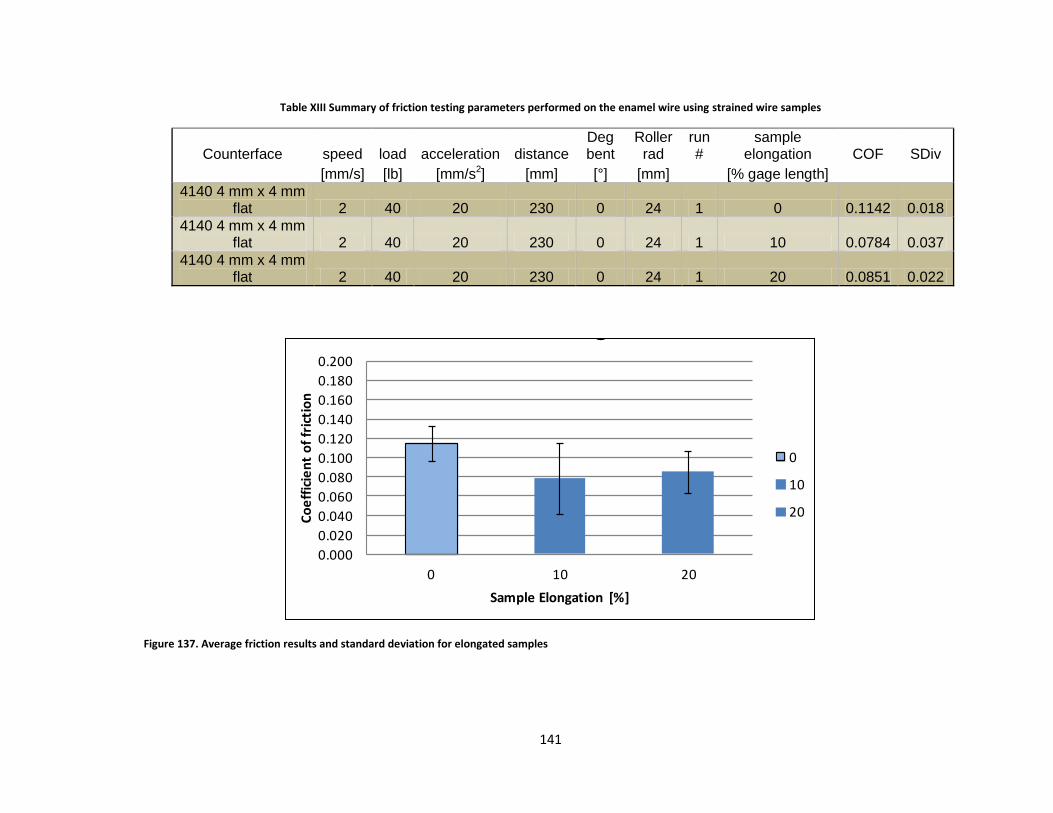
141
Table XIII Summary of friction testing parameters performed on the enamel wire using strained wire samples
Counterface speed load acceleration distance Deg bent
Roller rad
run #
sample elongation COF SDiv
[mm/s] [lb] [mm/s2] [mm] [°] [mm]
[% gage length]
4140 4 mm x 4 mm flat 2 40 20 230 0 24 1 0 0.1142 0.018
4140 4 mm x 4 mm flat 2 40 20 230 0 24 1 10 0.0784 0.037
4140 4 mm x 4 mm flat 2 40 20 230 0 24 1 20 0.0851 0.022
Figure 137. Average friction results and standard deviation for elongated samples
0.000
0.020
0.040
0.060
0.080
0.100
0.120
0.140
0.160
0.180
0.200
0 10 20
Co
eff
icie
nt
of
fric
tio
n
Sample Elongation [%]
COF for % elongation
0
10
20
142
4.7 Effect of bending angle and bending radius friction results
The effect of the forming angle and forming radius on the COF was studied through the
performance of friction tests while forming an enamelled wire sample at 30° and 60°. The wire
sample was formed by positioning each actuator at half the incline of the desired angle. In the
case of 30°, for example, each actuator was positioned at an incline of 15°. The straight wire
sample was then attached to the extended actuator and manually bent over the roller so that
the other end of the wire sample could be attached to the retracted actuator. The roller
controlled the percent strain on the wire by the forming radius and supported the pressure put
on the wire by the counterface surface during friction testing. The wire was then tensioned to a
load of 200 lbs, causing the wire to bend around the roller. After the pre-tensioning section of
the experiment, the counterface was applied on top of the wire sample, at the apex of the bend.
The normal load was then applied, and the friction testing was performed by drawing the wire
over the roller under the counterface.
The following parameters were used during this set of friction tests:
A normal applied load of 40 lbs,
A draw length of 230 mm,
An acceleration/deceleration speed of 20mm/s²,
A sample movement speed of 20 mm/s,
A flat 4140 polished steel counterface.
In addition to determining the influence of the forming angle and the forming radius on the COF,
the influence of sample surface cleaning was also observed.
All wire samples used in this series of tests were tested as received, with the exception of the
cleaned wire sample. In the cleaned sample friction test, the wire sample was cleaned before
testing by using ample water and a glassware cleaning solution designed to remove any oil or
grease residue on the wire surface. The 4140 flat steel counterface was also cleaned using an
ultrasonic ethanol bath prior to each friction test run.
As shown in the first four samples in Table XIV, the wires tested as received had a friction
coefficient of 0.16 under these conditions. The cleaned wire sample, however, had a friction
coefficient of 0.083, even though the small amount of lubricant on the wire was nominally used
by the manufacturer to reduce wire-to-wire friction during spooling.
143
The friction tests conducted used 3 mm and 24 mm radius rollers to bend the wire samples. The
samples were bent, alternatively, at 30° and 60° for each roller radius. These bending
procedures that used the following angles and bending radii of the wire sample were simulated
using the finite element analysis model that was validated by the method outlined in section
“5.2 ”. The strain values generated by the FEA model on the wire surface are shown in Table XIV
under the FEA Predicted Strain column. These values represent the strain of the surface
contacted by the friction counterface, and the values are used as bases to determine the strain
of the enamel wire in subsequent friction measurements. To achieve strain values intermediate
to the ones simulated, uniform tension was applied to the wire sample before testing using any
of the listed radii or angles.
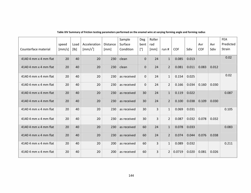
144
Table XIV Summary of friction testing parameters performed on the enamel wire at varying forming angle and forming radius
Counterface material
speed
[mm/s]
Load
[lb]
Acceleration
[mm/s2]
Distance
[mm]
Sample
Surface
Condition
Deg
bent
[°]
Roller
rad
[mm] run # COF Sdiv
Avr
COF
Avr
Sdiv
FEA
Predicted
Strain
4140 4 mm x 4 mm flat 20 40 20 230 clean 0 24 1 0.085 0.013
0.083 0.012
0.02
4140 4 mm x 4 mm flat 20 40 20 230 clean 0 24 2 0.081 0.011
4140 4 mm x 4 mm flat 20 40 20 230 as received 0 24 1 0.154 0.025
0.160 0.030
0.02
4140 4 mm x 4 mm flat 20 40 20 230 as received 0 24 2 0.166 0.034
4140 4 mm x 4 mm flat 20 40 20 230 as received 30 24 1 0.119 0.022
0.109 0.030
0.087
4140 4 mm x 4 mm flat 20 40 20 230 as received 30 24 2 0.100 0.038
4140 4 mm x 4 mm flat 20 40 20 230 as received 30 3 1 0.069 0.031
0.078 0.032
0.105
4140 4 mm x 4 mm flat 20 40 20 230 as received 30 3 2 0.087 0.032
4140 4 mm x 4 mm flat 20 40 20 230 as received 60 24 1 0.078 0.033
0.076 0.038
0.083
4140 4 mm x 4 mm flat 20 40 20 230 as received 60 24 2 0.074 0.044
4140 4 mm x 4 mm flat 20 40 20 200 as received 60 3 1 0.089 0.032
0.081 0.026
0.211
4140 4 mm x 4 mm flat 20 40 20 200 as received 60 3 2 0.0719 0.020
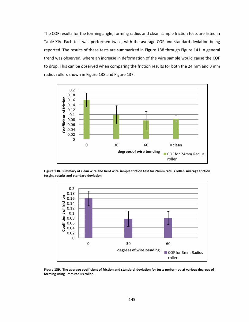
145
The COF results for the forming angle, forming radius and clean sample friction tests are listed in
Table XIV. Each test was performed twice, with the average COF and standard deviation being
reported. The results of these tests are summarized in Figure 138 through Figure 141. A general
trend was observed, where an increase in deformation of the wire sample would cause the COF
to drop. This can be observed when comparing the friction results for both the 24 mm and 3 mm
radius rollers shown in Figure 138 and Figure 137.
Figure 138. Summary of clean wire and bent wire sample friction test for 24mm radius roller. Average friction testing results and standard deviation
Figure 139. The average coefficient of friction and standard deviation for tests performed at various degrees of forming using 3mm radius roller.
00.020.040.060.08
0.10.120.140.160.18
0.2
0 30 60 0 clean
Co
eff
icie
nt
of
fric
tio
n
degrees of wire bending
COF for 24mm Radius roller
COF for 24mm Radius roller
00.020.040.060.08
0.10.120.140.160.18
0.2
0 30 60
Co
eff
icie
nt
of
fric
tio
n
degrees of wire bending
COF for 3mm Radius roller
COF for 3mm Radius roller
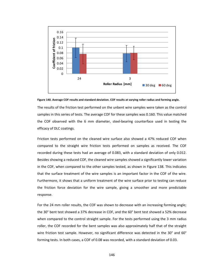
146
Figure 140. Average COF results and standard deviation. COF results at varying roller radius and forming angle.
The results of the friction test performed on the unbent wire samples were taken as the control
samples in this series of tests. The average COF for these samples was 0.160. This value matched
the COF observed with the 6 mm diameter, steel-bearing counterface used in testing the
efficacy of DLC coatings.
Friction tests performed on the cleaned wire surface also showed a 47% reduced COF when
compared to the straight wire friction tests performed on samples as received. The COF
recorded during these tests had an average of 0.083, with a standard deviation of only 0.012.
Besides showing a reduced COF, the cleaned wire samples showed a significantly lower variation
in the COF, when compared to the other samples tested, as shown in Figure 138. This indicates
that the surface treatment of the wire samples is an important factor in the COF of the wire.
Furthermore, it shows that a uniform treatment of the wire surface prior to testing can reduce
the friction force deviation for the wire sample, giving a smoother and more predictable
response.
For the 24 mm roller results, the COF was shown to decrease with an increasing forming angle;
the 30° bent test showed a 37% decrease in COF, and the 60° bent test showed a 52% decrease
when compared to the control straight sample. For the tests performed using the 3 mm radius
roller, the COF recorded for the bent samples was also approximately half that of the straight
wire friction test sample. However, no significant difference was detected in the 30° and 60°
forming tests. In both cases, a COF of 0.08 was recorded, with a standard deviation of 0.03.
0
0.02
0.04
0.06
0.08
0.1
0.12
0.14
0.16
24 3
Co
eff
icie
nt
of
fric
tio
n
Roller Radius [mm]
COF vs. Roller Radius
30 deg 60 deg
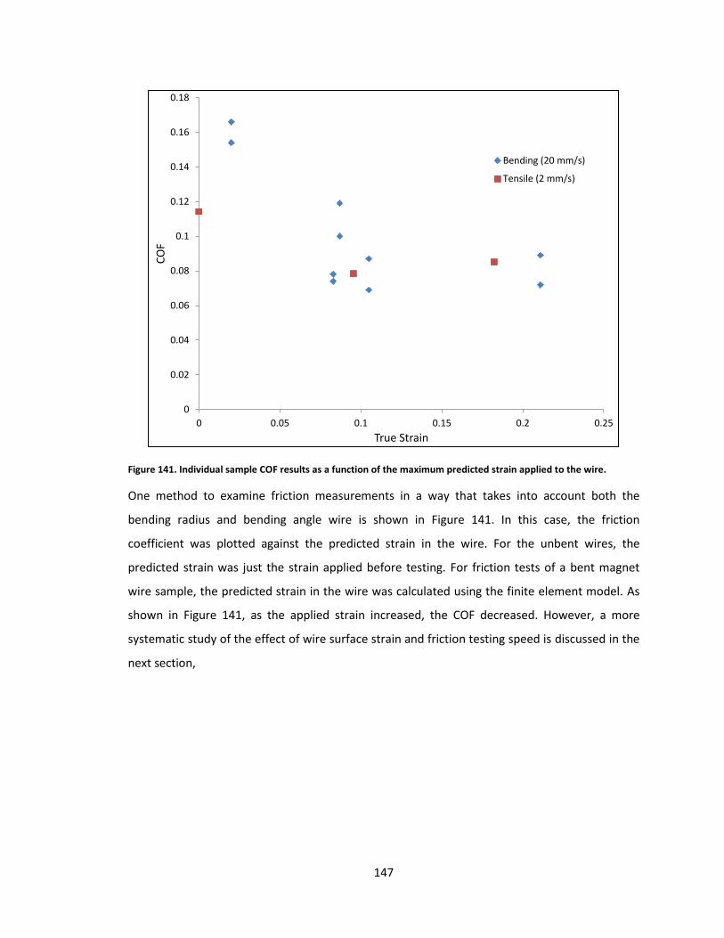
147
Figure 141. Individual sample COF results as a function of the maximum predicted strain applied to the wire.
One method to examine friction measurements in a way that takes into account both the
bending radius and bending angle wire is shown in Figure 141. In this case, the friction
coefficient was plotted against the predicted strain in the wire. For the unbent wires, the
predicted strain was just the strain applied before testing. For friction tests of a bent magnet
wire sample, the predicted strain in the wire was calculated using the finite element model. As
shown in Figure 141, as the applied strain increased, the COF decreased. However, a more
systematic study of the effect of wire surface strain and friction testing speed is discussed in the
next section,
0
0.02
0.04
0.06
0.08
0.1
0.12
0.14
0.16
0.18
0 0.05 0.1 0.15 0.2 0.25
CO
F
True Strain
Bending (20 mm/s)
Tensile (2 mm/s)
148
4.8 Friction testing of magnet wire samples at various speeds and
surface strains
These tests were conducted to determine the effect of sample surface strain and testing speed
on the COF between the magnet wire and the forming die. In this test series, the sample
movement speed in each test was controlled by programming the linear actuators; this value
varied between 1 mm/s and 20 mm/s. As mentioned in previous chapters, no direct strain
measuring method exists for determining the strain of the wire surface section in contact with
the friction counterface. A validated finite element analysis model, however, was used to
simulate friction testing conditions where the magnet wire samples were bent at particular
angles and radii. These FEA strain measurements were then used to achieve the desired surface
strain in a particular sample by adding pre-test linear strain through sample elongation. Using
this method, the control of surface strain is achieved during friction testing.
The following parameters were used during this set of friction tests:
A normal applied load of 40 lbs,
A sample length of 250 mm,
An acceleration/deceleration speed of 20 mm/s²,
A sample movement speed of 1 mm/s, 5 mm/s, 10 mm/s, 15 mm/s and 20 mm/s,
A sample contact surface strain of 2%, 5%, 10%, 15% and 20%
A flat 4140 polished steel counterface.
The friction coefficients plotted along the length of the wire sample are shown in Figure 142 to
Figure 146. Each of these figures outlines the test results at a particular magnet wire surface
strain at varying testing speeds.
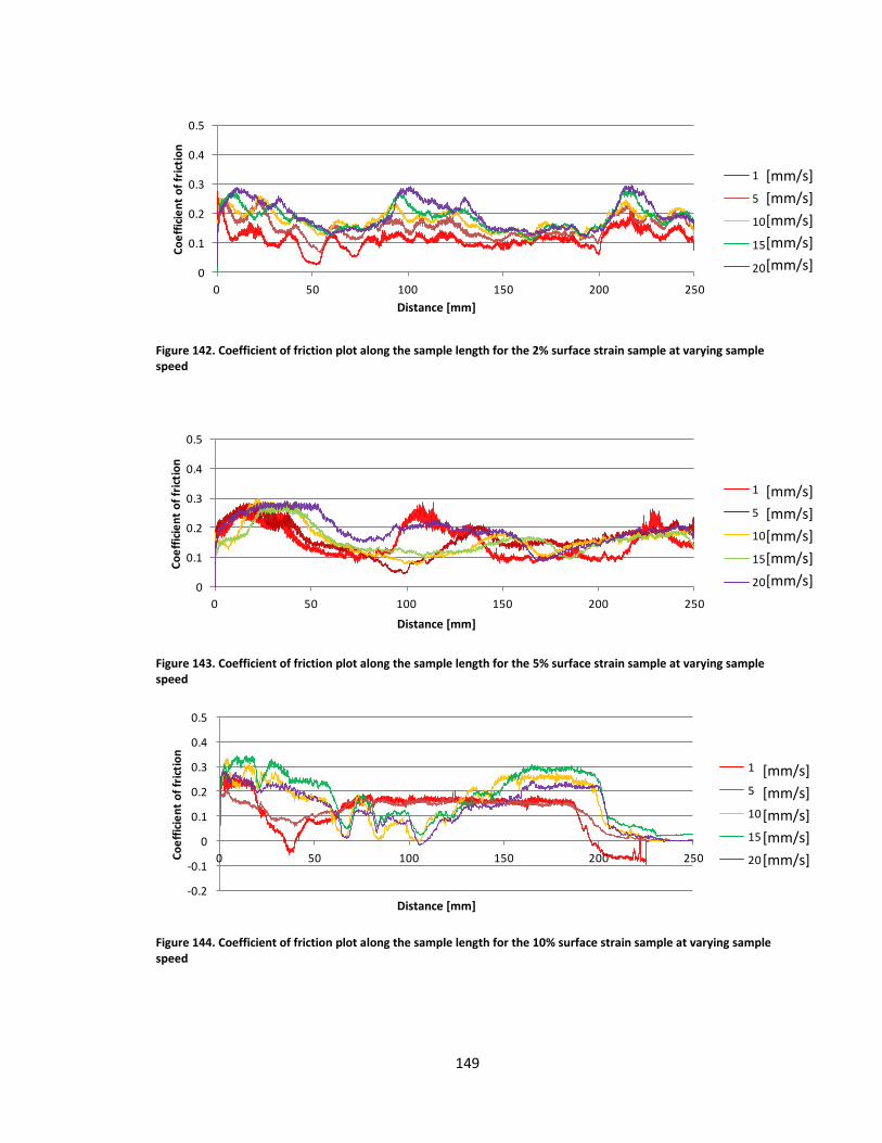
149
Figure 142. Coefficient of friction plot along the sample length for the 2% surface strain sample at varying sample speed
Figure 143. Coefficient of friction plot along the sample length for the 5% surface strain sample at varying sample speed
Figure 144. Coefficient of friction plot along the sample length for the 10% surface strain sample at varying sample speed
0
0.1
0.2
0.3
0.4
0.5
0 50 100 150 200 250
Co
eff
icie
nt
of
fric
tio
n
Sample distance [mm]
COF results of 2% strain sample per sample speed
1
5
10
15
20
0
0.1
0.2
0.3
0.4
0.5
0 50 100 150 200 250
Co
eff
icie
nt
of
fric
tio
n
Sample distance [mm]
COF results of 5% strain sample per sample speed
1
5
10
15
20
-0.2
-0.1
0
0.1
0.2
0.3
0.4
0.5
0 50 100 150 200 250Co
eff
icie
nt
of
fric
tio
n
Sample distance [mm]
COF results of 10% strain sample per sample speed
1
5
10
15
20
Distance [mm]
Distance [mm]
Distance [mm]
[mm/s]
[mm/s]
[mm/s]
[mm/s]
[mm/s]
[N]
[N]
[N]
[mm/s]
[mm/s]
[mm/s]
[mm/s]
[mm/s]
[N]
[N]
[N]
[mm/s]
[mm/s]
[mm/s]
[mm/s]
[mm/s]
[N]
[N]
[N]
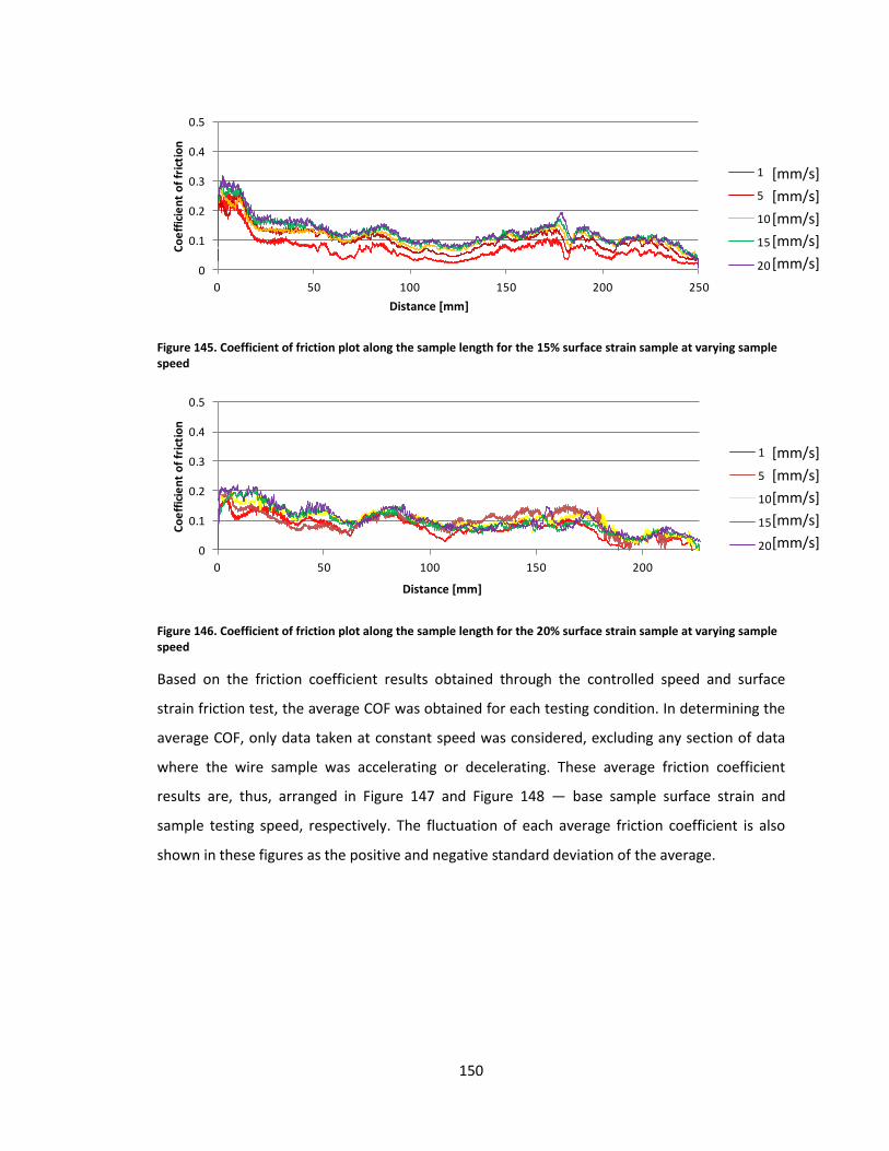
150
Figure 145. Coefficient of friction plot along the sample length for the 15% surface strain sample at varying sample speed
Figure 146. Coefficient of friction plot along the sample length for the 20% surface strain sample at varying sample speed
Based on the friction coefficient results obtained through the controlled speed and surface
strain friction test, the average COF was obtained for each testing condition. In determining the
average COF, only data taken at constant speed was considered, excluding any section of data
where the wire sample was accelerating or decelerating. These average friction coefficient
results are, thus, arranged in Figure 147 and Figure 148 — base sample surface strain and
sample testing speed, respectively. The fluctuation of each average friction coefficient is also
shown in these figures as the positive and negative standard deviation of the average.
0
0.1
0.2
0.3
0.4
0.5
0 50 100 150 200 250
Co
eff
icie
nt
of
fric
tio
n
Sample distance [mm]
COF results of 15% strain sample per sample speed
1
5
10
15
20
0
0.1
0.2
0.3
0.4
0.5
0 50 100 150 200
Co
eff
icie
nt
of
fric
tio
n
Sample distance [mm]
COF results of 20% strain sample per sample speed
1
5
10
15
20
Distance [mm]
Distance [mm]
[mm/s]
[mm/s]
[mm/s]
[mm/s]
[mm/s]
[N]
[N]
[N]
[mm/s]
[mm/s]
[mm/s]
[mm/s]
[mm/s]
[N]
[N]
[N]
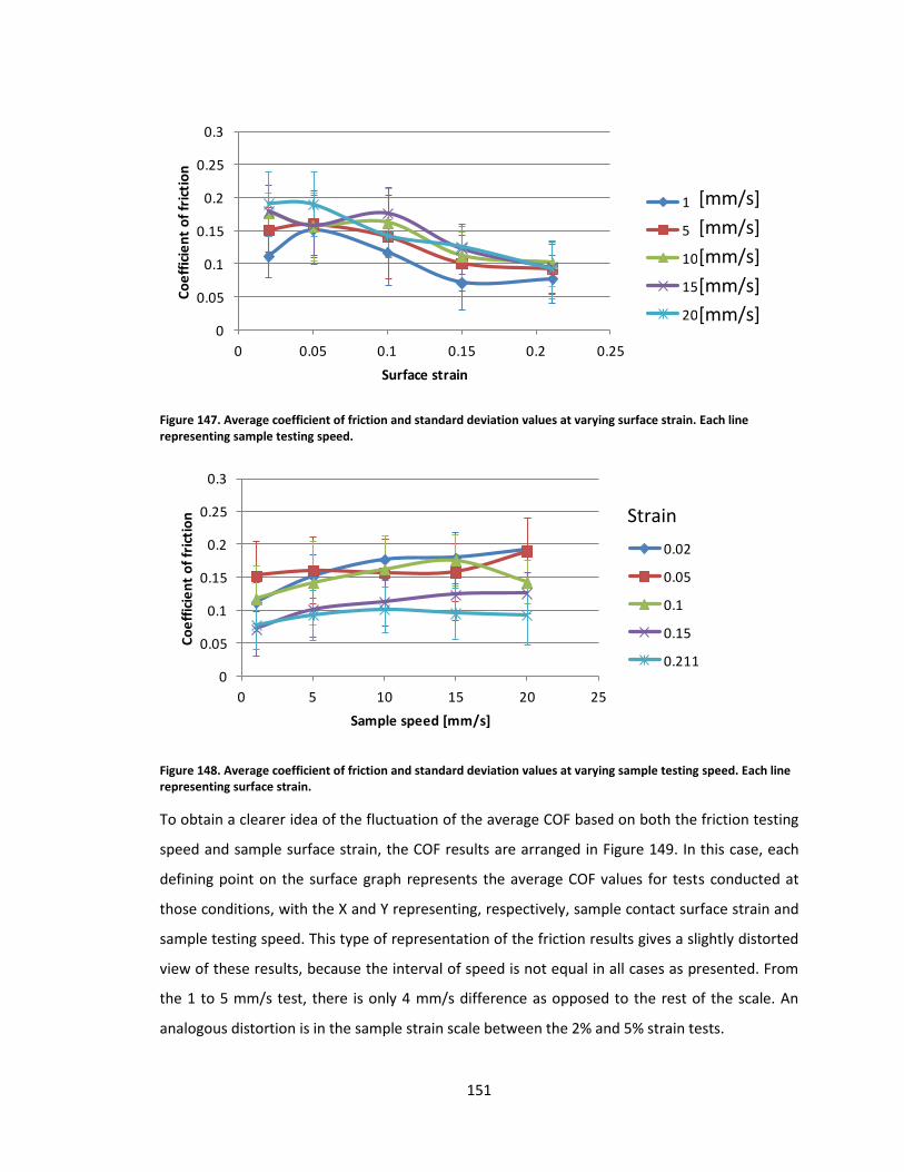
151
Figure 147. Average coefficient of friction and standard deviation values at varying surface strain. Each line representing sample testing speed.
Figure 148. Average coefficient of friction and standard deviation values at varying sample testing speed. Each line representing surface strain.
To obtain a clearer idea of the fluctuation of the average COF based on both the friction testing
speed and sample surface strain, the COF results are arranged in Figure 149. In this case, each
defining point on the surface graph represents the average COF values for tests conducted at
those conditions, with the X and Y representing, respectively, sample contact surface strain and
sample testing speed. This type of representation of the friction results gives a slightly distorted
view of these results, because the interval of speed is not equal in all cases as presented. From
the 1 to 5 mm/s test, there is only 4 mm/s difference as opposed to the rest of the scale. An
analogous distortion is in the sample strain scale between the 2% and 5% strain tests.
0
0.05
0.1
0.15
0.2
0.25
0.3
0 0.05 0.1 0.15 0.2 0.25
Co
eff
icie
nt
of
fric
tio
n
Surface strain
sample surface strain vs COF
1
5
10
15
20
0
0.05
0.1
0.15
0.2
0.25
0.3
0 5 10 15 20 25
Co
eff
icie
nt
of
fric
tio
n
Sample speed [mm/s]
Sample speed vs COF
0.02
0.05
0.1
0.15
0.211
[mm/s]
[mm/s]
[mm/s]
[mm/s]
[mm/s]
Strain
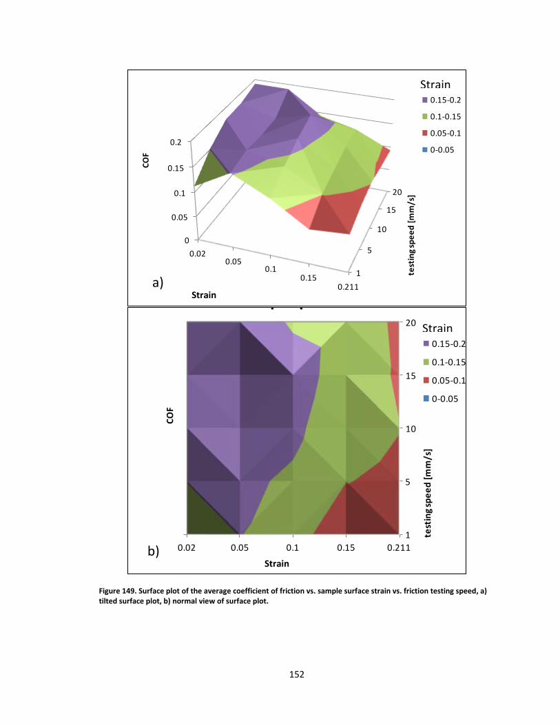
152
Figure 149. Surface plot of the average coefficient of friction vs. sample surface strain vs. friction testing speed, a) tilted surface plot, b) normal view of surface plot.
1
5
10
15
20
0
0.05
0.1
0.15
0.2
0.020.05
0.10.15
0.211
test
ing
spe
ed
[m
m/s
]
CO
F
Sample Strain
Strain map representation
0.15-0.2
0.1-0.15
0.05-0.1
0-0.05
1
5
10
15
20
0.02 0.05 0.1 0.15 0.211
test
ing
spe
ed
[m
m/s
]
CO
F
Sample Strain
Strain map representation
0.15-0.2
0.1-0.15
0.05-0.1
0-0.05
a)
b)
Strain
Strain
Strain
Strain
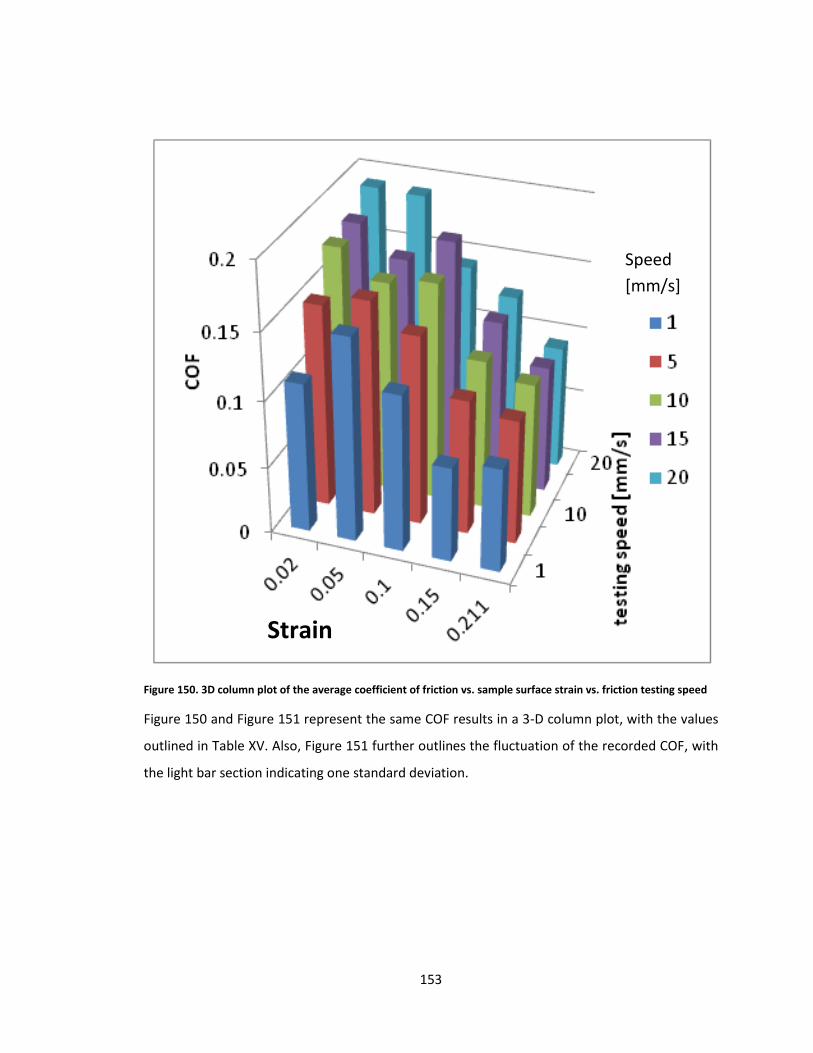
153
Figure 150. 3D column plot of the average coefficient of friction vs. sample surface strain vs. friction testing speed
Figure 150 and Figure 151 represent the same COF results in a 3-D column plot, with the values
outlined in Table XV. Also, Figure 151 further outlines the fluctuation of the recorded COF, with
the light bar section indicating one standard deviation.
Speed
[mm/s]
Strain
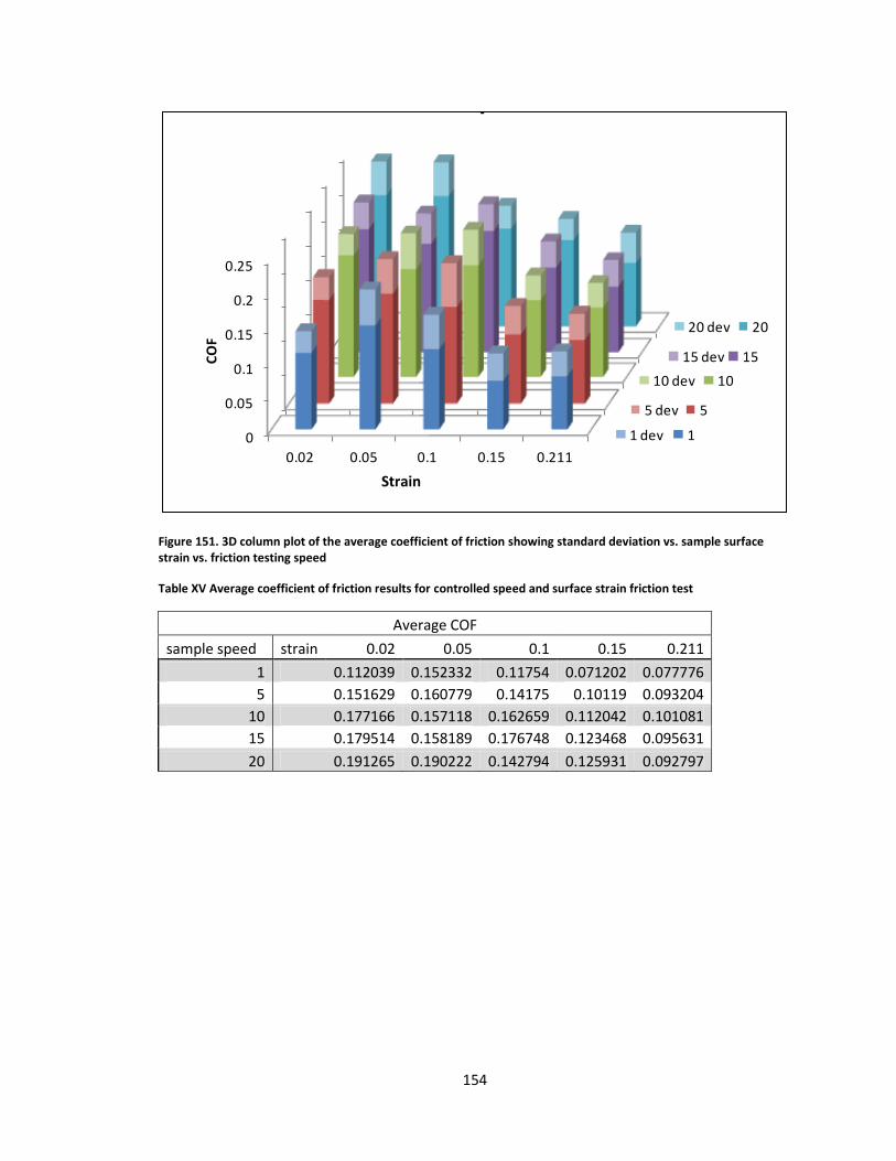
154
Figure 151. 3D column plot of the average coefficient of friction showing standard deviation vs. sample surface strain vs. friction testing speed
Table XV Average coefficient of friction results for controlled speed and surface strain friction test
Average COF
sample speed strain 0.02 0.05 0.1 0.15 0.211
1 0.112039 0.152332 0.11754 0.071202 0.077776
5 0.151629 0.160779 0.14175 0.10119 0.093204
10 0.177166 0.157118 0.162659 0.112042 0.101081
15 0.179514 0.158189 0.176748 0.123468 0.095631
20 0.191265 0.190222 0.142794 0.125931 0.092797
0
0.05
0.1
0.15
0.2
0.25
0.02 0.05 0.1 0.15 0.211
Axi
s Ti
tle
Axis Title
COF Vs speed Vs strain
20 dev 20
0
0.05
0.1
0.15
0.2
0.25
0.02 0.05 0.1 0.15 0.211
Axi
s Ti
tle
Axis Title
15 dev 15
0
0.05
0.1
0.15
0.2
0.25
0.02 0.05 0.1 0.15 0.211
Axi
s Ti
tle
Axis Title
10 dev 10
0
0.05
0.1
0.15
0.2
0.25
0.02 0.05 0.1 0.15 0.211
Axi
s Ti
tle
Axis Title
5 dev 5
0
0.05
0.1
0.15
0.2
0.25
0.02 0.05 0.1 0.15 0.211
CO
F
Sample strain
1 dev 1
Strain
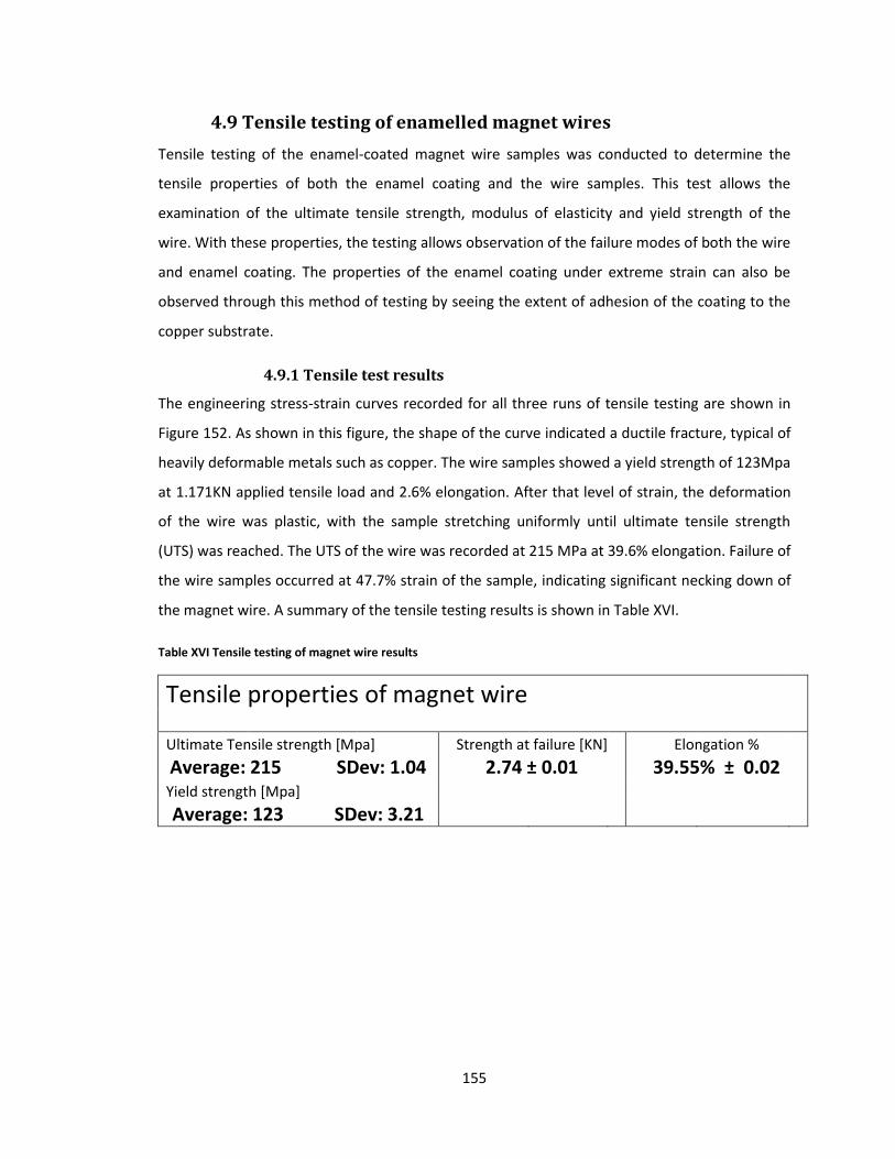
155
4.9 Tensile testing of enamelled magnet wires
Tensile testing of the enamel-coated magnet wire samples was conducted to determine the
tensile properties of both the enamel coating and the wire samples. This test allows the
examination of the ultimate tensile strength, modulus of elasticity and yield strength of the
wire. With these properties, the testing allows observation of the failure modes of both the wire
and enamel coating. The properties of the enamel coating under extreme strain can also be
observed through this method of testing by seeing the extent of adhesion of the coating to the
copper substrate.
4.9.1 Tensile test results
The engineering stress-strain curves recorded for all three runs of tensile testing are shown in
Figure 152. As shown in this figure, the shape of the curve indicated a ductile fracture, typical of
heavily deformable metals such as copper. The wire samples showed a yield strength of 123Mpa
at 1.171KN applied tensile load and 2.6% elongation. After that level of strain, the deformation
of the wire was plastic, with the sample stretching uniformly until ultimate tensile strength
(UTS) was reached. The UTS of the wire was recorded at 215 MPa at 39.6% elongation. Failure of
the wire samples occurred at 47.7% strain of the sample, indicating significant necking down of
the magnet wire. A summary of the tensile testing results is shown in Table XVI.
Table XVI Tensile testing of magnet wire results
Tensile properties of magnet wire
Ultimate Tensile strength [Mpa] Strength at failure [KN] Elongation %
Average: 215 SDev: 1.04 2.74 ± 0.01 39.55% ± 0.02 Yield strength [Mpa]
Average: 123 SDev: 3.21
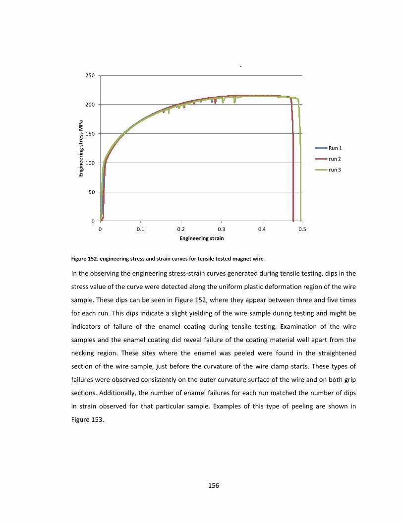
156
Figure 152. engineering stress and strain curves for tensile tested magnet wire
In the observing the engineering stress-strain curves generated during tensile testing, dips in the
stress value of the curve were detected along the uniform plastic deformation region of the wire
sample. These dips can be seen in Figure 152, where they appear between three and five times
for each run. This dips indicate a slight yielding of the wire sample during testing and might be
indicators of failure of the enamel coating during tensile testing. Examination of the wire
samples and the enamel coating did reveal failure of the coating material well apart from the
necking region. These sites where the enamel was peeled were found in the straightened
section of the wire sample, just before the curvature of the wire clamp starts. These types of
failures were observed consistently on the outer curvature surface of the wire and on both grip
sections. Additionally, the number of enamel failures for each run matched the number of dips
in strain observed for that particular sample. Examples of this type of peeling are shown in
Figure 153.
0
50
100
150
200
250
0 0.1 0.2 0.3 0.4 0.5
Engi
ne
eri
ng
stre
ss M
Pa
Engineering strain
Tensile test summary chart
Run 1
run 2
run 3
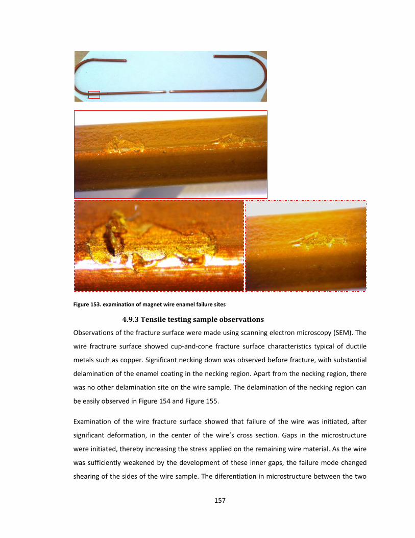
157
Figure 153. examination of magnet wire enamel failure sites
4.9.3 Tensile testing sample observations
Observations of the fracture surface were made using scanning electron microscopy (SEM). The
wire fractrure surface showed cup-and-cone fracture surface characteristics typical of ductile
metals such as copper. Significant necking down was observed before fracture, with substantial
delamination of the enamel coating in the necking region. Apart from the necking region, there
was no other delamination site on the wire sample. The delamination of the necking region can
be easily observed in Figure 154 and Figure 155.
Examination of the wire fracture surface showed that failure of the wire was initiated, after
significant deformation, in the center of the wire’s cross section. Gaps in the microstructure
were initiated, thereby increasing the stress applied on the remaining wire material. As the wire
was sufficiently weakened by the development of these inner gaps, the failure mode changed
shearing of the sides of the wire sample. The diferentiation in microstructure between the two
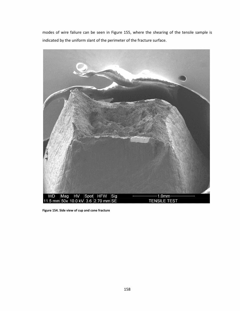
158
modes of wire faliure can be seen in Figure 155, where the shearing of the tensile sample is
indicated by the uniform slant of the perimeter of the fracture surface.
Figure 154. Side view of cup and cone fracture
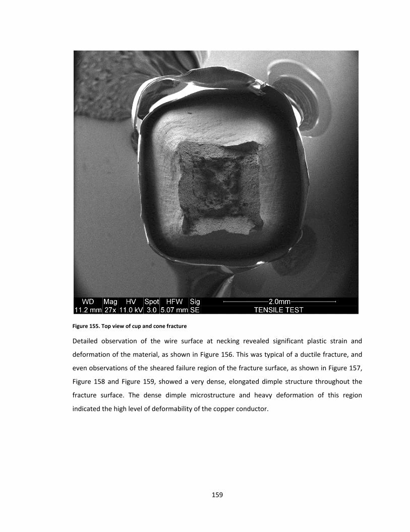
159
Figure 155. Top view of cup and cone fracture
Detailed observation of the wire surface at necking revealed significant plastic strain and
deformation of the material, as shown in Figure 156. This was typical of a ductile fracture, and
even observations of the sheared failure region of the fracture surface, as shown in Figure 157,
Figure 158 and Figure 159, showed a very dense, elongated dimple structure throughout the
fracture surface. The dense dimple microstructure and heavy deformation of this region
indicated the high level of deformability of the copper conductor.
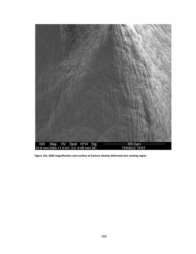
160
Figure 156. 200X magnification wire surface at fracture Heavily deformed wire necking region
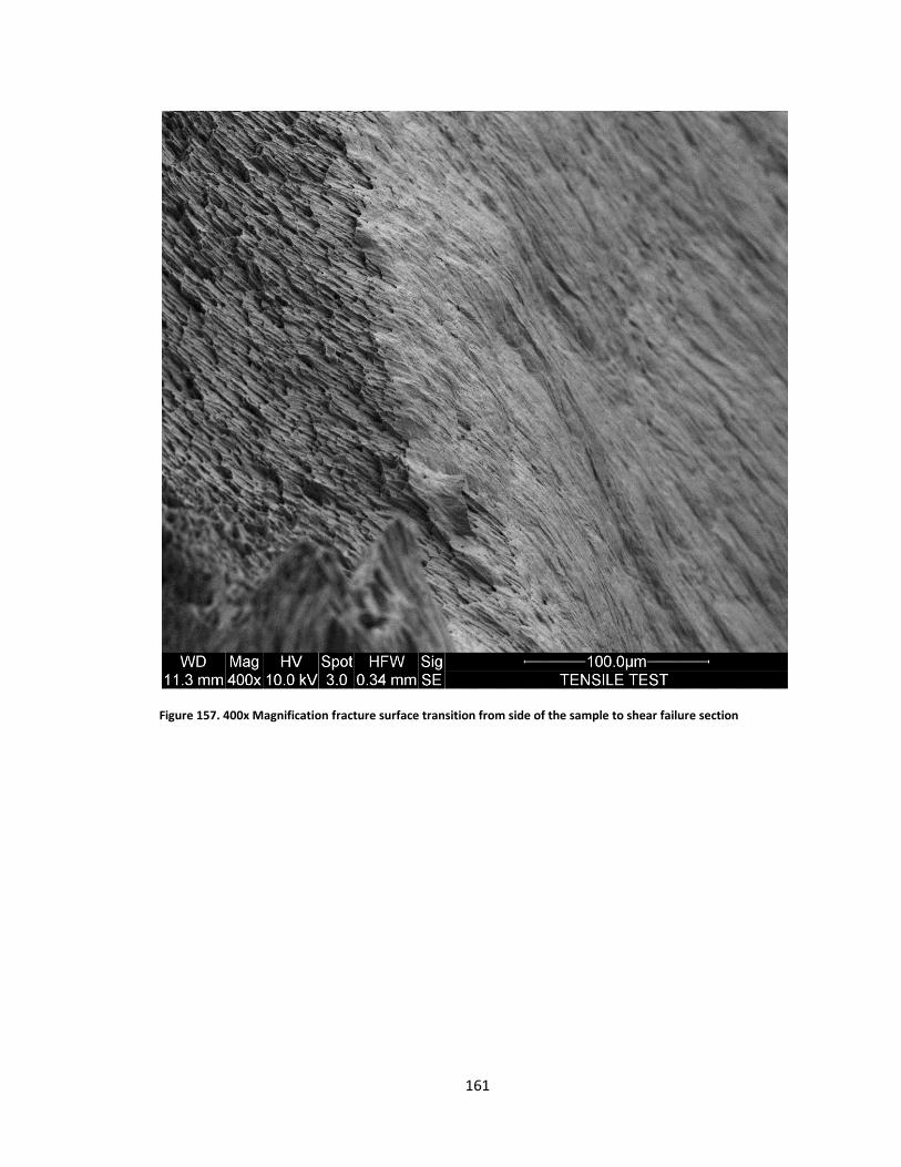
161
Figure 157. 400x Magnification fracture surface transition from side of the sample to shear failure section
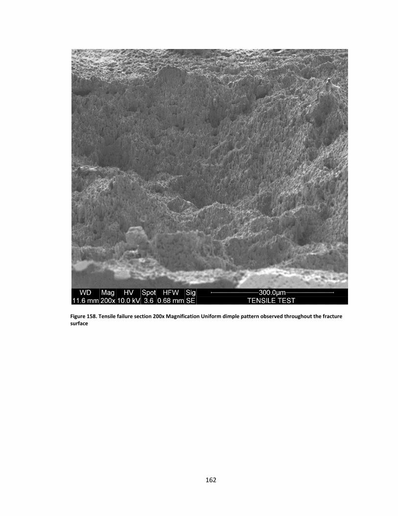
162
Figure 158. Tensile failure section 200x Magnification Uniform dimple pattern observed throughout the fracture surface
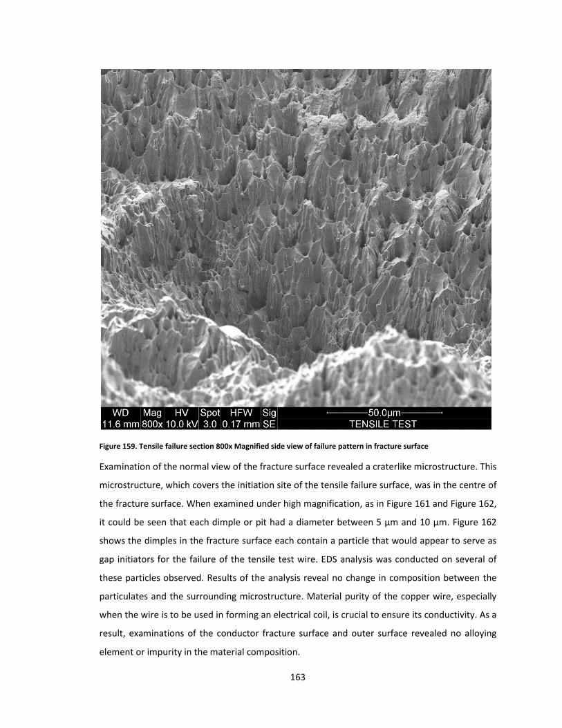
163
Figure 159. Tensile failure section 800x Magnified side view of failure pattern in fracture surface
Examination of the normal view of the fracture surface revealed a craterlike microstructure. This
microstructure, which covers the initiation site of the tensile failure surface, was in the centre of
the fracture surface. When examined under high magnification, as in Figure 161 and Figure 162,
it could be seen that each dimple or pit had a diameter between 5 µm and 10 µm. Figure 162
shows the dimples in the fracture surface each contain a particle that would appear to serve as
gap initiators for the failure of the tensile test wire. EDS analysis was conducted on several of
these particles observed. Results of the analysis reveal no change in composition between the
particulates and the surrounding microstructure. Material purity of the copper wire, especially
when the wire is to be used in forming an electrical coil, is crucial to ensure its conductivity. As a
result, examinations of the conductor fracture surface and outer surface revealed no alloying
element or impurity in the material composition.
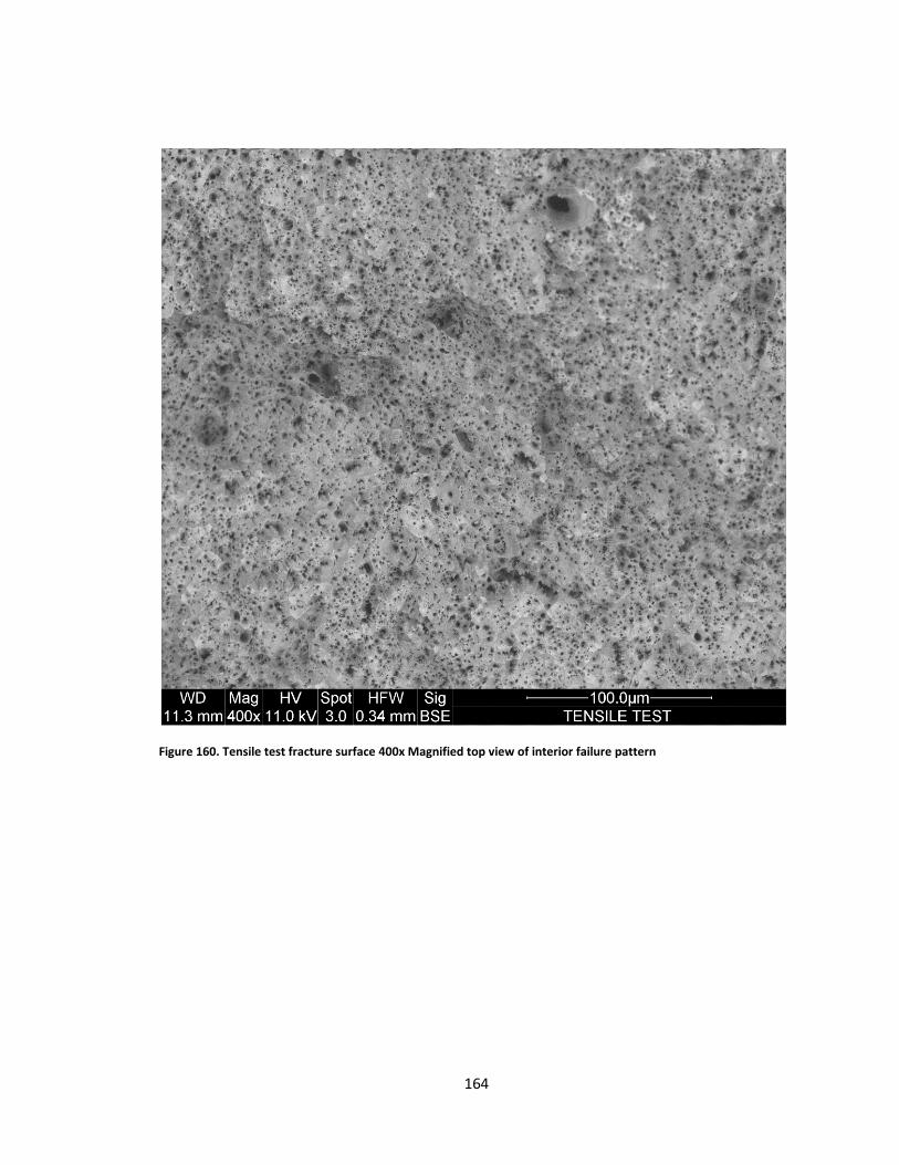
164
Figure 160. Tensile test fracture surface 400x Magnified top view of interior failure pattern
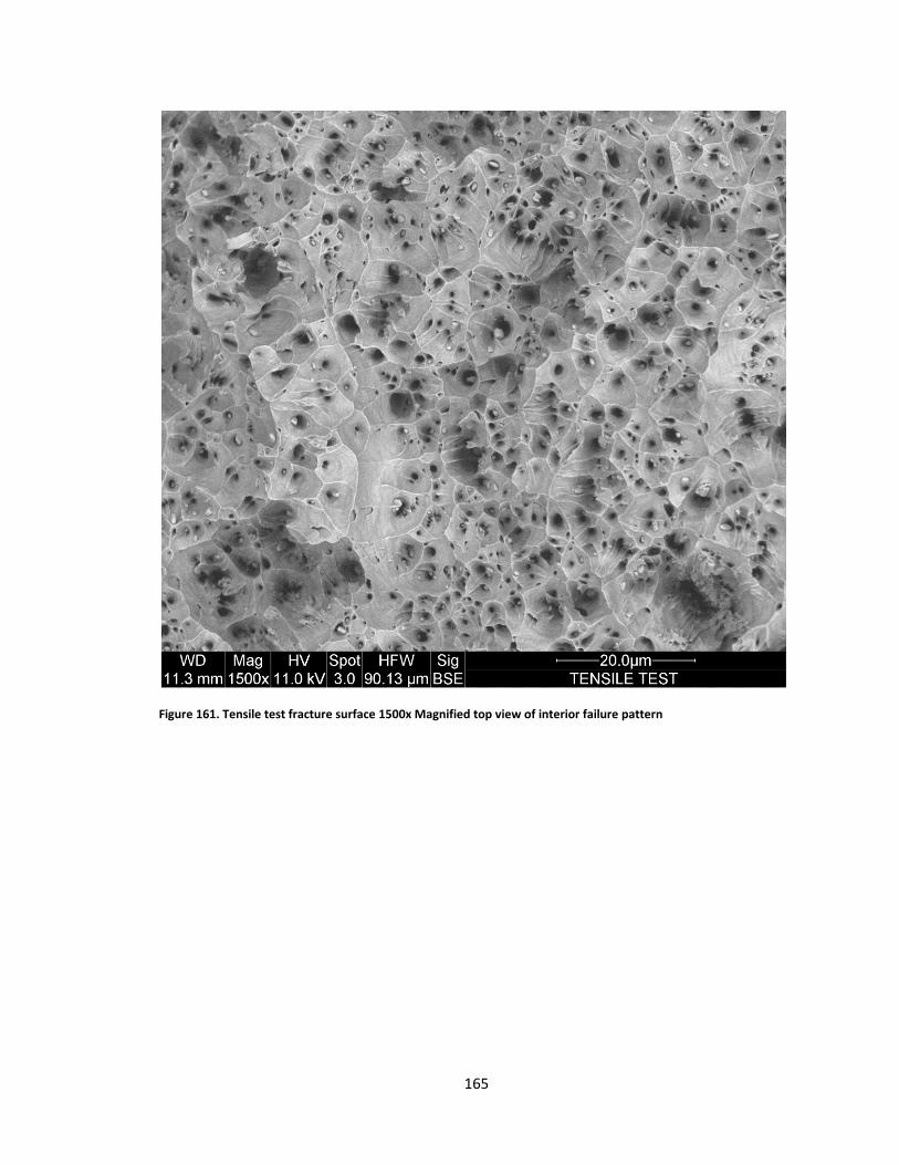
165
Figure 161. Tensile test fracture surface 1500x Magnified top view of interior failure pattern
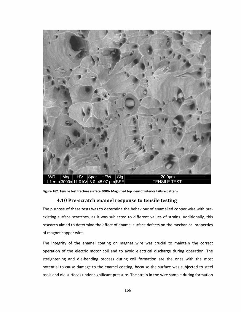
166
Figure 162. Tensile test fracture surface 3000x Magnified top view of interior failure pattern
4.10 Pre-scratch enamel response to tensile testing
The purpose of these tests was to determine the behaviour of enamelled copper wire with pre-
existing surface scratches, as it was subjected to different values of strains. Additionally, this
research aimed to determine the effect of enamel surface defects on the mechanical properties
of magnet copper wire.
The integrity of the enamel coating on magnet wire was crucial to maintain the correct
operation of the electric motor coil and to avoid electrical discharge during operation. The
straightening and die-bending process during coil formation are the ones with the most
potential to cause damage to the enamel coating, because the surface was subjected to steel
tools and die surfaces under significant pressure. The strain in the wire sample during formation
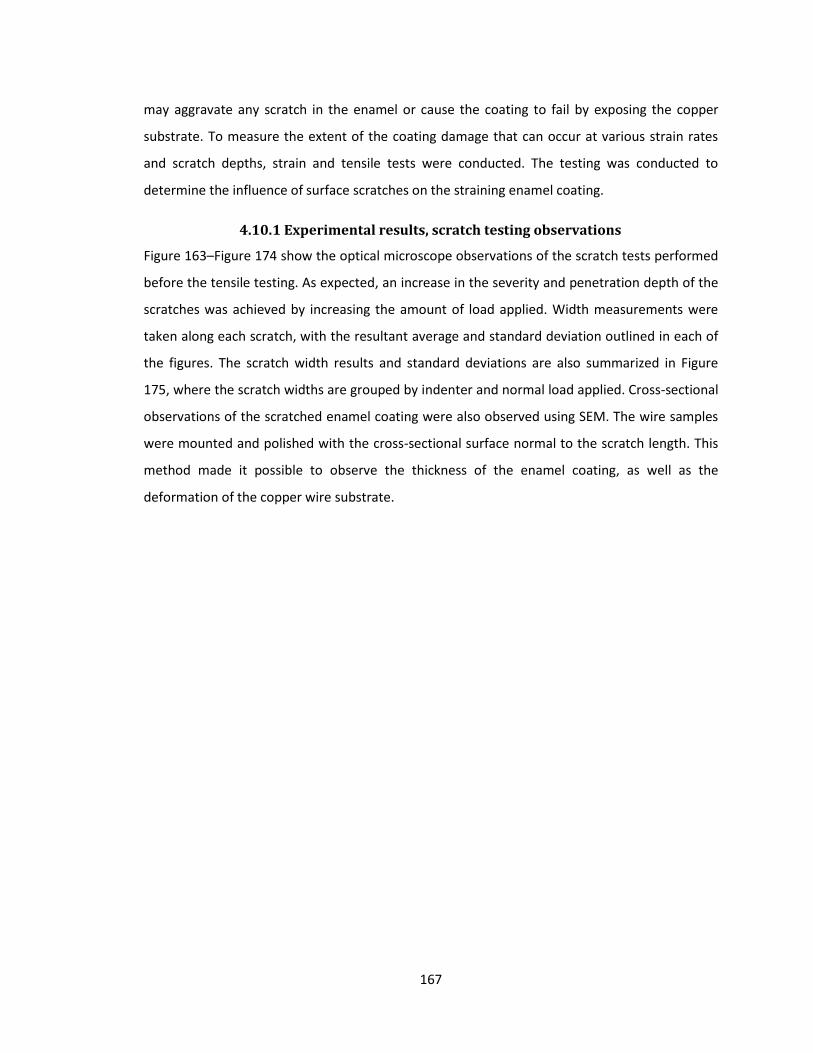
167
may aggravate any scratch in the enamel or cause the coating to fail by exposing the copper
substrate. To measure the extent of the coating damage that can occur at various strain rates
and scratch depths, strain and tensile tests were conducted. The testing was conducted to
determine the influence of surface scratches on the straining enamel coating.
4.10.1 Experimental results, scratch testing observations
Figure 163–Figure 174 show the optical microscope observations of the scratch tests performed
before the tensile testing. As expected, an increase in the severity and penetration depth of the
scratches was achieved by increasing the amount of load applied. Width measurements were
taken along each scratch, with the resultant average and standard deviation outlined in each of
the figures. The scratch width results and standard deviations are also summarized in Figure
175, where the scratch widths are grouped by indenter and normal load applied. Cross-sectional
observations of the scratched enamel coating were also observed using SEM. The wire samples
were mounted and polished with the cross-sectional surface normal to the scratch length. This
method made it possible to observe the thickness of the enamel coating, as well as the
deformation of the copper wire substrate.
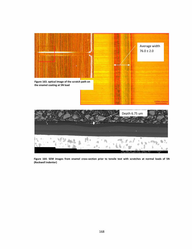
168
Figure 164. SEM images from enamel cross-section prior to tensile test with scratches at normal loads of 5N (Rockwell indenter)
Figure 163. optical image of the scratch path on the enamel coating at 5N load
Average width
76.0 ± 2.0
Depth 6.75 um
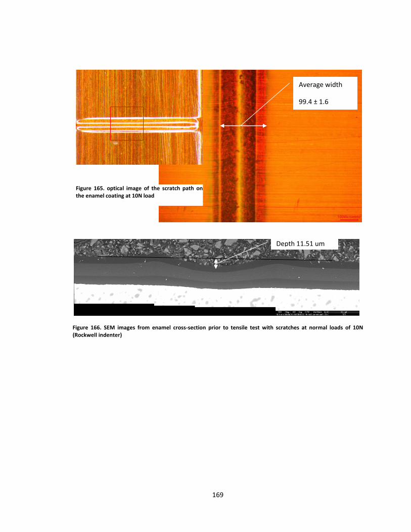
169
Figure 166. SEM images from enamel cross-section prior to tensile test with scratches at normal loads of 10N (Rockwell indenter)
Average width
99.4 ± 1.6
Figure 165. optical image of the scratch path on the enamel coating at 10N load
Depth 11.51 um
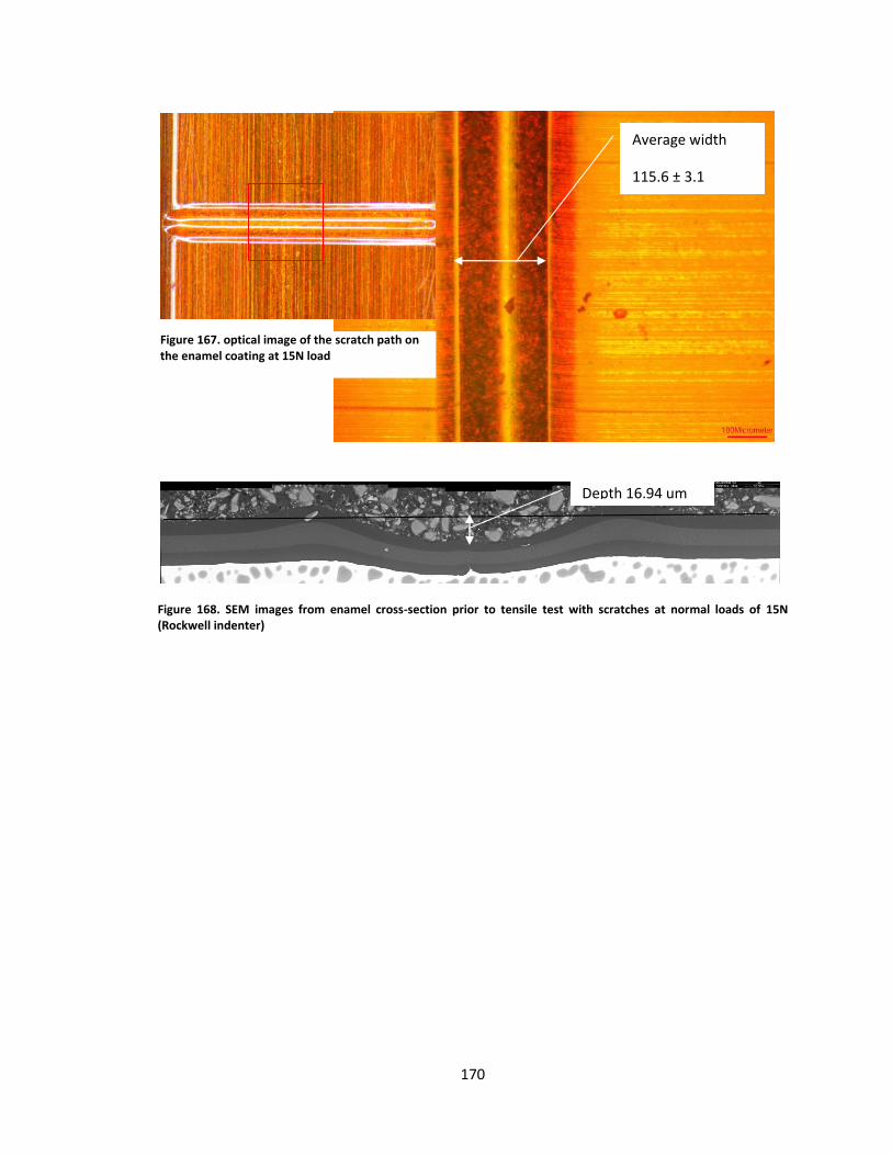
170
Figure 168. SEM images from enamel cross-section prior to tensile test with scratches at normal loads of 15N (Rockwell indenter)
Figure 167. optical image of the scratch path on the enamel coating at 15N load
Average width
115.6 ± 3.1
Depth 16.94 um
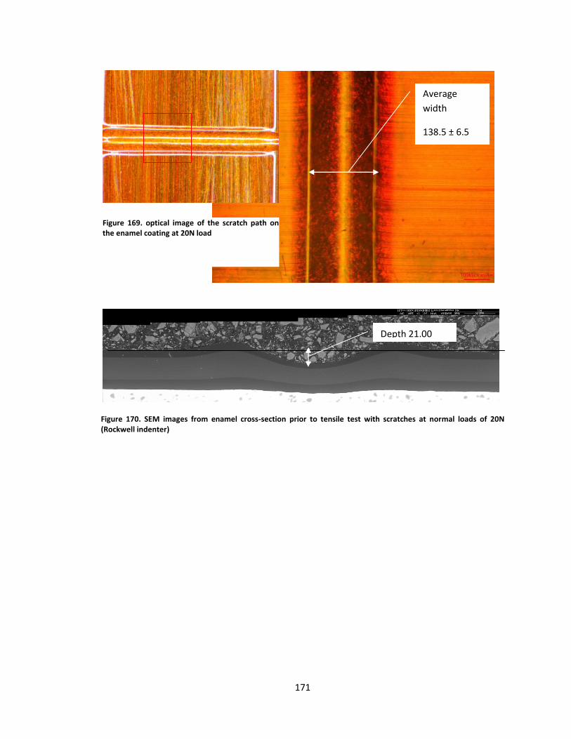
171
Figure 170. SEM images from enamel cross-section prior to tensile test with scratches at normal loads of 20N (Rockwell indenter)
Average
width
138.5 ± 6.5
Figure 169. optical image of the scratch path on the enamel coating at 20N load
Depth 21.00
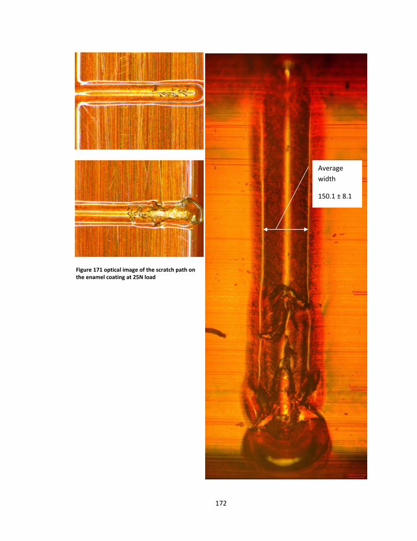
172
Figure 171 optical image of the scratch path on the enamel coating at 25N load
Average
width
150.1 ± 8.1
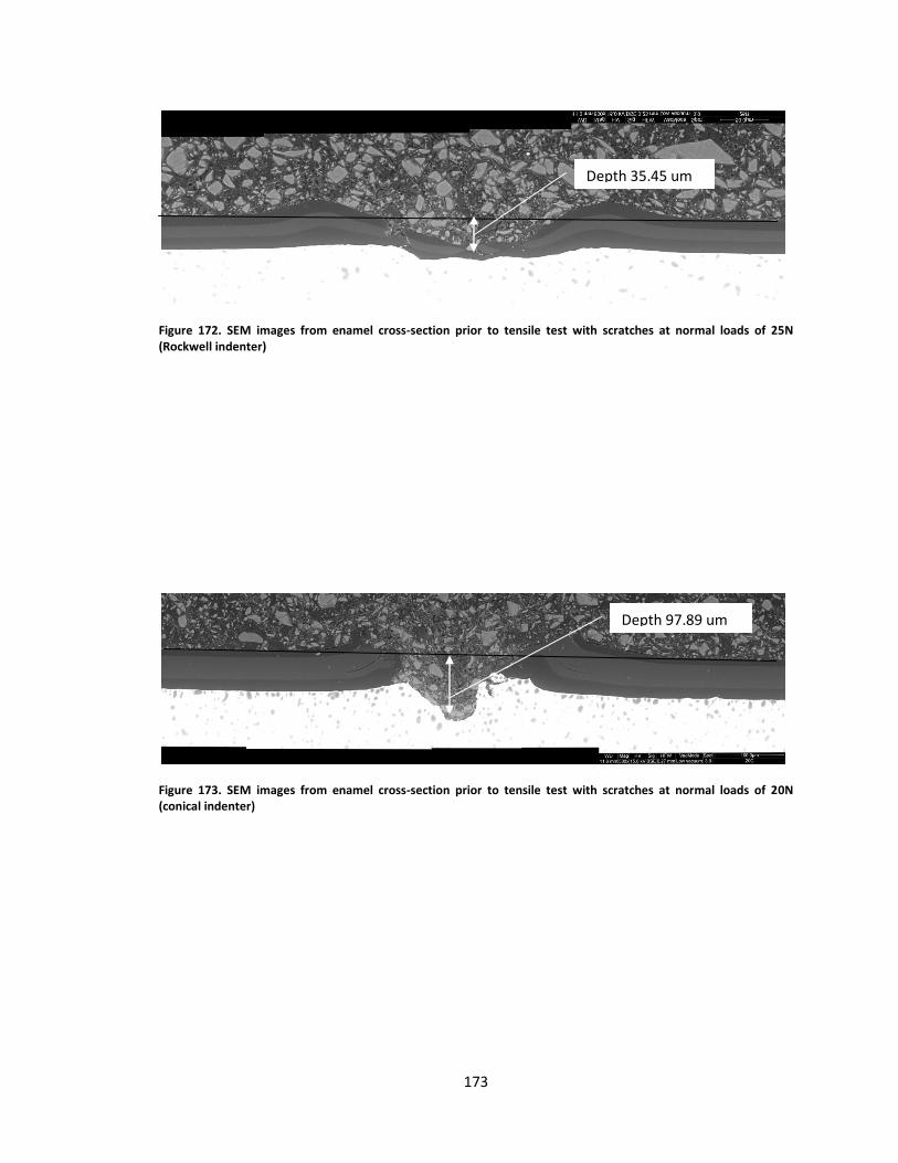
173
Figure 172. SEM images from enamel cross-section prior to tensile test with scratches at normal loads of 25N (Rockwell indenter)
Figure 173. SEM images from enamel cross-section prior to tensile test with scratches at normal loads of 20N (conical indenter)
Depth 35.45 um
Depth 97.89 um

174
Figure 174. optical image of the scratch path on the enamel coating at 20N load (90° cone steel indenter)
Average width
99.9 ± 4.9
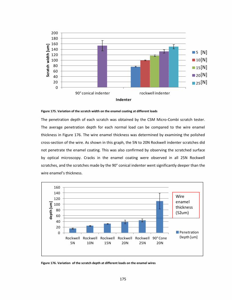
175
Figure 175. Variation of the scratch width on the enamel coating at different loads
The penetration depth of each scratch was obtained by the CSM Micro-Combi scratch tester.
The average penetration depth for each normal load can be compared to the wire enamel
thickness in Figure 176. The wire enamel thickness was determined by examining the polished
cross-section of the wire. As shown in this graph, the 5N to 20N Rockwell indenter scratches did
not penetrate the enamel coating. This was also confirmed by observing the scratched surface
by optical microscopy. Cracks in the enamel coating were observed in all 25N Rockwell
scratches, and the scratches made by the 90° conical indenter went significantly deeper than the
wire enamel’s thickness.
Figure 176. Variation of the scratch depth at different loads on the enamel wires
0
20
40
60
80
100
120
140
160
180
200
90° conical indenter rockwell indenter
Scra
tch
wid
th [
um
]
Indenter
Pre test Scratch width per normal load
5
10
15
20
25
0
20
40
60
80
100
120
140
160
Rockwell 5N
Rockwell 10N
Rockwell 15N
Rockwell 20N
Rockwell 25N
90° Cone 20N
de
pth
[um
]
Penetration Depth [um]
Penetration Depth [um]
Wire enamel thickness (52um)
[N]
[N]
[N]
[N]
[N]
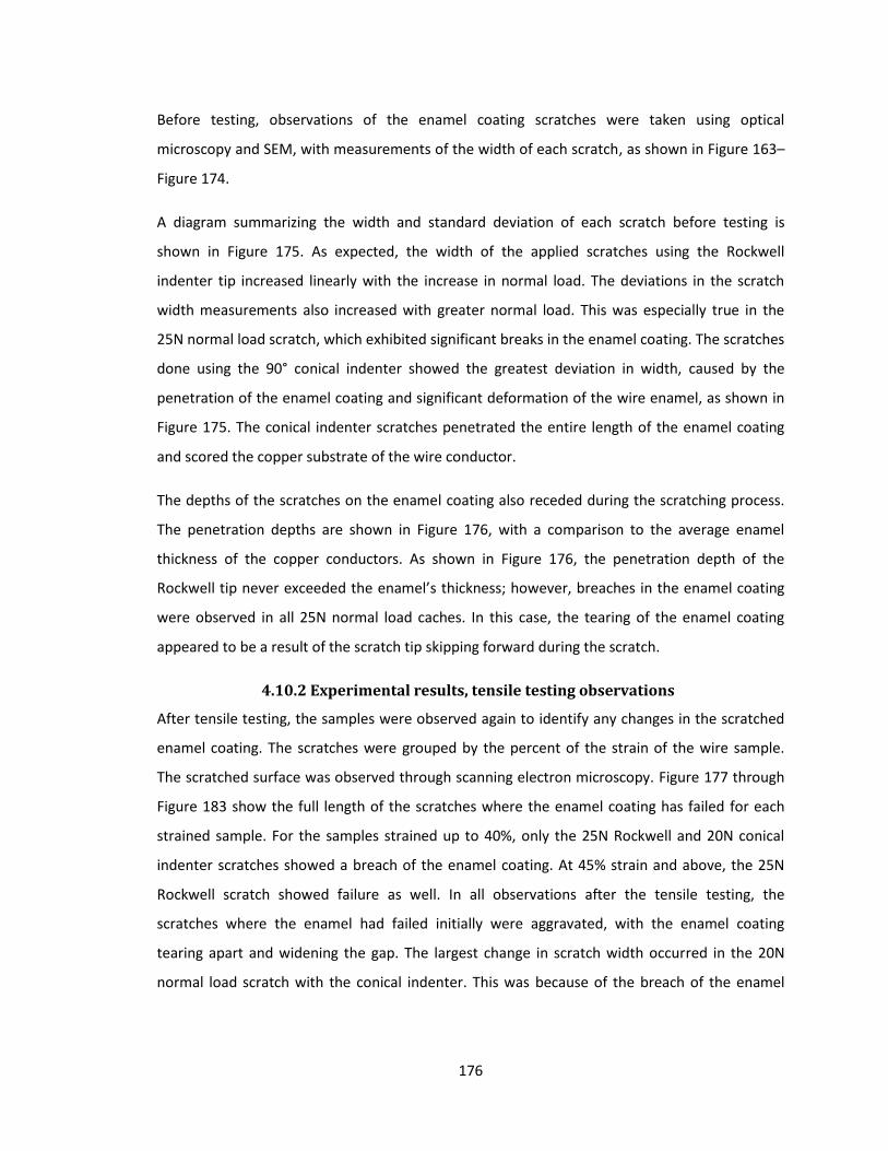
176
Before testing, observations of the enamel coating scratches were taken using optical
microscopy and SEM, with measurements of the width of each scratch, as shown in Figure 163–
Figure 174.
A diagram summarizing the width and standard deviation of each scratch before testing is
shown in Figure 175. As expected, the width of the applied scratches using the Rockwell
indenter tip increased linearly with the increase in normal load. The deviations in the scratch
width measurements also increased with greater normal load. This was especially true in the
25N normal load scratch, which exhibited significant breaks in the enamel coating. The scratches
done using the 90° conical indenter showed the greatest deviation in width, caused by the
penetration of the enamel coating and significant deformation of the wire enamel, as shown in
Figure 175. The conical indenter scratches penetrated the entire length of the enamel coating
and scored the copper substrate of the wire conductor.
The depths of the scratches on the enamel coating also receded during the scratching process.
The penetration depths are shown in Figure 176, with a comparison to the average enamel
thickness of the copper conductors. As shown in Figure 176, the penetration depth of the
Rockwell tip never exceeded the enamel’s thickness; however, breaches in the enamel coating
were observed in all 25N normal load caches. In this case, the tearing of the enamel coating
appeared to be a result of the scratch tip skipping forward during the scratch.
4.10.2 Experimental results, tensile testing observations
After tensile testing, the samples were observed again to identify any changes in the scratched
enamel coating. The scratches were grouped by the percent of the strain of the wire sample.
The scratched surface was observed through scanning electron microscopy. Figure 177 through
Figure 183 show the full length of the scratches where the enamel coating has failed for each
strained sample. For the samples strained up to 40%, only the 25N Rockwell and 20N conical
indenter scratches showed a breach of the enamel coating. At 45% strain and above, the 25N
Rockwell scratch showed failure as well. In all observations after the tensile testing, the
scratches where the enamel had failed initially were aggravated, with the enamel coating
tearing apart and widening the gap. The largest change in scratch width occurred in the 20N
normal load scratch with the conical indenter. This was because of the breach of the enamel
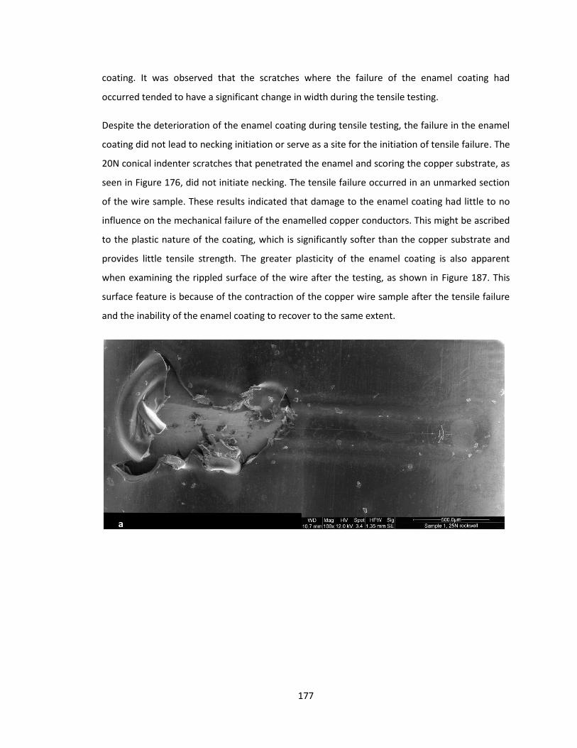
177
coating. It was observed that the scratches where the failure of the enamel coating had
occurred tended to have a significant change in width during the tensile testing.
Despite the deterioration of the enamel coating during tensile testing, the failure in the enamel
coating did not lead to necking initiation or serve as a site for the initiation of tensile failure. The
20N conical indenter scratches that penetrated the enamel and scoring the copper substrate, as
seen in Figure 176, did not initiate necking. The tensile failure occurred in an unmarked section
of the wire sample. These results indicated that damage to the enamel coating had little to no
influence on the mechanical failure of the enamelled copper conductors. This might be ascribed
to the plastic nature of the coating, which is significantly softer than the copper substrate and
provides little tensile strength. The greater plasticity of the enamel coating is also apparent
when examining the rippled surface of the wire after the testing, as shown in Figure 187. This
surface feature is because of the contraction of the copper wire sample after the tensile failure
and the inability of the enamel coating to recover to the same extent.
a
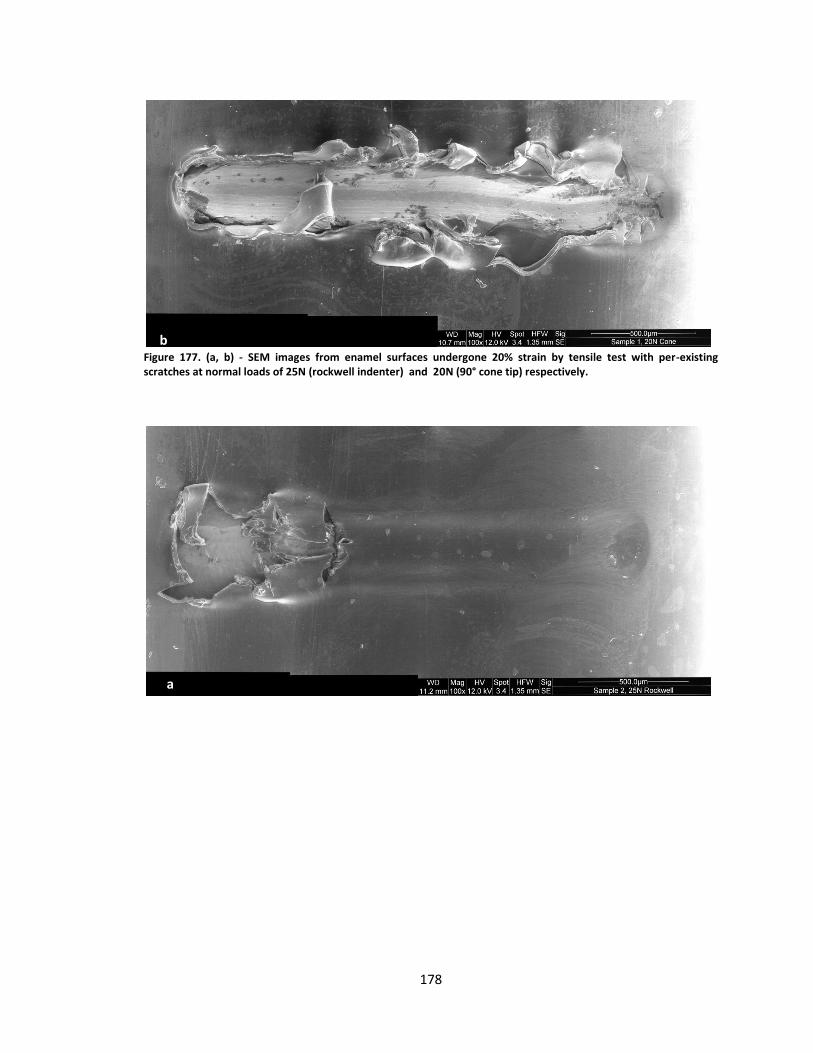
178
Figure 177. (a, b) - SEM images from enamel surfaces undergone 20% strain by tensile test with per-existing scratches at normal loads of 25N (rockwell indenter) and 20N (90° cone tip) respectively.
b
a
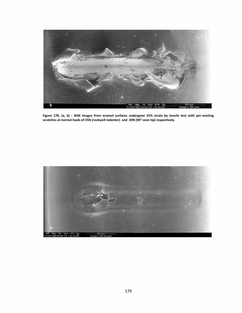
179
Figure 178. (a, b) - SEM images from enamel surfaces undergone 25% strain by tensile test with per-existing scratches at normal loads of 25N (rockwell indenter) and 20N (90° cone tip) respectively.
b
a
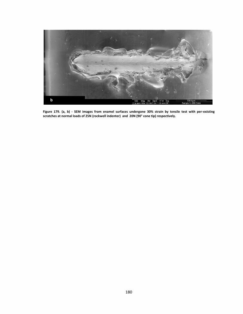
180
Figure 179. (a, b) - SEM images from enamel surfaces undergone 30% strain by tensile test with per-existing scratches at normal loads of 25N (rockwell indenter) and 20N (90° cone tip) respectively.
b
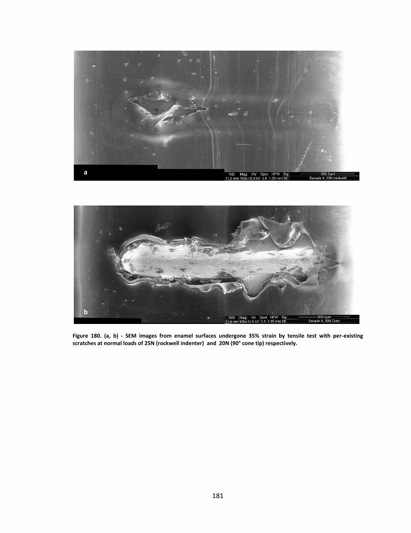
181
Figure 180. (a, b) - SEM images from enamel surfaces undergone 35% strain by tensile test with per-existing scratches at normal loads of 25N (rockwell indenter) and 20N (90° cone tip) respectively.
a
b
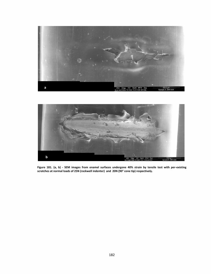
182
Figure 181. (a, b) - SEM images from enamel surfaces undergone 40% strain by tensile test with per-existing scratches at normal loads of 25N (rockwell indenter) and 20N (90° cone tip) respectively.
a
b
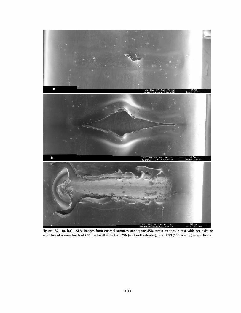
183
Figure 182. (a, b,c) - SEM images from enamel surfaces undergone 45% strain by tensile test with per-existing scratches at normal loads of 20N (rockwell indenter), 25N (rockwell indenter), and 20N (90° cone tip) respectively.
a
b
c
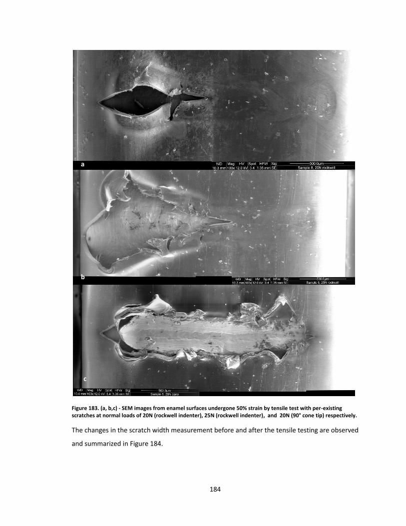
184
Figure 183. (a, b,c) - SEM images from enamel surfaces undergone 50% strain by tensile test with per-existing scratches at normal loads of 20N (rockwell indenter), 25N (rockwell indenter), and 20N (90° cone tip) respectively.
The changes in the scratch width measurement before and after the tensile testing are observed
and summarized in Figure 184.
a
b
c
c
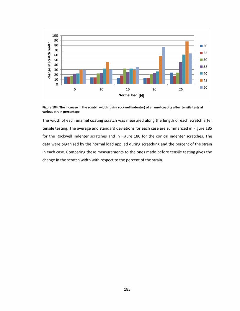
185
Figure 184. The increase in the scratch width (using rockwell indenter) of enamel coating after tensile tests at various strain percentage
The width of each enamel coating scratch was measured along the length of each scratch after
tensile testing. The average and standard deviations for each case are summarized in Figure 185
for the Rockwell indenter scratches and in Figure 186 for the conical indenter scratches. The
data were organized by the normal load applied during scratching and the percent of the strain
in each case. Comparing these measurements to the ones made before tensile testing gives the
change in the scratch width with respect to the percent of the strain.
0
10
20
30
40
50
60
70
80
90
100
5 10 15 20 25
chan
ge i
n s
crat
ch w
idth
Normal load
Change in scratch width rockwell indenter
20
25
30
35
40
45
50
[N]
[N]
[N]
[N]
[N]
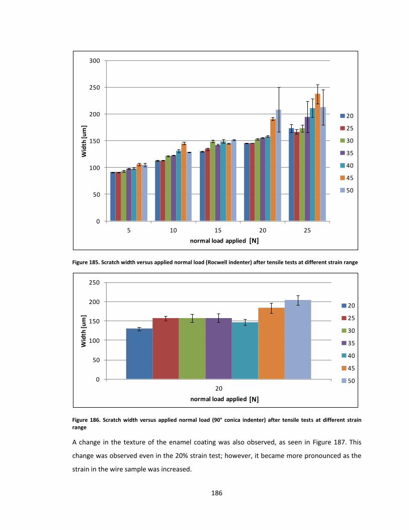
186
Figure 185. Scratch width versus applied normal load (Rocwell indenter) after tensile tests at different strain range
Figure 186. Scratch width versus applied normal load (90° conica indenter) after tensile tests at different strain range
A change in the texture of the enamel coating was also observed, as seen in Figure 187. This
change was observed even in the 20% strain test; however, it became more pronounced as the
strain in the wire sample was increased.
0
50
100
150
200
250
300
5 10 15 20 25
Wid
th [u
m]
normal load applied
Post test Scratch Width per tensile test strain
20
25
30
35
40
45
50
0
50
100
150
200
250
20
Wid
th [u
m]
normal load applied
Post test Scratch Width 90° conical indenter
20
25
30
35
40
45
50
[N]
[N]
[N]
[N]
[N]
[N]
[N]
[N]
[N]
[N]
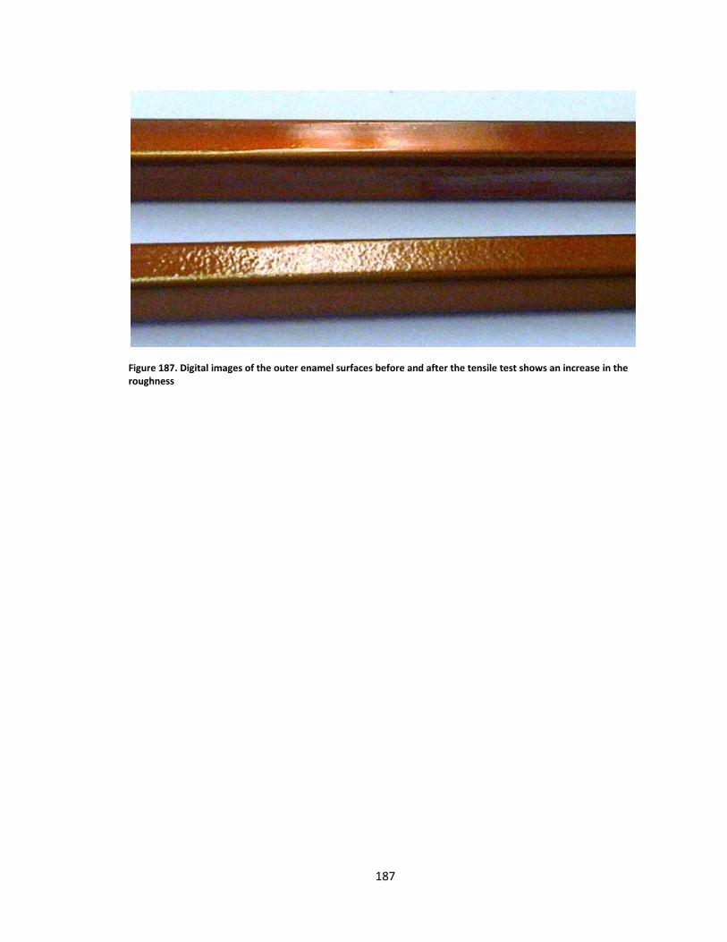
187
Figure 187. Digital images of the outer enamel surfaces before and after the tensile test shows an increase in the roughness
188
5: Discussion
5.1 Magnet wire friction coefficient fluctuation at reciprocating
friction test
Reciprocating ball-on-flat friction testing of the enamel wire samples was done to determine the
reaction of the wire enamel coating to repeated reciprocating passes by a rounded steel
counterface. When compared to the normal pressure exerted on the enamel coating during die
bending (500MPa), these tests are significantly lower pressure, at 188MPa and 309MPa for the
5N and 10N normal load, respectively. When examining the COF result obtained from these two
tests, a significantly lower initial COF was observed with the initial passes of the counterface,
with the COF gradually increasing with the progression of the test and then reaching a constant
level. This effect is easily observed in both Figure 94 and Figure 103.
In contrast to the initial stages of the test, the tangential force and COF recorded in the last
reciprocating passes of the 5N test, shown in Figure 98 to Figure 99, show an increase in both.
The general trend of the COF throughout the test is one of general increase, with the COF having
an average of 0.0534 with a standard deviation of 0.0025 in the final passes of 5N normal load
test. This increase in COF during the test was approximately 0.011, with most of the change
occurring in the first 100 seconds of testing.
Observations of the wear track in the magnet wire show noticeable deformation of the wire
substrate, with little to no surface damage on the enamel coating. The extent and rate of wire
substrate deformation are confirmed also by the vertical tracking of the ball-bearing
counterface, which shows depression of the surface, especially during the initial passes. These
results show that the COF, throughout friction testing, aligns with the deformation of the
enamelled surface. This trend is also observed when comparing the 5N and 10N normal load
tests. It can be expected from the spherical shape of the counterface that at 10N normal load,
the counterface would exert significantly more pressure and cause more pronounced plastic
deformation on the enamel coating.
The rate of deformation of the wire substrate throughout the testing process can be attributed
to the material properties of the copper wire. Being a relatively soft and malleable material
when annealled, copper’s hardness can significantly increase when deformed. This is because of
189
the dislocations amassed in the copper microstructure. The small grain size of wire grade
copper, which has been drawn into a wire, increases this effect by providing less space for the
deformations to glide within the grain. This combination of factors results in the copper wire
substrate deforming significantly in the initial stages of the test, and then staying constant
during its remainder.
5.2 Sample Tension, Strain Control and Calculation
During friction testing of the wire samples, it is crucial for the wire-forming simulator machine to
be able to impart tension on the wire sample to better approximate the conditions of the
formation of the wire during die formation. Tension in the wire sample is also crucial when
friction testing at a particular forming angle on the wire sample, because the tension helps the
wire conform to the radius of the forming roller. The strain of the wire sample is controlled by
simultaneously stretching the wire from both sides through the retraction of the two linear
actuators before testing. Tension is also constantly monitored and recorded during both the
initial tensioning of the enamel wire and the friction testing. The strain of the wire sample is
controlled by determining the bending angle and radius of curvature at which the sample is
tested. To bend the wire samples at a particular angle, each actuator arm can be positioned at
intervals of 5° — from 0° to 90° — on each side, as shown by the mounting holes in the front
plate in Figure 64. To control the amount of deformation of the wire, the wire sample was
wrapped around rolling cylinders with diameters ranging from 6 mm to 48 mm. The position of
the forming roller is shown in Figure 65. While using the 6 mm diameter roller to prevent any
deformation in the roller during testing, two additional support rollers were installed
underneath the forming roller, as shown in Figure 65.
Variation in strain of the wire surface can, thus, be controlled by the wire-bending simulator
machine. However, the exact strain vale at a particular bending angle, while using a certain
radius bending roller, cannot be measured by the machine during testing. As a result, the strain
of the wire sample during testing was determined by finite element modeling of the friction-
measuring process. The finite element model used to determine the strain values simulated the
bending and rolling of the friction-measurement process. The finite element model used was
developed and run by GM R&D. This FEA model was validated by comparing its predicted strain
values to those measured during die formation of the enameled wire. The strain of the wire
during die bedding was accurately measured by observing the deformation of the wire during
190
the bending procedure. By staining of one side of the wire enamel surface with spots of white
paint (which can be detected and tracked by a high-speed camera during the die’s bending the
wire), the relative position of each of the white spots could be tracked during deformation. A
computer program was then used to determine the change in distance between the individual
spots and, based on these calculations, the actual strain of the wire sample was determined.
Because in both die bending and friction testing the magnet wire the sample was bent within a
flat plane, it could be reasonably assumed that the strain of the wire was symmetrical to the
plane along the centre of the wire. As a result, observing the strain on only one side of the wire
profile was sufficient to determine the strain of the entire sample. Thus, the finite element
model was validated by comparing the predicted strain values of the wire generated during
simulated die forming to the actual strain values detected by marking the enamel surface.
Using this model, the strain of the contact surface between the wire sample and the friction
counterface was determined for specific diameter rollers and bending angles. These wire strain
values are used as bases for measuring the strain of the wire sample during testing. To achieve
intermediate values of strain, additional uniform strain was applied on the wires during testing
by elongating the wire sample before testing. Because of the overall length of the wire samples
and the fine control of the linear actuator, a precise level of strain can be applied to the wire
enamel surface.
5.3 Effect of counterface on coefficient of friction
The friction coefficient of two materials depends significantly both on the conditions at which
the two materials come into contact with each other and the composition of the two surfaces.
In addition to changes in the wire sample, changes in the counterface material were also
investigated. Friction between the diamond-like carbon (DLC) coatings TB41 and TB40 and the
wire enamel were tested to determine if there was any observable change in the COF. The
purpose of these tests was to determine if DLC, when added to the tools and forming dies,
would be beneficial in reducing friction during wire shaping. Since in this test all additional
parameters, such as counterface dimensions, testing speed, normal load and wire sample
condition, were kept constant, the friction coefficient results, summarized in Figure 136,
highlight the influence of the two DLC only. As shown by these results, the addition of DLC,
when compared to uncoated 52100 Steel High Carbon Anti-Friction ball bearings, slightly
increases the friction coefficient between it and the wire enamel. This slight increase in COF was
191
observed only in the TB40DLC and not in the TB41DLC (which is especially designed for reduced
friction). Because of the significant difference in hardness of the enamelled wire surface and the
counterface tested, similar deformation patterns on the enamel wire were observed for both
coated and uncoated counterfaces. The short duration of the friction test, having only one pass
each time over the wire sample, prevents debris formation from being a factor in the friction
coefficient measurement. A difference in composition between the two DLCs would account for
the light change adhesion, resulting in a higher COF. In both cases, the DLC is applied through
the use of a physical vapor deposition, with TB40DLC as a non-hydrogenated form of DLC, and
TB41DLC is hydrogenated. Both DLCs have a tungsten metal addition with the chemical formula
of a-C:H:W and a-C:H:W + a-C:H for TB40DLC and TB41DLC, respectively [31].
Based on these results, there appears to be no significant change in friction forces resulting from
the coating of the counterface surface using DLC TB41, and a 10% increase in COF when using
DLC TB40.
5.4 Effect of speed on coefficient of friction
Speed as a factor in the friction coefficient of enamel wire was tested between 1 and 20mm/s.
The effect of speed was examined with strain in the sample wire. This range of speed was
chosen to better represent the speeds utilized during die formation of the wire in motor coil
manufacturing. As a result, the counterface utilized in this series of tests was chosen to match
both the material and surface conditions of the forming die. The effects of speed on the COF
between these two materials was tested at 1 mm/s, 5 mm/s, 10 mm/s, 15 mm/s and 20 mm/s.
The resulting average COF is shown in Figure 148 to Figure 151, with the values summarized in
Table XV.
The general trend observed in these test results is a slight increase in COF with increased testing
speed. This trend, however, is not consistent in all cases of sample surface strain. As seen in
Figure 148, this trend generally holds true for the 2%, 5% and 15% strained samples. In these
cases, the COF can be observed increasing significantly between the 1 mm/s and 5 mm/s.
Beyond the initial low-speed tests at these strains, the average COF stabilizes. An exception to
this trend is the 5% strain series of tests, where the largest increase in COF is between the 15
mm/s and 20 mm/s trials. The trend of increasing COF with testing speed does not hold true for
all tests, however. For the 21% strain and 10%, for example, the maximum coefficient of friction
192
is detected at 10 mm/s and 15 mm/s test, respectively. In all cases, however, the lowest
coefficient of friction is detected at the lowest testing speed of 1 mm/s.
The general trends and fluctuations of the average COF, based on sample testing speed, can be
visualized easier using the 3-D representations of the average values shown in Figure 149 to
Figure 151. Using these figures, it is also easy to compare the overall influence of testing speed
with that sample surface strain. As it is shown in these figures, speed plays a weaker role in
influencing COF when compared to stain. The trends of testing speed provide less overall change
in COF and do not apply to all strain cases.
The observed pattern of increased COF at higher speeds can be attributed to the slight
viscoelastic properties of the coating. As stated in the results section, when testing using a flat
4140 steel counterface, there was no significant deformation of the copper wire substrate. The
extent of the sample deformation is limited to the ironing of the enamel coating.
5.5 Effect of surface strain on coefficient of friction
The strain of the enamel coating during friction testing was determined, as mentioned
previously in Section 3, by applying a finite element analysis model. The contact surface strain of
the wire sample was controlled through the use of wire-bending simulator machine. Through
the degree of bending of the wire sample, the radius of curvature of the bending roller and the
initial tension of the sample, the wire strain was controlled and fluctuated during testing from
2% to 21% strain.
The study of the effect of the wire deformation on the COF aimed to accurately determine the
interaction between the surfaces of the wire sample with the fuming die during electric motor
coils manufacturing. The results of the twenty five tests conducted at varying sample strains and
speeds are summarized in Figure 149 to Figure 151, with the average listed in Table XV. As when
considering the influence of testing speed on the average COF, when looking at surface strain,
general trends appear that fluctuate at varying sample testing speeds. The effect of sample
surface deformation is best illustrated in Figure 147, where the average COF and standard
deviation are graphed against sample strain for each testing speed.
The general trend of the COF observed is a decline in value with an increase in sample surface
strain. This pattern is observed for all speeds tested, as shown in Figure 144 and Figure 147. The
193
lowest values of the COF recorded are for tests conducted at a high strain of 21%. This can be
observed in Figure 147, where this trend is best highlighted. The graph also shows that the
results of these high strain tests seem to have a reduced fluctuation as a result of speed. This is
true when considering both the individual COF values along the sample, depicted in Figure 147,
and the overall average for each run. These results appear to indicate the limited influence of
testing speed at these high strains. When considering the results of the low strain friction tests,
however, a greater fluctuation in the COF is observed at varying testing speeds.
Although the general trend of decreased COF at increased sample strain is true for most friction
tests where strain was controlled, it is much less pronounced at low strains between 2% and
10% (rather than between 10% and 21%). In some tests, such as the one conducted at 1 mm/s
and 5mm/s, for example, the COF increases as the strain increases from 2% to 5%. At these low
strains, testing speed seems to play a much more decisive role than strain, as shown in Figure
150. As a result, the influence of sample strain on the COF appears to be much more influential
at higher levels of strain.
5.6 Enamel coating damage threshold in magnet wire
To determine the resilience of an enamel coating to external abrasion damage and to determine
the behaviour or extent of the enamel damage to wire strain, 10 wire samples were scratch
tested and tensile tested, as outlined above. The results and observations obtained from this
series of tests provide a reliable measure of the extent of damage that the enamel can sustain
before a breach of the enamel coating is detected. In these tests, the enamel coating was
considered to have failed when a gap was observed through the enamel and into the copper
substrate.
Initial observations of the pre-tensile tested scratch results of the enamel coating indicate a
significant dependence of the extent of wire damage on the load and contact shape of the
scratching head. In this series of tests, a Rockwell indenter and a 90 degree conical indenter
were used to do the scratches on the wire surface. It was observed that failure of the enamel
coating when using the Rockwell indenter, which consists of a round spherical tip, occurred only
at high loads of 25N normal load. Measuring the scratch width to determine the contact area
applied, the pressure applied in this case can be calculated to reach 1.42 GPa. At this pressure,
the wire enamel consistently failed, as shown in Figure 171 and Figure 172. At these pressures,
194
the enamel appeared clearly cracked and, in several cases, the copper substrate was clearly
visible. At a 20N normal load, however, no breach in the enamel coating was detected and,
using the same procedure, the normal pressure on the enamel coating can be calculated at
1.33GPa. When compared to scratches made on the enamel surface using the 90 degree conical
indenter, it was found that failure of the enamel coating would occur at normal loads as low as
3N. As for the Rockwell indenter, it was found that scratch width and penetration depth were
proportional to the applied normal load, as shown in Figure 175 and Figure 176. These types of
results are to be expected for, as shown in previous studies, for polymer materials, there is
significant dependence between the sharpness, or conical angle of the indenter, and the type of
reaction achieved by the scratch. This is shown in Section 2.8 maps of several polymers are
discussed.
After tensile testing, however, it was possible to observe the reaction of the damaged wire
enamel under varying degrees of tensile strain. The SEM observations of the post-strain wire
enamel scratches can be seen in Figure 177 to Figure 183. From these figures and the graph in
Figure 185 outlining the scratch width post-tensile test, it can be seen that the scratched enamel
coating suffered little degradation at low strains. At strains from 20% to 40%, new enamel
failure did not develop. At higher strains, such as 45%, failure of the more severe scratch sites
was observed. Also, any spots where the enamel had been previously breached suffered
significant widening of the enamel gap. These results indicate that severe indentation and strain
of the enamel coating are required for defects of the enamel coating to be generated, which
would lead to shortening the motor coil.
195
6: Summary and Conclusions
This section summarizes the principal results presented in chapters 4 and 5.
A custom-made machine was designed and built with required features to simulate wire
bending forming process. Unique capabilities of this machine include: a range of 0 to 356 N in
normal load, 0 to 67 N in friction force measurement, 0.5 to 20 mm/s in wire speed, and forming
angle of 0 to 90°. Maximum tensile load capacity is 3 kN, well beyond the tensile strength of the
enamel insulated copper wires used in this study. Features such as programmable motion
control and high-frequency data acquisition ensure that the COF, normal force and wire tension
can be measured reliably throughout testing. Additional features such as an interchangeable
counterface and a roller-forming radius make it possible for the wire-forming simulator to be
flexible in adapting to any wire-forming conditions. The experiments performed on a straight,
tensioned wire sample using a 4140 steel block as a counterface (with flat on flat configuration)
at 20mm/s showed an average COF of 0.160 with a standard deviation of 0.030. This value was
used as a base value to determine the effect of counterface, tensile strain, bending angle during
wire forming process on COF. The highlights of these results are listed below:
The 10% and 20% elongated wire sample showed a 31% and 25% decrease in the COF from a
base value. This indicates that sample strain before contact is a major factor in reducing the
COF. This change in COF can be attributed to the deformation of the enamel surface itself.
The speeds of 1 to 20 mm/s with the interval of 5 mm/s resulted in change in COF from 0.11 for
1 mm/s to 0.19 for 20 mm/s. The COF measured at various strains and contact speeds, provides
good basis for building of further FEA simulations of the die bending process. The COF results
also serve as a guide line for die movement speed during the wire bending process. These
results can help in identifying regions in the wire shape, such as sections of low strain and high
relative movement, where the friction force between the die and enamel may result in the
generation of defects.
The two major patterns observed are a positive correlation between the COF and testing speed
and a negative correlation between the COF and sample surface strain. Testing speed appears to
have less influence on the COF at higher strains.
196
COF decreased by 48%, when the wire was cleaned using a glassware cleaning solution, once
prior to testing, with an equal decrease in the standard deviation of the average COF value. This
COF change indicates that the lubrication and surface treatment of the wire enamel plays a
crucial role in the interaction between the enamel coating and the bending die surface. Cleaning
or pre-treatment of wire enamel surface with lubricant solvents might significantly reduce COF
during die bending.
The hydrogenated DLC coating had no significant effect on the nominal COF, whereas non-
hydrogenated DLC showed a 9.5% increase in the COF. As a result modification of the bending
dies by the application of DLC coatings would not give additional advantage to the bending
process by reducing the COF during bending.
Novel pressure-distributing tensile testing grips were used to avoid stress concentration of the
enameled magnet wire and prevent failure at grips. The ultimate tensile strength of the
enameled wire was found to be 215 MPa, with the Strength at failure of 428 MPa, and yield
strength 123MPa. The enamel coating maintained good adhesion to the wire substrate at low to
medium strains (0%-35%), and developed gaps in the coating along the corners of the wire at
higher strains. Delaminating of the enamel was observed at the onset of necking.
The threshold of wire enamel damage was determined through scratch testing of wire surface
prior to tensile testing. The main findings are listed as follow:
The insulating polymer coating failed under the scratch tests at severe loading conditions (20N
load using a Rockwell indenter and at 5N load using a 90° conical steel indenter). The integrity of
all three layers was maintained even at indentation depths equal to 70% of the total enamel
thickness.
The pre-existing surface scratches (at loads less than the critical loads) widened at the low (e.g.
20%) or moderate strain (e.g. 35%) during tensile testing.
The enamel coatings that failed during the scratch tests (e.g., 20N normal load using a Rockwell
tip) showed significant damage to the coating after the tensile testing at a strain level of 45%
and higher. The damage included tearing of the enamel surface over the scratch area, cracking
of the enamel, and exposure of the copper substrate. These results indicate that if defects,

197
tears, or splits are present in the enamel coating prior to bending, these discontinuities will be
severally aggravated during bending, even at low strain percentages.
198
6.1 Suggestions for future research
The current study concentrated on the characteristics and behaviour of copper enameled
magnet wire. The investigation of the wire coefficient of friction during die bending necessitated
the design and fabrication of a wire bending simulator machine. Future study of magnet wire
interaction during die forming procedure and friction characteristics of wire enamel can be
achieved by research in the following areas:
1) Investigation of additional material or varying wire gage: investigation of the effect of
strain and testing speed on COF can be conducted on magnet wire samples of varying
material composition and cross-sectional dimensions. Aluminum wires can be used
instead of copper conductors. This study would determine if the observed trends in COF
are subject to wire composition or wire size.
2) Counterface change: additional counterfaces can be tested, ranging from varying steel
grade or material composition, to surface treatments of existing counterface material.
Varying surface roughness on the counterface can also be tested in order to determine
its influence on the COF. This type of testing would be ideal in determining material
composition or surface treatment of the bending die.
3) Lubricating condition: the addition of lubricant at controlled levels during the die
bending procedure can significantly influence the contact mechanism between the
forming die and magnet wire. Investigating the contact characteristics of magnet wire
and forming die under lubricated conditions would serve to innovate the wire bending
procedure. Both dry and wet lubricants can be studied in their effect on the wire COF
199
References
[1] S Ghosh. Working or Operating Principle of DC Motor [Web page]. Online Electrical
Engineering Study Site, 2013 [January 13 cited access date, 2014 access year]. Available
from http://www.electrical4u.com/working-or-operating-principle-of-dc-motor/.
[2] Remly Electric Motors. Inside the HVH™ Hybrid Motor [PDF]. REMY INTERNATIONAL,
2009 [January 13 cited access date, 2014 access year]. Available from
http://www.remyinc.com/docs/102509_WHITE%20PAPER_fin.pdf.
[3] R. Obika, Y. Tatematsu, M. Mesaki, and A. Higashiura, “Development of magnet wire
having excellent windability”, Conference Proceedings: Electrical Insulation Conference
and Electrical Manufacturing and Coil Winding Conference, Cincinnati, OH, pp. 479–483,
1999.
[4] T. J. Murray, “Poly (amide-imides): Wire enamels with excellent thermal and chemical
properties”, Macromolecular Materials and Engineering, vol. 293, no. 5, pp. 350–360,
2008.
[5] W. Tillar Shugg, “Magnet Wire Enamels”, in Handbook of Electrical and Electronic
Insulating Materials, W. Tillar Shugg (Editor), Wiley-IEEE Press, New York, NY, 1995.
[6] F.R. Bohm, “New hydantoin free insulating enamels for rectangular wires”, Conference
Proceedings: Electrical Insulation Conference, and Electrical Manufacturing & Coil
Winding, Rosemont, IL. pp. 203–205, 1997.
[7] S.Susukida. Hitachi Cable,Ltd.Auto Parts Business Strategy [PDF]. Hitachi Cable, 2007
[January 13 cited access date, 2014 access year]. Available from
http://www.hitachi.com/IR-e/library/presentation/070330-3/070330_3.pdf.
[8] L. J. Payette, “The Properties of a Universal Magnet Wire Enamel”, Electrical Insulation
Magazine, IEEE Vol.2 , no. 5, pp. 40–43, 1986.
[9] M. Winkeler,P. D. G. Company, “Magnet Wire Enamels - Which One?”, IEEE Electrical
Insulation Magazine, Vol.7, no. 4, pp. 61–66, 1991.
[10] J. J. Xu, “Improved tough wire”, Conference Proceedings: Electrical Insulation Conference
and Electrical Manufacturing & Coil Winding Conference, Cincinnati, OH, pp. 469–473,
1999.
[11] J. A. Weh, “Repeated Scrape Abrasion Test”, Wire, vol. 16, no. 9, pp. 497–519, 1941.
[12] G.Boockmann, G.Boockmann, H. Niederlauer, K. Boockmann, R. Fichtner, “Innovation for
Magnet Wire Lubrication”, Conference Proceedings: Electrical Insulation Conference, and
Electrical Manufacturing & Coil Winding. Rosemont, IL, pp. 195–201, 1997.
200
[13] R. Iankov, “Finite element simulation of profile rolling of wire”, Journal of Materials
Processing and Technology, vol. 142, no. 2, pp. 355–361, 2003.
[14] R. Garza-garcia, J. S. Rodriguez, S. Peiia-rojas, “AFM and SEM Techniques in Magnet Wire
Manufacturing”, Conference Proceedings: Electrical Insulation Conference and Electrical
Manufacturing & Coil Winding Technology Conference, Indianapolis, IN, pp. 97–100.
2003.
[15] H. Pops, J. Walker, E. Group, F. Wayne, “ORIGINS OF HIGH VOLTAGE CONTINUITY
FAILURES IN ENAMEL COATED COPPER MAGNET WIRE”, Conference Proceedings:
Electrical Electronics Insulation Conference and Electrical Manufacturing & Coil
Winding Conference, Chicago, IL, pp. 457–484, 1993.
[16] E. Wardzińska, P. Penczek, “Polyesterimide resins with built-in polycyclic compounds”,
Journal of Applied Polymer Science, vol. 100, no. 5, pp. 4066–4073, 2006.
[17] D. C. Westervelt, E. J. Croop, “Elongation as a Factor in Evaluating the Thermal Stability or
Enameled Wire”, Power apparatus and systems, part iii. Transactions of the American
institute of electrical engineers, Vol.77, no. 3, pp. 814–817, 1958.
[18] L. J. Berberich T. W. Dakin, “Guiding Principles in the Thermal Evaluation of Electrical
Insulation”, Power apparatus and systems, part iii. Transactions of the American institute
of electrical engineers, Vol.75, no. 3, 1956.
[19] A. M. Bruning, F. J. Campbell, “Aging in wire insulation under multifactor stress”, IEEE
Transactions on Electrical Insulation, vol. 28, no. 5, 1993.
[20] J. F. Dexter, “Thermal Evaluation of Enameled Magnet Wire”, Power apparatus and
systems, part iii. transactions of the american institute of electrical engineers,
Vol.75, no.3, pp. 40–44, 1956.
[21] ANSI/IEEE Std 853 N. Standard, “An American National Standard IEEE Recommended Practice for Voltage-Endurance Testing of Enameled Wire”, IEEE Standards Board, American National Standards Institute, New York, NY, 1985.
[22] M. Spring, “Standard Test Methods for Film-Insulated Magnet Wire”, ASTM international,
Designation: D1676, vol. 03, pp. 1–34, 2011.
[23] B. J. Briscoe, P. D. Evans, E. Pelillo, S. K. Sinha, “Scratching maps for polymers”, Wear, vol.
200, no. 1, pp. 137–147, 1996.
[24] R. Consiglio, N. X. Randall, B. Bellaton, J. Von Stebut, “The nano-scratch tester ( NST ) as a
new tool for assessing the strength of ultrathin hard coatings and the mar resistance of
polymer films”, Thin Solid Films, vol. 332, no. 1, pp. 151–156, 1998.
201
[25] M. Johansson and A. Hult, “Use and interpretation of scratch tests on ductile polymer
coatings”, Progress in Organic Coatings, vol. 46, no.1, pp. 32–48, 2003.
[26] B. Y. Ni, A. Le Faou, “Scratching behaviour of polymer films using blunt spherical styli”,
Jurnal of Material Science, vol. 31, no. 15, pp. 3955–3963, 1996.
[27] P. C. Irwin, “Characterization of Commercial Corona Resistant Magnet Wire Enamels
Using Nanoindentation Techniques”, Conference Proceedings: Electrical Insulation
Conference and Electrical Manufacturing & Coil Winding Technology Conference,
Indianapolis, IN, pp. 105–108, 2003.
[28] B. Briscoe, “Isolated contact stress deformations of polymers: the basis for interpreting
polymer tribology”, Tribology International, vol. 31, no. 1, pp. 121–126, 1998.
[29] a Krupička, M. Johansson, A. Hult, “Use and interpretation of scratch tests on ductile
polymer coatings”, Progress in Organic Coatings, vol. 46, no. 1, pp. 32–48, 2003.
[30] T. Foss, PH and Benjamin, “Electric Motor Manufacturing: Forming of Enameled Wire
Process Sequence Optimization Part 2,” GM Res. Rep. MSR-378, 2011.
[31] Gali, Olufisayo, "The Effect of Sliding Contact Friction on Surface Quality of Aluminum
Sheet Products" (2011). Electronic Theses and Dissertations. Paper 187.
http://scholar.uwindsor.ca/etd/187

202
Appendix A: Wire Bending Machine Operating Manual
Written by: Sama Hussein, Chris Imeson
Directed and edited by: Albion Demiri
10/28/2013
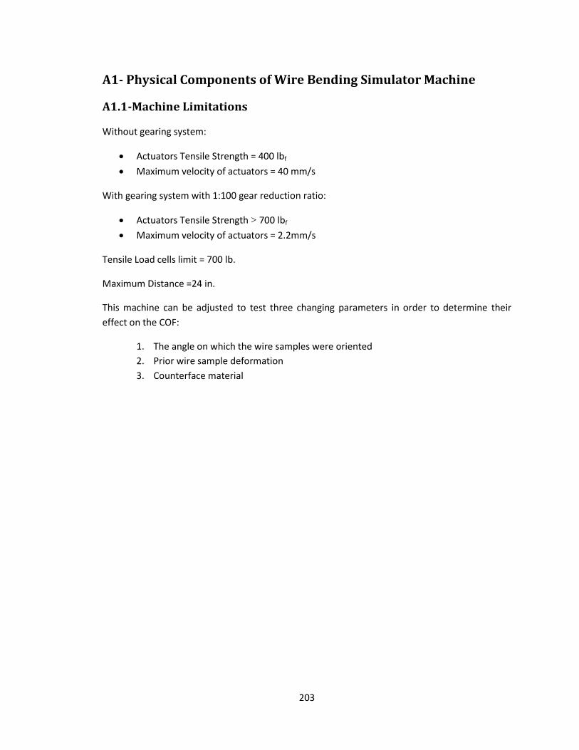
203
A1- Physical Components of Wire Bending Simulator Machine
A1.1-Machine Limitations
Without gearing system:
Actuators Tensile Strength = 400 lbf
Maximum velocity of actuators = 40 mm/s
With gearing system with 1:100 gear reduction ratio:
Actuators Tensile Strength > 700 lbf
Maximum velocity of actuators = 2.2mm/s
Tensile Load cells limit = 700 lb.
Maximum Distance =24 in.
This machine can be adjusted to test three changing parameters in order to determine their
effect on the COF:
1. The angle on which the wire samples were oriented
2. Prior wire sample deformation
3. Counterface material

204
A2-Programming
For general instructions about the program, you can refer to the following links.
MotionWorks IEC Quickstart (Pro Version1.x)
http://www.youtube.com/watch?v=U7Z8D9FD5eo
MotionWorks IEC - SFC Programming Introduction
http://www.youtube.com/watch?v=OzAxCNoGbt0
A2.1-Pre testing
How to operate the machine using MotionWorks?
To run the MotionWorks program:
1. Click on the “Make” icon on the top of the programming toolbar as shown below.
This “Make” tool is used to tell you whether you have any errors or warnings in the program or
not.
Figure 1- Compiling or Making the program
Errors and warnings can be seen at the bottom right hand side of the screen. 0 Errors indicates
that the program is good to go.
Figure 2 - Check for errors and warnings
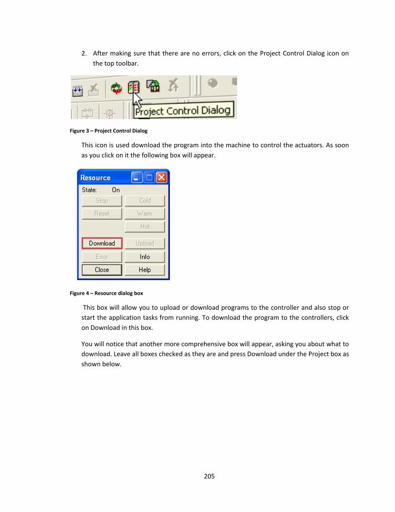
205
2. After making sure that there are no errors, click on the Project Control Dialog icon on
the top toolbar.
Figure 3 – Project Control Dialog
This icon is used download the program into the machine to control the actuators. As soon
as you click on it the following box will appear.
Figure 4 – Resource dialog box
This box will allow you to upload or download programs to the controller and also stop or
start the application tasks from running. To download the program to the controllers, click
on Download in this box.
You will notice that another more comprehensive box will appear, asking you about what to
download. Leave all boxes checked as they are and press Download under the Project box as
shown below.
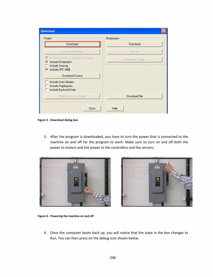
206
Figure 5 - Download dialog box
3. After the program is downloaded, you have to turn the power that is connected to the
machine on and off for the program to work. Make sure to turn on and off both the
power to motors and the power to the controllers and the sensors.
Figure 6 - Powering the machine on and off
4. Once the computer boots back up, you will notice that the state in the box changes to
Run. You can then press on the debug icon shown below.

207
Figure 7 - Machine status check
By turning on the debug icon you will be able to see what happens exactly as your program runs.
Red color indicates the current step and blue indicates off.
Figure 8 - Debug icon
Now you are ready to run your program and start testing.
There are three tasks on which the machine has to go through to perform the testing operation
1. Initialize
2. Preload
3. SFC_Example
All these three tasks can be seen at the right hand side in the Project Tree Window under a
folder that with the name of Logical POUs.
A2.2-Initialize
Figure 9 - Initialize tab
The initialize step initializes variables for the two axes, i.e. the two actuators of the machine, so
that the rest of the program can operate.
Double click on Initialize in the tree as shown below in blue color.
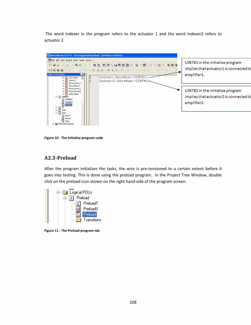
208
The word Indexer in the program refers to the actuator 1 and the word Indexer2 refers to
actuator 2.
Figure 10 - The Initialize program code
A2.3-Preload
After the program initializes the tasks, the wire is pre-tensioned to a certain extent before it
goes into testing. This is done using the preload program. In the Project Tree Window, double
click on the preload icon shown on the right hand side of the program screen.
Figure 11 - The Preload program tab
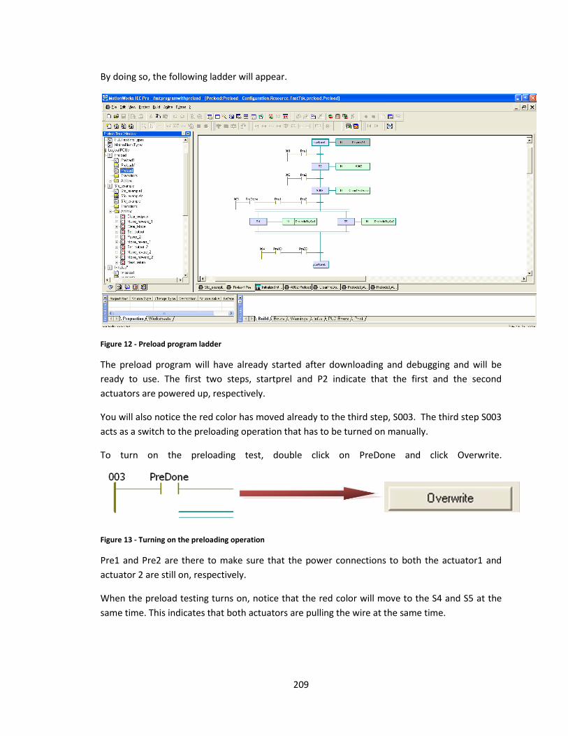
209
By doing so, the following ladder will appear.
Figure 12 - Preload program ladder
The preload program will have already started after downloading and debugging and will be
ready to use. The first two steps, startprel and P2 indicate that the first and the second
actuators are powered up, respectively.
You will also notice the red color has moved already to the third step, S003. The third step S003
acts as a switch to the preloading operation that has to be turned on manually.
To turn on the preloading test, double click on PreDone and click Overwrite.
Figure 13 - Turning on the preloading operation
Pre1 and Pre2 are there to make sure that the power connections to both the actuator1 and
actuator 2 are still on, respectively.
When the preload testing turns on, notice that the red color will move to the S4 and S5 at the
same time. This indicates that both actuators are pulling the wire at the same time.
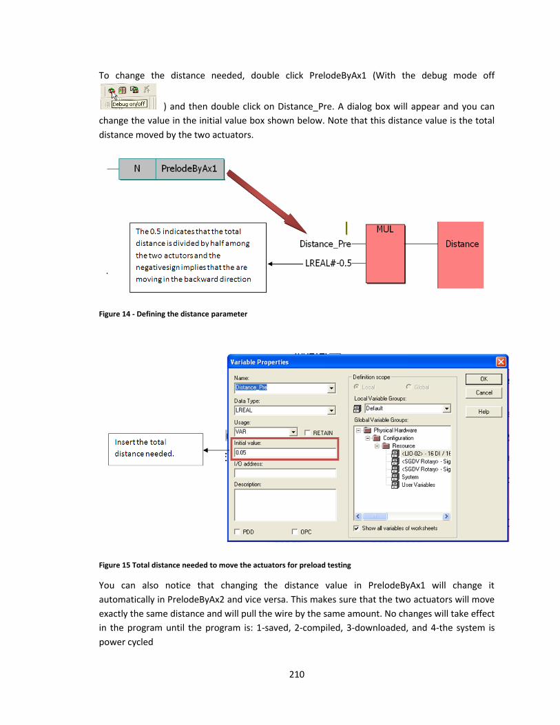
210
To change the distance needed, double click PrelodeByAx1 (With the debug mode off
) and then double click on Distance_Pre. A dialog box will appear and you can
change the value in the initial value box shown below. Note that this distance value is the total
distance moved by the two actuators.
Figure 14 - Defining the distance parameter
Figure 15 Total distance needed to move the actuators for preload testing
You can also notice that changing the distance value in PrelodeByAx1 will change it
automatically in PrelodeByAx2 and vice versa. This makes sure that the two actuators will move
exactly the same distance and will pull the wire by the same amount. No changes will take effect
in the program until the program is: 1-saved, 2-compiled, 3-downloaded, and 4-the system is
power cycled

211
After the preload loop is done, the actuators will have moved the required distance and will
stop.
However, the step shown on figure 16 indicates that the preload program will automatically
restart and be ready to use after the actuators move to the required distance. Keep repeating
the same steps again by overwriting PreDone until the required tension is reached in the wire.
Figure 16 - startprel step
A2.4-SFC_Example
Figure 17 - SFC_Example ladder
After preloading the wire to the required tension, you can move to the third program which is
SFC_Example by double clicking on it. This program, SFC_Example, will allow you to go for the
main testing process.
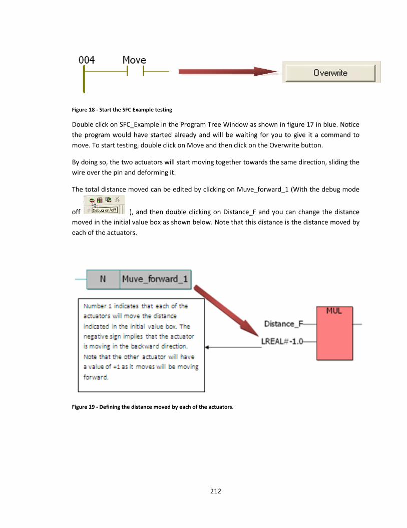
212
Figure 18 - Start the SFC Example testing
Double click on SFC_Example in the Program Tree Window as shown in figure 17 in blue. Notice
the program would have started already and will be waiting for you to give it a command to
move. To start testing, double click on Move and then click on the Overwrite button.
By doing so, the two actuators will start moving together towards the same direction, sliding the
wire over the pin and deforming it.
The total distance moved can be edited by clicking on Muve_forward_1 (With the debug mode
off ), and then double clicking on Distance_F and you can change the distance
moved in the initial value box as shown below. Note that this distance is the distance moved by
each of the actuators.
Figure 19 - Defining the distance moved by each of the actuators.
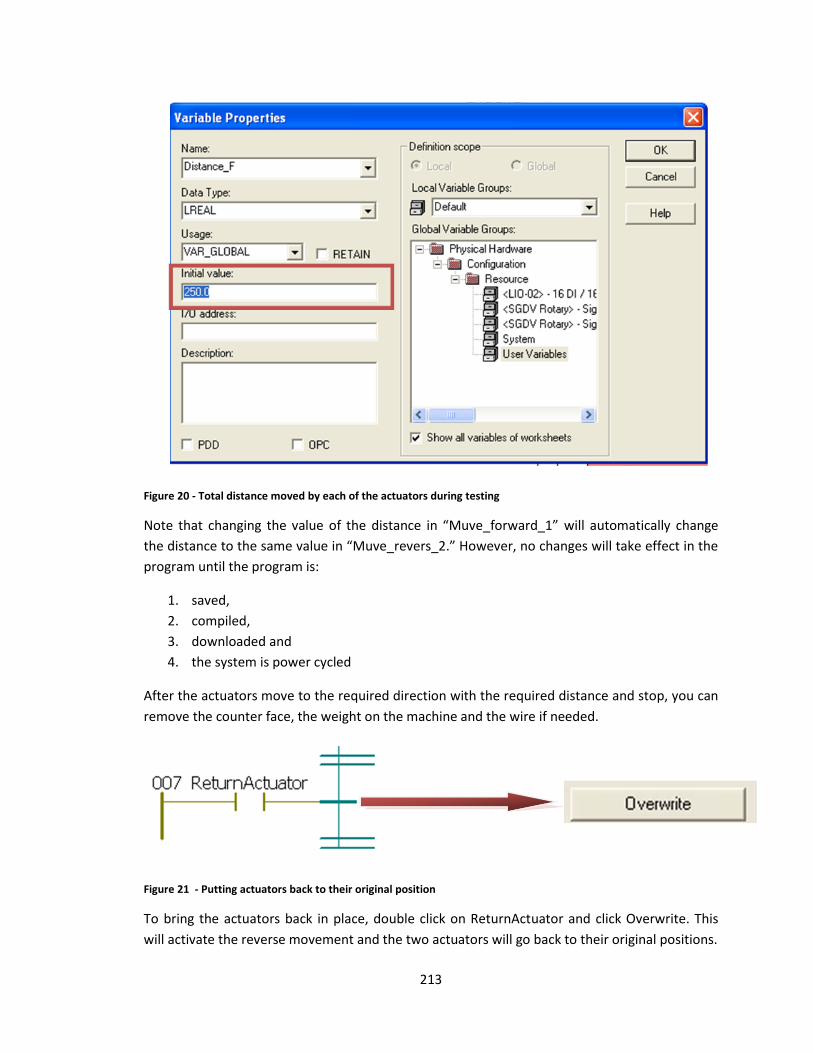
213
Figure 20 - Total distance moved by each of the actuators during testing
Note that changing the value of the distance in “Muve_forward_1” will automatically change
the distance to the same value in “Muve_revers_2.” However, no changes will take effect in the
program until the program is:
1. saved,
2. compiled,
3. downloaded and
4. the system is power cycled
After the actuators move to the required direction with the required distance and stop, you can
remove the counter face, the weight on the machine and the wire if needed.
Figure 21 - Putting actuators back to their original position
To bring the actuators back in place, double click on ReturnActuator and click Overwrite. This
will activate the reverse movement and the two actuators will go back to their original positions.
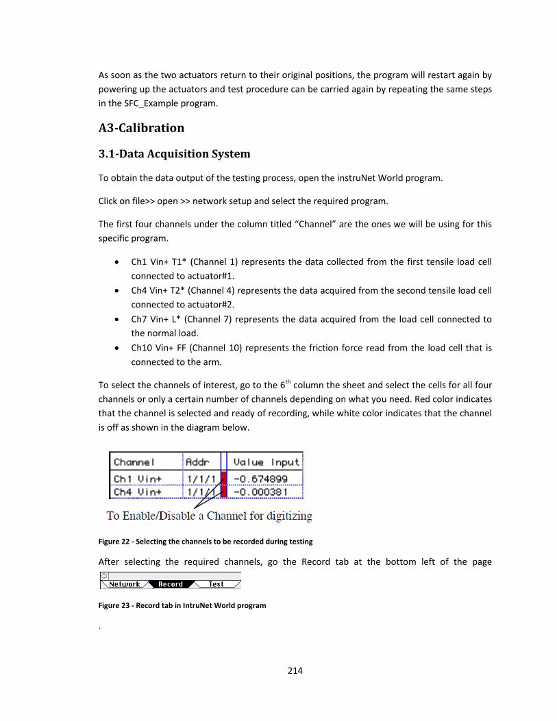
214
As soon as the two actuators return to their original positions, the program will restart again by
powering up the actuators and test procedure can be carried again by repeating the same steps
in the SFC_Example program.
A3-Calibration
3.1-Data Acquisition System
To obtain the data output of the testing process, open the instruNet World program.
Click on file>> open >> network setup and select the required program.
The first four channels under the column titled “Channel” are the ones we will be using for this
specific program.
Ch1 Vin+ T1* (Channel 1) represents the data collected from the first tensile load cell
connected to actuator#1.
Ch4 Vin+ T2* (Channel 4) represents the data acquired from the second tensile load cell
connected to actuator#2.
Ch7 Vin+ L* (Channel 7) represents the data acquired from the load cell connected to
the normal load.
Ch10 Vin+ FF (Channel 10) represents the friction force read from the load cell that is
connected to the arm.
To select the channels of interest, go to the 6th column the sheet and select the cells for all four
channels or only a certain number of channels depending on what you need. Red color indicates
that the channel is selected and ready of recording, while white color indicates that the channel
is off as shown in the diagram below.
Figure 22 - Selecting the channels to be recorded during testing
After selecting the required channels, go the Record tab at the bottom left of the page
Figure 23 - Record tab in IntruNet World program
.
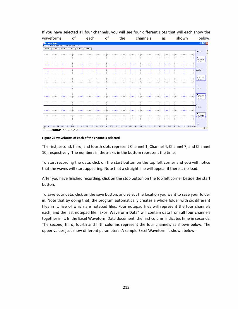
215
If you have selected all four channels, you will see four different slots that will each show the
waveforms of each of the channels as shown below.
Figure 24 waveforms of each of the channels selected
The first, second, third, and fourth slots represent Channel 1, Channel 4, Channel 7, and Channel
10, respectively. The numbers in the x-axis in the bottom represent the time.
To start recording the data, click on the start button on the top left corner and you will notice
that the waves will start appearing. Note that a straight line will appear if there is no load.
After you have finished recording, click on the stop button on the top left corner beside the start
button.
To save your data, click on the save button, and select the location you want to save your folder
in. Note that by doing that, the program automatically creates a whole folder with six different
files in it, five of which are notepad files. Four notepad files will represent the four channels
each, and the last notepad file “Excel Waveform Data” will contain data from all four channels
together in it. In the Excel Waveform Data document, the first column indicates time in seconds.
The second, third, fourth and fifth columns represent the four channels as shown below. The
upper values just show different parameters. A sample Excel Waveform is shown below.
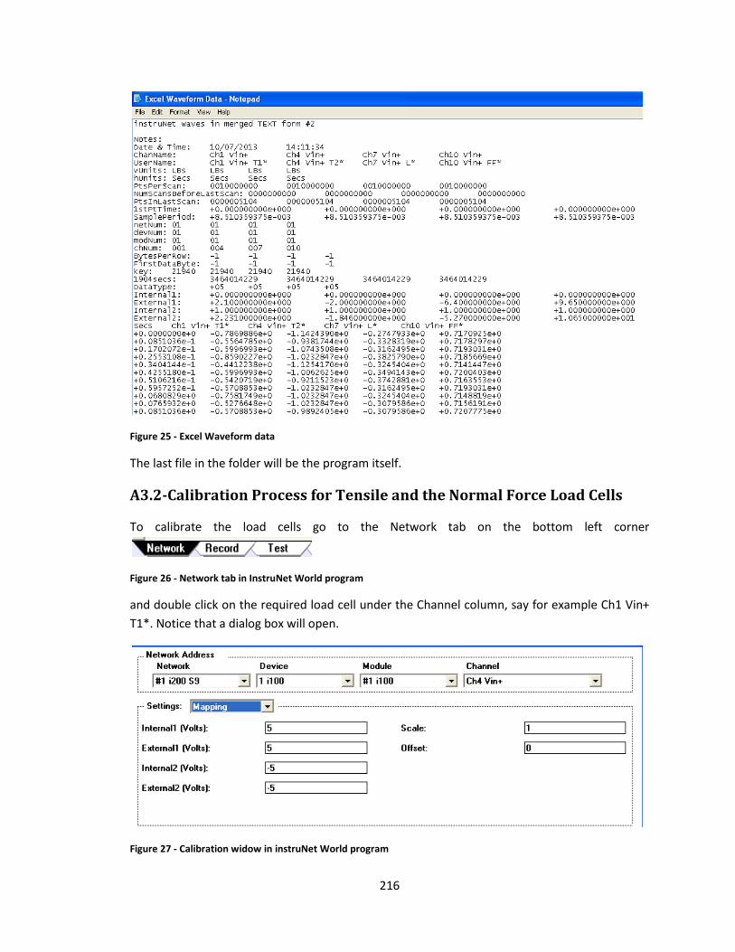
216
Figure 25 - Excel Waveform data
The last file in the folder will be the program itself.
A3.2-Calibration Process for Tensile and the Normal Force Load Cells
To calibrate the load cells go to the Network tab on the bottom left corner
Figure 26 - Network tab in InstruNet World program
and double click on the required load cell under the Channel column, say for example Ch1 Vin+
T1*. Notice that a dialog box will open.
Figure 27 - Calibration widow in instruNet World program
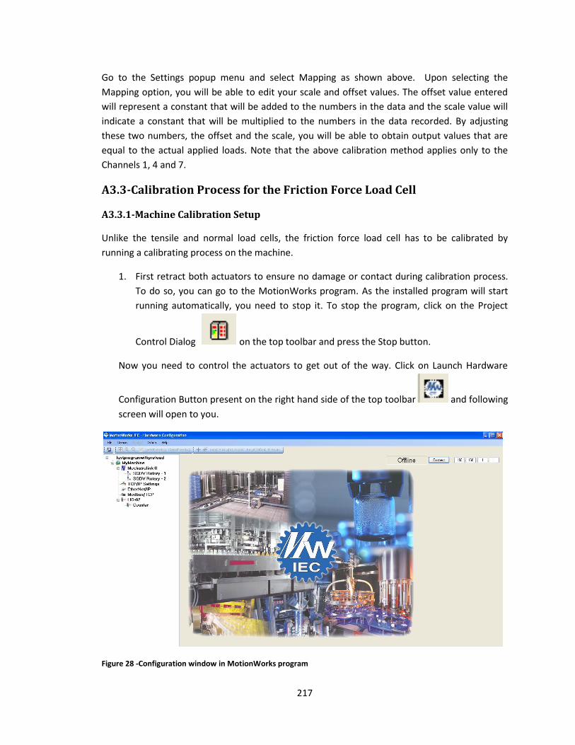
217
Go to the Settings popup menu and select Mapping as shown above. Upon selecting the
Mapping option, you will be able to edit your scale and offset values. The offset value entered
will represent a constant that will be added to the numbers in the data and the scale value will
indicate a constant that will be multiplied to the numbers in the data recorded. By adjusting
these two numbers, the offset and the scale, you will be able to obtain output values that are
equal to the actual applied loads. Note that the above calibration method applies only to the
Channels 1, 4 and 7.
A3.3-Calibration Process for the Friction Force Load Cell
A3.3.1-Machine Calibration Setup
Unlike the tensile and normal load cells, the friction force load cell has to be calibrated by
running a calibrating process on the machine.
1. First retract both actuators to ensure no damage or contact during calibration process.
To do so, you can go to the MotionWorks program. As the installed program will start
running automatically, you need to stop it. To stop the program, click on the Project
Control Dialog on the top toolbar and press the Stop button.
Now you need to control the actuators to get out of the way. Click on Launch Hardware
Configuration Button present on the right hand side of the top toolbar and following
screen will open to you.
Figure 28 -Configuration window in MotionWorks program
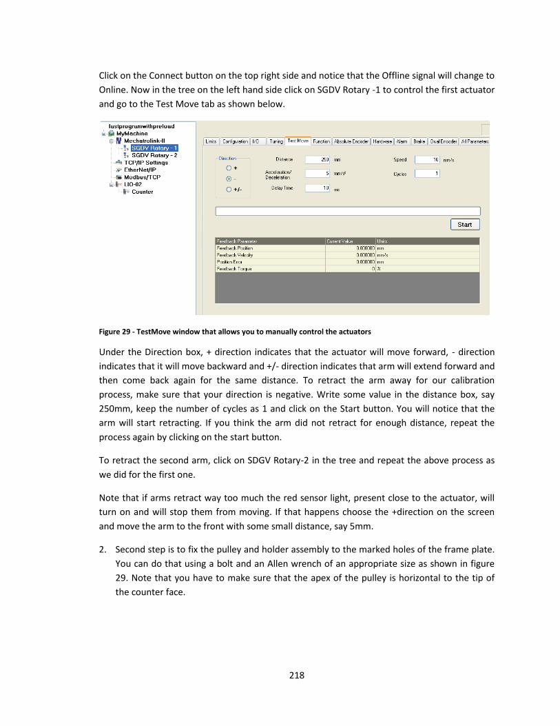
218
Click on the Connect button on the top right side and notice that the Offline signal will change to
Online. Now in the tree on the left hand side click on SGDV Rotary -1 to control the first actuator
and go to the Test Move tab as shown below.
Figure 29 - TestMove window that allows you to manually control the actuators
Under the Direction box, + direction indicates that the actuator will move forward, - direction
indicates that it will move backward and +/- direction indicates that arm will extend forward and
then come back again for the same distance. To retract the arm away for our calibration
process, make sure that your direction is negative. Write some value in the distance box, say
250mm, keep the number of cycles as 1 and click on the Start button. You will notice that the
arm will start retracting. If you think the arm did not retract for enough distance, repeat the
process again by clicking on the start button.
To retract the second arm, click on SDGV Rotary-2 in the tree and repeat the above process as
we did for the first one.
Note that if arms retract way too much the red sensor light, present close to the actuator, will
turn on and will stop them from moving. If that happens choose the +direction on the screen
and move the arm to the front with some small distance, say 5mm.
2. Second step is to fix the pulley and holder assembly to the marked holes of the frame plate.
You can do that using a bolt and an Allen wrench of an appropriate size as shown in figure
29. Note that you have to make sure that the apex of the pulley is horizontal to the tip of
the counter face.
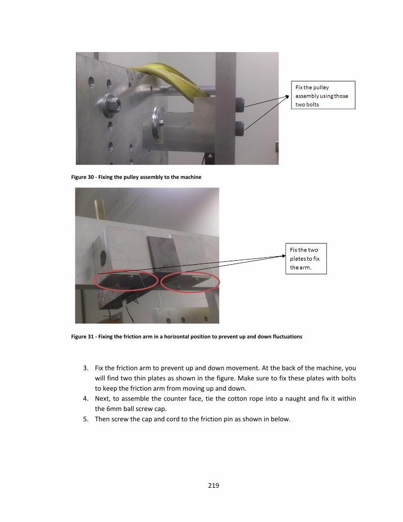
219
Figure 30 - Fixing the pulley assembly to the machine
Figure 31 - Fixing the friction arm in a horizontal position to prevent up and down fluctuations
3. Fix the friction arm to prevent up and down movement. At the back of the machine, you
will find two thin plates as shown in the figure. Make sure to fix these plates with bolts
to keep the friction arm from moving up and down.
4. Next, to assemble the counter face, tie the cotton rope into a naught and fix it within
the 6mm ball screw cap.
5. Then screw the cap and cord to the friction pin as shown in below.
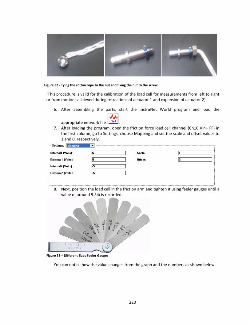
220
Figure 32 - Tying the cotton rope to the nut and fixing the nut to the screw
(This procedure is valid for the calibration of the load cell for measurements from left to right or from motions achieved during retractions of actuator 1 and expansion of actuator 2)
6. After assembling the parts, start the instruNet World program and load the
appropriate network file . 7. After loading the program, open the friction force load cell channel (Ch10 Vin+ FF) in
the first column, go to Settings, choose Mapping and set the scale and offset values to 1 and 0, respectively.
8. Next, position the load cell in the friction arm and tighten it using feeler gauges until a
value of around 9.5lb is recorded.
Figure 33 – Different Sizes Feeler Gauges
You can notice how the value changes from the graph and the numbers as shown below.
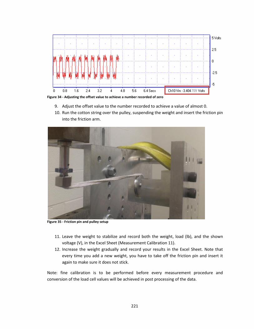
221
Figure 34 - Adjusting the offset value to achieve a number recorded of zero
9. Adjust the offset value to the number recorded to achieve a value of almost 0.
10. Run the cotton string over the pulley, suspending the weight and insert the friction pin
into the friction arm.
Figure 35 - Friction pin and pulley setup
11. Leave the weight to stabilize and record both the weight, load (lb), and the shown
voltage (V), in the Excel Sheet (Measurement Calibration 11).
12. Increase the weight gradually and record your results in the Excel Sheet. Note that
every time you add a new weight, you have to take off the friction pin and insert it
again to make sure it does not stick.
Note: fine calibration is to be performed before every measurement procedure and
conversion of the load cell values will be achieved in post processing of the data.
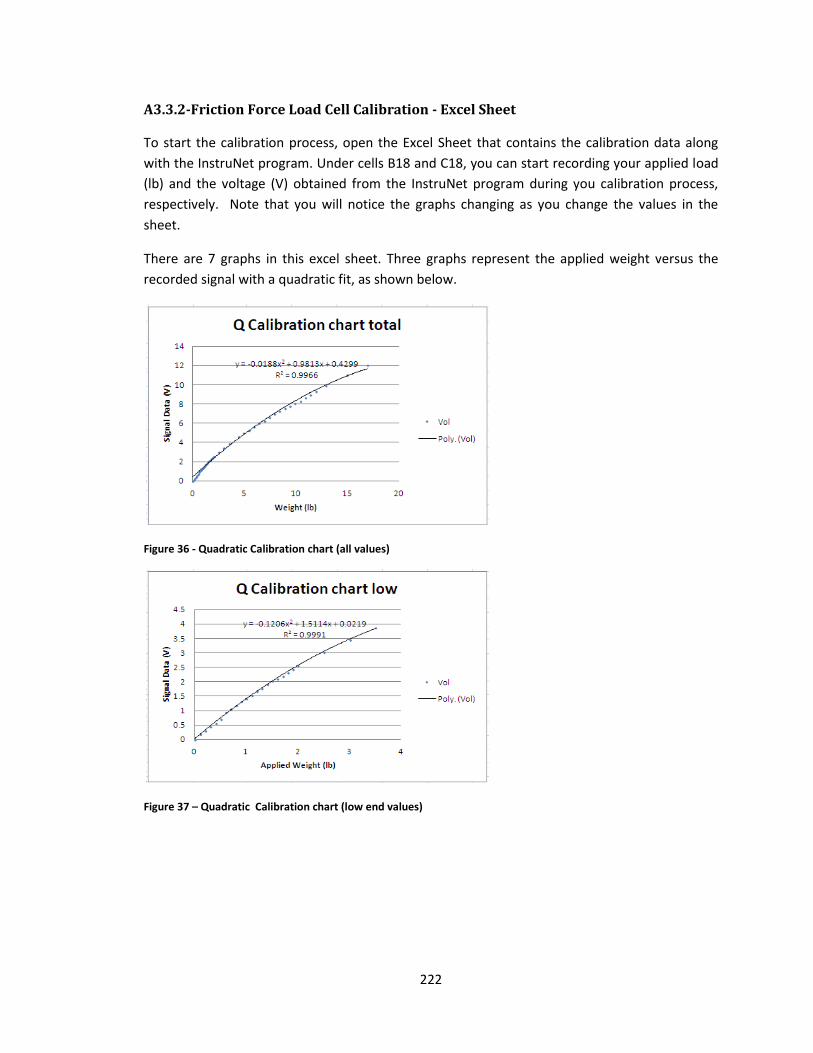
222
A3.3.2-Friction Force Load Cell Calibration - Excel Sheet
To start the calibration process, open the Excel Sheet that contains the calibration data along
with the InstruNet program. Under cells B18 and C18, you can start recording your applied load
(lb) and the voltage (V) obtained from the InstruNet program during you calibration process,
respectively. Note that you will notice the graphs changing as you change the values in the
sheet.
There are 7 graphs in this excel sheet. Three graphs represent the applied weight versus the
recorded signal with a quadratic fit, as shown below.
Figure 36 - Quadratic Calibration chart (all values)
Figure 37 – Quadratic Calibration chart (low end values)
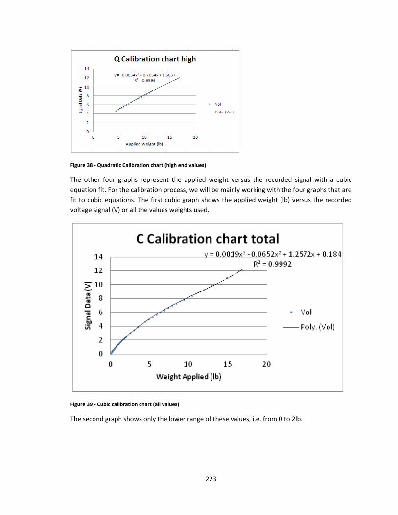
223
Figure 38 - Quadratic Calibration chart (high end values)
The other four graphs represent the applied weight versus the recorded signal with a cubic
equation fit. For the calibration process, we will be mainly working with the four graphs that are
fit to cubic equations. The first cubic graph shows the applied weight (lb) versus the recorded
voltage signal (V) or all the values weights used.
Figure 39 - Cubic calibration chart (all values)
The second graph shows only the lower range of these values, i.e. from 0 to 2lb.
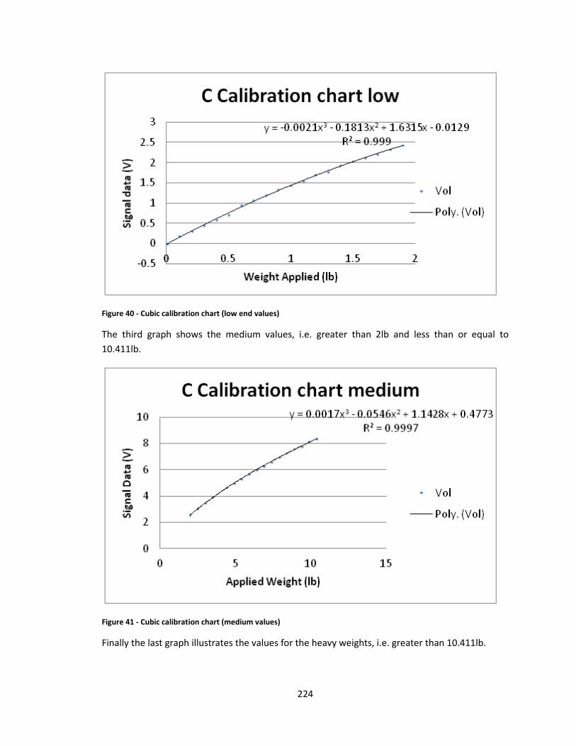
224
Figure 40 - Cubic calibration chart (low end values)
The third graph shows the medium values, i.e. greater than 2lb and less than or equal to
10.411lb.
Figure 41 - Cubic calibration chart (medium values)
Finally the last graph illustrates the values for the heavy weights, i.e. greater than 10.411lb.
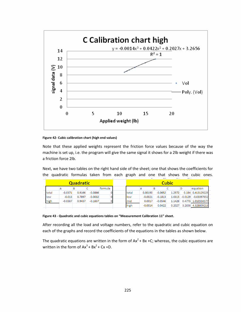
225
Figure 42- Cubic calibration chart (high end values)
Note that these applied weights represent the friction force values because of the way the
machine is set up, i.e. the program will give the same signal it shows for a 2lb weight if there was
a friction force 2lb.
Next, we have two tables on the right hand side of the sheet; one that shows the coefficients for
the quadratic formulas taken from each graph and one that shows the cubic ones.
Figure 43 - Quadratic and cubic equations tables on “Measurement Calibration 11” sheet.
After recording all the load and voltage numbers, refer to the quadratic and cubic equation on
each of the graphs and record the coefficients of the equations in the tables as shown below.
The quadratic equations are written in the form of Ax2 + Bx +C; whereas, the cubic equations are
written in the form of Ax3 + Bx2 + Cx +D.
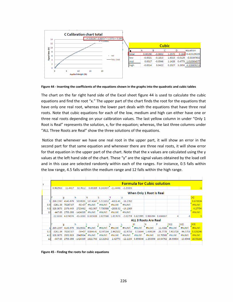
226
Figure 44 - Inserting the coefficients of the equations shown in the graphs into the quadratic and cubic tables
The chart on the far right hand side of the Excel sheet figure 44 is used to calculate the cubic
equations and find the root “x.” The upper part of the chart finds the root for the equations that
have only one real root, whereas the lower part deals with the equations that have three real
roots. Note that cubic equations for each of the low, medium and high can either have one or
three real roots depending on your calibration values. The last yellow column in under “Only 1
Root is Real” represents the solution, x, for the equation; whereas, the last three columns under
“ALL Three Roots are Real” show the three solutions of the equations.
Notice that whenever we have one real root in the upper part, it will show an error in the
second part for that same equation and whenever there are three real roots, it will show error
for that equation in the upper part of the chart. Note that the x values are calculated using the y
values at the left hand side of the chart. These “y” are the signal values obtained by the load cell
and in this case are selected randomly within each of the ranges. For instance, 0.5 falls within
the low range, 4.5 falls within the medium range and 12 falls within the high range.
Figure 45 - Finding the roots for cubic equations
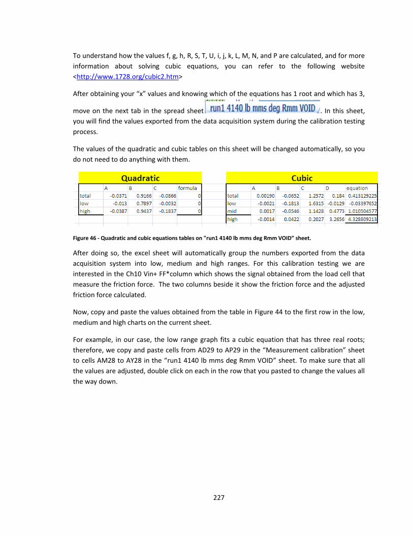
227
To understand how the values f, g, h, R, S, T, U, i, j, k, L, M, N, and P are calculated, and for more
information about solving cubic equations, you can refer to the following website
<http://www.1728.org/cubic2.htm>
After obtaining your “x” values and knowing which of the equations has 1 root and which has 3,
move on the next tab in the spread sheet . In this sheet,
you will find the values exported from the data acquisition system during the calibration testing
process.
The values of the quadratic and cubic tables on this sheet will be changed automatically, so you
do not need to do anything with them.
Figure 46 - Quadratic and cubic equations tables on "run1 4140 lb mms deg Rmm VOID” sheet.
After doing so, the excel sheet will automatically group the numbers exported from the data
acquisition system into low, medium and high ranges. For this calibration testing we are
interested in the Ch10 Vin+ FF*column which shows the signal obtained from the load cell that
measure the friction force. The two columns beside it show the friction force and the adjusted
friction force calculated.
Now, copy and paste the values obtained from the table in Figure 44 to the first row in the low,
medium and high charts on the current sheet.
For example, in our case, the low range graph fits a cubic equation that has three real roots;
therefore, we copy and paste cells from AD29 to AP29 in the “Measurement calibration” sheet
to cells AM28 to AY28 in the “run1 4140 lb mms deg Rmm VOID” sheet. To make sure that all
the values are adjusted, double click on each in the row that you pasted to change the values all
the way down.
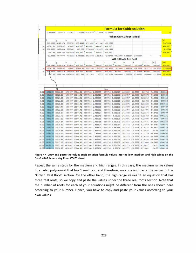
228
Figure 47 -Copy and paste the values cubic solution formula values into the low, medium and high tables on the "run1 4140 lb mms deg Rmm VOID" sheet
Repeat the same steps for the medium and high ranges. In this case, the medium range values
fit a cubic polynomial that has 1 real root, and therefore, we copy and paste the values in the
“Only 1 Real Root” section. On the other hand, the high range values fit an equation that has
three real roots, so we copy and paste the values under the three real roots section. Note that
the number of roots for each of your equations might be different from the ones shown here
according to your number. Hence, you have to copy and paste your values according to your
own values.
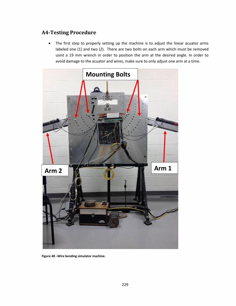
229
A4-Testing Procedure
The first step to properly setting up the machine is to adjust the linear acuator arms
labeled one (1) and two (2). There are two bolts on each arm which must be removed
usint a 19 mm wrench in order to position the arm at the desired angle. In order to
avoid damage to the acuator and wires, make sure to only adjust one arm at a time.
Figure 48 –Wire bending simulator machine.
Arm 1 Arm 2
Mounting Bolts
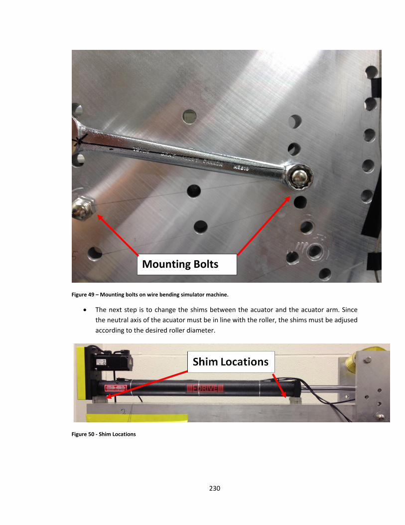
230
Figure 49 – Mounting bolts on wire bending simulator machine.
The next step is to change the shims between the acuator and the acuator arm. Since
the neutral axis of the acuator must be in line with the roller, the shims must be adjused
according to the desired roller diameter.
Figure 50 - Shim Locations
Mounting Bolts
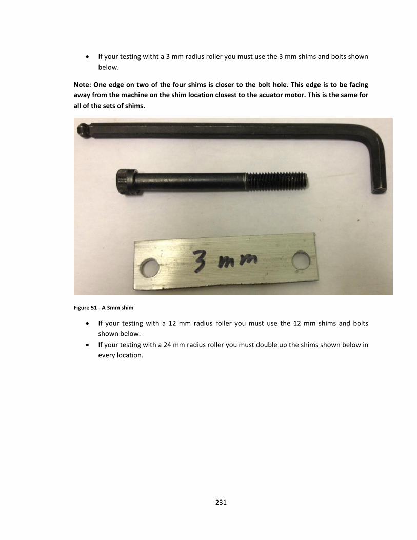
231
If your testing witht a 3 mm radius roller you must use the 3 mm shims and bolts shown
below.
Note: One edge on two of the four shims is closer to the bolt hole. This edge is to be facing
away from the machine on the shim location closest to the acuator motor. This is the same for
all of the sets of shims.
Figure 51 - A 3mm shim
If your testing with a 12 mm radius roller you must use the 12 mm shims and bolts
shown below.
If your testing with a 24 mm radius roller you must double up the shims shown below in
every location.
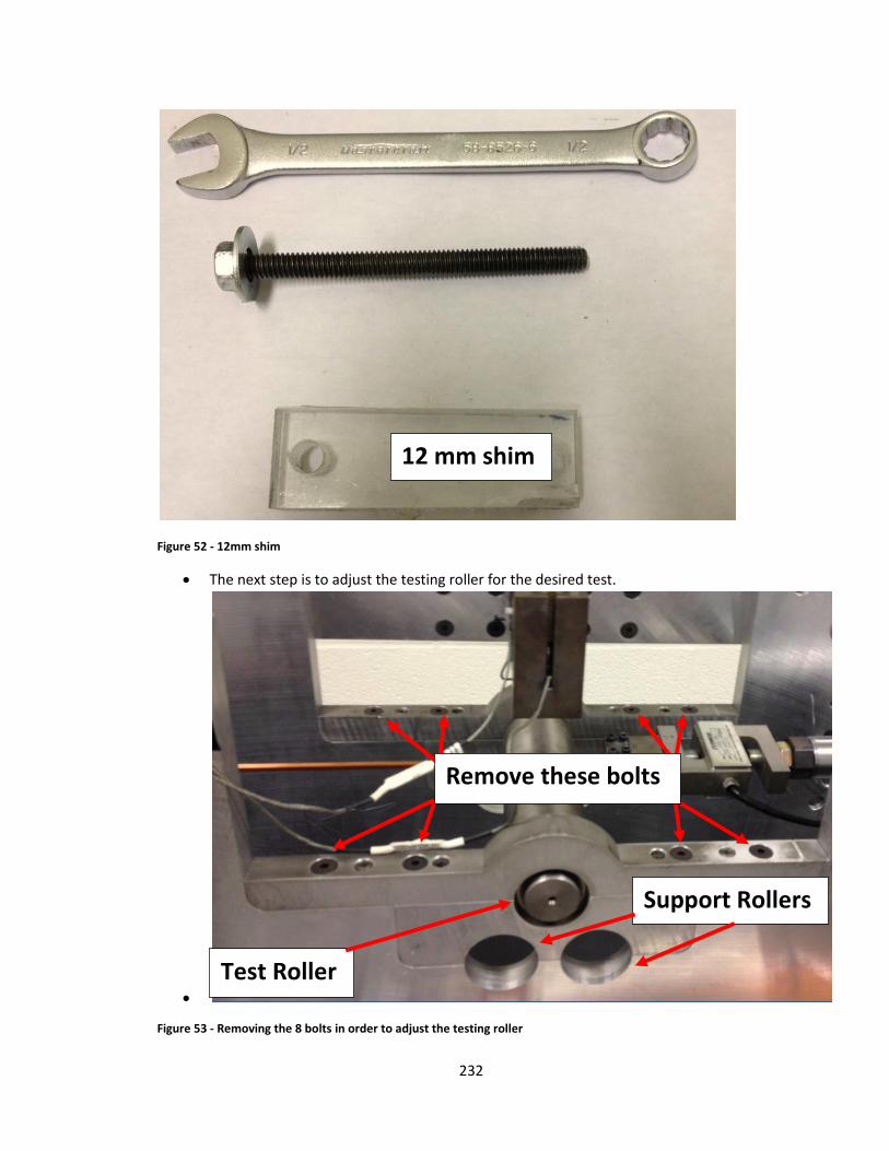
232
Figure 52 - 12mm shim
The next step is to adjust the testing roller for the desired test.
Figure 53 - Removing the 8 bolts in order to adjust the testing roller
12 mm shim
Remove these bolts
Test Roller
Support Rollers
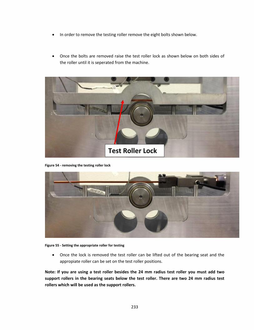
233
In order to remove the testing roller remove the eight bolts shown below.
Once the bolts are removed raise the test roller lock as shown below on both sides of
the roller until it is seperated from the machine.
Figure 54 - removing the testing roller lock
Figure 55 - Setting the appropriate roller for testing
Once the lock is removed the test roller can be lifted out of the bearing seat and the
appropiate roller can be set on the test roller positions.
Note: If you are using a test roller besides the 24 mm radius test roller you must add two
support rollers in the bearing seats below the test roller. There are two 24 mm radius test
rollers which will be used as the support rollers.
Test Roller Lock
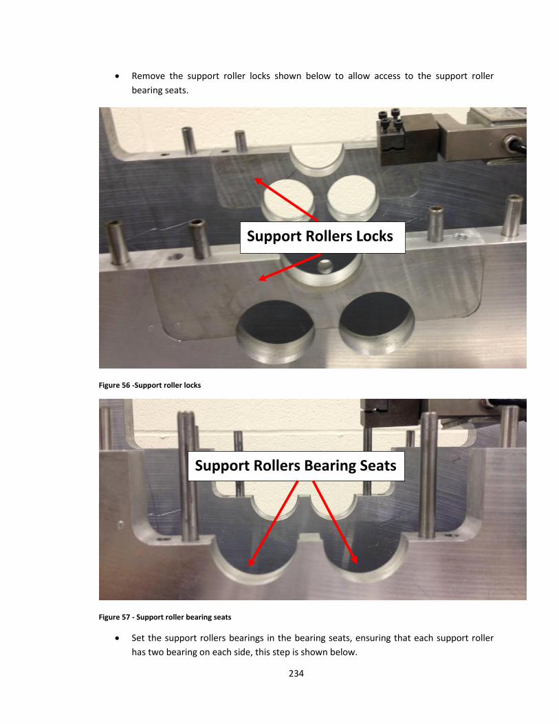
234
Remove the support roller locks shown below to allow access to the support roller
bearing seats.
Figure 56 -Support roller locks
Figure 57 - Support roller bearing seats
Set the support rollers bearings in the bearing seats, ensuring that each support roller
has two bearing on each side, this step is shown below.
Support Rollers Locks
Support Rollers Bearing Seats
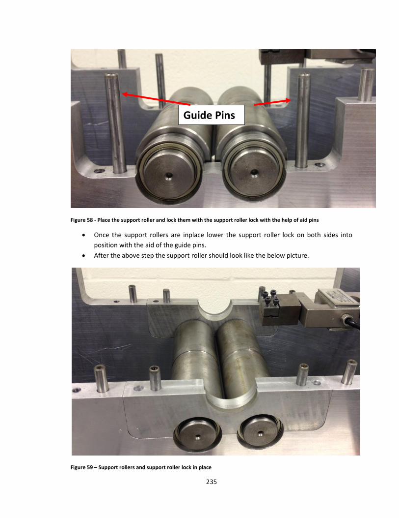
235
Figure 58 - Place the support roller and lock them with the support roller lock with the help of aid pins
Once the support rollers are inplace lower the support roller lock on both sides into
position with the aid of the guide pins.
After the above step the support roller should look like the below picture.
Figure 59 – Support rollers and support roller lock in place
Guide Pins
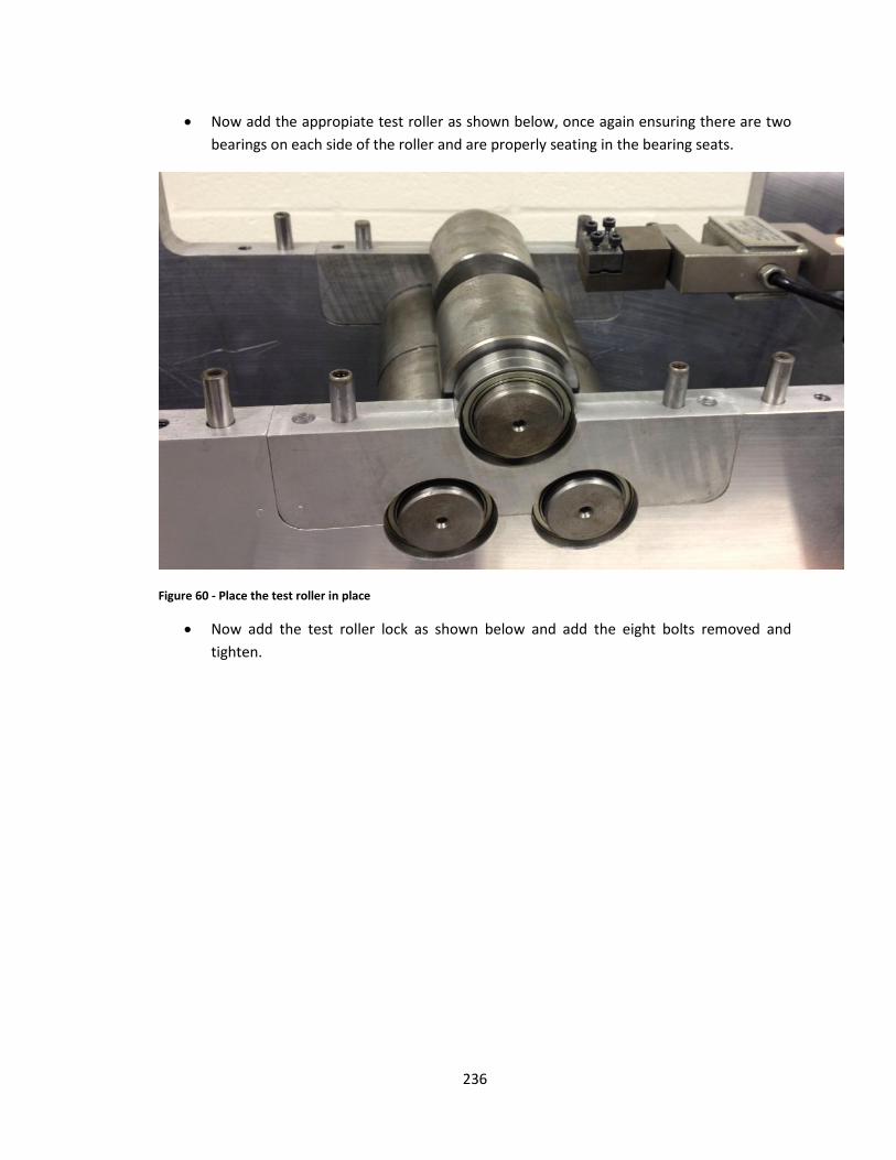
236
Now add the appropiate test roller as shown below, once again ensuring there are two
bearings on each side of the roller and are properly seating in the bearing seats.
Figure 60 - Place the test roller in place
Now add the test roller lock as shown below and add the eight bolts removed and
tighten.
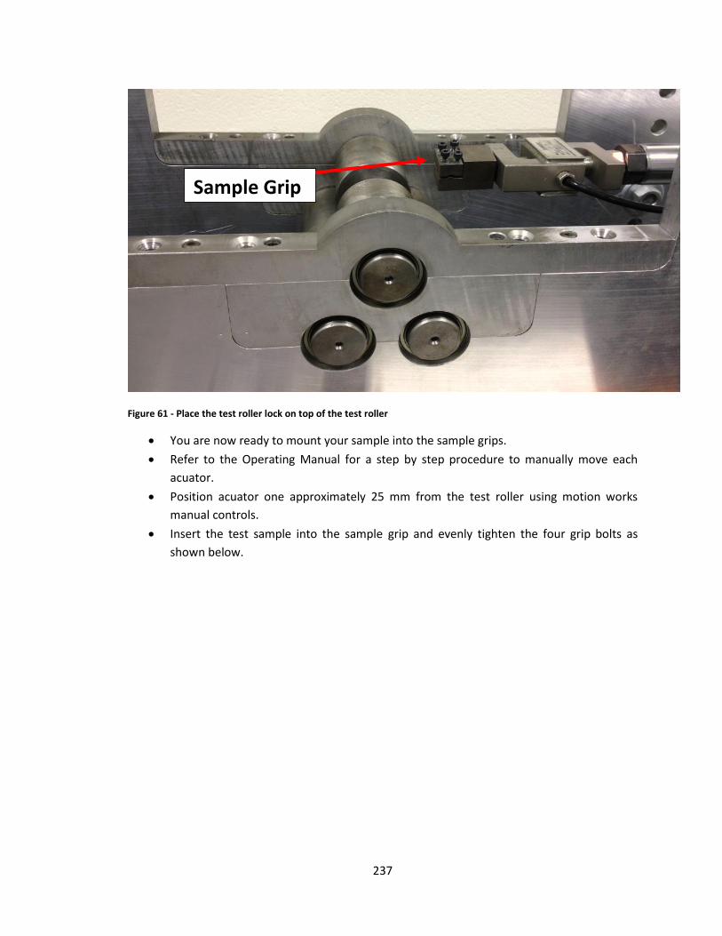
237
Figure 61 - Place the test roller lock on top of the test roller
You are now ready to mount your sample into the sample grips.
Refer to the Operating Manual for a step by step procedure to manually move each
acuator.
Position acuator one approximately 25 mm from the test roller using motion works
manual controls.
Insert the test sample into the sample grip and evenly tighten the four grip bolts as
shown below.
Sample Grip
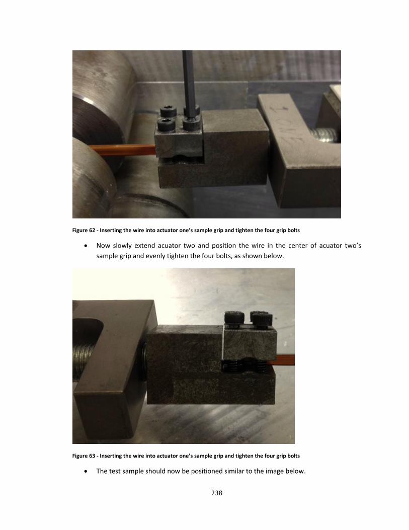
238
Figure 62 - Inserting the wire into actuator one’s sample grip and tighten the four grip bolts
Now slowly extend acuator two and position the wire in the center of acuator two’s
sample grip and evenly tighten the four bolts, as shown below.
Figure 63 - Inserting the wire into actuator one’s sample grip and tighten the four grip bolts
The test sample should now be positioned similar to the image below.
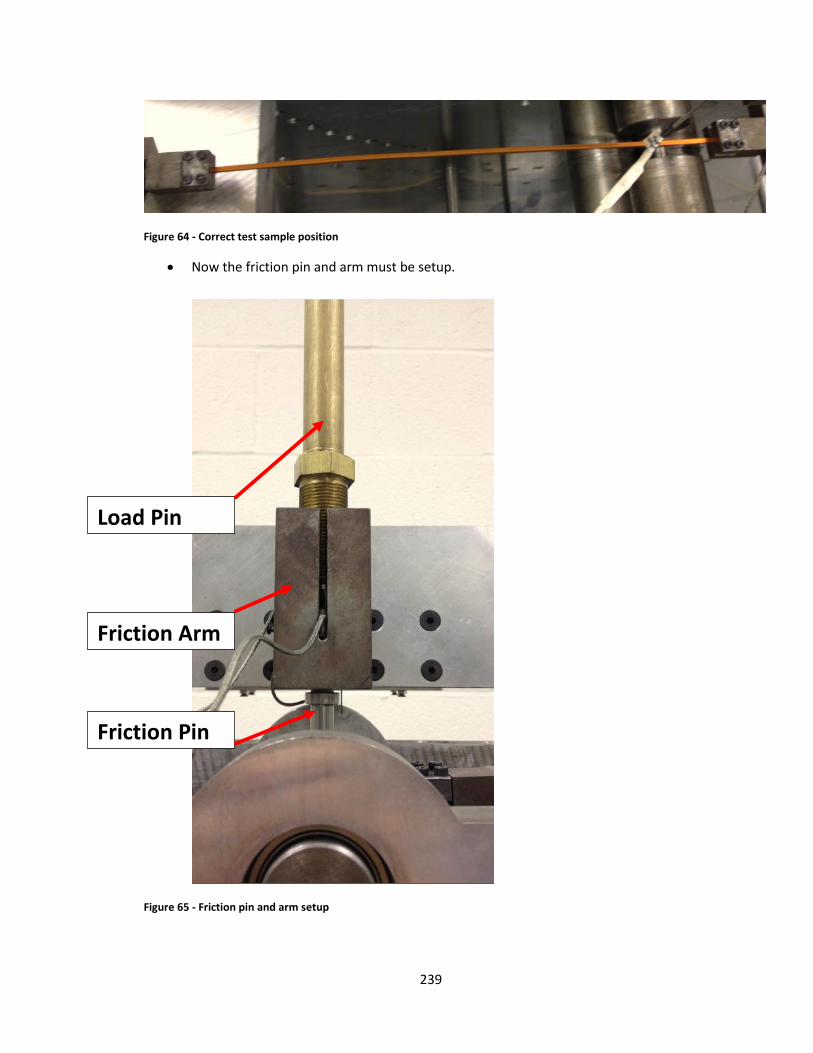
239
Figure 64 - Correct test sample position
Now the friction pin and arm must be setup.
Figure 65 - Friction pin and arm setup
Load Pin
Friction Pin
Friction Arm
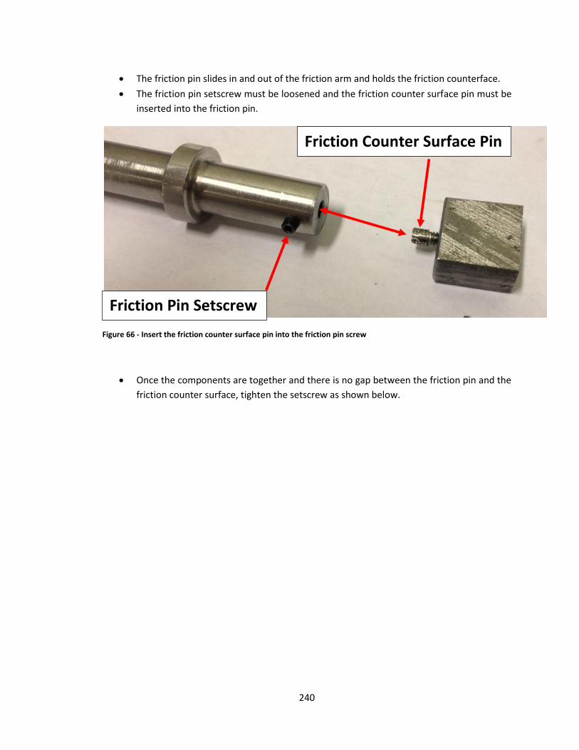
240
The friction pin slides in and out of the friction arm and holds the friction counterface.
The friction pin setscrew must be loosened and the friction counter surface pin must be
inserted into the friction pin.
Figure 66 - Insert the friction counter surface pin into the friction pin screw
Once the components are together and there is no gap between the friction pin and the
friction counter surface, tighten the setscrew as shown below.
Friction Counter Surface Pin
Friction Pin Setscrew
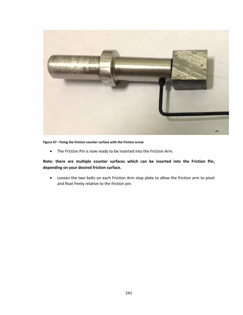
241
Figure 67 - Fixing the friction counter surface with the friction screw
The Friction Pin is now ready to be inserted into the Friction Arm.
Note: there are multiple counter surfaces which can be inserted into the Friction Pin,
depending on your desired friction surface.
Loosen the two bolts on each Friction Arm stop plate to allow the friction arm to pivot
and float freely relative to the friction pin.
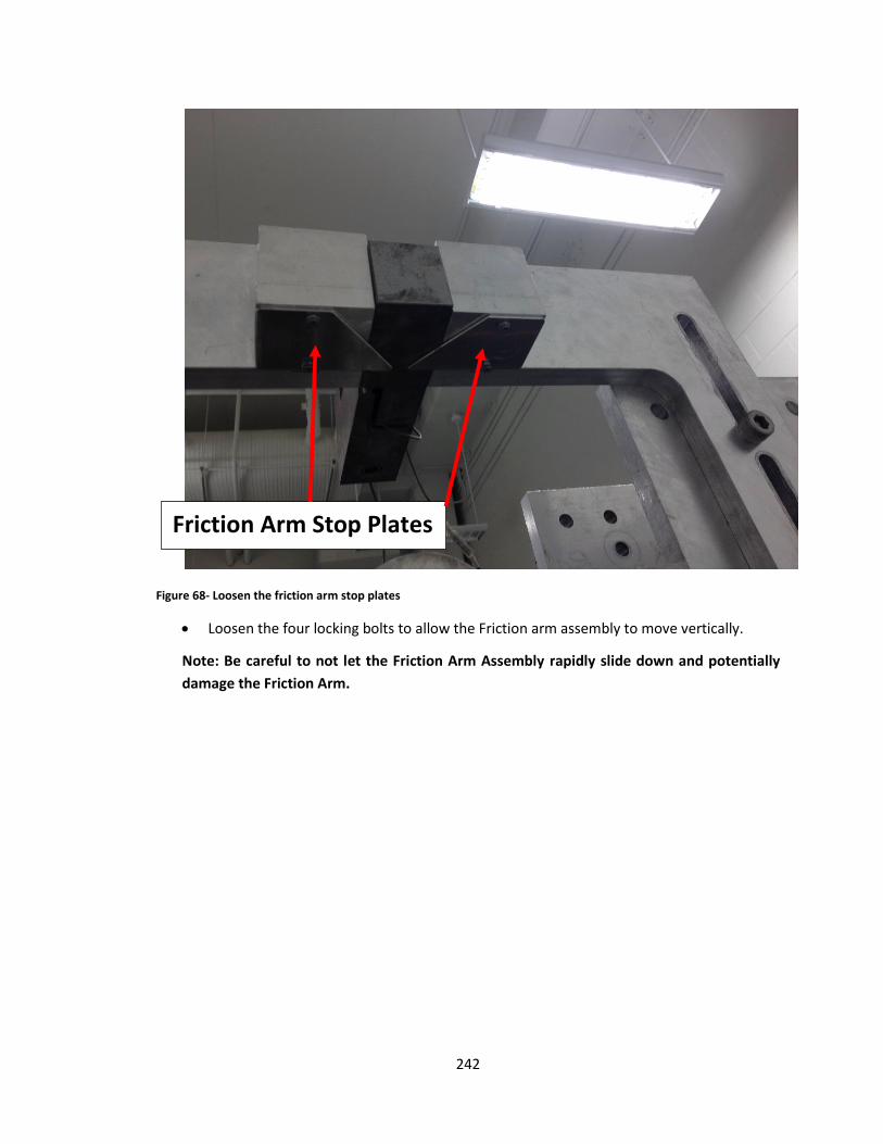
242
Figure 68- Loosen the friction arm stop plates
Loosen the four locking bolts to allow the Friction arm assembly to move vertically.
Note: Be careful to not let the Friction Arm Assembly rapidly slide down and potentially
damage the Friction Arm.
Friction Arm Stop Plates
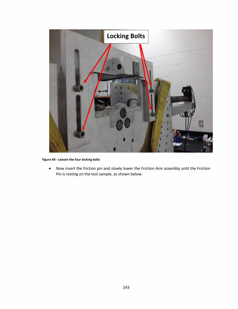
243
Figure 69 - Loosen the four locking bolts
Now insert the friction pin and slowly lower the Friction Arm assembly until the Friction
Pin is resting on the test sample, as shown below.
Locking Bolts
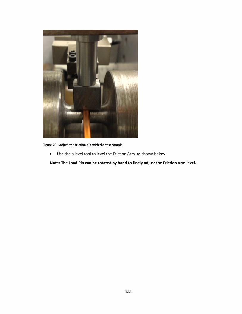
244
Figure 70 - Adjust the friction pin with the test sample
Use the a level tool to level the Friction Arm, as shown below.
Note: The Load Pin can be rotated by hand to finely adjust the Friction Arm level.
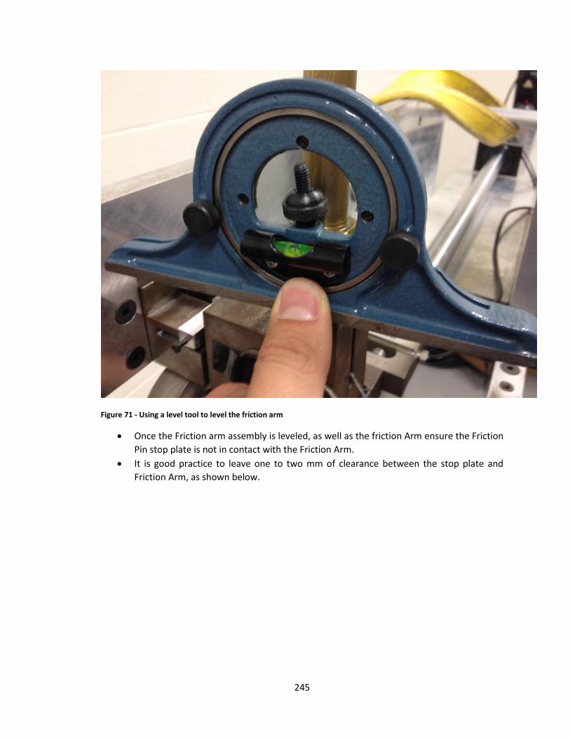
245
Figure 71 - Using a level tool to level the friction arm
Once the Friction arm assembly is leveled, as well as the friction Arm ensure the Friction
Pin stop plate is not in contact with the Friction Arm.
It is good practice to leave one to two mm of clearance between the stop plate and
Friction Arm, as shown below.
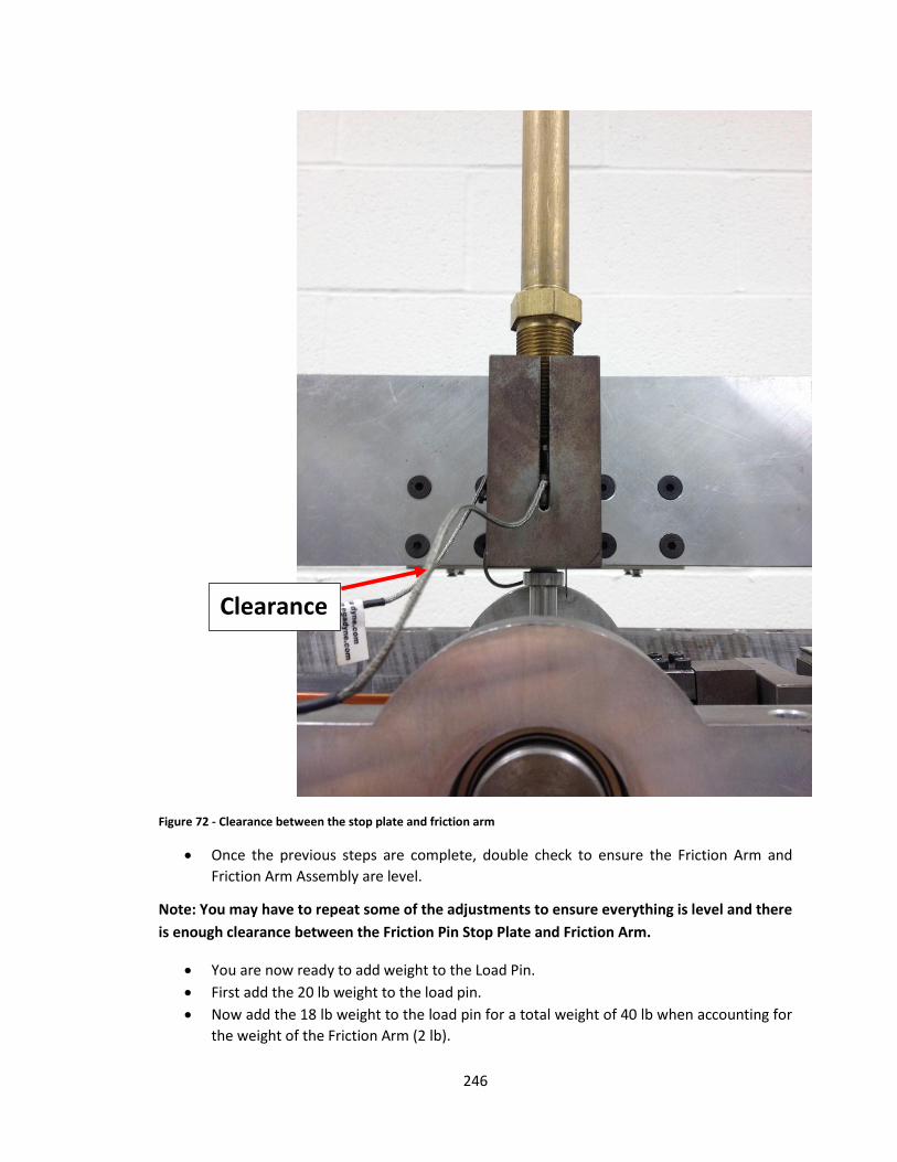
246
Figure 72 - Clearance between the stop plate and friction arm
Once the previous steps are complete, double check to ensure the Friction Arm and
Friction Arm Assembly are level.
Note: You may have to repeat some of the adjustments to ensure everything is level and there
is enough clearance between the Friction Pin Stop Plate and Friction Arm.
You are now ready to add weight to the Load Pin.
First add the 20 lb weight to the load pin.
Now add the 18 lb weight to the load pin for a total weight of 40 lb when accounting for
the weight of the Friction Arm (2 lb).
Clearance
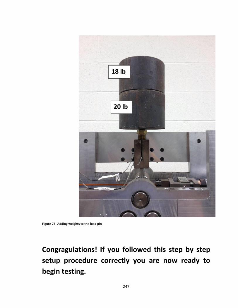
247
Figure 73- Adding weights to the load pin
Congragulations! If you followed this step by step
setup procedure correctly you are now ready to
begin testing.
18 lb
20 lb
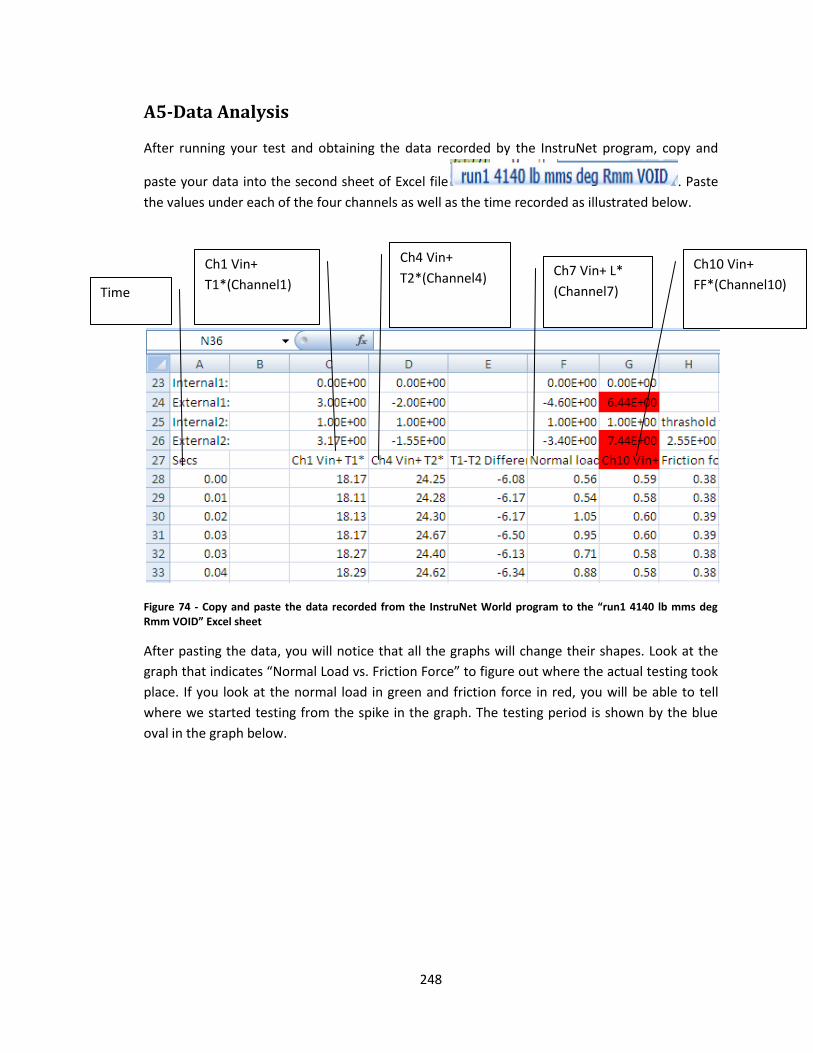
248
A5-Data Analysis
After running your test and obtaining the data recorded by the InstruNet program, copy and
paste your data into the second sheet of Excel file . Paste
the values under each of the four channels as well as the time recorded as illustrated below.
Figure 74 - Copy and paste the data recorded from the InstruNet World program to the “run1 4140 lb mms deg Rmm VOID” Excel sheet
After pasting the data, you will notice that all the graphs will change their shapes. Look at the
graph that indicates “Normal Load vs. Friction Force” to figure out where the actual testing took
place. If you look at the normal load in green and friction force in red, you will be able to tell
where we started testing from the spike in the graph. The testing period is shown by the blue
oval in the graph below.
Time
Ch4 Vin+
T2*(Channel4) Ch1 Vin+
T1*(Channel1)
Ch10 Vin+
FF*(Channel10) Ch7 Vin+ L*
(Channel7)
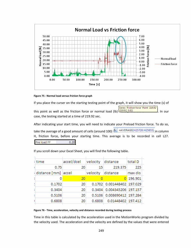
249
Figure 75 - Normal load versus friction force graph
If you place the curser on the starting testing point of the graph, it will show you the time (s) of
this point as well as the friction force or normal load (lb) . In our
case, the testing started at a time of 219.92 sec.
After indicating your start time, you will need to indicate your Preload friction force. To do so,
take the average of a good amount of cells (around 100) in column
H, friction force, before your starting time. This average is to be recorded in cell L27.
If you scroll down your Excel Sheet, you will find the following table.
Figure 76 - Time, acceleration, velocity and distance recorded during testing process
Time in this table is calculated by the acceleration used in the MotionWorks program divided by
the velocity used. The acceleration and the velocity are defined by the values that were entered
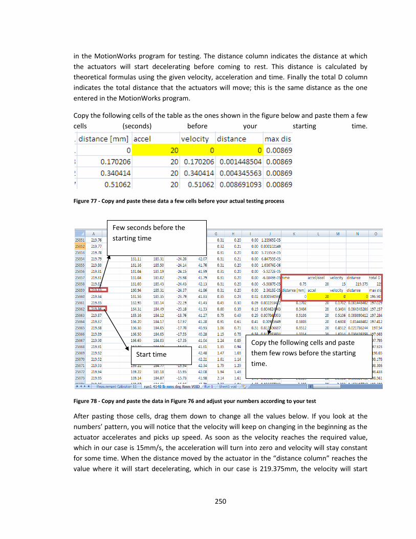
250
in the MotionWorks program for testing. The distance column indicates the distance at which
the actuators will start decelerating before coming to rest. This distance is calculated by
theoretical formulas using the given velocity, acceleration and time. Finally the total D column
indicates the total distance that the actuators will move; this is the same distance as the one
entered in the MotionWorks program.
Copy the following cells of the table as the ones shown in the figure below and paste them a few
cells (seconds) before your starting time.
Figure 77 - Copy and paste these data a few cells before your actual testing process
Figure 78 - Copy and paste the data in Figure 76 and adjust your numbers according to your test
After pasting those cells, drag them down to change all the values below. If you look at the
numbers’ pattern, you will notice that the velocity will keep on changing in the beginning as the
actuator accelerates and picks up speed. As soon as the velocity reaches the required value,
which in our case is 15mm/s, the acceleration will turn into zero and velocity will stay constant
for some time. When the distance moved by the actuator in the “distance column” reaches the
value where it will start decelerating, which in our case is 219.375mm, the velocity will start
Few seconds before the
starting time
Start time
Copy the following cells and paste
them few rows before the starting
time.
251
decreasing by the deceleration value that was indicated in the beginning. The actuators will
keep on slowing down until they reach a zero velocity at the required total distance, max dis.
Next in order to obtain the correct values the data of all the graphs located at the top of the
spreadsheet must be updated. Special care should be taken for the graphs displaying friction
force and normal load with respect to time.
When calculating average COF and its standard deviation, be sure to only include values where
the counterface speed is constant and avoid sections of acceleration and deceleration.
252
VITA AUCTORIS
NAME: Albion Demiri
PLACE OF BIRTH:
Elbasan, Albania
YEAR OF BIRTH:
1987
EDUCATION:
Ontario Secondary School Diploma
Catholic Central High School
Windsor, ON,
2001-2005
Bachelor of Applied Science
Mechanical Engineering-Material option (Co-op)
University of Windsor
Windsor, ON,
2005-2010
Masters of Applied Science
Engineering Materials
University of Windsor
Windsor, ON
2011-2013