El Niño Effects and Upwelling off South Australia

JOHN F. MIDDLETON,�,* CRAIG ARTHUR,� PAUL VAN RUTH,* TIM M. WARD,* JULIE L. MCCLEAN,@

MATHEW E. MALTRUD,& PETER GILL,** ANDREW LEVINGS,** AND SUE MIDDLETON�,#

*South Australian Research and Development Institute, West Beach, South Australia, Australia�School of Mathematics, University of New South Wales, Sydney, New South Wales, Australia

#School of Mathematics, University of Adelaide, South Australia, Australia@Scripps Institution of Oceanography, University of California, San Diego, La Jolla, California

&Los Alamos National Laboratory, Los Alamos, New Mexico**Deakin University, Warrnambool, Victoria, Australia

(Manuscript received 30 November 2005, in final form 26 September 2006)

ABSTRACT

To determine the possible importance of ENSO events along the coast of South Australia, an exploratoryanalysis is made of meteorological and oceanographic data and output from a global ocean model. Longtime series of coastal sea level and wind stress are used to show that while upwelling favorable winds havebeen more persistent since 1982, ENSO events (i) are largely driven by signals from the west Pacific Oceanshelf/slope waveguide and not local meteorological conditions, (ii) can account for 10-cm changes in sealevel, and (iii) together with wind stress, explain 62% of the variance of annual-averaged sea level. Thus,both local winds and remote forcing from the west Pacific are likely important to the low-frequency shelfedge circulation. Evidence also suggests that, since 1983, wintertime downwelling during the onset of an ElNiño is reduced and the following summertime upwelling is enhanced. In situ data show that during the 1998and 2003 El Niño events anomalously cold (10.5°–11.5°C) water is found at depths of 60–120 m and is morethan two standard deviations cooler than the mean. A regression showed that averaged sea level can providea statistically significant proxy for these subsurface temperature changes and indicates a 2.2°C decrease intemperature for the 10-cm decrease in sea level that was driven by the 1998 El Niño event. Limited current-meter observations, long sea level records, and output from a global ocean model were also examined andprovide support for the hypothesis that El Niño events substantially reduce wintertime (but not summer-time) shelf-edge currents. Further research to confirm this asymmetric response and its cause is required.

1. Introduction

It is now well recognized that El Niño–Southern Os-cillation (ENSO) events can have an important impacton both the ocean circulation of the western shelves ofthe Americas (e.g., Kosro 2002; Pizarro et al. 2001) andlead to a significant reduction in marine productivity(e.g., Etnoyer et al. 2004). The importance of ENSOvariability to coastal sea level along Australia’s westand southern shelves was recognized some time ago byPariwono et al. (1986). However, it is only recently thatENSO events have been shown to be important to thestrength of the Leeuwin Current (Feng et al. 2003) and

of likely importance to shelf-slope currents and com-mercial fisheries of the region (Clarke and Li 2004; Liand Clarke 2004). Indeed, we show here that El Niñoevents lead to enhanced upwelling along Australia’ssouthern shelves, the opposite to that found along theAmericas. However, with the exception of the sea sur-face height (SSH) analysis of Li and Clarke, almostnothing is known about the impact of ENSO events onthe circulation along Australia’s southern shelves.

These extensive zonal shelves (Fig. 1) host a circula-tion that is affected by seasonally varying zonal windsand by the Leeuwin Current. In the south, the 4-yrperiod Antarctic “Circumpolar Wave” (ACW) modu-lates sea surface temperature (SST) by around 0.5°C,although the effect of this wave on the circulation isunknown (e.g., White and Peterson 1996). In addition,the equatorward Sverdrup transport in the SouthernOcean drives the Flinders Current, which is a “north-

Corresponding author address: John Middleton, Aquatic Sci-ences Centre, P.O. Box 120, Henley Beach, South Australia 5024,Australia.E-mail: middleton.john@saugov.sa.gov.au

2458 J O U R N A L O F P H Y S I C A L O C E A N O G R A P H Y VOLUME 37

DOI: 10.1175/JPO3119.1

© 2007 American Meteorological Society

JPO3119

ern” boundary current that appears trapped to the shelfslope at depths of 600–1200 m (Middleton and Cirano2002). The summer winds drive a mean westward shelfcirculation and upwelling off Kangaroo Island and theBonney Coast (Robe) (Griffin et al. 1997; Hahn 1986;Middleton and Platov 2003; McClatchie et al. 2006).During winter, the winds and shelf circulation reverseand are directed to the east. In conjunction with strongcooling, water is mixed and downwelled to 200 m or so(Godfrey et al. 1986).

There are two possible mechanisms by which El Niñoevents can affect this circulation. The first is throughchanges in the local meteorology. Voice (1984) sug-gested that eastward zonal winds here would be re-duced during El Niño winters. Schahinger (1989) in-voked this change as an explanation for the markedreduction in the mean winter eastward currents foundoff the Bonney Coast.

The second mechanism for ENSO-related changes tothe shelf circulation was advanced by Allan Clarke andcoworkers (e.g., Clarke and Van Gorder 1994; Pizarroet al. 2001) and involves the propagation of ENSO sig-nals along the waveguide of the shelf slope. Near theequator, Clarke assumes that the ENSO signals may bewell approximated by two internal Kelvin wave modes.The external deformation radius here is large, sea levelgradients small, and little energy is assumed scatteredinto barotropic shelf modes. For the western PacificOcean, such internal waves are trapped to the shelfbreak (�200 m isobath) that is continuous from north-ern Papua New Guinea to Darwin. Thus, a waveguideexists to transmit the ENSO signals to the western andthen southern Australian shelves. Clarke and cowork-

ers then use a linear model to advance the signal pole-ward. Comparison of the model results with shelf-slopecurrent-meter and sea level data from the west coast ofSouth America has revealed some strengths and weak-nesses of this theory (Pizarro et al. 2001).

We do not have enough long time series of data toverify these theories and predictions, but through a va-riety of data and sources, we examine the followinghypotheses and, generally, the relation of ENSO-drivenshelf signals to local winds, shelf currents, sea level, andupwelling.

In section 2, an analysis of sea level and winds for theregion leads us to our first hypothesis:

(i) While upwelling favorable winds in the easternBight have been more persistent since 1982, localENSO-related events are driven largely through theshelf waveguide from the west Pacific.

In section 3, we examine observations of ocean tem-perature that lead us to our second hypothesis:

(ii) Since 1983, wintertime downwelling of the ther-mocline is reduced during the onset of an El Niñoand the following summertime upwelling of thethermocline is enhanced.

In section 4, we examine the available current-meterdata, which lead to the third related hypothesis:

(iii) El Niño events can substantially reduce wintertime(but not summertime) shelf-edge currents.

In section 5, support for these hypotheses is given ina brief analysis of the output of the Parallel OceanProgram (POP) global model (Maltrud and McClean

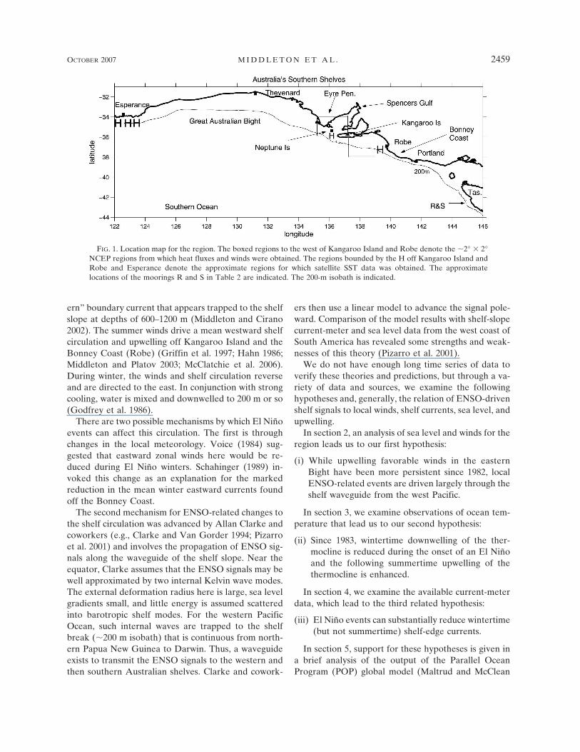
FIG. 1. Location map for the region. The boxed regions to the west of Kangaroo Island and Robe denote the �2° � 2°NCEP regions from which heat fluxes and winds were obtained. The regions bounded by the H off Kangaroo Island andRobe and Esperance denote the approximate regions for which satellite SST data was obtained. The approximatelocations of the moorings R and S in Table 2 are indicated. The 200-m isobath is indicated.

OCTOBER 2007 M I D D L E T O N E T A L . 2459

2005). We also speculate that the asymmetry in thesummer and winter responses to El Niño events maywell arise from thermohaline effects.

2. Wind stress, ENSO, and sea level

We consider first the observations for winds (Kanga-roo Island region), ENSO, and sea level, where for thelatter 40-yr coincident records are available. The sealevel data will supplement those for shelf currents andupwelling in the analysis below. In the following, weextend the analysis of Li and Clarke (2004) to show thatseasonal and interannual sea level variability are bothwell correlated with ENSO and the alongshore compo-nent of wind stress. Wind stress and ENSO events aregenerally not found to be statistically correlated.

A measure of ENSO variability is the Niño-3.4 indexthat is based on the difference in SST across the Pacific.We always use negative values of the Niño-3.4 index sothat El Niño events are negative and consistent withnegative (cooler) upwelling temperature anomalies andlower coastal sea level. We also define an El Niño sum-mer (e.g., 1998) to be that when the ENSO event islargest. An El Niño winter corresponds to that of theprevious year (e.g., 1997) when the onset and effects ofthe El Niño are largest.

a. Wind stress

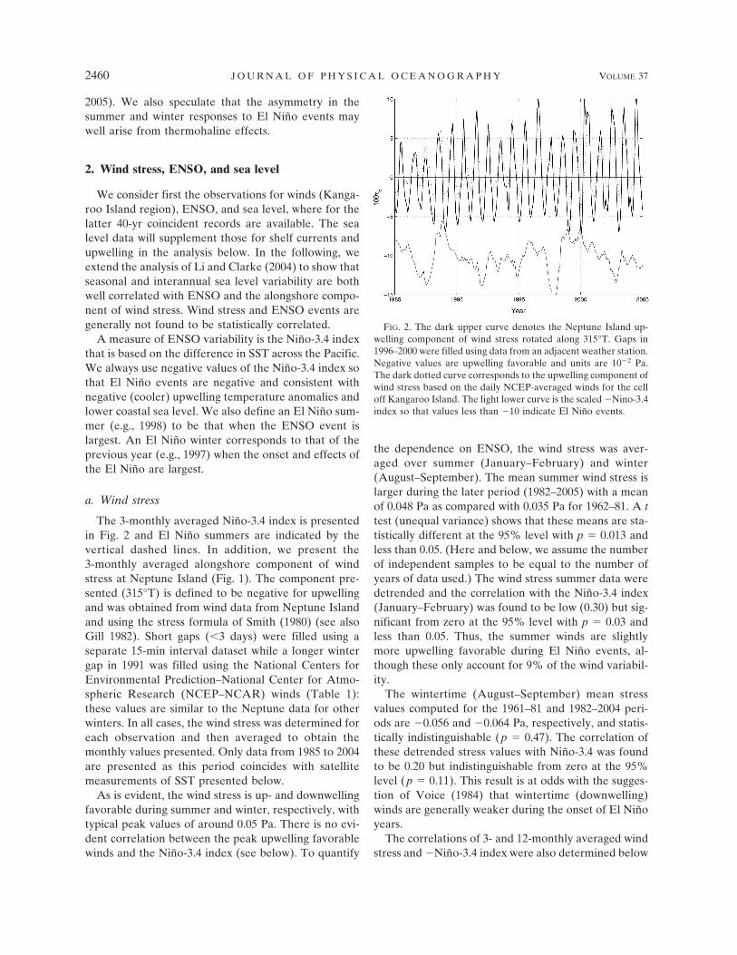
The 3-monthly averaged Niño-3.4 index is presentedin Fig. 2 and El Niño summers are indicated by thevertical dashed lines. In addition, we present the3-monthly averaged alongshore component of windstress at Neptune Island (Fig. 1). The component pre-sented (315°T) is defined to be negative for upwellingand was obtained from wind data from Neptune Islandand using the stress formula of Smith (1980) (see alsoGill 1982). Short gaps (�3 days) were filled using aseparate 15-min interval dataset while a longer wintergap in 1991 was filled using the National Centers forEnvironmental Prediction–National Center for Atmo-spheric Research (NCEP–NCAR) winds (Table 1):these values are similar to the Neptune data for otherwinters. In all cases, the wind stress was determined foreach observation and then averaged to obtain themonthly values presented. Only data from 1985 to 2004are presented as this period coincides with satellitemeasurements of SST presented below.

As is evident, the wind stress is up- and downwellingfavorable during summer and winter, respectively, withtypical peak values of around 0.05 Pa. There is no evi-dent correlation between the peak upwelling favorablewinds and the Niño-3.4 index (see below). To quantify

the dependence on ENSO, the wind stress was aver-aged over summer (January–February) and winter(August–September). The mean summer wind stress islarger during the later period (1982–2005) with a meanof 0.048 Pa as compared with 0.035 Pa for 1962–81. A ttest (unequal variance) shows that these means are sta-tistically different at the 95% level with p � 0.013 andless than 0.05. (Here and below, we assume the numberof independent samples to be equal to the number ofyears of data used.) The wind stress summer data weredetrended and the correlation with the Niño-3.4 index(January–February) was found to be low (0.30) but sig-nificant from zero at the 95% level with p � 0.03 andless than 0.05. Thus, the summer winds are slightlymore upwelling favorable during El Niño events, al-though these only account for 9% of the wind variabil-ity.

The wintertime (August–September) mean stressvalues computed for the 1961–81 and 1982–2004 peri-ods are �0.056 and �0.064 Pa, respectively, and statis-tically indistinguishable (p � 0.47). The correlation ofthese detrended stress values with Niño-3.4 was foundto be 0.20 but indistinguishable from zero at the 95%level (p � 0.11). This result is at odds with the sugges-tion of Voice (1984) that wintertime (downwelling)winds are generally weaker during the onset of El Niñoyears.

The correlations of 3- and 12-monthly averaged windstress and �Niño-3.4 index were also determined below

FIG. 2. The dark upper curve denotes the Neptune Island up-welling component of wind stress rotated along 315°T. Gaps in1996–2000 were filled using data from an adjacent weather station.Negative values are upwelling favorable and units are 10�2 Pa.The dark dotted curve corresponds to the upwelling component ofwind stress based on the daily NCEP-averaged winds for the celloff Kangaroo Island. The light lower curve is the scaled �Nino-3.4index so that values less than �10 indicate El Niño events.

2460 J O U R N A L O F P H Y S I C A L O C E A N O G R A P H Y VOLUME 37

TA

BL

E1.

Dat

ade

scri

ptio

nan

dso

urce

s.T

hehe

ight

and

dept

hof

the

data

sour

cear

ein

met

ers.

Nam

eSt

art

End

Sam

plin

gra

te/a

vgL

at(°

S)L

on(°

E)

Hei

ght/

dept

hC

omm

ents

Nep

tune

Isla

ndw

ind

data

1Ja

n19

6230

Sep

2004

12h

�19

85;3

h�

1985

35.3

3713

6.11

730

Bur

eau

ofM

eteo

rolo

gyW

inds

:Kan

gero

oIs

land

1Ja

n19

851

May

2004

Dai

lyav

g35

.2�

0.95

2413

6.9

�0.

935

10N

CE

P–N

CA

RH

eat

flux

:Kan

gero

oIs

land

1Ja

n19

851

May

2004

Mon

thly

avg

35.2

�0.

9524

136.

9�

0.93

510

NC

EP

–NC

AR

Hea

tfl

ux:R

obe

1Ja

n19

851

May

2004

Mon

thly

avg

37.1

4�

0.95

2413

8.27

�0.

935

10N

CE

P–N

CA

RSS

T:K

ange

roo

Isla

nd1

Jan

1985

1M

ay20

04M

onth

lyav

g36

.123

–35.

5078

135.

352–

135.

879

0P

athf

inde

r4

and

5:9-

kmbi

n,ni

ghtt

ime

imag

eSS

T:R

obe

1Ja

n19

851

May

2004

Mon

thly

avg

37.5

293–

36.5

186

138.

999–

139.

966

0P

athf

inde

r4

and

5:9-

kmbi

n,ni

ghtt

ime

imag

eSS

T:w

est

bigh

t1

Jan

1985

1M

ay20

04M

onth

lyav

g34

–35

120–

124

0P

athf

inde

r4

and

5:9-

kmbi

n,ni

ghtt

ime

imag

eSS

T:S

outh

ern

Oce

an1

Jan

1985

1M

ay20

04M

onth

lyav

g38

–54

133–

137

0P

athf

inde

r4

and

5:9-

kmbi

n,ni

ghtt

ime

imag

eR

obe

tem

pera

ture

logg

er1

Jan

1999

4Ja

n20

01D

aily

avg

37.1

413

9.47

52SA

RD

I:52

-mw

ater

dept

hSo

uthe

ndte

mpe

ratu

relo

gger

16D

ec19

985

Oct

2001

Dai

lyav

g37

.66

140.

0164

SAR

DI:

64-m

wat

erde

pth

Cap

eN

elso

nsi

teC

2Ja

n20

011

Sep

2002

2-ho

urly

sam

ple

38.5

014

1.54

345

and

80P

.Gill

:�90

-mw

ater

dept

hC

ape

Nel

son

site

B1

Sep

2002

16F

eb20

042-

hour

lysa

mpl

e38

.32

141.

105

45P

.Gill

:�90

-mw

ater

dept

hP

ort

Mac

Don

nell

8M

ay19

738

Oct

1981

Mon

thly

sam

ple

38.1

6714

0.83

50C

SIR

O:M

arL

IN,w

ater

dept

h60

mK

ange

roo

Isla

ndm

oori

ngte

mpe

ratu

resi

teO

7D

ec19

8811

2da

ys20

min

/30

hav

g35

.245

135.

581

Nun

esV

az:W

ater

dept

h10

1m

Kan

gero

oIs

land

moo

ring

tem

pera

ture

site

O6

Dec

1988

113

days

20m

in/3

0h

avg

35.8

3313

6.08

310

6N

unes

Vaz

:Wat

erde

pth

126

mK

ange

roo

Isla

ndth

erm

isto

rsi

teQ

1N

ov19

8030

Jun

1983

30m

in/3

0h

avg

35.7

713

5.75

120

Hah

n(1

986;

Fig

.48)

Rob

esi

teA

ther

mis

tor

tem

pera

ture

s8

Mar

1983

and

21Ja

n19

848

Apr

1983

and

21F

eb19

843.

75m

in/4

0h

avg

37.5

313

9.2

110

Scha

hing

er(1

987)

:wat

erde

pth

140

mR

obe

site

Bm

oori

ngte

mpe

ratu

res

8M

ar19

83an

d21

Jan

1984

8A

pr19

83an

d21

Feb

1984

30m

in/4

0h

avg

37.4

313

9.72

26Sc

hahi

nger

(198

7):w

ater

dept

h50

mT

heve

nard

aver

aged

sea

leve

l1

Mar

1992

30Se

p20

04H

ourl

y/m

onth

lyav

g32

.09

133.

39N

atio

nal

Tid

alO

ffic

eP

ortl

and

aver

aged

sea

leve

l1

Jul

1991

30Se

p20

04H

ourl

y/m

onth

lyav

g38

.21

141.

37N

atio

nal

Tid

alO

ffic

e

OCTOBER 2007 M I D D L E T O N E T A L . 2461

using the entire time series of data. However, these aresmall (�0.15) and also statistically insignificant at the95% level. Thus, with the exception of the summertimemean (larger in magnitude and more upwelling favor-able since 1982), the alongshore component of windstress is independent of ENSO events. This result pro-vides support for hypothesis (a) that ENSO activity offSouth Australia must arise through the shelf-slopewaveguide from the west Pacific via Western Australiaas suggested by Li and Clarke (2004).

b. Sea level

Forty years (1966–2005) of coincident, monthly aver-aged, coastal tide gauge data were obtained for Thev-enard, Port Lincoln, Adelaide (Outer Harbour), andVictor Harbour. The 3-monthly averaged records fromthese diverse sites were found to be very similar, andthose with the least gaps and errors (Thevenard andAdelaide) were averaged to reduce “noise” and pro-vide a single representative time series of sea level.Monthly averaged atmospheric pressure was also ob-tained for Port Lincoln and Cape Willoughby (the east-

ern end of Kangaroo Island) and found to be almostidentical. These were then averaged and used to re-move the inverse barometer effect from the represen-tative coastal sea level data.

Monthly averages were then obtained for both thistime series and the Neptune Island wind stress and theaverage seasonal cycle determined. For sea level, theseasonal signal has an amplitude close to 2.9 cm and islargest in late April (early winter) and smallest at thenew year (summer). For the wind stress, the amplitudewas close to 0.05 Pa, with a minimum in mid Februaryand maximum at the end of June.

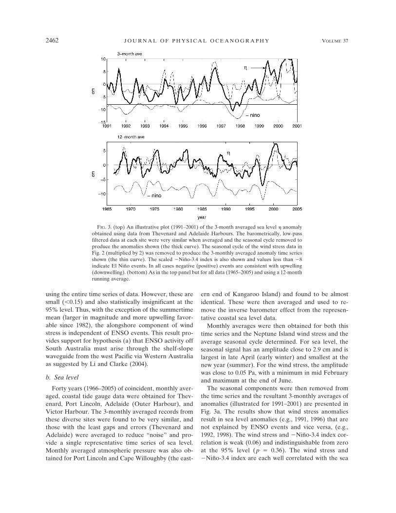
The seasonal components were then removed fromthe time series and the resultant 3-monthly averages ofanomalies (illustrated for 1991–2001) are presented inFig. 3a. The results show that wind stress anomaliesresult in sea level anomalies (e.g., 1991, 1996) that arenot explained by ENSO events and vice versa, (e.g.,1992, 1998). The wind stress and �Niño-3.4 index cor-relation is weak (0.06) and indistinguishable from zeroat the 95% level (p � 0.36). The wind stress and�Niño-3.4 index are each well correlated with the sea

FIG. 3. (top) An illustrative plot (1991–2001) of the 3-month averaged sea level anomalyobtained using data from Thevenard and Adelaide Harbours. The barometrically, low-passfiltered data at each site were very similar when averaged and the seasonal cycle removed toproduce the anomalies shown (the thick curve). The seasonal cycle of the wind stress data inFig. 2 (multiplied by 2) was removed to produce the 3-monthly averaged anomaly time seriesshown (the thin curve). The scaled �Niño-3.4 index is also shown and values less than �8indicate El Niño events. In all cases negative (positive) events are consistent with upwelling(downwelling). (bottom) As in the top panel but for all data (1965–2005) and using a 12-monthrunning average.

2462 J O U R N A L O F P H Y S I C A L O C E A N O G R A P H Y VOLUME 37

level anomalies, 0.60 (p � 0.002) and 0.48 (p � 0.0009),respectively, and together explain 56% of the total sealevel anomaly variance.

In Fig. 3b, the 12-monthly anomalies are also pre-sented along with the �Niño-3.4 index. The correlationbetween wind stress and Niño-3.4 is again small (0.15)and insignificant (p � 0.18). The correlation of thewind stress and �Niño-3.4 index with sea level anoma-lies is again visually apparent and equal to 0.55 (p �0.0001) and 0.62 (p � 0.000 01), respectively, both sta-tistically significant. [The correlation between interan-nual ENSO and sea level (0.62) is somewhat smallerthan that obtained for Fremantle (0.71) by Li andClarke (2004), but this might be expected given thescattering and/or frictional effects.] Some 60% of thesea level anomaly variance is explained by wind stressand Niño-3.4 for the 12-month averages. The conclu-sion that both effects are of comparable importanceimplies that ENSO effects on upwelling can be maskedby effects of wind stress.

3. Ocean temperature observations: ENSO andupwelling

In the following, we examine remotely sensed and insitu observations of ocean temperature for the BonneyCoast and Kangaroo Island regions. Events of anoma-lous warming by the Antarctic “Circumpolar Wave”extend to Australia’s southern shelves (White andPeterson 1996; White et al. 1998) and are reflected inthe coastal SST results below. In addition, the satellite-derived observations also show SST to be generallycooler during El Niño austral summers, although thestatistics are not conclusive. Time series of in situ tem-perature data also generally show upwelled water to bevery much cooler during recent El Niño events. Wenote that ENSO-related variations in SST and in situtemperature were also found for the West Australianshelf slope by Feng et al. (2003) and Wijffels and Mey-ers (2004). The former report the thermocline (below150 m) to be thicker and shallower (by about 10 m)during El Niño years and SST to be cooler (by 1°Cor so).

a. Sea surface temperature: Satellite data

Monthly averaged time series of SST were obtainedfrom the Pathfinder 4 and 5 satellites (nighttime data)from 1985 until 2004 (Table 1). The data has a listedaccuracy of 0.3°–0.5°C, and three sites were chosen toexamine the effects of ENSO events and the ACW.

We consider SST results for the Kangaroo Island andBonney Coast (Robe) regions (Fig. 1; Table 1). Sum-

mer (January–February) and winter (August–Septem-ber) averaged SST anomalies were obtained and areshown in Fig. 4 along with El Niño events (verticaldashed lines) and events of ACW warming (W). Thesummer SST anomalies (Fig. 4) do indicate influence byboth El Niño and ACW events. Relatively cool water isgenerally found during El Niño summers, suggestingthat upwelling may be enhanced during these years [hy-pothesis (ii)]. Indeed, in Fig. 4c, we present the summer(January–February) averages of both the �Niño-3.4 in-dex and the 3-monthly averaged sea level described insection 2. The correlation between these two time se-ries for 1985–2004 is high (0.70) with evident minimaduring the El Niño summers shown. There is a visualcorrelation between the SST off Kangaroo Island (andthe Bonney Coast) with both the ENSO signal and sealevel, although the numerical values are small (�0.25)and statistically indistinguishable from zero at the 95%level (p � 0.14).

FIG. 4. (a) The summer (January–February: dark curve) andwinter (August–September: light curve) averaged values of theSST anomaly for the Kangaroo Island region. The means are18.34° and 15.01°C for summer and winter, respectively. The Wdenotes warming periods due to the ACW. The vertical dashedlines indicate El Niño summers. Winter El Niño and La Niñaevents are labeled by the E and L. (b) Same as in (a) but for theRobe region. The means are 17.08° and 14.08°C for summer andwinter, respectively. (c) The summer (January–February) aver-ages of the 3-month averaged sea level and of the �Niño-3.4index. Negative values indicate El Niño events.

OCTOBER 2007 M I D D L E T O N E T A L . 2463

The summer SST results also appear to be influencedby the ACW. With the exception of 1989 (which followsthe 1987–88 El Niño cooling), each of the warmest SSTanomalies also correspond to the warmest (January)period of the 4-yr ACW. The correlation between thesummer SST off Kangaroo Island and the ACW wasfound to be 0.52 and significantly different from zero atthe 95% level (p � 0.009).

To separate out the ACW and ENSO effects, a re-gression model made up of the 4-yr period ACW andthe 3-monthly averaged sea level (or �Niño-3.4 index)was also fitted to the summer SST anomalies. Surpris-ingly, in both cases, the model was able to explain atmost 28% of the variance of SST, and the coefficientswere (just) not significant from zero at the 95% level(p � 0.062). The reason for this is thought in part re-lated to the use of satellite-derived SST as a measure ofsummertime coastal upwelling: the nighttime satellitedata used is monthly averaged, obtained from relativelylarge regions [�(100 km)2 ; see Table 1], and may beinfluenced by skin effects, errors (0.3°–0.5°C), andother factors. For example, an inspection of the SSTresults (Fig. 4) and winds (Fig. 2) shows that only in1999 does the SST summer minimum correspond toanomalously strong upwelling favorable winds that oc-cur in 1988, 1989, 1999, 2000, and 2003. As we will seebelow, there is a strong relation between subsurface insitu–measured temperature, winds, sea level, and theNiño-3.4 index.

Of course, the SST will be influenced by advection,diffusion, and surface heat fluxes. The latter have beenestimated (appendix) using the coarse (�2° � 2°)NCEP–NCAR products and converted to a monthlychange in temperature assuming a surface mixed layer(depth 50 m). The results shown in Fig. 5a do not ap-pear related to the SST data, the ACW, or ENSOevents and the implied changes in summer SST are oforder 1°C and of the opposite sign needed to explainthe cooler water generally found during El Niño years.The NCEP data and model used for assimilation arelikely too coarse to properly resolve atmosphericboundary layer effects near coastal upwelling regions.

In summary, the summertime SST data does showevidence of both ENSO and ACW influences. Surpris-ingly, multiple regressions made using these variables(and summertime sea level) showed that only 28% ofthe total SST variance was explained and the analysis(just) not statistically significant at the 95% level. Noclear relation was also found between SST and strongwind-forced upwelling events.

Our third hypothesis implies that wintertime intru-sions of the warm (light) Leeuwin Current water will bereduced (enhanced) during periods of weaker (stron-

ger) eastward advection during El Niño (La Niña)events. In agreement with this, the winter SST anoma-lies shown in Fig. 5b for the western bight show the ElNiño winters (labeled E) to be cooler or on averageneutral in 1986, 1987, 1994, 1997, and 2002. The exten-sive La Niña winters of 1988, 1999, and 2000 are alsogenerally warmer, as expected for a stronger LeeuwinCurrent. A similar result holds for the eastern bightresults in Fig. 4.

b. CTD and logger temperature data

We now consider subsurface observations of tem-perature taken through CTD surveys and from bottomloggers. One resource here is the Commonwealth Sci-entific and Industrial Research Organisation (CSIRO)Atlas of Regional Seas (CARS) that is made up of allobservations of temperature collected over the last 40years from ship surveys and historical data (Ridgway etal. 2002). The data is averaged in space and time toproduce output on 1⁄2° squares and as a weekly clima-tology for the year. Not all data were included in theatlas and no allowance made for interannual variabilityin its preparation. Thus, we first consider all availabledata for the Kangaroo Island region and for the sum-mer period (January–February). The source of thedata includes published work (Hahn 1986; Schahinger

FIG. 5. (a) The summer (January–February: dark curve) andwinter (August–September: light curve) averaged values of thenet heat flux for the Kangaroo Island region as converted into atemperature change per month for a 50-m deep surface mixedlayer. The dark and light dashed curves denote results for theRobe region. The vertical dashed lines indicate El Niño summers.(b) The summer (dark curve) and winter (light curve) averagedvalues of the SST anomaly for the western bight region (Esper-ance). The W denotes warming periods due to the ACW. Thevertical dashed lines indicate El Niño summers. Winter El Niñoand La Niña events are labeled by the E and L.

2464 J O U R N A L O F P H Y S I C A L O C E A N O G R A P H Y VOLUME 37

1987), the CARS data, the CSIRO Marine and Atmo-spheric Research Laboratories Information Network(MarLIN) data bank, and data collected by the SouthAustralian Research and Development Institute (SARDI).

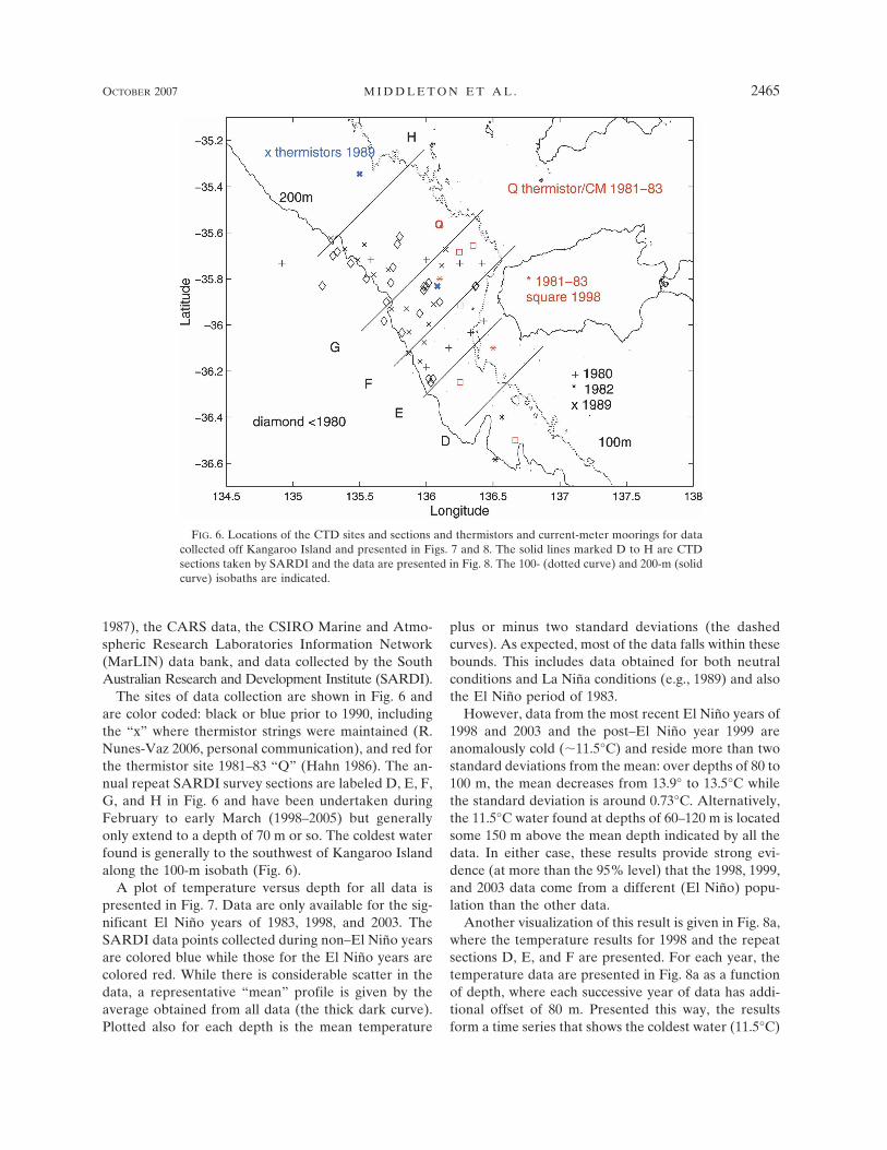
The sites of data collection are shown in Fig. 6 andare color coded: black or blue prior to 1990, includingthe “x” where thermistor strings were maintained (R.Nunes-Vaz 2006, personal communication), and red forthe thermistor site 1981–83 “Q” (Hahn 1986). The an-nual repeat SARDI survey sections are labeled D, E, F,G, and H in Fig. 6 and have been undertaken duringFebruary to early March (1998–2005) but generallyonly extend to a depth of 70 m or so. The coldest waterfound is generally to the southwest of Kangaroo Islandalong the 100-m isobath (Fig. 6).

A plot of temperature versus depth for all data ispresented in Fig. 7. Data are only available for the sig-nificant El Niño years of 1983, 1998, and 2003. TheSARDI data points collected during non–El Niño yearsare colored blue while those for the El Niño years arecolored red. While there is considerable scatter in thedata, a representative “mean” profile is given by theaverage obtained from all data (the thick dark curve).Plotted also for each depth is the mean temperature

plus or minus two standard deviations (the dashedcurves). As expected, most of the data falls within thesebounds. This includes data obtained for both neutralconditions and La Niña conditions (e.g., 1989) and alsothe El Niño period of 1983.

However, data from the most recent El Niño years of1998 and 2003 and the post–El Niño year 1999 areanomalously cold (�11.5°C) and reside more than twostandard deviations from the mean: over depths of 80 to100 m, the mean decreases from 13.9° to 13.5°C whilethe standard deviation is around 0.73°C. Alternatively,the 11.5°C water found at depths of 60–120 m is locatedsome 150 m above the mean depth indicated by all thedata. In either case, these results provide strong evi-dence (at more than the 95% level) that the 1998, 1999,and 2003 data come from a different (El Niño) popu-lation than the other data.

Another visualization of this result is given in Fig. 8a,where the temperature results for 1998 and the repeatsections D, E, and F are presented. For each year, thetemperature data are presented in Fig. 8a as a functionof depth, where each successive year of data has addi-tional offset of 80 m. Presented this way, the resultsform a time series that shows the coldest water (11.5°C)

FIG. 6. Locations of the CTD sites and sections and thermistors and current-meter moorings for datacollected off Kangaroo Island and presented in Figs. 7 and 8. The solid lines marked D to H are CTDsections taken by SARDI and the data are presented in Fig. 8. The 100- (dotted curve) and 200-m (solidcurve) isobaths are indicated.

OCTOBER 2007 M I D D L E T O N E T A L . 2465

Fig 6 live 4/C

to be found at depths of 70 m during the El Niño sum-mers of 1998 and 2003 and in the post–El Niño summerof 1999. To 95% probability, this cold water normallyresides at depths greater than 200 m or so. Notably,very warm water was found during the strong La Niñasummer of 2000. Similar results are found for section Hoff the Eyre Peninsula (Fig. 8b). While the water hereis generally warmer than off Kangaroo Island, the cold-est summers are again 1998 and 2003 and the post–ElNiño summer of 1999.

Similar evidence for El Niño–enhanced upwelling isalso found from CTD and logger data collected off theBonney Coast (Fig. 9), some 400 km to the southeastof Kangaroo Island. The CTD data is for the January–March period and mostly from 1989 and from amonthly repeat site (1973–81) off Port MacDonnell(Fig. 9). The temperature range from two moorings de-ployed off Robe (the summers of 1983 and 1984) isalso indicated by the red horizontal lines in Fig. 10(Schahinger 1987).

All data are presented in Fig. 10 and the mean tem-

FIG. 8. (a) CTD data collected between 1999 and 2005 from theSARDI sections D, E, F, and G in Fig. 6. Beginning with 1998, thedata is plotted against depth and then data for each subsequentyear shifted to the right by the 80-m spacing indicated. (b) As in(a) but for section H off the Eyre Peninsula.

FIG. 7. Summertime temperature data vs depth for the Kangaroo Island region and from a variety of sourcesindicated in the plot and in Fig. 6. The data points colored red are for the El Niño years 1983, 1998, and 2003 andthe years 1984 and 1999 that followed the largest El Niño events. The thick dark curve denotes the average of alldata shown. The dashed curves denote the average plus or minus two standard deviations.

2466 J O U R N A L O F P H Y S I C A L O C E A N O G R A P H Y VOLUME 37

Fig 7 live 4/C

perature and mean plus or minus two standard devia-tions are again indicated. Most of the non–El Niño yeardata falls within the bounds of the latter. The excep-tions include the latter years (1979–81) of the Port Mac-Donnell data obtained for neutral ENSO conditionsand at depths 40–50 m (see Fig. 11b). We have no ex-planation for this anomalously cold water as ENSO isneutral and the upwelling winds are not unusually largeand the annual sea level signal is also anomalously posi-tive (Fig. 3b).

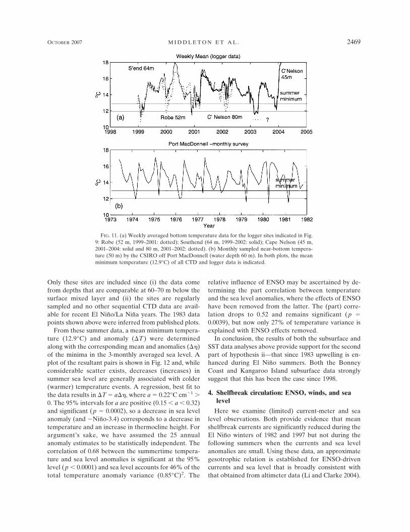
In subsequent years, anomalously cold (�10.5°–11°C) is found at depths 60–120 m and is up to threestandard deviations cooler than the mean (Fig. 10).These data were obtained during March 1983 (El Niño)and February 1984 (post–El Niño) and are the coldestmeasured until 1998, 1999, and 2003 (the O in Fig. 10).The latter data come from loggers deployed betweenRobe and Cape Nelson (Fig. 9). These data have beenaveraged to yield weekly means that are presented inFig. 11a. Between January 1999 and 2001, bottom datawas available from loggers at Robe (52-m depth) andSouthend (64-m depth). The results indicate the coldestwater (�11°C) to be obtained at the Robe logger dur-

ing 1999. After January 2001, data were obtained fromloggers at depths of 45 and 80 m and at the Cape Nelsonsites (Table 1). Unfortunately, the deeper logger failedbefore the El Niño summer of 2003. However, the tem-perature registered at this time by the logger at 45 mwas around 11.8°C. Given the evident stratification ofthe previous summer, we might well expect the watertemperature at the 80-m depth to have been around10.8°C, so the 2003 data are the coldest since 1999.

In summary, the coldest periods for the BonneyCoast are the El Niño summers of 1983, 1998, 2003, andthe post–El Niño summers of 1984 and 1999. Theanomalously cold water at depths 60–120 m is up tothree standard deviations cooler than the mean and islocated some 150 m above the mean depth indicated byall of the data. In agreement with the Kangaroo Islanddata, these results provide strong evidence (at morethan the 95% level) that the 1998, 1999, and 2003 datacome from a different population than the other dataand very likely are associated with El Niño events. Evi-dence off the Bonney Coast would also indicate that thestrong 1983 El Niño was important to raising the ther-mocline as well.

FIG. 9. Locations of the CTD sites and thermistors and current-meter moorings for data collected offthe Bonney Coast and presented in Fig. 10. The general locations of the temperature loggers for datapresented in Fig. 11 are also indicated. The Port MacDonnell repeat site (1973–81) is indicated by thediamond. The current-meter sites off Robe are indicated by the red circles offshore and inshore. The200-m isobath is indicated.

OCTOBER 2007 M I D D L E T O N E T A L . 2467

Fig 9 live 4/C

A possible cause of the anomalously cold waterfound during the post–El Niño summers of 1984 and1999 involves the winds and the very large prior ElNiño events. Both 1984 and 1999 summers follow twoof the largest El Niño events as measured by the Niño-3.4 index. The very cold water found on the shelf duringthe summers of 1983 and 1998 will be subsequentlydownwelled during the following winter. For both ElNiños, however, the downwelling winds were of order�0.04 Pa and relatively weak compared to the long-term mean of �0.06 Pa. During the following summersof 1984 and 1999, the upwelling winds are relativelylarge: for summer 1984 the upwelling winds are com-parable to the 1982–2004 long-term mean of 0.048 Pa,while for summer 1999 the 3-monthly averaged up-welling winds are amongst the strongest on record (0.07Pa). Thus, in both cases, very cold upwelled water fromthe previous El Niño might be brought back onto theshelf.

The only other time series of temperature data ofwhich we are aware is the repeat CTD station (water

depth 60 m) that was maintained for 9 years (1973–81)off Port MacDonnell by the CSIRO (Fig. 9). The sta-tion was occupied typically once per month and tem-peratures were measured at 10-m intervals throughoutthe water column. Results for temperature measured at50 m (10 m from the bottom) are presented in Fig. 11b.The only two significant El Niño events were in 1973and 1978, but no corresponding cold anomalies arefound for these periods. This result suggests thatanomalous El Niño–driven upwelling has been mostsignificant since 1982.

c. Sea level as a proxy for subsurface temperature

As noted, both winds and ENSO are important toupwelling and thermocline displacement and both alsoaffect sea level. Sea level may therefore provide a use-ful proxy for upwelling and allow the relative effects ofwind and ENSO to be statistically quantified. To thisend, we have extracted the minimum summertime tem-peratures from the post-1997 data from the regularCTD sections and logger data shown in Figs. 8 and 11a.

FIG. 10. Summertime temperature data vs depth for the Bonney coast region from a variety of sources indicatedin the plot and in Fig. 9. The data points colored red are for the El Niño years 1983, 1998, and 2003 and the years1984 and 1999 that followed the largest El Niño events. The large red circle denotes summer data collected byloggers for the anomalously cold years 1999 and 2003 (Fig. 11). The thick dark curve denotes the average of all datashown; the dashed curves denote the average plus or minus two standard deviations.

2468 J O U R N A L O F P H Y S I C A L O C E A N O G R A P H Y VOLUME 37

Fig 10 live 4/C

Only these sites are included since (i) the data comefrom depths that are comparable at 60–70 m below thesurface mixed layer and (ii) the sites are regularlysampled and no other sequential CTD data are avail-able for recent El Niño/La Niña years. The 1983 datapoints shown above were inferred from published plots.

From these summer data, a mean minimum tempera-ture (12.9°C) and anomaly (T ) were determinedalong with the corresponding mean and anomalies ()of the minima in the 3-monthly averaged sea level. Aplot of the resultant pairs is shown in Fig. 12 and, whileconsiderable scatter exists, decreases (increases) insummer sea level are generally associated with colder(warmer) temperature events. A regression, best fit tothe data results in T � a, where a � 0.22°C cm�1 �0. The 95% intervals for a are positive (0.15 � a � 0.32)and significant (p � 0.0002), so a decrease in sea levelanomaly (and �Niño-3.4) corresponds to a decrease intemperature and an increase in thermocline height. Forargument’s sake, we have assumed the 25 annualanomaly estimates to be statistically independent. Thecorrelation of 0.68 between the summertime tempera-ture and sea level anomalies is significant at the 95%level (p � 0.0001) and sea level accounts for 46% of thetotal temperature anomaly variance (0.85°C)2. The

relative influence of ENSO may be ascertained by de-termining the part correlation between temperatureand the sea level anomalies, where the effects of ENSOhave been removed from the latter. The (part) corre-lation drops to 0.52 and remains significant (p �0.0039), but now only 27% of temperature variance isexplained with ENSO effects removed.

In conclusion, the results of both the subsurface andSST data analyses above provide support for the secondpart of hypothesis ii—that since 1983 upwelling is en-hanced during El Niño summers. Both the BonneyCoast and Kangaroo Island subsurface data stronglysuggest that this has been the case since 1998.

4. Shelfbreak circulation: ENSO, winds, and sealevel

Here we examine (limited) current-meter and sealevel observations. Both provide evidence that meanshelfbreak currents are significantly reduced during theEl Niño winters of 1982 and 1997 but not during thefollowing summers when the currents and sea levelanomalies are small. Using these data, an approximategesotrophic relation is established for ENSO-drivencurrents and sea level that is broadly consistent withthat obtained from altimeter data (Li and Clarke 2004).

FIG. 11. (a) Weekly averaged bottom temperature data for the logger sites indicated in Fig.9: Robe (52 m, 1999–2001: dotted); Southend (64 m, 1999–2002: solid); Cape Nelson (45 m,2001–2004: solid and 80 m, 2001–2002: dotted). (b) Monthly sampled near-bottom tempera-ture (50 m) by the CSIRO off Port MacDonnell (water depth 60 m). In both plots, the meanminimum temperature (12.9°C) of all CTD and logger data is indicated.

OCTOBER 2007 M I D D L E T O N E T A L . 2469

The sea level data is also examined to show that anasymmetric response does occur when averaged overthe El Niños between 1972 and 2005. However, withthe limited data available, this asymmetry cannot beproven statistically. Nonetheless, such an asymmetricresponse is also found by Feng et al. (2003) in an analy-sis of transports of the Leeuwin Current off WesternAustralia and in the global POP model results de-scribed in section 5. A likely explanation for this asym-metric response is given in section 6 and involves thethermohaline circulation associated with the LeeuwinCurrent during winter and upwelling during summer.

As noted, Feng et al. (2003) have shown that thereare ENSO-related interannual variations in the strengthof the Leeuwin Current. Using long records of tem-perature off Fremantle, these authors showed that theENSO-related poleward transport increases by 1 Sv(Sv � 106 m3 s�1) between El Niño and La Niña years.(A 300-m level of no motion was adopted and the geo-strophic transports were calculated out to 150 km fromthe coast.) This ENSO-related transport is significantrelative to the summer and winter poleward transportsof 3 and 5 Sv, respectively, and corresponds to a 20%change in the mean speed of the Leeuwin Current (�30

cm s�1). An asymmetric response is also found in thesegeostrophic transports (Feng et al. 2003, their Fig. 16)whereby departures of the ENSO-related polewardtransport from the seasonal climatology is larger duringwinter than summer. It is worth noting here that Fenget al. (2003) used 12-monthly calendar averages begin-ning in January rather than July. The latter averagingperiod might be more appropriate since ENSO eventstypically occur over July to February and (Webster andYang 1992) become uncorrelated during the austral au-tumn (March–May).

For the South Australian region, Li and Clarke(2004) also examined interannual sea level anomalies asobtained from altimeter data. Using cross-shelf satellitetracks, they inferred a coherent ENSO-related sea levelsignal across the shelf and shelf slope. The largest gra-dients were found over the shelf slope, and the ampli-tudes of ENSO-driven geostrophic, average currentswere directed to the east (poleward) and around 6 and4 cm s�1 off Thevenard and Robe, respectively. Overthe shelf, these authors estimate the ENSO currents tobe smaller, although the validity of the altimeter-de-rived SSH data near the coast was acknowledged to bequestionable.

FIG. 12. A scatterplot of the anomalies of the summer subsurface temperature minima (T )vs summer sea level minima anomalies (). The former were obtained as the minimumsummertime temperature (less the mean) using the 1998–2005 SARDI data (sites D–G: Fig.8) and logger data (Fig. 11a). Sea level anomalies were obtained as the summer minimum (lessthe mean) for the 1998–2005 period and from the 3-monthly averaged sea level time series.The dark line corresponds to the regression fit T � a, where a � 0.22°C cm�1.

2470 J O U R N A L O F P H Y S I C A L O C E A N O G R A P H Y VOLUME 37

Indeed, a summary of current-meter observations inTable 2 suggests that the El Niño–related variabilityduring winter is larger than the average annual ENSOresponse of 4–6 cm s�1 inferred by Li and Clarke (2004)and of order 20 cm s�1 over the shelf break. In Table 2,we have paired all available estimates of El Niño andnon–El Niño mean alongshore currents at similar (orsame) sites for summer and winter (Figs. 1, 6, and 9).

For summer, the mean alongshore currents are gen-erally to the northwest but small in amplitude (�5cm s�1). There is no consistent difference between theresults for the 1983 El Niño and other non–El Niñoyears. The alongshore wind stress for the summers ofcurrent-meter deployments is also shown in Table 2. Noconsistent response in currents to the stronger up-welling favorable winds for 1981 and 1984 is apparent.The reason here may be related to the sites of the Q(Fig. 6) and A (Fig. 9) moorings that lie over the shelfbreak (depth �150 m). Numerical results suggest thatthese sites lie between stronger westward shelf andeastward slope currents (Middleton and Platov 2003),Fig. 13. Additional observations are provided by thelong time series of coastal sea level (demeaned) thathave been averaged over the periods of the current-

meter deployments shown in Table 2. For the summerperiods considered, the results (Table 2) are consistentwith the current-meter results in that the sea level val-ues are generally small (�2 cm) and do not show anyconsistent response to either winds or the ENSO eventsof 1981 to 1984.

In contrast, the winter mean currents and sea levelare both larger and appear to be influenced by El Niñoevents. At the shelfbreak sites off Spencer Gulf (Q),Robe (A), and Tasmania (S2, R2; Fig. 1), the polewardmean currents are reduced by around 20 cm s�1 duringthe 1982 and 1997 El Niño years: again we define an ElNiño winter to be that prior to the minimum in the�Niño-3.4 index. [At the inner shelf site off Tasmania(S1, R1), the mean currents are weaker but also re-duced during an El Niño winter.] A similar result is alsofound in sea level, again averaged over the periods ofcurrent-meter deployments indicated in Table 2. In thiscase, the El Niño year drop in eastward currents isaccompanied by a drop in sea level. The average dropis 11 cm for an 18 cm s�1 drop in eastward current. Thewinter wind stress for the years of current-meter de-ployments (Table 2) show that relative to 1981 and1983, the wind stress is much weaker for the El Niño

TABLE 2. Current-meter, sea level, and wind stress observations. The tables present mean current speeds and directions obtainedfrom available and published data for summer and winter periods. The first column indicates whether the data are from an El Niño year.Observations from El Niño and non–El Niño years are paired for repeat observation sites (the first being for a non–El Niño year). Thesecond column indicates the mooring site (as shown in Fig. 1), upper (U) or lower (L), and year. The columns labeled “1st record” and“Days” indicate the start time and number of days used to compute the statistics. The latitude and longitude are in degrees south andeast, respectively. The magnitude of the vector mean | U | (cm s�1) is given along with its direction � in degrees anticlockwise from east.In the final two columns are the sea level (averaged for the period of current-meter deployment; cm) and the summer or winter windstress (100 Pa).

Event Site 1st record Days Lat LonWaterdepth

Instrumentdepth |U| � 100

SummerEl Niño Q U 82 11 Nov 1981 78 35.70 135.78 138 22 2.4 289 0.8 �2.0

Q U 83 2 Dec 1982 95 35.70 135.78 146 15 2.9 267 0.8 �2.4El Niño Q L 81 12 Dec 1980 50 35.77 135.75 137 115 2.0 144 �2.0 �5.3

Q L 82 11 Nov 1981 78 35.77 135.75 137 133 3.5 298 0.8 �2.0Q L 83 2 Dec 1982 95 35.77 135.75 146 125 2.9 330 0.8 �2.4

El Niño B 84 21 Jan 1984 56 37.43 139.72 50 26 5.3 30 0.4 �4.1B 83 7 Feb 1983 60 37.43 139.72 52 24 3.5 113 4.0 �2.4

El Niño A 84 21 Jan 1984 56 37.53 139.52 146 115 4.9 332 0.4 �4.1A 83 7 Feb 1983 60 37.53 139.52 143 110 2.5 7 4.0 �2.4

WinterEl Niño Q U 81 6 Apr 1981 78 35.77 135.75 137 42 20.2 �30 7.8 7.7

Q U 82 26 Aug 1982 97 35.77 135.75 144 31 1.4 �108 �5.2 2.8El Niño Q L 81 6 Apr 1981 78 35.77 135.75 137 115 19.2 �54 7.8 7.7

Q L 82 26 Aug 1982 97 35.77 135.75 144 124 4.6 �57 �5.2 2.8El Niño A 83 7 Jul 1983 57 37.53 139.52 143 112 28.5 �49 2.6 7.3

A 82 8 Aug 1982 59 37.53 139.52 143 111 7.4 �60 �6.4 2.8El Niño S1 88 1 Jul 1988 90 42.65 145.01 93 72 4.0 �72 6.0 5.4

R1 97 1 Jul 1997 90 42.43 145.00 100 40–90 2.1 �97 �6.4 3.3El Niño S2 88 1 Jul 1988 90 42.75 144.92 200 190 26.4 �80 6.0 5.4

R2 97 1 Jul 1997 90 42.55 144.90 188 8–180 10.0 �89 �6.4 3.3

OCTOBER 2007 M I D D L E T O N E T A L . 2471

winter of 1982. For the El Niño winter of 1997, the windstress (0.033) is also smaller than that of 1988 (0.054).The changes in shelf break currents may thus be ENSOand/or wind forced.

An asymmetric response in shelf currents during ElNiño events should imply a similar response in sealevel. To investigate this further, we have calculated thewinter and summer average anomalies of coastal sealevel from the data presented in Fig. 3a and for the ElNiño years between 1972 and 2003. That data wasdetrended and demeaned and the seasonal cycle re-moved: the latter calculated for each month so as toremove the seasonal asymmetric winter–summer cycle.The results do show an asymmetric response in thatthe average winter sea level anomaly is �4 cm andlarger in magnitude than the summer anomaly of �2.6cm: the averaged value of �Niño-3.4 is �1.1 and �1.4,respectively, and the ENSO index, as expected, is largerin magnitude during summer. There is considerablescatter in these sea level anomalies. For the two largestEl Niño events, the asymmetry in the sea level anoma-lies is strong with winter and summer values of �8.0and �6.3 cm for 1982–83 and �10.1 and �6.2 cm for1997–98. For the averaged results, the standard devia-tions are, however, large (4.6 and 4.3 cm for winter andsummer) and an asymmetric response is not statisticallysignificant at the 95% level.

Last, we return to the relationship between currentsand sea level. As noted, the average change in sea leveland alongshore currents are 11 cm and 18 cm s�1 during

El Niño winters. For El Niño summers, the changes areboth effectively zero. Now, Li and Clarke (2004) as-sumed that geostrophy should pertain and their resultssuggest that sea level changes little across the shelf atinterannual periods. Let us adopt these assumptionsand an exponential model for sea level � c(t)exp(�x�/L), where c(t) denotes coastal sea level and x�is the distance from the shelf edge. For the changes insea level c(t) � 11 cm and velocity (18 cm s�1) at theshelf break (x � 0) the required length scale is L � 75km, which is comparable to the internal deformationradius for the region (40–80 km) and is consistent withthe analysis of Li and Clarke (2004).

The velocity response per unit centimeter change insea level for winter is 1.6 cm s�1. Averaged over a year,this is halved to be 0.8 cm s�1 per centimeter in sealevel and is close to that estimated from the EOF analy-sis of Li and Clarke (2004): they find a 4–6 cm s�1 (0.8–1.2 cm s�1) amplitude response to a 5 cm (1 cm) am-plitude change in ENSO sea level signal from an inter-annual analysis. Thus, an asymmetry in the summer andwinter response is not inconsistent with annual resultsof Li and Clarke (2004).

In conclusion, from the analysis here, there is evi-dence to support significant ENSO-induced changes inshelfbreak velocity (�18 cm s�1) and sea level (�10cm) during El Niño winters but with smaller changesduring the subsequent summers. The results are notinconsistent with the annual ENSO analysis of Li andClarke (2004). Winds likely play a role here as well andfor the 1983 and 1997 winters; the shelf-edge and pos-sibly shelf currents may have been largely shutdown.

5. Results from a global ocean model

Here we examine recent monthly averaged outputfrom the 1⁄10° POP global ocean model (Maltrud andMcClean 2005). The temperature and salinity of themodel is initialized with a global climatology and drivenusing NCEP–NCAR daily atmospheric fluxes of heat,salt, and momentum. Results for the period 1994 to2000 are presented. Along Australia’s southern shelves,the cross-shelf grid spacing is about 9 km and the shelfslope is barely resolved off Kangaroo Island.

Some model results for this period are in strikingqualitative agreement with the data: the largest minimain sea level occur during the summer El Niños of 1995and 1998, and the coldest water (strongest upwelling) isfound on the slope during these years and also in 1999.The model results also support aspects of the hypoth-eses advanced above, including that the ENSO signalsare remotely driven and that downwelling and winter-time shelf/slope currents during El Niños are sub-

FIG. 13. (a) The dark solid and dashed curves correspond tobarometrically adjusted sea level (monthly averaged) for the Port-land and Thevenard coastal sites. (b) The monthly averagedcoastal sea level from the POP global model. In both (a) and (b),the Thevenard results are offset by 10 cm relative to those fromPortland. The vertical dashed lines indicate El Niño summers.

2472 J O U R N A L O F P H Y S I C A L O C E A N O G R A P H Y VOLUME 37

stantially reduced. Moreover, the model results providean overview of the 1998 El Niño and change to the1999–2000 La Niña conditions. There are deficiencies inthe model results and the temperature, sea level, andshelf currents differ quantitatively from that expectedfrom the data record. For this reason, our discussion isonly descriptive.

a. Sea level

We begin with the monthly averaged sea level fromPOP (1994–2000) at the Thevenard and Portland sites,presented in Fig. 13 along with the observations. Forclarity, the results for Thevenard are again offset by 10cm. The model results are in crude agreement with theobservations, with summer minima and winter maximathat differ by about 15–20 cm within each year. Thelowest sea level is found for the El Niño summers of1995 and 1998, while the largest sea level occurs duringthe winters of 1996, 1999, and 2000—the strong LaNiñas (see Fig. 14). We have traced the ENSO and sealevel signals back along the West Australian shelf toPort Headland, indicating remote forcing from the westPacific.

As noted, the shelf currents and transports associatedwith the ENSO signals are of interest, particularly dur-ing the winter and summer of the El Niño events. InFig. 14, we present the net transport for a meridionalsection at 137.5° (Kangaroo Island) that is bounded bythe 200-m (and 400 m) isobath and within 1.5° of the

coast. Note: negative values are directed to the east sothat the results are in phase with the �Niño-3.4 indexand the upwelling component of NCEP wind stress.The transports bounded by 200 and 400 m are similar.

b. Thermohaline effects

The first feature of the results in Fig. 14 is that themaximum amplitude of the transports leads those of thewind by 1–2 months and occurs in December (summer)and May (winter). This phase lead provides likely evi-dence of the importance of the thermohaline circula-tion. Indeed, the maximum amplitude of summer heat-ing (winter cooling) of the NCEP fluxes occurs in Janu-ary (July) and likely explains the maximum amplitudeof the SST anomalies that occur about one month laterin February (August). The anomalies and implied ther-mohaline circulation are thus a maximum when thewinds are. However, for both seasons, the thermohalinecirculation will oppose that driven by the winds so thatthe maximum transports occur 1–2 months earlier asfound (in December and May).

c. Transports

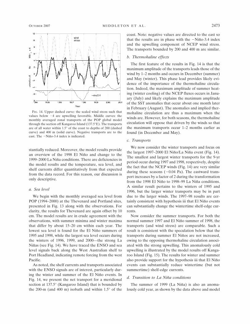
We now consider the winter transports and focus onthe largest 1997–2000 El Niño/La Niña event (Fig. 14).The smallest and largest winter transports for the 9-yrperiod occur during 1997 and 1998, respectively, despitethe fact that the NCEP winds (Fig. 14) are very similarduring these seasons (�0.04 Pa). The eastward trans-port increases by a factor of 2 during the transformationfrom the 1998 El Niño to 1998–99 La Niña conditions.A similar result pertains to the winters of 1995 and1996, but the larger winter transports may be in partdue to the larger winds. The 1997–98 results are cer-tainly consistent with hypothesis iii that El Niño eventscan substantially change the wintertime shelf-edge cur-rents.

Now consider the summer transports. For both thenormal summer 1997 and El Niño summer of 1998, thetransports (and wind stress) are comparable. Such aresult is consistent with the speculation below that thetransports during summer El Niños are not increased,owing to the opposing thermohaline circulation associ-ated with the strong upwelling. This anomalously coldupwelling is illustrated by the model results off Kanga-roo Island (Fig. 15). The results for winter and summeralso provide support for the hypothesis iii that El Niñoevents can substantially reduce wintertime (but notsummertime) shelf-edge currents.

d. Transition to La Niña conditions

The summer of 1999 (La Niña) is also an anoma-lously cold year, as shown by the data above and model

FIG. 14. Upper dashed curve: the scaled wind stress such thatvalues below �4 are upwelling favorable. Middle curves: themonthly averaged zonal transports of the POP global modelthrough the section off Kangaroo Island (137.5°E). The transportsare of all water within 1.5° of the coast to depths of 200 (dashedcurve) and 400 m (solid curve). Negative transports are to theeast. The �Niño-3.4 index is indicated.

OCTOBER 2007 M I D D L E T O N E T A L . 2473

results for Kangaroo Island (Fig. 15). The mechanismfor enhanced model upwelling in this La Niña summeris again likely to be due in part to the stronger NCEPwinds at this time (Fig. 14). However, the summer 2000winds are similar, but upwelling in the model is reducedfrom that in 1999 (Fig. 15). Possibly the degree of up-welling in 1999 is preconditioned by the previous 1998winter downwelling and summer upwelling that arisesfrom both winds and ENSO events. The winter maxi-mum temperature for 1998 is close to the smallest forthe 9 years of output, indicating smaller downward dis-placement of the thermocline.

The transports and upwelling between summer 1999and summer 2000 illustrate the continued effect of LaNiña conditions. The wind stress for both summer sea-sons is almost identical and yet the 2000 summer trans-ports (Fig. 14) and upwelling (Fig. 15) are much re-duced. These results are consistent with the expectedeffects of the extensive La Niña that should act to re-duce the westward currents and lower the thermocline.The progressive lowering of the thermocline after thesummer of 1999 is indicated by the increasing summerand winter temperatures in Fig. 15.

e. A spatial overview

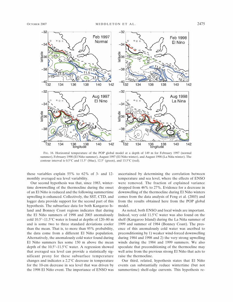
The ENSO effects are not just confined to the Kan-garoo Island region. In Fig. 16, we present the horizon-tal temperature field between mid bight and Portlandand at a depth of 149 m. In Figs. 16a,b, the Februarymonthly averaged temperature for the “normal” sum-mer of 1997 and El Niño summer of 1998 are shown.Note that, from Fig. 14, the up- and downwelling favor-able NCEP winds are similar for both years, so theanomalies are not directly wind driven. For the midbight region (132°E) the spatial extent of the relativelycold 13°C near-slope water is larger during the El Niño1998 summer. Similar results are found off the Robe–Portland region where the extent of the 12°C water islarger during 1998.

The winter (August) temperature fields are pre-

sented in Fig. 16 for 1997 (an El Niño winter) and 1998(a La Niña/normal winter). We hypothesized (ii) thatdownwelling of the thermocline is smaller (larger) dur-ing El Nino (La Niña) winters and this is supported bythe POP global model results where the near-slope wa-ter for El Niño August 1997 is generally 0.5°–1°C colderthan for August 1998. Again, winds are not the likelycause of this difference since the NCEP wind stress issimilar for these periods (Fig. 14).

In summary, the results of the global POP modelprovide support for the hypotheses (i) that ENSO ef-fects are important and driven by the shelf/slope wave-guide, (ii) that wintertime downwelling (summertimeupwelling) is reduced (enhanced) during El Niñoevents, and (iii) that wintertime (but not summertime)transports are substantially reduced during El Ninoevents.

6. Summary and discussion

We have examined oceanographic and meteorologi-cal data and output from a global ocean model so as toexamine the importance of ENSO signals to the oceancirculation and temperature structure of the waters ofthe South Australian region. ENSO events can alter thelocal meteorology, but also affect sea level and theheight of the thermocline through remote forcing alongthe shelf/slope waveguide from the west Pacific (e.g.,Clarke 1991). During El Niño events, the effects areopposite to those off the Americas: sea level is loweredand the thermocline raised.

Three hypotheses were tested against the data fromthe region. The first stated that, while upwelling favor-able winds in the eastern bight have been more persis-tent since 1982, local ENSO-related events are drivenlargely through the shelf waveguide from the west Pa-cific. An analysis of 40 years of wind and sea level dataprovides support for this hypothesis. Results show up-welling favorable winds to have been stronger since1982 although the correlation with the ENSO index(Niño-3.4) was weak. Moreover, in contrast with thesuggestion by Voice (1984), wintertime downwellingwinds were not found to be statistically related to ElNiño events. Indeed, the correlation between 3-monthly (or annually) averaged wind stress and �Niño-3.4 was found to be small (�0.06) and statistically in-significant, indicating that ENSO events off SouthernAustralia are forced by the shelf waveguide. Resultsfrom the global POP model and the original analyses ofPariwono et al. (1986) and Li and Clarke (2004) alsoshow that this is the case. Both ENSO and local windswere shown to be important to driving 5–10-cm changesin the local coastal sea level. A regression showed that

FIG. 15. Monthly averaged near-bottom temperature from thePOP global model (97 m in 104-m water) at two sites (138°E: solidcurve and 136.5°E: dotted curve) along the southern coast of Kan-garoo Island.

2474 J O U R N A L O F P H Y S I C A L O C E A N O G R A P H Y VOLUME 37

these variables explain 55% to 62% of 3- and 12-monthly averaged sea level variability.

Our second hypothesis was that, since 1983, winter-time downwelling of the thermocline during the onsetof an El Niño is reduced and the following summertimeupwelling is enhanced. Collectively, the SST, CTD, andlogger data provide support for the second part of thishypothesis. The subsurface data for both Kangaroo Is-land and Bonney Coast regions indicates that duringthe El Niño summers of 1998 and 2003 anomalouslycold 10.5°–11.5°C water is found at depths of 120–80 mand is some two to three standard deviations coolerthan the mean. That is, to more than 95% probability,the data come from a different El Niño population.Alternatively, the anomalously cold water found duringEl Niño summers lies some 150 m above the meandepth of the 10.5°–11.5°C water. A regression showedthat averaged sea level can provide a statistically sig-nificant proxy for these subsurface temperaturechanges and indicates a 2.2°C decrease in temperaturefor the 10-cm decrease in sea level that was driven bythe 1998 El Niño event. The importance of ENSO was

ascertained by determining the correlation betweentemperature and sea level, where the effects of ENSOwere removed. The fraction of explained variancedropped from 46% to 27%. Evidence for a decrease indownwelling of the thermocline during El Niño winterscomes from the data analysis of Feng et al. (2003) andfrom the results obtained here from the POP globalmodel.

As noted, both ENSO and local winds are important.Indeed, very cold 11.5°C water was also found on theshelf (Kangaroo Island) during the La Niña summer of1999 and summer of 1984 (Bonney Coast). The pres-ence of this anomalously cold water was ascribed topreconditioning by 1) weaker wind-forced downwellingduring 1984 and 1998 and 2) the very strong upwellingwinds during the 1984 and 1999 summers. We alsospeculate that preconditioning of the thermocline maywell arise from the previous strong El Niño that acts toraise the thermocline.

Our third, related, hypothesis states that El Niñoevents can substantially reduce wintertime (but notsummertime) shelf-edge currents. This hypothesis re-

FIG. 16. Horizontal temperature of the POP global model at a depth of 149 m for February 1997 (normalsummer), February 1998 (El Niño summer), August 1997 (El Niño winter), and August 1998 (La Niña winter). Thecontour interval is 0.5°C and 11.5° (blue), 12.5° (green), and 13.5°C (red).

OCTOBER 2007 M I D D L E T O N E T A L . 2475

Fig 16 live 4/C

ceived support from both the data and POP model. Forboth the 1983 El Niño and other non–El Niño summers,the observed alongshore currents and sea level anoma-lies were similar and smaller than the winter values. Forthe two El Niño winters for which current and sea leveldata were available (1982, 1997), an average 18 cm s�1

and an 11-cm reduction in currents and sea level wasfound compared to non–El Niño years. The results,however, might be due to a corresponding reduction inthe alongshore strength of the wind stress, although asimple geostrophic model for the winter shelf observa-tions was shown to be consistent with the analysis ofannual ENSO signals made by Li and Clarke (2004).Moreover, the wintertime SST anomalies were found tobe generally warmer (cooler) during La Niña (El Niño)events, suggesting that ENSO events do effect shelfcirculation.

An analysis was also made of the long sea levelrecord and provides further evidence that an asymme-try exists between winter and summer during El Niñoyears. Based on all El Niño year sea level anomalies(demeaned and seasonal cycle removed) between 1972and 2003, the winter average was found to be larger inmagnitude (�4.0 cm) than that for summer (�2.6 cm).The standard deviations here were large (�4.5 cm) andthe difference in the means not statistically significant.Nonetheless, for the two largest El Niño events, theasymmetry in the sea level anomalies is strong withwinter and summer values of �8.0 and �6.3 cm for1982–83 and �10.1 and �6.2 cm for 1997–98. In addi-tion, the POP model output showed the alongshorewinter (but not summer) transports to change by a fac-tor of 2 during the transition from the 1998 El Niño tonon–El Niño conditions.

The cause of the asymmetry in the summer and win-ter shelf/slope current response to El Niño events isunknown. We speculate that it could result in part fromsimple feedback mechanisms of the thermohaline cir-culation associated with the warm eastward inflow ofthe Leeuwin Current during winter and slope upwellingduring summer. In both cases, the changes in densityresult in a cross-shelf pressure gradient that can act todrive an eastward shelf current. Since the warm Leeu-win Current is reduced during El Niño events, the as-sociated eastward thermohaline circulation will be fur-ther reduced: a positive feedback mechanism. We haveno proof of this mechanism, although Cirano andMiddleton (2004) have demonstrated the importance ofthe thermohaline circulation to the region, and the SSTwinter anomalies presented here indicate that thestrength of the inflow of warm Leeuwin Current wateris influenced by ENSO events. During summer El Niñoevents, the eastward thermohaline currents may offset

the westward “upwelling” currents that would be oth-erwise enhanced by the El Niño event itself. Thus, alarge ENSO response might be expected during winter,while during summer the shelf and slope currents mayexhibit little change.

While an asymmetric response does occur, the pre-cise role of ENSO events, winds, and the thermohalinecirculation remains to be determined. Additional dataand idealized numerical experiments would be mostuseful.

Acknowledgments. The authors thank all ship’s crewand scientists who have labored in the collection of theextensive CTD, logger, and current-meter data that wehave examined. We also thank Ken Ridgway (CSIRO)and John Nairn (Australian Bureau of Meteorology)for making the CARS and Neptune Island data avail-able to us. NCEP reanalysis data were provided bythe NOAA–CIRES ESRL/PSD Climate Diagnosticsbranch, Boulder, Colorado, from their Web site athttp://www.cdc.noaa.gov/. The SST data was obtainedfrom http://podaac-www.jpl.nasa.gov/ at the Jet Propul-sion Laboratory, California Institute of Technology.The POP simulation was supported by the Departmentof Energy/Climate Change Prediction Program, the Of-fice of Naval Research, and the National Science Foun-dation. It was conducted at the Maui High PerformanceComputing Center as part of a DoD High PerformanceComputing Modernization Program grand challengegrant. We also thank Allan Clarke for his thoughtfulreview and comments.

APPENDIX

Surface Heat Fluxes

We consider the net flux of heat into the ocean asgiven by the NCEP reanalysis fields (Kalnay et al.1996). The fluxes are determined on an �2° � 2° gridand the monthly averaged flux was obtained for regionsoff Kangaroo Island and Robe (Fig. 1). These werethen averaged over summer (January–February) andwinter (August–September) fluxes (Q) and then con-verted into a monthly change in temperature (�T) of asurface mixed layer depth H. Following Gill (1982), thechange in temperature per month is given by �T �tQ/(� CH)�1, where � � 1026 kg m�3 is the density ofseawater, C � 4000 J (kg K) �1, and t is 1 month (seeFig. 5a).

REFERENCES

Cirano, M., and J. F. Middleton, 2004: Aspects of the mean win-tertime circulation along Australia’s southern shelves: Nu-merical studies. J. Phys. Oceanogr., 34, 668–684.

2476 J O U R N A L O F P H Y S I C A L O C E A N O G R A P H Y VOLUME 37

Clarke, A. J., 1991: On the reflection and transmission of low-fre-quency energy at the irregular western Pacific Ocean bound-ary. J. Geophys. Res., 96, 3289–3305.

——, and S. Van Gorder, 1994: On ENSO coastal currents and sealevels. J. Phys. Oceanogr., 24, 661–680.

——, and J. Li, 2004: El Niño/La Niña shelf edge flow and Aus-tralian western rock lobsters. Geophys. Res. Lett., 31, L11301,doi:10.1029/2003GL018900.

Etnoyer, P., D. Canny, B. Mate, and L. Morgan, 2004: Persistentpelagic habitats in the Baja California to Bering Sea (B2B)region. Oceanography, 17, 90–101.

Feng, M., G. Meyers, A. Pearce, and S. Wijffels, 2003: Annual andinterannual variations of the Leeuwin Current at 32°S. J.Geophys. Res., 108, 3355, doi:10.1029/2002JC001763.

Gill, A. E., 1982: Atmosphere–Ocean Dynamics. Academic Press,662 pp.

Godfrey, J. S., D. J. Vaudrey, and S. D. Hahn, 1986: Observationsof the shelf-edge current south of Australia, winter 1982. J.Phys. Oceanogr., 16, 668–679.

Griffin, D. A., P. A. Thompson, N. J. Bax, R. W. Bradford, andG. M. Hallegraeff, 1997: The 1995 mass mortality of pilchard:No role found for physical or biological oceanographic fac-tors in Australia. Mar. Freshwater Res., 48, 27–42.

Hahn, S. D., 1986: Physical structure of the waters of the SouthAustralian Continental Shelf. Flinders Institute for Atmo-sphere and Marine Sciences Res. Rep. 45, 284 pp.

Kalnay, E., and Coauthors, 1996: The NCEP/NCAR 40-Year Re-analysis Project. Bull. Amer. Meteor. Soc., 77, 437–471.

Kosro, P. M., 2002: A poleward jet and an equatorward under-current observed off Oregon and northern California, duringthe 1997–98 El Niño. Prog. Oceanogr., 54, 343–360.

Li, J., and A. J. Clarke, 2004: Coastline direction, interannualflow, and the strong El Niño currents along Australia’s nearlyzonal southern coast. J. Phys. Oceanogr., 34, 2373–2381.

Maltrud, M. E., and J. L. McClean, 2005: An eddy resolving global1/10th degree ocean simulation. Ocean Modell., 8, 31–54.

McClatchie, S., J. F. Middleton, and T. M. Ward, 2006: Watermass analysis and alongshore variation in upwelling intensityin the eastern Great Australian Bight. J. Geophys. Res., 111,C08007, doi:10.1029/2004JC002699.

Middleton, J. F., and M. Cirano, 2002: A northern boundary cur-rent along Australia’s southern shelves: The Flinders Cur-rent. J. Geophys. Res., 107, 3129, doi:10.1029/2000JC000701.

——, and G. Platov, 2003: The mean summertime circulationalong Australia’s southern shelves: A numerical study. J.Phys. Oceanogr., 33, 2270–2287.

Pariwono, J. I., J. A. T. Byre, and G. W. Lennon, 1986: Long-period variations of sea level in Australasia. Geophys. J. Roy.Astron. Soc., 87, 43–54.

Pizarro, O., A. J. Clarke, and S. Van Gorder, 2001: El Niño sealevel and currents along the South American coast: Compari-son of observations with theory. J. Phys. Oceanogr., 31, 1891–1903.

Ridgway, K. R., J. R. Dunn, and J. L. Wilkin, 2002: Ocean inter-polation by four-dimensional weighted least squares—Appli-cation to the waters around Australasia. J. Atmos. OceanicTechnol., 19, 1357–1375.

Schahinger, R., 1987: Structure of coastal upwelling events ob-served off the southeast coast of South Australia. Aust. J.Mar. Freshwater Res., 38, 439–459.

——, 1989: Marine dynamics of a narrow continental shelf. Ph.D.thesis, Flinders University, 164 pp.

Smith, S. D., 1980: Wind stress and heat flux over the ocean ingale force winds. J. Phys. Oceanogr., 10, 709–726.

Voice, M., 1984: Drought. Aust. Nat. Hist., 21, 3–9.

Webster, P. J., and S. Yang, 1992: Monsoon and ENSO: Selec-tively interactive systems. Quart. J. Roy. Meteor. Soc., 118,877–926.

White, W. B., and R. Peterson, 1996: An Antarctic CircumpolarWave in surface pressure, wind, temperature and sea-ice ex-tent. Nature, 380, 699–702.

——, S.-C. Chin, and R. G. Peterson, 1998: The Antarctic Cir-cumpolar Wave: A beta effect in ocean–atmospheric cou-pling over the Southern Ocean. J. Phys. Oceanogr., 28, 2345–2361.

Wijffels, S., and G. Meyers, 2004: An intersection of oceanicwaveguides: Variability in the Indonesian throughflow re-gion. J. Phys. Oceanogr., 34, 1232–1253.

OCTOBER 2007 M I D D L E T O N E T A L . 2477