efficient, parametrically-robust nonlinear model reduction using local reduced-order bases
TRANSCRIPT
IntroductionLocal Reduced-Order Models
ApplicationConclusion
Efficient, Parametrically-Robust NonlinearModel Reduction using Local Reduced-Order
Bases
Matthew J. Zahr and Charbel Farhat
Farhat Research GroupStanford University
SIAM Computational Science and Engineering ConferenceFebruary 25 - March 1, 2013
Zahr and Farhat
IntroductionLocal Reduced-Order Models
ApplicationConclusion
1 Introduction
2 Local Reduced-Order ModelsOffline PhaseOnline Phase
Fast, Reduced Basis Updating
Hyperreduction
3 ApplicationBurger’s Equation (Non-predictive)Potential Nozzle (Predictive)
4 Conclusion
Zahr and Farhat
IntroductionLocal Reduced-Order Models
ApplicationConclusion
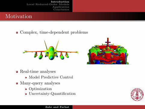
Motivation
Complex, time-dependent problems
REDUCED ORDER MODEL (ROM)
o Perturbation problems (stability, trends, control, etc.)!
o Response problems (behavior, performance, etc.)!
- linearized !
- nonlinear !
! Complex, time-dependent problems!
Real-time analyses
Model Predictive Control
Many-query analyses
OptimizationUncertainty-Quantification
Zahr and Farhat
IntroductionLocal Reduced-Order Models
ApplicationConclusion
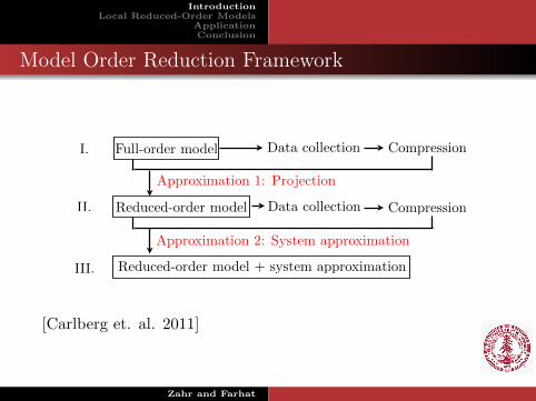
Model Order Reduction Framework
EFFICIENT NONLINEAR MODEL REDUCTION 7
2.4. Consistency-driven approach for nonlinear model reduction
Model reduction of nonlinear systems is often executed in a somewhat ad hoc manner, whereapproximations are constructed using intuition and past experience without much reference toproperties that a “good” approximation should satisfy. To avoid this pitfall, this work adoptsa strategy that enables approximations to be carefully constructed to meet desired conditions.In the proposed approach, if a given model is deemed too computationally expensive for real-time evaluation, an additional approximation is introduced, resulting in another less accuratebut more economical model. This results in a hierarchy of models characterized by tradeoffsbetween accuracy and computational efficiency. The approximations, which are introducedconsecutively, are constructed to generate minimal error with respect to the previous modelby satisfying optimality and consistency properties that are defined more precisely below.
As shown in Figure 1, the model hierarchy employed in this work consists of threecomputational models: an original model, and two increasingly “lighter” approximatedversions. Each approximated model is generated by acquiring data during the evaluation ofthe more accurate model for sample inputs, then compressing the data, and finally introducingthe approximation that exploits the compressed data.
The high-dimensional model will be referred to as Model I and is taken to be the “truth.”When evaluating this model is too computationally intensive for real-time prediction, aprojection approximation (Approximation 1) is introduced to reduce the dimensionality ofthe state equations. This leads to the reduced-order model (ROM), or Model II. If this ROMis still too CPU intensive for online computations, a system approximation (Approximation2) is introduced to reduce the computational complexity of its processing. The result of theapplication of this system approximation to Model II can be interpreted as a computationalmodel and therefore will be referred to as Model III in the remainder of this paper.
Data collection
I.
II.
III.
Full-order model
Reduced-order model
Data collection
Approximation 1: Projection
Compression
Compression
Approximation 2: System approximation
Reduced-order model + system approximation
Figure 1. Model hierarchy with approximations shown in red.
As previously stated, the approximations should introduce minimal error with respect tothe previous model in the hierarchy. To this end, Approximations 1 and 2 will be constructedto be: 1) consistent, and 2) optimal in the sense defined below.
Consistent approximation: An approximation is said here to be consistent if, whenimplemented without data compression, it introduces no additional error in the solution ofthe same problem for which data was acquired. �
Optimal approximation: An approximation is said here to be optimal if it leads toapproximated quantities that minimize some error measure with respect to the previous modelin the hierarchy. �
Copyright c� 2009 John Wiley & Sons, Ltd. Int. J. Numer. Meth. Engng 2009; 0:1–25Prepared using nmeauth.cls
[Carlberg et. al. 2011]
Zahr and Farhat
IntroductionLocal Reduced-Order Models
ApplicationConclusion
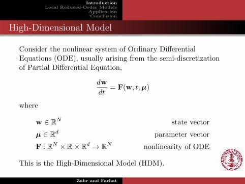
High-Dimensional Model
Consider the nonlinear system of Ordinary DifferentialEquations (ODE), usually arising from the semi-discretizationof Partial Differential Equation,
dw
dt= F(w, t,µ)
where
w ∈ RN state vector
µ ∈ Rd parameter vector
F : RN × R× Rd → RN nonlinearity of ODE
This is the High-Dimensional Model (HDM).
Zahr and Farhat
IntroductionLocal Reduced-Order Models
ApplicationConclusion
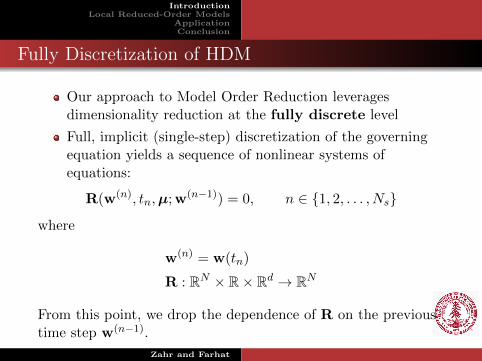
Fully Discretization of HDM
Our approach to Model Order Reduction leveragesdimensionality reduction at the fully discrete level
Full, implicit (single-step) discretization of the governingequation yields a sequence of nonlinear systems ofequations:
R(w(n), tn,µ;w(n−1)) = 0, n ∈ {1, 2, . . . , Ns}
where
w(n) = w(tn)
R : RN × R× Rd → RN
From this point, we drop the dependence of R on the previoustime step w(n−1).
Zahr and Farhat
IntroductionLocal Reduced-Order Models
ApplicationConclusion
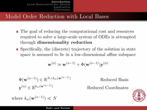
Model Order Reduction with Local Bases
The goal of reducing the computational cost and resourcesrequired to solve a large-scale system of ODEs is attemptedthrough dimensionality reduction
Specifically, the (discrete) trajectory of the solution in statespace is assumed to lie in a low-dimensional affine subspace
w(n) ≈ w(n−1) + Φ(w(n−1))y(n)
Φ(w(n−1)) ∈ RN×kw(w(n−1)) Reduced Basis
y(n) ∈ Rkw(w(n−1)) Reduced Coordinates
where kw(w(n−1))� N
Zahr and Farhat
IntroductionLocal Reduced-Order Models
ApplicationConclusion
Offline PhaseOnline PhaseHyperreduction
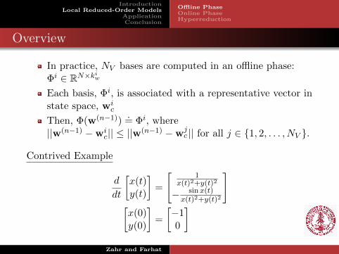
Overview
In practice, NV bases are computed in an offline phase:Φi ∈ RN×kiw
Each basis, Φi, is associated with a representative vector instate space, wi
c
Then, Φ(w(n−1)) .= Φi, where
||w(n−1) −wic|| ≤ ||w(n−1) −wj
c|| for all j ∈ {1, 2, . . . , NV }.
Contrived Example
d
dt
[x(t)y(t)
]=
[1
x(t)2+y(t)2
− sinx(t)x(t)2+y(t)2
][x(0)y(0)
]=
[−10
]Zahr and Farhat
IntroductionLocal Reduced-Order Models
ApplicationConclusion
Offline PhaseOnline PhaseHyperreduction
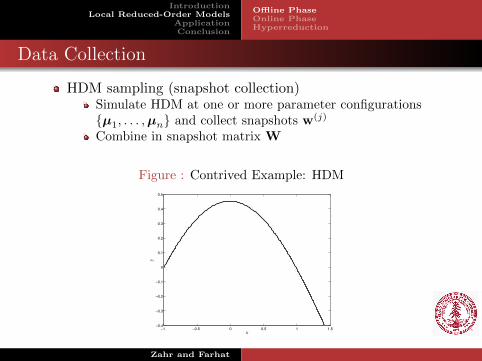
Data Collection
HDM sampling (snapshot collection)Simulate HDM at one or more parameter configurations{µ1, . . . ,µn} and collect snapshots w(j)
Combine in snapshot matrix W
Figure : Contrived Example: HDM
−1 −0.5 0 0.5 1 1.5−0.4
−0.3
−0.2
−0.1
0
0.1
0.2
0.3
0.4
0.5
x
y
Student Version of MATLAB
Zahr and Farhat
IntroductionLocal Reduced-Order Models
ApplicationConclusion
Offline PhaseOnline PhaseHyperreduction
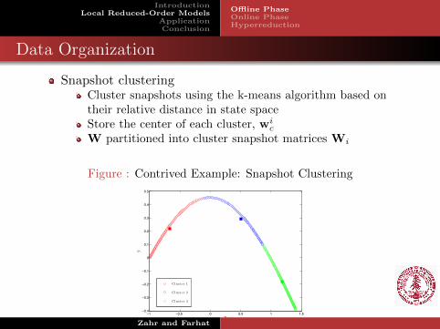
Data Organization
Snapshot clusteringCluster snapshots using the k-means algorithm based ontheir relative distance in state spaceStore the center of each cluster, wi
c
W partitioned into cluster snapshot matrices Wi
Figure : Contrived Example: Snapshot Clustering
−1 −0.5 0 0.5 1 1.5−0.4
−0.3
−0.2
−0.1
0
0.1
0.2
0.3
0.4
0.5
x
y
Cluster 1
Cluster 2
Cluster 3
Student Version of MATLAB
Zahr and Farhat
IntroductionLocal Reduced-Order Models
ApplicationConclusion
Offline PhaseOnline PhaseHyperreduction
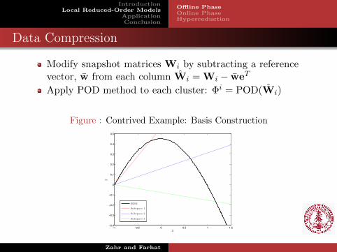
Data Compression
Modify snapshot matrices Wi by subtracting a referencevector, w from each column Wi = Wi − weT
Apply POD method to each cluster: Φi = POD(Wi)
Figure : Contrived Example: Basis Construction
−1 −0.5 0 0.5 1 1.5−0.4
−0.3
−0.2
−0.1
0
0.1
0.2
0.3
0.4
0.5
x
y
HDM
Subspace 1
Subspace 2
Subspace 3
Student Version of MATLAB
Zahr and Farhat
IntroductionLocal Reduced-Order Models
ApplicationConclusion
Offline PhaseOnline PhaseHyperreduction
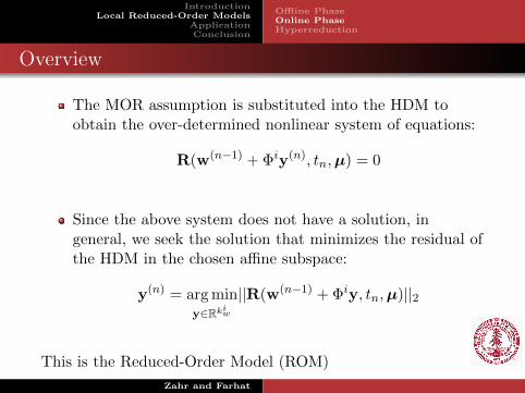
Overview
The MOR assumption is substituted into the HDM toobtain the over-determined nonlinear system of equations:
R(w(n−1) + Φiy(n), tn,µ) = 0
Since the above system does not have a solution, ingeneral, we seek the solution that minimizes the residual ofthe HDM in the chosen affine subspace:
y(n) = arg miny∈Rkiw
||R(w(n−1) + Φiy, tn,µ)||2
This is the Reduced-Order Model (ROM)
Zahr and Farhat
IntroductionLocal Reduced-Order Models
ApplicationConclusion
Offline PhaseOnline PhaseHyperreduction
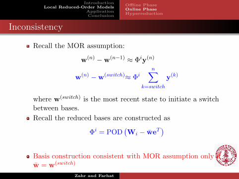
Inconsistency
Recall the MOR assumption:
w(n) −w(n−1) ≈ Φiy(n)
w(n) −w(switch)≈ Φin∑
k=switch
y(k)
where w(switch) is the most recent state to initiate a switchbetween bases.
Recall the reduced bases are constructed as
Φi = POD(Wi − weT
)Basis construction consistent with MOR assumption only ifw = w(switch)
Zahr and Farhat
IntroductionLocal Reduced-Order Models
ApplicationConclusion
Offline PhaseOnline PhaseHyperreduction
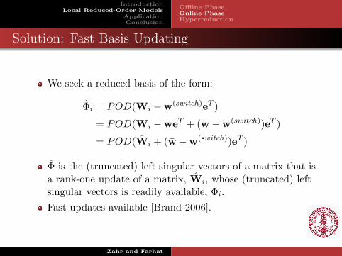
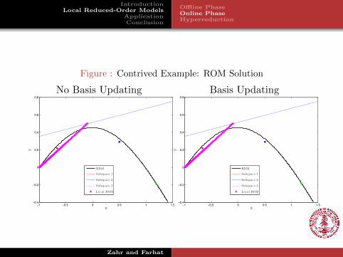
Solution: Fast Basis Updating
We seek a reduced basis of the form:
Φi = POD(Wi −w(switch)eT )
= POD(Wi − weT + (w −w(switch))eT )
= POD(Wi + (w −w(switch))eT )
Φ is the (truncated) left singular vectors of a matrix that isa rank-one update of a matrix, Wi, whose (truncated) leftsingular vectors is readily available, Φi.
Fast updates available [Brand 2006].
Zahr and Farhat
IntroductionLocal Reduced-Order Models
ApplicationConclusion
Offline PhaseOnline PhaseHyperreduction
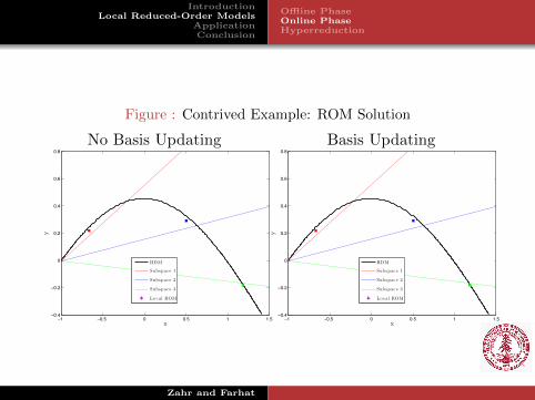
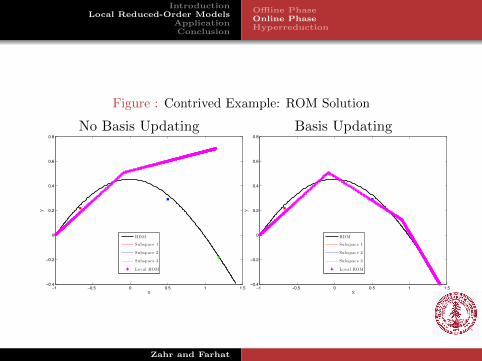
Figure : Contrived Example: ROM Solution
No Basis Updating
−1 −0.5 0 0.5 1 1.5−0.4
−0.2
0
0.2
0.4
0.6
0.8
x
y
HDM
Subspace 1
Subspace 2
Subspace 3
Local ROM
Student Version of MATLAB
Basis Updating
−1 −0.5 0 0.5 1 1.5−0.4
−0.2
0
0.2
0.4
0.6
0.8
x
y
HDM
Subspace 1
Subspace 2
Subspace 3
Local ROM
Student Version of MATLAB
Zahr and Farhat
IntroductionLocal Reduced-Order Models
ApplicationConclusion
Offline PhaseOnline PhaseHyperreduction
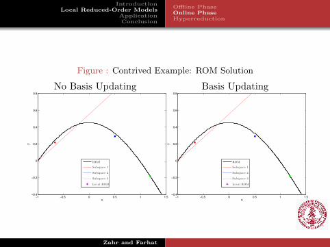
Figure : Contrived Example: ROM Solution
No Basis Updating
−1 −0.5 0 0.5 1 1.5−0.4
−0.2
0
0.2
0.4
0.6
0.8
x
y
HDM
Subspace 1
Subspace 2
Subspace 3
Local ROM
Student Version of MATLAB
Basis Updating
−1 −0.5 0 0.5 1 1.5−0.4
−0.2
0
0.2
0.4
0.6
0.8
x
y
HDM
Subspace 1
Subspace 2
Subspace 3
Local ROM
Student Version of MATLAB
Zahr and Farhat

IntroductionLocal Reduced-Order Models
ApplicationConclusion
Offline PhaseOnline PhaseHyperreduction
Figure : Contrived Example: ROM Solution
No Basis Updating
−1 −0.5 0 0.5 1 1.5−0.4
−0.2
0
0.2
0.4
0.6
0.8
x
y
HDM
Subspace 1
Subspace 2
Subspace 3
Local ROM
Student Version of MATLAB
Basis Updating
−1 −0.5 0 0.5 1 1.5−0.4
−0.2
0
0.2
0.4
0.6
0.8
x
y
HDM
Subspace 1
Subspace 2
Subspace 3
Local ROM
Student Version of MATLAB
Zahr and Farhat
IntroductionLocal Reduced-Order Models
ApplicationConclusion
Offline PhaseOnline PhaseHyperreduction
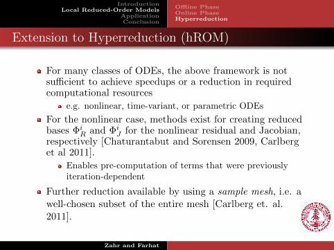
Extension to Hyperreduction (hROM)
For many classes of ODEs, the above framework is notsufficient to achieve speedups or a reduction in requiredcomputational resources
e.g. nonlinear, time-variant, or parametric ODEs
For the nonlinear case, methods exist for creating reducedbases Φi
R and ΦiJ for the nonlinear residual and Jacobian,
respectively [Chaturantabut and Sorensen 2009, Carlberget al 2011].
Enables pre-computation of terms that were previouslyiteration-dependent
Further reduction available by using a sample mesh, i.e. awell-chosen subset of the entire mesh [Carlberg et. al.2011].
Zahr and Farhat
IntroductionLocal Reduced-Order Models
ApplicationConclusion
Burger’s Equation (Non-predictive)Potential Nozzle (Predictive)
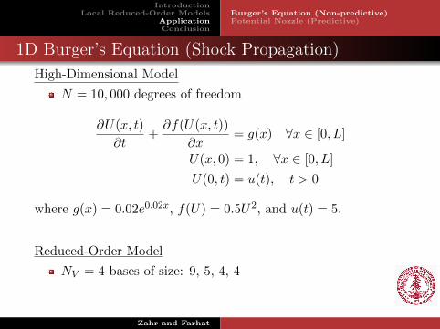
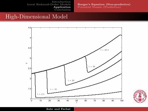
1D Burger’s Equation (Shock Propagation)
High-Dimensional Model
N = 10, 000 degrees of freedom
∂U(x, t)
∂t+∂f(U(x, t))
∂x= g(x) ∀x ∈ [0, L]
U(x, 0) = 1, ∀x ∈ [0, L]
U(0, t) = u(t), t > 0
where g(x) = 0.02e0.02x, f(U) = 0.5U2, and u(t) = 5.
Reduced-Order Model
NV = 4 bases of size: 9, 5, 4, 4
Zahr and Farhat
IntroductionLocal Reduced-Order Models
ApplicationConclusion
Burger’s Equation (Non-predictive)Potential Nozzle (Predictive)
High-Dimensional Model
0 10 20 30 40 50 60 70 80 90 1001
1.5
2
2.5
3
3.5
4
4.5
x
U
t = 2.5
t = 10
t = 20
t = 30
t = 42.5
Student Version of MATLAB
Zahr and Farhat
IntroductionLocal Reduced-Order Models
ApplicationConclusion
Burger’s Equation (Non-predictive)Potential Nozzle (Predictive)
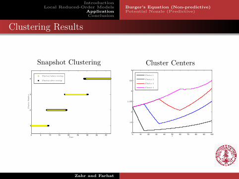
Clustering Results
Snapshot Clustering
0 5 10 15 20 25 30 35 40
1
2
3
4
Time
Clu
ster
Num
ber
Clusters before overlap
Clusters after overlap
Student Version of MATLAB
Cluster Centers
0 10 20 30 40 50 60 70 80 90 1001
1.5
2
2.5
3
3.5
4
x
U
Cluster 1
Cluster 2
Cluster 3
Cluster 4
Student Version of MATLAB
Zahr and Farhat
IntroductionLocal Reduced-Order Models
ApplicationConclusion
Burger’s Equation (Non-predictive)Potential Nozzle (Predictive)
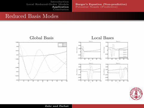
Reduced Basis Modes
Global Basis
0 10 20 30 40 50 60 70 80 90 100−0.02
−0.015
−0.01
−0.005
0
0.005
0.01
0.015
0.02
0.025
x
Mode
Shape
Mode 1Mode 2Mode 3Mode 4
Student Version of MATLAB
Local Bases
0 20 40 60 80 100−0.04
−0.02
0
0.02
0.04
0.06
x
Mode
Shape
Basi s 1
0 20 40 60 80 100−0.04
−0.02
0
0.02
0.04
x
Mode
Shape
Basi s 2
0 20 40 60 80 100−0.03
−0.02
−0.01
0
0.01
0.02
0.03
x
Mode
Shape
Basi s 3
0 20 40 60 80 100−0.03
−0.02
−0.01
0
0.01
0.02
0.03
x
Mode
Shape
Basi s 4
Mode 1
Mode 2
Mode 3
Mode 4
Student Version of MATLAB
Zahr and Farhat
IntroductionLocal Reduced-Order Models
ApplicationConclusion
Burger’s Equation (Non-predictive)Potential Nozzle (Predictive)
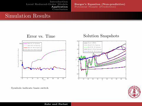
Simulation Results
Error vs. Time
0 5 10 15 20 25 30 35 401%
10%
100%
Time
Avera
ge
Rela
tive
L2
Err
or
inSta
te
Model I I , No Updating
Model I I I , No Updating
Model I I , With Updating
Model I I I , With Updating
Student Version of MATLAB
Solution Snapshots
0 10 20 30 40 50 60 70 80 90 1000
0.5
1
1.5
2
2.5
3
3.5
4
4.5
x
U
Model I (HDM)
Model I I , No Updating
Model I I I , No Updating
Model I I , With Updating
Model I I I , With Updating
Student Version of MATLAB
Symbols indicate basis switch
Zahr and Farhat
IntroductionLocal Reduced-Order Models
ApplicationConclusion
Burger’s Equation (Non-predictive)Potential Nozzle (Predictive)
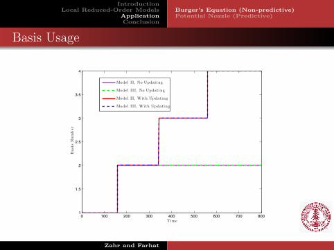
Basis Usage
0 100 200 300 400 500 600 700 8001
1.5
2
2.5
3
3.5
4
Time
Basi
sN
um
ber
Model I I , No Updating
Model I I I , No Updating
Model I I , With Updating
Model I I I , With Updating
Student Version of MATLAB
Zahr and Farhat
IntroductionLocal Reduced-Order Models
ApplicationConclusion
Burger’s Equation (Non-predictive)Potential Nozzle (Predictive)
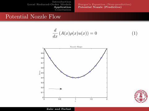
Potential Nozzle Flow
d
dx(A(x)ρ(x)u(x)) = 0 (1)
0 0.5 1 1.5 20
0.1
0.2
0.3
0.4
0.5
0.6
0.7
0.8
0.9
1
x
Are
a
No zz l e Shape
Student Version of MATLAB
Zahr and Farhat
IntroductionLocal Reduced-Order Models
ApplicationConclusion
Burger’s Equation (Non-predictive)Potential Nozzle (Predictive)
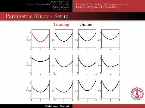
Parametric Study - Setup
Training Online
0 1 20
0.5
1
Area
0 1 20
0.5
1
0 1 20
0.5
1
0 1 20
0.5
1
0 1 20
0.5
1
Area
0 1 20
0.5
1
0 1 20
0.5
1
0 1 20
0.5
1
0 1 20
0.5
1
Area
x0 1 20
0.5
1
x0 1 20
0.5
1
x0 1 20
0.5
1
x
Zahr and Farhat
IntroductionLocal Reduced-Order Models
ApplicationConclusion
Burger’s Equation (Non-predictive)Potential Nozzle (Predictive)
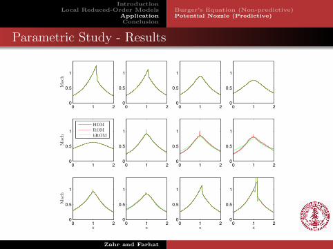
Parametric Study - Results
0 1 20
0.5
1
Mach
0 1 20
0.5
1
0 1 20
0.5
1
0 1 20
0.5
1
0 1 20
0.5
1
Mach
0 1 20
0.5
1
0 1 20
0.5
1
0 1 20
0.5
1
0 1 20
0.5
1
Mach
x0 1 2
0
0.5
1
x0 1 2
0
0.5
1
x0 1 2
0
0.5
1
x
HDM
ROM
hROM
Zahr and Farhat
IntroductionLocal Reduced-Order Models
ApplicationConclusion
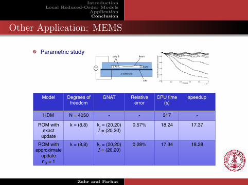
Other Application: MEMSMEMS
! Parametric study"
0 0.2 0.4 0.6 0.8 1x 10 4
2.3
1.8
1.3
0.8
0.3
0
Time (s)
Cen
ter P
oint
Def
lect
ion
(mic
rons
)
P8T1P6P3P2P5
P4
P1P7
T2
P9
!"#$%&$'()'*#
+"(# ,-.#/0##
1*)0# 2345#!"#
!"6#
Model" Degrees of "freedom"
GNAT" Relative error"
CPU time (s)"
speedup"
HDM" N = 4050" -" -" 317 " -"
ROM with"exact
update"
k = (8,8)" kr = (20,20)"I = (20,20)"
0.57%" 18.24" 17.37"
ROM with approximate
update"nQ = 1"
k = (8,8)" kr = (20,20)"I = (20,20)"
0.28%" 17.34" 18.28"
Zahr and Farhat
IntroductionLocal Reduced-Order Models
ApplicationConclusion
Conclusions
Local model reduction methodattractive for problems with distinct solution regimesmodel reduction assumption and data collection areinconsistent
Local model reduction with online basis updatesaddresses inconsistency of local MORinjects “online” data into pre-computed basis
Future workapplication to 3D turbulent flowsapplication to nonlinear structural dynamicsuse as surrogate in PDE-constrained optimization anduncertainty quantification
ReferencesAmsallem, D., Zahr, M. J., and Farhat, C., “Nonlinear Model Order ReductionBased on Local ReducedOrder Bases,” International Journal for NumericalMethods in Engineering, 2012.Washabaugh, K., Amsallem, D., Zahr, M., and Farhat, C., “Nonlinear ModelReduction for CFD Problems Using Local Reduced Order Bases,” 42nd AIAAFluid Dynamics Conference and Exhibit, New Orleans, LA, June 25-28 2012.
Zahr and Farhat

IntroductionLocal Reduced-Order Models
ApplicationConclusion
Acknowledgements
Zahr and Farhat