Journal of

Marine Science and Engineering

Article

Effectiveness Assessment of an Innovative Ejector Plant for PortSediment Management

Marco Pellegrini 1,2 , Arash Aghakhani 1, Maria Gabriella Gaeta 2,3 , Renata Archetti 2,3,* ,Alessandro Guzzini 2 and Cesare Saccani 1,2

�����������������

Citation: Pellegrini, M.; Aghakhani,

A.; Gaeta, M.G.; Archetti, R.; Guzzini,

A.; Saccani, C. Effectiveness

Assessment of an Innovative Ejector

Plant for Port Sediment Management.

J. Mar. Sci. Eng. 2021, 9, 197.

https://doi.org/10.3390/jmse9020197

Academic Editor: Ricardo Briganti

Received: 30 December 2020

Accepted: 8 February 2021

Published: 12 February 2021

Publisher’s Note: MDPI stays neutral

with regard to jurisdictional claims in

published maps and institutional affil-

iations.

Copyright: © 2021 by the authors.

Licensee MDPI, Basel, Switzerland.

This article is an open access article

distributed under the terms and

conditions of the Creative Commons

Attribution (CC BY) license (https://

creativecommons.org/licenses/by/

4.0/).

1 Department of Industrial Engineering, University of Bologna, 40136 Bologna, Italy;marco.pellegrini3@unibo.it (M.P.); arash.aghakhani2@unibo.it (A.A.); cesare.saccani@unibo.it (C.S.)

2 Interdepartmental Centre for Industrial Research in Building and Construction, 40131 Bologna, Italy;g.gaeta@unibo.it (M.G.G.); alessandro.guzzini2@unibo.it (A.G.)

3 Department of Civil, Environmental, Chemical and Materials Engineering, University of Bologna,40136 Bologna, Italy

* Correspondence: renata.archetti@unibo.it

Abstract: The need to remove deposited material from water basins is common and has been sharedby many ports and channels since the earliest settlements along coasts and rivers. Dredging, themost widely used method to remove sediment deposits, is a reliable and wide-spread technology.Nevertheless, dredging is only able to restore the desired water depth but without any kind of impacton the causes of sedimentation and so it cannot guarantee navigability over time. Moreover, dredgingoperations have relevant environmental and economic issues. Therefore, there is a growing marketdemand for alternatives to sustainable technologies to dredging able to preserve navigability. Thispaper aims to evaluate the effectiveness of guaranteeing a minimum water depth over time at theport entrance at Marina of Cervia (Italy), wherein the first industrial scale ejector demo plant hasbeen installed and operated from June 2019. The demo plant was designed to continuously removethe sediment that naturally settles in a certain area through the operation of the ejectors, which aresubmersible jet pumps. This paper focuses on a three-year analysis of bathymetries realized at theport inlet before and after ejector demo plant installation and correlates the bathymetric data withmetocean data (waves and sea water level) collected in the same period. In particular, this paperanalyses the relation between sea depth and sediment volume variation at the port inlet with ejectordemo plant operation regimes. Results show that in the period from January to April 2020, which wasalso the period of full load operation of the demo plant, the water depth in the area of influence ofthe ejectors increased by 0.72 mm/day, while in the whole port inlet area a decrease of 0.95 mm/daywas observed. Furthermore, in the same period of operation, the ejector demo plant’s impact onvolume variation was estimated in a range of 245–750 m3.

Keywords: ejectors; sediment transport rate; port sediment management; effectiveness assessment

1. Introduction

The presence of anthropic activity in the coastal environment strongly modifies waves,currents and sediment transport regimes. In particular, intense wave-induced currentsand sediment transport rates are present around ports and commonly influence theircommercial and recreational activities. The accumulated sediments reduce the admitteddraft of the navigation channel on the one hand and generate erosional effects on the leesidecoasts on the other. As a consequence, harbours frequently require ordinary maintenancedredging to remove the accumulated sediments [1]. Dredging is a consolidated andproven technology, but involves considerable drawbacks [2–5], since it has a notableenvironmental impact on the marine environment, contributes to the mobility and diffusionof contaminants and pollutants already present in the settled sediments, and obstructsnavigation during its operational phases. Periodic hydrographic surveys of the harbour

J. Mar. Sci. Eng. 2021, 9, 197. https://doi.org/10.3390/jmse9020197 https://www.mdpi.com/journal/jmse

J. Mar. Sci. Eng. 2021, 9, 197 2 of 25

area are essential for the accurate determination of quantities and timing of maintenancedredging. Since maintenance dredging is often performed on an as-needed basis, regularsurveys become an essential tool to properly time the work [6]. Furthermore, bathymetriesare surveyed before and after dredging operations to estimate the volume of the sedimentremoved. On the other hand, the use of dredging equipment allows the measuring of thematerial dredged, which is usually defined by contract.

New approaches have been developed over the years as alternative methods todredging. In particular, [7] classifies alternative solutions to dredging in three categories:(i) anti-sedimentation structures, (ii) remobilizing sediment systems, and (iii) sand by-passing plants. Anti-sedimentation structures considerably reduce the amount of sedimentto be removed from harbour inlets but present environmental concerns and still requiresediment removal [8]. Remobilizing sediment systems use an injection of water or themovement of mechanical devices such as dredger propellers to cause the lift and theseparation of the grains from the seabed. In particular, water injection dredging has beenwidely applied as a cheaper and less impacting solution than traditional dredging [9].Nevertheless, environmental issues due to the lack of control of the resuspended sedimentdeserve further investigation [10,11], while some technical limitations are present if thesediment is mainly composed of sand. Sand by-passing plants have limited environmentalimpacts but are characterized by relatively high installation costs and often uncertainoperational costs.

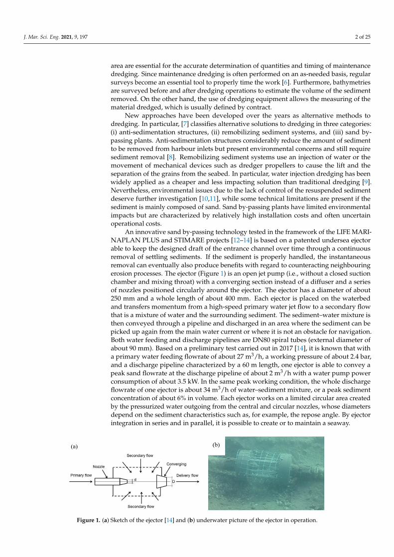
An innovative sand by-passing technology tested in the framework of the LIFE MARI-NAPLAN PLUS and STIMARE projects [12–14] is based on a patented undersea ejectorable to keep the designed draft of the entrance channel over time through a continuousremoval of settling sediments. If the sediment is properly handled, the instantaneousremoval can eventually also produce benefits with regard to counteracting neighbouringerosion processes. The ejector (Figure 1) is an open jet pump (i.e., without a closed suctionchamber and mixing throat) with a converging section instead of a diffuser and a seriesof nozzles positioned circularly around the ejector. The ejector has a diameter of about250 mm and a whole length of about 400 mm. Each ejector is placed on the waterbedand transfers momentum from a high-speed primary water jet flow to a secondary flowthat is a mixture of water and the surrounding sediment. The sediment–water mixture isthen conveyed through a pipeline and discharged in an area where the sediment can bepicked up again from the main water current or where it is not an obstacle for navigation.Both water feeding and discharge pipelines are DN80 spiral tubes (external diameter ofabout 90 mm). Based on a preliminary test carried out in 2017 [14], it is known that witha primary water feeding flowrate of about 27 m3/h, a working pressure of about 2.4 bar,and a discharge pipeline characterized by a 60 m length, one ejector is able to convey apeak sand flowrate at the discharge pipeline of about 2 m3/h with a water pump powerconsumption of about 3.5 kW. In the same peak working condition, the whole dischargeflowrate of one ejector is about 34 m3/h of water–sediment mixture, or a peak sedimentconcentration of about 6% in volume. Each ejector works on a limited circular area createdby the pressurized water outgoing from the central and circular nozzles, whose diametersdepend on the sediment characteristics such as, for example, the repose angle. By ejectorintegration in series and in parallel, it is possible to create or to maintain a seaway.

J. Mar. Sci. Eng. 2021, 9, x 3 of 26

Figure 1. (a) Sketch of the ejector [14] and (b) underwater picture of the ejector in operation.

An ejector demo plant has been realized at the port entrance of the Marina of Cervia (Italy) and has been in operation from June 2019 to September 2020.

The aim of the paper is to assess the ejector demo plant effectiveness, which can be defined as the ability to be successful in maintaining the navigability at the port entrance over time. The novelty of the study is related to the methodology applied for the evalua-tion of the impact of the ejector demo plant on both water depth and sediment volume variations at the port inlet. In fact, for dredging and other alternative technologies that operate over a short time, the evaluation of the impact is based on the comparison of bath-ymetries of the interested area before and after sediment removal; the ejector plant works continuously and so the effects are monitored over a long period. Therefore, natural sed-iment transport is also relevant and should be taken into account in the effectiveness eval-uation. The prediction of sediment transport is very complex: it always needs an accurate phase of calibration and validation based on measurements and it requires a good sedi-ment transport model driven by reliable input data of waves and currents, initial bathym-etry, sediment characteristics, etc. A large amount of literature is available and interesting examples can be found [18–22]. Nevertheless, the analysis of effectiveness of a continuous working sand by-passing system has never been approached, and in previous applica-tions the by-passed amount of sediment has been always estimated starting from dredg-ing needs [23]. This paper’s investigation was carried out by making a comparison of wa-ter depth and sediment volume variation over time before and after ejector demo plant installation through the analysis of bathymetries and metocean data. Therefore, the sedi-ment transport rate in the area of Cervia port entrance was firstly assessed, starting from the analysis of the detailed bathymetries realized in the last 3 years. Moreover, the 3-year metocean climate on the site was analysed and discussed together with the bathymetric evidence. Then, the operation period of the ejector demo plant was compared with the two previous years, from June 2017 to June 2019. The effectiveness of the demo plant was evaluated on the basis of the different operation and control strategies tested.

2. Description of the Ejector Demo Plant 2.1. Description of the Study Site: Cervia, North Italy

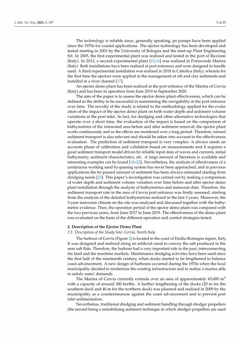
The harbour of Cervia (Figure 2) is located in the coast of Emilia-Romagna region, Italy. It was designed and realized along an artificial canal to convey the salt produced in the near salt flats. Therefore, the harbour had a very important role in the past, intercon-necting the land and the maritime markets. Maintenance dredging activities have been used since the first half of the nineteenth century, when docks started to be lengthened to balance coast advancement. A new design of harbours occurred during the 1970s when the local municipality decided to modernize the existing infrastructure and to realize a marina able to satisfy users’ demands.

The Marina of Cervia currently extends over an area of approximately 43,000 m2 with a capacity of around 300 berths. A further lengthening of the docks (20 m for the southern

Figure 1. (a) Sketch of the ejector [14] and (b) underwater picture of the ejector in operation.

J. Mar. Sci. Eng. 2021, 9, 197 3 of 25

The technology is reliable since, generally speaking, jet pumps have been appliedsince the 1970s for coastal applications. The ejector technology has been developed andtested starting in 2001 by the University of Bologna and the start-up Plant EngineeringSrl. In 2005, the first experimental plant was realized and tested in the port of Riccione(Italy). In 2012, a second experimental plant [15,16] was realized in Portoverde Marina(Italy). Both installations have been realized at port entrances and were designed to handlesand. A third experimental installation was realized in 2018 in Cattolica (Italy), wherein forthe first time the ejectors were applied in the management of silt and clay sediments andinstalled in a river channel [17].

An ejector demo plant has been realized at the port entrance of the Marina of Cervia(Italy) and has been in operation from June 2019 to September 2020.

The aim of the paper is to assess the ejector demo plant effectiveness, which can bedefined as the ability to be successful in maintaining the navigability at the port entranceover time. The novelty of the study is related to the methodology applied for the evalu-ation of the impact of the ejector demo plant on both water depth and sediment volumevariations at the port inlet. In fact, for dredging and other alternative technologies thatoperate over a short time, the evaluation of the impact is based on the comparison ofbathymetries of the interested area before and after sediment removal; the ejector plantworks continuously and so the effects are monitored over a long period. Therefore, naturalsediment transport is also relevant and should be taken into account in the effectivenessevaluation. The prediction of sediment transport is very complex: it always needs anaccurate phase of calibration and validation based on measurements and it requires agood sediment transport model driven by reliable input data of waves and currents, initialbathymetry, sediment characteristics, etc. A large amount of literature is available andinteresting examples can be found [18–22]. Nevertheless, the analysis of effectiveness of acontinuous working sand by-passing system has never been approached, and in previousapplications the by-passed amount of sediment has been always estimated starting fromdredging needs [23]. This paper’s investigation was carried out by making a comparisonof water depth and sediment volume variation over time before and after ejector demoplant installation through the analysis of bathymetries and metocean data. Therefore, thesediment transport rate in the area of Cervia port entrance was firstly assessed, startingfrom the analysis of the detailed bathymetries realized in the last 3 years. Moreover, the3-year metocean climate on the site was analysed and discussed together with the bathy-metric evidence. Then, the operation period of the ejector demo plant was compared withthe two previous years, from June 2017 to June 2019. The effectiveness of the demo plantwas evaluated on the basis of the different operation and control strategies tested.

2. Description of the Ejector Demo Plant2.1. Description of the Study Site: Cervia, North Italy

The harbour of Cervia (Figure 2) is located in the coast of Emilia-Romagna region, Italy.It was designed and realized along an artificial canal to convey the salt produced in thenear salt flats. Therefore, the harbour had a very important role in the past, interconnectingthe land and the maritime markets. Maintenance dredging activities have been used sincethe first half of the nineteenth century, when docks started to be lengthened to balancecoast advancement. A new design of harbours occurred during the 1970s when the localmunicipality decided to modernize the existing infrastructure and to realize a marina ableto satisfy users’ demands.

The Marina of Cervia currently extends over an area of approximately 43,000 m2

with a capacity of around 300 berths. A further lengthening of the docks (20 m for thesouthern dock and 40 m for the northern dock) was planned and realized in 2009 by themunicipality as a countermeasure against the coast advancement and to prevent portinlet sedimentation.

Nevertheless, traditional dredging and sediment handling through dredger propellers(the second being a remobilizing sediment technique in which dredger propellers are used

J. Mar. Sci. Eng. 2021, 9, 197 4 of 25

to remobilize the sediment from the seabed) were still planned and periodically operatedat the port entrance [14]. In the period 2009–2015, more than 17,000 m3 of sediment wasremoved yearly, with dredging from the basin being responsible for a total expenditureof about EUR 1 million—i.e., a weighted average cost of EUR 8.31 per dredged cubicmeter of sediment. Furthermore, in the same period, the Municipality of Cervia investedabout EUR 350,000 in propeller operations, almost once per year. The physical-chemicalcharacterization of the sediment present at the port inlet revealed that the main componentis sand (97%), while the specific weight is 1.9 g/mL.

J. Mar. Sci. Eng. 2021, 9, x 4 of 26

dock and 40 m for the northern dock) was planned and realized in 2009 by the municipal-ity as a countermeasure against the coast advancement and to prevent port inlet sedimen-tation.

Figure 2. Cervia position (a) and harbour aerial picture of the study area (b).

Nevertheless, traditional dredging and sediment handling through dredger propel-lers (the second being a remobilizing sediment technique in which dredger propellers are used to remobilize the sediment from the seabed) were still planned and periodically op-erated at the port entrance [14]. In the period 2009–2015, more than 17,000 m3 of sediment was removed yearly, with dredging from the basin being responsible for a total expendi-ture of about EUR 1 million—i.e., a weighted average cost of EUR 8.31 per dredged cubic meter of sediment. Furthermore, in the same period, the Municipality of Cervia invested about EUR 350,000 in propeller operations, almost once per year. The physical-chemical characterization of the sediment present at the port inlet revealed that the main compo-nent is sand (97%), while the specific weight is 1.9 g/mL.

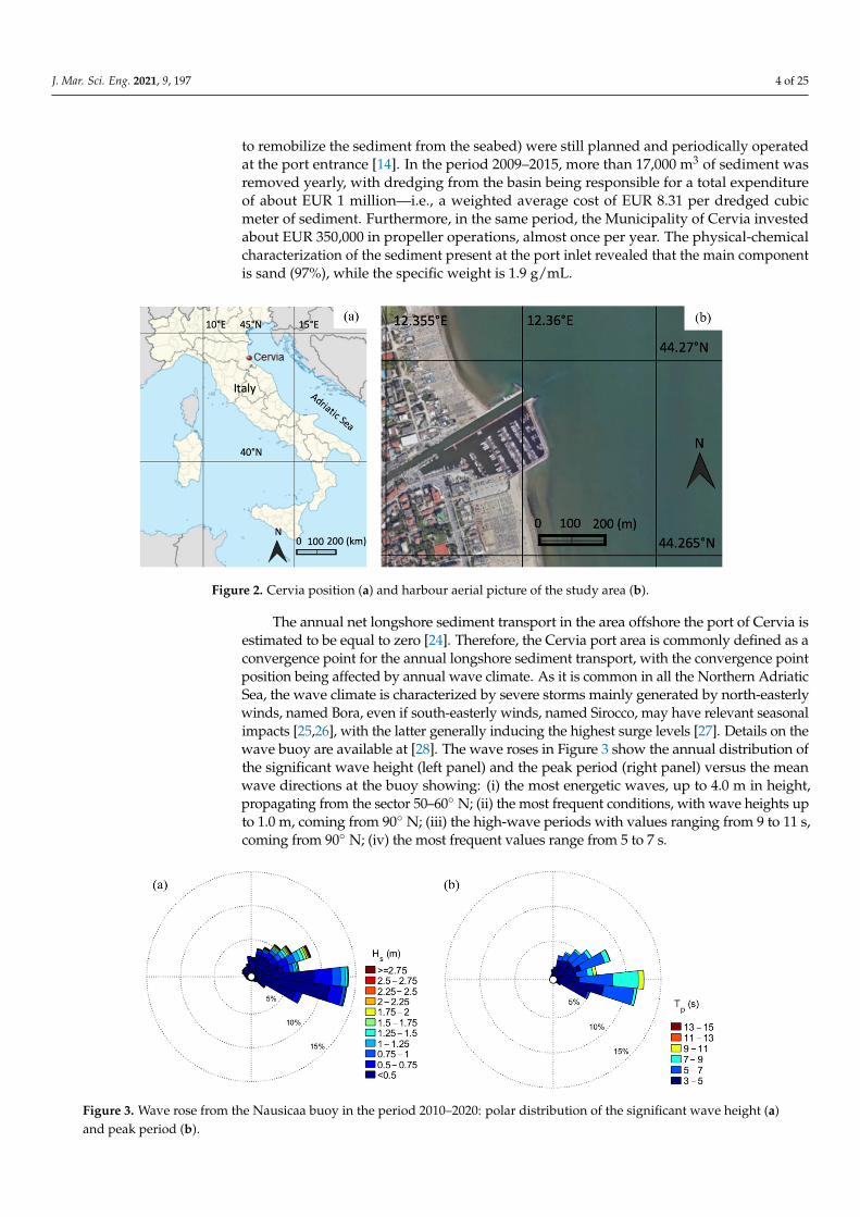
The annual net longshore sediment transport in the area offshore the port of Cervia is estimated to be equal to zero [24]. Therefore, the Cervia port area is commonly defined as a convergence point for the annual longshore sediment transport, with the convergence point position being affected by annual wave climate. As it is common in all the Northern Adriatic Sea, the wave climate is characterized by severe storms mainly generated by north-easterly winds, named Bora, even if south-easterly winds, named Sirocco, may have relevant seasonal impacts [25,26], with the latter generally inducing the highest surge lev-els [27]. Details on the wave buoy are available at [28]. The wave roses in Figure 3 show the annual distribution of the significant wave height (left panel) and the peak period (right panel) versus the mean wave directions at the buoy showing: (i) the most energetic waves, up to 4.0 m in height, propagating from the sector 50–60° N; (ii) the most frequent conditions, with wave heights up to 1.0 m, coming from 90° N; (iii) the high-wave periods with values ranging from 9 to 11 s, coming from 90° N; (iv) the most frequent values range from 5 to 7 s.

Figure 2. Cervia position (a) and harbour aerial picture of the study area (b).

The annual net longshore sediment transport in the area offshore the port of Cervia isestimated to be equal to zero [24]. Therefore, the Cervia port area is commonly defined as aconvergence point for the annual longshore sediment transport, with the convergence pointposition being affected by annual wave climate. As it is common in all the Northern AdriaticSea, the wave climate is characterized by severe storms mainly generated by north-easterlywinds, named Bora, even if south-easterly winds, named Sirocco, may have relevant seasonalimpacts [25,26], with the latter generally inducing the highest surge levels [27]. Details on thewave buoy are available at [28]. The wave roses in Figure 3 show the annual distribution ofthe significant wave height (left panel) and the peak period (right panel) versus the meanwave directions at the buoy showing: (i) the most energetic waves, up to 4.0 m in height,propagating from the sector 50–60◦ N; (ii) the most frequent conditions, with wave heights upto 1.0 m, coming from 90◦ N; (iii) the high-wave periods with values ranging from 9 to 11 s,coming from 90◦ N; (iv) the most frequent values range from 5 to 7 s.

J. Mar. Sci. Eng. 2021, 9, x 5 of 26

Figure 3. Wave rose from the Nausicaa buoy in the period 2010–2020: polar distribution of the significant wave height (a) and peak period (b).

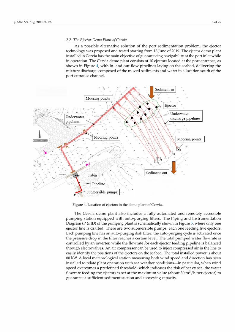
2.2. The Ejector Demo Plant of Cervia As a possible alternative solution of the port sedimentation problem, the ejector tech-

nology was proposed and tested starting from 13 June of 2019. The ejector demo plant installed in Cervia has the main objective of guaranteeing navigability at the port inlet while in operation. The Cervia demo plant consists of 10 ejectors located at the port en-trance, as shown in Figure 4, with in- and out-flow pipelines laying on the seabed, deliv-ering the mixture discharge composed of the moved sediments and water in a location south of the port entrance channel.

Figure 4. Location of ejectors in the demo plant of Cervia.

Figure 3. Wave rose from the Nausicaa buoy in the period 2010–2020: polar distribution of the significant wave height (a)and peak period (b).

J. Mar. Sci. Eng. 2021, 9, 197 5 of 25

2.2. The Ejector Demo Plant of Cervia

As a possible alternative solution of the port sedimentation problem, the ejectortechnology was proposed and tested starting from 13 June of 2019. The ejector demo plantinstalled in Cervia has the main objective of guaranteeing navigability at the port inlet whilein operation. The Cervia demo plant consists of 10 ejectors located at the port entrance, asshown in Figure 4, with in- and out-flow pipelines laying on the seabed, delivering themixture discharge composed of the moved sediments and water in a location south of theport entrance channel.

J. Mar. Sci. Eng. 2021, 9, x 5 of 26

Figure 3. Wave rose from the Nausicaa buoy in the period 2010–2020: polar distribution of the significant wave height (a) and peak period (b).

2.2. The Ejector Demo Plant of Cervia As a possible alternative solution of the port sedimentation problem, the ejector tech-

nology was proposed and tested starting from 13 June of 2019. The ejector demo plant installed in Cervia has the main objective of guaranteeing navigability at the port inlet while in operation. The Cervia demo plant consists of 10 ejectors located at the port en-trance, as shown in Figure 4, with in- and out-flow pipelines laying on the seabed, deliv-ering the mixture discharge composed of the moved sediments and water in a location south of the port entrance channel.

Figure 4. Location of ejectors in the demo plant of Cervia.

Figure 4. Location of ejectors in the demo plant of Cervia.

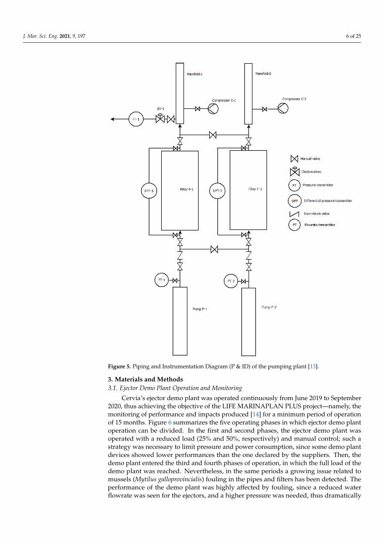
The Cervia demo plant also includes a fully automated and remotely accessiblepumping station equipped with auto-purging filters. The Piping and InstrumentationDiagram (P & ID) of the pumping plant is schematically shown in Figure 5, where only oneejector line is drafted. There are two submersible pumps, each one feeding five ejectors.Each pumping line has an auto-purging disk filter: the auto-purging cycle is activated oncethe pressure drop in the filter reaches a certain level. The total pumped water flowrate iscontrolled by an inverter, while the flowrate for each ejector feeding pipeline is balancedthrough electrovalves. An air compressor can be used to inject compressed air in the line toeasily identify the positions of the ejectors on the seabed. The total installed power is about80 kW. A local meteorological station measuring both wind speed and direction has beeninstalled to relate plant operation with sea weather conditions—in particular, when windspeed overcomes a predefined threshold, which indicates the risk of heavy sea, the waterflowrate feeding the ejectors is set at the maximum value (about 30 m3/h per ejector) toguarantee a sufficient sediment suction and conveying capacity.

J. Mar. Sci. Eng. 2021, 9, 197 6 of 25

J. Mar. Sci. Eng. 2021, 9, x 6 of 26

The Cervia demo plant also includes a fully automated and remotely accessible pumping station equipped with auto-purging filters. The Piping and Instrumentation Di-agram (P & ID) of the pumping plant is schematically shown in Figure 5, where only one ejector line is drafted. There are two submersible pumps, each one feeding five ejectors. Each pumping line has an auto-purging disk filter: the auto-purging cycle is activated once the pressure drop in the filter reaches a certain level. The total pumped water flowrate is controlled by an inverter, while the flowrate for each ejector feeding pipeline is balanced through electrovalves. An air compressor can be used to inject compressed air in the line to easily identify the positions of the ejectors on the seabed. The total installed power is about 80 kW. A local meteorological station measuring both wind speed and direction has been installed to relate plant operation with sea weather conditions—in par-ticular, when wind speed overcomes a predefined threshold, which indicates the risk of heavy sea, the water flowrate feeding the ejectors is set at the maximum value (about 30 m3/h per ejector) to guarantee a sufficient sediment suction and conveying capacity.

Figure 5. Piping and Instrumentation Diagram (P & ID) of the pumping plant [13].

Figure 5. Piping and Instrumentation Diagram (P & ID) of the pumping plant [13].

3. Materials and Methods3.1. Ejector Demo Plant Operation and Monitoring

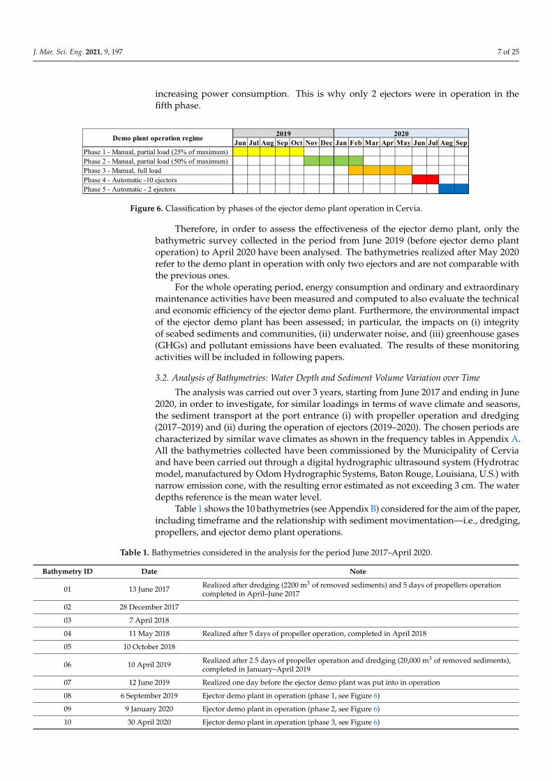
Cervia’s ejector demo plant was operated continuously from June 2019 to September2020, thus achieving the objective of the LIFE MARINAPLAN PLUS project—namely, themonitoring of performance and impacts produced [14] for a minimum period of operationof 15 months. Figure 6 summarizes the five operating phases in which ejector demo plantoperation can be divided. In the first and second phases, the ejector demo plant wasoperated with a reduced load (25% and 50%, respectively) and manual control; such astrategy was necessary to limit pressure and power consumption, since some demo plantdevices showed lower performances than the one declared by the suppliers. Then, thedemo plant entered the third and fourth phases of operation, in which the full load of thedemo plant was reached. Nevertheless, in the same periods a growing issue related tomussels (Mytilus galloprovincialis) fouling in the pipes and filters has been detected. Theperformance of the demo plant was highly affected by fouling, since a reduced waterflowrate was seen for the ejectors, and a higher pressure was needed, thus dramatically

J. Mar. Sci. Eng. 2021, 9, 197 7 of 25

increasing power consumption. This is why only 2 ejectors were in operation in thefifth phase.

J. Mar. Sci. Eng. 2021, 9, x 7 of 26

3. Materials and Methods 3.1. Ejector Demo Plant Operation and Monitoring

Cervia’s ejector demo plant was operated continuously from June 2019 to September 2020, thus achieving the objective of the LIFE MARINAPLAN PLUS project—namely, the monitoring of performance and impacts produced [14] for a minimum period of operation of 15 months. Figure 6 summarizes the five operating phases in which ejector demo plant operation can be divided. In the first and second phases, the ejector demo plant was op-erated with a reduced load (25% and 50%, respectively) and manual control; such a strat-egy was necessary to limit pressure and power consumption, since some demo plant de-vices showed lower performances than the one declared by the suppliers. Then, the demo plant entered the third and fourth phases of operation, in which the full load of the demo plant was reached. Nevertheless, in the same periods a growing issue related to mussels (Mytilus galloprovincialis) fouling in the pipes and filters has been detected. The perfor-mance of the demo plant was highly affected by fouling, since a reduced water flowrate was seen for the ejectors, and a higher pressure was needed, thus dramatically increasing power consumption. This is why only 2 ejectors were in operation in the fifth phase.

Therefore, in order to assess the effectiveness of the ejector demo plant, only the bath-ymetric survey collected in the period from June 2019 (before ejector demo plant opera-tion) to April 2020 have been analysed. The bathymetries realized after May 2020 refer to the demo plant in operation with only two ejectors and are not comparable with the pre-vious ones.

Figure 6. Classification by phases of the ejector demo plant operation in Cervia.

For the whole operating period, energy consumption and ordinary and extraordi-nary maintenance activities have been measured and computed to also evaluate the tech-nical and economic efficiency of the ejector demo plant. Furthermore, the environmental impact of the ejector demo plant has been assessed; in particular, the impacts on (i) integ-rity of seabed sediments and communities, (ii) underwater noise, and (iii) greenhouse gases (GHGs) and pollutant emissions have been evaluated. The results of these monitor-ing activities will be included in following papers.

3.2. Analysis of Bathymetries: Water Depth and Sediment Volume Variation over Time The analysis was carried out over 3 years, starting from June 2017 and ending in June

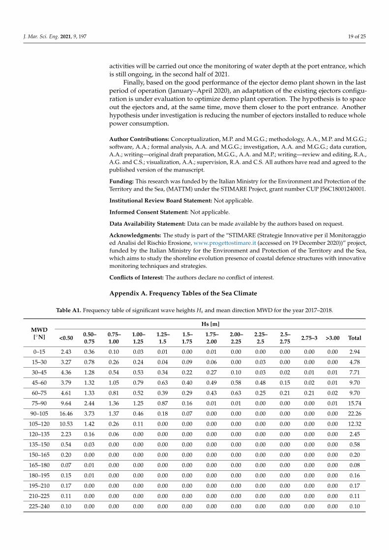
2020, in order to investigate, for similar loadings in terms of wave climate and seasons, the sediment transport at the port entrance (i) with propeller operation and dredging (2017–2019) and (ii) during the operation of ejectors (2019–2020). The chosen periods are characterized by similar wave climates as shown in the frequency tables in Appendix A. All the bathymetries collected have been commissioned by the Municipality of Cervia and have been carried out through a digital hydrographic ultrasound system (Hydrotrac model, manufactured by Odom Hydrographic Systems, Baton Rouge, Louisiana, U.S.) with narrow emission cone, with the resulting error estimated as not exceeding 3 cm. The water depths reference is the mean water level.

Table 1 shows the 10 bathymetries (see Appendix B) considered for the aim of the paper, including timeframe and the relationship with sediment movimentation—i.e., dredging, propellers, and ejector demo plant operations.

Jun Jul Aug Sep Oct Nov Dec Jan Feb Mar Apr May Jun Jul Aug Sep2019 2020Demo plant operation regime

Phase 1 - Manual, partial load (25% of maximum)Phase 2 - Manual, partial load (50% of maximum)Phase 3 - Manual, full loadPhase 4 - Automatic -10 ejectorsPhase 5 - Automatic - 2 ejectors

Figure 6. Classification by phases of the ejector demo plant operation in Cervia.

Therefore, in order to assess the effectiveness of the ejector demo plant, only thebathymetric survey collected in the period from June 2019 (before ejector demo plantoperation) to April 2020 have been analysed. The bathymetries realized after May 2020refer to the demo plant in operation with only two ejectors and are not comparable withthe previous ones.

For the whole operating period, energy consumption and ordinary and extraordinarymaintenance activities have been measured and computed to also evaluate the technicaland economic efficiency of the ejector demo plant. Furthermore, the environmental impactof the ejector demo plant has been assessed; in particular, the impacts on (i) integrityof seabed sediments and communities, (ii) underwater noise, and (iii) greenhouse gases(GHGs) and pollutant emissions have been evaluated. The results of these monitoringactivities will be included in following papers.

3.2. Analysis of Bathymetries: Water Depth and Sediment Volume Variation over Time

The analysis was carried out over 3 years, starting from June 2017 and ending in June2020, in order to investigate, for similar loadings in terms of wave climate and seasons,the sediment transport at the port entrance (i) with propeller operation and dredging(2017–2019) and (ii) during the operation of ejectors (2019–2020). The chosen periods arecharacterized by similar wave climates as shown in the frequency tables in Appendix A.All the bathymetries collected have been commissioned by the Municipality of Cerviaand have been carried out through a digital hydrographic ultrasound system (Hydrotracmodel, manufactured by Odom Hydrographic Systems, Baton Rouge, Louisiana, U.S.) withnarrow emission cone, with the resulting error estimated as not exceeding 3 cm. The waterdepths reference is the mean water level.

Table 1 shows the 10 bathymetries (see Appendix B) considered for the aim of the paper,including timeframe and the relationship with sediment movimentation—i.e., dredging,propellers, and ejector demo plant operations.

Table 1. Bathymetries considered in the analysis for the period June 2017–April 2020.

Bathymetry ID Date Note

01 13 June 2017 Realized after dredging (2200 m3 of removed sediments) and 5 days of propellers operationcompleted in April–June 2017

02 28 December 2017

03 7 April 2018

04 11 May 2018 Realized after 5 days of propeller operation, completed in April 2018

05 10 October 2018

06 10 April 2019 Realized after 2.5 days of propeller operation and dredging (20,000 m3 of removed sediments),completed in January–April 2019

07 12 June 2019 Realized one day before the ejector demo plant was put into in operation

08 6 September 2019 Ejector demo plant in operation (phase 1, see Figure 6)

09 9 January 2020 Ejector demo plant in operation (phase 2, see Figure 6)

10 30 April 2020 Ejector demo plant in operation (phase 3, see Figure 6)

J. Mar. Sci. Eng. 2021, 9, 197 8 of 25

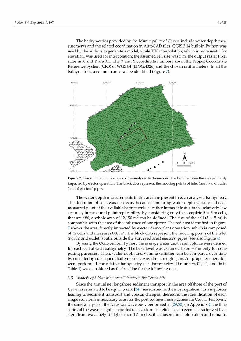
The bathymetries provided by the Municipality of Cervia include water depth mea-surements and the related coordination in AutoCAD files. QGIS 3.14 built-in Python wasused by the authors to generate a model, while TIN interpolation, which is more useful forelevation, was used for interpolation; the assumed cell size was 5 m, the output raster Pixelsizes in X and Y are 0.1. The X and Y coordinate numbers are in the Project CoordinateReference System (CRS) of WGS 84 (EPSG:4326) and the chosen unit is meters. In all thebathymetries, a common area can be identified (Figure 7).

J. Mar. Sci. Eng. 2021, 9, x 8 of 26

Table 1. Bathymetries considered in the analysis for the period June 2017–April 2020.

Bathymetry ID Date Note

01 13 June 2017 Realized after dredging (2200 m3 of removed sediments) and 5 days of propellers operation completed in April–June 2017

02 28 December 2017 03 7 April 2018

04 11 May 2018 Realized after 5 days of propeller operation, completed in April 2018

05 10 October 2018

06 10 April 2019 Realized after 2.5 days of propeller operation and dredg-ing (20,000 m3 of removed sediments), completed in Janu-ary–April 2019

07 12 June 2019 Realized one day before the ejector demo plant was put into in operation

08 6 September 2019 Ejector demo plant in operation (phase 1, see Figure 6) 09 9 January 2020 Ejector demo plant in operation (phase 2, see Figure 6) 10 30 April 2020 Ejector demo plant in operation (phase 3, see Figure 6)

The bathymetries provided by the Municipality of Cervia include water depth meas-urements and the related coordination in AutoCAD files. QGIS 3.14 built-in Python was used by the authors to generate a model, while TIN interpolation, which is more useful for elevation, was used for interpolation; the assumed cell size was 5 m, the output raster Pixel sizes in X and Y are 0.1. The X and Y coordinate numbers are in the Project Coordi-nate Reference System (CRS) of WGS 84 (EPSG:4326) and the chosen unit is meters. In all the bathymetries, a common area can be identified (Figure 7).

Figure 7. Grids in the common area of the analysed bathymetries. The box identifies the area pri-marily impacted by ejector operation. The black dots represent the mooring points of inlet (north) and outlet (south) ejectors’ pipes.

The water depth measurements in this area are present in each analysed bathymetry. The definition of cells was necessary because comparing water depth variation at each measured point of the available bathymetries is rather impossible due to the relatively low accuracy in measured point replicability. By considering only the complete 5 × 5 m cells, that are 486, a whole area of 12,150 m2 can be defined. The size of the cell (5 × 5 m) is

Figure 7. Grids in the common area of the analysed bathymetries. The box identifies the area primarilyimpacted by ejector operation. The black dots represent the mooring points of inlet (north) and outlet(south) ejectors’ pipes.

The water depth measurements in this area are present in each analysed bathymetry.The definition of cells was necessary because comparing water depth variation at eachmeasured point of the available bathymetries is rather impossible due to the relatively lowaccuracy in measured point replicability. By considering only the complete 5 × 5 m cells,that are 486, a whole area of 12,150 m2 can be defined. The size of the cell (5 × 5 m) iscompatible with the area of the influence of one ejector. The red area identified in Figure7 shows the area directly impacted by ejector demo plant operation, which is composedof 32 cells and measures 800 m2. The black dots represent the mooring points of the inlet(north) and outlet (south, outside the surveyed area) ejectors’ pipes (see also Figure 4).

By using the QGIS built-in Python, the average water depth and volume were definedfor each cell at each bathymetry. The base level was assumed to be −7 m only for com-puting purposes. Then, water depth and volume variation can be compared over timeby considering subsequent bathymetries. Any time dredging and/or propeller operationwere performed, the relative bathymetry (i.e., bathymetry ID numbers 01, 04, and 06 inTable 1) was considered as the baseline for the following ones.

3.3. Analysis of 3-Year Metocean Climate on the Cervia Site

Since the annual net longshore sediment transport in the area offshore of the port ofCervia is estimated to be equal to zero [24], sea storms are the most significant driving forcesleading to sediment transport and coastal changes; therefore, the identification of eachsingle sea storm is necessary to assess the port sediment management in Cervia. Followingthe same analysis of the Nausicaa wave buoy performed in [29,30] (in Appendix C the timeseries of the wave height is reported), a sea storm is defined as an event characterized by asignificant wave height higher than 1.5 m (i.e., the chosen threshold value) and remains

J. Mar. Sci. Eng. 2021, 9, 197 9 of 25

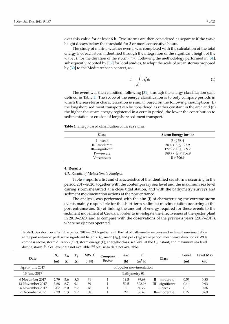
over this value for at least 6 h. Two storms are then considered as separate if the waveheight decays below the threshold for 3 or more consecutive hours.

The study of marine weather events was completed with the calculation of the totalenergy E of each storm, identified through the integration of the significant height of thewave Hs for the duration of the storm (dur), following the methodology performed in [31],subsequently adopted by [32] for local studies, to adapt the scale of ocean storms proposedby [30] to the Mediterranean context, as:

E =∫

dur

H2s dt (1)

The event was then classified, following [31], through the energy classification scaledefined in Table 2. The scope of the energy classification is to only compare periods inwhich the sea storm characterization is similar, based on the following assumptions: (i)the longshore sediment transport can be considered as rather constant in the area and (ii)the higher the storm energy registered in a certain period, the lower the contribution tosedimentation or erosion of longshore sediment transport.

Table 2. Energy-based classification of the sea storm.

Class Storm Energy (m2 h)

I—weak E ≤ 58.4II—moderate 58.4 < E ≤ 127.9

III—significant 127.9 < E ≤ 389.7IV—severe 389.7 < E ≤ 706.9V—extreme E > 706.9

4. Results4.1. Results of Meteoclimate Analysis

Table 3 reports a list and characteristics of the identified sea storms occurring in theperiod 2017–2020, together with the contemporary sea level and the maximum sea levelduring storm measured at a close tidal station, and with the bathymetry surveys andsediment movimentation actions at the port entrance.

The analysis was performed with the aim (i) of characterizing the extreme stormevents mainly responsible for the short-term sediment movimentation occurring at theport entrance and (ii) of linking the amount of energy required for these events to thesediment movement at Cervia, in order to investigate the effectiveness of the ejector plantin 2019–2020, and to compare with the observations of the previous years (2017–2019),where no ejectors operated.

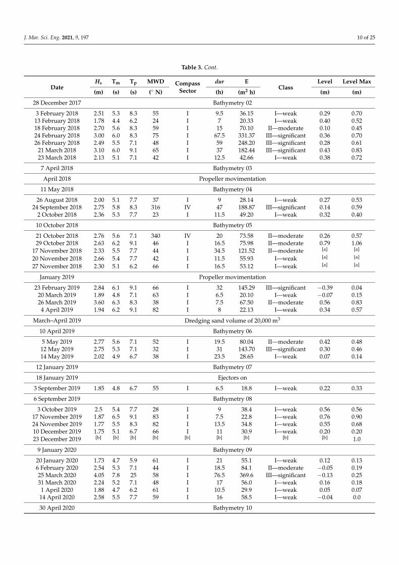
Table 3. Sea storm events in the period 2017–2020, together with the list of bathymetry surveys and sediment movimentationat the port entrance: peak wave significant height (Hs), mean (Tm), and peak (Tp) wave period, mean wave direction (MWD),compass sector, storm duration (dur), storm energy (E), energetic class, sea level at the Hs instant, and maximum sea levelduring storm. [a] Sea level data not available; [b] Nausicaa data not available.

DateHs Tm Tp MWD Compass

Sectordur E

ClassLevel Level Max

(m) (s) (s) (◦ N) (h) (m2 h) (m) (m)

April–June 2017 Propeller movimentation

13 June 2017 Bathymetry 01

6 November 2017 2.79 5.6 8.3 61 I 19.5 89.68 II—moderate 0.53 0.8313 November 2017 3.68 6.7 9.1 59 I 50.5 302.96 III—significant 0.44 0.9326 November 2017 3.07 5.0 7.7 46 I 11 50.77 I—weak 0.13 0.362 December 2017 2.39 5.3 7.7 58 I 22 86.48 II—moderate 0.27 0.69

J. Mar. Sci. Eng. 2021, 9, 197 10 of 25

Table 3. Cont.

DateHs Tm Tp MWD Compass

Sectordur E

ClassLevel Level Max

(m) (s) (s) (◦ N) (h) (m2 h) (m) (m)

28 December 2017 Bathymetry 02

3 February 2018 2.51 5.3 8.3 55 I 9.5 36.15 I—weak 0.29 0.7013 February 2018 1.78 4.4 6.2 24 I 7 20.33 I—weak 0.40 0.5218 February 2018 2.70 5.6 8.3 59 I 15 70.10 II—moderate 0.10 0.4524 February 2018 3.00 6.0 8.3 75 I 67.5 331.37 III—significant 0.36 0.7026 February 2018 2.49 5.5 7.1 48 I 59 248.20 III—significant 0.28 0.61

21 March 2018 3.10 6.0 9.1 65 I 37 182.44 III—significant 0.43 0.8323 March 2018 2.13 5.1 7.1 42 I 12.5 42.66 I—weak 0.38 0.72

7 April 2018 Bathymetry 03

April 2018 Propeller movimentation

11 May 2018 Bathymetry 04

26 August 2018 2.00 5.1 7.7 37 I 9 28.14 I—weak 0.27 0.5324 September 2018 2.75 5.8 8.3 316 IV 47 188.87 III—significant 0.14 0.59

2 October 2018 2.36 5.3 7.7 23 I 11.5 49.20 I—weak 0.32 0.40

10 October 2018 Bathymetry 05

21 October 2018 2.76 5.6 7.1 340 IV 20 73.58 II—moderate 0.26 0.5729 October 2018 2.63 6.2 9.1 46 I 16.5 75.98 II—moderate 0.79 1.06

17 November 2018 2.33 5.5 7.7 44 I 34.5 121.52 II—moderate [a] [a]

20 November 2018 2.66 5.4 7.7 42 I 11.5 55.93 I—weak [a] [a]

27 November 2018 2.30 5.1 6.2 66 I 16.5 53.12 I—weak [a] [a]

January 2019 Propeller movimentation

23 February 2019 2.84 6.1 9.1 66 I 32 145.29 III—significant −0.39 0.0420 March 2019 1.89 4.8 7.1 63 I 6.5 20.10 I—weak −0.07 0.1526 March 2019 3.60 6.3 8.3 38 I 7.5 67.50 II—moderate 0.56 0.834 April 2019 1.94 6.2 9.1 82 I 8 22.13 I—weak 0.34 0.57

March–April 2019 Dredging sand volume of 20,000 m3

10 April 2019 Bathymetry 06

5 May 2019 2.77 5.6 7.1 52 I 19.5 80.04 II—moderate 0.42 0.4812 May 2019 2.75 5.3 7.1 32 I 31 143.70 III—significant 0.30 0.4614 May 2019 2.02 4.9 6.7 38 I 23.5 28.65 I—weak 0.07 0.14

12 January 2019 Bathymetry 07

18 January 2019 Ejectors on

3 September 2019 1.85 4.8 6.7 55 I 6.5 18.8 I—weak 0.22 0.33

6 September 2019 Bathymetry 08

3 October 2019 2.5 5.4 7.7 28 I 9 38.4 I—weak 0.56 0.5617 November 2019 1.87 6.5 9.1 83 I 7.5 22.8 I—weak 0.76 0.9024 November 2019 1.77 5.5 8.3 82 I 13.5 34.8 I—weak 0.55 0.6810 December 2019 1.75 5.1 6.7 66 I 11 30.9 I—weak 0.20 0.2023 December 2019 [b] [b] [b] [b] [b] [b] [b] [b] [b] 1.0

9 January 2020 Bathymetry 09

20 January 2020 1.73 4.7 5.9 61 I 21 55.1 I—weak 0.12 0.136 February 2020 2.54 5.3 7.1 44 I 18.5 84.1 II—moderate −0.05 0.1925 March 2020 4.05 7.8 25 58 I 76.5 369.6 III—significant −0.13 0.2531 March 2020 2.24 5.2 7.1 48 I 17 56.0 I—weak 0.16 0.181 April 2020 1.88 4.7 6.2 61 I 10.5 29.9 I—weak 0.05 0.07

14 April 2020 2.58 5.5 7.7 59 I 16 58.5 I—weak −0.04 0.0

30 April 2020 Bathymetry 10

J. Mar. Sci. Eng. 2021, 9, 197 11 of 25

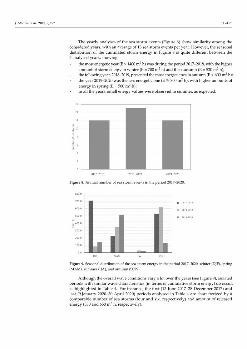
The yearly analyses of the sea storm events (Figure 8) show similarity among theconsidered years, with an average of 13 sea storm events per year. However, the seasonaldistribution of the cumulated storm energy in Figure 9 is quite different between the3 analysed years, showing:

- the most energetic year (E > 1400 m2 h) was during the period 2017–2018, with the higheramount of storm energy in winter (E = 700 m2 h) and then autumn (E = 520 m2 h);

- the following year, 2018–2019, presented the most energetic sea in autumn (E > 600 m2 h);- the year 2019–2020 was the less energetic one (E ∼= 800 m2 h), with higher amounts of

energy in spring (E = 500 m2 h);- in all the years, small energy values were observed in summer, as expected.

J. Mar. Sci. Eng. 2021, 9, x 11 of 26

23 December 2019 [b] [b] [b] [b] [b] [b] [b] [b] [b] 1.0 9 January 2020 Bathymetry 09

20 January 2020 1.73 4.7 5.9 61 I 21 55.1 I—weak 0.12 0.13 6 February 2020 2.54 5.3 7.1 44 I 18.5 84.1 II—moderate −0.05 0.19 25 March 2020 4.05 7.8 25 58 I 76.5 369.6 III—significant −0.13 0.25 31 March 2020 2.24 5.2 7.1 48 I 17 56.0 I—weak 0.16 0.18

1 April 2020 1.88 4.7 6.2 61 I 10.5 29.9 I—weak 0.05 0.07 14 April 2020 2.58 5.5 7.7 59 I 16 58.5 I—weak −0.04 0.0 30 April 2020 Bathymetry 10

The analysis was performed with the aim i) of characterizing the extreme storm events mainly responsible for the short-term sediment movimentation occurring at the port entrance and ii) of linking the amount of energy required for these events to the sed-iment movement at Cervia, in order to investigate the effectiveness of the ejector plant in 2019–2020, and to compare with the observations of the previous years (2017–2019), where no ejectors operated.

The yearly analyses of the sea storm events (Figure 8) show similarity among the considered years, with an average of 13 sea storm events per year. However, the seasonal distribution of the cumulated storm energy in Figure 9 is quite different between the 3 analysed years, showing: - the most energetic year (E > 1400 m2 h) was during the period 2017–2018, with the

higher amount of storm energy in winter (E = 700 m2 h) and then autumn (E = 520 m2 h);

- the following year, 2018–2019, presented the most energetic sea in autumn (E > 600 m2 h);

- the year 2019–2020 was the less energetic one (E ≅ 800 m2 h), with higher amounts of energy in spring (E = 500 m2 h);

- in all the years, small energy values were observed in summer, as expected. Although the overall wave conditions vary a lot over the years (see Figure 9), isolated

periods with similar wave characteristics (in terms of cumulative storm energy) do occur, as highlighted in Table 4. For instance, the first (13 June 2017–28 December 2017) and last (9 January 2020–30 April 2020) periods analysed in Table 4 are characterized by a compa-rable number of sea storms (four and six, respectively) and amount of released energy (530 and 650 m2 h, respectively).

Figure 8. Annual number of sea storm events in the period 2017–2020. Figure 8. Annual number of sea storm events in the period 2017–2020.

J. Mar. Sci. Eng. 2021, 9, x 12 of 26

Figure 9. Seasonal distribution of the sea storm energy in the period 2017–2020: winter (DJF), spring (MAM), summer (JJA), and autumn (SON).

Table 4. Summary of number of storms, related energy in periods under analysis, and the mean energy per day.

Period N° of Storms Energy Released in the Period (m2 h)

Mean Energy Per Day (m2 h/day)

13 June 2017–28 December 2017 4 530 2.68 28 December 2017–7 April 2018 7 930 9.30 11 May 2018–10 October 2018 3 266 1.75

10 April 2019–12 June 2019 4 275 4.37 12 June 2019–6 September 2019 1 19 0.22

6 September 2019–9 January 2020 4 127 1.02 9 January 2020–30 April 2020 6 653 5.83

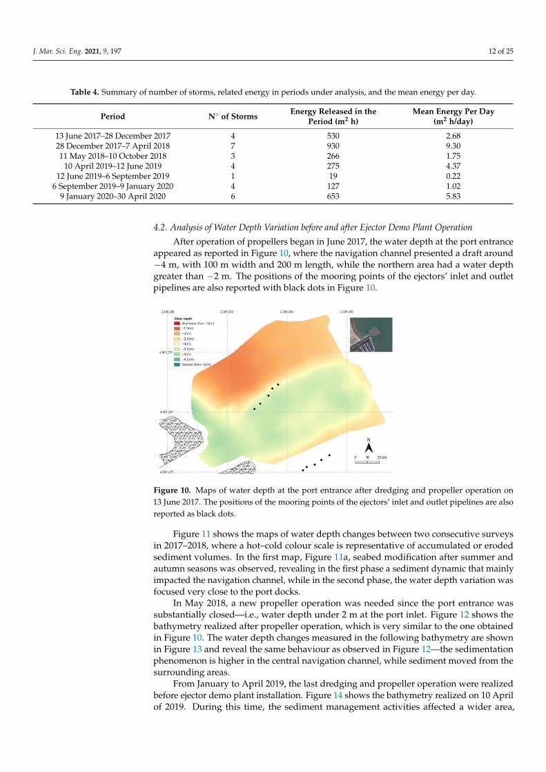
4.2. Analysis of Water Depth Variation before and after Ejector Demo Plant Operation After operation of propellers began in June 2017, the water depth at the port entrance

appeared as reported in Figure 10, where the navigation channel presented a draft around −4 m, with 100 m width and 200 m length, while the northern area had a water depth greater than −2 m. The positions of the mooring points of the ejectors’ inlet and outlet pipelines are also reported with black dots in Figure 10.

Figure 11 shows the maps of water depth changes between two consecutive surveys in 2017–2018, where a hot–cold colour scale is representative of accumulated or eroded sediment volumes. In the first map, Figure 11a, seabed modification after summer and autumn seasons was observed, revealing in the first phase a sediment dynamic that mainly impacted the navigation channel, while in the second phase, the water depth var-iation was focused very close to the port docks.

In May 2018, a new propeller operation was needed since the port entrance was sub-stantially closed—i.e., water depth under 2 m at the port inlet. Figure 12 shows the ba-thymetry realized after propeller operation, which is very similar to the one obtained in Figure 10. The water depth changes measured in the following bathymetry are shown in Figure 13 and reveal the same behaviour as observed in Figure 12—the sedimentation phenomenon is higher in the central navigation channel, while sediment moved from the surrounding areas.

Figure 9. Seasonal distribution of the sea storm energy in the period 2017–2020: winter (DJF), spring(MAM), summer (JJA), and autumn (SON).

Although the overall wave conditions vary a lot over the years (see Figure 9), isolatedperiods with similar wave characteristics (in terms of cumulative storm energy) do occur,as highlighted in Table 4. For instance, the first (13 June 2017–28 December 2017) andlast (9 January 2020–30 April 2020) periods analysed in Table 4 are characterized by acomparable number of sea storms (four and six, respectively) and amount of releasedenergy (530 and 650 m2 h, respectively).

J. Mar. Sci. Eng. 2021, 9, 197 12 of 25

Table 4. Summary of number of storms, related energy in periods under analysis, and the mean energy per day.

Period N◦ of Storms Energy Released in thePeriod (m2 h)

Mean Energy Per Day(m2 h/day)

13 June 2017–28 December 2017 4 530 2.6828 December 2017–7 April 2018 7 930 9.3011 May 2018–10 October 2018 3 266 1.75

10 April 2019–12 June 2019 4 275 4.3712 June 2019–6 September 2019 1 19 0.22

6 September 2019–9 January 2020 4 127 1.029 January 2020–30 April 2020 6 653 5.83

4.2. Analysis of Water Depth Variation before and after Ejector Demo Plant Operation

After operation of propellers began in June 2017, the water depth at the port entranceappeared as reported in Figure 10, where the navigation channel presented a draft around−4 m, with 100 m width and 200 m length, while the northern area had a water depthgreater than −2 m. The positions of the mooring points of the ejectors’ inlet and outletpipelines are also reported with black dots in Figure 10.

J. Mar. Sci. Eng. 2021, 9, x 13 of 26

Figure 10. Maps of water depth at the port entrance after dredging and propeller operation on 13 June 2017. The positions of the mooring points of the ejectors’ inlet and outlet pipelines are also reported as black dots.

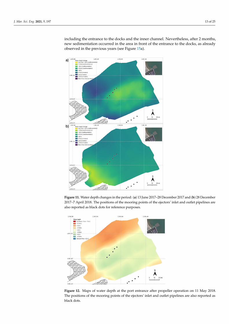
Figure 11. Water depth changes in the period: (a) 13 June 2017–28 December 2017 and (b) 28 De-cember 2017–7 April 2018. The positions of the mooring points of the ejectors’ inlet and outlet pipelines are also reported as black dots for reference purposes.

Figure 10. Maps of water depth at the port entrance after dredging and propeller operation on13 June 2017. The positions of the mooring points of the ejectors’ inlet and outlet pipelines are alsoreported as black dots.

Figure 11 shows the maps of water depth changes between two consecutive surveysin 2017–2018, where a hot–cold colour scale is representative of accumulated or erodedsediment volumes. In the first map, Figure 11a, seabed modification after summer andautumn seasons was observed, revealing in the first phase a sediment dynamic that mainlyimpacted the navigation channel, while in the second phase, the water depth variation wasfocused very close to the port docks.

In May 2018, a new propeller operation was needed since the port entrance wassubstantially closed—i.e., water depth under 2 m at the port inlet. Figure 12 shows thebathymetry realized after propeller operation, which is very similar to the one obtainedin Figure 10. The water depth changes measured in the following bathymetry are shownin Figure 13 and reveal the same behaviour as observed in Figure 12—the sedimentationphenomenon is higher in the central navigation channel, while sediment moved from thesurrounding areas.

From January to April 2019, the last dredging and propeller operation were realizedbefore ejector demo plant installation. Figure 14 shows the bathymetry realized on 10 Aprilof 2019. During this time, the sediment management activities affected a wider area,

J. Mar. Sci. Eng. 2021, 9, 197 13 of 25

including the entrance to the docks and the inner channel. Nevertheless, after 2 months,new sedimentation occurred in the area in front of the entrance to the docks, as alreadyobserved in the previous years (see Figure 15a).

J. Mar. Sci. Eng. 2021, 9, x 13 of 26

Figure 10. Maps of water depth at the port entrance after dredging and propeller operation on 13 June 2017. The positions of the mooring points of the ejectors’ inlet and outlet pipelines are also reported as black dots.

Figure 11. Water depth changes in the period: (a) 13 June 2017–28 December 2017 and (b) 28 De-cember 2017–7 April 2018. The positions of the mooring points of the ejectors’ inlet and outlet pipelines are also reported as black dots for reference purposes.

Figure 11. Water depth changes in the period: (a) 13 June 2017–28 December 2017 and (b) 28 December2017–7 April 2018. The positions of the mooring points of the ejectors’ inlet and outlet pipelines arealso reported as black dots for reference purposes.

J. Mar. Sci. Eng. 2021, 9, x 14 of 26

Figure 12. Maps of water depth at the port entrance after propeller operation on 11 May 2018. The positions of the mooring points of the ejectors’ inlet and outlet pipelines are also reported as black dots.

Figure 13. Water depth change in the period 11 May 2018–10 October 2018. The positions of the mooring points of the ejectors’ inlet and outlet pipelines are also reported in black dots.

From January to April 2019, the last dredging and propeller operation were realized before ejector demo plant installation. Figure 14 shows the bathymetry realized on 10 April of 2019. During this time, the sediment management activities affected a wider area, including the entrance to the docks and the inner channel. Nevertheless, after 2 months, new sedimentation occurred in the area in front of the entrance to the docks, as already observed in the previous years (see Figure 15a).

On 13 June 2019 the ejector demo plant was activated. The bathymetry realized on 12 June 2019 (Figure 15b) is the reference bathymetry to evaluate ejector demo plant effec-tiveness in keeping a sufficient water level at the port entrance. The minimum water depth at the port entrance to guarantee navigability was 2.5 m, since under this level fisherman and leisure boats that use the Marina of Cervia usually start having navigability issues. Figure 16 has been realized on the basis of bathymetries from June 2019 to April 2020 (included in Appendix B) and shows if and where the minimum water depth was reached in the common area at the port inlet.

The first relevant result is that at the end of the monitoring period (end of April 2020) there is still present a navigable channel (i.e., water depth over 2.5 m) to enter the port of Cervia. It is interesting to note how in January 2020 the situation appeared critical in the area of influence of the ejectors, and that this critical situation negatively evolved from

Figure 12. Maps of water depth at the port entrance after propeller operation on 11 May 2018.The positions of the mooring points of the ejectors’ inlet and outlet pipelines are also reported asblack dots.

J. Mar. Sci. Eng. 2021, 9, 197 14 of 25

J. Mar. Sci. Eng. 2021, 9, x 14 of 26

Figure 12. Maps of water depth at the port entrance after propeller operation on 11 May 2018. The positions of the mooring points of the ejectors’ inlet and outlet pipelines are also reported as black dots.

Figure 13. Water depth change in the period 11 May 2018–10 October 2018. The positions of the mooring points of the ejectors’ inlet and outlet pipelines are also reported in black dots.

From January to April 2019, the last dredging and propeller operation were realized before ejector demo plant installation. Figure 14 shows the bathymetry realized on 10 April of 2019. During this time, the sediment management activities affected a wider area, including the entrance to the docks and the inner channel. Nevertheless, after 2 months, new sedimentation occurred in the area in front of the entrance to the docks, as already observed in the previous years (see Figure 15a).

On 13 June 2019 the ejector demo plant was activated. The bathymetry realized on 12 June 2019 (Figure 15b) is the reference bathymetry to evaluate ejector demo plant effec-tiveness in keeping a sufficient water level at the port entrance. The minimum water depth at the port entrance to guarantee navigability was 2.5 m, since under this level fisherman and leisure boats that use the Marina of Cervia usually start having navigability issues. Figure 16 has been realized on the basis of bathymetries from June 2019 to April 2020 (included in Appendix B) and shows if and where the minimum water depth was reached in the common area at the port inlet.

The first relevant result is that at the end of the monitoring period (end of April 2020) there is still present a navigable channel (i.e., water depth over 2.5 m) to enter the port of Cervia. It is interesting to note how in January 2020 the situation appeared critical in the area of influence of the ejectors, and that this critical situation negatively evolved from

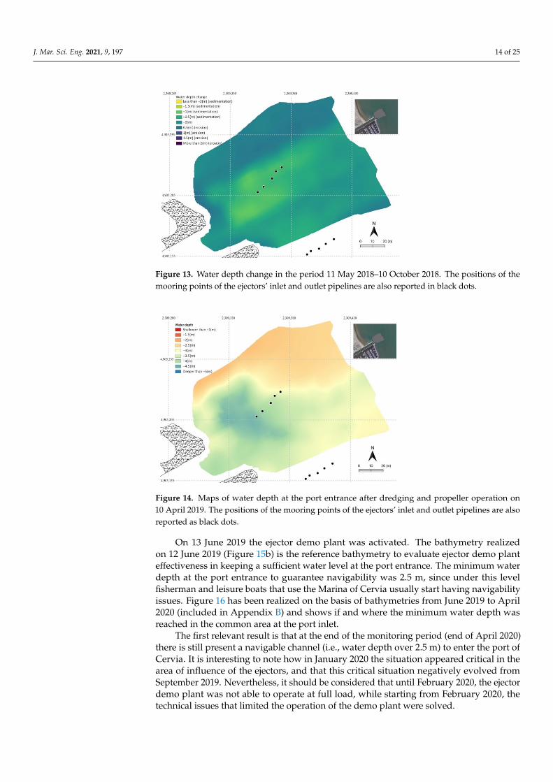
Figure 13. Water depth change in the period 11 May 2018–10 October 2018. The positions of themooring points of the ejectors’ inlet and outlet pipelines are also reported in black dots.

J. Mar. Sci. Eng. 2021, 9, x 15 of 26

September 2019. Nevertheless, it should be considered that until February 2020, the ejector demo plant was not able to operate at full load, while starting from February 2020, the technical issues that limited the operation of the demo plant were solved.

Figure 14. Maps of water depth at the port entrance after dredging and propeller operation on 10 April 2019. The positions of the mooring points of the ejectors’ inlet and outlet pipelines are also reported as black dots.

Figure 15. (a) Water depth change in the period 10 April 2019–12 June 2019, and (b) water depth measured on 12 June 2019. The positions of the mooring points of the ejectors’ inlet and outlet pipelines are also reported as black dots.

Figure 14. Maps of water depth at the port entrance after dredging and propeller operation on10 April 2019. The positions of the mooring points of the ejectors’ inlet and outlet pipelines are alsoreported as black dots.

On 13 June 2019 the ejector demo plant was activated. The bathymetry realizedon 12 June 2019 (Figure 15b) is the reference bathymetry to evaluate ejector demo planteffectiveness in keeping a sufficient water level at the port entrance. The minimum waterdepth at the port entrance to guarantee navigability was 2.5 m, since under this levelfisherman and leisure boats that use the Marina of Cervia usually start having navigabilityissues. Figure 16 has been realized on the basis of bathymetries from June 2019 to April2020 (included in Appendix B) and shows if and where the minimum water depth wasreached in the common area at the port inlet.

The first relevant result is that at the end of the monitoring period (end of April 2020)there is still present a navigable channel (i.e., water depth over 2.5 m) to enter the port ofCervia. It is interesting to note how in January 2020 the situation appeared critical in thearea of influence of the ejectors, and that this critical situation negatively evolved fromSeptember 2019. Nevertheless, it should be considered that until February 2020, the ejectordemo plant was not able to operate at full load, while starting from February 2020, thetechnical issues that limited the operation of the demo plant were solved.

J. Mar. Sci. Eng. 2021, 9, 197 15 of 25

J. Mar. Sci. Eng. 2021, 9, x 15 of 26

September 2019. Nevertheless, it should be considered that until February 2020, the ejector demo plant was not able to operate at full load, while starting from February 2020, the technical issues that limited the operation of the demo plant were solved.

Figure 14. Maps of water depth at the port entrance after dredging and propeller operation on 10 April 2019. The positions of the mooring points of the ejectors’ inlet and outlet pipelines are also reported as black dots.

Figure 15. (a) Water depth change in the period 10 April 2019–12 June 2019, and (b) water depth measured on 12 June 2019. The positions of the mooring points of the ejectors’ inlet and outlet pipelines are also reported as black dots.

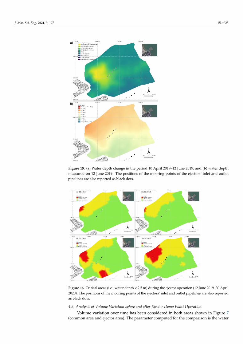
Figure 15. (a) Water depth change in the period 10 April 2019–12 June 2019, and (b) water depthmeasured on 12 June 2019. The positions of the mooring points of the ejectors’ inlet and outletpipelines are also reported as black dots.

J. Mar. Sci. Eng. 2021, 9, x 16 of 26

Figure 16. Critical areas (i.e., water depth < 2.5 m) during the ejector operation (12 June 2019–30 April 2020). The positions of the mooring points of the ejectors’ inlet and outlet pipelines are also reported as black dots.

4.3. Analysis of Volume Variation before and after Ejector Demo Plant Operation Volume variation over time has been considered in both areas shown in Figure 7

(common area and ejector area). The parameter computed for the comparison is the water depth variation per day, expressed in mm per day, which is calculated by dividing the volume variation between two consecutive bathymetries by the area under consideration (i.e., common area or ejector area) and by the number of days between two consecutive bathymetries. The results are shown in Figure 17.

Figure 17. Mean water depth variation per day (in mm/day) between two consecutive bathy-metries in the common area and in the ejector area before and after ejector demo plant operation.

Figure 16. Critical areas (i.e., water depth < 2.5 m) during the ejector operation (12 June 2019–30 April2020). The positions of the mooring points of the ejectors’ inlet and outlet pipelines are also reportedas black dots.

4.3. Analysis of Volume Variation before and after Ejector Demo Plant Operation

Volume variation over time has been considered in both areas shown in Figure 7(common area and ejector area). The parameter computed for the comparison is the water

J. Mar. Sci. Eng. 2021, 9, 197 16 of 25

depth variation per day, expressed in mm per day, which is calculated by dividing thevolume variation between two consecutive bathymetries by the area under consideration(i.e., common area or ejector area) and by the number of days between two consecutivebathymetries. The results are shown in Figure 17.

J. Mar. Sci. Eng. 2021, 9, x 16 of 26

Figure 16. Critical areas (i.e., water depth < 2.5 m) during the ejector operation (12 June 2019–30 April 2020). The positions of the mooring points of the ejectors’ inlet and outlet pipelines are also reported as black dots.

4.3. Analysis of Volume Variation before and after Ejector Demo Plant Operation Volume variation over time has been considered in both areas shown in Figure 7

(common area and ejector area). The parameter computed for the comparison is the water depth variation per day, expressed in mm per day, which is calculated by dividing the volume variation between two consecutive bathymetries by the area under consideration (i.e., common area or ejector area) and by the number of days between two consecutive bathymetries. The results are shown in Figure 17.

Figure 17. Mean water depth variation per day (in mm/day) between two consecutive bathy-metries in the common area and in the ejector area before and after ejector demo plant operation.

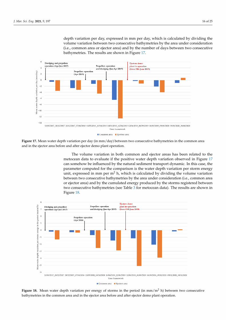
Figure 17. Mean water depth variation per day (in mm/day) between two consecutive bathymetries in the common areaand in the ejector area before and after ejector demo plant operation.

The volume variation in both common and ejector areas has been related to themetocean data to evaluate if the positive water depth variation observed in Figure 17can somehow be influenced by the natural sediment transport dynamic. In this case, theparameter computed for the comparison is the water depth variation per storm energyunit, expressed in mm per m2 h, which is calculated by dividing the volume variationbetween two consecutive bathymetries by the area under consideration (i.e., common areaor ejector area) and by the cumulated energy produced by the storms registered betweentwo consecutive bathymetries (see Table 3 for metocean data). The results are shown inFigure 18.

J. Mar. Sci. Eng. 2021, 9, x 17 of 26

The volume variation in both common and ejector areas has been related to the metocean data to evaluate if the positive water depth variation observed in Figure 17 can somehow be influenced by the natural sediment transport dynamic. In this case, the pa-rameter computed for the comparison is the water depth variation per storm energy unit, expressed in mm per m2 h, which is calculated by dividing the volume variation between two consecutive bathymetries by the area under consideration (i.e., common area or ejec-tor area) and by the cumulated energy produced by the storms registered between two consecutive bathymetries (see Table 3 for metocean data). The results are shown in Figure 18.

The implicit assumption in drafting Figure 18 is that sediment transport in both areas under investigation is mainly due to storms. Therefore, different periods considered in the analysis can be compared only if similar storm conditions occur.

Figure 18. Mean water depth variation per energy of storms in the period (in mm/m2 h) between two consecutive bathymetries in the common area and in the ejector area before and after ejector demo plant operation.

5. Discussion The analysis of Figures 10–15, it is clearly shown that dredging and propeller opera-

tion realized in the centre of the navigation channel partially solve the problem of naviga-bility of the port inlet, since in a few months the hole created at the centre of the channel was covered again by sediment. In particular, part of the sediment came from the sur-rounding area, and it is expected that natural sediment transport in the area produced by storm and longshore transport also contributes. The impact of dredging and propeller operation on the water depth variation rate is also confirmed by the analysis of Figures 17 and 18. In particular, both figures show sediment dynamics that seem to impact more on the area of ejectors than in the whole common area. Such a dynamic is justified by the fact that the ejector area is directly affected by both dredging and propeller operation, mean-ing that after artificial deepening of the seabed, the ejector area is usually characterized by a water depth that is higher than the mean value of the common area. The result is that the ejector area works as a sediment trap after dredging or propeller operation. Moreover, in the ejector area, in the first period after dredging or propeller operation (13 June 2017–28 December 2017, 11 May 2018–10 October 2018, 10 April 2019–12 June 2019), we ob-served a higher water depth variation than in the common area, while in the period 28 December 2017–7 April 2018, which is characterized by the highest number of storms,

Figure 18. Mean water depth variation per energy of storms in the period (in mm/m2 h) between two consecutivebathymetries in the common area and in the ejector area before and after ejector demo plant operation.

J. Mar. Sci. Eng. 2021, 9, 197 17 of 25

The implicit assumption in drafting Figure 18 is that sediment transport in both areasunder investigation is mainly due to storms. Therefore, different periods considered in theanalysis can be compared only if similar storm conditions occur.

5. Discussion

The analysis of Figures 10–15, it is clearly shown that dredging and propeller operationrealized in the centre of the navigation channel partially solve the problem of navigabilityof the port inlet, since in a few months the hole created at the centre of the channel wascovered again by sediment. In particular, part of the sediment came from the surroundingarea, and it is expected that natural sediment transport in the area produced by storm andlongshore transport also contributes. The impact of dredging and propeller operation onthe water depth variation rate is also confirmed by the analysis of Figures 17 and 18. Inparticular, both figures show sediment dynamics that seem to impact more on the areaof ejectors than in the whole common area. Such a dynamic is justified by the fact thatthe ejector area is directly affected by both dredging and propeller operation, meaningthat after artificial deepening of the seabed, the ejector area is usually characterized by awater depth that is higher than the mean value of the common area. The result is that theejector area works as a sediment trap after dredging or propeller operation. Moreover, inthe ejector area, in the first period after dredging or propeller operation (13 June 2017–28December 2017, 11 May 2018–10 October 2018, 10 April 2019–12 June 2019), we observed ahigher water depth variation than in the common area, while in the period 28 December2017–7 April 2018, which is characterized by the highest number of storms, related energyin the period as well as energy per day, the water depth variations in both areas arecomparable. Furthermore, Figure 18 shows a relevant decreasing water depth variationrate per storm energy unit in the two consecutive periods from June to December 2017and from December 2017 to April 2018, since in the first period the rate is −1.31 mm/m2 h,while in the second period it is −0.34 mm/m2 h. It can be concluded that after a fastervariation of water depth in the ejector area, which is the one mainly affected by dredgingand propeller operation, the water depth variation tends to homogenize in the commonarea. Therefore, the “artificial” increase in water depth modifies the natural sedimentdynamic since the depression created in the port inlet attracts the nearby sediment and thesediment that is naturally transported in the area. A better option would be to not dredgeor move the sediment via propeller operation along the navigable channel, but to workon the southern or northern areas. Such planning would be beneficial also in combinationwith ejector demo plant operation, since the dredging or propeller operation, which maybe needed to remove sediment accumulation out of the ejector area for beach nourishmentpurposes, would not affect the integrity of the ejector demo plant.

While Figure 17 indicates that there is not a constant relationship between the waterdepth variation in the common and in the ejector areas, the same figure suggests that waterdepth variation in the common area before and after ejector demo plant operation has acomparable intensity, i.e., −0.5 ÷ 2.5 mm/day of mean variation, with the exception ofthe period 10 April 2019–12 June 2019, in which the water depth variation in the commonarea reaches −6.5 mm/day. Such a huge water depth variation rate is justified by thecombined effects of (i) dredging and propeller operation realized on a wide area at the portentrance (see Figure 14) and of (ii) relative high storm energy measured in the period. Theperiod 12 June 2019–6 September 2019 is characterized by a very low level of storm energy,which is almost zero, yielding the highest value in Figure 18. In this case, it is probablethat the sediment transport has not only occurred due to the single storm registered inthe period, but natural longshore sediment transport also contributes. Therefore, thelongshore sediment dynamic is worth investigation in this area to better evaluate volumeand direction of the sediment transport during nice weather periods.

The most interesting evidence of Figures 17 and 18 is that in the last period of operationof the ejector demo plant (9 January 2020–30 April 2020), which overlaps with phase 3of operation (see Figure 6), a positive water depth variation (i.e., navigability increasing)

J. Mar. Sci. Eng. 2021, 9, 197 18 of 25

in the area of the ejectors can be observed, while in the common area, a negative waterdepth variation was observed in the same period. The last period of operation of the ejectordemo plant is comparable to the first period 13 June 2017–28 December 2017, since thetwo periods were characterized by similar energetic forcing from sea and similar metoceancharacteristics (see Tables 3 and 4). It is interesting to note that, in the comparing period,there is a relevant negative water depth variation, especially if compared with the commonarea. This fact suggests that in this period the impact of ejector demo plant operation isevident and contributed to keep the water depth almost constant in the ejector area.

By assuming the same mean rate of water depth variation for the period 13 June2017–28 December 2017, i.e., −1.31 mm/m2 h, it can be estimated that, without the ejectordemo plant in operation in the period 9 January 2020–30 April 2020, the water depth wouldvary by about −0.855 m in the ejector area, while a mean water depth variation of about0.081 m has been observed. Therefore, the net contribution of the ejector demo plant canbe evaluated with a maximum water depth variation of 0.936 m, which corresponds to amaximum volume of sediment by-passed of about 750 m3.

Nevertheless, since the water depth variation rate in the period 13 June 2017–28 De-cember 2017 may be influenced by the bathymetric changes produced in the area by theprevious dredging operation, the potential impact of the ejectors has been evaluated by as-suming the same mean rate of water depth variation of the following period, 28 December2017–7 April 2018—i.e., −0.34 mm/m2 h. If this water depth variation rate is applied, itcan be estimated that without the ejector demo plant in operation in the period 9 January2020–30 April 2020, the water depth would vary by about −0.223 m in the ejector area. Inthis case, the net contribution of the ejector demo plant can be evaluated in a maximumwater depth variation of 0.304 m, which corresponds to a maximum volume of sedimentby-passed of about 245 m3.

While the positive impact in the ejector area produced by the ejector demo plantoperation is evident in the period 9 January 2020–30 April 2020 and can be estimated, thesame cannot be said for the previous periods. The different impacts are justified by thedifferent operation regimes imposed on the ejector demo plant. In particular, the previousperiods are characterized by lower water flowrates feeding the ejectors. Nevertheless, itis not possible to exclude that some contributions were made by the ejector demo plantoperation in the periods of 12 June 2019–6 September 2019 and 6 September 2019–9 January2020. Further investigation is needed to design a model of sediment dynamic in the portentrance, which will be validated by the bathymetries realized before demo plant operation,and then the sediment dynamic in the same metocean frameworks registered during theejector demo plant operation will be simulated to verify the net contribution of the ejectordemo plant to water depth variation.

6. Conclusions

An innovative technology for sediment management in water infrastructure has beentested in the first industrial sized demo plant at the port entrance of the Marina of Cervia(Italy). The monitoring activities, concluded in September 2020, involved several activities,which include effectiveness, efficacy, and environmental impact assessments. This paperinvestigates the effectiveness achieved and the results demonstrate that the ejector demoplant was able to guarantee navigability at the port inlet after almost one year of operation(June 2019–April 2020). In particular, the maximum impact of the ejector demo plant onkeeping the water depth at the desired level (i.e., over the minimum threshold of 2.5 m)was observed in the period January–April 2020, wherein the ejector demo plant was able tooperate at the design water feeding flowrates and with an estimated by-passed sedimentvolume of between 245 and 750 m3.

Further investigation is needed to confirm the result through (i) the design of a modelof sediment dynamics at the port entrance and (ii) the simulation of the sediment transportin the same metocean frameworks registered during the ejector demo plant operation inorder to confirm the contribution on water depth and sediment volume variation. The

J. Mar. Sci. Eng. 2021, 9, 197 19 of 25

activities will be carried out once the monitoring of water depth at the port entrance, whichis still ongoing, in the second half of 2021.

Finally, based on the good performance of the ejector demo plant shown in the lastperiod of operation (January–April 2020), an adaptation of the existing ejectors configu-ration is under evaluation to optimize demo plant operation. The hypothesis is to spaceout the ejectors and, at the same time, move them closer to the port entrance. Anotherhypothesis under investigation is reducing the number of ejectors installed to reduce wholepower consumption.

Author Contributions: Conceptualization, M.P. and M.G.G.; methodology, A.A., M.P. and M.G.G.;software, A.A.; formal analysis, A.A. and M.G.G.; investigation, A.A. and M.G.G.; data curation,A.A.; writing—original draft preparation, M.G.G., A.A. and M.P.; writing—review and editing, R.A.,A.G. and C.S.; visualization, A.A.; supervision, R.A. and C.S. All authors have read and agreed to thepublished version of the manuscript.

Funding: This research was funded by the Italian Ministry for the Environment and Protection of theTerritory and the Sea, (MATTM) under the STIMARE Project, grant number CUP J56C18001240001.

Institutional Review Board Statement: Not applicable.

Informed Consent Statement: Not applicable.

Data Availability Statement: Data can be made available by the authors based on request.

Acknowledgments: The study is part of the “STIMARE (Strategie Innovative per il Monitoraggioed Analisi del Rischio Erosione, www.progettostimare.it (accessed on 19 December 2020))” project,funded by the Italian Ministry for the Environment and Protection of the Territory and the Sea,which aims to study the shoreline evolution presence of coastal defence structures with innovativemonitoring techniques and strategies.

Conflicts of Interest: The authors declare no conflict of interest.

Appendix A. Frequency Tables of the Sea Climate

Table A1. Frequency table of significant wave heights Hs and mean direction MWD for the year 2017–2018.

MWD[◦N]

Hs [m]

<0.50 0.50–0.75

0.75–1.00

1.00–1.25

1.25–1.5

1.5–1.75

1.75–2.00

2.00–2.25

2.25–2.5

2.5–2.75 2.75–3 >3.00 Total

0–15 2.43 0.36 0.10 0.03 0.01 0.00 0.01 0.00 0.00 0.00 0.00 0.00 2.94

15–30 3.27 0.78 0.26 0.24 0.04 0.09 0.06 0.00 0.03 0.00 0.00 0.00 4.78

30–45 4.36 1.28 0.54 0.53 0.34 0.22 0.27 0.10 0.03 0.02 0.01 0.01 7.71

45–60 3.79 1.32 1.05 0.79 0.63 0.40 0.49 0.58 0.48 0.15 0.02 0.01 9.70

60–75 4.61 1.33 0.81 0.52 0.39 0.29 0.43 0.63 0.25 0.21 0.21 0.02 9.70

75–90 9.64 2.44 1.36 1.25 0.87 0.16 0.01 0.01 0.00 0.00 0.00 0.01 15.74

90–105 16.46 3.73 1.37 0.46 0.18 0.07 0.00 0.00 0.00 0.00 0.00 0.00 22.26

105–120 10.53 1.42 0.26 0.11 0.00 0.00 0.00 0.00 0.00 0.00 0.00 0.00 12.32

120–135 2.23 0.16 0.06 0.00 0.00 0.00 0.00 0.00 0.00 0.00 0.00 0.00 2.45

135–150 0.54 0.03 0.00 0.00 0.00 0.00 0.00 0.00 0.00 0.00 0.00 0.00 0.58

150–165 0.20 0.00 0.00 0.00 0.00 0.00 0.00 0.00 0.00 0.00 0.00 0.00 0.20

165–180 0.07 0.01 0.00 0.00 0.00 0.00 0.00 0.00 0.00 0.00 0.00 0.00 0.08

180–195 0.15 0.01 0.00 0.00 0.00 0.00 0.00 0.00 0.00 0.00 0.00 0.00 0.16

195–210 0.17 0.00 0.00 0.00 0.00 0.00 0.00 0.00 0.00 0.00 0.00 0.00 0.17

210–225 0.11 0.00 0.00 0.00 0.00 0.00 0.00 0.00 0.00 0.00 0.00 0.00 0.11

225–240 0.10 0.00 0.00 0.00 0.00 0.00 0.00 0.00 0.00 0.00 0.00 0.00 0.10

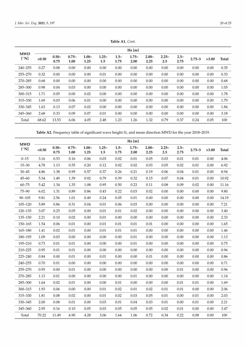
J. Mar. Sci. Eng. 2021, 9, 197 20 of 25

Table A1. Cont.

MWD[◦N]

Hs [m]

<0.50 0.50–0.75

0.75–1.00

1.00–1.25

1.25–1.5

1.5–1.75

1.75–2.00

2.00–2.25

2.25–2.5

2.5–2.75 2.75–3 >3.00 Total

240–255 0.27 0.08 0.00 0.00 0.00 0.00 0.00 0.00 0.00 0.00 0.00 0.00 0.35

255–270 0.32 0.00 0.00 0.00 0.01 0.00 0.00 0.00 0.00 0.00 0.00 0.00 0.33

270–285 0.68 0.00 0.00 0.00 0.00 0.00 0.00 0.00 0.00 0.00 0.00 0.00 0.68

285–300 0.98 0.04 0.03 0.00 0.00 0.00 0.00 0.00 0.00 0.00 0.00 0.00 1.05

300–315 1.71 0.05 0.00 0.02 0.00 0.00 0.00 0.00 0.00 0.00 0.00 0.00 1.78

315–330 1.69 0.03 0.06 0.01 0.00 0.00 0.00 0.00 0.00 0.00 0.00 0.00 1.79

330–345 1.63 0.13 0.07 0.02 0.00 0.00 0.00 0.00 0.00 0.00 0.00 0.00 1.84

345–360 2.68 0.33 0.09 0.07 0.01 0.00 0.00 0.00 0.00 0.00 0.00 0.00 3.18

Total 68.62 13.53 6.06 4.05 2.48 1.23 1.26 1.32 0.79 0.37 0.24 0.05 100

Table A2. Frequency table of significant wave height Hs and mean direction MWD for the year 2018–2019.

MWD[◦N]

Hs [m]

<0.50 0.50–0.75

0.75–1.00

1.00–1.25

1.25–1.5

1.5–1.75

1.75–2.00

2.00–2.25

2.25–2.5

2.5–2.75 2.75–3 >3.00 Total

0–15 3.16 0.53 0.16 0.06 0.03 0.02 0.01 0.05 0.03 0.01 0.01 0.00 4.06

15–30 4.78 1.13 0.55 0.20 0.12 0.02 0.02 0.03 0.05 0.02 0.01 0.00 6.92

30–45 4.86 1.38 0.99 0.57 0.37 0.26 0.21 0.19 0.06 0.04 0.01 0.00 8.94

45–60 5.34 1.49 1.39 0.92 0.79 0.39 0.32 0.15 0.07 0.04 0.01 0.00 10.92

60–75 5.42 1.34 1.35 1.08 0.95 0.50 0.23 0.11 0.08 0.09 0.02 0.00 11.16

75–90 6.02 1.31 0.89 0.86 0.43 0.22 0.03 0.02 0.00 0.00 0.00 0.00 9.80

90–105 9.81 2.56 1.01 0.49 0.24 0.05 0.01 0.00 0.00 0.00 0.00 0.00 14.19

105–120 5.89 0.86 0.31 0.04 0.01 0.06 0.03 0.00 0.00 0.00 0.00 0.00 7.21

120–135 3.07 0.25 0.05 0.00 0.01 0.01 0.02 0.00 0.00 0.00 0.00 0.00 3.40

135–150 2.21 0.10 0.02 0.00 0.01 0.00 0.00 0.00 0.00 0.00 0.00 0.00 2.33

150–165 1.54 0.06 0.01 0.00 0.01 0.01 0.01 0.01 0.00 0.00 0.00 0.00 1.65

165–180 1.41 0.02 0.01 0.00 0.01 0.01 0.01 0.00 0.00 0.00 0.00 0.00 1.46

180–195 1.09 0.03 0.00 0.00 0.00 0.00 0.01 0.00 0.00 0.00 0.00 0.00 1.13

195–210 0.73 0.01 0.01 0.00 0.00 0.00 0.01 0.00 0.00 0.00 0.00 0.00 0.75

210–225 0.95 0.01 0.01 0.00 0.00 0.00 0.00 0.00 0.00 0.00 0.00 0.00 0.96

225–240 0.84 0.00 0.01 0.00 0.01 0.00 0.00 0.01 0.00 0.00 0.00 0.00 0.86

240–255 0.70 0.01 0.00 0.00 0.00 0.00 0.00 0.00 0.00 0.00 0.00 0.00 0.71

255–270 0.95 0.00 0.01 0.00 0.00 0.00 0.00 0.00 0.00 0.01 0.00 0.00 0.96

270–285 1.13 0.01 0.00 0.00 0.00 0.00 0.01 0.00 0.00 0.00 0.00 0.00 1.14

285–300 1.64 0.02 0.01 0.00 0.00 0.01 0.00 0.00 0.00 0.01 0.01 0.00 1.69

300–315 1.93 0.06 0.00 0.00 0.01 0.02 0.01 0.02 0.01 0.01 0.00 0.00 2.06

315–330 1.81 0.08 0.02 0.00 0.01 0.02 0.03 0.05 0.01 0.00 0.01 0.00 2.03

330–345 2.00 0.08 0.01 0.00 0.03 0.01 0.04 0.03 0.01 0.00 0.01 0.00 2.21

345–360 2.95 0.16 0.10 0.05 0.03 0.05 0.05 0.05 0.02 0.01 0.00 0.00 3.47

Total 70.22 11.49 6.90 4.28 3.06 1.64 1.06 0.72 0.34 0.22 0.08 0.00 100

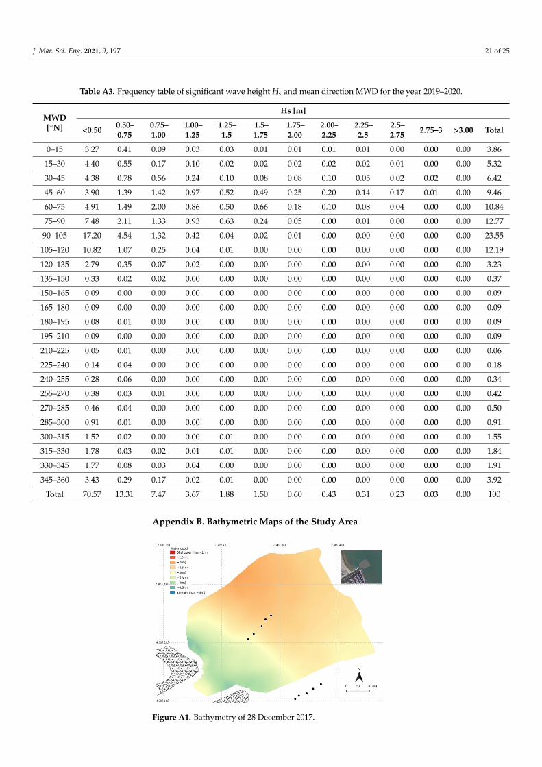
J. Mar. Sci. Eng. 2021, 9, 197 21 of 25

Table A3. Frequency table of significant wave height Hs and mean direction MWD for the year 2019–2020.

MWD[◦N]

Hs [m]

<0.50 0.50–0.75

0.75–1.00

1.00–1.25

1.25–1.5

1.5–1.75

1.75–2.00

2.00–2.25

2.25–2.5

2.5–2.75 2.75–3 >3.00 Total

0–15 3.27 0.41 0.09 0.03 0.03 0.01 0.01 0.01 0.01 0.00 0.00 0.00 3.86

15–30 4.40 0.55 0.17 0.10 0.02 0.02 0.02 0.02 0.02 0.01 0.00 0.00 5.32

30–45 4.38 0.78 0.56 0.24 0.10 0.08 0.08 0.10 0.05 0.02 0.02 0.00 6.42

45–60 3.90 1.39 1.42 0.97 0.52 0.49 0.25 0.20 0.14 0.17 0.01 0.00 9.46

60–75 4.91 1.49 2.00 0.86 0.50 0.66 0.18 0.10 0.08 0.04 0.00 0.00 10.84

75–90 7.48 2.11 1.33 0.93 0.63 0.24 0.05 0.00 0.01 0.00 0.00 0.00 12.77

90–105 17.20 4.54 1.32 0.42 0.04 0.02 0.01 0.00 0.00 0.00 0.00 0.00 23.55

105–120 10.82 1.07 0.25 0.04 0.01 0.00 0.00 0.00 0.00 0.00 0.00 0.00 12.19

120–135 2.79 0.35 0.07 0.02 0.00 0.00 0.00 0.00 0.00 0.00 0.00 0.00 3.23

135–150 0.33 0.02 0.02 0.00 0.00 0.00 0.00 0.00 0.00 0.00 0.00 0.00 0.37

150–165 0.09 0.00 0.00 0.00 0.00 0.00 0.00 0.00 0.00 0.00 0.00 0.00 0.09

165–180 0.09 0.00 0.00 0.00 0.00 0.00 0.00 0.00 0.00 0.00 0.00 0.00 0.09

180–195 0.08 0.01 0.00 0.00 0.00 0.00 0.00 0.00 0.00 0.00 0.00 0.00 0.09

195–210 0.09 0.00 0.00 0.00 0.00 0.00 0.00 0.00 0.00 0.00 0.00 0.00 0.09

210–225 0.05 0.01 0.00 0.00 0.00 0.00 0.00 0.00 0.00 0.00 0.00 0.00 0.06

225–240 0.14 0.04 0.00 0.00 0.00 0.00 0.00 0.00 0.00 0.00 0.00 0.00 0.18

240–255 0.28 0.06 0.00 0.00 0.00 0.00 0.00 0.00 0.00 0.00 0.00 0.00 0.34

255–270 0.38 0.03 0.01 0.00 0.00 0.00 0.00 0.00 0.00 0.00 0.00 0.00 0.42

270–285 0.46 0.04 0.00 0.00 0.00 0.00 0.00 0.00 0.00 0.00 0.00 0.00 0.50

285–300 0.91 0.01 0.00 0.00 0.00 0.00 0.00 0.00 0.00 0.00 0.00 0.00 0.91

300–315 1.52 0.02 0.00 0.00 0.01 0.00 0.00 0.00 0.00 0.00 0.00 0.00 1.55

315–330 1.78 0.03 0.02 0.01 0.01 0.00 0.00 0.00 0.00 0.00 0.00 0.00 1.84

330–345 1.77 0.08 0.03 0.04 0.00 0.00 0.00 0.00 0.00 0.00 0.00 0.00 1.91

345–360 3.43 0.29 0.17 0.02 0.01 0.00 0.00 0.00 0.00 0.00 0.00 0.00 3.92

Total 70.57 13.31 7.47 3.67 1.88 1.50 0.60 0.43 0.31 0.23 0.03 0.00 100

Appendix B. Bathymetric Maps of the Study Area

J. Mar. Sci. Eng. 2021, 9, x 22 of 26

300–315 1.93 0.06 0.00 0.00 0.01 0.02 0.01 0.02 0.01 0.01 0.00 0.00 2.06 315–330 1.81 0.08 0.02 0.00 0.01 0.02 0.03 0.05 0.01 0.00 0.01 0.00 2.03 330–345 2.00 0.08 0.01 0.00 0.03 0.01 0.04 0.03 0.01 0.00 0.01 0.00 2.21 345–360 2.95 0.16 0.10 0.05 0.03 0.05 0.05 0.05 0.02 0.01 0.00 0.00 3.47

Total 70.22 11.49 6.90 4.28 3.06 1.64 1.06 0.72 0.34 0.22 0.08 0.00 100

Table A3. Frequency table of significant wave height Hs and mean direction MWD for the year 2019–2020.

MWD [°N] Hs [m]

<0.50 0.50–0.75 0.75–1.00 1.00–1.25 1.25–1.5 1.5–1.75 1.75–2.00 2.00–2.25 2.25–2.5 2.5–2.75 2.75–3 >3.00 Total 0–15 3.27 0.41 0.09 0.03 0.03 0.01 0.01 0.01 0.01 0.00 0.00 0.00 3.86 15–30 4.40 0.55 0.17 0.10 0.02 0.02 0.02 0.02 0.02 0.01 0.00 0.00 5.32 30–45 4.38 0.78 0.56 0.24 0.10 0.08 0.08 0.10 0.05 0.02 0.02 0.00 6.42 45–60 3.90 1.39 1.42 0.97 0.52 0.49 0.25 0.20 0.14 0.17 0.01 0.00 9.46 60–75 4.91 1.49 2.00 0.86 0.50 0.66 0.18 0.10 0.08 0.04 0.00 0.00 10.84 75–90 7.48 2.11 1.33 0.93 0.63 0.24 0.05 0.00 0.01 0.00 0.00 0.00 12.77

90–105 17.20 4.54 1.32 0.42 0.04 0.02 0.01 0.00 0.00 0.00 0.00 0.00 23.55 105–120 10.82 1.07 0.25 0.04 0.01 0.00 0.00 0.00 0.00 0.00 0.00 0.00 12.19 120–135 2.79 0.35 0.07 0.02 0.00 0.00 0.00 0.00 0.00 0.00 0.00 0.00 3.23 135–150 0.33 0.02 0.02 0.00 0.00 0.00 0.00 0.00 0.00 0.00 0.00 0.00 0.37 150–165 0.09 0.00 0.00 0.00 0.00 0.00 0.00 0.00 0.00 0.00 0.00 0.00 0.09 165–180 0.09 0.00 0.00 0.00 0.00 0.00 0.00 0.00 0.00 0.00 0.00 0.00 0.09 180–195 0.08 0.01 0.00 0.00 0.00 0.00 0.00 0.00 0.00 0.00 0.00 0.00 0.09 195–210 0.09 0.00 0.00 0.00 0.00 0.00 0.00 0.00 0.00 0.00 0.00 0.00 0.09 210–225 0.05 0.01 0.00 0.00 0.00 0.00 0.00 0.00 0.00 0.00 0.00 0.00 0.06 225–240 0.14 0.04 0.00 0.00 0.00 0.00 0.00 0.00 0.00 0.00 0.00 0.00 0.18 240–255 0.28 0.06 0.00 0.00 0.00 0.00 0.00 0.00 0.00 0.00 0.00 0.00 0.34 255–270 0.38 0.03 0.01 0.00 0.00 0.00 0.00 0.00 0.00 0.00 0.00 0.00 0.42 270–285 0.46 0.04 0.00 0.00 0.00 0.00 0.00 0.00 0.00 0.00 0.00 0.00 0.50 285–300 0.91 0.01 0.00 0.00 0.00 0.00 0.00 0.00 0.00 0.00 0.00 0.00 0.91 300–315 1.52 0.02 0.00 0.00 0.01 0.00 0.00 0.00 0.00 0.00 0.00 0.00 1.55 315–330 1.78 0.03 0.02 0.01 0.01 0.00 0.00 0.00 0.00 0.00 0.00 0.00 1.84 330–345 1.77 0.08 0.03 0.04 0.00 0.00 0.00 0.00 0.00 0.00 0.00 0.00 1.91 345–360 3.43 0.29 0.17 0.02 0.01 0.00 0.00 0.00 0.00 0.00 0.00 0.00 3.92

Total 70.57 13.31 7.47 3.67 1.88 1.50 0.60 0.43 0.31 0.23 0.03 0.00 100

Appendix B. Bathymetric Maps of the Study Area

Figure A1. Bathymetry of 28 December 2017.

Figure A1. Bathymetry of 28 December 2017.

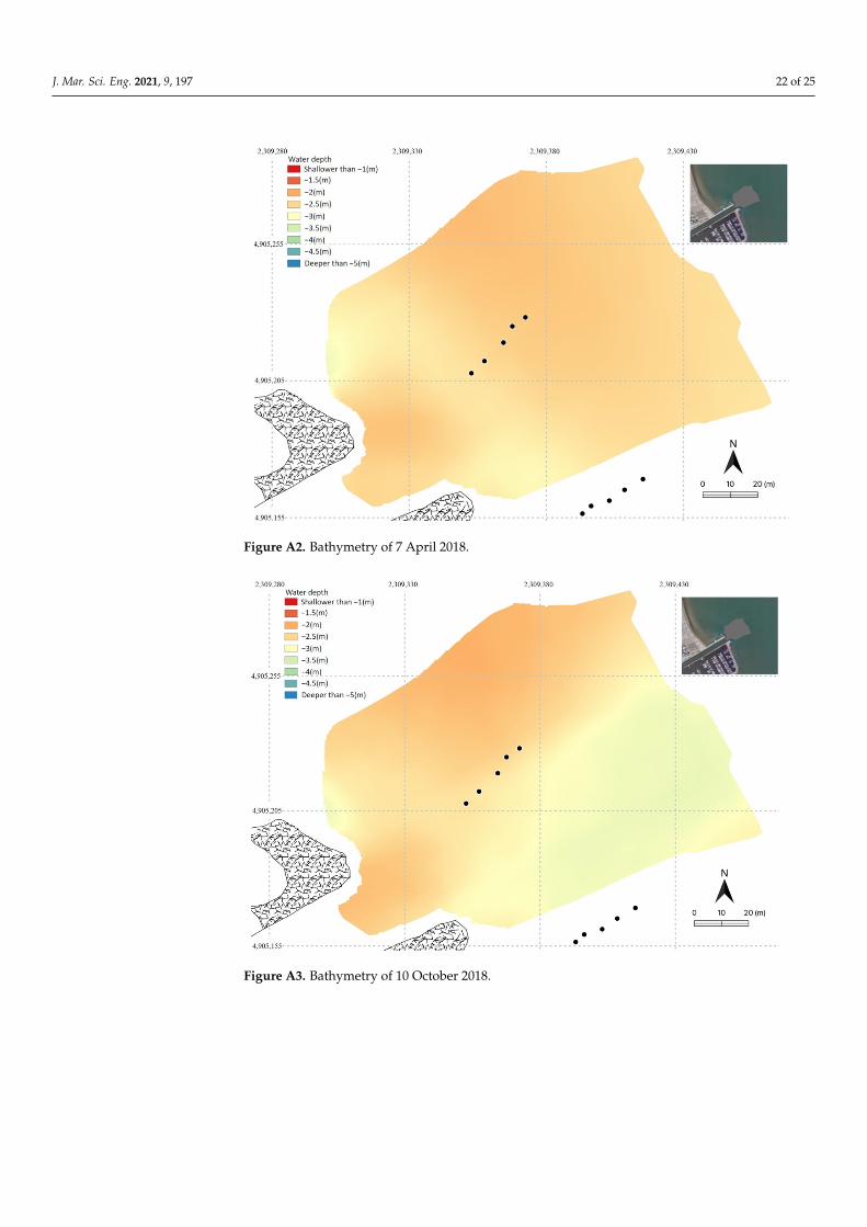
J. Mar. Sci. Eng. 2021, 9, 197 22 of 25J. Mar. Sci. Eng. 2021, 9, x 23 of 26

Figure A2. Bathymetry of 7 April 2018.

Figure A3. Bathymetry of 10 October 2018.

Figure A2. Bathymetry of 7 April 2018.

J. Mar. Sci. Eng. 2021, 9, x 23 of 26

Figure A2. Bathymetry of 7 April 2018.

Figure A3. Bathymetry of 10 October 2018. Figure A3. Bathymetry of 10 October 2018.

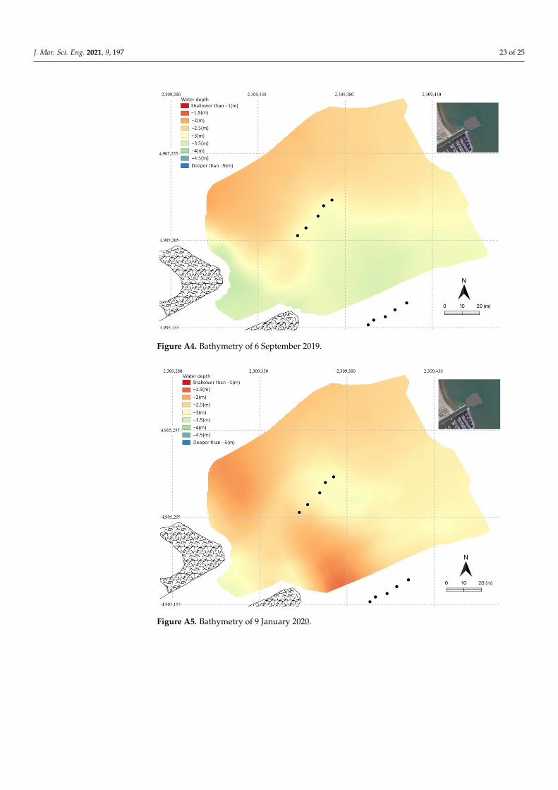
J. Mar. Sci. Eng. 2021, 9, 197 23 of 25J. Mar. Sci. Eng. 2021, 9, x 24 of 26

Figure A4. Bathymetry of 6 September 2019.

Figure A5. Bathymetry of 9 January 2020.

Figure A4. Bathymetry of 6 September 2019.

J. Mar. Sci. Eng. 2021, 9, x 24 of 26

Figure A4. Bathymetry of 6 September 2019.

Figure A5. Bathymetry of 9 January 2020. Figure A5. Bathymetry of 9 January 2020.

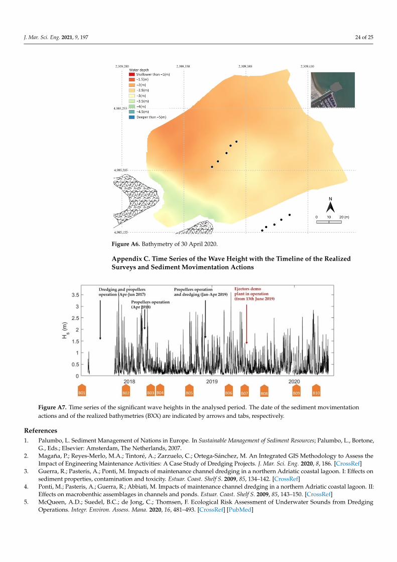
J. Mar. Sci. Eng. 2021, 9, 197 24 of 25J. Mar. Sci. Eng. 2021, 9, x 25 of 26

Figure A6. Bathymetry of 30 April 2020.

Appendix C. Time Series of the Wave Height with the Timeline of the Realized Surveys and Sediment Movimentation Actions

Figure A7. Time series of the significant wave heights in the analysed period. The date of the sedi-ment movimentation actions and of the realized bathymetries (BXX) are indicated by arrows and tabs, respectively.

References 1. Palumbo, L. Sediment Management of Nations in Europe. In Sustainable Management of Sediment Resources; Palumbo, L., Bortone,

G., Eds.; Elsevier: Amsterdam, The Netherlands, 2007. 2. Magaña, P.; Reyes-Merlo, M.A.; Tintoré, A.; Zarzuelo, C.; Ortega-Sánchez, M. An Integrated GIS Methodology to Assess the

Impact of Engineering Maintenance Activities: A Case Study of Dredging Projects. J. Mar. Sci. Eng. 2020, 8, 186. 3. Guerra, R.; Pasteris, A.; Ponti, M. Impacts of maintenance channel dredging in a northern Adriatic coastal lagoon. I: Effects on

sediment properties, contamination and toxicity. Estuar. Coast. Shelf S. 2009, 85, 134–142. 4. Ponti, M.; Pasteris, A.; Guerra, R.; Abbiati, M. Impacts of maintenance channel dredging in a northern Adriatic coastal lagoon.

II: Effects on macrobenthic assemblages in channels and ponds. Estuar. Coast. Shelf S. 2009, 85, 143–150. 5. McQueen, A.D.; Suedel, B.C.; de Jong, C.; Thomsen, F. Ecological Risk Assessment of Underwater Sounds from Dredging Op-

erations. Integr. Environ. Assess. Mana. 2020, 16, 481–493.

Figure A6. Bathymetry of 30 April 2020.

Appendix C. Time Series of the Wave Height with the Timeline of the RealizedSurveys and Sediment Movimentation Actions

J. Mar. Sci. Eng. 2021, 9, x 25 of 26

Figure A6. Bathymetry of 30 April 2020.

Appendix C. Time Series of the Wave Height with the Timeline of the Realized Surveys and Sediment Movimentation Actions

Figure A7. Time series of the significant wave heights in the analysed period. The date of the sedi-ment movimentation actions and of the realized bathymetries (BXX) are indicated by arrows and tabs, respectively.

References 1. Palumbo, L. Sediment Management of Nations in Europe. In Sustainable Management of Sediment Resources; Palumbo, L., Bortone,

G., Eds.; Elsevier: Amsterdam, The Netherlands, 2007. 2. Magaña, P.; Reyes-Merlo, M.A.; Tintoré, A.; Zarzuelo, C.; Ortega-Sánchez, M. An Integrated GIS Methodology to Assess the

Impact of Engineering Maintenance Activities: A Case Study of Dredging Projects. J. Mar. Sci. Eng. 2020, 8, 186. 3. Guerra, R.; Pasteris, A.; Ponti, M. Impacts of maintenance channel dredging in a northern Adriatic coastal lagoon. I: Effects on

sediment properties, contamination and toxicity. Estuar. Coast. Shelf S. 2009, 85, 134–142. 4. Ponti, M.; Pasteris, A.; Guerra, R.; Abbiati, M. Impacts of maintenance channel dredging in a northern Adriatic coastal lagoon.

II: Effects on macrobenthic assemblages in channels and ponds. Estuar. Coast. Shelf S. 2009, 85, 143–150. 5. McQueen, A.D.; Suedel, B.C.; de Jong, C.; Thomsen, F. Ecological Risk Assessment of Underwater Sounds from Dredging Op-

erations. Integr. Environ. Assess. Mana. 2020, 16, 481–493.

Figure A7. Time series of the significant wave heights in the analysed period. The date of the sediment movimentationactions and of the realized bathymetries (BXX) are indicated by arrows and tabs, respectively.

References1. Palumbo, L. Sediment Management of Nations in Europe. In Sustainable Management of Sediment Resources; Palumbo, L., Bortone,

G., Eds.; Elsevier: Amsterdam, The Netherlands, 2007.2. Magaña, P.; Reyes-Merlo, M.A.; Tintoré, A.; Zarzuelo, C.; Ortega-Sánchez, M. An Integrated GIS Methodology to Assess the

Impact of Engineering Maintenance Activities: A Case Study of Dredging Projects. J. Mar. Sci. Eng. 2020, 8, 186. [CrossRef]3. Guerra, R.; Pasteris, A.; Ponti, M. Impacts of maintenance channel dredging in a northern Adriatic coastal lagoon. I: Effects on

sediment properties, contamination and toxicity. Estuar. Coast. Shelf S. 2009, 85, 134–142. [CrossRef]4. Ponti, M.; Pasteris, A.; Guerra, R.; Abbiati, M. Impacts of maintenance channel dredging in a northern Adriatic coastal lagoon. II:

Effects on macrobenthic assemblages in channels and ponds. Estuar. Coast. Shelf S. 2009, 85, 143–150. [CrossRef]5. McQueen, A.D.; Suedel, B.C.; de Jong, C.; Thomsen, F. Ecological Risk Assessment of Underwater Sounds from Dredging

Operations. Integr. Environ. Assess. Mana. 2020, 16, 481–493. [CrossRef] [PubMed]

J. Mar. Sci. Eng. 2021, 9, 197 25 of 25

6. Memos, C.; Chiavaccini, P.; Dornhelm, R.; Hoekstra, R.; Inglis, P.; Sannasiraj, S.A.; Stoschek, O.; Willemsen, A.; Mink, E.; Sundar,V. Anti-Sedimentation Systems for Marinas and Yacht Harbours; PIANC Report 130; PIANC: Brussels, Belgium, 2015.

7. Bianchini, A.; Cento, F.; Guzzini, A.; Pellegrini, M.; Saccani, C. Sediment management in coastal infrastructures: Techno-economicand environmental impact assessment of alternative technologies to dredging. J. Environ. Manag. 2019, 248, 1–17. [CrossRef][PubMed]

8. Sane, M.; Yamagishi, H.; Tateishi, M.; Yamagishi, T. Environmental impacts of shore-parallel breakwaters along Nagahama andOhgata, District of Joetsu, Japan. J. Environ. Manag. 2007, 82, 399–409. [CrossRef] [PubMed]

9. International Association of Dredging Companies (IADC). Water Injection Dredging, Facts about–An Information Update from theIADC; International Association of Dredging Companies: Voorburg, The Netherlands, 2013.

10. Spencer, K.L.; Dewhurst, R.E.; Penna, P. Potential impacts of water injection dredging on water quality and ecotoxicity inLimehouse Basin, River Thames, SE England, UK. Chemosphere 2006, 63, 509–521. [CrossRef] [PubMed]

11. Pledger, A.G.; Brewin, P.; Mathers, K.L.; Phillips, J.; Wood, P.J.; Yu, D. The effects of water injection dredging on low-salinityestuarine ecosystems: Implications for fish and macroinvertebrate communities. Ecol. Indic. 2021, 122, 107244. [CrossRef]

12. Archetti, R.; Damiani, L.; Bianchini, A.; Romagnoli, C.; Abbiati, M.; Addona, F.; Airoldi, L.; Cantelli, L.; Gaeta, M.G.; Guerrero,M.; et al. Innovative strategies, monitoring and analysis of the coastal erosion risk: The STIMARE Project. In Proceedings of theTwenty-Nineth International Ocean and Polar Engineering Conference, Honolulu, HI, USA, 16–21 June 2019.

13. Bianchini, A.; Guzzini, A.; Pellegrini, M.; Saccani, C.; Gaeta, M.G.; Archetti, R. Coastal erosion mitigation through ejector devicesapplication. Ital. J. Eng. Geol. Environ. 2020, 1, 13–22.

14. Pellegrini, M.; Abbiati, M.; Bianchini, A.; Colangelo, M.A.; Guzzini, A.; Mikac, B.; Ponti, M.; Preda, G.; Saccani, C.; Willemsen,A. Sustainable sediment management in coastal infrastructures through an innovative technology: Preliminary results of themarinaplan plus life project. J. Soil. Sediment. 2020, 20, 2685–2696. [CrossRef]

15. Bianchini, A.; Pellegrini, M.; Saccani, C. Zero environmental impact plant for seabed maintenance. In Proceedings of the 4thInternational Symposium on Sediment Management (I2SM), Ferrara, Italy, 17–19 September 2014.

16. Pellegrini, M.; Saccani, C. Laboratory and field tests on photo-electric probes and ultrasonic Doppler flow switch for remotecontrol of turbidity and flowrate of a water-sand mixture flow. J. Phys. Conf. Ser. 2017, 882, 012008. [CrossRef]

17. Pellegrini, M.; Preda, G.; Saccani, C. Application of an Innovative Jet Pump System for the Sediment Management in a PortChannel: Techno-Economic Assessment based on Experimental Measurements. J. Mar. Sci. Eng. 2020, 8, 686. [CrossRef]

18. Bonaldo, D.; Antonioli, F.; Archetti, R.; Bezzi, A.; Correggiari, A.; Davolio, S.; De Falco, G.; Fantini, M.; Fontolan, G.; Furlani,S.; et al. Integrating multidisciplinary instruments for assessing coastal vulnerability to erosion and sea level rise: Lessons andchallenges from the Adriatic Sea, Italy. Coast. Conserv. 2019, 23, 19–37. [CrossRef]

19. Archetti, R.; Paci, A.; Carniel, S.; Bonaldo, D. Optimal index related to the shoreline dynamics during a storm: The case of Jesolobeach. Nat. Hazards Earth Syst. Sci. 2016, 16, 1107–1122. [CrossRef]

20. Gaeta, M.G.; Bonaldo, D.; Samaras, A.G.; Archetti, R.; Carniel, S. Coupled wave-2D hydrodynamics modeling at the Reno rivermouth (Italy) under climate change scenarios. Water 2019, 10, 1380. [CrossRef]

21. Gaeta, M.G.; Samaras, A.G.; Federico, I.; Archetti, R.; Maicu, F.; Lorenzetti, G. A coupled wave-3-D hydrodynamics model of theTaranto Sea (Italy): A multiple-nesting approach. Nat. Hazards Earth Syst. Sci. 2016, 16, 2071–2083. [CrossRef]

22. Samaras, A.G.; Gaeta, M.G.; Moreno Miquel, A.; Archetti, R. High-resolution wave and hydrodynamics modelling in coastalareas: Operational applications for coastal planning, decision support and assessment. Nat. Hazards Earth Syst. Sci. 2016, 16,1499–1518. [CrossRef]

23. Loza, P. Sand Bypassing Systems. Master Thesis in Environmental Engineering. Master′s Thesis, University of Porto, Porto,Portugal, June 2008.

24. Aguzzi, M.; Bonsignore, F.; De Nigris, N.; Morelli, M.; Paccagnella, T.; Romagnoli, C.; Unguendoli, S. Stato del Litorale Emiliano-Romagnolo al 2012-Erosione e Interventi di difesa; Arpae Emilia-Romagna: Bologna, Italy, 2016.

25. Poulain, P.M.; Kourafalou, V.H.; Cushman-Roisin, B. Northern Adriatic Sea. In Physical Oceanography of the Adriatic Sea Past,Present and Future; Cushman-Roisin, B., Gacic, M., Poulain, P.M., Artegiani, A., Eds.; Kluwer Academic Publishers: Dordrecht,The Netherlands, 2001.

26. Lionello, P.; Cavaleri, L.; Nissen, K.M.; Pino, C.; Raicich, F.; Ulbrich, U. Severe marine storms in the Northern Adriatic:Characteristics and trends. Phys. Chem. Earth Parts A/B/C 2012, 40–41, 93–105. [CrossRef]

27. Perini, L.; Calabrese, L.; Luciani, P.; Olivieri, M.; Galassi, G.; Spada, G. Sea-level rise along the Emilia-Romagna coast (NorthernItaly) in 2100: Scenarios and impacts. Nat. Hazards Earth Syst. Sci. 2017, 17, 2271–2287. [CrossRef]

28. ARPAE. Available online: https://www.arpae.it/sim/?mare/boa (accessed on 27 December 2020).29. Perini, L.; Calabrese, L.; Deserti, M.; Valentini, A.; Ciavola, P.; Armaroli, C. Le Mareggiate e gli Impatti Sulla Costa in Emilia-Romagna

1946–2010. I Quaderni di ARPA 2011; ARPAE: Bologna, Italy, 2011.30. Armaroli, C.; Ciavola, P.; Perini, L.; Calabrese, L.; Lorito, S.; Valentini, A.; Masina, M. Critical storm thresholds for significant

morphological changes and damage along the Emilia-Romagna coastline, Italy. Geomorphology 2012, 143–144, 34–51. [CrossRef]31. Dolan, R.; Davis, R.E. An intensity scale for Atlantic coast northeast storms. J. Coast. Res. 1992, 8, 352–364.32. Mendoza, E.; Jiménez, J. Storm-Induced Beach Erosion Potential on the Catalonian Coast. J. Coast. Res. 2004, 48, 81–88.