1

Effect of Head Shape Variations among

Individuals on the EEG/MEG Forward and

Inverse ProblemsNicolas von Ellenrieder, Carlos H. Muravchik, Arye Nehorai and Michael Wagner

Abstract

We study the effect of the head shape variations on the EEG/MEG forward and inverse problems.

We build a random head model such that each sample represents the head shape of a different individual,

and solve the forward problem assuming this random head model, using a Polynomial Chaos Expansion.

The random solution of the forward problem is used then to quantify the effect of the geometry when

the inverse problem is solved with a standard head model. The results derived with this approach are

valid for a continuous family of head models, rather than just for a set of cases. The random model

consists in three random surfaces that define layers of different electric conductivity, and we built an

example based on a set of 30 deterministic models from adults. Our results show that for a dipolar source

model the effect of the head shape variations on the EEG/MEG inverse problem due to the random head

model is slightly larger than the effect of the electronic noise present in the sensors. The variations in

the EEG inverse problem solutions are due to the variations in the shape of the volume conductor, while

the variations in the MEG inverse problem solutions, larger than the EEG ones, are caused mainly by the

variations of the absolute position of the sources in a coordinate system based on anatomical landmarks,

in which the magnetometers have a fixed position.

Index Terms

EEG/MEG average head model, stochastic modeling, Polynomial Chaos Expansion, Sparse Grids.

I. INTRODUCTION

The electroencephalography (EEG)/magnetoencephalography (MEG) inverse problem corresponds to

estimating the parameters of sources of electromagnetic activity in the brain from measurements of the

electric potential on the scalp and the magnetic field near the head. One of the factors that affects the

2

inverse problem solution is the shape of the head model. We are interested in determining the quality of

inverse problem solutions when the shape of the head is not known.

The effect of the head model geometry on the EEG/MEG forward and inverse problems has been

considered in several studies. The difference in the EEG inverse problem solution when using spherical

or realistically shaped models was studied by many authors [1]–[5]. The effect of variations in the

skull thickness was studied by [6]–[8]. In [9] the effect of random variations in the head shape on the

EEG forward and inverse problems was studied, but the analysis was restricted to variations of a few

millimeters. The mislocalization error when solving the inverse problem with head models from several

different individuals was studied by [10], [11]. These studies analyzed the effect of the model geometry

presenting the results for particular cases of head models. In this work we seek more general results

by adopting a random head model to represent a whole family of models, and solving the EEG/MEG

forward and inverse problems with it.

To study the effect of head shape variations among individuals first we build a random head model

such that each sample represents a possible shape of the head. The model is derived from a set of

observed head shapes from different individuals. In this paper we build a random head model based

on 30 deterministic head models from adult individuals, and solve the EEG/MEG forward problem with

this model. In addition, we define an average or standard head model as the expectation of the random

one, and use it in the solution of the EEG/MEG inverse problem.

With the random head model, the forward problem solution is also of random nature. We find the

coefficients of a Polynomial Chaos Expansion [12], [13] of the forward problem solution. Such an

expansion allows for an easy computation of the statistical moments of the solution, and hence of the

variations induced in the forward problem solution by the randomness of the head model. A similar

analysis could also be accomplished with Monte Carlo simulations (MCS). However, given the high

dimensionality of the problem, it would be computationally expensive. In fact, we compare the results

of our method with a MCS for a reduced size problem. The method we describe in this paper reaches

results with similar first and second order moments than MCS, with a lower computational load.

To determine the effect of the random geometry on the EEG/MEG inverse problem, we assume only

the average head model is known, and compute the error in the estimation of position parameters of a

dipolar source. The idea is to find the source parameters that, when used for solving the forward problem

with the average head shape, minimize the difference with the forward problem solution obtained with

samples of the random head model. In this way, through Monte Carlo Simulations, we obtain a statistical

characterization of the mislocalization error due to the randomness of the head model.

3

II. HEAD MODEL

In this section we propose a random model for the head shape, such that each sample of the model

corresponds to a head shape from a different individual. We adopt a head model with three nested layers

of constant electric conductivity representing the brain, skull and scalp tissues. The model is defined

then by the three interfaces between the layers. We describe these surfaces by their radius (distance to

the origin) as a function of the azimuth and elevation, with respect to a suitable coordinate system. The

random head model then consists of three random surfaces S1, S2 and S3, describing the interfaces

between tissues.

We present in this section a procedure to obtain the random surfaces Sq as a Karhunen–Loeve series

expansion truncated to a finite number Nc of terms

Sq = Sq0 +

Nc∑

i=1

χiSqi , q = 1, 2, 3, (1)

where Sq0 is a mean or standard surface, and χi are uncorrelated random variables with zero mean and unit

variance. If a Gaussian joint distribution is assumed χ=[χ1, χ2, . . . χNc]T∼N (0, I), then Sq

i may be seen

as the independent surface components of the random surface Sq. Note that since the Karhunen–Loeve

series expansion is assumed convergent, the surface components Sqi will tend to be smaller for higher

order terms. The size of these surface components will determine the appropriate number of terms Nc.

The procedure used to build the random head model is based on the work of [10], modified to obtain an

average head model and combine the individual models into an unique random one. We start from a set of

observed head models corresponding to NI different individuals. First we align the models; the y direction

is given by the line joining the left and right preauricular points, defining segment ab. The z direction is

normal to the plane defined by segment ab and the nasion, with positive values towards the top of the

head. The origin of the coordinate system is roughly in the center of the brain, at a point 50mm above

the intersection between segment ab and a line normal to this segment passing through the nasion.

The observed head models used to build the random model may differ in their lower sections e.g. if

the neck was included on the model. These differences are not related to the anatomical variations we

want to study. Hence, we replaced the lower part of the head model, i.e. elevations under −45◦, by the

average of the NI models. A linear transition of the actual head to the average shape between −25◦

and −45◦ was adopted.

Let Rqj , j=1, . . . NI be the the interfaces between tissues of different electric conductivities of the

observed head models, and let us assume that only a set of points of these surfaces are known, e.g. from

a segmentation of a magnetic resonance image.

4

Next a description is found of each brain-skull interface R1j based on spherical harmonics

R1j =

{x(ϕ, θ, r) : r =

NA∑

l=0

l∑

m=−l

ajlmYlm(ϕ, θ)

}, (2)

where (ϕ, θ, r) are the azimuth, elevation and distance to the origin. The functions Ylm are the spherical

harmonics [14]. NA is the order of the decomposition and determines the number of terms, equal

to (NA+1)2. The coefficients ajlm are chosen to minimize the functional

J(ajlm) =

N1j∑

n=1

(rjn −

NA∑

l=0

l∑

m=−l

ajlmYlm(ϕj

n, θjn)

)2

. (3)

where the points xjn = (ϕj

n, θjn, rj

n), n=1, . . . N1j are the sets of known points of the surfaces R1j ,

j=1, . . . NI .

Repeating this procedure we find the coefficients bjlm and cj

lm of the spherical harmonics decomposition

of the skull–scalp R2j and scalp–air R3

j interfaces. Then for each observed model we form a vector

with the coefficients of the different interfaces, dj=[aj00, . . . , aj

NANA, bj

00, . . . , bjNANA

, cj00, . . . , c

jNANA

]T .

Next we compute the mean value d of the coefficients among the different individuals to obtain the

standard surfaces Sq0 , q=1, 2, 3. We arrange the variations of the coefficients dj−d in a matrix A of

size 3(NA+1)2×NI . Each column j of the matrix A contains the coefficients of the spherical harmonics

decomposition of the surfaces Rqj . A singular values decomposition of matrix A yields

A = UDV T , (4)

where D is a diagonal matrix formed by the singular values of matrix A. Note that there are NI−1

non-zero singular values, since the rows of A have zero mean value. We define then the matrices B =

UD−/√

NI , W =√

NIV−T , so that A = BW , where D− and V − are formed by the NI−1 columns

of D and V associated with non-zero singular values. The size of matrix B is then 3(NA+1)2×(NI−1),

and the size of matrix W is (NI−1) × NI . The j-th column of B can be interpreted as the spherical

harmonics decomposition coefficients of surfaces Sqi , q = 1, 2, 3, that can be combined to represent the

original surfaces. The surfaces Sqi are obtained then replacing the aj

lm coefficients in (2) by the elements

in the corresponding column of B. Matrix W is a weight matrix that indicates how to combine the

surfaces Sqi to get the original surfaces Rq

j . The columns of B corresponding to the largest singular values

have more importance in the description of the surfaces, and it is possible to obtain good reconstructions

of the surfaces Rqj with a reduced number Nc of surfaces components Sq

i as will be seen later. We have

then

Rqj ≈ Sq

0 +Nc∑

i=1

Sqi wij , q = 1, 2, 3, (5)

5

where wij are the elements of W . By assuming that these coefficients are samples of uncorrelated

random variables χi we get the proposed expansion (1) of the the random surfaces Sq. This algorithm

produces coefficients wij that could come from uncorrelated random variables χi with zero mean and unit

variance, which we will group in a random vector χ. Assuming the samples also come from a normal

distribution χ∼N (0, I), the procedure is similar to an independent components decomposition of the

random surface Sq, and Sqi are the independent surface components. The choice of a normal distribution

(or any other distribution with probability density function with infinite support) is questionable because

it will lead to a non-zero possibility of models in which the interfaces intersect each other, which is

physically impossible. We expect that this probability will be small since the surface components are

derived from real head models. If an intersection between surfaces is found, an ad-hoc local modification

of the surfaces would be applied to avoid it.

The surfaces Sq0 , q=1, 2, 3, represent the average of all the subjects under consideration. These surfaces

define what we will refer to as standard head model, and we will use it later for solving the inverse

problem when the true shape of the head is unknown. The electrode positions in this average model are

obtained by projecting the average position of the electrodes on the outer surface.

We also built the random head model using local expansions for defining the surface components, i.e.

with spline interpolation [15, e.g.], instead of spherical harmonics. The resulting shape of the surface

components was essentially the same, especially for the first and most important surface components.

A. Example of a random head model

With the described procedure we obtained a random model for the shape of the head based on NI=30

different adult individuals. The Curry software (Compumedics Neuroscan, Charlotte, NC, USA) was

used to load each individual’s three-dimensional T1–weighted structural MRI scan and to automatically

segment the shape of the outer skin, outer skull, and inner skull surfaces [16]. Each surface was then

represented by Np ≈ 2000 equally distributed points [17]. The spherical harmonics expansion was

of order NA=19, giving a total of 400 coefficients for each surface. Extreme care should be taken

while working with high order spherical harmonics due to numerical instabilities [18]. If the order

of the expansion is too high overfitting to the points xjn could occur, increasing the overall error of

the approximation. With our choice of NA = 19, the difference between the true surfaces and their

expansions has a Root Mean Square (RMS) value under half a millimeter, with

RMS =

√√√√ 1Np

Np∑

n=1

(rn − rn)2, (6)

6

where rn is the distance to the origin of the points xn, and rn the distance to the origin of the point in

the approximated surfaces with the same azimuth and elevation angles than xn.

An average surface and NI−1=29 independent surface components were obtained for each head model

surface. To test the Normal distribution of the random coefficients χi we performed a Kolmogorov–

Smirnov test on the coefficients wij in (5). We performed the test for each of the 29 coefficients (i =

1, . . . 29), with sample size 30 (j = 1, . . . 30), at 5% significance level, and found no evidence (p>.35)

for rejecting a normal distribution, except for the smallest surface component χ29 (p=.005). Since this

last coefficient is associated to a surface component with a maximum radius smaller than 1mm we regard

this non–Gaussian behavior as negligible.

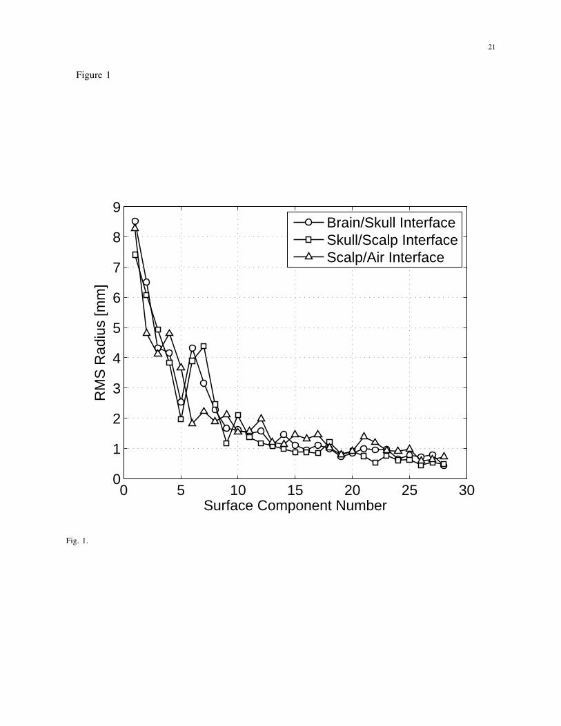
In Fig. 1 we show the RMS value of the radius of the different surface components. The figure shows

that only a few components have an important contribution to the overall shape, supporting the idea that

a reasonable approximation is possible with a limited number of surface components.

Next we want to determine the extent to which our random model can represent the shape of heads not

used in its construction and the number of surface components needed to attain a good approximation.

We performed a Leave–one–out Cross–Validation analysis [19], determining the difference between the

actual head model of each of the 30 individuals and the best approximation to these models built based

on the independent surface components, constructed by the remaining 29 head models. The error measure

is the RMS error (6) between the surfaces and their approximations at points xjn.

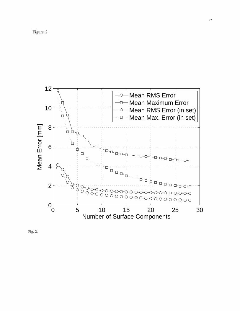
In Fig. 2 we show the RMS and maximum error between the true brain-skull interface and its

reconstructions, for the skull-scalp and scalp-air interfaces the errors are slightly smaller. The figure also

shows in dotted lines the average of the error in the representation of the head models that were used

to build the random model. The figure shows the results as a function of the number Nc of independent

surface components included in the random head model, this number may vary between Nc=1 (average

model and the first surface component) and Nc=NI−1=29. We see in the figure that beyond a certain

number of surface components, the effect of increasing Nc is not very significant. Note that although

the proposed procedure minimizes the RMS error, the maximum error between each surface and its

representation with surface components, also decreases when more surface components are used in the

model. The maximum error has values between 4 and 5mm for a large number (Nc > 16) of surface

components, as seen in the figure.

The figure also shows that for a number of surface components approaching NI − 1, the RMS dotted

line tends to a value under 0.5mm, which is the error of the expansion in spherical harmonics used to

describe the observed models. Since the order of this expansion is finite, details of high spatial frequency

7

are lost in the representation. It is important to note that if the head model differs from the real shape in

the order of one millimeter the effect on the inverse problem solution is not significant, as we showed

in a previous work [9].

The resulting random head model has a mean value of the outer surface radius of 85mm and variations

among individuals of 4mm standard deviation. The mean scalp thickness is 8.6mm with 1.8mm standard

deviation among individuals, and the mean skull thickness of 6.2mm with standard deviation among

individuals below 0.9mm.

B. Source Model

In this work we adopt a dipolar source model. Such a model represents some sources of interest [20]

or may be used to obtain results for distributed sources by convolution.

The coordinates of the source position are given by its azimuth and elevation in the coordinate system

defined at the beginning of this section for the alignment of the head models. The third coordinate is

the depth of the source, measured as the distance between the source and the surface of the brain at the

same azimuth and elevation. This choice of coordinates keeps the source depth constant when the shape

of the head varies. In this way we are certain that the source will always be inside the brain, which

would not be the case if the third coordinate was e.g. the distance from the source to the origin of the

coordinate system. Another possibility for establishing a correspondence among the source positions in the

individual models would be to use anatomically equivalent sources, instead of geometrically equivalent

ones. However, establishing anatomical equivalences among individuals is not a trivial task and it is

beyond the scope of this work.

Note that this specification of the source position relative to the surface of the brain seems favorable for

EEG, since the electrodes position also vary with the shape of the head. For the MEG helmet on the other

hand, the position of the coils is fixed in the absolute coordinate system defined by the fiducial points,

and variations of the shape of the head would change the relative position between the magnetometers

and the source.

III. FORWARD PROBLEM

In this section we show how to solve the EEG and MEG forward problems when the head model has

random geometry. The forward problem solutions will also be random since they depend on the geometry

of the head. We characterize the forward problem solution, validate the proposed method and present

some results for the random head model of section II-A.

8

A. Deterministic Solution

For solving the deterministic forward problem we adopt the Boundary Elements Method (BEM),

with triangular elements and linear variations over the elements [21]. The use of BEM for solving the

EEG/MEG forward problem is widespread [22], [23]; the surfaces are tesselated in small triangular

elements and a linear variation of the electric potential is assumed over each element. The integral

formulation of the forward problem is then reduced to a linear system that must be solved to obtain

the electric potential at the nodes, i.e. at the NN vertices of the elements, and magnetic field at the

sensor positions. To avoid numerical problems due to the low electric conductivity of the skull we use

the Isolated Problem Approach (IPA) [24], which solves the EEG forward problem in two steps, first

considering a null conductivity for the skull, and then modifying the result according to the true value

of the skull conductivity.

We restrict our analysis to one time snapshot, hence the solution of the EEG and MEG forward

problems is given by the vectors φ and υ formed by the electric potential and magnetic field components

in the respective sensors.

Under these conditions the EEG and MEG forward problem solutions are given by

φ = EφS , (7)

υ = MφS + υS (8)

where the linear operators E and M are related to the geometry and electric conductivity of the head

model, the vector φS is the electric potential at the nodes of the innermost surface that would be generated

by the source if the media were homogeneous and infinite, and the vector υS is the measured component

of the magnetic field generated by the primary current density. Note that even though the number of

rows of matrices E and M is equal to the number of electric potential and magnetic field sensors, the

number of operations needed for computing these matrices is proportional to N2N . For a detailed surface

tesselation, with several thousands nodes per surface this represents an important computational load.

B. Random Head Model Solution

To analyze the effect of the head shape variability on the forward problem solution, we must solve the

problem with the random head model presented previously. Since the forward problem solutions depend

on the geometry of the head model, they will also be random. We will denote these random forward

problem solutions as φ(χ) and υ(χ), where χ is the normalized Gaussian random vector used in the

random head model.

9

One possibility would be to use a “brute force” approach, running Monte Carlo Simulations to obtain

statistics of the forward problem solution. The drawback of this approach is the high computational

load it requires; a large number of samples of the random head model is necessary to obtain reliable

statistics, and each sample involves the assembling of the matrices associated to the forward problem

solution. Instead, we perform a Polynomial Chaos Expansion (PCE) [12], [13] of the random vectors

φ(χ) and υ(χ). This enables us to obtain a good approximation of the covariance matrices Cov{φ(χ)},

and Cov{υ(χ)}, which depend on the source parameters and are of uttermost importance in determining

the effect of the random geometry on the inverse problem solutions.

A PCE of any finite variance random variable α is a series expansion

α =∞∑

k=0

αkgk(χ), (9)

where αk are deterministic coefficients, gk(·) are multidimensional Hermite polynomials, and χ∼N (0, I)

is a normal random vector. The multidimensional polynomials gk(·) are obtained as product of one

dimensional ones hk(·). The first one dimensional Hermite polynomials are given by h0(x)=1, h1(x)=x,

h2(x)=x2−1. See e.g. [25] for information on how to obtain higher degree Hermite polynomials. The

degree of the multidimensional polynomial is the sum of the degree in each dimension, thus if χ in (9)

has N elements, there will be N first degree Hermite polynomials, N(N+1)/2 second degree Hermite

polynomials, and so on. We assume the index k grows with the degree of the polynomials, the ordering

among the polynomials of the same degree plays no role and thus is arbitrary. The Hermite polynomials

are orthogonal with respect to the Gaussian measure, and form a basis of the Hilbert space of finite

variance random variables [13], [26], with inner product given by the expectation Eχ{·}. Thus, the

coefficients of the PCE are computed as αk=E{αgk(χ)}.

The PCE is directly extended to a random vector, and thus it can be applied to the EEG forward

problem solution. Then, an approximation to the EEG forward problem solution is given by the first

terms of the PCE

φ(χ) ≈K∑

k=0

φk gk(χ), (10)

where φk are the deterministic vector coefficients which must be found. Once they are known, it is

possible to obtain the first and second order moments of the solution vector; note that since the random

10

variables gk(χ) have zero mean (except g0(χ)=1), the first moments of the solution are given by

E{φ(χ)} = φ0, (11)

E{φ(χ)φT (χ)} =∞∑

k=0

‖ gk ‖2 φkφTk

≈K∑

k=0

‖ gk ‖2 φkφTk , (12)

in this work we use normalized Hermite polynomials so ‖ gk ‖= 1.

The deterministic coefficients of the PCE are given by φk=E{gk(χ)φ(χ)}, k=0, . . . K. These expec-

tations are multidimensional integrals that we evaluate numerically. Then

φk ≈Nev∑

n=1

hngk(χn)φ(χn), (13)

where the proper values for the weights hn and the evaluation points χn are selected according to the

integration algorithm. The domain of integration is infinite hence, the adequate quadrature algorithm is

the Gauss-Hermite quadrature [25]. But a direct extension of a one dimensional quadrature algorithm to a

higher dimensional space is impractical because the number of evaluation points Nev grows exponentially

with the number of dimensions. We use instead a Smolyak or sparse grid algorithm [27]–[29]. A Smolyak

quadrature of order o is a combination of low dimensional quadrature algorithms yielding exact integration

for multidimensional polynomials of total degree up to 2o− 1, and for which the number of evaluation

points grows polynomically with the number of dimensions.

The use of (13) to obtain the PCE coefficients φk requires the computation of Nev forward problem

solutions φ(χn), each one a solution of the deterministic forward problem (7). A PCE of the MEG

forward problem solution can be obtained in the same way.

C. Validation

Next we validate the proposed methods for solving the forward problem when the head model is

random. First we find the right values for parameters involved in the forward problem solution, such as

the number of surface components and the numerical integration order needed to obtain accurate results.

Then we compare the forward problem solution with a Monte Carlo simulation for a small size problem.

We solved the EEG and MEG forward problems for the random head model of the previous section.

Each surface was tesselated in 1280 triangular elements, resulting in a total number of nodes NN=1926.

The assumed electric conductivity for the brain and scalp was 0.33Sm−1 and for the skull 0.022Sm−1.

11

This conductivity ratio of 1/15 is supported by recent studies [30]–[32]. The forward problem was solved

for 69 electrodes and 160 radial magnetometers.

The dipolar sources we adopt in this work are all of 20nAm intensity, with the dipole moment tangential

to the surface of a sphere centered at the origin, and in a plane containing the z-axis. In this section we

analyze the results for 106 dipolar sources regularly distributed on the upper hemisphere of the brain,

at 10mm depth under the brain–skull interface.

First we tested the numerical integration scheme. For this test the number of independent surface

components Nc does not play an important role, so we adopt Nc=4 to speed up the computations,

leading to a number of integration points of Nev=1, 9, 45, 165, 494 and 1278 for integration order o=1

to 6. The results obtained for o=6 were used as the reference. We quantify the error using the Relative

Difference Measure (RDM) [23] given by

RDM =‖ φ

(o)k − φ

(6)k ‖2

‖ φ(6)k ‖2

, (14)

where φ(o)k denotes the k–th coefficient of the PCE, computed with (13) using a numerical integration

order o.

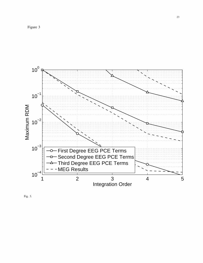
In Fig. 3 we show the error as a function of the integration order o. We plot the maximum RDM

among all the sources and among all the terms of the same degree in the PCE. Full lines are used

for the EEG and broken lines for the MEG forward problems. As expected the error decreases with

the integration order. The error is higher for terms related to higher degree Hermite polynomials in the

PCE (9), because these polynomials appear in the integrand, and the numerical integration algorithm is

exact only for polynomials of total degree up to 2o− 1.

We also computed the contribution of the terms of different degree in the PCE. Table I shows the

RMS value of the forward problem solution, the value corresponds to the mean value among the 106

sources mentioned earlier, and the maximum among the terms of the same degree in the PCE. The EEG

results are measured in µV and the MEG results in fT . It is clear that the contribution of higher degree

terms of the PCE is small compared to the expected value (degree 0) and first degree terms, and could

be neglected.

Next we study the effect of increasing the number of surface components Nc for the random head

model. To quantify the effect of the random head model on the forward problem solution we use the

Signal to Variations Ratio (SVR) defined as the ratio between the norm of the expected value of the

forward problem solution and the energy of the deviations with respect to this value. For a random

12

vector expressed by its PCE (9) the SVR is

SV R =‖ E{φ(χ)} ‖2

2

‖ E{φ(χ)− E{φ(χ)}} ‖22

=‖ φ0 ‖2

2∑Kk=1 ‖ φk ‖2

2

. (15)

Note that while the RDM is used to compare two deterministic vectors, the SVR quantifies the variations

of a random vector and is similar to a Signal to Noise measure, where the “noise” is due to the variations

of the head shape.

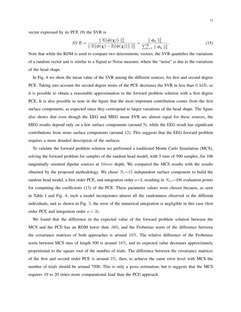
In Fig. 4 we show the mean value of the SVR among the different sources, for first and second degree

PCE. Taking into account the second degree terms of the PCE decreases the SVR in less than 0.3dB, so

it is possible to obtain a reasonable approximation to the forward problem solution with a first degree

PCE. It is also possible to note in the figure that the most important contribution comes from the first

surface components, as expected since they correspond to larger variations of the head shape. The figure

also shows that even though the EEG and MEG mean SVR are almost equal for these sources, the

MEG results depend only on a few surface components (around 5), while the EEG result has significant

contributions from more surface components (around 12). This suggests that the EEG forward problem

requires a more detailed description of the surfaces.

To validate the forward problem solution we performed a traditional Monte Carlo Simulation (MCS),

solving the forward problem for samples of the random head model, with 5 runs of 500 samples, for 106

tangentially oriented dipolar sources at 10mm depth. We compared the MCS results with the results

obtained by the proposed methodology. We chose Nc=15 independent surface component to build the

random head model, a first order PCE, and integration order o=3, resulting in Nev=496 evaluation points

for computing the coefficients (13) of the PCE. These parameter values were chosen because, as seen

in Table I and Fig. 4, such a model incorporates almost all the randomness observed in the different

individuals, and as shown in Fig. 3, the error of the numerical integration is negligible in this case (first

order PCE and integration order o = 3).

We found that the difference in the expected value of the forward problem solution between the

MCS and the PCE has an RDM lower than .005, and the Frobenius norm of the difference between

the covariance matrices of both approaches is around 10%. The relative difference of the Frobenius

norm between MCS runs of length 500 is around 18%, and its expected value decreases approximately

proportional to the square root of the number of trials. The difference between the covariance matrices

of the first and second order PCE is around 5%, then, to achieve the same error level with MCS the

number of trials should be around 7500. This is only a gross estimation, but it suggests that the MCS

requires 10 to 20 times more computational load than the PCE approach.

13

D. Results

For the random head model validated in the previous section (Nc=15, first order PCE, integration

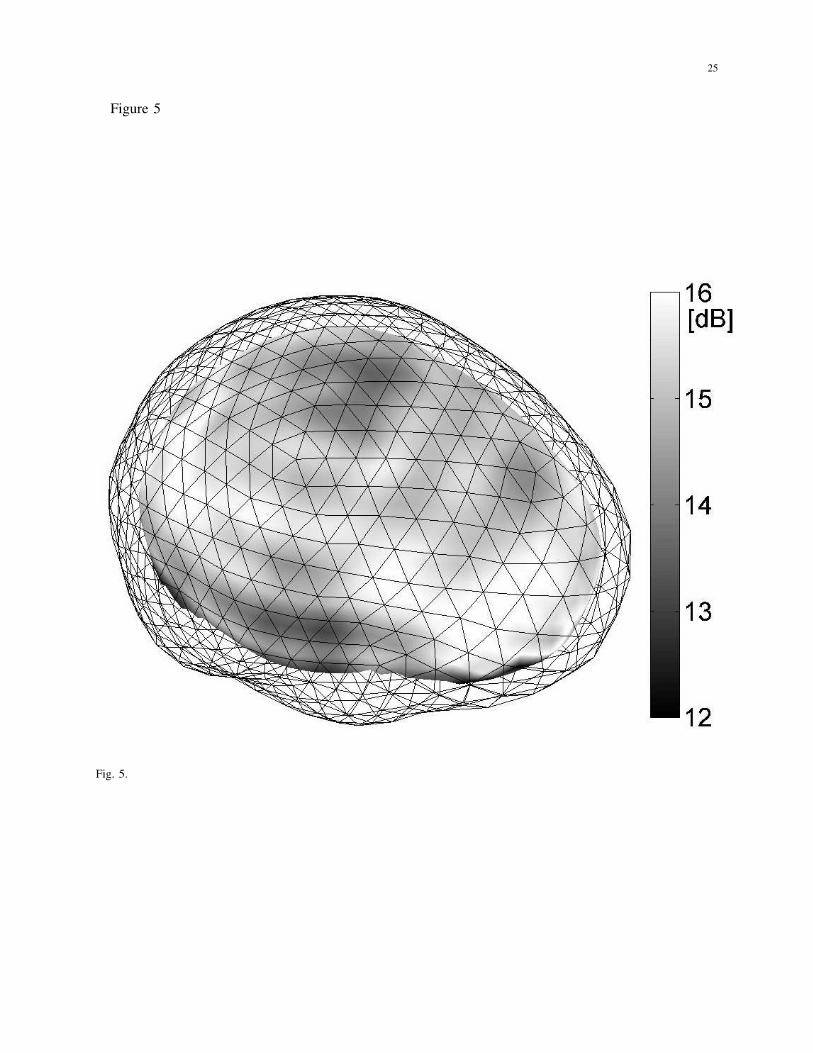
order o=3), we computed the SVR for tangentially oriented dipolar sources at 10mm depth. In Fig. 5 we

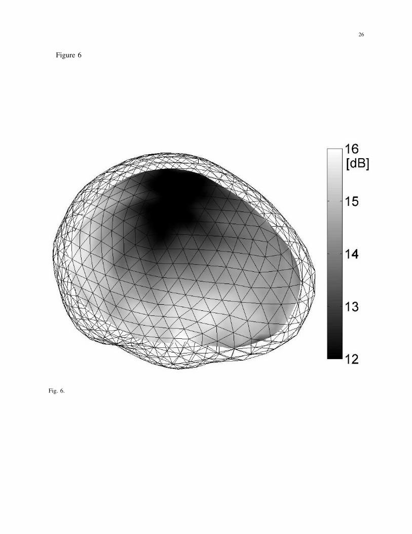
show the SVR of the EEG forward problem solution as a function of the dipole position. Fig. 6 shows

the same results for the MEG forward problem. The figures also show the tesselation of the standard

shape of the brain-scalp interface. We observe that the variations of the SVR with the source position

are in the range of 3dB, for both the EEG and MEG forward problems.

Comparing Fig. 5 and Fig. 6 we see that the effect of the random geometry on the forward problem is

slightly larger for MEG than for EEG, even though for the MEG forward problem this effect is produced

by a lower number of surface components, as seen in Fig. 4. The MEG forward problem solution (8)

is formed by two terms, one related to the volumetric currents and the other due to the primary current

density. We found that the contribution of the second term to the variance of the results is more than four

times larger than the contributions due to the volumetric currents, at least for the tangentially oriented

sources under analysis. This indicates that the main source of variations in the MEG forward problem

result is not due to the variations in the shape of the volume conductor but due to the variations of the

relative position between the source and the magnetometers.

In Table II we show more results, for a dipolar source that we will denote by D1, located on the

left frontal lobe, with azimuth −π/5rad and elevation π/4rad. The source has a tangential orientation,

with dipolar moment (11.4,−8.3,−14.1)nAm, i.e. 20nAm intensity. Later on, we will use source D1 in

other examples. The table shows the SVR, the mean value of the RDM among different samples of the

random forward problem, and the 95% quantile of the RDM among samples, for dipole D1 at 10mm

depth. We also include typical results for additive electronic noise, assuming the standard deterministic

head model, and a Gaussian distribution of the electronic noise, independent between sensors, with a

typical st. dev. of 0.4µV for EEG sensors and 32fT for MEG [33]–[35]. Observe that the noise term

does not include background brain activity. It is also important to note that the results for the electronic

noise depend on the source intensity, while the relative effect of the random head model is independent of

the source intensity. This is so because all the terms in the PCE are proportional to the source intensity,

and as a result the variation of the intensity cancels out in the computation of the SVR or any other

relative error measure. We see that the effect of the random geometry of the head model in the forward

problem solution is smaller than the effect of the electronic noise, but the former is spatially correlated.

Hence, we can draw no conclusions yet regarding the effect on the inverse problem. A deeper analysis

14

is necessary and we perform it in the next section.

IV. INVERSE PROBLEM

In this section we study the effect of the random geometry of the head model in the inverse problem.

We want to determine the error in the estimation of the source position with the standard head model,

when the true geometry is a sample of the random head model. We study the localization error due only

to the random geometry, i.e. when there are no noise sources present.

A. Method

For any dipolar source in the brain we want to obtain a statistical description of the localization error

when the inverse problem is solved with the standard head shape. This statistical description consists

in the first and second order moments, or an approximation to the distribution. An attempt to express

the localization error in any spatial direction with a PCE and to apply the same idea as for solving the

forward problem, showed that a high order PCE is needed. This leads to a large number of evaluation

points for computing the expectations numerically, yielding the procedure impractical.

We resort then to Monte Carlo Simulations, generating the samples of the forward problem solution

from (10). The algorithm is the following, for any given dipolar source: first, compute a sample of

the forward problem solution φm, which we will call the measurement. Then minimize the difference

(L2 norm) between the measurements and the forward problem solution of a dipolar source with the

deterministic standard head model. The parameters of the dipole that achieves this minimization are

the solution of the inverse problem. The minimization algorithm we use is a simple steepest descent

method, where the best fitting dipole moment is computed at every test location. This algorithm performs

adequately in the mentioned conditions, i.e. one dipolar source and no additive noise present.

B. Validation

To validate the proposed methodology for characterizing the inverse problem solution, we solve the

inverse problem for the dipolar source D1 defined above, at a depth of 10mm.

First, we perform a Monte Carlo Simulation; we generate a sample of an independent Normal random

vector χ, and build one sample of the random head model with (1). We solve the forward problem for

that head model, obtaining the vector of electric potential or magnetic field that would be present at

the sensor locations. With this data we solve the inverse problem assuming the standard head model.

15

Repeating this 1000 times we form a vector dMC with the distance between the true source position and

the estimated one in each case.

Then we form a second vector dPC with the distance between true and estimated source positions

when the forward problem solution is given by the PCE. In this case we also start from an independent

Normal random vector χ, and use (10) to obtain the forward problem solution for the corresponding

head shape without actually computing the surfaces of the model. Again we solve the inverse problem

assuming the standard head model, and repeat the procedure 1000 times.

We performed a Kolmogorov–Smirnov test to determine if the samples of dMC and dPC could be

samples from the same random variable. The test, at 1% significance level showed no evidence for

rejecting the null hypothesis that the samples came from the same variable, both for the EEG (p=.012)

and MEG (p=.105) inverse problems.

The results of the test show that a very good approximation of the inverse problem solution is obtained

when solving the forward problem with the proposed procedure. The approximation is good in the sense

that it produces inverse problem solutions, based in the standard head model, that are similar to the results

of a Monte Carlo Simulation.

C. Results

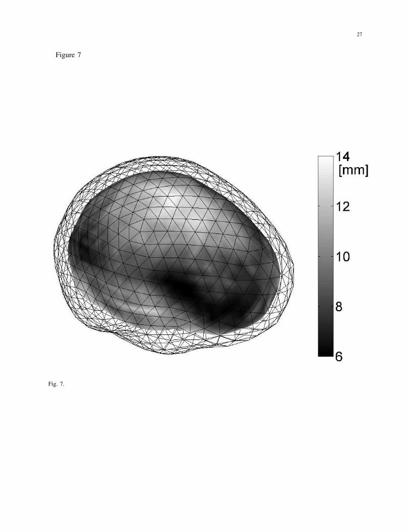
For the random head forward problem solution obtained in the previous section, we computed the

geometric distance between the true dipole positions and the estimated positions when solving the inverse

problem with the standard head model, for tangentially oriented dipolar sources at 10mm depth. We

repeated this for 1000 forward problem samples, and obtained an error measure for the inverse problem

as the 95% quantile of the distance between the real and estimated source positions. Fig. 7 shows the

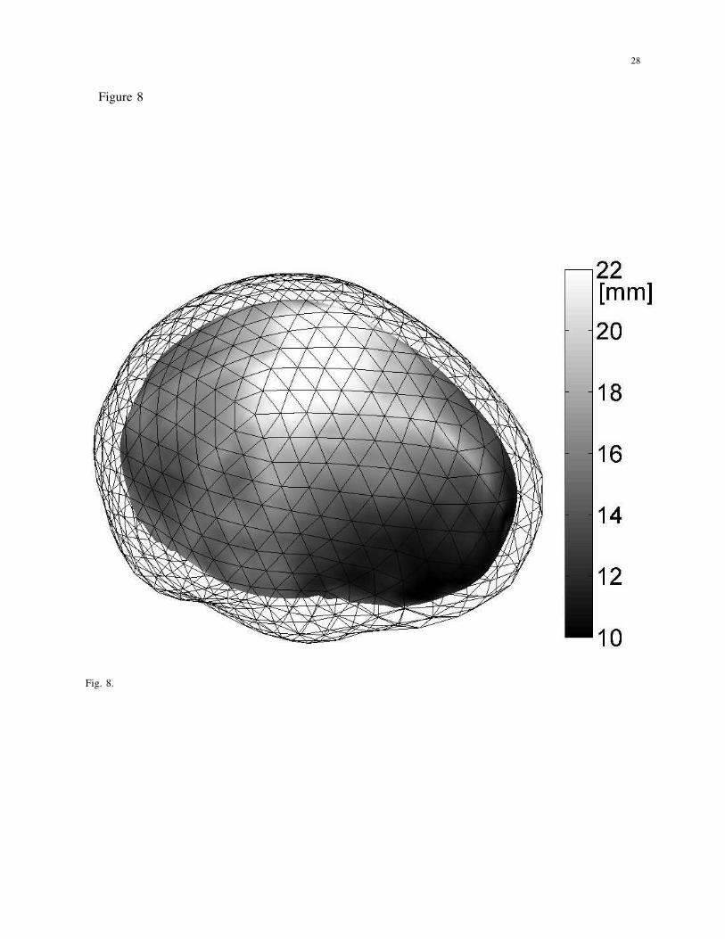
results for the EEG inverse problem solution as a function of the dipole position. Fig. 8 shows the same

results for the MEG inverse problem. We see in the figures that the variations of the localization error for

different positions of the source are around a factor 2 for the EEG and MEG results, as was the case for

the forward problem results. We also observe that the effect of the random head geometry is significantly

larger on the MEG inverse problem than on the EEG inverse problem.

The localization errors as a function of source depth are shown in Fig. 9. The results correspond to

dipole D1 at different depths. We observe that error does not vary very much with depth.

The method described in this paper is also useful when there is partial information regarding the shape

of the head model. To show an example of this we built a different random head model, for which we

assume the outer surface, or scalp-air interface, is known. In this case the random head model is given

16

by two random fields describing not the absolute shape of scalp and skull but rather the scalp and skull

thickness. The head model and forward problem solution are obtained with the methodology described

in the previous sections, and the results are shown for dipole D1 in Fig. 9. It is possible to see a 4–fold

reduction of the error for the MEG results while the EEG results do not vary significantly.

In Table III we show a comparison of localization errors obtained for dipole D1 at 10mm depth.

The table shows the mean value of the localization error, its standard deviation and the 95% quantile,

computed from a Monte Carlo Simulation with 1000 runs. We can see that the effect of electronic noise

in the measurements is smaller than the effect of the random head geometry, even though the effect of

the former in the forward problem was lower. This is because the variations due to the electronic noise

are not spatially correlated hence easier to differentiate from brain activity. It is important to note that the

results shown for the electronic noise are for one time snapshot, and if a certain dynamic is assumed for

the source, the error could be lowered using information from other instants. This is not true for the effect

of the random geometry; no error reduction is achieved by combining measurements from different time

slots, since they all correspond to the same sample of the random head model, i.e. the same individual.

V. DISCUSSION

The random head model used in this work consists in a combination of deterministic surfaces with

random coefficients. We build a model based on observed models of different adult individuals, and found

that a limited number of surface components can represent any head shape with a residual error of a few

millimeters. We believe that the use of large databases for the construction of the random model would

yield better results, i.e. reduce the residual error by choosing the most representative surface components

from a large set of different observed models. With the use of a large database of head models it would

also be possible to build gender or age specific random models.

We solved the forward problem with the random head model by finding the first terms of the PCE of

the solution. With this expansion we obtain a reasonable statistical characterization of the effect of the

random shape on the forward problem, with a practical amount of computational load. Another option we

studied in previous works [36], [37] is to use the Stochastic Finite Elements Method [13] for obtaining

the PCE of the forward problem solution, but it involves the solution of a larger linear system, which

increases the computational load of the problem.

We showed that a very good approximation of the effect of the random head model on the forward

problem solution is given by a Gaussian distribution, which is obtained by the first order terms of

the PCE. The deviations from the mean value are spatially correlated and are lower than the electronic

17

noise associated to the sensors.

Regarding the effect of the random geometry on the EEG/MEG inverse problem, we restricted our

analysis to the estimation of one dipolar source position assuming an average head model, and found that

the maximum localization error is in the order of 10mm for the EEG forward problem and between 15

and 20mm for the MEG forward problem. The difference between EEG and MEG results is due to the

specification of the source position relative to the brain surface. Nevertheless, the specification of the

source position cannot be given in an absolute coordinate system since then the source could lay outside

the brain. Also, it is sensible to assume an alignment between the MEG helmet and the head based on

the fiducial points (which define the absolute coordinate system). In conclusion, the errors we give for

the source position estimation with an average head model are due to the shape variations of the volume

conductor for EEG inverse problem, while for the MEG case the errors are due mainly to the change

of the relative position between the source and the MEG helmet. This is supported by the important

reduction of the MEG errors when the outer surface of the head is known, shown in Fig. 9.

With regards to our choice of a head model with three layers of isotropic electric conductivity and a

dipolar source model, we believe it is appropriate for studying the effect of the head shape variations

since the results are representative enough. In addition, more exact models e.g. with anisotropic and

inhomogeneous electric conductivity and distributed sources have too many parameters (conductivity

tensor of the tissues, extent and shape of the sources) that would complicate the interpretation of the

effects of the head shape variations.

In this work we assumed only the average head shape is known and used for solving the inverse problem.

An alternative approach may be to consider the independent surface components are also known. This

should lead to a reduction in the errors, since it involves some information regarding the structure of the

spatial correlation matrix. It is possible to compute the Cramer–Rao Bound in this situation, including a

term for the bias of the inverse problem solution.

We conclude that the use of an average or standard model for solving the EEG/MEG inverse problems

instead of the true head geometry of each individual leads to worst case localization errors under 10mm

for EEG and 20mm for MEG. This value is similar to the results of other studies [10], [11] with

deterministic approaches, but in this work we generalize these results to a large family of head models

instead of several cases. Note that this work does not aim to propose a particular average model, but to

quantify the localization errors when such an average model is used. To decide upon the significance of

these errors one should consider other sources of uncertainty in the EEG/MEG inverse problems. The

effect of electronic noise of the sensors is well established [35], but there are other important factors that

18

are sometimes overlooked in the literature of inverse problems, notably the background brain activity [38]

when working with dipolar source models, and in EEG the electrode noise related to the electrochemical

skin–gel interface, larger than the electronic noise of the sensors [39].

REFERENCES

[1] J. W. Meijs, B. ten Voorde, M. J. Peters, C. Stock, and F. H. da Silva, “On the influence of various head models on EEG’s

and MEG’s,” in Functional Brain Imaging, G. Pfurtscheller and F. H. da Silva, Eds. Berlin: Springer Verlag, 1988.

[2] B. Cuffin, “Effects of head shape on EEG’s and MEG’s,” IEEE Trans. Biomed. Eng., vol. 37, no. 1, pp. 44–52, 1990.

[3] B. Roth, A. Gorbach, and S. Sato, “How well does a three-shell model predict positions of dipoles in a realistically shaped

head?” Electroencephalography Clin. Neurophysiol., vol. 87, pp. 175–184, 1993.

[4] B. Yvert, O. Bertrand, M. Thvenet, J. F. Echallier, and J. Pernier, “A systematic evaluation of the spherical model accuracy

in EEG dipole localization,” Electroencephalography Clin. Neurophysiol., vol. 102, pp. 452–459, 1997.

[5] S. Baillet, J. J. Rivera, G. Marin, J. F. Mangin, J. Aubert, and L. Garnero, “Evaluation of inverse methods and head models

for EEG source localization using a human skull phantom,” Phys. Med. Biol., vol. 46, pp. 77–96, 2001.

[6] J. P. Ary, S. A. Klein, and D. H. Fender, “Location of sources of evoked potentials: Corrections for skull and scalp

thicknesses,” IEEE Trans. Biomed. Eng., vol. BME-28, pp. 447–452, 1981.

[7] B. N. Cuffin, “Effects of local variations in skull and scalp thickness on EEG’s and MEG’s,” IEEE Trans. Biomed. Eng.,

vol. 40, no. 1, pp. 42–48, Jan. 1993.

[8] G. Huiskamp, M. Vroeijenstijn, R. van Dijk, G. Wieneke, and A. van Huffelen, “The need for correct realistic geometry

in the inverse EEG problem,” IEEE Trans. Biomed. Eng., vol. 46, no. 11, pp. 1281–1287, Nov. 1999.

[9] N. von Ellenrieder, C. H. Muravchik, and A. Nehorai, “Effects of geometric head model perturbations on the EEG inverse

problem,” IEEE Trans. Biomed. Eng., vol. 53, no. 2, pp. 249–257, 2006.

[10] D. van’t Ent, J. C. de Munck, and A. L. Kaas, “A fast method to derive realistic BEM models for E/MEG source

reconstruction,” IEEE Trans. Biomed. Eng., vol. 48, no. 12, pp. 1434–1443, Dec. 2001.

[11] M. Fuchs, J. Kastner, M. Wagner, S. Hawes, and J. S. Ebersole, “A standarized boundary element method volume conductor

model,” Clinical Neurophysiology, vol. 113, pp. 702–712, 2002.

[12] N. Wiener, “The homogeneous chaos,” American Journal of Mathematics, vol. 60, pp. 897–936, 1938.

[13] R. G. Ghanem and P. D. Spanos, Stochastic Finite Elements: A Spectral Approach. Springer–Verlag, 1990.

[14] M. Abramowitz and I. A. Stegun, Handbook of Mathematical Functions. New York: Dover Publications, 1970.

[15] S. Zhao, H. Heer, A. A. Ioannides, M. Wagener, H. Halling, and H. W. Mller-Grtner, “Interpolation of magnetic fields

and their gradients for MEG data with 3D spline functions,” 1996. [Online]. Available: citeseer.ist.psu.edu/11751.html

[16] M. Wagner, M. Fuchs, R. Drenckhahn, H. A. Wischmann, T. Kohler, and A. Theiβen, “Automatic generation of BEM and

FEM meshes,” NeuroImage, vol. 5, no. 4, p. S389, 1997.

[17] M. Wagner, M. Fuchs, H. A. Wischmann, K. Ottenberg, and O. Dossel, “Cortex segmentation from 3D MR images for

MEG reconstructions,” in Biomagnetism: fundamental research and clinical applications. Amsterdam: Elsevier/IOS Press,

1995, pp. 433–438.

[18] W. Press, B. Flannery, S. Teukolsky, and W. Vetterling, Numerical Recipes. Cambridge University Press, 1986.

[19] D. M. Allen, “The relationship between variable selection and data augmentation and a method for prediction,”

Technometrics, vol. 16, no. 1, pp. 125–127, 1974.

19

[20] J. C. de Munck, B. W. van Dijk, and H. Spekreijse, “Mathematical dipoles are adequate to describe realistic generators of

human brain activity,” IEEE Trans. Biomed. Eng., vol. 35, no. 11, pp. 960–966, Nov. 1988.

[21] J. C. de Munck, “A linear discretization of the volume conductor boundary integral equation using analytically integrated

elements,” IEEE Trans. Biomed. Eng., vol. 39, no. 9, pp. 986–990, Sep. 1992.

[22] M. S. Hamalainen and J. Sarvas, “Realistic conductivity geometry model of the human head for interpretation of

neuromagnetic data,” IEEE Trans. Biomed. Eng., vol. 36, no. 2, pp. 165–171, Feb. 1989.

[23] H. A. Schlitt, L. Heller, R. Aaron, E. Best, and D. M. Ranken, “Evaluation of boundary element methods for the EEG

problem: Effect of linear interpolation,” IEEE Trans. Biomed. Eng., vol. 42, no. 1, pp. 52–58, Jan. 1995.

[24] J. W. H. Meijs, O. W. Weier, M. J. Peters, and A. van Oosterom, “On the numerical accuracy of the boundary element

method,” IEEE Trans. Biomed. Eng., vol. 36, no. 10, pp. 1038–1049, Oct. 1989.

[25] H. S. Wilf, Mathematics for the Physical Sciences. New York: Dover Publications, 1962.

[26] S. Kakutani, “Spectral analysis of stationary Gaussian processes,” in Proceedings of the fourth Berkeley Symposium on

Mathematical Statistics and Probability, vol. 2, Univeristy of California, 1961, pp. 239–247.

[27] S. A. Smolyak, “Quadrature and interpolation formulas for tensor products of certain classes of functions,” Soviet

Mathematics Dokl., vol. 4, pp. 240–243, 1963.

[28] G. W. Wasilkowski and H. Wozniakowski, “Explicit cost bounds of algorithms for multivariate tensor product problems,”

Journal of Complexity, vol. 8, pp. 337–392, 1995.

[29] F. Heiss and V. Winschel, “Estimation with numerical integration on sparse grids,” Department of Economics, University

of Munich, Discussion Paper 2006-15, Apr. 2006. [Online]. Available: http://epub.ub.uni-muenchen.de

[30] T. F. Oostendorp, J. Delbecke, and D. F. Stegeman, “The conductivity of the human skull: Results of in vivo and in vitro

measurements,” IEEE Transactions on Biomedical Engineering, vol. 47, no. 11, pp. 1467–1492, Nov. 2000.

[31] Y. Zhang, W. van Drongelen, and B. He, “Estimation of in vivo brain-to-skull conductivity ratio in humans,” Appl. Phys.

Lett., vol. 89, no. 22, p. 2239032239033, 2006.

[32] K. Wendel and J. Malmivuo, “Correlation between live and post mortem skull conductivity measurements,” in Proceedings

of the 28th IEEE EMBS Annual International Conference, New York, USA, 2006.

[33] J. C. Mosher, M. E. Spencer, R. M. Leahy, and P. S. Lewis, “Error bounds for MEG and EEG dipole source localization,”

Electroencephalogr. Clin. Neurophysiol., vol. 86, pp. 303–321, 1993.

[34] B. M. Radich and K. M. Buckley, “EEG dipole localization bounds and MAP algorithms for head models with parameter

uncertainties,” IEEE Transactions on Signal Processing, vol. 42, pp. 233–241, Mar. 1995.

[35] C. H. Muravchik and A. Nehorai, “EEG/MEG error bounds for a static dipole source with a realistic head model,” IEEE

Trans. Signal Process., vol. 49, no. 3, pp. 470–484, 2001.

[36] N. von Ellenrieder, C. H. Muravchik, and A. Nehorai, “Effect of head shape variations in magnetoencephalography,”

in International Congress Series, Volume 1300, New Frontiers in Biomagnetism. Proceedings of the 15th International

Conference on Biomagnetism, Vancouver, BC, Canada, August 21-25, 2006,, Jun. 2007, pp. 181–184.

[37] ——, “Effect of head shape variations on the EEG forward problem,” in Proceedings of the 1st British-Cuban Workshop

on Neuroimaging, Thecniques and Applications, Havana City, Cuba, Nov. 2006, p. 26.

[38] H. M. Huizenga, J. C. de Munck, L. J. Waldorp, and R. P. P. P. Grasman, “Spatiotemporal EEG/MEG source analysis

based on a parametric noise covariance model,” IEEE Trans. Biomed. Eng., vol. 49, no. 6, pp. 533–539, Jun. 2002.

[39] E. Huigen, A. Peper, and C. A. Grimbergen, “Investigation into the origen of the noise of surface electrodes,” Med. Biol.

Eng. Comput., vol. 40, pp. 332–338, 2002.

20

Fig. 1. Root Mean Square contribution of the independent surface components of the brain-skull, skull-scalp and scalp-air

interfaces.

Fig. 2. Root Mean Square error and Maximum error in the representation of the head surfaces as a function of the number

of independent surface components. The error was computed on the upper hemisphere of the surfaces for each of the 30 head

models when represented by the surface components derived from the remaining 29. The mean error of the 30 cases is shown

for the brain-skull interface. The dotted lines show the mean RMS and maximum errors in the representation of head models

used in the construction of the surface components.

Fig. 3. RDM as a function of the numerical integration order. The reference is the result for order 6. RDM of the coefficients

of the PCE of the EEG and MEG forward problem solution. Maximum RDM among all the PCE terms of the same order and

among 106 different sources in the upper hemisphere of the head at 10mm depth.

Fig. 4. Signal to Variations Ratio of the EEG and MEG forward problem solutions, as a function of the number of surface

components included in the random head model. Results for first and second order PCE are shown.

Fig. 5. Signal to Variations Ratio of the EEG forward problem solution due to the random geometry of the head model. The

random model of the head includes 15 surface components. The results correspond to a tangentially oriented dipolar source at

a depth of 10mm under the surface of the brain. The mesh corresponding to the average brain/skull interface is also shown.

The gray level indicates the SVR for a source located at each point.

Fig. 6. Signal to Variations Ratio of the MEG forward problem solution due to the random geometry of the head model. The

random model of the head includes 15 surface components. The results correspond to a tangentially oriented dipolar source at

a depth of 10mm under the surface of the brain. The mesh corresponding to the average brain/skull interface is also shown.

The gray level indicates the SVR for a source located at each point.

Fig. 7. Localization error of the EEG inverse problem when solved with the average head model, and the true geometry is

given by samples of the random head model. The results correspond to a tangentially oriented dipolar source at a depth of 1cm

under the surface of the brain. The gray level indicates the 95% quantile of the distance between the true and estimated dipole

position for a source located at each point.

Fig. 8. Localization error of the MEG inverse problem when solved with the average head model, and the true geometry is

given by samples of the random head model. The results correspond to a tangentially oriented dipolar source at a depth of 1cm

under the surface of the brain. The gray level indicates the 95% quantile of the distance between the true and estimated dipole

position for a source located at each point.

Fig. 9. 95% Quantile of EEG and MEG inverse problem localization errors. The results correspond to a tangentially oriented

dipolar source in the left temporal lobe. The results are shown for the random head model with three random surfaces and a

random model in which the outer surface is known.

21

Figure 1

0 5 10 15 20 25 300

1

2

3

4

5

6

7

8

9

Surface Component Number

RM

S R

adiu

s [m

m]

Brain/Skull InterfaceSkull/Scalp InterfaceScalp/Air Interface

Fig. 1.

22

Figure 2

0 5 10 15 20 25 300

2

4

6

8

10

12

Number of Surface Components

Mea

n E

rror

[mm

]

Mean RMS ErrorMean Maximum ErrorMean RMS Error (in set)Mean Max. Error (in set)

Fig. 2.

23

Figure 3

1 2 3 4 510

−4

10−3

10−2

10−1

100

Integration Order

Max

imum

RD

M

First Degree EEG PCE TermsSecond Degree EEG PCE TermsThird Degree EEG PCE TermsMEG Results

Fig. 3.

24

Figure 4

0 5 10 15 20 25 3013

14

15

16

17

18

19

20

SV

R [d

B]

Number of Surface Components

EEG First OrderMEG First OrderEEG Second OrderMEG Second Order

Fig. 4.

25

Figure 5

Fig. 5.

26

Figure 6

Fig. 6.

27

Figure 7

Fig. 7.

28

Figure 8

Fig. 8.

29

Figure 9

0 10 20 30 40 504

6

8

10

12

14

16

18

20

95%

Qua

ntile

of L

ocal

izat

ion

Err

or [

mm

]

Source depth [mm]

EEGMEGEEG Outer Surface KnownMEG Outer Surface Known

Fig. 9.

30

TABLE I

MAXIMUM RMS VALUE OF THE COEFFICIENTS OF DIFFERENT DEGREE IN THE EEG AND MEG FORWARD PROBLEM

SOLUTION PCE.

Degree EEG [µV RMS] MEG [fT RMS]

0 1.379 75.3

1 0.138 9.9

2 0.023 1.8

3 0.005 0.5

TABLE II

EEG AND MEG FORWARD PROBLEM SOLUTION STATISTICS FOR DIPOLE D1 IN THE FRONTAL LOBE AT 10mm DEPTH.

SVR [dB] RDM 95% RDM

Random head EEG 15.0 0.16 0.31

shape MEG 13.0 0.18 0.41

Electronic EEG 5.8 0.41 0.47

Noise MEG 4.3 0.37 0.40

TABLE III

STATISTIC OF THE EEG AND MEG INVERSE PROBLEM LOCALIZATION ERRORS [mm].

Mean St.Dev. 95% quantile

Random head EEG 3.5 2.1 7.2

shape MEG 7.1 5.3 16.6

Outer surface EEG 3.6 2.4 7.6

known MEG 2.2 1.5 4.8

Electronic EEG 2.9 1.3 5.2

Noise MEG 2.5 1.1 4.6