U4 ANl INVESTIGATION OF THE DYNAMIC RESPONSE OF SPUR GEAR 1/3TEETH WITH MOVING L (U) MICHIGAN TECHNOLOGICAL UNIVHOUGHTON DEPT OF MECHANICAL ENGIN

UNCLASSIFIED C E PASSERELLO ET AL AUG 87 NASA-CR-179643 F/G 3/9EIEIIEEIIIIEIEEEEEEEllEllEEIIIEIIEEEEE~iEElllElllElllIEllllEEEEEEEEEEEEllEEEEEEIhEEElllllEllllI

w1.2 .NKMCO RSW Mat

WMWco mnt*MpO *&4'BW

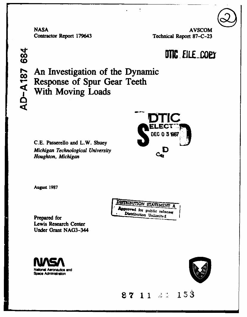
NASA AVSCOMContractor Report 179643 Technical Report 87-C-23

00CD

An Investigation of the Dynamic2 Response of Spur Gear Teeth

With Moving Loads

DTICDECO 3 187

C.E. Passerello and L.W. ShueyJMichigan Technological University DHoughton, Michigan

August 1987

D MItON SUEN'SA"Wved fl publi. r Ie,.

-Disthibut-on Undimite.1"

Prepared forLewis Research CenterUnder Grant NAG3-344

NASASwae Adwaon

8711.z1 153

TABLE OF CONTENTSPage

1. INTRODUCTION 1

1.1 Background 1

1.2 Problem Statement 6

1.3 Scooe of Work 6

2. MODEL DEVELOPMENT 8

2.1 Profile Generation 9

2.1.1 Involute Generation 9

2.1.2 Fillet Generation 19

2.1.3 Rim Generation 27

2.2 Finite Element Mesh Generation 29

2.3 Element Description 35

2.3.1 Planar Elements 35

2.3.2 General Element Description 36

2.3.3 Moving Loads 39

3. DISCUSSION OF NAGAYA ANALYSIS 43

3.1 Approximating A Gear Tooth 43with a Timoshenko Beam

3.2 Interpretation of Nagaya Results 47

4. FINITE ELEMENT ANALYSIS 51

4.1 Description of Test Gear 51

4.2 Determination of Normalized Plotting Parameters 52

and Their Application to the Gear Tooth

4.3 Description of Dynamic Loading Cases 57

I|

4.4 Finite Element Test Results 64

4.1.1 Comparison of Static Results 64

4.4.2 Modal Analysis-Determination of 66Mode Shapes and Natural Frequencies

4.4.3 Dynamic Deflections:Timoshenko Beam Constraints 69

4.4.3.1 Impact Loading 69

4.4.3.2 Finite Engagement Rise 74Time Loading

4.4.3.3 Wallace - Seireg Loading 78

4.4.4 Dynamic Delfections: Rim Included 78

5. DETERMINING THE EFFECTS OF INERTIA ON THE 84DYNAMIC RESPONSE OF MESHING GEAR TEETH

5.1 Analysis Using Massless Beams 85

5.1.1 Equations of Motion 86

5.1.2 Static Analysis .90

5.1.3 Dynamic Response Results 91

5.1.3.1 Constant Speed Moving Loads 94

5.1.3.2 Variable Speed Moving Loads 102

5.2 Analysis Including Beam Inertia 102

5.2.1 Equations of Motion 107

5.2.2 Dynamic Response Results: 117Foundation Mass - 1.0 lbs

5.2.3 Dynamic Response Results: 127Foundation Mass - 1.OE-4 lbs.

6. CONCLUSIONS 136

BIBLIOGRAPHY 137

APPENDICES

1.1. Finite Element Model Generation Program 140

2. Moving Load Generation Program Using 149Wallace-Seireg Load History

11

2. Contact Point Velocity of Meshing

Spur Gear Teeth 154

3. Deformed Shapes of Gear Tooth 159

1. Static Loading 160

2. Modal Analysis 170

3. Dynamic Response 182

4. Dynamic Response Curves for MeshingCantilever Beams 189

1. Massless Beams; Velocity - V(t) 190

2. Beams with Inertia; Velocity - V(t) 200

5. Use of Natural Modes in Equation ofMotion for Cantilever Beams 208

1. Constant of Integration 209

2. Evaluation of 12PHI1 and 12PHI2 210

3. Derivatives of the Mode Shape with Time 211

6. Development and Solution of Equations ofMotion with Inertial Terms Removed 212

7. Dymamic Response Algorithm for Meshing

Cantilever Beam 220

1. Massless Configuration 221

2. Inertia of Beam Included 223

Accesio For

NTIS CRA&,

DTIC TA . _]. ~. .. •. ..... .. .. ..... .... .. ... -I ---

Byy....... ...... . ...--Di tf i~.

.r

1. INTRODUCTION

(1.1) Background

The topics of dynamic loading of gear teeth and the

deflections of gear teeth due to dynamic loads have been

treated extensively.

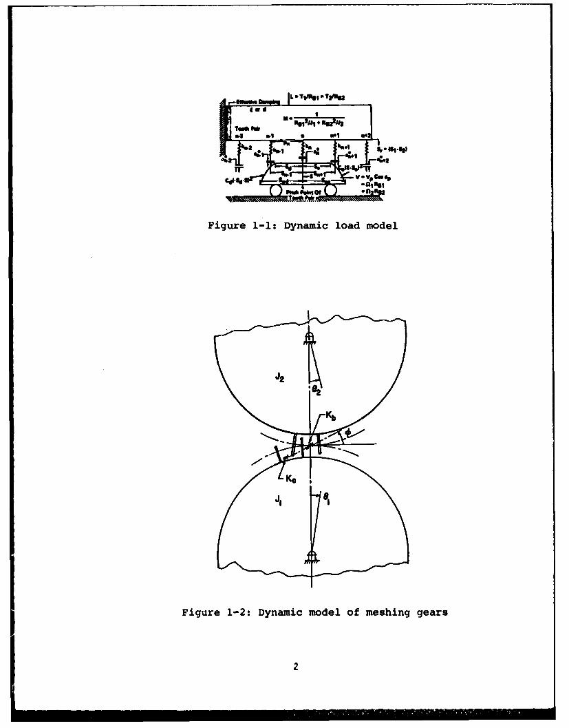
One such work, presented by Cornell and Westervelt (11,

utilizes an improved version of a model developed by Richardson

[4]. The model generates the dynamic loads for a meshing gear

using a cantilever beam with a cam moving along it, simulating

the engagement and disengagement of the adjacent tooth (see

Figure 1-1). These dynamic loads are then used in a dynamic

model of meshing gear teeth where the two gear hubs act as

rigid inertia and the teeth as variable stiffness springs as

shown in Figure 1-2. Of significant importance in this

investigation is the claim made by the authors that the effect

of variable tooth stiffness is small, changing the dynamic load

response slightly compared to a system with constant tooth

stiffness.

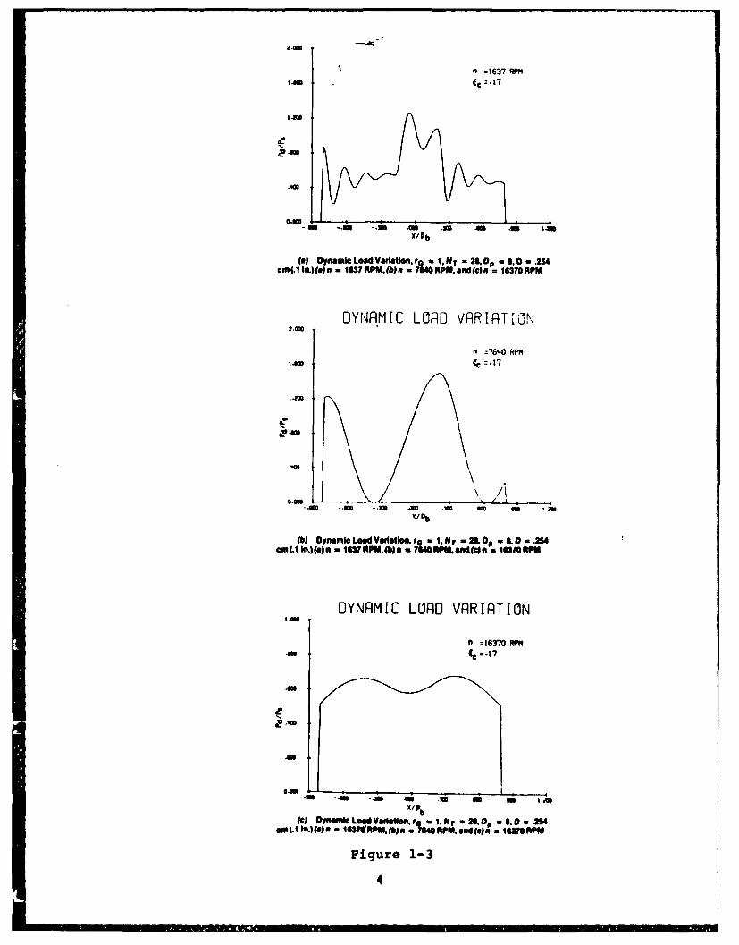
Another dynamic load response algorithm was developed by

Wang and Cheng (2-3], where they reported that both the dynamic

load and the induced dynamic response are highly dependent on

the speed of the moving load. In slow speed regions, the dyna-

mic load response is composed of a static response which varies

with the stiffness of the tooth. Superimposed on the static is

an oscillatory response caused by the excitation of the system

at the resonant frequency. Wang states that as the speed of

' ' ' r 1' 'I' .T -. , r, - ... -r ,, ,

.,,,.. , L -,,i., -,%W~

Cad sa

Ow.W2" W160

Figure 1-1: Dynamic load model

Figure 1-2: Dynamic model of meshing gears

I i ' I ' I ' ... '* ' " " " 'I' "' " " '2

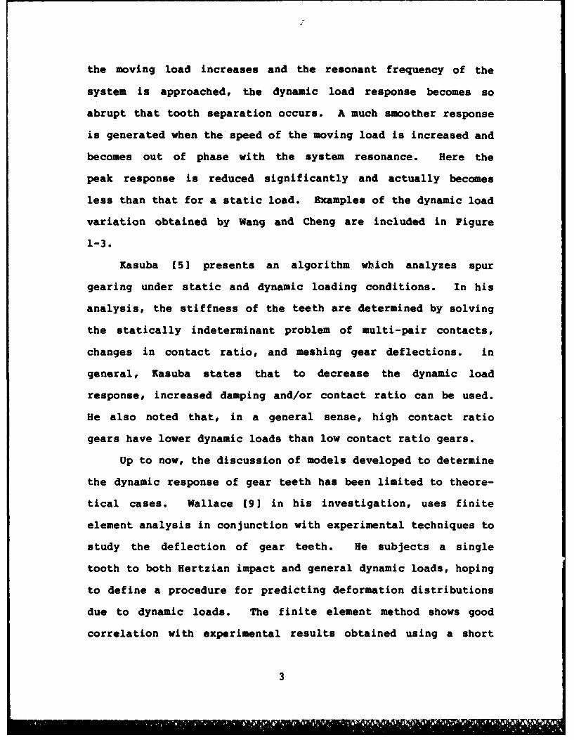
the moving load increases and the resonant frequency of the

system is approached, the dynamic load response becomes so

abrupt that tooth separation occurs. A much smoother response

is generated when the speed of the moving load is increased and

becomes out of phase with the system resonance. Here the

peak response is reduced significantly and actually becomes

less than that for a static load. Examples of the dynamic load

variation obtained by Wang and Cheng are included in Figure

1-3.

Kasuba (5) presents an algorithm wbich analyzes spur

gearing under static and dynamic loading conditions. In his

analysis, the stiffness of the teeth are determined by solving

the statically indeterminant problem of multi-pair contacts,

changes in contact ratio, and meshing gear deflections, in

general, Kasuba states that to decrease the dynamic load

response, increased damping and/or contact ratio can be used.

He also noted that, in a general sense, high contact ratio

gears have lower dynamic loads than low contact ratio gears.

Up to now, the discussion of models developed to determine

the dynamic response of gear teeth has been limited to theore-

tical cases. Wallace [91 in his investigation, uses finite

element analysis in conjunction with experimental techniques to

study the deflection of gear teeth. He subjects a single

tooth to both Hertzian impact and general dynamic loads, hoping

to define a procedure for predicting deformation distributions

due to dynamic loads. The finite element method shows good

correlation with experimental results obtained using a short

3

i = 1637 RP

-M

-, n --00 _10 O 4 AM 14%X/Pb

(a) Dynamic Load Vaoiton, 0 a 1,N T 29D. O SD - .2S4cm(.1 in.)(a)n - 1637 RPM. (b) n 7640 RPM, and (e) = 16370RPM

DYNRMIC LORD VRRIRTION

n =7640 RPIqt~~aCC =.:17

.0.

o,\ //.400s -i 4w Jos -ad .m 1.2w

(b) Dynamic LoadValaondr* a 1,g - . Do I. 0 .2..4com(.1 In.) (a) n U 137 RPM.j, a a IM PM.and(Cjn w into RPM

DYNAMIC LORD VRRIRTIONs.ug

n = 16370 RPM

0 . -- .. .. .. ..... .....

.i40 - -Aw -00 i n 41/p

(C) Dynamic LOW Vadlon.* t l. N - 6, 21 .0 , - 24ami-. I) a 1637fRPM~n a 7640RPM. aid(c)n I 1?60PM

Figure 1-3

4

cantilever beam subjected to impact loadings at different posi-

tions.

Another important contribution to the subject of gear

dynamics was made by Attia [6). He studied the effects of

including the rim when performing a static analysis to deter-

mine tooth spring constants. He concluded that the stiffness

of teeth with the rim included is significantly less compared

*to a variable cross-section cantilever beam rigidly fixed to

the gear body. With the added flexibility, the initial con-

ditions of two meshing teeth are highly dependent on the

deflections of the two previously engaging teeth. This fact is

very significant, as it will definitely affect the type of load

experienced by the upcoming gear pair.

Many of the theoretical models used to predict the deflec-

tions of gear teeth, such as those presented by Cornc! [1],

Wang [2-31 and Kasuba [51, make use of tooth stiffness

variations obtained from a static deflection analysis. The

equations of motion are expressed as functions of the load

position only.

Nagaya and Uematsu [71 state that because the contact

point moves along the involute, the dynamic load response

should be considered as a function of both the position and

speed of the moving load. In their analysis, they approximate

the deflections of actual gear teeth due to moving loads by

modelling the tooth as a tapered Timoshenko beam. They present

plots of normalized centerline deflections for different moving

load speeds, and claim that dynamic stiffness variations can be

derived from their results. However, as i.lustrated later,

this claim turns out to be false.

In order to make the theoretical developaqnts of models

used to determine the dynamic response of gear teeth more prac-

tical, some assumptions are made. One such assumption made by

the first three authors presented, is that the mass of the gear

tooth compared to the gear body is small and can be neglected.

Literature gives no hints to whether this assumption has been

thoroughly investigated.

(1.2) Problem Statement

In this study, two basic problems are investigated. The

first phase is to determine whether the dynamic response of a

single spur gear tooth is dependent on the speed of a moving

load acting on the tooth.

The second phase is nv ti tion to determine the

significance of omitting h inertia of the gear tooth from the

dynamic deflection model due the all mass relative to the

gear body.

(1.3) Scope of Work

A model based on involute geometry is developed to automa-

tically generate a spur gear tooth profile and finite element

mesh, including the rim, using a minimum of input parameters.

This model is then used to determine the effects of the speed

of a moving load on the deflection of a single gear tooth. Two

constraint configurations are tested; one where only the invo-

lute profile and fillet regions are allowed to deform, the

6

other with the entire rim included. The results are first

represented as normalized deflections of the tooth centerline.

Then the tooth tip deflection time histories are studied for

the entire load cycle.

The second phase of the work is to model a meshing gear

tooth pair using two cantilever beams attached to moveable

foundation masses. Relative displacements of the foundation

masses as well as beam deflections are determined for moving

load speeds bracketing the system resonant frequency.

7

2. MODEL DEVELOPMENT

In order to effectively perform a static and dynamic ana-

lysis of spur gear teeth using finite element techniques, a

model is needed to automatically generate a tooth profile and

the accompanying finite element mesh for different size gear

teeth. Also, the geometry of the tooth should be defined using

a minimum of parameters corresponding to those most generally

specified when generating a tooth profile. One such list of

parameters is:

Pressure Angle = op

Pitch Radius = RP

Addendum = AD

Dedendum = DED

Circular Pitch = CIRP

Backlash = BACKL

Fillet Radius = RF

Rim Thickness = RTH

With these parameters, the profile of any spur gear tooth can

be generated including the rim.

In the proceeding sections, the equations necessary to

construct the tooth profile using the preceeding parameters are

developed, including the implementation of these relationships

in a profile generation algorithm. The topic of finite element

mesh generation is also discussed, along with an overview of

the mesh generation algorithm used to generate the grid.

8

Later in this chapter, a brief discussion of the plane

strain finite element type used to model the gear is included.

Also, a general treatment of a linear quadrilateral element is

used to help develop equations describing the moving loads used

on the gear teeth. These relations are then implemented in a

moving load generation algorithm using idealized load time

history equations for a spur gear tooth.

(2.1) Profile Generation

The profile generation sequence is divided into three

sections; determining relationships, first for the involute,

then for the fillet, and finally for the rim.

(2.1.1) Involute Generation

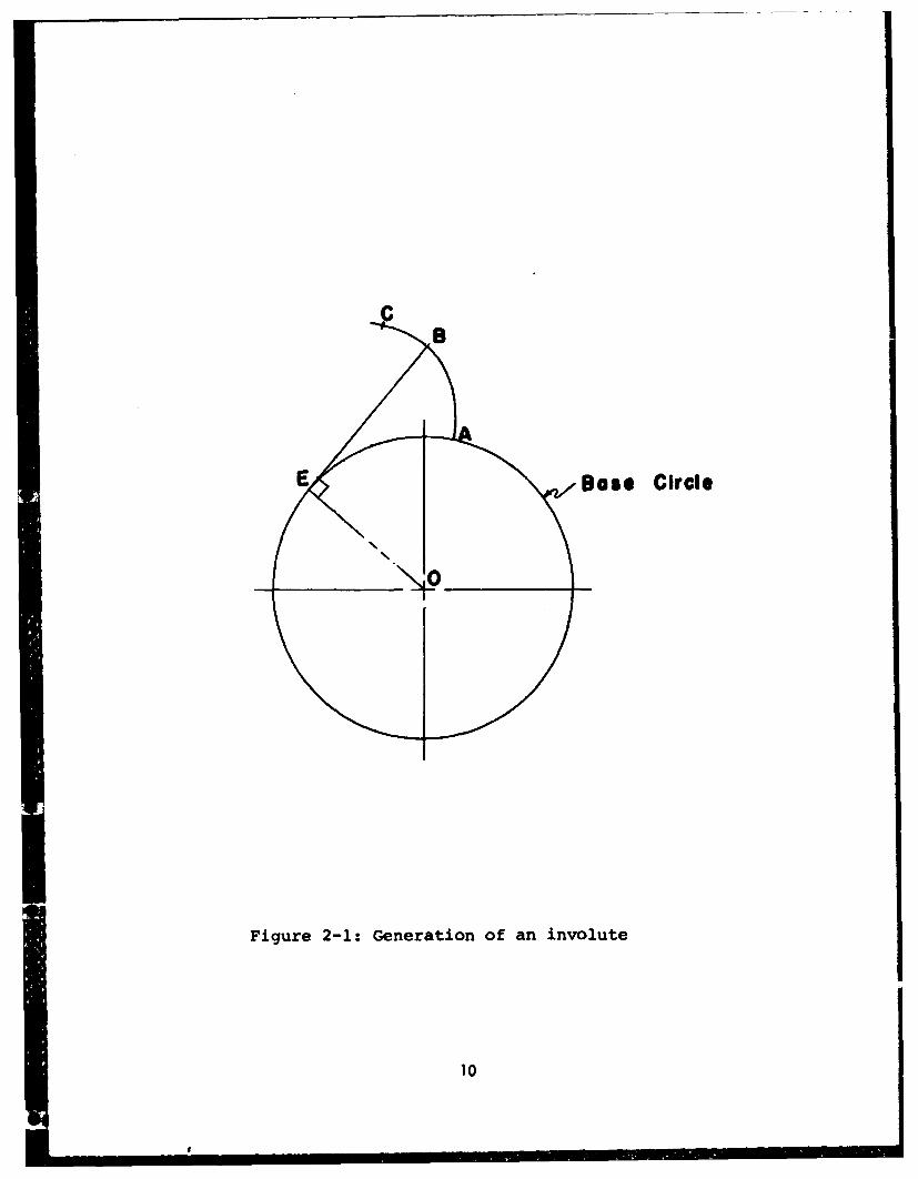
An involute curve is generated by unwrapping an inexten-

sible cord from a cylinder. Figure 2-1 illustrates that as the

cord is unwrapped from the cylinder, point B on the cord traces

an involute curve AC. The radius of curvature of the involute

varies continuously, being a zero at point A and increasing

towards C. At the instant shown, the radius is equal to BE, as

point E corresponds to the instantaneous center of rotation

about point B. When generating the involute of a spur gear

tooth, the cylinder from which the cord is unwrapped corresponds

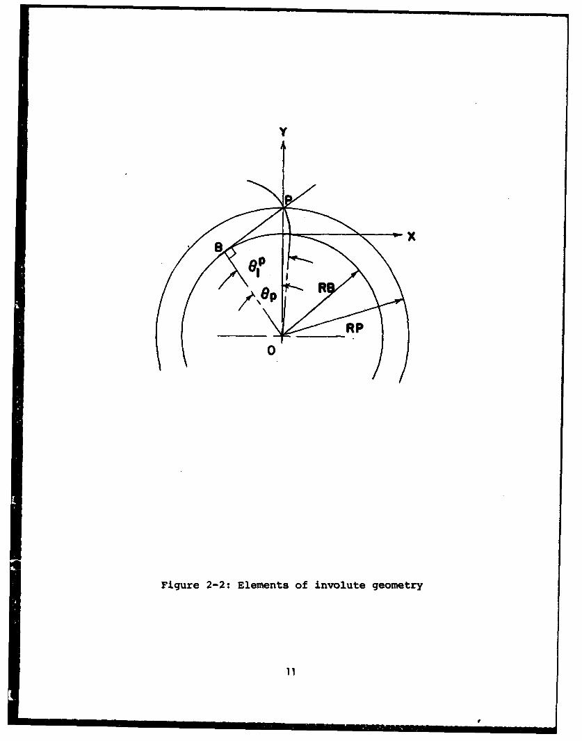
to the base circle. This concept is further developed as shown

in Figure 2-2. Here the local coordinate system X-Y, fixed to

the hub at the base circle, is used to determine relative coor-

dinates along the involute. The parameters shown are; the base

9

mC

/Bs Circle

\,4

Figure 2-1: Generation of an involute

10

yx

* °

Figure 2-2: Elements of involute geometry

| 11

'I 1 ' "P I ' I

circle radius RB, the pitch circle radius RP, the roll angle

e? and the pressure angle Op. The pressure angle is defined

by drawing a line perpendicular to the base circle and passing

through the point P. This line corresponds to the pressure

line or line of action of forces between meshing gear teeth.

The point P being the pitch point. From the triangle OBPO, the

base circle radius is defined in terms of the pitch radius as:

RB - RPcosep (2-1)

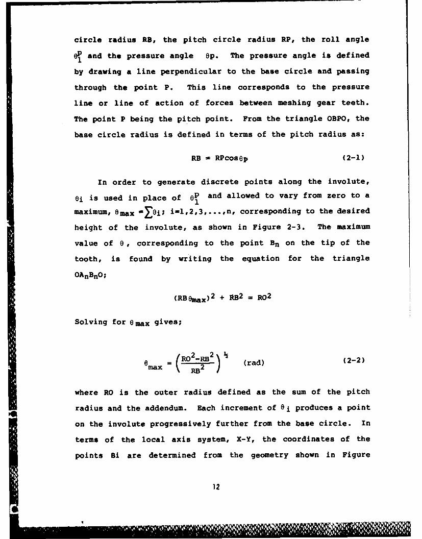
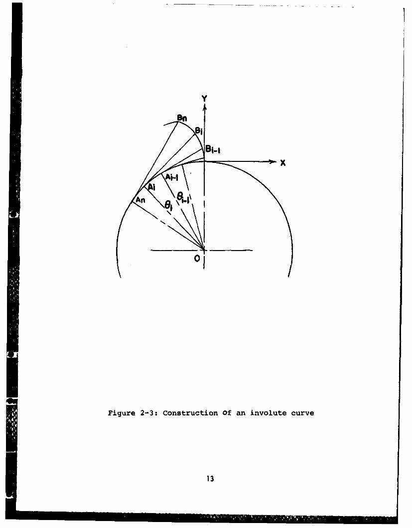
In order to generate discrete points along the involute,

Oi is used in place of OP and allowed to vary from zero to a1

maximum, (max =,6; i-l,2,3,...,n, corresponding to the desired

height of the involute, as shown in Figure 2-3. The maximum

value of 6, corresponding to the point Bn on the tip of the

tooth, is found by writing the equation for the triangle

OAnBnO;

(RBOmax)2 + gB2 = R02

Solving for emax gives;

max = (Ro2 R 2 (rad) (2-2)

where RO is the outer radius defined as the sum of the pitch

radius and the addendum. Each increment of 8i produces a point

on the involute progressively further from the base circle. In

terms of the local axis system, X-Y, the coordinates of the

points Bi are determined from the geometry shown in Figure

12

V 1 jiC

01

Figure 2-3: Construction Of an involute curve

13

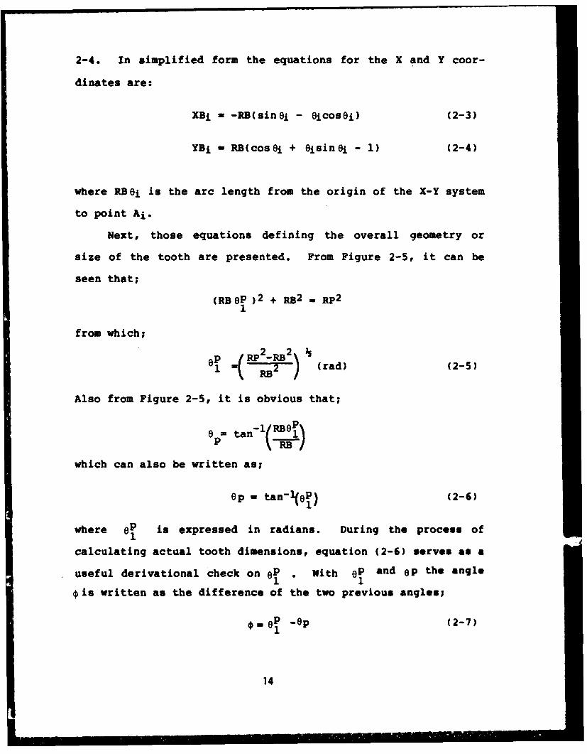
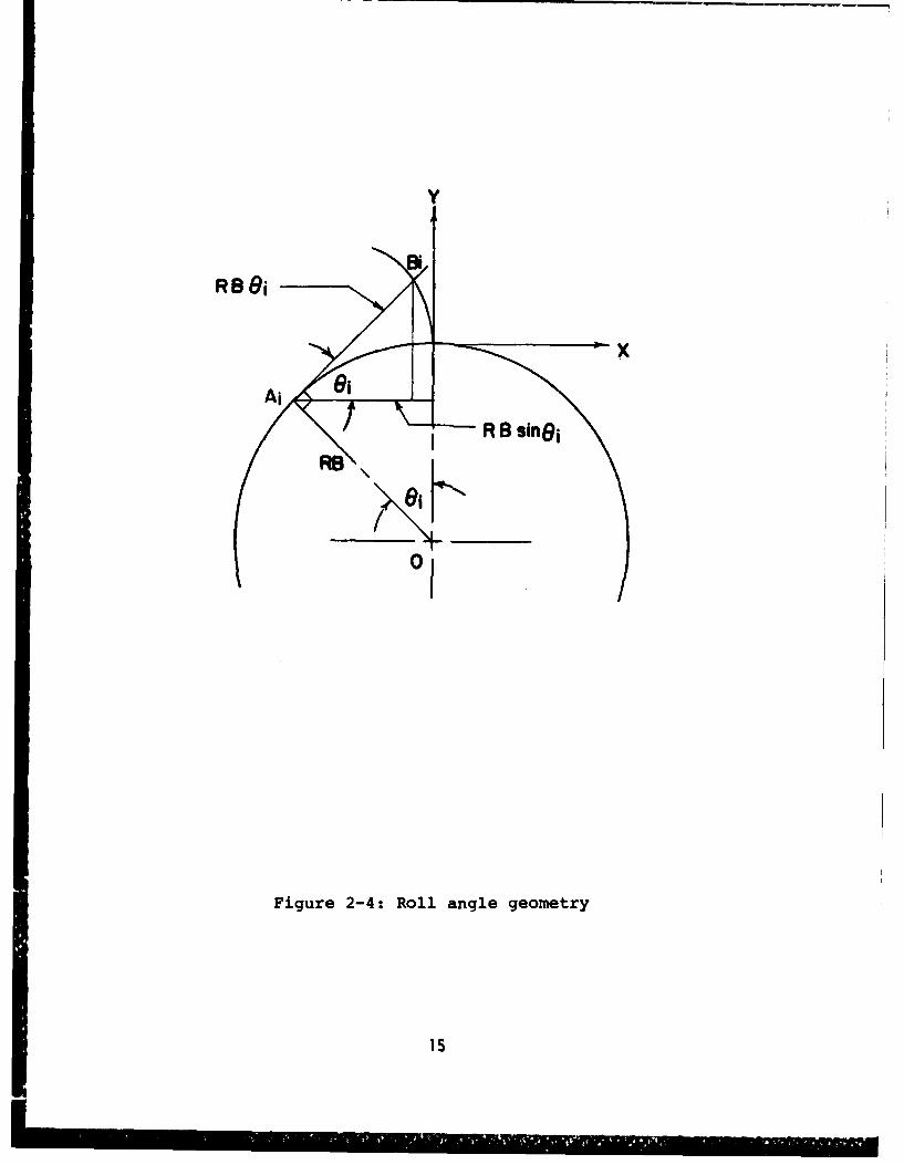
2-4. In simplified form the equations for the X and Y coor-

dinates are:

XBi - -RB(sinei - eicosei) (2-3)

YBi - RB(cose0 + Oisin i - 1) (2-4)

where RBei is the arc length from the origin of the X-Y system

to point Ai.

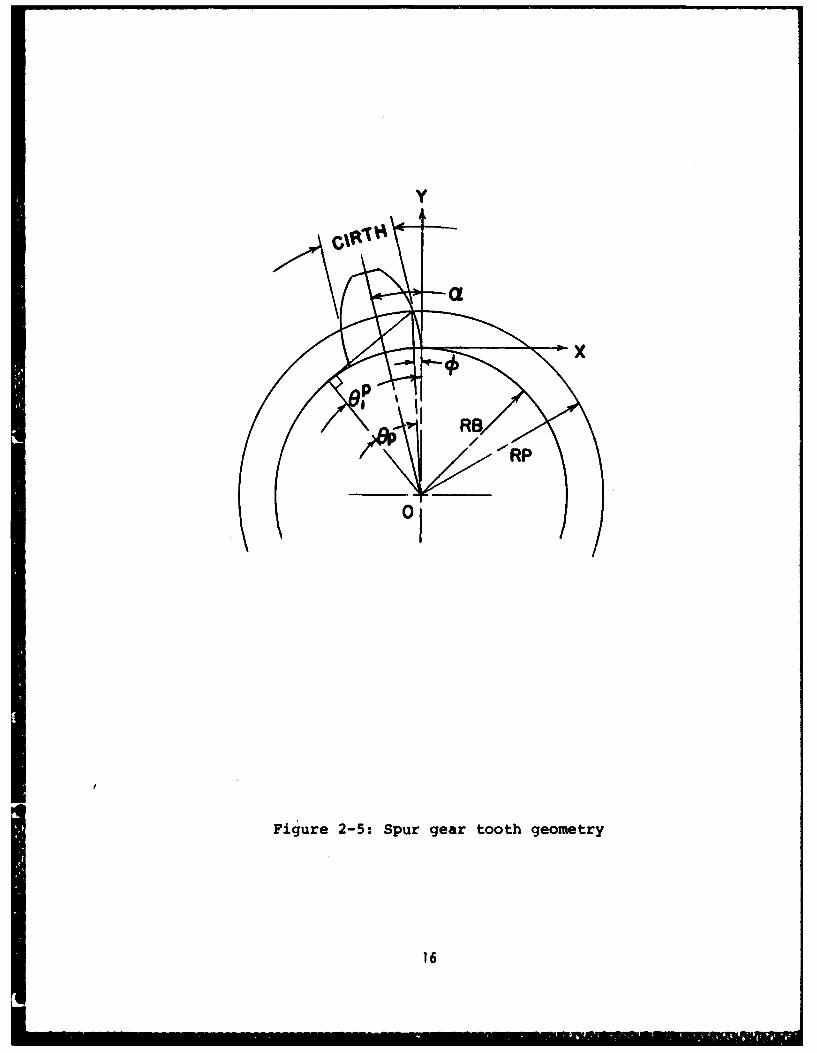
Next, those equations defining the overall geometry or

size of the tooth are presented. From Figure 2-5, it can be

seen that;

(RBeP )2 + RB 2 - Rp2

from which;

1p (PRB 2 ) C rad) (2-5)

Also from Figure 2-5, it is obvious that;

6=tan-1 RBO )

which can also be written as;

ep - tan- ()P) (2-6)

where eP is expressed in radians. During the process of1

calculating actual tooth dimensions, equation (2-6) serves as a

useful derivational check on OP . With ep and Op the angle1 1

*is written as the difference of the two previous angles;

*eOP -op (2-7)1

14

Y

RSSiBi

R 8 $inei

RBR

-, 0

Figure 2-4: Roll angle geometry

15

Y

-a

Figure 2-5: Spur gear tooth geometry

16

And finally, from Figure 2-5, c is found to be;

an eP - tan-l(e) + CIRTH (2-8)

where CIRTH is the circular thickness measured on the pitch

circle, given by;

CIRTH - CIRP - BACKL (2-9)2

Since one leg of a passes through the tooth center, this angle

is well suited for transforming the involute coordinates from

the X-Y axis system to a system whose Y axis passes through the

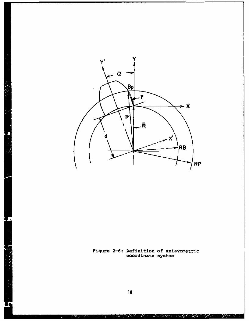
center of the tooth, such as Y' shown in Figure 2-6.

When analyzing a gear tooth to determine stresses, deflec-

tions, etc., it is very advantageous to make full use of the

axisymmetric properties of the tooth. The involute points

generated relative to the X-Y axis system are, therefore,

transformed into another system X'-Y', taking full advantage of

these properties.

Using the pitch point on one side of the tooth as a

reference, as seen in Figure 2-6, a vector F' is drawn from the

pitch point, Bp, to the gear center, O, which defines the ori-

gin of the X'-Y' coordinate system. The vector, ?', is com-

posed of two vectors, A and r;

r' - R + r (2-10)

where;

17

y, Y

nT

RP

Figure 2-6: Definition of axisymmetriccoordinate system

18

R - dJ' + RBsinril (2-11)

with;

d - RBcos

and;

= x1 + yT (2-12)

(x and y are the coordinates of point Bp calculated in terms of

X-Y using equations (2-3) and (2-4)).

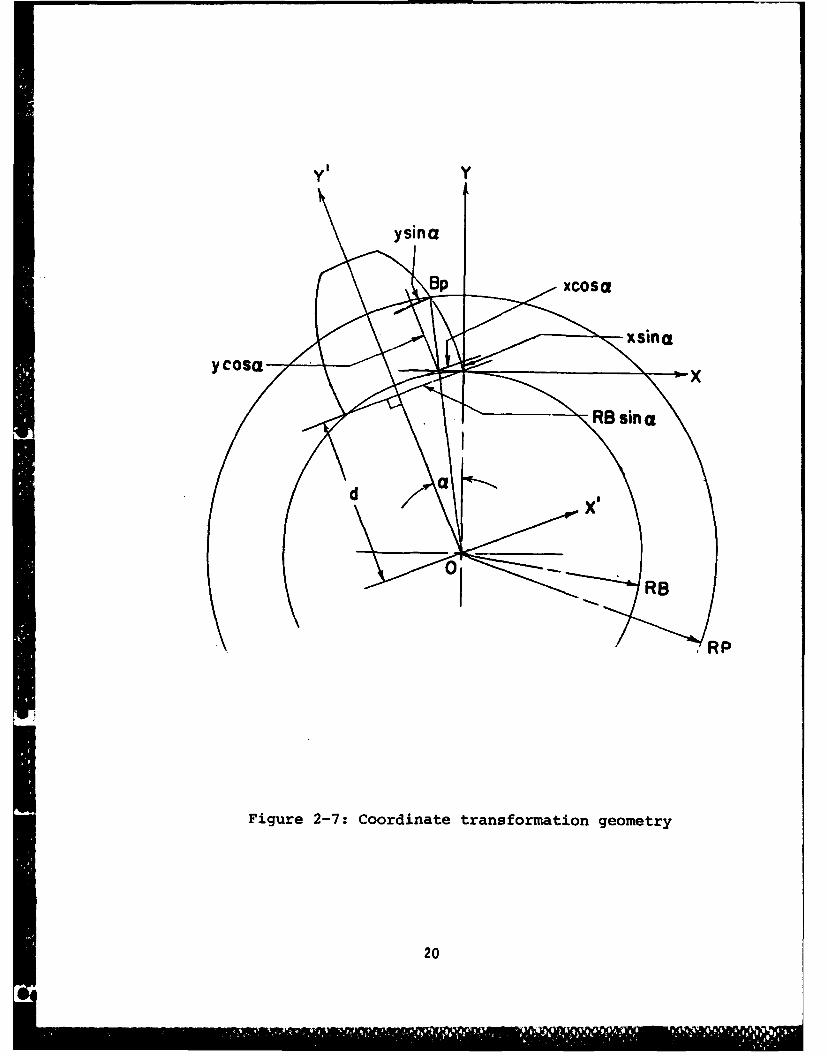
In the new coordinate system, the coordinates of point Bp

are now defined as;

X, = RBsin + xcosa + ysin (2-13)

Y',= d - xsina + ycosa (2-14)

Figure 2-7 illustrates more clearly the elements comprising

equations (2-13) and (2-14).

In the profile generation algorithm, included in Appendix

1, eleven points are calculated along the involute. Equations

(2-2), (2-3), (2-4); (2-5), (2-8), (2-13), and (2-14) are used

directly to calculate the point coordinates in the X'-Y' axis

system.

(2.1.2) Fillet Generation

In the present work, two different spur gear tooth

geometries are considered; low contact ratio gearing (LCRG)

and high contact ratio gearing (HCRG). By definition, the con-

tact ratio is the length of the path of contact of mating gears

19

y' Y

- Vysina

_. -_~~ yCosa - x

-- d a I q x'

" / ,RP

Figure 2-7: Coordinate transformation geometry

20

divided by the base pitch. More practically, it can be thought

of as the average number of teeth in contact during the meshing

cycle. A high contact ratio gear is one which has at least two

teeth in contact at all times.

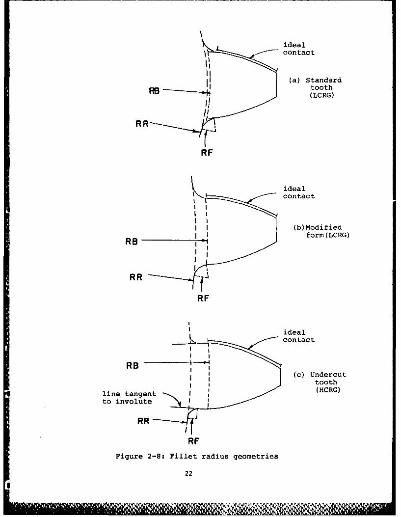
One of the main differences between the two forms (LCRG and

HCRG) is the fillet transition (see Figure 2-8). For an actual

low contact ratio gear, the fillet radius is placed tangent to

the involute and the root circle as shown in Figure 2-8a. The

amount of overlap of the involute may be different for any

given tooth design. in the current model, however, the fillet

radius is calculated to fit tangent to the involute at the base

circle and tangent to the root circle, as shown in the modified

case (see Figure 2-8b).

When designing the high contact ratio gears, the fillet

region is undercut to provide additional clearance for the

engaging teeth. Also, the HCRG tooth is generally longer due

to addendum or other profile modifications, thus the radial

distance between the base and root circles is also extended as

shown in Figure (2-8c).

Given the gear parameters defined for a particular gear,

the following equation can be used to determine whether the

gear is a low or high contact ratio gear [101.

RR2 + 2RF RR > RB2 (2-15)

In equation (2-15) RF is the fillet radius specified for a

given tooth. If this inequality is satisfied, the tooth is

21

! ! - , 'r , I' 'T . : " e -'' " '"'' 'all

ideal

contact

(a) Standard

__ _ tooth(LCRG)

RF

ideal

"_i Ii contact

(b) Modified

form (LCRG)

RR T

RF

ideal

contact

RB(C) Undercut

tooth

line tangent (HCRG)to involute

RR

RF

Figure 2-8: Fillet radius geometries

22

Ii , '

classified as LCRG. This means that the specified fillet radius

will overlap the involute, and thus must be changed to fit the

modified form as described in Figure 2-8b.

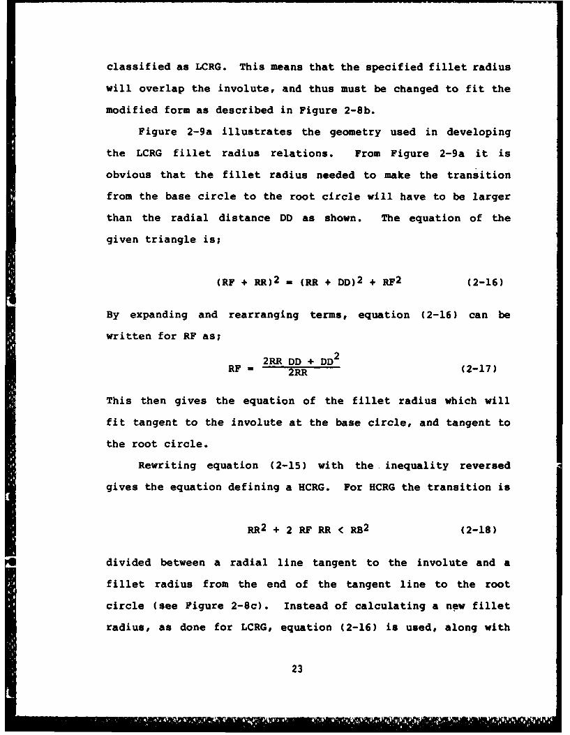
Figure 2-9a illustrates the geometry used in developing

the LCRG fillet radius relations. From Figure 2-9a it is

obvious that the fillet radius needed to make the transition

from the base circle to the root circle will have to be larger

than the radial distance DD as shown. The equation of the

given triangle is;

(RF + RR)2 - (RR + DD)2 + RF2 (2-16)

By expanding and rearranging terms, equation (2-16) can be

written for RF as;

2RR DD + DD2 (2-17)RF = 2RR

This then gives the equation of the fillet radius which will

fit tangent to the involute at the base circle, and tangent to

the root circle.

Rewriting equation (2-15) with the inequality reversed

gives the equation defining a HCRG. For HCRG the transition is

RR2 + 2 RF RR < RB2 (2-18)

divided between a radial line tangent to the involute and a

fillet radius from the end of the tangent line to the root

circle (see Figure 2-8c). Instead of calculating a new fillet

radius, as done for LCRG, equation (2-16) is used, along with

23

3RFK

7 RR+OD

RF

ODR

RB RRRR

a. Low contact ratio b. High contact ratio

Figure 2-9: Fillet geometry

24

the specified fillet radius, to calculate the length of the

radial line DR (see Figure 2-9b). Rewritten in another form,

equation (2-16) becomes;

DD2 + 2RR DD - 2RF RR - 0 (2-19)

and can be used to determine the radial distance DD spanned by

the fillet radius. Using the positive root of the quadratic

equation (2-19) for DD yields;

DD= -2RR+ (4RR2 + 8RF RR)h (2-20)

DD is then subtracted from the difference between the base and

root radii to give the length of the radial tangent line.

DR - (RB - RR) - DD (2-21)

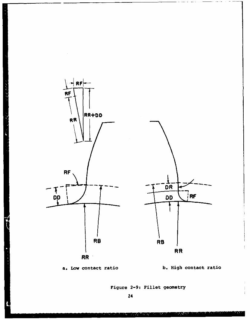
When programming the preceeding equations to calculate the

fillet coordinates, eight equally spaced points are used. For

LCRG, the arc AOB is divided up into eight equal angles, ei

(see Figure 2-10a). Coordinates of successive points are

calculated by adding ei's together for i-,2...,8 until the

arc from A to B is generated. The coordinates of Bi in Figure

2-10b are found from;

XBi - XA - RFcose

YBi - YA - RFsine

For HCRG, the radial distance required for the fillet

radius, and the radial distance of the tangent line may vary

25

o A

9'

BR

(a)

RR

(b)RR

Figure 2-10: Fillet radius generation

26

from one gear design to another. To insure equal point

spacing, integer arithmetic is used to weight the number of

points between the radial portion and the fillet radius

according to their respective sizes. This is done to facili-

tate the finite element mesh generation routine discussed

later. As in the involute profile generation scheme, the

points for the fillet are calculated in the X-Y coordinate

system, and then transformed to the XI-Y' system.

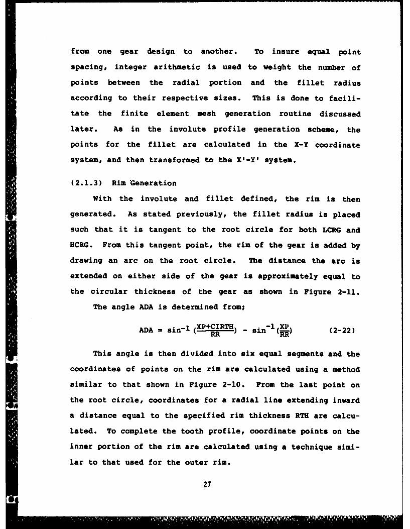
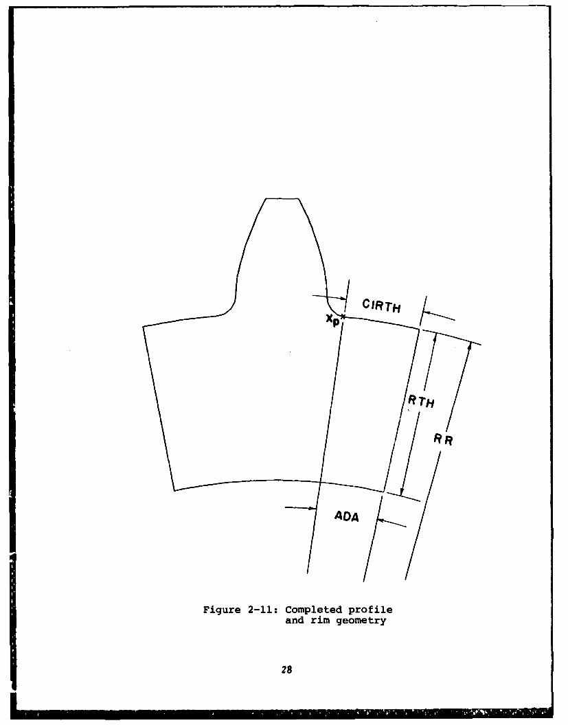
(2.1.3) Rim Generation

With the involute and fillet defined, the rim is then

generated. As stated previously, the fillet radius is placed

such that it is tangent to the root circle for both LCRG and

HCRG. From this tangent point, the rim of the gear is added by

drawing an arc on the root circle. The distance the arc is

extended on either side of the gear is approximately equal to

the circular thickness of the gear as shown in Figure 2-11.

The angle ADA is determined from;

ADA = sin 1 (XP+CIRTH . - XP

RR RR sin-( ) (2-22)

This angle is then divided into six equal segments and the

coordinates of points on the rim are calculated using a method

similar to that shown in Figure 2-10. From the last point on

the root circle, coordinates for a radial line extending inward

a distance equal to the specified rim thickness RTH are calcu-

lated. To complete the tooth profile, coordinate points on the

inner portion of the rim are calculated using a technique simi-

lar to that used for the outer rim.

27

'" CIRTH

RR

I ADA

Figure 2-11: Completed profile

and rim geometry

28

(2.2) Finite Element Mesh Generation

No absolutely correct method has been found to model a

system using a finite element mesh, even though the topic of

mesh development has been treated quite extensively. With dif-

ferent element types and solution techniques, several equally

valid methods are available for any particular application.

Indeed, Cook (141 states that although an optimum mesh can

be determined by requiring that element boundaries follow lines

of constant strain, this optimum condition only exists for

one set of loading conditions. As the load changes, so does

the optimum mesh configuration, and for problems involving

other than static loading, the difficulties are compounded.

However, when developing a mesh, simple guidelines can be

followed which will produce a well enough refined mesh to

obtain more than satisfactory results. To mention a few; ele-

ment boundaries should be aligned with structural or geometric

boundaries and principal load trajectories, element aspect

ratios should be kept low (less than 7), and when different

element sizes are used transitions between different size ele-

ments must be gradual (mesh grading).

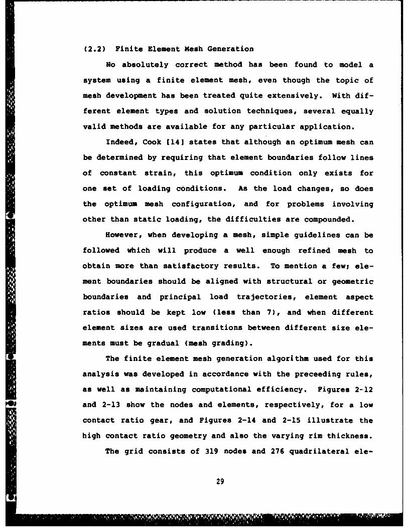
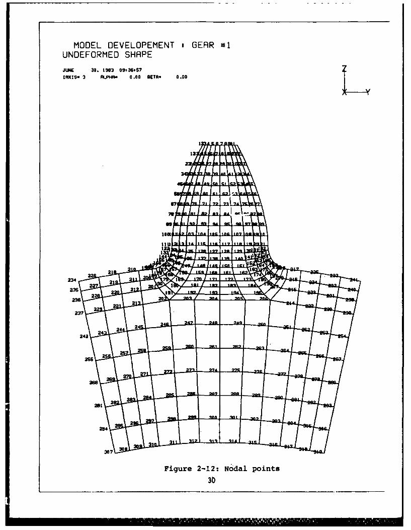
The finite element mesh generation algorithm used for this

analysis was developed in accordance with the preceeding rules,

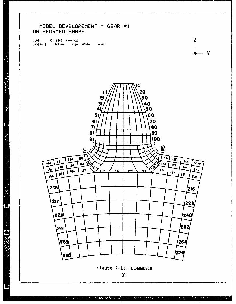
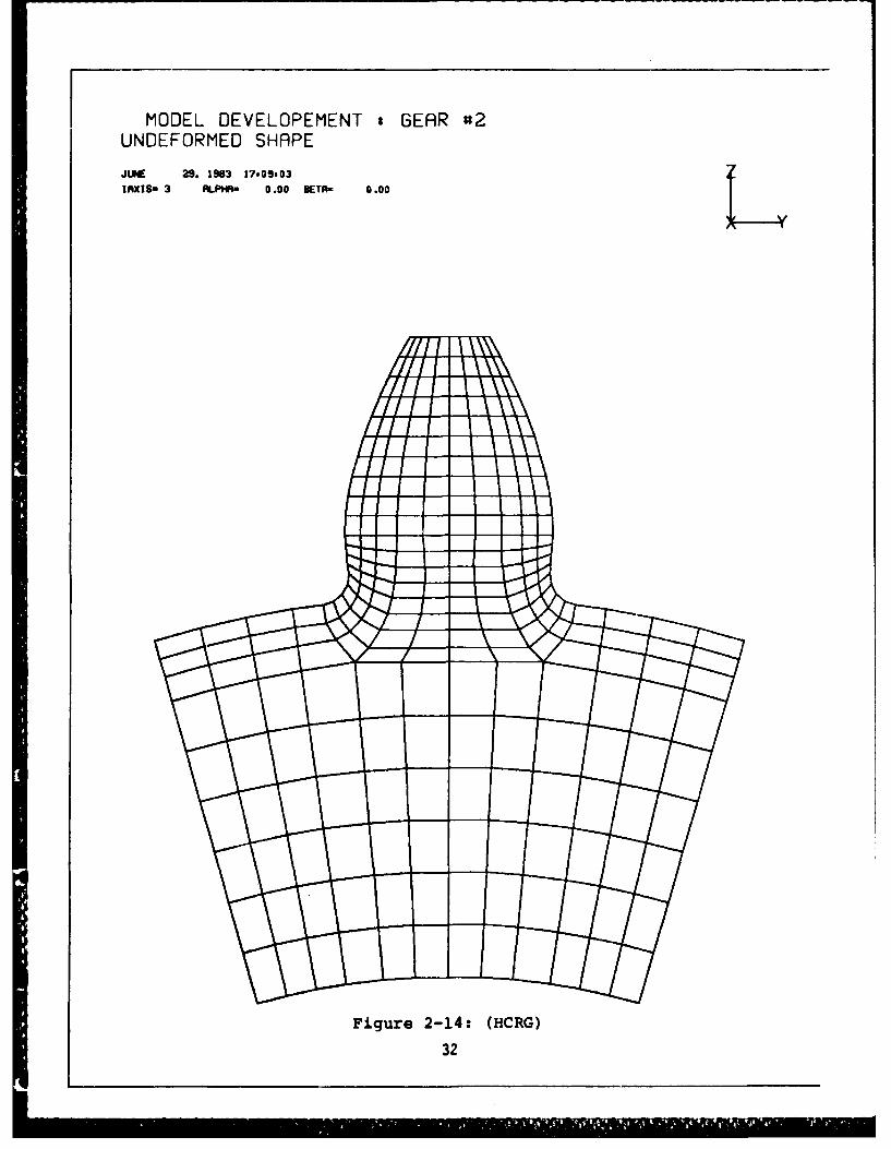
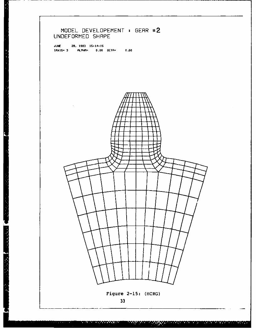
as well as maintaining computational efficiency. Figures 2-12

and 2-13 show the nodes and elements, respectively, for a low

contact ratio gear, and Figures 2-14 and 2-15 illustrate the

high contact ratio geometry and also the varying rim thickness.

The grid consists of 319 nodes and 276 quadrilateral ele-

29

MODEL DEVELOPEMENT a GEAR #1UNDEFORMED SHAPE

JUNE 30. 1963 09@36m57

IAXIS= 3 ALPR 0 .00 BETA- 0.00

2312

Figue21:Ndlpit

637

MODEL DEVELOPEMENT u GEAR #1UNOEFORMED SHAPE

JUNE 30. 1963 09.41823

IFIXIS- 3 ALPHR- 0.00 BETA- 0.00

1 '01 NT 20

21 3031 40

24 I 50

Ti 60

81 9091 1- 00

%C41~ " 'i 77 I93 20

20521

21T72

Figure 2-13: Elements

31

MODEL DEVELOPEMENT t GEAR #2UNDEFORMED SHAPE

JUNIE 29. 1983 17@09.03InEis- 3 ftPHR 0.00 BETA- 0.00

Figure 2-14: (HCRG)

32

MODEL DEVELOPEMENT s GEAR 2UNDEFORMED SHAPE

JUNE 29. 1983 l5s1lS

IRXIS= 3 ALPHA= 0.00 BETA= 0.00

Figure 2-15: (HCRG)

33

ments. Ten equally divided vertical rows are used to form the

involute portion of the gear (elements 1-100). Nodes on the

surface of the involute correspond to the actual coordinate

points calculated in the profile generation routine. Close to

the surface of the involute, the element spacing is small pro-

viding additional stiffness for the application of the load.

Towards the center of the tooth the element spacing is greater

where less stiffness is needed.

The transition from the end of the involute to the root

circle is accomplished using one of the two techniques

described in section (2.1.2). For both LCRG and HCRG, eight

equally spaced rows of elements are used for the transition,

again using the actual coordinate points calculated in the pro-

file generation section as surface nodes. When using the HCRG

transition, with the radial line and fillet radius, the eight

surface nodes are divided between the two sections keeping

nodal spacing as even as possible.

In order to maintain continuity between different gear

geometry finite element meshes, elements 1 through 204 remain

the same size relative to the actual tooth sizes. In other

words, no changes are made in the grid geometry during the

generation of a particular gear model. The exception to this

rule is that elements 205 through 276 do vary in size depending

on the rim thickness. Figures 2-14 and 2-15 show this variation.

The algorithm containing the equations developed for the

profile geometry, as well as those relationships used to create

the finite element mesh is included in Appendix 1.

34

L 1 1 1

(2.3) Element Description

(2.3.1) Planar Elements

Two element types are considered for this analysis; plane

strain and plane stress. Due to the geometry and loading con-

ditions of the tooth, it is modelled as a plane elastic problem.

A plane body is a region of uniform thickness contained within

two parallel planes. When the thickness of the body is large

compared to the lateral dimensions, the problem is considered to

be plane strain. If the thickness is small, it is considered to

be plane stress. The difference between plane strain and plane

stress elements is evidenced in the material property matrices.

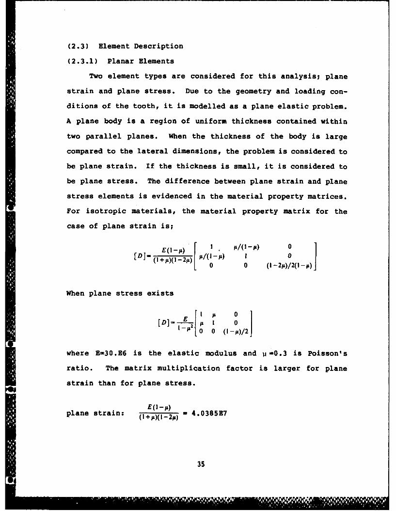
For isotropic materials, the material property matrix for the

case of plane strain is;

E(I-1) I . /(I- ) 0,[DJ= (l+ A)(l_-2 A) A/0 - 1) 1 0

-( 2 0 0 (I -2p)/2(I-I)

When plane stress exists

I IL 0

S-)A 2 o. 0 ( I - 1)/ 2

where E-30.E6 is the elastic modulus and U=0.3 is Poisson's

ratio. The matrix multiplication factor is larger for plane

strain than for plane stress.

plane strain. (I+ )(I-2p) - 4.0385E7

35

plane stress: E - 3.2967E7I- 'U2

The matrix elements are also larger (except for element 3,3) for

plane strain. When combined with the strain displacement rela-

tions to form the stiffness matrix, these differences result in

an increase in the stiffness for plane strain compared to plane

stress.

The thickness of the tooth used in the analysis is 0.25

inches. Comparatively, the largest and smallest planar dimen-

sions on the actual tooth (not including the rim) are 0.224 and

0.081 inches, respectively. Based on the dimensions it is dif-

ficult to make a judgement on the correct element type for this

analysis.

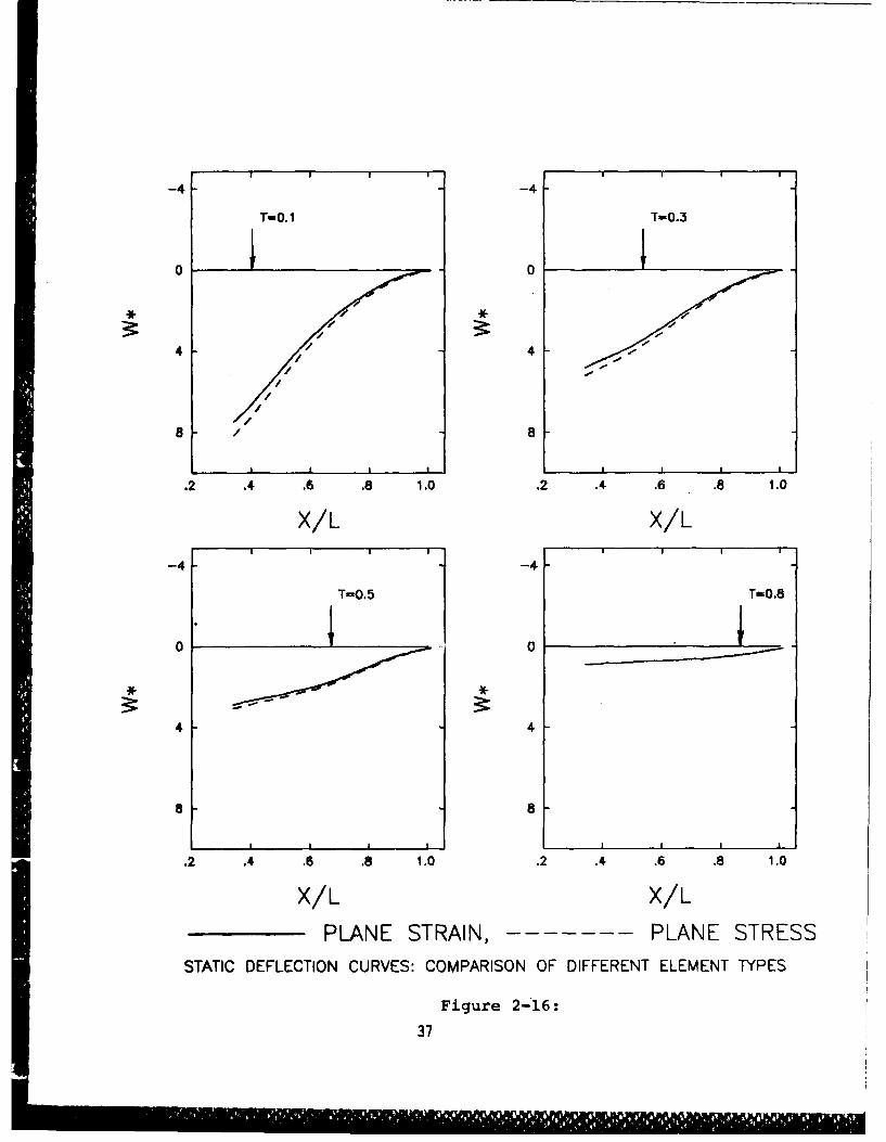
Figure 2-16 shows representative static deflection curves

for the plane strain and plane stress element types. The addi-

tional stiffness of the plane strain element is noted. Since the

difference in deflections between the two element types is small,

the plane strain element type is chosen for this analysis.

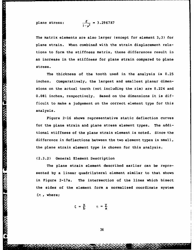
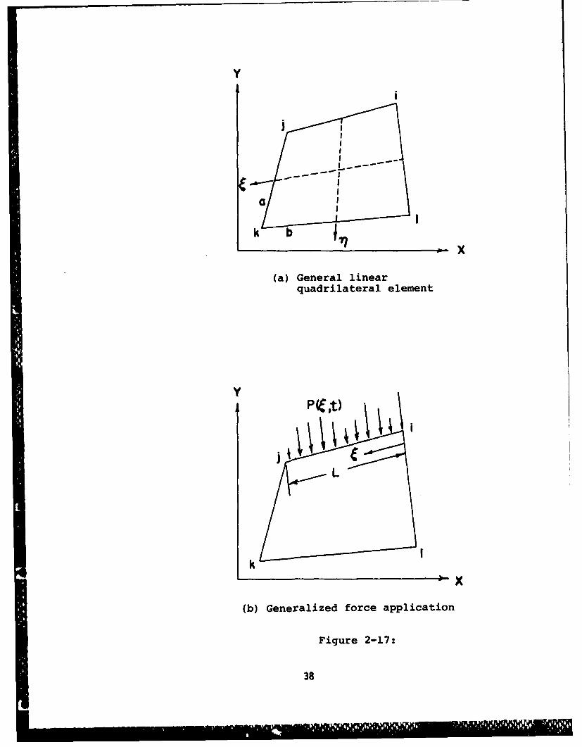
(2.3.2) General Element Description

The plane strain element described earlier can be repre-

sented by a linear quadrilateral element similar to that shown

in Figure 2-17a. The intersection of the lines which bisect

the sides of the element form a normalized coordinate system

, where;

x X6a

36

I I II I

-4 -4

T-0.i1 T-0.3

0 0

4 4 -

.2 .4 .6 .8 1.0 .2 .4 .6 .8 1.0

X/L x/L

-4 T-0.5 1 ~T-0.8

0 0

4 4

a a

.2 .4 .6 .8 1.0 .2 .4 .6 .8 1.0

X/L X/L

PLANE STRAIN,- -- --- -- PLANE STRESSSTATIC DEFLECTION CURVES: COMPARISON OF DIFFERENT ELEMENT TYPES

Figure 2- 16:

37

y

ai

Ik b

(a) General linearquadrilateral element

P

k

(b) Generalized force application

Figure 2-17:

38

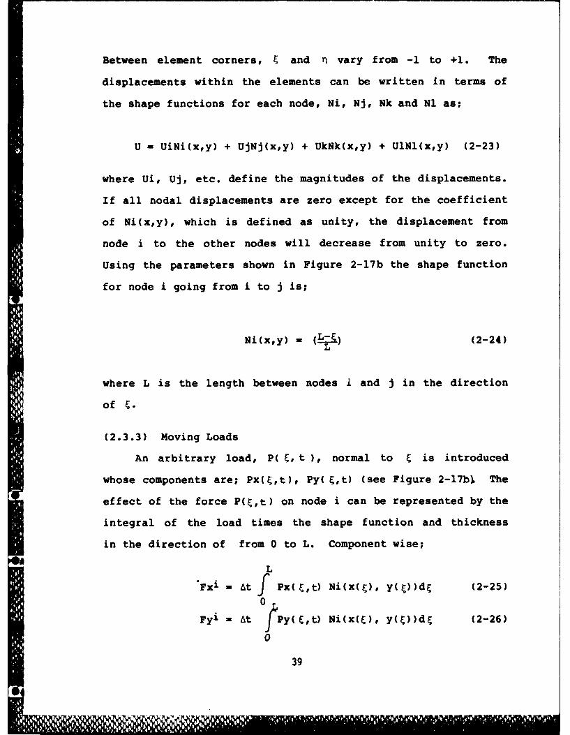
Between element corners, & and n vary from -1 to +1. The

displacements within the elements can be written in terms of

the shape functions for each node, Ni, Nj, Nk and Ni as;

U = UiNi(x,y) + UjNj(x,y) + UkNk(x,y) + UlNl(x,y) (2-23)

where Ui, Uj, etc. define the magnitudes of the displacements.

If all nodal displacements are zero except for the coefficient

of Ni(x,y), which is defined as unity, the displacement from

node i to the other nodes will decrease from unity to zero.

Using the parameters shown in Figure 2-17b the shape function

for node i going from i to j is;

Ni(x,y) - (L) (2-24)L

where L is the length between nodes i and j in the direction

of F-

(2.3.3) Moving Loads

An arbitrary load, P( &, t ), normal to is introduced

whose components are; Px(E,t), Py( &,t) (see Figure 2-17b The

effect of the force P(&,t) on node i can be represented by the

integral of the load times the shape function and thickness

in the direction of from 0 to L. Component wise;

L

Fxi - At f Px(E,t) Ni(x(), y(t))dE (2-25)0

Fyi - At fPy(&,t) Ni(x(), y(.))d& (2-26)

0

39

where; At is the element thickness (assumed to be unity).

Inserting the shape function for node i into equations (2-25)

and (2-26) yields;

L

Fxi - Px(E,t) ( ldE (2-27)

Fyi M Py(,t) (-L-)dE (2-28)

0Equations (2-27) and (2-28) give the load history at node i as

a function of &t), resulting from the arbitrary load PlE,t).

Conversely, the load history at node j is determined by

considering the shape function obtained when going from node

j to i with j at zero and i at unity. Here the shape function

starts at zero and increases to unity as;

Nj(x,y) =- (2-29)L

Substituting equation (2-29) into equations (2-25) and (2-26)

yields the force in the x and y directions experienced at node

J, resulting from P(,t).

Fxi . fPx(E,t) ( )dE (2-30)

Fyi - (,t) ( )dE (2-31)

0Equations (2-27), (2-28), (2-30) and (2-31) can be used to

represent a moving load by introducing the Dirac Delta

Function. When used in an integral, it translates a given

function to the origin and gives the value of a function at a

given time at the origin. The argument of the delta function

40

takes the form of the variation in the position variable. For

a moving load with constant velocity, the change in position

is given by the velocity times the time. The arbitrary moving

load then takes the form;

P(Ct) - P(t)V(C-Vot)

where Vo is the velocity and t the time. Using the delta

function in the integrand results in all occurences of being

replaced by Vot. Thus, the four force equations become;

Fx i - Px(t) (L-Vot, (2-32)L

Fyi = Py(t) (L (2-33)L

VotFxj = Px(t) (-) (2-34)

FyJ = Py(t) (--Vt ) (2-35)

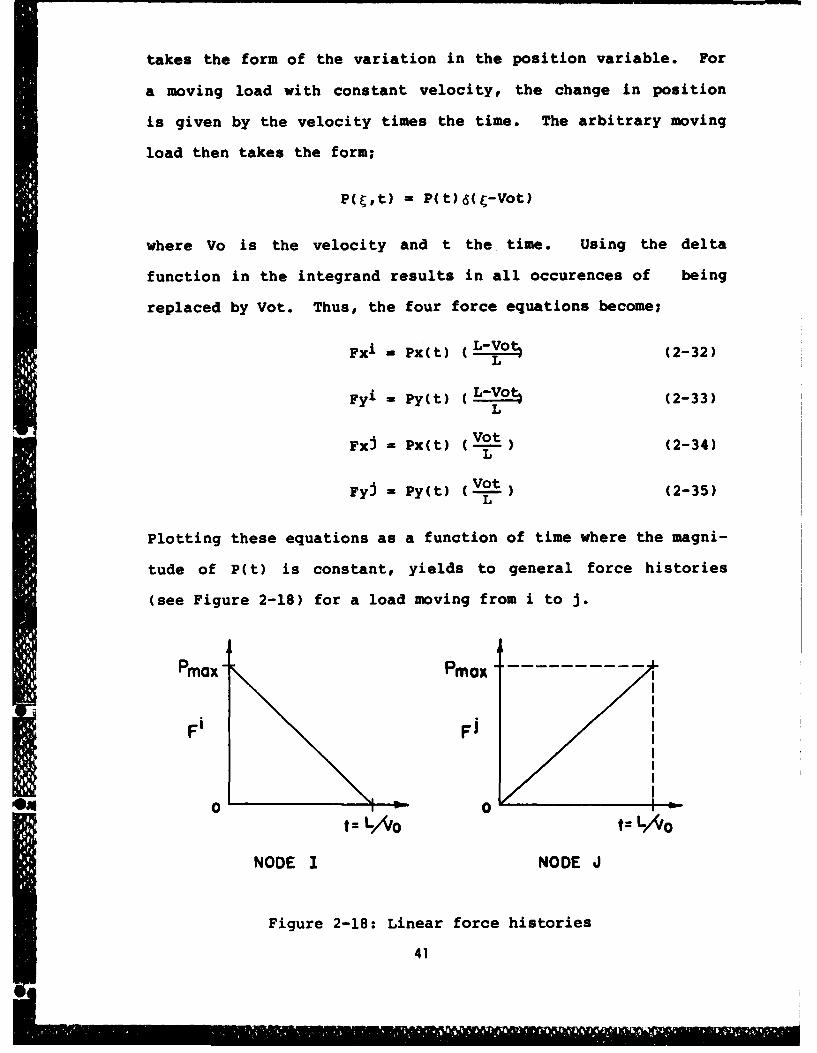
Plotting these equations as a function of time where the magni-

tude of P(t) is constant, yields to general force histories

(see Figure 2-18) for a load moving from i to j.

Pmox Pmox-------

F' Fj

0 0 it-t= O t= LAO

NODE I NODE J

Figure 2-18: Linear force histories

41

For an actual meshing gear set, the speed of the moving

load on a single tooth is not constant, but varies linearly

with time. The time varying speed can be seen to be (see

Appendix 2);

V(t) - RB w2 t

Now, the force equations take a different form with 8 being

replaced by the displacement resulting from the above velocity;

RB 2 t

S(t) 2

where A can replace the quantity RBw2/2;

S(t) - At 2

For the time varying load the force equations then become;

L-At2

Fi - P(t) ( L (2-36)

At2

FJ - P(t) (L--) (2-37)

where the x and y subscripts are assumed.

42

3. DISCUSSION OF NAGAYA ANALYSIS

Although the problem of theoretically analyzing dynamic

gear tooth deflections has been treated extensively [1-511101,

models addressing the problem assume that the variation in

tooth stiffness can be approximated using a static deflection

analysis. These models assume that the gear hubs act as rigid

bodies and that the teeth act as variable stiffness springs.

The stiffness of the teeth varies with the contact position

along the tooth and is generally arrived at using a static

deflection analysis such as the one developed by Weber (12).

Recently, K. Nagaya and S. Uematsu [71 proposed that since the

contact point moves along the tooth during the meshing cycle,

the dynamic load response should be considered as a function of

both the position and the speed of the moving load. In their

paper they generate plots of normalized gear tooth centerline

deflection curves from which they claim the equivalent spring

constant of gear teeth can be determined.

(3.1) Approximating A Gear Tooth with a Timoshenko Beam

In Nagaya's analysis, the differential equations for a

tapeuad Timoshenko beam are written and solved, in the form of

an eigenvalue problem, from which a modal response analysis is

used to determine tooth deflections due to moving loads.

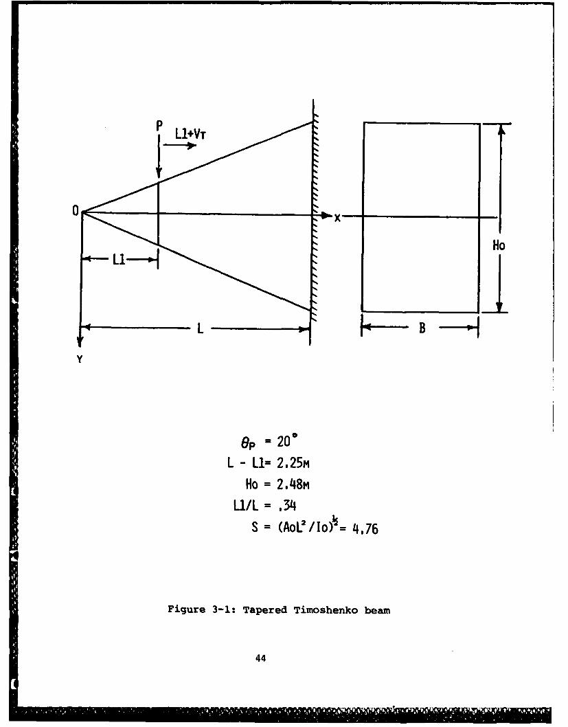
Nagaya assumed a load of constant magnitude moving along the

beam at a constant velocity from the tip to the base of the

tooth (see Figure 3-1).

Using Kara's [81 assumption for the profile of gear

43

0P

Ho

Op 200

L - L1= 2,25m

Ho = 2.48m

LI/L = .34S = (Aol!/Io) = 4.76

Figure 3-1: Tapered Timoshenko beam

44

teeth, Nagaya claimed that the deflections obtained using the

beam approximation were applicable to any spur gear defined by

the parameters

Pressure Angle = 200

L - Li = 2.25 m

Ho - 2.48 m

Ll/L - .34

S - (AoL2/Io) - 4.76

where m is the module, L, Li, Ho are shown in Figure 3-1, and S

is the slenderness ratio. The module, m, is the pitch diameter

divided by the number of teeth, measured in inches. When ana-

lyzing a gear tooth the above parameters are used to describe

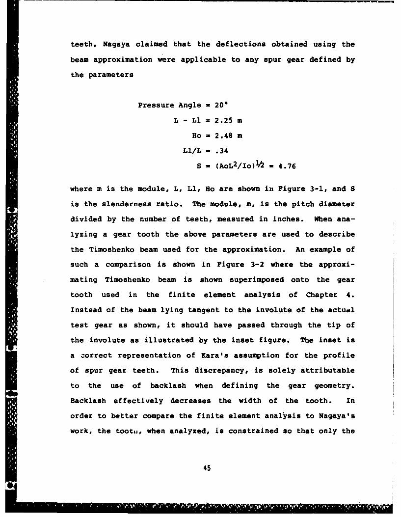
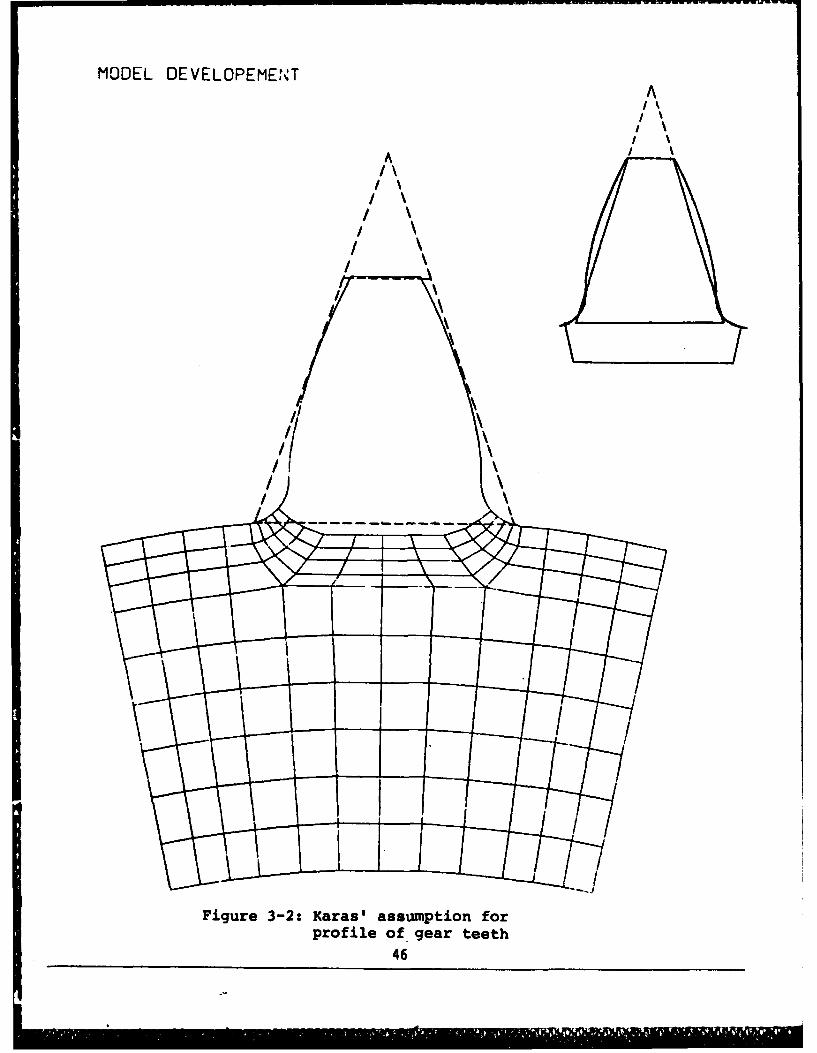
the Timoshenko beam used for the approximation. An example of

such a comparison is shown in Figure 3-2 where the approxi-

mating Timoshenko beam is shown superimposed onto the gear

tooth used in the finite element analysis of Chapter 4.

Instead of the beam lying tangent to the involute of the actual

test gear as shown, it should have passed through the tip of

the involute as illustrated by the inset figure. The inset is

a Correct representation of Kara's assumption for the profile

of spur gear teeth. This discrepancy, is solely attributable

to the use of backlash when defining the gear geometry.

Backlash effectively decreases the width of the tooth. In

order to better compare the finite element analysis to Nagaya's

work, the toot&, when analyzed, is constrained so that only the

45

MODEL DEVELOPEME.-JA

/ A

Figure 3-2: Karas' assumption forprofile of gear teeth

46

portion void of interior elements is allowed to deform (see

Figure 3-2). The foundation and rim are constrained against

motion. Later on, the deflection of the gear tooth is again

analyzed with the tooth, foundation, and rim allowed to deform.

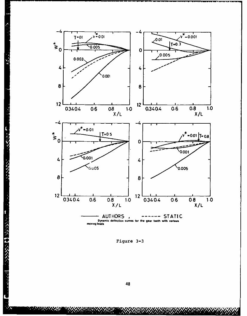
(3.2) Interpretation of Nagaya Results

When presenting his findings, Nagaya plotted normalized

tooth centerline deflections versus normalized load position

for different moving load speeds. Figure 3-3, taken directly

from reference 171, illustrates these results. The solid cur-

ves in the figure represent normalized tooth centerline deflec-

tions, each one for a different normalized velocity, V*. The

vertical arrows labelled T represent the load position relative

to the length of the tooth, where X/L is the ratio of the posi-

tion of the load on the tooth relative to the total length L.

The dotted lines are the static curves obtained from the Karas

analysis. By normalizing these parameters; deflection, load

position, and velocity, the results then become applicable to

any size gear tooth.

Non-dimensional deflections can be represented by;

W* - AoEW/PL

where

Ao - Area of the base of the tooth (in2 )

E = Elastic modulus (Psi)

W - Actual tooth deflection indirection of applied load (in)

P - Applied load (lbs)

L - Extended tooth length (in)

47

W.

-4 *-4

T-. V010.01 /V=0.001* T=0. 3

,000

44 4

8 8

12120Q3404 0.6 0.8 1.0 0.340.4 0.6 0.8 1.0

X /L X /L

0 0

12 1 1120.340.4 0.6 0.8 1.0 0.340.4 0.6 0.8 1.0

X/L X/L

AUTHORS --------------- STATICDynamic deflection curves for the gear teeth with various

moving loads

Figure 3-3

48

0111 1p

The velocity in normalized form is written as;

v* = vl

where;

V = Speed of moving load (in/sec)

E = Elastic modulus (Psi)

p - Material density (lb/in 3 )

In this equation the denominator represents the wave velocity

in bars. Finally, the position of the moving load is given by;

T = Vt/(L-LI)

where;

V = Speed of the moving load (in/sec)

t - Elapsed time (sec)

(L-Ll) = Actual tooth height (in)

From the plots shown in Figure 3-3, Nagaya claims that the

deflections of gearteeth, subjected to moving loads, vary with

the speed of the moving load. That is, for the same values of

T, the displacements are directly related to the speed of the

load. He states that for slowly moving loads, the dynamic

response reduces Lo the case of a step function impact load for

small values of T (see T-0.1, V*=0.001 in Figure 3-3). Since

Figure 3-3 indicates that the dynamic response is dependent on

the moving load speed (due to effects of inertia forces of the

mass of the tooth), Nagaya states that the stiffness of the

tooth must also depend on the moving load speed. he then

claims that the varying tooth stiffnesses can be determined

49

from these plots. However, as later demonstrated, Nagaya's

claim that the response, and therefore the stiffness, is depen-

dent on the speed of the moving load is a false one.

A major portion of the present work is directed towards

substantiation of this conclusion.

50

4. FINITE ELEMENT ANALYSIS

The deflections of single spur gear teeth with moving

loads acting on them are determined using finite element analy-

sis. A single gear tooth is used for six different moving load

cases. First, the same moving load scheme used by Nagaya [7)

(constant magnitude and speed) is applied to the tooth, which

is constrained according to the Timoshenko beam approximation.

Then the load application on the tip of the tooth is changed

slightly and the test repeated on the tooth with the same

constraints. The two preceeding load cases are then applied to

a tooth allowing the entire model to deform, including the rim.

Finally, an idealized load function, with variable load magni-

tude and speed, is applied to the tooth using both constraint

cases.

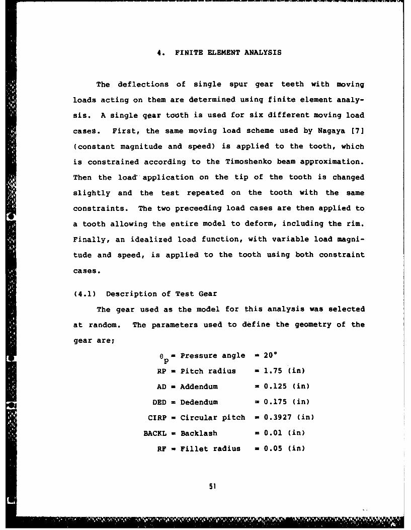
(4.1) Description of Test Gear

The gear used as the model for this analysis was selected

at random. The parameters used to define the geometry of the

gear are;

p Pressure angle = 20*

RP = Pitch radius = 1.75 (in)

AD = Addendum = 0.125 (in)

DED = Dedendum = 0.175 (in)

CIRP = Circular pitch - 0.3927 (in)

BACKL = Backlash = 0.01 (in)

RF - Fillet radius - 0.05 (in)

51

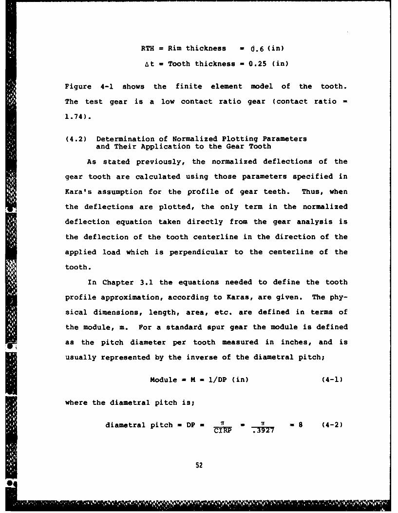
RTH = Rim thickness W d.6 (in)

At = Tooth thickness - 0.25 (in)

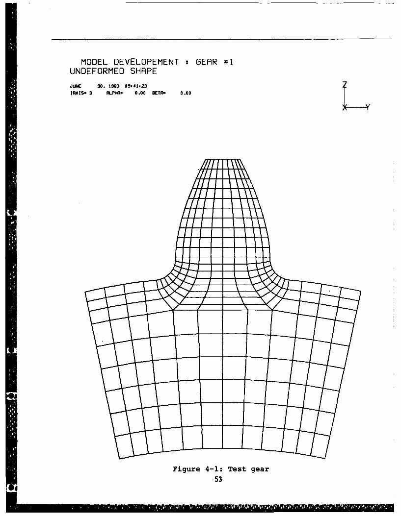
Figure 4-1 shows the finite element model of the tooth.

The test gear is a low contact ratio gear (contact ratio =

1.74).

(4.2) Determination of Normalized Plotting Parameters

and Their Application to the Gear Tooth

As stated previously, the normalized deflections of the

gear tooth are calculated using those parameters specified in

Kara's assumption for the profile of gear teeth. Thus, when

the deflections are plotted, the only term in the normalized

deflection equation taken directly from the gear analysis is

the deflection of the tooth centerline in the direction of the

applied load which is perpendicular to the centerline of the

tooth.

In Chapter 3.1 the equations needed to define the tooth

profile approximation, according to Karas, are given. The phy-

sical dimensions, length, area, etc. are defined in terms of

the module, m. For a standard spur gear the module is defined

as the pitch diameter per tooth measured in inches, and is

usually represented by the inverse of the diametral pitch;

Module - M - l/DP (in) (4-1)

where the diametral pitch is;

diametral pitch - DP - i - - 8 (4-2)

52

MODEL DEVELOPEMENT : GEAR #1UNDEFORMED SHAPE

JUNE 30. 1983 09@41o23IRXISm 3 RLPHR- 0.00 BETA- 0.00

Figure 4-1: Test gear

53

To further define the test gear, the number of teeth can be

calculated from;

number of teeth = N = 2RP*DP = 2(l.75)(8) - 28 (4-3)

Given either the diametral pitch or the number of teeth, the

module can easily be obtained.

m= 0.125 (in)

Using the value for the module and the relations of Chapter

3.1, the dimensions of the approximating Timoshenko beam are

determined. The height of the corresponding beam becomes;

(L-Li) = 2.25m = 0.28125 (in) (4-4)

and the extended length;

L - (L±1) - 0.42614 (in) (4-5)0.66

At the base, the beam thickness is;

Ho = 2.48m = 0.31 (in)

and thus the area at the base;

Ao = HoAt = (0.31)(0.25) - 0.775 (in) (4-6)

Given the above parameters, the non-dimensional deflections can

be plotted using;

W* - AoEW/PL (4-7)

Again, it should be emphasized that although the beam approxi-

mation (shown in Figure 3-2)'does not match the tooth exactly,

54

the dimensions just determined in equations (4-5) and (4-6) are

still used in the normalized deflection equation when plotting

results for the actual tooth.

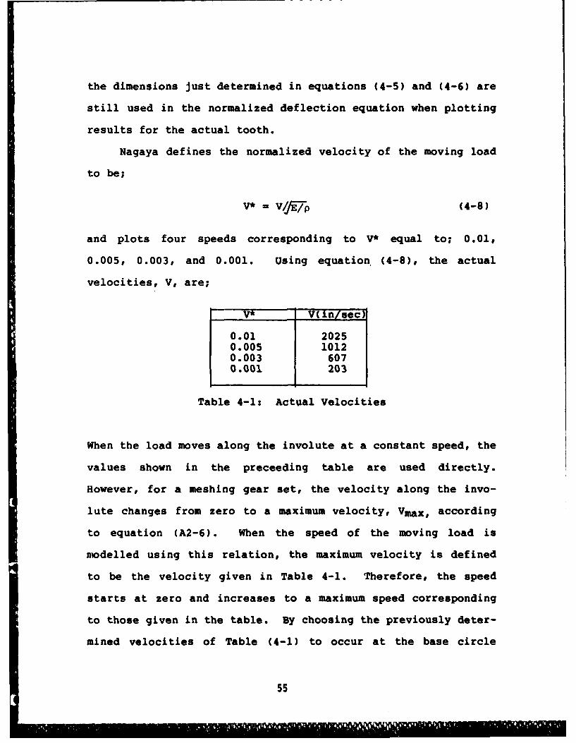
Nagaya defines the normalized velocity of the moving load

to be;

V* - V6/-p (4-8)

and plots four speeds corresponding to V* equal to; 0.01,

0.005, 0.003, and 0.001. Using equation (4-8), the actual

velocities, V, are;

V* V(in/sec)

0.01 20250.005 10120.003 6070.001 203

Table 4-1: Actual Velocities

When the load moves along the involute at a constant speed, the

values shown in the preceeding table are used directly.

However, for a meshing gear set, the velocity along the invo-

lute changes from zero to a maximum velocity, Vmax, according

to equation (A2-6). When the speed of the moving load is

modelled using this relation, the maximum velocity is defined

to be the velocity given in Table 4-1. Therefore, the speed

starts at zero and increases to a maximum speed corresponding

to those given in the table. By choosing the previously deter-

mined velocities of Table (4-1) to occur at the base circle

55

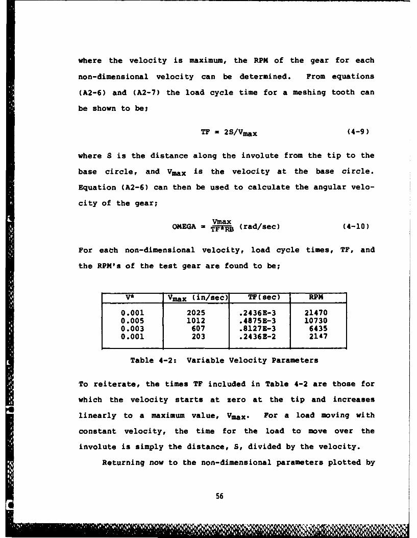
where the velocity is maximum, the RPM of the gear for each

non-dimensional velocity can be determined. From equations

(A2-6) and (A2-7) the load cycle time for a meshing tooth can

be shown to be;

TF = 2S/Vmax (4-9)

where S is the distance along the involute from the tip to the

base circle, and Vmax is the velocity at the base circle.

Equation (A2-6) can then be used to calculate the angular velo-

city of the gear;

VmaxOMEGA = T--B (rad/sec) (4-10)

For each non-dimensional velocity, load cycle times, TF, and

the RPM's of the test gear are found to be;

V* Vmax (in/sec) TF(sec) RPM

0.001 2025 .2436E-3 214700.005 1012 .4875E-3 107300.003 607 .8127E-3 64350.001 203 .2436E-2 2147

Table 4-2: Variable Velocity Parameters

To reiterate, the times TF included in Table 4-2 are those for

which the velocity starts at zero at the tip and increases

linearly to a maximum value, Vmax. For a load moving with

constant velocity, the time for the load to move over the

involute is simply the distance, S, divided by the velocity.

Returning now to the non-dimensional parameters plotted by

56

fflkmm C&. baf-.

Nagaya, for a constant speed moving load the position of the

load along the involute is given by;

T- Vt (4-11)

where T varies from 0.0 at the tip, to 1.0 at the root circle.

A value T=0.8 correponds to a point near the base circle

radius between nodes 110 and 121 (see Figure 2-12). Equation

(4-11) is valid only for constant speeds, V.

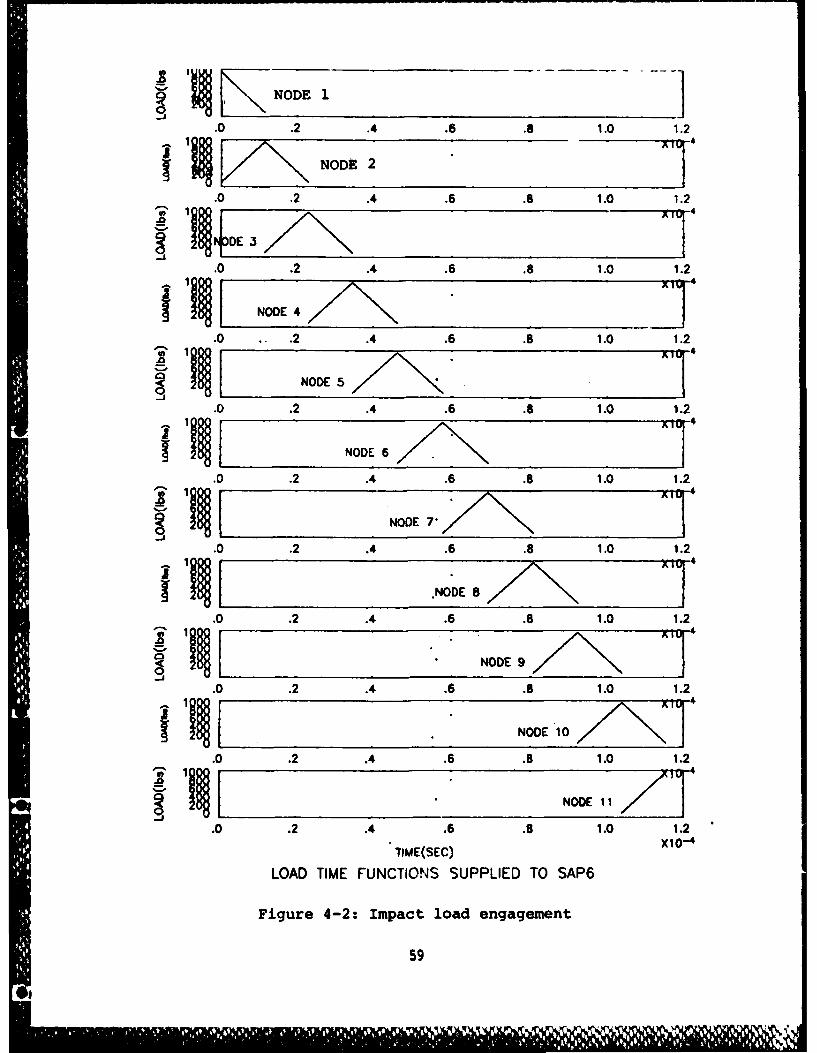
(4.3) Description of Dynamic Loading Cases

The dynamic deflections of single spur gear teeth are

generated using three loading cases; a constant speed constant

magnitude load with impact engagement, a constant speed

constant magnitude load using a finite load engagement rise

time (for these two loading cases the load is applied normal

to the tooth centerline), and a load with varying speed and

magnitude. In this last case the load is applied normal to

the involute.

The first of these three loading cases is designed to imi-

tate exactly the forcing function used by Nagaya. At time

equal to zero, a load of 1000 lbs, simulating an impact load,

is applied to the tip of the tooth, and maintained until the

end of the load cycle (i.e. from the tip to the base circle).

(Whenever the terms "impact loading" are used, the author is

describing a step function). To simulate this loading con-

dition for the finite element analysis, time functions repre-

senting nodal load histories are calculated for each node on

57

the involute. For the load moving between nodes i and j, the

force histories are described by equations (2-36) and (2-37);

VtF - P(t) ( -) (4-12)

Fj - P(t) (Vt) (4-13)

where; L is the distance between nodes, V is the velocity of

the moving load, and t the time. With several load value data

points defined along the involute, the finite element code uses

these points and linearly interpolates between them to define

the time functions. The time functions for this loading case

are shown in Figure 4-2. In Figure 4-2 the node numbers

correspond to the first eleven nodes on the right involute sur-

face of the tooth.

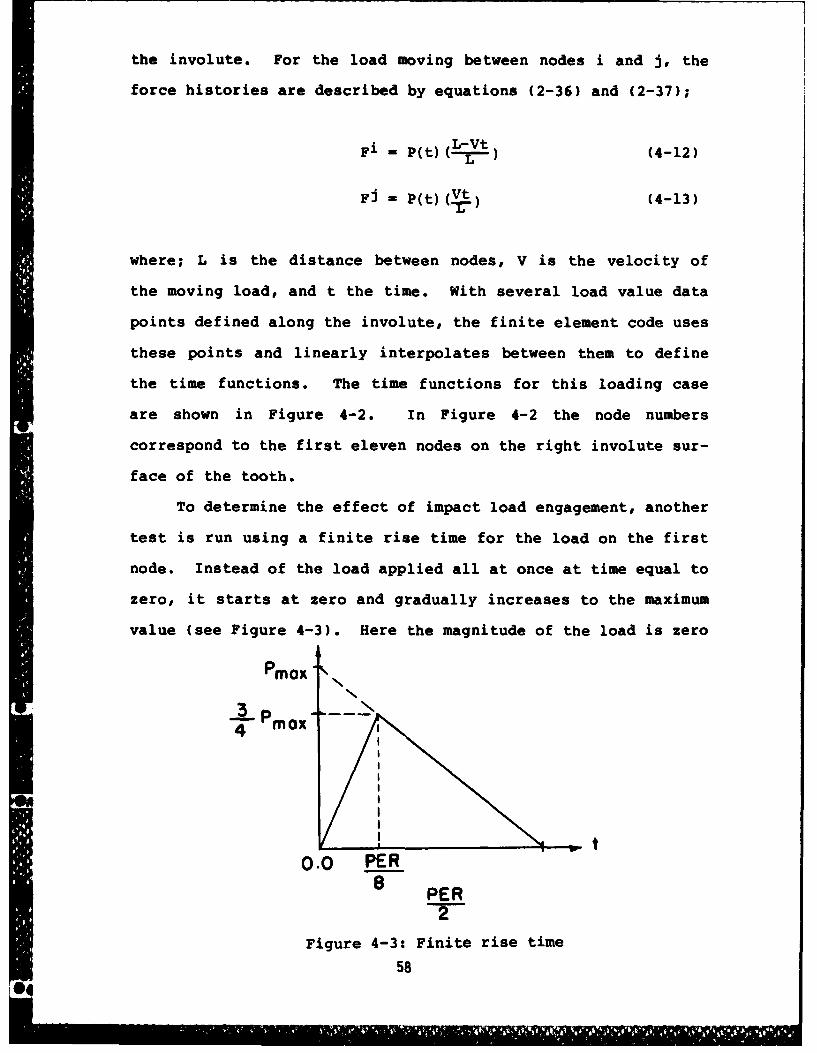
To determine the effect of impact load engagement, another

test is run using a finite rise time for the load on the first

node. Instead of the load applied all at once at time equal to

zero, it starts at zero and gradually increases to the maximum

value (see Figure 4-3). Here the magnitude of the load is zero

3PPmax

0.0 P__

8 PER

2

Figure 4-3: Finite rise time

58

NODEl 1

.0 .2 .4 .6 .8 1.0 1.2

i'NODE 2

•0 .2 .4 .6 .8 1.0 1.2

11D- Al

S•0.2 .4 .6 .8 1.01.

NDE 7"

.0 .2 .4 .6 .8 1.0 1.21-068 NOD NODE41

.0 .2 .4 .6 .8 1.0 1.20N OE NODE

.0 .2 .4 .6 .8 1.01.1Al 10

.2.4. NODE l 1

.0 .2 .4 .6 .8 1.01.

co~N D 11NDE 7

.0 .2 .4 .6 .8 1.0 1.2

Figure 4-2: Impact load engagement

59

e0

b0

Ii

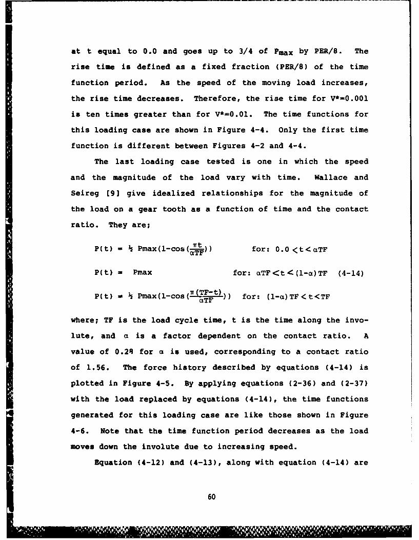
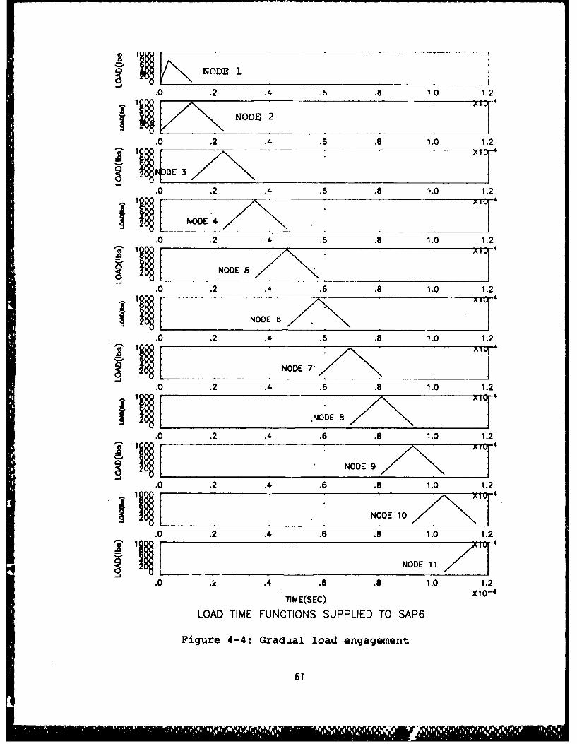
at t equal to 0.0 and goes up to 3/4 of Pmax by PER/8. The

rise time is defined as a fixed fraction (PER/8) of the time

function period. As the speed of the moving load increases,

the rise time decreases. Therefore, the rise time for V*=0.001

is ten times greater than for V*=0.01. The time functions for

this loading case are shown in Figure 4-4. Only the first time

function is different between Figures 4-2 and 4-4.

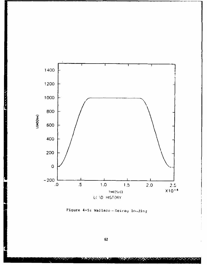
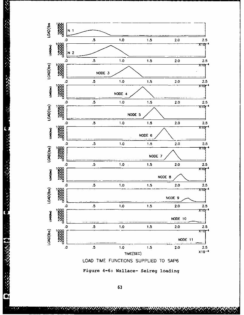
The last loading case tested is one in which the speed

and the magnitude of the load vary with time. Wallace and

Seireg [91 give idealized relationships for the magnitude of

the load on a gear tooth as a function of time and the contact

ratio. They are;

P(t) = Pmax(l-cos(--)) for: 0.0 <t<cTF

P(t) = Pmax for: aTF<t (l-a)TF (4-14)

P(t) - h Pmax(l-cos(tW(TF- t) for: (l-a)TF~t<TFcTF

where; TF is the load cycle time, t is the time along the invo-

lute, and a is a factor dependent on the contact ratio. A

value of 0.24 for a is used, corresponding to a contact ratio

of 1.56. The force history described by equations (4-14) is

plotted in Figure 4-5. By applying equations (2-36) and (2-37)

with the load replaced by equations (4-14), the time functions

generated for this loading case are like those shown in Figure

4-6. Note that the time function period decreases as the load

moves down the involute due to increasing speed.

Equation (4-12) and (4-13), along with equation (4-14) are

60

NODE 1

.0 .2 .4 .6 .8 1.0 1.2

NODE 2

.0 .2 .4 .6 .8 1.0 1.200 3

NDD 3!t ND

.0 .2 .4 .6 .8 1.0 1.2

.2 .4 .6 .81.12

100[ NODE 4 4

.2 .4 .6 .8 1.0 1.2

.0 .2 .4 .6 .8 1.0 1.2

1100

004

00 NODE 6

.0.2 .4 .6 .8 1.0 1.2

00 NODE 7 *

.0 .2 .4 .6 .8 1.01.

00 NODE 10

.0 .2 .4 .6 .8 1.0 1.2

llNODEE11

.0 .2 .4 .6 .8 1.0 1.21tME00C xl 4.

LODTM0UCINSSPLE0OSP

1igur 4-:Gada-oa4nagmn

060

1400 ]12001

1000

800

g 600

400

200

0

-200 I.0 .51.0 1.5 2.02.

TIME(stc) X10- 4

LU '.D HISToRY

Figure 4-5: Walace -Seit-ey 1oiding

62

.0 .5 1.0 1.5 2.0 2.5

.0 .5 1.0 1.5 2.0 2.5

00

NOE

.0 .5 1.0 1.5 2.0 2.5

I~j NODE 4_ _ _ _

.0.5 1.0 1.5 2.0 2.5

00

_ _ _ NODE5 52.25

1 _____NODE\_6:

0.51.0 1.5 2.0 2.5

00

_ _ _ NODE08

.0 .5 1015202.5

.0 .5 1.0 1.5 2.0 2.5110 4 nt

6001GOX NODE9

.. 51.0 1.5 2.02.

00 NODE 10.0 .5 1.0 1.5 2.0 2.5

00_ NODE

10 .0 .5 1.0 1.5 2.0 --2.5

TIME(SEC) X10-4

LOAD TIME FUNCTIONS SUPPLIED TO SAP6

Figure 4-6: Wallace- Seireg loading

63

used in a time function generation algorithm which is included

in Appendix 1.

(4.4) Finite Element Test Results

The results contained in the proceeding sections were

obtained using the SAP6 finite element code, implemented on the

UNIVAC 1100/80 computer facility at Michigan Technological

University.

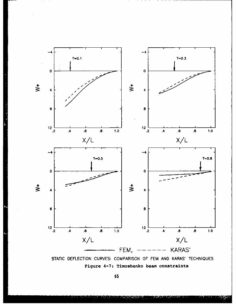
(4.4.1) Comparison of Static Results

As a preliminary check on the accuracy of the finite ele-

ment analysis technique applied to gear teeth, static-

deflections obtained using finite elements are compared to

those calculated by Nagaya using Kara's assumption for the pro-

file of gear teeth. Comparisons are made with and without the

rim included in the analysis. Figure 4-7 shows the plots of

the normalized centerline deflections obtained using Timoshenko

beam constraints. The dashed lines are the static deflections

calculated by Nagaya. From the figure it is apparent that the

Timoshenko beam (used to produce the dashed lines) is stiffer

than the tooth. Going back to Figure 3-2, it is seen that the

beam is considerably larger than the tooth, especially towards

the base. Thus one would expect the beam to be stiffer. As

the load is applied closer to the base of the tooth the dif-

ference between the static deflection curves becomes less

exaggerated. For T=0.8 the centerline of the tooth actually

deflects less than the beam. The reasons for this are not

completely clear. One possible explanation, however, is the

64

......

-4 -4T=0. 1 T=0.3

o oe

4

8 8

12 II 12.2 .4 .6 .8 1.0 .2 .4 .6 .8 1.0

X/L X/L

-4 -4T-0.5 T-0.8

0 0

4 4

12 I12a

.2 .4 .6 .8 1.0 .2 .4 .6 .8 1.0

x/L x/LFEM - -- -- -- KARAS'

STATIC DEFLECTION CURVES: COMPARISON OF FEM AND KARAS' TECHNIQUES

Figure 4-7: Timoshenko beam constraints

65

fact that as the load is applied closer to the base, the amount

of local deformation around the point of load application

increases due to increased nodal spacing. This causes the

tooth centerline to deform around the local deformation, thus

decreasing the overall deflection of the gear tooth. (Appendix

3 includes the actual tooth in the statically deformed con-

dition, illustrating the increase in local deformation). In

these figures, the compatibility of the element is not

violated. The deformation scale factor causes element overlap.

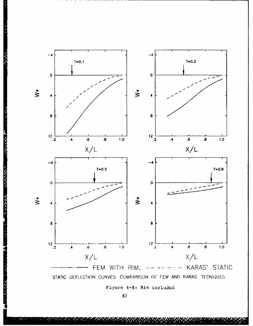
With the rim included in the analysis, the centerline

deflections are considerably more severe (see Figure 4-8).

The curves obtained by Nagaya, represented by the dashed line,

are exactly those pictured on Figure 4-7. The purpose of this

set of plots (Figure 4-8) is to emphasize the added flexibility

afforded by the rim material. (Appendix 3 also contains the

tooth in the deflected state with the rim included).

(4.4.2) Modal Analysis - Determination of Mode Shapes and

Natural Frequencies

In Nagaya's paper, the differential equation for the non-

dimensional deflection, W*, is derived and then solved numeri-

cally. The solution to the differential equation (eigenvalue

problem) includes an infinite number of natural frequencies

(eigenvalues) and an infinite number of mode shapes

(eigenvectors). However, he included only the first three

eigensolutions in the dynamic response analysis. It should

also be mentioned that the differential formulation is done for

transverse vibration so only bending modes are included.

66

-4 -4

T-O. 1 T-0.3

3: 4

8 8

12 I I 12 2 '.2 .4 .6 .8 1.0 .2 .4 .6 .8 1.0

X/L X/LI I I 1I , , I

-4 -4

T=0.5 T-0.8

0 ~1-- - -0---

4 4

8 a

12 ' . --. A , ___L 12 ,.2 .4 .6 .8 1.0 .2 .4 .6 .8 1.0

X/L X/L

-- FEM WITH RIM, KARAS' STATIC

STATIC DEFLECTION CURVES: COMPARISON OF FEM AND KARAS TECNIQUES

Figure 4-8: Rim included

67

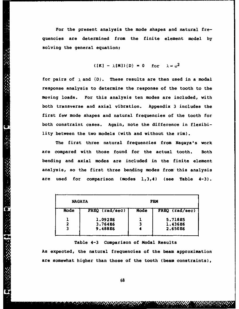
For the present analysis the mode shapes and natural fre-

quencies are determined from the finite element model by

solving the general equation;

([K] - A[M]){D} = 0 for X= W2

for pairs of X and {DI. These results are then used in a modal

response analysis to determine the response of the tooth to the

moving loads. For this analysis ten modes are included, with

both transverse and axial vibration. Appendix 3 includes the

first few mode shapes and natural frequencies of the tooth for

both constraint cases. Again, note the difference in flexibi-

lity between the two models (with and without the rim).

The first three natural frequencies from Nagaya's work

are compared with those found for the actual tooth. Both

bending and axial modes are included in the finite element

analysis, so the first three bending modes from this analysis

are used for comparison (modes 1,3,4) (see Table 4-3).

NAGAYA FEM

Mode FREQ (rad/sec) Mode FREQ (rad/aec)

1 1.092E6 1 5.718E52 3.764E6 3 1.436E63 9.488E6 4 2.650E6

Table 4-3 Comparison of Modal Results

As expected, the natural frequencies of the beam approximation

are somewhat higher than those of the tooth (beam constraints),

68

partly due to the additional material toward the base of the

beam.

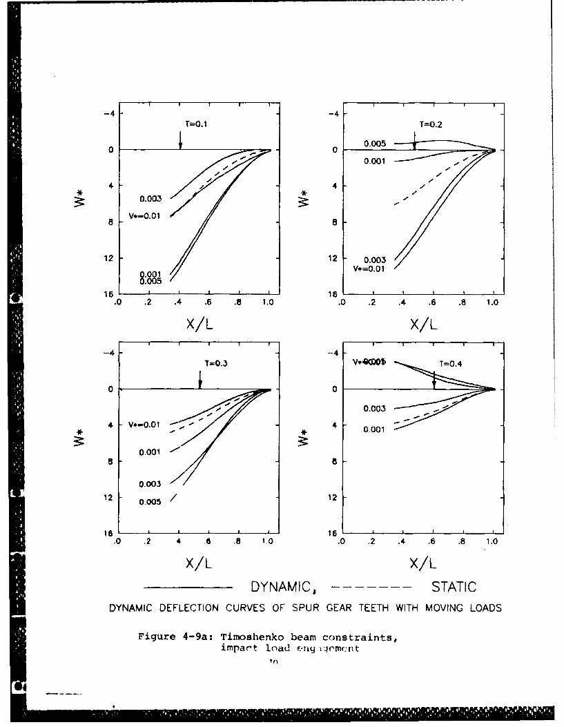
(4.4.3) Dynamic Deflections: Timoshenko Beam Constraints

(4.4.3.1) Impact Loading

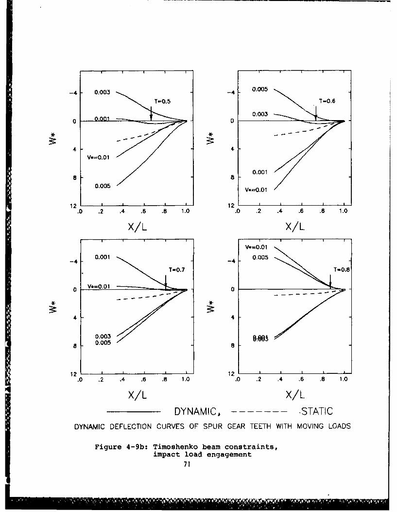
Shown in Figures 4-9a and 4-9b are the normalized cen-

terline deflections obtained using the impact engagement

loading case (see Figure 4-2). Results are obtained for load

positions of T-0.1,0.2,...,0.8. Each solid line represents

the non-dimensional centerline deflection;

W* - AoEW/PL

due to the applied moving load. Remember also that the deflec-

tions are plotted as a function of position;

Vt

and not as a function of time. So for T=0.1 the solid lines

show the normalized centerline deflections for the different

speeds with the load one tenth the distance between the tip and

the root. Remember also that the time for the load to move

from T-0 to T-0.1 is different for all velocities, V*. The

dashed lines correspond to the static deflections obtained for

the tooth with the load in the position shown.

Initial examination of these plots suggests that the

displacements are indeed dependent on the speed of the moving

load. For slow speeds and low values of T (V*=0.00l, T-0.1),

the deflection is approximately twice the static as Nagaya

69

-4 -4T=0.1 T=0.2

0 0 .0-- 0.001

4 40.003

V*-O.01

12 12 0.003

8.001 v*=0.018.005

16 1 1 16 _ _ _ _ _ _ _ _ __.0 .2 .4 .6 .8 1.0 .0 .2 .4 .6 .8 1.0

X/L X/L•I ! !! !I I I

-4 -4T=0.3T=.

0 0~0.003

4 V.-0.01 0.0

0.001

0.003

12 0.05 12

~16 k 16.0 .2 4 .6 .8 1.0 .0 .2 .4 .6 .8 1.0

X/L X/L

DYNAMIC, ------- STATICDYNAMIC DEFLECTION CURVES OF SPUR GEAR TEETH WITH MOVING LOADS

Figure 4-9a: Timoshenko beam constraints,impart load eng comcrt

I

-4 0.03 -4 0.005

T-0.6

0o ,0 -- 0 0.3

4 4Vs=0.0 1

0.00 1

0.00f5 V*=0.0i

12 12. .2 4 . .8 10.0 .2 .4 .6 .8 1.0

X/L X/L

-4 0.001 -4 0.5

T-0.7T=.

0*=0.010

4 4

0.003a 0.005 8

12 - L1.0 .2 .4 .6 .8 1.0 .0 .2 .4 .6 .8 1.0

X/L x/L

DYNAMIC,- -- --- --- STATICDYNAMIC DEFLECTION CURVES OF SPUR GEAR TEETH WITH MOVING LOADS

Figure 4-9b: Timoshenko beam constraints,impact load engagement

71

claimed. However, these plots do not give an accurate descrip-

tion of the dynamic deflections.

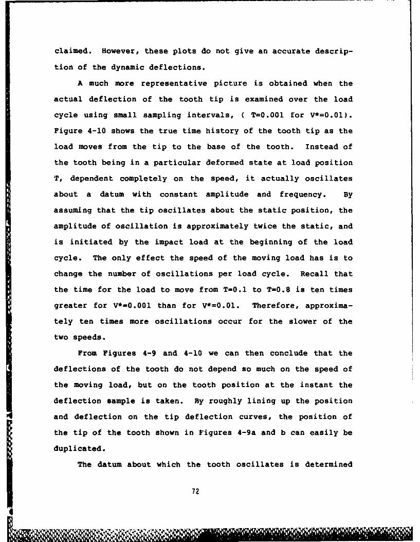
A much more representative picture is obtained when the

actual deflection of the tooth tip is examined over the load

cycle using small sampling intervals, ( T=0.001 for V*=0.01).

Figure 4-10 shows the true time history of the tooth tip as the

load moves from the tip to the base of the tooth. Instead of

the tooth being in a particular deformed state at load position

T, dependent completely on the speed, it actually oscillates

about a datum with constant amplitude and frequency. By

assuming that the tip oscillates about the static position, the

amplitude of oscillation is approximately twice the static, and

is initiated by the impact load at the beginning of the load

cycle. The only effect the speed of the moving load has is to

change the number of oscillations per load cycle. Recall that

the time for the load to move from T=0.l to T=0.8 is ten times

greater for V*=0.001 than for V*=0.01. Therefore, approxima-

tely ten times more oscillations occur for the slower of the

two speeds.

From Figures 4-9 and 4-10 we can then conclude that the

deflections of the tooth do not depend so much on the speed of

the moving load, but on the tooth position at the instant the

deflection sample is taken. By roughly lining up the position

and deflection on the tip deflection curves, the position of

the tip of the tooth shown in Figures 4-9a and b can easily be

duplicated.

The datum about which the tooth oscillates is determined

72

20

-0

20.05 .10 .1 .20 .25 .30 5 .40

2400

S-600

-6000TOOT TIP DEFEC 0O TIME .50oy;A CO.6A0T (RSE70 E~

20ou~ 480

A 73

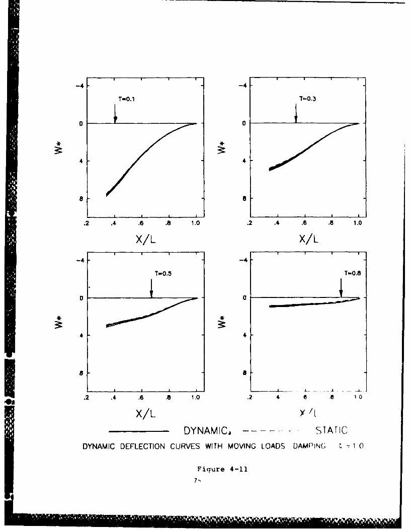
by repeating the previous analysis with the system critically

damped. The transient caused by the impact load is then

"filtered" out with only the steady state response remaining.

Figure 4-11 shows the non-dimensional centerline deflections

for all four moving load speeds. From the figure it is

apparent that all centerline deflections lay over the static

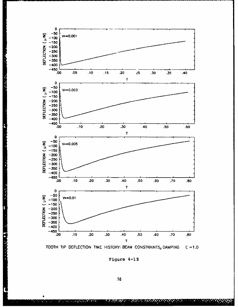
curve. To verify this claim, the tooth tip deflection

histories are again plotted. In Figure 4-12 the plots show the

tip following the static curve.

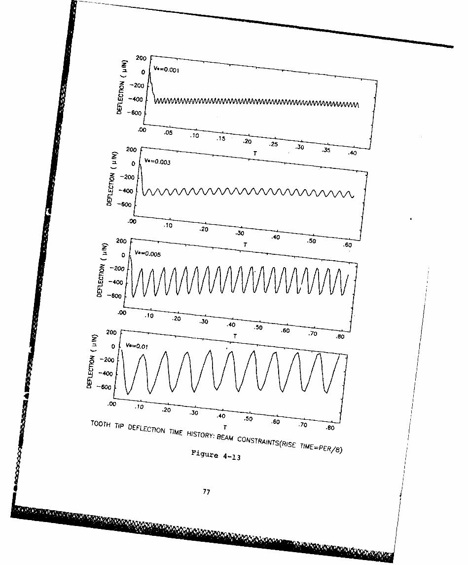
(4.4.3.2) Finite Engagement Rise Time Loading

In this test the tooth is subjected to the moving load

conditions illustrated in Figure 4-4 where the load on the

first node is gradually applied over a time of PER/B. This

loading case produces significantly different results compared

to the impact load test. (Since the normalized centerline

deflection curves do not accurately represent the dynamic

deflection phenomenon, they are not included). Figure 4-13

gives the tooth tip deflection history for this loading con-

dition. The tooth still oscillates about the static position

with constant frequency, but the amplitude varies significantly

with speed. The reason for this change, from the previous load

case, is best explained by again considering the load engage-

ment rise time.

In Chapter 4.3, Figure 4-3, the rise time is defined as a

fixed fraction of the time function nodal period (PER/8). For

V*=0.01, the rise time is ten times less than for V*-0.001.

74

0wy

I I I I

-4 -41

T-o.1 T=0.3

0 0

4 4

88

a i i l iI

.2 .4 .6 .8 1.0 .2 .4 .6 .8 1.0

X/L X/L

-4 -4

T-0.5 T-0.8

0 0

4 4

a

*A.2 .4 .6 .8 1.0 .2 .4 6 0

X/L y /t

DYNAMICA - SIATIC

DYNAMIC DEFLECTION CURVES WITH MOVING LOADS DAMPING ~-

Figure 4-11

"7

0~-50z 100V.-0.001

'--150

z - 2 0 0.....................~-250

43001,-

-450.00 .05 .10 .15 .20 25 .30 .35 .40

T0

*--150z -200

S-250w -300

-35

-4,50.00 .10 .20 .30 .40 .50 .60

T0

~--150Z-200~-250~-30~-350S-400

-450.00 .10 .20 .30 .40 .50 .60 .70 .80

T0

-.- 50

Z-200

-250_-300

~-350o-400

-450.00 .10 .20 .30 .40 .50 .60 .70 .80

T1

TOOTH TIP DEFLECTION TIME HISTORY-. BEAM CONSTRAINTS, DAMPING =1.0

Figure 4-12

76

2.00

-40

0

-20

~-600

Z 200

80o

OOU -40oEF~

BA CONS RWITS(

4001

-6077

It should then be obvious, that as the speed of the load

increases, the time function for the first node begins to

approximate the step function impact load of Figure 4-2.

Examination of the deflection amplitude for V*=0.01 of Figure

4-13 shows it to be nearly the same as V*=0.01 of Figure 4-10.

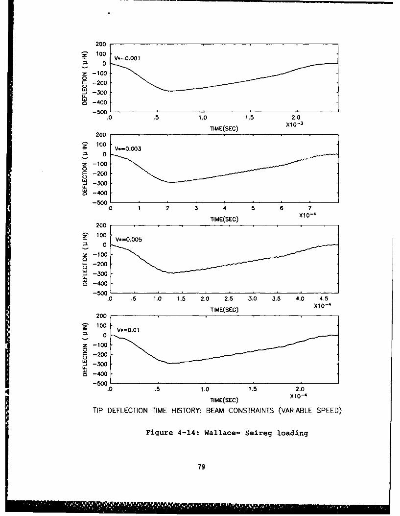
(4.4.3.3) Wallace - Seireg Loading

For this loading case (time function shown in Figure 4-6)

both the speed and magnitude of the load vary with time. With

a contact ratio of 1.56, the load doesn't reach the maximum

value of 1000 lbs until it is between the second and third

nodes. Since the magnitude increases smoothly and gradually,

no abrupt load changes are encountered.

The tooth tip deflection history curves for this loading

case are included in Figure 4-14. Due to the nature of the

speed variation, the deflections are plotted as a function of

time instead of position as done previously. Here it can be

seen that the tip of the tooth follows the static deflection

curve for each of the speeds. This is again due to the slow

and gradual engagement of the load.

(4.4.4) Dynamic Deflections: Rim Included

Including the rim adds flexibility to the system as

already mentioned. The tooth tip deflection history for the

impact loading case, shown in Figure 4-15, illustrates this

fact. As before, the amplitude and frequency of vibration are

the same for each of the four speeds. However, compared to the

beam constraint case of Figure 4-10, the amplitude is con-

78

1l

200

10 V*OO 001 0

z -1000

i~-200Q.LJ1 -300

~ 400-500

.0 .5 1.0 1.5 2.0

TIME(SEC) X10-

2 00

z -100 .... .0

wU-- 300

o 400

0 1 2 3 4 5 6 7

TIME(SEC) X1O-

2 00

z 1000

~-100

LAj -300w o400

-500.0 .5 1.0 1.5 2.0 2.5 3.0 3.5 4.0 4.5

TIME(SEC) X1O-200

S100 *00S 0

z -10005 -200w

.- 300o400

-500.0 .5 1.0 1.5 2.0

TIME(SEC) X10- 4

TIP DEFLECTION TIME HISTORY: BEAM CONSTRAINTS (VARIABLE SPEED)

Figure 4-14: Wallace- Seireg loading

79

400

2 200

00V

H-200P -800

00-8200

000

-800

020

-1000

40.0.70 .2o .30 T,.0.50 .60400

i 200

060

S-800

-1000

40 0 1 2 .30 .40 .50 .0 .70.800

200

S-800

-1000

.00 .?0 .20 .30 .40 .50 .60 70 .80

T 7

TOOTH TIP DEFLECTION TIME HISTORY: RIM INCLUDED (RISE TIME=O0)

Figure 4-15

80

siderably larger and the frequency slower.

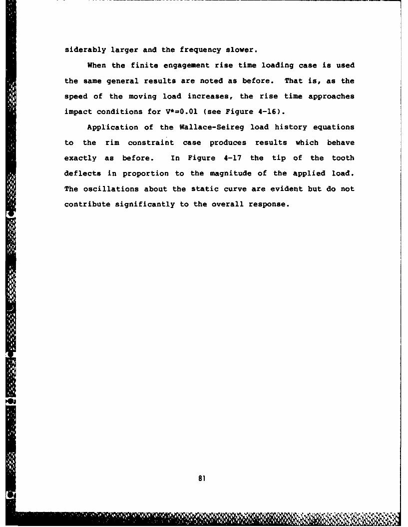
When the finite engagement rise time loading case is used

the same general results are noted as before. That is, as the

speed of the moving load increases, the rise time approaches

impact conditions for V*=0.01 (see Figure 4-16).

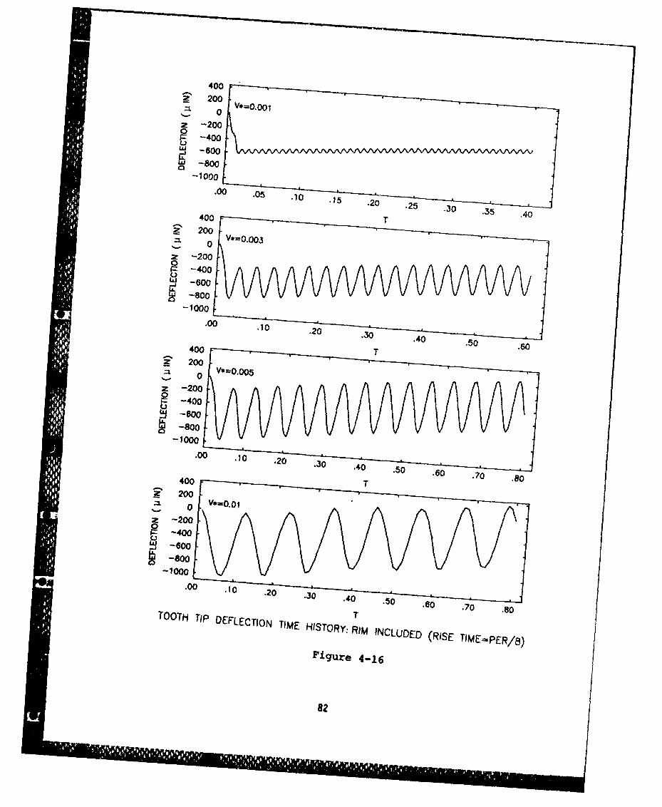
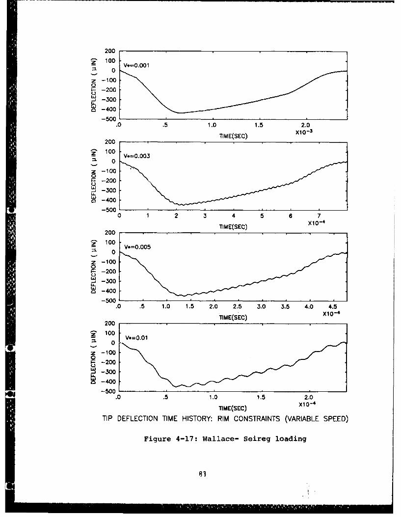
Application of the Wallace-Seireg load history equations

to the rim constraint case produces results which behave

exactly as before. In Figure 4-17 the tip of the tooth

deflects in proportion to the magnitude of the applied load.

The oscillations about the static curve are evident but do not

contribute significantly to the overall response.

81

4800-100 .00 .0 5 1 20 . 5 .3

440

200

0P -00Uw - 00'I

LaJ -800-1000

00. 00 . 5 .10 .0 .0 .5 . 0 5 .40

40z 200

040

-800-1000

4 0.0.0.0 .0 T 5 . 60 .0 .0400

' 20

z-2000P -400

-600~ 800

1000

4. 00 .10 .20 .30 .40 .50 .60 .70 .80

2082

200

z1000

z -100

0j30

-200-5 -00

.0 .5 1.0 1.5 2.0

20TIME( SEC) X10-

z 1000v*=0.003

~-100

F-20040

~-500

2-00

-500

~ 100V*=0.00520

z -100-200

~-300Ui

o 400-500

.0 .5 1.0 1.5 2.0 2.5 3.0 3.5 4.0 4.5

20.TIME(S IEC) X10- 4

10-v*=0.01

0

-500.0 .5 1.0 1.5 2.0

TIME(SEC) X1 0- 4

TIP DEFLECTION TIME HISTORY: RIM CONSTRAINTS (VARIABLE SPEED)

Figure 4-17: Wallace- Seireg loading

5. DETERMINING THE EFFECTS OF INERTIA ON THE

DYNAMIC RESPONSE OF MESHING GEAR TEETH

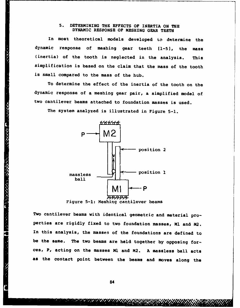
In most theoretical models developed to determine the

dynamic response of meshing gear teeth [1-51, the mass

(inertia) of the tooth is neglected in the analysis. This

simplification is based on the claim that the mass of the tooth

is small compared to the mass of the hub.

To determine the effect of the inertia of the tooth on the

dynamic response of a meshing gear pair, a simplified model of

two cantilever beams attached to foundation masses is used.

The system analyzed is illustrated in Figure 5-1.

P M2

position 2

massless position I

ball

MI P

Figure 5-1: Meshing cantilever beams

Two cantilever beams with identical geometric and material pro-

perties are rigidly fixed to two foundation masses, M1 and M2.

In this analysis, the masses of the foundations are defined to

be the same. The two beams are held together by opposing for-

ces, P, acting on the masses M1 and M2. A massless ball acts

as the contact point between the beams and moves along the

84

'1111

beams at a prescribed speed. As the contact point moves from

position 1 to position 2 at a velocity V, the change in stiff-

ness of the beams causes the masses to oscillate in the direc-

tion of P at the system resonant frequency. To simplify the

problem, movement only in the direction of P is allowed.

The dynamic response of the meshing cantilever beams is

determined for two loading cases; one where the beams are

assumed massless, the other where the masses of the beams are

included. The system is analyzed using constant and variable

speed moving loads of constant magnitude. Both impact and

smooth load engagement responses are examined by changing the

initial conditions of the system. These loading cases are ana-

lyzed using two values for the foundation masses of 1.0 and

1.OE-4 lbs.

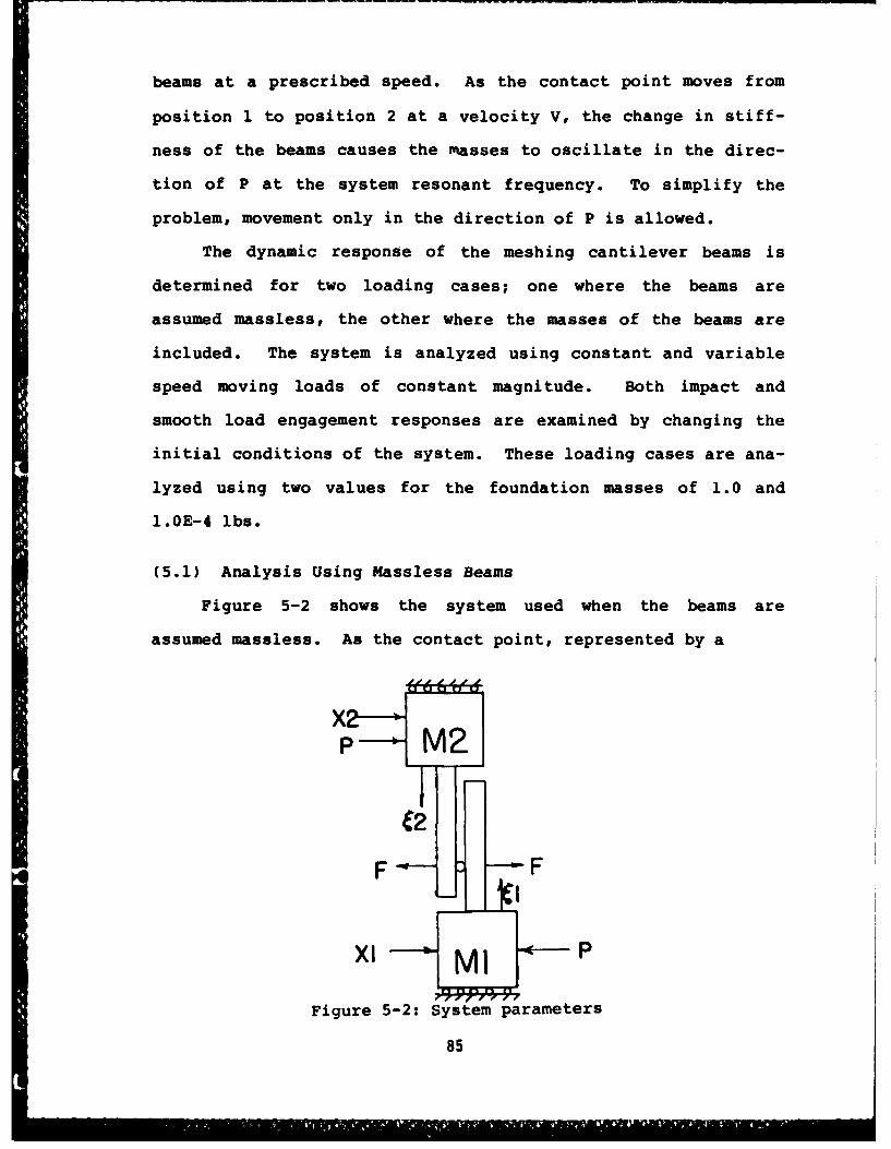
(5.1) Analysis Using Massless Beams

Figure 5-2 shows the system used when the beams are

assumed massless. As the contact point, represented by a

Ix

Pl!

C 2

Figure 5-2: System parameters

85

massless ball, moves along the beams, the deflection of the

beams will change due to the variation in stiffness. The

stiffness of each beam varies with the local coordinate, .

Since the beams are massless, they do not affect the system

resonant frequency, but follow the oscillations of Ml and M2

exactly. To determine the dynamic response for the massless

beam configuration, the differential equations of motion are

written and solved for this system.

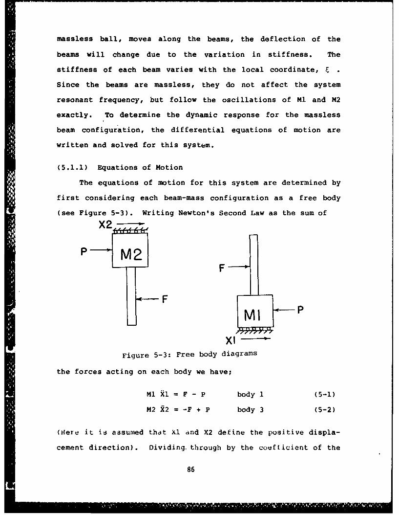
(5.1.1) Equations of Motion

The equations of motion for this system are determined by

first considering each beam-mass configuration as a free body

(see Figure 5-3). Writing Newton's Second Law as the sum of

X2

P M2F

F

Figure 5-3: Free body diagrams

the forces acting on each body we have;

Ml X1 = F - P body 1 (5-1)

M2 X2 = -F + P body 3 (5-2)

(Here it is assumed that Xl and X2 define the positive displa-

cement direction). Dividing through by the coefficient of the

86

second derivative term, and subtracting (5-1) from (5-2)

yields;

R2 - il = -F( 1n+ ) + P(1 + ) (5-3)

To further simplify equation (5-3), the right hand side is com-

bined and a common denominator is determined. This gives;

M1+ (5-4)i2 - Xl - (P-F) 02 54

where;

1 1+. m J 1" + 1 M1+2

M2f+ -N 41Q MI N2

Making simple substitutions, equation (5-4) can then be written

as;

MR - P-F (5-5)

where;

M 2

and;

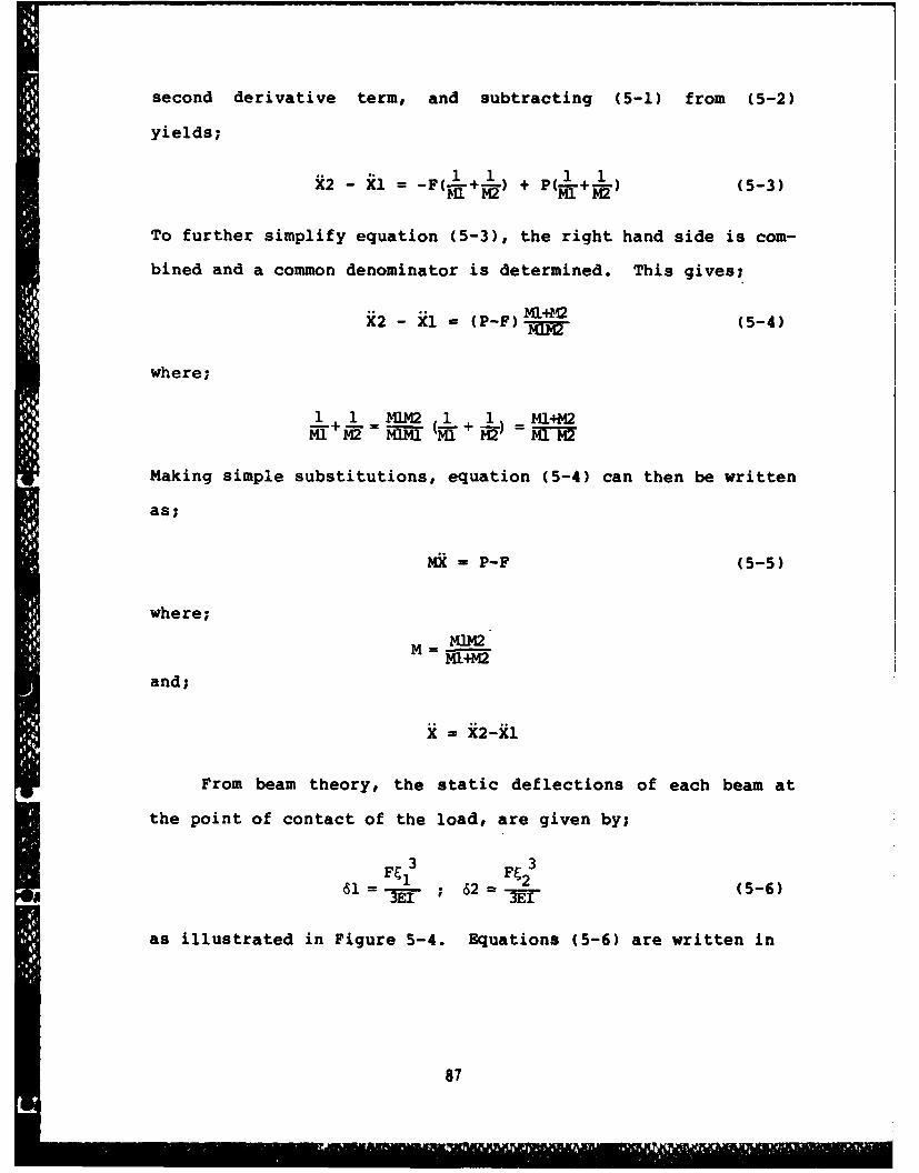
From beam theory, the static deflections of each beam at

the point of contact of the load, are given by;

-- 3 361 ; 62 -- (5-6)

as illustrated in Figure 5-4. Equations (5-6) are written in

87

FI I

'C2I

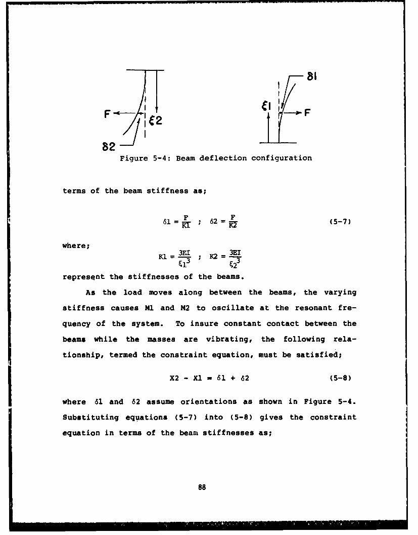
82Figure 5-4: Beam deflection configuration

terms of the beam stiffness as;

F F61 = ; 62 = F (5-7)

where;-l 3E1 K2 = 3EI

represent the stiffnesses of the beams.

As the load moves along between the beams, the varying

stiffness causes 1 and M2 to oscillate at the resonant fre-

quency of the system. To insure constant contact between the

beams while the masses are vibrating, the following rela-

tionship, termed the constraint equation, must be satisfied;

X2 - Xl - 61 + 62 (5-8)

where 61 and 62 assume orientations as shown in Figure 5-4.

Substituting equations (5-7) into (5-8) gives the constraint

equation in terms of the beam stiffnesses as;

88

F F

X2 - Xl = + (5-9)

Combining the right hand terms in equation (5-9),

K1 + K2X2 - Xl = F(l )

multiplying through by

K KlK2KL+K2

and letting X=X2-Xl, yields a familiar form of the constraint

equation, describing the deflection of a spring;

F = KX (5-10)

Inserting F from equation (5-10) into equation (5-5) gives the

equation of motion for the massless beam system;

M + KX =P (5-11)

where;

X = X2 - Xl

X =X2 -Xl

MIM

K KlK2K = i--

Initially, the system deflection is determined by assuming that

static equilibrium is satisfied. Thus, at time equal to zero,

the initial deflection is the applied load divided by the total

stiffness (the combined deflections of the beams);

89

El

X(0) = X2(0)-X1(0) = P/K

With the initial deflections, equation (5-11) is solved

using a fourth order Runge-Kutta integration algorithm. Since

the Runge-Kutta algorithm used is designed for systems of first

order equations, the second order differential equation (5-11)

must be converted to first order. This is done by defining;

Yl = X and Y2 = X

Substituting these relations into (5-11), we then have;

MYl + KY2 = P (5-12)

where at t=0.0,

Yl(0) = 0.0

Y2(0) = P/K

Given these initial values, the relations;

Yl = (P-KY2)/M

i2 - Yl = X

are used as input for Runge-Kutta and integrated to determine

the displacement, X-X2-Xl during the load cycle. (See Appendix

7 for solution algorithm).

(5.1.2) Static Analysis

Before any dynamic analysis is performed, a static

deflection test is done to provide a reference for dynamic

deflection comparisons. Solving the relationship;

90

im

X2 - Xl - P/K

at different load positions produced the plots shown in Figure

5-5. The three blocks represent the components comprising the

constraint equation (5-8). Deflections are determined between

load positions 1 and 2 illustrated in Figure 5-6. The load

position is measured relative to beam 1 as labelled on the

abscissa of Figure 5-5.

(5.1.3) Dynamic Response Results

The dynamic response of the massless beam system is deter-

mined for two loading cases; a constant speed 1000 lb load, and

a variable speed 1000 lb load. For each of these loading

cases, two sets of initial conditions are considered; those

defined for static equilibrium in equation (5-11), and another

set where the initial deflection, X2 - Xl, is equal to zero.

The second of these initial conditions will cause the load P to

be experienced as an impact load since the beams initially will

have no deflection and will attempt to return to static

equilibrium.

For loads moving with constant speed, speeds of; 1.0, 5.0,

10.0, 20.0, and 40.0 inches per second are used. This range of

speeds is chosen in order to bracket the cycle period asso-

ciated with the fundamental frequency of the system. The fre-

quency of vibration of the system is constantly changing with

the position of the load. However, a representative fundamen-

tal frequency is calculated when the load is halfway through

the load cycle. At this position the beam stiffnesses are

91

equal. Then, we simply have a spring mass system whose

undamped natural frequency is defined as;

= E (cycle/sec)

With beam dimensions the same as those given in Figure 5-6 and

the masses-Ml and M2 equal to 1.0, the period of oscillation is

approximately 0.03 seconds. Thus for a constant velocity of

7.0 in/sec, approximately two oscillations will occur during the

load cycle.

When a variable speed moving load is used, the speed ini-

tially is zero and increases linearly to 1.0, 5.0, 10.0, 20.0,

and 40.0 in/sec at the end of the cycle.

(5.1.3.1) Constant Speed Moving Loads

For slowly moving loads, relative to the fundamental

period of the system, one would expect near static deflections.

This is the case for a speed of 1.0 in/sec as shown in Figure

5-7. The figure gives the components of the constraint

equation resulting from an initial deflection equal to the

ratio of the load and stiffness. The only deviations from the

static deflection curve are caused by small oscillations at

the resonant frequency. As the speed of the moving load

increases, one would expect an increase in the amplitude of

oscillation as the period of the load cycle approaches the

resonant period. Increasing to 5.0 in/sec produced larger

deviations from static due to increased oscillation amplitudes

(Figure 5-8). This trend continues until the deflection is

94

-A187 684 AN INVESTIGATION OF THE DYNAMIC RESPONSE OF SPUR- GEAR 2/3TEETH NITN MOVING L (U) MICHIGAN TECHNOLOGICAL UNIVHOUGHTON DEPT OF MECHANICAL ENGIN

UNCLASSIFIED C E PASSERELLO ET AL AUG 87 NAS-CR-79642 F/6 1/9 U

1m EEEE00 EE11iEEEEEEEmohEohhhEEohEEmhhshhhhEEohEohmhEohhhEEhhmhEmhEEEmhIsmhEEEEEEEEEEEohhhshEEEEEEI

* 10 fw5

1125L.'oEm

k moc R-mfn i

WOWWMU f WUAMW

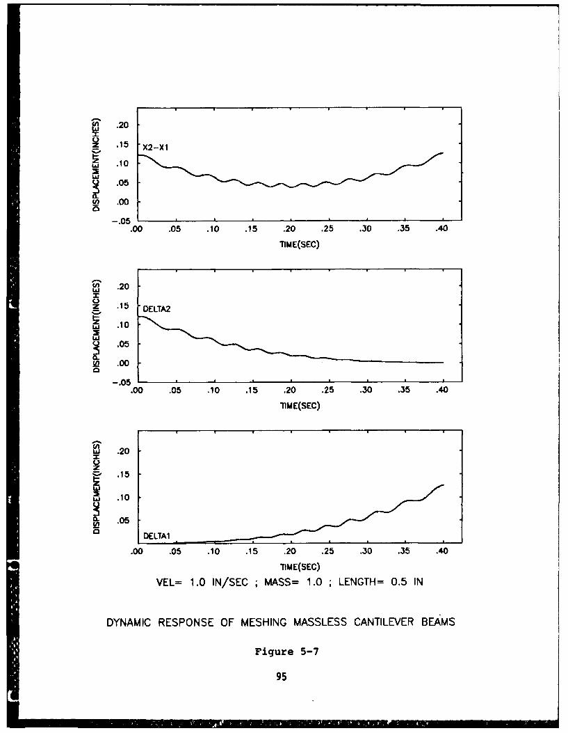
~.20

.1 -X2-XI

.10

.05

U) .00

-. 05.00 .05 .10 .15 .20 .25 .30 .35 .40

TIM E(SEC)

U) .20

.15 'DELTA2

.10

.05

so .00

-.05.00 .05 .10 .15 .20 .25 .30 .35 .40

TIME(SEC)

w .20

.-15

.10

.05In DELTAl

.00 .05 .10 .15 .20 .25 .30 .35 .40

TIME(SEC)

VEL= 1.0 IN/SEC ; MASS= 1.0 ; LENGTH= 0.5 IN

DYNAMIC RESPONSE OF MESHING MASSLESS CANTILEVER BEAMS

Figure 5-7

95

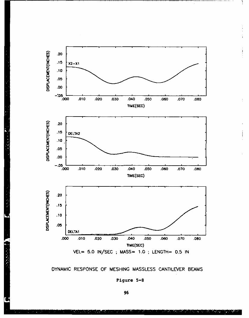
S .20

z .15 X2-Xl

.10

C) 05

0.LA .00

0

.000 .010 .020 .030 .040 .050 .060 .070 .080

-IME(SEC)

S .20

2.15 'DELTA2

.10~

~ 05

D) .0005

.000 .010 .020 .030 .040 .050 .060 .070 .080

T7hIE(SEC)

.20

.15

.10

S .05

DELTAl

.000 .010 .020 .030 .040 .050 .060 .070 .080

TIME(SEC)

VEL= 5.0 IN/SEC ; MASS= 1.0 ; LENGTH= 0.5 IN

DYNAMIC RESPONSE OF MESHING MASSLESS CANTILEVER BEAMS

Figure 5-8

96

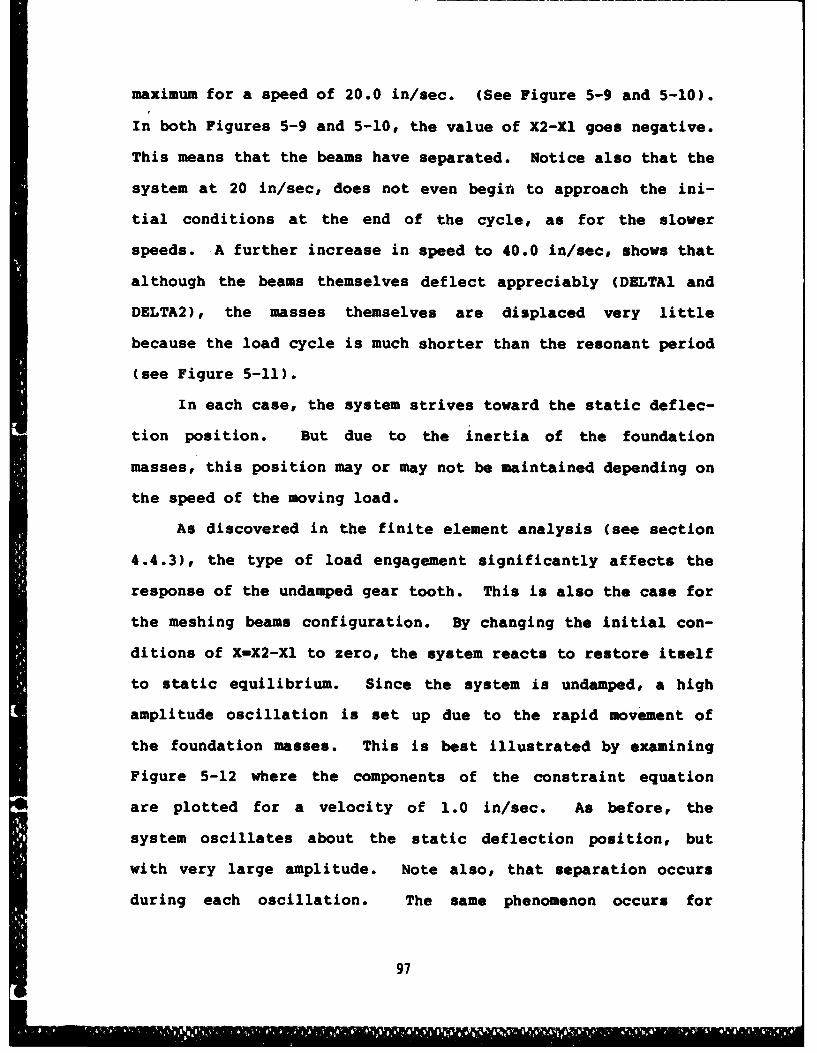
maximum for a speed of 20.0 in/sec. (See Figure 5-9 and 5-10).

In both Figures 5-9 and 5-10, the value of X2-Xl goes negative.

This means that the beams have separated. Notice also that the

system at 20 in/sec, does not even begin to approach the ini-

tial conditions at the end of the cycle, as for the slower

speeds. A further increase in speed to 40.0 in/sec, shows that

although the beams themselves deflect appreciably (DELTA1 and

DELTA2), the masses themselves are displaced very little

because the load cycle is much shorter than the resonant period

(see Figure 5-11).

In each case, the system strives toward the static deflec-

tion position. But due to the inertia of the foundation

masses, this position may or may not be maintained depending on

the speed of the moving load.

As discovered in the finite element analysis (see section

4.4.3), the type of load engagement significantly affects the

response of the undamped gear tooth. This is also the case for

the meshing beams configuration. By changing the initial con-

ditions of X-X2-Xl to zero, the system reacts to restore itself

to static equilibrium. Since the system is undamped, a high

amplitude oscillation is set up due to the rapid movement of

the foundation masses. This is best illustrated by examining

Figure 5-12 where the components of the constraint equation

are plotted for a velocity of 1.0 in/sec. As before, the

system oscillates about the static deflection position, but

with very large amplitude. Note also, that separation occurs

during each oscillation. The same phenomenon occurs for

97

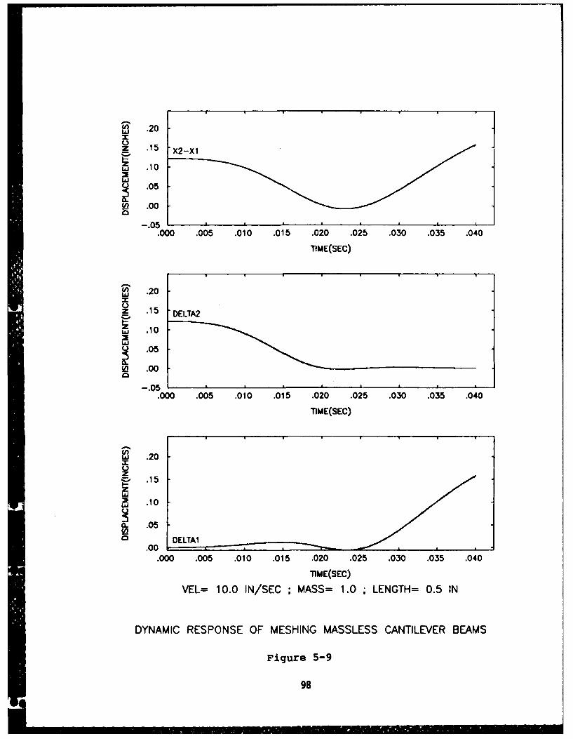
w .20

.10

.05

La~ .00

.000 .005 .010 .015 .020 .025 .030 .035 .040

11M E(SEC)

g3 .20

Z .15 DELTA2

w .10

.05

W) .00

.05.000 .005 .010 .015 .020 .025 .030 .035 .040

TIME(SEC)

gj .20

ww .10

.05

.001.000 .005 .010 .015 .020 .025 .030 .035 .040

TIME(SEC)

VEL= 10.0 IN/SEC ;MASS= 1.0 ; LENGTH= 0.5 IN

DYNAMIC RESPONSE OF MESHING MASSLESS CANTILEVER BEAMS

Figure 5-9

98

w .20

z .15 '2X

LaJ .10

.05

.00

-. 05.000 .005 .010 .015 .020

1IME(SEC)

~.20

% .1 DELTA2

.10

.05

so .00

-.05.000 .005 .010 .015 .020

TIME(SEC)

S.20

S.15

S.10

S.050) DELTAlo .00

.000 .005 .010 .015 .020

TIME(SEC)

VEL= 20.0 IN/SEC ;MASS= 1.0 ;LENGTH= 0.5 IN

DYNAMIC RESPONSE OF MESHING MASSLESS CANTILEVER BEAMS

Figure 5-10

99

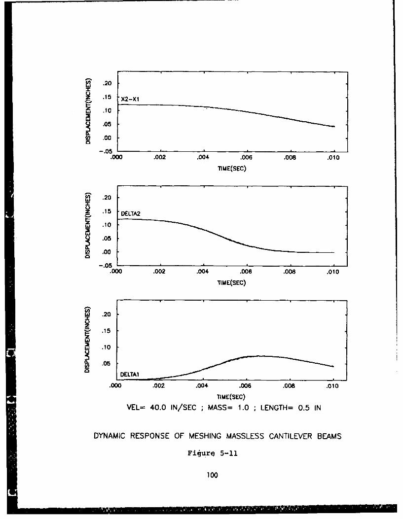
~.20

.15 X2-X1

g . 10

w.05

W .00C

-. 05.000 .002 .004 .006 .008 .010

TIME(SEC)

.20

05

z .15 ETA?

.05

0m .00

-. 05.000 .002 .004 .006 .008 .010

_ ME(SEC)

T.20

v .15

w .10

.05 DELTA1

.000 .002 .004 .006 .008 .010

TIME(SEC)VEL= 40.0 IN/SEC ; MASS= 1.0 ; LENGTH= 0.5 IN

DYNAMIC RESPONSE OF MESHING MASSLESS CANTILEVER BEAMS

Figure 5-11

100

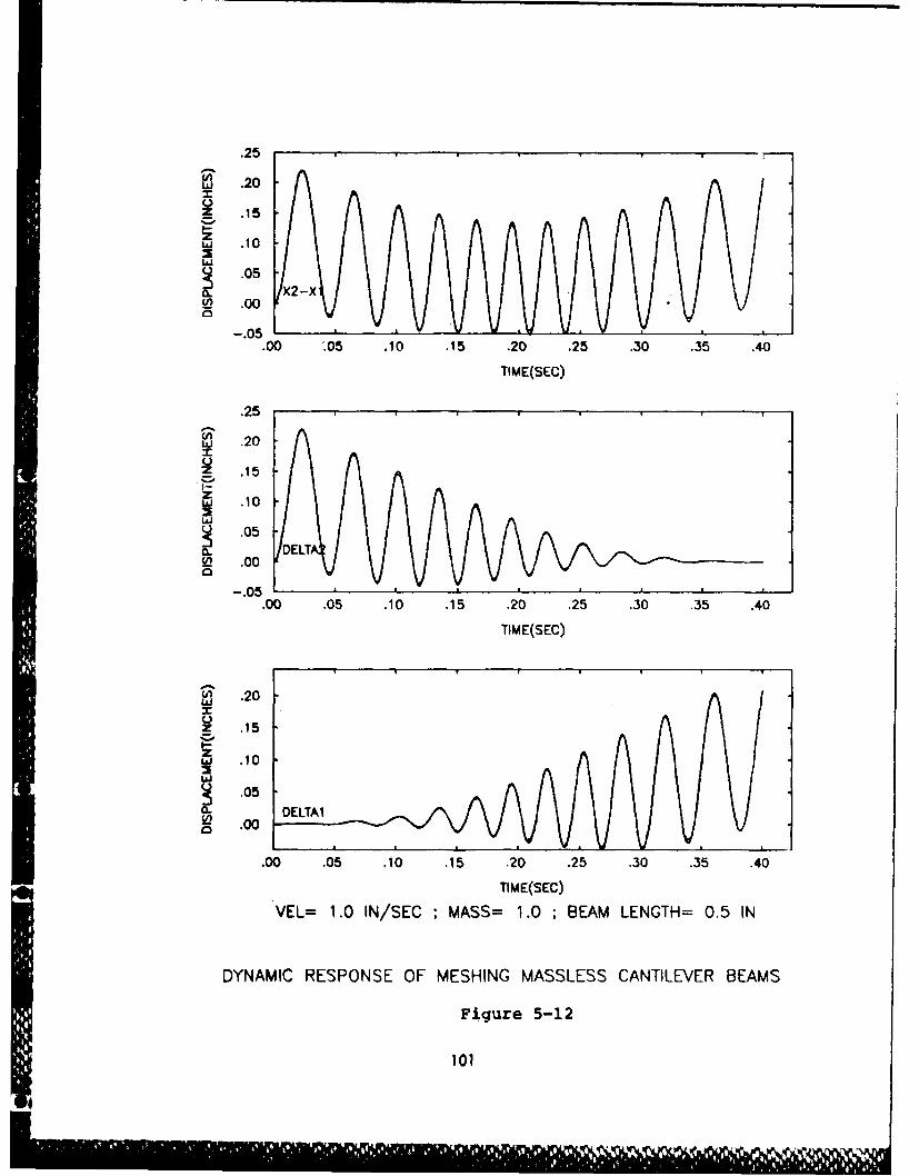
.25

_(nLJ .20

.15z,., .10

.05 X2-X

T .00

-. 05.00 .05 .10 .15 .20 .25 .30 .35 .40

TIME(SEC)

.25

- .20

z .15

,&, .10

S 05.05 DEL

LI .0005

.00 .05 .10 .15 .20 .25 .30 .35 .40

TIME(SEC)

,n .20

~ .15

w .102.05

0. DELTA1Wn .00

.00 .05 .10 .15 .20 .25 .30 .35 .40

TIME(SEC)

VEL= 1.0 IN/SEC ; MASS= 1.0 ; BEAM LENGTH= 0.5 IN

DYNAMIC RESPONSE OF MESHING MASSLESS CANTILEVER BEAMS

Figure 5-12

101

speeds of 5.0 and 10 in/sec (Figure 5-13 and 5-14). However,

with a further increase in speed, the system does not have suf-

ficient time to react and the oscillations become less signifi-

cant (see Figure 5-15 and 5-16). One should not be led to

believe that the separation occuring for these initial con-

ditions is caused by the characteristics of the system. It is

caused, however, by the application of a 1000 lb load to a beam

which in the physical sense could not support it. However,

since the system behaves linearly, the characteristics of the

response are the same for whatever load is applied, and the

1000 lb load is used simply to exaggerate that response.

(5.1.3.2) Variable Speed Moving Loads

Introducing a variable speed moving load, versus constant

speed, has little effect on the general behavior of the meshing

massless cantilever beam system. The same conclusions can be

drawn concerning the dynamic resonse trends due to increased

moving load speed. As a reference, the dynamic response curves

for both sets of initial conditions and the five different

speeds, plotted as a function of position, are included in

Appendix 4.

(5.2) Analysis Including Beam Inertia

Figure 5-17 illustrates the physical system used to deter-

mine the effects of including the inertia of the beams on the

dynamic response due to moving loads. This system is exactly

the same as the one used in Section 5.1 except the mass of the

beams is included. First, the equations of motion for this

system are developed.

102

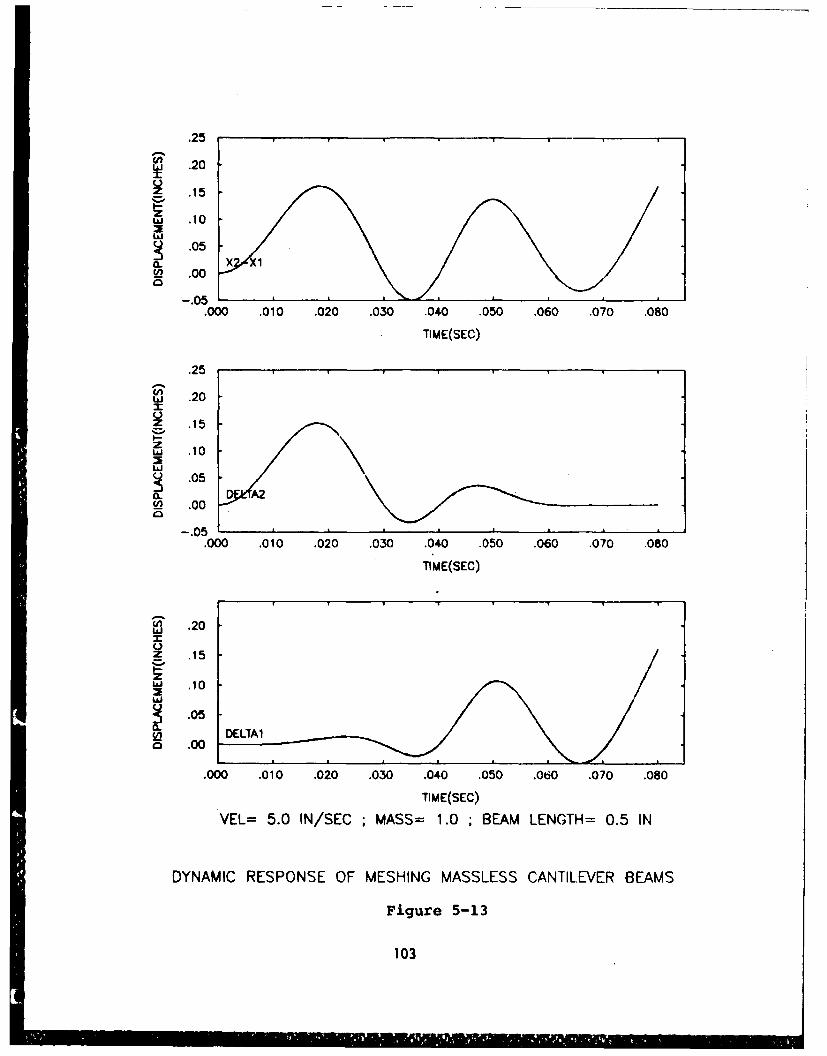
.25

w .20

10Li

.05

C-) .00

-. 05.000 .010 .020 .030 .040 .050 .060 .070 .080

TIME(SEC)

.25

ua .20" .15

I-zL. .10L&J

.05

_) .00

-. 05.000 .010 .020 .030 .040 .050 .060 .070 .080

TIME(SEC)

S .20

z .15

w .10

.050) DELTAlo .00

.000 .010 .020 .030 .040 .050 .060 .070 .080

TIME(SEC)

VEL= 5.0 IN/SEC ; MASS= 1.0 ; BEAM LENGTH= 0.5 IN

DYNAMIC RESPONSE OF MESHING MASSLESS CANTILEVER BEAMS

Figure 5-13

103

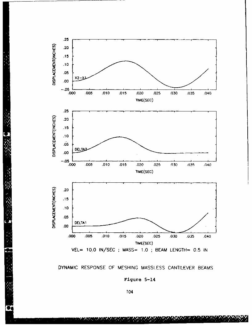
.25

(ALaw .20

.15)

Z .10

0-

(') .00

.000 .005 .010 .015 .020 .025 .030 .035 .040

TIM E(SEC)

.25

w .20

LK .15

zLU .10

-05a. D ,.,0l .00a

.000 .005 .010 .015 .020 .025 .030 .035 .040

TIM E(SEC)

w .20

.15

z Ui .10

.05o .00

.000 .005 .010 .015 .020 .025 .030 .035 .040

TI ME(SEC)

VEL= 10.0 IN/SEC ;MASS= 1.0 ; BEAM LENGTH= 0.5 IN

DYNAMIC RESPONSE OF MESHING MASSLESS CANTILEVER BEAMS

Figure 5-14

104

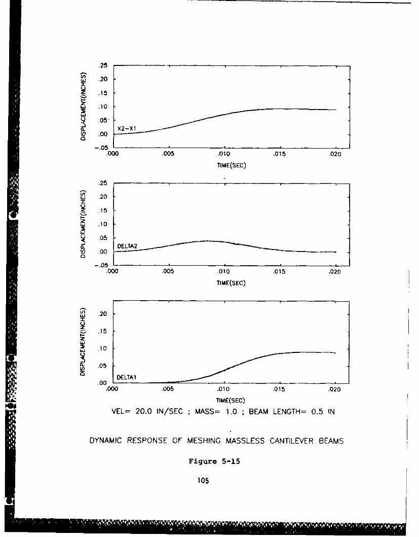
.25

ziA .10

L" .0005

.000 .005 .010 .015 .020

TIM E(SEC)

.25

W .20

Z .15

zLa. .10

.05

0" .00

-.05.000 .005 .010 .015 .020

TI ME(SEC)

wj .20

0.15

S .10

.00 1.000 .005 .010 .0 15 .020

TIM E(SEC)

VEL= 20.0 IN/SEC ;MASS= 1.0 ; BEAM LENGTH= 0.5 IN

DYNAMIC RESPONSE OF~ MESHING MASSLESS CANTILEVER BEAMS

Figure 5-15

105

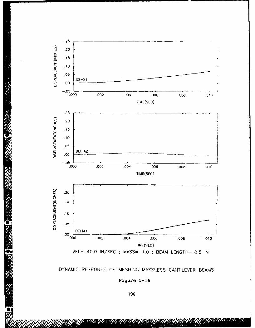
.25

w .2

K .15

zLi .10

j .05

0d .00

05

.000 .002 .004 .006 .008 010

TIM E(SEC)

.25

20

(-).150

On .00__

-05 ..000 .002 .004 .006 .008 .010

TIM E(SEC)

w .20

zS.15

zui .10

0 DELTAl.00

.000 .002 .004 .006 .008 .010

TIM E(SEC)

VEL= 40.0 IN/SEC ;MASS= 1.0 ; BEAM LENGTH= 0.5 IN

DYNAMIC RESPONSE OF MESHING MASSLESS CANTILEVER BEAMS

Figure 5-16

106

N l

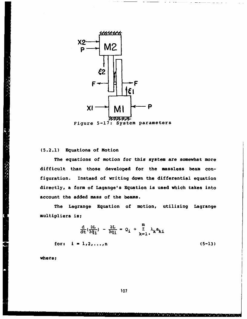
XI P

Figure 5-17: System parameters

(5.2.1) Equations of Motion

The equations of motion for this system are somewhat more

difficult than those developed for the massless beam con-

figuration. Instead of writing down the differential equation

directly, a form of Lagange's Equation is used which takes into

account the added mass of the beams.

The Lagrange Equation of motion, utilizing Lagrange

multipliers is;

d 3L ) L mT- qi) - 9 = Qi + kZlx ka ki

for: i - l,2,...,n (5-13)

where;

107

L = T - U - Lagrangian

T = System kinetic energy

U = System potential energy

qi = Generalized coordinates

Qi - Sum of non-potential forces

Ak = Lagrange Multipliers

af(ql,q2,...,qn) = first partialaki =Bqi

derivative of the constraint equation

with respect to the generalized coordinates

The last term on the right hand side of equation (5-13) repre-

sents the constraint forces which makes it possible to regard

all generalized coordinates, q1 , as independent.

Four generalized coordinates are used to describe the

system position, velocity, and acceleration. They are;

Xl - describing Ml

X2 - describing M2

ql - describing beam 2 relative to

foundation mass M1

q2 - describing beam 2 relative to

foundation mass M2

From the definition of generalized coordinates, these four

quantities are assumed independent of each other, and when used

together they describe the state of the dynamical system at any

time.

108

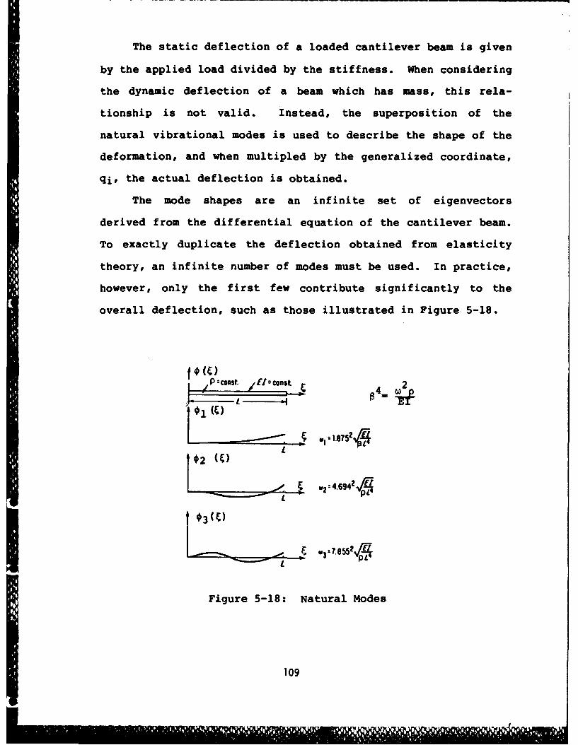
The static deflection of a loaded cantilever beam is given

by the applied load divided by the stiffness. When considering

the dynamic deflection of a beam which has mass, this rela-

tionship is not valid. Instead, the superposition of the

natural vibrational modes is used to describe the shape of the

deformation, and when multipled by the generalized coordinate,

qi, the actual deflection is obtained.

The mode shapes are an infinite set of eigenvectors

derived from the differential equation of the cantilever beam.

To exactly duplicate the deflection obtained from elasticity

theory, an infinite number of modes must be used. In practice,

however, only the first few contribute significantly to the

overall deflection, such as those illustrated in Figure 5-18.

" Co1ns . ,E €const 2

I 203 M

w3 7. 552OS 4

L

Figure 5-18: Natural Modes

109

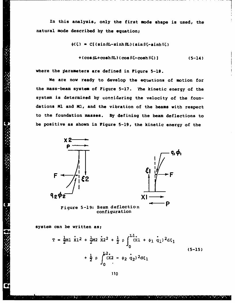
In this analysis, only the first mode shape is used, the

natural mode described by the equation;

*F)-C[CsinSL-sinhOL)CsinK-sinh8&)

+ (cos OL+ cosh OL) (cos 0 -cosh 0 U (5-14)

where the Oarameters are defined in Figure 5-18.

We are now ready to develop the equations of motion for

the mass-beam system of Figure 5-17. The kinetic energy of the

system is determined by ccneidering the velocity of the foun-

dations £41 and M2, and the vibration of the beams with respect

to the foundation masses. By defining the beam deflections to

be positive as shown in Figure 5-19, the kinetic energy of the

x 2-

F--

92S62

Figure 5-19: Beam deflectionconfiguration

system can be written as;

T = 4 l X 2 + r1 2 X 2 2 + -f Cf ( 1 +;i.~ ( - 51 P. j~ (X2+* q) 2j

+ 1 (, X2 - 02 ;2)d 1

0'

110

The potential energy consists only of the strain energy due to

the beam deflections;

1 r dl + 1I 2d&2 (5-16)

Where 0" is the second derivative of the mode shape with

respect to the length variable, . In equations (5-15) and

(5-16) the mass per unit length, p , the elastic modulus, E,

and the moment of inertia, I, are constant over the length of

the beams and can be left outside the integrals. Substracting

(5-16) from (5-15) to form the Lagrangian we have;

L - T - U 1 j12 + !M2 i22

1 L1 1 L2+~ i J (kl + Ol 41) 2d 1 + y pJf (A2 - 02 i2)2 d&2

0 0Ll .L 2 .

- EI f0; i d j - EI J0 2 q2 )2d2 (5-17)

For the meshing cantilever beam system there are four

unknown parameters, Xl, X2, ql, q2 and their derivatives, each

dependent on time, describing the dynamical system. At any

time, t, the position of the system can be described by the

constraint equation;

X2-Xl - O1ql - 2q2 = f(Xl,X2,ql,q2) = 0 (5-18)

If the constraint equation is not satisfied, separation occurs

between the beams at the point of contact.

A Lagrange Equation of motion is written for each degree

111

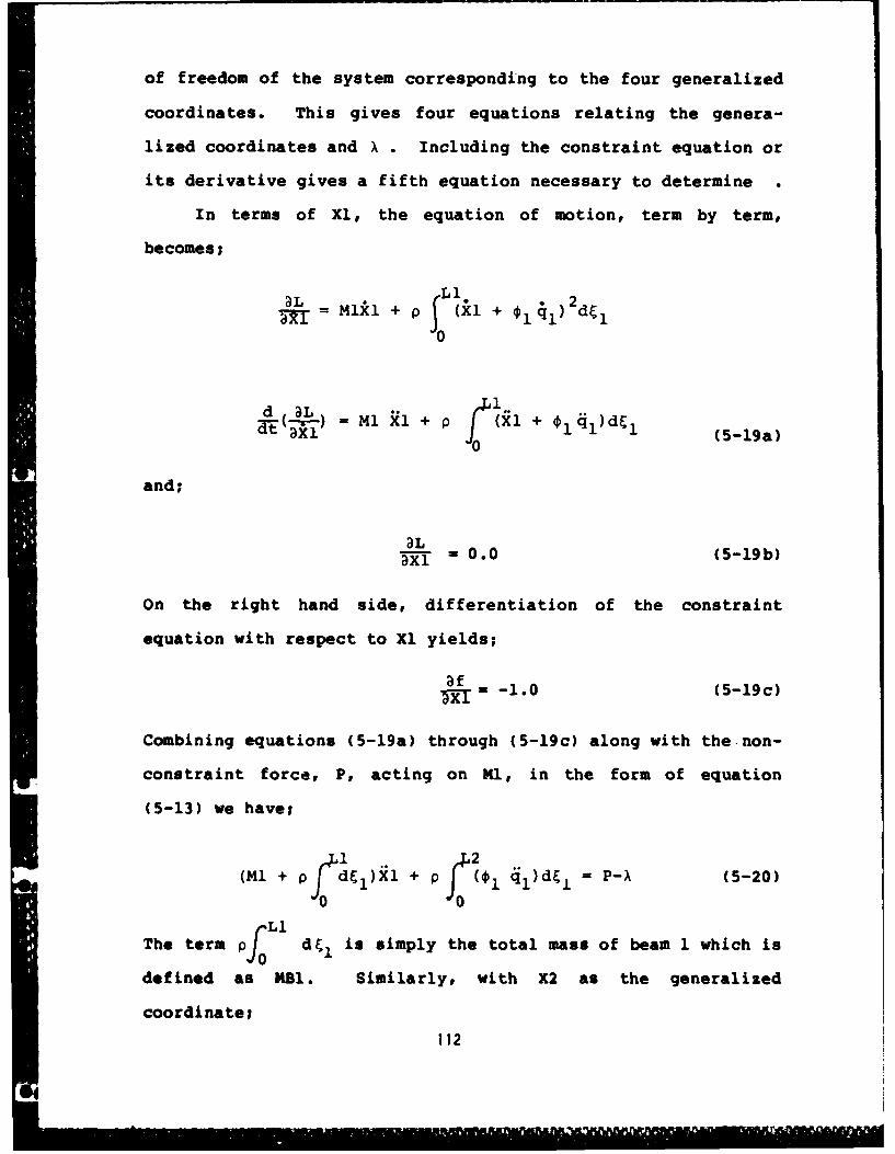
of freedom of the system corresponding to the four generalized

coordinates. This gives four equations relating the genera-

lized coordinates and X . Including the constraint equation or

its derivative gives a fifth equation necessary to determine .

In terms of Xl, the equation of motion, term by term,

becomes;

= MlXi + P (Xl + *i4q) 2

0

a = Ml X1 + p (Xl + 0 1)d3xi 0(5-19a)

and;

aXL - 0.0 (5-19b)

On the right hand side, differentiation of the constraint

equation with respect to X1 yields;

I - -1.0 (5-19c)

Combining equations (5-19a) through (5-19c) along with the.non-

constraint force, P, acting on Ml, in the form of equation

(5-13) we have;

(Ml + PJ d i)Xl + p (0I jl)dFl = P-X (5-20). 0 0

F~LlThe term p d~l is simply the total mass of beam 1 which is

defined as MBl. Similarly, with X2 as the generalized

coordinate;

112

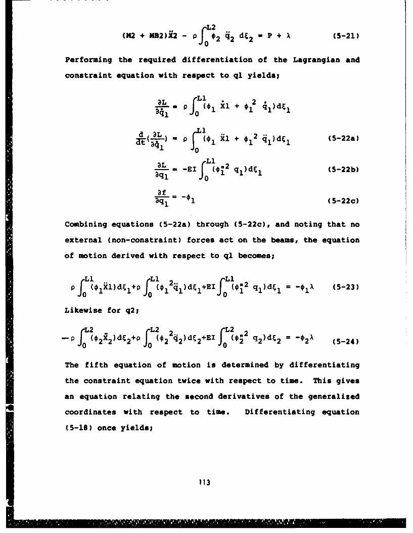
L 2

(142 + M82)X2 - p f 2 q2 d& 2 - P + X (5-21)

Performing the required differentiation of the Lagrangian and

constraint equation with respect to q1 yields;

P Jr 4*i Xl + *,ilq)d~l

d ) " p Xl + 2 dl (5-22a)"i

L -EI0 (.I ql)d~l (5-22b)

aff - (5-22c)

Combining equations (5-22a) through (5-22c), and noting that no

external (non-constraint) forces act on the beams, the equation

of motion derived with respect to q1 becomes;

r 1 • L 1 LPJ (lXl)d&l+P 4201 )d&1 +EIJ (.12 ql)dl - ,x (5-23)

Likewise for q2;

L2 . L2 2 rL2 ,2P f Yo)d& (+2 2) fo LE 2 q2)dt2 = - 2A (5-24)-- 0 (fX2d+ 2+EI)d0

The fifth equation of motion is determined by differentiating

the constraint equation twice with respect to time. This gives

an equation relating the second derivatives of the generalized

coordinates with respect to time. Differentiating equation

(5-18) once yields;

113

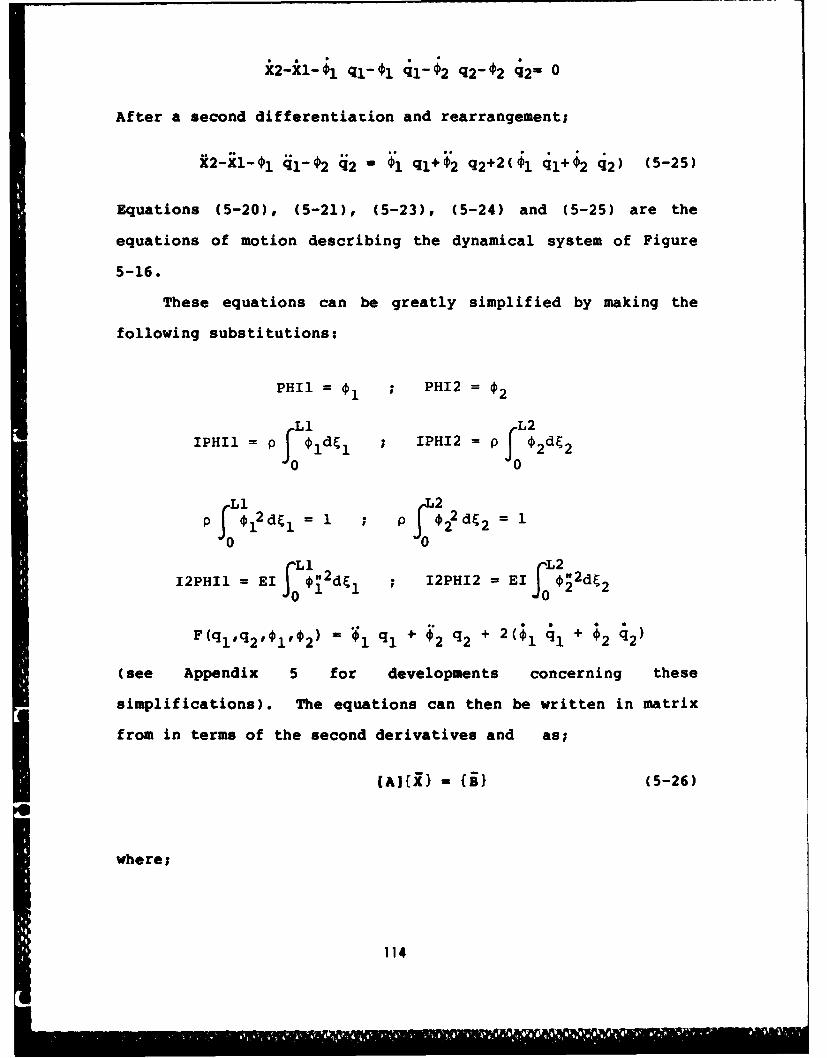
i2-i1-0l 1 --ilq-0 2 q2-$2 i2 = 0

After a second differentiation and rearrangement;

2t2-X1-0i 4j1 -0 2 q2 - *jl ql+0* q2 +2(0 1 q1+02 q2 ) (-5

Equations (5-20), (5-21)o (5-23), (5-24) and (5-25) are the

equations of motion describing the dynamical system of Figure

5-16.

These equations can be greatly simplified by making the

following substitutions:

PHIl = 01 PH12 = 0

Li L2IPHIl = Pf, O*1E1 ; IPHI2 = p f 02 d&2

0 0

p f= d 1 ; p 1L 2 = 1

0 0

12PHIl =-- El fN2d~ ; 12PHI2 -El f.2d~

F(ql,q 2 1 001 2) = 1 q, +*2 q 2 + 2(01 j,. + ;2 i2)

(see Appendix 5 for developments concerning these

simplifications). The equations can then be written in matrix

from in terms of the second derivatives and as;

(A][!) -{}(5-26)

where;

114

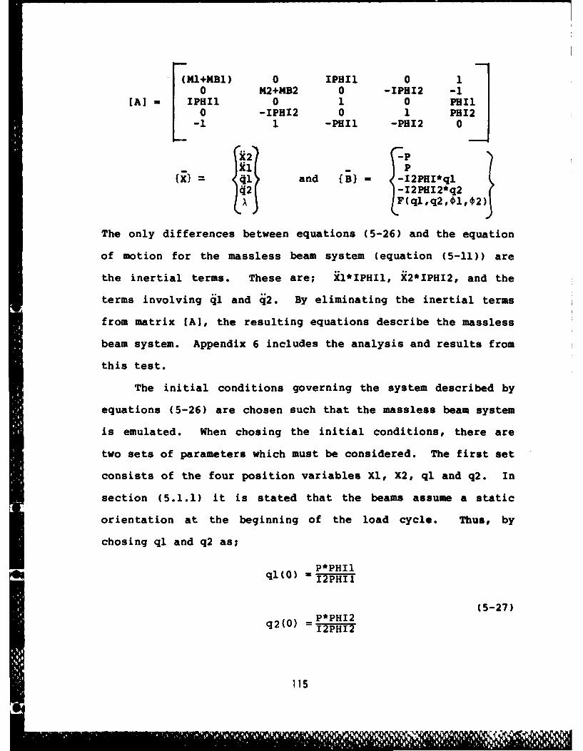
(MI+MB1) 0 IPHIl 0 10 M2+MB2 0 -IPHI2 -1

[A] - IPHIl 0 1 0 PHI10 -IPHI2 0 1 PR12-1 1 -PHI1 -PH12 0

'4 = <1> and fBI -12PHI*ql42 -12PHI2*q2

Flql,q2, 1, 2)

The only differences between equations (5-26) and the equation

of motion for the massless beam system (equation (5-11)) are

the inertial terms. These are; Xl*IPHIl, X2*IPHI2, and the

terms involving jl and q2. By eliminating the inertial terms

from matrix [A), the resulting equations describe the massless

beam system. Appendix 6 includes the analysis and results from

this test.

The initial conditions governing the system described by

equations (5-26) are chosen such that the massless beam system

is emulated. When chosing the initial conditions, there are

two sets of parameters which must be considered. The first set

consists of the four position variables Xl, X2, ql and q2. In

section (5.1.1) it is stated that the beams assume a static

orientation at the beginning of the load cycle. Thus, by

chosing ql and q2 as;

ql --- P*PHIlql(0) 12PHIT

(5-27)P'PHI2q2(0) = P2PH12

115

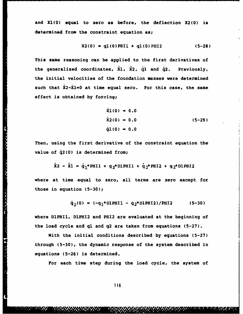
and Xl(O) equal to zero as before, the deflection X2(O) is

determined from the constraint equation as;

X2(0) - ql(0)PHIl + ql(0)PHI2 (5-28)

This same reasoning can be applied to the first derivatives of

the generalized coordinates, Xl, i2, 41 and q2. Previously,

the initial velocities of the foundation masses were determined

such that X2-Xl=0 at time equal zero. For this case, the same

effect is obtained by forcing;

xl(o) = 0.0

X2(0) = 0.0 (5-29)

41(0) = 0.0

Then, using the first derivative of the constraint equation the

value of 42(0) is determined from;

i2 - X*l = q1*PHIl + q2*DlPHIl + j2*PH12 + q 2*DlPHI2

where at time equal to zero, all terms are zero except for

those in equation (5-30);

42(0) = (-ql*DlPHIl - q2*DlPHI2)/PHI2 (5-30)

where DlPHIl, DlPHI2 and PHI2 are evaluated at the beginning of

the load cycle and ql and q2 are taken from equations (5-27).

With the initial conditions described by equations (5-27)

through (5-30), the dynamic response of the system described in

equations (5-26) is determined.

For each time step during the load cycle, the system of

116

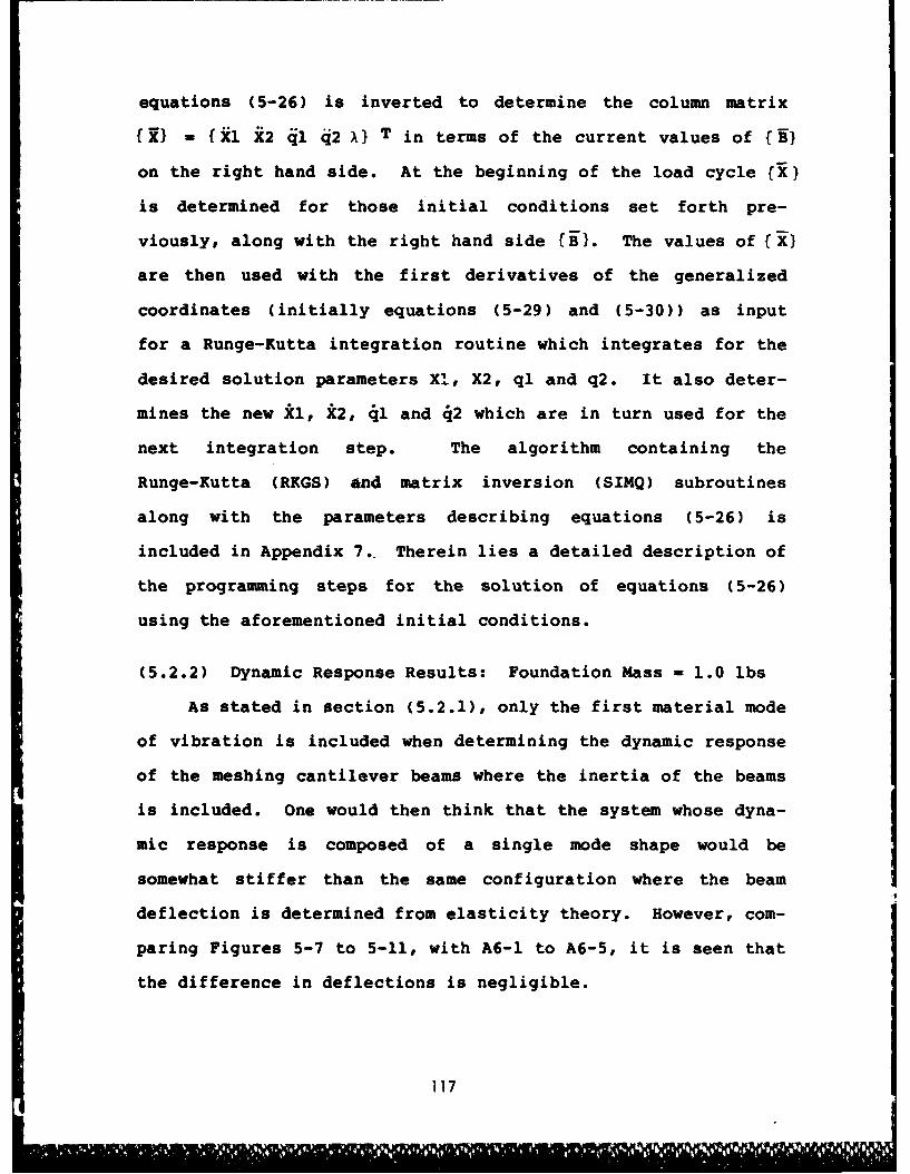
equations (5-26) is inverted to determine the column matrix

{1 - {Xl X2 ql q2 X} T in terms of the current values of fB}

on the right hand side. At the beginning of the load cycle fX }

is determined for those initial conditions set forth pre-

viously, along with the right hand side fB}. The values of f X}

are then used with the first derivatives of the generalized

coordinates (initially equations (5-29) and (5-30)) as input

for a Runge-Kutta integration routine which integrates for the

desired solution parameters Xl, X2, ql and q2. It also deter-

mines the new :1, k2, 41 and 42 which are in turn used for the

next integration step. The algorithm containing the

Runge-Kutta (RKGS) and matrix inversion (SIMQ) subroutines

along with the parameters describing equations (5-26) is

included in Appendix 7.. Therein lies a detailed description of

the programming steps for the solution of equations (5-26)

using the aforementioned initial conditions.

(5.2.2) Dynamic Response Results: Foundation Mass = 1.0 lbs

As stated in section (5.2.1), only the first material mode

of vibration is included when determining the dynamic response

of the meshing cantilever beams where the inertia of the beams

is included. One would then think that the system whose dyna-

mic response is composed of a single mode shape would be

somewhat stiffer than the same configuration where the beam

deflection is determined from elasticity theory. However, com-

paring Figures 5-7 to 5-11, with A6-1 to A6-5, it is seen that

the difference in deflections is negligible.

117

In this analysis, with the beam inertia included, the

dynamic response is compared to the massless beam problem. At

slow moving, constant speed loads, the dynamic response con-

sists of quasi-static deflection with the moving load response

superimposed over it (see Figure 5-20). (Results for moving

load speed of 1.0 in/sec were not obtainable due to lack of

convergence in the Runge-Kutta integration routine).

Continuing to increase the moving load speed causes an increase

in the response as the resonant frequency is further excited as

shown in Figure 5-21 and 5-22. Increasing the moving load

speed above the system resonant frequency produces a much

smoother response as illustrated in Figure 5-23. Now, examina-

tion of Figures 5-20 through 5-23 compared to Figures 5-7

through 5-11 shows that for values of the foundation masses of

1.0 lbs and moving load speeds of 5.0, 10.0, 20.0 and 40.0

in/sec, the responses of the two cantilever beam systems are

essentially the same. The same conclusions are drawn when exa-

mining Figures 5-24 through 5-27 as compared to Figures 5-13

through 5-16. Here, the initial conditions are changed such

that the beams experience an impact load at the beginning of

the load cycle. From the figures it can be seen that the

responses of the two systems are again, very much the same.

As done for the massless beam configuration, the speed of

the moving loads is allowed to vary linearly from zero to a

maximum value during the load cycle. This analysis serves as a

useful check since the initial conditions are easily defined

due to a stationary load. The results from this analysis are

contained in Appendix 4.

118

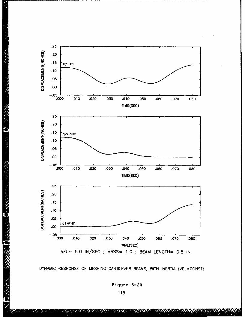
.25

~2 .20

.15 'X2-Xl

zLi .10

.05

L! .0005

.000 .010 .020 .030 .040 .050 .060 .070 .080

TIME(SEC)

.25

w .20

Z .15 q2*PHI2

LU .10

O .05

Ln .00

-.05.000 .010 .020 .030 .040 .050 .060 .070 .080

TIME(SEC)

.25

w .20x

~.15

w 10

.05 ql.PHIl02 .00

-.05.000 .010 .020 .030 .040 .050 .060 .070 .0;0

TIM E(SEC)

VEL= 5.0 IN/SEC ;MASS~= 1.0 ; BEAM LENGTH= C.5 IN

DYNAMIC RESPONSE OF MESHING CANTILEVER BEAMS, WITH INERTIA (VEufr!CONST)

Figure 5-20

119

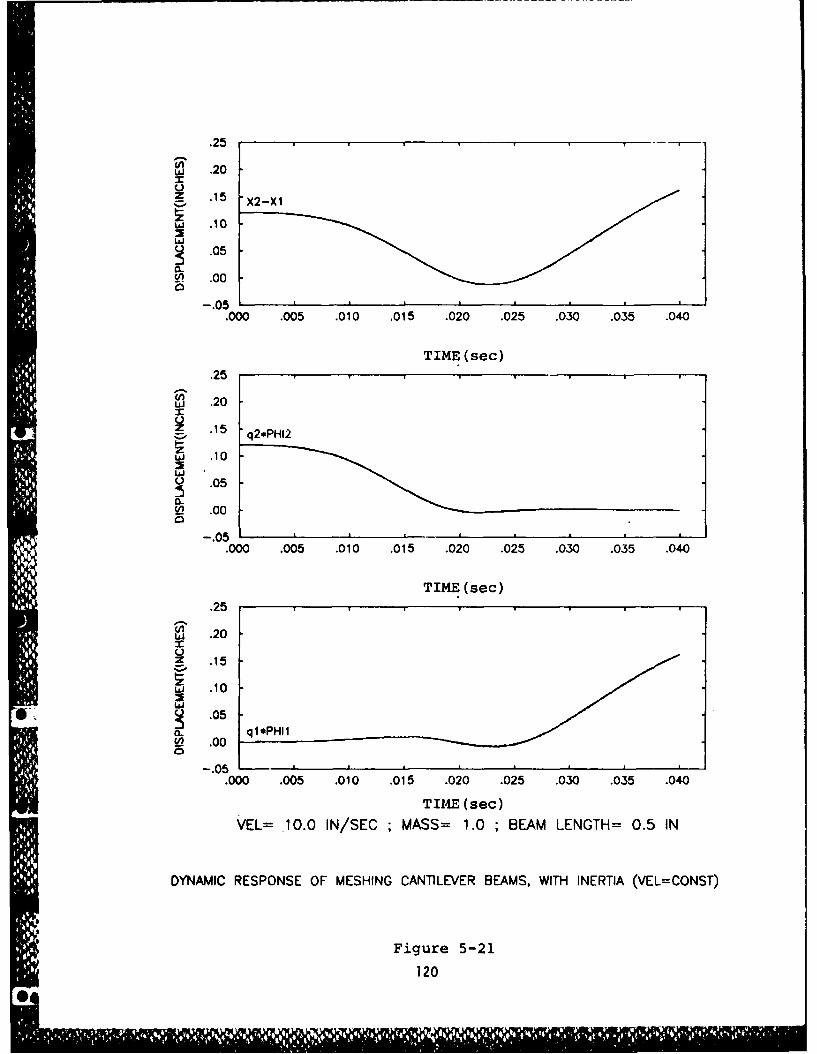
w .20.20

-05

q? .00

~' .05

.000 .005 .010 .015 .020 .025 .030 .035 .040

TIME (sec).25

15 q2*PHI2

w .10

0 5

C'n .00

-.05.000 .005 .010 .015 .020 .025 .030 .035 .040

TIME (sec).25

Li .20

.10

.05

£0 .00

0000 .1 .015 .020 .025 .030 .035 .040

TIME (sec)

VEL= 10.0 IN/SEC ; MASS= 1.0 ; BEAM LENGTH= 0.5 IN

DYNAMIC RESPONSE OF MESHING CANTILEVER BEAMS, WITH INERTIA (VEL=CONST)

Figure 5-21

120

[! l Slljj11

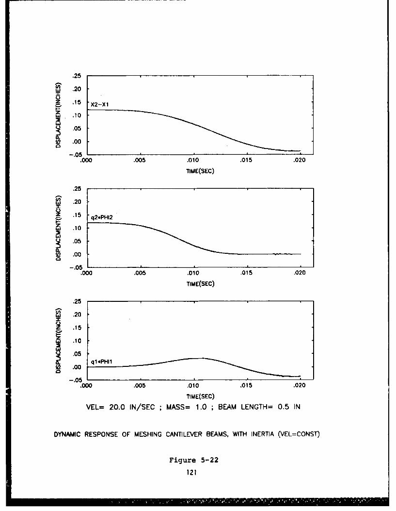
~.25.2

w .10

'~.05

0t .00

-.05.000 .005 .010 .015 .020

TIUE(SEC)

.25

S .20

05

onJ .0

-.05.000 .005 .010 .015 .020

TIME(SEC)

.25

~3 .20

_ .15

.10

.0 5 l P lW) .00

-.05.000 .005 .010 .015 .020

TIM E(SEC)

VEL= 20.0 IN/SEC ;MASS= 1.0 ; BEAM LENGTH= 0.5 IN

DYNAMIC RESPONSE OF MESHING CANTILEVER BEAMS, WITH INERTIA (VEL=CONsT)

Figure 5-22

121

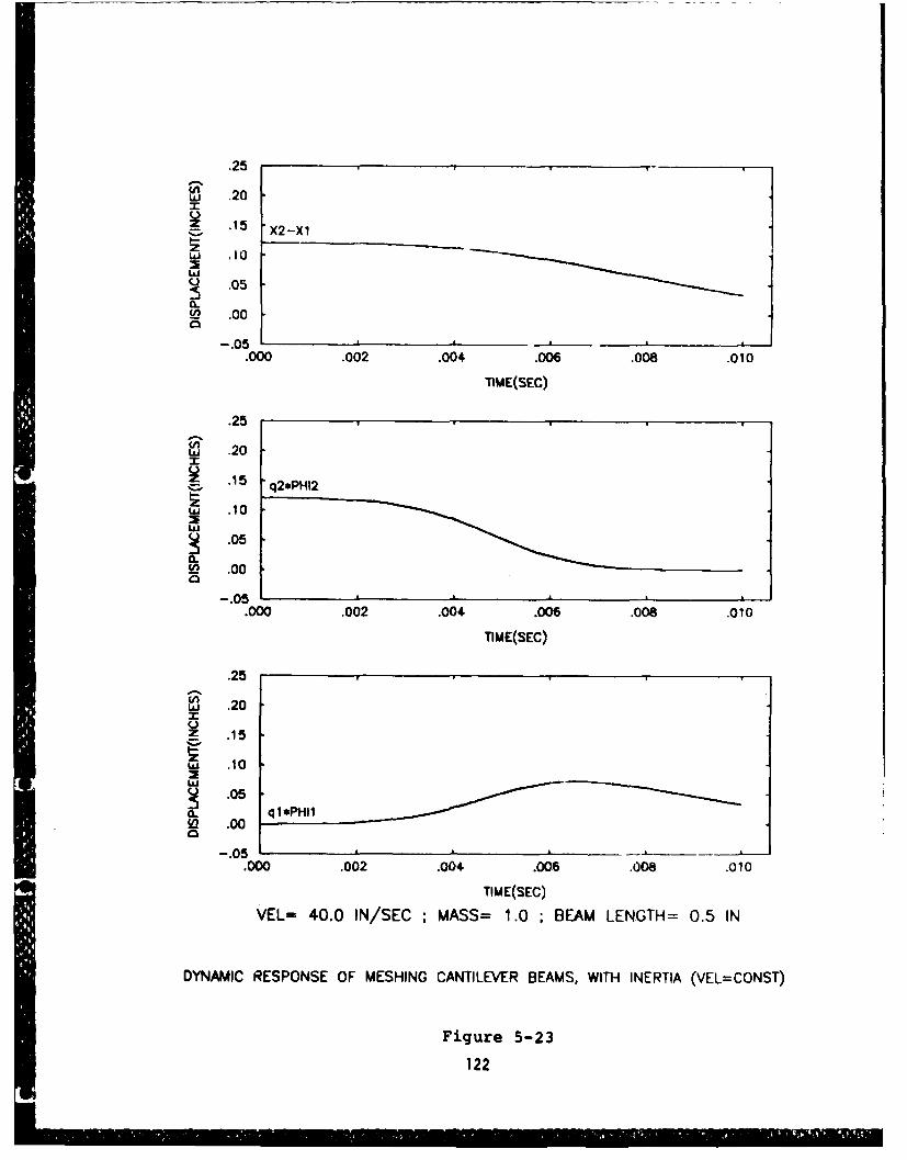
.25

3 .20

.15 X2-Xl

_ .10

505(LT1 .00

-. 05.000 .002 .004 .006 .008 .010

TIME(SEC)

.25

ol.20

.15 q2*PH12

~.10

-.050 .00

05

.000 .002 .004 .006 .008 .010

TIUE(SEC)

.25

Uj .20

1 .15

U.10

L0 .00 ql*PH1---; .00

am ~~-.05 ,

.000 .002 .004 .006 .008 .010, TIME(SEC)

VEL= 40.0 IN/SEC ; MASS= 1.0 ; BEAM LENGTH= 0.5 IN

DYNAMIC RESPONSE OF MESHING CANTILEVER BEAMS, WITH INERTIA (VEL=CONST)

Figure 5-23

122

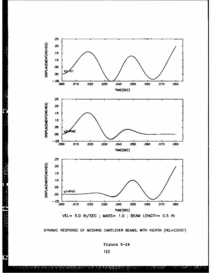
.25

~2 .20

.15

a .10

-.05000 .010 .020 .030 .040 .050 .060 .070 .080

TIME(SEC)

10

S 05

~.00

.000 '010 .020 .030 .040 .050 .060 .070 .080

TIME(SEC)

.253 .20

.15

i& .10

.05

01 .00.0

.000 .010 .020 .030 .040 .050 .060 .070 .080

1'JME(SEC)

VEL= 5.0 IN/SEC ;MASS= 1.0 ; BEAM LENGTH= 0.5 IN

DYNAMIC RESPONSE OF MESHING CANTILEVER BEAMS, WITH INERTIA (VEL=CONST)

Figure 5-24

123

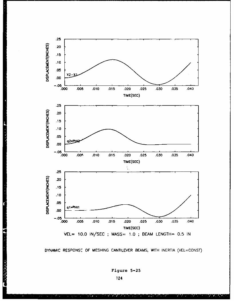
.25

w .20

.15

IA .10

Wf .00

05

.000 .005 .010 .015 .020 .025 .030 .035 .040

TIM E(SEC)

.25

S .20

tzZi .10

.05

0 .00

.000 .0 .00 .05 .020 .025 .030 .035 .040

TIM E(SEC)

.25

.20

.15

V10~ 05

0so .00 ql*PHl1

-05.000 .005 .010 .015 .020 .025 .030 .035 .040

TIME(SEC)

VEL= 10.0 IN/SEC ; MASS= 1.0 ; BEAM LENGTH= 0.5 IN

DYNAMIC RESPONS! OF MESHING CANTILEVER BEAMS, WITH INERTIA (VEL=CONST)

Figure 5-25

124

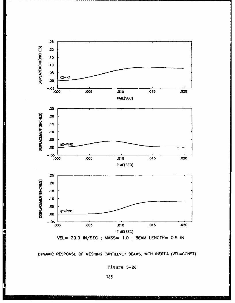
.25

S.20

.15

zw& .10

.05

Wo .00_, 0

-. 05.000 .005 .00 .015 .020

-nME(SEC)

.25

w 2 .20

.15

w .10LhJ

-0 q2*PHI2L4 .00

.05.000 .005 .010 .015 .020

TIME(SEC)

.25

" .20

.15

ti .10w

.00 q*PHI1

-.05.000 .005 .010 .015 .020

TIME(SEC)

VEL= 20.0 IN/SEC ; MASS= 1.0 ; BEAM LENGTH= 0.5 IN

DYNAMIC RESPONSE OF MESHING CANTILEVER BEAMS, WITH INERTIA (VEL=CONST)

Figure 5-26

125

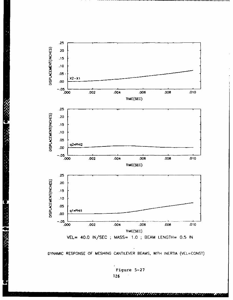
.25

~3 20

.15

zIjI .10

IA-.05.

On) .00

-. 05.000 .002 .004 .006 .008 .010

TIME (SEC)

.25

~3 .20

K .15

z .10

O .05

0I .00

05

.000 .002 .004 .006 .008 .010

TIM E(SEC)

.25

w3 .20m

Z .15

Li .10

0 .00

05

.000 .002 .004 .006 .008 .010

TIME (SEC )

VEL= 40.0 IN/SEC ;MASS= 1.0 ; BEAM LENGTH= 0.5 IN

DYNAMIC RESPONSE OF MESHING CANTILEVER BEAMS, WITH INERTIA (VEL=CONST)

Figure 5-27

126

(5.2.3) Dynamic Response Results:

Foundation Mass - 1.0E-4 lbs.

In order to substantiate the conclusion that the dynamic

response is not dependent on the mass of the beam, both the

massless beam and inertial beam configurations are analyzed

again with a decrease in the difference between the values of

the beam and foundation masses. Of course the mass of the beam

is not included in the massless beam analysis. Previously the

mass of the foundation was 1.0 lbs and the total mass of the

beam was approximately 3.6E-6 lbs. In this analysis, the

foundation mass is decreased to l.OE-4 lbs while the mass of

the beam remains the same. Since the overall mass of the

system is greatly decreased, the corresponding resonant fre-

quency is much larger. Using an approximation of the resonant

frequency using a single mass and the load at the midpoint of

the beam yields an approximate resonant frequency of;

= j::J, - (4) 0 3500 cycle/sec.

and a cycle period of approximately 2.875E-4 sec. Therefore,

in order to provide an adequate range of moving load speeds

such that the system resonance is bracketed, speeds of 100.,

500., 1000., 1500. and 2000. in/sec are used. (Approximately

one oscillation cycle occurs at 1700 in/sec). To facilitate

comparisons of respective systems, the results are presented in

a parallel fashion. Figures 5-28 and 5-29 show the respective

responses for a moving load speed of 500 in/sec. As seen from

the plots, the responses are virtually the same. The results

are similar for the other moving load speeds (see Figure 5-30

through 5-35).

127

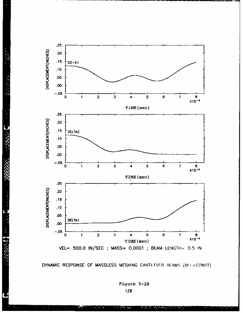
.25

S.20

Z .15 2X

z.10

"' 000

-.05

TIME (sec)

.25

gw .20

w 1

Q .050-soJ .0

0 .05

.2

.20

05

-050 1 2 13 45678

TIME (sec)X14

.128

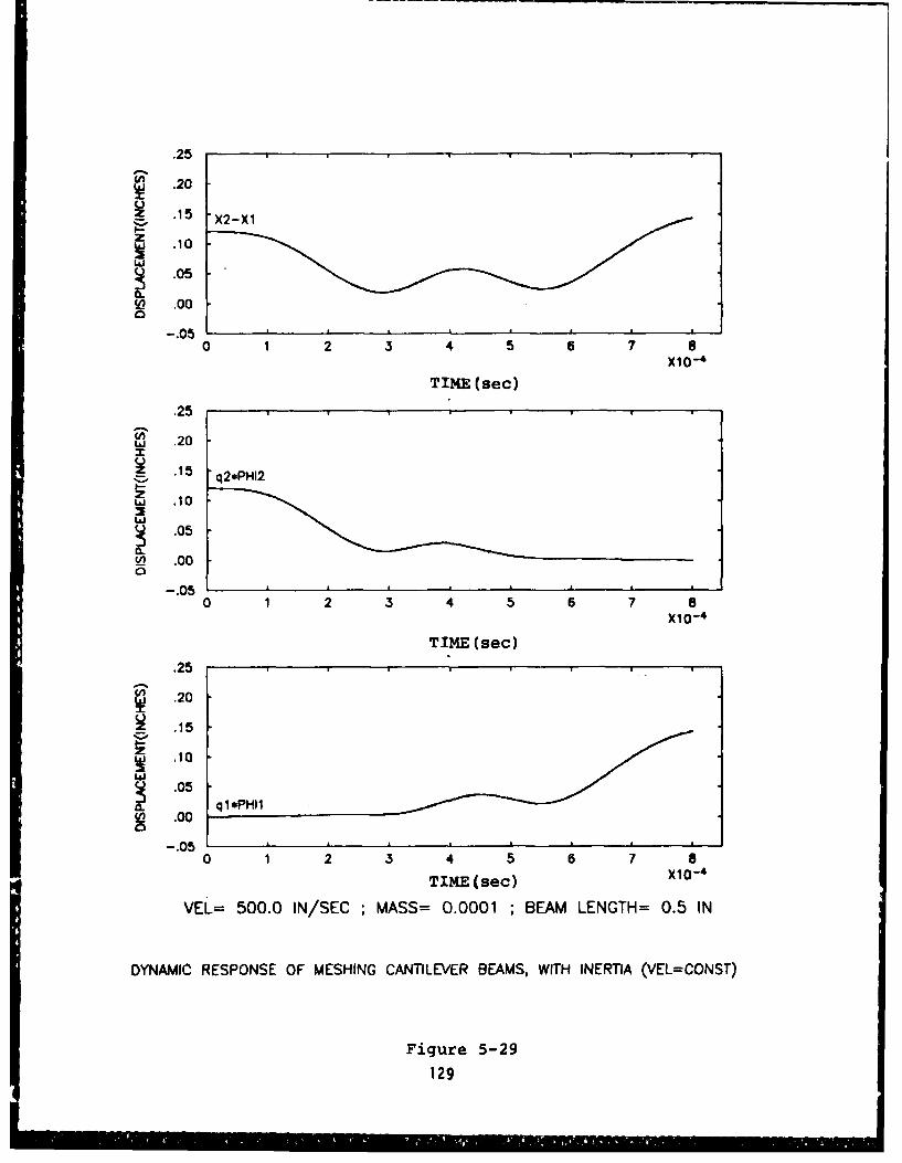
.25

.1 X2-X1.1-

.05

so .00

-.050 1 2 3 4 5 6 7 a

X1 0'

TIME (sec)

.25

w .20

.5 q2*PHI2

.10

.05

0n .0005

0 1 2 3 4 5 6 7 8X10- 4

TIME (sec)

.25

~3 .20

.15

tJ .10

~ 05

so .00.0

0 1 2 3 4 5 6 7 8

TIME (sec) X10-

VEL= 500.0 IN/SEC ;MASS= 0.0001 ; BEAM LENGTH= 0.5 IN

DYNAMIC RESPONSE OF MESHING CANTILEVER BEAMS, WITH INERTIA (VEL=CONST)

Figure 5-29

129

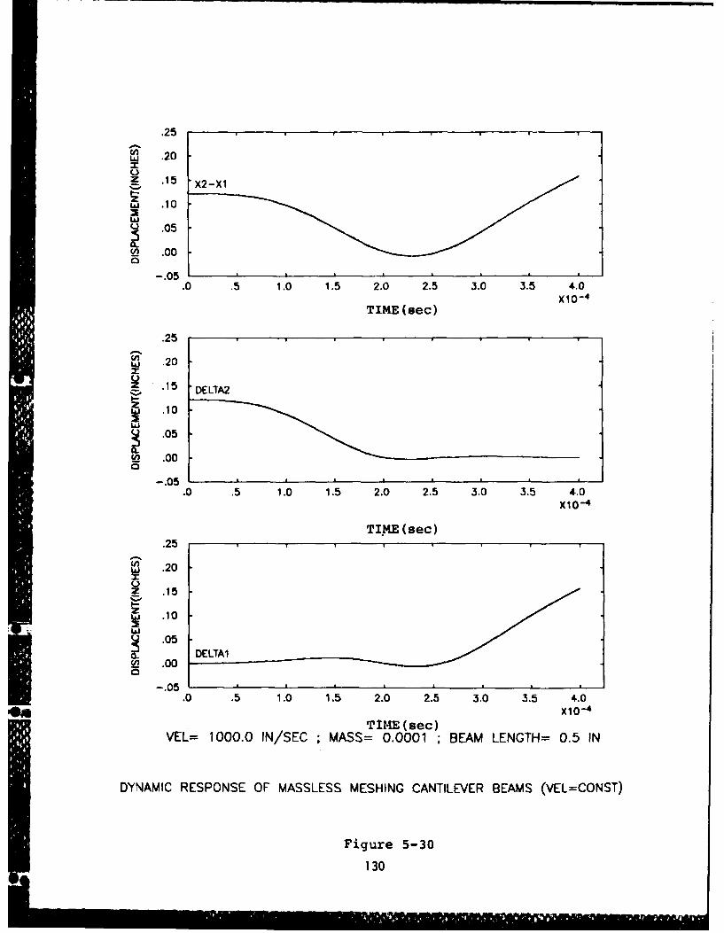
.25

S.20

Ui 1

Z 05

0 .00

.-'05

.0 .5 1.0 1.5 2.0 2.5 3.0 3.5 4.0

TIME (sec)X14

.25

S.20

.5DELTA2

L .10

.05

On .00

-.05.0 .5 1.0 1.5 2.0 2.5 3.0 3.5 4.0

X1 0-4

TI4E (sec).25

S.20

z .15

.10

.05 DELTAl

~?.000.0

.0 .5 1.0 1.5 2.0 2.5 3.0 3.5 4.0

TIME (sec)X1-VEL= 1000.0 IN/SEC ;MASS= 0.0001 ; BEAM LENGTH= 0.5 IN

DYNAMIC RESPONSE OF MASSLESS MESHING CANTILEVER BEAMS (VEL=CONsr)

Figure 5-30

130

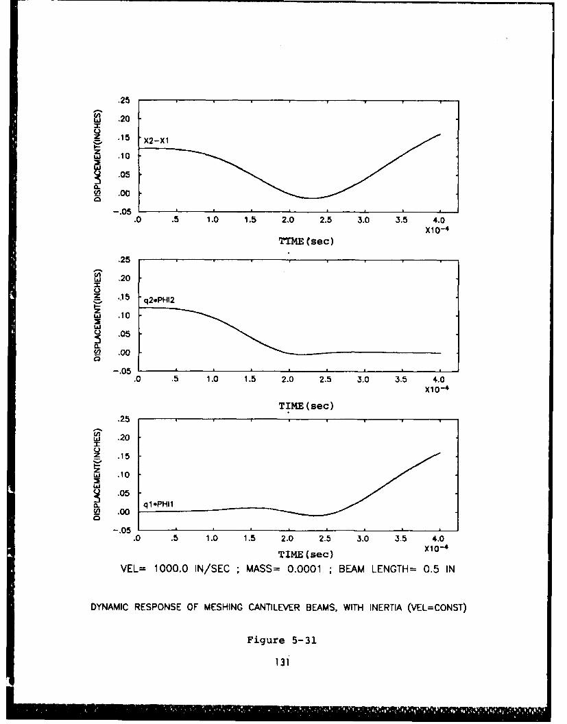
.25

~.20

_ .15 X2-X1

zL. .10

S.05

LA .00

.05.0 .5 1.0 1.5 2.0 2.5 3.0 3.5 4.0

X10- 4

LlIME (sec)

.25

.20

.15 q2*PHI2

Z. .10

.05

0 .00

-. 05.0 .5 1.0 1.5 2.0 2.5 3.0 3.5 4.0

X10-4

TIME (sec).25

.20

z .15

,10

.0 ql*PH1

-. 05.0 .5 1.0 1.5 2.0 2.5 3.0 3.5 4.0

TIME (sec) X14

VEL= 1000.0 IN/SEC ; MASS= 0.0001 ; BEAM LENGTH= 0.5 IN

DYNAMIC RESPONSE OF MESHING CANTILEVER BEAMS, WITH INERTIA (VEL=CONST)

Figure 5-31

131

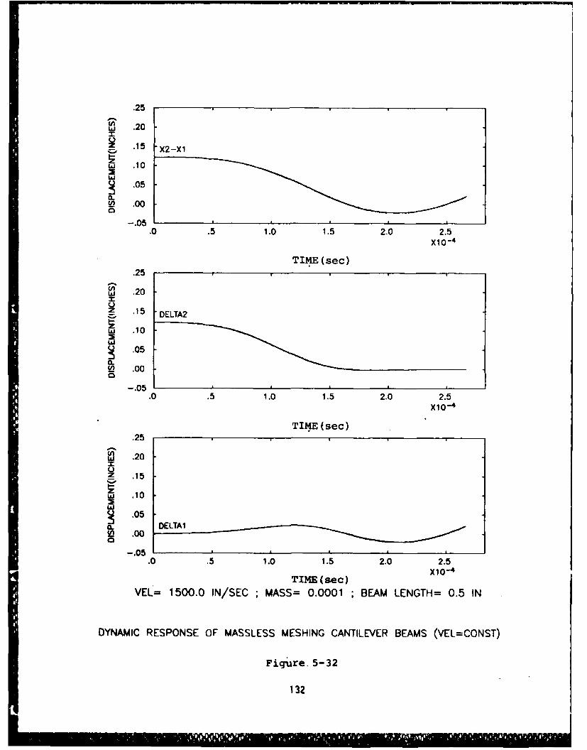
.25

w .20z1-1 -1 X2-X1

LI .10

.05

Ln .00a

.05.0 .5 1.0 1.5 2.0 2.5

X1 0-4

TIME (sec)

.25

w .20

w .10

-05

0) .00

.0

.0 .5 1.0 1.5 2.0 2.5X1 0-4

TIME (sec).25

LI .20

052 15A

0i .0

.05

.0 .5 1.0 1.5 2.0 2.5X1 0-4

TIME (sec)VEL= 1500.0 IN/SEC ;MASS= 0.0001 ;BEAM LENGTH= 0.5 IN

DYNAMIC RESPONSE OF MASSLESS MESHING CANTILEVER BEAMS (VEL=CONST)

Figure. 5-32

1 32

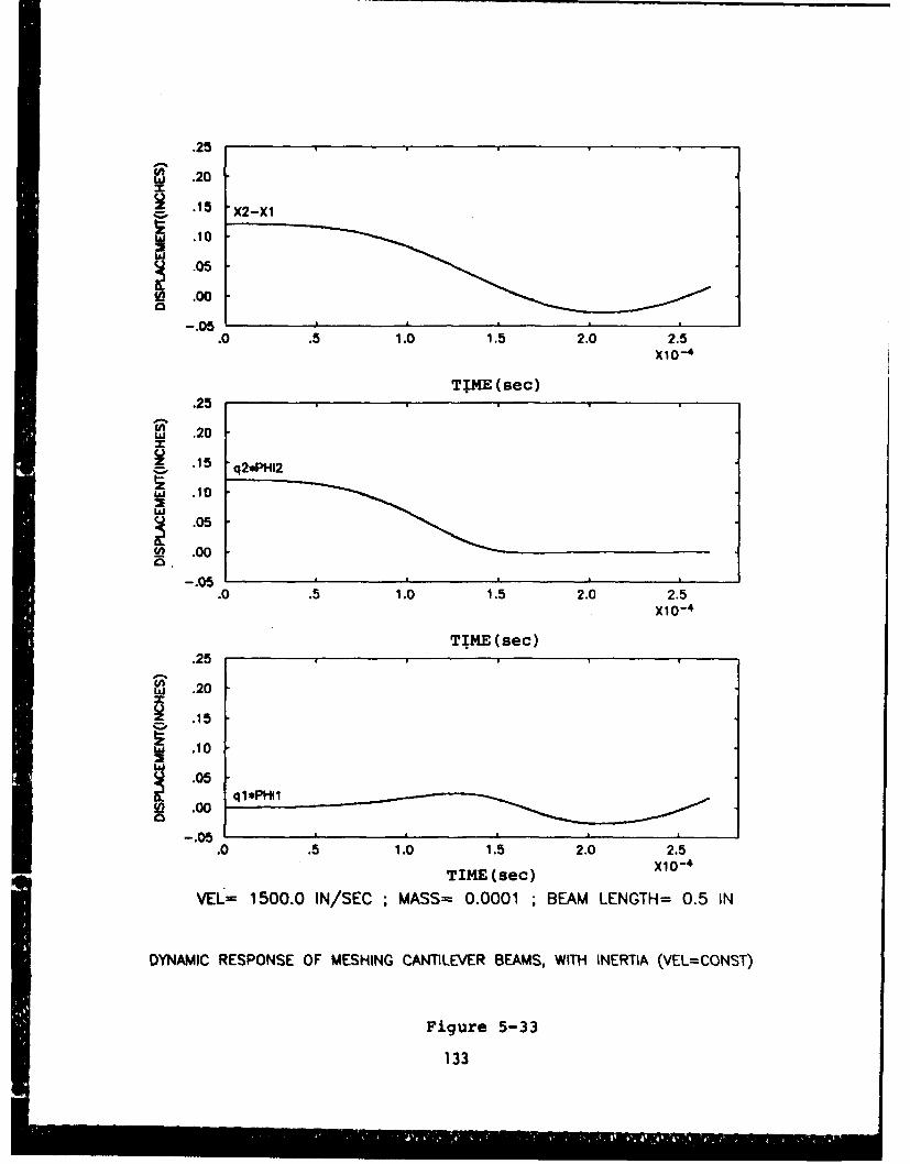
.25 .....

S.20

--,_ 15 X2-Xl

-. 10.0°5ia .00

00

.0 .5 1.0 1.5 2.0 2.5X10- 4

TIME(sec).25

w .20.15 q2*PHI2

w .10

05so .00

.05

.0 .5 1.0 1.5 2.0 2.5X10- 4

TIME (sec).25

' .20

.15

.10

05.00

-. 05.0 .5 1.0 1.5 2.0 2.5

X10-4TIME (sec)

VEL= 1500.0 IN/SEC ; MASS= 0.0001 ; BEAM LENGTH= 0.5 IN

DYNAMIC RESPONSE OF MESHING CANTILEVER BEAMS, WITH INERTIA (VEL=CONST)

Figure 5-33

133

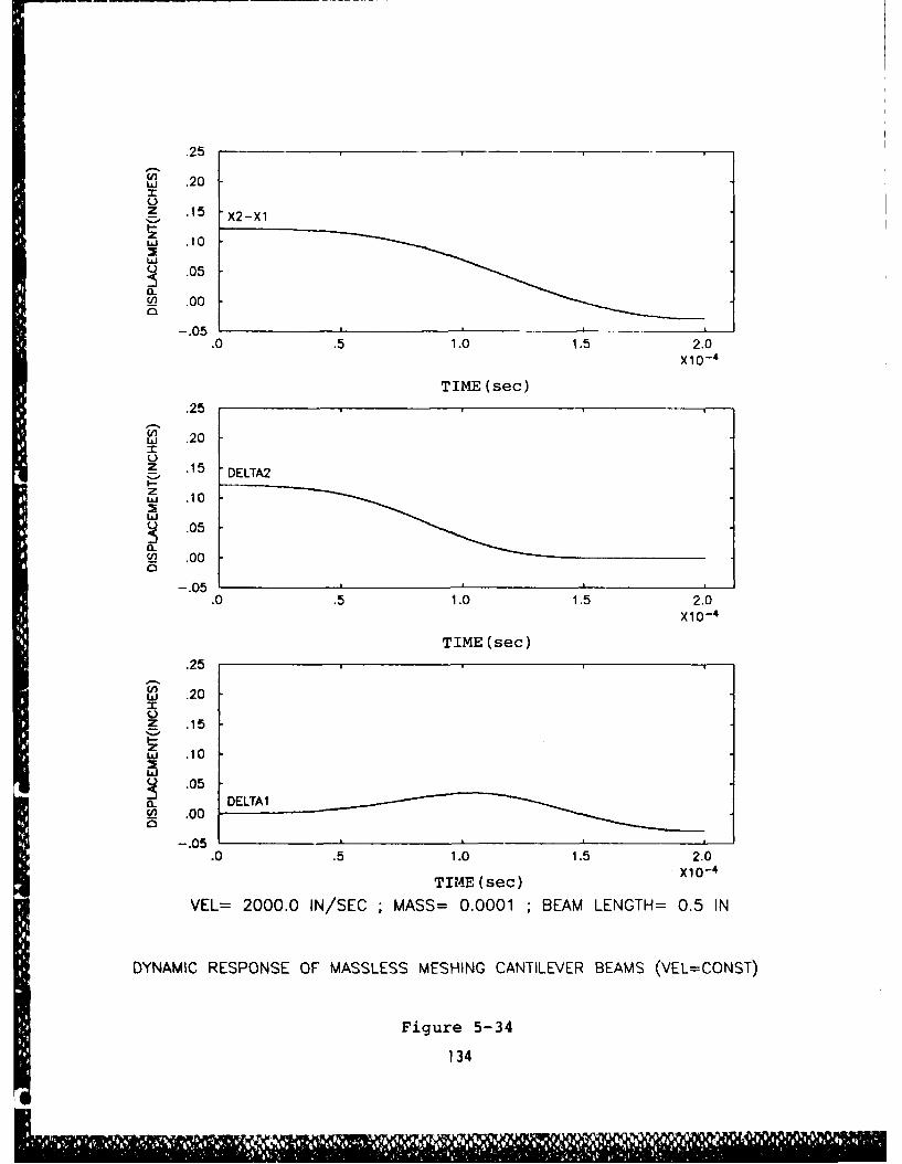
w .20

Z .15 -2X

zLii .10m

.05

On .00

- .05.0 .5 1.0 1.5 2.0

X10- 4

TIME (sec).25

S .20z

-15 DLA

zLai .10

.05

T)2 .00

-.05.0 .5 1.0 1.5 2.0

X10o-4

TIME (sec).25

w3 .20

z .15

zLii .10

-.0 5 -D L ~T) .00

- .05.0 .5 1.0 1.5 2.0

TIME (sec) X1O-

VEL= 2000.0 IN/SEC ;MASS= 0.0001 ;BEAM LENGTH= 0.5 IN

DYNAMIC RESPONSE OF MASSLESS MESHING CANTILEVER BEAMS (VEL=CONST)

Figure 5-34

134

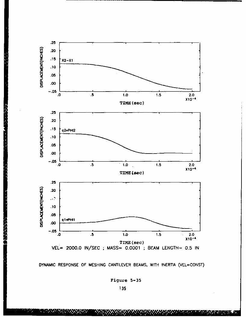
.25

~3 .20

_ .15 '2 X

tij .10

.05

.2

.2

-.15

.05

W .0

.05

.0 .5 1.0 1.5 2.0X10~-4

TIME ~sec)

.25F

Ui .20

.10

- .05.0 .5 1.0 1.5 2.0

TIME1 (sec)X1-VEL= 2000.0 IN/SEC ;MASS= 0.0001 ;BEAM LENGTH= 0.5 IN

DYNAMIC RESPONSE OF MESHING CANTILEVER BEAMS, WITH INERTIA (VEL=CONST)

Figure 5-35

135

6. CONCLUSIONS

The objectives of this analysis were twofold. First, the

dynamic response of a single spur gear tooth subject to moving

loads was studied to determine the effect of the speed of move-

ment of the load. A spur gear tooth, modelled using finite

element techniques, was used in the analysis. From this analy-

sis it was found that the dynamic response of a single gear

tooth is not dependent on the speed of the moving load, but

rather on the type of load engagement experienced at the

beginning of the load cycle. Including the rim in the analysis

added flexibility to the system but did not change the overall

response.

The second objective was to determine whether or not the

mass (inertial forces) of the tooth can be neglected when small

compared to the mass of the gear hub. A simplified analysis

using meshing cantilever beams was used. For the range of

speeds tested, it was found that the inertia forces of the

tooth are small and therefore, the mass of the tooth can be

neglected when determining the dynamic response of a meshing

gear system.

136

BIBLIOGRAPHY

[11 Cornell, R.W. and Westervelt, W.W., "Dynamic Tooth Loadsand Stressing for High Contact Ratio Spur Gears", ASME, J.Mech. Des., Vol. 100, No. 1, Jan. 1978.

[21 Wang, K.L. and Cheng, H.S., "A Numerical Solution to theDynamic Load, Film Thickness, and Surface Temperatures inSpur Gears, Part I - Analysisw, ASME, J. Mech. Des.,Vol. 103, Jan. 1981.

[3) Wang, K.L. and Cheng, H.S., *A Numerical Solution to theDynamic Load, Film Thickness, and Surface Temperatures inSpur Gears, Part II - Results., ASME, J. Mech. Des.Vol. 103, Jan. 1981.

[41 Richardson, H.H., "Static and Dynamic Load, Stress, andDeflection Cycles in Spur Gearing", Sc. D. Thesis, Dept.of Mech. Eng., MIT Cambridge, Mass, 1958.

[5] Kasuba, R. and Evans, J.W., NAn Extended Model for Deter-mining Dynamic Loads in Spur Gearing", ASME, J. Eng. Ind.,Vol. 103, No. 2, Apr. 1981.

[61 Attia, A.Y., "Deflection of Spur Gear Teeth Cut in ThinRims", ASME, J. Eng. Ind., Vol. 86, No. 4, Nov. 1964.

[71 Nagaya, K. and Uematsu, S., *Effects of Moving Load Speedsof Dynamic Loads on the Deflections of Gear Teethu, ASME,J. Mech. Des., Vol. 103, No. 2, Apr. 1981.

[8] Karas, F., "Elastiche Formanderung und Lasterverteilungheim Doppleleingriff geroder Stirnradzahne", V.D.I.Forschh. Vol. 406, 1941.

[91 Wallace, D.B. and Seireg, A., "Computer Simulation ofDynamic Stress, Deformation, and Fracture of Gear Teeth",ASME, J. Eng. Ind., Vol. 95, 1973.

[101 Cornell, R.W., "Compliance and Stress Sensitivity of SpurGear Teeth", ASME, J. Mech. Des., Vol. 103, No. 2, Apr.1981.

[111 Chang, S.H., Huston, R.L. and Coy, J.J., "A Finite ElementStress Analysis of Spur Gears Including Fillet Radii andRim Thickness Effects", ASME, J. Mech. Des., Paper No.82-WA/DE-35, 1982.

[12] Weber, C., "The Deformations of Loaded Gears and theEffect on Their Load Carrying Capacity", SponsoredResearch (Germany), British Dept. of Scientific andIndustrial Research, Report No. 3, 1949.

[131 Segerlind, L.J., Applied Finite Element Analysis, JohnWiley and Sons, Inc., New York, 1976.

137

31W.

[14) Cook, R.D., Concepts and Applications of Finite ElementAnalysis, 2nd Ed., John Wiley & Sons, New York, 1981.

(15) Meirovitch, L., Analytical Methods in Vibrations,MacMillan Comp., New York, 1967.

(16] Meirovitch, L., Methods of Analytical Dynamics, McGraw-Hill Inc., New York, 1970.

[171 Clough, R.W. and Penzien, J., Dynamics of Structures,McGraw-Hill, New York, 1975.

[181 Craig, R.R., Structural Dynamics an Introduction toComputer Methods, John Wiley and Sons, New York, 1981.

[19] Budynas, R.G., Advanced Strength and Applied StressAnalysis, McGraw-Hill, New York, 1977.

[201 Shigley, J.E., Mechanical Engineering Design, 3rd Ed.,McGraw-Hill, New York, 1977.

[21] Merritt, H.E., Gear Engineering, Halsted Press, New York,1971.

[221 Fryba, L., Vibration of Solids and Structures Under MovingLoads, Noordhoff International Publishing, Groningen, TheNetherlands, 1972.

138

APPENDIX 1

1Finite Element Model

Generation Program

2. Moving Load Generation Program

Using Wallace-Seireg Load History

139

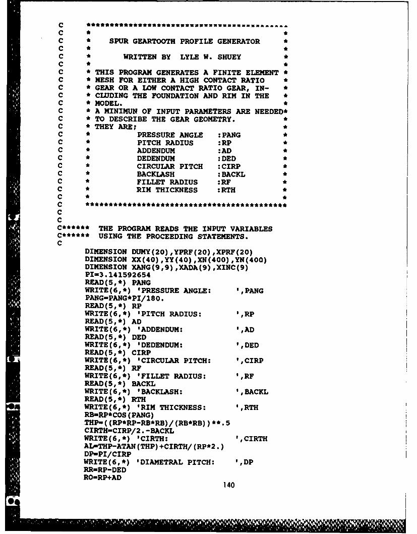
C **

C * SPUR GEARTOOTH PROFILE GENERATORCC *WRITTEN BY LYLE W. SHUEYC **C * THIS PROGRAM GENERATES A FINITE ELEMENT*C * MESH FOR EITHER A HIGH CONTACT RATIOC * GEAR OR A LOW CONTACT RATIO GEAR, IN- *C * CLUDING THE FOUNDATION AND RIM IN THE *C * MODEL.*C * A MINIMUN OF INPUT PARAMETERS ARE NEEDED*C * TO DESCRIBE THE GEAR GEOMETRY.C * THEY ARE;C *PRESSURE ANGLE :PANGC *PITCH RADIUS :RPC *ADDENDUM :AD*C *DEDENDUM :DED*C *CIRCULAR PITCH :CIRP*C *BACKLASH :BACKLC *FILLET RADIUS :RFC *RIM THICKNESS :RTHC *CCCC****** THE PROGRAM READS THE INPUT VARIABLESC****** USING THE PROCEEDING STATEMENTS.C

DIMENSION DUMY(20) ,YPRF(20) ,XPRF(20)DIMENSION XX(40) ,YY(40) ,XN(400) ,YN(400)DIMENSION XANG(9,9) ,XADA(9) ,XINC(9)PI-3.141592654READ(5,*) PANGWRITE(6,*) 'PRESSURE ANGLE: 'PANGPANG=PANG*PI/180.READ(5,*) RPWRITE(6,*) 'PITCH RADIUS: ',RPREAD(5,*) ADWRITE(6,*) 'ADDENDUM: 'ADREAD(5,*) DEDWRITE(6,*) 'DEDENDUM: 'DEDREAD(5,*) CIRPWRITE(6,*) 'CIRCULAR PITCH: ',CIRPREAD(5,*) RFWRITE(6,*) 'FILLET RADIUS: 'RFREAD(5,*) BACKLWRITE(6,*) 'BACKLASH: 'BACKLREAD(5,*) RTHWRITE(6,*) 'RIM THICKNESS: ',RTHRB-RP*COS (PANG)-THP-( (RP*RP-RB*RB)/(RB*RB) )**.5CIRTH-CIRP/2. -BACKLWRITE(6,*) 'CIRTH: 'CIRTHAL-THP-ATAN (THP) +CIRTH/ (RP* 2.)DP-PI/CIRPWRITE(6,*) 'DIAMETRAL PITCH: ',DPRR-RP-DEDRO-RP+AD

140

CC * THIS SECTION CALCULATES POINTS ON THE *C * INVOLUTE SURFACE, FOUNDATION, AND RIX *C * WHICH WILL LATER BE USED TO GENERATEC * NODAL COORDINATES. (BOTH HCRG AND LCRG) *CCC****** GENERATING POINTS ON THE INVOLUTE PROFILEC

DO 5 1-1,11IA1l+ (1-1)iffim(RO-RB) /10.H=RO-HH* (I-i)ANG-(C(H*H-RB*RB) /(RB*RB) )** *5X--RB* (SIN (ANG) -ANG*COS (ANG))Y-RB* (COS (ANG) 4ANG*SIN (ANG) -1)ANGF-ATAN(SIN(ANG)/COS (ANG) )-ALANGF-ANGF* 180 ./PIXP-RB*SIN (AL) +X*COS (AL) +Y*SIN (AL)YP-RB*COS (AL) -X*SIN (AL) +Y*CO5 (AL)XX(IA)-XPYY(IA)-YPWRITE(6,*) 'XP:I,XP,'YP:',YP,ITHETA:',ANGF

5 CONTINUECC****** CHECK IF GEAR IS LCRG OR HCEGC

CHECK-RR*RR+2 .*RFITAN-2IF(CHECK. LT.RB*RB) ITAN-1IF(ITAN.NE.1I) GO TO 15

CC****** STRAIGHT LINE TANGENT TO INVOLUTE (HCRG)C

DD-(-2.*RR+(4.*RR*RR+4.*2.*RF*RR)**.5)/2.D-RB- (RR+DD)DDD-RB-RRXTAN= (D/ DDD)XFILL- (DD/DDD)LTAN-INT(XTAN*8.)LFILL-INT (XFILL*8. )+1WRITE(6,*) 'DD: ',DDWRITE (6, *) ID: ,WRITE(6,*) ' DDD: ', DDEPWRITE(6,*) IXTAN: I,XTANWRITE(6,*) 'XFILL: ',XFILLWRITE(6,*) ILFILL: ',LFILLWRITE(6,*) 'LTAN: ,oLTANDRI-D/ LTANDR-0.0DO 10 I-1,LTAN

IA=12+ (I-i)XP-XP-( ((RB-DR) *SIN (AL)) -( (RB-DRI) *SIN (AL)))YP-YP- (C(RB-DR) *CO5(AL)) - ((RB-DRI) *COS(AL)))DR-DRIDRI-DRI+D/LTANXX(IA)-XPYY(IA) -YP

141

10 CONTINUECC********* FILLET RADIUS SECTION (HCRG)C

BETA-ATAN ( (RR+RF) /RF)BETA-BETA/LFI LLDO 11 1-1,LFILL

IA- (12+LTAN)+ (I-i)X-RF-RF*COS (BETA*I)Y-R*SIN (BETA*I)XP- (RB-D) *SIN (AL) +X*COS (AL) +Y*SIN (AL)YP- (RB-D) *COS (AL) -X*SIN (AL) +Y*COS (AL)XX(IA) -XPYY (IA)-YP

11 CONTINUEGO TO 21

CC****** GENERATING POINTS FOR FILLET RADIUS (LCRG)C15 DD=RB-RR

RF-( (DD*DD)+(2.*DD*RR) )/(2.*RR)WRITE(6,*) 'NEW FILLET RADIUS ',RFBETA-ATAN ((RR+DD) /RF)WRITE(6,*) 'BETA: ',BETA*180./PIBETA-BETA/8. 0DO 20 I=1,8

IA=12+ (I-i)X=RF-RF*COS (BETA* I)Y=-RF*SIN (BETA*I)XP=RB*SIN (AL) +X*COS (AL) +Y*SIN (AL)YP=RB*COS (AL) -X*SIN (AL) +Y*COS (AL)XX(IA)=XPYY(IA)-YPWRITE(6,*) 'XP:',XP,'YP:',YP

20 CONTINUECC****** GENERATING POINTS ON OUTER RIM SURFACEC21 ADA=ASIN( (XP+CIRTH)/RR)-ASIN(XP/RR)

DADA-ADA/ 6.ADAl-ASIN (XP/RR)WRITE(6,*) 'ADA: ',ADA*180./PIDO 30 1-1,4

IA=20+ (I-i)DUMY(I)=10.XP-XP+RR* (SIN (ADA1+DADA) -SIN (ADAl))YP=YP-RR* (COS (ADAl) -COS (ADA1+DADA))XX(IA) -XPYY(IA)-YPWRITE(6,*) 'XP:',XP,'YP:',YPDADA-ADA/4.ADA1-ADA1+DADA

30 CONTINUECC****** GENERATING POINTS ON RADIAL PORTION OF RIMC

DELTA-ASIN (XP/RR)RIM-RR-RTH

DRTH-RTH/4. 142

DX-RR*SIN (DELTA) -RIM*SIN (DELTA)DDX-DX/4 .0DO 40 1-1,4

IA-24+ (I-i)XPRF ( I) -XP-DDXYPRF(I) -YP-DRTHXX(IA)-XPRF(I)YY (IA) -YPRF (I)DRTH-DRTH+RTH/4.DDX-DDX+DX/4 .0WRITE(6,*) IXP:I,XPRP(I),'YP:I,YPRF(I)

40 CONTINUEXP-XPRF (4)YP-YPRF(4)

CC****** GENERATING POINTS ON INNER RIM SURFACEC

DELTA-ATAN (XP/YP)XLEG- ((XP*XP) +(YP*YP) )**.*5DELTA1-1)ELTA/4 .0DO 50 1-1,4

IA-28+ (I-i)DELTA-DELTA-DELTAlXPRF(I) =XLEG*SIN(DELTA)YPRF (I)-XLEG*COS (DELTA)XX (IA) -XPRF (I)YY(IA) -YPRF(I)WRITE(6,*) 'XP:',XPRF(I),'YP:',YPRF(I)

50 CONTINUECCC * THIS SECTION USES COORDINATES FROM *C * THE PREVIOUS SECTIONS TO CALCULATE *

C * NODAL NUMBERS AND COORDINATES.-THERE*C * ARE 319 NODES USED IN THIS MODEL.CCC****** GENERATING NODES 1-121C

11-0DO 60 1-1,11

YA-YY(I)XA-XX (I)AZ-XA*.15BZ-XA*.30CZ-XA*.50DZ->.A*.75XN(IA)--XAXN (IA+10) -XAXN(IA+1) --XA+AZXN (IA+9) -XA-AZXN(IA+2)--XA+BZXN(IA+8) -XA-BZXN (IA+3) --XA+CZXN (IA+7) -XA-CZXN (IA+4) --XA+DZXN (IA+6) -XA-DZXN (IA+5) -0. 0

143

DO 60 J-1, 1111-11+1YN (11) YA

60 CONTINUECC****** GENERATING NODES 122-209C

DANG-2.5SANG-1O.ODO 70 1-1,8

DXANG-SANGDO 75 J=1,4XANG(I,J) =DXANGDXANG-DXANG-DANGWRITE(6,*) XANG(I,J)XANG(I,J)=XANG(I,J) *PI/180.

75 CONTINUEDANG=DANG+2. 5SANG=SANG+10.

70 CONTINUEDO 71 I=1,8XANG(I,4)=0.0

71 CONTINUEC

DO 80 I=1,8IA=122+(I-1) *11XA-XX (11+1)YA=YY (11+1)AZ=XA*.15BZ=XA*.30CZ=XA*.50DZ=XA*.75DZDZ*(.+(I*.02))XN(IA) =-XAXN (IA+ 10) =XAXN(IA+1)=-XA+AZ*COS(XANG(I,1))XN(IA+9) =-XN(IA+1)XN(IA+2)=XN(IA+1)+(BZ-AZ) *COS(XANG(I,2))XN(IA+S)=-XN(IA+2)XN(IA+3)=XN(IA+2)+(CZ-BZ)*COS(XANG(I,3))XN(IA+7)--XN(IA+3)XN(IA+4)=XN(IA+3)+(DZ-CZ) *COS(XcANG(I,4))XN(IA+6) --XN(IA+4)XN(IA+5)=0.0IF(I.EQ.7) CZ-CZ*1.1IF(I.EQ.8) CZ=CZ*1.15YN(IA)-YAYN(IA+10) -YAYN(IA+1)=YA-AZ*SIN(XANG(I,1))YN(IA+9) -YN(IA+1)YN(IA+2)=YN(IA+l) _(BZ-AZ)*SIN(XANG(I,2))YN(IA+8) -YN(IA+2)_YN(IA+3)-YN(IA+2)-(CZ-BZ) *SIN(XANG(I,3))YN(IA+7)u.YN(IA+3)YN(IA+4)-YN(IA+3) -(DZ-CZ) *SIN(XANG(I,4))YN(IA+6)=YN(IA+4)YN(IA+5)-YN(IA+4)

80 CONTINUEC

144

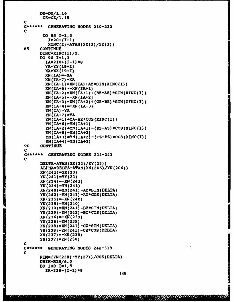
DZ-DZ/1. 16CZ-CZ/ 1. 15

CC****** GENERATING NODES 210-233C

DO 85 1-1,3J-20+ (I-i)XINC(I)=ATAN(XX(J)/YY(J))

85 CONTINUEDINC-XINC(1)/2.DO 90 1-1,3

IA-210+(I-1) *8YA-YY (19+1)XA-XX(19+I)DI (IA) --XAXN(IA+7) -XAXN(IA+1)=XN(IA)+AZ*SIN(XINC(I))XN(IA+6)--XN(IA+l)XN(IA+2)-XN(IA+1)+(BZ-AZ) *SIN(XINC(I))XN(IA+5)--XN(IA+2)XN(IA+3)-XN(IA+2)+(CZ-BZ)*SIN(XINC(I))XN(IA+4)--XN(IA+3)YN(IA) -YAYN(IA+7) =YAYN(IA+1) =YA-AZ*COS (XINC(I))YN(IA+6) =YN(IA+1)YN(IA+2)-YN(IA+1)-(BZ-AZ)*COS(XINC(I))YN(IA+5)-YN(IA+2)YN(IA+3)-YN(IA+2)-(CZ-BZ)*COS(XINC(I))YN(IA+4)=YN(IA+3)

90 CONTINUECC****** GENERATING NODES 234-241C

DELTA=ATAN(XX(23)/YY(23))ALPHA-DELTA-ATAN(XN(206)/YN(206))XN (241) -XX (23)YN(241)=YY(23)XN(234)=-XN(241)YN (234) =YN (241)XN(240)=XN(241) -AZ*SIN(DELTA)YN(240) =YN-(241) -AZ*COS (DELTA)XN(235)=-XN(240)YN (235) =YN (240)XN(239)=XN(241) -BZ*SIN(DELTA)YN(239) =YN(241) -BZ*COS (DELTA)XN (236) -- XN (239)YN (236) =YN (239)XN(238)=XN(241) -CZ*SIN(DELTA)YN(238)-YN(241) -CZ*COS(DELTA)XN(237)--XN(238)YN(237)-YN(238)

CC****** GENERATING NODES 242-319C

RIM-(YN(238)-YY(27) )/COS (DELTA)DRIM-RIM/6. 0DO 100 1-1,5

IA-238-(I-1) *8 145

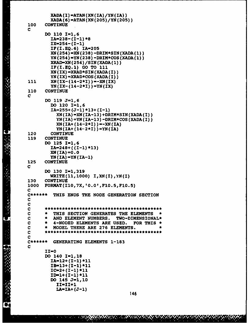
XADA(I)-ATAN(XN(IA)/YN(IA))XADA(6)-ATAN(XN(205)/YN(205))

100 CONTINUEC

DO 110 1-1,6IA=238- (I-1) *8IX=254- (I-1)IF(I.EQ.6) IA=205XN(254)=XN(238)-DRIM*SIN(XADA(1))YN(254)-YN(238)-DRIM*COS(XADA(1))XRAD-XN(254)/SIN(XADA(1))IF(I.EQ.1) GO TO 111XN (IX) =XRAD*SIN (XADA (I) )YN(IX)=XRAD*COS(XADA(I))

ill XN(IX-(14-2*I))=-XN(IX)YN(IX-(14-2*I) )=YN(IX)

110 CONTINUEC

DO 119 J=1,6DO 120 I=1,6IA=255+(J-1) *13+(I-1)

XN(IA)=XN(IA-13)+DRIM*SIN(XADA(I))YN(IA)=YN(IA-13)-DRIM*COS(XADA(I))XN(IA+(14-2*I) )=-XN(IA)YN(IA+(14-'2*I) )-YN(IA)

120 CONTINUE119 CONTINUE

DO 125 1-1,6IA-248+( (I-i) *13)XN(IA)=0.0YN (IA) =YN (IA- 1)

125 CONTINUEC

DO 130 1-1,319WRITE(11,1000) I,XN(I),YN(I)

130 CONTINUE1000 FORMAT(I10,7X,'O.0',F1O.5,F1O.5)CC****** THIS ENDS THE NODE GENERATION SECTIONCCCC * THIS SECTION GENERATES THE ELEMENTS*C * AND ELEMENT NUMBERS. TWO-DIMENSIONAL*C * 4-NODED ELEMENTS ARE USED. FOR THISC * MODEL THERE ARE 276 ELEMENTS.*CCC****** GENERATING ELEMENTS 1-183C

11=0DO 140 1-1,18

IA-12+(I-1) *111IBn13+ (1-1) *11IC-2+(I-1) *11IDinl+ (1-1) *11DO 145 J-1,10

I1-11+1LA-IA+ (J-1)

146

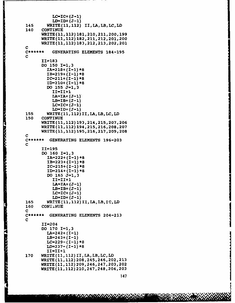
LC-IC+ (J-1)LD=-ID+ (J-1)

145 WRITE(11,112) II,LA,LB,LC,LD140 CONTINUE

WRITE(11,112) 181,210,211,200,199WRITE(11,112) 182,211,212,201,200WRITE(11,112) 183,212,213,202,201

CC****** GENERATING ELEMENTS 184-195C

11=183DO 150 I=1,3

IA=218+(I-1) *8IB=219+ (1-1) *8IC=211+ (1-1) *8ID=210+(I-1) *8DO 155 J=1,3

11=11+1LA=IA+ (J-1)-LB=IB+ (J-1)LC=IC+ (J-1)LD=-ID+ (J-1)

155 WRITE(11,112)II,LA,LB,LC,LD150 CONTINUE

WRITE(11,112) 193,214,215,207,206WRITE(11,112) 194,215,216,208,207WRITE(11, 112) 195,216,217,209,208

CC****** GENERATING ELEMENTS 196-203C

11=195DO 160 I=1,3

IA=222+(I-1) *8IB=223+ (I-1)*8IC=215+(I-1) *8ID=-214+ (I-i) *8DO 165 J=1,3

II=II+1LA=IA+ (J-1)LB=IB+ (J-1)LC=IC+ (J-1)LD=ID+ (J-1)

165 WRITE(11,112)II,LA,LB,lC,LD160 CONT.LNUE

C

C****** GENERATING ELEMENTS 204-213I11=204DO 170 I=1,3

LA=242+ (I-i)LB=243+ (1-1)LC=229-(I-1) *8LD=237- (I-i) *811=11+1

170 WRITE(11,112)II,LA,LB,LC,LDWRITE(11, 112) 208,245,246,202,213WRITE(11,112) 209,246,247,203,202WRITE(11,112)210,247,248,204,203

147

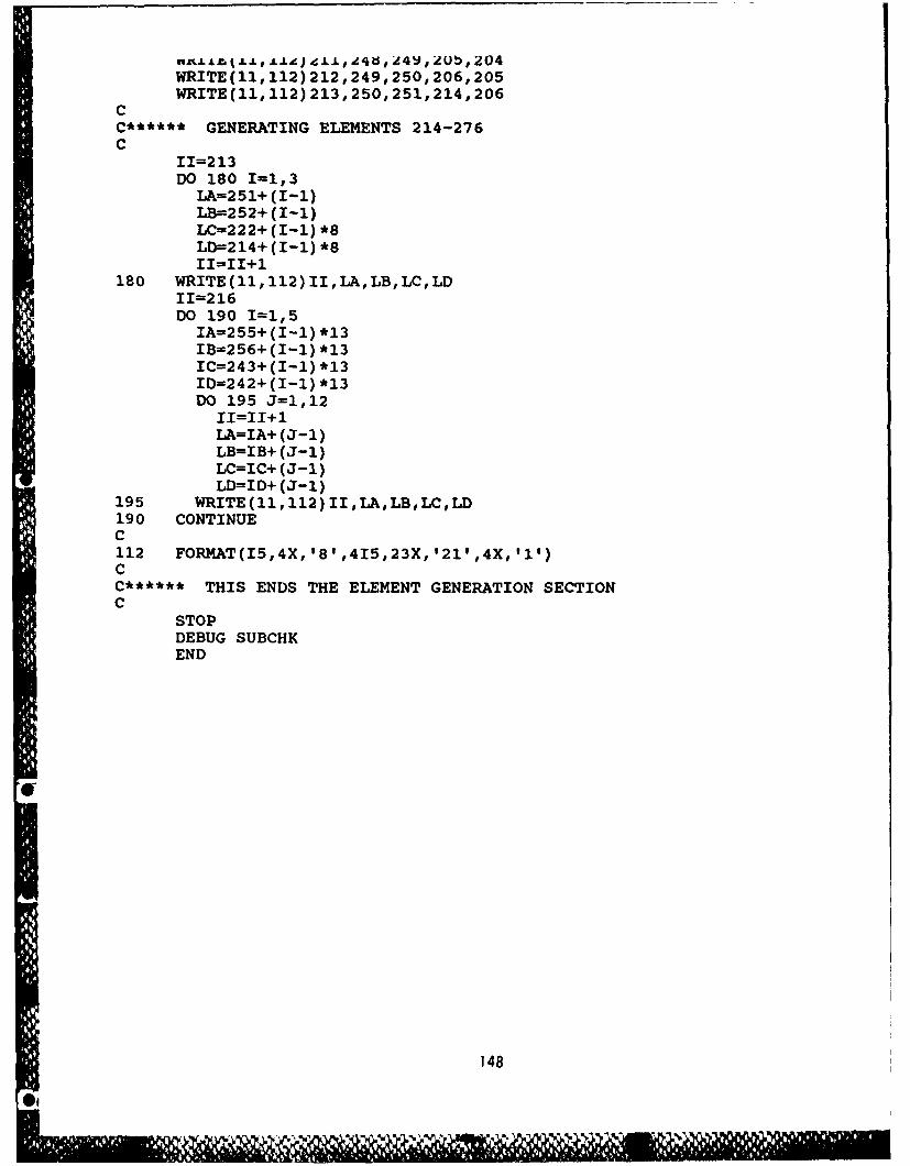
WRITE(11,112)212,249,250,206,205WRITE(11, 112) 213,250,251,214,206

CC****** GENERATING ELEMENTS 214-276C

11=213DO 180 I=1,3

LA=251+ (I-i)LB--252+ (I-1)LC=222+(I-1) *8LD=214+ (1-1) *811=11+1

180 WRITE(11,112)II,LA,LB,LC,LD11=216DO 190 I=1,5

IA=255+(I-1)*13IB=256+(I-1) *13IC=243+ (I-i) *13ID=2424-(I-1) *13DO 195 J=1,12

11=11+1LA=IA+ (J-1)LB=IB+ (J-1)LC=IC+ (J-1)LD=ID+ (J-1)

195 WRITE(11,112)II,LA,LB,LC,LD190 CONTINUEC112 FORMAT(I5,4X,'8',4I5,23X,'21',4X,'1)CC****** THIS ENDS THE ELEMENT GENERATION SECTIONC

STOPDEBUG SUBCHKEND

148

Oeli

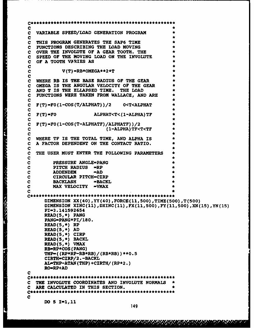
C *C VARIABLE SPEED/LOAD GENERATION PROGRAM *C *C THIS PROGRAM GENERATES THE SAP6 TIME *C FUNCTIONS DESCRIBING THE WAD MOVING *C OVER THE INVOLUTE OF A GEAR TOOTH. THE *C SPEED OF THE MOVING LOAD ON THE INVOLUTE *C OF A TOOTH VARIES AS *C *C V(T)=RB*OMEGA**2*T *C *C WHERE RB IS THE BASE RADIUS OF THE GEAR *C OMEGA IS THE ANGULAR VELOCITY OF THE GEAR *C AND T IS THE ELLAPSED TIME. THE LOAD *C FUNCTIONS WERE TAKEN FROM WALLACE, AND ARE *C *C F(T)=FO(1-COS(T/ALPHAT))/2 O<T<ALPHAT *C *C F(T)=F0 ALPHAT<T<(I-ALPHA)TF *C *C F(T)=FO(1-COS(T-ALPHATF)/ALPHATF) )/2 *C (1-ALPHA) TF<T<TF *C *C WHERE TF IS THE TOTAL TIME, AND ALPHA IS *C A FACTOR DEPENDENT ON THE CONTACT RATIO. *C *C THE USER MUST ENTER THE FOLLOWING PARAMETERS *C *C PRESSURE ANGLE=PANG *C PITCH RADIUS -RP *C ADDENDEM =AD *C CIRCULAR PITCH=CIRP *C BACKLASH =BACKL *C MAX VELOCITY -VMAX *C *

DIMENSION XX(40),YY(40),FORCE(11,500),TIME(500) ,T(500)DIMENSION XINC(11),DXINC(11),FX(11,500),FY(11,500),XN(15),YN(15)PI-3. 141592654READ(5,*) PANGPANG=PANG*PI/180.READ(5,*) RPREAD(5,*) ADREAD(5,*) CIRPREAD(5,*) BACKLREAD(5, *) VMAXRB-RP*COS (PANG)THP-( (RP*RP-RB*RB)/ (RB*RB)) **0.5CIRTH-CIRP/2 . -BACKLAL-THP-ATAN (THP) +CIRTH/(RP*2.)RO-RP+AD

C

C THE INVOLUTE COORDINATES AND INVOLUTE NORMALS *C ARE CALCULATED IN THIS SECTION. *

**************************** **** ****

CDO 5 1-1,11

149

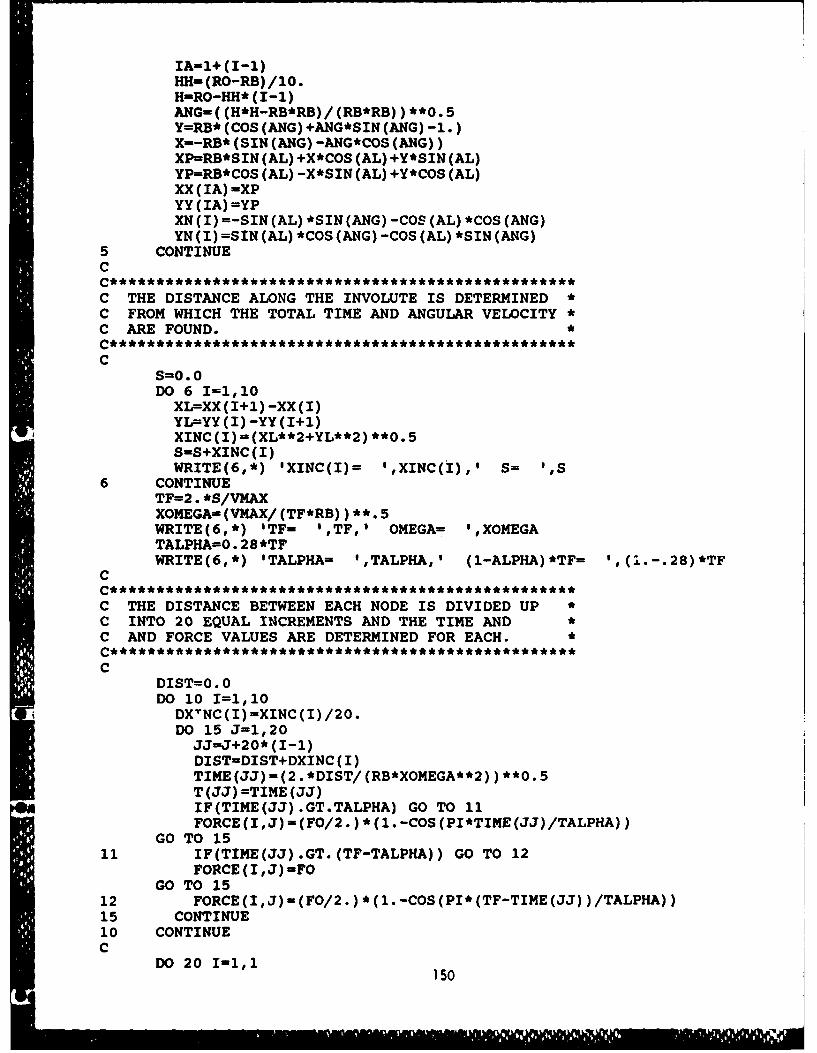
IA-1+ (I-1)HH- (RO-RE) /10.H=RO-HH* (I-1)ANG-( (H*H-RB*RB)/ (RB*RB) )**0.5Y=RB* (COS (ANG) +ANG*SIN (ANG) -1.)Xin-RB* (SIN (ANG) -ANG*COS (ANG))XP=RB*SIN (AL) +X*COS (AL) +Y*SIN (AL)YP=-RB*COS (AL) -X*SIN (AL) +Y*COS (AL)XX(IA) -XPYY (IA) =YPXN (I) =-SIN (AL) *SIN (ANG) -COS (AL) *COS (ANG)YN(I)=SIN(AL) *COS(ANG)-COS(AL) *SIN(PJNG)

5 CONTINUEC

C THE DISTANCE ALONG THE INVOLUTE IS DETERMINED *C FROM WHICH THE TOTAL TIME AND ANGULAR VELOCITY *C ARE FOUND.

CS=0.0DO 6 I=1 ,10

XL=-XX(I+1) -XX(I)YL-YY (I) -YY (I+1)XINC(I)=(XL**2+YL**2) **O.5S-S+XINC(I)WRITE(6,*) 'XINC(I)= ',XINC(i),' S= 1IS

6 CONTINUETF=2.*S/VMAXXOMEGA= (VMAX/ (TF*RB) )**.*5WRITE(6,*) ITF= ',TF,l OMEGA= ',XOMEGATALPHA-0.*28*TFWRITE(6,*) 'TALPHA= ',TALPHA,' (1-ALPHA)*TF= ',(!.-.28)*TF

C

C THE DISTANCE BETWEEN EACH NODE IS DIVIDED UP*C INTO 20 EQUAL INCREMENTS AND THE TIME AND*C AND FORCE VALUES ARE DETERMINED FOR EACH.

CDIST=O.ODO 10 I=1,10

DX'NC(I)=XINC(I)/20.DO 15 J-1,20JJ=J+20* (I-i)DIST-DIST+DXINC (I)TIME(JJ)=(2.*DIST/(RB*XOMEGA**2) )**0.5T (JJ) =TIME (JJ)IF(TIME(JJ).GT.TALPHA) GO TO 11FORCE(I,J)-(FO/2.)*(l.-COS(PI*TIME(JJ)/TALPHA))

GO TO 1511 IF(TIME(JJ).GT.(TF-TALPHA)) GO TO 12

FORCE (I ,J) -FO,GO TO 15

12 FORCE(I,J)-(FO/2.)*(1.-COS(PI*(TF-TIME(JJ))/TALPHA))15 CONTINUE10 CONTINUEC

DO 20 1-1,1 150

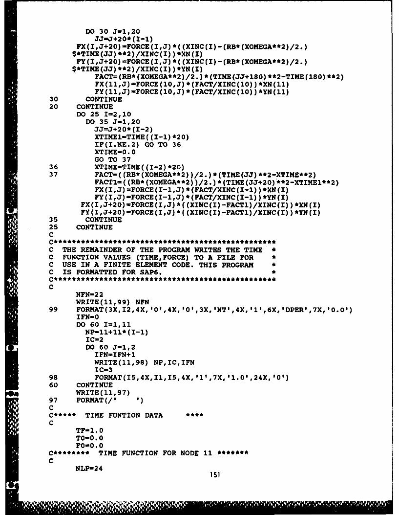
DO 30 J-1,20JJ-J+20* (I-1)

FX(I,J+20)-FORCE(I,J) *( (XINC(I)-(RB*(XOMEGA**2)/2.)

FY(I,J+20)-.FORCE(I,J)*((XINC(I)-(RB*(XOMEGA**2)/2.)$*TIME(JJ)**2)/XINC(I) )*YN(I)

FACT-(RB* (XOMEGA**2)/2. ) *(TIME (JJ+180) **2-TIME (180) **2)FX(11,J)=FORCE(10,J)*(FACT/XINC(10))*XN(11)FY(11,J)=FORCE(10,J)*(FACT/XINC(10))*YN(11)

30 CONTINUE20 CONTINUE

DO 25 1-2,10DO 35 J-1,20JJ=J+20* (1-2)XTIME1=TIME( (I-i) *20)IF(I.NE.2) GO TO 36XTIME=0.0GO TO 37

36 XTIME=TIME( (1-2) *20)37 FACT=((RB*(XOMEGA**2))/2.)*(TIE(JJ)**2-XTIME**2)

FACT1=( (RB* (XOMEGA**2) )/2. ) *(TIME(JJ+20) **2-XTIME1**2)FY(IJ)=FORCE(I-1,J)*(FACT/XINC(I-1) )*YN(I)

FX(I,J+20)=FORCE(I,J)*((XINC(l)-FACT1)/XINC(I))*XN(I)

35 CONTINUE25 CONTINUEC

C THE REMAINDER OF THE PROGRAM WRITES THE TIME*C FUNCTION VALUES (TIME,FORCE) TO A FILE FOR *C USE IN A FINITE ELEMENT CODE. THIS PROGRAM *C IS FORMATTED FOR SAP6 *

CNFN=22WRITE(11,99) NFN

99 FORMAT(3X,I2,4X,10',4X,'O',3X,'NT',4X,'11,6X,'DPER',7X,1O.01)IFN-0DO 60 1-1,11

NPu11+11* (I-1)IC=2DO 60 J-1,2

IFN=IFN+lWRITE(11,98) NP,IC,IFNIC=3

98 FORMAT(15,4X,I1,I5,4X, '11,7X, '1.0',24X, '0)60 CONTINUE

WRITE (11, 97)97 FORMAT(/$CC***** TIME FUNTION DATAC

TF-1.0TO-0.0F0-0.0

C******** TIME FUNCTION FOR NODE 11 **~

CNLP-2 4

151

.. ow

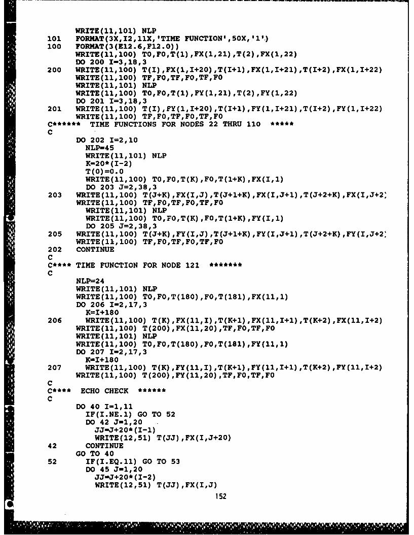
WRITE(11,101) NLP101 FORMAT(3X,12,11X, 'TIME FUNCTION',50X,1'l.)100 FORMAT(3(E12.6,F12.0))

WRITE(11,100) TO,FO,T(1),FX(1,21),T(2),FX(1,22)DO 200 1-3,18,3

200 WRITE(11,100) T(I),FX(1,I+20),T(I+1),FX(1,I+21),T(I+2),FX(1,I+22)WRITE(11,100) TF,FO,TF,FO,TF,FOWRITE(11,101) NLPWRITE(11,100) TO,FO,T(1),FY(1,21),T(2),FY(1,22)DO 201 I=3,18,3

201 WRITE(11,100) T(I),FY(1,I+20),T(I+1),FY(1,I+21),T(I+2),FY(1,I+22)WRITE(11,100) TF,FO,TF,FO,TF,FO

C****** TIME FUNCTIONS FOR NODES 22 THRU 110***C

DO 202 I=2,10NLP=-45WRITE(11,101) NLPK=20* (1-2)T(0)=0.0WRITE(11,100) TO,FO,T(K),FO,T(1+K),FX(I,1)DO 203 J=2,38,3

203 WRITE(11,100) T(J+K),FX(I,J),T(J+1+K),FX(I,J+1),T(J+2+K),FX(I,J+2,WRITE(11,100) TF,FO,TF,FO,TF,FO

WRITE(11,101) NLPWRITE(11,100) TO,FO,T(K),FO,T(1+K),FY(I,1)DO 205 J=2,38,3

205 WRITE(11,100) T(J+K),FY(I,J),T(J+1+K),FY(I,J+1),T(J+2+K),FY(I,J+2;WRITE(11,100) TF,FO,TF,FO,TF,FO

202 CONTINUECC**** TIME FUNCTION FOR NODE 121****C

NLP=-24WRITE(11,101) NLPWRITE(11,100) TO,FO,T(180),FO,T(181),FX(11,1)DO 206 1-2,17,3

K=I+180206 WRITE(11,100) T(K),FX(11,I),T(K+1),FX(11,I+1),T(K+2),FX(11,I+2)

WRITE(11,100) T(200),FX(11,20),TF,FO,TF,FOWRITE(11,101) NLPWRITE(11,100) TO,FO,T(180),FO,T(181),FY(11,1)DO 207 1-2,17,3

K=I+ 180207 WRITE(11,100) T(K),FY(11,I),T(K+1),FY(11,I+1),T(K+2),FY(11,I+2)

WRITE(11,100) T(200),FY(11,20),TF,FO,TF,FOCC**** ECHO CHECK ***

CDO 40 1-1,11

IF(I.NE.1) GO TO 52DO 42 J-1,20

JJ-J+20* (I-1)WRITE(12,51) T(JJ) ,FX(I,J+20)

42 CONTINUEGO TO 40

52 IF(I.EQ.11) GO TO 53DO 45 J-1,20

JJmJ+20* (1-2)WRITE(12,51) T(JJ),FX(I,J)

152

45 CONTINUEDO 46 J-1,20

JJ-J+20* (I-i)WRITE(12,51) T(JJ) ,FX(IJ+20)

46 CONTINUEGO TO 40

53 DO 50 J=1,20JJ-J+20* (1-2)WRITE(12,51) T(JJ),FX(I,J)

50 CONTINUE40 CONTINUE51 FORMAT(Fl2.8,12X,F8.O)

STOPEND

1 53

APPENDIX 2

Contact Point Velocity

Of Meshing Spur Gear Teeth

Ia

154

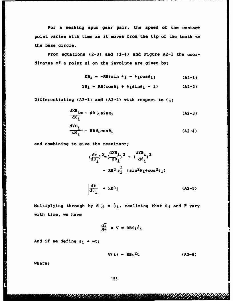
For a meshing spur gear pair, the speed of the contact

point varies with time as it moves from the tip of the tooth to

the base circle.

From equations (2-3) and (2-4) and Figure A2-1 the coor-

dinates of a point Bi on the involute are given by;

XB i - -RB(sin 61 - eicosei) (A2-1)

YBi - RB(cosei + eisinei - 1) (A2-2)

Differentiating (A2-1) and (A2-2) with respect to ei;

dXBi= - RB Oisin 0 (A2-3)

dYBid- --- RBeicosei (A2-4)

and combining to give the resultant;d2. dXBi 2 dYBi) ) (1 2

- RB2 of (sin 2ei+cos28i)

di RBBi (A2-5)17

Multiplying through by d ei 6 oi, realizing that ei and F vary

with time, we have

3-t V - RBeiei

And if we define ei - wt;

V(t) - RBw2 t (A2-6)

where; 1

1 55

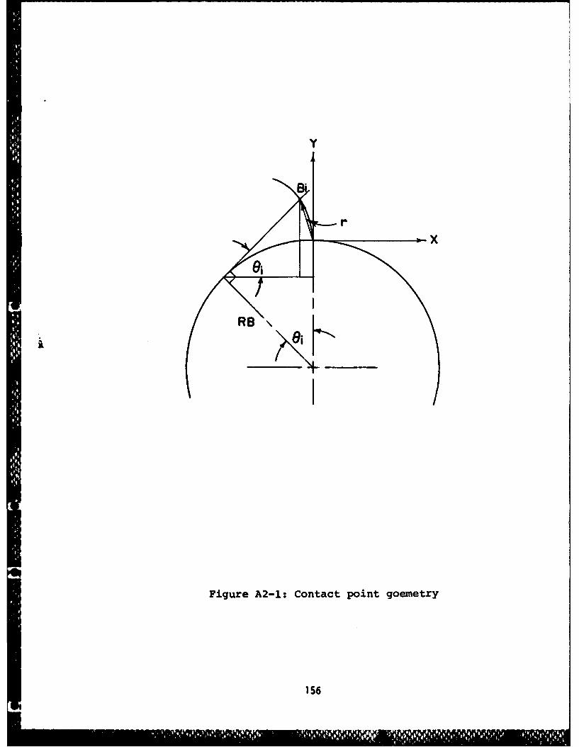
y

r

ei

RB\

Figure A2-1: Contact point goemetry

1 56

V(t) - the speed of the contact

point Bi at time t

w angular velocity of the gear (rad/sec)

At t = 0.0, corresponding to the load at the tip of the tooth,

the speed is zero, and at t - TF, time corresponding to the

load positioned at the base circle, the speed is maximum.

The position of the load as a function of time is found by

integrating equation (A2-6) with respect to time. By defining

the speed as the first derivative of the position;

V(t) = dS(t) = RBc2t

dS(t) = RBw2 ft dt

S(t) = RB 2 t2 + C (A2-7)

Evaluating the constant of integration for t = Ti, the time at

the tip of the tooth;

S(ti) - 0.0 = RBw2 Ti2+ C

then;

C - - RBw 2 T2 (A2-8)

The displacement then becomes;

S(t) - RBw 2 t2 - RBw2 Ti 2 (A2-9)

If we assume that the time at the tip position is zero the

constant term vanishes and we are left with only the first term

157

I' "

on the right hand side of equation A2-9 defining the position

along the involute.

I

APPENDIX 3

Deformed Shapes of Gear Tooth

1. Static Loading

2. Modal Analysis

3. Dynamic Response

159

Static Loading

Timoshenko Beam Constraints

Rim Included

160

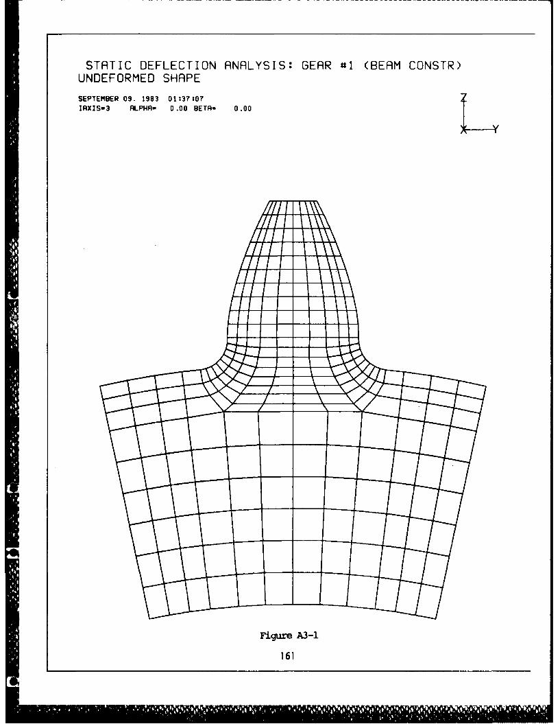
STATIC DEFLECTION ANALYSIS: GEAR '*1 (BEAM CONSTR)UNDEFORMED SHAPE

SEPTEMBER 09. 1993 01:31:07

IRXISs3 ALPHA- 0 .00 BETA= 0.00

Figure A3-1

161

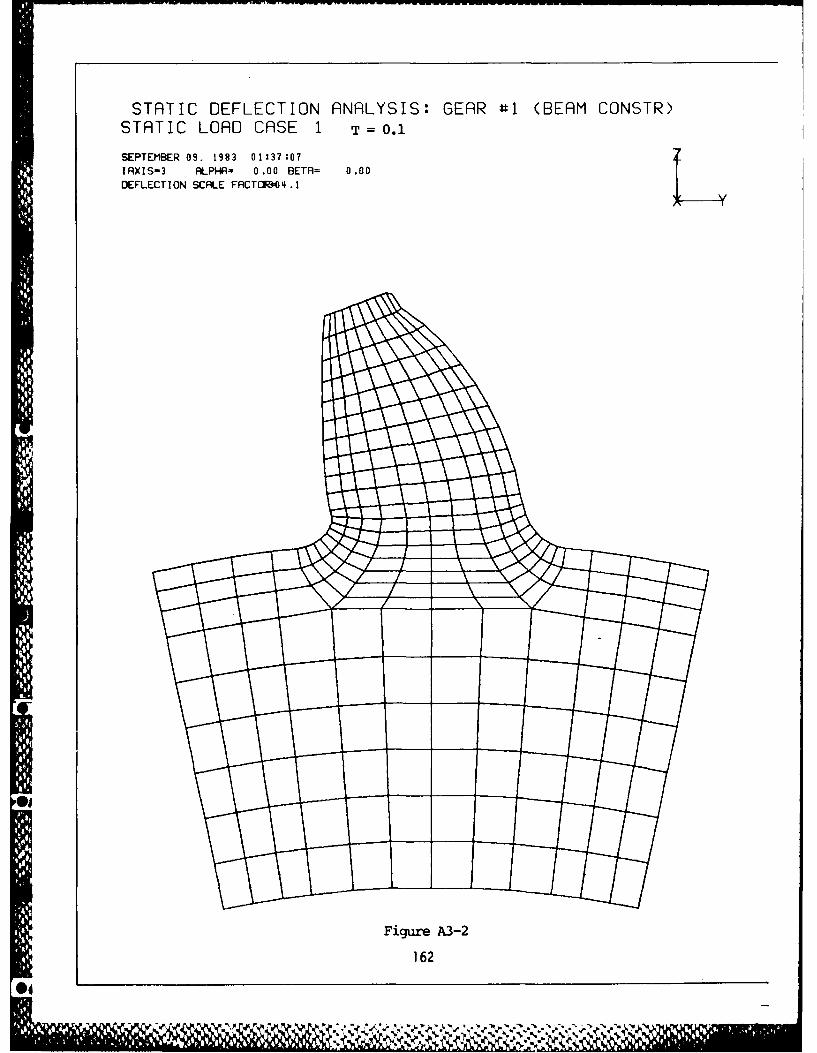
STATIC DEFLECTION ANALYSIS: GEAR #1 (BEAM CONSTR)STATIC LOAD CASE 1 T= 0.1

SEPTEMBER 09. 1983 01:3?:07IAXIS=3 ALPHR= 0.00 BETR= 0.00DEFLECTION SCRLE FACTCRI4 .1

Figure A3-2

162-@,

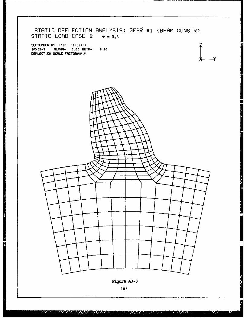
STATIC DEFLECTION ANALYSIS: GEOg #1 (BEAM CONSTR)STATIC LOAD CASE 2 T=O0.3

SEPTEMBER 09. 1993 01:37307IRXIS=3 ALPtfi- 0 .00 BETA= 0 .00DEFLECTI ON SCALE FRCOF9 .6

Figure A3-3

163

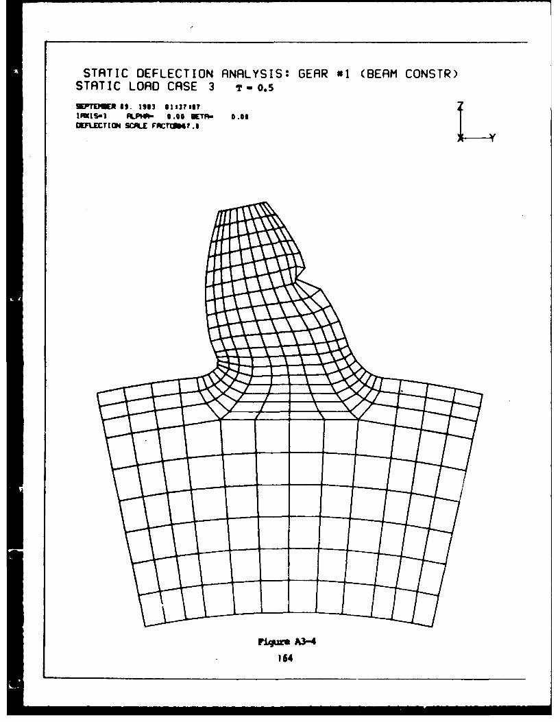
STATIC DEFLECTION ANALYSIS: GEAR #1 (BEAM CONSTR)STATIC LOAD CASE 3 T -o.5

KPloUC O. 1933 8113 toyM!1S-3 FPHPw 0.50 V3m- 0.00

DEFLICTI tSCAL FlCTi= 7.3

Fi9 mv A3-4

164

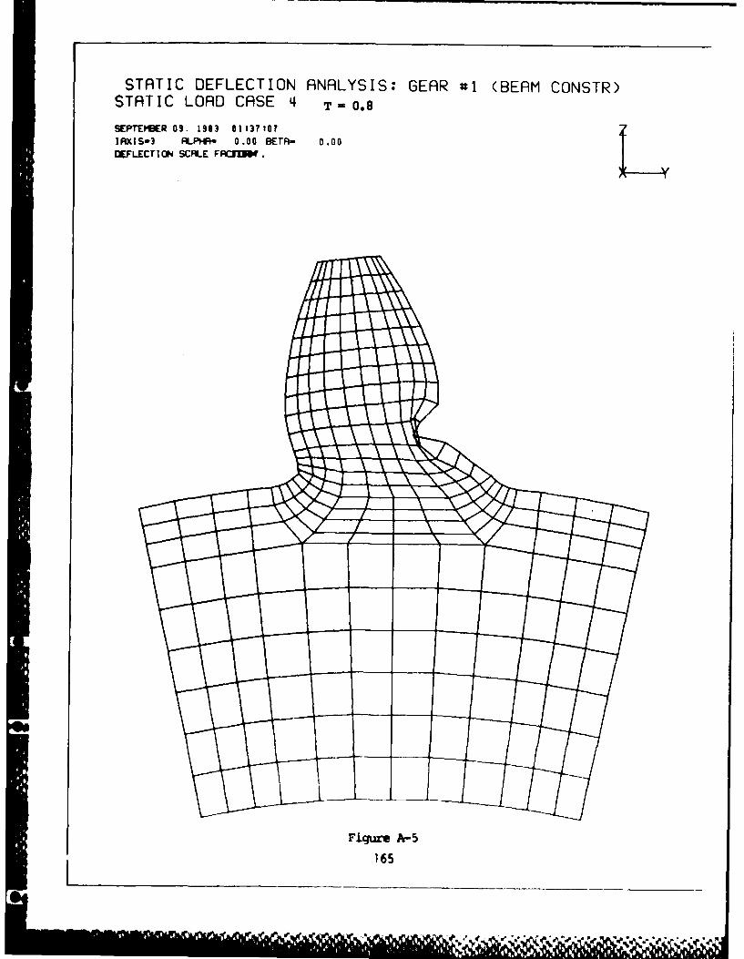
STATIC DEFLECTION ANALYSIS: GEAR #1 (BEAM CONSIR)STATIC LOAD CASE 4 T=O0.8

SEPTEMBER 09. 1963 01837,0?IRXIS-3 ALPHAR- 0.00 BETA- 0 .00DEFECTION SCALE FRC2UW.

F igure A-5

165

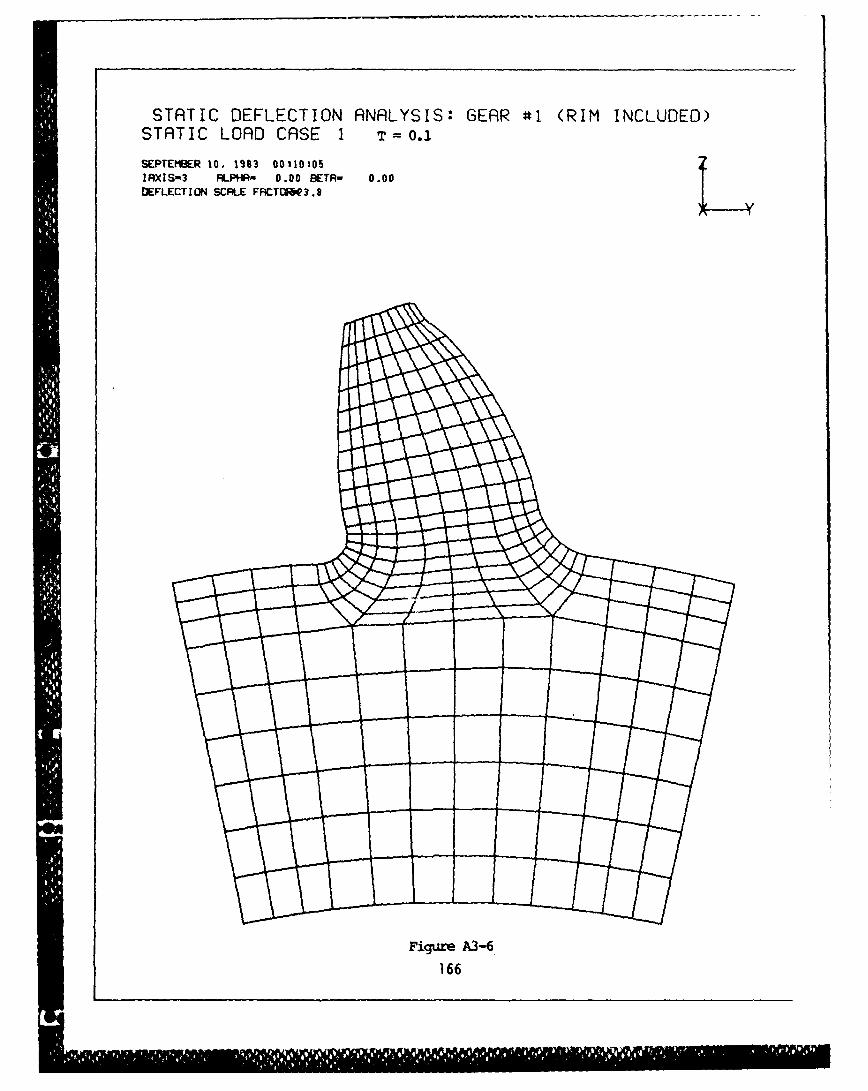
STATIC DEFLECTION ANALYSIS: GEAR #1i (RIM INCLUDED)STATIC LOAD CASE 1 T=O0.1

SEPTEMBER 10, 1S83 00110:05IRqXIS-3 RLPHA- 0.00 BETA- 0.00DEFLECTI ON SCALE FRCTO~Q 3.8

Figure A3-6166

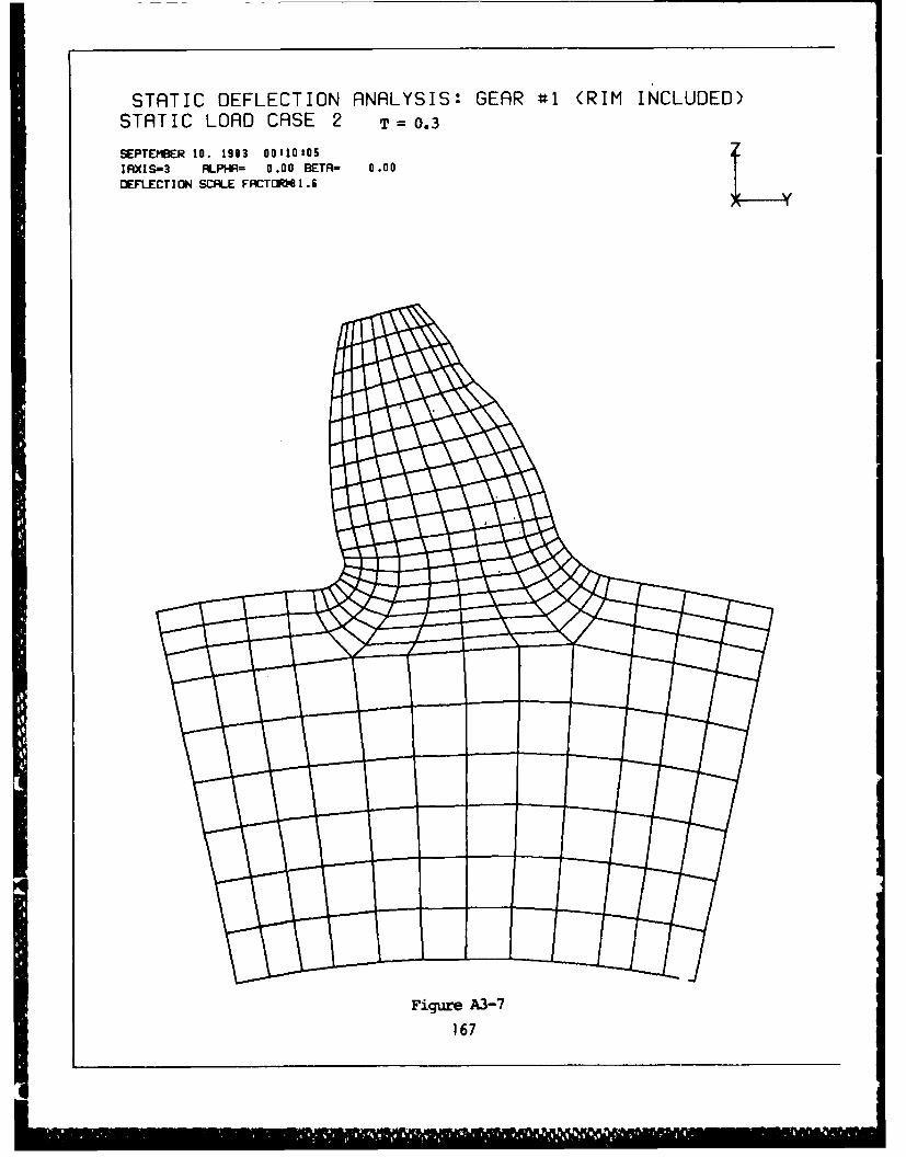
STATIC DEFLECTION ANALYSIS: GEAR #1 (RIM INCLUDED)STATIC LOAD CASE 2 T=0.3

SEPTEMBER 10. 1983 00110305IRXIS-3 ALPHR- 0 .00 BETRA 0 .00DEFLECTI ON SCALE FACT1R 1 .6f

Figure A3-7

167

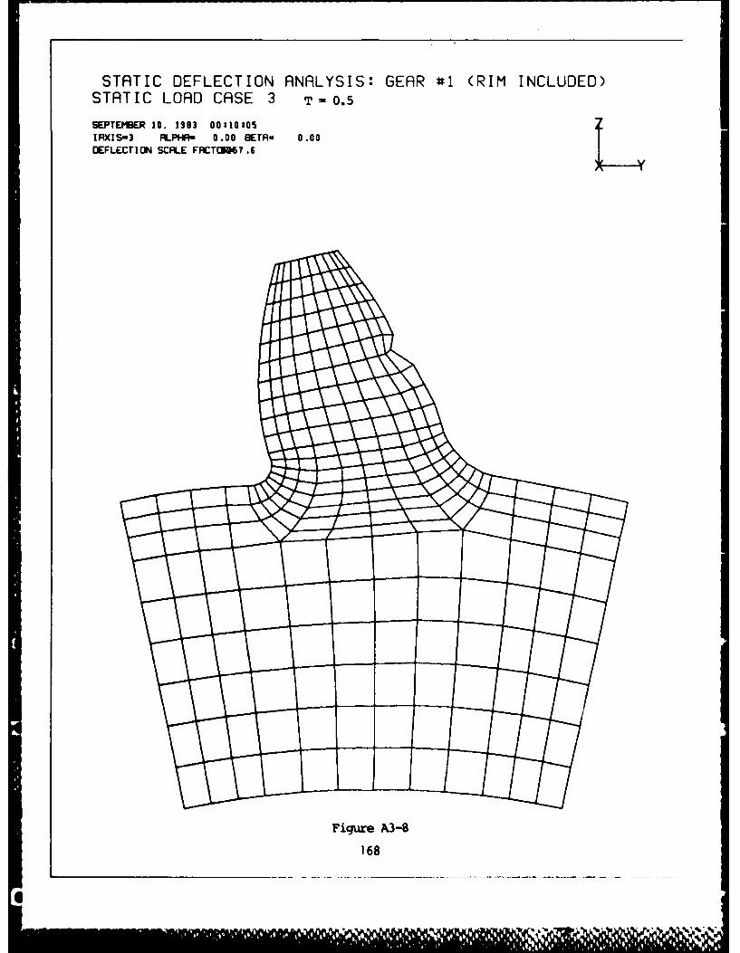
STATIC DEFLECTION ANALYSIS: GEAR #1 (RIM INCLUDED)STATIC LOAD CASE 3 T=O0.5

SEPTEMBER 10. 1903 008101051 RX!S- 3 ALPHR- 0 .00 BETA- 0 .00DEFLECT ION SCALE FFACF26? .6

Figure A3-8

168

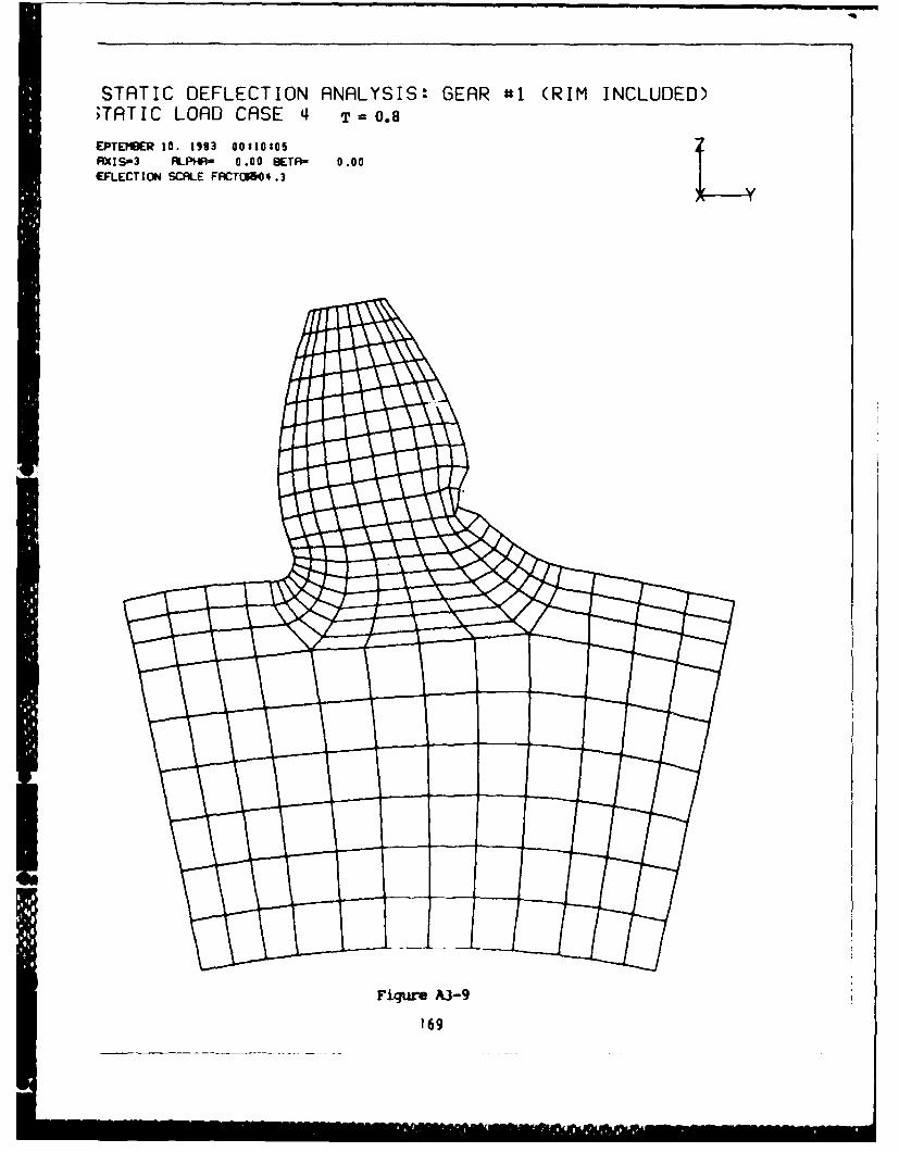
STATIC DEFLECTION ANALYSIS: GEAR #1 (RIM INCLUDED);TATIC LOAD CASE '4 T=O0.8

(PTEMUER 10. 1903 003l0aDSAXIS-3 PIPHR- 0 .00 13ER- 0.00EFLEC I ON SCALE FACC04 .3

Fiqure A.3-9

169

Modal Analysis

Timoshenko Beam Constraints

Rim Constraints

170

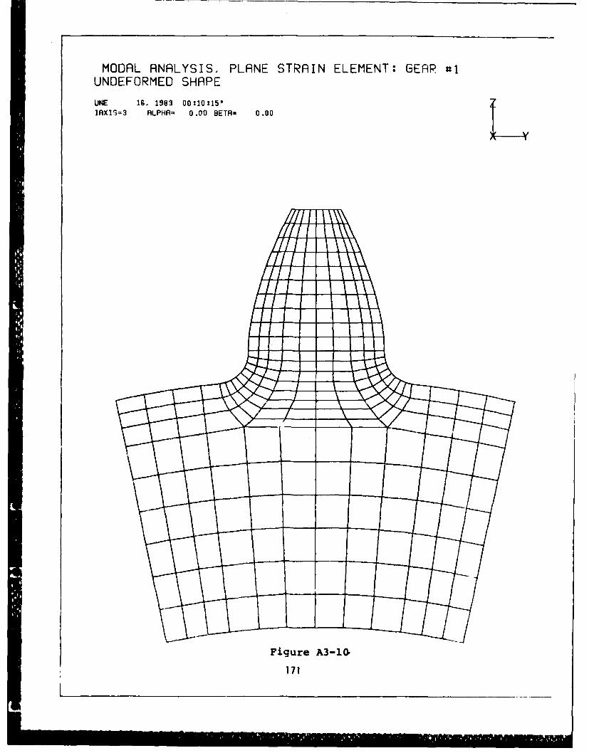
MODAL ANALYSIS. PLANE STRAIN ELEMENT: GEAR #1UNDEFORMED SHAPE

UNE 16, 1983 00:10:151

IRXI'3=3 RLPHA- 0.00 BETA= 0.00

Figure A3-1O

171

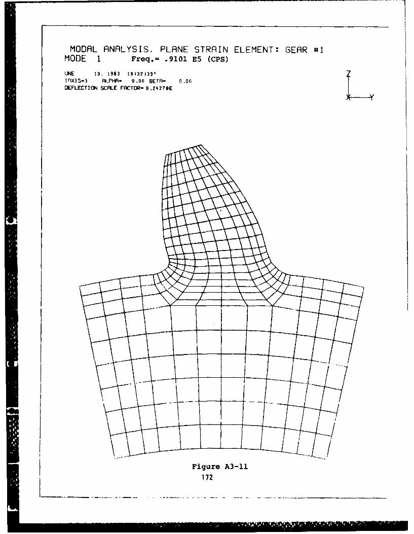
MODAL ANALYSIS, PLANE STRAIN ELEMENT: GEAR #1MODE 1 Freq.= .9101 E5 (CPS)

UNE 10, 1993 19 :32 :39'1I rxlSG3 ALPHA-f- D.onf BETR- r.00DEFLECTIOCN SCALE FACTOR- 0 .2427091

Figure A3-11

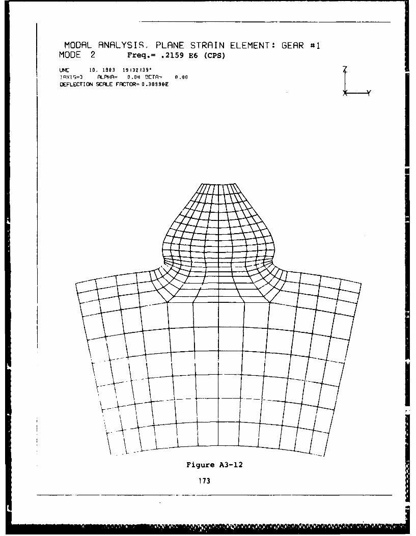
MODAL ANALYSIS. PLANE STRAIN ELEMENT: GEAR #1MODE 2 Freq.= .2159 E6 (CPS)

UNE 10, 1983 19 :3 2:3 91~1 cI 3=3 ALPHA= 0.0'! !JETR- I.0DEFLECTION SCALE FRCTOR= 0 .30999&[

Figure A3-12

173

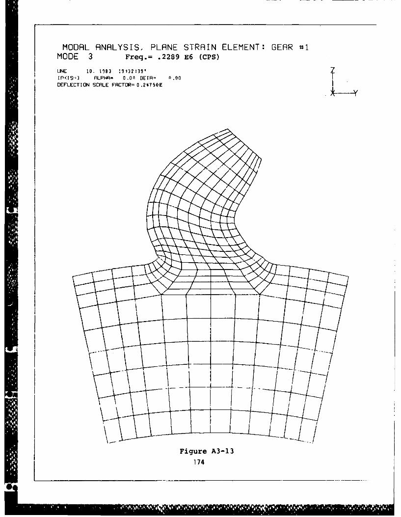
MODAL ANALYSIS, PLANE STRAIN ELEMENT: GEAR #*1MODE 3 Freq.= .2289 E6 (CPS)

UNE 10. 1983 1932:39'I PXI S-3 ALPHFI= 0.Ol BEIA' nl.0 fDEFLECT ION SCALE FACTOR= 0.2 4 75 K

Figure A3-13

174

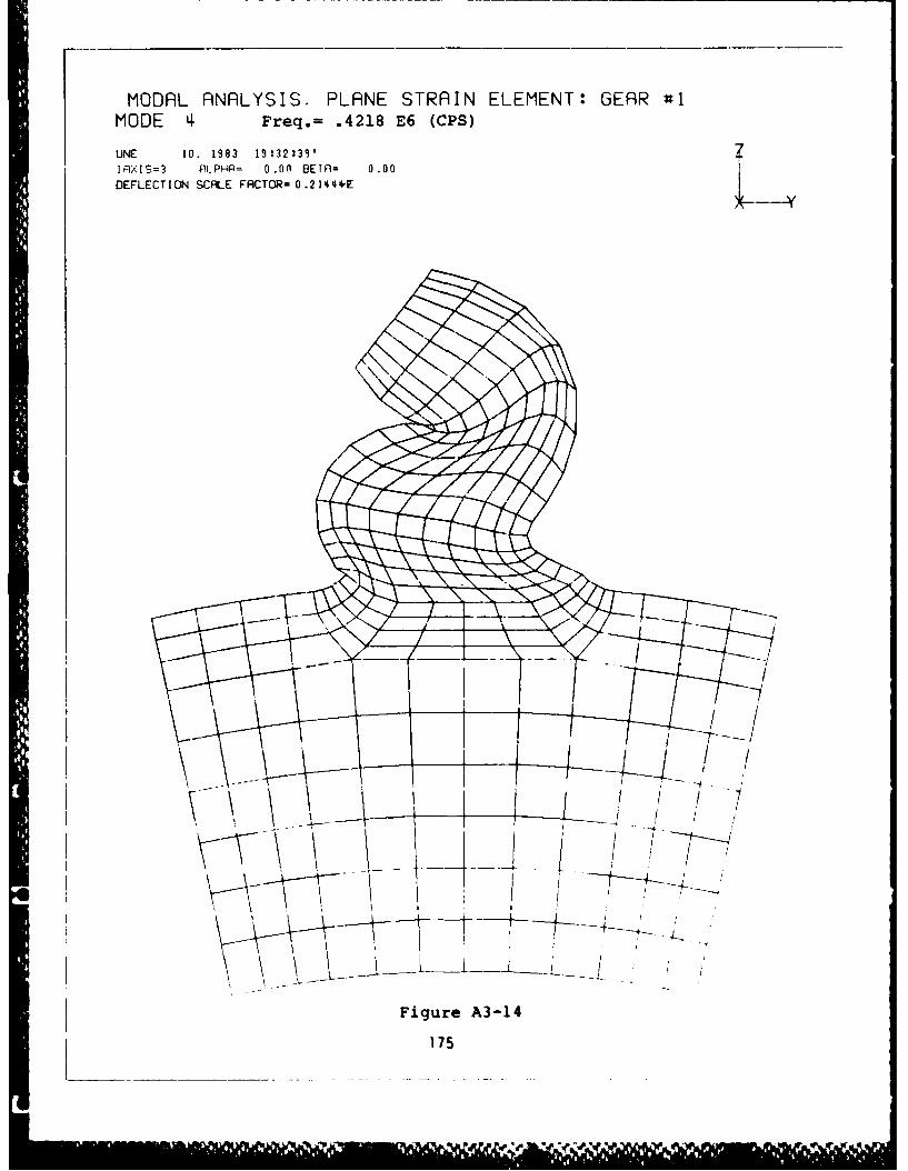
MODAL ANALYSIS. PLANE STRAIN ELEMENT: GEAR #~1MODE 4 Freq.= .4218 E6 (CPS)

UNE 10, 1983 19 :32 :39 ' 7I X IS= 3 01-PHA~= 0.00 BETA= 0 .00

DEFLECTION SCALE FACTOR= 0.2144+IE

Figure A3-14

175

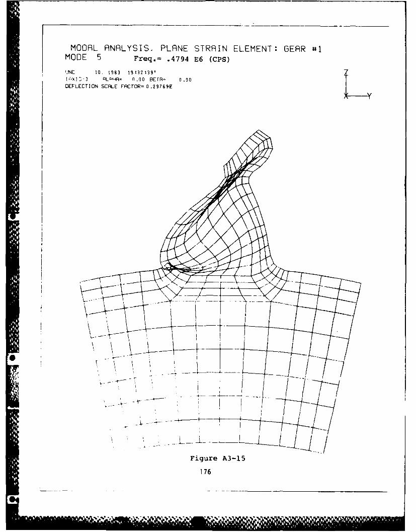
MODAL ANALYSIS. PLANE STRAIN ELEMENT: GEAR #1MODE 5 Freq.= .4794 E6 (CPS)

'iNC 10. 1183 13 '32 :39'1 i-,'l!3 ALPIHR= 11.Q EBErR= 0.00DEFLECTION SCRLE FACTOR= 0 .29769-E

Figure A3-15

176

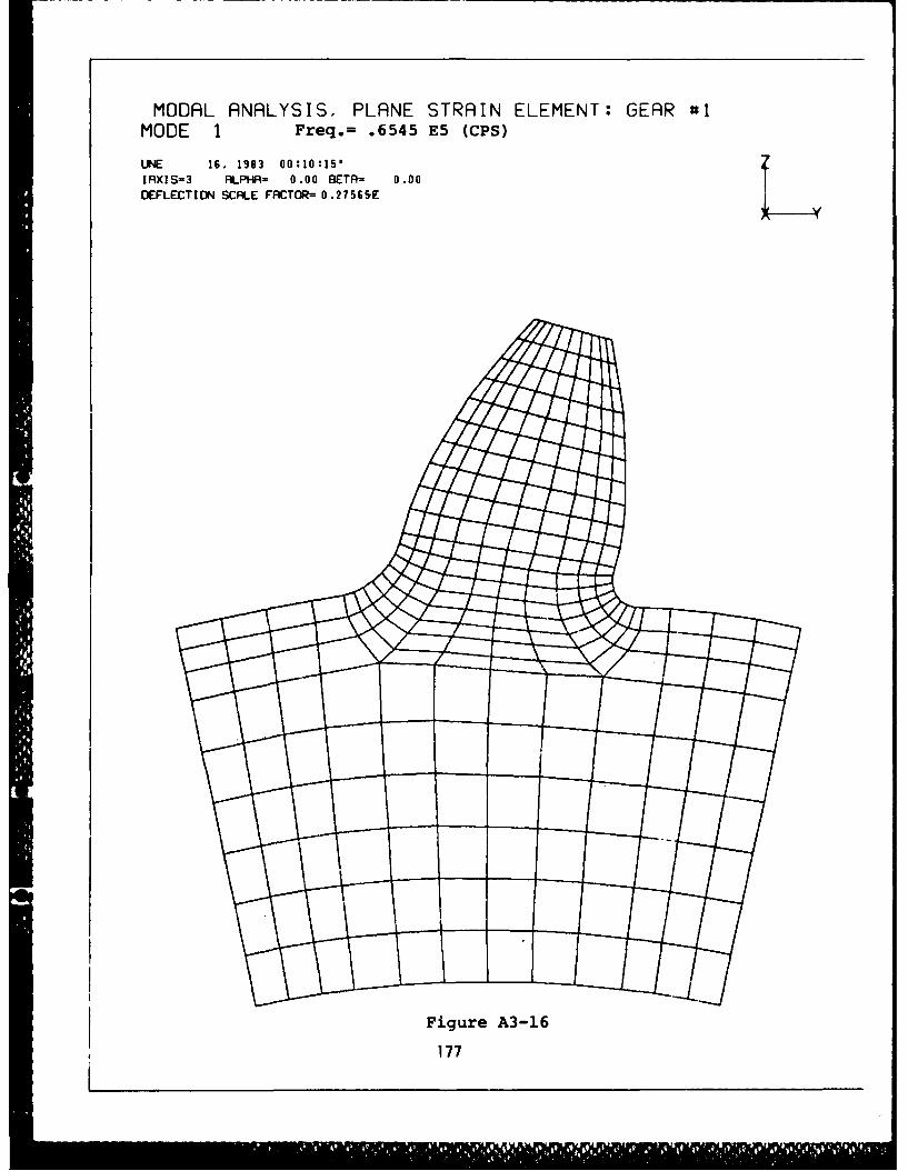
MODAL ANALYSIS. PLANE STRAIN ELEMENT: GEAR #1MODE 1 Freq.= .6545 E5 (CPS)

LINE 16, 1993 00:10:15'IAXIS-3 ALPHA- 0.00 BETA= 0 .00DEFLECT!I ON SCALE FRCUR 0 .2?7 5 6 51E

Figure A3-16

177

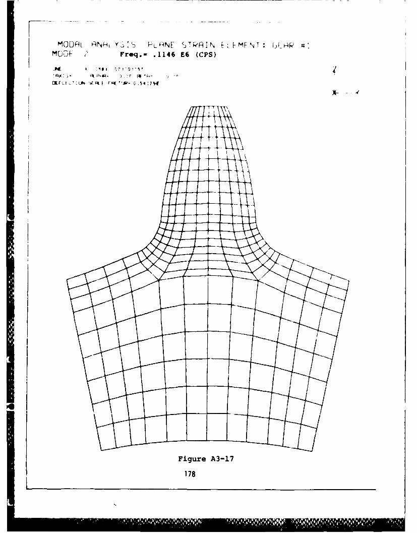
MGLAL FH-LV 'I3 PuFHNE 5:-'RIN El[-MFNT: UHMODE IfFreq.- .1146 E6 (CPS)

Figure A3-17

1 78

MGLJRL RiNHt YSf li1, -I-NE STPRIN ELEMENT: GERR #IMODE .4 F'req.- .1~517 Efi (CPS)

A~il T JN C t 0

-Y

Figure A3-18

179

L

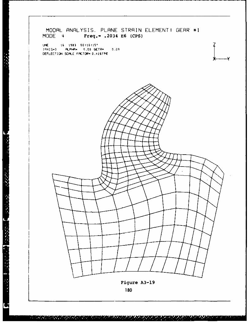
FMODAL ANALYSIS. PLANE STRAIN ELEMENT: GEAR #1MODE '4 Freq.- .2034 E6 (CPS)

LiNE 16 1583 00 110 15'I RX I S3 ALPHA4- n.00 EIETR- 0 .00DEFLECTION SCALE FAC TOR- 0.4 267ILE~

Figure A3-19

180

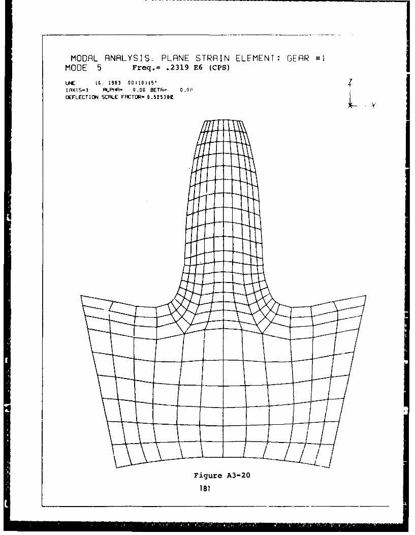
MODAL ANALYSIS. PLANE STRAIN ELEMENT: GEAR ulMODE 5 Freq.= .2319 E6 (CPS)

LiNE 16. 1983 00:10:15'I AXlIS-3 PLPR= 0 .00 BETR- 0 rcl~,DEFLECT ION SCALE FACTOR- 0 .5 2 53 K

Figure A3-20

181

Dynamic Response

Gear Tooth Profile Deflections

182

In the modal response analysis, modal superposition is

used to sum the effects of all the included oda shapes pro-

ducing the desired response. The more modes included, the more

accurate the analysis. However, there is a practical limit to

the number of modes used dictated by the type of loading used

(impact, constant, sinusoidal, etc.) and of course com-

putational efficiency. As previously mentioned, the first ten

modes are used for this analysis.

To better comprehend the dynamic deflection phenomena, the

deflected state of the tooth profile, subject to the impact

loading case, is plotted for diLferent load positions with

V*-0.01. Figure A3-21 shows the underformed shape and Figures

A3-22 through A3-25 are the various deformed shapes. From the

figure(s), one can see those modes which contribute noticeably

to the overall deflection of the tooth. It is apparent that

only the first three or four have a major effect (see Figure

A3-19, T-0.5). Thus the problem of local deformation encoun-

tered in the static analysis is not apparent here.

183

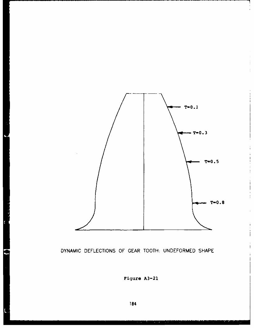
T-0.1

T-0. 3

T-0. 5

Tn0. 8

DYNAMIC DEFLECTIONS OF GEAR TOOTH: UNDEFORMED SHAPE

Figure A3-21

184

v.o0.O1 T=O. 1

DYNAMIC DEFLECTIONS OF GEAR TOOTH WITH MOVING LOADS

Figure A3-22

185

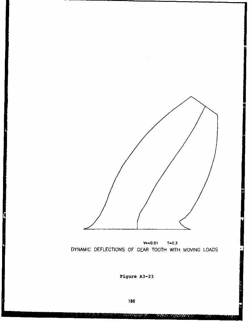
V*=O.01 T=0.3

DYNAMIC DEFLECTIONS OF GEAR TOOTH WITH MOVING LOADS

Figure A3-23

186

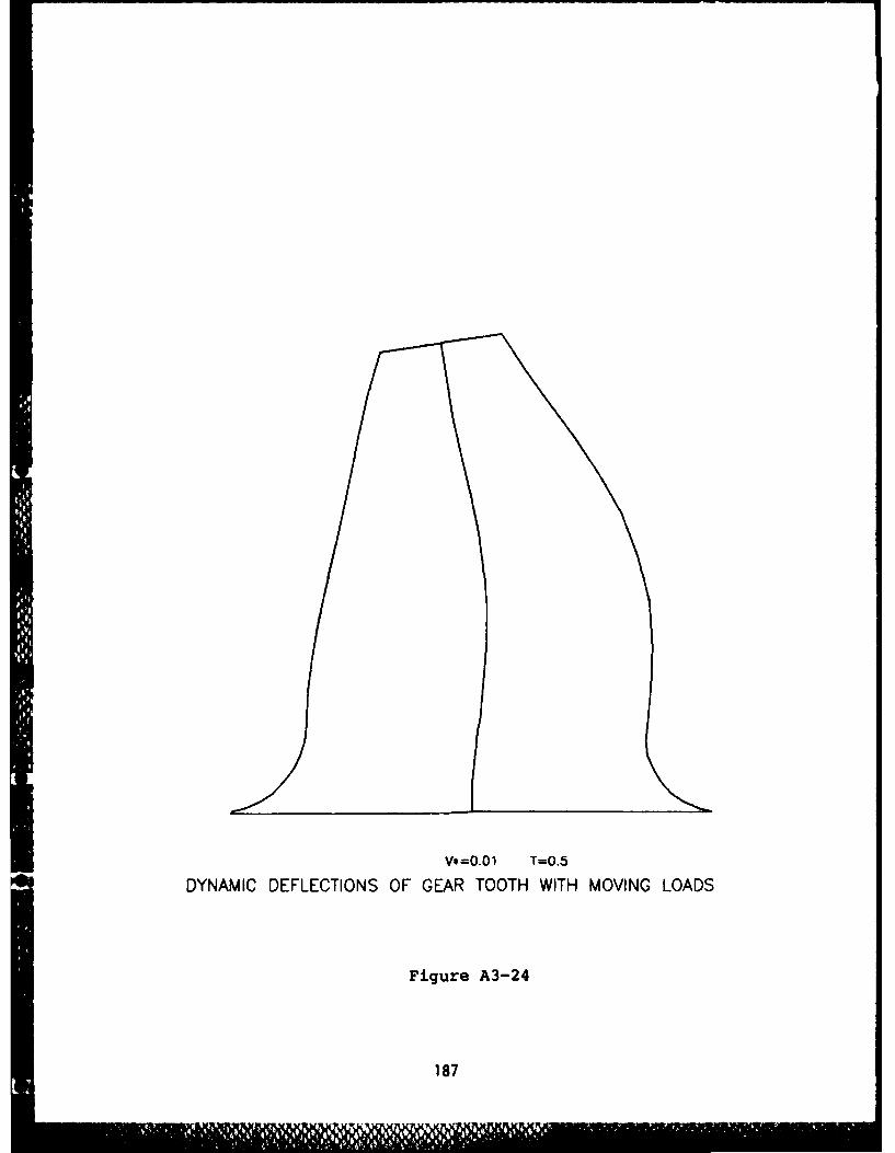
Vs=0OO1 T=0.5

DYNAMIC DEFLECTIONS OF GEAR TOOTH WITH MOVING LOADS

Figure A3-24

187

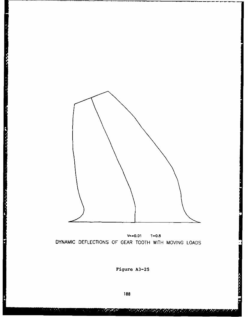
V*=O.01 1=0.8DYNAMIC DEFLECTIONS OF GEAR TOOTH WITH MOVING LOADS

Figure A3-25

188

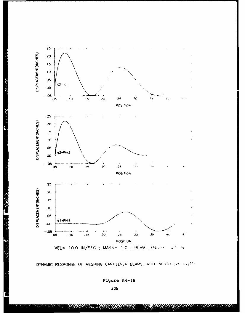
- ~.25 . ..

0 0

05 .1 5 126

25

2 20

15 -lo/

-. 05 '. . .

.05 10 15 20 25

POSITIL)N

.25

20

15

LJ 10

VEL= 10.0 IN/SEC ; MAS = 1.0 REAM L E N-, lb 'N

DYNAMIC RESPONSE OF MESHING CANTILEVER BEAMS, WITH INf TA ,',"L

Figure A4-16

205

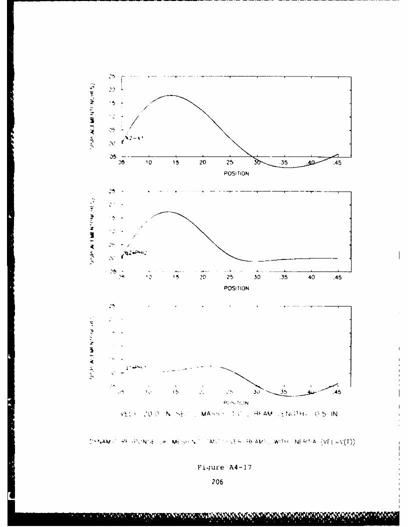
2,,-- - ---/'-

3

5 '0 ? 5 20 25 3 .35 . .45

POSITION

19, 20 25 30 .35 40 .45

POSITION

-- _ _35'-

.45

M1N

,L, . 'N , MA - - o,, AV I T.T- . 5 IN

NAM. Q '4 ~ ~ A.' .. ~ A )NT i iNf I' I A VE L v'(T),

Figure A4-17

206

* £4 A IVETGIO OFNETEETH WdITH MOVING L (U) MICHIGAN TECHNOLOGICAL UNIVHOUGHTON DEPT OF MECHANICAL ENGIN

UNCLASSIFIED C E PASSERELLO ET AL AUG 87 NASA-CR-179643 F/G i/9 U

EhhhEEmohmoiEEhhhmhEmhhhhhEsEEE

_1 .29"

pmo

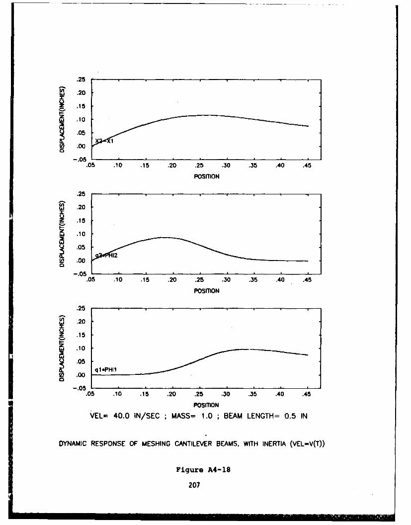
.25

~.20

.15

w~ .10

~.05

05

.05 .10 .15 .20 .25 .30 .35 .40 .45

POSITION

.25

LOL .20

_ .15

L .05

-.05.05 .10 .15 .20 .25 .30 .35 .40 .45

POSITION

.25

f3 .20

.15

V10so .05

.05 iPi

-.505 .10 .15 .20 .25 .30 .35 .40 .45

POSITION

VEL= 40.0 IN/SEC ;MASS= 1.0 ; BEAM LENGTH= 0.5 IN

DYNAMIC RESPONSE OF MESHING CANTILEVER BEAMS, WITH INERTIA (VEL=V(T))

Figure A4-18

207

APPUEDIX 5

Use of Uttural Modes in Uquation

of lotion for Cantilever Sans

1) Constant of Integration

2) Bvaluation of 121U1 AND 12P12

3) Derivatives of the Node Shape With Time

208

1.) Constant of Integration

In order to simplify the solution of the equation of

motion (5-26). the constant of integration associated with the

mode shape of a cantilever beam is determined such that;

) = 1 (AS-i)0

Since the beams are identical and the integral is over the

length of the beam, the constant is the same for both beams.

The first natural mode of vibration for a uniform fixed-

free cantilever beam is;

fM - C[(sinBL-sinhBL)(sin0FK-sinhO&)

(A5-2)

+ (cosOL+coshL) (cosBt-cosh8t)

where;

4. 2

EI

Equation (A5-2) is simplified by rewriting with;

S1 - sinOL-snhoL

S2 - cosBL+coshBL

We then have;

S( ) - C(Slsinx-Slsinhx+S2cosx-S2coshx] (A5-3)

where x is used in place of the argument BF.

209

Squaring equation (A5-3);

*2(F) - C2 [Sl2(sin 2x+sinh2x-2sinxsinhx)

+ S22(cos2 x+cosh2 x-2cosxsinhx) (A5-4)

+2S1S2(sinx cosx-sinx coshx-cosx sinhx+sinhx coshx)]

We can then solve for the constant C with the following

substitution;

C L )I (A5-5)p G(O)dt

where 0 C F )-CG( C ). Whenever the relation represented by

equation (A5-1) occurs in equations (5-26) it is replaced by 1.

Throughout the remainder of equations of motion the constant of

integration C is represented by equation (A5-5). This relation

is evaluted using Simpson's Rule.

2.) Evaluation of 12PHI1 and 12PHI2

Using the arbitrary constant of integration, C, determined

in the previous section, the relationship;

I2PHIl - 12PHI12 *o 2 (t)dt (A5-6)

can be evaluated. The integrand represents the second deriva-

tive of the mode shape with respect to the length variable, ,

quantity squared. The first derivative of the mode shape with

x again used in place of 0&;

- Cp[Slcosx-S2coshx-S2sinx-S2sinhx]

210

and the second derivative;

d20 - C82 [-Slsinx-Slsinhx-S2cosx-S2coshx

Squaring this relation and simplifying yields the desired

result;

d 2 2 2B4[Sl(sin2x+sinh2x+2sinx sinhx)

dE +S22 (cos2x+cosh2x+2cosx coshx) (A5-7)

+2SlS2(sinx cosx+sinx coshx+cosx sinhx+sinhx coshx)I

This relation is then used in equation (A5-6) which is eva-

luated using Simpson's Rule.

3.) Derivatives of the Mode Shape with Time

When the constraint equation is differentiated, first and

second derivatives of the mode shape result where the dependent

variable, E , must be considered as a function of time. The

first derivative of the mode shape with respect to time is;

t( C8t[Slcosx-Slcoshx-S2sinx-S2sinhxj (A5-8)

where x is used in place of the argument BE and 4 is the velo-

city of the moving load. Taking the second derivative, we

have;

- C[Sl(-0 2 k2(sinx+sinhx) 40cosx-coshx))dt

- S2(0 2 42 (cosx+cosh)

+0l(sinx+sinhx))] (A5-9)

where E is the acceleration of the moving load. For a moving

load with constant speed, E is of course zero.

211

i " " . . .

APPENDIX 6

Development and Solution of

Equations of Motion with

Inertial Terms Removed

212

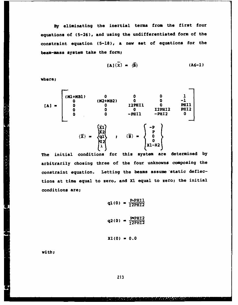
By eliminating the inertial terms from the first four

equations of (5-26), and using the undifferentiated form of the

constraint equation (5-18), a new set of equations for the

beam-mass system take the form;

(AI{X - ( (A6-1)

where;

(Ml+MB1 ) 0 0 0 10 (M2+1B2) 0 0 -1

[Al - 0 0 I2PHIl 0 PHIl0 0 0 12PHI2 PH120 0 -PHI1 -PH12 0

{X- 4q11 , {0}-

LX~ ~Xl-X2~The initial conditions for this system are determined by

arbitrarily chosing three of the four unknowns composing the

constraint equation. Letting the beams assume 'static deflec-

tions at time equal to zero, and Xl equal to zero; the initial

conditions are;

PaPHI 1ql(0) - 12PH12

P'PHI12q2(0) - 2PHI2

Xl(O) - 0.0

with;

213

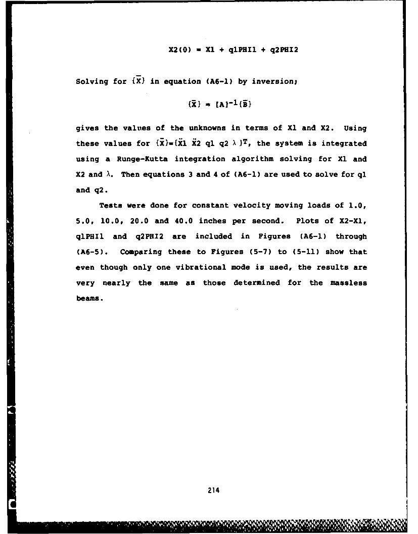
X2(0) - X1 + qlPHIl + q2PHI2

Solving for {Xl in equation (A6-1) by inversion;

{0 - [A]-l{B}

gives the values of the unknowns in terms of Xl and X2. Using

these values for {X}-{Xl X2 ql q2 X }T, the system is integrated

using a Runge-Kutta integration algorithm solving for Xl and

X2 and X. Then equations 3 and 4 of (A6-1) are used to solve for ql

and q2.

Tests were done for constant velocity moving loads of 1.0,

5.0, 10.0, 20.0 and 40.0 inches per second. Plots of X2-Xl,

qlPHIl and q2PHI2 are included in Figures (A6-1) through

(A6-5). Comparing these to Figures (5-7) to (5-11) show that

even though only one vibrational mode is used, the results are

very nearly the same as those determined for the massless

beams.

214

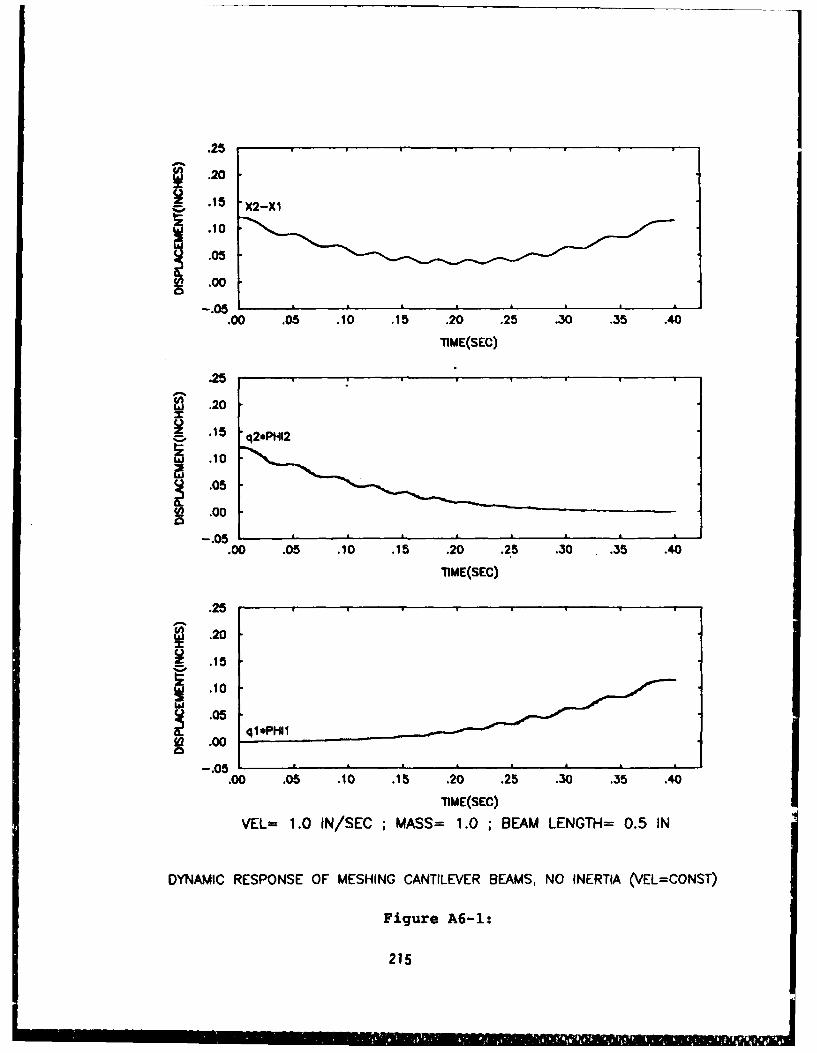
.25

20

.15 'X2-X1

-to

-.05

.00 .05 .10 .15 .20 .25 .30 .35 .40

TIME(SEC)

.25

~.20

.15 q2*PHI2

F10

.05

0 .0005

.00 .05 .10 .15 .20 .25 .30 .35 .40

TIM E(SEC)

.25

1.20

.15

.10

~ ql*PHiI

-05.00 .05 .10 .15 .20 .25 .30 .35 .40

TIME(SEC)

VEL= 1.0 IN/SEC ;MASS= 1.0 ; BEAM LENGTH= 0.5 IN

DYNAMIC RESPONSE OF MESHING CANTILEVER BEAMS, NO INERTIA (VEL=CONST)

Figure A6-1:

215

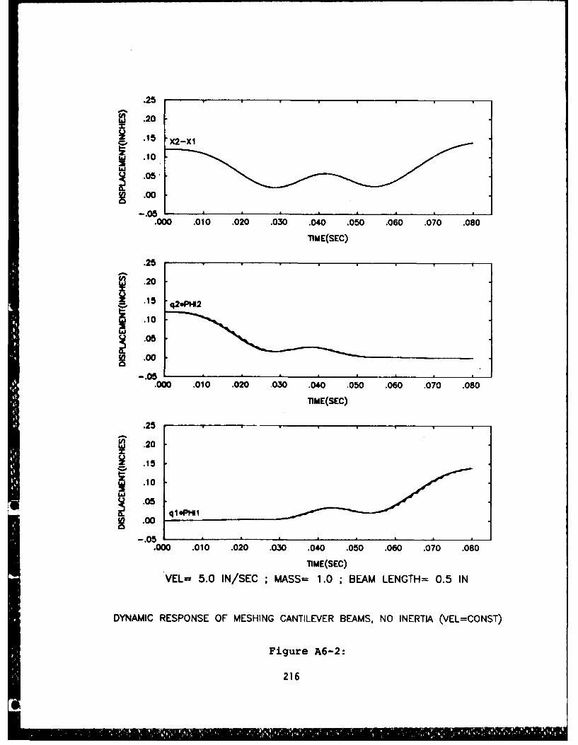
.25

" .20

.15 X2-Xl

~.10

-.05-~.00

-. 05.000 .010 .020 .030 .040 .050 .060 .070 .080

TIME(SEC)

.25

.20

.15 q2.PM2

.10.05

-.00.05

.000 .010 .020 .030 .040 .050 .060 .070 .080

TIME(SEC)

.25

-.20

.15

.10

.00

0 5 , I

.000 .010 .020 .030 .040 .050 .060 .070 .080

IM E(SEC)

VEL= 5.0 IN/SEC ; MASS= 1.0 ; BEAM LENGTH= 0.5 IN

DYNAMIC RESPONSE OF MESHING CANTILEVER BEAMS, NO INERTIA (VEL=CONST)

Figure A6-2:

216

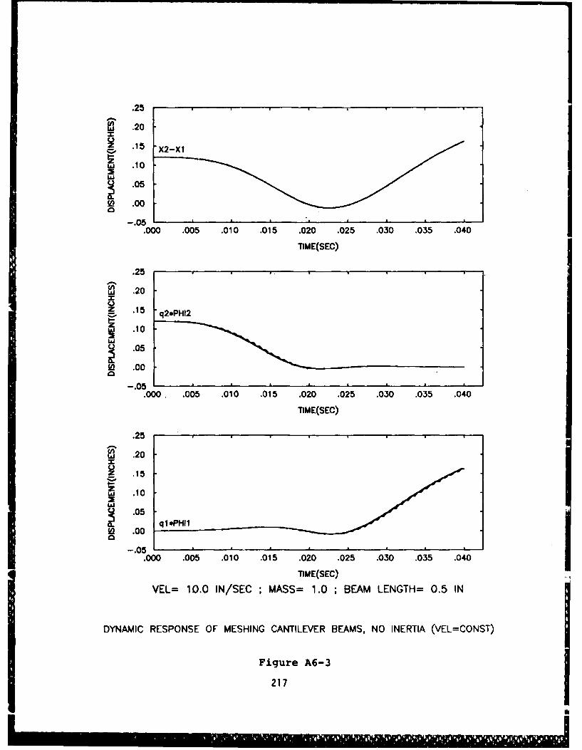
~3 .20

bJ .10

.05

(fl 00.0

.000 .005 .010 .015 .020 .025 .030 .035 .040

TIME(SEC)

.25

~.20

15 q2*PHI2

.10

.05

Wl .00

-.05.000. .005 .010 .015 .020 .025 .030 .035 .040

TIME(SEC)

.25

S .20

. 15

.0

-.05

.000 .005 .010 .015 .020 .025 .030 .035 .040

TIME(SEC)

VEL= 10.0 IN/SEC ; MASS= 1.0 ; BEAM LENGTH= 0.5 IN

DYNAMIC RESPONSE OF MESHING CANTILEVER BEAMS, NO INERTIA (VEL=CONST)

Figure A6-3

217

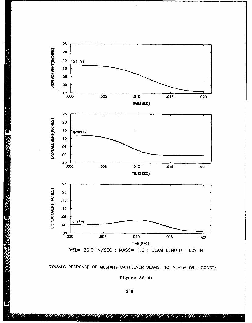
.25

S.20

.10

-.05

W .00

-.05.000 .005 .010 .015 .020

TIM E(SEC)

.25

f~.20

.1

V0CL

0 .0005

.000 .005 .010 .015 .020

TIM E(SEC)

.25

~.20

Z .15

.i10

.05

(LA .00

-.05.000 .005 .010 .015 .020

TIM E(SEC)VEL= 20.0 IN/SEC ;MASS= 1.0 ; BEAM LENGTH= 0.5 IN

DYNAMIC RESPONSE OF MESHING CANTILEVER BEAMS, NO INERTIA (VEL=CONST)

Figure A6-4:

218

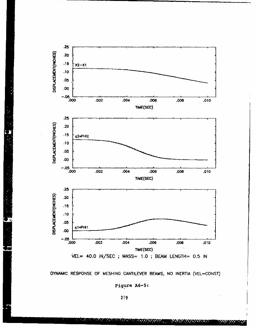
.25

jff .20

S .15 X2-Xl

.10

W) .00

-.05.000 .002 .004 .006 .008 .010

TIME(SEC)

.25

S .20

.10

.05so .00

-.05.000 .002 .004 .006 .008 .010

TIME(SEC)

.25

Iff .20

.15

~.10

.05

so .00

-.05.000 .002 .004 .006 .008 .010

TIME(SEC)

VEL= 40.0 IN/SEC ;MASS= 1.0 ; BEAM LENGTH= 0.5 IN

DYNAMIC RESPONSE OF MESHING CANTILEVER BEAMS, NO INERTIA (VEL=CONST)

Figure A6-5:

219

APPENDIX 7

Dynamic Response Algorithm

for Meshing Cantilever Beam

1. Massless Configuration

2. Inertia of Beam Included

220

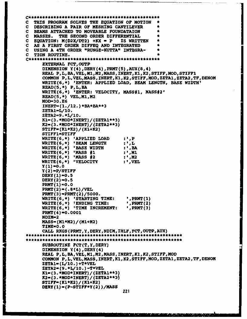
C THIS PROGRAM SOLVES THE EQUATION OF MOTIONC DESCRIBING A PAIR OF MESHING CANTILEVERC BEAMS ATTACHED TO MOVEABLE FOUNDATAXON*C MASSES.* THE SECOND ORDER DIFFERENTIAL*C EQUATION: N(D2X/DT2) +KX - P IS WRITTEN *C AS A FIRST ORDER DIFFEQ AND INTEGRATED*C USING A 4TH ORDER "RUNGE-KUTTA" INTEGRA- *

C TION ROUTINE.

EXTERNAL FCT, OUTPDIMENSION Y(4) ,DERY(4) ,PRMT(5) ,AUX(8,4)REAL P,LoBAoVEL,Nl,N2,MASS, INERT,K1,K2,STIFF,MOD,STIFF1COMMON P,L,VEL,MASS,INERT,K1,K2,STIFF,MOD,ZETA1,ZETA2,TFODENOMWRITE(60*) 'ENTER: APPLIED LOAD, BEAM LENGTH, BASE WIDTH'READ (5, *) P, L, BAWRITE(6,*) 'ENTER: VELOCITY, MASS#1, MASS#2'READ(5o*) VEL,Ml,M2MOD=30.E6INERT=(1./12..)*BA*BA**3ZETAI=L/1O.ZETA2=9. *L/1O.Ki- (3. *MOD*INERT)/ (ZETA1**3)K2-(3. *NOD*INERT)/ (ZETA2**3)STIFF- (Kl*K2) /(Kl+K2)STIFF1-STIFFWRITE(6o*) 'APPLIED LOAD :' ,PWRITE(6,*) 'BEAM LENGTH :,WRITE(6,*) 'BASE WIDTH :',BAWRITE(6o*) 'MASS #1 :',141WRITE(6,*) 'MASS #2 1MWRITE(6,*) 'VELOCITY :',VELY(1)=O.OY (2) -P/STIFFDERY(1)-O. 5DERY(2)-0.5PRMT (1) =0.0PRMT(2)-(.S*L)/VELPRNT(3)-PRMT(2)/5000.WRITE(6,*) 'STARTING TIME: ',PRMT(l)WRITE(6,*) 'ENDING TIME: ',PRMT(2)WRITE(6,*) 'TIME INCREMENT: ',PRMT(3)PRMT(4) -0. 0001NDIM-2MASS-(Ml*M2)/ (Ml+M2)TIME-O.OCALL RKGS(PRMT,Y,DERY,NDIMIHLF,FCT,OUTPAUX)

SUBROUTINE FCT(T, Y, DERY)DIMENSION Y(4) ,DERY(4)REAL PL,BA,VEL,K1,142,MASS,INERTK1,K2,STIFFMODCOMMON P,L,VEL,MASSoINERTK1,K2,STIFF,40D,ZETA1,ZETA2,TF,DENOMZETAl- (L/1O. )+T*VELZETA2-(9. *L/1O. )-T*VELKim (3. *MOD*INR) /(ZETA1**3)K2-(3. *MOD*INERT)/ (ZETA2** 3.STIFF-(K1*K2)/ (1(1+12)DE.RY(1)-(P-STIFF*Y(2) )/MASS

221

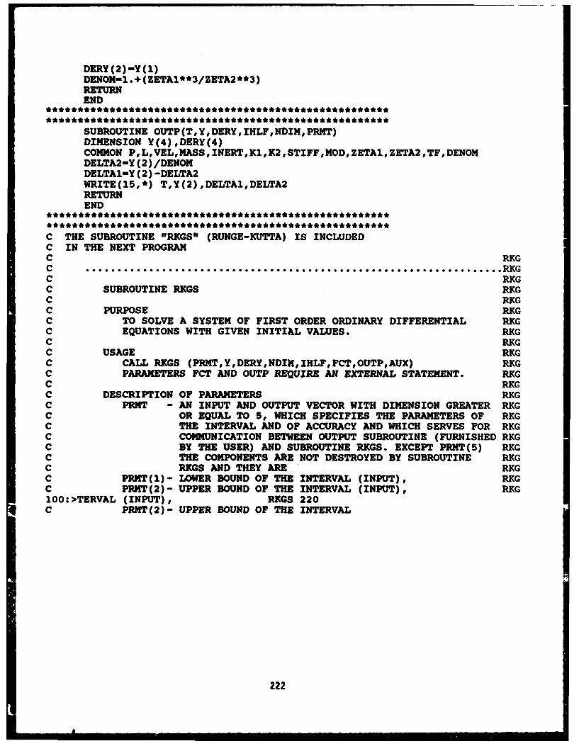
DERY (2) -Y (1)DENOM-1.+ (ZETA1**3/ZETA2**3)RETURNEND

SUBROUTINE OUTP(T,Y,DERY, IHLF,NDIM,PRMT)DIMENSION Y(4),DERY(4)COMMON PL,VEL,MASS,INERT,K1,K2,STIFF,MOD,ZETA1,ZETA2,TF,DENOMDELTA2-Y (2) /DENOMDELTAlY (2) -DELTA2WRITE(15,*) TY(2),DELTAI,DELTA2RETURNEND

C THE SUBROUTINE "RKGS" (RUNGE-KUTTA) IS INCLUDEDC IN THE NEXT PROGRAMC RKG

" C .. . . . . . . . . . . . . . . . . . . . . . . . . . . . . . .RKGC RKGC SUBROUTINE RKGS RKGC RKGC PURPOSE RKGC TO SOLVE A SYSTEM OF FIRST ORDER ORDINARY DIFFERENTIAL RKGC EQUATIONS WITH GIVEN INITIAL VALUES. RKGC RKGC USAGE RKGC CALL RKGS (PRMT,Y,DERY,NDIM,IHLF,FCT,OUTPAUX) RKGC PARAMETERS FCT AND OUTP REQUIRE AN EXTERNAL STATEMENT. RKGC RKGC DESCRIPTION OF PARAMETERS RKGC PRMT - AN INPUT AND OUTPUT VECTOR WITH DIMENSION GREATER RKGC OR EQUAL TO 5, WHICH SPECIFIES THE PARAMETERS OF RKGC THE INTERVAL AND OF ACCURACY AND WHICH SERVES FOR RKGC COMMUNICATION BETWEEN OUTPUT SUBROUTINE (FURNISHED RKGC BY THE USER) AND SUBROUTINE RKGS. EXCEPT PRMT(5) RKGC THE COMPONENTS ARE NOT DESTROYED BY SUBROUTINE RKGC RKGS AND THEY ARE RKGC PRMT(1)- LOWER BOUND OF THE INTERVAL (INPUT), RKGC PRT(2)- UPPER BOUND OF THE INTERVAL (INPUT), RKG100:>TERVAL (INPUT), RKGS 220C PRNT(2)- UPPER BOUND OF THE INTERVAL

222

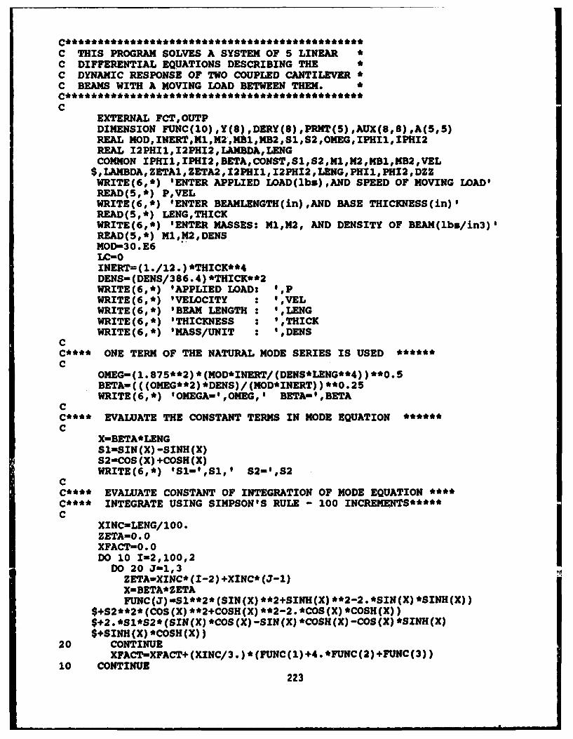
C THIS PROGRAM SOLVES A SYSTEM OF 5 LINEAR*C DIFFERENTIAL EQUATIONS DESCRIBING THE*C DYNAMIC RESPONSE OF TWO COUPLED CANTILEVERC BEAMS WITH A MOVING LOAD BETWEEN THEM. *

CEXTERNAL FCT, OUTPDIMENSION FUNC(1O),Y(8),DERY(8),PRMT(5),AUX(8,8),A(5,5)REAL MOD,INERT,M1,M2,Ma1,MB2,S1oS2,oMEGIPHI14IPHI2REAL 12PH11,I2PHI2,LAMBDA,LENGCOMM4ON IPHI1,IPHI2,BETA,CONST,S1,52o,N2,NB1,KB2,VEL

$, LAMBDA, ZETA1, ZETA2, I2PH11, 12PH12, LENG, PH11,PHI2,DZZWRITE(6t*) 'ENTER APPLIED WAD(lbs),AND SPEED OF MOVING LOAD$READ(5,*) P,VELWRITE (6,*) 'ENTER BEAMLENGTH (in) ,AND BASE THICIQIESS (in)'READ(5,*) LENG,THICKWRITE(6,*) 'ENTER MASSES: Ml,M2v AND DENSITY OF BEAM(lbs/in3)'READ(5,*) Ml,M2,DENSMOD-30.E6LC-OINERT= (1./12. )*THICK**4DENS- (DENS/3 86.4) *THICK**2WRITE(6,*) 'APPLIED LO)AD: ',PWRITE(6,*) 'VELOCITY : ,VELWRITE(6,*) 'BEAM LENGTH : 'LENGWRITE(6,*) 'THICKNIESS : ,THICKWRITE(6,*) 'MASS/UNIT : ,DENS

CC**** ONE TERM OF THE NATURAL MODE SERIES IS USED ***C

OMEG- (1.*875**2) *(MOD*INERT/ (DENS*LENG**4) )**0.*5BETA-((C(OMEG**2)*DENS)/(MOD*INERT) )**0.25WRITE(6l*) 'OMEGA-',OMEG,' BETA-',BETA

CC**** EVALUATE THE CONSTANT TERMS IN MODE EQUATION ***C

X-BETA*LENGSi-SIN CX) -S114(X)S2-COS CX) +COSH(X)WRITE(6,*) 'S1-',Sl,' S2-',52

CC**** EVALUATE CONSTANT OF INTEGRATION OF MODE EQUATION **C**** INTEGRATE USING SIMPSON'S RULE - 100 INCR EME NTS*****C

XINC-LENG/100.ZETA=O. 0XFACT-0.0DO 10 1-2,100,2

DO 20 J-113ZETA-XINC* (1-2) +XINC* (J-l)X-BETA* ZETAFUNC (3) Sl**2* (SIN CX) **2+SINH(X) **2-2.*SIN(X) *SINH~(X))

$+52**2* (COS (X) **2+COSH CX) **2-2 .*CO(X) *COSH CX))$+2.*Sl*52*(SIN(X) *COS CX) -SIN(X) *COSH(X)-COS(X) *SINH(X)$+SINH(X) *COSH CX))

20 CONTINUEXFACT-XFACT+(XINC/3.)*(FUNCC1)+4.*FUNCC2)+FUNC(3))

10 CONTINUE223

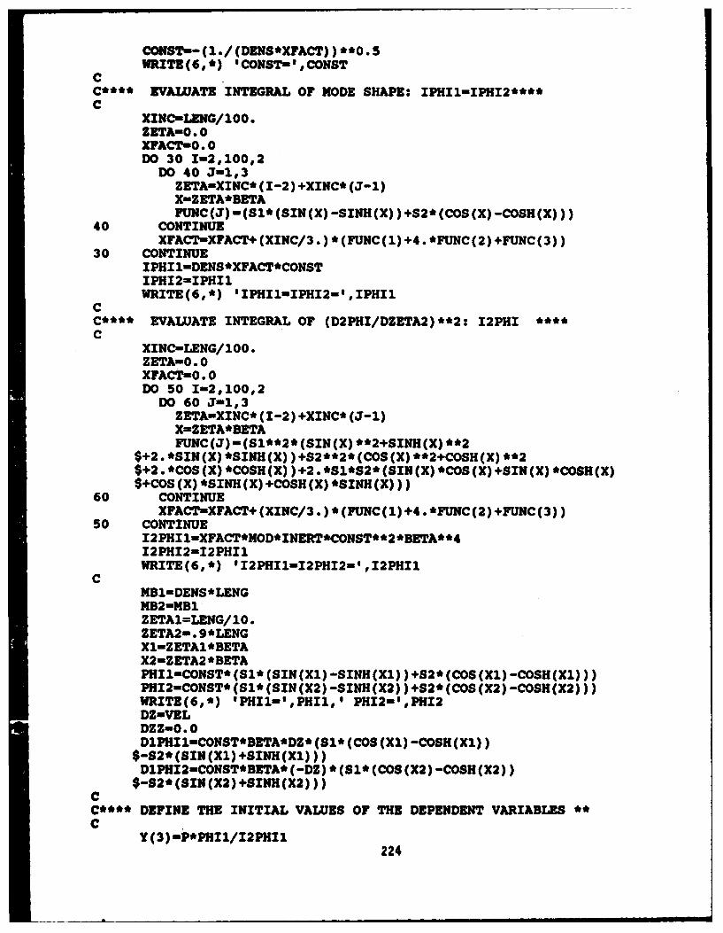
COIIST--(1./(DENS*XFACT) )**0.5WRITE (6, ) CONST-' CONST

CC**** EVALUATE INTEGRAL OF MODE SHAPE: IPHI1-IPHI2****C

XINC-LENG/100.ZETA-O. 0XFACT-0. 0DO 30 1-2,100#2

DO 40 J-1,3ZETA-XINC* (1-2) +XINC* (J-1)X-ZETA*BETAFUNC(J) -(Sl* (SIN (X)-SINH (X)) +S2* (COS (X) -COSH (X)))

40 CONTINUEXFACT-XFACT+(XINC/3.)*(FUNC(1)+4.*FUNC(2)+FUNC(3))

30 CONTINUEIPHI 1DENS*XFACT*CONSTIPH12-IPHIl1WRITE(6,*) 'IPHI1-IPHI2-' ,IPH11

CC**** EVALUATE INTEGRAL OF (D2PHI/DZETA2)**2: 12PHIC

XINC-LENG/100.ZETA-0.0XFACT-O. 0DO 50 1-2,100,2

DO 60 J-1,3ZETA-XINC* (1-2) +XINC* (J-1)X-ZETA* BETAFUNC(J)-(Sl**2* (SIN(X) **2+SINH(X) **2

$+2. *SIN(X) *SINH CX) )+S2**2* (COB (X) **2+COSH(X) **2$*2**COS(X) *COSH (X) )+2.**81*82* (SIN (X) *COSCX) +SIN(X)*COSH CX)

$+COS(X) *SINH (X)+COSH(X) *SUNI(X)))60 CONTINUE

XFACT-XFACT+(XINC/3.)*(FUNC(1)+4.*FUNC(2)+FUNC(3))50 CONTINUE

I2PHI1=XFACT*NOD*INERT*CONST**2 *BETA**412PH12-12PHIlWRITE(6,*) 'I2PHIl-I2PH12-' ,12PH11

CNB1-DENS *LENGNB2-NB1ZETA1=LENG/10.ZETA2-. 9*LENGXl-ZETA1*BETAX2-ZETA2 *BETAPH1CONST*(S1*(SIN(Xl)-SINH(X1) )+S2*(COS(Xl)-COSH(X1)))PHI2-CONST*(S*(SIN(X2)-SINH(X2))+S2*(COS(X2)-COSH(X2)))WRITE(6,*) 'PHI1-',PHI1,' PH12-',PHI2DZ-VELDZZ-O. 0DlPHI1CONST*BETA*DZ* (81*(COB (Xl) -COSH (Xl))

$-S2* (SIN (Xl) +SINH (Xl)) )DIPHI2-CONST*BEPTA* (-Di) *(81* (COS (X2) -COSH(X2))

$-S2*(SIN(X2)+SINH(X2)))CC**** DEFINE THE INITIAL VALUES OF THE DEPENDENT VARIABLES *C

Y (3) mP*MH11/I2PHIl224

Y (4) mP*P1112/12PH12

Y(2)-Y(1)+PHI1*Y(3)+PHI2*Y(4)V (7) -0.0

V (5) -0.0Y(6)-Y(5)+Y(3) *DlPHII1+Y(4) *Dl1W12WRIT(6,*) 'Y(l)-',Y(1)WRIT(6,*) 'Y(2)-',VY(2)VRXTZ(6,*) 'Y(3)-',Y(3)WRIT(60*) 'Y(4)m',Y(4)DO 55 1-1,8

DZR()-./S.55 CONTINUE-

PRWP(1) -0 *

PRNT(2) -. *LENG/ (VEL)PRMT (3) -(PRWT(2) -PRNT (1) )100.PRNT(4) -0. 0001NDIM-8CALL RKGS(PRNT,Y,DERY,NDXN,IHLF,FCT,OUTP,AUX)

SUBROUTINE FCT(TrD DRY)DIMENSION Y(g) ,DERY(8) ,A(5,5) ,B(5)REAL NOD,INERTN1,N2,NBl,NB2,S,S20OtEG,IPHI1,IPHI2REAL 12PII,12PH12, LAMDA, JZNGCOMMON IPHIlo1PHl2,BETA,CONSTS1,S2,N1,N2,NBlNB2,VEL

$, LAMBDA, ZETAl, ZETA2 ,I2PHI1, I2PH12 ,LENG, PH11, PHI2,DZZZETA1-(LENG/10. )+VEL*TZETA2-( .g*LENG) -VEL*TX1-ZETA1*BETAX2-ZETA2 *MBEA

CC**** EVALUATE NODE SHAPE EQUATIONS AT EACH LOAD POSITIONC

PHI1-ONST*(Sl*CSIN(Xl)-SINH(Xl))+S2*(COS(X1)-COSH(X1)))PHI2-CONST*(Sl*(SIN(X2)-SINH(X2))+S2*(COS(X2)-COSH(X2)))

CIF(LC.GT.10) GO TO 71WRITE(6,*) '**********TIMEI ,T

C**** EVALUATE DERIVATIVES OF NODE SHAPE EQUATIONS **

C71 DZ-VRL

DZZ-O.0D1PHI1mCONST*BETA*DZ* (S1*(COS (Xl) -COSH(Xl))

$-S2*(SIN(X1)+SINH(Xl)))DlPHI2-CONST*BETA* (DZ) *(51* (COS (X2) -COSH(X2))

$-S2* (SIN (X2)+SINII(X2)))D2PIICONST*BETA* (91*(-BETA*DZ**2*SIN(Xl) +DZZ*COS (Xl)

$-BETA*DZ**2*8INH(X1) -DZZ*COSH(X1) ) -2* (BETA*DZ**2*COS (Xl)$+DZZ*SIN(X1)+B3TA*DZ**2*COSH(X1)+DZZ*SINH(Xl)))D2PHI2-COKST*BETA* (Sl* (-SETA*DZ**2*SIN(X2)+DZZ*COS(X2)

$-BETA*DZ**2*SINH(X2)-DZZ*COSH(X2) )-S2*(BETA*DZ**2*COS(X2)$+DZZ*SIN(X2)+BETA*DZ**2*COSH(X2)+DZZ*SINH(X2)))

CC**** DEFINE MATRIX COEFFICIENTS A[5v5J *c

A(1, 1)-N14NBlA(2,1)-0.0 225

A(3, 1)-IPHIIA (4,91) -0. 0A(5,1I)--l.A (1,2) -0 *A(2t2)-M2+MB2A( 392) -0.0A(4,2)--IPHI2A(5,2)-1.0A(113)-IPHIlA (293) -0 *A(3,3)-l.0A (4,3) -0 *A(5,3)--PHIlA (1,4) -0.0A(2t4)--IPHI2A (3,4) =0 *A(4,4)-1.OA(5,4)--PHI2A(1,5)-1.0A(2,5)--1.OA (3,5) -PHI 1A'4, 5) -PHI2A(5,5)-O.O

CC**** DEFINE RIGHT HAND SIDE B[5] ***

CB (1) -- P.B (2) -PB(3)--2PH11*Y(3)B(4)--12PHI2*Y(4)B(5)-D2PHI1*Y(3)+D2PH12*Y(4)+2.*DlPHI1*Y(7)+2.*DlPH12*Y()IF(LC.GT.10) GO TO 1DO 63 1-1,5

63 WRITE(6,*) A(I,1) ,A(1,2) ,A(1,3) ,A(I,4) ,A(I,5) ,B(I)1 LC-LC+1

N-5CALL SINQ(A,B,N,KS)IF(KS.EQ.1) WRIT(6,*) 'NO SOWUTIONIIIII'IF(LC.GT.1O) GO TO 64WRITE(6,*) 'BACK FROM SIMQ (B]'DO 64-1-1,5WRITE(61*) B(I)

64 CONTINUEDERY (1) -Y (5)DERY (2) -Y (6)DERY (3) -Y (7)DERY (4) -Y (8)DERY (5) -B (1)DERY (6) -B (2)DERY (7) -B (3)DERY (8)-B (4)LAI'BDAB(5)IF(LC.GT.10) GO TO 62DO 61 1-1,8

61 WRITE(6,*) '(,,)'YI62 RETURN

END

226

SUBROUTINE OUTP (T, Y,DERY, IHLF, NDIM, PRMT)DIMENSION Y(8),DERY(8),PRMT(5)REAL MOD,INERT,M1,M2,MB1,MB2,S,S2,OMEG,IPHI1,IPHI2REAL I2PHI1, I2PHI2, LAMBDA, LENGCOMMON IPHI1,IPHI2,BETA,CONST,S1,S2,M1,M2,MB1,MB2,VEL

$,LAMBDA,ZETA1,ZETA2,12PHI1,12PHI2,LENG,PHI1,PHI2,DZZZETA1- (LENG/10. ) +VEL*TZETA2- ( . 9*LENG) -VEL*TX1IZETA1* BETAX2-ZETA2 *BETAPHIl=CONST*(SI*(SIN(XI)-SINH(XI))+S2*(COS(XI)-COSH(Xl)))PHI2-CONST*(Sl*(SIN(X2)-SINH(X2))+S2*(COS(X2)-COSH(X2)))WRITE(15,*) T,Y(2)-Y(1),Y(3)*PHI1,Y(4)*PHI2WRITE(6,*) 'ACCEL=',DZZRETURNEND

CC *..***.........*........*..........................CC SUBROUTINE SIMQCC PURPOSEC OBTAIN SOLUTION OF A SET OF SIMULTANEOUS LINEAR EQUATIONS,C AX-BCC USAGEC CALL SIMQ(A,B,N,KS)CC DESCRIPTION OF PARAMETERSC A - MATRIX OF COEFFICIENTS STORED COLUMNWISE. THESE AREC DESTROYED IN THE COMPUTATION. THE SIZE OF MATRIX A ISC N BYN.C B - VECTOR OF ORIGINAL CONSTANTS (LENGTH N). THESE AREC REPLACED BY FINAL SOLUTION VALUES, VECTOR X.C N - NUMBER OF EQUATIONS AND VARIABLES. N MUST BE .GT. ONE.C KS - OUTPUT DIGITC 0 FOR A NORMAL SOLUTIONC 1 FOR A SINGULAR SET OF EQUATIONSCC REMARKSC MATRIX A MUST BE GENERAL.C IF MATRIX IS SINGULAR , SOLUTION VALUES ARE MEANINGLESS.C AN ALTERNATIVE SOLUTION MAY BE OBTAINED BY USING MATRIXC INVERSION (MINV) AND MATRIX PRODUCT (GMPRD).CC SUBROUTINES AND FUNCTION SUBPROGRAMS REQUIREDC NONECC METHODC METHOD OF SOLUTION IS BY ELIMINATION USING LARGEST PIVOTALC DIVISOR. EACH STAGE OF ELIMINATION CONSISTS OF INTERCHANGINGC ROWS WHEN NECESSARY TO AVOID DIVISION BY ZERO OR SMALLC ELEMENTS.C THE FORWARD SOLUTION TO OBTAIN VARIABLE N IS DONE INC N STAGES. THE BACK SOLUTION FOR THE OTHER VARIABLES ISC CALCULATED BY SUCCESSIVE SUBSTITUTIONS. FINAL SOLUTIONC VALUES ARE DEVELOPED IN VECTOR B, WITH VARIABLE 1 IN B(1),

227

C VARIABLE 2 IN B(2), ........ , VARIABLE N IN B(N).C IF NO PIVOT CAN BE FOUND EXCEEDING A TOLERANCE OF 0.0,C THE MATRIX IS CONSIDERED SINGULAR AND KS IS SET TO 1. THISC TOLERANCE CAN BE MODIFIED BY REPLACING THE FIRST STATEMENT.C

CSUBROUTINE SIMQ(A,B,N,KS)DIMENSION A(1),B(1)

CC FORWARD SOLUTIONC

TOL-0.0KS-0JJ--NDO 65 J-1,NJY-J+lJJ-JJ+N+1BIGA-OIT-JJ-JDO 30 I-J,N

CC SEARCH FOR MAXIMUM COEFFICIENT IN COLUMNC

IJ-IT+IIF(ABS(BIGA)-ABS(A(IJ))) 20,30,30

20 BIGA-A(IJ)IMAX-I

30 CONTINUECC TEST FOR PIVOT LESS THAN TOLERANCE (SINGULAR MATRIX)C

IF(ABS(BIGA)-TOL) 35,35,4035 KS-I

RETURNCC INTERCHANGE ROWS IF NECESSARYC

40 I1-J+N*(J-2)IT-IMAX-JDO 50 K-J,N11-11+N12-I1+ITSAVE-A(Ii)A(Ii)-A(12)A (12) -SAVE

CC DIVIDE EQUATION BY LEADING COEFFICIENTC

50 A(Ii)-A(I1)/BIGASAVE-B (IMAX)B(IMAX)-B(J)B(J) -SAVE/BIGA

CC ELIMINATE NEXT VARIABLEC

IF(J-N) 55,70,5555 IQS-N*(J-1)

DO 65 IX-JY,N

228

IXJ-IQS+IXIT-J-IXDO 60 JX-JY,NIXJX-N* (JX-1) +IXJJX-IXJX+IT

60 A(IXJX)-A(IXJX)-(A(IXJ)*A(JJX))65 B(IX)-B(IX)-(B(J)*A(IXJ))

CC BACK SOLUTIONC

70 NY-N-iIT-N*NDO 80 J-l,NYIA-IT-JIB-N-JIC-NDO 80 K-I,JB(IB)-B(IB)-A(IA) *B(IC)IA-IA-N

80 IC-IC-iRETURNEND

CCe........... . . . . . . . . . . ...o.... ..... ........CC SUBROUTINE RKGSCC PURPOSEC TO SOLVE A SYSTEM OF FIRST ORDER ORDINARY DIFFERENTIALC EQUATIONS WITH GIVEN INITIAL VALUES.CC USAGEC CALL RKGS (PRMT,Y,DERY,NDIM,IHLF,FCTOUTP,AUX)C PARAMETERS FCT AND OUTP REQUIRE AN EXTERNAL STATEMENT.CC DESCRIPTION OF PARAMETERSC PRMT - AN INPUT AND OUTPUT VECTOR WITH DIMENSION GREATERC OR EQUAL TO 5, WHICH SPECIFIES THE PARAMETERS OFC THE INTERVAL AND OF ACCURACY AND WHICH SERVES FORC COMMUNICATION BETWEEN OUTPUT SUBROUTINE (FURNISHEDC BY THE USER) AND SUBROUTINE RKGS. EXCEPT PRMT(5)C THE COMPONENTS ARE NOT DESTROYED BY SUBROUTINEC RKGS AND THEY AREC PRMT(1)- LOWER BOUND OF THE INTERVAL (INPUT),C PRMT(2)- UPPER BOUND OF THE INTERVAL (INPUT),C PRMT(3)- INITIAL INCREMENT OF THE INDEPENDENT VARIABLEC (INPUT),C PRMT(4)- UPPER ERROR BOUND (INPUT). IF ABSOLUTE ERROR ISC GREATER THAN PRMT(4), INCREMENT GETS HALVED.C IF INCREMENT IS LESS THAN PRMT(3) AND ABSOLUTEC ERROR LESS THAN PRMT(4)/50, INCREMENT GETS DOUBLED.C THE USER MAY CHANGE PRMT(4) BY MEANS OF HISC OUTPUT SUBROUTINE.C PRMT(5)- NO INPUT PARAMETER. SUBROUTINE RKGS INITIALIZESC PRMT(5)-0. IF THE USER WANTS TO TERMINATEC SUBROUTINE RKGS AT ANY OUTPUT POINT, HE HAS TOC CHANGE P.MT(5) TO NON-ZERO BY MEANS OF SUBROUTINE

229

C OUTP. FURTHER COMPONENTS OF VECTOR PRMT AREC FEASIBLE IF ITS DIMENSION IS DEFINED GREATERC THAN 5. HOWEVER SUBROUTINE RKGS DOES NOT REQUIREC AND CHANGE THEM. NEVERTHELESS THEY MAY BE USEFULC FOR HANDING RESULT VALUES TO THE MAIN PROGRAMC (CALLING RKGS) WHICH ARE OBTAINED BY SPECIALC MANIPULATIONS WITH OUTPUT DATA IN SUBROUTINE OUTP.C Y - INPUT VECTOR OF INITIAL VALUES. (DESTROYED)C LATERON Y IS THE RESULTING VECTOR OF DEPENDENTC VARIABLES COMPUTED IT INTERMEDIATE POINTS X.C DERY - INPUT VECTOR OF ERROR WEIGHTS. (DESTROYED)C THE SUM OF ITS COMPONENTS MUST BE EQUAL TO 1.C LATERON DERY IS THE VECTOR OF DERIVATIVES, WHICHC BELONG TO FUNCTION VALUES Y AT A POINT X.C NDIM -AN INPUT VALUE, WHICH SPECIFIES THE NUMBER OFC EQUATIONS IN THE SYSTEM.C IHLF - AN OUTPUT VALUE, WHICH SPECIFIES THE NUMBER OFC BISECTIONS OF THE INITIAL INCREMENT. IF IHLF GETSC GREATER THAN 10, SUBROUTINE RKGS RETURNS WITHC ERROR MESSAGE IHLF=II INTO MAIN PROGRAM. ERRORC MESSAGE IHLF=12 OR IHLF=13 APPEARS IN CASEC PRMT(3)=O OR IN CASE SIGN(PRMT(3)).NE.SIGN(PRMT(2)-C PRMT(i)) RESPECTIVELY.C FCT - THE NAME OF AN EXTERNAL SUBROUTINE USED. THISC SUBROUTINE COMPUTES THE RIGHT HAND SIDES DERY OFC THE SYSTEM TO GIVEN VALUES X AND Y. ITS PARAMETERC LIST MUST BE X,Y,DERY. SUBROUTINE FCT SHOULDC NOT DESTROY X AND Y.C OUTP - THE NAME OF AN EXTERNAL OUTPUT SUBROUTINE USED.C ITS PARAMETER LIST MUST BE X,Y,DERY,IHLF,NDIM,PRMT.C NONE OF THESE PARAMETERS (EXCEPT, IF NECESSARY,C PRMT(4),PRMT(5),... ) SHOULD BE CHANGED BYC SUBROUTINE OUTP. IF PRMT(5) IS CHANGED TO NON-ZERO,C SUBROUTINE RKGS IS TERMINATED.C AUX - AN AUXILIARY STORAGE ARRAY WITH 8 ROWS AND NDIMC COLUMNS.CC REMARKSC THE PROCEDURE TERMINATES AND RETURNS TO CALLING PROGRAM, IFC (1) MORE THAN 10 BISECTIONS OF THE INITIAL INCREMENT AREC NECESSARY TO GET SATISFACTORY ACCURACY (ERROR MESSAGEC IHLF=11),C (2) INITIAL INCREMENT IS EQUAL TO 0 OR HAS WRONG SIGNC (ERROR MESSAGES IHLF=12 OR IHLF=13),C (3) THE WHOLE INTEGRATION INTERVAL IS WORKED THROUGH,C (4) SUBROUTINE OUTP HAS CHANGED PRMT(5) TO NON-ZERO.CC SUBROUTINES AND FUNCTION SUBPROGRAMS REQUIREDC THE EXTERNAL SUBROUTINES FCT(X,Y,DERY) ANDC OUTP(X,Y,DERY,IHLF,NDIM,PRMT) MUST BE FURNISHED BY THE USER.CC METHODC EVALUATION IS DONE BY MEANS OF FOURTH ORDER RUNGE-KUTTAC FORMULAE IN THE MODIFICATION DUE TO GILL. ACCURACY ISC TESTED COMPARING THE RESULTS OF THE PROCEDURE WITH SINGLEC AND DOUBLE INCREMENT.C SUBROUTINE RKGS AUTOMATICALLY ADJUSTS THE INCREMENT DURINGC THE WHOLE COMPUTATION BY HALVING OR DOUBLING. IF MORE THANC 10 BISECTIONS OF THE INCREMENT ARE NECESSARY TO GET

230

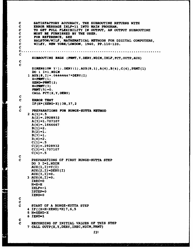
C SATISFACTORY ACCURACY, THE SUBROUTINE RETURNS WITHC ERROR MESSAGE IHLF-11 INTO MAIN PROGRAM.C TO GET FULL FLEXIBILITY IN OUTPUT, AN OUTPUT SUBROUTINEC MUST BE FURNISHED BY THE USER.C FOR REFERENCE, SEEC RALSTON/ILF, MATHEMATICAL METHODS FOR DIGITAL COMPUTERS,C WILEY, NEW YORK/LONDON, 1960, PP.110-120.CC....................................................................c

SUBROUT INE RKGS (PrlT, Y, DERY, NDIM, IHLF, FCT, OUTP, AUX)C

CDIMENSION Yt).DERY(l),AUX(8,l),A(4),B(4),C(4),PRMT(1)DO 1 I-1.NDiN

1 AUX(l,I)-.06666667*DERY(I)X-PWIT(1XEND-PINT (2)H-PUITr(3)PRMT(5)-0.CALL FCT(X,Y,DERY)

CC ERROR TEST

IF(H*(XEND-X))3S,37,2CC PREPARATIONS FOR RUNGE-KUTTA METHOD

2 A(1)-.5A(2)-. 2%26932A(3)-1.707107A(4)-. 1666667B(l)-2.B(2)-1.B(3)=1.B(4)=2.C(1)-.5C(2) -.2928932C(3)=1.707107C(4)=.5

CC PREPARATIONS OF FIRST RUNGE-KUTTA STEP

DO 3 I-INDIMAUX(1, I)-Y(I)AUX(2,I)-DERY(I)AUX(3,I)-0.

3 AUX(6,I)-0.IREC-0H-H+HIHLF--1ISTEP-0IEND-0

CCC START OF A RUNGE-KUTTA STEP

4 IF((X+H-XEND)*H)7,6,55 H-XEND-X6 IEND-I

CC RECORDING OF INITIAL VALUES OF THIS STEP

7 CALL OUTP(X,Y,DERY,IREC,NDIM,PRMT)

231

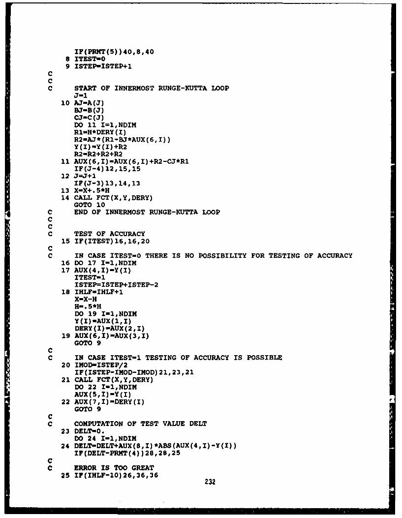
IF(PRMT(5) )40,8,408 ITESTO09 ISTEP-ISTEP+1

CCC START OF INNERMOST RUNGE-KUTTA LOOP

J-210 AJ-A(J)

53-B (J)CJ=C (3)DO 11 I=1,NDIMRl-H*DERY (I)R2-AJ* (R1-53*AUX(6, I))Y (I) -Y (I) +R2R2-R2+R2+R2

11 AUX(6,I)=AUX(6,I)+R2-CJ*RlIF(J-4) 12,15,15

12 J=J+lIF(J-3) 13, 14,13

13 X-X+.5*H14 CALL FCT(X,Y,DERY)

GOTO 10C END OF INNERMOST RUNGE-KUTTA LOOPCCC TEST OF ACCURACY

15 IF(ITEST)16,16,20CC IN CASE ITEST=0 THERE IS NO POSSIBILITY FOR TESTING OF ACCURACY

16 DO 17 I-1,NDIM17 AUX(4,I)=Y(I)

ITEST-1ISTEP=ISTEP+ISTEP-2

18 IHLF-IHLF+1X-X-HH-.5*HDO 19 I-1,NDIMY (I) -AUX (1,I)DERY (I) -AUX (2 ,I)

19 AUX (6, 1)-AUX (3,I1)GOTO 9

CC IN CASE ITEST-1 TESTING OF ACCURACY IS POSSIBLE

20 IMOD-ISTEP/2IF(ISTEP-IMOD-IMOD) 21,23,21

21 CALL FCT(X,Y,DERY)DO 22 Iinl,NDIMAUX (5,I) -Y (I)

22 AUX(7,I)-DERY(I)GOTO 9

CC COMPUTATION OF TEST VALUE DELT

23 DELT-0.DO 24 I-1,NDIM

24 DELT-DELT+AUX(8,I)*ABS(AUX(4,I)-Y(I))IF(DELT-PRMT(4) )28,28,25

CC ERROR IS TOO GREAT

25 IF(IHLF-10)26,36,36 232

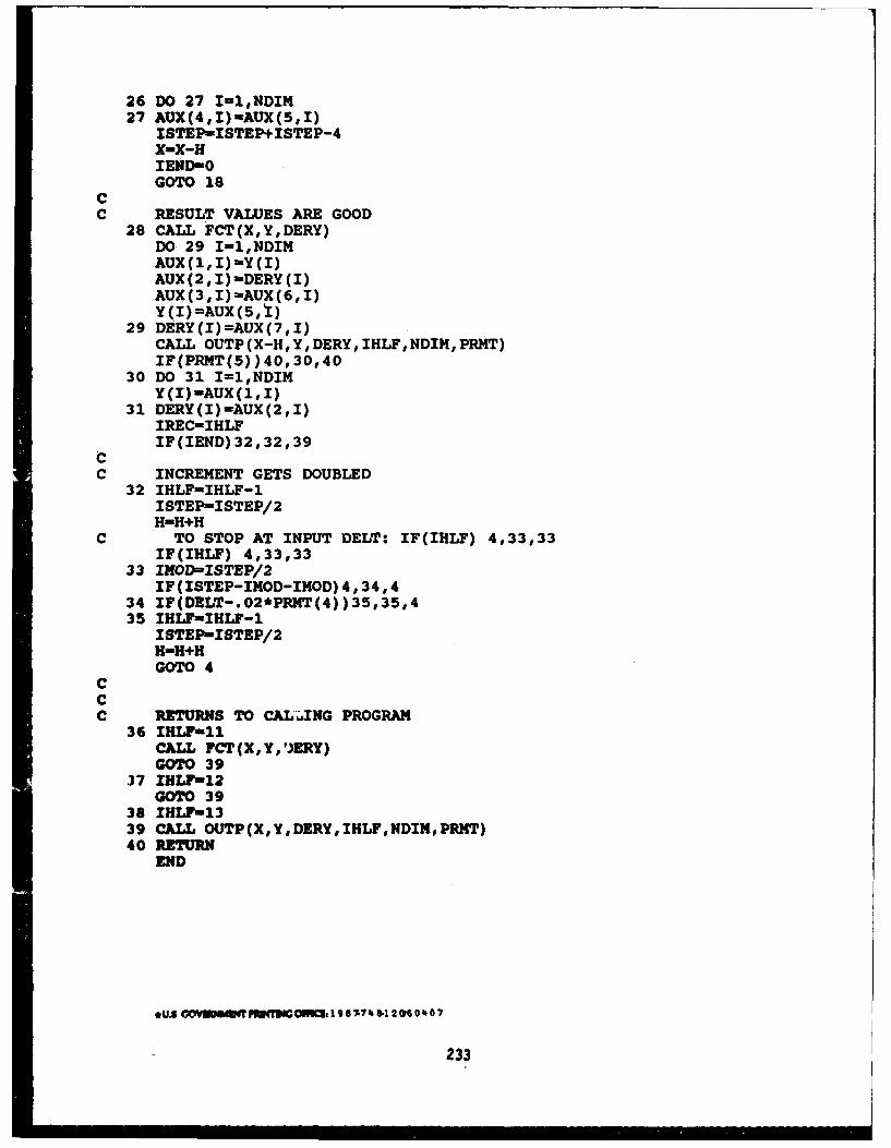
26 DO 27 I=1,NDIM27 AUX(4,I)-AUX(5,I)

ISTEP-ISTEP+ISTEP-4x-x-HIENDO0GoTo 18

C RESULT VALUES ARE GOOD28 CALL FCT(X,Y,DERY)

DO 29 I=1,NDIMAUX (1, 1) -Y (I)AUX (2 ,I) -DERY (I)AUX (3,I) -AUX (6,I)Y (I) =AUX (5, 'E)

29 DERY (I) =AUX (2,jICALL OUTP(X-H,Y,DERY, IHLF,NDI.,PRMT)IF(PRMT(5) )40, 30, 40

30 DO 31 I=1,NDIMY (I)-AUX (1, I)

31 DERY(I)=AUX(2,I)IREC=IHLFIF(IEND)32,32,39

C INCREMENT GETS DOUBLED32 IHLF-IHLF-1

ISTEP-ISTEP/2H-H+H

C TO STOP AT INPUT DELT: IF(IHLF) 4,33,33IF(IHLF) 4,33,33

33 IMO-ISTEP/2IF(ISTEP-INOD-INOD) 4,34,4

34 IF(DELT-.02*PRMT(4))35,35,435 IHLF-IHLF-1

ISTEP-ISTEP/2H-H+HGOTO 4

CCC RETURNS TO CAL .ING PROGRAM

36 IliLFillCALL FCT(X,Y,'IERY)GOTO 39

37 IHLF122GOTO 39

38 IHLF-1339 CALL OUTP(X,Y,DERY,IHLF,NDIM,PRMT)40 RETURN

END

OuS GoviETP34T"off= :19SOIL? 4 -120P6407

233

IReport Documentation Page

1.ppNO. NASA CR-179643 2.wetmi. Accm ionNo. 3.RFeciplW'S CateoNo.

AVSCOM TR-87-C-234. TOW S. Po Dat

An Investigation of the Dynamic Response of Spur August 1987Gear Teeth With Moving Loads . Pomi Orna z=Code

7. Aajulf a) 8. Peiorm"n Organization eo4.None/

C.E. Passerello and L.W. Shuey None

10. Work Un No1L161102AH45/

9. Pet o ,,ngotizaon N, , an Address 505-63-51Michigan Technological University 11. Conra or Gram No.

Department of Mechanical Engineering and NAG 3-344Engineering Mechanics

Houghton, Michigan 49931 13. TyM of Reu and Pedod Covered

12. Sporong Agency N o, m Contractor ReportU.S. Army Aviation Research and Technology Activity- FinalAVSCOH, Propulsion Directorate, Lewis Research Center, 14,.SporsoryngAgecyCode

Cleveland, Ohio 44135 and NASA Lewis Research Center,Cleveland, Ohio 44135

is. SwPpisena'y at

Project Manager, John 3. Coy, Propulsion Directorate, U.S. Army Aviation Researchand Technology Activity - AVSCON, Lewis Research Center, Cleveland, Ohio 44135.

m1S. ANtieact

In this investigation, o concepts relattng to gear dynamics were studied. Thefirst phase i-The.-enejfainvolved the'ttaft of the effect of the speed of amoving load on the dynamic deflections of a gear tooth. A single spur gear toothmodelled using finite elements was subjected to moving loads with variablevelocities. The tooth tip deflection time histories were plotted, from which itwas seen that the tooth tip deflection consisted of a quasistatic response with anoscillatory response superimposed on it whose amplitude was dependent on the typeof load engagement. Including the rim in the analysis added flexibility to themodel but did not change the general behavior of the system. The second-part-of pE-,

the analysislivolved an investigation to determine the effect on the dynamicresponse of the inertia of the gear tooth. A simplified analysis using meshingcantilever beams was used. In one case, the beams were assumed massless, in theother, the mass (inertia) of the beams were included. From this analysis it wasfound that the inertia of the tooth did not affect the dynamic response of meshingcantilever beams. ,

17. t f ia( b uw. A, m lmn

Gears; Vibration;(iets->Machine Unclassified - unlimiteddesign; Finite element analysis, . STAR Category 37

i. Ueeiu1ICmu . oft W. esq1luuyCU. , No of peon 22. Pvlo

Unclassified Unclassified 237 All

- "o~' -For se by the NionalTechncll nfor ion Sice. Sprngfiell Vginia 22161