State University of New York College at Buffalo - Buffalo State CollegeDigital Commons at Buffalo State

Applied Economics Theses Economics and Finance

5-2019

Economic and Demographic Determinants of theConsumption, Saving and Borrowing Behaviors ofHouseholdsMicaela JosephState University of New York College at Buffalo - Buffalo State College, josephm02@mail.buffalostate.edu

AdvisorTheodore F. Bryley, Ph.D., Professor of Economics & FinanceFirst ReaderTheodore F. Bryley, Ph.D., Professor of Economics & FinanceSecond ReaderFrederick Floss, Ph.D., Chair and Professor of Economics & FinanceThird ReaderXingwang Qian, Ph.D., Professor of Economics & FinanceDepartment ChairFrederick Floss, Ph.D., Chair and Professor of Economics & Finance

To learn more about the Economics and Finance Department and its educational programs,research, and resources, go to http://economics.buffalostate.edu/.

Follow this and additional works at: https://digitalcommons.buffalostate.edu/economics_theses

Part of the Finance Commons

Recommended CitationJoseph, Micaela, "Economic and Demographic Determinants of the Consumption, Saving and Borrowing Behaviors of Households"(2019). Applied Economics Theses. 39.https://digitalcommons.buffalostate.edu/economics_theses/39

i

Economic and demographic determinants

of the consumption, saving

and borrowing behaving of

households

Micaela Joseph

An Abstract of a Thesis

in

Applied Economics

Submitted in Partial Fulfillment

Of the Requirements

For the Degree of

Master of Arts

May 2019

Buffalo State College

State University of New York

Department of Economics and Finance

ii

ABSTRACT

Personal savings rate is an unsettling subject, because every economist has distinctive

opinions on the determinants of consumption, saving and borrowing behaviors of households. For

instance, many individuals assume that there is a positive relationship between real disposable

income and the personal savings rate. In other words, the saving amongst households have

increased with the growth of household wealth. On the other hand, some individuals deem that

there is an inverse relationship between both variables, so much that this topic has always

demanded further research to be completed. Because of my awareness and experience relating to

this topic, I have chosen to examine this question. This paper will review the effect and

significance of the savings rate by analyzing real disposable income, real household net worth,

interest rates, and labor productivity. I will make predictions on the results. I am going to study

the positive or negative outcomes between them through data examination and analysis. This

thesis will also compare the data and results of the households in the United States between 1980

and 2017. This will allow us to determine if these variables are the major determinants of the

personal saving rate.

Key words: Income, savings, household net worth, labor productivity, interest rates.

______________________________

Micaela Joseph

______________________________

Date

iii

Buffalo State College

State University of New York

Department of Economic and Finance

Economic determinants of the

consumption, saving and borrowing

behaviors of households

A Thesis in Applied Economics

by

Micaela Joseph

Submitted in Partial Fulfillment

of the Requirements

for the Degree of

Master of Arts

May 2019

Approved by:

Theodore F. Byrley, Ph. D.

Professor of Economics and Finance

Thesis Adviser

Frederick Floss, Ph. D.

Professor of Economics and Finance

Chairperson of the Department of Economics and Finance

Kevin Miller, Ed. D.

Dean of the Graduate School

iv

Thesis Committee Signatory

Approved By:

Theodore F. Byrley, Ph.D., CFA

Associate Professor of Economics and Finance

Frederick Floss, Ph.D.

Professor of Economics and Finance

Chairperson of the Department of Economics and Finance

Xingwang Qian

Professor of Economics and Finance

v

ACKNOWLEDGEMENT

It is with my great desire to confess my sincere appreciation to my thesis advisor Dr.

Theodore Bryley, who assisted me tremendously through this process. Without his extra

push, this thesis would not have been achievable. He has a profound knowledge of

finance. He always given me constructive criticism and beneficial advice through both

my undergraduate and graduate degree.

I would like to voice my deepest gratefulness to Dr. Frederick Floss, Chairperson of

the Department of Economics and Finance, for generously providing his time to help me

write my thesis and criticize my thesis defense. He is very proficient in econometrics and

provided me with a lot of valuable direction on which data to use for testing this thesis.

I would like to send my sincere thanks to the thesis committee members, and

to Professor Xingwang Qian, also for taking additional time out to attempt reading my

thesis. With his criticism and recommendations, it has pushed me to be more self-

confident to finish my Master Thesis. Additionally, I am grateful to be a graduate student

in the Department of Economics and Finance at Buffalo State College. I would like to

send a special thank you to Kevin Miller the Dean of the Graduate School, for securing

his dear time to read my thesis.

Lastly, I would like to send sincere gratitude to my family especially to my mom and

friends for their devotion and encouragement through this challenging process. They all

kept me going and encouraged me, and this thesis could not have been completed without

them. Without them I would have not been able to push forward to completing this thesis

in a timely fashion.

vi

TABLE OF CONTENTS

ABSTRACT ................................................................................................................................... II

ACKNOWLEDGEMENT ............................................................................................................ V

CHAPTER 1: INTRODUCTION ................................................................................................. 1

1.1 CONSUMPTION ....................................................................................................................... 3

1.2 SAVING ..................................................................................................................................... 5

1.3 SAVING MOTIVES................................................................................................................... 7

1.4 LIFE CYCLE HYPOTHESIS .......................................................................................................... 9

1.5 HOW IS THE PERSONAL SAVING RATE MEASURED? .................................................. 13

1.6 BORROWING ......................................................................................................................... 15

CHAPTER 2: LITERATURE REVIEW................................................................................... 16

CHAPTER 3: METHODOLOGY.............................................................................................. 35

3.1 SOURCE OF DATA ....................................................................................................................... 35

3.2 HYPOTHESES ............................................................................................................................... 36

3.3 EMPIRICAL ANALYSIS ............................................................................................................... 37

3.4 RESULTS ................................................................................................................................. 45

CHAPTER 4: CONCLUSION ................................................................................................... 46

CHAPTER 5: FURTHER RESEARCH AND EXPLANATIONS .......................................... 48

REFERENCES............................................................................................................................. 49

APPENDIXES .............................................................................................................................. 53

REGRESSION RESULTS .......................................................................................................... 54

1

CHAPTER 1: INTRODUCTION

Over the preceding decades, the personal savings rate in the United States has

sharply worsened and is nonetheless extremely low, compared to many other nations. For

instance, the personal savings rate as of 2018 for Switzerland is 13.50%, in Mexico

21.50%, and in Belgium 11.40%, while the average personal saving rate in the United

States was no higher than 6.2%. The growth and shrinking of the economy have triggered

a major strain on Americans financially. Countless low- income households have dipped

into their savings to compensate for bills compared to those wealthier households whose

saving rate is sufficiently higher. Savings rates tend to fall lower as individuals age and

exhaust their savings rather than adding to them. There are many factors that can affect

the consumption, saving and borrowing behaviors of American households. Some of the

major factors include income, economic expectations, household (family) size and the

life stage of the individual saver. Research have shown that economic and social factors

can have a substantial effect on the United States personal savings rate.

Households save to finance their retirement, fund their child(ren) education, cars,

mortgages, vacations, consumer goods, and any other added expenses. They generally

deposit their savings into bank accounts, invest them in financial securities such as stocks

or mutual funds, or save them as cash. The proportion of personal income that individuals

save rest on how confident they are about their potential income, their own personal

tendency to consume or save, their existing expenditures, and the interest rate or return

they anticipate getting by saving or investing. Due to the income gap in the economic

classes wealthier households are more likely to increase consumption and saving levels

which in turn decreases their urge to borrow. On the other hand, low- income households

2

are more likely to increase their consumption and borrowing behaviors therefore

decreasing their ability to save.

Consequently, the low personal saving rate and its downward descending trend

have constantly been a going concern equally for both U.S. policy makers and

economists. Economists commonly deem saving as useful because an economy can only

grow if some consumers abstain from spending and instead lend the money to companies

via the acquisition of stocks and extra investments to finance the growth of production.

However, economists have also indicated that when economic growth is jeopardized by

weak demand, excessive saving will hinder economic growth because consumers will

barely be consuming. Savings is the basis for investment and if those savings can shift

into investment efficiently, then such investments will endorse economic growth.

The major purpose of this thesis is to establish how economic and demographic

factors determines the consumption, saving and borrowing behaviors of households.

Social class influences the consumption, saving and borrowing behaviors of individuals.

This paper focuses on household’s consumption, saving and borrowing behaviors due to

demographic and economic factors such as income, age, wealth and household size.

Another purpose of this paper is to determine that household net worth is one of the

major economic determinants resulting in how much a household consumes, saves and

borrows. With the help of other theoretical and empirical analyses, it could be determined

that age and income combined are also among the economic and demographic factors

that affect these behaviors the most. Empirical studies and theoretical literatures have

shown that there are other defining factors that affect household saving behaviors as well

as consumption and borrowing.

3

1.1 CONSUMPTION

Consumption expenditure is one of the major sectors of any nation’s economy.

This expense is controlled by multiple factors such as wealth, availability of consumer

credit, consumer expectations about an individual’s future income, consumer perceptions

and preferences, capital gains among others. However, income is debatably considered

the main determinant of consumption. Consumption models elaborated the need for

income, consumption and saving patterns of individuals, in which existing saving was

expressed as current income minus current consumption.

The theories of consumption dates to John Maynard Keynes expressing a

consumption function, James Duesenberry introducing the Relative Income Hypothesis,

Milton Friedman with his Permanent Income Hypothesis and eventually Franco

Modigliani with his Life Cycle Hypothesis. These theories have their theoretical

foundations in the microeconomic theory of consumer choice. However, the life cycle

and permanent income hypotheses are the most comparable; both theories presume that

individuals attempt to maximize their utility or personal well-being by equalizing lifetime

stream of earnings with a lifetime pattern of consumption. Both the life-cycle and

permanent income models make comparable predictions about the consumption effects of

permanent and temporary changes in an individual and eventually the household income.

In contrast, Dusenberry hypothesized that individuals’ attitude to consumption and saving

is influenced more by income than by the hypothetical standard of living. The three

theories vary to an extent in which they explain the observed consumer behavior, and in

their hypotheses examining the consequences of government policies on an individual

savings behavior.

4

Individuals and households make conspicuous choices to purchase goods and

services. Ability to consume is based on the level of income households have. These

consumers allocate their own funds to purchase goods and services in a way that

maximizes utility. Marya Iftikhar et. al states the components of social class such as

income, status, occupation and education attainment have a direct impact on the way a

household exerts their income.1 Based on that concept, consumption behavior varies as

individuals move upward or downward in their rank of social class. Consumption

behavior also changes as individuals go through the different stages of the life cycle

coined from the Life Cycle Hypothesis proposed by Modigliani.

Other factors that influence consumer spending includes interest rates, an increase

in wages, inflation, deflation and housing prices. Interest rates effect the expense of

borrowing and mortgage interest payments. Greater interest rates boost the cost of

mortgage payments. Thus, high interest rates will indicate lower spending as consumers

have a lower disposable income. Higher wages are the most important factor in boosting

consumer spending. Inflation can be effective in determining spending. If inflation is

larger than nominal wage growth, then consumers will see a decline in disposable

income. Phases of deflation can also have a negative effect on consumer spending. If

prices are declining, consumers may assume that prices will be discounted in the future

and therefore, they hesitate to purchase goods and services. Housing is the major form of

wealth. When house prices are growing individuals are extra confident to spend and they

often chose to remortgage their homes. Rising housing prices triggers a wealth effect.

1 Marya Iftikhar et al., “Social Class Is a Myth or Reality in Buying Behavior?” African Journal of

Business Management 7, no. 9 (March 2013): 713-18.

5

Consumer confidence will persuade people to spend more. With confidence about

future incomes, consumers will be eager to borrow and spend more. If the finance option

is simply available, it will push individuals to take out more personal loans and use credit

on credit cards. A reduction in income tax would give consumers more disposable

income to source for spending, saving or even borrowing. If consumers become more

precautious and increase savings, then consumption will diminish.

1.2 SAVING

The ability to save money is one of the many skills individuals must comprehend

in order to become financially well-off and is one of the most problematic things to do.

There are countless explanations of what saving is, but the most acknowledged definition

is savings is the income that is not consumed. In other words, saving is the unconsumed

portion of real disposable income, and it represents a large part of a nation’s aggregate

savings and investment and thus is a major determinant of the growth of future income

and consumption.2 We often see that people have the choice between consuming or

saving money. How much a society chooses to save today for consumption tomorrow has

important influence for the welfare of the elderly, economic growth and consumption

levels.

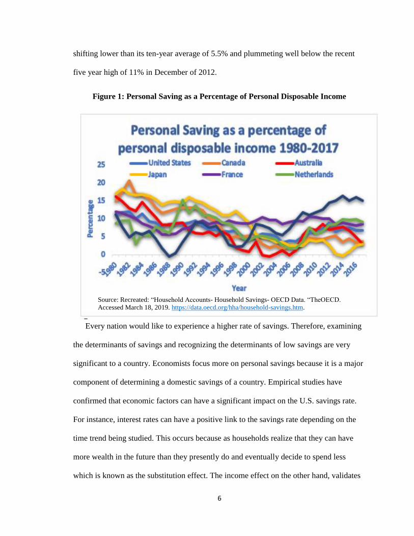
Figure 1 represents the behavior of U.S. personal savings as a percentage of

disposable income from 1980 to 2017 compared to other nations such as Canada,

Australia, Japan, France, Netherlands and Sweden. Figure 1 shows that the highest

personal saving rate in the United States occurred in 1981 at 11.3% and the lowest in

2005 at 3.2%. The U.S. personal saving rate detected in January of 2017 was 3.7%,

2 Lakshmi K. Raut and Arvind Virmani, “Determinants of Consumption and Savings Behavior in

Developing Countries,” The World Bank Economic Review 3, no. 3 (September 1989): 379-93.

6

shifting lower than its ten-year average of 5.5% and plummeting well below the recent

five year high of 11% in December of 2012.

Figure 1: Personal Saving as a Percentage of Personal Disposable Income

Every nation would like to experience a higher rate of savings. Therefore, examining

the determinants of savings and recognizing the determinants of low savings are very

significant to a country. Economists focus more on personal savings because it is a major

component of determining a domestic savings of a country. Empirical studies have

confirmed that economic factors can have a significant impact on the U.S. savings rate.

For instance, interest rates can have a positive link to the savings rate depending on the

time trend being studied. This occurs because as households realize that they can have

more wealth in the future than they presently do and eventually decide to spend less

which is known as the substitution effect. The income effect on the other hand, validates

Source: Recreated: “Household Accounts- Household Savings- OECD Data. “TheOECD.

Accessed March 18, 2019. https://data.oecd.org/hha/household-savings.htm.

7

that the lower interest rates imply less income for savings, therefore reducing saving

motives and encouraging more consumption. Economists assume that higher interest

rates lead to lower overall consumption and higher savings because the substitution effect

offsets the income effect. Age, motives, income, income uncertainty, wealth, risk

tolerance, saving horizon, homeownership, household consumption, health status,

education, race/ethnicity, self-employment, and unemployment have all been linked to

some aspect of saving.3 Corresponding to the earlier empirical studies, they were fixated

mostly on the relationship between savings motives and the consumption patterns of

households.

While savings are the actual amount an individual chooses not to spend, the choice to

save is based on setting aside a portion of income for future needs. There could be many

different motives that prompts individuals to save. The three major motives include (1)

the precautionary motive), (2) the life-cycle motive and (3) the bequest motive.

1.3 SAVING MOTIVES

Researchers have addressed the role of saving motives to explain household

savings and have found that households with saving motives have a higher propensity to

save.4 John Maynard Keynes (1936) listed eight motives for why individuals possibly

save money. Browning and Lusardi5 in their analysis added an extra motive to be labeled

as the down payment motive: (1) the precautionary motive is saving for protection

3 Patti J. Fisher and Sophia T. Anong, “Relationship of Saving Motives to Saving Habits,” Journal of

Financial Counseling and Planning 23, no. 1 (2012): 63-79. 4 Su Hyun Shin and Kyoung Tae Kim, “Perceived Income Changes, Saving Motives, and Household

Savings,” Journal of Financial Counseling and Planning 29, no. 2 (2018): 396-409. 5 Martin Browning and Annamaria Lusardi, “Household Saving: Micro Theories and Micro Facts,” Journal

of Economic Literature 34, no. 4 (December 1996): 1797-55.

8

against unexpected setbacks such as a loss of job or illness (2) the life-cycle motive is

saving to meet long term objectives such as retirement, college and house. (3) the

intertemporal substitution motive (4) the improvement motive (5) the independence

motive (6) the enterprise motive (7) the bequest motive is saving done for the purpose

of leaving an inheritance. (8) the avarice motive (9) the down payment motive.

According to Keynes, individuals keep savings accounts for a precautionary

motive in order to cover unexpected events. Not every household participates in the

savings behavior. Individuals must have the ability to save in order to make savings

decisions.6 There are many different theoretical views about the prime motivation for

saving. Every household has their own motive for saving whether it be for physiological

(basic) needs, safety needs, a need for security in the future, love and societal needs or

even for esteem and luxury needs. The interpretation of basic needs has been modified

over time. As an individual’s level of income increases, consumption behaviors are then

determined more by taste than by physiological needs. Households with limited resources

are now expected to save for daily expenses rather than for their wants and desires.

Saving for safety needs include purchasing a home, saving for rainy days, unexpected

illness or job loss and for investment.

The purpose of saving is to increase the resources available for future

consumption. Individuals mostly save because we cannot foresee the future. Saving

money can help individuals and households become financially secured and ultimately

provide a safety net in case of an emergency. Households put aside some of their current

6 Sondra G. Beverly, Amanda M. McBride, and Mark Schreiner, “A Framework of Asset Accumulation

Stages and Strategies,” Journal of Family and Economic Issues 24, no. 2 (2003): 143-56.

9

income to provide for future consumption, such as a major vacation or basic living

expenses during retirement. Households who prefer to save for their children education,

save for weddings, save for procreation, save for their own education, or save for death

costs are labeled as being on the level of love and societal needs. With no money set

aside in savings or investments, individuals expose themselves to other risks such as not

having enough money to pay for an emergency may resulting in a loan that savings could

have covered.

Personal saving is also equally important for the nation. While savings is

associated with a country’s growth, an increase in consumption may have important

beneficial consequences as well.7 Today’s saving influences future consumption because

investments in financial assets are channeled into productive investments in factories,

industrial machinery, computers, and other kinds of capital. Increases in the capital stock

raises the nation’s ability to produce consumer goods and services in the future. A higher

capital stock also raises the productivity of future workers and their wages, providing

increased income with which to purchase the increased quantity of consumer goods and

services.

1.4 LIFE CYCLE HYPOTHESIS

The benchmark model for explaining the concept of savings is the Life Cycle

Hypothesis. Life cycle theory attempts at describing the dynamics of the propensity to

consume as a function of accumulating wealth, since the individuals tend to save more

7 Hua Chen, Wen-Yen Hsu, and Mary A. Weiss, “The Pension Option in Labor Insurance and Its Effect on

Household Saving and Consumption: Evidence from Taiwan,” The Journal of Risk and Insurance 82, no. 4

(December 2015): 947-75.

10

while young in order to finance a smooth consumption path when old.8 The Life Cycle

hypothesis is an economic theory that pertains to the spending and saving habits of

people over the course of a lifetime. The concept was coined by Franco Modigliani and

his student Richard Brumberg. Modigliani’s model emphasized how saving could be used

to transfer purchasing power from one phase of life to another. The model states that

there are three stages of life cycles in one’s life that is the basis for one’s spending. Three

stages include: early working life, mid working life and retirement. In early life, labor

income is usually low relative to later working years. Income typically peaks in the last

part of the working life, then drops at retirement. Consumers who wish to smooth

consumption would prefer to borrow during the early low-income years, repay these

loans and build up wealth during the high-income years, then spend off the accrued

savings during retirement.

During the early working like phase, the amount of money spent by an individual

may exceed the earnings of the individual. A certain amount of dissaving is observed

during this period. Assets such as a house or car are purchased, and such achievement is

enabled by borrowing or obtaining a loan. The individual will borrow based on

anticipated levels of wealth and income in the future. The next stage of the life cycle is

the mid working life. At this stage the individual seeks to repay loans and compensate for

the excess spending in the previous stage. Large expenses are not indulged during this

time, rather the individual prepares for the next stage of the life cycle. Individuals would

choose to save rather than over spend. The final stage of the cycle is retirement. At this

8 Pietro Senesi, “Population Dynamics and Life-Cycle Consumption,” Journal of Population Economics

16, no. 2 (2003): 389-94.

11

stage consumption remains constant, however there are no earnings being made during

this point. The savings gathered in the previous cycle sustain and cater for all expenses

incurred during retirement. Dissaving is once again observed during this cycle. The

individual’s savings made from the previous stage is gradually depleted during retirement

till death.

Life Cycle hypothesis presumes that individuals plan their spending over their

lifetimes, considering their future income. They take on debt when they are young

assuming future wages will enable them to pay of accumulated debts. They then save

during middle age in order to maintain their level of consumption when they retire. The

LCHO is based on the common-sense idea that households do not make saving or

dissaving decisions solely based on their current income, but rather that they also

consider their expected future circumstances and are affected by their experience. 9

According to the life-cycle model, individuals work and save when they are

young and run down their savings during retirement10. Age plays as a huge role in how

much we as Americans save. Expenses are adjusted as we undergo the different phases of

our life. As lots of Americans complete their college degrees and move into the work

force, they are confronted with a lot of new expenses. The average twenty-four-year-old

will have thousands of dollars’ worth of student loans they are then required to begin

repaying. This huge debt alone will influence how much of their income will be

deposited into savings. As Americans age and start to procreate, many recognize the

9 Sheldon Danziger et al., “The Life-Cycle Hypothesis and the Consumption Behavior of the

Elderly,” Journal of Post Keynesian Economics 5, no. 2 (1982): 208-27. 10 John Thornton, “Age Structure and the Personal Savings Rate in the United States,” Southern Economic

Journal 68, no. 1 (2001): 166-70.

12

significance of saving for rough patches or even for their family’s future. As they get to

the middle of their lives, many parents become “empty nesters” and stop aiding their

children. This frees up a substantial amount of their income and allows them to at least

start saving. As we reach the later stages of our lives, many retire, travel and begin

contributing to charitable organizations.

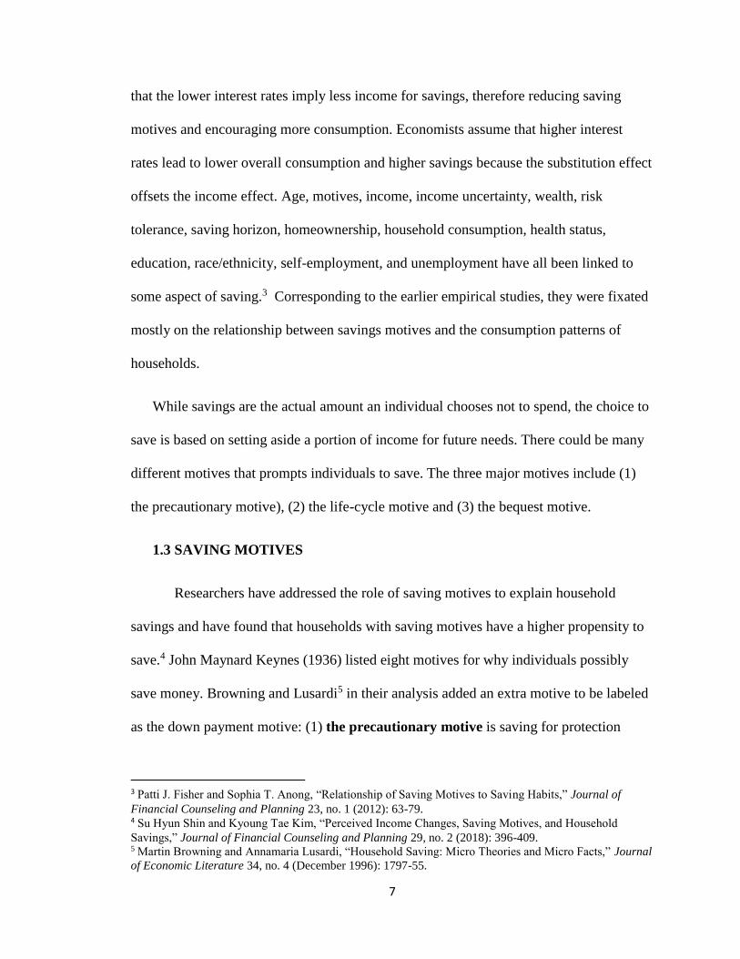
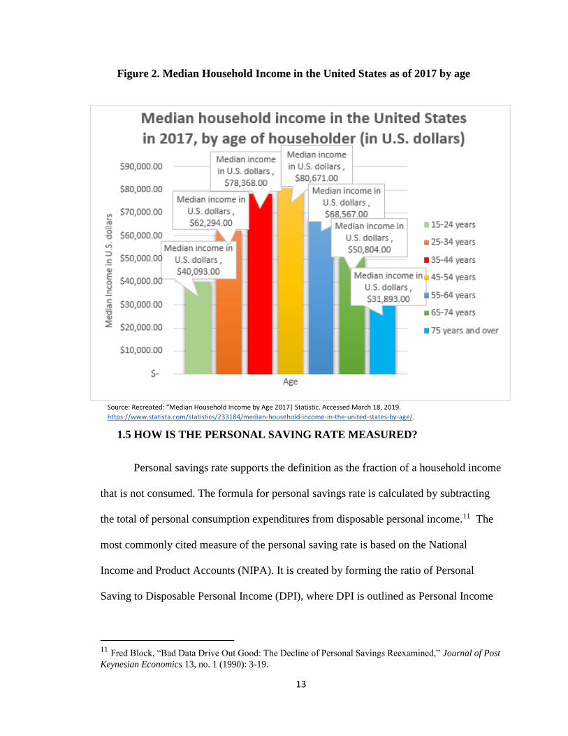
Figure 2 presents the median household income in the United States as of 2017.

Figure 2 shows that between the age of 15-24 and the age of 75 years and over are the

two lowest points which can evidently explain the Life Cycle Hypothesis theory. Age 15-

24 are younger adults working low-income jobs while attending school so their income

will continue to be low before they hit the next stage in the life cycle phase. Age 75 and

over are the retired age adults who are no longer employed and are receiving no income

and therefore are dissaving. Figure 2 shows that between the retirement ages of 64-74 and

75 years and over the median income between those years have decreased by $18,911.00.

Figure 2 presents that the two highest points of the median income in the U.S is at 35-44

years old and at 45-54 years old. Figure 2 could be mainly based off of education

attainment, skills and attributes to the labor force, wealth and other underlying factors.

13

Figure 2. Median Household Income in the United States as of 2017 by age

1.5 HOW IS THE PERSONAL SAVING RATE MEASURED?

Personal savings rate supports the definition as the fraction of a household income

that is not consumed. The formula for personal savings rate is calculated by subtracting

the total of personal consumption expenditures from disposable personal income.11 The

most commonly cited measure of the personal saving rate is based on the National

Income and Product Accounts (NIPA). It is created by forming the ratio of Personal

Saving to Disposable Personal Income (DPI), where DPI is outlined as Personal Income

11 Fred Block, “Bad Data Drive Out Good: The Decline of Personal Savings Reexamined,” Journal of Post

Keynesian Economics 13, no. 1 (1990): 3-19.

Source: Recreated: “Median Household Income by Age 2017| Statistic. Accessed March 18, 2019.

https://www.statista.com/statistics/233184/median-household-income-in-the-united-states-by-age/.

14

(including wage and salary income, net proprietors’ income, income from interest and

dividends) less tax and non-tax payments to governments.12 Personal savings rate only

briefly informs people how to calculate their saving rate by providing people with what

proportion their savings can cover.

An alternate measure of the personal saving rate that frequently receives attention

is calculated by the Federal Reserve and reported in the Flow of Funds accounts (FOFA).

The FOFA measure of personal saving, unlike NIPA measure, is expressed as net

additions to wealth from one phase to another. For this concept, household saving totals

net acquisition of financial assets plus net investment in tangible assets minus net

increase in liabilities. The FOFA personal saving rate is the fraction of net additions to

wealth to personal disposable income. The two savings rates differ theoretically in many

ways, but the three important differences that are discussed below.

To begin, NIPA and FOFA measures differ in their management of consumer

durable goods. For instance, FOFA considers acquisition of consumer durables as a form

of saving, and services from these goods as consumption, whereas NIPA regards

consumer durable expenditures as personal consumption. Regarding housing, NIPA treats

expenses on owner-occupied housing as personal saving while FOFA deems only equity

in the home as wealth, and mortgage payments as lasting liabilities. Second, the FOFA

and NIPA measures treat private pensions differently. The NIPA includes employee

contributions to 401(k) plans and pensions as part of wages and salaries, and employer

contributions as other labor income. Finally, Social Security contributions in NIPA are

12 Milt Marquis, “What's Behind the Low United States Personal Saving Rate?” FRBSF Economic Letter

(March 29, 2002): 1-3.

15

computed in personal taxes, not as personal saving while FOFA considers both private

and government pensions, and life insurance reserves as household saving. Although

evaluated differently, the continuing trends in the NIPA and the FOFA personal saving

rate turn out to be quite related. Both have declined considerably over the years.

1.6 BORROWING

Household debt has escalated sharply in every nation in the past two decades, and

that debt is perceived as being a significant role in economic outcomes. Specifically,

households face income uncertainty and potentially high returns to entrepreneurial

investments, which give motives to save and/or borrow. 13 Homes, automobiles and lately

higher education justify the need for most of the household borrowing. Households

typically borrow early in their lifetimes to purchase these assets, but the purpose is not to

smooth consumption which is defined in many theoretical analyses. The necessity to

acquire these assets tends to affect current consumption, since all these forms of

borrowing consist of extensive direct out of pocket costs as well as indirect costs making

it nearly impossible to finance the entire purchase of these assets with just debt. The

lifecycle model has little to no significance on actual household borrowing behaviors.

An increase in housing prices could also boost household debt. First, a wealth

effect may boost consumption. During the recession of 2007, many households witnessed

their wealth degenerating quickly and their income and employment opportunities

diminish. During that period, the net worth of U.S. households fell by the largest amount

13 Joseph P. Kaboski, Molly Lipscomb, and Virgiliu Midrigan, “The Aggregate Impact of Household

Saving and Borrowing Constraint: Designing a Field Experiment in Uganda,” The American Economic

Review 104, no. 5 (May 2014): 171-76.

16

in more than a half-century. 14The probability of having negative net worth is

substantially increased across countries if households are in the lowest income quantile.15

CHAPTER 2: LITERATURE REVIEW

Numerous empirical studies have been conducted to examine the determinants of

the consumption, saving and borrowing behaviors of households. Each empirical study

has coined their own idea or theory of the different variables that determine such

behaviors. Each study has either supported the Life Cycle Hypothesis theory or rejected

the theory. Many of these studies corroborated that income, household wealth, and age

are the underlying determinants along with other demographic variables such as race,

gender, household size, education attainment and more.

The determinants that influences households’ consumption/saving behaviors dates

back to the era of Keynesian Economics. John Maynard Keynes proposed that current

disposable income is the main determinant of households’ consumption/saving

behaviors.16 He argued that consumers save a proportion of their additional income and

therefore the marginal propensity to save is between zero and one. He listed eight

motives for why people save money. (1) Precautionary motive (2) the life-cycle motive

(3) the intertemporal substitution motive (4) the improvement motive (5) independence

motive (6) the enterprise motive (7) the bequest motive and (8) the avarice motive. Since

then several new theories were developed to explain this empirical observation. Including

14 Martin Crutsinger, “U.S. household net worth plunges by record amount,” Canadian Press, March 13,

2009. 15Sarah Brown and Karl Taylor, “Household Debt and Financial Assets: Evidence from Germany, Great

Britain and the USA,” Journal of the Royal Statistical Society. Series A (Statistics in Society) 171, no. 3

(2008): 615-43. 16 John Maynard Keynes, The General Theory of Employment, Interest and Money (London: Macmillan,

1936), 1-427.

17

Milton’s Friedman’s Permanent Income Hypothesis and Franco Modigliani’s Life Cycle

Income Hypothesis which are the two theories most commonly used to explain personal

saving behavior over the long run.

Interest rate is another factor that influences individual’s consumption-saving

behaviors. Bailey analytical model explained how changes in the interest rate influences

consumers’ consumption-saving behaviors through the substitution and wealth effects.17

Bailey study intended to separate the income or wealth effect of an interest rate change

from the substitution effect. His argument aims to prove that saving must be positively

related to changes in the interest rate. His analysis discloses that he has combined the

effect of the compensating income variation with the effect of the interest rate change in

attaining his conclusions. Bailey found that the substitution effect is always positive

because a decrease in the interest rate reduces the opportunity cost of current

consumption. This then promotes more individuals to save because it increases the

opportunity cost of current consumption. He concluded that the trend of the wealth effect,

could be negative and might affect the substitution effect.

Ramanathan purpose of the study was to enlighten readers on the saving behavior

of urban Indian households.18 The nature of the effects on saving on income and net

worth and their interactions are examined in detail for different socio-economic sub-

groups. The results of this study show that there is strong evidence that income and net

worth significantly influence the level of saving. He concluded: (1) there is substantial

17 Martin J. Bailey, “Saving and the Rate of Interest,” Journal of Political Economy 65, no. 4 (August

1957): 279-305. 18 R. Ramanathan, “An Econometric Exploration of Indian Saving Behavior,” Journal of the American

Statistical Association 64, no. 325 (March 1969): 90-101.

18

evidence that current income plays a very important role in accounting for variations in

saving. (2) the study also provided evidence for the “Pigou” effect. There was no

significant interaction between income and wealth was found, except for low-income

occupations such as service, unskilled workers and artisans. (3) The saving-income ratio

of renters was much higher than that of home-owners even though the former had a much

lower average income. Both average and marginal propensities to save with respect to

income were high for the renter class as compared to home-owners. (4) Ownership of a

business or professional practice brings about strong needs for investment funds which

are expected to bring high rates of return thus resulting in high saving. (5) Among the age

groups, mean income, saving and saving-income ratio increased with age up to 45 years

but declined after, with the exception of the 65 year or over group. The oldest age groups

had the highest mean income and their average and marginal propensities to save was

also the highest compared to the younger age groups. Retired people generally live with

their children and are nominal heads of the households. Such households have more

income earners resulting in high levels of income and saving.

Katona reported the results from surveys conducted in 1960 and 1966, where

individuals were asked about their reasons for saving.19 He found in his research that

saving for rainy days were the most frequent mentioned purpose for saving. Katona

proposed three categories of saving habits among average persons: (1) contractual saving,

where one makes routine installment payments for an asset like a home mortgage, which

is forced or obligatory saving; (2) discretionary saving, where one deliberately saves; and

19 George Katona, Psychological Economics (New York: Elsevier Scientific Publishing Company, 1975),

1-438.

19

(3) residual saving, where one does not spend all of income and therefore saves by

default. He offered six more general saving motives: (a) for emergencies, (b) to have

funds in reserve for necessities, (c) for retirement or old age, (d) for children’s needs, (e)

to buy a house or durable goods, and (f) for holidays.

Bovenberg and Evans examined several possible explanations for the downward

trend in the U.S. personal saving rate.20 Bovenberg and Evans demonstrates that

structural changes in capital markets, as well as improvements in wealth positions, living

standards of the elderly, and private and public insurance mechanisms have all

contributed to the declining trend in personal saving. They found that improvements in

wealth positions associated with rising values of stock market and housing have been an

important factor behind the declining trend in personal saving. They also discovered that

the changing age structure of the population and lower inflation may have also reduced

the personal saving rate. The empirical results suggest that demographic factors may have

also played an important role.

Hefferan studies the relative importance of income, wealth, and family

characteristics in explaining the decisions to save, the level of saving in households, and

the patterns of saving in several types of families.21 The results supported the general

hypotheses that the decision to save and the level of saving is influenced by income,

wealth, and family characteristics and that saving patterns vary among different types of

families. Findings suggest that the level of saving is best explained by a family’s current

20 A. Lans Bovenberg and Owen Evans, “National and Personal Saving in the United States: Measurement

and Analysis of Recent Trends,” Staff Papers (International Monetary Fund) 37, no. 3 (September 1990):

636-69. 21 Colien Hefferan, “Determinants and Patterns of Family Saving,” American Association of Family and

Consumer Sciences 11, no. 1 (September 1982): 47-55.

20

wealth position. Hefferan measured savings as the difference between current

expenditure and income. He found that savings to be primarily an increasing function of

income and wealth. Home ownership appeared to be positively related to the decision to

save as well as the level of savings. Hefferan found that home owners with mortgages to

be both more likely to save as well as saving more than families with similar educations

and family life cycle characteristics.

Sturm proposed that there are four main motives leading to individuals’ decision

to save current income rather than to consume: saving for retirement, precautionary

saving, saving for bequest, and saving for acquisition of tangible assets.22 Sturm argues

that individuals saving decisions can be determined by various motives and savings

decisions should be based on some kind of optimizing behavior by which the levels of

consumption and saving are chosen to equalize the marginal benefits of these alternative

uses of income. He distinguishes main determinants of aggregate saving behavior. First,

he argues that only in a growing economy the various saving motives of an old individual

will lead to a positive aggregate saving while the retirement saving for young individuals

will be offset by dissaving of individuals in retirement age. He also states that the bequest

motive of saving does not generate any net saving in stationary equilibrium while a

constant level of assets is transferred from generation to generation. He pointed out that

precautionary saving motive does not generate positive net saving of individuals in

stationary state because once reached its target level will remain constant. Next, he states

that depending on the individual’s income expectations, the implications of the different

22 Peter H. Sturm, “Determinants of Saving: Theory and Evidence,” OECD Journal: Economic Studies 1

(1983): 147-96.

21

types of economic growth in terms of sources and nature for the aggregate saving ratio

may be different. Finally, he distinguishes a number of demographic variables that can

have a direct effect on the aggregate saving ratio.

Furnham analysis investigated the relationship between demographic (age, sex,

education, vote and income) and attitudes toward saving money in Britain.23 He

concluded that age is strongly and linearly related to respondents’ attitudes toward

saving, and age has been found to determine how regularly a household saves, where a

household saves, and why household saves. Analysis of the saving habits questionnaire in

his study showed that sex, age, and income were among the most important

discriminators of saving habits.

Modigliani paper presents a reevaluation of the theory of the determinants of

individual and national thrift that eventually became known as the Life Cycle Hypothesis

(LCH) of saving.24 He suggested that income fluctuates over an individual’s lifetime.

Individuals will apply saving and borrowing behaviors to transfer income from high-

income periods to low-income periods. Individuals base their consumption behaviors on

their anticipated future income, wealth and life-expectancy so that consumption can be

allocated smoothly over the remaining years of life. Modigliani argued that the basic

LCH implies that, with retirement, saving should become negative, and thus assets

decline at a continuous rate, reaching zero at death. He found that there is significant

23Adrian F. Furnham, “Why Do People Save? Attitudes To, and Habits Of, Saving Money in Britain,”

Journal of Applied Social Psychology 15, no. 4 (1985): 354-73. 24 Franco Modigliani, “Life Cycle, Individual Thrift, and the Wealth of Nations,” American Economic

Review 76, no. 3 (November 1986): 297-313.

22

evidence that wealth decreases slowly in old age which indicates that households leave

substantial bequests relative to peak wealth.

Montgomery paper used a modified life-cycle model to analyze determinants of

the recent decline in the personal savings rate.25 The empirical results do not support the

hypothesis that the decline in the saving rate was the result of a reduction in the real rate

of return. He found that the reduction in the rate of growth of income and the changing

demographic profile of the labor force are the most important factors in accounting for

the fall in the personal saving rate. He indicated that increases in wealth and in expected

future income relative to current income account for about 40 percent of the fall in the

personal saving rate during this period.

Davis and Schumm investigated family savings behavior and the satisfaction with

the current savings of low- and high-income households.26 They found that above the

income threshold level, savings rise very rapidly as income increased. Among couples

whose incomes were above the threshold, satisfaction with savings was primarily a

function of income, savings and family size, while level of savings was primarily a

function of income, education, family size, and home ownership. Home ownership was

shown to be positively correlated with the actual level of savings. They found that below

a threshold level of income of $9,000, it appeared that couples simply could not afford to

save very much of their limited incomes. They concluded that the motivation to save was

25 Edward Montgomery, “Where Did All the Saving Go? A Look at the Recent Decline in the Personal

Saving Rate,” Economic Inquiry 24, no. 4 (October 1986): 681-97. 26 Elizabeth P. Davis and Walter R, Schumm, “Savings Behavior and Satisfaction with Savings: A

Comparison of Low-And High- Income Groups, “Home Economics Research Journal 15, no. 4 (June

1987): 247-56.

23

associated with both savings and satisfaction with savings in terms of significant

quadratic relationship.

Deaton paper focuses on the four reasons for studying saving in developing

countries separately from the saving behavior in developed economies.27 Four reasons

include: (1) at the microeconomic level, developing country households tend to be larger

and poorer, they have a different demographic structure, majority of them participate in

agriculture and their income prospects are much more uncertain. (2) at the

macroeconomic level, both developing and developed countries are concerned with

saving and growth. (3) much of the postwar literature expresses the belief that saving is

too low and sometimes the problem is blamed on the lack of government policy. (4)

saving is even more difficult to measure in developing than in advanced economies,

whether at the household level or as a macroeconomic aggregate.

Bunting researched the relation between income and savings.28 He concluded that

the reason for the recent decline in savings has more to do with non-savers than savers.

The amount of household savings has remained relatively steady since 1972, while the

dissaving’s rate has been drastically increasing. Dissaving goes a step beyond not saving.

With dissaving, households are either spending all their income plus money they had

previously put away or making purchases on credit, essentially spending money they do

not have and paying interest. In some cases, individuals could be doing both. This

27 Angus Deaton, “Saving in Developing Countries: Theory and Review,” World Bank Economic Review,

Proceedings of the World Bank Annual Conference on Development Economics (1989): 61-96. 28 David Bunting, “Savings and the Distribution of Income,” Journal of Post Keynesian Economics 14, no.

1 (1991): 3-22.

24

increase in the dissaving’s rate has caused the overall savings rate to decrease. He also

found that the tendency to save increases as income increases.

Hebbel, Webb and Corsetti study tests several hypotheses about saving behavior

using panel data from the U.N. system of National Accounts.29 The study tests how

household saving in developing countries responds to income and growth, rates of return,

monetary wealth, foreign saving, and demographic variables. The empirical findings of

this study confirm the central role of income and wealth in determining household saving

in developing countries. The results show that income and wealth variables affect saving

strongly and in ways consistent with standard theories. Inflation and interest rate do not

show clear effects on saving, which is also consistent with theoretical ambiguity.

Households save a larger share of their income when the income is higher and when it is

growing faster. They save less the greater their monetary wealth. They found that

borrowing constraints are also major determinants of household savings.

Bae, Hanna and Lindamood paper applies financial ratio analysis to study

overspending of households.30 They calculated an income to spending ratio for each

consumer unit to identify patterns of overspending in households. They found that 40%

of American households spent more than their take home incomes and 25% of the sample

spent at least 127% of their take home income. At least 25% of households in each family

size and age group spent more than they brought home. The income variable used in this

study represented the amount a household can spend on current consumption, repayment

29 Klaus Schmidt Hebbel, Steven B. Webb, and Giancarlo Corsetti, “Household Saving in Developing

Countries: First Cross-Country Evidence,” The World Bank Economic Review 6, no. 3 (September 1992):

529-47. 30 MiKyeong Bae, Sherman Hanna, and Suzanne Lindamood, “Patterns of Overspending in U.S.

Households,” Journal of Financial Counseling and Planning 4 (1993): 11-31.

25

of loans, and other forms of savings. There were some households with annual income of

zero. Households with zero income were counted as over spenders.

Xiao and Noring paper proposed six saving motives that imply family financial

needs.31 These saving motives are saving for daily expenses, purchases, emergencies,

retirement, children, and growth. They classified saving motives for daily expenses,

purchases, and emergencies as lower level needs, and saving motives for retirement,

children, and growth as higher-level needs. They assumed that these needs have similar

features of human needs described by Maslow (human needs theory), implying that

family financial needs are motivated by family financial resources. When families have

low levels of financial resources, they seek to meet lower level needs such as survival and

security. When family financial resources increase and lower level needs are met,

families will generate higher level needs.

Alessie, Lusardi and Aldershof examine household wealth and income in the

Netherlands between 1987 and 1989.32 They found that there is substantial heterogeneity

in the behavior of households, and wealth holdings vary substantially even among the

same age group. They also found that a sizeable fraction of households does not dissave

when old and evidence in favor of the bequest motive. They note that in order to study

how wealth holdings evolve over the life cycle it is important to disentangle age and

cohort effects. They found that savings are higher for households that indicate they were

saving. The questionnaire for this study lists several possibilities for the motives to save.

31 Jing Jian Xiao and Fanzika E. Noring, “Perceived Saving Motives and Hierarchical Financial Needs,”

Journal of Financial Counseling and Planning (January 1994): 25-45. 32 Rob Alessie, Annamaria Lusardi, and Trea Aldershof, “Income and Wealth Over the Life Cycle:

Evidence from Panel Data,” Review of Income and Wealth 43, no. 1 (March 1997): 1-32.

26

The main responsibilities are: to buy a house, to buy a car, to buy other durables, for

unforeseen events, for children, for old age, for no specific purpose, and all possible

combinations of the above motives. They noted that the precautionary saving motive

remains relatively stable across the life cycle but it is somewhat greater for young and old

households

Horioka and Watanbe paper estimates the contribution of net saving for each of

twelve motives to overall saving in Japan.33 They lists the motives for which households

save can be grouped into three categories: (1) life cycle motives, which are motives that

arise from temporary imbalances between income and expenditures at various stages in

one’s life cycle; (2) precautionary motives, which are motives arising from uncertainties

concerning future income and/or expenditures, and (3) the bequest motive, which arises

from the desire to leave assets behind to one’s children and other heirs in the form of

transfer and/or bequests. They found that net saving for the retirement and precautionary

motives, both of which are consistent with the life-cycle model, is of dominant

importance in Japan and that the Japanese save in each life stage for motives that are

appropriate for that life stage.

Attanasio analyzes the pattern of saving behavior by U.S. households.34 The main

goal of this paper was to explain the decline in aggregate personal saving in the United

States in the 1980s. Attanasio discovered that the level of saving of a given cohort is

determined by the propensity to save of that cohort and by the total amount of resources

33 Charles Yuji Horioka and Wako Watanbe, “Why Do People Save? A Micro-Analysis of Motives for

Household Saving in Japan,” The Economic Journal 107 (May 1997): 537-52. 34 Orazio P. Attanasio, “A Cohort Analysis of Saving Behavior by U.S. Households,” Journal of Human

Resources 33, no. 3 (Summer 1998): 575-609.

27

available to it. He stated that differences in the average level of saving across cohorts can

be explained by differences either in saving propensity or in resources. The main element

emerging from the analysis is that the cohorts that were in their 40s and 50s during the

1980s are those mainly responsible for the decline in aggregate saving. The lower level of

saving for those cohorts was reflected in a strong decline in aggregate saving because

those cohorts were in the part of their life cycle when saving are the highest.

Attanasio paper illustrates recent trends in household consumption and personal

savings in the UK and the US and discusses some theoretical models that can be used to

interpret them.35 The decline in the personal savings rate in the US during the 1980s is an

unresolved puzzle. This paper stresses the need to analyze individual data to shed some

light on these aggregate trends. The theoretical framework discussed throughout the

paper is the life-cycle model, which views consumption and saving decisions as part of a

dynamic optimization process. He discusses the development of the model and the

current research agenda and ways that it can be enriched with various degrees of

sophistication.

Lee paper examines how the proportion of United States saving that represents

life-cycle accumulation changed over the last century.36 He discovered as individuals

retire earlier and live longer than before, the expected length of male retirement has

increased by more than six-fold since 1850. He estimated that the fraction of lifetime

income saved for retirement tripled between 1900 and 1990. Based on his result, he

35 Orazio Attanasio, “Consumption and Saving Behaviour: Modelling Recent Trends,” Fiscal Studies 18,

no. 1 (February 1997): 23-47. 36 Chulhee Lee, “Life Cycle Savings in the United States, 1900-90,” Review of Income and Wealth 47, no. 2

(June 2001): 165-79.

28

argues that the relative contribution of the life-cycle saving to the US wealth

accumulation increased substantially, perhaps two to three times, over the last hundred

years. He questioned why it is unclear why the aggregate household saving rates

remained stable in spite of the huge increase in the life-cycle savings. His possible

explanation for this is that precautionary saving declined over time due to the

development of various social insurance programs and increases annuitization of income

during the last century. He then concluded that further studies on this issue should

sharpen our understanding of the long-term trend of the US household savings.

Lusardi, Skinner and Venti made three general observations about the decline in

the personal saving rate: (1) stock market capital gains are driving down the measured

rate of personal saving. (2) second observation focuses on the aggregate implications of

the decline in personal saving. (3) third observation emphasizes that NIPA personal

saving is not a useful measure of whether households are prepared for retirement or an

economic downturn.37 They believed that there is a significant group of households with

saving rates too low to be explained by the conventional life-cycle models. They

proposed that some households have difficulty recognizing the need to save and

calculating the saving they need to do. They found that capital gains in the stock market

have explained much of the decline in the NIPA saving rate, through both behavioral and

accounting channels.

37 A. Lusardi, J. Skinner, and S. Venti, “Saving Puzzles and Saving Policies in the United States,” Oxford

Review of Economic Policy 17, no. 1 (March 2001): 95-115.

29

Maki and Palumbo investigated the effect of household wealth in the personal

saving rate in using household level data for 1990s.38 They acknowledged that

researchers do not agree about just what behavior links these two events, or how to

interpret the negative correlation between wealth and the saving rate over a longer time

span. Their findings indicated that high-income and high-education cohorts experienced

both largest gains in wealth and largest decreases in savings rates. However, the results

also showed that other cohorts experienced modest changes in household wealth and

saving rates during the same period. Maki and Palumbo found that the groups of

households whose balance sheets were boosted the most by surging equity prices were

also the groups that substantially decreased their saving rates. Their results corroborate a

direct view of the wealth effect on consumption. They concluded that the increase in

household financial wealth, which was fueled by the increase in the stock market prices,

partly explained the decrease in the personal saving rate in the United States in the 1990s.

Thornton examined whether age has a direct relation with the personal savings

rate in the United States.39 Thornton tested a simple life- cycle savings model for the

United States by applying cointegration techniques to time series data on personal

savings and the age structure of the population over the period 1956-1995. He came

across that savings is cointegrated with the ratios of minors to the working age population

and the aged to the working age population. Thornton discovered that both of these ratios

had a negative and significant impact on the savings rate. Therefore, he determined that

38 Dean M. Maki and Michael G. Palumbo, “Disentangling the Wealth Effect: A Cohort Analysis of

Household Saving in the 1990s,” Finance and Economics Discussion Series 2001-21, Board of Governors

of the Federal Reserve System (2001). 39 John Thornton, “Age Structure and the Personal Savings Rate in the United States,1956-1995,” Southern

Economic Journal 68, no. 1 (July 2001): 166-70.

30

the U.S personal savings rate will eventually continue to sink as the population continues

to age.

Marquis analysis concentrated on the growth in household wealth as a main factor

describing the low saving rates in the United States in the 1990s and early 2000s.40

Marquis introduced the measurement of the personal saving rate using National Income

and Product Accounts (NIPA). He calculates disposable income minus personal outlays

in NIPA and then calculates personal saving rate by dividing personal savings by

disposable personal income. Marquis also analyzes why the NIPA personal savings rate

has fallen by focusing on two factors: (1) the wealth effect, where in general individuals

would like to spend more money when they are rich or they perceive themselves to be

rich and (2) an increase in labor productivity, through which total income will increase

due to the high labor productivity if consumption remains the same and the personal

saving rate will go down. His third explanation recommended for the decline of saving

rate during that period is the increased access to consumer credit, which relaxed

consumers’ liquidity constraints and increased their consumption. Marquis argued that

the low personal saving rate could be a cause for concern if the country may become too

reliant on foreign capital for economic growth.

Harris et.al researched the determinants of household saving in Australia.41 They

found that the top three motives for saving for households was the retirement motive,

saving for holidays and the precautionary motive. Based on the results they indicated that

the main difference in saving motives between households with and without children was

40 M. Marquis, “What's Behind the Low U.S. Personal Saving Rate,” FRBSF Economic Letter (2002): 1-3. 41 Mark N. Harris, Joanne Loundes, and Elizabeth Webster, “Determinants of Household Saving in

Australia,” Economic Record 78, no. 241 (June 2002): 207-23.

31

saving for educational purposes. They divided the results into different age categories,

and found that the motives for saving were different when the age of the respondents was

different. For young respondents (aged 18 to 24) buying durables and saving for holiday

were the most important motive. Respondents aged 25-44 gave saving for retirement

higher importance and the age group 45-64 rated this as their most important reason for

saving. They proposed that the importance of the retirement motive increase as the

household income increased.

Pryor empirical study argues that a shift in the demographic composition of the

population will be a much more important case for a decline in personal saving in the

future.42 The model used to examine this phenomenon considers the interest rate, the

growth rate of the economy, the retirement age, the growth of the population, and the life

expectancy. A major part of the model deals with the changing age structure of the

population and the ratio between retired to active workers. He points out that these

demographic considerations have two important implications: (1) it is necessary to

consider both the rising life expectancy and the possible postponement of retirement. (2)

if the customary retirement remain the same, future cohorts will have to have a higher

annual saving to finance the longer retirement period brought about by the longer life

span.

Solveig Erlandsen and Ragnar Nymoen stated that a key question in economics is

whether changes in the age structure of the population affect macroeconomic variables

42 Frederic L. Pryor, “Demographic Effects on Personal Saving in the Future,” Southern Economic Journal

69, no. 3 (January 2003): 541-59.

32

such as aggregate consumption and the savings rate. 43 In their paper, they test for age

structure effects on aggregate consumption in Norway, by estimating a consumption

function which takes account of changes in the age distribution of the population. They

found significant and numerically important age structure effects on Norwegian

aggregate consumption. Their results are consistent with the life cycle model;

consumption falls when the share of middle-aged persons in the population increases.

Their analysis results showed that age structure changes are represented by the ratio of

middle-aged persons, defined as those between the age 50 and 66, to the rest of the adult

population. They stated that although their analysis for this paper was restricted for

Norwegian data, there are good reasons to believe that the results can also apply to other

countries. Both determined that identifying age structure effects consumption may be of

increasing importance in many countries.

Fisher and Montalto purpose of their study was to explore saving motives and

saving horizon.44 The framework of the study was based on the prospect theory, in which

consumption and saving decisions are based on a reference point rather than on lifetime

income. Fisher and Montalto stated that there are two reasons why it is important to

analyze household motives for saving and saving horizons. (1) It provides a better

understanding of the saving behavior of households, differences among household saving

rates, factors influencing the level of household saving, trends in the household saving

rate, and a variety of other issues related to saving. (2) Analyzing the motives for which

households save provides information on which economic model is of greater

43 Solveig Erlandsen and Ragnar Nymoen, “Consumption and Population Age Structure,” Journal of

Population Economics 21, no. 3 (July 2008): 505-20. 44 Patti J. Fisher and Catherine P. Montalto, “Effect of Saving Motives and Horizon on Saving Behaviors,”

Journal of Economic Psychology 31, no. 1 (February 2010): 92-105.

33

applicability in the “real world”. They found that emergency and retirement saving

motives are found to significantly increase the likelihood of saving regularly. The results

show that the saving motives held by households differ by saving horizon. They

determined that further research on the link between saving motives, saving horizon, and

saving behaviors is needed. The results of this study support features of other theoretical

frameworks.

Yao et.al study compared saving motives between Chinese and American urban

households.45 Results showed that Chines households were more likely to report

precautionary and education saving motives and Chinese households with lower incomes

were more likely to report a retirement saving motive. Yao discovered that in the United

States, policy makers are concerned about the low rate of household savings and have

encouraged households to save more by establishing various retirement saving programs

through tax incentives. The results in this study indicated that the likelihood of having

retirement saving motives varies by income, net worth, emergency fund adequacy,

homeownership, age, education, and employment status. They concluded with the notion

of Americans with lower incomes are less likely to report a retirement saving motive.

Kasilingam and Jayabal analyzed the effect of saving motives on household

saving in India.46 They argued that the saving rate of an individual or household is

affected not only by their ability to save but also their willingness to save. While an

individual’s ability to save is determined by his/her income and expenditures, his/her

45 Rui Yao, Robert Weagley, and Li Liao, “Household Saving Motives: Comparing American and Chinese

Consumers,” Family and Consumer Sciences 40, no. 1 (September 2011): 28-44 46 R. Kasilingam and G. Jayabal, “Impact of Saving Motives on Household Savings,” Pranjana: The

Journal of Management Awareness 14, no. 1 (January 2011): 67-75.

34

willingness to save is the saving motives of the individual. An important finding of their

study was that the level of motives had a significant influence on the size of saving. They

determined that the reason for India’s high savings rate was due to the Indians high level

of motives to save and as long as the Indians continued to have high level of saving

motives, the high level of saving rate would continue to increase.

Brounen et.al studied the behavioral factors, which lead households toward

savings and financial planning across a panel of 1253 Dutch Households.47 They found

that an individual’s propensity to save declines with age and is greater among the

financial literate. They observed that saving behaviors differs across generations and is

notably dominant among baby boomers. Their analysis focused on clarifying why some

Dutch households save or invest, while others do not. Brounen describes this difference

by viewing at a set of well described household characteristics (demographics, income,

skills, education, and financial literacy). An extended survey analyzes and evaluates the

effects of household demographics, skills, upbringing, and personality on Dutch

household saving. Their results indicate that the willingness to save reveals a time

preference and is stronger among younger households with high levels of financial

literacy.

Kapounek et.al study acknowledged the economic and psychological factors

influencing the households’ saving behavior.48 The major research questions for this

study were the emphasis on the analysis of the scientific literature related to household

47 Dirk Brounen, Kees G. Koedijk, and Rachel A.J. Pownall, “Household Financial Planning and Savings

Behavior,” Journal of International Money and Finance 69 (2016): 95-107. 48 Svatopluk Kapounek, Petr Korab, and Vilma Deltuvaite, “Irrational households' Saving Behavior? An

Empirical Investigation,” Procedia Economics and Finance 39 (2016): 625-33.

35

saving behaviors during different stages of economic cycle, the reaction of households to

the external shocks, the role of sentiments in the households saving behavior, and the

factors stimulating households to save in foreign currency rather than in national

currency. They focused on savings in the foreign currencies and pointed out irrationalities

of the economic agents. The outcomes of this empirical study showed that the

households’ saving behavior is more irrational specifically during economic downturn

and financial crisis periods. Their findings rectified that there is not a substantial impact

of traditional motives, such as interest rate or inflation on the way households save.

CHAPTER 3: METHODOLOGY

3.1 SOURCE OF DATA

This study examined the period from 1980 to 2017. This was chosen due to

intense declines of the personal savings rate during that period in the United States. Data

for the personal saving rate were obtained from the Bureau of Economic Analysis (BEA)

website.49 Personal saving rate data represent annual personal saving as a percentage of

disposable personal income. Real per capita disposable income statistics were constructed

from disposable personal income data obtained from the BEA. The INC variable in this

model represents the real disposable personal income. Annual net worth data was

obtained from the Bureau of Economic Analysis.50 The real net worth was computed by

dividing the nominal net worth that was obtained by the Consumer Price Index (CPI).

The interest rate (INT) in this model is represented by the bank prime rate data as

49 U.S. Bureau of Economic Analysis, Personal Saving Rate [PSAVERT], retrieved from FRED, Federal Reserve Bank

of St. Louis; https://fred.stlouisfed.org/series/PSAVERT, March 4, 2019. 50 Board of Governors of the Federal Reserve System (US), Households and nonprofit organizations; net worth, Level

[HNONWRA027N], retrieved from FRED, Federal Reserve Bank of St. Louis;

https://fred.stlouisfed.org/series/HNONWRA027N, March 4, 2019.

36

reported by the Federal Reserve.51 Labor productivity data were obtained from the

Bureau of Labor Statistics (BLS) web site. 52 PROD variable in this model represents

annual percentage in labor productivity.

3.2 HYPOTHESES

Initially, we assume all variables have an impact on the personal savings rate. The

theoretical model is:

sav = f (-inc, + nwr, + int, +prod)

For the econometric model, a five variable function is considered:

savt = β0 + β1(Inc) + β2(Nwr) + β3(Int) + β4(Prod) + ε

Where:

Sav = Personal Saving rate

Inc = Real Disposable Income

Nwr = Real household net worth

Int = The interest rate

Prod = Labor Productivity

ε= error term

As explained in the earlier sections, the leading factors that affect the

personal saving rate are current income, wealth, expected future earnings and the interest

rate. As the data on current income, wealth and interest rates are accessible expected

future earnings are often unobservable. As a result, expected future earnings was then

51 US Federal Reserve, Federal Reserve Statistics Release H.15: Selected Interest Rates,

http://www.federalreserve.gov/releaes/h15/data.htm, accessed March 4, 2019 52 U.S. Bureau of Labor Statistics, Nonfarm Business Sector: Real Output Per Hour of All Persons [PRS85006092],

retrieved from FRED, Federal Reserve Bank of St. Louis; https://fred.stlouisfed.org/series/PRS85006092, March 4,

2019.

37

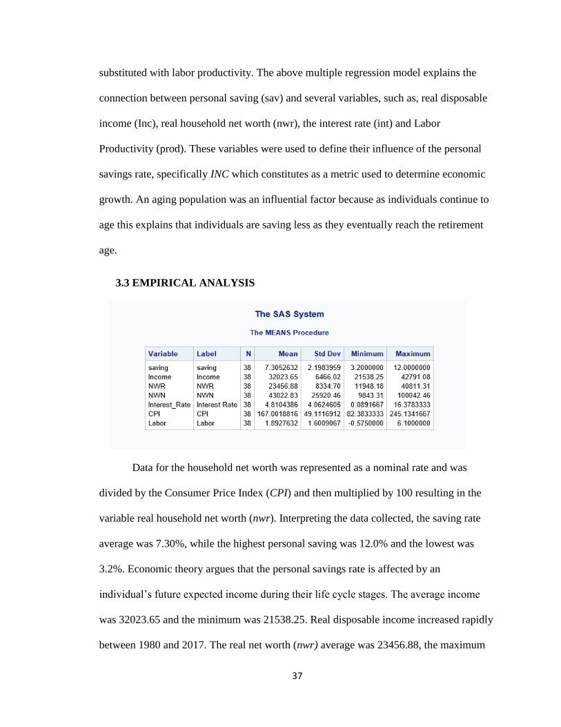
substituted with labor productivity. The above multiple regression model explains the

connection between personal saving (sav) and several variables, such as, real disposable

income (Inc), real household net worth (nwr), the interest rate (int) and Labor

Productivity (prod). These variables were used to define their influence of the personal

savings rate, specifically INC which constitutes as a metric used to determine economic

growth. An aging population was an influential factor because as individuals continue to

age this explains that individuals are saving less as they eventually reach the retirement

age.

3.3 EMPIRICAL ANALYSIS

Data for the household net worth was represented as a nominal rate and was

divided by the Consumer Price Index (CPI) and then multiplied by 100 resulting in the

variable real household net worth (nwr). Interpreting the data collected, the saving rate

average was 7.30%, while the highest personal saving was 12.0% and the lowest was

3.2%. Economic theory argues that the personal savings rate is affected by an

individual’s future expected income during their life cycle stages. The average income

was 32023.65 and the minimum was 21538.25. Real disposable income increased rapidly

between 1980 and 2017. The real net worth (nwr) average was 23456.88, the maximum

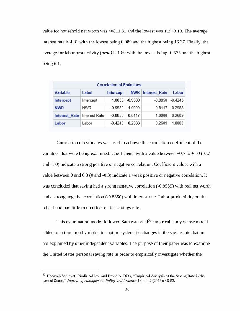
38

value for household net worth was 40811.31 and the lowest was 11948.18. The average

interest rate is 4.81 with the lowest being 0.089 and the highest being 16.37. Finally, the

average for labor productivity (prod) is 1.89 with the lowest being -0.575 and the highest

being 6.1.

Correlation of estimates was used to achieve the correlation coefficient of the

variables that were being examined. Coefficients with a value between +0.7 to +1.0 (-0.7

and -1.0) indicate a strong positive or negative correlation. Coefficient values with a

value between 0 and 0.3 (0 and -0.3) indicate a weak positive or negative correlation. It

was concluded that saving had a strong negative correlation (-0.9589) with real net worth

and a strong negative correlation (-0.8850) with interest rate. Labor productivity on the

other hand had little to no effect on the savings rate.

This examination model followed Samavati et al53 empirical study whose model

added on a time trend variable to capture systematic changes in the saving rate that are

not explained by other independent variables. The purpose of their paper was to examine

the United States personal saving rate in order to empirically investigate whether the

53 Hedayeh Samavati, Nodir Adilov, and David A. Dilts, “Empirical Analysis of the Saving Rate in the

United States,” Journal of management Policy and Practice 14, no. 2 (2013): 46-53.

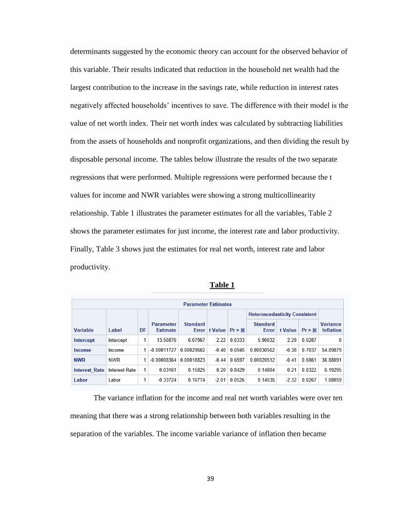
39

determinants suggested by the economic theory can account for the observed behavior of

this variable. Their results indicated that reduction in the household net wealth had the

largest contribution to the increase in the savings rate, while reduction in interest rates

negatively affected households’ incentives to save. The difference with their model is the

value of net worth index. Their net worth index was calculated by subtracting liabilities

from the assets of households and nonprofit organizations, and then dividing the result by

disposable personal income. The tables below illustrate the results of the two separate

regressions that were performed. Multiple regressions were performed because the t

values for income and NWR variables were showing a strong multicollinearity

relationship. Table 1 illustrates the parameter estimates for all the variables, Table 2

shows the parameter estimates for just income, the interest rate and labor productivity.

Finally, Table 3 shows just the estimates for real net worth, interest rate and labor

productivity.

Table 1

The variance inflation for the income and real net worth variables were over ten

meaning that there was a strong relationship between both variables resulting in the

separation of the variables. The income variable variance of inflation then became

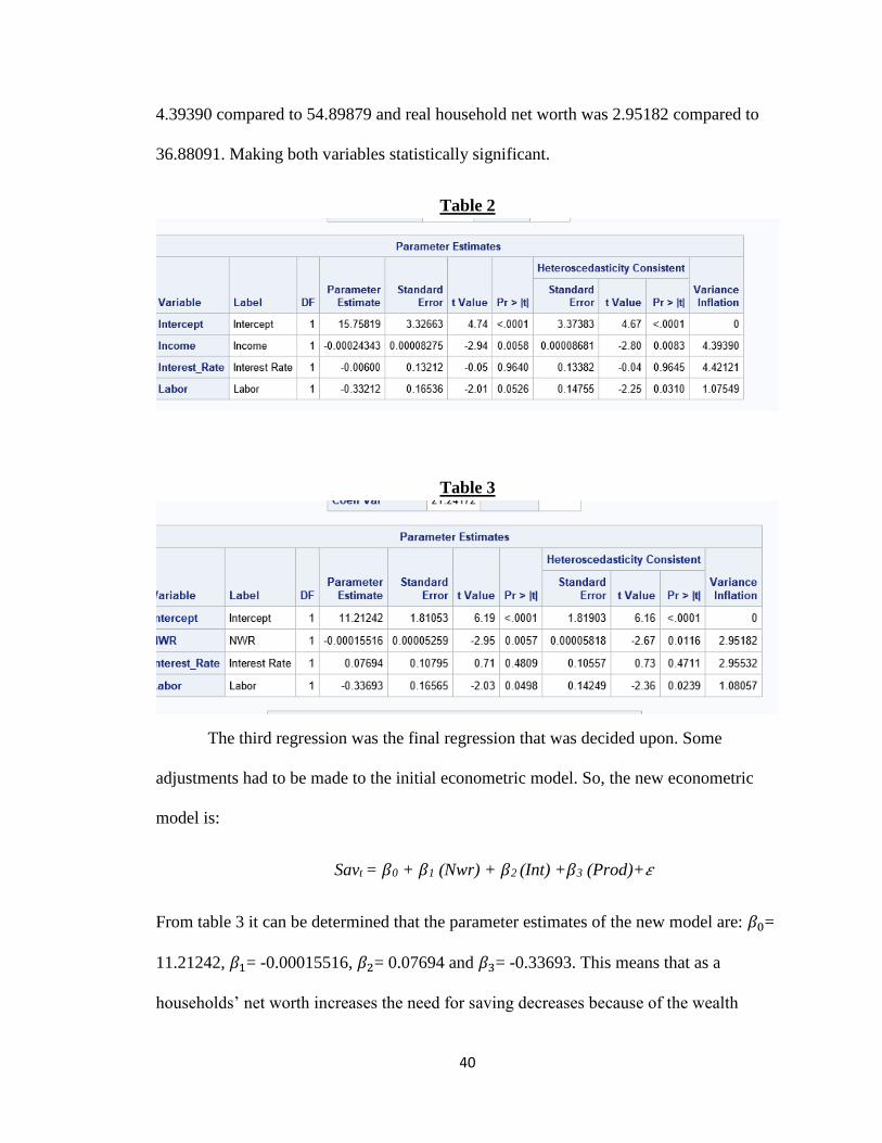
40

4.39390 compared to 54.89879 and real household net worth was 2.95182 compared to

36.88091. Making both variables statistically significant.

Table 2

Table 3

The third regression was the final regression that was decided upon. Some

adjustments had to be made to the initial econometric model. So, the new econometric

model is:

Savt = 𝛽0 + 𝛽1 (Nwr) + 𝛽2 (Int) +𝛽3 (Prod)+𝜀

From table 3 it can be determined that the parameter estimates of the new model are: 𝛽0=

11.21242, 𝛽1= -0.00015516, 𝛽2= 0.07694 and 𝛽3= -0.33693. This means that as a

households’ net worth increases the need for saving decreases because of the wealth

41

effect coined by Bailey. The results from these regressions for the personal saving rate

are support what was expected. The new econometric model is a multiple regression

analysis and we use the ordinary least squares (OLS) method. The sample regression

function is:

Sav = 11.21242 + (-0.00015516) Nwr + (0.07694) Int + (-0.33693) prod + ε

Interpreting the coefficients: The coefficient -0.00015516 is the partial regression

coefficient for real household net worth.

(1) T-test

We investigated three estimated coefficients one by one using t-tests. The

hypothesized true coefficient β1 = 0. The estimated value for �̂�1 = −0.00015516 and

standard error of this estimate is (�̂�1) = 0.0005259. The degree of freedom is 34.

Assuming α = 5%, and 𝑡𝛼 = 1.9966 ,so 𝐻0: 𝛽1 = 0 and 𝐻1: 𝛽1 ≠ 0. 𝑡 =(−0.0001516−0)

0.00005259=

2.88. Absolute value of t is larger than 𝑡𝛼 = 1.9966, so we reject null hypothesis.

The hypothesized true coefficient 𝛽2 = 0. The estimated value for �̂�2 = 0.07694

and standard error of this estimate is (�̂�2) = 0.10795 and the degree of freedom is 34. If

we assume α = 5% and 𝑡𝛼 = 1.9966, so 𝐻0: 𝛽2 = 0 and 𝐻1: 𝛽2 ≠ 0. 𝑡 =(0.07694−0)

0.10795=

0.713. Absolute value of t is less than 𝑡𝛼 = 1.9966, so we do not reject null hypothesis.

The hypothesized true coefficient 𝛽3 = 0. The estimated value for �̂�3 =

−0.33693 and the standard error of this estimate is (�̂�3) = 0.16565 and the degree of

freedom is 34. If we assume α = 5% and 𝑡𝛼 = 1.9966, so 𝐻0: 𝛽3 = 0 and 𝐻1: 𝛽3 ≠ 0. 𝑡 =

(−0.33693−0)

0.16565= 2.03. Absolute value of t is less than 𝑡𝛼 = 1.9966, so we reject null

hypothesis.

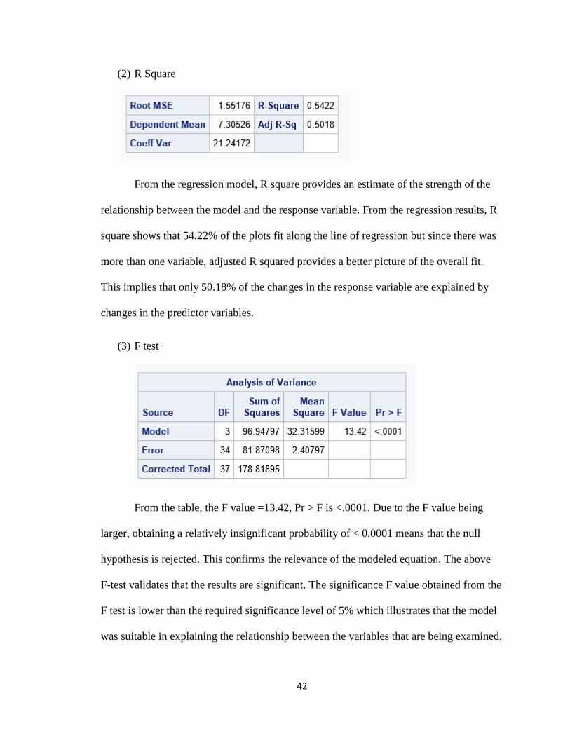
42

(2) R Square

From the regression model, R square provides an estimate of the strength of the

relationship between the model and the response variable. From the regression results, R

square shows that 54.22% of the plots fit along the line of regression but since there was

more than one variable, adjusted R squared provides a better picture of the overall fit.

This implies that only 50.18% of the changes in the response variable are explained by

changes in the predictor variables.

(3) F test

From the table, the F value =13.42, Pr > F is <.0001. Due to the F value being

larger, obtaining a relatively insignificant probability of < 0.0001 means that the null

hypothesis is rejected. This confirms the relevance of the modeled equation. The above

F-test validates that the results are significant. The significance F value obtained from the

F test is lower than the required significance level of 5% which illustrates that the model

was suitable in explaining the relationship between the variables that are being examined.

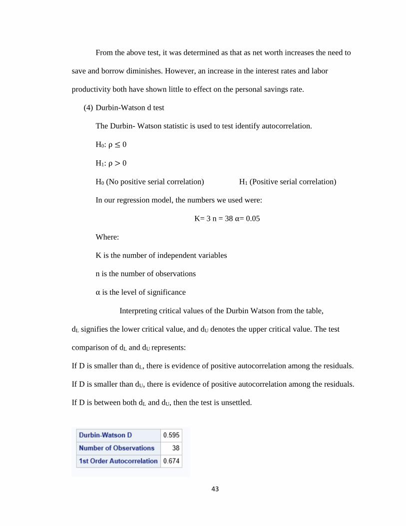
43

From the above test, it was determined as that as net worth increases the need to

save and borrow diminishes. However, an increase in the interest rates and labor

productivity both have shown little to effect on the personal savings rate.

(4) Durbin-Watson d test

The Durbin- Watson statistic is used to test identify autocorrelation.

H0: ρ ≤ 0

H1: ρ > 0

H0 (No positive serial correlation) H1 (Positive serial correlation)

In our regression model, the numbers we used were:

K= 3 n = 38 α= 0.05

Where:

K is the number of independent variables

n is the number of observations

α is the level of significance

Interpreting critical values of the Durbin Watson from the table,

dL signifies the lower critical value, and dU denotes the upper critical value. The test

comparison of dL and dU represents:

If D is smaller than dL, there is evidence of positive autocorrelation among the residuals.

If D is smaller than dU, there is evidence of positive autocorrelation among the residuals.

If D is between both dL and dU, then the test is unsettled.

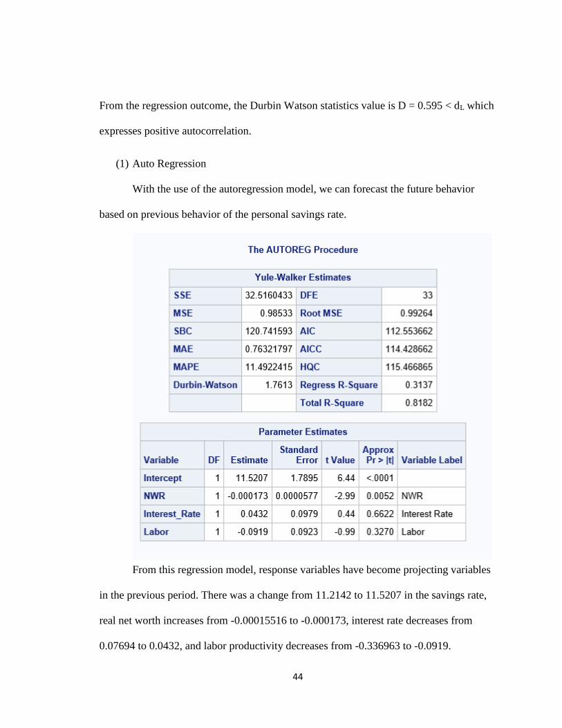
44

From the regression outcome, the Durbin Watson statistics value is D = 0.595 < dL which

expresses positive autocorrelation.

(1) Auto Regression

With the use of the autoregression model, we can forecast the future behavior

based on previous behavior of the personal savings rate.

From this regression model, response variables have become projecting variables

in the previous period. There was a change from 11.2142 to 11.5207 in the savings rate,

real net worth increases from -0.00015516 to -0.000173, interest rate decreases from

0.07694 to 0.0432, and labor productivity decreases from -0.336963 to -0.0919.

45

3.4 RESULTS

The results in this study differs from Samavati et al study because they ran their

regression using all the variables listed in the equation. The final regression for this study

only included the variables real household net worth (NWR), labor productivity (PROD)

and the interest rate (INT). Numerous regressions were conducted to decide which one

gave the more suitable results and would support the notion that as household net worth

increases the need to save diminishes. The model was estimated omitting INC variable

because income was the only variable that exhibited a high correlation with the real

household net worth. In Samavati, their estimation model excluded the PROD variable

because their labor productivity was the only variable that exhibited a high correlation

with current income.

The regression for this study differed from Samavati et al because they found that

the interest rate was positive and statistically significant at the one percent level, which

implied that the substitution effect of interest rate changes dominates the wealth effect

and that higher interest rates encourage saving by increasing the opportunity cost of

current consumption. We got different results from Samavati because of the timing of

their data set. Their original data set started from 1980 to 2013 and I extended the data to

include the recent years up to 2017. I found that both the interest rate and labor

productivity variables were positive and not statistically significant on the personal

savings rate due to interest rates decreasing over the years. Distinctly signifying that an

increase in interest rates will make saving more attractive and should encourage saving

while a cut in interest rates will reduce the rewards of saving and will lead to dissaving.

46

CHAPTER 4: CONCLUSION

The sharply declining trend of the personal savings rate over the past decades has

triggered important concerns among economists and policymakers. The downward

sloping personal savings rate, consequently national savings rate, presents numerous

economic and social problems, triggering disparities in the structure of the economic

system. Thus, the ongoing declining savings trend is a real-life phenomenon that needs

further research as time goes on and populations continue to age. The long-term decline

in the personal saving measure is due to multiple factors such as rising consumption, the

wealth effect, increased transfer payments, shifts from traditional saving instruments and

the increase of consumer credit card debt. 54

Researchers proposed that explanations for the downward declining trend in

savings could be due to the low economic growth, the high level of household wealth and

others. Majority of the factors that some of the theoretical and empirical studies used to

explain the household saving behavior were found to have little to no effect on the

savings rate trend. Other possible explanations for the low savings rate have been an

availability of consumer credits, a higher level of household wealth, improved social

security and pension systems, booms in stock and housing markets, recent technological

advances and increases in labor productivity and many other determinants.

The results of this study validate that changes in the determinants of the saving

rate suggested by economic theory can explain much of the recent trend in the personal

saving rate. Specifically, it can be determined that fluctuations in household net worth

54 Lynn Elaine Browne and Joshua Gleason, “The Saving Mystery, or Where Did the Money Go?” New

England Review (September/October 1996): 15-27.

47

play an important role and negatively affect the saving rate. As net worth increases the

need for saving decreases even with age and income being the underlying determinants.

As household net worth increases, the consumption level increases while both saving and

borrowing decreases. The consumption, saving and borrowing behaviors of the different

economic classes is indeed affected by the variables age, income and net worth. Results

also illustrates that age plays a vital role in savings, consistent with the conclusions of

Thornton. Since age is a focal determinant of preferences, a variation in age distribution

may change the significance of different commodities in the structure of consumption.

Individuals and households save for various reasons as old age, education, foreign

travel, to purchase goods and services, houses and lands, illness and hospitalization and

to meet any unexpected expenses. Motives, saving habits, age, income, income

uncertainty, wealth, risk tolerance, saving horizon, homeownership, household

composition, health status, education, race/ethnicity, self-employment, and

unemployment have all been linked to some aspect of saving. As individuals move

through early working phase in the life cycle, their consumption and borrowing behaviors

increases while their ability to save declines. Individuals are beginning their careers and

starting to encounter expenses resulting in their consumption level to increase as they

age, until they reach retirement age.

Even though there have been quite a few agreeing explanations for the declining

propensity of U.S. households to save, it seems that such theories continue to support the

significance of the recent transformation of the United States into a nation of spendthrifts.

For this exact reason, the U.S. personal saving rate will continue to remain a puzzle.

48

CHAPTER 5: FURTHER RESEARCH AND EXPLANATIONS

Doing further research for a topic of such importance is required as time

progresses. Digging deeper into research can ultimately explain the declining trend of the

personal savings rate. The highest recording of the personal savings rate is in 1971

reaching the highest of 13.5% and then dropping to just 10.3% in 1979, one year before

the date for this study. In the 1980s, the financial sector experienced a period of difficulty

that was focused on the nation’s savings and loan industry. Inflation and interest rates

both rose tremendously in the late 1970s and early 1980s. In December 2017, the

personal savings rate dropped to 2.4% being the third lowest rate ever recorded. The

housing market crash of 2007 affected the way individuals and households saved during

that recession period. With the fall in house prices, there tends to be a negative wealth

effect and a negative impact on economic growth. Because households observed a fall in

housing prices during the recession it reduced their confidence to spend. Households are

more likely to allocate a higher percentage of their income to try to pay off their

mortgage early.

While declining personal savings rates are their own cause for concern, the drop

has been accompanied by a fixed increase in consumer debt. While mortgages make up

majority of consumer debt, aggregate auto, student loan, and credit card debts also have

increased over time. These three leading categories of non-mortgage debt are driving the

total increase in consumer debt. As household’s debt increases the ability to save initially

decreases.

49

REFERENCES

Alessie, Rob, Annamaria Lusardi, and Trea Aldershof. “Income and Wealth Over the

Life Cycle: Evidence from Panel Data.” Review of Income and Wealth 43, no. 1

(March 1997): 1-32.

Attanasio, Orazio. “Consumption and Saving Behaviour: Modelling Recent Trends.”

Fiscal Studies 18, no. 1 (February 1997): 23-47.

Attanasio, Orazio P. “A Cohort Analysis of Saving Behavior by U.S. Households.”

Journal of Human Resources 33, no. 3 (Summer 1998): 575-609.

Bae, MiKyeong, Sherman Hanna, and Suzanne Lindamood. “Patterns of Overspending in

U.S. Households.” Journal of Financial Counseling and Planning 4 (1993): 11-31.

Bailey, Martin J. “Saving and the Rate of Interest.” Journal of Political Economy 65, no.

4 (August 1957): 279-305.

Beverly, Sondra G., Amanda M. McBride, and Mark Schreiner. “A Framework of Asset

Accumulation Stages and Strategies.” Journal of Family and Economic Issues 24, no. 2

(2003): 143-56.

Block, Fred. “Bad Data Drive Out Good: The Decline of Personal Savings Reexamined.” Journal

of Post Keynesian Economics 13, no. 1 (1990): 3-19.

Bovenberg, A. Lans, and Owen Evans. “National and Personal Saving in the United

States: Measurement and Analysis of Recent Trends.” Staff Papers (International

Monetary Fund) 37, no. 3 (September 1990): 636-69.

Brounen, Dirk, Kees G. Koedijk, and Rachel A.J. Pownall. “Household Financial

Planning and Savings Behavior.” Journal of International Money and Finance 69

(2016): 95-107.

Brown, Sarah, and Karl Taylor. “Household Debt and Financial Assets: Evidence from Germany,

Great Britain and the USA.” Journal of the Royal Statistical Society. Series A (Statistics in

Society) 171, no. 3 (2008): 615-43

Browne, Lynn Elaine, and Joshua Gleason. “The Saving Mystery, or Where Did the

Money Go?” New England Review (September/October 1996): 15-27.

Bunting, David. “Savings and the Distribution of Income.” Journal of Post Keynesian Economics

14, no. 1 (1991): 3-22.

Chen, Hua, Wen-Yen Hsu, and Mary A. Weiss. “The Pension Option in Labor Insurance

and Its Effect on Household Saving and Consumption: Evidence from Taiwan.” The

Journal of Risk and Insurance 82, no. 4 (December 2015): 947-75.

50

Crutsinger, Martin. 2009. U.S. Household Net Worth Plunges by Record Amount.

Canadian Press, March 13.

Deaton, Angus. “Saving in Developing Countries: Theory and Review.” World Bank

Economic Review, Proceedings of the World Bank Annual Conference on

Development Economics (1989): 61-96.

Danziger, Sheldon, Jacques Van Der Gaag, Eugene Smolensky, and Michael K Taussig. “The

Life-Cycle Hypothesis and the Consumption Behavior of the Elderly.” Journal of Post

Keynesian Economics 5, no. 2 (1982): 208-27.

Davis, Elizabeth P., and Walter R, Schumm. “Savings Behavior and Satisfaction with

Savings: A Comparison of Low-And High- Income Groups.” Home Economics

Research Journal 15, no. 4 (June 1987): 247-56.

Erlandsen, Solveig, and Ragnar Nymoen. “Consumption and Population Age Structure.”

Journal of Population Economics 21, no. 3 (July 2008): 505-20.

Fisher, Patti J., and Catherine P. Montalto. “Effect of Saving Motives and Horizon on

Saving Behaviors.” Journal of Economic Psychology 31, no. 1 (February 2010): 92-

105.

Furnham, Adrian F. “Why Do People Save? Attitudes To, and Habits Of, Saving Money

in Britain.” Journal of Applied Social Psychology 15, no. 4 (1985): 354-73.

Harris, Mark N., Joanne Loundes, and Elizabeth Webster. “Determinants of Household Saving in

Australia.” Economic Record 78, no. 241 (June 2002): 207-23.

Hebbel, Klaus Schmidt, Steven B. Webb, and Giancarlo Corsetti. “Household Saving in

Developing Countries: First Cross-Country Evidence.” The World Bank Economic

Review 6, no. 3 (September 1992): 529-47.

Horioka, Charles Yuji, and Wako Watanbe. “Why Do People Save? A Micro-Analysis of

Motives for Household Saving in Japan.” The Economic Journal 107 (May 1997): 537-

52.

Hourwich, Isaac A. “The Social-Economic Classes of the Population of the United States:

I.” Journal of Political Economy 19, no. 3 (1911): 188-215.

Iftikhar, Marya, Farooq Hussain, Zulfiqar Ali Kahn, and Saqib Liyas. “Social Class Is a

Myth or Reality in Buying Behavior?” African Journal of Business Management 7, no.

9 (March 2013): 713-18.

Kaboski, Joseph P., Molly Lipscomb, and Virgiliu Midrigan. “The Aggregate Impact of

Household Saving and Borrowing Constraint: Designing a Field Experiment in Uganda.” The

American Economic Review 104, no. 5 (May 2014): 171-76.

51

Kapounek, Svatopluk, Petr Korab, and Vilma Deltuvaite. “Irrational households' Saving

Behavior? An Empirical Investigation.” Procedia Economics and Finance 39 (2016):

625-33.

Katona, George. Psychological Economics. New York: Elsevier Scientific Publishing

Company, 1975.

Keynes, John Maynard. The General Theory of Employment, Interest and Money.

London: Macmillan, 1936.

Lee, Chulhee. “Life Cycle Savings in the United States, 1900-90.” Review of Income and

Wealth 47, no. 2 (June 2001): 165-79

Maki, Dean M., and Michael G. Palumbo. “Disentangling the Wealth Effect: A Cohort

Analysis of Household Saving in the 1990s.” Finance and Economics Discussion

Series 2001-21, Board of Governors of the Federal Reserve System (2001).

Marquis, Milt. “What's Behind the Low United States Personal Saving Rate?” FRBSF

Economic Letter (March 29, 2002): 1-3.

Modigliani, Franco. “Life Cycle, Individual Thrift, and the Wealth of Nations.” American

Economic Review 76, no. 3 (November 1986): 297-313.

Noel, Reginald A. “Race, Economics, and Social Status.” U.S. Bureau of Labor Statistics

(May 2018): 1-12.

Pryor, Frederic L. “Demographic Effects on Personal Saving in the Future.” Southern

Economic Journal 69, no. 3 (January 2003): 541-59.

Ramanathan, R. “An Econometric Exploration of Indian Saving Behavior.” Journal of

the American Statistical Association 64, no. 325 (March 1969): 90-101.

Raut, Lakshmi K., and Arvind Virmani. “Determinants of Consumption and Savings

Behavior in Developing Countries.” The World Bank Economic Review 3, no. 3

(September 1989): 379-93.

Samavati, Hedayeh, Nodir Adilov, and David A. Dilts. “Empirical Analysis of the Saving

Rate in the United States.” Journal of Management Policy and Practice 14, no. 2

(2013): 46-53.

Sturm, Peter H. “Determinants of Saving: Theory and Evidence.” OECD: economic

studies 1 (1983): 147-96.

Shin, Su Hyun, and Kyoung Tae Kim. “Perceived Income Changes, Saving Motives, and

Household Savings.” Journal of Financial Counseling and Planning 29, no. 2

(2018): 396-409.

52

Thornton, John. “Age Structure and the Personal Savings Rate in the United States.” Southern

Economic Journal 6, no. 1 (2001): 166-70.

Xiao, Jing Jian, and Fanziska E. Noring. “Perceived Saving Motives and Hierarchical

Financial Needs.” Journal of Financial Counseling and Planning (January 1994): 25-45.

Yao, Rui, Robert Weagley, and Li Liao. “Household Saving Motives: Comparing

American and Chinese Consumers.” Family and Consumer Sciences 40, no. 1

(September 2011): 28-44

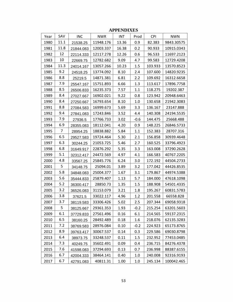
53

APPENDIXES

Year SAV INC NWR INT Prod CPI NWN

1980 11.1 21538.25 11948.176 13.36 0.9 82.383 9843.30575

1981 11.8 21844.083 12003.337 16.38 0.2 90.933 10915.0343

1982 12 22114.333 12117.278 12.26 0.6 96.533 11697.2123

1983 10 22669.75 12782.682 9.09 4.7 99.583 12729.4208

1984 11.3 24014.167 13057.266 10.23 1.5 103.933 13570.8523

1985 9.2 24518.25 13774.092 8.10 2.4 107.600 14820.9235

1986 8.8 25219.5 14871.381 6.81 2.2 109.692 16312.6658

1987 7.9 25547.167 15751.893 6.66 1.3 113.617 17896.7758

1988 8.5 26506.833 16235.373 7.57 1.1 118.275 19202.387

1989 8.4 27027.667 16902.021 9.22 0.8 123.942 20948.6463

1990 8.4 27250.667 16793.654 8.10 1.0 130.658 21942.3083

1991 8.8 27084.583 16999.673 5.69 3.3 136.167 23147.888

1992 9.4 27841.083 17243.846 3.52 4.4 140.308 24194.5535

1993 7.9 27936.5 17766.733 3.02 -0.6 144.475 25668.488

1994 6.9 28355.083 18112.041 4.20 0.9 148.225 26846.5733

1995 7 28954.25 18838.882 5.84 1.1 152.383 28707.316

1996 6.5 29527.583 19724.464 5.30 2.1 156.858 30939.4648

1997 6.3 30244.25 21053.725 5.46 2.7 160.525 33796.4923

1998 6.8 31649.917 22876.292 5.35 3.3 163.008 37290.2628

1999 5.1 32312.417 24472.569 4.97 4.1 166.583 40767.2205

2000 4.8 33567.25 25845.776 6.24 3.0 172.192 44504.2733

2001 5 34148.75 25094.01 3.89 3.2 177.042 44426.8535

2002 5.8 34848.083 25004.377 1.67 3.1 179.867 44974.5388

2003 5.6 35444.833 25879.407 1.13 5.7 184.000 47618.1098

2004 5.2 36300.417 28850.73 1.35 1.5 188.908 54501.4335

2005 3.2 36526.083 31153.079 3.21 1.8 195.267 60831.5783

2006 3.8 37621.5 33022.117 4.96 1.2 201.558 66558.828

2007 3.7 38119.583 33306.426 5.02 2.5 207.344 69058.9318

2008 5 38125.667 29361.353 1.93 -0.2 215.254 63201.5603

2009 6.1 37729.833 27561.496 0.16 6.1 214.565 59137.2315

2010 6.5 38160.25 28492.489 0.18 1.6 218.076 62135.3283

2011 7.2 38769.583 28976.084 0.10 -0.2 224.923 65173.8765

2012 8.9 39763.417 30067.537 0.14 0.3 229.586 69030.8798

2013 6.4 38973.75 33248.537 0.11 1.5 232.952 77453.0485

2014 7.3 40249.75 35602.491 0.09 0.4 236.715 84276.4378

2015 7.6 41598.083 37294.693 0.13 0.7 236.998 88387.6155

2016 6.7 42004.333 38464.141 0.40 1.0 240.008 92316.9193

2017 6.7 42791.083 40811.31 1.00 1.0 245.134 100042.465

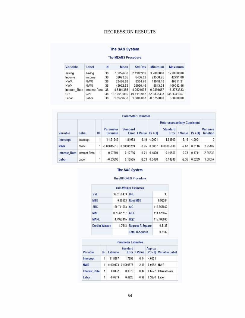
54

REGRESSION RESULTS