east and southeast asia commercial integration during the
TRANSCRIPT
i
Connected by conquest: East and Southeast Asia
commercial integration during the Age of Empires.
Alejandro Ayuso Díaz
Tesis depositada en cumplimiento parcial de los requisitos para el
grado de Doctor en
Doctorado Interuniversitario en Historia Económica
(UB/UV/UC3M)
Universidad Carlos III de Madrid
Director/a (es/as):
Antonio Tena Junguito
Tutor/a:
Antonio Tena Junguito
Enero 2021

ii
Esta tesis se distribuye bajo licencia “Creative Commons Reconocimiento – No Comercial – Sin Obra Derivada”.
iii
ACKNOWLEDGEMENTS
First of all, I would want to thank the department of Social Sciences of the Carlos
III University for bringing me those grants to study a Master and a 1st year PhD that opened
me the possibility to opt for a FPU grant. In that sense, I would also want to thank the
Spanish Ministry (Ministerio de Ciencia, Innovación y Universidades) for conceding this
scholarship that has permitted me to consolidate my work, finish my thesis and travel to
Japan in order to make a researching visit at Hitotsubashi University.
Of course, behind scholarships there are persons and in that sense I should thank
Mar Rubio, Jorge Alcalde and José Enrique Galdón for their priceless advise of abandoning
Pamplona and their recommendation to choose Carlos III University. Inside my new home I
should thank Jordi Doménech for its support on the application for a Master scholarship
without even knowing me. Thanks to Antonio Tena for his offer to become a supervisor
during my Master thesis and for rescuing me when it was impossible to find a supervisor
for my PhD dissertation. Your intellectual and spiritual inspiration during these 5 years is
invaluable. Thanks to Esperanza Castro and Maria José Gutiérrez for their tireless work and
the infinite aid offered for administrative procedures. Thanks to Víctor Gómez for fixing
my disastrous applications and bringing me valuable advises for the future Finally, thanks
to all the workers of the library, especially those in charge of “Préstamo Interbibliotecario”
for bring closer to me all the manuscripts containing information about Asia.
Once the Carlos III library couldn’t provide more Asian materials, there they were
all the members of the Asian Historical Statistics (ASHTAT) project of the Institute of
Economic Research of the Hitotsubashi University for offering me every material with
which they’ve been working for decades. Thanks to all of them for their kind treatment, for
making me participant of every success and for their aid with translations. A special
mention deserve Kyoji Fukao, my supervisor and the true architect of my visit to Japan (I
owe you a lunch and a tea whenever you travel to Spain), Yumiko Moriyama for her
continuous support with the search for materials and for integrating me in the office and
finally Reiko Doi for helping me with accommodation. Thanks to Chiaki Moriguchi for
letting me learning about teaching in Japan and to enjoy a live class. Gratitude also to
illustrious visitors like Debin Ma, Jean-Pascal Bassino or Bishnupriya Gupta for
illuminating me with their knowledge about Asia economic history.

iv
Relative to personal support I should show my gratitude to all the professors I’ve
been able to assist: Jordi Doménech, Katharina Mühlhoff, Vicente Palacio, Leandro Prados
de la Escosura, Pablo Martinelli and Miguel Artola. All of them have made me better
teacher, better person and taught me lots of things about economics and history. Above all,
I should thank Carlos Santiago and Stefan Houpt for their continuous support,
recommendations and patience bearing with the difficult task of coordinating teaching
organization. Thanks also to all of them for their help with job applications.
The line between professional support and friendship is sometimes quite thin and
this paragraph is devoted to remember all of those that have crossed it. Thanks to my
classmates of the MADE-MEDEG 2015/2016 for all those afternoons learning
Macroeconomics in “The Basement” and for following me to those plans that let me fresh
my mind (concerts, basket, football, beer). Special thanks to David for offering me his
home every time I needed and to Patri for the opposite, for being a fantastic guest in my
town. I am also grateful to all of the great researches that have being part of the 18.2.C02
office during all these years, both those of the first (Wilfried, thanks for your aid dealing
with long term trade series, Chris whose help with translations has substantially improved
this thesis, Laura and Benoit,) and second generations (Alberto, Digno, Alejandro my
basket mates, Ester, Olena, David, Onur). An honorable position in this office is held by
Víctor and Maricia, the nexus between both generations, thank you for all the hours we’ve
spent having lunch on the grass with Dacil, which was also part of this intellectual family
despite her superior academic position. My gratitude also to the members of my futsal
teams (Lotina, ahora baja and FeliZidane for satiating my infinite thirst for competition)
and to my roommates of Alicante 3 (Óscar, my football and basket mate, Adrián and
Adriana) for receiving me with a smile every time I arrived home.
All these acknowledgements will end with those that deserve a preeminent
position, those that have always been there. Thanks to the members of “Asociación
Gastrónomica I.U” for 28 years of happiness and continuous learning, and for following me
to every inch of the world I decide to travel. Thanks to my whole family, especially to my
parents for making me as I am today, with the strengths and weaknesses that has taken me
here and to my sister for being my perfect complement. Last but not least, thanks to my
fiancée Sonia for bringing me the self-confidence I needed to progress in my life, for
bearing my long absences and bad humor and offering her helping hand every time I
needed.

v
vi
PUBLISHED AND PRESENTED MATERIALS.
Chapter 3 previously published as Ayuso‐Díaz, A., & Tena‐Junguito, A. (2020).
Trade in the shadow of power: Japanese industrial exports in the interwar years. The
Economic History Review, 73(3), 815-843.
Chapter 2 has been presented for publication at the European Review of Economic
History under the title "Natural Trading Partners? Power and historical Networks in East
and Southeast Asian integration (1840-1938)" authored by Alejandro Ayuso Díaz.
Part of Appendix B appears published as an appendix to the article “Trade in the
shadow of power: Japanese industrial exports in the interwar years”, published on The
Economic History Review, 73(3).
Part of Chapter 1 and Appendix A have been presented for publication at the
European Review of Economic History as an appendix to the article "Natural Trading
Partners? Power and historical Networks in East and Southeast Asian integration (1840-
1938)".
vii
CONTENT . Introduction ....................................................................................................................... 1 1 . Chapter 1: The comparative historical regional integration of East and Southeast Asia 2
(1840-1938). A reconstruction ............................................................................................... 5 2.1. Introduction. ................................................................................................................ 5 2.2. East and Southeast Asia reporting countries and trade sources consulted. .............. 7
2.2.1. East and Southeast Asia definition. ...................................................................... 7 2.2.2. Data sources ......................................................................................................... 8
2.3. Adjustments performed to original data sources. .................................................... 10 2.4. Examining data reliability: Comparison with published trade databases. ................ 15 2.5. Mixing Databases Ricardo and A&T. ......................................................................... 24 2.6. Measuring regional integration: East and Southeast Asia compared with Europe and Latin America. ................................................................................................................... 26 2.7. Conclusions ................................................................................................................ 35
Chapter 2: Natural Trading Partners? Power and historical Networks in East and 3Southeast Asian integration (1840-1938) ............................................................................ 37
3.1. Introduction ............................................................................................................... 37 3.2. Theory and History on Natural Trade Blocs .............................................................. 39
3.2.1.Theoretical Determinants: Trade costs, demand complementarities and factor endowments ................................................................................................................. 40 3.2.2. History of Imperial policies in East and Southeast Asia. .................................... 41 3.2.3. Local merchants and their influence over regional trade across history. .......... 43
3.3. Regional Trade and its Determinants ........................................................................ 45 3.3.1. Regional imports evolution ................................................................................ 45 3.3.2. First regional expansion: Transit trade and its determinants ............................ 48 3.3.3. Network Consolidation: Trade Inside and Trade Between Empires .................. 49
3.4. Model ......................................................................................................................... 50 3.5. Data ............................................................................................................................ 53
3.5.1. Imports Data. ...................................................................................................... 53 3.5.2. Gravity and economic determinants .................................................................. 54 3.5.3. Trade Costs variables. ......................................................................................... 54 3.5.4. Power, migration network and infrastructure variables. ................................... 55
3.6. Results ........................................................................................................................ 56 3.6.1. General Results ................................................................................................... 56 3.6.2. Robustness Checks ............................................................................................. 61
3.7. Conclusions ................................................................................................................ 65 Chapter 3: Trade in the Shadow of Power: Japanese Industrial Exports in the Interwar 4
years ..................................................................................................................................... 68 4.1. Introduction ............................................................................................................... 68 4.2. Regional Trade and the Japanese Empire ................................................................. 71 4.3. Empire and the Determinants of Japanese Exports .................................................. 74
4.3.1. Productivity or Empire, Which was More Relevant? ......................................... 76 4.3.2. Did Empire Facilitate New Exports or Reinforce Pre-Existing Comparative Advantage? ................................................................................................................... 78
4.4. Margins of Trade Model. ........................................................................................... 82 4.5. The New Data Set ...................................................................................................... 84
4.5.1 Trade Data. .......................................................................................................... 84
viii
4.5.2. GDP and Productivity .......................................................................................... 86 4.5.3. Trade Costs ......................................................................................................... 87
4.6. Results ........................................................................................................................ 88 4.6.1. Presentation of Results....................................................................................... 88 4.6.2. Robustness Checks ............................................................................................. 94
4.7. Conclusions .............................................................................................................. 100 Chapter 4: Winners of Japanese colonization in Manchuria 1907-1945 ........................ 102 5
5.1. Introduction. ............................................................................................................ 102 5.2. Theoretical Framework: Models of Business-State interactions across history. .... 105 5.3. Winners of colonization: Strategic industrialization and Elite Exchange ................ 107
5.3.1. Why Manchuria? Japan economic and strategic objectives. ........................... 107 5.3.2. Early Manchurian development: Exchanges between SMR Co. and the State (1907-1931) ................................................................................................................ 110 5.3.3. Consolidation stage: Kwantung Army captures the SMR Co. and MHID Co. raises (1931-1945). ..................................................................................................... 112
5.4. Descriptive Statistics: Interactions between Business and the State ..................... 116 5.4.1. SMR Co. and State Control ............................................................................... 116 5.4.2. Beneficiaries of SMR capture inside Manchuria .............................................. 119 5.4.3. Beneficiaries of SMR Capture inside Japan. ..................................................... 122
5.5. Model and Data sources .......................................................................................... 123 5.5.1. Model ................................................................................................................ 123 5.5.2. Data Sources ..................................................................................................... 124
5.6. Results ...................................................................................................................... 126 5.6.1. Production by Japanese companies in Manchuria. .......................................... 126 5.6.2. Japanese Exports to Manchuria. ...................................................................... 127 5.6.3. Robustness Checks ........................................................................................... 129
5.7. Conclusion ............................................................................................................... 135 . Conclussions. ................................................................................................................. 138 6 .Bibliography .................................................................................................................... 142 7 . APPENDIX ....................................................................................................................... 165 8
A . Submersion Inside East and Southeast Asia Historical Trade Determinants. ............... 165 A.1. Sources and estimation of independent variables ................................................. 165 A.2 Discussion ................................................................................................................. 167 A.3. Counterfactual exercise and Econometric concerns .............................................. 176
B . A deeper understanding of Japanese trade supremacy. ............................................... 183 B.1. Sources of Japanese exports and estimation of independent variables ................ 183 B.2. Discussion ................................................................................................................ 200 B.3. Econometric concerns and counterfactual exercise. .............................................. 215
Understanding Japanese colonization of Manchuria. ................................................ 220 C.C.1. Sources and estimation procedures ........................................................................ 220 C.2.Discussion. ................................................................................................................ 220 C.3. Econometric concerns. ............................................................................................ 230
ix
LIST OF FIGURES
Figure 2.1: Share of bullion and specie over total India, Siam, Malaysia and Sri Lanka imports (left) and share over total and regional imports for our 13 countries (right) 1840-1938. ..................................................................................................................................... 12 Figure 2.2: Share of Hong Kong and Singapore over total Transit imports destined to East and Southeast Asia. (1840-1938) ......................................................................................... 14 Figure 2.3:Regional and European Share over total Asian imports under new and conventional transit treatment (left) and % misvaluation on Regional and European shares by the original data source distribution (right) 1840-1938. ................................................. 15 Figure 2.4: Number of partners presented by East and Southeast Asia countries under Fouquin & Hugot and A&T databases (1820-1885). ............................................................ 17 Figure 2.5: Total East and Southeast Asian imports under A&T and Ricardo (as Reported) 1840-1938. (left) and discrepancies as % of total A&T imports (right). ............................... 21 Figure 2.6: Total East and Southeast Asia Imports A&T with and without and specie and Ricardo using the same reporting countries (1841-1870) ................................................... 21 Figure 2.7: Territorial distribution of the excess imports presented by A&T in comparison with Ricardo (1929-1937) ..................................................................................................... 23 Figure 2.8: Discrepancies between A&T and Federico-Tena for Asia (1841-1938) ............. 23 Figure 2.9: Number of flows per year on A&T, Ricardo and the Mixed database (under A&T unification criteria) 1840-1938. ............................................................................................ 26 Figure 2.10: Share of regional imports over the total in East and Southeast Asia, Western Europe and Latin America (1840-1938) ................................................................................ 28 Figure 3.1: East and Southeast Asia Constant Imports 3 different samples (1840-1938) ... 46 Figure 3.2: Regional Distribution of East and Southeast Asian imports 1840-1938 ............ 47 Figure 3.3: Partner Decomposition of Regional Imports in East and Southeast Asia 1840-1938. ..................................................................................................................................... 48 Figure 3.4: Kilometers of Railway at the region, ethnic Chinese Population in Transit Ports (right axis) and Regional Transit trade (left) (1871-1938). ................................................... 49 Figure 3.5: Distribution of Regional Imports within and Between Empires (1840-1938) . .. 50 Figure 4.1: Japanese Exports (1934-36 $) and GDP per Capita (1913 $) and Japanese and World Manufacturing Export Performance (1953=100) ...................................................... 75 Figure 4.2: Japanese Productivity and Exports (1912-1938) ................................................ 76 Figure 4.3: Japanese Manufacturing Exports by Region (1912-1938) (%) ........................... 77 Figure 4.4: Japanese total manufacturing exports by skills and region. .............................. 79 Figure 4.5: Index of Machinery Exports, Imports, and Domestic Production (1912=100). . 80 Figure 4.6: Number of Japanese diplomats and products exported towards Japanese “Future Conquests” (1912-1938). ........................................................................................ 81 Figure 5.1: Share of Social spending on SMR Zone public budget 1907-1937 (left) and police and education real expenditure in thousands of 1935 Manchoukuo Yuan (right) . 110 Figure 5.2: Profits of principal Japanese Zaibatsu (1907-1929) ......................................... 112 Figure 5.3: Annual Profits of SMR Co.(left axis), Nissan and Sumitomo (right axis) 1933-1941. ................................................................................................................................... 116 Figure 5.4: SMR Overall Profit and Profitability (1907-1944)............................................. 117 Figure 5.5: SMR Co. investment by sector (left) and profit per unit of capital invested (right) 1907-1938. ............................................................................................................... 118
x
Figure 5.6: Average Prices Charged by SMR on Passenger and Freight Transport compared with expenditures in 1935 Yen per Ton (left) and Real Freights Per Kilometer Of Railway (right) 1907-1943. ............................................................................................................... 119 Figure 5.7: Production of Japanese Companies in Manchuria (1935 prices) and SMR freights (inverse right axis). ................................................................................................ 120 Figure 5.8: Share MHID and SMR over Japanese Paid Up Capital and total investment on Manchurian Iron (1936-1939). ........................................................................................... 121 Figure A.1: Japan GDP and imports share over region. ...................................................... 168 Figure A.2: GDP per Capita evolution in Japan and China in 1990 GK Dollars (1850-1938). ............................................................................................................................................ 168 Figure A.3: The price of Silver (left) and regional imports share (right) (1885-1912). ....... 173 Figure A.4: Number of East and Southeast Asia countries under the Gold Standard (right) and Regional share on Chinese imports (left) (1870-1938). .............................................. 175 Figure B.1: Freight Factor (trade-weighted by route) 1912-1938 (1912=100). ................. 193 Figure B.2: Japanese average number of products exported in 3-digit SITC sector by region. ............................................................................................................................................ 201 Figure B.3: Japanese number of exporting sectors by region. ........................................... 202 Figure B.4: Share of low-end and high-end textiles over total Japanese textile exports. . 206 Figure B.5: Distribution of low-end and high-end Japanese textile exports by regions (1912-1938). ....................................................................................................................... 206 Figure B.6: Distribution of Japanese Manufacturing exports towards Asia Pacific territories outside Empire. ................................................................................................................... 210 Figure B.7: Distribution of Japanese exports to India 1929-1938 ...................................... 211 Figure B.8: Japanese exports increase 1932-38 (%) by groups of products and region. ... 213 Figure C.1: Share of different components over total Japanese Machinery exports to Manchuria (1912-1938). ..................................................................................................... 224 Figure C.2: Evolution of the share of coal, petroleum and machinery oil over total Japan’s fuel exports to Manchuria (1932-1938). ............................................................................ 225 Figure C.3: % Increase in Japan's Raw Materials exports to Manchuria by component 1932-38 (left axis) and total exports in 1938 (right axis). ............................................................ 225 Figure C.4: Sector Distribution of the raise in Japanese Machinery exports to Manchuria (1932-1938). ....................................................................................................................... 226 Figure C.5: Distribution of the raise in Japanese Machinery exports to Manchuria (1932-1938). .................................................................................................................................. 227 Figure C.6: Japanese Imports from Manchuria by sector (1930-1939) .............................. 228 Figure C.7: Manchurian Soya Bean exports by country partner in 1933-34 million Yen. .. 229 Figure C.8: Margins plot for production in Chemicals, Basic Metals and Paper Manufacturing. ................................................................................................................... 232
xi
LIST OF TABLES Table 2.1: Main features of A&T, Ricardo, Fo-Hu and Barbieri East and Southeast Asia databases (1840-1938). ........................................................................................................ 16 Table 2.2: Average Number of reporting countries, partners and partners per reporting by decade A&T vs. Ricardo (1840-1938). .................................................................................. 18 Table 2.3: Regression results for East and Southeast Asia, Western Europe and Latin American imports (1840-1938). ........................................................................................... 30 Table 2.4: Regression results for East and Southeast Asia, Western Europe and Latin American imports (1840-1913 and 1914-1938). .................................................................. 31 Table 2.5: East and Southeast Asia trade determinants without South Asia territories (1840-1938) .......................................................................................................................... 33 Table 2.6: Regression Results for Western Europe countries with access to the sea (1840-1913 and 1914-1938). .......................................................................................................... 34 Table 3.1: Overall imports determinants 1840-1938 (Transit trade included). ................... 57 Table 3.2: Total imports determinants 1840-1938 (Transit trade not included). ................ 58 Table 3.3: Regional and Southeast Asia imports determinants 1840-1938. ........................ 61 Table 3.4: Regional imports determinants under different estimation methods (1840-1938) ..................................................................................................................................... 63 Table 3.5: Results using the same sample for every period. ................................................ 64 Table 3.6: Determinants of Regional imports using lagged independent variables. ........... 65 Table 4.1: Revealed Comparative Advantage by Country in Three Main Commodities. ..... 78 Table 4.2: Japanese Total Export Determinants. .................................................................. 90 Table 4.3: Japanese Export Determinants by Skill Level ...................................................... 92 Table 4.4: Japanese Export Determinants According to Extensive and Intensive Margins . 93 Table 4.5: Japanese Export Determinants Using Alternative Estimation Methods. ............ 95 Table 4.6: Japanese Export Determinants Towards Countries Inside Its Formal and Informal Empire. .................................................................................................................................. 96 Table 4.7: Diff-in-Diff Estimation for Japanese Exports Before and After Colonization. ..... 98 Table 4.8: Japanese Exports Determinants (Lagged Independent Variables). ..................... 99 Table 5.1: Coefficients of Regressing SMR real freights on Production by sector (1931-1941). .................................................................................................................................. 120 Table 5.2: Coefficients of Regressing SMR real freights on Exports by sector (1932-1938). ............................................................................................................................................ 122 Table 5.3: Regression Results for Japanese Production in Manchuria (1931-1941). ......... 127 Table 5.4: Regression Results for Japanese Exports to Manchuria (1912-1938). .............. 129 Table 5.5: Regression Results for Japanese Production in Manchuria using real freights per kilometer as independent variable (1931-1941). ............................................................... 131 Table 5.6: Regression Results for Japanese Exports to Manchuria (1912-1938). .............. 132 Table 5.7: Regression Results for Japanese Production in Manchuria using Five Years Plan as independent variable (1931-1941). ............................................................................... 134 Table 5.8: Regression Results for Japanese Exports to Manchuria using Five Years Plan as independent variable (1912-1938). .................................................................................... 135 Table A.1: Population density on major East and Southeast Asia territories (1860-1938) 169 Table A.2: Monetary Systems in the World 1868 and 1908. ............................................. 172 Table A.3: Total imports determinants in East and Southeast Asian countries (1840-1938) accounting for Gold Standard adoption. ............................................................................ 174
xii
Table A.4: Wooldridge test for autocorrelation Total Imports .......................................... 178 Table A.5: Wooldridge test for autocorrelation Regional imports..................................... 178 Table A.6: Determinants total imports under First Order Autocorrelation. ...................... 179 Table A.7: Determinants of total imports controlling structural multilateral resistance to trade ................................................................................................................................... 180 Table A.8: Determinants of total imports including population as a substitute of GDP 1840-1938 (Transit trade included). ........................................................................................... 182 Table A.9: Determinants of Total Imports including population as a complement of GDP 1840-1938 (Transit trade included). .................................................................................. 182 Table B.1: Main Regression Employing Distance Instead Of Freights. ............................... 190 Table B.2: Japan Freight rates in different routes (1912-1938). ........................................ 192 Table B.3: Number of Japanese Diplomats Abroad. ........................................................... 195 Table B.4: Number of foreign diplomats in Japan .............................................................. 196 Table B.5: Japanese Colonies Status and Main Features. .................................................. 198 Table B.6: Japanese Future Conquests and Main Features ............................................... 199 Table B.7: Japanese Export Determinants at the Margins of Trade. ................................. 203 Table B.8: Skill intensity ranking. ........................................................................................ 205 Table B.9: Determinants of high- and low-end textile exports .......................................... 208 Table B.10: Japanese Total exports determinants by time period (1912-1938) ................ 214 Table B.11: Effect of export increase on productivity. ....................................................... 215 Table B.12: Effect of Changes in Exports on the Number of Japanese Diplomats Abroad 217 Table B.13: Japanese Exports Determinants (Lagged Independent Variables) ................. 218 Table C.1: Sector specific impact of SMR freights on production by Japanese companies in Manchuria (1931-1941). ..................................................................................................... 231 Table C.2: Sector specific impact of SMR freights in Japanese exports to Manchuria by sector (1912-1938). ............................................................................................................ 233 Table C.3: Wald Test of equality of coefficients 1912-1929 vs. 1932-1938 regressions. .. 234 Table C.4: Wald Test of equality of coefficients: Machinery exports with and without controls (1932-38). ............................................................................................................. 234 Table C.5: Sector specific impact of SMR freights in Japanese exports to Manchuria by sector (1912-1938). ............................................................................................................ 235 Table C.6: Sector specific impact of SMR freights per Kilometer in Japanese exports to Manchuria by sector (1912-1938). ..................................................................................... 235 Table C.7: Sector specific impact of Five Year Plans on production by Japanese companies in Manchuria (1931-1941). ................................................................................................. 236 Table C.8: Sector specific impact of Five Year Plans in Japanese exports to Manchuria by sector (1912-1938). ............................................................................................................ 236
xvi
LIST OF MAPS: Map 1: Empires dominating East and Southeast Asia and nº of ethnic Chinese (thousands) in each country by 1938. ........................................................................................................ 2 Map 2: Japanese Conquests during imperial period (1880-1945) ......................................... 3 Map 3: Manchoukuo State frontiers and main industrial centers (1932-1945) ................ 221 Map 4: Japan-Manchuria Railway Connections 1928. ....................................................... 223
1
. INTRODUCTION 1Globalization is a process that across history has been driven by rich countries,
which were generally reaping benefits from poorer territories. Nonetheless, this tendency
has been reverted during recent decades during which peripheral regions have become
prominent traders, spurring the latest wave of commercial liberalizations. These trends have
given rise to a literature that studies the evolution of the commercial expansion experienced
by peripheral countries, as well as their recent integration into the global economy. These
works survey, among other things, the prospect of a deepening of regional integration
through the establishment of Customs or Monetary Unions in the analyzed territories.
Among their most relevant findings, they highlight East and Southeast Asia as one of the
most regionally integrated peripheral territories, and infer that the high level of intra-
regional trade shown by member States has its roots in events preceding the establishment
of Free Trade Areas between them. All these signals point in the same direction: the
potential historical origins of East and Southeast Asian regional integration. Effectively,
this is the main motivation of the present work, which, in order to be demonstrative, should
cover the longest possible time span before the era of multilateralism began after World
War II.
During the present work, East and Southeast Asia will be considered as a regional
entity composed of countries depicted in maps 1 and 2; that is, by the sub-regions of East,
Southeast and South Asia. The inclusion of this last set of territories is controversial,
bearing in mind that another close territory like Australia is excluded from the analysis.
Nevertheless, this decision makes the most sense given that South Asia shares a tradition of
trade and migration with East and Southeast Asian territories in which Australia was not a
participant. Across history, this region created wealthy commercial networks that were
exploited by local merchants. This led, for example, to an Age of Commerce between the
15th and 17th Centuries, in which commodity trade integrated the entire region. Regrettably,
the following thesis doesn’t capture those exchanges as it attempts to investigate trade at
the country-level, creating consistent political units, and the first evidence of trade returns
for complete country-level only dates back to 1840.
Fortunately, the reconstructed database captures the rapid commercial expansion
experienced once the region started to trade in manufacturing products around the second
half of the 19th century, which can be considered the starting point of contemporary
regional integration in East and Southeast Asia. This was only possible thanks to the
expansion of the Industrial Revolution brought by Imperial Powers that conquered the
2
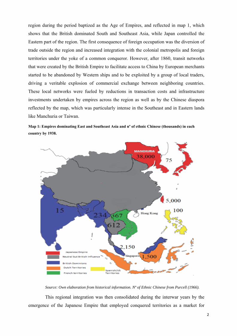
region during the period baptized as the Age of Empires, and reflected in map 1, which
shows that the British dominated South and Southeast Asia, while Japan controlled the
Eastern part of the region. The first consequence of foreign occupation was the diversion of
trade outside the region and increased integration with the colonial metropolis and foreign
territories under the yoke of a common conqueror. However, after 1860, transit networks
that were created by the British Empire to facilitate access to China by European merchants
started to be abandoned by Western ships and to be exploited by a group of local traders,
driving a veritable explosion of commercial exchange between neighboring countries.
These local networks were fueled by reductions in transaction costs and infrastructure
investments undertaken by empires across the region as well as by the Chinese diaspora
reflected by the map, which was particularly intense in the Southeast and in Eastern lands
like Manchuria or Taiwan.
Map 1: Empires dominating East and Southeast Asia and nº of ethnic Chinese (thousands) in each country by 1938.
Source: Own elaboration from historical information. Nº of Ethnic Chinese from Purcell (1966).
This regional integration was then consolidated during the interwar years by the
emergence of the Japanese Empire that employed conquered territories as a market for
3
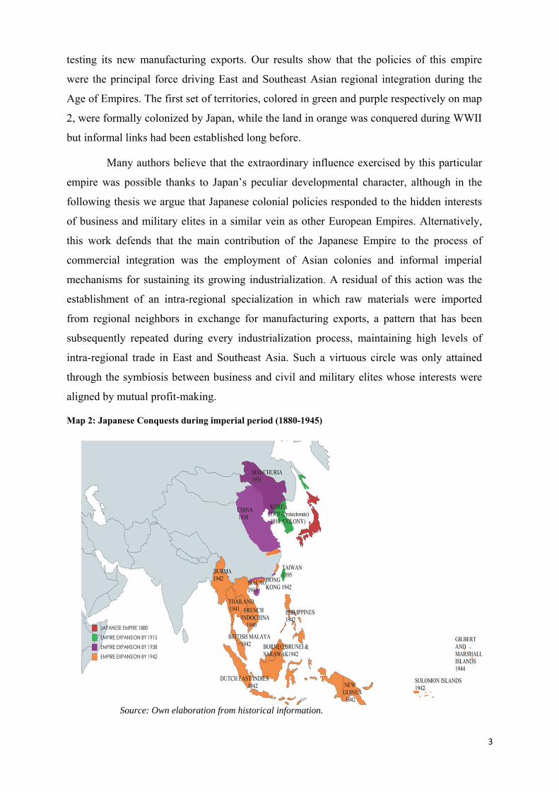
testing its new manufacturing exports. Our results show that the policies of this empire
were the principal force driving East and Southeast Asian regional integration during the
Age of Empires. The first set of territories, colored in green and purple respectively on map
2, were formally colonized by Japan, while the land in orange was conquered during WWII
but informal links had been established long before.
Many authors believe that the extraordinary influence exercised by this particular
empire was possible thanks to Japan’s peculiar developmental character, although in the
following thesis we argue that Japanese colonial policies responded to the hidden interests
of business and military elites in a similar vein as other European Empires. Alternatively,
this work defends that the main contribution of the Japanese Empire to the process of
commercial integration was the employment of Asian colonies and informal imperial
mechanisms for sustaining its growing industrialization. A residual of this action was the
establishment of an intra-regional specialization in which raw materials were imported
from regional neighbors in exchange for manufacturing exports, a pattern that has been
subsequently repeated during every industrialization process, maintaining high levels of
intra-regional trade in East and Southeast Asia. Such a virtuous circle was only attained
through the symbiosis between business and civil and military elites whose interests were
aligned by mutual profit-making.
Map 2: Japanese Conquests during imperial period (1880-1945)
Source: Own elaboration from historical information.
2
This story is summarized in two parts. On the one hand, chapters 1 and 2 offer a
long-term overview of regional integration in East and Southeast Asia. The former
confirms that the levels of intra-regional trade were remarkable long before the
establishment of FTAs by performing a comparison with levels found in Western Europe
and Latin America. For a more precise understanding of the evolution of East and
Southeast Asian trade, we have reconstructed bilateral imports of 13 countries in the region
over the long-run (1840-1938). The novelty of the constructed database is that the data is
mainly culled from information collected by Asian or colonial customs, is constructed for a
unique research purpose, and follows single construction criteria for the first time.
Throughout the chapter, we review the main sources of information and transformations
performed on the database to fit it to our research purposes. These include the subtraction
of bullion and specie imports, the estimation of the regional origin of transit trade, and the
construction of consistent political units.
In addition, it is shown that for most of the period, this new database outperforms
existing ones with respect to the number of trade flows or total imports presented, although
is worth noting the superiority of the Ricardo database in certain countries and periods. For
this reason, the analysis of regional integration in East and Southeast Asia is performed on
a mixed database that contains the best information from both sources. To demonstrate the
superiority of Asian integration with respect to European and South American, we use a
Gravity Model in which a positive coefficient of the regional dummy shows an intra-
regional trade effect that is superior to what GDP and trade costs might indicate in
principle. This is the case of East and Southeast Asia whose coefficient is double that of
Western Europe, but not the case of Latin America, which did not show significant regional
bias at that time.
The second chapter conceptualizes the special trade intensity found in East and
Southeast Asia and disentangles its main determinants. To achieve this aim, it revives the
concept of Natural Trading Partners, according to which the establishment of Customs
Unions between them would be welfare enhancing. The paper defines three criteria that
neighboring territories should meet in order to be considered Natural Trading Partners, and
employs the previously described imports database and a Gravity Model similar to the one
presented previously in order to confirm that the studied countries met all such criteria. We
then estimate a regression in which we try to check whether the special Asian integration at
that time was better explained by economic forces, as the literature points to in the case of
3
Western Europe, or if historical phenomena like imperial conquest or the exploitation of
local trading networks were more influential.
One of the main conclusions from chapter 2 is that imperial activity was the main
decisive factor behind East and Southeast Asian regional integration in the late-19th and
early-20th centuries. Amongst their many contributions, empires shaped an intra-regional
specialization that was subsequently repeated whenever a member country experienced an
industrialization process, and which has permitted the region to maintain high standards of
regional trade interactions until nowadays. The Japanese Empire was the first territory
benefiting from this process and for that reason, the second part of the thesis (chapters 3
and 4) focus in Japan’s industrialization and how it fostered regional integration during the
interwar years. The former one reconstructs Japan’s margins of industrial exports to
descriptively and empirically demonstrate that occupation of Taiwan, Korea and Manchuria
permitted Japan to easily allocate high skills manufactures to those territories. Japanese
formal empire also permitted the incorporation of new sectors to exports’ markets, thus
completing its industrialization at the same time as it contributed to raising regional trade.
Apart from that, we also discover that Japanese military occupation was preceded by the
economic penetration of economic actors that also facilitated regional exports. In other
words, chapter 3 demonstrates that Japan’s shadow of power permitted an expansion of
industrial exports inversely related to productivity.
The main example of the efficacy of those informal empire connections and how
they anticipate military conquest is Manchuria, which can be used as a case study on the
influence exercised by certain Japanese elites over colonial policies. For that reason, the
last chapter uncovers the existence of cooperation between those businesses that were
installed in Manchuria during colonization and Japanese imperial authorities. The objective
is to see whether the colonization of Manchuria by Japanese businesses fits any model of
Business or State Capture. For that purpose, we collect information on the foundation acts,
profits and investments of the main Japanese companies operating in Manchuria during
colonization (1907-1945) in order to theorize that there was a constant exchange of favors
between them and civil and military authorities that proved to be mutually beneficial.
Besides this, we use the capture of the South Manchurian Railway (SMR) Company by the
Kwantung Army during the 1930s in order to demonstrate that military interests prevailed
during the last stage of the Japanese Empire, burying any glimpse of developmentalism
inherent in Japanese imperial intentions. This is demonstrated by the application of a Diff-
4
in-Diff Model in which the transport freights established by SMR on behalf of the military
were associated with a relevant increment of chemicals and metals production and of
machinery exports, sectors that were dominated by Nissan, which transferred to Manchuria,
coined as MHID thanks to its personal links with the military.
In sum, this thesis argues that the extraordinary levels of regional intensity shown
by the evolution of trade in East and Southeast Asian countries originated during the Age
of Empires (second half of the 19th century) thanks to the exploitation of British transit
networks by local merchants. They were consolidated during the interwar years thanks to
Japanese Imperial expansion, which was employed to support its incipient industrialization.
This experience sparked a process of intra-regional specialization in which every territory
inside the region was able to obtain raw materials and to export manufactures to its
neighbors, maintaining high levels of regional trade until today. In the end, this process
only succeeded thanks to the intense and mutually beneficial cooperation established
between business and political elites operating in different territories.
5
. CHAPTER 1: THE COMPARATIVE HISTORICAL REGIONAL 2INTEGRATION OF EAST AND SOUTHEAST ASIA (1840-1938). A
RECONSTRUCTION
2.1. Introduction. After more than a century of Western dominion of multilateral trade liberalization,
the end of the Cold War permitted an increasing participation of developing countries in
this process. This growing global integration by peripheral countries has been accompanied
by free trade agreements between regional neighbors, starting a process known as open
regionalism. In fact, this new tendency has motivated a vast literature aiming to disentangle
the main characteristics of commercial relationships established by those territories and
their principal determinants (Pizarro, 1999). Among the most important findings found on
these works we can glimpse a contrast between integration processes experienced in
different regions like East Asia and South America. While the former presents higher levels
of regional integration, which were remarkable long before the establishment of free trade
agreements, Latin America provides a lower degree of intra-regional trade that only
emerged after the signature of commercial agreements. In brief, this literature suggests that
historical developments have a great influence over the different extents of regionalization
presented by peripheral regions and this motivates us to comparatively analyze the levels of
regional trade in East and Southeast Asia across history.
Similar studies have found surprisingly high levels of regional trade between
Asian partners, comparable to those of Western Europe and far superior to those of other
underdeveloped areas in Africa or the Americas before WWII (Aminian et al., 2009). Those
results challenge economic theory since they depict a relatively poor and scattered region
whose levels of intra-regional trade were among the highest in the world and that’s why
they are going to be checked through a Gravity Model in the present paper. In the end, the
idea is to compare coefficients obtained in this model for East and Southeast Asian regional
trade with the ones found under similar circumstances for the same period in Western
Europe or South America.
For that purpose we need to reconstruct the long run bilateral trade flows
disaggregated by country of origin provided by East and Southeast Asian countries before
the Second World War. Nevertheless there is a marked absence of such data since most
studies focus on the high colonial period (1870-1914) and neither covers the previous
6
decades nor the interwar years, while others just focus on particular cases and forget about
the overall behavior of the region. 1The most notable exceptions are the works by Sugihara
which reconstruct East and Southeast Asia bilateral trade between 1800 and 1938 using
local official sources (Sugihara 1985; 1998 and 2013). Nevertheless, data compilation
didn’t respond to a single purpose but solved different research needs (all of them related
with determining the degree of intra-Asia trade by the way) and that’s why it doesn’t cover
all the years or reporting countries necessary for a comprehensive analysis. For example
they have trade data for Bengal, Bombay, Singapore, Canton, Hong Kong, Java and
Madura during 1811 and 1840, and obtained annual data for all the countries covered on the
present article with the exception of Sri Lanka and Philippines between 1913 and 1938.
Those gaps on the compilation of trade statistics provoked that the only way to
access to comprehensive long term bilateral trade data for East and Southeast Asia on an
annual basis and following unified criteria was to look at public international trade
databases like Ricardo. They were however not specifically focused on the region so the
sources employed were more limited and lacked information for some territories and
periods (Dedinger & Girard, 2017). This paper presents a new database that solves these
problems using mainly secondary sources collected from local customs on a similar way as
Sugihara and adapted to econometric analysis after transforming original data.
In other words, the confection of the following database is intended to fill a gap in
the analysis of East and Southeast Asia trade statistics since it covers 99 years of
uninterrupted bilateral imports for 13 countries inside the region, attending to a single
research purpose and following coherent unique criteria. Those features represent the main
strength of the database which along the paper demonstrates its historical reliability and
high quality since it proofs to offer more flows and bigger total imports than other relevant
trade databases for most of the period. Furthermore, the way we organize it by constructing
stable political units makes it perfectly suitable for every kind of analysis regarding imports
determinants and regional composition of East and Southeast Asia trade.
All in all, the present paper aims to historically compare the degree of regional
integration experienced by East and Southeast Asia territories and countries in Latin
America and Western Europe long before the establishment of free trade agreements. First 1 Kobayashi (2019) only includes data from Singapore until 1913, Michiro et al. (2018) only cover India between 1905 and 1911, Shimpo (2011) focuses its attention on China and Japan during the interwar years or Kobayashi & Sugihara (2020) that in this case cover more than a Century of exports but only of Sarawak.
7
of all, we are going to review the different sources from which imports data have been
collected as well as the main features of the data sources employed. On part three, we are
going to mention the different adjustments made to original data in order to better cover our
research needs. For an evaluation of the degree of reliability of our database, the fourth part
of this article will compare it with other already published ones on the basis of total flows
presented and the amount of total imports reported by our 13 Asian countries at every
period. The recognition of certain limitations in our database will lead us to propose a
mixture between our data and Ricardo in part 5, trying to offer a more precise image of East
and Southeast Asia trade during the late 19th and early 20th century. Finally, on the last
section of the paper and by means of a Gravity Model, we are going to check our main
hypothesis regarding the superior degree of regionalization inside East and Southeast Asia
compared with Western Europe and South America countries.
2.2. East and Southeast Asia reporting countries and trade sources consulted. 2.2.1. East and Southeast Asia definition.
The main research purpose of the following database is to disentangle the levels of
regional integration in East and Southeast Asia countries at different periods before WWII,
analyze its main determinants and compare those levels with the ones presented by other
regions like Europe or the Americas. For that purpose, the first step that must be taken is to
provide a definition of the criteria followed in order to define East and Southeast Asia as a
region and which countries are eligible to be part of it.
The first condition that defines our region is that it should only be composed by
Asian countries, excluding Oceania, which could be considered to be part of East and
Southeast Asia if we only attend to commercial purposes. Nevertheless, there are cultural
discrepancies that push us to exclude Australia from our study. We consider that many
Asian countries have historically shared a cultural identity that has nothing to do with
Australian idiosyncrasy inherited from British colonizers. Furthermore, Australia doesn’t
have racial similarities with East and Southeast Asia inhabitants, especially after the
colonization process that meant the settlement of white men and ended up with aboriginal
population (Moses, 2000). Lastly, as we’ll explain later, Asia has a long tradition of
international trade, while Australia only started its commercial activity after the
colonization, that’s why it is often qualified as a new settler (McLean, 2012).
8
According to geographic conditions, Asia boundaries are the following ones: the
Suez isthmus represents the frontier with Africa, the line that goes between the Aegean Sea,
the Dardanelles-Sea of Marmora-Bosporus and the Black Sea, along the watershed of the
Greater Caucasus, the northwestern portion of the Caspian Sea and along the Ural River
and Ural Mountains is the imaginary frontier with Europe. Finally Asia boundary with
Oceania is located somewhere in the Malay Archipelago. All in all, mainland Asia ranges
through about 77° of latitude and 195° of longitude (The New Encyclopedia Britannica,
15th ed.; United Nations, 2019)
Nevertheless, the vast territory represented by Asia makes necessary the creation
of a deeper division. In that sense, Asia could be divided between the Middle East, Central
Asia, East Asia, South Asia and Southeast Asia. In that sense, the region analyzed in the
following paper is created through the addition of the last three. Nowadays, the countries of
East Asia include China, Japan, North Korea, South Korea, and Mongolia (as well as Hong
Kong, Macau, and Taiwan). South Asia is also referred to as the Indian Subcontinent,
separated from East Asia by the Himalayan Mountains between China and India and
defined largely by the Indian Tectonic Plate on which its countries largely rest. South Asian
countries include Bangladesh, Bhutan, India, Maldives, Nepal, Pakistan, and Sri Lanka.
Lastly, the Southeast Asian region defines the tropical and equatorial countries between
South and East Asia to the North and Oceania to the South. The countries of Southeast Asia
include Brunei, Cambodia, Indonesia, Laos, Malaysia, Myanmar (or Burma), the
Philippines, Singapore, Thailand, East Timor (or Timor-Leste), and Vietnam (World Atlas,
2019).
All in all, attending to the previously mentioned conditions, our East and Southeast
Asia region will be composed by Asiatic countries, that are not landlocked but has access to
the see, located between 40 North and 10 South Parallels and 80 and 140 East Meridian and
which have more than 50,000 inhabitants, thus excluding some islands on the pacific. This
brings us a region composed by the following 13 countries to which we’ve found trade
information for more than one year: Japan, Indonesia, India, Philippines, Sri Lanka, French
Indochina, China, Siam, Korea, Taiwan, Myanmar, British Malaya and British Borneo
2.2.2. Data sources
Most of the data is obtained from secondary sources either obtained on online
libraries, microform or physical volumes. Among the sources employed some of them
correspond to British or French colonial reports, but the majority are official statistics
9
published by specific countries’ maritime customs, something which could portray a
significant advantage with respect to international public databases consulted. Starting with
East Asian countries, Japanese imports by country of origin between 1870-1879 are
obtained from Barbieri et al. (2016). We also employ Statistical Abstract For The Principal
And Other Foreign Countries (various annual volumes from 1880 to 1899). Then data for
1900-1938 comes from Annual Returns of the foreign trade of Japan (various volumes), to
which we add imports from Korea and Taiwan that don’t appear on the official sources
since they are considered imperial imports. Taiwan exports to Japan, as well as its imports
by trade partner are found on Returns of the Trade of Taiwan for Forty Years (1896-1935)
and Annual return of trade of Taiwan (Formosa) (1936-1942). Both Japanese and
Taiwanese reports were published by their corresponding Ministry of Finance. Korean
exports to Japan and imports by trade partner are obtained from Ricardo (1882-1889 and
1900-1918) and on Long Term Economic Statistics for Japan estimated by Ohkawa et al.
(1967-1989) for the years 1919-1938. Chinese imports are obtained from Commercial
Reports from H.M Consuls in China (1864-1869), Statistical Abstract For The Principal
And Other Foreign Countries (1870-1906), Report on the trade of China and abstract of
Statistics. Foreign Trade of China (1908-1938).
For the case of British colonies we start from Indian imports which are obtained
from Statistical Abstract for British India (1840-1938) and Statistical Abstract for the
Several Colonial Possessions of the United Kingdom (1877-1891). Imports of its neighbor
Sri Lanka come from different sources like An Outline of the Commercial Statistics of
Ceylon 1840, Reports On The Finance And Commerce Of The Island Of Ceylon 1847,
Statistical tables relating to the colonial and other possessions of the United Kingdom
(1854-1866), Statistical Abstract for the several Colonial and Other Possessions of the
United Kingdom (1870-1891), Statistical Abstract for the several British Colonies,
Possessions and Protectorates (1892-1906), Statistical Abstract for the several British
Overseas Dominions and Protectorates (1909-1923) and Statistical Abstract for the British
Empire (1925-1938). The last four sources are also employed for obtaining imports from
British Malaysia, British Borneo or Hong Kong.
In addition, imports from Indonesia are obtained from Korthals Altes, (1991),
from the Philippines data comes from Census of the Philippine Islands (1954) and Annual
Report of the Bureau of Customs (various years, data summarized and visible at
http://www.ier.hit-u.ac.jp/COE/Japanese/discussionpapers/DP97.28/table3.htm), while data
10
from Siam comes from Commercial Reports of H.M Consuls in Siam (1864-1895),
Statistical abstract of foreign countries. Part I-III. Statistics of foreign commerce. October,
1909 (1896-1909), the Foreign Trade and Navigation of the Port of Bangkok (1910-1927)
and Statistical Yearbook Thailand (1928-1938).2 Finally, French Indochina imports are
found on Annuarie Statistique de la France (1882-1930) and Annuarie Statistique de L’
Indochine (1931-1938). Lastly, Myanmar and Borneo imports data is obtained from
Ricardo database (available online at http://ricardo.medialab.sciences-po.fr), which will be
also employed to fill periods for which our sources don’t contain information as it will be
analyzed lately.
2.3. Adjustments performed to original data sources. According to historiography, the consulted trade statistics were collected mainly
attending to tax and purposes and for that reason its application to econometric research
requires some readjustments on the data. The first decision that has been adopted when
managing original data sources is which criteria we should adopt for establishing political
units. In that sense, Ricardo database has solved the problem by reflecting literally the
territorial division performed by each consulted data source and specifying whether the
corresponding political unit is a country, a city/port part of a country, a colonial area, a
geographical area or a group of countries. This solution is not useful for our research
objectives because we needed consistent political units from which we can obtain economic
information like GDP. For that reason, we decided to group the territories offered by
original data sources into countries following 1913 frontiers and adding also those new
states created after WWI, on a similar way as done by Federico & Tena (2019).
First of all, this unification criterion has been followed to construct reporting
political units. For example we have decided to group the territories corresponding to The
Straits Settlements (Singapore, Penang and Malacca) and the Federated (we only found
data for 1905 in Ricardo and 1909-1914 on British reports) and Unfederated Malay States
(no data has been found for this territory) under British Malaya. British Borneo, which was
a different political until it joined Malaysia in the 1960s, is composed by Sabah, Sarawak,
Brunei and the Labuan Island. Lastly, territories of what it is today Thailand will receive
2 Until 1928 it only includes data from the Port of Bangkok, the major port in Siam. After that it also includes data of imports on the whole Siam, although we keep the same nomenclature for guaranteeing the stability of the political units.
11
the name of Siam, which was the official one during the interwar years (even though until
1928 information obtained just corresponds to imports from the Port of Bangkok).
Secondly, we have followed the same criteria for building partner political units
since we have grouped imports from cities or ports into single countries. Those unifications
are performed by summing up imports from every major independent territory composing a
political unit. For example we have added imports coming from Java and Madura in order
to form Indonesia or sum imports from Cape Colony and Natal in order to obtain imports
coming from South Africa. In addition, original data sources many times include
information for unspecified territories that can’t be associated to any particular political unit
(i.e. Africa N.S, British Colonies, Other Territories…etc.) and for that reason they are
eliminated from our database, although others like Ricardo keep this information. All in all,
those different standards employed for constructing political units might affect the number
of flows presented by our database in comparison with others as it will be analyzed
throughout the paper.
In addition, the analysis of commercial integration and its economic determinants
requires some adjustments that might disturb total imports. Among them, one of the most
relevant has consisted on subtracting bullion and specie imports from those sources that
explicitly accounted them, which were British India, Siam, British Malaya and Sri Lanka.
Those treasury imports are believed to distort the image of a country’s trade because they
don’t offer any productive information and that’s why they are eliminated from our
database. Their relevance was especially important on early years (1840-1880), although
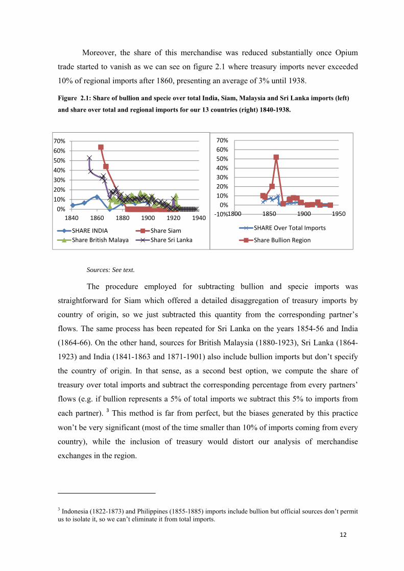
after that their share became very low as we can appreciate on the left hand side of figure
2.1. In that sense, we can see that Siam and Sri Lanka imports were the most affected by
this adjustment, since bullion and specie imports represented more than half of their totals
during the second half of the 1880s.
The right part of the figure assesses the overall impact of subtracting treasury
imports. We can see that including those figures would overestimate total imports from our
13 countries by a maximum of 10% during 1860s. The bias amount is bigger if we just
study regional imports since bullion and specie represented a 50% of total regional imports
on the very same year. The totality of this bullion was imported by India and seems to be
related with exchanges of Opium by Silver vis a vis China (Feige & Miron 2008; Deming
2011). This intuition is partially confirmed by our data which shows that during 1864-1866
most regional treasury imports performed by India had their origin on China.
12
Moreover, the share of this merchandise was reduced substantially once Opium
trade started to vanish as we can see on figure 2.1 where treasury imports never exceeded
10% of regional imports after 1860, presenting an average of 3% until 1938.
Figure 2.1: Share of bullion and specie over total India, Siam, Malaysia and Sri Lanka imports (left) and share over total and regional imports for our 13 countries (right) 1840-1938.
Sources: See text.
The procedure employed for subtracting bullion and specie imports was
straightforward for Siam which offered a detailed disaggregation of treasury imports by
country of origin, so we just subtracted this quantity from the corresponding partner’s
flows. The same process has been repeated for Sri Lanka on the years 1854-56 and India
(1864-66). On the other hand, sources for British Malaysia (1880-1923), Sri Lanka (1864-
1923) and India (1841-1863 and 1871-1901) also include bullion imports but don’t specify
the country of origin. In that sense, as a second best option, we compute the share of
treasury over total imports and subtract the corresponding percentage from every partners’
flows (e.g. if bullion represents a 5% of total imports we subtract this 5% to imports from
each partner). 3 This method is far from perfect, but the biases generated by this practice
won’t be very significant (most of the time smaller than 10% of imports coming from every
country), while the inclusion of treasury would distort our analysis of merchandise
exchanges in the region.
3 Indonesia (1822-1873) and Philippines (1855-1885) imports include bullion but official sources don’t permit us to isolate it, so we can’t eliminate it from total imports.
0%10%20%30%40%50%60%70%
1840 1860 1880 1900 1920 1940
SHARE INDIA Share SiamShare British Malaya Share Sri Lanka
-10%0%
10%20%30%40%50%60%70%
1800 1850 1900 1950
SHARE Over Total Imports
Share Bullion Region
13
Finally, a detailed analysis of commercial integration inside a certain region
requires a precise determination of the origin of traded merchandise. In this regard, the
treatment of transit trade passing through Hong Kong and Singapore requires a
transformation because most trade flows passing through those two ports were assumed by
the literature to be transit (Dennys, 1867,pp 51). In other words, most imports coming from
Singapore or Hong Kong weren’t produced there, but had their origin somewhere else.
That’s why accounting for those flows as Southeast Asian imports would overestimate
regional share on our analysis.
First of all, we assume the limitations of the approach followed by this research, but
we are fairly convinced that the adjustments performed really add value to the database
because our assumptions are more realistic than simply accounting for transit trade as it was
fully regional. Of course this division will artificially increment the number of flows
included on our database since imports from Hong Kong and Singapore will be divided into
Regional, Europe/Africa, Americas and Oceania transit, but for comparative purposes we
will only account for them as if they compose a single import flow. In addition, this
estimation permits us to capture a historical phenomenon as it was the employment of
transit networks for expanding regional trade on the last quarter of the 19th century,
something that, as the cited article shows, was key for explaining extraordinary levels of
trade integration presented by the region.
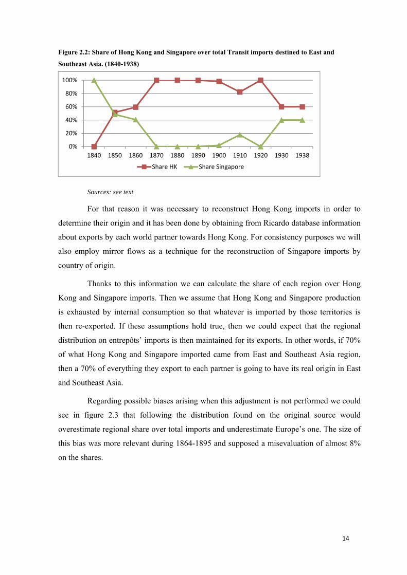
In any case, the process for reconstructing the origin of transit trade flows has
overcome certain difficulties. The first one is the scarcity of trade data for Hong Kong
during the 19th century, which at least is not shared by Singapore. There was a possibility of
estimating transit by only using Singapore flows but we would be losing an important part
of the story, probably the most important one if we attend to historiography and
information obtained on figure 2.2 where we can see that after 1870 most transit trade came
from Hong Kong.
14
Figure 2.2: Share of Hong Kong and Singapore over total Transit imports destined to East and Southeast Asia. (1840-1938)
Sources: see text
For that reason it was necessary to reconstruct Hong Kong imports in order to
determine their origin and it has been done by obtaining from Ricardo database information
about exports by each world partner towards Hong Kong. For consistency purposes we will
also employ mirror flows as a technique for the reconstruction of Singapore imports by
country of origin.
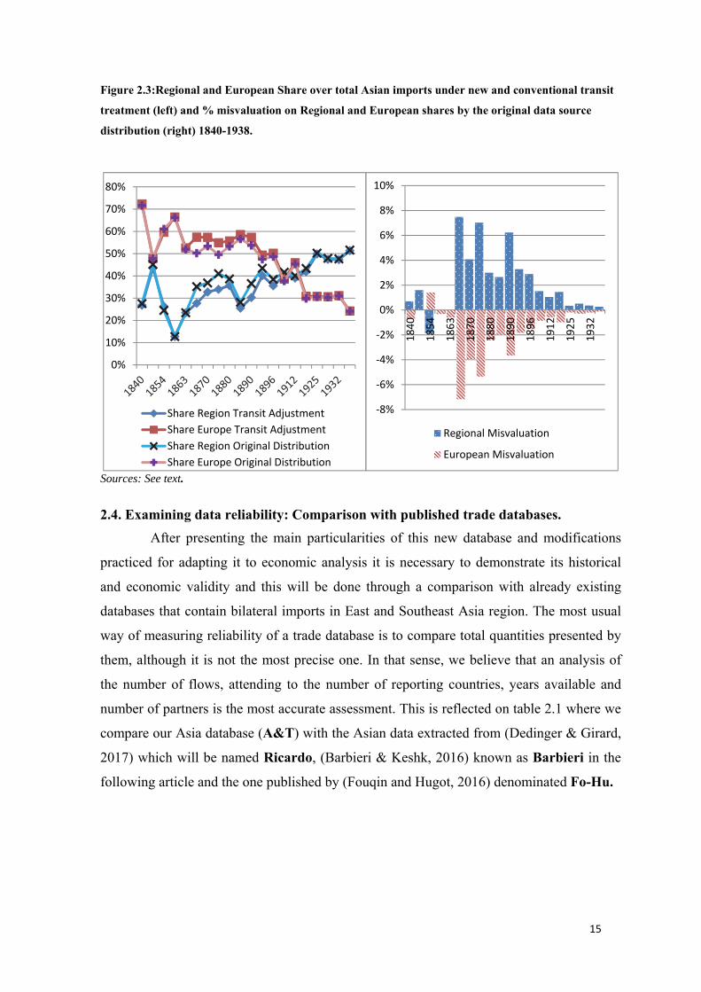
Thanks to this information we can calculate the share of each region over Hong
Kong and Singapore imports. Then we assume that Hong Kong and Singapore production
is exhausted by internal consumption so that whatever is imported by those territories is
then re-exported. If these assumptions hold true, then we could expect that the regional
distribution on entrepôts’ imports is then maintained for its exports. In other words, if 70%
of what Hong Kong and Singapore imported came from East and Southeast Asia region,
then a 70% of everything they export to each partner is going to have its real origin in East
and Southeast Asia.
Regarding possible biases arising when this adjustment is not performed we could
see in figure 2.3 that following the distribution found on the original source would
overestimate regional share over total imports and underestimate Europe’s one. The size of
this bias was more relevant during 1864-1895 and supposed a misevaluation of almost 8%
on the shares.
0%
20%
40%
60%
80%
100%
1840 1850 1860 1870 1880 1890 1900 1910 1920 1930 1938Share HK Share Singapore
15
Figure 2.3:Regional and European Share over total Asian imports under new and conventional transit treatment (left) and % misvaluation on Regional and European shares by the original data source distribution (right) 1840-1938.
Sources: See text.
2.4. Examining data reliability: Comparison with published trade databases. After presenting the main particularities of this new database and modifications
practiced for adapting it to economic analysis it is necessary to demonstrate its historical
and economic validity and this will be done through a comparison with already existing
databases that contain bilateral imports in East and Southeast Asia region. The most usual
way of measuring reliability of a trade database is to compare total quantities presented by
them, although it is not the most precise one. In that sense, we believe that an analysis of
the number of flows, attending to the number of reporting countries, years available and
number of partners is the most accurate assessment. This is reflected on table 2.1 where we
compare our Asia database (A&T) with the Asian data extracted from (Dedinger & Girard,
2017) which will be named Ricardo, (Barbieri & Keshk, 2016) known as Barbieri in the
following article and the one published by (Fouqin and Hugot, 2016) denominated Fo-Hu.
0%
10%
20%
30%
40%
50%
60%
70%
80%
Share Region Transit AdjustmentShare Europe Transit AdjustmentShare Region Original DistributionShare Europe Original Distribution
-8%
-6%
-4%
-2%
0%
2%
4%
6%
8%
10%
1840
1854
1863
1870
1880
1890
1896
1912
1925
1932
Regional Misvaluation
European Misvaluation
16
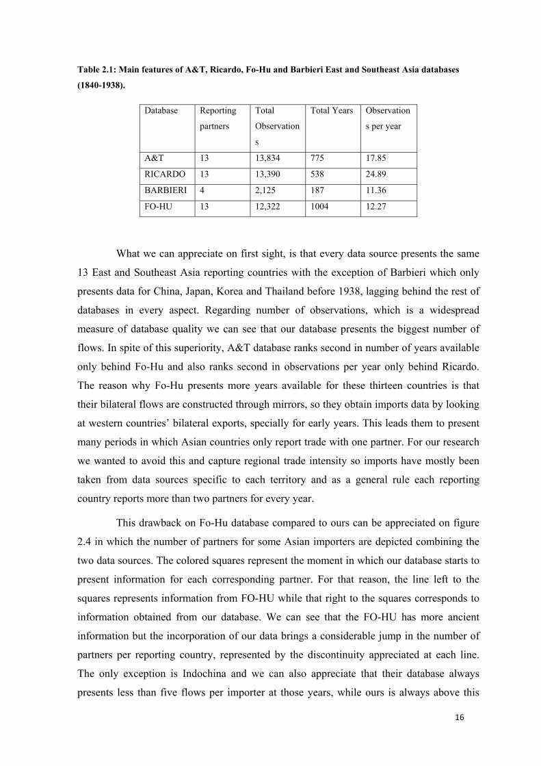
Table 2.1: Main features of A&T, Ricardo, Fo-Hu and Barbieri East and Southeast Asia databases (1840-1938).
Database Reporting
partners
Total
Observation
s
Total Years Observation
s per year
A&T 13 13,834 775 17.85
RICARDO 13 13,390 538 24.89
BARBIERI 4 2,125 187 11.36
FO-HU 13 12,322 1004 12.27
What we can appreciate on first sight, is that every data source presents the same
13 East and Southeast Asia reporting countries with the exception of Barbieri which only
presents data for China, Japan, Korea and Thailand before 1938, lagging behind the rest of
databases in every aspect. Regarding number of observations, which is a widespread
measure of database quality we can see that our database presents the biggest number of
flows. In spite of this superiority, A&T database ranks second in number of years available
only behind Fo-Hu and also ranks second in observations per year only behind Ricardo.
The reason why Fo-Hu presents more years available for these thirteen countries is that
their bilateral flows are constructed through mirrors, so they obtain imports data by looking
at western countries’ bilateral exports, specially for early years. This leads them to present
many periods in which Asian countries only report trade with one partner. For our research
we wanted to avoid this and capture regional trade intensity so imports have mostly been
taken from data sources specific to each territory and as a general rule each reporting
country reports more than two partners for every year.
This drawback on Fo-Hu database compared to ours can be appreciated on figure
2.4 in which the number of partners for some Asian importers are depicted combining the
two data sources. The colored squares represent the moment in which our database starts to
present information for each corresponding partner. For that reason, the line left to the
squares represents information from FO-HU while that right to the squares corresponds to
information obtained from our database. We can see that the FO-HU has more ancient
information but the incorporation of our data brings a considerable jump in the number of
partners per reporting country, represented by the discontinuity appreciated at each line.
The only exception is Indochina and we can also appreciate that their database always
presents less than five flows per importer at those years, while ours is always above this
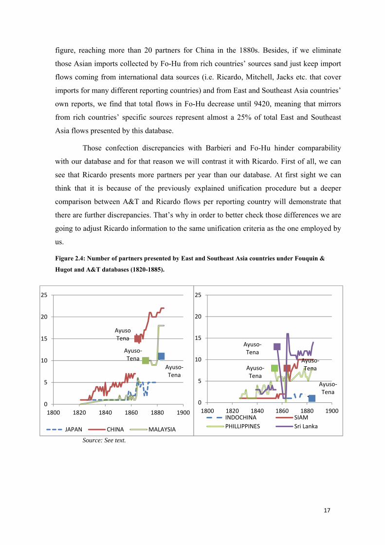
17
figure, reaching more than 20 partners for China in the 1880s. Besides, if we eliminate
those Asian imports collected by Fo-Hu from rich countries’ sources sand just keep import
flows coming from international data sources (i.e. Ricardo, Mitchell, Jacks etc. that cover
imports for many different reporting countries) and from East and Southeast Asia countries’
own reports, we find that total flows in Fo-Hu decrease until 9420, meaning that mirrors
from rich countries’ specific sources represent almost a 25% of total East and Southeast
Asia flows presented by this database.
Those confection discrepancies with Barbieri and Fo-Hu hinder comparability
with our database and for that reason we will contrast it with Ricardo. First of all, we can
see that Ricardo presents more partners per year than our database. At first sight we can
think that it is because of the previously explained unification procedure but a deeper
comparison between A&T and Ricardo flows per reporting country will demonstrate that
there are further discrepancies. That’s why in order to better check those differences we are
going to adjust Ricardo information to the same unification criteria as the one employed by
us.
Figure 2.4: Number of partners presented by East and Southeast Asia countries under Fouquin & Hugot and A&T databases (1820-1885).
Source: See text.
Ayuso-Tena
Ayuso Tena
Ayuso-Tena
0
5
10
15
20
25
1800 1820 1840 1860 1880 1900
JAPAN CHINA MALAYSIA
Ayuso-Tena
Ayuso-Tena
Ayuso-Tena
Ayuso-Tena
0
5
10
15
20
25
1800 1820 1840 1860 1880 1900INDOCHINA SIAMPHILLIPPINES Sri Lanka
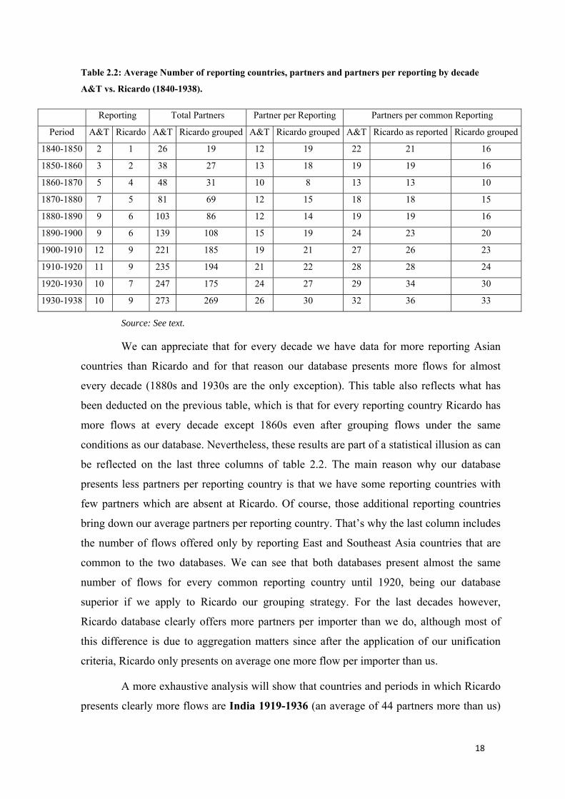
18
Table 2.2: Average Number of reporting countries, partners and partners per reporting by decade A&T vs. Ricardo (1840-1938).
Reporting Total Partners Partner per Reporting Partners per common Reporting
Period A&T Ricardo A&T Ricardo grouped A&T Ricardo grouped A&T Ricardo as reported Ricardo grouped
1840-1850 2 1 26 19 12 19 22 21 16
1850-1860 3 2 38 27 13 18 19 19 16
1860-1870 5 4 48 31 10 8 13 13 10
1870-1880 7 5 81 69 12 15 18 18 15
1880-1890 9 6 103 86 12 14 19 19 16
1890-1900 9 6 139 108 15 19 24 23 20
1900-1910 12 9 221 185 19 21 27 26 23
1910-1920 11 9 235 194 21 22 28 28 24
1920-1930 10 7 247 175 24 27 29 34 30
1930-1938 10 9 273 269 26 30 32 36 33
Source: See text.
We can appreciate that for every decade we have data for more reporting Asian
countries than Ricardo and for that reason our database presents more flows for almost
every decade (1880s and 1930s are the only exception). This table also reflects what has
been deducted on the previous table, which is that for every reporting country Ricardo has
more flows at every decade except 1860s even after grouping flows under the same
conditions as our database. Nevertheless, these results are part of a statistical illusion as can
be reflected on the last three columns of table 2.2. The main reason why our database
presents less partners per reporting country is that we have some reporting countries with
few partners which are absent at Ricardo. Of course, those additional reporting countries
bring down our average partners per reporting country. That’s why the last column includes
the number of flows offered only by reporting East and Southeast Asia countries that are
common to the two databases. We can see that both databases present almost the same
number of flows for every common reporting country until 1920, being our database
superior if we apply to Ricardo our grouping strategy. For the last decades however,
Ricardo database clearly offers more partners per importer than we do, although most of
this difference is due to aggregation matters since after the application of our unification
criteria, Ricardo only presents on average one more flow per importer than us.
A more exhaustive analysis will show that countries and periods in which Ricardo
presents clearly more flows are India 1919-1936 (an average of 44 partners more than us)
19
and Indonesia (1928-1938), when they have an average of 31 partners more than us. This
compensates the higher partners we have for Japan (26 on average between 1914-1938)
while for the rest of countries we generally present more flows, although there are no
significant differences. Those differences in flows per reporting partner in India have their
origin in 1912 when they employ a database which includes much more partners than us,
although they are generally small territories like Algeria, Argentina, Dutch Borneo, Eritrea,
British Somalia or Fiji whose share over Indian imports is not very relevant. In addition, the
source employed by us for reporting Indonesia imports is much less comprehensive than
the one employed by Ricardo and that’s why we present much fewer flows after 1928.
However, we decided to maintain our original source for coherence reasons since it brings
data since the 1840s including the same partners, while Ricardo source starts in 1902.
This would lead us to a first conclusion of this section, which is that our database
for Asia includes more reporting countries than Ricardo at every decade and coherent
information for more years, making our data more useful for long term analysis. After
applying our reunification criteria to Ricardo, our database seems to be slightly more
complete for 1840-1920 since we present more flows for every active importer.
Nevertheless, it is true that Ricardo database is more accurate for analysis regarding
interwar years (1920-1938) as they present more flows per partner, although most of those
differences are explained by aggregation maters.
As explained on the introduction for this section, many scholars compare trade
databases according to total quantities presented by them. In that sense, the superiority
shown by our data regarding total flows should be reflected on total imports. The first thing
that should be done in order to make both databases comparable is to translate them to a
common currency, which is going to be the one employed by Ricardo, Sterling pounds. In
the case of our database, data is expressed in current dollars after translating original
currencies through exchange rates found on (Federico & Tena, 2019), while the exchanges
rates employed by Ricardo come from another source. This might generate a first
discrepancy, although we believe the exchange rates employed by us have superior
quality.4
4 An exhaustive analysis of discrepancies in total imports generated by the use of different exchange rates is far from the scope of this paper but would be interesting in the future.
20
Another possible problem lies on the definition of imports since general trade
defines them as all goods entering the country, no matter their final destination, whereas
special trade only includes goods put at the disposal of importers as well as goods stored in
warehouses destined for domestic consumption. Anyway, we believe this technical concern
won’t affect the comparison since both Ricardo and this database bring priority to special
trade flows when both kinds are available. The only difference arises with the treatment of
transit trade passing through Hong Kong and Singapore, which has been addressed on
previous sections. However this issue will only affect regional distribution of imports, not
the totals.
Figure 2.5 depicts total imports presented by our selected Asian countries under
our database compared with the totals for those same countries on Ricardo “World as
reported”. Ricardo database has other ways of computing totals like summing total imports
between the reporting countries and all its partners (“World sum of partners”) or
performing some estimation (“World Bestguess”) and although figures differ between those
different methods, the tendency is more or less the same for everyone.
After all, we can appreciate how our database offers lower values of East and
Southeast Asian total imports between 1840-1866 than Ricardo (World as reported) and
substantially higher ones for the rest of the period (with the exception of the early 20th
century before WWI in which we present slightly lower values). Discrepancies reach a 30%
of our total Asian imports which is a considerable and unexpected figure, taking into
account that for this period Ricardo only offers data for India, while we also have imports
for Indonesia, Philippines for most periods and sporadic information for Sri Lanka and
Siam. Furthermore, the sources employed by Ricardo and us for determining India imports
offer similar totals at those decades.
The main reason explaining such low value on our database until 1860 has to do
with the series of adjustments explained on section 2 which were destined to eliminate
bullion and specie imports from the totals offered by the original data sources for India, Sri
Lanka, Siam and also British Malaysia. On figure 2.6 we can see that if we account for the
same reporting countries our database presents substantially smaller totals after eliminating
bullion and specie but offers slightly higher totals than Ricardo if we add the bullion and
specie imports with the exception of some years between 1864-1870 in which official
sources don’t include India treasury imports.
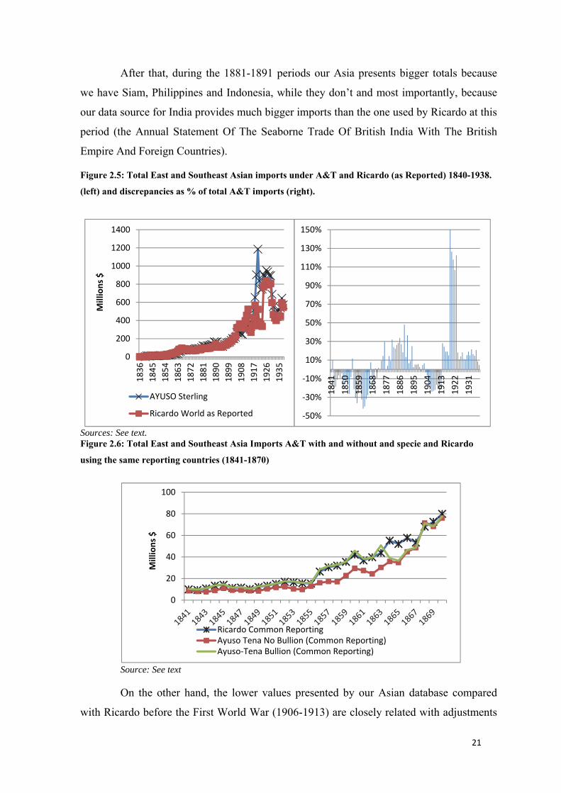
21
After that, during the 1881-1891 periods our Asia presents bigger totals because
we have Siam, Philippines and Indonesia, while they don’t and most importantly, because
our data source for India provides much bigger imports than the one used by Ricardo at this
period (the Annual Statement Of The Seaborne Trade Of British India With The British
Empire And Foreign Countries).
Figure 2.5: Total East and Southeast Asian imports under A&T and Ricardo (as Reported) 1840-1938. (left) and discrepancies as % of total A&T imports (right).
Sources: See text. Figure 2.6: Total East and Southeast Asia Imports A&T with and without and specie and Ricardo using the same reporting countries (1841-1870)
Source: See text
On the other hand, the lower values presented by our Asian database compared
with Ricardo before the First World War (1906-1913) are closely related with adjustments
0
20
40
60
80
100
Mill
ions
$
Ricardo Common ReportingAyuso Tena No Bullion (Common Reporting)Ayuso-Tena Bullion (Common Reporting)
0
200
400
600
800
1000
1200
1400
1836
1845
1854
1863
1872
1881
1890
1899
1908
1917
1926
1935
Mill
ions
$
AYUSO Sterling
Ricardo World as Reported -50%
-30%
-10%
10%
30%
50%
70%
90%
110%
130%
150%
1841
1850
1859
1868
1877
1886
1895
1904
1913
1922
1931
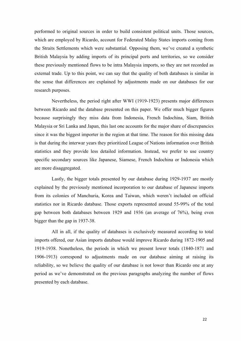
22
performed to original sources in order to build consistent political units. Those sources,
which are employed by Ricardo, account for Federated Malay States imports coming from
the Straits Settlements which were substantial. Opposing them, we’ve created a synthetic
British Malaysia by adding imports of its principal ports and territories, so we consider
these previously mentioned flows to be intra Malaysia imports, so they are not recorded as
external trade. Up to this point, we can say that the quality of both databases is similar in
the sense that differences are explained by adjustments made on our databases for our
research purposes.
Nevertheless, the period right after WWI (1919-1923) presents major differences
between Ricardo and the database presented on this paper. We offer much bigger figures
because surprisingly they miss data from Indonesia, French Indochina, Siam, British
Malaysia or Sri Lanka and Japan, this last one accounts for the major share of discrepancies
since it was the biggest importer in the region at that time. The reason for this missing data
is that during the interwar years they prioritized League of Nations information over British
statistics and they provide less detailed information. Instead, we prefer to use country
specific secondary sources like Japanese, Siamese, French Indochina or Indonesia which
are more disaggregated.
Lastly, the bigger totals presented by our database during 1929-1937 are mostly
explained by the previously mentioned incorporation to our database of Japanese imports
from its colonies of Manchuria, Korea and Taiwan, which weren’t included on official
statistics nor in Ricardo database. Those exports represented around 55-99% of the total
gap between both databases between 1929 and 1936 (an average of 76%), being even
bigger than the gap in 1937-38.
All in all, if the quality of databases is exclusively measured according to total
imports offered, our Asian imports database would improve Ricardo during 1872-1905 and
1919-1938. Nonetheless, the periods in which we present lower totals (1840-1871 and
1906-1913) correspond to adjustments made on our database aiming at raising its
reliability, so we believe the quality of our database is not lower than Ricardo one at any
period as we’ve demonstrated on the previous paragraphs analyzing the number of flows
presented by each database.
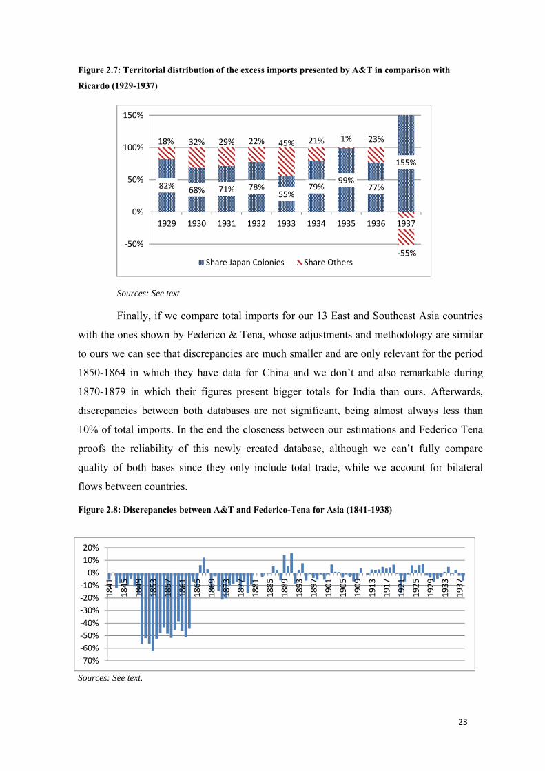
23
Figure 2.7: Territorial distribution of the excess imports presented by A&T in comparison with Ricardo (1929-1937)
Sources: See text
Finally, if we compare total imports for our 13 East and Southeast Asia countries
with the ones shown by Federico & Tena, whose adjustments and methodology are similar
to ours we can see that discrepancies are much smaller and are only relevant for the period
1850-1864 in which they have data for China and we don’t and also remarkable during
1870-1879 in which their figures present bigger totals for India than ours. Afterwards,
discrepancies between both databases are not significant, being almost always less than
10% of total imports. In the end the closeness between our estimations and Federico Tena
proofs the reliability of this newly created database, although we can’t fully compare
quality of both bases since they only include total trade, while we account for bilateral
flows between countries.
Figure 2.8: Discrepancies between A&T and Federico-Tena for Asia (1841-1938)
Sources: See text.
82% 68% 71% 78%55%
79%99%
77%
155%
18% 32% 29% 22% 45% 21% 1% 23%
-55%-50%
0%
50%
100%
150%
1929 1930 1931 1932 1933 1934 1935 1936 1937
Share Japan Colonies Share Others
-70%-60%-50%-40%-30%-20%-10%
0%10%20%
1841
1845
1849
1853
1857
1861
1865
1869
1873
1877
1881
1885
1889
1893
1897
1901
1905
1909
1913
1917
1921
1925
1929
1933
1937
24
2.5. Mixing Databases Ricardo and A&T. The main objective of the present paper is to apply this newly created Asian
imports database to an economic research about the degree of regional integration in East
and Southeast Asia. Prior sections have shown that our information is superior, but we must
also recognize the contributions that those previously presented databases have made to our
data and, most importantly, to which degree the present database could contribute to the
already existing ones.
First of all, there are some periods in which official sources were missing and
others in which we considered sources employed by published databases more reliable or
accurate than ours. For that reason we’ve taken data from external databases as we’ve
already mentioned with Japanese imports between 1870-1879 obtained from Barbieri
database. In addition, Ricardo data is employed to fill periods in which we lack proper data
sources. For example we use Ricardo database, adjusted to our unification criteria, when
presenting data for India between 1867-1870, for Sri Lanka (1867) and for Malaysia during
1907-1908. We also take from Ricardo data on total Chinese imports during 1932-34 and
1937 and Chinese imports from Manchuria (1868-1899) and French Indochina (1932-
1938). For the case of Japan, as it has been explained before, we obtain imports from Korea
using Ricardo database between 1882-1889 and 1900-1918. We also use Ricardo in order
to collect Japanese imports by partner in 1862 and 1880-1882. This data source has also
been employed for getting Indonesian imports from French Indochina and Siam during
1902-1918 and 1924-1938 and from Korea during 1924-1936. Another country that is
complemented using Ricardo database is Siam for which we obtain imports disaggregated
by country level between 1910-1918 and 1924-1927.5 From Ricardo, we’ve also obtained a
full disaggregation of French Indochina imports for the years 1903-1912 and flows coming
from Myanmar, India, Indonesia, Philippines and Siam (1913-1918). Finally, we’ve also
used Ricardo for filling Taiwan imports by partner during 1907-1918.
Summing up, we’ve demonstrated that the collection of data from different sources
could contribute to the accuracy of trade statistics, focusing in East and Southeast Asia
imports. This idea has inspired us to create a new database that will mix A&T and Ricardo
5 For those periods we have a local primary source as it is the Foreign Trade and Navigation of the Port of Bangkok which has slightly more flows than Ricardo. However we’ve found that most of these extra flows represent ports and parts of countries. In addition, we believe Ricardo is superior because flows are expressed in Sterling Pounds which is a more stable currency than the Thai Bath employed by the primary source and because they employ natural years, whereas the local source uses the Thai calendar.
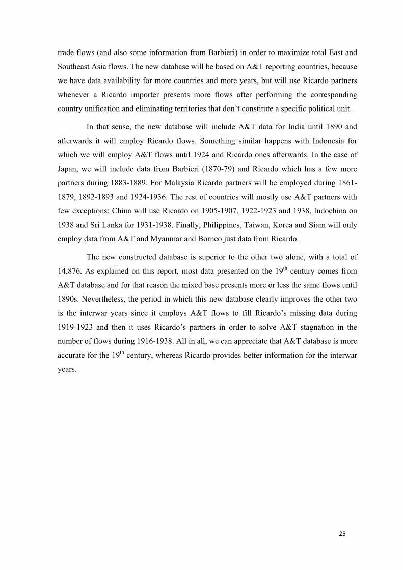
25
trade flows (and also some information from Barbieri) in order to maximize total East and
Southeast Asia flows. The new database will be based on A&T reporting countries, because
we have data availability for more countries and more years, but will use Ricardo partners
whenever a Ricardo importer presents more flows after performing the corresponding
country unification and eliminating territories that don’t constitute a specific political unit.
In that sense, the new database will include A&T data for India until 1890 and
afterwards it will employ Ricardo flows. Something similar happens with Indonesia for
which we will employ A&T flows until 1924 and Ricardo ones afterwards. In the case of
Japan, we will include data from Barbieri (1870-79) and Ricardo which has a few more
partners during 1883-1889. For Malaysia Ricardo partners will be employed during 1861-
1879, 1892-1893 and 1924-1936. The rest of countries will mostly use A&T partners with
few exceptions: China will use Ricardo on 1905-1907, 1922-1923 and 1938, Indochina on
1938 and Sri Lanka for 1931-1938. Finally, Philippines, Taiwan, Korea and Siam will only
employ data from A&T and Myanmar and Borneo just data from Ricardo.
The new constructed database is superior to the other two alone, with a total of
14,876. As explained on this report, most data presented on the 19th century comes from
A&T database and for that reason the mixed base presents more or less the same flows until
1890s. Nevertheless, the period in which this new database clearly improves the other two
is the interwar years since it employs A&T flows to fill Ricardo’s missing data during
1919-1923 and then it uses Ricardo’s partners in order to solve A&T stagnation in the
number of flows during 1916-1938. All in all, we can appreciate that A&T database is more
accurate for the 19th century, whereas Ricardo provides better information for the interwar
years.
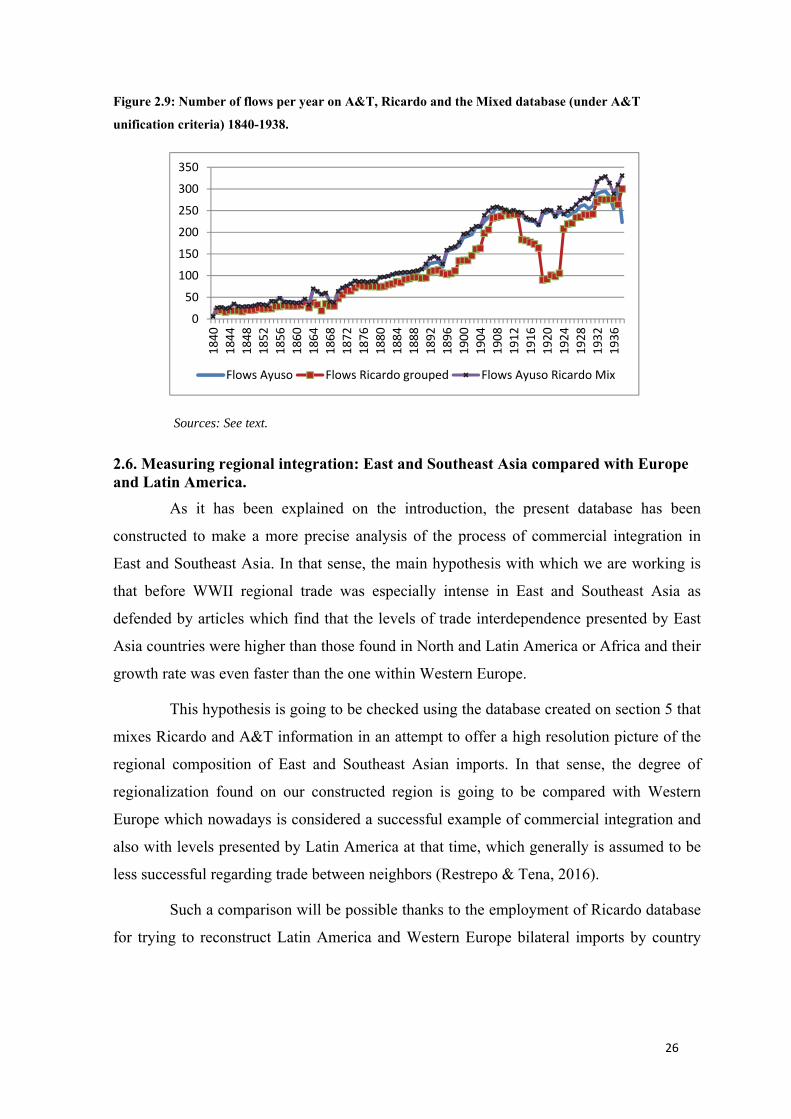
26
Figure 2.9: Number of flows per year on A&T, Ricardo and the Mixed database (under A&T unification criteria) 1840-1938.
Sources: See text.
2.6. Measuring regional integration: East and Southeast Asia compared with Europe and Latin America.
As it has been explained on the introduction, the present database has been
constructed to make a more precise analysis of the process of commercial integration in
East and Southeast Asia. In that sense, the main hypothesis with which we are working is
that before WWII regional trade was especially intense in East and Southeast Asia as
defended by articles which find that the levels of trade interdependence presented by East
Asia countries were higher than those found in North and Latin America or Africa and their
growth rate was even faster than the one within Western Europe.
This hypothesis is going to be checked using the database created on section 5 that
mixes Ricardo and A&T information in an attempt to offer a high resolution picture of the
regional composition of East and Southeast Asian imports. In that sense, the degree of
regionalization found on our constructed region is going to be compared with Western
Europe which nowadays is considered a successful example of commercial integration and
also with levels presented by Latin America at that time, which generally is assumed to be
less successful regarding trade between neighbors (Restrepo & Tena, 2016).
Such a comparison will be possible thanks to the employment of Ricardo database
for trying to reconstruct Latin America and Western Europe bilateral imports by country
050
100150200250300350
1840
1844
1848
1852
1856
1860
1864
1868
1872
1876
1880
1884
1888
1892
1896
1900
1904
1908
1912
1916
1920
1924
1928
1932
1936
Flows Ayuso Flows Ricardo grouped Flows Ayuso Ricardo Mix
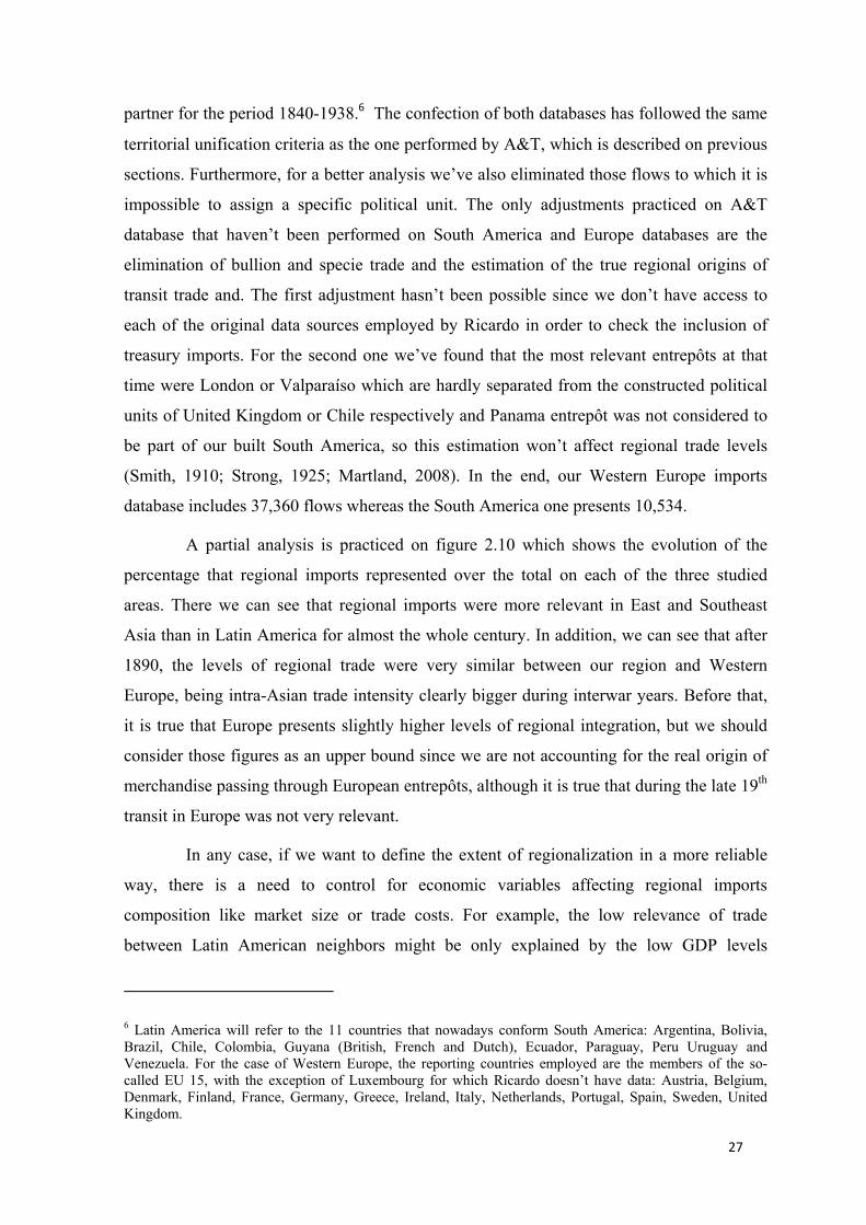
27
partner for the period 1840-1938.6 The confection of both databases has followed the same
territorial unification criteria as the one performed by A&T, which is described on previous
sections. Furthermore, for a better analysis we’ve also eliminated those flows to which it is
impossible to assign a specific political unit. The only adjustments practiced on A&T
database that haven’t been performed on South America and Europe databases are the
elimination of bullion and specie trade and the estimation of the true regional origins of
transit trade and. The first adjustment hasn’t been possible since we don’t have access to
each of the original data sources employed by Ricardo in order to check the inclusion of
treasury imports. For the second one we’ve found that the most relevant entrepôts at that
time were London or Valparaíso which are hardly separated from the constructed political
units of United Kingdom or Chile respectively and Panama entrepôt was not considered to
be part of our built South America, so this estimation won’t affect regional trade levels
(Smith, 1910; Strong, 1925; Martland, 2008). In the end, our Western Europe imports
database includes 37,360 flows whereas the South America one presents 10,534.
A partial analysis is practiced on figure 2.10 which shows the evolution of the
percentage that regional imports represented over the total on each of the three studied
areas. There we can see that regional imports were more relevant in East and Southeast
Asia than in Latin America for almost the whole century. In addition, we can see that after
1890, the levels of regional trade were very similar between our region and Western
Europe, being intra-Asian trade intensity clearly bigger during interwar years. Before that,
it is true that Europe presents slightly higher levels of regional integration, but we should
consider those figures as an upper bound since we are not accounting for the real origin of
merchandise passing through European entrepôts, although it is true that during the late 19th
transit in Europe was not very relevant.
In any case, if we want to define the extent of regionalization in a more reliable
way, there is a need to control for economic variables affecting regional imports
composition like market size or trade costs. For example, the low relevance of trade
between Latin American neighbors might be only explained by the low GDP levels
6 Latin America will refer to the 11 countries that nowadays conform South America: Argentina, Bolivia, Brazil, Chile, Colombia, Guyana (British, French and Dutch), Ecuador, Paraguay, Peru Uruguay and Venezuela. For the case of Western Europe, the reporting countries employed are the members of the so-called EU 15, with the exception of Luxembourg for which Ricardo doesn’t have data: Austria, Belgium, Denmark, Finland, France, Germany, Greece, Ireland, Italy, Netherlands, Portugal, Spain, Sweden, United Kingdom.
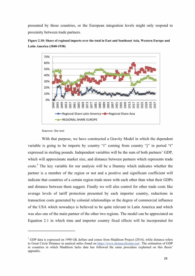
28
presented by those countries, or the European integration levels might only respond to
proximity between trade partners.
Figure 2.10: Share of regional imports over the total in East and Southeast Asia, Western Europe and Latin America (1840-1938)
Sources: See text
With that purpose, we have constructed a Gravity Model in which the dependent
variable is going to be imports by country “i” coming from country “j” in period “t”
expressed in sterling pounds. Independent variables will be the sum of both partners’ GDP,
which will approximate market size, and distance between partners which represents trade
costs.7 The key variable for our analysis will be a Dummy which indicates whether the
partner is a member of the region or not and a positive and significant coefficient will
indicate that countries of a certain region trade more with each other than what their GDPs
and distance between them suggest. Finally we will also control for other trade costs like
average levels of tariff protection presented by each importer country, reductions in
transaction costs generated by colonial relationships or the degree of commercial influence
of the USA which nowadays is believed to be quite relevant in Latin America and which
was also one of the main partner of the other two regions. The model can be appreciated on
Equation 2.1 in which time and importer country fixed effects will be incorporated for
7 GDP data is expressed on 1990 GK dollars and comes from Maddison Project (2014), while distance refers to Great Circle Distance in nautical miles found on https://www.distancefromto.net/. The estimation of GDP in countries in which Maddison lacks data has followed the same procedure explained on this thesis’ appendix.
0%
10%
20%
30%
40%
50%
60%
70%18
4018
4518
4918
5318
5718
6118
6518
6918
7318
7718
8118
8518
8918
9318
9719
0119
0519
0919
1319
1719
2119
2519
2919
3319
37
Regional Share Latin America Regional Share Asia
REGIONAL SHARE EUROPE
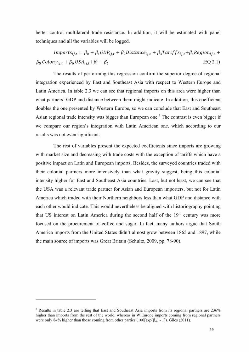
29
better control multilateral trade resistance. In addition, it will be estimated with panel
techniques and all the variables will be logged. 𝐼𝑚𝑝𝑜𝑟𝑡𝑠 , = 𝛽 + 𝛽 𝐺𝐷𝑃 , + 𝛽 𝐷𝑖𝑠𝑡𝑎𝑛𝑐𝑒 , + 𝛽 𝑇𝑎𝑟𝑖𝑓𝑓𝑠 , +𝛽 𝑅𝑒𝑔𝑖𝑜𝑛 , +𝛽 𝐶𝑜𝑙𝑜𝑛𝑦 , + 𝛽 𝑈𝑆𝐴 , +𝛽 + 𝛽 (EQ 2.1)
The results of performing this regression confirm the superior degree of regional
integration experienced by East and Southeast Asia with respect to Western Europe and
Latin America. In table 2.3 we can see that regional imports on this area were higher than
what partners’ GDP and distance between them might indicate. In addition, this coefficient
doubles the one presented by Western Europe, so we can conclude that East and Southeast
Asian regional trade intensity was bigger than European one.8 The contrast is even bigger if
we compare our region’s integration with Latin American one, which according to our
results was not even significant.
The rest of variables present the expected coefficients since imports are growing
with market size and decreasing with trade costs with the exception of tariffs which have a
positive impact on Latin and European imports. Besides, the surveyed countries traded with
their colonial partners more intensively than what gravity suggest, being this colonial
intensity higher for East and Southeast Asia countries. Last, but not least, we can see that
the USA was a relevant trade partner for Asian and European importers, but not for Latin
America which traded with their Northern neighbors less than what GDP and distance with
each other would indicate. This would nevertheless be aligned with historiography pointing
that US interest on Latin America during the second half of the 19th century was more
focused on the procurement of coffee and sugar. In fact, many authors argue that South
America imports from the United States didn’t almost grow between 1865 and 1897, while
the main source of imports was Great Britain (Schultz, 2009, pp. 78-90).
8 Results in table 2.3 are telling that East and Southeast Asia imports from its regional partners are 236% higher than imports from the rest of the world, whereas in W.Europe imports coming from regional partners were only 84% higher than those coming from other parties (100[exp(β ) - 1]). Giles (2011).
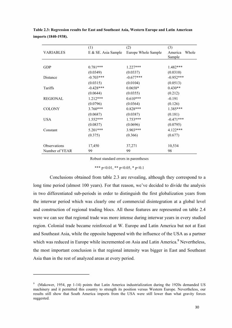
30
Table 2.3: Regression results for East and Southeast Asia, Western Europe and Latin American imports (1840-1938).
(1) (2) (3) VARIABLES E & SE. Asia Sample Europe Whole Sample America Whole
Sample GDP 0.781*** 1.227*** 1.482*** (0.0349) (0.0337) (0.0310) Distance -0.703*** -0.677*** -0.952*** (0.0315) (0.0104) (0.0513) Tariffs -0.428*** 0.0658* 0.430** (0.0644) (0.0355) (0.212) REGIONAL 1.212*** 0.610*** -0.191 (0.0796) (0.0364) (0.126) COLONY 3.760*** 0.828*** 1.385*** (0.0687) (0.0387) (0.181) USA 1.552*** 1.753*** -0.471*** (0.0837) (0.0696) (0.0795) Constant 5.201*** 3.903*** 4.122*** (0.375) (0.366) (0.677) Observations 17,450 37,271 10,534 Number of YEAR 99 99 98
Robust standard errors in parentheses
*** p<0.01, ** p<0.05, * p<0.1
Conclusions obtained from table 2.3 are revealing, although they correspond to a
long time period (almost 100 years). For that reason, we’ve decided to divide the analysis
in two differentiated sub-periods in order to distinguish the first globalization years from
the interwar period which was clearly one of commercial disintegration at a global level
and construction of regional trading blocs. All those features are represented on table 2.4
were we can see that regional trade was more intense during interwar years in every studied
region. Colonial trade became reinforced at W. Europe and Latin America but not at East
and Southeast Asia, while the opposite happened with the influence of the USA as a partner
which was reduced in Europe while incremented on Asia and Latin America.9 Nevertheless,
the most important conclusion is that regional intensity was bigger in East and Southeast
Asia than in the rest of analyzed areas at every period.
9 (Makower, 1954, pp 1-14) points that Latin America industrialization during the 1920s demanded US machinery and it permitted this country to strength its position versus Western Europe. Nevertheless, our results still show that South America imports from the USA were still lower than what gravity forces suggested.
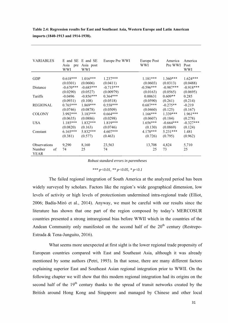
31
Table 2.4: Regression results for East and Southeast Asia, Western Europe and Latin American imports (1840-1913 and 1914-1938).
Robust standard errors in parentheses
*** p<0.01, ** p<0.05, * p<0.1
The failed regional integration of South America at the analyzed period has been
widely surveyed by scholars. Factors like the region’s wide geographical dimension, low
levels of activity or high levels of protectionism undermined intra-regional trade (Elliot,
2006; Badía-Miró et al., 2014). Anyway, we must be careful with our results since the
literature has shown that one part of the region composed by today’s MERCOSUR
countries presented a strong intraregional bias before WWII which in the countries of the
Andean Community only manifested on the second half of the 20th century (Restrepo-
Estrada & Tena-Junguito, 2016).
What seems more unexpected at first sight is the lower regional trade propensity of
European countries compared with East and Southeast Asia, although it was already
mentioned by some authors (Petri, 1993). In that sense, there are many different factors
explaining superior East and Southeast Asian regional integration prior to WWII. On the
following chapter we will show that this modern regional integration had its origins on the
second half of the 19th century thanks to the spread of transit networks created by the
British around Hong Kong and Singapore and managed by Chinese and other local
VARIABLES
E and SE Asia pre WWI
E and SE Asia post WWI
Europe Pre WWI
Europe Post WWI
America Pre WWI
America Post WWI
GDP 0.618*** 1.016*** 1.237*** 1.181*** 1.360*** 1.624*** (0.0301) (0.0606) (0.0411) (0.0603) (0.0313) (0.0488) Distance -0.670*** -0.685*** -0.715*** -0.596*** -0.987*** -0.918*** (0.0290) (0.0527) (0.00979) (0.0163) (0.0565) (0.0695) Tariffs -0.0496 -0.856*** 0.364*** 0.00631 0.609** 0.285 (0.0931) (0.108) (0.0518) (0.0590) (0.261) (0.214) REGIONAL 0.765*** 1.869*** 0.558*** 0.687*** -0.275** -0.219 (0.0746) (0.0878) (0.0509) (0.0460) (0.125) (0.167) COLONY 3.992*** 3.183*** 0.664*** 1.166*** 1.339*** 1.961*** (0.0635) (0.0886) (0.0298) (0.0607) (0.184) (0.278) USA 1.185*** 1.832*** 1.819*** 1.656*** -0.664*** -0.327*** (0.0820) (0.163) (0.0746) (0.130) (0.0869) (0.124) Constant 6.165*** 5.832*** 4.607*** 4.178*** 5.231*** 1.481 (0.381) (0.577) (0.463) (0.726) (0.795) (0.962) Observations 9,290 8,160 23,563 13,708 4,824 5,710 Number of YEAR
74 25 74 25 73 25
32
merchants. Intra-regional trade was then fueled by demand complementarities that arose
during the subsequent industrialization processes experienced by almost every country
inside the region across the whole 20th century. The first one was Japan, whose economic
development was linked with its imperial expansion and similar dynamics have been
repeated during Southeast Asia industrialization in the 1960s and 1970s and Chinese and
Indian ones during 1980s and 1990 as will be explained on chapter 3.
Apart from that, the construction of East and Southeast Asia as a regional entity
might be controversial since it includes a region like South Asia, that has been very active
historically, but which doesn’t share most of the cultural tights existing among East and
Southeast Asia countries. The main motives behind its inclusion are historical commercial
links with China and the share of British networks and institutions with Malaysia, apart
from the spread of Indian merchants all over Southeast Asia which contributed to
commercial trade inside the region. Anyway, the constructed database permits us to see if
the inclusion of South Asia explains by itself the special regional intensity found in East
and Southeast Asia. Under this premise, we’ve calculated the levels of regional integration
once South Asian territories have been eliminated and results in table 2.5 reveal that East
and Southeast Asian regional integration is still remarkable and superior to European one.
Furthermore, coefficients are higher this time, suggesting that intra-regional trade was
slightly undermined rather than enhanced by the inclusion of South Asia territories.
On the other hand, it is possible that imperial aims of European countries,
especially the British, diverted trade away from regional partners and in favor of colonies
all over the world. This could explain the lower degree of regional imports presented by
Western Europe at the analyzed period, although historiography arguments that European
empires valued more their colonies as a market than as a source of primary products, so
imperial diversion would be more noticeable if we dealt with exports rather than imports
(Meredith, 1996). In fact, results in tables 2.3 and 2.4 confirmed this hypothesis because the
coefficient of colonial imports is much higher for East and Southeast Asia than for Europe.
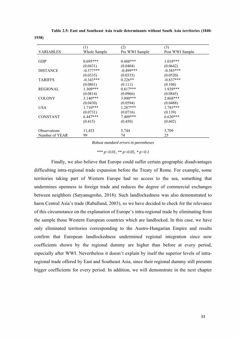
33
Table 2.5: East and Southeast Asia trade determinants without South Asia territories (1840-1938)
(1) (2) (3) VARIABLES Whole Sample Pre WWI Sample Post WWI Sample GDP 0.695*** 0.488*** 1.018*** (0.0431) (0.0404) (0.0642) DISTANCE -0.577*** -0.499*** -0.585*** (0.0335) (0.0335) (0.0520) TARIFFS -0.343*** 0.226** -0.837*** (0.0861) (0.111) (0.104) REGIONAL 1.309*** 0.817*** 1.939*** (0.0814) (0.0966) (0.0845) COLONY 3.140*** 3.090*** 2.868*** (0.0430) (0.0594) (0.0488) USA 1.710*** 1.287*** 1.785*** (0.0731) (0.0716) (0.139) CONSTANT 6.447*** 7.409*** 6.620*** (0.415) (0.450) (0.602) Observations 11,453 5,744 5,709 Number of YEAR 99 74 25
Robust standard errors in parentheses
*** p<0.01, ** p<0.05, * p<0.1
Finally, we also believe that Europe could suffer certain geographic disadvantages
difficulting intra-regional trade expansion before the Treaty of Rome. For example, some
territories taking part of Western Europe had no access to the sea, something that
undermines openness to foreign trade and reduces the degree of commercial exchanges
between neighbors (Satyanugroho, 2018). Such landlockedness was also demonstrated to
harm Central Asia’s trade (Raballand, 2003), so we have decided to check for the relevance
of this circumstance on the explanation of Europe’s intra-regional trade by eliminating from
the sample those Western European countries which are landlocked. In this case, we have
only eliminated territories corresponding to the Austro-Hungarian Empire and results
confirm that European landlockedness undermined regional integration since now
coefficients shown by the regional dummy are higher than before at every period,
especially after WWI. Nevertheless it doesn’t explain by itself the superior levels of intra-
regional trade offered by East and Southeast Asia, since their regional dummy still presents
bigger coefficients for every period. In addition, we will demonstrate in the next chapter
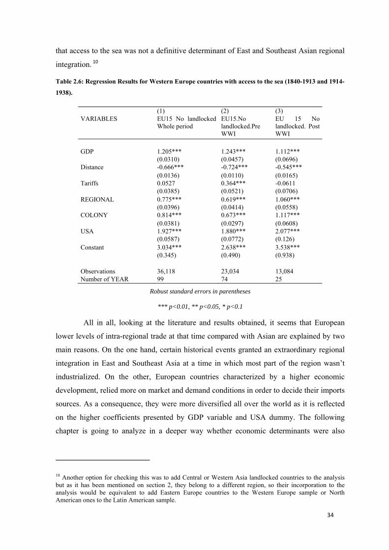
34
that access to the sea was not a definitive determinant of East and Southeast Asian regional
integration. 10
Table 2.6: Regression Results for Western Europe countries with access to the sea (1840-1913 and 1914-1938).
(1) (2) (3) VARIABLES EU15 No landlocked
Whole period EU15.No landlocked.Pre WWI
EU 15 No landlocked. Post WWI
GDP 1.205*** 1.243*** 1.112*** (0.0310) (0.0457) (0.0696) Distance -0.666*** -0.724*** -0.545*** (0.0136) (0.0110) (0.0165) Tariffs 0.0527 0.364*** -0.0611 (0.0385) (0.0521) (0.0706) REGIONAL 0.775*** 0.619*** 1.060*** (0.0396) (0.0414) (0.0558) COLONY 0.814*** 0.673*** 1.117*** (0.0381) (0.0297) (0.0608) USA 1.927*** 1.880*** 2.077*** (0.0587) (0.0772) (0.126) Constant 3.034*** 2.638*** 3.538*** (0.345) (0.490) (0.938) Observations 36,118 23,034 13,084 Number of YEAR 99 74 25
Robust standard errors in parentheses
*** p<0.01, ** p<0.05, * p<0.1
All in all, looking at the literature and results obtained, it seems that European
lower levels of intra-regional trade at that time compared with Asian are explained by two
main reasons. On the one hand, certain historical events granted an extraordinary regional
integration in East and Southeast Asia at a time in which most part of the region wasn’t
industrialized. On the other, European countries characterized by a higher economic
development, relied more on market and demand conditions in order to decide their imports
sources. As a consequence, they were more diversified all over the world as it is reflected
on the higher coefficients presented by GDP variable and USA dummy. The following
chapter is going to analyze in a deeper way whether economic determinants were also
10 Another option for checking this was to add Central or Western Asia landlocked countries to the analysis but as it has been mentioned on section 2, they belong to a different region, so their incorporation to the analysis would be equivalent to add Eastern Europe countries to the Western Europe sample or North American ones to the Latin American sample.
35
explaining Asian regional integration or, as we believe, were historical events the ones
motivating the intra-regional trade expansion appreciated on this chapter.
2.7. Conclusions The present paper intends to throw more light in the debate about commercial
integration in the periphery by adding a long run perspective. In order to do that, we
analyze the evolution of East and Southeast Asian regional integration and demonstrate by
means of a Gravity Model that before the Second World War it was superior to the
European or Latin American ones in spite of its GDP and geographical disadvantages.
With this objective in mind we have constructed a bilateral imports database
which covers commercial exchanges between 13 East and Southeast Asia countries and
each of its partners for almost a century that goes between 1840 and 1938. To our
knowledge, this is the first attempt to reconstruct trade flows for all the countries in the
region during such a long time span, using mostly local statistics and maintaining
consistent unification criteria. For that reason, the core of the paper has dealt with
explanations regarding sources employed for disentangling bilateral trade for each country,
data transformation performed in order to adapt original information to our research needs
and assessments of the statistical validity of this new database. This last step has consisted
on a comparison of total imports and number of flows presented by every country on our
database with information obtained on multipurpose international databases that also cover
East and Southeast Asia area.
What has been obtained is that the present database in general provides superior
statistics than the ones of Ricardo, Fo-Hu and Barbieri. Specifically, our database contains
information for more years and more reporting countries than the others and for that reason
it includes many more flows. Ricardo database is the only one that gets close to our
estimates if we perform a more exhaustive analysis since for most of the century both
databases present a similar number of flows when we only consider reporting countries
common to both databases. Such statistical similarity is mostly explained by the territorial
adjustments performed in our database’s partners intended to conform consistent political
units and which diminish the number of flows presented by our data contrasted with
Ricardo. In fact, if a similar territorial unification is applied to Ricardo we obtain that our
database presents more flows per reporting country for every period with the exception of
the last two decades (1920-1940). The validity of our database is countersigned when we
analyze total imports presented by the region: our database shows higher totals than
36
Ricardo for almost the whole period and the years in which their imports are bigger are
explained by the subtraction of bullion and specie and elimination of coastal trade
performed in our data. Furthermore, our totals are very close to Federico& Tena ones,
whose internationally approved estimates are obtained following similar criteria as we do,
adding validity to our database.
In any case and despite the manifest quality of the recently created database, we
believe that in order to perform the most reliable analysis of regional intensity in East and
Southeast Asia trade it is necessary to complement our database with information from
Ricardo at those countries and periods in which their quality was noticeably superior.
Basing on this mixed database we have created a Gravity Model which is employed to
demonstrate that East and Southeast Asian regional trade was more intense than what
market size and trade costs shown by those countries might suggest and that this intensity
was bigger than the one exhibited by countries in Western Europe and South America
before and after WWII. In this line, the following chapter will check if Asia’s exceptional
intra-regional trade had its origins on certain historical events, or if market forces were
more relevant as happened with Western Europe.
37
CHAPTER 2: NATURAL TRADING PARTNERS? POWER AND 3HISTORICAL NETWORKS IN EAST AND SOUTHEAST ASIAN
INTEGRATION (1840-1938)
3.1. Introduction Findings contained on the first chapter might contribute to the debate about the
necessity of deepening the integration process inside East and Southeast Asia (Webber,
2001).11 Notwithstanding, the discovery of an intra-Asian regional trade superior to
Western Europe and Latin American ones before the signature of any FTA, could catalogue
those territories as “Natural Trading Partners”. In case these special trade relationships are
confirmed, this would enhance the welfare created by hypothetic Customs or Monetary
Unions signed on the region.
In this regard, this article wants to conceptualize the previously found regional
trade intensity by demonstrating that East and Southeast Asia countries were Natural
Trading Partners. For doing this, we will study the degree of regional trade in East and
Southeast Asia long before the creation of any Free Trade Area, including also potential
South Asia partners like India or Sri Lanka. The region has been commercially active since
ancient times and most important of all, by the early 20th century its levels of regional trade
were comparable to those in Europe as we’ve seen on the previous chapter (Petri, 1993).
How was it possible for a relatively poor region like that (Basino, Forthcoming)?12 In the
case of Western Europe it seems that countries based their commercial decisions on
economic variables but this article is going to show that the case of East and Southeast Asia
was rather different.
These theoretical determinants have been widely analyzed by scholars dealing
with Natural Trading Partners’ hypothesis. Nevertheless, this literature doesn’t pay enough
attention to historical developments that might have favored special trade relationships
11 Those discussions crystallized in 1992 when the Association of Southeast Asia Nations (ASEAN) became a Free Trade Area in 1992, consolidated in 2015 when ten Southeast Asian countries formed the ASEAN Economic Community (AEC). Nonetheless, the Asian Financial Crisis in 1997 showed the weaknesses of ASEAN and revealed the need for enlarging the integration process in order to fight foreign influence. A possibility that is on the table is the creation of a Currency Union on ASEAN to which countries like Japan, Korea and China might join into an organization called the ASEAN Plus Three (APT). 12 Relative poverty refers to the comparison with the European core and USA. We acknowledge that the region was not uniform and living standards in Southeast Asia were higher than in India and China.
38
between different territories. In that sense, the main contribution of this article consists of
bringing a historical perspective to Natural Trading Partners’ literature through the analysis
of those special events that upgraded region’s intrinsic economic advantages in order to
forge East and Southeast Asia commercial integration.
As the historiography has demonstrated, commercial networks were quite active in
East and Southeast Asia since the 15th century (Age of Commerce), but they acquired a new
dimension from the second half of the 19th century (Age of Empires). The years previous to
this shift saw trade dominated by exchanges of silver and opium between China and India,
orchestrated basically by Great Britain. This trade was affected by subsequent restrictions
during the 1830s and 1840s which lead to the Opium Wars won by the British. As a result,
they forced the opening of Chinese ports to free trade and developed an intense commercial
network linking Europe with China and India across the British intermediate ports of Hong
Kong and Singapore. Consequently, the rest of European empires settled in the region like
the Dutch, the French or the Spanish (replaced by the USA in 1898) started to adhere to this
network and to improve it through investment in transport and communications
infrastructure.
This sequence of events not only facilitated the integration of the region on the
global economy but also permitted the development of a purely regional network in East
and Southeast Asia. According to our data, the first traces of this intensification date back
from the 1860s and 1870s in which the transit networks created by the British started to get
exploited by Chinese merchants dispersed all over the region. The study of the construction
of Chinese and other local networks like Hindi or Malay and their interactions with
imperial ones contribute to a vast literature about commercial networks and their influence
on regional integration. Those merchants mainly transported goods from Southeast Asia
territories towards China and other countries in the region, using Hong Kong and Singapore
as entrepôts until the late 1890s. At the same time, British colonies started to get rid of
reduced transaction costs generated by imperial policies to raise commercial exchanges
between them. Nevertheless, after WWI, the British dominion of regional trade was
substituted by the newly created Japanese Empire which employed the growing intra-
regional trade in order to sustain its industrialization. Furthermore, direct routes between
countries in the region substituted transit once the information costs of entry in China’s
market vanished.
39
All in all, the objective of the present paper is twofold: to demonstrate that East
and Southeast Asia countries were Natural Trading Partners and to show that this
singularity is shaped by historical events. For that purpose, we will employ the previously
described imports database, which in this case won’t be mixed with Ricardo because we
want to preserve the treatment to transit trade provided in our database in order to better
explain a phenomenon that was decisive on the region’s early contemporary integration.
Our conclusions will point that East and Southeast Asia countries might be
considered Natural Trading Partners because they satisfied a set of conditions long before
the creation of any Free Trade Area. Those special commercial relationships are maintained
until today thanks to a sequence in which each country employed local raw materials and
exported manufactures to its neighbors during every industrialization process (Sugihara,
2019). The mentioned interactions were based on low transaction costs and demand
complementarities inside the region during pre and post WWII but we demonstrate that the
roots of post-Industrial Revolution regional integration in East and Southeast Asia laid on
the transit networks created by the British around Hong Kong and Singapore and managed
by Chinese merchants. Those networks were supported by British colonial aspirations and
investment in infrastructure. Furthermore, regional integration was subsequently
consolidated during the interwar years through the exercise of imperial power from Japan,
whose influence seems bigger than the British because its planned industrialization had an
impact on the above mentioned demand complementarities and was also sustained by
investments in railway and local commercial networks.
In that sense, section 2 will look at the different theoretical and historical factors
that, according to the literature allowed countries in the region to become Natural Trading
Partners. Section 3 in the paper will provide some descriptive statistics about the evolution
of imports in the region and their main features. Sections 4 and 5 will describe the model
employed and characteristics of the database, while section 6 will bring the principal results
and section 7 the main conclusions.
3.2. Theory and History on Natural Trade Blocs As it has been mentioned in the introduction, the establishment of a Free Trade
Area between Natural Trading Partners might be welfare enhancing. In that sense, a review
of the literature brings three different conditions that determine whether two countries are
Natural Trading Partners before the signature of any FTA. The first one is that those
countries trade more with each other than with the rest of the world (Lipsey, 1960), the
40
second is that countries trade disproportionately with their neighbors (Summers, 1991) and
the last one that those territories show demand complementarities (Schiff, 1999).
In the end, one of the main objectives of the following chapter is to demonstrate
that East and Southeast Asian countries were Natural Trading Partners since they met each
criteria before 1938: The growth in intra-regional trade surpassed the one with the rest of
the world (Sugihara, 1985), they traded with each other more than what gravity forces may
indicate (Sugihara, 2005; Petri, 1993) and they presented demand complementarities
(Sugihara, 2019). The following section is intended to provide some theoretical and
historical mechanisms explaining those special commercial relationships between
neighbors in East and Southeast Asia at that time.
3.2.1.Theoretical Determinants: Trade costs, demand complementarities and factor
endowments
The most basic versions of the Natural Trading Partners’ hypothesis remark that
trade between neighbors might be specially intense because trade costs between them are
small. This idea is defended by (Wonnacott and Lutz, 1989) or (Krugman, 1993, pp. 58-79)
among others. In that sense, the archipelagic character of East and Southeast Asia territories
might favor their commercial integration with each other since access to sea contributed
positively to region’s international trade (Satyanugroho, 2018), while Central Asia’s
landlockedness undermined trade (Raballand, 2003).
Alternatively, other authors conclude that two countries will trade intensively in
manufactures if they have similar demand structures (Linder, 1961). An alternative theory
also deals with demand, but opposing Linder it defends that countries are more likely to
trade with each other if their demands are different and one country imports what the other
exports (Schiff, 1999). This could be the case of East and Southeast Asia in which on the
one hand Japan exported mainly heavy industrial products to its colonies (in exchange of
rice and raw materials) and cotton textiles to the rest of the region. On the other hand,
Southeast Asia countries mostly exported primary products: Indonesia exported sugar as
well as rubber, which was also highly exported by British Malaya across with tin, whereas
Burma, Thailand and Southern Vietnam became rice exporting regions (Booth, 2007;
Bassino 2000).
This intraregional specialization is also reflected on British India which exported
manufactured goods to Southeast Asia in exchange of primary products and followed an
41
opposite pattern, exporting raw cotton to Japan. Besides, it also heavily exported opium and
cotton manufactures to China, which in turn was a tea and silk exporter (Sugihara, 1985;
Keller & Shiue, 2011 and Latham, 1978). There is a vast literature dealing with demand
complementarities inside East and Southeast Asia and how they prevailed on the
industrialization processes arising after the Second World War, guaranteeing high levels of
intra-regional trade that persist nowadays (Sugihara, 2019). Nevertheless, on next chapter
we show that part of this intra-regional specialization might be institutionally driven
(Ayuso-Díaz & Tena-Junguito, 2019)
Finally, a set of authors rather argue that differences in factor endowments are the
drivers of regional trade. It is the case of the famous Hecksher-Ohlin model (Ohlin, 1952).
Summing up, economic theory brings some factors that might explain the intensity of
regional trade in East and Southeast Asia on the period studied. Nevertheless, we provide
some historical events that influenced these economic variables, like imperial networks
created by western institutions and enlarged through investment in infrastructure and the
connections established by local merchants all over the region.
3.2.2. History of Imperial policies in East and Southeast Asia.
From the late 18th to the first half of the 20th century, the region we are studying
was occupied by empires of different nature and subject to different policies and
regulations, being the British and Japanese Empires the most influential. The former started
their dominion over the region in 1757 through the East India Company and its army rule in
India. After 1858, it was the British Crown which administered this territory and further
conquests, a mandate which was prolonged until the mid-20th century in most cases (Bose
& Jalal, 2017, pp. 67-107). On the other hand, the construction of the Japanese Empire was
fast since most of it was completed between 1896 and 1915. The commercial preeminence
obtained during WWI and the establishment of an imperial bloc policy in the 1930s
consolidated Japanese dominion over East and Southeast Asia. (Ayuso-Díaz & Tena-
Junguito, 2019).
Historiography has widely demonstrated the positive links between colonies and
trade expansion through reductions in transaction costs or the application of discriminatory
policies. Nevertheless, colonial regimes established in the region were not homogeneous,
and this shaped the different trade behaviors appreciated on this research. Commercial
policies were not uniform inside the region as the Japanese Empire established a system of
preferential colonial access and discrimination to foreign products following American and
42
French policies on the Philippines and Indochina respectively. By contrast, the regimes
established on Siam, Indonesia and specially the British Empire were more liberal. The
Great Depression and the 1932 Ottawa agreement changed this landscape after the British
imposition of imperial preferences (Booth, 2003; Chase, 2004; Ferguson, 2003).
Empires also fostered regional trade through investments in infrastructure, while
the economic policies applied on conquered territories facilitated the intra-regional
specialization mentioned before: British capital and expertise favored India
industrialization and, most importantly, the Japanese Government actively supported the
establishment of new industries after the Meiji restoration (Roy, 2002; Tanimoto, 2019;
Booth, 2007a). Apart from that, the creation of currency blocs during the 1930s
strengthened intra-empire trade. This phenomenon affected British and Japanese colonies,
although implementations differed since international transactions inside the Japanese
Empire were carried by Central Banks, while the Sterling Bloc relied on government
intervention to fix exchange rates (Eichengreen & Irwin, 1993; Moon, 2008). Besides,
membership on Sterling bloc was supposed voluntary, whereas entrance on the Yen bloc
responded to Japan’s needs (Hunsberger, 1938).
Finally, different treatment of Chinese immigrants would condition their merchant
activities: in general regional empires favored a policy of open frontiers (Kaur, 2009),
although some territories like British Malaya, Burma, Dutch East Indies and French
Indochina applied ethnic segmentation policies. On the other hand, in the Philippines or
Siam intermarriage was encouraged, and Chinese enjoyed unrestricted access to business
(Sidel, 2008).
In conclusion, imperial activity in East and Southeast Asia was everything but
uniform, although all of them shared common features like commercial policies, investment
in infrastructure or the establishment of currency blocs that reduced transaction costs and
contributed decisively to the creation of active commercial networks inside the region. The
most dense one was created by the British and looked for an easier access to China by
Western Powers, using Singapore (British since 1819) and Hong Kong (1842) entrepôts.
During the first stages of network construction there was some trade diversion towards
imperial masters and colonial partners but the process culminated once Western Powers
43
could reach China directly and countries inside the region started to exploit these networks
for expanding intra-regional trade (Xu, 2015, pp-91-126). 13
3.2.3. Local merchants and their influence over regional trade across history.
One of the main hypotheses of this research is that the efficacy of imperial
institutions and investments depended on the activity of different local trading
communities. In that sense, links between Chinese migrant networks and international trade
based on information sharing or sanctions enforcement were already demonstrated by the
literature dealing with the late 20th century (Rauch & Trinidade, 2002). The following
paragraphs will, however, review how Chinese and other regional migrants facilitated East
and Southeast Asia commercial integration long before, from the second half of the 19th
century.
The first contacts between the Chinese and their Southeast Asian neighbors go
back in time more than 2000 years when Chinese soldiers got rid of inland contiguity for
reaching Indochina and Siam in the Third century B.C, Myanmar and Siam later and finally
overseas Malaya or Sumatra. The origins of those migrants were varied: Cantonese was the
predominant group in Siam, the Federated and Unfederated Malay States and were
important on the rest of the region, whereas Fukien Chinese were the majority on the Straits
Settlements and Indonesia (Purcell, 1966). The process of southern migration was
accentuated during the 17th century internal conflicts after the fall of the Ming dynasty,
although the new rulers kept strong restrictions to migrations abroad. Those restrictions
were gradually lifted by the forced signature of treaties with foreign Imperial Powers (Mc
Nair, 1923) leading to an escalation of migration to Burma, Malaya and Thailand after 1881
(Huff & Caggiano, 2007). Furthermore, after 1928 there was a relevant expansion of
Chinese migration to Manchuria, linked with the infrastructure development of the territory
(Lattimore, 1932).14
In the end, the Chinese diaspora supposed around 5% of total Southeast Asia
population but was economically influential thanks to dedication to retail activities (Purcell,
1966). First of all, Chinese merchants started dominating regional transit trade through their
13 In the end Singapore dominated regional transshipment, while Hong Kong became more international. 14 We should highlight that migrants from different Chinese regions established independent networks employing their own dialects as seen on Sang (1982). In any case the mechanisms by which each independent network favored regional trade were very similar, that’s why the concept of Chinese merchant networks employed on this paper encompasses all independent networks.
44
merchant communities in Singapore and Hong Kong often acting as Compradores carrying
operations for Western enterprises or forming their own companies (Rawski, 1969; Post,
2002). In addition, Chinese intermediaries supported the penetration of British capital
investments that permitted the development of transports and telecommunication
infrastructure, from which they benefited substantially (Duara, 2010; Shuyong, 1997; Xu,
2015).
Afterwards, with the entrance of the 20th century, the relevance of regional transit
trade started to decrease as direct connections between Asian ports became more profitable
(Keller & Shiue, 2011). However, the Chinese merchants still controlled most retail and
wholesale trade in Siam, the Philippines, French Indochina or Malaysia (Huff, 2003;
Fukuda, 1995, pp. 62, 72). What’s more, during the interwar years the dominion of regional
trade in East and Southeast Asia shifted towards the Japanese Empire which was
completing its industrialization as analyzed in the following chapter, and employed Chinese
intermediaries for distributing light manufactures towards Southeast Asia.
Nonetheless, the support of China migrants to intraregional trade expansion was
not limited to the activity of merchants. The settlement of Chinese day laborers relieved
labor scarcity at land abundant Burma, Siam or French Indochina, generating a surplus of
rice which was exported to British Malaysia, Dutch Indonesia or Philippines in order to
feed a growing number of Chinese workers in mines and plantations (Tagliacozzo &
Chang, 2011, pp. 336-359; Huff & Caggiano, 2007).
Apart from the Chinese, other local merchants participated on regional exchanges.
A prime example was the construction of a network of Malay traders since the Middle
Ages, which reached the Straits Settlements, Indonesia, Brunei and North Borneo (Hussin,
2005). After 1850 they were overcame by the Chinese, with whom they cooperated
throughout the whole studied period (Kobayashi, 2019; Cleary, 1996). Other relevant
network was constructed by Indian traders which controlled maritime trade with the rest of
Asia between 1850 and 1914 (Markovits, 2000, pp. 1-20) and land trade with China
through a community in Xinjiang (Thampi, 2010).
Summing up, it seems that economic variables like demand complementarities
have maintained high levels of intra-Asian trade for Centuries, until very recently.
Nevertheless, this paper tries to demonstrate that the explosion of regional trade during the
Age of Empires was possible thanks to interactions between imperial policies,
infrastructure and local networks, promoted by the British (19th century) and the Japanese
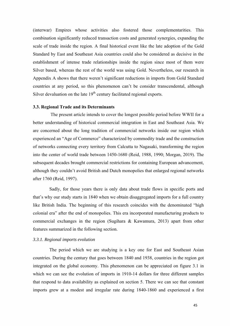
45
(interwar) Empires whose activities also fostered those complementarities. This
combination significantly reduced transaction costs and generated synergies, expanding the
scale of trade inside the region. A final historical event like the late adoption of the Gold
Standard by East and Southeast Asia countries could also be considered as decisive in the
establishment of intense trade relationships inside the region since most of them were
Silver based, whereas the rest of the world was using Gold. Nevertheless, our research in
Appendix A shows that there weren’t significant reductions in imports from Gold Standard
countries at any period, so this phenomenon can’t be consider transcendental, although
Silver devaluation on the late 19th century facilitated regional exports.
3.3. Regional Trade and its Determinants The present article intends to cover the longest possible period before WWII for a
better understanding of historical commercial integration in East and Southeast Asia. We
are concerned about the long tradition of commercial networks inside our region which
experienced an “Age of Commerce” characterized by commodity trade and the construction
of networks connecting every territory from Calcutta to Nagasaki, transforming the region
into the center of world trade between 1450-1680 (Reid, 1988, 1990; Morgan, 2019). The
subsequent decades brought commercial restrictions for containing European advancement,
although they couldn’t avoid British and Dutch monopolies that enlarged regional networks
after 1760 (Reid, 1997).
Sadly, for those years there is only data about trade flows in specific ports and
that’s why our study starts in 1840 when we obtain disaggregated imports for a full country
like British India. The beginning of this research coincides with the denominated “high
colonial era” after the end of monopolies. This era incorporated manufacturing products to
commercial exchanges in the region (Sugihara & Kawamura, 2013) apart from other
features summarized in the following section.
3.3.1. Regional imports evolution
The period which we are studying is a key one for East and Southeast Asian
countries. During the century that goes between 1840 and 1938, countries in the region got
integrated on the global economy. This phenomenon can be appreciated on figure 3.1 in
which we can see the evolution of imports in 1910-14 dollars for three different samples
that respond to data availability as explained on section 5. There we can see that constant
imports grew at a modest and irregular rate during 1840-1860 and experienced a first
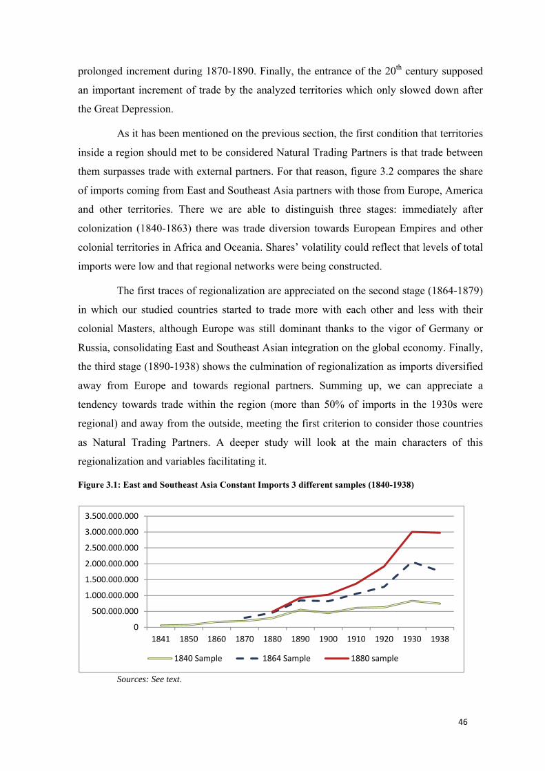
46
prolonged increment during 1870-1890. Finally, the entrance of the 20th century supposed
an important increment of trade by the analyzed territories which only slowed down after
the Great Depression.
As it has been mentioned on the previous section, the first condition that territories
inside a region should met to be considered Natural Trading Partners is that trade between
them surpasses trade with external partners. For that reason, figure 3.2 compares the share
of imports coming from East and Southeast Asia partners with those from Europe, America
and other territories. There we are able to distinguish three stages: immediately after
colonization (1840-1863) there was trade diversion towards European Empires and other
colonial territories in Africa and Oceania. Shares’ volatility could reflect that levels of total
imports were low and that regional networks were being constructed.
The first traces of regionalization are appreciated on the second stage (1864-1879)
in which our studied countries started to trade more with each other and less with their
colonial Masters, although Europe was still dominant thanks to the vigor of Germany or
Russia, consolidating East and Southeast Asian integration on the global economy. Finally,
the third stage (1890-1938) shows the culmination of regionalization as imports diversified
away from Europe and towards regional partners. Summing up, we can appreciate a
tendency towards trade within the region (more than 50% of imports in the 1930s were
regional) and away from the outside, meeting the first criterion to consider those countries
as Natural Trading Partners. A deeper study will look at the main characters of this
regionalization and variables facilitating it.
Figure 3.1: East and Southeast Asia Constant Imports 3 different samples (1840-1938)
Sources: See text.
0
500.000.000
1.000.000.000
1.500.000.000
2.000.000.000
2.500.000.000
3.000.000.000
3.500.000.000
1841 1850 1860 1870 1880 1890 1900 1910 1920 1930 1938
1840 Sample 1864 Sample 1880 sample
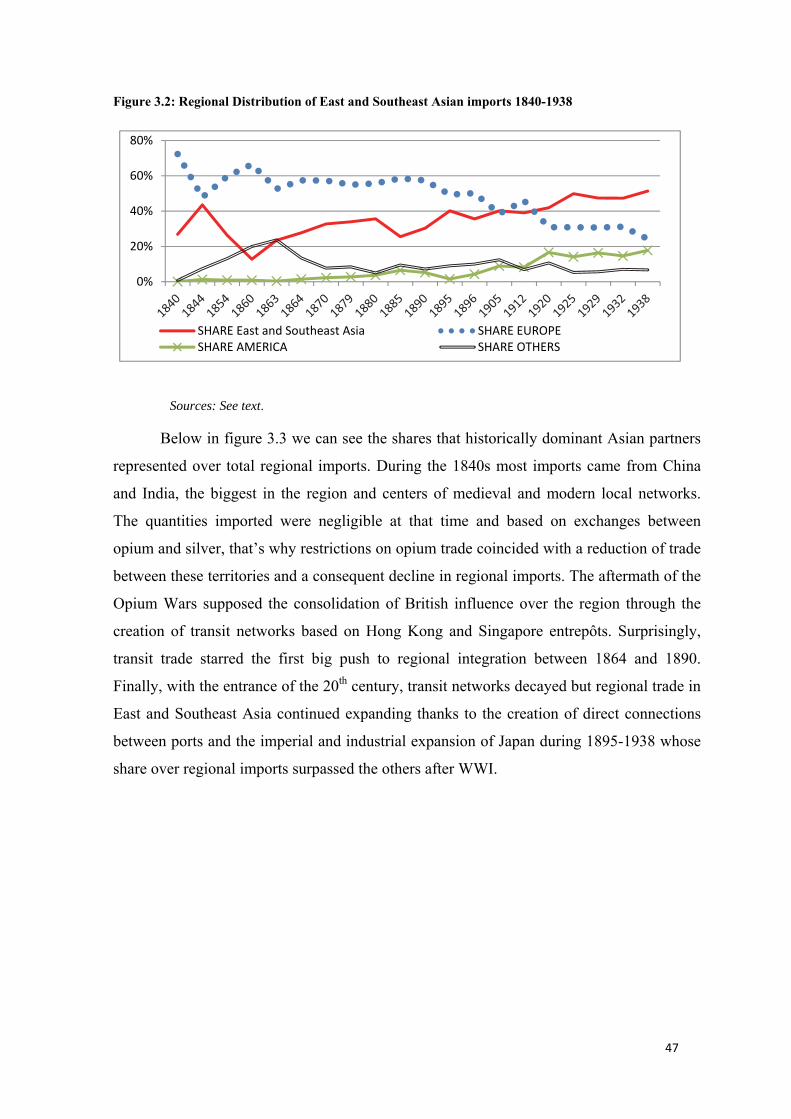
47
Figure 3.2: Regional Distribution of East and Southeast Asian imports 1840-1938
Sources: See text.
Below in figure 3.3 we can see the shares that historically dominant Asian partners
represented over total regional imports. During the 1840s most imports came from China
and India, the biggest in the region and centers of medieval and modern local networks.
The quantities imported were negligible at that time and based on exchanges between
opium and silver, that’s why restrictions on opium trade coincided with a reduction of trade
between these territories and a consequent decline in regional imports. The aftermath of the
Opium Wars supposed the consolidation of British influence over the region through the
creation of transit networks based on Hong Kong and Singapore entrepôts. Surprisingly,
transit trade starred the first big push to regional integration between 1864 and 1890.
Finally, with the entrance of the 20th century, transit networks decayed but regional trade in
East and Southeast Asia continued expanding thanks to the creation of direct connections
between ports and the imperial and industrial expansion of Japan during 1895-1938 whose
share over regional imports surpassed the others after WWI.
0%
20%
40%
60%
80%
SHARE East and Southeast Asia SHARE EUROPESHARE AMERICA SHARE OTHERS
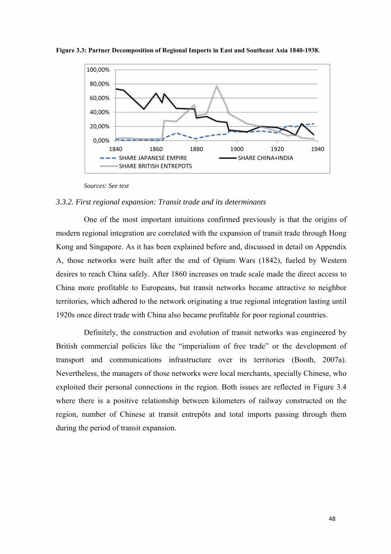
48
Figure 3.3: Partner Decomposition of Regional Imports in East and Southeast Asia 1840-1938.
Sources: See text
3.3.2. First regional expansion: Transit trade and its determinants
One of the most important intuitions confirmed previously is that the origins of
modern regional integration are correlated with the expansion of transit trade through Hong
Kong and Singapore. As it has been explained before and, discussed in detail on Appendix
A, those networks were built after the end of Opium Wars (1842), fueled by Western
desires to reach China safely. After 1860 increases on trade scale made the direct access to
China more profitable to Europeans, but transit networks became attractive to neighbor
territories, which adhered to the network originating a true regional integration lasting until
1920s once direct trade with China also became profitable for poor regional countries.
Definitely, the construction and evolution of transit networks was engineered by
British commercial policies like the “imperialism of free trade” or the development of
transport and communications infrastructure over its territories (Booth, 2007a).
Nevertheless, the managers of those networks were local merchants, specially Chinese, who
exploited their personal connections in the region. Both issues are reflected in Figure 3.4
where there is a positive relationship between kilometers of railway constructed on the
region, number of Chinese at transit entrepôts and total imports passing through them
during the period of transit expansion.
0,00%
20,00%
40,00%
60,00%
80,00%
100,00%
1840 1860 1880 1900 1920 1940SHARE JAPANESE EMPIRE SHARE CHINA+INDIASHARE BRITISH ENTREPOTS
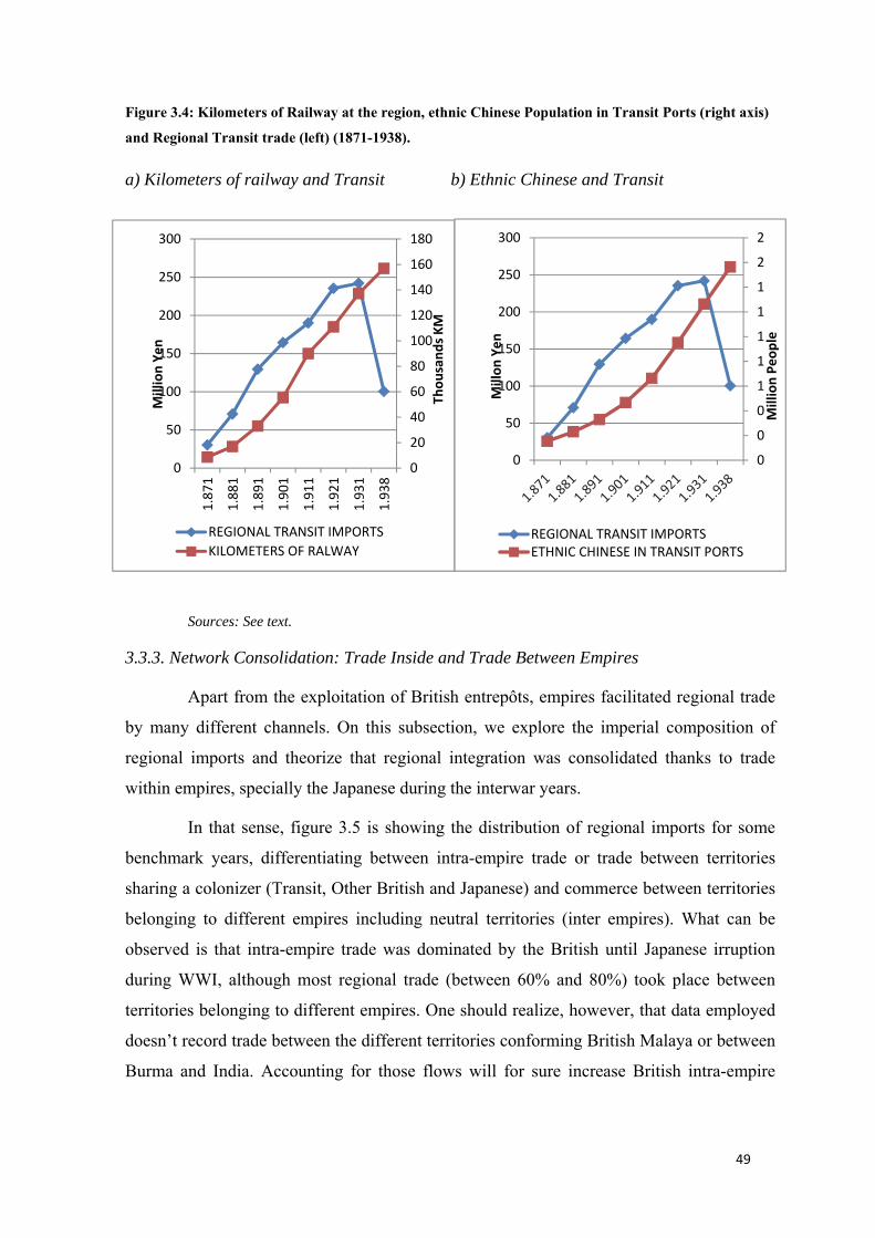
49
Figure 3.4: Kilometers of Railway at the region, ethnic Chinese Population in Transit Ports (right axis) and Regional Transit trade (left) (1871-1938).
a) Kilometers of railway and Transit b) Ethnic Chinese and Transit
Sources: See text.
3.3.3. Network Consolidation: Trade Inside and Trade Between Empires
Apart from the exploitation of British entrepôts, empires facilitated regional trade
by many different channels. On this subsection, we explore the imperial composition of
regional imports and theorize that regional integration was consolidated thanks to trade
within empires, specially the Japanese during the interwar years.
In that sense, figure 3.5 is showing the distribution of regional imports for some
benchmark years, differentiating between intra-empire trade or trade between territories
sharing a colonizer (Transit, Other British and Japanese) and commerce between territories
belonging to different empires including neutral territories (inter empires). What can be
observed is that intra-empire trade was dominated by the British until Japanese irruption
during WWI, although most regional trade (between 60% and 80%) took place between
territories belonging to different empires. One should realize, however, that data employed
doesn’t record trade between the different territories conforming British Malaya or between
Burma and India. Accounting for those flows will for sure increase British intra-empire
0
20
40
60
80
100
120
140
160
180
0
50
100
150
200
250
300
1.87
1
1.88
1
1.89
1
1.90
1
1.91
1
1.92
1
1.93
1
1.93
8
Thou
sand
s KM
Mill
ion
Yen
REGIONAL TRANSIT IMPORTSKILOMETERS OF RALWAY
00
0
1
1
1
1
1
2
2
0
50
100
150
200
250
300
Mill
ion
Peop
le
Mill
on Y
en
REGIONAL TRANSIT IMPORTSETHNIC CHINESE IN TRANSIT PORTS
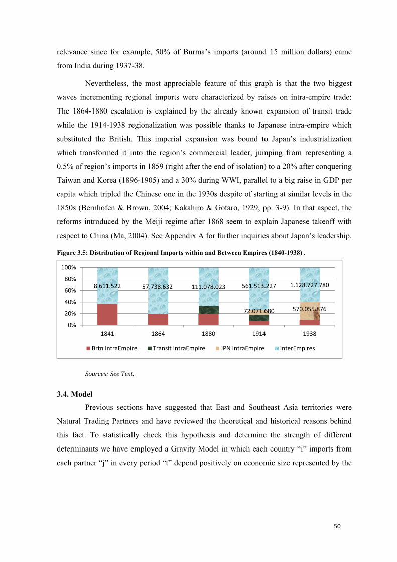
50
relevance since for example, 50% of Burma’s imports (around 15 million dollars) came
from India during 1937-38.
Nevertheless, the most appreciable feature of this graph is that the two biggest
waves incrementing regional imports were characterized by raises on intra-empire trade:
The 1864-1880 escalation is explained by the already known expansion of transit trade
while the 1914-1938 regionalization was possible thanks to Japanese intra-empire which
substituted the British. This imperial expansion was bound to Japan’s industrialization
which transformed it into the region’s commercial leader, jumping from representing a
0.5% of region’s imports in 1859 (right after the end of isolation) to a 20% after conquering
Taiwan and Korea (1896-1905) and a 30% during WWI, parallel to a big raise in GDP per
capita which tripled the Chinese one in the 1930s despite of starting at similar levels in the
1850s (Bernhofen & Brown, 2004; Kakahiro & Gotaro, 1929, pp. 3-9). In that aspect, the
reforms introduced by the Meiji regime after 1868 seem to explain Japanese takeoff with
respect to China (Ma, 2004). See Appendix A for further inquiries about Japan’s leadership.
Figure 3.5: Distribution of Regional Imports within and Between Empires (1840-1938) .
Sources: See Text.
3.4. Model Previous sections have suggested that East and Southeast Asia territories were
Natural Trading Partners and have reviewed the theoretical and historical reasons behind
this fact. To statistically check this hypothesis and determine the strength of different
determinants we have employed a Gravity Model in which each country “i” imports from
each partner “j” in every period “t” depend positively on economic size represented by the
72.071.680 570.055.876
8.611.522 57.738.632 111.078.023 561.513.227 1.128.727.780
0%
20%
40%
60%
80%
100%
1841 1864 1880 1914 1938
Brtn IntraEmpire Transit IntraEmpire JPN IntraEmpire InterEmpires
51
sum between GDP of the importer and GDP of the partner (Egger, 2002).15 They also
depend negatively on trade costs (𝑇𝐶 , ) with country partners as equation 3.1 shows.16
Trade costs in that equation are represented by the distance between countries and by their
average levels of tariff protection.
In order to check the first hypothesis, we have created some dummies to uncover
the existence of commercial networks and measuring their intensity. The key one is 𝑅𝑒𝑔𝑖𝑜𝑛 , which takes value 1 when the trade partner comes from East and Southeast Asia
and a positive and significant coefficient would show that regional trade was higher than
what gravity forces might predict, thus labeling East and Southeast Asia countries as
Natural Trading Partners. Then, 𝐶𝑜𝑙𝑜𝑛𝑦 , shows whether a certain trading partner is the
colonizer or a colony of the reporting one, 𝐸𝑈𝑅𝑂𝑃𝐸 , equals 1 when the partner is a
European country and finally 𝑆ℎ𝑎𝑟𝑒𝑑 𝐶𝑜𝑙𝑜𝑛𝑖𝑧𝑒𝑟 , accounts for trade between territories
colonized by the same imperial power. In the end, we have an unbalanced panel estimated
with importer country (𝛽 ) and time (𝛽 ) fixed effects for better control multilateral
resistance (Redding & Venables, 2004). The dependent and continuous independent
variables are going to be logged so coefficients can be interpreted as elasticities (Lye &
Hirschberg, 2002).17 The whole sample can be then divided into other subsamples to
determine how the direction and significance of trade biases evolve through different
periods. 𝐼𝑚𝑝𝑜𝑟𝑡𝑠 , = 𝛽 + 𝛽 𝐺𝐷𝑃 , + 𝛽 𝑇𝐶 , + 𝛽 𝑅𝑒𝑔𝑖𝑜𝑛 , + 𝛽 𝐶𝑜𝑙𝑜𝑛𝑦 , +𝛽 𝐸𝑈𝑅𝑂𝑃𝐸 , + 𝛽 𝑆ℎ𝑎𝑟𝑒𝑑 𝐶𝑜𝑙𝑜𝑛𝑖𝑧𝑒𝑟 , + 𝛽 + 𝛽 (EQ 3.1)
The second hypothesis deals with the determinants of regional intensity, so our
new dependent variable will be imports from regional partners. 18 The model will be quite
similar to the one shown in equation 3.1, with the incorporation of additional trade cost
variables like the evolution of the nominal exchange rate between the importer country and 15 We employ this sum instead of separate GDPs and follow the same procedure for the rest of bilateral variables so we avoid that the number of variables duplicate. 16 Another proxy for market size could be total population who might capture raises on demand of rice, extensively traded inside East and Southeast Asia. Nevertheless, the inclusion of this variable has not changed the results since we still find a positive and significant coefficient for regional trade. See Appendix A. 17 A 1% increase on a continuous variable will be associated to a β% increase on imports. For the case of dummies imports will be a ((e − 1) ∗ 100)% higher between countries sharing certain characteristics compared with other not sharing them. 18 A test for serial correlation has been performed at both panels and results show autocorrelation on equation 1. The good news is that the estimation assuming autocorrelation gives similar results as the ones offered on this paper, offering an even higher coefficient for regional integration. See appendix A
52
each of its partners (1913=1) or average maritime freight factors for shipments between
countries inside the region. This last variable tries to see if maritime transport costs are
more relevant than general costs, which would point that access to the sea by every country
is a relevant driver of the regional character of East and Southeast Asian imports. General
transport costs are represented by distance and tariffs are included as on Equation 3.1 for
illustrating non-transport trade costs.19
In this case the model tries to determine whether economic or historical variables
were more relevant on the determination of intra-regional trade. On the side of economic
determinants there are differences on demand structure approximated by the absolute
difference in GDP per capita between the importer and each trading partner or differences
in factor endowments proxied by absolute differences in population density. On the other
hand, we have historical explanations like commercial infrastructure available, measured by
the sum of railways kilometers on both countries. We also incorporate two complementary
variables for measuring the influence of local merchants and migrant workers: the first one
employs the sum of ethnic Chinese living every year on both the importer and the partner
country and tries to measure the specific influence of Chinese workers on regional trade
(𝐶ℎ𝑖𝑛𝑎𝑀𝑖𝑔𝑟𝑎𝑛𝑡𝑠).20 Among them there was an important number of Chinese merchants
who interacted with other local communities like Indian and Malay in order to foster
regional connections. We believe that the role of those local merchants is better reflected by
linguistic ties than by migratory flows and that’s why we’ve created a dummy
(LOCALLANGUAGE) which is equal 1 in case two territories speak a common Asian
language, excluding those speaking English whose role will be analyzed by variables
presented below. They will check for British imperial networks either through trade
between British colonies (𝐵𝑟𝑖𝑡𝑖𝑠ℎ 𝐼𝑛𝑡𝑟𝑎𝐸𝑚𝑝𝑖𝑟𝑒 , ) or through Transit trade
(𝑇𝑅𝐴𝑁𝑆𝐼𝑇 , ) and the influence of the Japanese Empire either through trade with its
colonies(𝐽𝑃𝑁𝐼𝑁𝑇𝑅𝐴𝐸𝑀𝑃𝐼𝑅𝐸 , ) or with the rest of the region (𝐽𝑃𝑁𝑅𝐸𝐺𝐼𝑂𝑁 , ). The
19 The existence of land borders is another variable commonly employed by the literature to represent trade costs. Nevertheless, most East and Southeast Asia trade was performed by sea so land borders are not binding in this case. In fact this variable has a positive sign on regressions performed which doesn’t make economic sense and that’s why this variable is not included in the present regression. 20 We aware of the many concerns regarding the use of a gross variable like that. Nevertheless, we also tried to use the share of ethnic Chinese over total population or an index measuring the evolution of the stock of Chinese and regression coefficients don’t almost change.

53
estimated model on this second section is shown in equation 3.2 and it will be also
estimated through panel estimation with fixed effects.21 𝑅𝑒𝑔𝑖𝑜𝑛𝑎𝑙 𝐼𝑚𝑝𝑜𝑟𝑡𝑠 , = 𝛽 + 𝛽 𝐺𝐷𝑃 , + 𝛽 𝑇𝐶 , + 𝛽 𝐸𝑐𝑜𝑛𝑜𝑚𝑖𝑐 𝑑𝑖𝑓𝑓 , +𝛽 𝐼𝑛𝑓𝑟𝑎𝑠𝑡𝑟𝑢𝑐𝑡𝑢𝑟𝑒 , + 𝛽 𝐶ℎ𝑖𝑛𝑎𝑀𝑖𝑔𝑟𝑎𝑛𝑡𝑠 , + 𝛽 𝐵𝑟𝑖𝑡𝑖𝑠ℎ𝑃𝑜𝑤𝑒𝑟 +𝛽 𝐽𝑎𝑝𝑎𝑛𝑃𝑜𝑤𝑒𝑟 , , + 𝛽 + 𝛽 + 𝛽 (EQ 3.2)
3.5. Data 3.5.1. Imports Data.
To measure the degree of regional integration in East and Southeast Asia, we are
going to study the evolution of imports coming from regional neighbors and compare them
with imports having their origin outside Asia. There was an option for studying also the
evolution of bilateral regional exports, but we believe Customs information regarding
country of origin is more accurate for imports than for exports flows since custom officials
were more interested in the geographical origin of imports for fiscal purposes. (Federico &
Tena, 1991).
The database includes imports for 13 countries in East and Southeast Asia
disaggregated by partner country.22 For the purpose of the present research it is very
important to maintain a consistent accounting for the origin of transit trade and for that
reason A&T database presented on chapter 1 will be utilized instead of the mixture between
A&T and Ricardo employed previously.
For this analysis we have divided the whole sample (1840-1938) into different
sub-periods to make a more thorough analysis. The subsamples chosen respond to the
number of countries for which imports data becomes available; during 1840-1863 there are
only 4 countries with complete information, which become 8 in 1864-1879 and 12 during
1880-1913 and 1914-1938, which are however divided in order to measure changes during
and after the First World War.
21 The employment of only regional partners permits us to also incorporate partners fixed effects without losing degrees of freedom. 22 The countries are: Japan, Indonesia, India, Philippines, Sri Lanka, French Indochina, China, Siam, Korea, Taiwan, Myanmar, British Malaya and British Borneo.
54
3.5.2. Gravity and economic determinants
The first objective of the Gravity Model construction is to see whether trade inside
the region was more intense than what total GDP and distance among countries may
indicate, so we need to obtain information about both variables. Distance variable refers to
Great Circle distance between the closest ports of a determined pair of countries.23 Then,
we obtain information about the importer and country partners’ GDPs, which will measure
market size. The principal source has been (Maddison Project, 2014) which collects GDP
information in 1990 GK Dollars for many countries.24 For the estimation of missing flows,
see Appendix A.
Differences in demand structure are proxied by the absolute value of differences in
GDP per capita between partners. Data on GDP is divided by the total population found
also in Maddison to calculate this variable. Finally, we measure differences in population
density (in absolute value also) between regional partners by dividing the total population
by the extension in square kilometers, with the purpose of representing differences in factor
endowments.
3.5.3. Trade Costs variables.
Apart from distance, we incorporate three additional variables reflecting trade
costs between partners. The first one refers to bilateral nominal exchange rates between
currencies. They are expressed as units of foreign currency per unit of the local currency, so
increments on the variable reflect an appreciation of local currency relative to the foreign
one (Federico & Tena, 2018). This variable is normalized through the creation of a scale
(1913=1) to reflect its evolution. Secondly, we measure the evolution of freight factors
indices for several routes as a specific measure for maritime costs which are believed to be
specially relevant on this archipelagic region. They are obtained from (Isserlis, 1938) and
complemented with (Federico & Tena, 2018) when necessary.25 Finally, levels of average
tariff protection come from (Blatman et al., 2003).
23 It is measured on nautical miles and obtained from https://www.distancefromto.net/. 24 One must be careful when using Maddison estimates for Asia. (Bassinoand Van der Eng, 2016) show that the use of historical PPPs rather than Maddison one based on 1990 GK dollars yield higher GDP for Asian countries relative to Japan in 1913. In any case we have also tried to measure size with alternative indicators like population and results hold very much the same. 25 We assume territories inside a route to share the same index (1913=100). The chosen routes cover the whole region: East Asia-East Asia, East Asia-Southeast Asia, East Asia-South Asia, Southeast Asia-Southeast Asia, Southeast Asia-South Asia, South Asia-South Asia.
55
3.5.4. Power, migration network and infrastructure variables.
To capture other relevant trade costs, we incorporate new variables that we believe
are key for our study. First of all, we build a set of dummy variables that permit us to check
whether regional trade, imports from the colonizer, imports from Europe, imports from
countries sharing the same colonizer or transit imports are higher than what distance and
economic size would predict. Those dummies are going to be a first approximation to
Western colonizers and European power. We also create dummies accounting for the
Japanese influence, both through its direct trade with its colonies and through exchanges
with other Asian territories. We consider, as previously mentioned, imperial networks
benefited from the construction of transport infrastructure and the connections of local
merchants. For that reason, we have decided to include total railway kilometers as a
variable which approximates the development of land transport infrastructure in every
country in the region. The information has been obtained from (Mitchell, 2003).
To analyze the role played by migrants on regional trade in East and Southeast
Asia, we measure on the one hand the role of Chinese workers (both merchants and wage-
earners) and on the other the influence of local merchant networks, including also Indian
and Malay. The last one assumes that a country whose people speak a certain language is
more likely to hold communities of merchants speaking this same idiom as it is implicit on
the literature connecting linguistic ties with migratory flows (Pytlikova & Adsera, 2010).
Under this assumption we create a dummy which is equal 1 when two countries have a
common Asian tongue (Chinese, Hindi or Malay, English is excluded since it was
employed by European merchants, not local ones) among their commonly spoken
languages found at (Melitz & Toubal, 2014).
The role of Chinese workers is analyzed through information on ethnic Chinese
population at every country studied. We assume that this variable is problematic because
the definition of Chinese population vary from source to source, but it is relatively stable
and works well for approximating the influence of Chinese immigrants on regional trade
networks in East and Southeast Asia. Information for Southeast Asian countries for
benchmark years comes from (Purcell, 1966), based on census data and from estimates
coming from secondary sources. The number of Chinese migrants living in India and
Myanmar came from The India Census (1891-1911), and for the rest of territories, we have
employed secondary sources (See Appendix A for further detail on sources).
56
3.6. Results The first thing we appreciated on the descriptive statistics is that regional trade
increased and surpassed foreign one during the studied period, suggesting that countries in
East and Southeast Asia might be Natural Trading Partners. Our data also seems to the
point that historical events were behind regional integration; early signs were appreciated
after 1860 coinciding with the exploitation by Chinese merchants of transit and imperial
networks created by the British. Regionalization consolidated after WWI in parallel with
Japanese industrialization and empire building. We will try to confirm that presumption in
the following section. Firstly the study of R2 found on the following tables shows that our
model explains around 40% of changes on total imports (almost 50% on regional ones) on
the selected countries.26
3.6.1. General Results
The results would show that regional countries in our sample are trading more with
their neighbors than what their total GDPs and distance might suggest (regional dummy
significant), so East and Southeast Asia territories meet the second criteria to be considered
Natural Trading Partners along with the whole series but with different intensity according
to the period. 27Following this, we observe the same three stages described on section 3:
during the period 1840-1863 regional exchanges were not significant and trade was
diverted towards the colonizers. Diversion continued in the second stage where imports
from other European territories and colonial fellows outside Asia became notable, although
we can also appreciate the first traces of regional integration which was culminated on the
third stage (1880-1938).
Across the paper, we’ve argued that empires were decisive on the origins of
regionalization. The British created transit networks around Hong Kong and Singapore and
their wide use by regional partners after 1860 triggered the first expansion of intra-regional
trade. To check this, Table 3.2 analyses imports determinants excluding from the sample
trade coming from Hong Kong and Singapore. Elimination of transit flows reduces the
intensity of the regional network and most importantly, the regional dummy ceases to be
26 Within and between R-squared coefficients are telling that the model for total imports represents better changes within countries while the regional one is superior explaining variance between countries. 27 The overall coefficient of Regional dummy suggests that East and Southeast Asian countries trade a 346% more with regional partners than with the rest of countries. This effect is substantially higher to the one found for Western Europe by the same author on a working paper which also shows an insignificant regional integration for Latin America on the same period.
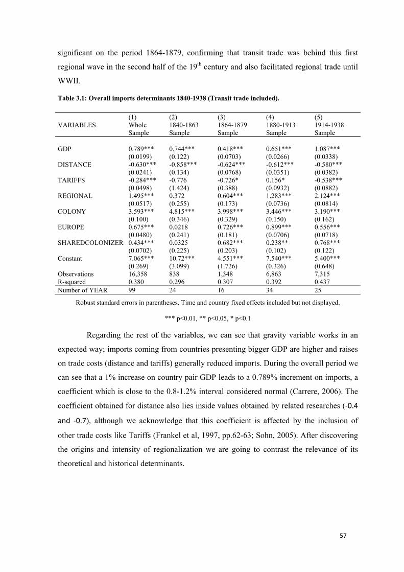
57
significant on the period 1864-1879, confirming that transit trade was behind this first
regional wave in the second half of the 19th century and also facilitated regional trade until
WWII.
Table 3.1: Overall imports determinants 1840-1938 (Transit trade included).
(1) (2) (3) (4) (5) VARIABLES Whole
Sample 1840-1863 Sample
1864-1879 Sample
1880-1913 Sample
1914-1938 Sample
GDP 0.789*** 0.744*** 0.418*** 0.651*** 1.087*** (0.0199) (0.122) (0.0703) (0.0266) (0.0338) DISTANCE -0.630*** -0.858*** -0.624*** -0.612*** -0.580*** (0.0241) (0.134) (0.0768) (0.0351) (0.0382) TARIFFS -0.284*** -0.776 -0.726* 0.156* -0.538*** (0.0498) (1.424) (0.388) (0.0932) (0.0882) REGIONAL 1.495*** 0.372 0.604*** 1.283*** 2.124*** (0.0517) (0.255) (0.173) (0.0736) (0.0814) COLONY 3.593*** 4.815*** 3.998*** 3.446*** 3.190*** (0.100) (0.346) (0.329) (0.150) (0.162) EUROPE 0.675*** 0.0218 0.726*** 0.899*** 0.556*** (0.0480) (0.241) (0.181) (0.0706) (0.0718) SHAREDCOLONIZER 0.434*** 0.0325 0.682*** 0.238** 0.768*** (0.0702) (0.225) (0.203) (0.102) (0.122) Constant 7.065*** 10.72*** 4.551*** 7.540*** 5.400*** (0.269) (3.099) (1.726) (0.326) (0.648) Observations 16,358 838 1,348 6,863 7,315 R-squared 0.380 0.296 0.307 0.392 0.437 Number of YEAR 99 24 16 34 25
Robust standard errors in parentheses. Time and country fixed effects included but not displayed.
*** p<0.01, ** p<0.05, * p<0.1
Regarding the rest of the variables, we can see that gravity variable works in an
expected way; imports coming from countries presenting bigger GDP are higher and raises
on trade costs (distance and tariffs) generally reduced imports. During the overall period we
can see that a 1% increase on country pair GDP leads to a 0.789% increment on imports, a
coefficient which is close to the 0.8-1.2% interval considered normal (Carrere, 2006). The
coefficient obtained for distance also lies inside values obtained by related researches (-0.4
and -0.7), although we acknowledge that this coefficient is affected by the inclusion of
other trade costs like Tariffs (Frankel et al, 1997, pp.62-63; Sohn, 2005). After discovering
the origins and intensity of regionalization we are going to contrast the relevance of its
theoretical and historical determinants.
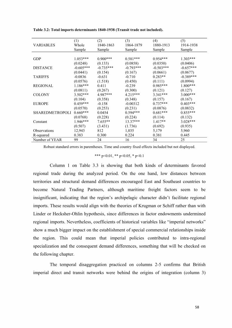
58
Table 3.2: Total imports determinants 1840-1938 (Transit trade not included).
(1) (2) (3) (4) (5) VARIABLES Whole
Sample 1840-1863 Sample
1864-1879 Sample
1880-1913 Sample
1914-1938 Sample
GDP 1.053*** 0.900*** 0.581*** 0.954*** 1.303*** (0.0248) (0.133) (0.0858) (0.0350) (0.0406) DISTANCE -0.605*** -0.735*** -0.793*** -0.503*** -0.657*** (0.0441) (0.154) (0.167) (0.0661) (0.0677) TARIFFS -0.0836 -0.631 -0.710 0.283** -0.389*** (0.0576) (1.518) (0.450) (0.111) (0.0994) REGIONAL 1.186*** 0.411 -0.239 0.985*** 1.800*** (0.0811) (0.267) (0.300) (0.121) (0.127) COLONY 3.502*** 4.987*** 4.215*** 3.341*** 3.000*** (0.104) (0.358) (0.348) (0.157) (0.167) EUROPE 0.459*** -0.158 -0.00312 0.737*** 0.403*** (0.0570) (0.253) (0.231) (0.0876) (0.0832) SHAREDMETROPOLI 0.660*** 0.0454 0.594*** 0.681*** 0.855*** (0.0768) (0.228) (0.224) (0.114) (0.132) Constant 1.946*** 7.655** 13.37*** 1.417** 3.028*** (0.507) (3.431) (1.736) (0.692) (0.935) Observations 12,943 812 1,035 5,179 5,960 R-squared 0.383 0.300 0.224 0.381 0.445 Number of YEAR 99 24 16 34 25
Robust standard errors in parentheses. Time and country fixed effects included but not displayed.
*** p<0.01, ** p<0.05, * p<0.1
Column 1 on Table 3.3 is showing that both kinds of determinants favored
regional trade during the analyzed period. On the one hand, low distances between
territories and structural demand differences encouraged East and Southeast countries to
become Natural Trading Partners, although maritime freight factors seem to be
insignificant, indicating that the region’s archipelagic character didn’t facilitate regional
imports. These results would align with the theories of Krugman or Schiff rather than with
Linder or Hecksher-Ohlin hypothesis, since differences in factor endowments undermined
regional imports. Nevertheless, coefficients of historical variables like “imperial networks”
show a much bigger impact on the establishment of special commercial relationships inside
the region. This could mean that imperial policies contributed to intra-regional
specialization and the consequent demand differences, something that will be checked on
the following chapter.
The temporal disaggregation practiced on columns 2-5 confirms that British
imperial direct and transit networks were behind the origins of integration (column 3)
59
supported by Chinese workers and investment on railway infrastructure.28 This is
complemented with the insignificance of trade costs (only tariffs harmed imports) and the
negative coefficient of demand complementarities. Later, after WWI, British relevance
decreased and regionalization was consolidated through the Japanese colonial networks and
their informal connections with the rest of the region (columns 4 and 5).29 The reduced
strength of the British Empire with the entrance of the 20th century is in line with (Jacks et
al.,2020) which also finds a reduced significance of distance coefficient in this period.
Moreover, overall results in column 1 demonstrate that the Japanese role was more
relevant than the British one in the determination of regional imports during the studied
century. This evidence could support those theories about superior impact and positive
legacy of the Japanese Empire on the development of conquered territories (Kohli, 1994),
although more recent literature suggests that Japan wasn’t different to European Empires
which prioritized their own benefit and missed a good opportunity for further developing
conquered territories (Booth, 2007a). In that aspect, the hypothetical use of colonies to
expand Japan’s industrial base could be the real progenitor of demand complementarities
demonstrated below, potentially explaining the superior coefficient presented by its
colonial networks.
Such debate will be addressed on the last two chapters of the thesis were we will
also explain the relevance that the construction of the South Manchurian railway had on
this process as derived from the high coefficient found on railway during interwar years
(column 5). Japanese supremacy was also supported by Chinese and other local merchants,
although on a lower extent compared with the period of British dominion. The rest of the
variables behaved as usual with economic size attracting regional imports, currency
appreciation facilitated imports, especially during years of Silver devaluation (Column 4)
and tariffs were not generally significant because most territories were influenced by the
British low tariff policies.
All in all, coefficients presented in column 1 suggest that historical variables like
imperial networks exercised a stronger impact in East and Southeast Asia special trading
relationships than economic determinants like demand complementarities, whose positive
28A parallel study has shown that the influence of Chinese diaspora was stronger on Southeast Asia than on the rest of the region. 29 Prior to 1896 the Japanese Empire was reduced to Japan mainland, so variables representing formal and informal imperial networks are exhausted by country fixed effects during 1840-1879.
60
coefficient indicate that those territories met the third criteria to be considered Natural
Trading Partners.
Nevertheless, we are putting together a Dummy and a continuous variable whose
coefficients are not comparable. To determine which variable played a bigger role, we have
constructed two different kinds of counterfactuals. In both cases, the absence of imperial
networks would generate higher reductions on regional imports than lack of demand
complementarities: On the first one, total regional imports in 1938 would have been 79%
lower than they were in reality in case no imperial networks were ever created (we assume
that each country’s total imports evolve at the same path as average imports from countries
with which it doesn’t share colonial ties), whereas they would have been 71% lower in case
there were no demand complementarities (each country’s imports are assumed to evolve at
the same rhythm as those from a set of countries whose GDP per capita doesn’t double the
reporter’s one). The contrast is more evident under the second counterfactual in which
rather than basing our estimates on sets of countries, we employ imports from an
independent country like Thailand for illustrating the absence of empires and imports from
the partner presenting the most similar GDP per capita for computing trade in the absence
of demand complementarities. Once more, absence of empires reduced total imports a 29%
and lack of demand complementarities reduced imports by just a 9%. Full explanations of
these estimations are found on Appendix A.
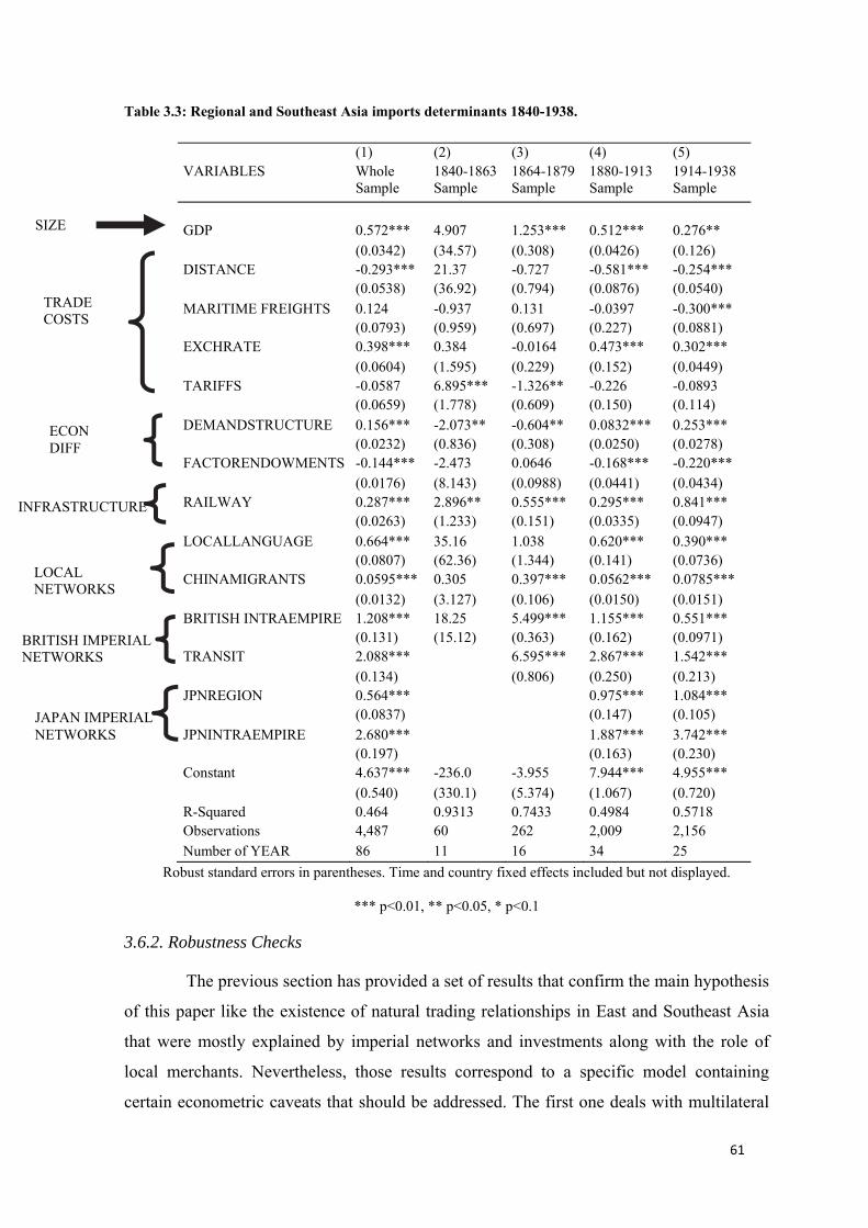
61
SIZE
TRADE COSTS
ECON DIFF
INFRASTRUCTURE
LOCAL NETWORKS
BRITISH IMPERIAL NETWORKS
JAPAN IMPERIAL NETWORKS
Table 3.3: Regional and Southeast Asia imports determinants 1840-1938.
Robust standard errors in parentheses. Time and country fixed effects included but not displayed.
*** p<0.01, ** p<0.05, * p<0.1
3.6.2. Robustness Checks
The previous section has provided a set of results that confirm the main hypothesis
of this paper like the existence of natural trading relationships in East and Southeast Asia
that were mostly explained by imperial networks and investments along with the role of
local merchants. Nevertheless, those results correspond to a specific model containing
certain econometric caveats that should be addressed. The first one deals with multilateral
(1) (2) (3) (4) (5) VARIABLES Whole
Sample 1840-1863 Sample
1864-1879 Sample
1880-1913 Sample
1914-1938 Sample
GDP 0.572*** 4.907 1.253*** 0.512*** 0.276** (0.0342) (34.57) (0.308) (0.0426) (0.126) DISTANCE -0.293*** 21.37 -0.727 -0.581*** -0.254*** (0.0538) (36.92) (0.794) (0.0876) (0.0540) MARITIME FREIGHTS 0.124 -0.937 0.131 -0.0397 -0.300*** (0.0793) (0.959) (0.697) (0.227) (0.0881) EXCHRATE 0.398*** 0.384 -0.0164 0.473*** 0.302*** (0.0604) (1.595) (0.229) (0.152) (0.0449) TARIFFS -0.0587 6.895*** -1.326** -0.226 -0.0893 (0.0659) (1.778) (0.609) (0.150) (0.114) DEMANDSTRUCTURE 0.156*** -2.073** -0.604** 0.0832*** 0.253*** (0.0232) (0.836) (0.308) (0.0250) (0.0278) FACTORENDOWMENTS -0.144*** -2.473 0.0646 -0.168*** -0.220*** (0.0176) (8.143) (0.0988) (0.0441) (0.0434) RAILWAY 0.287*** 2.896** 0.555*** 0.295*** 0.841*** (0.0263) (1.233) (0.151) (0.0335) (0.0947) LOCALLANGUAGE 0.664*** 35.16 1.038 0.620*** 0.390*** (0.0807) (62.36) (1.344) (0.141) (0.0736) CHINAMIGRANTS 0.0595*** 0.305 0.397*** 0.0562*** 0.0785*** (0.0132) (3.127) (0.106) (0.0150) (0.0151) BRITISH INTRAEMPIRE 1.208*** 18.25 5.499*** 1.155*** 0.551*** (0.131) (15.12) (0.363) (0.162) (0.0971) TRANSIT 2.088*** 6.595*** 2.867*** 1.542*** (0.134) (0.806) (0.250) (0.213) JPNREGION 0.564*** 0.975*** 1.084*** (0.0837) (0.147) (0.105) JPNINTRAEMPIRE 2.680*** 1.887*** 3.742*** (0.197) (0.163) (0.230) Constant 4.637*** -236.0 -3.955 7.944*** 4.955*** (0.540) (330.1) (5.374) (1.067) (0.720) R-Squared 0.464 0.9313 0.7433 0.4984 0.5718 Observations 4,487 60 262 2,009 2,156 Number of YEAR 86 11 16 34 25
62
resistance to trade since the inclusion of fixed effects is not enough for controlling it. A first
reason is that importer and exporter fixed effects must be time varying and in order to do
that we are going to interact them with time fixed effects on the first column of table 3.4
(Yang & Martínez-Zarzoso, 2014). However, there is still a set of authors claiming that
multilateral resistance is only controlled after incorporating structural characteristics
(Anderson & Van Wincoop, 2003), so we reconcile those approaches in column 2 by
estimating the model by PPML but incorporating country and time fixed effects (Fally,
2015).
Another methodological concern we have to address is the treatment of zero trade
flows. As explained before, the impossibility of determining if a flow was really zero or
unknown forced us to not include them. Anyway, the belief that those flows can provide
interesting information persuaded us to include them on the PPML estimation due to
method’s suitability (Santos Silva & Tenreyro, 2006). Nevertheless, we appreciate a
possible excess of zeros, since they represent more than half total flows. For that reason, in
column 3 we show the results estimating the model by Zero-inflated Poisson (ZIP) in order
to solve this problem (Martin & Pham, 2015).
What can be appreciated is that results obtained on section 6.1 still hold under
these new specifications: GDP attracts imports, trade costs generally undermine them and
demand differences favored regional trade, although on a lower extent than imperial
networks (the only exceptions are British non-transit networks that become negative in
column 2). Finally, investments in railway infrastructure and the diaspora of local
merchants positively attracted regional trade although they are less significant.30
Nevertheless, it could be the case that changes in sample composition might be the
true drivers of results appreciated in table 3.3. To demonstrate that the incorporation of six
new countries (including Japan and its newly created empire) to the sample doesn’t affect
the main conclusions of the paper, table 3.5 shows results keeping the same seven-country
sample for the whole period.31 Results show that our main conclusions are not driven by
30 On appendix A we also control for multilateral resistance on the equation studying total trade determinants and results are maintained, reasserting the special intra-regional trade intensity enjoyed by East and Southeast Asia partners. 31 The regression is done using the seven countries included on the 1864-1879 sample for every period. We could use the four countries available on 1840-1863 but they are not representative of total region’s imports since they only account for 22% of the total, whereas the chosen sample is responsible for 66% of total regional imports.
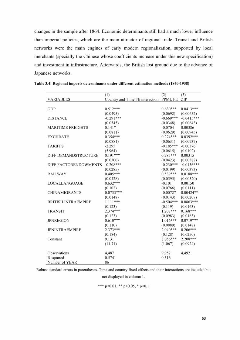
63
changes in the sample after 1864. Economic determinants still had a much lower influence
than imperial policies, which are the main attractor of regional trade. Transit and British
networks were the main engines of early modern regionalization, supported by local
merchants (specially the Chinese whose coefficients increase under this new specification)
and investment in infrastructure. Afterwards, the British lost ground due to the advance of
Japanese networks.
Table 3.4: Regional imports determinants under different estimation methods (1840-1938)
(1) (2) (3) VARIABLES Country and Time FE interaction PPML FE ZIP GDP 0.512*** 0.630*** 0.0413*** (0.0495) (0.0692) (0.00652) DISTANCE -0.291*** -0.669*** -0.0415*** (0.0545) (0.0348) (0.00643) MARITIME FREIGHTS 0.141* -0.0704 0.00386 (0.0811) (0.0629) (0.00945) EXCHRATE 0.354*** 0.274*** 0.0392*** (0.0881) (0.0631) (0.00937) TARIFFS -2.295 -0.185*** -0.00376 (5.964) (0.0615) (0.0102) DIFF DEMANDSTRUCTURE 0.191*** 0.285*** 0.00315 (0.0300) (0.0423) (0.00382) DIFF FACTORENDOWMENTS -0.208*** -0.230*** -0.0136*** (0.0285) (0.0199) (0.00373) RAILWAY 0.405*** 0.539*** 0.0188*** (0.0428) (0.0595) (0.00520) LOCALLANGUAGE 0.632*** -0.101 0.00150 (0.102) (0.0766) (0.0111) CHINAMIGRANTS 0.0733*** -0.00727 0.00424** (0.0148) (0.0143) (0.00207) BRITISH INTRAEMPIRE 1.111*** -0.504*** 0.0863*** (0.123) (0.119) (0.0163) TRANSIT 2.374*** 1.207*** 0.168*** (0.123) (0.0983) (0.0163) JPNREGION 0.610*** 1.016*** 0.0719*** (0.110) (0.0889) (0.0148) JPNINTRAEMPIRE 2.373*** 2.040*** 0.206*** (0.184) (0.128) (0.0250) Constant 9.131 8.056*** 2.208*** (11.71) (1.067) (0.0924) Observations 4,487 9,952 4,492 R-squared 0.5741 0.516 Number of YEAR 86
Robust standard errors in parentheses. Time and country fixed effects and their interactions are included but
not displayed in column 1.
*** p<0.01, ** p<0.05, * p<0.1
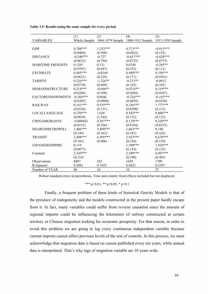
64
Table 3.5: Results using the same sample for every period.
(1) (2) (4) (5) VARIABLES Whole Sample 1864-1879 Sample 1880-1913 Sample 1913-1938 Sample GDP 0.708*** 1.253*** 0.373*** -0.913*** (0.0404) (0.308) (0.0562) (0.152) DISTANCE -0.240*** -0.727 -0.657*** -0.428*** (0.0632) (0.794) (0.0725) (0.0757) MARITIME FREIGHTS 0.126* 0.131 0.0748 -0.285** (0.0707) (0.697) (0.253) (0.111) EXCHRATE 0.405*** -0.0164 0.490*** 0.356*** (0.0621) (0.229) (0.171) (0.0301) TARIFFS 0.226*** -1.326** -0.331** -0.0912 (0.0778) (0.609) (0.162) (0.102) DEMANDSTRUCTURE 0.214*** -0.604** 0.0716** 0.319*** (0.0204) (0.308) (0.0284) (0.0347) FACTORENDOWMENTS -0.268*** 0.0646 -0.226*** -0.183*** (0.0305) (0.0988) (0.0459) (0.0338) RAILWAY 0.181*** 0.555*** 0.336*** 1.777*** (0.0236) (0.151) (0.0390) (0.123) LOCALLANGUAGE 0.270*** 1.038 0.543*** 0.806*** (0.0858) (1.344) (0.132) (0.132) CHINAMIGRANTS -0.000942 0.397*** 0.118*** 0.220*** (0.0153) (0.106) (0.0184) (0.0155) SHAREDMETROPOLI 1.406*** 5.499*** 1.663*** 0.190 (0.149) (0.363) (0.181) (0.162) TRANSIT 2.408*** 6.595*** 2.923*** 0.678*** (0.183) (0.806) (0.334) (0.159) JAPANESEEMPIRE 0.119 1.390*** 1.918*** (0.0877) (0.134) (0.125) Constant 2.245*** 2.299*** 6.097*** (0.214) (0.190) (0.403) Observations 4487 262 1650 1709 R-Squared 0.5081 0.7433 0.4423 0.5397 Number of YEAR 86 16 34 25
Robust standard errors in parentheses. Time and country fixed effects included but not displayed.
*** p<0.01, ** p<0.05, * p<0.1
Finally, a frequent problem of these kinds of historical Gravity Models is that of
the presence of endogeneity and the models constructed in the present paper hardly escape
from it. In fact, many variables could suffer from reverse causation since the amount of
regional imports could be influencing the kilometers of railway constructed at certain
territory or Chinese migration looking for economic prosperity. For that reason, in order to
avoid this problem we are going to lag every continuous independent variable because
current imports cannot affect previous levels of the rest of controls. In this process, we must
acknowledge that migration data is based on census published every ten years, while annual
data is interpolated. That’s why lags of migration variable are 10 years wide.
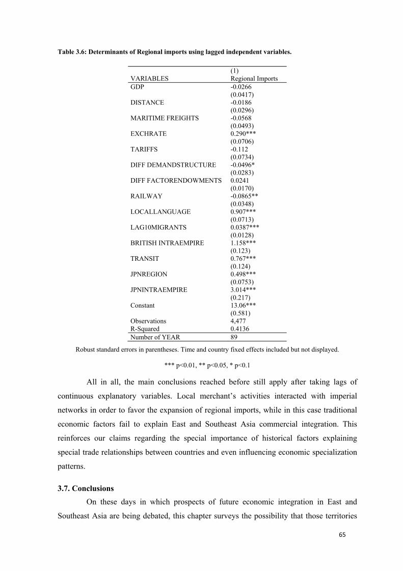
65
Table 3.6: Determinants of Regional imports using lagged independent variables.
(1) VARIABLES Regional Imports GDP -0.0266 (0.0417) DISTANCE -0.0186 (0.0296) MARITIME FREIGHTS -0.0568 (0.0493) EXCHRATE 0.290*** (0.0706) TARIFFS -0.112 (0.0734) DIFF DEMANDSTRUCTURE -0.0496* (0.0283) DIFF FACTORENDOWMENTS 0.0241 (0.0170) RAILWAY -0.0865** (0.0348) LOCALLANGUAGE 0.907*** (0.0713) LAG10MIGRANTS 0.0387*** (0.0128) BRITISH INTRAEMPIRE 1.158*** (0.123) TRANSIT 0.767*** (0.124) JPNREGION 0.498*** (0.0753) JPNINTRAEMPIRE 3.014*** (0.217) Constant 13.06*** (0.581) Observations 4,477 R-Squared 0.4136 Number of YEAR 89
Robust standard errors in parentheses. Time and country fixed effects included but not displayed.
*** p<0.01, ** p<0.05, * p<0.1
All in all, the main conclusions reached before still apply after taking lags of
continuous explanatory variables. Local merchant’s activities interacted with imperial
networks in order to favor the expansion of regional imports, while in this case traditional
economic factors fail to explain East and Southeast Asia commercial integration. This
reinforces our claims regarding the special importance of historical factors explaining
special trade relationships between countries and even influencing economic specialization
patterns.
3.7. Conclusions On these days in which prospects of future economic integration in East and
Southeast Asia are being debated, this chapter surveys the possibility that those territories
66
are Natural Trading Partners conditioned by historical and institutional settings. Through
the reconstruction of almost a century of bilateral imports in East and Southeast Asia,
together with other relevant economic and trade cost variables, we can conclude that before
WWII those territories met every criterion that according to this article grant the label of
Natural Trading Partners. Following the existing literature, this phenomenon would
enhance welfare effects generated by the subsequently established Free Trade Area and
Customs Unions, so deepening regional integration would be positive for the economic
development of East and Southeast Asia.
The reasons behind this regional commercial intensity respond to economic factors
traditionally explained by the Natural Trading Partners’ literature like GDP growth,
reductions in trade costs or demand complementarities between territories. However, those
features which are still present today, only complemented the effects of certain historical
events which according to this research were the main characters of special trading
relationships between territories and should be incorporated to the natural trading partner’s
debate. Regional trade during the British colonization period was already high as a
remainder of regional networks created during the Age of commerce (15th-17th Centuries).
Nonetheless, it was based on commodity trade between China and India and diverted
outside the region as a first reaction to European conquest.
After that, the process of regional integration in East and Southeast Asia
experienced a big push related with the colonization from the British Empire which by the
1860s got rid of economic characteristics of the region in order to consolidate a dense
commercial infrastructure supported by European style institutions and organized around
Singapore and Hong Kong entrepôts. This network was managed by Chinese merchants
whose number expanded all over the region during the second half of the 19th century and
got rid of their commercial abilities and market knowledge. On a parallel way, the second
half of the nineteenth century also saw an intensification of direct connections between
British colonies confirming British supremacy on Southeast Asian regional integration.
Transit networks gained popularity until the entrance of the 20th century when they
started to shrink. However, the following period brought an intensification of regional
trade, which was possible thanks to the Japanese imperial and industrial policies that
strongly intensified trade between the mainland and its colonies, supported also by
consolidated local networks. In fact, our results suggest that the overall influence of the
Japanese Empire over East and Southeast Asian regional integration was bigger than the
67
British. This could either mean that Japanese developmental capacity was superior to that
of European Empires or that the use of neighbor territories to support its own
industrialization shaped the intra-regional specialization pattern exposed by the literature
and demonstrated on this chapter. For that reason the last two chapters will deeply analyze
the relationship between Japanese industrial and imperial expansions and the cooperation
mechanisms between institutions leading the process.
All in all, this chapter conceptualizes the previously found special trading
relationships between East and Southeast Asia partners, cataloguing them as Natural
Trading Partners. In order to do that, we collect three different criteria that the literature
presents as potential evidence confirming the existence of special trading relationships.
This set of criteria means a good legacy since they can help future researchers in their quest
to identify Natural Trading Partners. In addition, it adds evidence of the pivotal role played
by certain historical events at the roots of special trade relationships between territories,
which survive until nowadays supported by certain demand complementarities that were
also influenced by historical institutional settings. This is demonstrated through the analysis
of the commercial activity of empires and their interactions with merchants inside the
region.
68
CHAPTER 3: TRADE IN THE SHADOW OF POWER: JAPANESE 4INDUSTRIAL EXPORTS IN THE INTERWAR YEARS
4.1. Introduction The previous chapter has demonstrated the relevance that imperial activity had on
the regionalization of East and Southeast Asia before the Second World War. Specifically,
it has suggested that the raise of empires favored the industrialization of certain territories,
favoring an intra-regional specialization that has maintained high levels of trade between
neighbors until nowadays. Among the empires operating at the region, the Japanese was the
most influential according to our results which leave an open debate regarding the true
nature of that influence: was it developmental in nature? Or simply used its colonies to
sustain its incipient industrialization?
On the present chapter we will demonstrate that Japanese newly created empire was
very efficient in developing a peculiar imperial trade in the shadow of power throughout
East and Southeast Asia in conjunction with a more aggressive imperial regional policy
through conquest (Findlay and O’Rourke, 2007; Garfinkel. et al, 2012).32 In order to do
that, we will survey the links between Japanese imperial settings and its industrial
expansion.
Of course, such protectionist and imperial policies in the international economy
were not confined to Japan during the interwar years. Britain, for example, instituted a
system of imperial preference with its colonies and mandated territories in the framework
of the Commonwealth at the Ottawa Conference of 1932. Germany, having neither
complete customs autonomy as a result of the Treaty of Versailles nor an informal or
formal geographically contiguous empire, fostered a complex and oppressive system of
clearing arrangements with Central European and Balkan neighbors even before the Nazi
regime. Trade barriers rose all over the world, and the most prominent economies
abandoned global multilateral free trade policies in favor of commercial exchanges within
their empires. Fragmented regional or global empires, both formal and informal, were
reconciled ambivalently with bilateral agreements that included tariffs, quotas, import
licenses, exchange controls, barter and clearing agreements, and other protectionist policies.
32 Trade has taken place in the shadow of power for all almost all of recorded human history. We argue that power matters for trade, as critically as the traditional determinants of endowments, preferences, and technology.
69
Japanese imperialist history is well known. During the Meiji Period (1868-1912),
Japan annexed Ezo (Hokkaidô) in 1869, the Ryûkyû Islands in 1879, Taiwan in 1895, and
Korea between 1905 and 1910. Until the 1920s, Japan allowed free access to foreigners in
their occupied territories and only then created a real imperial bloc in conjunction with an
escalation of domestic trade barriers. By the early 1930s, Japan already had consolidated a
decisive policy of protectionism and an empire-wide regional market with trading
privileges for Japanese industrial firms. Tariff policy in the Japanese occupied territories
privileged Japan or was assimilated into Japan’s tariff system. Korea adopted Japan’s tariff
system in 1923, as would Manchuria ten years later upon the territory’s separation from the
Chinese customs system, allowing preferential access for Japanese manufactures (Chase,
2005, pp. 62-64).
Along with the protectionist backlash experienced around the world, the
development of the Japanese Imperial Bloc in the interwar years also responded to the
demand of Zaibatsu heavy industrialists for exclusive access to broader markets and the
military’s desire to control vital strategic materials, such as oil, rubber, and iron ore. These
interests were consolidated by the conquest of Manchuria as well as the regional expansion
of commercial and investment networks in other areas later called ‘The Greater East Asia
Co-Prosperity Sphere’(Fletcher, 1989, pp. 144-50).33
This chapter will assess how much of the development of Japan’s industrial exports
during the interwar years was based on this combination of imperial soft power and its
policy of aggressive conquest in East and Southeast Asia. Specifically, we examined
whether the expansion of high-skill exports to Japan’s neighbors can be better explained by
improvements in productivity or by imperial policy variables. For that purpose, we
ascertained the mechanisms that linked Japanese imperial activity to its exports. We
defined the ‘Japanese Empire’ (JE) as including both previously occupied colonies and
what we call ‘Future Conquests’—those countries or polities in the region that was of
strategic interest for Japan, as proven by their occupation between 1941 and 1945.34 We
argue that Japan exerted regional commercial influence through the creation of 33 Similar to the term ‘Third Reich’, this was one of a number of slogans and concepts used in the justification of Japanese aggression in East Asia from the 1930s through the end of World War II. 34 Formal colonies include: Taiwan, Korea, Kwantung Leased Territory, Manchuria (1932), and China (1938). The “Future Conquests” are: Manchuria (1912-1929), China (1912-1932), Thailand, Burma, French Indochina, Hong Kong, Dutch East Indies, British Borneo and Sarawak, New Guinea, British Malaya (including Singapore), the Philippine Islands, and the Solomon, Gilbert, and Marshall Islands in the Pacific. For more information on the main features of the colonies and future conquest territories, see Appendix B.
70
transnational business and investment networks and cultural diplomacy, which facilitated
commercial information and created merchant community trust in the region. This soft
power thrust, combined with a more traditional imperial policy of military conquest, was
decisive for the consolidation of a new stage of industrial modernization during the 1930s.
To study the determinants of Japanese exports, we digitized Japanese commercial
returns (Annual Returns of the Foreign Trade of the Empire of Japan) for several
benchmark years (1912, 1915, 1925, 1929, 1932, and 1938) and created an exhaustive
granular product data set of exports by country of destination for each of the chosen years.
Using this data set, we analyzed the main determinants of Japanese exports by skill bias,
focusing mainly in East and Southeast Asia, and comparing them with Japan’s export
performance with the rest of the world. The methodology employed for that purpose is in
line with extensive and intensive marginal Gravity Models. The specification used in this
paper includes the usual factor endowments, demand structure and trade cost variables
(such as tariffs, transport cost, and political factors). The basic Gravity Model is
augmented by a new series of freight factors from Japan to respective destinations
(disaggregated by product line), commercial diplomacy appointments, and dependency
relationships with Japan (occupation, annexation, colonization, and lease) before and after
1932.
Japan’s second stage of industrial expansion in the interwar years was mainly based
on exports of high-skill manufactured goods, and fostered by the imperial shadow of
power. The literature in Japanese industrialization in the interwar years describes heavy
industries’ interests in gaining access to broader markets to increase economies of scale and
reduce unit costs. There exists no quantitative evidence that proves the success of those
mechanisms in expanding exports to regional markets. In this paper, we use a new data set
and other empirical evidence to answer the following questions. First, were improvements
in Japanese relative productivity or comparative advantage the main drivers of its industrial
export expansion? Or, conversely, was trade expansion driven mainly by administrative
enforcement related to imperial privileges? Our hypothesis, in short, is that the Imperial
Bloc was a much stronger driver of Japanese export expansion than the conventional
reduction of trade costs or improvements in relative productivity. Japan reacted to the
interwar context of global commercial disintegration with aggressive import substitution
and an imperial strategy to foster exports of manufactures, as did Britain and Germany in
other ways.
71
4.2. Regional Trade and the Japanese Empire What mechanisms link imperial expansion with increases in exports towards a
determined region? Either international context or domestic industrial policy helps to
understand the Japanese compound interest in East and Southeast Asia, and its
expansionary policy of trade in the shadow of power (Garfinkel et al., 2012; Eichengreen &
Irwin, 1995).
The British commercial relationship with its colonies after 1932, specially with
India, with Britain turning away from almost a century of free trade policy, is probably the
most well-known case study of the use of trade in the shadow of power. However, most of
the literature presents the Commonwealth Trade Bloc as being less discriminatory towards
outsiders than initially suggested by the text of the Ottawa Agreement of July 1932.
Nevertheless, the alliance succeeded in implementing preferential access by Britain to the
dominions and vice versa. Great Britain imposed a general tariff of 10% for manufacturers
and other goods, increasing the empire’s share of British imports by approximately 70%
between 1930 and 1933 (De Bromhead et al., 2019). The British partially closed down
Indian, African, and other imperial markets, into which some competitive Japanese textiles
had expanded since the end of the 19th century. Indeed, the Manchurian invasion of 1931
preceded Ottawa, but this international context influenced Japanese expansionist
commercial policy towards its empire during the 1930s nevertheless (Cain & Hopkins,
1980; Gallagher & Robinson, 1953)35
The Third Reich followed other practices emulating strategies of trade in the
shadow of power during this period, and Germany consolidated its imperial ambitions in
the Balkans and Central Europe during the Nazi regime. Germany used political
enforcement on their neighbors to guarantee those primary and mineral resources necessary
for geostrategic military considerations (Milward, 1981; Ritschl, 2001). During the 1930s,
German trade facilitated bilateral clearing agreements, mainly signed with countries in
Central and Southeastern Europe, but also in South America. Under this new regime,
German acquisition credited against purchases by foreigners in German markets (Neal,
1979 ; Gross, 2016).
The case of Japanese imperial policy is peculiar not only because it predated World
War I but also, most importantly, because it was advanced by a relatively poor developing
35 (See discussion in Appendix B).
72
country and restricted to a regional framework (Matsusaka, 2007). In addition to its formal
colonies, Japanese economic agents built a severe business and political networks with
other countries in East and Southeast Asia. The motive behind this activity was mostly
commercial as it will manifest in the subsequent military occupations, during the Second
World War, of the vast majority of Southeast Asian territories.
The literature in Japanese colonialism had mainly focused on colonial trade links
with Japan after occupation, although the literature also observed that the Japanese
demonstrated their interest in Korean markets when they forced the opening of Korean
ports and signed the unequal commercial treaties of 1876 (Kublin, 1952;Duus, 1998). After
the occupation in 1905, colonial trade policy was directed by Tokyo to ensure the safe
supply of foodstuffs and raw materials to Japan and to guarantee a market for Japanese
manufacturers. This imperial policy industrialization after the global rise of protectionism
following the Great Depression. Japan pursued growth with an empire-wide economic
strategy. The annexation of Manchuria in 1931 and the adoption of an import substitution
strategy signaled the beginning of Japanese planned industrialization within its colonies
(Kohli, 1994). This strategy generated a significant increase in the production of high-skill
manufactures, like steel for rail construction and machinery that was directed mainly
towards the Japanese domestic market but was also exported to foster Korean
industrialization (Chenery, et al., 1962).
Another mechanism granting Japanese exports access to its colonies was the fact
that the Taiwanese and Korean economies were integrated with Japan by the removal of
trade barriers and the introduction of fixed exchange rates. Additionally, Japan invested in
the transport and communication infrastructure and imposed the assimilation of the
Japanese language, which further reduced transaction costs. The commercial exchange was
further facilitated by private sector investment and the establishment of Japanese
companies (in fact, 97% of corporations in Korea were owned by Japanese) along with the
opening of Japanese financial institutions like the Bank of Chosen (Aziz, 2012).
The above scenario is what happened in the better-known Japanese colonies.
However, the Japanese Empire also included two other territories, which provide relevant
examples. The most pertinent case was Manchuria, which became a Japanese puppet state
in 1931, and was considered an additional Japanese colony. The Japanese had a presence in
Manchuria before annexation, however, and this presence became more pronounced during
the First World War. Japanese economic activity consisted mainly in the establishment of
73
large companies (such as banks, similar to the Bank of Chosen), of raising FDI flows, and
of increasing Japanese private investment in transport infrastructure (aided by government
subsidies). These activities permitted the Japanese to dodge most trade barriers and to
reduce other transaction costs (Bix, 1972; Encarnation, 1999). Historiography suggests that
Japanese investment before 1930 fostered Manchurian industrialization. After the
annexation, the Japanese created in Manchuria a puppet state with the primary objective of
influencing the direction and materials necessary for the rapid industrialization of the
region (Kublin, 1959; Duus, 1998).
The second relevant case is that of the Kwantung Leased Territory, commonly
presented as the most representative example of the ‘conquest by railway’ strategy. In
1906, after acquiring the territory during the Russo-Japanese War, the Japanese
Government founded the South Manchurian Railway Company (SMR) to operate the
railway network left by the Russians. By 1930 it had become the largest joint-stock
company operating in the Japanese Empire. The company diversified in activities other
than railway construction, but it remained a steady source of demand for Japanese goods
like iron, machinery, and transport equipment used for mining, manufacturing, and railway
construction (IYenaga, 1912).
The example of Manchuria illustrates the peculiar nature of the Japanese imperial
shadow of power: a process in which Japan established economic links with neighboring
territories as a demonstration of interest or announcement of future military occupation. We
follow this historical case to justify the inclusion of a sample of countries and polities, prior
occupation during WWII (‘future conquest’), as part of Japan’s informal empire. It is worth
distinguishing between former European colonies and other territories. In the old case,
Japanese investment was severely restricted by Europeans, whereas in the latter, Japanese
investment diversification permitted an expansion of commercial relations.
China was the country in which Japan had stronger economic penetration. Japanese
Zaibatsu (leading industrial conglomerates) and banks characterized Japan’s presence and
served to elude trade barriers and to reduce transaction costs (Howe, 1999; Osterhammel,
1986). The operation of Japanese economic interests was reflected not only in Japanese
exports to China but also was related to Japanese military campaigns in its neighboring
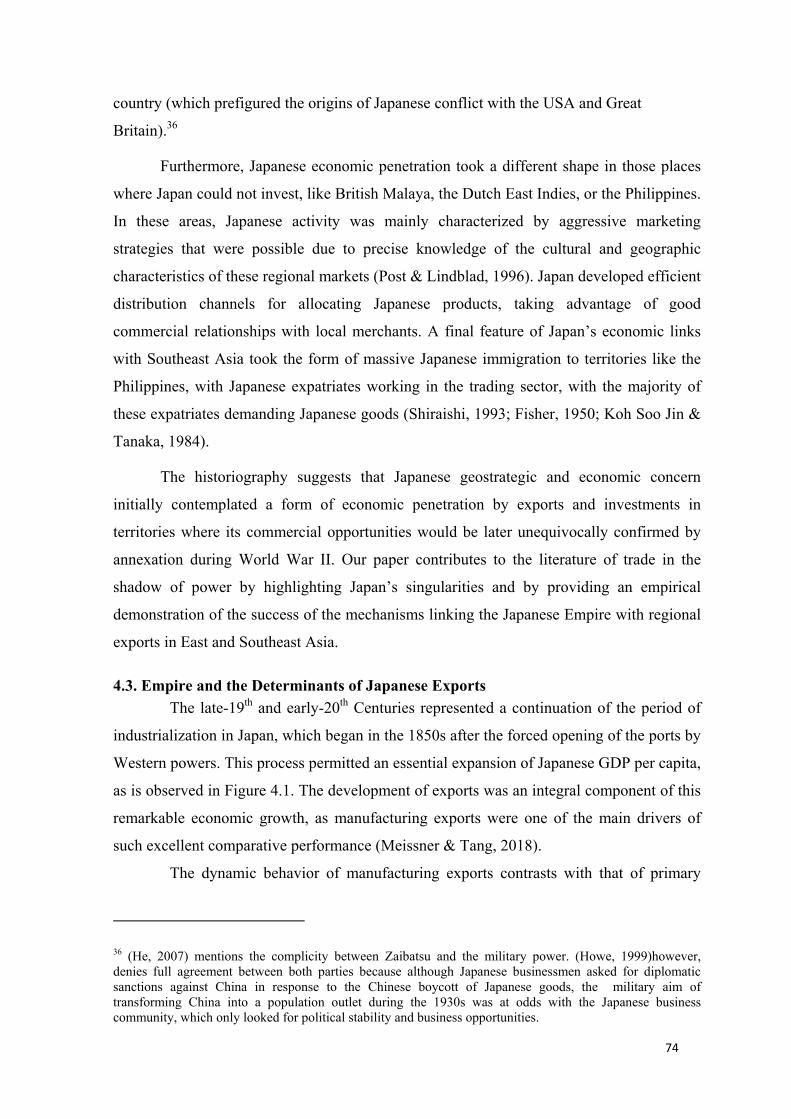
74
country (which prefigured the origins of Japanese conflict with the USA and Great
Britain).36
Furthermore, Japanese economic penetration took a different shape in those places
where Japan could not invest, like British Malaya, the Dutch East Indies, or the Philippines.
In these areas, Japanese activity was mainly characterized by aggressive marketing
strategies that were possible due to precise knowledge of the cultural and geographic
characteristics of these regional markets (Post & Lindblad, 1996). Japan developed efficient
distribution channels for allocating Japanese products, taking advantage of good
commercial relationships with local merchants. A final feature of Japan’s economic links
with Southeast Asia took the form of massive Japanese immigration to territories like the
Philippines, with Japanese expatriates working in the trading sector, with the majority of
these expatriates demanding Japanese goods (Shiraishi, 1993; Fisher, 1950; Koh Soo Jin &
Tanaka, 1984).
The historiography suggests that Japanese geostrategic and economic concern
initially contemplated a form of economic penetration by exports and investments in
territories where its commercial opportunities would be later unequivocally confirmed by
annexation during World War II. Our paper contributes to the literature of trade in the
shadow of power by highlighting Japan’s singularities and by providing an empirical
demonstration of the success of the mechanisms linking the Japanese Empire with regional
exports in East and Southeast Asia.
4.3. Empire and the Determinants of Japanese Exports The late-19th and early-20th Centuries represented a continuation of the period of
industrialization in Japan, which began in the 1850s after the forced opening of the ports by
Western powers. This process permitted an essential expansion of Japanese GDP per capita,
as is observed in Figure 4.1. The development of exports was an integral component of this
remarkable economic growth, as manufacturing exports were one of the main drivers of
such excellent comparative performance (Meissner & Tang, 2018).
The dynamic behavior of manufacturing exports contrasts with that of primary
36 (He, 2007) mentions the complicity between Zaibatsu and the military power. (Howe, 1999)however, denies full agreement between both parties because although Japanese businessmen asked for diplomatic sanctions against China in response to the Chinese boycott of Japanese goods, the military aim of transforming China into a population outlet during the 1930s was at odds with the Japanese business community, which only looked for political stability and business opportunities.
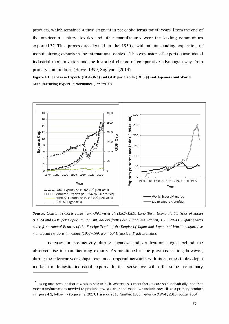
75
products, which remained almost stagnant in per capita terms for 60 years. From the end of
the nineteenth century, textiles and other manufactures were the leading commodities
exported.37 This process accelerated in the 1930s, with an outstanding expansion of
manufacturing exports in the international context. This expansion of exports consolidated
industrial modernization and the historical change of comparative advantage away from
primary commodities (Howe, 1999; Sugiyama,2013). Figure 4.1: Japanese Exports (1934-36 $) and GDP per Capita (1913 $) and Japanese and World Manufacturing Export Performance (1953=100)
Source: Constant exports come from Ohkawa et al. (1967-1989) Long Term Economic Statistics of Japan
(LTES) and GDP per Capita in 1990 Int. dollars from Bolt, J. and van Zanden, J. L. (2014). Export shares
come from Annual Returns of the Foreign Trade of the Empire of Japan and Japan and World comparative
manufacture exports in volume (1953=100) from UN Historical Trade Statistics.
Increases in productivity during Japanese industrialization lagged behind the
observed rise in manufacturing exports. As mentioned in the previous section; however,
during the interwar years, Japan expanded imperial networks with its colonies to develop a
market for domestic industrial exports. In that sense, we will offer some preliminary 37 Taking into account that raw silk is sold in bulk, whereas silk manufactures are sold individually, and that most transformations needed to produce raw silk are hand-made, we include raw silk as a primary product in Figure 4.1, following (Sugiyama, 2013; Francks, 2015; Smitka, 1998; Federico &Wolf, 2013; Souza, 2004).
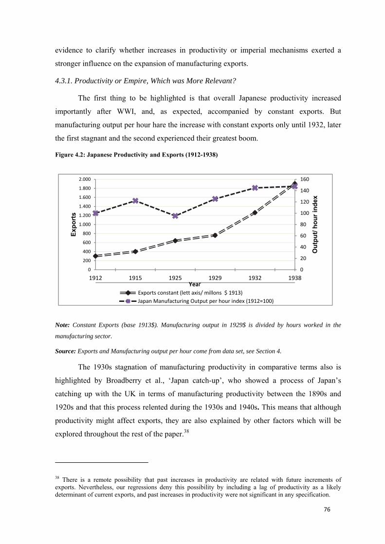
76
evidence to clarify whether increases in productivity or imperial mechanisms exerted a
stronger influence on the expansion of manufacturing exports.
4.3.1. Productivity or Empire, Which was More Relevant?
The first thing to be highlighted is that overall Japanese productivity increased
importantly after WWI, and, as expected, accompanied by constant exports. But
manufacturing output per hour hare the increase with constant exports only until 1932, later
the first stagnant and the second experienced their greatest boom.
Figure 4.2: Japanese Productivity and Exports (1912-1938)
Note: Constant Exports (base 1913$). Manufacturing output in 1929$ is divided by hours worked in the
manufacturing sector.
Source: Exports and Manufacturing output per hour come from data set, see Section 4.
The 1930s stagnation of manufacturing productivity in comparative terms also is
highlighted by Broadberry et al., ‘Japan catch-up’, who showed a process of Japan’s
catching up with the UK in terms of manufacturing productivity between the 1890s and
1920s and that this process relented during the 1930s and 1940s. This means that although
productivity might affect exports, they are also explained by other factors which will be
explored throughout the rest of the paper.38
38 There is a remote possibility that past increases in productivity are related with future increments of exports. Nevertheless, our regressions deny this possibility by including a lag of productivity as a likely determinant of current exports, and past increases in productivity were not significant in any specification.
0
20
40
60
80
100
120
140
160
0
200
400
600
800
1.000
1.200
1.400
1.600
1.800
2.000
1912 1915 1925 1929 1932 1938
Out
put/
hour
inde
x
Expo
rts
YearExports constant (lett axis/ millons $ 1913)Japan Manufacturing Output per hour index (1912=100)
77
On the other hand, Figure 4.3 shows that during the period of the faster growth of
Japanese manufacturing exports, the main destinations of these exports were within the
Japanese sphere of influence. More than 50% of exports after WWI went to territories
within this sphere where we include both colonies receiving the majority of manufacturing
exports and regions in Southeast Asia occupied during WWII. Further, these territories’
share of Japanese exports rose faster than for destinations outside of Japan’s sphere of
influence during the 1930s, reaching 73% of the total in 1938.
Figure 4.3: Japanese Manufacturing Exports by Region (1912-1938) (%)
Note: The remaining share of 100% corresponds to poor countries outside Asia.
Source: Annual Return of Trade for the Empire of Japan (various years).
Indeed, the international context in the interwar years had changed drastically,
especially after the Great Depression, and international markets increase manufacturing
trade barriers and conditioned the creation of new regional trade blocs. What happened in
the Indian market, where Japan had increased its share of textile exports in competition
with Britain, is a clear example of the trade diversion forced by these policies. Japan was
forced to retreat from those territories after the Commonwealth’s Trade Bloc policy,
adopted after the 1932 Ottawa conference, raised tariffs (for an extended discussion of this
point, see Appendix B).
Japan’s remarkable success in manufacturing exports during 1932-38 is not
comparable to any other country’s experience during the period (see Figure 4.1). Evidence
of improvements in productivity does not explain such success. We think this success is
principally determined by the reinforced bias of manufactures towards countries under
63%47%
65% 63% 56%73%
10%28%
17% 18% 24%11%
26% 24% 14% 13% 11% 8%
0%10%20%30%40%50%60%70%80%90%
100%
1912 1915 1925 1929 1932 1938
% S
hare
Year
% Rich Countries %Other Asia and Pacific % Imperial
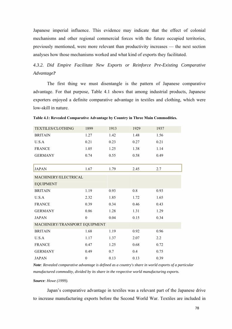
78
Japanese imperial influence. This evidence may indicate that the effect of colonial
mechanisms and other regional commercial forces with the future occupied territories,
previously mentioned, were more relevant than productivity increases — the next section
analyses how those mechanisms worked and what kind of exports they facilitated.
4.3.2. Did Empire Facilitate New Exports or Reinforce Pre-Existing Comparative
Advantage?
The first thing we must disentangle is the pattern of Japanese comparative
advantage. For that purpose, Table 4.1 shows that among industrial products, Japanese
exporters enjoyed a definite comparative advantage in textiles and clothing, which were
low-skill in nature.
Table 4.1: Revealed Comparative Advantage by Country in Three Main Commodities.
TEXTILES/CLOTHING 1899 1913 1929 1937
BRITAIN 1.27 1.42 1.48 1.56
U.S.A 0.21 0.23 0.27 0.21
FRANCE 1.05 1.25 1.38 1.14
GERMANY 0.74 0.55 0.58 0.49
JAPAN
1.67 1.79 2.45
2.7
MACHINERY/ELECTRICAL
EQUIPMENT
BRITAIN 1.19 0.93 0.8 0.93
U.S.A 2.32 1.85 1.72 1.65
FRANCE 0.39 0.34 0.46 0.43
GERMANY 0.86 1.28 1.31 1.29
JAPAN 0 0.04 0.15 0.34
MACHINERY/TRANSPORT EQUIPMENT
BRITAIN 1.68 1.19 0.92 0.96
U.S.A 1.17 1.37 2.07 2.2
FRANCE 0.47 1.25 0.68 0.72
GERMANY 0.49 0.7 0.4 0.75
JAPAN 0 0.13 0.13 0.39
Note: Revealed comparative advantage is defined as a country's share in world exports of a particular
manufactured commodity, divided by its share in the respective world manufacturing exports.
Source: Howe (1999).
Japan’s comparative advantage in textiles was a relevant part of the Japanese drive
to increase manufacturing exports before the Second World War. Textiles are included in
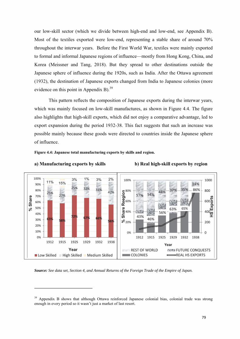
79
our low-skill sector (which we divide between high-end and low-end, see Appendix B).
Most of the textiles exported were low-end, representing a stable share of around 70%
throughout the interwar years. Before the First World War, textiles were mainly exported
to formal and informal Japanese regions of influence—mostly from Hong Kong, China, and
Korea (Meissner and Tang, 2018). But they spread to other destinations outside the
Japanese sphere of influence during the 1920s, such as India. After the Ottawa agreement
(1932), the destination of Japanese exports changed from India to Japanese colonies (more
evidence on this point in Appendix B).39
This pattern reflects the composition of Japanese exports during the interwar years,
which was mainly focused on low-skill manufactures, as shown in Figure 4.4. The figure
also highlights that high-skill exports, which did not enjoy a comparative advantage, led to
export expansion during the period 1932-38. This fact suggests that such an increase was
possible mainly because these goods were directed to countries inside the Japanese sphere
of influence.
Figure 4.4: Japanese total manufacturing exports by skills and region.
a) Manufacturing exports by skills b) Real high-skill exports by region
a) low and high skill b) high skilled exports by reg
Source: See data set, Section 4, and Annual Returns of the Foreign Trade of the Empire of Japan.
39 Appendix B shows that although Ottawa reinforced Japanese colonial bias, colonial trade was strong enough in every period so it wasn’t just a market of last resort.
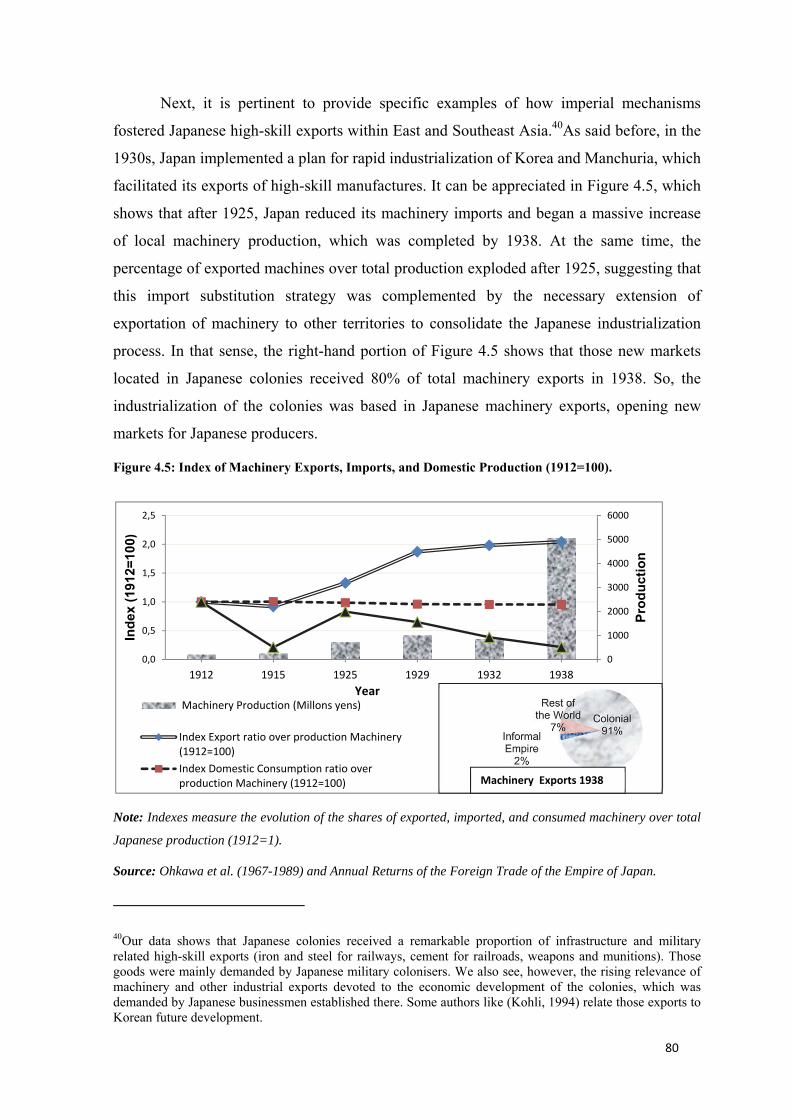
80
Next, it is pertinent to provide specific examples of how imperial mechanisms
fostered Japanese high-skill exports within East and Southeast Asia.40As said before, in the
1930s, Japan implemented a plan for rapid industrialization of Korea and Manchuria, which
facilitated its exports of high-skill manufactures. It can be appreciated in Figure 4.5, which
shows that after 1925, Japan reduced its machinery imports and began a massive increase
of local machinery production, which was completed by 1938. At the same time, the
percentage of exported machines over total production exploded after 1925, suggesting that
this import substitution strategy was complemented by the necessary extension of
exportation of machinery to other territories to consolidate the Japanese industrialization
process. In that sense, the right-hand portion of Figure 4.5 shows that those new markets
located in Japanese colonies received 80% of total machinery exports in 1938. So, the
industrialization of the colonies was based in Japanese machinery exports, opening new
markets for Japanese producers.
Figure 4.5: Index of Machinery Exports, Imports, and Domestic Production (1912=100).
Note: Indexes measure the evolution of the shares of exported, imported, and consumed machinery over total
Japanese production (1912=1).
Source: Ohkawa et al. (1967-1989) and Annual Returns of the Foreign Trade of the Empire of Japan.
40Our data shows that Japanese colonies received a remarkable proportion of infrastructure and military related high-skill exports (iron and steel for railways, cement for railroads, weapons and munitions). Those goods were mainly demanded by Japanese military colonisers. We also see, however, the rising relevance of machinery and other industrial exports devoted to the economic development of the colonies, which was demanded by Japanese businessmen established there. Some authors like (Kohli, 1994) relate those exports to Korean future development.
0
1000
2000
3000
4000
5000
6000
0,0
0,5
1,0
1,5
2,0
2,5
1912 1915 1925 1929 1932 1938
Prod
uctio
n
Inde
x (1
912=
100)
Year Machinery Production (Millons yens)
Index Export ratio over production Machinery(1912=100)Index Domestic Consumption ratio overproduction Machinery (1912=100) Machinery Exports 1938
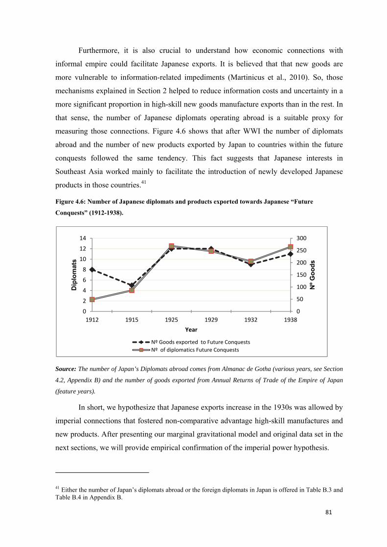
81
Furthermore, it is also crucial to understand how economic connections with
informal empire could facilitate Japanese exports. It is believed that that new goods are
more vulnerable to information-related impediments (Martinicus et al., 2010). So, those
mechanisms explained in Section 2 helped to reduce information costs and uncertainty in a
more significant proportion in high-skill new goods manufacture exports than in the rest. In
that sense, the number of Japanese diplomats operating abroad is a suitable proxy for
measuring those connections. Figure 4.6 shows that after WWI the number of diplomats
abroad and the number of new products exported by Japan to countries within the future
conquests followed the same tendency. This fact suggests that Japanese interests in
Southeast Asia worked mainly to facilitate the introduction of newly developed Japanese
products in those countries.41
Figure 4.6: Number of Japanese diplomats and products exported towards Japanese “Future Conquests” (1912-1938).
Source: The number of Japan’s Diplomats abroad comes from Almanac de Gotha (various years, see Section
4.2, Appendix B) and the number of goods exported from Annual Returns of Trade of the Empire of Japan
(feature years).
In short, we hypothesize that Japanese exports increase in the 1930s was allowed by
imperial connections that fostered non-comparative advantage high-skill manufactures and
new products. After presenting our marginal gravitational model and original data set in the
next sections, we will provide empirical confirmation of the imperial power hypothesis.
41 Either the number of Japan’s diplomats abroad or the foreign diplomats in Japan is offered in Table B.3 and Table B.4 in Appendix B.
0
50
100
150
200
250
300
02468
101214
1912 1915 1925 1929 1932 1938N
º Goo
ds
Dip
lom
ats
Year
Nº Goods exported to Future ConquestsNº of diplomatics Future Conquests
82
4.4. Margins of Trade Model. The traditional Gravity Model assumes that trade flows travel between two
countries attracted by two main forces. Countries’ economical size attracts trade flows,
whereas the distance between countries discourages flows. Providing that our dataset is a
panel with information for many countries across six different periods and that trade flows
are sometimes equal to zero, we have decided to estimate the model following the standard
PPML procedure (Santos Silva and Tenreyro, 2006). The independent variables (with the
exceptions of dummies) are nevertheless logged for the sake of simplicity in their
coefficients’ interpretations because this practice would permit us to interpret them as
slopes.
This model, of course, can be augmented by controlling for more variables, which is
a common practice in the literature. Two groups of variables are included, first, those
variables associated with comparative advantage, 𝐶𝐴 (related either with productivity,
relative wages, factor endowments, or similar demand structure), and second, those
variables associated with trade or transaction costs (transport cost, tariffs, exchange rates,
and empire connections).
In the comparative advantage group, first, we used relative productivity measures,
such as the Japanese GDP per hour worked relative to partner countries.42 Second, we used
a variable measuring relative real wage trends as a ratio, so that a rise of the variable
reflects increases in Japanese wages relative to a trading partner. Next, the third type of
variable refers to differences in demand structure (proxied by GDP per capita differentials).
43It captures whether Japanese exports were more intensive towards countries presenting
similar demand structures (Linder, 1961). This hypothesis has been successfully tested for
Latin America and for Japan (Restrepo and Tena-Junguito, 2016; Meissner and Tang,
2018). Finally, we checked whether Japanese trade followed a Hecksher-Ohlin pattern in
42 The variable refers to GDP per hour worked excluding agriculture productivity. Additionally, for sector-level analysis, we include Japanese product per hour on high- and low-skill manufactures found in LTES. Then it is compared with the partner’s overall productivity following the same methodology as for real wages. For further discussion regarding this variable, see appendix B. 43 The log of the absolute differences in GDP per capita between Japan and the corresponding partner proxies for differences in demand structure. We have also tried to measure differential in demand structure as the product of the bilateral income share (Yi)/(Yi+Yj)* (Yj)/(Yi+Yj), obtaining similar results because taking logs reduces the differences between relative and absolute figures. Finally, several authors suggest the use of differences in the degree of urbanisation or industrialization as a proxy, these measures are very controversial as representative of differential in demand structure, however, and in our case, it is very difficult to collect representative data.
83
which exports revealed comparative advantage is founded or not in differences in relative
factor endowments (population density in this case).
On the trade cost group, we include a variable called 𝑇𝐶 That is intended to
capture the effects of trade costs like average freight factors, average levels of protection in
partner countries, exchange rates index with the Japanese Yen, the imposition of exchange
controls, or the number of Japanese diplomats abroad. Following our previous discussion
on the relevance of empire, we add other transaction cost variables, which are the most
relevant ones in our analysis, including: 𝐶𝑂𝐿𝑂𝑁𝑌 (a dummy taking the value 1 if a
country is a Japanese colony 0 if not and that is dynamic as it changes whenever a territory
is conquered) that captures all those mechanisms by which Japanese imperial aims fostered
exports, and 𝐹𝑈𝑇𝑈𝑅𝐸 𝐶𝑂𝑁𝑄𝑈𝐸𝑆𝑇𝑆 , a static dummy that determines whether Japanese
exports were already biased towards countries occupied during WWII.
Finally, two additional variables are intended to capture the difference between
international and domestic demand occasioned by trade distortions and other path
dependence fundamentals. The first variable controls for Japanese partners’ imports and is
primarily devoted to capturing the trade blocs and other trade diversion protectionist
measures that affected bilateral international demand above domestic GDP variations. This
variable would be specially relevant during the 1930s. The second one β represents time
dummies that permit us to control changes related to the passage of time (like inflation or
the First World War international disintegration) and ε , that are standard errors clustered
by the country partner, as show equation 4.1. 𝐸𝑥𝑝 = 𝛽 + 𝛽 𝑙𝑛𝐺𝐷𝑃 + 𝛽 𝐶𝐴 + 𝛽 𝑇𝐶 + 𝛽 𝐶𝑂𝐿𝑂𝑁𝑌 +𝛽 𝐹𝑈𝑇𝑈𝑅𝐸 𝐶𝑂𝑁𝑄𝑈𝐸𝑆𝑇𝑆 +𝛽 𝐼𝑀𝑃𝑂𝑅𝑇𝑆 + 𝛽 + 𝜀 (EQ 4.1)
Another novelty of this article lies in the employment of margins of trade
framework that allows us to determine by which channels the different independent
variables affected Japanese exports. In that sense, the extensive margin represents the
number of active sectors exported by Japan to each country (i) and during each period (t)
(Meissner and Tang, 2018). This margin better explains the structural change. In our claim,
sectors are defined according to the 3-digit level of the SITC Revision 2 description, in the
sense that all products sharing the first three digits will be collected within the same sector,
so we avoid accounting for different varieties of existing products as they were new goods
84
(for an extended discussion of this issue see Appendix B).44 Using this methodology, we
observe that Japan moved from exporting in 117 sectors to exporting in 164. The intensive
margin, on the other hand, represents the average export value by sector to each country in
every period.45 In this sense, equation 4.2 displays the extensive margins by employing the
number of active sectors exported as the dependent variable and equation 4.3 uses exports
per sector to country i in period t for presenting intensive margins. 𝑁º𝑆𝐸𝐶𝑇𝑂𝑅 = 𝛽 + 𝛽 𝑙𝑛𝐺𝐷𝑃 + 𝛽 𝐶𝐴 + 𝛽 𝑇𝐶 + 𝛽 𝐶𝑂𝐿𝑂𝑁𝑌 +𝛽 𝐹𝑈𝑇𝑈𝑅𝐸 𝐶𝑂𝑁𝑄𝑈𝐸𝑆𝑇𝑆 +𝛽 𝐼𝑀𝑃𝑂𝑅𝑇𝑆 + 𝛽 + 𝜀 (EQ 4.2)
𝐸𝑥𝑝𝑆𝐸𝐶𝑇𝑂𝑅 = 𝛽 + 𝛽 𝑙𝑛𝐺𝐷𝑃 + 𝛽 𝐶𝐴 + 𝛽 𝑇𝐶 + 𝛽 𝐶𝑂𝐿𝑂𝑁𝑌 +𝛽 𝐹𝑈𝑇𝑈𝑅𝐸 𝐶𝑂𝑁𝑄𝑈𝐸𝑆𝑇𝑆 +𝛽 𝐼𝑀𝑃𝑂𝑅𝑇𝑆 + 𝛽 + 𝜀 (EQ 4.3)
Finally, the model might experience some modifications because the dependent
variable could be divided by different skills products (high- and low-skills manufactures
and primary products) or what were the main determinants of exports to a specific region.
4.5. The New Data Set 4.5.1 Trade Data.
As mentioned in the introduction, one of the principal contributions of this paper is
the construction of a granular data-set that provides a high-resolution image of the value of
Japanese exports by product, year and the geographical destination following the same
level of disaggregation as official Japanese trade records. We digitized information found
in different volumes (1912, 1915, 1925, 1929, 1932, and 1938) of the Annual Return of the
Foreign Trade of the Empire of Japan. Official statistics collected and published annually
by the Japanese Bureau of Customs appear disaggregated at the product level and show
quantities and values exported from Japan by destination.46 According to our data set,
44 We also employed a method similar to (Huberman and Meissner, 2007) in which the extensive margin represents each single good exported by Japan. Results hold very similar. This method has been disregarded, however, because it might bias our results as this method might show different varieties of existing products as new products. See Appendix B. 45 IM= 46 We discuss the accuracy of the Japan trade statistics in Appendix B.1. Although, we assume Japan used quite accurate declared values for exports, but some inaccuracy on country real destination records for goods moving through Hong Kong and Singapore. We have evidence that the Hong Kong share of total China
85
Japan moved from exporting 512 different products to 37 different countries in 1912, to
exporting 1135 goods to 117 countries in 1938, although this evolution might be subject to
specific statistical concerns (See Appendix B).
The main drawback of the Annual Return as a source is that it does not include data
in Japanese exports towards its main colonies, Korea and Taiwan. (Although, thankfully,
they account for exports towards the Kwantung Leased Territory and Manchuria, both
before and after being occupied by Japan). On the one hand, it is a fundamental inaccuracy
in the statistical records; on the other hand, Japanese export patterns towards its colonies is
vital for our research interests. We resolve this contradiction using a second-best option
with more aggregate information in Japanese exports to Taiwan.47
The level of disaggregation included in this data set is lower than that of the main
statistics after 1915, so it would underestimate Taiwan’s extensive margins of trade. We
have assumed that the number of products exported to Taiwan after 1915 follows the same
rate of increase as that of the Kwangtung Leased Territory—the only Japanese colony for
which there is full information throughout the period. For the case of Korea, the Annual
Returns of the Foreign Trade of the Empire of Japan in their volumes from 1914-1920
include an appendix with data in Japanese exports to Korea at the product level.48
The data set that we constructed provides for the value of Japanese exports (in
current Yen) of each product exported to every country. Each different product exported has
been categorized using the Standard International Trade Classification (SITC) Revision 2 to
a 5 digit-level disaggregation to achieve a proper and precise product classification. The imports declined from around 40% at the turn of the Century to less than 20% in the 1920s, and less than 5% in the 1930s. This implies that inaccuracy of Japan’s direction of trade records due to transit is more limited for the interwar years than for previous periods (see Figure 5 in Keller et al, 2011). 47 For 1912 and 1915, there is full disaggregation of exports at the product level. For the period 1925-1938, LTES includes data on Japanese exports to Korea in five different sectors that match our skill distribution. Thus, the number of goods at every skill level exported by Japan will be equal to the corresponding 1915 figure assumed to evolve along the same path as that of Kwantung, which shared a similar economic structure to Korea. See discussion in Appendix B. 48 The data came from the Returns of the Trade of Taiwan for Forty Years (1896-1935) and the annual Return of Trade of Taiwan (Formosa) (1936-1942), both published by the Department of Finance of the Government of Taiwan. These returns include Taiwanese imports from Japan (or, equivalently, Japanese exports to Taiwan) at product level. For the rest of the period, Japanese exports to Korea have been estimated by the Japanese Long Term Economic Statistics (LTES) database. The Kwangtung Leased Territory was the colony that received the greatest number of Japanese goods that is why it could be considered an upper-bound for calculating the evolution of the extensive margin to Taiwan. See an extended discussion in Section Appendix B.
86
different goods have also been divided according to skill intensity (Tena-Junguito, 2010).
Skill intensity is constructed based on wages earned by workers in each sector and permits
us to differentiate between high-skill (Skill intensity higher than 10), medium-skill
(between 9 and 10), low-skill manufactures (between 5 and 9), and primary products (less
than 5 skill intensity).49
4.5.2. GDP and Productivity
Information on GDP and GDP per capita is taken from the latest version of the
Maddison Project and refers to GDP in 1990 GK dollars or real GDP (Bolt and van Zanden,
2014). For missing countries, we took data on real GDP for 1950 and translated it to the
interwar years by assuming the same evolution as constant exports (Federico and Tena-
Junguito, 2019).
Besides, we estimated GDP levels and other statistics for Japanese colonies of
Kwantung Leased Territory and Manchukuo (Manchuria). First, we obtained population
data (Kang, 1981). Then, the corresponding GDP is calculated as the proportion of
Japanese GDP equal to the percentage each population represents over the Japanese total
(the exercise for Manchuria is the same except China is used as the reference because it was
part of China until 1932). We considered Kwantung’s GDP to follow the same rate of
growth as Japan’s (because it was a Japanese colony), whereas we found Manchuria’s GDP
to follow the same tendency as China’s until 1932. Afterwards, we assumed Manchuria’s
GDP to grow at the same rate as Manchurian exports (Federico & Tena-Junguito, 2019).
We use GDP information, complemented by data on total hours worked.50 Then, we
construct non-agrarian GDP per hour worked as a measure of productivity for 27 partner
countries, which represent 92% of Japanese exports. The real wages index for capturing
productivity evolution for 30 partner countries comes from Williamson article and
population density from the League of Nations (Huberman and Mins, 2007; Maddison,
1995). Finally, we construct price indexes for deflating GDP measures (Mitchell, 2003).
49 We recognize that, on one hand, this division represents a very rudimentary way of capturing skill improvements inside sectors, especially productivity increases in Japanese textile industries in the 1920s and 1930s (Wolcott, 1994), but on the other hand, this strategy captures better Japan’s manufacturing dual aggregate sectoral advance in the second industrial revolution technologies as an indicator of industrial modernization in the inter-war years, which is the main objective of the paper. In Appendix B, we offer an extended discussion of the general division of total exports by skill intensity in conjunction with a complementary analysis of the geography and main drivers that explain the Japanese textile exports increase in the interwar period.
87
Finally, one essential part of this analysis is the study of Japanese productivity and
the study’s determination of exports by skill level. To disentangle this relationship, we
employed data in Japanese manufacturing output and employment by sectors. To
approximate hours worked at every sector, we use data derived from total hours according
to the Long Term Economic Statistics of Japan (LTES) database from Hitotsubashi
University.
4.5.3. Trade Costs
Distance between countries is the most common variable to measure transport costs
in the literature on gravity, but this variable is time and product invariant. This paper makes
an effort to overcome the implications of this limited assumption on the measure of
transport cost. So we use a data set of estimated freight factors (cost of transport per
ton/product price per ton) between Japan and each partner country, for every single product
exported by Japan for each of our corresponding benchmark years. In our strategy, the
geographical distance between Japanese partners is combined with different freight rates,
routes, and differences in freight factors by the composition of products.51
The information on the number of Japanese diplomats operating in each different
country has been obtained from the Almanac de Gotha (various years), which includes a
section with the names and country of origin of every diplomat operating in every country,
so we have counted the Japanese ones. Additional variables representing trade costs are
average levels of tariff protection and exchange rate control (Blattman, 2003; Bethell, 1994;
Eichengreen, 1996; Meisel, 1990; Reinhart and Rogoff, 2004).52 Finally, bilateral nominal
exchange rates with the Japanese Yen, determined as being the quantity of foreign currency
per one Yen. Then we construct an index (1912=1) to measure the evolution of different
exchange rates from a joint base. Besides, we have used data about nominal imports to
capture the differences introduced by the protectionist backlash between domestic and
international demand, especially in the 1930s (Federico and Tena-Junguito, 2019).
51 The alternative use of the conventional great-circle distance in our equations offers weak results similar to the use of freight cost by products and regions. Apparently, this happens because freight factors of manufactures are low. Additionally, international freight rates during the interwar years were not volatile but stagnant. See an extended discussion in Appendix B. 52 Tariffs between Japan and its colonies are assumed to be zero.
88
4.6. Results 4.6.1. Presentation of Results
The descriptive statistics presented in Section 3 showed that Japanese exports
increased significantly between 1912 and 1938, specially during the 1930s. These data also
suggested that, although Japanese improvements in productivity contributed to the
expansion of exports (either by different product varieties or more diverse destinations),
specially before 1929, they were not the primary determinant of the structural change in
Japanese industrial exports. Evidence presented in previous sections also suggested that
among industrial exporters, Japan persisted with a comparative advantage in low-skill
manufactures, such as textiles, although high-skill exports increased substantially during
the 1930s. That evidence leads to our central hypothesis, developed in Section 3, that
imperial mechanisms, not productivity, were the main drivers that facilitated high-skill
manufacturing exports, and links with future conquests fostered the introduction of new
Japanese products in the region.
This section will test the resilience of that hypothesis using the previously
mentioned models. First of all, we examine which factors determined Japan’s total exports
during the whole period. Table 4.2 shows how one of the measures employed for
approximating Japanese relative productivity is significant when we do not control for
Japanese colonies. However, upon the inclusion of the colony dummy and other potential
links with future conquests in Southeast Asia, productivity measures cease to be significant.
Of which, we deduce that this evidence reinforces the trade in the shadow of power
hypothesis. That´s we assume that Japanese imperial connections are compensating the
existence of low productivity to facilitate overall exports. In that sense, the bias of Japanese
exports towards its colonies has the expected reaction. Furthermore, it is also evident that
Japan already had established certain economic relations that facilitated exports towards
those territories, which Japan subsequently occupied during WWII.
The trade generation capacity of the Japanese Empire during the interwar years was
much higher than the ones shown by the literature for the preceding period (1870-1913)
(Mitchener & Weidenmier, 2008). We should be careful with those results because they
might be subject to particular statistical concerns, but they are in line with related works
studying intra-bloc trade bias in the Japanese Empire during the same period (Okubo,
2007). Specifically, we’ve found that Japanese Empire membership increases in trade by
more than ten times than those associated by the British, German and French Empires, and
89
more than two times more significant than those of the US and Spanish Empires. It could
be the case that our coefficients are more prominent because they are capturing the strong
intra-bloc bias that emerged after the Great Depression. However, the Japanese Empire
trade generating effect is also around ten times bigger than the ones found on the Sterling
and Reichsmark blocs in the 1930s (Ritschl and Wolf, 2003). Furthermore, the trade bias
experienced between Japan and its informal empire was comparable to the ones of those
currency areas.53
According to the literature, another variable that may capture Japanese economic
interests in a territory before annexation is the number of diplomats in that territory, which
in this case is positive and significant, although its influence in Japanese exports vanishes
when we account for informal imperial links. The positive correlation between the number
of diplomats abroad and the Japanese informal empire dummy variables would suggest, as
mentioned in Section 2, that both worked through similar mechanisms.
Regarding the Japanese specialization pattern, we can appreciate how Japan tended
to export more towards countries presenting more significant differences in demand
structure (GDP per capita) and population density (factor endowments). This fact
contradicts the Linder hypothesis for interwar Japan and places its exports pattern closer to
a Hecksher-Ohlin model. Japan’s GDP per capita was converging with rich countries and
diverging with poor ones in contradiction with demand convergence Lindert hypothesis.
Furthermore, it suggests that Japanese industrial exports pattern contributed to the demand
complementarities found on chapter 2. Finally, it is also remarkable how among all the
possible trade costs undermining Japanese exports, the only significant one is the relative
appreciation of the Yen (the significant negative effect of tariffs vanishes when we account
for the colonial framework).
53 (Larch et al., 2017) shows that the interpretation of dummy coefficients like Colony or Informal Empire is the following: 𝑒 . − 1 = 2271% higher exports for colonies in comparison with non-colonial territories and 𝑒 . − 1 = 167% for future occupied territories.
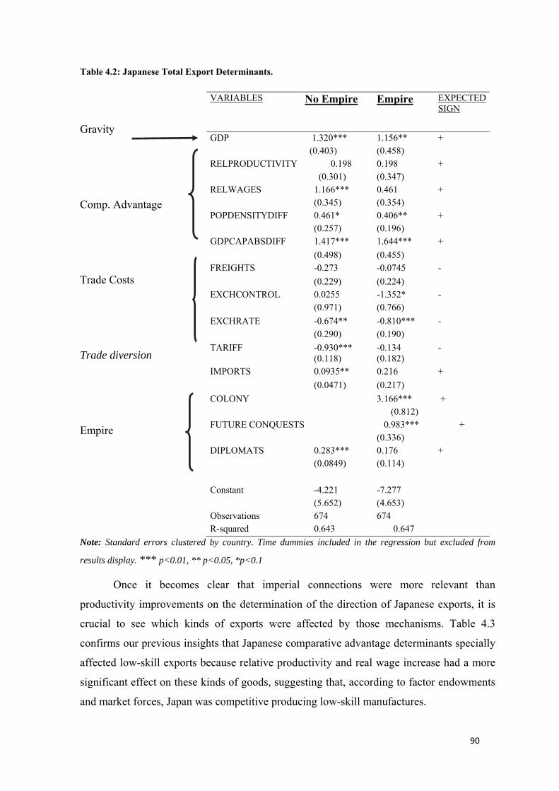
90
Table 4.2: Japanese Total Export Determinants.
Gravity
Comp. Advantage
Trade Costs
Trade diversion
Empire
Note: Standard errors clustered by country. Time dummies included in the regression but excluded from
results display. *** p<0.01, ** p<0.05, *p<0.1
Once it becomes clear that imperial connections were more relevant than
productivity improvements on the determination of the direction of Japanese exports, it is
crucial to see which kinds of exports were affected by those mechanisms. Table 4.3
confirms our previous insights that Japanese comparative advantage determinants specially
affected low-skill exports because relative productivity and real wage increase had a more
significant effect on these kinds of goods, suggesting that, according to factor endowments
and market forces, Japan was competitive producing low-skill manufactures.
VARIABLES No Empire Empire EXPECTED SIGN
GDP 1.320*** 1.156** + (0.403) (0.458) RELPRODUCTIVITY 0.198 0.198 + (0.301) (0.347) RELWAGES 1.166*** 0.461 + (0.345) (0.354) POPDENSITYDIFF 0.461* 0.406** + (0.257) (0.196) GDPCAPABSDIFF 1.417*** 1.644*** + (0.498) (0.455) FREIGHTS -0.273 -0.0745 - (0.229) (0.224) EXCHCONTROL 0.0255 -1.352* - (0.971) (0.766) EXCHRATE -0.674** -0.810*** - (0.290) (0.190) TARIFF -0.930*** -0.134 - (0.118) (0.182) IMPORTS 0.0935** 0.216 + (0.0471) (0.217) COLONY 3.166*** + (0.812) FUTURE CONQUESTS 0.983*** + (0.336) DIPLOMATS 0.283*** 0.176 + (0.0849) (0.114) Constant -4.221 -7.277 (5.652) (4.653) Observations 674 674 R-squared 0.643 0.647
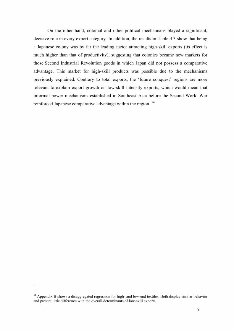
91
On the other hand, colonial and other political mechanisms played a significant,
decisive role in every export category. In addition, the results in Table 4.3 show that being
a Japanese colony was by far the leading factor attracting high-skill exports (its effect is
much higher than that of productivity), suggesting that colonies became new markets for
those Second Industrial Revolution goods in which Japan did not possess a comparative
advantage. This market for high-skill products was possible due to the mechanisms
previously explained. Contrary to total exports, the ‘future conquest’ regions are more
relevant to explain export growth on low-skill intensity exports, which would mean that
informal power mechanisms established in Southeast Asia before the Second World War
reinforced Japanese comparative advantage within the region. 54
54 Appendix B shows a disaggregated regression for high- and low-end textiles. Both display similar behavior and present little difference with the overall determinants of low-skill exports.
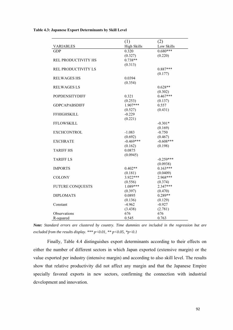
92
Table 4.3: Japanese Export Determinants by Skill Level
(1) (2) VARIABLES High Skills Low Skills GDP 0.320 0.680*** (0.327) (0.220) REL PRODUCTIVITY HS 0.738** (0.313) REL PRODUCTIVITY LS 0.887*** (0.177) RELWAGES HS 0.0394 (0.354) RELWAGES LS 0.628** (0.302) POPDENSITYDIFF 0.321 0.467*** (0.253) (0.137) GDPCAPABSDIFF 1.907*** 0.557 (0.527) (0.431) FFHIGHSKILL -0.229 (0.221) FFLOWSKILL -0.301* (0.169) EXCHCONTROL -1.083 -0.750 (0.692) (0.467) EXCHRATE -0.469*** -0.608*** (0.162) (0.198) TARIFF HS 0.0875 (0.0945) TARIFF LS -0.259*** (0.0938) IMPORTS 0.402** 0.163*** (0.181) (0.0409) COLONY 3.922*** 2.968*** (0.556) (0.374) FUTURE CONQUESTS 1.089*** 2.347*** (0.397) (0.470) DIPLOMATS 0.0895 0.289** (0.136) (0.129) Constant -4.962 -0.927 (3.438) (2.781) Observations 676 676 R-squared 0.545 0.763
Note: Standard errors are clustered by country. Time dummies are included in the regression but are
excluded from the results display. *** p<0.01, ** p<0.05, *p<0.1
Finally, Table 4.4 distinguishes export determinants according to their effects on
either the number of different sectors in which Japan exported (extensive margin) or the
value exported per industry (intensive margin) and according to also skill level. The results
show that relative productivity did not affect any margin and that the Japanese Empire
specially favored exports in new sectors, confirming the connection with industrial
development and innovation.
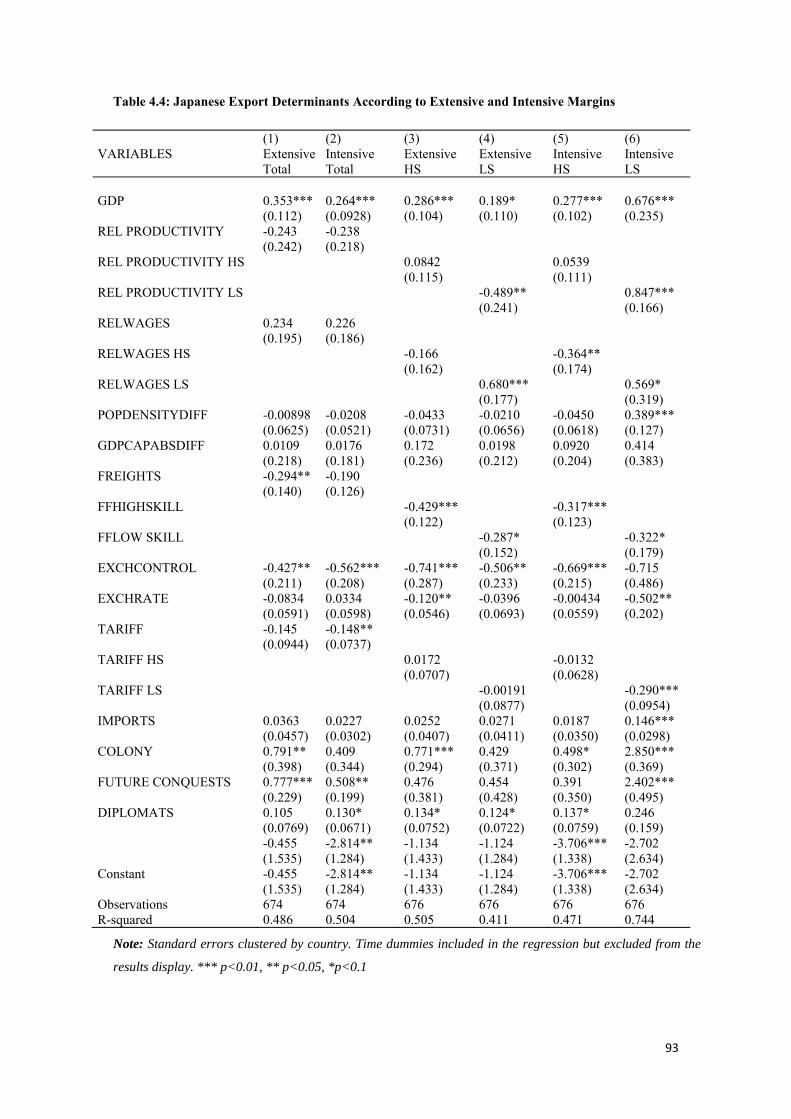
93
Table 4.4: Japanese Export Determinants According to Extensive and Intensive Margins
(1) (2) (3) (4) (5) (6) VARIABLES Extensive
Total Intensive Total
Extensive HS
Extensive LS
Intensive HS
Intensive LS
GDP 0.353*** 0.264*** 0.286*** 0.189* 0.277*** 0.676*** (0.112) (0.0928) (0.104) (0.110) (0.102) (0.235) REL PRODUCTIVITY -0.243 -0.238 (0.242) (0.218) REL PRODUCTIVITY HS 0.0842 0.0539 (0.115) (0.111) REL PRODUCTIVITY LS -0.489** 0.847*** (0.241) (0.166) RELWAGES 0.234 0.226 (0.195) (0.186) RELWAGES HS -0.166 -0.364** (0.162) (0.174) RELWAGES LS 0.680*** 0.569* (0.177) (0.319) POPDENSITYDIFF -0.00898 -0.0208 -0.0433 -0.0210 -0.0450 0.389*** (0.0625) (0.0521) (0.0731) (0.0656) (0.0618) (0.127) GDPCAPABSDIFF 0.0109 0.0176 0.172 0.0198 0.0920 0.414 (0.218) (0.181) (0.236) (0.212) (0.204) (0.383) FREIGHTS -0.294** -0.190 (0.140) (0.126) FFHIGHSKILL -0.429*** -0.317*** (0.122) (0.123) FFLOW SKILL -0.287* -0.322* (0.152) (0.179) EXCHCONTROL -0.427** -0.562*** -0.741*** -0.506** -0.669*** -0.715 (0.211) (0.208) (0.287) (0.233) (0.215) (0.486) EXCHRATE -0.0834 0.0334 -0.120** -0.0396 -0.00434 -0.502** (0.0591) (0.0598) (0.0546) (0.0693) (0.0559) (0.202) TARIFF -0.145 -0.148** (0.0944) (0.0737) TARIFF HS 0.0172 -0.0132 (0.0707) (0.0628) TARIFF LS -0.00191 -0.290*** (0.0877) (0.0954) IMPORTS 0.0363 0.0227 0.0252 0.0271 0.0187 0.146*** (0.0457) (0.0302) (0.0407) (0.0411) (0.0350) (0.0298) COLONY 0.791** 0.409 0.771*** 0.429 0.498* 2.850*** (0.398) (0.344) (0.294) (0.371) (0.302) (0.369) FUTURE CONQUESTS 0.777*** 0.508** 0.476 0.454 0.391 2.402*** (0.229) (0.199) (0.381) (0.428) (0.350) (0.495) DIPLOMATS 0.105 0.130* 0.134* 0.124* 0.137* 0.246 (0.0769) (0.0671) (0.0752) (0.0722) (0.0759) (0.159) -0.455 -2.814** -1.134 -1.124 -3.706*** -2.702 (1.535) (1.284) (1.433) (1.284) (1.338) (2.634) Constant -0.455 -2.814** -1.134 -1.124 -3.706*** -2.702 (1.535) (1.284) (1.433) (1.284) (1.338) (2.634) Observations 674 674 676 676 676 676 R-squared 0.486 0.504 0.505 0.411 0.471 0.744
Note: Standard errors clustered by country. Time dummies included in the regression but excluded from the
results display. *** p<0.01, ** p<0.05, *p<0.1
94
The most important conclusion we reach disaggregating by skill level is that high-
skill exports are more sensitive to the extensive margin than low-skill exports. The more
significant connection between fixed costs and increases in new export products in the
high-skill sector helps to understand that higher sensitivity. We can also appreciate how
improvements in Japanese productivity mainly increased the intensive margin for low-skill
products, that´s with the low technological and less innovative sectors. On the other hand,
being colonized by Japan was the main driver of new extensive exports of high-skill
manufactures, suggesting that those more modern and more sophisticated products were not
internationally competitive and mainly traded in the colonies under the shadow of power
coverage. This situation does not exclude the fact that both colonies and future conquests
also facilitated low-skill exports at the intensive margin in a proper way.
This section confirms some of the hypotheses offered in the descriptive analysis:
Imperial connections (both formal and informal) were more relevant than productivity in
the determination of exports. In that sense, colonies became a new market for high-skill
exports, while the informal empire reinforced comparative advantage in low-skill
manufactures. Both also fostered exports from new sectors, confirming that Japanese
industrialization was supported by conquest and suggesting that its imperial institutions
influenced East and Southeast Asian regional specialization patterns.
4.6.2. Robustness Checks
To check whether our results are robust, we tested whether the previous conclusions
still held when we employed different estimation methods and limited the potential
endogeneity between the key variables. In that sense, Table 4.5 shows our main results
estimated by a Tobit estimator, employing OLS, and a later panel estimation using Random
Effects to finish with some checks on endogeneity.
Our results generally hold true to our hypothesis that Japanese relative productivity
did not, in general, affect Japanese exports. First, being a Japanese colony was always the
most crucial determinant of Japanese exports. Second, being part of Japan’s future
dominions was a significant additional attractor of Japanese exports in all estimation
methods. Finally, trade costs and comparative advantage worked in the same direction as
before.
We also checked the determinants of exports inside the formal and informal empire
across benchmarks years to detect the different influences of change in imperial policy
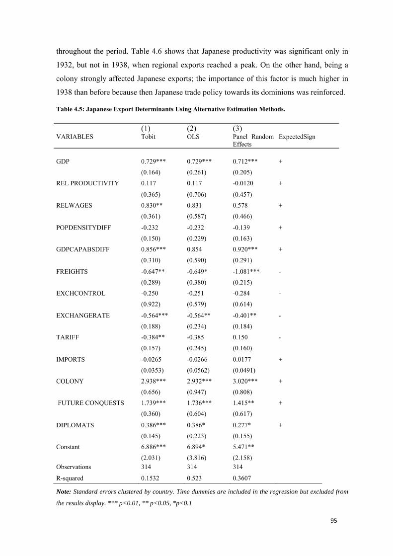
95
throughout the period. Table 4.6 shows that Japanese productivity was significant only in
1932, but not in 1938, when regional exports reached a peak. On the other hand, being a
colony strongly affected Japanese exports; the importance of this factor is much higher in
1938 than before because then Japanese trade policy towards its dominions was reinforced.
Table 4.5: Japanese Export Determinants Using Alternative Estimation Methods.
(1) (2) (3) VARIABLES Tobit OLS Panel Random
Effects ExpectedSign
GDP 0.729*** 0.729*** 0.712*** + (0.164) (0.261) (0.205) REL PRODUCTIVITY 0.117 0.117 -0.0120 + (0.365) (0.706) (0.457) RELWAGES 0.830** 0.831 0.578 + (0.361) (0.587) (0.466) POPDENSITYDIFF -0.232 -0.232 -0.139 + (0.150) (0.229) (0.163) GDPCAPABSDIFF 0.856*** 0.854 0.920*** + (0.310) (0.590) (0.291) FREIGHTS -0.647** -0.649* -1.081*** - (0.289) (0.380) (0.215) EXCHCONTROL -0.250 -0.251 -0.284 - (0.922) (0.579) (0.614) EXCHANGERATE -0.564*** -0.564** -0.401** - (0.188) (0.234) (0.184) TARIFF -0.384** -0.385 0.150 - (0.157) (0.245) (0.160) IMPORTS -0.0265 -0.0266 0.0177 + (0.0353) (0.0562) (0.0491) COLONY 2.938*** 2.932*** 3.020*** + (0.656) (0.947) (0.808) FUTURE CONQUESTS 1.739*** 1.736*** 1.415** + (0.360) (0.604) (0.617) DIPLOMATS 0.386*** 0.386* 0.277* + (0.145) (0.223) (0.155) Constant 6.886*** 6.894* 5.471** (2.031) (3.816) (2.158) Observations 314 314 314 R-squared 0.1532 0.523 0.3607 Note: Standard errors clustered by country. Time dummies are included in the regression but excluded from
the results display. *** p<0.01, ** p<0.05, *p<0.1
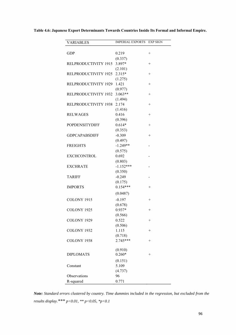
96
Table 4.6: Japanese Export Determinants Towards Countries Inside Its Formal and Informal Empire.
Note: Standard errors clustered by country. Time dummies included in the regression, but excluded from the
results display.*** p<0.01, ** p<0.05, *p<0.1
VARIABLES IMPERIAL EXPORTS EXP SIGN
GDP 0.219 + (0.337) RELPRODUCTIVITY 1915 3.897* + (2.101) RELPRODUCTIVITY 1925 2.315* + (1.275) RELPRODUCTIVITY 1929 1.421 + (0.977) RELPRODUCTIVITY 1932 3.063** + (1.494) RELPRODUCTIVITY 1938 2.174 + (1.416) RELWAGES 0.416 + (0.396) POPDENSITYDIFF 0.614* + (0.353) GDPCAPABSDIFF -0.309 + (0.497) FREIGHTS -1.249** - (0.575) EXCHCONTROL 0.692 - (0.803) EXCHRATE -1.152*** - (0.350) TARIFF -0.249 - (0.175) IMPORTS 0.154*** + (0.0487) COLONY 1915 -0.197 + (0.678) COLONY 1925 0.937* + (0.566) COLONY 1929 0.522 + (0.506) COLONY 1932 1.115 + (0.718) COLONY 1938
2.745*** +
(0.910) DIPLOMATS 0.260* + (0.151) Constant 5.109 (4.737) Observations 96 R-squared 0.771
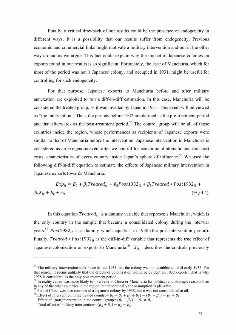
97
Finally, a critical drawback of our results could be the presence of endogeneity in
different ways. It is a possibility that our results suffer from endogeneity. Previous
economic and commercial links might motivate a military intervention and not in the other
way around as we argue. This fact could explain why the impact of Japanese colonies on
exports found in our results is so significant. Fortunately, the case of Manchuria, which for
most of the period was not a Japanese colony, and occupied in 1931, might be useful for
controlling for such endogeneity.
For that purpose, Japanese exports to Manchuria before and after military
annexation are exploited to run a diff-in-diff estimation. In this case, Manchuria will be
considered the treated group, as it was invaded by Japan in 1931. This event will be viewed
as “the intervention”. Thus, the periods before 1932 are defined as the pre-treatment period
and that afterwards as the post-treatment period.55 The control group will be all of those
countries inside the region, whose performances as recipients of Japanese exports were
similar to that of Manchuria before the intervention. Japanese intervention in Manchuria is
considered as an exogenous event after we control for economic, diplomatic and transport
costs, characteristics of every country inside Japan’s sphere of influence.56 We used the
following diff-in-diff equation to estimate the effects of Japanese military intervention in
Japanese exports towards Manchuria. 𝐸𝑥𝑝 = 𝛽 + 𝛽 𝑇𝑟𝑒𝑎𝑡𝑒𝑑 + 𝛽 𝑃𝑜𝑠𝑡1932 + 𝛽 𝑇𝑟𝑒𝑎𝑡𝑒𝑑 ∗ 𝑃𝑜𝑠𝑡1932 +𝛽 𝑋 + 𝛽 + 𝜀 (EQ 4.4)
In this equation 𝑇𝑟𝑒𝑎𝑡𝑒𝑑 is a dummy variable that represents Manchuria, which is
the only country in the sample that became a consolidated colony during the interwar
years.57 𝑃𝑜𝑠𝑡1932 is a dummy which equals 1 in 1938 (the post-intervention period).
Finally, 𝑇𝑟𝑒𝑎𝑡𝑒𝑑 ∗ 𝑃𝑜𝑠𝑡1932 is the diff-in-diff variable that represents the true effect of
Japanese colonization on exports to Manchuria.58 𝑋 describes the controls previously
55 The military intervention took place in late-1931, but the colony was not established until early-1932. For that reason, it seems unlikely that the effects of colonization would be evident on 1932 exports. That is why 1938 is considered as the only post treatment period. 56 In reality Japan was more likely to intervene in China or Manchuria for political and strategic reasons than in any of the other countries in the region, but theoretically the assumption is plausible. 57 Part of China was also considered a Japanese colony by 1938, but it was not consolidated at all. 58 Effect of intervention in the treated country=(𝛽 + 𝛽 + 𝛽 + 𝛽 ) − (𝛽 + 𝛽 ) = 𝛽 + 𝛽 Effect of (non)intervention in the control group= (𝛽 + 𝛽 ) − 𝛽 = 𝛽 Total effect of military intervention= (𝛽 + 𝛽 ) − 𝛽 = 𝛽
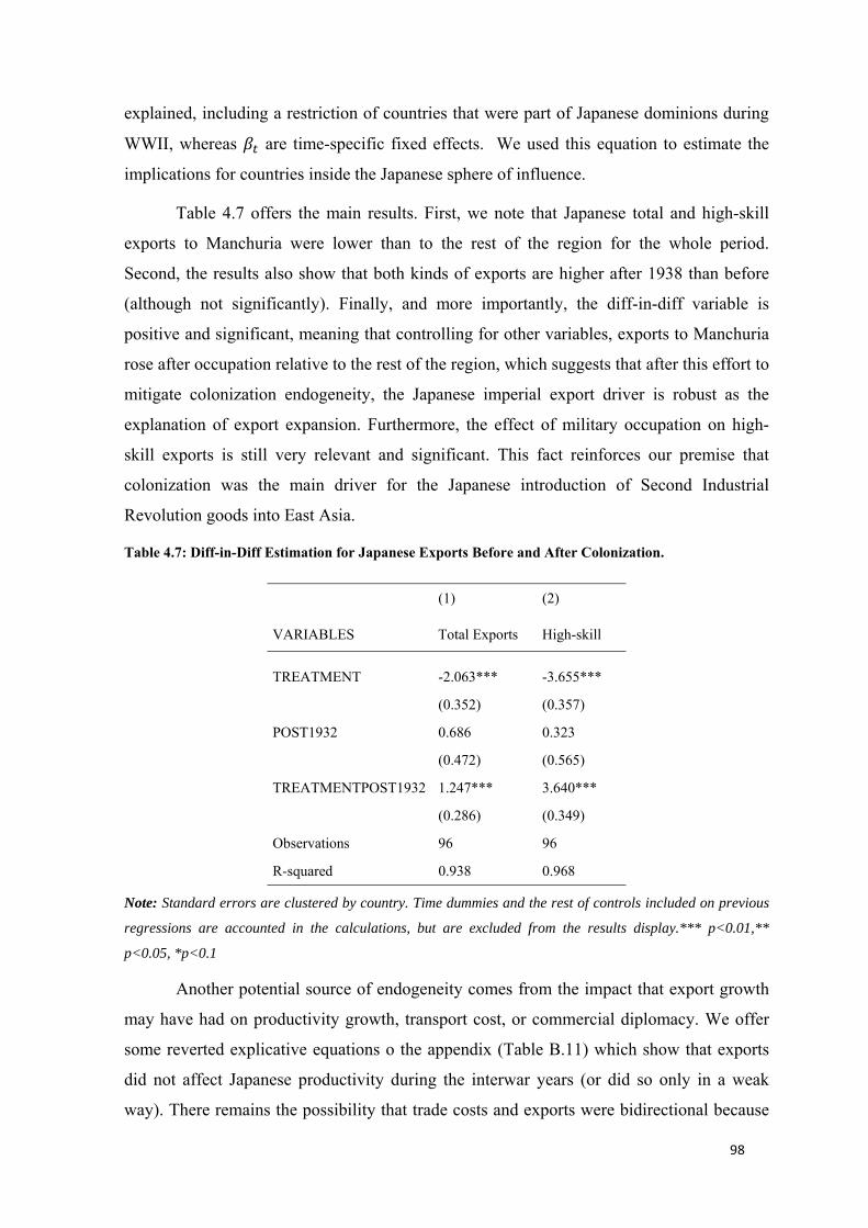
98
explained, including a restriction of countries that were part of Japanese dominions during
WWII, whereas 𝛽 are time-specific fixed effects. We used this equation to estimate the
implications for countries inside the Japanese sphere of influence.
Table 4.7 offers the main results. First, we note that Japanese total and high-skill
exports to Manchuria were lower than to the rest of the region for the whole period.
Second, the results also show that both kinds of exports are higher after 1938 than before
(although not significantly). Finally, and more importantly, the diff-in-diff variable is
positive and significant, meaning that controlling for other variables, exports to Manchuria
rose after occupation relative to the rest of the region, which suggests that after this effort to
mitigate colonization endogeneity, the Japanese imperial export driver is robust as the
explanation of export expansion. Furthermore, the effect of military occupation on high-
skill exports is still very relevant and significant. This fact reinforces our premise that
colonization was the main driver for the Japanese introduction of Second Industrial
Revolution goods into East Asia.
Table 4.7: Diff-in-Diff Estimation for Japanese Exports Before and After Colonization.
(1) (2)
VARIABLES Total Exports High-skill
TREATMENT -2.063*** -3.655***
(0.352) (0.357)
POST1932 0.686 0.323
(0.472) (0.565)
TREATMENTPOST1932 1.247*** 3.640***
(0.286) (0.349)
Observations 96 96
R-squared 0.938 0.968
Note: Standard errors are clustered by country. Time dummies and the rest of controls included on previous
regressions are accounted in the calculations, but are excluded from the results display.*** p<0.01,**
p<0.05, *p<0.1
Another potential source of endogeneity comes from the impact that export growth
may have had on productivity growth, transport cost, or commercial diplomacy. We offer
some reverted explicative equations o the appendix (Table B.11) which show that exports
did not affect Japanese productivity during the interwar years (or did so only in a weak
way). There remains the possibility that trade costs and exports were bidirectional because
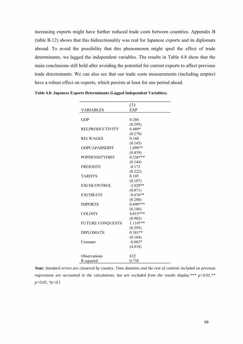
99
increasing exports might have further reduced trade costs between countries. Appendix B
(table B.12) shows that this bidirectionality was real for Japanese exports and its diplomats
abroad. To avoid the possibility that this phenomenon might spoil the effect of trade
determinants, we lagged the independent variables. The results in Table 4.8 show that the
main conclusions still hold after avoiding the potential for current exports to affect previous
trade determinants. We can also see that our trade costs measurements (including empire)
have a robust effect on exports, which persists at least for one period ahead.
Table 4.8: Japanese Exports Determinants (Lagged Independent Variables).
(1) VARIABLES EXP GDP 0.280 (0.295) RELPRODUCTIVITY 0.480* (0.270) RELWAGES 0.160 (0.145) GDPCAPABSDIFF 1.098** (0.439) POPDENSITYDIFF 0.536*** (0.144) FREIGHTS -0.173 (0.222) TARIFFS 0.105 (0.187) EXCHCONTROL -2.028** (0.871) EXCHRATE -0.676** (0.280) IMPORTS 0.698*** (0.186) COLONY 4.015*** (0.902) FUTURE CONQUESTS 1.114*** (0.395) DIPLOMATS 0.381** (0.164) Constant -8.062* (4.818) Observations 632 R-squared 0.738
Note: Standard errors are clustered by country. Time dummies and the rest of controls included on previous
regressions are accounted in the calculations, but are excluded from the results display.*** p<0.01,**
p<0.05, *p<0.1
100
4.7. Conclusions Trade blocs in the interwar years were used as instruments of imperial power to
foster exports and as a substitute for productivity in encouraging industrial production. In
that sense, Japan’s total exports in 1938 were between 28% and 47% higher thanks to
imperial mechanisms. The figure is much higher when we capture the imperial effect on
high-skill exports (between 66% and 76% higher thanks to imperial connections).
Furthermore, the present research has also found that the trading bias created inside the
Japanese formal and informal empire was much higher than those obtained by other authors
in other territories during the same period.59
We have assumed here that the imperial shadow of power in interwar Japan
predicted the regional trade bloc formation of ‘The Greater East Asia Co-Prosperity
Sphere’. Although this bloc was achieved only through military intervention in the 1940s, it
began working through specific previous economic networks and imperial soft power that
fostered regional exports in East and Southeast Asia along the period. This is perfectly
illustrated by Manchuria colonization and, for that reason, the last chapter will provide a
more in-depth study of the specific role of Japanese companies (Zaibatsu), which, in
concert with strategic military measures, profited from colonization of Manchuria during
both the informal and the formal imperial stages.
Japan was a latecomer to 20th-century industrialization, but during the interwar
years, and especially in the 1930s, was able to activate a complex an aggressive
industrialization policy to foster the modernization of its industrial production. That policy
consisted of overlapping of protectionist import substitution and imperial systems to
stimulate domestic production and industrial exports in its region of influence. That new
strategy reshaped previous Japanese export specialization patterns, based on exporting low-
skill manufactures to poor countries in the region with similar demand preferences and
climatic characteristics. Previous networks of distribution created in old and future colonies
were reinforced and followed by an investment of transport and communication
infrastructure to foster the demand for steel, mechanical engineering machinery and other
new manufactured products. We proved that this expansion occurred even before
annexation and not forced by international trade bloc diversion in the 1930s. In that sense,
59 See Appendix B.
101
we can identify a dual relationship between Japanese economic imperialism and military
imperialism which will be addressed on the final chapter of this dissertation.
We are aware that a potential endogeneity problem exists that relates to import
dependence or bilateral trade connections with military interventions (Bonfani &
O’Rourke, 2014). Nevertheless, we believe that these results reasonably prove the colonial
trade bias mechanism used by imperial institutions, inversely related to productivity, to
support Japanese industrialization in the first half of the twentieth century. The market
potential for high-skill manufactures was minimal and colonial intervention, therefore, was
used to expand the market of the most intensive human capital sector of Japanese
industrialization. The implicit counterfactual hypothesis would be that without imperial
intervention in the region, Japan would not have expanded its high-skill exports and would
not have exported such a variety of new products. In other words, Japan’s industrialization
was supported by imperial expansion, confirming that the Japanese ascendancy over East
and Southeast Asian regional integration was sustained on its strong influence over the
origins of intra-regional specialization patterns. Nevertheless, we still have to determine
whether the intentions of colonizers were truly developmental or if they acted on behalf of
the interests of certain Japanese elites.
102
CHAPTER 4: WINNERS OF JAPANESE COLONIZATION IN 5MANCHURIA 1907-1945
5.1. Introduction. Chapter 3 has shown that Japanese military conquest was anticipated by prior
economic penetration of Japanese business on neighbor territories. It has also demonstrated
that Japanese industrial expansion and the subsequent intra-regional specialization it
generated were linked with Japanese imperial aims. Nonetheless we still have to uncover
the intentions of Japanese elites behind the colonization of neighbor territories for trying to
finally close the debate about the singular developmental character of the Japanese Empire.
In order to do that, we have to describe the exchanges between ruling and
economic elites that took place during Japanese colonization of Manchuria. Those
interactions have been widely surveyed by academics across history all over the world and
we can deduct that the separation between State and business has not always being clear as
can be appreciated in the establishment of public corporations. Even nowadays, in the era
of multinationals and the mindful companies, the State is an important player that must be
taken into account (Mayer, 2018). For example, the growing influence of multinationals on
country specific competition laws is being analyzed by scholars claiming that it can
undermine productive capacity and welfare all over the world (Phillippon, 2019).
Therefore, we believe that the understanding of these interactions is fundamental
for achieving a precise perception of economic landscapes across history, where we’ve
found that colonization and rent seeking by states where at the roots of early corporations.
There we can find for example the foundation of Royal Companies on the 17th century for
discovery and trade promotion or public corporations created by parliamentary acts for the
construction of railways and infrastructure. Closely related to them, this article will study
colonial corporations, focusing its attention on the Manchuria colonization by Japan whose
institutional setting however differs from the classical examples.
Japanese economic interests on Manchuria materialized in the Russo Japanese War
(1904-1905) whose aftermath gave Japan control over the Kwantung Leased Territories and
the South Manchurian Railway Zone (SMR Zone) in the southern part of the region. In
order to colonize those territories Japan created a semipublic company named South
Manchurian Railway Company (SMR Co.) based on the British East India Company’s
functions, activities and economic structure. This more classical system in which economic
penetration prevailed over strategic objectives also favored Old Zaibatsu like Mitsui Co.
103
which profited from distributing food and raw materials to Japan and lasted until 1932
when Japanese conquered the whole Manchuria.
A consequence of this occupation was that Japan had to consolidate its dominion
over a vast territory and the control of the newly established Soviet frontier became
essential. With this objective the Kwantung Army gained the leadership in Manchurian
affairs and the Japanese colonization model started to divert from the British becoming
closer to the Soviet or Fascist ones. As an example, the SMR CO. started to lose relevance
and after 1937 was substituted on its role of developer by another semipublic company
which in this case aligned with the military interests as it was the new version of Nissan,
denominated Manchuria Heavy Industrial Development Corporation (MHID Co.). In
addition, the Old Zaibatsu were set aside from the profits of industrialization as a
consequence of the military latent anti capitalism. All in all, this new stage responded to
Kwantung Army’s eagerness of transforming the region into a self-sufficient industrial base
for military purposes, in which basic metals and chemicals production were going to play a
leading role. It is easy to figure out that the main beneficiary of this new policy was the
newly created MHID Co. who largely controlled both strategic sectors thanks to bilateral
exchanges practiced with the military elites.
Obviously this new colonization strategy was meticulously designed and the core
of this plan consisted on ensuring a cheap transportation of industrial products towards the
Soviet frontier with which the Kwantung Army held strong animosity. Under this
motivation, South Manchurian Railway Company’s operation became captured by the
Kwantung Army for military reasons as reflected by sharp reductions experienced on
transport freights after 1935, a period in which the company held a monopolistic position.
This capture and the extraordinary benefits it rendered to strategic sectors under the control
of military friendly MHID are used in this paper to demonstrate that exchanges on this
second colonization stage mostly aimed at satisfying military objectives.
In addition, we use this capture to demonstrate that those military plans were not
limited to Manchuria but required machinery supplies from Japanese exporters. In that
sense, the degree of influence that the military exercised over Imperial Japan’s economic
plans is going to be demonstrated by showing the correlation between price controls over
SMR Co., raising production of Heavy industries in Manchuria and Japanese machinery
exports to its colony. They will be checked through the construction of diff in diff models
which cover this militaristic period between 1932 and 1941.
104
In sum, Japanese colonization of Manchuria was characterized by bilateral
Business-State interactions, maintained during informal and formal imperial stages. This is
appreciated on the prevalence of a model in which public benefits are granted to certain
businesses at their own benefit, in exchange of performing determined administrative tasks
and having to be subject to specific government involvement on company’s decision
making. The prime example of this model coined as Elite Exchange was the British East
India Company and this paper is going to show how this model applies to interactions
between Japanese Government and the SMR Co. first and between the Kwantung Army
and the MHID Co. lately.
In view of the above, one of the biggest contributions of the present article consists
of adapting this literature of State Capture which was engendered on the analysis of
national markets to a colonization setting. Our hypothesis is that Elite Exchange
frameworks are the ones that better fit the interaction between business and political elites
during colonization processes. This concept aimed at reconciling two opposing models like
those of State Capture and Business Capture and its pervasiveness during Manchuria
colonization demonstrates that Japanese empire-wide industrialization required cooperation
between businesses and rulers. Similarly, we contribute to the literature of Japanese
historical economic development by demonstrating how during the 1930s economic and
business outcomes were designed by the military elites which many times imitated Stalin’s
command economy. Such military dominion during the culmination of the colonization
process is the definitive evidence against theories supporting a singular developmental
nature of the Japanese Empire: before the 1930s colonial policies were more favorable to
economic growth but were not singular since they resembled those of the British at other
territories. Afterwards, we demonstrate that Manchuria industrialization was subject to
Japanese warfare needs in the style of Nazi or Soviet Total War models.
In order to confirm these hypothesis, section II will provide a theoretical
description about the main features of State Capture models all over the world, section III
will summarize exchanges between special companies and Manchurian elites during the
colonization process and section IV will show the mechanisms by which the Military were
able to capture the SMR Co. and how they used that power to foster an industrialization
process that benefited specially MHID Co. Furthermore, section V will on the one hand
describe the model constructed for demonstrating that basic metals and chemical
production inside Manchuria and machinery exports from Japan were the main winners of
105
railway freight rates set by the Kwantung Army, and the data sources consulted on the
other. Finally section VI will show the main results and section VII will conclude.
5.2. Theoretical Framework: Models of Business-State interactions across history. Across history many scholars have studied Business-State interactions as a
unilateral process in which companies are able to capture State regulations. The framework
in this case is set by a scheme of supply and demand for regulation in which some firms
were able to use public resources to improve their economic status (Stigler, 1971). Under
this premises, some authors explain how during the last 20 years lobby capacity has been
employed by dominant firms in the US to influence regulatory process and restrict
competition (Gutiérrez & Phillippon, 2019).
This structure has also worked as a reference for many authors studying the
transitional economies in the former Eastern Bloc countries where the beneficiaries of
partial reforms have struggled to avoid further expansion of regulations, condemning the
whole economy to permanent imbalances (Hellman, 1998). Other studies show how
influential businessmen ended up controlling major Russian industrial firms and other
sectors like banking and finance or oil and gas during the process of mass privatization and
lastly the Government itself (Black et al.,1999, pp.1746-1750; Johnson. 2000; Lane, 2018).
All in all, this phenomenon of private firms shaping State regulations in their own benefits
was conceptualized under the term State Capture (Hellman et al., 2000).
This situation was however gradually substituted in Russia by a system in which
the position of the State became stronger and enterprises started to work under the
command of bureaucratic interests, leading to a phenomenon denominated Business
Capture (Yakovlev, 2006). This framework can also be applied to predatory states in which
rents from public companies are employed by the ruling elites for personal purposes as it
happened with Nigeria’s oil sales in the World market under Babangida and Abacha
(Zalanga, 1996). Another example is found on 21st century rural China where local
official’s implemented reforms aiming to maximize rents extracted from rural business,
thus deteriorating market environment (Zhang & Liu, 2010).
Nonetheless, Business Capture can also have positive connotations as it is the case
of State-led development adopted after WWII by countries in Latin America, East and
Southeast Asia and Africa which aimed at reaching industrial modernization through the
control of business (Reed & Reed, 2009). Some successful examples of this control might
be found in South Korea in which large conglomerates were exporting with very low profits
106
as a national service (Kohli, 2004). This last model differs from industrialization under the
Japanese dominion in the smaller degree of state intervention by the Korean Government
during the 1960s, which was eased by Japanese institutional, social and infrastructure
legacy (Kohli, 1994). All of this fits those theories about higher degrees of state
intervention observed during the industrialization of backward economies (Gerschenkron,
1962).
Lastly, both kinds of cooperation models are reconciled when State-business
interactions are studied as a bilateral process. This system is denominated Elite Exchange in
which certain companies are able to influence government decisions at their own benefit
but are also subject to certain government controls in prices and decision making. The
original model is applied to State-business interactions in post-Communist Russia, but we
find that it could also be adapted to imperial dominion frameworks like the British or Nazi
ones (Frye, 2002).
Certainly, those interactions overlap at both colonial and national frameworks as
they respond to a country’s interests, although in the former case they present an unequal
relationship in which the richer country extract gains from the poorer at the expense of
having to develop it. Scarce business capacity of acquired territories forces the creation of
multinational companies acting on behalf of colonizer’s interests as happened with the East
India Company on the case of British India (Vaughn, 2009). The Elite Exchange is
appreciated since the company exercised political and military functions on behalf of the
British Parliament which supervised company’s Board of Control, at the same time as it
enjoyed commercial benefits from the Crown like a Monopoly over Indian trade until 1813
or the exclusive right to trade tea with China until 1833. The key difference with Business
Capture is that in this case company’s profitability and stockholders’ returns significantly
grow as a consequence of public benefits (the East India Company remained profitable
until its dissolution in 1874) (Farooqui, 2007; Webster, 1990). Such a process can be also
appreciated on the Dutch strategy with the Dutch India Company or in the French example
which however employed a bunch of privileged French companies instead of funding
semipublic multinationals for rent extraction from conquered territories (Gerstell, 1991;
Tadei, 2013).
Opposing all of them, there were colonization models where the economic
development of conquered territories was subjugated by strategic needs of conquerors.
Their strategies consisted on a quick industrialization of the occupied territories in order to
satisfy warfare needs. A prime example is Nazi Germany which didn’t employ semipublic
107
companies to administer the economies of its conquered territories but transferred joint
stock companies to the German Share Law Regime. This permitted the State to dissolve the
companies if they went against the public welfare (Štolleová, 2018). In exchange,
conquered companies benefited from German technical assistance and expertise or cheap
labor of Jews forced by the German administration and enjoyed raises in production until
1943 due to Nazi’s war requirements.
Lastly, the case of Japanese colonization of Manchuria, which is the one we are
going to deal with, employed semipublic companies as drivers of exchanges with political
authorities. Nevertheless the colonization strategy diverged across two differentiated stages:
Early development (1907-1931) resembled the British model under the management of the
South Manchurian Railway Company (SMR Co.) founded by Government decree, whereas
late industrialization (1932-1945) responded to warfare needs as in the case of the Nazi
conquered territories during the same period or the Soviet ones after WWII and was
coordinated by Nissan in cooperation with the Kwantung Army.
After all, this paper contributes to the literature of State Capture by adapting this
national framework to a context of colonial dominion and conquests. In that aspect, the
main feature under those circumstances was the bidirectional character of exchanges
present in British, German or French imperialism and which according to our main
hypothesis also applies to Japanese colonialism.
5.3. Winners of colonization: Strategic industrialization and Elite Exchange Once the theoretical model has been set, the following section will analyze the
process of colonization in Manchuria, paying special attention to the set of interests
presented by the different ruling elites and the cooperation mechanisms established
between them.
5.3.1. Why Manchuria? Japan economic and strategic objectives.
Japanese soldiers put their feet on Manchuria for the first time in 1894 during the
Sino-Japanese War fought for the control of resource rich and strategically located Korea
(Fung, 1996). Nevertheless, the control of Manchuria has been an old aspiration of
Japanese officials as it was reflected in 1904 by the occupation of Port Arthur by Japanese
soldiers aiming to defend empire’s position in Korea and originating the Russo-Japanese
War. The aftermath of this conflict brought the Japanese Empire the control of the
Kwantung Leased Territories and the South Manchurian Railway Zone. As it can be
108
appreciated, the reasons that the Japanese Government had to invade Manchuria varied
between economic and strategic, with the former prevailing until 1931.
First of all, Japan tried to imitate the imperial frameworks created in the region by
the Europeans, with the precise objective of self-development in order to avoid foreign
conquest of its territory. For that reason Manchuria, as well as Korea and Taiwan had to be
a supplier of raw materials like fuels, ferrous minerals or food staples like soya bean cake
and a consumer of Japanese manufactures (Reardon-Anderson, 1986; Webster, 1990;
Young, 1928; Grajdanzev, 1945). Such a colonial objective was firstly impulsed by
demographic pressures since at the start of the 20th century Japan was facing difficulties to
feed its growing population. In that sense, Manchuria annexation could facilitate Japanese
immigration to a territory which was not densely populated, relieving Japan’s excess
population (Alder, 1991)
At this point many Japanese firms started to develop an economic interest in
Manchuria and funded enterprises there in order to better supply Japanese migrants
(Yasuyuki,). They were precisely those investments and Japanese textile commercial
interests the ones that fostered Japanese Government intervention in Manchuria economic
affairs by investing in transport infrastructure and financial development with the objective
of market enlargement (Bix, 1972). The Japanese also invested in education trying to
increment public legitimacy of the new regime and wishing a prepared and loyal base of
public servants (Kohli, 1994; Hall, 2004). At this stage, that fits the informal empire
characteristics mentioned on the previous chapter, imperial targets resembled those of
British colonialism whose policies attended to industrial capitalists, landowners or financial
sector interests (Cain & Hopkins, 1986, 1987; Gallagher & Robinson, 1953).
Nevertheless, this strategy shifted after the Mukden incident in 1931 which gave
Japan full control over the whole Manchuria (Murakami, 2012). In that sense, the huge
enlargement experienced by Japanese dominions in North China (they changed from 3 to
1300 km2) carried increasing tensions with Soviet rivals, whose menace and proximity
already motivated Japanese 19th century’s imperial expansion. The new conquest
augmented the relevance of strategic and warlike considerations in Manchurian decision
making as it could be reflected on the substitution of the Japanese Government by the
Kwantung Army as rulers of the region or the establishment of railway connections
between Japan mainland and the Soviet frontier evidence this new strategy (Yamamuro,
2006, pp. 25-29; Rodgers, 1942). Frontier’s security and northward expansion towards
109
Siberia natural resources became a priority for the new rulers who started to draw Five
Year Industrialization Plans for trying to shorten the gap in munitions between the Japanese
Empire and the Soviet Union (Okazaki, 2013; Coox, 1990, pp. 1033-1094). This process
meant the submission of a whole economic system to Total War, following precisely
Stalinist policies established on the Soviet Union after 1928, which were then applied to its
Central Asia and Eastern Europe internal colonies after WWII (Zinam 1972; Bunce 1985).
Similar objectives were prevalent in Nazi Germany after 1936, which also exploited
occupied territories to strengthen Reich’s army (Klemann & Kudryashov, 2013, pp. 19-40)
As a conclusion Japanese development of Manchuria could be divided in two
stages. The first one can be delimited between 1907 and 1931 and considered to illustrate
informal empire mechanisms as it was driven by business interests. On the other hand, the
second one refers to a formal colonization, lasts for 1932-1945 and is characterized by the
military dominion of economic decisions and investments. In the end, it seems that the
Japanese Empire was not particularly developmental in nature since Manchuria’s
colonization responded to the interests of Japanese elites, resembling British intentions
during the first stage and the Soviet or Nazi ones during the second. In spite of the marked
divergence between colonial objectives at both stages, the employment of semipublic
companies as drivers of the process was maintained, although the identity of the political
and business elites was modified. Figure 5.1 illustrates those two stages. On the left hand
side we can appreciate how social development share (education plus Medicare) over total
public expenditure on the SMR Zone rose substantially during the 1920s and was reduced
after Japan full conquest in the 30s. On the right hand side we can appreciate how real
educational expenses in Manchuria stagnated after 1935, while police expenditures rose
remarkably. The employed mechanisms of Elite Exchange will be analyzed on the
following sections.
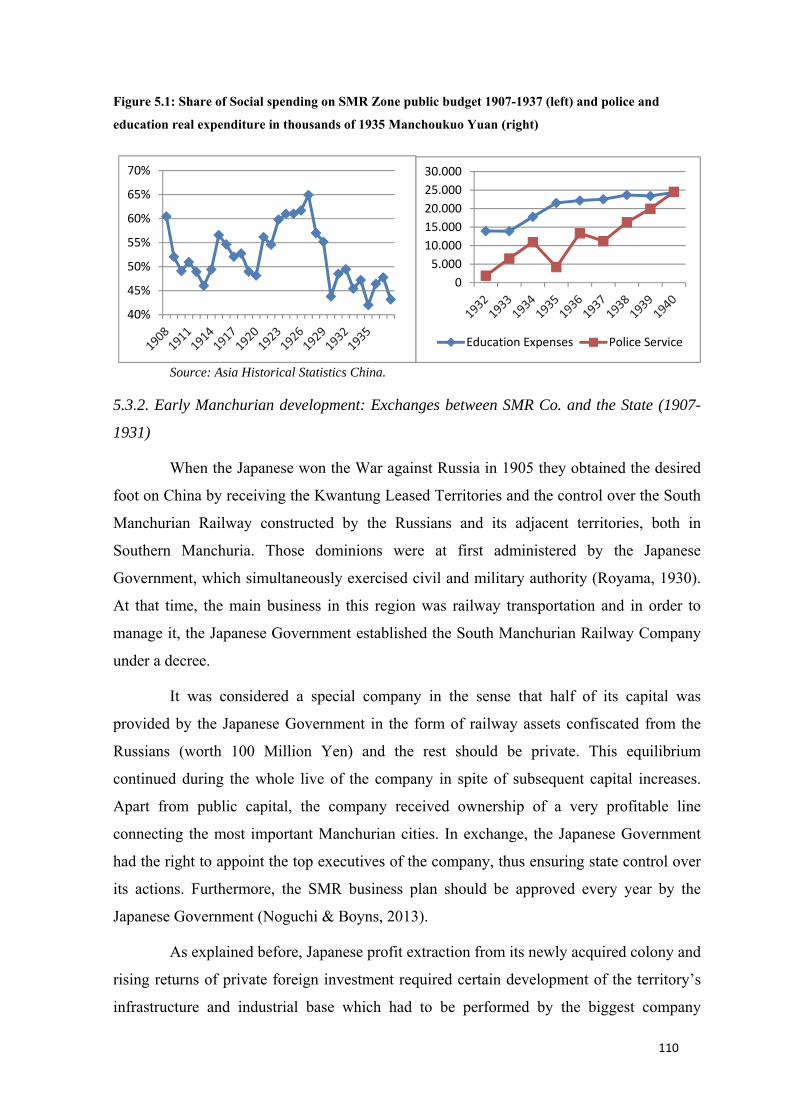
110
Figure 5.1: Share of Social spending on SMR Zone public budget 1907-1937 (left) and police and education real expenditure in thousands of 1935 Manchoukuo Yuan (right)
Source: Asia Historical Statistics China.
5.3.2. Early Manchurian development: Exchanges between SMR Co. and the State (1907-
1931)
When the Japanese won the War against Russia in 1905 they obtained the desired
foot on China by receiving the Kwantung Leased Territories and the control over the South
Manchurian Railway constructed by the Russians and its adjacent territories, both in
Southern Manchuria. Those dominions were at first administered by the Japanese
Government, which simultaneously exercised civil and military authority (Royama, 1930).
At that time, the main business in this region was railway transportation and in order to
manage it, the Japanese Government established the South Manchurian Railway Company
under a decree.
It was considered a special company in the sense that half of its capital was
provided by the Japanese Government in the form of railway assets confiscated from the
Russians (worth 100 Million Yen) and the rest should be private. This equilibrium
continued during the whole live of the company in spite of subsequent capital increases.
Apart from public capital, the company received ownership of a very profitable line
connecting the most important Manchurian cities. In exchange, the Japanese Government
had the right to appoint the top executives of the company, thus ensuring state control over
its actions. Furthermore, the SMR business plan should be approved every year by the
Japanese Government (Noguchi & Boyns, 2013).
As explained before, Japanese profit extraction from its newly acquired colony and
rising returns of private foreign investment required certain development of the territory’s
infrastructure and industrial base which had to be performed by the biggest company
40%
45%
50%
55%
60%
65%
70%
05.000
10.00015.00020.00025.00030.000
Education Expenses Police Service
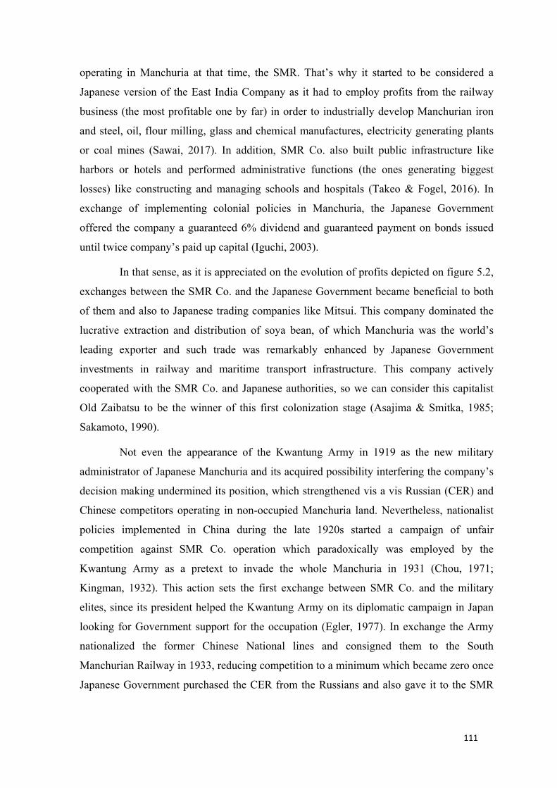
111
operating in Manchuria at that time, the SMR. That’s why it started to be considered a
Japanese version of the East India Company as it had to employ profits from the railway
business (the most profitable one by far) in order to industrially develop Manchurian iron
and steel, oil, flour milling, glass and chemical manufactures, electricity generating plants
or coal mines (Sawai, 2017). In addition, SMR Co. also built public infrastructure like
harbors or hotels and performed administrative functions (the ones generating biggest
losses) like constructing and managing schools and hospitals (Takeo & Fogel, 2016). In
exchange of implementing colonial policies in Manchuria, the Japanese Government
offered the company a guaranteed 6% dividend and guaranteed payment on bonds issued
until twice company’s paid up capital (Iguchi, 2003).
In that sense, as it is appreciated on the evolution of profits depicted on figure 5.2,
exchanges between the SMR Co. and the Japanese Government became beneficial to both
of them and also to Japanese trading companies like Mitsui. This company dominated the
lucrative extraction and distribution of soya bean, of which Manchuria was the world’s
leading exporter and such trade was remarkably enhanced by Japanese Government
investments in railway and maritime transport infrastructure. This company actively
cooperated with the SMR Co. and Japanese authorities, so we can consider this capitalist
Old Zaibatsu to be the winner of this first colonization stage (Asajima & Smitka, 1985;
Sakamoto, 1990).
Not even the appearance of the Kwantung Army in 1919 as the new military
administrator of Japanese Manchuria and its acquired possibility interfering the company’s
decision making undermined its position, which strengthened vis a vis Russian (CER) and
Chinese competitors operating in non-occupied Manchuria land. Nevertheless, nationalist
policies implemented in China during the late 1920s started a campaign of unfair
competition against SMR Co. operation which paradoxically was employed by the
Kwantung Army as a pretext to invade the whole Manchuria in 1931 (Chou, 1971;
Kingman, 1932). This action sets the first exchange between SMR Co. and the military
elites, since its president helped the Kwantung Army on its diplomatic campaign in Japan
looking for Government support for the occupation (Egler, 1977). In exchange the Army
nationalized the former Chinese National lines and consigned them to the South
Manchurian Railway in 1933, reducing competition to a minimum which became zero once
Japanese Government purchased the CER from the Russians and also gave it to the SMR
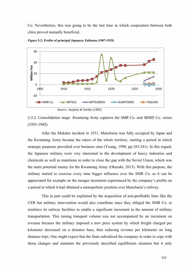
112
Co. Nevertheless, this was going to be the last time in which cooperation between both
elites proved mutually beneficial.
Figure 5.2: Profits of principal Japanese Zaibatsu (1907-1929)
Source: Asajima & Smitka (1985)
5.3.3. Consolidation stage: Kwantung Army captures the SMR Co. and MHID Co. raises
(1931-1945).
After the Mukden incident in 1931, Manchuria was fully occupied by Japan and
the Kwantung Army became the rulers of the whole territory, starting a period in which
strategic purposes prevailed over business ones (Young, 1998, pp.183-241). In this regard,
the Japanese military were very interested in the development of heavy industries and
chemicals as well as munitions in order to close the gap with the Soviet Union, which was
the main potential enemy for the Kwantung Army (Okazaki, 2013). With this purpose, the
military started to exercise every time bigger influence over the SMR Co. as it can be
appreciated for example on the meager increment experienced by the company’s profits on
a period in which it had obtained a monopolistic position over Manchuria’s railway.
This in part could be explained by the acquisition of non-profitable lines like the
CER but military intervention would also contribute since they obliged the SMR Co. to
reinforce its railway facilities to enable a significant increment in the amount of military
transportation. This raising transport volume was not accompanied by an increment on
revenue because the military imposed a new price system by which freight charged per
kilometer decreased on a distance base, thus reducing revenue per kilometer on long
distance trips. One might expect that the State subsidized the company in order to cope with
those changes and maintain the previously described equilibrium situation but it only
-20
0
20
40
60
1905 1910 1915 1920 1925 1930
Mill
ion
Yen
SMR Co. MITSUI MITSUBISHI SUMITOMO YASUDA
113
received a financial loan from the State of Manchuria aiming at increasing cargo capacity
of trains and improving locomotives. The rest of required funds had to be raised from
private sources (Noguchi & Boyns, 2013). That’s why in this point we can be talking about
the military capturing the South Manchurian Railway Company.
This new price system remarkably favored the industrial objectives of the
Kwantung Army in Manchuria in the sense that it facilitated resource mobilization from
Southern factories towards their final destination in the North where the military were
preparing for a war against the Soviets. For example it permitted a sharp reduction in the
cost of transport iron and steel to supply railway construction around the Manchuria-Soviet
frontier in the North and Northeast or in the distribution of explosives and munitions
produced at chemical and arsenal factories in Mukden (South) towards the frontier with the
Soviet Union where Japan had to face the Soviets at different incidents between 1937 and
1939 (Ginsburg, 1949; Goldman, 2012). 60
The rest of economic activities in Manchuria were not so benefited by this new
pricing policy since sources of raw materials were next to iron and steel and chemicals
plants and the main industries, mines and most productive agrarian fields were concentrated
in the Southern region next to the main urban settlements (Avila-Tapies, 2013; Rodgers,
1948) and Murakoshi & Trewartha, 1930).61 Furthermore, we show on appendix 5 how
soya bean exports stagnated because of international repulse to the new Manchurian
regime. That’s why we argue in this paper that Kwantung Army’s controls over SMR
freights reflect the military interests on a rapid growth of iron and steel and chemicals
production, which in Manchuria was dominated by Nissan as will be analyzed during the
rest of the paper.62
Besides, the military strategy was not limited to Manchuria but also required for
Japanese support in the form of technology and expertise. For that reason, the imposed
pricing system over SMR railway was also designed for reducing costs of transport
machinery from Japan to Manchurian factories (United States Bureau of Foreign and
Domestic commerce, 1935, 1937, 1946). In fact, those new transport tariffs became very
effective after 1937, when oil shortages produced after conflicts with China and the Soviet
60 Armur River affair (1937), Changfuken incident (1938) and Nomonhan (1939). 61 We should mention that there was also extensive agriculture on Northern Manchuria. 62 In addition, it also benefited chemical production since it reduced long distance transport of sulphate of ammonia from the Southern factories to act as a fertilizer in the soya bean fields at Manchuria central plains.
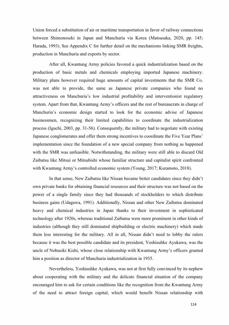
114
Union forced a substitution of air or maritime transportation in favor of railway connections
between Shimonoseki in Japan and Manchuria via Korea (Matsusaka, 2020, pp. 145;
Harada, 1993). See Appendix C for further detail on the mechanisms linking SMR freights,
production in Manchuria and exports by sector.
After all, Kwantung Army policies favored a quick industrialization based on the
production of basic metals and chemicals employing imported Japanese machinery.
Military plans however required huge amounts of capital investments that the SMR Co.
was not able to provide, the same as Japanese private companies who found no
attractiveness on Manchuria’s low industrial profitability and interventionist regulatory
system. Apart from that, Kwantung Army’s officers and the rest of bureaucrats in charge of
Manchuria’s economic design started to look for the economic advise of Japanese
businessmen, recognizing their limited capabilities to coordinate the industrialization
process (Iguchi, 2003, pp. 31-56). Consequently, the military had to negotiate with existing
Japanese conglomerates and offer them strong incentives to coordinate the Five Year Plans’
implementation since the foundation of a new special company from nothing as happened
with the SMR was unfeasible. Notwithstanding, the military were still able to discard Old
Zaibatsu like Mitsui or Mitsubishi whose familiar structure and capitalist spirit confronted
with Kwantung Army’s controlled economic system (Young, 2017; Kuramoto, 2018).
In that sense, New Zaibatsu like Nissan became better candidates since they didn’t
own private banks for obtaining financial resources and their structure was not based on the
power of a single family since they had thousands of stockholders to which distribute
business gains (Udagawa, 1991). Additionally, Nissan and other New Zaibatsu dominated
heavy and chemical industries in Japan thanks to their investment in sophisticated
technology after 1920s, whereas traditional Zaibatsu were more prominent in other kinds of
industries (although they still dominated shipbuilding or electric machinery) which made
them less interesting for the military. All in all, Nissan didn’t need to lobby the rulers
because it was the best possible candidate and its president, Yoshisuhke Ayukawa, was the
uncle of Nobusiki Kishi, whose close relationship with Kwantung Army’s officers granted
him a position as director of Manchuria industrialization in 1935.
Nevertheless, Yoshisuhke Ayukawa, was not at first fully convinced by its nephew
about cooperating with the military and the delicate financial situation of the company
encouraged him to ask for certain conditions like the recognition from the Kwantung Army
of the need to attract foreign capital, which would benefit Nissan relationship with
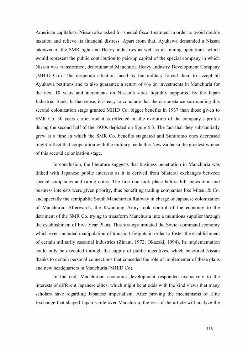
115
American capitalists. Nissan also asked for special fiscal treatment in order to avoid double
taxation and relieve its financial distress. Apart from that, Ayukawa demanded a Nissan
takeover of the SMR light and Heavy industries as well as its mining operations, which
would represent the public contribution to paid-up capital of the special company in which
Nissan was transformed, denominated Manchuria Heavy Industry Development Company
(MHID Co.). The desperate situation faced by the military forced them to accept all
Ayukawa petitions and to also guarantee a return of 6% on investments in Manchuria for
the next 10 years and increments on Nissan’s stock liquidity supported by the Japan
Industrial Bank. In that sense, it is easy to conclude that the circumstance surrounding this
second colonization stage granted MHID Co. bigger benefits in 1937 than those given to
SMR Co. 30 years earlier and it is reflected on the evolution of the company’s profits
during the second half of the 1930s depicted on figure 5.3. The fact that they substantially
grew at a time in which the SMR Co. benefits stagnated and Sumitomo ones decreased
might reflect that cooperation with the military made this New Zaibatsu the greatest winner
of this second colonization stage.
In conclusion, the literature suggests that business penetration in Manchuria was
linked with Japanese public interests as it is derived from bilateral exchanges between
special companies and ruling elites: The first one took place before full annexation and
business interests were given priority, thus benefiting trading companies like Mitsui & Co.
and specially the semipublic South Manchurian Railway in charge of Japanese colonization
of Manchuria. Afterwards, the Kwantung Army took control of the economy to the
detriment of the SMR Co. trying to transform Manchuria into a munitions supplier through
the establishment of Five Year Plans. This strategy imitated the Soviet command economy
which even included manipulation of transport freights in order to foster the establishment
of certain militarily essential industries (Zinam, 1972; Okazaki, 1994). Its implementation
could only be executed through the supply of public incentives, which benefited Nissan
thanks to certain personal connections that conceded the role of implementer of these plans
and new headquarters in Manchuria (MHID Co).
In the end, Manchurian economic development responded exclusively to the
interests of different Japanese elites, which might be at odds with the kind views that many
scholars have regarding Japanese imperialism. After proving the mechanisms of Elite
Exchange that shaped Japan’s rule over Manchuria, the rest of the article will analyze the
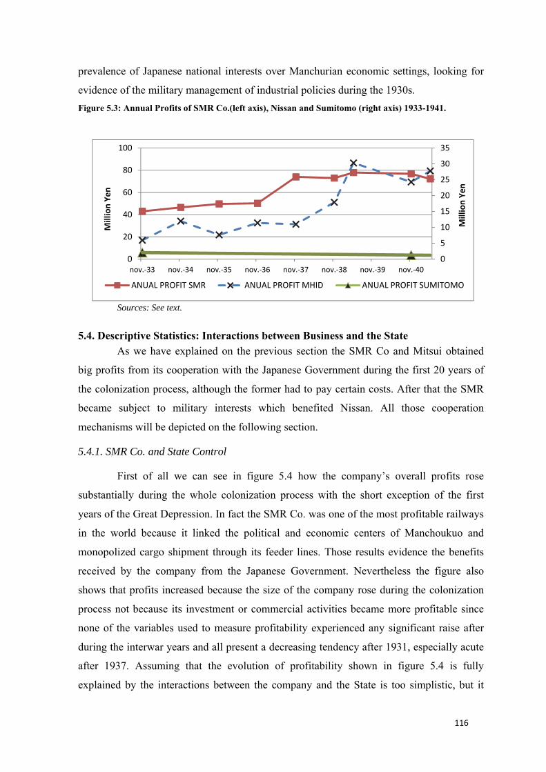
116
prevalence of Japanese national interests over Manchurian economic settings, looking for
evidence of the military management of industrial policies during the 1930s. Figure 5.3: Annual Profits of SMR Co.(left axis), Nissan and Sumitomo (right axis) 1933-1941.
Sources: See text.
5.4. Descriptive Statistics: Interactions between Business and the State As we have explained on the previous section the SMR Co and Mitsui obtained
big profits from its cooperation with the Japanese Government during the first 20 years of
the colonization process, although the former had to pay certain costs. After that the SMR
became subject to military interests which benefited Nissan. All those cooperation
mechanisms will be depicted on the following section.
5.4.1. SMR Co. and State Control
First of all we can see in figure 5.4 how the company’s overall profits rose
substantially during the whole colonization process with the short exception of the first
years of the Great Depression. In fact the SMR Co. was one of the most profitable railways
in the world because it linked the political and economic centers of Manchoukuo and
monopolized cargo shipment through its feeder lines. Those results evidence the benefits
received by the company from the Japanese Government. Nevertheless the figure also
shows that profits increased because the size of the company rose during the colonization
process not because its investment or commercial activities became more profitable since
none of the variables used to measure profitability experienced any significant raise after
during the interwar years and all present a decreasing tendency after 1931, especially acute
after 1937. Assuming that the evolution of profitability shown in figure 5.4 is fully
explained by the interactions between the company and the State is too simplistic, but it
0
5
10
15
20
25
30
35
0
20
40
60
80
100
nov.-33 nov.-34 nov.-35 nov.-36 nov.-37 nov.-38 nov.-39 nov.-40
Mill
ion
Yen
Mill
ion
Yen
ANUAL PROFIT SMR ANUAL PROFIT MHID ANUAL PROFIT SUMITOMO
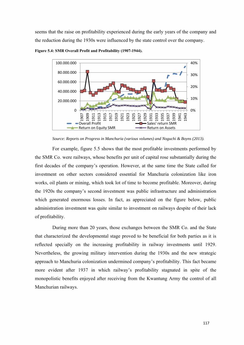
117
seems that the raise on profitability experienced during the early years of the company and
the reduction during the 1930s were influenced by the state control over the company.
Figure 5.4: SMR Overall Profit and Profitability (1907-1944).
Source: Reports on Progress in Manchuria (various volumes) and Noguchi & Boyns (2013).
For example, figure 5.5 shows that the most profitable investments performed by
the SMR Co. were railways, whose benefits per unit of capital rose substantially during the
first decades of the company’s operation. However, at the same time the State called for
investment on other sectors considered essential for Manchuria colonization like iron
works, oil plants or mining, which took lot of time to become profitable. Moreover, during
the 1920s the company’s second investment was public infrastructure and administration
which generated enormous losses. In fact, as appreciated on the figure below, public
administration investment was quite similar to investment on railways despite of their lack
of profitability.
During more than 20 years, those exchanges between the SMR Co. and the State
that characterized the developmental stage proved to be beneficial for both parties as it is
reflected specially on the increasing profitability in railway investments until 1929.
Nevertheless, the growing military intervention during the 1930s and the new strategic
approach to Manchuria colonization undermined company’s profitability. This fact became
more evident after 1937 in which railway’s profitability stagnated in spite of the
monopolistic benefits enjoyed after receiving from the Kwantung Army the control of all
Manchurian railways.
0%
10%
20%
30%
40%
0
20.000.000
40.000.000
60.000.000
80.000.000
100.000.000
1907
1909
1911
1913
1915
1917
1919
1921
1923
1925
1927
1929
1931
1933
1935
1937
1939
1941
1943
Overall Profit Sales' return SMRReturn on Equity SMR Return on Assets
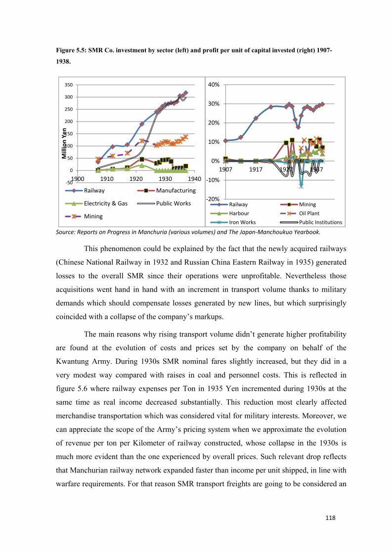
118
Figure 5.5: SMR Co. investment by sector (left) and profit per unit of capital invested (right) 1907-1938.
Source: Reports on Progress in Manchuria (various volumes) and The Japan-Manchoukuo Yearbook.
This phenomenon could be explained by the fact that the newly acquired railways
(Chinese National Railway in 1932 and Russian China Eastern Railway in 1935) generated
losses to the overall SMR since their operations were unprofitable. Nevertheless those
acquisitions went hand in hand with an increment in transport volume thanks to military
demands which should compensate losses generated by new lines, but which surprisingly
coincided with a collapse of the company’s markups.
The main reasons why rising transport volume didn’t generate higher profitability
are found at the evolution of costs and prices set by the company on behalf of the
Kwantung Army. During 1930s SMR nominal fares slightly increased, but they did in a
very modest way compared with raises in coal and personnel costs. This is reflected in
figure 5.6 where railway expenses per Ton in 1935 Yen incremented during 1930s at the
same time as real income decreased substantially. This reduction most clearly affected
merchandise transportation which was considered vital for military interests. Moreover, we
can appreciate the scope of the Army’s pricing system when we approximate the evolution
of revenue per ton per Kilometer of railway constructed, whose collapse in the 1930s is
much more evident than the one experienced by overall prices. Such relevant drop reflects
that Manchurian railway network expanded faster than income per unit shipped, in line with
warfare requirements. For that reason SMR transport freights are going to be considered an
-20%
-10%
0%
10%
20%
30%
40%
1907 1917 1927 1937
Railway MiningHarbour Oil PlantIron Works Public Institutions
-50
0
50
100
150
200
250
300
350
1900 1910 1920 1930 1940
Mill
ion
Yen
Railway Manufacturing
Electricity & Gas Public Works
Mining
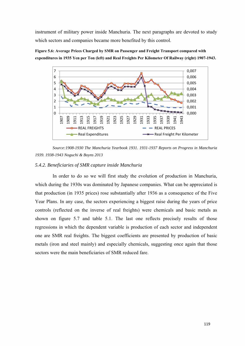
119
instrument of military power inside Manchuria. The next paragraphs are devoted to study
which sectors and companies became more benefited by this control.
Figure 5.6: Average Prices Charged by SMR on Passenger and Freight Transport compared with expenditures in 1935 Yen per Ton (left) and Real Freights Per Kilometer Of Railway (right) 1907-1943.
Source:1908-1930 The Manchuria Yearbook 1931. 1931-1937 Reports on Progress in Manchuria
1939. 1938-1943 Noguchi & Boyns 2013
5.4.2. Beneficiaries of SMR capture inside Manchuria
In order to do so we will first study the evolution of production in Manchuria,
which during the 1930s was dominated by Japanese companies. What can be appreciated is
that production (in 1935 prices) rose substantially after 1936 as a consequence of the Five
Year Plans. In any case, the sectors experiencing a biggest raise during the years of price
controls (reflected on the inverse of real freights) were chemicals and basic metals as
shown on figure 5.7 and table 5.1. The last one reflects precisely results of those
regressions in which the dependent variable is production of each sector and independent
one are SMR real freights. The biggest coefficients are presented by production of basic
metals (iron and steel mainly) and especially chemicals, suggesting once again that those
sectors were the main beneficiaries of SMR reduced fare.
0,0000,0010,0020,0030,0040,0050,0060,007
01234567
1907
1909
1911
1913
1915
1917
1919
1921
1923
1925
1927
1929
1931
1933
1935
1937
1939
1941
1943
REAL FREIGHTS REAL PRICESReal Expenditures Real Freight Per Kilometer
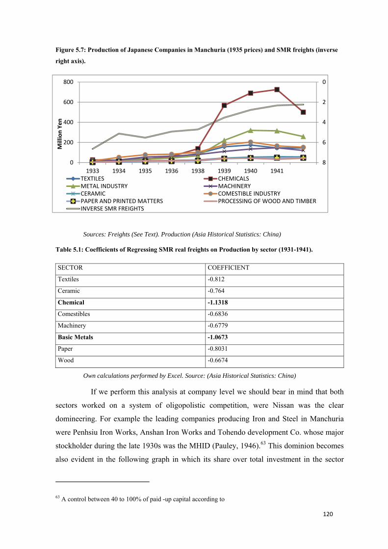
120
Figure 5.7: Production of Japanese Companies in Manchuria (1935 prices) and SMR freights (inverse right axis).
Sources: Freights (See Text). Production (Asia Historical Statistics: China)
Table 5.1: Coefficients of Regressing SMR real freights on Production by sector (1931-1941).
SECTOR COEFFICIENT
Textiles -0.812
Ceramic -0.764
Chemical -1.1318
Comestibles -0.6836
Machinery -0.6779
Basic Metals -1.0673
Paper -0.8031
Wood -0.6674
Own calculations performed by Excel. Source: (Asia Historical Statistics: China)
If we perform this analysis at company level we should bear in mind that both
sectors worked on a system of oligopolistic competition, were Nissan was the clear
domineering. For example the leading companies producing Iron and Steel in Manchuria
were Penhsiu Iron Works, Anshan Iron Works and Tohendo development Co. whose major
stockholder during the late 1930s was the MHID (Pauley, 1946).63 This dominion becomes
also evident in the following graph in which its share over total investment in the sector
63 A control between 40 to 100% of paid -up capital according to
0
2
4
6
80
200
400
600
800
1933 1934 1935 1936 1938 1939 1940 1941
Mill
ion
Yen
TEXTILES CHEMICALSMETAL INDUSTRY MACHINERYCERAMIC COMESTIBLE INDUSTRYPAPER AND PRINTED MATTERS PROCESSING OF WOOD AND TIMBERINVERSE SMR FREIGHTS
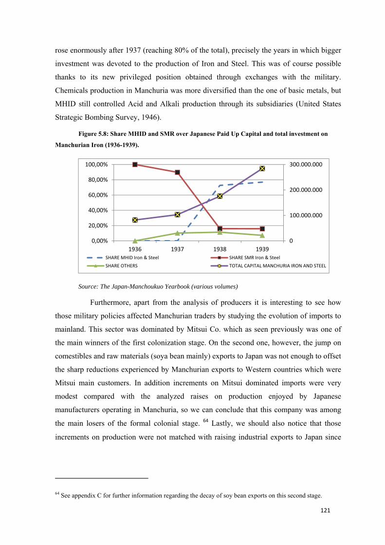
121
rose enormously after 1937 (reaching 80% of the total), precisely the years in which bigger
investment was devoted to the production of Iron and Steel. This was of course possible
thanks to its new privileged position obtained through exchanges with the military.
Chemicals production in Manchuria was more diversified than the one of basic metals, but
MHID still controlled Acid and Alkali production through its subsidiaries (United States
Strategic Bombing Survey, 1946).
Figure 5.8: Share MHID and SMR over Japanese Paid Up Capital and total investment on Manchurian Iron (1936-1939).
Source: The Japan-Manchoukuo Yearbook (various volumes)
Furthermore, apart from the analysis of producers it is interesting to see how
those military policies affected Manchurian traders by studying the evolution of imports to
mainland. This sector was dominated by Mitsui Co. which as seen previously was one of
the main winners of the first colonization stage. On the second one, however, the jump on
comestibles and raw materials (soya bean mainly) exports to Japan was not enough to offset
the sharp reductions experienced by Manchurian exports to Western countries which were
Mitsui main customers. In addition increments on Mitsui dominated imports were very
modest compared with the analyzed raises on production enjoyed by Japanese
manufacturers operating in Manchuria, so we can conclude that this company was among
the main losers of the formal colonial stage. 64 Lastly, we should also notice that those
increments on production were not matched with raising industrial exports to Japan since
64 See appendix C for further information regarding the decay of soy bean exports on this second stage.
0
100.000.000
200.000.000
300.000.000
0,00%
20,00%
40,00%
60,00%
80,00%
100,00%
1936 1937 1938 1939SHARE MHID Iron & Steel SHARE SMR Iron & SteelSHARE OTHERS TOTAL CAPITAL MANCHURIA IRON AND STEEL
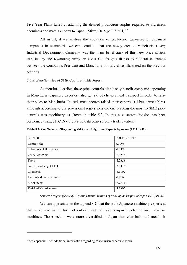
122
Five Year Plans failed at attaining the desired production surplus required to increment
chemicals and metals exports to Japan (Miwa, 2015,pp303-304).65
All in all, if we analyze the evolution of production generated by Japanese
companies in Manchuria we can conclude that the newly created Manchuria Heavy
Industrial Development Company was the main beneficiary of this new price system
imposed by the Kwantung Army on SMR Co. freights thanks to bilateral exchanges
between the company’s President and Manchuria military elites illustrated on the previous
sections.
5.4.3. Beneficiaries of SMR Capture inside Japan.
As mentioned earlier, these price controls didn’t only benefit companies operating
in Manchuria. Japanese exporters also got rid of cheaper land transport in order to raise
their sales to Manchuria. Indeed, most sectors raised their exports (all but comestibles),
although according to our provisional regressions the one reacting the most to SMR price
controls was machinery as shown in table 5.2. In this case sector division has been
performed using SITC Rev 2 because data comes from a trade database.
Table 5.2: Coefficients of Regressing SMR real freights on Exports by sector (1932-1938).
SECTOR COEFFICIENT
Comestibles 6.9006
Tobacco and Beverages -1.719
Crude Materials -2.7518
Fuels -2.2858
Animal and Vegetal Oil -3.1146
Chemicals -4.3602
Unfinished manufactures -2.906
Machinery -5.2614
Finished Manufactures -3.3802
Source: Freights (See text), Exports (Annual Returns of trade of the Empire of Japan 1932, 1938))
We can appreciate on the appendix C that the main Japanese machinery exports at
that time were in the form of railway and transport equipment, electric and industrial
machines. Those sectors were more diversified in Japan than chemicals and metals in
65See appendix C for additional information regarding Manchurian exports to Japan.
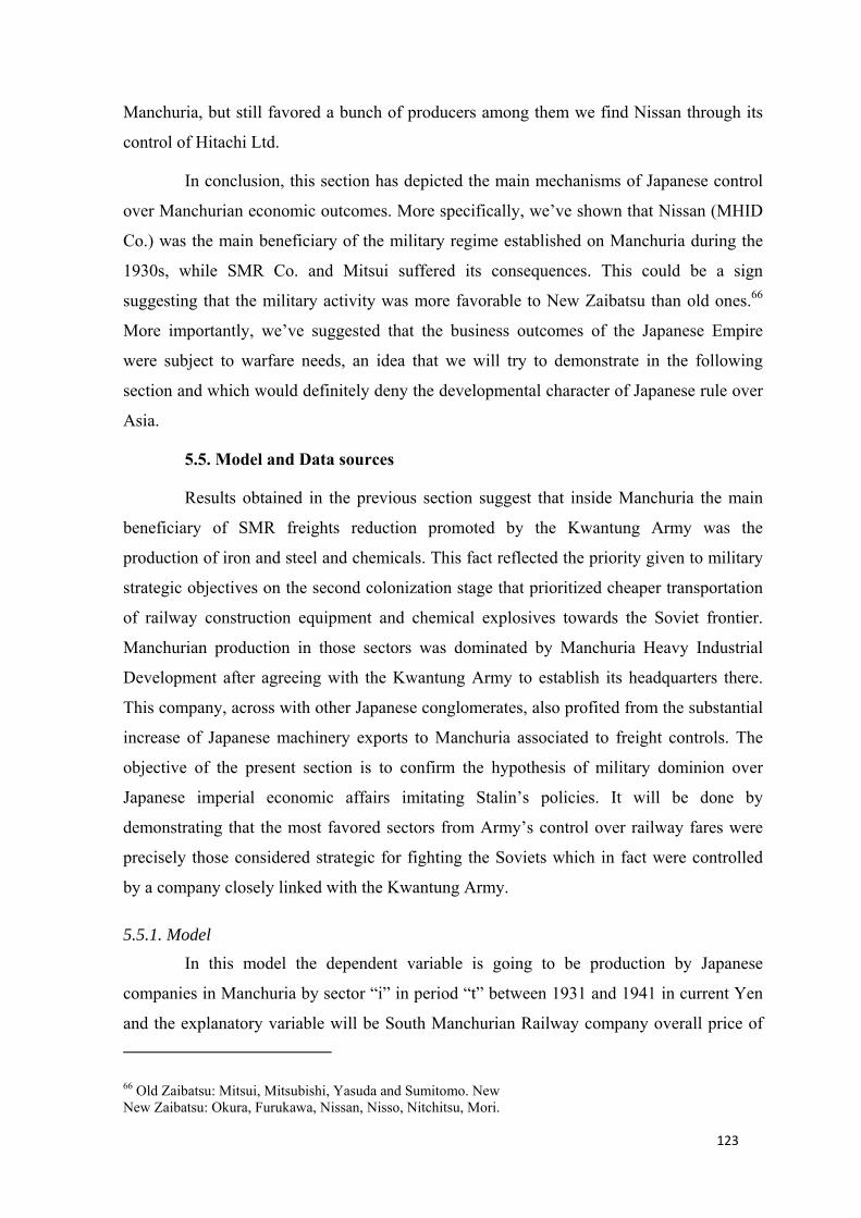
123
Manchuria, but still favored a bunch of producers among them we find Nissan through its
control of Hitachi Ltd.
In conclusion, this section has depicted the main mechanisms of Japanese control
over Manchurian economic outcomes. More specifically, we’ve shown that Nissan (MHID
Co.) was the main beneficiary of the military regime established on Manchuria during the
1930s, while SMR Co. and Mitsui suffered its consequences. This could be a sign
suggesting that the military activity was more favorable to New Zaibatsu than old ones.66
More importantly, we’ve suggested that the business outcomes of the Japanese Empire
were subject to warfare needs, an idea that we will try to demonstrate in the following
section and which would definitely deny the developmental character of Japanese rule over
Asia.
5.5. Model and Data sources
Results obtained in the previous section suggest that inside Manchuria the main
beneficiary of SMR freights reduction promoted by the Kwantung Army was the
production of iron and steel and chemicals. This fact reflected the priority given to military
strategic objectives on the second colonization stage that prioritized cheaper transportation
of railway construction equipment and chemical explosives towards the Soviet frontier.
Manchurian production in those sectors was dominated by Manchuria Heavy Industrial
Development after agreeing with the Kwantung Army to establish its headquarters there.
This company, across with other Japanese conglomerates, also profited from the substantial
increase of Japanese machinery exports to Manchuria associated to freight controls. The
objective of the present section is to confirm the hypothesis of military dominion over
Japanese imperial economic affairs imitating Stalin’s policies. It will be done by
demonstrating that the most favored sectors from Army’s control over railway fares were
precisely those considered strategic for fighting the Soviets which in fact were controlled
by a company closely linked with the Kwantung Army.
5.5.1. Model In this model the dependent variable is going to be production by Japanese
companies in Manchuria by sector “i” in period “t” between 1931 and 1941 in current Yen
and the explanatory variable will be South Manchurian Railway company overall price of 66 Old Zaibatsu: Mitsui, Mitsubishi, Yasuda and Sumitomo. New New Zaibatsu: Okura, Furukawa, Nissan, Nisso, Nitchitsu, Mori.
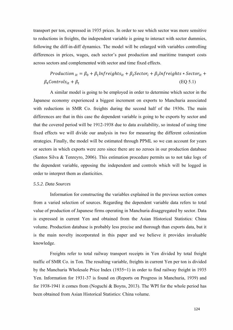
124
transport per ton, expressed in 1935 prices. In order to see which sector was more sensitive
to reductions in freights, the independent variable is going to interact with sector dummies,
following the diff-in-diff dynamics. The model will be enlarged with variables controlling
differences in prices, wages, each sector’s past production and maritime transport costs
across sectors and complemented with sector and time fixed effects. 𝑃𝑟𝑜𝑑𝑢𝑐𝑡𝑖𝑜𝑛 = 𝛽 + 𝛽 𝑙𝑛𝑓𝑟𝑒𝑖𝑔ℎ𝑡𝑠 + 𝛽 𝑆𝑒𝑐𝑡𝑜𝑟 + 𝛽 𝑙𝑛𝑓𝑟𝑒𝑖𝑔ℎ𝑡𝑠 ∗ 𝑆𝑒𝑐𝑡𝑜𝑟 +𝛽 𝐶𝑜𝑛𝑡𝑟𝑜𝑙𝑠 + 𝛽 (EQ 5.1)
A similar model is going to be employed in order to determine which sector in the
Japanese economy experienced a biggest increment on exports to Manchuria associated
with reductions in SMR Co. freights during the second half of the 1930s. The main
differences are that in this case the dependent variable is going to be exports by sector and
that the covered period will be 1912-1938 due to data availability, so instead of using time
fixed effects we will divide our analysis in two for measuring the different colonization
strategies. Finally, the model will be estimated through PPML so we can account for years
or sectors in which exports were zero since there are no zeroes in our production database
(Santos Silva & Tenreyro, 2006). This estimation procedure permits us to not take logs of
the dependent variable, opposing the independent and controls which will be logged in
order to interpret them as elasticities.
5.5.2. Data Sources
Information for constructing the variables explained in the previous section comes
from a varied selection of sources. Regarding the dependent variable data refers to total
value of production of Japanese firms operating in Manchuria disaggregated by sector. Data
is expressed in current Yen and obtained from the Asian Historical Statistics: China
volume. Production database is probably less precise and thorough than exports data, but it
is the main novelty incorporated in this paper and we believe it provides invaluable
knowledge.
Freights refer to total railway transport receipts in Yen divided by total freight
traffic of SMR Co. in Ton. The resulting variable, freights in current Yen per ton is divided
by the Manchuria Wholesale Price Index (1935=1) in order to find railway freight in 1935
Yen. Information for 1931-37 is found on (Reports on Progress in Manchuria, 1939) and
for 1938-1941 it comes from (Noguchi & Boyns, 2013). The WPI for the whole period has
been obtained from Asian Historical Statistics: China volume.
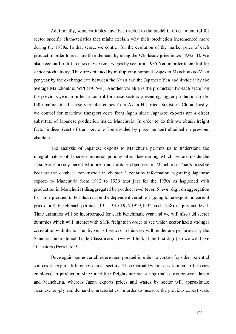
125
Additionally, some variables have been added to the model in order to control for
sector specific characteristics that might explain why their production incremented more
during the 1930s. In that sense, we control for the evolution of the market price of each
product in order to measure their demand by using the Wholesale price index (1935=1). We
also account for differences in workers’ wages by sector in 1935 Yen in order to control for
sector productivity. They are obtained by multiplying nominal wages in Manchoukuo Yuan
per year by the exchange rate between the Yuan and the Japanese Yen and divide it by the
average Manchoukuo WPI (1935=1). Another variable is the production by each sector on
the previous year in order to control for those sectors presenting bigger production scale.
Information for all those variables comes from Asian Historical Statistics: China. Lastly,
we control for maritime transport costs from Japan since Japanese exports are a direct
substitute of Japanese production inside Manchuria. In order to do this we obtain freight
factor indices (cost of transport one Ton divided by price per ton) obtained on previous
chapters.
The analysis of Japanese exports to Manchuria permits us to understand the
integral nature of Japanese imperial policies after determining which sectors inside the
Japanese economy benefited more from military objectives in Manchuria. That’s possible
because the database constructed in chapter 3 contains information regarding Japanese
exports to Manchuria from 1912 to 1938 (not just for the 1930s as happened with
production in Manchuria) disaggregated by product level (even 5 level digit disaggregation
for some products). For that reason the dependent variable is going to be exports in current
prices in 6 benchmark periods (1912,1915,1925,1929,1932 and 1938) at product level.
Time dummies will be incorporated for each benchmark year and we will also add sector
dummies which will interact with SMR freights in order to see which sector had a stronger
correlation with them. The division of sectors in this case will be the one performed by the
Standard International Trade Classification (we will look at the first digit) so we will have
10 sectors (from 0 to 9).
Once again, some variables are incorporated in order to control for other potential
sources of export differences across sectors. Those variables are very similar to the ones
employed in production since maritime freights are measuring trade costs between Japan
and Manchuria, whereas Japan exports prices and wages by sector will approximate
Japanese supply and demand characteristics. In order to measure the previous export scale
126
of every sector we are going to lag the variable as we did with production in the first
regression.
Maritime freights are obtained on previous chapters while information regarding
the rest of controls appear on (Ohkawa et al., 1967-1989) which includes data for Japan
exports price index (1935=100), nominal daily wages in Yen (translated to 1934-36 prices
using Japanese WPI) and Japan exports prices for a determined set of commodities. This
information is adapted to our sector classification by assuming that the most exported
commodity inside every sector represents the whole sector. See appendix C in order to
check which commodity has been chosen to represent each sector.
5.6. Results 5.6.1. Production by Japanese companies in Manchuria.
Results interpretation should be done in a careful way. First of all, as can be
appreciated on table 5.3 the relationship between SMR freights and production is negative,
in the sense that reductions in tariffs experienced after 1931 were related with an overall
increment in the production of Japanese firms in Manchuria. Secondly, the size of this
impact is reduced at those sectors presenting positive and significant interactions, which
were all but chemicals, basic metals and paper. Those three sectors show very low
coefficients which are even statistically insignificant, suggesting that the enhancing effect
of reduced railway costs was relatively bigger for them.67
Nevertheless, these results might be explained by certain peculiarities intrinsic to
these sectors rather than by the military plans. That’s why we add in column 2 variables
that complement sector fixed effects in order to control these characteristics and results are
maintained. A third concern with the results is that R2 is extraordinarily high for a model in
which few variables are included, which could reflect a low variation among our
observations. This problem is not present on exports’ regressions but in spite of it, we
believe results to reasonably complement the story presented on previous sections as
evidence of military control of Manchurian economy during the 1930s.
67 We should notice that for example a one percent reduction on SMR real freights is associated with an increase of 3.9719% ((-3.986+0.0141)*-1)=3.9719) in production of chemicals and with a raise of just 2.516% in comestibles ((-3.986+1.47)*-1=2.516). In fact, a higher and significant interaction coefficient denotes a smaller impact of SMR freights on a certain sector production. See appendix C for further details on this overall effect.
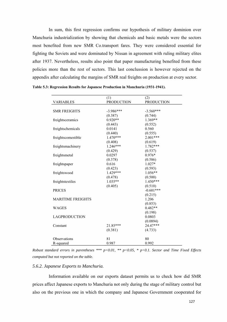
127
In sum, this first regression confirms our hypothesis of military dominion over
Manchuria industrialization by showing that chemicals and basic metals were the sectors
most benefited from new SMR Co.transport fares. They were considered essential for
fighting the Soviets and were dominated by Nissan in agreement with ruling military elites
after 1937. Nevertheless, results also point that paper manufacturing benefited from these
policies more than the rest of sectors. This last conclussion is however rejected on the
appendix after calculating the margins of SMR real freights on production at every sector.
Table 5.3: Regression Results for Japanese Production in Manchuria (1931-1941).
(1) (2) VARIABLES PRODUCTION PRODUCTION SMR FREIGHTS -3.986*** -3.560*** (0.387) (0.744) freightsceramics 0.920** 1.369** (0.443) (0.552) freightschemicals 0.0141 0.560 (0.440) (0.555) freightscomestible 1.470*** 2.001*** (0.408) (0.619) freightsmachinery 1.246*** 1.782*** (0.429) (0.537) freightsmetal 0.0297 0.976* (0.378) (0.586) freightspaper 0.616 1.027* (0.423) (0.593) freightswood 1.429*** 1.056** (0.478) (0.500) freightstextiles 1.035** 1.450*** (0.405) (0.510) PRICES -0.601*** (0.215) MARITIME FREIGHTS 1.206 (0.853) WAGES 0.482** (0.198) LAGPRODUCTION 0.0803 (0.0894) Constant 21.85*** 24.47*** (0.381) (4.733) Observations 81 80 R-squared 0.987 0.992
Robust standard errors in parentheses *** p<0.01, ** p<0.05, * p<0.1. Sector and Time Fixed Effects
computed but not reported on the table.
5.6.2. Japanese Exports to Manchuria.
Information available on our exports dataset permits us to check how did SMR
prices affect Japanese exports to Manchuria not only during the stage of military control but
also on the previous one in which the company and Japanese Government cooperated for
128
economically developing the region. That’s why the analysis will be divided in two time
periods: the 1912-1929 period will represent the first stage whereas the 1932-1938 will
illustrate the second one.
Results are confirming what we suspected on previous sections. The first period is
a developmental one in which raises on freights set by SMR were linked with Manchurian
prosperity. For that reason Japan exports to that region are increasing at the same time as
railway transport prices incremented. This effect seems to be bigger for comestible exports
to feed Japanese migrants and most importantly to machinery exports, which at this stage
were characterized by an increment on light industrial machinery and transport equipment
exports which tried to complement Japanese business investments.68
The period 1932-1938 is however one of reduced SMR tariffs due to military
control and of increasing exports for most of the sectors, that’s why coefficients are
negative. Machinery is the most benefited sector since it was essential to complete
industrialization planned by the Kwantung Army. In this period transport equipment
became the main component and metal working machinery rose its share, suggesting that
this new stage was more focused on heavy industrial development for military purposes.
This conclusion is also obtained after adding the previously presented controls since we
find that machinery is still among the sectors whose exports received a relevant impulse by
military policies, although in this case beverages, fuels and raw materials were more
sensitive to railway freights reduction. Anyway, those exports also complemented
machinery ones (except for beverages) since most fuels were machine lubricants and a big
part of raw materials exports were wood for railway construction. Furthermore, the
performance of a Wald test confirms that the influence of freights over machinery exports
is the same with and without controls, confirming that it was the most sensitive sector to
this policy. See appendix C for further information.
As a summary, this section permits us to better distinguish the two different stages
in Manchuria colonization by Japan, which are confirmed on the appendix through the
performance of a Wald test showing that coefficients on the first period are significantly
different to those on the second. We also demonstrate the influence of military plans over
68 In order to measure the overall influence of SMR freights on every sector’s exports we should add the coefficient for each specific sector to the general coefficient of SMR freights. For example in 1932-38 a 1% reduction in railway freights was associated with an increment of 8.276% on Japanese machinery exports to Manchuria. For further detail on overall effect by sector see appendix C.
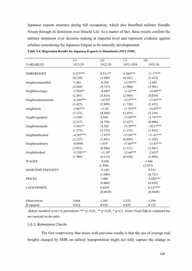
129
Japanese exports structure during full occupation, which also benefited military friendly
Nissan through its dominion over Hitachi Ltd. As a matter of fact, these results confirm the
military dominion over decision making at imperial level and represent evidence against
scholars considering the Japanese Empire to be naturally developmental. Table 5.4: Regression Results for Japanese Exports to Manchuria (1912-1938).
(1) (2) (3) (4) VARIABLES 1912-29 1912-29 1932-1938 1932-38 SMRFREIGHT 9.237*** 8.311** 9.384*** 11.77*** (0.239) (3.948) (0.391) (2.472) freightcommestible -1.481 -0.394 -12.59*** -2.495 (2.888) (5.737) (1.980) (3.901) freightbeverages -5.584** -8.696* -11.42*** -14.44*** (2.581) (4.816) (2.068) (4.029) freightcrudematerials -6.248*** -10.78* -15.57*** -17.03*** (1.425) (5.899) (1.728) (2.422) freightfuels -5.067** -11.82 -11.93*** -14.95*** (2.321) (8.948) (2.455) (3.234) freightvegetaloil -5.298* 4.294 -13.69*** -2.747*** (3.217) (8.798) (1.627) (0.808) freightchemicals -3.201** -4.302 -15.39*** -10.27*** (1.375) (5.233) (1.233) (1.818) freightunfinished -4.283*** -7.475* -15.04*** -11.41*** (1.227) (3.841) (0.893) (1.303) freightmachinery -0.0696 1.079 -17.66*** -13.43*** (2.053) (6.906) (1.211) (2.961) freightfinished -5.320*** -11.39* -13.66*** -2.019* (1.589) (6.215) (0.926) (1.056) WAGES 0.696 -1.666 (1.494) (3.073) MARITIME FREIGHTS -0.140 0.533 (1.049) (0.723) PRICES 1.000 4.420*** (0.800) (0.839) LAGEXPORTS 0.0265 0.127*** (0.0620) (0.0448) Observations 5,064 1,505 2,532 1,394 R-squared 0.016 0.034 0.039 0.122
Robust standard errors in parentheses *** p<0.01, ** p<0.05, * p<0.1. Sector Fixed Effects computed but
not reported on the table.
5.6.3. Robustness Checks
The first controversy that arises with previous results is that the use of average real
freights charged by SMR on railway transportation might not fully capture the change in
130
policies favoring distant trips. As explained before, this policy established lower prices per
kilometer for longer trips and we believe this caused a reduction on overall railway freights.
Nevertheless, the variable chosen in this paper might not fully reflect distance based
curtailment established on behalf of the Kwantung Army and that’s why in this regression
we are going to approximate a measure of railway transport freights per kilometer. Bearing
in mind that we don’t have data for costs of transport per kilometer we will approximate it
by dividing SMR transport freights in 1935 Yen per ton by total active kilometers of
railway operated by the SMR at every year. This variable not only reflects the expansion of
Manchurian railway network but also the increasing distance covered by SMR trains as a
consequence of this northward extension, that was not accompanied by comparable raises
in fares.
Conclusions under this new variable are very similar if we have a look at tables 5.5
and 5.6: Basic metals and chemicals are the most favored sectors by SMR pricing policy
(although if we add controls we obtain that wood is also strongly affected) and machinery
is the most sensitive exports sector at both stages, although after adding controls there are
other sectors more influenced by this pricing policy on the second stage.
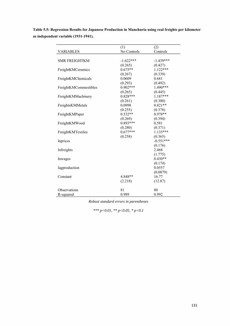
131
Table 5.5: Regression Results for Japanese Production in Manchuria using real freights per kilometer as independent variable (1931-1941).
(1) (2) VARIABLES No Controls Controls SMR FREIGHTKM -1.622*** -1.439*** (0.265) (0.427) FreightKMCeramics 0.675** 1.122*** (0.267) (0.339) FreightKMChemicals 0.0609 0.681 (0.293) (0.492) FreightKMCommestibles 0.902*** 1.490*** (0.265) (0.445) FreightKMMachinery 0.828*** 1.187*** (0.261) (0.300) FreightsKMMetals 0.0998 0.821** (0.255) (0.378) FreightKMPaper 0.532** 0.978** (0.269) (0.394) FreightKMWood 0.893*** 0.581 (0.280) (0.371) FreightKMTextiles 0.677*** 1.135*** (0.258) (0.365) lnprices -0.551*** (0.176) lnfreights 2.468 (1.775) lnwages 0.430** (0.174) lagproduction 0.0557 (0.0879) Constant 4.848** 16.77 (2.218) (12.87) Observations 81 80 R-squared 0.989 0.992
Robust standard errors in parentheses
*** p<0.01, ** p<0.05, * p<0.1
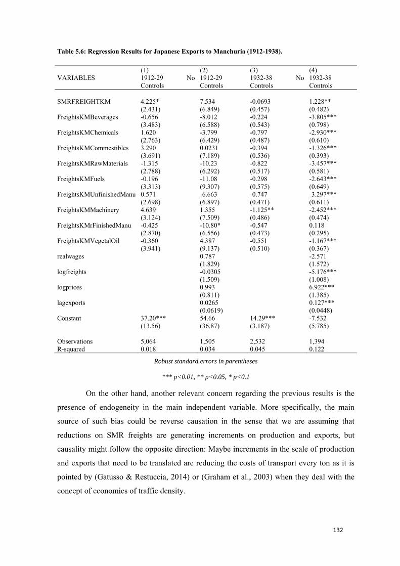
132
Table 5.6: Regression Results for Japanese Exports to Manchuria (1912-1938).
(1) (2) (3) (4) VARIABLES 1912-29 No
Controls 1912-29 Controls
1932-38 No Controls
1932-38 Controls
SMRFREIGHTKM 4.225* 7.534 -0.0693 1.228** (2.431) (6.849) (0.457) (0.482) FreightsKMBeverages -0.656 -8.012 -0.224 -3.805*** (3.483) (6.588) (0.543) (0.798) FreightsKMChemicals 1.620 -3.799 -0.797 -2.930*** (2.763) (6.429) (0.487) (0.610) FreightsKMCommestibles 3.290 0.0231 -0.394 -1.326*** (3.691) (7.189) (0.536) (0.393) FreightsKMRawMaterials -1.315 -10.23 -0.822 -3.457*** (2.788) (6.292) (0.517) (0.581) FreightsKMFuels -0.196 -11.08 -0.298 -2.643*** (3.313) (9.307) (0.575) (0.649) FreightsKMUnfinishedManu 0.571 -6.663 -0.747 -3.297*** (2.698) (6.897) (0.471) (0.611) FreightsKMMachinery 4.639 1.355 -1.125** -2.452*** (3.124) (7.509) (0.486) (0.474) FreightsKMrFinishedManu -0.425 -10.80* -0.547 0.118 (2.870) (6.556) (0.473) (0.295) FreightsKMVegetalOil -0.360 4.387 -0.551 -1.167*** (3.941) (9.137) (0.510) (0.367) realwages 0.787 -2.571 (1.829) (1.572) logfreights -0.0305 -5.176*** (1.509) (1.008) logprices 0.993 6.922*** (0.811) (1.385) lagexports 0.0265 0.127*** (0.0619) (0.0448) Constant 37.20*** 54.66 14.29*** -7.532 (13.56) (36.87) (3.187) (5.785) Observations 5,064 1,505 2,532 1,394 R-squared 0.018 0.034 0.045 0.122
Robust standard errors in parentheses
*** p<0.01, ** p<0.05, * p<0.1
On the other hand, another relevant concern regarding the previous results is the
presence of endogeneity in the main independent variable. More specifically, the main
source of such bias could be reverse causation in the sense that we are assuming that
reductions on SMR freights are generating increments on production and exports, but
causality might follow the opposite direction: Maybe increments in the scale of production
and exports that need to be translated are reducing the costs of transport every ton as it is
pointed by (Gatusso & Restuccia, 2014) or (Graham et al., 2003) when they deal with the
concept of economies of traffic density.
133
The following section tries to avoid this problem and keep showing that the
Kwantung Army controlled the industrialization process in Manchuria by substituting the
dependent variable, SMR Co. real freights, by an exogenous variable that is not affected by
the level of production or exports as it was the establishment of Five Year Plans for
industrializing Manchuria by the Kwantung Army. 69 This is going to be a dummy variable
whose value equals 0 before the establishment of the first plan in 1937 and 1 afterwards. As
we’ve done previously, this variable is interacted with sector fixed effects in order to see
which sector’s production and exports were more favored by the establishment of this Five
Year Plan. 70
69 Those plans looked for Manchuria industrial self-sufficiency so deceptive levels of manufacturing production could prompt the adoption of these plans. Nevertheless, those plans were not adopted until the Military confronted the Soviets for the first time in 1937, that’s why we consider it as independent from production levels. 70 A problem associated with this variable is that it is time-specific and not associated with geographic or sector differences but it still represents a turning point on Manchuria economic development lead by the military.
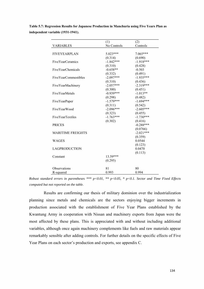
134
Table 5.7: Regression Results for Japanese Production in Manchuria using Five Years Plan as independent variable (1931-1941).
(1) (2) VARIABLES No Controls Controls FIVEYEARPLAN 5.023*** 7.065*** (0.314) (0.690) FiveYearCeramics -1.842*** -1.918*** (0.310) (0.428) FiveYearChemicals -0.658** -0.503 (0.332) (0.491) FiveYearCommestibles -2.097*** -1.935*** (0.310) (0.436) FiveYearMachinery -2.057*** -2.319*** (0.300) (0.451) FiveYearMetals -0.939*** -1.013** (0.298) (0.482) FiveYearPaper -1.579*** -1.694*** (0.311) (0.542) FiveYearWood -2.096*** -2.605*** (0.323) (0.455) FiveYearTextiles -1.763*** -1.730*** (0.302) (0.416) PRICES -0.288*** (0.0766) MARITIME FREIGHTS -2.021*** (0.359) WAGES 0.0544 (0.123) LAGPRODUCTION 0.0470 (0.113) Constant 13.59*** (0.295) Observations 81 80 R-squared 0.993 0.994
Robust standard errors in parentheses *** p<0.01, ** p<0.05, * p<0.1. Sector and Time Fixed Effects
computed but not reported on the table.
Results are confirming our thesis of military dominion over the industrialization
planning since metals and chemicals are the sectors enjoying bigger increments in
production associated with the establishment of Five Year Plans established by the
Kwantung Army in cooperation with Nissan and machinery exports from Japan were the
most affected by these plans. This is appreciated with and without including additional
variables, although once again machinery complements like fuels and raw materials appear
remarkably sensible after adding controls. For further details on the specific effects of Five
Year Plans on each sector’s production and exports, see appendix C.
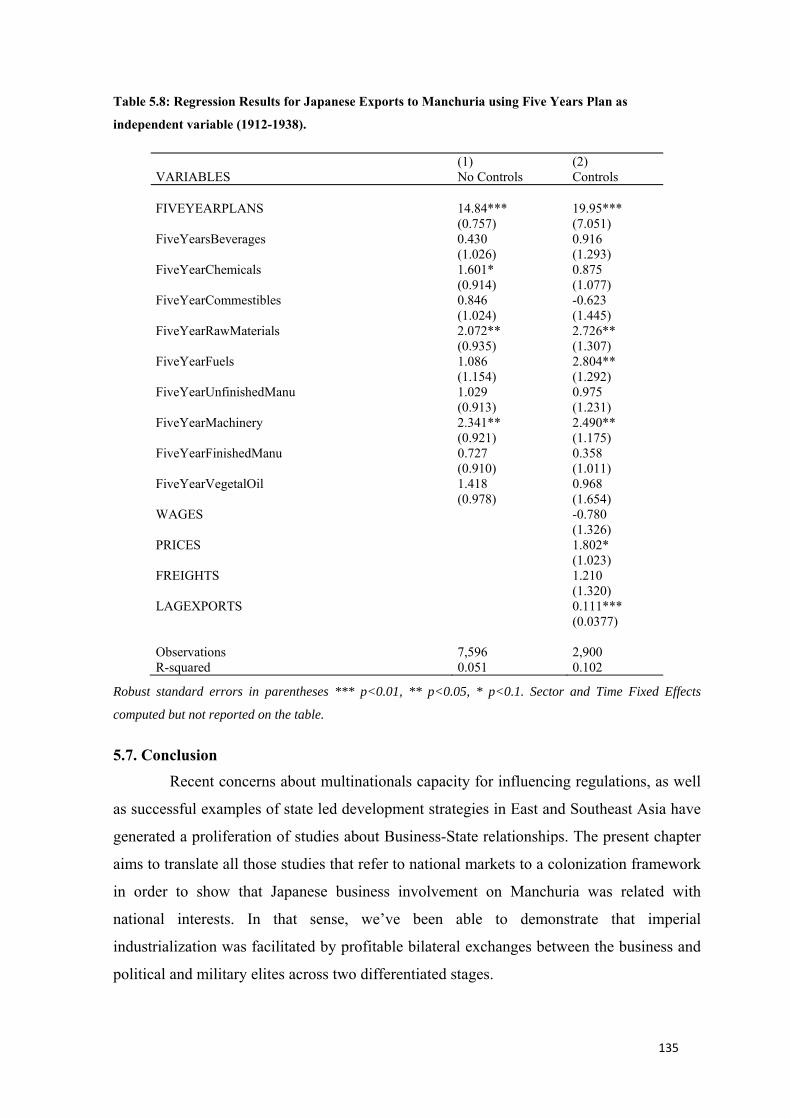
135
Table 5.8: Regression Results for Japanese Exports to Manchuria using Five Years Plan as independent variable (1912-1938).
(1) (2) VARIABLES No Controls Controls FIVEYEARPLANS 14.84*** 19.95*** (0.757) (7.051) FiveYearsBeverages 0.430 0.916 (1.026) (1.293) FiveYearChemicals 1.601* 0.875 (0.914) (1.077) FiveYearCommestibles 0.846 -0.623 (1.024) (1.445) FiveYearRawMaterials 2.072** 2.726** (0.935) (1.307) FiveYearFuels 1.086 2.804** (1.154) (1.292) FiveYearUnfinishedManu 1.029 0.975 (0.913) (1.231) FiveYearMachinery 2.341** 2.490** (0.921) (1.175) FiveYearFinishedManu 0.727 0.358 (0.910) (1.011) FiveYearVegetalOil 1.418 0.968 (0.978) (1.654) WAGES -0.780 (1.326) PRICES 1.802* (1.023) FREIGHTS 1.210 (1.320) LAGEXPORTS 0.111*** (0.0377) Observations 7,596 2,900 R-squared 0.051 0.102
Robust standard errors in parentheses *** p<0.01, ** p<0.05, * p<0.1. Sector and Time Fixed Effects
computed but not reported on the table.
5.7. Conclusion Recent concerns about multinationals capacity for influencing regulations, as well
as successful examples of state led development strategies in East and Southeast Asia have
generated a proliferation of studies about Business-State relationships. The present chapter
aims to translate all those studies that refer to national markets to a colonization framework
in order to show that Japanese business involvement on Manchuria was related with
national interests. In that sense, we’ve been able to demonstrate that imperial
industrialization was facilitated by profitable bilateral exchanges between the business and
political and military elites across two differentiated stages.
136
Firstly, during the years in which Japanese dominions were only reduced to
Kwantung Leased Territories and the South Manchurian Railway Zone (1907-1931) the
most relevant ruling elite was the Japanese Government. On this informal empire stage, the
settlement of Japanese business was aided by the Government and the SMR Co. in charge
of improving transport and communications and directing territorial administration. All of
this aimed to guarantee profitable investment for Japanese entrepreneurs under policies that
were relatively developmental but were not original since they resembled the British ones.
In exchange for these administrative and developmental activities, the company received
important benefits from the State, although it was also subject to strong government
supervision. In fact, those exchanges granted substantial increments on profits experienced
also by trading companies like Mitsui which controlled the distribution of soya beans,
Manchuria’s leading export commodity.
After the Mukden Incident in September 1931 the whole Manchuria became
occupied by Japanese troops of the Kwantung Army. This quick victory gave the military
enormous popularity and the needs of controlling the Soviet frontier granted them
Manchuria’s rule. Of course the nature of the new rulers lead to a deep change on the
political economy performed on this territory, which is deeply analyzed on the present
paper. Strategic and military objectives became preeminent and the Kwantung Army
launched a campaign of fast industrialization in order to equate Japanese arsenal with the
Soviet, the principal enemy for this military group (1932-1945).
This campaign consisted on continuous increments in production of basic metals
(iron and steel) and chemicals on Manchurian Southern factories which then were
employed as explosives and railway construction materials in the Soviet frontier. In order to
do this they required the support of railway infrastructure which was obtained through a
progressive military capture of SMR Co. pricing policies that favored industrial shipments
over soya bean transportation. On a parallel way, Manchuria industrialization required huge
amounts of capital and economic expertise which were provided by a New Zaibatsu like
Nissan, denominated as MHID Co. after its establishment on Manchuria in 1937 and which
enjoyed personal links with the military. As it has been proof in this article, this company
received important benefits from the Government in exchange for its administrative activity
and capital provided on the industrialization, permitting MHID to become the largest
beneficiary of Japanese industrialization of Manchuria. Last, but not least, this process also
required the use of Japanese machinery and expertise which was exported to Manchuria
137
and which made clear that military influence was not limited to colonized territories but
also affected economic activity on the homeland, rendering also substantial benefits to
Nissan.
All in all, this business study of Japanese colonization in Manchuria contributes to
the literature of State Capture by showing how colonial development models fit an Elite
Exchange framework in which cooperation between the main semipublic businesses and
political elites responds to pre-established national interests and proves to be mutually
beneficial. The proved military influence over imperial affairs after 1931 supports the
literature defending Japanese admiration of Soviet command economy at that time and
brings definitive evidence against a singular developmental character intrinsic to the
Japanese Empire. Notwithstanding, the permanent exchanges between business and rulers
remained intact, deviating from the Stalinist total control over production factors.
Moreover, they contributed to create a pattern of intra-regional specialization that has
granted high levels of regional trade and welfare in East and Southeast Asia maintained
until today.
138
. CONCLUSSIONS. 6The Age of Empires (1840-1938) didn’t only give East and Southeast Asian
countries access to European manufactures but also drove the region to unprecedented
scales of intra-regional trade, far superior to those observed during the Age of Commerce
(1450-1680). The century studied in this dissertation saw the arrival of European empires
and the rise of a local one (Japan) that ultimately led the integration process. Foreign
conquest involved institutional development, investments in infrastructure and the creation
of commercial networks that complemented the historical ones created by local merchants,
bringing a significant reduction in the transaction costs faced by traders.
Among the networks created by foreign invaders, the most emblematic ones were
those established during the first half of the nineteenth century by the British, centering on
Hong Kong and Singapore that tried to facilitate access to China by the European Powers.
This web began to be exploited by Chinese and other local merchants during the second
half of the century, which is considered the origin of East and Southeast Asian
contemporary integration. During the interwar years, a leafy forest of regional commercial
exchanges sprouted thanks to the decisive influence of the Japanese Empire. Contrary to the
opinions of many scholars, Japanese ascendancy over the regional integration process was
not based on a peculiar developmental characteristic of its imperial institutions but on the
employment of colonial territories as a source of raw materials and, most importantly, an
outlet for its most sophisticated industrial exports. In fact, the process of industrialization
experienced by the Japanese Empire during the interwar years, which was supported by
business-State cooperation, ignited a process of regional specialization that has continued to
evolve ever since, granting high levels of intra-regional trade inside East and Southeast
Asia.
In that sense, the apparent inseparability of Japanese industrialization and its
imperial expansion represents the heart of East and Southeast Asian regional integration
during early-20th century. The use of conquest as a substitute for productivity for
consolidating the industrialization process fits classical theories regarding industrial
development, according to which backward countries tend to have more interventionist
governments during the course of industrial expansion. A decisive element of those theories
is the extraordinary emphasis that backward countries placed on the most technologically
advanced sectors, a fact that is also observed in the industrial plans of the Japanese Empire.
In sum, the late-comer condition of Japan and its needs to converge with the most advanced
139
nations instigated the employment of imperial mechanisms for sustaining the production of
the most sophisticated manufactures. Moreover, the condition of late-comer is also
applicable to Japan as an Imperial Power, which at first tried to imitate the policies of
traditional Empires like the British. Afterwards, both industrial and imperial strategies
aligned with that promulgated by analogous countries like Germany or the Soviet Union.
All in all, the present thesis pivots around two main themes. The first one is the
disentanglement of commercial relationships in East and Southeast Asia at their historical
roots. In that aspect, this work bequeaths a new imports database that depicts commercial
activity inside East and Southeast Asia in a more reliable way than already existing ones. It
consists of almost a hundred years of imports for 13 countries, disaggregated by country
partner. This new dataset has permitted us to illustrate the superior degree of intra-regional
trade enjoyed by East and Southeast Asia from the second half of the 19th century in
comparison with other regions like Western Europe or Latin America. These results add a
historical perspective to the literature of open regionalism in the periphery by
demonstrating that an outlying region was already commercially integrated long before the
second globalization. Moreover, we believe that they are applicable to a diverse set of
studies regarding East and Southeast Asia’s incorporation into the global economy.
Nonetheless, the particularly high levels of regional exchanges found in East and
Southeast Asia during the period analyzed in this thesis, deserve to be framed in a narrower
literature that helps us to understand their historical meaning and present implications. In
this regard, the conceptualization of the case studies as Natural Trading Partners would
make it highly advisable to continue the present integration process. For this purpose, we
have surveyed the literature on this topic to establish a set of conditions that should be
complied to deserve this label. Such categorization will be useful to those who want to add
to the debate on special trade relationships between countries before the establishment of
Free Trade Areas. The suitability of these criteria is tested by demonstrating that East and
Southeast Asian countries met such criteria by the eve of the Second World War.
Moreover, we also demonstrate that historical determinants were more relevant than
economic factors in the establishment of such special trade relationships, showing that
history should be incorporated into the Natural Trading Partners literature as a decisive
factor.
The second axis sustaining the arguments of this thesis is the recognition of the
mechanisms linking Japanese imperial expansion and its economic development, its legacy
140
in East and Southeast Asian regional integration apart. This is done by an empirical
demonstration of the employment of power mechanisms by Japan to expand industrial
exports during a period of stagnant productivity. In fact, the use of colonial markets as an
outlet for Japan’s least productive manufactures exemplifies the use of trade in the shadow
of power by a backward country in its process of self-development. These conclusions are
reached thanks to the reconstruction of Japanese intensive and extensive export margins
between 1912 and 1938, which complements previous works that calculated them between
1880-1910 (Meissner & Tang, 2018) and permits other researchers to expand their research
on the Japanese export expansion during its whole industrialization process.
Many historians believe that the above-mentioned practices and their positive
implications on the consolidation of regional trade networks denote a peculiar
developmental character attached to Japanese Imperial institutions. Nevertheless, the
present thesis argues that the conquest of colonial markets was also employed to complete
the industrialization processes of other late-comers and that imperial policies responded to
the interests of different Japanese elites. At first they were inspired by traditional empires
like the British and attended to the dictates of big business, while during the 1930s they
rode the wave of Total War models promoted by Nazi Germany or the Soviet Union,
satisfying military desires. Both kinds of elites established mutually beneficial relationships
with imperial authorities, which enter the category of Elite Exchange, a concept applied in
the present work to colonization frameworks in contrast with models of Business/State
Capture that were created to depict those interactions in National systems.
Certainly, all those contributions are remarkable, but the present research faces
some limitations, the resolution of which will be the subject of future research. First of all,
our understanding of commercial upgrades in peripheral regions is based on research of the
historical singularities of East and Southeast Asian regional integration. Nonetheless, this
work is worth complementing with research surveying the main characteristics of regional
integration of other peripheral regions, like Latin America, during a coeval era as a way of
appraising the whole picture. In addition, the regional integration of East and Southeast
Asia is studied looking only at import flows, but we are missing the other side of the coin,
which is the evolution of regional exports. Moreover, in the future there are other indicators
that can be exploited to enlarge our understanding of the regional integration dynamics
between the studied territories, an example being the existence of price convergence.
141
Apart from that, our study of the origins of regional integration of East and
Southeast Asia is restricted to a century in which Empires were particularly active, so
maybe their observed relevance on the integration process is simply a consequence of
timing. For that reason, we should extend our analysis back in time to see if the process of
regional integration began before the arrival of the Imperial Powers, which would mean
that there were other factors behind the growth of East and Southeast Asian regional
integration. This could be done because we have information regarding trade at certain
Asian ports during the second half of the 18th century, although one would have to
renounce the consistency of political units created in the present thesis. Similarly, the
extrapolation of the high levels of intra-regional trade found for East and Southeast Asia
before 1938 until nowadays is based on evidence found in the literature, which should
nevertheless be empirically demonstrated. As a consequence, future projects will be
devoted to better understanding the evolution of regional trade in the analyzed territories
across the Second Globalization era and how the tendency towards trade in parts and
components has affected commercial exchanges between neighbors.
Finally, one of the principal cornerstones in which this thesis is sustained deals
with the appraisal of Japanese Imperial policies and their commercial legacy. The results of
this evaluation are portrayed by the observed influence that military targets exercised over
business outcomes inside the Japanese Empire during the interwar years. Nevertheless, this
conclusion is limited to a certain territory like Manchuria, so in order to complement this
analysis we should study exchanges between economic and military elites on the Japanese
mainland and how they influenced the process of colonization in territories like Taiwan or
Korea during the same period.
142
.BIBLIOGRAPHY 7Adam, C., & Cobham, D. (2007, August). Modelling multilateral trade resistance
in a Gravity Model with exchange rate regimes. In Centre for dynamic macroeconomic
analysis conference papers.
Alder, N. D. (1991). Japan's Manchukuo Economic Development or Militaristic
Seizure.
Allen R.G,D. and Edward Ely (1953): International Trade Statistics. Edt. By
Wiley and Sons, Inc. New York.
Almanac de Gotha. Annuaire généalogique, diplomatique et statistique. Gotha:
Perthes. various years.
Anderson, J. E., & Van Wincoop, E. (2003). Gravity with gravitas: A solution to
the border puzzle. American economic review, 93(1), 170-192.
Asajima, S., & Smitka, M. (1985). Flow-of-Funds Analysis of the Sumitomo
Zaibatsu. Japanese Yearbook on Business History, 1, 72-103.
Avila-Tàpies, R. (2013). Imperial expansion, human mobility and the organization
of urban space in Manchuria (Part I). 社会科学, 43(3), 35-56.
Ayuso‐Díaz, Alejandro., & Tena‐Junguito, Antonio (2020). Trade in the shadow
of power: Japanese industrial exports in the interwar years. The Economic History Review,
73(3), 815-843.
Aziz, M. A. (2012). Japan’s Colonialism and Indonesia, Vol. I. Berlin: Springer
Science & Business Media.
Badia-Miró, M., Carreras-Marín, A., & Meissner, C. M. (2014). Geography,
Policy, or Productivity? Regional Trade in five South American Countries, 1910-1950 (No.
w20790). National Bureau of Economic Research.
Barbieri, Katherine and Omar M. G. Omar Keshk. (2016). Correlates of War
Project Trade Data Set Codebook, Version 4.0. Online: http://correlatesofwar.org.
Barclay, G. W. (2015). Colonial development and population in Taiwan (Vol.
2149). Princeton University Press.
Bassino, J. P. (2000). Economic Development in Vietnam, Japan, Korea and
Taivvan, 1900-1945. Journal of international economic studies, (14), 127-146.
143
Bassino, J. P., & Nakagawa, H. (1990). Exchange rates and exchange rate policies
in Vietnam under French rule, 1878–1945. Quantitative economic history of Vietnam,
1990.
Bassino, J. P., & Van der Eng, P. (2016). Asia's' Little Divergence'in the 20th
century: Evidence from PPP-based direct estimates of GDP per capita, 1913-1969.
Bassino, J. P., and van der Eng, P. (2002). ‘Economic divergence in East Asia:
new benchmark estimates of levels of wages and GDP, 1913-1970’. Thirteenth IEHA
Congress, Buenos Aires, 22-26 July 2002.
Bassino, JP. (Forthcoming). Sustainable Development in South East Asia. in
Stephen Broadberry and Kyoji Fukao (Ed), The Cambridge Economic History of the
Modern World, Vol. I, 1700-1870 (Ch 6).
Bernhofen, D. M., & Brown, J. C. (2004). A direct test of the theory of
comparative advantage: the case of Japan. Journal of Political Economy, 112(1), 48-67.
Bethell, L. -Ed-(1994). The Cambridge History of Latin America.1930 to the
Present.Volume VI, Part 1.Cambridge University Press.
Bix, H. (1972). ‘Japanese Imperialism and the Manchurian Economy, 1900-31’.
The China Quarterly, 51: 425-443, available at http://www.jstor.org/stable/652483.
Black, B., Kraakman, R., & Tarassova, A. (1999). Russian privitization and
corporate governance: What went wrong. Stan. L. Rev., 52, 1731.
Blattman, C., Clemens, M. A., and Williamson, J. G. (2003) ‘Who Protected and
Why? Tariffs the World Around 1870-1938’. Harvard Institute of Economic Research
Working Papers 2010.
Board of Trade (1905). The comparative incidence of foreign and colonial import
tariffs on the principal classes of manufactures exported from the United Kingdom. British
Parliamentary Papers, 84, 280-320.
Bolt, J. and J. L. van Zanden (2014). The Maddison Project: collaborative research
on historical national accounts. The Economic History Review, 67 (3): 627–651, working
paper.
144
Bonfatti, R. and O’Rourke, K. (2014). ‘Growth, Import Dependence and War’.
University of Oxford Discussion Papers in Economic and Social History. No. 132, July
2014.
Booth, A. (2003). Four colonies and a kingdom: A comparison of fiscal, trade and
exchange rate policies in South East Asia in the 1930s. Modern Asian Studies, 37(2), 429-
460.
Booth, A. (2007a). Night watchman, extractive, or developmental states? Some
evidence from late colonial Southeast Asia 1. The Economic History Review, 60(2), 241-
266.
Booth, A. (2007b). Colonial legacies: Economic and social development in East
and Southeast Asia. University of Hawaii Press.
Bose, S., & Jalal, A. (2017). Modern South Asia: history, culture, political
economy. Routledge.
Broadberry, S. N., Fukao, K., and Zammit, N. (2015). ‘How Did Japan Catch-up
on the West? A Sectoral Analysis of Anglo-Japanese Productivity Differences, 1885-2000’.
Working Paper Series 231, Competitive Advantage in the Global Economy (CAGE).
Brown, I. (2005). A colonial economy in crisis: Burma's rice cultivators and the
world depression of the 1930s. Routledge.
Brown, I. (2011). Tracing Burma's economic failure to its colonial inheritance.
Business History Review, 85(4), 725-747.
Bunce, V. (1985). The empire strikes back: The evolution of the Eastern Bloc from
a Soviet asset to a Soviet liability. International Organization, 39(1), 1-46.
Burdekin, R. C. (2008). US pressure on China: Silver flows, deflation, and the
1934 Shanghai credit crunch. China Economic Review, 19(2), 170-182.
Cain, P. J. and Hopkins, A. G. (1980). ‘The Political Economy of British
Expansion Overseas, 1750–1914’. The Economic History Review, 33 (4): 463-490.
Cain, P. J., & Hopkins, A. G. (1986). Gentlemanly capitalism and British
expansion overseas I. The old colonial system, 1688-1850. Economic History Review, 501-
525.
145
Cain, P. J., & Hopkins, A. G. (1987). Gentlemanly capitalism and British
expansion overseas II: New imperialism, 1850-1945. Economic History Review, 1-26.
Carrere, C. (2006). Revisiting the effects of regional trade agreements on trade
flows with proper specification of the Gravity Model. European Economic Review, 50(2),
223-247.
Cazenave-Lacroutza, A., & Lina, V. (2019). The estimation of the autocorrelation
coefficient in panel data models with AR (1) disturbances.
Charney, M. W. (2009). A history of modern Burma. Cambridge University Press.
Chase, K. (2004). Imperial protection and strategic trade policy in the interwar
period. Review of International Political Economy, 11(1), 177-203.
Chase, K. A. (2005). Trading Blocs: States, Firms, and Regions in the World
Economy. Ann Arbor: University Michigan Press.
Chen, T. (1948). The need of population research in China. Population Studies,
1(4), 342-352.
Chen,D. (1923). Chinese migrations, with special reference to labor conditions
(Vol. 340). US Government Printing Office.
Chenery, H. B., Shishido, S., & Watanabe, T. (1962). ‘The Pattern of Japanese
Growth, 1914-1954’. Econometrica, 30: 98-139.
Chiu, T. N. (1973). The port of Hong Kong: a survey of its development (Vol. 1).
Hong Kong University Press.
Chou, S. H. (1971). Railway development and economic growth in Manchuria.
The China Quarterly, 45, 57-84.
Choy, K. M., & Sugimoto, I. (2013). Trade, the Staple Theory of Growth, and
Fluctuations in Colonial S ingapore, 1900–39. Australian Economic History Review, 53(2),
121-145.
Cleary, M. C. (1996). Indigenous trade and European economic intervention in
North-West Borneo c. 1860–1930. Modern Asian Studies, 30(2), 301-324.
Coox, A. D. (1990). Nomonhan: Japan Against Russia, 1939 (Vol. 1). Stanford
University Press.
146
De Bromhead, A., Fernihough, A., Lampe, M., & O'Rourke, K. H. (2019). When
Britain Turned Inward: The Impact of Interwar British Protection. American Economic
Review, 109(2), 325-52.
Dedinger, B., & Girard, P. (2017). Exploring trade globalization in the long run:
The RICardo project. Historical Methods: A Journal of Quantitative and Interdisciplinary
History, 50(1), 30-48.
Deming, S. (2011). The Economic Importance Of Indian Opium And Trade With
China On Britain’s Economy, 1843–1890. Economics Working Papers, 25. Doi:
10.1093/oxfordhb/9780199936694.013.0012
Dennys, N. B. (1867). The Treaty Ports of China and Japan. A Complete Guide to
the Open Ports of Those Countries, Together with Peking, Yedo, Hongkong and Macao.
Forming a Guide Book & Vade Mecum... With 29 Maps and Plans. By Wm. Fred.
Mayers... NB Dennys... and Chas. King... Compiled and Edited by NB Dennys.[With a
Bibliography.]. Trübner & Company.-Duara, P. (2010). Asia redux: Conceptualizing a
region for our times. The Journal of Asian Studies, 69(4), 963-983.
Duara, P. (2010). Asia redux: Conceptualizing a region for our times. The Journal
of Asian Studies, 69(4), 963-983.
Duus, P. (1998). Modern Japan. Boston: Houghton Mifflin.
Eckstein, A., Chao, K., and Chang, J. (1974). ‘The Economic Development of
Manchuria: The Rise of a Frontier Economy’. The Journal of Economic History, 34 (1):
239-264.
Egler, D. G. (1977). Japanese mass organizations in Manchuria, 1928-1945: the
ideology of racial harmony.
Egreteau, R. (2008). India's Ambitions in Burma: More Frustration Than Success?.
Asian Survey, 48(6), 936-957.
Eichengreen, B. (1996). Golden Fetters: The Gold Standard and the Great
Depression, 1919-1939. Oxford University Press.
Eichengreen, B., & Irwin, D. A. (1993). Trade blocs, currency blocs and the
disintegration of world trade in the 1930s (No. w4445). National Bureau of Economic
Research.
147
Eichengreen, B. and Irwin, D. A. (1995). ‘Trade Blocs, Currency Blocs and the
Reorientation of World Trade in the 1930s’. Journal of International Economics, 38 (1-2):
1-24.
Eichengreen, B. and Irwin, D. A. (1998). ‘The Role of History in Bilateral Trade
Flows’. In Frankel, J. A. (ed.), The Regionalization of the World Economy. University of
Chicago Press, 33-62.
Eichengreen, B., Reis, J., & de Macedo, J. B. (2005). The geography of the Gold
Standard. In Currency Convertibility (pp. 125-156). Routledge.
Ellinger, B. and Ellinger, H. (1930). ‘Japanese Competition in the Cotton Trade’.
Journal of the Royal Statistical Society, 93: 185-232.
Elliott, J. H. (2006). Empires of the Atlantic world: Britain and Spain in America,
1492-1830. Yale University Press.
Encarnation, D. J. (ed.) (1999). Japanese Multinationals in Asia: Regional
Operations in Comparative Perspective. Oxford University Press.
Fally, T. (2015). Structural gravity and fixed effects. Journal of International
Economics, 97(1), 76-85.
Farooqui, A. (2007). Governance, Corporate Interest and Colonialism: The Case of
the East India Company. Social Scientist, 44-51.
Federico, G. (2010): Feeding the World. An Economic History of Agriculture
1800-2000. Princeton University Press. Princeton.
Federico, G., & Tena, A. (1991). On the accuracy of foreign trade statistics (1909–
1935): Morgenstern revisited. Explorations in Economic History, 28(3), 259-273.
Federico, G. and Tena-Junguito A. (2019): World trade, 1800-1938: a new
synthesis. Revista de Historia Económica-Journal of Iberian and Latin America Economic
History, Vol 37 (1): 9-41. http://www.uc3m.es/tradehist_db .
Federico, G., & Wolf, N. (2013). A long-run perspective on comparative
advantage. In The Oxford handbook of the Italian economy since unification.
Feenstra, R. C., & Hanson, G. H. (2004). Intermediaries in entrepôt trade: Hong
Kong re‐exports of Chinese goods. Journal of Economics & Management Strategy, 13(1),
3-35.
148
Feige, C., & Miron, J. A. (2008). The opium wars, opium legalization and opium
consumption in China. Applied Economics Letters, 15(12), 911-913.
Ferguson, N. (2003). British Imperialism Revisited: The Costs and Benefits of"
Anglobalization". Historically Speaking, 4(4), 21-27.
Findlay, R. and O’Rourke, K. (2007). Power and Plenty. Princeton, NJ: Princeton
University Press.
Fisher, C. (1950). ‘The Expansion of Japan: A Study in Oriental Geopolitics: Part
II. The Greater East Asia Co-Prosperity Sphere’. The Geographical Journal, 115 (4/6):
179-193, available at doi:10.2307/1790152
Fletcher, W. M. (1989). The Japanese Business Community and National Trade
Polity, 1920-1940. Chapel Hill: University of North Carolina Press.
Fouquin, M., & Hugot, J. (2016). Two Centuries of bilateral trade and gravity
data: 1827-2014 (No. 015129). Universidad Javeriana-Bogotá.
France. Annuaire Statistique de la France, Ministère de l'agriculture et du
commerce, Service de la statistique générale de France by Institutnational de la statistique
et des études économiques (France), Paris.
Francks, P. (2015). Japanese Economic Development: Theory and Practice.
Abingdon: Routledge
Frankel, J. A., Stein, E., & Wei, S. J. (1997). Regional trading blocs in the world
economic system. Peterson Institute.
Fukuda, S. (1995). With sweat & abacus: economic roles of Southeast Asian
Chinese on the eve of World War II. Select Books.
Gallagher, J. and Robinson, R. (1953). ‘The Imperialism of Free Trade’. The
Economic History Review, New Series, 6 (1): 1-15, available at doi:10.2307/2591017.
Garfinkel, M, Skaperdas, S., and Syropoulos, C. (2012). ‘Trade in the Shadow of
Power’. In Skaperdas, S., and Syropoulos, C. (eds.), Oxford Handbook on the Economics of
Peace and Conflict. Oxford University Press.
Gattuso, D., & Restuccia, A. (2014). A tool for railway transport cost evaluation.
Procedia-Social and Behavioral Sciences, 111, 549-558.
149
Gerschenkron, A. (1962). Economic Backwardness in Historical Perspective
(1962). The Political Economy Reader: Markets as Institutions, 211-228.
Gerstell, D. (1991). Administrative adaptability: The Dutch East India Company
and its rise to power. Journal of Political Economy, 99(6), 1307.
Giles, D. E. (2011). Interpreting dummy variables in semi-logarithmic regression
models: Exact distributional results. University of Victoria Department of Economics
Working Paper EWP, 1101, 1-24.
Ginsburg, N. S. (1949). Manchurian railway development. The Journal of Asian
Studies, 8(4), 398-411.
Glickman, D. L. (1947). The British imperial preference system. The Quarterly
Journal of Economics, 61(3), 439-470.
Goldman, S. (2012). Nomonhan, 1939: the Red Army's victory that shaped World
War II. Naval Institute Press.
Gómez-Herrera, E. (2013). ‘Comparing Alternative Methods to Estimate Gravity
Models of Bilateral Trade’. Empirical Economics, 44 (3): 1087-1111.
Government of Taiwan (Taiwan Soutokuhu), 1936. Taiwan Boueki 40 nen hyou
(Returns of the trade of Taiwan for fourty years).
Government of Taiwan (Taiwan Soutokuhu), 1940. Taiwan Gaikoku Boueki
Gaikyou (Foreign Trade of Taiwan).
Graham, D. J., Couto, A., Adeney, W. E., & Glaister, S. (2003). Economies of
scale and density in urban rail transport: effects on productivity. Transportation Research
Part E: Logistics and Transportation Review, 39(6), 443-458.
Grajdanzev, A. J. (1945). Manchuria: an industrial survey. Pacific Affairs, 18(4),
321-339.
Gross, S. (2016). Export Empire: German Soft Power in Southeastern Europe,
1890–1945, Cambridge University Press.
Gruner, W. (2006). Jewish forced labor under the Nazis: economic needs and
racial aims, 1938-1944. Cambridge University Press.
Gutiérrez, G., & Philippon, T. (2019). The failure of free entry (No. w26001).
National Bureau of Economic Research.
150
Hall, A. R. (2004). Constructing a'Manchurian'Identity: Japanese Education in
Manchukuo, 1931-1945 (Doctoral dissertation, University of Pittsburgh).
Harada, K. (1993). Chap. 6: Transportation during Wartime (1938-1945): Policy
He, Y. (2007). ‘History, Chinese Nationalism and the Emerging Sino–Japanese
Conflict’. Journal of Contemporary China, 16 (50): 1-24.
Hellman, J. S. (1998). Winners take all: the politics of partial reform in
postcommunist transitions. World politics, 50(2), 203-234.
Hellman, J. S., Jones, G., Kaufmann, D., & Schankerman, M. (2000). Measuring
Governance, Corruption, and State Capture.
Howe, C. (1999). The Origins of Japanese Trade Supremacy: Development and
Technology in Asia from 1540 to the Pacific War. University of Chicago Press.
Huberman, M. and Minns, C. (2007). ‘The Times They are Not Changin’: Days
and Hours of Work in Old and New Worlds, 1870–2000’. Explorations in Economic
History, 44 (4): 538-567.
Huberman, M., Meissner, C. M, and Oosterlinck, K. (2017). Technology and
geography in the second industrial revolution: new evidence from the margins of trade. The
Journal of Economic History, 77(1), 39-89.
Huff, G., & Angeles, L. (2011). Globalization, industrialization and urbanization
in pre-World War II Southeast Asia. Explorations in Economic History, 48(1), 20-36.
Huff, G., & Caggiano, G. (2007). Globalization and labor market integration in
late nineteenth-and early twentieth-century Asia. In Research in Economic History (pp.
285-347). Emerald Group Publishing Limited.
Huff, W. G. (2003). Currency boards and Chinese banking development in pre-
World War II Southeast Asia: Malaya and the Philippines.
Hummels, D., and Klenow, P. J. (2005). ‘The Variety and Quality of a Nation’s
Exports’. American Economic Review, 95 (3): 704-723.
Hunsberger, W. S. (1938). The Yen Bloc in Japan's Expansion Program. Far
Eastern Survey, 7(22), 251-258.
Hussin, N. (2005). Networks of Malay Merchants and the Rise of Penang as a
regional Trading Centre. Japanese Journal of Southeast Asian Studies, 43(3), 215-237.
151
Iguchi, H. (2003). Unfinished Business: Ayukawa Yoshisuke and US-Japan
Relations, 1937-1953 (Vol. 199). Harvard Univ Asia Center.
Isserlis, L. (1938). ‘Tramp Shipping Cargoes, and Freights’. Journal of the Royal
Statistical Society, 101 (1): 53-146.
Istat, Italia, & Direzione generale della statistica. (various years). Annuario
statistic italiano. Tip. Elzeviriana.
IYenaga, T. (1912). ‘Japan in South Manchuria’. The Journal of Race
Development, 2 (4): 373-398, available at doi: 10.2307/29737926.
Jacks, D., O'Rourke, K., & Taylor, A. M. (2020). The Gravitational Constant?.
Johnson, J. (2000). A fistful of rubles: The rise and fall of the Russian banking
system. Cornell University Press.
Kakajiro, Y., & Gotaro, O. (1929). Effect of the World War upon the Commerce
and Industry of Japan (The). Yale University Press, New Haven.
Kang, C. (1981). ‘Demographic Development in Manchuria, 1924-1941’. 近代史
研究所集刊 (Bulletin of the Academia Sinica), 10: 351-375.
Kaur, A. (2009). Labor Crossings In Southeast Asia: Linking Historical and
Contemporary Labor Migration. New Zealand Journal of Asian Studies, 11(1), 276-303.
Kazushi Ohkawa, Miyohei Shinohara, and Mataji Umemura, Long-Term
Economic Statistics (LTES), published by Toyo Keizai Shinposha, Inc., (1967-1989)
Keller, W., Li, B., & Shiue, C. H. (2011). China’s foreign trade: Perspectives from
the past 150 years. The World Economy, 34(6), 853-892.
Kim, Y. (2017). Interfirm Relationships in the Japanese Machine Tool Industry,
1910s-1980s: Market and Organizational Principles. Journal of Innovation Management,
14, 39-64.
Kingman, H. L. (1932). Effects of Chinese nationalism upon Manchurian railway
developments, 1925-1931. University of California Press, Berkeley.
Klemann, H. A. (2008). Did the German occupation (1940–1945) ruin Dutch
industry?. Contemporary European History, 17(4), 457-481.
Klemann, H. A., & Kudryashov, S. (2013). Occupied economies: an economic
history of Nazi-occupied Europe, 1939-1945. Bloomsbury Publishing.
152
Kobayashi, A., & Sugihara, K. (2020). Changing Patterns of Sarawak’s Exports, c.
1870–2013. In Anthropogenic Tropical Forests (pp. 563-585). Springer, Singapore.
Koh Soo Jin, D. and Tanaka, K. (1984). “Japanese Competition in the Trade of
Malaya in the 1930s”. Southeast Asian Studies, (21) 4, March.
Kohli, A. (1994). ‘Where Do High Growth Political Economies Come From? The
Japanese Lineage of Korea's “Developmental State”’. World Development, 22 (9): 1269-
1293.
Kohli, A. (2004). State-directed development: political power and industrialization
in the global periphery. Cambridge university press.
Kondo, A. (2002). The development of immigration policy in Japan. Asian and
Pacific migration journal, 11(4), 415-436.
Korthals Altes, W. L. (1991). Changing Economy in Indonesia, Vol. 12A: General
Trade Statistics 1822-1940. Amsterdam: Royal Tropical Institute.
Krugman, P. (1993), “Regionalism versus multilateralism: analytical notes.”
Chapter 3 In De Melo, J. and A. Panagariya eds. New Dimensions in Regional
Integration.Cambridge: Cambridge Univ. Press.
Kublin, H. (1959). ‘The Evolution of Japanese Colonialism’. Comparative Studies
in Society and History, 2 (1): 67-84.
Kuramoto, Y. (2018). Public-Private Partnerships in Manchuria: Japan's Colonial
Economic Development Policy.
Lane, D. (2018). The political economy of Russian oil. In Business and State in
Contemporary Russia (pp. 101-128). Routledge.
Larch, M., Wanner, J., Yotov, Y., and Zylkin, T. (2017). ‘The Currency Union
Effect: A PPML Re-assessment with High-Dimensional Fixed Effects’. School of
Economics Working Paper Series 2017-7, LeBow College of Business, Drexel University.
Latham, A. J. H. (1978). Merchandise trade imbalances and uneven economic
development in India and China. Journal of European Economic History, 7(1), 33.
Lawrence H. Officer and Samuel H. Williamson, 'The Price of Gold, 1257-2014,'
MeasuringWorth, 2019.
153
League of Nations. (1927-1945). Statistical Year-book of the League of Nations.
Geneva: League of Nations Economic and Financial Section.
Linder, S. (1961). An Essay on Trade and Transformation. Uppsala: Almqvist &
Wiksell.
Lipsey, R. (1960), “The theory of Customs Unions: A general survey.” Economic
Journal 70, 498-513.
Llorca-Jaña, M. (2011). To be Waterproof or to be soaked: importance of packing
in British textile exports to distant markets: The cases of Chile and the River Plate, c. 1810-
1859. Revista de Historia Economica-Journal of Iberian and Latin American Economic
History, 29(1), 11-37.
Lye, J. N., & Hirschberg, J. G. (2002). Tests of inference for dummy variables in
regressions with logarithmic transformed dependent variables. Department of Economics,
University of Melbourne.
Ma, D. (2004). Why Japan, not China, was the first to develop in East Asia:
Lessons from sericulture, 1850–1937. Economic Development and Cultural Change, 52(2),
369-394.
MacNair, H. F. (1923). The Relation of China to her Nationals Abroad. Chinese
Soc. & Pol. Sci. Rev., 7, 23.
Maddison Project Database, version 2013. Bolt, J. and J. L. van Zanden (2014).
The Maddison Project: collaborative research on historical national accounts. The
Economic History Review, 67 (3): 627–651, working paper.
Maddison, A. (1995). Monitoring the World Economy, 1820-1992. Paris: OECD
Development Centre.
Maddison, A. (2007). The World Economy: Two-in-One Edition (Vol. 1: A
Millennial Perspective, Vol. 2: Historical Statistics). Geneva: OECD Development Centre
& New Delhi: Academic Foundation.
Makower, H. (1954). A Study of Trade between Latin America and Europe.
Martin, W., & Pham, C. S. (2015). Estimating the Gravity Model when zero trade
flows are frequent and economically determined. The World Bank.
154
Martincus, C. V., Estevadeordal, A., Gallo, A., and Luna, J. (2010). ‘Information
Barriers, Export Promotion Institutions, and the Extensive Margin of Trade’. Review of
World Economics, 146 (1): 91-111.
Martland, S. J. (2008). Trade, Progress, and Patriotism: Defining Valparaiso,
Chile, 1818-1875. Journal of Urban History, 35(1), 53-74.
Matsusaka, Y. T. (2007). ‘The Japanese Empire’. In Tsutsui, M. (ed.), A
Companion to Japanese History. Malden: Blackwell, 224-40.
Matsusaka, Y. T. (2020). The Making of Japanese Manchuria, 1904–1932. Brill.
Mayer, C. (2018). Prosperity: better business makes the greater good. Oxford
University Press.
McLean, I. W. (2012). Why Australia prospered: The shifting sources of economic
growth (Vol. 43). Princeton University Press.
Meisel, A. (1954 - [et al.] (1990). El Banco de la República: antecedentes,
evolución y estructura. Bogotá: Banco de la República. Departamento editorial.
Meissner, C. M., and Tang, J. P. (2018). ‘Upstart Industrialization and Exports:
Evidence from Japan, 1880-1910’. The Journal of Economic History, 78 (4): 1068-1102.
Melitz, J., & Toubal, F. (2014). Native language, spoken language, translation and
trade. Journal of International Economics, 93(2), 351-363.
Meredith, D. (1996). British Trade Diversion Policy and the Colonial Issue in the
1930's. Journal of European Economic History, 25(1), 33.
Michihiro, O., Noriyuki, O., & Tsubota, K. (2018). The structure of coasting trade
in British India from 1905 to 1931 (No. 710). Institute of Developing Economies, Japan
External Trade Organization (JETRO).
Milward, A. S. (1981). ‘The Reichsmark Bloc and the International Economy’, in
G. Hirschfeld, G. And Kettenacker, L. (eds.), Der ‘Führerstaat’: Mythos und Realität:
Studien zur Struktur und Politik des Dritten Reiches. Stuttgart: Klett-Cotta.
Ministry of Finance. Annual Return of the Foreign Trade of the Empire of Japan.
Tokyo: Yushodo (1912, 1915, 1925, 1929, 1932, 1938).
Mitchell, B. (2003). International Historical Statistics: the Americas 1750-1993.
M.
155
Mitchell, B. (Ed.). (1998). International historical statistics: Europe 1750-1993.
Springer.
Mitchell, B. R. (1971). Abstract of British Historical Statistics. Cambridge
University Press.
Mitchell, B. R. (ed.) (2003). International Historical Statistics: Africa, Asia &
Oceania, 1750–2000. Basingstoke & New York: Palgrave Macmillan.
Mitchener, K. J., & Voth, H. J. (2011). Trading Silver for Gold: Nineteenthcentury
Asian Exports and the Political Economy of Currency Unions. Costs and benefits of
economic integration in Asia. Oxford University Press, Oxford, 126-156.
Mitchener, K. J., & Weidenmier, M. (2008). Trade and empire. The Economic
Journal, 118(533), 1805-1834.
Miwa, Y. (2015). Japan's Economic Planning and Mobilization in Wartime,
1930s–1940s. Cambridge University Press
Mizuno, H., & Prodöhl, I. (2019). Mitsui Bussan and the Manchurian soybean trade:
Geopolitics and economic strategies in China’s Northeast, ca. 1870s–1920s. Business History, 1-22.
Moneta, C. (1959). ‘The Estimation of Transportation Costs in International
Trade’. Journal of Political Economy, 67 (1): 41-58.
Mood, J. R. (1930). Handbook of foreign currency and exchange.
Moon, W. (2008). Destined to Fail? The History of the Yen Bloc before the
Second World War.
Morgan, S. (2019). Commodity flows between Southeast Asia and China, 15-18th
Centuries: An evaluation of recent Chinese-language research at: Southeast Asia in shaping
the Global Economy, Lund University 27-29 May 2019.
Moses, A. D. (2000). An antipodean genocide? The origins of the genocidal
moment in the colonization of Australia. Journal of Genocide Research, 2(1), 89-106.
Murakami, H. (2012). Emergence of the Japanese Developmental State: Japanese
Management of ‘Manchukuo’through Special Corporations. Asian Journal of Political
Science, 20(2), 129-153.
Murakoshi, N., & Trewartha, G. T. (1930). Land utilization maps of Manchuria.
Geographical Review, 20(3), 480-493.
156
Nakamura, O. (2003). The Economic History of Japan, 1600-1990: Economic
history of Japan, 1914-1955: a dual structure (Vol. 3). Oxford University Press on Demand.
Neal, L. (1979). ‘The Economics and Finance of Bilateral Clearing Agreements:
Germany, 1934-38’. The Economic History Review, Second Series, 32 (3): 391-404.
Noguchi, M., & Boyns, T. (2013). The South Manchuria Railway Company and its
Interactions with the Military: An Accounting and Financial History. The Japanese
Accounting Review, 3-2013.
Nun, N. and Trefler, D. (2010). The Structure of Tariffs and Long-Term Growth.
American Economic Journal: Macroeconomics Vol. 2 No. 4: 158–194.
Ohkawa, K., Shinohara, M., and Umemura, M. (1967-89). Long-Term Economic
Statistics (LTES), Tokyo: Toyo Keizai Shinposha.
Ohlin, B. (1952). Interregional and International Trade, Vol. 39. Cambridge,
Mass.: Harvard University Press.
Okazaki, T. (1994). The Japanese firm under the wartime planned economy. The
Japanese firm: Sources of competitive strength, 350-75.
Okazaki, T. (2013). Development and Management of Manchurian Economy
under the Japan Empire (No. CIRJE-F-899). CIRJE, Faculty of Economics, University of
Tokyo.
Okubo, T. (2007). Trade bloc formation in inter-war Japan.: A gravity model
analysis. Journal of the Japanese and International Economies, 21(2), 214-236.
Osterhammel, J. (1986). ‘Semi-Colonialism and Informal Empire in Twentieth-
century China: Towards a Framework of Analysis’. In Mommsen, W. J. (ed.), Imperialism
and After: Continuities and Discontinuities. London: Allen & Unwin, 290-314.
Pan, M. L. (2014). The Changing Character and Survival Strategies of the Chinese
Community in India. China Report, 50(3), 233-242.
Pauley, E. W. (1946). Report in Japanese Assets in Manchuria to the President of
the United States, July, 1946. US Government Printing Office.
Petri, P. A. (1993). ‘The East Asian Trading Bloc: An Analytical History’. In
Frankel, J. and Kahler, M. (eds.), Regionalism and Rivalry: Japan and the United States in
Pacific Asia. University of Chicago Press, 21-52.
157
Philippon, T. (2019). The Great Reversal: How America Gave Up on Free
Markets. Harvard University Press.
Pizarro, R. (1999). Comparative analysis of regionalism in Latin America and
Asia-Pacific. ECLAC.
Post, P. (1996). ‘Characteristics of Japanese Entrepreneurship in the Pre-War
Indonesian Economy’. In Lindblad, J. T. (ed.), Historical Foundations of a National
Economy in Indonesia, 1890s-1990s, Amsterdam: Royal Netherlands Academy of Arts and
Sciences, 297-314.
Post, P. (2002). The Kwik Hoo Tong trading society of semarang, Java: A Chinese
business network in late Colonial Asia. Journal of Southeast Asian Studies, 33(2), 279-296.
Purcell, V. (1966). The Chinese in Southeast Asia.
Pytlikova, M., & Adsera, A. (2010). The Role of language in shaping international
migration: Evidence from OECD countries 1985-2006. In IZA Annual Migration Meeting.
Raballand, G. (2003). Determinants of the negative impact of being landlocked on
trade: an empirical investigation through the Central Asian case. Comparative economic
studies, 45(4), 520-536.
RAUCH, J.E. and V. TRINDADE (2002): "Ethnic Chinese Networks in
International Trade," Review of Economics and Statistics vol. 84, No. l,pp. 116-130.
[41,42,6].
Rawski, T. G. (1969). Chinese dominance of treaty port commerce and its
implications, 1860–1875. Explorations in Economic History, 7(1-2), 451-473.
Reardon-Anderson, J. (1986). Chemical Industry in China, 1860-1949. Osiris, 2,
177-224.
Redding, S., & Venables, A. J. (2004). Economic geography and international
inequality. Journal of international Economics, 62(1), 53-82.
Reed, A. M., & Reed, D. (2009). Partnerships for development: Four models of
business involvement. Journal of Business Ethics, 90(1), 3.
Reid, A. (1988). Southeast Asia in the Age of Commerce, 1450-1680: Expansion
and crisis (Vol. 2). Yale University Press.
158
Reid, A. (1997). A new phase of commercial expansion in Southeast Asia, 1760–
1850. In The Last Stand of Asian Autonomies (pp. 57-81). Palgrave Macmillan, London.
Reinhart, C. and Rogoff, K. (2004). ‘The Modern History of Exchange Rate
Arrangements: A Reinterpretation’. The Quarterly Journal of Economics, 119 (1): 1-48.
Remer, C. F. (1926). International trade between gold and silver countries: China,
1885–1913. The Quarterly Journal of Economics, 40(4), 597-643.
Resnick, S. A. (1970). The decline of rural industry under export expansion: a
comparison among Burma, Philippines, and Thailand, 1870–1938. The Journal of
Economic History, 30(1), 51-73.
Restrepo-Estrada, M. I., & Tena Junguito, A. (2016). The roots of regional trade in
the Americas 1870 to 1950 (No. 23304). Universidad Carlos III de Madrid. Instituto
Figuerola.
Ritschl, A. O. (2001). ‘Nazi Economic Imperialism and the Exploitation of the
Small: Evidence from Germany’s Secret Foreign Exchange Balances, 1938-1940’,
Economic History Review 54 (2): 324-45.
Ritschl, A., & Wolf, N. (2003). Endogeneity of currency areas and trade blocs:
evidence from the inter-war period.
Robertson, A. J. (1990). Lancashire and the Rise of Japan, 1910–1937. Business
History, 32(4), 87-105
Rodgers, A. (1948). The Manchurian iron and steel industry and its resource base.
Geographical Review, 38(1), 41-54.
Roy, T. (2002). Economic history and modern India: redefining the link. Journal of
Economic Perspectives, 16(3), 109-130.
Royal Statistical Office. Statistical Abstract for the Several Colonial and Other
Possessions of the United Kingdom (Statistical Abstract for the British Empire).London:
1880f.
Royama, M. (1930). The South Manchuria Railway Zone: And the Nature of Its
Administration. Pacific Affairs, 3(11), 1018-1034.
Sakamoto, M. (1990). Diversification: the case of Mitsui Bussan. Shin’ichi
Yonekawa, ed., General Trading Companies: A Comparative and Historical Study.
159
Sanderson, A. E. (1926). Ocean Freight Rates in the United States Foreign Trade.
Washington: Government Printing Office [United States Bureau of Foreign and Domestic
Commerce].
Sanderson, A. E. (1940). Wartime Control of Ocean Freight Rates and Foreign
Trade: A World Survey. Washington: Government Printing Office.
Sang, L. Y. (1982). Regional rivalry in mid-nineteenth century Shanghai:
Cantonese vs. Ningpo men. Ch'ing-shih wen-t'i, 4(8), 29-50.
Santos Silva, J. C. M., and Tenreyro, S. (2006). ‘The Log of Gravity’. The Review
of Economics and Statistics, 88 (4): 641-658.
Satyanugroho, R. (2018). Intra-National Versus International Trade in Southeast
Asia: Do National Borders Matter?. Available at SSRN 3460396.
Sawai, M. (Ed.). (2017). The Development of Railway Technology in East Asia in
Comparative Perspective. Springer Singapore.
Saxonhouse, Gary, and Gavin Wright (1984a). "New Evidence on the Stubborn
English Mule and the Cotton Industry, 1878-1920," Economic History Review 37: 507-519.
Saxonhouse, Gary, and Gavin Wright (1984b). "Rings and Mules around the
World: A Comparative Study in Technological Choice," in Saxonhouse and Wright
(eds.), Technique, Spirit and Form in the Making of the Modern Economies: Essays in
Honor of William N. Parker. Research in Economic History, Supplement 3: 271-300.
Schiff, M. (1999). Will the real natural trading partner please stand up?. The
World Bank.
Schultz, L. (2009). Beneath the United States: a history of US policy toward Latin
America. Harvard University Press.
Schuler, K. (2004). Tables of Modern Monetary History: Asia. Preliminary
version, 29.
Sessions of the United Kingdom (Statistical Abstract for the British Empire).
Shimizu, H. (1988). Dutch-Japanese competition in the shipping trade on the Java-
Japan route in the inter-war period. Japanese Journal of Southeast Asian Studies, 26(1), 3-
23.
160
Shimpo, H. (2011). A Study on World Trade and Global Imbalance in the Inter-
War Period: With a focus on trade and the balance of payments in Japan and China.
Shiraishi, T. and Shiraishi, S. S. (eds.) (1993). The Japanese in Colonial Southeast
Asia, Vol. 3. Ithaca, N.Y.: Cornell University Press.
Shuyong, L. (1997). Hong Kong: A survey of its political and economic
development over the past 150 years. The China Quarterly, 151, 583-592.
Sidel, J. T. (2008). Social origins of dictatorship and democracy revisited: colonial
state and Chinese immigrant in the making of modern Southeast Asia. Comparative
Politics, 40(2), 127-147.
Silva, J. S., & Tenreyro, S. (2006). The log of gravity. The Review of Economics
and statistics, 88(4), 641-658.
Smith, J. R. (1910). The World Entrepôt. Journal of Political Economy, 18(9),
697-713.
Smitka, M. (ed.) (1998). Agricultural Growth and Japanese Economic
Development, Vol. 7. New York & London: Garland.
Sohn, C. H. (2005). Does the Gravity Model explain South Korea's trade
flows?. The Japanese Economic Review, 56(4), 417-430.
Souza, G. B. (2004). The Survival of Empire: Portuguese Trade and Society in
China and the South China Sea, 1630-1754. Cambridge University Press.
Stewart, J. R. (1942). Japan's Manchurian Base. Far Eastern Survey, 11(17), 180-
186.
Stigler, G. J. (1971). The theory of economic regulation. The Bell journal of
economics and management science, 3-21.
Štolleová, B. (2018). Legal Regulation of Joint-stock Companies in the Bohemian
Lands and its Changes during the Nazi occupation (1939–1945). Prague Economic and
Social History Papers, (1), 75-93.
Strong, H. M. (1925). Changes in entrepot markets for tropical and other exotic
products. Annals of the Association of American Geographers, 15(4), 180-189.
Sugihara, K. (1985). Patterns and Development of Intra-Asian Trade, 1880-1913.
The Socio-Economic History (Shakai-Keizai-Shigaku), 51(1).
161
Sugihara, K. (1998). Intra-Asian Trade and East Asia's Industrialization, 1919-
1939. Industrial Growth in the Third World, c, 25-57.
Sugihara, K. (Ed.). (2005). Japan, China, and the growth of the Asian international
economy, 1850-1949 (Vol. 1). Oxford University Press.
Sugihara, K. (2013). The resurgence of intra-Asian trade, 1800–1850. In How
India Clothed the World (pp. 139-169). Brill.
Sugihara, K. (2019). The Asian Path of Economic Development: Intra-regional
Trade, Industrialization and the Developmental State. In Emerging States and Economies
(pp. 73-99). Springer, Singapore.
Sugihara, K., & Kawamura, T. (2013). < Special Focus> Introduction:
Reconstructing Intra-Southeast Asian Trade, c. 1780–1870: Evidence of Regional
Integration under the Regime of Colonial Free Trade.
Sugiyama, S. (2013). Japan's Industrialization in the World Economy: 1859-1899:
Export, Trade and Overseas Competition. London: Bloomsbury Academic.
Summers, L. (1991). Regionalism and the world trading system. Policy
implications of trade and currency zones, 295-301.
Tadei, F. (2013). Extractive institutions and gains from trade: Evidence from
colonial Africa. IGIER Wor ing Paper, (536).
Tagliacozzo, E., & Chang, W. C. (2011). Chinese circulations: Capital,
commodities, and networks in Southeast Asia. Duke University Press.
Tanimoto, M. (2019). Labour-intensive industrialization and the emerging state in
pre-war Japan. In Paths to the Emerging State in Asia and Africa (pp. 115-140). Springer,
Singapore.
Tena-Junguito, A. (2010). ‘Bairoch Revisited: Tariff Structure and Growth in the
Late Nineteenth century’. European Review of Economic History, 14 (1): 111-143.
Thampi, M. (2010). Indian Traders in Xinjiang in the Nineteenth and Twentieth
Centuries. China Report, 46(4), 371-385.
Travis, A. S. (2018). Imperial Japan: From Cyanamide to Synthetic Ammonia. In
Nitrogen Capture (pp. 329-346). Springer, Cham.
162
Udagawa, M. (1991). The Move into Manchuria of the Nissan Combine. Japanese
Yearbook on Business History, 7, 3-29.
Unger, L. (1944). The Chinese in Southeast Asia. Geographical review, 34(2),
196-217.
United Nations. (2018). Standard country or area codes for statistical use.
United States Bureau of Foreign and Domestic commerce (1935). Industrial
Machinery in Principal Foreign Countries.
United States Bureau of Foreign and Domestic commerce (1937). Expansion of
Japan's Foreign Trade and Industry.
United States Bureau of Foreign and Domestic commerce (1944). Foreign
Commerce Weekly (14).
United States Bureau of Foreign and Domestic commerce (1946). Foreign
Commerce Weekly (22-23).
United States Strategic Bombing Survey (1946). Pacific War (Vol. 39).
Vaughn, J. M. (2009). The politics of empire: Metropolitan socio-political
developmentand the imperial transformation of the British East India Company, 1675–
1775. The University of Chicago.
Wandschneider, K. (2008). The stability of the interwar gold exchange standard:
Did politics matter?. The Journal of Economic History, 68(1), 151-181.
Webber, D. (2001). Two funerals and a wedding? The ups and downs of
regionalism in East Asia and Asia-Pacific after the Asian crisis. The Pacific Review, 14(3),
339-372.
Webster, A. (1990). The political economy of trade liberalization: the East India
Company Charter Act of 1813. Economic History Review, 404-419.
Williamson, J. A. (2002). ‘Is Protection Bad for Growth? Will Globalization Last?
Looking for Answers in History’. Thirteenth IEHA Congress, Buenos Aires, 22-26 July
2002.
Williamson, J. G. (1995). ‘The Evolution of Global Labor Markets since 1830:
Background Evidence and Hypotheses’. Explorations in Economic History, 32 (2): 141-
196.
163
Wolcott, S. (1994). ‘The Perils of Lifetime Employment Systems: Productivity
Advance in the Indian and Japanese Textile Industries, 1920–1938’. The Journal of
Economic History, 54 (2): 307-324.
Wonnacott, P., Lutz, M., & Schott, J. J. (1989). Is there a case for free trade areas?
Free trade areas and US trade policy (No. E71 S397j). Institute for International
Economics, Washington, DC (EUA).
Wu, C. C. (1974). Chinese immigration in the Pacific area: a dissertation, the
University of Chicago, 1926. R and E Research Associates.
Xu, X. (2015). Genesis of a growth triangle in Southeast Asia: a study of
economic connections between Singapore, Johor and the Riau Islands, 1870s–1970s
(Doctoral dissertation, Instiute of History, Faculty of the Humanities, Leiden University).
Yamamuro, S. I. (2006). Manchuria under Japanese dominion. University of
Pennsylvania Press.
Yang, S., & Martinez-Zarzoso, I. (2014). A panel data analysis of trade creation
and trade diversion effects: The case of ASEAN–China Free Trade Area. China Economic
Review, 29, 138-151.
Yasuba, Y. (1978). ‘Freight Rates and Productivity in Ocean Transportation for
Japan, 1875-1943’. Explorations in Economic History, 15 (1): 11-39.
Yasuyuki, H. I. K. I. T. A. Japanese Investment to Manchuria and the
establishment of Zaibatsu subsidiaries.
Young, C. W. (1928). Sino-Japanese interests and issues in Manchuria. Pacific
Affairs, 1(7), 1-20.
Young, L. (1998). Japan's total empire: Manchuria and the culture of wartime
imperialism (Vol. 8). Univ of California Press.
Young, L. (2017). When fascism met empire in Japanese-occupied Manchuria.
Journal of Global History, 12(2), 274-296.
Zalanga, S. (1996). Ruling Elite Coalitions and State Bureaucratic Capacity:
Accounting for Developmental and Predatory States in Malaysia and Nigeria. Department
of Sociology University of Minnesota, USA.
Zhang, Q., & Liu, M. (2010). Local political elite, partial reform symptoms, and
the business and market environment in rural China. Business and Politics, 12(1), 1-39.
164
Zinam, O. (1972). Soviet Regional Problems: Specialization Versus Autarky. The
Russian Review, 31(2), 126-
. APPENDIX 8
A . SUBMERSION INSIDE EAST AND SOUTHEAST ASIA HISTORICAL TRADE DETERMINANTS.
A.1. Sources and estimation of independent variables The following appendix will contain detailed information necessary for
computing missing data regarding the independent variables included on chapter 2. The
principal source for GDP information has been (Maddison Project, 2014) which collects
GDP in 1990 GK Dollars for many countries. However, there are some territories for
which Maddison data only covers some benchmarks (for some there is data every ten
years, other just cover 1820, 1850, 1870, 1890, 1913 and 1938). In any case we assume
a constant annual growth rate of real GDP between every benchmark in order to
interpolate the desired figures. In addition, there are some countries, especially in the
Middle East, Africa and the Caribbean for which there is no data prior to 1950. In order
to fill this gap we have translated back in time 1950 data by assuming Maddison GDP
to follow the same trend as constant GDP obtained from (Federico & Tena, 2019).
Lastly, for some marginal territories for which there is no constant GDP data we have
taken back in time Maddison 1950 GDP by using the growth rate of each territory
corresponding exports at constant 1913 prices, obtained from (Federico & Tena, 2019).
Data on GDP is divided by total population found in (Maddison, 2014) in order to
calculate GDP per capita of importer and partner countries.
The absolute value of differences in GDP per capita is going to approximate
differences in demand structure. Finally we measure differences in population density
between regional partners by dividing total population by the extension in squared
kilometers which is found on the League of Nations. This source includes data in 1913
and 1938 so we can account for changes in the borders during WWI and the Sino-
Japanese wars. In fact, the only territories whose extension was modified were China,
French Indochina and the Kwantung Leased territories whose frontiers expanded in
1931. This measure represents differences in factor endowments.
Regarding trade costs we start with exchange rate which is constructed by
dividing the nominal exchange rate between partner currency and the dollar by the one
between local currency and the dollar (local currency per dollar), data which mainly
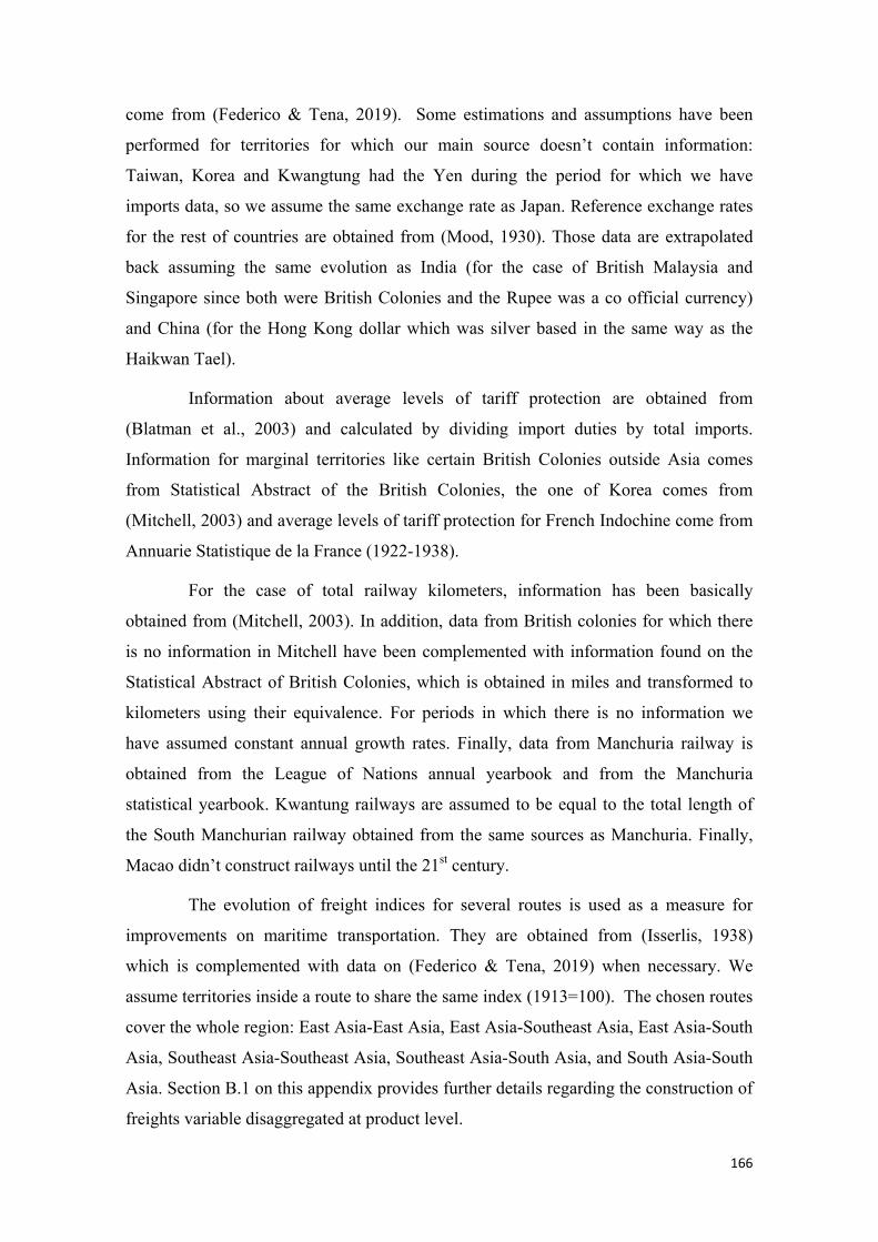
166
come from (Federico & Tena, 2019). Some estimations and assumptions have been
performed for territories for which our main source doesn’t contain information:
Taiwan, Korea and Kwangtung had the Yen during the period for which we have
imports data, so we assume the same exchange rate as Japan. Reference exchange rates
for the rest of countries are obtained from (Mood, 1930). Those data are extrapolated
back assuming the same evolution as India (for the case of British Malaysia and
Singapore since both were British Colonies and the Rupee was a co official currency)
and China (for the Hong Kong dollar which was silver based in the same way as the
Haikwan Tael).
Information about average levels of tariff protection are obtained from
(Blatman et al., 2003) and calculated by dividing import duties by total imports.
Information for marginal territories like certain British Colonies outside Asia comes
from Statistical Abstract of the British Colonies, the one of Korea comes from
(Mitchell, 2003) and average levels of tariff protection for French Indochine come from
Annuarie Statistique de la France (1922-1938).
For the case of total railway kilometers, information has been basically
obtained from (Mitchell, 2003). In addition, data from British colonies for which there
is no information in Mitchell have been complemented with information found on the
Statistical Abstract of British Colonies, which is obtained in miles and transformed to
kilometers using their equivalence. For periods in which there is no information we
have assumed constant annual growth rates. Finally, data from Manchuria railway is
obtained from the League of Nations annual yearbook and from the Manchuria
statistical yearbook. Kwantung railways are assumed to be equal to the total length of
the South Manchurian railway obtained from the same sources as Manchuria. Finally,
Macao didn’t construct railways until the 21st century.
The evolution of freight indices for several routes is used as a measure for
improvements on maritime transportation. They are obtained from (Isserlis, 1938)
which is complemented with data on (Federico & Tena, 2019) when necessary. We
assume territories inside a route to share the same index (1913=100). The chosen routes
cover the whole region: East Asia-East Asia, East Asia-Southeast Asia, East Asia-South
Asia, Southeast Asia-Southeast Asia, Southeast Asia-South Asia, and South Asia-South
Asia. Section B.1 on this appendix provides further details regarding the construction of
freights variable disaggregated at product level.
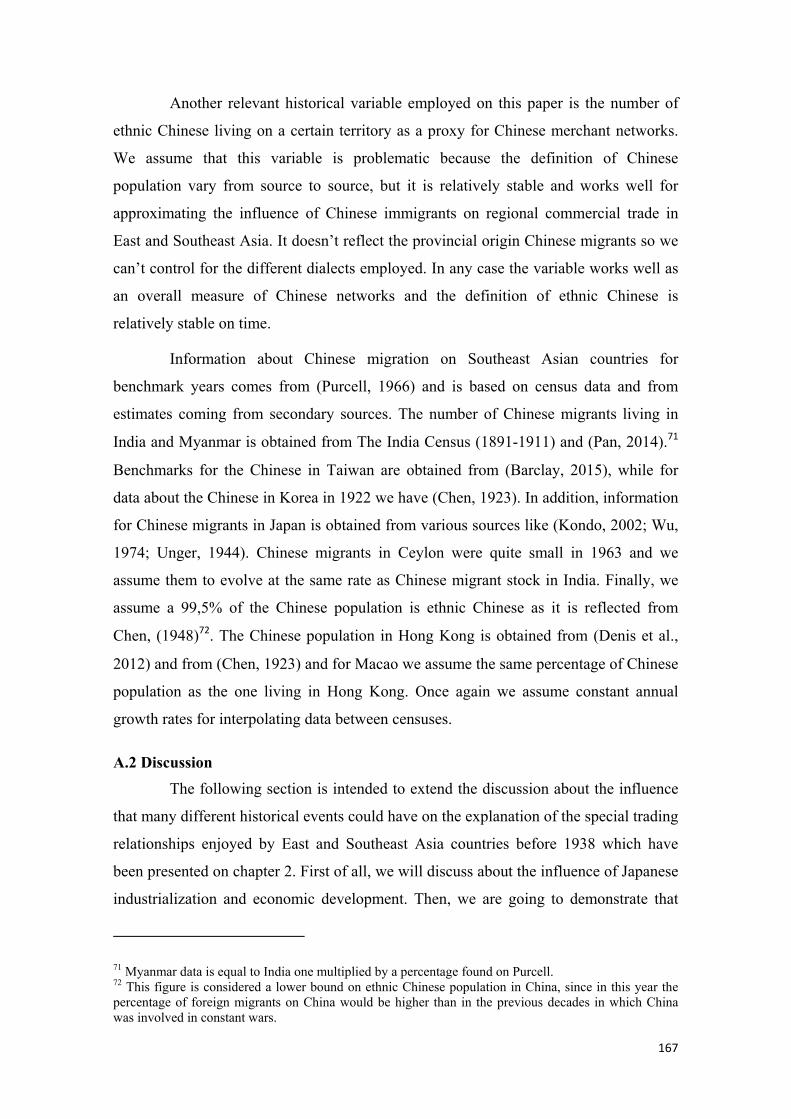
167
Another relevant historical variable employed on this paper is the number of
ethnic Chinese living on a certain territory as a proxy for Chinese merchant networks.
We assume that this variable is problematic because the definition of Chinese
population vary from source to source, but it is relatively stable and works well for
approximating the influence of Chinese immigrants on regional commercial trade in
East and Southeast Asia. It doesn’t reflect the provincial origin Chinese migrants so we
can’t control for the different dialects employed. In any case the variable works well as
an overall measure of Chinese networks and the definition of ethnic Chinese is
relatively stable on time.
Information about Chinese migration on Southeast Asian countries for
benchmark years comes from (Purcell, 1966) and is based on census data and from
estimates coming from secondary sources. The number of Chinese migrants living in
India and Myanmar is obtained from The India Census (1891-1911) and (Pan, 2014).71
Benchmarks for the Chinese in Taiwan are obtained from (Barclay, 2015), while for
data about the Chinese in Korea in 1922 we have (Chen, 1923). In addition, information
for Chinese migrants in Japan is obtained from various sources like (Kondo, 2002; Wu,
1974; Unger, 1944). Chinese migrants in Ceylon were quite small in 1963 and we
assume them to evolve at the same rate as Chinese migrant stock in India. Finally, we
assume a 99,5% of the Chinese population is ethnic Chinese as it is reflected from
Chen, (1948)72. The Chinese population in Hong Kong is obtained from (Denis et al.,
2012) and from (Chen, 1923) and for Macao we assume the same percentage of Chinese
population as the one living in Hong Kong. Once again we assume constant annual
growth rates for interpolating data between censuses.
A.2 Discussion The following section is intended to extend the discussion about the influence
that many different historical events could have on the explanation of the special trading
relationships enjoyed by East and Southeast Asia countries before 1938 which have
been presented on chapter 2. First of all, we will discuss about the influence of Japanese
industrialization and economic development. Then, we are going to demonstrate that
71 Myanmar data is equal to India one multiplied by a percentage found on Purcell. 72 This figure is considered a lower bound on ethnic Chinese population in China, since in this year the percentage of foreign migrants on China would be higher than in the previous decades in which China was involved in constant wars.
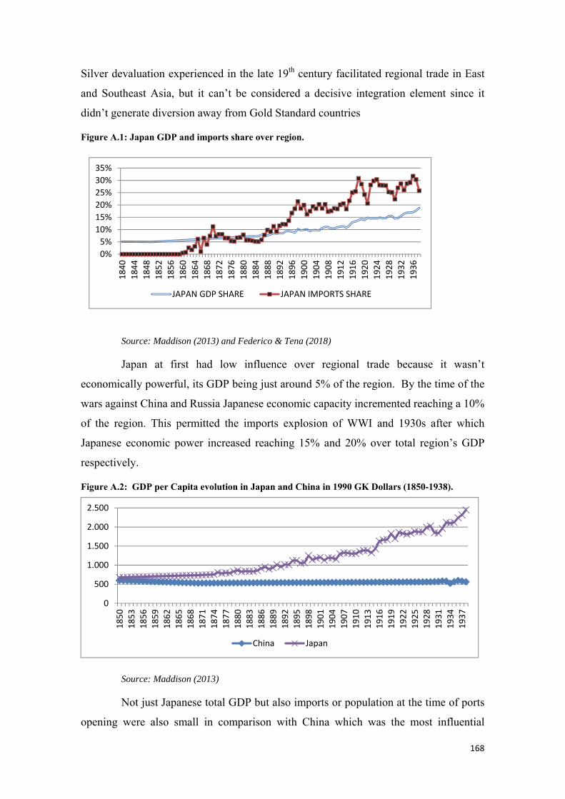
168
Silver devaluation experienced in the late 19th century facilitated regional trade in East
and Southeast Asia, but it can’t be considered a decisive integration element since it
didn’t generate diversion away from Gold Standard countries
Figure A.1: Japan GDP and imports share over region.
Source: Maddison (2013) and Federico & Tena (2018)
Japan at first had low influence over regional trade because it wasn’t
economically powerful, its GDP being just around 5% of the region. By the time of the
wars against China and Russia Japanese economic capacity incremented reaching a 10%
of the region. This permitted the imports explosion of WWI and 1930s after which
Japanese economic power increased reaching 15% and 20% over total region’s GDP
respectively.
Figure A.2: GDP per Capita evolution in Japan and China in 1990 GK Dollars (1850-1938).
Source: Maddison (2013)
Not just Japanese total GDP but also imports or population at the time of ports
opening were also small in comparison with China which was the most influential
0
500
1.000
1.500
2.000
2.500
1850
1853
1856
1859
1862
1865
1868
1871
1874
1877
1880
1883
1886
1889
1892
1895
1898
1901
1904
1907
1910
1913
1916
1919
1922
1925
1928
1931
1934
1937
China Japan
0%5%
10%15%20%25%30%35%
1840
1844
1848
1852
1856
1860
1864
1868
1872
1876
1880
1884
1888
1892
1896
1900
1904
1908
1912
1916
1920
1924
1928
1932
1936
JAPAN GDP SHARE JAPAN IMPORTS SHARE
169
country in the region. Furthermore, Japan also presented similar GDP per capita levels
to China and other poor countries at that time. Nevertheless, by the time of the two wars
with China and Russia Japanese GDP per capita already doubled Chinese one and was
three times bigger by the years before WWI showing that Japan already had economic
potential to become the region’s commercial leader. This potential was based on labor
abundance as depicted on table A.1 which shows that it was the country presenting
bigger population density by the time Perry arrived (1850s). Nonetheless, they only
seized this advantage after the institutional reforms carried by the Meiji regime which
brought Japan a superior provision of public goods, better structured economic
incentives and more aligned interest groups in comparison to China (Ma, 2004).
Table A.1: Population density on major East and Southeast Asia territories (1860-1938)
YEAR China India Indonesia Japan Philippines Thailand Malaysia
Sri
Lanka
French
Indochina
1860 34.03 52.32 13.57 85.56 14.35 10.61 4.79 37.66 17.65
1870 32.31 54.20 17.23 88.76 16.99 11.15 5.88 42.21 19.16
1880 33.21 55.10 19.05 94.86 19.22 11.98 8.28 45.77 21.79
1890 34.30 59.90 21.33 103.29 21.73 12.88 11.65 50.65 24.79
1900 36.10 60.95 23.74 113.67 24.58 14.13 16.41 59.27 28.23
1910 38.18 64.72 26.33 127.62 29.73 16.03 21.27 70.73 32.18
1920 42.60 65.47 28.94 143.86 35.99 18.92 26.07 79.55 35.67
1930 44.13 72.07 32.53 165.47 44.28 23.92 32.45 86.47 38.12
1938 46.23 80.57 37.62 185.26 53.47 28.92 38.29 91.59 38.25 Source: Maddison (2014)
All in all, it seems that the little influence exercised by the Japanese Empire on
regional trade during the 19th century was related with its small economic size. In
addition, its income per capita was average, something that didn’t permit it to overcome
its small size. Nevertheless, the country had strong potential as it enjoyed huge
population density and this advantage was subsequently exploited after winning wars
against China and Russia in order to raise its commercial influence in East and
Southeast Asia. Lastly, WWI and the Manchuria incident consolidated the Japanese
Empire and its influence all over the region.
170
Regarding the influence of monetary regimes, it is pointed by historiography
that in 1871 Silver started to lose much of its value in comparison with Gold. This fact
forced many countries to leave Silver and adopt the Gold Standard consequently
affecting trade patterns all over the world, including East and Southeast Asia. In that
region many countries kept Silver currencies between the 1870s and early 1900s and
this could have generated trade diversion with Western countries that were massively
adopting the Gold Standard and a parallel trade creation with regional partners. In that
sense, this phenomenon could also be part of the historical events that permitted East
and Southeast Asian countries to become Natural Trading Partners. That’s why this
section will analyze the gradual change from Bimetallic or Silver Standards to one
based on Gold and how it affected regional and international trade in East and Southeast
Asia.
Table A.2 shows the different monetary systems prevailing in different
territories in the world prior to silver depreciation. As we can see, in 1868 all countries
in our region were under a Silver or bimetallic standard as most countries in the world,
being the United Kingdom the most remarkable exception. Some scholars argue that the
decision of whether to adopt a Gold or Silver standard depended on income as richer
countries opted for the Gold Standard and poorer ones by the Silver. Nevertheless,
(Eichengreen et al., 2005) does not follow this line and suggest that countries tended to
adopt the legal tender employed by their main commercial partners. He also argues that
before 1873 there was a stable equilibrium between Gold and Silver exchange rate
which was broken during that decade, especially after the abandonment of France and
the Latin Union from the bimetallic system.
The greater involvement of Great Britain on international trade until becoming
the world’s commercial leader made more comfortable to adopt the Gold Standard in
order to avoid transaction costs related with the exchange of Silver by Gold. This
phenomenon attracted many countries to change to the Gold Standard and as the
number of Gold countries increased the system became more attractive. As a
consequence, the price of Silver decreased enormously during the 1870s and by 1908
most countries were inside the Gold Standard. East and Southeast Asia was not an
exception since only China continued under a Silver standard. Nevertheless, the process
was not sudden but the transition to a Gold Standard lasted for more than 20 years in
which Asian currencies were at a disadvantage with Western ones regarding imports.
171
The long path to the Gold Standard and Chinese currency exceptionality could have
diverted trade away from Gold Standard countries in favor of regional Silver or
bimetallic partners.
First of all, it is necessary to explain the path followed by East and Southeast
Asian countries towards the Gold Standard adoption. During the 1870s and 1880s they
suffered from the Silver depreciation vis a vis Gold since most of them had imperial ties
with Western countries that were adopting the Gold Standard. Consequently, on the
1890s they started to limit the coinage of Silver and moved to a Gold Standard
exchange system that differed from the traditional Gold Standard.73
The process of adjustment to the new system affected both regional and
international trade in East and Southeast Asia. As (Mitchener & Voth, 2011) explain,
intra- Asian trade grew much faster than trade with the rest of the world after 1880
partly as a consequence of Silver depreciation that made more attractive to trade with
other Silver countries. Thereafter once Asian countries adopted the Gold Standard,
intra-Asian trade declined its relative importance as imports from Western countries
resumed. This phenomenon could be behind the leap forward experienced by regional
share between 1885 and 1895 and its stagnation from then to the First World War
appreciated on Figure 3.2 in the main body of the thesis. On the same vein, Western
share in East and Southeast Asian imports sharply decreased during 1885-1895 and
slightly recovered after Asian territories adopted Gold, although their shares were never
close to the ones showed before Silver Depreciation.
73 Philippines adopted the Gold Standard after US military occupation in 1898, India in 1899, Ceylon in 1901, Korea in 1904. Japan was on Silver since 1868 and authorized a Bimetallic system in 1871. Then it followed a period of inconvertibility due to the wars and rebellions until 1886. Finally, the victory against China in 1895 and the huge amount of Sterling Pounds received as indemnity forced them to adopt the Gold Standard in 1897.
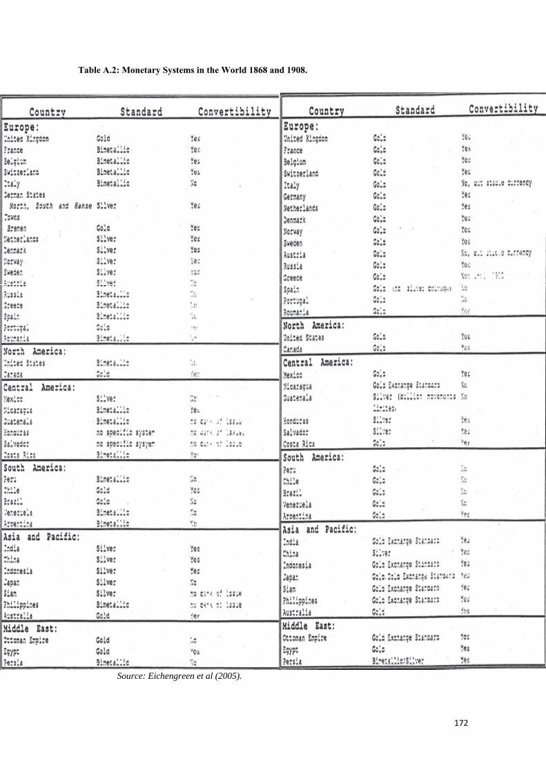
172
Table A.2: Monetary Systems in the World 1868 and 1908.
Source: Eichengreen et al (2005).
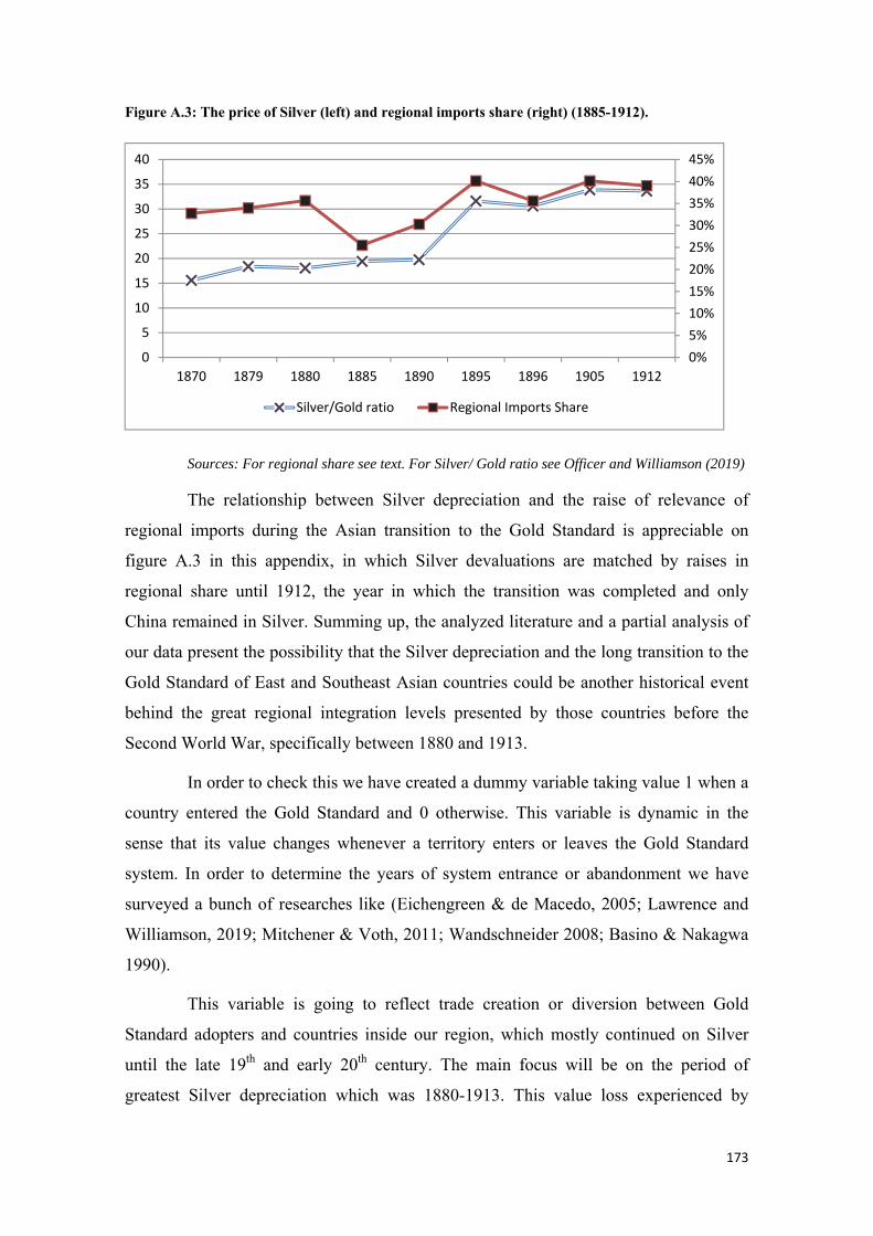
173
Figure A.3: The price of Silver (left) and regional imports share (right) (1885-1912).
Sources: For regional share see text. For Silver/ Gold ratio see Officer and Williamson (2019)
The relationship between Silver depreciation and the raise of relevance of
regional imports during the Asian transition to the Gold Standard is appreciable on
figure A.3 in this appendix, in which Silver devaluations are matched by raises in
regional share until 1912, the year in which the transition was completed and only
China remained in Silver. Summing up, the analyzed literature and a partial analysis of
our data present the possibility that the Silver depreciation and the long transition to the
Gold Standard of East and Southeast Asian countries could be another historical event
behind the great regional integration levels presented by those countries before the
Second World War, specifically between 1880 and 1913.
In order to check this we have created a dummy variable taking value 1 when a
country entered the Gold Standard and 0 otherwise. This variable is dynamic in the
sense that its value changes whenever a territory enters or leaves the Gold Standard
system. In order to determine the years of system entrance or abandonment we have
surveyed a bunch of researches like (Eichengreen & de Macedo, 2005; Lawrence and
Williamson, 2019; Mitchener & Voth, 2011; Wandschneider 2008; Basino & Nakagwa
1990).
This variable is going to reflect trade creation or diversion between Gold
Standard adopters and countries inside our region, which mostly continued on Silver
until the late 19th and early 20th century. The main focus will be on the period of
greatest Silver depreciation which was 1880-1913. This value loss experienced by
0%5%10%15%20%25%30%35%40%45%
0
5
10
15
20
25
30
35
40
1870 1879 1880 1885 1890 1895 1896 1905 1912
Silver/Gold ratio Regional Imports Share
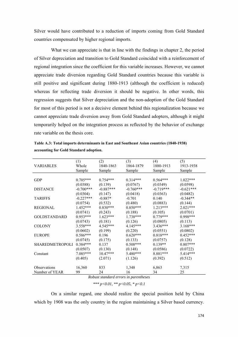
174
Silver would have contributed to a reduction of imports coming from Gold Standard
countries compensated by higher regional imports.
What we can appreciate is that in line with the findings in chapter 2, the period
of Silver depreciation and transition to Gold Standard coincided with a reinforcement of
regional integration since the coefficient for this variable increases. However, we cannot
appreciate trade diversion regarding Gold Standard countries because this variable is
still positive and significant during 1880-1913 (although the coefficient is reduced)
whereas for reflecting trade diversion it should be negative. In other words, this
regression suggests that Silver depreciation and the non-adoption of the Gold Standard
for most of this period is not a decisive element behind this regionalization because we
cannot appreciate trade diversion away from Gold Standard adopters, although it might
temporarily helped on the integration process as reflected by the behavior of exchange
rate variable on the thesis core.
Table A.3: Total imports determinants in East and Southeast Asian countries (1840-1938) accounting for Gold Standard adoption.
(1) (2) (3) (4) (5) VARIABLES Whole
Sample 1840-1863 Sample
1864-1879 Sample
1880-1913 Sample
1913-1938 Sample
GDP 0.705*** 0.754*** 0.314*** 0.564*** 1.022*** (0.0388) (0.139) (0.0767) (0.0349) (0.0598) DISTANCE -0.700*** -0.887*** -0.760*** -0.719*** -0.621*** (0.0304) (0.147) (0.0418) (0.0363) (0.0482) TARIFFS -0.227*** -0.887* -0.701 0.140 -0.344** (0.0754) (0.532) (0.480) (0.0883) (0.144) REGIONAL 1.452*** 0.830*** 0.850*** 1.213*** 2.021*** (0.0741) (0.243) (0.188) (0.105) (0.0701) GOLDSTANDARD 0.953*** 1.623*** 1.738*** 0.779*** 0.998*** (0.0743) (0.181) (0.126) (0.0805) (0.113) COLONY 3.558*** 4.545*** 4.145*** 3.436*** 3.168*** (0.0602) (0.199) (0.220) (0.0551) (0.0802) EUROPE 0.586*** 0.196 0.620*** 0.818*** 0.452*** (0.0745) (0.175) (0.133) (0.0757) (0.128) SHAREDMETROPOLI 0.384*** 0.137 0.508*** 0.139** 0.807*** (0.0507) (0.130) (0.148) (0.0586) (0.0722) Constant 7.085*** 10.47*** 5.480*** 8.881*** 5.414*** (0.405) (2.071) (1.126) (0.392) (0.512) Observations 16,360 833 1,348 6,863 7,315 Number of YEAR 99 24 16 34 25
Robust standard errors in parentheses
*** p<0.01, ** p<0.05, * p<0.1
On a similar regard, one should realize the special position held by China
which by 1908 was the only country in the region maintaining a Silver based currency.
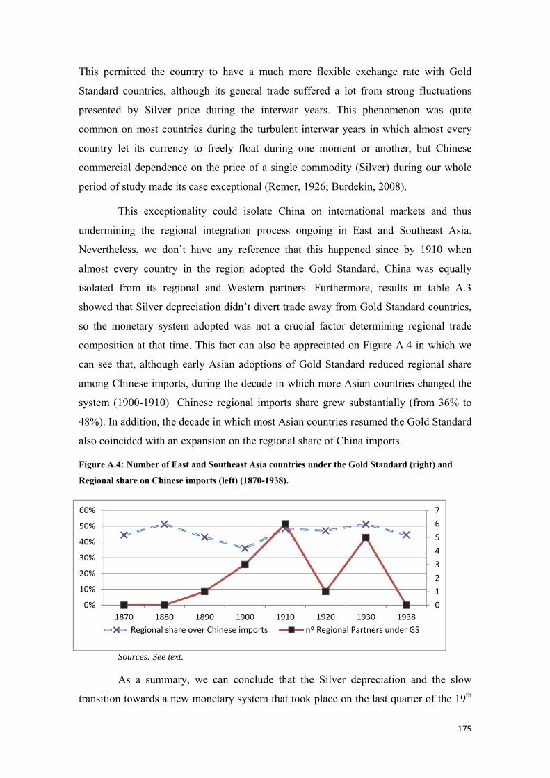
175
This permitted the country to have a much more flexible exchange rate with Gold
Standard countries, although its general trade suffered a lot from strong fluctuations
presented by Silver price during the interwar years. This phenomenon was quite
common on most countries during the turbulent interwar years in which almost every
country let its currency to freely float during one moment or another, but Chinese
commercial dependence on the price of a single commodity (Silver) during our whole
period of study made its case exceptional (Remer, 1926; Burdekin, 2008).
This exceptionality could isolate China on international markets and thus
undermining the regional integration process ongoing in East and Southeast Asia.
Nevertheless, we don’t have any reference that this happened since by 1910 when
almost every country in the region adopted the Gold Standard, China was equally
isolated from its regional and Western partners. Furthermore, results in table A.3
showed that Silver depreciation didn’t divert trade away from Gold Standard countries,
so the monetary system adopted was not a crucial factor determining regional trade
composition at that time. This fact can also be appreciated on Figure A.4 in which we
can see that, although early Asian adoptions of Gold Standard reduced regional share
among Chinese imports, during the decade in which more Asian countries changed the
system (1900-1910) Chinese regional imports share grew substantially (from 36% to
48%). In addition, the decade in which most Asian countries resumed the Gold Standard
also coincided with an expansion on the regional share of China imports.
Figure A.4: Number of East and Southeast Asia countries under the Gold Standard (right) and Regional share on Chinese imports (left) (1870-1938).
Sources: See text.
As a summary, we can conclude that the Silver depreciation and the slow
transition towards a new monetary system that took place on the last quarter of the 19th
01234567
0%
10%
20%
30%
40%
50%
60%
1870 1880 1890 1900 1910 1920 1930 1938Regional share over Chinese imports nº Regional Partners under GS
176
century were not decisive factors explaining regionalization in East and Southeast Asia
before WWII. As pointed by the literature it could have contributed to increasing
regional trade volumes during the years in which most Asia was under Silver and the
West was in Gold as it is appreciated on chapter 2 with the behavior of exchange rate
variable. However we don’t appreciate any significant trade diversion away from
Western Gold Standard countries and in favor of regional partners, which would have
demonstrated a true regional bloc creation. For that reason the core of the thesis controls
for exchange rates between currencies at the different periods as an explanatory variable
for regional trade but we don’t consider them to be overriding determinants.
A.3. Counterfactual exercise and Econometric concerns One of the principal contributions of this thesis to the literature of Natural
Trading Partners is the empirical demonstration of the significant influence that
historical events exercised in shaping special trade relationships between territories. In
that sense, regressions performed have shown much bigger coefficients for historical
variables like colonial institutions and networks than for economic variables
traditionally explaining why two countries could be considered Natural Trading
Partners. For example we find that a 1% raise on differences in demand structure lead to
an increment on regional imports of 0.156%, whereas regional imports associated to
members of the British and the Japanese Empires were respectively 235% and 1358%
higher than those to non-members (𝑒 . -1= 2.35 and 𝑒 . -1=13.58). The size of the
influence of colonial and transit networks gets even bigger at certain time periods,
which might indicate that those historical phenomenom were much more decisive than
economic characteristics in the formation of a natural trade bloc in East and Southeast
Asia.
Nevertheless, we must be careful with this assertion because we are comparing
variables of different nature and characteristics because historical variables like transit,
British and Japanese imperial networks are proxied using Dummies and economic
variables like differences in demand structure or factor endowments and trade costs are
continuous variables. For that reason, in order to measure the size of the effects
associated to these two kinds of variables on a comparable way we are going to make a
counterfactual exercise.
The objective of this exercise is to measure the impact that direct colonial
networks (exchanges between countries sharing a colonizer) and complementarities in
177
demand had on regional imports. We are trying to see how large regional imports would
have been in case no imperial relations at all were established on the region on the one
hand and in case demand structures were very similar on the other. That’s why we are
going to construct two scenarios choosing as a reference total regional imports on 1938
which is the last year of our database: The first one will estimate the total amount of
regional imports in 1938 if the growth path followed by every country from the very
first year in our sample was the same as average growth of imports coming from
countries with which it had no imperial relationship at all. On the second scenario we
estimate how large would regional imports be in case they have grown in every country
at the same rhythm as imports coming from the territories presenting the most similar
demand structures. In order to do so we have decided arbitrarily that the most similar
partners are those with which absolute difference in GDP per capita in 1938 doesn’t
exceed total GDP per capita on the importer country. In other words, we eliminate those
partners whose GDP per capita is at least twice the importer’s which are considered in
our paper to be the complementariness These approximations are not probably the most
exact but permit us to check how much lower would regional imports be in case any
country would have hold imperial relationships and in case there are no
complementarities in demand.
Our results show that in case no imperial networks had ever existed, regional
imports in East and Southeast Asia would have been 79% lower than they were in
reality. On the other hand they would have been 71% lower if there were no significant
demand complementarities inside the region. All in all, what it is found is that the
impact of a historical event like imperial networks was slightly higher than the one of
economic characteristics like demand complementarities.
The reason for choosing this approach in which the counterfactual evolution of
imports is based on a set of partners is to avoid fluctuations related with the election of
only one partner country as a reference. Nonetheless, we have practiced another
exercise in which we assume on the one hand that each country’s total imports follow
the same growth rate as imports from an independent (and not too big) country like
Thailand. On the other side we assume that individual total imports evolve at the same
path as imports from the country presenting the lowest differences on demand structure.
This situation although much more reasonable from an empirical point of view has the
statistical problem that imports from the reference country might begin from very low
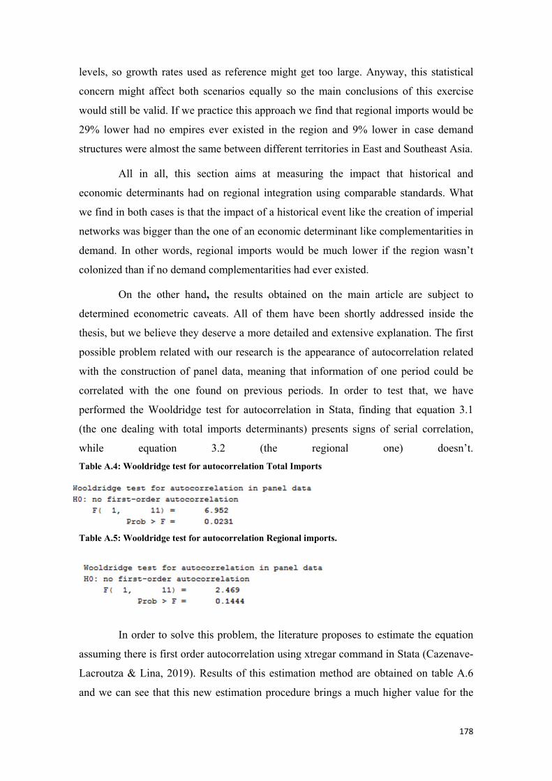
178
levels, so growth rates used as reference might get too large. Anyway, this statistical
concern might affect both scenarios equally so the main conclusions of this exercise
would still be valid. If we practice this approach we find that regional imports would be
29% lower had no empires ever existed in the region and 9% lower in case demand
structures were almost the same between different territories in East and Southeast Asia.
All in all, this section aims at measuring the impact that historical and
economic determinants had on regional integration using comparable standards. What
we find in both cases is that the impact of a historical event like the creation of imperial
networks was bigger than the one of an economic determinant like complementarities in
demand. In other words, regional imports would be much lower if the region wasn’t
colonized than if no demand complementarities had ever existed.
On the other hand, the results obtained on the main article are subject to
determined econometric caveats. All of them have been shortly addressed inside the
thesis, but we believe they deserve a more detailed and extensive explanation. The first
possible problem related with our research is the appearance of autocorrelation related
with the construction of panel data, meaning that information of one period could be
correlated with the one found on previous periods. In order to test that, we have
performed the Wooldridge test for autocorrelation in Stata, finding that equation 3.1
(the one dealing with total imports determinants) presents signs of serial correlation,
while equation 3.2 (the regional one) doesn’t. Table A.4: Wooldridge test for autocorrelation Total Imports
Table A.5: Wooldridge test for autocorrelation Regional imports.
In order to solve this problem, the literature proposes to estimate the equation
assuming there is first order autocorrelation using xtregar command in Stata (Cazenave-
Lacroutza & Lina, 2019). Results of this estimation method are obtained on table A.6
and we can see that this new estimation procedure brings a much higher value for the
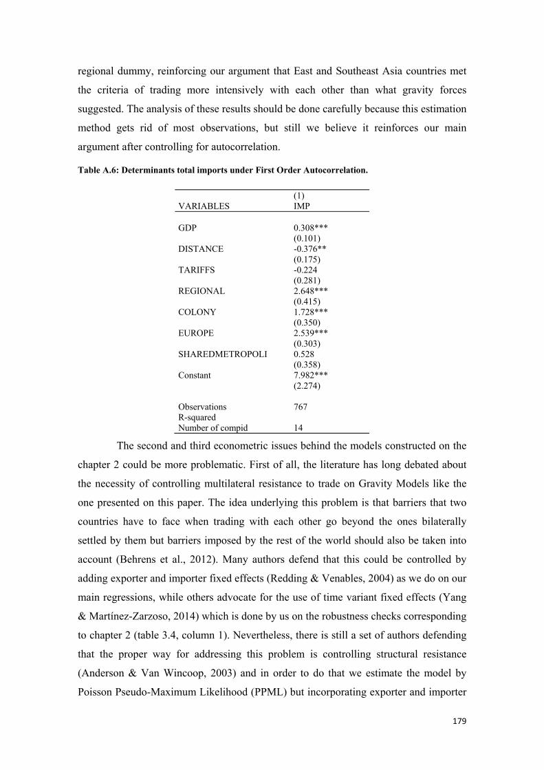
179
regional dummy, reinforcing our argument that East and Southeast Asia countries met
the criteria of trading more intensively with each other than what gravity forces
suggested. The analysis of these results should be done carefully because this estimation
method gets rid of most observations, but still we believe it reinforces our main
argument after controlling for autocorrelation.
Table A.6: Determinants total imports under First Order Autocorrelation.
(1) VARIABLES IMP GDP 0.308*** (0.101) DISTANCE -0.376** (0.175) TARIFFS -0.224 (0.281) REGIONAL 2.648*** (0.415) COLONY 1.728*** (0.350) EUROPE 2.539*** (0.303) SHAREDMETROPOLI 0.528 (0.358) Constant 7.982*** (2.274) Observations 767 R-squared Number of compid 14
The second and third econometric issues behind the models constructed on the
chapter 2 could be more problematic. First of all, the literature has long debated about
the necessity of controlling multilateral resistance to trade on Gravity Models like the
one presented on this paper. The idea underlying this problem is that barriers that two
countries have to face when trading with each other go beyond the ones bilaterally
settled by them but barriers imposed by the rest of the world should also be taken into
account (Behrens et al., 2012). Many authors defend that this could be controlled by
adding exporter and importer fixed effects (Redding & Venables, 2004) as we do on our
main regressions, while others advocate for the use of time variant fixed effects (Yang
& Martínez-Zarzoso, 2014) which is done by us on the robustness checks corresponding
to chapter 2 (table 3.4, column 1). Nevertheless, there is still a set of authors defending
that the proper way for addressing this problem is controlling structural resistance
(Anderson & Van Wincoop, 2003) and in order to do that we estimate the model by
Poisson Pseudo-Maximum Likelihood (PPML) but incorporating exporter and importer
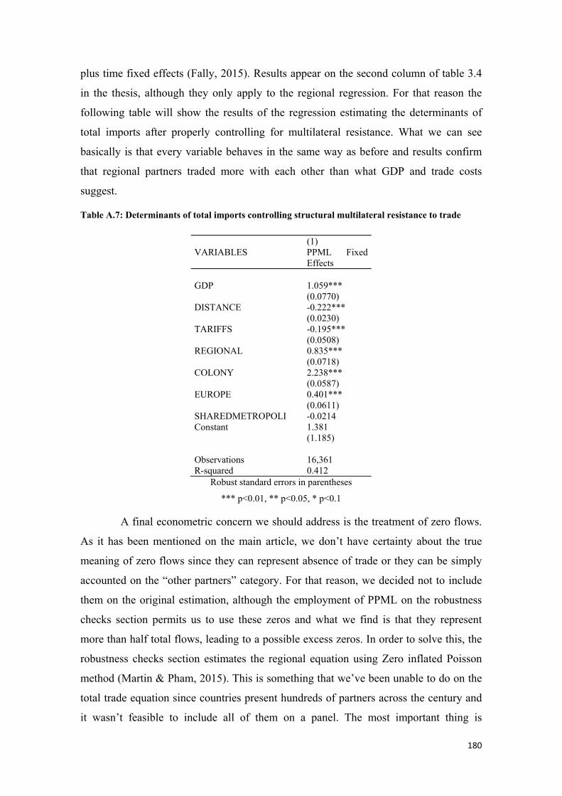
180
plus time fixed effects (Fally, 2015). Results appear on the second column of table 3.4
in the thesis, although they only apply to the regional regression. For that reason the
following table will show the results of the regression estimating the determinants of
total imports after properly controlling for multilateral resistance. What we can see
basically is that every variable behaves in the same way as before and results confirm
that regional partners traded more with each other than what GDP and trade costs
suggest.
Table A.7: Determinants of total imports controlling structural multilateral resistance to trade
(1) VARIABLES PPML Fixed
Effects GDP 1.059*** (0.0770) DISTANCE -0.222*** (0.0230) TARIFFS -0.195*** (0.0508) REGIONAL 0.835*** (0.0718) COLONY 2.238*** (0.0587) EUROPE 0.401*** (0.0611) SHAREDMETROPOLI -0.0214 Constant 1.381 (1.185) Observations 16,361 R-squared 0.412
Robust standard errors in parentheses
*** p<0.01, ** p<0.05, * p<0.1
A final econometric concern we should address is the treatment of zero flows.
As it has been mentioned on the main article, we don’t have certainty about the true
meaning of zero flows since they can represent absence of trade or they can be simply
accounted on the “other partners” category. For that reason, we decided not to include
them on the original estimation, although the employment of PPML on the robustness
checks section permits us to use these zeros and what we find is that they represent
more than half total flows, leading to a possible excess zeros. In order to solve this, the
robustness checks section estimates the regional equation using Zero inflated Poisson
method (Martin & Pham, 2015). This is something that we’ve been unable to do on the
total trade equation since countries present hundreds of partners across the century and
it wasn’t feasible to include all of them on a panel. The most important thing is
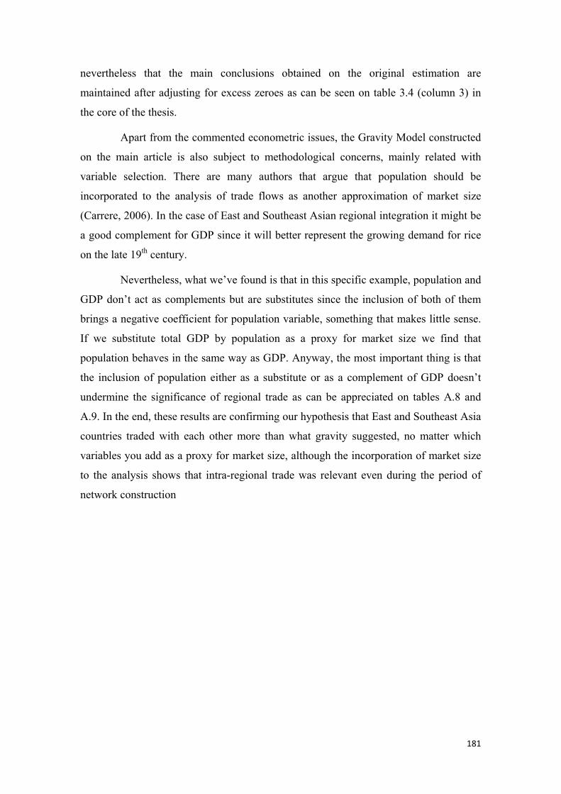
181
nevertheless that the main conclusions obtained on the original estimation are
maintained after adjusting for excess zeroes as can be seen on table 3.4 (column 3) in
the core of the thesis.
Apart from the commented econometric issues, the Gravity Model constructed
on the main article is also subject to methodological concerns, mainly related with
variable selection. There are many authors that argue that population should be
incorporated to the analysis of trade flows as another approximation of market size
(Carrere, 2006). In the case of East and Southeast Asian regional integration it might be
a good complement for GDP since it will better represent the growing demand for rice
on the late 19th century.
Nevertheless, what we’ve found is that in this specific example, population and
GDP don’t act as complements but are substitutes since the inclusion of both of them
brings a negative coefficient for population variable, something that makes little sense.
If we substitute total GDP by population as a proxy for market size we find that
population behaves in the same way as GDP. Anyway, the most important thing is that
the inclusion of population either as a substitute or as a complement of GDP doesn’t
undermine the significance of regional trade as can be appreciated on tables A.8 and
A.9. In the end, these results are confirming our hypothesis that East and Southeast Asia
countries traded with each other more than what gravity suggested, no matter which
variables you add as a proxy for market size, although the incorporation of market size
to the analysis shows that intra-regional trade was relevant even during the period of
network construction
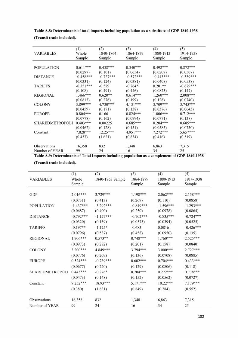
182
Table A.8: Determinants of total imports including population as a substitute of GDP 1840-1938 (Transit trade included).
(1) (2) (3) (4) (5) VARIABLES Whole
Sample 1840-1864 Sample
1864-1879 Sample
1880-1913 Sample
1914-1938 Sample
POPULATION 0.611*** 0.438*** 0.340*** 0.492*** 0.872*** (0.0297) (0.101) (0.0654) (0.0207) (0.0507) DISTANCE -0.458*** -0.727*** -0.572*** -0.443*** -0.339*** (0.0331) (0.124) (0.0381) (0.0408) (0.0538) TARIFFS -0.351*** -0.579 -0.764* 0.201** -0.679*** (0.108) (0.491) (0.446) (0.0823) (0.147) REGIONAL 1.466*** 0.620** 0.614*** 1.260*** 2.008*** (0.0813) (0.276) (0.199) (0.128) (0.0740) COLONY 3.899*** 4.730*** 4.131*** 3.709*** 3.745*** (0.0459) (0.171) (0.138) (0.0376) (0.0643) EUROPE 0.804*** 0.166 0.824*** 1.006*** 0.712*** (0.0778) (0.162) (0.0994) (0.0771) (0.138) SHAREDMETROPOLI 0.403*** 0.00225 0.685*** 0.204*** 0.685*** (0.0462) (0.128) (0.151) (0.0585) (0.0750) Constant 7.828*** 12.25*** 4.951*** 7.272*** 5.657*** (0.437) (1.621) (0.834) (0.416) (0.519) Observations 16,358 832 1,348 6,863 7,315 Number of YEAR 99 24 16 34 25 Table A.9: Determinants of Total Imports including population as a complement of GDP 1840-1938 (Transit trade included).
(1) (2) (3) (4) (5) VARIABLES Whole
Sample 1840-1863 Sample 1864-1879
Sample 1880-1913 Sample
1914-1938 Sample
GDP 2.016*** 3.729*** 1.198*** 2.062*** 2.158*** (0.0731) (0.413) (0.269) (0.110) (0.0858) POPULATION -1.437*** -3.292*** -0.849*** -1.596*** -1.293*** (0.0687) (0.400) (0.250) (0.0978) (0.0864) DISTANCE -0.792*** -1.127*** -0.702*** -0.835*** -0.724*** (0.0320) (0.159) (0.0575) (0.0394) (0.0525) TARIFFS -0.197** -1.125* -0.683 0.0816 -0.426*** (0.0796) (0.587) (0.458) (0.0950) (0.135) REGIONAL 1.906*** 0.573** 0.748*** 1.760*** 2.525*** (0.0973) (0.272) (0.201) (0.158) (0.0840) COLONY 3.200*** 4.849*** 3.794*** 3.000*** 2.727*** (0.0776) (0.209) (0.136) (0.0708) (0.0885) EUROPE 0.524*** -0.739*** 0.602*** 0.704*** 0.433*** (0.0677) (0.220) (0.129) (0.0806) (0.118) SHAREDMETROPOLI 0.443*** -0.276* 0.704*** 0.272*** 0.778*** (0.0473) (0.148) (0.152) (0.0562) (0.0727) Constant 9.252*** 18.93*** 5.171*** 10.22*** 7.179*** (0.380) (1.831) (0.849) (0.284) (0.552) Observations 16,358 832 1,348 6,863 7,315 Number of YEAR 99 24 16 34 25
183
B . A DEEPER UNDERSTANDING OF JAPANESE TRADE SUPREMACY.
B.1. Sources of Japanese exports and estimation of independent variables The first point in this section is going to describe the main features of data
construction, starting by the description of Japanese exports’ database. We have
constructed a granular database of the value of bilateral Japanese exports by product for
different benchmark years at the same level of disaggregation as those offered by the
official Japanese trade statistics. We have digitized information found in different
volumes (1912, 1915, 1925, 1929, 1932 and 1938) of the Annual Return of the Foreign
Trade of the Empire of Japan. Official statistics collected and published annually by the
Japanese Bureau of Customs include a section that collects Japanese exports to every
country, disaggregated by single product. Japan used a quite accurate declared values
c.i.f system, for imports and f.o.b valuation for exports, and gold and silver are excluded
from trade statistics. Japan followed as far as possible the origin-destination method of
crediting trade by countries. However, one faces difficulties in getting information on
country of origin and destination for goods moving through Hong Kong and Singapore
(Allen & Elly, 1953) As we have evidence that Hong Kong’s share of total Chinese
imports reduced from around 40% at the turn of the century to less than 20% in the
1920’s and less than 5% in the 1930´s, we assume that the inaccuracy of the Japanese
direction of trade records due to transit is more limited for the interwar years than for
previous periods (see Figure 5 in Keller et al., 2011).74
According to our database, Japan moved from exporting 512 different products
to 37 different countries in 1912, to exporting 1135 goods to 117 countries in 1938.75
On one hand, more countries records is related with a more precise record of
destination, but also with a more extended geographical diversification of Japanese
exports. On the other hand, we suspect that the increment in the number of goods
exported is neither related with true changes in the Japanese industrial capacity nor with
changes on market characteristics, but simply with a change in the classification rules
followed by the official statistics as it will be seen in the following section. In addition,
74 By instance, Meissner and Tang (2018) do not make any adjustment to overcome Hong Kong and Singapore transit trade problems on Japan geographical trade records assignment before 1910. 75The category “Exports to other countries” has been omitted because its inclusion didn’t permit us to control for partner country characteristics.
184
it is important to clarify that we also include the zero values of countries to which Japan
exported in a determined period, so zeros are included in this database and in the main
regressions.
However, this data source presents a relevant drawback since it doesn’t include
data in Japanese exports towards its main colonies, Korea and Taiwan (although,
thankfully they account for exports towards Kwantung province and Manchuria both
before and after being occupied for Japan). In order to solve this relevant inaccuracy of
the statistical records, and believing that the study of Japanese export patterns towards
its colonies is vital for our research target, we have obtained information in Japanese
exports towards Taiwan from the Returns of the trade of Taiwan for forty years (1896-
1935) and annual Return of trade of Taiwan (Formosa) (1936-1942) both published by
the Department of Finance of the Government of Taiwan. Such returns also include
Taiwanese imports from Japan (or equivalently Japanese exports to Taiwan) at the
product level. The quality of this database is acceptable; however the level of
disaggregation is not the same as the one of the Annual Return of the Foreign Trade of
the Empire of Japan as it includes a lower disaggregation by product, a fact which could
underestimate the extensive margin for Japanese colonies. This is a problem in our data
that remains impossible to fully solve, but we have taken several steps to remedy the
problem. First, we take the bilateral trade records of Japan with Taiwan in 1915 as a
base year because it is the last year in which the number of goods exported to Taiwan
employs the same disaggregation level as the other Japanese bilateral records, and then
we assume that every 3 SITC category follows the same tendency as the respective ones
of the Kwantung Leased Territories.
For the case of Korea, the Annual Returns of the Foreign Trade of the Empire
of Japan in their volumes from 1914-1920 include an Appendix with data in Japanese
exports to Korea disaggregated at the same product level as Japanese exports to the rest
of the countries. For the rest of the period, however there is no alternative available
source in English that breaks down Japanese exports to Korea at the product level. This
is problematic for our research because Korea was probably the most important colony
throughout the period. In order to solve this we have obtained from the Long Term
Economic Statistics of Japan (LTES tables J1411__001 to J1411__007) at Hitotsubashi
University (http://www.ier.hit-u.ac.jp/English/databases/ltes.html) a collection of
Japanese exports to Korea disaggregated in this case at the 5 sector level (which
185
include: I Agricultural Marine and Forest Products, II Mineral Products, III
Manufactured Processed Food, IV Textiles and V Chemical, Metals and Machinery)
Sectors I and II correspond to Primary products according to our skill classification,
sectors III and IV to our low skilled manufactures and sector V to our high skilled.
Finally, in order to obtain the extensive margin of Japanese exports to Korea for 1925-
1938 we have used, as in the case of Taiwan, 1915 as a base year of skill disaggregated
margins and assumed that the number of goods exported inside each sector follows the
same tendency as the one of Kwantung, so as to keep the skill breakdown of total
exports to Korea unaltered.
We make a conscious decision on the uncontrolled potential bias introduced by
this in our data base, but we believe this is our best option and an acceptable assumption
for several reasons: first, because Kwantung is the only stable Japanese colony
throughout the period, it is affected by the same political changes as Korea and Taiwan.
Kwantung was at first strongly influenced by the railway construction like Korea and
the economic structures of those three colonies were similar, being its industrialization
after the 1930s resembling the one experienced by Korea; second, because Kwantung is
across from Manchuria, the territory receiving the biggest number of Japanese product
varieties records, rising from 339 products received in 1912 to 911 in 1938, by
employing it as a reference we are computing an upper bound on Korea and Taiwan’s
extensive margin growth.
Regarding the possible determinants of Japanese exports, we’ve obtained
information on GDP and GDP per capita from the last version of the Maddison project
and refers to GDP in 1990 GK dollars or real GDP (Bolt and Van Zanden, 2014). This
database does not provide information for every country to which Japan exported during
the period 1912-1938, but it includes information for future periods. This information is
interpolated back to the interwar years by assuming that they have followed the same
rate of change as total exports of the corresponding countries (in constant prices)
obtained from (Federico & Tena-Junguito, 2019). This last method is far from perfect
because exports didn’t grow at the same rhythm as total GDP but is a method generally
accepted for computing upper bounds on GDP growth.
Another incorporation to the literature is the estimation of GDP levels and
other statistics for Japanese colonies of Kwantung Leased Territories and Manchukuo.
Population data has been obtained from (Kang, 1981) and the corresponding GDP is
186
calculated as the proportion of Japanese GDP equal to the percentage each population
represents over the Japanese total (the exercise for Manchuria is the same but using
China as a reference because until 1932 it was part of China). The Kwantung GDP is
considered to follow the same rate of growth as the Japanese one (since it is a Japanese
colony), whereas Manchuria’s follows the same tendency as China until 1932.76
Afterwards, its GDP is assumed to grow at the same rate as Manchurian exports taken
from (Federico & Tena-Junguito, 2019).
There still remains a group of territories that are provinces, colonies or
autonomous territories belonging to European Empires for which no data is available
but which appear as independent entities in Japanese statistics and for that reason are
treated as such in the present research. So, we use also marginal data recorded for
Africa and the Caribbean polities. We include their GDP proxied as a proportion of its
colonizer’s GDP, according to total population. Population from those territories is
obtained either from the League of Nations or from censuses obtained on the mainland
official statistics (like Annuarie Statistique de la France, Spanish INE data, Annuario
Statistico Italiano, British Parliamentary papers etc…). This procedure allows us to
extend GDP estimations for as many countries as possible in order to get partners’
demand by their respective economic size growth (dividing it by population obtained
from the League of Nations and Mitchell).
Then productivity is estimated through the division of GDP by the
corresponding data on total hours worked found mostly in (Huberman and Mins, 2007)
in order to construct GDP per hour worked. Working hours refer to total hours worked
per worker (male and females) in productive non-agricultural activities. This first source
only includes data of hours worked per employee for 15 advanced countries. Our
database is complemented with information on total working hours for 9 peripheral
countries in Europe including Russia obtained from (Maddison, 2007; Maddison, 1995).
Information on both databases is not annual, so it has been translated to our benchmark
years assuming constant annual rates of change.
76Kang includes data for 1912 and for the period 1924 to 1941. Population for Manchuria in 1915 has been obtained by multiplying 1912 data by the rate of change of total Chinese population and for the case of Kwantung Leased Territories the same has been done but assuming the same rate of change of Japan’s population (as it was a Japanese colony) in order to differentiate development of Japanese colonies from other East Asian territories
187
This data is likely to refer to a subset of economic activities, excluding
agriculture that is a sector with complex seasonal working hours. (Huberman, 2007;
Maddison, 1995) would show that the average number of hours per worker decreased
substantially during the first third of the twentieth century. We know, according to
(Federico, 2005) that the number of hours and part time work in advanced countries
reduced the number of working hours in agriculture, probably at a slower rate, but
adapting to the general trend of the wide economy in the period. Unfortunately,
(Federico, 2005 Table 4.2 p.63) data on agricultural working hours is too scarce and
provisional to be used to introduce a different correction for agriculture than for the
general data on the wider economy. In order to avoid measurement errors in the
construction of the variable we have decided to deduct agrarian output from total
Maddison GDP. Agrarian share over National product is found in (Mitchell, 2003) and
we subtract the corresponding percentage from Maddison’s data in 1990 GK dollars. To
estimate non-agrarian GDP per hour worked for those 24 countries and for Japan we
multiply hours worked on average by the employment in the non-agrarian sector which
is also obtained from (Mitchell, 2003).
Finally, all this information is complemented with data on GDP per hour
worked for Taiwan (representative of productivity in Japanese colonies), Indonesia
(representing productivity in Japan’s future dominions), India (which is the leader
among other Asian poor territories outside the Japanese sphere of influence) and bigger
South American countries like Argentina and Brazil. We use total hours per worker for
those territories in 1950, from (Maddison, 1995), multiplied by non-agrarian
employment obtained in (Mitchell, 2003). We interpolate back in time assuming they
follow the same trend as total employment (excluding agriculture), following the same
source.77 All in all, GDP per hour worked in non-agrarian sectors is a variable that in
this database is offered for Japan and 27 country partners which represent 92% of
Japanese exports. In order to capture Japanese productivity improvements relative to
partner countries we divide Japanese non agrarian GDP per hour worked by the
corresponding partner’s one.
We also use relative real wage growth between Japan and its partners as an
77 India and Indonesia total hours in 1950 are assumed to be equal to the ones that appear under the section “other Asia”.
188
additional variable to capture productivity gaps. The use of this variable generates
controversy among scholars, because when there is no perfect competition, as in Japan
during the interwar years, real wage differentials may not reflect productivity
differentials. The first strategy consists of building a wage index ratio by dividing
Japanese real wage growth in relation with the corresponding partner along benchmarks
(so an increase of the index means that Japanese wages are rising faster than those of its
trade partners). Data for real wages is obtained from (Williamson, 1995) which includes
information for 30 countries on the five continents including the Japanese colonies of
Korea and Taiwan and future conquests like the Philippine Islands, Indonesia or Siam.
Regarding countries with no information, as is the case of GDP per hour, we include a
zero value.
The second strategy is based on the assumption that Japanese comparative
advantage was not necessarily related with higher wages that might reflect higher
quality production, but perhaps sectorial lower unit costs. Following this idea, we
estimate an additional productivity measure to capture, as much possible, the
differences in the evolution of relative skill sectorial productivity in Japan. We have
found data in Japanese manufacturing output in different sectors and their respective
employment during the period. We use the machinery sector to capture the evolution of
the high skilled sector and the cotton textiles sector for low skilled manufactures. Data
is offered in LTES (Long Term Economic Statistics of Japan, tables JPA19__008,
JPA19__002 and JPA16__008 respectively) from Hitotsubashi University. We use the
employment share of each sector over total hours worked as a proxy of the number of
hours worked in every sector. This allows us to construct two productivity differential
indices for Japan in high skilled and low skilled manufactures. We use each of them
divided by partners’ overall productivity. Lastly, information regarding population
density as a proxy for the difference between Japan and its commercial partner’s factor
endowments has been obtained from League of Nations (1927-1945) Statistical
Yearbooks data.
The next thing is to study the sources of trade costs. The most common
variable employed in the literature on gravity to measure transport costs is distance
between countries, but it is time and product invariant. This paper makes an effort to
overcome the implications of this limited assumption on the measure of transport costs.
A relevant contribution of this paper is the construction of a database of estimated
189
freight factors (cost of transport per ton/product price per ton) between Japan and each
country partner, for every single product exported by Japan for each of our
corresponding benchmark years. In our strategy geographical distance between
Japanese partners is combined with different freight rate routes and differences in
freight factors by composition of products. Freight rates are better proxies for transport
costs than simple geographical distance, as they reflect the variations in number, size,
tonnage, speed and oil consumption on vessels employed in the different routes or the
freight price differentials driving by shipping competition along each route.
In order to do so, we have first delimited the world into three freight regions:
Europe (including Africa), America (North and South) and Asia (including Oceania),
the latter crucial for the study and subsequently divided into three further regions: the
East Asia route, which includes those Asian countries which were closer to Japan and
with which it had strong colonial or other political relationships, the Southeast Asia
route, including countries conquered by Japan and annexed to the empire during WWII,
and the Other Asia and Pacific route, with very distant Asia and Pacific countries with
which Japan did not have any economic nor political stake.
Those freights also vary between product sectors since we have a different
freight factor for every 3-digit- SITC, making our trade costs variable sensitive to
changes in trade composition by trade partners and in consequence by skill level. We
are able to compare these results only for the general equation without skills with those
obtained using the conventional method of Great Circle Distances (in kilometers)
between Capital Cities (Source: own calculations using Latitude and Longitude data
from worldatlas.com ), and in this case the results are very similar, with coefficients
presenting almost the same levels and significance as is shown by Table B.1, the
coefficient of Colonies and Future Conquests being even more powerful.
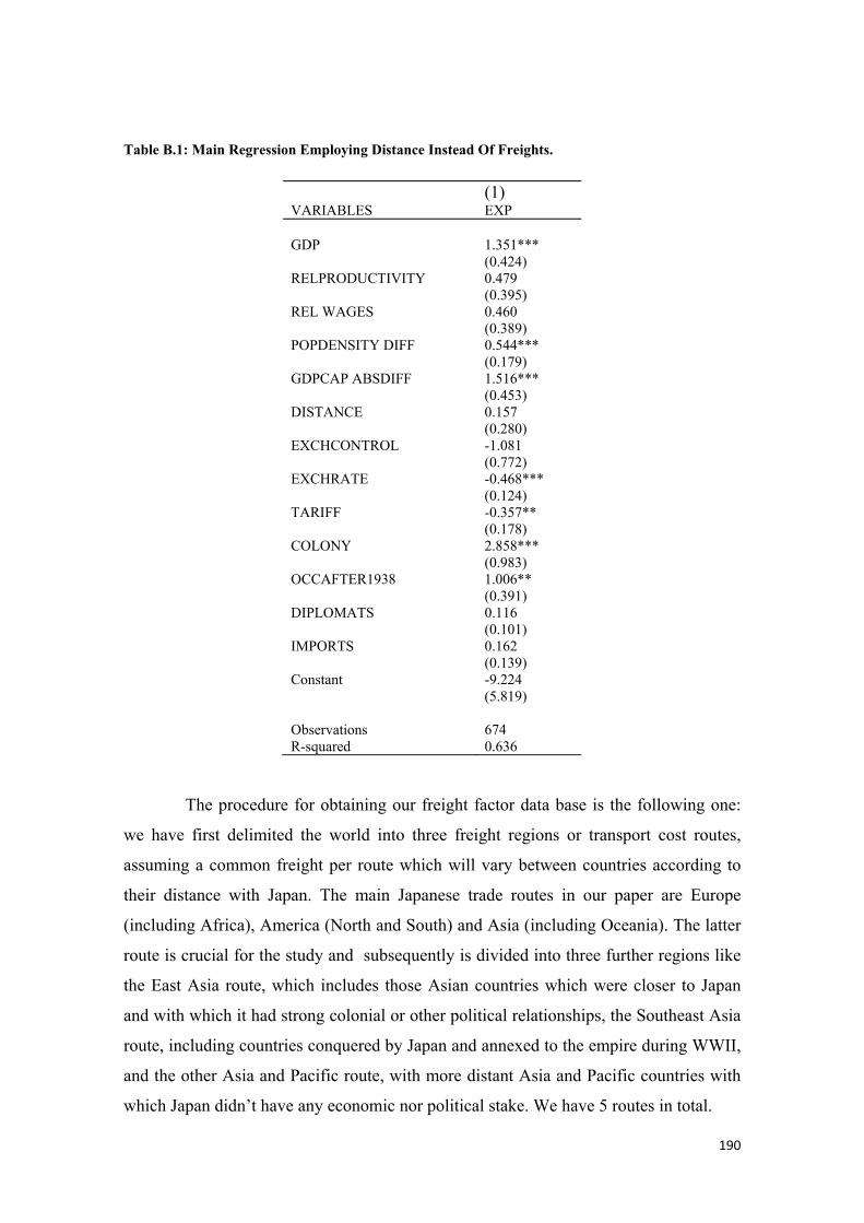
190
Table B.1: Main Regression Employing Distance Instead Of Freights.
(1) VARIABLES EXP GDP 1.351*** (0.424) RELPRODUCTIVITY 0.479 (0.395) REL WAGES 0.460 (0.389) POPDENSITY DIFF 0.544*** (0.179) GDPCAP ABSDIFF 1.516*** (0.453) DISTANCE 0.157 (0.280) EXCHCONTROL -1.081 (0.772) EXCHRATE -0.468*** (0.124) TARIFF -0.357** (0.178) COLONY 2.858*** (0.983) OCCAFTER1938 1.006** (0.391) DIPLOMATS 0.116 (0.101) IMPORTS 0.162 (0.139) Constant -9.224 (5.819) Observations 674 R-squared 0.636
The procedure for obtaining our freight factor data base is the following one:
we have first delimited the world into three freight regions or transport cost routes,
assuming a common freight per route which will vary between countries according to
their distance with Japan. The main Japanese trade routes in our paper are Europe
(including Africa), America (North and South) and Asia (including Oceania). The latter
route is crucial for the study and subsequently is divided into three further regions like
the East Asia route, which includes those Asian countries which were closer to Japan
and with which it had strong colonial or other political relationships, the Southeast Asia
route, including countries conquered by Japan and annexed to the empire during WWII,
and the other Asia and Pacific route, with more distant Asia and Pacific countries with
which Japan didn’t have any economic nor political stake. We have 5 routes in total.
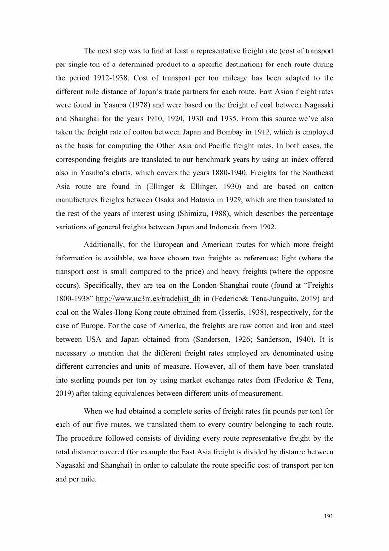
191
The next step was to find at least a representative freight rate (cost of transport
per single ton of a determined product to a specific destination) for each route during
the period 1912-1938. Cost of transport per ton mileage has been adapted to the
different mile distance of Japan’s trade partners for each route. East Asian freight rates
were found in Yasuba (1978) and were based on the freight of coal between Nagasaki
and Shanghai for the years 1910, 1920, 1930 and 1935. From this source we’ve also
taken the freight rate of cotton between Japan and Bombay in 1912, which is employed
as the basis for computing the Other Asia and Pacific freight rates. In both cases, the
corresponding freights are translated to our benchmark years by using an index offered
also in Yasuba’s charts, which covers the years 1880-1940. Freights for the Southeast
Asia route are found in (Ellinger & Ellinger, 1930) and are based on cotton
manufactures freights between Osaka and Batavia in 1929, which are then translated to
the rest of the years of interest using (Shimizu, 1988), which describes the percentage
variations of general freights between Japan and Indonesia from 1902.
Additionally, for the European and American routes for which more freight
information is available, we have chosen two freights as references: light (where the
transport cost is small compared to the price) and heavy freights (where the opposite
occurs). Specifically, they are tea on the London-Shanghai route (found at “Freights
1800-1938” http://www.uc3m.es/tradehist_db in (Federico& Tena-Junguito, 2019) and
coal on the Wales-Hong Kong route obtained from (Isserlis, 1938), respectively, for the
case of Europe. For the case of America, the freights are raw cotton and iron and steel
between USA and Japan obtained from (Sanderson, 1926; Sanderson, 1940). It is
necessary to mention that the different freight rates employed are denominated using
different currencies and units of measure. However, all of them have been translated
into sterling pounds per ton by using market exchange rates from (Federico & Tena,
2019) after taking equivalences between different units of measurement.
When we had obtained a complete series of freight rates (in pounds per ton) for
each of our five routes, we translated them to every country belonging to each route.
The procedure followed consists of dividing every route representative freight by the
total distance covered (for example the East Asia freight is divided by distance between
Nagasaki and Shanghai) in order to calculate the route specific cost of transport per ton
and per mile.
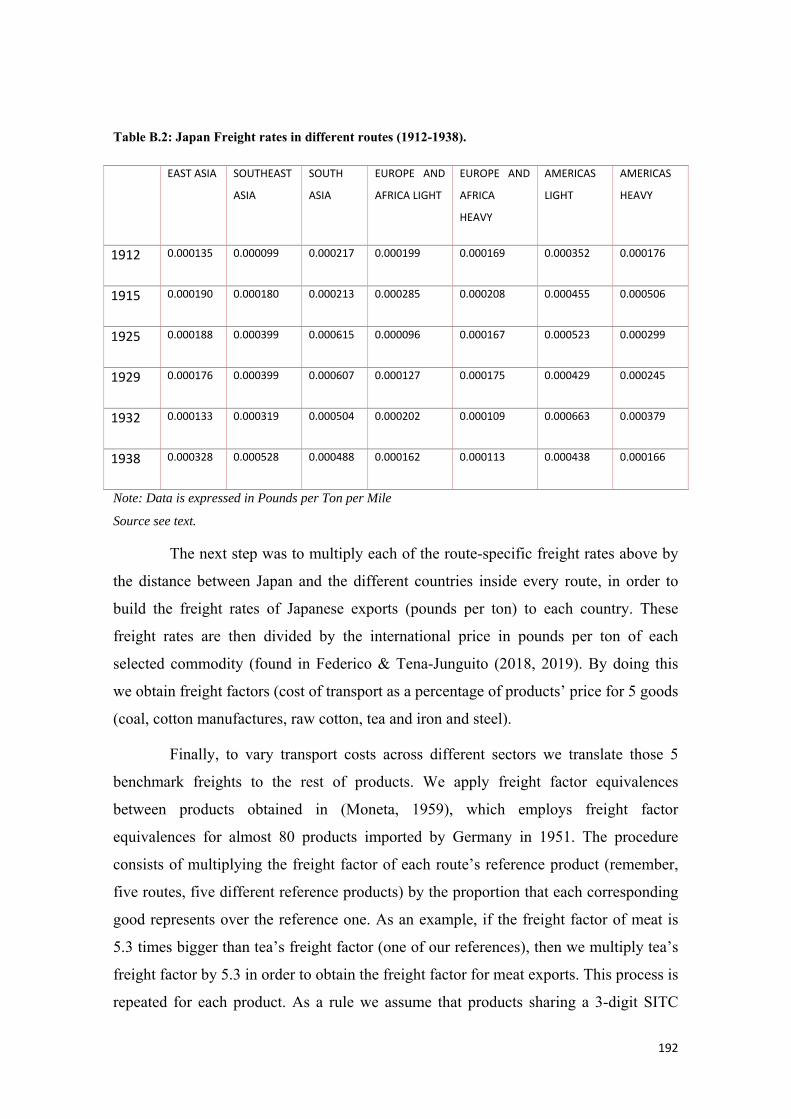
192
Table B.2: Japan Freight rates in different routes (1912-1938).
EAST ASIA SOUTHEAST
ASIA
SOUTH
ASIA
EUROPE AND
AFRICA LIGHT
EUROPE AND
AFRICA
HEAVY
AMERICAS
LIGHT
AMERICAS
HEAVY
1912 0.000135 0.000099 0.000217 0.000199 0.000169 0.000352 0.000176
1915 0.000190 0.000180 0.000213 0.000285 0.000208 0.000455 0.000506
1925 0.000188 0.000399 0.000615 0.000096 0.000167 0.000523 0.000299
1929 0.000176 0.000399 0.000607 0.000127 0.000175 0.000429 0.000245
1932 0.000133 0.000319 0.000504 0.000202 0.000109 0.000663 0.000379
1938 0.000328 0.000528 0.000488 0.000162 0.000113 0.000438 0.000166
Note: Data is expressed in Pounds per Ton per Mile
Source see text.
The next step was to multiply each of the route-specific freight rates above by
the distance between Japan and the different countries inside every route, in order to
build the freight rates of Japanese exports (pounds per ton) to each country. These
freight rates are then divided by the international price in pounds per ton of each
selected commodity (found in Federico & Tena-Junguito (2018, 2019). By doing this
we obtain freight factors (cost of transport as a percentage of products’ price for 5 goods
(coal, cotton manufactures, raw cotton, tea and iron and steel).
Finally, to vary transport costs across different sectors we translate those 5
benchmark freights to the rest of products. We apply freight factor equivalences
between products obtained in (Moneta, 1959), which employs freight factor
equivalences for almost 80 products imported by Germany in 1951. The procedure
consists of multiplying the freight factor of each route’s reference product (remember,
five routes, five different reference products) by the proportion that each corresponding
good represents over the reference one. As an example, if the freight factor of meat is
5.3 times bigger than tea’s freight factor (one of our references), then we multiply tea’s
freight factor by 5.3 in order to obtain the freight factor for meat exports. This process is
repeated for each product. As a rule we assume that products sharing a 3-digit SITC
193
classification have the same freight factors. In addition we also assume that freight
factor equivalences did not change too much between our period (1912-1938) and
1951.78 Graph 1 shows the evolution of the freight factors created on this article by
means of an index number (1912=100) capturing changes in the average freight factors
for each trade route. Those averages have been weighted according to the proportion
that each corresponding product possesses in total Japanese exports. The graph shows
how freights fluctuate considerably, reflecting technological, market and trade
composition factors, as opposed to distance, which is fixed. Furthermore, it is
remarkable to observe that during the 1930s, the period in which Japanese exports
towards East and Southeast Asia experienced their sharpest raise, freight factors to both
routes increased.
Figure B.1: Freight Factor (trade-weighted by route) 1912-1938 (1912=100).
Source see text
In addition, there are other trade costs that are not related with transport.
Average levels of tariff protection come from (Blattman et al., 2003) and represent total
import duties collected by each country as a percentage of total imports.79 This database
has been extended following the same procedure using data obtained from the British
Parliamentary Papers and the Annuarie Statistique de la France for their respective
colonies all over the world (including Africa and the Caribbean). For other countries,
we assume that levels of protection are the same as those of their respective
78 That’s a strong assumption but this is the best possible option for translating our freight factors to every single product exported by Japan. 79Tariffs between Japan and its colonies are assumed to be zero.
0
0,5
1
1,5
2
2,5
3
1912 1915 1925 1929 1932 1938
East Asia SouthEast Asia South Asia Europe and Africa Americas
194
Metropolis.80 All in all, we have data on tariffs for every country to which Japan
exported during the interwar years.
On the other hand, exchange rates between every currency and the Japanese
Yen (relative exchange rates) are obtained from (Federico & Tena-Junguito, 2019).
This source gives nominal exchange rates between local currencies in different
territories (among which Japan is included) and the dollar, expressed in local
currency/dollar. The new rate is expressed in local currency per Yen and obtained
through the division of partners’ currency nominal exchange rate (foreign currency per
dollar) by Japanese nominal exchange rate (Yen per dollar) and has been created for 44
partners. In other words, an increment of this variable reflects a relative nominal
appreciation of the Yen. This assumes that nominal devaluation with the Yen affects
trade independently of the behavior of their respective partners domestic price.
Unfortunately, there is a scarcity data on domestic prices for the cross-section of
countries, which impedes the inclusion of bilateral effective real exchange rates in our
gravity equations. Nevertheless, this variable presents many different scales responding
to the strength of each currency with which Japan traded. For exchange rate variable to
really represent evolution of Yen acquisitive power we have decided to re scale it by
constructing an index with base 1 in 1912. Furthermore, we have also obtained data on
exchange rate controls obtained from various sources including (Bethell, 1994;
Eichengreen, 1996; Meisel, 1990; Reinhart & Rogoff, 2002).
The last variable chosen to represent trade costs refers to the number of
Japanese diplomats operating in each country, which has been obtained from Almanac
de Gotha (various years), which includes a section with the names and country of origin
of every diplomat operating in each country. We have meticulously counted the number
of Japanese diplomats that worked in each country and the number of foreign diplomats
that worked in Japan.
80 An example of this could be the Canary Island on Spain. For an extended discussion on tariffs sources and methods see Appendix A.1.
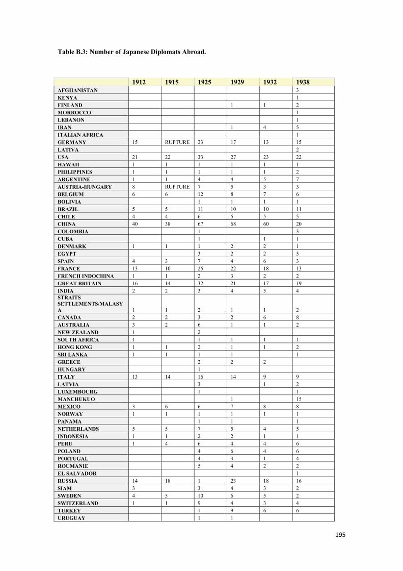
195
Table B.3: Number of Japanese Diplomats Abroad.
1912 1915 1925 1929 1932 1938 AFGHANISTAN 3 KENYA 1 FINLAND 1 1 2 MORROCCO 1 LEBANON 1 IRAN 1 4 5 ITALIAN AFRICA 1 GERMANY 15 RUPTURE 23 17 13 15 LATIVA 2 USA 21 22 33 27 23 22 HAWAII 1 1 1 1 1 1 PHILIPPINES 1 1 1 1 1 2 ARGENTINE 1 1 4 4 5 7 AUSTRIA-HUNGARY 8 RUPTURE 7 5 3 3 BELGIUM 6 6 12 8 7 6 BOLIVIA 1 1 1 1 BRAZIL 5 5 11 10 10 11 CHILE 4 4 6 5 5 5 CHINA 40 38 67 68 60 20 COLOMBIA 1 3 CUBA 1 1 1 DENMARK 1 1 1 2 2 1 EGYPT 3 2 2 5 SPAIN 4 3 7 4 6 3 FRANCE 13 10 25 22 18 13 FRENCH INDOCHINA 1 1 2 3 2 2 GREAT BRITAIN 16 14 32 21 17 19 INDIA 2 2 3 4 5 4 STRAITS SETTLEMENTS/MALASYA 1 1 2 1 1 2 CANADA 2 2 3 2 6 8 AUSTRALIA 3 2 6 1 1 2 NEW ZEALAND 1 2 SOUTH AFRICA 1 1 1 1 1 HONG KONG 1 1 2 1 1 2 SRI LANKA 1 1 1 1 1 GREECE 2 2 2 HUNGARY 1 ITALY 13 14 16 14 9 9 LATVIA 3 1 2 LUXEMBOURG 1 1 MANCHUKUO 1 15 MEXICO 3 6 6 7 8 8 NORWAY 1 1 1 1 1 1 PANAMA 1 1 1 NETHERLANDS 5 5 7 5 4 5 INDONESIA 1 1 2 2 1 1 PERU 1 4 6 4 4 6 POLAND 4 6 4 6 PORTUGAL 4 3 1 4 ROUMANIE 5 4 2 2 EL SALVADOR 1 RUSSIA 14 18 1 23 18 16 SIAM 3 3 4 3 2 SWEDEN 4 5 10 6 5 2 SWITZERLAND 1 1 9 4 3 4 TURKEY 1 9 6 6 URUGUAY 1 1
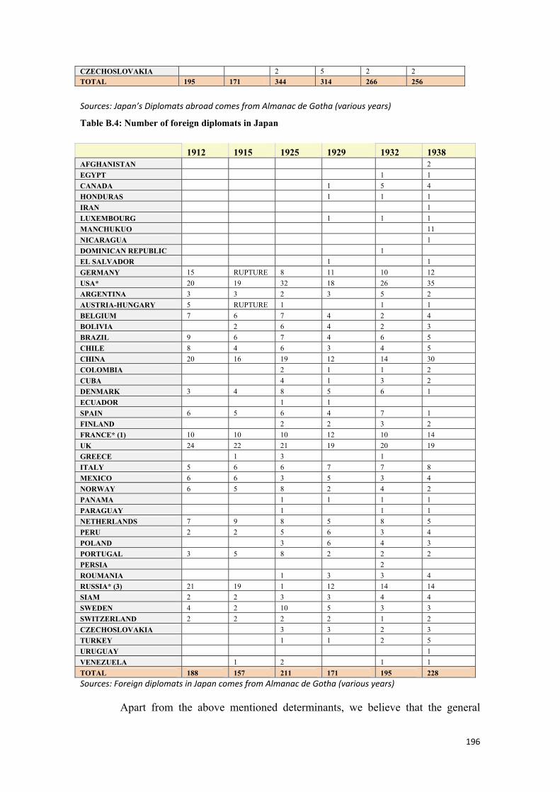
196
Sources: Japan’s Diplomats abroad comes from Almanac de Gotha (various years)
Table B.4: Number of foreign diplomats in Japan
1912 1915 1925 1929 1932 1938 AFGHANISTAN 2 EGYPT 1 1 CANADA 1 5 4 HONDURAS 1 1 1 IRAN 1 LUXEMBOURG 1 1 1 MANCHUKUO 11 NICARAGUA 1 DOMINICAN REPUBLIC 1 EL SALVADOR 1 1 GERMANY 15 RUPTURE 8 11 10 12 USA* 20 19 32 18 26 35 ARGENTINA 3 3 2 3 5 2 AUSTRIA-HUNGARY 5 RUPTURE 1 1 1 BELGIUM 7 6 7 4 2 4 BOLIVIA 2 6 4 2 3 BRAZIL 9 6 7 4 6 5 CHILE 8 4 6 3 4 5 CHINA 20 16 19 12 14 30 COLOMBIA 2 1 1 2 CUBA 4 1 3 2 DENMARK 3 4 8 5 6 1 ECUADOR 1 1 SPAIN 6 5 6 4 7 1 FINLAND 2 2 3 2 FRANCE* (1) 10 10 10 12 10 14 UK 24 22 21 19 20 19 GREECE 1 3 1 ITALY 5 6 6 7 7 8 MEXICO 6 6 3 5 3 4 NORWAY 6 5 8 2 4 2 PANAMA 1 1 1 1 PARAGUAY 1 1 1 NETHERLANDS 7 9 8 5 8 5 PERU 2 2 5 6 3 4 POLAND 3 6 4 3 PORTUGAL 3 5 8 2 2 2 PERSIA 2 ROUMANIA 1 3 3 4 RUSSIA* (3) 21 19 1 12 14 14 SIAM 2 2 3 3 4 4 SWEDEN 4 2 10 5 3 3 SWITZERLAND 2 2 2 2 1 2 CZECHOSLOVAKIA 3 3 2 3 TURKEY 1 1 2 5 URUGUAY 1 VENEZUELA 1 2 1 1 TOTAL 188 157 211 171 195 228 Sources: Foreign diplomats in Japan comes from Almanac de Gotha (various years)
Apart from the above mentioned determinants, we believe that the general
CZECHOSLOVAKIA 2 5 2 2 TOTAL 195 171 344 314 266 256
197
international protectionist backlash prevalent in Europe, the USA, and other relevant
markets for Japan, such as India, during the 1930s influenced Japan’s commercial focus
on its empire and regional markets. In order to capture the global trade diversion
generated by the Great Depression, we have included in our database a variable
capturing the contraction of international trade over domestic demand represented by
the GDP. It is represented by total imports for every Japanese country partner in each of
our benchmark years. Information is obtained from (Federico and Tena-Junguito, 2019)
and refers to total imports in current dollars. This source includes information for
almost every Japanese trade partner. Exceptions are Hong Kong, Kwantung and
Manchuria (1912-1929, our source contains information for 1932-1938), which were
part of Japan’s future dominions and colonial possessions, respectively. In order to
account for these omissions, we have obtained Hong Kong imports from the British
Parliamentary Papers (Statistical Abstract for the British Empire 1924-1938). The rest
of the years have been extrapolated assuming Hong Kong exports to follow the same
path as British Malaysia as both were British Colonies and were famous entrepôts
(British Malaysia includes the Singapore entrepôt). To calculate Kwantung imports, we
assume them to be equal to the proportion of Japanese imports based on the percentage
of the population of Kwantung represented over the Japanese population and assuming
parallel trends. Finally, Manchurian imports have been interpolated back from 1932 to
the previous benchmarks by assuming imports to evolve at the same rate as its
population.
The last set of variables we’ve added to the model are linked mainly with
political factors that imply severe changes in trade costs related with the variations of
the connection of different territories within the Japanese Empire. As has been
explained in chapter 3, there are two forms: the first one consists of the Japanese
creation of formal colonies in the conventional way and the second one, on the
economic penetration that anticipated future conquests. We believe that both kinds of
imperialism allowed Japan to reduce trade costs with its neighbors and we build two
separate dummies for representing them. The first one captures Japanese trade bias
towards its colonies, whereas the second tries to measure the extent to which Japan’s
interest towards its future conquered territories implied bigger exported quantities than
what is suggested by the rest of the model’s variables. The following tables summarize
which countries were part of Japan’s Colonies and future dominions and their main
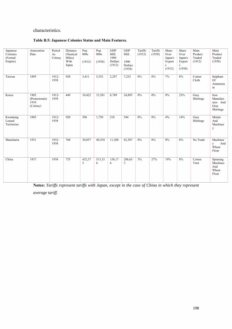
198
characteristics.
Table B.5: Japanese Colonies Status and Main Features.
Japanese Colonies (Formal Empire)
Annexation Date
Period As Colony
Distance (Nautical Miles) With Japan
Pop 000s
(1912)
Pop 000s
(1938)
GDP Mill. 1990 Dollars (1912)
GDP Mill.
1990 Dollars (1938)
Tariffs (1912)
Tariffs (1938)
Share Over Japan's Exports (1912)
Share Over Japan's Exports (1938)
Main Product Traded (1912)
Main Product Traded (1938)
Taiwan 1895 1912-1938
920 3,411 5,552 2,297 7,252 0% 0% 7% 8% Cotton Cloth
Sulphate Of Ammonium
Korea 1905 (Protectorate) 1910 (Colony)
1912-1938
449 10,422 15,381 8,789 24,895 0% 0% 8% 23% Gray Shirtings
Iron Manufactures And Gray Shirtings
Kwantung Leased Territories
1905 1912-1938
920 596 1,750 218 544 0% 0% 4% 14% Gray Shirtings
Metals And Machinery
Manchuria 1931 1932-1938
768 30,857 40,354 11,288 42,307 0% 0% 0% 8% No Trade Machinery And Wheat Flour
China 1937 1938 735 432,375
513,336
158,176
288,653
3% 27% 19% 8% Cotton Yarn
Spinning Machines And Wheat Flour
Notes: Tariffs represent tariffs with Japan, except in the case of China in which they represent
average tariff.
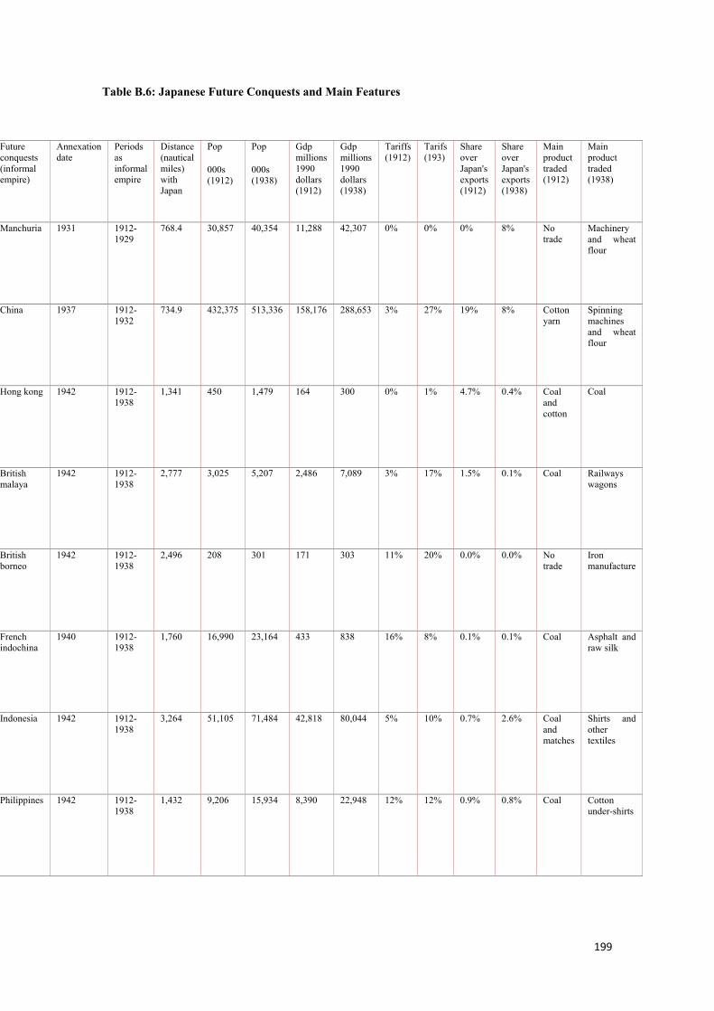
199
Table B.6: Japanese Future Conquests and Main Features
Future conquests (informal empire)
Annexation date
Periods as informal empire
Distance (nautical miles) with Japan
Pop
000s (1912)
Pop
000s (1938)
Gdp millions 1990 dollars (1912)
Gdp millions 1990 dollars (1938)
Tariffs (1912)
Tarifs (193)
Share over Japan's exports (1912)
Share over Japan's exports (1938)
Main product traded (1912)
Main product traded (1938)
Manchuria 1931 1912-1929
768.4 30,857 40,354 11,288 42,307 0% 0% 0% 8% No trade
Machinery and wheat flour
China 1937 1912-1932
734.9 432,375 513,336 158,176 288,653 3% 27% 19% 8% Cotton yarn
Spinning machines and wheat flour
Hong kong 1942 1912-1938
1,341 450 1,479 164 300 0% 1% 4.7% 0.4% Coal and cotton
Coal
British malaya
1942 1912-1938
2,777 3,025 5,207 2,486 7,089 3% 17% 1.5% 0.1% Coal Railways wagons
British borneo
1942 1912-1938
2,496 208 301 171 303 11% 20% 0.0% 0.0% No trade
Iron manufacture
French indochina
1940 1912-1938
1,760 16,990 23,164 433 838 16% 8% 0.1% 0.1% Coal Asphalt and raw silk
Indonesia 1942 1912-1938
3,264 51,105 71,484 42,818 80,044 5% 10% 0.7% 2.6% Coal and matches
Shirts and other textiles
Philippines 1942 1912-1938
1,432 9,206 15,934 8,390 22,948 12% 12% 0.9% 0.8% Coal Cotton under-shirts
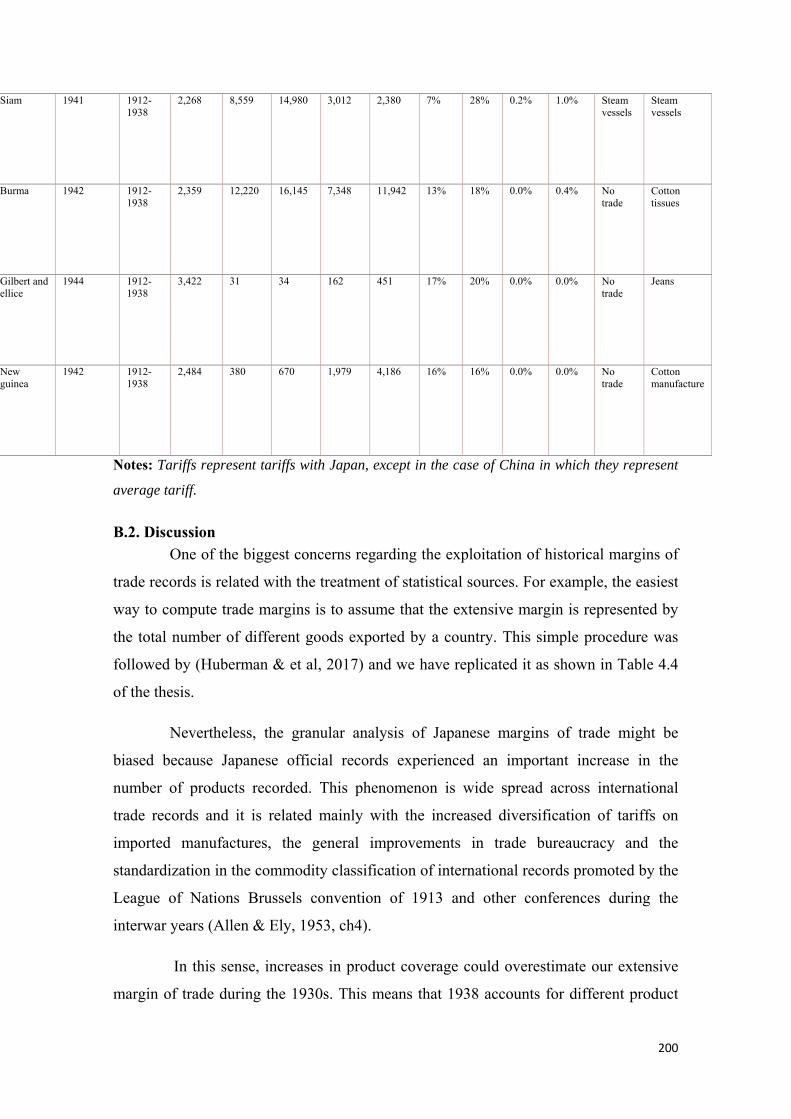
200
Notes: Tariffs represent tariffs with Japan, except in the case of China in which they represent
average tariff.
B.2. Discussion One of the biggest concerns regarding the exploitation of historical margins of
trade records is related with the treatment of statistical sources. For example, the easiest
way to compute trade margins is to assume that the extensive margin is represented by
the total number of different goods exported by a country. This simple procedure was
followed by (Huberman & et al, 2017) and we have replicated it as shown in Table 4.4
of the thesis.
Nevertheless, the granular analysis of Japanese margins of trade might be
biased because Japanese official records experienced an important increase in the
number of products recorded. This phenomenon is wide spread across international
trade records and it is related mainly with the increased diversification of tariffs on
imported manufactures, the general improvements in trade bureaucracy and the
standardization in the commodity classification of international records promoted by the
League of Nations Brussels convention of 1913 and other conferences during the
interwar years (Allen & Ely, 1953, ch4).
In this sense, increases in product coverage could overestimate our extensive
margin of trade during the 1930s. This means that 1938 accounts for different product
Siam 1941 1912-1938
2,268 8,559 14,980 3,012 2,380 7% 28% 0.2% 1.0% Steam vessels
Steam vessels
Burma 1942 1912-1938
2,359 12,220 16,145 7,348 11,942 13% 18% 0.0% 0.4% No trade
Cotton tissues
Gilbert and ellice
1944 1912-1938
3,422 31 34 162 451 17% 20% 0.0% 0.0% No trade
Jeans
New guinea
1942 1912-1938
2,484 380 670 1,979 4,186 16% 16% 0.0% 0.0% No trade
Cotton manufacture
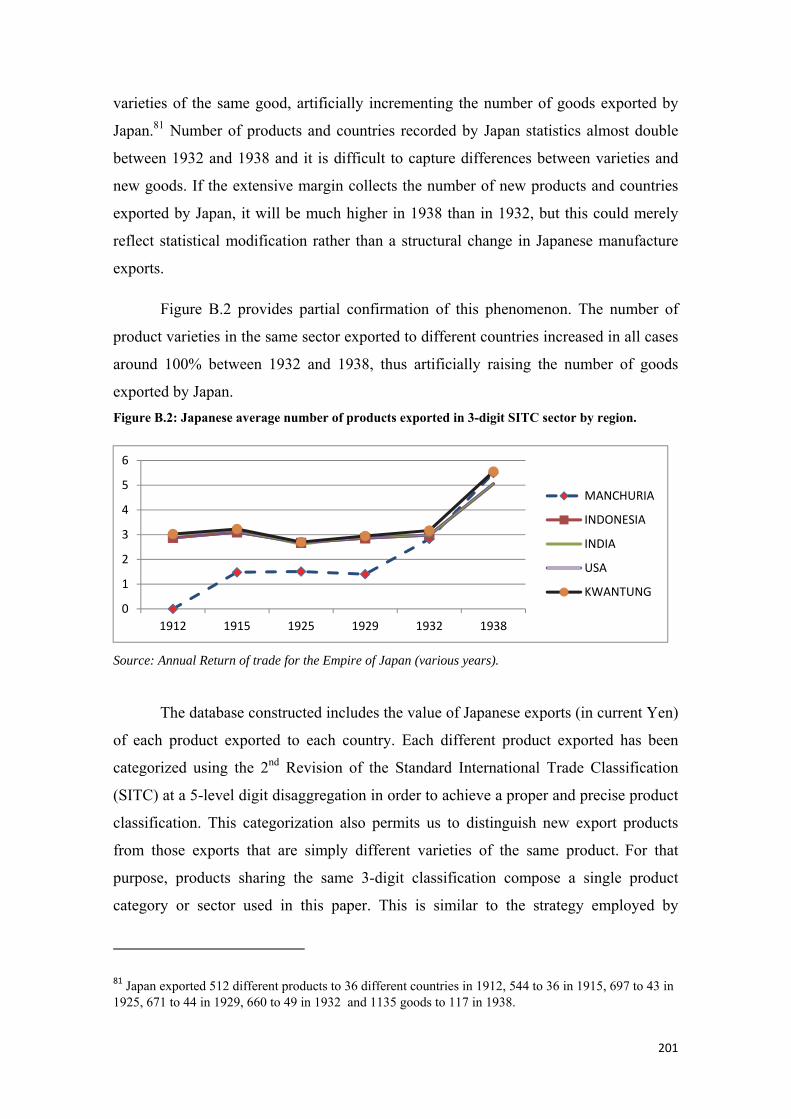
201
varieties of the same good, artificially incrementing the number of goods exported by
Japan.81 Number of products and countries recorded by Japan statistics almost double
between 1932 and 1938 and it is difficult to capture differences between varieties and
new goods. If the extensive margin collects the number of new products and countries
exported by Japan, it will be much higher in 1938 than in 1932, but this could merely
reflect statistical modification rather than a structural change in Japanese manufacture
exports.
Figure B.2 provides partial confirmation of this phenomenon. The number of
product varieties in the same sector exported to different countries increased in all cases
around 100% between 1932 and 1938, thus artificially raising the number of goods
exported by Japan. Figure B.2: Japanese average number of products exported in 3-digit SITC sector by region.
Source: Annual Return of trade for the Empire of Japan (various years).
The database constructed includes the value of Japanese exports (in current Yen)
of each product exported to each country. Each different product exported has been
categorized using the 2nd Revision of the Standard International Trade Classification
(SITC) at a 5-level digit disaggregation in order to achieve a proper and precise product
classification. This categorization also permits us to distinguish new export products
from those exports that are simply different varieties of the same product. For that
purpose, products sharing the same 3-digit classification compose a single product
category or sector used in this paper. This is similar to the strategy employed by
81 Japan exported 512 different products to 36 different countries in 1912, 544 to 36 in 1915, 697 to 43 in 1925, 671 to 44 in 1929, 660 to 49 in 1932 and 1135 goods to 117 in 1938.
0
1
2
3
4
5
6
1912 1915 1925 1929 1932 1938
MANCHURIA
INDONESIA
INDIA
USA
KWANTUNG
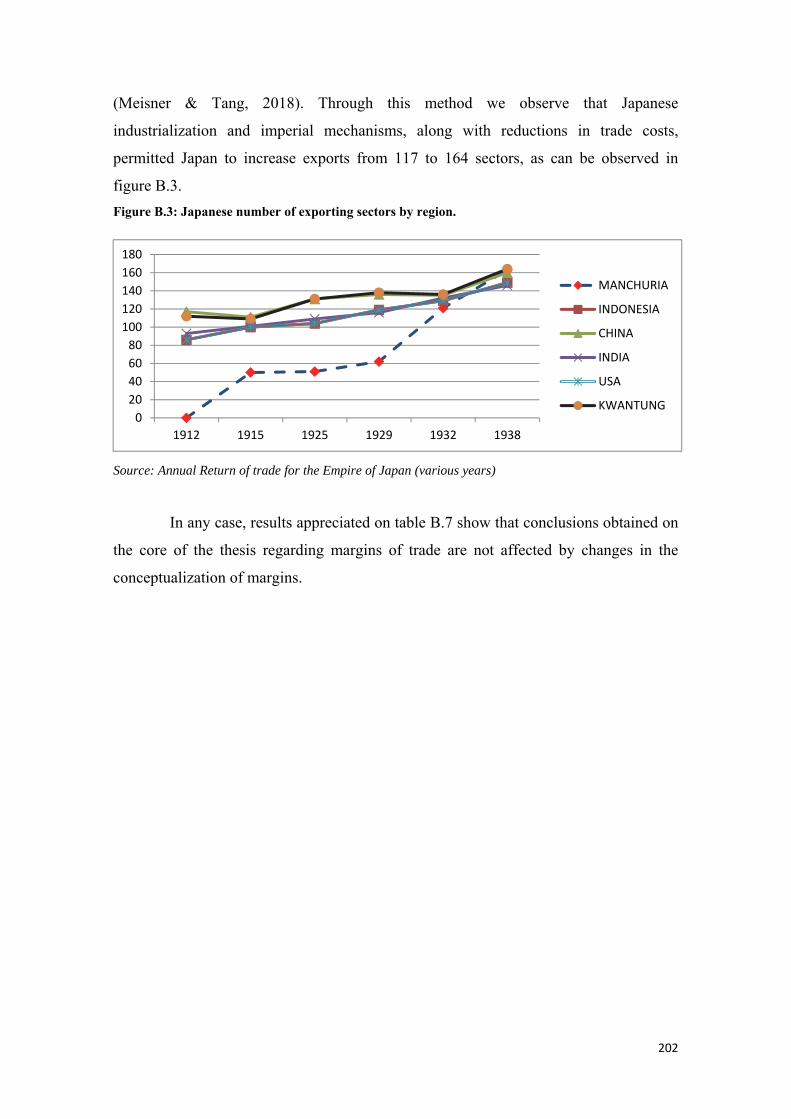
202
(Meisner & Tang, 2018). Through this method we observe that Japanese
industrialization and imperial mechanisms, along with reductions in trade costs,
permitted Japan to increase exports from 117 to 164 sectors, as can be observed in
figure B.3. Figure B.3: Japanese number of exporting sectors by region.
Source: Annual Return of trade for the Empire of Japan (various years)
In any case, results appreciated on table B.7 show that conclusions obtained on
the core of the thesis regarding margins of trade are not affected by changes in the
conceptualization of margins.
020406080
100120140160180
1912 1915 1925 1929 1932 1938
MANCHURIA
INDONESIA
CHINA
INDIA
USA
KWANTUNG
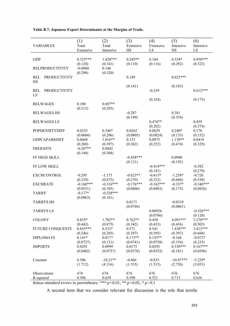
203
Table B.7: Japanese Export Determinants at the Margins of Trade.
(1) (2) (3) (4) (5) (6) VARIABLES Total
Extensive Total Intensive
Extensive HS
Extensive LS
Intensive HS
Intensive LS
GDP 0.325*** 1.428*** 0.245** 0.164 0.534* 0.958*** (0.120) (0.341) (0.110) (0.116) (0.292) (0.322) RELPRODUCTIVITY -0.0880 0.146 (0.290) (0.320) REL PRODUCTIVITY HS
0.189 0.623***
(0.141) (0.183) REL PRODUCTIVITY LS
-0.239 0.612***
(0.324) (0.173) RELWAGES 0.180 0.697** (0.215) (0.285) RELWAGES HS -0.287 0.381 (0.199) (0.354) RELWAGES LS 0.474** 0.459 (0.202) (0.374) POPDENSITYDIFF 0.0325 0.346* 0.0262 0.0829 0.240* 0.170 (0.0666) (0.206) (0.0805) (0.0824) (0.133) (0.152) GDPCAPABSDIFF 0.0668 1.016** 0.153 0.0975 1.139** 0.0419 (0.260) (0.397) (0.262) (0.252) (0.474) (0.329) FREIGHTS -0.287** 0.0842 (0.140) (0.308) FF HIGH SKILL -0.458*** 0.0980 (0.121) (0.192) FF LOW SKILL -0.414*** -0.382 (0.141) (0.270) EXCHCONTROL -0.295 -1.173 -0.623** -0.413* -1.258* -0.726 (0.239) (0.875) (0.270) (0.233) (0.660) (0.530) EXCHRATE -0.168*** -0.316*** -0.176*** -0.162*** -0.337* -0.340*** (0.0531) (0.105) (0.0606) (0.0493) (0.175) (0.0826) TARIFF -0.177* -0.528*** (0.0963) (0.181) TARIFFS HS 0.0171 -0.0319 (0.0746) (0.0861) TARIFFS LS 0.00926 -0.526*** (0.0786) (0.120) COLONY 0.835* 1.782** 0.762** 0.458 4.091*** 3.270*** (0.442) (0.875) (0.342) (0.433) (0.436) (0.502) FUTURE CONQUESTS 0.855*** 0.533* 0.571 0.541 1.438*** 3.413*** (0.246) (0.285) (0.397) (0.395) (0.397) (0.660) DIPLOMATS 0.141* 0.0177 0.173** 0.153** -0.168 -0.0727 (0.0737) (0.131) (0.0741) (0.0758) (0.154) (0.235) IMPORTS 0.0291 0.0999 0.0175 0.0293 0.530*** 0.167*** (0.0402) (0.0757) (0.0378) (0.0352) (0.181) (0.0396) Constant 0.506 -10.21** -0.466 -0.833 -10.87*** -5.229* (1.712) (4.316) (1.535) (1.515) (2.726) (3.053) Observations 674 674 676 676 676 676 R-squared 0.596 0.639 0.590 0.521 0.713 0.636 Robust standard errors in parentheses: *** p<0.01, ** p<0.05, * p<0.1
A second item that we consider relevant for discussion is the role that textile
204
exports had in Japanese industrialization. The first thing we will do in this section is to
clarify the criteria employed for dividing the different products exported by Japan into
skill layers. We have adapted the 3 digit SITC categorization to a contemporaneous
group of 16 manufacturing sectors following the (British Board of Trade, 1905)
classification of British manufacturing exports. We have ranked these according to skill
intensity following (Tena-Junguito, 2010). Table B.8 shows these manufacture sectors
ranked from high to low median earning workers at the turn of the century (High skilled
(skill intensity between 11 and 13, ranked 1-6), Medium skilled (skill intensity between
9 and 10, which are ranked from 7 to 9) and Low skilled manufactures (between 5 and 8
skill intensity, ranked from 10 to 16). This strategy, suggested by (Num and Trefler,
2009), consists of differentiating high and low cut-offs inside the ranking to categorize
in a more effective way high skills and low skill sectors. This strategy is hopefully less
vulnerable to technological change during the first third of the twentieth century.
We have extended this strategy to primary products as a residual (assuming less
skill intensity than in manufactures). Thus, we work with a simple division between
high skill sectors that were more influenced by the second industrial revolution
technologies and those that were less influenced. We recognize that, on one hand, this
division represents a very rudimentary of capturing skill improvements inside sectors,
specially productivity increases in Japanese textile industries in the 1920s and 1930s
(Wolcott, 1994), but on the other hand, this strategy captures better Japan’s
manufacturing dual aggregate sectorial advance in the second industrial revolution
technologies as an indicator of industrial modernization in the inter-war years, which is
the main objective of the paper.
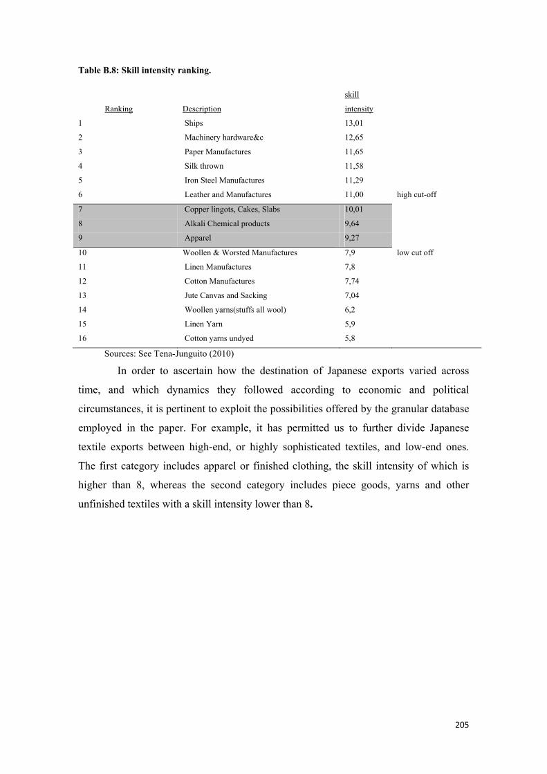
205
Table B.8: Skill intensity ranking.
Ranking Description
skill
intensity
1 Ships 13,01
2 Machinery hardware&c 12,65
3 Paper Manufactures 11,65
4 Silk thrown 11,58
5 Iron Steel Manufactures 11,29
6 Leather and Manufactures 11,00 high cut-off
7 Copper lingots, Cakes, Slabs 10,01
8 Alkali Chemical products 9,64
9 Apparel 9,27
10 Woollen & Worsted Manufactures 7,9 low cut off
11 Linen Manufactures 7,8
12 Cotton Manufactures 7,74
13 Jute Canvas and Sacking 7,04
14 Woollen yarns(stuffs all wool) 6,2
15 Linen Yarn 5,9
16 Cotton yarns undyed 5,8
Sources: See Tena-Junguito (2010) In order to ascertain how the destination of Japanese exports varied across
time, and which dynamics they followed according to economic and political
circumstances, it is pertinent to exploit the possibilities offered by the granular database
employed in the paper. For example, it has permitted us to further divide Japanese
textile exports between high-end, or highly sophisticated textiles, and low-end ones.
The first category includes apparel or finished clothing, the skill intensity of which is
higher than 8, whereas the second category includes piece goods, yarns and other
unfinished textiles with a skill intensity lower than 8.
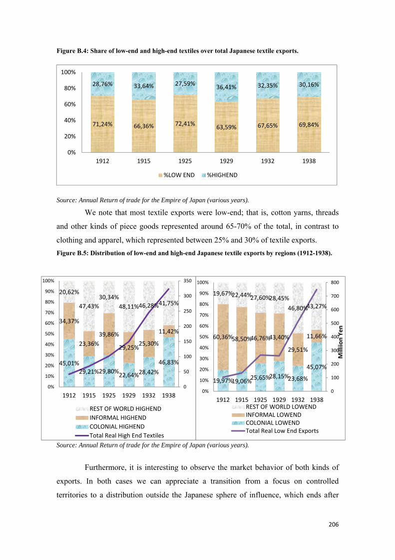
206
Figure B.4: Share of low-end and high-end textiles over total Japanese textile exports.
Source: Annual Return of trade for the Empire of Japan (various years).
We note that most textile exports were low-end; that is, cotton yarns, threads
and other kinds of piece goods represented around 65-70% of the total, in contrast to
clothing and apparel, which represented between 25% and 30% of textile exports. Figure B.5: Distribution of low-end and high-end Japanese textile exports by regions (1912-1938).
Source: Annual Return of trade for the Empire of Japan (various years).
Furthermore, it is interesting to observe the market behavior of both kinds of
exports. In both cases we can appreciate a transition from a focus on controlled
territories to a distribution outside the Japanese sphere of influence, which ends after
71,24% 66,36% 72,41% 63,59% 67,65% 69,84%
28,76% 33,64% 27,59% 36,41% 32,35% 30,16%
0%
20%
40%
60%
80%
100%
1912 1915 1925 1929 1932 1938
%LOW END %HIGHEND
45,01%29,21%29,80%22,64%28,42%
46,83%
34,37%
23,36%39,86%
29,25%25,30%
11,42%
20,62%
47,43%30,34%
48,11%46,28%41,75%
0
50
100
150
200
250
300
350
0%
10%
20%
30%
40%
50%
60%
70%
80%
90%
100%
1912 1915 1925 1929 1932 1938
Mill
i
REST OF WORLD HIGHENDINFORMAL HIGHENDCOLONIAL HIGHENDTotal Real High End Textiles
19,97%19,06%25,65%28,15%23,68%
45,07%
60,36%58,50%46,76%43,40%
29,51%
11,66%
19,67%22,44%27,60%28,45%46,80%43,27%
0
100
200
300
400
500
600
700
800
0%
10%
20%
30%
40%
50%
60%
70%
80%
90%
100%
1912 1915 1925 1929 1932 1938
Mill
iion
Yen
REST OF WORLD LOWENDINFORMAL LOWENDCOLONIAL LOWENDTotal Real Low End Exports
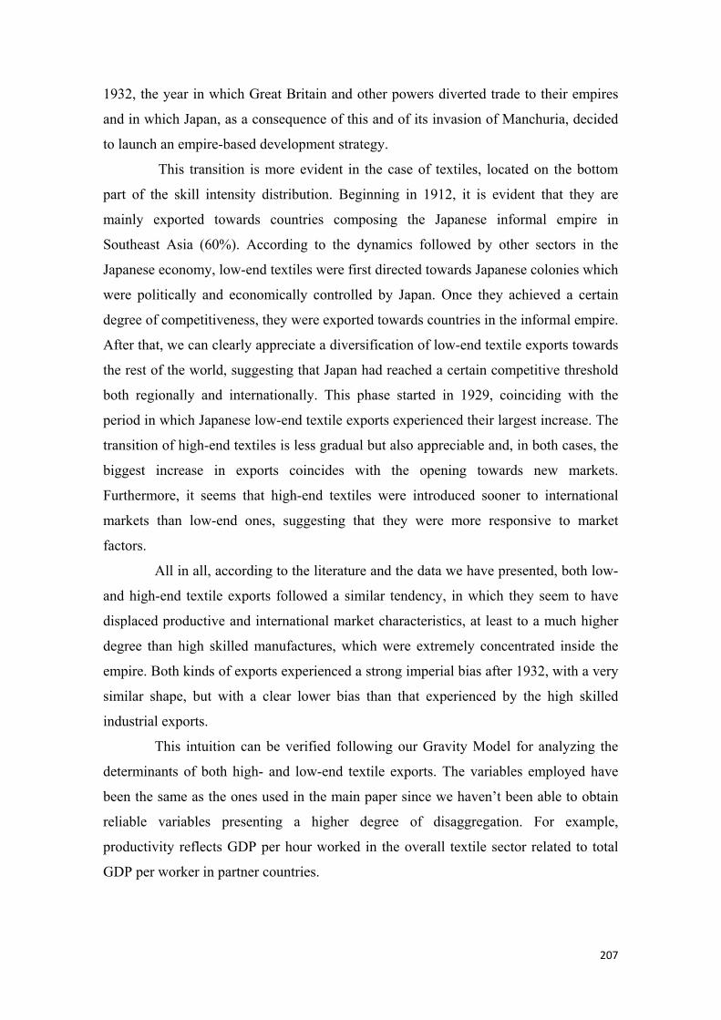
207
1932, the year in which Great Britain and other powers diverted trade to their empires
and in which Japan, as a consequence of this and of its invasion of Manchuria, decided
to launch an empire-based development strategy.
This transition is more evident in the case of textiles, located on the bottom
part of the skill intensity distribution. Beginning in 1912, it is evident that they are
mainly exported towards countries composing the Japanese informal empire in
Southeast Asia (60%). According to the dynamics followed by other sectors in the
Japanese economy, low-end textiles were first directed towards Japanese colonies which
were politically and economically controlled by Japan. Once they achieved a certain
degree of competitiveness, they were exported towards countries in the informal empire.
After that, we can clearly appreciate a diversification of low-end textile exports towards
the rest of the world, suggesting that Japan had reached a certain competitive threshold
both regionally and internationally. This phase started in 1929, coinciding with the
period in which Japanese low-end textile exports experienced their largest increase. The
transition of high-end textiles is less gradual but also appreciable and, in both cases, the
biggest increase in exports coincides with the opening towards new markets.
Furthermore, it seems that high-end textiles were introduced sooner to international
markets than low-end ones, suggesting that they were more responsive to market
factors.
All in all, according to the literature and the data we have presented, both low-
and high-end textile exports followed a similar tendency, in which they seem to have
displaced productive and international market characteristics, at least to a much higher
degree than high skilled manufactures, which were extremely concentrated inside the
empire. Both kinds of exports experienced a strong imperial bias after 1932, with a very
similar shape, but with a clear lower bias than that experienced by the high skilled
industrial exports.
This intuition can be verified following our Gravity Model for analyzing the
determinants of both high- and low-end textile exports. The variables employed have
been the same as the ones used in the main paper since we haven’t been able to obtain
reliable variables presenting a higher degree of disaggregation. For example,
productivity reflects GDP per hour worked in the overall textile sector related to total
GDP per worker in partner countries.
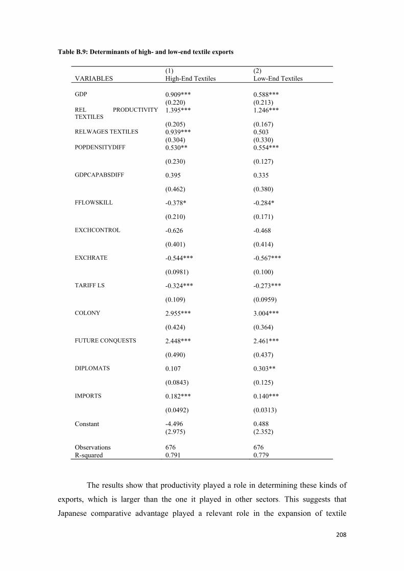
208
Table B.9: Determinants of high- and low-end textile exports
(1) (2) VARIABLES High-End Textiles Low-End Textiles GDP 0.909*** 0.588*** (0.220) (0.213) REL PRODUCTIVITY TEXTILES
1.395*** 1.246***
(0.205) (0.167) RELWAGES TEXTILES 0.939*** 0.503 (0.304) (0.330) POPDENSITYDIFF 0.530** 0.554***
(0.230) (0.127)
GDPCAPABSDIFF 0.395 0.335
(0.462) (0.380)
FFLOWSKILL -0.378* -0.284*
(0.210) (0.171)
EXCHCONTROL -0.626 -0.468
(0.401) (0.414)
EXCHRATE -0.544*** -0.567***
(0.0981) (0.100)
TARIFF LS -0.324*** -0.273***
(0.109) (0.0959)
COLONY 2.955*** 3.004***
(0.424) (0.364)
FUTURE CONQUESTS 2.448*** 2.461***
(0.490) (0.437)
DIPLOMATS 0.107 0.303**
(0.0843) (0.125)
IMPORTS 0.182*** 0.140***
(0.0492) (0.0313)
Constant -4.496 0.488 (2.975) (2.352) Observations 676 676 R-squared 0.791 0.779
The results show that productivity played a role in determining these kinds of
exports, which is larger than the one it played in other sectors. This suggests that
Japanese comparative advantage played a relevant role in the expansion of textile
209
exports and its strength was similar at both ends of the skill classification. Contrary to
high skill manufactures, textiles were driven by productivity with the difference that a
relevant share of their exports were directed towards colonies and future conquered
territories, although both kinds of textiles were more biased towards the first than to the
second. Interestingly, we can also appreciate that high-end textiles were slightly more
responsive to changes in comparative advantage variables and less sensitive to imperial
controls.
Both low- and high-end textiles were first introduced in the colonies, then in
the Japanese future conquests territories, and once they became internationally
competitive, they were distributed all over the world. What’s more, they demonstrated
significant expansion in the world market in spite of the backlash bias towards its
colonies experienced after the reaction of the British Commonwealth Trade Bloc to the
Manchuria invasion that partially excluded Japanese textiles from India and other
markets. In addition, the comparison with second industrial revolution exports and the
fact that productivity played a bigger role in determining textile exports, along with the
dynamics presented above, suggest that textile exports responded more to productivity
determined comparative advantage than high skilled manufactures, which were more
strongly affected by Japanese imperial aims.
Following the discussion we believe that we should provide an extended
explanation about how the Great Depression and the creation of colonial blocs all over
the world after the Ottawa agreement affected Japanese manufacturing exports towards
the region. The reasons behind Japan’s considerable commercial concentration in its
colonies and neighboring countries inside the region are varied and not fully reviewed
in the thesis. Many authors view the Japanese invasion of Manchuria in 1931 as a
turning point in the sense that after this great victory, the military gained important
political power that permitted them to continue lobbying the government for a
continued pursuit of imperial expansion. Of course, this historical event was of
relevance to the subsequent commercial, economic and political decisions adopted by
the Japanese Government during the 1930s, as were the needs of the Japanese Zaibatsu
for gaining access to bigger markets and achieving economies of scale in a context of a
protected market with monopolistic privileges. Nevertheless, there are other factors that
might have also facilitated Japan’s strong focus on its empire as a source of exports. In
that sense, the international landscape might have played a significant role.
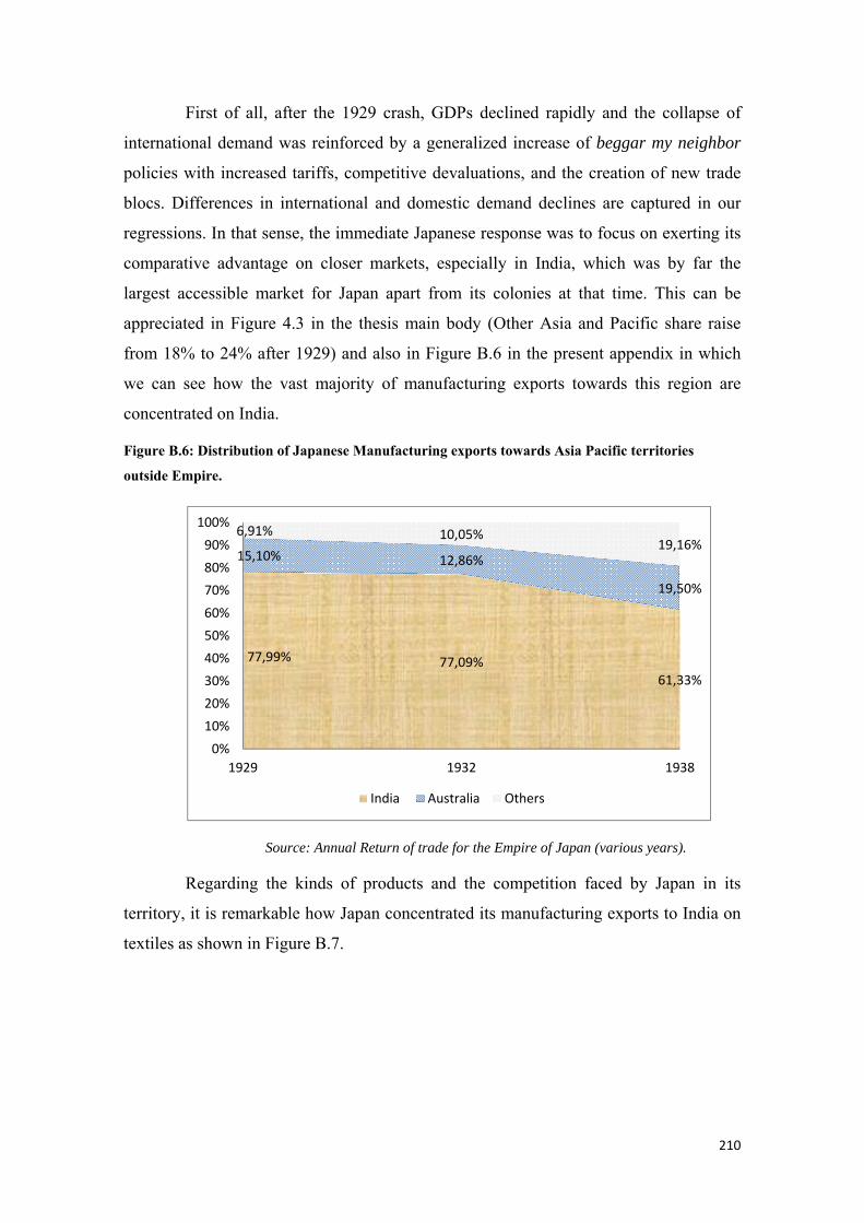
210
First of all, after the 1929 crash, GDPs declined rapidly and the collapse of
international demand was reinforced by a generalized increase of beggar my neighbor
policies with increased tariffs, competitive devaluations, and the creation of new trade
blocs. Differences in international and domestic demand declines are captured in our
regressions. In that sense, the immediate Japanese response was to focus on exerting its
comparative advantage on closer markets, especially in India, which was by far the
largest accessible market for Japan apart from its colonies at that time. This can be
appreciated in Figure 4.3 in the thesis main body (Other Asia and Pacific share raise
from 18% to 24% after 1929) and also in Figure B.6 in the present appendix in which
we can see how the vast majority of manufacturing exports towards this region are
concentrated on India.
Figure B.6: Distribution of Japanese Manufacturing exports towards Asia Pacific territories outside Empire.
Source: Annual Return of trade for the Empire of Japan (various years).
Regarding the kinds of products and the competition faced by Japan in its
territory, it is remarkable how Japan concentrated its manufacturing exports to India on
textiles as shown in Figure B.7.
77,99% 77,09%61,33%
15,10% 12,86%
19,50%
6,91% 10,05%19,16%
0%10%20%30%40%50%60%70%80%90%
100%
1929 1932 1938
India Australia Others
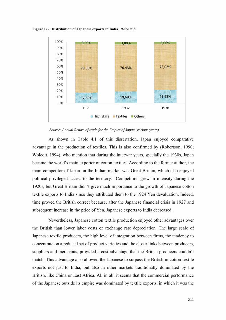
211
Figure B.7: Distribution of Japanese exports to India 1929-1938
Source: Annual Return of trade for the Empire of Japan (various years).
As shown in Table 4.1 of this dissertation, Japan enjoyed comparative
advantage in the production of textiles. This is also confirmed by (Robertson, 1990;
Wolcott, 1994), who mention that during the interwar years, specially the 1930s, Japan
became the world’s main exporter of cotton textiles. According to the former author, the
main competitor of Japan on the Indian market was Great Britain, which also enjoyed
political privileged access to the territory. Competition grew in intensity during the
1920s, but Great Britain didn’t give much importance to the growth of Japanese cotton
textile exports to India since they attributed them to the 1924 Yen devaluation. Indeed,
time proved the British correct because, after the Japanese financial crisis in 1927 and
subsequent increase in the price of Yen, Japanese exports to India decreased.
Nevertheless, Japanese cotton textile production enjoyed other advantages over
the British than lower labor costs or exchange rate depreciation. The large scale of
Japanese textile producers, the high level of integration between firms, the tendency to
concentrate on a reduced set of product varieties and the closer links between producers,
suppliers and merchants, provided a cost advantage that the British producers couldn’t
match. This advantage also allowed the Japanese to surpass the British in cotton textile
exports not just to India, but also in other markets traditionally dominated by the
British, like China or East Africa. All in all, it seems that the commercial performance
of the Japanese outside its empire was dominated by textile exports, in which it was the
17,59% 19,69% 21,93%
79,38% 76,43% 75,02%
3,03% 3,89% 3,06%
0%10%20%30%40%50%60%70%80%90%
100%
1929 1932 1938
High Skills Textiles Others
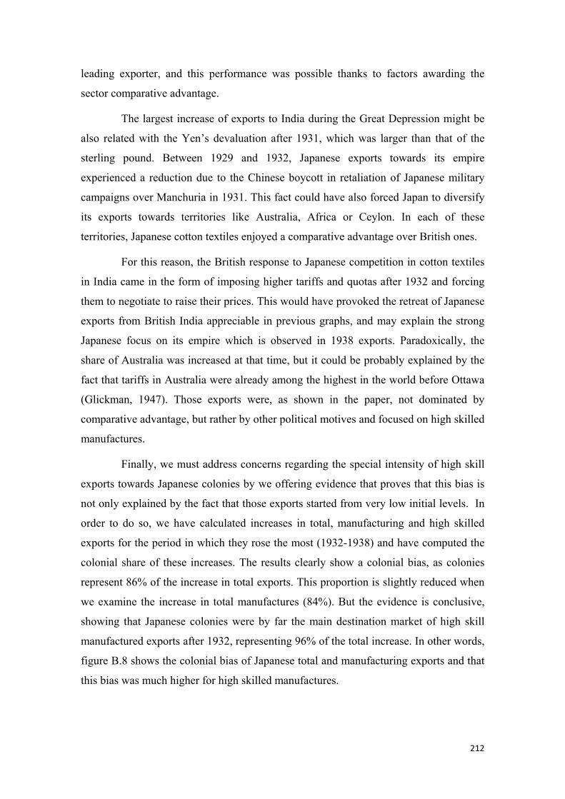
212
leading exporter, and this performance was possible thanks to factors awarding the
sector comparative advantage.
The largest increase of exports to India during the Great Depression might be
also related with the Yen’s devaluation after 1931, which was larger than that of the
sterling pound. Between 1929 and 1932, Japanese exports towards its empire
experienced a reduction due to the Chinese boycott in retaliation of Japanese military
campaigns over Manchuria in 1931. This fact could have also forced Japan to diversify
its exports towards territories like Australia, Africa or Ceylon. In each of these
territories, Japanese cotton textiles enjoyed a comparative advantage over British ones.
For this reason, the British response to Japanese competition in cotton textiles
in India came in the form of imposing higher tariffs and quotas after 1932 and forcing
them to negotiate to raise their prices. This would have provoked the retreat of Japanese
exports from British India appreciable in previous graphs, and may explain the strong
Japanese focus on its empire which is observed in 1938 exports. Paradoxically, the
share of Australia was increased at that time, but it could be probably explained by the
fact that tariffs in Australia were already among the highest in the world before Ottawa
(Glickman, 1947). Those exports were, as shown in the paper, not dominated by
comparative advantage, but rather by other political motives and focused on high skilled
manufactures.
Finally, we must address concerns regarding the special intensity of high skill
exports towards Japanese colonies by we offering evidence that proves that this bias is
not only explained by the fact that those exports started from very low initial levels. In
order to do so, we have calculated increases in total, manufacturing and high skilled
exports for the period in which they rose the most (1932-1938) and have computed the
colonial share of these increases. The results clearly show a colonial bias, as colonies
represent 86% of the increase in total exports. This proportion is slightly reduced when
we examine the increase in total manufactures (84%). But the evidence is conclusive,
showing that Japanese colonies were by far the main destination market of high skill
manufactured exports after 1932, representing 96% of the total increase. In other words,
figure B.8 shows the colonial bias of Japanese total and manufacturing exports and that
this bias was much higher for high skilled manufactures.
213
Figure B.8: Japanese exports increase 1932-38 (%) by groups of products and region.
Source: Annual Return of trade for the Empire of Japan (various years).
Finally, the discussions practiced on this section about the role of the Great
Depression and Ottawa agreements in Japanese exports regionalization made us
wonder about the role of Japanese colonies as a market for the mainland. In
principle we believe that colonial trade was severe enough at every period, even if
increased intensity during the 1930s.
Nevertheless, there is an option that Japan only used its colonies as a
market of last resort in the 1930s as a consequence of trade diversion produced by
global disintegration. Table 4.6 on the thesis core, shows that Japanese trade with its
colonies was very similar to the one with informal empire territories, with a
remarkable intensity only for 1938. Tariff policy in the Japanese occupied territories
privileged Japan or was assimilated into Japan’s own tariff system before 1930´s.
Korea adopted Japan’s tariff system in 1923, as would Manchuria ten years later
upon the territory’s separation from the Chinese custom system, allowing
preferential access for Japanese manufactures. Japan exported to its dominions
before international trade blocs were in force diverting Japan trade from
international markets. Surely international context reinforced Japan connections
with colonies in greater extent than on future conquered lands. However, for a
definitive answer to the main question there is a need to analyze Japan total exports
not just imperial ones.
86% 84%96%
14% 16%4%
0%10%20%30%40%50%60%70%80%90%
100%
Total Exports Manufactures High Skills
Colonies Rest of the World
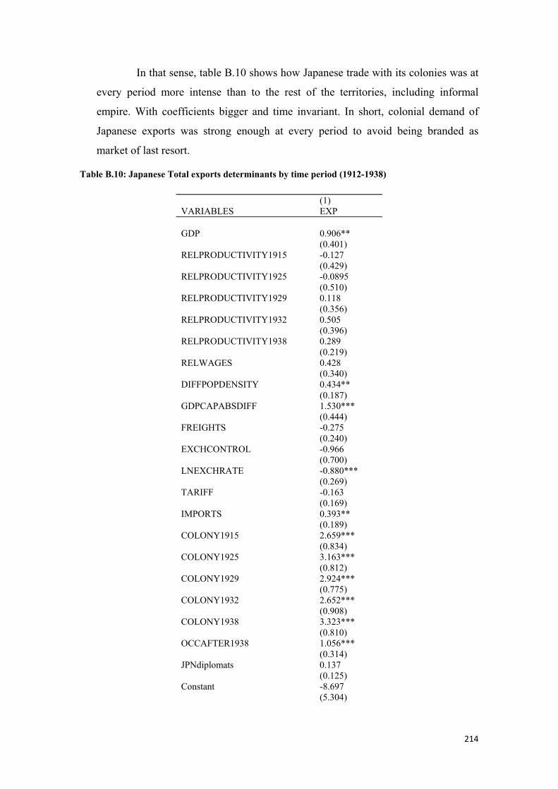
214
In that sense, table B.10 shows how Japanese trade with its colonies was at
every period more intense than to the rest of the territories, including informal
empire. With coefficients bigger and time invariant. In short, colonial demand of
Japanese exports was strong enough at every period to avoid being branded as
market of last resort.
Table B.10: Japanese Total exports determinants by time period (1912-1938)
(1) VARIABLES EXP GDP 0.906** (0.401) RELPRODUCTIVITY1915 -0.127 (0.429) RELPRODUCTIVITY1925 -0.0895 (0.510) RELPRODUCTIVITY1929 0.118 (0.356) RELPRODUCTIVITY1932 0.505 (0.396) RELPRODUCTIVITY1938 0.289 (0.219) RELWAGES 0.428 (0.340) DIFFPOPDENSITY 0.434** (0.187) GDPCAPABSDIFF 1.530*** (0.444) FREIGHTS -0.275 (0.240) EXCHCONTROL -0.966 (0.700) LNEXCHRATE -0.880*** (0.269) TARIFF -0.163 (0.169) IMPORTS 0.393** (0.189) COLONY1915 2.659*** (0.834) COLONY1925 3.163*** (0.812) COLONY1929 2.924*** (0.775) COLONY1932 2.652*** (0.908) COLONY1938 3.323*** (0.810) OCCAFTER1938 1.056*** (0.314) JPNdiplomats 0.137 (0.125) Constant -8.697 (5.304)
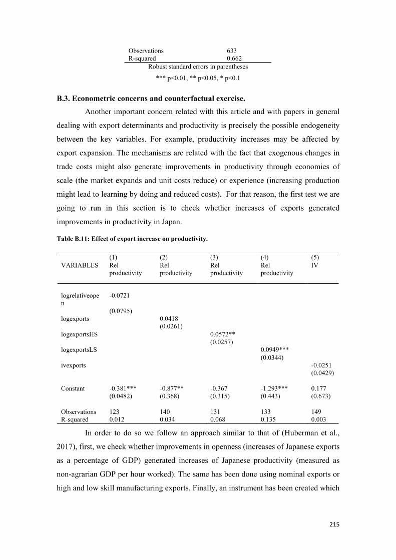
215
Observations 633 R-squared 0.662
Robust standard errors in parentheses
*** p<0.01, ** p<0.05, * p<0.1
B.3. Econometric concerns and counterfactual exercise. Another important concern related with this article and with papers in general
dealing with export determinants and productivity is precisely the possible endogeneity
between the key variables. For example, productivity increases may be affected by
export expansion. The mechanisms are related with the fact that exogenous changes in
trade costs might also generate improvements in productivity through economies of
scale (the market expands and unit costs reduce) or experience (increasing production
might lead to learning by doing and reduced costs). For that reason, the first test we are
going to run in this section is to check whether increases of exports generated
improvements in productivity in Japan.
Table B.11: Effect of export increase on productivity.
(1) (2) (3) (4) (5) VARIABLES Rel
productivity Rel productivity
Rel productivity
Rel productivity
IV
logrelativeopen
-0.0721
(0.0795) logexports 0.0418 (0.0261) logexportsHS 0.0572** (0.0257) logexportsLS 0.0949*** (0.0344) ivexports -0.0251 (0.0429)
Constant -0.381*** -0.877** -0.367 -1.293*** 0.177 (0.0482) (0.368) (0.315) (0.443) (0.673) Observations 123 140 131 133 149 R-squared 0.012 0.034 0.068 0.135 0.003
In order to do so we follow an approach similar to that of (Huberman et al.,
2017), first, we check whether improvements in openness (increases of Japanese exports
as a percentage of GDP) generated increases of Japanese productivity (measured as
non-agrarian GDP per hour worked). The same has been done using nominal exports or
high and low skill manufacturing exports. Finally, an instrument has been created which
216
is called ivexports and is constructed by the predicted value of exports regressed on the
usual variables with the exception of productivity measures.
IVEXPORTS=𝛽 + 𝛽 𝑙𝑛𝐺𝐷𝑃 + 𝛽 𝐶𝐴 + 𝛽 𝑇𝐶 + 𝛽 𝐶𝑂𝐿𝑂𝑁𝑌 +𝛽 𝐹𝑈𝑇𝑈𝑅𝐸 𝐶𝑂𝑁𝑄𝑈𝐸𝑆𝑇𝑆 +𝛽 𝐼𝑀𝑃𝑂𝑅𝑇𝑆 + 𝛽 + 𝜀 The results show that in general increments of exports didn’t increase Japanese
productivity. However, there is a perceivable effect at the skill level, although the effect
of increases of high and low skilled exports on productivity is very weak. In other
words, the results in table B.11 permit us to reject the possibility that productivity
growth was endogenous to export growth for the case of 1912-1938 Japan.
Another possible source of endogeneity could be present in trade costs in the
sense that their causality relation with exports might be bidirectional. The clearest
example is that of diplomats, since increases in the number of Japanese diplomats in a
country might increase Japanese exports to that country, but the fact that Japan is
trading with the country might also attract a larger number of Japanese consuls there.
This possibility is real, as is demonstrated in Table B.12, in which the value of Japanese
exports affected in a positive and significant way the number of Japanese Diplomats
abroad, the number of foreign diplomats in Japan and total Diplomatic representation
(the sum of diplomats abroad and foreign diplomats in Japan). Furthermore, this
phenomenon could also appear in the rest of trade costs or even in productivity
measures.
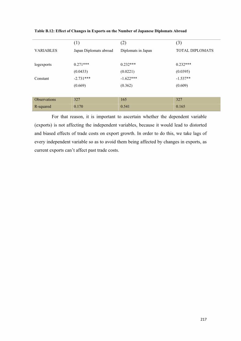
217
Table B.12: Effect of Changes in Exports on the Number of Japanese Diplomats Abroad
(1) (2) (3) VARIABLES Japan Diplomats abroad Diplomats in Japan TOTAL DIPLOMATS
logexports 0.271*** 0.232*** 0.232***
(0.0433) (0.0221) (0.0395)
Constant -2.731*** -1.622*** -1.537**
(0.669) (0.362) (0.609)
Observations 327 165 327
R-squared 0.170 0.541 0.165
For that reason, it is important to ascertain whether the dependent variable
(exports) is not affecting the independent variables, because it would lead to distorted
and biased effects of trade costs on export growth. In order to do this, we take lags of
every independent variable so as to avoid them being affected by changes in exports, as
current exports can’t affect past trade costs.
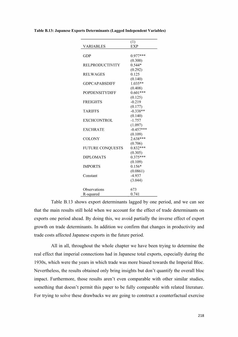
218
Table B.13: Japanese Exports Determinants (Lagged Independent Variables)
(1) VARIABLES EXP GDP 0.977*** (0.300) RELPRODUCTIVITY 0.544* (0.292) RELWAGES 0.125 (0.140) GDPCAPABSDIFF 1.035** (0.408) POPDENSITYDIFF 0.601*** (0.125) FREIGHTS -0.219 (0.177) TARIFFS -0.338** (0.140) EXCHCONTROL -1.757 (1.097) EXCHRATE -0.457*** (0.109) COLONY 2.638*** (0.706) FUTURE CONQUESTS 0.832*** (0.305) DIPLOMATS 0.375*** (0.109) IMPORTS 0.156* (0.0861) Constant -4.937 (3.044) Observations 673 R-squared 0.741
Table B.13 shows export determinants lagged by one period, and we can see
that the main results still hold when we account for the effect of trade determinants on
exports one period ahead. By doing this, we avoid partially the inverse effect of export
growth on trade determinants. In addition we confirm that changes in productivity and
trade costs affected Japanese exports in the future period.
All in all, throughout the whole chapter we have been trying to determine the
real effect that imperial connections had in Japanese total exports, especially during the
1930s, which were the years in which trade was more biased towards the Imperial Bloc.
Nevertheless, the results obtained only bring insights but don’t quantify the overall bloc
impact. Furthermore, those results aren’t even comparable with other similar studies,
something that doesn’t permit this paper to be fully comparable with related literature.
For trying to solve these drawbacks we are going to construct a counterfactual exercise
219
that is intended to show approximately the level of Japanese exports in case the Empire
had never existed.
The strategy is going to consist on an estimation of Japanese overall exports in
case it hadn’t enjoyed imperial benefits inside the region. This exercise would imply
that exports towards regional countries would have evolved following the same path as
those towards neighbor territories with which Japan never enjoyed any privileged
economic connections. In that sense, the two main territories presenting those
characteristics were India and Australia, so we are going to assume Japanese exports
towards the remaining regional neighbors is going to follow the same path as those two
British colonies for the period 1932-1938.
The exercise is far from realistic because each territory is subject to different
characteristics that we are not controlling for. In order to try to solve this drawback we
will exploit differences between the two base countries: British India trade policy
towards Japanese products turned to be really restrictive after Ottawa agreements in
1932 and for that reason Japanese exports towards this territory didn’t increase and were
even slightly reduced for the 1932-1938. On the other hand post Ottawa tariffs on
Australia were not as binding (see previous section), permitting a raise in Japanese
exports towards this territory. For that reason, the counterfactual using India as a base
will be considered a lower bound for the evolution of Japanese exports without empire,
whereas the Australian one will be an upper bound.
According to our calculations, if regional exports would have followed the
same pattern as Australia, total Japanese exports would have been 28% lower. What’s
more, if they had followed the same evolution as India, total Japanese exports would
have been 47% lower. Overall it seems that imperial connections permitted Japan to
enjoy an exports increase ranging between 28%-47% according to our estimates. The
imperial effect gets much bigger if we account for increases on high skilled
manufacturing exports. Specifically, without imperial connections, Japanese high
skilled exports would have been between 66% and 76% lower.
220
UNDERSTANDING JAPANESE COLONIZATION OF C.MANCHURIA.
C.1. Sources and estimation procedures The control variables for regressions using Japanese exports to Manchuria as
the dependent variable have been constructed using data from (Ohkawa et al.,1967-
1989). This database contains information about export prices, wages of workers,
production or total exports for Japanese main exported commodities. In order to adapt
them to the sectors artificially constructed for our purpose using SITC Rev 2 we are
obtaining data for the main commodity exported inside each sector and assume the
whole sector to present the same data as this one.
For sectors like beverages, comestibles, chemicals, machinery or miscellaneous
this assumption is straightforward because the employed data source presents overall
information for each of them. On the other hand, information for sectors like unfinished
manufactures is represented by textiles, finished manufactures by iron and steel, animal
and vegetable oil by fishery because most animal oil was fish oil, mineral fuels are
represented by mining products and crude materials by wood and wood products,
because the leading crude material exported was wood.
C.2.Discussion. The following section will extend explanations about the mechanisms linking
South Manchurian Railway Company freights and Japanese exports of machinery, their
role on Manchurian industrialization and a description of company composition of those
exports. In addition, we will discuss the military influence over Manchurian exports to
Japan.
One of the main objectives in this thesis is to demonstrate how national
interests can shape economic and business outcomes in determined territories and how
certain companies could win by cooperating with the ruling elites. In order to do that,
we employ the case of the Japanese colonization of Manchuria as an example of this
process denominated as Elite Exchange.
In short, chapter 4 provides a set of mechanisms by which the Kwantung
Army, a branch of the Japanese Army, was able to influence Manchurian economic
landscape to its own will. The most relevant one was the control exercised over the
transport network by establishing a new price system on the South Manchurian Railway
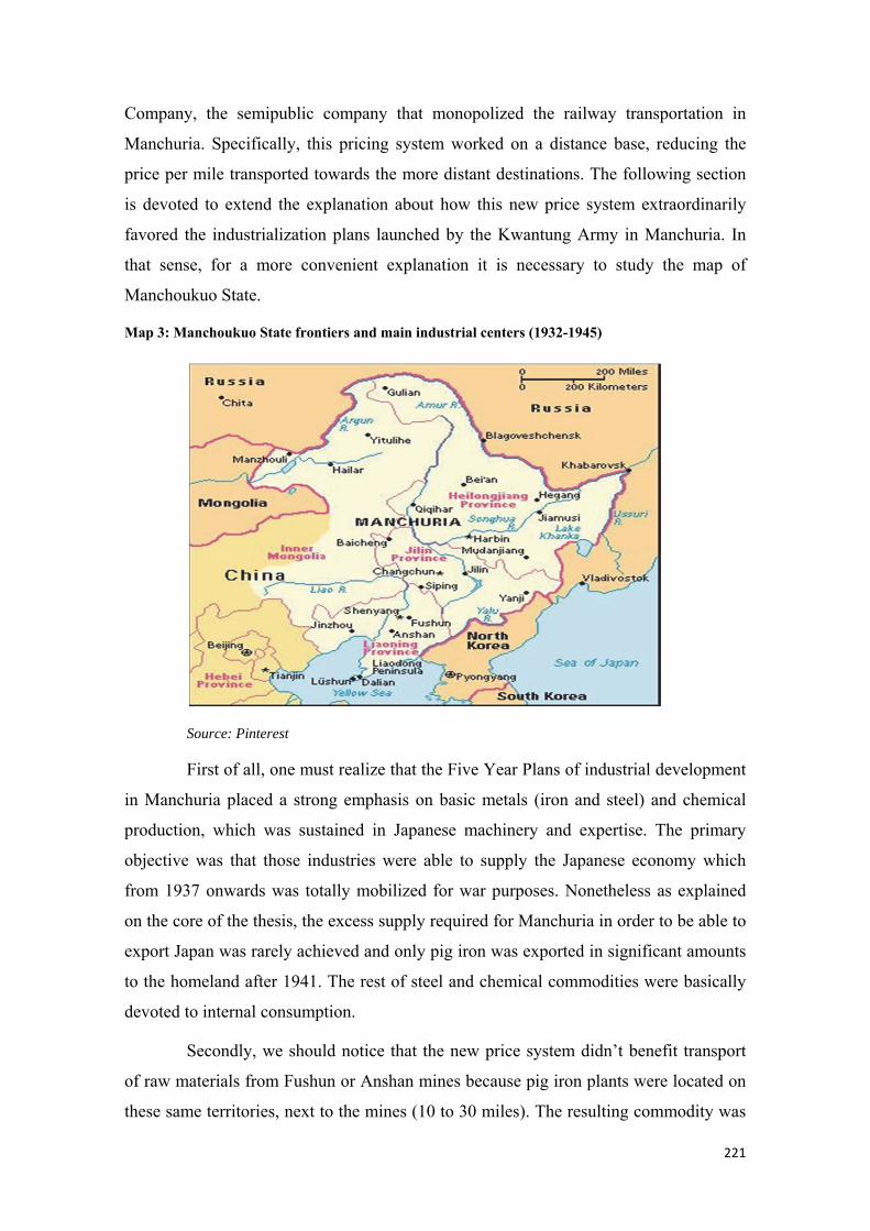
221
Company, the semipublic company that monopolized the railway transportation in
Manchuria. Specifically, this pricing system worked on a distance base, reducing the
price per mile transported towards the more distant destinations. The following section
is devoted to extend the explanation about how this new price system extraordinarily
favored the industrialization plans launched by the Kwantung Army in Manchuria. In
that sense, for a more convenient explanation it is necessary to study the map of
Manchoukuo State.
Map 3: Manchoukuo State frontiers and main industrial centers (1932-1945)
Source: Pinterest
First of all, one must realize that the Five Year Plans of industrial development
in Manchuria placed a strong emphasis on basic metals (iron and steel) and chemical
production, which was sustained in Japanese machinery and expertise. The primary
objective was that those industries were able to supply the Japanese economy which
from 1937 onwards was totally mobilized for war purposes. Nonetheless as explained
on the core of the thesis, the excess supply required for Manchuria in order to be able to
export Japan was rarely achieved and only pig iron was exported in significant amounts
to the homeland after 1941. The rest of steel and chemical commodities were basically
devoted to internal consumption.
Secondly, we should notice that the new price system didn’t benefit transport
of raw materials from Fushun or Anshan mines because pig iron plants were located on
these same territories, next to the mines (10 to 30 miles). The resulting commodity was
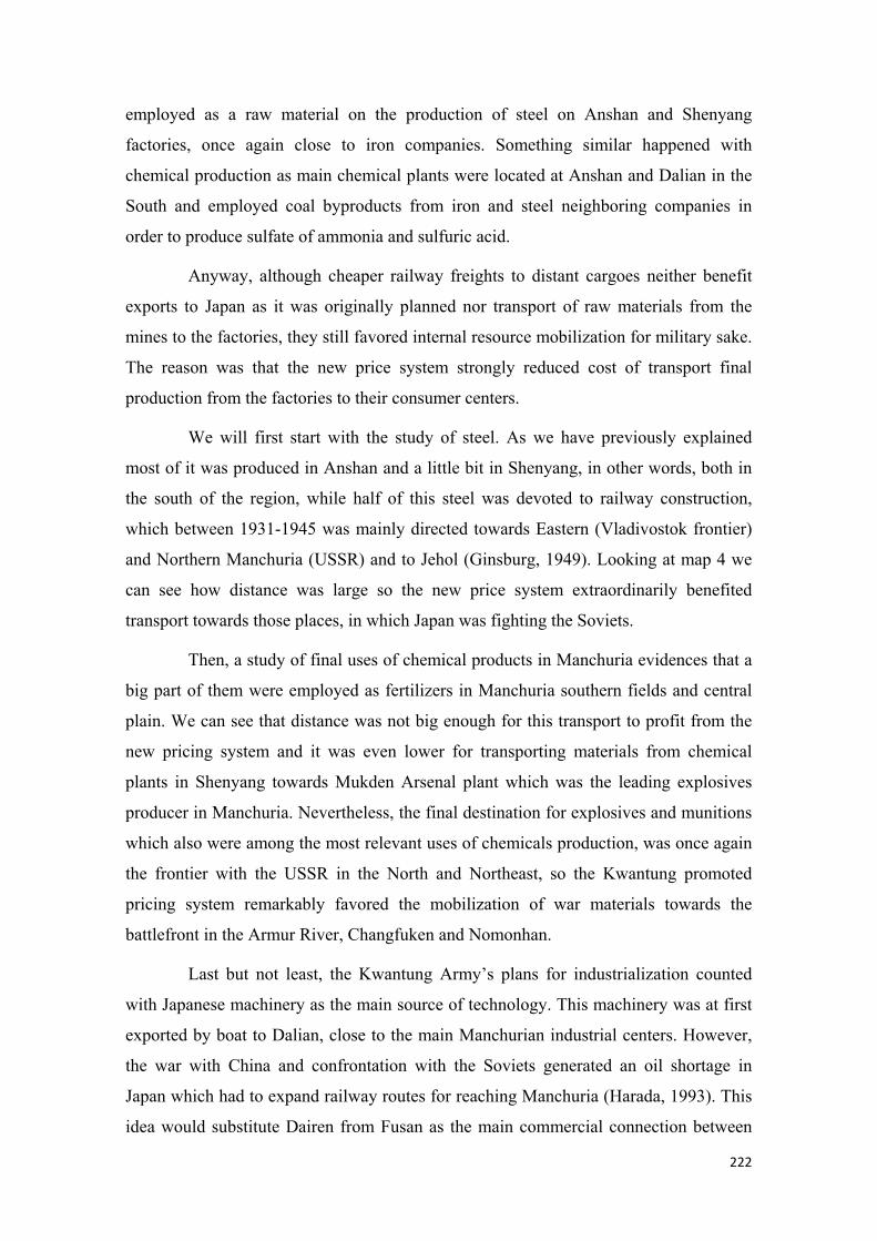
222
employed as a raw material on the production of steel on Anshan and Shenyang
factories, once again close to iron companies. Something similar happened with
chemical production as main chemical plants were located at Anshan and Dalian in the
South and employed coal byproducts from iron and steel neighboring companies in
order to produce sulfate of ammonia and sulfuric acid.
Anyway, although cheaper railway freights to distant cargoes neither benefit
exports to Japan as it was originally planned nor transport of raw materials from the
mines to the factories, they still favored internal resource mobilization for military sake.
The reason was that the new price system strongly reduced cost of transport final
production from the factories to their consumer centers.
We will first start with the study of steel. As we have previously explained
most of it was produced in Anshan and a little bit in Shenyang, in other words, both in
the south of the region, while half of this steel was devoted to railway construction,
which between 1931-1945 was mainly directed towards Eastern (Vladivostok frontier)
and Northern Manchuria (USSR) and to Jehol (Ginsburg, 1949). Looking at map 4 we
can see how distance was large so the new price system extraordinarily benefited
transport towards those places, in which Japan was fighting the Soviets.
Then, a study of final uses of chemical products in Manchuria evidences that a
big part of them were employed as fertilizers in Manchuria southern fields and central
plain. We can see that distance was not big enough for this transport to profit from the
new pricing system and it was even lower for transporting materials from chemical
plants in Shenyang towards Mukden Arsenal plant which was the leading explosives
producer in Manchuria. Nevertheless, the final destination for explosives and munitions
which also were among the most relevant uses of chemicals production, was once again
the frontier with the USSR in the North and Northeast, so the Kwantung promoted
pricing system remarkably favored the mobilization of war materials towards the
battlefront in the Armur River, Changfuken and Nomonhan.
Last but not least, the Kwantung Army’s plans for industrialization counted
with Japanese machinery as the main source of technology. This machinery was at first
exported by boat to Dalian, close to the main Manchurian industrial centers. However,
the war with China and confrontation with the Soviets generated an oil shortage in
Japan which had to expand railway routes for reaching Manchuria (Harada, 1993). This
idea would substitute Dairen from Fusan as the main commercial connection between
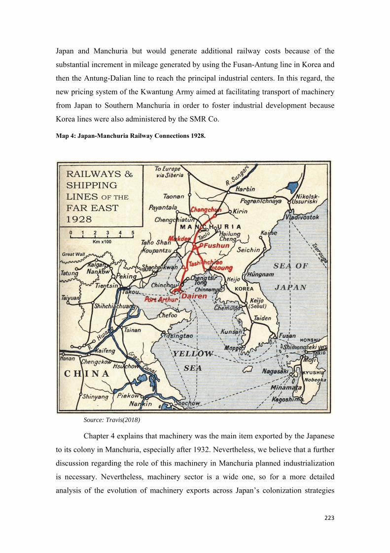
223
Japan and Manchuria but would generate additional railway costs because of the
substantial increment in mileage generated by using the Fusan-Antung line in Korea and
then the Antung-Dalian line to reach the principal industrial centers. In this regard, the
new pricing system of the Kwantung Army aimed at facilitating transport of machinery
from Japan to Southern Manchuria in order to foster industrial development because
Korea lines were also administered by the SMR Co.
Map 4: Japan-Manchuria Railway Connections 1928.
Source: Travis(2018)
Chapter 4 explains that machinery was the main item exported by the Japanese
to its colony in Manchuria, especially after 1932. Nevertheless, we believe that a further
discussion regarding the role of this machinery in Manchuria planned industrialization
is necessary. Nevertheless, machinery sector is a wide one, so for a more detailed
analysis of the evolution of machinery exports across Japan’s colonization strategies
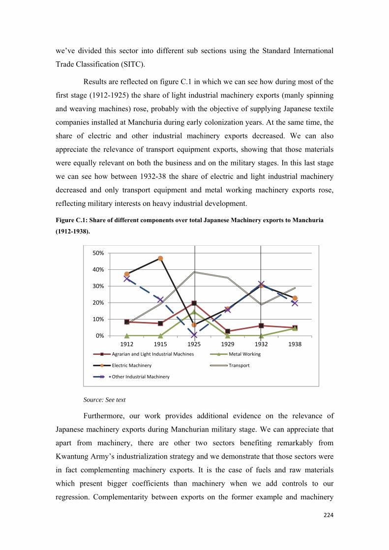
224
we’ve divided this sector into different sub sections using the Standard International
Trade Classification (SITC).
Results are reflected on figure C.1 in which we can see how during most of the
first stage (1912-1925) the share of light industrial machinery exports (manly spinning
and weaving machines) rose, probably with the objective of supplying Japanese textile
companies installed at Manchuria during early colonization years. At the same time, the
share of electric and other industrial machinery exports decreased. We can also
appreciate the relevance of transport equipment exports, showing that those materials
were equally relevant on both the business and on the military stages. In this last stage
we can see how between 1932-38 the share of electric and light industrial machinery
decreased and only transport equipment and metal working machinery exports rose,
reflecting military interests on heavy industrial development.
Figure C.1: Share of different components over total Japanese Machinery exports to Manchuria (1912-1938).
Source: See text
Furthermore, our work provides additional evidence on the relevance of
Japanese machinery exports during Manchurian military stage. We can appreciate that
apart from machinery, there are other two sectors benefiting remarkably from
Kwantung Army’s industrialization strategy and we demonstrate that those sectors were
in fact complementing machinery exports. It is the case of fuels and raw materials
which present bigger coefficients than machinery when we add controls to our
regression. Complementarity between exports on the former example and machinery
0%
10%
20%
30%
40%
50%
1912 1915 1925 1929 1932 1938Agrarian and Light Industrial Machines Metal Working
Electric Machinery Transport
Other Industrial Machinery
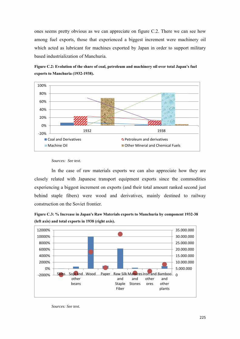
225
ones seems pretty obvious as we can appreciate on figure C.2. There we can see how
among fuel exports, those that experienced a biggest increment were machinery oil
which acted as lubricant for machines exported by Japan in order to support military
based industrialization of Manchuria.
Figure C.2: Evolution of the share of coal, petroleum and machinery oil over total Japan’s fuel exports to Manchuria (1932-1938).
Sources: See text.
In the case of raw materials exports we can also appreciate how they are
closely related with Japanese transport equipment exports since the commodities
experiencing a biggest increment on exports (and their total amount ranked second just
behind staple fibers) were wood and derivatives, mainly destined to railway
construction on the Soviet frontier.
Figure C.3: % Increase in Japan's Raw Materials exports to Manchuria by component 1932-38 (left axis) and total exports in 1938 (right axis).
Sources: See text.
-20%
0%
20%
40%
60%
80%
100%
1932 1938
Coal and Derivatives Petroleum and derivativesMachine Oil Other Mineral and Chemical Fuels
05.000.00010.000.00015.000.00020.000.00025.000.00030.000.00035.000.000
-2000%0%
2000%4000%6000%8000%
10000%12000%
Skins Soja andotherbeans
Wood Paper Raw Silkand
StapleFiber
Manuresand
Stones
Iron andotherores
Bambooand
otherplants
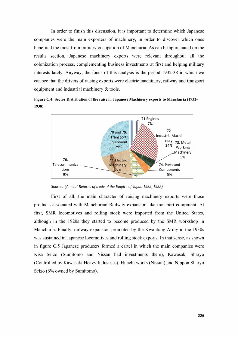
226
In order to finish this discussion, it is important to determine which Japanese
companies were the main exporters of machinery, in order to discover which ones
benefited the most from military occupation of Manchuria. As can be appreciated on the
results section, Japanese machinery exports were relevant throughout all the
colonization process, complementing business investments at first and helping military
interests lately. Anyway, the focus of this analysis is the period 1932-38 in which we
can see that the drivers of raising exports were electric machinery, railway and transport
equipment and industrial machinery & tools.
Figure C.4: Sector Distribution of the raise in Japanese Machinery exports to Manchuria (1932-1938).
Source: (Annual Returns of trade of the Empire of Japan 1932, 1938)
First of all, the main character of raising machinery exports were those
products associated with Manchurian Railway expansion like transport equipment. At
first, SMR locomotives and rolling stock were imported from the United States,
although in the 1920s they started to become produced by the SMR workshop in
Manchuria. Finally, railway expansion promoted by the Kwantung Army in the 1930s
was sustained in Japanese locomotives and rolling stock exports. In that sense, as shown
in figure C.5 Japanese producers formed a cartel in which the main companies were
Kisa Seizo (Sumitomo and Nissan had investments there), Kawasaki Sharyo
(Controlled by Kawasaki Heavy Industries), Hitachi works (Nissan) and Nippon Sharyo
Seizo (6% owned by Sumitomo).
71 Engines7%
72 IndustrialMachi
nery24%
73. Metal Working
Machinery5%
74. Parts and Components
5%
76. Telecommunica
tions8%
77. Electric Machinery
22%
78 and 79. Transport
Equipment29%
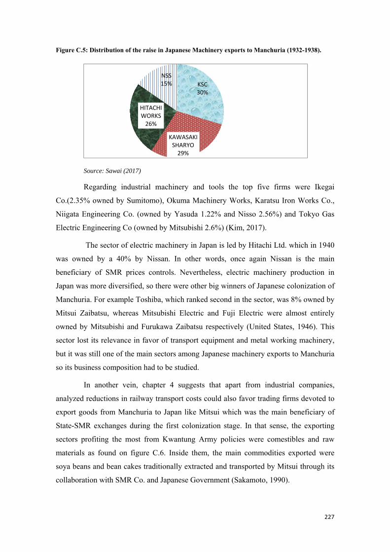
227
Figure C.5: Distribution of the raise in Japanese Machinery exports to Manchuria (1932-1938).
Source: Sawai (2017)
Regarding industrial machinery and tools the top five firms were Ikegai
Co.(2.35% owned by Sumitomo), Okuma Machinery Works, Karatsu Iron Works Co.,
Niigata Engineering Co. (owned by Yasuda 1.22% and Nisso 2.56%) and Tokyo Gas
Electric Engineering Co (owned by Mitsubishi 2.6%) (Kim, 2017).
The sector of electric machinery in Japan is led by Hitachi Ltd. which in 1940
was owned by a 40% by Nissan. In other words, once again Nissan is the main
beneficiary of SMR prices controls. Nevertheless, electric machinery production in
Japan was more diversified, so there were other big winners of Japanese colonization of
Manchuria. For example Toshiba, which ranked second in the sector, was 8% owned by
Mitsui Zaibatsu, whereas Mitsubishi Electric and Fuji Electric were almost entirely
owned by Mitsubishi and Furukawa Zaibatsu respectively (United States, 1946). This
sector lost its relevance in favor of transport equipment and metal working machinery,
but it was still one of the main sectors among Japanese machinery exports to Manchuria
so its business composition had to be studied.
In another vein, chapter 4 suggests that apart from industrial companies,
analyzed reductions in railway transport costs could also favor trading firms devoted to
export goods from Manchuria to Japan like Mitsui which was the main beneficiary of
State-SMR exchanges during the first colonization stage. In that sense, the exporting
sectors profiting the most from Kwantung Army policies were comestibles and raw
materials as found on figure C.6. Inside them, the main commodities exported were
soya beans and bean cakes traditionally extracted and transported by Mitsui through its
collaboration with SMR Co. and Japanese Government (Sakamoto, 1990).
KSC30%
KAWASAKI SHARYO
29%
HITACHI WORKS
26%
NSS15%
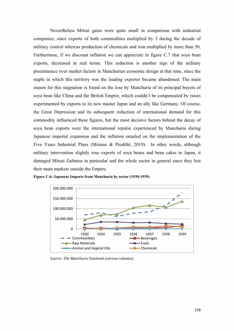
228
Nevertheless Mitsui gains were quite small in comparison with industrial
companies, since exports of both commodities multiplied by 3 during the decade of
military control whereas production of chemicals and iron multiplied by more than 50.
Furthermore, if we discount inflation we can appreciate in figure C.7 that soya bean
exports, decreased in real terms. This reduction is another sign of the military
preeminence over market factors in Manchurian economic design at that time, since the
staple in which this territory was the leading exporter became abandoned. The main
reason for this stagnation is found on the lose by Manchuria of its principal buyers of
soya bean like China and the British Empire, which couldn’t be compensated by raises
experimented by exports to its new master Japan and an ally like Germany. Of course,
the Great Depression and its subsequent reduction of international demand for this
commodity influenced these figures, but the most decisive factors behind the decay of
soya bean exports were the international repulse experienced by Manchuria during
Japanese imperial expansion and the inflation entailed on the implementation of the
Five Years Industrial Plans (Mizuno & Prodöhl, 2019). In other words, although
military intervention slightly rose exports of soya beans and bean cakes to Japan, it
damaged Mitsui Zaibatsu in particular and the whole sector in general since they lost
their main markets outside the Empire. Figure C.6: Japanese Imports from Manchuria by sector (1930-1939)
Source: The Manchuria Yearbook (various volumes).
0
50.000.000
100.000.000
150.000.000
200.000.000
1930 1934 1935 1936 1937 1938 1939Commestibles BeveragesRaw Materials FuelsAnimal and Vegetal Oils Chemicals
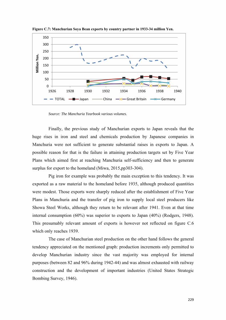
229
Figure C.7: Manchurian Soya Bean exports by country partner in 1933-34 million Yen.
Source: The Manchuria Yearbook various volumes.
Finally, the previous study of Manchurian exports to Japan reveals that the
huge rises in iron and steel and chemicals production by Japanese companies in
Manchuria were not sufficient to generate substantial raises in exports to Japan. A
possible reason for that is the failure in attaining production targets set by Five Year
Plans which aimed first at reaching Manchuria self-sufficiency and then to generate
surplus for export to the homeland (Miwa, 2015,pp303-304).
Pig iron for example was probably the main exception to this tendency. It was
exported as a raw material to the homeland before 1935, although produced quantities
were modest. Those exports were sharply reduced after the establishment of Five Year
Plans in Manchuria and the transfer of pig iron to supply local steel producers like
Showa Steel Works, although they return to be relevant after 1941. Even at that time
internal consumption (60%) was superior to exports to Japan (40%) (Rodgers, 1948).
This presumably relevant amount of exports is however not reflected on figure C.6
which only reaches 1939.
The case of Manchurian steel production on the other hand follows the general
tendency appreciated on the mentioned graph: production increments only permitted to
develop Manchurian industry since the vast majority was employed for internal
purposes (between 82 and 96% during 1942-44) and was almost exhausted with railway
construction and the development of important industries (United States Strategic
Bombing Survey, 1946).
0
50
100
150
200
250
300
350
1926 1928 1930 1932 1934 1936 1938 1940
Mill
ion
Yen.
TOTAL Japan China Great Britain Germany
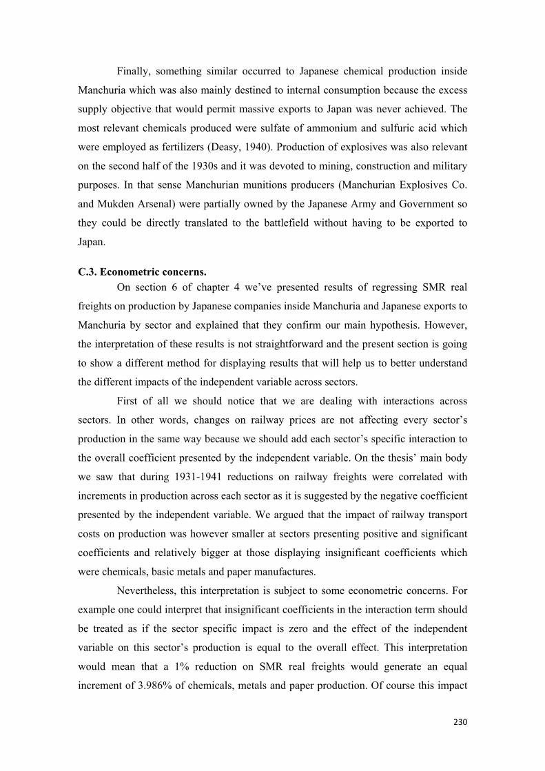
230
Finally, something similar occurred to Japanese chemical production inside
Manchuria which was also mainly destined to internal consumption because the excess
supply objective that would permit massive exports to Japan was never achieved. The
most relevant chemicals produced were sulfate of ammonium and sulfuric acid which
were employed as fertilizers (Deasy, 1940). Production of explosives was also relevant
on the second half of the 1930s and it was devoted to mining, construction and military
purposes. In that sense Manchurian munitions producers (Manchurian Explosives Co.
and Mukden Arsenal) were partially owned by the Japanese Army and Government so
they could be directly translated to the battlefield without having to be exported to
Japan.
C.3. Econometric concerns. On section 6 of chapter 4 we’ve presented results of regressing SMR real
freights on production by Japanese companies inside Manchuria and Japanese exports to
Manchuria by sector and explained that they confirm our main hypothesis. However,
the interpretation of these results is not straightforward and the present section is going
to show a different method for displaying results that will help us to better understand
the different impacts of the independent variable across sectors.
First of all we should notice that we are dealing with interactions across
sectors. In other words, changes on railway prices are not affecting every sector’s
production in the same way because we should add each sector’s specific interaction to
the overall coefficient presented by the independent variable. On the thesis’ main body
we saw that during 1931-1941 reductions on railway freights were correlated with
increments in production across each sector as it is suggested by the negative coefficient
presented by the independent variable. We argued that the impact of railway transport
costs on production was however smaller at sectors presenting positive and significant
coefficients and relatively bigger at those displaying insignificant coefficients which
were chemicals, basic metals and paper manufactures.
Nevertheless, this interpretation is subject to some econometric concerns. For
example one could interpret that insignificant coefficients in the interaction term should
be treated as if the sector specific impact is zero and the effect of the independent
variable on this sector’s production is equal to the overall effect. This interpretation
would mean that a 1% reduction on SMR real freights would generate an equal
increment of 3.986% of chemicals, metals and paper production. Of course this impact
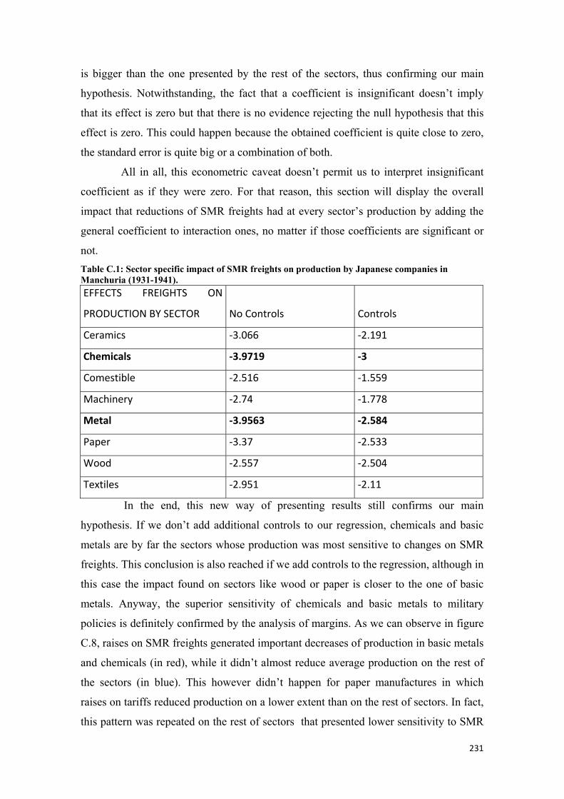
231
is bigger than the one presented by the rest of the sectors, thus confirming our main
hypothesis. Notwithstanding, the fact that a coefficient is insignificant doesn’t imply
that its effect is zero but that there is no evidence rejecting the null hypothesis that this
effect is zero. This could happen because the obtained coefficient is quite close to zero,
the standard error is quite big or a combination of both.
All in all, this econometric caveat doesn’t permit us to interpret insignificant
coefficient as if they were zero. For that reason, this section will display the overall
impact that reductions of SMR freights had at every sector’s production by adding the
general coefficient to interaction ones, no matter if those coefficients are significant or
not. Table C.1: Sector specific impact of SMR freights on production by Japanese companies in Manchuria (1931-1941). EFFECTS FREIGHTS ON
PRODUCTION BY SECTOR No Controls Controls
Ceramics -3.066 -2.191
Chemicals -3.9719 -3
Comestible -2.516 -1.559
Machinery -2.74 -1.778
Metal -3.9563 -2.584
Paper -3.37 -2.533
Wood -2.557 -2.504
Textiles -2.951 -2.11
In the end, this new way of presenting results still confirms our main
hypothesis. If we don’t add additional controls to our regression, chemicals and basic
metals are by far the sectors whose production was most sensitive to changes on SMR
freights. This conclusion is also reached if we add controls to the regression, although in
this case the impact found on sectors like wood or paper is closer to the one of basic
metals. Anyway, the superior sensitivity of chemicals and basic metals to military
policies is definitely confirmed by the analysis of margins. As we can observe in figure
C.8, raises on SMR freights generated important decreases of production in basic metals
and chemicals (in red), while it didn’t almost reduce average production on the rest of
the sectors (in blue). This however didn’t happen for paper manufactures in which
raises on tariffs reduced production on a lower extent than on the rest of sectors. In fact,
this pattern was repeated on the rest of sectors that presented lower sensitivity to SMR
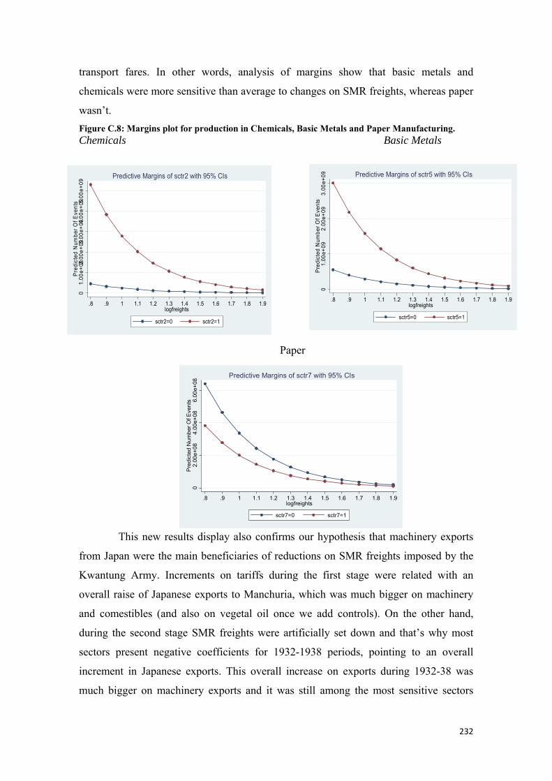
232
transport fares. In other words, analysis of margins show that basic metals and
chemicals were more sensitive than average to changes on SMR freights, whereas paper
wasn’t. Figure C.8: Margins plot for production in Chemicals, Basic Metals and Paper Manufacturing. Chemicals Basic Metals
This new results display also confirms our hypothesis that machinery exports
from Japan were the main beneficiaries of reductions on SMR freights imposed by the
Kwantung Army. Increments on tariffs during the first stage were related with an
overall raise of Japanese exports to Manchuria, which was much bigger on machinery
and comestibles (and also on vegetal oil once we add controls). On the other hand,
during the second stage SMR freights were artificially set down and that’s why most
sectors present negative coefficients for 1932-1938 periods, pointing to an overall
increment in Japanese exports. This overall increase on exports during 1932-38 was
much bigger on machinery exports and it was still among the most sensitive sectors
01.
00e+
092.0
0e+0
93.00
e+094
.00e
+095.
00e+
09Pr
edic
ted
Num
ber O
f Eve
nts
.8 .9 1 1.1 1.2 1.3 1.4 1.5 1.6 1.7 1.8 1.9logfreights
sctr2=0 sctr2=1
Predictive Margins of sctr2 with 95% CIs
01.
00e+
092.
00e+
093.
00e+
09Pr
edic
ted
Num
ber O
f Eve
nts
.8 .9 1 1.1 1.2 1.3 1.4 1.5 1.6 1.7 1.8 1.9logfreights
sctr5=0 sctr5=1
Predictive Margins of sctr5 with 95% CIs
02.
00e+
084.
00e+
086.
00e+
08Pr
edic
ted
Num
ber O
f Eve
nts
.8 .9 1 1.1 1.2 1.3 1.4 1.5 1.6 1.7 1.8 1.9logfreights
sctr7=0 sctr7=1
Predictive Margins of sctr7 with 95% CIs
Paper
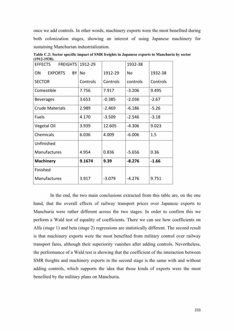
233
once we add controls. In other words, machinery exports were the most benefited during
both colonization stages, showing an interest of using Japanese machinery for
sustaining Manchurian industrialization. Table C.2: Sector specific impact of SMR freights in Japanese exports to Manchuria by sector (1912-1938). EFFECTS FREIGHTS
ON EXPORTS BY
SECTOR
1912-29
No
Controls
1912-29
Controls
1932-38
No
controls
1932-38
Controls
Comestible 7.756 7.917 -3.206 9.495
Beverages 3.653 -0.385 -2.036 -2.67
Crude Materials 2.989 -2.469 -6.186 -5.26
Fuels 4.170 -3.509 -2.546 -3.18
Vegetal Oil 3.939 12.605 -4.306 9.023
Chemicals 6.036 4.009 -6.006 1.5
Unfinished
Manufactures 4.954 0.836 -5.656 0.36
Machinery 9.1674 9.39 -8.276 -1.66
Finished
Manufactures 3.917 -3.079 -4.276 9.751
In the end, the two main conclusions extracted from this table are, on the one
hand, that the overall effects of railway transport prices over Japanese exports to
Manchuria were rather different across the two stages. In order to confirm this we
perform a Wald test of equality of coefficients. There we can see how coefficients on
Alfa (stage 1) and beta (stage 2) regressions are statistically different. The second result
is that machinery exports were the most benefited from military control over railway
transport fares, although their superiority vanishes after adding controls. Nevertheless,
the performance of a Wald test is showing that the coefficient of the interaction between
SMR freights and machinery exports in the second stage is the same with and without
adding controls, which supports the idea that those kinds of exports were the most
benefited by the military plans on Manchuria.
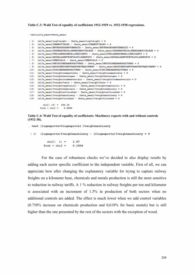
234
Table C.3: Wald Test of equality of coefficients 1912-1929 vs. 1932-1938 regressions.
Table C.4: Wald Test of equality of coefficients: Machinery exports with and without controls (1932-38).
For the case of robustness checks we’ve decided to also display results by
adding each sector specific coefficient to the independent variable. First of all, we can
appreciate how after changing the explanatory variable for trying to capture railway
freights on a kilometer base, chemicals and metals production is still the most sensitive
to reduction in railway tariffs. A 1 % reduction in railway freights per ton and kilometer
is associated with an increment of 1.5% in production of both sectors when no
additional controls are added. The effect is much lower when we add control variables
(0.758% increase on chemicals production and 0,618% for basic metals) but is still
higher than the one presented by the rest of the sectors with the exception of wood.
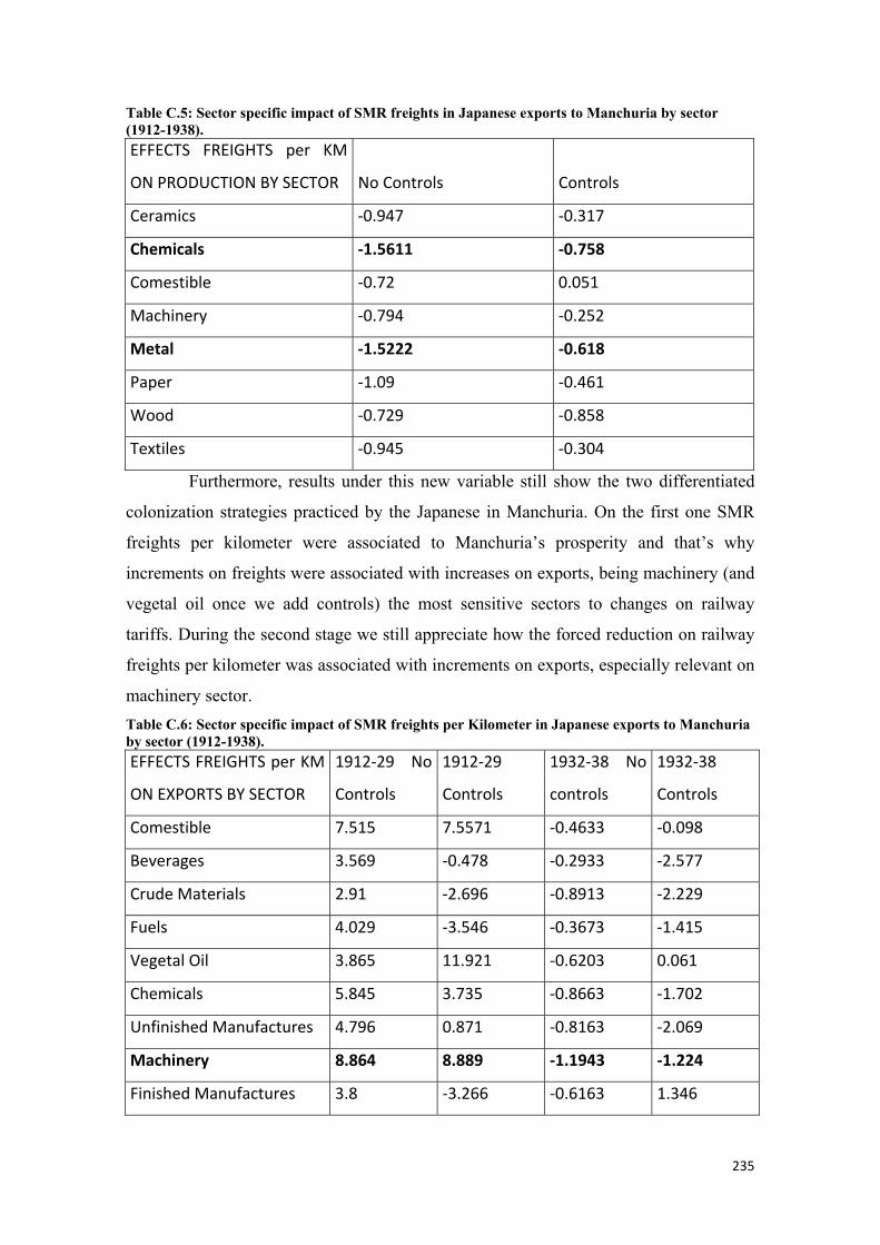
235
Table C.5: Sector specific impact of SMR freights in Japanese exports to Manchuria by sector (1912-1938). EFFECTS FREIGHTS per KM
ON PRODUCTION BY SECTOR No Controls Controls
Ceramics -0.947 -0.317
Chemicals -1.5611 -0.758
Comestible -0.72 0.051
Machinery -0.794 -0.252
Metal -1.5222 -0.618
Paper -1.09 -0.461
Wood -0.729 -0.858
Textiles -0.945 -0.304
Furthermore, results under this new variable still show the two differentiated
colonization strategies practiced by the Japanese in Manchuria. On the first one SMR
freights per kilometer were associated to Manchuria’s prosperity and that’s why
increments on freights were associated with increases on exports, being machinery (and
vegetal oil once we add controls) the most sensitive sectors to changes on railway
tariffs. During the second stage we still appreciate how the forced reduction on railway
freights per kilometer was associated with increments on exports, especially relevant on
machinery sector. Table C.6: Sector specific impact of SMR freights per Kilometer in Japanese exports to Manchuria by sector (1912-1938). EFFECTS FREIGHTS per KM
ON EXPORTS BY SECTOR
1912-29 No
Controls
1912-29
Controls
1932-38 No
controls
1932-38
Controls
Comestible 7.515 7.5571 -0.4633 -0.098
Beverages 3.569 -0.478 -0.2933 -2.577
Crude Materials 2.91 -2.696 -0.8913 -2.229
Fuels 4.029 -3.546 -0.3673 -1.415
Vegetal Oil 3.865 11.921 -0.6203 0.061
Chemicals 5.845 3.735 -0.8663 -1.702
Unfinished Manufactures 4.796 0.871 -0.8163 -2.069
Machinery 8.864 8.889 -1.1943 -1.224
Finished Manufactures 3.8 -3.266 -0.6163 1.346
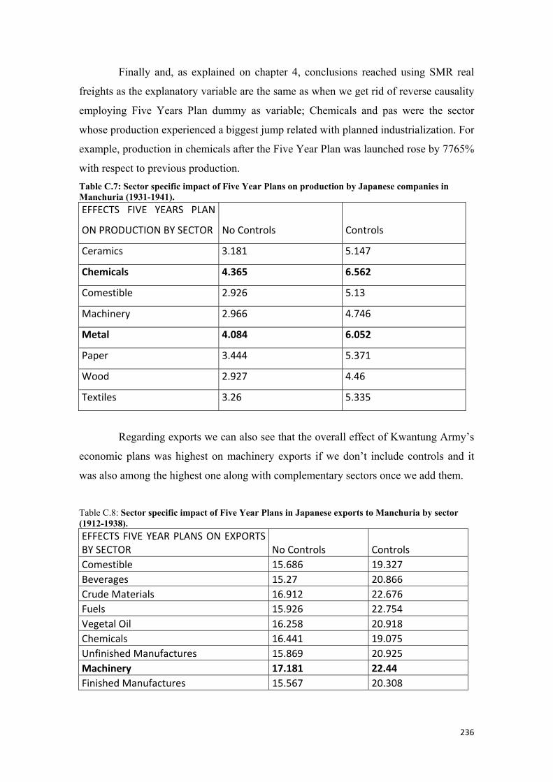
236
Finally and, as explained on chapter 4, conclusions reached using SMR real
freights as the explanatory variable are the same as when we get rid of reverse causality
employing Five Years Plan dummy as variable; Chemicals and pas were the sector
whose production experienced a biggest jump related with planned industrialization. For
example, production in chemicals after the Five Year Plan was launched rose by 7765%
with respect to previous production. Table C.7: Sector specific impact of Five Year Plans on production by Japanese companies in Manchuria (1931-1941). EFFECTS FIVE YEARS PLAN
ON PRODUCTION BY SECTOR No Controls Controls
Ceramics 3.181 5.147
Chemicals 4.365 6.562
Comestible 2.926 5.13
Machinery 2.966 4.746
Metal 4.084 6.052
Paper 3.444 5.371
Wood 2.927 4.46
Textiles 3.26 5.335
Regarding exports we can also see that the overall effect of Kwantung Army’s
economic plans was highest on machinery exports if we don’t include controls and it
was also among the highest one along with complementary sectors once we add them.
Table C.8: Sector specific impact of Five Year Plans in Japanese exports to Manchuria by sector (1912-1938). EFFECTS FIVE YEAR PLANS ON EXPORTS BY SECTOR No Controls Controls Comestible 15.686 19.327 Beverages 15.27 20.866 Crude Materials 16.912 22.676 Fuels 15.926 22.754 Vegetal Oil 16.258 20.918 Chemicals 16.441 19.075 Unfinished Manufactures 15.869 20.925 Machinery 17.181 22.44 Finished Manufactures 15.567 20.308