earth system model evaluation tool (esmvaltool) v2.0
TRANSCRIPT
Geosci. Model Dev., 13, 3383–3438, 2020https://doi.org/10.5194/gmd-13-3383-2020© Author(s) 2020. This work is distributed underthe Creative Commons Attribution 4.0 License.
Earth System Model Evaluation Tool (ESMValTool) v2.0 – anextended set of large-scale diagnostics for quasi-operational andcomprehensive evaluation of Earth system models in CMIPVeronika Eyring1,2, Lisa Bock1, Axel Lauer1, Mattia Righi1, Manuel Schlund1, Bouwe Andela3, Enrico Arnone4,5,Omar Bellprat6, Björn Brötz1, Louis-Philippe Caron6, Nuno Carvalhais7,8, Irene Cionni9, Nicola Cortesi6,Bas Crezee10, Edouard L. Davin10, Paolo Davini4, Kevin Debeire1, Lee de Mora11, Clara Deser12, David Docquier13,Paul Earnshaw14, Carsten Ehbrecht15, Bettina K. Gier2,1, Nube Gonzalez-Reviriego6, Paul Goodman16,Stefan Hagemann17, Steven Hardiman14, Birgit Hassler1, Alasdair Hunter6, Christopher Kadow15,18,Stephan Kindermann15, Sujan Koirala7, Nikolay Koldunov19,20, Quentin Lejeune10,21, Valerio Lembo22,Tomas Lovato23, Valerio Lucarini22,24,25, François Massonnet26, Benjamin Müller27, Amarjiit Pandde16,Núria Pérez-Zanón6, Adam Phillips12, Valeriu Predoi28, Joellen Russell16, Alistair Sellar14, Federico Serva29,Tobias Stacke17,30, Ranjini Swaminathan31, Verónica Torralba6, Javier Vegas-Regidor6, Jost von Hardenberg4,32,Katja Weigel2,1, and Klaus Zimmermann13
1Deutsches Zentrum für Luft- und Raumfahrt (DLR), Institut für Physik der Atmosphäre, Oberpfaffenhofen, Germany2University of Bremen, Institute of Environmental Physics (IUP), Bremen, Germany3Netherlands eScience Center, Science Park 140, 1098 XG Amsterdam, the Netherlands4Institute of Atmospheric Sciences and Climate, Consiglio Nazionale delle Ricerche (ISAC-CNR), Turin, Italy5Department of Physics, University of Torino, Turin, Italy6Barcelona Supercomputing Center (BSC), Barcelona, Spain7Department of Biogeochemical Integration, Max Planck Institute for Biogeochemistry, Jena, Germany8Departamento de Ciências e Engenharia do Ambiente, DCEA, Faculdade de Ciências e Tecnologia, FCT, Universidade Novade Lisboa, 2829-516 Caparica, Portugal9Agenzia nazionale per le nuove tecnologie, l’energia e lo sviluppo economico sostenibile (ENEA), Rome, Italy10ETH Zurich, Institute for Atmospheric and Climate Science, Zurich, Switzerland11Plymouth Marine Laboratory (PML), Plymouth, UK12National Center for Atmospheric Research (NCAR), Boulder, CO, USA13Rossby Centre, Swedish Meteorological and Hydrological Institute (SMHI), Norrköping, Sweden14Met Office, Exeter, UK15Deutsches Klimarechenzentrum, Hamburg, Germany16Department of Geosciences, University of Arizona, Tucson, AZ, USA17Institute of Coastal Research, Helmholtz-Zentrum Geesthacht (HZG), Geesthacht, Germany18Freie Universität Berlin (FUB), Berlin, Germany19MARUM, Center for Marine Environmental Sciences, Bremen, Germany20Alfred-Wegener-Institut Helmholtz-Zentrum für Polar- und Meeresforschung, Bremerhaven, Germany21Climate Analytics, Berlin, Germany22CEN, University of Hamburg, Meteorological Institute, Hamburg, Germany23Fondazione Centro Euro-Mediterraneo sui Cambiamenti Climatici (CMCC), Bologna, Italy24Department of Mathematics and Statistics, University of Reading, Department of Mathematics and Statistics, Reading, UK25Centre for the Mathematics of Planet Earth, University of Reading, Centre for the Mathematics of Planet Earth Departmentof Mathematics and Statistics, Reading, UK26Georges Lemaître Centre for Earth and Climate Research, Earth and Life Institute, Université catholique de Louvain,Louvain-la-Neuve, Belgium27Ludwig Maximilians Universität (LMU), Department of Geography, Munich, Germany
Published by Copernicus Publications on behalf of the European Geosciences Union.
3384 V. Eyring et al.: ESMValTool v2.0
28NCAS Computational Modelling Services (CMS), University of Reading, Reading, UK29Institute of Marine Sciences, Consiglio Nazionale delle Ricerche (ISMAR-CNR), Rome, Italy30Max Planck Institute for Meteorology (MPI-M), Hamburg, Germany31Department of Meteorology, University of Reading, Reading, UK32Department of Environment, Land and Infrastructure Engineering, Politecnico di Torino, Turin, Italy
Correspondence: Veronika Eyring ([email protected])
Received: 19 October 2019 – Discussion started: 26 November 2019Revised: 30 April 2020 – Accepted: 29 May 2020 – Published: 30 July 2020
Abstract. The Earth System Model Evaluation Tool (ESM-ValTool) is a community diagnostics and performance met-rics tool designed to improve comprehensive and routineevaluation of Earth system models (ESMs) participating inthe Coupled Model Intercomparison Project (CMIP). It hasundergone rapid development since the first release in 2016and is now a well-tested tool that provides end-to-end prove-nance tracking to ensure reproducibility. It consists of (1) aneasy-to-install, well-documented Python package providingthe core functionalities (ESMValCore) that performs com-mon preprocessing operations and (2) a diagnostic part thatincludes tailored diagnostics and performance metrics forspecific scientific applications. Here we describe large-scalediagnostics of the second major release of the tool that sup-ports the evaluation of ESMs participating in CMIP Phase 6(CMIP6). ESMValTool v2.0 includes a large collection of di-agnostics and performance metrics for atmospheric, oceanic,and terrestrial variables for the mean state, trends, and vari-ability. ESMValTool v2.0 also successfully reproduces fig-ures from the evaluation and projections chapters of the In-tergovernmental Panel on Climate Change (IPCC) Fifth As-sessment Report (AR5) and incorporates updates from tar-geted analysis packages, such as the NCAR Climate Vari-ability Diagnostics Package for the evaluation of modes ofvariability, the Thermodynamic Diagnostic Tool (TheDiaTo)to evaluate the energetics of the climate system, as well asparts of AutoAssess that contains a mix of top–down perfor-mance metrics. The tool has been fully integrated into theEarth System Grid Federation (ESGF) infrastructure at theDeutsches Klimarechenzentrum (DKRZ) to provide evalua-tion results from CMIP6 model simulations shortly after theoutput is published to the CMIP archive. A result browserhas been implemented that enables advanced monitoring ofthe evaluation results by a broad user community at muchfaster timescales than what was possible in CMIP5.
1 Introduction
The Intergovernmental Panel on Climate Change (IPCC)Fifth Assessment Report (AR5) concluded that the warm-ing of the climate system is unequivocal and that the hu-
man influence on the climate system is clear (IPCC, 2013).Observed increases in greenhouse gases, warming of the at-mosphere and ocean, sea ice decline, and sea level rise, incombination with climate model projections of a likely tem-perature increase between 2.1 and 4.7 ◦C for a doubling ofatmospheric CO2 concentration from pre-industrial (1980)levels make it an international priority to improve our under-standing of the climate system and to reduce greenhouse gasemissions. This is reflected for example in the Paris Agree-ment of the United Nations Framework Convention on Cli-mate Change (UNFCCC) 21st session of the Conference ofthe Parties (COP21; UNFCCC, 2015).
Simulations with climate and Earth system models(ESMs) performed by the major climate modelling centresaround the world under common protocols have been coor-dinated as part of the World Climate Research Programme(WCRP) Coupled Model Intercomparison Project (CMIP)since the early 90s (Eyring et al., 2016a; Meehl et al., 2000,2007; Taylor et al., 2012). CMIP simulations provide a fun-damental source for IPCC Assessment Reports and for im-proving our understanding of past, present, and future cli-mate change. Standardization of model output in a commonformat (Juckes et al., 2020) and publication of the CMIPmodel output on the Earth System Grid Federation (ESGF)facilitates multi-model evaluation and analysis (Balaji et al.,2018; Eyring et al., 2016a; Taylor et al., 2012). This effort isadditionally supported by observations for the Model Inter-comparison Project (obs4MIPs) which provides the commu-nity with access to CMIP-like datasets (in terms of variabledefinitions, temporal and spatial coordinates, time frequen-cies, and coverages) of satellite data (Ferraro et al., 2015;Teixeira et al., 2014; Waliser et al., 2019). The availability ofobservations and models in the same format strongly facili-tates model evaluation and analysis.
CMIP is now in its sixth phase (CMIP6, Eyring et al.,2016a) and is confronted with a number of new challenges.More centres are running more versions of more modelsof increasing complexity. An ongoing demand to resolvemore processes requires increasingly higher model resolu-tions. Accordingly, the data volume of 2 PB in CMIP5 isexpected to grow by a factor of 10–20 for CMIP6, result-ing in a CMIP6 database of between 20 and 40 PB, de-
Geosci. Model Dev., 13, 3383–3438, 2020 https://doi.org/10.5194/gmd-13-3383-2020
V. Eyring et al.: ESMValTool v2.0 3385
pending on model resolution and the number of modellingcentres ultimately contributing to the project (Balaji et al.,2018). Archiving, documenting, subsetting, supporting, dis-tributing, and analysing the huge CMIP6 output togetherwith observations challenges the capacity and creativity ofthe largest data centres and fastest data networks. In addi-tion, the growing dependency on CMIP products by a broadresearch community and by national and international cli-mate assessments, as well as the increasing desire for opera-tional analysis in support of mitigation and adaptation, meansthat systems should be set in place that allow for an efficientand comprehensive analysis of the large volume of data frommodels and observations.
To help achieve this, the Earth System Model EvaluationTool (ESMValTool) is developed. A first version that wastested on CMIP5 models was released in 2016 (Eyring et al.,2016c). With the release of ESMValTool version 2.0 (v2.0),for the first time in CMIP an evaluation tool is now avail-able that provides evaluation results from CMIP6 simula-tions as soon as the model output is published to the ESGF(https://cmip-esmvaltool.dkrz.de/, last access: 13 July 2020).This is realized through text files that we refer to as recipes,each calling a certain set of diagnostics and performancemetrics to reproduce analyses that have been demonstratedto be of importance in ESM evaluation in previous peer-reviewed papers or assessment reports. ESMValTool is de-veloped as a community diagnostics and performance met-rics tool that allows for routine comparison of single or mul-tiple models, either against predecessor versions or againstobservations. It is developed as a community effort currentlyinvolving more than 40 institutes with a rapidly growing de-veloper and user community. Given the level of detailed eval-uation diagnostics included in ESMValTool v2.0, several di-agnostics are of interest only to the climate modelling com-munity, whereas others, including but not limited to those onglobal mean temperature or precipitation, will also be valu-able for the wider scientific user community. The tool allowsfor full traceability and provenance of all figures and outputsproduced. This includes preservation of the netCDF meta-data of the input files including the global attributes. Thesemetadata are also written to the products (netCDF and plots)using the Python package W3C-PROV. Details can be foundin the ESMValTool v2.0 technical overview description pa-per by Righi et al. (2020).
The release of ESMValTool v2.0 is documented in fourcompanion papers: Righi et al. (2020) provide the technicaloverview of ESMValTool v2.0 and show a schematic repre-sentation of the ESMValCore, a Python package that providesthe core functionalities, and the diagnostic part (see theirFig. 1). This paper describes recipes of the diagnostic partfor the evaluation of large-scale diagnostics. Recipes for ex-treme events and in support of regional model evaluation aredescribed by Weigel et al. (2020) and recipes for emergentconstraints and model weighting by Lauer et al. (2020). In thepresent paper, the use of the tool is demonstrated by show-
ing example figures for each recipe for either all or a subsetof CMIP5 models. Section 2 describes the type of modellingand observational data currently supported by ESMValToolv2.0. In Sect. 3 an overview of the recipes for large-scalediagnostics provided with the ESMValTool v2.0 release isgiven along with their diagnostics and performance metricsas well as the variables and observations used. Section 4 de-scribes the workflow of routine analysis of CMIP model out-put alongside the ESGF and the ESMValTool result browser.Section 5 closes with a summary and an outlook.
2 Models and observations
The open-source release of ESMValTool v2.0 that accom-panies this paper is intended to work with CMIP5 andCMIP6 model output and partly also with CMIP3 (althoughthe availability of data for the latter is significantly lower,resulting in a limited number of recipes and diagnosticsthat can be applied with such data), but the tool is com-patible with any arbitrary model output, provided that itis in CF-compliant netCDF format (CF: climate and fore-cast; http://cfconventions.org/, last access: 13 July 2020) andthat the variables and metadata follow the CMOR (ClimateModel Output Rewriter, https://pcmdi.github.io/cmor-site/media/pdf/cmor_users_guide.pdf, last access: 13 July 2020)tables and definitions (see, e.g., https://github.com/PCMDI/cmip6-cmor-tables/tree/master/TablesforCMIP6, last access:13 July 2020). As in ESMValTool v1.0, for the evaluation ofthe models with observations, we make use of the large ob-servational effort to deliver long-term, high-quality observa-tions from international efforts such as obs4MIPs (Ferraro etal., 2015; Teixeira et al., 2014; Waliser et al., 2019) or obser-vations from the ESA Climate Change Initiative (CCI; Laueret al., 2017). In addition, observations from other sources andreanalysis data are used in several diagnostics (see Table 3 inRighi et al., 2020). The processing of observational data foruse in ESMValTool v2.0 is described in Righi et al. (2020).The observations used by individual recipes and diagnosticsare described in Sect. 3 and listed in Table 1. With the broadevaluation of the CMIP models, ESMValTool substantiallysupports one of CMIP’s main goals, which is the comparisonof the models with observations (Eyring et al., 2016a, 2019).
3 Overview of recipes included in ESMValTool v2.0
In this section, all recipes for large-scale diagnostics thathave been newly added in v2.0 since the first release ofESMValTool in 2016 (see Table 1 in Eyring et al., 2016c,for an overview of namelists, now called recipes, included inv1.0) are described. In each subsection, we first scientificallymotivate the inclusion of the recipe by reviewing the mainsystematic biases in current ESMs and their importance andimplications. We then give an overview of the recipes thatcan be used to evaluate such biases along with the diag-
https://doi.org/10.5194/gmd-13-3383-2020 Geosci. Model Dev., 13, 3383–3438, 2020
3386 V. Eyring et al.: ESMValTool v2.0
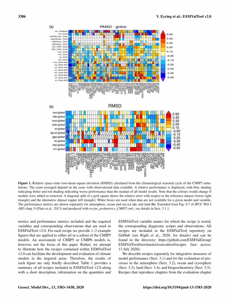
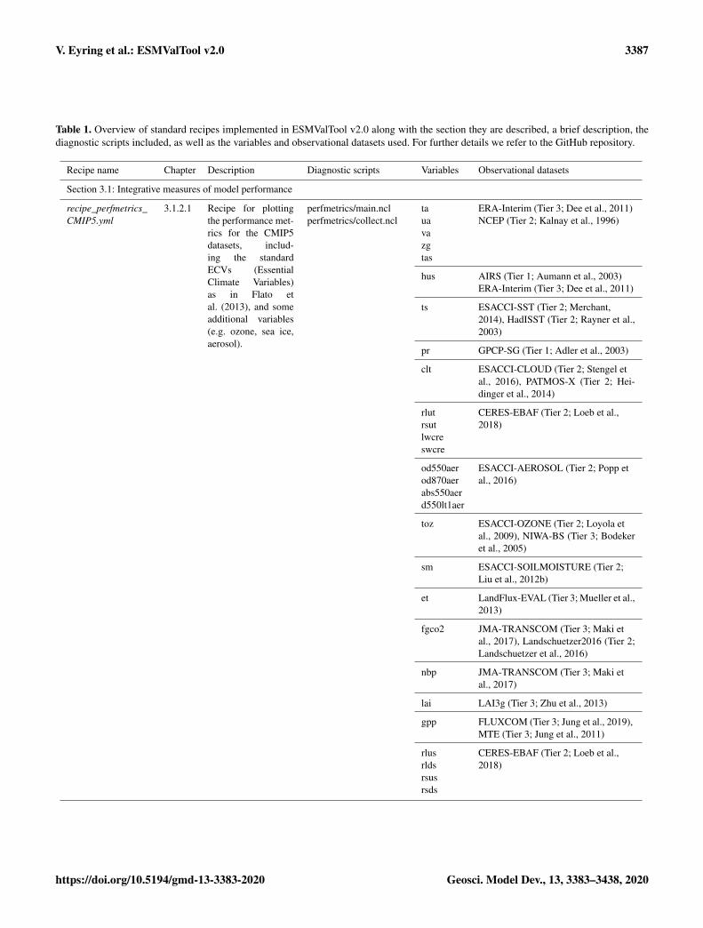
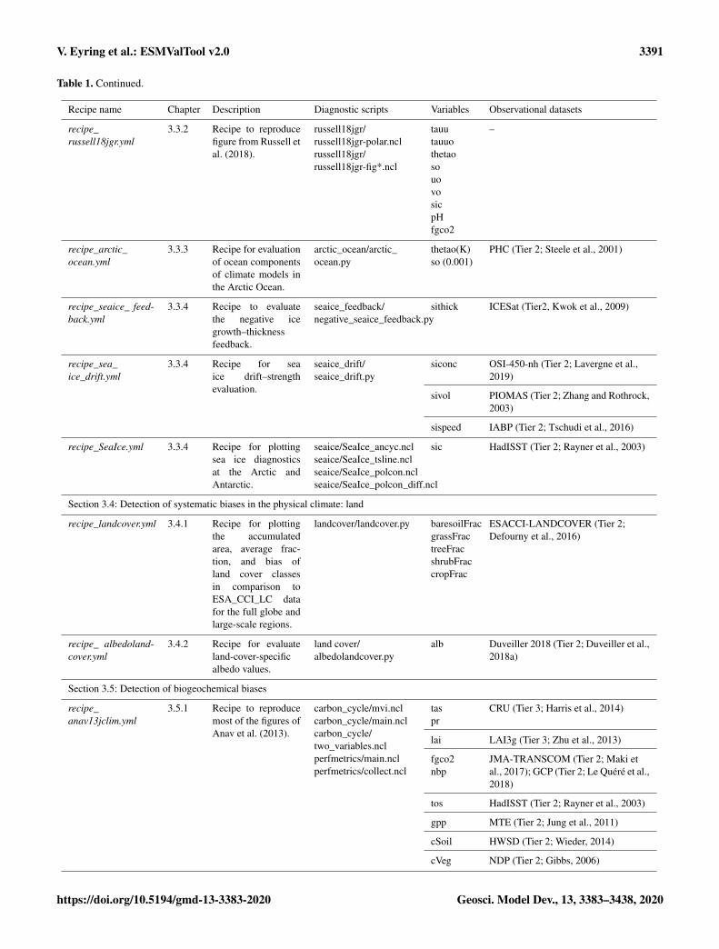
Figure 1. Relative space–time root-mean-square deviation (RMSD) calculated from the climatological seasonal cycle of the CMIP5 simu-lations. The years averaged depend on the years with observational data available. A relative performance is displayed, with blue shadingindicating better and red shading indicating worse performance than the median of all model results. Note that the colours would change ifmodels were added or removed. A diagonal split of a grid square shows the relative error with respect to the reference dataset (lower righttriangle) and the alternative dataset (upper left triangle). White boxes are used when data are not available for a given model and variable.The performance metrics are shown separately for atmosphere, ocean and sea ice (a), and land (b). Extended from Fig. 9.7 of IPCC WG IAR5 chap. 9 (Flato et al., 2013) and produced with recipe_perfmetrics_CMIP5.yml.; see details in Sect. 3.1.1.
nostics and performance metrics included and the requiredvariables and corresponding observations that are used inESMValTool v2.0. For each recipe we provide 1–2 examplefigures that are applied to either all or a subset of the CMIP5models. An assessment of CMIP5 or CMIP6 models is,however, not the focus of this paper. Rather, we attemptto illustrate how the recipes contained within ESMValToolv2.0 can facilitate the development and evaluation of climatemodels in the targeted areas. Therefore, the results ofeach figure are only briefly described. Table 1 provides asummary of all recipes included in ESMValTool v2.0 alongwith a short description, information on the quantities and
ESMValTool variable names for which the recipe is tested,the corresponding diagnostic scripts and observations. Allrecipes are included in the ESMValTool repository onGitHub (see Righi et al., 2020, for details) and can befound in the directory: https://github.com/ESMValGroup/ESMValTool/tree/master/esmvaltool/recipes (last access:13 July 2020).
We describe recipes separately for integrative measures ofmodel performance (Sect. 3.1) and for the evaluation of pro-cesses in the atmosphere (Sect. 3.2), ocean and cryosphere(Sect. 3.3), land (Sect. 3.4), and biogeochemistry (Sect. 3.5).Recipes that reproduce chapters from the evaluation chapter
Geosci. Model Dev., 13, 3383–3438, 2020 https://doi.org/10.5194/gmd-13-3383-2020
V. Eyring et al.: ESMValTool v2.0 3387
Table 1. Overview of standard recipes implemented in ESMValTool v2.0 along with the section they are described, a brief description, thediagnostic scripts included, as well as the variables and observational datasets used. For further details we refer to the GitHub repository.
Recipe name Chapter Description Diagnostic scripts Variables Observational datasets
Section 3.1: Integrative measures of model performance
recipe_perfmetrics_CMIP5.yml
3.1.2.1 Recipe for plottingthe performance met-rics for the CMIP5datasets, includ-ing the standardECVs (EssentialClimate Variables)as in Flato etal. (2013), and someadditional variables(e.g. ozone, sea ice,aerosol).
perfmetrics/main.nclperfmetrics/collect.ncl
tauavazgtas
ERA-Interim (Tier 3; Dee et al., 2011)NCEP (Tier 2; Kalnay et al., 1996)
hus AIRS (Tier 1; Aumann et al., 2003)ERA-Interim (Tier 3; Dee et al., 2011)
ts ESACCI-SST (Tier 2; Merchant,2014), HadISST (Tier 2; Rayner et al.,2003)
pr GPCP-SG (Tier 1; Adler et al., 2003)
clt ESACCI-CLOUD (Tier 2; Stengel etal., 2016), PATMOS-X (Tier 2; Hei-dinger et al., 2014)
rlutrsutlwcreswcre
CERES-EBAF (Tier 2; Loeb et al.,2018)
od550aerod870aerabs550aerd550lt1aer
ESACCI-AEROSOL (Tier 2; Popp etal., 2016)
toz ESACCI-OZONE (Tier 2; Loyola etal., 2009), NIWA-BS (Tier 3; Bodekeret al., 2005)
sm ESACCI-SOILMOISTURE (Tier 2;Liu et al., 2012b)
et LandFlux-EVAL (Tier 3; Mueller et al.,2013)
fgco2 JMA-TRANSCOM (Tier 3; Maki etal., 2017), Landschuetzer2016 (Tier 2;Landschuetzer et al., 2016)
nbp JMA-TRANSCOM (Tier 3; Maki etal., 2017)
lai LAI3g (Tier 3; Zhu et al., 2013)
gpp FLUXCOM (Tier 3; Jung et al., 2019),MTE (Tier 3; Jung et al., 2011)
rlusrldsrsusrsds
CERES-EBAF (Tier 2; Loeb et al.,2018)
https://doi.org/10.5194/gmd-13-3383-2020 Geosci. Model Dev., 13, 3383–3438, 2020
3388 V. Eyring et al.: ESMValTool v2.0
Table 1. Continued.
Recipe name Chapter Description Diagnostic scripts Variables Observational datasets
Section 3.1: Integrative measures of model performance
recipe_smpi.yml 3.1.2.3 Recipe for comput-ing single-modelperformance index.Follows Reichler andKim (2008).
perfmetrics/main.nclperfmetrics/collect.ncl
tavauahustaspslhfdstauutauv
ERA-Interim (Tier 3; Dee et al., 2011)
pr GPCP-SG (Tier 1; Adler et al., 2003)
tossic
HadISST (Tier 2; Rayner et al., 2003)
recipe_autoassess_*.yml
3.1.2.4 Recipe for mix oftop–down metricsevaluating key modeloutput variables andbottom–up metrics.
autoassess/autoassess_area_base.pyautoassess/plot_autoassess_metrics.pyautoassess/autoassess_radiation_rms.py
rtntrsntswcrelwcrersnsrlnsrsutrlutrsutcs
CERES-EBAF (Tier 2; Loeb et al.,2018)
rlutcsrldscs
J RA-55 (Tier 1; Onogi et al., 2007)
prw SSMI-MERIS (Tier 1; Schröder, 2012)
pr GPCP-SG (Tier 1; Adler et al., 2003)
rtntrsntswcrelwcrersnsrlnsrsutrlutrsutcs
CERES-EBAF (Tier 2; Loeb et al.,2018), CERES-SYN1deg (Tier 3;Wielicki et al., 1996)
rlutcsrldscs
JRA-55 (Tier 1; ana4mips)CERES-SYN1deg (Tier 3; Wielicki etal., 1996)
prw SSMI-MERIS (Tier 1; obs4mips)SSMI (Tier 1; obs4mips)
cllmtisccpclltkisccpclmmtisccpclmtkisccpclhmtisccpclhtkisccp
ISCCP (Tier 1; Rossow and Schiffer,1991)
tauahus
ERA-Interim (Tier 3; Dee et al., 2011)
Geosci. Model Dev., 13, 3383–3438, 2020 https://doi.org/10.5194/gmd-13-3383-2020
V. Eyring et al.: ESMValTool v2.0 3389
Table 1. Continued.
Recipe name Chapter Description Diagnostic scripts Variables Observational datasets
Section 3.2: Detection of systematic biases in the physical climate: atmosphere
recipe_flato13ipcc.yml 3.1.23.2.13.3.1
Recipe to reproduceselected figures fromIPCC AR5, chap. 9(Flato et al., 2013)9.2, 9.4, 9.5, 9.6, 9.8,9.14.
clouds/clouds_bias.nclclouds/clouds_ipcc.nclipcc_ar5/tsline.nclipcc_ar5/ch09_fig09_06.nclipcc_ar5/ch09_fig09_06_collect.nclipcc_ar5/ch09_fig09_14.py
tas ERA-Interim (Tier 3; Dee et al., 2011)HadCRUT4 (Tier 2; Morice et al.,2012)
tos HadISST (Tier 2; Rayner et al., 2003)
swcrelwcrenetcrerlut
CERES-EBAF (Tier 2; Loeb et al.,2018)
pr GPCP-SG (Tier 1; Adler et al., 2003)
recipe_quantilebias.yml
3.2.2 Recipe for calcula-tion of precipitationquantile bias.
quantilebias/quantilebias.R
pr GPCP-SG (Tier 1; Adler et al., 2003)
recipe_zmnam.yml 3.2.3.1 Recipe for zonalmean Northern An-nular Mode. Thediagnostic computesthe index and thespatial pattern toassess the simulationof the stratosphere–troposphere couplingin the boreal hemi-sphere.
zmnam/zmnam.py zg –
recipe_miles_block.yml
3.2.3.2 Recipe for comput-ing 1-D and 2-D at-mospheric blockingindices and diagnos-tics.
miles/miles_block.R zg ERA-Interim (Tier 3; Dee et al., 2011)
recipe_thermodyn_diagtool.yml
3.2.4 Recipe for the com-putation of variousaspects associatedwith the thermody-namics of the climatesystem, such as en-ergy and water massbudgets, meridionalenthalpy trans-ports, the Lorenzenergy cycle, andthe material entropyproduction.
thermodyn_diagtool/thermo-dyn_diagnostics.py
hflshfssprpsprsnrldsrlusrlutrsdsrsusrsdtrsuttshustasuasvastauavawap
–
https://doi.org/10.5194/gmd-13-3383-2020 Geosci. Model Dev., 13, 3383–3438, 2020
3390 V. Eyring et al.: ESMValTool v2.0
Table 1. Continued.
Recipe name Chapter Description Diagnostic scripts Variables Observational datasets
Section 3.2: Detection of systematic biases in the physical climate: atmosphere
recipe_CVDP.yml 3.2.5.1 Recipe for execut-ing the NCAR CVDPpackage in the ESM-ValTool framework.
cvdp/cvdp_wrapper.py pr GPCP-SG (Tier 1; Adler et al., 2003)
psl ERA-Interim (Tier 3; Dee et al., 2011)
tas Berkeley Earth (Tier 1; Rohde andGroom, 2013)
ts ERSSTv5 (Tier 1; Huang et al. 2017)
recipe_modes_of_variability.yml
3.2.5.2 Recipe to computethe RMSE betweenthe observed andmodelled patterns ofvariability obtainedthrough classificationand their relativebias (percentage)in the frequency ofoccurrence and thepersistence of eachmode.
magic_bsc/weather_regime.r
zg –
recipe_miles_regimes.yml
3.2.5.2 Recipe for comput-ing Euro-Atlanticweather regimesbased on k meanclustering.
miles/miles_regimes.R zg ERA-Interim (Tier 3; Dee et al., 2011)
recipe_miles_eof.yml 3.2.5.3 Recipe for comput-ing the NorthernHemisphere EOFs.
miles/miles_eof.R zg ERA-Interim (Tier 3; Dee et al., 2011)
recipe_combined_indices.yml
3.2.5.4 Recipe for comput-ing seasonal meansor running averages,combining indicesfrom multiple mod-els and computingarea averages.
magic_bsc/ com-bined_indices.r
psl –
Section 3.3: Detection of systematic biases in the physical climate: ocean and cryosphere
recipe_ocean_scalar_fields.yml
3.3.1 Recipe to reproducetime series figures ofscalar quantities inthe ocean.
ocean/diagnostic_time series.py
gtintppgtfgco2amocmfothetaogasogazostoga
–
recipe_ocean_amoc.yml
3.3.1 Recipe to reproducetime series figuresof the AMOC, theDrake passage cur-rent, and the streamfunction.
ocean/diagnostic_time series.pyocean/diagnostic_transects.py
amocmfomsftmyz
–
Geosci. Model Dev., 13, 3383–3438, 2020 https://doi.org/10.5194/gmd-13-3383-2020
V. Eyring et al.: ESMValTool v2.0 3391
Table 1. Continued.
Recipe name Chapter Description Diagnostic scripts Variables Observational datasets
recipe_russell18jgr.yml
3.3.2 Recipe to reproducefigure from Russell etal. (2018).
russell18jgr/russell18jgr-polar.nclrussell18jgr/russell18jgr-fig*.ncl
tauutauuothetaosouovosicpHfgco2
–
recipe_arctic_ocean.yml
3.3.3 Recipe for evaluationof ocean componentsof climate models inthe Arctic Ocean.
arctic_ocean/arctic_ocean.py
thetao(K)so (0.001)
PHC (Tier 2; Steele et al., 2001)
recipe_seaice_ feed-back.yml
3.3.4 Recipe to evaluatethe negative icegrowth–thicknessfeedback.
seaice_feedback/negative_seaice_feedback.py
sithick ICESat (Tier2, Kwok et al., 2009)
recipe_sea_ice_drift.yml
3.3.4 Recipe for seaice drift–strengthevaluation.
seaice_drift/seaice_drift.py
siconc OSI-450-nh (Tier 2; Lavergne et al.,2019)
sivol PIOMAS (Tier 2; Zhang and Rothrock,2003)
sispeed IABP (Tier 2; Tschudi et al., 2016)
recipe_SeaIce.yml 3.3.4 Recipe for plottingsea ice diagnosticsat the Arctic andAntarctic.
seaice/SeaIce_ancyc.nclseaice/SeaIce_tsline.nclseaice/SeaIce_polcon.nclseaice/SeaIce_polcon_diff.ncl
sic HadISST (Tier 2; Rayner et al., 2003)
Section 3.4: Detection of systematic biases in the physical climate: land
recipe_landcover.yml 3.4.1 Recipe for plottingthe accumulatedarea, average frac-tion, and bias ofland cover classesin comparison toESA_CCI_LC datafor the full globe andlarge-scale regions.
landcover/landcover.py baresoilFracgrassFractreeFracshrubFraccropFrac
ESACCI-LANDCOVER (Tier 2;Defourny et al., 2016)
recipe_ albedoland-cover.yml
3.4.2 Recipe for evaluateland-cover-specificalbedo values.
land cover/albedolandcover.py
alb Duveiller 2018 (Tier 2; Duveiller et al.,2018a)
Section 3.5: Detection of biogeochemical biases
recipe_anav13jclim.yml
3.5.1 Recipe to reproducemost of the figures ofAnav et al. (2013).
carbon_cycle/mvi.nclcarbon_cycle/main.nclcarbon_cycle/two_variables.nclperfmetrics/main.nclperfmetrics/collect.ncl
taspr
CRU (Tier 3; Harris et al., 2014)
lai LAI3g (Tier 3; Zhu et al., 2013)
fgco2nbp
JMA-TRANSCOM (Tier 2; Maki etal., 2017); GCP (Tier 2; Le Quéré et al.,2018)
tos HadISST (Tier 2; Rayner et al., 2003)
gpp MTE (Tier 2; Jung et al., 2011)
cSoil HWSD (Tier 2; Wieder, 2014)
cVeg NDP (Tier 2; Gibbs, 2006)
https://doi.org/10.5194/gmd-13-3383-2020 Geosci. Model Dev., 13, 3383–3438, 2020
3392 V. Eyring et al.: ESMValTool v2.0
Table 1. Continued.
Recipe name Chapter Description Diagnostic scripts Variables Observational datasets
recipe_carval-hais2014nat.yml
3.5.2 Recipe to evaluatedthe biases in ecosys-tem carbon turnovertime.
regrid_areaweighted.pycompare_tau_modelVobs_matrix.pycompare_tau_modelVobs_climatebins.pycompare_zonal_tau.pycompare_zonal_correlations_tauVclimate.py
tau (non-CMORvariable,which isderived asthe ratioof totalecosystemcarbonstockand grossprimaryproductiv-ity)
Carvalhais et al. (2014)
recipe_ocean_bgc.yml 3.5.3 Recipe to evaluatethe marine biogeo-chemistry models ofCMIP5. There arealso some physicalevaluation metrics.
ocean/diagnostic_time series.pyocean/diagnostic_profiles.pyocean/diagnostic_maps.pyocean/diagnostic_model_vs_obs.py ocean/diagnostic_transects.pyocean/diagnostic_maps_multimodel.py
thetaosono3o2si
WOA (Tier 2; Locarnini, 2013)WOA (Tier 2; Garcia et al., 2013)
intpp Eppley-VGPM-MODIS (Tier 2;Behrenfeld and Falkowski, 1997)
chl ESACCI-OC (Tier 2;Volpe et al., 2019)
fgco2 Landschuetzer2016 (Tier 2;Landschuetzer et al., 2016)
dfetalkmfo
recipe_eyring06jgr.yml
3.5.4 Recipe to reproducestratospheric dynam-ics and chemistry fig-ures from Eyring etal. (2006).
eyring06jgr/eyring06jgr_fig*.ncl
taua
ERA-Interim (Tier 3; Dee et al., 2011)
vmro3vmrh2o
HALOE (Tier 2; Russell et al., 1993;Grooß and Russell III, 2005)
toz NIWA-BS (Tier 3; Bodeker et al.,2005)
of the IPCC Fifth Assessment Report (Flato et al., 2013) aredescribed within these sections.
3.1 Integrative measures of model performance
3.1.1 Performance metrics for essential climatevariables for the atmosphere, ocean, sea ice, andland
Performance metrics are quantitative measures of agreementbetween a simulated and observed quantity. Various sta-tistical measures can be used to quantify differences be-tween individual models or generations of models and ob-servations. Atmospheric performance metrics were alreadyincluded in namelist_perfmetrics_CMIP5.nml of ESMVal-
Tool v1.0. This recipe has now been extended to includeadditional atmospheric variables as well as new variablesfrom the ocean, sea ice, and land. Similar to Fig. 9.7 ofFlato et al. (2013), Fig. 1 shows the relative space–timeroot-mean-square deviation (RMSD) for the CMIP5 histor-ical simulations (1980–2005) against a reference observa-tion and, where available, an alternative observational dataset(recipe_perfmetrics_CMIP5.yml). Performance varies acrossCMIP5 models and variables, with some models comparingbetter with observations for one variable and another modelperforming better for a different variable. Except for globalaverage temperatures at 200 hPa (ta_Glob-200), where mostbut not all models have a systematic bias, the multi-modelmean outperforms any individual model. Additional vari-ables can easily be added if observations are available, by
Geosci. Model Dev., 13, 3383–3438, 2020 https://doi.org/10.5194/gmd-13-3383-2020
V. Eyring et al.: ESMValTool v2.0 3393
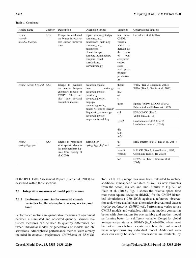
Figure 2. Centred pattern correlations for the annual mean clima-tology over the period 1980–1999 between models and observa-tions. Results for individual CMIP5 models are shown (thin dashes),as well as the ensemble average (longer thick dash) and median(open circle). The correlations are computed between the modelsand the reference dataset. When an alternate observational datasetis present, its correlation to the reference dataset is also shown (solidgreen circles). Similar to Fig. 9.6 of IPCC WG I AR5 chap. 9 (Flatoet al., 2013) and produced with recipe_flato13ipcc.yml; see detailsin Sect. 3.1.2.
providing a custom CMOR table and a Python script to dothe calculations in the case of derived variables; see furtherdetails in Sect. 4.1.1 of Eyring et al. (2016c). In addition tothe performance metrics displayed in Fig. 1, several otherquantitative measures of model performance are included insome of the recipes and are described throughout the respec-tive sections of this paper.
3.1.2 Centred pattern correlations for different CMIPensembles
Another example of a performance metric is the pattern cor-relation between the observed and simulated climatologicalannual mean spatial patterns. Following Fig. 9.6 of the IPCCAR5 chap. 9 (Flato et al., 2013), a diagnostic for computingand plotting centred pattern correlations for different modelsand CMIP ensembles has been implemented (Fig. 2) andadded to recipe_flato13ipcc.yml. The variables are firstregridded to a 4◦× 5◦ longitude by latitude grid to avoidfavouring a specific model resolution. Regridding is done bythe Iris package, which offers different regridding schemes(see https://esmvaltool.readthedocs.io/projects/esmvalcore/en/latest/recipe/preprocessor.html#horizontal-regridding,last access: 13 July 2020). The figure shows both a largemodel spread as well as a large spread in the correlationdepending on the variable, signifying that some aspects of
the simulated climate agree better with observations thanothers. The centred pattern correlations, which measure thesimilarity of two patterns after removing the global mean,are computed against a reference observation. Should theinput models be from different CMIP ensembles, they aregrouped by ensemble and each ensemble is plotted side byside for each variable with a different colour. If an alternatemodel is given, it is shown as a solid green circle. Theaxis ratio of the plot reacts dynamically to the number ofvariables (nvar) and ensembles (nensemble) after it surpassesa combined number of nvar× nensemble= 16, and the y axisrange is calculated to encompass all values. The centredpattern correlation is a good measure to quantify both thespread in models within a single variable as well as obtaininga quick overview of how well other variables and aspects ofthe climate on a large scale are reproduced with respect toobservations. Furthermore when using several ensembles,the progress made by each ensemble on a variable basis canbe seen at a quick glance.
3.1.3 Single-model performance index
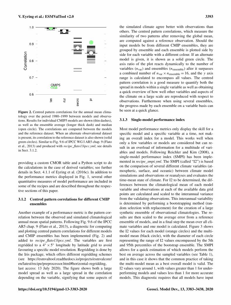
Most model performance metrics only display the skill for aspecific model and a specific variable at a time, not mak-ing an overall index for a model. This works well whenonly a few variables or models are considered but can re-sult in an overload of information for a multitude of vari-ables and models. Following Reichler and Kim (2008), asingle-model performance index (SMPI) has been imple-mented in recipe_smpi.yml. The SMPI (called “I2”) is basedon the comparison of several different climate variables (at-mospheric, surface, and oceanic) between climate modelsimulations and observations or reanalyses and evaluates thetime-mean state of climate. For I2 to be determined, the dif-ferences between the climatological mean of each modelvariable and observations at each of the available data gridpoints are calculated and scaled to the interannual variancefrom the validating observations. This interannual variabilityis determined by performing a bootstrapping method (ran-dom selection with replacement) for the creation of a largesynthetic ensemble of observational climatologies. The re-sults are then scaled to the average error from a referenceensemble of models, and in a final step the mean over all cli-mate variables and one model is calculated. Figure 3 showsthe I2 values for each model (orange circles) and the multi-model mean (black circle), with the diameter of each circlerepresenting the range of I2 values encompassed by the 5thand 95th percentiles of the bootstrap ensemble. The SMPIallows for a quick estimation of which models perform thebest on average across the sampled variables (see Table 1),and in this case it shows that the common practice of takingthe multi-model mean as a best overall model is valid. TheI2 values vary around 1, with values greater than 1 for under-performing models and values less than 1 for more accuratemodels. This diagnostic requires that all models have input
https://doi.org/10.5194/gmd-13-3383-2020 Geosci. Model Dev., 13, 3383–3438, 2020
3394 V. Eyring et al.: ESMValTool v2.0
Figure 3. Single-model performance index I2 for individual models (orange circles). The size of each circle represents the 95 % confidenceinterval of the bootstrap ensemble. The black circle indicates the I2 of the CMIP5 multi-model mean. The I2 values vary around 1, withunderperforming models having a value greater than 1, while values below 1 represent more accurate models. Similar to Reichler and Kim(2008, Fig. 1) and produced with recipe_smpi.yml; see details in Sect. 3.1.3.
for all of the variables considered, as this is the basis for hav-ing a meaningful comparison of the resulting I2 values.
3.1.4 AutoAssess
While highly condensed metrics are useful for comparing alarge number of models, for the purpose of model develop-ment it is important to retain granularity on which aspectsof model performance have changed and why. For this rea-son, many modelling centres have their own suite of met-rics which they use to compare candidate model versionsagainst a predecessor. AutoAssess is such a system, devel-oped by the UK Met Office and used in the developmentof the HadGEM3 and UKESM1 models. The output of Au-toAssess contains a mix of top–down metrics evaluating keymodel output variables (e.g. temperature and precipitation)and bottom–up metrics which assess the realism of modelprocesses and emergent behaviour such as cloud variabil-ity and El Niño–Southern Oscillation (ENSO). The outputof AutoAssess includes around 300 individual metrics. Tofacilitate the interpretation of the results, these are groupedinto 11 thematic areas, ranging from broad-scale ones suchas global tropic circulation and stratospheric mean state andvariability, to region- and process-specific, such as monsoonregions and the hydrological cycle.
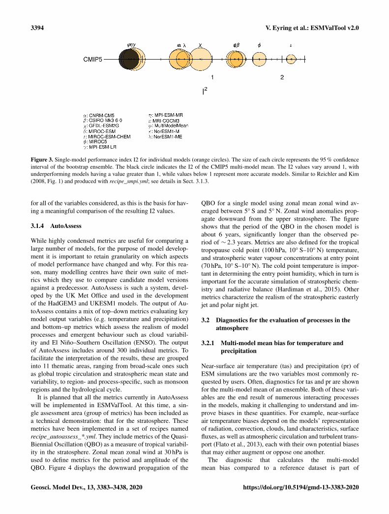
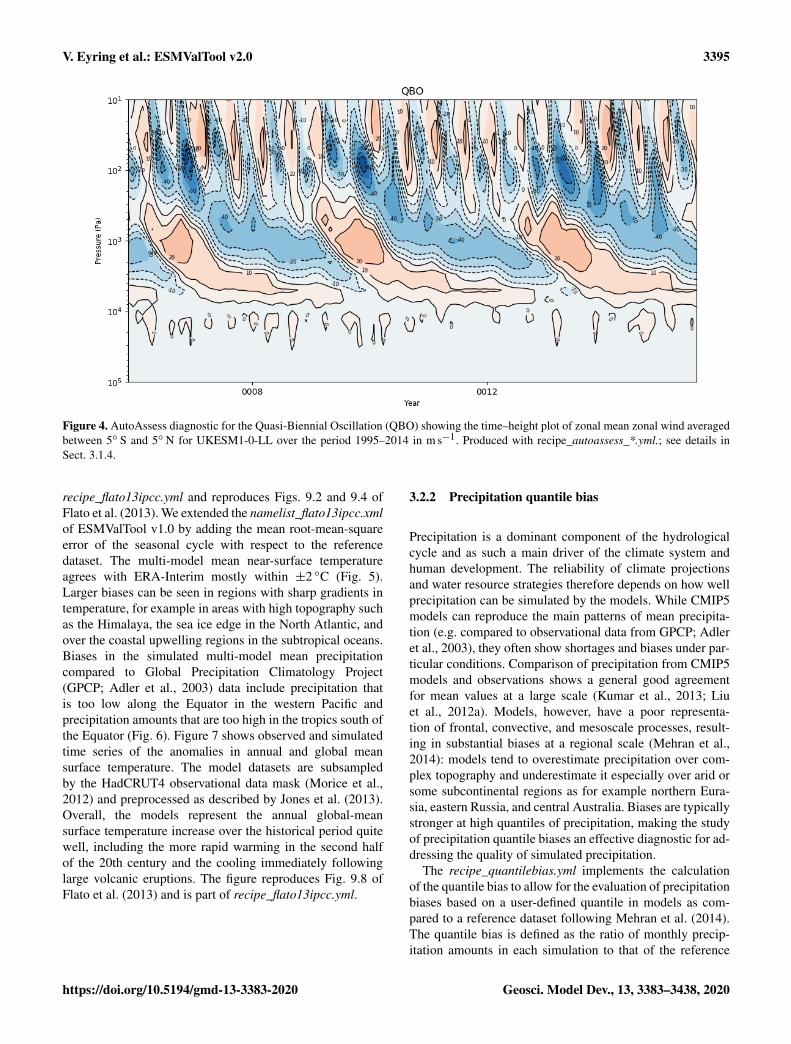
It is planned that all the metrics currently in AutoAssesswill be implemented in ESMValTool. At this time, a sin-gle assessment area (group of metrics) has been included asa technical demonstration: that for the stratosphere. Thesemetrics have been implemented in a set of recipes namedrecipe_autoassess_*.yml. They include metrics of the Quasi-Biennial Oscillation (QBO) as a measure of tropical variabil-ity in the stratosphere. Zonal mean zonal wind at 30 hPa isused to define metrics for the period and amplitude of theQBO. Figure 4 displays the downward propagation of the
QBO for a single model using zonal mean zonal wind av-eraged between 5◦ S and 5◦ N. Zonal wind anomalies prop-agate downward from the upper stratosphere. The figureshows that the period of the QBO in the chosen model isabout 6 years, significantly longer than the observed pe-riod of ∼ 2.3 years. Metrics are also defined for the tropicaltropopause cold point (100 hPa, 10◦ S–10◦ N) temperature,and stratospheric water vapour concentrations at entry point(70 hPa, 10◦ S–10◦ N). The cold point temperature is impor-tant in determining the entry point humidity, which in turn isimportant for the accurate simulation of stratospheric chem-istry and radiative balance (Hardiman et al., 2015). Othermetrics characterize the realism of the stratospheric easterlyjet and polar night jet.
3.2 Diagnostics for the evaluation of processes in theatmosphere
3.2.1 Multi-model mean bias for temperature andprecipitation
Near-surface air temperature (tas) and precipitation (pr) ofESM simulations are the two variables most commonly re-quested by users. Often, diagnostics for tas and pr are shownfor the multi-model mean of an ensemble. Both of these vari-ables are the end result of numerous interacting processesin the models, making it challenging to understand and im-prove biases in these quantities. For example, near-surfaceair temperature biases depend on the models’ representationof radiation, convection, clouds, land characteristics, surfacefluxes, as well as atmospheric circulation and turbulent trans-port (Flato et al., 2013), each with their own potential biasesthat may either augment or oppose one another.
The diagnostic that calculates the multi-modelmean bias compared to a reference dataset is part of
Geosci. Model Dev., 13, 3383–3438, 2020 https://doi.org/10.5194/gmd-13-3383-2020
V. Eyring et al.: ESMValTool v2.0 3395
Figure 4. AutoAssess diagnostic for the Quasi-Biennial Oscillation (QBO) showing the time–height plot of zonal mean zonal wind averagedbetween 5◦ S and 5◦ N for UKESM1-0-LL over the period 1995–2014 in m s−1. Produced with recipe_autoassess_*.yml.; see details inSect. 3.1.4.
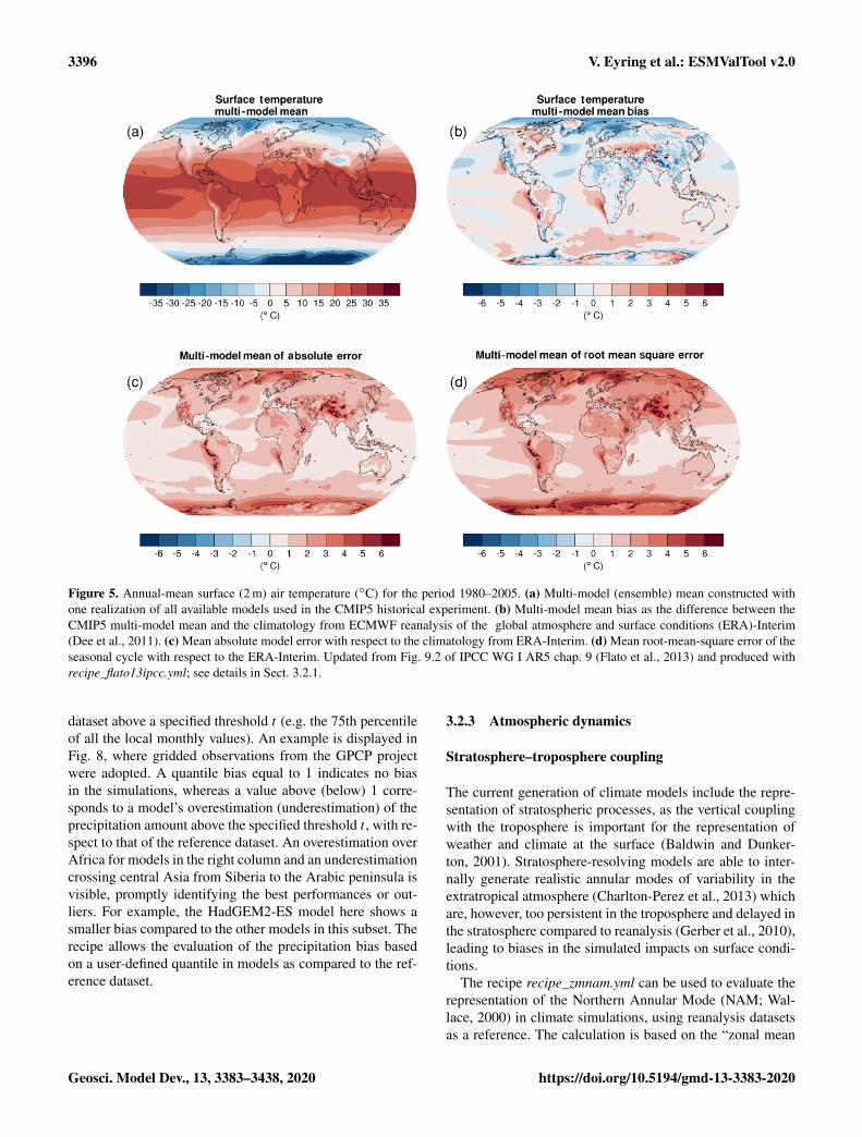
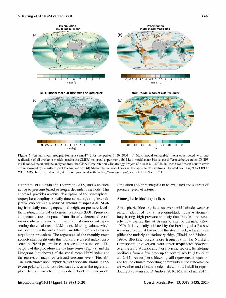
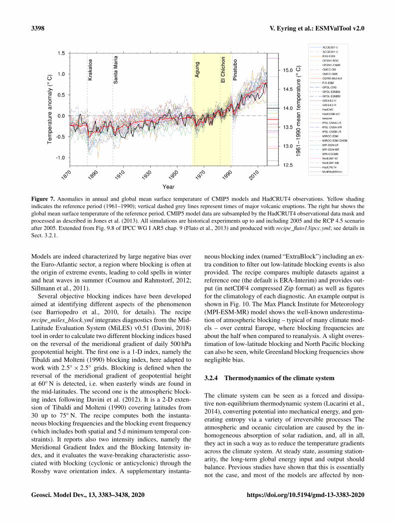
recipe_flato13ipcc.yml and reproduces Figs. 9.2 and 9.4 ofFlato et al. (2013). We extended the namelist_flato13ipcc.xmlof ESMValTool v1.0 by adding the mean root-mean-squareerror of the seasonal cycle with respect to the referencedataset. The multi-model mean near-surface temperatureagrees with ERA-Interim mostly within ±2 ◦C (Fig. 5).Larger biases can be seen in regions with sharp gradients intemperature, for example in areas with high topography suchas the Himalaya, the sea ice edge in the North Atlantic, andover the coastal upwelling regions in the subtropical oceans.Biases in the simulated multi-model mean precipitationcompared to Global Precipitation Climatology Project(GPCP; Adler et al., 2003) data include precipitation thatis too low along the Equator in the western Pacific andprecipitation amounts that are too high in the tropics south ofthe Equator (Fig. 6). Figure 7 shows observed and simulatedtime series of the anomalies in annual and global meansurface temperature. The model datasets are subsampledby the HadCRUT4 observational data mask (Morice et al.,2012) and preprocessed as described by Jones et al. (2013).Overall, the models represent the annual global-meansurface temperature increase over the historical period quitewell, including the more rapid warming in the second halfof the 20th century and the cooling immediately followinglarge volcanic eruptions. The figure reproduces Fig. 9.8 ofFlato et al. (2013) and is part of recipe_flato13ipcc.yml.
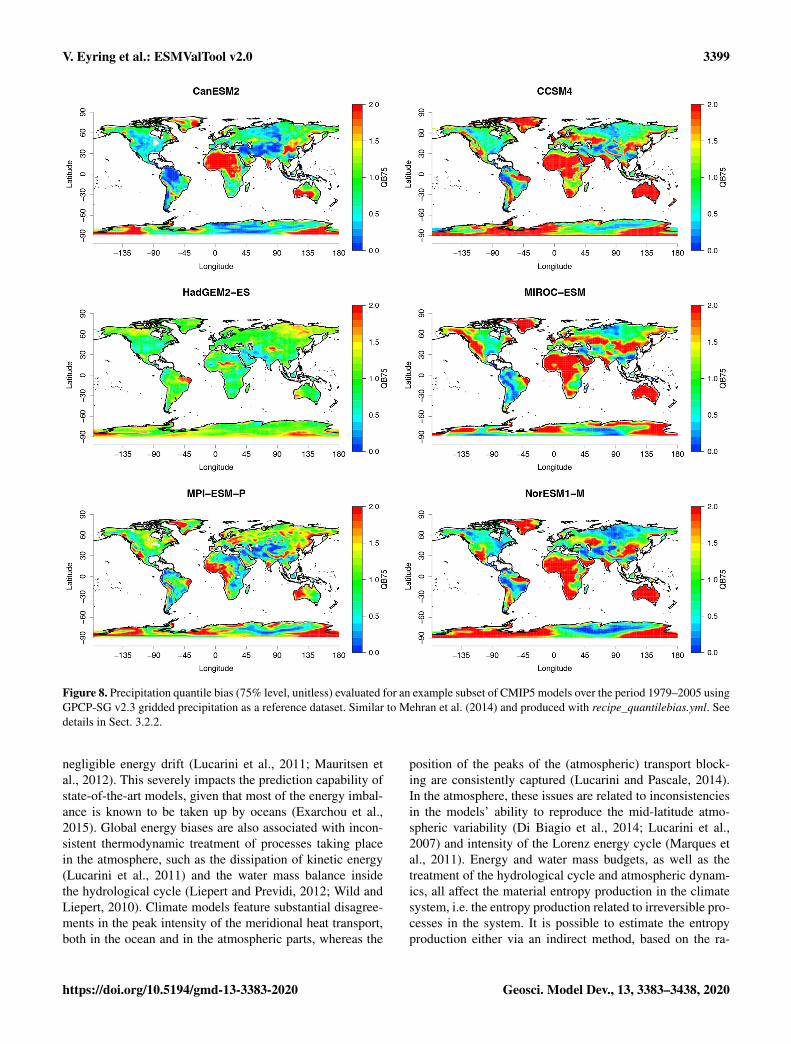
3.2.2 Precipitation quantile bias
Precipitation is a dominant component of the hydrologicalcycle and as such a main driver of the climate system andhuman development. The reliability of climate projectionsand water resource strategies therefore depends on how wellprecipitation can be simulated by the models. While CMIP5models can reproduce the main patterns of mean precipita-tion (e.g. compared to observational data from GPCP; Adleret al., 2003), they often show shortages and biases under par-ticular conditions. Comparison of precipitation from CMIP5models and observations shows a general good agreementfor mean values at a large scale (Kumar et al., 2013; Liuet al., 2012a). Models, however, have a poor representa-tion of frontal, convective, and mesoscale processes, result-ing in substantial biases at a regional scale (Mehran et al.,2014): models tend to overestimate precipitation over com-plex topography and underestimate it especially over arid orsome subcontinental regions as for example northern Eura-sia, eastern Russia, and central Australia. Biases are typicallystronger at high quantiles of precipitation, making the studyof precipitation quantile biases an effective diagnostic for ad-dressing the quality of simulated precipitation.
The recipe_quantilebias.yml implements the calculationof the quantile bias to allow for the evaluation of precipitationbiases based on a user-defined quantile in models as com-pared to a reference dataset following Mehran et al. (2014).The quantile bias is defined as the ratio of monthly precip-itation amounts in each simulation to that of the reference
https://doi.org/10.5194/gmd-13-3383-2020 Geosci. Model Dev., 13, 3383–3438, 2020
3396 V. Eyring et al.: ESMValTool v2.0
Figure 5. Annual-mean surface (2 m) air temperature (◦C) for the period 1980–2005. (a) Multi-model (ensemble) mean constructed withone realization of all available models used in the CMIP5 historical experiment. (b) Multi-model mean bias as the difference between theCMIP5 multi-model mean and the climatology from ECMWF reanalysis of the global atmosphere and surface conditions (ERA)-Interim(Dee et al., 2011). (c) Mean absolute model error with respect to the climatology from ERA-Interim. (d) Mean root-mean-square error of theseasonal cycle with respect to the ERA-Interim. Updated from Fig. 9.2 of IPCC WG I AR5 chap. 9 (Flato et al., 2013) and produced withrecipe_flato13ipcc.yml; see details in Sect. 3.2.1.
dataset above a specified threshold t (e.g. the 75th percentileof all the local monthly values). An example is displayed inFig. 8, where gridded observations from the GPCP projectwere adopted. A quantile bias equal to 1 indicates no biasin the simulations, whereas a value above (below) 1 corre-sponds to a model’s overestimation (underestimation) of theprecipitation amount above the specified threshold t , with re-spect to that of the reference dataset. An overestimation overAfrica for models in the right column and an underestimationcrossing central Asia from Siberia to the Arabic peninsula isvisible, promptly identifying the best performances or out-liers. For example, the HadGEM2-ES model here shows asmaller bias compared to the other models in this subset. Therecipe allows the evaluation of the precipitation bias basedon a user-defined quantile in models as compared to the ref-erence dataset.
3.2.3 Atmospheric dynamics
Stratosphere–troposphere coupling
The current generation of climate models include the repre-sentation of stratospheric processes, as the vertical couplingwith the troposphere is important for the representation ofweather and climate at the surface (Baldwin and Dunker-ton, 2001). Stratosphere-resolving models are able to inter-nally generate realistic annular modes of variability in theextratropical atmosphere (Charlton-Perez et al., 2013) whichare, however, too persistent in the troposphere and delayed inthe stratosphere compared to reanalysis (Gerber et al., 2010),leading to biases in the simulated impacts on surface condi-tions.
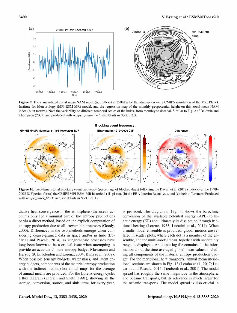
The recipe recipe_zmnam.yml can be used to evaluate therepresentation of the Northern Annular Mode (NAM; Wal-lace, 2000) in climate simulations, using reanalysis datasetsas a reference. The calculation is based on the “zonal mean
Geosci. Model Dev., 13, 3383–3438, 2020 https://doi.org/10.5194/gmd-13-3383-2020
V. Eyring et al.: ESMValTool v2.0 3397
Figure 6. Annual-mean precipitation rate (mm d−1) for the period 1980–2005. (a) Multi-model (ensemble) mean constructed with onerealization of all available models used in the CMIP5 historical experiment. (b) Multi-model mean bias as the difference between the CMIP5multi-model mean and the analyses from the Global Precipitation Climatology Project (Adler et al., 2003). (c) Mean root-mean-square errorof the seasonal cycle with respect to observations. (d) Mean relative model error with respect to observations. Updated from Fig. 9.4 of IPCCWG I AR5 chap. 9 (Flato et al., 2013) and produced with recipe_flato13ipcc.yml; see details in Sect. 3.2.1.
algorithm” of Baldwin and Thompson (2009) and is an alter-native to pressure-based or height-dependent methods. Thisapproach provides a robust description of the stratosphere–troposphere coupling on daily timescales, requiring less sub-jective choices and a reduced amount of input data. Start-ing from daily mean geopotential height on pressure levels,the leading empirical orthogonal functions (EOFs)/principalcomponents are computed from linearly detrended zonalmean daily anomalies, with the principal component repre-senting the zonal mean NAM index. Missing values, whichmay occur near the surface level, are filled with a bilinear in-terpolation procedure. The regression of the monthly meangeopotential height onto this monthly averaged index repre-sents the NAM pattern for each selected pressure level. Theoutputs of the procedure are the time series (Fig. 9a) and thehistogram (not shown) of the zonal-mean NAM index andthe regression maps for selected pressure levels (Fig. 9b).The well-known annular pattern, with opposite anomalies be-tween polar and mid-latitudes, can be seen in the regressionplot. The user can select the specific datasets (climate model
simulation and/or reanalysis) to be evaluated and a subset ofpressure levels of interest.
Atmospheric blocking indices
Atmospheric blocking is a recurrent mid-latitude weatherpattern identified by a large-amplitude, quasi-stationary,long-lasting, high-pressure anomaly that “blocks” the west-erly flow forcing the jet stream to split or meander (Rex,1950). It is typically initiated by the breaking of a Rossbywave in a region at the exit of the storm track, where it am-plifies the underlying stationary ridge (Tibaldi and Molteni,1990). Blocking occurs more frequently in the NorthernHemisphere cold season, with larger frequencies observedover the Euro-Atlantic and North Pacific sectors. Its lifetimeoscillates from a few days up to several weeks (Davini etal., 2012). Atmospheric blocking still represents an open is-sue for the climate modelling community since state-of-the-art weather and climate models show limited skill in repro-ducing it (Davini and D’Andrea, 2016; Masato et al., 2013).
https://doi.org/10.5194/gmd-13-3383-2020 Geosci. Model Dev., 13, 3383–3438, 2020
3398 V. Eyring et al.: ESMValTool v2.0
Figure 7. Anomalies in annual and global mean surface temperature of CMIP5 models and HadCRUT4 observations. Yellow shadingindicates the reference period (1961–1990); vertical dashed grey lines represent times of major volcanic eruptions. The right bar shows theglobal mean surface temperature of the reference period. CMIP5 model data are subsampled by the HadCRUT4 observational data mask andprocessed as described in Jones et al. (2013). All simulations are historical experiments up to and including 2005 and the RCP 4.5 scenarioafter 2005. Extended from Fig. 9.8 of IPCC WG I AR5 chap. 9 (Flato et al., 2013) and produced with recipe_flato13ipcc.yml; see details inSect. 3.2.1.
Models are indeed characterized by large negative bias overthe Euro-Atlantic sector, a region where blocking is often atthe origin of extreme events, leading to cold spells in winterand heat waves in summer (Coumou and Rahmstorf, 2012;Sillmann et al., 2011).
Several objective blocking indices have been developedaimed at identifying different aspects of the phenomenon(see Barriopedro et al., 2010, for details). The reciperecipe_miles_block.yml integrates diagnostics from the Mid-Latitude Evaluation System (MiLES) v0.51 (Davini, 2018)tool in order to calculate two different blocking indices basedon the reversal of the meridional gradient of daily 500 hPageopotential height. The first one is a 1-D index, namely theTibaldi and Molteni (1990) blocking index, here adapted towork with 2.5◦× 2.5◦ grids. Blocking is defined when thereversal of the meridional gradient of geopotential heightat 60◦ N is detected, i.e. when easterly winds are found inthe mid-latitudes. The second one is the atmospheric block-ing index following Davini et al. (2012). It is a 2-D exten-sion of Tibaldi and Molteni (1990) covering latitudes from30 up to 75◦ N. The recipe computes both the instanta-neous blocking frequencies and the blocking event frequency(which includes both spatial and 5 d minimum temporal con-straints). It reports also two intensity indices, namely theMeridional Gradient Index and the Blocking Intensity in-dex, and it evaluates the wave-breaking characteristic asso-ciated with blocking (cyclonic or anticyclonic) through theRossby wave orientation index. A supplementary instanta-
neous blocking index (named “ExtraBlock”) including an ex-tra condition to filter out low-latitude blocking events is alsoprovided. The recipe compares multiple datasets against areference one (the default is ERA-Interim) and provides out-put (in netCDF4 compressed Zip format) as well as figuresfor the climatology of each diagnostic. An example output isshown in Fig. 10. The Max Planck Institute for Meteorology(MPI-ESM-MR) model shows the well-known underestima-tion of atmospheric blocking – typical of many climate mod-els – over central Europe, where blocking frequencies areabout the half when compared to reanalysis. A slight overes-timation of low-latitude blocking and North Pacific blockingcan also be seen, while Greenland blocking frequencies shownegligible bias.
3.2.4 Thermodynamics of the climate system
The climate system can be seen as a forced and dissipa-tive non-equilibrium thermodynamic system (Lucarini et al.,2014), converting potential into mechanical energy, and gen-erating entropy via a variety of irreversible processes Theatmospheric and oceanic circulation are caused by the in-homogeneous absorption of solar radiation, and, all in all,they act in such a way as to reduce the temperature gradientsacross the climate system. At steady state, assuming station-arity, the long-term global energy input and output shouldbalance. Previous studies have shown that this is essentiallynot the case, and most of the models are affected by non-
Geosci. Model Dev., 13, 3383–3438, 2020 https://doi.org/10.5194/gmd-13-3383-2020
V. Eyring et al.: ESMValTool v2.0 3399
Figure 8. Precipitation quantile bias (75% level, unitless) evaluated for an example subset of CMIP5 models over the period 1979–2005 usingGPCP-SG v2.3 gridded precipitation as a reference dataset. Similar to Mehran et al. (2014) and produced with recipe_quantilebias.yml. Seedetails in Sect. 3.2.2.
negligible energy drift (Lucarini et al., 2011; Mauritsen etal., 2012). This severely impacts the prediction capability ofstate-of-the-art models, given that most of the energy imbal-ance is known to be taken up by oceans (Exarchou et al.,2015). Global energy biases are also associated with incon-sistent thermodynamic treatment of processes taking placein the atmosphere, such as the dissipation of kinetic energy(Lucarini et al., 2011) and the water mass balance insidethe hydrological cycle (Liepert and Previdi, 2012; Wild andLiepert, 2010). Climate models feature substantial disagree-ments in the peak intensity of the meridional heat transport,both in the ocean and in the atmospheric parts, whereas the
position of the peaks of the (atmospheric) transport block-ing are consistently captured (Lucarini and Pascale, 2014).In the atmosphere, these issues are related to inconsistenciesin the models’ ability to reproduce the mid-latitude atmo-spheric variability (Di Biagio et al., 2014; Lucarini et al.,2007) and intensity of the Lorenz energy cycle (Marques etal., 2011). Energy and water mass budgets, as well as thetreatment of the hydrological cycle and atmospheric dynam-ics, all affect the material entropy production in the climatesystem, i.e. the entropy production related to irreversible pro-cesses in the system. It is possible to estimate the entropyproduction either via an indirect method, based on the ra-
https://doi.org/10.5194/gmd-13-3383-2020 Geosci. Model Dev., 13, 3383–3438, 2020
3400 V. Eyring et al.: ESMValTool v2.0
Figure 9. The standardized zonal mean NAM index (a, unitless) at 250 hPa for the atmosphere-only CMIP5 simulation of the Max PlanckInstitute for Meteorology (MPI-ESM-MR) model, and the regression map of the monthly geopotential height on this zonal-mean NAMindex (b, in metres). Note the variability on different temporal scales of the index, from monthly to decadal. Similar to Fig. 2 of Baldwin andThompson (2009) and produced with recipe_zmnam.yml; see details in Sect. 3.2.3.
Figure 10. Two-dimensional blocking event frequency (percentage of blocked days) following the Davini et al. (2012) index over the 1979–2005 DJF period for (a) the CMIP5 MPI-ESM-MR historical r1i1p1 run, (b) the ERA-Interim Reanalysis, and (c) their differences. Producedwith recipe_miles_block.yml; see details in Sect. 3.2.3.2.
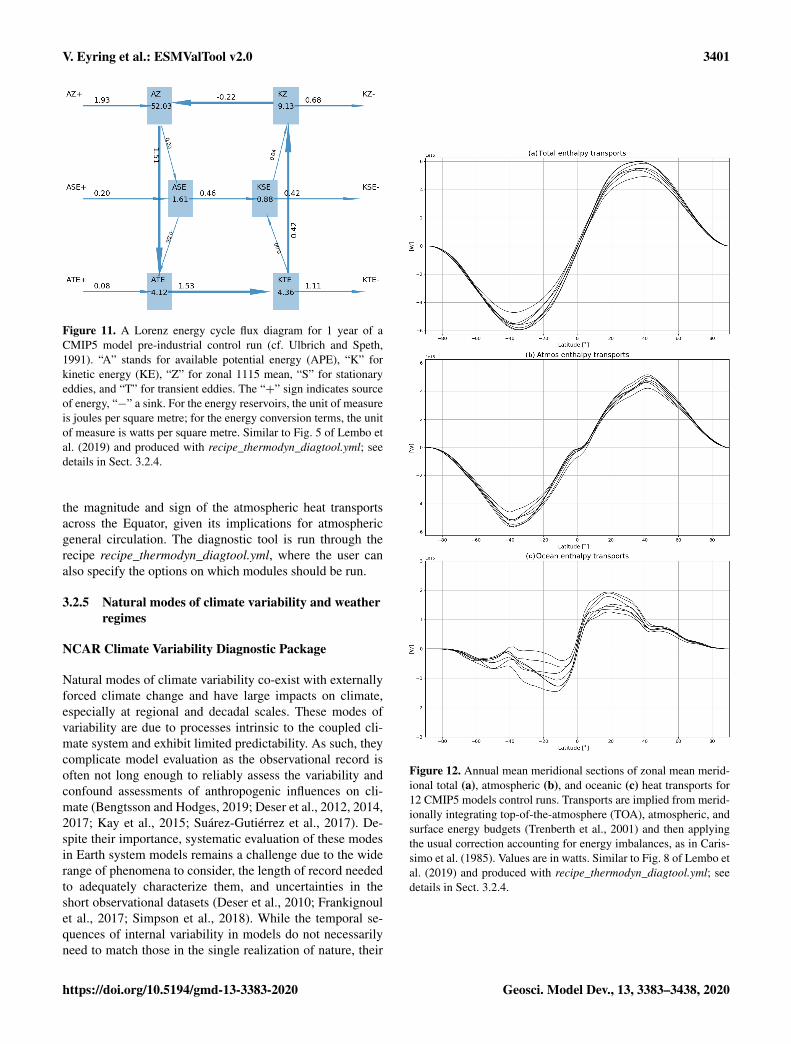
diative heat convergence in the atmosphere (the ocean ac-counts only for a minimal part of the entropy production)or via a direct method, based on the explicit computation ofentropy production due to all irreversible processes (Goody,2000). Differences in the two methods emerge when con-sidering coarse-grained data in space and/or in time (Lu-carini and Pascale, 2014), as subgrid-scale processes havelong been known to be a critical issue when attempting toprovide an accurate climate entropy budget (Gassmann andHerzog, 2015; Kleidon and Lorenz, 2004; Kunz et al., 2008).When possible (energy budgets, water mass, and latent en-ergy budgets, components of the material entropy productionwith the indirect method) horizontal maps for the averageof annual means are provided. For the Lorenz energy cycle,a flux diagram (Ulbrich and Speth, 1991), showing all thestorage, conversion, source, and sink terms for every year,
is provided. The diagram in Fig. 11 shows the baroclinicconversion of the available potential energy (APE) to ki-netic energy (KE) and ultimately its dissipation through fric-tional heating (Lorenz, 1955; Lucarini et al., 2014). Whena multi-model ensemble is provided, global metrics are re-lated in scatter plots, where each dot is a member of the en-semble, and the multi-model mean, together with uncertaintyrange, is displayed. An output log file contains all the infor-mation about the time-averaged global mean values, includ-ing all components of the material entropy production bud-get. For the meridional heat transports, annual mean merid-ional sections are shown in Fig. 12 (Lembo et al., 2017; Lu-carini and Pascale, 2014; Trenberth et al., 2001). The modelspread has roughly the same magnitude in the atmosphericand oceanic transports, but its relevance is much larger forthe oceanic transports. The model spread is also crucial in
Geosci. Model Dev., 13, 3383–3438, 2020 https://doi.org/10.5194/gmd-13-3383-2020
V. Eyring et al.: ESMValTool v2.0 3401
Figure 11. A Lorenz energy cycle flux diagram for 1 year of aCMIP5 model pre-industrial control run (cf. Ulbrich and Speth,1991). “A” stands for available potential energy (APE), “K” forkinetic energy (KE), “Z” for zonal 1115 mean, “S” for stationaryeddies, and “T” for transient eddies. The “+” sign indicates sourceof energy, “−” a sink. For the energy reservoirs, the unit of measureis joules per square metre; for the energy conversion terms, the unitof measure is watts per square metre. Similar to Fig. 5 of Lembo etal. (2019) and produced with recipe_thermodyn_diagtool.yml; seedetails in Sect. 3.2.4.
the magnitude and sign of the atmospheric heat transportsacross the Equator, given its implications for atmosphericgeneral circulation. The diagnostic tool is run through therecipe recipe_thermodyn_diagtool.yml, where the user canalso specify the options on which modules should be run.
3.2.5 Natural modes of climate variability and weatherregimes
NCAR Climate Variability Diagnostic Package
Natural modes of climate variability co-exist with externallyforced climate change and have large impacts on climate,especially at regional and decadal scales. These modes ofvariability are due to processes intrinsic to the coupled cli-mate system and exhibit limited predictability. As such, theycomplicate model evaluation as the observational record isoften not long enough to reliably assess the variability andconfound assessments of anthropogenic influences on cli-mate (Bengtsson and Hodges, 2019; Deser et al., 2012, 2014,2017; Kay et al., 2015; Suárez-Gutiérrez et al., 2017). De-spite their importance, systematic evaluation of these modesin Earth system models remains a challenge due to the widerange of phenomena to consider, the length of record neededto adequately characterize them, and uncertainties in theshort observational datasets (Deser et al., 2010; Frankignoulet al., 2017; Simpson et al., 2018). While the temporal se-quences of internal variability in models do not necessarilyneed to match those in the single realization of nature, their
Figure 12. Annual mean meridional sections of zonal mean merid-ional total (a), atmospheric (b), and oceanic (c) heat transports for12 CMIP5 models control runs. Transports are implied from merid-ionally integrating top-of-the-atmosphere (TOA), atmospheric, andsurface energy budgets (Trenberth et al., 2001) and then applyingthe usual correction accounting for energy imbalances, as in Caris-simo et al. (1985). Values are in watts. Similar to Fig. 8 of Lembo etal. (2019) and produced with recipe_thermodyn_diagtool.yml; seedetails in Sect. 3.2.4.
https://doi.org/10.5194/gmd-13-3383-2020 Geosci. Model Dev., 13, 3383–3438, 2020
3402 V. Eyring et al.: ESMValTool v2.0
statistical properties (e.g. timescale, autocorrelation, spectralcharacteristics, and spatial patterns) need to be realisticallysimulated for credible climate projections.
In order to assess natural modes of climate variability inmodels, the NCAR Climate Variability Diagnostics Package(CVDP; Phillips et al., 2014) has been implemented into ES-MValTool. The CVDP has been developed as a standalonetool. To allow for easy updating of the CVDP once a newversion is released, the structure of the CVDP is kept inits original form and a single recipe recipe_CVDP.yml hasbeen written to enable the CVDP to be run directly withinESMValTool. The CVDP facilitates evaluation of the ma-jor modes of climate variability, including ENSO (Deser etal., 2010), the Pacific Decadal Oscillation (PDO; Deser etal., 2010; Mantua et al., 1997), the Atlantic Multi-decadalOscillation (AMO; Trenberth and Shea, 2006), the AtlanticMeridional Overturning Circulation (AMOC; Danabasogluet al., 2012), and atmospheric teleconnection patterns suchas the Northern and Southern Annular Modes (NAM andSAM; Hurrell and Deser, 2009; Thompson and Wallace,2000), North Atlantic Oscillation (NAO; Hurrell and Deser,2009), and Pacific North and South American (PNA andPSA; Thompson and Wallace, 2000) patterns. For details onthe actual calculation of these modes in CVDP we refer tothe original CVDP package and explanations available athttp://www.cesm.ucar.edu/working_groups/CVC/cvdp/ (lastaccess: 13 July 2020).
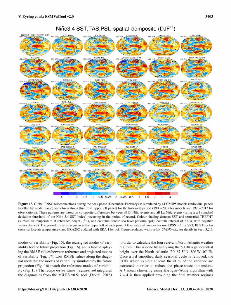
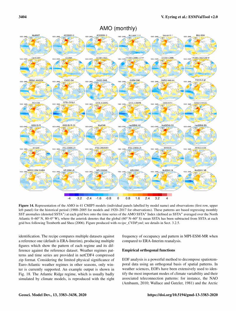
Depending on the climate mode analysed, the CVDPpackage uses the following variables: precipitation (pr), sealevel pressure (psl), near-surface air temperature (tas), skintemperature (ts), snow depth (snd), sea ice concentration(siconc), and basin-average ocean meridional overturningmass stream function (msftmz). The models are evaluatedagainst a wide range of observations and reanalysis data, forexample, the Berkeley Earth System Temperature (BEST)for near-surface air temperature, the Extended ReconstructedSea Surface Temperature v5 (ERSSTv5) for skin tempera-ture, and ERA-20C extended with ERA-Interim for sea levelpressure. Additional observations or reanalysis can be addedby the user for these variables. The ESMValTool v2.0 reciperuns on all CMIP5 models. As an example, Fig. 13 showsthe representation of ENSO teleconnections during the peakphase (December–February). Models produce a wide rangeof ENSO amplitudes and teleconnections. Note that evenwhen based on over 100 years of record, the ENSO com-posites are subject to uncertainty due to sampling variabil-ity (Deser et al., 2017). Figure 14 shows the representationof the AMO as simulated by 41 CMIP5 models and obser-vations during the historical period. The pattern of SSTA∗
associated with the AMO is generally realistically simulatedby models within the North Atlantic basin, although its am-plitude varies. However, outside of the North Atlantic, themodels show a wide range of spatial patterns and polaritiesof the AMO.
Weather regimes
Weather regimes (WRs) refer to recurrent large-scale at-mospheric circulation structures that allow the characteriza-tion of complex atmospheric dynamics in a particular region(Michelangeli et al., 1995; Vautard, 1990). The identifica-tion of WRs reduces the continuum of atmospheric circula-tion to a few recurrent and quasi-stationary (persistent) pat-terns. WRs have been extensively used to investigate atmo-spheric variability in the mid-latitudes, as they are associatedwith extreme weather events such as heat waves or droughts(Yiou et al., 2008). For example, there is a growing recog-nition of their significance especially over the Euro-Atlanticsector during the winter season, where four robust weatherregimes have been identified – namely the NAO+, NAO−,Atlantic Ridge, and Scandinavian Blocking (Cassou et al.,2005). These WRs can also be used as a diagnostic to investi-gate the performance of state-of-the-art climate forecast sys-tems: difficulties in reproducing the Atlantic Ridge and theScandinavian Blocking have been often reported (Dawson etal., 2012; Ferranti et al., 2015). Forecast systems which arenot able to reproduce the observed spatial patterns and fre-quency of occurrence of WRs may have difficulties in repro-ducing climate variability and its long-term changes (Han-nachi et al., 2017). Hence, the assessment of WRs can helpimprove our understanding of predictability on intra-seasonalto interannual timescales. In addition, the use of WRs toevaluate the impact of the atmospheric circulation on essen-tial climate variables and sectoral climatic indices is of greatinterest to the climate services communities (Grams et al.,2017). The diagnostic can be applied to model simulationsunder future scenarios as well. However, caution must be ap-plied since large changes in the average climate, due to largeradiative forcing, might affect the results and lead to some-what misleading conclusions. In such cases further analysiswill be needed to assess to what extent the response to cli-mate change projects on the regimes patterns identified bythe tool in the historical and future periods and to verify howfuture anomalies project onto the regime patterns identifiedin the historical period.
The recipe recipe_modes_of_variability.yml takes daily ormonthly data from a particular region, season (or month), andperiod as input and then applies k mean clustering or hierar-chical clustering either directly to the spatial data or aftercomputing the EOFs. This recipe can be run for both a refer-ence or observational dataset and climate projections simul-taneously, and the root-mean-square error is then calculatedbetween the mean anomalies obtained for the clusters fromthe reference and projection datasets. The user can specifythe number of clusters to be computed. The recipe outputconsists of netCDF files of the time series of the cluster oc-currences, the mean anomaly corresponding to each clusterat each location and the corresponding p value, for both theobserved and projected WR and the RMSE between them.The recipe also creates three plots: the observed or reference
Geosci. Model Dev., 13, 3383–3438, 2020 https://doi.org/10.5194/gmd-13-3383-2020
V. Eyring et al.: ESMValTool v2.0 3403
Figure 13. Global ENSO teleconnections during the peak phase (December–February) as simulated by 41 CMIP5 models (individual panelslabelled by model name) and observations (first row, upper left panel) for the historical period (1900–2005 for models and 1920–2017 forobservations). These patterns are based on composite differences between all El Niño events and all La Niña events (using a ±1 standarddeviation threshold of the Niño 3.4 SST Index) occurring in the period of record. Colour shading denotes SST and terrestrial TREFHT(surface air temperature at reference height) (◦C), and contours denote sea level pressure (psl); contour interval of 2 hPa, with negativevalues dashed). The period of record is given in the upper left of each panel. Observational composites use ERSSTv5 for SST, BEST for tas(near-surface air temperature), and ERA20C updated with ERA-I for psl. Figure produced with recipe_CVDP.yml.; see details in Sect. 3.2.5.
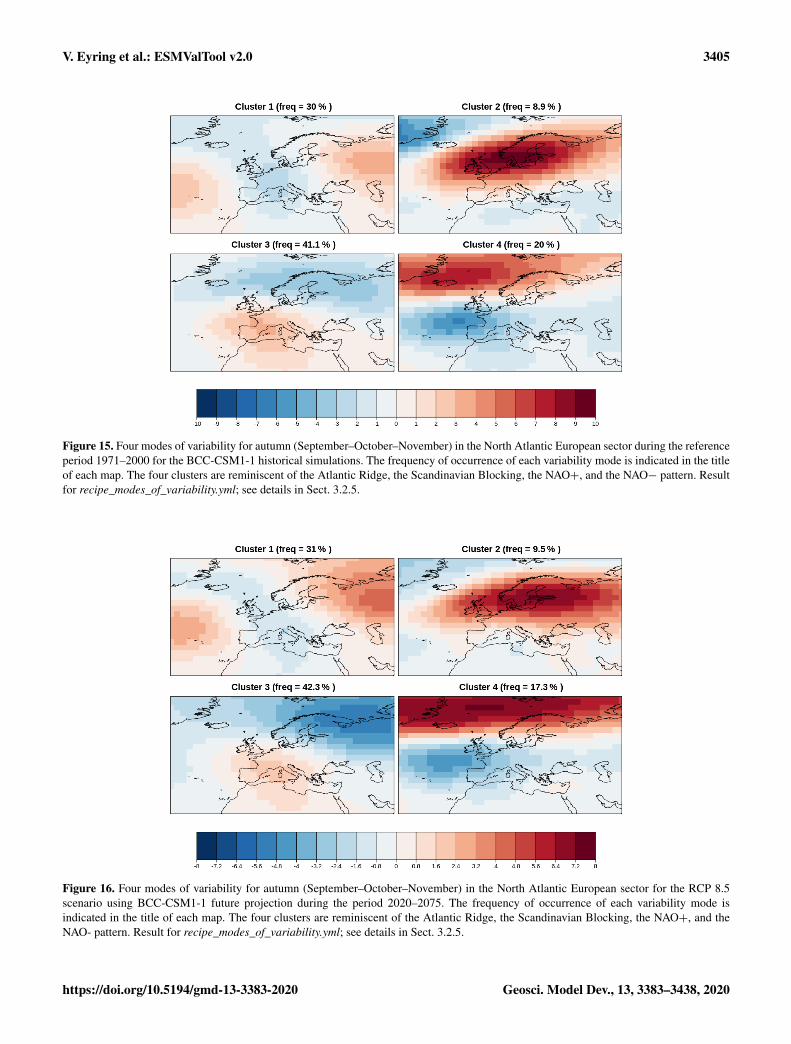
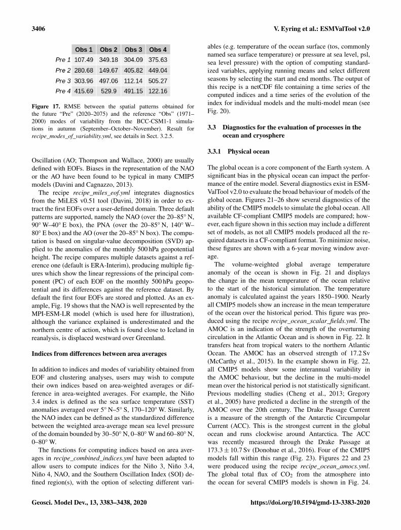
modes of variability (Fig. 15), the reassigned modes of vari-ability for the future projection (Fig. 16), and a table display-ing the RMSE values between reference and projected modesof variability (Fig. 17). Low RMSE values along the diago-nal show that the modes of variability simulated by the futureprojection (Fig. 16) match the reference modes of variabil-ity (Fig. 15). The recipe recipe_miles_regimes.yml integratesthe diagnostics from the MiLES v0.51 tool (Davini, 2018)
in order to calculate the four relevant North Atlantic weatherregimes. This is done by analysing the 500 hPa geopotentialheight over the North Atlantic (30–87.5◦ N, 80◦W–40◦ E).Once a 5 d smoothed daily seasonal cycle is removed, theEOFs which explain at least the 80 % of the variance areextracted in order to reduce the phase-space dimensions.A k mean clustering using Hartigan–Wong algorithm withk = 4 is then applied providing the final weather regimes
https://doi.org/10.5194/gmd-13-3383-2020 Geosci. Model Dev., 13, 3383–3438, 2020
3404 V. Eyring et al.: ESMValTool v2.0
Figure 14. Representation of the AMO in 41 CMIP5 models (individual panels labelled by model name) and observations (first row, upperleft panel) for the historical period (1900–2005 for models and 1920–2017 for observations). These patterns are based regressing monthlySST anomalies (denoted SSTA∗) at each grid box onto the time series of the AMO SSTA∗ Index (defined as SSTA∗ averaged over the NorthAtlantic 0–60◦ N, 80–0◦W), where the asterisk denotes that the global (60◦ N–60◦ S) mean SSTA has been subtracted from SSTA at eachgrid box following Trenberth and Shea (2006). Figure produced with recipe_CVDP.yml; see details in Sect. 3.2.5.
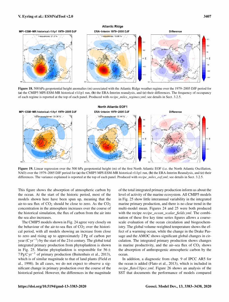
identification. The recipe compares multiple datasets againsta reference one (default is ERA-Interim), producing multiplefigures which show the pattern of each regime and its dif-ference against the reference dataset. Weather regimes pat-terns and time series are provided in netCDF4 compressedzip format. Considering the limited physical significance ofEuro-Atlantic weather regimes in other seasons, only win-ter is currently supported. An example output is shown inFig. 18. The Atlantic Ridge regime, which is usually badlysimulated by climate models, is reproduced with the right
frequency of occupancy and pattern in MPI-ESM-MR whencompared to ERA-Interim reanalysis.
Empirical orthogonal functions
EOF analysis is a powerful method to decompose spatiotem-poral data using an orthogonal basis of spatial patterns. Inweather sciences, EOFs have been extensively used to iden-tify the most important modes of climate variability and theirassociated teleconnection patterns: for instance, the NAO(Ambaum, 2010; Wallace and Gutzler, 1981) and the Arctic
Geosci. Model Dev., 13, 3383–3438, 2020 https://doi.org/10.5194/gmd-13-3383-2020
V. Eyring et al.: ESMValTool v2.0 3405
Figure 15. Four modes of variability for autumn (September–October–November) in the North Atlantic European sector during the referenceperiod 1971–2000 for the BCC-CSM1-1 historical simulations. The frequency of occurrence of each variability mode is indicated in the titleof each map. The four clusters are reminiscent of the Atlantic Ridge, the Scandinavian Blocking, the NAO+, and the NAO− pattern. Resultfor recipe_modes_of_variability.yml; see details in Sect. 3.2.5.
Figure 16. Four modes of variability for autumn (September–October–November) in the North Atlantic European sector for the RCP 8.5scenario using BCC-CSM1-1 future projection during the period 2020–2075. The frequency of occurrence of each variability mode isindicated in the title of each map. The four clusters are reminiscent of the Atlantic Ridge, the Scandinavian Blocking, the NAO+, and theNAO- pattern. Result for recipe_modes_of_variability.yml; see details in Sect. 3.2.5.
https://doi.org/10.5194/gmd-13-3383-2020 Geosci. Model Dev., 13, 3383–3438, 2020
3406 V. Eyring et al.: ESMValTool v2.0
Figure 17. RMSE between the spatial patterns obtained forthe future “Pre” (2020–2075) and the reference “Obs” (1971–2000) modes of variability from the BCC-CSM1-1 simula-tions in autumn (September–October–November). Result forrecipe_modes_of_variability.yml, see details in Sect. 3.2.5.
Oscillation (AO; Thompson and Wallace, 2000) are usuallydefined with EOFs. Biases in the representation of the NAOor the AO have been found to be typical in many CMIP5models (Davini and Cagnazzo, 2013).
The recipe recipe_miles_eof.yml integrates diagnosticsfrom the MiLES v0.51 tool (Davini, 2018) in order to ex-tract the first EOFs over a user-defined domain. Three defaultpatterns are supported, namely the NAO (over the 20–85◦ N,90◦W–40◦ E box), the PNA (over the 20–85◦ N, 140◦W–80◦ E box) and the AO (over the 20–85◦ N box). The compu-tation is based on singular-value decomposition (SVD) ap-plied to the anomalies of the monthly 500 hPa geopotentialheight. The recipe compares multiple datasets against a ref-erence one (default is ERA-Interim), producing multiple fig-ures which show the linear regressions of the principal com-ponent (PC) of each EOF on the monthly 500 hPa geopo-tential and its differences against the reference dataset. Bydefault the first four EOFs are stored and plotted. As an ex-ample, Fig. 19 shows that the NAO is well represented by theMPI-ESM-LR model (which is used here for illustration),although the variance explained is underestimated and thenorthern centre of action, which is found close to Iceland inreanalysis, is displaced westward over Greenland.
Indices from differences between area averages
In addition to indices and modes of variability obtained fromEOF and clustering analyses, users may wish to computetheir own indices based on area-weighted averages or dif-ference in area-weighted averages. For example, the Niño3.4 index is defined as the sea surface temperature (SST)anomalies averaged over 5◦ N–5◦ S, 170–120◦W. Similarly,the NAO index can be defined as the standardized differencebetween the weighted area-average mean sea level pressureof the domain bounded by 30–50◦ N, 0–80◦W and 60–80◦ N,0–80◦W.
The functions for computing indices based on area aver-ages in recipe_combined_indices.yml have been adapted toallow users to compute indices for the Niño 3, Niño 3.4,Niño 4, NAO, and the Southern Oscillation Index (SOI) de-fined region(s), with the option of selecting different vari-
ables (e.g. temperature of the ocean surface (tos, commonlynamed sea surface temperature) or pressure at sea level, psl,sea level pressure) with the option of computing standard-ized variables, applying running means and select differentseasons by selecting the start and end months. The output ofthis recipe is a netCDF file containing a time series of thecomputed indices and a time series of the evolution of theindex for individual models and the multi-model mean (seeFig. 20).
3.3 Diagnostics for the evaluation of processes in theocean and cryosphere
3.3.1 Physical ocean
The global ocean is a core component of the Earth system. Asignificant bias in the physical ocean can impact the perfor-mance of the entire model. Several diagnostics exist in ESM-ValTool v2.0 to evaluate the broad behaviour of models of theglobal ocean. Figures 21–26 show several diagnostics of theability of the CMIP5 models to simulate the global ocean. Allavailable CF-compliant CMIP5 models are compared; how-ever, each figure shown in this section may include a differentset of models, as not all CMIP5 models produced all the re-quired datasets in a CF-compliant format. To minimize noise,these figures are shown with a 6-year moving window aver-age.
The volume-weighted global average temperatureanomaly of the ocean is shown in Fig. 21 and displaysthe change in the mean temperature of the ocean relativeto the start of the historical simulation. The temperatureanomaly is calculated against the years 1850–1900. Nearlyall CMIP5 models show an increase in the mean temperatureof the ocean over the historical period. This figure was pro-duced using the recipe recipe_ocean_scalar_fields.yml. TheAMOC is an indication of the strength of the overturningcirculation in the Atlantic Ocean and is shown in Fig. 22. Ittransfers heat from tropical waters to the northern AtlanticOcean. The AMOC has an observed strength of 17.2 Sv(McCarthy et al., 2015). In the example shown in Fig. 22,all CMIP5 models show some interannual variability inthe AMOC behaviour, but the decline in the multi-modelmean over the historical period is not statistically significant.Previous modelling studies (Cheng et al., 2013; Gregoryet al., 2005) have predicted a decline in the strength of theAMOC over the 20th century. The Drake Passage Currentis a measure of the strength of the Antarctic CircumpolarCurrent (ACC). This is the strongest current in the globalocean and runs clockwise around Antarctica. The ACCwas recently measured through the Drake Passage at173.3± 10.7 Sv (Donohue et al., 2016). Four of the CMIP5models fall within this range (Fig. 23). Figures 22 and 23were produced using the recipe recipe_ocean_amocs.yml.The global total flux of CO2 from the atmosphere intothe ocean for several CMIP5 models is shown in Fig. 24.
Geosci. Model Dev., 13, 3383–3438, 2020 https://doi.org/10.5194/gmd-13-3383-2020
V. Eyring et al.: ESMValTool v2.0 3407
Figure 18. 500 hPa geopotential height anomalies (m) associated with the Atlantic Ridge weather regime over the 1979–2005 DJF period for(a) the CMIP5 MPI-ESM-MR historical r1i1p1 run, (b) the ERA-Interim reanalysis, and (c) their differences. The frequency of occupancyof each regime is reported at the top of each panel. Produced with recipe_miles_regimes.yml; see details in Sect. 3.2.5.
Figure 19. Linear regression over the 500 hPa geopotential height (m) of the first North Atlantic EOF (i.e. the North Atlantic Oscillation,NAO) over the 1979–2005 DJF period for (a) the CMIP5 MPI-ESM-MR historical r1i1p1 run, (b) the ERA-Interim Reanalysis, and (c) theirdifferences. The variance explained is reported at the top of each panel. Produced with recipe_miles_eof.yml; see details in Sect. 3.2.5.
This figure shows the absorption of atmospheric carbon bythe ocean. At the start of the historic period, most of themodels shown here have been spun up, meaning that theair-to-sea flux of CO2 should be close to zero. As the CO2concentration in the atmosphere increases over the course ofthe historical simulation, the flux of carbon from the air intothe sea also increases.
The CMIP5 models shown in Fig. 24 agree very closely onthe behaviour of the air-to-sea flux of CO2 over the histori-cal period, with all models showing an increase from closeto zero and rising up to approximately 2 Pg of carbon peryear (C yr−1) by the start of the 21st century. The global totalintegrated primary production from phytoplankton is shownin Fig. 25. Marine phytoplankton is responsible for 56±7 Pg C yr−1 of primary production (Buitenhuis et al., 2013),which is of similar magnitude to that of land plants (Field etal., 1998). In all cases, we do not expect to observe a sig-nificant change in primary production over the course of thehistorical period. However, the differences in the magnitude
of the total integrated primary production inform us about thelevel of activity of the marine ecosystem. All CMIP5 modelsin Fig. 25 show little interannual variability in the integratedmarine primary production, and there is no clear trend in themulti-model mean. Figures 24 and 25 were both producedwith the recipe recipe_ocean_scalar_fields.yml. The combi-nation of these five key time series figures allows a coarse-scale evaluation of the ocean circulation and biogeochem-istry. The global volume-weighted temperature shows the ef-fect of a warming ocean, while the change in the Drake Pas-sage and the AMOC shows significant global changes in cir-culation. The integrated primary production shows changesin marine productivity, and the air–sea flux of CO2 showsthe absorption of anthropogenic atmospheric carbon by theocean.
In addition, a diagnostic from chap. 9 of IPCC AR5 forthe ocean is added (Flato et al., 2013), which is included inrecipe_flato13ipcc.yml. Figure 26 shows an analysis of theSST that documents the performance of models compared
https://doi.org/10.5194/gmd-13-3383-2020 Geosci. Model Dev., 13, 3383–3438, 2020
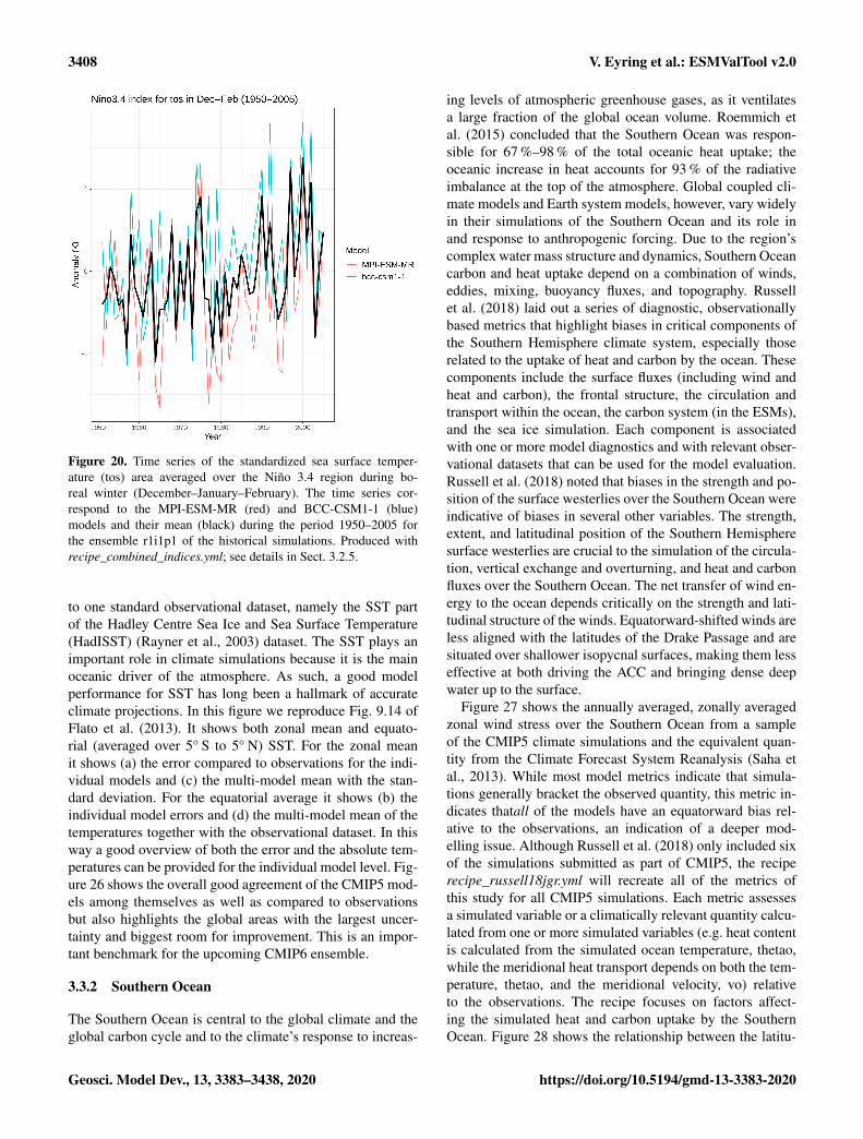
3408 V. Eyring et al.: ESMValTool v2.0
Figure 20. Time series of the standardized sea surface temper-ature (tos) area averaged over the Niño 3.4 region during bo-real winter (December–January–February). The time series cor-respond to the MPI-ESM-MR (red) and BCC-CSM1-1 (blue)models and their mean (black) during the period 1950–2005 forthe ensemble r1i1p1 of the historical simulations. Produced withrecipe_combined_indices.yml; see details in Sect. 3.2.5.
to one standard observational dataset, namely the SST partof the Hadley Centre Sea Ice and Sea Surface Temperature(HadISST) (Rayner et al., 2003) dataset. The SST plays animportant role in climate simulations because it is the mainoceanic driver of the atmosphere. As such, a good modelperformance for SST has long been a hallmark of accurateclimate projections. In this figure we reproduce Fig. 9.14 ofFlato et al. (2013). It shows both zonal mean and equato-rial (averaged over 5◦ S to 5◦ N) SST. For the zonal meanit shows (a) the error compared to observations for the indi-vidual models and (c) the multi-model mean with the stan-dard deviation. For the equatorial average it shows (b) theindividual model errors and (d) the multi-model mean of thetemperatures together with the observational dataset. In thisway a good overview of both the error and the absolute tem-peratures can be provided for the individual model level. Fig-ure 26 shows the overall good agreement of the CMIP5 mod-els among themselves as well as compared to observationsbut also highlights the global areas with the largest uncer-tainty and biggest room for improvement. This is an impor-tant benchmark for the upcoming CMIP6 ensemble.
3.3.2 Southern Ocean
The Southern Ocean is central to the global climate and theglobal carbon cycle and to the climate’s response to increas-
ing levels of atmospheric greenhouse gases, as it ventilatesa large fraction of the global ocean volume. Roemmich etal. (2015) concluded that the Southern Ocean was respon-sible for 67 %–98 % of the total oceanic heat uptake; theoceanic increase in heat accounts for 93 % of the radiativeimbalance at the top of the atmosphere. Global coupled cli-mate models and Earth system models, however, vary widelyin their simulations of the Southern Ocean and its role inand response to anthropogenic forcing. Due to the region’scomplex water mass structure and dynamics, Southern Oceancarbon and heat uptake depend on a combination of winds,eddies, mixing, buoyancy fluxes, and topography. Russellet al. (2018) laid out a series of diagnostic, observationallybased metrics that highlight biases in critical components ofthe Southern Hemisphere climate system, especially thoserelated to the uptake of heat and carbon by the ocean. Thesecomponents include the surface fluxes (including wind andheat and carbon), the frontal structure, the circulation andtransport within the ocean, the carbon system (in the ESMs),and the sea ice simulation. Each component is associatedwith one or more model diagnostics and with relevant obser-vational datasets that can be used for the model evaluation.Russell et al. (2018) noted that biases in the strength and po-sition of the surface westerlies over the Southern Ocean wereindicative of biases in several other variables. The strength,extent, and latitudinal position of the Southern Hemispheresurface westerlies are crucial to the simulation of the circula-tion, vertical exchange and overturning, and heat and carbonfluxes over the Southern Ocean. The net transfer of wind en-ergy to the ocean depends critically on the strength and lati-tudinal structure of the winds. Equatorward-shifted winds areless aligned with the latitudes of the Drake Passage and aresituated over shallower isopycnal surfaces, making them lesseffective at both driving the ACC and bringing dense deepwater up to the surface.
Figure 27 shows the annually averaged, zonally averagedzonal wind stress over the Southern Ocean from a sampleof the CMIP5 climate simulations and the equivalent quan-tity from the Climate Forecast System Reanalysis (Saha etal., 2013). While most model metrics indicate that simula-tions generally bracket the observed quantity, this metric in-dicates thatall of the models have an equatorward bias rel-ative to the observations, an indication of a deeper mod-elling issue. Although Russell et al. (2018) only included sixof the simulations submitted as part of CMIP5, the reciperecipe_russell18jgr.yml will recreate all of the metrics ofthis study for all CMIP5 simulations. Each metric assessesa simulated variable or a climatically relevant quantity calcu-lated from one or more simulated variables (e.g. heat contentis calculated from the simulated ocean temperature, thetao,while the meridional heat transport depends on both the tem-perature, thetao, and the meridional velocity, vo) relativeto the observations. The recipe focuses on factors affect-ing the simulated heat and carbon uptake by the SouthernOcean. Figure 28 shows the relationship between the latitu-
Geosci. Model Dev., 13, 3383–3438, 2020 https://doi.org/10.5194/gmd-13-3383-2020

V. Eyring et al.: ESMValTool v2.0 3409
Figure 21. The volume-weighted thermosteric sea level change anomaly in several CMIP5 models, in the historical experiment, and inthe r1i1p1 ensemble member, with a 6-year moving average smoothing function. The anomaly is calculated against the mean of all yearsin the historical experiment before 1900. The multi-model mean is shown as a dashed line. Produced with recipe_ocean_scalar_fields.ymldescribed in Sect. 3.3.1.
Figure 22. The Atlantic Meridional Overturn Circulation (AMOC) in several CMIP5 models, in the historical experiment, and in the r1i1p1ensemble member, with a 6-year moving average smoothing function. The multi-model mean is shown as a dashed line. The AMOC in-dicates the strength of the northbound current and this current transfers heat from tropical water to the North Atlantic. Produced withrecipe_ocean_amoc.yml described in Sect. 3.3.1.
dinal width of the surface westerly winds over the SouthernOcean with the net heat uptake south of 30◦ S – the correla-tion (−0.8) is significant above the 98 % level.
3.3.3 Arctic Ocean
The Arctic Ocean is one of the areas of the Earth where theeffects of climate change are especially visible today. The
two most prominent processes are Arctic atmospheric tem-perature warming amplification (Serreze and Barry, 2011)and a decrease in the sea ice area and thickness (seeSect. 3.3.2). Both receive good coverage in the literature andare already well-studied. Much less attention is paid to theinterior of the Arctic Ocean itself. In order to increase our
https://doi.org/10.5194/gmd-13-3383-2020 Geosci. Model Dev., 13, 3383–3438, 2020
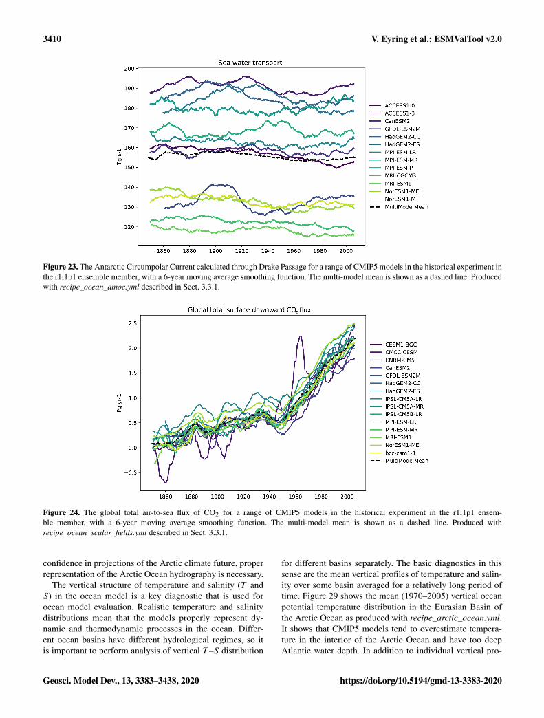
3410 V. Eyring et al.: ESMValTool v2.0
Figure 23. The Antarctic Circumpolar Current calculated through Drake Passage for a range of CMIP5 models in the historical experiment inthe r1i1p1 ensemble member, with a 6-year moving average smoothing function. The multi-model mean is shown as a dashed line. Producedwith recipe_ocean_amoc.yml described in Sect. 3.3.1.
Figure 24. The global total air-to-sea flux of CO2 for a range of CMIP5 models in the historical experiment in the r1i1p1 ensem-ble member, with a 6-year moving average smoothing function. The multi-model mean is shown as a dashed line. Produced withrecipe_ocean_scalar_fields.yml described in Sect. 3.3.1.
confidence in projections of the Arctic climate future, properrepresentation of the Arctic Ocean hydrography is necessary.
The vertical structure of temperature and salinity (T andS) in the ocean model is a key diagnostic that is used forocean model evaluation. Realistic temperature and salinitydistributions mean that the models properly represent dy-namic and thermodynamic processes in the ocean. Differ-ent ocean basins have different hydrological regimes, so itis important to perform analysis of vertical T –S distribution
for different basins separately. The basic diagnostics in thissense are the mean vertical profiles of temperature and salin-ity over some basin averaged for a relatively long period oftime. Figure 29 shows the mean (1970–2005) vertical oceanpotential temperature distribution in the Eurasian Basin ofthe Arctic Ocean as produced with recipe_arctic_ocean.yml.It shows that CMIP5 models tend to overestimate tempera-ture in the interior of the Arctic Ocean and have too deepAtlantic water depth. In addition to individual vertical pro-
Geosci. Model Dev., 13, 3383–3438, 2020 https://doi.org/10.5194/gmd-13-3383-2020
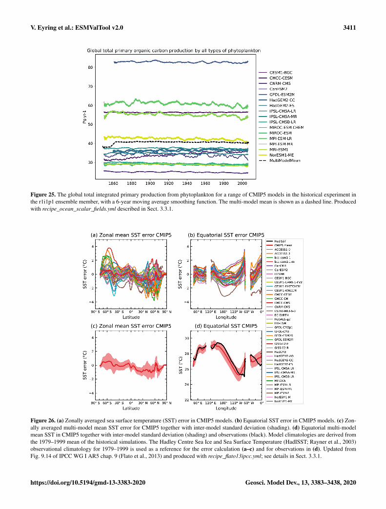
V. Eyring et al.: ESMValTool v2.0 3411
Figure 25. The global total integrated primary production from phytoplankton for a range of CMIP5 models in the historical experiment inthe r1i1p1 ensemble member, with a 6-year moving average smoothing function. The multi-model mean is shown as a dashed line. Producedwith recipe_ocean_scalar_fields.yml described in Sect. 3.3.1.
Figure 26. (a) Zonally averaged sea surface temperature (SST) error in CMIP5 models. (b) Equatorial SST error in CMIP5 models. (c) Zon-ally averaged multi-model mean SST error for CMIP5 together with inter-model standard deviation (shading). (d) Equatorial multi-modelmean SST in CMIP5 together with inter-model standard deviation (shading) and observations (black). Model climatologies are derived fromthe 1979–1999 mean of the historical simulations. The Hadley Centre Sea Ice and Sea Surface Temperature (HadISST; Rayner et al., 2003)observational climatology for 1979–1999 is used as a reference for the error calculation (a–c) and for observations in (d). Updated fromFig. 9.14 of IPCC WG I AR5 chap. 9 (Flato et al., 2013) and produced with recipe_flato13ipcc.yml; see details in Sect. 3.3.1.
https://doi.org/10.5194/gmd-13-3383-2020 Geosci. Model Dev., 13, 3383–3438, 2020
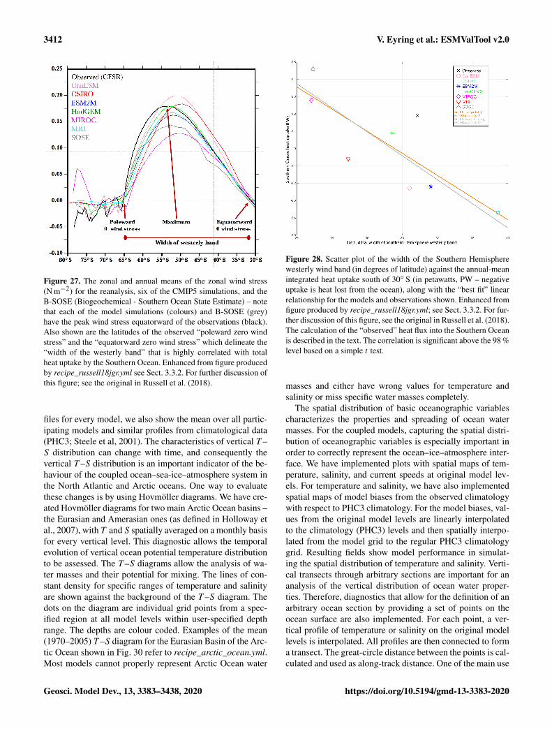
3412 V. Eyring et al.: ESMValTool v2.0
Figure 27. The zonal and annual means of the zonal wind stress(N m−2) for the reanalysis, six of the CMIP5 simulations, and theB-SOSE (Biogeochemical - Southern Ocean State Estimate) – notethat each of the model simulations (colours) and B-SOSE (grey)have the peak wind stress equatorward of the observations (black).Also shown are the latitudes of the observed “poleward zero windstress” and the “equatorward zero wind stress” which delineate the“width of the westerly band” that is highly correlated with totalheat uptake by the Southern Ocean. Enhanced from figure producedby recipe_russell18jgr.yml see Sect. 3.3.2. For further discussion ofthis figure; see the original in Russell et al. (2018).
files for every model, we also show the mean over all partic-ipating models and similar profiles from climatological data(PHC3; Steele et al, 2001). The characteristics of vertical T –S distribution can change with time, and consequently thevertical T –S distribution is an important indicator of the be-haviour of the coupled ocean–sea-ice–atmosphere system inthe North Atlantic and Arctic oceans. One way to evaluatethese changes is by using Hovmöller diagrams. We have cre-ated Hovmöller diagrams for two main Arctic Ocean basins –the Eurasian and Amerasian ones (as defined in Holloway etal., 2007), with T and S spatially averaged on a monthly basisfor every vertical level. This diagnostic allows the temporalevolution of vertical ocean potential temperature distributionto be assessed. The T –S diagrams allow the analysis of wa-ter masses and their potential for mixing. The lines of con-stant density for specific ranges of temperature and salinityare shown against the background of the T –S diagram. Thedots on the diagram are individual grid points from a spec-ified region at all model levels within user-specified depthrange. The depths are colour coded. Examples of the mean(1970–2005) T –S diagram for the Eurasian Basin of the Arc-tic Ocean shown in Fig. 30 refer to recipe_arctic_ocean.yml.Most models cannot properly represent Arctic Ocean water
Figure 28. Scatter plot of the width of the Southern Hemispherewesterly wind band (in degrees of latitude) against the annual-meanintegrated heat uptake south of 30◦ S (in petawatts, PW – negativeuptake is heat lost from the ocean), along with the “best fit” linearrelationship for the models and observations shown. Enhanced fromfigure produced by recipe_russell18jgr.yml; see Sect. 3.3.2. For fur-ther discussion of this figure, see the original in Russell et al. (2018).The calculation of the “observed” heat flux into the Southern Oceanis described in the text. The correlation is significant above the 98 %level based on a simple t test.
masses and either have wrong values for temperature andsalinity or miss specific water masses completely.
The spatial distribution of basic oceanographic variablescharacterizes the properties and spreading of ocean watermasses. For the coupled models, capturing the spatial distri-bution of oceanographic variables is especially important inorder to correctly represent the ocean–ice–atmosphere inter-face. We have implemented plots with spatial maps of tem-perature, salinity, and current speeds at original model lev-els. For temperature and salinity, we have also implementedspatial maps of model biases from the observed climatologywith respect to PHC3 climatology. For the model biases, val-ues from the original model levels are linearly interpolatedto the climatology (PHC3) levels and then spatially interpo-lated from the model grid to the regular PHC3 climatologygrid. Resulting fields show model performance in simulat-ing the spatial distribution of temperature and salinity. Verti-cal transects through arbitrary sections are important for ananalysis of the vertical distribution of ocean water proper-ties. Therefore, diagnostics that allow for the definition of anarbitrary ocean section by providing a set of points on theocean surface are also implemented. For each point, a ver-tical profile of temperature or salinity on the original modellevels is interpolated. All profiles are then connected to forma transect. The great-circle distance between the points is cal-culated and used as along-track distance. One of the main use
Geosci. Model Dev., 13, 3383–3438, 2020 https://doi.org/10.5194/gmd-13-3383-2020
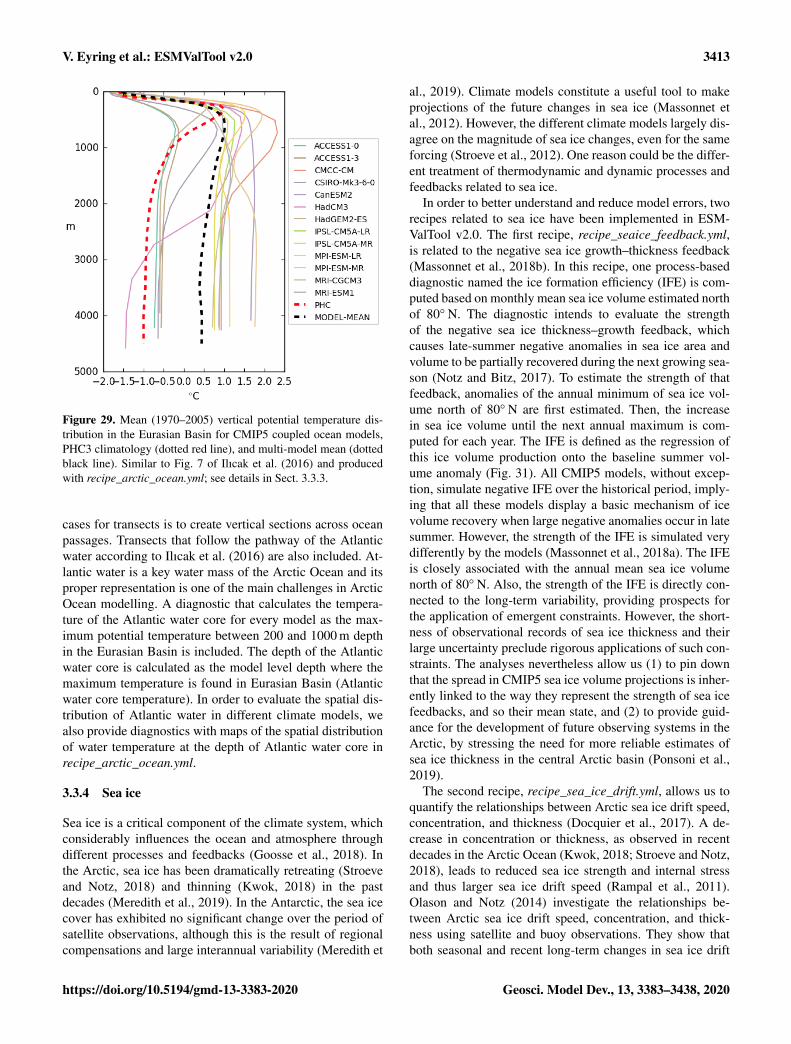
V. Eyring et al.: ESMValTool v2.0 3413
Figure 29. Mean (1970–2005) vertical potential temperature dis-tribution in the Eurasian Basin for CMIP5 coupled ocean models,PHC3 climatology (dotted red line), and multi-model mean (dottedblack line). Similar to Fig. 7 of Ilıcak et al. (2016) and producedwith recipe_arctic_ocean.yml; see details in Sect. 3.3.3.
cases for transects is to create vertical sections across oceanpassages. Transects that follow the pathway of the Atlanticwater according to Ilıcak et al. (2016) are also included. At-lantic water is a key water mass of the Arctic Ocean and itsproper representation is one of the main challenges in ArcticOcean modelling. A diagnostic that calculates the tempera-ture of the Atlantic water core for every model as the max-imum potential temperature between 200 and 1000 m depthin the Eurasian Basin is included. The depth of the Atlanticwater core is calculated as the model level depth where themaximum temperature is found in Eurasian Basin (Atlanticwater core temperature). In order to evaluate the spatial dis-tribution of Atlantic water in different climate models, wealso provide diagnostics with maps of the spatial distributionof water temperature at the depth of Atlantic water core inrecipe_arctic_ocean.yml.
3.3.4 Sea ice
Sea ice is a critical component of the climate system, whichconsiderably influences the ocean and atmosphere throughdifferent processes and feedbacks (Goosse et al., 2018). Inthe Arctic, sea ice has been dramatically retreating (Stroeveand Notz, 2018) and thinning (Kwok, 2018) in the pastdecades (Meredith et al., 2019). In the Antarctic, the sea icecover has exhibited no significant change over the period ofsatellite observations, although this is the result of regionalcompensations and large interannual variability (Meredith et
al., 2019). Climate models constitute a useful tool to makeprojections of the future changes in sea ice (Massonnet etal., 2012). However, the different climate models largely dis-agree on the magnitude of sea ice changes, even for the sameforcing (Stroeve et al., 2012). One reason could be the differ-ent treatment of thermodynamic and dynamic processes andfeedbacks related to sea ice.
In order to better understand and reduce model errors, tworecipes related to sea ice have been implemented in ESM-ValTool v2.0. The first recipe, recipe_seaice_feedback.yml,is related to the negative sea ice growth–thickness feedback(Massonnet et al., 2018b). In this recipe, one process-baseddiagnostic named the ice formation efficiency (IFE) is com-puted based on monthly mean sea ice volume estimated northof 80◦ N. The diagnostic intends to evaluate the strengthof the negative sea ice thickness–growth feedback, whichcauses late-summer negative anomalies in sea ice area andvolume to be partially recovered during the next growing sea-son (Notz and Bitz, 2017). To estimate the strength of thatfeedback, anomalies of the annual minimum of sea ice vol-ume north of 80◦ N are first estimated. Then, the increasein sea ice volume until the next annual maximum is com-puted for each year. The IFE is defined as the regression ofthis ice volume production onto the baseline summer vol-ume anomaly (Fig. 31). All CMIP5 models, without excep-tion, simulate negative IFE over the historical period, imply-ing that all these models display a basic mechanism of icevolume recovery when large negative anomalies occur in latesummer. However, the strength of the IFE is simulated verydifferently by the models (Massonnet et al., 2018a). The IFEis closely associated with the annual mean sea ice volumenorth of 80◦ N. Also, the strength of the IFE is directly con-nected to the long-term variability, providing prospects forthe application of emergent constraints. However, the short-ness of observational records of sea ice thickness and theirlarge uncertainty preclude rigorous applications of such con-straints. The analyses nevertheless allow us (1) to pin downthat the spread in CMIP5 sea ice volume projections is inher-ently linked to the way they represent the strength of sea icefeedbacks, and so their mean state, and (2) to provide guid-ance for the development of future observing systems in theArctic, by stressing the need for more reliable estimates ofsea ice thickness in the central Arctic basin (Ponsoni et al.,2019).
The second recipe, recipe_sea_ice_drift.yml, allows us toquantify the relationships between Arctic sea ice drift speed,concentration, and thickness (Docquier et al., 2017). A de-crease in concentration or thickness, as observed in recentdecades in the Arctic Ocean (Kwok, 2018; Stroeve and Notz,2018), leads to reduced sea ice strength and internal stressand thus larger sea ice drift speed (Rampal et al., 2011).Olason and Notz (2014) investigate the relationships be-tween Arctic sea ice drift speed, concentration, and thick-ness using satellite and buoy observations. They show thatboth seasonal and recent long-term changes in sea ice drift
https://doi.org/10.5194/gmd-13-3383-2020 Geosci. Model Dev., 13, 3383–3438, 2020
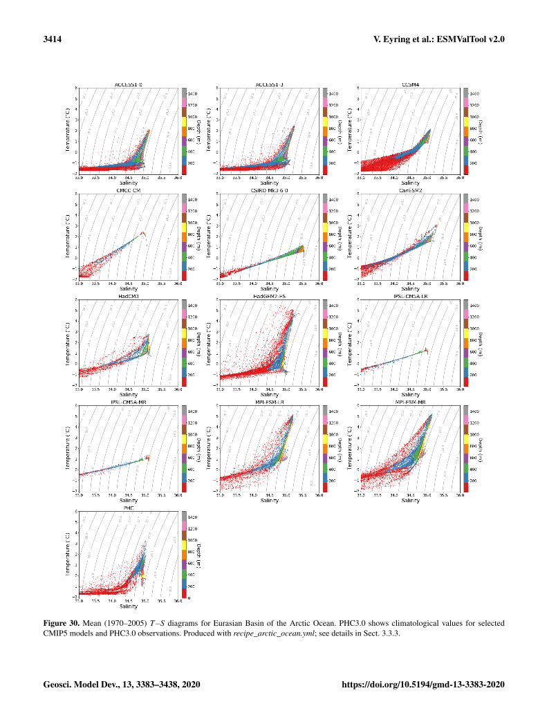
3414 V. Eyring et al.: ESMValTool v2.0
Figure 30. Mean (1970–2005) T –S diagrams for Eurasian Basin of the Arctic Ocean. PHC3.0 shows climatological values for selectedCMIP5 models and PHC3.0 observations. Produced with recipe_arctic_ocean.yml; see details in Sect. 3.3.3.
Geosci. Model Dev., 13, 3383–3438, 2020 https://doi.org/10.5194/gmd-13-3383-2020
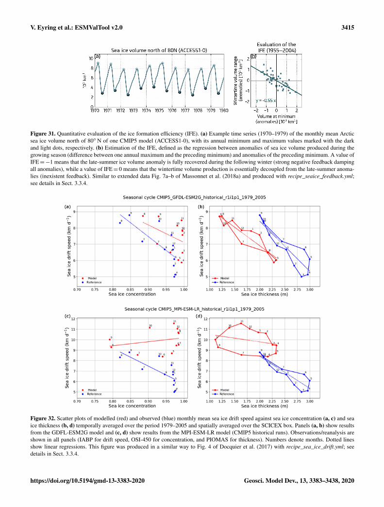
V. Eyring et al.: ESMValTool v2.0 3415
Figure 31. Quantitative evaluation of the ice formation efficiency (IFE). (a) Example time series (1970–1979) of the monthly mean Arcticsea ice volume north of 80◦ N of one CMIP5 model (ACCESS1-0), with its annual minimum and maximum values marked with the darkand light dots, respectively. (b) Estimation of the IFE, defined as the regression between anomalies of sea ice volume produced during thegrowing season (difference between one annual maximum and the preceding minimum) and anomalies of the preceding minimum. A value ofIFE=−1 means that the late-summer ice volume anomaly is fully recovered during the following winter (strong negative feedback dampingall anomalies), while a value of IFE= 0 means that the wintertime volume production is essentially decoupled from the late-summer anoma-lies (inexistent feedback). Similar to extended data Fig. 7a–b of Massonnet et al. (2018a) and produced with recipe_seaice_feedback.yml;see details in Sect. 3.3.4.
Figure 32. Scatter plots of modelled (red) and observed (blue) monthly mean sea ice drift speed against sea ice concentration (a, c) and seaice thickness (b, d) temporally averaged over the period 1979–2005 and spatially averaged over the SCICEX box. Panels (a, b) show resultsfrom the GDFL-ESM2G model and (c, d) show results from the MPI-ESM-LR model (CMIP5 historical runs). Observations/reanalysis areshown in all panels (IABP for drift speed, OSI-450 for concentration, and PIOMAS for thickness). Numbers denote months. Dotted linesshow linear regressions. This figure was produced in a similar way to Fig. 4 of Docquier et al. (2017) with recipe_sea_ice_drift.yml; seedetails in Sect. 3.3.4.
https://doi.org/10.5194/gmd-13-3383-2020 Geosci. Model Dev., 13, 3383–3438, 2020
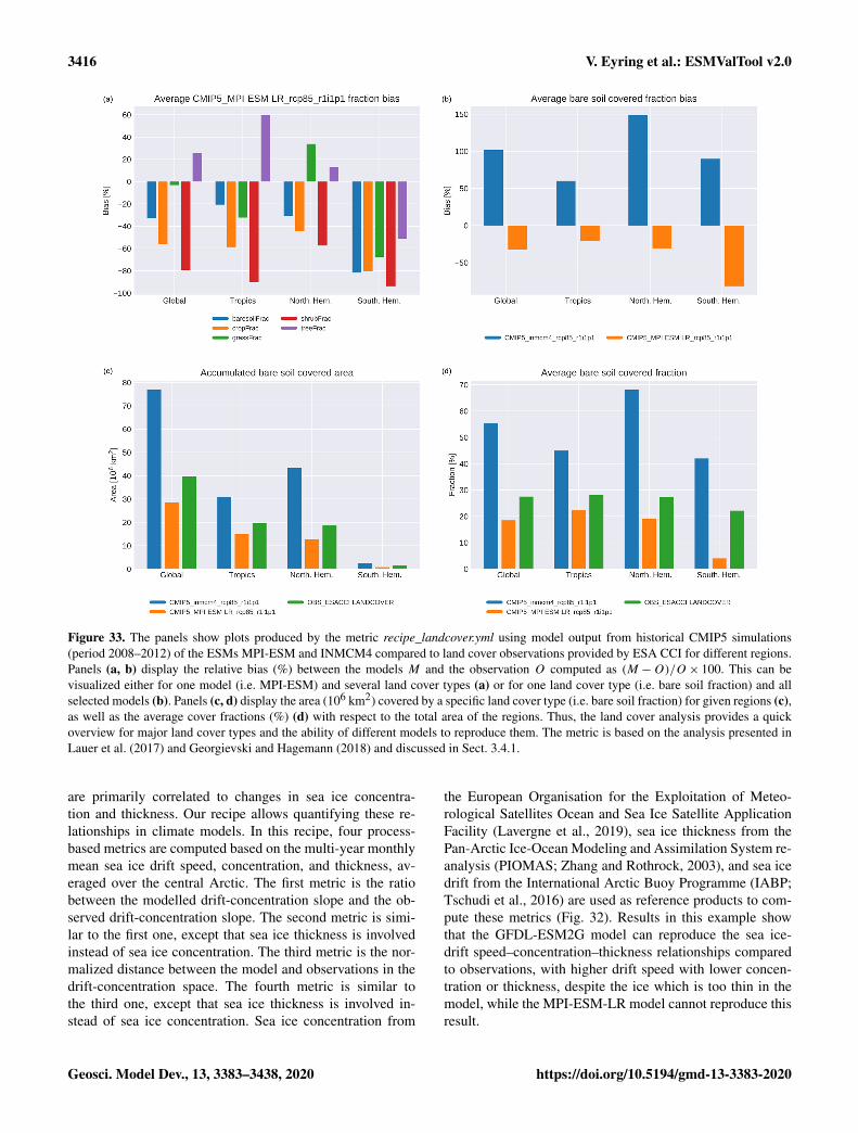
3416 V. Eyring et al.: ESMValTool v2.0
Figure 33. The panels show plots produced by the metric recipe_landcover.yml using model output from historical CMIP5 simulations(period 2008–2012) of the ESMs MPI-ESM and INMCM4 compared to land cover observations provided by ESA CCI for different regions.Panels (a, b) display the relative bias (%) between the models M and the observation O computed as (M −O)/O × 100. This can bevisualized either for one model (i.e. MPI-ESM) and several land cover types (a) or for one land cover type (i.e. bare soil fraction) and allselected models (b). Panels (c, d) display the area (106 km2) covered by a specific land cover type (i.e. bare soil fraction) for given regions (c),as well as the average cover fractions (%) (d) with respect to the total area of the regions. Thus, the land cover analysis provides a quickoverview for major land cover types and the ability of different models to reproduce them. The metric is based on the analysis presented inLauer et al. (2017) and Georgievski and Hagemann (2018) and discussed in Sect. 3.4.1.
are primarily correlated to changes in sea ice concentra-tion and thickness. Our recipe allows quantifying these re-lationships in climate models. In this recipe, four process-based metrics are computed based on the multi-year monthlymean sea ice drift speed, concentration, and thickness, av-eraged over the central Arctic. The first metric is the ratiobetween the modelled drift-concentration slope and the ob-served drift-concentration slope. The second metric is simi-lar to the first one, except that sea ice thickness is involvedinstead of sea ice concentration. The third metric is the nor-malized distance between the model and observations in thedrift-concentration space. The fourth metric is similar tothe third one, except that sea ice thickness is involved in-stead of sea ice concentration. Sea ice concentration from
the European Organisation for the Exploitation of Meteo-rological Satellites Ocean and Sea Ice Satellite ApplicationFacility (Lavergne et al., 2019), sea ice thickness from thePan-Arctic Ice-Ocean Modeling and Assimilation System re-analysis (PIOMAS; Zhang and Rothrock, 2003), and sea icedrift from the International Arctic Buoy Programme (IABP;Tschudi et al., 2016) are used as reference products to com-pute these metrics (Fig. 32). Results in this example showthat the GFDL-ESM2G model can reproduce the sea ice-drift speed–concentration–thickness relationships comparedto observations, with higher drift speed with lower concen-tration or thickness, despite the ice which is too thin in themodel, while the MPI-ESM-LR model cannot reproduce thisresult.
Geosci. Model Dev., 13, 3383–3438, 2020 https://doi.org/10.5194/gmd-13-3383-2020
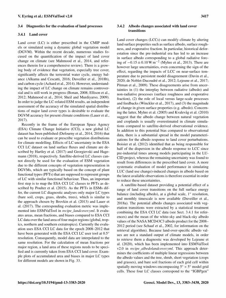
V. Eyring et al.: ESMValTool v2.0 3417
3.4 Diagnostics for the evaluation of land processes
3.4.1 Land cover
Land cover (LC) is either prescribed in the CMIP mod-els or simulated using a dynamic global vegetation model(DGVM). Within the recent decade, numerous studies fo-cused on the quantification of the impact of land coverchange on climate (see Mahmood et al., 2014, and refer-ences therein for a comprehensive review). There is a grow-ing body of evidence that vegetation, especially tree cover,significantly affects the terrestrial water cycle, energy bal-ance (Alkama and Cescatti, 2016; Duveiller et al., 2018b),and carbon cycle (Achard et al., 2014). However, understand-ing the impact of LC change on climate remains controver-sial and is still work in progress (Bonan, 2008; Ellison et al.,2012; Mahmood et al., 2014; Sheil and Murdiyarso, 2009).In order to judge the LC-related ESM results, an independentassessment of the accuracy of the simulated spatial distribu-tions of major land cover types is desirable to evaluate theDGVM accuracy for present climate conditions (Lauer et al.,2017).
Recently in the frame of the European Space Agency(ESA) Climate Change Initiative (CCI), a new global LCdataset has been published (Defourny et al., 2014, 2016) thatcan be used to evaluate or prescribe vegetation distributionsfor climate modelling. Effects of LC uncertainty in the ESACCI LC dataset on land surface fluxes and climate are de-scribed by Hartley et al. (2017) and Georgievski and Hage-mann (2018), respectively. Satellite-derived LC classes can-not directly be used for the evaluation of ESM vegetationdue to the different concepts of vegetation representation inDGVMs, which are typically based on the concept of plantfunctional types (PFTs) that are supposed to represent groupsof LC with similar functional behaviour. Thus, an importantfirst step is to map the ESA CCI LC classes to PFTs as de-scribed by Poulter et al. (2015). As the PFTs in ESMs dif-fer, the current LC diagnostic analyses only major LC types(bare soil, crops, grass, shrubs, trees), which is similar tothe approach chosen by Brovkin et al. (2013) and Lauer etal. (2017). The corresponding evaluation metric was imple-mented into ESMValTool in recipe_landcover.yml. It evalu-ates areas, mean fractions, and biases compared to ESA CCILC data over the land area of four major regions (global, trop-ics, northern and southern extratropics). Currently the evalu-ation uses ESA CCI LC data for the epoch 2008–2012 thathave been generated with the ESA CCI LC user tool at 0.5◦
resolution. Consequently, model data are interpolated to thesame resolution. For the calculation of mean fractions permajor region, a land area of these regions needs to be speci-fied and is currently taken from ESA CCI land cover. Exam-ple plots of accumulated area and biases in major LC typesfor different models are shown in Fig. 33.
3.4.2 Albedo changes associated with land covertransitions
Land cover changes (LCCs) can modify climate by alteringland surface properties such as surface albedo, surface rough-ness, and evaporative fraction. In particular, historical defor-estation since the pre-industrial era has led to an increasein surface albedo corresponding to a global radiative forc-ing of −0.15± 0.10 W m−2 (Myhre et al., 2013). There arehowever large uncertainties, even concerning the sign of theeffect, regarding the impacts of LCC on near-surface tem-perature due to persistent model disagreement (Davin et al.,2020; de Noblet-Ducoudré et al., 2012; Lejeune et al., 2017;Pitman et al., 2009). These disagreements arise from uncer-tainties in (1) the interplay between radiative (albedo) andnon-radiative processes (surface roughness and evaporativefraction), (2) the role of local versus large-scale processesand feedbacks (Winckler et al., 2017), and (3) the magnitudeof change in given surface properties (e.g. albedo). Concern-ing the latter, Myhre et al. (2005) and Kvalevåg et al. (2010)suggest that the albedo change between natural vegetationand croplands is usually overestimated in climate simula-tions compared to satellite-derived observational evidence.In addition to this potential bias compared to observationaldata, there is a substantial spread in the model parameteri-zations for the albedo response to land cover perturbations.Boisier et al. (2012) identified that as being responsible forhalf of the dispersion in the albedo response to LCC sincepre-industrial times among models participating in the LU-CID project, whereas the remaining uncertainty was found toresult from differences in the prescribed land cover. A moresystematic evaluation of model performance in simulatingLUC (land use change)-induced changes in albedo based onthe latest available observations is therefore essential in orderto reduce these uncertainties.
A satellite-based dataset providing a potential effect of arange of land cover transitions on the full surface energybalance (including albedo), at a global scale, 1◦ resolution,and monthly timescale is now available (Duveiller et al.,2018a). The potential albedo changes associated with veg-etation transitions were extracted by a statistical treatmentcombining the ESA CCI LC data (see Sect. 3.4.1 for refer-ences) and the mean of the white-sky and black-sky albedovalues of the NASA MCD43C3 albedo product for the 2008–2012 period (see Schaaf et al., 2002, for information on theretrieval algorithm). Because land-over-specific albedo val-ues are not a standard output of climate models, in orderto retrieve them a diagnostic was developed by Lejeune etal. (2020), which has been implemented into ESMValToolv2.0 in recipe_albedolandcover.yml. This approach deter-mines the coefficients of multiple linear regressions betweenthe albedo values and the tree, shrub, short vegetation (cropsand grasses), and bare soil fractions of each grid cell withinspatially moving windows encompassing 5◦×5◦ model gridcells. These four LC classes correspond to the “IGBPgen”
https://doi.org/10.5194/gmd-13-3383-2020 Geosci. Model Dev., 13, 3383–3438, 2020
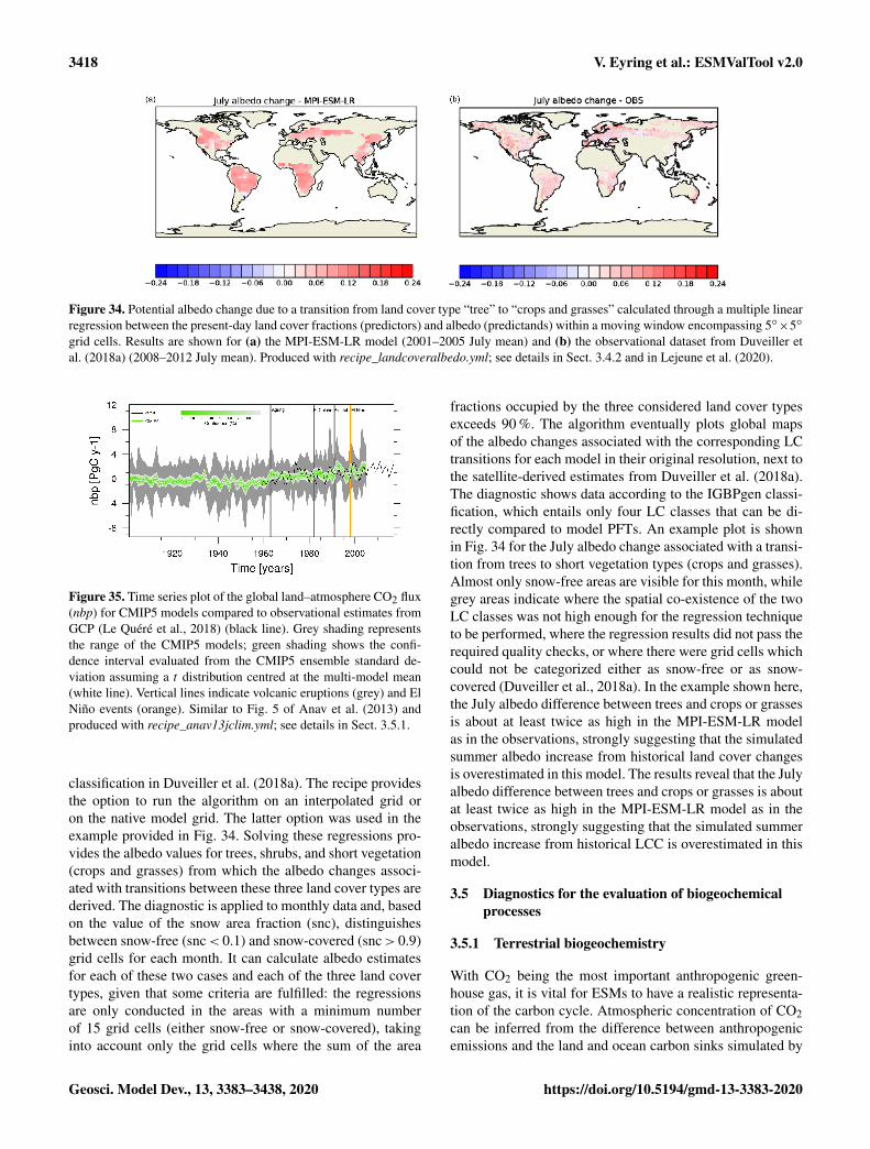
3418 V. Eyring et al.: ESMValTool v2.0
Figure 34. Potential albedo change due to a transition from land cover type “tree” to “crops and grasses” calculated through a multiple linearregression between the present-day land cover fractions (predictors) and albedo (predictands) within a moving window encompassing 5◦×5◦
grid cells. Results are shown for (a) the MPI-ESM-LR model (2001–2005 July mean) and (b) the observational dataset from Duveiller etal. (2018a) (2008–2012 July mean). Produced with recipe_landcoveralbedo.yml; see details in Sect. 3.4.2 and in Lejeune et al. (2020).
Figure 35. Time series plot of the global land–atmosphere CO2 flux(nbp) for CMIP5 models compared to observational estimates fromGCP (Le Quéré et al., 2018) (black line). Grey shading representsthe range of the CMIP5 models; green shading shows the confi-dence interval evaluated from the CMIP5 ensemble standard de-viation assuming a t distribution centred at the multi-model mean(white line). Vertical lines indicate volcanic eruptions (grey) and ElNiño events (orange). Similar to Fig. 5 of Anav et al. (2013) andproduced with recipe_anav13jclim.yml; see details in Sect. 3.5.1.
classification in Duveiller et al. (2018a). The recipe providesthe option to run the algorithm on an interpolated grid oron the native model grid. The latter option was used in theexample provided in Fig. 34. Solving these regressions pro-vides the albedo values for trees, shrubs, and short vegetation(crops and grasses) from which the albedo changes associ-ated with transitions between these three land cover types arederived. The diagnostic is applied to monthly data and, basedon the value of the snow area fraction (snc), distinguishesbetween snow-free (snc< 0.1) and snow-covered (snc> 0.9)grid cells for each month. It can calculate albedo estimatesfor each of these two cases and each of the three land covertypes, given that some criteria are fulfilled: the regressionsare only conducted in the areas with a minimum numberof 15 grid cells (either snow-free or snow-covered), takinginto account only the grid cells where the sum of the area
fractions occupied by the three considered land cover typesexceeds 90 %. The algorithm eventually plots global mapsof the albedo changes associated with the corresponding LCtransitions for each model in their original resolution, next tothe satellite-derived estimates from Duveiller et al. (2018a).The diagnostic shows data according to the IGBPgen classi-fication, which entails only four LC classes that can be di-rectly compared to model PFTs. An example plot is shownin Fig. 34 for the July albedo change associated with a transi-tion from trees to short vegetation types (crops and grasses).Almost only snow-free areas are visible for this month, whilegrey areas indicate where the spatial co-existence of the twoLC classes was not high enough for the regression techniqueto be performed, where the regression results did not pass therequired quality checks, or where there were grid cells whichcould not be categorized either as snow-free or as snow-covered (Duveiller et al., 2018a). In the example shown here,the July albedo difference between trees and crops or grassesis about at least twice as high in the MPI-ESM-LR modelas in the observations, strongly suggesting that the simulatedsummer albedo increase from historical land cover changesis overestimated in this model. The results reveal that the Julyalbedo difference between trees and crops or grasses is aboutat least twice as high in the MPI-ESM-LR model as in theobservations, strongly suggesting that the simulated summeralbedo increase from historical LCC is overestimated in thismodel.
3.5 Diagnostics for the evaluation of biogeochemicalprocesses
3.5.1 Terrestrial biogeochemistry
With CO2 being the most important anthropogenic green-house gas, it is vital for ESMs to have a realistic representa-tion of the carbon cycle. Atmospheric concentration of CO2can be inferred from the difference between anthropogenicemissions and the land and ocean carbon sinks simulated by
Geosci. Model Dev., 13, 3383–3438, 2020 https://doi.org/10.5194/gmd-13-3383-2020
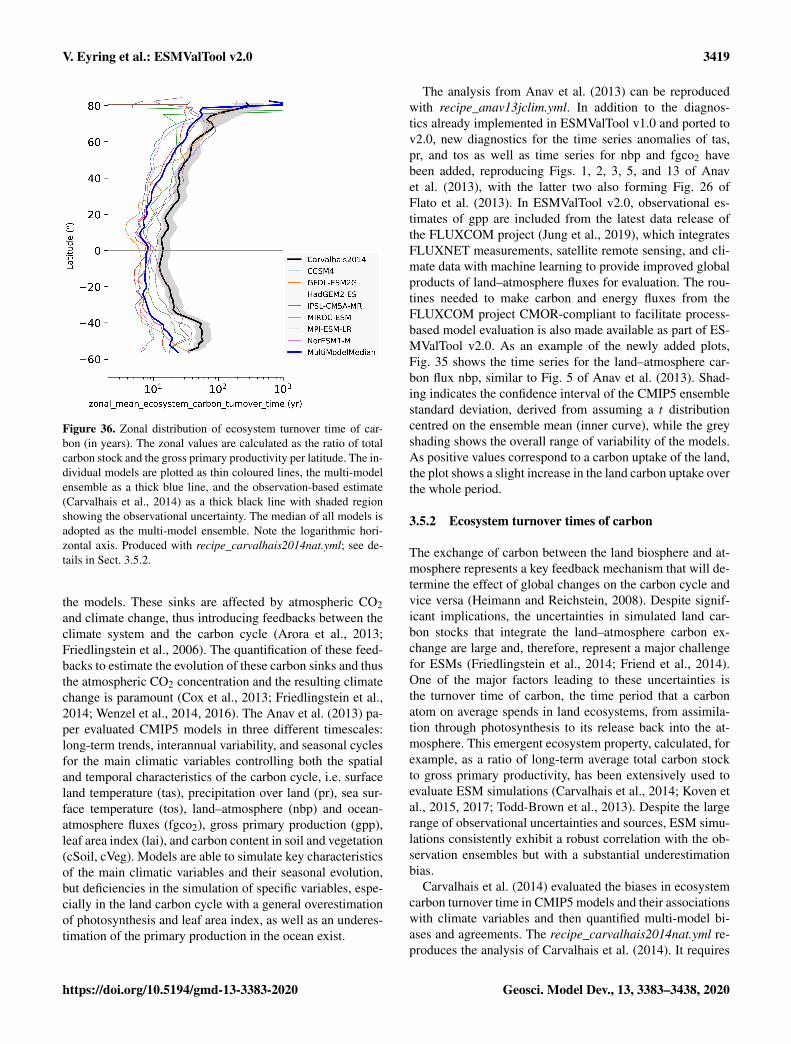
V. Eyring et al.: ESMValTool v2.0 3419
Figure 36. Zonal distribution of ecosystem turnover time of car-bon (in years). The zonal values are calculated as the ratio of totalcarbon stock and the gross primary productivity per latitude. The in-dividual models are plotted as thin coloured lines, the multi-modelensemble as a thick blue line, and the observation-based estimate(Carvalhais et al., 2014) as a thick black line with shaded regionshowing the observational uncertainty. The median of all models isadopted as the multi-model ensemble. Note the logarithmic hori-zontal axis. Produced with recipe_carvalhais2014nat.yml; see de-tails in Sect. 3.5.2.
the models. These sinks are affected by atmospheric CO2and climate change, thus introducing feedbacks between theclimate system and the carbon cycle (Arora et al., 2013;Friedlingstein et al., 2006). The quantification of these feed-backs to estimate the evolution of these carbon sinks and thusthe atmospheric CO2 concentration and the resulting climatechange is paramount (Cox et al., 2013; Friedlingstein et al.,2014; Wenzel et al., 2014, 2016). The Anav et al. (2013) pa-per evaluated CMIP5 models in three different timescales:long-term trends, interannual variability, and seasonal cyclesfor the main climatic variables controlling both the spatialand temporal characteristics of the carbon cycle, i.e. surfaceland temperature (tas), precipitation over land (pr), sea sur-face temperature (tos), land–atmosphere (nbp) and ocean-atmosphere fluxes (fgco2), gross primary production (gpp),leaf area index (lai), and carbon content in soil and vegetation(cSoil, cVeg). Models are able to simulate key characteristicsof the main climatic variables and their seasonal evolution,but deficiencies in the simulation of specific variables, espe-cially in the land carbon cycle with a general overestimationof photosynthesis and leaf area index, as well as an underes-timation of the primary production in the ocean exist.
The analysis from Anav et al. (2013) can be reproducedwith recipe_anav13jclim.yml. In addition to the diagnos-tics already implemented in ESMValTool v1.0 and ported tov2.0, new diagnostics for the time series anomalies of tas,pr, and tos as well as time series for nbp and fgco2 havebeen added, reproducing Figs. 1, 2, 3, 5, and 13 of Anavet al. (2013), with the latter two also forming Fig. 26 ofFlato et al. (2013). In ESMValTool v2.0, observational es-timates of gpp are included from the latest data release ofthe FLUXCOM project (Jung et al., 2019), which integratesFLUXNET measurements, satellite remote sensing, and cli-mate data with machine learning to provide improved globalproducts of land–atmosphere fluxes for evaluation. The rou-tines needed to make carbon and energy fluxes from theFLUXCOM project CMOR-compliant to facilitate process-based model evaluation is also made available as part of ES-MValTool v2.0. As an example of the newly added plots,Fig. 35 shows the time series for the land–atmosphere car-bon flux nbp, similar to Fig. 5 of Anav et al. (2013). Shad-ing indicates the confidence interval of the CMIP5 ensemblestandard deviation, derived from assuming a t distributioncentred on the ensemble mean (inner curve), while the greyshading shows the overall range of variability of the models.As positive values correspond to a carbon uptake of the land,the plot shows a slight increase in the land carbon uptake overthe whole period.
3.5.2 Ecosystem turnover times of carbon
The exchange of carbon between the land biosphere and at-mosphere represents a key feedback mechanism that will de-termine the effect of global changes on the carbon cycle andvice versa (Heimann and Reichstein, 2008). Despite signif-icant implications, the uncertainties in simulated land car-bon stocks that integrate the land–atmosphere carbon ex-change are large and, therefore, represent a major challengefor ESMs (Friedlingstein et al., 2014; Friend et al., 2014).One of the major factors leading to these uncertainties isthe turnover time of carbon, the time period that a carbonatom on average spends in land ecosystems, from assimila-tion through photosynthesis to its release back into the at-mosphere. This emergent ecosystem property, calculated, forexample, as a ratio of long-term average total carbon stockto gross primary productivity, has been extensively used toevaluate ESM simulations (Carvalhais et al., 2014; Koven etal., 2015, 2017; Todd-Brown et al., 2013). Despite the largerange of observational uncertainties and sources, ESM simu-lations consistently exhibit a robust correlation with the ob-servation ensembles but with a substantial underestimationbias.
Carvalhais et al. (2014) evaluated the biases in ecosystemcarbon turnover time in CMIP5 models and their associationswith climate variables and then quantified multi-model bi-ases and agreements. The recipe_carvalhais2014nat.yml re-produces the analysis of Carvalhais et al. (2014). It requires
https://doi.org/10.5194/gmd-13-3383-2020 Geosci. Model Dev., 13, 3383–3438, 2020
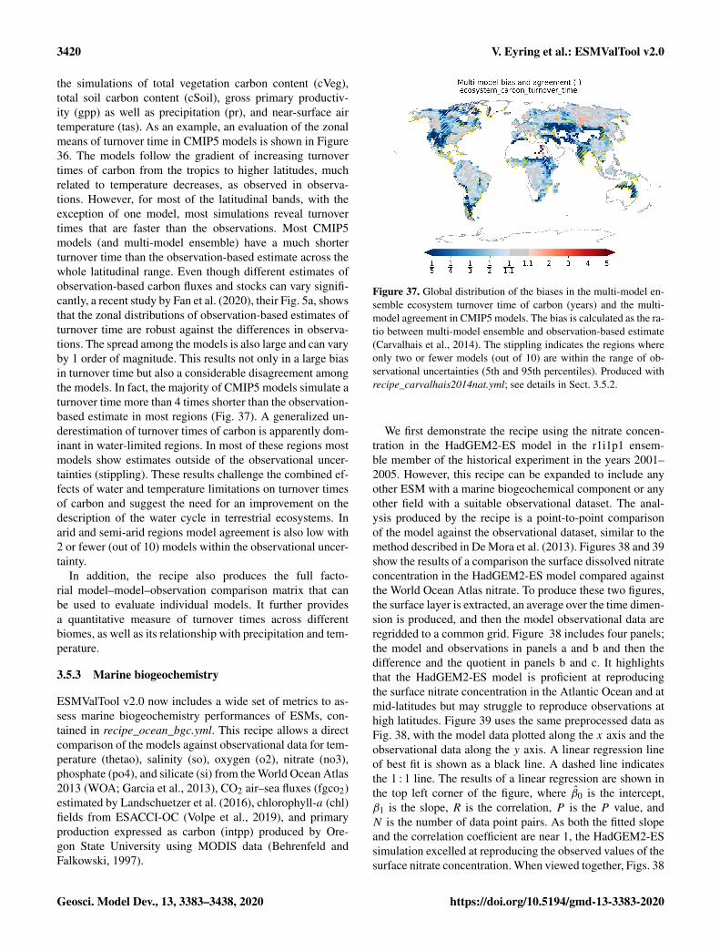
3420 V. Eyring et al.: ESMValTool v2.0
the simulations of total vegetation carbon content (cVeg),total soil carbon content (cSoil), gross primary productiv-ity (gpp) as well as precipitation (pr), and near-surface airtemperature (tas). As an example, an evaluation of the zonalmeans of turnover time in CMIP5 models is shown in Figure36. The models follow the gradient of increasing turnovertimes of carbon from the tropics to higher latitudes, muchrelated to temperature decreases, as observed in observa-tions. However, for most of the latitudinal bands, with theexception of one model, most simulations reveal turnovertimes that are faster than the observations. Most CMIP5models (and multi-model ensemble) have a much shorterturnover time than the observation-based estimate across thewhole latitudinal range. Even though different estimates ofobservation-based carbon fluxes and stocks can vary signifi-cantly, a recent study by Fan et al. (2020), their Fig. 5a, showsthat the zonal distributions of observation-based estimates ofturnover time are robust against the differences in observa-tions. The spread among the models is also large and can varyby 1 order of magnitude. This results not only in a large biasin turnover time but also a considerable disagreement amongthe models. In fact, the majority of CMIP5 models simulate aturnover time more than 4 times shorter than the observation-based estimate in most regions (Fig. 37). A generalized un-derestimation of turnover times of carbon is apparently dom-inant in water-limited regions. In most of these regions mostmodels show estimates outside of the observational uncer-tainties (stippling). These results challenge the combined ef-fects of water and temperature limitations on turnover timesof carbon and suggest the need for an improvement on thedescription of the water cycle in terrestrial ecosystems. Inarid and semi-arid regions model agreement is also low with2 or fewer (out of 10) models within the observational uncer-tainty.
In addition, the recipe also produces the full facto-rial model–model–observation comparison matrix that canbe used to evaluate individual models. It further providesa quantitative measure of turnover times across differentbiomes, as well as its relationship with precipitation and tem-perature.
3.5.3 Marine biogeochemistry
ESMValTool v2.0 now includes a wide set of metrics to as-sess marine biogeochemistry performances of ESMs, con-tained in recipe_ocean_bgc.yml. This recipe allows a directcomparison of the models against observational data for tem-perature (thetao), salinity (so), oxygen (o2), nitrate (no3),phosphate (po4), and silicate (si) from the World Ocean Atlas2013 (WOA; Garcia et al., 2013), CO2 air–sea fluxes (fgco2)estimated by Landschuetzer et al. (2016), chlorophyll-a (chl)fields from ESACCI-OC (Volpe et al., 2019), and primaryproduction expressed as carbon (intpp) produced by Ore-gon State University using MODIS data (Behrenfeld andFalkowski, 1997).
Figure 37. Global distribution of the biases in the multi-model en-semble ecosystem turnover time of carbon (years) and the multi-model agreement in CMIP5 models. The bias is calculated as the ra-tio between multi-model ensemble and observation-based estimate(Carvalhais et al., 2014). The stippling indicates the regions whereonly two or fewer models (out of 10) are within the range of ob-servational uncertainties (5th and 95th percentiles). Produced withrecipe_carvalhais2014nat.yml; see details in Sect. 3.5.2.
We first demonstrate the recipe using the nitrate concen-tration in the HadGEM2-ES model in the r1i1p1 ensem-ble member of the historical experiment in the years 2001–2005. However, this recipe can be expanded to include anyother ESM with a marine biogeochemical component or anyother field with a suitable observational dataset. The anal-ysis produced by the recipe is a point-to-point comparisonof the model against the observational dataset, similar to themethod described in De Mora et al. (2013). Figures 38 and 39show the results of a comparison the surface dissolved nitrateconcentration in the HadGEM2-ES model compared againstthe World Ocean Atlas nitrate. To produce these two figures,the surface layer is extracted, an average over the time dimen-sion is produced, and then the model observational data areregridded to a common grid. Figure 38 includes four panels;the model and observations in panels a and b and then thedifference and the quotient in panels b and c. It highlightsthat the HadGEM2-ES model is proficient at reproducingthe surface nitrate concentration in the Atlantic Ocean and atmid-latitudes but may struggle to reproduce observations athigh latitudes. Figure 39 uses the same preprocessed data asFig. 38, with the model data plotted along the x axis and theobservational data along the y axis. A linear regression lineof best fit is shown as a black line. A dashed line indicatesthe 1 : 1 line. The results of a linear regression are shown inthe top left corner of the figure, where β̂0 is the intercept,β1 is the slope, R is the correlation, P is the P value, andN is the number of data point pairs. As both the fitted slopeand the correlation coefficient are near 1, the HadGEM2-ESsimulation excelled at reproducing the observed values of thesurface nitrate concentration. When viewed together, Figs. 38
Geosci. Model Dev., 13, 3383–3438, 2020 https://doi.org/10.5194/gmd-13-3383-2020
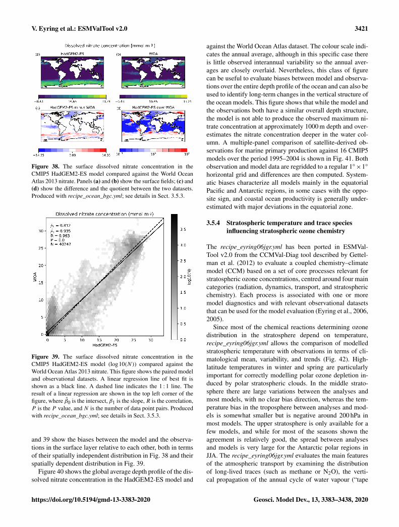
V. Eyring et al.: ESMValTool v2.0 3421
Figure 38. The surface dissolved nitrate concentration in theCMIP5 HadGEM2-ES model compared against the World OceanAtlas 2013 nitrate. Panels (a) and (b) show the surface fields; (c) and(d) show the difference and the quotient between the two datasets.Produced with recipe_ocean_bgc.yml; see details in Sect. 3.5.3.
Figure 39. The surface dissolved nitrate concentration in theCMIP5 HadGEM2-ES model (log10(N)) compared against theWorld Ocean Atlas 2013 nitrate. This figure shows the paired modeland observational datasets. A linear regression line of best fit isshown as a black line. A dashed line indicates the 1 : 1 line. Theresult of a linear regression are shown in the top left corner of thefigure, where β̂0 is the intersect, β1 is the slope, R is the correlation,P is the P value, and N is the number of data point pairs. Producedwith recipe_ocean_bgc.yml; see details in Sect. 3.5.3.
and 39 show the biases between the model and the observa-tions in the surface layer relative to each other, both in termsof their spatially independent distribution in Fig. 38 and theirspatially dependent distribution in Fig. 39.
Figure 40 shows the global average depth profile of the dis-solved nitrate concentration in the HadGEM2-ES model and
against the World Ocean Atlas dataset. The colour scale indi-cates the annual average, although in this specific case thereis little observed interannual variability so the annual aver-ages are closely overlaid. Nevertheless, this class of figurecan be useful to evaluate biases between model and observa-tions over the entire depth profile of the ocean and can also beused to identify long-term changes in the vertical structure ofthe ocean models. This figure shows that while the model andthe observations both have a similar overall depth structure,the model is not able to produce the observed maximum ni-trate concentration at approximately 1000 m depth and over-estimates the nitrate concentration deeper in the water col-umn. A multiple-panel comparison of satellite-derived ob-servations for marine primary production against 16 CMIP5models over the period 1995–2004 is shown in Fig. 41. Bothobservation and model data are regridded to a regular 1◦×1◦
horizontal grid and differences are then computed. System-atic biases characterize all models mainly in the equatorialPacific and Antarctic regions, in some cases with the oppo-site sign, and coastal ocean productivity is generally under-estimated with major deviations in the equatorial zone.
3.5.4 Stratospheric temperature and trace speciesinfluencing stratospheric ozone chemistry
The recipe_eyring06jgr.yml has been ported in ESMVal-Tool v2.0 from the CCMVal-Diag tool described by Gettel-man et al. (2012) to evaluate a coupled chemistry–climatemodel (CCM) based on a set of core processes relevant forstratospheric ozone concentrations, centred around four maincategories (radiation, dynamics, transport, and stratosphericchemistry). Each process is associated with one or moremodel diagnostics and with relevant observational datasetsthat can be used for the model evaluation (Eyring et al., 2006,2005).
Since most of the chemical reactions determining ozonedistribution in the stratosphere depend on temperature,recipe_eyring06jgr.yml allows the comparison of modelledstratospheric temperature with observations in terms of cli-matological mean, variability, and trends (Fig. 42). High-latitude temperatures in winter and spring are particularlyimportant for correctly modelling polar ozone depletion in-duced by polar stratospheric clouds. In the middle strato-sphere there are large variations between the analyses andmost models, with no clear bias direction, whereas the tem-perature bias in the troposphere between analyses and mod-els is somewhat smaller but is negative around 200 hPa inmost models. The upper stratosphere is only available for afew models, and while for most of the seasons shown theagreement is relatively good, the spread between analysesand models is very large for the Antarctic polar regions inJJA. The recipe_eyring06jgr.yml evaluates the main featuresof the atmospheric transport by examining the distributionof long-lived traces (such as methane or N2O), the verti-cal propagation of the annual cycle of water vapour (“tape
https://doi.org/10.5194/gmd-13-3383-2020 Geosci. Model Dev., 13, 3383–3438, 2020
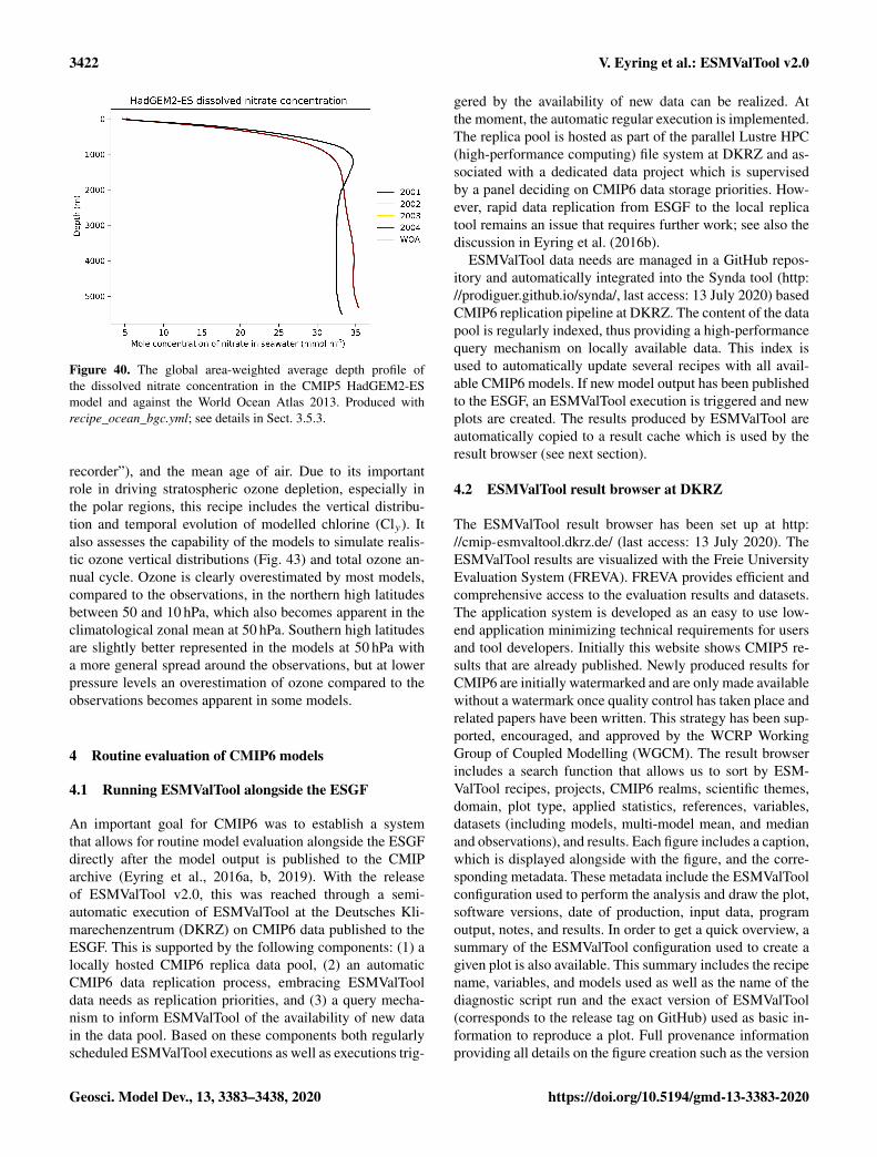
3422 V. Eyring et al.: ESMValTool v2.0
Figure 40. The global area-weighted average depth profile ofthe dissolved nitrate concentration in the CMIP5 HadGEM2-ESmodel and against the World Ocean Atlas 2013. Produced withrecipe_ocean_bgc.yml; see details in Sect. 3.5.3.
recorder”), and the mean age of air. Due to its importantrole in driving stratospheric ozone depletion, especially inthe polar regions, this recipe includes the vertical distribu-tion and temporal evolution of modelled chlorine (Cly). Italso assesses the capability of the models to simulate realis-tic ozone vertical distributions (Fig. 43) and total ozone an-nual cycle. Ozone is clearly overestimated by most models,compared to the observations, in the northern high latitudesbetween 50 and 10 hPa, which also becomes apparent in theclimatological zonal mean at 50 hPa. Southern high latitudesare slightly better represented in the models at 50 hPa witha more general spread around the observations, but at lowerpressure levels an overestimation of ozone compared to theobservations becomes apparent in some models.
4 Routine evaluation of CMIP6 models
4.1 Running ESMValTool alongside the ESGF
An important goal for CMIP6 was to establish a systemthat allows for routine model evaluation alongside the ESGFdirectly after the model output is published to the CMIParchive (Eyring et al., 2016a, b, 2019). With the releaseof ESMValTool v2.0, this was reached through a semi-automatic execution of ESMValTool at the Deutsches Kli-marechenzentrum (DKRZ) on CMIP6 data published to theESGF. This is supported by the following components: (1) alocally hosted CMIP6 replica data pool, (2) an automaticCMIP6 data replication process, embracing ESMValTooldata needs as replication priorities, and (3) a query mecha-nism to inform ESMValTool of the availability of new datain the data pool. Based on these components both regularlyscheduled ESMValTool executions as well as executions trig-
gered by the availability of new data can be realized. Atthe moment, the automatic regular execution is implemented.The replica pool is hosted as part of the parallel Lustre HPC(high-performance computing) file system at DKRZ and as-sociated with a dedicated data project which is supervisedby a panel deciding on CMIP6 data storage priorities. How-ever, rapid data replication from ESGF to the local replicatool remains an issue that requires further work; see also thediscussion in Eyring et al. (2016b).
ESMValTool data needs are managed in a GitHub repos-itory and automatically integrated into the Synda tool (http://prodiguer.github.io/synda/, last access: 13 July 2020) basedCMIP6 replication pipeline at DKRZ. The content of the datapool is regularly indexed, thus providing a high-performancequery mechanism on locally available data. This index isused to automatically update several recipes with all avail-able CMIP6 models. If new model output has been publishedto the ESGF, an ESMValTool execution is triggered and newplots are created. The results produced by ESMValTool areautomatically copied to a result cache which is used by theresult browser (see next section).
4.2 ESMValTool result browser at DKRZ
The ESMValTool result browser has been set up at http://cmip-esmvaltool.dkrz.de/ (last access: 13 July 2020). TheESMValTool results are visualized with the Freie UniversityEvaluation System (FREVA). FREVA provides efficient andcomprehensive access to the evaluation results and datasets.The application system is developed as an easy to use low-end application minimizing technical requirements for usersand tool developers. Initially this website shows CMIP5 re-sults that are already published. Newly produced results forCMIP6 are initially watermarked and are only made availablewithout a watermark once quality control has taken place andrelated papers have been written. This strategy has been sup-ported, encouraged, and approved by the WCRP WorkingGroup of Coupled Modelling (WGCM). The result browserincludes a search function that allows us to sort by ESM-ValTool recipes, projects, CMIP6 realms, scientific themes,domain, plot type, applied statistics, references, variables,datasets (including models, multi-model mean, and medianand observations), and results. Each figure includes a caption,which is displayed alongside with the figure, and the corre-sponding metadata. These metadata include the ESMValToolconfiguration used to perform the analysis and draw the plot,software versions, date of production, input data, programoutput, notes, and results. In order to get a quick overview, asummary of the ESMValTool configuration used to create agiven plot is also available. This summary includes the recipename, variables, and models used as well as the name of thediagnostic script run and the exact version of ESMValTool(corresponds to the release tag on GitHub) used as basic in-formation to reproduce a plot. Full provenance informationproviding all details on the figure creation such as the version
Geosci. Model Dev., 13, 3383–3438, 2020 https://doi.org/10.5194/gmd-13-3383-2020
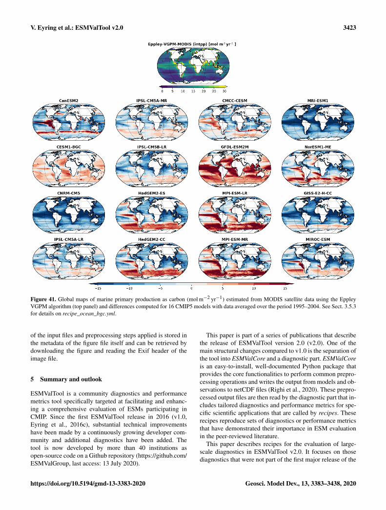
V. Eyring et al.: ESMValTool v2.0 3423
Figure 41. Global maps of marine primary production as carbon (mol m−2 yr−1) estimated from MODIS satellite data using the EppleyVGPM algorithm (top panel) and differences computed for 16 CMIP5 models with data averaged over the period 1995–2004. See Sect. 3.5.3for details on recipe_ocean_bgc.yml.
of the input files and preprocessing steps applied is stored inthe metadata of the figure file itself and can be retrieved bydownloading the figure and reading the Exif header of theimage file.
5 Summary and outlook
ESMValTool is a community diagnostics and performancemetrics tool specifically targeted at facilitating and enhanc-ing a comprehensive evaluation of ESMs participating inCMIP. Since the first ESMValTool release in 2016 (v1.0,Eyring et al., 2016c), substantial technical improvementshave been made by a continuously growing developer com-munity and additional diagnostics have been added. Thetool is now developed by more than 40 institutions asopen-source code on a Github repository (https://github.com/ESMValGroup, last access: 13 July 2020).
This paper is part of a series of publications that describethe release of ESMValTool version 2.0 (v2.0). One of themain structural changes compared to v1.0 is the separation ofthe tool into ESMValCore and a diagnostic part. ESMValCoreis an easy-to-install, well-documented Python package thatprovides the core functionalities to perform common prepro-cessing operations and writes the output from models and ob-servations to netCDF files (Righi et al., 2020). These prepro-cessed output files are then read by the diagnostic part that in-cludes tailored diagnostics and performance metrics for spe-cific scientific applications that are called by recipes. Theserecipes reproduce sets of diagnostics or performance metricsthat have demonstrated their importance in ESM evaluationin the peer-reviewed literature.
This paper describes recipes for the evaluation of large-scale diagnostics in ESMValTool v2.0. It focuses on thosediagnostics that were not part of the first major release of the
https://doi.org/10.5194/gmd-13-3383-2020 Geosci. Model Dev., 13, 3383–3438, 2020
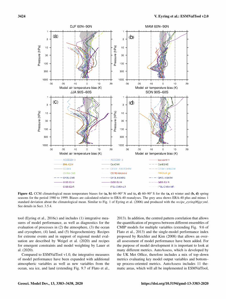
3424 V. Eyring et al.: ESMValTool v2.0
Figure 42. CCM climatological mean temperature biases for (a, b) 60–90◦ N and (c, d) 60–90◦ S for the (a, c) winter and (b, d) springseasons for the period 1980 to 1999. Biases are calculated relative to ERA-40 reanalyses. The grey area shows ERA-40 plus and minus 1standard deviation about the climatological mean. Similar to Fig. 1 of Eyring et al. (2006) and produced with the recipe_eyring06jgr.yml.See details in Sect. 3.5.4.
tool (Eyring et al., 2016c) and includes (1) integrative mea-sures of model performance, as well as diagnostics for theevaluation of processes in (2) the atmosphere, (3) the oceanand cryosphere, (4) land, and (5) biogeochemistry. Recipesfor extreme events and in support of regional model eval-uation are described by Weigel et al. (2020) and recipesfor emergent constraints and model weighting by Lauer etal. (2020).
Compared to ESMValTool v1.0, the integrative measuresof model performance have been expanded with additionalatmospheric variables as well as new variables from theocean, sea ice, and land (extending Fig. 9.7 of Flato et al.,
2013). In addition, the centred pattern correlation that allowsthe quantification of progress between different ensembles ofCMIP models for multiple variables (extending Fig. 9.6 ofFlato et al., 2013) and the single-model performance indexproposed by Reichler and Kim (2008) that allows an over-all assessment of model performance have been added. Forthe purpose of model development it is important to look atmany different metrics. AutoAssess, which is developed bythe UK Met Office, therefore includes a mix of top–downmetrics evaluating key model output variables and bottom–up process-oriented metrics. AutoAssess includes 11 the-matic areas, which will all be implemented in ESMValTool,
Geosci. Model Dev., 13, 3383–3438, 2020 https://doi.org/10.5194/gmd-13-3383-2020
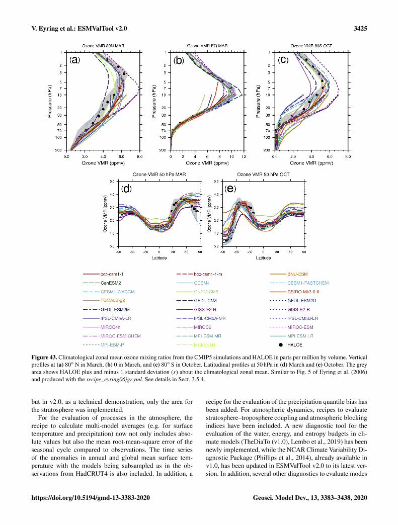
V. Eyring et al.: ESMValTool v2.0 3425
Figure 43. Climatological zonal mean ozone mixing ratios from the CMIP5 simulations and HALOE in parts per million by volume. Verticalprofiles at (a) 80◦ N in March, (b) 0 in March, and (c) 80◦ S in October. Latitudinal profiles at 50 hPa in (d) March and (e) October. The greyarea shows HALOE plus and minus 1 standard deviation (s) about the climatological zonal mean. Similar to Fig. 5 of Eyring et al. (2006)and produced with the recipe_eyring06jgr.yml. See details in Sect. 3.5.4.
but in v2.0, as a technical demonstration, only the area forthe stratosphere was implemented.
For the evaluation of processes in the atmosphere, therecipe to calculate multi-model averages (e.g. for surfacetemperature and precipitation) now not only includes abso-lute values but also the mean root-mean-square error of theseasonal cycle compared to observations. The time seriesof the anomalies in annual and global mean surface tem-perature with the models being subsampled as in the ob-servations from HadCRUT4 is also included. In addition, a
recipe for the evaluation of the precipitation quantile bias hasbeen added. For atmospheric dynamics, recipes to evaluatestratosphere–troposphere coupling and atmospheric blockingindices have been included. A new diagnostic tool for theevaluation of the water, energy, and entropy budgets in cli-mate models (TheDiaTo (v1.0), Lembo et al., 2019) has beennewly implemented, while the NCAR Climate Variability Di-agnostic Package (Phillips et al., 2014), already available inv1.0, has been updated in ESMValTool v2.0 to its latest ver-sion. In addition, several other diagnostics to evaluate modes
https://doi.org/10.5194/gmd-13-3383-2020 Geosci. Model Dev., 13, 3383–3438, 2020
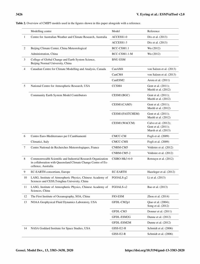
3426 V. Eyring et al.: ESMValTool v2.0
Table 2. Overview of CMIP5 models used in the figures shown in this paper alongside with a reference.
Modelling centre Model Reference
1 Centre for Australian Weather and Climate Research, Australia ACCESS1-0 Dix et al. (2013)
ACCESS1-3 Dix et al. (2013)
2 Beijing Climate Center, China Meteorological BCC-CSM1.1 Wu (2012)
Administration, China BCC-CSM1.1-M Wu (2012)
3 College of Global Change and Earth System Science,Beijing Normal University, China
BNU-ESM
4 Canadian Centre for Climate Modelling and Analysis, Canada CanAM4 von Salzen et al. (2013)
CanCM4 von Salzen et al. (2013)
CanESM2 Arora et al. (2011)
5 National Centre for Atmospheric Research, USA CCSM4 Gent et al. (2011);Meehl et al. (2012)
Community Earth System Model Contributors CESM1(BGC) Gent et al. (2011);Meehl et al. (2012)
CESM1(CAM5) Gent et al. (2011);Meehl et al. (2012)
CESM1(FASTCHEM) Gent et al. (2011);Meehl et al. (2012)
CESM1(WACCM) Calvo et al. (2012);Gent et al. (2011);Marsh et al. (2013)
6 Centro Euro-Mediterraneo per I Cambiamenti CMCC-CM Fogli et al. (2009)
Climatici, Italy CMCC-CMS Fogli et al. (2009)
7 Centre National de Recherches Meteorologiques, France CNRM-CM5 Voldoire et al. (2012)
CNRM-CM5-2 Voldoire et al. (2012)
8 Commonwealth Scientific and Industrial Research Organizationin collaboration with Queensland Climate Change Centre of Ex-cellence, Australia
CSIRO-Mk3-6-0 Rotstayn et al. (2012)
9 EC-EARTH consortium, Europe EC-EARTH Hazeleger et al. (2012)
10 LASG, Institute of Atmospheric Physics, Chinese Academy ofSciences and CESS,Tsinghua University, China
FGOALS-g2 Li et al. (2013)
11 LASG, Institute of Atmospheric Physics, Chinese Academy ofSciences, China
FGOALS-s2 Bao et al. (2013)
12 The First Institute of Oceanography, SOA, China FIO-ESM Zhou et al. (2014)
13 NOAA Geophysical Fluid Dynamics Laboratory, USA GFDL-CM2p1 Qiao et al. (2004);Song et al. (2012)
GFDL-CM3 Donner et al. (2011)
GFDL-ESM2G Dunne et al. (2012)
GFDL-ESM2M Dunne et al. (2012)
14 NASA Goddard Institute for Space Studies, USA GISS-E2-H Schmidt et al. (2006)
GISS-E2-R Schmidt et al. (2006)
Geosci. Model Dev., 13, 3383–3438, 2020 https://doi.org/10.5194/gmd-13-3383-2020
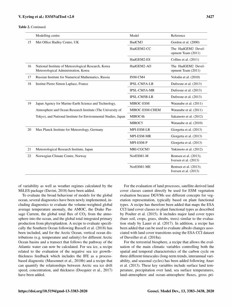
V. Eyring et al.: ESMValTool v2.0 3427
Table 2. Continued.
Modelling centre Model Reference
15 Met Office Hadley Centre, UK HadCM3 Gordon et al. (2000)
HadGEM2-CC The HadGEM2 Devel-opment Team (2011)
HadGEM2-ES Collins et al. (2011)
16 National Institute of Meteorological Research, KoreaMeteorological Administration, Korea
HadGEM2-AO The HadGEM2 Devel-opment Team (2011)
17 Russian Institute for Numerical Mathematics, Russia INM-CM4 Volodin et al. (2010)
18 Institut Pierre Simon Laplace, France IPSL-CM5A-LR Dufresne et al. (2013)
IPSL-CM5A-MR Dufresne et al. (2013)
IPSL-CM5B-LR Dufresne et al. (2013)
19 Japan Agency for Marine-Earth Science and Technology, MIROC-ESM Watanabe et al. (2011)
Atmosphere and Ocean Research Institute (The University of MIROC-ESM-CHEM Watanabe et al. (2011)
Tokyo), and National Institute for Environmental Studies, Japan MIROC4h Sakamoto et al. (2012)
MIROC5 Watanabe et al. (2010)
20 Max Planck Institute for Meteorology, Germany MPI-ESM-LR Giorgetta et al. (2013)
MPI-ESM-MR Giorgetta et al. (2013)
MPI-ESM-P Giorgetta et al. (2013)
21 Meteorological Research Institute, Japan MRI-CGCM3 Yukimoto et al. (2012)
22 Norwegian Climate Centre, Norway NorESM1-M Bentsen et al. (2013);Iversen et al. (2013)
NorESM1-ME Bentsen et al. (2013);Iversen et al. (2013)
of variability as well as weather regimes calculated by theMiLES package (Davini, 2018) have been added.
To evaluate the broad behaviour of models for the globalocean, several diagnostics have been newly implemented, in-cluding diagnostics to evaluate the volume-weighted globalaverage temperature anomaly, the AMOC, the Drake Pas-sage Current, the global total flux of CO2 from the atmo-sphere into the ocean, and the global total integrated primaryproduction from phytoplankton. A recipe to evaluate specifi-cally the Southern Ocean following Russell et al. (2018) hasbeen included, and for the Arctic Ocean, vertical ocean dis-tributions (e.g. temperature and salinity) for different ArcticOcean basins and a transect that follows the pathway of theAtlantic water can now be calculated. For sea ice, a reciperelated to the evaluation of the negative sea ice growth–thickness feedback which includes the IFE as a process-based diagnostic (Massonnet et al., 2018b) and a recipe thatcan quantify the relationships between Arctic sea ice driftspeed, concentration, and thickness (Docquier et al., 2017)have been added.
For the evaluation of land processes, satellite-derived landcover classes cannot directly be used for ESM vegetationevaluation because DGVMs use different concepts for veg-etation representation, typically based on plant functionaltypes. A recipe has therefore been added that maps the ESACCI land cover classes to plant functional types as describedby Poulter et al. (2015). It includes major land cover types(bare soil, crops, grass, shrubs, trees) similar to the evalua-tion study by Lauer et al. (2017). In addition, a recipe hasbeen added that can be used to evaluate albedo changes asso-ciated with land cover transitions using the ESA CCI datasetof Duveiller et al. (2018a).
For the terrestrial biosphere, a recipe that allows the eval-uation of the main climatic variables controlling both thespatial and temporal characteristics of the carbon cycle onthree different timescales (long-term trends, interannual vari-ability, and seasonal cycles) has been added following Anavet al. (2013). These key variables include surface land tem-perature, precipitation over land, sea surface temperatures,land–atmosphere and ocean–atmosphere fluxes, gross pri-
https://doi.org/10.5194/gmd-13-3383-2020 Geosci. Model Dev., 13, 3383–3438, 2020
3428 V. Eyring et al.: ESMValTool v2.0
mary production, leaf area index, and carbon content in soiland vegetation. To evaluate the simulated land carbon stocksthat integrate the land–atmosphere carbon exchange, a recipeto evaluate biases in ecosystem carbon turnover time, thetime period that a carbon atom on average spends in landecosystems, from assimilation through photosynthesis to itsrelease back into the atmosphere (Carvalhais et al., 2014)has been added. For marine biogeochemistry, v2.0 now in-cludes a recipe that allows a direct comparison of the mod-els against observational data for several variables includ-ing temperature, salinity, oxygen, nitrate, phosphate, silicate,CO2 air–sea fluxes, chlorophyll a, and primary production.The point-to-point comparison of the model against the ob-servational dataset is similar to De Mora et al. (2013). Toevaluate stratospheric dynamics and chemistry a recipe basedon a set of core processes relevant for stratospheric ozoneconcentrations, centred around four main categories (radia-tion, dynamics, transport, and stratospheric chemistry) hasbeen added (Eyring et al., 2006). Overall these recipes to-gether with those already included in v1.0 allow a broad char-acterization of the models for key variables (such as temper-ature and precipitation) on the large scale, but v2.0 also in-cludes several process-oriented diagnostics.
With this release, for the first time in CMIP it is now possi-ble to evaluate the models as soon as the output is publishedto the ESGF in a quasi-operational manner. To achieve this,ESMValTool has been fully integrated into the ESGF struc-ture at DKRZ. The data from the ESGF are first copied toa local replica, and ESMValTool is then automatically ex-ecuted alongside the ESGF as soon as new output arrives.An ESMValTool result browser has been set up that makesthe evaluation results available to the wider community (http://cmip-esmvaltool.dkrz.de/, last access: 13 July 2020).
Another major advancement of ESMValTool v2.0 is thatit provides full provenance and traceability (see Sect. 5.2 inRighi et al., 2020, for details). Provenance information, forexample, includes technical information such as global at-tributes of all input netCDF files, preprocessor settings, diag-nostic script settings, and software version numbers but alsodiagnostic script name and recipe authors, funding projects,references for citation purposes, as well as tags for categoriz-ing the result plots into various scientific topics (like chem-istry, dynamics, sea ice) realms (land, atmosphere, ocean,etc.) or the statistics applied (RMSE, anomaly, trend, clima-tology, etc.). This not only facilitates the sorting of the resultsin the ESMValTool result browser but also qualifies the toolfor the use in studies or assessments where provenance andtraceability is particularly important. The current approach toprovenance and tags (i.e. what is reported) can be adjusted tointernational provenance standards as they become available.
These recent ESMValTool developments and their cou-pling to the ESGF results can now be exploited by global andregional ESM developers as well as by the data analysis anduser communities, to better understand the large CMIP en-semble and to support data exploitation. In particular with the
addition of provenance, the tool can also provide a valuablesource for producing figures in national and international as-sessment reports (such as the IPCC climate assessments) toenhance the quality control, reproducibility, and traceabilityof the figures included.
The ESMValTool development community will further en-hance the capabilities of the tool with the goal of taking cli-mate model evaluation – together with other activities – tothe next level (Eyring et al., 2019). Targeted technical en-hancements will, for example, include the development ofquick-look capabilities that allow users to monitor the sim-ulations while they are running to help identify errors in thesimulations early on, a further extension to the applicationto regional models so that a consistent evaluation betweenglobal and regional models can be provided, and distributedcomputing functionalities. In addition, the tool will be ex-panded with additional process-oriented diagnostics in var-ious projects to further enhance comprehensive evaluationand analysis of the CMIP models.
Code and data availability. ESMValTool v2.0 is released un-der the Apache License, VERSION 2.0. The latest releaseof ESMValTool v2.0 is publicly available on Zenodo athttps://doi.org/10.5281/zenodo.3759523 (Andela et al., 2020a). Thesource code of the ESMValCore package, which is installed asa dependency of the ESMValTool v2.0, is also publicly availableon Zenodo at https://doi.org/10.5281/zenodo.3952695 (Andela etal., 2020b). ESMValTool and ESMValCore are developed on theGitHub repositories available at https://github.com/ESMValGroup(last access: 13 July 2020).
CMIP5 data are available freely and publicly from the Earth Sys-tem Grid Federation. Observations used in the evaluation are de-tailed in the various sections of the paper and listed in Table 1. Theyare not distributed with ESMValTool, which is restricted to the codeas open-source software.
Author contributions. VE coordinated the ESMValTool v2.0 diag-nostic effort and led the writing of the paper. LB, AL, MR, and MScoordinated the diagnostic implementation in ESMValTool v2.0.CE and SK helped with the coupling of ESMValTool v2.0 andCK with the visualization of the results in the ESMValTool resultbrowser. All other co-authors contributed individual diagnostics tothis release. All authors contributed to the text.
Competing interests. The authors declare that they have no conflictof interest.
Acknowledgements. We dedicate this paper to our great friend andcolleague, Alexander Loew, who lost his life in a tragic traffic ac-cident. Our thoughts are with his family and his department. Thediagnostic development of ESMValTool v2.0 for this paper wassupported by different projects with different scientific focuses,in particular by (1) the European Union’s Horizon 2020 Frame-
Geosci. Model Dev., 13, 3383–3438, 2020 https://doi.org/10.5194/gmd-13-3383-2020
V. Eyring et al.: ESMValTool v2.0 3429
work Programme for Research and Innovation “Coordinated Re-search in Earth Systems and Climate: Experiments, kNowledge,Dissemination and Outreach (CRESCENDO)” project under grantagreement no. 641816, (2) the Copernicus Climate Change Service(C3S) ”Metrics and Access to Global Indices for Climate Projec-tions (C3S-MAGIC)” project, (3) the European Union’s Horizon2020 Framework Programme for Research and Innovation “Ad-vanced Prediction in Polar regions and beyond: Modelling, ob-serving system design and LInkages associated with a ChangingArctic climate (APPLICATE)” project under grant agreement no.727862, (4) the European Union’s Horizon 2020 Framework Pro-gramme for Research and Innovation “PRocess-based climate sIM-ulation: AdVances in high-resolution modelling and European cli-mate Risk Assessment (PRIMAVERA)” project under grant agree-ment no. 641727, (5) the Federal Ministry of Education and Re-search (BMBF) CMIP6-DICAD project, (6) the ESA ClimateChange Initiative Climate Model User Group (ESA CCI CMUG),(7) the Helmholtz Society project “Advanced Earth System ModelEvaluation for CMIP (EVal4CMIP)”, (8) project S1 (Diagnosis andMetrics in Climate Models) of the Collaborative Research Cen-tre TRR 181 “Energy Transfer in Atmosphere and Ocean” fundedby the Deutsche Forschungsgemeinschaft (DFG, German ResearchFoundation) project no. 274762653, and (9) the National Envi-ronmental Research Council (NERC) National Capability ScienceMulti-Centre (NCSMC) funding for the UK Earth System Mod-elling project (grant NE/N018036/1). In addition, we received tech-nical support on the ESMValTool v2.0 development from the Eu-ropean Union’s Horizon 2020 Framework Programme for Researchand Innovation “Infrastructure for the European Network for EarthSystem Modelling (IS-ENES3)” project under grant agreement no.824084. We acknowledge the World Climate Research Program’s(WCRP’s) Working Group on Coupled Modelling (WGCM), whichis responsible for CMIP, and we thank the climate modelling groupslisted in Table 2 for producing and making available their modeloutput. We thank Mariano Mertens (DLR, Germany) for his helpfulcomments on a previous version and Michaela Langer (DLR, Ger-many) for her help with editing the paper. The computational re-sources of the Deutsches Klimarechenzentrum (DKRZ, Hamburg,Germany) were essential for developing and testing this new ver-sion and are kindly acknowledged.
Financial support. This research has been supported by Horizon2020 (grant nos. 641816, 727862, 641727, and 824084), theCopernicus Climate Change Service (C3S) (Metrics and Access toGlobal Indices for Climate Projections, MAGIC), the HelmholtzAssociation (Advanced Earth System Model Evaluation for CMIP,EVal4CMIP), the Deutsche Forschungsgemeinschaft (grant no.274762653), the Federal Ministry of Education and Research(BMBF) (grant no. CMIP6-DICAD), and the European SpaceAgency (ESA Climate Change Initiative Climate Model UserGroup, ESA CCI CMUG).
The article processing charges for this open-accesspublication were covered by a ResearchCentre of the Helmholtz Association.
Review statement. This paper was edited by Juan Antonio Añel andreviewed by two anonymous referees.
References
Achard, F., Beuchle, R., Mayaux, P., Stibig, H. J., Bodart, C., Brink,A., Carboni, S., Desclee, B., Donnay, F., Eva, H. D., Lupi, A.,Rasi, R., Seliger, R., and Simonetti, D.: Determination of tropicaldeforestation rates and related carbon losses from 1990 to 2010,Glob. Change Biol., 20, 2540–2554, 2014.
Adler, R. F., Huffman, G. J., Chang, A., Ferraro, R., Xie, P.-P., Janowiak, J., Rudolf, B., Schneider, U., Curtis, S., andBolvin, D.: The version-2 global precipitation climatologyproject (GPCP) monthly precipitation analysis (1979–present),J. Hydrometeorol., 4, 1147–1167, 2003.
Alkama, R. and Cescatti, A.: Biophysical climate impacts of recentchanges in global forest cover, Science, 351, 600–604, 2016.
Ambaum, M. H.: Thermal physics of the atmosphere, John Wiley& Sons, 2010.
Anav, A., Friedlingstein, P., Kidston, M., Bopp, L., Ciais, P., Cox,P., Jones, C., Jung, M., Myneni, R., and Zhu, Z.: Evaluating theLand and Ocean Components of the Global Carbon Cycle in theCMIP5 Earth System Models, J. Climate, 26, 6801–6843, 2013.
Andela, B., Brötz, B., de Mora, L., Drost, N., Eyring, V.,Koldunov,N., Lauer, A., Mueller, B., Predoi, V., Righi, M.,Schlund, M.,Vegas-Regidor, J., Zimmermann, K., Adeniyi,K., Amarjiit, P.,Arnone, E., Bellprat, O., Berg, P., Bock, L.,Caron, L.-P., Carval-hais, N., Cionni, I., Cortesi, N., Corti,S., Crezee, B., Davin, E.L., Davini, P., Deser, C., Diblen, F.,Docquier, D., Dreyer, L., Ehbrecht, C., Earnshaw, P., Gier,B., Gonzalez-Reviriego, N., Goodman, P., Hagemann, S., vonHardenberg, J., Hassler, B., Hunter, A., Kadow, C., Kinder-mann, S., Koirala, S., Lledó, L.,Lejeune, Q., Lembo, V., Lit-tle, B., Loosveldt-Tomas, S., Lorenz, R., Lovato, T., Lucarini,V., Massonnet, F., Mohr, C. W., Pérez-Zanón, N., Phillips, A.,Russell, J., Sandstad, M., Sellar, A., Senftleben, D., Serva,F., Sillmann, J., Stacke, T., Swaminathan, R., Torralba, V.,and Weigel, K.: ESMValTool (Version v2.0.0b4), Zenodo,https://doi.org/10.5281/zenodo.3759523, 2020a.
Andela, B., Brötz, B., de Mora, L., Drost, N., Eyring, V.,Koldunov, N., Lauer, A., Predoi, V., Righi, M., Schlund,M., Vegas Regidor, J., Zimmermann, K., Bock, L., Diblen,F., Dreyer, L., Earnshaw, P., Hassler, B., Little, B., andLoosveldt-Tomas, S.: ESMValCore (Version v2.0.0), Zenodo,https://doi.org/10.5281/zenodo.3952695, 2020b.
Arora, V. K., Boer, G. J., Friedlingstein, P., Eby, M., Jones, C. D.,Christian, J. R., Bonan, G., Bopp, L., Brovkin, V., Cadule, P.,Hajima, T., Ilyina, T., Lindsay, K., Tjiputra, J. F., and Wu, T.:Carbon-Concentration and Carbon-Climate Feedbacks in CMIP5Earth System Models, J. Climate, 26, 5289–5314, 2013.
Arora, V. K., Scinocca, J. F., Boer, G. J., Christian, J. R., Denman,K. L., Flato, G. M., Kharin, V. V., Lee, W. G., and Merryfield,W. J.: Carbon emission limits required to satisfy future repre-sentative concentration pathways of greenhouse gases, Geophys.Res. Lett., 38, L05805, https://doi.org/10.1029/2010GL046270,2011.
Aumann, H. H., Chahine, M. T., Gautier, C., Goldberg, M. D.,Kalnay, E., McMillin, L. M., Revercomb, H., Rosenkranz, P. W.,
https://doi.org/10.5194/gmd-13-3383-2020 Geosci. Model Dev., 13, 3383–3438, 2020
3430 V. Eyring et al.: ESMValTool v2.0
Smith, W. L., and Staelin, D. H.: AIRS/AMSU/HSB on the Aquamission: Design, science objectives, data products, and process-ing systems, IEEE T. Geosci. Remote, 41, 253–264, 2003.
Balaji, V., Taylor, K. E., Juckes, M., Lawrence, B. N., Durack, P.J., Lautenschlager, M., Blanton, C., Cinquini, L., Denvil, S., Elk-ington, M., Guglielmo, F., Guilyardi, E., Hassell, D., Kharin, S.,Kindermann, S., Nikonov, S., Radhakrishnan, A., Stockhause,M., Weigel, T., and Williams, D.: Requirements for a globaldata infrastructure in support of CMIP6, Geosci. Model Dev., 11,3659–3680, https://doi.org/10.5194/gmd-11-3659-2018, 2018.
Baldwin, M. P. and Dunkerton, T. J.: Stratospheric harbingers ofanomalous weather regimes, Science, 294, 581–584, 2001.
Baldwin, M. P. and Thompson, D. W. J.: A critical comparisonof stratosphere–troposphere coupling indices, Q. J. Roy. Meteor.Soc., 135, 1661–1672, 2009.
Bao, Q., Lin, P., Zhou, T., Liu, Y., Yu, Y., Wu, G., He, B., He, J., Li,L., Li, J., Li, Y., Liu, H., Qiao, F., Song, Z., Wang, B., Wang, J.,Wang, P., Wang, X., Wang, Z., Wu, B., Wu, T., Xu, Y., Yu, H.,Zhao, W., Zheng, W., and Zhou, L.: The Flexible Global Ocean-Atmosphere-Land system model, Spectral Version 2: FGOALS-s2, Adv. Atmos. Sci., 30, 561–576, 2013.
Barriopedro, D., García-Herrera, R., and Trigo, R. M.: Applica-tion of blocking diagnosis methods to general circulation models.Part I: A novel detection scheme, Clim. Dynam., 35, 1373–1391,2010.
Behrenfeld, M. J. and Falkowski, P. G.: Photosynthetic rates de-rived from satellite-based chlorophyll concentration, Limnol.Oceanogr., 42, 1–20, 1997.
Bengtsson, L. and Hodges, K. I.: Can an ensemble climate simu-lation be used to separate climate change signals from internalunforced variability?, Clim. Dynam., 52, 3553–3573, 2019.
Bentsen, M., Bethke, I., Debernard, J. B., Iversen, T., Kirkevåg,A., Seland, Ø., Drange, H., Roelandt, C., Seierstad, I. A.,Hoose, C., and Kristjánsson, J. E.: The Norwegian Earth Sys-tem Model, NorESM1-M – Part 1: Description and basic evalu-ation of the physical climate, Geosci. Model Dev., 6, 687–720,https://doi.org/10.5194/gmd-6-687-2013, 2013.
Bodeker, G. E., Shiona, H., and Eskes, H.: Indicators of Antarc-tic ozone depletion, Atmos. Chem. Phys., 5, 2603–2615,https://doi.org/10.5194/acp-5-2603-2005, 2005.
Boisier, J. P., de Noblet-Ducoudré, N., Pitman, A. J., Cruz, F.T., Delire, C., van den Hurk, B. J. J. M., van der Molen, M.K., Müller, C., and Voldoire, A.: Attributing the impacts ofland-cover changes in temperate regions on surface tempera-ture and heat fluxes to specific causes: Results from the firstLUCID set of simulations, J. Geophys. Res., 117, D12116,https://doi.org/10.1029/2011JD017106, 2012.
Bonan, G.: Forests and climate change: forcings, feedbacks, and theclimate benefits of forests, Science, 320, 1444–1449, 2008.
Brovkin, V., Boysen, L., Raddatz, T., Gayler, V., Loew, A., andClaussen, M.: Evaluation of vegetation cover and land-surfacealbedo in MPI-ESM CMIP5 simulations, J. Adv. Model. EarthSy., 5, 48–57, 2013.
Buitenhuis, E. T., Hashioka, T., and Le Quéré, C.: Combined con-straints on global ocean primary production using observationsand models, Global Biogeochem. Cy., 27, 847–858, 2013.
Calvo, N., Garcia, R. R., Marsh, D. R., Mills, M. J., Kinnison, D.E., and Young, P. J.: Reconciling modeled and observed temper-
ature trends over Antarctica, Geophys. Res. Lett., 39, L16803,https://doi.org/10.1029/2012GL052526, 2012.
Carissimo, B., Oort, A., and Vonder Haar, T.: Estimating the merid-ional energy transports in the atmosphere and ocean, J. Phys.Oceanogr., 15, 82–91, 1985.
Carvalhais, N., Forkel, M., Khomik, M., Bellarby, J., Jung, M.,Migliavacca, M., Mu, M., Saatchi, S., Santoro, M., Thurner, M.,Weber, U., Ahrens, B., Beer, C., Cescatti, A., Randerson, J. T.,and Reichstein, M.: Global covariation of carbon turnover timeswith climate in terrestrial ecosystems, Nature, 514, 213–217,2014.
Cassou, C., Terray, L., and Phillips, A. S.: Tropical Atlantic influ-ence on European heat waves, J. Climate, 18, 2805–2811, 2005.
Charlton-Perez, A. J., Baldwin, M. P., Birner, T., Black, R. X., But-ler, A. H., Calvo, N., Davis, N. A., Gerber, E. P., Gillett, N., andHardiman, S.: On the lack of stratospheric dynamical variabilityin low-top versions of the CMIP5 models, J. Geophys. Res., 118,2494–2505, 2013.
Cheng, W., Chiang, J. C., and Zhang, D.: Atlantic meridional over-turning circulation (AMOC) in CMIP5 models: RCP and histor-ical simulations, J. Climate, 26, 7187–7197, 2013.
Collins, W. J., Bellouin, N., Doutriaux-Boucher, M., Gedney, N.,Halloran, P., Hinton, T., Hughes, J., Jones, C. D., Joshi, M., Lid-dicoat, S., Martin, G., O’Connor, F., Rae, J., Senior, C., Sitch,S., Totterdell, I., Wiltshire, A., and Woodward, S.: Developmentand evaluation of an Earth-System model – HadGEM2, Geosci.Model Dev., 4, 1051–1075, https://doi.org/10.5194/gmd-4-1051-2011, 2011.
Coumou, D. and Rahmstorf, S.: A decade of weather extremes, Nat.Clim. Change, 2, 491–496, 2012.
Cox, P. M., Pearson, D., Booth, B. B., Friedlingstein, P., Hunting-ford, C., Jones, C. D., and Luke, C. M.: Sensitivity of tropicalcarbon to climate change constrained by carbon dioxide variabil-ity, Nature, 494, 341–344, 2013.
Danabasoglu, G., Bates, S. C., Briegleb, B. P., Jayne, S. R., Jochum,M., Large, W. G., Peacock, S., and Yeager, S. G.: The CCSM4ocean component, J. Climate, 25, 1361–1389, 2012.
Davin, E. L., Rechid, D., Breil, M., Cardoso, R. M., Coppola, E.,Hoffmann, P., Jach, L. L., Katragkou, E., de Noblet-Ducoudré,N., Radtke, K., Raffa, M., Soares, P. M. M., Sofiadis, G.,Strada, S., Strandberg, G., Tölle, M. H., Warrach-Sagi, K., andWulfmeyer, V.: Biogeophysical impacts of forestation in Eu-rope: first results from the LUCAS (Land Use and ClimateAcross Scales) regional climate model intercomparison, EarthSyst. Dynam., 11, 183–200, https://doi.org/10.5194/esd-11-183-2020, 2020.
Davini, P.: MiLES – Mid Latitude Evaluation System (Versionv0.51), Zenodo, https://doi.org/10.5281/zenodo.1237838, 2018.
Davini, P. and Cagnazzo, C.: On the misinterpretation of the NorthAtlantic Oscillation in CMIP5 models, Clim. Dynam., 43, 1497–1511, 2013.
Davini, P., Cagnazzo, C., Gualdi, S., and Navarra, A.: Bidimen-sional diagnostics, variability, and trends of Northern Hemi-sphere blocking, J. Climate, 25, 6496–6509, 2012.
Davini, P. and D’Andrea, F.: Northern Hemisphere atmosphericblocking representation in global climate models: Twenty yearsof improvements?, J. Climate, 29, 8823–8840, 2016.
Geosci. Model Dev., 13, 3383–3438, 2020 https://doi.org/10.5194/gmd-13-3383-2020
V. Eyring et al.: ESMValTool v2.0 3431
Dawson, A., Palmer, T., and Corti, S.: Simulating regime structuresin weather and climate prediction models, Geophys. Res. Lett.,39, L21805, https://doi.org/10.1029/2012GL053284, 2012.
de Mora, L., Butenschön, M., and Allen, J. I.: How shouldsparse marine in situ measurements be compared to a con-tinuous model: an example, Geosci. Model Dev., 6, 533–548,https://doi.org/10.5194/gmd-6-533-2013, 2013.
de Noblet-Ducoudré, N., Boisier, J.-P., Pitman, A., Bonan, G.,Brovkin, V., Cruz, F., Delire, C., Gayler, V., Van den Hurk,B., and Lawrence, P.: Determining robust impacts of land-use-induced land cover changes on surface climate over North Amer-ica and Eurasia: results from the first set of LUCID experiments,J. Climate, 25, 3261–3281, 2012.
Dee, D. P., Uppala, S. M., Simmons, A. J., Berrisford, P., Poli,P., Kobayashi, S., Andrae, U., Balmaseda, M. A., Balsamo, G.,Bauer, P., Bechtold, P., Beljaars, A. C. M., van de Berg, I., Biblot,J., Bormann, N., Delsol, C., Dragani, R., Fuentes, M., Greer, A.J., Haimberger, L., Healy, S. B., Hersbach, H., Holm, E. V., Isak-sen, L., Kallberg, P., Kohler, M., Matricardi, M., McNally, A. P.,Mong-Sanz, B. M., Morcette, J.-J., Park, B.-K., Peubey, C., deRosnay, P., Tavolato, C., Thepaut, J. N., and Vitart, F.: The ERA-Interim reanalysis: Configuration and performance of the dataassimilation system, Q. J. Roy. Meteorol. Soc., 137, 553–597,https://doi.org/10.1002/qj.828, 2011.
Defourny, P., Boettcher, M., Bontemps, S., Kirches, G., Krueger, O.,Lamarche, C., Lembrée, C., Radoux, J., and Verheggen, A.: Al-gorithm theoretical basis document for land cover climate changeinitiative, Technical report, European Space Agency, 2014.
Defourny, P., Boettcher, M., Bontemps, S., Kirches, G., Lamarche,C., Peters, M., Santoro, M., and Schlerf, M.: Land cover cciProduct user guide version 2, Technical report, European SpaceAgency, 2016.
Deser, C., Alexander, M. A., Xie, S. P., and Phillips, A. S.: SeaSurface Temperature Variability: Patterns and Mechanisms, Ann.Rev. Mar. Sci., 2, 115–143, 2010.
Deser, C., Knutti, R., Solomon, S., and Phillips, A. S.: Communi-cation of the role of natural variability in future North Americanclimate, Nat. Clim. Change, 2, 77–779, 2012.
Deser, C., Phillips, A. S., Alexander, M. A., and Smoliak, B. V.:Projecting North American Climate over the Next 50 Years: Un-certainty due to Internal Variability, J. Climate, 27, 2271–2296,2014.
Deser, C., Simpson, I. R., McKinnon, K. A., and Phillips, A. S.:The Northern Hemisphere extratropical atmospheric circulationresponse to ENSO: How well do we know it and how do weevaluate models accordingly?, J. Climate, 30, 5059–5082, 2017.
Di Biagio, V., Calmanti, S., Dell’Aquila, A., and Ruti, P. M.: North-ern Hemisphere winter midlatitude atmospheric variability inCMIP5 models, Geophys. Res. Lett., 41, 1277–1282, 2014.
Dix, M., Vohralik, P., Bi, D., Rashid, H. A., Marsland, S., O’Farrell,S., Uotila, P., Hirst, A. C., Kowalczyk, E. A., Sullivan, A., Yan,H., Franklin, C., Sun, Z., Watterson, I., Collier, M., Noonan, J.,Stevens, L., Uhe, P., and Puri, K.: The ACCESS Coupled Model:Documentation of core CMIP5 simulations and initial results,Aust. Met. Oceanog. J., 63, 41–64, 2013.
Docquier, D., Massonnet, F., Barthélemy, A., Tandon, N. F.,Lecomte, O., and Fichefet, T.: Relationships between Arcticsea ice drift and strength modelled by NEMO-LIM3.6, The
Cryosphere, 11, 2829–2846, https://doi.org/10.5194/tc-11-2829-2017, 2017.
Donner, L. J., Wyman, B. L., Hemler, R. S., Horowitz, L. W., Ming,Y., Zhao, M., Golaz, J. C., Ginoux, P., Lin, S. J., Schwarzkopf, M.D., Austin, J., Alaka, G., Cooke, W. F., Delworth, T. L., Freiden-reich, S. M., Gordon, C. T., Griffies, S. M., Held, I. M., Hurlin,W. J., Klein, S. A., Knutson, T. R., Langenhorst, A. R., Lee, H.C., Lin, Y. L., Magi, B. I., Malyshev, S. L., Milly, P. C. D., Naik,V., Nath, M. J., Pincus, R., Ploshay, J. J., Ramaswamy, V., Se-man, C. J., Shevliakova, E., Sirutis, J. J., Stern, W. F., Stouffer,R. J., Wilson, R. J., Winton, M., Wittenberg, A. T., and Zeng, F.R.: The Dynamical Core, Physical Parameterizations, and BasicSimulation Characteristics of the Atmospheric Component AM3of the GFDL Global Coupled Model CM3, J. Climate, 24, 3484–3519, 2011.
Donohue, K., Tracey, K., Watts, D., Chidichimo, M. P., and Chere-skin, T.: Mean antarctic circumpolar current transport measuredin drake passage, Geophys. Res. Lett., 43, 11760–11767, 2016.
Dufresne, J. L., Foujols, M. A., Denvil, S., Caubel, A., Marti, O.,Aumont, O., Balkanski, Y., Bekki, S., Bellenger, H., Benshila,R., Bony, S., Bopp, L., Braconnot, P., Brockmann, P., Cadule, P.,Cheruy, F., Codron, F., Cozic, A., Cugnet, D., Noblet, N., Duvel,J. P., Ethé, C., Fairhead, L., Fichefet, T., Flavoni, S., Friedling-stein, P., Grandpeix, J. Y., Guez, L., Guilyardi, E., Hauglus-taine, D., Hourdin, F., Idelkadi, A., Ghattas, J., Joussaume, S.,Kageyama, M., Krinner, G., Labetoulle, S., Lahellec, A., Lefeb-vre, M. P., Lefevre, F., Levy, C., Li, Z. X., Lloyd, J., Lott, F.,Madec, G., Mancip, M., Marchand, M., Masson, S., Meurdes-oif, Y., Mignot, J., Musat, I., Parouty, S., Polcher, J., Rio, C.,Schulz, M., Swingedouw, D., Szopa, S., Talandier, C., Terray, P.,Viovy, N., and Vuichard, N.: Climate change projections usingthe IPSL-CM5 Earth System Model: from CMIP3 to CMIP5,Clim. Dynam., 40, 2123–2165, https://doi.org/10.1007/s00382-012-1636-1, 2013.
Dunne, J. P., John, J. G., Adcroft, A. J., Griffies, S. M., Hallberg,R. W., Shevliakova, E., Stouffer, R. J., Cooke, W., Dunne, K. A.,Harrison, M. J., Krasting, J. P., Malyshev, S. L., Milly, P. C. D.,Phillipps, P. J., Sentman, L. T., Samuels, B. L., Spelman, M. J.,Winton, M., Wittenberg, A. T., and Zadeh, N.: GFDL’s ESM2Global Coupled Climate-Carbon Earth System Models. Part I:Physical Formulation and Baseline Simulation Characteristics, J.Climate, 25, 6646–6665, 2012.
Duveiller, G., Hooker, J., and Cescatti, A.: A dataset mapping thepotential biophysical effects of vegetation cover change, Sci.Data, 5, 180014, https://doi.org/10.1038/sdata.2018.14, 2018a.
Duveiller, G., Hooker, J., and Cescatti, A.: The mark of vegeta-tion change on Earth’s surface energy balance, Nature commu-nications, 9, 679, https://doi.org/10.1038/s41467-017-02810-8,2018b.
Ellison, D., N. Futter, M., and Bishop, K.: On the forest cover–water yield debate: from demand-to supply-side thinking, Glob.Change Biol., 18, 806–820, 2012.
Exarchou, E., Kuhlbrodt, T., Gregory, J. M., and Smith, R. S.: Oceanheat uptake processes: a model intercomparison, J. Climate, 28,887–908, 2015.
Eyring, V., Harris, N. R. P., Rex, M., Shepherd, T. G., Fahey, D. W.,Amanatidis, G. T., Austin, J., Chipperfield, M. P., Dameris, M.,Forster, P. M. D. F., Gettelman, A., Graf, H. F., Nagashima, T.,Newman, P. A., Pawson, S., Prather, M. J., Pyle, J. A., Salawitch,
https://doi.org/10.5194/gmd-13-3383-2020 Geosci. Model Dev., 13, 3383–3438, 2020
3432 V. Eyring et al.: ESMValTool v2.0
R. J., Santer, B. D., and Waugh, D. W.: A Strategy for Process-Oriented Validation of Coupled Chemistry–Climate Models, B.Am. Meteorol. Soc., 86, 1117–1134, 2005.
Eyring, V., Butchart, N., Waugh, D., Akiyoshi, H., Austin, J., Bekki,S., Bodeker, G., Boville, B., Brühl, C., and Chipperfield, M.: As-sessment of temperature, trace species, and ozone in chemistry-climate model simulations of the recent past, J. Geophys. Res.-Atmos., 111, D22308, https://doi.org/10.1029/2006JD007327,2006.
Eyring, V., Bony, S., Meehl, G. A., Senior, C. A., Stevens, B.,Stouffer, R. J., and Taylor, K. E.: Overview of the CoupledModel Intercomparison Project Phase 6 (CMIP6) experimen-tal design and organization, Geosci. Model Dev., 9, 1937–1958,https://doi.org/10.5194/gmd-9-1937-2016, 2016a.
Eyring, V., Gleckler, P. J., Heinze, C., Stouffer, R. J., Taylor,K. E., Balaji, V., Guilyardi, E., Joussaume, S., Kindermann,S., Lawrence, B. N., Meehl, G. A., Righi, M., and Williams,D. N.: Towards improved and more routine Earth systemmodel evaluation in CMIP, Earth Syst. Dynam., 7, 813–830,https://doi.org/10.5194/esd-7-813-2016, 2016b.
Eyring, V., Righi, M., Lauer, A., Evaldsson, M., Wenzel, S., Jones,C., Anav, A., Andrews, O., Cionni, I., Davin, E. L., Deser, C.,Ehbrecht, C., Friedlingstein, P., Gleckler, P., Gottschaldt, K.-D., Hagemann, S., Juckes, M., Kindermann, S., Krasting, J.,Kunert, D., Levine, R., Loew, A., Mäkelä, J., Martin, G., Ma-son, E., Phillips, A. S., Read, S., Rio, C., Roehrig, R., Sen-ftleben, D., Sterl, A., van Ulft, L. H., Walton, J., Wang, S., andWilliams, K. D.: ESMValTool (v1.0) – a community diagnos-tic and performance metrics tool for routine evaluation of Earthsystem models in CMIP, Geosci. Model Dev., 9, 1747–1802,https://doi.org/10.5194/gmd-9-1747-2016, 2016c.
Eyring, V., Cox, P. M., Flato, G. M., Gleckler, P. J., Abramowitz, G.,Caldwell, P., Collins, W. D., Gier, B. K., Hall, A. D., Hoffman, F.M., Hurtt, G. C., Jahn, A., Jones, C. D., Klein, S. A., Krasting, J.P., Kwiatkowski, L., Lorenz, R., Maloney, E., Meehl, G. A., Pen-dergrass, A. G., Pincus, R., Ruane, A. C., Russell, J. L., Sander-son, B. M., Santer, B. D., Sherwood, S. C., Simpson, I. R., Stouf-fer, R. J., and Williamson, M. S.: Taking climate model evalua-tion to the next level, Nat. Clim. Change, 9, 102–110, 2019.
Fan, N., Koirala, S., Reichstein, M., Thurner, M., Avitabile,V., Santoro, M., Ahrens, B., Weber, U., and Carvalhais,N.: Apparent ecosystem carbon turnover time: uncertain-ties and robust features, Earth Syst. Sci. Data Discuss.,https://doi.org/10.5194/essd-2019-235, in review, 2020.
Ferranti, L., Corti, S., and Janousek, M.: Flow-dependent verifica-tion of the ECMWF ensemble over the Euro-Atlantic sector, Q.J. Roy. Meteor. Soc., 141, 916–924, 2015.
Ferraro, R., Waliser, D. E., Gleckler, P., Taylor, K. E., and Eyring,V.: Evolving Obs4MIPs to Support Phase 6 of the CoupledModel Intercomparison Project (CMIP6), B. Am. Meteorol.Soc., 96, ES131–ES133, 2015.
Field, C. B., Behrenfeld, M. J., Randerson, J. T., and Falkowski, P.:Primary Production of the Biosphere: Integrating Terrestrial andOceanic Components, Science, 281, 237–240, 1998.
Flato, G., Marotzke, J., Abiodun, B., Braconnot, P., Chou, S. C.,Collins, W., Cox, P., Driouech, F., Emori, S., Eyring, V., Forest,C., Gleckler, P., Guilyardi, E., Jakob, C., Kattsov, V., Reason, C.,and Rummukainen, M.: Evaluation of Climate Models, in: Cli-mate Change 2013: The Physical Science Basis, Contribution of
Working Group I to the Fifth Assessment Report of the Inter-governmental Panel on Climate Change, edited by: Stocker, T.F., Qin, D., Plattner, G.-K., Tignor, M., Allen, S. K., Boschung,J., Nauels, A., Xia, Y., Bex, V., and Midgley, P. M., CambridgeUniversity Press, Cambridge, UK, New York, NY, USA, 2013.
Fogli, P. G., Manzini, E., Vichi, M., Alessandri, A., Patara, L.,Gualdi, S., Scoccimarro, E., Masina, S., and Navarra, A.: INGV-CMCC Carbon: A Carbon Cycle Earth System Model, CMCConline RP0061, available at: http://www.cmcc.it/publications/rp0061-ingv-cmcc-carbon-icc-a-carbon-cycle-earth-system-model(last access: 13 July 2020), 2009.
Frankignoul, C., Gastineau, G., and Kwon, Y.-O.: Estimation ofthe SST response to anthropogenic and external forcing and itsimpact on the Atlantic Multidecadal Oscillation and the PacificDecadal Oscillation, J. Climate, 30, 9871–9895, 2017.
Friedlingstein, P., Cox, P., Betts, R., Bopp, L., von Bloh, W.,Brovkin, V., Cadule, P., Doney, S., Eby, M., Fung, I., Bala, G.,John, J., Jones, C., Joos, F., Kato, T., Kawamiya, M., Knorr,W., Lindsay, K., Matthews, H. D., Raddatz, T., Rayner, P., Re-ick, C., Roeckner, E., Schnitzler, K.-G., Schnur, R., Strassmann,K., Weaver, A. J., Yoshikawa, C., and Zeng, N.: Climate–CarbonCycle Feedback Analysis: Results from the C4MIP Model Inter-comparison, J. Climate, 19, 3337–3353, 2006.
Friedlingstein, P., Meinshausen, M., Arora, V. K., Jones, C. D.,Anav, A., Liddicoat, S. K., and Knutti, R.: Uncertainties inCMIP5 Climate Projections due to Carbon Cycle Feedbacks, J.Climate, 27, 511–526, 2014.
Friend, A. D., Lucht, W., Rademacher, T. T., Keribin, R., Betts, R.,Cadule, P., Ciais, P., Clark, D. B., Dankers, R., Falloon, P. D., Ito,A., Kahana, R., Kleidon, A., Lomas, M. R., Nishina, K., Ostberg,S., Pavlick, R., Peylin, P., Schaphoff, S., Vuichard, N., Warsza-wski, L., Wiltshire, A., and Woodward, F. I.: Carbon residencetime dominates uncertainty in terrestrial vegetation responses tofuture climate and atmospheric CO2, P. Natl. Acad. Sci. USA,111, 3280–3285, 2014.
Garcia, H. E., Locarnini, R. A., Boyer, T. P., Antonov, J. I., Bara-nova, O. K., Zweng, M. M., Reagan, J. R., Johnson, D. R., Mis-honov, A. V., and Levitus, S.: World ocean atlas 2013, Vol. 4, Dis-solved inorganic nutrients (phosphate, nitrate, silicate), NOAA,2013.
Gassmann, A. and Herzog, H. J.: How is local material entropy pro-duction represented in a numerical model?, Q. J. Roy. Meteor.Soc., 141, 854–869, 2015.
Gent, P. R., Danabasoglu, G., Donner, L. J., Holland, M. M., Hunke,E. C., Jayne, S. R., Lawrence, D. M., Neale, R. B., Rasch, P. J.,Vertenstein, M., Worley, P. H., Yang, Z. L., and Zhang, M. H.:The Community Climate System Model Version 4, J. Climate,24, 4973–4991, 2011.
Georgievski, G. and Hagemann, S.: Characterizing uncertainties inthe ESA-CCI land cover map of the epoch 2010 and their impactson MPI-ESM climate simulations, Theor. Appl. Climatol., 137,1587–1603, 2018.
Gerber, E. P., Baldwin, M. P., Akiyoshi, H., Austin, J., Bekki,S., Braesicke, P., Butchart, N., Chipperfield, M., Dameris, M.,and Dhomse, S.: Stratosphere-troposphere coupling and annularmode variability in chemistry-climate models, J. Geophys. Res.-Atmos., 115, D00M06, https://doi.org/10.1029/2009JD013770,2010.
Geosci. Model Dev., 13, 3383–3438, 2020 https://doi.org/10.5194/gmd-13-3383-2020
V. Eyring et al.: ESMValTool v2.0 3433
Gettelman, A., Eyring, V., Fischer, C., Shiona, H., Cionni, I., Neish,M., Morgenstern, O., Wood, S. W., and Li, Z.: A communitydiagnostic tool for chemistry climate model validation, Geosci.Model Dev., 5, 1061–1073, https://doi.org/10.5194/gmd-5-1061-2012, 2012.
Gibbs, H. K.: Olson’s Major World Ecosystem Complexes Rankedby Carbon in Live Vegetation: An Updated Database Us-ing the GLC2000 Land Cover Product (NDP-017b), Car-bon Dioxide Information Analysis Center (CDIAC), OakRidge National Laboratory (ORNL), Oak Ridge, USA,https://doi.org/10.3334/CDIAC/lue.ndp017.2006, 2006.
Giorgetta, M. A., Jungclaus, J., Reick, C. H., Legutke, S., Bader,J., Bottinger, M., Brovkin, V., Crueger, T., Esch, M., Fieg, K.,Glushak, K., Gayler, V., Haak, H., Hollweg, H. D., Ilyina, T.,Kinne, S., Kornblueh, L., Matei, D., Mauritsen, T., Mikolajew-icz, U., Mueller, W., Notz, D., Pithan, F., Raddatz, T., Rast, S.,Redler, R., Roeckner, E., Schmidt, H., Schnur, R., Segschnei-der, J., Six, K. D., Stockhause, M., Timmreck, C., Wegner, J.,Widmann, H., Wieners, K. H., Claussen, M., Marotzke, J., andStevens, B.: Climate and carbon cycle changes from 1850 to2100 in MPI-ESM simulations for the Coupled Model Intercom-parison Project phase 5, J. Adv. Model. Earth Sys., 5, 572–597,2013.
Goody, R.: Sources and sinks of climate entropy, Q. J. Roy. Meteor.Soc., 126, 1953–1970, 2000.
Goosse, H., Kay, J. E., Armour, K. C., Bodas-Salcedo, A., Chep-fer, H., Docquier, D., Jonko, A., Kushner, P. J., Lecomte, O.,and Massonnet, F.: Quantifying climate feedbacks in polar re-gions, Nat. Commun., 9, 1919, https://doi.org/10.1038/s41467-018-04173-0, 2018.
Gordon, C., Cooper, C., Senior, C. A., Banks, H., Gregory, J. M.,Johns, T. C., Mitchell, J. F. B., and Wood, R. A.: The simulationof SST, sea ice extents and ocean heat transports in a versionof the Hadley Centre coupled model without flux adjustments,Clim. Dynam., 16, 147–168, 2000.
Grams, C. M., Beerli, R., Pfenninger, S., Staffell, I., and Wernli,H.: Balancing Europe’s wind-power output through spatial de-ployment informed by weather regimes, Nat. Clim. change, 7,557–562, 2017.
Gregory, J., Dixon, K., Stouffer, R., Weaver, A., Driesschaert,E., Eby, M., Fichefet, T., Hasumi, H., Hu, A., and Jung-claus, J.: A model intercomparison of changes in the At-lantic thermohaline circulation in response to increasing atmo-spheric CO2 concentration, Geophys. Res. Lett., 32, L12703,https://doi.org/10.1029/2005GL023209, 2005.
Grooß, J.-U. and Russell III, J. M.: Technical note: A stratosphericclimatology for O3, H2O, CH4, NOx , HCl and HF derived fromHALOE measurements, Atmos. Chem. Phys., 5, 2797–2807,https://doi.org/10.5194/acp-5-2797-2005, 2005.
Hannachi, A., Straus, D. M., Franzke, C. L., Corti, S., andWoollings, T.: Low-frequency nonlinearity and regime behaviorin the Northern Hemisphere extratropical atmosphere, Rev. Geo-phys., 55, 199–234, 2017.
Hardiman, S. C., Boutle, I. A., Bushell, A. C., Butchart, N., Cullen,M. J., Field, P. R., Furtado, K., Manners, J. C., Milton, S. F., andMorcrette, C.: Processes controlling tropical tropopause temper-ature and stratospheric water vapor in climate models, J. Climate,28, 6516–6535, 2015.
Harris, I., Jones, P. D., Osborn, T. J., and Lister, D. H.: Updatedhigh-resolution grids of monthly climatic observations – theCRU TS3.10 Dataset, Int. J. Climatol., 34, 623–642, 2014.
Hartley, A., MacBean, N., Georgievski, G., and Bontemps, S.: Un-certainty in plant functional type distributions and its impact onland surface models, Remote Sens. Environ., 203, 71–89, 2017.
Hazeleger, W., Wang, X., Severijns, C., Stefanescu, S., Bintanja,R., Sterl, A., Wyser, K., Semmler, T., Yang, S., van den Hurk, B.,van Noije, T., van der Linden, E., and van der Wiel, K.: EC-EarthV2.2: description and validation of a new seamless earth systemprediction model, Clim. Dynam., 39, 2611–2629, 2012.
Heidinger, A. K., Foster, M. J., Walther, A., and Zhao, X.: ThePathfinder Atmospheres–Extended AVHRR Climate Dataset, B.Am. Meteorol. Soc., 95, 909–922, 2014.
Heimann, M. and Reichstein, M.: Terrestrial ecosystem carbon dy-namics and climate feedbacks, Nature, 451, 289–292, 2008.
Holloway, G., Dupont, F., Golubeva, E., Häkkinen, S., Hunke,E., Jin, M., Karcher, M., Kauker, F., Maltrud, M., MoralesMaqueda, M. A., Maslowski, W., Platov, G., Stark, D., Steele,M., Suzuki, T., Wang, J., and Zhang, J.: Water properties and cir-culation in Arctic Ocean models, J. Geophys. Res., 112, C04S03,https://doi.org/10.1029/2006JC003642, 2007.
Hurrell, J. W. and Deser, C.: North Atlantic climate variability: Therole of the North Atlantic Oscillation, J. Mar. Syst., 78, 28–41,2009.
Ilıcak, M., Drange, H., Wang, Q., Gerdes, R., Aksenov, Y., Bailey,D., Bentsen, M., Biastoch, A., Bozec, A., and Böning, C.: Anassessment of the Arctic Ocean in a suite of interannual CORE-II simulations. Part III: Hydrography and fluxes, Ocean Model.,100, 141–161, 2016.
Iversen, T., Bentsen, M., Bethke, I., Debernard, J. B., Kirkevåg,A., Seland, Ø., Drange, H., Kristjansson, J. E., Medhaug,I., Sand, M., and Seierstad, I. A.: The Norwegian EarthSystem Model, NorESM1-M – Part 2: Climate responseand scenario projections, Geosci. Model Dev., 6, 389–415,https://doi.org/10.5194/gmd-6-389-2013, 2013.
Jones, G. S., Stott, P. A., and Christidis, N.: Attribution of observedhistorical near-surface temperature variations to anthropogenicand natural causes using CMIP5 simulations, J. Geophys. Res.-Atmos., 118, 4001–4024, 2013.
Juckes, M., Taylor, K. E., Durack, P. J., Lawrence, B., Mizielinski,M. S., Pamment, A., Peterschmitt, J.-Y., Rixen, M., and Sénési,S.: The CMIP6 Data Request (DREQ, version 01.00.31), Geosci.Model Dev., 13, 201–224, https://doi.org/10.5194/gmd-13-201-2020, 2020.
Jung, M., Koirala, S., Weber, U., Ichii, K., Gans, F., Camps-Valls,G., Papale, D., Schwalm, C., Tramontana, G., and Reichstein,M.: The FLUXCOM ensemble of global land-atmosphere en-ergy fluxes, Sci. Data, 6, 74, https://doi.org/10.1038/s41597-019-0076-8, 2019.
Jung, M., Reichstein, M., Margolis, H. A., Cescatti, A., Richardson,A. D., Arain, M. A., Arneth, A., Bernhofer, C., Bonal, D., Chen,J., Gianelle, D., Gobron, N., Kiely, G., Kutsch, W., Lasslop, G.,Law, B. E., Lindroth, A., Merbold, L., Montagnani, L., Moors,E. J., Papale, D., Sottocornola, M., Vaccari, F., and Williams,C.: Global patterns of land-atmosphere fluxes of carbon diox-ide, latent heat, and sensible heat derived from eddy covariance,satellite, and meteorological observations, J. Geophys. Res., 116,G00J07, https://doi.org/10.1029/2010JG001566, 2011.
https://doi.org/10.5194/gmd-13-3383-2020 Geosci. Model Dev., 13, 3383–3438, 2020
3434 V. Eyring et al.: ESMValTool v2.0
Kalnay, E., Kanamitsu, M., Kistler, R., Collins, W., Deaven, D.,Gandin, L., Iredell, M., Saha, S., White, G., Woollen, J., Zhu, Y.,Leetmaa, A., Reynolds, R., Chelliah, M., Ebisuzaki, W., Higgins,W., Janowiak, J., Mo, K. C., Ropelewski, C., Wang, J., Jenne, R.,and Joseph, D.: The NCEP/NCAR 40-Year Reanalysis Project,B. Am. Meteorol. Soc., 77, 437–471, 1996.
Kay, J., Deser, C., Phillips, A., Mai, A., Hannay, C., Strand,G., Arblaster, J., Bates, S., Danabasoglu, G., and Edwards, J.:The Community Earth System Model (CESM) large ensembleproject: A community resource for studying climate change inthe presence of internal climate variability, B. Am. Meteorol.Soc., 96, 1333–1349, 2015.
Kleidon, A. and Lorenz, R. D.: Non-equilibrium thermodynamicsand the production of entropy: life, earth, and beyond, SpringerScience & Business Media, 2004.
Koven, C. D., Chambers, J. Q., Georgiou, K., Knox, R., Negron-Juarez, R., Riley, W. J., Arora, V. K., Brovkin, V., Friedlingstein,P., and Jones, C. D.: Controls on terrestrial carbon feedbacks byproductivity versus turnover in the CMIP5 Earth System Models,Biogeosciences, 12, 5211–5228, https://doi.org/10.5194/bg-12-5211-2015, 2015.
Koven, C. D., Hugelius, G., Lawrence, D. M., and Wieder, W. R.:Higher climatological temperature sensitivity of soil carbon incold than warm climates, Nat. Clim. Change, 7, 817–822, 2017.
Kumar, S., Merwade, V., Kinter III, J. L., and Niyogi, D.: Evaluationof temperature and precipitation trends and long-term persistencein CMIP5 twentieth-century climate simulations, J. Climate, 26,4168–4185, 2013.
Kunz, T., Fraedrich, K., and Kirk, E.: Optimisation of simplifiedGCMs using circulation indices and maximum entropy produc-tion, Clim. Dynam., 30, 803–813, 2008.
Kvalevåg, M. M., Myhre, G., Bonan, G., and Levis, S.: Anthro-pogenic land cover changes in a GCM with surface albedochanges based on MODIS data, Int. J. Climatol., 30, 2105–2117,2010.
Kwok, R.: Arctic sea ice thickness, volume, and multiyear icecoverage: losses and coupled variability (1958–2018), En-viron. Res. Lett., 13, 105005, https://doi.org/10.1088/1748-9326/aae3ec, 2018.
Kwok, R., Cunningham, G., Wensnahan, M., Rigor, I., Zwally, H.,and Yi, D.: Thinning and volume loss of the Arctic Ocean seaice cover: 2003–2008, J. Geophys. Res.-Oceans, 114, C07005,https://doi.org/10.1029/2009JC005312, 2009.
Landschuetzer, P., Gruber, N., and Bakker, D. C.: Decadal variationsand trends of the global ocean carbon sink, Global Biogeochem.Cy., 30, 1396–1417, 2016.
Lauer, A., Eyring, V., Bellprat, O., Bock, L., Gier, B. K., Hunter, A.,Lorenz, R., Pérez-Zanón, N., Righi, M., Schlund, M., Senftleben,D., Weigel, K., and Zechlau, S.: Earth System Model EvaluationTool (ESMValTool) v2.0 – diagnostics for emergent constraintsand future projections from Earth system models in CMIP,Geosci. Model Dev. Discuss., https://doi.org/10.5194/gmd-2020-60, in review, 2020.
Lauer, A., Eyring, V., Righi, M., Buchwitz, M., Defourny, P.,Evaldsson, M., Friedlingstein, P., de Jeu, R., de Leeuw, G., Loew,A., Merchant, C. J., Müller, B., Popp, T., Reuter, M., Sandven, S.,Senftleben, D., Stengel, M., Van Roozendael, M., Wenzel, S., andWillén, U.: Benchmarking CMIP5 models with a subset of ESA
CCI Phase 2 data using the ESMValTool, Remote Sens. Environ.,203, 9–39, 2017.
Lavergne, T., Sørensen, A. M., Kern, S., Tonboe, R., Notz,D., Aaboe, S., Bell, L., Dybkjær, G., Eastwood, S., Gabarro,C., Heygster, G., Killie, M. A., Brandt Kreiner, M., Lavelle,J., Saldo, R., Sandven, S., and Pedersen, L. T.: Version 2of the EUMETSAT OSI SAF and ESA CCI sea-ice con-centration climate data records, The Cryosphere, 13, 49–78,https://doi.org/10.5194/tc-13-49-2019, 2019.
Lejeune, Q., Davin, E. L., Duveiller, G., Crezee, B., Meier, R.,Cescatti, A., and Seneviratne, S. I.: Biases in the albedo sensi-tivity to deforestation in CMIP5 models and their impacts on theassociated historical Radiative Forcing, Earth Syst. Dynam. Dis-cuss., https://doi.org/10.5194/esd-2019-94, in review, 2020.
Lejeune, Q., Seneviratne, S. I., and Davin, E. L.: Historical land-cover change impacts on climate: comparative assessment of LU-CID and CMIP5 multimodel experiments, J. Climate, 30, 1439–1459, 2017.
Lembo, V., Folini, D., Wild, M., and Lionello, P.: Energy budgetsand transports: global evolution and spatial patterns during thetwentieth century as estimated in two AMIP-like experiments,Clim. Dynam., 48, 1793–1812, 2017.
Lembo, V., Lunkeit, F., and Lucarini, V.: TheDiaTo (v1.0) –a new diagnostic tool for water, energy and entropy bud-gets in climate models, Geosci. Model Dev., 12, 3805–3834,https://doi.org/10.5194/gmd-12-3805-2019, 2019.
Le Quéré, C., Andrew, R. M., Friedlingstein, P., Sitch, S., Pongratz,J., Manning, A. C., Korsbakken, J. I., Peters, G. P., Canadell,J. G., Jackson, R. B., Boden, T. A., Tans, P. P., Andrews, O.D., Arora, V. K., Bakker, D. C. E., Barbero, L., Becker, M.,Betts, R. A., Bopp, L., Chevallier, F., Chini, L. P., Ciais, P.,Cosca, C. E., Cross, J., Currie, K., Gasser, T., Harris, I., Hauck,J., Haverd, V., Houghton, R. A., Hunt, C. W., Hurtt, G., Ily-ina, T., Jain, A. K., Kato, E., Kautz, M., Keeling, R. F., KleinGoldewijk, K., Körtzinger, A., Landschützer, P., Lefèvre, N.,Lenton, A., Lienert, S., Lima, I., Lombardozzi, D., Metzl, N.,Millero, F., Monteiro, P. M. S., Munro, D. R., Nabel, J. E. M.S., Nakaoka, S., Nojiri, Y., Padin, X. A., Peregon, A., Pfeil, B.,Pierrot, D., Poulter, B., Rehder, G., Reimer, J., Rödenbeck, C.,Schwinger, J., Séférian, R., Skjelvan, I., Stocker, B. D., Tian, H.,Tilbrook, B., Tubiello, F. N., van der Laan-Luijkx, I. T., van derWerf, G. R., van Heuven, S., Viovy, N., Vuichard, N., Walker,A. P., Watson, A. J., Wiltshire, A. J., Zaehle, S., and Zhu, D.:Global Carbon Budget 2017, Earth Syst. Sci. Data, 10, 405–448,https://doi.org/10.5194/essd-10-405-2018, 2018.
Li, L. J., Lin, P. F., Yu, Y. Q., Wang, B., Zhou, T. J., Liu, L., Liu,J. P., Bao, Q., Xu, S. M., Huang, W. Y., Xia, K., Pu, Y., Dong,L., Shen, S., Liu, Y. M., Hu, N., Liu, M. M., Sun, W. Q., Shi,X. J., Zheng, W. P., Wu, B., Song, M.-R., Liu, H. L., Zhang,X. H., Wu, G. X., Xue, W., Huang, X. M., Yang, G. W., Song,Z. Y., and Qiao, F. L.: The Flexible Global Ocean-Atmosphere-Land System Model version g2, Adv. Atmos. Sci., 30, 543–560,10.1007/s00376-012-2140-6, 2013.
Liepert, B. G. and Previdi, M.: Inter-model variability and bi-ases of the global water cycle in CMIP3 coupled climate mod-els, Environ. Res. Lett., 7, 014006, https://doi.org/10.1088/1748-9326/7/1/014006, 2012.
Liu, C., Allan, R. P., and Huffman, G. J.: Co-variationof temperature and precipitation in CMIP5 models and
Geosci. Model Dev., 13, 3383–3438, 2020 https://doi.org/10.5194/gmd-13-3383-2020
V. Eyring et al.: ESMValTool v2.0 3435
satellite observations, Geophys. Res. Lett., 39, L13803,https://doi.org/10.1029/2012GL052093, 2012a.
Liu, Y. Y., Dorigo, W. A., Parinussa, R. M., de Jeu, R. A. M.,Wagner, W., McCabe, M. F., Evans, J. P., and van Dijk, A. I. J.M.: Trend-preserving blending of passive and active microwavesoil moisture retrievals, Remote Sens. Environ., 123, 280–297,2012b.
Locarnini, R. A., Mishonov, A. V., Antonov, J. I., Boyer, T. P., Gar-cia, H. E., Baranova, O. K., Zweng, M. M., Paver, C. R., Reagan,J. R., Johnson, D. R., Hamilton, M., and Seidov, D.: World OceanAtlas 2013, vol. 1: Temperature 40 pp., 2013.
Loeb, N. G., Doelling, D. R., Wang, H., Su, W., Nguyen, C., Cor-bett, J. G., Liang, L., Mitrescu, C., Rose, F. G., and Kato, S.:Clouds and the Earth’s Radiant Energy System (CERES) EnergyBalanced and Filled (EBAF) Top-of-Atmosphere (TOA) Edition-4.0 Data Product, 31, 895–918, 2018.
Lorenz, E. N.: Available Potential Energy and the Maintenance ofthe General Circulation, Tellus, 7, 157–167, 1955.
Loyola, D. G., Coldewey-Egbers, R. M., Dameris, M., Garny, H.,Stenke, A., Van Roozendael, M., Lerot, C., Balis, D., and Kouk-ouli, M.: Global long-term monitoring of the ozone layer – a pre-requisite for predictions, Int. J. Remote Sens., 30, 4295–4318,2009.
Lucarini, V., Blender, R., Herbert, C., Ragone, F., Pascale, S., andWouters, J.: Mathematical and physical ideas for climate science,Rev. Geophys., 52, 809–859, 2014.
Lucarini, V., Calmanti, S., Dell’Aquila, A., Ruti, P. M., and Sper-anza, A.: Intercomparison of the northern hemisphere wintermid-latitude atmospheric variability of the IPCC models, Clim.Dynam., 28, 829–848, 2007.
Lucarini, V., Fraedrich, K., and Ragone, F.: New Results on theThermodynamic Properties of the Climate System, J. Atmos.Sci., 68, 2438–2458, 2011.
Lucarini, V. and Pascale, S.: Entropy production and coarse grain-ing of the climate fields in a general circulation model, Clim.Dynam., 43, 981–1000, 2014.
Mahmood, R., Pielke Sr, R. A., Hubbard, K. G., Niyogi, D.,Dirmeyer, P. A., McAlpine, C., Carleton, A. M., Hale, R.,Gameda, S., and Beltrán-Przekurat, A.: Land cover changes andtheir biogeophysical effects on climate, Int. J. Climatol., 34, 929–953, 2014.
Maki, T., Ikegami, M., Fujita, T., Hirahara, T., Yamada, K., Mori,K., Takeuchi, A., Tsutsumi, Y., Suda, K., and Conway, T. J.: Newtechnique to analyse global distributions of CO2 concentrationsand fluxes from non-processed observational data, Tellus B, 62,797–809, 2017.
Mantua, N. J., Hare, S. R., Zhang, Y., Wallace, J. M., and Fran-cis, R. C.: A Pacific interdecadal climate oscillation with impactson salmon production, B. Am. Meteorol. Soc., 78, 1069–1079,1997.
Marques, C., Rocha, A., and Corte-Real, J.: Global diagnostic ener-getics of five state-of-the-art climate models, Clim. Dynam., 36,1767–1794, 2011.
Marsh, D. R., Mills, M. J., Kinnison, D. E., Lamarque, J.-F., Calvo,N., and Polvani, L. M.: Climate Change from 1850 to 2005 Sim-ulated in CESM1 (WACCM), J. Climate, 26, 7372–7391, 2013.
Masato, G., Hoskins, B. J., and Woollings, T.: Winter and summerNorthern Hemisphere blocking in CMIP5 models, J. Climate, 26,7044–7059, 2013.
Massonnet, F., Fichefet, T., Goosse, H., Bitz, C. M., Philippon-Berthier, G., Holland, M. M., and Barriat, P.-Y.: Constrainingprojections of summer Arctic sea ice, The Cryosphere, 6, 1383–1394, https://doi.org/10.5194/tc-6-1383-2012, 2012.
Massonnet, F., Vancoppenolle, M., Goosse, H., Docquier, D.,Fichefet, T., and Blanchard-Wrigglesworth, E.: Arctic sea-icechange tied to its mean state through thermodynamic processes,Nat. Clim. Change, 8, 599–603, 2018a.
Massonnet, F., Vancoppenolle, M., Goosse, H., Docquier, D.,Fichefet, T., and Blanchard-Wrigglesworth, E.: Arctic sea-icechange tied to its mean state through thermodynamic processes,Nat. Clim. Change, 8, 599–603, 2018b.
Mauritsen, T., Stevens, B., Roeckner, E., Crueger, T., Esch,M., Giorgetta, M., Haak, H., Jungclaus, J., Klocke,D., Matei, D., Mikolajewicz, U., Notz, D., Pincus, R.,Schmidt, H., and Tomassini, L.: Tuning the climate ofa global model, J. Adv. Model. Earth Sy., 4, M00A01,https://doi.org/10.1029/2012MS000154, 2012.
McCarthy, G., Smeed, D., Johns, W. E., Frajka-Williams, E., Moat,B., Rayner, D., Baringer, M., Meinen, C., Collins, J., and Bryden,H.: Measuring the Atlantic meridional overturning circulation at26◦ N, Prog. Oceanogr., 130, 91–111, 2015.
Meehl, G. A., Boer, G. J., Covey, C., Latif, M., and Stouffer, R.J.: The Coupled Model Intercomparison Project (CMIP), B. Am.Meteorol. Soc., 81, 313–318, 2000.
Meehl, G. A., Covey, C., Taylor, K. E., Delworth, T., Stouffer, R.J., Latif, M., McAvaney, B., and Mitchell, J. F. B.: THE WCRPCMIP3 Multimodel Dataset: A New Era in Climate Change Re-search, B. Am. Meteorol. Soc., 88, 1383–1394, 2007.
Meehl, G. A., Washington, W. M., Arblaster, J. M., Hu, A. X., Teng,H. Y., Tebaldi, C., Sanderson, B. N., Lamarque, J. F., Conley, A.,Strand, W. G., and White, J. B.: Climate System Response toExternal Forcings and Climate Change Projections in CCSM4, J.Climate, 25, 3661–3683, 2012.
Mehran, A., AghaKouchak, A., and Phillips, T. J.: Evaluation ofCMIP5 continental precipitation simulations relative to satellite-based gauge-adjusted observations, J. Geophys. Res.-Atmos.,119, 1695–1707, 2014.
Merchant, C. J., Embury, O., Roberts-Jones, J., Fiedler, E.K., Bulgin, C. E., Corlett, G. K., Good, S., McLaren, A.,Rayner, N. A., and Donlon, C.: ESA Sea Surface Tem-perature Climate Change Initiative (ESA SST CCI): analy-sis long term product version 1.0., NERC Earth ObservationData Centre, https://doi.org/10.5285/878bef44-d32a-40cd-a02d-49b6286f0ea4, 2014.
Meredith, M., Sommerkorn, M., Cassotta, S., Derksen, C., Ekaykin,A., Hollowed, A., Kofinas, G., Mackintosh, A., Melbourne-Thomas, J., Muelbert, M. M. C., Ottersen, G.,. Pritchard, H, andSchuur, E. A. G.: Polar Regions, in: IPCC Special Report on theOcean and Cryosphere in a Changing Climate, edited by: Pört-ner, H.-O., Roberts, D. C., Masson-Delmotte, V., Zhai, P., Tig-nor, M., Poloczanska, E., Mintenbeck, K., Alegría, A., Nicolai,M., Okem, A., Petzold, J., Rama, B., and Weyer, N. M., in press,2019.
Michelangeli, P.-A., Vautard, R., and Legras, B.: Weather regimes:Recurrence and quasi stationarity, J. Atmos. Sci., 52, 1237–1256,1995.
Morice, C. P., Kennedy, J. J., Rayner, N. A., and Jones, P.D.: Quantifying uncertainties in global and regional tempera-
https://doi.org/10.5194/gmd-13-3383-2020 Geosci. Model Dev., 13, 3383–3438, 2020
3436 V. Eyring et al.: ESMValTool v2.0
ture change using an ensemble of observational estimates: TheHadCRUT4 data set, J. Geophys. Res.-Atmos., 117, D08101,https://doi.org/10.1029/2011JD017187, 2012.
Mueller, B., Hirschi, M., Jimenez, C., Ciais, P., Dirmeyer, P. A.,Dolman, A. J., Fisher, J. B., Jung, M., Ludwig, F., Maignan,F., Miralles, D. G., McCabe, M. F., Reichstein, M., Sheffield,J., Wang, K., Wood, E. F., Zhang, Y., and Seneviratne, S.I.: Benchmark products for land evapotranspiration: LandFlux-EVAL multi-data set synthesis, Hydrol. Earth Syst. Sci., 17,3707–3720, https://doi.org/10.5194/hess-17-3707-2013, 2013.
Myhre, G., D. Shindell, F.-M. Breìon, W. Collins, J. Fuglestvedt, J.Huang, D. Koch, J.-F. Lamarque, D. Lee, B. Mendoza, T. Naka-jima, A. Robock, G. Stephens, Takemura, T., and Zhang, H.: An-thropogenic and Natural Radiative Forcing, in: Climate Change2013: The Physical Science Basis, Contribution of WorkingGroup I to the Fifth Assessment Report of the Intergovernmen-tal Panel on Climate Change, edited by: Stocker, T. F., Qin, D.,Plattner, G.-K., Tignor, M., Allen, S. K., Boschung, J., Nauels,A., Xia, Y., Bex, V., and Midgley, P. M., Cambridge UniversityPress, Cambridge, UK, New York, NY, USA, 2013.
Myhre, G., Kvalevåg, M. M., and Schaaf, C. B.: Radiativeforcing due to anthropogenic vegetation change based onMODIS surface albedo data, Geophys. Res. Lett., 32, L21410,https://doi.org/10.1029/2005GL024004, 2005.
Notz, D. and Bitz, C. M.: Sea ice in Earth system mod-els, in: Sea Ice, edited by: Thomas. D. N., 304–325,https://doi.org/10.1002/9781118778371.ch12, 2017.
Olason, E. and Notz, D.: Drivers of variability in A rctic sea-icedrift speed, J. Geophys. Res.-Oceans, 119, 5755–5775, 2014.
Onogi, K., Tsutsui, J., Koide, H., Sakamoto, M., Kobayashi, S., Hat-sushika, H., Matsumoto, T., Yamazaki, N., Kamahori, H., Taka-hashi, K., Kadokura, S., Wada, K., Kato, K., Oyama, R., Ose, T.,Mannoji, N., and Taira, R.: The JRA-25 Reanalysis, J. Meteorol.Soc. Jpn., 85, 369–432, 2007.
Phillips, A. S., Deser, C., and Fasullo, J.: Evaluating modes of vari-ability in climate models, Eos T. Am. Geophys. Un., 95, 453–455, 2014.
Pitman, A. J., de Noblet-Ducoudré, N., Cruz, F., Davin,E. L., Bonan, G., Brovkin, V., Claussen, M., Delire, C.,Ganzeveld, L., and Gayler, V.: Uncertainties in climate re-sponses to past land cover change: First results from the LU-CID intercomparison study, Geophys. Res. Lett., 36, L14814,https://doi.org/10.1029/2009GL039076, 2009.
Ponsoni, L., Massonnet, F., Docquier, D., Van Achter, G., andFichefet, T.: Statistical predictability of the Arctic sea ice vol-ume anomaly: identifying predictors and optimal sampling loca-tions, The Cryosphere Discuss., https://doi.org/10.5194/tc-2019-257, in review, 2019.
Popp, T., De Leeuw, G., Bingen, C., Brühl, C., Capelle, V.,Chedin, A., Clarisse, L., Dubovik, O., Grainger, R., Gries-feller, J., Heckel, A., Kinne, S., Klüser, L., Kosmale, M., Kol-monen, P., Lelli, L., Litvinov, P., Mei, L., North, P., Pinnock,S., Povey, A., Robert, C., Schulz, M., Sogacheva, L., Stebel,K., D., S. Z., Thomas, G., Tilstra, L. G., Vandenbussche, S.,Veefkind, P., Vountas, M., and Xue, Y.: Development, Produc-tion and Evaluation of Aerosol Climate Data Records from Euro-pean Satellite Observations (Aerosol_cci), Remote Sens., 8, 421,https://doi.org/10.3390/rs8050421, 2016.
Poulter, B., MacBean, N., Hartley, A., Khlystova, I., Arino, O.,Betts, R., Bontemps, S., Boettcher, M., Brockmann, C., De-fourny, P., Hagemann, S., Herold, M., Kirches, G., Lamarche, C.,Lederer, D., Ottlé, C., Peters, M., and Peylin, P.: Plant functionaltype classification for earth system models: results from the Eu-ropean Space Agency’s Land Cover Climate Change Initiative,Geosci. Model Dev., 8, 2315–2328, https://doi.org/10.5194/gmd-8-2315-2015, 2015.
Qiao, F., Yuan, Y., Yang, Y., Zheng, Q., Xia, C., and Ma, J.: Wave-induced mixing in the upper ocean: Distribution and applicationto a global ocean circulation model, Geophys. Res. Lett., 31,L11303, https://doi.org/10.1029/2004GL019824, 2004.
Rampal, P., Weiss, J., Dubois, C., and Campin, J. M.: IPCCclimate models do not capture Arctic sea ice drift accel-eration: Consequences in terms of projected sea ice thin-ning and decline, J. Geophys. Res.-Oceans, 116, C00D07,https://doi.org/10.1029/2011JC007110, 2011.
Rayner, N., Parker, D. E., Horton, E., Folland, C. K., Alexander, L.V., Rowell, D., Kent, E., and Kaplan, A.: Global analyses of seasurface temperature, sea ice, and night marine air temperaturesince the late nineteenth century, J. Geophys. Res.-Atmos., 108,4407, https://doi.org/10.1029/2002JD002670, 2003.
Reichler, T. and Kim, J.: How well do coupled models simulate to-day’s climate?, B. Am. Meteorol. Soc., 89, 303–312, 2008.
Rex, D. F.: Blocking action in the middle troposphere and its effectupon regional climate: I. An aerological study of blocking action,Tellus, 2, 196–211, 1950.
Righi, M., Andela, B., Eyring, V., Lauer, A., Predoi, V., Schlund,M., Vegas-Regidor, J., Bock, L., Brötz, B., de Mora, L., Di-blen, F., Dreyer, L., Drost, N., Earnshaw, P., Hassler, B.,Koldunov, N., Little, B., Loosveldt Tomas, S., and Zimmer-mann, K.: Earth System Model Evaluation Tool (ESMValTool)v2.0 – technical overview, Geosci. Model Dev., 13, 1179–1199,https://doi.org/10.5194/gmd-13-1179-2020, 2020.
Roemmich, D., Church, J., Gilson, J., Monselesan, D., Sutton, P.,and Wijffels, S.: Unabated planetary warming and its oceanstructure since 2006, Nat. Clim. change, 5, 240–245, 2015.
Rohde, R., Muller, R. A., Jacobsen, R., Muller, E., Perlmutter, S.,Rosenfeld, A., Wurtele, J., Groom, D., Wickham, C.: A New Es-timate of the Average Earth Surface Land Temperature Spanning1753 to 2011, Geoinfor Geostat: An Overview, 1, 1–7, 2013.
Rossow, W. B. and Schiffer, R. A.: ISCCP Cloud Data Products, B.Am. Meteorol. Soc., 72, 2–20, 1991.
Rotstayn, L. D., Jeffrey, S. J., Collier, M. A., Dravitzki, S.M., Hirst, A. C., Syktus, J. I., and Wong, K. K.: Aerosol-and greenhouse gas-induced changes in summer rainfall andcirculation in the Australasian region: a study using single-forcing climate simulations, Atmos. Chem. Phys., 12, 6377–6404, https://doi.org/10.5194/acp-12-6377-2012, 2012.
Russell, J. L., Kamenkovich, I., Bitz, C., Ferrari, R., Gille, S. T.,Goodman, P. J., Hallberg, R., Johnson, K., Khazmutdinova, K.,and Marinov, I.: Metrics for the evaluation of the Southern Oceanin coupled climate models and earth system models, J. Geophys.Res.-Oceans, 123, 3120–3143, 2018.
Russell, J. M., III, Gordley, L. L., Park, J. H., Drayson, S. R., Hes-keth, W. D., Cicerone, R. J., Tuck, A. F., Frederick, J. E., Harries,J. E., and Crutzen, P. J.: The Halogen Occultation Experiment, J.Geophys. Res., 98, 10777–10797, 1993.
Geosci. Model Dev., 13, 3383–3438, 2020 https://doi.org/10.5194/gmd-13-3383-2020
V. Eyring et al.: ESMValTool v2.0 3437
Saha, S., Moorthi, S., Wu, X., Wang, J., Nadiga, S., Tripp, P.,Behringer, D., Hou, Y.-T., Chuang, H.-y., Iredell, M., Ek, M.,Meng, J., Yang, R., Mendez, M. P., van den Dool, H., Zhang, Q.,Wang, W., Chen, M., and Becker, E.: The NCEP Climate Fore-cast System Version 2, J. Climate, 27, 2185–2208, 2013.
Sakamoto, T. T., Komuro, Y., Nishimura, T., Ishii, M., Tatebe, H.,Shiogama, H., Hasegawa, A., Toyoda, T., Mori, M., Suzuki,T., Imada, Y., Nozawa, T., Takata, K., Mochizuki, T., Ogochi,K., Emori, S., Hasumi, H., and Kimoto, M.: MIROC4h-A NewHigh-Resolution Atmosphere-Ocean Coupled General Circula-tion Model, J. Meteorol. Soc. Jpn., 90, 325–359, 2012.
Schaaf, C. B., Gao, F., Strahler, A. H., Lucht, W., Li, X., Tsang, T.,Strugnell, N. C., Zhang, X., Jin, Y., and Muller, J.-P.: First oper-ational BRDF, albedo nadir reflectance products from MODIS,Remote Sens. Environ., 83, 135–148, 2002.
Schmidt, G. A., Ruedy, R., Hansen, J. E., Aleinov, I., Bell, N.,Bauer, M., Bauer, S., Cairns, B., Canuto, V., Cheng, Y., Del Ge-nio, A., Faluvegi, G., Friend, A. D., Hall, T. M., Hu, Y. Y., Kelley,M., Kiang, N. Y., Koch, D., Lacis, A. A., Lerner, J., Lo, K. K.,Miller, R. L., Nazarenko, L., Oinas, V., Perlwitz, J., Perlwitz, J.,Rind, D., Romanou, A., Russell, G. L., Sato, M., Shindell, D. T.,Stone, P. H., Sun, S., Tausnev, N., Thresher, D., and Yao, M. S.:Present-day atmospheric simulations using GISS ModelE: Com-parison to in situ, satellite, and reanalysis data, J. Climate, 19,153–192, 2006.
Schröder, M., Lindstrot, R., and Stengel, M.: Total column wa-ter vapourfrom SSM/I and MERIS at 0.5◦ – Daily Compos-ites/Monthly Means, Deutscher Wetterdienst, European SpaceAgency, 2012.
Serreze, M. C. and Barry, R. G.: Processes and impacts of Arcticamplification: A research synthesis, Global Planet. Change, 77,85–96, 2011.
Sheil, D. and Murdiyarso, D.: How forests attract rain: an examina-tion of a new hypothesis, Bioscience, 59, 341–347, 2009.
Sillmann, J., Croci-Maspoli, M., Kallache, M., and Katz, R. W.:Extreme cold winter temperatures in Europe under the influenceof North Atlantic atmospheric blocking, J. Climate, 24, 5899–5913, 2011.
Simpson, I. R., Deser, C., McKinnon, K. A., and Barnes, E. A.:Modeled and Observed Multidecadal Variability in the North At-lantic Jet Stream and Its Connection to Sea Surface Tempera-tures, J. Climate, 31, 8313–8338, 2018.
Song, Z., Qiao, F., and Song, Y.: Response of the equatorial basin-wide SST to non-breaking surface wave-induced mixing in a cli-mate model: An amendment to tropical bias, J. Geophys. Res.-Oceans, 117, C00J26, https://doi.org/10.1029/2012JC007931,2012.
Steele, M., Morley, R., and Ermold, W.: PHC: A global oceanhydrography with a high-quality Arctic Ocean, J. Climate, 14,2079–2087, 2001.
Stengel, M., Sus, O., Stapelberg, S., Schlundt, C., Poulsen,C., and Hollmann, R.: ESA Cloud Climate Change Initia-tive (ESA Cloud_cci) data: AVHRR-PM CLD_PRODUCTSv2.0, Deutscher Wetterdienst, available at: https://catalogue.ceda.ac.uk/uuid/004fd44ff5124174ad3c03dd2c67d548 (last ac-cess: 13 July 2020), 2016.
Stroeve, J. and Notz, D.: Changing state of Arctic seaice across all seasons, Environ. Res. Lett., 13, 103001,https://doi.org/10.1088/1748-9326/aade56, 2018.
Stroeve, J. C., Kattsov, V., Barrett, A., Serreze, M., Pavlova, T.,Holland, M., and Meier, W. N.: Trends in Arctic sea ice extentfrom CMIP5, CMIP3 and observations, Geophys. Res. Lett., 39,L16502, https://doi.org/10.1029/2012GL052676, 2012.
Suárez-Gutiérrez, L., Li, C., Thorne, P. W., and Marotzke, J.: In-ternal variability in simulated and observed tropical tropospherictemperature trends, Geophys. Res. Lett., 44, 5709–5719, 2017.
Taylor, K. E., Stouffer, R. J., and Meehl, G. A.: An Overview ofCMIP5 and the Experiment Design, B. Am. Meteorol. Soc., 93,485–498, 2012.
Teixeira, J., Waliser, D., Ferraro, R., Gleckler, P., Lee, T., andPotter, G.: Satellite Observations for CMIP5: The Genesis ofObs4MIPs, B. Am. Meteorol. Soc., 95, 1329–1334, 2014.
The HadGEM2 Development Team: G. M. Martin, Bellouin, N.,Collins, W. J., Culverwell, I. D., Halloran, P. R., Hardiman, S.C., Hinton, T. J., Jones, C. D., McDonald, R. E., McLaren, A. J.,O’Connor, F. M., Roberts, M. J., Rodriguez, J. M., Woodward,S., Best, M. J., Brooks, M. E., Brown, A. R., Butchart, N., Dear-den, C., Derbyshire, S. H., Dharssi, I., Doutriaux-Boucher, M.,Edwards, J. M., Falloon, P. D., Gedney, N., Gray, L. J., Hewitt,H. T., Hobson, M., Huddleston, M. R., Hughes, J., Ineson, S., In-gram, W. J., James, P. M., Johns, T. C., Johnson, C. E., Jones, A.,Jones, C. P., Joshi, M. M., Keen, A. B., Liddicoat, S., Lock, A. P.,Maidens, A. V., Manners, J. C., Milton, S. F., Rae, J. G. L., Rid-ley, J. K., Sellar, A., Senior, C. A., Totterdell, I. J., Verhoef, A.,Vidale, P. L., and Wiltshire, A.: The HadGEM2 family of Met Of-fice Unified Model climate configurations, Geosci. Model Dev.,4, 723–757, https://doi.org/10.5194/gmd-4-723-2011, 2011.
Thompson, D. W. J. and Wallace, J. M.: Annular modes in the ex-tratropical circulation. Part I: Month-to-month variability, J. Cli-mate, 13, 1000–1016, 2000.
Tibaldi, S. and Molteni, F.: On the operational predictability ofblocking, Tellus A, 42, 343–365, 1990.
Todd-Brown, K. E. O., Randerson, J. T., Post, W. M., Hoffman, F.M., Tarnocai, C., Schuur, E. A. G., and Allison, S. D.: Causesof variation in soil carbon simulations from CMIP5 Earth systemmodels and comparison with observations, Biogeosciences, 10,1717–1736, https://doi.org/10.5194/bg-10-1717-2013, 2013.
Trenberth, K. E., Caron, J. M., and Stepaniak, D. P.: The atmo-spheric energy budget and implications for surface fluxes andocean heat transports, Clim. Dynam., 17, 259–276, 2001.
Trenberth, K. E. and Shea, D. J.: Atlantic hurricanes and nat-ural variability in 2005, Geophys. Res. Lett., 33, L12704,https://doi.org/10.1029/2006GL026894, 2006.
Tschudi, M., Fowler, C., Maslanik, J., Stewart, J., and Meier, W.:Polar Pathfinder daily 25 km EASE-Grid Sea Ice motion vectors,version 3, National Snow and Ice Data Center Distributed ActiveArchive Center, available at: https://nsidc.org/data/NSIDC-0116/versions/3 (last access: 13 July 2020), 2016.
Ulbrich, U. and Speth, P.: The global energy cycle of stationaryand transient atmospheric waves: results from ECMWF analy-ses, Meteorol. Atmos. Phys., 45, 125–138, 1991.
UNFCCC: Report of the Conference of the Parties on its twenty-first session, held in Paris from 30 November to 13 December2015, available at: http://unfccc.int/resource/docs/2015/cop21/eng/10.pdf (last access: 13 July 2020), 2015.
Vautard, R.: Multiple weather regimes over the North Atlantic:Analysis of precursors and successors, Mon. Weather Rev., 118,2056–2081, 1990.
https://doi.org/10.5194/gmd-13-3383-2020 Geosci. Model Dev., 13, 3383–3438, 2020
3438 V. Eyring et al.: ESMValTool v2.0
Voldoire, A., Sanchez-Gomez, E., Salas y Mélia, D., Decharme, B.,Cassou, C., Sénési, S., Valcke, S., Beau, I., Alias, A., Cheval-lier, M., Déqué, M., Deshayes, J., Douville, H., Fernandez, E.,Madec, G., Maisonnave, E., Moine, M. P., Planton, S., Saint-Martin, D., Szopa, S., Tyteca, S., Alkama, R., Belamari, S.,Braun, A., Coquart, L., and Chauvin, F.: The CNRM-CM5.1global climate model: description and basic evaluation, Clim.Dynam., 40, 2091–2121, 2012.
Volodin, E. M., Dianskii, N. A., and Gusev, A. V.: Simulatingpresent-day climate with the INMCM4.0 coupled model of theatmospheric and oceanic general circulations, Izv Atmos. OceanPhy, 46, 414–431, 2010.
Volpe, G., Santoleri, R., Colella, S., Forneris, V., Brando, V. E.,Garnesson, P., Taylor, B., and Grant, M.: PRODUCT USERMANUAL For all Ocean Colour Products, 75 pp., avail-able at: http://resources.marine.copernicus.eu/documents/PUM/CMEMS-OC-PUM-009-ALL.pdf (last access: 13 July 2020),2019.
von Salzen, K., Scinocca, J. F., McFarlane, N. A., Li, J. N., Cole,J. N. S., Plummer, D., Verseghy, D., Reader, M. C., Ma, X. Y.,Lazare, M., and Solheim, L.: The Canadian Fourth GenerationAtmospheric Global Climate Model (CanAM4). Part I: Repre-sentation of Physical Processes, Atmos. Ocean, 51, 104–125,2013.
Waliser, D., Gleckler, P. J., Ferraro, R., Taylor, K. E., Ames, S.,Biard, J., Bosilovich, M. G., Brown, O., Chepfer, H., Cinquini,L., Durack, P., Eyring, V., Mathieu, P.-P., Lee, T., Pinnock, S.,Potter, G. L., Rixen, M., Saunders, R., Shulz, J., Thepaut, J.-N.,and Tuma, M.: Observations for Model Intercomparison Project(Obs4MIPs): Status for CMIP6, Geosci. Model Dev. Discuss.,https://doi.org/10.5194/gmd-2019-268, in review, 2019.
Wallace, J. M.: North Atlantic oscillatiodannular mode: twoparadigms – one phenomenon, Q. J. Roy. Meteor. Soc., 126, 791–805, 2000.
Wallace, J. M. and Gutzler, D. S.: Teleconnections in the Geopoten-tial Height Field during the Northern Hemisphere Winter, Mon.Weather Rev., 109, 784–812, 1981.
Watanabe, M., Suzuki, T., O’ishi, R., Komuro, Y., Watanabe, S.,Emori, S., Takemura, T., Chikira, M., Ogura, T., Sekiguchi, M.,Takata, K., Yamazaki, D., Yokohata, T., Nozawa, T., Hasumi, H.,Tatebe, H., and Kimoto, M.: Improved Climate Simulation byMIROC5. Mean States, Variability, and Climate Sensitivity, J.Climate, 23, 6312–6335, 2010.
Watanabe, S., Hajima, T., Sudo, K., Nagashima, T., Takemura, T.,Okajima, H., Nozawa, T., Kawase, H., Abe, M., Yokohata, T.,Ise, T., Sato, H., Kato, E., Takata, K., Emori, S., and Kawamiya,M.: MIROC-ESM 2010: model description and basic results ofCMIP5-20c3m experiments, Geosci. Model Dev., 4, 845–872,https://doi.org/10.5194/gmd-4-845-2011, 2011.
Weigel, K., L. Bock, B. K. Gier, A. Lauer, M. Righi, M. Schlund, K.Adeniyi, B. Andela, E. Arnone, P. Berg, L.-P. Caron, I. Cionni,S. Corti, N. Drost, A. Hunter, L. Lledó, C. W. Mohr, A. Paçal,N. Pérez-Zanón, V. Predoi, M. Sandstad, J. Sillmann, A. Sterl,J. Vegas-Regidor, J. von Hardenberg, and V. Eyring, Earth Sys-tem Model Evaluation Tool (ESMValTool) v2.0 – diagnostics forextreme events, regional and impact evaluation and analysis ofEarth system models in CMIP, Geosci. Model Dev., submitted,2020.
Wenzel, S., Cox, P. M., Eyring, V., and Friedlingstein, P.: Emer-gent constraints on climate-carbon cycle feedbacks in the CMIP5Earth system models, J. Geophys. Res.-Biogeo., 119, 794–807,2014.
Wenzel, S., Cox, P. M., Eyring, V., and Friedlingstein, P.: Projectedland photosynthesis constrained by changes in the seasonal cycleof atmospheric CO 2, Nature, 538, 499, 2016.
Wieder, W.: Regridded Harmonized World Soil Databasev1.2, ORNL DAAC, Oak Ridge, Tennessee, USA,https://doi.org/10.3334/ORNLDAAC/1247, 2014.
Wielicki, B. A., Barkstrom, B. R., Harrison, E. F., Lee III, R. B.,Smith, G. L., and Cooper, J. E.: Clouds and the Earth’s Radi-ant Energy System (CERES): An earth observing system experi-ment, B. Am. Meteorol. Soc., 77, 853–868, 1996.
Wild, M. and Liepert, B.: The Earth radiation balance as driver ofthe global hydrological cycle, Environ. Res. Lett., 5, 025203,10.1088/1748-9326/5/2/025203, 2010.
Winckler, J., Reick, C. H., and Pongratz, J.: Robust identificationof local biogeophysical effects of land-cover change in a globalclimate model, J. Climate, 30, 1159–1176, 2017.
Wu, T. W.: A mass-flux cumulus parameterization scheme for large-scale models: description and test with observations, Clim. Dy-nam., 38, 725–744, 2012.
Yiou, P., Goubanova, K., Li, Z. X., and Nogaj, M.: Weather regimedependence of extreme value statistics for summer tempera-ture and precipitation, Nonlin. Processes Geophys., 15, 365–378,https://doi.org/10.5194/npg-15-365-2008, 2008.
Yukimoto, S., Adachi, Y., Hosaka, M., Sakami, T., Yoshimura, H.,Hirabara, M., Tanaka, T. Y., Shindo, E., Tsujino, H., Deushi, M.,Mizuta, R., Yabu, S., Obata, A., Nakano, H., Koshiro, T., Ose,T., and Kitoh, A.: A New Global Climate Model of the Meteoro-logical Research Institute: MRI-CGCM3-Model Description andBasic Performance, J. Meteorol. Soc. Jpn., 90, 23–64, 2012.
Zhang, J. and Rothrock, D.: Modeling global sea ice with a thick-ness and enthalpy distribution model in generalized curvilinearcoordinates, Mon. Weather Rev., 131, 845–861, 2003.
Zhou, T. J., Chen, X. L., Dong, L., Wu, B., Man, W. M., Zhang, L.X., Lin, R. P., Yao, J. C., Song, F. F., and Zhao, C. B.: ChineseContribution to CMIP5: An Overview of Five Chinese Models’Performances, J. Meteorol. Res., 28, 481–509, 2014.
Zhu, Z. C., Bi, J., Pan, Y. Z., Ganguly, S., Anav, A., Xu, L., Samanta,A., Piao, S. L., Nemani, R. R., and Myneni, R. B.: Global DataSets of Vegetation Leaf Area Index (LAI)3g and Fraction of Pho-tosynthetically Active Radiation (FPAR)3g Derived from GlobalInventory Modeling and Mapping Studies (GIMMS) NormalizedDifference Vegetation Index (NDVI3g) for the Period 1981 to2011, Remote Sens., 5, 927–948, 2013.
Geosci. Model Dev., 13, 3383–3438, 2020 https://doi.org/10.5194/gmd-13-3383-2020