development of an integrated earth system model on the earth simulator

Journal of the Earth Simulator, Volume 4, December 2005, 18–30

18

Development of an Integrated Earth System Model

on the Earth Simulator

Michio Kawamiya1*, Chisato Yoshikawa1, Tomomichi Kato1, Hisashi Sato1, Kengo Sudo1, Shingo Watanabe1 and Taroh Matsuno1

1 Frontier Research Center for Global Change, Japan Agency for Marine-Earth Science and Technology, Yokohama, Japan.

(Received February 8, 2005; Revised manuscript accepted October 18, 2005)

Abstract The project aims at development of an integrated earth system model, where biological and chemi-cal processes important for the global environment are included to interact with climate changes. The modelis developed by adding individual component models to atmospheric and oceanic general circulation models(GCMs). The component models are terrestrial and oceanic carbon cycle models and an atmospheric chem-istry model. Improvements of the physical climate model are required in order to extend the model top to themiddle atmosphere. Preliminary results with fully-coupled climate - carbon cycle model show a significantpositive feedback between climate change and carbon cycle, while another preceding model exhibits an evenstronger feedback. Experiments with the atmospheric chemistry component model demonstrate that impact ofclimate change on other green house gases such as tropospheric ozone and methane could be significant. As afirst step to improve the atmospheric GCM (AGCM), resolution-dependence of momentum transfer by gravi-ty waves is investigated using high resolution AGCMs which explicitly resolve gravity waves.

Keywords: Earth system, Carbon cycle, Vegetation dynamics, Atmospheric chemistry, Gravity wave

1. IntroductionAn integrated earth-system model is being developed

at the Frontier Research Center for Global Change(FRCGC) in collaboration with the Center for ClimateSystem Research (CCSR) of the University of Tokyo andthe National Institute for Environmental Studies (NIES).The project started October 2002 as a component of theJapan Model Mission of the Kyousei Project and willcontinue until March 2007.

The objective of the project is to model variations andchanges of the global environment as a whole, as an inte-grated system including physical climatic processes, bio-geochemical processes and eco-dynamical processes.Necessity of such modeling is recently appreciated in thecontext of global warming projection, because climatechange caused by emission of CO2 is supposed to influ-ence the carbon cycle to change significantly terrestrialand oceanic uptakes of CO2 and hence the atmosphericCO2 concentration which, in turn, feeds back to climatechange [1, 2]. Thus the carbon cycle and climate changeshould be treated simultaneously including their interac-tions. In the same way changes of other greenhouse

gasses such as CH4 and O3 must be treated in the coupledchemistry-climate model. Change of vegetation that mayoccur following climate change is also a critical factoramong many impacts of global warming and must be pro-jected by use of a model as realistic as possible.Furthermore, some phenomena that involve stratosphericprocesses, such as ozone exchange between the strato-sphere and the troposphere, could have a significantimpact on surface climate [3]. An ideal earth systemmodel should therefore include land and ocean carboncycle components with dynamic vegetation, and anatmospheric chemistry component with a sophisticatedrepresentation of the stratosphere.

For developing such an integrated model of the globalenvironment, FRCGC has an advantage in that there areresearch programs to study individual processes anddevelop models of various subsystems of the global envi-ronmental system, such as atmospheric chemistry, terres-trial and oceanic carbon cycles and so forth. Thus ourstrategy is to couple existing sub-models of biogeochemi-cal and ecological processes to the already working phys-ical climate model which was developed at CCSR, NIES,

* Corresponding author: Dr. Michio Kawamiya, Frontier Research Center for Global Change, Japan Agency for Marine-EarthScience and Technology, 3173-25, Showamachi, Kanazawa-ku, Yokohama, 236-0001, Japan. E-mail: [email protected]

M. Kawamiya et al.

19J. Earth Sim., Vol. 4, Dec. 2005, 18–30

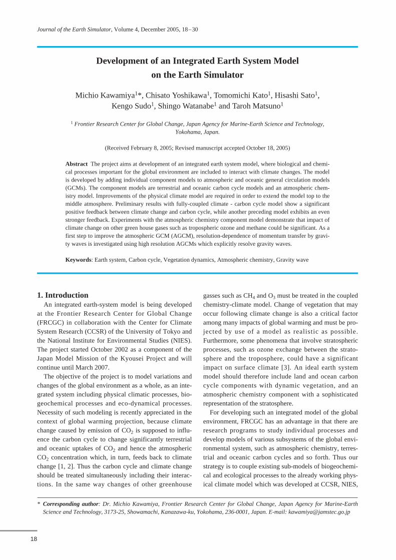
and FRCGC. The whole system is code-named “Kyousei-2 Integrated Synergetic System Model of the Earth(KISSME)” (Fig. 1).

As to vegetation dynamics we are developing a newtype of model which explicitly simulates individualplants. In what follows the present status of our activitiesis reported. Section 2 introduces results from the carboncycle component and provides a brief explanation on thedynamic vegetation model, although it is yet to be run onthe Earth Simulator (ES). Section 3 describes the atmos-pheric chemistry component CHASER, together withsome discussion on results obtained by CHASER-onlyexperiments. Attempts to improve the representation ofthe stratospheric circulation are described in Section 4.Section 5 summarizes this report.

2. Global Carbon Cycle Model2.1 Description of the model and experiment

The terrestrial carbon cycle model, Sim-CYCLE wasoriginally developed by scientists at the University ofTsukuba [4] and brought in to FRCGC when they joinedthe project. In the model carbon storage is divided into 5compartments, that is, leaves, stems, roots, litter or deadbiota and soil organic matters, and processes to representflows among carbon pools including exchanges betweenthe atmosphere and vegetation/soil are included. Biota isclassified into 20 types and their geographical distribution isfixed, meaning that change of vegetation types due to cli-mate change is not represented. The model was used in var-ious studies and known to show reasonable behaviors. Inthe context of the present project, so called off-line calcula-tions on the response of terrestrial carbon storage to someprojected future climate changes were performed [5, 6].

The ocean component of the carbon cycle model wasnewly developed for the present project’s objectives.(The pre-existing model at FRCGC is more eco-dynamics

oriented and complicated [7].) The ocean GCM and thecoupled AOGCM developed at CCSR/NIES/FRCGC areadopted as the base model and ecological/biogeochemicalprocesses have been introduced. As the ecosystemprocess model a nutrient-phytoplankton-zooplankton-detritus type model [8, 9] was adopted. In addition to thisa series of inorganic carbon reactions were introducedfollowing the recommended form by the Ocean CarbonCycle Model Intercomparison Project (OCMIP).

The physical climate system model in which these car-bon cycle components are embedded is the lower resolu-tion version of MIROC, developed by CCSR, NIES, andFRCGC. The atmospheric model has a horizontal resolu-tion of T42, approximately equivalent to 2.8° grid size,and 20 σ-layers in the vertical with relatively fine verticalresolution in the planetary boundary layer. The height ofthe model top is currently ~30 km. The ocean model hasa zonal resolution of 1.4° (= 360/256), and a spatiallyvarying meridional resolution that is about 0.56° at lati-tudes lower than 8°, 1.4° at latitudes higher than 65°, andsmoothly changes in between. The ocean model adopts ahybrid vertical coordinate system; the uppermost 8 levelsout of the 43 use the σ-coordinate and the rest the z-coor-dinate. The model has a bottom boundary layer in addi-tion to the 43 levels. No flux adjustment is applied for thecoupling. Further details of the coupled model are provid-ed in a dedicated report [10].

An experiment is carried out to examine the magnitudeof positive feedback between global warming and carboncycle found in preceding works [1, 2]. The spin-up isconducted by running the integrated model for 280 yearsstarting from the initial conditions based on climatologi-cal data sets until globally integrated net CO2 fluxes atland and sea surfaces vanish. Three different runs are per-formed: the control run in which atmospheric CO2 con-centration is fixed at 285 ppmv throughout the entire inte-gration period after the spin-up, i.e., for 1850-2100; andthe other two runs (coupled and uncoupled run), in whichthe observed time series of the atmospheric CO2 concen-tration is given to the model during 1850-1900, and from1901 to 2100, CO2 emission data (SRES A2 scenario) aregiven to the model instead of concentration data. In thecoupled run atmospheric CO2 concentration was allowedto vary as calculated by the carbon cycle components, butin the uncoupled run, the changing CO2 concentrationhad no impact on climate because the fixed value of 285ppmv was used for radiation routines. In the coupled run,on the other hand, CO2 concentration calculated by thecarbon cycle components was used for radiation calcula-tion so that climate change takes place, which in turnaffects the carbon cycle.

Atmosphere

Climate

Aerosol(SPRINTARS)

Chemistry(CHASER)

(COCO)

Climate(CCRS/NIES AGCM5.7)

Climate(MATSIRO)

Biogeochemistry(MPZD-type)

Biogeochemistry(Sim-CYCLE)

LandOcean

Biogeography(Veg.dynamics)

Fig. 1 Structure of the integrated earth system model, Kyousei-2 Integrated Synergetic System Model of the Earth(KISSME). Note that the vegetation dynamics model isnow separately developed and yet to be incorporated inKISSME.

Integrated earth system model development

20 J. Earth Sim., Vol. 4, Dec. 2005, 18–30

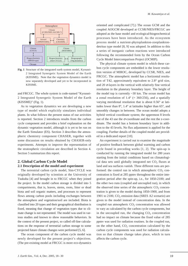
2.2 Results and discussionFig. 2 shows model calculations of CO2 concentration

by the integrated model. It can be seen that the modelresults agree well with the observed evolution of CO2

concentration until 2000. There are two lines correspon-ding to the coupled (red) and the uncoupled (green) run.There is a significant difference between the two experi-ments, and it is seen that the effect of global warming oncarbon cycle is to increase CO2 in the atmosphere; inother words, it accelerates global warming. This isbecause decomposition of soil organic carbon is enhancedby the soil temperature rise following the surface temper-ature rise of 4.0°C projected by this particular model. Thestrength of positive feedback due to climate – carboncycle interactions is 130 ppmv in terms of difference inglobal mean atmospheric CO2 concentration at 2100between the coupled and uncoupled runs, while othermodels show a variety of feedback strength (e.g., 225ppmv by the Hadley centre model [1], 75 ppmv by theIPSL model [2]). The present results should be seen withsome caution because the parameter tuning for the terres-trial carbon cycle component is still underway since theinitialized state of land carbon storage of 3100 PgC waslarger than typical simulation values of 2100 – 2200 PgC[11, 12], although it is within the range of uncertainty

(1746 – 3392 PgC) suggested by an observation-basedstudy [13]. It would certainly deepen our understandingson the global carbon cycle to compare results from vari-ous models and identify what causes such differencesbetween models.

An international project C4MIP (Coupled Carbon-Cycle Climate Model Inter-comparison Project) has beenestablished in order to facilitate such comparative studies,and discussions made in C4MIP will be reflected in the 4th

assessment report of IPCC (Intergovernmental Panel onClimate Change). We regard C4MIP as an important steptoward our international contribution, and shall examineour results following a method adopted by C4MIP

An analysis method has been devised to facilitate com-parison among different models [14] by dividing the cli-mate – carbon cycle feedback into four elements, that is,land and ocean carbon cycle sensitivity to atmosphericCO2 (βAB and βAO in Table 1) and land and ocean carboncycle sensitivity to temperature change (γAB and γAO). Themethod was applied to the results by the Hadley centre [1]and IPSL [2] and the figures displayed in Table 1 wereobtained. The table also shows the figures from our pres-ent experiment. In this particular experiment, our modelyields γAB and γAO similar to those by IPSL. The resultantgain factor g, which shows relative increase of atmospher-ic CO2 concentration due to the climate – carbon cyclefeedback, is thus similar to that of the IPSL model, whilethe gain factor is slightly higher in the present experimentdue to its lower βAB and βAO. Although it is not clear yetwhat leads to the differences in sensitivities, the impact ofthe large land carbon storage in the present experimentsshould be checked when comparisons are made amongdifferent models. As pointed out in a previous report [15],release of CO2 from organic carbon stored on land is amajor component for the climate – carbon cycle feedback.It is planned to perform experiments with the presentmodel, whose results will be presented elsewhere, usingdifferent parameter sets to examine the model’s behaviorswith different terrestrial and oceanic carbon stocks.

Table 1 Estimate of the climate – carbon cycle feedback for three simulations

AB

−201

−89.8

−80.9

AO

0.94

1.7

1.29

Hadley

IPSL

FRCGC

0.0086

0.0072

0.0070

AB

1.66

1.675

1.29

AO

−26.4

−36.8

−36.3

g

0.41

0.166

0.23

f

1.69

1.2

1.30

α is the climate sensitivity to CO2 (K ppmv–1), βAB and βAO are the land and ocean carboncycle sensitivity to atmospheric CO2 (GtC ppmv–1), γAB and γAO are the land and ocean car-bon cycle sensitivity to climate change (GtC K−1), g is the gain of the feedback, namely therelative increase of atmospheric CO2 due to the feedback, and f is the net feedback factordefined as 1/(1 _ g). For the calculation of γAB and γAO, we isolated the direct climate impacton the fluxes from the indirect climate effect through increased atmospheric CO2 [9].

Fig. 2 Development of atmospheric CO2 concentrationobtained by providing CO2 emission data as model inputafter 1900. The red line shows the case where interac-tions between climate and carbon cycle are considered,and the green line not. Units are ppmv.

900+

700+

500+

300+

210020502000195019001850

Global mean CO2 concentration (ppmv)

M. Kawamiya et al.


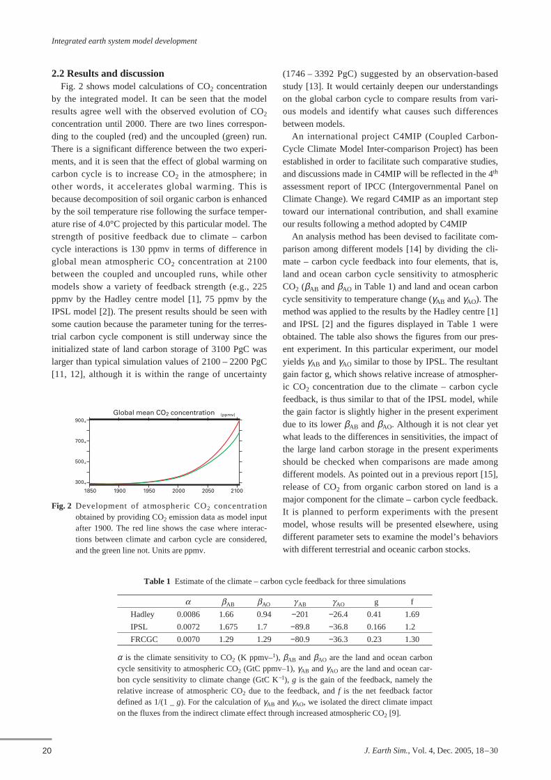
Another result of the integrated model experiment isdepicted in Fig. 3, which shows distribution of anthro-pogenic CO2 accumulated in the ocean until 1994 fromthe coupled run and observations [16]. The simulatedanthropogenic CO2 is estimated as the difference betweentotal inorganic carbon (TIC) and another tracer calculatedin the same way as TIC but with the fixed atmosphericCO2 concentration of 285 ppmv. It is seen in both the sim-ulation and the observations that the northern NorthAtlantic and the Southern Ocean, where deep waters arebeing formed, are capable of carrying much CO2. It can besaid that the simulation and the observations show overallagreement on the global and a basin scale. In particular,since it has been pointed out that the greatest uncertaintyregarding oceanic uptake of anthropogenic CO2 is foundin the Southern Ocean [14, 17], it is encouraging that ourmodel shows a reasonable match for Southern Ocean stor-age in both the magnitude and the latitudinal extent. Thecumulative anthropogenic CO2 until 1994 is 98 PgC in themodel, and close to the lower limit of the observation-based estimate of 118 ± 19 PgC [16], which may include abias toward a larger value by 7% due to the assumption ofconstant disequilibria between atmospheric and oceanicCO2 partial pressures [18].

2.3 Development of a new dynamic vegetationmodel

The terrestrial carbon cycle model in our integratedmodel, Sim-CYCLE does not represent change of vegeta-tion type caused by environmental conditions; only the

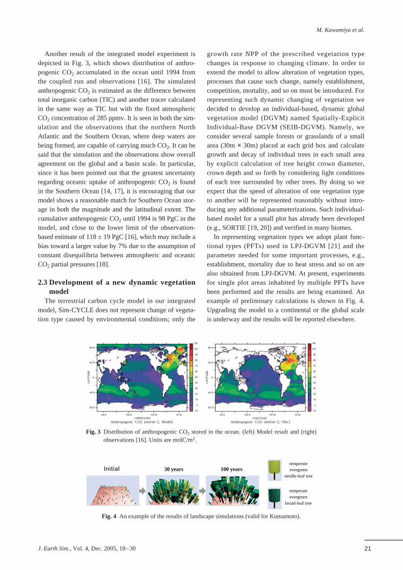
growth rate NPP of the prescribed vegetation typechanges in response to changing climate. In order toextend the model to allow alteration of vegetation types,processes that cause such change, namely establishment,competition, mortality, and so on must be introduced. Forrepresenting such dynamic changing of vegetation wedecided to develop an individual-based, dynamic globalvegetation model (DGVM) named Spatially-ExplicitIndividual-Base DGVM (SEIB-DGVM). Namely, weconsider several sample forests or grasslands of a smallarea (30m × 30m) placed at each grid box and calculategrowth and decay of individual trees in each small areaby explicit calculation of tree height crown diameter,crown depth and so forth by considering light conditionsof each tree surrounded by other trees. By doing so weexpect that the speed of alteration of one vegetation typeto another will be represented reasonably without intro-ducing any additional parameterizations. Such individual-based model for a small plot has already been developed(e.g., SORTIE [19, 20]) and verified in many biomes.

In representing vegetation types we adopt plant func-tional types (PFTs) used in LPJ-DGVM [21] and theparameter needed for some important processes, e.g.,establishment, mortality due to heat stress and so on arealso obtained from LPJ-DGVM. At present, experimentsfor single plot areas inhabited by multiple PFTs havebeen performed and the results are being examined. Anexample of preliminary calculations is shown in Fig. 4.Upgrading the model to a continental or the global scaleis underway and the results will be reported elsewhere.

Anthropogenic CO2 (mol/m~2, Model) Anthropogenic CO2 (mol/m~2, Obs.)

180

100

90

70

60

80

50

40

30

20

10

0

-10

180

100

90

70

60

80

50

40

30

20

10

0

-10

LONGITUDE

LAT

ITU

DE

LAT

ITU

DE

LONGTIUDE

80°N

40°N

0°

40°S

80°S

50°E 150°E 10°W110°W

80°N

40°N

0°

40°S

80°S

50°E 150°E 10°W110°W

Fig. 3 Distribution of anthropogenic CO2 stored in the ocean. (left) Model result and (right)observations [16]. Units are molC/m2.

Initial 30 years 100 yearstemperateevergreen

needle-leaf tree

temperateevergreen

broad-leaf tree

Fig. 4 An example of the results of landscape simulations (valid for Kumamoto).



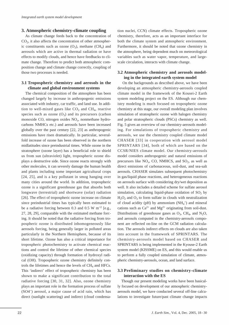
3. Atmospheric chemistry-climate couplingAs climate change feeds back to the concentration of

CO2, it also affects the concentration of other atmospher-ic constituents such as ozone (O3), methane (CH4) andaerosols which are active in thermal radiation or haveeffects to modify clouds, and hence have feedbacks to cli-mate change. Therefore to predict both atmospheric com-position change and climate change correctly, coupling ofthose two processes is needed.

3.1 Tropospheric chemistry and aerosols in theclimate and global environment systems

The chemical composition of the atmosphere has beenchanged largely by increase in anthropogenic emissionsassociated with industry, car traffic, and land use. In addi-tion to well-mixed gases like CO2 and CH4, reactivespecies such as ozone (O3) and its precursors (carbonmonoxide CO, nitrogen oxides NOx, nonmethane hydro-carbons NMHCs etc.) and aerosols have been increasedglobally over the past century [22, 23] as anthropogenicemissions have risen dramatically. In particular, several-fold increase of ozone has been observed in the northernmidlatitudes since preindustrial times. While ozone in thestratosphere (ozone layer) has a beneficial role to shieldus from sun (ultraviolet) light, tropospheric ozone dis-plays a destructive side. Since ozone reacts strongly withother molecules, it can severely damage the human healthand plants including some important agricultural crops[24, 25], and is a key pollutant in smog hanging overmany cities around the world. In addition, troposphericozone is a significant greenhouse gas that absorbs bothlongwave (terrestrial) and shortwave (solar) radiation[26]. The effect of tropospheric ozone increase on climatesince preindustrial times has typically been estimated tobe a radiative forcing between 0.3 and 0.5 W m−2 [e.g.,27, 28, 29], comparable with the estimated methane forc-ing. It should be noted that the radiative forcing from tro-pospheric ozone is distributed inhomogeneously likeaerosols forcing, being generally larger in polluted areasparticularly in the Northern Hemisphere, because of itsshort lifetime. Ozone has also a critical importance fortropospheric photochemistry to activate chemical reac-tions and control the lifetime of other chemical species(oxidizing capacity) through formation of hydroxyl radi-cal (OH). Tropospheric ozone chemistry definitely con-trols the lifetimes and hence the levels of CH4 and HFCs.This ‘indirect’ effect of tropospheric chemistry has beenshown to make a significant contribution to the totalradiative forcing [30, 31, 32]. Also, ozone chemistryplays an important role in the formation process of sulfate(SO4−) aerosol, a major cause of acid rain, which hasdirect (sunlight scattering) and indirect (cloud condensa-

tion nuclei, CCN) climate effects. Tropospheric ozonechemistry, therefore, acts as an important interface forboth the climate system and atmospheric environment.Furthermore, it should be noted that ozone chemistry inthe atmosphere, being dependent much on meteorologicalvariables such as water vapor, temperature, and large-scale circulation, interacts with climate change.

3.2 Atmospheric chemistry and aerosols model-ing in the integrated earth system model

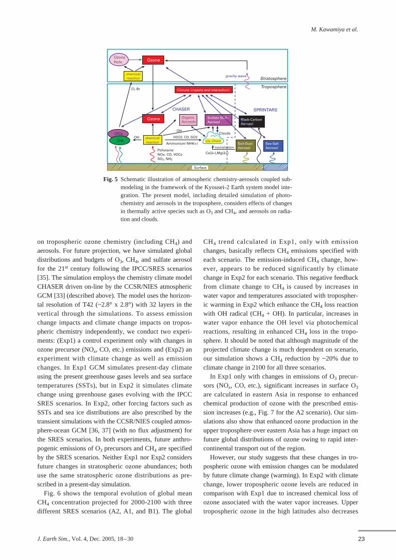
On the backgrounds as described above, we have beendeveloping an atmospheric chemistry-aerosols coupledclimate model in the framework of the Kousei-2 Earthsystem modeling project on the ES. Although our chem-istry modeling is much focused on tropospheric ozonechemistry at this stage, our overall modeling plan involvessimulation of stratospheric ozone with halogen chemistryand polar stratospheric clouds (PSCs) chemistry as well.Fig. 5 gives an overview of our chemistry-aerosols model-ing. For simulations of tropospheric chemistry andaerosols, we use the chemistry coupled climate modelCHASER [33] in cooperation with aerosol modelSPRINTARS [34], both of which are based on theCCSR/NIES climate model. Our chemistry-aerosolsmodel considers anthropogenic and natural emissions ofprecursors like NOx, CO, NMHCS, and SO2, as well asdirect emissions of carbonaceous, soil-dust, and sea-saltaerosols. CHASER simulates subsequent photochemistryin gas/liquid phase reactions, and heterogeneous reactionson aerosols surface with considering dry/wet deposition aswell. It also includes a detailed scheme for sulfate aerosolsimulation, calculating liquid-phase oxidation of SO2 byH2O2 and O3 to form sulfate in clouds with neutralizationof cloud acidity (pH) by ammonium (NH4

+) and mineralcations such as Ca2+ and Mg2+ originating from soil-dust.Distributions of greenhouse gases as O3, CH4, and N2O,and aerosols computed in the chemistry-aerosols compo-nent are reflected on-line on the GCM radiation calcula-tion. The aerosols indirect effects on clouds are also takeninto account in the framework of SPRINTARS. Thechemistry-aerosols model based on CHASER andSPRINTARS is being implemented in the Kyouse-2 Earthsystem model (KISSME) on ES, and this would enable usto perform a fully coupled simulation of climate, atmos-pheric chemistry-aerosols, ocean, and land surface.

3.3 Preliminary studies on chemistry-climateinteraction with the ES

Though our present modeling works have been basical-ly focused on development of our atmospheric chemistry-aerosols model, we have conducted several off-line calcu-lations to investigate future/past climate change impacts

M. Kawamiya et al.


on tropospheric ozone chemistry (including CH4) andaerosols. For future projection, we have simulated globaldistributions and budgets of O3, CH4, and sulfate aerosolfor the 21st century following the IPCC/SRES scenarios[35]. The simulation employs the chemistry climate modelCHASER driven on-line by the CCSR/NIES atmosphericGCM [33] (described above). The model uses the horizon-tal resolution of T42 (~2.8° x 2.8°) with 32 layers in thevertical through the simulations. To assess emissionchange impacts and climate change impacts on tropos-pheric chemistry independently, we conduct two experi-ments: (Exp1) a control experiment only with changes inozone precursor (NOx, CO, etc.) emissions and (Exp2) anexperiment with climate change as well as emissionchanges. In Exp1 GCM simulates present-day climateusing the present greenhouse gases levels and sea surfacetemperatures (SSTs), but in Exp2 it simulates climatechange using greenhouse gases evolving with the IPCCSRES scenarios. In Exp2, other forcing factors such asSSTs and sea ice distributions are also prescribed by thetransient simulations with the CCSR/NIES coupled atmos-phere-ocean GCM [36, 37] (with no flux adjustment) forthe SRES scenarios. In both experiments, future anthro-pogenic emissions of O3 precursors and CH4 are specifiedby the SRES scenarios. Neither Exp1 nor Exp2 considersfuture changes in stratospheric ozone abundances; bothuse the same stratospheric ozone distributions as pre-scribed in a present-day simulation.

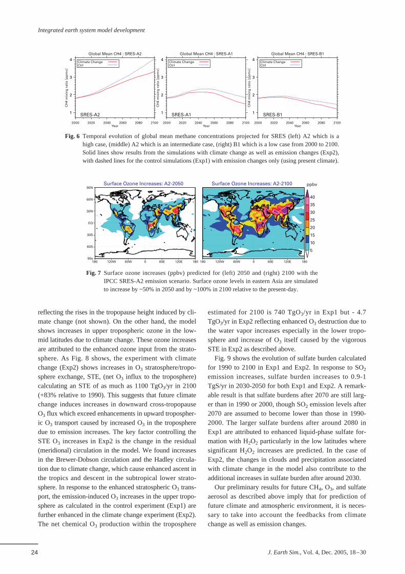
Fig. 6 shows the temporal evolution of global meanCH4 concentration projected for 2000-2100 with threedifferent SRES scenarios (A2, A1, and B1). The global

CH4 trend calculated in Exp1, only with emissionchanges, basically reflects CH4 emissions specified witheach scenario. The emission-induced CH4 change, how-ever, appears to be reduced significantly by climatechange in Exp2 for each scenario. This negative feedbackfrom climate change to CH4 is caused by increases inwater vapor and temperatures associated with tropospher-ic warming in Exp2 which enhance the CH4 loss reactionwith OH radical (CH4 + OH). In particular, increases inwater vapor enhance the OH level via photochemicalreactions, resulting in enhanced CH4 loss in the tropo-sphere. It should be noted that although magnitude of theprojected climate change is much dependent on scenario,our simulation shows a CH4 reduction by ~20% due toclimate change in 2100 for all three scenarios.

In Exp1 only with changes in emissions of O3 precur-sors (NOx, CO, etc.), significant increases in surface O3

are calculated in eastern Asia in response to enhancedchemical production of ozone with the prescribed emis-sion increases (e.g., Fig. 7 for the A2 scenario). Our sim-ulations also show that enhanced ozone production in theupper troposphere over eastern Asia has a huge impact onfuture global distributions of ozone owing to rapid inter-continental transport out of the region.

However, our study suggests that these changes in tro-pospheric ozone with emission changes can be modulatedby future climate change (warming). In Exp2 with climatechange, lower tropospheric ozone levels are reduced incomparison with Exp1 due to increased chemical loss ofozone associated with the water vapor increases. Uppertropospheric ozone in the high latitudes also decreases

OzoneOzoneHole

Ozone

chemicalreaction

chemicalreaction

CI, Br

CFCs

CH4

CHASER SPRINTARS

gravity wave

OrganicAerosols

Climate (inpacts and interaction)

Sulfate SO4--Aerosol

Stratosphere

Troposphere

Black-CarbonAerosol

Soil-DustAerosol

Sea-SaltAerosol

OH

OHClouds

Liq.-ChemH2O2, O3, SO2

Ammonium NH4(+)

PollutantsNOx, CO, VOCsSO2, NH3

neutralization

Ca(2+),Mg(2+)

Surface

Fig. 5 Schematic illustration of atmospheric chemistry-aerosols coupled sub-modeling in the framework of the Kyousei-2 Earth system model inte-gration. The present model, including detailed simulation of photo-chemistry and aerosols in the troposphere, considers effects of changesin thermally active species such as O3 and CH4, and aerosols on radia-tion and clouds.



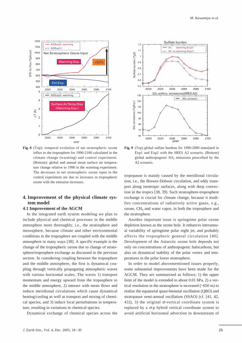
reflecting the rises in the tropopause height induced by cli-mate change (not shown). On the other hand, the modelshows increases in upper tropospheric ozone in the low-mid latitudes due to climate change. These ozone increasesare attributed to the enhanced ozone input from the strato-sphere. As Fig. 8 shows, the experiment with climatechange (Exp2) shows increases in O3 stratosphere/tropo-sphere exchange, STE, (net O3 influx to the troposphere)calculating an STE of as much as 1100 TgO3/yr in 2100(+83% relative to 1990). This suggests that future climatechange induces increases in downward cross-tropopauseO3 flux which exceed enhancements in upward tropospher-ic O3 transport caused by increased O3 in the tropospheredue to emission increases. The key factor controlling theSTE O3 increases in Exp2 is the change in the residual(meridional) circulation in the model. We found increasesin the Brewer-Dobson circulation and the Hadley circula-tion due to climate change, which cause enhanced ascent inthe tropics and descent in the subtropical lower strato-sphere. In response to the enhanced stratospheric O3 trans-port, the emission-induced O3 increases in the upper tropo-sphere as calculated in the control experiment (Exp1) arefurther enhanced in the climate change experiment (Exp2).The net chemical O3 production within the troposphere

estimated for 2100 is 740 TgO3/yr in Exp1 but - 4.7TgO3/yr in Exp2 reflecting enhanced O3 destruction due tothe water vapor increases especially in the lower tropo-sphere and increase of O3 itself caused by the vigorousSTE in Exp2 as described above.

Fig. 9 shows the evolution of sulfate burden calculatedfor 1990 to 2100 in Exp1 and Exp2. In response to SO2

emission increases, sulfate burden increases to 0.9-1TgS/yr in 2030-2050 for both Exp1 and Exp2. A remark-able result is that sulfate burdens after 2070 are still larg-er than in 1990 or 2000, though SO2 emission levels after2070 are assumed to become lower than those in 1990-2000. The larger sulfate burdens after around 2080 inExp1 are attributed to enhanced liquid-phase sulfate for-mation with H2O2 particularly in the low latitudes wheresignificant H2O2 increases are predicted. In the case ofExp2, the changes in clouds and precipitation associatedwith climate change in the model also contribute to theadditional increases in sulfate burden after around 2030.

Our preliminary results for future CH4, O3, and sulfateaerosol as described above imply that for prediction offuture climate and atmospheric environment, it is neces-sary to take into account the feedbacks from climatechange as well as emission changes.

4

3

2

1

CH

4 m

ixin

g r

atio

[p

pm

v]

Global Mean CH4 : SRES-A2

Climate ChangeCtrl

SRES-A2

2000 2020 2040 2060 2080 2100Year

4

3

2

1

CH

4 m

ixin

g r

atio

[p

pm

v]

Global Mean CH4 : SRES-A1

Climate ChangeCtrl

SRES-A1

2000 2020 2040 2060 2080 2100Year

4

3

2

1

CH

4 m

ixin

g r

atio

[p

pm

v]

Global Mean CH4 : SRES-B1

Climate ChangeCtrl

SRES-B1

2000 2020 2040 2060 2080 2100Year

Fig. 6 Temporal evolution of global mean methane concentrations projected for SRES (left) A2 which is ahigh case, (middle) A2 which is an intermediate case, (right) B1 which is a low case from 2000 to 2100.Solid lines show results from the simulations with climate change as well as emission changes (Exp2),with dashed lines for the control simulations (Exp1) with emission changes only (using present climate).

Surface Ozone Increases: A2-205090N

60N

30N

EQ

30S

60S

90s180 120W 60W 0 60E 120E

Surface Ozone Increases: A2-2100

180180 120W 60W 0 60E 120E 180

ppbv

40

35

30

25

20

15

10

5

Fig. 7 Surface ozone increases (ppbv) predicted for (left) 2050 and (right) 2100 with theIPCC SRES-A2 emission scenario. Surface ozone levels in eastern Asia are simulatedto increase by ~50% in 2050 and by ~100% in 2100 relative to the present-day.

M. Kawamiya et al.


4. Improvement of the physical climate sys-tem model

4.1 Improvement of the AGCMIn the integrated earth system modeling we plan to

include physical and chemical processes in the middleatmosphere more thoroughly, i.e., the stratosphere andmesosphere, because climate and other environmentalconditions in the troposphere are coupled with the middleatmosphere in many ways [38]. A specific example is thechange of the tropospheric ozone due to change of strato-sphere/troposphere exchange as discussed in the previoussection. In considering coupling between the troposphereand the middle atmosphere, the first is dynamical cou-pling through vertically propagating atmospheric waveswith various horizontal scales. The waves 1) transportmomentum and energy upward from the troposphere tothe middle atmosphere, 2) interact with mean flows andinduce meridional circulations which cause dynamicalheating/cooling as well as transport and mixing of chemi-cal species, and 3) induce local perturbations in tempera-ture, resulting in variations in chemical species.

Dynamical exchange of chemical species across the

tropopause is mainly caused by the meridional circula-tion, i.e., the Brewer-Dobson circulation, and eddy trans-port along isentropic surfaces, along with deep convec-tion in the tropics [38, 39]. Such stratosphere-troposphereexchange is crucial for climate change, because it modi-fies concentrations of radiatively active gases, e.g.,ozone, CH4 and water vapor, in both the troposphere andthe stratosphere.

Another important issue is springtime polar ozonedepletion known as the ozone hole. It enhances interannu-al variability of springtime polar night jet, and probablyaffects the tropospheric general circulation [40].Development of the Antarctic ozone hole depends notonly on concentrations of anthropogenic halocarbons, butalso on dynamical stability of the polar vortex and tem-peratures in the polar lower stratosphere.

In order to model abovementioned issues properly,some substantial improvements have been made for theAGCM. They are summarized as follows; 1) the upperlimit of the model is extended to about 0.01 hPa, 2) a ver-tical resolution in the stratosphere is increased (~650 m) torealize the equatorial quasi-biennial oscillation (QBO) andstratopause semi-annual oscillation (SSAO) (cf. [41, 42,43]), 3) the original σ-vertical coordinate system isreplaced by a σ-p hybrid vertical coordinate system toavoid artificial horizontal advection in downstream of

1200

1100

1000

900

800

700

600

500

400

ST

E O

3 Fl

ux

[Tg

O3/

yr]

A2(Exp2): warming

A2(Exp2): warming

A2(Exp1):

Net Stratospheric Ozone Input

2000 2020 2040 2060 2080 2100

2000 2020 2040 2060 2080 2100

T [

K]

5

4

3

2

1

0

year

Surface Air Temp.Rise(Warming Exp.)

Ctrl.Exp.

Warming Exp. +83%

1.2

1.1

1

0.9

0.8

0.7

0.6

0.5

130

120

110

100

90

80

70

60

A2: warming (Exp2)

SO2 emission

SO

2 em

issi

on

s [T

gS

/yr]

A2: no warming (Exp1)

2000 2020 2040 2060 2080 2100

2000 2020 2040 2060 2080 2100

Su

lfat

e b

urd

en [

Tg

S]

Sulfate burden

year

SO2 anthro. emissions(SRES:A2)

Fig. 8 (Top): temporal evolution of net stratospheric ozoneinflux to the troposphere for 1990-2100 calculated in theclimate change (warming) and control experiment.(Bottom): global and annual mean surface air tempera-ture change relative to 1990 in the warming experiment.The decreases in net stratospheric ozone input in thecontrol experiment are due to increases in troposphericozone with the emission increases.

Fig. 9 (Top) global sulfate burdens for 1990-2000 simulated inExp1 and Exp2 with the SRES A2 scenario. (Bottom)global anthropogenic SO2 emissions prescribed by theA2 scenario.



mountains [44], 4) an updated version of radiation schemeis employed to decrease cold biases near the tropicaltropopause and the summertime lower stratosphere, and 5)a non-orographic gravity wave drag (GWD) parameteriza-tion of Hines [45, 47] is employed to obtain a realistic sea-sonal march of the polar vortex (by eliminating the coldpole bias problem), as well as the equatorial QBO andSSAO. The GWD parameterization is necessary becausethe standard horizontal resolution of the AGCM is T42,which is not fine enough to explicitly resolve gravitywaves effective to large scale stratospheric circulation.

4.2 High-resolution AGCM simulationsThe Hines scheme requires information on global dis-

tribution and characteristics of gravity waves, which aredifficult to evaluate from observations. In order to obtaininformation on global morphology of gravity waves andtheir propagation direction and momentum fluxes, weperformed several high-resolution AGCM simulations(e.g., [43, 47, 48]). Here, results of two AGCM simula-tions with different horizontal resolutions are compared.This comparison is analogous to what has been conductedfor the GFDL SKYHI GCM simulations [49].

The horizontal resolutions are T106 and T213. Theminimal resolvable horizontal wavelengths are about 380km and 190 km, respectively. Other experimental settingsare almost the same for each other. The AGCM has 250layers from the surface to 0.01 hPa. A vertical resolutionis 300 m throughout the middle atmosphere. The AGCMincludes realistic topography and a full set of physicalparameterizations [50]. Any GWD parameterizations areexcluded for these simulations in order to focus on explic-itly resolved gravity waves. Results are shown as monthlyaverages of June in a typical year of each simulation.

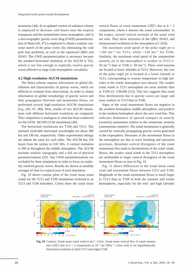
Fig. 10 shows contour plots of the zonal mean zonalwinds for the T213 and T106 simulations (referred to asT213 and T106 hereafter). Colors show the zonal mean

vertical fluxes of zonal momentum ( ) due to k > 5components, where k denotes the zonal wavenumber. Inthe tropics, several vertical reversals of the zonal windare seen. They show structures of the QBO, SSAO, andintraseasonal oscillation in the mesosphere (cf. [43]).

The maximum wind speed of the polar night jet is~100 ms−1 for T213, while ~130 ms−1 for T106.Similarly, the maximum wind speed of the summertimeeasterly jet in the mesosphere is weaker in T213 (~50 ms−1) than in T106 (~ 60 ms−1). These wind maximaare located at lower altitudes in T213. Moreover, the coreof the polar night jet is located at a lower latitude inT213, corresponding to warmer temperature in high lati-tudes in the whole stratosphere (not shown). The weakerzonal winds in T213 mesosphere are more realistic thanin T106 (cf. CIRA86 [51]). This fact suggests that zonalflow decelerations due to gravity waves are larger andmore realistic in T213 than in T106.

Signs of the zonal momentum fluxes are negative inthe southern hemisphere middle atmosphere, and positivein the northern hemisphere above the zero wind line. Thisindicates dominance of upward transport of easterly(westerly) momentum relative to the wintertime westerly(summertime easterly). The zonal momentum is generallycarried by vertically propagating gravity waves generatedin the troposphere. Decreases of the momentum fluxes inthe mesosphere are due to wave breaking and saturationprocesses. Resultant vertical divergence of the zonalmomentum flux leads to decelerations of the zonal winds.Hence, the weaker zonal winds in the T213 mesosphereare attributable to larger vertical divergence of the zonalmomentum fluxes as seen in Fig. 10.

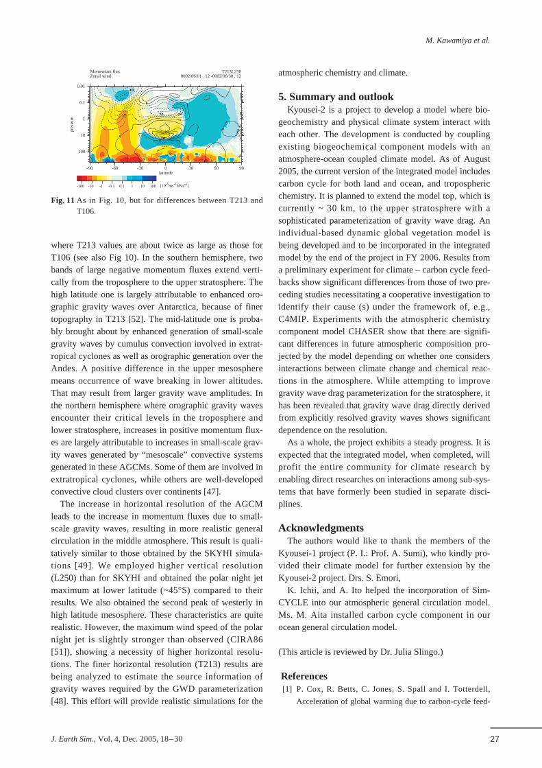
Fig. 11 shows differences in the zonal mean zonalwind and momentum fluxes between T213 and T106.Magnitude of the zonal momentum fluxes is much largerin T213 than in T106 in both the summer and winterhemispheres, especially for the mid- and high latitudes

u' 'ω

Momentum fluxZonal wind

T213L2500002/06/01 . 12 -0002/06/30 . 12

0.01

0.1

1

10

100

pres

sure

-90 -60 -30 0 30 60 90latitude

-100 -10 -1 -0.1 0.1 1 10 100 [10-5ms-1hPas-1]


T106L2500003/06/01 . 12 -0003/06/30 . 12

0.01

0.1

1

10

100

pres

sure

-90 -60 -30 0 30 60 90latitude

-100 -10 -1 -0.1 0.1 1 10 100 [10-5ms-1hPas-1]

Fig. 10 Contour: Zonal mean zonal wind in ms–1. Color: Zonal mean vertical flux of zonal momen-tum ( ) due to k > 5 components in 10–1 ms–1hPas–1. Color scale is set logarithmically.Horizontal resolution is (left) T213 and (right) T106.

u' 'ω

M. Kawamiya et al.


where T213 values are about twice as large as those forT106 (see also Fig 10). In the southern hemisphere, twobands of large negative momentum fluxes extend verti-cally from the troposphere to the upper stratosphere. Thehigh latitude one is largely attributable to enhanced oro-graphic gravity waves over Antarctica, because of finertopography in T213 [52]. The mid-latitude one is proba-bly brought about by enhanced generation of small-scalegravity waves by cumulus convection involved in extrat-ropical cyclones as well as orographic generation over theAndes. A positive difference in the upper mesospheremeans occurrence of wave breaking in lower altitudes.That may result from larger gravity wave amplitudes. Inthe northern hemisphere where orographic gravity wavesencounter their critical levels in the troposphere andlower stratosphere, increases in positive momentum flux-es are largely attributable to increases in small-scale grav-ity waves generated by “mesoscale” convective systemsgenerated in these AGCMs. Some of them are involved inextratropical cyclones, while others are well-developedconvective cloud clusters over continents [47].

The increase in horizontal resolution of the AGCMleads to the increase in momentum fluxes due to small-scale gravity waves, resulting in more realistic generalcirculation in the middle atmosphere. This result is quali-tatively similar to those obtained by the SKYHI simula-tions [49]. We employed higher vertical resolution(L250) than for SKYHI and obtained the polar night jetmaximum at lower latitude (~45°S) compared to theirresults. We also obtained the second peak of westerly inhigh latitude mesosphere. These characteristics are quiterealistic. However, the maximum wind speed of the polarnight jet is slightly stronger than observed (CIRA86[51]), showing a necessity of higher horizontal resolu-tions. The finer horizontal resolution (T213) results arebeing analyzed to estimate the source information ofgravity waves required by the GWD parameterization[48]. This effort will provide realistic simulations for the

atmospheric chemistry and climate.

5. Summary and outlookKyousei-2 is a project to develop a model where bio-

geochemistry and physical climate system interact witheach other. The development is conducted by couplingexisting biogeochemical component models with anatmosphere-ocean coupled climate model. As of August2005, the current version of the integrated model includescarbon cycle for both land and ocean, and troposphericchemistry. It is planned to extend the model top, which iscurrently ~ 30 km, to the upper stratosphere with asophisticated parameterization of gravity wave drag. Anindividual-based dynamic global vegetation model isbeing developed and to be incorporated in the integratedmodel by the end of the project in FY 2006. Results froma preliminary experiment for climate – carbon cycle feed-backs show significant differences from those of two pre-ceding studies necessitating a cooperative investigation toidentify their cause (s) under the framework of, e.g.,C4MIP. Experiments with the atmospheric chemistrycomponent model CHASER show that there are signifi-cant differences in future atmospheric composition pro-jected by the model depending on whether one considersinteractions between climate change and chemical reac-tions in the atmosphere. While attempting to improvegravity wave drag parameterization for the stratosphere, ithas been revealed that gravity wave drag directly derivedfrom explicitly resolved gravity waves shows significantdependence on the resolution.

As a whole, the project exhibits a steady progress. It isexpected that the integrated model, when completed, willprofit the entire community for climate research byenabling direct researches on interactions among sub-sys-tems that have formerly been studied in separate disci-plines.

AcknowledgmentsThe authors would like to thank the members of the

Kyousei-1 project (P. I.: Prof. A. Sumi), who kindly pro-vided their climate model for further extension by theKyousei-2 project. Drs. S. Emori,

K. Ichii, and A. Ito helped the incorporation of Sim-CYCLE into our atmospheric general circulation model.Ms. M. Aita installed carbon cycle component in ourocean general circulation model.

(This article is reviewed by Dr. Julia Slingo.)

References[1] P. Cox, R. Betts, C. Jones, S. Spall and I. Totterdell,

Acceleration of global warming due to carbon-cycle feed-


T213L2500002/06/01 . 12 -0002/06/30 . 12

0.01

0.1

1

10

100

pres

sure

-90 -60 -30 0 30 60 90latitude

-100 -10 -1 -0.1 0.1 1 10 100 [10-5ms-1hPas-1]

Fig. 11 As in Fig. 10, but for differences between T213 andT106.



backs in a coupled climate model, Nature, vol.408,

pp.184 – 187, 2000.

[2] P. Friedlingstein, L. Bopp, P. Ciais, J.-L. Dufresne,

L. Fairhead, H. LeTreut, P. Monfray and J. Orr, Positive

feedback between future climate change and the carbon

cycle, Geophysical Research Letters, vol.28, pp.1543 – 1546,

2001.

[3] K. Sudo, M. Takahashi, and H. Akimoto, Future changes

in stratosphere-troposphere exchange and their impacts on

fugure tropospheric simulations, Geophysical Research

Letters, vol.30, 24, 2256, doi:10.1029/2003GL018526,

2003.

[4] A. Ito and T. Oikawa, A simulation model of the carbon

cycle in land ecosystems Sim-CYCLE: A description

based on dry-matter production theory and plot-scale vali-

dation, Ecological Modelling, vol.151, pp.147 – 179, 2002.

[5] A. Ito, Climate-related uncertainties in projections of the

21st century terrestrial carbon budget: Off-line model

experiments using IPCC greenhouse gas scenarios and

AOGCM climate projections, Climate Dynamics, 2005 (in

press).

[6] A. Ito, Regional variability in the terrestrial carbon-cycle

response to global warming in the 21st century: simulation

analysis with AOGCM-based climate projections, Journal

of the Meteorological Society of Japan, 2005 (in press).

[7] M. Aita, N., Y. Yamanaka and M. J. Kishi, Effect of onto-

genetic vertical migration of zooplankton on annual pri-

mary production — Using NEMURO embedded in general

circulation model —, Fish. Oceanogr, vol.12, pp.284 – 290,

2003.

[8] A. Oschlies, and V. Garçon, An eddy-permitting coupled

physical-biological model of the North Atlantic 1.

Sensitivity to advection numerics and mixed layer physics,

Global Biogeochemical Cycles, vol.13, pp.135 – 160, 1999.

[9] A. Oschlies, Model-derived estimates of new production:

New results point towards lower values, Deep-Sea

Research II, vol.48, pp.2173 – 2197, 2001.

[10] H. Hasumi, and S. Emori, K-1 Coupled GCM (MIROC)

Description, K-1 Technical Report No.1, Center for

Climate System Research (Univ. of Tokyo), National

Institute for Environmental Studies, and Frontier Research

Center for Global Change, 2004.

[11] I. C. Prentice, M. T. Sykes, M. Lautenschlager,

S. P. Harrison, O. Denissenko and P. J. Bartlein, Modelling

vegetaion patterns and terrestrial carbon sorage at the last

glacial maximum, Global Ecology and Biogeography

Letters, vol.3, pp.67 – 76, 1993.

[12] L. M. François, C. Delire, P. Warnant and G. Munhoven,

Modelling the glacial-interglacial changes in the continen-

tal biosphere, Global and Planetary Change, vol.16 – 17,

pp.37 – 52, 1998.

[13] J. M. Adams and H. Faure, A new estimate of changing

carbon storage on land since the last glacial maximum,

based on global land ecosystem reconstruction, Global

and Planetary Change, vol.16 – 17, pp.3 – 24, 1998.

[14] P. Friedlingstein, J.-L. Dufresne, P. M. Cox and P. Rayner,

How positive is the feedback between climate change and

the carbon cycle, Tellus, vol.55B, pp.692 – 700, 2003.

[15] J.-L. Dufresne, P. Friedlingstein, M. Berhelot, L. Bopp,

P. Ciais, L. Fairhead, H. LeTreut and P. Monfray, On the

Magnitude of Positive Feedback between Future Climate

Change and the Carbon Cycle, Geophysical Research

Letters, vol.29, doi:10.1029/2001GL013777, 2002.

[16] C. L. Sabine, R. A. Feely, N. Gruber, R. M. Key, K. Lee,

J. L. Bullister, R. Wanninkhof, C. S. Wong, D. W. R.

Wallace, B. Tilbrook, F. J. Millero, T.-H. Peng, A. Kozyr,

T. Ono, and A. F. Rios, The Oceanic Sink for

Anthropogenic CO2, Science, vol.305, pp.367 – 371, 2004.

[17] J. C. Orr, E. Maier-Reimer, U. Mikolajewicz, P. Monfray,

J. L. Sarmiento, J. R. Toggweiler, N. K. Taylor, J. Palmer,

N. Gruber, C. L. Sabine, C. LeQuèrè, R. M. Key and

J. Boutin, Estimates of anthropogenic carbon uptake from

four three-dimensional global ocean models, Global

Biogeochemical Cycles, vol.15, pp.43 – 60, 2001.

[18] K. Matsumoto and N. Gruber, How accurate is the estima-

tion of anthropogenic carbon in the ocean? An evaluation

of the ∆C* method, Global Biogeochemical Cycles, in

press, 2005.

[19] S. W. Pacala, C. D. Canham, and J. A. J. Silander., Forest

models defined by field measurements: I. The design of a

northeastern forest simulator, Can. J. For. Res., vol.23,

pp.1980 – 1988, 1993.

[20] S. W. Pacala, C. D. Canham, and A. J. Silander, R.

K. Kobe, and E. Ribbens. Forest models defined by field

measurements: Estimation, error analysis and dynamics.

Ecol, Monogr., vol.66, pp.1 – 43, 1996.

[21] S. Sitch, B. Smith, I. C. Prentice, A. Arneth, A. Bondeau,

W. Cramer, J. O. Kaplan, S. Levis, W. Lucht, M. T. Sykes,

K. Thonicke, and S. Venevsky, Evaluation of ecosystem

dynamics, plant geography and terrestrial carbon cycling in

the LPJ dynamic global vegetation model, Global Change

Biology, vol.9, pp.161 – 185, 2003.

[22] WMO, Report of the International Ozone Trends Panel:

1988, Global Ozone Research and Monitoring Project:

Report No.18, Geneva, 1990.

[23] P. J. Crutzen and P. H. Zimmermann, The changing photo-

chemistry of the troposphere, Tellus, vol.43, pp.136 – 151,

1991.

[24] World Health Organization (WHO), Update and revision

of the WHO air quality guidelines for Europe. Classical air

pollutants: ozone and other photochemical oxidants,

European centre for environment and health, Bilthoven,

the Netherlands, 1996.

[25] World Health Organization (WHO), Update and revision

M. Kawamiya et al.


of the WHO air quality guidelines for Europe. Ecotoxic

effects, ozone effects on vegetation, European centre for

environment and health, Bilthoven, the Netherlands, 1996.

[26] W. Wang, J.P. Pinto, and Y.L. Yung, Greenhouse effects

due to man-made perturbations of trace gases, J. Atmos.

Sci., vol.37, pp.333 – 338, 1980.

[27] P. M. Forster, C. E. Johnson, K. S. Law, J. A. Pyle, and

K. P. Shine, Further estimates of radiative forcing due to

tropospheric ozone changes, Geophys. Res. Lett., vol.23,

pp.3321 – 3324, 1996.

[28] T. K. Berntsen, I. S. A. Isaksen, G. Myhre, J. S. Fuglestvedt,

F. Stordal, T. Alsvik, Larsen, R. S. Freckleton, and K. P.

Shine, Effects of anthropogenic emissions on tropospheric

ozone and its radiative forcing, J. Geophys. Res., vol.102,

pp.28,101 – 28,126, 1997.

[29] L. J. Mickley, P. P. Murti, D. J. Jacob, J. A. Logan,

D. M. Koch, and D. Rind, Radiative forcing from tropos-

pheric ozone calculated with a unified chemistry-climate

model, J. Geophys. Res., vol.104, pp.30,153 – 30,172, 1999.

[30] D. A. Hauglustaine, C. Granier, G. P. Brasseur, and

G. Megie, The importance of atmospheric chemistry in the

calculation of radiative forcing on the climate system, J.

Geophys. Res., vol.99, pp.1173 – 1186, 1994.

[31] C. E. Johnson and R. G. Derwent, Relative radiative forc-

ing consequences of global emissions of hydrocarbons,

carbon monoxide and NOx from human activities estimat-

ed with a zonally averaged two-dimensional model,

Climate Change, vol.34, pp.439 – 462, 1996.

[32] O. Wild, M.J. Prather, and H. Akimoto, Indirect long-term

global radiative cooling from NOx emissions, Geophys.

Res. Lett., vol.28, pp.1719– 1722, 2001.

[33] K . Sudo , M. Takahash i , J . Ku rokawa , and H .

Akimoto, CHASER: A global chemical model of the

troposphere 1. Model description, J. Geophys. Res.,

vol.107, doi:10.1029/2001JD001113, 2002.

[34] T. Takemura, H. Okamoto, Y. Maruyama, A. Numaguti,

A. Higurashi, and T. Nakajima, Global three-dimensional

simulation of aerosol optical thickness distribution of vari-

ous origins, J. Geophys. Res., vol.105, pp.17,853 – 17,873,

2000.

[35] K. Sudo., M. Takahashi, and H. Akimoto, Future changes

in stratosphere-troposphere exchange and their impacts on

future tropospheric ozone simulations Geophys. Res.

Letters., vol.30, 2256, doi:10.1029/2003GL018526, 2003.

[36] S. Emori, T. Nozawa, A. Abe-Ouchi, A. Numaguti,

M. Kimoto, and T. Nakajima, Coupled ocean-atmosphere

model experiments of future climate change with an

explicit representation of sulfate aerosol scattering, J.

Meteor. Soc. Japan, vol.77, pp.1299 – 1307, 1999.

[37] T. Nozawa, S. Emori, A. Numaguti, Y. Tsushima,

T. Takemura, T. Nakajima, A. Abe-Ouchi, and

M. Kimoto, Projections of future climate change in the

21st century simulated by the CCSR/NIES CGCM under

the IPCC SRES scenarios, in Present and Future of

Modeling Global Environmental Change toward

Integrated Modeling, ed. T. Matsuno and H. Kida, Terra

Scientific Publishing, pp.15 – 28, 2001.

[38] T. G. Shepherd, Issues in stratosphere-troposphere cou-

pling, J. Meteor. Soc. Japan, vol.80, no.4B, pp.769 – 792,

2002.

[39] J. R. Holton, P. H. Haynes, M. E. McIntyre, A. R. Douglass,

R. B. Rood, and L. Pfister, Stratosphere-troposphere

exchange, Rev. Geophys, vol.33, no.4, pp.403 – 409, 1995.

[40] S. Watanabe, T. Hirooka, and S. Miyahara, Interannual

variations of the general circulation and polar stratospheric

ozone losses in a general circulation model, J. Meteor.

Soc. Japan, vol.80, no.4B, pp.877 – 895, 2002.

[41] M. Takahashi, Simulation of the stratospheric quasi-bien-

nial oscillation using a general circulation model,

Geophys. Res. Lett., vol.23, no.6, pp.661 – 664, 1996.

[42] M. Takahashi, Simulation of the quasi-biennial oscillation

using a general circulation model, Geophys. Res. Lett.,

vol.26, no.9, pp.1307 – 1310, 1999.

[43] S. Watanabe, and M. Takahashi, Kelvin waves and ozone

Kelvin waves in the QBO and SAO; a simulation by a

high-resolution chemistry-coupled GCM, J. Geophys. Res.,

vol.110, no. 18, D18303, doi:10.1029/2004JD005424,

2005.

[44] H. Miura, Vertical differencing of the primitive equations

in a Sigma-p hybrid coordinate (for spectral AGCM),

CCSR internal report, pp.1 – 19, University of Tokyo,

2002.

[45] C. O. Hines, Doppler-spread parameterization of gravi-

ty–wave momentum deposition in the middle atmosphere.

Part 1: Basic formulation, J. Atmos. Solar Terr. Phys.,

vol.59, no.4, pp.371 – 386, 1997.

[46] C. O. Hines, Doppler-spread parameterization of gravi-

ty–wave momentum deposition in the middle atmosphere.

Part 2: Broad and quasi monochromatic spectra, and

implementation, J. Atmos. Solar Terr. Phys., vol.59, no.4,

pp.387 – 400, 1997.

[47] S. Watanabe, An explicit simulation of gravity waves

using a T213L250 middle atmosphere GCM Part I: GCM

results, in preparation, 2005.

[48] S. Watanabe and T. Nagashima, An explicit simulation of

gravity waves using a T213L250 middle atmosphere GCM

Part II: implications for gravity wave drag parameteriza-

tions, in preparation, 2005.

[49] K. Hamilton, R. J. Wilson, and R. S. Hemler, Middle

atmosphere simulated with high vertical and horizontal res-

olution versions of a GCM: Improvements in the cold pole

bias and generation of a QBO-like oscillation in the tropics,

J. Atmos. Sci., vol.55, no.22, pp.3829 – 3846, 1999.

[50] A. Numaguchi, S. Sugata, M. Takahashi, T. Nakajima, and



A. Sumi, Study on the climate system and mass transport

by a climate model, CGER’s Supercomputer Monograph,

vol.3, Center for Global Environmental Research,

National Institute for Environmental Studies, Tsukuba,

Japan, 1997.

[51] Fleming, E.L., S. Chandra, J.J. Barnett, and M. Corney,

Zonal mean temperature, pressure, zonal wind, and geopo-

tential height as functions of latitude, COSPAR

International Reference Atmosphere: 1986, Part II: Middle

Atmosphere Models, Adv. Space Res., vol.10, no.12,

pp.11 – 59, 1990.

[52] S. Watanabe, K. Sato, and M. Takahashi, A GCM study of

orographic gravity waves over Antarctica excited by kata-

batic winds, submitted to J. Geophys. Res., 2005.

development of an integrated earth system model on the earth simulator

Documents