dynamics and control linkage mechanisms having
TRANSCRIPT
UNIVERSITY OF NEWCASTLE UPON TYNE
DYNAMICS AND CONTROL
- of
LINKAGE MECHANISMS
having
TWO DEGREES OF FREEDOM
BY
A. H. YOUSSEF M. Sc.
A Thesis submitted for the -
Degree of Doctor of Philosophy in the
Faculty of Applied Science,
University of Newcastle upon Tyne
r
March 1974

BEST COPY AVAILABLE
Variable print quality
SYN0PSIS
The work described in this thesis concerns
the dynamics and control of linkage mechanisms
having two degrees of freedom. The work,
basically, deals with three topics. The first
concerns the derivation of equations of motion,
their numerical solution and linearised analysis
involving the studies of resonance and stability.
The second concerns optimisation of a general
planar linkage to generate a given output and also
controlling some of the linkage inputs to generate
an output more closely. The third concerns
experimental investigations to check the validity
of the numerical solutions and the linearised
analysis.
I
ACKNOWLEDGEMENTS
I
I am greatly indebted to Professor L.
Maunder for his constant encouragement and
guidance throughout this work and also for
making available the facilities of the
Mechanical Engineering Department.
My thanks to Mr. J. Burdess, Dr. J. R.
Hewit, Mr. C. Grant and Mr. K. Oldham and
other colleagues for their helpful comments.
My thanks to the workshop and design
office staff of the Department of Mechanical
Engineering for their help in manufacturing
the experimental rigs and preparing some of
the figures in this thesis.
My thanks to Mrs. M. Macpherson for
typing this thesis.
Lastly, my special thanks and appreciation
to my wife Kathy for her encouragement and
understanding.
C0NTENTS
Page No.
SYNOPSIS
ACKNOWLEDGEMENTS
CONTENTS
PART I INTRODUCTION I
CHAPTER I GENERAL INTRODUCTION 1
1.0 Introduction 1
1.1 Scope of Investigation 6
1.1.1 The dynamics 7
1.1.2 Optimisation and control 8
1.2 Layout of Thesis 9
PART II DYNAMICS
CHAPTER II EQUATIONS OF MOTION 11
2.1 The Kinematics 11
2.2 The Derivation of Equations of Motion 13
2.2.1 Constant speed input 14
2.2.2 Torque input 16
2-. 3 Associating the Lagrangian'Multipliers with Pin Forces and Torques 18
2.3.1 Analysis 18
2.4 Methods of Solution 24
Page No.
CHAPTER III DIGITAL COMPUTER SOLUTION OF EQUATIONS OF MOTION 29
3.1 The Formulation of Equations of Motion for Digital Solution 29
3.2 Forced Motion 33
3.2.1 Constant speed input 33
3.2.2 Torque input 38
. 3.3 Free Motion 41
-3.4 Computer Programs 43
CHAPTER . 1V THE LINEARISED EQUATIONS AND RESONANCE ANALYSIS 44
4.1 The Linearised Kinematics 44
4.2 The Linearised Equations of Motion 46
4.3 Simplication of the Linearised Equations of Motion 52
4.4 Resonance Analysis- 54
4.4.1 No damping; Xc, =0 54
4.4.2 Viscous damping; coefficient of damping '= p. t 56
4.5 Results 57
4.5.1 Resonance in the absence of damping, ---57
4.5.2 Resonance in the presence of damping 58
4.5.3 Remarks 58
4.6 Computer Programs 59
CHAPTER V STABILITY ANALYSIS 60
5.1 Stability Analysis by a Perturbation Method 61
5.1.1 No damping XC 0 61
I Page No.
5.2 Stability Analysis in the Presence of damping "66
5.2.1 Stability analysis using a substitution method 66
5.2.2 Stability analysis using. a computer orientated method 66
5.3 Results 68
5.3.1 Stability in the absence of damping 68
5.3.2 Stability in the presence of damping 69
5.3.3 Remarks 70
5.4 Computer Programs 70
PART III : OPTIMISATION AND CONTROL
CHAPTER VI PARAMETER OPTIMISATION 72
6.1 Strategy 72
6.2 Problem Definition. 73
6.2.1 The desired output 73
. 6.2.2 The quality function 74
6.2.3 The constraints 76
6.3 Optimisation 77
6.3.1 Optimisation routine 77
6.3.2 Constraints 79
6.3.3 Flow chart of the computer algorithm 80
6.4 Results 81
6.4.1 Introduction to the results 81
6.4.2 Function generation 85
6.4.3 Path generation 89
6.5 Further Remarks and Computer Programs 91
Page No.
CHAPTER VII CONTROL 92
7.0 Introduction 92
7.1 Conceivable Control Methods 93
7.1.1 Off-line methods 94
7.1.2 Partial-on-line methods 95
7.1.3 Adaptive methods 95
7.2 Analysis 96
7.2.1 Problem definition 96
7.2.2 Variational method, 97
7.2.3 Direct search methods 98
7.3 Results 98
7.3.1 Examples: series 1 99
7.3.2 Examples: series 2 105
7.4 A Strategy in Search for the Optimum Linkage 106
PART IV : EXPERIMENT AND CONCLUSIONS
CHAPTER VIII EXPERIMENTAL INVESTIGATIONS AND DISCUSSION OF RESULTS 108
8.0 Aim of Experiment -- --108
8.1 Apparatus 109
8.2 Description of Apparatus-, 109
8.2.1 Experimental rig 1 109
8.2.1.1 'Mechanical components 109
8.2.1.2 Electrical components ill
8.2.2 Experimental rig 2 112
' Page' No.
8.3 Calibration 113
8.3. l.. Linkage input parameters 113
8.3.2 Spring stiffness. 114
8.3.3 Damping coefficient 114
8.3.4 The slider displacement 114
8.4 Results 114
8.4.1 Experimental rig 1 114
8.4.1.1 Comparison of experimental and theoretical results 115
8.4.1.2 Variation of the slider oscillation with crank speed 117
8.4.2 Experimental rig. 2 119
8.4.2.1 Slider oscillation 119
8.4.2.2 Resonance curves 119
CHAPTER IX CONCLUSIONS AND RECOMMENDATIONS FOR FURTHER WORK 122
9.1 Concluding Remarks 122
9.2 Recommendations for Further Work 125
PART V: - REFERENCES. P. ND APPENDICES
REFERENCES
APPENDICES
F
I

PARTI
INTRODUCTION
Chapter 1
GENERAL INTRODUCTION
1.0. Introduction
Mechanisms of various types are present in
great numbers in present day engineering industry.
It is not surprising, therefore, to find a
substantial interest in investigating the various
aspects of motion, function and design of
mechanisms, ref. (1 - 3).
The main function of a mechanism is, in most
cases, to generate a specified output motion. In
doing so, the mechanism must work in harmony with
its surroundings, be efficient and have acceptable
dynamic characteristics. The first step towards
designing a mechanism is therefore kinematic
synthesis, that is finding the dimensions and the
inputs that will generate the desired output motion.
The'second step is a kinematical motion analysis.
investigating the motion of the constitutive parts
and ensuring they work in harmony and do not
interfere with the motion or components of neighbouring
mechanisms. The third step is the study of the dynamic
effects resulting from the distribution of masses and
inertias and the flexibility of the various components.
These dynamic studies include items such as balancing,
resonance and stability, and power transmission
characteristics.

-2-
Linkages constitute an important class of
mechanisms. A number of researchers have
therefore focused their attention on studying
the various phenomena concerning this type of
mechanism. The greatest part of these studies
fall into two categories (a) kinematic, which
constitute the major part and (b) dynamic. -
The kinematic studies concern two aspects :
synthesis and kinematic analysis. Examples of
the work in synthesis may be found in refs. (4 -
16) which, briefly, concern ways of finding the
type of linkage and dimensions to achieve a
desired output motion. The most widely used
method of specifying the desired motion" is by
means of a number of points or positions often
called in the literature "precision points". A
limit on the number of precision points is
determined by the type and form of the linkage
being studied. For example, in a four-bar linkage
the number of parameters sufficient to define the
linkage is four (five, if the initial configuration
is considered) and hence orily four precision points
in the output may be considered in finding the
values of these parameters. Briefly the methods
adopted in obtaining the results include such
methods as solving a simultaneous set of N equations,
when N is the number of parameters sufficient to
define the mechanism, describing the different
-3-
configurations corresponding to the prescribed
output motion or methods such as constructing an
error function in output generation and finding
the stationary values with respect to the
mechanism parameters. Various techniques are
used in achieving the solution. Among them are
included least square fit, iterative techniques
such as Newton-Raphson, displacement matrix and
others. Other methods are based on graphical
solutions in which, again, different techniques
are used. These include techniques such as
inversion of the mechanism, taking the tracing
point through the output and choosing a linkage,
fixing the values of-some of its parameters and
pin joint locations and determining the dimensions
and form of the remaining links.
Recently there has been an interest in applying
optimal control methods, ref. (17 - 22), in
synthesis problems. Such work may be found in
refs. (23 - 31). The methods employed are gradient
methods, non linear programming and random methods
and direct search methods. In the opinion of the
author gradient methods are difficult to apply in
linkages, except in simple ones, because of the
difficulty in obtaining the gradient and the
existence of numerous stationary values in the error
criterion. All the methods rely on initial guesses
to start them. The gradient methods descend along
the gradient until a minimum is located. The direct
-4-
search methods search along n-orthogonal vectors
in linkage parameter space and choose values of
the linkage parameters that produce a reduction
in the value of the error criterion. The random
methods investigate the values of the error
criterion for random values of linkage parameters
and choose the best set of parameters that yield
minimum error. All these methods obviously need
an error and convergence criteria, the choice of
which depends upon the type of problem being
studied. This choice, however, greatly influences
the progress and efficiency of the type of method
used.
Examples of the work in kinematic analysis may
be found in. refs. (32 - 40). Briefly the work
consists of setting up the kinematic equations of
motion describing the loop closure of the
mechanism and solving them to find the displacements
of the individual links of the mechanism. The
velocities and accelerations are obtained by taking
the first and second time derivatives of the
displacements respectively. The kinematic
equations are set up in'vector or scalar forms and.
various techniques ranging from use of complex:
harmonic analysis to iterative techniques and
straight forward elimination are used in the solution.
Studies concerning the dynamics of mechanisms
have received less attention than those concerning
the kinematics. A number of workers have, however.
contributed to this field and examples of their work
5_
may be found in ref. (41 - 69). The work on
balancing (41,44) concerns adding counterweights
and springs and finding the distribution of masses
and inertias to yield minimum values of pin forces,
shaking moments and input torques.. The dynamics
of mechanisms with flexible elements have also
been studied1refs. (45 - 54), in which in most cases
the equations of motion are linearised to yield
Hill's type equations on which standard solutions
are performed. Other work in dynamicsjrefs. (55 - 64),,
constitute dynamical analysis involving the solution
of the non linear equations of motion; finding the
torques, pin forces, response, velocities and
accelerations. Recently there has been some work
done on the dynamic effects of clearance in linkages.
Such work may be found in refs. (65 - 69) and briefly
concerns the effects of the clearance on the pin
forces transmitted to the bearings and currently
ref. (68) deals with eliminating the undesirable
effects of clearances and altering the shapes of the
loci plots of pin forces to minimise wear in the
bearings.
The complexity of modern devices demand a
sophisticated class of mechanisms. ROSE (70)
considered the use of a five bar linkage with two
inputs to generate a complex motion. His method
consisted of determining graphically a five bar loop
to bound any desired plane notion by an area,
establishing functional relationships between the two
-6-
inputs- and coupling them together with a
simple mechanism to match the output motion
requirements. The work that follows springs
from a comparable idea by finding the optimum
four bar to approximate an output and releasing
the rocker-to-ground joint, which effectively
results in a five bar loop, and controlling
this joint, in_tuch a manner that the output is
achieved closely. The dynamics of this type of
mechanism when the slider is constrained by a
linear spring and opposed by viscous friction is
also studied and experimental investigations are
performed to support some of the computer solutions
obtained in the theoretical analysis.
1.1. Scope of Investigation
The following investigation proceeds to study
the dynamics and kinematics of a two degree of
freedom mechanism. The mechanism chosen is a four
bar linkage with the rocker-to-ground joint
replaced by a slider. The slider movement is
opposed by viscous friction and constrained by a
linear spring along its direction of travel. The
mechanism is a representative two degree of freedom
linkaga and the methods of solution may be applied
to any other two degree-of freedom linkage. The
mechanism can also generate a variety of outputs by
using different spring rates or controlling the
slider movement. It can also be looked upon as a
four bar linkage with a flexible mounting and hence
rnäy be treated as a "vibration problem.
7_
The investigation falls into three phases.
The first studies the dynamics, the second
finds the optimum four bar to generate a given
output and controls its slider in an optimum
fashion and the third performs an-experimental.
investigation.
1.1.1 The dynamics.
The equations of motion are
derived using the Lagrangian multiplier method.
The multipliers are associated with the
corresponding pin forces and torques. A method
of solution is established giving minimum errors in
the numerical integration of the equations of
motion. The equations of motion are solved for
three cases of (a) constant speed input, (b) torsion
bar input and (c) free motion condition. In each
case the motion of the slider is investigated for
different spring rates and viscous coefficient values
and in case (a) the input torque required to
maintain constant speed input is found. In the free
motion case, (c), a phase plane plot of the slider
motion and the variation of the crank speed with
time are obtained.
The equations of motion are linearised and
solutions are obtained. The resonance frequency
and resonance curves are obtained for various values
of viscous coefficient values and rocker inertias.
The stability of the slider motion is studied using
a perturbation method and a numerical computer
orientated method. The numerical method is used
g
when the damping terms are included in the
analysis and relies on an optimisation method
to locate the unstable regions. These unstable
regions are found for a constant spring stiffness
and a viscous coefficient varying the crank length,
the coupler length and rocker inertia. The value
of the viscous coefficient to eliminate instability
for all ranges of crank speeds within a range of
values of the rocker inertia is also found. The
method is established to deal with any Mathieu type
equation and produces results which when compared
with the perturbation results give good agreement.
1.1.2. Optimisation and Control
A general and conversational
optimisation procedure is written to deal with
finding the optimum of any general planar linkage
to produce minimum errors, in generating a given
output. The procedure is applied to a four bar
linkage to produce outputs in the form of a path
dependent or independent of time. The procedure
can cope with equality and non equality constraints
explicit or implicit and is able to generate
portions of an output more accurately by introducing
weighting factors.
The optimum four bar produced by the above
optimisation is considered with a sliding rocker-to-
ground pivot to which an input is introduced. This
input is controlled in an optimum manner leading to
r
-9-
acceptable errors in the output. Alternatively
as a , result of releasing the pivot an output
area becomes accessible and a desired output
defined within this area may be achieved by proper
control of the pivot.
1.1.3. Experimental investigations
Two experimental rigs are used, the
first is built by the author and the second built
under his supervision ref. (53). The investigation
carried out on the first rig, concerns finding the
steady state motion of the slider for different
spring rates and crank constant input speeds and
also compares them with the theoretical results. The
second rig is used to investigate the resonance of
the slider with the linkage having a small crank
length relative to the other links and a small viscous
coefficient value for different spring rates. The
results are also compared with those obtained from the
theoretical analysis.
1.2. Layout of thesis
The thesis is divided into five parts, the layout
of which is as follows. Part I includes the general
introduction; Part II consists of four chapters, the
first contains the derivation of equations of motion,
the second the solutions of the equations of motion,
the third resonance analysis and the fourth stability
analysis. Part III consists of two chapters, the
first deals with parameter optimisation and the
second with control. Part IV consists of two

- 10 -
chapters, the first contains the experimental
investigations and the second the conclusions.
Part V contains the references and appendices.

I
1
FART'' II
"DYNAMICS
5
- 11 -
CHAPTER II
EQUATIONS OF MOTION
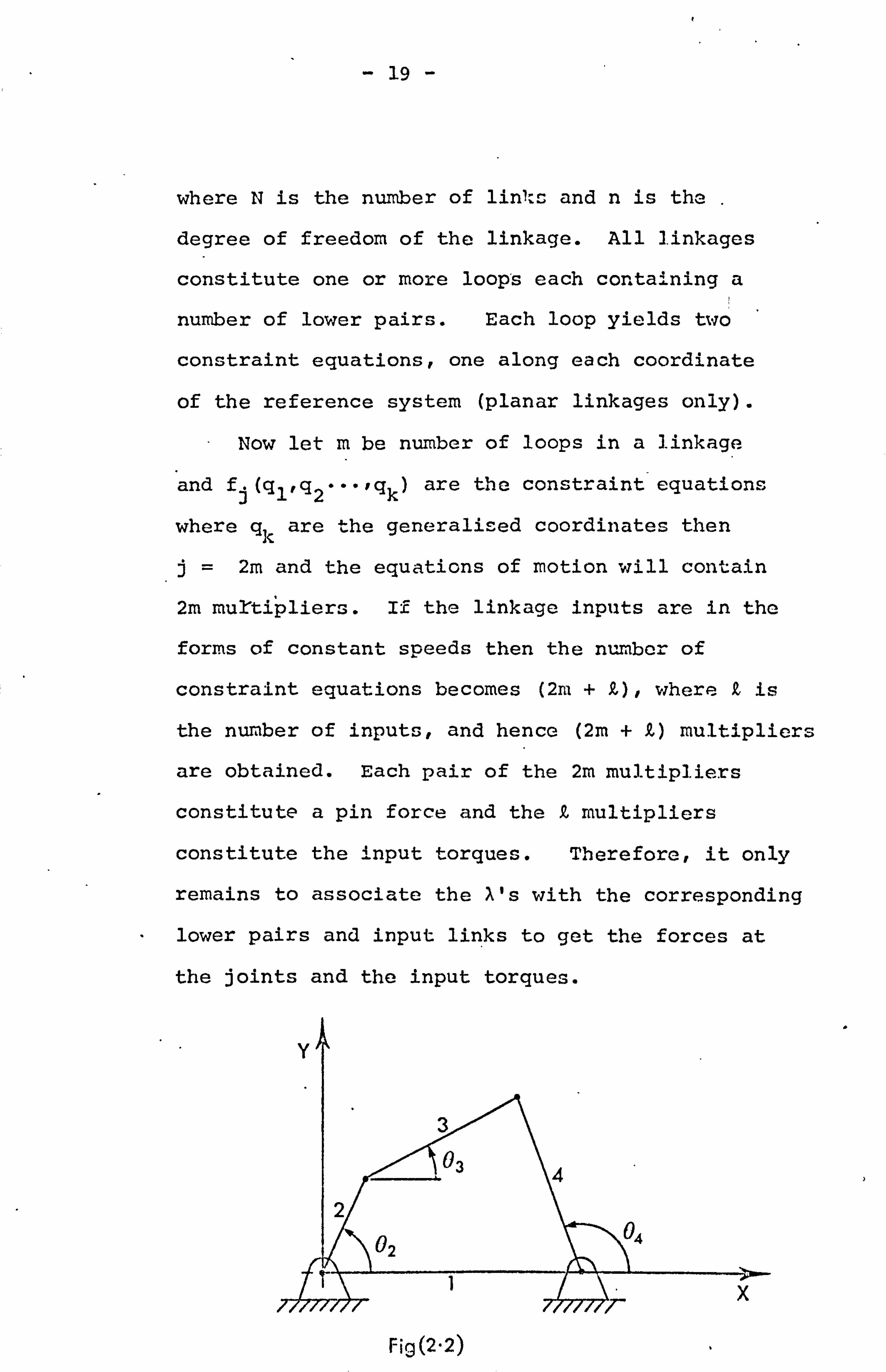
Consider the linkage shown in fig. (2.1). It
is a two degree of freedom mechanism, the degrees
being the crank angle "02" and the displacement of
the slider "u". The imposed external forces are
the driving torque T1(02), the loading force F1
acting on point p and the controller or constraint
force F2 acting on the slider. The viscous damping
force is represented by F3 and the coefficient of
damping by u. The link dimensions, masses and
inertias are as shown in the figure and the reference
coordinates are X and Y with origin at A.
2.1. The Kinematics
The kinematics may be defined by writing the
two constraint equations along and perpendicular to the
ground link Li, i. e.
£2CosO2 + Q3 CosO3 - R4 Cos(04 + a) -u Cosa =0
(2.1)
R2SinO2 + Q3SinO3 - k4 Sin(04 + a) -u Sinct =0

0 Ü
w 0
z
N 0)
U-
rý.
- 12 -
In addition, in the case of a constant speed
input w of the crank, a further equation of the
form
02 - wt =0 (2.2)
is required. The above equations may be represented
in suffix notation as
fý (021031041u) = 0, X2.3)
where -j = 1,2,3.
The constraint equations expressed in terms of
velocities may be derived from (2.3) and written in
suffix notation as,
vi (02,03'04ºu, ¬591E3,041d )=0 (2.4)
Equation (2.3) can be solved explicitly to give
the angles 03 and 04 as functions of angle 02 and
displacement u. Similarly the angular velocities "r
03 and 04 may he obtained from (2.4) as functions of
positions and speeds of crank and slider. The
accelerations may also be obtained by taking the first
derivative of equation (2.4). It is, therefore, clear
that equation (2.3) is sufficient for the complete
kinematic solution of the linkage.
- 13 -
2.2. The Derivation of Equations of Motion
The equations of motion are derived using the
Lagrangian multipliers method. This may be stated
as follows :-
DT -3T = Q. + En A. . . 8±. (2.5)
ýt ýq' i
-q i.
1i =1 aql
where T is the total kinetic energy of the system qi
and qi are the generalised coordinates and velocities,
Qi the generalised forces including conservative and non
conservative effects, n the number of-constraint
equations,, ai the Lagrangian multipliers and fi the
Constraint equations.
The generalised forces Qi may be written in the
form
Qi = mj. (g. ate) + Fi
. ri + Ta (2.61
Dqi Dqi 3 aqi
where m represents the masses, g the gravitational
vector, the coordinate vector of the point of
application of the external forces Fi and Ti the vector
of torques.
Let the generalised coordinates qi be 02,03,04 and
u. Now in order to obtain the kinetic energy in terms of
these coordinates the velocities of the centres of masses
must be found. These can be obtained by writing the x and
y coordinates of the centres of masses and taking the first
derivative. This yields, for centres C3 and G4, the
following velocities.
- 14 -
ýýG3 = ýSCZ
02+2. G3032+22G3. k2Cos (02-03-v3) Ö3p3
222 (2.8)
VG4 =
ýü +lCG404 -2RG4 . SinO4.04 . uý
l
J
Hence the total kinetic energy of the mechanism
may be expressed as
T= 2 IA . 022 2 IG3.0632 +2 IG4.042 +2 m5ü
2
1212 +2m3VG3+2m4 VG4
Finally, in order that equation (2.5) may
be expanded and written for this linkage the
coordinates of the points of application of the
external forces must be known. These are
xp = £2 cos(02+ai) + d1cos(03+a3+a1)
yP = £2 sin (02+a2) + cl1sin (03+a., +al)
and
XD = Qlcosal'+ u cos(a+al)
YD - ß1sina1 +u sin(a+a1)
Assuming ideal pin joints, gravitational
forces and no frictional forces apart from a
(2.9)
(2.10)
viscous force acting on the slider with a damping
coefficient of u the equations of motion may be
written for the following two cases.
2.2.1 Constant Speed Input.
Assume a constant crank angular speed, w,
i. e.,
02 = wt
- 15 -
This is considered as a further constraint
equation in addition to equations (2.1) and
replaces the need for specifying an expression
for the torque T1. In fact it leads to a
Lagrangian multiplier A3 which, as will be shown
later, is itself the external torque.
Assuming that Fi and Fi are the values of
the force F1 in the x and y directions the
equations of motion may be written as follows :
m3 R2 !C G3 Cos (0 2-0 3-v 3 ). 0 3 +m 3Q2R, G3 Sin (0 2-0 3Iv 3 )-0 2 3
+X1 !C2 SinO 2a2R2 Cos® 2a 3 +m 2gR G2 Cos (0 2+a 1) (1.11)
+ m3g£2Cos (02+a1)+F1X£2Sin (02+a1)-F1yz2Cos (02+a1)=O
(IG3+m3ZG3) 03-m3 £2 £G3Sin (02-03-v3) 02 +A1£3Sin03
-x 2Q3CosO3+m3gQG3Cos (03+v3+. a1)+Fid1Sin (C13+a3+a1)
-F1'"d1"Cos(03+a3+a1 )=0
(IG4+m42 4) 04 m4 tG4Sin04 -J119,4 . Sin (04+cc)
+X224Cos (04+a)+m0ZG4Cos (04+a+a1) =0
2
(m +m ) ü'-m Z SinO . d' -m k CosO .0 +71 Cosa 454 G4 444 G4 44 .1
+X Sina+mp-, Sin (a+('l)-F2+ul vý =O
(2.12)
(2.13)
(2.14)
ý:
- 16 -
Equations (2.11) through to (2.14) are
second order non-linear differential equations.
Together with the following two equations which
are obtained by taking the second. derivatives of N "" .I
equations (2.1) they may be solved for 0 3, ä4, u
al, a2, and' X3.
P, 'SinO3.03 -Q4 Sin(04+a) - 0! ' + ü' Cosa (2.15)
+Q2Cos02 "022 +A, 3Cos03.632 -Q4Cos(04+a)"042 = 0"
23CosO3.03 -Q4Cos(04+a)0o - ü"Sina (2.16)
- Q2SinO2 ". 022 -L Sin® 62 +Q4Sin (®4+a) "O42 =03 3
2.2.2 Torque Input
Assume an input torque Tl acting on the
crank. This may be a function of the crank
angular position, as in the case of a torsion bar
input or a function of the crank angular speed, as in
the case of an induction motor. These may be
expressed in the forms of
T1 = T1 b
(0 2) (a)
(2.17)
and T1 = T1 (02) (b) m
respectively. It is clear that, in both cases, the
- 17 -
constraints are only the two equations specified
in (2.1). By application of equations (2.5) and
as before assuming gravitational forces, ideal
pin joints and no frictional forces apart from the
viscous force acting on the slider, a set of four
differential equations may be obtained. Two of
these equations are :
(IA+m3Z22)02 +M391 291 G3Cos(02-03-v3)03+M3Q2ZG3Sin(02-03-v3)032
+ ý191 2Sin02 -x291 2Cos02 - T1 + m2gZC2Cos(02+a1)
+ m3gR2Cos(02+a1)+F1XR2. Sin(02+a1)-Fik2Cos(02+a1) = 0. (2.18)
G3 3 G3 +M 91 ) 03+m391 3 G3 Z Cos (02-03-v3) 02-m32.2
G3 9, Sin (02-03-v3)02L (1
+ ýl. Q3Sin03-A2QJCos03+m3g, C3Cos(03+v3+a1)
+ F1X. di. Sin(03+a3+ai)-Fly. d1. Cos(03+a3+ai) =0 (2.19)
The remaining two equations are similar to
equations (2.13) and (2.14) exactly. As mentioned
before the set of four equations may be solved
simultaneously with equations obtained from the
second derivatives of equations (2.1). In this case
these are :
R2SinO2.02+Q3Sin030ý3 - . 4Cos (04+a) d4 +ü' Cosa
+Q2Cos02 . 02+Q3 Cos 0303 214 Cos (04+a) 04' = 01
(2.20)
- 18 -
A. 2Cos02.02 +2 3Cos03.03 -RQCos (04+a) 04 u Sine
-Z2Sin02.0c22 -Q3Sin030r32 +R4Sin(04+a)042 = 0. (2.21)
2.3. Associating the Lagrangian Multipliers with
Pin Forces and Torques.
In many mechanisms the Newtonian approach to
formulating the equations of motion is usually
cumbersome and time consuming. However, the
Lagrangian formulation is easier and more compact.
The Lagrangian multiplier method facilitates the
formulation even more but at the expense of dealing
with larger numbers of differential equations. The
present day numerical methods and computer hard
and soft wear make the solution of large number of
equations a straightforward matter. The Lagrangian
multiplier, unfortunately, does not include the
internal forces explicitly but as will be seen later
an association between the two is possible. Once this
association is accomplished all the remaining
internal forces are easily obtainable since the
accelerations are available from the solution of the
equations of motion.
2.3.1 Analysis
The number of lower pairs in a linkage may
be expressed in the form
h=3 (N-1)-n (2.22) 2
- 19 -
where N is the number of links and n is the .
degree of freedom of the linkage. All linkages
constitute one or more loops each containing a
number of lower pairs. Each loop yields two
constraint equations, one along each coordinate
of the reference system (planar linkages only).
Now let m be number of loops in a linkage
and fj(gl, q2"""yqk) are the constraint equations
where qk are the generalized coordinates then
j= 2m and the equations of motion will contain
2m murtipliers. If the linkage inputs are in the
forms of constant speeds then the number of
constraint equations becomes (2m + Q), where Z is
the number of inputs, and hence (2m + £) multipliers
are obtained. Each pair of the 2m multipliers
constitute a pin force and the k multipliers
constitute the input torques. Therefore, it only
remains to associate the A's with the corresponding
lower pairs and input links to get the forces at
the joints and the input torques.
Fig (2.2)
- 20 -
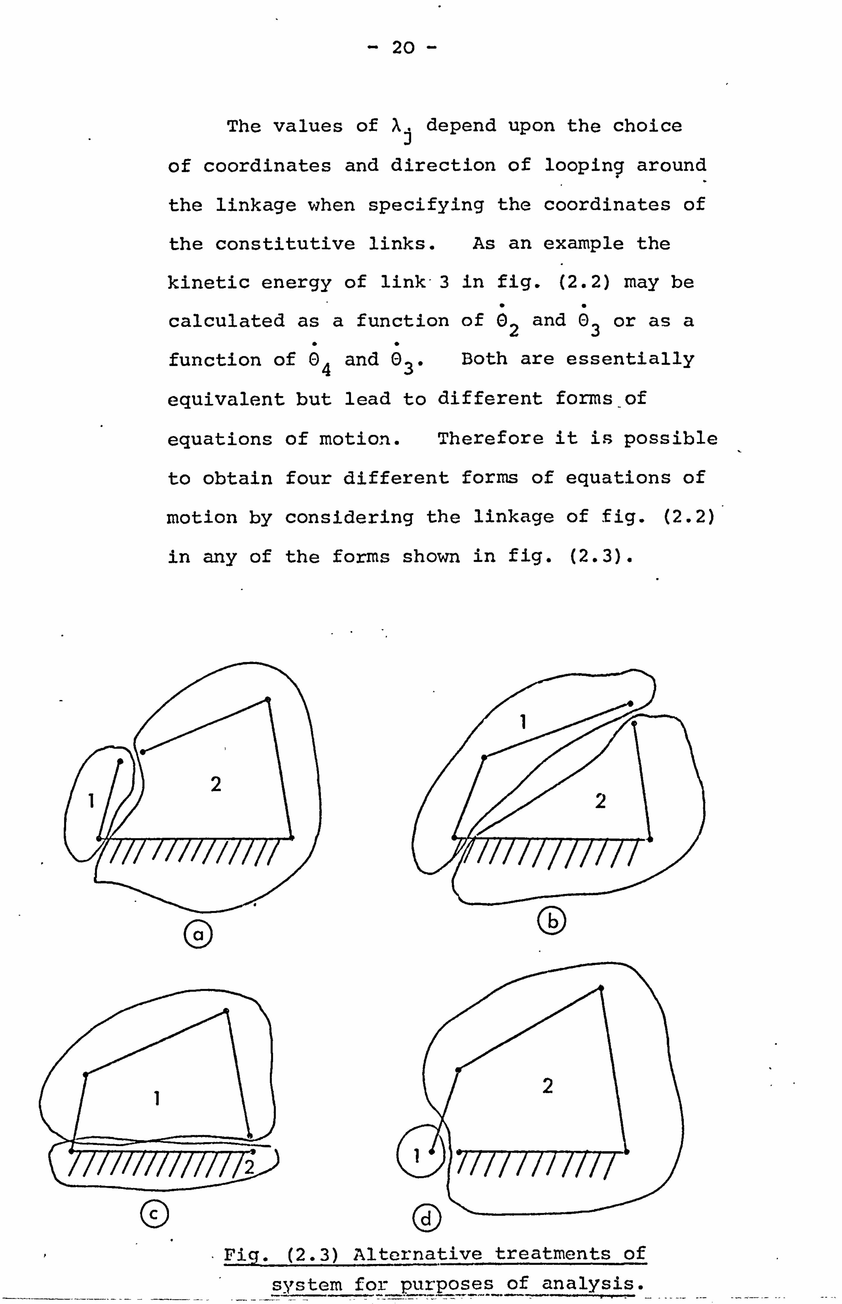
The values of ai depend upon the choice
of coordinates and direction of looping around
the linkage when specifying the coordinates of
the constitutive links. As an example the
kinetic energy of link-3 in fig. (2.2) may be
calculated as a function of 02 and 03 or as a
function of 04 and 03. Both are essentially
equivalent but lead to different forms-of
equations of motion. Therefore it is possible
to obtain four different forms of equations of
motion by considering the linkage of fig. (2.2)
in any of the forms shown in fig. (2.3).
G)
0
(D
v -Pig. (2.3) Alternative treatments of
system for purposes of analysis.
- 21 -
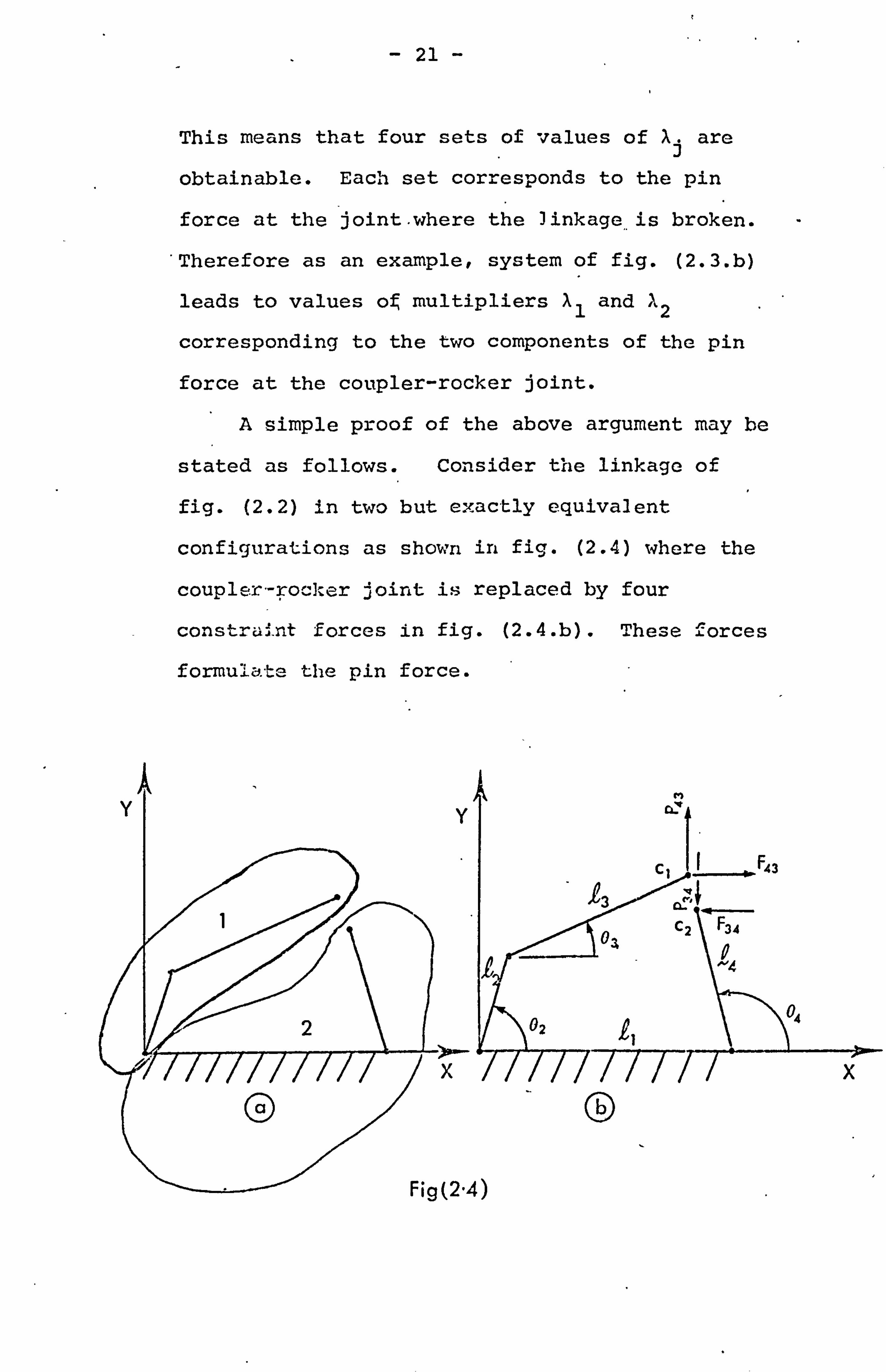
This means that four sets of values of Xi are
obtainable. Each set corresponds to the pin
force at the joint. where the ]inkage,. is broken.
Therefore as an example, system of fig. (2.3. b)
leads to values of multipliers Al and A2
corresponding to the two components of the pin
force at the coupler-rocker joint.
A simple proof of the above argument may he
stated as follows. Consider the linkage of
fig. (2.2) in two but exactly equivalent
configurations as shown in fig. (2.4) where the
coupler, -rocker joint is replaced by four
constraint forces in fig. (2.4. b). These forces
formulate the pin force.
Fig(2.4)
- 22 -
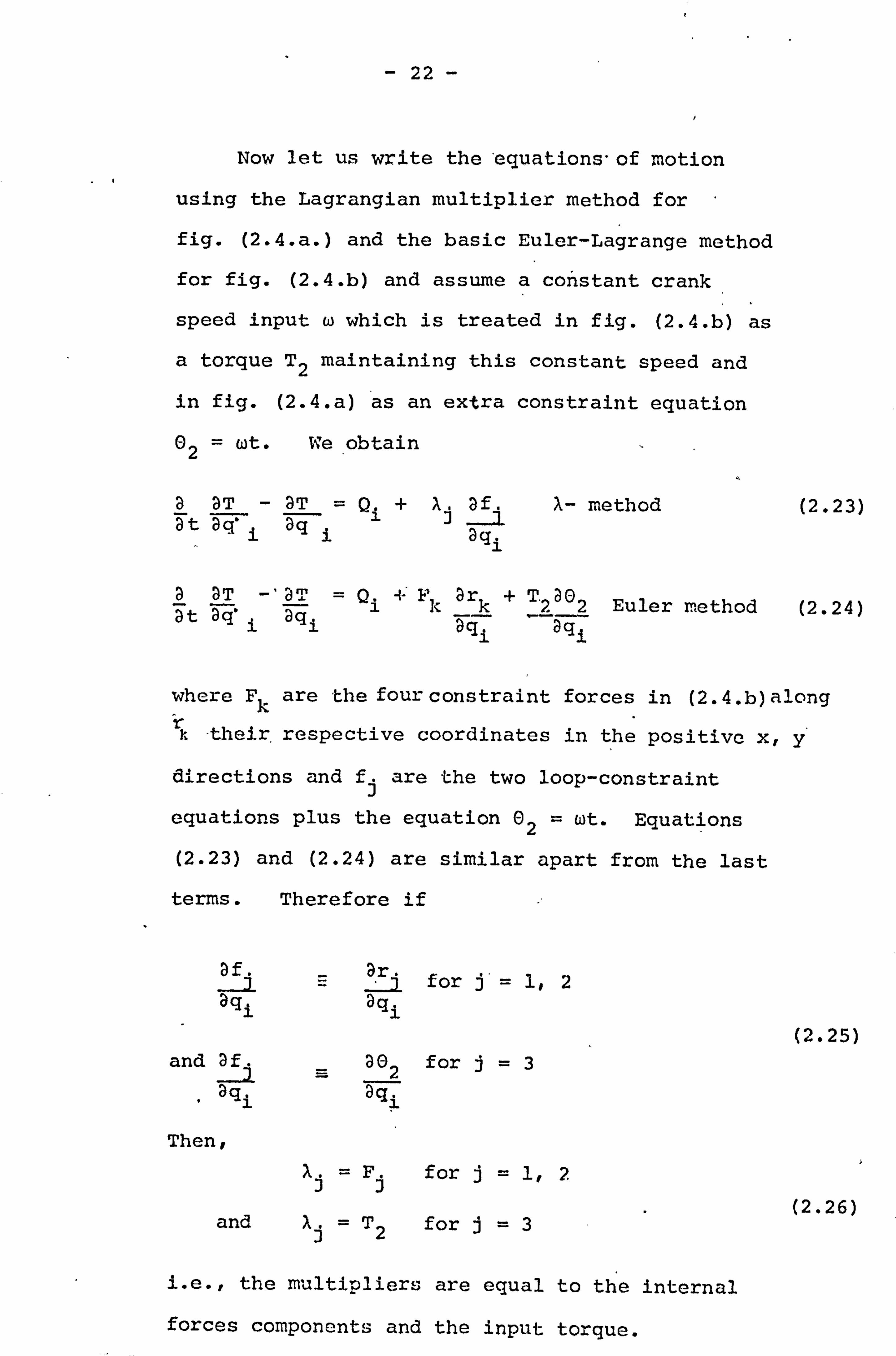
Now let us write the'equations"of motion
using the Lagrangian multiplier method for
fig. (2.4. a. ) and the basic Euler-Lagrange method
for fig. (2.4. b) and assume a constant crank
speed input co which is treated in fig. (2.4. b) as
a torque T2 maintaining this constant speed and
in fig. (2.4. a) as an extra constraint equation
02 = wt. We obtain
a aT - aT = Q. + X. af. A- method (2.23) at aq" i aq i aqi
a DT -' DT = Q. +F ar + T-30 at aq. i
qi 1 ]c Dqi 2agi
Euler method (2.24)
where Fk are the four constraint forces in (2.4. b) along r.
-their . respective coordinates in the positive x, y
directions and fi are the two loop-constraint
equations plus the equation 02 = wt. Equations
(2.23) and (2.24) are similar apart from the last
terms. Therefore if
a =
aý for j' = 1,2 aqi aqi
and af 30 for j =3 t 2
" aqi aqi
Then, 7ý =F for j= 1,2 j j
and A. = T2 for j= 3
i. e., the multipliers are equal to the internal
forces components and the input torque.
(2.25)
(2.26)
- 23 -
The coordinates of forces acting on C1 are :
o= 22CosO2 + 2.3CosO3
1
Y_ k2SinO 2+Q3 SinO c3 1
and of forces on C2 are :
xc =-2 (Q1+Q4CosO)4
Y-L Sin0 c44 1
Now fig. (2.4. b) has three degrees of freedom
because; by releasing the lower pair C two
degrees are added. Hence (2.23) yields three
equations and similarly (2.24). Thus by
expanding a
and a
we have 8ql 8qj.
of aX
a01- -Q2Sin02 and a0 c1 =- R2 SinO2.
2 Last terms in
of ay 1st equation of
302 - Q2CosO2 and a021 = Q2 Cos02 motion.
of a0 3
a02 =1 302 =1
8fl Dxcl I- ) DO 9,3 Sin03 and ý0 = -t3 Sin03
33 Last terms in
af_ 8x1 2nd equation of c a03 P3 Ccs03 and 303 = k3 Cos03 motion.
8f 8f
803 =0 a03 =O

- 24 -
of axC2 1= 2'4 SinO4 and a0 = 1C 4 SinO DO 44) Last terms in
aft ayc2 3rd equation =-R4 Cos04 and a0 =-k4 Cos0 DO 4
44 of motion.
af3 _
af3 a04 O a04 = G.
i. e., equation (2.25) is true and therefore
x1 = F43 ' A2 = P43 and A3 = T2.
Since the accelerations, velocities and
positions are given from the solution, the
remaining pin forces at A, B and D may be easily
obtained.
2.4 METHODS OF SOLUTION
The equations of motion stated earlier are
highly non-linear second order differential
equations. A straightforward generalised analytic
solution is an impossible task with present day
mathematical methods. An attempt to linearise the
equations in the variable u is possible bearing in
mind that the coefficients of the then obtained
equation will be the results of the solution of the
four-bar linkage with no movable pivot; this can only
be obtained using a computer. Therefore, even if the
equations have been linearised a solution can only be
obtained for a particular case. Ilowevor, in some
cases, as will be seen later in chapters IV and V,
if further simplifying assumptions are made a
- 25 -
lincarised equation with periodic coefficients,
which can be evaluated by straightforward
analLytic algebraic methods, may be obtained.
Consequently, a near exact solution can
only be obtained using either an analogue or digital
computer. The analogue, once set up, is quick and
efficient; however, the setting up stage can be
complex and time consuming. On the other hand, the
digital computer is more flexible, easily set up and
possesses time sharing characteristics; this is
compared with the analogue which can be used by one
researcher only at one time. Owing to the above
and the availability of a time sharing digital
computer installation, the IBM 360/67, it was decided
upon a digital solution.
The accuracy and efficiency of a numerical
solution depend on the method of integration adopted.
The most widely used methods of integration are the
Runge-kutta methods, the series methods and the
predicted-corrector methods. Each has its own
advantages and disadvantages and the choice depends
on the nature and complexity of the equations.
The equations of motion derived earlier can be
expressed in a form equivalent to (see 3.1)
Z" _ dD (t, Z) (2.27)
where Z represents the unknowns of the equation3
02,03,04 and u and Z the derivatives. The
Runge-kutta methods are one step methods, i. e. to
- 26 -
evaluate Z at time t+dt we only require the
information available at point Z at time t.
Secondly, they do not require the evaluation
of the derivative of the function to be integrated.
This makes them suitable for digital computer
applications, especially in cases where the
derivative is not easily obtained. Their serious
drawbacks are, firstly, the lack of simple means
of estimating the errors; this makes them highly
susceptible to numerical instabilities and,
secondly, the large number of evaluation of the
function 0; four times for each step in a fourth
order method. The second of these drawbacks makes
them unfavourable for use with our Lagrangian
multiplier formulation of the equations of the
motion because of the large number of equations
, and hence the lengthy time involved in computation
of the function 4).
Series methods such as Taylor Series and
Picard's method are the most straightforward
methods. However, they involve tedious work in
finding the derivatives of the function . For
example, to obtain a solution equivalent to a
fourth order Runge-kutta method we need to evaluate
the fourth derivative of the function 0. A simple
look at the equations of motion stated earlier shows
immediately the impracticability of these methods in
this case.
- 27 -
Lastly, there are the predictor-corrector
methods. They provide an easy estimate of the
errors, inherent, roundoff or truncation, from
the information already calculated. These errors
are in all cases convergent and, thus the methods
are highly stable. One of their most attractive
qualities is that they require only two evaluations
of the function (D per step of integration. Their
only relative drawback is that since they use
information about prior points they are not
self-starting. This drawback is easily solved by
employing a Runge-kutta method to start them.
Owing to these above qualities they are the most
suitable for use with this type of formulation of
equations of motion.
The Hamming fourth order modified predictor-
corrector is the method chosen here but in some
cases where simulation is performed using the IBM
Continuous system modelling program (CSMP) the Milne
method is employed. The only reason for choosing
the Milne, which is incidentally a predictor-
corrector, is its availability for use in the IBM
subroutine package. The various steps involved in
application of the Hamming's methods are as follows: -
1. A predicted value for Z in (2.27) is obtained
using the formula I
P ' Z
j+1 =
j-3 +4h3 (2 Zj - Zj_1 +2 Zj-21 (2.28)
- 28 -
where h represents the time step, j the number
of integration step and Zj, Z. and j _2 are
the function 1D at the current point and the
previous two points respectively.
2. A modifie
obtained using
of the current
m 2_ "=Z.
j+l
of this predicted point is
sdicted and corrected values
i. e.,
112 pc (2.29) 121
ýZ -G
J
3 value
the pry
point,
p
j+l
where letters m, p and c above Z indicate modified,
predicted and corrected values respectively.
3. The corrected point is obtained using the
derivatives and values of the modified point, the
current and previous points as follows :
C
Z9 z-z
j+l j-2
m + 3h Z+2 Z- z
j+l (2.30) j j-3
4. The final values Z j+l is obtained using the
above predicted and corrected points, thus
cp_C Z, =Z (2.31) ý 12
91ZZ
J+1 j +l 3+1 3+1
This above method is used on the equations of motion
formulated in the form of equation (2.27). The
method of transformation to this form is discussed in
the next chapter.
.: r
- 29 -
CHAPTER III
DIGITAL COMPUTER SOLUTION OF EQUATIONS OF MOTION
It was stated earlier that an analytic sdlution
cannot be found owing to the gross non-linearities
of the equations. It was also decided that a
digital solution would be performed. Hamming's
integration method was also chosen to find the
solution. It only remains therefore, to put the
equations into a form to which the integration can be
applied directly.
Solutions for both the cases of forced and free
motion will be considered. It will also be assumed
that the slider will either be free or constrained by
viscous friction and/or linear spring.
3.1 The Formulation of Equations of Motion for Digital
Solution.
It is desired that the equations of motion be
transformed into a form similar to that of equation
(2.27). In order to make this possible we must
isolate each of the second order quantities Ei , 0; 3,
04 and if and express them in terms of velocities,
positions and other already known or calculated
quantities.
The equations of motion may be written in the form
Ai j
- 30 -
Where Wj ;j=1,2, .... 6 is the
(X3, Ö3,04, ü, )L1 X2) for the consta:
case or (Ö 2,03,04, ü, X1, X2)for the
input case, matrix Aij; i=1,2,
2, .... 6 is the square matrix of
column vector
at speed input
known torque
..... 6, j=1,
coefficients and
Bi is the remaining terms independent of W3 .
If Aid is non singular, equation (3.1) may be
written in the form
Wý = hi. Bi (3.2)
where
C= A1 C. ij
Two relations may how be obtained from this equation,
these are N
Zk = Cki. B1 (3.3)
and
xm Cmi'Bi (3.4)
Where k=1,2, .... 3, n=1,2,.... 3 for a constant speed
input or k=1,2,.... 4, m=1,2 for a torque input and
i=1,2,..... 6. Zk represents the second order
derivatives and ). m
the Langrangian multipliers.
Equation (3.3) may be! Written in the form - --- - -- --
Z k_ 41(t, Z (3.5)
and integrated giving rný
Zk Yt, Zk) (3. G)
Where Zk is calculated using the values of Zk and Zk
obtained from the previous integration step. Equations
(3.5) andd (3.6) are in the form of equation (2.27)
and hence numerical integration can be applied directly.
- 31 -
Equation (3.1) is solved by using the Gaussian
direct elimination method with provisions for row
and column interchanges and error bounds corrections.
The error corrections are made as follows
The values of Wi obtained from (3.2) are substituted
in (3.1) and B. (O) = Aid . W. is calculated. If
round off errors are small; i. e.
if 1
131 -Pi (°) 1<e, (3.7)
where e is small positive error constant, then we
proceed with the integration. If this condition is
not satisfied then
Aid. 6(o) (Bi-B(°)
is solved. The values of dý°) are added to the
already found values for Wj. These are in turn
substituted in equation (3.1) and the process is
repeated until equation (3.7) is satisfied.
The preceding analysis allows for integration of
all the second order derivatives, Ö2, Ö3,04 and u. This
means that the kinematic equations described in
equation (2.1) and (2.4) need only be solved once in
order to find the initial conditions. Contrasting
with this approach is that in which the second order
derivatives of 02 and ü are calculated once and are
integrated to give 00 2 and ü. The remaining first
order derivatives may be obtained from the solution of
equation (2.4). 2 and ü are then integrated giving
02 and u which when used in equation (2.1) give the
remaining angular positions. It is clearly seen
that this latter approach . requires the solution of the
- 32 -
kinematics at every time step in contrast with the
first which requires it only at the initial point.
The first approach may be useful especially when
dealing with mechanisms having complex kinematic
equations. It also has the further advantage that
it gives a complete solution carried out wholly by
the computer and at no stage is there any tedious
work involved on the part of the designer. In
contrast with this the kinematic solution must either
be performed by elimination or iteration. The first
of these is manual and can be lengthy and time
consuming in complex mechanisms; the second can be
computationally difficult.
It is strongly recommended, albeit, unmentioned
in all literature, that the first approach be used
at first hand no matter how simple or complex the
mechanism may be. The accuracy or even the debugging
of the integration procedure may then be examined by
simple checks on loop closure. It is important to 1 1,
recognise that a loop closure check is meaningful
other than for trivial arithmetical checks, only if
used in conjunction with the first approach. This is
so, because the second approach integrates only the
derivatives of'-the generalised coordinates determining
the degree of freedom of the system. The remaining
ones are obtained from the kinematics thus large errors
may be involved in the numerical integrations yet they
are not realised by the designer because the kinematics
are used to force the closure of the mechanism and
hence no simple check is available to indicate whether

- 33 -
the solution is accurate. On the other hand the
first approach is wholly dependent on the results
of the integration thus if the designer obtains large
erros in loop closure checks he can immediately
recognise that the integration needs further,
refinement.
Based on the above arguments our policy in the
coming solutions will be to integrate all the second
order derivatives and make sure that the errors in
loop closure are within acceptable bounds, then due
to the relatively simple kinematic solution of our
mechanism, the second approach of integration will be
adopted. This will ensure that the integration
method is reliable and leads to accurate results.
3.2 Forced Motion
3.2.1 Constant Speed Input
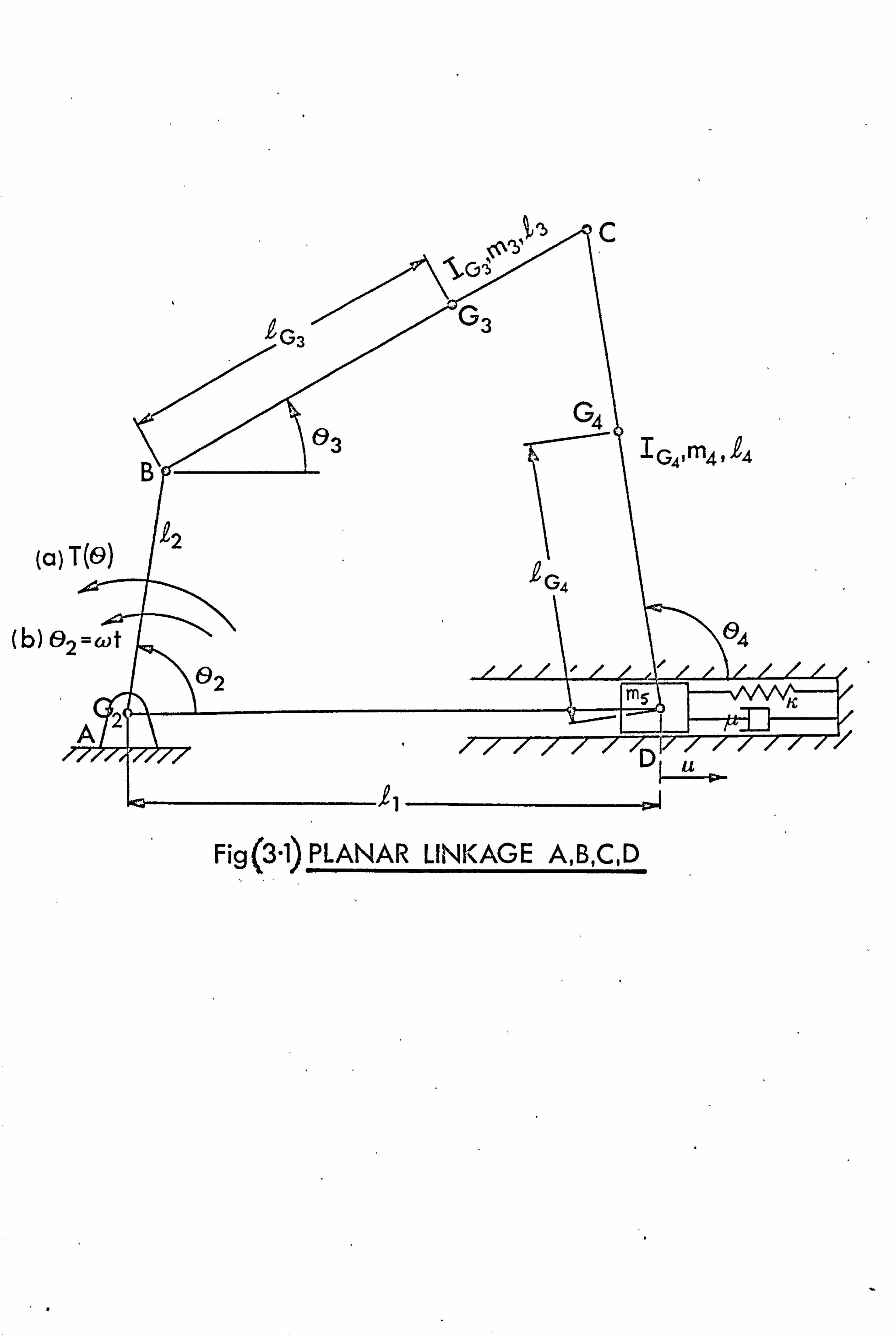
Consider the mechanism shown in Fig. (3.1) and
assume that the crank rotates at a constant angular
speed to and its centre of gravity lies on pin joint 1
A. Also assume that the force opposing the motion
of the slider consists of a viscous force of coefficient
i and a spring force of coefficient K. By assuming the
linkage to be in the vertical plane the equations of
motion may be written in the form of equation (3.1)
where Aid is the square matrix.
(a)
(b)6
Fig(3.1) PLANAR LINKAGE A, B, C, D
- 34 -
-1 2 CosO2 92 Sin02 0 0 m3Q2ZG3 Cos(32-e3)
0 -Z3 Cos03 Q3 Sin03 0 0 IG3+m3QG3
0 Z4 Cos04 -Q4 Sin®4 -m42G4Sin04 IG4+mkG4 0
00 1 m4 + m5 -m491 G4Sin04
00 0 1 -Q4 Sin04 23 Sin03
00 0 0 -Q4 Coso4 Z3 CosO3
(3.8)
W. is the column vector J
Wý _ (X 3'x21XlIU, 04,03) (3.9)
where Al and 12 are the pin forces along the x and y
directions at joint c in Fig. (3.1) and 13 is the input
torque required to maintain constant speed input.
The matrix B. is the colwnn vector
-m3g£2 Cos02 -m3£2£G3 Sin(02 -03)0'32
-m3g£G3 Cos03 + m3£2£G3 Sin(02 -03)022
-m4g£G4 Cos04 (3.10}
4 -u. u - k2 u+ m4£G4 Cos040 2
-£2 Cos02.022 - £3 Cos03032 + £4 CosO4.042
£2Sin02022 + £3 Sin03032 - £4 Sin04042
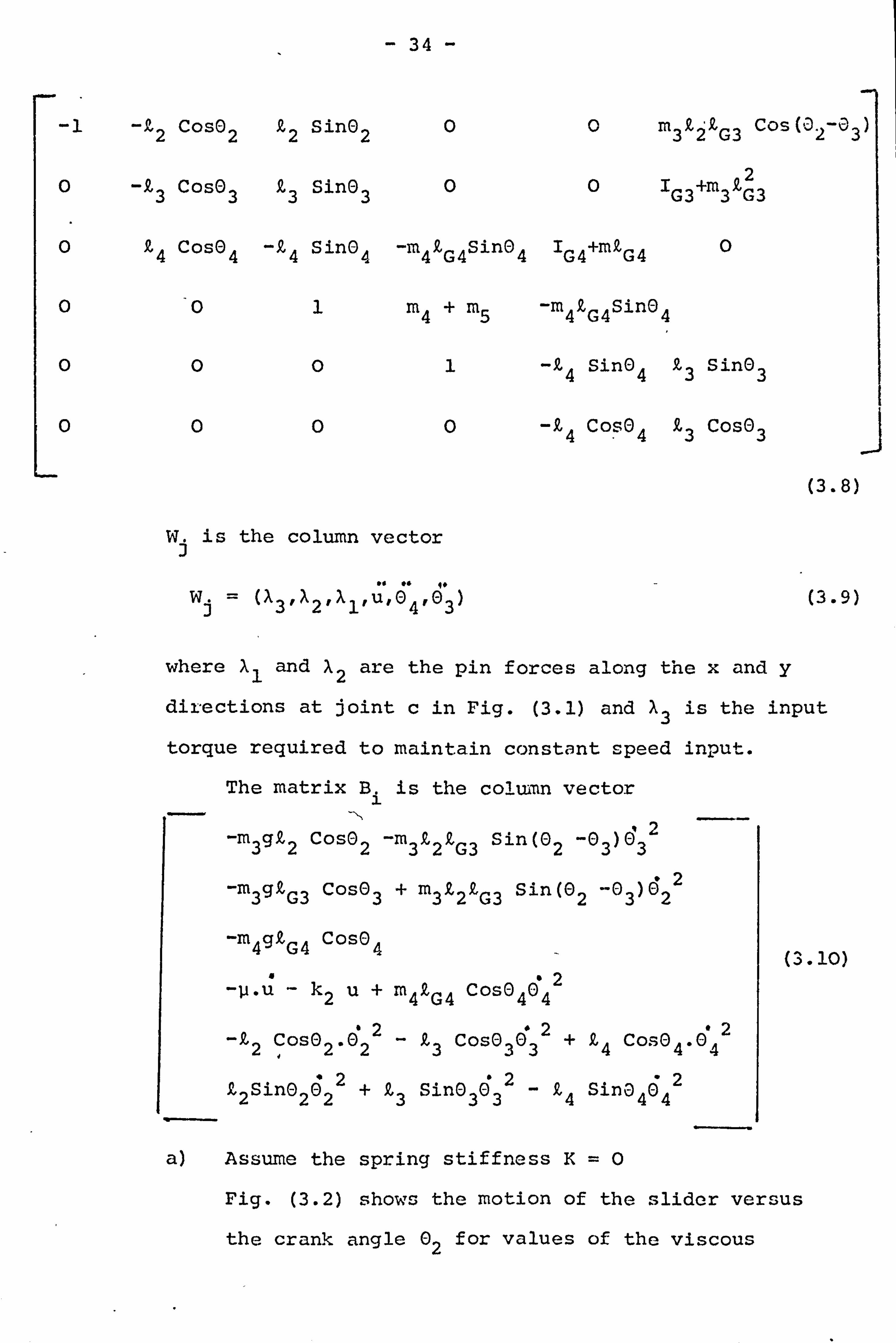
a) Assume the spring stiffness K=0
Fig. (3.2) shows the motion of the slider versus
the crank angle 02 for values of the viscous
C. )
nJ h O+ x
O r-
Ot
O u
.r to wow Cn
("WO) R NOIIOI. d3OflS
-W n C4 a;
ry
k"
C ri ra C- c,
it
K" IA- I"
k ý. u cr ai
K mý "W
K `Y C mac:
C: 3 ILI
Y. s:
OC fr) I r- 7J C. 3 irs
cc
W C3
try W x ~ li- U
ci
ki Q __ cv týJ
F-
clý Q C)
1A
0
- 35 -
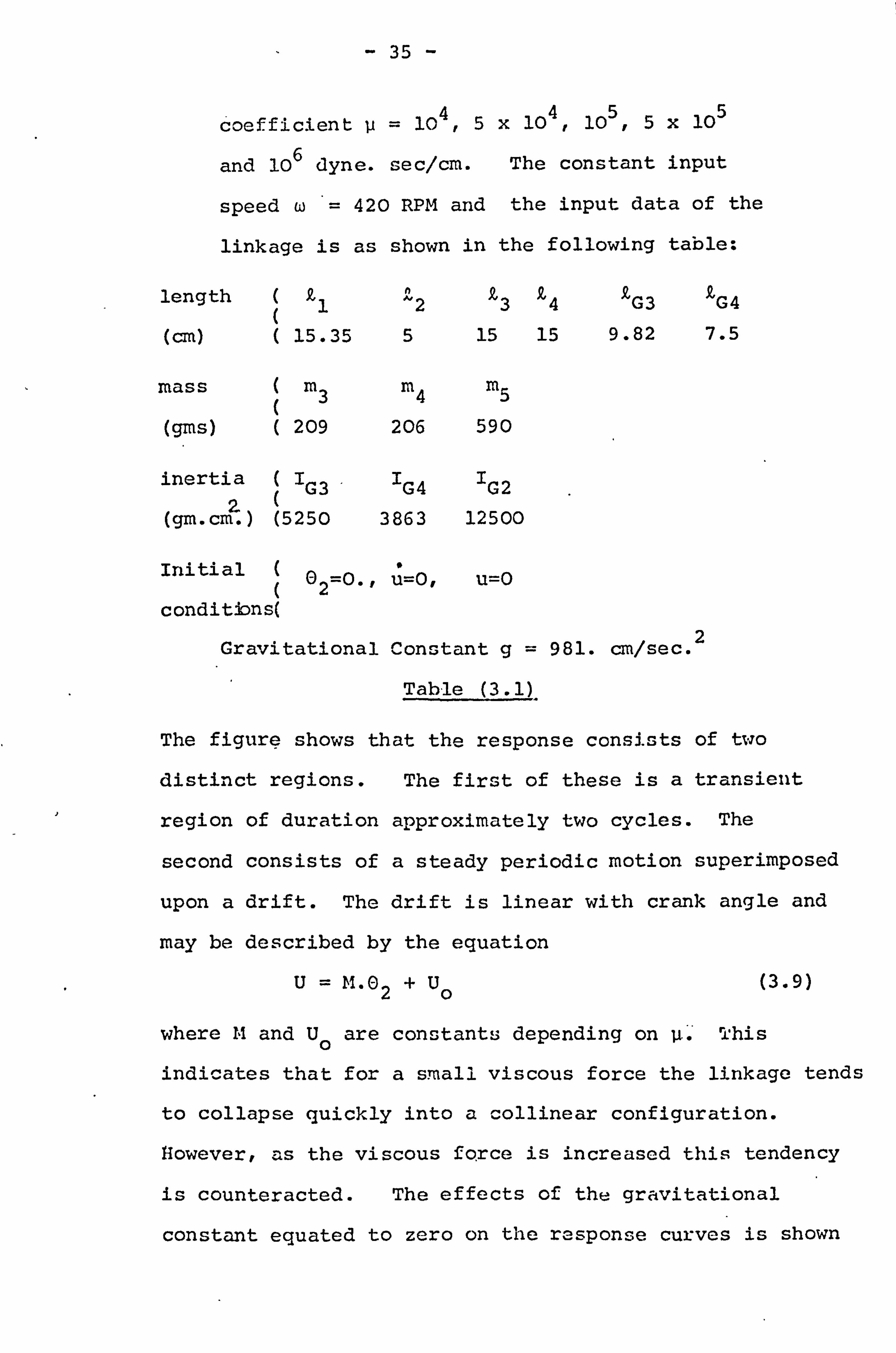
coefficient u= 104,5 x 104,105,5 x 105
and 106 dyne. sec/cm. The constant input
speed w= 420 RPM and the input data of the
linkage is as shown in the following table:
length ( R1 N2 L3 L4 LG3 k G4
(cm) ( 15.35 5 15 15 9.82 7.5
mass ( m3 m4 m5
(gms) ( 209 206 590
inertia IG3 'G4 'G2
(gm. cm ) (5250 3863 12500
Initial ( 02=0., u=0, u=0
conditions(
Gravitational Constant g= 981. cm/sec. 2
Table (3.1)
The figure shows that the response consists of two
distinct regions. The first of these is a transient
region of duration approximately two cycles. The
second consists of a steady periodic motion superimposed
upon a drift. The drift is linear with crank angle and
may be described by the equation
u=M. 02+up (3.9)
where 11 and U0 are constants depending on p: This
indicates that for a small viscous force the linkage tends
to collapse quickly into a collinear configuration.
However, as the viscous force is increased this tendency
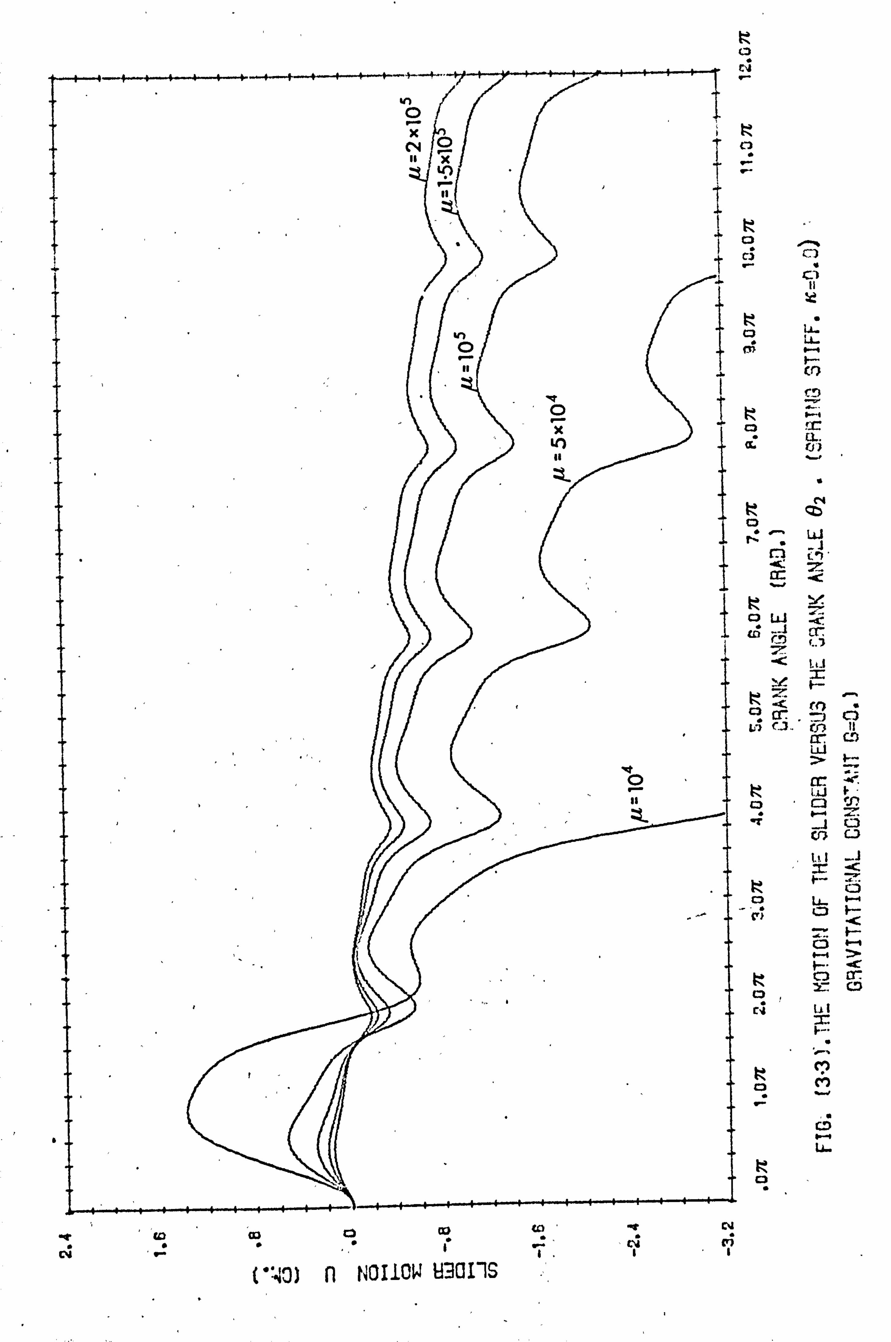
is counteracted. The effects of the gravitational
constant equated to zero on the response curves is shown

- 36 -
in fig. (3.3). It is clear from this figure that
because the gravitational forces are eliminated the
value of M in equation (3.9) is slightly reduced.
b) Assume a constant viscous coefficient u=3x 10⁴.
Fig. (3.4) shows the motion of the slider versus
the crank angle 02 for values of the spring stiffness
coefficient k=5x 105,106 and 2x 10⁶ dyne/cm. The
input data is as shown in table (3.1) and the input
speed is 420 rpm. The figure shows that due to the
initial condition assumptions that u and u=0a
transient effect is shown over the first cycle. The
steady state motion is periodic and oscillates about a
mean position between the initial position of the slider
and the crank shaft. This mean position shifts towards
the slider initial position as the spring stiffness is
increased. The minimum value of the oscillation for
the case of k=5x 10⁵ dyne/cm occurs at crank angle
02 = 220. However, as k is increased this minimum
oscillation occurs at smaller crank angle and eventually
occurs at zero degrees for k=2, x 106 dyne/ m. The
rate of change of the slider position is approximately
the same for all the response curves between the minimum
and maximum values. However, as the spring stiffness
is increased the spring force becomes dominant and the
width of the response curve is decreased. Eventually,
although not shown on this figure, as k increases
further the slope of the response curve takes a constant
value between the maximum and minimum values of the
oscillation on the portions of the curve below the zero
degree crank angle positions.
K cý cv
K c-ý r
K 0 ci C)
Cl
O U' " L6.
(S} H
C_") k F^I a
tl1
"
km "r-. W n
_J
OW to ýý
"< 1 ýJ
" krCPjO.
cr )Q ýý C]. cß 11
W
cc: " rN
i
co ü
ItI _J h-
p (yam H ci
(ý H
= CD O
Li I ri I. -.
kM aM
U-
0
to +! N
CV 111
r z) n NOHOW 9O11S

K
"k
ca LAI
a
C, to
. kc-J
cr) a ti
C rý
9ýýkz-3/ öw
-j cr M C3 7t 'ý tv
Cf1 t
cr. o C,
to
tai z
cl ý-.
q
" CJ La S
CID L_
N ao ,ravw cv a
( "W0) n NOIICW U3011S
- 37 -
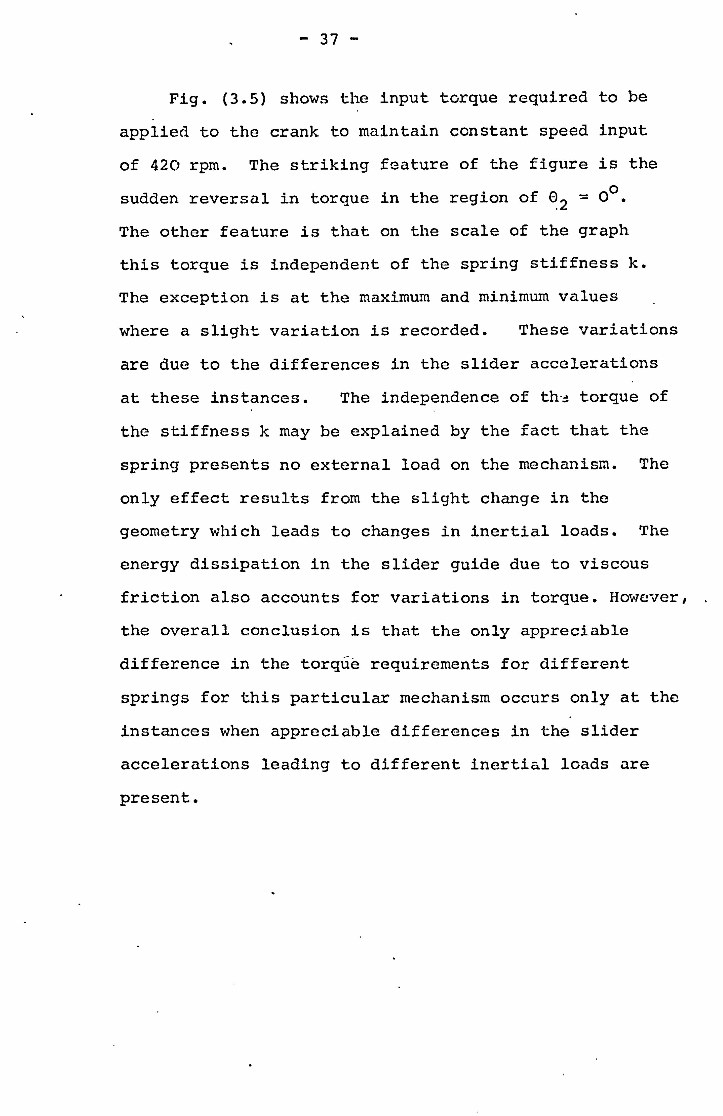
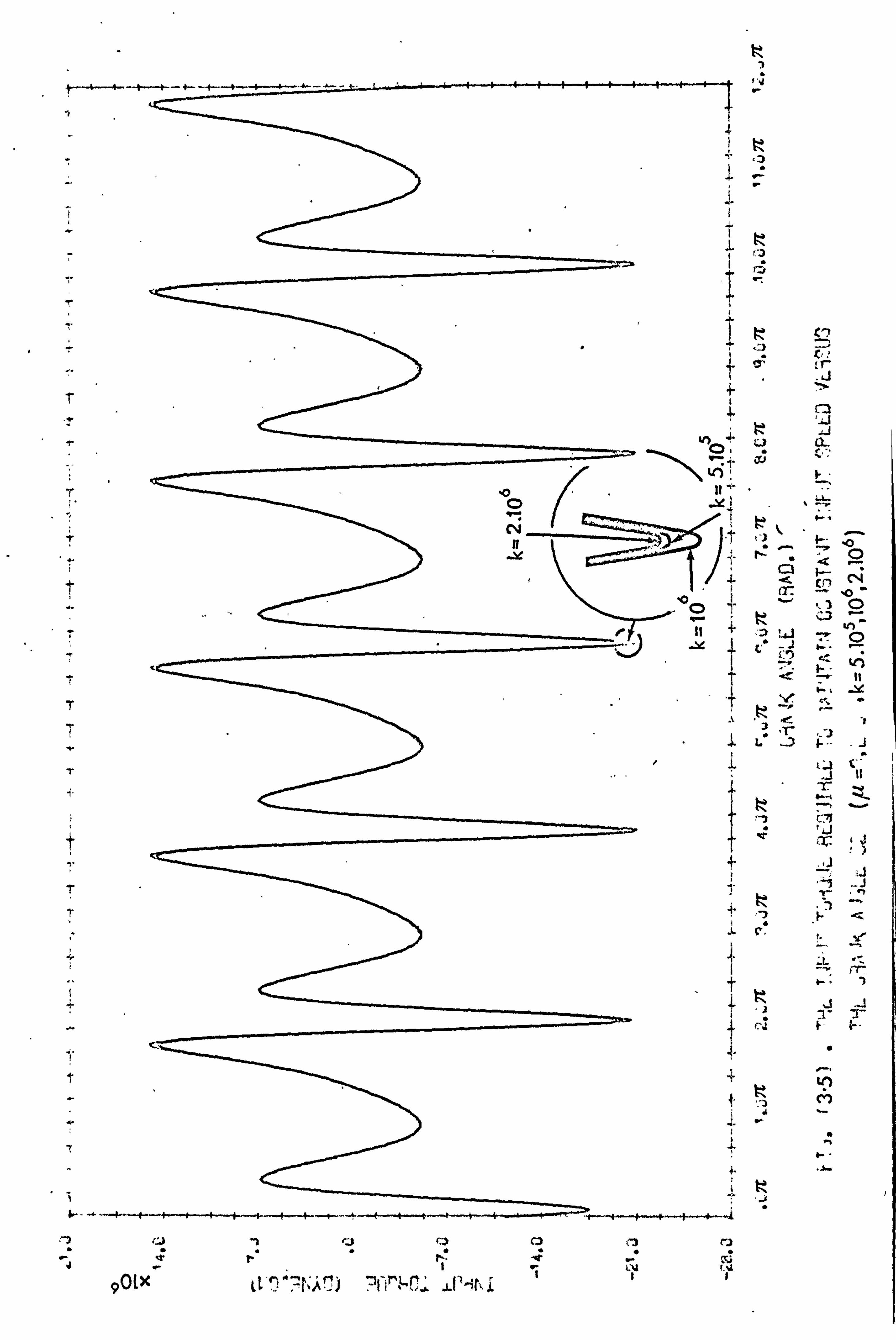
Fig. (3.5) shows the input torque required to be
applied to the crank to maintain constant speed input
of 420 rpm. The striking feature of the figure is the
sudden reversal in torque in the region of 02 = 00.
The other feature is that on the scale of the graph
this torque is independent of the spring stiffness k.
The exception is at the maximum and minimum values
where a slight variation is recorded. These variations
are due to the differences in the slider accelerations
at these instances. The independence of th-4 torque of
the stiffness k may be explained by the fact that the
spring presents no external load on the mechanism. The
only effect results from the slight change in the
geometry which leads to changes in inertial loads. The
energy dissipation in the slider guide due to viscous
friction also accounts for variations in torque. However,
the overall conclusion is that the only appreciable
difference in the torque requirements for different
springs for this particular mechanism occurs only at the
instances when appreciable differences in the slider
accelerations leading to different inertial loads are
present.
ýý
i
T
1
t
r
t
r
7 1
T
4
9"
r 1
K
ýýJ r
k .ý
K r3
K { ' o :r
. ýJ
aJ CL. "
Cy6 W
1
F-
C3 f--
^ 10
ý
1 .,
, 2
ý=k 1,4J
1- i
" .. 3 L h- J
l C {{
yam. ýR
"Z
0
r
a. -_-
J
K LO . -, c)
3
C3 C3 C. )
AN t-A
90LX
- 38 -
3.2.2 Torque Input
There are only two constraint equations for
the input torque case. These equations define the
loop closure of the linkage along the x and y
direction. Therefore only two Lagrangian multipliers
exist for this case as opposed to three in the previous
case. These multipliers are Al and X2 representing
the pin forces along the x and y directions in pin
joint C of fig. (3.1).
The torque input
T= T0(1-82) if 02 ý912
and 'T=0 thereafter
is applied to the crank, where T0 is the initial value
of the torque and 46.2 is a pre-given constant value of
crank angle ©2. Assuming the centre of gravity of
the crank lies on the crank shaft A the equation of
motion (3.1) can
The matrix Aid is
for the following
A11 =1 2A +.
be expressed in the following terms.
as given in equation (3.8) except
elements. 2
m3 ! C2 .
A21 = m3Q2ZG3 Cos(02 -03).
A51 = Q2 Sin02.
A61 = 9.2 Cos02.
Where I2A is the crank inertia about the crank shaft A.
The column vecror Wi is given by
Wý _ (62'XVa1, u, 04,03)
39
And the matrix Bi is as given in equation (3.10)
except for the following element.
B1 =-m3. g. L2 Cos02 -m391291 G3 Sin(02-03)0032+T0(1-02) .
The crank speed and the slider response are both
investigated varying
(1) the input torque To and keeping the spring
stiffness k and viscous coefficientp constants, and
(2) varying the stiffness k and keeping the
input torque T0 and viscous coefficient u constants.
In both cases the torque is assumed to act during
the first 57.3 degrees (1 rad. ) rotation of the crank.
The kinematic and dynamic input data and the initial
conditions are as shown in table (3.1).
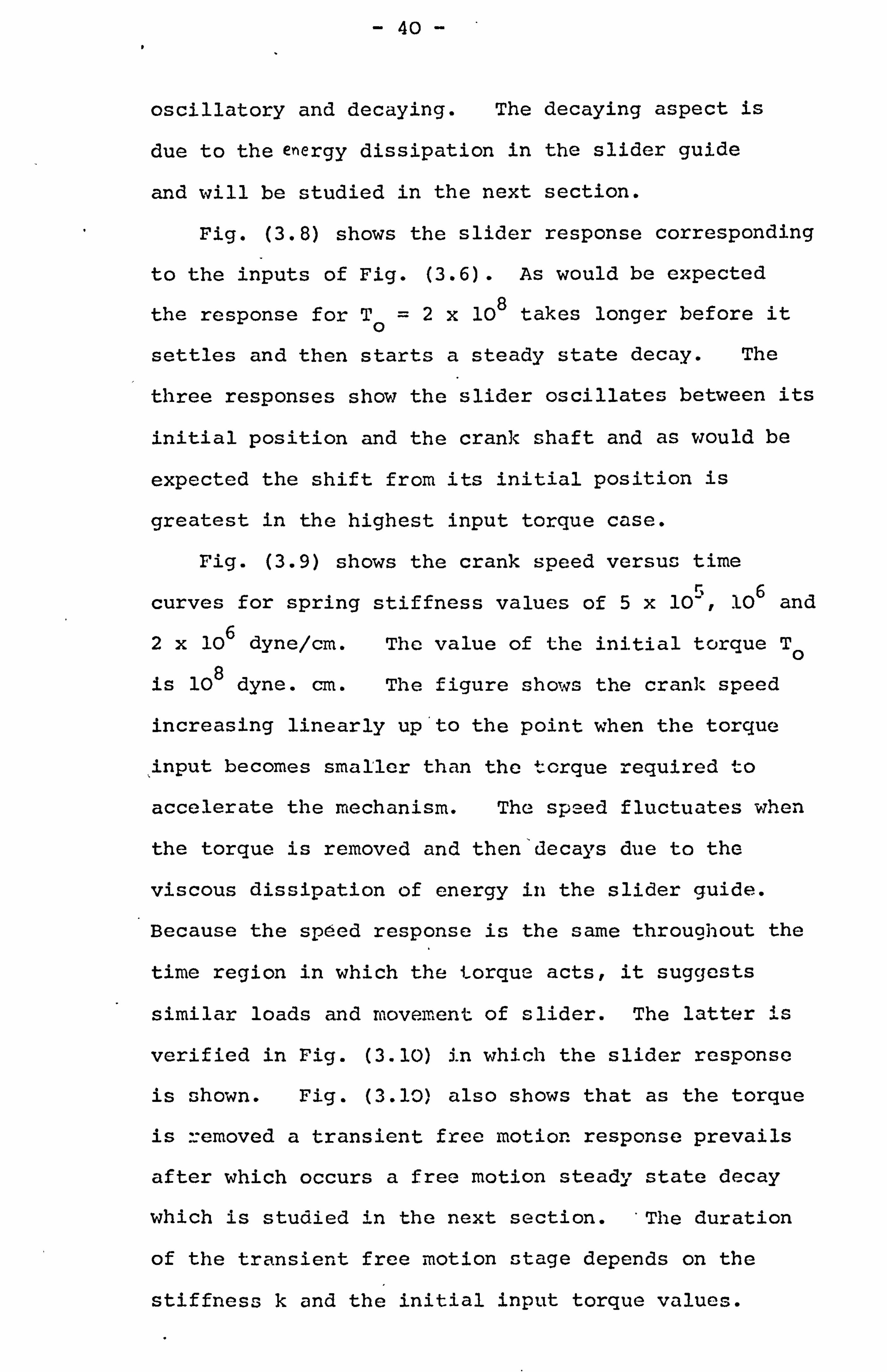
Fig. (3.6) shows the crank speed plotted against
time for values of initial torque T0 = 107,108 and
2x 10⁸ dyne-cm. The torque T becomes zero, when the
I points e2 -1 rad. marked on the curves are reached.
It is clear from the figure that during the time in
which the torque T is acting the crank speed behaves
in a linear manner up to the stage when the input
torque becomes less than the torque sufficient to
accelerate the mechanism. This stage occurs when
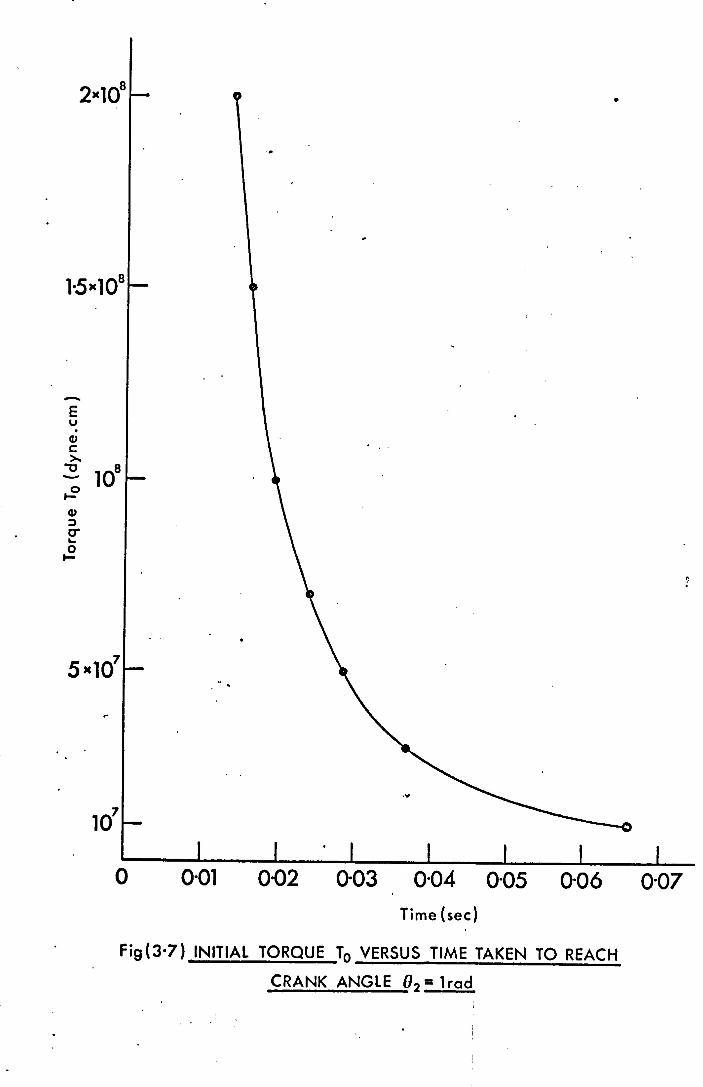
the points pl and p2 are reached. A plot of the
initial torque T0 against the time taken to reach
02 =1 rad. is shown in Fig. (3.7). It shows a
hyperbolic relationship-between T0 and T asymptotic
to To =o and T= o. The behaviour of the crank
speed beyond 02 =1 rad. in Fig. (3.6) is governed by
the free motion equations of motion. However, it is

CN ,0 0000
00
(Das/spot) paads juoao
CV 0
00
O
'0 r- O
N 0
-q a)
E I-
N r-- O
O
00 O Ö
10 O Ö
mot' O Ö
\ C.. 4 O Ö
O O N
LLJ
z 0 0.. (! ) W W
0 W W Q
z U
C) rn
LE
ýY
J
t 3
i
5
ý_ L
vvý Oý
XvN ý. o
2x10
5x1O'
E V
Q) c
10
0
Q' I- 0 f-
5x 10'
10'
Time (sec)
Fig(3.7) INITIAL TORQUE To VERSUS TIME TAKEN TO REACH CRANK ANGLE ©2 -- 1rad
0 0.01 0.02 0.03 0.04 0.05 0.06 0.07
- 40 -
oscillatory and decaying. The decaying aspect is
due to the energy dissipation in the slider guide
and will be studied in the next section.
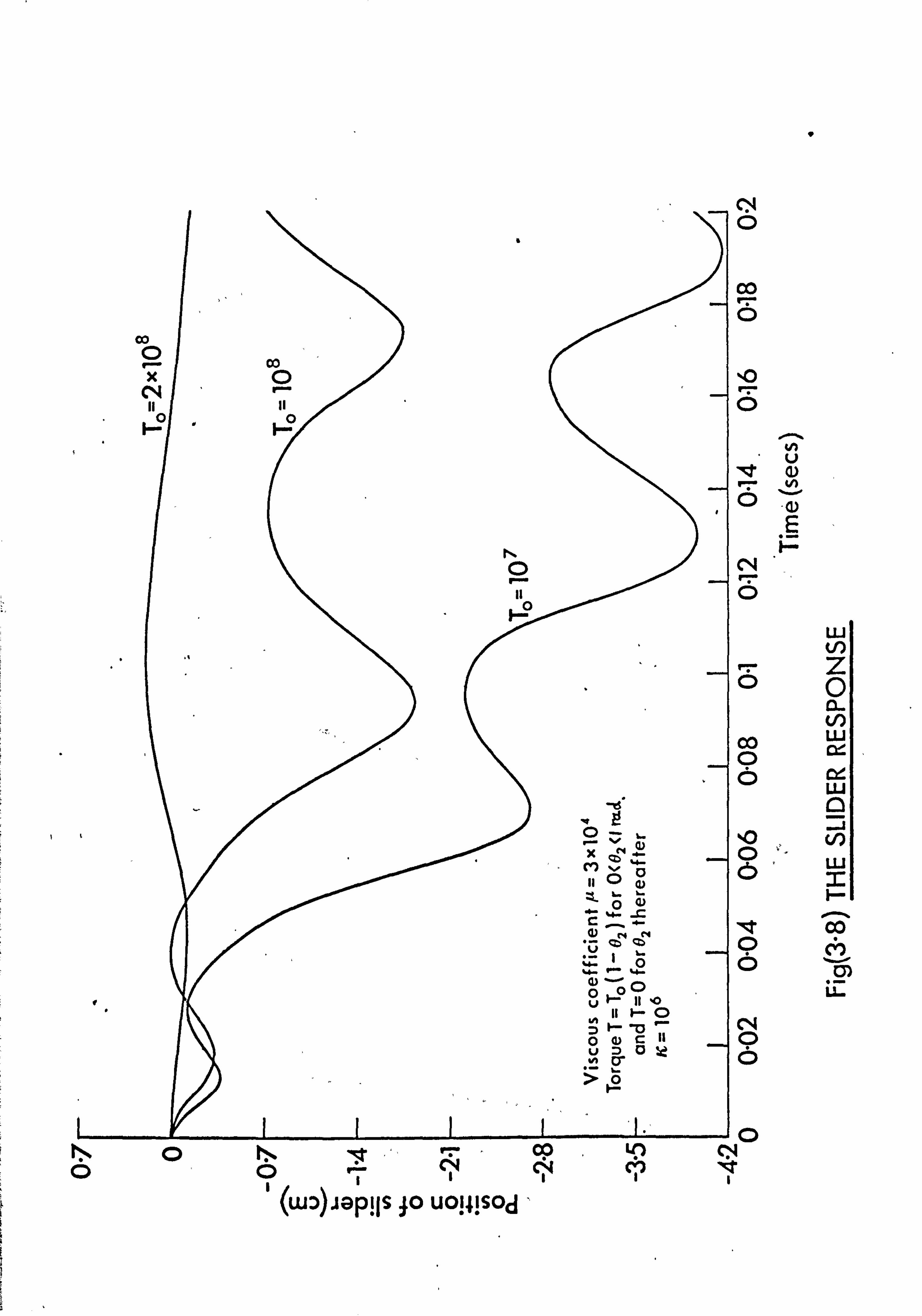
Fig. (3.8) shows the slider response corresponding
to the inputs of Fig. (3.6). As would be expected
the response for To =2x 10⁸ takes longer before it
settles and then starts a steady state decay. The
three responses show the slider oscillates between its
initial position and the crank shaft and as would be
expected the shift from its initial position is
greatest in the highest input torque case.
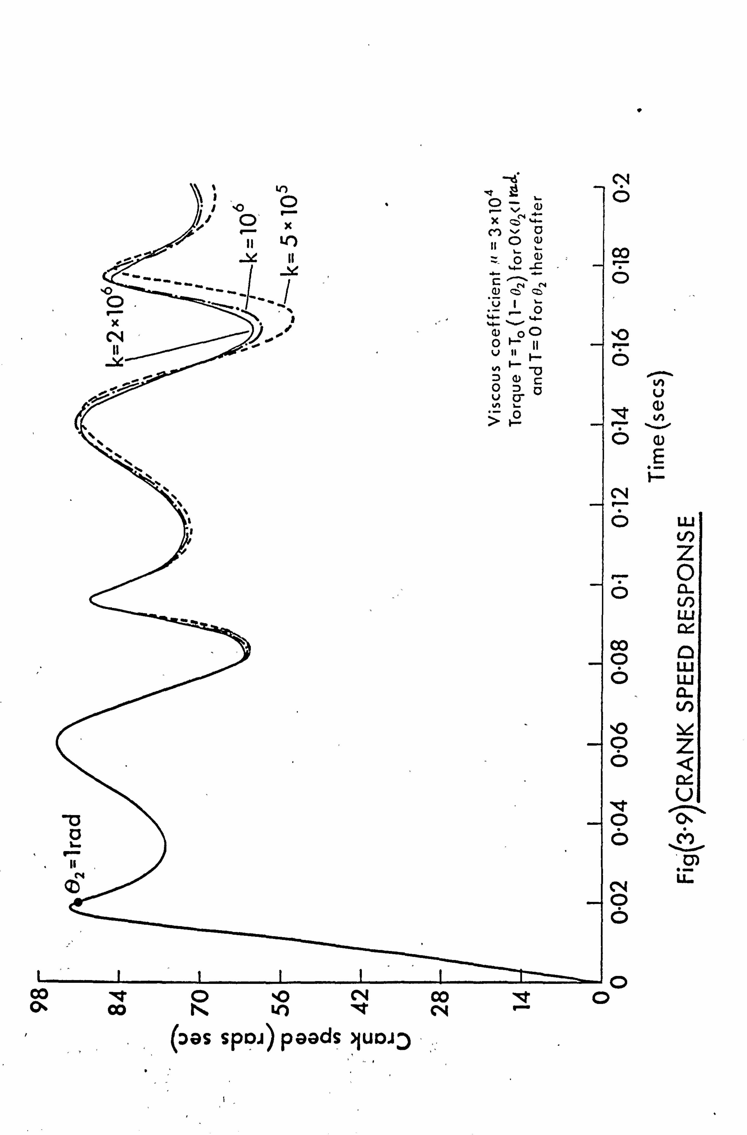
Fig. (3.9) shows the crank speed versus time
curves for spring stiffness values of 5x 105,106 and
2x 10⁶ dyne/cm. The value of the initial torque To
is 108 dyne. cm. The figure shows the crank speed
increasing linearly up to the point when the torque
input becomes smaller than the torque required to
accelerate the mechanism. The speed fluctuates when
the torque is removed and then decays due to the
viscous dissipation of energy in the slider guide.
Because the speed response is the same throughout the
time region in which the torque acts, it suggests
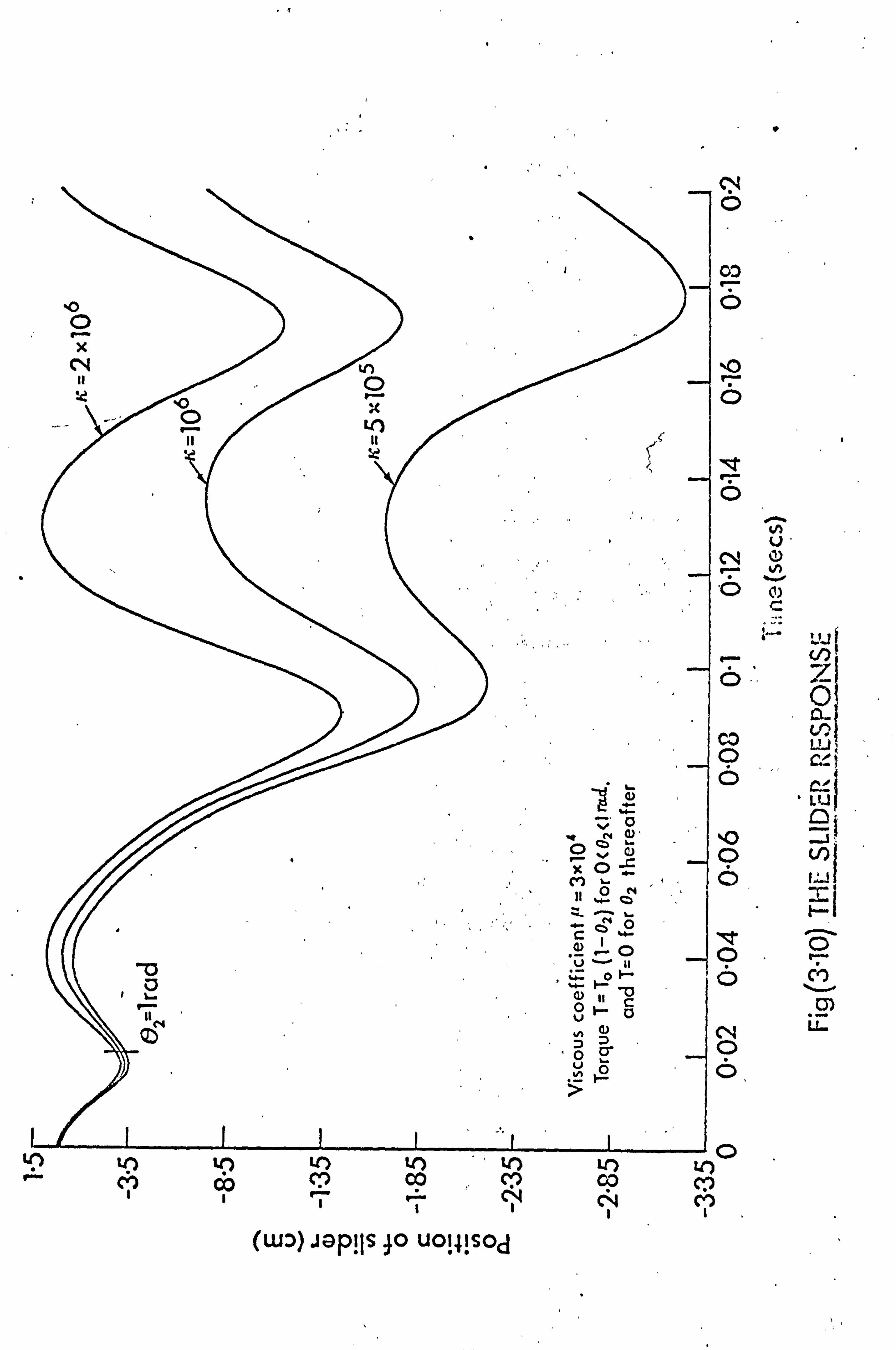
similar loads and movement of slider. The latter is
verified in Fig. (3.10) in which the slider response
is shown. Fig. (3.10) also shows that as the torque
is :. -emoved a transient free motion response prevails
after which occurs a free motion steady state decay
which is studied in the next section. The duration
of the transient free motion stage depends on the
stiffness k and the initial input torque values.
N 0
00 O
ýO 0
N V
'd' a) r- v)
. aý E
f-- N 0
r- O
00 0 6
b"
114* 0 6
N O 0
-o N
9
W N
z 0 a- U) W w
ce. W O
J
W
I--
co CY)
CD LL.
rý o tý , n. r- oo L OO ý-- NN ci
i (wD)iap! Is 40 UOi4isOd
0
00 ýgt NO 00 0` Co 0N
(as s na aads uo
--ä
'-
N 0
00 r: - CD
INO O
V
N
O aý E
N I- OW
z 0 o a- w
co a ow
CL
ýO Y 9z oQ
V, u
O 0% Ö
. . 21 N 0 6
O 0
0
N 6
03 O
1O O
I
LM L(00 ). 'M I- CO
L) co CV
1
u . Cy r
u N
.o Q)
V
co tn. I. U
O 9 G%Ä , '
l
U
o 0 6 ý. ý -r-ý ö 0 fl Cl)
rn (V O
LL.
Ö
-1 o LO M Cl)
I
(wD)-JGP! ls JO UO! 4! sOd
- 41 -
3.3 Free Motion
The equations of motion for the free motion are
the same as for the forced motion input torque case
except that the element B1 in matrix B3 . has no
torque component, i. e.
B1= -m3gk2 Cos02 -m3S. 2QG3 Sin(02-03)032
In order to investigate the response of the
mechanism in its free motion let us assume that
initially we have a forced motion with constant speed
input. The input torque to maintain the constant
speed input is then removed and the responses of the
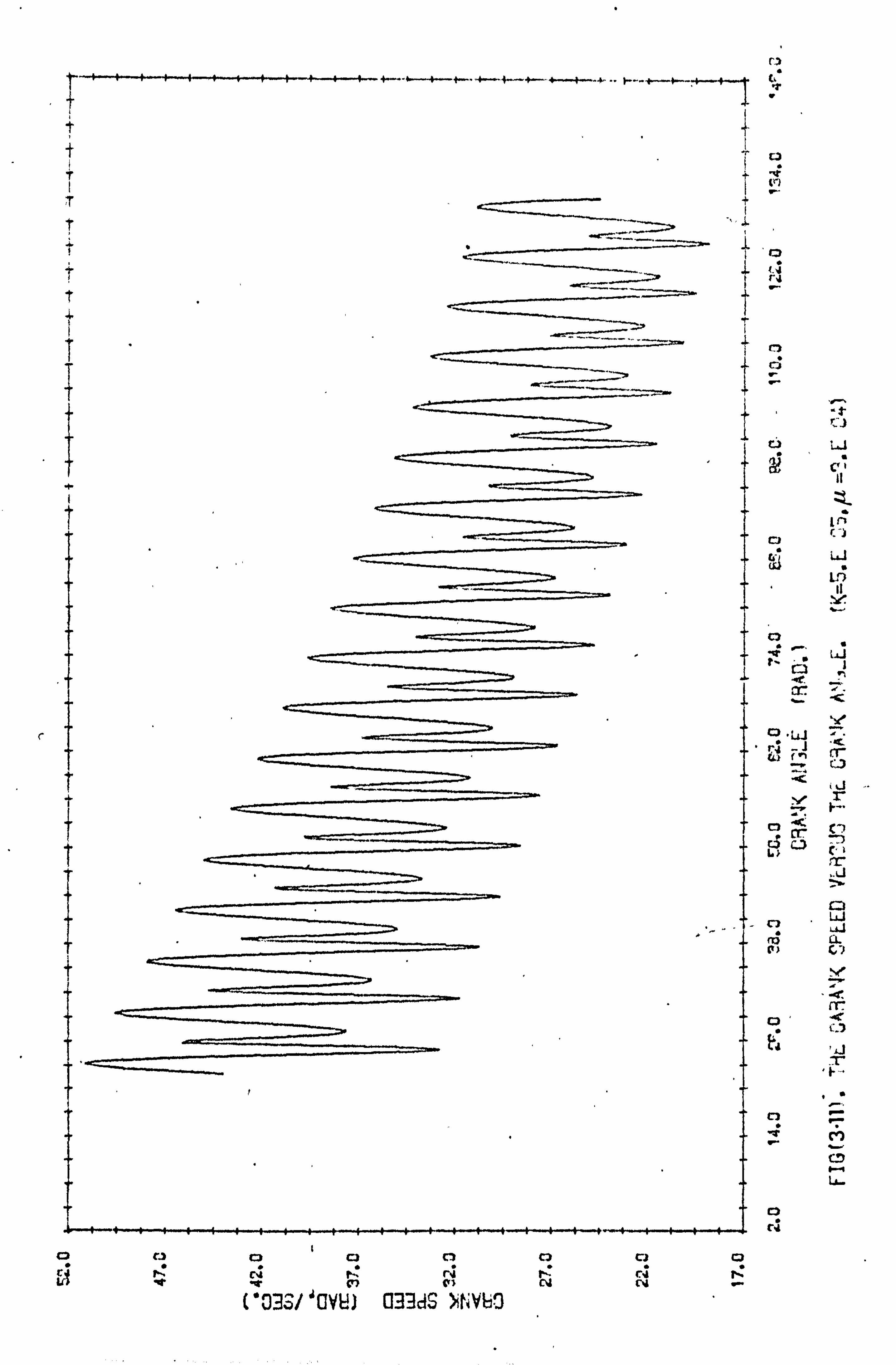
slider and crank are studied. Figs. (3.11) and
(3.12) show the crank speed versus crank angle for
k=5x 10 5 and 2x 10⁶ dyne/cm respectively. The
initial speed of the crank is 420 rpm and the viscous
coefficient u 3x10⁴ dyne. sec/cm. The input data is
as shown in table (3.1).
Both figures show that
(1) The crank speed behaviour is oscillatory
(2) The amplitude of oscillations decreases
with crank angle and
(3) The mean position of oscillation reduces
with crank angle.
The oscillatory behaviour of the speed is due to
the non-linearities of the system and the reduction
in speed is due to viscous dissipation of energy in
the slider.
r
tfj f i 7
# -- `"
r. ) tý 7
a
cri ý"
4
rJ r, t
C) C)
-r
c if -,
Gfj
LAD Ü
. Y.
C7 t ý" t, J
Q. Lj
4i
I ýs f_"
Q rr CL'
C
.. J
C=l
QW LAJ
rra Cl. Rý G1
" 4, fl"
d4 t_7
rj
o
IT cm H
U-
b vi
a C) m C) C, C, c. ) a9 r-4 irk "v C" c c4
("OB3/ ' UYIiJ O33dS MV1 3

0 ri
-+---º---+--- $---+--- 4 -°+- -"4--+---4^---1---$ -- -'--+-- +--"
f
9 c3
j C)
c) , LAU Ci
ul
Y
0 Li
c Lj --i CT'
7V
Y
. _r.
. ýl
ci C
1l
C ci Ca
rv t4J
H U-
a CJ
0 r C7 ci
s {a cý c3 c3
9N Cu Lý "r v r) of C ct
t'333/'CVL) 033dS 'ANVO
- 42 -
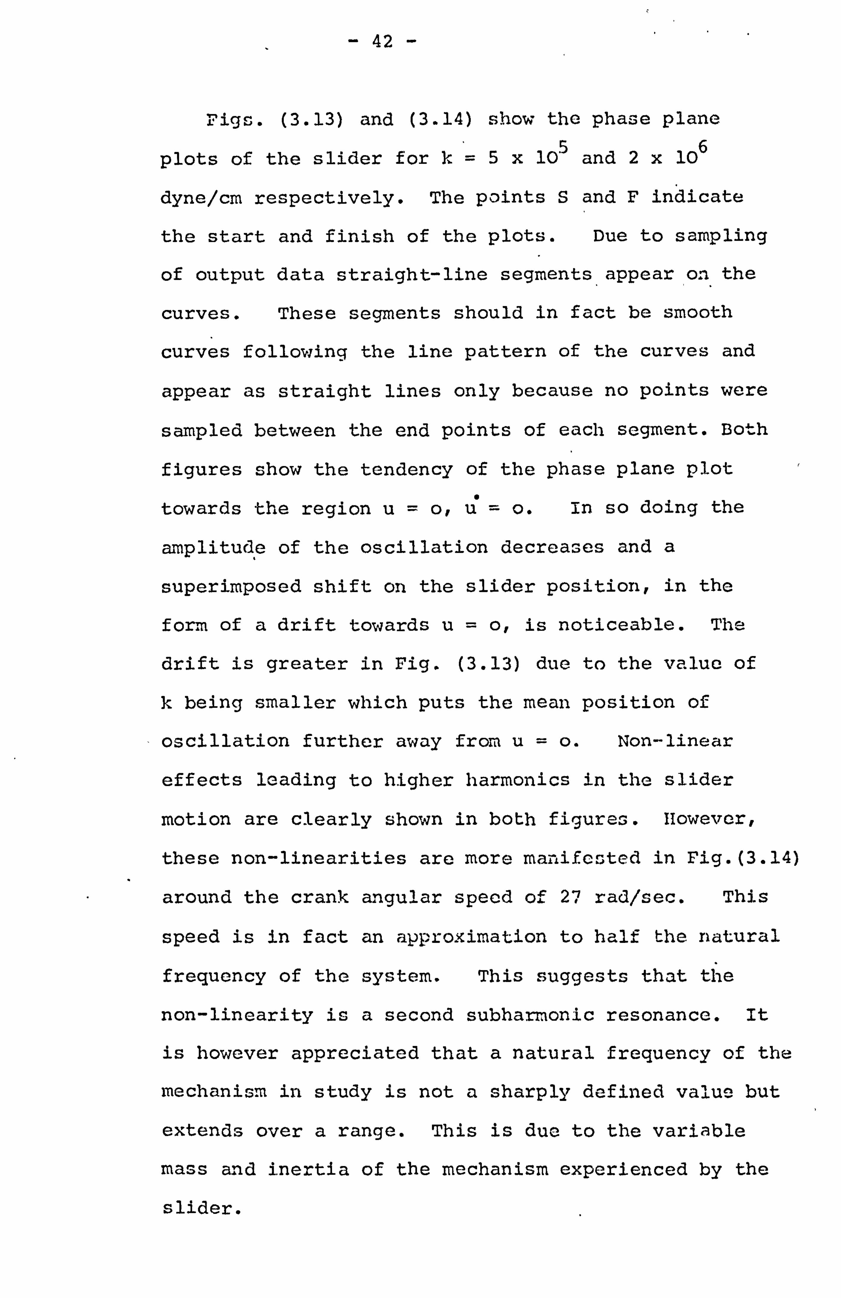
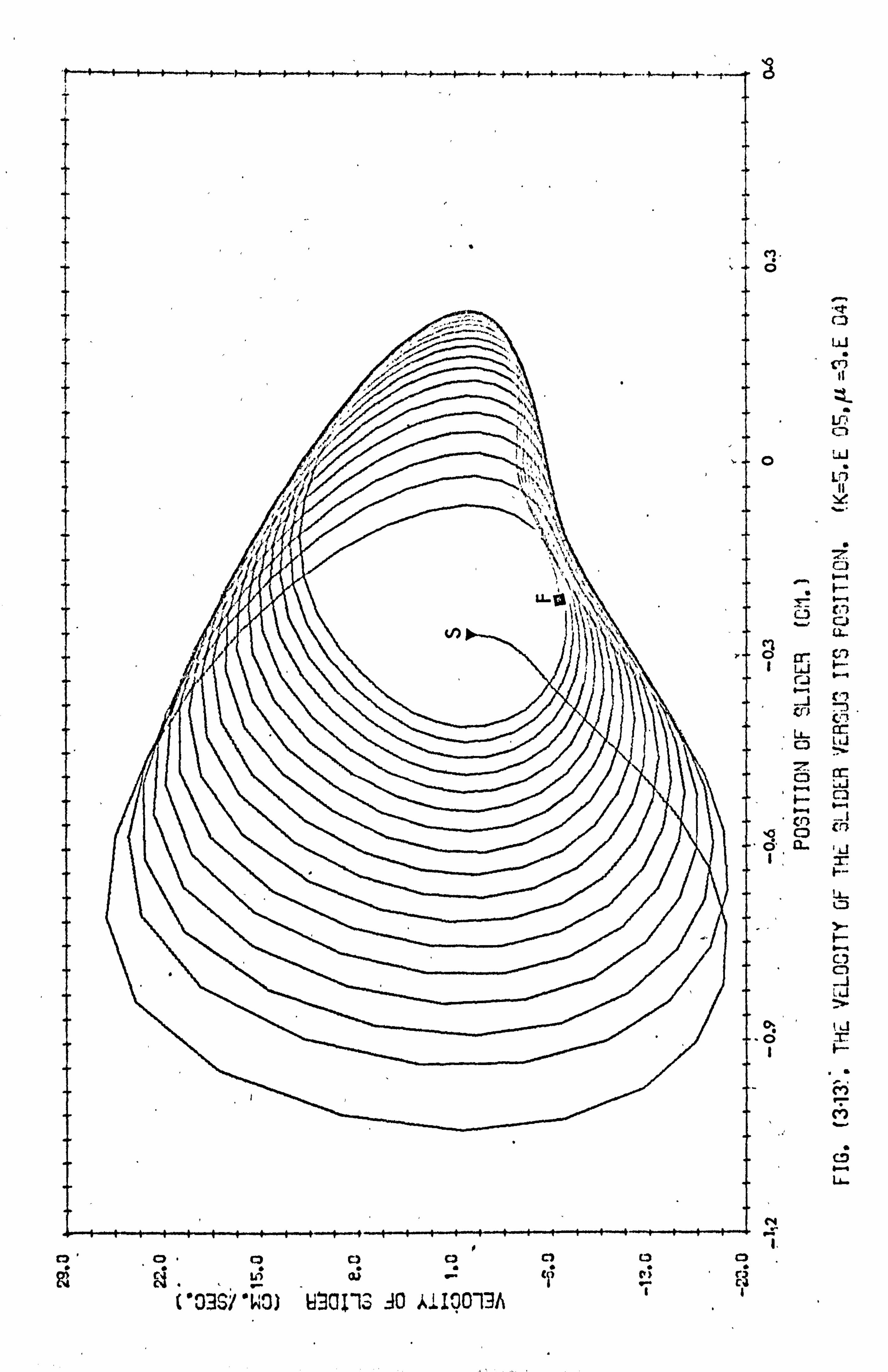
Figs. (3.13) and (3.14) show the phase plane
plots of the slider for k=5x 10⁵ and 2x 10⁶
dyne/cm respectively. The points S and F indicate
the start and finish of the plots. Due to sampling
of output data straight-line segments appear on the
curves. These segments should in fact be smooth
curves following the line pattern of the curves and
appear as straight lines only because no points were
sampled between the end points of each segment. Both
figures show the tendency of the phase plane plot
towards the region u=o, ü=o. In so doing the
amplitude of the oscillation decreases and a
superimposed shift on the slider position, in the
form of a drift towards u=o, is noticeable. Thome
drift is greater in Fig. (3.13) due to the value of
k being smaller which puts the mean position of
oscillation further away from u=o. Non-linear
effects leading to higher harmonics in the slider
motion are clearly shown in both figures. However,
these non-linearities are more manifested in Fig. (3.14)
around the crank angular speed of 27 rad/sec. This
speed is in fact an approximation to half the natural
frequency of the system. This suggests that the
non-linearity is a second subharmonic resonance. It
is however appreciated that a natural frequency of the
mechanism in study is not a sharply defined value but
extends over a range. This is due to the variable
mass and inertia of the mechanism experienced by the
slider.
I i
i
+4-
0 ooa c2 cl c2 a
("33S% 'wo) d1QI13 30 AiI0013h
9
Cl) 6
r. . 1. cý w
w
oL ýn
.
23 .ý u..
Ö rr Cr)
1LF
ra rC
cc: q
cc
i-- ca
p Cr) a.
I--
t7
H
C, C) _J LJ
t L1 OF
M
C7
Lý..
N ":
ul
" . --ma""""r--ý-ý
7
LLwl
r�ý N'I
Gfi h- i -r 4
ca ca ri r
c) ) C) aao ti Co ,r Oi cl
tý"J J% ýý, Vý ý3CTL 13 -IC %i1'JO1 A1
ýI
v
cn
Mt
CW oil
(o W
it
a" 7 V
r. ~
" `-.
C. 3 Cr, CL
1" (ý N
U {
Cl7 -)
CI !L C
LJ ca I
n" Lß. 1 F
!L C.,
. C' 7" 1 I-
rH C. 3 cl J
61 tai
CV) tý
fý 1

- 43 -
3.4 Computer Program
A computer program, the details of which are
shown in Appendix , 1, was written to solve the
equations of motion. It consists of a main program
which calls for several subroutines. The Hamming's
method which performs the numerical integration is
shown in subroutine "DHAM" and the Gaussian
elimination method which performs the solution for
the second order derivatives is shown in subroutine
"Gauss". The solution of the kinematics is shown
in subroutine "Kine" and subroutines "Block data"
and "Outp" are used for input and output requirements
respectively.
The language in which the program is written is
FORTRAN IV and double precision arithmetics are used
throughout.
- 44 -
Chapter IV
THE LINEARISED EQUATIONS
AND
RESONANCE ANALYSIS
The dynamic analysis performed in Chapter II led to
a set of highly non-linear differential equations. These
equations can be linearised in parameters describing the
deviation of motion from that of the four-bar with no
movable pivot. This can be performed by expressing each of
the generalised coordinates as the sum of two quantities.
The first of these quantities accounts for the motion of the
fixed four bar, the second only for the deviation from this
motion due to the movable pivot. It must, however, be
appreciated that in order that the results are true and
meaningful the motion of the movable pivot must be small.
Two important aspects of the mechanism may be directly
studied from the linearised motion; these are resonance and
stability. The first will be studied in this chapter, the
second in the next.
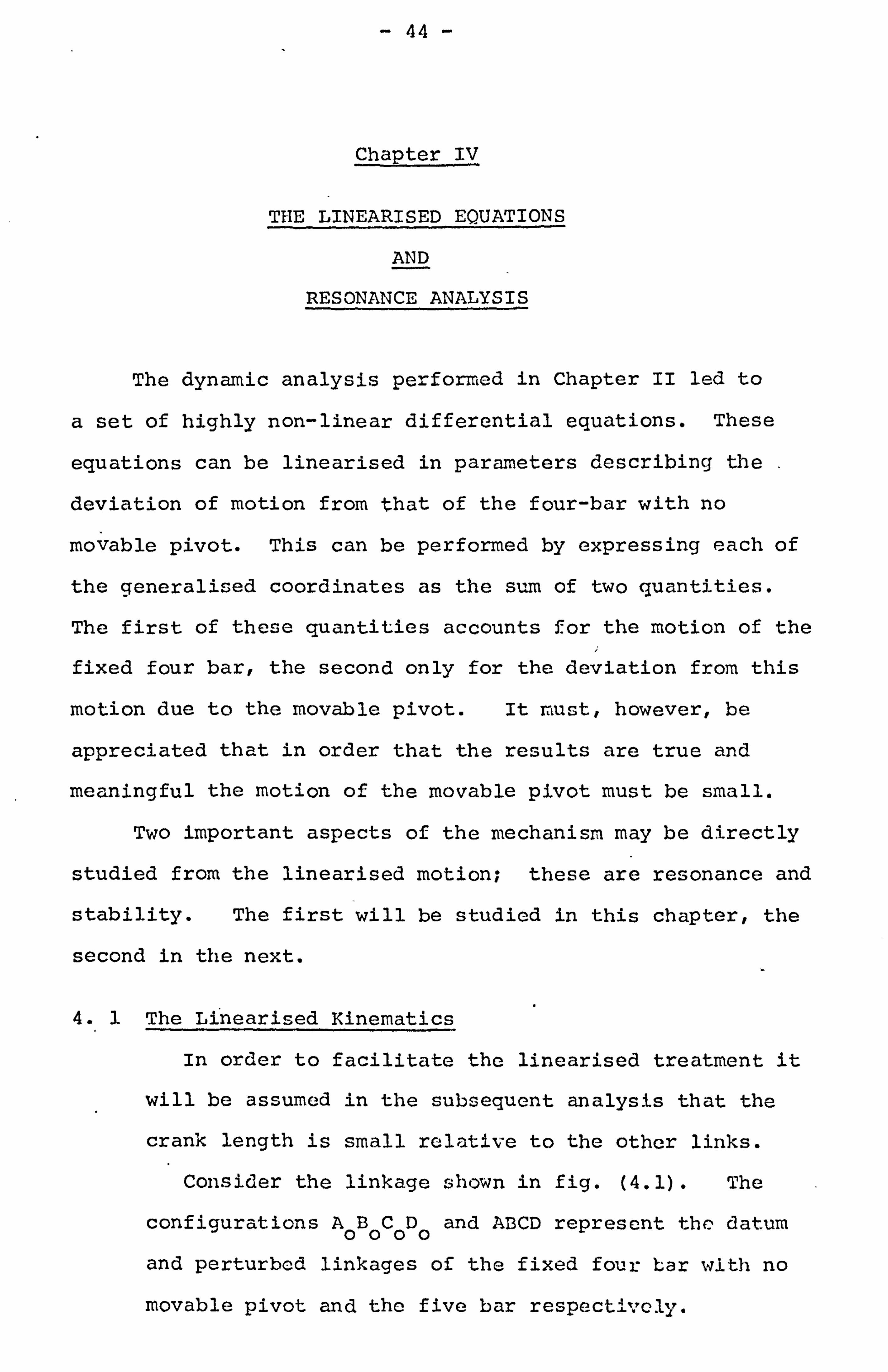
4.1 The Linearised Kinematics
In order to facilitate the linearised treatment it
will be assumed in the subsequent analysis that the
crank length is small relative to the other links.
Consider the linkage shown in fig. (4.1). The
configurations A0B0C0D0 and ABCD represent the datum
and perturbed linkages of the fixed four bar with no
movable pivot and the five bar respectively.
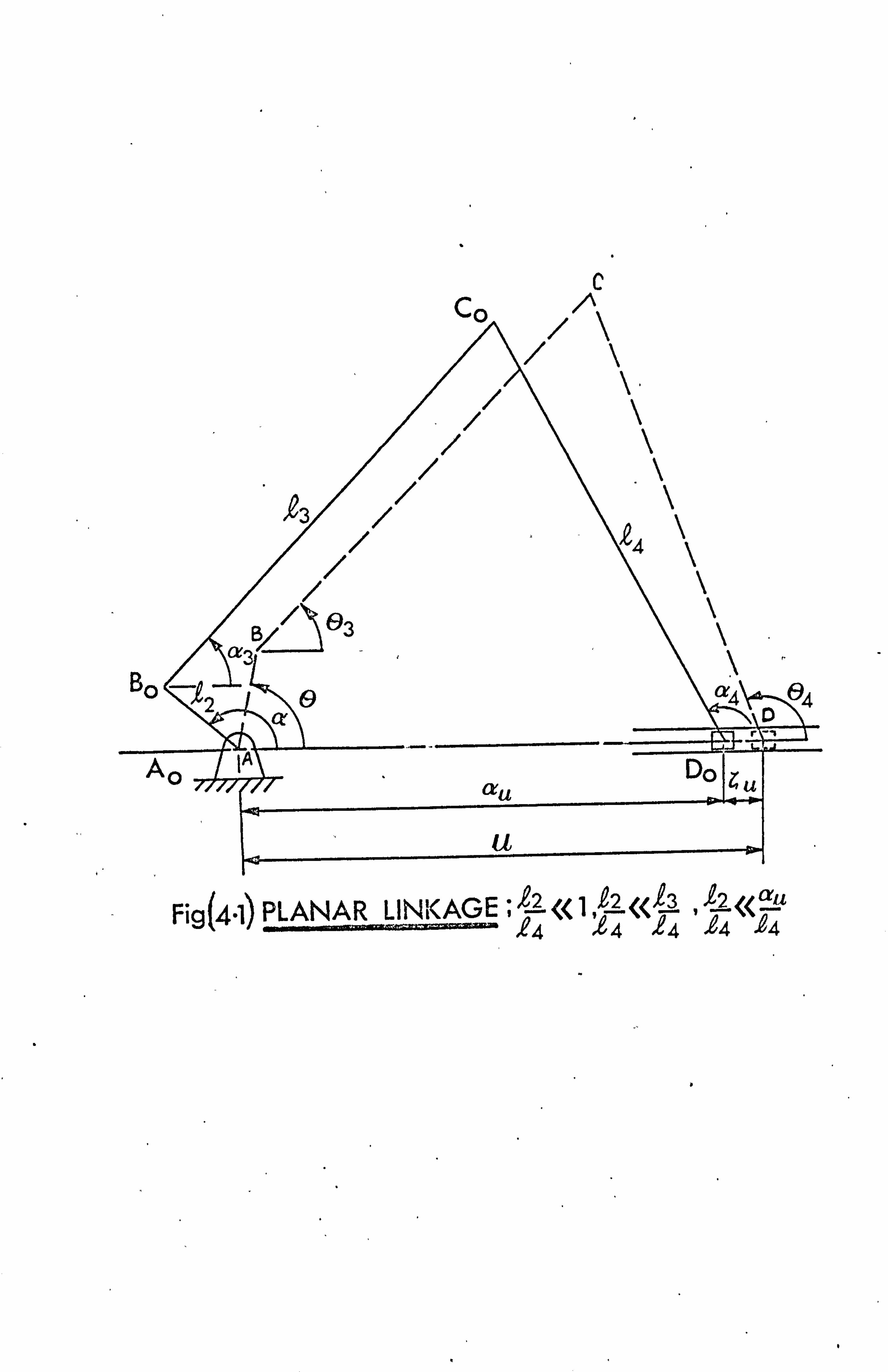
c Co
. /*", X
Fig(4.1) PLANAR LINKAGE ;? «1, L? «13 ý? <u . e4 £4 14 ,4 14
- 45 -
A0B0C0D0 is arrived at by defining :-
a4 = a4 max.
+' a4 min. (. 4.1) 2
where a4 max and a4 min are the maximum and minimum angles
of the rocker C0 0 when the crank A0 B0 is rotated through
360 degrees in the fixed four bar case. The angles a and
a3 are then calculated accordingly.
The constraint equations may be written :-
Q2 CosO + R3CosO3 - Q4 Coso4 -u=0
(4.2) k2 SinO + Q3SinO3 - z4 SinO4 =0
Now, dividing equation (4.2) by Q4 and defining
03 = a3 + ý3 , 04 = a4 + ý4? u= au + ýu (a)
and
-2 << 3, o'= au _ ýu (ö) (4.3) 2 j4 3 Ti 74 Qý.
where ý3, C4 and Cu are the deviations from the four bar
motion, and assuming
Cos13 = Cost4 = 1, Sint3 = 13 , Sim 4= 14 (4.4)
the following two equations may be obtained : -
-Cosa4 + Sina4.14 + a2 CosO + (13 Cosa3
- a3 Sina3 t3 -a-=0 (4.5)
-Sina4 - Cosa4.4 +a2 SinO + (13 Sinai
+ Q3 Cosa3. t3 = 0.
Now using the datum configuration A0B0Cö 0 we obtain
a2 Cosa =a+ Cosa4 c13 Cosa3 (4.6)
a2 Sina = Sina4 cri Sinai.

- 46 -
Substituting equations (4.6v into equations (4.5) we obtain: -
-a3 Sina3 C3 + Sinct 4 C4 -C= -02 Cos® + 62 Cosa (4.7)
03 Cosa3 ý3 - Cosa4 ý4 = -62 SinO + C2 Sina
and hence
_ Cosa4ý -ctg . Cos (0-(14) + a2 Cos (a - a4)
3 a3 Sin (a4-a3)
C_ Cosa 3r - 62 Cos(0 - a3) + a2 Cos(a -a C4 Sin (a4 -a3)
(4.8)
4.2 The Linearised Equations of Motion
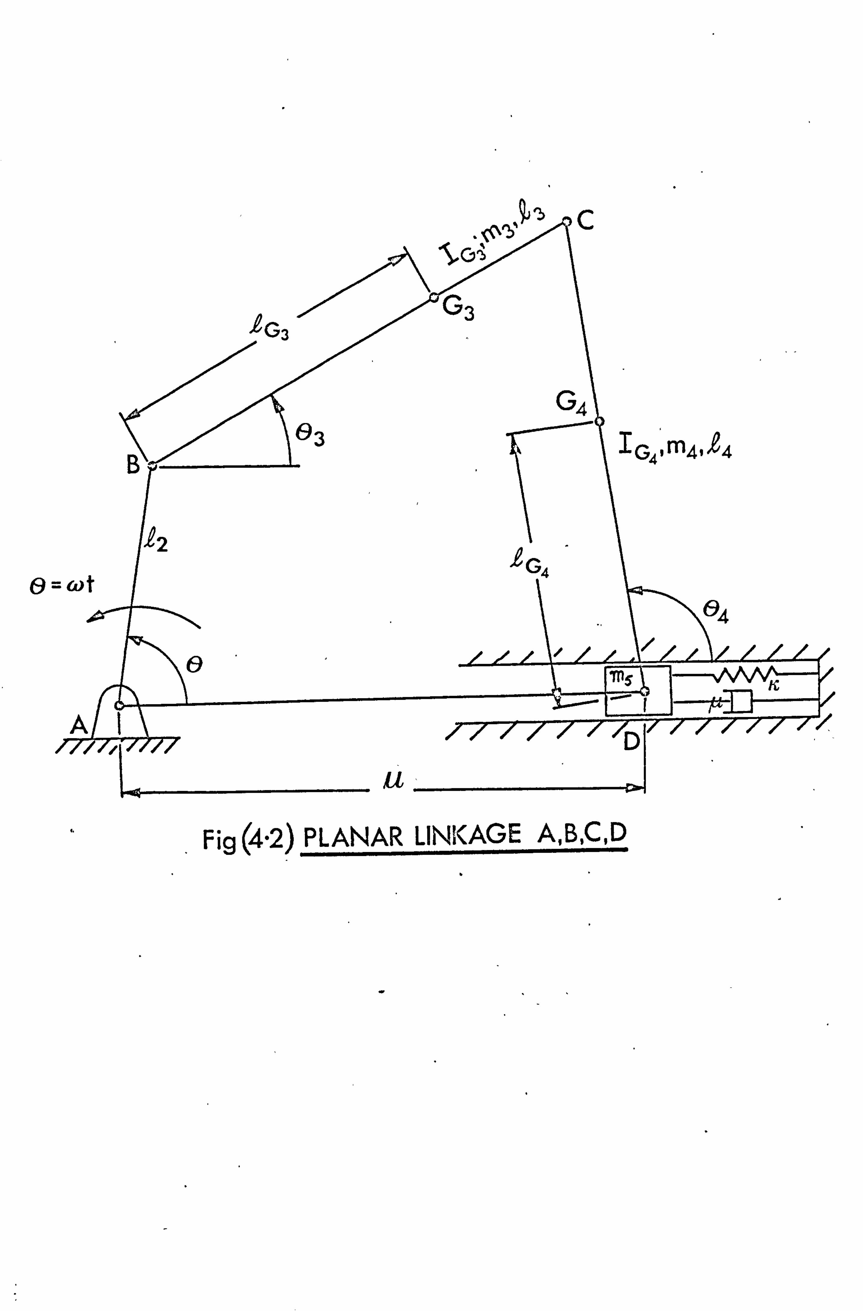
Consider the linkage shown in fig. (4'. 2) with a spring
of stiffness k and a damping friction of coefficient V. The
symbols indicated on the figure are as follows : "~
R, m and I denote length, mass and inertia respectively.
Subscript G denotes centre of gravity. Subscripts 2,3,4
denote crank, coupler and rocker respectively.
4.2.1 Derivation
Assuming a constant crank angular speed w, i. e.
0= (-, , (4.9)
and no gravitational forces, then by application of the
Lagrangian multiplier method stated in equation (2.5) the
following equations are obtained.
m3A. 2&G3 Cos (0 - 03)(5 3+ m32.3 Y, Q G3 Sin (0 - 03) 032 +a1ß, 2 SinO
-X2Z2 CosO -13 =0 (4.10)
C 'S, 15
'eG3 G3,
0 =wt
G4 03 IG49m4,2a
12 1 G4
0, z,
ý.
x
K
AIN /7 1-7 /v
Fig (4.2) PLANAR LINKAGE A, B, C, D
- 47 -
(IG3 + m3QC32)03 - m3Q2QG3 Sin(0-03)02 +X193 Sin03
-X2'3 Cos03 = 0. (4.11)
G4 + m4ýG42)04 m4QG4 Sin04 ýu -a1Q4 Sin04
+X2Z4 Cos04 = 0. (4.12)
(m4 + m5) ýu - m491 G4 S1n0404 - m491G4 Cos04.042
(4.13)
+al+u. ýu + k. Cu = 0.
Divide equations (4.10), (4.11) and (4.12) by (m4w2Q42) and
equation (4.13) by (m4w. R. 4) and let 2
mr3 = m3*k2'QG3 I3 =
IG3 + m3QG3 22
m4. Q4 m4 Q4.
2 I4 =
IG4 + m4kG4 r4 lCG4/
m4 Q42 £4
u_-k We wk =� (m4 + m5)
(m4+m5 )
P= m4 We ýx-
Wk 45 (m4 + m5) C-Wk W_
_ X1 x2
_ A3
2- 19 º_ 2 1 m4 uº2Q, 4
2 m4cu 2.4 3
m4w2£4
Now, transform the differentiation with respect to time to
that with respect to crank angle 0 and denote the first
derivative of this by '/ '' above the variable symbol, and
(4.14.. )
- 48 -
the second by 'AI''. The equations of motion may then be
written :-
mr3. Cos (0-03)0 3+ a2 Sin0 . 91 -ßs2 CosO ., g2 -, % _ -mr3Sin (0-03) X32
(4.15) h
1303+ cs3Sin03 ý1
M /I
1404 - r4Sin04C 4p
ý- p45. r4SinO404
a3CosO3 '2 = mr3 Sin(0-03) (4.16)
SinO4C1 + Cos04 2=0. (4.17)
+ Cý + ak2 C+ p45ý1=p45r4Cos040O42 (4.18)
Divide Equations (4.2) by e4 and differentiate twice with
respect to 0, we obtain NM
c 3Sin030' - Sin0404 +_ -62,. Cos® (4.19)
22 -., a 3 Cos0303 + Cos0404
N // 12 2 Q3Cos0303 -Cos0404 = cr2Sin0 +a3Sin0303 - Sin04 04
. (4.20)
au By eliminating 03,04, ýl C2 and F; 3 from the above equations
a second order differential equation describing the notion
of the slider may be obtained. If equations (4.3a) and (4.8)
are substituted into this slider equation, and second and higher
order multiples of r and its derivatives-are ignored the following
linearised equation of motion of the slider may be obtained.
ao (Al + Bl . CosO + C1. SinO) D1 + E1. CosO+ F1. Sin0
+Xk2 (PI1+B1Cos0+C1Sin0) + (G1+H1CosO+P1Sin®) D1+E1. CosO + F1. SinO
Q1+R1CosO+S1. SinO
'D1+E1Cos- + F1S1 O (4.21)
49 -
This may also be written as :
ý +. W1(0) + Vý2 (ý) _13 (O)
i. e. a second order linear differential equation with
periodic coefficients of yl(0) and ý2 (0) and a forcing term
of x13 (0) .
The various coefficients of equation (4.21) are as
follows : -
Al = cs2{Sin 2 (a4-a3) -2c2Cos (a4a3)
[C0s4) -Cos (a-3)
1}
63 JJJ
}. B=-a2{2cCos(a-a) rL_ Cosa 4+ Cosa 3] l2 43
cr 3
Cl =-cs3{2a2Cos (a4-a3) r- Sina4 + Sinai }. L cr 3
1"1 Al 2p45r4cr 3{ Sina4Cosa 3Sin(a4-a3)
_ a2
[Sin4Cos(a4-2a3)Cos(a-(x 4)
Sin (a4 a3) a3
- Cosa 3Sin (2a4-a3) Cos (a-a3) ]}
+ p45. {I4a [c23
- a2Sin2a3Cos(a-(14)
Q3 Sin (a 4-a 3)
+13 [Cos
c4- a2Sin2a4Cos(a-a3) Sin (a4 (x3)
Ei = B1 - P45ý4a3a2 { Sin2a4Cos(a4-2a3)-2Q3Cos2a3Sin(2a4-a3)
Sin(a4 - a3)
(` + p45 { I4a3o2
rsin2a3cos4l + 13cr2 L43}
Sin ((x4-a3) Sin (a4-a3)
- 50 -
F1 = C1 P45r44o2 { 2Sin244Cos(a4-2a3) -a3Sin2a3Sin(2a4-a3)
Sin (a4 - a3)
r.
+ p45 {I4a362 rSin2a3 Sina4 + 13a2
ISin2a4 Sinai
Sin (a4 - a3) Sin (a4 - a3)
G= p45'I3'62 -Cos
2a 4.
Cos(a4-a3) +o3 Cos(2a 4-a 3) 63
{ Cosa3
Sin(a4 - a3)
J
HH1 =2
[I4Y3Cosc4Sinc3+I3Sin2c4_ 2r4a3Sin2a4Cs(c4-2a3)
Cosa 3
Sin (a4 - a3)
r4 a2Cosa 3Sin(2a4-a3)
Sin(a4 - a3)
I
- 51 -
HH2 =
[_mr3Cos2c4Cos(a4-a3)+mr3f3Cosa3Cosa4-I4 a2a3Cosa4Cosa 3
Sin(a4 - a3)
_ I3CT2 .
Cos 3
a4 +
la2a3r4Sin2a4 a3 Cosa3 2
Sin (a4 - a3)
H1 -_ P45{ mr3. Cos2a4
+ HH1. Cosa3 - HH2. Sina9 }. Cosa3
J
F1 P45' {HH1. Sina3 + HH2. COS 3).
Q1 P45o2{ I3 Cosa4 Sin(a4-a3) + I4cs3 Cosa 3+ I3 Cos 2 a4
Cosa3 Cosa3
R1 P45a3'{SIn (a4 -a3) LCF203r4Sina4Cosa
3-mr3Sina3Cosa 4}
S1 p45o3{ Sin(a4 la3) Ea23r4sin3sin4+mr3cos3cosa4
}
- 52 -
4.3 Simplification of the Linearised Equations of Motion
The coefficients B1, Cl, Hl, PI, Dl, El and P`l
are much smaller than those of A1 aril D1 by at least a
factor l in the worst cases. Therefore we may write :-
D1 = ko ,
Dl = kl. e,
D1 = k2. E
11
D1 Dl = ho ,
ýl = k3s ,1= k4E
111
D1 =k5. ß,
D1 = k6. e
11
S D1 = g0, D1 = k7e , D1 = k8c
111
(4.22)
where c is a small parameter and ho, g0« k0.
Let us now consider the damping term in equation (4.21). This
may be written as :- I- -1 . ac. (ko + (k1CosO+k2SinO) E) (1 + (k5CosO+k6SinG) E: )
By multiplying out, ignoring the terms in second and higher
powers of e and rearranging in an increasing powers of s
we obtain
X'. - {k0 (kl kö 5) CosO + (k2-kä 6) SinO c+
+ : (ko (k5CosO+k6SinO) 2- (k1CosO+ k2SinO) (k5CosO+k6SinO)e2+... }
which, if terms in the order of third and higher powers of e
are ignored, may be written
aý {k0+(a1Cos0+b1SinO) + (a2Cos20+b2Sin20)e2+.... } r (4.23)
ry
- 53 -
where
al kl - kö 5
bl = k2 - kok6 (4.24)
a2 = 1. {k0 (k25 - k26) - (klk5-k2k6) }
b2 =2 {2ko 5k6- (klk6+k2k5)}
Similarly the stiffness term may be written : -
{, 2k (kö (a1CosO+b1SinO) ý+ (ä2Cos20+b2Sin20)c 2+.... ý
(4.25)
+. { ho + (a3Cos0+b3Sin0) c +(a4Cos20+b4Sin0ýý2 + .ý 1c
where
a3 = k3 hok5
b3 = k4 - ho G
a= 2{ h(k2-k2)
(4.26)
4o 56 - (k3k5-k4k6 )}
b4 =2{ 2ho k5k6 - (k3k5+k4k5) }
In a similar manner the right hand side may be written : -
g+ (a5Cos0+b5Sinp) E+ (a6Cos2p+b6Sin20)c 2 0
+.... (4.27)
where a5 = It 7-go
It 5
b5 = k8 8-go It
6 (4.28)
a6 = 2' { go (k25-k26)-(k 7k5-k8k6 )}
b6 =2{ 2go c5 k6 - (kýk6+k8k5)}
- 54 -
The equation of motion (3.21) may thus be written in its
final form as
4IV '+ Xc {ko+(a1Cos0+b1Sin0)c+(a2Cos20+b2Sin20)e2 + ... }
+ {Alk (ko+ (a1CosO+b1SinO) e+ (a2Cos20+b2Sin20) c2 + ... ý
+ ýho+ (a3Cos0+b3SinO)E + (a4Cos20+b4Sin20) c2 + ... ý }
- gö (a5CosG+b5SinO)c+(a6Cos20+b, Sin2O)c2 + ... (4.29)
4.4 Resonance Analysis
4.4.1 No damning; Xo =0
Assume that C has a series periodic solution of the form
= E1=O (XmCos m wt + YMSin m wt). (4.30)
By substituting equation (4.30) into (4.29) and limiting the
expansion of ý to m=2, then multiplying out and rearranging
we obtain
- (X1Cos0+ Y1Sin0-r 4X2Cos20+ 4Y2Sin20)
2 . kö ho) (Xö X1CosO+ Y1Sin0+ X2Cos2®+ Y2Sin20) + (Xk
+ Xo ( (aka1+3) CosO + (anbi+b3) Sino+ (X a2+ä4) Cos20
(a2. b +b )Sin20 )
k24
X ((a2ä 0. t1+Cos2O)+(X2h- ^)Sin?. 0 + (X2ä +a ) (Cos3S_-CosO) )
1( 1: 1a2k l+5 )2k242
(a2Ä +b ) Si( 2TinO (k242
(2.. Sir. 23 2 1-Cos2e. 2 +Y1. ((X a1 3) (2 )-r (fix Y-(X k a2+a4) (2)f
Cose -Cos3® ' + (ak2b2-r 4) (2
- 55 -
+X( (X2ä +ä ) (Cos30+Cos0)+(X2p +b. ) (Sin30-SinO)"+(a2ä +a ) 2( k132k132k2 4) ( 1+Cos40 '2*. ((2)+ (), kb+b4) Sin40
Sin30+SinO 2. Coso-Cos30 + y2 (Xkä1+a3) (2)+ (Xkbl+b3) (2))
+ (a2ä +ä ) Sin40 +(X2b" +b4) (1-Cos40) ) k242k242)
= go + ä5Cos0+ b5Sin0 + ä6Cos20 + b6Sin20 (4.31)
where a, bl, ä3, b3, a5, bý arc al, b1, a3, b3, a5 and b5
multiplied by e respectively and ä2, b'2,
are'-a2, b2, a4, b., a6 and bb multiplied
Equating constant terms and coefficients
a4, b4, a6, and b6
by e2 respectively.
of Cos®, Sin®, Cos20
and Sin20 on both sides of equation (4.31) we obtain the
Following recurrence relationships.
2 (X} . k0 ho) Xo+
+
2(X ä1+ä3)Xo
ä1+ä3)R1+ (Xk 51+):: 73) Y1
ä2+ä4)X2 + (X3 b'2+b"4) Y2 = 2g0
: -2ho+2Xk. ko+ak ä`+ä4)XZ + (X b'2+b4) Y1
ä1-; -ä3)X2 + (X) b1+b'3) Y2 =2 a5
xk
gk
(A2 k
2(ßk b'1+b3) o+
(ak b2+b"ý)X1+ (-2+2hö 2X . k0 -a "--a) Y1 (4.32)
+ (-ak b'1-b'3) X2+ (Xk . ä1+ä3) Y2 = 215» 5
2 (X ä +ä )x + (X2 ä +ä )X+ (ýx b1 -bam) Yk240k131k131
(-8 + 2h0 + 2X . k0) R2 - 2ä6
2 (X D2+äý) Xo + (a b1+1$3) ýý + (), K äl+äý) Y1
+ (-E +2 h0+2X . k0)Y2 = 2bE
- 56 -
The above relationships may be written as a matrix equation
of the form
(Aij) " (Wi )_ (Bi) (4.33)
where W. is a column matrix (X0, X1, Yl, X2, Y2), Aid is its
square matrix of coefficients and III is the column matrix of
the right hand side of (4.32). Equations (4.33) may be
solved using a digital computer, thus yielding the values of
the coefficients Wj.
4.4.2. Viscous damping; Coefficient of damping =u
Assuming a solution of ý as described in (4.30) and
substituting it in equation (4.29), then multiplying and
equating the coefficients of the trignometric functions of 0
on both sides of that equation in a similar manner to the
preceding section, we obtain the following recurrence
relationships,
2 boo. Xo r (b11. "d12)X 1 -i- (b12+d11)Y 1+ (b13-2d14)X 2+
(b14-ß-2d13)Y 2= 2go )
2 b11. Xo + (-2+2boö b13-d14)X1 + (2AC+b14+d13)Y1
+ (b 2d )X+ (b +2d )Y= 2ä ) 11 12 2 12 11 25
2 b12Xo + (-2X +b14+d13)X 1+ (-2+2b00-b13-+d14)Y 1 c+
(-b 2d )X+ (b 2d )Y 25 ) 12 11 2 1]. 12 25
2 b13X0 + (b11+d12) X1 + (-b12+d11)Y 1+ (-8+2b00) x2+4X . Y2 = 2a 6
2 . b14Xo + (b12-dll) Xl + (bll+d12) Yl - 4XoX2+ (-8+2boo) 2= 2b6
(4.34)
- 57 -
where, 2
boo = Xk. k0 + ho
2" b11=ýk. al+a3' d11=X C. al
b12 = Xkb"1 + b3 d12 =A bl (4.35)
2, b13 = Ak. a2 + a4 d13 = AC. a2
b14 = ak 12 + b4 ' d14 = ac. b2.
The above equations may be written in a matrix form
similar to equation (3.33). A numerical solution may then
be found for Xo, X1, Yi, X2 and Y2 and substituted in equation
(3.30) to give a'so"lution for the slider motion ý.
4.5 Results
To illustrate the theory discussed earlier let us consider
the linkage shown in fig. (4.2) and assume that :
(i) the mass and inertia of the coupler are negligible,
(ii) the centre of mass of the rocker lies on the centre
line of the slider, and
(iii) the input data are (see equations 4.3b) and (4.14)
wk = 10 3, A45 = 0.2, a2 = 0.05, a3 = 1.
4.5.1. Resonance in The Absence of Damping
Figs. (4.3) and (4.4) show the amplitude curves of the
first and second harmonics against the crank angular speed w
for three values of the inertia ratio I4. These amplitudes
correspond to ýY12
+ Y12 and �x22 + Y22 of equation (4.30)
respectively. The figures show that resonance for the first
harmonic occurs in the region of (wk-d) <w< wk where d=1
rad. /sec. These results are as would be expected and their
deviation from the idealised spring-mass system accounts for

ý I
M
ý rý J H /" 0 Q. 0 N
--------- Z CY) c"ý
be Z
c
f M ý
Hý I Z o" O N
ý. CY- Q
" ýI in "00 CY_
N U- 0
I J
" ý Q
N
' : . - 1 11[1111 el. p ON 0.0 I. e LO `. T
11 11 ý- (") N - 0 U - r- , i- pOO. OOO, OO
D! UOWAD4 ISJ! 10 apn4! 1dWy

.' ,, '..
_ý -ý' ý.
3
I Z
V a
ý. ' z Z3
3 V
w w C-
N N
0'
ýO ü
w
v Z
ý v ýV =
z 0 i U
L 0 w
CV) I--
J C- <
1 JO LL
%0 W) m C%4
DIUOWJoy puoDas 4o apn4! 1dwd
- 58 -
the oscillating inertia of the rocker. However, as shown
in fig. (4.5), this deviation decreases linearly with
decrease of inertia ratio 14 and becomes zero when 14=0.
In fact for the case 14=0 the equation of motion of the
slider reduces to a second order linear differential equation
describing an idealised spring-mass system. Fig. (4.3) and
fig. (4.4) also show that the amplitude of oscillation
decreases with decrease of 14 and that as 14 increases it
widens the region of resonance. It is also clear by comparing
the amplitude values in both figures that the first harmonic
of the solution is dominant and the second harmonic may be
neglected in comparison.
4.5.2 Resonance in the Presence of Damping
Figs. (4.6) and (4.7) show the effect of damping on the
amplitude curves for the two values of I4= 1 and 0.5
respectively. The amplitude of oscillation is not affected,
on the scale of the graph, outside the resonance region. The
natural frequency decreases slightly with increase of damping.
It also shows that a smaller value of damping eliminated
resonance for the case of 14=0.5 than that for 14 = 1.
4.5.3 Remarks
a) Resonance occurs below the value of w= Im +m 45 k
and w=2 _m +m How much below
45 depends on the value of I4.
b) The increase in the inertia of the rocker widens the
band of resonance and increases the amplitude of
oscillation.
C) The viscous damping affects the solution only in the

4ýý
I
NM M
Das/spot kuanbail aDuouosaZI
-- r O
W
Z I-
0
U o Z
0. o w
ED (1) LL.
w u
%O Qz O z
0 V) w LL- 0 O Z 0
ö Q
P U- o 0 M
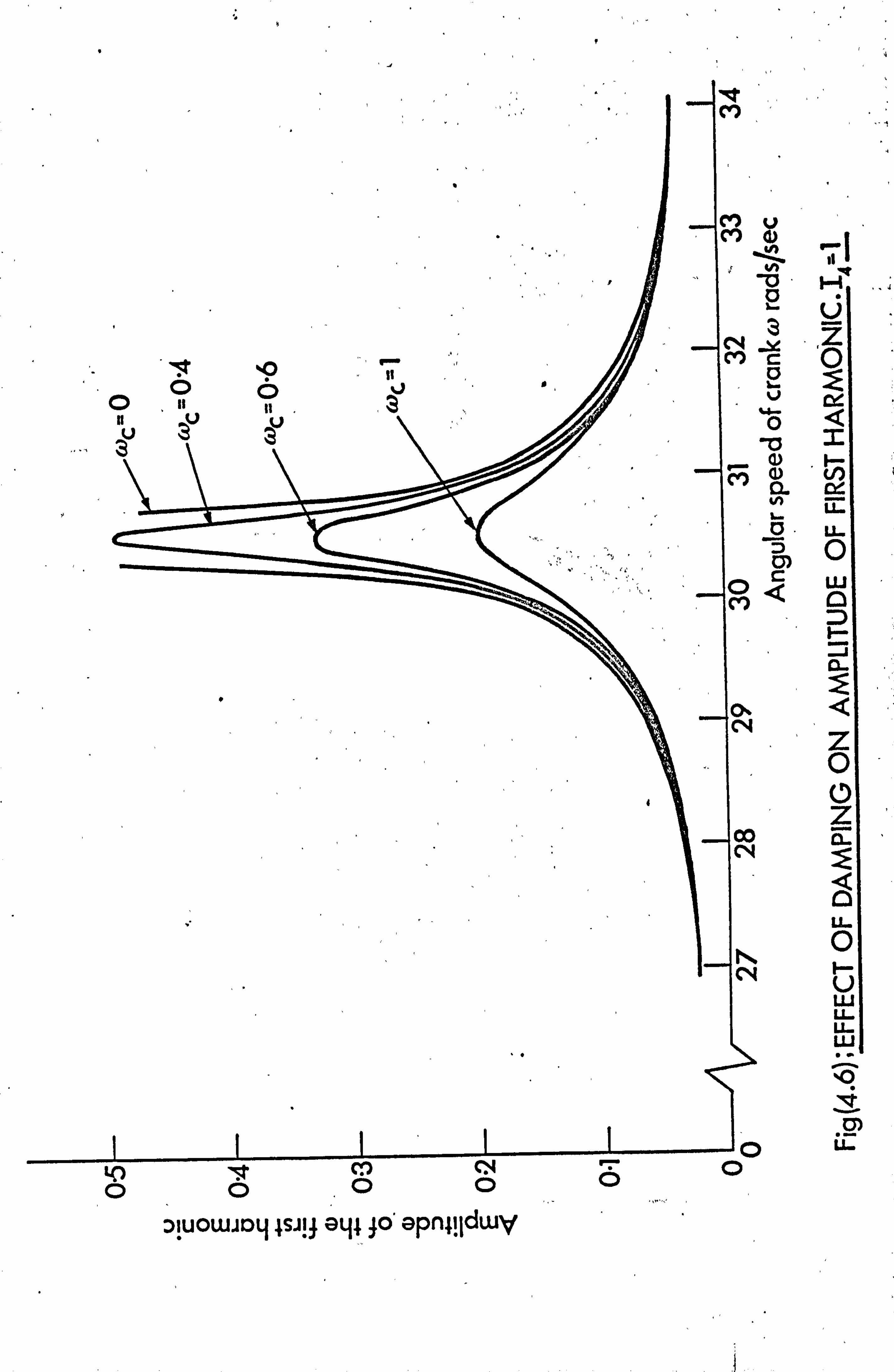
y
f
V a) N
2
3 C ß i V
'4- O
N Q. N L a
0) C
Q
V ÖÖ IT M. %. m
.OO Diuouaaay 4sai9 e4 ; o' 9pn4! jdwv
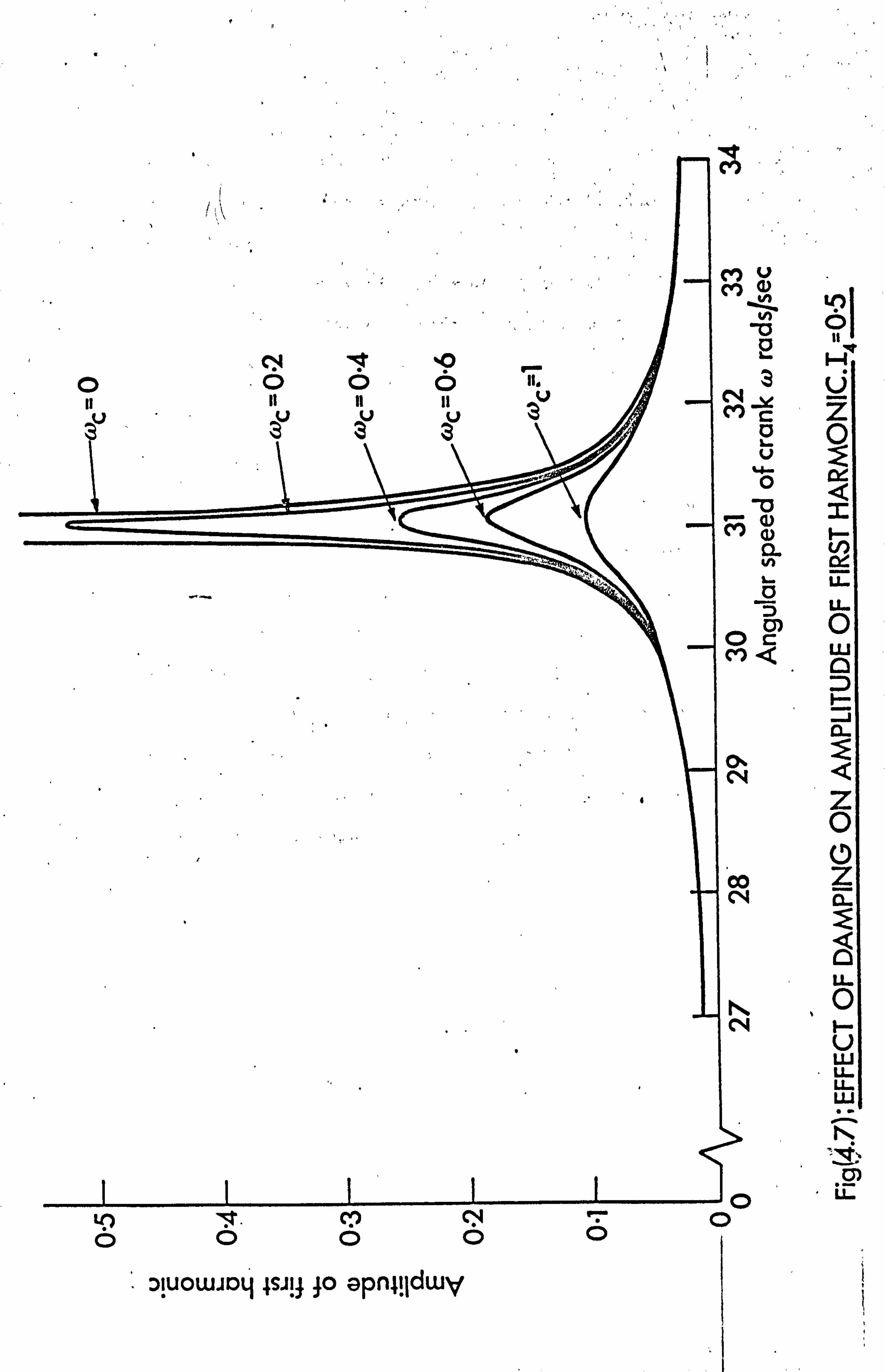
C'7 '.
C'; ) NÖ pOOO
D UOWJDI 14sJI J Jo apn4i1dwy
u (D
-42 NOI
2H 3U
"c Z D0
Ö
"D =
a V~)
N
LL-
U- 5
D) O W
J
Q z
O
CL
LL 0V
W U- LL.
- 0
- 59 -
vicinity of resonance.
d) The resonance curves are similar to a second order
linear system
e) The dominant harmonic in the solution is the first,
the second and higher harmonics are negligible in
comparison.
4.6 Computer Programs
4.6.1 Brief Description
Two programs are written - the first deals with
the case of no damping and the second with the damping case.
Both follow similar steps. They start by calculating the
elements of matrix Aid of equation (4.33). They then use
Gaussian elimination with error bounds correction to solve
this equation for Wj . The crank speed is then incremented
to a new value and the solution is repeated. Because of the
similarities of the two programs only the second program
dealing with the damping case is shown in Appendix 2.
- 60 -
Chapter V
STABILITY ANALYSIS
The stability problem is usually more difficult
than the resonance. However there are vaious methods
for dealing with it, the most commonly used are the
perturbation methods. These methods can become very
complex and involved especially when dealing with a large
damping factor in the analysis.
We shall therefore study the stability of motion of
the slider using a perturbation method for-the case of no
damping and a general solution substitution computer
orientated method for the damping case. The latter will
employ an optimisation routine to find the unstable
boundaries.
- 61 -
5.1 STABILITY ANALYSIS BY A PERTURBATION METHOD
The stability of equation (4.29) may be investigated by
considering the homogeneous part of it only.
5.1.1 No damping Ac =0
The equation of motion reduces to 22an ii 2
+ {alb A2 [(a1Cos0+ b1Sin0)e + (a2Cos20 + b2Sin20)e +... ]
+ [(a3CosO+ b3SinO)e + (a4Cos20+b4Sin20)c2 + ... ] }r=0 (5.1)
where
ýl = ý2 + h0
2 ý2 - ý'2 k ko
(5.2)
If It ho
al, bl, a2 and b2 are al, bl, a2 and h2 divided-by k0 and
a3, b3, a4 and b4 are as defined in (4.26) exactly.
2 Assume that the solution C of (5.1) as well as X1 can be
expanded in series of powers of e as follows :
I= to + CC1 + e2C2 + .... (5.3)
n a12 =42+ CS1 + e2 S2 + .... {5.4)
where A12 is expanded about the square of half integers i. e.
solution is periodic in 27r if n is even and 41r if n is odd.
The quantities 6l, S2, .... are constants and Co' Cl'
C2, .... are unknown functions of 0 to be determined such
that there exists a periodic solution of C. Inserting
equation (5.3) and (5.4) into (5.1) and assuming that the
coefficients of all powers of c vanish; we obtain the following
relationships.
- 62 -
2
o+4 co =0 (5.5)
22MM ý1 +n4 ý1 = -{S1+(4 -ho)(a1CosO+b1SinO)+(a3CosO+b3SinO)} o
(5.6)
n2 Ny n2 ., y 4= -{
[S2+ö1 (a1Cos0+b1Sin0) + (4 -ho) (a2CosO+b2Sin20) 2
+ (a4Cos20 +b4Sin20) ýo 2
+ Cd+( -h)(aCos0+b1Sin0)+(a 3 CosO+b 3 SinO)] C 1011
from (S. 5) it may be written
ýo = ßoCos2 0+ Yo Sin i
(5.7)
(5.8)
where ßo and y0 are arbitrary constants.
Substituting this equation in (5.6) and rearranging, we obtain, 22
rl + ýl =-öi (ßoCos20 +ýyo in20) -2 (4 -ho) (aIf .0 lßo-blyo) Cos ( --) 0
42+
(G1+b lyo) Cos (22n) 0+ (aiyo+b1ßo)Sin (22n) 0
+ (a1yo+b1ß0) Sin (? 2n) 0ý- 1 (a3ß0-b3yo) Cos (? Zn) 0
+ (a3 ßo+b3yo) Cos (22n) 0+ (a3yo+b3ß9) Sin (22n) 0
+ (-a3yö b3 00) Sin (22n) 0 (5.9)
In order that 1 be periodic it is necessary that the coefficients
of Cos -Q and Sin20 vanish,
(a) The case of n=0i. e. the zero region of instability.
The solution of equation (5.5) may be written as
ý0 ° ý0
Since ßo is arbitrary we may write
Co = 1. (5.10)

- 63 -
Substituting this equation in (5.6), then in order that ý1
be periodic we must have
o1 = O.
The corresponding solution of Cl is then
it to ý1 (a3-ho. a )CosO+(b3-ho. b1)SinO+(NI),
1
where (NI) is a constant.
(5.11)
Substituting (5.11) in (5.7), then in order that C2 be periodic
we must have
S2 = (a3-ho. a, ) 2 -ý- (b3-hö 1)
2'
Therefore from (S. 2), (5.4) and (5.12) we obtain
k-k( [(a3-hoa1) z+ (b3-hob1) 2]
c2-ho )
0
(5.12)
(5.13)
Notice that (5.13) results from the second approximation i. e.
from terms involving the second power of E. Also notice that
a region was not obtained but merely a boundary of two stable
regions.
(b) The case of n=1i. e. the first region of instability.
Substituting (5.8) into (5.9), and applying the condition
of periodicity, we obtain IV [26
1+ (4-ho) a +a3] ßo -; ( -ho) bl+b3' yo =U
and (5.14)
C(4-ho)bl+b 31 ßo + L2ä1-(4-ho)a1-a3j'yo = O.
Equating the determinant of the above system to zero, we obtain
+1( 1_ ý' 22 )1/2 ]=2( (4 ho) a1+a3' + C(24
-ho) b1+b3J ) (5.15)
- 64 -
Therefore from (5.2), (5.4) and (5.15), a region for X2
may be defined by :
ko { (4 ho) -2 [(4-ho) aN l+a3 j2+ [(4- -ho) bl+b3' 2}< ak
(5.16) ký { (4 -ho) +2i(
0-h0) al+a3]
2+ [(4 -ho) b1+b31
}
in which the system is unstable.
(c) The case, of n=2i. e. the second region of instability.
Substituting equation (5.8) into (5.9) and demanding that
be periodic we obtain
61 =
and
{(N1ß0+N2yo)+(Nlßo-N2yo)Cos20 +(N2ß0+N1yo)Sin20
where
N1 = (1-h0) al+a3
N2 = (1-ho) bl+b3
(5.19-t I
and
Hence l=-2 (N1ß0+N2Yo)+6 { (Nlßo-N2yo) Cos20 +(N2ß0+Niio) Sin20}
+ ß1CosO + y1SinO . (5.2o) l
Substituting equation (5.20) into (5.7) and applying the condition
of periodicity on 2, i. e. coefficients of CosO and SinO must
vanish, we obtain :
- 65 -
a2 + N22 - 5N12 + ti ßo + III - NN21 Yo _0 1 12 JL2
and
I22 1--2 M2 N1N2
Jß+[g+ N1 5N2
°2 12
where m1 = (1-ho) a2 + a4,
and M2 = (1-ho) b2 + b4 .
M1 Yo - 0º
2
Equations (5.21) may now be written as
L62 + Pl ßo + {Q] yo = of
and IQ] ß0 +[S2 + R]'yo = O.
where,
(5.21)
(5.22)
(5.23)
R N2 2- 5N1 2+
M1
12 2 (5.24)
R= N12 - 5N22 - M1 and Q= M2 N1N2
22 12 2
For non trivial solutions of (5.23) its determinant must vanish
i. e.
(S2 + P) (S2 + R) - Q2 =0
which gives, 1/2 P+R +1I (P+R) 2+ 4Q2ý
222
From equations (5.2), (5.4) and (5.25) the second region of
instability may now be defined by :-
1 [(l-h)- P+r + k0 o
Ef 22�
(P " R) 2+ 442}J < Ak2
(5.25)
(5.26)
[l_k0_cPýR 2fj -1 (P+R) 2+ 4Q2 f1
o(J
- 66 -
5.2 Stability Analysis in the Presence of Damping.
5.2.1 Stability Analysis using a Substitution Method.
Equation (4.29) may be written in the form
1 C+ý1 (0) C+ý2 (0) C=0, (5.27)
where ý1 (0) and ßy2 (0) are periodic functions of time.
Let
2
fV1 (6) db"
=xe (5.28)
Then by substituting (5.28) into (5.27) we obtain
. 11 dý 1 4) x+ ('2 -2
dO o- 12)X = 0. (5.29)
4
Equation (5.29) may now be expanded and written as : -
X1 +{ [Ak2
. ko+ho- 4 ko2. ao2 ]+c [gi
(0)] +c2 [g2
(0). J I+... }x = 0.
(5.30)
It is clearly seen that regions of instability of the above
system will resemble those obtained for the case of no damping
but shifted by a small amount represented by the second order
quantity of 4 Ac2. ko2 in (5-30). However, all solutions of
1 (8) dB this equation are multiplied by the factor. e2 Yi as
shown in (5.28).
It may be appreciated by examining the above that an analysis
to determine the regions of instabilities can become tedious.
Therefore, we shall turn to a more sophisticated and computer
oriented approach to analyse the stability when damping is
present.
5.2.2 Stability Analysis using aComputer Orientated Method.
Let the solution of the characteristic equation (5.27) be
expanded in a series such
= e. 'E) n
E Xm. Cos20 + Ysin20 (5.31) m=o
- 67 -
where A the characteristic component is complex, i. e.,
A= sl +. i s2 (5.32)
To investigate the stability of the solution it is
enough to locate the boundaries between-stable and unstable
regions. At the boundary the value of the real part of A
i. e. s1 is zero and therefore A becomes
A=i s2 (5.33)
By substituting this value of A into (5.27) and equating
the coefficients of the trignometric functions and the constant
terms to zero, a system of equations may be obtained as follows:
[viii [W31
= 0. (5.34)
where [7. ] is a column vector (Xo, X1, Yl, ... Xn, Yn) and
[c1
is a square matrix of complex elements and is a function of s2
and the crank speed w.
If the system of equations (5.34) is to have a solution
other than trivial the determinant of the matrix [ciii
must
vanish, i. e.
This means that
Det. [Cif] = O.
Real {det rCij1
}=O
(5.35) Imaginery{det cii1 }=O
The values of w and s2 that satisfy equations (5.35)
determine the boundaries of the unstable regions. These values
are obtained using "The Simplex" ; which is an optimisation
* The details of the Simplex and its merits will be discussed
in Chapter'VISection 6.2.1; see also Section 5.4 at the end
of this chapter.
- 68 -
method that minimises in here the absolute values of the real
and imaginery parts of the determinant. For a particular
mechanism the method is capable of giving all the boundaries
of the unstable regions without any extra work. This, if
compared with the perturbation methods which require lengthy
treatment for each region, is both useful and favourable.
5.3 RESULTS
To illustrate the theory discussed earlier, let us
consider the linkage of fig. (4.2) and assume that;
(i) the mass and inertia of the coupler are negligible,
and
(ii) the centre Qf gravity of the rocker lies on the centre
line of the slider.
5.3.1 Stability in The Absence of Damping.
Fig. (5.1) shows the first region of instability in
2_w2 k k2 with varying I,,. The input data is
p45 = 0.2, x2 = 0.05, a3 = 1.
As is clearly seen the region is narrow and its width increases
with increase of I4. The region in Ak2 as a band also
increases linearly with 14 indicating thatlnsta. bility occurs
when w=A. wk with A=2 when 14=0 and decreasing with
increase of I4.
Fig. (5.2) shows the first region of instability in Ak2
with varying a2. The input data is
a3 = 1, p45 = 0.2, I4 =1
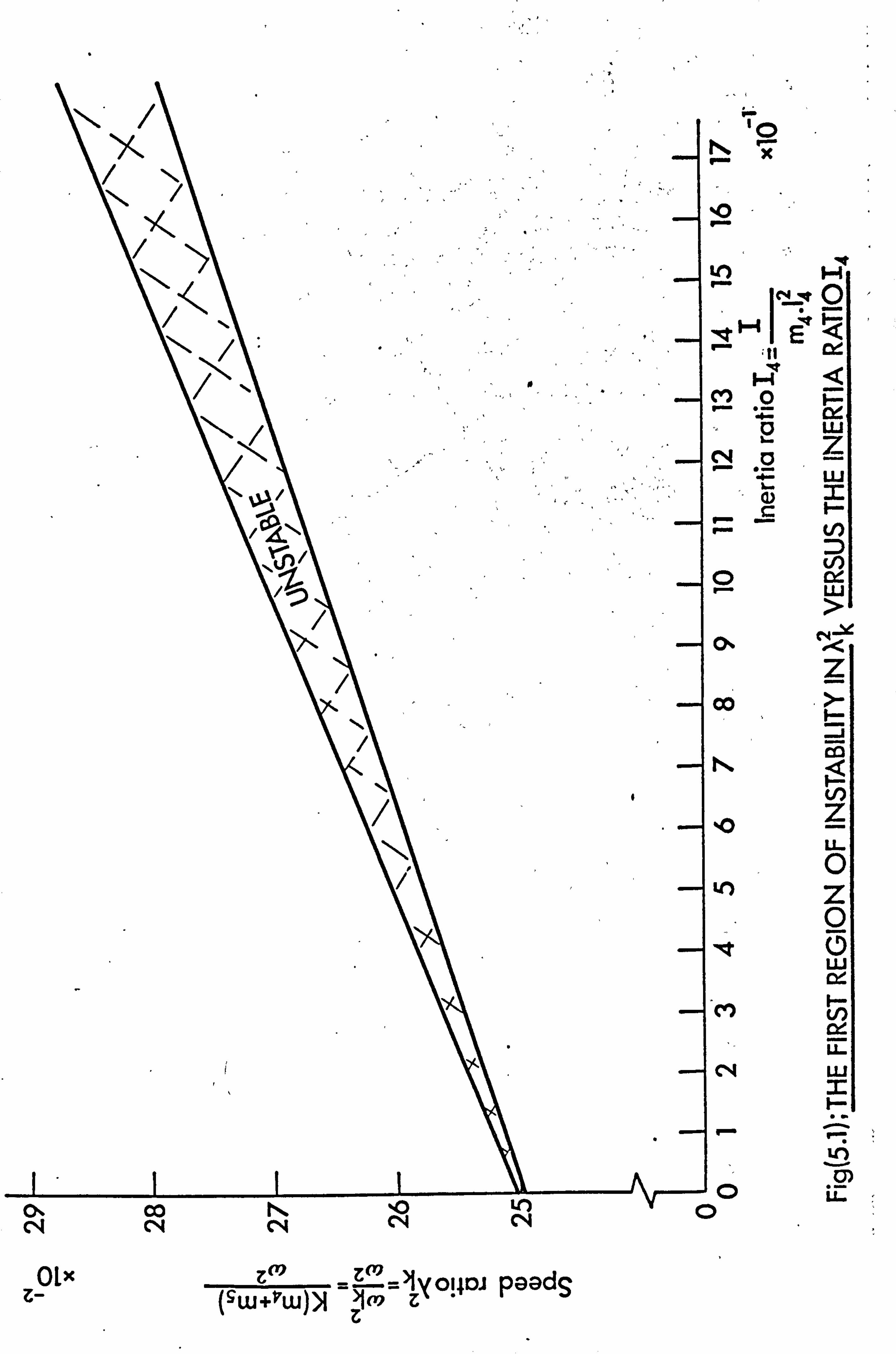
:= ýO ý '' x
rO
L) H
NCO
t H Q
CV) 0 v w
N ` 0 7_ w
r- cn
O ý r- w
A Ný
Zý H
LL
0 Z 0 W
M
U- N W
f- I
ü) O 0
OLx Z°' - loi4rýa PaadS Z- (SUJ+V'UJýý
Zm Z'
NNNNN
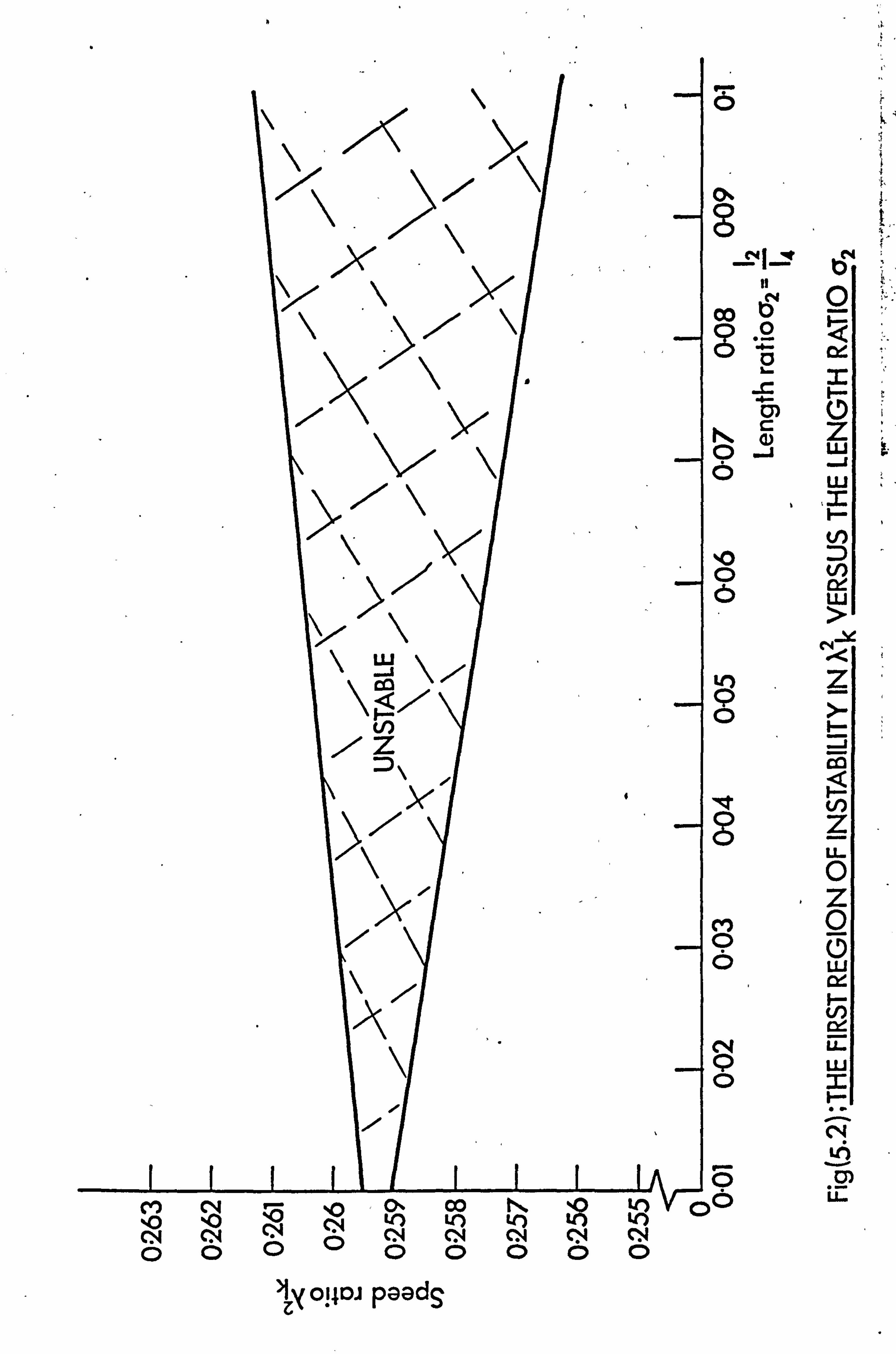
0
Nf ý
11
co 6 o a
rn C
Ö t
ýO 0 b
0
M 0 Ö
N 4 0
J 0^ o° NNNNNNNNN
OOO0OOOOO
Zý 01401 paads
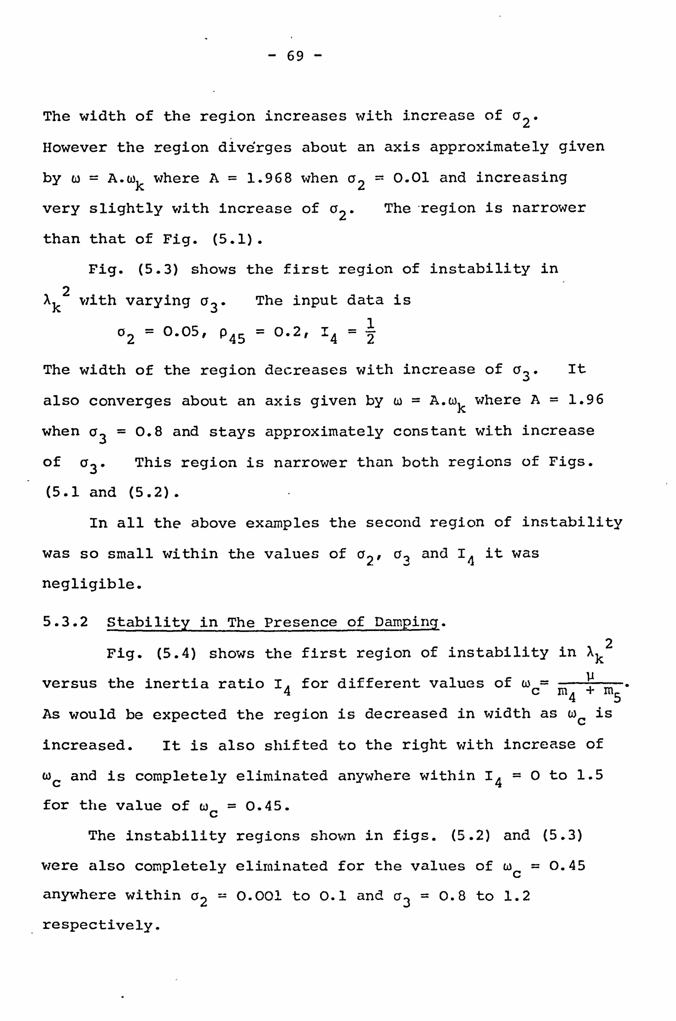
- 69 -
The width of the region increases with increase of v2.
However the region diverges about an axis approximately given
by w=A. wk where A=1.968 when a2 = 0.01 and increasing
very slightly with increase of a2. The-region is narrower
than that of Fig. (5.1).
Fig. (5.3) shows the first region of instability in
Ak2 with varying a3. The input data is
02 = 0.05, p45 = 0.2,14 =2
The width of the region decreases with increase of c3. It
also converges about an axis given by w=A. wk where A=1.96
when a3 = 0.8 and stays approximately constant with increase
of a3. This region is narrower than both regions of Figs.
(5.1 and (5.2).
In all the above examples the second region of instability
was so small within the values of a2, ay and 14 it was
negligible.
5.3.2 Stability in The Presence of Damping.
Fig. (5.4) shows the first region of instability in Akt
versus the inertia ratio I4 for different values of wc= 11 m4 +m 5'
As would be expected the region is decreased in width as we is
increased. It is also shifted to the right with increase of
we and is completely eliminated anywhere within 14 =O to 1.5
for the value of we = 0.45.
The instability regions shown in figs. (5.2) and (5.3)
were also completely eliminated for the values of We = 0.45
anywhere within a2 = o. 001 to 0.1 and a3 = 0.8 to 1.2
respectively.
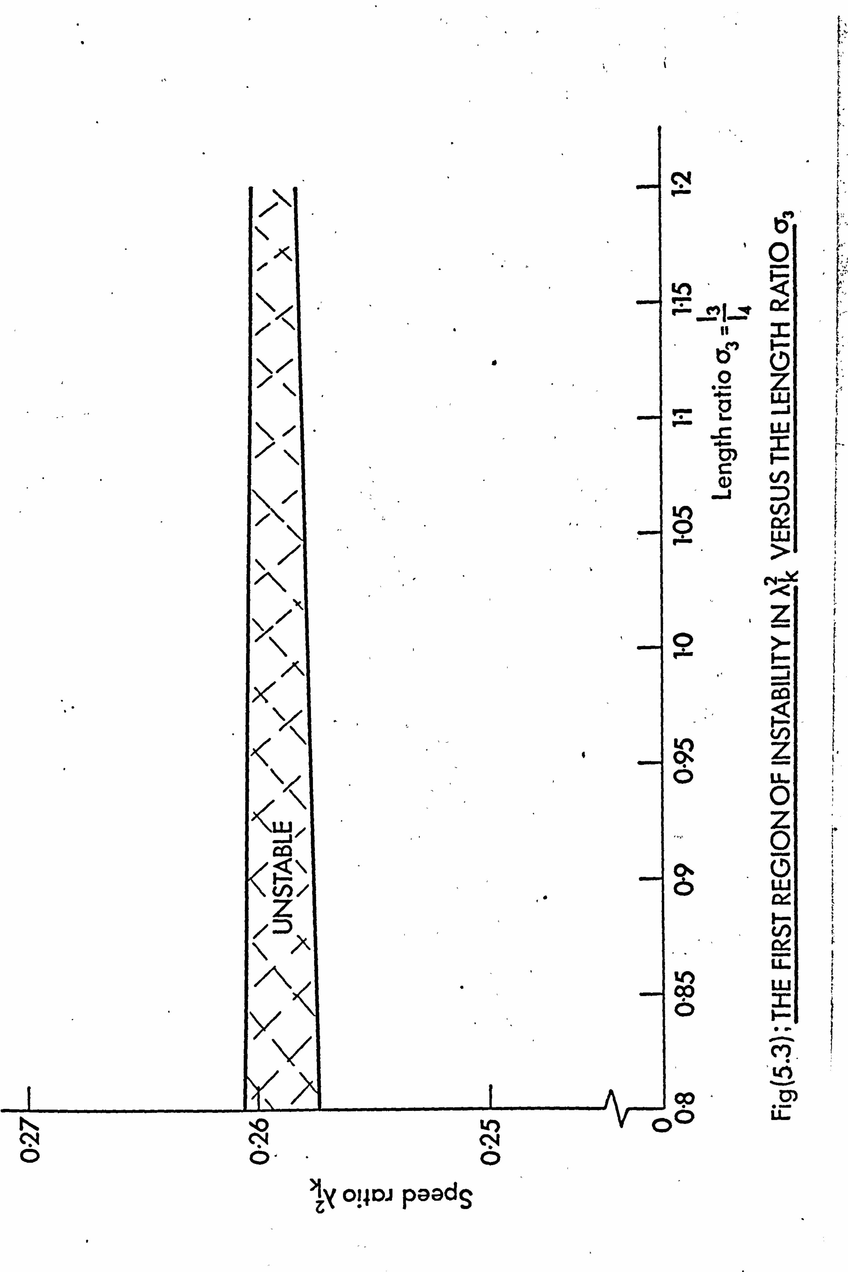
N
' 0 to. Q
ce.
00 Z LLJ
w
Ö w
N
r- ý m
173 z 0 U- 0
z 0 w
01-
- co L w
Ö I
M
co U) p 0 Li
ly o! 4oa PaadS
NNN
0 0- -0
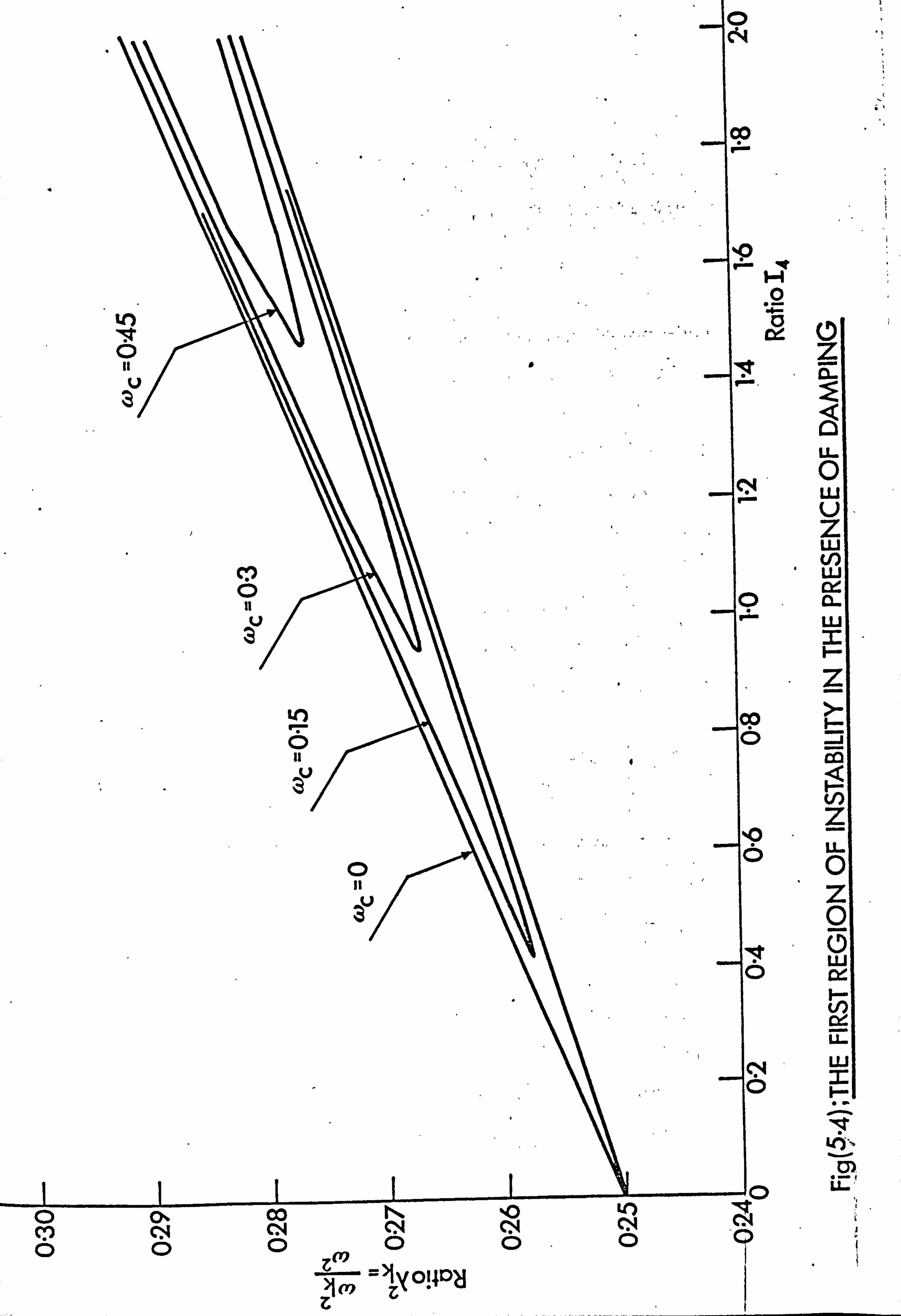
0 C4
W
to
O
V 3
o o" MN 00
M O n u 3
I-I
}
tl
LL.
CN. O
U Z w w
Z
00
p
vi Z o ° U- O
0 0
O cý
. a%
v
O LL' CC) NNN N N
OOO © i
=1ýOI4DS
Zum Z

-- 70-
In all the above examples the solution for ?
described in equation (5.31) was truncated after the ninth
term.
5.3.3. Remarks
a) The stability of the linkage under study increased with
increase of the coupler length and decrease of the
crank length and vice versa.
b) The stability decreased with increase of the rocker
inertia. Also as this inertia was increased
instability occurred further below the value of
w=2wß
c) Viscous damping had a stabilising effect. It was also
possible to choose a value for this damping making the
linkage under study completely stable for all ranges of
speeds.
d) The computer orientated method provided a fast method
for solving the stability problem.
e) The computer orientated method gave results which are in
good agreement with the perturbation method; see the
outer boundary of fig. (5.4) and fig. (5.1).
5.4 COMPUTER PROGRAMS
Two programs were written- the first dealing with the
perturbation method without damping and the second dealing
with damping using the computer orientated method. The first
program, which is shown in Appendix 3, is relatively simple
because it only evaluates the constant relationships described
- 71 -
in equations (5.16) and (5.26). However, the second program,
which is. shown in Appendix 4, is complex; it makes use of the
Harwell library in order to evaluate the value of the complex
determinant. It also uses the subroutine "simplx" which is
fully explained and listed in Part III, Chapter VI.
The Harwell routines are not listed but may be obtained
from the Harwell Atomic Energy Authority under the title
"Harwell Subroutines Library". The routines employed are
included in the call statement of subroutine NMA23CD.
Real double precision arithmetic was used throughout the
perturbation method and complex double precision throughout the
computer orientated method.

PAR TITI
OPTIMISATION AND CONTROL
72 -
Chapter VI'
PARAMETER OPTIMISATION
The versatility of introducing control principles into
the study of mechanisms is enormous. However, in most
cases, the practical applications become subject to the
importance of the role played by the mechanism. It is
feasible to introduce minor changes in the construction and
riode of operation of mechanisms to give major versatility
and adaptability. The extent of modifications that can be
introduced to existent linkages may, in some ways, be
limited while future ones may prove to be in demanding
necessity for design and control different to what is
classically acceptable.
In this part of the. thesis we shall firstly establish a
method for the optimisation of a mechanism parameters such as
length and initial position, to achieve a desired output.
This output will be assumed a path independent of or dependent
on time. Secondly, we shall study ways of controlling the
mechanism inputs in order to achieve an output.
6.1 STRATEGY
Optimisation techniques are widely used in control theory.
Of these techniques, multivariable search methods are often
employed in non-linear problems where the gradient of the
objective or quality function is difficult to determine. In
mechanisms it is often found that the kinematic analysis yields
- 73 -
a set of non-linear equations the solution of which may be
obtained only by iteration or complicated mathematical
analysis. The outputs are often required as functions of
some of the variable parameters in the kinematic equations
or independent of them as in position only dependent outputs.
It is clear therefore that in the synthesis the quality
function may take the form of an implicit function of the
linkage parameters, which then makes the evaluation of its
gradient complicated and hence makes the choice of multi-
variable direct search methods most attractive.
Now we have determined the type of methods to be used
we shall proceed to define the problem.
6.2 PROBLEM DEFINITION AND QUALITY FUNCTIONS
6.2.1 The desired output
Let us consider a desired output in the form
20=e in) (6.1)
where 00 is the desired output expressed as a function of
inputs Oin. This may take several forms which include
coupler curves; time dependent or independent and link
angular rotations. In all the cases that follow we shall
call the task of achieving a desired output dependent on time
as function generation and that independent of time as path
generation. In function generation the desired output may
be stated as :-
(x, Y, t) - of, (6.2)

- 74 -
while in path generation
42 , (xºY) = O. (6.3)
In both cases the coordinates (x, y) defining the actual
output position in cartesian coordinates are functions of
the controlling parameters. If the analytic relations for the
desired output are not determinable equations (6.2) and (6.3)
may be replaced by their equivalent numerical relations.
In the case of a desired angular rotation we shall consider
function generation only; this may be written as
dý3 (O, t) = O.
where 0 is the actual angular output.
(6.4)
6.2.2 The quality function
In function generation it is sufficient to consider the
error as the summation of the squares or absolute values of
the linear distances between desired and actual outputs over a
discrete number of points N. These points are specified in
both position and time within one output cycle. This may be
stated in general as : N 2 El j=1
N or Ni =E
ýý77
j=1
(6.5)
where cßj and ýj are the desired and actual outputs at instance
j respectively. In*coupler curve generation the summation of
the squares of the instantaneous positional error thus takes
the form
10
- 75 -
N ElP =E (xý -xi)
2+ (Yj -yj) 2 (6.6 )
j=l
where (x', y) are values of (x, y) that satisfy equation (6.2)
at instance j.
Similarly in angular function generation the same
summation is expressed as
N Ela =E (O. -0 )2
j-1 j (6.7)
where 0 is the value of 0 that satisfies equation (6.4) at
instance j.
If the above quality functions are minimised they ensure
that the mechanism will achieve the discrete desired output at
the specified times with minimum positional error.
In path generation it is clear that minimisation of the
above quality function would yield a minizxam error. It does,
however, impose the unnecessary condition that the mechanism
pass the desired points at the specified times. This is no
longer required and it is sufficient to minimise the area between
the desired and actual output curves. This area may be stated
as
E2 = q
dA (G. ü)
i=1 fJJ dA S.
where q is the numberof enclosed areas between the desired and
actual outputs, Si is the surface of one enclosure, i=1,
2, ------q and dA is an element in the surface Si. A finite
approximation of this relation is obtained by taking a large
and equal number of points on the desired and actual curves.
- 76 -
Triangular areas are then constructed using these points and
the total area E2 is taken as the summation of the absolute
values of these areas.
A modified quality function may be formulated as a
combination of (6.5) and (6.8). An approximation to the
desired output may, therefore, be obtained by taking both
function and path generation into consideration. Weighting
functions may also be introduced permitting a more accurate
generation of certain parts of the output at the expense of
the rest.
6.2.3 The constraints
in linkages, the kinematic equations (loop closure)
may be written as
f1 (01, ..... On) =01=I..... s<n (6.9)
which form a set of equality constraints implicit in time.
Together with the external constraints imposed by the designer
hi < Pi <H. i=1,.... n (r. 1O)
where Pi are the linkage parameters and hi and Hi are their
specified lower and upper bounds respectively, they form the
complete set of constraints imposed on the problem.
The minimisation of the quality functions subject to the
constraints stated above represent the complete constrained
optimum problem. As will be seen the constraints have to be
handled in a manner appropriate to the linkage in question.
For instance, the constraints specified in (6.9) are dependent
on time implicitly and thus may be satisfied at some instance
in time while violated later. Therefore, when possible these
- 77 -
constraints should he transformed to equivalent forms that
are time independent. This often saves tedious work and
time in com; Duter applications.
6.3 OPTIMISATION
6.3.1 Optimisation routine
The Simplex method as described in ref. (17) is
chosen (ref. 18) and modified to accommodate the constraints.
Essentially the method consists of constructing a geometric
shape of (M + 1) apexes, where M is the number of parameters
to be optimised. This shape, for example, is a triangle if
M=2 and a tetrahedron if M=3. Initially, the method is
provided with (M + 1) sets of values of the parameters to be
optimised corresponding to (M + 1) apexes. It then evaluates
the quality function for each of these apexes and reflects
the apex with maximum quality function value through the
centroid of the remaining apexes. This yields a new set of
values for the parameters. The method continues in this
manner halving or doubling the reflection action depending
upon increase or decrease in quality function values. The
method stops when a convergence criterion is satisfied and is
said'then to have located a minimum It must be recognised,
as in all optimisation methods, that this located minimum may
not be a global minimum. It is therefore necessary to begin
the optimisation from as many initial points as possible. The
various minima thus located are compared and the best is taken
as the ". Best Located Optimum". in the proceeding work this
will be called "The Global Optimum".
- 78 -
It is found that the global optimum is always reached
quickly if some of the minima already located are included
as initial values in a fresh optimisation cycle. It is also
found that the number of minima of the quality function
increases with the number of specified output points. A
good technique is to find the optimum values of linkage
parameters to yield a minimum error over a decreased number
of specified output points. These values are then used again
in the optimisation but this time taking all the specified
output points into consideration. Another useful technique
is to perform the optimisation for a decreased number of
linkage parameters and to use the values obtained in the
initial guesses of the complete optimisation programme. These
techniques have, in all cases tried, located the global
minimum quickly and efficiently.
In order to generate the different initial sets of
parameter values to start the method, it is sufficient to supply
one set only. This set must satisfy all the problem constraints.
The remaining sets are then obtained using the following
equation
Pi = hi + LH
i- hi . Sin2X (6.11)
where Pi, hi and H. are as defined in equation (6.10) and X is
any real random number. This generates quickly and efficiently
all the sets of required initial values and ensures that they
satisfy all the explicit externally imposed constraints
described in equation (6.10). Each new set obtained through
this technique is then tested for'violations of the constraint
- 79 -
equations (6.9) and if so, a new set is obtained by moving
back quarter the distance towards the centroid of the sets
already obtained.
6.3.2 Constraints
As mentioned previously, the constraints specified
in equation (6.9) are usually time dependent. It is,
therefore, necessary (a) to solve the kinematics for a
complete cycle checking they are always satisfied, or (b) to
transform these constraints into a more convenient form
independent of . time.
a) The improved set of linkage parameter values
returned from the optimisation routine is used to evaluate
the quality function. If at some point in the solution cycle
the constraints are violated this improved set is rejected.
The Simplex is then instructed to yield a set of values by
moving back a quarter the distance between the rejected set
(i. e., current set) and the set with maximum quality function
value. The move is in a direction towards the centroid of the
remaining sets in the current Simplex configuration. The
kinematic solution is then restarted from time zero and the
process is repeated until the constraints are satisfied.
b) In linkages, it is often possible to transform the
time dependent constraints into a more convenient form for
digital computer solution. For, example, in the four bar link
shown in fig. (6.1) the following term
c= 4Q4 (Z2+R, 2-2ß, 1Q2Coswt) - (9,3-Q2-L -Q2+2L1Q2Coswt)
2 (6.12)
appears in the solution of equation (6.9) as a square root
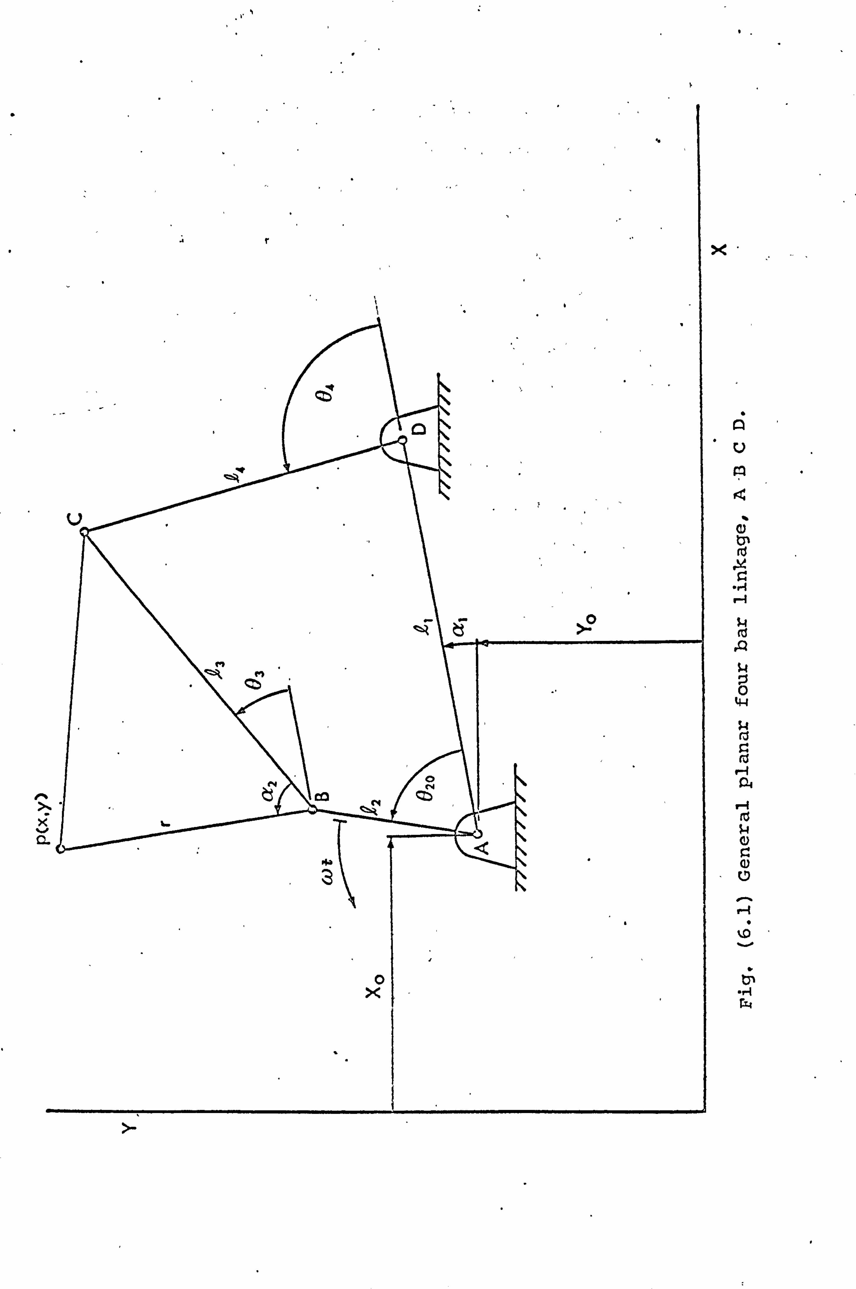
,. 4
e
X
A
U
q
a aý
r4
n
Q
. s2
0 w
C)
., 4 w
>-
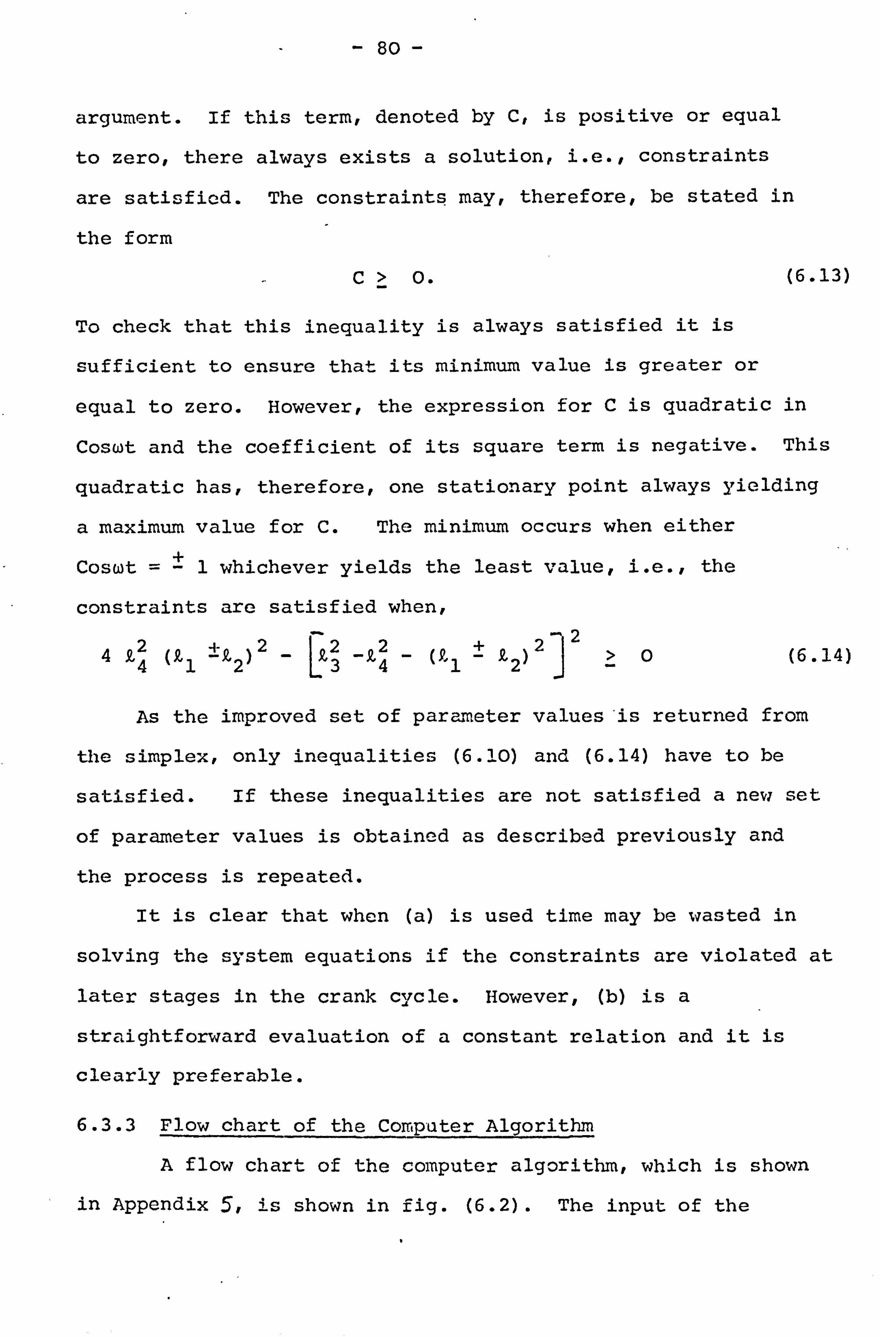
- 80 -
argument. If this term, denoted by C, is positive or equal
to zero, there always exists a solution, i. e., constraints
are satisfied. The constraints may, therefore, be stated in
the form
C> 0. (6.13)
To check that this inequality is always satisfied it is
sufficient to ensure that its minimum value is greater or
equal to zero. However, the expression for C is quadratic in
Coswt and the coefficient of its square term is negative. This
quadratic has, therefore, one stationary point always yielding
a maximum value for C. The minimum occurs when either
Coswt =±1 whichever yields the least value, i. e., the
constraints are satisfied when,
_2 4 Q4 (R, 1 ý k2) 2- Lp-2
-R, 4
- (F, 1 ± ! C2) 2!
>0 (6.14)
As the improved set of parameter values'is returned from
the simplex, only inequalities (6.10) and (6.14) have to be
satisfied. If these inequalities are not satisfied a new set
of parameter values is obtained as described previously and
the process is repeated.
It is clear that when (a) is used time may be wasted in
solving the system equations if the constraints are violated at
later stages in the crank cycle. However, (b) is a
straightforward evaluation of a constant relation and it is
clearly preferable.
6.3.3 Flow chart of the Computer Algorithm
A flow chart of the computer algorithm, which is shown
in Appendix 5, is shown in fig. (6.2). The input of the
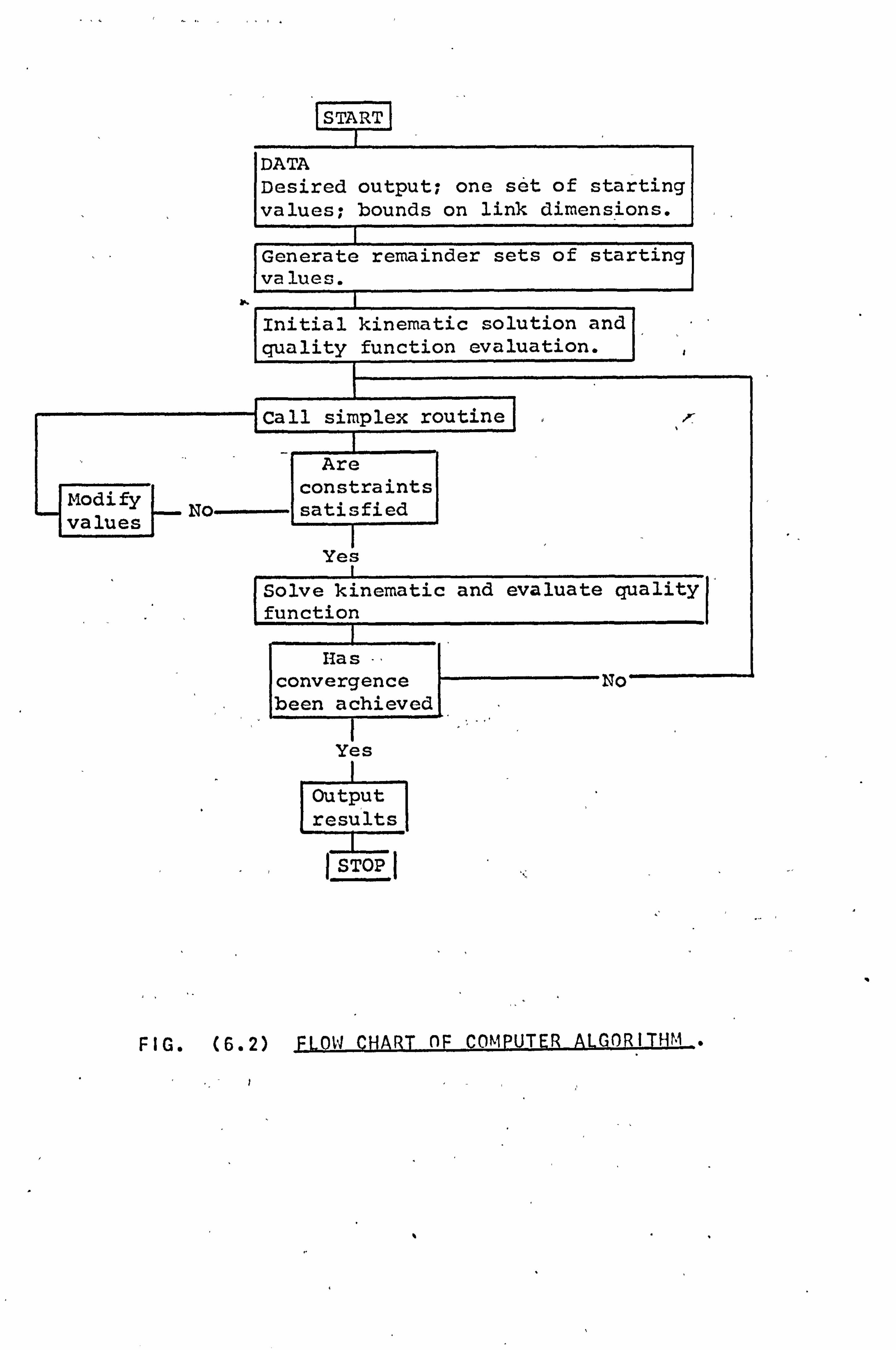
START
DATA Desired output; one set of starting values; bounds on link dimensions.
Generate remainder sets of starting values.
Initial kinematic solution and quality function evaluation.
Call simplex routine
Are
Modify constraints
values No---- satisfied
Yes
Solve kinematic and evaluate quality function
Ilas convergence No'-' been achieved
Yes
Output results
+STOPI
FIG. (6.2) F Low CHART nF COMPUTER ALGORITHM .
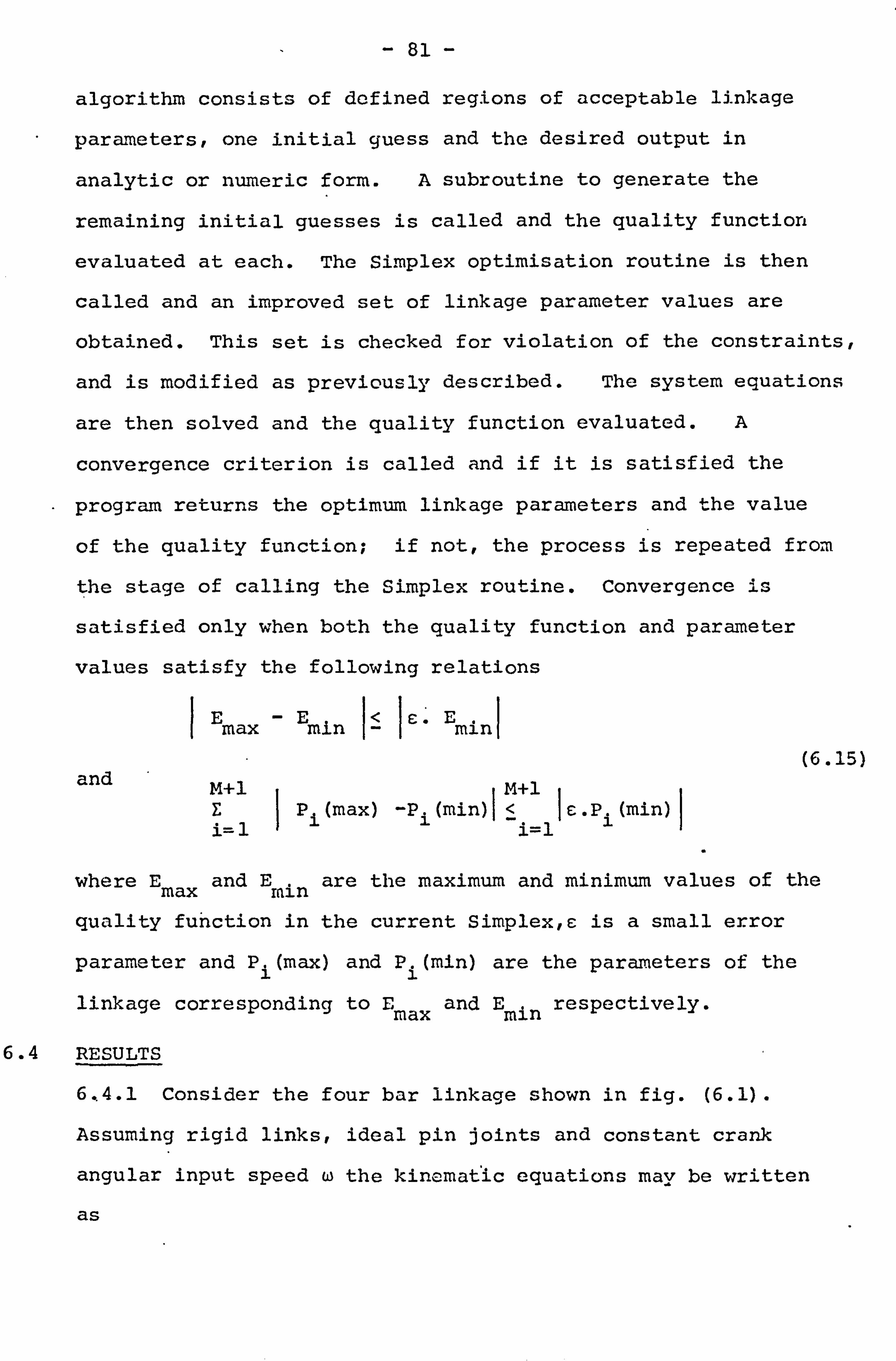
- 81 -
algorithm consists of defined regions of acceptable linkage
parameters, one initial guess and the desired output in
analytic or numeric form. A subroutine to generate the
remaining initial guesses is called and the quality function
evaluated at each. The Simplex optimisation routine is then
called and an improved set of linkage parameter values are
obtained. This set is checked for violation of the constraints,
and is modified as previously described. The system equations
are then solved and the quality function evaluated. A
convergence criterion is called and if it is satisfied the
program returns the optimum linkage parameters and the value
of the quality function; if not, the process is repeated from
the stage of calling the Simplex routine. Convergence is
satisfied only when both the quality function and parameter
values satisfy the following relations
Emax min ,- !
e' Eminl
and M+1 M+1 E Pi (max) -Pi (min)
I<Ie. Pi (min)
i=1 + i=1
(6.15)
where Emax and Erain are the maximum and minimum values of the
quality function in the current Simplex, c is a small error
parameter and Pi(max) and Pi(min) are the parameters of the
linkage corresponding to Emax and Emin respectively.
6.4 RESULTS
6.. 4.1 Consider the four bar linkage shown in fig. (6.1).
Assuming rigid links, ideal pin joints and constant crank
angular input speed w the kinematic equations may be written
as
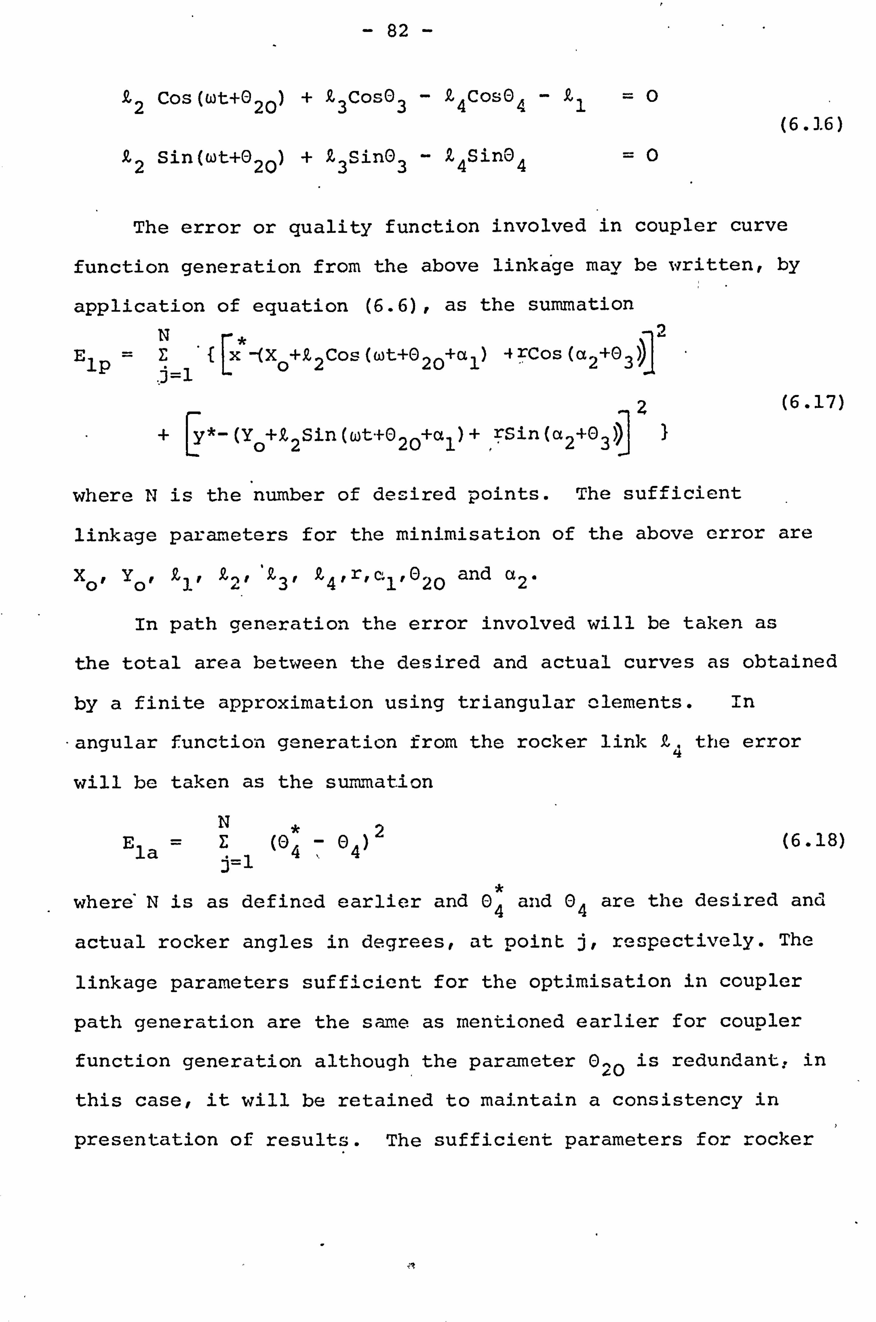
- 82 -
Q2 Cos(wt+020) + £3CosO3 - Q4Cos®4 - kl =0
£2 Sin(Wt+020) + Q3SinO3 - Z4SinO4 =0
(6.16)
The error or quality function involved in coupler curve
function generation from the above linkage may be written, by
application of equation (6.6), as the summation N (' i
ElP =E{ Lx -(Xo+2Cos (Wt+02O+al) +rCos (a2+03))]
. j=1
(6.17)
+ [y*(Y+2Sifl(wt.
fý20+1)+ rSin (a2+03)) 21
where N is the number of desired points. The sufficient
linkage parameters for the minimisation of the above error are
xo, Yo, Q1, £2, Q3, £4, r, c: 1, O20 and a2.
In path generation the error involved will be taken as
the total area between the desired and actual curves as obtained
by a finite approximation using triangular Clements. In
angular function generation from the rocker link k4 the error
will be taken as the summation
N Ela _E (04 _ 04)
2
j=1 (6.18)
where N is as defined earlier and 04 and 04 are the desired and
actual rocker angles in degrees, at point j, respectively. The
linkage parameters sufficient for the optimisation in coupler
path generation are the same as mentioned earlier for coupler
function generation although the parameter 020 is redundant; in
this case, it will be retained to maintain a consistency in
presentation of results. The sufficient parameters for rocker
41
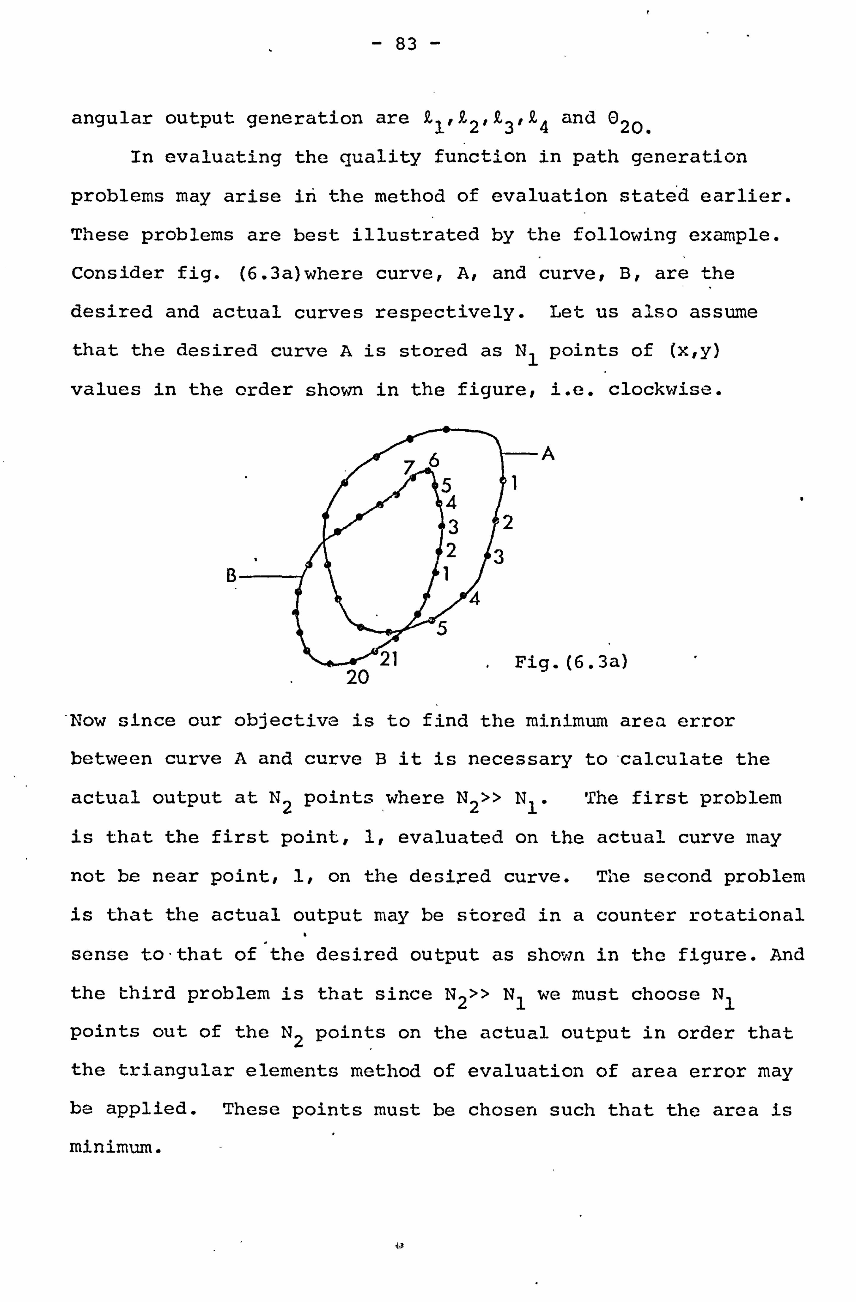
- 83 -
angular output generation are l'2'3'44 and 020.
in evaluating the quality function in path generation
problems may arise in the method of evaluation stated earlier.
These problems are best illustrated by the following example.
Consider fig. (6.3a)where curve, A, and curve, B, are the
desired and actual curves respectively. Let us also assume
that the desired curve A is stored as N1 points of (x, y)
values in the order shown in the figure, i. e. clockwise.
A
B
20 g. (6.3a)
Now since our objective is to find the minimum area error
between curve A and curve B it is necessary to-calculate the
actual output at N2 points where N2» N1. The first problem
is that the first point, 1, evaluated on the actual curve may
not be near point, 1, on the desired curve. The second problem
is that the actual output may be stored in a counter rotational
sense to-that of the desired output as shoan in the figure. And
the third problem is that since N2» N1 we must choose N1
points out of the N2 points on the actual output in order that
the triangular elements method of evaluation of area error may
be applied. These points must be chosen such that the area is
minimum. -
0
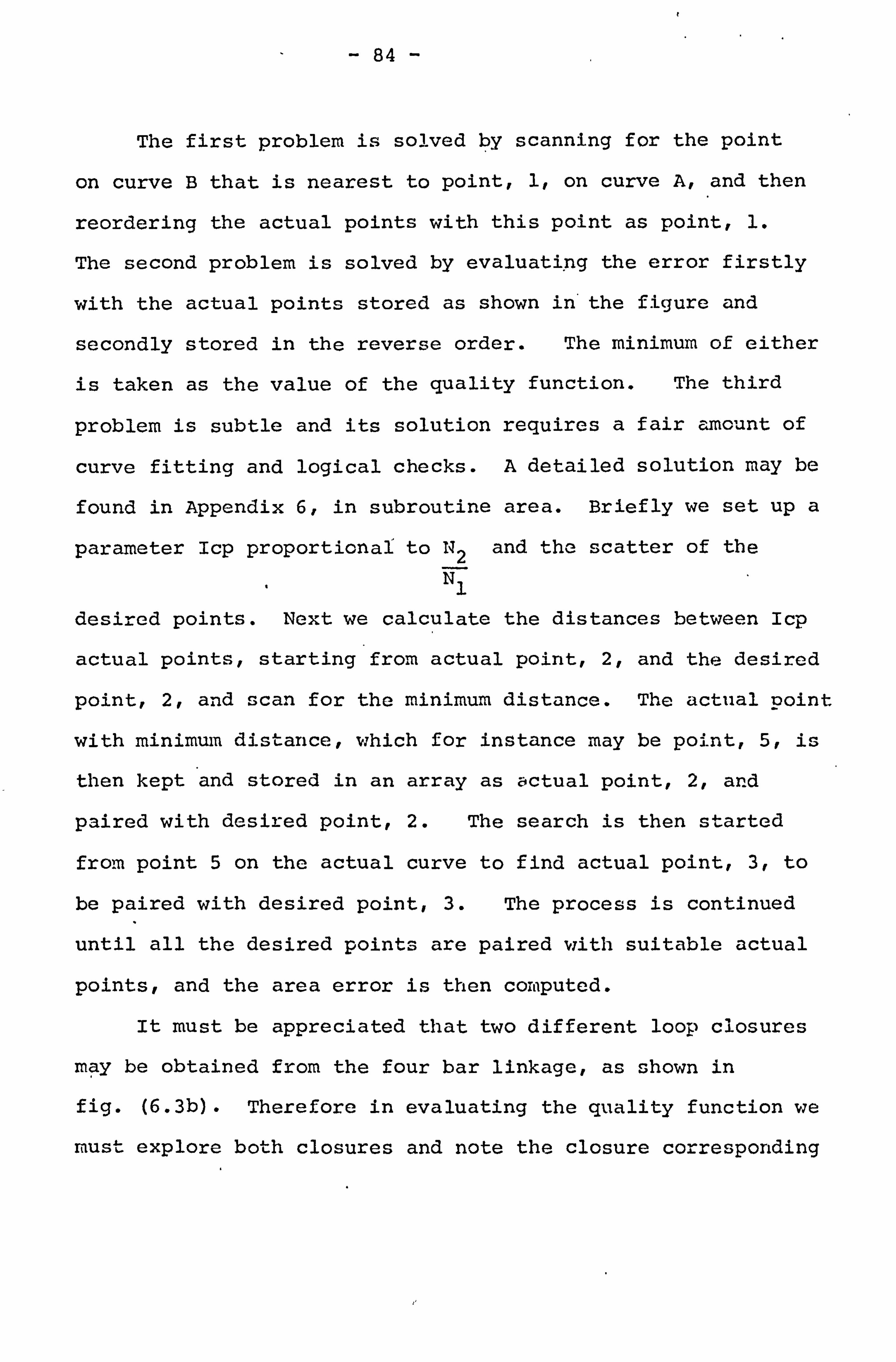
- 84 -
The first problem is solved by scanning for the point
on curve B that is nearest to point, 1, on curve A, and then
reordering the actual points with this point as point, 1.
The second problem is solved by evaluating the error firstly
with the actual points stored as shown in the figure and
secondly stored in the reverse order. The minimum of either
is taken as the value of the quality function. The third
problem is subtle and its solution requires a fair amount of
curve fitting and logical checks. A detailed solution may be
found in Appendix 6, in subroutine area. Briefly we set up a
parameter Icp proportional to N2 and the scatter of the
N1
desired points. Next we calculate the distances between Icp
actual points, starting from actual point, 2, and the desired
point, 2, and scan for the minimum distance. The actual point
with minimum distance, which for instance may be point, 5, is
then kept and stored in an array as actual point, 2, and
paired with desired point, 2. The search is then started
from point 5 on the actual curve to find actual point, 3, to
be paired with desired point, 3. The process is continued
until all the desired points are paired with suitable actual
points, and the area error is then computed.
It must be appreciated that two different loop closures
may be obtained from the four bar linkage, as shown in
fig. (6.3b). Therefore in evaluating the quality function we
must explore both closures and note the closure corresponding
- 85 -
to the minimum error in output generation.
Fig. (6.3b)
In the results that. follow all the curves, except those in
fig. (6.11), are shown plotted at twenty degrees (20°)
intervals of crank angular rotation. The start of each
output cycle is marked by wt -0° and increases in an anti-
clockwise direction. However, it is important to note that,
when the crank is at wt =00 the angle between it and the
fixed-link is 020.
6.4.2 Function Generation
A) Let the desired output be of the type described in
equation (6.2) and expressed as
x* = ßl -1 ß2 Coswt
y* = ß3 + ß4 Sinwt
where ßl, ß2, ß3 and ß4 are constants. This output is
required to be generated from point P(x, y) on the coupler
link.
(6.19)
Starting the optimisation from different initial points,
a best set of optimum values of the linkage parameters is
obtained by comparing the various minima of the error
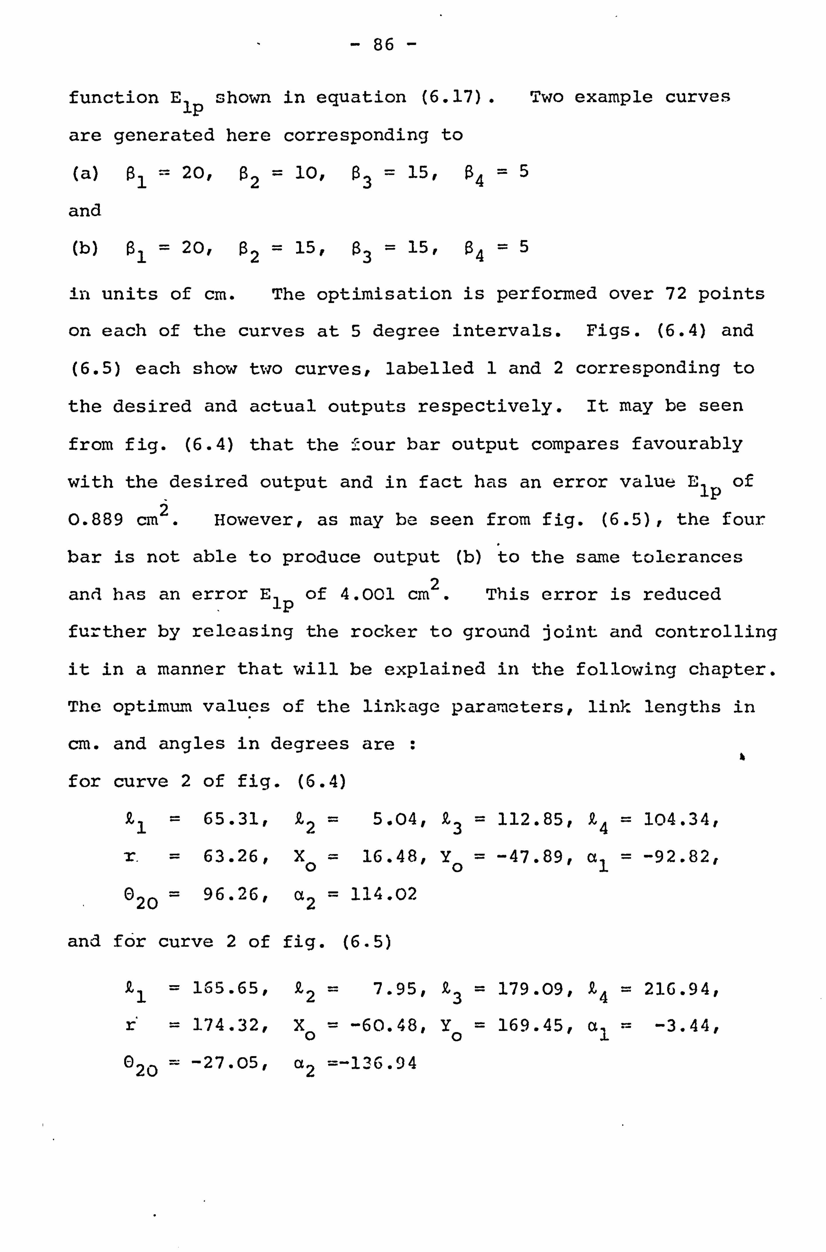
- 86 -
function Elp shown in equation (6.17). Two example curves
are generated here corresponding to
(a) ßl = 20,2 = 10,3 = 15, ß4 =5
and
(b) ß1 = 20,0 2= 15, ß3 = 15,0 4=5
in units of cm. The optimisation is performed over 72 points
on each of the curves at 5 degree intervals. Figs. (6.4) and
(6.5) each show two curves, labelled 1 and 2 corresponding to
the desired and actual outputs respectively. It may be seen
from fig. (6.4) that the : '-our bar output compares favourably
with the desired output and in fact has an error value Llp of
0.889 cm2. However, as may be seen from fig. (6.5), the four
bar is not able to produce output (b) to the same tolerances
and has an error Elp of 4.001 cm2. This error is reduced
further by releasing the rocker to ground joint and controlling
it in a manner that will be explained in the following chapter.
The optimum values of the linkage parameters, link lengths in
cm. and angles in degrees are :
for curve 2 of fig. (6.4)
£1 = 65.31, Q2 = 5.04, Q, 3 = 112.85, Q4 = 104.34,
r. = 63.26, X0 = 16.48, Yo = -47.89, al = -92.82,
020 = 96.26, a2 = 114.02
and for curve 2 of fig. (6.5)
Rl = 165.65,
174.32,
Q2 = 7.95, Q3 = 179.09, P4 = 216.94,
Xp = -60.48, Yo = 169.45, a1 = -3.44,
020 = -27.05, a2 =-136.94
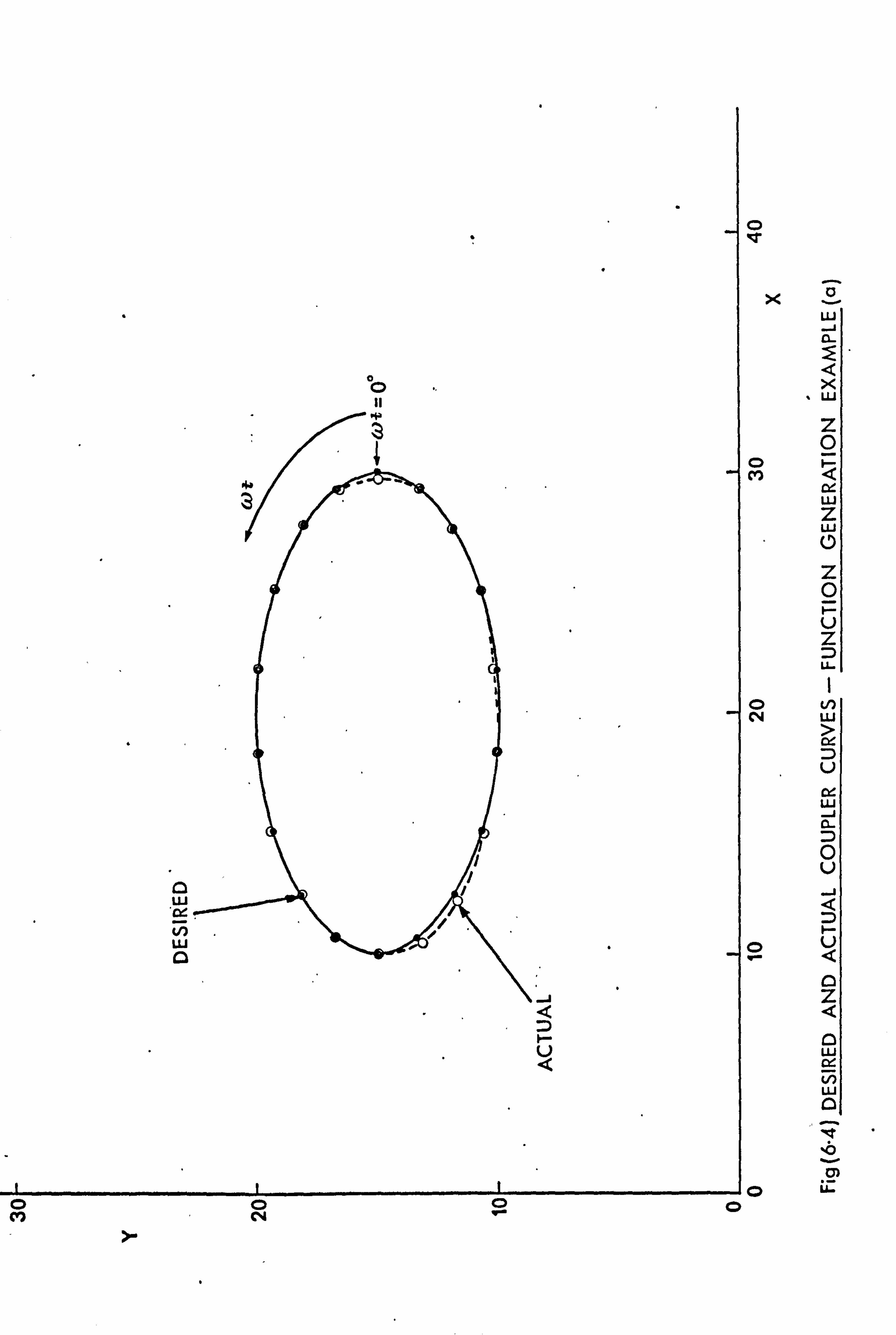
0 v
X C W J dC
X W
Z 0
M QI
W Z! w 0 z 0
u z L-
ON N
ix D u
w w J
0
V J
U
rQ
z O w
N W
'O v
C) p u"
0000 (v) N

0 ýr
r
N
>-
X
0 CV)
0 N
0
-o C
W J
X W
z 0
W
z W
0
Z 0 ý-_ 'V Z
N w
V
w J d
0
V J
V
Ö
Z
iz w OG
L/) w
i1
C)
U-
000 CV) -N m-
87 -
The above outputs are obtained with no imposed
constraints. If, however, the link dimensions are constrained
to have valt s within a defined range a different linkage is
obtained. Let us illustrate this by requiring that output (a)
be generated from a four bar linkage with the following
constraints
10 < Q1, k3, Q4 < 30
10 2
Fig. (6.6) shows the optimum linkage with its actual output and
the desired output. The optimum values of the linkage parameters,
link lengths in cm. and angles in degrees are now
£1 = 16.4, Q2 = 5.01, Q3 = 26.5, Q4 = 22.0
r= 15.4, X° = 19.6 ,- Y° = 0.03, a1 = 93.8°,
020 = 93.2°, a2 = 127.3°
The resulting minimum error is now 53.6 cm2 which when
compared with the error resulting from the unconstrained case
gives an increase of 52.7 cm2.
B) Let the desired output be of the type described by equation
(6.4) and expressed as
. 0ý = ß5 + ß6. Sin wt 21
(6.20)
where and and ß6 are constants in degrees and 04 is the desired
angular output in degrees to be produced from the-'!: ocker link P. 4.
This output is firstly to be produced in whole with no weighting
factors and secondly with a weighting factor equal to 1000
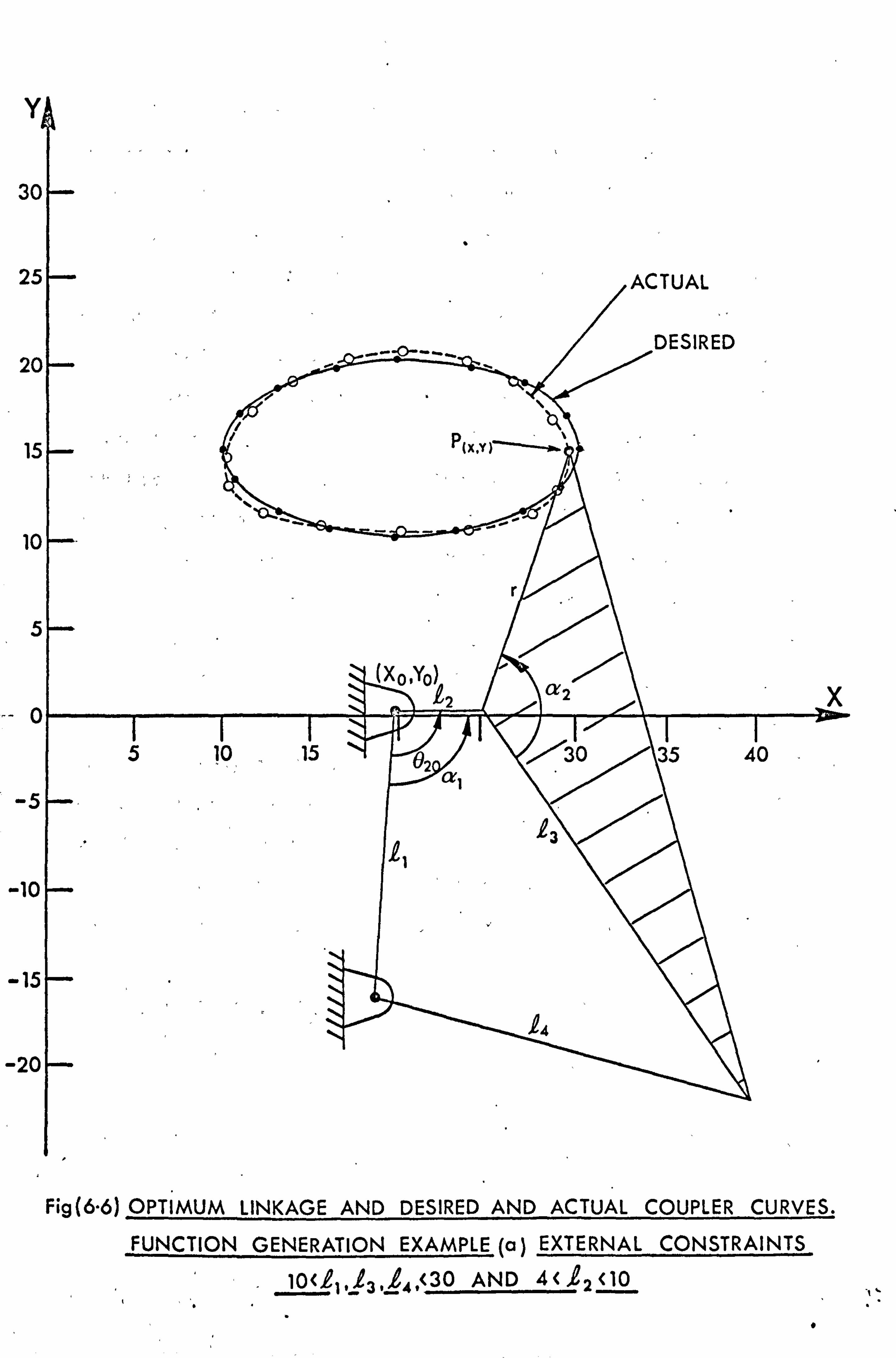
Y
30
25 ACTUAL
20 DESIRED
15
10
5-
x0 'YO) 0
12 2
5 10 15 02 30 35 40
13
'Q1
-10-
-15-
14 -20
Fig(6.6) OPTIMUM LINKAGE AND DESIRED AND ACTUAL COUPLER CURVES.
FUNCTION GENERATION EXAMPLE (a) EXTERNAL CONSTRAINTS
I0<1 , 23,14 (30 AND 4< 12 <10
- 88 -
applied on the portion of the output between 600< wt <260°.
The remaining portions of the output have a weighting factor
equal to unity. The results are shown in figs. (6.7) and
(6.8) respectively where the curves 1 and 2 describe the
desired and actual outputs. The values of the constants
ß4 and ß5 of the desired output are 70 and 100 degrees
respectively. The values of the error function Ela of equation
(6.18) produced by the linkage in generating the unweighted and
weighted outputs are 700.0 and 35.0 degree2 respectively. These
are further reduced by releasing and controlling the rocker to
ground joint as will be seen in the following chapter. It is
clearly seen from the figures that by weighting a portion of
the output it is generated closely but at the expense of the
remaining portions of the output. This is however acceptable
since our. interest lies in the weighted portion only. This
procedure of weighting factors may be used when outputs in the
form of straight lines are required by giving the straight line
portion of the output a weighting of unity and the remainder a
weighting of zero.
The optimum parameters of the four bar link to produce
the unweighted output, link lengths in cros and angles in degrees,
are;
Q1 = 5.083, Z2 = 2.615, Q3 = 4.148, £4 = 3.75
02O= 41.88
and to produce the weighted output
t1 = 15.65, ß2 = 6.91, £3 = 11.77, £4 =11.56,
020 42.74
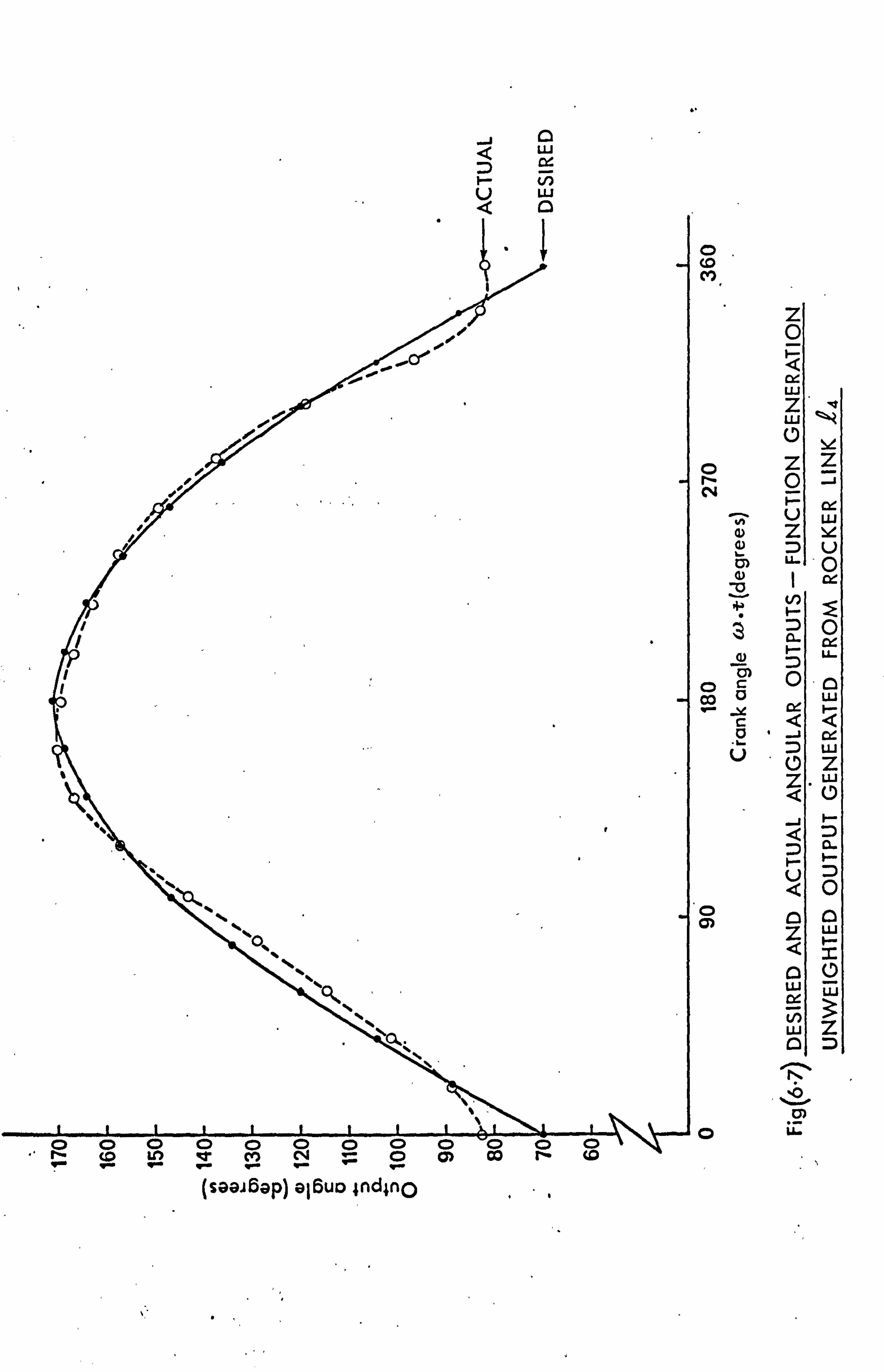
J0 w
F- V) U W Q 0
0 c0 M
Z 0
w Z
(D
OZ ti Q N-
V äý Z
C
C ýý LL
C
CD c LL F
cQQ ß'J
u LL 0Z Z LL <C
J
f- ý äC
Ooc
Z LL Q~
C
LLB LL
wZ
rn
}
(saai6ap) al6uo 4nd4np
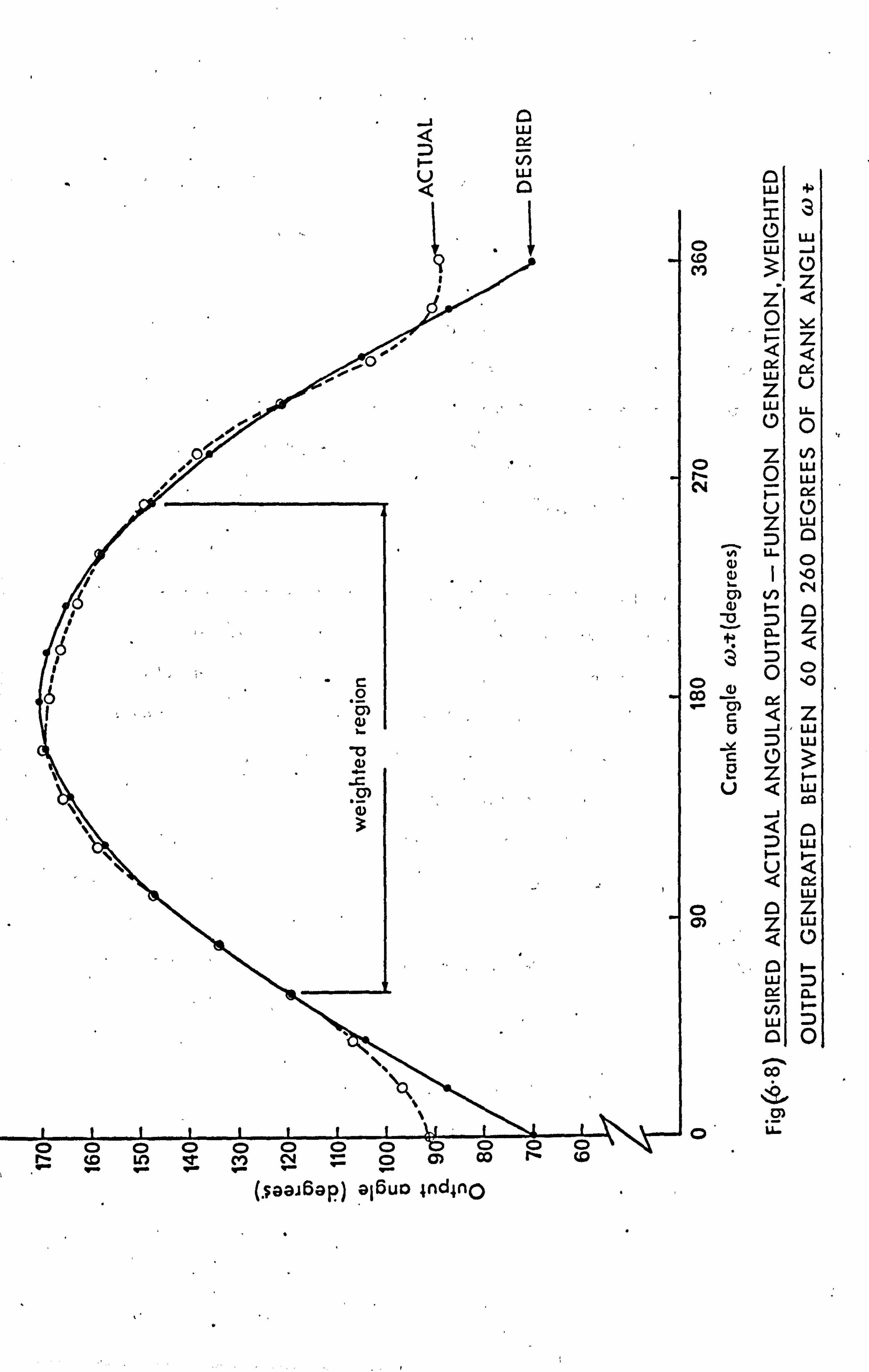
" -j
f-
0
N V Q
W D o
~3 = O_
o "' W
M3O ZI ZQ OY QZ
w Z ww 0O
Oöw W
F- ý U0 Zw
N LL O
a) N G) F- 0
ý=Z
3ýo o (,
O le- cQZ
a -+ w w
äO Z- Qw
CO J
W ÜQ Q
w 0oZ oQ Cý
ui W 12- N w Z) oO
00
lzýI 0) o, ü.
(. Faaý6ap) al6uo 4nd4np
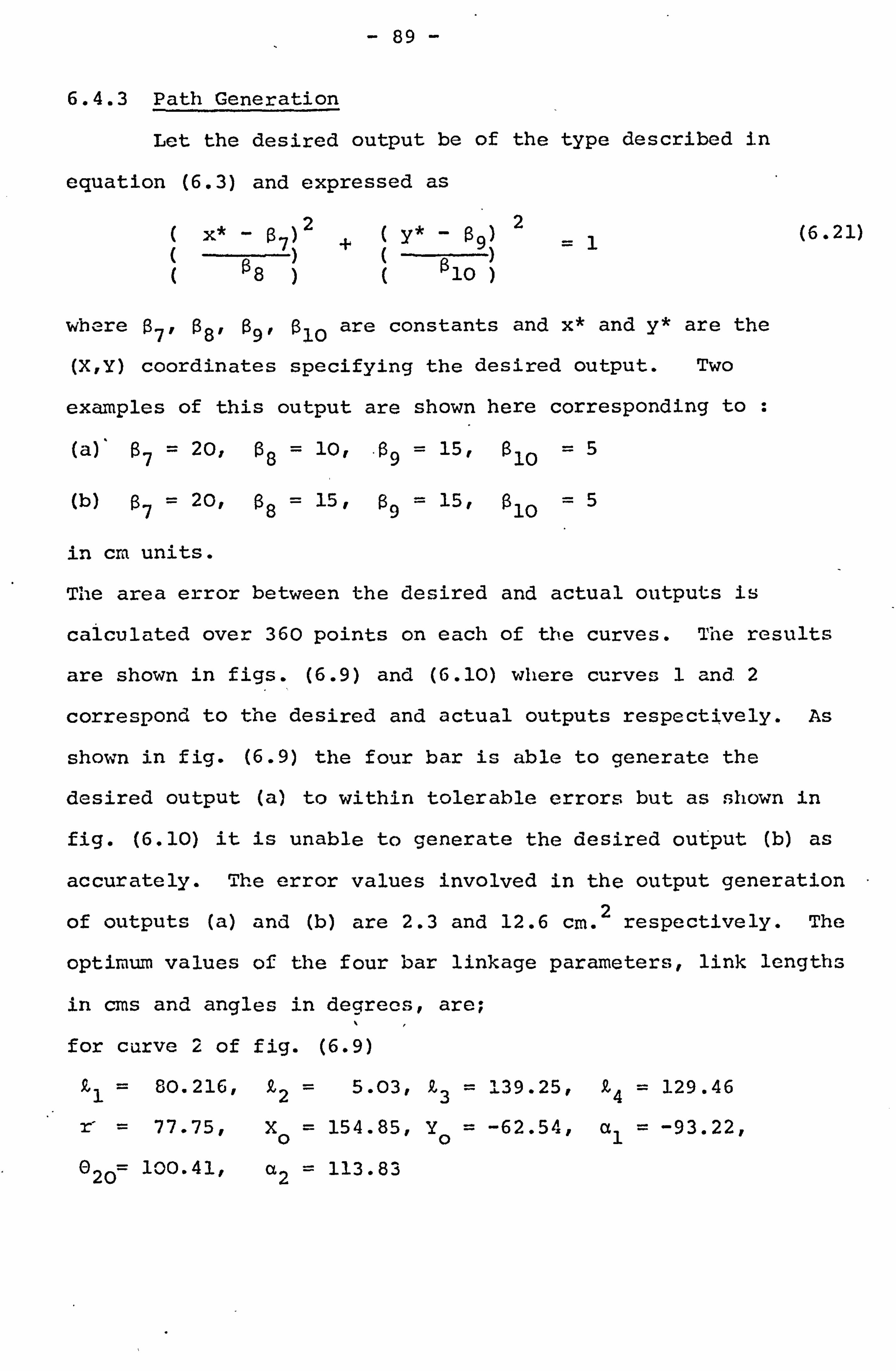
- 89 -
6.4.3 Path Generation
Let the desired output be of the type described in
equation (6.3) and expressed as
( x* - 7) 2+(
Y* - ß9) 2=1
( ß8 )( ß1O )
where ß7' ß8, ß9,010 are constants and x* and y* are the
(X, Y) coordinates specifying the desired output. Two
examples of this output are shown here corresponding to :
(a)' ý=
20, ß5 = 10, ý= 15, ß10 =5
(b) 07= 20, ß$ = 15, ß9 = 15,0 lo =5
in cm units.
The area error between the desired and actual outputs is
(6.21)
calculated over 360 points on each of the curves. The results
are shown in figs. (6.9) and (6.10) where curves 1 and. 2
correspond to the desired and actual outputs respectively. As
shown in fig. (6.9) the four bar is able to generate the
desired output (a) to within tolerable errors but as shown in
fig. (6.10) it is unable to generate the desired output (b) as
accurately. The error values involved in the output generation
of outputs (a) and (b) are 2.3 and 12.6 cm. 2
respectively. The
optimum values of the four bar linkage parameters, link lengths
in cms and ang
for curve 2 of
Q1 = 80.216,
77.75,
0 2O 100.41,
Les in degrees, are;
fig. (6.9)
R, 2 = 5.03, £3 = 139.25,
Xo = 154.85, Yo = -62.54,
a2 = 113.83
Q4 = 129.46
al = -93.22,
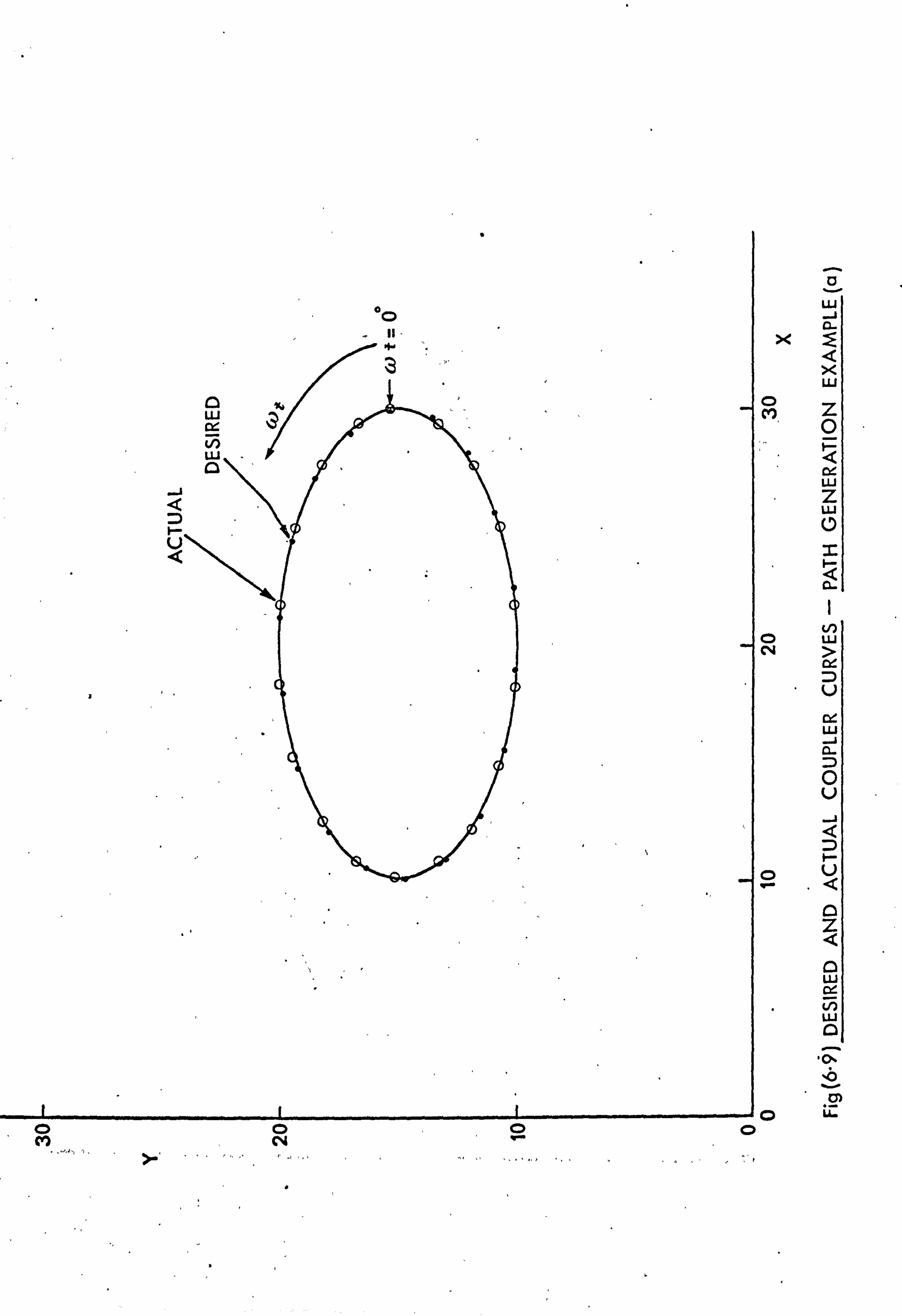
C
X
0 M
0 N
0
W J
X W
z 0
w ui
z W
0
N w
rill U
W J CL
0
U J
U
Z
w cy- N w D
,a
a) W III'o
0000 Cr) N ''
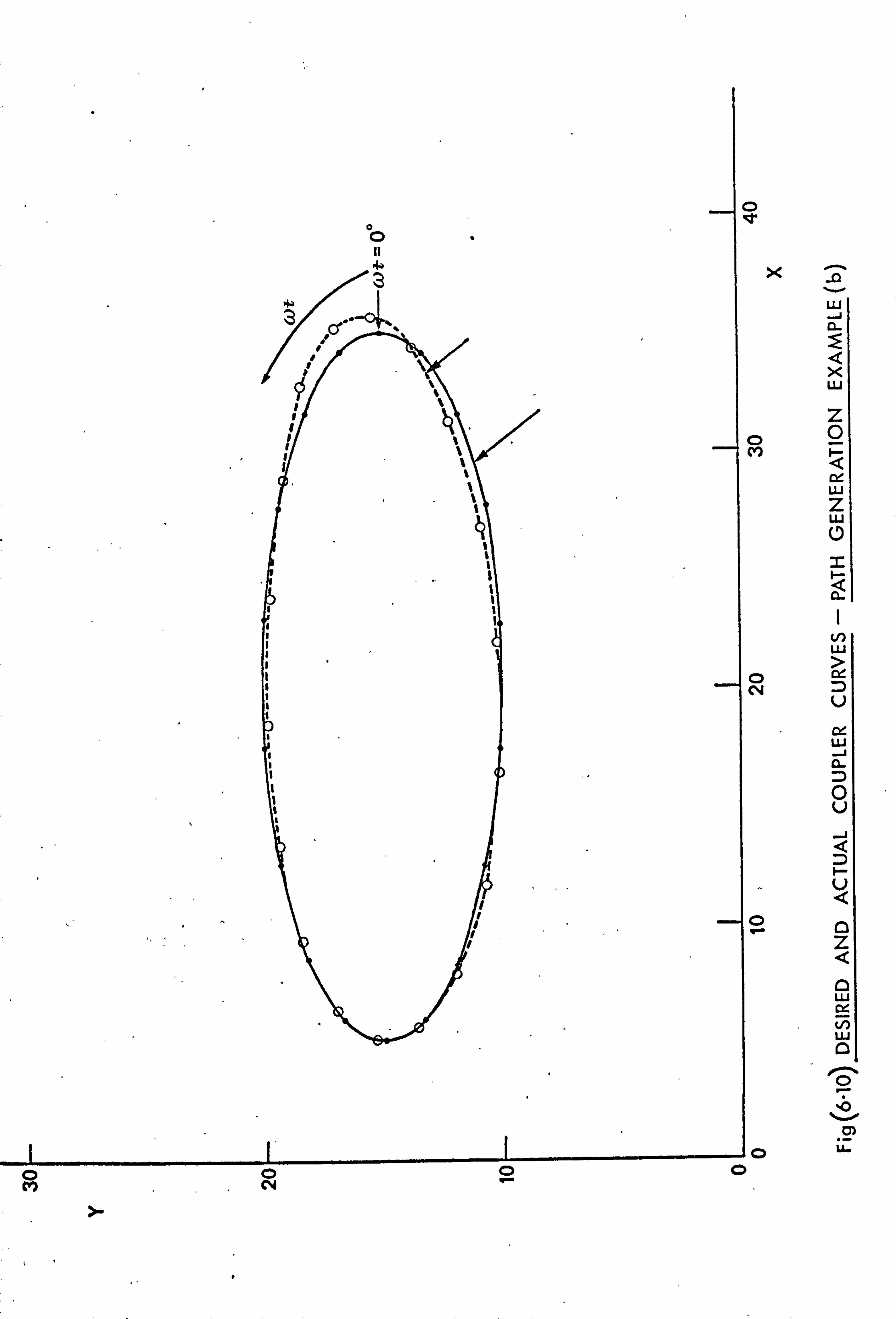
D qr
Xp
W J
X
W
Z 02 MQ
04 W
z w
2
a V) W
U 0 N
W J
D 0 u J Q
H
U Q
C Z Q
Z w w N w a
ö I
}
v) L.
-o 0 00 MN "-
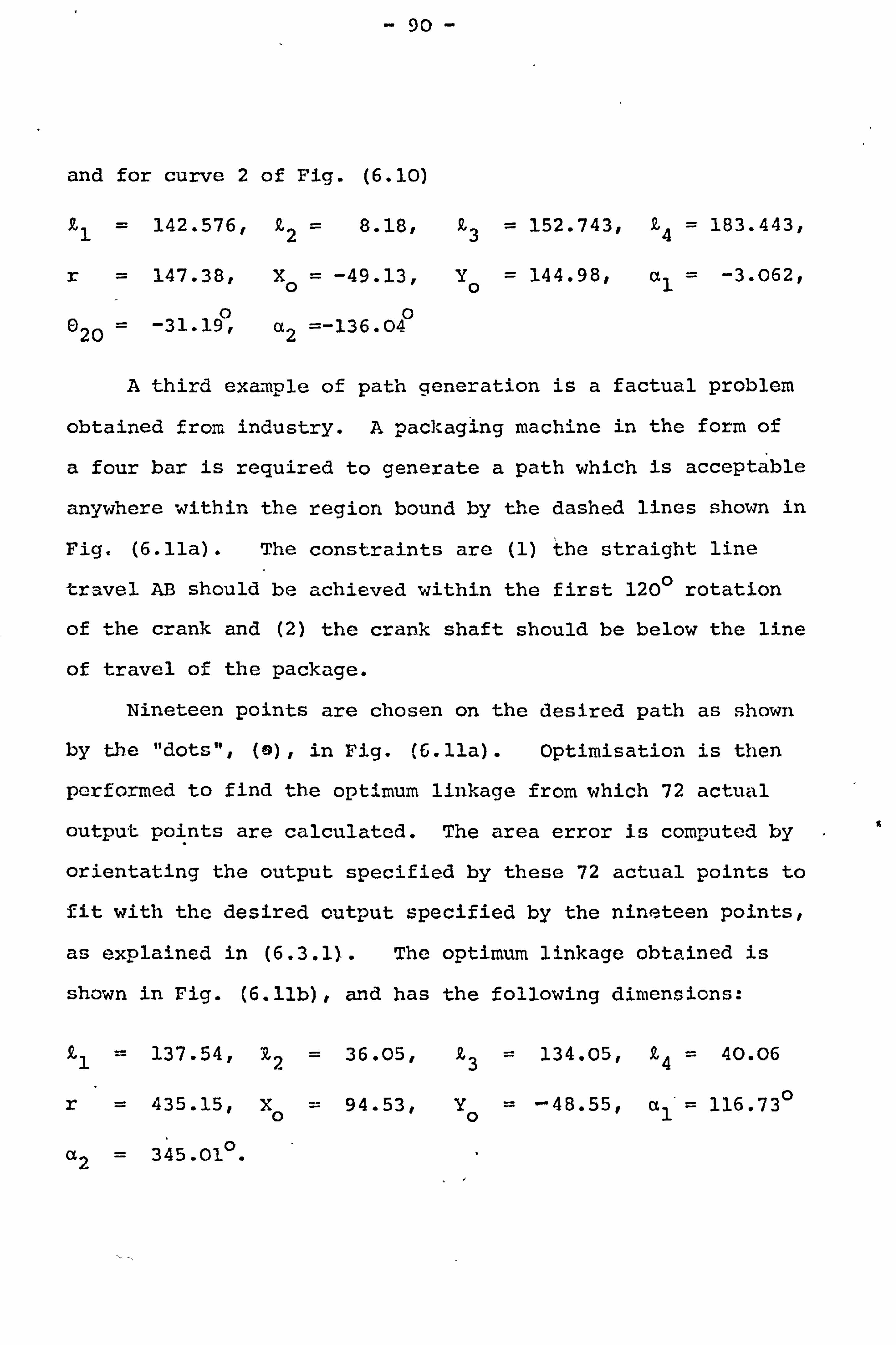
90
and for curve 2 of Fig. (6.10)
ý1 = 142.576, k2 = 8.18,
r= 147.38, Xo = -49.13,
020 = -31.19, a2 =-136.04
93 = 152.743,2.4 = 183.443,
Yo = 144.98, al = -3.062,
A third example of path generation is a factual problem
obtained from industry. A packaging machine in the form of
a four bar is required to generate a path which is acceptable
anywhere within the region bound by the dashed lines shown in
Fig. (6.11a). The constraints are (1) the straight line
travel AB should be achieved within the first 120° rotation
of the crank and (2) the crank shaft should be below the line
of travel of the package.
Nineteen points are chosen on the desired path as shown
by the "dots", (a), in Fig. (6. lla). Optimisation is then
performed to find the optimum linkage from which 72 actual
output points are calculated. The area error is computed by
orientating the output specified by these 72 actual points to
fit with the desired output specified by the nineteen points,
as explained in (6.3.1). The optimum linkage obtained is
shown in Fig. (6. llb), and has the following dimensions:
91 1= 137.54, 'Z 2= 36.05,9,3 = 134.05, Q4 = 40.06
r= 435.15, X0 = 94.53, Yo = -48.55, a1 = 116.73°
a2 = 345.01. °
R
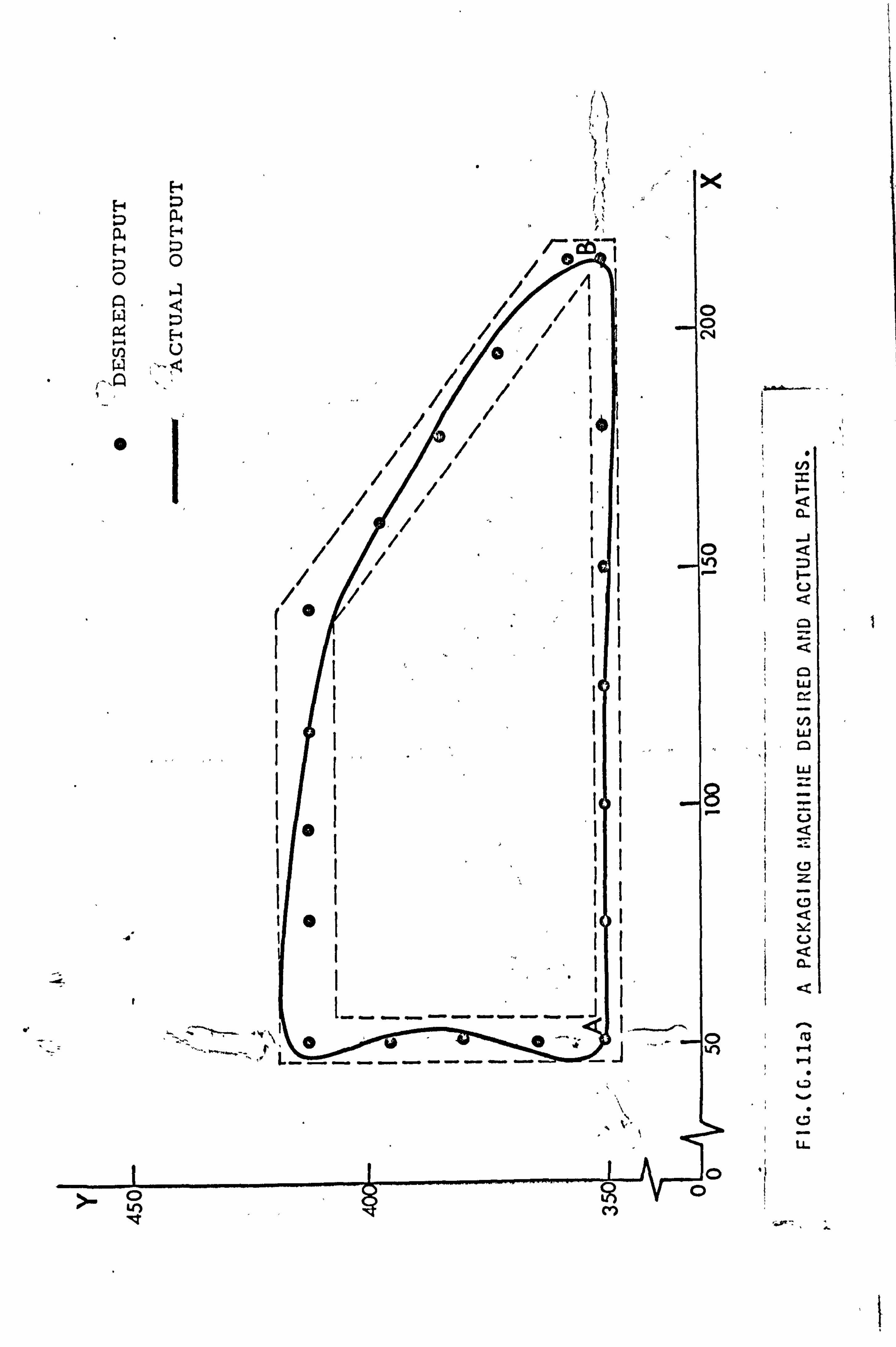
H H
a o, H H ao oa Aý w] xH v, U
rÄ 'Q
0l
r
;. 1
I\
'-3? t;
o/
I /1' I
// I'
// /1/
1 I, / //
/ (®
// Iii 1 'II
III I Ill Il
I
I 'I
I ®t
"ix 0 0 04
ý8
i
V-Oj
C)
I
N rZ
I
J
I- U
N W
W
a
V a a
ü
LL
ý-
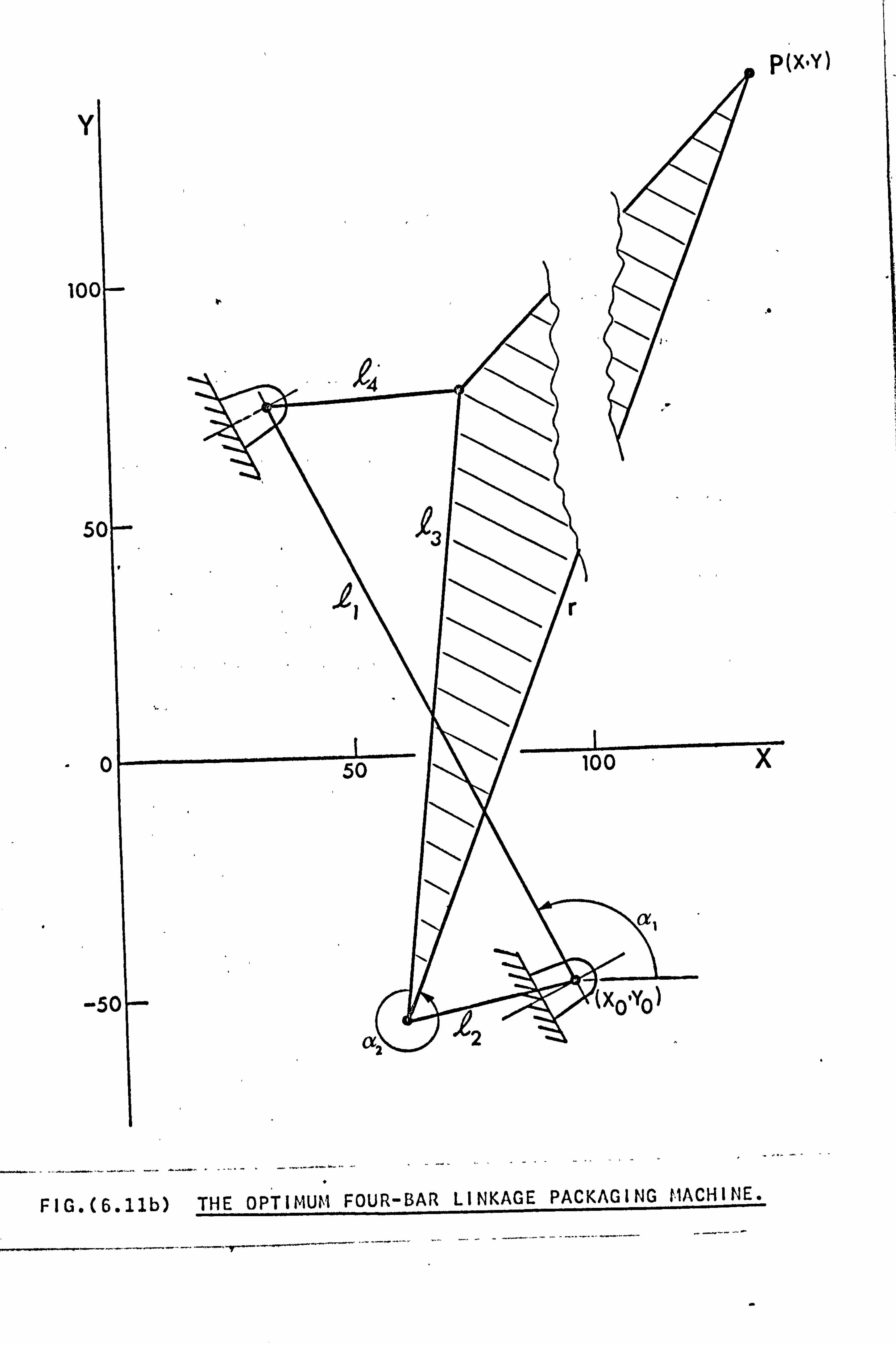
P(X-Y)
YI
100I-
5or
-o
-50
. _... X
FIG. (6.11b) THE OPTIMUM FOUR-BAR LINKAGE PACKAGING MACHINE.
- 91 -
6.5 Further Remarks and Computer Programs.
The method described can find a planar linkage to
generate a given output. It can dcci with any type of
planar linkage yielding in all cases a minimum. It can
be made to follow a logical process in the choice of the
type of linkage until it finds a satisfactory result.
The method is programmed using IBM Fortran IV
language. The program, shown in Appendix 5, is
conversational, adaptive and can deal with either function
or path generation by setting a parameter denoted by Ipath
to ± 1. Other features of its adaptability may be seen in
the appendix.
The compilation time of the program is about 17 seconds
and the running time depends on the form of the desired
output and the quality of the initial guess of linkage
parameters.
92
Chapter VII
CONTROL
7.0 INTRODUCTION
In many engineering applications the potential of
controlling the input motion to achieve a specified output
offers numerous attractive prospects. Many examples are
readily seen; for instance, in many designs the output is
required to prescribe a finite number of points often called
precision points. In the past most of the analysis concerned
setting up a number of equations, describing the kinematics of
the mechanism, the number of which equals the number of precision
points. These equations are then solved simultaneously for the
kinematic parameters of the mechanism. It is readily understood
that the number of precision points, hence the number of
equations, cannot exceed the number of kinematic parameters
sufficient to describe the mechanism. However, although the
mechanism readily prescribes the precision points what happens
in between is fixed. If the designer wishes to modify the
motion in between he must perform a new analysis on an increased
mobility mechanism. If, however, a second input is established
to which a controller is attached the output may be modified,
anywhere in an infinite variety, yet still prescribing the same
originally desired precision points. To fix ideas, a particular
mechanism, a simple planar linkage, ABCD is taken as an example
(Fig. 7.1). The assumptions of rigidity, ideal pin-points and
constant speed input are maintained, and attention is focused on
the variations possible in coupler-point curves when a second
input is provided by releasing the constraint of fixity at D.
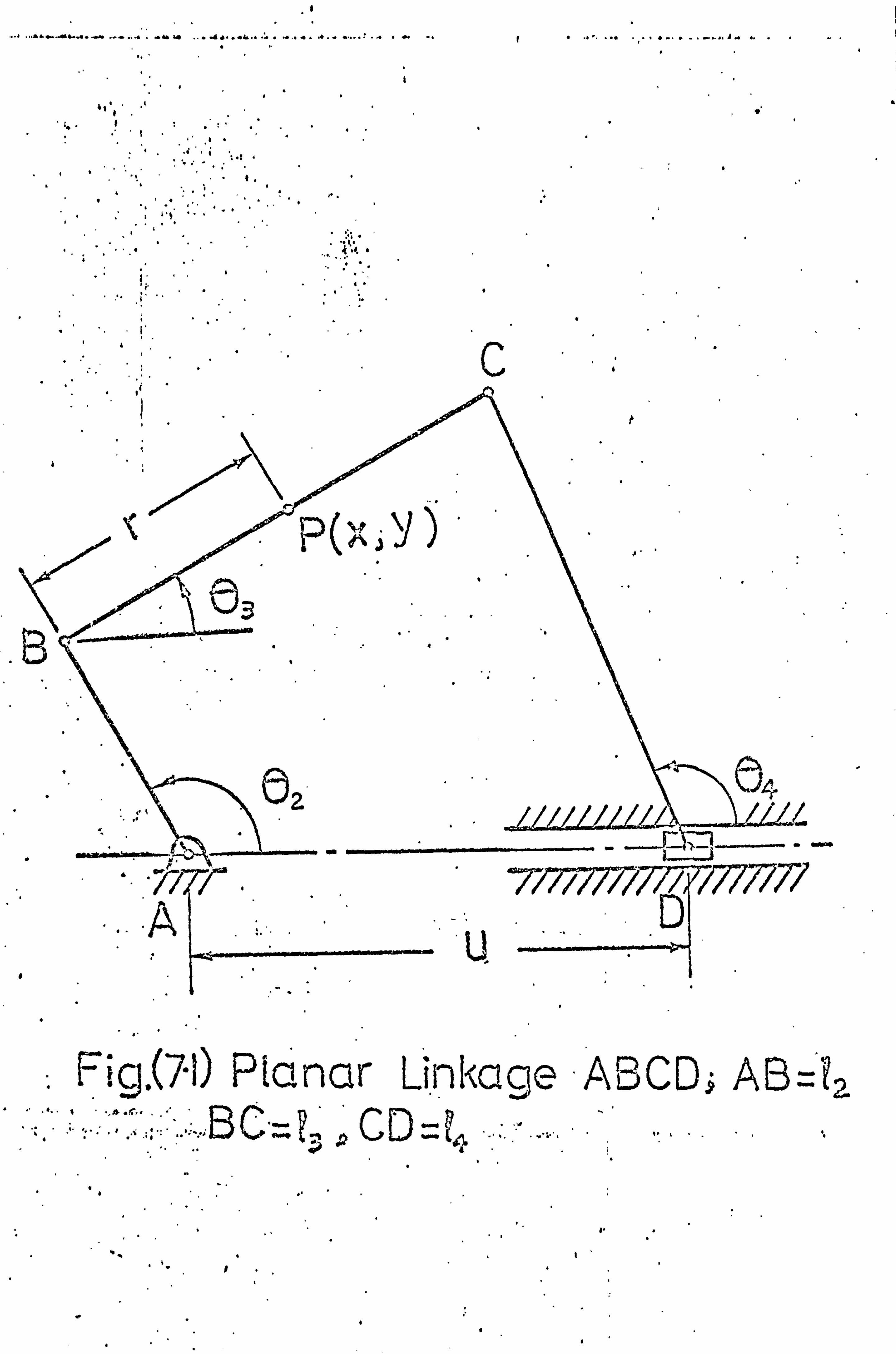
. _. ... *..... a........ .. ". ".. '* . rV r .... d4".. Y. " .. " r-" ý. A.. .. ". ". n"v ."f" .".. " " ".. " ý".. a ". ....
"". ýf
Lam. /"
U
fý . tö"ýý Planar Lnkage - ABCD ; =`1
B C. = CD
- 93 -
Several alternative definitions of input and output are
possible. For purposes of illustration we shall consider the
crank-angle as the primary input, the length AD =U as the
secondary or modifying input, and the two-dimensional path of
a chosen point on the coupler as the output. Equally, the
roles of the two inputs could be considered in reverse and/or
the output to be the angular position of the'link CD.
Fig. (7.2) shows a family of cyclic coupler-points paths,
each drawn for a fixed value of U within chosen limits, the
series of points marked on each path referring to an invariable
set of consecutive crank-angle position. Two observations may
be made from this presentation. First, any point lying on or
within the outer boundaries of the family is accessible to the
chosen coupler-point by suitable combination of 02 and U.
Subject to the constraint that 02 increases at a constant rate,
a coupler-point path may thus be achieved anywhere within this
envelope, thereby permitting a closer approximation to a desired
path by suitable control of U than could otherwise be obtained.
Secondly, to take account of the assumed time-dependence of 02,
a set of constant 02 curves may be constructed, as shown by the
dotted lines. Such 'isochronous' curves, which are arcs of
circles centred at the corresponding fixed position, of B, can be
regarded simply as a reference grid from which the resulting
motion can be determined once a particular continuous variation
of U is specified. Alternatively, they may be regarded as.
providing a starting point from which a desired variation in U
may be deduced.
7.1 CONCEIVABLE CONTROL METHODS
Obviously, the envisaged system discussed earlier provides
an enlarged versatility, albeit in some cases at the expense of
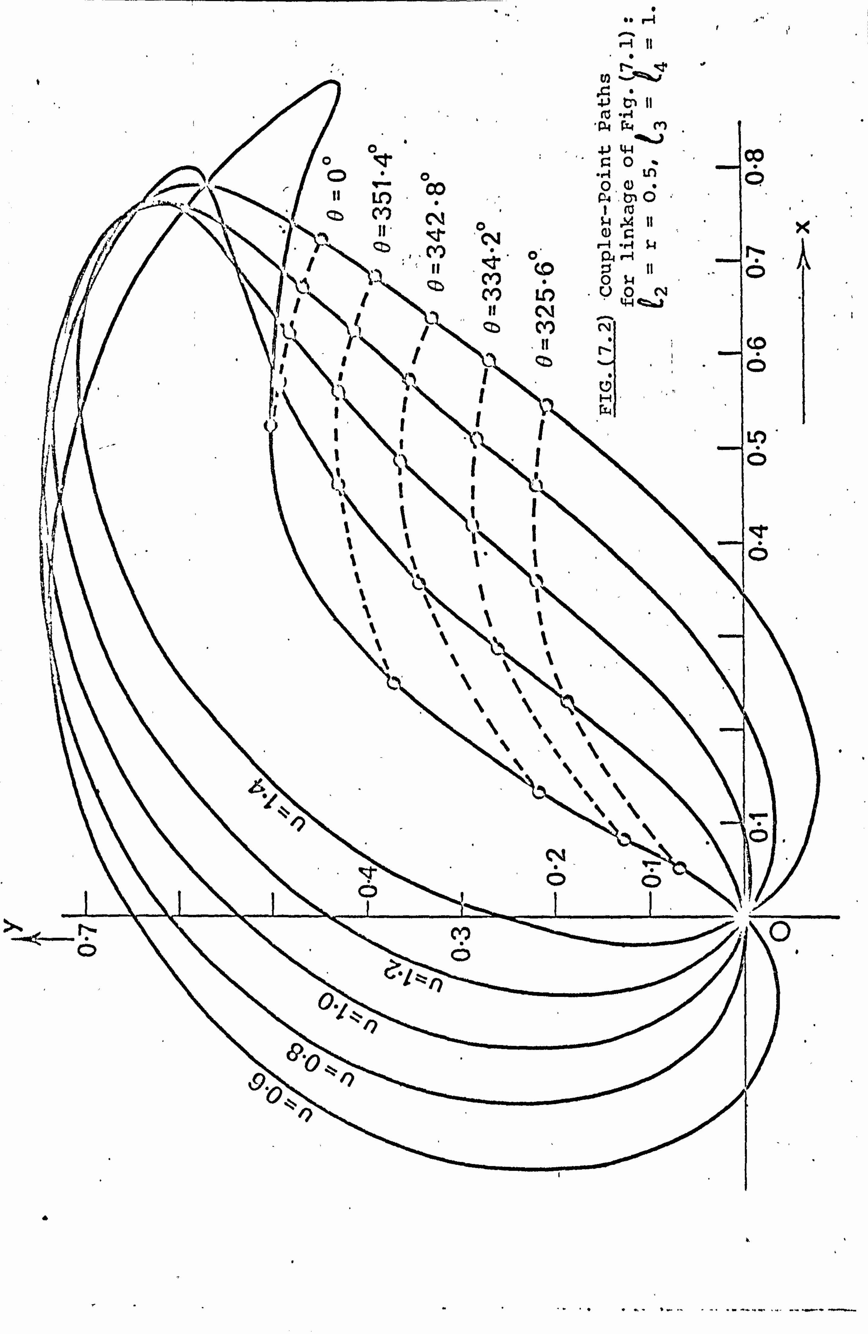
H II
Cn11 rý r+ P4 W tM
.v C
[r' ý(.,, ö% co
o0a to 0 0. a) Lo
c? P4 tn C;
o r7 I 'ý
r-4 -r4
UON MN uacý
t ý4 m (ý N
J'
ý10
.N^, .
. d' o0
l"n Olýý
0 N"
0

- 94 -
mechanical complication. Its use must therefore be justified
by the role of importance of the mechanism in the whole of the
engineering plant. There are, however, certain alternatives.
They vary from simple mechanical controls to advanced computer-
based strategies, and their suitability will obviously relate
to the nature of their application.
7.1.1 Off-Line Methods
The required motion of the secondary inputs are determined
from the kinematics of the mechanism. A drive is then chosen to
approximate as closely as rossible to the requirement. At least
three principal types of drive may be distinguished.
(a) An intermittent or continuous drive coupled to the primary
input by means of direct mechanical connections, an arrangement
that is simple in principle but suffers from the defects of
limited adaptability and mechanical complications. Examples
include secondary linkages, cams and latch mechanisms.
(b) A passive mechanical system embodying elements such as springs
or latches whose operation depend on the pre-determined load or on
inertia or other forces transmitted through the mechanism. The
mode could be continuous or intermittent and its advantages and
disadvantages are similar to the preceding option, and
(c) An independent drive of the appropriate periodic fcrm
maintained in correct phase with the primary input by non
mechanical means, e. g. electrical signals: this offers considerable
versatility although reproduction of a sufficiently accurate cyclic
variation may be difficult.
There is no extrinsic feed back in these methods which may
thus be regarded as open loop.
- 95 -
7.1.2 Partial-on-line Methods
The required motion of the input is determined as
previously. This is stored as a refý-, rence model to which the
actual motion is required to adhere by means of feedback.
Measurement of the motion can be compared with the reference
values and the corresponding independent drive can then be
controlled by error signals. A variant of this arrangement
is to take the mechanism manually through its correct path for
the desired overall output and to record simultaneously and
separately the values of the inputs. In practice this may be
accomplished with primary input operating in its normal mode.
This establishes inter alia, the necessary cyclic variation of
the secondary input for reference model purposes, thus eliminating
the prior calculation. Whichever the first stage may be,
considerable demands will be placed on the drive to achieve the
appropriate mechanical response, which clearly establishes a
limit of the range of application.
7.1.3 Adapt'ive' Methods
The same consideration of drive capacity applies to
-adaptive methods, in which the drive characteristics are adjustable.
A reference model of the desired motion is established as in the
preceding method and is used as a basis of comparison for the
actual motion. Trial cycles may then be completed in which the
adjustable parameters of the drive are progressively changed until
a satisfactory correspondence is achieved. If the adjustments are
made automatically on the basis of a defined error criterion, the
mechanism becomes self adaptive to its reference, and is thus a
self-learning device converging to the desired output.
- 96 -
Of these and other methods, the simplest and the most
widely used is the mechanically coupled arrangement of type
(7.1.1). The choice of either of the above methods depends
on the accuracy required and the role of importance the
mechanism plays in an overall plant.
7.2 ANALYSIS
7.2.1 Problem Definition
We suppose the desired path can be represented in an
analytic form as
ý1 (X, y, t) =o (7.1)
if path is time dependent or as
2 (XlY) =0 (7.2)
if it is not. In both cases the coordinates (x, y) defining
the actual output position are functions of 02 and U, and 02
is a specified function of time. If the analytic functions are
not determinable, equations (7.1) and (7.2) may be replaced by
their equivalent numerical relations. The problem is to determine
the variation of U which satisfies equations (7.1) or (7.2) as
closely as possible subject to the constraint conditions of the
mechanism fj (02, ..... U) =O, j=1,2,... m (7.3)
A quality function is formulated as a positional error
E1 = (x - x*) 2+ (y -Y *) 2 (7.4)
where (x*, y*) are the values of (x, y) that satisfy equation
(7.1) or equation (7.2) exactly, or as
E2 =Z E1 (7.5)
- 97 -
where N is the number of desired points. The minimisation of
the error described in equation (7.4) or (7.5) results in a
solution to the problem.
Two methods will be attempted here namely (1) variational
optimisation and (2) direct search optimisation.
7.2.2 Variational Method
A multiplier method is chosen here. The multipliers are
introduced so that the constraints can be dealt with directly.
The method is formulated by finding the stationary value of the
quality function (i. e., error) subject to the constraints f
This may be expressed as follows :-
DE1 m aql +E xj. aq =0 (7.6)
j=1 i
where qi are the generalised coordinates i=1,2,.... n and
are the multipliers.
Equation (7.6) gives n non-linear relations involving (n+m)
unknowns. These may be solved simultaneously with the m
relations expressed in (7.3) to give the gi (i = 1,2,..... n)
describing the mechanism.
There are two points to mention at this stage; a) the
error used in the above analysis is that expressed in (7.4) and
is time dependent. b) The optimisation is not carried out for
all the n parameters of the mechanism but just for the controlling
input ones. However, since our interest lies only in these
controlling ör secondary inputs, as will be called from now on,
an explicit solution of the remaining ones is not required and
they may be eliminated from the equations whenever possible.
- 98 -
7.2.3 Direct Search Methods
These consist of searching along a number of directions
in parameter space. They require only the evaluation of the
objective function for the whole cycle and thuse the second
formulation of the error function, i. e., E2 is suitable for use
with these methods.
There are three types of these methods: Tabulation
Methods; Sequential Methods, and Linear Methods. The first
assumes the region in which the minimum lies is known. The
region is divided into N sub regions and the objective function
is evaluated at each. A table of these evaluations is then
drawn from which the minimum is located by comparison. The
second explores the behaviour of the objective function by using
some form of a geometric shape. This geometric configuration is
progressively modified and altered until finally it locates the
optimum conditions. The third involves a search along n
orthogonal vectors and as it progresses its-direction is orientated
towards the optimum.
A sequential method "the Simplex", which is described in the.
previous chapter, is used here to search for the optimum motion
of the secondary inputs which in turn, as stated earlier, lead to
achieving the desired output.
7.3 RESULTS
Let us consider the mechanism shown in Fig. (7.3). The
constraints may be stated as follows:
fl = Z2Cos02+Z3Cos03-91 4Cos(04+v)-u Cosv =0
f2 = Z2Sin02+Q3Sin03-91 4Sin(04+v)-u Sinv =0 (7.7)
where 02 = 020 + wt
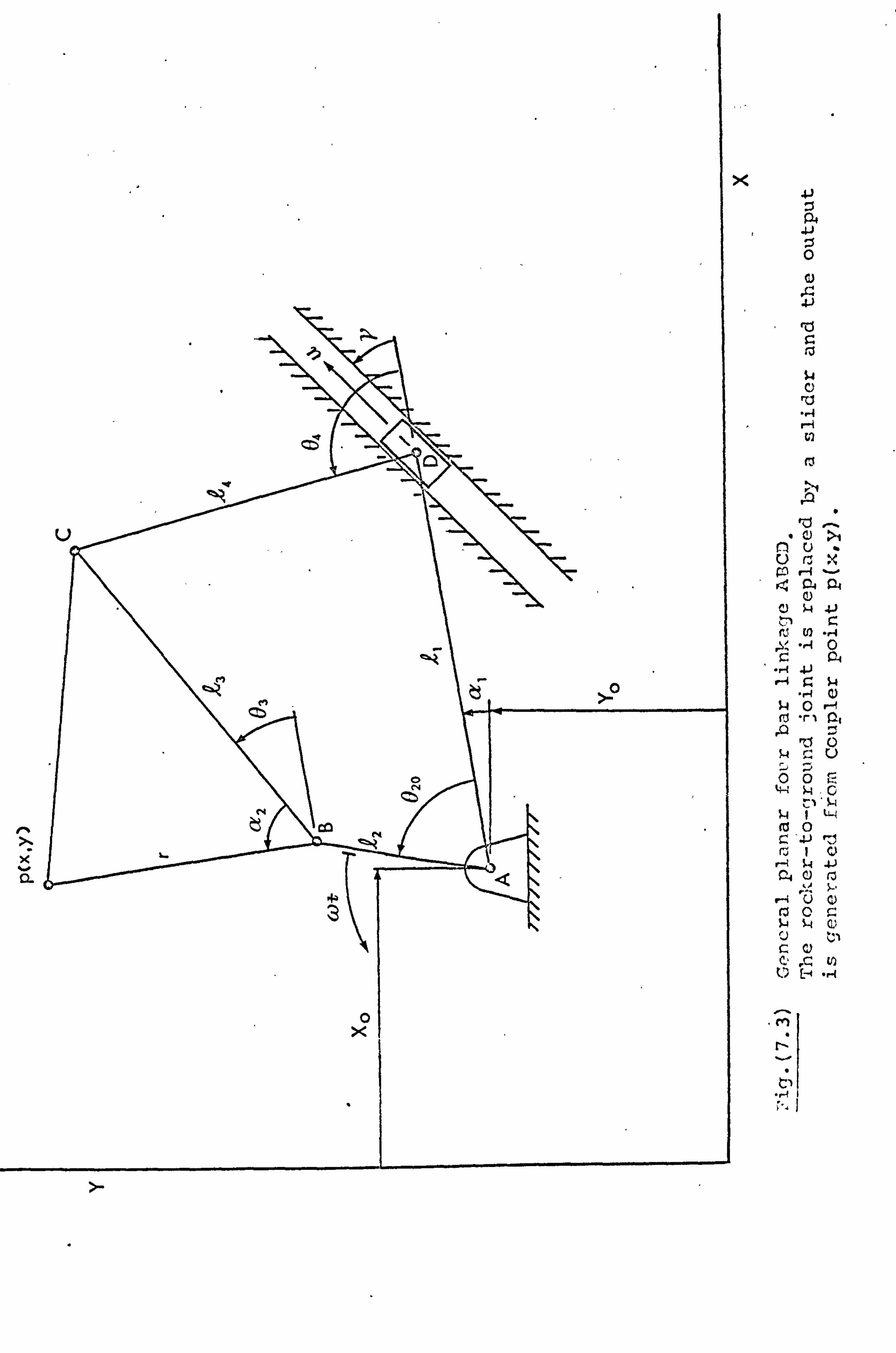
X
z a 4J 0 C)
rd
u cs u
r1l
M
ter. rU
04 a Q) ý$4 rt N .. 4
0
"ý+. u 1
O r-+ cJ rt Q4
rj O
OOH 44 S4
," 4t Y4
.41L (a O 0 4j z, rý 10 04
Vr
V y)
cZ e0 $4 s4 a- U
C)
t7 E . r1
M
N
>-
- 99 -
Let the output be generated from coupler point p(x, y) the
positional error can then be given as
r2 El ="{ L(k2Cos (02+a1)+rCos (03+a1+a2) - x*}
+{J (02+a1) +rSin (03+a1+a3)] - y* }2
The error E2 is computed by summating the values of El over
the number of desired points.
(7.8)
7.3.1 Examples: Series 1
Let the desired output be numerically given as shown in
Fig. (7.4). It is time dependent and is obtained from within
the envelope shown in Fig. (7.2). Therefore, we could assume
that a1 = a2 =v-0 and let U=u+ Ql, which in actual
fact is Fig. (7-1).
Let us assume that the crank AB is rotating at constant
angular speed w, i. e.
02 = wt (7.9)
The goal is then to control the secondary input U so as to lead
to close approximation of the desired function. The motion
that U must perform may be obtained by the direct application
of equation (7.6) to equations (7.7) and (7.8). This gives
-2r(Q2. CosO2+r CosO3-x*)SinO3 + 2r(i2SinO2+r SinO3-y*)CosO3
- A1(Z3Sin03); -X 2 (£3C0s03) =0
x1(k4Sin04) -x2(94 Cos04) =0
Al = O.
(a) (b) (7.10)
(C)
and as explained earlier these equations are solved simultaneously
with equations (7.7) to yield the optimum U.
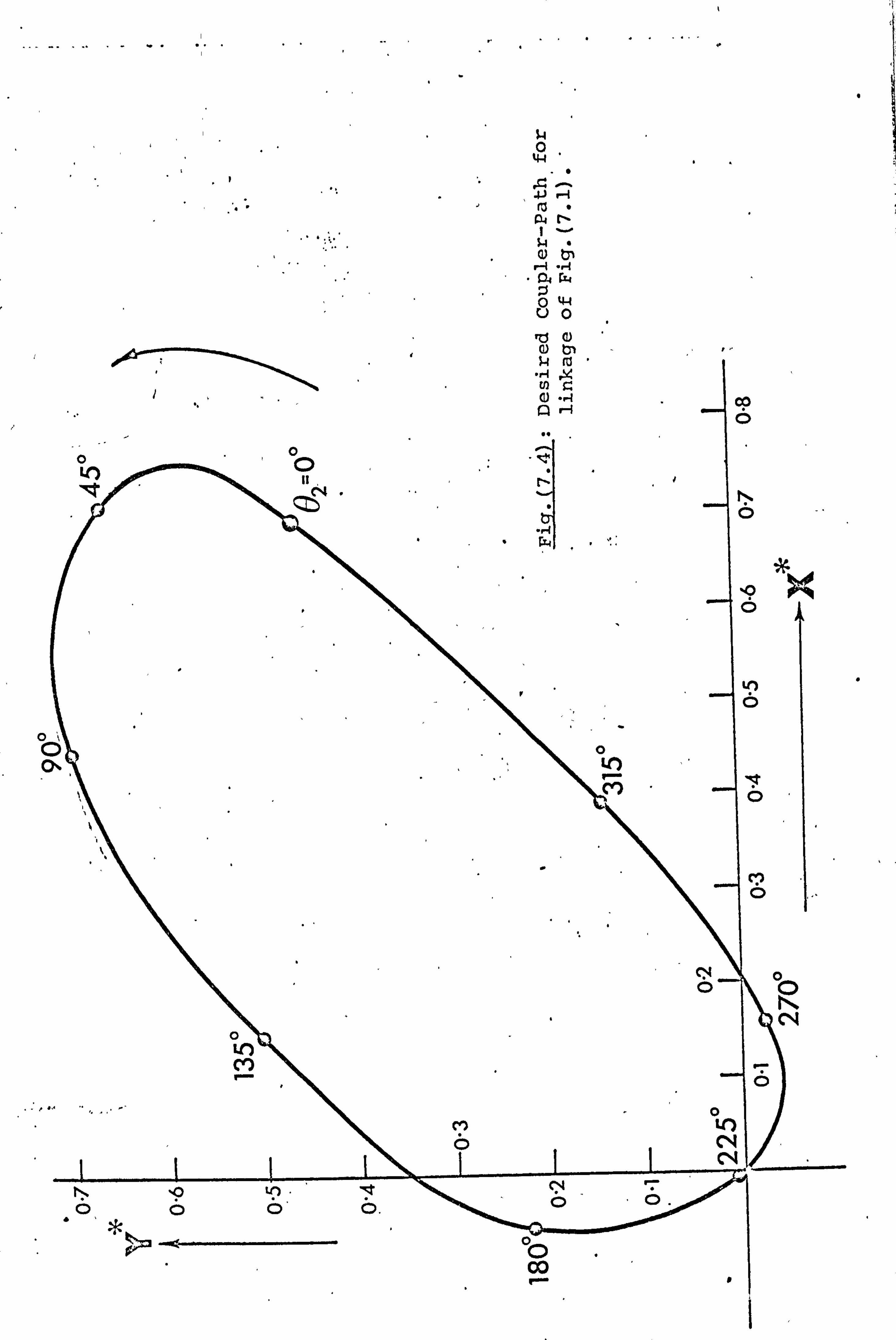
-.
O C C
....
0 ua
. ur4 r ar I -- N bn r4 "r4 so w 04- 00
ýö

- 100 -
Now from (7.1Oc) and (7.1Ob)
a2 =d (ü)
or (7.11)
Cos04 =O (b)
Taking the first solution, i. e. (7. lla) and substituting
in (7.10a) we obtain
-c* - 03 = tan1 y R2 Sin02
x* - ! '2 Cos02
(7.12)
or 03 = tan 1(A) where A corresponds with (7.12).
This corresponds to the relation that for minimum error the
coupler takes the position of a straight line with the point
p(x*, y*). However, we may now solve equations (7.7) to give: -
U2 - 2(k 2Cos02+R, 3Cos03) U+ IOL
22 +z 3 2_ L. 42 )+2Z 2Z3Cos(E) 2-03)] =0 (7.13)
Equation (7.12) may be substituted in (7.13) to give a solution
for U, i. e. 2
U1,2 = L2coso2+3cos(tan_1(A))] ±. {
L2c05023c05t_1]
222 -1 1/2 (7-14)
an (A) )] ) - [2--3
"4 )+223Cos (02-tan-
i. e. two solutions corresponding to two positions of the rocker
CD as shown in Fig. (7.5)
P ý'ý'Yl ,C 03
04 0 02 ý9 LI
4
L r777 I' ' i' ///, 77 7
U1
U2 Fig. (7.5)
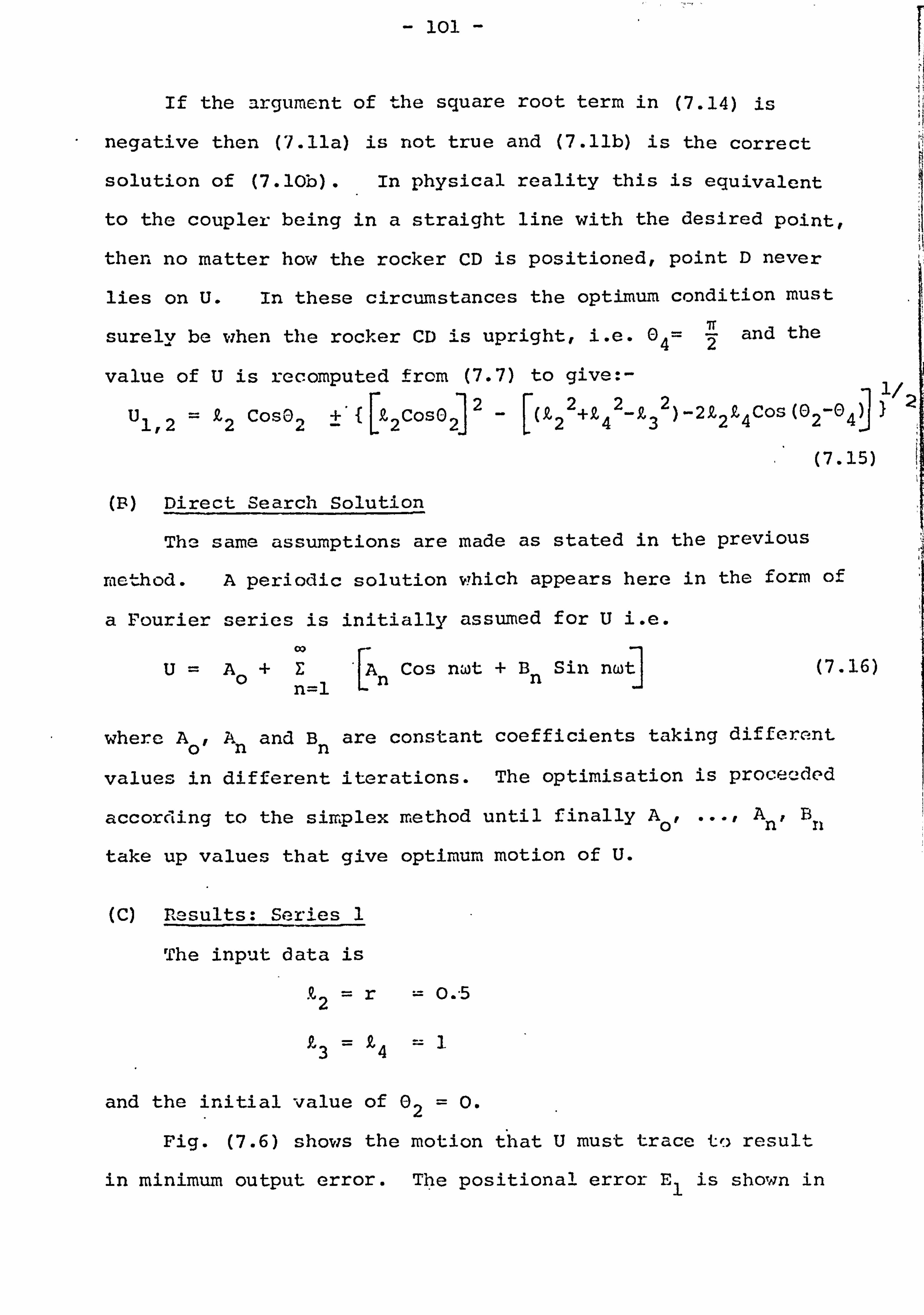
- poi -
If the argument of the square root term in (7.14) is
negative then (7. lla) is not true and (7. llb) is the correct
solution of (7. lOb). In physical reality this is equivalent
to the coupler being in a straight line with the desired point,
then no matter how the rocker CD is positioned, point D never
lies on U. In these circumstances the optimum condition must
surely be when the rocker CD is upright, i. e. 04= 2 and the
value of U is recomputed from (7.7) to give: - 'ý
U1,2 = R2 Cos72 +'{ Q2CosO2 2- ['2 2+R, 42-Q32)-2Q2Q4Cos(02-04J
(7.15)
(R) Direct Search Solution
The same assumptions are made as stated in the previous
method. A periodic solution which appears here in the form of
a Fourier series is initially assumed for U i. e.
U= A0 + E_ ' An Cos n; ýt + Bn Sin ncwtl (7.16) n-1
where A, An and Bn are constant coefficients taking different
values in different iterations. The optimisation is proceeded
according to the simplex method until finally A0, ..., An, B
take up values that give optimum motion of U.
(C) Results: Series 1
The input data is
Q, 2=r =0. "5
23 = £4 == 1
and the initial value of 02 = 0.
Fig. (7.6) shows the motion that U must trace to result
in minimum output error. The positional error El is shown in

K N
KJ N
M
KO
N
W J
0 Z
Z
KID" V
n
r:. .-- .-

ui w 0
w J
z 0 ý N 0
W
F-
ýý N% 0
W
0 LL.
J
z 0
D
O O = i-- w
2 V x Q w V)
F- V w
0
-o
............
0"
1t NOc -O et "NO
// OL X 13 2ib21213 1VNOILISOd
N
cv M
WO- 0
W J.
Z
Z
t+N U
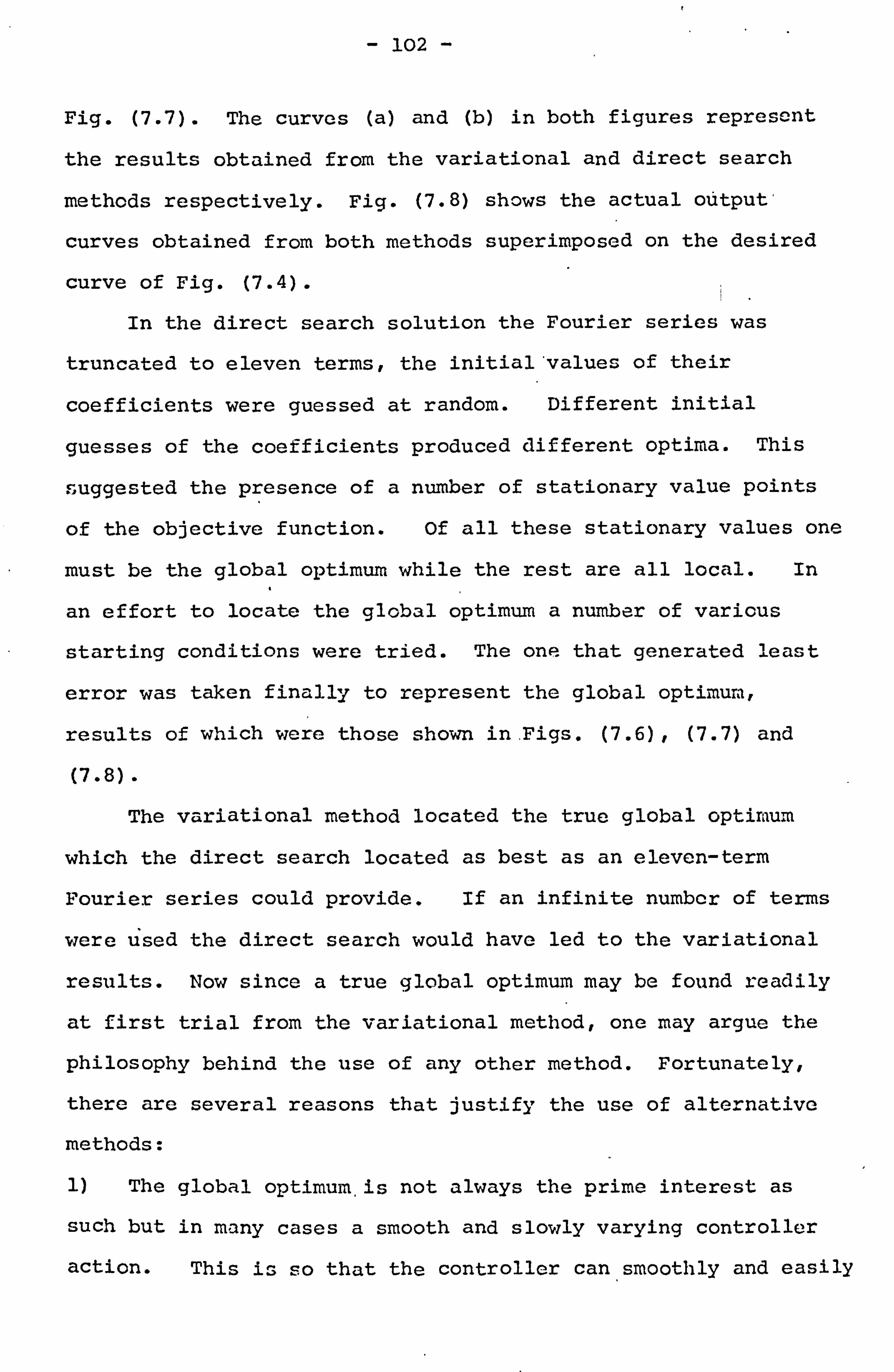
- 102 -
Fig. (7.7). The curves (a) and (b) in both figures represent
the results obtained from the variational and direct search
methods respectively. Fig. (7.8) shows the actual output
curves obtained from both methods superimposed on the desired
curve of Fig. (7.4).
In the direct search solution the Fourier series was
truncated to eleven terms, the initial'values of their
coefficients were guessed at random. Different initial
guesses of the coefficients produced different optima. This
suggested the presence of a number of stationary value points
of the objective function. Of all these stationary values one
must be the global optimum while the rest are all local. In
an effort to locate the global optimum a number of various
starting conditions were tried. The one, that generated least
error was taken finally to represent the global optimum,
results of which were those shown in . Figs. (7.6), (7.7) and
(7.8).
The variational method located the true global optimum
which the direct search located as best as an eleven-term
Fourier series could provide. If an infinite number of terms
were used the direct search would have led to the variational
results. Now since a true global optimum may be found readily
at first trial from the variational method, one may argue the
philosophy behind the use of any other method. Fortunately,
there are several reasons that justify the use of alternative
methods:
1) The global optimum, is not always the prime interest as
such but in many cases a smooth and slowly varying controller
action. This is so that the controller can smoothly and easily
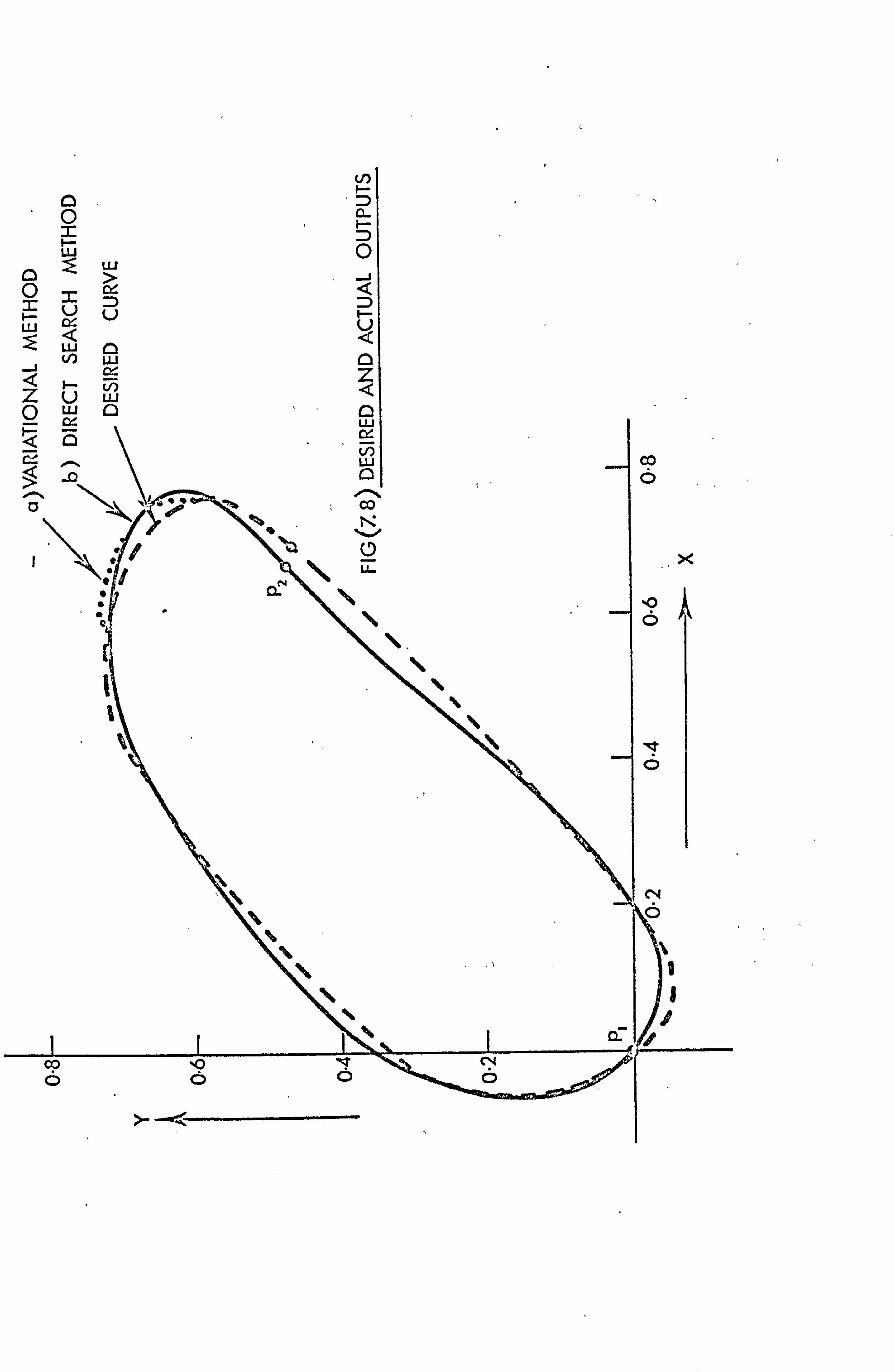
O 2 I- w
w
O z V
LLI w Lw
ZÜw 0 44 p
cn
I- r 0
0
- l03 -
cope with its task and thus eliminate undesirable and
complicated dynamic situations. By studying curve (a) of
Fig. (7.6) we find it very difficult, if not impossible, to
accomplish at high speeds while curve (b) of the same figure
is a more feasible task.
2) The direct search permits an easier use of stricter error
conditions or constraints at some portion of a desired function.
Thus provisions may be incorporated to cater for cases where
for instance certain priorities or weighting functions are
added to certain parts of an output. As an example, let the
portions plp2 of Fig. (7.8) be generated as closely as possible
while the rest is not so rigorously required. Let us assume
weighting functions wl, w2 where wl is used within the range
P1P2 and w2 without. Now let:
w1 =. 5w 2
and w2 =1
Then the error E2 may be formulated thus:
N1 N2 N E2 = W2 El +w1 El + w2 El (7.17)
0 N1 N2
where N1 and N2 are the number of desired points up to pl and
p2 respectively. The required motion U of the controller for
this case is then shown in Fig. (7.9) and the actual output
curve is shown in Fig. (7.10) superimposed on the desired one.
It is clearly seen from Fig. (7.10) how a close generation of
range plp2 is accomplished while larger errors are tolerated
outside it. Another interesting point is that if the
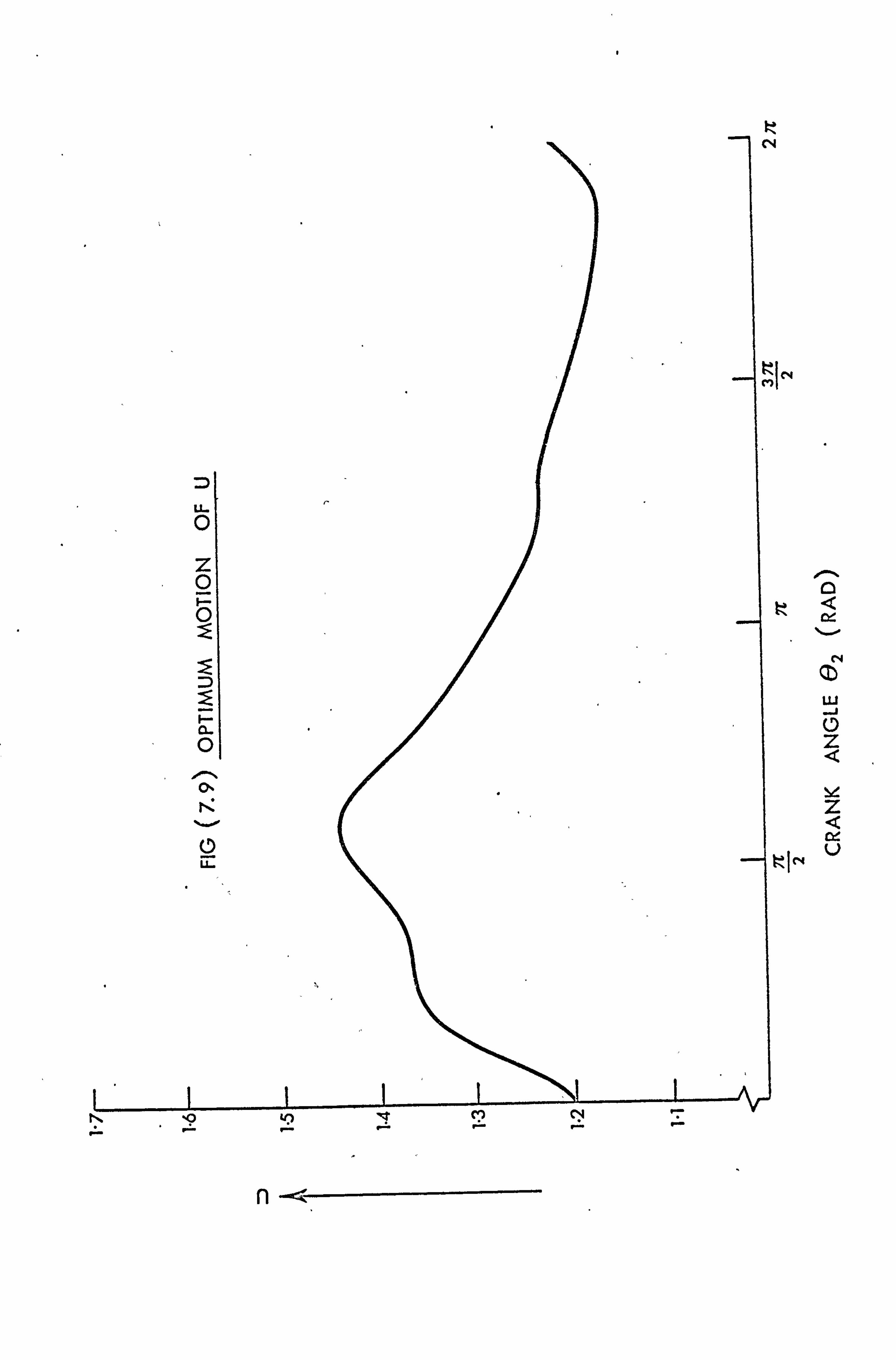
k
:1 C4
Ö
N
W J
0 Z
Z
K1c4 U
ný
tý "O to Qc
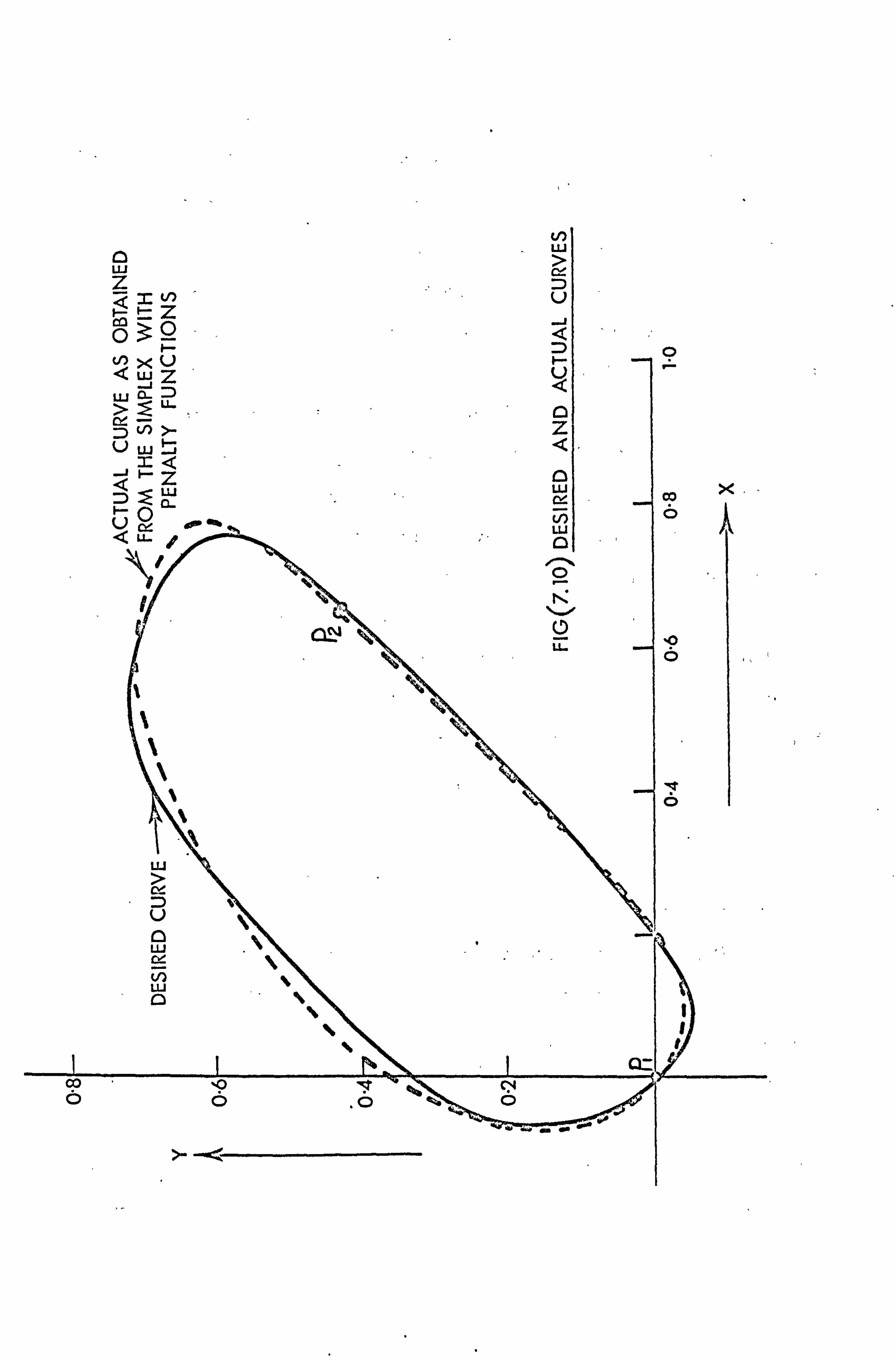
O w Z
O
N
z O
N w
V
J Q
n

- 104 -
requirements outside plp2 are very relaxed the controller
motion U involved there, may be modified further to give a
more favourable dynamic condition.
3) With reference to secton 7.1, the two methods cater for
two distinct control applications, the variational method is
used off line to precompute the would-be required controller
motion of U. The controller is assumed to be able to produce
this motion despite the dynamic problems that may arise. The
direct search method, however, may be used "on-line" and
accommodate the dynamic considerations into its structure. This
is done by monitoring the error over, one cycle with the actual
mechanism operating. The controller is then asked to vary its
motion according to the optimisation routine. The error
incurred is monitored again and further modifications in U by
the controller are performed. Thus as can be seen from this
procedure the dynamics are automatically taken into consideration.
4) With the variational method, any change in the operating
conditions require a recalculation of optimum conditions. The
direct search merely experiments with a number of cycles, after
which the controller adjusts itself, in an optimum manner, to
the changes. Thus for automation purposes a heavy swing in
favour of the direct search method is justified.
5) The variational method requires the solution of (n+m) non-
linear equations. In many cases this entails a far greater
effort than would otherwise be needed with a direct search. In
fact, in some cases, the direct search method is required to
solve these equations.
-105-
Finally, it may be summarised that the chdp e of the
methcd depends upon the complexity of the problem and the
type of application required.
7.3.2 Examples; Series 2
In this series of examples we show how the errors
obtained in the previous chapter are further reduced by
increasing the mobility of the optimised four bar by replacing
the rocker-to-ground joint by a slider and controlling it, to
prescribe a motion described by the following equation.
00 u=E (An Cos nwt + Bn Sin nwt) (7.18)
n=0
Since we specify the general form of motion of the slider the
variational method fails and therefore only the direct search
method "the simplex" will be considered here. The link
dimensions obtained from the optimisation in the previous
chapter are retained. The new optimisation parameters are
obtained by limiting n to the value of 3 in equation (7.18).
The parameters are thus 0, Al, A2, B2 and the angle v between
the slider line of travel and the ground link. The reason for
choosing n=3 is to reduce the mechanical complications
involved in producing the controlled motion of the slider.
All the examples discussed in the previous chapter have
been tried and in all cases the errors were reduced. However,
only two of the examples will be discussed here.
1) The desired output is to be generated from the rocker
link R, 4 of Fig. (7.4) as an angular function
0ý = 65+ ß6 }Sin 2I
where ß5 and ý6 have the same values as in chapter 6, section
6.4.2, sub-section B. The output is to be given a weighting
- 106 -
factor of 1000 in the range 600 <wt <2600 and the remainder
a weighting factor of unity.
The optimisation produced the following optimum values :
A0 = 1.46, A1= -0.425,131 = -0.256, A2 ='-0.855,
B2 = 0.569, V= -41°.
The optimum output curve, 2, is shown together with the desired
output curve, 1, in Fig. (7.11). The figure shows that the
weighted portion is generated very closely. In fact the error
involved is 4.8 degrees2 as compared with 35.0 degrees2 in
chapter 2. This presents an enormous reduction which would
have been even more if terms in equation (7.19) were considered.
2) The desired, output is to be generated'from coupler point
p (x, y) of Fig. (7.4) as a path
(x* _ß7) 2+ (y* ß9) 2=1
ß8 ß10
where ß7' ß8, ß9 and ßl0 have the same values as in chapter 6,
section 6.4.3, example (b)
The optimisation produced the following optimum values
A0 = 3.1, A1=0.772, B1 = -0.34, A2 = 0.568
B2 = -0.136, v= -0.9°
The optimum output curve, 2, together with the desired output
curve 1, are shown in Fig. (7.12). The error is 4.3 cm2 as
compared with 12.6 cm2 in chapter 6.
7.4 /A Strategy in Search for the Optimum Linkage
Based on the work described in chapters 6 and 7a
strategy for the search of an optimum linkage may be formulated.
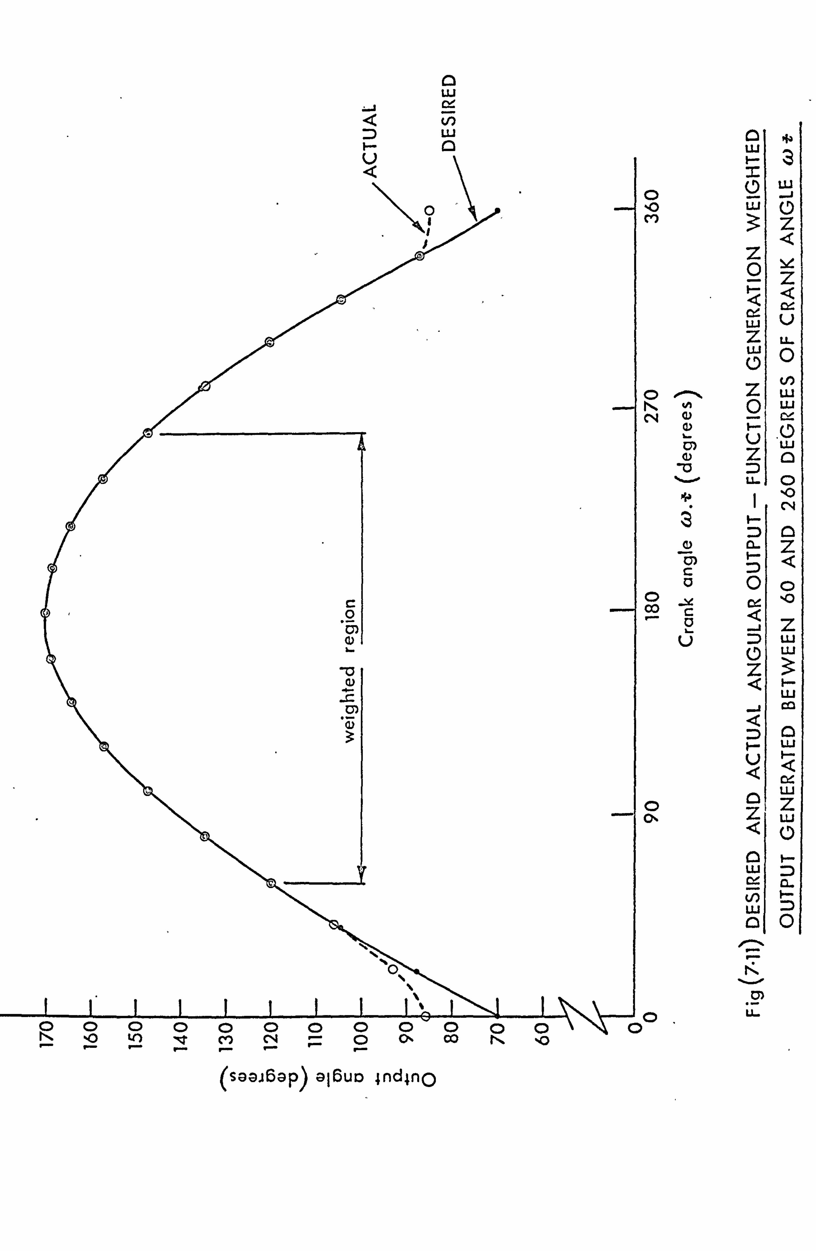
0 W
(I, LU F'- ý
0 ,o M
N
N
0)
'Z3
00 c
0 0
0 LU
U LU
w 1 z
z v 0 N w w C: e
.O w
O
N
O Z
O
Z w w
I- w
w F- a w Z w
n. ti O
"Q t7 MNQ ON OD %0
(saai6ap) al6uo 4nd4np
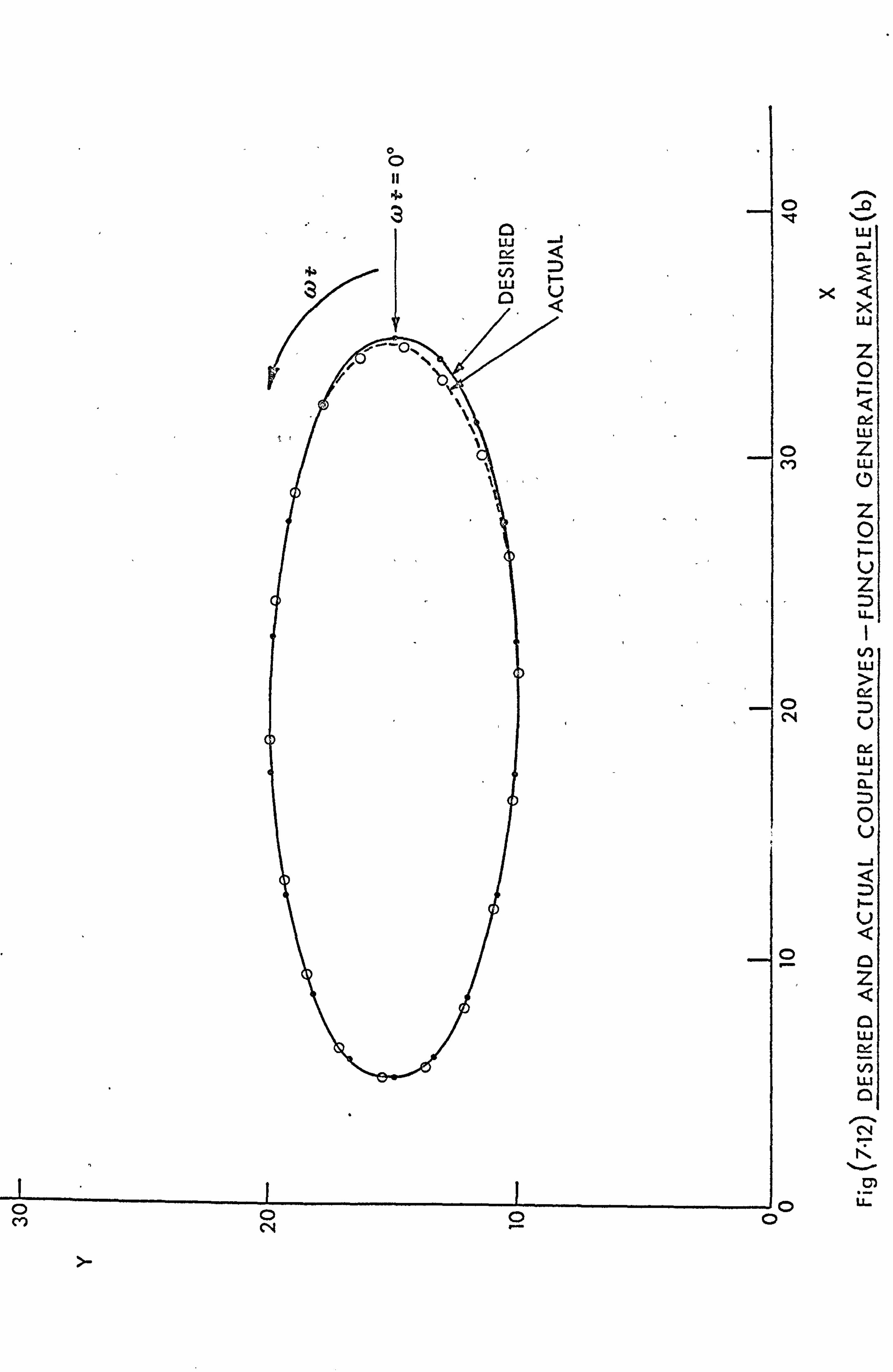
O
O II
3 . 0. J
Ly Q
4 _
r, o0
}
0 IT
0 Cl)
0 N
0
J0 0
x
ti- V
ci Z
0 w V) LU ci
N
K
Im
U-
- 107 -
Firstly, we start with the simple four bar linkage and optimise
its link dimensions so as to lead to minimum error in output
generation. Secondly, if unacceptable errors occur in the
output we'increase the mobility of the four bar by introducing
a second input and control its motion in an optimum manner so
as to lead to acceptable errors. The second input could be a
slider as discussed in this chapter or could be another link
resulting in a five bar loop. This fifth link can be driven výct
by the crank gears or may be independently driven. If
unacceptable errors still occur we could continue introducing
further inputs or indeed building a chain of linkages.
The computer program shown in Appendix, 5, can cope with
the above defined strategy producing optimum results in each
case. Obviously, the fortran function "error" shown in the
program of the above appendix should in every case contain the
kinematic equations of the type of linkage being treated.

V ART
EXPERIMENT' '&- CONCLUSIONS
I
ti
- 108 -
CHAPTER VIII
EXPERIMENTAL INVESTIGATIONS
AND
DISCUSSION OF RESULTS
8.0 AIMS OF EXPERIMENT
The theoretical investigations in this thesis concerned
two aspects of mechanism study. The first dealt with the
dynamics of a five bar linkage with a sliding joint. The
response of this mechanism has been analyzed using results
obtained mainly from computer solutions. A linearised
analysis has also been performed to study the resonance and
stability of the mechanism. The resonance analysis showed a
behaviour similar to a second order system while the stability
analysis showed instability in the second region, i. e. in the
vicinity of twice the natural frequency only. The instability,
however, disappeared completely by addition of a small value of
damping. The second aspect of the study dealt with the
optimisation of the linkage kinematic parameters and also the
control of its inputs to achieve a desired output.
The theoretical investigations considered two types of
inputs, (a) a constant speed input and (b) a torque input. In
this experimental work we shall consider a constant speed input
only, applied to the crank.
The main aims of the experiment are :-
1. ) To investigate the motion of the slider with different
input speeds and springs and also to compare the experimental.
and theoretical results.
- 109 -
2) To investigate the resonance of the slider when the ratio
of crank length to other links is small. This, if in good
agreement with the theoretical results, sukports the analysis
described in Chapter IV.
8.1 APPARATUS
Two experimental apparatus were built. The first, which
will be referred to as Experimental Rig 1, was used to achieve
the first aim of the experiment set out above. The second
apparatus, which will be referred to as Experimental Rig 2, was
used to achieve the second aim of the experiment also set out
above. The first apparatus operates in the vertical-plane and
the second in the horizontal plane.
8.2 DESCRIPTION OF APPARATUS
8.2.1 Experimental Rig 1
8.2.1.1 Mechanical Components
Fig. (8.1) shows a view of the apparatus with
one side plate of the slider guide removed to show the slider
and spring arrangement. Fig. (8.2) shows a top view of the
linkage showing the coupling arrangement to the motor and also
the slider and its guide in more detail.. Figs. (8.3a) and
(8.3b) show exploded views of the various components of the
linkage and the slider guide respectively.
The apparatus, including the motor, is mounted on a pedestal
which is bolted to a block. The crank or input link is a fly-
wheel (1) mounted on an input shaft via a taper lock. The input
shaft (2) (see Fig. (8.2) ) is located in two pedestal bearings
(3) and connected to the motor via a coupling. A further fly-
wheel (4) is mounted on the shaft to ensure constant speed input.
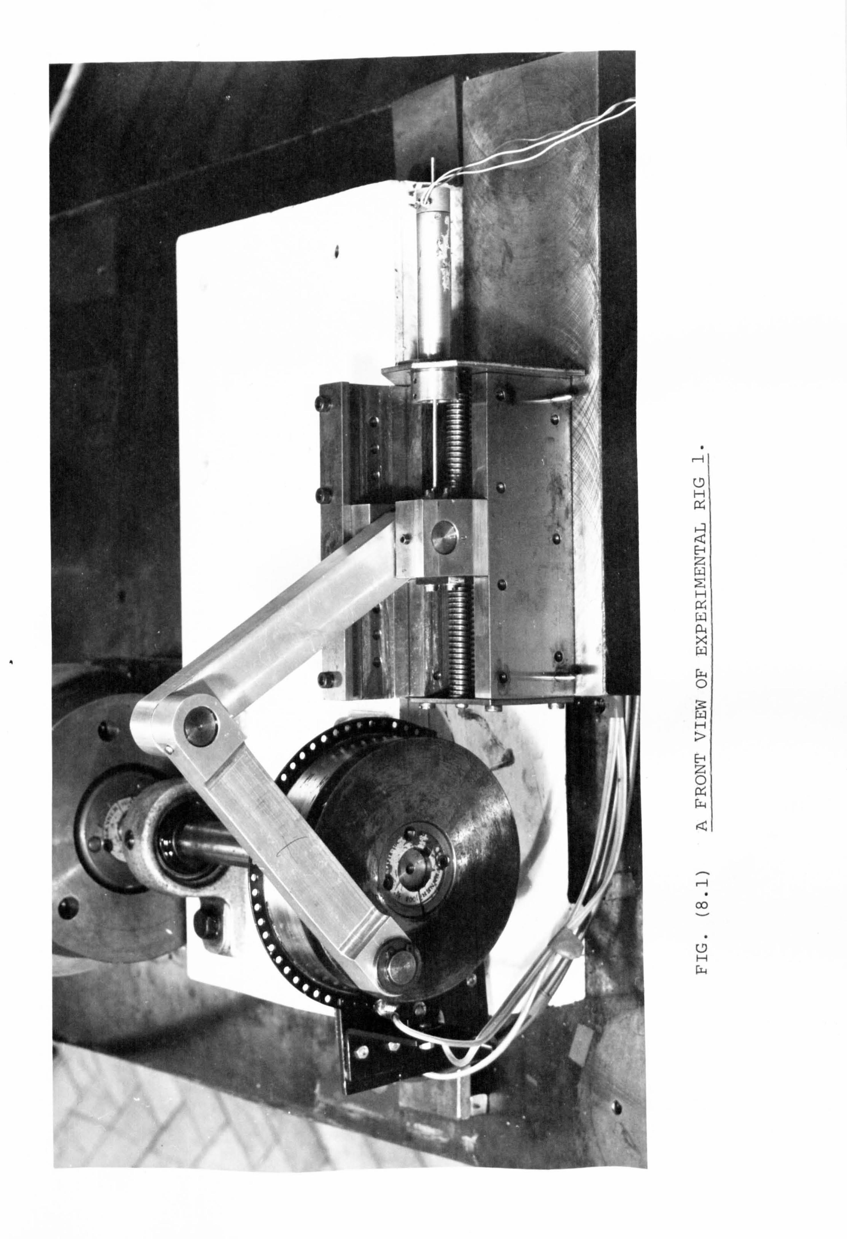
0i H.
a N z w H H
a w a x w i., 0
W H
z 0
C4 w
H w
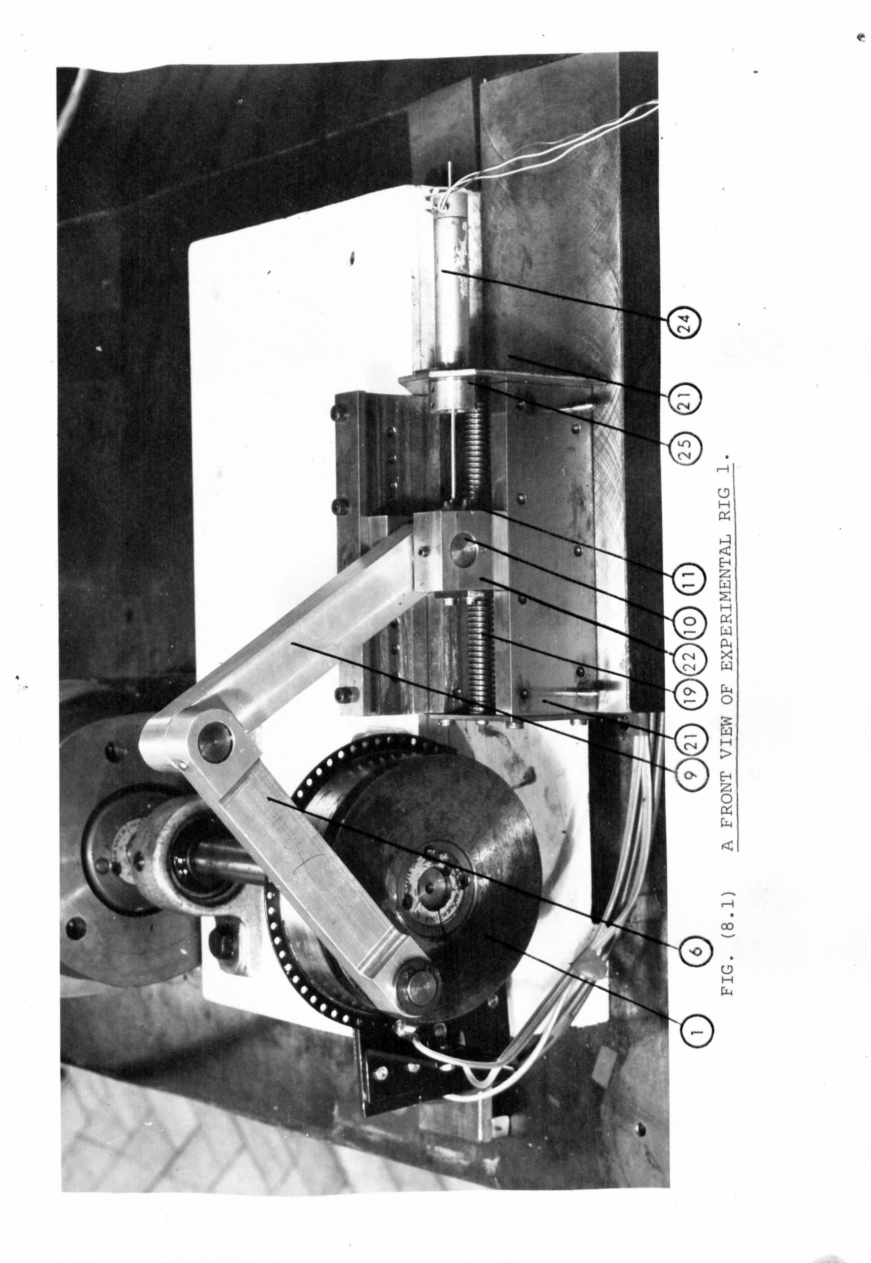
4rh
i
I:: -.
"`ý...
aýý,;
c7 H
w .J
P4 X
ö
H
DID E-1 z 0 w
(D - H w
n

týý ýý
ý`ý- ýý
,,,
I Yeti
N
OD
0 H [x4
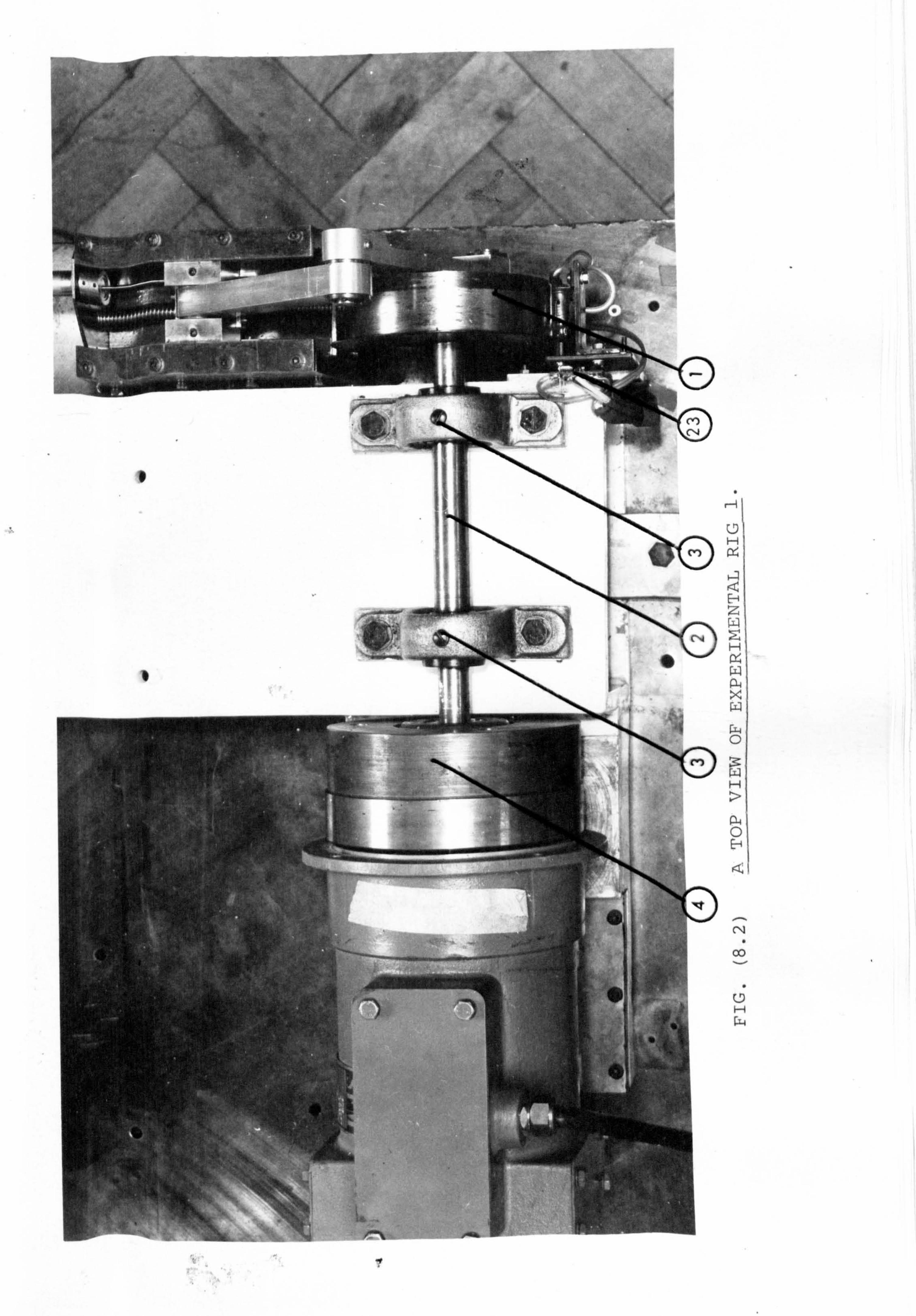
r
ýýý ý, +,
a
., 4
r-
H
z H ry. w a x w w 0
H
a 0 N Fýý
N
0 H w
_____ -
01
oO I
O
I /Ey
ý°
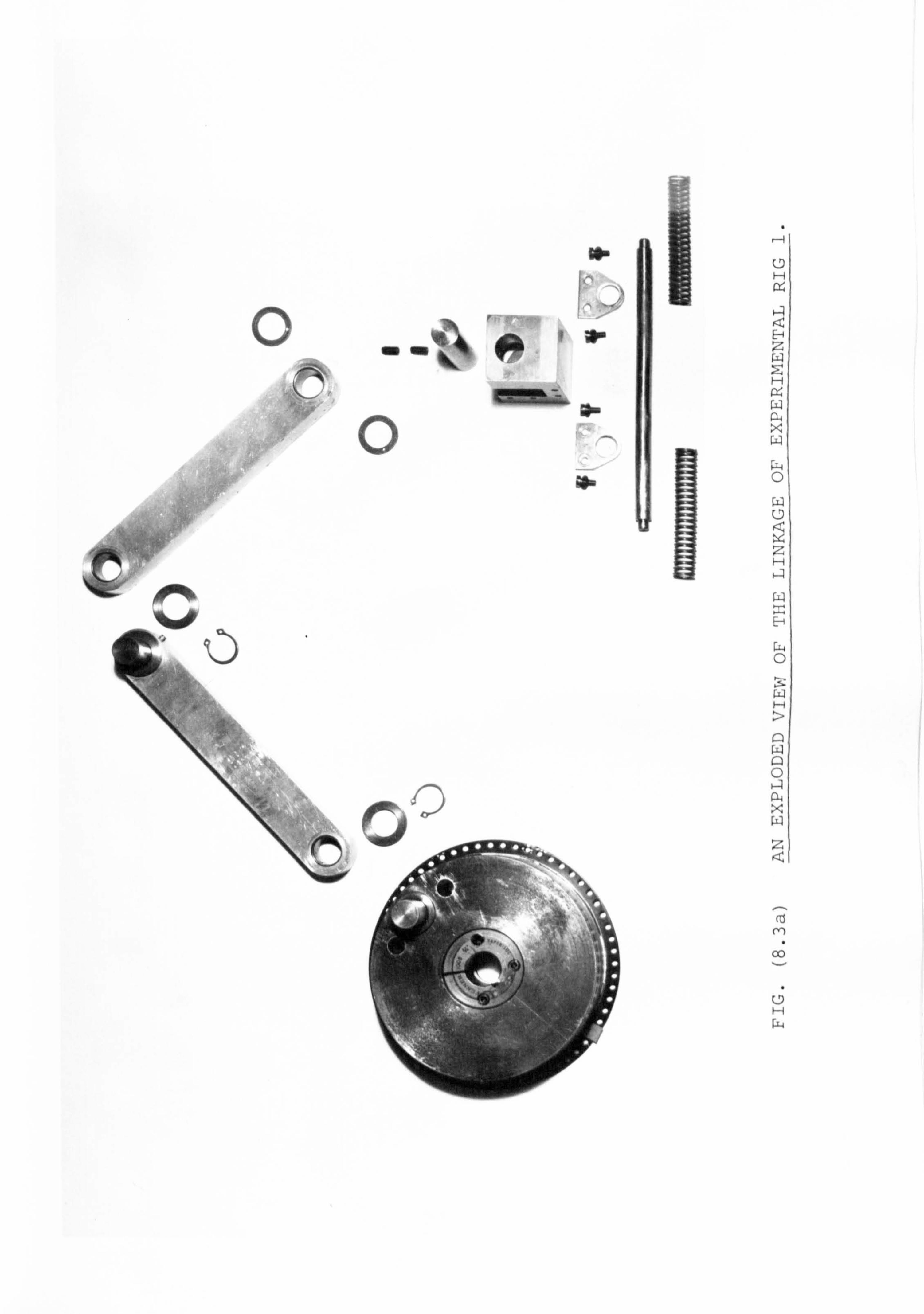
0 a
%MMA
" -IN
46 V4 ýý
0 CIEW6 a-
w
. -, H LY,
Z
H
X 41
F--1 0
wIh V
j
H
a w
w 0
0
a a X
2
c-fl
c-U
1a
Cj ID

Yh
low
j
a E-1 w H
w O w U
z H
w H
F14 0
Qi
0 a a X w z
M
H
ö
N N
ýýn 5
`' i
ý
.. r.
r, -- %10
-
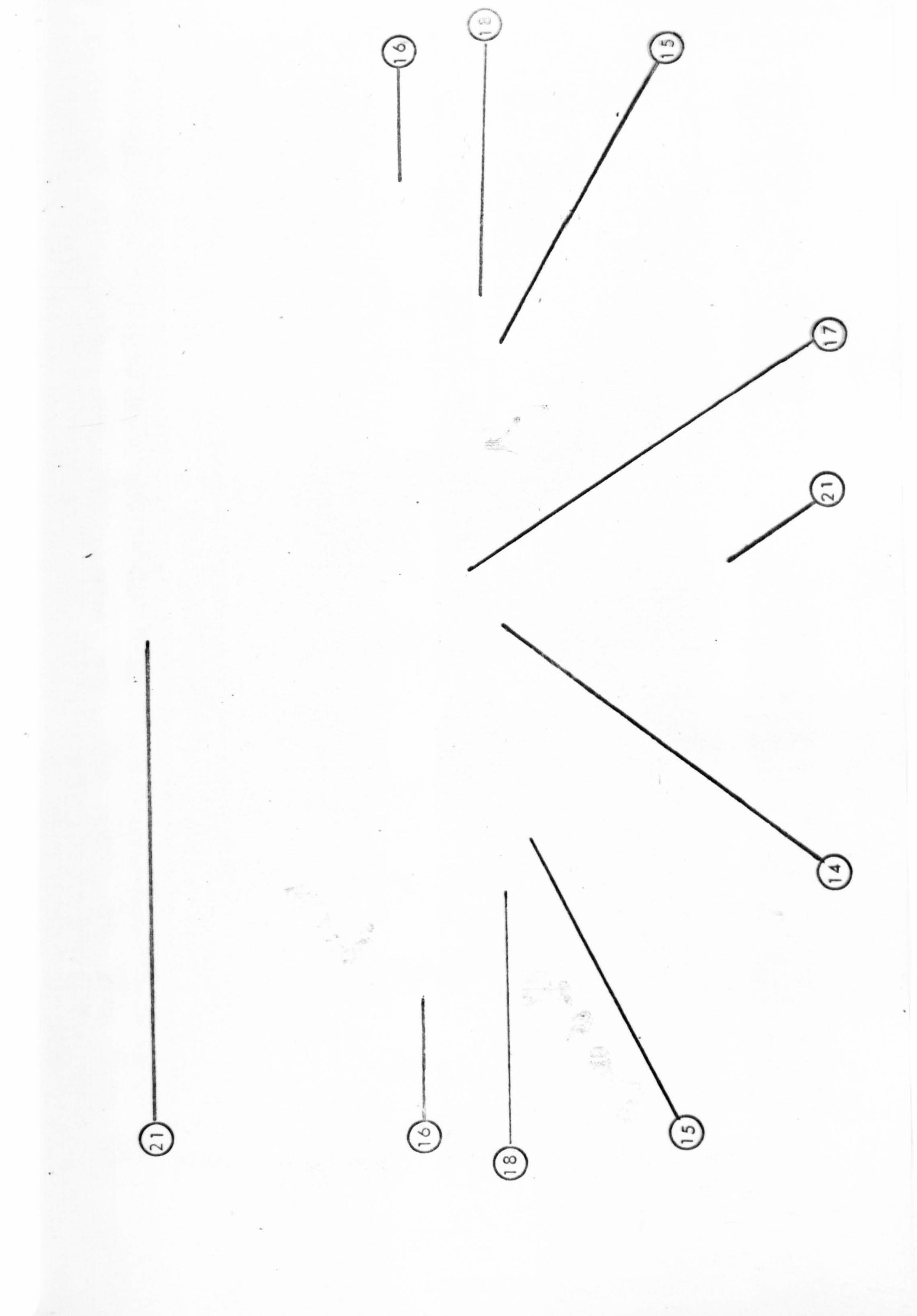
T
0
/, rý
0
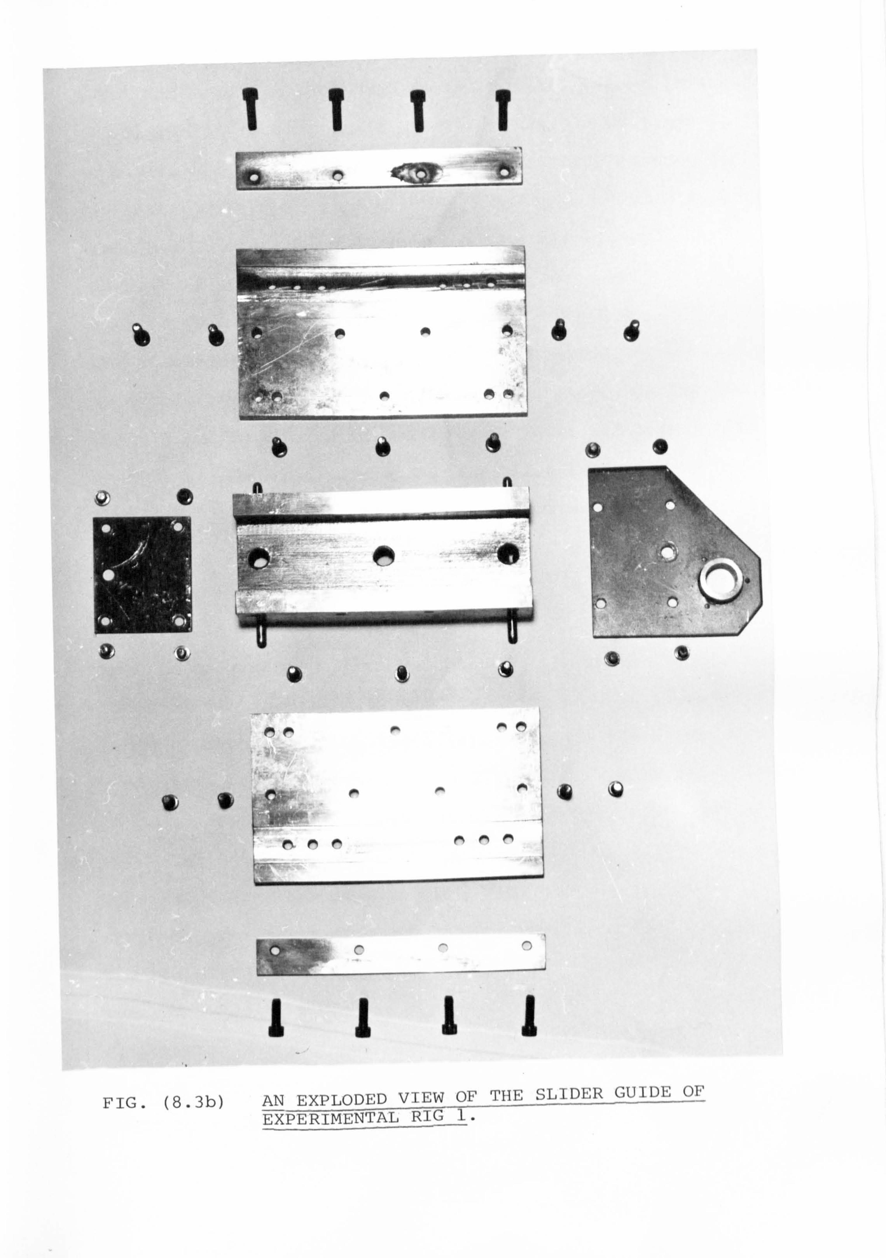
I1 TT
.:
6 64
aý Yý-ä km
low i
l1l1 FIG. (8.3b) AN EXPLODED VIEW OF THE SLIDER GUIDE OF
EXPERIMENTAL RIG 1.
604
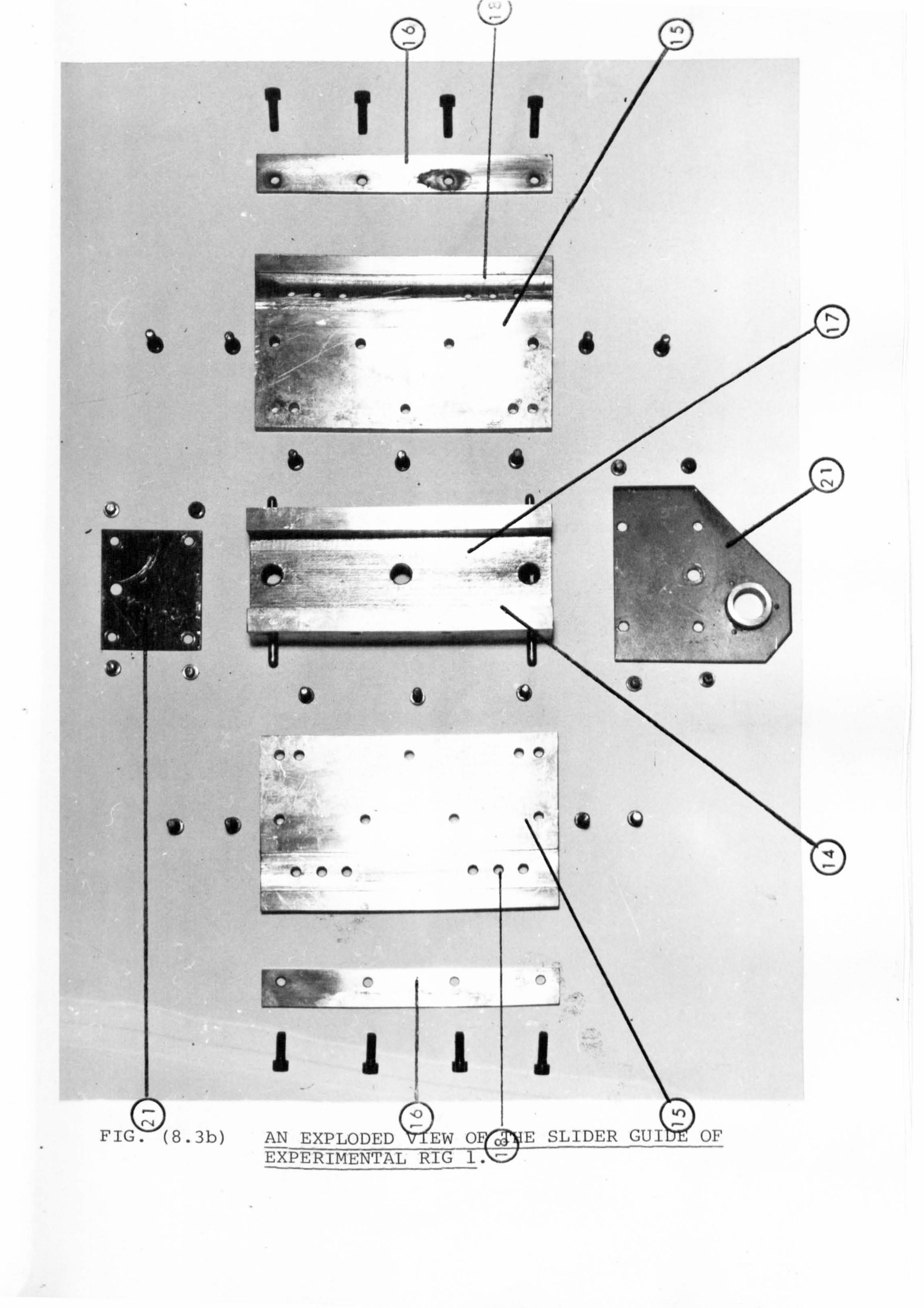
4
QI
Oft
91 Jow
es ný
ýn
I
4
014
l11 FIG (8.3b) AN EXPLODED
cýý
PIEW OF EXPERIMENTAL RIG 1.
i 0
T1 1
Il
AAA i.
. iýý ýA
r, / ýi
i SLIDER GUIDE OF
.-
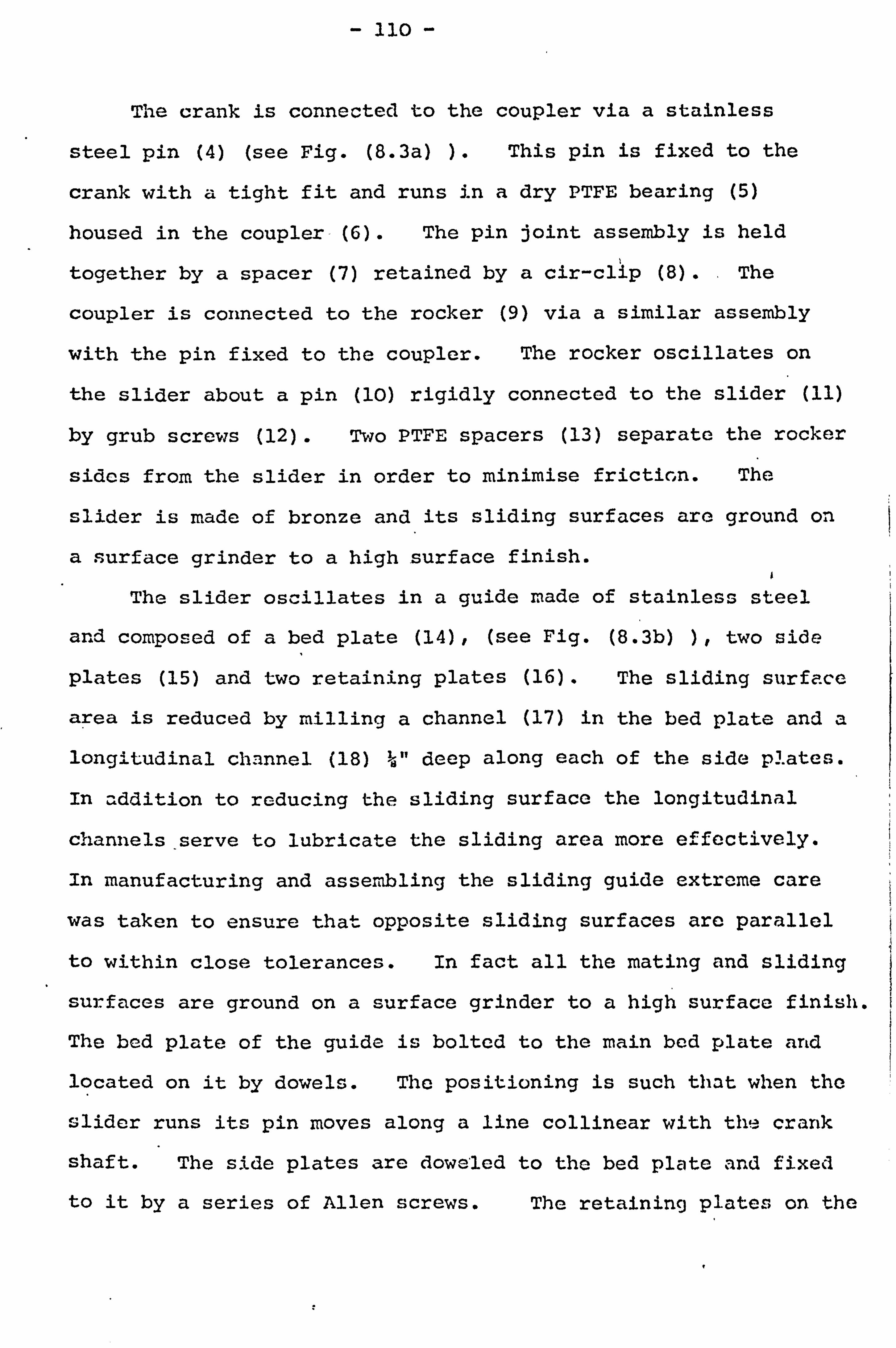
- lio -
The crank is connected to the coupler via a stainless
steel pin (4) (see Fig. (8.3a) ). This pin is fixed to the
crank with a tight fit and runs in a dry PTFE bearing (5)
housed in the coupler-(6). The pin joint assembly is held
together by a spacer (7) retained by a cir-clip (8). The
coupler is connected to the rocker (9) via a similar assembly
with the pin fixed to the coupler. The rocker oscillates on
the slider about a pin (10) rigidly connected to the slider (11)
by grub screws (12). Two PTFE spacers (13) separate the rocker
sides from the slider in order to minimise friction. The
slider is made of bronze and its sliding surfaces are ground on
a surface grinder to a high surface finish.
The slider oscillates in a guide made of stainless steel
and composed of a bed plate (14), (see Fig. (8.3b) ), two side
plates (15) and two retaining plates (16). The sliding surface
area is reduced by milling a channel (17) in the bed plate and a
longitudinal channel (18) d" deep along each of the side plates.
In addition to reducing the sliding surface the longitudinal
channels serve to lubricate the sliding area more effectively.
In manufacturing and assembling the sliding guide extreme care
was taken to ensure that opposite sliding surfaces are parallel
to within close tolerances. In fact all the mating and sliding
surfaces are ground on a surface grinder to a high surface finish.
The bed plate of the guide is bolted to the main bed plate and
located on it by dowels. The positioning is such that when the
slider runs its pin moves along a line collinear with the crank
shaft. The side plates are doweled to the bed plate and fixed
to it by a series of Allen screws. The retaining plates on the
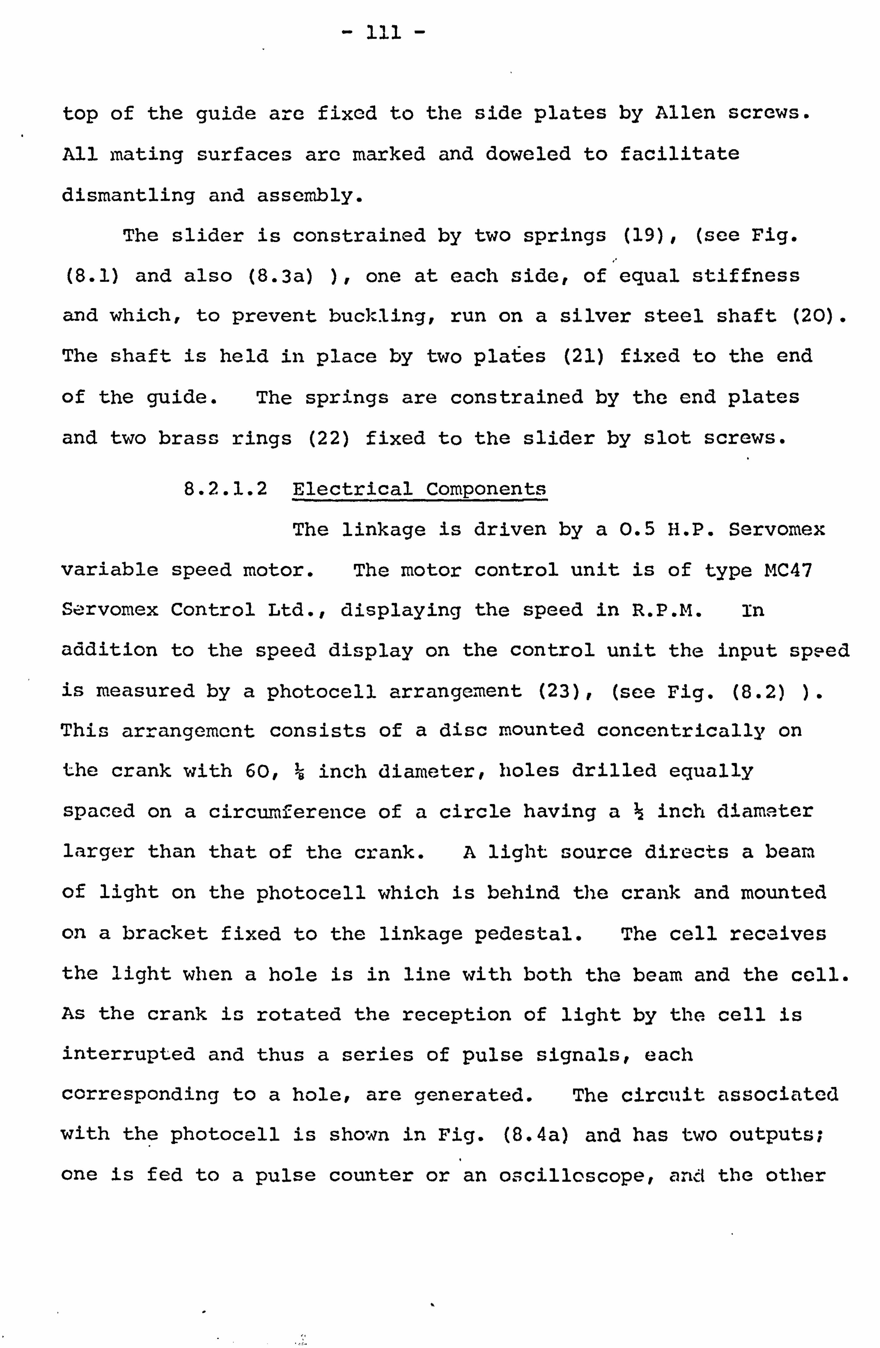
- 111 -
top of the guide are fixed to the side plates by Allen screws.
All mating surfaces are marked and doweled to facilitate
dismantling and assembly.
The slider is constrained by two springs (19), (see Fig.
(8.1) and also (8.3a) ), one at each side, of equal stiffness
and which, to prevent buckling, run on a silver steel shaft (20).
The shaft is held in place by two plates (21) fixed to the end
of the guide. The springs are constrained by the end plates
and two brass rings (22) fixed to the slider by slot screws.
8.2.1.2 Electrical Components
The linkage is driven by a 0.5 H. P. Servomex
variable speed motor. The motor control unit is of type MC47
S rvomex Control Ltd., displaying the speed in R. P. M. in
addition to the speed display on the control unit the input speed
is measured by a photocell arrangement (23), (see Fig. (8.2) ).
This arrangement consists of a disc mounted concentrically on
the crank with 60, B inch diameter, holes drilled equally
spaced on a circumference of a circle having ag inch diameter
larger than that of the crank. A light source directs a beam
of light on the photocell which is behind the crank and mounted
on a bracket fixed to the linkage pedestal. The cell receives
the light when a hole is in line with both the beam and the cell.
As the crank is rotated the reception of light by the cell is
interrupted and thus a series of pulse signals, each
corresponding to a hole, are generated. The circuit associated
with the photocell is shown in Fig. (8.4a) and has two outputs;
one is fed to a pulse counter or an oscilloscope, and the other
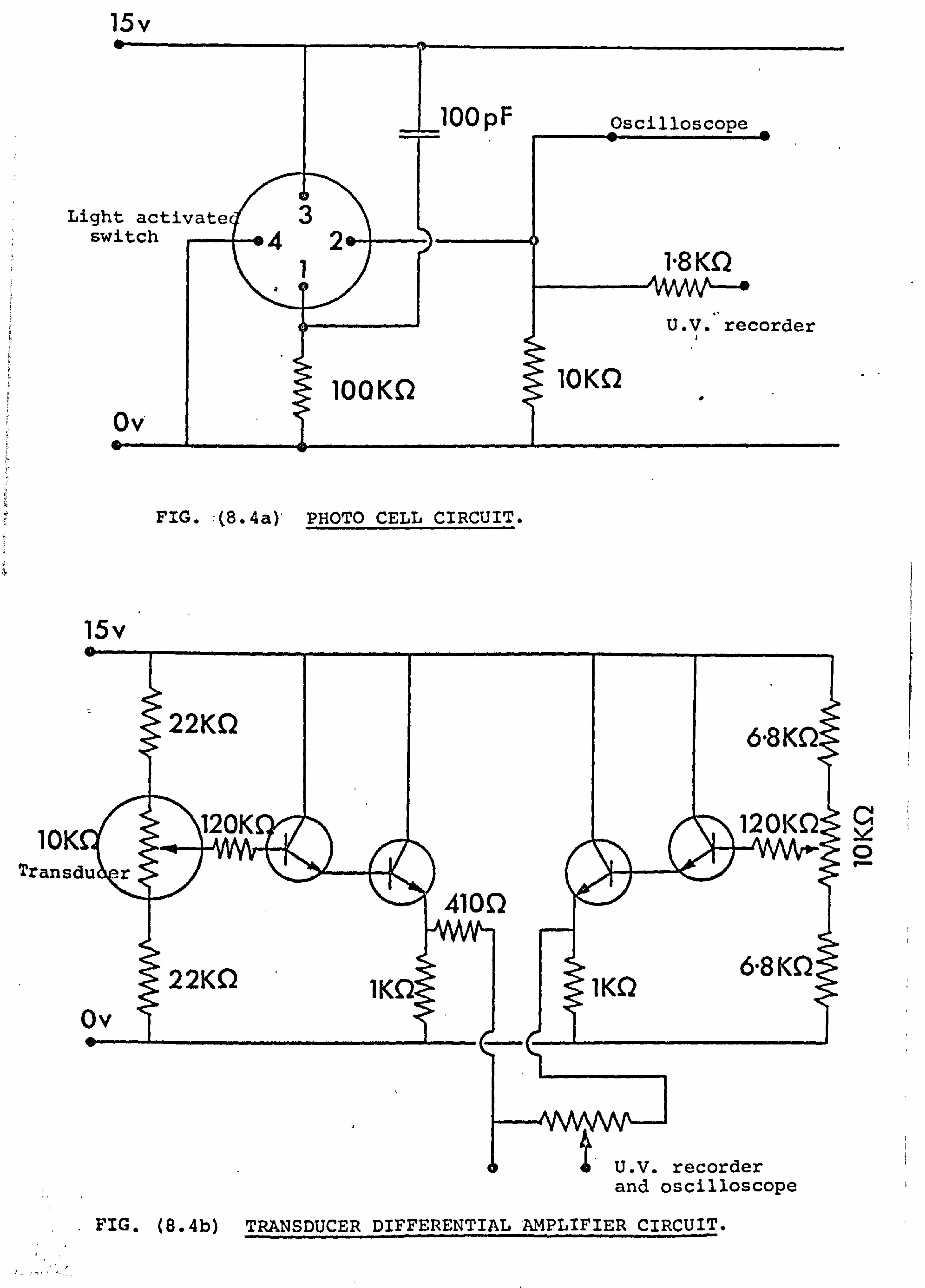
15v
Ligh sw
FIG. =(8.4a) PHOTO CELL CIRCUIT.
10 Tran,
and oscilloscope
15v
0
FIG. (8.4b) TRANSDUCER DIFFERENTIAL AMPLIFIER CIRCUIT.
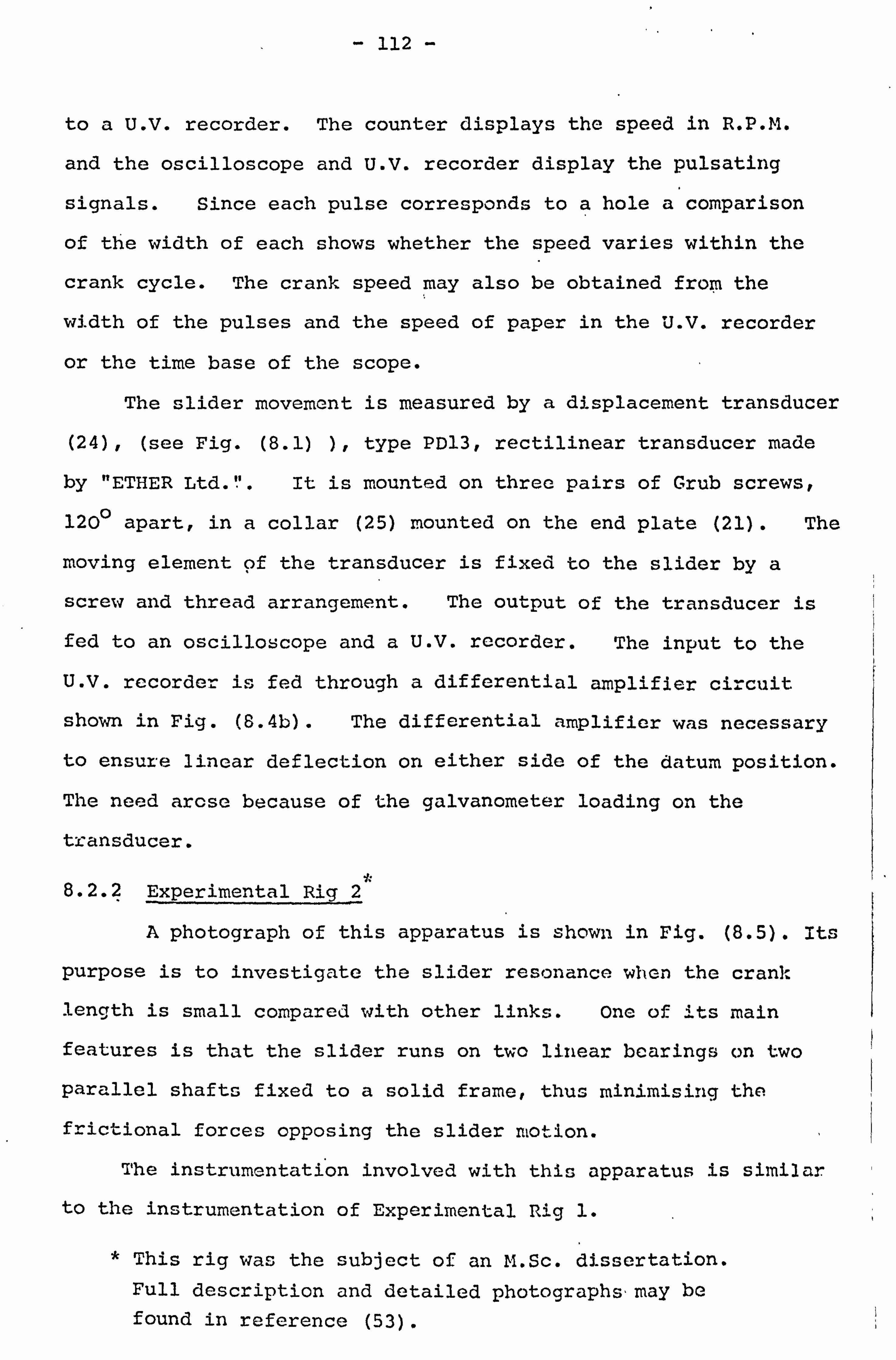
- 112 -
to a U. V. recorder. The counter displays the speed in R. P. M.
and the oscilloscope and U. V. recorder display the pulsating
signals. Since each pulse corresponds to a hole a comparison
of the width of each shows whether the speed varies within the
crank cycle. The crank speed may also be obtained from the
width of the pulses and the speed of paper in the U. V. recorder
or the time base of the scope.
The slider movement is measured by a displacement transducer
(24), (see Fig. (8.1) ), type PD13, rectilinear transducer made
by "ETHER Ltd. % it is mounted on three pairs of Grub screws,
120° apart, in a collar (25) mounted on the end plate (21). The
moving element of the transducer is fixed to the slider by a
screw and thread arrangement. The output of the transducer is
fed to an oscilloscope and a U. V. recorder. The input to the
U. V. recorder is fed through a differential amplifier circuit
shown in Fig. (8.4b). The differential amplifier was necessary
to ensure linear deflection on either side of the datum position.
The need arose because of the galvanometer loading on the
transducer.
8.2.2 Experimental Rig 2
A photograph of this apparatus is shown in Fig. (8.5). Its
purpose is to investigate the slider resonance when the crank
length is small compared with other links. One of its main
features is that the slider runs on two linear bearings on two
parallel shafts fixed to a solid frame, thus minimising the
frictional forces opposing the slider motion.
The instrumentation involved with this apparatus is similar.
to the instrumentation of Experimental Rig 1.
* This rig was the subject of an M. Sc. dissertation. Full description and detailed photographs may be found in reference (53).

I7
IL A54
iPf
FIG. (8.5) A GENERAL VIEW OF EXPERIMENTAL RIG 2.
... n y` ý
Aw
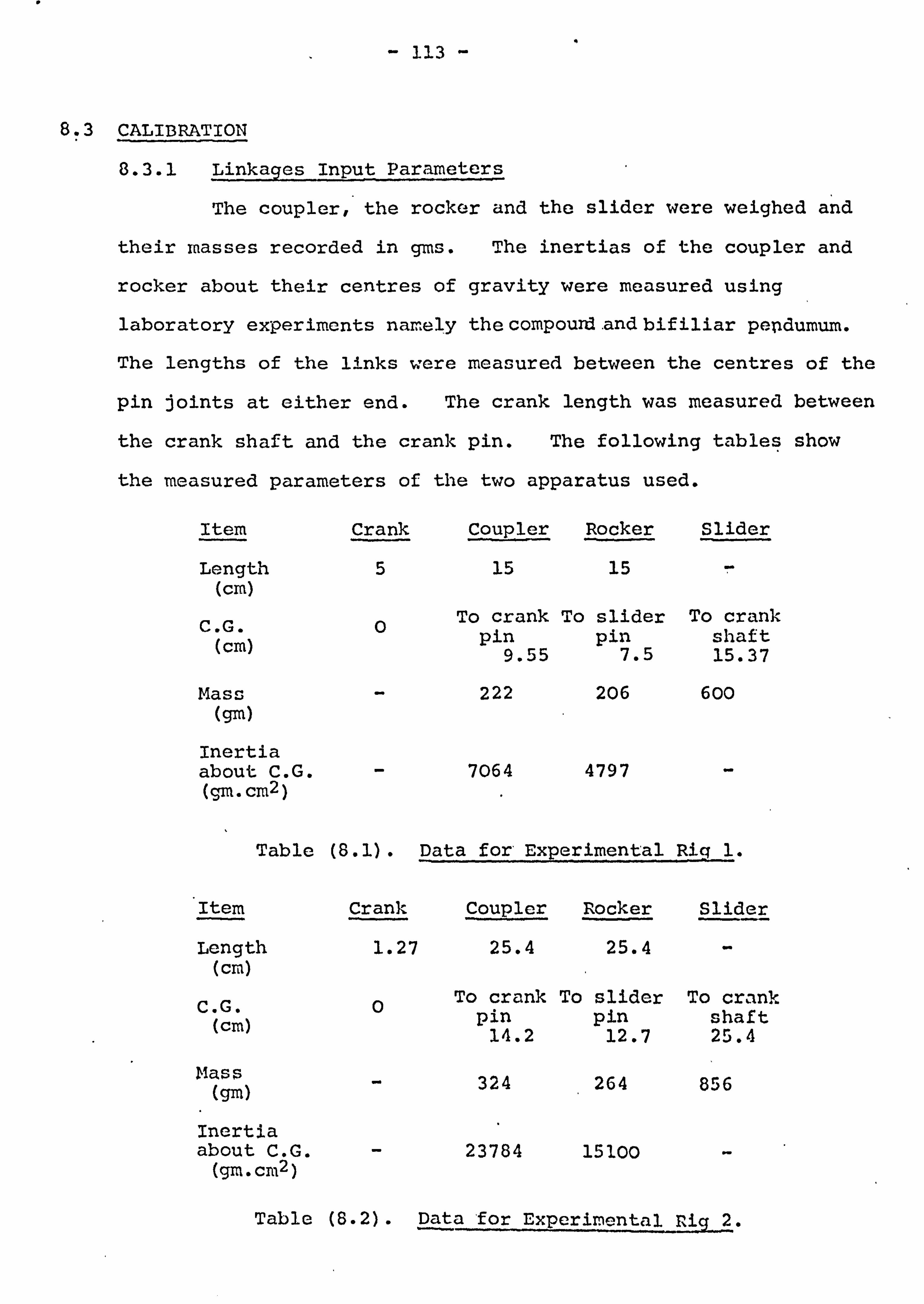
- 113 -
8.3 CALIBRATION
8.3.1 Linkages Input Parameters
The coupler, the rocker and the slider were weighed and
their masses recorded in gms. The inertias of the coupler and
rocker about their centres of gravity were measured using
laboratory experiments namely the compourd d-and bifiliar pelidumum.
The lengths of the links were measured between the centres of the
pin joints at either end. The crank length was measured between
the crank shaft and the crank pin. The following tables show
the measured parameters of the two apparatus used.
Item
Length (cm)
C. G. (cm)
Mass
(gm) Inertia about C. G. (gm. cm2)
Crank Coupler Rocker Slider
5 15 15 71
0 To crank To slider To crank pin pin shaft
9.55 7.5 15.37
- 222 206 600
- 7064 4797 -
Table (8.1). Data for' Experimental Rig1.
Item Crank Coupler Rocker Slider
Length 1.27 25.4 25.4 (cm)
C. G. 0 To crank To slider To crank
(cm) pin pin shaft 14.2 12.7 25.4
Mass - 324 264 856 (gm)
Inertia about C. G. - 23784 15100 - (gm. cm2 )
Table (8.2). Data for Experimental Rig 2.
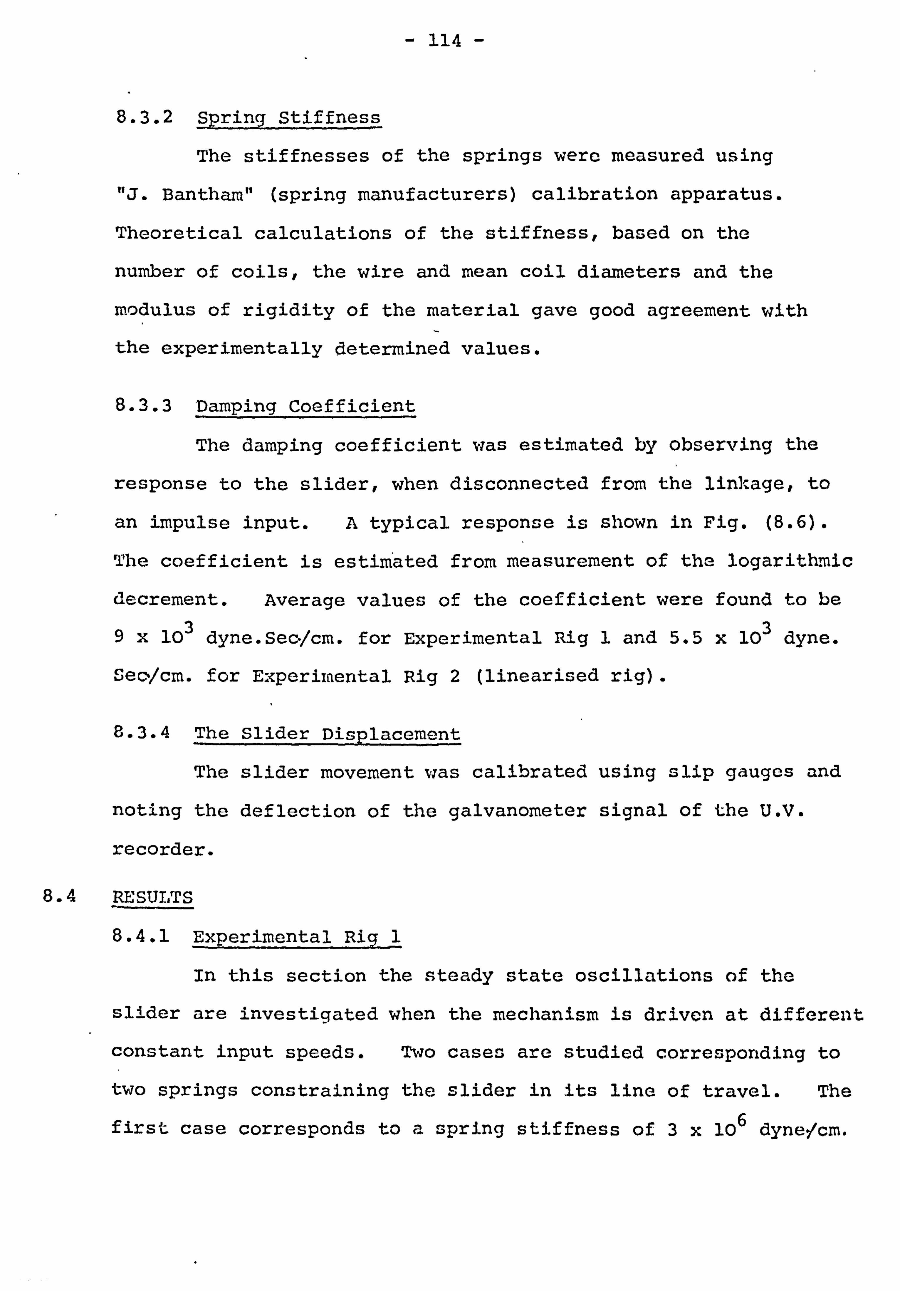
- 114 -
8.3.2 Spring Stiffness
The stiffnesses of the springs were measured using
"J. Bantham" (spring manufacturers) calibration apparatus.
Theoretical calculations of the stiffness, based on the
number of coils, the wire and mean coil diameters and the
modulus of rigidity of the material gave good agreement with
the experimentally determined values.
8.3.3 Damping Coefficient
The damping coefficient was estimated by observing the
response to the slider, when disconnected from the linkage, to
an impulse input. A typical response is shown in Fig. (8.6).
The coefficient is estimated from measurement of the logarithmic
decrement. Average values of the coefficient were found to be
9x 10³ dyne. Sec/cm. for Experimental Rig 1 and 5.5 x 10³ dyne.
Sec'/cm. for Experimental Rig 2 (linearised rig).
8.3.4 The Slider Displacement
The slider movement was calibrated using slip gauges and
noting the deflection of the galvanometer signal of the U. V.
recorder.
8.4 RESULTS 8.4.1 Experimental Rig 1
In this section the steady state oscillations of the
slider are investigated when the mechanism is driven at different
constant input speeds. Two cases are studied corresponding to
two springs constraining the slider in its line of travel. The
first case corresponds to a spring stiffness of 3x 10⁶ dyne/cm.
N
0 W-
i
v
c) " (L
N
7
I
u n,
Cl v) Cl) Cl t: )
apn4! dwy apfl ! 1dwy
z H U H
w O U
z H P+
ul
00
C9
CO)
- 115 -
and the second to a stiffness of 11 x 106 dyne/cm. The
first spring will be referred to as spring A and the second
as spring B. The results are compared with those obtained
using the theory developed in Chapters II and III.
1 8.4.1.1 Comparison of Experimental and Theoretical Results
The theory predicts the steady state slider motion
to be oscillatory and periodic with one crank cycle. This
is verified experimentally as shown in Fig. (8.7) in which a
typical experimentally observed steady state motion of the
slider is shown against the crank angle. The particular
motion shown in this figure is obtained with spring A and a
constant crank speed of 360 RPM. However, for all other speeds,
using this spring and also spring B, the motion was always
periodic with one crank cycle.
In order to investigate the agreement between the
experimental and theoretical results the slider experimental
steady state motion was recorded, at a number of speeds below
the natural frequency, with both springs A and B and compared
with the theoretical motion. For illustration purposes the
comparison shown in here is at a selection of these speeds only.
These are 390,420 and 450 RPM with spring A and 600,660 and
720 RPM with spring B. The choice of these speeds was arbitrary
and only one slider oscillation corresponding to one crank cycle
is shown at each speed. The results with spring A are shown in
Figs. (8.8), (8.9) and (8.10) and with spring B in Figs. (8.11),
(8.12) and (8.13).
As may be seen from Figs. (8.8), (8.9) and (8.10) the
theoretical and experimental results are in good agreement in

s C-4
: Z: cL
O ýO cý
H
O a
2 H
H 0
Z 0 H
O Z
a H
H
E4 U)
H
ýi
I N co .6
H GJ+
w, apn4! ldwy
'n 0 to ) NN
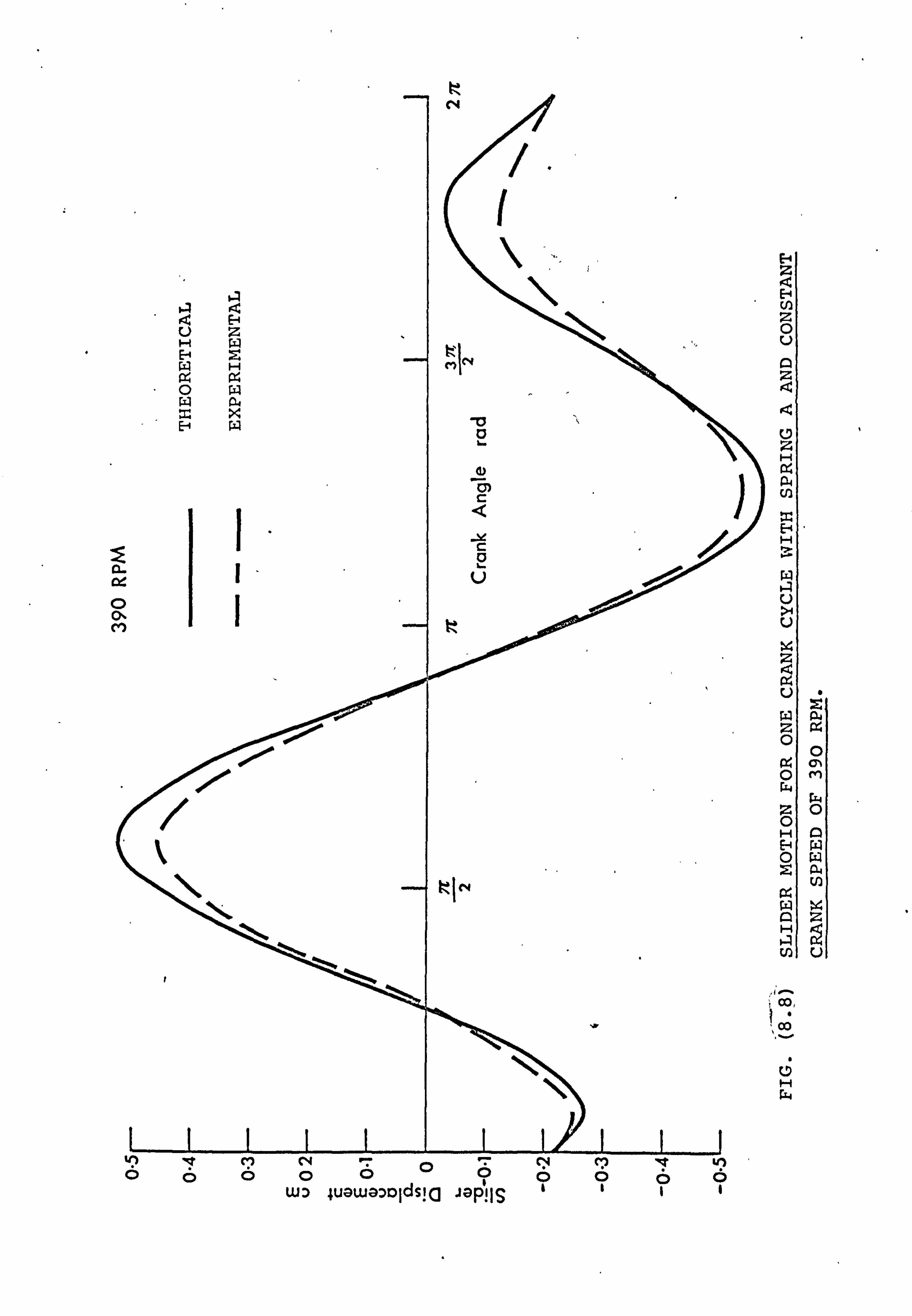
k
i c c c c
H z Q
uJ z 0 V
z
C7 z H
a a
H H
V
V
U
w z 0 x 0 w z 0 H H 0 z
H
Ua
Co,
H W
0 M
W O
U7
z
U
hv C) C4 ý7 pN C7 `I h 6pO00O
WD 4uawa, o dsid JOP! IS oO oI
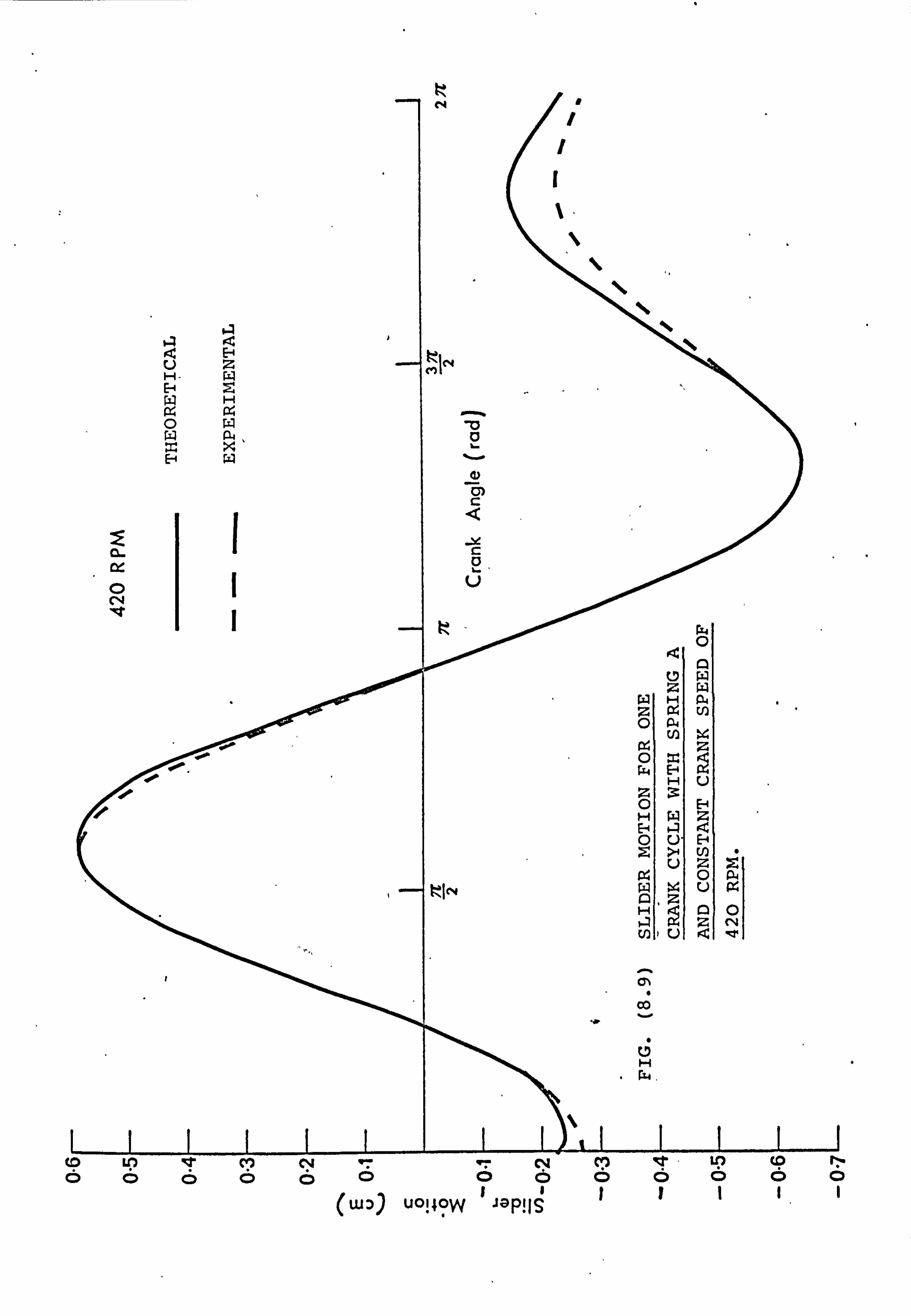
t+
t0 u') qt MN q" r' CV C7 a' > 1.9 9 9,121 ÖpOppOOÖOÖOÖO
(wa) U0140W JapiIs I1I1
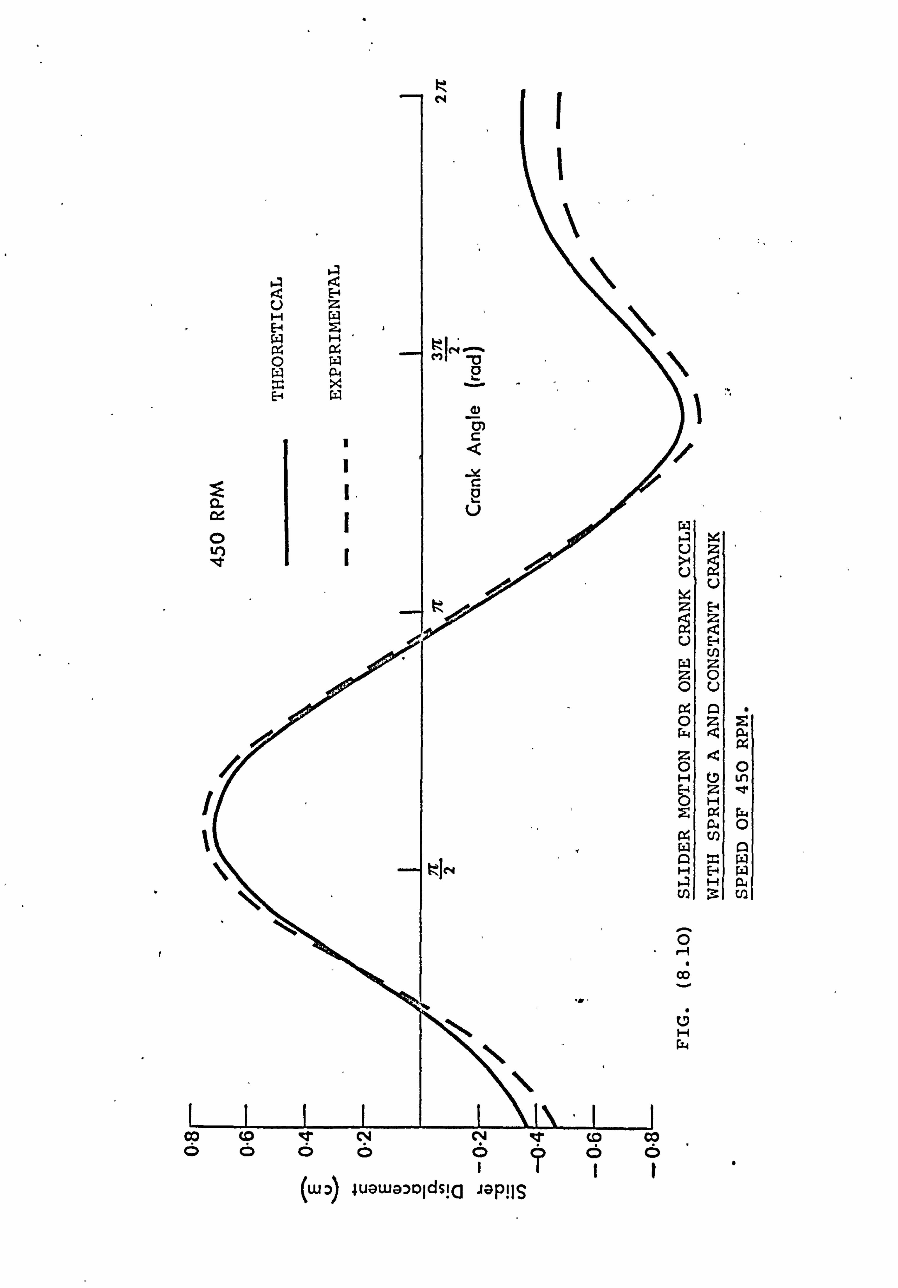
LO
1
I
x
U 5-1
H
Ö'
Ui
t9 2 H
H H 3
) i
7 i 4
Q
C u IC:
rz C
a u
0
co O qt N qt CO Co ÖÖÖOÖQÖÖ
111
ýuaý} 4uaw olds! Q JaP! IS
t
- 116 -
both phase and amplitude. It can however be observed that
while the phase is almost in total agreement the amplitude shows
slight variations. This may be explained by the fact that the
frictional forces opposing the slider motion are considered
solely viscous in the theory. However in practice these
frictional forces are a combination of viscous and Coloumb
friction forces, although in this experiment the viscous forces
are dominant. Because a Coloumb friction force varies with the
normal force and since in this experiment this normal force,
which is the vertical force in the rocker-slider joint, varies
with crank speed and also within a crank cycle, this explains
the difference in amplitude between the theoretical and
experimental motions with variation of crank speed and also
within one crank cycle. Other factors contributing to the
difference are (a) only an average estimation of the damping
coefficient is considered in the theory and (b) the friction in
the pin joints of the linkage is also ignored in the theory.
Figs. (8-11), (8.12) and (8.13) show the selection of
experimentally observed slider oscillations compared with
corresponding theoretical results obtained with spring B and
corresponding to crank speeds of 600,660 and 720 RPM respectively.
As may be seen the theoretical and experimental results are
almost in total agreement in phase. The agreement in amplitude
is, however, not as good but nevertheless reasonable. The
differences may be attributed to the same factors as previously
described with spring A.
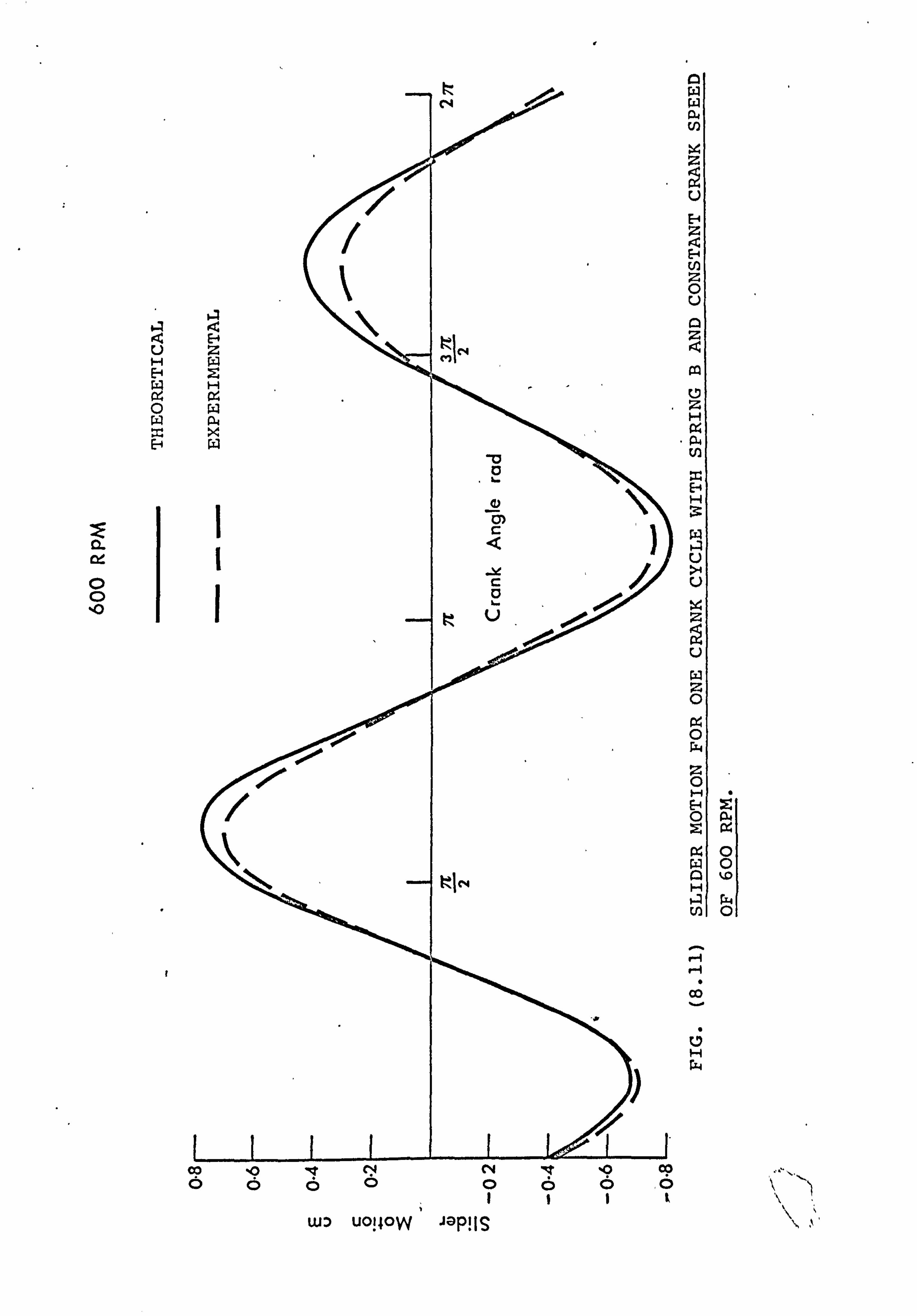
:: E Q
O O O
U H H
0
H
I
6.
UI z
9 U
H z a H W z 0 U
as
z H
a a U)
E-4 H
U
U
x z
9 U
w z 0
a 0 P4
z 0 H H 0
H
U)
0 0
w 0
c7 H W
ýý ý ýl ýý,
Co .p er NN et 'O CO ÖÖpO0ÖO0
11
W u0! 40W Jap! IS
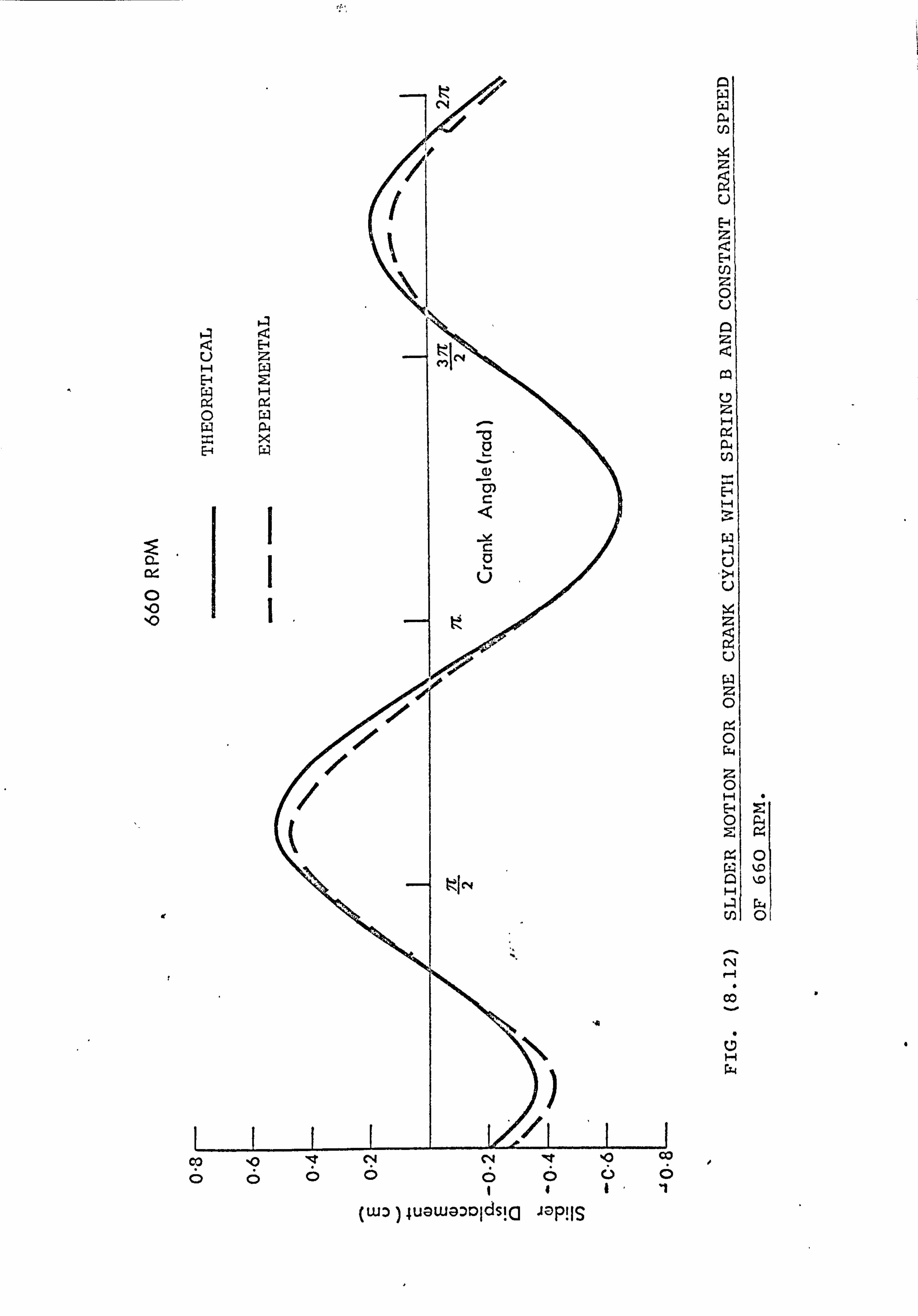
Q a'
0
9
r
a
U E-1
E-i
z 0 U
A z
z H
ELI Ei
H
1.4 U
U x z 9 U
W z 0 a 0 w z 0 H H 0 z
A H
U)
0
w 0
N e--I
aD
C7 H w
I Co 10 Q cv cr vv -r ÖOOOOOUO
1( `1
(w D) 4uawaDolds! Q aaP! IS
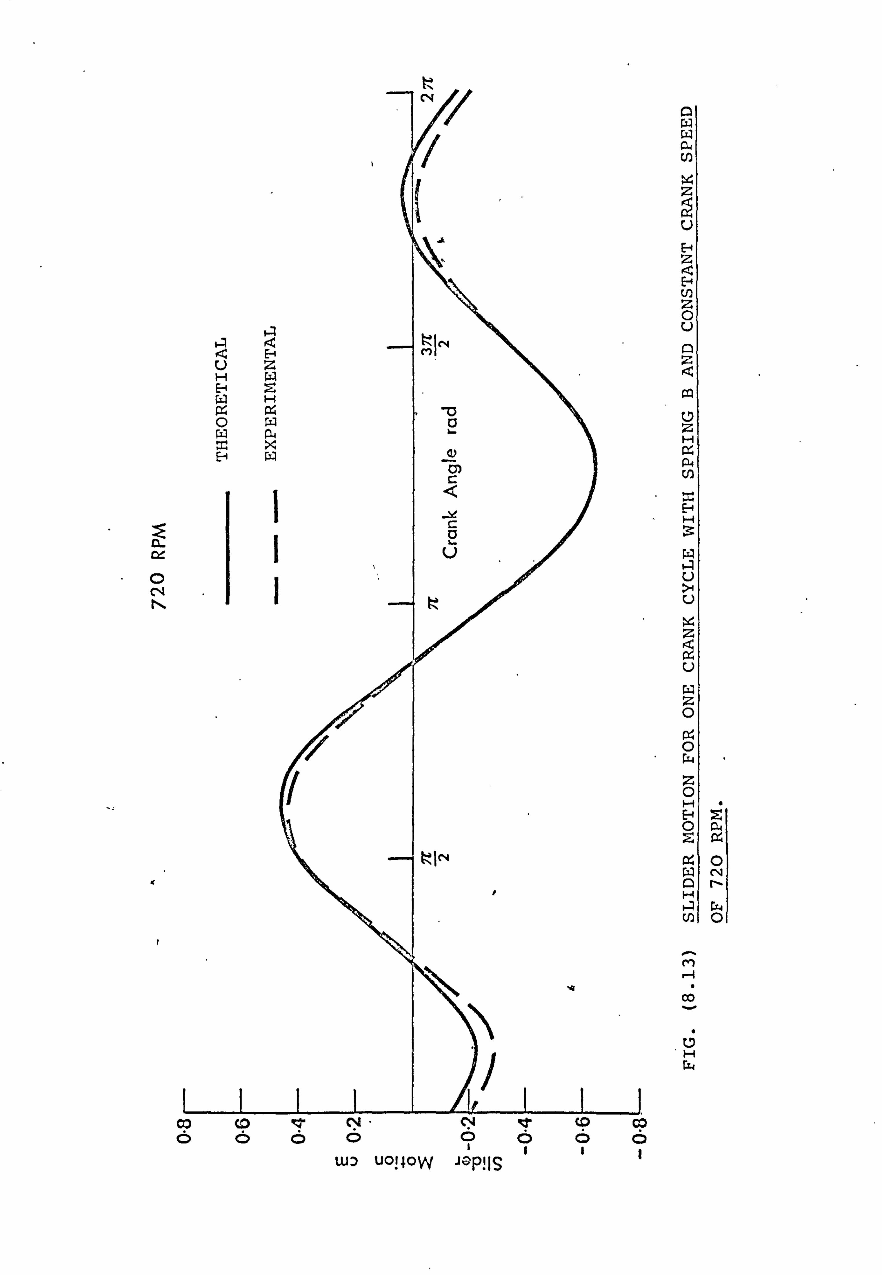
K
ä
0 N
K
r
E4 z l< N U) z O U
CqI
C7.
a U)
z O
P., O w z O H H O z
a co
0 N r-
W 0
M H
C9 H W
Co (P le c9 "N ýt tD p pppÖOpOÖ
11 WD UOI4OW Jo P! IS
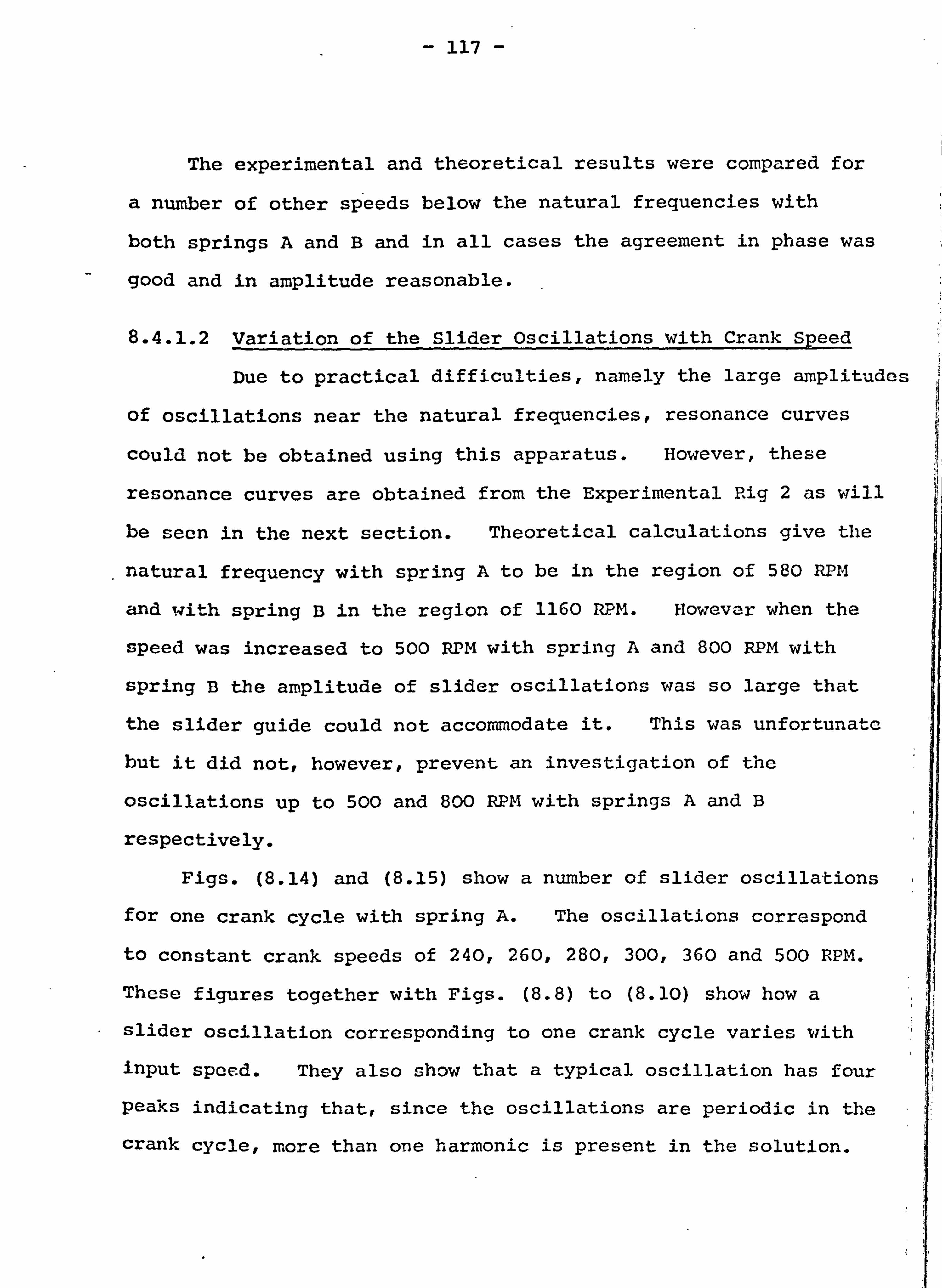
- 117 -
The experimental and theoretical results were compared for
a number of other speeds below the natural frequencies with
both springs A and B and in all cases the agreement in phase was
good and in amplitude reasonable.
8.4.1.2 Variation of the Slider Oscillations with Crank Speed
Due to practical difficulties, namely the large amplitudes
of oscillations near the natural frequencies, resonance curves
could not be obtained using this apparatus. However, these
resonance curves are obtained from the Experimental Rig 2 as will
be seen in the next section. Theoretical calculations give the
natural frequency with spring A to be in the region of 580 RPM
and with spring B in the region of 1160 RPM. However when the
speed was increased to 500 RPM with spring A and 800 RPM with
spring B the amplitude of slider oscillations was so large that
the slider guide could not accommodate it. This was unfortunate
but it did not, however, prevent an investigation of the
oscillations up to 500 and 800 RPM with springs A and B
respectively.
Figs. (8.14) and (8.15) show a number of slider oscillations
for one crank cycle with spring A. The oscillations correspond
to constant crank speeds of 240,260,280,300,360 and 500 RPM.
These figures together with Figs. (8.8) to (8.10) show how a
slider oscillation corresponding to one crank cycle varies with
input speed. They also show that a typical oscillation has four
peaks indicating that, since the oscillations are periodic in the
crank cycle, more than one harmonic is present in the solution.
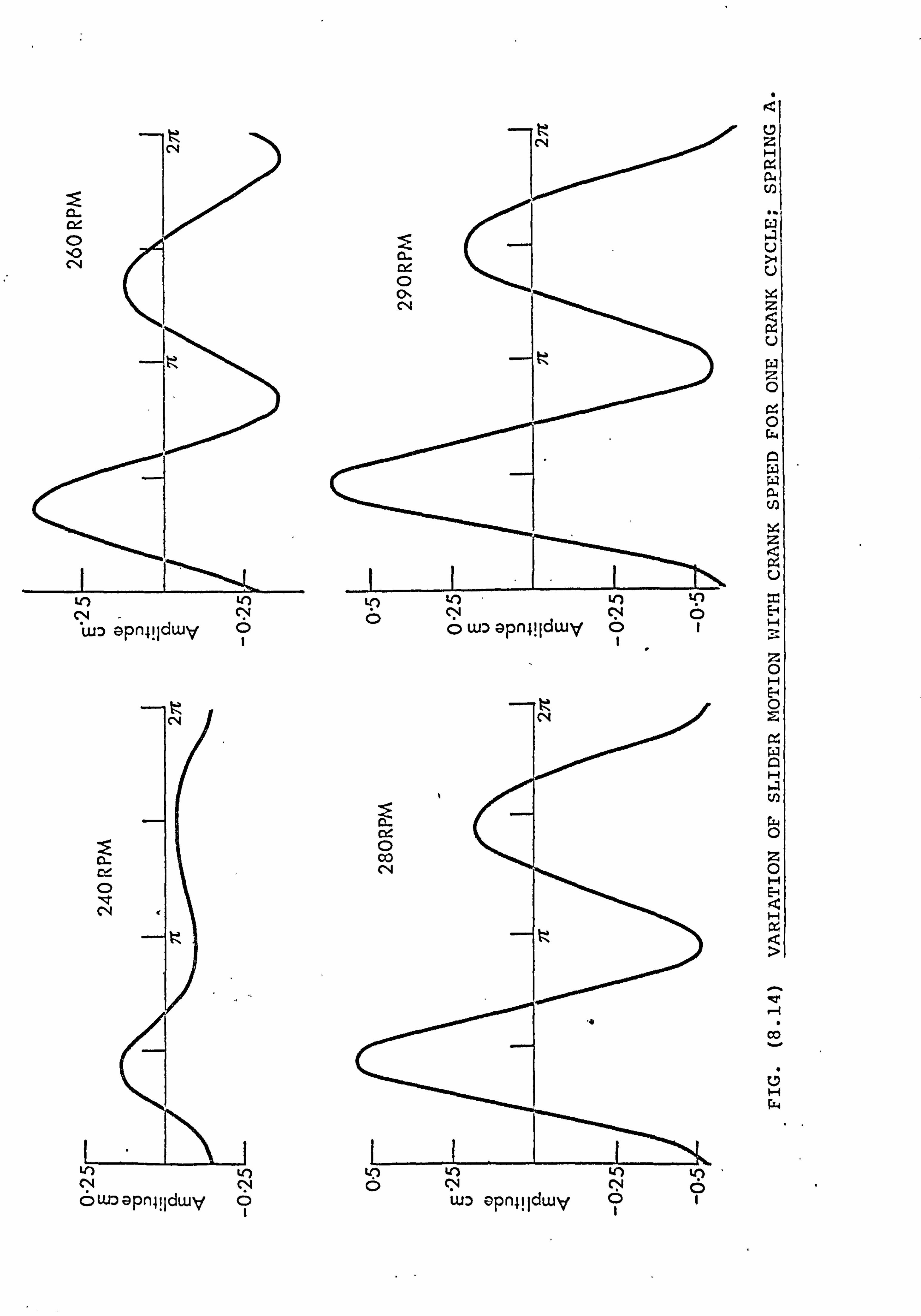
c9 z H
a
U
U
x zl 9 U
0 C4 0 w
a
U
H H
zi 0 H
H 0 z
H
w 0 z 0 H H
H
ca
6 H
LP LO LO L) 0 (V CV
o wD apn4! idwy o of
i
LO (N CV
L u: ) 1
LO LO to K) 0NNp
WD v^pf 4! 1dWy O
to NN tr) 6w: ) apn49dwy
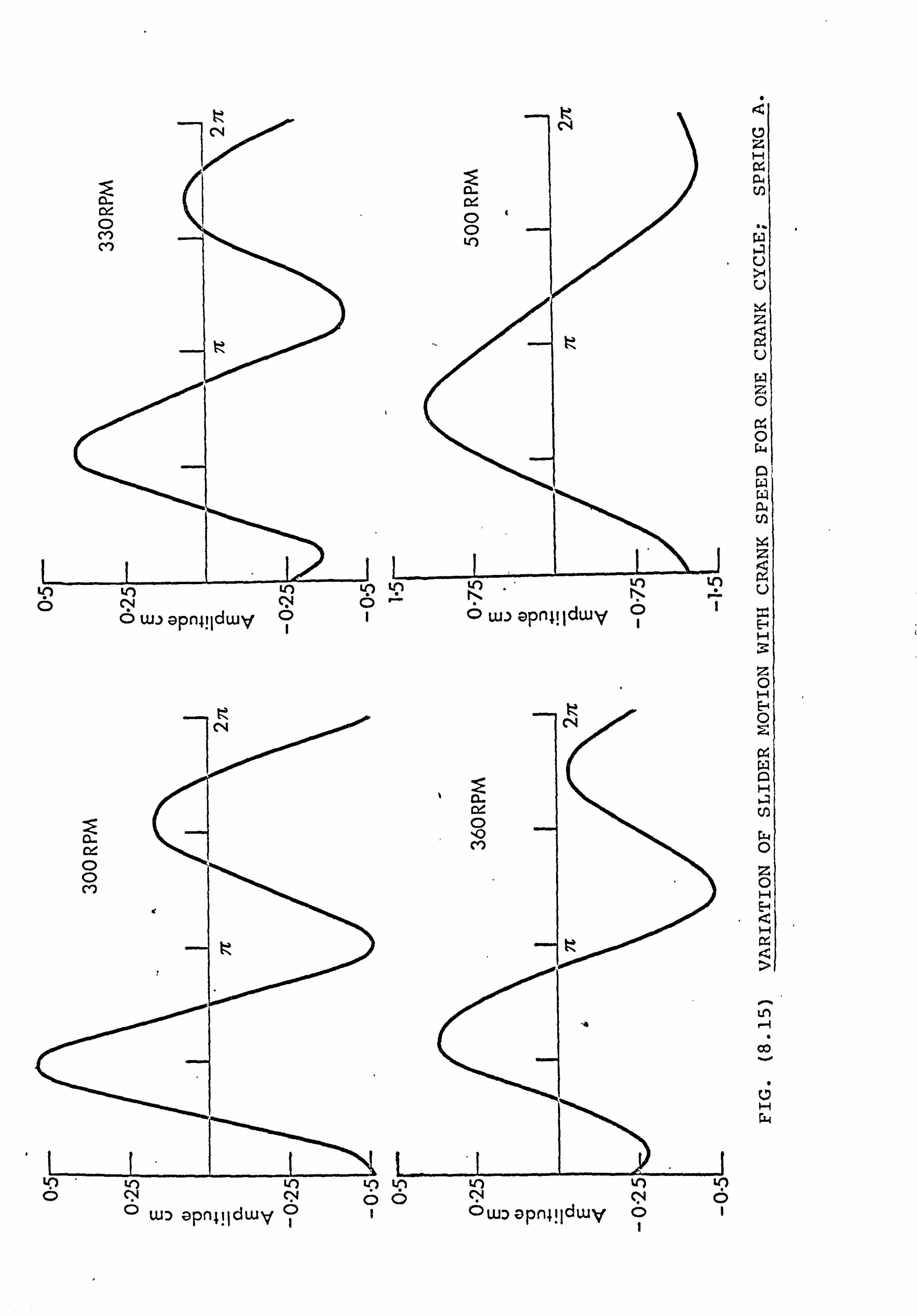
t-b 4 c7
H
a ri)
tmb Lý
U 7"1 U
z
9 U
WI z 0
C4 0
LLI
U
F H
z 0 H
0
H
w 0 z 0 H F
H
o- Ln r-q
V
C7 H
w
L)L OC 1
La. ' apnli lduay 01 1 '
owe opn4ildwy öi i
w: ) apn}iIdwy 0
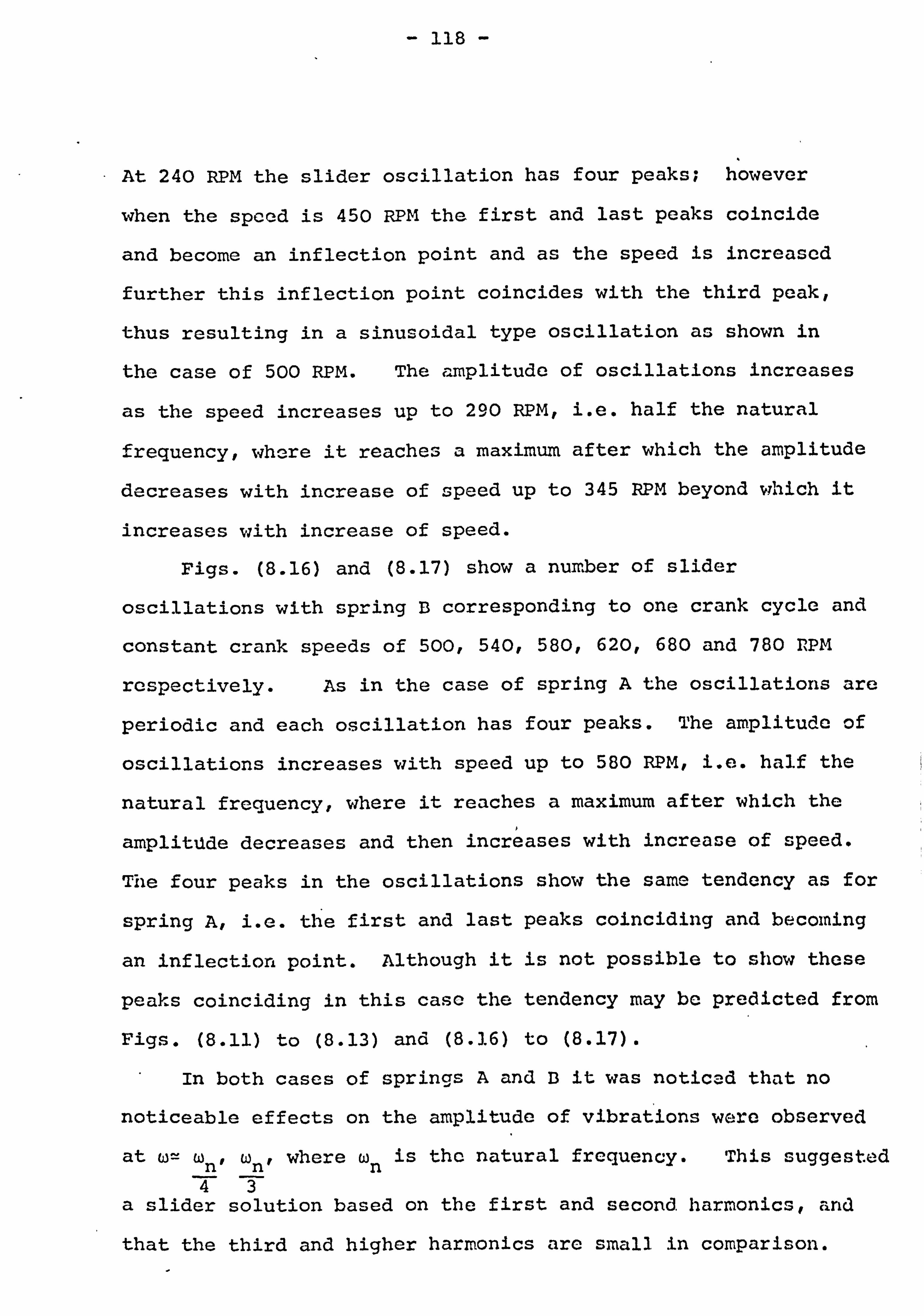
- 118 -
At 240 RPM the slider oscillation has four peaks; however
when the speed is 450 RPM the first and last peaks coincide
and become an inflection point and as the speed is increased
further this inflection point coincides with the third peak,
thus resulting in a sinusoidal type oscillation as shown in
the case of 500 RPM. The amplitude of oscillations increases
as the speed increases up to 290 RPM, i. e. half the natural
frequency, where it reaches a maximum after which the amplitude
decreases with increase of speed up to 345 RPM beyond which it
increases with increase of speed.
Figs. (8.16) and (8.17) show a number of slider
oscillations with spring B corresponding to one crank cycle and
constant crank speeds of 500,540,580,620,680 and 780 RPM
respectively. As in the case of spring A the oscillations are
periodic and each oscillation has four peaks. The amplitude of
oscillations increases with speed up to 580 RPM, i. e. half the
natural frequency, where it reaches a maximum after which the
amplitude decreases and then increases with increase of speed.
The four peaks in the oscillations show the same tendency as for
spring A, i. e. the first and last peaks coinciding and becoming
an inflection point. Although it is not possible to show these
peaks coinciding in this case the tendency may be predicted from
Figs. (8.11) to (8.13) and (8.16) to (8.17).
In both cases of springs A and B it was noticd that no
noticeable effects on the amplitude of vibrations were observed
at w= wn, wn, where wn is the natural frequency. This suggested 43
a slider solution based on the first and second. harmonics, and
that the third and higher harmonics are small in comparison.

oa
U) o ö0
LO Lo CV p ÖIO
LO tn 41 -11 cV Np p0
wD apn4! ldwy
U z H
a
U
U
u
z
0
OI L4 Ca W W C+
z u
Ow 1H
H
z 0 I
H
"v
w apn4! Idwy
t-
c
r
to v? 0 to v7 v) OpO Oj O
wD apn4! 1dwy
10') N0N to Opp Oj O
w) apn4! Idwy
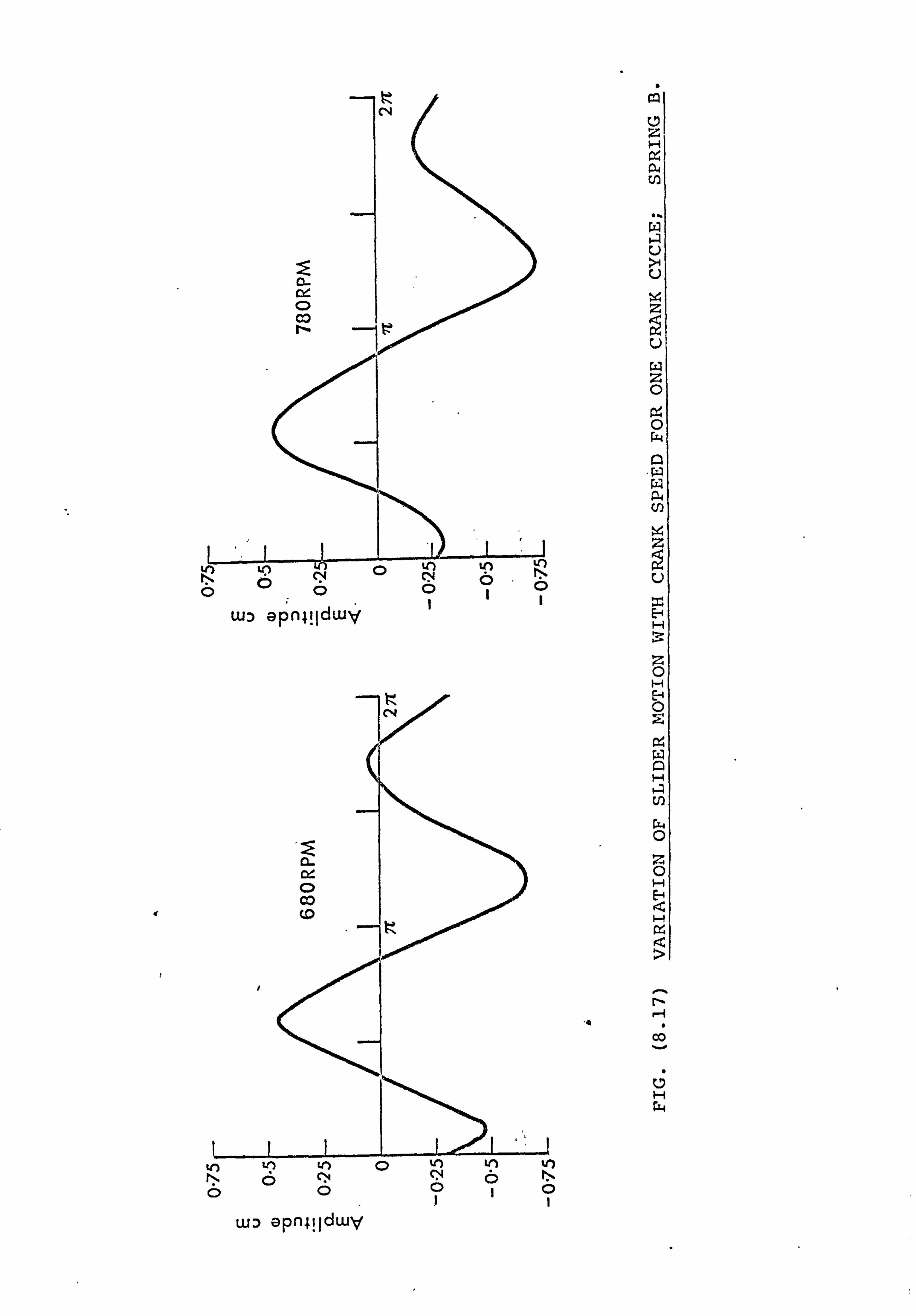
Cl C
F P P U
f
I
U
U
z
U
z 0
0
Z
n
00
H w
wD apn4! Idwy
LO (V
0 'n N
OO00 Oj
W: ) apn;! Idwy
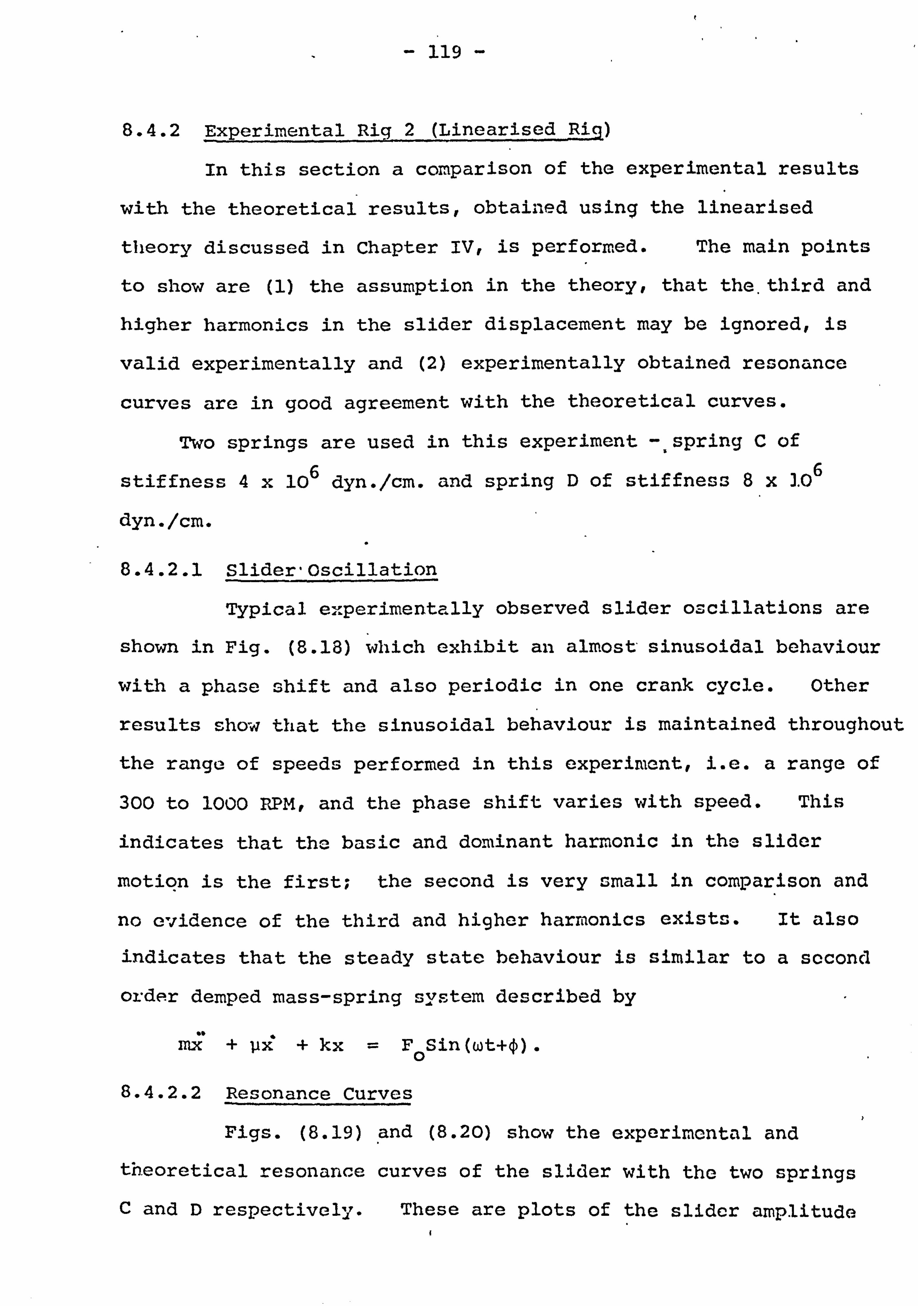
r
- 119 -
8.4.2 Experimental Rig 2 (Linearised Rig)
In this section a comparison of the experimental results
with the theoretical results, obtained using the linearised
theory discussed in Chapter IV, is performed. The main points
to show are (1) the assumption in the theory, that the. third and
higher harmonics in the slider displacement may be ignored, is
valid experimentally and (2) experimentally obtained resonance
curves are in good agreement with the theoretical curves.
Two springs are used in this experiment -=spring C of
stiffness 4x 10⁶ dyn. /cm. and spring D of st iffness 8x ]. 06
dyn. /cm.
8.4.2.1 Slider-Oscillation
Typical experimentally observed slider oscillations are
shown in Fig. (8.18) which exhibit an almost sinusoidal behaviour
with a phase shift and also periodic in one crank cycle. Other
results show that the sinusoidal behaviour is maintained throughout
the range of speeds performed in this experiment, i. e. a range of
300 to 1000 RPM, and the phase shift varies with speed. This
indicates that the basic and dominant harmonic in the slider
motion is the first; the second is very small in comparison and
no evidence of the third and higher harmonics exists. It also
indicates that the steady state behaviour is similar to a second
order demped mass-spring system described by
. mx + ux + kx =F0 Sin (wt+fl '"
8.4.2.2 Resonance Curves
Figs. (8.19) and (8.20) show the experimental and
theoretical resonance curves of the slider with the two springs
C and D respectively. These are plots of the slider amplitude
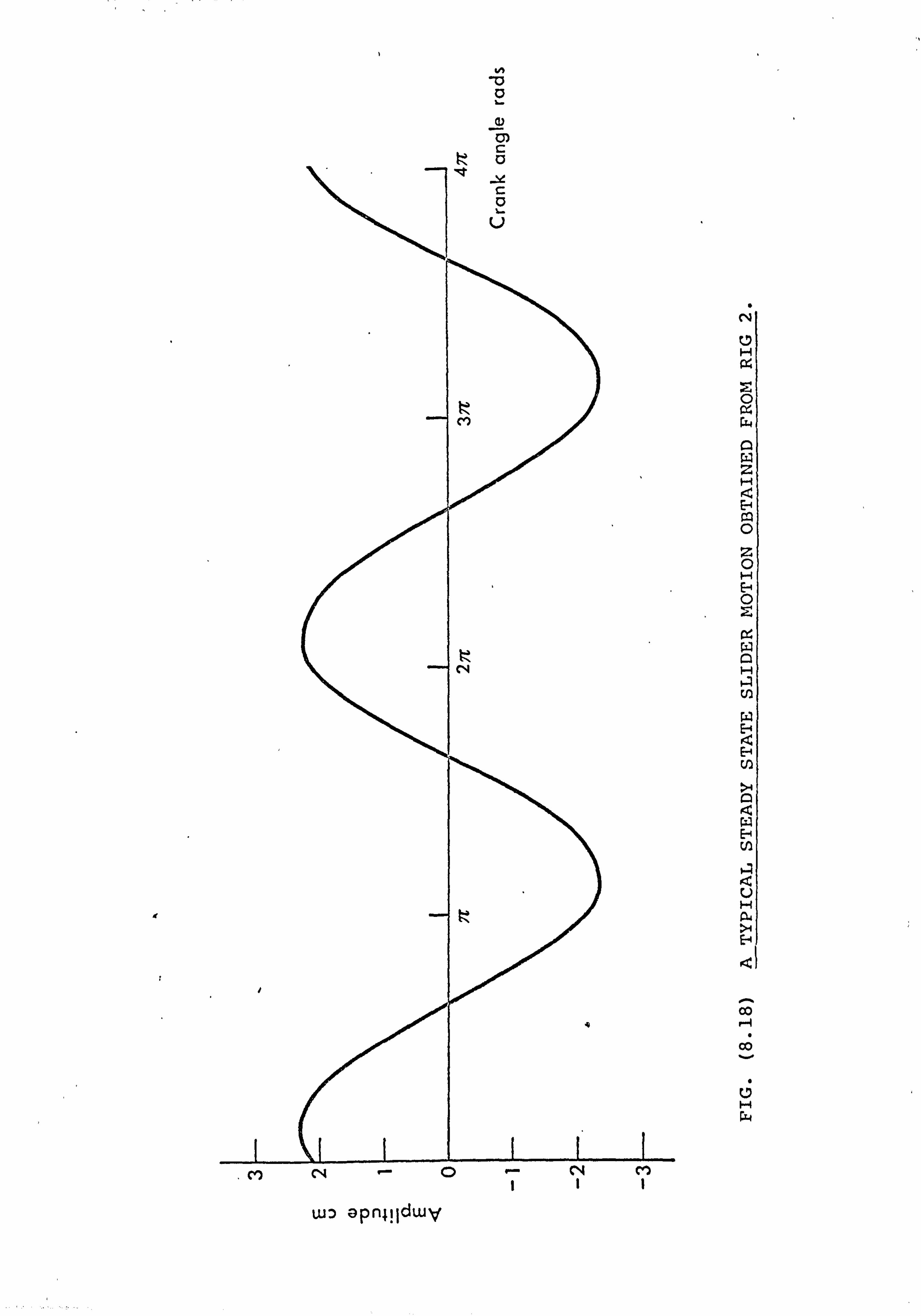
N
a f..
Q)
C,
ta
a
w apn4! Idwy
C7 H
C a
2 H
H cc c 2 C H F C
H
H H
H
Q
00 co
C7 w
Cl) Np r- N 111
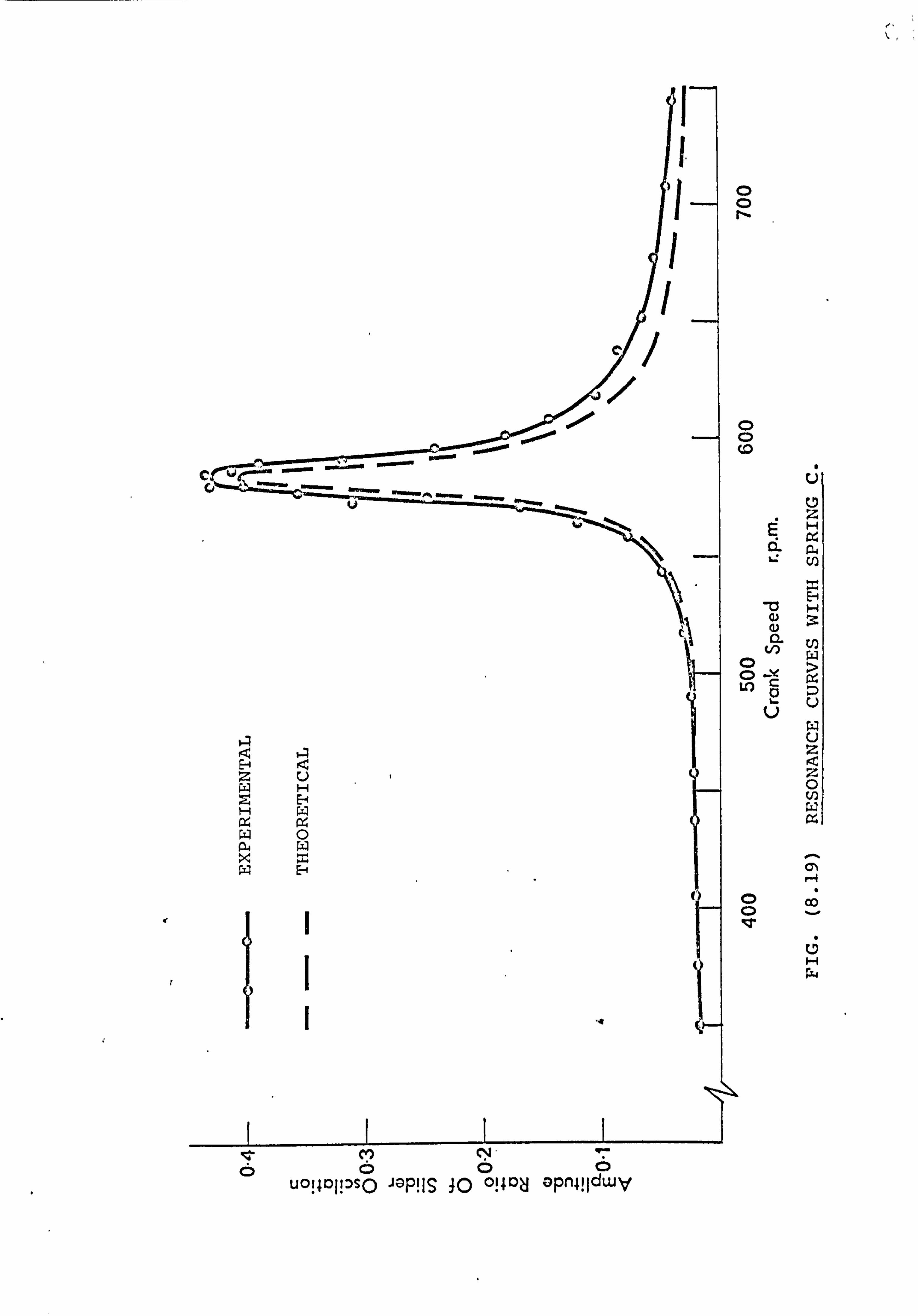
,. ý,
.F
r
0 0
C-) C7 z EH
CL a a
-fl H 03 N 1
w O 0 -Ü
V
u z z 0
H O OD o .ý
H w
° u014oi! ý p0
(5 JGP! IS 30 O! 4O opn4! IdWV
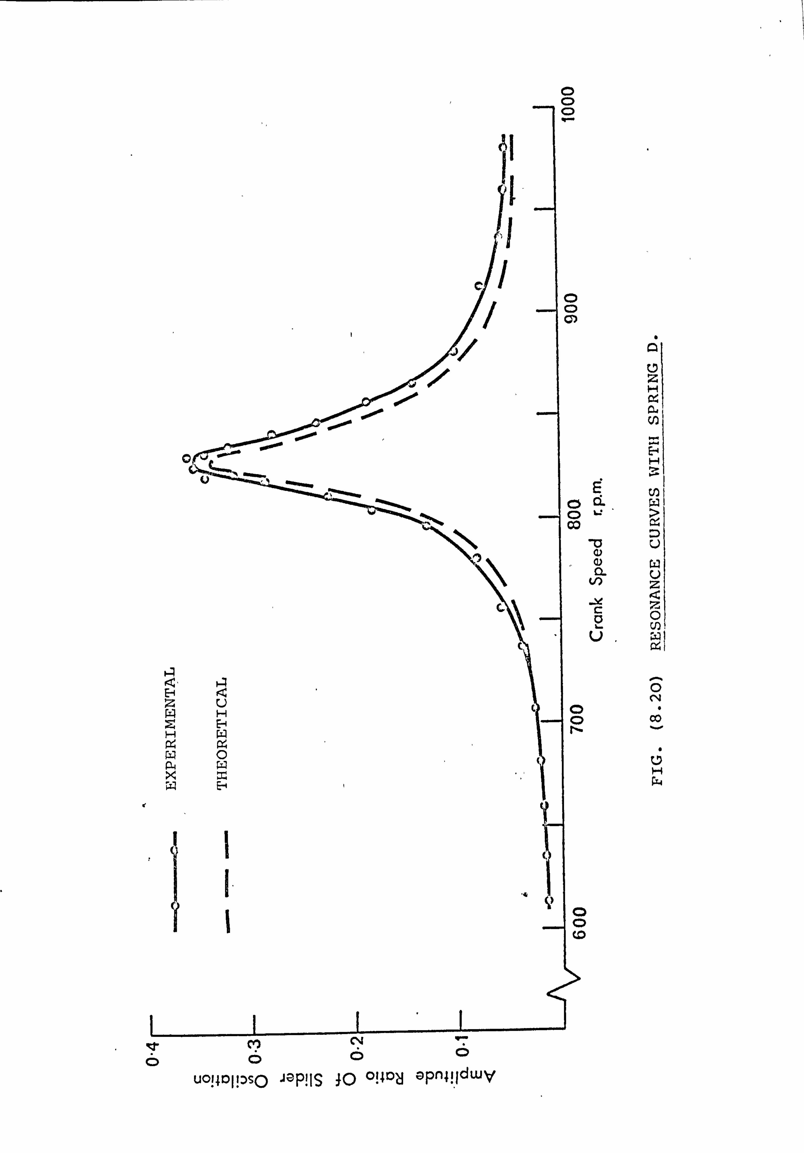
0 0
) )
E CL w
C) C) Q
N
C 0 V
z H
H
WI
U
U z z 0
0
00
H
C cr Cl?
uoi4qj! x0 aaP! IS 10 o! 4°ä opn4!.! dwy
- 120 -
ratio, i. e. the amplitude divided by the length of the rocker,
versus the crank speed. The experimental and theoretical
curves agree in the region of speed leading up to resonance at
w= Wn However the width of the resonance region and the
amplitude of vibration beyond resonance obtained from the theory
is smaller than that of the experiment but, nevertheless, a
reasonable agreement is evident. These differences may however
be attributed to the fact that quantities involving the second
and higher orders of ý34'ý and 62, and their derivatives are
ignored in the theory. Other factors contributing to the
differences may, as before, be attributed to the presence of
Coloumb friction in the guide and pin joints and to the fact that
only an average value of the damping is considered in the theory.
Figs. (8.19) and (8.20) also show a natural frequency in the
region of 585 RPM with spring C and in the region of 825 RPM
with spring D. These are in good agreement with theoretical
calculations based on the equivalent mass of the linkage which
are 582 and 829 for springs C and D respectively.
There were no experimentally observable changes in the
amplitude of oscillations at quarter, third and half the natural
frequency, which again indicated a slider motion based on the
first harmonic. The theoretical resonance curves corresponding
to the second harmonic for both springs C and D are shown in
Fig. (8.21). These are smaller than those corresponding to the
first harmonic by a factor in magnitude of 50 and hence are in
agreement with the experiment.
The above results stated in (8.4.2.1) and (8.4.2.2) support
the theoretical analysis performed in Chapter IV. This support
may be deduced from the following points which are, mainly :

vv
O U
O O Co
H
O o
H H
a
oW ox %0 Q E+
c te ow
VA OW OH
O
o
Wý U z
7 O0 U) oä
U H
öa N
UI
Wi
N o Om
Z c E- c 2 a
zr
E-1 z
z c
uoi4O11 Sp aap! IS ui Dluoua. AH puo»S }o ol4oJ apn4! IdWV

- 121 -
(1) The third and higher harmonics in the slider displacement
are negligible; the second is very small. (2) The resonance
and steady state behaviour is similar to a linear second order
damped mass-spring system and (3) the theoretical and
experimental resonance curves are in good agreement indicating
that the assumption in the theory that the second and higher
orders of ý3 and ý4 and their derivatives are negligible is a
reasonable assumption.
- 122 -
CHAPTER IX
CONCLUSIONS
AND
RECOMMENDATIONS FOR FURTHER WORK
9.1 CONCLUDING REMARKS
The releasing of some constraints in linkage mechanisms
and treating them as inputs that may be controlled yield
versatile and powerful mechanisms. For example the introduction
of a second input to a four bar linkage gives a variety of
outputs thus making the linkage a multipurpose mechanism which
may be adapted to generate a family of cutput motions.
A four bar linkage with the rocker to ground joint replaced
by a slider has been used throughout the analysis to illustrate
the results. ,A
proper control of the slider enabled
modifications and more accurate generation of outputs than could
otherwise be obtained. However, the control of this second input
produced changes that were limited by an envelope dictated by the
linkage kinematics. Therefore it was logical firstly to find
the linkage that would approximately generate the desired output
and then secondly to introduce a second input and control it for
more accurate generation. As a result an optimisation method
was developed, the output of which gave a planar linkage that
minimised the errors involved in function or path generation. The
method could be applied to any planar linkage and was implemented
as a package of subroutines for general use. The package was
also made conversational to facilitate usage.
- 123 - t
The optimisation method was applied to a variety of
examples and in most cases produced satisfactory results.
Recommendations on its use and various techniques relating
to finding the best solution were also discussed.
The dynamics of the mechanism were studied by developing
the equations of motion using the Lagrangian multipliers
method. The multipliers were associated with the pin forces
and suitable methods of solution of the equations of motion
were discussed. It was found that, when performing the
numerical integrations, it was better if all the derivatives
of the generalised coordinates used in the multipliers method
were integrated.
The response of the above linkage with the slider
constrained by a spring and opposed by viscous friction was
studied for a variety of cases. Inputs to the crank included
a torsion bar type input and a constant-speed input. It was
found that the spring stiffness had little effect on the torque
required to drive the mechanism. It was also found that when
the slider was opposed by both spring and viscous damping its
motion was a transient followed by periodic oscillations of
period 27r of the crank angle. However, when the spring was
eliminated the slider moved with periodic oscillations
superimposed on a linear shift in its position thus making the
linkage fall into a collinear configuration. For a forced
input (torsion bar input applied to the crank) it was found
that the linkage accelerated until the input torque became
smaller than the load offered by the linkage after which the
- 124 -t
slider executed periodic oscillations in 2i of the crank
angle. The oscillations, however, decayed due to the
viscous dissipation of energy in the slider guide.
A linearised analysis of the equations of. motion was
developed and conditions of resonance and stability of the
slider were studied.
Results for a short crank showed similarity to a damped
second order linear system behaviour. The major harmonic in
the solution was the first harmonic; the remaining ones were
almost negligible. Resonance curves were obtained varying
the rocker inertia and the coefficient of damping. It was
found that the increase in the rocker inertia decreased the
natural frequency linearly, increased the amplitude of
vibrations and widened the region of resonance. The stability
analysis showed a narrow region of instability in the viscinity
of w= 2wn only, where wn is the natural frequency. Instability
of the slider motion was shown to increase with increase of
crank length, decrease of coupler length and increase of output
inertia.
The experimental investigations were conducted on two
experimental rigs. The first rig was used to compare the
results of the numerical solutions obtained in Chapter III with
the experimental results. It was found that good agreement
existed between the two in both phase and amplitude. The rig
was also used to study the variation of slider displacement
with different crank input speeds. The second rig was used to.
validate the assumptions made mainly in Chapter IV and also to
study the resonance curves of the slider and compare them with
- 125 -
the results obtained from the linearised theory. The
assumptions were found to be reasonable and good agreement
between theory and experiment was found in the resonance
behaviour.
9.2 RECOMMENDATIONS FOR FURTHER WORK
The investigation relating to optimisation and control
discussed in this thesis is based mainly on a kinematic treatment.
However, the dynamic effects have an appreciable influence on the
motion. Such influence is manifested in the forces and moments
which lead to wear causing a change in the kinematic conditions
or producing undesirable effects. Therefore, as a part of the
search for an optimum linkage for a desired output it is
recommended that in addition to finding the kinematic requirements
a parallel study involving the optimisation of dynamic parameters,
such as masses and inertias, should be carried out. It would-be
useful to have such a work in the form of a well documented
package of computer programs available to industrial and research
establishments.
In this thesis we discussed ways of controlling a second
input in order to achieve a better approximation of a desired
output. Illustrative examples Were shown in which it was assumrmed
that a suitable controller able to produce the required input
motion may be found. However although constraints were
incorporated, these concerned only the position and length of
links, it would be very useful to extend the work to examples in
which constraints are applied on the dynamic characteristics of
the controller.
- 126 -
A number of the control methods mentioned in Chapter VII
were off line passive methods involving continuous or
intermittent motion and relying on mechanical elements such as
springs and latches for their operation. These are attractive,
basically for their relative low cost compared with other
sophisticated methods. It is therefore recommended that an
optimisation study involving the finding of optimum values of
such parameters as mass, position and release and hold times of
latches and other dynamic parameters is performed. The study
should incorporate the optimisation of masses and inertias of
the mechanism components such that the controller experiences
desirable dynamic characteristics. For example, in the linkage
considered in the theory the slider may be controlled by latches
'which are released and held at appropriate times in the crank
cycle. The inertias and masses of the links may be optimised
such that when the latches, for example, are released the forces
transmitted to the slider by the linkage would cause it to move
in a desirable manner.
It would be useful to study the practical problem involved
in the adaptive control of mechanisms. This would consist of
measuring the errors, experimentally on line, in the output and
processing them by a digital computer, also on line, using some
optimisation technique. The digital computer would be
interfaced with the controller which would provide the optimum
input motion. Such work would take into account both kinematic
and dynamic requirements simultancously.

- 127 -
In many industrial examples it is found that when
designers are confronted with a complex motion they tend
to think of complex multi-link mechanisms which are not
necessarily of more than one degree of freedom. We have
shown that in a four bar linkage the releasing of one
constraint and replacing it by an input makes any point
within an output area accessible by a suitable control of
this input. Therefore, rather than using a series of four
bar linkages coupled in some manner to produce some complex
motion it is recommended that the basic four bar is looked
into more deeply by releasing some of its constraints and
replacing them by controlled inputs.
Finally, it would be interesting to see the linearised
theory developed in Chapters IV and V extended to mechanisms
flexibly supported at the slider and crank shaft ends. It
would also be interesting to see the theory and programs
developed in Chapter V cn finding the unstable regions by a
computer applied optimisation method, on a variety of problems
such as transverse and longitudinal flexibility in the links of
a four bar linkage and also flexibility in its input and output
shafts.
4

PA RT' V
REFERENCES''& APPENDICES
I
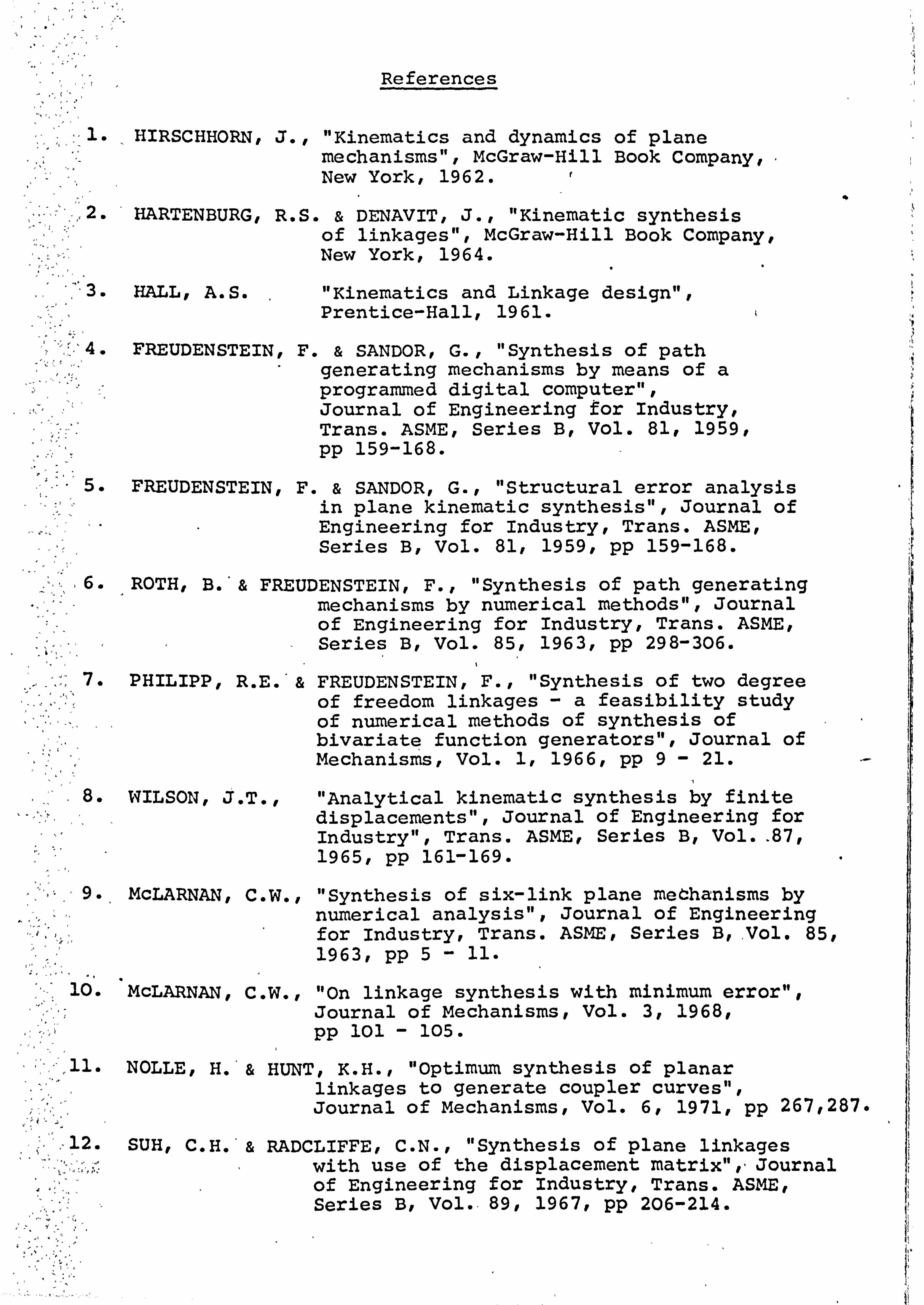
" Y
References
1. HIRSCHHORN, J., "Kinematics and dynamics of plane mechanisms", McGraw-Hill Book Company,. New York, 1962.
HARTENBURG, R. S. & DENAVIT, J., "Kinematic synthesis of linkages", McGraw-Hill Book Company, New York, 1964.
3. HALL, A. S. "Kinematics and Linkage design", Prentice-Hall, 1961.
4. FREUDENSTEIN, F. & SANDOR, G., "Synthesis of path generating mechanisms by means of a programmed digital computer", Journal of Engineering for Industry, Trans. ASME, Series B, Vol. 81,1959, pp 159-168.
5. FREUDENSTEIN, F. & SANDOR, G., "Structural error analysis in plane kinematic synthesis", Journal of Engineering for Industry, Trans. ASME, Series B, Vol. 81,1959, pp 159-168.
, 6. ROTH, B. '& FREUDENSTEIN, F., "Synthesis of path generating mechanisms by numerical methods", Journal of Engineering for Industry, Trans. ASME, Series B, Vol. 85,1963, pp 298-306.
7. PHILIPP, R. E. '& FREUDENSTEIN, F., "Synthesis of two degree of freedom linkages -a feasibility study of numerical methods of synthesis of bivariate function generators", Journal of Mechanisms, Vol. 1,1966, pp 9- 21.
8. WILSON, J. T., "Analytical kinematic synthesis by finite displacements", Journal of Engineering for Industry", Trans. ASME, Series B, Vol.. 87, 1965, pp 161-169.
9. "
MCLARNAN, C. W., "Synthesis of six-link plane mechanisms by numerical analysis", Journal of Engineering for Industry, Trans. ASME, Series B,, Vol. 85, 1963, pp 5- 11.
10. McLARNAN, C. W., "On linkage synthesis with minimum error", Journal of Mechanisms, Vol. 3,1968, pp 101 - 105.
11. NOLLE, H. "& HUNT, K. H., "Optimum synthesis of planar linkages to generate coupler curves", Journal of Mechanisms, Vol. 6,1971, pp 267,287.
12. SUH, C. H. & RADCLIFFE, C. N., "Synthesis of plane linkages with use of the displacement matrix",, Journal of Engineering for Industry, Trans. ASME, Series B, Vol.. 89,1967, pp 206-214.
"
ý4

ý.
13. BUSSELL, W. H. '&. MARTIN, G. H., "An analytical method for synthesizing mechanisms based on Roulette theory", Journal of Engineering for Industry, Vol. 89, 1967, pp 77-83.
14. WORTHLEY, W. W. `& HINKLE, R. T., "Four-bar linkages - approximate synthesis", Journal of Engineering for Industry, Trans. ASME, Vol. 81,1959, pp 293-300.
15. ALLEN, C. W.,
16. D'V SMAN, E. A.,
"The design of linkages to generate functions of two variables", Journal of Engineering for Industry, Trans. ASME, Vol. 8,1959, pp 23-29.
17. BOX, SWAN & DAVIES,
18. FLETCHER, R.
19. FIACO'& McCORMICK,
"How to compare mechanisms with parallel moving bars (with' application on a level-buffing jib-crane consisting of a four-bar linkage and exploiting a coupler-point curve), EUROMECH 22, Newcastle upon Tyne University, 1971.
"Nonlinear optimisation", ICI Monograph, Oliver and Boyd, 1969.
"Methods of solution of Optimisation problems", Computer physics.
"Nonlinear programming: sequential unconstrained minimisation techniques", John Wiley'& Sons, 1968.
20. POLLAK, E. "Computational Methods in Optimisation", Academic Press, 1971.
21. FLETCHER, R., "Optimisation", Academic Press, 1969.
22. FLETCHER, R. & POWELL, M. J. D., "A rapidly, convergent descent
method for minimisation", The Computer Journal, Vol. 6,1963, pp 163-168.
23. YOUSSEF, A. H. '& MAUNDER, L. "Motion of a two degree of freedom
mechanism", Institution of Mechanical Engineers, Conference of Mechanisms, 1972.
24. YOUSSEF, ' A. H.; "Optimisation of mechanisms for path and function generation", institution of Mechanical Engineers, Conference on Mechanisms, 1973.
25. MUELLER, G. S. '& OSMAN, M. O.. M., "Multivariable search for optimum synthesis of planar mechanisms", Institution of Mechanical Engineers, Conference on Mechanisms, 1972.
26. OSMAN, M. O. M. '& MANSOOR, W. M., "A computer-orientated numerical approach to the kinematic analysis and synthesis of mechanisms", proceedings of the Third World Congress on Theory of Machines & Mechanisms, Vol. 14,1971, pp 299-309.
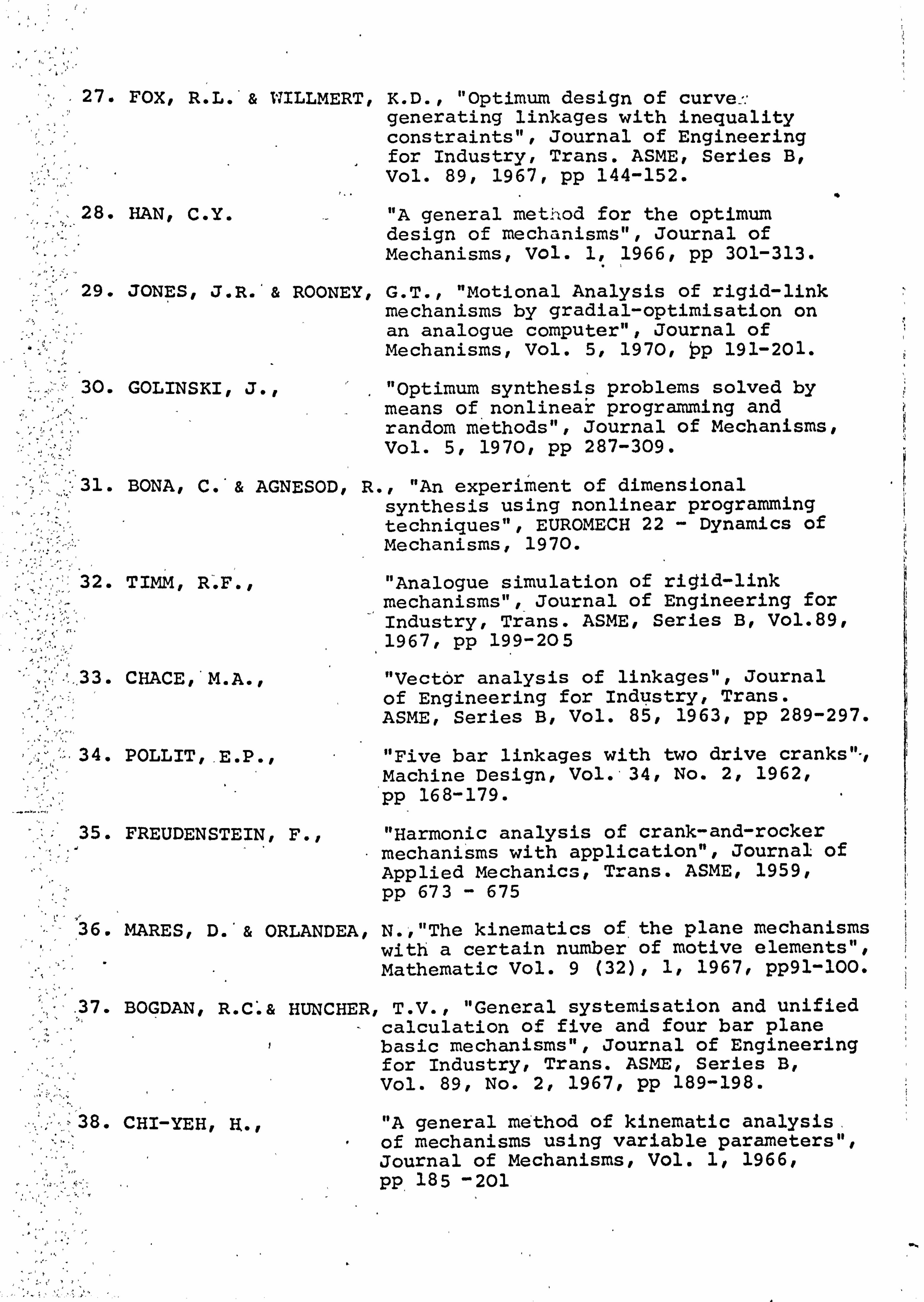
27. FOX, R. L. *& WILLMERT, K. D., "Optimum design of curve-,. - generating linkages with inequality constraints", Journal of Engineering for Industry, Trans. ASME, Series B, Vol. 89,1967, pp 144-152.
28. HAN, C. Y. "A general method for the optimum design of mechanisms", Journal of Mechanisms, Vol. 1,1966, pp 301-313.
29. JONES, J. R. '& ROONEY, G. T., "Motional Analysis of rigid-link mechanisms by gradial-optimisation on an analogue computer", Journal of Mechanisms, Vol. 5,1970, ýp 191-201.
30. GOLINSKI, J., "Optimum synthesis problems solved by means of nonlinear programming and random methods", Journal of Mechanisms, Vol. 5,1970, pp 287-309.
31. BONA, C. "& AGNESOD, R., "An experiment of dimensional
synthesis using nonlinear programming techniques", EUROMECH 22 - Dynamics of Mechanisms, 1970.
32. TIMM, R. F., "Analogue simulation of rigid-link mechanisms", Journal of Engineering for Industry, Trans. ASME, Series B, Vol. 89, 1967, pp 199-205
33. CHACE, *M. A., "Vector analysis of linkages", Journal of Engineering for Industry, Trans. ASME, Series B, Vol. 85,1963, pp 289-297.
34. POLLIT, _E. P., "Five bar linkages with two drive cranks"-,
Machine Design, Vol. 34, No. 2,1962, pp 168-179.
35. FREUDENSTEIN, F., "Harmonic analysis of crank-and-rocker mechanisms with application", Journal of Applied Mechanics, Trans. ASME, 1959, pp 673 - 675
36. MARES, D. "& ORLANDEA, N., "The kinematics of the plane mechanisms with a certain number of motive elements", Mathematic Vol. 9 (32), 1,1967, pp9l-100.
. 37. BOGDAN, R. C. & HUNCHER, T. V., "General systemisation and unified
calculation of five and four bar plane basic mechanisms", Journal of Engineering for Industry, Trans. AS, Series B, Vol. 89, No. 2,1967, pp 189-198.
38. CHI-YEH, 1J., "A general method of kinematic analysis, of mechanisms using variable parameters", Journal of Mechanisms, Vol. 1,1966, pp, 185 -201
q
"'39. MARKUS, L., "A general method for the kinematic analysis of planar mechanisms by the computer", ASME Conference on Mechanisms and International Symposium on bearing and transmissions", Trans. ASME, 72 - MECH -58,1972.
40. BOGDAN, R. C., "General study of five bar mechanisms with the aid of complex harmonic series", Studii si.,. cerccharide mecanica applicatii, Acad. F. P. R., Vol. 15, No. 2,1964, pp 851-868.
41. SMITH, M. R. '& MAUNDER, L., "Inertia forces in a four bar linkage", JMES, Vol. 9, No. 3,1967.
42. PORTER, B. '& SANGER, D. J., "Synthesis of dynamically optimal four bar linkages", Institution of Mechanical Engineers, Conference on Mechanisms, 1972.
43. MAUNDER, L., "The balancing of elastically coupled mechanisms", Proceedings of the Third World Congress for the Theory of Machines'& Mechanisms, Vol. B, 1971,
. pp 103-114..
44. BERKOF, R. S., "Complete force and moment balancing of inline four bar linkages", Journal of Mechanisms, Vol. '8,1973, pp 397-410.
45. SMITH, M. R., '& MAUNDER, L., "Stability of a four bar linkage
with flexible coupler", JMES, Vol. 13, No. 4,1971, pp 237-242.
46. BARR, A. D. S "Some general aspects of the analysis of the vibration and stability of mechanisms", EUROMECH 22, Dynamics of Mechanisms, 1970.
47. VISCOM, B. V.. *& AYRE, R. S., "Nonlinear dynamic response of elastic slider-crank mechanism", Journal
of Engineering for Industry, Trans. ASME, Vol. 93, No. 1,. 1971, pp 251-262.
48. SEEVERS, J. A. *& YANA, A. T., "Dynamic stability analysis of linkages with elastic members via analogue simulations", ASME, paper 70 - MECH - 48,1970.
49. SMITH, M. R., "The dynamics of rigid and flexible four bar linkage mechanisms", Ph. D. Thesis,
University of Newcastle upon Tyne, 1972.
50. MEYER ZUR CAPELLEN, W., "Torsional vibrations in the shafts of linkage mechanisms", Journal of Engineering for Industry, Trans. ASME, Series B., Vol. 89,1967, pp 126-136.
' a,
51. MEYER ZUR CAPELLEN, W, < 'Q cxllation of an elastically suspended coupler of a four bar linkage", Journal of Mechanisms, Vol. 6,1971, pp 351 - 365.
52. YOUSSEF, A. H., "A study in resonance and stability of special five bar linkage", Internal Report No.,, ',, Department of Mechanical Engineering, University of Newcastle upon Tyne.
53. ILEY, L., "An investigation into'a special two degree of freedom mechanism", M. Sc. dissertation, University of Newcastle upon Tyne, 1973.
54... _LAKSHMINARAYANA,
K. &'DIZIOGLUE, B, "Synthesis of-spring constrained mechanisms for amplitude independent natural frequency of oscillation", Mechanisms, and Machine Theory, Vol. 7,1972, pp 167 - 190.
55. CHACE, M. A., "Analysis of the time dependence of multi-freedom mechanical systems in relative coordinates", Journal of Engineering for Industry, Trans. ASME, 1967, pp 119-125.
.
56. BENEDICT, C. E.:. & TESAR, D., "Dynamic response analysis of quasi-rigid mechanical systems using kinematic-influence coefficients", Journal of Mechanisms, Vol. 6,1971, pp 383 - 403.
57. TIMM, R. F. '& ELLIS, J. R., "The use of digital simulation languages in mechanism study", Private communications.
58. KOZEVNIKOV, S. N., "Dynamics of mechanisms with two degree of freedom", Sovrem. Prob. 1. Teorri Mashin, I. Mekhanzmove, Moscow, Nanka.
59. SKREINER, M., "Dynamic Analysis used to complete the design of a mechanism", Journal of Mechanisms, Vol. 5,1970, pp 105 - 119.
r
60. SKREINER, M. '& ROBERTS, B. W., "The dynamics of hydraulically
actuated linkage mechanisms", The Institution of Engineers, Australia, Mechanical and Chemical Engineering Transaction, 1967, pp 207 - 215.
61. STEWART, D., "A platform with six degrees of freedom", Proceedings of the Institution of Mechanical Engineers, Vol. 180, Part 1, No. 15,1965, pp 371 - 386.
62. SONI, A. H.,
63. PEARCE, G. F.,
"Design of the crank-rocker mechanism with unit time ratio", Journal of Mechanisms, Vol. 5,1970, pp 1-4.
"Dynamic Characteristics of mechanisms using linear independence", Journal of Mechanisms, Vol. 5,1970, pp 351-355.
64. MACLEOD, I. N., "The dynamic behaviour of two degree of freedom linkage mechanisms", Ph. D. Thesis, Liverpool Polytechnic, 1970.
65. WILSON, R. "& FAWCETT, J. N., "The dynamics of piston slap", ASME, paper 72 - MECH - 63,1972.
66. FAWCETT, J. N. '& BURDESS, J. S., "Effects of bearing clearance in a four bar linkage", Proceedings of the Third World Congress for the Theory of Machines & Mechanisms", Vol. Cr paper C-9,1971, pp 111-126.
67. EARLES, S. W. E. '& WU, C. L. S., "Motion analysis of a rigid- link mechanism with clearance at a bearing using Lagrangian mechanics and digital computation", Institution of Mechanical Engineers Conference on Mechanisms, 1972.
68. GRANT, S. '& FAWCETT, J. N., "Research colloquium 6n clearance of mechanisms and also private communi- cations", Department of Mechanical Engineering, Newcastle University.
69. DU$OWSKY, S,
70. ROSE, S. E.,
71. LANCOZ, C.,
72. WELLS, D. A.,
73. GOLDSTEIN, H.,
74. McLACHLAN, N. W.,
75. STOKER, J. J.,
, "On predicting the dynamic effects of clearances in planar mechanisms", ASME publication, paper 72 - Mech. 91,1972.
"Five bar loop synthesis", Machine design, Vol. 33, No. 21,1961, pp 189-195.
"Variational principles of mechanics", University of Toronto Press, 1964.
"Theory-and problems of Lagrangian dynamics", Schaum Publishing Co., 1967.
"Classical Mechanics", Addison-Wesley Publishing Co., 1964.
"Theory and Application of -functions", Dover Publication, 1964.
"Nonlinear Vibrations", Interscience Publishers, 1950.

76" MALKIN, I. G., "On the stability of Motion", Moscow- Leningrad, Translation by U. S. Atomic Energy Commission, Office of Technical Information, 1952.
77. MALKIN, I. G., "Some problems in the theory of non- linear oscillations", Volumes 1*& 2, The state publishing house of technical and theoretical literature, Moscow, Translation by U. S. Atomic Energy Commission, 1956.
78. KOBRINSKII, A. E., "Dynamics of Mechanisms with elastic connections and impact systems", ILIFFE Books Ltd., 1969.
79. RAYEVSKII, N. P., "The measurement of'mechanical parameters in machines", Pergamon Press, 1965.
80. HILDEBRAND, F. B. "Methods of Applied Mathematics", Prentice-Hall, '1963.
81. BUTLER, R. '& KERR, , E., "An introduction to numerical
methods", Sci. Isaac Pitman, 1962.
82. REDISH, K. A., "An Introduction to computational methods", The English Universities Press, 1961.
83. I. B. M., "IBM System 360, Fortran IV Language Manual", IBM Systems Reference Library.
84. HOPPER, M. J., "Harwell subroutine library; U. K. Atomic Energy Authority, 1971.
5
ýý

AP PEN DIX1
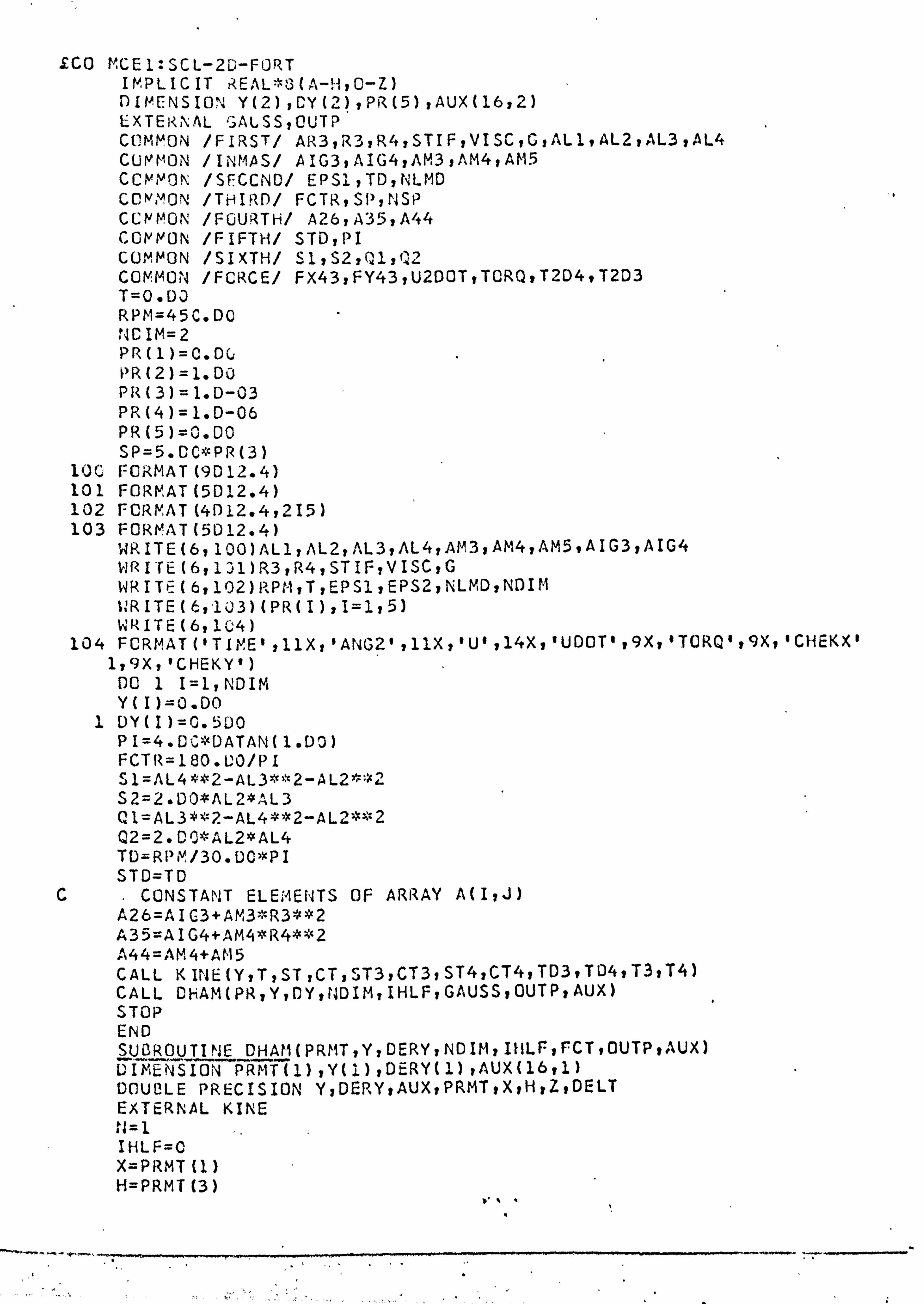
£C0 MCEI: SCL-20-FORT IMPLICIT REAL*3(A-H, 0-Z) DIMENSION Y(2), CY(2), PR(5), AUX(16,2) EXTERNAL GALSS, OUTP COMMON /FIRST/ AR3, R3, R4, STIF, VISC, G, AL1, AL2, AL3, AL4 CUMMON /INMAS/ AIG3, AIG4, AM3, AM4, AM5 COMMON /SFCCENC/ EPSI, TD, NLMD COMMON /THIRD/ FCTR, S1), NSP COMMON /FOURTH/ A26, A35, A44 COMMON /FIFTH/ STD, PI COMMON /SIXTH/ S1, S2, Ql, Q2 COMMON /FCRCE/ FX43, FY43, U2D0T, TORQ, T2D4"T2D3 T=0. D3 RPM=45C. DC NCIM=2 PR(1)=C. D0 PR(2)=1. D0 PR(3)=1.0-03 PR(4)=1. D-06 PR(5)=0. D4 SP=5. CC*PR(3)
10C FORMAT (9D12.4) 101 FORMAT (5D12.4) 102 FORMAT (4012.4,215) 103 FORMAT(5012,4)
WRITE(6,100)ALl, AL2, AL3, AL4, AM3, AM4, AM5, AI03, AI04 WRITE (6,1)1)R3, R4, STIF, VISC, G WRITE (6,102) RPt"1, T, EP SI ,E PS2, NLMD, ND IM WRITE(6, -1J3)(PR(I), I=1,5) WR ITE(6,104)
104 FCRMAT('TIME', 11X, 'ANG2', 11X, 'U', l4X, 'UDOT', 9X, 'TORQ', 9X, 'CHEKX' l, 9X, 'CHEKY')
00 1 I=1, NDIM Y(I)=O. DO
1 UY(I)=0.500 P I=4. DC*DATAN(1. D0) FCTR=180.0`0/PI S 1=AL4**2-AL3* 2-AL2''2 S2=2.00*AL2*AL3 Q1=AL3**2 AL4**2-AL2**2 Q2=2. DO* AL2*AL4 TD=RPM/30.00*PI STD=TD
C. CONSTANT ELEMENTS OF ARRAY A(I, J) A26=AIG3+AM3*R3**2 A35=A I G4+AM4*R4**2 A44=AM4+AM5 CALL KINE(Y, T, ST, CT, ST3, CT3, ST4, CT4, TD3, TD4, T3, T4) CALL CRAM(PR, Y, DY, NDIM, IHLF, GAUSS, OUTP, AUX) STOP END SUBROUTINE DHAII(PRMT, Y, DERV, NDIM, IIILF, FCT, QUTP, AUX) DIMENSION PRMT(1), Y(1), DERY(1), AUX(16,1) DO UCLE PRECISION Y, DERY, AUX, PRMT, X, H, Z, DELT EXTERNAL KINE l1=1 IHLF=O X=PRMT (1 ) H=PRMT(3)
-, -.. -... _ý., _ý.. ý.. . e.... _, _.., _.. _... _ý
PR; llT (5)=(). DO DO 1 I=1, NDIPI AUX(16, I)=0. D0 AUX(15, I)=DERY(I)
1 AUX(1, I)=Y(I) IF(H=(PRMT(2)-X))3,2,4
C. ERROR RETURNS 2 IHLF=12
GCTO 4 3 IHLF=13
C COMPLTATION OF DERY FOR STARTING VALUES 4 CALL FCT(X, Y, DERY)
C RECORCING"OF STARTING VALUES CALL OUTP(X, Y, DERY, IHLF, NDIM, PRMT) IF (PRNT(5) )6,5P6
5 IF(IHLF)7,7,6 6 RETURN 7 DC 8 1=1, NDIM 8 AUX(8, I)=DERY(I)
C COMPUTATION OF AUX(2, I) ISw=1 GOTO ICO
9 X=X+H DO 10 I=1, NDIM
10 AUX(2, I)=Y(I) C INCREMENT H IS TESTED BY MEANS OF BISECTION
11 IHLF=IF-LF+1 X=X-N VO 12 I=1, NDIM
12 AUX(4, I)=AUX(2, I) H=. 5004H N=1 ISW=2 GOTO 100
13 X=X+H CALL FCT(X, Y, DERY) N=2 DC 14 1=1, NýCIM AUX(2, I')=Y(I)
14 ALX(9, I)=DERY(I) ISW=3 GOTO 1CO
C COMPUTATION OF TEST VALUE DELT, 15 DELT=0.90
DO 16 I=1, NCIM 16 DELT=DELT+AUX(15, I)*DABS(Y(I)-AUX(4, I))
DELT=. C66666666666666667D0*DELT IF(OELT-PRMT(4))19,19,17
17 IF(IHLF-10)11,18,18 C NO SATISFACTORY ACCURACY AFTER 10 BISECTIONS. ERROR MESSAGE.
18 IHLF=11 X=X+H COTO 4
C THERE IS SATISFACTORY ACCURACY AFTER LESS THAN 11 BISECTIONS. 19 X=X+H
CALL FCT(X, Y, DERY) DC 20 I=1, NDIM AUX(3, I)=Y(I)
2p AUX(10, I)=DERY(I) N=3
,"..
I SW=4 GOTO 1C3
21 N=1 X=X+H CALL FCT(X, Y, CERY) X=P, 4MT (1) DO 22 I=1, NDIN AUX(11, I)=DERY(I)
220Y(I)=AUX(1, I)+li*(. 375DO*AUX(8, I)+. 7916666666666667D0*AUX(9, I) 1-. 20833333333333333D0MAUX(10, I)+. 041666666666666E67D0*DERY(I))
23 X=X+H N=N+1 CALL FCT(X, Y, DERY) CALL CUTP(X, Y, DERY, IHLF, NDIM, PRMT) IF(PRM. T(5) )6,24,6
24 IF (N-4 )25,200,200 25 DO 26 I=1, NCIM
ALX(N, I)=Y(I) 26 AUX(N+7, I)=DERY(I)
IF(N-3)27,29,200 27 DO 28 I=1, NDIM
DELT=ALX(9, I)+AUX(9, I) DELT=DELT+DELT
28 Y(I)=AUX(1, I)+. 33333333333333333D0*I*(AUX(8, I)+DELT+AUX(10, I)) GOT0 23
29 DO 30 I=1, NDIM DELT=AUX(9, I)+AUX(10, I) DELT=DELT+DELT+CELT
30 Y(I)=AUX(1, I)+. 375DO*H*(AUX(8, I)+DELT+AUX(11, I)) GUTO 23
C THE FCLLCWING PART OF SUBROUTINE DHAM COMPUTES BY MEANS OF C RUNGE-KUTTA METHOD STARTING VALUES FUR THE NOT SELF-STARTING C PREDICTOR-CORRECTOR METHOD.
100 DC 101 I=1, NDIM Z=H*AUX(N+7, I) AUX(5, I)=Z
101 Y(I)=AUX(tl, I)+. 4DO*Z CZ IS AN AUXILIARY STORAGE LOCATION
Z=X+. 4D0*ii CALL FCT(Z, Y, DERY) DC 102 I=1, NDIM Z=H*DERY(I) AUX(6, I)=Z
102 Y(I)=AUX(N, I)+. 29697760924775360D0*AUX(5, I)+. 15875964497103583D0*Z Z=X+. 45573725421878943D0*H CALL FCT(Z, Y, DERY) DO 103 I=1, NDIM Z=ti*DERY (I ) AUX(7, I)=Z
103 Y(I)=ALX(N, I)+. 21810033822592047D0*AUX(5, I)-3.0509651486929308DO* 1AUX(6, I)+3.832864760467010300*Z
Z=X+H CALL FCT(Z, Y, DERY) DC 104 I=1, NDIM
1040Y(I)=AUX(N, I)+. 17476028226269037D0*AUX(5, I)-. 55148066287873294D0* 1AUX(6, I)+1.2055355993965235D0*AUX(7, I)+. 17118478121951903D0* 2H*DERY(I)
6010(9,13,15,21) , ISVJ C POSSIELE BREAK-POINT FOR LINKAGE C STARTING VALUES ARE COMPUTED.
y,
,'_
C NOW START HANMINGS MODIFIED PREDICTOR-CORRECTOR METHOD. 20C ISTEP=3 201 IF (N- 8) 204,24) 2,20 4
C N=8 CAUSES THE ROWS OF AUX TO CHANGE THEIR STORAGE LOCATIONS 202 DC 203 r4=2,7
DO 203 I=1, NDIh AUX(N-1, I)=AUX(N, I)
203 AUX(N+6, I)=AUX(N+7, I) N=7
C. N LESS THAN 8 CAUSES N+1 TO GET N 204 N=N+1
C COMPUTATION OF NEXT VECTOR Y DO 205 I=1, NDIM AUX(N-1, I)=Y(I)
205 AUX(N+6, I)=CERY(I)' X=X+H
206 ISTEP=ISTEP+1 DC 207 I=I, NDIM
ODEL'T=AUX(N-4, I)+1.3333333333333333D0*H, (AUX(N+6, I)+AUX(N+6, I)- 1AL. X(iN+5, I)+AUX(N+4, I)+AUX(N+4, I))
Y(I)=DELT-. 9256198347107438[)0*AUX(16, I) 207 AUX(16, I)=DELT
C PREDICTOR IS NOW GE14ERATED IN ROW 16 OF AUX, MODIFIED PREDICTOR C IS GENERATED IN Y. DELT MEANS'AN AUXILIARY STORAGE.
CALL FCT(X, Y, CERY) C DERIVATIVE OF MCDIFIED PREDICTOR IS GENERATED IN DERV
DO 208 I=1, NDIM ODELT=. 12500*('9.00*AUX(N-1, I)-AUX(N-3, I)+3. DO*H*(DERY(I)+AUX(N+6, I 1+AUX(N+6,1)-AUX(N+5, I)))
AUX(16,1)=AUX(16, I)-DELT 208 Y(I)=CELT+. 0743801652892562JD0*AUX(16, I)
C TEST WHETHER H MUST BE HALVED OR DOUBLED DELT=C. D0 DU 209 I=1, NUIM
209 DELT=CELT+AUX(15, I)*DABS(AUX(16, I)) IF(DELT-PRMT(4))210,222,222
CH MUST NOT BE HALVED. THAT MEANS Y(I) ARE GOOD. 210 CALL FCT(X, Y, DERY)
CALL OUTP(X, Y, DERY, IHLF, NDIM, PRMT) IF(PRMT(5))212,211,212
211 IF(IHLF-21')213,212,212 212 RETURN 213 IF(H*(X-PRMT(2)))214,212,212 214 IF(DABS(X-PRMT(2))-. 1DO*DAF3S(H) )212,2 15,215 215 IF(DELT-. 02D0*PRMT(4))216,216,201
CH COULD BE DOUBLED IF ALL NECESSARY PRECEEDING VALUES ARE C AVAILABLE
216 IF(IHLF)201,201,217 217 IF(N-7)201,218,218 218 IF(ISTEP-4)201,219,219 219 IISOD=ISTEP/2
IF(IS'TEP-IMOD-IMOD)201,220,201 220 H=H+H
IHLF=IHLF-1 'ISTEP=0 DO 221 1=1, NDIM AUX(N-1, I)=AUX(N-2,1) AUX(N-2, I)=AUX(N-4, I) AUX(N-3, I)=AUX(N-6, I) AUX(N+6, I)=AUX(N+5, I) '
AUX(N+5, I)=AUX(N+3, I) AUX (tJ+4, I)=AUX (N+1, I) DELT=ALX(N+6, I)+AUX(N+5, I) DLLT=DELT+DELT+CELT
2210AUX(16, I)=8.962962962962963DG*(Y(I)-AUX(N-3, I)) 1-3.3611111111111111D0*HH*(DERY(I)+DELT+AUX(N+4, I))
GOTO 2 ý1 CH MUST BE HALVED
222 I HLF= I F-LF+1 IF(IHLF-20)223,223,210
223 H=. 5UJ*H ISTEP=C DC 224 I=1, NDIf1
OY(I)=. 390625D-2-Y(8. D1**AUX(N-1, I)+135.00*AUX(N-2, I)+4. D1*AUX(N-3, I) 1+AUX(N-4, I))-. 11713.75L)J*(AUX(Pd+6, I)-6. D0*AUX(N+5, I)-AUX(N+4, I))*Il QAUX(N-4, I)=. 390625D-2: x(12. Dn*AUX(N-11I)+135. DO*AUX(14-2, I)+ 1108. DC'AUX(N-3,1)+AUX(N-4, I))-. 023437500*(AUX(N+6, I)+ 218. DJ*AUX(N+5, I)-9.00*AUX(N+4, I))cH
AUX(N-3, I)=AUX(N-2, I) 224 AUX(N+4, I)=AUX(N+5, I)
X= X-H DELT=X-(H+H) CALL FCT(DELT, Y, DERY) DO 225 I=1, NDIh1 AUX(N-29 I)=Y(I) AUX (N+5, I)=CE} Y (I )
225 Y(I)=AUX(N-4, I) [)ELT=CELT-(H+H) CALL FCT(DELT, Y, DERY) DC 226 I=1, NDIi4 DELT=ALX(N+5, I)+AUX(N+4, I) DELT=D ELT+DELT+DELT
OAUX(16, I)=8.96296296296296300*(AUX(N-1, I)-Y(I)) 1-3.36'11111111111111DO*H*(AUX(N+6, I)+DELT+DERY(I))
226 AUX(N+3: I)=DERY(I) GOTO 206 END SUBROUTINE GAUSS(TIME, Y, CY) IMPLICIT KEAL*8(A-11, O-Z) DIMENSION W(6), DW(6), A(6,6), 8(6), TEMPA(6,6),
1TEMPB(6), DWO(6), Elü(6), ALMD(3), Y(2), DY(2) COMMON /FIRST/ AR3, R3, R4, STIF, VISC, G, AL1, AL2, AL3, AL4 COMMON /INMAS/ AIG3, AIG4, AM3, AM4, AM5 COMMON /SECOND/ EPSI, TD, NLMD COMMON /FOURTH/ A26, A35, A44 COMMON /FORCE/ FX43, FY43, U2DOT, TGRQ, T2D4, T203 T=TD*TIME CALL KINE(Y, T, ST, CT, ST3, CT3, ST4, CT4, TD3, TD4, T3, T4) EPS3=0. DO NFLAG1=-1 NCOUNT=0
C COMPLTATICN OF ARRAY A(I, J) ELEMENTS DU 1 I=1,6 DG 1 J=1,6
1 A(I, J)=0.00 A(1,6)=AM3*AL2*R3*(CT*CT3+ST*ST3) A(1,3)=AL2*ST A(1,2)=-AL24CT A(1,1)=-1.00 B(1)=AM3*G*A(1,2)-AM3*AL2*R3*(ST*CT3-CT*ST3)*TD3**2
A (2,3) =AL3*ST3 A(2,2)=-AL3*CT3 A(2,6)=A26 B (2)=-A; 43 -G*R3*CT3+AM3*AL2*R3* (ST*CT3-CT*ST3) *TO**2 A(3,4)=-At4*R4' ST4 A(3,3) =-AL4*ST4 A(3,2)=AL4*CT4 A(3,5)=A35 ß(3)=-AM4*G*R4'CT4 A(4,3)=1.00 A(4,4)=A44 A(4,5)=A(3,4) B (4) =-VI SC*Y (1) -STIF*Y (2)+AN'4*R4*CT4*TD4**2 A(5,4)=1.00 A(5,6)=A(2,3) A(5,5)=A(3,3) B(5)=A (3,2)**TU4**2+A(2,2)*TL'3**2+A(1,2)*TC**2 A(6,6)=-A(2,2) A(6,5)=-A(3,2) B(6)=A(1,3)*TD**2+A(2,3)*TD3**2+A(3,3)*TD4**2
C SET MATRICES A(I, J) AND B(I) TO DUMMY MATRICES DC 10 1=1,6 DC 16 J=1,6
16 TEMPA(I, J)=A(I, J) 10 TEMPB(I)=B(I)
C START GAUSS ELEMIr4ATION METHD 12 DO 2 K=1,5
L=K+1 C REARRANGE ROWS SO THAT PIVOT ELEMENT A(K, K) HAS THE. GREATEST C ABSOLUTE VALUE IN IT'S COLCUMN
? i=K DO 6 I=L, 6
6 IF(DABS(A(I, K)). GT. DABS(A(M, K)))M=I IF(M. EC,. K)GC TO 7 DO 8 J=K, 6 TEMP=A(K, J) A(K, J)=A(M, J)
8 A(M, J)=TEMP TEMP=B(K) B(K)=B(M) U(M)=TEMP
C FORWARD ELEMINATION 7 DO 2 I=L, 6
FACTOR=A(I, K)/A(K, K) DO 3 J=L, 6
3 A(I, J)=A(I, J)-FACTOR*A(K, J) 2 B(I)=B(I)-FACTOR*B(K)
C BACK SUBSTITUTION DW(6)=B(6)/A(6,6) 1=5
4 L=I+1 SUM=0. C0
`DC 5 J=L, 6 5 SUM=SUN+A(I, J)*DW(J)
DW(I)=(B(I)-SUM)/A(I, I) . 1=I-1
IF(I. GE. 1)GO TO 4 C CHECK ON ERROR BOUNDS IF BELOW A SPECIFIED MIN. ERROR THEN C DO GAUSS ELEMINATION ONCE MCRE, COMPUTING ERRORS AND ADDING C THEM TO THE PREVIOUSLY CALCULATED VALUES OF DW(J)
IF(NFLAGI. LT. o)GO TO 13 NCCUNT=NCCUNT+1 DO 14 1=1,6 IF(DAfS(Dt: (I)). GT. EPS1)EPS3=UW(I)
14 DW(I)=CWO(I)+DW(I) IF(EPS3. LT. l. 1D-10)GO TC 15 IF(NCCLNT. GE. 4)GC TO 15
13 NFLAG1=1 CC 11 1=1,6 DWC(I)=DW(I) SUM1=0. D0 DO 9 J=1,6 A(I, J) =TENPA(I, J) sO(I)=A(I, J)*DW'(J)+SUM1'
9 SUMi=ec(I ) 11 E3(I)=TEMPB(I)-B0(I)
GO TO 12 C THE VECTOR OF 2ND. ORDER QUANTS. (TORQ, FY43, FX43, U2DOT, T2D4, T2D3)
15" DO 20 I=1, NLMD 20 ALMD(I)=DW(I)
DY(1)=DW(4) DY(2)=Y(1) TORQ=D'W(1 ) rY43=DW(2) FX43=DW(3) U2D0T=CW(4) T204=CW(5) T2D3=Dt(6) RETURN END SUBROUTINE CUTP(TIME, Y, DY, IHLF, tNDIM, PR) IMPLICIT REAL*8(A-t1,11-Z) DIMENSION Y(2), DY(2), P. R(5) COMMON /FIRST/ AR3, R3, R4, STIF, VISC, G, AL1, AL2, AL3, AL4 COMMON /IRMAS/ AIG3, AIG4, AM3, AM4, AM5 COMMON /THIRD/ FCTR, SP, NSP COMMON /FIFTH/ STD, PI COMMON /FORCE/ FX43, FY43, U2DOT, TORQ, T2D4, T2D3 IF(IHLF-20)6,1,1
6 INT=TINE/SP IF(INT-NSP)3,2,2
2 NSP=NSF+1 1 T=STD*TIME
CALL KINE(Y, T, ST, CT, ST3, CT3, ST4, CT4, T03, TD4, T3, T4) CHEKX=AL2vCT+AL3*CT3-AL4*CT4-(Y(2)+AL1) CHEKY=AL2*ST+AL3*ST3-AL4*ST4 XACT=AL2*CT+AR3*CT3 YACT=AL2*ST+AR3*ST3 ANG2=T*FCTR IANG2=ANG2/360. DO ANG2=ANG2-IANG2*360. D0 ANG3=T3*FCTR ANG4=T4*FCTR
C FORCES ON SLIDER: SUFFICES X Y"DENOTE X@Y DIRECTIONSC FX45=AM4*R4*(TD4**2*CT4+T2D4vST4)-FX43-AM4*U2DOT FY45=AM4*K4*(TD4**2cST4-T2U4*CT4)-FY43+AM4*G FORCE4=DSQRT(FX45**2+FY45**2) PHASE=45. DO/DATAN(1. DO)*C fAN(FY45/FX45) UDOT=Y(1) U=Y(2) 0
NR 1TE (6,100)TIME ONG2, U, UDOT, TOR Q, CHEKX, CHE KY C WRITE(3, lfO)TIME, ANNG2, U, UDOT, TORG, FX45, FY45
100 FORMAT(2D14.6,5D13.5) 101 FURMAT(7D15.7)
3 CONTINUE RETURN [ND ýROUTINE KIr. E(Y, T, ST, CT, ST31CT3, ST4, CT4, TD3, TD4, T3, T4) IMPLICIT REAL*8 (A - tl, U -L ) DIMENSION Y(2) COMMON /FIRST/ AR3, R3, R4, STIF, VISC, G, AL1, AL2, AL3, AL4 COMMON /I MAS/ AIG3, AIG4, AM3, AM4, AM5 COMMON /FIFTH/ STU, PI COMMON /SIXTH/ S1, S2, Q1, Q2 ST=DSIN(T) CT=DCCS(T) C1=2. DC*AL4*((Y(2)+AL1)-AL2*CT) C2=Q2*ST C3=Q1+2. D0*AL2--(Y(2)+AL1)*CT-(Y(2)+AL1)**2 ST4=(-C2*C3+DSQRT((C14*2-C3**2)*C1**2+(C1*C2)**2))/(C1**2+C2**2) CT4=(C3+C2*ST4)/C1 ST3=(AL4*ST4-AL2*ST)/AL3 CT3=((Y(2)+AL1)+AL4*CT4-AL2*CT)/AL3 IF(CT4. EQ. O. D0. AND. ST4. GT. 0. D0)T4=PI/2. DO IF(CT4. EQ. O. DO. APJD. ST4. LT. 0. D0)T4=-PI/2. D0 IF(CT4. EQ. O. DO)GC TO 19 T4=DATAN(ST4/CT4) IF(CT4. LT. 0. DO)T4=T4+PI
19 CONTINUE IF(CT3. EQ. 0. DO. AND. ST3. GT. 0. DQ)T3=PI/2. DO IF(CT3. EQ. O. U03. AND. ST3. LT. 0.00)T3=-PI/2. D0 IF(CT3. EQ. 0.00)GO TO 18 T3=DATAN(ST3/CT3) IF(CT3. LT. O. DO)T3=T3+PI
18 CONTINUE T03=(AL2*DSIH"Z(T-T4)MSTD+DCOS(T4)*Y(1))/(AL3*DSIN(T4-T3)) TD4=(AL2*DSIN(T-T3)*STD+DCOS(T3)*Y(1))/(AL4*DSIN(T4-T3))
17 CONTINUE RETURN END BLOCK OATH IMPLICIT REAL#8(A-H, O-Z) COMMON /FIRST/ AR3, R3, R4, STIF, VISC, G, ALI, AL2, AL3, AL4 COMMON /INMAS/ AIG3, AIG4, AM3, AM4, AM5 COMMON /SECOND/ EPS1, TD, NLMD COMMON /THIRD/ FCTR, SP, NSP COMMON /FOURTH/ A26, A35, A44 COMMON /FIFTH/ STD, PI COMMON /SIXTH/ S1, S2, Q1, Q2 COMMON /FORCE/ FX43, FY43, U2D0T, TORQ, T2D4, T2D3 DATA AL1, AL2, AL31AL4/15.35D0,5.00,15. D0,15.00/
1, AM3, AM4, AM5/209. D0,206. D0,590. DO/ 2, AIG3, AIG4/5250. DC, 3863. D0/, STIF, VISC, G/1.5D 06,2.8D 04 3,981. C0/, EPS1/1. D-10/, NSP, NLMD/0,3/ 4, AR3, R3, R4/22.500,9.82D0,7.500/
END
p' ý. 7
+i
ý .1
" .. -
" .,

A P'P'ENDI 'X' 2
.ý
£CO MCE1: RSn-DMP-TRt15 IMPLICIT >. ýL BtA-Iý, O-L)
C C C
THIS-PROG. IHVISTIG/TES RESONANCE IN PRE: SLir'CE CF DAMPING
L)IMENSION A(5,5), D(5), Y(5), TEMPB(5), TEMPA(5t5) tYO(5), [fU(5) C DATA OF MECHANISM
DATA S2, S3, AM4, AM5, AK, P45/0.05,1., 200. tßOO., 1. D 06tC. 2/ 1, ALF, ALF3, ALF4,0MGAO, N1, h2/149., 57., 120.99., 5,4/
C INITIALISATION OF PARAMETERS AND INITIAL CALCULATIONS TIME=0: 100 AG=1.00 VISC=0.00
PI=4.00*DATAN(1.00) FCTR=P I/1 dOO. DO F=ALF*FCTR' F3=ALF3*FCTR F4=ALF4*FCTR SF3=[ºSIN(F3) CF3=DCCS(F3) SF4=DS Itl(F4) CF4=UCCS(F4) SF43=CSIN(F4-F3) CF43=OCOS(F4-F3) CF04=OC0S: (F-F4) CF03=DCUS(F-F3)
C LOOP OPTIONAL FOR VARYING INETIAS, MASSES, OR LENGTHS 17 C=-SF43**2+S2*CF43*(-CF03+CF04/S3)
AA=-AG*CF3**2+AG*S2/S3*(SF3*CF3*CF04)/SF43 G1=AG*S2/S3*3F3*CF3/SF43 G2=S2*CF43 H2=AG*S2/S3*SF3*CF4/SF43 1iß=G2*CF3-G2/S3*CF4 CC=G2*SF3-G2/S3*SF4 D=P45*H2*CF3 E=P454H2*SF3 P=C+P45'*AA Q=G2*CF3-(G2/S3+P45*G1)*CF4 R=G2*SF3-(G2/S3+P45*G1)*SF4 AC=C/ P A1=(BB-AO*Q)/C U1=(CC-AO*R)/C A2=0.5C0*((Q$*2-R* 2)/P**2-(BB*Q-CC*R)/(C*P)) 82=Q*R/P**2-(BBsR+CC*Q)/(2. D0*C*P) A3=D/P `, U3=E/P H3=E/P A4=0.5C0*(E*R-D*Q)/P**2 34=-0.: DO*(D*R+E#C)/P**2 U=P45*AG*S2*CF3**2'"' V=P45*AG*S2*SF3*CF3 A5=U/P C5=V/P A6=0.5 C0* (R*V-Q*U) /P**2 B6=-0.500*(RuU+Q*V)/P**2 AB0=(0.25D0+0.125D0*(A1**2+B1**2))*AO'*2 WRITE(6,101)
101 FORMAT('PARAMETERS ARE: OMGA, Y(1), Y(2), Y(3)tY(4), Y(5), Z1tZ2')
A"
C START OF DYNANIC SECTION UNGA=CVGA0
1 OMGA=ONGA+TItIE ALC= (V IS C/ (Atl4+At15)) /Ut4GA ALM=(AK/(AM4+AM5))/OIIGA**2 FWI=ALr*AI+A3 FW2=ALN*R1+i13 FW3=ALP*A2+A4 rW4=ALf *I)2+U4 FZ1=ALC*A1 FZ2=ALC*U1 FL3=ALC*A2 rZ4=ALC*132 FKO=2.00*ALM*AO
C INITIALISATION OP MATRIX EQUATION'S COEFFECIENTS A(1,1)=FKt) A(1,2)=FW1-FZ2 A(1,3)=FW2+FZ1 A(1,4)=FW3-2. DO*FZ4 A(1,5)=FW4+2.00*1L3 A(2,1)=2.00*FW1 A(2,2)=-2. D04-FKC+FW3-FL4 A(2,3)=FW4+FL3+2. D0)*ALC A (2,4) =FW1-2. DO*FZ2 A(2,5)=FW2+2. DO*FZ1 A(3,1)=2.00*FW2 A(3,2)=F114+FL3-2. D0*ALC A(3,3)=-2. D0+FK0-FW3+FL4 A(3,4)=-A(2,5)
"A(3,5)=A(2,4) A(4,1)=2. ü0*FW3 A(4,2)=FWI+FZ2 A(4,3)=-FW2+FL1 A(4,4)=-8. D0+FK0 A(4,5)=4. DO*ALC A(5,1)=2.00*FW4 A(5,2)=-A(4,3) A(5,3)=A(4,2) A(5,4)=-, A(4,5) A(5,5)=A(4,4) ". C(1)=0. D0 13(2)=2. DO*A5 B(3)=2. D0*B5 ß(4)=2. DO*A6 ü(5)=2. DO*B6
C C SET MATRICES A(I, J) AND B(I) TO DUMMY MATRICES
DO 10 I=1, N1' DO 16 J=1, N1
16 TEMPA(I, J)=A(I, J) 10 TEMPi3(I)=U(I) ". C START GAUSS ELEMINATION METFID 12 DO 2 K=1, N2
L=K+1 C 'REARRANGE ROWS SO THAT PIVOT ELEMENT A(K, K) HAS THE GREATEST C ABSOLUTE VALUE IN IT'S COLOUMN
M=K DO 6 I=L, N1
6 IF(DABS(A(I, K)). GT. DABS(A(M, K)))M=I IF(M. EC. K)GO TO 7
-'r
8
C 7
3 2
C
4
5
C C C
14
13
y 11
15
C
100 C
DC 8 J=K, N1 TEMP=A(K, J) A(K, J)=A(M, J) A(M, J)=TEMP TFMP=ß(K) E(K)=ß(M) B(M)=TEMP
FORWARD ELEMINATION 00 2 I=L, Nl FACTOR=A(I, K)/A(K, K) DO 3 J=L, N1 A(l, J)=A(1, J)-FACTOR*A(K, J) B(I)=13(I )-FACTOR*L3(K)
BACK SUBSTITUTION Y(N1)=B(N1)/AUPJ1, N17 I=N2 L=I+1 SUM=O. DC 5 J=L, N1 SUM=SUM+A(I'J)*Y(J) Y(I)=(e(I)-SUM)/A(I, 1) I=1-1 IF(I. GE. 1)GC TO 4
CHECK ON ERROR BOUNDS IF BELOW A SPECIFIED MIN. DO GAUSS ELEMINATIOt) ONCE MORE, COMPUTING ERRORS THEM TO THE PREVIOUSLY CALCULATED VALUES OF Y(J)
IF(FLAG1. LT. 0. )GO TO 13 AMINER=1.0-10
" COONr=COUNT+1.. DO 14 I=1, N1 IF(Y(I). GT. AMINER)AMINER=Y(I) '.. "a: i'r "{ Y(I)=YC(I)+Y(I) IF(AMINER. LT. 1.1D-10)GO TO 15 IF(COUNT. GE. 4. DC)GO. TO 15 FLAGI=1. D0 DO 11 I=1, N1. YO(I)=Y(I) SUM1=0.00 DO 9 J=1, N1 A(I, J)=TEMPA(I, J) S. BO(I)=A(I, J)*Y(J)+SUM1. SUM1=BG(I) B(I)=TEMPB(I)-B0(I) GO TO 12 Z1=DSQRT(Y(2)**2+Y(3)**2) Z2=DSQRT(Y(4)**2+Y(5)'ß*2)
OUTPLT FORMATS WRITE(6,100)OMGA, Y(1), Y(2)'Y(3)'Y(4)'Y(5)9Z1,22 FORMAT (8D12.4)
ERROR THEN AND ADDING
LOGIC TO END PROD. OR RECYCLE DEPENDING UPON CONDITIONS IF(OMGA. LE. 40.00)GO TO. 1 VISC=VISC+2. D 02 WR ITE( E, 102)VISC .' 102 FORMAT ('DAMPING COEFFECIENT.... '9/D20.5) NMR=NMR+1 IF (NMR. LE. 6)GO . TO: 17'-`": ' STOP EI D
rit, rr aýr'... 'A.. 'ý 1 i, rý, Äi
".;, .iý'f`. ý
'/ 'i 't 1G 1f 'Ji1''l,:
ti

S
I
APP END. 'I X3J
r

NCO MCE1: STB-PER-REG1 IPPLICIT KEAL*8(A-II, O-L)
C ............................................... C THIS PROG. INVISTIGATES STABILITY IN ABSENCE CF DAMPING C ...............................................
DATA , SGºS2, AM4, AM5ýAKýP45/0.5ý0.05,200., 800., 1. D C6,0.2/ 1rALF, ALF3, ALF4, CMGA0, N1, N2/149., 57. r120.99., 5r4/
TIME=091D0 S3=0.8C0 t'tlR=0 t' I=4. CC*DATAI (1.00 ) FCTR=PI/180.00 F=ALF*ICTR F3=ALF3*FCTR F4=ALF4*FCTR SF3=US IN (F3 ) CF3=DCCS(F3) SF4=DSIN(F4) CF4=DCCS(F4) SF43=05IN(F4-F3) CF43=DCOS(F4-F3) CF04=DSIN(F-F4) CFO3=CCOS(F-F3)
17 C=-SF43**2+S2*CF43*(-CF03+CF04/S3) AA=-AG*CF3**2+AG*S2/S3*(SF3*CF3*CF04)/SF43 (; 1=AG*S2/S3*SF3*CF3/SF43 G2=S2*CF43 H2=AG*S2/S3*SF3*CF4/SF43 BB=G2*CF3-G2/S3*CF4 CC=G2*5F3-G2/S3*SF4 D=P45*I-2*CF3 L"=P45*H2*SF3 P=C+P45*AA Q=G2*CF3-(G2/S3+P45*G1)*CF4 R=G2*SF3-(G2/S3+P45*G1)*SF4 AO=C/P A1=(0B-AO*Q)/C IZ1=(CC-AO*R)/C A2=0.5CO*((G't*2-R**2)/P**2-(Bl3*Q_CC*R)/(C*P) ) ß2=Q*R/P**2-(BB*R+CC*Q)/(2. D0*C*P) A3=D/P 83=E/P AN1=(A1/4. D0+A3)**2+(b1/4. D0+83)**2 AN2=1. C0/2. C0*DSCRT(Ah11) ALUW=1. DO/(4. DO*AC)-AN2 HIGH=1. D0/(4. D0*A0)+AN2 WRITE(6,100)S31ALCW, HIGHtAN2'A0
100 FORMAT(5D15.6), S3=S3+0.01D0 IF(S3. LE. 1.200)CO TO 17 STOP END
.. -- ti. <ýý ý.. ý .ý _ ... ý.,. ý3Ai ., t usw' ý d', ý., « ? ýýý1 ý '' -ý+ý''ý ý'ý ý' lý ý '' ý" ti ýý ý(ST3ý L'W
iA. n. . "ýiýi. `'. itýw2`f:. ýiAiu. if. 1,
ýý_ iJ.....
........ . ý. ý)f':
^ ý"ýk: ý4. .I"..

v., ý. ý.... n-t_.. -. - n..,. ý.
APPENDIX4
£CO >`'CE1: F4 IMPLICIT REAL ßtA-II, [1-Z)
C C C
THIS PROG. INVIST. IGATES STABILITY IN, PRESENCE CF DAMPING
DIMENSION F(5) COMMON /FIRST/ AO, Al, D1, A2,32, A3, B3, A4,649GAK, GAC COMMON /SECCND/ IAONU EXTERNAL VOET
C. DATA OF MECHANISM DATA S2, S3, AM4, AM5, AK, PP45/0. t)5,1., 200., 800., 1. D 06,0.2/
1, ALF, ALF3, ALF4, OMGA0, N1, N2/149.957., 120.. 15.2,5,4/ C INITIALISATION OF PARAMETERS AND INITIAL CALCULATIONS
N=2 IA=9 NU=9 FRR=1. C-12 READ(5,100)AG, VISC
100 FORMAT (2D9.2 ) WRITE(6,300)AG, VISC
300 FORMAT(7X, 2HAG, 14X, 4HVISC, /2D16.3) NMR=O PI=4.00*DATAN(1. D0) FCTR=PI/180. DO FA=ALF*FCTR F3=ALF3*FCTR' F4=ALF4*FCTR' SF3=DSIN(F3) CF3=DCOS(F3) SF4=DSIN(F4) CF4=DCCS(F4) SF43=DSIN(F4-F3) CF43=DCOS(F4-F3) CF04=DCOS(FA-F4) CF03=DCOS(FA-F3)
C LOOP OPTIONAL FOR VARYING INETIAS, MASSES, OR LENGTHS 17 C=-SF43**2+S2*CF43*(-CF03+CF04/S3)
AA=-AG*CF3**2+AG*S2/53*(SF3*CF3*CF04)/SF43 G1=AG*S2/S3*SF3*CF3/SF43 G2=S2*CF43 H2=AG*S2/S3*SF3*CF4/SF43 BB=G2*CF3-G2/S3*CF4 CC=G2*SF3-G2/S3*SF4 AD=P45*H2*CF3 F=P45#1-2*SF3 P=C+P45*AA Q=G2*CF3-(G2/S3+P45*G1)*CF4
"R=G2*SF3-(G2/S3+P45*G1)*SF4 AO=C/F A1=(BB-A0*Q)/C. B1=(CC-A0*R)/C A2=0.5C0*((C**2-R**2)/P**2-(ßB*Q-CC*R)/(C*P)) B2=Q*R/P**2-(BB*R+CC*Q)/(2. D0*C*P) A3=AD/P`.
. B3=E/F A4=0.5C0*(E*R-AD*Q)/P**2 B4=-0.5D0*(AD*R+E*Q)/P**2 U=P45*AG*S2*CF3**2 -,, V=P45*AG*S2*SF3*CF3
"", }. "ar FYI 1tfýý'ý"'

GAK=AK/(AM4+AM5) GAG=VISC/(AM4+AM5) ABO=(0.25D0+0.125DO*(A1**2+31#*2))*A0**2 CALL SIMPLX(VDET, F, N, ERR) -" STOP END rUNCrICtd VDET(V, JJ) IMPLICIT REAL*8(E-H, O-L) IMPLICIT COMPLLX*16(A-D) COMMON /FIRST/ FAO, FA1, FU1, FA2, F[l2, FA3, F83, FA4, Fl34, GAK, GAC COMMON /SECODU/ IA, NU COMMON /THIRD/ NOK DIMENSION A(9,9), AW(9,9)rV(1) P1=DA©S(V(JJ+1)) V (JJ+1)=P1 P2=V(JJ+2) AP2=DCNPLX(0. DO, P2) FLC=GAC*OSQRT(P1/GAI) FW1=Pl*FA1+FA3 FW2=P1*FB1+FB3 FW3=P1*FA2+FA4 FW4=P1*FB2+FB4 FL1=FLC*FA1 FL2=FLC*FU1 FZ3=FLC*FA2 FZ4=FLC*FH2 FK0=2.00*Pl*FAO FC0=2. C0*FLC*FAC
C INITIALISATION OF MATRIX EQUATION'S COEFFECIENTS DO 2 I=1, NU DC 2 J=1, NUý
2 A(I, J)=(0. D0,0. C0) FNF1=-2. DO*(P2**2+0.25DO)+FKO FNF2=FNF1-1.500 FNF3=FNF1-4. DO FNF4=FIF1-7.500 FL1=FW1-0.500*FZ2 FL2=FW2+0.560*FZ1 FL3=FW 1r1.560*FZ2" `' FL4=FW3-1.5DO*FZ4 FL5=FW2+1.5C0*FZ1 FL6=FW4+1.500*FZ3 FM1=FW3-FZ4 FM2=FW4+FZ3 FM3=FW1-2.00*FZ2 FM4=FW2+2. DC*FZI FN1=FW 1+0.500*FZ2 FN2=FW3-0.5CO*FZ4 FN3=FW2-0.5D0*FZ1, FN4=FW4+0.500*FL3 F01=FW1+FL2 F02=FW2-FL1 A(l, l)=FKO A(1,4) =-FL2+FW1+FZ1'xAP2 A(1,5)-FZ1+FW2+FZ2*AP2 AC 1,8) =-2.00*FZ4+FW3+FZ3*CAP2 A(1,9)=2.00*FL34FW4+FZ4*AP2 A(2,2)=FNFI+FL1+(FCO+FL1)*AP2 A(2,3)=0.500*FCO+FZ1+FL2+(2.00+FZ2)*AP2 A(2,6)=FL3+FL4+(FZ1+FZ3)*AP2
A(2,7)=FL5+FL6+(FL2+FZ4)*AP2 A(3,2)=-0.5C0* C0+FL2+(-2. DO+FZ2)*AP2 A(3,3)=FNF1-FL1+(FCO-FZ1)*AP2 A(3,6)=FL5+FL6+(-FZ2+FZ4)*AP2 A(3,7)=FL3-FL4+(FL1-FL3)*AP2 A (4,1) =2. L)O*FW'1 A (4,4) =FtlF2+FMl+ (FCO+FZ3) *AP2 A(4,5)=FCU+FM2+(4. D0+FZ4)*AP2 A(4,8)=FM3+FZ1*AP2 A(4,9)=FM4+FZ2*AP2 A(5,1)=2.00*FW2 A(5,4)=-FCO+FM2+(-4. DU+FL4)*AP2 A(5,5)=FNF2-FM1+(FC0-FL3)*AP2 A (5,8) =-FTt4-FZ2*AP2 A(5,9)=FM3+FZ1*AP2' A (6,2) =FN1+F! 42+ (F L1+FZ3) *AP2 A(6,3)=-FN3+FN4+(-FZ2+FZ4)*AP2 A(6,6)=FNF3+FCO*AP2 A(6,7)=1.5D0*FC0+6. D0, xAP2 A (7,2) =FN3+FI14+ (F Z3+FZ4) *AP2 :.. A(7,3)=FN1-FN2+(FL1-FZ3)*AP2 A(7,6)=-1.5C0*FC4-6. D0*AP2 A(7,7)=FNF3+FCO*AP2 A(8,1)=2. DO*FW3 A(8,4)=FO1+FZ1*AP2 A(8,5)=-FC2-FZ2*AP2 A (8,8) =FNF4+FCO*AP2 A(8,9)=2.004FCO+8'. D0*AP2 A(9,1)=2. DO*FK4 A(9,4)=F02+FZ2*AP2 A(9,5)=FO1+FZ1*AP2 A(9,8)=-2.00*FCO-8.00*AP2 A(9,9)=FNF4+FCO*AP2 CALL MA23CD(A, IA, NU, DET, IDET, AW) VDET=CDABS(CET)
C WRITE(3,100)DET, VDET, Pl, P2 100 FORMAT(5020.10)
IF(NOK. LT. 1) GO TO 3 WRITE(6,100)DET, VDET, P1, P2
3 CONTINL. E RETURN END SUBROUTINE SIMPLX(FUNC, F, N, ERR) IMPLICIT REAL*8(A-H, O-Z)
C ACTUAL NO. OF PARAMETERS =N C DIMENSION OF 'V' IS V(N*(N+3)) C DIMENSION OF 'F' IS F(N+3),
DIMENSION V(10), F(1) COMMON /THIRD/ NOK EXTERNAL PA23CD DATA LP, LC, ITER, MAX, MIN/20,5,0,2*1/. 00 31 1=1,10
31 V(I)=0.00 READ(5,199)(V(I)9I=1,6)
199 FORMAT(6D9.2) 150 FORMAT(12X, 21iPl, 24X, 2HP2, /2D26.14)
101 FORMAT('INIT. FUNCTION VALUES', /12X, 2HF1,24X, 2HF2,24X, 2HF3) 107 FORMAT(3D26.14) 102 FORMAT('SIMPLEX IS BEEING HALVED')
119 FORMAT(12X, 2HP1,24X, 2HP2,24X, 4HFMAX)
.. `a.
_ ý,
ýý'r`. ý' i ý. ý ý.., ý ýýý

I
r
A P P E N D I X 5
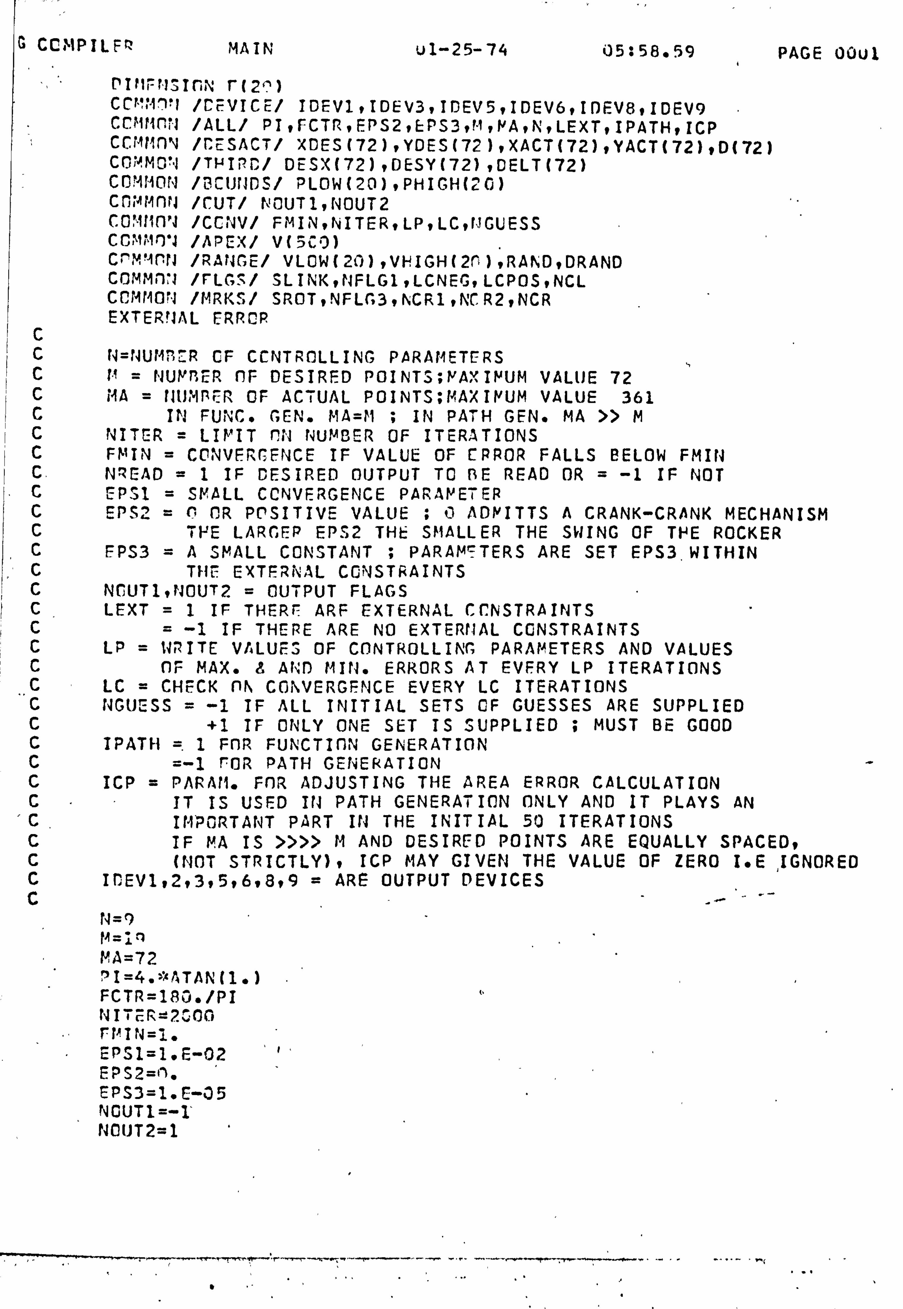
G CCýMPILFfz MAIN ul-25-74 05: 58.59 PAGE OOU1
PI? 1Fr"I, InN r(2^) ccm: i. '. 1'1 /Cc"VICE/ IDEVI, IDEV3, IDEV5, IDEV6, IDEVB, IDEV9 CC`1P1flN /ALL/ PI, FCTR, EPS29EPS3, º"1, NA, N, LEXT, IPATHIICP ccMrInN /CESACT/ XDES(72), YDES(72), XACT(72), YACT(72), D(72) COMMON /THIRD/ DEESX(72), DESY(72), DELT(72) C0M110N /3CUrJDS/ PLOW (20) 9 PHI GH (2 0) crj; Mn1J /CUT/ NOUT1, NOUT2 CO'1tin}J /CGVV/ FMIN, NITER, LP, LC, rJGUESS CCM I10"4 /APEX/ V (--')C-0) crMMnrJ /RANGE/ VLOW(2O), VHIGH(2rr), RAMD, DRAND COMMf; J /FLGS/ SLINK, NFLG1, LCNEG, LCPOS, NCL CCMMOrJ /MRKS/ SROT, NFLr3, NCR19NCR2, NCR EXTER! JAL ERRCP
N=NUMP, ̀R CF CCNTROLLING PARAMETERS tt = NUVRER OF DESIRED POINTS; NAXIMUM VALUE 72 MA = DUMBER OF ACTUAL POINTS; MAXIMUM VALUE 361
IN FUNC. GEN. MA=M ; IN PATH GEN. MA »M NITER = LIMIT ON NUMBER OF ITERATIONS FMIN = CONVERGENCE IF VALUE OF ERROR FALLS BELOW FMIN NREAD =1 IF DESIRED OUTPUT TO RE READ OR = -1 IF NOT EPSI = SMALL CCNVERGENCE PARAMETER EPS2 =G OR POSITIVE VALUE ;0 ADMITTS A CRANK-CRANK MECHANISM
T}'E LARGEP EP S2 THE SMALLER THE SWING OF THE ROCKER EPS3 =A SMALL CONSTANT ; PARAMETERS ARE SET EPS3 WITHIN
THE EXTERNAL CONSTRAINTS NOUT1, NOUT2 = OUTPUT FLAGS LEXT =I IF THERE ARF EXTERNAL CONSTRAINTS
= -1 IF THERE ARE NO EXTERNAL CONSTRAINTS LP = WRITE VALUES OF CONTROLLING PARAMETERS AND VALUES
OF MAX. A AND MIN. ERRORS AT EVERY LP ITERATIONS LC = CHECK ON CONVERGENCE EVERY LC ITERATIONS NGUESS = -1 IF ALL INITIAL SETS OF GUESSES ARE SUPPLIED
+1 IF ONLY ONE SET IS SUPPLIED ; MUST BE GOOD IPATH 1 FOR FUNCTION GENERATION
=-1 OUR PATH GENERATION ICP = PARAM. FOR ADJUSTING THE AREA ERROR CALCULATION
IT IS USED IN PATH GENERATION ONLY AND IT PLAYS AN IMPORTANT PART IN THE INITIAL 50 ITERATIONS IF MA IS »» M AND DESIRED POINTS ARE EQUALLY SPACED, (NOT STRICTLY), ICP MAY GIVEN THE VALUE OF ZERO I. E
, IGNORED
IDEV1.2,3,5,6,8,9 = ARE OUTPUT DEVICES
N=9 14 =1 '1 MA=72 ')I=4. eAATAh(1 FCTR=180. /PI NI T; f: =2CQ0
EPS1=1. F-02 EPS2=11. EPS3=1. E-35 NOUT1=-1' NQUT2=1
+-, . -"rr-.. r+e . r-: r,. -* -ý. -� T --ar t --"- -"-"-- +r" ý, r -- . -+-- _... - .,

CCMMPIL' 7 MA IN, u1-25-74 0558.59 PAGE 0002
; ýF-. ýn=+1 L7 X7=-1 LP= ,,. LC=1
IPAT11=-1 ICP=2 IDc: VI=1 IDEV2=2 IDEV3=3 ID7V4=4 ID=V5=5 IDFV6=6 IDEVE=8 IDEV9=9
C C DATA FOR'FLGS AND MRKS LABELLED CGMMGNS C (JFLG1, I4FLG3 = -1 COMBINED WITH VALUES GF SLINK AND SROT C ALLOWEi FOR CHOICE -OF LINK-CLOSURE AND ROT. DIRN. OF CRANK C IF NO CHOICE IS DESIRED THEN LEAVE AS BELOW C
SLINK=1. SROIT=I. NFLGI=1 NFLG3=1 LC'IEG=0
LCPOS=n NCR2=r '4CL=203 NCR=211
C. WRITE (IDFV6, IIn)M, MA WRITr(IDEV6,111)
C C DESIRED OUTPUT C
IF(IIREAD. LE. C)GO TO 1 RFAD(IDEVI, 101)(XCES(I), I=1, M) READ(IDEV1,101)(YDES(I), I=1, M) IF(IPATH. LT. 0) GO TO 4 READ(IDEV1,101)(DELT(I)9I=1, M) GO TO 4 ,,. _.... .
C C DESIRED X8Y COORDINATES C
1 CCrIT INuE XADf=51. YARD=35::. XDFS(1)=164. +XACD YDES(1)=8. +YA0D' XDEZ(2)=164. +XADD YCE S(2)=O. +YAnf XDES(3)=1GO. +XADD YDES(: 3)=O. +YADD
S
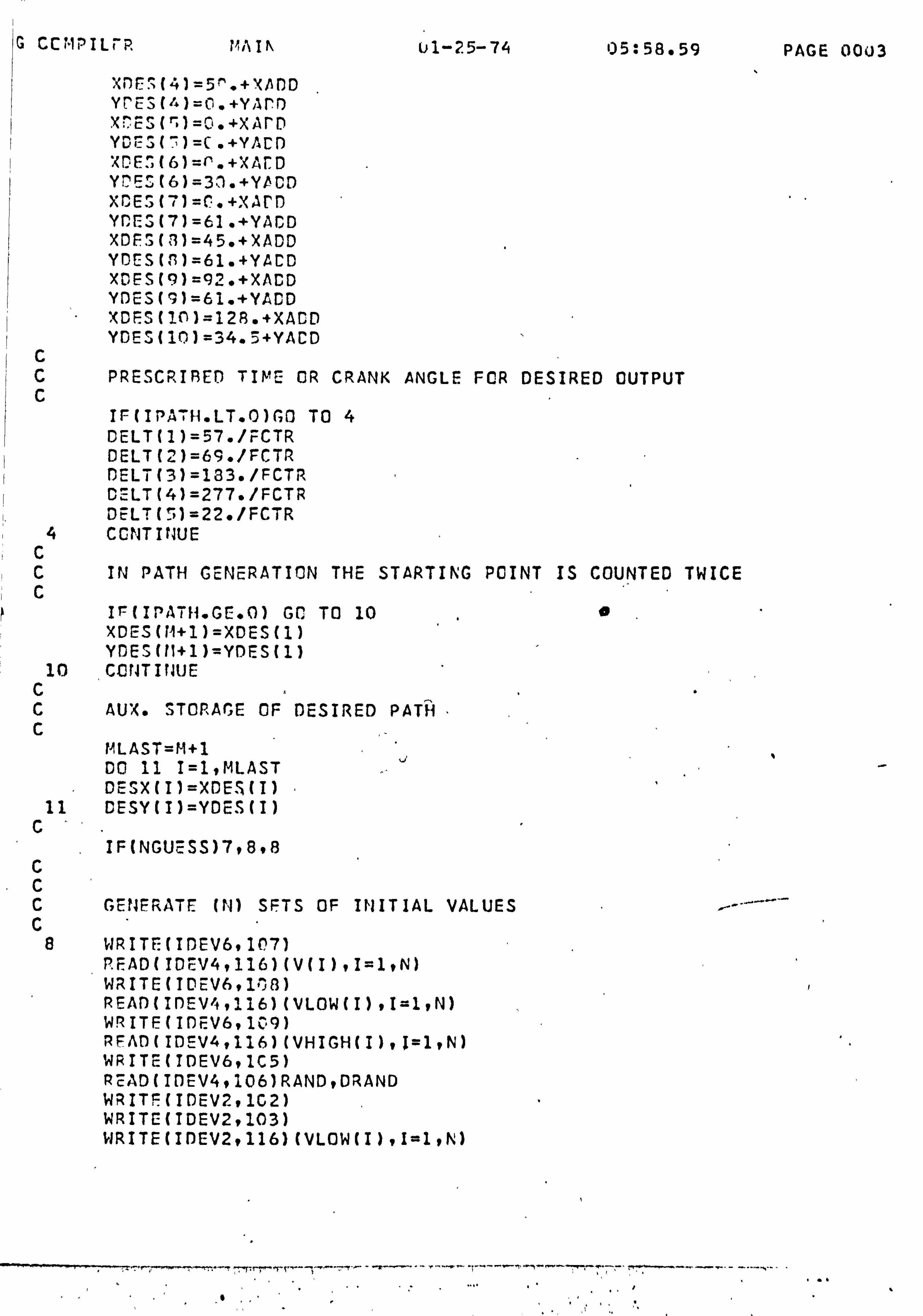
G CC', -Ii-)IL; -P, VA Ifx u1-25-74 05: 58.59 PAGE 0003
XDE; (4)=5n. +XADD YrES (')=o. +YArf) X^ES(r)=10. +xArD Yw S(: ')=C. +YAC1)
YnES(6)=31. +YADD XCES(7)=C. +XArD YCES(7)=61. +YACD XDES(8)=45. +XADD YDES(S)=61. +YACD XDES(9)=92. +XACD YDES(9)=61. +YACD XDES(1O)=I28. +XACD YDES(10)=34.5+YACD
C C PRESCRIBED TIME OR CRANK ANGLE FOR DESIRED OUTPUT C
IF(IPA H. LT. O)GD TO 4 DELT(1)=57. /FCTR DELT(2)=69. /FCTR DELT(3)=183. /FCTR CELT(4)=277. /FCTR DELT(51=22. /FCTR
4 CONTINUE C C IN PATH GENERATION THE STARTING POINT IS COUNTED TWICE C
IF(IPATH. GE. 0) GO TO 10 XDES(11+1)=XDES(1) YDES(11+1)=YDES(1)
10 CLNTINUE C C AUX. STORAGE OF DESIRED PATH C
MLAST=M+1 00 11 1=1, MLAST - DESX(I)=XDES(I)
11 DESY(I)=YDES(I) C.
IF(NGUEESS)7,8,8 C
.C C GENERATE (N) SETS OF INITIAL VALUES C
8 WRITE(IDEV6,107) PFAD(IDEV4,116)(V(I), I=1, N) WRITE(IDEEV6, I)8) READ(IDEV4,116)(VLOW(I)91=1, N) WRITE(IDEEV6,109) RFAD(IDEV4,116)(VHIGH(I), I=1, N) WRITE(I0EV6,1C5) READ(IDEV4,106)RAND, DRAND WRITF(IDEV2,162) WRITE(IDEV2,103) WRITE(IDEV2,116)(VLOW(I), I=1, N)
------r---- rr. -tý'- -e -""- - -' r: "-ý^ ^- t+. - -- -. - -. _ w
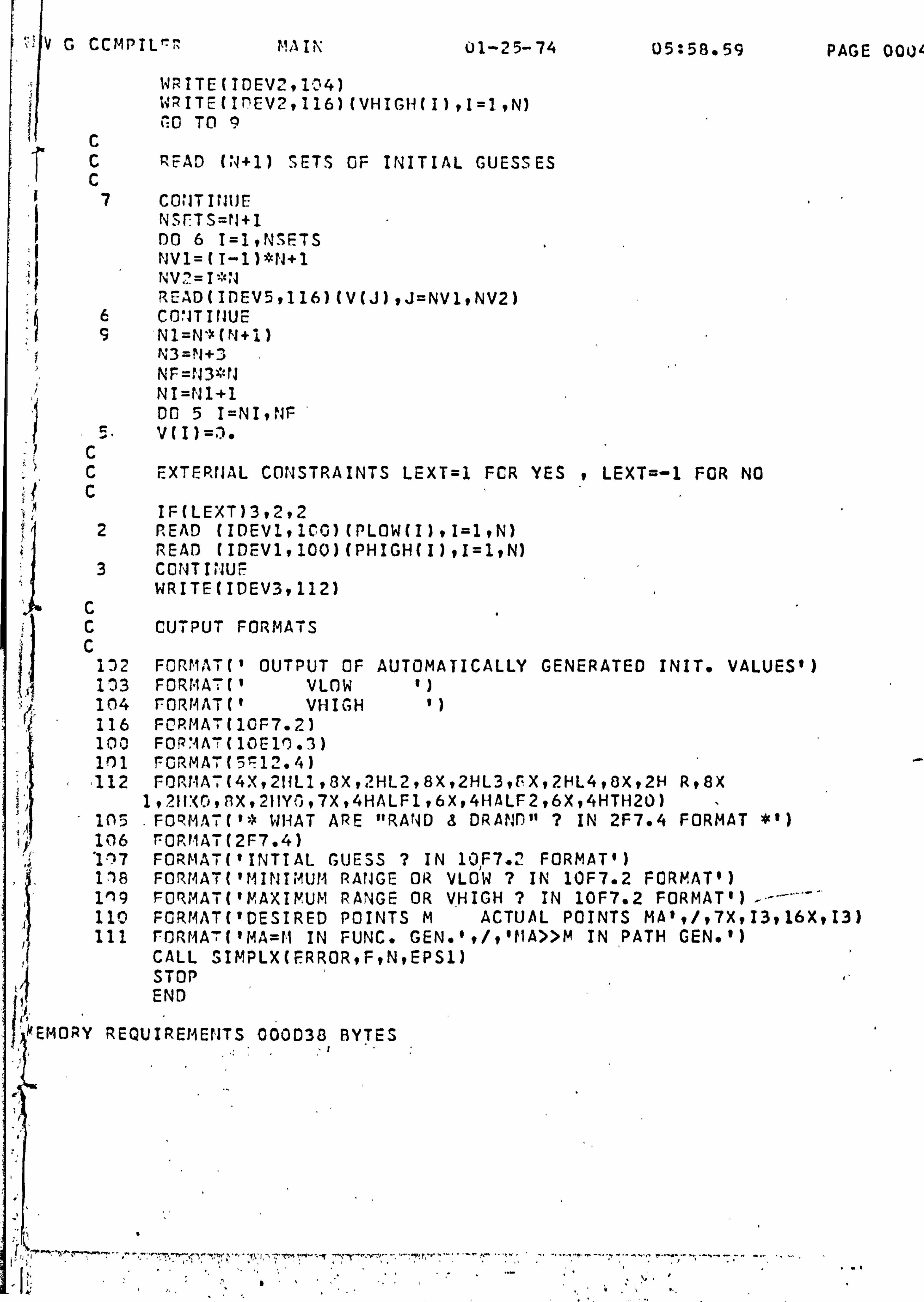
'V
I
t f
G CCMPIL'-T MA IIN 01-25-74 05: 58.59 PAGE 000'
WRITE(IDEV2ºI'34) k4RITE(IfEV2,1I6) (VHIGH(I), I=1, N) CO : TO 9
C C READ M+1) SETS OF INITIAL GUESSES C
7 CONTINUE NSr'TS=r(+1 DO 6 I=1, NSETS NVI= (I-1)*N+ I NV'=1 N READ(IDEV5,116)(V(J), J=NV1, NV2)
6 C0'1TINUE 5 N1=N' (N+i)
N3=N+3 NF=N3*N NI=NI+1 DO 5 I=NI, NF
C C EXTERNAL CONSTRAINTS LEXT=1 FCR YES , LEXT=-1 FOR NO C
IF(LEXT)3,2,2 2 READ (IDEVI, ICG)(PLOW(I), I=1, N)
READ (IDEV1,100)(PHIGH()9I=10) 3 CCNTIPJUr
WRITE(IDEV3,112) C C CUTPUT FORMATS C
1D2 FORMAT(' OUTPUT OF AUTOMATICALLY GENERATED INIT. VALUES') 103 FORMAT(' VLOW ') 104 FORMAT(' VHIGH ') 116 FORMAT(1GF7.2) 100 FORMA', (10E10.3 ) 101 FORMAT(5F12.4) 112 FORT-IAT (4X, 2HLI, 8X, 2HL2,8X, 2HL3, £X, 2HL4, QX, 2H R, 8X
1,2lIX0, SX, 2HY), 7X, 4HALF1 , 6X, 4HALF2,6X, 4HTH2O ) 105 FORMAT('* WHAT ARE "RAND 8 DRANO" ? IN 2F7.4 FORMAT *1) 106 FORt1AT(2F7.4) '117 FORMAT('INTTAL GUESS ? IN 10F7.2 FORMAT') 118 FORMAT('MINTMUM RANGE OR VLOW ? IN 1OF7.2 FORMAT') 1'9 FORMAT('MAXIMUM RANGE OR VHIGH ? IN 10F7.2 FORMAT') 110 FORMAT('DESIRED POINTS M ACTUAL POINTS MA', /, 7X, I3,16X, 13) 111 PATH GEN. ') FORMA; ('MA=(1 IN FUNC. GEN. ', /, 'PMA»M IN
, CALL SIMPLX(ERROR, F, N, EPS1) STOP
i,? END
JEMORY REQUIREMENTS 000038 BYTES
,, ý"`
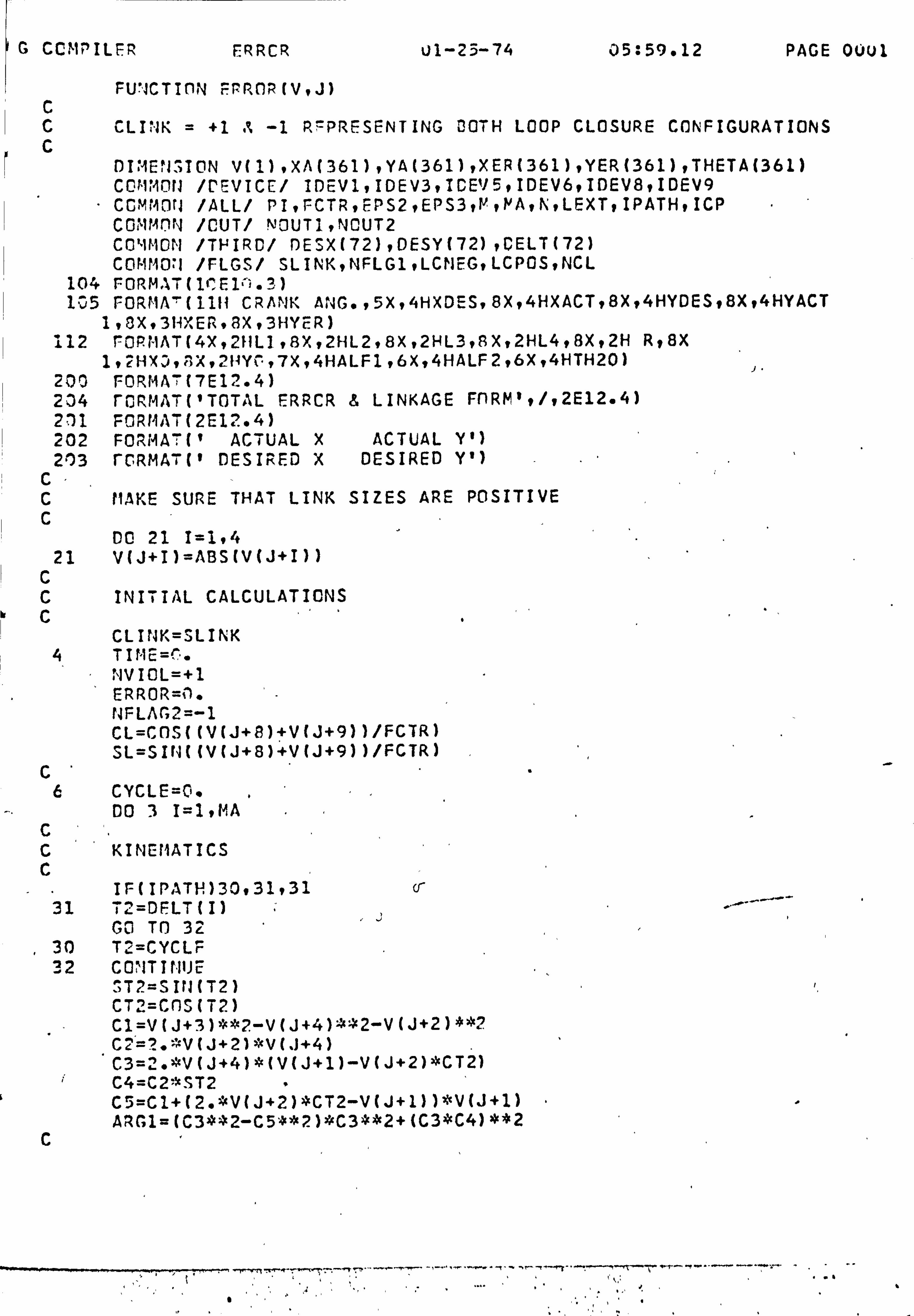
G COMPILER ERRCR ul-23-74 05: 59.12 PAGE OOu1
FUNCTION FRROP(V, J) C C CLINK = +1 A -1 R"PRESENTING BOTH LOOP CLOSURE CONFIGURATIONS C
DINEN3ION V(1), XA(361), YA(361), XER(361), YER(361), THETA(361) COMMON /CEVICE/ IDEV1, IDEV3, ICE'15, IDEV6, IDEV8, IDEV9 COMMON /ALL/ PI, FCTR, EPS2, EPS3, M, MA, N, LEXT, IPATH, ICP CGMMnrJ /CUT/ NI3UT1, NCUT2 COMMON /THIRD/ DESX(72), DESY(72), CELT(72) COMM071 /FLGS/ SLINK, NFLG1, LCNEG, LCPOS, NCL
104 FORM. %T(1' E1V). 3) 135 FORIA'(111( CRANK ANG., 5X, 4HXDES, 8X, 4HXACT, 8X, 4HYDES, 8X, 4HYACT
1,8X. 3HXER. 8X, 3HYER) 112 FORtNAT(4X, 2}HL1, BX, 2HL2,8X, 2HL3, RX, 2HL4,8X, 2H R, 8X
1,2HX3, SX, 2HYi", 7X, 4HALF1,6X, 4HALF2,6X, 4HTH2O) 200 FORMA7(7E12.4) 204 rORMAT('TOTAL ERRCR 8 LINKAGE FfRM', /, 2E12.4) 201 FORMAT(2E12.4) 202 FORMAT(' ACTUAL X ACTUAL Y') 203 rORMAT(' DESIRED X DESIRED Y')
C- C MAKE SURE THAT LINK SIZES ARE POSITIVE C
DU 21 I=1.4 21 V(J+I)=ABS(V(J+I))
C C INITIAL CALCULATIONS C
CLINK=SLINK 4 TI%1E=(".
NVIOL=+1 ERROR=+'1. - NFLAG2=-1 CL=CDS((V(J+8)+V(J+9)1/FCTR) SL=SINJ((V(J+8)+V(J+9))/FCTR)
C E CYCLE=C.
DO 3 I=1, MA C C KINEMATICS C
IF(IPATH)30931,31 cr 31 T2=DFLT(I)
GO TO 322- 30 T2=CYCLF 32 CONTINUE
"T2=S IN (T2 ) CT2=CnS(T2) C1=V(J+3)* 2-V(J+4)**2-V(J+2)**2 C 2= ?. °»V (J+21 *V (. J+4) C3=2. *V(J+4)*(V(J+1)-V(J+2)PCT2) C4=C2*ST2 C5=C1+(2. MV(J+2)4CT2-V(J+1))*V(J+1) ARG1=(C3**2-C54*2)*C3**2+(C3*C4)**2
C
-rin-. ý. ý-+-"-«. R'r : "-, -r-'.. M. - -, .,. ...... ý. ý. ,. ý. -+? -"^-ý---'ýý-ýc---i-"-r-. + ........ _.. _ -- '-
....
1G CCº1PILEh FRRf R ul-25-74 05: 59.12 PAGE 001)2
C ARF- CnNNSTRAINTS VIOLATED C
CALL CONSTR(ARG1, V, J, NVIOL) C C LOOP CONSTRAINTS HAVE BEEN VIOLATED C
IF(rlVIOL)22,23,23 22 GO TO 4 23 CONTINUE
C C CONTINUE WITH THE KINEMATICS C
ST4=(-C4cC5+CLINK*SQRT(ARG1))/(C34*2+C4**2) CT4=(C5+C4*ST4)/C3 ST3=(V(J+4)*ST4-V(J+2)*ST2)/V(J+3) CT3=(V(J+I)+V(J+4)*CT4-V(J+2)*CT2)/V(J+3)
C C ACTUAL MOTION C,
XA(I)=V(J+6)+V(J+2)cCOS(T2+V(J+8)/FCTR)+V(J+5)*(CL*CT3-SL*ST3) YA(I)=V(J+7)+V(J+2)*SIN(T2+V(J+8)/FCTR)+V(J+5)*(SL*CT3+CL*ST3)
C IF(IPATH)33,34,34
C C EVALUATION OF OBJECTIVE FUNCTION. I. E ERROR CRITERION C `"
34 XER(I)=(XA(I)-DESX(I))**2 YER(I)=(YA(I)-DESY(I))4*2 ERROR=ERROR+XE_R(I)+YER(I) GO TO 3
C. 33 CYCLE=CYCLE+2. *PI/MA 3 CONTINUE
C C IF PATH GENERATION CALL PATH SURRCUTINE£ C
IT(IPATH. GE. C) GO TO 35 CALL PATH($UM, XA, YA) ' ERROR=SUM
C C SORT OUT LINKAGE CLOSURE CONFIGURATION C
35 IF(NFLAG2. GT. G) GO TO 13 IF(I4rLG1. LT. 0) GO TO '41 IF(CLTNK)7,8,8
a CLIrJK=-1. TERR=Frp. OR ERROR=-I. GO TO 6
7 IF(TEERR-ERROR)9, -11,11 9 FRRCIR=TERR
CLINK=1. LCPnS=LCPOS+1 GO TO 40
11 LCNEG=LCNEG+1
"'
S
G CCMPILER ERRPR vl-25-74 05: 59.12 PAGE 0003
40 CCNTItIU IF(LCPnS. 'E. NCL)5LINK=1. IF(LCNEG. Gr:. NCL)SLINK=-1. IF((LCPOS. CE. NCL). OR. (LCNEG. GE. NCL))NFLG1=-1
41 CONTINUE C C OUTPUT C
IF(NJOUT2)17.18,12 I8 KP=J+I
KPAR=KP+N, -1 WRITE(IDEV3,1D4)(V(I), I=KP, KPAR)
17 CONTINUE C C THIS IS THE CPTIMISED OUTPUT C OPTIMISATION SUCCESS ***** C
IF(NOUT1)12,12,5 C C ORGAN73E FINAL CALL AND OUTPUT RESULTS C
NFLA =1. ERROR='?. GO TO 6
13 CONTINUE C
IF(IPATH)36,37,37 C C PATH Gi: NERAT ION OUTPUT C
36 WRITF(IDEV6,112) WRITE(IfEV6,1: 14) (V(I), I=1, N) '4RITC(IDEV6,202) 00 33 I=1, MA WRITE(IDEV6,201)XA(I), YA(I)
38 CONTINUE %IRITE(IDEV6,, 203) DO 39 I=1, M WRIT(IDEV6,201)CESX(I), OESY(I)
39 CONTINUE GO TO 66
C 37 CONTINUE
C C FUNCTIf1N GENERATION OUTPUT C
WRITF (IDFV6,112) WRITE(IDEV6,104)(V(I, ), I=19N) WRITE(IDEV691051 on 16 I=1, M THETA(I)=DELT(I)*FCTR WRITE(IDEV6,20O)THETA(I), DESX(I), XA(I), DESY(I), YA(I)
1, XER(I), YER(I) 16 C014TINNUF! 60 CONTINUE
G CCMPIL^^ ERRCP U1-25-74 05: 59.12 PAGE 00U4
WRITr(IfF. V6,204)FRROR, CLINK 12 CONTINUE
RETURN =ND
I FMORY REQUIREMENTS 002890 BYTES
1 r�'_.
ýý
i
1",
^. nýnn .. -. + mt -a rý++ý... .. +. ý. rýr....... ýy.. ». _y,. n.. n .. y. ý. »rýT`i^ .. y .-.. e r .., y'ý^R r.. ý. ý .. - .: ý.,.. n, nr . +. ý . i. ý... ýý "ý
G CCMPILFR STIIPLX u1-25- 74 05: 59.26 PAGE OOU1
SU^, RnUTINS ! IWr'LX(FUNC, F, N, EPS1) C ACTUAL NO. CF PARAMr`. TERS = 11 C DI'IENSinN OF 'V' IS V(N4(N+3) ) C DIr1ENSIDN OF 'F' 15 F(N+3) C DINENSION nr 'VC' IS VC(N)
FXTE UJAL FUNC COMrInrN /CFVTCE/ IDEV1, IDEV3, ICEV5, IDEV6, IDEV8, IDEV9 COMMON /CCNV/ FMIN, NITER, LP, LC, NGUESS COMMON) /OUT/ NnUT1, NOUT2 COMMON /CENTRF/ VC(20) COMMON /APEX/ V(500) 0IM3r4SION F(1) DATA ITLR, r"IAX, MM, MIt4/0,3*1/
101 ? -0R? 4AT('INITIAL FUNCTION VALUES, FI,.. F(N+1) ARE: ') 107 F0RMAT(1X, 5F15.5) 102 FORMAT('SIMPLEX IS BEEING HALVED')
103 FORMAT(' THIS THE END OF SUBROUTINE "START") 119 FCRMV ('PARAMS. FOR F(MAX)') 120 cGRMt4Tt'PARAMS. FOR F(MIN)')
104 FGRMAT('NAX. ERRGR VALUE IN CURRENT SIMPLEX', /, E15.6) 105 FORMAT('MIN. ERROR VALUE IN CURRENT SIMPLEX', /, EI5.6)
117 FORMAT('CONVERGENCE***SUCCESS*** ', /) 112 FORMAT('OITERATIONS ='0I1U)
4.21 FORr1AT('FINAL VALUES OF LINKAGE PARAMETERS') 115 FORMAT(IX, 5E15.6) 122 FORMAT('MINIVUM ERROR', /E15.6)
C C C
C C C C
43
c c c
42
46 45
2 44
CALCULATE STARTING VERTICES AND FUNCTION VALUES
N1 = rs +1 N3 =N+3 NN = rl*N1
IF (t4Gl1'SS)42,43,43
, GENERATE INITIAL VALUES
CONTIi4U7
-CALL START (FUNC, F, V, N) WRITE(IDFV4,103) GO T(1 44
INITIAL SETS ARE GIVEN
CONTINUE DO 45 I=19N VC(I)=J. 00 46 L=1, fl1 VC(I)=VC(I)+0.5*V(I+(L-1)*N)_ CONTINUE DO 2 I=1, NI ' F(I) = FIJNC(V, (I-1)*N) CONTINUE WRITE(IDEV3,101) WRITE(IDEV3,1C7) (F(I), I=1, N1')
ý,,..
1.
+ýwý. r . w+.., w. -+ý-+-...... +. -,.. g...... ý.. ý, T ..
, "r".... -. -r-.. s- ,-..... ... ... .. -ý .., ". `ý? t! ý T^. X, ̂ 'Y'T"'p; 4'Iý'R, -nA 4_'T! q'.. ý»,
ý Cß'3"
:V -}wC".. ý. "
,.. ', 'ý'"Tti . --... r
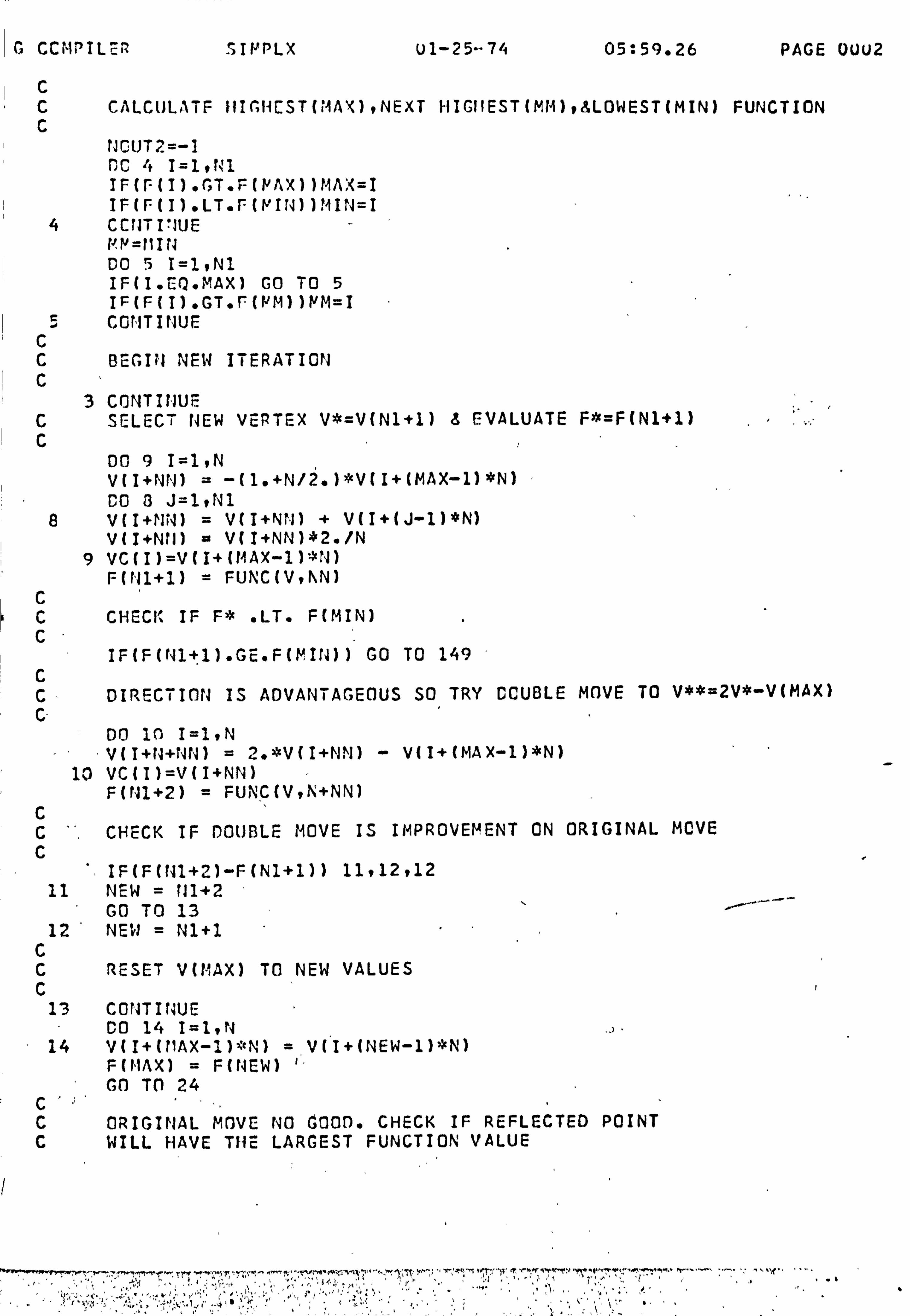
C CCMPILEP SIVPLX U1-25"-74 05: 59.26 PAGE UUU2
C C CALCULATF IIIGNCST(t1AX), NEXT HIGIIEST(MM), BLOWEST(MIN) FUNCTION C
NJCUT2=-i DC ' I=1, N1 IF(F(I). GT. F(NAX) )M11X=I IF (F(I) . LT. F(NIN) )! IIN=I
4 CCIITI'JUE N. N=f1ItJ 00 5 i=1, N1 IF(I. EQ. MAX) GO TO 5 IF(F(I). GT. F(NM))NM=I
5 CONTINUE C C BEGIN NEW ITERATION C
3 CONTINUE C SELECT NEW VERTEX V*=V(N1+1) 8 EVALUATE F*=F(N1+1) C
DO 9 I=19N V(I+NN) = -(1. +N/2. )*V(I+(MAX-1)*N) CO 3 J=1, N1
8 VII+Ni4) = V(I+NN) + V(I+(J-1)*N) V(I+Ntl) = V(I+NN)*2. /N
9 VC(I)=V(I+(MAX-1)*N4) F U41+1) = FUNC (V, I\N )
C C CHECK IF F* LT. F(MIN) C.
IF(F(N1+1). GE. F(MItJ)) GO TO 149 c C- DIRECTION IS ADVANTAGEOUS SO TRY CCUBLE MOVE TO V**=2V*-V(MAX) C- '
C C, C
11
12 C C C
13
14
DO 10 I =1, N V(I+N+NN) = 2. *V(I+NN) - V(I+(MAX-1)*N)
10 VC(I)=V(I+NN) F(111+2) = FUNC(V, N+NN)
CHECK IF DOUBLE MOVE IS IMPROVEMENT ON ORIGINAL MOVE
IF(F(tdl+2)-F(N1+1)) 11,12,12 NEW = 111+2 GO TO 13 NEW = N1+1
RESET MAX) TO NEW VALUES
CaNTI1IJE
C C C
CO 14 I=19N V(I+(11AX-1)'N) = V(I+(NEW-1)*N) F(MAX) = F(NEW) GO TO 24
ORIGINAL MOVE NO GOOD. CHECK IF REFLECTED POINT WILL HAVE THE LARGEST FUNCTION VALUE
I
. -r±ý^*ý!. »ýrý. ýI.,, t. F., ý...., , ryi; -S"ý; c . ,.., ý., t". N yi'ýný. Mýý w., S. iý'(r ý,. " ., i'"ýn, -ý. ýý. i... ý . "r av++.. ýýe ry` . r... ±m ýý..
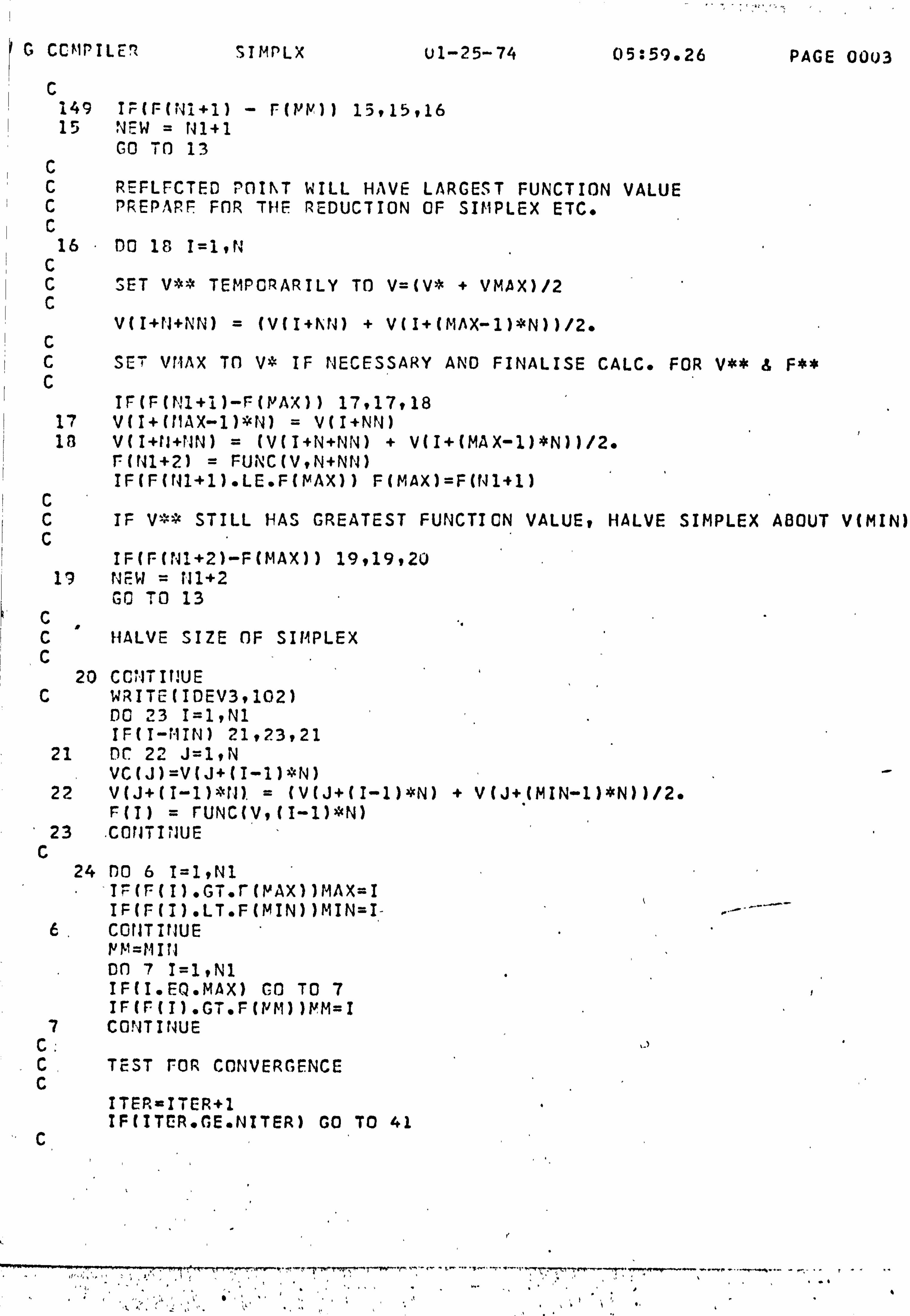
G MIPILE- SIMPLX U1-25-74 05: 59.26 PAGE 0003
149 IF(F(N1+I) - F(7 )) 15,15,16 15 NEW = N1+1
GO TO 13 C C REFLECTED POINT WILL HAVE LARGEST FUNCTION VALUE C PREPARE FOR THE REDUCTION OF SIMPLEX ETC. C
16 DO 18 1=1, N C C SET V** TEMPORARILY TO V=(V* + VMAX)/2 C
V(I+f1+NN) = (V(I+Nt4) + V(I+(MAX-I)*N))/2. C C SE-'+ VTIAX TO V* IF NECESSARY AND FINALISE CALC. FOR V** d F** C
IF(F(N1+i)-F(MAX)) 17,17,18 17 V(I+(11AX-I)*N) = V(I+NN) in V(I+tt+rIN) = (V(I+N+NN) + V(I+(MAX-1)*N)l/2.
F(tN1+2) = FUNC(V, N+NN) IF(F(N1+1). LE. F(MAX)) F(MAX)=F(141+1)
C C IF V-* STILL HAS GREATEST FUNCTION VALUE, HALVE SIMPLEX ABOUT V(MIN)
IF(F(N1+2)-F(MAX)) 19,19,20 19 NEW = N1+2
GO TO 13 C C HALVE SIZE OF SIMPLEX C
20 CMITINUE C WRITE(IDEV3,102)
DO 23 I=1, N1 IF(I-MIN) 21,23,21
21 DC 22 J=1, N VC(J)=V(J+(I-I)*N) -
22 V(J+(I-I)*NNJ). = (V(J+(I-1)*N) + V(J+(MIN-1)*N))/2. F(I) = rUNC(V, (I-I)*N)
23 . CONTINUE C
24 DO 6 1=101 IF(F(I). GT. r(MAX))MAX=I IF(F(I). LT. F(MIN))MIN=I- -- '`"
6. CONTINUE NM=MITJ on 7 I=1, N1 IF(I. ER. MAX) GO TO 7 IF(F(I). GT. F(MM))MM=I
7 CONTINUE C: C TEST FOR CONVERGENCE CS
ITER=ITER+1 IF(ITER. GE. NITER) GO TO 41
C
V
! '. R,. "[r+....., -. r.. -. ", " T-ý, -ro"T-a, r^"... 7". -�ýs....,.,, ,., -. ,. -" at.,.. ten-. -t+-rew"-"---, T-""+*+r. 'ý-"--........ -.. _... ý....,. ý_. _ ... , ....

+j G CCMPIUR SIPPLX U1-25-74 05: 59.26 PAGE U004
C WRITE i'P, (7GRr: 55 OF flPTIMISATION EVERY LP ITERATIONS C
Ir(ITrR/LP-(ITF-R-1)/LP*EQ*U) GO TC 40 WRITF(IDEV3,112)ITER I=(MAX-1)*N+1 J=MAX*iJ WRITE(IDEV3,119) 1" JZITE(IDEV3,115) (V(K), K=I, J) WRITE(IDEV3,104)F(MAX) I=(MIP! -1)PJ+1
WKITE(IDEV3,120) WRITE(IDEV3,115)(V(K), K=I, J)
} WRTTF(IDEV3,105)r(MIN) CC
C CHECK CONVERGENCE EVERY LC ITERATIONS C
40 IF(IT'! R/LC-(ITFR-1)/LC. EQ. U) GO TO 3 TF(F(tlIN). LE. FMIN) GO TO 41
C C CONVERGENCE IF ABS. (FMAX-FMIN) LESS THAN ABS. (EPS1 * FMIN) C C IF(F(MAX)-F(MIN). GT. ABS(EPS1*F(1.11N)))GO TO 3 C C CONVERGENCE IF ABS. (VMAX-VMIN) LESS THAN ABS. (EPS1 * VMIN) C
DO 99 I=1, t! IF(ABS(V(I+(MAX-1)*N)-V(I+(MIN-1)*N)). GT. ABS(EPS1*V(I+(MIN-1)*N))
1)GO TO 3 59 CONTINUE
41 CONTINUE C C FILL F WITH PARAMETER VALUES AND F(MIN) C
26 - WRITE(IDEV6,117) WRITF(IDEV6,112)ITER DO 27 1=1, N . 27 V(1) = V(I+(MIN-1)*N) WRITE(IDEV6,121) WRITE(IDEV6,115)(V(1), I=1, N). 4IRITE(IDEV6,122)F(MIN) NOUT1=1 F(td1)=FUNC(V, O) RETURN END
MORY REQUIREMENTS 001272 BYTES
r ..,
I
q : TTT , n. ý.... _,., p. r "r. -ý... r-, -.. -. - ...., T.,,. ý..,. ýw,. ý.,,. ýr+o. n... ý. ý. ý.... ý-.., -.,.,..... -, «. e., ',.,... ý.. ., -
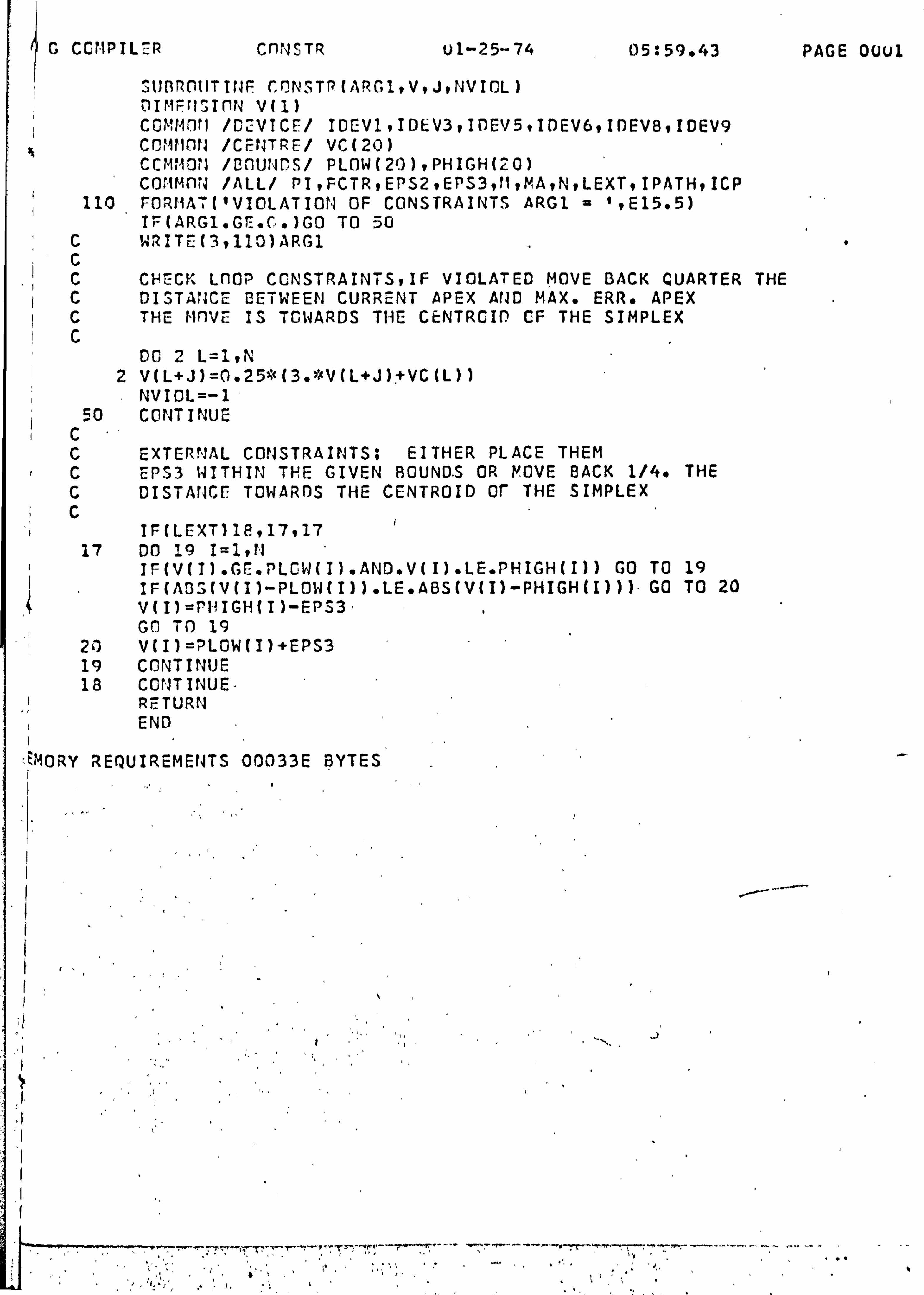
G CCi"1PILER CENJSTR u1-25--74 05: 59.43
SURRO11TTNF CRNSTR(ARG1, V, J, NV IOL ) DiMFrl; InN v(1) COMMON /D2VTCF'/ IDEV1, IDEV3, IDEV5. IDEV6, IDEVB, IDEV9
,4 COMtION /CENTRE/ VC(20) CCMMON /BfUINCS/ PLOW(20), PHIGH(20) COMMnN /ALL/ PI, FCTR, EPS2, EPS3,11, MA, N, LEXT, IPATH, ICP
110 FORHAT('VIOLATION OF CONSTRAINTS ARGI = ', E15.5) Ir (ARG1. Gr: ':. C,. )GO TO 50
C WRITE(3,11O)ARG1 C C CHECK LOOP CCNSTRAINTS, IF VIOLATED MOVE BACK QUARTER THE C DISTANCE BETWEEN CURRENT APEX AND MAX. ERR. APEX C THE MnVE IS TOWARDS THE CENTRCID CF THE SIMPLEX C
DO 2 L=1, N 2 V(L+J)=0.25*(3. *V(L+J)±VC(L) )
NVIDL=-1 50 CONTINUE
C ' C EXTERNAL CONSTRAINTS; EITHER PLACE THEM C EPS3 WITHIN THE GIVEN BOUNDS OR ROVE BACK 1/4. THE C DISTANCE' TOWARDS THE CENTROID Or THE SIMPLEX C
IF(LEXT)18,17,17 17 DO 19 I=1, NNJ
IF(V(I). GE. PLCW(I). AND. V(I). LE. PHIGH(I)) GO TO 19 IF(ADS(V(I)-PLOW(I)). LE. ABS(V(I)-PHIGH(I))) GO TO 20 V(I)=PHIGH(I)-EPS3 Gil TO 19
20 V(I)=PLOW(I)+EPS3 19 CONTINUE 18 CONTINUE
RETURN END
-EMORY REQUIREMENTS 00033E BYTES
PAGE ODUI
0
ý,. `"
'\
») ý
". ý,
ý'
TT I
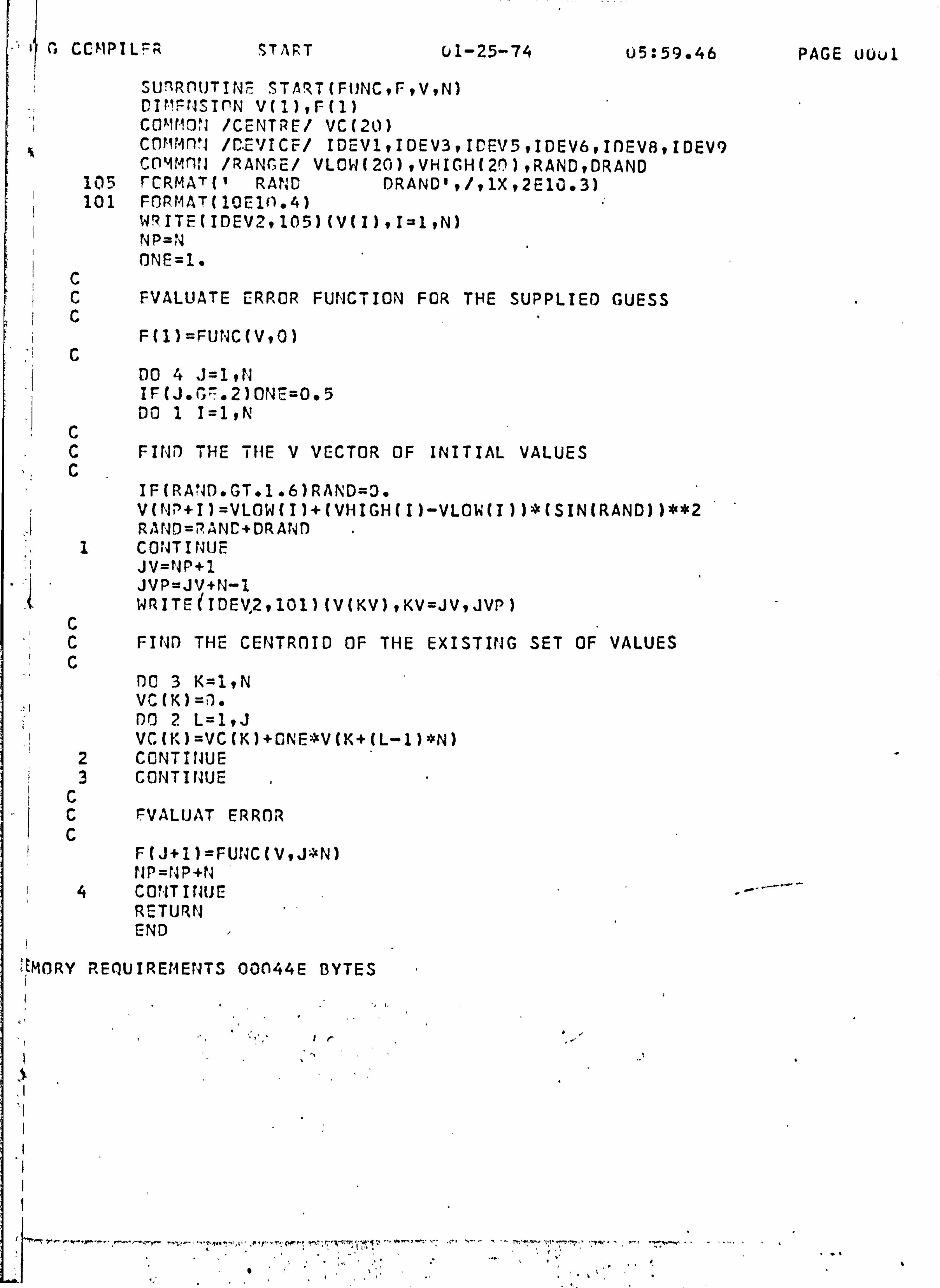
G CCMPILFR START U1-25-74 05: 59.46
SUTRDIJTIN'c START(F(JNC, F, V, N) DI1IFNSIDN V(I), F(1) CO^1r"10"J /CENTRE/ VC(20) COr"IMnol /CLYICE/ IDEVI, IOEV3, ICEV5, IDEV6, IDEV8, IDEV9 COMMn; 1 /RANGE/ VLOW(20), VHIGH(2'), RAND, DRANO
105 FCRMAT(' RAND DRAND', /, 1X, 2E10.3) 101 FORMAT(14Elfl. 4)
WRITE(IDEV2,105)(V(I), I=1, N) NP=N ONE=1.
C c FVALUATE ERROR FUNCTION FOR THE SUPPLIED GUESS C
F(I)=FUNC(V, 0) C
00 4 J=1, N IF(J. G7.2)ONc=0.5 DO 1 1=1, N
C C FIND THE THE V VECTOR OF INITIAL VALUES C
IF (RA'JD. GT. 1 . 6) R1\ND=D. V(1. lP+I)=VLOW(I)+(VHIGH(I)-VLOW(I))*(SIN(RAND))**2 RAND=PANG+DRAND
I CONTINUE JV=NP+1 JVP=JV+N-1 WRITE(IDEV, 2,101)(V(KV), KV=JV, JVP)
C C FIND THE CENTROID OF THE EXISTING SET OF VALUES C
DC 3 K=19N VC(K)=D. 00 2 L=1, J VC(K)=VC(K)+ONE-V(K+(L-1)*N)
2 CONTINUE 3 CONTINUE
C C FVALUAT ERROR C
F (J+1) =FU14C (V, J*N) tlP=NP+N
4 CO? ITINU E RETURN END
EMORY REQUIREMENTS 00044E BYTES
"
PAGE Uüul
,.. ý... ý.... r... . -. Y-",... .. ; a, "-. r. ý. ný ý, ýý,. `. P.,. . ýýrwýýn
1".
ý"ýr'ýn týw"S f. . w.., ý .... ý
... ý'
''
., ý,., "' ,.
'..
ý, ý., a, -.... .. LF
IG CCMPTL R PATH ui-25-74 i)5: 59.51 PAGE UOu1
S1J? RflU, IN= rATM(S(M, XA, YA) nIME1JSIClN XA(3A1)9YA(361) 9TXA(361) , TYA(361), DA(361) COMr1n 1 /ALL/t PI, rCTR, F. PS2, EPS3, M. MAt N, LEXT, IPATH , ICP cm-mvi /DESACT/ 'IDES(72), YDES(72 ), XACT(72), YACT(72), D(72). CO'1t10f1 /MRKS/ SROT, NFLG3, NCR1, NCR2, NCR
C C FIND STARTING POINT FOR CALCULATION OF THE AREA ERROR C
Rf1T=SROT iJRN=1 DC 1 I=1, P'A TXA (I) =XA (I )
-1 TYA(I)=YA(I) D(I)=5t)RT((XDES(1)-XA('1) )4*2+(YOES(1)-YA(1))**2) DA(1)=D(1) MK1=1 DO" 2 I=2, MA )A(I)=SORT((XDES(1)-XA(I))**2+(YDES(1)-YA(I))**2) IF(DA(I). LT. DA(MK1))MK1=I
2 CONTINUE C C INDEX ACTUAL OUTPUT ACCORDING TO POSITION OF STARTING POINT C ALSO MAKE WINDOW SEARCH IN THE NEIGHBOURHOOD OTHE DESIRED POINT C
MR2=MK1-1 MR1=MA-MR2 DO 4 I=1, t1R1 XA(I)=TXA(MK1+I-1)
4 YA (I) =TYA (tlK I+I-1) IF(MR^. EC. O) GO TO 10 DO I J=1, MR2 MRi=F"1R1+1 XA(MR1)=TXA(J)
9 YA(t"1R1)=TYA(J) 10 CCNT IIJUE c 27 CONTINUE
IF(ROT)19,19,20 20 "IF (14FLG3. LT. O) GO TO 21
ROT=-i. GO Tfl 21
19 00 17 I=1, MA, TXA(I)=XA(MA-I+1)
17 TYA(I)=YA(ftA-I+1) DO ID I=1, NA XA(I)=TXA(I) YA(I)=TYA(T)
1n CONTINUE 21 XACT(1)=XA(1)
YACT(1)=YA(1) XACT(M+1)=XA(1)' '
-YACT(M+1)=YA(1),
MKP=2, D0, ,5 I=2 `M
ý0ý
t ý»...... 7ýr, -r. _a. -.., . r.. ,.,,. -,. ', ' ý+n r+ý^-, -.. ý. ýr-,.. -. - ... x'
ý, pL ý_ýýiýý
ý- n% C^ýýýI. ý ýt ýýýýef; ! ý%,, i'. ýý1ýý1 . h. ' e ýý", .aý. ý' ýý Ve tý
. o'. 'ý «'
,G CCMPILCP PATH u1-25-74 05: 59.51 PAGE OOU2
fl(i)=Sý%T((XDFS(I)-XA(MKP1)**7+(vnýcrrý_vntMknýýýýýº
t. ' r; ý
30 7
12
{. - 29 5 16
32
C
C C
-r
MK1=f1KP NCtJT=0 CA(f1KI)=D(I) on 7 J=t'K, f"1: 1 DA(J)=SQRT((XDES(I)-XA(J))**2+(YDES(I)-YA(J))**2) I1-(DA(J). LT. DA(MK1) )MK1=J NCNT=NCNT+I IF((lA-J)-(M-I))12.12,30 IF(14CWT. GE. ICP*MA/M)GO TO 11 CCrITItdUE GO TO 11 iF ((t-1A-MK1)-(M-I)) 16,16,11 N, K=t1K1+2 XACT(I)=XA(MKI) YACT(I)=YA(f1KI) IF(MK-MA )29.29,15 MKP=MA MK=MA GO TO 5 MKP=I. 1K-1 CONTINUE 00 32 K=I"M XACT(K)=XA(MK1) YACT(t: )=YA(MK1) MK1=MKI+1
WE HAVE NOW EQUAL NUMBER OF DESIRED AND ACTUAL POINTS ALSO THEY ARE CHOSEN SO AS TO MAKE CALCULATION OF AREA ACCURATE
AREA FRROR BETWEEN DESIRED AND ACTUAL FUNCTIONS
00 8 K=1, M AREA=0.5*(ARS((XDES(K)*YACT(K)-YDES(K)*XACT(K))
1+(XACT(K)*YACT(K+1)-YACT(K)*XACT(K+1)) 2+(XAC7(K+I)*YCFS(K)-YACT(K+1)*XDES(K))) 3+A3S((XDES(K)*YDES(K+1)-YDES(K)*XCES(K+1)) 4+(XDE7, (K+1)*PACT(K+1)-YOES(K+1)*XACT(K+1)) 5+(XACT(K+1)cYDES(K)-YACT(K+1)*XDES(K)')))
8 SUM=SU11+AREA IF(NFLr, 3. LT. 0) GO TO 22 IF(t"1Rt1)23,23,24
24 NRN=-1 SUM1=S11M SLJh1=0. GO 70 27
23 IF (SUM1-SUM) 25,26,26 25 SUM=SUM1
NCR1=1 CR1+1 Ga Tn 28
261=" NCR2=NCR2+1 28F (NCR 1. GE. NCR) SROT=1.
-': IF(tJCR2. GE. NCR )SRCT=-1. '-IF((NCRI. GE. NCR). CR. (NCR2. GE. NCR))NFLG3=-1
22' CONTINUE
. r. +,. srn+.. gý"ýT, ryt"^a-. ". w, -.. ", ". r"",. t:., l.. ^r. r"^"R'"s! ý'JiS rr: t""'-t-r "'YR,.. ý,;. tw.;. �, 3"....... .. y. R_,.. ý.,. y . -"ii"T"ý, r. . ry«ýý". ý., -. -, -"-- , rt»...,. ý..,; "., - 5 . _..,

G CCMPILE't . PATH
RETURN END
1ORY REQUIREMENTS 001850 BYTES
MINATED
U1-25-74 05359.51 PAGE 41)03
r
r'
"ý ýl
aý
f
ýr - "'
+r^+; Mrý', '.,! "T"'3i. 'ýT'"""7:! 'ýr+" .. ýý-". n i".. eým+'n' "^ýý! -+. q+. +. w"ý, T"*'^'^; w... ýr. N,.... ý. ý..... n......,, ý+ý+ý... -+"r .,. .ý... «.. .... r'
,. _". ,,, e".: -ý`: "Std.,: "a iýý; ý,. ' Q J7
yý: 1, t' °y l' i",.. titi
ßh'1 ý' ". .. ' .ý
45