dynamic simulation of the leaching and adsorption sections of
TRANSCRIPT

Univers
ity of
Cap
e Tow
n
DYNAMIC SIMULATION OF THE LEACHING AND ADSORPTION SECTIONS
OF A GOLD PLANT
by Joachim Hans Schubert
Submitted to the University of Cape Town
in fulfilment of the requirements for the
degree of Master of Science in Engineering.
April 1992

The copyright of this thesis vests in the author. No quotation from it or information derived from it is to be published without full acknowledgement of the source. The thesis is to be used for private study or non-commercial research purposes only.
Published by the University of Cape Town (UCT) in terms of the non-exclusive license granted to UCT by the author.
Univers
ity of
Cap
e Tow
n

1
SYNOPSIS
This dissertation describes the development of a dynamic simulator for the leaching and
adsorption sections of a gold plant.
In contrast to the milling stage which precedes the leaching and which is a purely
mechanical process, leaching and adsorption are hydrometallurgical processes which are
of particular interest to chemical engineers. Leaching is a well defined chemical processes
in which gold is dissolved out of the rock by reaction with cyanide ions. The leaching
process occurs in a series of stirred tank reactors and is easily modelled.
The adsorption process is far more challenging to model. The adsorption occurs on carbon
particles which are mixed into the pulp and this gives rise to the name carbon-in-pulp
(CIP). The actual adsorption of the gold cyanide complex on the lattice structure of the
carbon particles is a surface phenomenon which, while it has not been totally defined, can
yet be described by conventional rate processes. The adsorption also takes place in a
cascade of stirred tank reactors, but the occasional pumping of carbon up the cascade and
the resulting counter-current movement of carbon and pulp present modelling challenges.
A dynamic simulator was regarded necessary for this process to determine what the short
and long term effects of process disturbances are. While steady state models have been
developed before, they are not able to describe the transient responses to such changes.
Disturbances are all too common on an operating plant and as a result the plant never
truly reaches a steady-state. Any control strategy for the plant must necessarily be
developed by taking the transient responses into consideration. Another requirement was
for the simulator to be flexible enough to be adapted quickly to various plants. It was also
to be able to read in any applicable and easily available information from plant data files
and to use the data to recreate reasonably accurate outputs.
The simulator is written as a collection of ordinary differential equations each of which
is a mole balance of one of the components (or state variables) in the system. The mole
balances include the effect of chemical reactions between the various reactants describing

11
the production and depletion of these components; The hydrodynamics of the bulk pulp
phase are also accounted for by considering the amount of all components within process
units and the movement of components between the units.
Various factors affecting the two sections of the plant have been investigated, most of
which have been considered in theory or were included in simulators by earlier
investigators. Some aspects, such as attrition and screen overflows, have been included
in a dynamic simulator for the first time. Attrition was found to have a major effect on
the efficiency of the adsorption process by levelling out the gold solution profile and
thereby reducing the rate of loading on coarse carbon. Other inefficiencies are the result
of unsteady operation, especially of wildly fluctuating feed flowrates which make the
addition of reagents difficult to control, and various process upsets in the CIP such as
screen breakages and overflows, which allow loaded carbon to move downstream with the
pulp.

iii
ACKNOWLEDGEMENTS
I would like to thank the following :
Mintek and especially the Measurement and Control Division for inviting me to use this
work as an MSc project;
Dr Ian Barker, as my local supervisor, for his constant guidance and support;
Dr Chris Swartz, as my academic supervisor, for his enthusiasm and his good ideas;
The staff of the South African gold mine who allowed me to use their plant as a basis for
this project; and
my fiancee, Mahalia Riemann, and my colleague, Roger Henning, for proof-reading this
dissertation.

IV
TABLE OF CONTENTS
SYNOPSIS • • • • • • • • • • • • • • • • • • • • • •. • • • • • • • • • • • • • • • • • • • • • • 1
ACKNOWLEDGEMENTS • • • • • • • • • • • • • • • • 0 • • • • • • • • • • • • • • • • lll
NOMENCLATURE . . . . . . . . . . . . . . . . . . . . . . . . . . . . . . . . . . . . . . Xl
SYMBOLS USED IN LEACH AND ADSORPTION EQUATIONS . . . . . x1
SYMBOLS USED IN INTEGRATOR EQUATIONS . . . . . . . . . . . . . xiii
1 INTRODUCTION ....................................... 1
2 THE CHEMISTRY OF LEACHING AND ADSORPTION . . . . . . . . . . . . . 6
2.1 LEACHING . . . . . . . . . . . . . . . . . . . . . . . . . . . . . . . . . . . . 6
2.1.1 The Process . . . . . . . . . . . . . . . . . . . . . . . . . . . . . . . 6
2.1.2 Mechanism . . . . . . . . . . . . . . . . . . . . . . . . . . . . . . . 6
2.1.3 General Chemistry of Gold, its Ions and Complexes . . . . . . 9
2.1.4 Rate Equation . . . . . . . . . . . . . . . . . . . . . . . . . . . . . . 11
2.2 ADSORPTION ON CARBON : CARBON-IN-PULP . . . . . . . . . . . 14
2.2.1 The History of Carbon in Gold Extraction . . . . . • . . . . . . 14
2.2.2 Activated Carbon . . . . . . . . . . . . . . . . . . . . . . . . . . . . 15
2.2.3 Mechanism ............................... 16
2.2.4 Factors Affecting Adsorption . . . . . . . . . . . . . . . . . . . . 19
2.2.5 Rate Equations ........................... ~ . 20
2.3 CONCLUDING REMARKS . . . . . . . . . . . . . . . . . . . . . . . . . . 24
3 THE SIMULA TOR . . . . . . . . . . . . . . . . . . . . . . . . . . . . . . . . . . . . . . 25
3.1 SIMULATED PROCESS ............................ 25
3.2 SIMULATION APPROACH .......................... 29
3.3 DYNAMIC MODEL ............................... 31
3. 3. 1 Leach Section . . . . . . . . . . . . . . . . . . . . . . . . . . . . . . 32
3.3.1.1 Leach Species . . . . . . . . . . . . . . . . . . . . . . . . 32

v
3.3.1.2 Leach Mole Balances . . . . . . . . . . . . . . . . . . . . 33
3.3.1.3 Leach Reactions . . . . . . . . . . . . . . . . . . . . . . . 33
3.3.1.4 Leach Hydrodynamics . . . . . . . . . . . . . . . . . . . 37
3.3.2 CIP Section . . . . . . . . . . . .. . . . . . . . . . . . . . . . . . . . 39
3.3.2.1 CIP Species . . . . . . . . . . . . . . . . . . . . . . . . . 39
3.3.2.2 CIP Mol-Balances ..................... .40
3.3.2.3 CIP Reactions . . . . . . . . . . . . . . . . . . . . . . . . 40
3.3.2.4 CIP Hydrodynamics . . . . . . . . . . . . . . . . . . . . 43
3.3.3 Rate Constants . . . . . . . . . . . . . . . . . . . . . . . . . . . . . 46
3.4 NUMERICAL INTEGRATION ........................ 50
3.4.1 The Bulirsch-Stoer Integrator . . . . . . . . . . . . . . . . . . . . 50
3.4.2 Extrapolation . . . . . . . . . . . . . . . . . . . . . . . . . . . . . . 52
3.4.3 Step-Size Selection . . . . . . . . . . . . . . . . . . . . . . . . . . . 53
3.4.4 Discontinuities . . . . . . . . . . . . . . . . . . . . . . . . . . . . . 54
3.4.5 Errors .................................. 56
3.5 THE PROGRAM . . . . . . . . . . . . . . . . . . . . . . . . . . . . . . . . . 58
3.5.1 Organization of the State and Algebraic Variable Vectors . . . 58
3.5.2 Main Program ............................. 59
3.5.3 Integration Package .......................... 59
3.5.4 Algebraic Variable Routines . . . . . . . . . . . . . . . . . . . . . 60
3.5.4.1 Algebraic Variables of the Units . . . . . . . . . . . . . 61
3.5.4.2 Feed Streams ........................ 61
3.5.4.3 Mixed Streams ....................... 61
3.5.4.4 Screened Streams . . . . . . . . . . . . . .. . . . . . . . . 62
3.5.4.5 Transformed Streams .................... 62
3.5.4.6 Pre-leach Stream . . . . . . . . . . . . . . . . . . . . . . 62
3.5.4.7 Leach Streams ........................ 63
3.5.4.8 CIP Streams . . . . . . . . . . . . . . . . . . . . . . . . . 63
3.5.5 Derivative Routines .......................... 64
3.5.5.1 Unit Routines ........................ 64
3.6 COMPARISON WITH OTHER PROCESS MODELS . . . . . . . . . . . 65

VI
4 SIMULATION RESULTS AND DISCUSSION .................... 68
4.1 THE LEACH . . . . . . .. . . . . . . . . . . . . . . . . . . . . . . . . . . . . . 68
4.1.1 Base Case ................................ 71
4.1.2 Effect of Oxygen ............................ 75
4.1.3 Effect of Cyanide ........................... 76
4.1.4 Effect of Flowrate . . . . . . . . . . . . . . . . . . . . . . . . . . . 77
4.1.5 Effect of Cyanide and Flowrate Combined . . . . . . . . . . . . 79
4.1.6 Effect of Returned Eluate ....................... 80
4.2 THE ADSORPTION SECTION ........................ 81
4.2.1 Base Case . . . . . . . . . . . . . . . . . . . . . . . . . . . . . . . . 84
4.2.2 Effect of Attrition . . . . . . . . . . . . . . . . . . . . . . . . . . . 87
4.2.3 Effect of Frequent Small Transfers . . . . . . . . . . . . . . . . . 88
4.2.4 Effect of Continuous Transfers . . . . . . . . . . . . . . . . . . . 89
4.2.5 Effect of Consecutive Transfers . . . . . . . . . . . . . . . . . . . 91
4.2.6 Effect of Leaking Carbon ....................... 93
4.2.7 Effect of a Non-uniform Carbon Profile .............. 94
4.2.8 Effect of Regular Transfers with Unequal Flowrates . . . . . . 95
4.2.9 Effect of Irregular Transfers and Equal Flowrates . . . . . . . . 96
4.2.10 Effect of Irregular Pulp Flowrates . . . . . . . . . . . . . . . . . 98
4.2.11 Effect of Irregular Unequal Transfers and Irregular Pulp
Flowrate . . . . . . . . . . . . . . . . . . . . . . . . . . . . . . . . 98
4.2.12 Effect of a Screen Overflow .................... 99
4.3 GENERAL DISCUSSION ... · . . . . . . . . . . . . . . . . . . . . . . . . 102
4.3.1 Fluctuations in the Feed Flowrate . . . . . . . . . . . . . . . . . 103
4.3.2 Cyanide Control . . . . . . . . . . . . . . . . . . . . . . . . . . . 105
4.3.3 Carbon Transfers and Carbon Concentration . . . . . . . . . . 107
5 CONCLUSION . . . . . . . . . . . . . . . . . . . . . . . . . . . . . . . . . . . . . . . 110
REFERENCES . . . . . . . . . . . . . . . . . . . . . . . . . . . . . . . . . . . . . . . . 113
APPENDIX I: PRINT OUT OF THE COMPUTER PROGRAM ......... 124

vii
1.1 SIMU.F : MAIN PROGRAM . . . . . . . . . . . . . . . . . . . . . . . . . 124
1.2 BSINT.F: INTEGRATION SUBROUTINE . . . . . . . . . . . . . . . . 138
1.3 DERIV.F : DERIVATIVES SUBROUTINE . . . . . . . . . . . . . . . . 151
1.4 ALGUS.F : ALGEBRAIC VARIABLES SUBROUTINES . . . . . . . 158
1.5 CHEM.DAT : CHEMICAL DATA FILE . . . . . . . . . . . . . . . . . 173
1.6 PHYS.DAT: PHYSICAL CONSTANTS DATA FILE . . . . . . . . . 173

Vlll
TABLE OF FIGURES -~ ....
Figure 1 : Diagram of the Simulated Leach and CIP Sections . . . . . . . . . . . . . 2
Figure 2 : The Dissolution of Gold in a Corrosion Cell . . . . . . . . . . . . . . . . . 8
Figure 3 : Pourbaix Diagram of the Au-cN--H20 System at 25°C . . . . . . . . . . 11
Figure 4 : Multilayer Adsorption of Au(CN); and Other Ions . . . . . . . . . . . . . 17
Figure 5 : Au(CN); Adsorbed on Graphite . . . . . . . . . . . . . . . . . . . . . . . . . 18
Figure 6 : Schematic of Carbon Particle . . . . . . . . . . . . . . . . . . . . . . . . . . 22
Figure 7 : The Simulated Plant Units ............................ 25
Figure 8 : Leach Pachuca . . . . . . . . . . . . . . . . . . . . . . . . . . . . . . . . . . . 26
Figure 9 : Top and Front Views of a CIP Contactor . . . . . . . . . . . . . . . . . . . 27
Figure 10 : The Path of Gold Through a Gold Plant . . . . . . . . . . . . . . . . . . . 28
Figure 11 : The Horizontal Carbon Screen . . . . . . . . . . . . . . . . . . . . . . . . . 44
Figure 12 : Normalized Gold and Metal Profiles in the Leach (Plant Data) . . . . . 47
Figure 13 : Normalized Gold and Metal Profiles in the Leach (Model) . . . . . . . . 48
Figure 14 : A First Order Discontinuity .......................... 54
Figure 15 : Higher Order Discontinuities . . . . . . . . . . . . . . . . . . . . . . . . . . 55
Figure 16 : Gold in Ore and Solution in the Leach for Steady Feed . . . . . . . . . . 72
Figure 17 : Metal in Ore and Solution in the Leach for Steady Feed . . . . . . . . . 73
Figure 18 : Dissolved Oxygen Levels in the Leach Pachucas .............. 74
Figure 19 : Dissolved Oxygen Concentrations in the Leach without Pre-aeration . . 75
Figure 20 : Flowrate and Density Fluctuations in the Feed to the Leach . . . . . . . 78
Figure 21 : Cyanide Concentrations in the Leach with Random Cyanide
Additions . . . . . . . . . . . . . . . . . . . . . . . . . . . . . . . . . . . . . . 79
Figure 22 : Cyanide Concentrations with Additions of Spent Eluate . . . . . . . . . . 80
Figure 23 : Mass of Carbon in Tanks and Transferred . . . . . . . . . . . . . . . . . . 84
Figure 24 : Gold-Cyanide Profiles in Solution and on Carbon . . . . . . . . . . . . . 85
Figure 25 : Metal-Cyanide Profiles in Solution and on Carbon . . . . . . . . . . . . . 86
Figure 26 : Gold-Cyanide Profiles with Small, Frequent Transfers . . . . . . . . . . 89
Figure 27 : Gold-Cyanide Profiles with Continuous Transfers . . . . . . . . . . . . . 90
Figure 28 : Gold in Solution and on Carbon after Large Consecutive Transfers . . 92

ix
Figure 29 : Mass of Carbon in Selected Tanks following Leakage without Top-
ups ...................... ·. . . . . . . .. . . . . . . . . . . . 93
Figure 30 : Mass of Carbon in Selected Tanks following Leakage with Top-ups . . 94
Figure 31 : Irregular Transfers and the Resulting Mass of Carbon in CIP 4 . . . . . 97
Figure 32 : Gold-Cyanide Profiles following Irregular, Unequal Transfers and
Irregular Feed . . . . . . . . . . . . . . . . . . . . . . . . . . . . . . . . . . . 99
Figure 33 : Mass of Carbon in Selected Tanks following an Overflow in CIP 1 . 100

x
TABLE OF TABLES
Table I : Pore Definitions . . . . . . . . . . . . . .. . . . . . . . . . . . . . . . . . . . . . 16
Table II : Leach Species with Physical Constants . . . . . . . . . · . . . . . . . . . . . . 32
Table III : CIP Species with Physical Constants . . . . . . . . . . . . . . . . . . . . . . 39
Table IV : Leach Simulation Results . . . . . . . . . . . . . . . . . . . . . . . . . . . . 70
Table V : CIP Simulation Results . . . . . . . . . . . . . . . . . . . . . . . . . . . . . . 83

Xl
NOMENCLATURE
SYMBOLS USED IN LEACH AND ADSORPTION EQUATIONS
The following section briefly explains the significance of the various symbols which are
used in the equations describing the leaching and adsorption reactions.
The components of interest (gold and its derivatives) occur in three phases within the
different sections of the plant and it is therefore important to distinguish which phase each
component occurs in. The three phases are:
The solid phase : the ore enters plant in its solid form and is physically reduced
by milling. The gold within the ore is also solid, as are the other metals. Any
concentrations of these materials or their grades are represented by q, where j is
the particular component. G is always measured in mot.m·1 •
. The liquid phase : the ore is mixed with water. Various other reagents are
dissolved in the water and react with the solid gold to bring it into solution. The
concentration of any soluble component j is indicated by Cj and is also measured
in mot.m·1•
The carbon phase is also a solid phase but is quite separate from the ore. Only
certain components j are adsorbed onto the carbon and are then represented as
loading terms CL with units of mol.mol of carbon-1•
The following symbols are used:
A = frequency factor in activation energy equation (same units as k)
Aj = exposed surface area of component j (m2)
B = buffering constant (.s-1)
Dj = diffusivity coefficient of component j (m2.s-1)
E 0 = activation energy as Gj - 0 (kJ.kmoi-1)
f = fraction of carbon containing macropores.
Gj = grade of component j in the ore (moI.m-3)
k = reaction rate constant (usually .s·1, also (kmoI.m·3)-1.s-1
)

Kr = Freundlich equilibrium cohstaht ((mol of C)11n.in.3)
K1 = Langmuir equilibrium constant (dimensionless)
K = Linear equilibrium constant (mol of C.m.3)
mi = mass of component j
n = Freundlich power (dimensionless)
n; = mols of component j
n;j = mols of component j in tank i
il;j = mols of substance j leaving tank i (moI.s·1)
N = total number of species
NT = total number of process units in cascade
Cl; = loading of component j on carbon (mol. mol of carbon·1)
Q; = volume flowrate out of tank i (m3.s·1)
r = radial distance from centre of carbon particle (m)
rm = rate of reaction m (moI.s·1)
R = Universal Gas Constant
R; = total radius of particles of component j (m)
R; = average radius of particles of component j (m)
s = surface factor (dimensionless)
t = time variable (s)
T = absolute temperature (K)
vij = volume fraction of component j in tank i
vi = volume of tank i (m3)
V1 = volume of liquid (m3)
w = distribution function
Greek letters:
a = constant in Brittan's (1975) rate equation
a;.m = stoichiometric constant of species j in reaction m
6 = thickness of boundary layer (m)
µ; = molecular mass of species j (g.mo1·1)
P; = density of component j (kg. m·3)
x = ratio of the stoichiometric constants of cyanide to oxygen
xii

Subscripts:
Au = solid gold
Au(CN); = aurocyanide complex
C =carbon
Ca2+ = calcium ion
Ca(OH)2 = calcium hydroxide
CN- = cyanide
M = solid metal
M(CN)!- = metal cyanide complex
OH- = hydroxide ion
f = fast leaching fraction
s = slow leaching fraction
b = in micropores
m = in macropores
p = in the pores
R = at the surface
Superscripts:
+ = concentration in equilibrium with loading
o =at t=O
eq = equilibrium at ambient conditions
co = at t=«>
SYMBOLS USED IN INTEGRATOR EQUATIONS
a = entry in Richardson extrapolation table
with subscript s = position from right end of line
with superscript r = position from left end of line
A = vector of algebraic variables
E =Error
H = integration step size
H-1 = estimate of next step size based on present performance
xiii

H_ = step size resulting in acceptable error
i = number of integration attempts
imax = maximum number of integration attempts
i. = standard number of integration attempts
INA = index of algebraic variable vector
INX = index of state variable vector
ni = number of sub-intervals used in the i-th integration attempt
x = X = state variable vector
XT = state variable vector at t = T
xn = n-th estimate of x
Greek symbols:
a = estimate of ~
€ = user specified accuracy
~ = position of the discontinuity
XIV

1
CHAPTER 1
INTRODUCTION
Despite the weak gold price of the past months, the importance of gold to the South
African economy remains unchallenged. Towards the end of last year the Chamber of
Mines of South Africa announced that the gold production for 1991 was the same as the,
production of the previous year at approximately 600 tons. Production was maintained
despite the financially motivated closure of a few mines during the past year. The
remaining producers made up for the lost output through better utilization of the available
ore, by using better ore grades and (one hopes) by improving the efficiency of the
extraction processes.
To ensure the competitiveness of the South African gold industry on the world market in
future, further improvements will be necessary, especially in the efficiency of the
extraction as the rich ores are depleted. The theory is available following a period of high
activity in the research of gold extraction processes caused by the high gold price of the
early eighties. The parallel development of ever more sophisticated computers during the
last decade made the progression from batch experiments via steady-state simulators to
dynamic simulators a natural evolution.
The system which was to be modelled was based on an existing gold plant. It consists of
a leaching cascade followed by an adsorption cascade as shown in Figure 1 below.
The leach is preceded by a s all aeration and buffer tank and the distributor box in which
the cyanide is mixed with th pulp. The leach itself consists of ten large pachucas, which
are deep continuous stirred nk reactors (CSTRs).

Lime
Cyanide Spent Eluat:
LEACH
to Elution
CIP
Figure 1 : Diagram of the Simulated Leach and CIP Sections
2
The carbon-in-pulp (CIP) section consists of eight smaller contactors. The pulp enters
from the leach, flows down the cascade by gravity and then flows out to the dump. The
carbon, in the form of roughly 1-2 mm diameter granules, is added at the bottom and is
pumped up the cascade. It is screened from the pulp in the top-most tank and is trans ..
ferred to the pre-elution tank. In the elution the gold is stripped off the carbon. The
carbon is then regenerated by heating and is reused.
From the data collected on the plant by the central computer and from casual observation
it was obvious that the operations never reach steady state. Partly this is the result of
fluctuating amounts of ore available from the mine, varying milling characteristics and
changing operation of the thickeners. What little buffering capacity is available in the pre
leach tank is not used. The overall result is a feed with constantly varying flowrate and
density.
Any change in the many operating variables results in a transient response which theoreti-

3
cally dies away to leave the plant at a steady state. The problem on most operating plants
is that the changes follow each other so quickly that the plant never leaves the period of
transient response. It is precisely for this reason that a dynamic simulator is vital to study
how the plant functions and how it could possibly be improved. A steady state model may
be suitable for design purposes or to do an approximate mass balance over the plant, but
it is simply not capable of giving enough insight on the situation within each reactor which
is needed if either local loops or an overall control strategy are to be implemented.
Dynamic models have the advantage over steady state ones that temporary dips in
efficiency on a plant can be identified and studied.
Typically the efficiencies of both the leach and the adsorption sections are high. While the
leaching reaction is relatively slow, large residence times ensure that about 95 % of the
exposed gold will be dissolved. The counter-current operation of the CIP ensures even
higher efficiencies, with 96-98 % of the dissolved gold usually being recovered. Yet the
value of the material being treated is such that even small increases in efficiency will be
financially quite rewarding. Take for instance the example of a 100 kt per month
operation with a grade of 9 g.ton·•; 97 % of the gold is available for dissolving, and of
this 95 % is leached. If the efficiency of the CIP operation were increased by 0,25 % , then
the increase in return would be more than$ 33 000 per month.
The model was written in Fortran to comply with the Measurement and Control standard.
All process equations are written in terms of mols of the different components present.
Differential equations took the form of mot-balances of the pertinent species contained in
each reactor, with these variables being called state variables. The total flows and
individual numbers of mols leaving a tank are calculated on the basis of volume
differences and are treated as algebraic variables. Flows between tanks are assumed to be
instantaneous and it is also assumed that no reactions occur in the connecting streams. The
integrator is a variable step method, using seconds as the time unit. A routine was
specially included to track down and cross discontinuities.
The dissertation is composed of the following chapters:
Chapter 2 discusses the chemistry of leaching and adsorption by investigating how the

4
stoichiometry of the leaching reaction was determined, how the rate of the leaching
reaction was first measured and how it was modelled. For the adsorption chemistry the
nature of the activated carbon is first discussed, before a similar approach to that used in
the leaching section is followed.
Chapter 3 first discusses the physical process of the plant which was modelled and then
includes a section in which various simulation methods are discussed. This is followed by
the detailed description of all the species included in the model, the reactions that occur
between them and the rate laws by which these reactions are governed. The hydrody
namics are also discussed. Separate sections are again maintained for the two main
simulated sections of the physical plant.
This chapter also describes the Numerical Integration techniques which were used and
closes with a listing of alt the routines as used in the actual computer program, explaining
what each routine does and which part of the theory it contains.
Chapter 4 initially lists and discusses the results of the leaching section. The base case
simulates the plant in its approach to steady state at constant inputs. The effect of the two
main variables, the concentration of oxygen and cyanide, are investigated, followed by the
effect which fluctuations in the feed flowrate and density have on the efficiency of the
leach. The combined effect of badly controlled feed characteristics together with control
of cyanide is outlined, while the integration of returned eluate into a control strategy of
the leach completes the investigation into the leach.
The adsorption section has more variables which had to be investigated. The base case
investigates the cyclic steady state which can be achieved if carbon transfers are perfectly
timed and maintained at design levels. The important effect which attrition has on the
efficiency is then investigated by simulating the plant without any attrition occurring. The
next few subsections investigate what the effect of various different carbon transfer
schemes would be. The amount of gold carried downstream by leaking carbon is simulated
before the related topic of uneven carbon profiles is presented. Various plant measured
variations in carbon transfer tlowrate and/or starting times are shown and discussed next,
followed by the effect of irregular feed flowrate. As the effect of flow irregularities often
becomes visible by the blocking and overflowing of the carbon screens, the effect of such

5
overflows is finally also investigated.
This chapter ends with a general discussion of the major disturbances on the plant and if
or how they could be controlled. Three sections are included, viz. the fluctuations in the
feed to the leach and how affect the adsorption section, the possibility of controlling
cyanide more effectively and finally the effect and control of carbon transfers and the
carbon concentration profile.
Chapter 5 presents the conclusions of the dissertation. It summarizes the findings of the
investigation and includes recommendations on the future control strategy of leaching and .
especially the adsorption section.

6
CHAPTER 2
THE CHEMISTRY OF LEACHING AND ADSORPTION
2.1 LEACHING
2.1.1 The Process
The alchemists of the eighteenth century already knew that dilute cyanide solutions were
able to dissolve gold (Mellor, 1941). In 1840 A.Parkes applied for a patent for "the
separation of gold or silver from their ores by digesting with a 3 to 6 per cent. soln. of
cyanide of sodium, potassium, or ammonium for 3 days at 150°F to 180°F." By 1867
J.H.Rae patented the leaching of gold using cyanide and the subsequent electroplating of
the dissolved gold onto copper plates and in 1885 J.W.Simpson suggested adding metallic
zinc to the solution to displace the gold. (Mellor, 1941)
But it was only in 1887 that J.S.Macarthur and the brothers W. and R.W.Forrest turned
cyanide leaching into an economically viable process by increasing the pH of acidic pulps
to prevent the loss of cyanide, by stipulating a concentration of "8 parts of cyanogen to
1000 parts of water" and by introducing zinc powder to displace gold from solution.
2.1.2 Mechanism
In 1846 Elsner recorded that oxygen was necessary for the leaching of gold in cyanide
solutions and wrote the chemical equation which is now known as Eisner's equation. In
its ionic form this is :
4Au + 8cN- + 02 + 2H20 ~ 4Au(CN)2 + 40H- . . . . . . . . . . (L-1)
At the end of the same century, Bodlander published his ideas on the chemistry of

7
leaching. He proposed a two step process :
... 2Au(CN)2 + 2on- .......... (L-2b)
Added together these two equations are the same as Eisner's equation, but with the
important difference, that the presence of H20 2, which Bodlander had detected in the
solution, could be explained.
Barsky et.al. (1934), showed that the equilibrium constants of all three reactions were ·large
and positive, indicating that thermodynamically the products are stable and the reaction
should proceed as written. Which mechanism is actually the most important remained a
point of contention for a long time, especially as various authors disputed the presence of
the H20 2 intermediate (Deitz and Halpern, 1953; Kudryk and Kellogg, 1954).
Kudryk and Kellogg (1954) postulated that the leaching process was essentially equivalent
to corrosion, with the anodic and cathodic reaction halves occurring in adjacent regions
on the gold surface. The anodic reaction in Eisner's and both Bodtander's equations is the
same:
Au + 2CN- ,... Au(CN)2 + e- (L-3)
The differences lie in the cathodic reactions:
In (L-1): . . . . . . . . . . . . . . . . . . . . . . (L-4)
(L-5)
In (L-2b): H20 2 + 2e- ...... 2on- .. · · · · · · · · · · · · · · · · · · · · · · · · · (L-6)
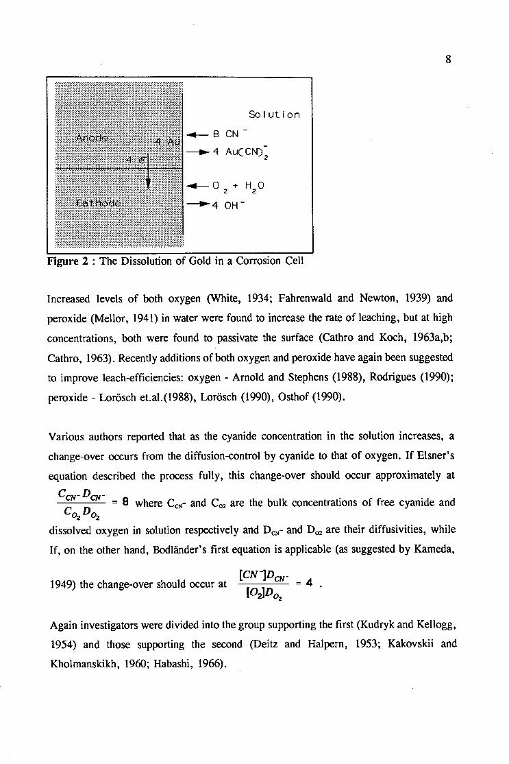
Figure 2, taken from Kudryk and Kellogg, shows these interacting cells diagrammatically.
They assumed that equation L-4 represents the cathodic reaction.
So I ut ion
CN
Au(CN)2
+ H 0 2
Figure 2 : The Dissolution of Gold in a Corrosion Cell
8
Increased levels of both oxygen (White, 1934; Fahrenwald and Newton, 1939) and
peroxide (Mellor, 1941) in water were found to increase the rate of leaching, but at high
concentrations, both were found to passivate the surface (Cathro and Koch, 1963a,b;
Cathro, 1963). Recently additions of both oxygen and peroxide have again been suggested
to improve leach-efficiencies: oxygen - Arnold and Stephens (1988), Rodrigues (1990);
peroxide - Lorosch et.al.(1988), Lorosch (1990), Osthof (1990).
Various authors reported that as the cyanide concentration in the solution increases, a
change-over occurs from the diffusion-control by cyanide to that of oxygen. If Eisner's
equation described the process fully, this change-over should occur approximately at
CcwDcN-C D = 8 where CcN- and C02 are the bulk concentrations of free cyanide and
02 02
dissolved oxygen in solution respectively and DcN- and D02 are their diffusivities, while
If, on the other hand, Bodlander's first equation is applicable (as suggested by Kameda,
1949) the change-over should occur at
Again investigators were divided into the group supporting the first (Kudryk and Kellogg,
1954) and those supporting the second (Deitz and Halpern, 1953; Kakovskii and
Kholmanskikh, 1960; Habashi, 1966).

9
Finkelstein (1972) showed that 85 % of the H20 2 produced in Bodlander's first equation
diffuses away, while part of the remaining 15% undergoes auto-oxidation to 02
and H20
and only the remaining portion takes part in the second reaction.
2.1.3 General Chemistry of Gold, its Ions and Complexes
Gold, Silver and Copper are among the most noble metals. They occur in the earth's
surface in their metallic form in pockets of relatively high concentrations, so that they
were discovered early in human history and were the first metals that were mined and
used (Dickerson et.al.,1984). The nobility of these metals is the effect of their valence
electron configuration (or autbau): essentially their outer d-orbitals should be filled with
the exception of one place. But as a completely filled d-orbital has a lower energy, one
electron from the next s-orbital is used to fill the d-orbital completely. This gives the
metal a highly stable state. Gold has the following autbau:
Au(O) : Xe 4f14 5d10 6s1
where Xe refers to the autbau of the previous noble gas xenon.
When gold is involved in chemical reactions, it will usually form either the Au(I) or the
Au(III) states, with the Au(ll) and Au(IV) states being much less common.The electron
configurations of the two more common gold ions are:
Au(I) : Xe 4f14 5d10 6s0
Au(III) : Xe 4f14 5d8 6s0
In the reaction with cyanide two gold complexes are possible: the aurous cyanide complex
(Au(CN);) and the auric cyanide complex (Au(CN)~). Their respective autbaus are:
Au(I) in :N=C-Au-C=N: : Xe 4f14 5d10 6s2 6p2
Au(III) in fil : Xe 4f14 5d10 6s2 6p4 (Wells, 1962)
9 :N=C-Au-C=N:
I
ITI N

10
Both complexes are very stable. The gold atom in the first complex involves two sp
hybridized orbitals forming a linear molecule which has a stability constant of 2. l<Y8
(Finkelstein, 1972). The second involves bonds of four dsp2-hybridized orbitals, giving
a square planar shape (Wells, 1962) to the molecule which is even more stable as shown
by its stability constant of 1<>56. In both cases the 6s orbital is filled, while the 6p orbital
is only partly filled. The great stability of both complexes lies in the filling of the 6s
orbitals which shields all lower orbitals and in the covalent bonds between the gold and
carbon atoms.
The effectiveness of cyanide in leaching noble metals like gold and silver lies in its
provision of reaction paths at lower potentials. The standard reduction potentials of the
two gold-ion producing reactions are shown below. These indicate that under normal
circumstances (ie. in the absence of cyanide but in the presence of a strong oxidant), the
auric ion has a lower reduction potential and would therefore be more likely to form than
the aurous ion.
Au+ + e- ... Au , E0 =1,68V (L-7)
Au 3 + + 3e- ... Au , E0 =1,50V (L-8)
Both the aurous and auric ions are stronger oxidants than water and would therefore, if
added to the system be reduced to metal gold by oxidizing water to oxygen (in the
opposite reaction to the one in equation L-9 below):
4H+ + 0 2 + 4e- ... 21120 , E0 =1,228V . . . . . . . . . . . . . . . . . (L-9)
In the case where cyanide is added to the system, though, a different picture emerges. The
standard reduction potential of the reaction of Au(CN);/ Au reaction is shown below:
Au(CN)2 + e- ... Au + 2CN- , E 0 =0,50V ................ (L-10)
The effect of this couple is shown on the Pourbaix Diagram (adapted from Finkelstein,
1972) of the Gold-Water-Cyanide system in Figure 3: The potential of the reaction shown
in equation L-10 lies below that of the H20/02 pair and thus metallic gold will be oxidised
to aurocyanide in the presence of cyanide.

/\ > u
3+
CO 2 0
Au ~
+-' c (J)
+-' 0
AuO 2
~ 1
'
0 --== -AU(eNJ~ -------- 2·························· ---------
--------!Au + 2CN ';: A~CN) ~ ······
····················• ····••·· 2H 0 + 2e-· 20H-+ H
-1,01'--'-'--'--'--'--L-L-'--'--'-..___..'--'-_._~ • • 4 6 8 10 12 0 2
pH
Figure 3 : Pourbaix Diagram of the Au-cN--H20 System at 25 ° C. Concentration of all dissolved substances = 1Q·4 mol.1·1
•
Partial pressures of H2 and 0 2 = 1 atm.
2.1.4 Rate Equation
11
Already the first researchers to study the leaching of gold by cyanide noticed that the rate
of gold dissolution increased with increasing concentrations of cyanide and oxygen (White,
1934; Fahrenwald and Newton, 1939). Fink and Putnam (1950) found other factors which
affected the rate: sulphides retarded the rate, while traces of lead, bismuth, mercury and
thallium salts were found to accelerate it. As explained by Cathro (1963) the base metal
salts prevent passivation. Habashi (1970) mentions the coating effect of Ca02 from the
oxidation of lime.
Kameda (1949) was the first to publish a rate equation to describe the leaching of gold.
It models the diffusion of cyanide to the gold surface through a stagnant layer using Fick's
law:
12
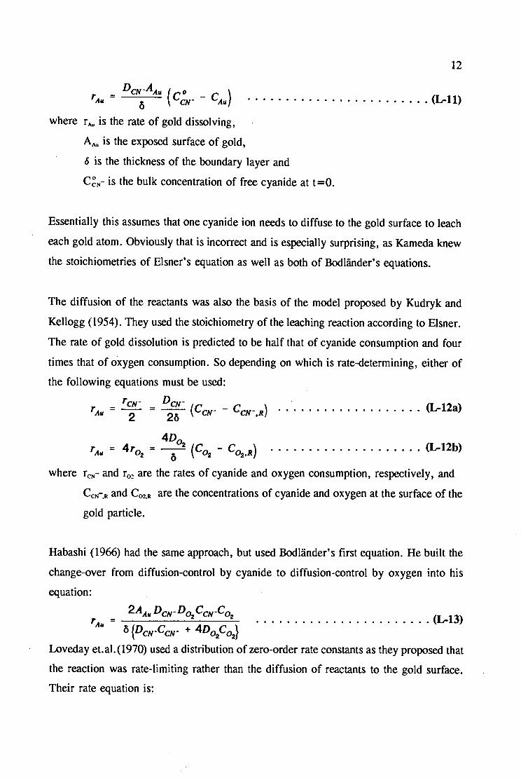
DcwAAu { o } TAU = 0 ccN- - CAu ........................ (lrll)
where rAu is the rate of gold dissolving,
AAu is the exposed surface of gold,
6 is the thickness of the boundary layer and
C~N- is the bulk concentration of free cyanide at t=O.
Essentially this assumes that one cyanide ion needs to diffuse to the gold surface to leach
each gold atom. Obviously that is incorrect and is especially surprising, as Kameda knew
the stoichiometries of Eisner's equation as well as both of Bodlander's equations.
The diffusion of the reactants was also the basis of the model proposed by Kudryk and
Kellogg ( 1954). They used the stoichiometry of the leaching reaction according to Elsner.
The rate of gold dissolution is predicted to be half that of cyanide consumption and four
times that of oxygen consumption. So depending on which is rate-determining, either of
the following equations must be used:
TcN- DcN- c· 2 ) TAu = 2 = ~ (CcN- - CcN-,R) • • • • • • • • • · · · · · • • • • • .u-1 a
4Do2 T = 4T0 = -- (C0 - C0 R) .................... (.lr12b)
Au 2 O 2 2•
where rcN- and r0~ are the rates of cyanide and oxygen consumption, respectively, and
CcN-,R and Co2,R are the concentrations of cyanide and oxygen at the surface of the
gold particle.
Habashi (1966) had the same approach, but used Bodlander's first equation. He built the
change-over from diffusion-control by cyanide to diffusion-control by oxygen into his
equation:
....................... (lr13)
the reaction was rate-limiting rather than the diffusion of reactants to the gold surface.
Their rate equation is:

13
.. TA,, = f kw{k,O)dk ............................... (L-14)
0
For w(k,0) they used the Schumann distribution.
Brittan and van Vuuren (1973) proposed a fairly complex model taking into account many
variables which had been recorded ·on daily log-sheets of various mines. These variables
included the temperature, pH and cyanide concentrations in the first and last leach
pachucas. Various densities and size group percentages were also included.
Brittan (1975) then published a rate equation which essentially lumps all rate-controlling
effects into an Activation Energy term, which changes with changing concentration of gold
in the ore:
r•• = A exp[-:; (1 - 11 G .. )] .... • · · · · · · · ...... · · · · · · · (I.AS)
where a is a constant and
GAu is the grade of gold in the ore.

14
2.2 ADSORYfION ON CARBON : CARBON-IN-PULP
2.2.1 The History of Carbon in Gold Extraction
The absorptive powers of charcoal have been known for centuries. McDougall (1991)
reports that it was already used as a clarifying agent in the Egyptian civilization and
Bailey (1987) reported that the ancient Hindus used activated carbon to clarify water. The
use of carbon was developed further throughout the centuries to absorb colours, odours
and poisons from various media.
By the 1880s carbon was added to clarified chloride-leach liquors to 'precipitate' the gold.
The carbon was subsequently burned to release the gold. A similar process was patented
in 1894 after the cyanidation-route became common for gold leaching, in which the gold
cyanide was precipitated using carbon (Laxen et al, 1979). Despite the cost of the carbon,
which could obviously be used only once, a few plant~ continued to use carbon
precipitation into this century. Most plants rather chose filtration followed by either zinc
precipitation or electroplating instead.
It was only in the fifties of the present century that Zadra at the U.S.Bureau of Mines,
at the request of the Getchell Mine in Nevada (Laxen et.al., 1979), investigated the
possibility of stripping the gold off the carbon by chemical means rather than burning it.
The first patent used sodium sulphide (Zadra, 1950) but because the proposed process was
not able to retrieve the adsorbed silver, another process was developed using sodium
hydroxide together with cyanide (Zadra, 1952). The solution was circulated through an
elution column containing the loaded carbon and an electroplating chamber which stripped
the solution of its gold content.
The first application of this new technology was at Carlton Mill, Cripple Creek, Colorado
in 1961 (Laxen et.al., 1979), where it was used to retrieve gold from slimes. The next
milestone was reached when a large carbon-in-pulp (CIP) plant was put into operation at
the Homestake Mine, South Dakota in 1973 (Sisselman, 1976).

15
In 1974 Davidson developed a new process (now called the AARL process) for the elution
of gold from carbon. Instead of recycling the eluate through the elution column and the
electroplating chamber, he initially pretreated the carbon with a carbonate solution and
then washed the carbon with hot deionized water (Davidson, 1974). The solution was then
stripped of its gold in batches before being pumped to the leach. An improvement was
suggested by Davidson and Duncanson (1977) which used a strong cyanide solution during
the pre-treatment instead.
While the first CIP plant to be commissioned in South Africa in 1978 was fairly small -
treating 10 000 t/m at Modderfontein 74 - by 1980 two larger plants were already
operational, and by 1985 the total had risen to 17 (Bailey, 1987). Davidson and Schoeman
(1991) estimated the present number of CIP operations in South Africa at about 60.
2.2.2 Activated Carbon
Activated carbon has the ability to absorb large amounts of various substances from
aqueous solutions. This is caused by the structure of carbon within the particles of
activated carbon.
The activation of carbon involves taking some organic material, such as peach pips, wood
or, as is usual today, coconut shell, and heating it to high temperatures in a controlled
atmosphere. All volatile constituents within the organic material are gasified, leaving only
the carbon backbone behind. Part of the carbon reacts with oxygen in the air so that pores
are burnt into the carbon. The pores are divided into groups according to their sizes. Cho
et.al.(1979a) divided them into three size groups: macropores, transitional pores and
micropores. The exact sizes of these pores obviously depend on the size definition used.
McDougall (1991) categorizes pores as shown in Table I.
The percentages of total area that the different pore sizes contribute depends on the type
of raw material used and clearly also on the definition of the pore sizes and the associated
method of measuring them (eg. see Peel et.al.(1981) and Cho and Pitt (1983) for different
definitions). The percentages quoted above refer to coconut carbon, which produces an

16
unusually large number of micropores. The large surface area associated with the
micropores, which is available for adsorption of gold makes this the favourite carbon in
CIP plants today.
Pore Types Size Range % of Surface (in A) Area
Macro pores 500-20000 -0%
Mesopores 100-500 5%
Micropores 8-100 95%
Table I : Pore Definitions
The structure of the Carbon backbone is very similar to graphite. It consists of little
graphite platelets (Cho and Pitt,1983) a few atoms thick and 20 - 100 A in diameter,
which are randomly stacked on one another giving a 'turbostatic' structure (McDougall,
1991). The edges of these platelets stick out into the pores and the unsatisfied bonds of
the surface atoms result in reactive sites (Cho and Pitt, 1979a).
The nature of these active sites has been the topic of many discussions as the type of site
would determine the type of adsorption process that would be most likely to occur on it.
This is discussed below.
2.2.3 Mechanism
Various mechanisms have in the past been suggested for the form in which the gold is
adsorbed on the surface of the carbon and have been discussed at length by various
authors (eg. McDougall et.al., 1980; Bailey, 1987; Adams et.al., 1987). Essentially they can
be grouped into the following mechanisms:
- reduction of Au(CN); to metallic gold,
- loss of CN- from Au(CN); to give either
- AuCN, or
- neutral macromolecules with the general formula Aun+(cN-)n, (Jones
et.al., 1988)

17
- oxidation of the gold atom in Au{CN); to give Aun+(cN-t,
- adsorption of ions in an electrical multilayer,
- specific adsorption of ion pairs [Mn+][Au(CN);]n, where M is a metal,
eg.Ca,Na,K
- non-specific adsorption of ions on the carbon surface.
In the normal conditions of an adsorption circuit (high pH, high [CN-], low temperatures)
the reduction of Au(CN); is unlikely {Tsuchida et.al., 1984). This is supported by Jones
et.al. (1989) who found that the adsorption of Au(CN); is thermodynamically 'reversible
even in the absence of cN-, which would not be possible if adsorption was accompanied
by a loss of cyanide from the complex. Adams et.al.(1987b) found that the formation of
AuCN may occur at low pH or at high temperatures, such as in the pre-elution acid-wash
or during regeneration .
.-----Stern Plane
Gouy Plane
8 Au(CN);
E) CN
G) Na+
Q Hp
Figure 4 : Multilayer Adsorption of Au(CN); and Other Ions
The mechanism postulated by Cho and Pitt (1979b) describes the adsorption of the
Au(CN); ion on active sites on the carbon, balanced by positive ions which adsorb non
speci fically in a multilayer of positive metal ions and more negative ions including cN-

18
and Au(CN); (refer to Figure 4 for a schematic representation, taken from Cho and Pitt).
Their use of Salvation Theory explained why the larger Au(CN); molecules adsorbed
more readily than the smaller Ag(CN); molecules or the more negatively charged
Cu(CN)!-.
While Adams et.a1.(1987b) agreed that activated carbon has a greater affinity for larger
and less charged molecules, they discounted the multilayer type of adsorption because it
could not explain why ClO; doesn't load as well as Au(CN);. They suggested that
loading was rather due to adsorption of ion pairs on certain active sites.
Jones et.al.(1989) found that the two -C=N bonds were perfectly symmetrical. As the two a- a+ a-
nitrogen atoms are slightly negative with respect to the gold atom :N=C".Au:C=N:
any interaction with a cation would have to occur at the nitrogen atoms. The formation
of a definite ion pair implies that only one cation is involved and this cation could only
have interacted with one of the two nitrogen atoms. Such one-sided interaction would have
caused the molecule to become asymmetric but as this is contrary to observation, the
formation of definite ion pairs can be discounted.
Figure 5 : Au(CN); Adsorbed on Graphite
Instead, the Au(CN); ion is "adsorbed in a linear state parallel to the graphitic planes of
the carbon. The adsorption bond is formed by charge donation (0.3 - 0.Se·) to the central

19
gold cation from the delocalised 7T-electron system of graphite" (quoted from Jones
et.al., 1988). Jones et.al showed diagrammatically how well (NC-Au-CNt fits onto the
carbon backbone. Their diagram is reproduced in Figure 5. The positive metal ions adsorb
non-specifically onto the carbon with the charge being balanced by the delocalised electron
cloud. McDougall (1991) suggests that the main function of the various surface groups
which were reported to be present on activated carbon (Tsuchida et.al., 1984; Adams
et.al.,1987; Adams, 1989), is to make the essentially hydrophobic carbon more
hydrophillic, rather than functioning as adsorption sites.
2.2.4 Factors Affecting Adsorption
From the first articles published on CIP, factors which affect the rate of loading and the
equilibrium loading have been discussed.
Factors influencing the rate are :
carbon particle size (Dixon et.al., 1978; Davidson et.al., 1979; Fleming and Nicol,
1984)
ionic strength (Davidson, 1974; Cho and Pitt, 1979b)
type of cations in solution (Davidson, 1974; McDougall et.al.,1980; Davidson
et.al., 1982; Tsuchida et.al.,1984)
temperature (Davidson, 1974; Dixon et.al.,1978; Cho et.al.,1979b; McDougall
et.al.,1982; Davidson et.al.,1982; Splaine et.al.,1982)
pH (Davidson, 1974; Davidson et.al.1979; Davidson et.al.,1982; Bailey, 1987)
stirring (Fleming and Nicol, 1984; Hughes and Linge, 1989)
dissolved oxygen concentration (v.d.Merwe and v.Deventer, 1988)
ore particles (Jones and Linge, 1989; Jordi et.al., 1991)
pulp density (Fleming and Nicol, 1984)
Factors affecting the equilibrium loading are :
competing species (Davidson et.al., 1982; Fleming and Nicol, 1984; Tsuchida
et.al.,1984; Adams et.al.,1987b). The competing species in order of their
loadabilities are:
Hg(CN)2 > Ag(CN); > Cu(CN); > Cu(CN)i- > Ni(CN);- > Cu(CN)!- >

Co(CN)!- > Fe(CN)!-
carbon type and preparation (Menne, 1982; Cho and Pitt, 1983)
temperature (Splaine et.al., 1982)
20
pH (Dixon et.al.,1978; Cho and Pitt,1979b; Davidson et.al.,1979; Davidson,
1986)
dissolved oxygen (v.d.Merwe and v.Deventer, 1988)
ionic strength (Fleming and Nicol, 1984)
calcium carbonate scale (Davidson, 1986; Mattioli et.al.,1990)
other inorganic foulants (La Brooy et.al., 1986; Jones et.al., 1988b)
organic foulants (Fleming and Nicol, 1984; La Brooy et.al., 1986)
Good summaries of these effects are give by Fleming and Nicol (1984), Johns (1987) and
Vetter (1987).
The efficiency of any adsorption circuit will also be affected by other factors, such as the
loss of carbon from the circuits by degradation or leakage through the intermediate screens
(Sorensen, 1989; Whyte et.al., 1990) or the loss of cyanide from the circuit through side
reactions which are catalyzed by the activated carbon (Muir et.al., 1988; Adams 1990 a,b).
2.2.5 Rate Equations
Quite a number of possible rate expressions have been suggested for the adsorption of
aurocyanide onto activated carbon (Woollacott et.al.1990). It is usual to divide the models
into empirical and mechanistic ones.
The first empirical models were not in the form of differential equations, but rather
incorporated time into the expression:
Fleming et.al.(1980): qAu(CN)2_ = kc;u(CN)2_tn ••••••••••••••• (C-1)
where qAu<cN>2.;. is the loading of aurocyanide on carbon,
C~u<CN>;- is the bulk solution concentration at t=O of aurocyanide and
n is a constant

21
La Brooy et.al.(1986): q = kC -tn Au(CN)2
. . . . . . . . . . . . . . . . . . (C-2)
where CAu<CN>2- is the bulk solution concentration of aurocyanide
These are obviously useless for dynamic simulations. Later investigators used the film
diffusion model instead:
. . . . . . . . . . . . . . . . . . . . • . (C-3)
where c+ Au<cN12- is the concentration of aurocyanide in solution which is in equilibrium
with the loading of aurocyanide on carbon qAu<CN>2-. Some relationship between
c+ Au(CN)2- and qAu(CN)2- mUSt be SUbStitUted into the equation (WoollaCOtt et.al.,
1990), such as
- a linear relationship as used by Nicol et.al.(1984) :
'Au(CN)2 = k(C..tu(CN)2 - K qAu(CN)2) • • • • • • • • • • • • • • • • ' • • ' • (C-4)
- a Freundlich isotherm as used by Johns (1986) :
[ (qAu(CN)2];]
'Au(CN)2 = k CAu(CN)2 - Kl • • ' • • • ' ' • • ' • • ' • • • • • • • (C-5)
where b is a constant and
K, is the Freundlich equilibrium constant
- a Langmuir isotherm suggested in this form by Woollacott et.al.(1990) :
_ k[C _ KzqAu(CN)2 'Au(CN)2 - A.u(CN)2 .., _ _
q Au(CN)2 qAu(CN)2
. . . . . . . . . . . . . . . . (C-6)
where K1 is the Langmuir equilibrium isotherm, and
q~u<cN>2- is the loading capacity of aurocyanide on the particular carbon.
At low loadings, each of these equations may be reduced to
. . . . . . . . . . . . . . . . . . . . . . . . . . . . . . . (C-7)
If the loading is far from equilibrium, so that (q=u<CN>2- - qAu<cN>2-) does not vary
significantly, equation (C-6) reduces to the more familiar equation used by Dixon
et.al.(1978):

22
The film diffusion model assumes that the rate limiting step lies in the diffusion of the
aurocyanide ion from bulk solution to the carbon surface. That is not necessarily correct.
As Peel et.al.(1981) note, there are four steps involved in the transport of the ion from
the solution to the surface of the micropore:
i) first it diffuses through the boundary layer to the carbon surface,
ii) then it must adsorb onto the outside surface,
iii) diffuse along the macropore surface and
iv) from there diffuse into the micropore.
A mechanistic model will try to take into account which ever of these are needed to
describe the process more closely (le Roux, 1991).
c
Figure 6 : Schematic of Carbon Particle
Peel et.al.(1981) describe their system with the following equations (see Figure 6 for a
schematic of the carbon particle showing the various· concentration and loading terms):
film diffusion to particle surface:
dC c N)-Au C 2 = -k(C -- CAu(CN)2- ,R) • • . • . • .... • . • • • • • • • (C-9) dt Au(CN)2
equilibrium at the particle surface:
.......... (C-10)
surface diffusion in macropore:
J {)qAu(CN)2,m = fDAu(CN)2,R
at r2 •••.•• (C-11)

23
diffusion into micropore:
CqAu(CN)2 ,b '.it11(CN)2,b = (1-/) Ot = kb(qA11(CN}z,m - qA11(CN}z,b) ••••••• (C-12)
together with the necessary Initial and Boundary Conditions.
qAu<CN>2-.m is the loading of aurocyanide in the macropore
qAu<CN>2-,b is the loading of aurocyanide in the micropore
CAu<CN>2-,R is the solution concentration of aurocyanide at the particle surface
D Au<CN>2-.R is the diffusivity of aurocyanide at the particle surface
Cc is the concentration of carbon in the tank
The macropore diffusion equation is simply the equation of continuity for constant density
and diffusivity in spherical coordinates with the assumption that diffusion occurs only in
a radial direction (Bird et.al., 1960) and was first suggested for aurocyanide adsorption by
Cho and Pitt (1979a). The carbon has been subdivided into the fraction containing
macropores, f, and the remaining fraction containing micropores, (1-t).
Peel et.al.(1981) used the Freundlich isotherm to describe the relationship between the
solution concentration at the interface CAu<CN>2-.R and the loading at the interface qAu<CN>2-,R:
van Deventer (1984a) defines the Freundlich isotherm in terms of the bulk solution CAu<CN>2
which is related to the loading at the interface:
. (CA11(CN)z)n qAu(CN)z ,R = qAu(CN)2 ,m (R,t) = Kl
Used as a boundary condition, this makes the linear film diffusion gradient in (C-9) and
(C-10) redundant. On eliminating the diffusion gradient from these equations we get:
-fDAu(CN}z.RCc oqA11(CN}z,m ................. (C-13) re ar
In his later papers van Deventer (1984b and 1986b) replaces the radial diffusion term

24
. (. )2 ( 2 7
2 aqAu(CN)'2 ,m by a quadratic approximation qAu(CN)i ,R - qAu(CN)2 ,m} . This
ar 2qAu(CN)2 ,m
automatically removes the dependence of macropore loading on radial distance, reducing
the qAu<cNi2-,m(r,t) to the average loading qAu<cN12-,m(t) and also reducing the partial
derivatives with respect to time to simple derivatives. An extension is made to a
multicomponent system (van Deventer, 1986c) which uses the Sheindorf multicomponent
isotherm. In that particular paper, van Deventer uses this to model a two-component
system.
Brinkmann and King (1987) used a slightly different approach to that suggested by Peel
et.al. in that they simply assume that the concentration of aurocyanide at the mouth of the
macropore is the same as the concentration in the bulk solution, CAu<cNi2-, (i.e. no film
diffusion). The aurocyanlde complex then diffuses along the macropore and adsorbs only
once it reaches the micropores. The equations are similar to those of Peel et.al.(1981)
except that qAu<cN12-,m has to be replaced by CAu<CN>2-.p .(the concentration of aurocyanide in
the solution within the pore) and qAuccN>2-,b essentially signifies the adsorbed species.
2.3 CONCLUDING REMARKS
The amount of knowledge on gold leaching and adsorption has grown rapidly during the
last century. For the largest part of this period most researchers were involved with
explaining how leaching works and how it can be modelled.
With the sharp rise of the gold price in the early 1980's and the introduction of the CIP
processes on South African plants, most researchers' attentions shifted to the adsorption
process. Intensive investigation started into the fundamentals of the loading process and
the factors affecting it. As a result the amount of information available in this area of
research is unusually large, despite the short period of investigation.
Dynamic simulators of the CIP process appeared in the second half of the 1980's and the
interest in this application continues into the present decade as the use of these simulators
for better process and control design of the adsorption section becomes a necessity.

25
CHAPTER 3
THE SIMULATOR
The aim of this project was to write a dynamic model to simulate the leach and adsorption
sections of a gold plant. The simulator was to be able to read in data collected on a
running plant and to use these to make predictions of the amount of gold leached,
adsorbed and lost. It was also to be flexible enough for efficiency studies to be conducted
on it.
3.1 SIMULATED PROCESS
Figure 7 : The Simulated Plant Units
Unit No.
1 2 3 4 5 6 7-16 17 18 19 20 21-26 27 28 29
Description
Pulp Feed Unit Lime Addition Unit Pre-leach Tank Cyanide Addition Unit Spent Eluate Addition Unit Distributor Box Leach Pachucas Magic Box First CIP Tank Carbon Screen Loaded Carbon Sink CIP Tanks Fresh Carbon Feed Last CIP Tank Discard Pulp Sink

26
The data used in the simulator was collected at a South African gold plant on an earlier
Mintek project over a period of two years. The configuration of that plant was therefore
also used and is shown diagrammatically in Figure 7. It is similar to Figure 1 but in
Figure 7 the units are numbered as they ate referred to in the simulation program and the
feed units and sink units (the need for which is described in section 3.2) are included.
The part of the plant which was simulated consists of:
- The pre-leach tank, into which the exit stream from the thickeners is pumped after·
being screened. The pulp is air-agitated to keep it well mixed. Any extra lime
needed to correct the pH in the leach is added here.
- The distributor box, in which the leach feed pulp is mixed with cyanide and the
eluate which is returned from the smelt house,
- The leach cascade consisting of ten large pachucas. Each pachuca is agitated by
a large mechanical stirrer inside a downdraught tube as shown in Figure 8. This
ensures good mixing and minimizes short-circuiting of the pulp. Compressed air
is added in the downdraught tubes so that it is carried to the bottom of the tank by
the pulp. This gives the air maximum contact time with the pulp which ensures
that dissolved oxygen levels are high throughout the cascade.
Downdraught Tube
Air Bubbles
Figure 8 : Leach Pachuca
- The carbon-in-pulp section consisting of eight small contactors which are shown
in Figure 9. The pulp is mechanically agitated, but no air is added. The carbon is
retained in the contactors by horizontal screens while the pulp is forced through
by its own hydrostatic pressure. The pulp flows down the cascade under the force

27
of gravity while carbon-containing pulp is periodically pumped up the cascade. A
mixture of reactivated and fresh carbon is added to the bottom-most contactor '
while the carbon is screened out of the pulp originating in the top-most tank.
pulp In
agitator
active
~--+screen
area
Figure 9 : Top and Front Views of a CIP Con tac tor
- The carbon screen at the top of the CIP cascade separates the coarse carbon from
the pulp in the carbon transfer stream originating in the top-most contactor. The
carbon is transferred to the elution section of the plant, while the pulp is returned
to the first CIP contactor.
Besides those sections of the plant that were included in the simulation there are a few
other processes that are closely related to the simulated processes and influence the
functioning of both the CIP and the leach sections through interconnecting streams. Refer
to Figure 10 for a representation of the path followed by the gold through the simulated
and adjacent sections. Fortunately the interactions between the various parts are quite
weak, because of the intermittent nature of the transport of material between them. The
sections not simulated include:

28
- The pre-elution carbon storage: a large tank in which the loaded carbon from the
CIP is stored before it can be transferred to the actual elution column.
- The elution column where the carbon is first treated with concentrated acid to
remove build ups of inorganic foulants such as calcite. Depending on the type of
elution (Zadra or AARL) the carbonwill then be eluted using hot, very alkaline,
concentrated cyanide solutions after which (in the AARL process used at the plant
on which the simulator was based) the carbon will be washed with hot deionized
water, to elute the carbon. The eluate (the concentrated gold-cyanide solution), is
then taken to the gold retrieval system.
I ru
" z u l...J ::J
<t:
Au In Ore
-c CIP
l pulp to durrp
REDUCTION
............ . ......... . . . . . . . . . . . . . . . . . . . . . . . . . . . . . . . . . . . ......... .. ~: ~: ~: ~: ~: ~: ~: ~: ~ :~ :~:~
c
REGEN
So I id Au
In
Figure 10 : The Path of Gold Through a Gold Plant
- The gold retrieval system precipitates the gold from the gold cyanide solution.
Two processes are commonly used: electroplating employs steel wool cathodes on
which the gold will be deposited as the electric current reduces the gold ion in the
Au(CN); complex to metallic gold. The other process, which has been in use for
a long time and is used on the present plant, involves sprinkling zinc dust into the

29
gold cyanide solution. The zinc displaces the gold in the complex, leaving the gold
to precipitate out of solution. The resultant solution, which has a low gold content,
is called the spent eluate and is pumped back to the top of the leach cascade, so
that all the excess hydroxide and cyanide will be put to use.
- The carbon regeneration circuit consists of essentially more storage tanks and a
furnace in which the carbon is heated to high temperatures (600 - 700 "C) in a
controlled atmosphere. The carbon reacts with the oxygen and new pores are burnt
into the carbon interior. The hydro-carbon foulants which collected on the carbon
will largely volatilize or decompose under these conditions. The carbon on leaving
the furnace will be reactivated. It is quenched in cold water before being mixed
with fresh carbon and being pumped back into the bottom-most adsorber.
3.2 SIMULATION APPROACH
The physical process is divided into process units, streams and connections, where the
first two categories correspond with their intuitive meanings. A connection constitutes any
transfer of information such as signals from a measuring instrument to the controller, or
signals from the controller to the final control element. This structure was decided upon
as a standard within the Measurement and Control Division to make all flow sheet
simulations written in the Division compatible. A process-based approach was used: by
definition a stream must originate and terminate at processes. A feed stream therefore has
to leave a feed unit, while an exit stream needs to terminate at a sink unit.
The variables used in the simulation were divided into state variables and algebraic
variables as suggested by Hulbert (1983). The state variables are all those variables
describing the contents of the process units at any time and in terms of which the
differential equations describing the changes are written. They are all collected in the state
variable vector X with their derivatives in vector X. The algebraic variables in contrast
include all derived variables (such as volume) and all flows between units (streams and
connections). They are needed to calculate the derivatives of the state variables and are
all contained in the algebraic variable vector A.

30
The sequence of calculation is as follows:
i) Calculate all algebraic variables at time t using the values of the state variables at
t, all of which are known. (In flowsheets which are more complicated than this
one, eg. with many recycle streams, it may always be possible that some algebraic
variable is based on others, which occur later within the algebraic vector. As the
integrator was also to be usable in such cases provision was made for the
calculation process to be repeated until all algebraic variables have definitely been
calculated. A maximum of four such repetitions is allowed before the program
exits with an error message.)
ii) Calculate the rates of the chemical reactions using the state variables at time t.
iii) Calculate the derivatives of all state variables at time t, using the algebraic
variables and rates of reactions calculated in (i) and (ii). X = f(X,A(X),t).
iv) Calculate the values of all state variables at a later time t+ cSt using a numerical
integration method, ensuring that the error in this step does not exceed a specified
maximum.
v) Repeat steps (i) to (iv) until the required interval has been covered.
The above approach is called the chunked or simultaneous approach. An alternative
approach, called the sequential-modular approach, repeats the above sequence separately
for each individual unit over a pre-specified time horizon fl. t. This has the advantage that
each unit will only take as many integration steps as it needs (eg. a unit with small
changes needs only a few large steps, while a unit in which the state variables change
rapidly, can proceed with many small steps, without affecting the first unit).
The disadvantage of the sequential-modular approach is that the data from an earlier unit
used in the integration of a later unit will not be available at the exact time intervals at
which it is needed. This means that an interpolation routine must be included to provide
the information as and when it is required. While this is not difficult for a linear process
in which later units do not affect earlier ones, it is inefficient in a process such as the CIP
cascade, in which there is backward and forward flow between adjacent units. Interaction
between such units requires iterative recalculation of later states, so that all the time saved
by doing the calculations for individual processes separately is quickly lost.

31
The sequential-clustered approach (described by Fagley and Carnahan, 1990) uses a hybrid
of the two above approaches. It divides the flowsheet into clusters of associated units,
which are integrated together, with only the interconnecting streams having to be interpo
lated. It thereby makes it possible to limit the effect of stiffness in large systems to small
clusters.
The integration method used in the simulator is the Bulirsch-Stoer method. It is an explicit
method for which the chunked approach was considered the most efficient one in terms
of the amount of programming required and the reliability which could be expected.
At present the flowsheet information is entered via a flowsheet data file which has to be
written manually. Within the Measurement and Control Division, Mintek, a procedure is
to be written which will allow a user to choose the required flowsheet units from a list of
available units and to arrange them on the computer screen, complete with connecting
streams, as they occur on the plant.
3.3 DYNAMIC MODEL
The equations on which the simulator is based fall into two categories : (i) differential
equations which describe how the state variables change with time, and (ii) algebraic
equations which describe the dependence of the algebraic variables on the state variables.
All state variables, and most algebraic variables, are actually mots of the various species
present in the system. Some algebraic variables are derived quantities (such as mol totals,
volumes and flows in mol.s-1) which are needed to make the results more immediately
meaningful. Concentrations (in mol.m-3) are not kept explicitly, but are calculated when
needed.
In an effort to keep the sizes of the algebraic and state variable vectors as small as
possible to save memory space, the species used in the leach and CIP sections are not the
same. Rather each section has its own selection of species, with a 'magic box' between
the sections which transposes the algebraic variables of the stream leaving the leach onto
the CIP feed stream vector (refer to section 3.5.4.5).

32
3.3.1 Leach Section
The leach section consists of the leach cascade consisting of ten pachucas and the pre
leach tank. The reactions and equations given for the leach below apply equally well to
the pre-leach tank, which incorporates exactly the same species and reactions as the leach.
The only and significant difference is that no cyanide is present in the pre-leach tank. This
prevents all reactions involving cyanide to proceed, leaving only the oxygen dissolution
reaction which can proceed. This tank is therefore often described as the pre-aeration
tank.
3.3.1.1 Leach Species Table II lists all the species included in the leach section.
Species Chemical Density Mot.Mass No. Formula (kgJ-1) (kg.kmo1·1)
1 H20 1,00 18,015
2 Si02 2,70 60,085
3 Ca(OH)2 2,43 74,094
4 Ca2+ O* 40,080
5 OR O* 17,007
6 CN· O* 26,018
7 02 (aq) O* 31,998
8 Aur 19,30 196,967
9 Au. 19,30 196,967
10 Au(CN); O* 249,003
11 Mr 8,95 63,546
12 M. 8,95 63,546
13 M(CN)!· O* 167,618
Table Il : Leach Species with Physical Constants
Note: * all dissolved species are assumed to have negligible volume)
The significance of the subscripts f and s on Au and M is explained below.

33
3.3.1.2 Leach Mole Balances The differential equations for all species in the leach are
written as mole balances. For species j in tank i:
dn .. _y_
dt
M
= ni-1,j - niJ + E «j,lrlr,,.(ni,1•ni,2•· ... n,,N) "'=1 for i=1, ... ,NT;j=1, ... ,N
where ilij is the number of mols of j flowing out of tank i,
............ (L-18)
aj.m is the stoichiometric constant of component j in reaction m, and
rm is the rate of reaction m which is potentially a function of all n in tank i. (See
section 3.3.1.3 for the reaction rate equations.)
it is calculated from
P· n. · n . . Q, n = v Q -1.. = _.!.!l.Q = ----'·,,__} --i,j i,j i V i N
µJ. 1' n II
E~ t=1 Pt
where vij is the volume fraction of component j in tank i,
Q is the volume flowrate out of tank i,
pj is the density of component j,
µj is the molecular mass of component j,
nij is the number of mols of species j in tank i, and
Vi is the volume occupied by material in tank i.
3.3.1.3 Leach Reactions Besides the reaction of gold with cyanide, countless other
reactions take place in the pulp as its various constituents react with the oxygen, the lime,
the water, the cyanide or with each other. As can be seen in Table 1 above, only 13
species have been chosen for the simulation. While this is a limited choice, it is sufficient
for a first approximation as all reactions of interest can be described in terms of these
species.
The solid phase is assumed to consist of only inert quartz (referred to as Si02 in Table II),
solid gold and solid 'metal', where 'metal' is a collective term for all the metals which
compete with gold for the cyanide and oxygen. It is given a coordination number of 4 to
fall within the range of the four main competing metals of the tested ore, viz. silver (in
Ag(CN);), copper (in Cu(CN)!-), nickel (in Ni(CN);-) and iron (in Fe(CN)!-). These

34
metals are listed in order of their increasing grade in the ore and also in decreasing order
of reactivity (ie. even though silver is the rarest of the metals, it is the most likely to react
with the cyanide.)
Both gold and metal particles are each assumed to occur in two discrete classes with
respect to the rate at which they leach. The first, or fast-leaching, group is directly
exposed to the solution and therefore leaches relatively quickly. The other class of
particles is assumed to be partially occluded by the gangue material and therefore leaches
more slowly. Overall this results in a fast initial rate of leaching followed by a marked
decrease as is typically observed. This dual-rate model was suggested by Vetter (1987)
as a simplification of the distribution of rate constants as suggested by Loveday
et.al.(1973).
The rate equation chosen for the leaching of both gold and metal is based on Habashi's
(1966) rate equation, which has the advantage that it is written in terms of the three
reactants involved, viz. gold/metal, cyanide and oxygen. According to Habashi (1966)
most gold leaches according to Bodlander's first equation:
About 10% of the H20 2 produced in this reaction is consumed by Bodtander's second
reaction (Finkelstein, 1972):
... 2Au(CN)2 + 2on- .......... (~2b)
Overall this results in an equation with rather odd stoichiometric constants:
Au + 2CN- + 0,454502 + 0,909H20 ,.. Au(CN)2 + OH- + 0,409H20 2
............. (~19) According to Habashi, the rate of gold leaching is:
= 2AAuDcN-Do
2 CcN-Co
2
l)(DcN-CcN- + XD02Co) ........ · .............. (~13)

35
= 2 + ' ~ as ~::::1,5 2AAuDo ( 1 1 5 v)-1 D
a Co2 Ccw DcN-
The term x stands for the ratio of cyanide to oxygen ( = 2:0,4545 = 4,4) in equation (L-
19) above. Dividing by the volume of liquid, V" on both sides gives
dCAu = 2AAflo2 (-1- + 1,5 X)-1
dt a V, C02 CcN-
By manipulating the term before the large bracket one can express the rate in terms of the
concentration of solid gold in liquid, CAu:
dC,,,, = 6µ..,Do,s c (-1- + 1,5 xi-1 ................. (L-20) dt p R a Au Co CcN-Au Au 2
where s is a factor relating the exposed surface of gold AAu to the total surface of the gold
particles, and
RAu is the average radius of the gold particles.
Similarly one can write the corresponding equation for metal:
M + 4CN- + 0,454502 + 0,909H20 .... M(CN):- + on- + 0,409H202
...................... (L-21) which has the rate equation of:
dCM = 6µMDol CM (-1- + 1,5 xi-1 dt pMRMf> Co2 CcN-
............... (L-22)
where again x = 4,4.
A list of all reactions which are included in the leach simulation is given below. The rate
constants that are shown, are those used in the simulator. Unless otherwise indicated, they
were chosen on the basis of the data from the sampling campaign and other data available
from the gold plant. See section 3.3.3 for an explanation on how the constants were
chosen.
1) Ca(OH)2(s) ,.... Ca 2•(aq) + 20H-(aq) ................... (L-23)
with the rate equation:

36
( (Cea2.)(C0 w) 2
] · r Ca(OH)2 = k1 CCa(OHh 1 - K · · · · · · · · · · · · · · · · (L-24)
sp .
where k1 = 3.10·3.s·1, and
K.p = 2,937 ·l0-5(kmol1 .m-3)
3 is the solubility product of calcium hydroxide.
This reaction indicates how the lime acts as a pH buffer to keep the pH -10. The
concentration of calcium hydroxide is in equilibrium with its two products, Ca2+ and OH·,
as determined by the solubility product.
2) 02 (g) ..... 02(aq) . . . . . . . . . . . . . . . . . . . . . . . . . . . . . . . . (L-25)
with rate equation:
r02 = ~(c~! - C02 ) .............................. (L-26)
where k2 = 7,62I.10·5.s·1, and
C~~ = 0,331 ·10-6 kmoI.m·3 is the equilibrium concentration of dissolved oxygen
in the pulp as measured on the plant.
The form of the equation chosen is a compromise between the behaviour which it was
expected to predict and the available information. No data was available on the addition -
of compressed air, so that the assumption was made that aeration was always more than
adequate to make dissolution independent of the amount of air actually present. To prevent
the concentration rising above the observed maximum concentration, the equilibrium term
had to be included.
3) CN- + ~02 .,.. CNO- . . . . . . . . . . . . . . . . . . . . . . . . . . . . (L-27)
with a rate equation similar to that proposed by Adams (1990a) but adapted to include the
limiting effect of the oxygen concentration:
Co2 r cNo- = ka CcN- - · • • · • · • • • • • • · • · · · • • • • · · · · • • • • (L-28) ceq
02
where k3 = 1,58.10-6.s-1, which was interpolated from the selection of constants supplied
by Adams for various different cases.
Equations (L-19) to (L-22) are then written twice, once for the fast leaching fraction and
once for the slow leaching fraction:
4 and 5)

37
.................... (lr19a/b) with rate equations:
'A"tf, = k415 CAu.J/s ( c1 + c6'
6 ]-
1
•••••••••••.••.•••• (lr20a/b) 02 CN-
where k4 = 1,215.103.m3.kmo1·1.s·1, and
k5 = 8,501.101.m3.kmol·1.s·1
6 and 7)
Mils + 4CN- + 0,454502 + 0,909H20,.... M{CN):- +OH- + 0,409H20 2
.................... (lr21a/b) with rate equations:
( 1 + 6,61-
1
r =k C -M//, 6/7 MJ/s C C
02 CN-
................... (lr22a/b)
where ~ = 2,036.103.m3.kmo1·1.s·1, and
k7 = 1,169.103.m3.kmo1·1.s·1
The side reactions which consume oxygen and cyanide are represented by (L-21a and b)
and by (L-27). This limited selection is again sufficient for a first approximation.
A reaction which was earlier considered for inclusion in the simulator, is the dissociation
of NaCN to CN· and Na+. This reaction is fast in comparison to the leaching reactions and
the hydrodynamics of the leach. It was thus assumed to have already gone to completion
in the cyanide feed unit before the cyanide stream is mixed with the pulp.
3.3.1.4 Leach Hydrodynamics The leach cascade is arranged in such a way that the
pulp which is fed into the first leach tank flows down the cascade under gravity. The tanks
themselves are arranged at the same height, though, and all interconnections between the
tanks are also on a common level about 3 m below the top of the pachucas. This means
that the pulp levels in all the ten leach tanks are dynamically dependant on each other.
This arrangement gives the leach circuit a potentially very large buffering capacity.
Regardless of whether this is consciously used to control the feed flow to the CIP or not,
any fluctuations in the feed to the leach will have been reduced significantly before
reaching the CIP.

38
The interaction of the levels was regarded important enough to be included in the model.
Levels in the leach pachucas were therefore not taken as being constant, but are calculated
from the volumes of the individual species in the tank. The flow from one tank to the next
is represented as an interaction between the two volumes:
O; = BCV; - V;.1) ••• • •••••••.•.•••••.••••••••••• (L-29)
where B is the buffering constant.
In the case where the next tank in line has not filled sufficiently for interaction to occur,
the above equation reduces to
O; = B CV; - V max). • · · · · · · · · • · · • · · · · • · · · • . • . • • . . . • (L-30)
where V max is the volume of the tank up to the top of the weir. This is also the equation
which is used for the last tank, which obviously has no succeeding tank with which to
interact.

3.3.2 CIP Section
3.3.2.1 CIP Species
Species Chemical No. Formula
1 H20
2 Si02
3 CN-
4 02 (aq)
5 Au(CN);
6 M(CN)!-
7 C-granules
8 C-fines
9 qAu(CNl1,fin
10 qAu(CNl2,m
11 qAu(CNl2,b
12 qM(CN)4,fm
13 QM(CN)4,m
14 qM(CN)4,b
15 QcN,fm
16 QcN,m
17 QcN,b
18 C-transfd
Density Mot.Mass (kgJ·I) (kg.kmoI-1
)
1,00 18,015
2,70 60,085
O* 26,018
o· 31,998
O* 249,003
O* 167,618
1,40 12,011
1,40 12,011
o- 249,003
o- 249,003
o- 249,003
o- 167,618
o- 167,618
o- 167,618
o- 26,018
o- 26,018
o- 26,018
o+ 12,011
Table m : CIP Species with Physical Constants
Notes: • all dissolved species are assumed to have negligible volume.
- all adsorbed species are assumed to have negligible volume.
39
: this variable is only needed to keep track of how much carbon has been
transferred to each particular tank. It should in essence be an algebraic variable,
but is easier to handle as a state variable.

40
3.3.2.2 CIP Mol-Balances As in the leach, all differential equations in the adsorption
section are mot-balances. They are essentially the same as those in the leach except for
the extra terms for the transfer streams.
For species j in tank i:
dn;j ~ = np,i-1j - np,ij + nt,i+1j - nt,ij + L..J aj,lftrlft(n;,11n;,21·•·1n;,N) & m~ . (C-14)
for i =1 •.•. NT;j =1, ... N
where np,ij is the number of mols of j flowing out of tank i in the pulp stream,
n 1,ij is the number of mols of j flowing out of tank i in the carbon transfer stream,
aj,m is the stoichiometric constant of component j in reaction m, and
rm is the rate of reaction m which is potentially a function of all n in tank i.
np,ij and n 1.ij are both calculated using
. - P,· n .. n V Q = _!!l.Q = . . . - ..•. - ..
.,,I,) I,) .,,1 v. .,,I µj I
n .. Q •. . '·' .... ~ E {t,p} N L n,,1µ1
k=1 P1
where V;j is the volume fraction of component j in tank i,
Qp,i is the volume flowrate out of tank i in the pulp stream,
Q,,; is the volume flowrate out of tank i in the carbon transfer stream,
pi is the density of component j,
µ.i is the molecular mass of component j,
n;j is the number of mols of species j in tank i, and
V; is the volume occupied by material in tank i.
These equations are very flexible and allow the movement of pulp and carbon to be
simulated within the cascade. As long as the fl-terms are set to zero when the pulp or
transfer streams are cut, this equation will automatically take care of the various transfer
schemes, overflows etc. as is discussed below in the section on hydrodynamics.
3.3.2.3 CIP Reactions Again a great variety of reactions occur simultaneously in the
adsorption section of a gold plant. Only a few representative ones have been chosen in this
simulation to present an approximate picture of what happens. The choice of unreferenced
kinetic constants is again described in section 3.3.3.

41
The process of adsorption may be described by the following stoichiometric equation:
Au(CN)2 (aq) ,.... Au(CN)2 ( !) ..................... (C-15)
where .l. refers to the adsorbed species.
The rate of adsorption is calculated using a slightly modified version of Nicol's linear
isotherm adsorption rate equation (C-4):
rAu(CN)2 = k ( CAu(CN)2 - KqAu(CN)2) nc .................... (C-16)
The modification is necessary as the concentration of carbon in the pulp varies and can
be quite low during carbon transfers. According to Nicol's original rate equation the
amount of gold adsorbed from solution would not be affected by a lack of carbon but that
can obviously not be the case.
In experiments it was observed that fast adsorption occurs initially on the surface and in
the macropores of the carbon. The rate of adsorption then slows down significantly when
the only remaining sites are located in the micropores. To take this observed effect into
account, Vetter's (1987) approach was used in which it is assumed that part of the carbon
contains only macropores, which are filled quickly. The rest of the carbon contains only
micropores for which loading is slow. As the aurocyanide in each pore not only adsorbs
independently, but can also desorb independently, the number of mols stored in each kind
of pore needs to be stored separately. A stoichiometric equation can then be written for
each adsorbed species :
Au(CN)2 (aq) ,.... Au(CN)2 ( !) j E {m,b} . . . . . . . . (C-lSa/b)
where J. m refers to adsorption in the macropores,and
J. b refers to adsorption in the micropores.
The loading of a species on carbon is calculated by dividing the number of loaded mols
of the species by the number of mols of carbon (or the volume of carbon, etc.). Loadings
are therefore automatically assumed to be average loadings and no loading distribution is
considered within a tank. As Willacott et.al.(1990) noted, this approximation is acceptable
as long as the loading rate equation is linear in the loading term.

42
Attrition of the carbon is a major source of gold loss on a running plant (Sorensen, 1989).
The breakage of carbon particles was thus included in the simulation and is described as
follows:
nc-granuies - nc-fines ••••••••••••••••••••••••••••••• (C-16)
with the rate equation as suggested by Whyte et.al.(1990):
7c = ksCc-8ranuks • • • • • • • • • • • • • • • • • • • • • • • • • • •••••• (C-17)
where ks = 1,30.104 .s-•
The adsorption of Au(CN); on the fine carbon fraction was also monitored. The equilib
rium loading capacity of fine carbon is the same as that of the coarse carbon, but
adsorption onto and desorption from fine carbon is much faster because of the smaller
diameter of the fine carbon particles. The fine carbon is therefore treated as a single
medium of high rate micropores. In total there are then three loading terms for every
species as shown in Table 3 above and each has the rate equation:
7Au(CN)2J = k9,j(CAu(CN)2 - K9JqAu(CN)2.i)ncj jEfm,bJin} · • (C-18a/b/c)
where ~.m = 4,393.10-4 m1.kmo1-•.s·1, ~.m = 0,1.6,513.10-6kmol.m·1
~.b = 2, 196.10-4 m1.kmo1·1.s-1, ~.b = 0,9.6,513.10-6 kmoI.m·1
~.rm = 4,393.10-4 m1.kmol"1.s-1, K9,r.n = 1,0.6,513.10-6 kmol.m·1
The cyanide complex of the competing metal species also loads onto carbon.Its rate of
loading is slower than that of gold and its equilibrium capacity on the carbon is much
lower:
rM(cN)!-J = k10J(CM(cN)!- - K10.iqM(CN'J!-.i)ncJ jEfm,bJin} • (C-19a/b/c)
where k10,m = 9,0.10-s m1.kmol"1.s·1, K10,m = O,l.1,2.10·1 kmoI.m·1
k10,b = 4,5.10-s m1.kmo1-•.s·1, K10,b = 0,9.1,2.10·1 kmoI.m·1
k10.r.n = 9,0.10-s m1.kmo1·•.s·1, K10,rm = 1,0.1,2.10-1 kmoI.m·1
Similarly, the free cyanide ion loads onto the carbon as well, but the carbon is again more
selective towards gold:
j E fm,bJin}
where k11,m = 2,0.10-s m1• kmoi-1.s-1, K11 ,m = 0, 1.1,5 .10-1 kmol. m·1
k11.b = l ,0.10-s m1• kmoi-1.s-1, K11,b = 0, 9. i ,5 .10-1 kmol. m·1
k11,rm = 2,0.10-s m1.kmo1-•.s·1, Ku.rm= 1,0.1,5.10-1 kmoI.m·3
(C-20a/b/c)

43
All the different reactions of cyanide (Adams, 1990a) are accounted for by the following
one reaction which was also used for the leach simulation.
cN- + iD2 .. CNo- ............................. (C-21)
Because this reaction is catalyzed by carbon, though, it proceeds at a faster rate than the
same reaction in the leach, where no carbon is present. The rate equation is an equation
suggested by Adams (1990a) modified to account for the need of oxygen in the production
of cyanate. As the presence of oxygen is included only as a fraction of concentration over
equilibrium concentration, it was still possible to use a rate constant interpolated from the
rate constants supplied in the paper by Adams:
Co2 r CNo- = k12 CcN-- .............................. (C-22)
ceq 02
3.3.2.4 CIP Hydrodynamics The adsorption contactors are much smaller than the
leach pachucas. They are arranged at successively lower heights above ground level so
that the pulp flows down the cascade by gravity. The levels in the various tanks are
independent of each other and each is only affected by the amount of pulp flowing into
the tank.
At periodic intervals carbon has to be transferred up the cascade. For this purpose carbon
transfer pumps are switched on which move pulp together with the associated carbon to
next contactor above. The pulp drains back through the carbon screen, but the carbon is
held back by the screen and has thus been transferred to a tank with higher solution
concentrations of gold-cyanide.
The carbon screens make the hydrodynamics more complicated. Not only do they present
a resistance to the flow of the pulp out of the tank, but they also tend to block and
overflow, thereby allowing the loaded carbon to pass downstream.
Under normal circumstances, the amount of pulp above the screen is negligible, and it is
therefore assumed that as soon as the pulp has passed through the screen it is already in

44
the pulp stream to the next tank.
The diagram in Figure 11 shows the horizontal carbon screen during normal operation.
The difference in heights (i:1h) ensures enough hydrostatic pressure to force the pulp
through the screen, while the carbon particles are too large to pass through the screen.
h max
Figure 11 : The Horizontal Carbon Screen
But when a tank gets too full, the following happens:
1) The hydrostatic pressure becomes too great and the carbon, instead of being mixed into
the pulp is pressed against the screen. Individual holes are covered by carbon pieces until
the entire screen becomes blocked.
2) The pulp level in the annulus around the screen rises, without any pulp flowing to the
next tank.
3) Once the level rises above ~ the pulp overflows into the area above the screen and
from there to the next tank taking carbon with it.
4) The operator then has to close the exit valve to the next tank to allow the level above
the screen to rise.
5) When the levels in the annulus and above the screen equalize (roughly ~), the feed
valve to the tank must also be closed. The pressures above and below the screen are then
also equalized and the screen unblocks.
6) The exit valve is opened to allow the screen and the tank to empty.
7) Once the level has dropped far enough, the feed valve is opened to allow normal
operation again.
A potential problem with leaving the feed valve to any tank closed for too long, is that

45
the screen in the tank before may overflow, requiring its own feed valve to be closed.
This happens because the volumes of both the screen and of the annulus around the screen
are relatively small. A single blocked screen may therefore cause the successive closure
of all tanks above it in the cascade, which will affect the production negatively. The
option of opening the feed valve to a blocked tank earlier to prevent overflow of the
previous tank simply causes the screen to reblock, and is therefore also not a solution to
the problem.
The amount of carbon carried downstream during such an overflow could potentially take
quite a large amount of retrieved gold with it, especially if the overflow occurred in one
of the earlier stages. The carbon not only carries the gold downstream with it, but if the
solution concentration in the next tank is sufficiently much lower, gold may start
desorbing from the carbon, increasing the solution losses of gold as well.
The screens are most likely to block during carbon transfers, as the volume of pulp which
norma11y passes through the screen is augmented by the extra pulp which is carried into
the tank by the carbon transfer stream. More pulp than usual has to drain via the screen
into the next tank, which causes the level in the tank to rise. The extra pressure on the
screen increases the probability of a blockage occurring. When the screen does get
blocked, it is common practice to stop the transfers both into and out of the affected
contactor.
Various transfer schemes have been used in practice or in simulators. These include:
- Simultaneous transfers along the whole cascade. The advantage of this scheme
is that, provided the transfer flowrates are the same, it should be easy to ensure
that the carbon profile along the cascade remains constant. It also disturbs the cas
cade for only a short time.
- Sequential transfers starting at the top. The advantage of this scheme is that the
carbon in each tank is not mixed with less loaded carbon before it is pumped to
the next tank. This prevents short-circuiting of carbon, ie carbon particles moving
more than one tank during a single transfer cycle. The disadvantage is that the cas
cade is disturbed for a long time, during which at least one tank contains less than

46 its normal amount of carbon.
- Sequential transfers starting from the bottom. While the short-circuiting
problem is aggravated by this transfer scheme, the time needed for transfers is
reduced because of the higher carbon concentration in the tank from which carbon
is being transferred.
- Continuous transfers. In this scheme pumps are kept going continuously, but at
a reduced tlowrate. While this permanently disturbs the process, it is the only
transfer mechanism that could potentially allow the CIP section to reach a steady
state. All other schemes can at best only reach a pseudo or cyclic steady state, in
which the loading curve of one cycle will be exactly the same as the next.
- Instantaneous transfers. All carbon is transferred from one tank to the next at the
same instant, or during a negligibly short time. This was the preferred method of
transfer in pilot plants and because of its ease in simulation, was the preferred
method of early simulators. Recently the carousel configuration of adsorption
vessels (Whyte et.al, 1990) has allowed complete nearly-instantaneous transfers:
the point of fresh feed addition can be moved from tank to tank, so that the carbon
does not need to be moved at all. The advantage of this transfer method is that the
cascade is disturbed for a minimal period of time. If the transfers are complete,
as described above, then short-circuiting and distributions of loadings are
prevented.
- Random transfers are most likely to occur in practise. These are likely to be most
inefficient, as they prevent even a cyclic steady state from being achieved.
The transfer schemes which have been incorporated into the present simulation are the
simultaneous, the continuous, the consecutive from the top and plant recorded (near
random) transfer methods. The efficiencies of the various schemes are discussed later.
3.3.3 Rate Constants
A sampling campaign was carried out on the plant used as a basis for the simulator in
September 1991. Samples were taken from the feed to the leach, various positions along
the leach and adsorption cascades and from the stream flowing to dump. These samples

\
47
were filtered to stop all reactions and analyzed at Mintek for gold, cyanide and metals
contents. Dissolved oxygen levels and pH were also monitored both before and during the
sampling campaign.
The results collected on the plant were not in the correct form for a deep mathematical
analysis or curve fitting. It was used instead to guide the choice of approximate kinetic
constants for the various reactions. The importance here lay more in getting the relative
shapes of the curves right, rather than ensuring that the numbers fitted exactly.
In the leaching reaction, for instance, it is important to take the relative amounts of the
gold and metal into account which will leach, as well as the relative rates of the gold and
metal leaching process. As was explained before; the 'metal' species, M, is an imaginary
metal, which sums up the effect of all the competing metals, the most important of which
are silver, copper, nickel and iron. These metals behave quite differently and the approach
of lumping them all into one makes it easy to sum up their effect on cyanide and oxygen
consumption. From the normalised plant data it was evident (Figure 12), that even though
the competing 'metal' occurs at a far higher concentration in the ore than gold, the gold
dissolves much faster and to a much greater extent.
1 -· x
x x x x o.e -.,
u ., ~
& CI0.6 ,_ ....
~ i = 0.4 I-
f1 ~
• • 0.2 - ll
• 0 I I I I I I I I I I I I I I I I I I ' 0 1 2 3 4 5 6 7 e 9 10 11 12 13 14 15 16 17 18
Tank No.
I Gold Metal I • x
Figure 12 : Normalized Gold and Metal Profiles in the Leach (Plant Data)

48
In the above diagram tank 0 is equivalent to the feed grade, tanks 1 to 10 are the leach
pachucas, while tanks 11 to 18 are the CIP contactors.
The different rates of leaching are taken into account by the choice of constants in the
model (see Figure 13 which shows the normalised leaching profiles of gold and metal
along the cascade). Two simplifying assumptions have had an effect on the shape of the
profile: firstly only the dissolvable fractions of gold and metal are included, and secondly
all leaching is assumed to occur only while the pulp is actually resident in the leach
cascade. The feed grade of gold is therefore slightly higher in reality while the true feed
· grade of the competing metal is much higher than indicated in the model. Applying these
conditions yields a metal-cyanide concentration roughly ten times as large as that of gold
cyanide concentration, as was recorded on the plant.
1 ..... G:ild (M:xlel)
• ~tal (Model)
x o.e ·-
()) 1J 11'.l L
(..'.) x 0.6 -
-0 Q) (I)
·--~ 0.4 - x L 0 z
• x 0.2 ....
x
• x
T x
~ 0 I I I ' • ll! iii ;I: * 0 1 2 3 " s 6 7 8 9 10
Leach Tank Nurrber
Figure 13 : Normalized Gold and Metal Profiles in the Leach (Model)
Besides the consumption of cyanide by the formation of the gold and metal complexes,
some cyanide is also lost in its reaction with oxygen to give cyanate, in its hydrolysis to
HCN and various other reactions as discussed by Adams (1990). As he suggests that the
cyanate-producing reaction is the most important of the side reactions, it was assumed for
simplicity that this was the only other reaction involving cyanide. A rate constant was

49
therefore chosen so that the concentration of free cyanide corresponded approximately to
an average value recorded during the sampling campaign.
The rate constant of oxygen dissolution reaction was chosen such that the simulated profile
of dissolved oxygen concentration in the cascade corresponded to the one recorded on the
plant.
For the adsorption section the choice of constants was also guided by the results from the
sampling campaign. In the adsorption reaction it was found, that the loading capacity of
gold cyanide on the activated carbon was much higher than for all the other metals
combined, and the rate of Au(CN); adsorption was much higher than for M(CN)~. The
desorption constant, K, which governs the loading equilibrium was therefore chosen to be
much smaller for gold cyanide than for the metal cyanide species. In contrast the rate
constant for gold adsorption mirrors the faster loading of gold by being about five times
as large as the rate constant for the metal loading.
The kinetic and loading terms for each species on the three available types of sites
(micropores on the fines and micro- and macropores on the coarse carbon) were linked
to make their determination easier. For instance, the rate constant for the adsorption on
fast-filling sites (micropores on the fine carbon and macropores on the coarse carbon) are
assumed equal and double the rate constant for the slow filling sites (the micropores on
the coarse carbon). Similarly the equilibrium loading capacity of a carbon must be the
same for a single species, regardless of whether the carbon is fine or coarse. A single
loading constant (eg. 6,513 kmol of carbon per m3 of solution for gold in equation C-16)
is chosen for each species and is scaled according to the relative percentage of pores in
the carbon fraction : All pores in the fines are assumed to be micropores, so for the fines
fraction the loading constant is multiplied by 1. In contrast, the coarse carbon contains
90% micropores and 10% macropores. Therefore of the total loading capacity for each
species on coarse carbon, 90% is reserved for sites in the micropores, hence Kb =
0,9.K,"'.
Furthermore, it seems from analyses of adsorption behaviour that the equilibrium

50
capacities of individual species is dependent on the loading of all species present. The
cyanide loading was therefore included for possible later incorporation into a competitive
loading model. For this work analyses of CN· on carbon were not available and therefore
no information on either its equilibrium loading or rate of loading was available. The
constants for cyanide were thus guessed and have no physical significance.
3.4 NUMERICAL INTEGRATION
The integration of the differential equations within the simulator is performed by a
variable step-length Bulirsch-Stoer method. It is a highly efficient explicit method for
smooth systems and was adapted for the present simulator to be able to deal with
discontinuities.
3.4.1 The Bulirsch-Stoer Integrator
This relatively new integration method is the suggested method for non-stiff systems of
ordinary differential equations (ODEs) in Press et.al. 's (1986) book "Numerical Recipes".
Most information in this section and the original versions of some of the integrator
subroutines were taken from that book.
The Bulirsch-Stoer method uses a modified-midpoint method to generate a number of
estimates of the state variable vector at the end of a pre-specified time step using an ever
increasing number of sub-steps. A Richardson extrapolation is then performed on these
estimates to use the information available from previous estimates to extrapolate to the
result at an infinite number of substeps. This allows the method to safely take relatively
large steps using far fewer function calls than a fourth-order Runge-Kutta method would
use.
An explicit integration method was thought to be more practical for integrating a system
with such a large number of variables as the present one. An implicit method, such as
predictor-corrector, needs data from a few previous steps for its calculation, which have
to be kept in memory. This could pose a difficulty in a system with many variables, where

51
a large percentage of the available memory space will be used up by the stored values of
previous integration results.
The modified mid-point formulae are:
Zo = x(t) Z1 = Zo + hi (t,Zo) Zm+1 = Zm_1 + 2hi(t + mh,zm) m E { 1,2, ... , n -1 }
x(t+H) = Xn = ~ [zn + Zn_1 + i(t+H,zn)]
where Zo is the value of x at the beginning of the integration interval, at t=t,
zm is the intermediate function estimate at the end of sub-step m,
h is the distance between successive z's,
H is the total length of the integration step ( =n.z), and
(C-1)
xn is the final estimate of the value of x at the end of the integration interval.
If estimates of the complete state variable vectors ~ have been calculated for a number
of different sub-step sizes, they are compared and by using a Richardson extrapolation a
new vector ~- is calculated, which is anticipated to be the vector of values which would
have been determined if an infinite number of substeps had been used. (The next section
explains how this extrapolation works.)
The error in calculation is estimated by dividing each component of the local truncation
vector !err by a corr.esponding value in a scale vector (usually a function of an earlier
version of x(t) plus its derivative multiplied by the length of the integration interval - see
the section on errors) and then finding its largest component. If the error is too large (this
is user definable) then the integration will be repeated with the interval divided into six
subintervals, etc. An ever increasing number of subintervals ni is used, where the
suggested sequence was ni € {2,4,6,8, 12, 16,24,32,48,64,96}. As each function call in the
present simulator involves a large number of calculations, this was reduced to ni €
{2,4,6,8, 10, 12} to speed up the integration.
If at any stage the error is small enough, Kn- is accepted as correct and the simulation

52
proceeds to the next interval. If after the maximum number of subdivisions the error is
still too large, the size of the interval is reduced significantly, and the integration will be
reattempted. If the error is very large at any stage, the program assumes that a
discontinuity has been encountered. The time interval and the relevant information at the
start of the interval are passed to a subroutine which locates and crosses the discontinuity
(see the section on discontinuities: 3.4.4).
3.4.2 Extrapolation
Once the end of an integration interval is reached, and an x.. has been calculated for a new
number of subintervals, ni, (so that x.. = x..(i)) it is passed to the extrapolation routine, to
allow calculation of an estimate of x.. •. x... is the vector of state variables which is
attainable if the integration interval is divided into an infinite number of sub-intervals.
The extrapolation is done by filling in the following table for each component of the
vector x..1(i), with the number of terms in line i equal to the number of extrapolation
attempts i + 1 :
2: 0 no = ao
4: 0 1 n1 = a1 ao
6: 0 1 2 n2 = a2 a1 ao
n5 = 12 :
The first term after the colon is simply the new value of x(i), ie a~ = x(s) . Each other
term is calculated from those above and to the left of it by the following formula
(Lambert, 1976):

53
...•..••.•.•.•.. (S-2)
r = 1,2, ... 5 s = 0, 1, ... 5
where a~1 = 0.
The extrapolated value xn.(i) is the number on the right end of row i, ~.
The local truncation error associated with the extrapolated value~ is the second term in
(S-2) so that E = ~ - a;·1 (ie. the difference between the last term in row i and the term
to the left of it).
3.4.3 Step-Size Selection
The method for choosing the step-size of the next step used in the simulator and described
here is taken largely from Press et.al.(1986) but was adapted slightly using ideas by Gear
and 0sterby (1984).
The size of the next integration step is found by scaling the size of the present step
according to the amount of effort involved in integrating across it. This amount of effort
is calculated by comparing the number of integration attempts i (using the associated
number of sub-steps n;) which were needed to reduce the error to an acceptable level, with
a desired or standard number of attempts ~:
if i = i. then the next step will be decreased slightly,
if i = i.-1 then the next step will be increased slightly,
otherwise, if the number of the successful attempt lies further from the standard
number, the step size will be increased or decreased by a scaled amount. This
amount depends on the ratio of the number of substeps which should have been
used to the number ,which were actually used.
In the case where the integration over the previous interval failed (ie if the error was still
too large even when the maximum number of substeps was used), the step-size needs to

54
be decreased substantially. (If a discontinuity had been discovered, a different approach
would be used.)
As a safety precaution a minimum step size is stipulated. This prevents the simulator from
crashing on rough spots, where it would try to cut the step-size down further and further
until it became zero.
3.4.4 Discontinuities
When the error within an integration interval is very large (see next section on errors) so
that a discontinuity is suspected to lie in the interval, the method suggested by Gear and
0sterby (1984) is used to find and cross it.
An interval-halving technique is used to narrow down the range in which the discontinuity
lies. The process of halving the interval continues until the algorithm decides that the error
involved in crossing the discontinuity will be of acceptable size. The magnitude of this .
final step depends on the order of the discontinuity. For instance a first order discontinuity
is one with a finite jump in the function value as shown in Figure 14. This is the most
difficult type of discontinuity to cross and if the order of a discontinuity cannot be
determined, it is assumed to be first order.
x
t t+fH t .. H
Figure 14 : A First Order Discontinuity
(It must just be mentioned here that this method works only for a change in the state
variable x from zero. This means that if the value of the state variable was not zero, a
function would have to be fitted to the previously known values of the state variable and

55
this fitted function would then have to be subtracted out. Luckily in the present model,
all discontinuities actually do involve changes from zero and the fitting of functions was
not necessary.)
All discontinuities of order larger than one involve only a change in gradient without the
finite jump. The second order discontinuities involve a sudden change of gradient (solid
line in Figure 15), while any higher order discontinuity involves a gradual change, as
shown below (dashed line). Discontinuities of order larger than two do not present a
problem for the integrator and can often be crossed by simply cutting down the step size.
x ~
/ /
I I
I /
/ /
T t t+fH t+H
Figure 15 : Higher Order Discontinuities
The sequence of successes and failures is used to decide on the most likely order and
position of the discontinuity. (For the detailed decision process used in this method, refer
to the article of Gear and 0sterby (1984).) A failure occurs when the integration over an
interval (eg. length H) and the integration over the two half-intervals give different results,
which indicates that the discontinuity lies within the interval H. A success is the opposite
case where the two integration attempts yield very similar answers, indicating that no
discontinuity lies within the interval.
The need to decide on the order of the discontinuity arises out of the possible saving of
computational effort and time when discontinuities are of order greater than one. As
mentioned above, first order discontinuities are the most difficult to cross : the error
incurred when crossing a first order discontinuity is far greater than for higher order
discontinuities and therefore the step in which the discontinuity can be crossed must be
much shorter. This means that far more effort needs to be spent on locating the position

56
of the discontinuity.
Second order discontinuities are easier to cross as the error involved is relatively small
and the integration step across the discontinuity can be relatively large. A further
advantage of a second order discontinuity is that under certain special circumstances its
exact position may be estimated reliably. Once its position has been determined, the
integrator can step right up to the discontinuity and cross it, which may potentially save
a great deal of computational effort.
Third and higher order discontinuities pose no problem to the integrator. The error
involved in crossing such a discontinuity is very sma11 and the crossing can be done in
large steps. Similar processes for locating the exact position of the discontinuities exist but
the increased complexity in the mathematics is usually not worth the trouble considering
the ease with which these discontinuities are crossed.
For each order of discontinuity a method exists of predicting the size of the step with
which the discontinuity can be crossed without exceeding the permitted error magnitude.
Apart from knowing what order the discontinuity has it is also necessary to calculate the
divided differences (DD's) associated ~ith previously attempted integration steps. The first
DD is a simple gradient calculated across a single interval. The second DD is the change
in gradient calculated over two consecutive intervals.
Once a discontinuity, regardless of its order, has been crossed, the integration has to be
restarted. As an explicit integration method is used in this simulator, restarting is not a
problem, and normal integration can resume immediately after the discontinuity has been
crossed.
3.4.5 Errors
At every integration attempt over an interval, the ·size of the error is checked, to ensure
reliable integration even over very long time spans. To determine the error each
component of the local truncation error vector which is available at the end of the

57
integration interval is divided by the corresponding component in the scale vector. The
largest component of the scaled error vector is finally determined and, depending on its
magnitude, one of various options will be followed, as will be explained below.
The scaling factors of component j in the scaling vector !.c.1c is calculated as follows:
XJ.rcak = e(1x1(t=t)1 + Hdx;:=t) ) · · · · · · ... · · ........ (S-3)
where xj(t=t) is the value of component j in x at the beginning of the time interval.
The scale vector is calculated at the beginning of every time interval·(oflength H), which
is sent to the integrator, and is only recalculated within the interval if a discontinuity has
been crossed. In essence the scaling factor of each component is a simple estimate of the
value of the component at the end of the interval as the sum of the value at the beginning
plus the expected change over the interval. This is multiplied by the user-specified
accuracy €.
The problem of this method of determining the scaling vector, is that it exaggerates the
discontinuities: If at the beginning of the interval a component of x and its derivative are
equal to zero, the scaling factor will be zero. To prevent the program from crashing, all
scaling factors equal to zero are reassigned a very small value: Tiny = 10-:io. If the
variable changes its value from zero within the interval, the division by the scaling factor
will make the error estimate very large.
The decision of whether an error is too large or acceptable is taken by comparing it to a
cut-off value Big. Here Big is a single user-specified variable and should be chosen with
care: The larger Big is chosen, the less sensitive the discontinuity triggering will be. If
an error is larger than Big, a discontinuity is anticipated and the simulator will change
over to a special discontinuity handling routine. If the error is smaller than Big but larger
than one, the integration over the interval is repeated, using a larger number of sub
intervals. Only when the error has been reduced to below l, is the result of the integration
over an interval accepted and integration of the next interval can proceed.

58
3.5 THE PROGRAM
The simulator package was written in the UNIX version of Fortran-77, with a printout
available in Appendix I. A short description of the program follows, in which important
details will be highlighted, followed by descriptions of the individual subroutines.
3.5.1 Organization of the State and Algebraic Variable Vectors
In a commercial simulator package any recompilation of code after changes in flowsheet
design is highly undesirable. To prevent such recompilation, enough space should be
available in the state and algebraic vectors to accommodate a certain maximum number
of units with their connecting streams and connections, occupied by a certain maximum
number of components.
Under normal circumstances, it is unlikely that all units, streams and connections will be
used all the time with the maximum number of components. To prevent holes within the
state and algebraic variable vectors, it is necessary to keep track of exactly how many
variables are involved and to shift these as close to the front of the vectors as possible.
In the present simulator, this was achieved by using' an index for each of the two variable
vectors, which 'remember' where the variables associated with a specific unit, stream or
connection are to be found within the vectors. These indexes are organised as follows:
INX(l) = 0
INX(i) = (no. of components)'(i-1)
ie. the index for unit i is always given as the position before the first of its variables. This
makes it convenient to retrieve any variable, eg. component j in unit i is given by
X(INX(i)+j). In other words each component is represented by the index position of its
unit plus its own number in the sequence of the components.
The algebraic vector index, INA, is organised similarly, except that it contains an index
for each unit, each stream and each connection, whereas the state variable vector contains
information on the units only. For instance the derived variable j in unit i (eg. the volume

59
of unit i) is found at A(IN A(i) + j). If we want the position of component j in stream i, this
will be found at A{INA(i + total no. of units)+j).
This method of indices allows easy access to all variables by the procedures that have
'knowledge' of the plant layout and process. On the other hand, procedures that do not
need to know about the flowsheet details (such as the integration routines) are simply
presented with the vectors of the state variable and their derivatives, without needing to
consider where each is to be found or what it signifies.
3.5.2 Main Program
The main program first reads in the flowsheet information from a data file and sets up the
data structure accordingly. It then reads in data on the physical and chemical properties
of the components involved. After asking for various decisions regarding the simulation
details (via its subroutine: OPTIONS), it coordinates the simulation by allowing the
integrator to calculate results in one minute (simulation time) steps. This will later allow
the simulator to interface with a controller which gives control directives in discrete time
intervals.
Plant data such as flowrates, densities, carbon transfers etc. was recorded in data files at
ten minute intervals. The data is read in by the main program and is passed on to the
integrator. Carbon transfer information (for schemes other than the plant recorded one)
is also generated within the main program.
At specified time intervals, the simulation results are stored in data files for later retrieval
and processing (this is done by the subroutine: WRITE).
3.5.3 Integration Package
ODEINT is the coordinating procedure or driver of the simulator. It divides the time
interval from the main program into smaller parts and sends these to the integrating
procedure. If a discontinuity is suspected, the discontinuity-handling procedure is called.

60
The actual integration is performed by the Bulirsch-Stoer integrator BSSTEP. From here
the modified-midpoint routine MMID is called, which estimates the value of the state
variables at the end of a time interval using the number of substeps given by BSSTEP.
The results are passed to the extrapolation routine RZEXTR, which performs the
Richardson extrapolation on the new vector using previous estimates if these are available.
The extrapolated values are checked for their errors.
If the error is very large, a discontinuity is suspected and the whole time interval is passed
back to ODEINT.
If the error is not so large, but also not satisfactory, MMID is called again with a larger
number of subintervals, followed by another extrapolation. If the error at the maximum
number of subintervals is still too large, the interval is decreased, and the integration is
re-attempted.
If the integration has succeeded, a suggested new step size is calculated, which is passed
back to ODEINT (see section 3.4.3).
The discontinuity handling routine PASS_DISCONT is called only when a discontinuity
is suspected (refer to section 3.4.5 to see how that happens). It uses an interval-halving
method to narrow down on the discontinuity and determines its order, by considering the
sequence of successful and unsuccessful integration attempts and their associated divided
differences. Based on the order of the discontinuity a minimum step-size is calculated,
which will give an acceptable error if the discontinuity is crossed. The error associated
with every successful step is also monitored, and if it is not acceptable, will be repeated,
by passing it to BSSTEP via a special driver routine DRIVER2. Normally the integration
will be done by either the modified-midpoint method in MMID (see section 3.4.1), or
otherwise by a four-step Runge-Kutta method in RK4.
After the discontinuity has been passed, the remaining interval is passed back to ODEINT,
which passes it to BSSTEP to restart the integration.
3.5.4 Algebraic Variable Routines
Before the derivatives of the state variables can been calculated, all algebraic variables

61
must first be calculated. To be able to calculate these variables, information on the
particular process units and their interconnecting streams and connections is required. The
calculations depend on the specific hydrOdynamics and conditions of each unit and must
therefore be performed by specialised procedures.
3.5.4.1 Algebraic Variables of the Units Only two algebraic variables are calculated
for each unit in the subroutine ALGU. These are the mol total and the volume. They are
calculated by simply summing the individual molar amounts or the individual molar
amounts multiplied by the respective molar volume.
3.5.4.2 Feed Streams The algebraic variables associated with feed streams are
calculated in the routine ALGS 1 (as these are the Streams leaving the feed units which are
assigned the defining number 1 ). The calculations depend on the specific feed unit, the
amount of information available on it and the simulation options that have been chosen.
The most complex calculations are required for the pulp feed, especially when the data
recorded on the plant is to be used. This requires the total volume of the stream to be
adapted to the recorded volume flowrate, taking into consideration the individual volume
fractions and also the recorded density which changes the relative amounts of solids and
liquids.
For the other feed streams, the individual amounts can either be taken as equivalent to the
variables in the associated feed unit or they can be scaled in proportion to the recorded
flowrate of that particular stream or according to the flowrate of feed pulp.
3.5.4.3 Mixed Streams In the present setup on the simulated plant the stream coming
from the pre-leach storage tank is mixed with cyanide and spent eluate in a distribution
box, from where the combined exit stream is fed to the first leach tank. The distributor
box has no holdup (ie. the pulp spends a negligibly short time in the box) so that it is not
necessary to keep track of the state variables in the distributor box. The exit stream from
this unit is therefore the sum of all the streams entering the box, as calculated by the
routine ALGS3.

62
3.5.4.4 Screened Streams In more or less the opposite procedure to that employed by
the last routine, ALGS4 separates the components of a single stream into two separate
streams, according to the nature of these components. For instance a screen is employed
to separate the coarse carbon and all its associated adsorbed species from the rest of the
pulp. Again the screen has no holdup and the two exit streams are calculated directly from
the incoming stream.
3.5.4.5 Transformed Streams To save space the variables monitored in different
sections of the plant need not be identical. For instance all the carbon and associated
capacity variables are of no interest in the leaching section and are therefore not included
in the list of available components in the leach. Instead, a 'magic box' has been included
at the transition between the two sections of the plant. This maps those variables in the
leach, which are also of interest in the CIP, onto their new positions in the algebraic
vector. Again this 'magic box' has no holdup and the exit stream can be calculated
directly from the incoming stream (ALGS8).
3.5.4.6 Pre-leach Stream Unlike the streams before, this stream originates in a unit
with holdup and therefore it is dependent on the hydrodynamics of that unit. The main
function of the tank as it is at present, is to aerate the pulp and possibly to act as a buffer
for the fluctuations in flowrate from the thickeners. Any extra lime needed to stabilise the
pH in the leach would be added here as well.
The hydrodynamics of the pre-leach tank have been written as if the tank overflows into
the distributor box. This is a reasonable assumption even though the exit stream is in
reality controlled by a variable speed pump, as the level is controlled so tightly, that the
effect is exactly as if the tank had just overflowed. The buffering capacity is therefore
minimal.
The individual component flowrates out of the tank are calculated using the volume
fractions of the components in the tank, making the assumption that the tank is perfectly
mixed. All dissolved species are assumed to have negligible volume and flow out in molar
proportion to the amount of water flowing out.

63
3.5.4. 7 Leach Streams The stream out of one of the first nine leach pachucas depends
not only on the level within the tank from which it leaves, but is rather dependent on the
interaction of the levels in its tanks of origin and destination (refer to section 3.3.1.4).
Only the stream leaving the last tank is calculated as a simple overflow from the tank.
Once the flowrate of the stream has been calculated (ALGS6), the individual component
flows are calculated using their volume fractions in the unit, again assuming that the
contents are perfectly mixed. The dissolved species do not contribute to the volume and
their flow out is proportional (on a molar basis) to that of water.
3.5.4.8 CIP Streams During normal operation the calculations performed in ALGS7
of the streams leaving the CIP tanks are fairly simple. Each tank overflows independently
and the pulp stream volume is thus a function of the volume in the tank. (Refer to the
theoretical section on CIP hydrodynamics in Section 3.3.2.4 for a more detailed
explanation of points raised here.)
The important difference between these streams and the other exit streams is that even
though the contents of the tank are assumed to be perfectly mixed, the pulp stream does
not contain any coarse carbon or any of the associated adsorbed species. (The only
exception occurs if the leaking of carbon through the screens is being simulated.) In
contrast, the fine carbon and its adsorbed species flow along with the pulp. The relative
amount of fine carbon leaving the tank depends on its volume fraction in the tank
(ignoring the volume occupied by the coarse carbon). The adsorbed species on fine carbon
do not contribute to the volume and flow out in proportion to the amount of fine carbon
just as the dissolved species flow out in proportion to the water.
When the transfer streams are turned on the hydrodynamics change. The transfer stream
leaving a tank is calculated first. It contains all constituents in their volumetric proportions
(molar proportions for dissolved and adsorbed species), with the total volume prespecified
according to the simulation options chosen.
The pulp stream leaving the same tank must be influenced by the transfer of pulp from

64
it. Therefore its volumetric flowrate is determined from the volume in the tank as before '
but the volume flowrate of the transfer stream is subtracted, to ensure that the total
amount of pulp leaving the tank is not too large. Only then are the individual component
flows calculated, taking into account the volume (or molar) fraction as was explained
above.
Another condition requires consideration of how the streams leaving a tank are affected
by screen blockages in the tank under consideration or the adjacent tanks. The transfer
streams into and out of a tank with a blocked screen are stopped immediately. Pulp
continues pouring into the tank, but the exit pulp. stream is stopped so that the tank
continues filling. When the screen unblocks, the exit valve is opened and pulp containing
coarse carbon is carried downstream. The feed stream to the tank is stopped to allow the
pressures above and below the carbon screen to equalize. Normal operation resumes only
after unblocking and equalisation. (Refer back to section 3.3.2.4 for a further explana
tion.)
3.5.5 Derivative Routines
After all algebraic variables have been calculated, the derivatives of the state variables are
determined.
The DERIVS subroutine is the supervisor routine for calculations of the derivatives
vector. It first calls the relevant algebraic routines and makes sure that all algebraic
variables have been calculated, before calling the derivative routines. A maximum of four
cycles of algebraic calculations are permitted, before the program is aborted with an error
message (refer to 3.2 for an explanation of why this is necessary). The derivatives are all
calculated together without problem.
3.5.5.1 Unit Routines Derivatives are only calculated for units with holdup as these
units have state variables associated with them. This section therefore excludes the
distributor box, the screen .and the 'magic box' which were discussed in sections 3.5.4.3,
3.5.4.4 and 3.5.4.5 respectively.

65
The state variables in the feed units do not change and therefore their derivatives are
immediately set to zero.
In contrast, sink units can be used to monitor production and efficiency of the plant. By
definition they have no exit stream. They are fictional units but can be imagined as very
large tanks collecting all products leaving the plant. The state variables in sink units are
updated by calculating their derivatives (in DIV2) from the information available for the
product streams.
The three other types of units for which the derivatives are calculated are the reaction
vessels. Streams flow in and out of the reactors and chemical reactions proceed between
the various components within the unit. The extents of reactions could have been
calculated as algebraic variables associated with the units, but it is easier and less
memory-consuming to calculate them as temporary variables before the derivatives are
calculated. The reactions which are incorporated have been mentioned earlier (for pre
leach and leach in 3.3.1.3 and for CIP in 3.3.2.3).
The derivatives are calculated by summing up all inflows, outflows and amounts produced
or used up (according to the mol balances listed in equations L-18 and C-14).
3.6 COMPARISON WITH OTHER PROCESS MODELS
Steady-state models are useful to determine how the performance of a plant will be
affected by a constant disturbance. Sophisticated commercial simulators have become
available in the past few years and are used extensively when new processes are designed.
The first steady-state adsorption simulation was written by Fleming et.al. (1980). They
assumed that carbon transfers along the cascade are continuous and equal. The same
approach was used by Fleming et.al.(1983). In contrast Menne (1982) and Nicol et.al.
(1984 a,b) used periodic movement of (part or allot) the carbon and assumed steady-state
for the solution concentrations between transfers. The problem was that the loading of
gold on carbon was time dependent and could not satisfactorily be modelled by any
steady-state approach. The simulations of Nicol et.al. therefore became semi-dynamic to

66
take into account the pseudo or cyclic steady-state between transfers.
Similarly van Deventer applied his model (discussed in section 3.3.1.3) in a dynamic
simulation of adsorption in a cascade of contactors (van Deventer, 1984c; van Deventer,
1986a) but assumed that time occupied by transfers was negligible with respect to total
time. Another application of this model was the simulation of a packed bed (Jansen van
Rensburg and van Deventer, 1985) where again no carbon was moved. This was extended
to a packed column (van Deventer and Jansen van Rensburg, 1987) which allowed only
instantaneous carbon transfers to be made.
Glasser and Williams (1985) used Dixon's rate equation in applications to a column and
a perfectly mixed continuous stirred tank reactor (CSTR) with either continuous or
instantaneous transfers. Johns (1986) used essentially the same transfer schemes as Glasser
and Williams, but used different adsorption rate equations.
The first dynamic simulation of the adsorption process which took into account movements
of the pertinent reagents through the plant was presented by Carrier et.al.(1987) for a
cascade of CSTRs. They wrote detailed mass balances for the ore, solution and carbon
in each tank, allowing for sequential transfers starting at the top of the cascade and
proceeding down the cascade as each transfer is completed. The model was kept very
simple, using very few variables and simulating only the adsorption of gold from a gold
cyanide solution. Their assumptions included : no leaching in the CIP; attrition and
poisoning of the carbon are negligible.
Stange and King (1987a) used a population balance approach to write mass balances for
carbon particles with a range of sizes and a range of loadings. Various transfer schemes
were possible. In this first paper they made a few simplifying assumptions (no carbon
breakage, no leaching in the adsorption section and finally only one size class of carbon).
The distribution of loadings is very cumbersome and in a second paper Stange and King
(1987b) used the method of moments to solve the equations. In another paper on the
subject (Stange et.al., 1990) a range of carbon sizes was used. The loading distribution was
approximated by the average loading, which is permissable as long as the loading rate

67
equation is linear with respect to the loading term. Attrition, and hence the movement of
carbon from one size class to the other, were still not considered.
In contrast to all previous models the importance of using plant data to describe the
constantly changing concentrations, flowrates and hence rates was considered in this study.
The influence of a badly controlled leach was considered significant enough for the whole
leaching section to be included in the model. The hydrodynamics of all units, various side
reactions, process disturbances (such as overflows, leakage and attrition of carbon) and
process upsets were also included with the intention of creating a more realistic simulation
than was previously possible. Such a realistic simulation does not only give insight into
what happens during 'abnormal' operation, but is also vital in the development and testing
of a control strategy for any real plant.

68
CHAPTER 4
SIMULATION RESULTS AND DISCUSSION
The simulator is based on an idealised version of a particular South African gold plant.
It is able to approximate the true behaviour of the plant and can consequently be used to
give insight into the effect of individual variables on the efficiencies of the plant sections
being simulated. In trying to keep the simulator as simple as possible, only the most
important factors influencing the efficiencies were taken into account. Others which did
not change much under normal plant operating conditions were either not included as
variables or were kept constant. Factors which fall into this category include the
temperature of the pulp, the rate of agitation, air-audition rate, the fineness of grind, the
type of ore etc. A lot of scope therefore exists to investigate the effects of these factors
and to allow for them in the simulator at a later stage.
This report is restricted to those variables which were expected to be relevant and for
which enough information was available, either in the literature or from plant samples,
so that an approximate model could be formulated.
It is again convenient to look at the two sections of the plant separately. They do
obviously form a whole as far as plant efficiency studies are concerned, but they are so
different and affected by such different variables, that is easiest to treat them as merely
connected but totally individual processes. F.ach can then be evaluated according to its
own efficiency and hence improvements for each can be suggested separately.
4.1 THE LEACH
This section is mainly concerned with the leaching of gold from the ore and its efficiency
is of prime interest. Any other process taking place is only significant in the degree to

69
which it hinders or improves the leaching process.
As a result the reactions chosen to represent the leaching process (as outlined in 3.3.1.3
above) contain only few variables. The variables, besides gold, which are involved in the
leaching reaction are the concentrations of oxygen and cyanide. They are the critical
variables in the leaching process and are therefore included in various side reactions as
well. The side reactions consume these often costly reagents without producing an
economically useful product. They are included in the simulation as they play an important
role in determining the profitability of the plant.
By looking at Table II, one can see that these are not the only species included in the
leach simulation. Water and the rock material (represented by SiOJ provide most of the
bulk, even though they are hardly affected by the reactions. They have to be included to
make the hydrodynamics in the leach more realistic. The dissolution of lime was included
to make it possible for the pH to be changed dynamically. At present the pH is not used
in the rate reactions as the pH control on the plant was good (it was nearly constant at 10)
and information on the effect of changes in pH on the rate of leaching was thus not
available for this particular case. In general, the loss of cyanide and the leaching reactions
are dependent on the concentration of OH". If the simulator is therefore to be applied to
another gold plant, in which the pH fluctuates enough for its effect to be measurable, the
affected reaction rates can and would be made a function of the OH- concentration.
All those factors which are known to affect the leach and for which enough information
was available were therefore investigated. These are: the effect of oxygen addition, the
effect of cyanide addition, the effect of flowrate variations and the effect of spent eluate
addition. The results of all the simulation runs are summarized in Table IV below.

Simulation Description Efficiency Average Discard (%) Gold Grade (mg/t)
Constant Feed, Constant Cyanide 99,594 45,7
No 0 2 in Leach Feed 99,554 50,2
Lower Equilibrium Dissolved 0 2 Cone. 99,175 92,9
1 hr Cut in CN- Addition 99,592 46,0
Plant Feed Q and p. Const. CN- Addition 99,554 50,2
Plant Feed Q and p. Prop. CN- Addition 99,558 49,8
Plant Feed Q and p. Plant CN- Addition 99,236 86,1
Plant Feed Q and p. Plant CN- and Spent 99,372 70,7 Eluate Addition
Table IV : Leach Simulation Results
The leach efficiency is calculated as
Efficiency = (GAu.f,in + GAu,s,in) - {GAu,f.out + GAu,s,out) •1 OO GAu.f,in + GAu,s,in
70
...................... ~29)
where GAu,r,1n and GAu, •. 1n are the grades of fast and slow leaching gold in the feed ore, and
GAu.r,a.a and GAu.•.a.a are the corresponding grades in the ore leaving the leach.
(grades are calculated as the mass of valuables (g) per mass of total ore (t).)
The first week in all simulations allows ~e system to reach an approximate steady-state,
with efficiency being evaluated over the second week. The efficiencies were not evaluated
as instantaneous values. Instead, the amounts of gold entering and leaving the leach were
summed over the whole second week giving an average efficiency over the week in each
case. At true steady-state the numerator should be equal to the amount of dissolved gold
which left the leach.
The fact that the leach efficiencies are all unusually high has two reasons:
- All leaching which in reality occurs in the leach and in the CIP ·is assumed to
occur in the leaching section of the plant only. From the plant data it was evident

71
that most leaching does occur in the first five leach tanks but another significant ·
amount of gold dissolves in the first CIP tank. The assumption of no leaching in
the CIP was nevertheless made to allow separate evaluations of the leaching and
adsorption efficiencies.
While the dissolvable gold was divided into the fast and the slow leaching
fractions, the undissolvable gold was ignored for the simulation. Undissolvable
gold is usually assumed to be that fraction of the gold which is totally occluded by
the gangue material and would only be liberated by finer milling or another
physicochemical process such as roasting. The undissolvable gold usually
constitutes about 2,5 % of the total gold entering the leach.
The true efficiencies would therefore lie substantially below the reported figures. The.
importance of the listed efficiencies therefore lies in their relative magnitudes rather than
in the actual values.
4.1.1 Base Case
As described above the system in each investigation is initially empty and is allowed to
fill up and approach steady state if this is possible. To make an objective evaluation of
different simulation conditions easier, one reference case was chosen against which each
of the others can then measured.
The reference or base case for the leach efficiency comparisons is the case for which all
additions are smooth and nearly optimal. Initially the plant is completely empty, sq that
all state variables and their derivatives and all algebraic variables are zero. The pulp is
added at a constant rate and density, with lime and cyanide additions in correct proportion
to the flowrate of pulp. The concentration of dissolved oxygen in the pulp coming from
the thickeners is constant and relatively high.
The dynamic changes of the .gold concentration in the ore and in solution are shown in
Figure 16 from the time when the plant is still empty until it has filled and reached an
approximate steady state. As the pulp flows into the first pachuca (leach 1) it is mixed
with cyanide. At the first moment when the first bit of pulp flows into the tank and

72
leaching has only just started (shown by the first vertical line on the left), the-amount of
solid gold is still high, but the gold dissolves very rapidly, reaching an equilibrium value
of about 25 % of the feed concentration. This fast dissolution is mirrored by the sharp rise
in the Au(CN); concentration of the first tank, reaching its equilibrium at just above 0.04
kmol.m·3•
The change in the amounts of solid and dissolved gold in the next two tanks (leach 2 and
leach 3) is also shown: as pulp first flows into each tank (next two vertical lines) the gold
grade is still the same as in the previous tank but in each tank the gold grade quickly
decreases as the tank fills up. As can be seen from the graph for the last leach tank (leach
10) the amount leached in the last seven pachucas is very small, but not insignificant.
100
~ .. .., Q
e's ~ 50 <( .,, .,
.'!? 0 E leach 1 ~ z
\ leach 3 leach 10 leach 2
0 I' 0 2 4 6 8 10 12 14
Time (days)
~ 0.06 E leach 3 ....... leach 10
0 .§, I
leach 2
c .2 0.04 leach 1
:; 0 Vl
.s 'N 0.02 z u '5' .:5..
0 0 2
Time (days)
Figure 16 : Gold in Ore and Solution in the Leach for Steady Feed
In contrast, the relatively slow leaching rate of the competing metal species is shown by
the more widely separated concentration lines in the first three pachucas (see Figure 17:
leachl, leach2 and leach3), with the amount dissolving in each pachuca being roughly a
third of the amount of metal entering.

73
As was explained before, the 'metal; species is an imaginary metal, which sums up the
effect of all the competing metals. The competing metals (the most important of which are
silver, copper, nickel and iron) behave quite differently and this method of summing up
their effects was intended to make the modelling sir/pl er. For instance silver occurs in
very small amounts in the ore but leaches to near completion, while iron occurs in very
large amounts but little of it actually leaches. Therefore only the dissolvable fractions of
each of theses metals were added to represent the dissolvable fraction of 'metal', which
was included in the model. The rate equation for 'metal' dissolution is also written to take
only this dissolvable portion into account.
100
g "' u 0
(5 :.; 50 u
"' .'!' 0 E 0 z
0
;;;- 0.6 E ...... 0 _§,
§ 0.4 :5 0 (fl
.S
';" 0.2 z u
\
\"
0
t ! / 0
0
leach 1
leach 2
leach 3
leach 10
2 4 6 8 10 Time (days)
leach 10
leach 3
leach 2
leach 1
2 4 6 8 10 Time (days)
Figure 17 : Metal in Ore and Solution in the Leach for Steady Feed
12 14
12 14
The inclusion of the 'metal' species in the model was important as it accounts for the
consumption of most of the cyanide and dissolved oxygen. This is partly an effect of the
larger number of cyanide ions used in the formation of its complex partly caused by the
greater amount which dissolves - the final concentration of metal-cyanide leaving the leach
is about ten times of the gold-cyanide concentration (compare the solution concentrations
for metal and gold cyanide in leach 10 in Figure 17 and Figure 16).

74
The change of dissolved oxygen concentration in the leach cascade as a function of time
is shown in Figure 18. Note how the concentrations of dissolved oxygen in the early part
of the week are still changing before reaching equilibrium. The concentration in the pre
leach tank (feed) rises steadily until it reaches its equilibrium at just above 0,2 mol.m-3•
In contrast, the dissolved oxygen level in the pulp flowing into the first leach pachuca
initially is the same as that in the pre-leach tank (the vertical line closest to the vertical
axis reaches the feed curve). The pulp has already been mixed with cyanide and as the
reaction starts in this first pachuca, the dissolved oxygen level drops. It recovers slightly
as the concentration in the pulp from the pre-leach tank increases and the initial rate of
reaction slows down so that it finally reaches an equilibrium of approximately 0,18
mol.m-3 • As each of the later tanks fill, the concentration of dissolved oxygen rises further
indicating that the rate of consumption has become less than the rate of dissolution.
;;)' E ......
0.0003
~ 0.0002 ~ c:
.Q :; 0 C/l 0.0001 .!:
0
feed/
I [\./
0
- leach 10
leach .3
leach 1
2 4 6 8 Time (days)
Figure 18 : Dissolved Oxygen Levels in the Leach Pachucas
10 12 14
The slight increase in the dissolved oxygen concentration in tank 3 on day 3 (also visible
in Figure 16 and Figure 17) is a result of the hydrodynamics of the plant. Before this
point, the pulp in each leach pachuca overflows into the next tank as soon as the level
reaches the top of the weir in the particular tank. When the last tank fills, though, the
pulp does not overflow at the same volume as the earlier tanks but at a slightly larger
volume. As a result the levels in all the previous tanks start rising and begin to interact
with each other. This increase in capacity of the tanks allows the dissolved oxygen levels
to rise slightly further than before, giving the extra little bump in all the curves.

75
The efficiency of the base case was 99 ,594 % . All other efficiencies lie between 99 % and
this value .. As was explained on page 70, these efficiency figures are all artificially high
because only the dissolvable fraction of gold is considered and the leaching reaction is
restricted to the leaching section of the plant. It may therefore seem arbitrary to compare
numbers which are so similar, but if one considers the amount of gold passing through
the plant, an improvement of only 0, 1 % represents an increase in production of nearly
a third of a kilogram of gold per week. At a value of R30 000. kg·1 this represents an
increased return of R 10 000 per week.
4.1.2 Effect of Oxygen
The particular plant studied does not have a problem with dissolved oxygen concentra
tions. This is partly a result of the pre-aeration of the pulp before it enters the leach
pachucas. Another reason is that the air in the pachucas is added within the downdraught
tubes (refer to Figure 8). This not only ensures a long contact time of the air with the
pulp, but also, because the pachucas are so deep (19 m), the pressure at the bottom of the
tank causes oxygen to dissolve to supersaturation.
;:;)' E
.......
0.000.3
~ 0.0002 ~
leoch 10
leoch .3
Time (doys)
Figure 19 : Dissolved Oxygen Concentrations in the Leach without Pre-aeration
To see what the effect of pre-aeration is, a simulation was run with no air being added to
the pre-leach tank. The resulting oxygen curves are shown in Figure 19. While the
dissolved oxygen levels are significantly lower in the first tank for this simulation than
those shown in the corresponding graphs in Figure 18, the steady state value in the last

76
tank is only marginally lower than before. If one remembers that normally about 80 %
of all leaching occurs in the first leach tank, it is not surprising, that the efficiency of the
leach has dropped to 99,554 %. The pre-aeration of the pulp alone therefore ensures an
increase of gold dissolution of nearly 0, 15 kg of gold a week.
Weichselbaum et.al.(1989) report that at normal atmospheric pressure at 1800 m above
sea level, the equilibrium concentration of oxygen in pulp is 7,4 mg.I"', which is
equivalent to 0,231 mmol.l'. This is the concentration which would be achieved if the air
were not carried right to the bottom of the tank but if it were introduced outside the
downdraught tubes instead (refer to Figure 8 again). In that. case - if it can be assumed
that the agitation is as vigorous as before and oxygen therefore dissolves at the same rate
as before - the leach efficiency is reduced to 99, 175 % ! This lends credibility to the
various attempts to improve leaching performances by adding more oxygen, as described
by Arnold and Stephens (1988) and by Rodrigues (1990).
4.1.3 Effect of Cyanide
Cyanide is consumed very quickly in the pulp. Because of a lack of suitable instruments,
the concentration of cyanide is impossible to control accurately, regardless of whether
control is automatic or manual. To prevent any loss of gold due to the lack of cyanide,
it is usually added to the leach pulps in great excess. This implies that the concentration
of cyanide is not rate limiting, and a strong dependence such as on the concentration of
dissolved oxygen is not to be expected. (Remember the form of rate equation of gold
dissolution, L-20, incorporates this switch-over of rate dependence from control by
cyanide to control by oxygen. As long as the concentration of cyanide is more than 6,6
times that of oxygen, the concentration of oxygen will be rate limiting.)
The effect of cutting the cyanide addition for one hour caused a noticeable drop in the
concentration of cyanide in the first tank, mirrored by a marked rise in the undissolved
gold. This is smoothed out, though, as the pulp proceeds through the other nine leach
pachucas, and overall this causes an increased loss of gold of only 5,5 g.

77
The simulations above were run with a cyanide addition of 0,25 mol.s-1• When the
addition rate is increased to 0,32 mol.s-1 (an increase of 28 % ) the concentration in the
first leach tank increases from 5,5 mmol.1·1 (143 ppm CN·) to 7,2 mmol.1·1 (187 ppm CN")
which is not an unusual concentration for leach pulps. The 1gold dissolution efficiency
increased by 0.061 % to 99,655%. This shows that excessive cyanide additions do have
a beneficial effect in forcing the reaction towards the products, but this effect becomes
less pronounced the higher the cyanide concentration. At some stage an economic cut-off
point will be reached where the cyanide added will cost more than the extra amount of
dissolved gold is worth.
The risks involved in working at such high cyanide levels should also not be forgotten.
In the production of gold it can be detrimental, by for instance passivating the surface of
the gold by the formation of an insoluble AuCN layer (Fink and Putnam, 1950). This is
usually prevented by the natural occurrence of lead and other metal salts in the ore,
though. The adsorption of cyanide later in the CIP is detrimental to the adsorption of gold
and the loss of cyanide by hydrolysis presents acute danger for employees on the plant.
The dumping of cyanide containing pulps underground or on dumps also presents a health
risk to those exposed to the cyanide.
Another simulation was run using the addition intervals as recorded on the plant. This is
discussed later in Section 4.1.5.
4.1.4 Effect of Flowrate
Data logged on the same gold plant as was simulated in this project was available for
testing the effect of changing flowrates on the leach efficiency.
With expansion plans in mind, the leach pachucas were chosen with very large volumes.
The residence time of the pulp in the leach cascade is of the order of two and a half days,
which is unusually long for such an operation. Also, as was explained before (section
3.3.1.4), the pachucas are built in such a way that the levels can vary over about 3 min
all ten tanks. This gives the leach train enormous buffering capacity of nearly 2000 m3 or

78
about 10 hr at normal pulp flowrate.
At the same time the feed to the leach fluctuates considerably (see Figure 20) and a fairly
obvious question is whether the buffering capacity is enough to ensure a maintained
leaching efficiency. A simulation was therefore run with plant data on feed flowrate and
density as shown in Figure 20. Cyanide addition was kept proportional to the feed
flowrate. The feed flowrate was scaled in such a way that the average flowrate of the
week was the same as the constant flowrate used before. The effect of the changes in
density was such, though, that relatively more solids, and hence more gold, were added
in the week than before.
..c ....... ")
_§,
500
~ 250 ~ 0
G:
" ., .. "-
0.1--------:!:----~.---'--_.,..,.--...._ _ _,_ __ ,__-':-----,'";:----'----:-' 8 10 11 12 13 14
~ ·;;; c .,
0
1.6
"O J! 1.2
7 Time (days)
1.0...__ ___ .__ __ ___. ___ __._,..---......_ _ __._ ___ _..._ ___ ~----' 7 8 9 10 11 12 13 14
Time (days)
Figure 20 : Flowrate and Density Fluctuations in the Feed to the Leach
The total effect of these conditions was to reduce the efficiency of the leach to 99 ,558 % .
The extra amount of gold which was not dissolved as a result of the fluctuations amounted
to nearly 0, 12 kg for the week.

79
4.1.5 Effect of Cyanide and Flowrate Combined
A simulation was also run in which the cyanide addition was kept constant instead of
being proportional to the fluctuating pulp flowrate. This was done to see whether the
inclusion of a proportional controller would pay for itself instead of adding a constant
amount of cyanide. The efficiency in this case was actually not much lower : 99,554 %
as compared to the 99 ,558 % reported above for constant cyanide addition. The small
difference is a result of scaling the magnitude of the pulp flowrate in the previous section,
which ensures that the average of the variable feed flowrate over the week is equal to the
constant flowrate used before. Had the flowrate not been scaled and the long-term average
flowrate been higher, the efficiency would have suffered more with constant cyanide
addition. If, on the other hand, the long-term average flowrate had been lower, more
cyanide would have been wasted with only a small increase in associated efficiency. A
proportional controller is therefore highly desirable, even if the results above do not
necessarily indicate that.
;;;E
'
0.009
~ 0.006
-=-
2 3 Time (days) 4 5 6
Figure 21 : Cyanide Concentrations in the Leach with Random Cyanide Additions
7
In contrast to the controlled or constant addition of cyanide the addition on the plant is
nearly random. Among the data which was collected, information on the addition of
cyanide was also available. As with the feed pulp flowrate the flowrate of cyanide
fluctuates greatly, and usually not even in approximate proportion to the pulp flowrate.
As a result the concentration of cyanide in the pulp fluctuates dramatically as shown in
Figure 21.

80
As may be expected, the effect of these large fluctuations is a relatively large drop in
leaching efficiency over the week to 99 ,236 % . Again this may not seem too bad, as
compared to the base case of 99,594 %, but the extra mass of dissolvable gold, which did
not dissolve during this week alone had a mass of 1, 19 kg, worth about R36 000 !
Any kind of control scheme, even a simple flow controller, would definitely improve the
efficiency of the leach. In all likelihood such a controller would pay for itself in a matter
of weeks.
4.1.6 Effect of Returned Eluate
Before one is tempted to attach too much significance to the above result, there is one
very important effect which may not be overlooked, and that is the addition of spent eluate
to the leach pulp. The eluate is extremely alkaline and also tends to contain large amounts
of cyanide and will therefore have a balancing effect on the cyanide ~oncentration.
;:;;E .......
0.009
~ 0.006 ~
Figure 22 : Cyanide Concentrations with Additions of Spent Eluate
Information on the addition of spent eluate is available but despite the fact that the
addition rate is variable, only an on/off signal was sent to the plant computer. This
obviously makes it difficult to simulate the true concentration of cyanide during the time
of data collection as neither the amount of spent eluate added nor its composition are
known. The method used here was simply to assume that the eluate flowrate was of
constant magnitude during the pumping intervals indicated by the data and to keep the

81
composition constant.
The situation as compared to the previous one is much improved (Figure 22) with an
efficiency of 99,372 % . This can explained by the method of operation of the plant: When
spent eluate is to be pumped to the leach, the addition of cyanide is either reduced or cut
completely. Therefore the periods of low cyanide concentration as portrayed earlier
(Figure 21) are actually exaggerated. If more accurate information on the flowrate of spent
eluate had been available, it might have been possible to show how returned eluate
additions are planned into the cyanide housekeeping and that the cyanide concentrations
never quite drop to the levels shown in Figure 21.
This shows what an important effect the controlled addition of the spent eluate has on the
efficiency on the plant. Some kind of an intelligent control for total cyanide addition
(including the spent eluate addition) is worth considering as the fluctuations in the cyanide
levels are still excessive as shown in Figure 22. Such a control strategy would need to
involve some reliable measure of cyanide concentration, but it is likely to pay for itself,
even on a well maintained plant.
4.2 THE ADSORPTION SECTION
The factors which affect the adsorption efficiency most strong I y are the concentration of
the dissolved species in solution, the concentration of the adsorbed species on carbon and
the carbon concentration. The two last factors are dependent on both the rate of pulp flow
through the cascade and the scheme of carbon transfers. Other factors which have been
included in the simulator include the attrition of carbon to fine particles which pass
through the screens unhindered, the effect of leakage of large carbon particles through the
screens and screen overflows.
As indicated in Table III (in section 3.3.2.1), water and gangue (SiOJ are included in the
species to provide the pulp with bulk volume which is necessary for the calculation of the
hydrodynamics. While the concentration of OH- is included as a separate state variable
within each tank, the rate equations describing adsorption or the oxidation of cyanide were

82
not written in terms of pH. This was again the result of a lack of suitable information on
how the pH affects these reactions because the pH in the adsorption cascade did not vary
enough during the sampling campaign for a reliable dependence to be determined.
Similarly the desorption parts of the adsorption equations should be functions of all
adsorbed species, which would be the only way of simulating competitive adsorption. The
data available until now did not suffice to find suitable rate equations, but it would be very
desirable to include competitive adsorption in any extension of the simulator.
As can be seen in section 3.3.2.3, the division of the coarse carbon into two fractions (one
of which contains only micropores while the other contains only macropores) and by also
considering the fine carbon as a separate adsorption medium, it means that three rate
equations have to be written for each of the adsorbing species. Taking into account only
the gold cyanide, the metal cyanide and the free cyanide ion this gives a total of nine
adsorption rate equations (C-18a,b,c; C-19a,b,c and C-20a,b,c), each requiring its own
adsorption term. This may seem very clumsy, but is essentially the simplest simplification
possible of a distributed description of the adsorption system above the trivial case
simulated in most previous attempts (section 2.2.5).
Table V below summarizes the results achieved in the various simulation runs carried out
to test what the effect of the factors listed above will have on the efficiency of the
adsorption cascade.
The efficiency is measured in terms of the total amount of gold adsorbed and transferred
to the elution as compared to the total amount of dissolved gold which entered the
adsorption section. Only the gold adsorbed on the coarse pieces of carbon can be
retrieved, while the fine carbon is carried out of the bottom end of the cascade together
with its adsorbed gold and is lost.
As in the case of the leach efficiency calculations, the efficiency is measured in terms of
the summed amounts of gold in the various fractions over the duration of a second week,
after the system was allowed to approach (cyclic) steady-state during the first week. The

83
problem with the cyclic nature of the steady state is that the efficiency depends on the
time relative to a transfer that the efficiency is calculated: The efficiency is higher if it is
calculated before a transfer than if it is calculated after the transfer. That is why the
efficiencies listed in Table V are given to only 2 decimal places. The error in the second
decimal place is significant, so that slight differences in the results may well be caused
to the timing of the efficiency calculation rather than process changes.
Simulation Description Efficiency Average Mass Gold Holdup (%) of C (kg) (kg)
No Attrition 99,99 5711 43,1
Simultaneous, 5000 kg/16 hr 97,99 5624 48,4
Simultaneous, 2500 kg/8 hr 98,09 5624 47,9
Continuous, 5000 kg/ 16 hr 98,08 5685 48,4
Continuous, 2500 kg/ 16 hr 97,78 5658 90,3
Consecutive, 5000 kg/ 16 hr 97,66 4294 31,9
Consecutive, 2500 kg/8 hr 98,07 5260 41, 1
Carbon Leaking, no Top-ups 98,01 5505 46,7
Carbon leaking with Top-ups 97,97 5724 49,2
Top Heavy Carbon Profile 97,73 6667 62,5
Bottom Heavy Carbon Profile 98,11 6679 49,l
Regular Unequal Transfers 98,08 5711 52,3
Irregular Equal Transfers 96,62 3650 29,3
Plant Recorded Feed Flowrate 97,75 5686 54,4
Plant Recorded Transfers and 96,15 5714 65,7 Feed
Screen Overflow (Ideal Case) 97,99 5603 47,8
Screen Overflow (Plant Data) 96,13 5718 67,0
Table V : CIP Simulation Results

84
4.2.1 Base Case
,
The case with which all others are compared represents an idealized version of existing
plant conditions. The carbon profile is initially smooth and the carbon transfers are all
started at the same time and have equal flowrates, so that the carbon profile is essentially
never disturbed. The attrition of carbon causes a steady drop in the total mass of carbon
in each tank (see Figure 23) as the carbon fines are not compensated for by the transfers.
5.8
~
.. c 0 I-
.c:: 5.6 (_}
0
"' "' 0 ::;;
5.4 0 2 4 6 8 10 12 14
6 Time (days)
~
Q.
u 4
2 -0 (;; c: ~ I-
(_} 2
0 Ill Ill 0 ::;;
0 0 2 4 6 8 10 12 14
Time (days)
Figure 23 : Mass of Carbon in Tanks and Transferred
The plant target is to pump 7500 kg of loaded carbon to elution per day, and hence 7500
kg must be pumped from each tank to the one above. The mass of carbon in each tank is
only about 5600 kg and therefore the transfers are limited to 5000 kg which are pumped
in every second shift. This means that three transfers are carried out in two days, giving
the desired throughput of 7500 kg per day. Pumping 5000 kg of a possible 5600 kg from
each tank implies that transfers are nearly 'complete' - if one ignores the amount of
carbon which short-circuits, and the tenth that is left behind (ie. the difference between
the 5600 kg in the tank and the 5000 kg transferred).

85
The effect of the periodic transfers is, as can be expected, highly disruptive for the
loading process. The profiles for the solution concentrations of gold-cyanide and the
masses of adsorbed gold in each of the tanks are shown in Figure 24.
c: 0 ·~
0.06
0 0.03 V1
.<:
N
z u
I
" <i:
" Cl> -g 20 0
_J
"' "' 0 :::;
feed
CIP 1
CIP 2
Time (doys}
Figure 24 : Gold-Cyanide Profiles in Solution and on Carbon
As in the case of the leaching rate, the adsorption of Au(CN); is also very rapid. The
solution concentration in the first tank drops by more than two·thirds of its feed concentra
tion. The equilibrium loading was found to be so high that all gold loadings under normal
conditions lie far from equilibrium, making adsorption dependent on the solution
concentration only. As a result the loading on carbon rises linearly between transfers, only
to fall sharply when the transfer starts. As the carbon transferred from the lower tanks
contains progressively more gold, the loading range (between peak and valley) rises and
• reaches an approximate pseudo-equilibrium after a week. A pseudo-equilibrium is evident
in the similar shapes of successive saw-teeth in the graph. These show that the cascade
has reached a state where successive loading cycles are identical, with the carbon always
entering the stage with the same loading and always leaving at a specific higher loading.
The loading behaviour of metal-cyanide is different to that of gold-cyanide (Figure 25) in

86
that its maximum loading capacity is lower and is thus reached fairly quickly. In actual
fact the maximum loading of the metal-cyanide is so low that the amount of metal-cyanide
which can load is only roughly double as much the amount of gold-cyanide that is usually
loaded and this despite the 10: 1 ratio in their solution concentrations.
0.6
;;:)' E
CIP 1 ' 0 ..§. 0.4 feed
c 0
:;:, ~
0 "' c CIP 8 ·- 0.2 .. z u
! 0
0 2 6 8 10 12 14
30 Time (days)
~ 0 :::;: 20
"O
"' "O 0 0
...J
0 10
"' "' 0 :::;:
0 0 2 4 6 8 10 12 14
Time (days)
Figure 25 : Metal-Cyanide Profiles in Solution and on Carbon
Initially most metal-cyanide (like the aurocyanide) is adsorbed in the first few tanks, but
it quickly reaches maximum loading. The effect is that the concentration of M(CN)~ in
solution passing to the lower tanks is quite high. The metal-cyanide therefore starts to load
to quite a significant degree on the carbon in these lower stages. As this more loaded
carbon is transferred up the cascade, little additional metal-cyanide can be adsorbed. This
then explains the shape of the metal-cyanide profiles at pseudo-equilibrium: Little loading
occurs in the top tanks and therefore both the solution and loading profiles are bunched
for these tanks. Lower down the cascade, where the fresh carbon still has a higher capac
ity, metal-cyanide is adsorbed and the profiles lie further apart . .
The efficiency of this base case was calculated as 97,99 %. Other measures which were

87
recorded for all simulations for comparison purposes are the average mass of carbon in
the cascade adsorbers (averaged over time and all tanks) and the total retrievable adsorbed
gold in the cascade at any point in time (as an average over the week). The average mass
of carbon in each tank during the week used as the base case was 5624 kg. The mass of
retrievable gold locked in the cascade averaged 48,392 kg. Obviously this amount will be
significantly higher just before a transfer and quite a bit lower afterwards.
4.2.2 Effect of Attrition
Attrition was included in the base case as it is inseparable from any application of
activated carbon. Unlike carbon leakage for instance, it cannot be prevented. It is a
natural process of degradation of the brittle carbon particles as they bump into each other
and are scoured away by the abrasive particles of rock. Whyte et.al.(1990) noted that the
rate of attrition is proportional to the concentration of carbon in a tank. Regardless of
whether the concentration is low as in normal CIP tanks or as high as in the pump cell
described by Whyte et.al., attrition is inevitable.
And yet it is necessary to determine what the effect of this attrition will be. One
simulation was therefore run to see how much the base case would have been improved
if no attrition had occurred. The conditions are exactly the same as those chosen for the
base case : constant feed flowrate of constant composition with large (5000 kg)
simultaneous transfers regularly started every 16 hr and all with equal flowrate.
As can be expected, when no attrition, leakage or overflows occur the mass of carbon in
each tank remains constant throughout the operation. The effect on the efficiency was to
increase it to a remarkable 99,99 % ! This shows what a detrimental effect attrition has
and hence the limit in achievable improvement should be kept in mind when any
optimisation of the CIP circuit is attempted.
The reasons why attrition affects the efficiency of the adsorption section so strongly are:
- Some gold is carried out the bottom of the cascade by being adsorbed on the fine
carbon particles. The larger of these may be recovered by the Delkor screen,

88
through which the discard stream passes.
- The more important effect of the fine carbon is the way in which it changes the
solution profiles. The gold-cyanide ions load onto the fine carbon particles very
quickly because of the small particle sizes. As a result the loading on the carbon
fines is much higher than on the coarse carbon particles. As the carbon fines are
carried downstream and into contact with more dilute solutions, some of the loaded
gold will desorb again. While this has not removed any gold from the system, it
distributes the gold along the cascade. The gold solution concentration at the top
of the cascade is lower than it should be and hence the carbon in the top tank will
not adsorb the theoretical amount of gold. Meanwhile, the solution concentration
lower down in the cascade is higher than it ought to be, and hence the scavenging
effect of the fresh carbon is reduced.
4.2.3 Effect of Frequent Small Transfers
A simulation was carried out (Figure 26) to compare the effect of transferring half the
amount of carbon (2500 kg) every eight hours with the base case above (section 4.2.1)
where 5000 kg were transferred at 16-hourly intervals. The total amount transferred is still
the same, the pumps have to pump for approximately the same total length of time, and
therefore the running costs of the two schemes should be roughly equal. It is therefore
interesting to see whether the efficiency of the adsorption section could possibly be
improved without any extra cost being involved.
Unfortunately the efficiency of this transfer scheme was only slightly higher, at 98,09 % ,
which may be a result of the timing of the efficiency calculation, as explained above. The
gold lockup was slightly down at 47,908 kg, while the amount of carbon was essentially
unchanged. While the improvement in efficiency is not exactly overwhelming, the next
section investigates the extension of this idea, to see if a trend in this regard can be·
determined.

89
0.06
;;;- feed
E ....... 0 _§, c
.!:?
~ 0.03 Vl
.S
N' CIP 1 z u
~ :>
CIP 2 .:s 0 CIP 8
0 2 6 8 10 12 14 40 Time (days)
a. ~ :0
<{
u ., '8 20 0 -'
0 U> U> 0
:::;
0 0 2 4 6
Time (days) 8 10 12 14
Figure 26 : Gold-Cyanide Profiles with Small, Frequent Transfers
4.2.4 Effect of Continuous Transfers
The continuous method of transfers was one of the usual transfer schemes used in early
simulators. It is relatively easy to program, as the transfer streams do not have to be
started and stopped at all. Unfortunately this transfer scheme is difficult to implement in
reality, as the transfer pumps would have to. run continuously, which would simply be
impractical on most plants, as maintenance would be difficult or standby pumps would
have to be provided. The resulting smooth profiles (see the gold solution and loading
profiles in Figure 27 for instance) are certainly more appealing than the saw-tooth results
of periodic transfers, though.
If the trend observed before of increased efficiency with an increase in the number of
transfers (but keeping the amount transferred the same) was correct, then the continuous
transfer scheme should be the most effective with respect to transfer frequency and
duration. It is the extension of the investigation into the effect of smaller more frequent

90
transfers, as it represents the ideal case of an infinite number of infinitely small transfers.
If the transfer flowrates are then set so that the same amount of carbon is transferred in
a day as in the two previous transfer schemes, the efficiency would be expected to be even
higher than the efficiency of the case where small transfers were made every eight hours.
0.06
;:;:;- feed
E ....... 0 .s c .2 ~ O.OJ VI
c:
"' CIP I z ~ l " CIP 2 ~
0 I CIP 8
0 2 4 6 8 10 12 14
30 Time (days)
CIP 1
:I"
" <
"' "' il 15 0 _J
0
"' CIP 2
"' 0 ::ii CIP 3
0 CIP 8
0 2 4 6 Time (days)
8 10 12 14
Figure 27 : Gold-Cyanide Profiles with Continuous Transfers
Unfortunately the calculated efficiency was actually slightly lower at 98,08 % , with a
slightly higher gold lockup of 48,371 kg. The reduction efficiency may be due to the
slightly higher mass of carbon in the tanks (with an average of 5685 kg) which caused the
higher gold lockup and hence allowed less gold to be recovered. Essentially, though, the
size and period of transfers seem to have hardly any effect on the adsorption efficiency.
Instead the total amount of carbon transferred is likely to be of much greater importance:
In the continuous transfer method the flowrate of fresh carbon needs to be reduced to such
an extent, that the total amount of carbon transferred will be equal to the total transferred
with the other transfer schemes. Calculating the correct flowrate is obviously not difficult,
but it was found that even very small rounding errors caused considerable errors in the
amount transferred over a two week period.

91
The reduced efficiency (apart from having been caused by the inaccurate method of
calculating the efficiency) is thus most likely the consequence of the sensitivity which the
process exhibits to the magnitude of the fresh carbon flowrate. To see what effect a
smaller transfer flowrate in continuous transfers would have on the efficiency, another
simulation was run in which the flowrate was reduced by half. Only half the amount of
carbon transferred before was therefore transferred in this case.
As can be expected more gold loaded onto the carbon because the contact time was twice
as long as it was before and the total gold holdup increased to a massive 90,318 kg. As
the gold loading lay closer to its maximum loading where desorption becomes important,
the rate of loading will have been slower than before. This is especially so in the first tank
where most loading should occur and where the highest loading is encountered. It is
therefore to be expected that the efficiency should be lower by a significant amount, which
it is at 97, 78 % . The average mass of carbon in all the tanks was closer to the ideal 5600
kg at 5658 kg than for the case with the larger transfers.
4.2.5 Effect of Consecutive Transfers
Another method of transfer entails the consecutive switching on of transfer pumps only
when the previous transfer has been completed. The advantage of this transfer scheme,
if it is carried out from the top to the bottom of the cascade, is that either the concentra
tion of carbon in the destination tank or the amount of carbon transferred can be
controlled easily. To have a better point of comparison with previous simulations the
amount of transferred carbon was controlled instead of the concentration in the tank -
which would be the usual choice on a plant. The gold cyanide concentration in solution
and on carbon are shown in Figure 28.
The efficiency for this transfer scheme is low (97 ,66 % ). The main problem is the size
of the transfer: 5000 of 5600 kg available are to be moved out of the tank before any new
carbon is added. Especially towards the end of the transfer the concentration of carbon
in the pulp is very low, requiring a lot of pulp to be moved to transfer only a small
amount of carbon. As a result transfer times are very long, and at least one tank usually

92
contains nearly no carbon with an associated very low adsorption capacity. It is therefore
not surprising that the average mass of carbon in the tanks was only 4294 kg and the
holdup of carbon was very low at 31,9 kg.
0.06
c: .2
~ 0.0.3 (/)
.S
u
"' ~ 15 0 ..J
"' "' 0 ::;
feed
CIP 1
CIP .3
Figure 28 : Gold in Solution and on Carbon after Large Consecutive Transfers
In this case smaller transfers would be expected to be beneficial, as transfer times are
much shorter (there would be no problem with too little carbon in the source tank). That
is why another simulation run was performed using small transfers (2500 kg) which are
started in the top tank every eight hours. The average mass of carbon in the adsorbers is
still slightly lower than for simultaneous transfers but, as expected, the efficiency is higher
at 98,07 %.
One problem with consecutive transfers which was experienced in both simulations, is that
one transfer sequence would be started (this is done at regular intervals) before the
previous one could be completed, so that more than one tank would not be at peak
performance at any given moment. Also this transfer method would be impractical on a
plant with manually controlled transfers as the pumps would have to be started and

93
stopped at frequent and unpredictable intervals.
4.2.6 Effect of Leaking Carbon
On most plants the screens are far from perfect. From the constant flow of abrasive pulp
through the screens, the holes wear out and apart from the normal carbon fines larger
pieces of carbon begin to pass through. The shape of a carbon particle often determines
whether it will pass through the screens or not, with flat or oblong particles more likely
to pass through than round ones of the same volume. To see what effect this has on the
efficiency of the plant, a simulation was run in which a l~kage function was included,
which allows 0, 1 % of the carbon in a tank to leak out through the screen per second.
c 0 .0
6
~s
l/I l/I 0 ::i
CIP 8
CIP 2
4.__~'-----'~--'-~-'--~-'-~_._~_..__~_._~..__~.__--'~--'-~-'--~~
0 2 4 6 8 Time (days)
10 12 14
Figure 29 : Mass of Carbon in Selected Tanks following Leakage without Top-ups
Initially the carbon transfers were kept at a constant magnitude, allowing the concentration
of carbon to drift over the two week period. What essentially happens (see Figure 29) is
that only the concentration of carbon in the first tank drops significantly. The carbon in
the feed and outlet streams of all the later tanks is roughly equal, even off-setting the
effect of the carbon attrition to some degree. The efficiency is very close to that of the
base case (98,01 % as compared to 97 ,99 % ), while it should intuitively have been
slightly lower. The total amount of gold locked into the carbon in the cascade is less than
before though, as expected. Actually the only tank that contains less gold than before is
the first, while all the other tanks actually have more gold locked into the carbon than
before.

94
To study the more realistic case of carbon leakage, where the concentration of carbon in
each tank would be controlled rather than the size of the transfer, a scheme was
introduced (such as is used in practice on the plant) in which the transfer pumps are
restarted individually after normal transfers, to top up the mass of carbon in each tank.
The top-up transfer times are relatively short, visible in Figure 30 as the almost vertical
lines on the left side of every saw tooth. Top-ups ensure that the mass of carbon in the
top tank drifts only over the short period between transfers and is restored to normal
levels during transfers.
a. c .S
5.8
g 5.6 -e 0 u
0
"' "' 0 :::;;
5·4 0!--____,...__----L.
2-__,__ __ 4_.___...__~6---'---;;-8 ---'---;1o;;-----'---:':::12-~--:,4
Time (days)
Figure 30 : Mass of Carbon in Selected Tanks following Leakage with Top-ups
The average mass of carbon in this case is higher than before (making up nearly exactly
the specified volume concentration of 2 % , or 20 ml.1·1). The gold holdup is correspon
dingly higher and the efficiency is lower, even if only marginally so, at 97 ,97 % •
Essentially it seems that carbon leakage - in contrast to attrition - does not affect the
running of an adsorption circuit too badly as long as the concentration of carbon in all
tanks is maintained.
4.2. 7 Effect of a Non-uniform Carbon Profile
It has previously been reported (Stange et.al., 1990a) that a carbon profile loaded toward
the bottom end would be more effective for carbon-in-leach (CIL) applications. It was
therefore decided to investigate what the effect would be of loading certain tanks with
carbon more heavily than the rest.
95
Two cases were studied. The first involved adding 1,5 times the normal amount of carbon
to the first three tanks of the cascade, while leaving all the others with the usual amounts.
With the larger amount of carbon in three of the eight contactors, it is not surprising that
the holdup of gold increased, while the efficiency decreased (to 97, 73 %).
In the second case, 1,5 times the normal amount of carbon was added to the three tanks
at the lower end of the cascade. This effectively increased the scavenging action of the last
contactors and increased the efficiency of the adsorption section to 98, 11 % . That is the
highest efficiency value recorded for all simulations which took attrition into account.
While the increased mass of carbon in the lower contactors was effective in removing
more of the gold from the dilute solutions encountered there, the weighting of the carbon
profile towards the lower end of the cascades is usually avoided in the plant situation. The
reason lies in the increased length of time that the carbon has to spend in the lower
contactors, where it absorbs not only gold, but also all sorts of organic and inorganic
foulants. As this carbon is pumped upstream its loading capacity for gold has been
reduced, counteracting the beneficial effect of the extra amount of carbon. Very often the
foulants (especially the inorganic ones) are not removed to a satisfactory degree during
the acid wash and regeneration steps, leading to a long-term reduction of efficiency.
This particular simulation seemed more efficient only because the effect of foulants was
not included in the present form of the simulator. A smooth carbon profile, in which the
carbon can be moved up the cascade as fast as possible, is therefore the usual and correct
one to choose in any practical situation where problems with organic or inorganic foulant
are to be expected. Only in a relatively clean system would the loading of the bottom end
of the cascade be beneficial.
4.2.8 Effect of Regular Transfers with Unequal Flowrates
The flowrates of the transfer streams at the gold plant from which data was acquired,
change with time. The highly abrasive pulp wears away the pump impellers so that the
flowrates slowly decrease. As fixed speed pump are used, the only way of speeding them

96
up without replacing the impellers is by an improvised system of using ever larger
differential ratios within the driving mechanism of the pump. Usually the exact flowrates
are not known and are adjusted according to rules of thumb. They were measured
especially for this project with a clamp-on flowmeter and were found to lie in a range of
7,1 ·10·3 m3.s"1 to 2,9·10·2 m3.s"1•
To see what the effect of this distribution of transfer flowrates is, a simulation was run
in which all transfers were started together at regular intervals of 16 hr, but each transfer
then continued for as long as was necessary to move the specified mass of carbon.
Intuitively one would expect that this should not have a very pronounced effect on the
efficiency. This is mirrored in the results which indicate an efficiency (98,08 % ) only just
larger than for the base case. This higher efficiency may be caused by the higher mass of
carbon in the upper tanks for which the incoming carbon transfer stream has a higher
flowrate than the exit transfer stream, so that for a short time the mass of carbon in these
tanks is higher than usual. This assumption is supported by the slightly higher average
mass of carbon in the tanks than during normal operation (5711 kg as compared to 5600
kg).
4.2.9 Effect of Irregular Transfers and Equal Flowrates
The efficiency of the adsorption process with irregular, nearly random, transfers is far
worse than the efficiency achieved with the regular transfers encountered until now. On
the plant simulated in this project it was observed that the carbon transfers are poorly
coordinated: The pumps are seldomly started at the same time or in a specific sequence.
Some pumps are then left running for long periods, while others are stopped almost
immediately.
As an example the on/off signals of the transfer pumps that transfer carbon into and out
of CIP contactor 4 are shown in Figure 31, as they were recorded on the plant, together
with the resultant mass of carbon in the contactor. As the two pumps were not
coordinated, the tank sometimes contained more than double the amount of carbon which
it is designed to hold (see day 9) and then for about 3 days at the end of the week it

97
contained just about no carbon at all. This is not an unusually bad example, but rather
shows what effect the unsatisfactory control of carbon transfers has.
!:i ~~ nrn m ~ 1rnrn ~ ~.~~ ~~~ ~ n J 8 9 10 11 12 13
12
.s u 6
"' "' 0 :::;;
[[ 7
8 9
~rn ~. 8 9
Time (days)
10 11 12 13 Time (days)
l~l .~ ~ .~ 10 11 12 13
Time (days)
Figure 31 : Irregular Transfers and the Resulting Mass of Carbon in CIP 4
' 14
14
~ 14
Part of the fault must lie with the inaccurate method in which the carbon concentration
is measured: a sample of pulp is taken from the tank and is poured through a small
screen. The carbon retained in the screen is rinsed under running water and is then
washed into a little measuring cylinder where an approximate measure of the volume of
carbon is taken.
If the carbon concentration is too low, as determined by the illustrated method, the
transfer to the tank should ideally be restarted to rectify the concentration. Similarly, if
the concentration is too high, more carbon should be transferred from the tank in question
to the one above. But again no information exists on how long these equalization transfers
should be kept going and essentially the performance of the plant depends on the feel
which the operator has developed for corrective action. With such an - at best - subjective
method of control, a plant will usually not operate at design carbon concentrations.

98
This situation was simulated by using the irregular periods of transfers as recorded on the
plant. These transfers periods were read into the simulator (with equal transfer flowrates)
and caused the efficiency of the adsorption circuit to drop to 96,62 % . This is hardly
surprising if one considers how the concentration of carbon in the contactors varies with
time.
4.2.10 Effect of Irregular Pulp Flowrates
As has been discussed earlier in section 4.1.4, the pulp feed flowrate to the leach section
fluctuates greatly. The interconnectedness of the leach pachucas smooths out the worst of
the fluctuations, but cannot prevent the feed to the CIP from also fluctuating and this
particular simulation was run to see what the effect of these fluctuations would be. The
carbon transfers were the same equally sized transfers simultaneously started at 16 hr
intervals as in the base case.
The results indicated that the effect of the fluctuations is not as bad as it was in the leach.
The efficiency has still dropped to 97, 75 % , though, with the average carbon mass in the
tanks at normal levels, but the gold holdup slightly higher at 54,4 kg. The higher holdup
is a result of the greater loading on the available carbon caused by the increase in the gold
cyanide concentration coming from the leach.
4.2.11 Effect of Irregular Unequal Transfers and Irregular Pulp Flowrate
The effect of having both an irregular feed and also transferring carbon at irregular
intervals, for varying lengths of time and with different flowrates as happens on the plant
is expected to be especially inefficient. This expectation is confirmed by the simulation
efficiency for this run, which lies at 96, 15 % . The cumulative effect of these factors
resembles normal plant conditions most closely. Figure 32 shows both the solution
concentration profiles of Au(CN); and the gold loadings on carbon.
The fluctuations of gold on carbon in the first tank are quite remarkable. Note how nearly
all the additional gold being carried into the first tank by the more concentrated feed

99
solution is adsorbed by the carbon in this tank. The mass of gold on carbon in the first
tank rises as the feed solution concentration rises, while the gold solution concentration
in the first tank changes only slightly. The mass of adsorbed gold in the second and all
following tanks similarly increase only to a very small degree.
0.08
c .Q
~ 004 0 . Vl
.S
"' z u
I
"' "' 0 :::;;
f~ed
CIP 1
01--~~~'--~~--'-~~~--'-~~~-'-~~~--'-~~~~~~~~ 10 11 12 13 14
7 8 9 Time (doys)
Figure 32 : Gold-Cyanide Profiles following Irregular, Unequal Transfers and Irregular
Feed
4.2.12 Effect of a Screen Overflow
In the ideal plant as symbolised by the base case, the effect of an overflow on the CIP
efficiency is insignificant (the efficiency was the same as for the base case at 97 ,99 % ).
The duration of an overflow as simulated is about 20 min, but the amount of carbon
carried downstream is not very large (only about 400 kg, or 7 % of the carbon in the
tank) resulting in the slight imbalance of carbon in tanks 1 and 2 as shown in Figure 33.
In reality the amount of carbon carried downstream is likely to be larger, but because of
the limitations of the simulator with respect to the sequence and timing of events, the
above approximation had to suffice.

c: 0
D
6.0
3 55
II> II> 0
::::<
.
CIP 2
~ ~ CIP 8
A A A
-'---'~--CIP 1 .____,.......__. - - ~
5.0~-.L---'-----''------'---'----L--'---.1..-----'----'---'---L---....L----:' 0 2 4 6 8 10 12 14
Time (days}
Figure 33 : Mass of Carbon in Selected Tanks following an Overflow in CIP 1
100
The simulator has to run through the sequence of events as outlined in section 3.3.2.4 for
a single tank by assuming that this is possible without a hitch and without affecting other
tanks. In reality a single blockage can cause a whole chain reaction of further blockages
as the result of attempts to unblock the previously blocked tanks. To rectify the operation
of the adsorption section, it may become necessary to shut off the feed to the CIP cascade
completely and to separately unblock each one of the screens. Such an operation may put
the whole CIP train out of action for an hour or more.
A second reason for the small quantity of carbon to be carried downstream lies in the
limits set in the simulator. Carbon is assumed to be carried downstream only during the
time spans between overflowing into the screen and the closing of the exit valve, and
from unblocking until the pressures within and outside the screen have normalised. All
the carbon which was carried over into the screen before normal operation is again
restored will in reality be washed downstream afterwards, but this is ignored by the
simulator. The reason for this limitation lies in a conscious decision to keep the number
of variables small: had the overflow of carbon been modelled realistically, an extra state
variable would have been needed for each tank to keep track of the carbon which is
located above the screen.
On the other hand the simulation also takes a worst case approach by assuming that the
concentration of carbon in the tank which overflowed will not be restored at the next

101
transfer, t?ut that only the usual amount of carbon will be moved. (Figure 33 shows that
the mass of carbon in tank 1 remains below design levels after the overflow.) This creates
a distributed carbon profile with less carbon in the first tank and more in the second. The
short term effects of allowing the more highly loaded carbon to move downstream are
outweighed by the long term effects of the new carbon distribution. During the actual
overflow it was reported above that approximately 7 % of the carbon from tank 1 is lost
to tank 2. This means that 7 % (or 1,9 kg) of the adsorbed gold in this tank must also
have leaked downstream. Meanwhile, at the end of the week the total amount of gold
recovered was only 0,55 kg less than that recovered in the base case. This implies that the
reduced mass of gold adsorbed by the smaller amount of carbon in the first tank caused
the solution concentration in this tank to rise. The higher solution concentration in turn
forced more gold onto each particle of available carbon. Hence having less carbon, which
is more highly loaded, reduces the overall recovery only slightly.
In the case of the non-ideal plant as outlined in section 4.2.11 an overflow in the first tank
further reduced the efficiency from 96, 15 % to 96, 13 % . This means that the overflow
reduced the amount of gold retrieved by 56 g. This loss is hardly significant, but the exact
time of overflow was possibly not well chosen, as the concentrations of carbon in both
tanks were very high and the effect of the overflow was negligible.
Overflows do reduce the overall efficiency of the CIP circuit and cause gold to be lost.
However small the amounts lost seem to be, it would still be wise to avoid them if
possible.

102
4.3 GENERAL DISCUSSION
For the Measurement and Control Division at Mintek the question which naturally arises
is what the results presented above imply for the past and future development of
measuring instruments within the Division and the possible control applications in gold
plants. In an extensive drive over the past decade the Division has come up with a number
of novel instruments and in these economically hard pressed times one would like to know
whether any further development is justified. Should one market the availa~le instruments
more aggressively using the new information or does it reveal that these instruments and
control applications are unlikely to produce the expected improvements ?
The plant management at the same time would like to know how the profitability of the
plant can be increased by spending as little extra money as possible. The poor perform
ance of gold over the last year has reduced the amount of money available for fancy and
expensive controllers. Yet at the same time the shareholders still want the maximum
return possible on their investments and efficient control is one of the best routes of
ensuring maximum profitability.
A final answer is obviously beyond the scope of this dissertation, but the new insight that
was gained can be used to partially answer the above questions. The factors which have
been investigated all apply to the particular case of the gold plant modelled. The variables
which were monitored by the plant computer over the months of the Mintek data-logging
project were combined as far as possible with the extra information gained through
measurements of physical plant parameters and the analysis of samples taken on the plant.
Any insight gained will therefore apply directly only to the plant in question, but it is
possible to apply them to other similar operations if the limitations of the analogy are kept
in mind.
Many of the factors which were investigated are interdependent so that it is sometimes
difficult to see exactly what the effect of each separate one is. At the same time the
interdependencies themselves are important and will be highlighted where necessary.

103
4.3.1 Fluctuations in the Feed Flowrate
The one factor which is most noticeable when looking at the performance of the plant on
the plant computer is the flowrate of feed pulp to the leach. The fluctuations in the
flowrate are enormous and always present. Upstream processes and the set points chosen
by the operators contribute to the constant change in the volume of pulp flowing to the
leach.
The upstream processes which have an influence are i) the mine, with varying amounts
of ore supplied, ii) the mills, which react differently to varying rock hardness etc., and
iii) the thickeners. The thickeners are built to provide a pulp with an essentially constant
density to the leach. They have an enormous capacity for pulp but can only be used to a
very limited extent as buffers between the mills and the leach. The pulp flowrate coming
from the thickeners is controlled by a cascade controller which ensures that the density
remains constant. For the leach a constant density is convenient because it makes the
cyanide addition easier to control: It was explained earlier already that the higher the
density of the pulp is, the more gold will be available to be dissolved. This means that
more cyanide will have to be added to dissolve all the gold. At the same time, the smaller
water fraction will have to carry more aurocyanide in solution, implying that the solution
will need to become more concentrated. For cyanide addition control it is therefore best
if the density remains roughly constant.
When the density in the thickener underflow is too low, the flowrate is reduced to give
the particles in the thickener more time to settle which produces a pulp with less water.
If, on the other hand, the density is too high, the flowrate is increased to reduce the time
available for settling. The density control is very tight giving it a fast response and it is
therefore often misused:
The only way of cutting the flow of pulp from the thickeners, while leaving the cascade
controller on automatic is to increase the density set point. This is the control action
chosen when, for instance, the leach pachucas are too full because the flow to the CIP had
to be stopped or because spent eluate is being added. It was also the remedy chosen when
a problem with the supply of process water was being experienced: the density set point

104
was increased so that the pulp being delivered to the leach was as dense as possible and
more water was available to be returned to the mills. These adjustments to the density set
point are unfortunately all too frequent.
Overall the density and flowrate of pulp flowing to the leach fluctuate significantly,
contrary to the original design specification. To calm the system down it would be
beneficial to use the buffering capacity of the thickeners to the maximum extent without
unduly interfering with the operation of the thickeners. Normal operation of the plant
implies that the effect of density is not critical enough to warrant the tight control which
it is receiving. Even though density was not considered separately in this dissertation it
would seem that the system can handle changes in density satisfactorily as long as the
cyanide addition is adjusted. The fluctuations in flowrate are detrimental both to the leach
efficiency as well as the adsorption efficiency (the efficiency of gold retrieval was reduced
from 97,590 % for the base case to 97,314 % for the case with plant recorded flowrates).
The plant is therefore likely to become more efficient if the fluctuations in flow of the
feed to the leach were reduced. This could easily be done (without installing any
additional controllers) by relaxing the tight control on the density somewhat and thereby
reducing the exaggeratedly fast flow adjustments required for this tight control.
This change in control strategy was already suggested during the data-logging project but
practical problems prevented its implementation. The operators have become accustomed
to controlling the level in the leach with the density set point on the thickeners. A change
in the control scheme would remove the most effective method available to the operators
for handling upsets in the leach or the CIP. The operators would therefore have to be
retrained before such a change could be implemented.
One major disturbance in the leach, for which a suitable control mechanism to cut back
on the amount of feed pulp is required, is the addition of spent eluate. A fairly large
volume of solution is usually pumped from the smelt house to the top of the leach in a
short time span. Accordingly, the levels in the leach rise suddenly and very often the feed
to the leach has to be trimmed. Initially the extra volume of pulp is absorbed by the pre
leach aeration tank but as this has only a relatively small buffering capacity, the thickener

105
underflow stream has to be reduced as well.
The best solution to the problem (which was already suggested during the data-logging
project on the gold plant) would be to install a buffer tank for the returned eluate,
allowing it to be bled into the process continuously instead of being added in sudden
bursts. Apart from reducing the disturbance which the spent eluate presents to the
hydrodynamics, this would also have the beneficial effect of making cyanide addition
easier, as it would not have to be cut every time spent eluate was added. The buffer tank
would obviously require extra capital and if this were not available, the option of adding
the spent eluate to the process water storage tank instead of the leach could be
investigated. The questions which would have to be addressed are: whether the process
water is alkaline enough to prevent the hydrolysis of free cyanide, and what the effect of
leaching in the mills and in the thickeners would be.
Similarly the addition of storm water caught in the leach and CIP sumps would have to
be diverted from the leach, possibly also to the process water tank. With the feed
fluctuations to the leach reduced, the feed fluctuations passed on to the CIP would also
be substantially reduced. This is likely to reduce the frequency of screen blockages, which
are most likely caused by the increased pressure of pulp on the screens during periods of
high flowrates.
4.3.2 Cyanide Control
The addition of cyanide is critical for the efficient operation of the leach. One of the
simulations which took the pulp feed fluctuations, the cyanide addition rate and spent
eluate additions into account, showed that the efficiency of the ieach was 0, 182 % less
than for the case where cyanide addition was kept constant, resulting in an increase of the
discard grade of 20,5 mg.r•.
The amount of cyanide that needs to be added to the leach is much larger than what is
needed to satisfy the stoichiometry of the gold leaching reaction. Large quantities of
cyanide are consumed by the side reactions, eg. other metals dissolve to form cyanide

106
complexes and oxygen reacts with the cyanide to produce cyanate. Enough cyanide must
therefore always be present to dissolve all the remaining gold despite the destruction in
these side reactions. At the same •time cyanide is added in excess to drive the reaction
forwards.
The fluctuations in the pulp feed flowrate and density and the addition of spent eluate
make the control of cyanide concentration in the leach more difficult. The cyanide addition
setpoint is chosen by the operator based on information provided by titrations done on
filtrate of pulp in the first leach tank. Samples of pulp are taken at regular intervals, are
filtered and titrated. As long as the worker has basic training in titrating and especially
endpoint detection, this should essentially not be a problem. Unfortunately from
discussions held with these workers, it seemed that they did not necessarily understand
what they were doing. They would also consciously adjust the readings taken to satisfy
the operator without appreciating the consequences. The results that the operator bases his
decisions on are thus not the true values and similarly his reaction will be a biased one.
Cyanide measuring instruments are notoriously expensive and must be maintained well to
give meaningful results. They all require the pulp to be filtered. The most simple type of
analyzer handles only the clear filtrate. More advanced analyzers allow the operator to
simply place the pulp sample in the reception vessel, where it will be automatically
filtered before being analyzed. On-line instruments have been developed, which employ
hydrostatic filters which can be left in the pulp for considerable lengths of time. The
instruments are supplied with a constant supply of clear filtrate which is analyzed at
intervals of a few minutes. An instrument is being developed by the Measurement and
Control Division, which will be able to supply a continuous reading of the concentration
of cyanide in the pulp at a significantly lower cost and without requiring the pulp to be
filtered.
If a reliable instrument were available to give either a continuous reading or a sufficiently
regular non-continuous reading, an automatic cyanide control strategy could easily be
implemented. The best option would be to use ratio-control to add the cyanide in
proportion to the pulp flowrate. This would make the cyanide controller independent of

107
attempts to reduce fluctuations of feed flowrate as was discussed above. A slightly more
intelligent controller would also be able to take the density variations into account and
would be able to adjust the cyanide rate during periods of spent eluate addition - if
periodic additions are maintained. The reading of cyanide concentration would best be
used in a cascade controller which adjusts the ratio of the cyanide addition rate to the pulp
feed flowrate.
The improved cyanide control, if implemented separately from any smoothing of flowrate
or spent eluate addition has the potential of increasing the amount of gold dissolved which
becomes available for adsorption by over 500 g a week. Depending on which cyanide
analyzer is used, the new control strategy would be expected to pay for itself within a
time span lying between two to eight months.
4.3.3 Carbon Transfers and Carbon Concentration
The state of carbon transfers at the particular gold plant used in this study is unacceptable
if the data logged on the plant is anything to go by. The timing of transfers is not
controlled intelligently, transfer pumps are sometimes left running for hours and others
are sometimes not switched on for four shifts in a row. With such irregular transfers the
carbon concentration in the various tanks cannot be maintained at the required levels.
The simplest strategy would be to let the plant computer start the transfer pumps simulta
neously at regular intervals and to stop them after a specified length of time. This would
ensure a minimum in regularity and would maintain a relatively constant but possibly
distorted carbon profile. The operator should only be able to override the computer in case
of screen blockages or some other emergency.
As was discussed earlier in section 4.2.8, the transfer flowrates are not equal and change
with time. If all transfers were kept going for an equal length of time, the carbon profile
would quickly become distorted. The duration of transfers would therefore have to be
adjusted somehow to ensure that the carbon concentrations in all tanks are kept at the
correct levels. This could either be done by measuring the transfer flowrates at regular

108
intervals (eg. once a week) and adjusting the lengths of the transfers as set on the plant
computer accordingly. Another option would be to keep the transfer durations for all tanks
the same and then to top up the concentration in each tank separately.
Controlling the top-ups is not expected to be easy. It is nearly impossible to get an
accurate measure of the carbon concentration in the tanks. The method used on the plant
as described previously is inaccurate and should ideally be repeated to give a more reliable
value. A carbon concentration meter has been developed to give a continuous reading of
the concentration, which also takes the movement of carbon within the carbon into
account. If such an instrument were available in each tank, the top-up transfers could be
started individually and continued until the concentration in the tank being topped up had
reached the correct value. If carbon concentration meters are not available, it would be
up to the person starting and stopping the pumps to use his knowledge of the process to
estimate the approximate lengths of time necessary for each top-up and possibly doing a
check of the concentrations when the estimated time is nearly over. This would be a very
laborious process though, and would in all likelihood give no better results than the
present system of transfers.
Top-ups will be necessary not only to correct the carbon profile distorted by unequal
transfers but also to counteract the effect of attrition and carbon leakage. The leakage of
carbon can be picked up by using leakage detectors and can then be prevented (or at least
be reduced) by replacing those horizontal screens which have worn out. The plant already
has a maintenance schedule, in which the screens are periodically replaced, so this would
not present too much extra work. A program such as this may not prevent leakages totally
but at least reduces it to acceptable levels. As long as the leaked carbon is compensated
for, the efficiency of the CIP should not be affected too badly.
Carbon attrition is a more intricate problem in that it occurs whenever activated carbon
is used and it cannot be prevented. As was shown in section 4.2.2, attrition reduces the
efficiency of the adsorption section quite significantly. This is not only done by carrying
gold out of the adsorption section, but also happens because of the levelling out of the
solution concentration profile along the cascade. The only method of reducing the effect

109
of attrition is to ensure correct hardness of the carbon to start off with and to wash the
carbon thoroughly before adding it to the last adsorption contactor.
The efficiency of the CIP depends on the correct maintenance of the carbon profile in the
cascade. Even if the implementation of a control scheme would not be cheap or easy, it
should definitely be considered if the efficiency of the CIP section is to be improved.
-------------~---·-·- ------- ---- ------ --- ----c --- ----------- -- -.-- --- ---

110
CHAPTER 5
CONCLUSION
The aim of this project was to write a flexible dynamic simulator of the gold leaching and
adsorption processes to be used at a later stage for fault finding, optimization and control
of existing gold plants. While it was applied to only one specific plant, it was to be
flexible enough for quick application to any such operation.
The simulator is written on a molar basis, with mole balances serving as the dynamic
equations for the molar species in the reaction units, ie. for the state variables. The
pertinent reactions of the major constituents are included, as well as the hydrodynamics
of the process units, which allow the transfer of material between reactors to be modelled
realistically. Realistic modelling of the hydrodynamics was especially important in the case
of the carbon-in-pulp (CIP) section in which complex interactions exist between the
adsorption contactors.
The computer program for the simulation was written in Fortran and consists of four main
sections:
- The first is the main program, which sets up the variable vectors according to the
flowsheet information which it reads in from a data file. The flowsheet information
includes the type and number of units and the streams running between them. The
flexibility of the program lies in this setting up of the physical process outside the
simulator, with the simulator being able to cope with any set of internally consistent data.
The main program section also interfaces with the user and stores the results.
- The integrator is based on the Bulirsch-Stoer numerical integration technique. It is an
explicit method, which is unusually stable and therefore allows the integration to proceed
with very large steps in comparison to other explicit methods. The error in integration is
monitored and forms the basis for step-size selection. A special feature was included for

111
the tracking down and crossing of discontinuities.
- The algebraic variables section calculates the values of a11 algebraic variables based on
the value of the state variables at the same instant. The algebraic variables are all those
variables such as mols in streams, mol totals etc. for which no derivatives are calculated.
- The derivatives routine evaluates the vector of derivatives of a11 state variables using the
algebraic variables. The state variables are all the molar amounts of reactants in the
process units.
The simulator which has been developed has made possible the investigation of a few of
the factors that affect either the leach section, the adsorption section or both. The
numerical results a11ow comparisons relative to base cases to show how strong the effect
of each factor is on the efficiency of the respective section. With information gathered on
a particular South African gold plant a case study was available with which the relative
importance of the effects could be established.
The factors which affect the leach most strongly are the addition of cyanide and the
concentration of dissolved oxygen in the pulp, where the latter is not a problem at the
plant studied. The amount of costly fresh cyanide needed can be reduced if the addition
of spent eluate is properly coordinated. The effect of fluctuations in the pulp feed flow and
density does not critica11y affect the efficiency of the leach. Better control for the
thickener underflow should be considered, though, as this represents an inexpensive and
easy method of improving the efficiency of the leach. This would also make the addition
of cyanide easier to control, which is a much more pressing problem. The efficiency of
the leach is usually fairly high but improvements, even if they seem relatively small
percentage wise, may translate into large financial returns.
Similarly, the inherent efficiency of the adsorption circuit is high as a result of the special
affinity of the carbon for the aurocyanide complex and the counter-current method of
contacting the activated carbon and the pulp phase. Various cases have been simulated to
show what the effect is of process upsets or the different options which are available in
running the process.

112
Attrition of the carbon is a process which cannot be prevented. It reduces the efficiency
significantly, not only by reducing the amount of carbon in the cascade or by carrying
gold out to dump but more significantly by upsetting the solution profile in the cascade.
The most effective carbon profile seems to be the one in which the lower contactors have
more carbon than the others so that the discard stream is effectively scavenged before
being dumped. If problems with foulants are expected, though, the same amount of carbon
should be maintained in each tank. The amount of carbon transferred in every cycle
should be of the same magnitude as the total amount of carbon contained in the tank. The
type of transfer is relatively unimportant, with the simultaneous transfer scheme being the
easiest to implement.
Most other factors have an indirect influence on the efficiency by altering the carbon
profile in the cascade. For instance, carbon leakages and overflows distort the profile by
carrying carbon down the cascade. Similarly badly coordinated and irregular transfers can
distort the profile significantly. Meanwhile the choice of the correct transfer scheme is
potentially the best tool to stabilize the carbon profile and thereby to compensate for the
effect of other disturbances.
The simulator should possibly be extended by including the effect that process conditions
have on the various reactions (eg. pH and temperature). Another effect which seems
important and should be investigated is the competitive loading of the various species on
carbon.
Overall this study has highlighted the possibilities of improving the efficiencies of the gold
recovery processes, partly through simple control of feed flowrates and addition of major
reagents. A more sophisticated control system may have to be developed to maintain the
optimal carbon profile and ensure maximum adsorption efficiency in the CIP section.

113
REFERENCES
Adams M.D. 1989. The Chemistry of the Carbon-In-Pulp Process. PhD thesis submitted
to the University of the Witwatersrand.
Adams M.D. 1990a. The chemical behaviour of cyanide in the extraction of gold. 1. Ki
netics of cyanide loss in the presence and absence of activated carbon. J. S.Afr.
Inst.Min. Metal!., vol.90, no.2. pp.37-44.
Adams M.D. 1990b. The chemical behaviour of cyanide in the extraction of gold. 2.
Mechanisms of cyanide loss in the carbon-in-pulp process. J.S.Afr.lnst.Min.
Metall., vol.90, no.3. pp.67-73.
Adams M. D., McDougall G .J. and Hancock. 1987a. Models for the adsorption of aurocy
anide onto activated carbon. Part II. Extraction of aurocyanide ion pairs by poly
meric adsorbents. Hydrometallurgy, vol.18. pp.139-154.
Adams M.D., McDougall G.J. and Hancock. 1987b. Models for the adsorption of aurocy
anide onto activated carbon. Part III. Comparison between extraction of aurocya
nide by activated carbon, polymeric adsorbents and 1-pentanol. Hydrometallurgy,
vol.19. pp.95-115.
Arnold K.M. and Stephens T. 1988. Pure oxygen for gold leaching in South African and
Australian gold mines. Presented at : Perth '88 Conference on Gold and Silver,
Perth, Randol. pp.189-194.
Bailey P.R. 1987. Application of activated carbon to gold recovery. Chapter 9 of The
Extractive Metallurgy of Gold in South Africa, vol. I. G.G.Stanley (ed.). SAIMM
monograph series M7. pp.379-405.

114
Bird R.B., Stewart W.E. and Lightfoot E.N. 1960. Transport Phenomena. John Wiley
& Sons, Inc., New York. p. 559.
Brinkmann E.A. and King R.P. 1987. A kinetic model framework for combined diffusion
and adsorption processes. Presented at : APCOM '87 : The 20th International
Symposium on the Application of Computers and Mathematics in the Mineral
Industries, Johannesburg, SAIMM, vol.2. pp.189-195.
Brittan M.I. and van Vuuren E.J.J. 1973. Computer analysis, modelling and optimisation
of gold recovery plants of the Anglo American Group. J.S.Afr.lnst.Min.Metall.,
vol.73, no.2. pp.211-222.
Brittan M. I. 1975. Variable activation energy model for leaching kinetics.Int.]. Miner. Pro
cess., vol.2. pp.321-331.
Carrier C., Houdouin D. and Courchesne M. 1987. Dynamic simulation of the CIP gold
recovery process. Presented at the International Symposium on Gold Metallurgy,
Winipeg. R.S.Salter (ed.), Pergamon Press. pp.309-325.
Cathro K.J. 1963. The effect of oxygen in the cyanidation process for gold recovery.
Proc.Aust.lnst.Min.Met., no.207,pp.181-205.
Cathro K.J. and Koch D.F.A. 1964a. The dissolution of gold in cyanide solutions -an
electrochemical study. Trans.Australas. lnst.Min.Metall., no.210. pp.111-126.
Cathro K.J. and Koch D.F.A. 1964b. The anodic dissolution of gold in cyanide solutions.
J.Electrochem.Soc., vol.111, no.12. pp.1416-1420.
Cho E.H. and Pitt C.H. 1979a. Kinetics and thermodynamics of silver cyanide adsorption
on activated charcoal. Metall. Trans., vol. IOB. pp.165-169.
Cho E.H. and Pitt C.H. 1979b. The adsorption of silver cyanide on activated charcoal.

115
Metal/. Trans., vol. IOB. pp.159-164.
Cho E.H. and Pitt C.H. 1983. The adsorption of gold and silver cyanide from solution
by activated carbon. Chapter 7 : Gold, Silver, Uranium and Coal : Geology,
Mining, Extraction and the Environment. M.C.Fuerstenau and B.R.Palmer (eds.).
A.I.Min. Metall.Petr.Engineers, Inc. New York. pp.114-133.
Cho E.H., Dixon S.N. and Pitt C.H. 1979. The kinetics of gold cyanide adsorption on
activated charcoal. Metal/. Trans. , vol. IOB. pp.185-189.
CRC Handbook of Chemistry and Physics. 1978. R.C.Weast (ed.), CRC Press, Inc. Palm
Beach, USA. p. F-213.
Davidson R.J. 1974. The mechanism of gold adsorption on activated charcoal. J.S.Afr.
Inst.Min.Meta/I., vol.75, no.4. pp.67-76.
Davidson R.J. 1986. A pilot plant study on the effect of cyanide concentration on the CIP
process. Presented at : Gold 100. International Conference on Gold, vol.2:
Extractive Metallurgy of Gold, Johannesburg, SAIMM. pp.209-223.
Davidson R.J., Douglas W.D. and Tumilty J.A. 1982. Aspects of laboratory and pilot
plant evaluation of CIP with relation to gold recovery. Presented at the XIV
International Mineral Processing Congress, Toronto, Canada. pp.II.6.1-11.6.19.
Davidson R.J. and Duncanson D. 1977. The elution of gold from activated carbon using
deionized water. J.S.Afr.lnst.Min.Metall., vol.77, no.12. pp.254-261.
Davidson R.J. and Schoeman N. The management of carbon in a high-tonnage CIP op
eration. J.S.Afr.lnst.Min.Metall., vol.91, no.6. pp.195-208.
Davidson R.J., Veronese V. and Nkosi M. V. The use of activated carbon for the recovery
of gold and silver from gold-plant solutions. J. S.Afr. Inst. Min. Metal/., vol. 79,

116
no.10. pp.281-297.
Deitz G.A. and Halpern J. 1953. Reaction of silver with aqueous solutions of cyanide and
oxygen. J. of Metals, Trans AIME, pp.1109-1116.
Dickerson R.E., Gray H.B., Darensbourg M. Y. and Darensbourg D.J. 1984. Chemical
Principles, 4th ed. The Benjamin/Cummings Publishing Company, Inc. Menlo
Park, USA. pp.334-335.
Dixon S., Cho E.H. and Pitt C.H. 1978. The interaction between gold cyanide, silver
cyanide and high surface area charcoal. AIChE Symposium Series, vol. 74, part
173. pp.75-83
Fahrenwald A.W. and Newton J. 1939. Some studies on the gold-dissolution rate in cya
nide solutions. Engng.Mining.J., vol.140, no.1. pp.44-47.
Fink C.G. and Putnam G.L. 1950. The action of sulphide ion and of metal salts on the
dissolution of gold in cyanide solutions. Mining Engng Trans AIME, vol. 187,
pp.952-955.
Finkelstein N.P. 1972. The chemistry of the extraction of gold from its ores. Chapter 10
: Gold Metallurgy in South Africa. R.J. Adamson (ed.) Chamber of Mines of
South Africa. Cape Town. pp.284-351.
Fleming C.A. and Nicol M.J. 1984. The adsorption of gold cyanide onto activated car
bon. Part III : Factors influencing the rate of loading and the equilibrium capacity.
J.S.Afr.Inst.Min.Metall., vol.84, no.4. pp.85-93.
Fleming C.A., Nicol M.J. and Nicol D.I. 1980. The optimisation of a carbon-in-pulp
adsorption circuit based on the kinetics of extraction of aurocyanide by activated
carbon. Presented at the Ion Exchange and Solvent Extraction in Mineral
Processing Symposium, National Institute of Metallurgy, Randburg.

117
Gear C.W. and 0sterby 0. 1984. Solving differential equations with discontinuities. ACM
Transactions on Mathematical Software, vol. IO, no. I. pp.23-44.
Habashi F. 1966. The theory of cyanidation. Trans.Min.Soc.AIME, no.235. pp.C219-
C225.
Habashi F. 1970. Leaching of metals. From : The Principles of Extractive Metallurgy
Volume 2: Hydrometa1lurgy. Gordon and Breach Science Publishers, New York.
Hulbert D.G. 1983. Dynamic simulations of networks of unit operations. Mintek Tech
nical Memorandum No.12224.
Jansen van Rensburg P. and van Deventer J.S.J. 1985. Simulation of adsorption of metal
cyanides in packed beds of activated carbons. Presented at : Extraction Metallurgy
'85, London (IMM). pp.289-308.
Jansen van Rensburg P. and van Deventer J.S.J. 1987. Computer program for the design
of a counter-current moving carbon bed used for the recovery of gold from sol
utions. Presented at : APCOM '87 : The 20th International Symposium on the
Application of Computers and Mathematics in the Mineral Industries,
Johannesburg, SAIMM, vol.2. pp.197-207
Johns M.W. 1986. Model application. Lecture 5 at the SA/MM Carbon School, Mintek.
Johns M.W. 1987. The Simulation of Gold Adsorption by Carbon Using a Film Diffusion
Model. MSc Dissertation submitted to the University of the Witwatersrand.
Jones W., Klauber C. and Linge H.G. 1988a. The adsorption of Au(CN); onto activated
carbon. Presented at : Penh '88 Conference on Gold and Silver, Perth, Randol.
pp.243-248.
Jones W., Klauber C. and Linge H.G. 1989. Fundamental aspects of gold cyanide ad-

118
sorption on activated carbon. Chapter 32 of Gold Forum on Technology and
Practices. World Gold '89,Reno, Nevada, R.B.Bhappu and R.J.Harden (eds.),
SME and AusIMM. pp.278-281.
Jones W. and Linge H.G. 1989. Effect of ore pulp on the adsorption rate of gold cyanide
on activated carbon. Hydrometallurgy, vol.22. pp.231-238.
Jones M.H., MacRae C.M., Sparrow G.J. and Woodcock J.T. 1988b. Distribution of
inorganics and gold on the external and internal surfaces of activated carbons from
CIP plants. Bull.Proc.Australas.lnst.Min.Metall., vol.293, no.6. pp.121-128.
Jordi R.G., Young B.D. and Bryson A.W. 1991. Gold adsorption on activated carbon and
the effect of suspended solids and dissolved silicon dioxide. Chem.Eng. Comm.,
vol.102. pp.127-147.
Kakovskii I.A. and Kholmanskikh N.B. 1960. A study of the kinetics of the cyaniding
process of copper and gold. Translation from: Izvest. Akad. Nauk SSR, Otdel.
Tekh Nauk, Met. i Toplivo, no.5. pp.207-218.
Kameda M. 1949. Fundamental studies on dissolution of gold in cyanide solutions. II: On
equations of reactions and effects of cyanide strength and other variables on -
dissolution rate. Sci. Report Research Inst. Tohoku Univ., Series A, vol.1, no.3,
pp.223-230.
Kirk-Othmer Encyclopedia of Chemical Technology. 1976. 3rd ed. John Wiley & Sons,
New York. Vol. 11, pp.972-995.
Kudryk V. and Kellogg H.H. 1954. Mechanism and rate-controlling factors in the dissolu
tion of gold in cyanide solution. J. of Metals, Trans Al¥E, vol.6, no.5, pp.541-
548.
La Brooy S.R., Bax A.R. Muir D.M., Hosking J.W., Hughes H.C. and Parentich A.

119
1986. A fouling of activated carbon by circuit organics. Presented at : Gold JOO
International Conference on Gold, Johannesburg, SAIMM. pp.123-132.
Laxen P.A., Becker G.S.M. and Rubin R. 1979. Developments in the application of car
bon-in-pulp to the recovery of gold from South African ores. J.S.Afr.lnst. Min.
Metall. , vol. 79, no.11. pp. 315-326.
le Roux J.D., Bryson A.W. and Young B.D. 1991. A comparison of several kinetic mo
dels for the adsorption of gold cyanide onto activated carbon. J. S.Afr. Inst. Min.
Metall., vol.91, no.3. pp.95-103.
Lorosch J., Knorre H., Merz F., Gos S. and Marais H. 1988. The Degussa PAL-system
a future technology in cyanidation. Presented at : Perth '88 Conference on Gold
and Silver, Perth, Randol. pp.202-205.
Lorosch J. 1990. Peroxide-assisted leach : three years of increasing success. Presented
at : Squaw Valley '90, Randol. pp.215-219.
Loveday B.K. 1975. A model for the leaching of non-porous particles. J.S.Afr.lnst.Min.
Metall., vol.76, no.2. pp.16-19.
Loveday B.K., Robinson C.G. and Paynter J.C. 1970. A model for the prediction of
leaching curves and the determination of activation energies in leaching of a low
grade ore. 1st National Meeting, S.Afr. Inst.Chem.Engineers, Johannesburg, vol
2, pp.1-12.
McDougall G.J. 1988. The mechanism of adsorption of gold cyanide onto activated car
bon. Presented at : Perth '88 Conference on Gold and Silver, Perth, Randol.
pp.249-252.
McDougall G.J. 1991. The physical nature and manufacture of activated carbon. J.S.Afr.
Inst.Min.Meta/I., vol.91, no.4. pp.109-120.

120
McDougall G.J., Adams M.D. and Hancock R.D. 1987. Models for the adsorption of
aurocyanide onto activated carbon. Part I. Solvent extraction of aurocyanide ion
pairs by 1-pentanol. Hydrometallurgy, vol.18. pp.125-138.
· McDougall·G.J., Hancock R.D., Nicol M.J., Wellinton O.L. and Copperthwaite R.G.
1980. The mechanism of the adsorption of gold cyanide on activated carbon.
J.S.Afr.lnst. Min.Metal/., vol.80, no.9. pp.344-356.
Mellor J. W. 1941. A Comprehensive Treatise on Inorganic and Theoretical Chemistry.
Longman, Green and Co.,Ltd, London. Vol.III, Chapter XXIII, pp. 491-618.
Menne D. 1982. Predicting and assessing carbon-in-pulp circuit performance. Presented
at the XIV International Mineral Processing Congress, Toronto, Canada. pp.11.5.1-
II.5.19.
Muir D.M. Aziz M. and Roeker W. 1988. Cyanide losses under CIP conditions and effect
of carbon on cyanide oxidation. Presented at : Perth '88 Conference on Gold and
Silver, Perth, Randol. pp.253-257.
Nicol M.J. 1980. The anodic behaviour of gold. Part II. Oxidation in alkaline solutions.
Gold Bull., vol.13, no.3. pp.105-111.
Nicol M.J., Fleming C.A. and Cromberge G. 1984. The adsorption of gold cyanide onto
activated carbon. Part I: The kinetics of adsorption from pulps. J.S.Afr.lnst. Min.
Metal!., vol.84, no.2. pp.50-54.
Osthof H. Application of the carbon-in-leach process for gold ores difficult to leach. Pre
sented at : Squaw Valley '90, Randol. pp.279-282.
Peel R.G., Benedek A. and Crowe C.M. 1981. A branched pore kinetic model for activa
ted carbon adsorption. AIChE Journal, vol.27, no. I. pp.26-32.

121
Press W.H., Flannery B.P., Teucholsky S.A. and Vetterling W.T. 1986. Numerical Reci
pes: The an of scientific computing. Cambridge University Press, Cambridge.
pp.547-577.
Rodrigues J.C.P. and Hallinan M.S. 1990. The effect of oxygen addition on the gold
leaching process at a reclamation plant. ChemSA. pp.258-262.
Sisselman R. 1976. New exploration and development at Lead : frosting on Homestake's
1 OOth birthday cake. Engng Mining J. pp. 90-96.
Sorensen P. 1989. The origins and treatment of fine carbon in carbon-in-pulp plants. Pre
sented at: The Role of the Practical Metallurgist Symposium, Johannesburg, Mine
Metallurgical Managers Association. pp.98-120.
Stange W. and King R.P. 1987a. A flexible model for the simulation of CIP/CIL adsorp
tion circuits. Private Communication.
Stange W. and King R.P. 1987b. A population balance approach to the modelling of the
CIP process. Presented at : APCOM '87 : The 20th International Symposium on
the Application of Computers and Mathematics in the Mineral Industries,
Johannesburg, SAIMM, vol.2. pp.
Stange W. and King R.P. 1990. The optimization of the CIP process. Presented at: AP
COM '90 : The 22nd International Symposium on the Application of Computers
and Optimisation in the Minerals Industries, Berlin.
Stange W., Woollacott L.C. and King R.P. 1990a. Towards more effective simulation of
CIP and CIL processes. 2. A population-balance-based simulation approach.
J.S.Afr.lnst. Min.Metal/., vol. 90, no.11, pp.307-314.
Stange W., Woollacott L.C. and King R.P. 1990b. Towards more effective simulation of
CIP and CIL processes. 3. Validation and use of a new simulator. J.S.Afr.lnst.

122
Min.Metal/., vol. 90, no.12, pp.323-331.
Tsuchida N., Ruane M. and Muir D.M. 1984. Studies on the mechanism of gold adsorp
tion on carbon. Presented at : MINTEK 50 International Conference on Recent
Advances in Mineral Science and Technology, Randburg, vol.2. pp.647-656.
van der Merwe P. and van Deventer J.S.J. 1988. Studies on the interaction between metal
cyanides, oxygen and activated carbon. Presented at : Penh '88 Conference on
Gold and Silver, Perth, Randol. pp. 258-260.
van Deventer J.S.J. 1984a. Kinetic models for the adsorption of gold onto activated car
bon. Presented at : MINTEK 50 International Conference on Recent Advances in
Mineral Science and Technology, Randburg, vol.2. pp. 487-494.
van Deventer J.S.J. 1984b. Criteria for the selection of activated carbon used in carbon
in-pulp plants. Presented at the : Reagents in the Mineral Industry Conference of
the IMM and the Instituto Per II Trattamento Dei Minerali, Rome. pp.155-160.
van Deventer J.S.J. 1984c. Modelling of the adsorption of gold on activated carbon in a
periodic counter-current cascade of continuous stirred tank reactors. Institute of
Chemical Engineers Symposium Series, no. 87. pp.619-626.
van Deventer J .S.J. 1986a. Factors influencing the efficiency of a carbon-in-pulp adsorp
tion circuit for the recovery of gold from cyanided pulps. Presented at : Gold 100.
International Conference on Gold, vol.2: Extractive Metallurgy of Gold,
Johannesburg, SAIMM. pp.85-95.
van Deventer J.S.J. 1986b. Kinetic model for the reversible adsorption of gold cyanide
on activated carbon. Chem.Eng. Comm., vol.44. pp.257-274.
van Deventer J.S.J. 1986c. Competitive equilibrium adsorption of metal cyanides on acti
vated carbons. Separation Science and Technology, vol.21, no.IO. pp.1025-1037.

123
Vetter D.A. 1987. A dynamic gold leaching model for process control studies - an initial
perspective. Mintek Technical Memorandum No.12328.
Weichselbaum J., Tumilty J.A. and Schmidt C.G. 1989. Improved gold recovery by cya
nidation - a kinetic problem. Presented at Extraction Metallurgy '89, IMM,
London. pp.679-690.
Wells A.F. 1962. Structural Inorganic Chemistry, 3rd ed. Oxford University Press. Chap
ter 23, pp. 856-886.
Whyte R.M., Dempsey P. and Stange W. 1990. The development and testing of the AAC
'pump-cell' at Vaal Reefs Exploration and Mining Company Limited. Presented
at the : International Deep Mining Conference : Innovations in Metallurgical
Plants, Johannesburg, SAIMM Symposia Series no. SIO, vol.1. pp.169-180.
Williams D.F. and Glasser D. The modelling and simulation of processes for the adsorpti
on of gold by activated charcoal. J.S.Afr.lnst.Min. Metall., vol.85, no.5. pp.237-
243.
Woollacott L.C., Stange W. and King R.P. 1990. Towards more effective simulation of
CIP and CIL processes. 1. The modelling of adsorption and leaching. J.S.Afr.
lnst.Min.Metall., vol.90, no. IO. pp.275-282.

APPENDIX I PRINT OUT OF TIIE COMPUTER PROGRAM
1.1 SIMU.F MAIN PROGRAM
c •••••••••••••••••••••••••••••••••••••••••••••••••••••••••••••••••••••• c c c c c c c c c c c c c c c c c c c c c c c c c c c c c c c c c c c c c c c
• Program to simulate the gold-leaching and adsorption process • ~~~~~~~~~~~~~~~~~~~~~~~~~~ . This is a simulation of a leach cascade of a variable number of CSTR's and a CIP cascade, also with a variable number of adsorption vessels.The simulation can start with empty tanks to simulate the start-up of the plant. Another option is to carry on from where the last simulation ended or as a third option, steady state data for a fixed number of filled tanks can be read in from a data file. Dynamic plant data is read in from plant data files.
The variables are divided into state and algebraic variables which are contained in separate condensed vectors (X and A). The individual variables (mols, volumes or mols/s) are referenced by means of the starting position indeces (INX and INA) for each unit, stream or connection.
The plant configuration data is read in from PLNT.PDT (ie. number and types of units, number and direction of streams and connections). The stoichiometric constants (STOI) and reaction rate constants are read in from CHEM.DAT. The physical constants of each species (PHYS[l) = molecular mass (in kg/kmol), PHYS[2) = relative density (in kg/I)) are read in from PHYS.DAT and are used to calculate the molar volumes CONV (in kmol/m3)
Information on the species, reactions and plant set-up used in the present configuration is available in the file PLANT. DOC.
The integration is performed using the Bulirsch-Stoer method which is called via the ODEINT subroutine in file BSINT.FOR. The derivatives needed by the integration routine are called in the DERIVS routine (in file DERIVS.FOR), which in turn calls the routines in ALGUS.FOR to calculate all algebraic variables.
• • • • • • • • • • • • • • • • • • • • • • • • • • • • • • • • • • • • c ••••••••••••••••••••••••••••••••••••••••••••••••••••••••••••••••••••••
PARAMETER (NUNIT = 30, NSTRM = 40, NCONN = 40, NTYPl = 9) PARAMETER (NTYP2 = 2, NCOMP = 18, NTOTS = 2, NREAC = 12) PARAMETER (KMAX = 10) PARAMETER (NALGB = NUNIT•NTOTS + NSTRM•(NTOTS+NCOMP)
& + NCONN•2) PARAMETER (NSTAT = NUNIT•NCOMP) PARAMETER (NPROC = NUNIT + NSTRM + NCONN)
DOUBLE PRECISION X,A,TT,ZERO,CONV,VOL,Pl,TRLIMIT,GOLD, & AUCN,CCLIMIT
DOUBLE PRECISION VTNK,VSCR DOUBLE PRECISION XP,AP,Tl,TI,TE,DT,TSAV,tsav2,TP,Hl,HMIN INTEGER UNIT, STREAM, CONN CHARACTER ANS
124
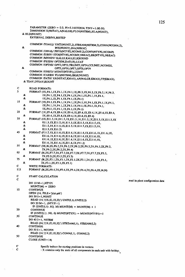
PARAMETER (ZERO= 0.0, Pl=3.141592654; TINY=l.OE•30) DIMENSION X(NST AT),A(NALGB),FLO l(NSTRM),HLA(NUNm,
&HLD(NUNm EXTERNAL DERIVS,BSSTEP
COMMON fl'OALU UNIT(NUNIT,2),STREAM(NSTRM,2),CONN(NCONN,2), & INX(NUNm,INA(NPROC)
c 5
15
25
35
45
55
65
75
c 115
c c
10
COMMON /DINAU PHYS(NTYP2,NCOMP,2),CONV(NTYP2,NCOMP) COMMON /DIRIV/ STOl(NTYP2,NCOMP,NREAC),RK(NTYP2,NREAC) COMMON /MNNDV/ KALLS,KALLS2,KROUND COMMON /FEEDS/ OPTSIM,DAT(l8),LUAT COMMON /OPTNS/ OPT2,0PT3,TRLIMIT,OPT4,CCLIMIT,NCOND2,
& OPT5,0PT6,0PT7,0PT8,0PT9 COMMON /UNICOI MUNIT(NTYPl),LUNIT COMMON /CARBN/ FLO(NSTRM),IBLK(NUNm COMMON /PATH/ XP(NSTAT,KMAX),AP(NALGB,KMAX),TP(KMAX),
& TSAV,DTSAV,KOUNT
& &
& &
&
& & &
& & &
&
&
&
READ FORMATS: FORMAT (IX,F4.l,lX,F4.l,lX,F4.l,lX,F6.3,1X,F6.3,1X,F6.3,lX,F6.3,
lX,F4.l,1X,F4.l,lX,F4.l,lX,F4.l,lX,F4.l,IX,F4.l, 1X,F4. l, IX,F4. l, lX,F4.1,lX,F4. I)
FORMAT (IX,F4.l ,IX,F4. I ,IX,F4.1,IX,F4. I ,IX,F4. I, 1X,F4.l ,IX,F4.l, IX,F4.l,IX,F4.l,IX,F4.1,1X,F4.l,IX,F4.l,IX,F4.l, IX,F4.l,IX,F4.l,IX,F4.l,IX,F4.l)
FORMAT (IX,E9.4,IX,E9.4,IX,E9.4,IX,E9.4,IX,E9.4,IX,E9.4,IX,E9.4, IX,E9.4,IX,E9.4,IX,E9.4,IX,E9.4,1X,E9.4)
FORMAT (IX,El 1.5,IX,EI 1.5,IX,El 1.5,IX,El 1.5,IX,El 1.5,IX,EI 1.5,IX El 1.5, IX,El 1.5,IX,El 1.5, IX,El 1.5, IX,EI 1.5,IX, El 1.5,IX,EI 1.5,IX,EI 1.5, IX,El 1.5, IX,El 1.5, IX, El 1.5, IX,EI 1.5)
FORMAT (Fl 1.2,IX,EI 1.6,IX,El 1.6,IX,EI 1.6,IX,El 1.6,IX,El 1.6,IX, El 1.6,IX,EI 1.6,IX,EI 1.6,IX,El 1.6,IX,El 1.6,IX, El 1.6,IX,El 1.6,IX,EI 1.6,IX,El 1.6,IX,El 1.6,IX, El 1.6,IX,EI 1.6,IX,EI 1.6,IX,Fl 1.2)
FORMAT (3X,16,2X,F6.2,2X,F6.2,2X,F6.2,2X,F6.3,2X,F6.3,2X,F6.2, 2X,F6.2,2X,F6.2,2X,F6.4)
FORMAT (16,3X,F7.7,3X,F7.7,3X,F7.7,3X,F7.7,3X,F7.7,2X,F3.3, 2X,F3.3,2X,F3.3,2X,F3.3)
FORMAT (16,2X,F3.l,2X,F3.l,2X,F3.l,2X,F3.l,2X,F3.l,2X,F3.I, 2X,F3.l,2X,F3.l,2X,F3.l)
WRITE FORMATS: FORMAT (16,3X,F9.4,3X,F9.4,3X,F9.4,3X,F6.4,3X,F6.4,3X,14,l4)
START CALCULATION
DO IOM=l,NTYPI MUNIT(M) = ZERO
CONTINUE OPEN (14, FILE='plnt.pdt') DO 30 l=l,NUNIT
READ (14, '(I X,12, IX,12)') UNIT(l, I), UNIT(l,2) DO 20 M=l, (NTYPl-1) .
IF (UNIT(l,I) .EQ. M) MUNIT(M) = MUNIT(M) + 1 20 CONTINUE
IF (UNIT(l,I) .NE. 0) MUNIT(NTYPI) = MUNIT(NTYPl)+ I 30 CONTINUE
DO 40 I= I, NSTRM READ (14,'(IX,12,IX,12)') STREAM(l,I), STREAM(l,2)
40 CONTINUE DO 50 l=l, NCONN
READ (14,'(lX,12, IX,12)') CONN(l, l), CONN(l,2) 50 CONTINUE
CLOSE (UNIT= 14)
C Specify indices for starting positions in vectors: C - X contains only the mols of all components in each unit with holdup . .
125
read in plant configuration data

126
C - A contains the total number of mols, the total volume and the liquid volume in each unit C with holdup, the number of mols of each component, the total number of mols and the C total volume in each of the streams.
INX(I) = 0 INA(!)= 0 DO 601=2,NUNIT
LUO= UNIT(l-1,1) IF ((LUO .EQ. I) .OR. (LUO .EQ. 2) .OR. (LUO .EQ. 5) .OR.
& (LUO .EQ. 6) .OR. (LUO .EQ. 7)) THEN
C assign space in X and A only for units with holdup INX(I) = INX(l-1) + NCOMP INA(I) = INA(l-1) + NTOTS
ELSE INX(I) = INX(l-1) INA(I) = INA(l-1)
ENDIF 60 CONTINUE
DO 70 l=l,NSTRM INA(NUNIT+I) = NUNIT*NTOTS + (1-l)*(NCOMP+NTOTS)
70 CONTINUE DO 80 I= l ,NCONN
INA(NUNIT+NSTRM+I) = NUNIT*NTOTS + NSTRM*(NCOMP+ & NTOTS) + (1-1)*2
80 CONTINUE
C read in densities and molar masses
c
c
OPEN (16, FILE='phys.dat') DO 100 M=l,NTYP2
DO 90 J =I ,NCOMP READ (16, '(F7.3,2X,F7.3)') PHYS(M,J, l),PHYS(M,J,2) IF (PHYS(M,J,2) .NE. 0.0) THEN
PHYS(M,J,2) = PHYS(M,J,2)*1000.0
CONV(M,J) = PHYS(M,J,l)/PHYS(M,J,2)
ELSE CONV(M,J) = ZERO
ENDIF 90 CONTINUE 100 CONTINUE
CLOSE (16)
= > PHYS(2) units of kg/m3
CONV has units of m3/kmol
C read stoichiometric constants from file OPEN (17, FILE='chem.dat') DO llOJ=l,NCOMP
READ (17,5) STOl{l ,J, l),STOI(l ,J ,2),STOl(l ,J,3),STOI(l ,J ,4), & STOl(l ,J,5),STOI{l ,J ,6),STOl(l ,J, 7),STOI{l ,J ,8),STOI(l ,J ,9), & STOl(l ,I;I 0),STOI{l ,J, I I ),STOl{l ,J, 12)
110 CONTINUE READ (17,25) RK{l,l),RK{l,2),RK(l,3),RK(l,4),RK(l,5),RK{l,6),.
& RK{I, 7),RK{l ,8),RK(l,9),RK{l,10),RK(I, 11),RK{l ,12} DO 120J=l,NCOMP
READ (17, 15) STOI(2,J, I ),STOI(2,J ,2),STOI(2,J ,3),STOI(2,J ,4), & ST01(2,J ,5),ST01(2,J ,6),ST01(2,J, 7),STOI(2,J ,8),STOI(2,J ,9), & STOl(2,J, l 0},STOI(2,J, l l),STOl(2,J, 12)
120 CONTINUE
c
130
140 c
READ (17,25) RK(2, 1),RK(2,2),RK(2,3),RK(2,4),RK(2,5),RK(2,6), & RK(2,7),RK(2,8),RK(2,9},RK(2,10),RK(2,l l),RK(2,l2)
CLOSE (17)
DO 1301=1,NSTAT X(I) \ZERO
CONTINUE DO 1401=1,NALGB
A(I) =ZERO CONTINUE
OT= 60.0
initially set all variables equal to zero
integration constants

HI = 1.0 IT= ZERO HMIN = 1.0E-4 D = 5.0E+7 EPS = 5.0E-6 DTSAV = 600.0 TSAV = -1.l•DTSAV TSAV2 =ZERO KOUNT = 0 NBAD = 0 NOK = 0 KALLS = 0 KALLS2 = 0 LUAT = 0 KROUND = 0 NCOND2 = 0 NCOLL = 0 NI= 0 VTNK = 6.0•PJ•(7.0/2) .. 2 VSCR = 0.7•PJ•(3.9/2) .. 2 CALL COLLECT (X,NSTAT,A,NALGB,NT,GOLD,AUCN,NCOLL)
DO 150M=l,NSTRM FLO(M) = ZERO
150 CONTINUE
PRINT •,'Would you like to:' PRINT •,'(I): Start the simulation with empty tanks and constant',
& 'flows' PRINT •,' 2 : Start the simulation where the last has ended off',
& ' again with' PRINT • ,' constant flows, or' PRINT•; 3: Use steady-state data as IC's with plant data?' OPTSIM = 'l'
160 READ (•,'(A)') OPTSIM
c
IF ((OPTSIM .NE. 'I') .AND. (OPTSIM .NE. '2') .AND. & (OPTSIM .NE. '3')) THEN
PRINT •,'Please choose option 1,2 or 3' GOTO 160
ELSE OPEN (18, FILE = 'inflos.pdt')
IF (OPTSIM .EQ. 'l') THEN PRINT •,'How long is the simulation to run for (in minutes) ?' READ (• ,'(16)') NT TE= NT•60.0 Tl= ZERO T2 =Tl+ DT
VOL= 3.5•3.5•PJ•5.3 PRINT •,'Is the Carbon profile to be :' PRINT •,'(I): Smooth ?' PRINT •,' 2 : Weighted to the top ?' PRINT •,' 3 : Weighted to the bottom ?' OPTI ='I'
170 READ (•,'(A)') OPTI IF ((OPTl.NE.'l ') .AND. (OPTl.NE.'2') .AND. (OPTl.NE.'3'))
& THEN PRINT •,'Please choose one of these options.' GOTO 170
ENDIF DO 180 L= I ,NUNIT
LUI = UNIT(L,I) IF (LUI .EQ. I) THEN
READ (18,35) X(INX(L)+ l),X{INX(L)+2),X(INX{L)+3), & X(INX(L) +4),X(INX{L) + 5),X(INX{L) +6),X(INX{L) + 7), & X(INX(L)+8),X(INX(L)+9).X(INX(L)+ 10),X{INX(L)+ 11),
127
read in data for feed units

128
& X(INX(L)+ 12),X(INX(L)+ 13),X{INX(L)+ 14);X{INX(L)+ 15), & X(INX(L)+ 16),X{INX(L)+ 17),X(INX(L)+ 18)
ELSEIF (LUI .EQ. 7) THEN HLA(L) = 1.0 HLD(L) = 0.0 IBLK(L) = 0
c IF (OPT! .EQ. 'I') THEN
add coarse carbon to CIP tanks only
c all tanks contain 2 % C by volume X(INX(L)+ 7) = VOL•0.02/CONV{2,7)
ELSEIF (OPT! .EQ. '2') THEN IF ((L.EQ.18) .OR. (L.EQ.21) .OR. (L.EQ.22)) THEN
c the first three tanks contain 3 % C by volume X(INX(L)+ 7) = VOL•0.03/CONV{2,7)
ELSE X(INX(L)+ 7) = VOL•0.02/CONV(2,7)
ENDIF ELSE
IF ((L .EQ. 25) .OR. (L .EQ. 26) .OR. (L .EQ. 28)) THEN c the last three tanks contain 3 % C by volume
X(INX(L)+ 7) = VOL•0.03/CONV(2,7) ELSE
X(INX(L)+ 7) = VOL•0.02/CONV{2,7) ENDIF
ENDIF ENDIF
180 CONTINUE
ELSEIF (OPTSIM .EQ. '2') THEN PRINT •,'How long is the simulation to run for (in minutes) ?' READ (•,'(16)') NT OPEN (19, FILE = 'psdata.pdt') DO 200 L= l ,NUNIT
LUI = UNIT(L,I) IF (LUI .EQ. I) THEN
READ (18,35) X(INX(L) + l).X(INX(L) + 2),X(INX{L) + 3), & X(INX(L)+4),X(INX(L)+5),X(INX(L)+6),X(INX(L)+7), & X(INX(L) + 8),X(INX(L) +9),X(INX(L)+ 10),X(INX(L) + 11), & X(INX(L) + 12).X(INX(L) + 13),X(INX(L) + 14),X(INX(L)+ 15), & X(INX(L)+ 16),X{INX(L)+ 17),X(INX(L)+ 18)
ELSEIF ((LUI .EQ. 2) .OR. (LUI .EQ. 5) .OR. (LUl.EQ.6) .OR. & (LUI .EQ. 7)) THEN
READ (19 ,45) TE,X(INX(L) + l),X(INX(L)+ 2),X(INX(L) + 3), & X(INX(L)+4),X(INX(L) + 5),X(INX(L)+6),X(INX(L) + 7), & X(INX(L) + 8),X(INX(L) +9),X(INX(L) + 10),X(INX(L) + 11), & X(INX(L)+ 12),X(INX(L)+ 13),X(INX(L)+ 14),X(INX(L)+ 15), & X(INX(L)+ 16),X{INX(L)+ 17),X{INX(L)+ 18),TT
tsav2 = te IF (LUI .EQ. 2) THEN
IF ((L .EQ. 20) .AND. (X{INX(L)+ 18) .GT. 5.0)) THEN FL0(18) = 1.0
ENDIF ELSEIF (LUI .EQ. 7) THEN
HLA(L) = 1.0 HLD(L) = 0.0 IBLK(L) = 0
c recognise engaged transfer stream IF (X(INX(L)+ 18) .GT. 5.0) THEN
DO 190M=l,NSTRM IF ((STREAM(M,2) .EQ. L) .AND.
& (STREAM(M+l,2) .EQ. STREAM(M,l))) THEN FLO(M) = 1.0
ENDIF 190 . CONTINUE
IF (L .EQ. 28) THEN FL0(35) = 1.0
ENDIF

ENDIF ENDIF
ENDIF 200 CONTINUE
c
c
210
& & & &
&
& & & &
&
Tl =TE TE = NT•6o.o + Tl T2=Tl+DT CLOSE (19)
ELSE
OPEN (18, FILE = 'inflos.pdt') OPEN (19, FILE = 'ssdata.pdt') DO 220 L=l,NUNIT
LUI = UNIT(L,l) IF (LUI .EQ. I) THEN
READ (18,35) X(INX(L)+ l),X(INX(L)+2),X(INX(L)+3), X(INX(L) + 4),X(INX(L) + 5),X(INX(L) +6),X(INX(L) + 7), X(INX(L)+8),X(INX(L)+9),X(INX(L)+ 10),X(INX(L)+ 11), X(INX(L)+ 12),X(INX(L)+ 13),X{INX(L)+l4),X(INX(L)+ 15), X(INX(L) + 16),X(INX(L) + 17),X(INX(L) + 18) ELSEIF ((LUI .EQ. 2) .OR. (LUI .EQ. 5) .OR. (LUl.EQ. 6).0R.
(LUI .EQ. 7)) THEN READ (19,45) TE,X(INX(L)+ l),X(INX(L)+2),X(INX(L)+3),
X(INX(L)+4),X(INX(L)+5),X(INX(L)+6),X(INX(L)+7), X(INX(L) + 8),X(INX(L) +9),X(INX(L) + 10),X(INX(L)+ 11),
X(INX(L)+ 12),X(INX(L)+ 13),X(INX(L)+ 14),X(INX(L)+ 15), X(INX(L) + 16),X(INX(L) + 17),X(INX(L) + 18),TI
IF (LUI .EQ. 2) THEN IF ((L .EQ. 20) .AND. (X(INX(L)+ 18).GT.5.0)) THEN
FLO{l8) = 1.0 print •,'started transfer stream 18'
ENDIF ELSEIF (LUI .EQ. 7) THEN
HLA(L) = 1.0 HLD(L) = 0.0 lBLK(L) = 0°
IF (X(INX(L)+ 18) .GT. 5.0) THEN D0210M=l,NSTRM
IF ((STREAM(M,2) .EQ. L) .AND. (STREAM(M + 1,2) .EQ. STREAM(M,l))) THEN
FLO(M) = 1.0 print •,'started transfer stream',M
ENDIF CONTINUE IF (L .EQ. 28) THEN
FL0(35) = 1.0 print •,'started transfer stream 35'
ENDIF ENDIF
ENDIF ENDIF
220 CONTINUE CLOSE (18) CLOSE (19) 1T =TI-TE TE= ZERO
ENDIF CLOSE (18)
CALL OPI'IONS PRINT•; Time ScrT Vol LIO Vol CIPS Vol',
& ' Leh eff CIP eff Fnc Calls' IF ((OPTSIM .EQ. 'I') .OR. (OPTSIM .EQ.'2')) GOTO 260 OPEN(31, FILE= 'avl2_0.pdt') OPEN(32, FILE = 'abs2_0.pdt') OPEN(33, FILE= 'abs3_0.pdt')
129
for OPl'SIM equal to 3 :
recognise engaged lfl\nsfer stream

OPEN(34, FILE= 'av23_0.pdt') ENDIF
230 READ(J 1,55) MT ,DAT(l),DAT(2),DAT(3),DAT(4),DAT(5),DAT(6),DAT(7), & DAT(8),DAT(9)
C plant data is read in here: dat(I) : CN-flow C dat(2) : thick2-flow dat(3) : thick2-fl-sp C dat( 4) : conductivity dat(5) : conduct-sp C dat(6) : CIP-feed dat{7) : leach-feed C dat(8) : leach-fd-sp dat(9) : leach-densty
READ(32,65) MT,DAT(IO),DAT(l l),DAT(l2),DAT(l3),DAT(l4),DAT(l5), & DAT(l6),DAT(l7),DAT(l8)
IF (DAT(l6) .EQ. 0.0) THEN LUAT = 0
ELSE LUAT =I
ENDIF C dat(lO) : lime lvl dat(l 1) : caustic lvl C dat(l2) : elu.CN.lvl dat(13) : lch.CN.lvll C dat(l4): lch.CN.lvl2 dat(l5): elu.p 1 C dat(l6): eluat p2 dat(l7): sump 1 C dat(18) : sump 2
IF (OPT9 .EQ. '3') THEN FLO I (18) = FLO(l 8) FL01(21) = FL0(21) FLO I (23) = FL0(23) FL01(25) = FL0(25) FL01(27) = FL0(27) FLO I (29) = FL0(29) FL01(31) = FL0(31) FLOl(33) = FL0(33) FLO I (35) = FL0(35) READ(33, 75) MT ,FLO(l 8),FL0(2 I ),FL0(23),FL0(25),FL0(27),FL0(29),
& FL0(31),FL0(33),CLO C flo(l9) : C trans 1 flo(21) : C trans 2 C flo(23) : C trans 3 flo(25) : C trans 4 C flo(27) : C trans 5 flo(29) : C trans 6 C flo(3 I) : C trans 7 flo(33) : C trans 8 C clo : C leak
IF (FL0(33) .GT. ZERO) THEN FL0(35) = 1.0
ELSE FL0(35) = ZERO
ENDIF IF (FL01(18) .EQ. 1.0) THEN
IF (FLO(l 8) .NE. 1.0) THEN PRINT •,'Stopped transfer stream 18' X(INX(20)+ 18) = 0.1
ENDIF ELSE
IF (FL0(18) .NE. ZERO) PRINT •,'Started transfer stream 18' ENDIF DO 240 N=l,8
IF (FLOl(N•2+ 19) .EQ. 1.0) THEN IF (FLO(N•2 + 19) .NE. 1.0) THEN
PRINT •,'Stopped transfer stream ',(N•2+ 19) X(INX(STREAM(N•2+19,2))+18) = 0.1
ENDIF ELSE
IF (FLO(N•2 + 19) .NE. ZERO) THEN PRINT •,'Started transfer stream• ,(N•2+ 19)
ENDIF ENDIF
240 CONTINUE ENDIF
c READ(34, 75) MT ,HLA(l 8),HLA(21),HLA(22),HLA(23),HLA(24),HLA(25),
130

c & c c c c
HLA(26),HLA(28)
Tl= TE T2 =Tl+ DT TE= 60.0•MT KROUND = 0 HI= 15.0
CONTINUE
hla(l8) : hilvl alml hla(22) : hilvl alm3 hla(24) : hilvl almS hla(26) : hilvl alm7
hla(21) : hilvl alm2 hla(23) : hilvl alm4 hla(25) : hilvl alm6 hla(28) : hilvl alm8
131
250 c c
screen blockage : remove e's if screen blockage is to be included in simulation
c IF ((T2 .GT. 5400.0*60.0) .AND. (NI .EQ. 0)) THEN c NI = I c HLA(18) = 0.0 c ENDIF
DO 260 M =I ,NU NIT IF (UNIT(M,1) .EQ. 7) THEN
IF (IBLK(M) .EQ. 0) THEN IF (HLA(M) .EQ. 0.0) THEN
IF (HLD(M) .EQ. 0.0) THEN HLD(M) = 1.0
ELSE HLD(M) = 2.0 print •,'Screen blocked in tank ',M IBLK(M) = I
ENDIF ELSE
IF (HLD(M) .EQ. 1.0) HLD(M) = 0.0 ENDIF
ELSEIF (IBLK(M) .EQ. 1) THEN print *,'vol =',A(INA(M)+2),' vtnk=',VTNK IF (A(INA(M)+2) .GE. (VTNK)) THEN
IBLK(M) = 2 print •,'Screen overflowed in tank ',M
ENDIF ELSE
IF (A(INA(M)+2) .LE. (VTNK-VSCR)) THEN print •,'Screen unblocked in tank • ,M IBLK(M) = 0 HLA(M) ~ 1.0 HLD(M) = 0.0
ENDIF ENDIF
ENDIF 260 CONTINUE
c
CALL ODEINT(X,NST AT ,A,NALGB,TI ,T2,H I ,HMIN,D,EPS,NOK,NBAD, & DERIVS,BSSTEP)
NT= T2/60
OPEN (37, FILE = 'store.dat')
DO 270 L= I ,NUNIT LUI = UNIT(L, I) IF ((LUI .EQ.2).0R.(LUI .EQ.5).0R.(LUI .EQ.6).0R.(LUl.EQ.7)) THEN
WRITE (37,45) T2,X(INX(L)+ l),X(INX(L)+2),X(INX(L)+3), & X(INX(L)+4),X(INX(L)+5),X(INX(L)+6),X(INX(L)+ 7), & X(INX(L) + 8),X(INX(L) +9),X(INX(L) + 10),X(INX(L)+ 11), & X(INX(L)+ 12),X(INX(L)+ 13),X(INX(L)+ 14),X(INX(L)+ 15), & X(INX(L)+ 16),X(INX(L)+ 17),X(INX(L)+ 18),TT
ENDIF 270 CONTINUE
CLOSE (37)
save state variables after each step

c c
c
c
IF ((f2-TSAV2) .GE. DTSAV) THEN NT= T2160 TSAV2 = T2 GOLD = (X(INX(3)+8)+X(INX(3)+9))1(100.0•X(INX(3)+2)+TINY) AUCN = X(INX(16)+5)f(IOO.O•X(INX(l6)+ !)+TINY) WRITE (•,t 15) NT,A(INA(3)+2),A(INA(l6)+2),A(INA(28)+2),
& (X(INX(l6)+8)+X(INX(l6)+9))f(GOLD•X(INX(l6)+2)+TINY), & X(INX(28)+5)f(AUCN•X(INX(28)+ l)+TINY),KALLS2,KALLS
CALL COLLECT(X,XSTAT,A,NALGB,NT,GOLD,AUCN,NCOLL) ENDIF
KOUNT = 0
IF corn .EQ. 'l') THEN TRLIMIT = 5000.0IPHYS(2,7,I)
ELSE TRLIMIT = 2500.0IPHYS(2,7,I)
ENDIF
IF (OPT9 .EQ. 'I') THEN HR= 16.0
ELSEIF (OPT9 .EQ. '2') THEN HR= 8.0
ENDIF
IF ((OPT9.NE. '3') .AND. (X(INX(29)+ l).GT.ZERO)) THEN
132
regular carbon transfers : set maximum C-conc for top-ups
set the size of transfer
set beginning time of transfer
C start transfers if not using data and whole cascade is full IF ((OPT4.EQ.'O') .OR.((OPT4.EQ.'l ') .AND.(NCOND2.EQ.0))) THEN
IF ((TT .EQ. ZERO) .OR. ((f2-TT) .GE. HR•3600.0)) THEN C start only if its the I st time or HR hr passed since previous one
IF ((OPT2 .EQ. 'I') .OR. (OPT2.EQ.'3') .OR. (OPT2.EQ.'4')) & THEN
DO 280 M=l,NSTRM C for simultaneous and continuous transfers start all transfers
IF ((STREAM(M,l) .NE. 0) .AND. (FLO(M) .EQ. ZERO)) THEN IF ((STREAM(M,I) .EQ. STREAM(M+l,2)) .AND.
& (STREAM(M,2) .EQ. STREAM(M+ 1,1))) THEN FLO(M) = 1.0 print •,'starting transfer stream' ,m
ENDIF IF (STREAM(M,l) .EQ. 27) THEN
FLO(M) = 1.0 print •,'starting transfer stream' ,m KROUNO = 0
ENDlF ENDIF
280 CONTINUE ELSEIF ((OPT2.EQ. '2') .OR. (OPT2.EQ. '5')) THEN
C for consecutive transfer scheme start only first transfer
c
FLO(l 8) = 1.0 PRINT •,'Starting transfer stream 18'
ENDIF TI= T2
ENDIF IF (OPT2 .NE. '3') THEN
DO 310 M= l,NSTRM IF (FLO(M) .EQ. 1.0) THEN
IF (STREAM(M,2) .EQ. 19) THEN IF (X(INX(20)+ 18) .GE. TRLIMm THEN
FLO(M) = ZERO PRINT •,'stopped transfer stream',m X(INX(20)+ 18) = X(INX(20J+ 18) -TRLIMIT
for continuous transfer scheme don't stop streams

c
&
290
c
&
300
IF ((0Pf2.EQ.'2') .OR. (0Pf2.EQ. '5;)) THEN
DO 290 N =I ,NSTRM IF ((STREAM{N,2) .EQ. STREAM{M,I)) .AND.
(STREAM{N,I) .EQ. STREAM(N+I,2))) THEN FLO(N) = 1.0 PRINT •,'started transfer stream',n
ENDIF CONTINUE
ENDIF ENDIF
ELSE IF {X(INX(STREAM{M,2))+ 18) .GE. TRLIMIT) THEN
FLO{M) = ZERO print •,'stopping transfer stream',m NST = STREAM{M,2) X(INX(NST)+ 18) = X{INX(NST)+ I8) -TRLIMIT IF (STREAM{M,1) .EQ. 27) THEN
KROUND = 0 NCONDI = 1
ENDIF IF ((0Pf2.EQ.'2').0R.(0Pf2.EQ.'5')) THEN
IF (STREAM{M,1) .EQ. 28) THEN FL0(35) = 1.0 PRINT •,'started transfer stream 35' KROUND = 0
ELSE DO 300 N = l ,NSTRM
IF ((STREAM{N,2) .EQ. STREAM{M,I)) .AND. (STREAM{N,I) .EQ. STREAM(N+l,2))) THEN
FLO{N) = 1.0 PRINT •,'started transfer stream' ,n
ENDIF CONTINUE
ENDIF ENDIF
ENDIF ENDIF
ENDIF 310 CONTINUE
END
133
only for consecutive transfer start next stream
only for consecutive transfer start next stream
C decide whether it is time for a top-up NOFLO = 0 DO 320 M = I ,NSTRM
IF (FLO{M) .EQ. 1.0) NOFLO = 1 320 CONTINUE C conditions are needed to ensure only one top-up after each transfer
c
c
IF ({NOFLO .EQ. 0) .AND. (NCONDI .EQ. I)) THEN NCOND2 =I
ENDIF ELSE
DO 340 M= l,NSTRM IF (FLO(M) .EQ. ZERO) THEN
IF ((STREAM(M,2) .EQ. 18) .AND. (NCONDI .EQ.l)) THEN IF (X(INX(STREAM(M,2))+7) .LT. CCLIMIT) THEN
FL0(21) = 1.0 PRINT •,'topping up tank ',STREAM{M,2)
ELSE NCOND2 = 0
top-up tanks sequentially from top tank down
if the first tank needs no topup, leave others as well ENDIF NCONDI = 0
ENDIF ELSE
IF {X(INX(STREAM{M,2))+ 7) .GE. CCLIMIT) THEN

330
FLO(M) = zero NST = STREAM(M,2) PRINT •,'stopped topping up tank ',NST X{INX(STREAM(M,2))+ 18) = 0.1 IF (STREAM(M,l) .EQ. 27) THEN
KROUND = 0 NCOND2 = 0
ELSEIF (STREAM(M,l) .EQ. 28) THEN FL0(35) = 1.0 . PRINT •,'started topping up tank ',STREAM(M,l) KROUND = 0
ELSE DO 330 N = l ,NSTRM
IF ((STREAM(N,2) .EQ. STREAM(M,l)) .AND. & (STREAM(N,l) .EQ. STREAM(N+l,2)))THEN
FLO(N) = 1.0 PRINT •,'started topping up tank ',STREAM(N,2)
ENDIF CONTINUE
END IF ENDIF
ENDIF 340 CONTINUE
ENDIF ENDIF
IF (T2 .LT. TE) THEN Tl= T2 T2=T2+DT IF (T2 .GT. TE) T2 = TE GOTO 250
ENDIF
IF (OPTSIM .EQ. '3') THEN IF (TE .LT. 604800.0) THEN
GOT0230 ELSE
CLOSE (31) CLOSE (32) CLOSE (33) CLOSE (34)
ENDIF END IF
NCOLL = 2 CALL COLLECT(X,NST AT,A,NALGB,NT,GOLD,AUCN ,NCOLL)
STOP END
c •••••••••••••••••••••••••••••••••••••••••••••••••••••••••••••••••••••• c •
SUBROUTINE OPTIONS c c c c
This subroutine asks the user for his choice in simulating various different prespecified options.
• • • • c ••••••••••••••••••••••••••••••••••••••••••••••••••••••••••••••••••••••
DOUBLE PRECISION TRLIMIT,CCLIMIT COMMON /FEEDS/ OPTSIM,DAT(l8),LUAT COMMON /OPTNS/ OPT2,0PT3,TRLIMIT,OPT4,CCLIMIT,NCOND2,0PT5,
& OPT6,0PT7,0PT8,0PT9 CHARACTER ANS
PRINT •,'Would you like the Carbon Transfers to be :' PRINT •,'(l): Equal and simultaneous?'
134

PRINT • ,' 2 : Equal and consecutive ?' PRINT • ,' 3 : Equal and continuous ?' PRINT•; 4: Plant tlowrates and simultaneous' PRINT • ,' 5 : Plant tlowrates and consecutive' 0Pr2 = '1'
10 READ (•,'(A)') 0Pr2 IF ((0Pr2.NE.'l') .AND. (0Pr2.NE.'2') .AND. (0Pr2.NE.'3')
& .AND. (0Pr2.NE.'4') .AND. (0Pr2.NE.'5')) THEN PRINT •,'Please choose one of the available options.' GOTOIO
ENDIF
IF (0Pr2 .NE. '3') THEN
PRINT •,'Should the Transfers start:' PRINT •,'(I): Regularly every 16hr ?' PRINT • ,' 2 : Regularly every 8hr ?' IF ((OPTSIM .EQ. 'I') .OR. (OPTSIM .EQ. '2')) THEN
20 READ (•,'(A)') OPT9 IF ((OPT9.NE.'1 ') .AND. (OPT9.NE.'2')) THEN
PRINT •,'Please choose one of the available options.' GOT020
ENDIF ELSE
PRINT •, • 3 : As recorded on the plant ?' OPT9 = 'I'
30 READ (•,'(A)') OPT9 IF ((OPT9.NE.'I ') .AND.(OPT9.NE.'2') .AND. (OPT9.NE.'3')) THEN
PRINT •,'Please choose either option l, 2 or 3.' GOT030
ENDIF ENDIF
PRINT •;And should the Transfers be :' PRINT • ,'(!): Large (5000kg) ?' PRINT • ,' 2 : Small (2500kg) ?' OPT3 = '1'
40 READ (•,'(A)') OPT3 IF ((OPT3 .NE. 'I') .AND. (OPT3 .NE. '2')) THEN
PRINT •,'Please choose either option l or 2.' GOT040
ENDIF
PRINT •,'Should the amount of Carbon be topped up after', & 'transfers ((Y) or NJ ?'
ANS= 'Y' 50 READ (•,'(A)') ANS
IF ((ANS .EQ. 'y') .OR. (ANS .EQ. 'Y')) OPT4 = 'l' IF ((ANS .EQ. 'n') .OR. (ANS .EQ. 'N')) OPT4 = ·o· IF ((OPT4.NE.'l') .AND. (OPT4.NE.'0')) THEN
PRINT •,'Please choose either Y or N' GOTO SO
ENDIF ELSE
PRINT •,'And should the Transfers be :' PRINT•,'(!): Large (5000kg every 16hr) ?' PRINT•; 2: Small (2500kg every 16hr) ?' OPT3 ='I'
60 READ (•,'(A)') OPT3 IF ((OPT3 .NE. 'I') .AND. (OPT3 .NE. '2')) THEN
PRINT •;Please choose either option 1 or 2.' GOT060
ENDIF OPT4 = '0'
ENDIF
PRINT •;rs Carbon allowed to leak through the screens',
135

& '[(Y) or NJ ?' ANS= 'Y'
70 READ (*,'(A)') ANS IF ((ANS .EQ. 'y') .OR. (ANS .EQ. 'Y')) 0Yr5 = 'l' IF ((ANS .EQ. 'n') .OR. (ANS .EQ. 'N')) 0Yr5 = ·o· IF ((0Yr5.NE. 'l ') .AND. (0Yr5.NE. '0')) THEN
PRINT •,'Please choose either Y or N' GOT070
ENDIF
IF (OYrSIM .EQ. '3') THEN PRINT *,'Is the pulp flow to be:' PRINT *,'(l) : Constant?' PRINT •,' 2 : As recorded in the plant data ?' 0Yr6 = 'l'
80 READ (*,'(A)') 0Yr6 IF ((0Yr6 .NE. 'l ') .AND. (0Yr6 .NE. '2')) THEN
PRINT •,'Please choose either option I or 2.' GOT080
ENDIF
IF (0Yr6 .EQ. '2') THEN PRINT *,'Is the lime addition to be:' PRINT *,'(l) : Constant?' PRINT*,' 2 : Proportional to the recorded flow?' 0Yr1 ='I'
90 READ (*,'(A)') 0Yr7 IF ((0Yr7 .NE. 'I') .AND. (0Yr7 .NE. '2')) THEN
PRINT •,'Please choose either option I or 2.' GOT090
ENDIF
PRINT *,'I~ the cyanide addition to be:' PRINT *,'{l) : Constant?' PRINT •,' 2 : Proportional to the recorded flow ?' PRINT •,' 3 : As recorded in the plant data ?' 0Yr8 = 'I'
100 READ (*,'(A)') 0Yr8 IF ((0Yr8.NE.'l ').AND.(0Yr8.NE.'2').AND.(0Yr8.NE.'3')) THEN
PRINT *,'Please choose either option 1,2 or 3.' GOTO 100
ENDIF ELSE
0Yr1 ='I' 0Yr8 = 'I'
ENDIF ENDIF
RETURN END
c •••••••••••••••••••••••••••••••••••••••••••••••••••••••••••••••••••••• c
c c c
SUBROUTINE COLLECT(X,NS,A,NA,NT,GOLD,AUCN,NCOLL)
This subroutine writes the required data to file.
•
• • • c ••••••••••••••••••••••••••••••••••••••••••••••••••••••••••••••••••••••
PARAMETER (NUNIT = 30, NSTRM = 40, NCONN = 40, NTYPI = 9) PARAMETER (NTYP2 = 2; NCOMP = 18, NTOTS = 2, NREAC = 12) PARAMETER (KMAX = 10) PARAMETER (NALGB = NUNIT•NTOTS + NSTRM•(NTOTS+NCOMP)
& + NCONN*2) PARAMETER (NSTAT = NUNIT•NCOMP) PARAMETER (NPROC = NUNIT + NSTRM + NCONN)
136

DOUBLE PRECISION X,A,lT,ZERO,CONV,VOL,GOLD,AUCN INTEGER UNIT, STREAM, CONN
PARAMETER (ZERO= 0.0, TINY=l.OE-30) DIMENSION X(NSTAn,A(NALGB)
COMMON trOALU UNIT(NUNIT ,2),STREAM(NSTRM,2),CONN(NCONN,2), & INX(NUNfn,INA(NPROC)
COMMON /DINAU PHYS(NTYP2,NCOMP,2),CONV(NTYP2,NCOMP) COMMON /FEEDS/ OPTSIM,DAT(l8),LUAT
5 FORMAT (16, l X,EI 1.6, I X,EI 1.6, I X,E 11.6, I X,EI 1.6, IX,EI 1.6, IX, & El 1.6,IX,EI 1.6,IX,EI 1.6, IX,El 1.6,IX,EI 1.6,IX,El 1.6,lX, & Ell.6,IX,EI 1.6,IX,EI 1.6,lX.El 1.6,IX,EI 1.6,IX,Et 1.6,tX, & El t.6,IX,Ell.6,IX.El l.6,IX,EI 1.6)
15 FORMAT {18,IX,F8.3,IX,F8.3,IX,F8.3,IX,F8.3,IX,F8.3,lX,F8.3,lX, & F8.3, 1X,F8.3, IX,F8.3, IX,F8.3, IX,F8.3, IX,F8.3,IX,F8.3, IX, & F8.3,IX.F8.3, IX,F8.3, IX,F8.3, I X,F8.3, IX,F8.3,tX,F8.3,lX, & F8.3)
IF (NCOLL .EQ. 0) THEN NCOLL =I OPEN (36, FILE = 'outflos.sim') OPEN (21, FILE= 'solgold.sim') OPEN (22, FILE= 'disgold.sim') OPEN (23, FILE= 'adsgold.sim') OPEN (24, FILE= 'solmetl.sim') OPEN (26, FILE = 'dismetl.sim') OPEN (27, FILE= 'adsmetl.sim') OPEN (28, FILE= 'cyanide.sim') OPEN (29, FILE = 'disoxyg.sim') OPEN (38, FILE = 'carbtm.sim') OPEN (39, FILE = 'sollime.sim') OPEN (41, FILE = 'carbonp.sim') OPEN (42, FILE= 'effncy.sim') OPEN (43, FILE = 'lcffcy.sim')
ELSEIF (NCOLL .EQ. I) THEN
137
C save volume flows out of selected tanks IF (OPTSIM .EQ. '3') THEN
WRITE (36,15) NT,DAT(7), & A(INA(NUNIT+3)+NCOMP+2)•3600, & A(INA(NUNIT+6)+NCOMP+2)•3600, & A(IN A(Nl:JNIT + 7) + NCOMP+ 2)•3600, & A(INA(NUNIT+8)+NCOMP+2)•3600, & A(INA(NUNIT+9)+NCOMP+2)•3600, & A(INA(NUNIT +IO)+ NCOMP+ 2)•3600, & A(INA(NUNIT+ ll)+NCOMP+2)•3600, & A(INA(NUNIT + 12) + NCOMP+ 2)•3600, & A(INA(NUNIT+ 13)+NCOMP+2)•3600, & A(INA(NUNIT+l4)+NCOMP+2)•3600,DAT(6)
ELSE WRITE (36,15) NT,
& A(INA(NUNIT+l)+NCOMP+2)•3600, & A(INA(NUNIT+6)+NCOMP+2)•3600, & A(INA(NUNIT+7)+NCOMP+2)•3600, & A(INA(NUNIT+8)+NCOMP+2)•3600, & A(INA(NUNIT+9)+NCOMP+2)•3600, & A(INA(NUNIT+ IO)+NCOMP+2)•3600, & A(INA(NUNIT+ 11)+ NCOMP+2)•3600, & A(INA(NUNIT+ 12)+ NCOMP+2)•3600, & A(INA(NUNIT+ 13)+ NCOMP+2)•3600, & A(INA(NUNIT+ 14)+NCOMP+2)•3600, & A(IN A(NUNIT + 15) + NCOMP+ 2)•3600, & A(INA(NUNIT+l6)+NCOMP+2)•3600, & A(INA(NUNIT+l7)+NCOMP+2)•3600, & A(INA(NUNIT + 22) + NCOMP+ 2)•3600, & A(INA(NUNIT + 24) + NCOMP+ 2)•3600,

& & & & & &
c
& & & & & & & & & &
A(IN A(NUNIT + 26) + NCOMP + 2)*3600, A(IN A(NUNIT + 28) + NCOMP+ 2)*3600, A(INA(NUNIT + 30) + NCOMP+ 2)*3600, A(IN A(NUNIT + 32) + NCOMP+ 2)*3600, A(INA(NUNIT+34)+ NCOMP+2)*3600, A(INA(NUNIT + 34) + NCOMP+ 2)*3600
END IF
WRITE (21,S) NT, (X(1NX(7)+8)+X(1NX(7)+9))/(GOLD*(X(1NX(7)+2)f.TINY)), (X(INX(8)+8)+X(INX(8)+9))/(GOLD*(X(INX(8)+2)+TINY)), (X(1NX(9)+8)+X(INX(9)+9))/(GOLD*(X(1NX(9)+2)+TINY)), (X(1NX(l0)+8)+X(1NX(l0)+9))/(GOLD*(X(1NX(l0)+2)+TINY)), (X(INX(l 1)+8)+X(INX(l 1)+9))/(GOLD*(X(1NX(l l)+2)+TINY)), (X(INX(l 2) + 8) + X(INX(l 2) +9))/(GOLD*(X(INX(l2) + 2) +TINY)), (X(INX(l3) + 8) + X(1NX(l3) +9))/(GOLD*(X(INX(l3) + 2) +TINY)), (X(1NX(l4)+8)+X(INX(l4)+9))/(GOLD*(X(INX(l4)+2)+TINY)), (X(INX(lS) + 8)+ X(INX(lS) +9))/(GOLD*(X(INX(IS) + 2)+ TINY)), (X(INX(l6) + 8)+ X(INX(l 6) +9))/(GOLD*(X(1NX(l6) + 2) +TINY))
(a few pages of WRITE statements are omitted here)
ELSE CLOSE (21) CLOSE (22) CLOSE (23) CLOSE (24) CLOSE (26) CLOSE (27) CLOSE (28) CLOSE (29) CLOSE (36) CLOSE (38) CLOSE (39) CLOSE (41) CLOSE (42)
ENDIF RETURN END
c •••••••••••••••••••••••••••••••••••••••••••••••••••••••••••••••••••••• c • C Copyright (C) MINTEK 1991. Right of Reproduction Reserved. • c • c ••••••••••••••••••••••••••••••••••••••••••••••••••••••••••••••••••••••
1.2 BSINT.F: INTEGRATION SUBROUTINE
c •••••••••••••••••••••••••••••••••••••••••••••••••••••••••••••••••••••• c
c c c c c c c c c c c c
• SUBROUTINE ODEINT(XST ART,NS,A,NA,Tl ,T2,H l ,HMIN ,D,EPS,NOK,
*NBAD,DERIVS,BSSTEP)
This integration package uses the Bulirsch-Stoer method with adaptive stepsize control as given by W.H.Press et.al. in their book 'Numerical Recipes: The Art of Scientific Computing', Cambridge University Press,1986. It has been modified to deal with discontinuities, using the method supplied by Gear C.W. and 0sterby 0, Solving Ordinary Differential Equations with Discontinuities, ACM Trans. on Math. Software, Vol 10, No.I, 1984.
The following (in CAPITALS) must be supplied: - the NS starting values, XST ART, of the state variables which are to be integrated from Tl to T2 with accuracy EPS, using the
• • • • • • • • • • • •
138
save normalized solid cone of gold

c NA algebraic variables A. HJ should be set as a guessed first • c stepsi7.e, HMIN as the minimum allowed stepsize. On output NOK • c and NBAD are the numbers of good and bad (but retried and fixed) • c steps taken, and XST ART is replaced by the values at the end of • c the integration interval. • c - DERIVS is the user-supplied subroutine for calculating the • c right-hand side derivative. (Bsstep is the name of the stepper • c routine to be used, which performs the integration, while Pass_ • c Discont uses a fourth-order Runge-Kutta method to bypass any • c discontinuities.) • c - the COMMON block /PATH/ in the STORE subroutine contains the • c information about the minimum span, DTSA V, between successive • c values of the independent variable, TP, at which intermediate • c values, XP and AP, are to be stored. KOUNT is the total number • c of the intermediate values that have been saved, with a maximum • c value ofKMAX. (See included file ODEINT.PAS) • c • c NB : When changing the number of state or algebraic variables, • c remember to change the value of NST ATE or N ALGE in the included • c parameter file ODEINT.PAS. • c Similarly, when changing the length of integration or the mini- • c mum recording span (DTSA V), change KMAX correspondingly. • c After editing ODEINT.PAR, remember to recompile this program. • c • c ••••••••••••••••••••••••••••••••••••••••••••••••••••••••••••••••••••••
5
PARAMETER (NUNIT = 30, NSTRM = 40, NCONN = 40) PARAMETER (NCOMP = 18, NTOTS = 2) PARAMETER (NALGB = NUNIT•NTOTS + NSTRM•(NTOTS+NCOMP)
& + NCONN•2) PARAMETER (NSTAT = NUNIT•NCOMP)
DOUBLE PRECISION XSTART,XSCAL,X,DXDT,A DOUBLE PRECISION T,Tl,T2,H,Hl,HMIN,HDID,HNEXT,BlG DOUBLE PRECISION ZERO,TWO,TINY PARAMETER (ZERO = 0.0,TWO = 2.0,TINY = 1.0E-30) DIMENSION XST ART(NS),XSCAL(NSTA T), DIMENSION X(NSTAT),DXDT(NSTAT),A(NA) EXTERNAL BSSTEP,DERIVS FORMAT ('I :Discontinuity between ',Fl 1.4,' and ',Fl 1.4,' !
& ')
BIG= D/EPS T =Tl H = SIGN(Hl,T2-TI) KENO= 0 DO 101=1,NS
X(I) = XST ART(I)
' '
10 CONTINUE 20 CONTINUE
139
C start of main calculation loop
c 30 c
c
IF (T .EQ. ZERO) CALL DERIVS(X,DXDT,NS,A,NA,T) DO 30 I= l,NSTAT
XSCAL(I) = ABS(X(I)) + ABS(H•DXDT(I)) + TINY
CONTINUE
CALL STORE(X,NS,A,NA,T,KEND)
IF ((T+H-T2)•(T+H-TI) .GT. ZERO) H = T2 -T NDIS = 0 IF (H .LE. ZERO) PAUSE 'h = zero in ODEINT' HDID = HMIN CALL BSSTEP(X,DXDT,NS,A,NA,T,H,HDID,HNEXT,EPS,BIG,XSCAL,
& NDIS,DERIVS) IF (NDIS .EQ. I) THEN
WRITE (•,5) T, (T+H)
scaling factor to monitor accuracy
store results
ensure that no step overshoots the end

c
40
CALL PASS_DISCONT(X,DXDT,NS,A,NA,T,H,HMIN,EPS,BIG,XSCAL, & DERIVS)
WRITE (•,5) (T-H),T DO 40 I=l,NSTAT
XSCAL(I) = ABS(X(I)) + ABS(H•DXDT(I)) + TINY CONTINUE IF (H•O.l .GT. HMIN) THEN
HNEXT = H•O.l ELSE
HNEXT = HMIN ENDIF NDIS = 0
ENDIF IF (HDID .EQ. H) THEN
NOK = NOK + 1 ELSE
NBAD = NBAD + I ENDIF IF ((T-T2)•(T2-Tl) .GE. ZERO) THEN
140
recalculate scaling factor
C check if end has been reached KENO= 1 DO 50 I= l,NSTAT
XST ART(I) = X(I) 50 CONTINUE C recalculate DXDT and A
c
c
CALL DERIVS(X,DXDT,NS,A,NA,T)
CALL STORE(X,NS,A,NA,T,KEND) HI= HNEXT RETURN
ENDIF H = HNEXT
and save results at end of step
exit integrator
c recalculate DXDT and A before going back for the next step CALL DERIVS(X,DXDT,NS,A,NA,T)
GOT020 END
c •••••••••••••••••••••••••••••••••••••••••••••••••••••••••••••••••••••• c •
SUBROUTINE STORE(X,NS,A,NA,T,KEND) c c c c c c c
The COMMON block /PATH/ contains the information about the minimum span, DTSAV, between successive values of the independent variable, TP, at which intermediate values, XP, are to be stored. KOUNT is the total number of the intermediate values that have been saved .• with a maximum value of KMAX.
• • • • • • • c ••••••••••••••••••••••••••••••••••••••••••••••••••••••••••••••••••••••
PARAMETER (NUNIT = 30, NSTRM = 40, NCONN = 40, NTYPI = 9) PARAMETER (NCOMP = 18, NTOTS = 2, KMAX = 10) PARAMETER (NALGB = NUNIT•NTOTS + NSTRM•(NTOTS+NCOMP)
& + NCONN•2) PARAMETER (NSTAT = NUNIT•NCOMP)
DOUBLE PRECISION X,A,T,TP,TSAV,XP,AP COMMON /UNICOI MUNIT(NTYPl),LUNIT COMMON /PATH/ XP(NSTAT,KMAX),AP(NALGB,KMAX),TP(KMAX),
& TSAV ,DTSAV ,KOUNT DIMENSION X(NS),A(NA)
15 FORMAT{Fl2.4,3X,F9.4,3X,F9.4,3X,F9.4,3X,F9.4,11X)
IF ((KMAX .GT. 0) .AND. (KOUNT .LT. KMAX-1)) THEN IF ((KENO .EQ. 1) .OR. (ABS(T-TSAV) .GT. ABS(DTSAV)}) THEN
c store only final or new intermediate results

KOUNT = KOUNT + l TP(KOUNT) = T TSAV = T DO IO l=l,NSTAT
XP(l,KOUNT) = X(I) IO CONTINUE
DO 20 l=l,NALGB AP(l,KOUNT) = A(I)
20 CONTINUE ENDIF
ENDIF c WRITE(• ,15) T,A(32),A(40),A(46),A(50)
RETURN END
c •••••••••••••••••••••••••••••••••••••••••••••••••••••••••••••••••••••• c •
SUBROUTINE BSSTEP(X,D~DT,NS,A,NA,T,HTRY,HDID,HNEXT,EPS, &BIG,XSCAL,NDIS,DERlVS)
c • c Bulirsch-Stoer step with monitoring of local truncation error • c to ensure accuracy and adjust stepsize. Input are the dependent • c state variable vector X and its derivative DXDT, of length NS, • c at the starting value of the independent variable T. Also input • c the stepsize to be attempted HTRY, the required accuracy EPS, • c and the vector XSCAL against which the error is scaled. On out- • c put, X, A and Tare replaced by the new values, HDID is the • c stepsize which was actually accomplished and HNEX'f is the esti- • c mated next stepsize. DERIVS is the user-supplied subroutine • c that computes the right-hand side derivatives. • c • c In the case where the error in any step is very large, and a • c discontinuity is suspected, the flag NDIS is changed to I. Then • c the program returns to ODEINT,from where PASS_DISCONT • c is called to pass the discontinuity. • c • c All 'print' statements are used in debuggin~ and are thus optional. • c • c ••••••••••••••••••••••••••••••••••••••••••••••••••••••••••••••••••••••
PARAMETER (NUNIT = 30, NSTRM = 40, NCONN = 40) PARAMETER (NCOMP = 18, NTOTS = 2, NUSE = 6, IMAX= 6) PARAMETER (NALGB = NUNIT•NTOTS + NSTRM•(NTOTS+NCOMP)
& + NCONN•2) PARAMETER (NSTAT = NUNIT•NCOMP)
DOUBLE PRECISION X,XSCAL,XERR,Xl ,XSAV,DXDT,DXSAV,XSEQ,EXT,A DOUBLE PRECISION T,TSAV,H,HTRY,HDID,HNEXT,HMIN,TEST,TK DOUBLE PRECISION ERRMAX,BIG,BIGN DOUBLE PRECISION ZERO,ONE,TINY PARAMETER (SHRINK = 0.95,GROW = 1.2,TINY = l .OE-30) PARAMETER (ZERO = 0.0, ONE = 1.0) COMMON /KEEP/ EXT(NSTAT,NUSE),TK(NSTAT) DIMENSION X(NS),DXDT(NS),XSCAL(NST A T),XERR(NST AT), DIMENSION XI (NSTAT),XSAV(NSTAT),DXSAV(NSTAT) DIMENSION XSEQ(NSTAT),NSEQ(IMAX),A(NA) EXTERNAL DERIVS DATA NSEQ /2,4,6,8,10,12/
H=HTRY if (h :le. zero) pause 'stop 3 !' TSAV = T HMIN = HDID
c print •;TIME= ',T DO 101=1,NS
XSAV(I) = X(l) DXSAV(I) = DXDT(l)
141

c 10 CONTINUE 20 CONTINUE
EPSN = ABS(EPS/H .. 0.5) BIGN = ABS(BIG/H••0.5} D0601=1,IMAX
142
keep the starting values
C evaluate sequence of modified midpoint integrations CALL MMID(XSAV ,DXSAV ,XSEQ,NS,A,NA,TSAV ,H,NSEQ(l},DERIVS} TEST = (H/NSEQ(l)) .. 2.0
C this is squared because the error series is even CALL RZEXTR(XSEQ,Xl,XERR,NS,TEST,I) ERRMAX = ZERO DO 30 J= l,NSTAT
ERRMAX = MAX(ERRMAX,ABS(XERR(J}/XSCAL(J}}} 30 CONTINUE
if (emnax .gt. l.OE+30} errmax= l.OE+30 ERRMAX = ERRMAX/EPSN IF (ERRMAX .LT. ONE} THEN
C a} this step has been successfully integrated DO 40 J=l,NSTAT
X(J} = Xl(J} 40 CONTINUE
T=T+H HDID = H IF (I .EQ. NUSE-2) THEN
HNEXT = H•SHRINK ELSE IF (I .EQ. NUSE-3) THEN
HNEXT = H•GROW ELSE
IF (H .GE. ONE} THEN HNEXT = H•(NSEQ(NUSE-1)•1.0}/(NSEQ(l)•l.O}
ELSE C ensure that step won't grow too fast after discontinuity
HNEXT = H•(J.0 + (NSEQ(NUSE-3)•1.0}/(NSEQ(l)•l.0}}/2.0 ENDIF
ENDIF IF (HNEXT .LT. HMIN} HNEXT = HMIN RETURN
ELSEIF (ERRMAX .GT. BIGN} THEN IF (NDIS .EQ. 0) THEN
C b) use alternative method as this step contains a dis.
so
c
NDIS = I HDID =ZERO DOSOJ=l,NSTAT
DXDT(J} = DXSAV(J} X(J} = XSAV(J}
CONTINUE RETURN
ELSE
ENDIF ENDIF
60 CONTINUE IF (H .LE. HMIN} THEN
unless dis. has already been discovered
C we have to accept the error DO 70 J=l,NSTAT
X(J} = Xl(J} 70 CONTINUE
c
T=T+H HDID = H HNEXT = H RETURN
END IF H = 0.25•H
IF (H .LT. HMIN) THEN H = HMIN
c) try using a smaller step as error is too large

ENDIF GOT020 END
c •••••••••••••••••••••••••••••••••••••••••••••••••••••••••••••••••••••• c
c c c c c c c c
• SUBROUTINE MMID(X,DXDT,XOUT,NS,A,NA,TS,HTOT,NSTEP,DERIVS)
Modified midpoint step. Dependent variable vector X of length NS and its derivative vector DXDT are input at TS. Also input is HTOT, the total step to be made, and NSTEP, the number of substeps to be used. The output is returned as XOUT, which need not be a distinct array from X; if it is different, however, then X and DXDT are returned undamaged.
• • • • • • • • c ••••••••••••••••••••••••••••••••••••••••••••••••••••••••••••••••••••••
c
c JO
PARAMETER (NUNIT = 30, NSTRM = 40, NCONN = 40) PARAMETER (NCOMP = 18, NTOTS = 2) PARAMETER (NALGB = NUNIPNTOTS + NSTRM•(NTOTS+NCOMP)
& + NCONN•2) PARAMETER (NSTAT = NUNIT•NCOMP)
DOUBLE PRECISION X,DXDT,XOUT,XM,XN,SWAP,A,ZERO DOUBLE PRECISION T,TS,H,HTOT PARAMETER (ZERO = 0.0) DIMENSION X(NS),DXDT(NS),XOUT(NS),XM(NST AT),
& XN(NSTAT),A(NA) EXTERNAL DERIVS H = HTOT/NSTEP
DO JO I= l,NSTAT XM(I) = X(I) XN(I) = X(I) + H•DXDT(I) XOUT(I) = ZERO
CONTINUE T=TS+H CALL DERIVS(XN,XOUT,NS,A,NA,T)
143
find stepsize for this round
first step
c use XOUT for temp. storage of derivatives
c 20
H2 = 2.0•H DO 30 N=2,NSTEP
DO 20 I= l,NSTAT SW AP = XM(I) + H2•XOUT(I) XM(I) = XN(I) XN(I) =SWAP
CONTINUE T=T+H CALL DERIVS(XN,XOUT,NS,A,NA,T)
30 CONTINUE
c 40
DO 40 I= l,NSTAT XOUT(I) = 0.5•(XM(I) + XN(I) + H•XOUT(I))
CONTINUE RETURN END
c •••••••••••••••••••••••••••••••••••••••••••••••••••••••••••••••••••••• c •
SUBROUTINE RZEXTR(XEST,XZ,DX,NS,TEST,IEST) c c c c c c
Use diagonal rational function extrapolation to evaluate NS functions at T=O by fitting a diagonal rational function to a sequence of estimates with progressively smaller values T=TEST, and corresponding function vectors XEST. This call is number JEST in the sequence of calls. The extrapolation uses only the
• • • • • •
general step
last step

c c c
last NUSE estimates. Extrapolated function values are output as XZ, and their estimated error is output as DX.
• • • c ••••••••••••••••••••••••••••••••••••••••••••••••••••••••••••••••••••••
PARAMETER (NUNIT = 30, NSTRM = 40, NCONN = 40) PARAMETER (NCOMP = 18, NTOTS = 2, NUSE= 6) PARAMETER (NALGB = NUNIT*NTOTS + NSTRM*(NTOTS+NCOMP)
& + NCONN*2) PARAMETER (NSTAT = NUNIT•NCOMP)
DOUBLE PRECISION XEST,XZ,DX,EXT,Fr,XX,V,C,BI ,B,DDX,TEST,TK DOUBLE PRECISION ZERO DIMENSION XEST(NS),XZ(NS),DX(NS),Fr(NUSE) PARAMETER (ZERO = 0.0) COMMON /KEEP/ EXT(NSTAT,NUSE),TK(NSTAT)
TK(IEST) = TEST
144
C keep the current value of independent variable IF (IEST .EQ. I) THEN
DO IOJ=I, NSTAT XZ(J) = XEST(J) EXT(J,I) = XEST(J) DX(J) = XEST(J)
10 CONTINUE ELSE
Ml = MIN(IEST,NUSE) C use at most NUSE previous values
D020K=I, Ml-I Fr(K+I) = TK(IEST-K)/TK(IEST)
20 CONTINUE DO 40 J= l,NSTAT
C evaluate next .diagonal in tableau XX= XEST(J) V = EXT(J,l) c =xx EXT(J,l) =XX DO 30K=2,MI
Bl = Ff(K)•V B =Bl -C IF (8 .NE. ZERO) THEN
B = (C-V)/B DDX = c•B C = Bl•B
ELSE DDX=V
C so that we don't divide by 0 later END IF IF (K .NE. Ml) V = EXT(J,K) EXT(J,K) = DDX XX= XX+ DDX
30 CONTINUE DX(J) = DDX XZ(J) =XX
40 CONTINUE ENDIF RETURN END
c •••••••••••••••••••••••••••••••••••••••••••••••••••••••••••••••••••••• c
c c c c
SUBROUTINE PASS_DISCONT{XO,DXDT,NS,A,NA,Tl,H,HMIN,EPS, &BIG,XSCAL,DERIVS)
This procedure finds the order and location of a discontinuity (dis.) according to the method proposed by Gear & Osterby: Each step is tested for the presence of the dis. by comparing
•
• • • •

c the results of each integration step with the result obtained • c by doing two half-steps. If the error is larger than BIG, the • c dis. is assumed to lie within the step, and the integration • c therefore fails. Depending on the sequence of successes and • c failures, and using the calculated slopes, the order can be • c determined. • c Once the location can be determined exacily or the integration • c step is small enough to limit the error,the method steps right • c up to or just over the dis. and then restarts. • c • c ••••••••••••••••••••••••••••••••••••••••••••••••••••••••••••••••••••••
PARAMETER (NUNIT = 30, NSTRM = 40, NCONN = 40) PARAMETER (NCOMP = 18, NTOTS = 2) PARAMETER (NALGB = NUNIT•NTOTS + NSTRM•(NTOTS+NCOMP)
& + NCONN•2) PARAMETER (NSTAT = NUNIT•NCOMP) PARAMETER (NPROC = NUNIT + NSTRM + NCONN)
DOUBLE PRECISION XO,DXDT,XSCAL,XF,XM,XF2,DXMDT,A DOUBLE PRECISION ERRMAX,TI ,T2,TM,TEND,H,HMIN,HPASS,HREM DOUBLE PRECISION ALPHA,AKl,AK2,AK3,Dl,D2,DINEW,D2NEW DOUBLE PRECISION XMMAX,ZERO,TWO,TINY,BIG,BIGN PARAMETER (SAFETY = 0.9, PSHRINK = -0.25, TINY = l .OE-30) PARAMETER (ZERO = 0.0, TWO = 2.0) DIMENSION XO(NS),DXDT(NS),XSCAL(NS),XF(NST AT),XM(NST AT) DIMENSION XF2(NSTAT),DXMDT(NSTAT),A(NA) EXTERNAL DERIVS,RK4,BSSTEP
5 FORMAT ('2:Discontinuity between ',F13.6,' and ',Fl3.6,' ! ' & ')
NORDER= I NCONFIRM = 0 NFAIL = 0 NSUCCESS = 0 ALPHA= ZERO DINEW =ZERO D2NEW =ZERO D2 =ZERO DO 10 J=l,NSTAT
XF(J) =ZERO XF2(J) = ZERO XM(J) =ZERO DXMDT(J) = ZERO
10 CONTINUE
c
TEND= Tl+H H = HfTWO
CALL RK4(XO,DXDT ,XF,NS,A,N A,Tl ,H,DERIVS)
145
test 1st half step
c initially assume 1st order and calculate DI AKI= ZERO NORDER= 1 DO 20 I=l,NSTAT
AKI = MAX(AKl,ABS(XF(I) - XO(I))) 20 CONTINUE
c 30
c
DI= AKl/H HPASS = EPS/AKI
CONTINUE IF ((TEND-Tl) .LE. ZERO) THEN
Tl= TEND CALL DERIVS(XO,DXDT,NS,A,NA,Tl) RETURN
ENDIF IF (H .LT. TWO•HMIN) THEN
Start of main loop:
end of interval was reached

c
c
H = TWO•HMIN CALL RK4(XO,OXOT,XF,NS,A,NA,TI ,H,DERIVS)
ENDIF WRITE (•,5) Tl, (Tl + 2.0•H) EPSN = ABS(EPS/H .. 0.5) BIGN = ABS(BIGfH••0.5)
H = Hrrwo NSTEP = 3 CALL MMID(XO,DXDT,XM,NS,A,NA,Tl,H,NSTEP,OERIVS)
c print•,• TESTING BETWEEN',Tl,' AND',TI +2•H TM=TI +H CALL DERIVS(XM.DXMOT,NS,A,NA,TM) CALL MMID(XM,DXMDT,XF2,NS,A,NA,TM,H,NSTEP,DERIVS)
ERRMAX = ZERO. DO 40 I= l,NSTAT
ERRMAX = MAX(ERRMAX,ABS((XF2(1) - XF(l))IXSCAL(I))) 40 CONTINUE
IF (ERRMAX .GT. l.OE+30) ERRMAX = l.OE+30 ERRMAX = ERRMAX/EPSN
146
this will be last step
I) Calculate error when step length is halved
C 2) Find order and location of dis. IF (ERRMAX .GT. BIGN) THEN
C dis. lies in the I st half step AKI= ZERO DO 50 l=l,NSTAT
AKI = MAX(AKl,ABS(XM(I) - XO(I))) 50 CONTINUE
c
c
c
60
c
70
DINEW = AKl/H
IF (02 .EQ. ZERO) THEN
IF (DLNEW .GT. DI) THEN
NORDER= I NCONFIRM = NCONFIRM + I HPASS = EPS/AKI
ELSE
AK2 =ZERO DO 60 l=l,NSTAT
AK2 = MAX(AK2,ABS(XF2(1) - TWO•XM(I) + XO(I))) CONTINUE D2NEW = AK2/(TWO•H•H) NORDER= 2 NCONFIRM = 0
ENDIF ELSE
AKI= ZERO DO 701=1,NSTAT
AKI = MAX(AKl,ABS(XF2(1) - XO(I))) CONTINUE DINEW = AKl/H
IF (DINEW .GT. DI) THEN IF (NORDER .NE. I) THEN
NORDER= I NCONFIRM = 0
ELSE NCONFIRM = NCONFIRM + I
END IF HPASS = EPS/AKI
ELSE AK2 =ZERO DO 80 I=l,NSTAT
we have previous info on DI only
either the dis. is 1st order
or the dis. is 2nd order
we have previous info on both DI and D2

80
c
90
c
100
AK2 = MAX(AK2,ABS(XF2(1) - TWO•XM(I) + XO(I))) CONTINUE D2NEW = AK2/(TWO•H•H)
IF (NFAIL .GE. 2) THEN
IF (D2NEW .GT. TWO•D2) THEN IF (NORDER .EQ. 2) THEN
NCONFIRM = NCONFIRM + I ELSE
NORDER= 2 NCONFIRM = 0
ENDIF AK2 =ZERO XMMAX =ZERO DO 90 l=l,NSTAT
AK2 = MAX(AK2,ABS(XF2(1) - XM(I))) XMMAX = MAX(XMMAX,(XM(I) - XO(I)))
CONTINUE AK2 = AK2/H HPASS = SQRT(EPS/AK2) ALPHA= TM-XMMAX/AK2
ELSE IF (NORDER .EQ. 3) THEN
NCONFIRM = NCONFIRM + 1 ELSE
NORDER= 3 NCONFIRM = 0
ENDIF AK3 = TWO•D2NEW HPASS = (TWO•EPS/AK3)••(1.0/3.0)
ENDIF ELSE
IF (D2NEW .GT. TWO•D2) THEN IF (NORDER .EQ. 2) THEN
NCONFIRM = NCONFIRM + 1 ELSE
NORDER= 2 NCONFIRM = 0
ENDIF AK2 =ZERO XMMAX =ZERO DO JOO I=l,NSTAT
AK2 = MAX{AK2,ABS(XF2(1) - XM(I))) XMMAX = MAX(XMMAX,(XM(I) - XO(I)))
CONTINUE AK2 = AK2/H HPASS = SQRT(EPS/AK2) ALPHA = TM-XMMAX/ AK2
ELSE ENDIF
ENDIF ENDIF
ENDIF D2 = D2NEW DI= DINEW NFAIL = NFAIL + 1
ELSE IF (ERRMAX .GT. 1.0) THEN
147
at least two successive steps contained the dis.
previous step didn't contain dis., but this one does
C the accuracy of integration is not satisfactory DO 1101=1,NSTAT
XM(I) = XO(I) 110 CONTINUE
C therefore calculate new XM TM=Tl+H HREM = H

120 c
c
&
&
CALL DRlVER2(XM,DXDT,NS,A,NA,Tl,TM,lt,HMIN,EPS,BIG, XSCAL,DERlVS,BSSTEP)
CALL DERlVS(XM,DXMDT,NS,A,NA,TM) DO 120 I= l,NSTAT
XF2(1) = XM(I) CONTINUE
H = HREM T2=TM+H CALL DRlVER2(XF2,DXMDT,NS,A,NA,TM,T2,H,HMIN,EPS,BIG,
XSCAL,DERlVS,BSSTEP) H = HREM
ENDIF
IF (NFAIL .GE. I) THEN
148
and new XF2
dis. lies in 2nd half step
C deduction possible as previous step failed AK2 =ZERO DO 130 I= l,NSTAT
AK2 = MAX(AK2,ABS(XF2(1) - TWO•XM(I) + XO(I))) 130 CONTINUE
c
c
D2NEW = AK21(TWO•H•H)
IF (D2NEW .GE. 0.65•D2) THEN IF (NORDER .EQ. 2) THEN
NCONFIRM = NCONFIRM +I ELSE
NORDER= 2 NCONFIRM = 0
ENDIF ELSE ENDIF DI= DINEW 02 = D2NEW
ELSE
ENDIF NFAIL = 0
ENDIF IF (HPASS .LT. (1.l•HMIN)) HPASS = l.l•HMIN
IF (H .GT. HPASS) THEN IF (NFAIL .EQ. 0) THEN
Tl = Tl + TWO•H
no deduction possible
3) Decide whether to restart or to take more steps
C step forward to the endpt for another step DO 140 l=l,NSTAT
XO(I} = XF2(1) 140 CONTINUE
CALL DERlVS(XO,DXDT,NS,A,NA,TI) CALL RK4(XO,DXDT,XF,NS,A,NA,Tl,H,DERIVS)
ELSE
C take another step from original start DO 150 l=l,NSTAT
XF(I) = XM(I) 150 CONTINUE
c
160
ENDIF GOT030
ELSE H = TWO•H IF (NFAIL .EQ. 0) THEN
IF (NSUCCESS .EQ.l) THEN
Tl = Tl+H DO 160 I= l,NSTAT
XO(I) = XF2(1) CONTINUE RETURN
if 2 equal successive steps were successful, restart

149 ELSE
IF ((NORDER .EQ. 2) .AND. (NCONFIRM .NE. 0)) THEN c
.C
restart ONLY if dis. is definitely 2nd order IF ((ALPHA .GT. (I'l+H)) .AND. (ALPHA .LT.(1'1+2•H)))THEN
c
KENO= 1 CALL STORE(XF2,NS,A,NA,Tl ,KENO) Tl = Tl+H H = (ALPHA-TWl.05
CALL DERIVS(XF2,DXDT,NS,A,NA,Tl) CALL RK4(XF2,DXDT,XO,NS,A,NA,Tl ,H,DERIVS) Tl= Tl+ H RETURN
ENDIF ENDIF
AND if alpha lies within the next step
go just beyond the dis.
c otheiwise take another step equal to one before from prev endpoint Tl= Tl+ H
170
DO 1701=1,NSTAT XO(l) = XF2(l)
CONTINUE KENO= 1 CALL STORE(XO,NS,A,NA,TI ,KENO) CALL DERIVS(XO,DXOT,NS,A,NA,TI) CALL RK4(XO,DXOT,XF,NS,A,NA,Tl,H,OERIVS) NSUCCESS = 1 GOTO 30
ENDIF ELSE
C dis. overstepped in small enough step, therefore restart Tl= Tl+ H DO 180 l=l,NSTAT
XO(I) = XF2(l) 180 CONTINUE
RETURN ENDIF
ENDIF END
c •••••••••••••••••••••••••••••••••••••••••••••••••••••••••••••••••••••• c ·~ •
SUBROUTINE RK4(X,DXDT,XOUT,NS,A,NA,T,H,DERIVS) c c c c c c c
Given values for NS variables X and their derivatives DXDT, known at T, use the 4th-order Runge-Kutta method to advance the solution over an interval H and return the incremented variables as XOUT, which need not be distinct from X. The user supplies the subroutine DERIVS which returns DXOT and A at T.
• • • • • • • c ••••••••••••••••••••••••••••••••••••••••••••••••••••••••••••••••••••••
PARAMETER (NUNIT = 30, NSTRM = 40, NCONN = 40) PARAMETER (NCOMP = 18, NTOTS = 2) PARAMETER (NALGB = NUNIT•NTOTS + NSTRM•(NTOTS+NCOMP)
& + NCONN•2) PARAMETER (NSTAT = NUNIPNCOMP)
DOUBLE PRECISION X,DXOT,XOUT,XT,DXT,DXM,A,T,TH,H,HH,H6 DOUBLE PRECISION ZERO PARAMETER (ZERO = 0.0) DIMENSION X(NS),DXOT(NS),XOUT(NS),XT(NST AT),DXT(NST AT),
& DXM(NSTAT),A(NA) EXTERNAL DERIVS
HH = H•o.s H6 = H/6.0

c
IO
c
20
c
30
c
TH= T + HH DO 10 l=l,NSTAT
DXT(I) = ZERO DXM(I) = ZERO XT(I) = X(I) + HH•DXDT(I)
CONTINUE CALL DERIVS(XT,DXT,NS,A,NA,TH)
DO 20 l=l,NSTAT XT(I) = X(I) + HH•DXT(I)
CONTINUE CALL DERIVS(XT,DXM,NS,A,NA,TH)
DO 30 l=l,NSTAT XT(I) = X(I) + H•DXM(I) DXM(I) = DXT(I) + DXM(I)
CONTINUE CALL DERIVS(XT,DXT,NS,A,NA,T+H)
DO 40 l=l,NSTAT XOUT(I) = X(I) + H6•(DXDT(I) + DXT(I) + 2. •DXM(I))
150
first step
second step
third step
fourth step
c 40
accumulate increments with proper weights CONTINUE RETURN END
c •••••••••••••••••••••••••••••••••••••••••••••••••••••••••••••••••••••• c
c c c c c
• SUBROUTINE DRIVER2(XST ART,DXDT,NS,A,NA,TI ,T2,H I ,HMIN ,EPS,BIG,
•XSCAL.DERIVS,BSSTEP)
This driver is similar to the ODEINT subroutine, but is called only from the PASS_DISCONT routine when more accurate integration of discontinuity-free steps is needed.
• • • • • c ••••••••••••••••••••••••••••••••••••••••••••••••••••••••••••••••••••••
PARAMETER (NUNIT = 30, NSTRM = 40, NCONN = 40) PARAMETER (NCOMP = 18, NTOTS = 2) PARAMETER (NALGB = NUNIT•NTOTS + NSTRM•(NTOTS+NCOMP)
& + NCONN*2) PARAMETER (NSTAT = NUNIT•NCOMP)
DOUBLE PRECISION XST ART ,XSCAL,DXDT ,X,A DOUBLE PRECISION T ,Tl ,T2,H,H I ,HMIN ,HNEXT ,HDID,BIG DOUBLE PRECISION ZERO,TWO,TINY PARAMETER (ZERO = 0.0, TWO = 2.0, TINY = l .E-30) DIMENSION XST ART(NS),XSCAL(NS),DXDT(NS),X(NST AT),A(NA) EXTERNAL DERIVS,BSSTEP,STORE
T =Tl KEND = 0 H = SIGN(Hl,T2-Tl)
c print •;H'=',H DO 10 l=l,NSTAT
X(I) = XST ART(I) IO CONTINUE 20 CONTINUE
CALL STORE(X,NS,A,NA,T ,KENO) NDIS = I HDID = HMIN IF ((T+H-TI)•(T+H-TI) .GT. ZERO) H = T2 -T if (H .le. ZERO) pause 'stop 2 !' CALL BSSTEP(X,DXDT,NS,A.NA,T,H,HDID,HNEXT,EPS,BIG,XSCAL,
& NDIS,DERIVS) IF (ABS(T-T2) .NE. ZERO) THEN

CALL DERIVS(X,DXDT,NS,A.NA,T) ENDIF IF ((f-T2)•(f2-Tl) .GE. ZERO) THEN
KEND =I DO 30 l=l,NSTAT
XSTART(I) = X(I) 30 CONTINUE
CALL STORE(X,NS,A,NA,T,KEND) HI= HNEXT RETURN
ENDIF H = HNEXT
GOT020 END
c •••••••••••••••••••••••••••••••••••••••••••••••••••••••••••••••••••••• c C Copyright (C) MINTEK 1992. Right of Reproduction Reserved.
• •
c • c •••••••••••••••••••••.•••••••••••••••••••••••••••••••••••••••••••••••••
1.3 DERIV.F: DERIVATIVES SUBROUTINE
c c c c
This file contains the master derivative subroutine and those subroutines which calculate the actual derivatives of the state variahles.
• • • • c ••••••••••••••••••••••••••••••••••••••••••••••••••••••••••••••••••••••
c • SUBROUTINE DERIVS(X,DX,NS,A,NA,T)
c • c The differentiation procedure returns the values of the deriva- • c lives DX at time T, which it calculates using the values of the • c state variables X at T. All algebraic variables A are first cal- • c culated, before DX can be evaluated. This particular subroutine • c selects the applicable subroutine to calculate the algebraic • c variables of each unit, stream or connection. Only after it has • c checked that all algebraic variables have been calculated does • c it then select the particular unit-routine to calculate the de- • c rivatives of the state variables for the unit being considered. • c • c The types of units are: • c I : feed unit 2: sink unit • c 3: mixer 4 : screen • c 5 : tank 6 : leach pachuca • c 7: CIP tank 8 : component changer • c • c ••••••••••••••••••••••••••••••••••••••••••••••••••••••••••••••••••••••
PARAMETER (NUNIT = 30, NSTRM = 40, NCONN = 40, NTYPI = 9) PARAMETER (NTYP2 = 2, NCOMP = 18, NTOTS = 2) PARAMETER (NALGB = NUNIT•NTOTS + NSTRM•(NTOTS+NCOMP)
& + NCONN•2) PARAMETER (NSTAT = NUNIT•NCOMP) PARAMETER (NPROC = NUNIT + NSTRM + NCONN)
DOUBLE PRECISION X,DX,A,T,ZERO,CONV,TRLIMIT,CCLIMIT INTEGER UNIT, STREAM, CONN PARAMETER (ZERO= 0.0, Pl = 3.1415927) DIMENSION X(NS),DX{NS),A(NA)
COMMON fTOALU UNIT(NUNIT ,2),STREAM(NSTRM,2), & CONN(NCONN,2),INX(NUNIT),INA(NPROC)
COMMON /ALALG/ KALG(NPROC) COMMON /MNNDV/ KALLS,kalls2,KROUND COMMON /UNICOI MUNIT(NTYPl),LUNIT
151

COMMON/SCREN/NOONE COMMON /FEEDS/ OPfSIM,DAT(l8),LUAT COMMON IDINAU PHYS(NTYP2,NCOMP,2},CONV(NTYP2,NCOMP) COMMON /CARBN/ FLO(NSTRM),HLA(NUNIT),HLD(NUNIT),NCOND2
S FORMAT (Fl2.4,51X,12,16)
KREP = 0 LUNIT = 0 NOONE= I DO 10 l=l,NPROC
KALG(I) = 0 lO CONTINUE
D020J=l,NS DX(J} =ZERO
20 CONTINUE TRLIMIT = SOOO.O/PHYS{2,7,l) CCLIMIT = 0.02•PJ•3.5•3.S•S.3/CONV{2,7)
30 CONTINUE
152
C initially calculate all algebraic variables
c
c
&
DO 40 L=l,NUNIT IF (KALG(L) .EQ. 0) THEN
LUI = UNIT(L,I) IF (LUI .EQ. I) THEN
IF (KROUND .EQ. 0) THEN CALL ALGU{X,NS,A,NA,T,L)
ELSE KALG(L) = I
ENDIF
calculate algebraic variables of feed units the first time only
calculate algebraic variables for only those units with hold up ELSEIF ((LUI .EQ. 2) .OR. (LUI .EQ. 5) .OR. (LUI .EQ. 6) .OR.
(LUI .EQ. 7)) THEN CALL ALGU(X,NS,A,NA,T,L)
ELSE C for the other units, alg vars remain zero
KALG(L) = I ENDIF
ENDIF 40 CONTINUE
DO 80 I=l,NSTRM IF (KALG(NUNIT+I) .EQ. 0) THEN
IF (STREAM{l,I) .EQ. 0) THEN C for non-connected streams, set KALG = 1
KALG(NUNIT+I) = I ELSE
DO 70 L= I ,NUNIT IF (STREAM(l,I) .EQ. L) THEN
IF (UNIT(L,l) .EQ. 1) THEN IF (OPfSIM .EQ. '3') THEN
CALL ALGSl{X,NS,A,NA,T,l,L) ELSE
CALL ALGSl{X,NS,A,NA,T,l,L) ENDIF
ELSEIF (UNIT{L,I) .EQ. 2) THEN KALG(NUNIT+I) = 1
ELSEIF (UNIT{L,I) .EQ. 3) THEN CALL ALGS3(X,NS,A,NA,T,l,L)
ELSEIF (UNIT(L, 1) .EQ. 4) THEN CALL ALGS4{X,NS,A,NA,T,l,L)
ELSEIF (UNIT(L,I) .EQ. 5) THEN IF {X(INX(L)+ 1).GT.ZERO) THEN
CALL ALGS5{X,NS,A,NA,T,l,L) ELSE
KALG(NUNIT+I) = I DO 50 J = I ,(NCOMP+ NTOTS)
A(INA(NUNIT+l)+J) =ZERO

50 CONTINUE ENDIF
ELSEIF (UNIT(L,I) .EQ. 6) THEN IF (X(INX(L)+ !).GT.ZERO) THEN
CALL ALGS6{X,NS,A,NA,T ,l,L) ELSE
KALG(NUNIT +I) = I DO 60 J =I ,(NCOMP+ NTOTS)
A(INA(NUNIT+l)+J) = ZERO 60 CONTINUE
ENDIF EL.SEIF (UNIT(L,I) .EQ. 7) THEN
CALL ALGS7{X,NS,A,NA,T,l,L) ELSEIF (UNIT(L,I) .EQ. 8) THEN
CALL ALGSS{X,NS,A,NA,T ,l,L) ENDIF
ENDIF 70 CONTINUE
ENDIF ENDIF
80 CONTINUE DO 90 l=l,NCONN
IF (KALG(NUNIT+NSTRM+I) .EQ. 0) THEN KALG(NUNIT + NSTRM +I) = I
ENDIF 90 CONTINUE
KALL= I DO 100 l=l,NPROC
153
C if any algebraic variables have not been calculated IF (KALG(I) .EQ. 0) THEN
PRINT •,I,'KALG=',KALG(I) KALL= 0
ENDIF 100 CONTINUE C go back to calculate them
c
IF (KALL .EQ. 0) THEN IF (KREP .LE. 3) THEN
KREP = KREP + I GOTO 30
ELSE PRINT •,'Problem with calculation of algebraic variables !' STOP
ENDIF ENDIF
DO 120L=l,NUNIT LUI = UNIT(L,I) IF (LUI .EQ. I) THEN
DO 110 J= l,NCOMP DX(INX(L)+J) =ZERO
otheiwise continue by calculating the derivatives
C state variables in feed units don't change 110 CONTINUE
ELSEIF (LUI .EQ. 2) THEN CALL DIF2{X,DX,NS,A,NA,T,L)
ELSEIF (LUI .EQ. 5) THEN CALL DIF5(X,DX,NS,A,NA,T,L)
ELSEIF (LUI .EQ. 6) THEN CALL DIF6{X,DX,NS,A,NA,T,L)
ELSEIF (LUI .EQ. 7) THEN CALL DIF7{X,DX,NS,A,NA,T,L)
END IF 120 CONTINUE
KALLS = KALLS + I KROUND =I IF (KALLS .EQ. 10000) THEN
KALLS = 0

KALLS2 = KALLS2 + I ENDIF RETURN END
c•••••••••••••••••••••••••••••••••••••••••••••••••••••••••••••••••••••• c •
SUBROUTINE DIF2(X,DX,NS,A,NA,T,L) c C This is the subroutine to calculate the derivatives of the
• •
C state variables associated with a sink unit. • c • c ••••••••••••••••••••••••••••••••••••••••••••••••••••••••••••••••••••••
PARAMETER (NUNIT = 30, NSTRM = 40, NCONN = 40, NTYPI = 9) PARAMETER (NTYP2 = 2, NCOMP = 18, NTOTS = 2, NREAC = 12) PARAMETER (NALGB = NUNIT•NTOTS + NSTRM•(NTOTS+NCOMP)
& + NCONN•2) PARAMETER (NSTAT = NUNIT•NCOMP) PARAMETER (NPROC = NUNIT + NSTRM + NCONN)
DOUBLE PRECISION X,DX,A,T,ZERO,CONV,RATE,XR INTEGER UNIT, STREAM, CONN PARAMETER (ZERO= 0.0) DIMENSION X(NS),DX(NS),A(NA),XR(NCOMP),XE(NCOMP) DIMENSION RATE(NREAC)
COMMON rroALU UNIT(NUNIT ,2),STREAM(NSTRM,2), & CONN(NCONN,2),INX(NUNIT),INA(NPROC)
COMMON /CARBN/ FLO(NSTRM).HLA(NUNIT),HLD(NUNIT),NCOND2
TA =T LUI = UNIT(L,I) LU2 = UNIT(L,2)
154
c calculate differentials of tank components DO 20 J=l.NCOMP
DX(INX(L)+J) = ZERO DO 10 l=l,NSTRM
C add mots from any incoming stream IF (STREAM(l,2) .EQ. L) DX(lNX(L)+J) = DX(lNX(L)+J) +
& A(lNA(NUNIT+l)+J) 10 CONTINUE 20 CONTINUE
RETURN END
c •••••••••••••••••••••••••••••••••••••••••••••••••••••••••••••••••••••• c •
SUBROUTINE DIF5(X,DX,NS,A,NA,T,L) c • C This is the subroutine to calculate the derivatives of the • C state variables associated with a tank. • c • c ••••••••••••••••••••••••••••••••••••••••••••••••••••••••••••••••••••••
PARAMETER (NUNIT = 30, NSTRM = 40, NCONN = 40, NTYPI = 9) PARAMETER (NTYP2 = 2, NCOMP;,. 18, NTOTS = 2, NREAC = 12) PARAMETER (NALGB = NUNIT•NTOTS + NSTRM•(NTOTS+NCOMP)
& + NCONN"'2) PARAMETER (NSTAT = NUNIT"'NCOMP) PARAMETER (NPROC = NUNIT + NSTRM + NCONN)
DOUBLE PRECISION X,DX,A,T,ZERO,CONV,RATE.XR INTEGER UNIT, STREAM, CONN PARAMETER (ZERO= 0.0) DIMENSION X(NS),DX(NS),A(NA),XR(NCOMP),XE(NCOMP) DIMENSION RATE(NREAC)

COMMON fTOALU UNIT(NUNIT,2),STREAM(NSTRM,2), & CONN(NCONN,2),INX(NUNIT),INA(NPROC)
COMMON IDINAU PHYS(NTYP2,NCOMP,2),CONV(NTYP2,NCOMP) COMMON /DIRIV I STOl(NTYP2,NCOMP,NREAC),RK(NTYP2,NREAC)
TA=T LUI = UNIT{L,1) LU2 = UNIT{L,2) DO 10J=1,NCOMP
XE(J) =ZERO 10 CONTINUE
XE(7) = 0.331E-06 DO 20 K= 1,NREAC
RATE(K) = ZERO 20 CONTINUE
IF (X(INX{L)+ 1) .GT. ZERO) THEN DO 30J=1,NCOMP
155
C calculate concentrations in tenns of liquid volumes (in kmol/I) XR(J) = X(INX(L)+J)/(X(INX{L)+ l)+CONV(LU2,1)+1000.0)
30 CONTINUE C calculate rates of the chemical reactions : C if Ca(OH)2 is present, it dissociates
IF (XR(3) .GE. 3.0E-9) & RATE(I) = RK(LU2,l)•XR(3)•(1-XR(4)•XR(5)•XR(5)/2.937E-05)
c 02 dissolves in water if (02) < its equilibrium value
c
c
c
c
c
c
& c
& 40
IF (XR(7) .LE. XE(7)) RATE(2) = RK(LU2,2)•(XE(7)-XR(7))
IF ((XR(7) .GT. ZERO) .AND. (XR(6) .GT. ZERO)) THEN
RATE(4) = RK(LU2,4)•XR(8)/(6.316/XR(6) + l/XR(7)) RATE(5) = RK(LU2,5)•XR(9)/(6.316/XR(6) + 1/XR(7))
RATE(6) = RK(LU2,WXR(l l)/(9.81/XR(6) + l/XR(7)) RATE(7) = RK(LU2,7)•XR(l2)/(9.81/XR(6) + 11XR(7))
END IF ENDIF
DO 60 J = l ,NCOMP DX(INX(L)+J) = ZERO DO 40 l=l,NSTRM
IF (STREAM(l,2) .EQ. L) DX(INX(L)+J) = DX(INX(L)+J) + A(INA(NUNIT+l)+J)
IF (STREAM(l,l) .EQ. L) DX(INX(L)+J) = DX(INX(L)+J) -A(IN A(NUNIT +I)+ J)
CONTINUE IF (X(INX{L)+ l) .GT. ZERO) THEN
DO 50 K=l,NREAC
only if 02 and CN- are present
CN- is oxydised to cyanate
gold is dissolved
metal is dissolved
calculate differentials of tank components
add mots from any incoming stream
subtract mots for any leaving stream
C rates are in tenns of concentrations, thus multiply by liquid volume DX(INX(L)+J) = DX(INX(L)+J) + STOl(LU2,J,K)•RATE(K)•
& X(INX(L)+l)•CONV(LU2,t)•lOOO.O • 50 CONTINUE
ENDIF 60 CONTINUE
RETURN END
c •••••••••••••••••••••••••••••••••••••••••••••••••••••••••••••••••••••• c
c c
SUBROUTINE DIF6(X,DX,NS,A,NA,T ,L)
This is the subroutine to calculate the derivatives of the state
•
• •

c c
variables associated with leach pachuca L; • •
c••••••••••••••••••••••••••••••••••••••••••••••••••••••••••••••••••••••
PARAMETER (NUNrr = 30, NSTRM = 40, NCONN = 40, NTYPl '"' 9) . PARAMETER (NTYP2 = 2, NCOMP = 18, NTOTS = 2, NREAC = 12) PARAMETER (NALGB = NUN~NTOTS + NSTRM•(NTOTS+NCOMP)
& + NCONN•2) . PARAMETER (NSTAT = NUN~NCOMP) PARAMETER (NPROC = NUNrr + NSTRM + NCONN)
DOUBLE PRECISION X,DX,A,T,ZERO,CONV,RATE,XR PARAMETER (ZERO = 0.0) INTEGER UNIT, STREAM, CONN DIMENSION X(NS),DX(NS),A(NA),XR(NCOMP),XE(NCOMP) DIMENSION RATE(NREAC)
COMMON trOALU UNrr(NUNrr,2),STREAM(NSTRM,2), & CONN(NCONN,2),INX(NUNIT),INA(NPROC)
COMMON /DINAU PHYS(NTYP2,NCOMP,2),CONV(NTYP2,NCOMP) COMMON /DIRIV/ STOl(NTYP2,NCOMP,NREAC),RK(NTYP2,NREAC)
TA=T LUI = UNIT{L,l) LU2 = UNIT{L,2) DO 101=1,NCOMP
XE(J) =ZERO 10 CONTINUE
XE(7) = 0.331E-06 DO 20 K=l,NREAC
RATE(K) =ZERO 20 CONTINUE
IF (X(INX{L)+ 1) .GT. ZERO) THEN DO 30 J = l ,NCOMP
156
C calculate concentrations in tenns of liquid volumes (in krnol/I) XR(J) = X(INX{L)+J)/(X(INX(L)+ t)•CONV(LU2,l)•tOOO.O)
30 CONTINUE . C calculate rates of chemical reactions C if Ca(OH)2 is present, it dissociates
IF (XR(3) .GE. zero) & RATE(l) = RK{LU2,t)•XR(3)•(1-XR(4)•XR(S)•XR(5)/2.937E-05)
C 02 diBSOlves in water if (02) < its equilibrium value
c
c
IF (XR{7) .LE. XE(7)) RATE(2) = RK(LU2,2)•(XE(7)-XR{7))
IF ((XR{7) .GT. ZERO) .AND. (XR(6) .GT. ZERO)) THEN only if 02 and CN- are present
CN- is oxydised to cyanate
C gold dissolves IF (XR(8) .GT. ZERO)
& RATE(4) = RK(LU2,4)•XR(8)/(6.316/XR(6) + l/XR{7)) IF (XR(9) .GT. ZERO)
& RATE(S) = RK{LU2,S)•XR(9)/(6.316/XR(6) + l/XR{7)) C metal dissolves
c
c
IF (XR(ll) .GT. ZERO) & RATE(6) = RK(LU2,6)•XR(l l)/(9.81/XR(6) + l/XR{7))
IF (XR(l2) .GT. ZERO) & RATE(7) = RK(LU2,7)•XR(l2)/(9.81/XR(6) + 11XR{7))
ENDIF
&
ENDIF
DO 60 J = l ,NCOMP DX(INX{L)+J) =ZERO DO 40 l=l,NSTRM
IF (STREAM(l,2) .EQ. L) DX(INX(L)+J) = DX(INX(L)+J) + A(INA(NUNrr+ l)+J)
calculate derivatives of tank components
add mots from any incoming stream .

c IF (STREAM(l,I) .EQ. L) DX(INX(L)+J) = DX(INX(L)+J) -
& A(INA(NUNIT+l)+J) 40 CONTINUE
IF (X(INX(L)+ I) .GT. ZERO) THEN DO 50 K=l,NREAC
157
subtract mots for any leaving stream
c rates are in terms of concentrations, thus multiply by liquid volume DX(INX(L)+J) = DX(INX(L)+J) + STOl(LU2,J,K)•RATE(K)•
& X(INX(L)+l)•CONV(LU2,t)•tooo. 50 CONTINUE
ENDIF 60 CONTINUE
RETURN END
c •••••••••••••••••••••••••••••••••••••••••••••••••••••••••••••••••••••• c •
SUBROUTINE DIF7(X,DX,NS,A,NA,T,L) c c c c
This is the subroutine to calculate the derivatives of the state variables associated with an adsorption tank.
• • • •
c ••••••••••••••••••••••••••••••••••••••••••••••••••••••••••••••••••••••
PARAMETER (NUNIT = 30, NSTRM = 40, NCONN = 40, NTYPI = 9) PARAMETER (NTYP2 = 2, NCOMP = 18, NTOTS = 2, NREAC = 12) PARAMETER (NALGB = NUNIT•NTOTS + NSTRM•(NTOTS+NCOMP)
& + NCONN•2) PARAMETER (NSTAT = NUNIT•NCOMP) PARAMETER (NPROC = NUNIT + NSTRM + NCONN)
DOUBLE PRECISION X,DX,A,T,TA,ZERO,CONV,XR.RATE,CON,XE DOUBLE PRECISION XAR,CR,CAR INTEGER UNIT, STREAM, CONN PARAMETER (ZERO = 0.0) DIMENSION X(NS),DX(NS),A(NA),XR(NCOMP),XE(NCOMP) DIMENSION RATE(NREAC),CON(NCOMP)
COMMON TfOALLI UNIT(NUNIT,2),STREAM(NSTRM,2), & CONN(NCONN,2),INX(NUNIT),INA(NPROC)
COMMON /DINAL/ PHYS(NTYP2,NCOMP,2),CONV(NTYP2,NCOMP) COMMON /DIRIV/ STOl(NTYP2,NCOMP,NREAC),RK(NTYP2,NREAC) COMMON /CARBN/ FLO(NSTRM),HLA(NUNIT),HLD(NUNIT),ncond2
TA =T LUI = UNIT(L,I) LU2 = UNIT(L,2) DO 10 J = l ,NCOMP
CON(J) = ZERO XE(J) =ZERO
10 CONTINUE XE(4) = 0.331E-06 CON(9) = O.J•6.513E-06 CON(IO) = 0.9•6.513E-06 CON(l I) = 6.513E-06 CON(l2) = 0.1•1200.0E-06 CON(l3) = 0.9•1200.0E-06 CON(l4) = 1200.0E-06 CON(l6) = 0.1•1500.0E-06 CON(l7) = 0.9•1500.0E-06 CON(18) = 1500.0E-06 DO 20 K= I ,NREAC
RATE(K) = ZERO 20 CONTINUE
IF (X(INX(L)+ I) .GT. ZERO) THEN

158
DO 30 J = l ,NCOMP c calculate concentrations ito liquid volumes (in kmol/I)
XR{J) = X(INX{L)+J)/{X(INX(L)+ l)•CONV(LU2,Wl000.0) 30 CONTINUE
CR= X(INX(L)+7)/475.5 c calculate rates of the chemical reactions :
c
D040K=l,3 IF {K .EQ. 1) THEN
XAR = XR{8) CAR= 1.0
ELSE
for adsorption on carbon fines
c for adsorption in meso- and micropores of coarse carbon
c
c
c
XAR = XR{7) CAR= CR
ENDIF IF {XAR .GT. ZERO) THEN
RATE(6 + K) = RK(LU2,6 + K)•(XR(3) - CON (14 + K)•XR(l 4 + K)/XAR)•CAR ENDIF
40 CONTINUE
Au(CN) adsorption
M(CN) adsorption
CN adsorption
C destruction of CN
c
c
c
c &
IF {XR{3) .GE. ZERO) RATE{lO) = RK{LU2,to)•XR(3)•XR(4)/XE{4)
IF {XR{7) .GE. ZERO) RATE{ll) = RK{LU2,l WXR(7) ENDIF
DO 70 J = l ,NCOMP DX{INX(L)+J) = ZERO D050I=l,NSTRM
IF (STREAM{l,2) .EQ. L) DX(INX{L)+J) = DX(INX(L)+J) + A(INA{NUNIT+l)+J)
IF {(STREAM(l,l) .EQ. L) .AND. {J .NE. 18)) & DX(INX{L)+J) = DX(INX(L)+J) - A(INA{NUNIT+l)+J)
50 CONTINUE IF {X(INX(L)+ 1) .GT. ZERO) THEN
DO 60 K= l,NREAC
carbon attrition
calculate derivatives of tank components
add mots from any incoming stream
subtract mols for any leaving stream
C rates are in terms of concentrations, thus multiply by liquid volumes DX(INX(L)+J) = DX(INX(L)+J) + STOI(LU2,J,K)•RATE(K)•
& X(INX(L)+ n•cONV(LU2,l)•lOOO.O 60 CONTINUE
END IF 70 CONTINUE
RETURN END
c •••••••••••••••••••••••••••••••••••••••••••••••••••••••••••••••••••••• c c c
Copyright {C) MINTEK 1992. Right of Reproduction Reserved. • • •
c ••••••••••••••••••••••••••••••••••••••••••••••••••••••••••••••••••••••
1.4 ALGUS.F : ALGEBRAIC VARIABLES SUBROUTINES
C THIS FILE CONTAINS ALL ALGEBRAIC ROUTINES FOR SIMU.FOR c • c •••••••••••••••••••••••••••••••••••••••••••••••••••••••••••••••••••••• c •
SUBROUTINE ALGU{X.NS,A,NA.T,I)

c c c c c c
This routine calculates the algebraic variables of any unit, with holdup :
- the total number of mols and - the total volume in the tank.
• • • • • •
c ••••••••••••••••••••••••••••••••••••••••••••••••••••••••••••••••••••••
PARAMETER (NUNIT = 30, NSTRM = 40, NCONN = 40, NTYPI = 9) PARAMETER (NTYP2 = 2, NCOMP = 18, NTOTS = 2) PARAMETER (NALGB = NUNIT*NTOTS + NSTRM*(NTOTS+NCOMP)
& + NCONN*2) PARAMETER (NSTAT = NUNIT*NCOMP) PARAMETER (NPROC = NUNIT + NSTRM + NCONN)
DOUBLE PRECISION X,A,T,ZERO,CONV INTEGER UNIT, STREAM, CONN PARAMETER (ZERO = 0.0) DIMENSION X(NS),A(NA) DIMENSION MUNIT(NTYPI)
COMMON fTOALU UNIT(NUNIT,2),STREAM(NSTRM,2), & CONN(NCONN,2),INX(NUNm,INA(NPROC)
COMMON /DINAU PHYS(NTYP2,NCOMP,2).CONV(NTYP2,NCOMP) COMMON I ALA LG/ KALG(NPROC)
TA= T LU2 = UNIT(l.2)
159
C zero mol total and total volume in tank
DO 10 K= l,NTOTS A(INA(l)+K) =ZERO
10 CONTINUE C then sum for mol total and total vol in tank
DO 20 J =I ,(NCOMP-1) C (but don't include the transferred carbon)
A(INA(l)+ l) = A(INA(l)+ I) + X(INX(l)+J) A(INA(l)+2) = A(INA(l)+2) + X(INX(l)+J)*CONV(LU2,J)
20 CONTINUE KALG(l) = l RETURN END
c •••••••••••••••••••••••••••••••••••••••••••••••••••••••••••••••••••••• c •
SUBROUTINE ALGSl(X,NS,A,NA,T,l,L) c c c c
This is the subroutine to calculate the algebraic variables of the exit stream of a feeder unit.
• • • •
c ••••••••••••••••••••••••••••••••••••••••••••••••••••••••••••••••••••••
PARAMETER (NUNIT = 30, NSTRM = 40, NCONN = 40, NTYPI = 9) PARAMETER (NTYP2 = 2, NCOMP = 18, NTOTS = 2) PARAMETER (NALGB = NUNIT*NTOTS + NSTRM*(NTOTS+NCOMP)
& + NCONN*2) PARAMETER (NSTAT = NUNIT*NCOMP) PARAMETER (NPROC = NUNIT + NSTRM + NCONN)
DOUBLE PRECISION X,A,T ,ZERO,ONE,CONV ,DLIQ,DSOL DOUBLE PRECISION DTOT,WLIQ,WSOL,WfOT,VSOL,VTOT DOUBLE PRECISION VFRS,WFRP,VFEED,VLIME,VCYAR,VCYAN DOUBLE PRECISION VLFRC,VCFRC,TRLIMIT,CCLIMIT INTEGER UNIT, STREAM, CONN PARAMETER (ZERO = 0.0, ONE = 1.0) DIMENSION X(NS),A(NA) DIMENSION VFRS(NCOMP), WFRP(NCOMP) DIMENSION MUNIT(NTYPl)

c
COMMON ffOALIJ UNIT(NUNIT,2),S'i'R.EAM(NSTRM,2), & CONN(NCONN ,2),INX(NUNIT),INA(NPROC)
COMMON /DIN AU PHYS(NTYP2,NCOMP,2),CONV(NTYP2,NCOMP) COMMON /ALALG/ KALG(NPROC) COMMON /CARBN/ FLO(NSTRM),IBLK(NUNIT) COMMON /FEEDS/ OPTSIM,DAT(l8),LUAT COMMON /OPTNS/ OPT2,0PT3,TRLIMIT,OPT4,CCLIMIT,NCOND2,
& OPT5,0PT6,0PT7,0PT8,0PT9
TA =T LU2 = UNIT(L,2)
IF ((OPTSIM .EQ. 'I') .OR. (OPTSIM .EQ. '2')) THEN IF ((L .EQ. 4) .AND. (A(INA(NUNIT+3)+ l).EQ. ZERO)) THEN
160
CN-stream starts flowing only if tank 3 overflows
DO 10 J = l,NCOMP+ NTOTS A(IN A(NUNIT +I)+ J) = ZERO
10 CONTINUE
c
20
c
30
40
c
ELSEIF ((L .EQ. 5) .AND. ((A(INA(NUNIT+3)+ I) .EQ. ZERO) .OR. & (LUAT .EQ. 0))) THEN
&
Eluate stream flows only if tank 3 overflows and it is turned on DO 20 J = l ,NCOMP+ NTOTS
A(INA(NUNIT+l)+J) =ZERO CONTINUE
ELSEIF (L .EQ. 27) THEN ~
calculate amts added in regenerated carbon transfer
DO 30 J= l,NCOMP+NTOTS A(INA(NUNIT+l)+J) =ZERO
CONTINUE IF ((FL0(35).EQ.l.0) .AND. (IBLK(28) .EQ. 0)) THEN
IF (OPT2.NE.'3') THEN IF ((X(INX(28)+ 18).LT.TRLIMIT) .OR. ((OPT4.EQ.'I ') .AND.
(NCOND2.EQ.1) .AND. (X(INX(28)+7) .LT. CCLIMIT))) THEN DO 40 J =I ,NCOMP
IF (J .NE. 18) THEN A(INA(NUNIT+l)+J) = X(INX(L)+J)
ENDIF CONTINUE A(INA(NUNIT+I)+ 18) = A(INA(NUNIT+l)+7)
ENDIF ELSE
IF (OPT3 .EQ. 'I') THEN FACT= 1.0
ELSE FACT= 0.5
ENDIF DO 50 J= l,NCOMP
IF (J.EQ.1) THEN
for continuous transfer, reduce flowrate of fresh carbon
A(INA(NUNIT+l)+J) = X(INX(L)+W0.1117362•FACT ELSEIF (J.EQ.7) THEN
A(INA(NUNIT+l)+J) = X(INX(L)+W0.1117362•FACT ELSEIF (J.EQ.18) THEN
A(INA(NUNIT+l)+J) = A(INA(NUNIT+l)+7) ELSE
A(INA(NUNIT+ l)+J) = X(INX(L)+J) ENDIF
50 CONTINUE ENDIF
ENDIF ELSE
DO 60 1 =I ,NCOMP A(INA(NUNIT+l)+J) = X(INX(L)+J)
60 CONTINUE DO 70 J=l,NTOTS
A(INA(NUNIT+ I)+ NCOMP+J) = A(INA(L)+J) 70 CONTINUE

c
80
ENDIF ELSE
DO 80J=l,NCOMP+NTOTS A(INA(NUNIT+l)+J)=ZERO
CONTINUE IF (L .EQ. l} THEN
161
for optsim = 3
C for the pulp feed stream IF (OJ7f6 .EQ. 'l') THEN
DO 90J=l, NCOMP A(INA(NUNIT+l)+J) = X(INX(L)+J)
90 CONTINUE DO lOOJ=l,NTOTS
A(INA(NUNIT+l)+NCOMP+J) = A(INA(L)+J) 100 CONTINUE
ELSE C calculate total mass and solid mass and volume
WTOT =ZERO WSOL =ZERO VSOL =ZERO DO llOJ=l,NCOMP
WTOT = WTOT + X(INX(L)+J)•PHYS(LU2,J,l) IF ((J .NE. I) .AND. (CONV(LU2,J) .NE. ZERO)) THEN
VSOL = VSOL + X(INX{L)+J)•CONV(LU2,J) WS.OL = WSOL + X(INX(L)+WPHYS(LU2,J,l)
ENDIF 110 CONTINUE
DO 120J=J,NCOMP IF (WTOT .NE. ZERO) THEN
c calculate individual mass fractions for all components
&
c
WFRP(J) = X(INX(L)+WPHYS(LU2,J,l)IWTOT ENDIF IF ((J .NE. 1) .AND. (CONV(LU2,J) .NE. ZERO) .AND.
(VSOL .NE. ZERO)) THEN
VFRS(J) = X(INX{L)+WCONV(LU2,J)NSOL ENDIF
120 CONTINUE
calculate solid volume fractions
C calculate liquid, solid and total densities
c
c
c
c
c
c
&
DLIQ = PHYS(LU2, 1,2) OSOL = WSOLNSOL DTOT = DAT(9)•1000.0
= > tot density in kg/m3
FRL = (DSOL-DTOT)/(DSOL-DLIQ) = > mass fraction of liq
VTOT = (DAT(7)/3600.0)•(l94.4688/173.47) = > pulp flow in m3/s
DO 1301=1,NCOMP calculate mols of each substance in pulp stream :
IF (J .EQ. I) THEN
A(INA(NUNIT+l)+J) = FRL•VTOT/CONV(LU2,l) El.SEIF (CONV(LU2,J) .EQ. ZERO) THEN
A(INA(NUNIT +I)+ J) = A(INA(NUNIT +I)+ l)•X(INX{L)+ J)/ X(INX(L)+ I)
ELSE
- for water
- for dissolved substs
C - for solid components A(IN A(NUNIT +I)+ J) = (1-FRL)•VTOT•VFRS(J)/CONV(LU2,J)
ENDIF 130 CONTINUE
ENDIF
El.SEIF (L .EQ. 2) THEN c calculate amounts added in lime stream
IF (OPT7 .EQ. '1 ')THEN

140 c
150
160
c
&
&
DO 1401=1,NCOMP A(INA(NUNIT+l)+J) = X(INX(L)+J)
CONTINUE
ELSE VLIME =ZERO VFEED =ZERO VTOT = {DAT(7)/3600.0)•(t94.468S/173.47) DO 1501=1,NCOMP
VLIME = VLIME + X(INX(L)+WCONV(LU2,J) VFEED = VFEED + X(INX(l)+J)•CONV(LU2,J)
CONTINUE DO 1601=1,NCOMP
IF (CONV(LU2,J) .NE. ZERO) THEN VLFRC = X(INX(L)+J)•CONV(LU2,J)NLIME A(INA(NUNIT+l)+J) =
VLFRC•VLIME•VTOT/(VFEED•CONV(LU2,J)) ELSE
A(INA(NUNIT+l)+J) = A(INA(NUNIT+I)+ WX(INX{L)+1)/ X(INX(L)+ I)
ENDIF CONTINUE
ENDIF
ELSEIF (L .EQ. 4) THEN
IF (OPTS .EQ. 'I') THEN
162
add lime in proportion to feed
calculate amts added in CN stream
C option I : add const amt of CN
DO 1701=1,NCOMP A(INA(NUNIT+l)+J) = X(INX(L)+J)
170 CONTINUE C option 2 : add cyanide in proportion to feed
ISO
&
&
190
ELSEIF (OPTS .EQ. '2') THEN VCYAN =ZERO VFEED =ZERO VTOT = (DAT(7)/3600.0)•(194.468S/173.47) DO 1801=1,NCOMP
VCY AN = VCYAN + X(INX(L)+WCONV(LU2,J) VFEED = VFEED + X(INX(l)+WCONV(LU2,J)
CONTINUE DO 1901=1,NCOMP
IF (CONV(LU2,1) .NE .. ZERO) THEN VCFRC = X(INX(L)+1)•CONV(LU2,J)NCYAN A(INA(NUNIT+l)+J) =
VCFRC•VCYAN•VTOT/(VFEED•CONV(LU2,J)) ELSE
A(INA(NUNIT+l)+J) = A(INA(NUNIT+I)+ t)•X(INX(L)+J)/ X(INX{L)+ 1)
ENDIF CONTINUE
ELSE c option 3 : add CN according to recorded plant data
VCY AR = DAT(l)/(I000.0•3600.0) C = > CN flow in m3/s
VCYAN =ZERO DO 200 1 =I ,NCOMP
VCYAN = VCYAN + X(INX(L)+WCONV(LU2,J) 200 CONTINUE
DO 2101=1,NCOMP IF (VCYAN .GT. ZERO) THEN
A(INA(NUNIT+l)+J) = X(INX(L)+WVCYARNCYAN ENDIF
210 CONTINUE ENDIF
ELSEIF (L .EQ. 5) THEN c calculate amts added in spent eluate

IF (LUAT .EQ. 1) THEN DO 220 J= l,NCOMP
A(INA(NUNIT+l)+J) = X(INX(L)+J) 220 CONTINUE
ENDIF
ELSEIF (L .EQ. 27) THEN
163
c calculate amts added in regenerated carbon transfer
&
230
c
IF ((FL0(35).EQ.l.0) .AND. (IBLK(28) .EQ. 0)) THEN IF (OPT2.NE.'3') THEN
IF ((X(INX(28)+ 18).LT.TRLIMIT) .OR. ((OPT4.EQ.'l') .AND. (NCOND2.EQ.l) .AND. (X(INX(28)+7) .LT. CCLIMIT)))THEN
DO 230J=l,NCOMP IF (J .NE. 18) THEN A(INA(NUNIT+l)+J) = X(INX(L)+J)
ENDIF CONTINUE A(INA(NUNIT+l)+l8) = A(INA(NUNIT+l)+7)
ENDIF ELSE
IF (OPT3 .EQ. 'l ')THEN FACT= l.O
ELSE FACT= 0.5
ENDIF DO 240 J = l ,NCOMP
IF (J.EQ.l) THEN
for continuous transfer, reduce addn of fresh carbon
A(INA(NUNIT+l)+J) = X(INX(L)+J)•O.lll7362•FACT ELSEIF (J.EQ.7) THEN
A(INA(NUNIT+l)+J) = X(INX(L)+J)•O.l l 17362•FACT ELSEIF (J.EQ.18) THEN
A(IN A(NUNIT +I)+ J) = A(IN A(NUNIT +I)+ 7) ELSE
A(INA(NUNIT+l)+J) = X(INX(L)+J) ENDIF
240 CONTINUE ENDIF
ENDIF ENDIF
C calculate mol total and total volume
DO 250J=l,NCOMP IF (J .NE. 18) THEN
A(INA(NUNIT+l)+NCOMP+l) = A(INA(NUNIT+l)+NCOMP+l) + & A(INA(NUNIT+l)+J)
A(INA(NUNIT+l)+NCOMP+2) = A(INA(NUNIT+l)+NCOMP+2) + & A(INA(NUNIT+ l)+WCONV(LU2,J)
ENDIF 250 CONTINUE
ENDIF KALG(NUNIT +I) = 1 RETURN END
c •••••••••••••••••••••••••••••••••••••••••••••••••••••••••••••••••••••• c •
SUBROUTINE ALGS3(X,NS,A,NA,T,l,L) c c c c c c c
This routine calculates the algebraic variables of stream I leaving distributor box L: - the number of mols of each component in the stream, - the total number of mols in the stream, and - the total volume taken up by the stream.
• .. • • • • •
c ••••••••••••••••••••••••••••••••••••••••••••••••••••••••••••••••••••••

PARAMETER (NUNIT = 30, NSTRM = 40, NCONN = 40, NTYPI = 9) PARAMETER (NTYP2 = 2, NCOMP = 18, NTOTS = 2) PARAMETER (NALGB = NUNIT•NTOTS + NSTRM•(NTOTS+NCOMP)
& + NCONN•2) PARAMETER (NSTAT = NUNIT•NCOMP) PARAMETER (NPROC = NUNIT + NSTRM + NCONN)
DOUBLE PRECISION X,A,T,ZERO,CONV INTEGER UNIT, STREAM, CONN PARAMETER (ZERO = 0.0) DIMENSION X(NS),A(NA) DIMENSION MUNIT(NTYPI)
COMMON frOALU UNIT(NUNIT ,2),STREAM(NSTRM,2), & CONN(NCONN,2),INX(NUNm,INA(NPROC)
COMMON /DINAU PHYS(NTYP2,NCOMP,2),CONV(NTYP2,NCOMP) COMMON /ALALG/ KALG(NPROC)
TA =T LU2 = UNIT(L,2)
164
C zero mol total and total volume out of box DO 10 K=l,(NCOMP+NTOTS)
A(INA(NUNIT+l)+K) =ZERO 10 CONTINUE
DO 30 M = l ,NSTRM IF (STREAM(M,2) .EQ. L) THEN
DO 20 J = 1,NCOMP C calculate individual molar flows out of box
A(INA(NUNIT+l)+J) = A(INA(NUNIT+l)+J) + A(INA(NUNIT+M)+J) 20 CONTINUE
ENDIF 30 CONTINUE
DO 40 J = I ,NCOMP C sum for total flow and total volume
A(INA(NUNIT+l)+NCOMP+I) = A(INA(NUNIT+l)+NCOMP+I) + & A(INA(NUNIT+l)+J)
A(INA(NUNIT+l)+NCOMP+2) = A(INA(NUNIT+l)+NCOMP+2) + & A(INA(NUNIT+ l)+J)+CONV(LU2,J)
40 CONTINUE KALG(NUNIT +I) = 1 RETURN END
c •••••••••••••••••••••••••••••••••••••••••••••••••••••••••••••••••••••• c •
SUBROUTINE ALGS4(X,NS,A,NA,T,l,L) c • c This routine calculates the algebraic variables of both the • c streams leaving a screen. Automatically the first stream en- • c countered is assumed to be the underflow, while the second one • c is the overflow. Variables calculated are : • c - the number of mots of each component in the stream, • c - the total number of mots in the stream, and • c - the total volume taken up by the stream. • c • c ••••••••••••••••••••••••••••••••••••••••••••••••••••••••••••••••••••••
PARAMETER (NUNIT = 30, NSTRM = 40, NCONN = 40, NTYPI = 9) PARAMETER (NTYP2 = 2, NCOMP = 18, NTOTS = 2) PARAMETER (NALGB = NUNIT•NTOTS + NSTRM•(NTOTS+NCOMP)
& + NCONN•2) PARAMETER (NSTAT = NUNIT•NCOMP) PARAMETER (NPROC = NUNIT + NSTRM + NCONN)
DOUBLE PRECISION X,A,T,ZERO,CONV INTEGER UNIT, STREAM, CONN

PARAMETER (ZERO = 0.0) DIMENSION X(NS),A(NA) DIMENSION MUNIT(NTYPl)
COMMON fTOALU UNIT(NUNIT ,2),STREAM(NSTRM,2), & CONN(NCONN ,2),INX(NUNm,INA(NPROC)
COMMON /DINAU PHYS(NTYP2,NCOMP,2),CONV(NTYP2,NCPMP) COMMON /ALALG/ KALG(NPROC) COMMON /SCREN/ NOONE
TA =T LU2 = UNIT(L,2)
165
C zero mot total and total volume out of screen
DO JO J =I ,NCOMP+ NTOTS A(INA(NUNIT+l)+J) = ZERO
JO CONTINUE
DO 40 M = 1,NSTRM IF (STREAM(M,2) .EQ. L) THEN
IF (NOONE .EQ. I) THEN c for the underflow calculate molar flows out of screen
c
20
c
30
& &
&
&
& &
&
DO 20 J =I ,NCOMP
IF ((J .NE. 7) .AND. (J .NE. 10) .AND. (J .NE. 11) .AND. (J .NE. 13) .AND. (J .NE. 14) .AND. (J .NE. 16) .AND. (J .NE. 17) .AND. (J .NE. 18)) THEN
A(IN A(NUNIT +I)+ J) = A(IN A(NUNIT + M) + J)
ENDIF CONTINUE A(INA(NUNIT+l)+NCOMP+ I)= A(INA(NUNIT+M)+NCOMP+ 1)
A(IN A(NUNIT + M) + 7) A(INA(NUNIT+l)+NCOMP+2) = A(INA(NUNIT+M)+NCOMP+2)
A(INA(NUNIT + M) + 7)•CONV(LU2, 7) NOONE= 0
ELSE
DO 30 J =I ,NCOMP IF ((J .EQ. 7) .OR. (J .EQ. JO) .OR. (J .EQ. II) .OR. (J .EQ. 13) .OR. (J .EQ. 14) .OR. (J .EQ. 16) .OR. (J .EQ. 17)) A(INA(NUNIT+l)+J) = A(INA(NUNIT+M)+J) IF (J .EQ. 18) A(INA(NUNIT+l)+J) = A(INA(NUNIT+l)+7)
CONTINUE A(INA(NUNIT+l)+NCOMP+l) = A(INA(NUNIT+l)+7) A(INA(NUNIT +I)+ NCOMP+ 2) =
NOONE= I ENDIF
ENDIF
A(IN A(NUNIT +I)+ 7)•CONV(LU2, 7)
40 CONTINUE KALG(NUNIT +I) = I RETURN END
c •••••••••••••••••••••••••••••••••••••••••••••••••••••••••••••••••••••• c •
SUBROUTINE ALGS5(X,NS,A,N A,T ,l,L) c • c This routine calculates the algebraic variables of stream I • c leaving a general tank L : • c - the number of mots of each component in the stream, • c - the total number of mots in the stream, and • c - the total volume taken up by the stream. • c • c ••••••••••••••••••••••••••••••••••••••••••••••••••••••••••••••••••••••
PARAMETER (NUNIT = 30, NSTRM = 40, NCONN = 40, NTYPI = 9) PARAMETER (NTYP2 = 2, NCOMP = 18, NTOTS = 2)
this stream contains no coarse carbon
the overflow contains only coarse carbon

PARAMETER (NALGB = NUNIT•NTOTS + NSTRM•(NTOTS+NCOMP) & + NCONN•2)
PARAMETER (NSTAT = NUNIT•NCOMP) PARAMETER (NPROC = NUNIT + NSTRM + NCONN)
DOUBLE PRECISION X,A,T ,ZERO,CONV, VFR,DV ,AREA,HALFHT DOUBLE PRECISION VMAX
INTEGER UNIT, STREAM, CONN PARAMETER (ZERO = 0.0) DIMENSION X(NS),A(NA) DIMENSION VFR(NCOMP) DIMENSION MUNIT(NTYPl)
COMMON ffOALU UNIT(NUNIT ,2),STREAM(NSTRM,2) & CONN(NCONN,2),INX(NUNm,INA(NPROC)
COMMON /DINAU PHYS(NTYP2,NCOMP,2),CONV(NTYP2,NCOMP) COMMON /ALALG/ KALG(NPROC)
TA =T PI = 3.1415926536 AREA = PI•(4.5) .. 2 HALFHT = 9.2212 VMAX = AREA•HALFHT
LU2 = UNIT(L,2)
166
C zero mo! total and total volume out of tank
DO 10 K= I ,NCOMP+ NTOTS A(INA(NUNIT+l)+K) = ZERO
10 CONTINUE
c
c
c
c
c
20 c
&
&
DV =ZERO
IF (A(INA(L)+2) .GT. VMAX) THEN DV = O.Ol•(A(INA(L)+2)- VMAX) IF (DV .GT. A(INA(L)+2)) DV = A(INA(L)+2)
DO 20 J = l ,NCOMP
VFR(J) = X(INX(L)+J) • CONV(LU2,J) I A(INA(L)+2)
IF (CONV(LU2,J).NE.ZERO) THEN
A(INA(NUNIT+l)+J) = DV•VFR(J)/CONV(LU2,J) ELSE
calculate volume fraction VFR of each component
calculate individual molar Dows out of tank
for components with volume use volume fractions
for dissolved species, flow out is proportional to water A(INA(NUNIT+l)+J) = A(INA(NUNIT+ I)+ l)•X(INX(L)+J)/
X(INX(L) + 1) ENDIF
A(INA(NUNIT+l)+NCOMP+I) = A(INA(NUNIT+l)+NCOMP+l) + A(INA(NUNIT+l)+J)
CONTINUE
A(INA(NUNIT+l)+NCOMP+2) = DV ENDIF KALG(NUNIT +I) = I RETURN END
and sum for total flow
calculate total volume out of tank
c •••••••••••••••••••••••••••••••••••••••••••••••••••••••••••••••••••••• c •
SUBROUTINE ALGS6(X,NS,A,NA,T ,l,L) c • c This routine calculates the algebraic variables of stream I • c leaving leach pachuca L: • c - the number of mols of each component in the stream, • c - the total number of mols in the stream, and • c - the total volume taken up by the stream. ~

167
c • c ••••••••••••••••••••••••••••••••••••••••••••••••••••••••••••••••••••••
PARAMETER (NUNIT = 30, NSTRM = 40, NCONN = 40, NTYPl = 9) PARAMETER (NTYP2 = 2, NCOMP = 18, NTOTS = 2) PARAMETER (NALGB = NUNIT•NTOTS + NSTRM•(NTOTS+NCOMP)
& + NCONN•2) PARAMETER (NSTAT = NUNIT•NCOMP) PARAMETER (NPROC = NUNIT + NSTRM + NCONN)
DOUBLE PRECISION X,A,T,ZERO,CONV,VFR,DV INTEGER UNIT, STREAM, CONN PARAMETER (ZERO = 0.0) DIMENSION X(NS),A(NA) DIMENSION VFR(NCOMP),LON(NUNIT)
COMMON ffOALU UNIT(NUNIT ,2),STREAM(NSTRM,2), & CONN(NCONN ,2),INX(NUNIT),INA(NPROC)
COMMON /DINAU PHYS(NTYP2,NCOMP,2),CONV(NTYP2,NCOMP) COMMON /ALALG/ KALG(NPROC) COMMON /UNICOI MUNIT(NTYPl),LUNIT
TA = T Pl = 3.1415926536 AREA = PJ•(4.5••2)
LU2 = UNIT(L,2) LUNIT = LUNIT + I IF (LUNIT .EQ. MUNIT(6)) THEN
VMAX = AREA•!8.0 ELSE
VMAX = AREA•!6.9 ENDIF
C zero mots, mot total and total vol out of tank
DO 10 K= l,NCOMP+NTOTS A(INA(NUNIT+l)+K) =ZERO
10 CONTINUE DV =ZERO
IF (A(INA(L)+2) .GT. ZERO) THEN LSON = 0 DO 20 M =I ,NSTRM
IF (STREAM(M,2) .EQ. L) LSON = 1 20 CONTINUE
IF (LSON .EQ. 0) THEN C if no stream flows into tank L, empty it at constant flow
c
& c
c
c
c
c
DV = VMAX/(3600.0•24.0) IF (DV .GT. A(INA(L)+2)) DV = A(INA(L)+2) ,,
ELSEIF (A(INA(L)+2) .GT. VMAX) THEN
IF ((LUNIT .EQ. MUNIT(6)) .OR.
otherwise, only if tank overflows, calculate exit stream
(A(INA(STREAM(l,2))+2) .LT. VMAX)) THEN
DV = O.O!•(A(INA(L)+2) - VMAX) ELSE
DV = o.ot•(A(INA(L)+2)-A(INA(L+l)+2)) ENDIF
ENDIF IF (DV .GT. ZERO) THEN
DO 30 J =I ,NCOMP
VFR(J) = X(INX(L)+J) • CONV(LU2,J) I A(INA(L)+2)
IF (CONV(LU2,J).NE.ZERO) THEN
A(INA(NUNIT+l)+J) = ov•VFR(J)/CONV(LU2,J)
tank L is the last in line, or the next tank is too empty
if levels of tank L and L+ I interact
calculate volume fraction VFR of each component
calculate individual molar flows out of tank
for compts with volume use volume fractions

168
ELSE c for dissolved species, flow out is proportional to water
A(IN A(NUNIT +I)+ J) = A(IN A(NUNIT +I)+ I )•X(INX(L) + J)/ & X(INX(L)+ 1)
ENDIF c ~~b~~
A(INA(NUNIT+l)+NCOMP+l) = A(INA(NUNIT+l)+NCOMP+l) + & A(INA(NUNIT+l)+J)
30 CONTINUE C calculate total volume out of tank
A(INA(NUNIT+l)+NCOMP+2) = DV ENDIF
ENDIF KALG(NUNIT +I) = 1 RETURN END
c •••••••••••••••••••••••••••••••••••••••••••••••••••••••••••••••••••••• c •
SUBROUTINE ALGS7(X,NS,A,NA,T,l,L) c • c This routine calculates the algebraic variables of streams I • c leaving CIP contactor L. The composition of the stream depends • c on whether it is a pulp stream or a carbon transfer stream. • c Find - the number of mots of each component in the stream, • c - the total number of mots in the stream, and • c - the total volume taken up by the stream. • c • c ••••••••••••••••••••••••••••••••••••••••••••••••••••••••••••••••••••••
PARAMETER (NUNIT = 30, NSTRM = 40, NCONN = 40, NTYPl = 9) PARAMETER (NTYP2 = 2, NCOMP = 18, NTOTS = 2, NADS = 8) PARAMETER (NALGB = NUNIT•NTOTS + NSTRM•(NTOTS+NCOMP)
& + NCONN•2) PARAMETER (NSTAT = NUNIT•NCOMP) PARAMETER (NPROC = NUNIT + NSTRM + NCONN)
DOUBLE PRECISION X,A,T,ZERO,PI,CONV, VFR,DV ,T AREA,SAREA DOUBLE PRECISION AAREA,PAREA,CLEAK,CFLO,ACVOL,VMIN DOUBLE PRECISION VOVR,VANN,VSCR,VMAX,TRLIMIT,CCLIMIT INTEGER UNIT, STREAM, CONN PARAMETER (ZERO= 0.0, Pl= 3.1415926536) DIMENSION X(NS),A(NA) DIMENSION VFR(NCOMP),CFLO(NSTRM) DIMENSION MUNIT(NTYPl)
COMMON ITOALU UNIT(NUNIT,2),STREAM(NSTRM,2), & CONN(NCONN,2),INX(NUNm,INA(NPROC)
COMMON /DINAL/ PHYS(NTYP2,NCOMP,2),CONV(NTYP2,NCOMP) COMMON /ALALG/ KALG(NPROC) COMMON /CARBN/ FLO(NSTRM),IBLK(NUNm COMMON /FEEDS/ OPTSIM,DAT(18),LUAT COMMON /OPTNS/ OPT2,0PT3,TRLIMIT,OPT4,CCLIMIT,NCOND2,
& OPT5,0PT6,0PT7,0PT8,0PT9
TA = T HSCR = 5.3 HTRN = 4.8 HTNK = 6.0 DC = 7.0 OS = 3.9 DSA = 3.6 DP = 0.11 T AREA = Pl•(DC/2) .. 2 SAREA = PI•(DS/2) .. 2 AAREA = PI•(DSA/2) .. 2 PAREA = PI•(DP/2)••2

VMIN = TAREA•HTRN VOVR = TAREA•HSCR VANN = (f AREA • SAREA)•(HTNK - HSCR) VSCR = SAREA•(HTNK - HSCR) VMAX = VOVR + VANN IF (OPTS .EQ. 'I') THEN
CLEAK = 0.001•X(INX(L)+7) ELSE.
CLEAK =ZERO ENDIF
169
c 0.1 % of coarse carbon in tank leaks into pulp stream FAC = O.o2 RES = 0.03
LU2 = UNIT(L,2) IF ((OPT2.EQ.'l') .OR. (OPT2.EQ.'2')) THEN
CFL0(18) = PAREA•3.0 DO lOJ=l,7
CFLO(J•2+ 19) = PAREA•3.0 10 CONTINUE
ELSEIF (OPT2 .EQ. '3') THEN IF(OPT3 .EQ. 'l')THEN
FACT= 1.0 ELSE
FACT= 0.5 ENDIF CFL0(18) = PAREA•0.3299•FACT DO 201=1,7
CFLOW2+ 19) = PAREA•0.3299•FACT 20 CONTINUE
ELSE CFL0(18) = PAREA•0.75 CFL0(21) = PAREA•l.14 CFL0(23) = PAREA•2.12 CFL0(25) = PAREA•J.12 CFL0(27) = PAREA•2.92 CFL0(29) = PAREA•2.72 CFL0(31) = PAREA•2.80 CFL0(33) = PAREA•2.16
ENDIF
DO 30 M = l ,NSTRM IF ((FLO(M) .EQ. 0.0) .OR. (IBLK(STREAM(M,l)).NE.0) .OR.
& (IBLK(STREAM(M,2)).NE.0)) THEN CFLO(M) = ZERO
ELSEIF ((OPT2 .NE.'3') .AND. (0PT9.NE.'3')) THEN IF ((OPT4.EQ.'Y'} .AND. (NCOND2 .EQ.'l')} THEN
IF (STREAM(M,2) .EQ. 19) THEN IF (X(INX(20)+7) .GE. CCLIMm CFLO(M) =ZERO
ELSE IF (X(INX(STREAM(M,2))+7) .GE. CCLIMm CFLO(M) =ZERO
ENDIF ELSE
IF (STREAM(M,2) .EQ. 19} THEN IF (X(INX(20)+ 18) .GE. TRLIMm CFLO(M)= ZERO
ELSE IF (X(INX(STREAM(M,2))+ 18} .GE. TRLIMm CFLO(M)= ZERO
ENDIF ENDIF
ENDIF 30 CONTINUE C zero mot total and total volume out of tank
DO 40 K=l,NCOMP+NTOTS A(INA(NUNIT+l)+K) = ZERO
40 CONTINUE DV =ZERO

c
c
c
c
c
c
50
IF (IBLK(L) .EQ. 0) THEN
IF ((STREAM(l,2) .EQ. STREAM(l+l,l)) .AND. & (STREAM(I+ 1,2) .EQ. L)) THEN
IF ((A(INA(L)+2) .GT. VMIN) .AND. (CFLO(l) .GT. ZERO)) THEN KARBON = 1 DV = CFLO(l) ACVOL = A(INA(L)+2)
ENDIF ELSE
170
the screen is not blocked
this is a carbon transfer stream
this is a pulp stream IF ((A(INA(L)+2).GT.VOVR).AND. (IBLK(STREAM(l,2)) .NE.2)) THEN
&
KARBON = 0 ACVOL = A(INA(L)+2) - (X(INX(L)+7) - CLEAK)•CONV(LU2,7) DV = FAC•(SAREA/AAREA)•(A(INA(L)+2) - VOVR) DO 50 M =I ,NSTRM
IF ((STREAM(M,l) .EQ. L) .AND. (STREAM(M,2) .EQ. STREAM(M+ 1,1))) THEN
IF (CFLO(M) .GT. ZERO) DV = DV - CFLO(M)
IF (DV .LT. ZERO) DV =ZERO ENDIF
CONTINUE ENDIF
ENDIF ELSEIF (IBLK(L) .EQ. 1) THEN
which normally contains little carbon
this is the corresponding transfer stream
subtract volume of carbon transfer stream
C the screen is blocked
IF ((STREAM(I,2) .EQ. STREAM(l+l,l)) .AND. & (STREAM(I + 1,2) .EQ. L)) THEN
C no transfer stream leaves the tank
c
c
c
DV =ZERO ELSE
IF (A(INA(L)+2) .LT. (VMAX +VSCR)) THEN print •,'volm =',a(ina(l)+2),' vmx+vsc=',(VMAX+VSCR)
DV =ZERO ELSE
KARBON = 1 ACVOL = A(INA(L)+2) DV = FAC•(SAREA/(TAREA-SAREA))•(A(INA(L)+2) -VMAX)
DO 60 J = l ,NCOMP+ NTOTS IF (L .EQ. 18) THEN
A(INA(NUNIT+I-2)+1) = ZERO ELSE
A(INA(NUNIT+l-l)+J) = ZERO END IF
no pulp stream leaves the tank
unless the screen has filled and flow out starts
but then pulp stream into tank must be cut
60 CONTINUE
c
c
c
IF (L .EQ. 18) THEN KALG(NUNIT + I-2) = 1
ELSE KALG(NUNIT+I-1) = 1
ENDIF ENDIF
END IF ELSE
IF (A(INA(L)+2) .GT. VMAX) THEN
IF (L .EQ. 18) THEN
DO 70 J = l ,NCOMP+ NTOTS A(INA(NUNIT+I-2)+1) = ZERO
IBLK(L) = 2
the screen is eptying; C is carried along
ensure that no pulp enters blocked first CIP tank

171
A(INA(NUNIT+l-l)+J) = ZERO 70 CONTINUE
c
c
c
c
c
c
80 c
KALG(NUNIT + 1-2) = 1 KALG(NUNIT+l-1) = 1
END IF KARBON = 1 ACVOL = A(INA(L)+2) DV = FAC•(SAREA/(TAREA-SAREA))•(A(INA(L)+2) -
& O.S•(VMAX + VOVR))
&
&
& &
&
&
&
ELSE
KARBON = 0 ACVOL = A(INA(L)+2) - (X(INX(L)+7) - CLEAK)•CONV(LU2,7) DV = FAC•(SAREA/AAREA)•(A(INA(L)+2) - VOVR)
END IF ENDIF
IF (DV .GT. ZERO) THEN DO 80 J = l ,NCOMP
back to nonnal operation
calculate volume fraction VFR of each component IF ((KARBON .EQ. 0) .AND. (J .EQ. 7)) THEN
VFR(J) = CLEAK•CONV(LU2,J)/ACVOL ELSE
VFR(J) = X(INX(L)+J) • CONV(LU2,J) I ACVOL ENDIF
calculate individual molar flows out of tank
IF (CONV(LU2,J) .NE. ZERO) THEN A(INA(NUNIT+l)+J) = DV•VFR(J)/CONV(LU2,J)
all amts of adsorbed species are proportional to amt of carbon ELSEIF (((J .EQ. 9) .OR. (J .EQ. 12) .OR. (J .EQ. 15)) .AND.
(X(INX(L)+8) .GT. ZERO)) THEN A(INA(NUNIT+l)+J) =
A(INA(NUNIT+l)+8)•X(INX(L)+J)/X(INX(L)+8) ELSEIF (((J .EQ. 10) .OR. (J .EQ. 11) .OR. (J .EQ. 13) .OR.
(J .EQ. 14) .OR. (J .EQ. 16) .OR. (J .EQ. 17)) .AND. (X(INX(L)+7) .GT. ZERO)) THEN
A(INA(NUNIT+l)+J) = A(IN A(NUNIT +I)+ 7)•X(INX(L) +J)/X(INX(L) + 7)
ELSEIF (J .NE. 18) THEN for dissolved species, flow out is proportional to water
A(INA(NUNIT+l)+J) = A(INA(NUNIT+I)+ l)•X(INX(L)+J)/ X(INX(L)+ 1)
ENDIF
A(INA(NUNIT+l)+NCOMP+l) = A(INA(NUNIT+l)+NCOMP+l) + A(INA(NUNIT+l)+J)
CONTINUE
A(INA(NUNIT+l)+NCOMP+2) = DV
and sum for total flow
calculate total volume out of tank
C the carbon transferred must'nt be added twice
IF ((KARBON .EQ. 1) .AND. (STREAM(l,2) .EQ. STREAM(l+l,l)) .AND. & (STREAM(l+l,2).EQ. L)) & A(IN A(NUNIT +I)+ 18) = A(IN A(NUNIT +I)+ 7)
END IF KALG(NUNIT +I) = 1 RETURN END
c •••••••••••••••••••••••••••••••••••••••••••••••••••••••••••••••••••••• c
c c c c c c
SUBROUTINE ALGS8(X,NS,A.NA,T,l,L)
This routine rearranges the components in the stream between the leach and CIP cascades. This is necessary as the carbon and loading terms for the ions on the carbon are not needed in the leach, and leaching is assumed to be completed before CIP. Components in leach : Components in CIP :
•
• • • • • •

c I: H20 I: H20 c 2: SiO 2: Si02 c 3: Ca(OH)2 3: CN-c 4: Ca++ 4: 02 (aq) c 5: OH- 5: Au(CN)2-c 6: CN- 6: M(CN)3= c 7: 02 (aq) 7 : Carbon Granules c 8: Au-f 8 : Carbon Fines c 9: Au-s 9: G-Au-fin c 10 : Au(CN)2- 10: G-Au-s c 11 : M-f 11: G-Au-f c 12: M-s 12 : G-M-fin c 13: M(CN)3= 13: G-M-s c 14: G-M-f c 15 : G-CN-fin c 16: G-CN-s c 17: G-CN-f c 18 : Total Camon Transfd c ••••••••••••••••••••••••••••••••••••••••••••••••••••••••••••••••••••••
PARAMETER (NUNIT = 30, NSTRM = 40, NCONN = 40, NTYPI = 9) PARAMETER (NTYP2 = 2, NCOMP = 18, NTOTS = 2) PARAMETER (NALGB = NUNIT*NTOTS + NSTRM•(NTOTS+NCOMP)
& + NCONN*2) PARAMETER (NSTAT = NUNIT•NCOMP) PARAMETER (NPROC = NUNIT + NSTRM + NCONN)
DOU~LE PRECISION X,A,T,ZERO,CONV. INTEGER UNIT, STREAM, CONN PARAMETER (ZERO= 0.0) DIMENSION X(NS),A(NA) DIMENSION MUNIT(NTYPI)
COMMON ffOALU UNIT(NUNIT ,2),STREAM(NSTRM,2), & CONN(NCONN,2),INX(NUNIT),INA(NPROC)
COMMON /DINAL/ PHYS(NTYP2,NCOMP,2),CONV(NTYP2,NCOMP) COMMON I ALALG/ KALG(NPROC) COMMON /MNNDV/ KALLS
TA =T LU2 = UNIT(L,2)
172
• • • • • • • • • • • • • • • • • •
C zero mol total and total vol out of tank
DO IOJ=l,NCOMP+NTOTS A(INA(NUNIT+l)+J) = ZERO
10 CONTINUE
DO 20 M =I ,NSTRM IF (STREAM(M,2) .EQ. L) THEN
A(INA(NUNIT+I)+ I)= A(INA(NUNIT+M)+ I) A(INA(NUNIT+l)+2) = A(INA(NUNIT+M)+2) A(INA(NUNIT+l)+3) = A(INA(NUNIT+M)+6) A(INA(NUNIT+l)+4) = A(INA(NUNIT+M)+7} A(IN A(NUNIT +I)+ 5) = A(IN A(NUNIT + M) + I 0) A(INA(NUNIT+l)+6) = A(INA(NUNIT+M)+ 13)
ENDIF 20 CONTINUE
DO 30 J =I ,NCOMP IF (CONV(LU2,J) .NE. ZERO) THEN
C sum for total flow and total volume A(INA(NUNIT+l)+NCOMP+I) = A(INA(NUNIT+l)+NCOMP+l) +
& A(INA(NUNIT+l)+J) A(INA(NUNIT+l)+NCOMP+2) = A(INA(NUNIT+l)+NCOMP+2) +
& A(INA(NUNIT+l)+J)*CONV(LU2,2) ENDIF
30 CONTINUE KALG(NUNIT+I) = I RETURN

END
c •••••••••••••••••••••••••••••••••••••••••••••••••••••••••••••••••••••• c c c
Copyright (C) MINTEK 1992. Right of Reproduction Reserved. • • •
c ························································~·············
1.5 CHEM.DAT : CHEMICAL DATA FILE
Stoichiometric Constants for Leach Reactions : 0.0 0.0 0.0 -0.955 -0.955 -1.835 -1.835 0.0 0.0 0.0 0.0 0.0 0.0 0.0 0.0 0.000 0.000 0.000 0.000 0.0 0.0 0.0 0.0 0.0
-1.0 0.0 0.0 0.000 0.000 0.000 0.000 0.0 0.0 0.0 0.0 0.0 1.0 0.0 0.0 0.000 0.000 0.000 0.000 0.0 0.0 0.0 0.0 0.0 2.0 0.0 0.0 1.000 1.000 1.000 1.000 0.0 0.0 0.0 0.0 0.0 0.0 0.0 -1.0 -2.000 -2.000 -4.000 -4.000 0.0 0.0 0.0 0.0 0.0 0.0 1.0 -0.5 -0.478 -0.478 -0.917 -0.917 0.0 0.0 0.0 0.0 0.0 0.0 0.0 0.0 -1.000 0.000 0.000 0.000 0.0 0.0 0.0 0.0 0.0 0.0 0.0 0.0 0.000 -1.000 0.000 0.000 0.0 0.0 0.0 0.0 0.0 0.0 0.0 0.0 1.000 1.000 0.000 0.000 0.0 0.0 0.0 0.0 0.0 0.0 0.0 0.0 0.000 0.000 -1.000 0.000 0.0 0.0 0.0 0.0 0.0 0.0 0.0 0.0 0.000 0.000 0.000 -1.000 0.0 0.0 0.0 0.0 0.0 0.0 0.0 0.0 0.000 0.000 1.000 1.000 0.0 0.0 0.0 0.0 0.0 0.0 0.0 0.0 0.000 0.000 0.000 0.000 0.0 0.0 0.0 0.0 0.0 0.0 0.0 0.0 0.000 0.000 0.000 0.000 0.0 0.0 0.0 0.0 0.0 0.0 0.0 0.0 0.000 0.000 0.000 0.000 0.0 0.0 0.0 0.0 0.0 0.0 0.0 0.0 0.000 0.000 0.000 0.000 0.0 0.0 0.0 0.0 0.0 0.0 0.0 0.0 0.000 0.000 0.000 0.000 0.0 0.0 0.0 0.0 0.0
Kinetic Constants for Leach Reactions :
173
.3000E-02 .7621E-04 .1580E-05 .1215E+04 .8501E+02 .2036E+03 .1169E+03 .OOOOE+OO .OOOOE+OO .OOOOE+OO
.OOOOE+OO .OOOOE+OO Stoichiometric Constants for CIP Reactions : ·
0.0 0.0 0.0 0.0 0.0 0.0 0.0 0.0 0.0 0.0 0.0 0.0 0.0 0.0 0.0 0.0 0.0 0.0 0.0 0.0 0.0 0.0 0.0 0.0 0.0 0.0 0.0 0.0 0.0 0.0 -1.0 -1.0 -1.0 -1.0 0.0 0.0 0.0 0.0 0.0 0.0 0.0 0.0 0.0 0.0 0.0 -0.5 0.0 0.0
-1.0 -1.0 -1.0 0.0 0.0 0.0 0.0 0.0 0.0 0.0 0.0 0.0 0.0 0.0 0.0 -1.0 -1.0 -1.0 0.0 0.0 0.0 0.0 0.0 0.0 0.0 0.0 0.0 0.0 0.0 0.0 0.0 0.0 0.0 0.0 -1.0 0.0 0.0 0.0 0.0 0.0 0.0 0.0 0.0 0.0 0.0 0.0 1.0 0.0 1.0 0.0 0.0 0.0 0.0 0.0 0.0 0.0 0.0 0.0 0.0 0.0 0.0 1.0 0.0 0.0 0.0 0.0 0.0 0.0 0.0 0.0 0.0 0.0 0.0 0.0 1.0 0.0 0.0 0.0 0.0 0.0 0.0 0.0 0.0 0.0 0.0 0.0 0.0 1.0 0.0 0.0 0.0 0.0 0.0 0.0 0.0 0.0 0.0 0.0 0.0 0.0 1.0 0.0 0.0 0.0 0.0 0.0 0.0 0.0 0.0 0.0 0.0 0.0 0.0 1.0 0.0 0.0 0.0 0.0 0.0 0.0 0.0 0.0 0.0 0.0 0.0 0.0 1.0 0.0 0.0 0.0 0.0 0.0 0.0 0.0 0.0 0.0 0.0 0.0 0.0 1.0 0.0 0.0 0.0 0.0 0.0 0.0 0.0 0.0 0.0 0.0 0.0 0.0 1.0 0.0 0.0 0.0 0.0 0.0 0.0 0.0 0.0 0.0 0.0 0.0 0.0 0.0 0.0 0.0
Kinetic Constants for CIP Reactions : .4393E-03 .2196E-03 .4393E-03 .9000E-04 .4500E-04 .9000E-04 .2000E-04 .lOOOE-04 .2000E-04 .1300E-04 .2300E-07 .OOOOE+OO
1.6 PHYS.DAT : PHYSICAL CONSTANTS DATA FILE
IL P 18.015 1.000 60.085 2.650 74.094 2.430

174
40.080 0.000 17.007 0.000 26.018 0;000 31.998 0.000 196.967 19.300 196.967 19.300 249.003 0.000 63.546 8.950 63.546• 8.950 115.582 0.000
0.000 0.000 0.000 0.000 0.000 0.000 0.000 0.000 0.000 0.000
18.015 1.000 60.085 2.650 26.018 0.000 31.998 0;000
249.003 0.000 115.582 0.000 12.011 1.400 12.011 1.400
0.000 0.000 0.000 0.000 0.000 0.000 0.000 0.000 0.000 0.000 0.000 0.000 0.000 0.000 0.000 0.000 0.000 0.000 0.000 0.000