dynamic simulation of fouling in a circulating fluidized biomass-fired boiler

Applied Energy 88 (2011) 1813–1824

Contents lists available at ScienceDirect

Applied Energy

journal homepage: www.elsevier .com/locate /apenergy

Dynamic simulation of fouling in a circulating fluidized biomass-fired boiler

Jan Sandberg a,⇑, Rebei Bel Fdhila a,b, Erik Dahlquist a, Anders Avelin a

a Department of Energy Technology, Fluid Dynamics Research Group, Mälardalen University, Box 883, SE – 721 23 Västerås, Swedenb ABB Corporate Research, Department of Automation Technology, Forsgränd 7, SE – 721 78 Västerås, Sweden

a r t i c l e i n f o a b s t r a c t

Article history:Received 2 December 2009Received in revised form 24 November 2010Accepted 3 December 2010Available online 30 December 2010

Keywords:Dynamic modelCFB boilerFoulingSuperheater tubesDeposit layerBiomass-fired boiler

0306-2619/$ - see front matter � 2010 Elsevier Ltd. Adoi:10.1016/j.apenergy.2010.12.006

⇑ Corresponding author. Tel.: +46 21 10 15 69; fax:E-mail address: [email protected] (J. Sandberg

A dynamic model is presented for a biomass-fired circulating fluidized bed boiler. The model is based onenergy and mass balances for the components in the boiler and on a combustion model for the fluidizedbed. The main purpose of the model is to simulate how deposits affect the boiler efficiency and perfor-mance. The model is verified against the municipal circulating fluidized bed boiler in Västerås, Sweden,which produces 157 MW. The distribution of deposits on the surfaces in the boiler is well known frominspections. These observations are used as inputs to the model to simulate their effects on boiler perfor-mance.

The heat exchanger most affected by fouling is Superheater 2, which is the first heat exchanger in theflue gas channel. Deposits typically reduce the heat transfer rate by half over a season despite soot blow-ing. This and other fouling scenarios are simulated and presented in this article.

The simulations show that fouling on superheaters redistributes the heat transfer rate from the super-heaters to Reheater 1 and partially redistributes turbine power from the high pressure turbine to theintermediate pressure turbine. If the boiler is running at maximum load, water injection to Reheater 1has to increase to maintain temperatures below the permitted limit. The dynamic effects of fouling aresmall and the total efficiency of the boiler is only marginally affected.

Fouling on evaporating surfaces has major dynamic effects and dramatically decreases the boiler effi-ciency. A decrease in fuel rate flow is needed to maintain temperatures in the fluidised bed and in the fluegas channel within acceptable limits.

� 2010 Elsevier Ltd. All rights reserved.

1. Introduction

Compared to coal and oil fuelled boilers, the heat transfer sur-faces of biomass fuelled boilers are more prone to complicationsrelated to both fouling and corrosion [1–4]. The main reason forthis appears to be the increased alkali metal and chlorine contentof biomass fuels compared to fossil fuels. The mechanisms forthe formation of deposit layers on heat transfer surfaces in biomassboilers is very complex and the details are not well understood.The deposits are formed of unburnt material such as vapours, meltsand solid particles that are transported in the flue gas. These frac-tions are formed by the combustion process and are carried alongin the flue gas. The fractions can impinge on any surfaces in the fluegas path and condense or accumulate under specific conditions.These deposits can build up over time and sinter to form a thicklayer that reduces heat transfer between the flue gas and the water

ll rights reserved.

+46 21 10 13 70.).

or steam in the tubes and thereby decreases the efficiency of theboiler.

Earlier investigations of Boiler 5 in Västerås [5,6] show thatdeposits consist of both ‘‘loose’’ deposits that can be removed bysoot blowing and ‘‘hard’’ deposits that cannot be removed whenthe boiler is running.

Fouling affects both boiler efficiency and performance, but inreal boilers it can be difficult to separate the effects of fouling fromother sources of disturbances such as heterogeneity in fuel compo-sition, fluctuating fuel flow rate, and variations in variables causedby interacting controlling loops. A simulation model is likely to beuseful for improving understanding of how fouling affects boilerperformance. A model also makes it possible to study effects ofindividual fouling phenomena in isolation or in combination withothers.

Stationary models have been used for a long time, both fordesigning boilers and to improve understanding of new operatingconditions. However, a dynamic model is preferable for deeperunderstanding of boiler performance.

Boiler models have been developed and used for control pur-poses for several decades. Combustion in these models is oftentreated as a simple heat power release function [7–9].

Nomenclature

Symbol Meaning (unit)A circumferential area (m2)cp specific heat at constant pressure (kJ kg�1 K�1)cv specific heat at constant volume (kJ kg�1 K�1)f mass fraction (–)h enthalpy (kJ kg�1)H lower heating value (kJ kg�1)ks calibration constant for steam flow (kg s�1)/(MPa)M mass (kg)_m mass flow rate (kg s�1)

P turbine power (W)p pressure (Pa)Q heat transfer rate (W)s entropy (kJ kg�1 K�1)T temperature (K)t time (s)DT temperature difference (�C, K)U overall heat transfer coefficient (W m�2 K�1)v specific volume (m3 kg�1)

Greekg efficiency

Subscriptsair airbed sand beddrum drumflue gas flue gasfuel fuelgas gasi species, fraction or numberin into a control volumeis isentropicout out from a control volumeRH2 reheater 2 (in Intrex)SH3 superheater 3 (in Intrex)steam steamwater water

1814 J. Sandberg et al. / Applied Energy 88 (2011) 1813–1824

There is ongoing research into modelling combustion with dif-ferent types of fuels [10,11] and with different boiler designs[12,13]. These combustion models are not usually coupled to mod-els of the rest of the boiler. Kataja presented a dynamic model of abubbling fluidized bed boiler (BFB) [14] which included both thewater steam cycle and a moderately complex combustion modelwhich takes into account the physical phenomena that occur inthe bubbling fluidized bed.

A circulating fluidized bed boiler (CFB) adds complexity, as bedmaterial and ash follow the flue gas, are then separated from theflue gas (by 98–100%) in a cyclone, and are re-injected into thebed [15].

Chen and Xiaolong [16] presented a model that focused on thecirculating bed and included a simplified steam cycle and flue gaschannel.

The model presented in this report includes a dynamic model ofa circulating fluidized bed, most of the flue gas channel and thewater/steam cycle, including the turbines. The air, fuel and fluegas are divided into nine species that include ash and sandparticles.

The model is based on a combustion model developed for ‘‘datareconciliation and quality assurance of signals’’ [17], but is furtherdeveloped with heat exchangers and turbines in order to make itpossible to study the effects of fouling of heat exchanger surfaceson overall boiler performance.

The model is calibrated and verified to Boiler 5 in Västerås, abiomass fired CFB boiler (Fig. 1).

All equations in the model are developed in Modellica 2.1 usingthe Dymola 6.1 graphical interface.

2. Materials and methods

2.1. Boiler design and performance

The boiler is a circulating fluidized bed boiler (CFB-boiler), witha thermal power of 157 MW, which produces both heat and elec-tricity. It is equipped with a flue gas condensation system with amaximum heat power of 48.5 MW. The boiler is designed as adrum boiler with sliding pressure depending on load.

Other properties include:Maximum steam data at turbine inlet: 55 kg/s, 540 �C, 173 bar.Bed temperature: 800–850 �C.

Flue gas cleaning system:

– Reduction of NOx by catalytic cleaning.– Flue gas textile filter for particle trapping.– Gas species such as SO2 and HCl are mainly trapped in the flue

gas condenser.

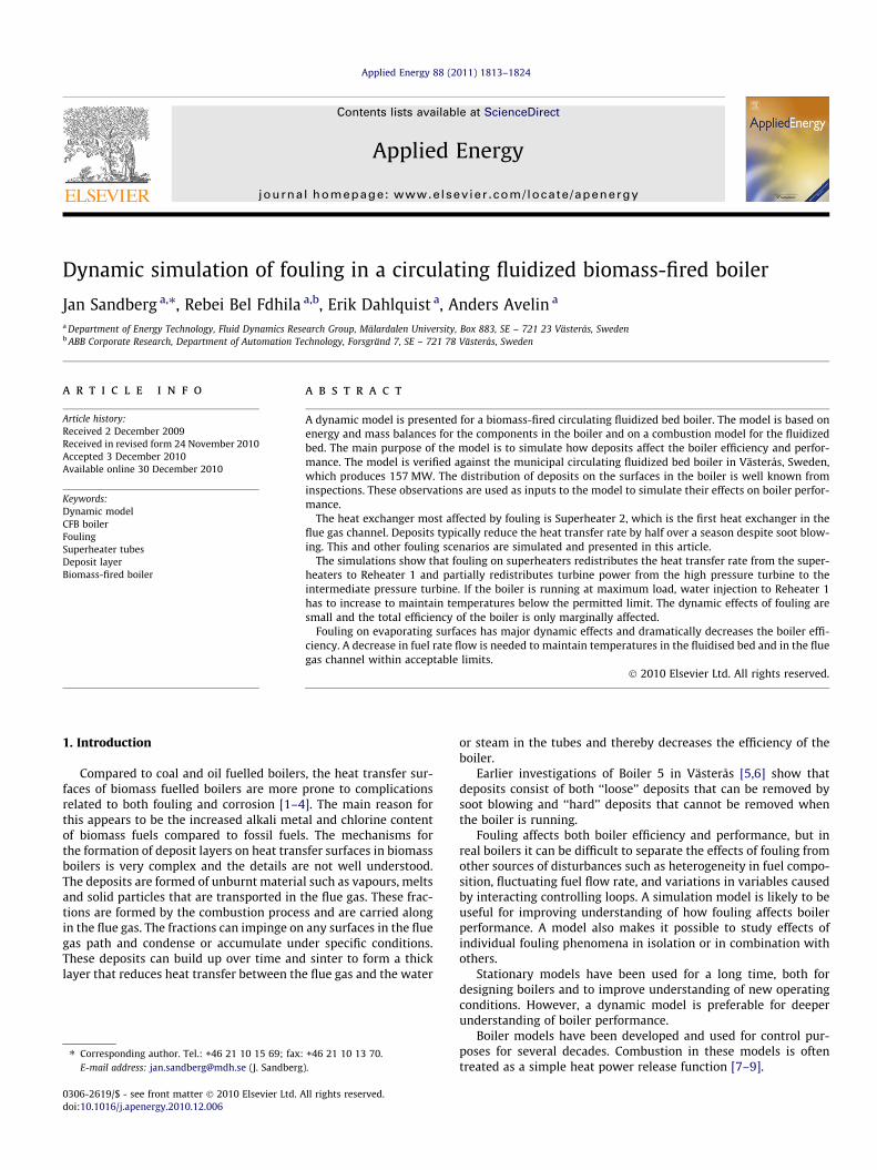
The main components of the boiler are shown in Fig. 1. The flu-idized bed is surrounded by evaporating tubes that connect to adrum. The majority of the circulating sand is separated from theflue gas in a steam cooled cyclone. The flue gas, together withthe remaining sand and ash, enters the superheaters in the down-ward direction as shown in Fig. 1. Superheater 2 and Superheater 1each consist of two tube bundles which are designated SH2,p1;SH2,p2 and SH1,p1; SH1,p2 respectively. Reheater 1 consists ofthree tube bundles (RH1,p1; RH1,p2 and RH1,p3 respectively inthe flue gas direction). The tube bundles are separated by between0.5 and 1 m, making visual inspections possible through theinspection openings (shown in Fig. 1 as small circles between thetube bundles). The boiler is designed with one superheater (SH3)and one reheater (RH2) in the fluidized sand-lock in the cycloneleg, where the circulating fluidized sand is re-injected into the boi-ler bed-zone. The section that includes Superheater 3 and Reheater2 is referred to as Intrex. The walls in the flue gas channel are alsocooled by steam and are labelled ‘‘Superheater Convection’’. Afterflowing through Reheater 1 the flue gas passes through the Econo-miser and the Air Preheater.

2.2. Fouling on heat exchanger surfaces in Boiler 5

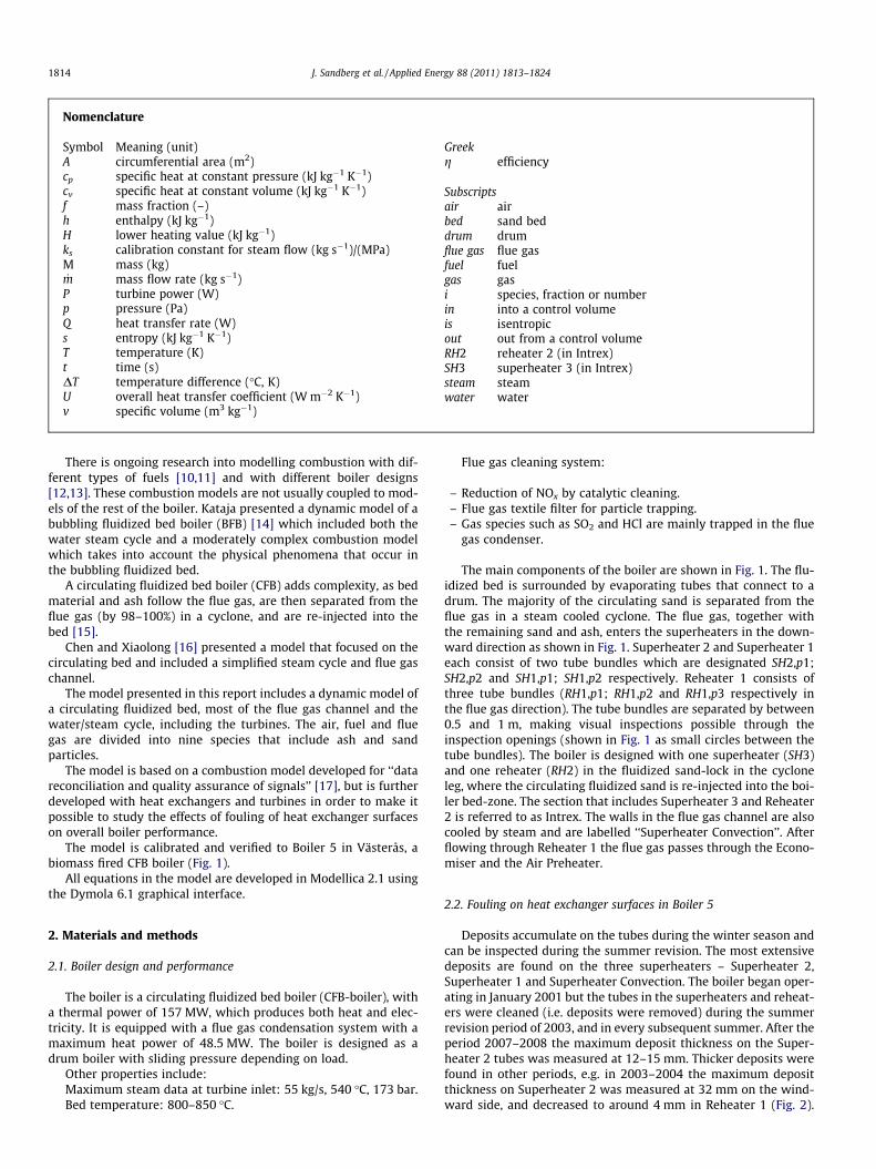
Deposits accumulate on the tubes during the winter season andcan be inspected during the summer revision. The most extensivedeposits are found on the three superheaters – Superheater 2,Superheater 1 and Superheater Convection. The boiler began oper-ating in January 2001 but the tubes in the superheaters and reheat-ers were cleaned (i.e. deposits were removed) during the summerrevision period of 2003, and in every subsequent summer. After theperiod 2007–2008 the maximum deposit thickness on the Super-heater 2 tubes was measured at 12–15 mm. Thicker deposits werefound in other periods, e.g. in 2003–2004 the maximum depositthickness on Superheater 2 was measured at 32 mm on the wind-ward side, and decreased to around 4 mm in Reheater 1 (Fig. 2).

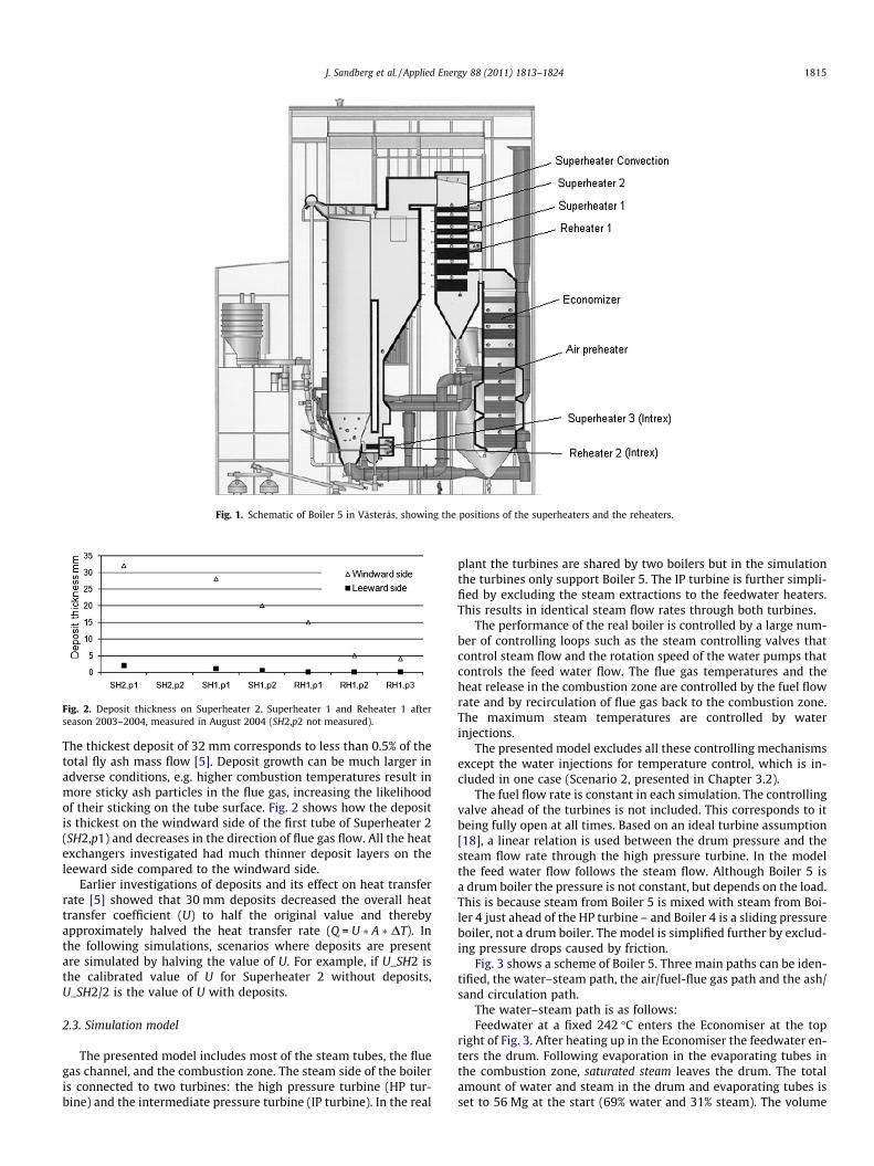
Fig. 1. Schematic of Boiler 5 in Västerås, showing the positions of the superheaters and the reheaters.

Fig. 2. Deposit thickness on Superheater 2, Superheater 1 and Reheater 1 afterseason 2003–2004, measured in August 2004 (SH2,p2 not measured).

J. Sandberg et al. / Applied Energy 88 (2011) 1813–1824 1815

The thickest deposit of 32 mm corresponds to less than 0.5% of thetotal fly ash mass flow [5]. Deposit growth can be much larger inadverse conditions, e.g. higher combustion temperatures result inmore sticky ash particles in the flue gas, increasing the likelihoodof their sticking on the tube surface. Fig. 2 shows how the depositis thickest on the windward side of the first tube of Superheater 2(SH2,p1) and decreases in the direction of flue gas flow. All the heatexchangers investigated had much thinner deposit layers on theleeward side compared to the windward side.

Earlier investigations of deposits and its effect on heat transferrate [5] showed that 30 mm deposits decreased the overall heattransfer coefficient (U) to half the original value and therebyapproximately halved the heat transfer rate (Q = U � A � DT). Inthe following simulations, scenarios where deposits are presentare simulated by halving the value of U. For example, if U_SH2 isthe calibrated value of U for Superheater 2 without deposits,U_SH2/2 is the value of U with deposits.

2.3. Simulation model

The presented model includes most of the steam tubes, the fluegas channel, and the combustion zone. The steam side of the boileris connected to two turbines: the high pressure turbine (HP tur-bine) and the intermediate pressure turbine (IP turbine). In the real

plant the turbines are shared by two boilers but in the simulationthe turbines only support Boiler 5. The IP turbine is further simpli-fied by excluding the steam extractions to the feedwater heaters.This results in identical steam flow rates through both turbines.

The performance of the real boiler is controlled by a large num-ber of controlling loops such as the steam controlling valves thatcontrol steam flow and the rotation speed of the water pumps thatcontrols the feed water flow. The flue gas temperatures and theheat release in the combustion zone are controlled by the fuel flowrate and by recirculation of flue gas back to the combustion zone.The maximum steam temperatures are controlled by waterinjections.

The presented model excludes all these controlling mechanismsexcept the water injections for temperature control, which is in-cluded in one case (Scenario 2, presented in Chapter 3.2).

The fuel flow rate is constant in each simulation. The controllingvalve ahead of the turbines is not included. This corresponds to itbeing fully open at all times. Based on an ideal turbine assumption[18], a linear relation is used between the drum pressure and thesteam flow rate through the high pressure turbine. In the modelthe feed water flow follows the steam flow. Although Boiler 5 isa drum boiler the pressure is not constant, but depends on the load.This is because steam from Boiler 5 is mixed with steam from Boi-ler 4 just ahead of the HP turbine – and Boiler 4 is a sliding pressureboiler, not a drum boiler. The model is simplified further by exclud-ing pressure drops caused by friction.

Fig. 3 shows a scheme of Boiler 5. Three main paths can be iden-tified, the water–steam path, the air/fuel-flue gas path and the ash/sand circulation path.

The water–steam path is as follows:Feedwater at a fixed 242 �C enters the Economiser at the top

right of Fig. 3. After heating up in the Economiser the feedwater en-ters the drum. Following evaporation in the evaporating tubes inthe combustion zone, saturated steam leaves the drum. The totalamount of water and steam in the drum and evaporating tubes isset to 56 Mg at the start (69% water and 31% steam). The volume

Fig. 3. Scheme of Boiler 5 model.


of the drum is fixed at 120 m3. After leaving the drum the steam issuperheated in the heat exchangers in the order Cyclone surfaces –Superheater Convection – Superheater 1 – Superheater 2 – Super-heater 3. After Superheater 3 the steam enters the HP turbine. Theback pressure of the HP turbine is fixed at 35 bar (3.5 MPa). Thesteam is reheated in Reheater 1, and then in Reheater 2 beforeentering the IP turbine. The back pressure of the IP turbine is fixedat 1.2 bar (0.12 MPa). The steam leaves the model via the hot con-denser. To simulate a realistic and plausible heat transfer rate inthe hot condenser it is assumed that steam condenses at 1.2 barfollowed by a subcooling of 10 �C before leaving the condenser. Itis possible within the model to inject high pressure water (at242 �C) into the steam to reduce its temperature. In the real boilerthe water is injected before and after the superheaters and reheat-ers, but this is simplified in the model and the water is injected di-rectly into the heat exchangers.

The air/fuel-flue gas path is as follows:Air enters the Air Preheater at a fixed 65 �C. After preheating the

air is mixed with the fuel in the fluidized bed. After complete com-bustion the flue gas exchanges heat to the following heat transfersurfaces in order: Evaporating tubes – Cyclone surfaces – Super-heater Convection – Superheater 2 – Superheater 1-Reheater 1 –Economiser – Air Preheater. As Superheater Convection comprisesthe walls in the flue gas path surrounding Superheater 2, Super-heater 1 and Reheater 1, the heat transfer rate is difficult to de-scribe as a theoretical model. In order to simplify this,Superheater Convection is located upstream of these three heatexchangers in the model.

The sand-ash cycle is as follows:The main fluidized bed consists of 100 Mg of sand. New sand

enters the bed at 25 �C at a rate of approximately 0.2 kg/s (on theleft of Fig. 3) and leaves the bed at 0.2 kg/s as ash (at the bottomof Fig. 3). In the simulation sand and ash have the same specificheat value (0.82 kJ/kg K) and are treated as a single mass fraction.Sand is re-injected to the fluidized bed from Intrex (Superheater 3and Reheater 2) at 307.6 kg/s with 7.6 kg/s air [15,17]. Air must bemixed with the sand to maintain the circulating flow. The sand andash follow the flue gas but are almost entirely separated in the cy-clone. In the simulation 99.825% of the total sand (and ash) floware separated in the cyclone and returned to the Intrex. The totalamount of sand in the Intrex is set to 80 Mg. The cycles are termi-nated by mixing sand with air at 200 �C and re-injecting this mix-ture back to the main bed.

2.4. Fuel combustion and the state equation of air, flue gas and water/steam

Fuel, air and flue gas are divided into total nine mass fractions.

(1) Carbon (C) in fuel.(2) Hydrogen (H) in fuel.(3) Oxygen (O or O2) – O in fuel and O2 in air and flue gas.(4) Carbon dioxide (CO2) in flue gas.(5) Water (H2O_l) in fuel.(6) Steam (H2O_s) in flue gas.(7) Nitrogen (N or NO2) – N in fuel and NO2 in flue gas.


(8) Sand/ash in fuel and flue gas.(9) Nitrogen (N2) in air and flue gas.

Fuel enters the boiler at 25 �C together with specified mass frac-tions of six components: C, H, O, H2O_l, N, and sand/ash.

Air enters the boiler as specified mass fractions of twocomponents:

O2ð20%Þ and N2ð80%Þ:

The combustion model is based on two main chemicalreactions.

CþO2 ! CO2

4Hþ O2 ! 2H2O

As an approximation all the elementary nitrogen (N) in fuel isassumed to react with oxygen to form NO2.

All water in the fuel evaporates to steam, and ash in fuel ismixed with the sand and ash that flows with the flue gas. Aftercombustion (in and above the fluidized bed) the flue gas includessix components:

O2; CO2; H2O s; NO2; sand=ash and N2:

The lower heating value in the fuel is calculated from [19].

Hi ¼ 34:1 � Cþ 102 �Hþ 6:3 �Nþ 19:1 � S� 9:85 � O� 2:5

� H2O ðMJ=kgÞ ð1Þ

The sulphur content (S) is zero and is not included.The enthalpy of the fuel and combustion gases (during combus-

tion) are calculated as the sum of the fraction of each component.Enthalpy,

h ¼X

i

ðf � cp � TÞi ð2Þ

Specific heat (cp) values are obtained from [15,20].

Component
cp (and cv) (kJ/kg K)
C
0.82 H 0.82 O (O2) 1.1 CO2 1.1 H2O_l 4.2 H2O_s 2.0 N (NO2) 1.1 Sand/ash 0.82 N2 1.1
Enthalpies for air and flue gas (from the outlet of the cycloneand in the subsequent flue gas path) are calculated from a polyno-mial expression [20,21] which is presented in Appendix A as Eq.(A.1). The inputs to this expression are the temperature (T) andthe mass fraction (fi) of each component – oxygen (O2), carbondioxide (CO2), steam (H2O_s) and nitrogen (N2).

It is assumed that NO2 does not affect the flue gas enthalpy.Enthalpy,

h ¼ f ðT; fiÞ ð4Þ

(Appendix A, Eq. (A.1)).For sand and ash, enthalpy is calculated as

h ¼ cp � T ð5Þ

For water and steam, enthalpies, entropies and specific volumesare calculated by the polynomial expression [20,22] presented inAppendix B, with pressure (p) and temperature (T) as inputs.

Enthalpy,

h ¼ f ðT;pÞ ð6Þ

(Appendix B, Eqs. (B.3, B.4, B.5))B.3: Enthalpy for water (calculated by saturated condition atgiven temperature).B.4: Enthalpy for saturated steam.B.5: Enthalpy for superheated steam.

Entropy,

s ¼ f ðT;pÞ ð7Þ

(Appendix B, Eq. (B.6))Specific volume,

m ¼ f ðT;pÞ ð8Þ

(Appendix B, Eq. (B.2))In the drum, under saturated conditions, the pressure–temper-

ature relation is calculated by the equations presented in AppendixB [20,22].

T ¼ f ðpÞ ð9Þ

(Appendix B, Eq. (B.1))Specific heat at constant volume (cv) for saturated water and

saturated steam at 16–17 Mpa are approximately [20]:

cv;water ¼ 3 ðkJ=kg;KÞ

cv;steam ¼ 4 ðkJ=kg;KÞ

2.5. Energy and continuity equations

In the model there are three main mass species (point masses):the sand bed (M1_bed+gas), the Intrex (M2_bed+gas) and the water andsteam in tubes surrounding the combustion zone (the bed) and inthe drum (Mdrum).

For each heat exchanger surfaces (i) the heat transfer rate Qi iscalculated by

Qi ¼ Ui � Ai � DTi ð10Þ

The temperature difference DTi is the arithmetic averagetemperature difference between the two fluids in the heat exchan-ger based on inlet and outlet temperatures ((Tin + Tout)1/2 � (Tin + Tout)2/2). The same equation is used for all heat exchang-ers independent of the heat exchanger design. For heat transfer inthe beds, the bed temperature is used.

2.5.1. Sand bed and combustion zoneGas and sand side:The mass flow into the control volume is made up of four main

components:air, fuel, sand and sand/ash (from the Intrex).The mass flow out of the control volume is made up of two main

components: flue gas and ash/sand.

@T1 bedþgas

@t¼P

inð _m � cp � TÞin �P

outð _m � cp � TÞout þ _mfuel � Hi � Q 1

M1 bedþgas �P

iðf � cv � TÞið11Þ

@M1 bedþgas

@t¼X

in

_min �Xout

_mout ð12Þ

For steam and water in the drum and in the evaporating tubessurrounding the combustion zone:

@Tdrum

@t¼ ð _m � hÞwater � ð _m � hÞsteam þ Q 1

Mdrum � ðcv;water � fwater þ cv;steam � fsteamÞð13Þ


@Mdrum

@t¼ _mwater � _msteam ð14Þ

Vdrum ¼ Mdrum � ðvwater � fwater þ v steam � fsteamÞ ð15Þ

2.5.2. IntrexGas and sand side:The mass flow into the control volume is made up of two main

components: Air for fluidization and sand/ash from the cyclone.The mass flow out of the control volume is made up of a mix-

ture of the input components.

@T2 bedþgas

@t¼P

inð _m � cp � TÞin �P

outð _m � cp � TÞout � Q SH3 � Q RH2

M2 bedþgas �P

iðf � cv � TÞið16Þ

@M2 bedþgas

@t¼X

in

_min �Xout

_mout ð17Þ

Steam side:For SH3 and RH2 respectively

_msteam;out � hsteam;out ¼ _msteam;in � hsteam;in þ Q i ð18Þ

_msteam;out ¼ _msteam;in ð19Þ

2.5.3. Cyclone



_mfluegas;out � hfluegas;out þ _msand;out � cp;sand � Tsand;out

¼X

in

ð _m � cp � TÞin � Q i ð22Þ

Xin

_min ¼Xout

_mout ð23Þ

2.5.4. SH1, SH2 and RH1

_msteam;out � hsteam;out ¼ _msteam;in � hsteam;in þ Q i þ _mwater;injection

� hwater ð24Þ

_msteam;out ¼ _msteam;in þ _mwater;injection ð25Þ

_mfluegas;out � hfluegas;out ¼ _mfluegas;in � hfluegas;in � Q i ð26Þ

_mfluegas;out ¼ _mfluegas;in ð27Þ

2.5.5. Economizer

_mwater;out � hwater;out ¼ _mwater;in � hwater;in þ Q ;i ð29Þ

_mwater;out ¼ _mwater;in ð30Þ



2.5.6. Superheater convection





2.5.7. Air preheater

_mair;out � hair;out ¼ _mair;in � hair;in þ Q i ð37Þ

_mair;out ¼ _mair;in ð38Þ



2.5.8. HP turbine and IP turbineIsentropic efficiency gis = 0.85 (constant)

gis ¼hin � hout

hin � hout;isð42Þ


_msteam ¼ ks � pdrum ð44Þ

P ¼ _msteam � ðhin � houtÞ ð45Þ

2.5.9. Hot condenser

Q ¼ _msteam � ðhsteam;in � hwater;outÞ ð46Þ

3. Calculation

The model is calibrated by adjusting the product AU for the heatexchanger surfaces.

Following the calibration procedure, three scenarios are set upfor calculations.

Scenarios 1 and 3 are based on the calibration procedure pre-sented in Chapter 3.1. In Scenario 2 water injections in heatexchangers (Superheater 1, Superheater 2 and Reheater 1) are in-cluded to maintain the maximum steam temperature (540 �C).

3.1. Calibration of the model

The model is calibrated and verified with values measured on28 November 2007. This data is used because the time point isearly the season, the deposit thickness is small following cleaningthe previous summer, the boiler is running at maximum load, andthe data have been examined in detail in a previous investigationwhere the fuel was also defined [17].

The fuel mass fraction used in all the calculations is as follows:

Carbon (C) = 0.306Hydrogen (H) = 0.036Oxygen (O) = 0.217Water (H2O) = 0.4Nitrogen (N) = 0.0099Ash = 0.032

Measured data from 28 November 2007, as min and max valuesover the 24 h period:

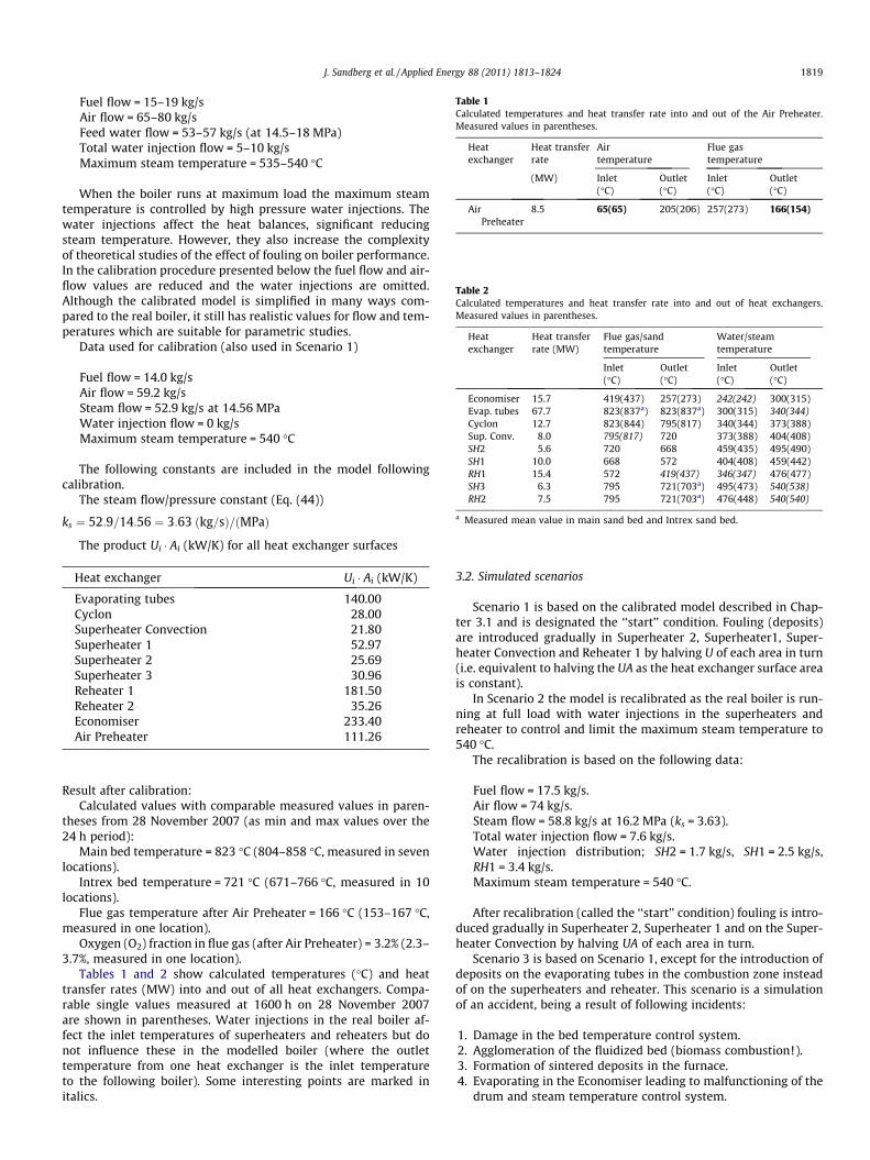
Table 1Calculated temperatures and heat transfer rate into and out of the Air Preheater.Measured values in parentheses.

Heatexchanger

Heat transferrate

Airtemperature

Flue gastemperature

(MW) Inlet(�C)

Outlet(�C)

Inlet(�C)

Outlet(�C)

AirPreheater

8.5 65(65) 205(206) 257(273) 166(154)

Table 2Calculated temperatures and heat transfer rate into and out of heat exchangers.Measured values in parentheses.

Heatexchanger

Heat transferrate (MW)

Flue gas/sandtemperature

Water/steamtemperature

Inlet(�C)

Outlet(�C)

Inlet(�C)

Outlet(�C)

Economiser 15.7 419(437) 257(273) 242(242) 300(315)Evap. tubes 67.7 823(837a) 823(837a) 300(315) 340(344)Cyclon 12.7 823(844) 795(817) 340(344) 373(388)Sup. Conv. 8.0 795(817) 720 373(388) 404(408)SH2 5.6 720 668 459(435) 495(490)SH1 10.0 668 572 404(408) 459(442)RH1 15.4 572 419(437) 346(347) 476(477)SH3 6.3 795 721(703a) 495(473) 540(538)RH2 7.5 795 721(703a) 476(448) 540(540)

a Measured mean value in main sand bed and Intrex sand bed.


Fuel flow = 15–19 kg/sAir flow = 65–80 kg/sFeed water flow = 53–57 kg/s (at 14.5–18 MPa)Total water injection flow = 5–10 kg/sMaximum steam temperature = 535–540 �C

When the boiler runs at maximum load the maximum steamtemperature is controlled by high pressure water injections. Thewater injections affect the heat balances, significant reducingsteam temperature. However, they also increase the complexityof theoretical studies of the effect of fouling on boiler performance.In the calibration procedure presented below the fuel flow and air-flow values are reduced and the water injections are omitted.Although the calibrated model is simplified in many ways com-pared to the real boiler, it still has realistic values for flow and tem-peratures which are suitable for parametric studies.

Data used for calibration (also used in Scenario 1)

Fuel flow = 14.0 kg/sAir flow = 59.2 kg/sSteam flow = 52.9 kg/s at 14.56 MPaWater injection flow = 0 kg/sMaximum steam temperature = 540 �C

The following constants are included in the model followingcalibration.

The steam flow/pressure constant (Eq. (44))

ks ¼ 52:9=14:56 ¼ 3:63 ðkg=sÞ=ðMPaÞ

The product Ui � Ai (kW/K) for all heat exchanger surfaces

Heat exchanger
Ui � Ai (kW/K)
Evaporating tubes
140.00 Cyclon 28.00 Superheater Convection 21.80 Superheater 1 52.97 Superheater 2 25.69 Superheater 3 30.96 Reheater 1 181.50 Reheater 2 35.26 Economiser 233.40 Air Preheater 111.26
Result after calibration:Calculated values with comparable measured values in paren-

theses from 28 November 2007 (as min and max values over the24 h period):

Main bed temperature = 823 �C (804–858 �C, measured in sevenlocations).

Intrex bed temperature = 721 �C (671–766 �C, measured in 10locations).

Flue gas temperature after Air Preheater = 166 �C (153–167 �C,measured in one location).

Oxygen (O2) fraction in flue gas (after Air Preheater) = 3.2% (2.3–3.7%, measured in one location).

Tables 1 and 2 show calculated temperatures (�C) and heattransfer rates (MW) into and out of all heat exchangers. Compa-rable single values measured at 1600 h on 28 November 2007are shown in parentheses. Water injections in the real boiler af-fect the inlet temperatures of superheaters and reheaters but donot influence these in the modelled boiler (where the outlettemperature from one heat exchanger is the inlet temperatureto the following boiler). Some interesting points are marked initalics.

3.2. Simulated scenarios

Scenario 1 is based on the calibrated model described in Chap-ter 3.1 and is designated the ‘‘start’’ condition. Fouling (deposits)are introduced gradually in Superheater 2, Superheater1, Super-heater Convection and Reheater 1 by halving U of each area in turn(i.e. equivalent to halving the UA as the heat exchanger surface areais constant).

In Scenario 2 the model is recalibrated as the real boiler is run-ning at full load with water injections in the superheaters andreheater to control and limit the maximum steam temperature to540 �C.

The recalibration is based on the following data:

Fuel flow = 17.5 kg/s.Air flow = 74 kg/s.Steam flow = 58.8 kg/s at 16.2 MPa (ks = 3.63).Total water injection flow = 7.6 kg/s.Water injection distribution; SH2 = 1.7 kg/s, SH1 = 2.5 kg/s,RH1 = 3.4 kg/s.Maximum steam temperature = 540 �C.

After recalibration (called the ‘‘start’’ condition) fouling is intro-duced gradually in Superheater 2, Superheater 1 and on the Super-heater Convection by halving UA of each area in turn.

Scenario 3 is based on Scenario 1, except for the introduction ofdeposits on the evaporating tubes in the combustion zone insteadof on the superheaters and reheater. This scenario is a simulationof an accident, being a result of following incidents:

1. Damage in the bed temperature control system.2. Agglomeration of the fluidized bed (biomass combustion!).3. Formation of sintered deposits in the furnace.4. Evaporating in the Economiser leading to malfunctioning of the

drum and steam temperature control system.


3.3. The solver

DASSL, a solver for differential algebraic equations built intoModellica, is used to solve the equation system. It is particularlyuseful for complex equation systems. Nonlinear equations are lin-earized and simple and fast methods, both implicit (such as Eulerbackward) and explicit (such as Euler forward), are used forintegrations.

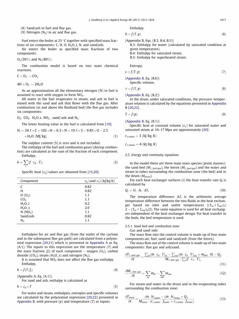
Fig. 4. Heat transfer rates of superheaters and Reheater 1 as a function of reduced U.

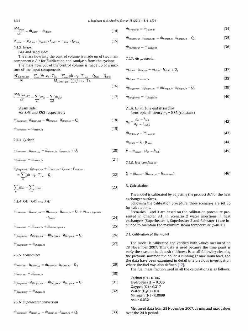
Fig. 5. Inlet turbine temperatures as a function of fouling.

Fig. 6. Turbine power as a function of fouling.

4. Results and discussion

4.1. Scenario 1

Based on the calibration, fouling is simulated by first reducing Ufor Superheater 2 by half (U_SH2/2), then sequentially halving U forSuperheater 1 (U_SH1/2) and then halving U for the SuperheaterConvection (U_CONV/2).

The effects on dynamics and the overall boiler performance arevery small. Table 3 shows some of the variables from the stationarysolution.

The main reason why fouling on the superheaters does not havea large effect on the main variables can be seen in Fig. 4, whichshows the heat transfer rates of Superheater 2, Superheater 1,Superheater Convection and Reheater 1. Fouling on the superheat-ers does not affect the main variables much because loss of heattransfer rate in the superheaters is offset by a gain of heat transferrate in Reheater 1. As the three main masses in the model are at al-most constant temperature, the dynamic effects are very small.More realistic dynamic behaviour would be expected if the modelwas extended with additional masses in the superheaters andReheater 1.

Fouling on the superheater surfaces decreases the steam tem-peratures into the HP turbine and increases the steam tempera-tures into the IP turbine (Fig. 5), thereby shifting turbine powerfrom the HP turbine to the IP turbine (Fig. 6).

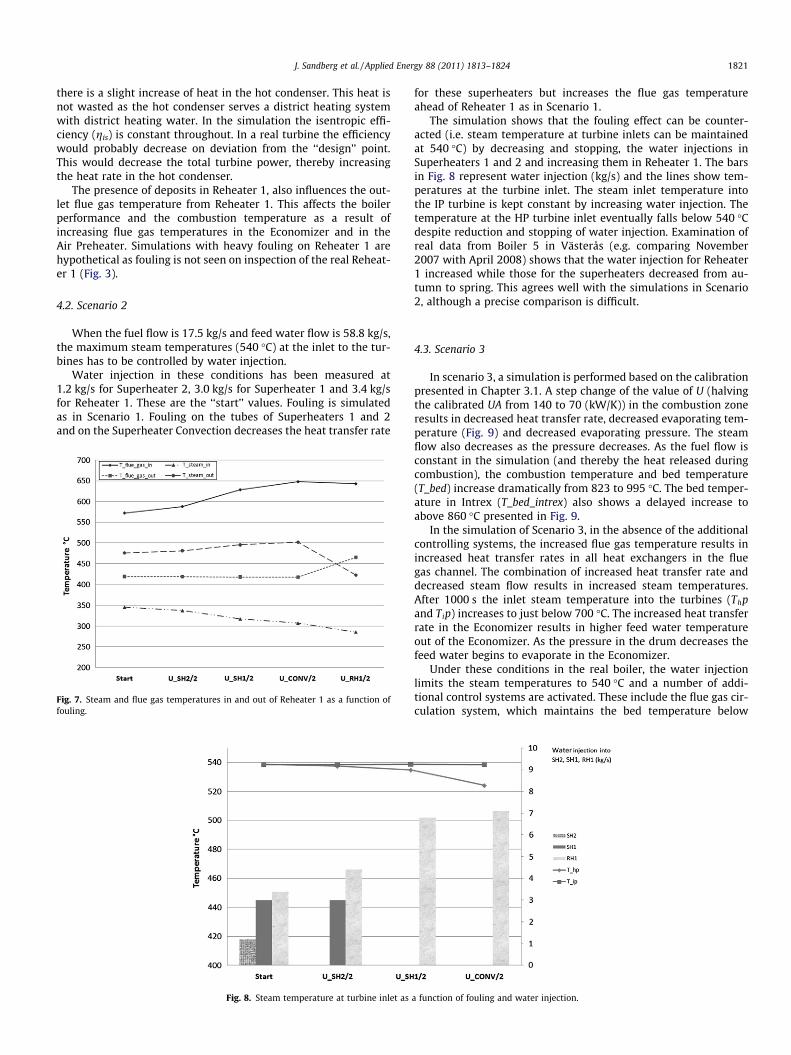
There are two main reasons for the nearly complete recovery ofheat transfer rate from the superheaters by Reheater 1. Firstly, theflue gas temperature ahead of Reheater 1 increases as the heattransfer rate for the superheaters decreases because of the de-creased U. The second reason is that the inlet steam temperatureinto Reheater 1 decreases (Fig. 7). The inlet steam temperature intoReheater 1 is the same as the outlet steam temperature from theHP turbine, and as the inlet steam temperature into the HP turbinedecreases, the outlet steam temperature from the HP turbine alsodecreases (and the turbine power only slightly decreases). Theoverall effect causes the temperature difference between the fluegas and steam to increase significantly as does the heat transferrate of Reheater 1. However, the outlet flue gas temperature fromReheater 1 is almost unaffected. The overall effects on the rest ofthe boiler variables, combustion, furnace temperature, steam flowrate etc. are minimal. As the flue gas temperature out of the AirPreheater is unchanged, the total boiler efficiency remainsrelatively constant.

The increase in power of the IP turbine does not completely off-set the reduction in power of the HP turbine (Fig. 6) and as a result

Table 3Calculated variables from Scenario 1.

Simulation Temp. in fliudized.bed (�C)

Evap. pressure(Mpa)

Feed water flow(kg/s)

Temp. flue gas afterAir Preheater (�C)

Power HPturbine (MW)

Power IPturbine (MW)

Heat hotcond. (MW)

Start 823.4 14.56 52.94 166.0 16.9 38.8 127.6+U_SH2/2 823.0 14.54 52.88 166.0 16.5 39.0 127.7+U_SH1/2 821.9 14.50 52.74 166.0 15.7 39.4 128.0+U_CONV/2 821.4 14.48 52.66 166.0 15.4 39.5 128.1


there is a slight increase of heat in the hot condenser. This heat isnot wasted as the hot condenser serves a district heating systemwith district heating water. In the simulation the isentropic effi-ciency (gis) is constant throughout. In a real turbine the efficiencywould probably decrease on deviation from the ‘‘design’’ point.This would decrease the total turbine power, thereby increasingthe heat rate in the hot condenser.

The presence of deposits in Reheater 1, also influences the out-let flue gas temperature from Reheater 1. This affects the boilerperformance and the combustion temperature as a result ofincreasing flue gas temperatures in the Economizer and in theAir Preheater. Simulations with heavy fouling on Reheater 1 arehypothetical as fouling is not seen on inspection of the real Reheat-er 1 (Fig. 3).

4.2. Scenario 2

When the fuel flow is 17.5 kg/s and feed water flow is 58.8 kg/s,the maximum steam temperatures (540 �C) at the inlet to the tur-bines has to be controlled by water injection.

Water injection in these conditions has been measured at1.2 kg/s for Superheater 2, 3.0 kg/s for Superheater 1 and 3.4 kg/sfor Reheater 1. These are the ‘‘start’’ values. Fouling is simulatedas in Scenario 1. Fouling on the tubes of Superheaters 1 and 2and on the Superheater Convection decreases the heat transfer rate

Fig. 7. Steam and flue gas temperatures in and out of Reheater 1 as a function offouling.

Fig. 8. Steam temperature at turbine inlet as

for these superheaters but increases the flue gas temperatureahead of Reheater 1 as in Scenario 1.

The simulation shows that the fouling effect can be counter-acted (i.e. steam temperature at turbine inlets can be maintainedat 540 �C) by decreasing and stopping, the water injections inSuperheaters 1 and 2 and increasing them in Reheater 1. The barsin Fig. 8 represent water injection (kg/s) and the lines show tem-peratures at the turbine inlet. The steam inlet temperature intothe IP turbine is kept constant by increasing water injection. Thetemperature at the HP turbine inlet eventually falls below 540 �Cdespite reduction and stopping of water injection. Examination ofreal data from Boiler 5 in Västerås (e.g. comparing November2007 with April 2008) shows that the water injection for Reheater1 increased while those for the superheaters decreased from au-tumn to spring. This agrees well with the simulations in Scenario2, although a precise comparison is difficult.

4.3. Scenario 3

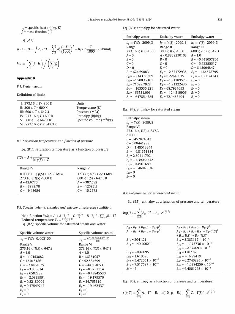
In scenario 3, a simulation is performed based on the calibrationpresented in Chapter 3.1. A step change of the value of U (halvingthe calibrated UA from 140 to 70 (kW/K)) in the combustion zoneresults in decreased heat transfer rate, decreased evaporating tem-perature (Fig. 9) and decreased evaporating pressure. The steamflow also decreases as the pressure decreases. As the fuel flow isconstant in the simulation (and thereby the heat released duringcombustion), the combustion temperature and bed temperature(T_bed) increase dramatically from 823 to 995 �C. The bed temper-ature in Intrex (T_bed_intrex) also shows a delayed increase toabove 860 �C presented in Fig. 9.

In the simulation of Scenario 3, in the absence of the additionalcontrolling systems, the increased flue gas temperature results inincreased heat transfer rates in all heat exchangers in the fluegas channel. The combination of increased heat transfer rate anddecreased steam flow results in increased steam temperatures.After 1000 s the inlet steam temperature into the turbines (Thpand Tip) increases to just below 700 �C. The increased heat transferrate in the Economizer results in higher feed water temperatureout of the Economizer. As the pressure in the drum decreases thefeed water begins to evaporate in the Economizer.

Under these conditions in the real boiler, the water injectionlimits the steam temperatures to 540 �C and a number of addi-tional control systems are activated. These include the flue gas cir-culation system, which maintains the bed temperature below

a function of fouling and water injection.

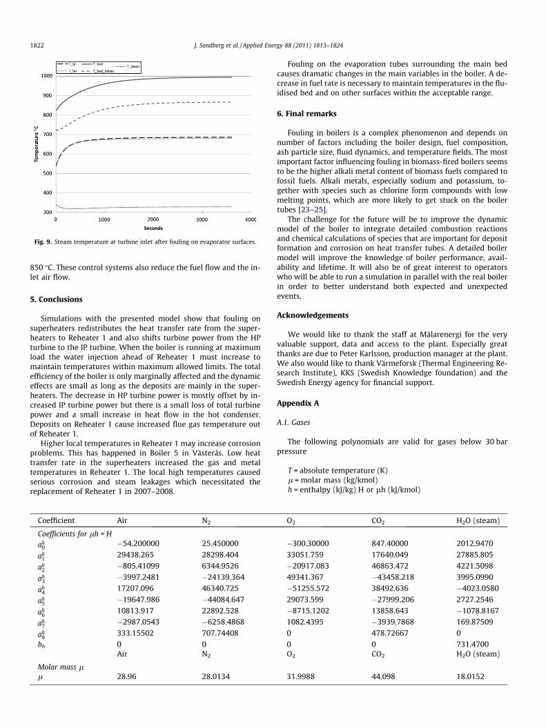
Fig. 9. Steam temperature at turbine inlet after fouling on evaporator surfaces.


850 �C. These control systems also reduce the fuel flow and the in-let air flow.

5. Conclusions

Simulations with the presented model show that fouling onsuperheaters redistributes the heat transfer rate from the super-heaters to Reheater 1 and also shifts turbine power from the HPturbine to the IP turbine. When the boiler is running at maximumload the water injection ahead of Reheater 1 must increase tomaintain temperatures within maximum allowed limits. The totalefficiency of the boiler is only marginally affected and the dynamiceffects are small as long as the deposits are mainly in the super-heaters. The decrease in HP turbine power is mostly offset by in-creased IP turbine power but there is a small loss of total turbinepower and a small increase in heat flow in the hot condenser.Deposits on Reheater 1 cause increased flue gas temperature outof Reheater 1.

Higher local temperatures in Reheater 1 may increase corrosionproblems. This has happened in Boiler 5 in Västerås. Low heattransfer rate in the superheaters increased the gas and metaltemperatures in Reheater 1. The local high temperatures causedserious corrosion and steam leakages which necessitated thereplacement of Reheater 1 in 2007–2008.

Coefficient Air N2

Coefficients for lh = Hah

0�54.200000 25.450000

ah1

29438.265 28298.404

ah2

�805.41099 6344.9526

ah3

�3997.2481 �24139.364

ah4

17207.096 46340.725

ah5

�19647.986 �44084.647

ah6

10813.917 22892.528

ah7

�2987.0543 �6258.4868

ah8

333.15502 707.74408

bh 0 0Air N2

Molar mass ll 28.96 28.0134

Fouling on the evaporation tubes surrounding the main bedcauses dramatic changes in the main variables in the boiler. A de-crease in fuel rate is necessary to maintain temperatures in the flu-idised bed and on other surfaces within the acceptable range.

6. Final remarks

Fouling in boilers is a complex phenomenon and depends onnumber of factors including the boiler design, fuel composition,ash particle size, fluid dynamics, and temperature fields. The mostimportant factor influencing fouling in biomass-fired boilers seemsto be the higher alkali metal content of biomass fuels compared tofossil fuels. Alkali metals, especially sodium and potassium, to-gether with species such as chlorine form compounds with lowmelting points, which are more likely to get stuck on the boilertubes [23–25].

The challenge for the future will be to improve the dynamicmodel of the boiler to integrate detailed combustion reactionsand chemical calculations of species that are important for depositformation and corrosion on heat transfer tubes. A detailed boilermodel will improve the knowledge of boiler performance, avail-ability and lifetime. It will also be of great interest to operatorswho will be able to run a simulation in parallel with the real boilerin order to better understand both expected and unexpectedevents.

Acknowledgements

We would like to thank the staff at Mälarenergi for the veryvaluable support, data and access to the plant. Especially greatthanks are due to Peter Karlsson, production manager at the plant.We also would like to thank Värmeforsk (Thermal Engineering Re-search Institute), KKS (Swedish Knowledge foundation) and theSwedish Energy agency for financial support.

Appendix A

A.1. Gases

The following polynomials are valid for gases below 30 barpressure

T = absolute temperature (K)l = molar mass (kg/kmol)h = enthalpy (kJ/kg) H or lh (kJ/kmol)

O2 CO2 H2O (steam)

�300.30000 847.40000 2012.9470

33051.759 17640.049 27885.805�20917.083 46863.472 4221.5098

49341.367 �43458.218 3995.0990�51255.572 38492.636 �4023.0580

29073.599 �27999.206 2727.2546�8715.1202 13858.643 �1078.81671082.4395 �3939.7868 169.875090 478.72667 0

0 0 731.4700O2 CO2 H2O (steam)

31.9988 44.098 18.0152

J. Sandberg et al. / Applied Ener

cp = specific heat (kJ/kg, K)fi = mass fraction (–)

Eq. (A1):

l � h ¼ H ¼Z

cp � dT ¼Xn¼8

n¼0

ahn

T1000

� �n

þ bh � lnT

1000ðkJ=kmolÞ

htot ¼X

i

fi � hi

!, Xi

fi

!

Appendix B

B.1. Water–steam

Definition of limits

I: 273.16 6 T < 300 K
Units II: 300 6 T < 600 K Temperature (K) III: 600 6 T 6 647.3 Pressure (MPa) IV: 273.16 6 T < 600 K Enthalpy (kJ/kg) V: 600 6 T 6 647.3 K Specific volume (m3/kg) VI: 273.16 6 T 6 647.3 K
B.2. Saturation temperature as a function of pressure

Eq. (B1); saturation temperature as a function of pressure

TðSÞ ¼ Aþ Bln pðSÞ þ C

Range IV
Range V
0.000611 6 p(S) < 12.33 MPa
12.336 p(S) < 22.1 MPa 273.16 6 T(S) < 600 K 600 6 T(S) < 647.3 K A = 42.6776 A = �387.592 B = �3892.70 B = �12587.5 C = �9.48654 C = �15.2578
B.3. Specific volume, enthalpy and entropy at saturated conditions

Help function YðSÞ ¼ Aþ B � T1=3r þ C � T5=6

r þ D � T7=8t þ

P7n¼1En � Tn

r

Reduced temperature Tr ¼ 647;3�TðSÞ647;3

Eq. (B2); specific volume for saturated steam and water

Specific volume water
Specific volume steam
v f ¼ YðSÞ � 0;003155
vg ¼ YðSÞ�22;089�0;003155pðSÞ
Range VI
Range VI 273.16 6 T(S) 6 647.3 273.16 6 T(S) 6 647.3 A = 1.0 A = 1.0 B = �1.9153882 B = 1.6351057 C = 12.015186 C = 52.584599 D = �7.8464025 D = �44.694653 E1 = �3.888614 E1 = �8.9751114 E2 = 2.0582238 E2 = �0.43845530 E3 = �2.0829991 E3 = �19.179576 E4 = 0.82180004 E4 = 36.765319 E5 = 0.47549742 E5 = �19.462437 E6 = 0 E6 = 0 E7 = 0 E7 = 0
Eq. (B3); enthalpy for saturated water

gy 88 (2011) 1813–1824 1823

Enthalpy water
Enthalpy water Enthalpy water
hf ¼ YðSÞ � 2099;3
hf ¼ YðSÞ � 2099;3 hf ¼ YðSÞ � 2099;3 Range I Range II Range III 273.16 6 T(S) < 300 300 6 T(S) < 600 600 6 T(S) 6 647.3 A = 0 A = 0.8839230108 A = 1.0 B = 0 B = 0 B = �0.441057805 C = 0 C = 0 C = �5.52255517 D = 0 D = 0 D = 6.43994847 E1 = 624.69883 E1 = �2.67172935 E1 = �1.64578795 E2 = �2343.85369 E2 = 6.22640035 E2 = �1.30574143 E3 = �9508.12101 E3 = �13.1789573 E3 = 0 E4 = 71628.7928 E4 = �1.91322436 E4 = 0 E5 = �163535.221 E5 = 68.7937653 E5 = 0 E6 = 166531.093 E6 = �124.819906 E6 = 0 E7 = �64785.4585 E7 = 72.1435404 E7 = 0
Eq. (B4); enthalpy for saturated steam

Enthalpy steamhg ¼ YðSÞ � 2099;3Range VI273.16 6 T(S) 6 647.3A = 1.0B = 0.457874342C = 5.08441288D = �1.48513244E1 = �4.81351884E2 = 2.69411792E3 = �7.39064542E4 = 10.4961689E5 = �5.46840036E6 = 0E7 = 0

B.4. Polynomials for superheated steam

Eq. (B5); enthalpy as a function of pressure and temperature

hðp; TÞ ¼X2

n¼0

An � Tn � A3 � eðTðSÞ�T

M Þ

A0 = B11 + B12�p + B13�p2
A2 = B31 + B32�p + B33�p2
A1 = B21 + B22�p + B23�p2
A3 = B41 + B42�T(S) + B43�T(S)2
+ B44�T(S)3 + B45�T(S)4

B11 = 2041.21
B31 = 3.383117� 10�4
B12 = �40.40021
B32 = �1.975736 � 10�5
B33 = �2.87409 � 10�7

B13 = �0.48095
B41 = 1707.82 B21 = 1.610693 B42 = �16.99419 B22 = 5.472051 � 10�2 B43 = 6.2746295 � 10�2
B23 = 7.517537 � 10�4
B44 = �1.0284259 � 10�4
M = 45
B45 = 6.4561298 � 10�8
Eq. (B6); entropy as a function of pressure and temperature

sðp; TÞ ¼X4

n¼0

An � Tn þ B1 � lnð10 � pþ B2Þ �X4

n¼0

Cn � TðSÞn � eðTðSÞ�T

M Þ


A0 = 4.6162961
B1 = �0.4650306 A1 = 1.039008 � 10�2 B2 = 1.0 � 10�3
C0 = 1.777804
A2 = �9.873085 � 10�6 C1 = �1.802468 � 10�2
A3 = 5.43411 � 10�9
C2 = 6.854459 � 10�5
A4 = �1.170465 � 10�12
C3 = �1.184424 � 10�7
M = 85
C4 = 8.142201 � 10�11
References

[1] Bryers RW. Fireside slagging, fouling and high-temperature corrosion of heat-transfer surface due to impurities in steam-raising fuels. Prog Energy CombustSci 1996;22:29–120.

[2] Nordin A, Leven P. Askrelaterade driftsproblem i biobränsleeldadeanläggningar. O3-515, Stiftelsen för Värmeteknisk forskning; 1997 [InSwedish].

[3] Baxter LL. Ash deposition during biomass and coal combustion, a mechanisticapproach. Biomass Bioenergy 1993;4(2):85–102.

[4] Nielsen HP, Baxter LL, Sclippab G, Morey C, Frandsen FJ, Dam-Johansen K.Deposition of potassium salts on heat transfer surfaces in straw-fired boiler, apilot-scale study. Fuel 2000;79:131–9.

[5] Sandberg J, Sand U, Fdhila RB. Long time investigation of the effect of foulingon the super-heaters in a circulating fluidised biomass boiler. Int J Energy Res2006;30:1037–53. doi:10.1002/er.1202.

[6] Sandberg J, Sand U, Fdhila RB. Measurements, theories and simulations ofparticle deposits on super-heater tubes in a CFB biomass boiler. Int J GreenEnergy 2006;3:43–61.

[7] Åström KJ, Bell R. Simple drum-boiler models. In: IFAC internationalsymposium on power systems, modelling and control applications; 1988,Brussel, Belgium.

[8] Åström KJ, Bell R. Drum boiler dynamics. Automatica 2000;36:363–78.[9] Maffezzoni C. Issues in modeling and simulation of power plants. In:

Proceedings of IFAC symposium on control of power plants and powersystems, vol. 1; 1992. p. 19–27.

[10] Sand U, Sandberg J, Larfeldt J, Fdhila RB. Numerical prediction of the transportand pyrolysis in the interior and surrounding of dry and wet wood log. ApplEnergy 2008;85:1208–24.

[11] Dong C, Yang Y, Yang R, Zhang J. Numerical modelling of the gasification basedbiomass co-firing in a 600 MW, pulverized coal boiler. Appl Energy 2009.

[12] Scala F, Salatino P. Modelling fluidized bed combustion of high-volatile solidfuels. Chem Eng Sci 2002;57:1175–96.

[13] Galgano A, Salatino P, Crescitelli S, Scala F, Maffettone PL. A model of thedynamics of a fluidized bed combustor burning biomass. Combust Flame2005;140(4):271–84.

[14] Kataja T, Majanne Y. Dynamic model of a bubbling fluidized bed boiler. In: The48th Scandinavian conference on simulation and modeling (SIMS 2007),Göteborg (Särö), Sweden; 30–31 October, 2007.

[15] Bartusch C. Bed behaviour and solids circulation algorithms for Boiler 5 atMälarEnergi AB. Diploma work at Mälardalens Högskola, IST, Västerås; 2002[Serial Number 2002-093].

[16] Chen Y, Xiaolong G. Dynamic modeling and simulation of a 410 t/h PyroflowCFB boiler. Comput Chem Eng 2006;31(1):21–31.

[17] Dahlquist E, Widarsson B, Lilja R, Avelin A. Data-reconciliation-qualityassurance of signals. Report nr 1050, Värmeforsk Service AB; 2008.

[18] Traupel W. Thermische Turbomaschinen, Zweiter Band. Springer-Verlag;1960.

[19] Mörtstedt S-E, Hellsten G. Data och Diagram 1987, Norstedts tryckeri; 1987.[20] Wester L. Charts and graphs for energy calculations 2008. Mälardalens

högskola, Västerås, Sweden; 2008.[21] Rivkin SL. Thermodynamic properties of gases. 4th ed. revised. Hemisphere

Publishing Corporation; 1988.[22] Irvine TF, Liley PE. Steam and gas tables with computer equations. Academic

Press; 1984.[23] Andersson C, Högberg J. Fouling and slagging problems at recovered wood fuel

combustion. F9-821. Värmeforsk Service AB; 2001.[24] Andersson M. Avlagringstrender i pannor eldade med biobränsle. M4-204,

Värmeforsk service AB; 2003.[25] Gyllenhammar M. Measures for simultaneous minimization of alkali

related operation problems, phase 2. Report nr 1037, Värmeforsk Service AB;2007.

dynamic simulation of fouling in a circulating fluidized biomass-fired boiler

Documents