dynamic angle selection in binary tomography

Computer Vision and Image Understanding 117 (2013) 306–318

Contents lists available at SciVerse ScienceDirect

Computer Vision and Image Understanding

journal homepage: www.elsevier .com/ locate /cviu

Dynamic angle selection in binary tomography

K. Joost Batenburg a,b,⇑, Willem Jan Palenstijn b, Péter Balázs c, Jan Sijbers b

a Centrum Wiskunde & Informatica, Science Park 123, NL-1098 XG Amsterdam, The Netherlandsb Vision Lab, University of Antwerp, Universiteitsplein 1, B-2610 Wilrijk, Belgiumc Department of Image Processing and Computer Graphics, University of Szeged, Árpád tér 2, H-6720 Szeged, Hungary

a r t i c l e i n f o a b s t r a c t

Article history:Received 1 November 2011Accepted 3 July 2012Available online 8 December 2012

Keywords:Binary tomographyDiscrete tomographyAngle selection

1077-3142/$ - see front matter � 2012 Elsevier Inc. Ahttp://dx.doi.org/10.1016/j.cviu.2012.07.005

⇑ Corresponding author at: Centrum Wiskunde & INL-1098 XG Amsterdam, The Netherlands.

E-mail address: [email protected] (K.J. Baten

In this paper, we present an algorithm for the dynamic selection of projection angles in binary tomogra-phy. Based on the information present in projections that have already been measured, a new projectionangle is computed, which aims to maximize the information gained by adding this projection to the set ofmeasurements. The optimization model used for angle selection is based on a characterization of solu-tions of the binary reconstruction problem, and a related definition of information gain. From this formalmodel, an algorithm is obtained by several approximation steps. Results from a series of simulationexperiments demonstrate that the proposed angle selection scheme is indeed capable of finding anglesfor which the reconstructed image is much more accurate than for the standard angle selection scheme.

� 2012 Elsevier Inc. All rights reserved.

1. Introduction

Tomography deals with the reconstruction of an image from itsprojections, acquired along a range of angles. The Inverse RadonTransform provides a closed-form inversion formula for this recon-struction problem, provided that projections are available for allangles. Although this assumption is clearly not satisfied in practice,an accurate reconstruction can be computed if a large number ofprojections are available, for a full angular range, by using thewell-known Filtered Backprojection algorithm [1,2].

In several applications of tomography, only few projections canbe acquired. Such reconstruction problems are known as limited-data problems. In electron tomography, for example, the electronbeam damages the sample, limiting the number of projections thatcan be acquired [3]. In industrial tomography for quality assurance,cost considerations impose limitations on the duration of a scan,and thereby on the number of projections.

Applying classical reconstruction algorithms such as FilteredBackprojection to limited-data problems often results in inferiorreconstruction quality. Several approaches have been proposed toovercome these problems, by incorporating various forms of priorknowledge about the object in the reconstruction algorithm.Recently, advances in the field of Compressed Sensing have dem-onstrated high potential in obtaining a reduction of the numberof required projection images by exploiting sparsity of the imagewith respect to a certain set of basis functions [4–8]. Following a

ll rights reserved.

nformatica, Science Park 123,

burg).

different approach, the field of discrete tomography focuses on thereconstruction of images that consist of a small, discrete set of grayvalues [9,10]. By exploiting the knowledge of these gray values inthe reconstruction algorithm, it is often possible to computeaccurate reconstructions from far fewer projections than requiredby classical ‘‘continuous’’ tomography algorithms [11,12].

When reconstructing an image from a small set of projections(i.e., less than 20), the particular set of projection angles can havea large influence on the quality of the reconstruction. In [13,14],it was shown that the choice of the projection angles can have acrucial influence on the reconstruction quality in binary tomogra-phy, i.e., discrete tomography based on just two gray levels. Theauthors also presented algorithms to identify optimal projectionangles based on a blueprint image, which is known to be similarto the scanned object. For more general grayscale tomography, aframework was recently proposed for optimizing the acquisitionof projections, based on certain prior knowledge on the object tobe scanned [15].

These findings naturally lead to the question if ‘‘optimal’’ anglescan also be selected in cases where no blueprint image is available.As the optimal angles depend on the scanned object, they can cer-tainly not be selected prior to the scanning procedure. Instead, weconsider an on-line variant of the problem, where projections aremeasured one-by-one, and the new angle is selected based onthe information present in the currently available projections.

In this paper, we present an algorithm for angle selection in bin-ary tomography that is based on a concise model of the availableprojection information and prior knowledge of the binary charac-ter of the unknown object. The algorithm depends on two keyingredients: sampling of the set of images that adhere to thecurrently available projections, and determining the amount of

http://dx.doi.org/10.1016/j.cviu.2012.07.005

mailto:[email protected]

http://dx.doi.org/10.1016/j.cviu.2012.07.005

http://www.sciencedirect.com/science/journal/10773142

http://www.elsevier.com/locate/cviu

Fig. 1. Discretized strip projection model.

K.J. Batenburg et al. / Computer Vision and Image Understanding 117 (2013) 306–318 307

information that can be gained by adding a particular angle to theset of measurements.

This paper is structured as follows. In Section 2, we introduce aformal model for the tomography problem, as well as several re-lated concepts, which are necessary to define the angle selectionproblem. Although our formulation of the angle selection problemcharacterizes the optimal angle, it does not directly lead to an algo-rithm for computing this angle, which requires several approxima-tions. Section 3 describes how the current set of binary solutions tothe reconstruction problem can be approximated by a samplingprocedure, leading to so-called surrogate solutions. In Section 4,we describe how the information gain can be approximated for aparticular candidate angle. These two approximation steps arethen combined into an algorithm for the angle selection problem,which is presented in Section 5. An example is discussed in Sec-tion 6, where the concepts involved in the angle estimation algo-rithm are related to actual images involved in the computations.Section 7 describes a series of simulation experiments that havebeen performed to investigate how the reconstructions obtainedby the proposed angle selection scheme compare to several alter-native angle selection strategies. In the experimental results, pres-ent in Section 8, it is shown that the proposed method is indeedcapable of finding angles for which the reconstructed image ismuch more accurate than for the standard angle selection scheme.The approach and experimental findings are discussed in Section 9,followed by conclusions in Section 10.

2. Notation and concepts

Our description is restricted to the reconstruction of two-dimensional images from one-dimensional projections, but canbe generalized to higher-dimensional settings in a straightforwardmanner. The reconstructed image is represented on a rectangulargrid of size n = w � h.

For setting up the tomography model, we make the idealizedassumption that the unknown original object is a binary image thatcan also be represented on this grid, even though the proposedalgorithm can still be used if the grid assumption is not satisfied.The unknown original image can be represented by a vector�v ¼ ð�v iÞ 2 f0;1gn, where the entries �v i correspond to the pixel val-ues of the reconstruction.1

Projections are measured as sets of detector values for variousangles, rotating around the object. For each angle, the detectorsregister a parallel projection of the object. The finite set H = {h1,. . . ,hd} of angles for which projection data has been measured isgradually expanded: each time, an angle is selected based on theprojections available so far, and the projection corresponding tothat angle is added to the set of measurements.

We denote the number of detector values for each projection byk. For any angle h 2 [0,p), the projection process in tomography,assuming noiseless measurements, can be modeled as a linearoperator W(h), which maps the image �v to the vector p(h) of mea-sured data:

pðhÞ ¼W ðhÞ �v : ð1Þ

The k � n matrix W ðhÞ ¼ ðwðhÞij Þ is called the projection matrix forangle h. The entry wðhÞij determines the weight of the contribution ofpixel j to measurement i, which represents the area of the intersec-tion between the image pixel and a strip that intersects with theimage and projects onto the ith detector pixel. These conceptsare illustrated in Fig. 1.

1 Throughout this paper, we indicate a vector or a scalar that has a binary domainby putting a bar above its symbol.

From this point on, we assume that each matrix W(h) has the

property thatPk

i¼1wðhÞij ¼ 1 for all j = 1, . . . ,n. Assuming that the im-age is completely covered within the field of view of the detector,this property is satisfied for the strip projection model that we usehere, as the total pixel weight for each projection angle is equal tothe area of a pixel, which is 1. For most other projection modelscommonly used in tomography, such as the line model, wherethe weight of a pixel is determined by the length of its intersectionwith a line, this property is approximately satisfied, but not alwaysexactly.

For a set of projection angles H = {h1,h2, . . . ,hd}, the projectionmatrix W(H) consists of a stack of projection matrices for the indi-vidual angles, resulting in measurements p(H) of the form

pðHÞ ¼pðh1Þ

..

.

pðhdÞ

0BB@

1CCA ¼

W ðh1Þ

..

.

W ðhdÞ

0BB@

1CCA�v : ð2Þ

For a given projection matrix W(H) and projection datapðHÞ ¼W ðHÞ �v , let SWðHÞ ðpðHÞÞ ¼ fx 2 Rn : W ðHÞx ¼ pðHÞg be the setof all real-valued solutions corresponding with the projection data,and let SWðHÞ ðpðHÞÞ ¼ SWðHÞ ðpðHÞÞ \ f0;1gn be the set of binarysolutions of the system. We focus on the case where the totalnumber of measurements m = dk is small with respect to n,such that the real-valued reconstruction problem is severelyunderdetermined.

For any two binary images �x; �y 2 f0;1gn, define the image dis-tance by k�x� �yk2. For any set V � {0,1}n, define the diameter of thisset by diamðVÞ ¼maxfk�x� �yk2 j �x; �y 2 Vg. If the diameter of V issmall, all images in the set must be quite similar, whereas a largediameter indicates that strong variations occur within the set.

We now turn to the problem of angle selection. Let H = {h1,. . . ,hd} be the current set of d directions for which projection datapðHÞ ¼W ðHÞ �v of the unknown original image �v have already beenmeasured. The task is now to select the next angle for which a pro-jection will be measured in such a way that as much ‘‘information’’as possible is gained by the new measurement.

A principal obstacle in constructing a formal model of this prob-lem is the fact that the original image can be any element of the setSWðHÞ ðpðHÞÞ, unless additional prior knowledge is available about theoriginal image. A projection angle that yields much information fora particular element of this set, might yield very little informationfor other images in the same set.

To quantify the amount of information that is contained in acertain set of projections p(H), we propose to use

diam SWðHÞ ðpðHÞÞ� �

: the diameter of the set of binary solutions that

adhere to all current projections. Note that even when largeswitching components exist for the given set of projection

308 K.J. Batenburg et al. / Computer Vision and Image Understanding 117 (2013) 306–318

directions (i.e., pairs of binary images that have the same projec-

tions in all directions), diam SWðHÞ ðpðHÞÞ� �

may still be small, or even

0, as p may uniquely determine a binary solution. For any binaryimage �x and set of angles H = {h1,h2, . . .}, define the uncertainty ofð�x;HÞ by

Uð�x;HÞ ¼ diam SWðHÞ ðW ðHÞ�xÞ� �

: ð3Þ

The uncertainty corresponds with the diameter of the set of bin-ary images that have the same projections as �x for all angles in H.Similarly, we define the information gain of ð�x;H; hÞ by

Gð�x;H; hÞ ¼ Uð�x;HÞ � Uð�x;H [ fhgÞ; ð4Þ

which can be used as a measure for the information gained by mea-suring the projection for angle h, if the projections for all angles inH are already available and �x is the original object. Clearly, theinformation gain is always nonnegative, and is zero for any h thatis already in H. We extend this concept to the mean information gainof a set of binary images V � {0,1}n, defined by

GðV ;H; hÞ ¼ffiffiffiffiffiffiffiffiffiffiffiffiffiffiffiffiffiffiffiffiffiffiffiffiffiffiffiffiffiffiffiffiffiffiffiffi1jV jX�x2V

Gð�x;H; hÞ2s

: ð5Þ

We have now defined all concepts and notation required for for-mulating the angle estimation problem:

Problem 1. Let H = {h1, . . . ,hd} be the current set of d directions forwhich projection data pðHÞ ¼W ðHÞ �v of the unknown original image�v have already been measured. Find

hdþ1 ¼ arg maxh2½0;pÞ

G SWðHÞ ðpðHÞÞ;H; h� �

:

This problem can be interpreted as follows: we seek the newprojection angle hd+1, such that the total information gained byadding this angle, over all binary images that adhere to the currentset of known projections, is maximized.

Although Problem 1 effectively captures all concepts involved inthe angle estimation problem, its formulation is not suitable for di-rect translation into an algorithm. It is well known that certainvariants of the problem of reconstructing binary images from morethan two projections are NP-hard [16], and for the strip model weare not aware of any feasible approach to enumerate the set of bin-ary solutions for a large-scale reconstruction problem. Such anenumeration is needed at two levels: (1) to compute the total gainover all binary solutions that adhere to the available projections,and (2) to compute the diameter of the solution set within thecomputation of the gain for an individual image.

To construct an algorithm based on the concepts in Problem 1,we propose to use three approximations. Firstly, the summationover all binary solutions within the computation of the total gainis replaced by a summation over a set of surrogate solutions, whichare real-valued solutions to the reconstruction problem for whichall pixel values are in the interval [0,1]. Secondly, within thecomputation of the gain for an individual image, the diameter ofthe binary solution set is approximated by an upper bound ofthe diameter, which was recently proposed in [17]. Based on theexperimental results presented in that paper, we expect thatthis upper bound can be used effectively as a substitute for thetrue diameter. Finally, the continuous domain of the candidateangle hd+1 is replaced by a finite discretization, with an angularstep of 1 degree.

In the next two sections, we provide a description of theseapproximation steps, which are then combined into a completealgorithm for angle selection in Section 5.

3. Surrogate solutions

To approximate the evaluation of G SWðHÞ ðpðHÞÞ;H; h� �

, we resort

to computing the mean information gain for a set of surrogate solu-

tions, which are not necessarily binary. The surrogate solutions arereal-valued solutions of the reconstruction problem for which allentries have values in the interval [0,1]. These surrogate solutionsare then used as samples to represent the true set SWðHÞ ðpðHÞÞ of bin-ary solutions.

The starting point for generating a surrogate solution is a graylevel template image c 2 [0,1]n, which is randomly generated froma given parameterized family of gray level images. The templateimage is used as a starting point for an iterative algorithm thatcomputes a real-valued surrogate solution v 2 SWðHÞ ðpðHÞÞ \ ½0;1�n.The generation of surrogate images can be considered as samplingbased on a prior distribution, where the particular family of tem-plate images determines the prior distribution. Features presentin the template images are partially preserved within the corre-sponding surrogate solutions, and therefore control the approxi-mation of the current set of binary solutions.

In preliminary experiments, we also considered the case thatthe gray levels for surrogate solutions are not constrained. In thatcase, surrogate solutions are sometimes formed with values thatare considerably greater than 1, or smaller than 0, and thereforefar away from any binary image (which they are supposed to rep-resent). This behavior is effectively avoided by including the graylevel constraint.

In our implementation, the basic algorithm for computing areal-valued surrogate solution is the iterative SIRT algorithm[18], defined as follows. Let v(0) = c. For q = 1,2, . . . , let r(q) = p(H)

�W(H)v(q�1) be the projection difference before the qth iteration.In each iteration q, the current reconstruction v(q�1) is updated,yielding a new reconstruction v(q), as follows:

v ðqÞj ¼ v ðq�1Þj þ 1Pm

i¼1wðHÞij

Xm

i¼1

wðHÞij rðqÞiPnj¼1wðHÞij

: ð6Þ

with m the total number of detector measurements. It can be shownthat for a consistent system of equations, the SIRT-algorithm as de-scribed in Eq. (6) converges to the solution ~v that is closest to theinitial image v(0) with respect to a certain norm (a weighted sumof squares, see [18]). Here, we use an adaptation of this algorithmwhich confines the solution to the interval [0,1]. After each itera-tion, the pixels that have a negative value are set to 0, and those thatare greater than 1 are set to 1. As this truncation operation is theprojection onto a convex set, the resulting algorithm still convergesto a solution of the tomography problem, yet it is not guaranteed tobe the solution that is closest to the initial image.

We remark that the real-valued equation system W(H)x = p isseverely underdetermined, such that the algorithm can typicallyreach a solution that still resembles the template image. As a con-sequence, allowing sufficient variation within the set of templateimages will result in variations in the set of surrogate solutionsformed.

The surrogate solutions are typically not binary images, and it isnot at all clear that by sampling these grayscale images, the prop-erties of the set of binary solutions can be ‘‘represented’’ with suf-ficient detail to allow for effective angle selection. Yet, theexperimental results presented in Section 8 suggest that for thephantoms considered, the mean information gain for a set of surro-gate solutions can often approximate the information gain with re-spect to the actual unknown object quite accurately. The examplethat is presented in Section 6 shows that particular properties ofthe binary solution set, such as the presence of binary switching


components can indeed be observed in the set of surrogatesolutions.

4. Computing an upper bound for the diameter

Once a surrogate solution v has been computed, the informationgain needs to be computed for each of the candidate angles. We re-call that the information gain for a candidate angle h is defined asthe difference between the diameter of the current set of binarysolutions, and the diameter of the set of binary images that havethe same projections as v for all angles in H [ {h}. In this section,we derive an upper bound on the diameter of SWðHÞ ðpðHÞÞ, whichcan be used effectively as a substitute for the true diameter.

An important concept in the derivation of this upper bound isthe central reconstruction: the shortest real-valued solution inSWðHÞ ðpðHÞÞ with respect to the ‘2 norm. Throughout this section,we denote this solution by x⁄. The central reconstruction can becomputed by standard linear algebra methods. In our implementa-tion, we use an iterative Krylov subspace method for solving thesystem W(H)x = p(H), called CGLS (Conjugate Gradient LeastSquares, [19]). The CGLS algorithm can effectively exploit thesparse structure of the projection matrix to reduce the requiredcomputation time, and does not require storage of large, densematrices. Apart from numerical errors, applying CGLS to the sys-tem W(H)x = p(H) results, after convergence, in the computationof x⁄.

Although the derivation of the upper bound on the diameter isalready included in [17], we include a slightly modified versionhere, for easy reference and clarity. We start by showing that theEuclidean norm of any binary solution of W(H)x = p(H) is com-pletely determined by p(H). This property follows from two basicobservations: (1) summing the measured values over all detectorelements for a projection angle yields the sum of the pixel valuesin the image, and (2) the squared Euclidean norm of a binary imageis equal to the sum of its pixel values.

Fig. 2. Algorithmic steps for computing the mean information g

Lemma 2. Let �x 2 SW ðHÞ ðpðHÞÞ. Then, k�xk22 ¼

kpðHÞk1d .

Proof. By the definition of the ‘1-norm, kpðHÞk1 ¼Pmi¼1jp

ðHÞi j ¼

Pmi¼1pðHÞi , since pðHÞi P 0 ði ¼ 1; . . . ;mÞ. Also,

Xm

i¼1

pðHÞi ¼Xm

i¼1

Xn

j¼1

wðHÞij�xj

!¼Xn

j¼1

Xm

i¼1

wðHÞij

!�xj ¼

Xn

j¼1

d�xj; ð7Þ

and therefore kpðHÞk1 ¼ dPn

j¼1�xj. As �x 2 f0;1gn, we havek�xk2

2 ¼ k�xk1 ¼Pn

j¼1�xj ¼ kpðHÞk1d . h

Define the central radius by R ¼ffiffiffiffiffiffiffiffiffiffiffiffiffiffiffiffiffiffiffiffiffiffiffiffiffiffiffiffiffiffiffiffiffiffikpðHÞk1

d � kx�k22

� �r. The following

Lemma states that all binary solutions of the reconstruction prob-lem lie on the hypersphere centered in x⁄ with radius R:

Lemma 3. Let �x 2 SW ðpðHÞÞ. Then k�x� x�k2 ¼ffiffiffiffiffiffiffiffiffiffiffiffiffiffiffiffiffiffiffiffiffiffiffiffiffiffiffiffiffikpðHÞk1

d � kx�k22

q.

Proof. LetNðWÞ denote the nullspace of W. Then ð�x� x�Þ 2 N ðWÞ.As the shortest solution of a linear system is orthogonal to the null-space of that system, we have x� ? ð�x� x�Þ. Applying Pythagoras’Theorem and Lemma 2 yields

k�x� x�k22 ¼kpðHÞk1

d� kx�k2

2: � ð8Þ

Supposing the existence of at least two different binary solu-tions, Lemma 3 allows us to derive an upper bound on the numberof pixel differences between those solutions.

Theorem 4. Let �x; �y 2 SWðHÞ ðpðHÞÞ. Then k�x� �yk2 6 2R.

Proof. According to Lemma 3, we have k�x� x�k2 ¼ k�y � x�k2 ¼ R.Therefore,

k�x� �yk2 6 k�x� x�k2 þ k�y � x�k2 ¼ 2R: �

ain for a candidate angle h, based on K surrogate solutions.

0 20 40 60 80 100 120 140 160 1800

50

100

150

200

250

300

350

400

Angle (o)

Info

rmat

ion

gain

Phantom gainSample gain

Fig. 3. Illustration of various steps in the angle selection procedure, where two projections (horizontal and vertical) are already available, and the third projection angle mustbe selected.


The upper bound from Theorem 4 can be computed simplyby evaluating the radius R of the sphere centered in x⁄ that con-tains the binary solutions. We remark that there is no guaranteethat different binary solutions are indeed so far apart, or eventhat one or more binary solutions exist. Still, the experimentalresults in Section 7 demonstrate that the radius R correlatesstrongly with the reconstruction error that is made when recon-structing a binary image from a small number of projections. Itcan therefore serve as a substitute of the true diameter, to cal-culate the amount of ‘‘information’’ present in the projectiondata.

5. Angle selection algorithm

Combining the ingredients from Sections 3 and 4, we can nowdefine an algorithm for approximating the mean information gainfor a candidate angle h, over the current set of binary solutions.Fig. 2 shows each of the algorithmic steps. Note that this descrip-tion is formulated for maximum clarity and includes unnecessaryrecomputation steps, which can be optimized in the actualimplementation.

Based on this algorithm for computing the mean informationgain, the angle selection algorithm is formed by iterating over all

(a) Phantom 1 (b) Phantom 2 (c) Phantom 3 (d) Phantom 4

Fig. 4. Original phantom images used for the experiments.


possible candidate angles, and selecting the angle that yields thehighest mean information gain.

6. Example of an angle selection problem

To illustrate the concepts of surrogate solutions and informa-tion gain, we now consider an example. Fig. 3(a) shows a binaryphantom image �x that has two principal orientations. Let us sup-pose that the projection of this image has already been measuredfor the horizontal and vertical directions. The central reconstruc-tion x⁄ corresponding to these two projections is shown inFig. 3b. The difference image ð�x� x�Þ is shown in Fig. 3c. TheEuclidean norm of this image corresponds with the central radius,

Fig. 5. Information gain and rNMP as a functi

and therefore provides, after multiplication by two, an upperbound on the diameter of the set of binary solutions that adhereto the two given projections.

Fig. 3d–f shows three template images that were formed as arandom superposition of Gaussian elliptic blobs. The templateimages are set to 0 outside the circular reconstruction region.The corresponding surrogate solutions are shown in Fig. 3g–i,respectively. The surrogate solutions adhere to the two availableprojections and contain only pixel values in the interval [0,1].Although the surrogate solutions share the same horizontal andvertical projections, there are substantial differences between thethree images. In particular, the white arrows in Fig. 3g and i indi-cate our visual impression of where the major axis of the large el-lipse should be. Both surrogate solutions suggest an opposite

on of the projection angle for Phantom 1.

Fig. 6. Information gain and rNMP as a function of the projection angle for Phantom 2.

2 For interpretation of color in Fig. 3, the reader is referred to the web version ofthis article.


orientation, which corresponds with the fact that the phantomcontains a large binary switching component: two identical blocksof white pixels can be selected in the bottom left and top right partof the large ellipse. When these blocks are flipped vertically (mov-ing them to the top left and bottom right, respectively, and replac-ing them by background pixels), a new image is formed that hasidentical projections to the phantom, yet has a general orientationthat is rotated 90� compared to the phantom. The phantom imageand this second image will likely have quite different informationgain characteristics, yet the angle selection algorithm has no wayto determine which one is the actual unknown original image. InFig. 3j, we see that the information gain computed based on thedifferent surrogate solutions has an additional peak around 55�,reflecting the uncertainty about the principal feature direction ofthe original object. For high quality angle selection, it is importantthat the different possibilities for binary solutions are properly rep-resented within the set of surrogate solutions, thereby averagingamong the information gains for different solutions.

Although it may be possible to gain information about favorabledirections using the central reconstruction, it cannot be used as asurrogate solution in our approach. The central reconstruction isthe shortest solution that adheres to the available projections,using the Euclidean metric. If one would compute the projectionsof the central reconstruction for all candidate angles and deter-mine the information gain for each of these angles, this gain willalso be 0, as the central reconstruction does not change: the cur-rent central reconstruction will also be the shortest solution ofthe new equation system that is formed by adding the extraprojection.

After computing the surrogate solutions, the information gaincan now be computed for each angle, and for each surrogate solu-tion, by first computing the projection of the surrogate solution forthe new angle, and then computing an upper bound on the diam-eter of the set of binary solutions for the reconstruction problemthat is formed by adding this projection to the current measureddata. Fig. 3(j) shows plots of the information gain for each candi-date angle, based on knowledge of the phantom image (in red2),and the mean information gain based on the three surrogate solu-tions (in blue). We observe that, even though the phantom imageis hardly recognizable in the three surrogate solutions, the peak ofthe information gain for the phantom can also be seen in the infor-mation gain for the set of surrogate images. A secondary peak can beobserved in the plot based on the surrogate solutions, caused by theuncertainty about the original binary object, as the original imagecontains a large switching component.

7. Experiments

Simulation experiments have been performed to assess the abil-ity of the proposed algorithm to select favorable projection angles.Starting with a general description of the methodology of theexperiments in Section 7.1, two sets of experiments are describedin Sections 7.2 and 7.3. The results are presented in Section 8.

Fig. 7. Information gain and rNMP as a function of the projection angle for Phantom 3.


7.1. General methodology

The experiments are all based on simulated projection data ob-tained by computing the projections of the test images (so-calledphantoms) in Fig. 4: (a) a single ellipse; (b) a double ellipse; (c) ahand phantom; (d) a foam phantom. All phantoms have a size of128 � 128 pixels. The reconstruction area, however, was confinedto the pixels within a disk of radius 64.

Ideally, a quantitative evaluation of the proposed angle selec-tion algorithm should include an experiment that shows how wellthe approximate information gain, computed based on a surrogatesolutions and an upper bound on the diameter of the current bin-ary solution set, can approximate the actual information gain asdefined by Eq. (5). However, we resorted to this approximationin the first place, because of the complexity of this evaluation.

As an alternative, we evaluate the quality of the selected angleswith respect to the actual unknown object, based on the assump-tion that a good angle selection scheme should lead to an accuratereconstruction of the object from fewer angles than the number ofangles that would be needed for the standard equi-angularscheme. We remark that this problem should be approached froma statistical point-of-view: in particular cases, an angle for whichlimited information is gained with respect to the actual unknownobject, might yield significantly more information for other candi-date solutions that adhere to the currently known projections.

As discussed in Section 3, the class of images from which thetemplate images are sampled can have a substantial impact onthe sampling of surrogate solutions. We believe that some formof prior knowledge about the object, represented in the template

images, might help to achieve better angle choices. We considera full exploration of the various possibilities for generating tem-plate images to be outside the scope of the present paper, yet rec-ommend such a study for future research. In preliminaryexperiments, we found that for the type of phantom images weconsider here, each template image should contain a substantialnumber of randomly generated ‘‘features’’, representing a varietyof orientations. In particular, for all experimental results presentedhere, the template images are generated as a superposition of 2Dgaussian blobs. Each template image is formed by adding theintensity for 50 such blobs, where the orientation of the blob ischosen randomly and the standard deviation along both the majorand minor axis are chosen randomly between 3 and 10 pixels.Examples of such template images are shown in Fig. 3d–f. For allexperiments, K = 10 surrogate solutions where generated for theselection of each angle. In preliminary experiments we observedthat for the considered phantoms, increasing the number of surro-gate images beyond this number did not result in a clear improve-ment of the angle selection quality. As the computation timeincreases linearly with the number of surrogate solutions, wedecided to use this number. We remark that the information fromthe available projection data is incorporated in the surrogate solu-tions that are derived from the template images. So, starting with atemplate image (that does not contain information related to thecurrent projections), a solution of the current tomography problemis computed that is ‘‘close to’’ the template image. In that way, thesampling diversity of the template images is retained within theset of surrogate solutions, while the available projection data areincorporated as well.


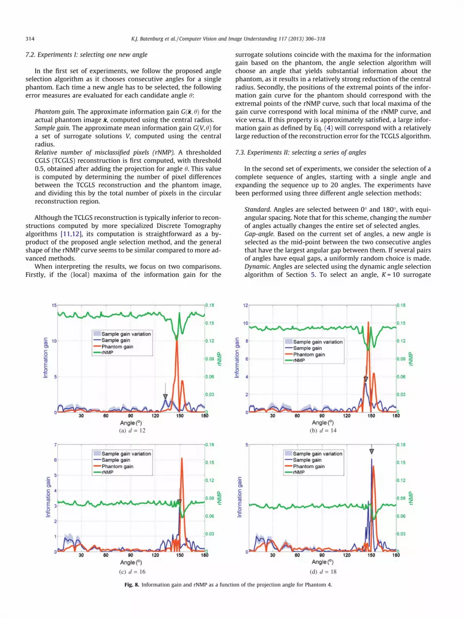
7.2. Experiments I: selecting one new angle

In the first set of experiments, we follow the proposed angleselection algorithm as it chooses consecutive angles for a singlephantom. Each time a new angle has to be selected, the followingerror measures are evaluated for each candidate angle h:

Phantom gain. The approximate information gain Gð�x; hÞ for theactual phantom image �x, computed using the central radius.Sample gain. The approximate mean information gain G(V,h) fora set of surrogate solutions V, computed using the centralradius.Relative number of misclassified pixels (rNMP). A thresholdedCGLS (TCGLS) reconstruction is first computed, with threshold0.5, obtained after adding the projection for angle h. This valueis computed by determining the number of pixel differencesbetween the TCGLS reconstruction and the phantom image,and dividing this by the total number of pixels in the circularreconstruction region.

Although the TCLGS reconstruction is typically inferior to recon-structions computed by more specialized Discrete Tomographyalgorithms [11,12], its computation is straightforward as a by-product of the proposed angle selection method, and the generalshape of the rNMP curve seems to be similar compared to more ad-vanced methods.

When interpreting the results, we focus on two comparisons.Firstly, if the (local) maxima of the information gain for the

Fig. 8. Information gain and rNMP as a functi

surrogate solutions coincide with the maxima for the informationgain based on the phantom, the angle selection algorithm willchoose an angle that yields substantial information about thephantom, as it results in a relatively strong reduction of the centralradius. Secondly, the positions of the extremal points of the infor-mation gain curve for the phantom should correspond with theextremal points of the rNMP curve, such that local maxima of thegain curve correspond with local minima of the rNMP curve, andvice versa. If this property is approximately satisfied, a large infor-mation gain as defined by Eq. (4) will correspond with a relativelylarge reduction of the reconstruction error for the TCGLS algorithm.

7.3. Experiments II: selecting a series of angles

In the second set of experiments, we consider the selection of acomplete sequence of angles, starting with a single angle andexpanding the sequence up to 20 angles. The experiments havebeen performed using three different angle selection methods:

Standard. Angles are selected between 0� and 180�, with equi-angular spacing. Note that for this scheme, changing the numberof angles actually changes the entire set of selected angles.Gap-angle. Based on the current set of angles, a new angle isselected as the mid-point between the two consecutive anglesthat have the largest angular gap between them. If several pairsof angles have equal gaps, a uniformly random choice is made.Dynamic. Angles are selected using the dynamic angle selectionalgorithm of Section 5. To select an angle, K = 10 surrogate

on of the projection angle for Phantom 4.


solutions are generated, and their mean information gain isevaluated for all candidate angles, with steps of 1�.

To reduce the dependency of the results on the particular start-ing angle, as well as the dependency on the random seed (for theDynamic and Gap-angle strategies), a series of runs has beenperformed for each angle selection method, using nine randomlyselected starting angles, and five different random seeds for eachstarting angle.

8. Results

In this section, we report on the results of the two sets of exper-iments, described in Sections 7.2 and 7.3.

8.1. Results I: selecting one new angle

Figs. 5–8 show the Phantom gain and the Sample gain, for eachcandidate angle between 0� and 180� (in steps of 1�), and for eachphantom image, respectively. The Phantom gain is shown alongwith its variation (shaded area), indicating the range from the min-imum to the maximum value observed for a surrogate solution. Asonly the positions of the local optima of the gain curves areimportant for angle selection, and not the absolute values of theapproximate information gain, the curve for the Sample gain isscaled such that the total area under the graph is the same as forthe Phantom gain. In addition to the gain curves, the rNMP of the

2 4 6 8 10 12 14 16 18 200

0.05

0.1

0.15

Number of projections

rNM

P

DynamicGap angleStandard

(a) Phantom 1

2 4 6 8 10 12 14 16 18 200

0.05

0.1

0.15

0.2

0.25

0.3


rNM

P


(c) Phantom 3

Fig. 9. rNMP as a function of t

TCGLS reconstruction for each candidate angle, obtained by recon-structing the image after adding the projection for the candidateangle, is shown in the same plot.

In Figs. 5a and 6a, it can be clearly observed that if the numberof projections is extremely small (two, in this case), the dynamicangle selection algorithm does not select the angle that corre-sponds to the maximum Phantom gain. This can be explained bythe fact that for d = 2, the reconstruction problem is highly under-determined, and there are large differences between the surrogatesolutions. An angle choice that is optimal with respect to the phan-tom does not appear to be optimal with respect to the combinedset of surrogate solutions.

However, for more than two projections, the correlation be-tween the Sample gain curve and the Phantom gain curve is muchhigher, for both Phantoms 1 and 2. Indeed, for three projections,the dynamic angle selection selects an angle that closely matchesthat of the maximum Phantom gain (see Figs. 5b and 6b). Similarobservations can be made for four and five projections. For themore complex Phantoms 3 and 4, the number of projections thatis needed to reach a reasonable agreement between the Phantomgain and the Sample gain is substantially higher. For Phantom 3,there is a high correlation between both curves for d P 4, whereas14 projections are required to properly localize the ‘‘best’’ projec-tion angle for Phantom 4.

Another observation that can be made, is that for all four phan-toms, there is generally a good agreement between the rNMP thatis computed with respect to the phantom, and the Phantom gain.Local minima of the rNMP curve tend to correspond with local

2 4 6 8 10 12 14 16 18 200

0.02

0.04

0.06

0.08

0.1

0.12

0.14

0.16

0.18


rNM

P


(b) Phantom 2

2 4 6 8 10 12 14 16 18 200

0.05

0.1

0.15

0.2

0.25

0.3


rNM

P


(d) Phantom 4

he number of projections.


maxima of the Phantom gain, and vice versa. This correspondenceis crucial for the ability of the dynamic angle selection algorithm torapidly achieve a high reconstruction quality with respect to thephantom object, even though the phantom is not known to thealgorithm.

8.2. Results II: selecting a series of angles

To compare the results for the three angle selection methods,two plots have been generated for each phantom. The first seriesof plots, presented in Fig. 9, shows the rNMP of TCGLS as afunction of the number of projection angles. For each number dof angles, the TCGLS reconstruction was computed based on theprojections for the first d angles in the sequence. The secondseries of plots, presented in Fig. 10 shows the central radius as afunction of the number of projection angles. For each number dof projection angles, the central radius, which scales proportion-ally to the upper bound on the diameter of the set of binarysolutions, is determined based on the first d angles in the se-quence. The shaded regions denote the standard deviation origi-nating from repeating the experiments with varying startingangles and random seeds.

The results show that for Phantoms 1, 2, and 4, the rNMP theDynamic strategy is never clearly outperformed by the Standardand Gap-angle methods, while at substantial intervals for the

2 4 6 8 10 12 14 16 18 200

5

10

15

20

25

30

35

40


Cen

tral r

adiu

s


(a) Phantom 1

2 4 6 8 10 12 14 16 18 200

5

10

15

20

25

30

35

40

45

50


Cen

tral r

adiu

s


(c) Phantom 3

Fig. 10. Central radius as a function

number of projection angles, the rNMP are substantially betterfor the Dynamic strategy. For Phantom 1, the proposed angle selec-tion method works particularly well if the number of angles is verysmall (between 3 and 10), whereas for the more complex Phantom4, the key advantage of the Dynamic strategy shows up when usinga larger number of projections (10 or more). The advantage ofdynamic angle selection is smallest for Phantom 3 (the hand phan-tom), which has a relatively large number of features, each havinga different orientation.

What is also clear from the plots in Figs. 9 and 10, is that thecurves for the rNMP with respect to the unknown phantom, andfor the central radius, have similar shapes and roughly show thesame ordering between the performance of the different meth-ods. Just as for the results in the first series of experiments, con-firmation of this correspondence is important for establishing theability of the dynamic angle selection algorithm to rapidlyachieve a high reconstruction quality with respect to the phan-tom object, even though the phantom is not known to thealgorithm.

In Fig. 11, a selection of TCGLS reconstructions is shown thatwas obtained after a run of the three angle selection strategies.For each phantom, the number of angles was selected such that areasonable reconstruction could already be obtained, quite similarto the phantom, yet the number of projections was still too small toobtain an almost perfect reconstruction.

2 4 6 8 10 12 14 16 18 200

5

10

15

20

25

30

35

40


Cen

tral r

adiu

s


(b) Phantom 2

2 4 6 8 10 12 14 16 18 200

5

10

15

20

25

30

35

40

45

50


Cen

tral r

adiu

s


(d) Phantom 4

of the number of projections.

Fig. 11. Illustration of TCGLS reconstructions obtained after using the different angle selection algorithms, for the four phantoms. Next to each binary reconstruction, animage is shown that represents the difference between the reconstruction and the phantom. From left to right: standard, gap angle, dynamic; from top to bottom: Phantom 1(6 angles), Phantom 2 (8 angles), Phantom 3 (12 angles), Phantom 4 (16 angles).


9. Discussion

The experimental results for the four phantom images suggestthat the proposed dynamic angle selection strategy is indeed capa-ble of finding angles for which the reconstructed image is substan-tially more accurate than for the standard angle selection scheme,if the number of angles is not too small. It seems that although thecentral radius provides an upper bound on the diameter of the setof binary solutions, a strategy that aims to reduce this upper boundalso reduces the actual reconstruction error with respect to the un-known phantom.

It should also be noted that the proposed angle selection algo-rithm lacks computational efficiency. Within the context of thisarticle, we focused on the capabilities of the algorithm with respectto reconstruction quality, and on avoiding the exponential timecomplexity of enumerating the set of binary solutions. However,in our implementation which utilizes a modern GPU for perform-ing the SIRT and CGLS subroutines, selecting a single angle for animage of size 128 � 128 takes around 30 s if the current numberof angles is 4.

By far the most computation time is spent in the CGLS subrou-tine, which computes the central reconstruction within the evalu-ation of the information gain for a surrogate solution. As thiscomputation is performed for each surrogate solution, and for eachangle, it is called around 180 K times just to select a single angle.We expect that the algorithm can be made far more efficient ifthe complete recomputation of the central radius can be avoidedby using the results from earlier computations.

Despite these computational obstacles, we feel that the type ofalgorithm proposed here should be seen as a proof-of-concept formore efficient, or more advanced algorithms that utilize the con-cepts of information gain. Formal modeling of the amount of infor-mation that is present in a set of projection data is notstraightforward, in particular for underdetermined reconstructionproblems, where many solutions may exist.

The results also demonstrate that dynamic angle selection is notonly useful in the domain of an extremely small number of projec-tion angles (i.e. less than 10). In fact, for the more complex Phan-tom 4, which clearly has a certain ‘‘preferential orientation’’, thedynamic angle selection scheme mainly outperforms the standardmethod if there are more than 10 projections. This means that theapproach can potentially be useful for angle selection in the recon-struction of quite complex objects, such as trabecular bones, whereit is crucial to use as few projection images as possible, due to radi-ation damage.

For the derivation of our angle selection algorithm, we made theidealized assumption that the projection data contains no noise.The actual algorithm can also be used when there is noise, as bothSIRT (used for generating the surrogate solutions) and CGLS (usedfor computing the information gain) are convergent even if therighthand side of the linear system is perturbed. We consider acomplete exploration of the capabilities and limitations to handlenoisy data to be outside of the scope of the current article.

10. Conclusions

In this article, we proposed a formal model for the angle selec-tion problem in binary tomography, and an actual algorithm thatwas obtained by introducing several approximation steps with re-spect to the idealized model.

It was shown that for a set of phantom images, the proposed dy-namic angle selection strategy compares favorably to other strate-gies that do not take specific properties of the binaryreconstruction problem into account.

Although the computational requirements for the dynamic an-gle selection method are currently restricting its use for largeexperimental dataset, we consider this work as a starting pointfor developing more efficient algorithm variants, based on thesame underlying ideas.


An important question that was not addressed in this work, ishow the class of template images influences the results. Ideally,these images should represent properties that can occur in the truescanned objects, while also having sufficient variations to provide atrustful sampling of the current set of binary solutions. In futurework, we intend to explore this relation further.

Acknowledgments

This research was partially supported by the TÁMOP-4.2.2/08/1/2008-0008 Program of the Hungarian National DevelopmentAgency, the European Union and the European Regional Develop-ment Fund under the Grant Agreement TÁMOP-4.2.1/B-09/1/KONV-2010-0005. Part of the research was performed when PBwas visiting the ASTRA Group at Vision Lab, University of Antwerpin Belgium. The research was also supported by the János BolyaiResearch Scholarship of the Hungarian Academy of Sciences andthe Grant PD100950 of the Hungarian Scientific Research Fund(OTKA). K.J.B. acknowledges support from the Netherlands Fundfor Scientific Research (NWO), Project Number 639.072.005.

References

[1] G.T. Herman, Fundamentals of Computerized Tomography: Imagereconstruction from projections, Springer, 2009.

[2] A.C. Kak, M. Slaney, Principles of Computerized Tomographic Imaging, SIAM,2001.

[3] P.A. Midgley, R.E. Dunin-Borkowski, Electron tomography and holography inmaterials science, Nat. Mater. 8 (4) (2009) 271–280.

[4] E.J. Candès, J. Romberg, T. Tao, Robust uncertainty principles: exact signalreconstruction from highly incomplete frequency information, IEEE Trans.Inform. Theory 52 (2) (2006) 489–509.

[5] G.-H. Chen, J. Tang, S. Leng, Prior image constrained compressed sensing(PICCS): a method to accurately reconstruct dynamic CT images from highlyundersampled projection data sets, Med. Phys. 35 (2) (2008) 660–663.

[6] D. Donoho, Compressed sensing, IEEE Trans. Inform. Theory 52 (4) (2006)1289–1306.

[7] E.Y. Sidky, M.A. Anastasio, X. Pan, Image reconstruction exploiting objectsparsity in boundary-enhanced X-ray phase-contrast tomography, Opt.Express 18 (10) (2010) 10404–10422.

[8] E.Y. Sidky, C.M. Kao, X. Pan, Accurate image reconstruction from few-views andlimited-angle data in divergent-beam CT, J. X-ray Sci. Technol. 14 (2006) 119–139.

[9] G.T. Herman, A. Kuba (Eds.), Discrete Tomography: Foundations, Algorithmsand Applications, Birkhäuser, Boston, 1999.

[10] G.T. Herman, A. Kuba (Eds.), Advances in Discrete Tomography and itsApplications, Birkhäuser, Boston, 2007.

[11] K.J. Batenburg, J. Sijbers, DART: a practical reconstruction algorithm fordiscrete tomography, IEEE Trans. Image Process. 20 (9) (2011) 2542–2553.

[12] T. Schüle, C. Schnörr, S. Weber, J. Hornegger, Discrete tomography by convex–concave regularization and D.C. programming, Discrete Appl. Math. 151 (2005)229–243.

[13] L. Varga, P. Balázs, A. Nagy, Direction-dependency of binary tomographicreconstruction algorithms, Graph. Models (73) (2011) 365–375.

[14] L. Varga, P. Balázs, A. Nagy, Projection selection dependency in binarytomography, Acta Cybernet. 20 (1) (2011) 167–187.

[15] Z. Zheng, K. Mueller, Identifying sets of favorable projections for few-viewlow-dose cone-beam CT scanning, in: 11th International Meeting on FullyThree-Dimensional Image Reconstruction in Radiology and Nuclear Medicine,2011, pp. 314–317.

[16] R.J. Gardner, P. Gritzmann, D. Prangenberg, On the computational complexityof reconstructing lattice sets from their X-rays, Discrete Math. 202 (1999) 45–71.

[17] K.J. Batenburg, W. Fortes, L. Hajdu, R. Tijdeman, Bounds on the differencebetween reconstructions in binary tomography, in: Proceedings of the 16thIAPR International Conference on Discrete Geometry for Computer Imagery,DGCI’11, Springer-Verlag, Berlin, Heidelberg, 2011, pp. 369–380. <http://dl.acm.org/citation.cfm?id=1987119.1987156>.

[18] J. Gregor, T. Benson, Computational analysis and improvement of SIRT, IEEETrans. Med. Imag. 27 (7) (2008) 918–924.

[19] Y. Saad, Iterative Methods for Sparse Linear Systems, SIAM, Philadelphia, PA,USA, 2003.

http://www.dl.acm.org/citation.cfm?id=1987119.1987156

http://www.dl.acm.org/citation.cfm?id=1987119.1987156

dynamic angle selection in binary tomography

Documents