dsc: scheduling parallel tasks on an unbounded number of processors
TRANSCRIPT
DSC: Scheduling Parallel Tasks on an Unbounded Number of
Processors
�
Tao Yang and Apostolos Gerasoulis
Department of Computer Science
Rutgers University
New Brunswick, NJ 08903
Email: ftyang, [email protected]
August 1992, Revised February 1993
Abstract
We present a low complexity heuristic named the Dominant Sequence Clustering algorithm (DSC) for
scheduling parallel tasks on an unbounded number of completely connected processors. The performance
of DSC is comparable or even better on average than many other higher complexity algorithms. We
assume no task duplication and nonzero communication overhead between processors. Finding the
optimum solution for arbitrary directed acyclic task graphs (DAGs) is NP-complete. DSC �nds optimal
schedules for special classes of DAGs such as fork, join, coarse grain trees and some �ne grain trees.
It guarantees a performance within a factor of two of the optimum for general coarse grain DAGs.
We compare DSC with three higher complexity general scheduling algorithms, the MD by Wu and
Gajski [19], the ETF by Hwang, Chow, Anger and Lee [12] and Sarkar's clustering algorithm [17]. We
also give a sample of important practical applications where DSC has been found useful.
Index Terms { Clustering, directed acyclic graph, heuristic algorithm, optimality, parallel processing,
scheduling, task precedence.
1 Introduction
We study the scheduling problem of directed acyclic weighted task graphs (DAGs) on unlimited processor
resources and a completely connected interconnection network. The task and edge weights are determin-
istic. This problem is important in the the development of parallel programming tools and compilers for
scalable MIMD architectures [17, 19, 21, 23]. Sarkar [17] has proposed a two step method for scheduling
with communication. (1) Schedule on unbounded number of a completely connected architecture. The
result of this step will be clusters of tasks, with the constraint that all tasks in a cluster must execute
in the same processor. (2) If the number of clusters is larger than the number of processors then merge
�
Supported by a Grant No. DMS-8706122 from NSF. A preliminary report on this work has appeared in Proceedings of
Supercomputing 91 [23].
1
the clusters further to the number of physical processors and also incorporate the network topology in the
merging step.
In this paper, we present an e�cient algorithm for the �rst step of Sarkar's approach. Algorithms for
the second step are discussed elsewhere [23]. The objective of scheduling is to allocate tasks onto the
processors and then order their execution so that task dependence is satis�ed and the length of the schedule,
known as the parallel time, is minimized. In the presence of communication, the complexity of the above
scheduling problem has been found to be much more di�cult than the classical scheduling problem where
communication is ignored. The general problem is NP-complete and even for simple graphs such as �ne
grain trees or the the concatenation of a fork and a join together the complexity is still NP-complete,
Chretienne [3], Papadimitriou and Yannakakis [15] and Sarkar [17]. Only for special classes of DAGs, such
as join, fork, and coarse grain tree, special polynomial algorithms are known, Chretienne [4], Anger, Hwang
and Chow [2].
There have been two approaches in the literature addressing the general scheduling problem. The �rst
approach considers heuristics for arbitrary DAGs and the second studies optimal algorithms for special
classes of DAGs. When task duplication is allowed, Papadimitriou and Yannakakis [15] have proposed an
approximate algorithm for a DAG with equal task weights and equal edge weights, which guarantees a
performance within 50% of the optimum. This algorithm has a complexity of O(v
3
(v log v+ e)) where v is
the number of tasks and e is the number of edges. Kruatrachue and Lewis [14] have also given an O(v
4
)
algorithm for a general DAG based on task duplication. One di�culty with allowing task duplication is
that duplicated tasks may require duplicated data among processors and thus the space complexity could
increase when executing parallel programs on real machines.
Without task duplication, many heuristic scheduling algorithms for arbitrary DAGs have been proposed in
the literature, e.g. Kim and Browne [13], Sarkar [17], Wu and Gajski [19]. A detailed comparison of four
heuristic algorithms is given in Gerasoulis and Yang [10]. One di�culty with most existing algorithms for
general DAGs is their high complexity. As far as we know no scheduling algorithm exists that works well
for arbitrary graphs, �nds optimal schedules for special DAGs and also has a low complexity. We present
one such algorithm in this paper with a complexity of O((v + e) logv), called the Dominant Sequence
Clustering (DSC) algorithm. We compare DSC with ETF algorithm by Hwang, Chow, Anger, and Lee [12]
and discuss the similarities and di�erences with the MD algorithm proposed by Wu and Gajski [19].
The organization is as follows: Section 2 introduces the basic concepts. Section 3 describes an initial
design of the DSC algorithm and analyzes its weaknesses. Section 4 presents an improved version of DSC
that takes care of the initial weaknesses and analyzes how DSC achieves both low complexity and good
performance. Section 5 gives a performance bound for a general DAG. It shows that the performance of
DSC is within 50% of the optimum for coarse grain DAGs, and it is optimal for join, fork, coarse grain
trees and a class of �ne grain trees. Section 6 discusses the related work, presents experimental results and
compares the performance of DSC with Sarkar's, ETF and MD algorithms.
2
2 Preliminaries
A directed acyclic task graph (DAG) is de�ned by a tuple G = (V;E;C;T ) where V is the set of task
nodes and v = jV j is the number of nodes, E is the set of communication edges and e = jEj is the number
of edges, C is the set of edge communication costs and T is the set of node computation costs. The value
c
i;j
2 C is the communication cost incurred along the edge e
i;j
= (n
i
; n
j
) 2 E, which is zero if both nodes
are mapped in the same processor. The value �
i
2 T is the execution time of node n
i
2 V . PRED(n
x
)
is the set of immediate predecessors of n
x
and SUCC(n
x
) is the set of immediate successors of n
x
. An
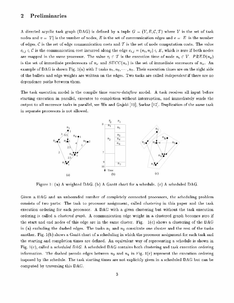
example of DAG is shown Fig. 1(a) with 7 tasks n
1
; n
2
; � � � ; n
7
. Their execution times are on the right side
of the bullets and edge weights are written on the edges. Two tasks are called independent if there are no
dependence paths between them.
The task execution model is the compile time macro-data ow model. A task receives all input before
starting execution in parallel, executes to completion without interruption, and immediately sends the
output to all successor tasks in parallel, see Wu and Gajski [19], Sarkar [17]. Duplication of the same task
in separate processors is not allowed.
n1
n 6
n3n2
n4
n7
n5
n1
n 6
n3n2
n4
n7
n5
1
6 1
1
2
1
1
3
2
2.5
41
2.5
Time
10
0
7
n1
n 6
n3n2 n4
n7
n5
9
P1P0
(a) (c)(b)
0.5
Figure 1: (a) A weighted DAG. (b) A Gantt chart for a schedule. (c) A scheduled DAG.
Given a DAG and an unbounded number of completely connected processors, the scheduling problem
consists of two parts: The task to processor assignment, called clustering in this paper and the task
execution ordering for each processor. A DAG with a given clustering but without the task execution
ordering is called a clustered graph. A communication edge weight in a clustered graph becomes zero if
the start and end nodes of this edge are in the same cluster. Fig. 1(c) shows a clustering of the DAG
in (a) excluding the dashed edges. The tasks n
1
and n
2
constitute one cluster and the rest of the tasks
another. Fig. 1(b) shows a Gantt chart of a scheduling in which the processor assignment for each task and
the starting and completion times are de�ned. An equivalent way of representing a schedule is shown in
Fig. 1(c), called a scheduled DAG. A scheduled DAG contains both clustering and task execution ordering
information. The dashed pseudo edges between n
3
and n
4
in Fig. 1(c) represent the execution ordering
imposed by the schedule. The task starting times are not explicitly given in a scheduled DAG but can be
computed by traversing this DAG.
3
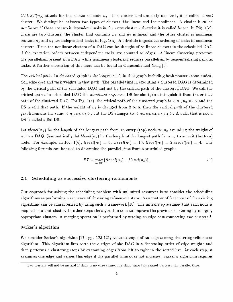
CLUST (n
x
) stands for the cluster of node n
x
. If a cluster contains only one task, it is called a unit
cluster. We distinguish between two types of clusters, the linear and the nonlinear. A cluster is called
nonlinear if there are two independent tasks in the same cluster, otherwise it is called linear. In Fig. 1(c),
there are two clusters, the cluster that contains n
1
and n
2
is linear and the other cluster is nonlinear
because n
3
and n
4
are independent tasks in Fig. 1(a). A schedule imposes an ordering of tasks in nonlinear
clusters. Thus the nonlinear clusters of a DAG can be thought of as linear clusters in the scheduled DAG
if the execution orders between independent tasks are counted as edges. A linear clustering preserves
the parallelism present in a DAG while nonlinear clustering reduces parallelism by sequentializing parallel
tasks. A further discussion of this issue can be found in Gerasoulis and Yang [9].
The critical path of a clustered graph is the longest path in that graph including both nonzero communica-
tion edge cost and task weights in that path. The parallel time in executing a clustered DAG is determined
by the critical path of the scheduled DAG and not by the critical path of the clustered DAG. We call the
critical path of a scheduled DAG the dominant sequence, DS for short, to distinguish it from the critical
path of the clustered DAG. For Fig. 1(c), the critical path of the clustered graph is < n
1
; n
2
; n
7
> and the
DS is still that path. If the weight of n
5
is changed from 2 to 6, then the critical path of the clustered
graph remains the same < n
1
; n
2
; n
7
>, but the DS changes to < n
5
; n
3
; n
4
; n
6
; n
7
>. A path that is not a
DS is called a SubDS.
Let tlevel(n
x
) be the length of the longest path from an entry (top) node to n
x
excluding the weight of
n
x
in a DAG. Symmetrically, let blevel(n
x
) be the length of the longest path from n
x
to an exit (bottom)
node. For example, in Fig. 1(c), tlevel(n
1
) = 0, blevel(n
1
) = 10, tlevel(n
3
) = 2; blevel(n
3
) = 4. The
following formula can be used to determine the parallel time from a scheduled graph:
PT = max
n
x
2V
ftlevel(n
x
) + blevel(n
x
)g: (1)
2.1 Scheduling as successive clustering re�nements
Our approach for solving the scheduling problem with unlimited resources is to consider the scheduling
algorithms as performing a sequence of clustering re�nement steps. As a matter of fact most of the existing
algorithms can be characterized by using such a framework [10]. The initial step assumes that each node is
mapped in a unit cluster. In other steps the algorithm tries to improve the previous clustering by merging
appropriate clusters. A merging operation is performed by zeroing an edge cost connecting two clusters
1
.
Sarkar's algorithm
We consider Sarkar's algorithm [17], pp. 123-131, as an example of an edge-zeroing clustering re�nement
algorithm. This algorithm �rst sorts the e edges of the DAG in a decreasing order of edge weights and
then performs e clustering steps by examining edges from left to right in the sorted list. At each step, it
examines one edge and zeroes this edge if the parallel time does not increase. Sarkar's algorithm requires
1
Two clusters will not be merged if there is no edge connecting them since this cannot decrease the parallel time.
4
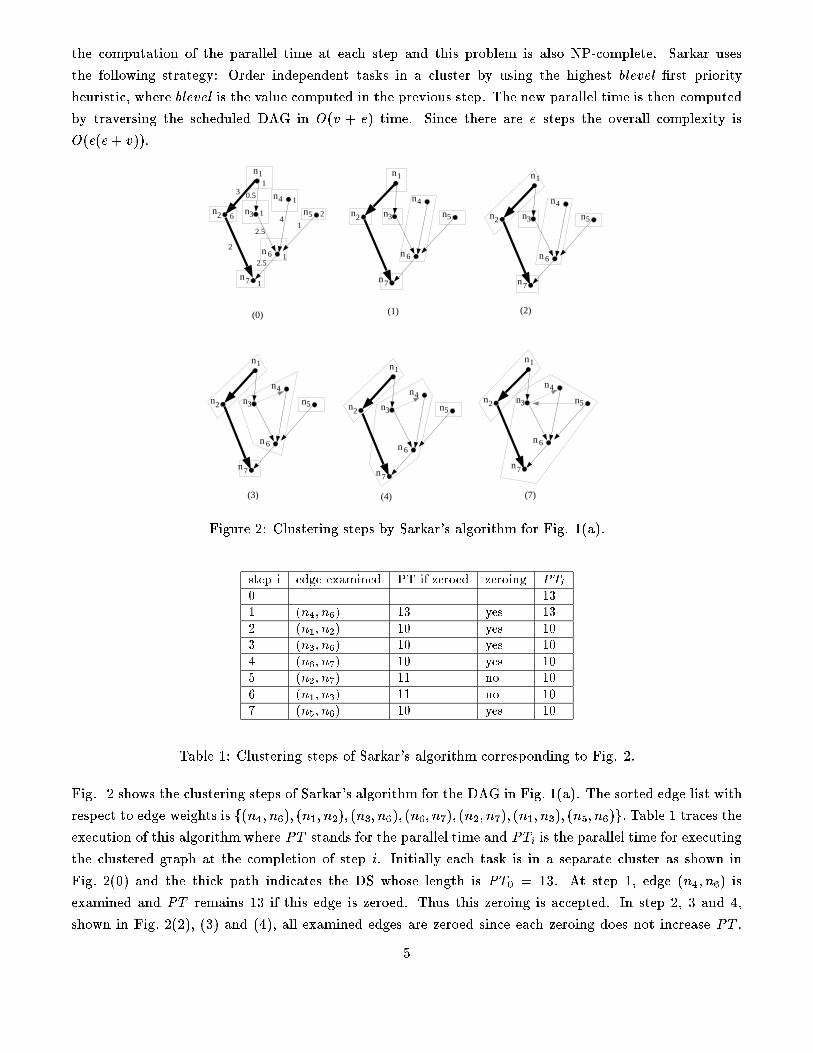
the computation of the parallel time at each step and this problem is also NP-complete. Sarkar uses
the following strategy: Order independent tasks in a cluster by using the highest blevel �rst priority
heuristic, where blevel is the value computed in the previous step. The new parallel time is then computed
by traversing the scheduled DAG in O(v + e) time. Since there are e steps the overall complexity is
O(e(e+ v)).
n1
n 6
n3n2
n4
n7
n5
1
6 1
1
2
1
1
3
2
2.5
41
2.5
(0) (2)(1)
(3) (7)(4)
n1
n 6
n3n2
n4
n7
n5
n1
n 6
n3n2
n4
n7
n5
n1
n 6
n3n2
n4
n7
n5
n1
n 6
n3n2
n4
n7
n5
n1
n 6
n3n2
n4
n7
n5
0.5
Figure 2: Clustering steps by Sarkar's algorithm for Fig. 1(a).
step i edge examined PT if zeroed zeroing PT
i
0 13
1 (n
4
; n
6
) 13 yes 13
2 (n
1
; n
2
) 10 yes 10
3 (n
3
; n
6
) 10 yes 10
4 (n
6
; n
7
) 10 yes 10
5 (n
2
; n
7
) 11 no 10
6 (n
1
; n
3
) 11 no 10
7 (n
5
; n
6
) 10 yes 10
Table 1: Clustering steps of Sarkar's algorithm corresponding to Fig. 2.
Fig. 2 shows the clustering steps of Sarkar's algorithm for the DAG in Fig. 1(a). The sorted edge list with
respect to edge weights is f(n
4
; n
6
); (n
1
; n
2
); (n
3
; n
6
); (n
6
; n
7
); (n
2
; n
7
); (n
1
; n
3
); (n
5
; n
6
)g: Table 1 traces the
execution of this algorithm where PT stands for the parallel time and PT
i
is the parallel time for executing
the clustered graph at the completion of step i. Initially each task is in a separate cluster as shown in
Fig. 2(0) and the thick path indicates the DS whose length is PT
0
= 13. At step 1, edge (n
4
; n
6
) is
examined and PT remains 13 if this edge is zeroed. Thus this zeroing is accepted. In step 2, 3 and 4,
shown in Fig. 2(2), (3) and (4), all examined edges are zeroed since each zeroing does not increase PT .
5
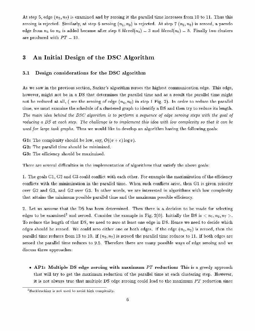
At step 5, edge (n
2
; n
7
) is examined and by zeroing it the parallel time increases from 10 to 11. Thus this
zeroing is rejected. Similarly, at step 6 zeroing (n
1
; n
3
) is rejected. At step 7 (n
5
; n
6
) is zeroed, a pseudo
edge from n
5
to n
3
is added because after step 6 blevel(n
3
) = 3 and blevel(n
5
) = 5. Finally two clusters
are produced with PT = 10.
3 An Initial Design of the DSC Algorithm
3.1 Design considerations for the DSC algorithm
As we saw in the previous section, Sarkar's algorithm zeroes the highest communication edge. This edge,
however, might not be in a DS that determines the parallel time and as a result the parallel time might
not be reduced at all, ( see the zeroing of edge (n
4
; n
6
) in step 1 Fig. 2). In order to reduce the parallel
time, we must examine the schedule of a clustered graph to identify a DS and then try to reduce its length.
The main idea behind the DSC algorithm is to perform a sequence of edge zeroing steps with the goal of
reducing a DS at each step. The challenge is to implement this idea with low complexity so that it can be
used for large task graphs. Thus we would like to develop an algorithm having the following goals:
G1: The complexity should be low, say, O((v + e) log v).
G2: The parallel time should be minimized.
G3: The e�ciency should be maximized.
There are several di�culties in the implementation of algorithms that satisfy the above goals:
1. The goals G1, G2 and G3 could con ict with each other. For example the maximization of the e�ciency
con icts with the minimization in the parallel time. When such con icts arise, then G1 is given priority
over G2 and G3, and G2 over G3. In other words, we are interested in algorithms with low complexity
that attains the minimum possible parallel time and the maximum possible e�ciency.
2. Let us assume that the DS has been determined. Then there is a decision to be made for selecting
edges to be examined
2
and zeroed. Consider the example in Fig. 2(0). Initially the DS is < n
1
; n
2
; n
7
>.
To reduce the length of that DS, we need to zero at least one edge in DS. Hence we need to decide which
edges should be zeroed. We could zero either one or both edges. If the edge (n
1
; n
2
) is zeroed, then the
parallel time reduces from 13 to 10. If (n
2
; n
7
) is zeroed the parallel time reduces to 11. If both edges are
zeroed the parallel time reduces to 9.5. Therefore there are many possible ways of edge zeroing and we
discuss three approaches:
� AP1: Multiple DS edge zeroing with maximum PT reduction: This is a greedy approach
that will try to get the maximum reduction of the parallel time at each clustering step. However,
it is not always true that multiple DS edge zeroing could lead to the maximum PT reduction since
2
Backtracking is not used to avoid high complexity.
6
after zeroing one DS edge of a path, the other edges in that path may not be in the DS of the new
graph.
� AP2: One DS zeroing of maximum weight edge: Considering a DS could become a SubDS by
zeroing only one edge of this DS, we do not need to zero multiple edges at one step. We could instead
make smaller reductions in the parallel time at each step and perform more steps. For example, we
could chose one edge to zero at each step, say the largest weight edge in DS. In Fig. 2(0), the length
of current DS < n
1
; n
2
; n
7
> could be reduced more by zeroing edge (n
1
; n
2
) instead of (n
2
; n
7
).
Zeroing the largest weighted edge, however, may not necessarily lead to a better solution.
� AP3: One DS edge zeroing with low complexity: Instead of zeroing the highest edge weight
we could allow for more exibility and chose to zero the one DS edge that leads to a low complexity
algorithm.
Determining a DS for a clustered DAG could take at least O(v + e) time if the computation is not
done incrementally. Repeating this computation for all steps will result in at least O(v
2
) complexity.
Thus it is necessary to use an incremental computation of DS from one step to the next to avoid the
traversal of the entire DAG at each step. The proper DS edge selection for zeroing should assist in
the incremental computation of the DS in the next step.
It is not clear how to implement AP1 or AP2 with a low complexity and also there is no guarantee that
AP1 or AP2 will be better than AP3. We will use AP3 to develop our algorithm.
3. Since one of the goals is G3, i.e. reducing the number of unnecessary clusters and increase the e�ciency,
we also need to allow for zeroing non-DS edges. The questions is when to do SubDS zeroing. One approach
is to always zero DS edges until the algorithm stops and then follow up with non-DS zeroing. Another
approach followed in this paper is to interleave the non-DS zeroing with that of DS zeroing. Interleaving
SubDS and DS zeroing provides for more exibility which allows to reduce the complexity.
4. Since we do not allow backtracking the only zeroing steps that we should allow are the ones that do
not increase the parallel time from one step to the next: PT
i�1
� PT
i
: Sarkar imposes this constraint
explicitly in his edge zeroing process, by comparing the parallel time at each step. Here, we will use an
implicit constraint to avoid the explicit computation of parallel time in order to reduce the complexity.
In the next subsection, we present an initial version of DSC algorithm and then identify its weaknesses so
that we can improve its performance.
3.2 DSC-I: An initial version of DSC
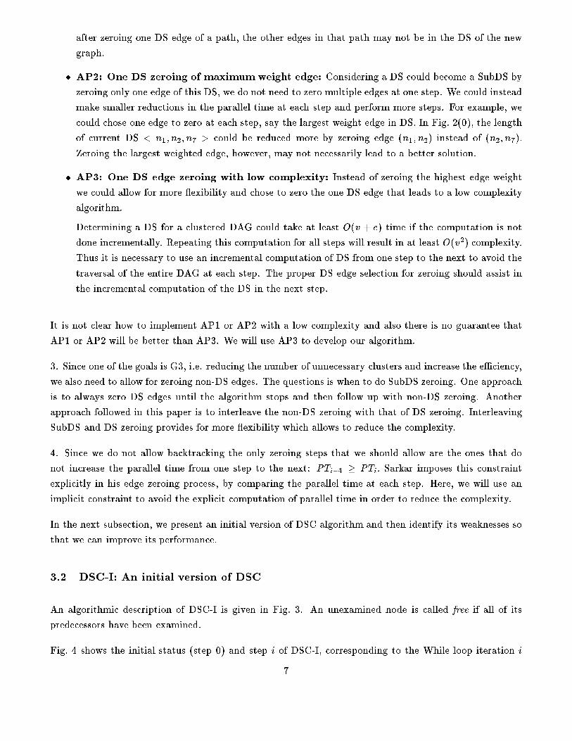
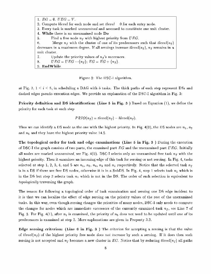
An algorithmic description of DSC-I is given in Fig. 3. An unexamined node is called free if all of its
predecessors have been examined.
Fig. 4 shows the initial status (step 0) and step i of DSC-I, corresponding to the While loop iteration i
7
1. EG = ;. UEG = V .
2. Compute blevel for each node and set tlevel = 0 for each entry node.
3. Every task is marked unexamined and assumed to constitute one unit cluster.
4. While there is an unexamined node Do
5. Find a free node n
f
with highest priority from UEG.
6. Merge n
f
with the cluster of one of its predecessors such that tlevel(n
f
)
decreases in a maximum degree. If all zeroings increase tlevel(n
f
), n
f
remains in a
unit cluster.
7. Update the priority values of n
f
's successors.
8. UEG = UEG� fn
f
g; EG = EG+ fn
f
g.
9. EndWhile
Figure 3: The DSC-I algorithm.
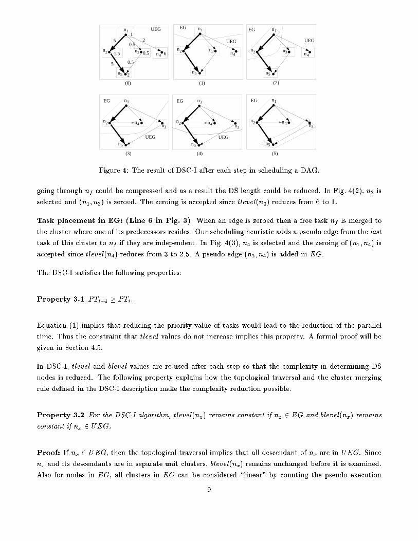
at Fig. 3, 1 � i � 5, in scheduling a DAG with 5 tasks. The thick paths of each step represent DSs and
dashed edges pseudo execution edges. We provide an explanation of the DSC-I algorithm in Fig. 3:
Priority de�nition and DS identi�cation: (Line 5 in Fig. 3 ) Based on Equation (1), we de�ne the
priority for each task at each step
PRIO(n
f
) = tlevel(n
f
) + blevel(n
f
):
Thus we can identify a DS node as the one with the highest priority. In Fig. 4(0), the DS nodes are n
1
, n
2
and n
5
and they have the highest priority value 14.5.
The topological order for task and edge examination: (Line 5 in Fig. 3 ) During the execution
of DSC-I the graph consists of two parts, the examined part EG and the unexamined part UEG. Initially
all nodes are marked unexamined, see Fig. 4(0). DSC-I selects only an unexamined free task n
f
with the
highest priority. Then it examines an incoming edge of this task for zeroing or not zeroing. In Fig. 4, tasks
selected at step 1, 2, 3, 4, and 5 are n
1
, n
2
, n
4
, n
3
and n
5
respectively. Notice that the selected task n
f
is in a DS if there are free DS nodes, otherwise it is in a SubDS. In Fig. 4, step 1 selects task n
1
which is
in the DS but step 3 selects task n
4
which is not in the DS. The order of such selection is equivalent to
topologically traversing the graph.
The reason for following a topological order of task examination and zeroing one DS edge incident to
it is that we can localize the e�ect of edge zeroing on the priority values of the rest of the unexamined
tasks. In this way, even though zeroing changes the priorities of many nodes, DSC-I only needs to compute
the changes for nodes which are immediate successors of the currently examined task n
f
, see Line 7 of
Fig. 3. For Fig. 4(1), after n
1
is examined, the priority of n
5
does not need to be updated until one of its
predecessors is examined at step 2. More explanations are given in Property 3.2.
Edge zeroing criterion: (Line 6 in Fig. 3 ) The criterion for accepting a zeroing is that the value
of tlevel(n
f
) of the highest priority free node does not increase by such a zeroing. If it does then such
zeroing is not accepted and n
f
becomes a new cluster in EG. Notice that by reducing tlevel(n
f
) all paths
8
n1
n3n2 n4
n5
1.5
1
0.5 6
25
5
0.5
0.5
2
UEG n1
n3n2 n4
n5
EG
UEG
n1
n3n2 n4
n5
EG
UEG
(0) (1) (2)
(3) (4) (5)
n1
n3
n2 n4
n5
EG
UEG
n1
n3
n2 n4
n5
EG
UEG
n1
n3
n2 n4
n5
EG
Figure 4: The result of DSC-I after each step in scheduling a DAG.
going through n
f
could be compressed and as a result the DS length could be reduced. In Fig. 4(2), n
2
is
selected and (n
1
; n
2
) is zeroed. The zeroing is accepted since tlevel(n
2
) reduces from 6 to 1.
Task placement in EG: (Line 6 in Fig. 3) When an edge is zeroed then a free task n
f
is merged to
the cluster where one of its predecessors resides. Our scheduling heuristic adds a pseudo edge from the last
task of this cluster to n
f
if they are independent. In Fig. 4(3), n
4
is selected and the zeroing of (n
1
; n
4
) is
accepted since tlevel(n
4
) reduces from 3 to 2.5. A pseudo edge (n
2
; n
4
) is added in EG.
The DSC-I satis�es the following properties:
Property 3.1 PT
i�1
� PT
i
.
Equation (1) implies that reducing the priority value of tasks would lead to the reduction of the parallel
time. Thus the constraint that tlevel values do not increase implies this property. A formal proof will be
given in Section 4.5.
In DSC-I, tlevel and blevel values are re-used after each step so that the complexity in determining DS
nodes is reduced. The following property explains how the topological traversal and the cluster merging
rule de�ned in the DSC-I description make the complexity reduction possible.
Property 3.2 For the DSC-I algorithm, tlevel(n
x
) remains constant if n
x
2 EG and blevel(n
x
) remains
constant if n
x
2 UEG.
Proof: If n
x
2 UEG, then the topological traversal implies that all descendant of n
x
are in UEG. Since
n
x
and its descendants are in separate unit clusters, blevel(n
x
) remains unchanged before it is examined.
Also for nodes in EG, all clusters in EG can be considered \linear" by counting the pseudo execution
9
edges. When a free node is merged to a \linear" cluster it is always attached to the last node of that
\linear" cluster. Thus tlevel(n
x
) remains unchanged after n
x
has been examined. 2
Property 3.3 The time complexity of DSC-I algorithm is O(e+ v log v).
Proof: From Property 3.2, the priority of a free node n
f
can be easily determined by using
tlevel(n
f
) = max
n
j
2PRED(n
f
)
ftlevel(n
j
) + �
j
+ c
j;f
g:
Once tlevel(n
j
) is computed after its examination at some step, where n
j
is the predecessor of n
f
, this
value is propagated to tlevel(n
f
). Afterwards tlevel(n
j
) remains unchanged and will not a�ect the value
of tlevel(n
f
) anymore.
We maintain a priority list FL that contains all free tasks in UEG at each step of DSC-I. This list can be
implemented using a balanced search tree data structure [7]. At the beginning, FL is empty and there is
no initial overhead in setting up this data structure. The overhead occurs to maintain the proper order
among tasks when a task is inserted or deleted from this list. This operation costs O(log jFLj) [7] where
jFLj � v. Since each task in a DAG is inserted to FL once and is deleted once during the entire execution
of DSC-I, the total complexity for maintaining FL is at most 2v log v.
The main computational cost of DSC-I algorithm is spent in the While loop (Line 4 in Fig. 3). The number
of steps (iterations) is v. For Line 5, each step costs O(log v) for �nding the head of FL and v steps cost
O(v log v). For Line 6, each step costs O(jPRED(n
f
)j) in examining the immediate predecessors of task
n
f
. For the v steps the cost is
P
n
f
2V
O(jPRED(n
f
)j) = O(e). For line 7, each step costs O(jSUCC(n
f
)j)
to update the priority values of the immediate successors of n
f
, and similarly the cost for v steps is O(e).
When a successor of n
f
is found free at Line 7, it is added to FL, and the overall cost has been estimated
above to be O(v log v). Thus the total cost for DSC-I is O(e+ v log v). 2
3.3 An Evaluation of DSC-I
In this subsection, we study the performance of DSC-I for some DAGs and propose modi�cations to
improve its performance. Because a DAG is composed of a set of join and fork components, we consider
the strengths and weaknesses of DSC-I in scheduling fork and join DAGs. Then we discuss a problem
arising when zeroing non-DS edges due to the topological ordering of the traversal.
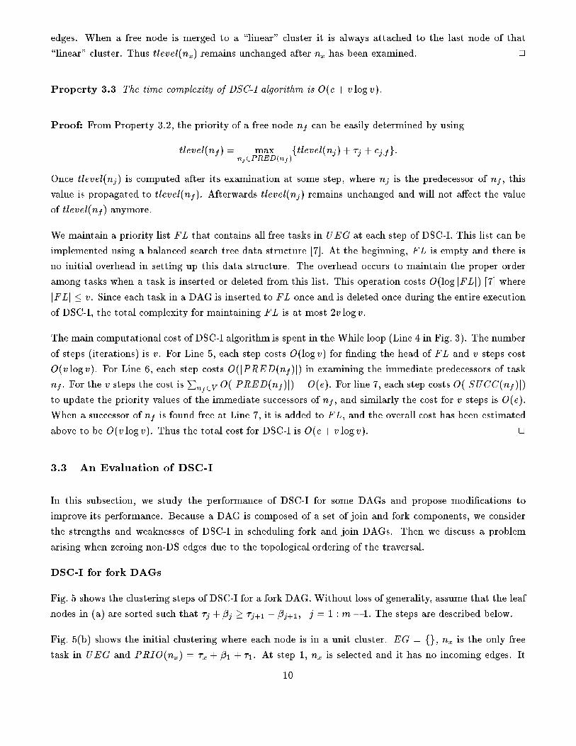
DSC-I for fork DAGs
Fig. 5 shows the clustering steps of DSC-I for a fork DAG. Without loss of generality, assume that the leaf
nodes in (a) are sorted such that �
j
+ �
j
� �
j+1
+ �
j+1
; j = 1 :m� 1: The steps are described below.
Fig. 5(b) shows the initial clustering where each node is in a unit cluster. EG = fg, n
x
is the only free
task in UEG and PRIO(n
x
) = �
x
+ �
1
+ �
1
. At step 1, n
x
is selected and it has no incoming edges. It
10
0 0 0
21 nn mnkn kn +1
. . . . . .
xn
mβkβ +1
(a) Fork DAG
(d) Step k+1
. . . . . .
2 mk1 nnnn
xn
mβkβ
2β1β
. . . . . .
2 mk1 nnnn
xn
mβkβ
2β1β
. . . . . .
2 mk1 nnnn
xn
mβkβ
2β0
(b) Initial clustering
(c) Step 2, n1 is examined.
Figure 5: (c) and (d) are the results of DSC-I after step 2 and k + 1 for a fork DAG.
remains in a unit cluster and EG = fn
x
g. After that, n
1
; n
2
; � � � ; n
m
become free and n
1
has the highest
priority, PRIO(n
1
) = �
x
+ �
1
+ �
1
, and tlevel(n
1
) = �
x
+ �
1
. At step 2 shown in 5(c), n
1
is selected and
merged to the cluster of n
x
and tlevel(n
1
) is reduced in a maximum degree to �
x
. At step k + 1, n
k
is
selected. The original leftmost scheduled cluster in 5(d) is a \linear" chain n
x
; n
1
; � � � ; n
k�1
. If attaching
n
k
to the end of this chain does not increase tlevel(n
k
) = �
x
+ �
k
, the zeroing of edge (n
x
; n
k
) is accepted
and the new tlevel(n
k
) = �
x
+
P
k�1
j=1
�
j
. Thus the condition for accepting or not accepting a zeroing can
be expressed as:
P
k�1
j=1
�
j
� �
k
:
It is easy to verify that DSC-I always zeroes DS edges at each step for a fork DAG and the parallel time
strictly decreases monotonically. It turns out the DSC-I algorithm is optimal for this case and a proof will
be given in section 5.
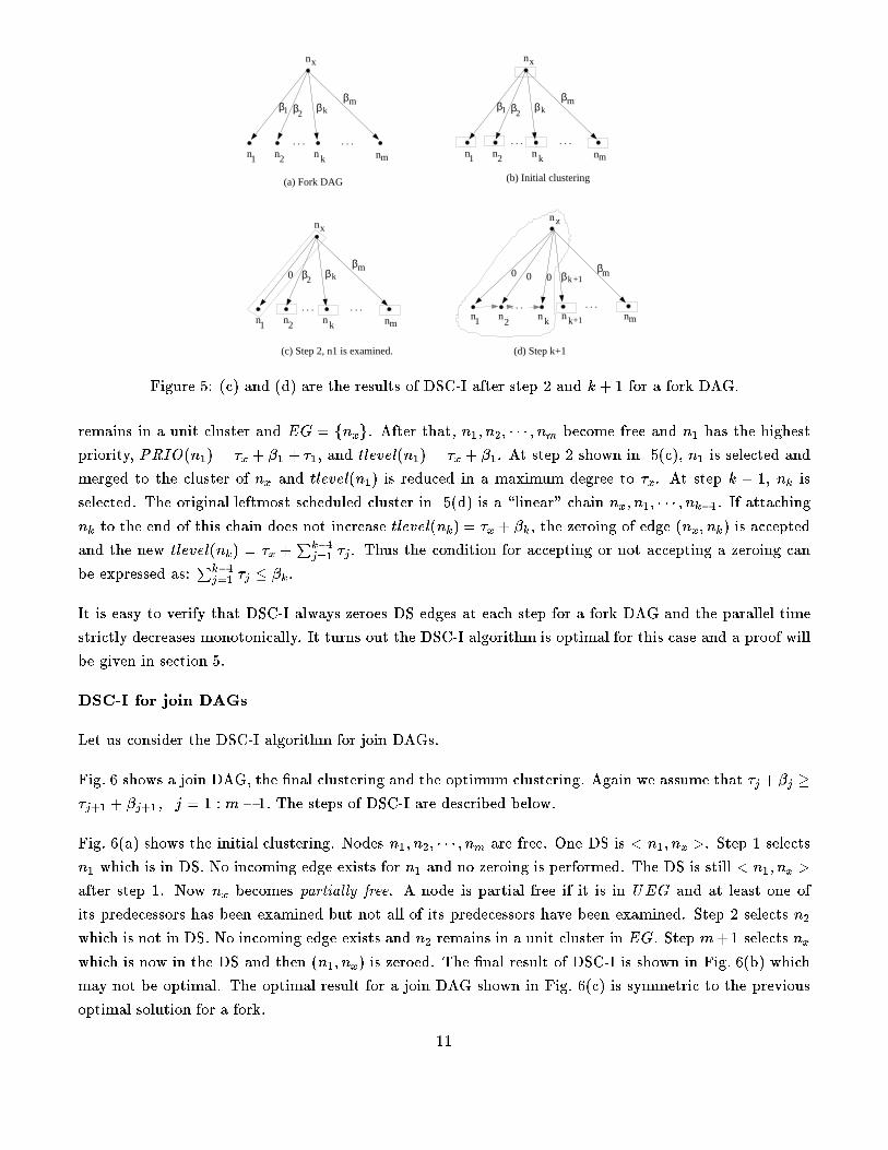
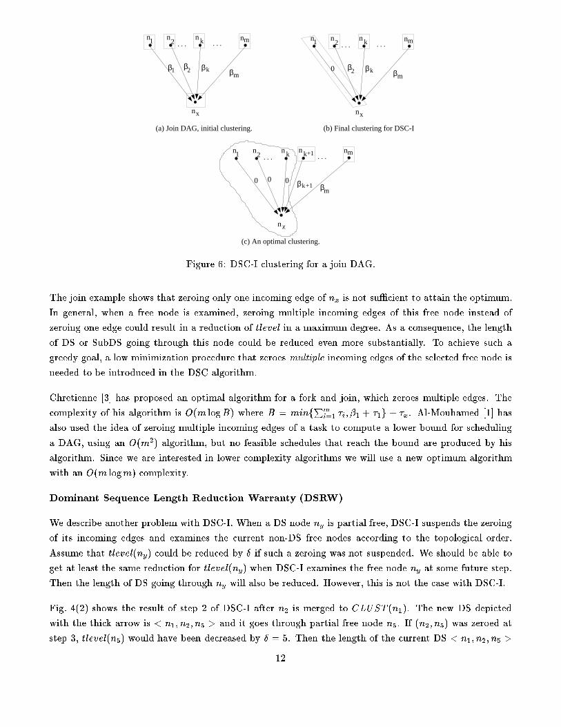
DSC-I for join DAGs
Let us consider the DSC-I algorithm for join DAGs.
Fig. 6 shows a join DAG, the �nal clustering and the optimum clustering. Again we assume that �
j
+�
j
�
�
j+1
+ �
j+1
; j = 1 :m� 1: The steps of DSC-I are described below.
Fig. 6(a) shows the initial clustering. Nodes n
1
; n
2
; � � � ; n
m
are free. One DS is < n
1
; n
x
>. Step 1 selects
n
1
which is in DS. No incoming edge exists for n
1
and no zeroing is performed. The DS is still < n
1
; n
x
>
after step 1. Now n
x
becomes partially free. A node is partial free if it is in UEG and at least one of
its predecessors has been examined but not all of its predecessors have been examined. Step 2 selects n
2
which is not in DS. No incoming edge exists and n
2
remains in a unit cluster in EG. Step m+1 selects n
x
which is now in the DS and then (n
1
; n
x
) is zeroed. The �nal result of DSC-I is shown in Fig. 6(b) which
may not be optimal. The optimal result for a join DAG shown in Fig. 6(c) is symmetric to the previous
optimal solution for a fork.
11
. . . . . .
x
mk21
n
nnnn
mk21β β β β
. . . . . .
x
mk21
n
nnnn
mk2β β β0
(a) Join DAG, initial clustering. (b) Final clustering for DSC-I
. . . . . .
x
21
n
nn mnkn kn
0 0 0
+1
kβ +1mβ
(c) An optimal clustering.
Figure 6: DSC-I clustering for a join DAG.
The join example shows that zeroing only one incoming edge of n
x
is not su�cient to attain the optimum.
In general, when a free node is examined, zeroing multiple incoming edges of this free node instead of
zeroing one edge could result in a reduction of tlevel in a maximum degree. As a consequence, the length
of DS or SubDS going through this node could be reduced even more substantially. To achieve such a
greedy goal, a low minimization procedure that zeroes multiple incoming edges of the selected free node is
needed to be introduced in the DSC algorithm.
Chretienne [3] has proposed an optimal algorithm for a fork and join, which zeroes multiple edges. The
complexity of his algorithm is O(m logB) where B = minf
P
m
i=1
�
i
; �
1
+ �
1
g + �
x
. Al-Mouhamed [1] has
also used the idea of zeroing multiple incoming edges of a task to compute a lower bound for scheduling
a DAG, using an O(m
2
) algorithm, but no feasible schedules that reach the bound are produced by his
algorithm. Since we are interested in lower complexity algorithms we will use a new optimum algorithm
with an O(m logm) complexity.
Dominant Sequence Length Reduction Warranty (DSRW)
We describe another problem with DSC-I. When a DS node n
y
is partial free, DSC-I suspends the zeroing
of its incoming edges and examines the current non-DS free nodes according to the topological order.
Assume that tlevel(n
y
) could be reduced by � if such a zeroing was not suspended. We should be able to
get at least the same reduction for tlevel(n
y
) when DSC-I examines the free node n
y
at some future step.
Then the length of DS going through n
y
will also be reduced. However, this is not the case with DSC-I.
Fig. 4(2) shows the result of step 2 of DSC-I after n
2
is merged to CLUST (n
1
). The new DS depicted
with the thick arrow is < n
1
; n
2
; n
5
> and it goes through partial free node n
5
. If (n
2
; n
5
) was zeroed at
step 3, tlevel(n
5
) would have been decreased by � = 5. Then the length of the current DS < n
1
; n
2
; n
5
>
12
would also have been reduced by 5. But due to the topological traversal rule, a free task n
4
is selected
at step 3 because PRIO(n
4
) = 9 � PRIO(n
3
) = 4:5. Then n
4
is merged to CLUST (n
1
) since tlevel(n
4
)
can be reduced from 3 to �
1
+ �
2
= 2:5. Such process a�ects the future compression of DS < n
1
; n
2
; n
5
>.
When n
5
is free at step 5, tlevel(n
5
) = �
1
+ �
2
+ c
2;5
= 7:5 and it is impossible to reduce tlevel(n
5
)
further by moving it to CLUST (n
2
). This is because n
5
will have to be linked after n
4
, which makes
tlevel(n
5
) = �
1
+ �
2
+ �
4
= 8:5.
4 The Final Form of the DSC Algorithm
The main improvements to DSC-I are the minimization procedure for tlevel(n
f
), maintaining a partial free
list(PFL) and imposing the constraint DSRW.
4.1 Priority Lists
At each clustering step, we maintain two node priority lists, a partial free list PFL and a free list FL
both sorted in a descending order of their task priorities. When two tasks have the same priority we
choose the one with the most immediate successors. If there is still a tie, we break it randomly. Function
head(L) returns the �rst node in the sorted list L, which is the task with the highest priority. If L = fg,
head(L) = NULL and the priority value is set to 0.
The tlevel value of a node is propagated to its successors only after this node has been examined. Thus
the priority value of a partial free node can be updated using only the tlevel from its examined immediate
predecessors. Because only part of predecessors are considered, we de�ne the priority of a partial free task:
pPRIO(n
y
) = ptlevel(n
y
) + blevel(n
y
); ptlevel(n
y
) = max
n
j
2PRED(n
y
)
T
EG
ftlevel(n
j
) + �
j
+ c
j;y
g:
In general, pPRIO(n
y
) � PRIO(n
y
) and if a DS goes through an edge (n
j
; n
y
) where n
j
is an examined
predecessor of n
y
, then we have pPRIO(n
y
) = PRIO(n
j
) = PRIO(n
y
). By maintaining pPRIO instead
of PRIO the complexity is reduced considerably. As we will prove later maintaining pPRIO does not
adversely a�ect the performance of DSC since it can still correctly identify the DS at each step. The DSC
algorithm is described in Fig. 7.
4.2 The minimization procedure for zeroing multiple incoming edges
To reduce tlevel(n
x
) in DSC a minimization procedure that zeroes multiple incoming edges of free task n
x
is needed. An optimal algorithm for a join DAG has been described in [9] and an optimal solution is shown
in Fig. 6(c). The basic procedure is to �rst sort the nodes such that �
j
+ �
j
� �
j+1
+ �
j+1
; j = 1 :m� 1,
and then zeroes edges from left to right as long as the parallel time reduces after each zeroing, i.e. linear
searching of the optimal point. This is equivalent to satisfying the condition (
P
k�1
j=1
�
j
� �
k
) for each
13
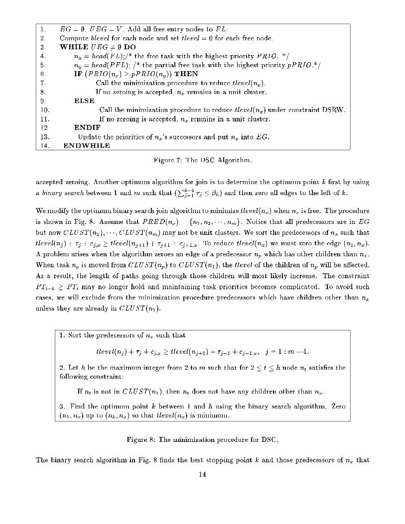
1. EG = ;. UEG = V . Add all free entry nodes to FL.
2. Compute blevel for each node and set tlevel = 0 for each free node.
3. WHILE UEG 6= ; DO
4. n
x
= head(FL);/* the free task with the highest priority PRIO. */
5. n
y
= head(PFL); /* the partial free task with the highest priority pPRIO.*/
6. IF (PRIO(n
x
) � pPRIO(n
y
)) THEN
7. Call the minimization procedure to reduce tlevel(n
x
).
8. If no zeroing is accepted, n
x
remains in a unit cluster.
9. ELSE
10. Call the minimization procedure to reduce tlevel(n
x
) under constraint DSRW.
11. If no zeroing is accepted, n
x
remains in a unit cluster.
12 ENDIF
13. Update the priorities of n
x
's successors and put n
x
into EG.
14. ENDWHILE
Figure 7: The DSC Algorithm.
accepted zeroing. Another optimum algorithm for join is to determine the optimum point k �rst by using
a binary search between 1 and m such that (
P
k�1
j=1
�
j
� �
k
) and then zero all edges to the left of k.
We modify the optimum binary search join algorithm to minimize tlevel(n
x
) when n
x
is free. The procedure
is shown in Fig. 8. Assume that PRED(n
x
) = fn
1
; n
2
; � � � ; n
m
g. Notice that all predecessors are in EG
but now CLUST (n
1
); � � � ; CLUST (n
m
) may not be unit clusters. We sort the predecessors of n
x
such that
tlevel(n
j
) + �
j
+ c
j;x
� tlevel(n
j+1
) + �
j+1
+ c
j+1;x
. To reduce tlevel(n
x
) we must zero the edge (n
1
; n
x
).
A problem arises when the algorithm zeroes an edge of a predecessor n
p
which has other children than n
x
.
When task n
p
is moved from CLUST (n
p
) to CLUST (n
1
), the tlevel of the children of n
p
will be a�ected.
As a result, the length of paths going through those children will most likely increase. The constraint
PT
i�1
� PT
i
may no longer hold and maintaining task priorities becomes complicated. To avoid such
cases, we will exclude from the minimization procedure predecessors which have children other than n
x
unless they are already in CLUST (n
1
).
1. Sort the predecessors of n
x
such that
tlevel(n
j
) + �
j
+ c
j;x
� tlevel(n
j+1
) + �
j+1
+ c
j+1;x
; j = 1 :m� 1:
2. Let h be the maximum integer from 2 to m such that for 2 � t � h node n
t
satis�es the
following constraint:
If n
t
is not in CLUST (n
1
), then n
t
does not have any children other than n
x
.
3. Find the optimum point k between 1 and h using the binary search algorithm. Zero
(n
1
; n
x
) up to (n
k
; n
x
) so that tlevel(n
x
) is minimum.
Figure 8: The minimization procedure for DSC.
The binary search algorithm in Fig. 8 �nds the best stopping point k and those predecessors of n
x
that
14
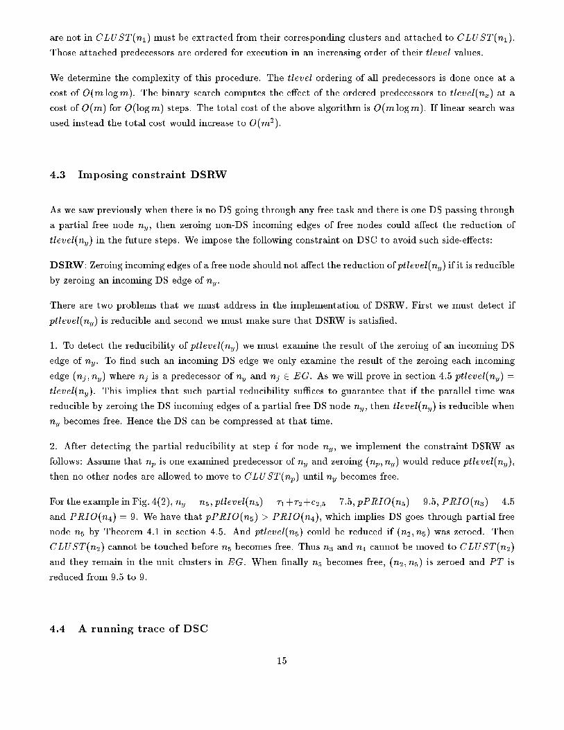
are not in CLUST (n
1
) must be extracted from their corresponding clusters and attached to CLUST (n
1
).
Those attached predecessors are ordered for execution in an increasing order of their tlevel values.
We determine the complexity of this procedure. The tlevel ordering of all predecessors is done once at a
cost of O(m logm). The binary search computes the e�ect of the ordered predecessors to tlevel(n
x
) at a
cost of O(m) for O(logm) steps. The total cost of the above algorithm is O(m logm). If linear search was
used instead the total cost would increase to O(m
2
).
4.3 Imposing constraint DSRW
As we saw previously when there is no DS going through any free task and there is one DS passing through
a partial free node n
y
, then zeroing non-DS incoming edges of free nodes could a�ect the reduction of
tlevel(n
y
) in the future steps. We impose the following constraint on DSC to avoid such side-e�ects:
DSRW: Zeroing incoming edges of a free node should not a�ect the reduction of ptlevel(n
y
) if it is reducible
by zeroing an incoming DS edge of n
y
.
There are two problems that we must address in the implementation of DSRW. First we must detect if
ptlevel(n
y
) is reducible and second we must make sure that DSRW is satis�ed.
1. To detect the reducibility of ptlevel(n
y
) we must examine the result of the zeroing of an incoming DS
edge of n
y
. To �nd such an incoming DS edge we only examine the result of the zeroing each incoming
edge (n
j
; n
y
) where n
j
is a predecessor of n
y
and n
j
2 EG. As we will prove in section 4.5 ptlevel(n
y
) =
tlevel(n
y
). This implies that such partial reducibility su�ces to guarantee that if the parallel time was
reducible by zeroing the DS incoming edges of a partial free DS node n
y
, then tlevel(n
y
) is reducible when
n
y
becomes free. Hence the DS can be compressed at that time.
2. After detecting the partial reducibility at step i for node n
y
, we implement the constraint DSRW as
follows: Assume that n
p
is one examined predecessor of n
y
and zeroing (n
p
; n
y
) would reduce ptlevel(n
y
),
then no other nodes are allowed to move to CLUST (n
p
) until n
y
becomes free.
For the example in Fig. 4(2), n
y
= n
5
, ptlevel(n
5
) = �
1
+�
2
+c
2;5
= 7:5, pPRIO(n
5
) = 9:5, PRIO(n
3
) = 4:5
and PRIO(n
4
) = 9. We have that pPRIO(n
5
) > PRIO(n
4
), which implies DS goes through partial free
node n
5
by Theorem 4.1 in section 4.5. And ptlevel(n
5
) could be reduced if (n
2
; n
5
) was zeroed. Then
CLUST (n
2
) cannot be touched before n
5
becomes free. Thus n
3
and n
4
cannot be moved to CLUST (n
2
)
and they remain in the unit clusters in EG. When �nally n
5
becomes free, (n
2
; n
5
) is zeroed and PT is
reduced from 9.5 to 9.
4.4 A running trace of DSC
15
n1
n 6
n3n2
n4
n7
n5
1
6 1
1
2
1
1
3
2
2.5
41
2.5
(0) (1)
n1
n 6
n3n2
n4
n7
n5
(2)
n1
n 6
n3n2
n4
n7
n5
n1
n 6
n3n2
n4
n7
n5
n1
n 6
n3n2
n4
n7
n5
(7)(6)(5)
0.5
n1
n 6
n3n2
n4
n7
n5
EG
UEG
UEG
UEGUEG
EG
EG
EGUEG
EG
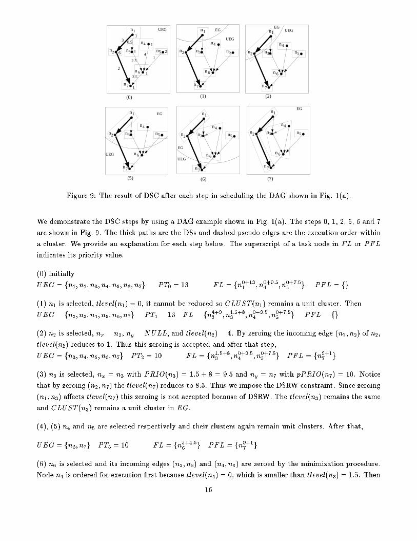
Figure 9: The result of DSC after each step in scheduling the DAG shown in Fig. 1(a).
We demonstrate the DSC steps by using a DAG example shown in Fig. 1(a). The steps 0, 1, 2, 5, 6 and 7
are shown in Fig. 9. The thick paths are the DSs and dashed pseudo edges are the execution order within
a cluster. We provide an explanation for each step below. The superscript of a task node in FL or PFL
indicates its priority value.
(0) Initially
UEG = fn
1
; n
2
; n
3
; n
4
; n
5
; n
6
; n
7
g PT
0
= 13 FL = fn
0+13
1
; n
0+9:5
4
; n
0+7:5
5
g PFL = fg
(1) n
1
is selected, tlevel(n
1
) = 0, it cannot be reduced so CLUST (n
1
) remains a unit cluster. Then
UEG = fn
2
; n
3
; n
4
; n
5
; n
6
; n
7
g PT
1
= 13 FL = fn
4+9
2
; n
1:5+8
3
; n
0+9:5
4
; n
0+7:5
5
g PFL = fg
(2) n
2
is selected, n
x
= n
2
, n
y
= NULL, and tlevel(n
2
) = 4. By zeroing the incoming edge (n
1
; n
2
) of n
2
,
tlevel(n
2
) reduces to 1. Thus this zeroing is accepted and after that step,
UEG = fn
3
; n
4
; n
5
; n
6
; n
7
g PT
2
= 10 FL = fn
1:5+8
3
; n
0+9:5
4
; n
0+7:5
5
g PFL = fn
9+1
7
g
(3) n
3
is selected, n
x
= n
3
with PRIO(n
3
) = 1:5 + 8 = 9:5 and n
y
= n
7
with pPRIO(n
7
) = 10. Notice
that by zeroing (n
2
; n
7
) the tlevel(n
7
) reduces to 8.5. Thus we impose the DSRW constraint. Since zeroing
(n
1
; n
3
) a�ects tlevel(n
7
) this zeroing is not accepted because of DSRW. The tlevel(n
3
) remains the same
and CLUST (n
3
) remains a unit cluster in EG.
(4), (5) n
4
and n
5
are selected respectively and their clusters again remain unit clusters. After that,
UEG = fn
6
; n
7
g PT
5
= 10 FL = fn
5+4:5
6
g PFL = fn
9+1
7
g
(6) n
6
is selected and its incoming edges (n
3
; n
6
) and (n
4
; n
6
) are zeroed by the minimization procedure.
Node n
4
is ordered for execution �rst because tlevel(n
4
) = 0, which is smaller than tlevel(n
3
) = 1:5. Then
16
tlevel(n
6
) is reduced to 2.5 and
UEG = fn
7
g PT
6
= 10 FL = fn
9+1
7
g PFL = fg
(7), n
7
is selected and (n
2
; n
7
) is zeroed so that tlevel(n
7
) is reduced from 9 to 7.
UEG = fg PT
7
= 8 FL = fg PFL = fg
Finally three clusters are generated with PT = 8.
4.5 DSC Properties
In this section, we study several properties of DSC related to the identi�cation of DS, the reduction of the
parallel time and the computational complexity. Theorem 4.1 indicates that DSC (Line 6 and 9 in Fig. 7)
correctly locates DS nodes at each step even if we use the partial priority pPRIO. Theorems 4.2 and 4.3
show how DSC warranties in the reduction of the parallel time. Theorem 4.4 derives the complexity.
The correctness in locating DS nodes
The goal of DSC is to reduce the DS in a sequence of steps. To do that it must correctly identify unexamined
DS nodes. In this subsection, we assume that a DS goes through UEG, since it is only then that DSC needs
to identify and compress DS. If DS does not go through UEG but only through EG, then all DS nodes
have been examined and the DS can no longer be compressed because backtracking is not allowed.
Since the DSC algorithm examines the nodes topologically the free list FL is always non-empty. By
de�nition all tasks in FL and PFL are in UEG. It is obvious that a DS must go through tasks in either
FL or PFL, when it goes through UEG. The interesting question is if a DS also goes through the heads
of the priority lists of FL and PFL, since then the priority lists will correctly identify DS nodes to be
examined. The answer is given in the following two Lemmas and Theorem.
Lemma 4.1 Assume that n
x
= head(FL) after step i. If there are DSs going through free nodes in FL,
then one DS must go through n
x
.
Proof: At the completion of step i the parallel time is PT
i
= PRIOR(n
s
), where n
s
is a DS node. Assume
that no DS goes through n
x
. Then one DS must go through another non-head free node n
f
. This implies
that PRIO(n
f
) = PT
i
> PRIO(n
x
), which is a contradiction because n
x
has the highest priority in FL.
2
Lemma 4.2 Assume that n
y
= head(PFL) after step i. If DSs only go through partial free nodes in PFL,
then one DS must go through n
y
. Moreover, pPRIO(n
y
) = PRIO(n
y
).
Proof: First observe that the starting node of a DS must be an entry node of this DAG. If this node
17
is in UEG, then it must be free which is impossible since the assumption says that DSs only go through
partial free nodes in UEG. Thus the starting node must be in EG. As a result a DS must start from
a node in EG and go through an examined node n
j
to its unexamined partial free successor n
p
. Then
because they are in the same DS we have that PRIO(n
p
) = PRIO(n
j
) = pPRIO(n
p
). The proof
now becomes similar to the previous Lemma. Suppose that no DS goes through n
y
. We have that
pPRIO(n
y
) � PRIO(n
y
) < PT
i
= PRIO(n
p
) = pPRIO(n
p
) which contradicts the assumption that n
y
is
the head of PFL.
Next we prove that pPRIO(n
y
) = PRIO(n
y
). Suppose pPRIO(n
y
) < PRIO(n
y
). This implies that
the DS, where n
y
belongs to, does not pass through any examined immediate predecessor of n
y
. As
a result DS must go through some other nodes in UEG. Thus, there exists an ancestor node n
a
of
n
y
, such that the DS passes through an edge (n
q
; n
a
) where n
q
is the examined predecessor of n
a
and
n
a
is partial free since it is impossible to be free by the assumptions of this Lemma. We have that
pPRIO(n
a
) = PRIO(n
a
) = PRIO(n
y
) > pPRIO(n
y
) which shows n
y
is not the head of PFL. This a
contradiction. 2
The following theorem shows that the condition PRIO(n
x
) � pPRIO(n
y
) used by DSC algorithm in Line
6 of Fig. 7), correctly identi�es DS nodes.
Theorem 4.1 Assume that n
x
= head(FL) and n
y
= head(PFL) after step i and that there is a DS going
through UEG. If PRIO(n
x
) � pPRIO(n
y
) then a DS goes through n
x
. If PRIO(n
x
) < pPRIO(n
y
), then
the DS it goes through n
y
and also does not go through any free node in FL.
Proof: If PRIO(n
x
) � pPRIO(n
y
), then we will show that DS goes through n
x
. First assume DS
goes through FL or both FL and PFL. Then according to Lemma 4.1 it must go through n
x
. Next
assume that DS goes through PFL only. Then from Lemma 4.2 it must go through n
y
, implying that
pPRIO(n
y
) = PRIO(n
y
) = PT
i
> PRIO(n
x
) which is a contradiction since PRIO(n
x
) � pPRIO(n
y
).
If PRIO(n
x
) < pPRIO(n
y
), suppose that a DS passes a free node. Then according to Lemma 4.1,
PRIO(n
x
) = PT
i
� PRIO(n
y
) � pPRIO(n
y
) which is a contradiction again. Thus the DSs must go
through partial free nodes and one of them must go through n
y
by Lemma 4.2. 2
The warranty in reducing parallel time
In this subsection, we show that if the parallel time could be reduced at some clustering step then the
DSC algorithm makes sure that the parallel time will be reduced before the algorithm terminates. The
�rst Lemma gives an expression for the parallel time in terms of the priorities. The second Lemma shows
that the parallel time cannot increase from one step to the next. The Theorem proves that the parallel
time will be reduced if it is known that it is reducible. A Corollary of the Theorem gives an even stronger
result for the reduction of the parallel time. If it can be detected that the parallel time is reducible by a
certain amount at some step, the DSC guarantees that the reduction of the parallel time will be at least
as much as this amount.
18
Lemma 4.3 Assume that n
x
= head(FL) and n
y
= head(PFL) after step i. The parallel time for
executing the clustered graph after step i of DSC is:
PT
i
= maxfPRIO(n
x
); pPRIO(n
y
); max
n
e
2EG
fPRIO(n
e
)gg:
Proof: There are three cases in the proof. (1) If DS nodes are only within EG, then by de�nition
PT
i
= max
n
e
2EG
fPRIO(n
e
)g: (2) If a DS goes through a free node, then PT
i
= PRIO(n
x
) by Lemma 4.1.
(3) If there is a DS passing through UEG but this DS only passes through partial free nodes, then
PT
i
= PRIO(n
y
) = pPRIO(n
y
) by Lemma 4.2 . 2
Theorem 4.2 For each step i of DSC, PT
i�1
� PT
i
.
Proof: For this proof we rename the priority values of n
x
= head(FL), and n
y
= head(PFL) after step
i� 1 as PRIO(n
x
; i� 1) and pPRIO(n
y
; i� 1) respectively. We need to prove, that PT
i�1
� PT
i
, where
PT
i�1
= maxfPRIO(n
x
; i� 1); pPRIO(n
y
; i� 1); max
n
e
2EG
fPRIO(n
e
; i� 1)gg
PT
i
= maxfPRIO(n
�
x
; i); pPRIO(n
�
y
; i); max
n
e
2EG
S
fn
x
g
fPRIO(n
e
; i)gg
and n
�
x
and n
�
y
are the new heads of FL and PFL after step i.
We prove �rst that PRIO(n
�
x
; i) � PT
i�1
Since n
�
x
is in the free list after step i� 1, it must be in UEG and also it must be either the successor of
n
x
or it is independent to n
x
. At step i, DSC picks up task n
x
to examine its incoming edges for zeroing.
We consider the e�ect of such zeroing on the priority value of n
�
x
. Since the minimization procedure does
not increase tlevel(n
x
), the length of the paths going through n
x
decreases or remains unchanged. Thus
the priority values of the descendants of n
x
could decrease but not increase. The priority values of other
nodes in EG remain the same since the minimization procedure excludes those predecessors of n
x
that
have children other than n
x
. Thus if n
�
x
is the successor of n
x
, then PRIO(n
�
x
; i) � PRIO(n
�
x
; i � 1),
otherwise PRIO(n
�
x
; i) = PRIO(n
�
x
; i� 1). Since PRIO(n
�
x
; i� 1) � PT
i�1
, then PRIO(n
�
x
; i) � PT
i�1
.
Similarly we can prove that PRIO(n
�
y
; i) � PT
i�1
.
Next we prove that max
n
e
2EG
S
fn
x
g
fPRIO(n
e
; i)gg � PT
i�1
. We have PRIO(n
x
; i) � PRIO(n
x
; i� 1)
from the minimization procedure. We only need to examine the e�ect of zeroing for n
x
on the priorities
of nodes in EG. The minimization procedure may increase the tlevel values of some predecessors of n
x
,
say n
p
, but it guarantees that the length of the paths going through n
p
and n
x
do not increase. Thus the
new value of PRIO(n
p
) satis�es PRIO(n
p
; i) � PRIO(n
x
; i� 1). Since PRIO(n
x
; i� 1) � PT
i�1
, then
PRIO(n
p
; i) � PT
i�1
.
The minimization procedure may also increase the blevel values of some nodes in the cluster in EG to
which n
x
is attached. A pseudo edge is added from the last node of that cluster, say n
e
, to n
x
if n
e
19
and n
x
are independent. If there is an increase in the priority value of n
e
, then the reason must be that
adding this pseudo edge introduces a new path going through n
x
with longer length compared with the
other existing paths for n
e
. Since the minimization procedure has considered the e�ect of attaching n
x
after n
e
on tlevel(n
x
), the length of paths will be less than or equal to PRIO(n
x
; i� 1) � PT
i�1
. Thus
PRIO(n
e
; i) � PT
i�1
. Similarly we can prove that other nodes in CLUST (n
e
) satisfy this inequality.
Since the priority values of nodes, say n
o
, that are not the predecessors of n
x
or not in CLUST (n
e
)
will not be a�ected by the minimization procedure, we have PRIO(n
o
; i � 1) = PRIO(n
o
; i). Thus
max
n
e
2EG
S
fn
x
g
fPRIO(n
e
; i)gg � PT
i�1
. 2
Theorem 4.3 After step i of DSC, if the current parallel time is reducible by zeroing one incoming edge
of a node in UEG, then DSC guarantees that the parallel time will be reduced at some step greater or equal
to i+ 1.
Proof: The assumption that the parallel time reduces by zeroing one edge (n
r
; n
s
), implies that a DS must
go through UEG. This implies that the edge (n
r
; n
s
) belongs to all DSs that go through UEG, otherwise
the parallel time is not reducible. There are three cases:
(1) n
r
2 EG and n
s
is free.
We prove that the node n
s
must be the head of FL. If it is not, then another free node in UEG, n
f
,
must have the same priority and thus belong to a DS. Because all DSs go through (n
r
; n
s
), n
f
must be a
predecessor of n
s
implying that n
s
is partial free which is a contradiction.
Also since PT
i
= blevel(n
s
) + tlevel(n
s
) is reducible by zeroing (n
r
; n
s
), and blevel(n
s
) does not change
by such a zeroing, then tlevel(n
s
) is reducible. Thus during the DSC execution, n
s
= head(FL) will be
picked up at step i+1, and since tlevel(n
s
) is reducible the minimization procedure will accept the zeroing
of (n
r
; n
s
) and the parallel time will reduce at that step.
(2) n
r
2 EG and n
s
is partial free.
Since all DSs go through (n
r
; n
s
), no free nodes are in DSs and other partial free nodes, n
f
in the DSs must
be successors of n
s
. Thus pPRIO(n
s
) = PRIO(n
s
) but pPRIO(n
f
) < PRIO(n
f
). Since PRIO(n
f
) =
PRIO(n
s
) then pPRIO(n
f
) < pPRIO(n
s
) and n
s
must be the head of PFL.
Assume that PT
i
= blevel(n
s
) + ptlevel(n
s
) is reducible by � > 0 when zeroing (n
r
; n
s
), and blevel(n
s
)
does not change by such a zeroing. Then ptlevel(n
s
) is reducible by at least �. Thus, during the execution
of DSC, the reducibility of ptlevel(n
s
) will be detected at step i+ 1. Afterwards non-DS edges are zeroed
until n
s
becomes free. However, the reducibility of ptlevel(n
s
) is not a�ected by such zeroings because of
DSRW. A non-DS node remains a non-DS node and no other nodes are moved to CLUST (n
r
). When n
s
becomes free, ptlevel(n
s
) is still reducible by at least �, and since other SubDS either decrease or remain
unchanged, then the parallel time is also reducible by at least �. The rest of the proof becomes the same
as in the previous case.
(3) n
r
2 UEG.
20
Assume that n
r
becomes examined at step j � i + 1. At step i + 1 all DSs must go through (n
r
; n
s
). If
from i+1 to step j the parallel time has been reduced then the theorem is true. If the parallel time has not
been reduced then at least one DS has not been compressed and all DSs still go through (n
r
; n
s
) because
the minimization procedure guarantees that no other DSs will be created. Thus the parallel time will be
reducible at step j and the proof becomes the same as in the above cases. 2
The following corollary is the direct result of Case 2 in the above Theorem.
Corollary 4.3 Assume that n
y
2 PFL, n
y
2 DS at step i and that zeroing of an incoming edge of n
y
from a scheduled predecessor would have reduced PT by �. Then DSC guarantees that when n
y
becomes
free at step j (j > i), PT can be reduced by at least �.
The complexity
Lemma 4.4 For any node n
s
in FL or PFL, tlevel(n
j
) for n
j
2 PRED(n
s
)
T
EG remains constant after
n
j
is examined, and blevel(n
s
) remains constant until it is examined.
Proof: Referring to Property 3.2 of DSC-I, DSC is the same as DSC-I except that the minimization
procedure changes tlevel values of some examined predecessors, say n
h
, of the currently-selected free task,
say n
x
. But such change does not a�ect any node in FL or PFL since n
h
does not have children other
than n
x
. 2
Theorem 4.4 The time complexity of DSC is O((v + e) log v) and the space complexity is O(v + e).
Proof: The di�erence in the complexity between DSC-I and DSC results from the minimization proce-
dure within the While loop in Fig. 7. In DSC we also maintain PFL but the cost for the v steps is the
same O(v log v) when we use the balanced search trees. Therefore, for Line 4 and 5 in Fig. 7, v steps cost
O(v log v). For Line 7 and 8 (or Line 9 and 10), the minimization procedure costsO(jPRED(n
x
)j log jPRED(n
x
)j)
at each step. Since
P
n
x
2V
jPRED(n
x
)j = e and jPRED(n
x
)j < v, v steps cost O(e log v).
For Line 13, the tlevel values of the successors of n
x
are updated. Those successors could be in PFL and
the list needs to be rearranged since their pPRIO values could be changed. The cost of adjusting each
successor in PFL is O(log jPFLj) where jPFLj < v. The step cost for Line 13 is O(jSUCC(n
x
)j logv).
Since
P
n
x
2V
jSUCC(n
x
)j = e, the total cost for maintaining PFL during v steps is O(e log v).
Also for Line 13 when one successor becomes free, it needs to be added to FL with cost O(log jFLj) where
jFLj � v. Since there are total v task that could become free during v steps, the total cost in Line 13
spent for FL during v steps is O(v log v).
Notice that according to lemma 4.4, after n
x
has been moved to EG at Line 13, its tlevel value will not
a�ect the priority of tasks in PFL and FL in the rest of steps. Thus the updating of FL or PFL occurs
only once with respect to each task. Thus the overall time complexity is O((e+v) log v). The space needed
for DSC is to store the DAG and FL=PFL. The space complexity is O(v + e). 2
21
5 Performance Bounds and Optimality of DSC
In this section we study the performance characteristics of DS. We give an upper bound for a general
DAG and prove the optimality for forks, joins, coarse grain trees and a class of �ne grain trees. Since this
scheduling problem is NP-complete for a general �ne grain tree and for a DAG which is a concatenation of
a fork and a join (series parallel DAG) [3, 5], the analysis shows that DSC not only has a low complexity
but also attains an optimality degree that a general polynomial algorithm could achieve.
5.1 Performance bounds for general DAGs
A DAG consists of fork (F
x
) and/or join (J
x
) structures such as the ones shown in Fig. 5(a) and 6(a).
In [9], we de�ne the grain of DAG as follows:
Let
g(F
x
) = min
k=1:m
f�
k
g= max
k=1:m
fc
x;k
g; g(J
x
) = min
k=1:m
f�
k
g= max
k=1:m
fc
k;x
g:
Then the granularity of G is: g(G) = min
n
x
2V
fg
x
g where g
x
= minfg(F
x
); g(J
x
)g
We call a DAG coarse grain if g(G) � 1. For a coarse grain DAG, each task receives or sends a small
amount of communication compared to the computation of its neighboring tasks. In [9], we prove the
following two theorems:
Theorem 5.1 For a coarse grain DAG, there exists a linear clustering that attains the optimal solution.
Theorem 5.2 Let PT
opt
be the optimum parallel time and PT
lc
be the parallel time of a linear clustering,
then PT
lc
� (1 +
1
g(G)
)PT
opt
: For a coarse grain DAG, PT
lc
� 2� PT
opt
:
The following theorem is a performance bound of DSC for a general DAG.
Theorem 5.3 Let PT
dsc
be the parallel time by DSC for a DAG G, then PT
dsc
� (1 +
1
g(G)
)PT
opt
: For a
coarse grain DAG, PT
dsc
� 2� PT
opt
:
Proof: In the initial step of DSC, all nodes are in the separate clusters, which is a linear clustering. By
Theorem 5.2 and Theorem 4.2 we have that
PT
dsc
� : : : � PT
k
� : : :� PT
1
� PT
0
� (1 +
1
g(G)
)PT
opt
:
For coarse grain DAGs the statement is obvious. 2
22
5.2 Optimality for join and fork
Theorem 5.4 DSC derives optimal solutions for fork and join DAGs.
Proof: For a fork, DSC performs the exact same zeroing sequence as DSC-I. The clustering steps are
shown in Fig. 5. After n
x
is examined, DSC will examine free nodes n
1
; n
2
; � � � ; n
m
in a decreasing order of
their priorities. The priority value for each free node is the length of each path < n
x
; n
1
>, � � �, < n
x
; n
m
>.
If we assume that �
k
+ �
k
� �
k+1
+ �
k+1
for 1 � k � m� 1, then the nodes are sorted as n
1
, n
2
; � � � ; n
m
in
the free list FL.
We �rst determine the optimal time for the fork and then show that DSC achieves the optimum. Assume
the optimal parallel time to be PT
opt
. If PRIO(n
h
) = �
x
+ �
h
+ �
h
> PT
opt
for some h, then �
i
must have
been zeroed for i = 1 : h, otherwise we have a contradiction. All other edges i > h need not be zeroed
because zeroing such edge does not decrease PT but could increase PT . Let the optimal zeroing stopping
point be h and assume �
m+1
= �
m+1
= 0. Then the optimal PT is: PT
opt
= �
x
+max(
P
h
j=1
�
j
; �
h+1
+�
h+1
):
DSC zeroes edges from left to right as many as possible up to the point k as shown in Fig. 5(d) such that:
P
k�1
j=1
�
j
� �
k
and
P
k
j=1
�
j
> �
k+1
. We will prove that PT
opt
= PT
dsc
by contradiction. Suppose that
k 6= h and PT
opt
< PT
dsc
. There are two cases:
(1) If h < k, then
P
h
j=1
�
j
<
P
k
j=1
�
j
� �
k
+ �
k
� �
h+1
+ �
h+1
: Thus PT
opt
= �
x
+ �
h+1
+ �
h+1
�
�
x
+ �
k
+ �
k
� �
x
+max(
P
k
j=1
�
j
; �
k+1
+ �
k+1
) = PT
dsc
:
(2) If h > k, then since
P
h
j=1
�
j
�
P
k+1
j=1
�
j
> �
k+1
+�
k+1
� �
h+1
+�
h+1
, we have that PT
opt
= �
x
+
P
h
j=1
�
j
�
�
x
+max(
P
k
j=1
�
j
; �
k+1
+ �
k+1
) = PT
dsc
:
There is a contradiction in both cases.
For a join, the DSC uses the minimization procedure to minimize the tlevel value of the root and the
solution is symmetrical to the optimal result for a fork. 2
5.3 Optimality for in/out trees
An in-tree is a directed tree in which the root has outgoing degree zero and other nodes have the outgoing
degree one. An out-tree is a directed tree in which the root has incoming degree zero and other nodes have
the incoming degree one.
Scheduling in/out trees is still NP-hard in general as shown by Chretienne [5] and DSC will not give the
optimal solution. However, DSC will yield optimal solutions for coarse grain trees and a class of �ne grain
trees.
Coarse grain trees
23
Theorem 5.5 DSC gives an optimal solution for a coarse grain in-tree.
Proof: Since all paths in an in-tree go through the tree root, say n
x
, PT = tlevel(n
x
) + blevel(n
x
) =
tlevel(n
x
) + �
x
. We claim tlevel(n
x
) is minimized by DSC. We prove it by induction on the depth of the
in-tree (d). When d = 0, it is trivial. When d = 1, it is a join DAG and tlevel(n
x
) is minimized. Assume
it is true for d < k.
When d = k, let the predecessors of root n
x
be n
1
; � � � ; n
m
. Since each sub-tree rooted with n
i
has depth
< k and the disjoint subgraphs cannot be clustered together by DSC, DSC will obtain the minimum tlevel
time for each n
j
where 1 � j � m according to the induction hypothesis.
When n
x
becomes free, tlevel(n
x
) = max
1�j�m
fCT (n
j
)+c
j;x
g; CT (n
j
) = tlevel(n
j
)+�
j
. Without loss of
generality, assume that (n
1
; n
x
) is in a DS and tlevel(n
1
)+�
1
+c
1;x
has the highest value and tlevel(n
2
)+�
2
+
c
2;x
has the second highest value. DSC will zero (n
1
; n
x
), and tlevel(n
x
) = max(CT (n
1
);max
2�j�m
fCT (n
j
)+
c
j;x
g): (DSC will not zero anymore edges because of the coarse grain condition. DSC might zero (n
2
; n
x
)
when g(G) = 1, but tlevel(n
x
) does not decrease.)
We need to prove that tlevel(n
x
) is the smallest possible. Since the tree is coarse-grain, by Theorem 5.1,
linear clustering can be used for deriving the optimal solution. Thus we can assume S
�
is an optimal
schedule that uses linear clustering. Let tlevel
�
(n
j
) be the tlevel value of n
j
in schedule S
�
, and CT
�
(n
j
) =
tlevel
�
(n
j
) + �
j
, CT
�
(n
j
) � CT (n
j
) for 1 � j � m from the assumption that CT (n
j
) is minimum. Now
we will show that tlevel
�
(n
x
) � tlevel(n
x
). There are two cases:
(1) If in S
�
the zeroed incoming edge of n
x
is (n
1
; n
x
), then
tlevel
�
(n
x
) = max(CT
�
(n
1
); max
2�j�m
fCT
�
(n
j
) + c
j;x
g) � max(CT (n
1
); max
2�j�m
fCT (n
j
) + c
j;x
g) = tlevel(n
x
):
(2) If in S
�
the zeroed incoming edge of n
x
is not (n
1
; n
x
), say it is (n
m
; n
x
). Thus
tlevel
�
(n
x
) = max(CT
�
(n
m
); max
1�j�m�1
fCT
�
(n
j
) + c
j;x
g) � max(CT (n
m
); max
1�j�m�1
fCT (n
j
) + c
j;x
g):
Because of g(G) � 1, CT (n
1
) + c
1;x
� max
2�j�m
fCT (n
j
) + c
j;x
g; then tlevel
�
(n
x
) � CT (n
1
) + c
1;x
�
tlevel(n
x
): 2
DSC solves an in-tree in time O(v log v) where v is the number of nodes in this tree. Chretienne [4]
developed an O(v
2
) dynamic programming algorithm and Anger, Hwang and Chow [2] proposed an O(v)
algorithm for tree DAGs with the condition that all communication edge weights are smaller than the task
node execution weights, which are special cases of coarse grain tree DAGs. Both of these two algorithms
are only speci�c to this kind of trees.
For an out-tree, we can always inverse this DAG and use DSC to schedule the inverted graph. Then the
optimal solution can be obtained. We call this approach the backward dominant sequence clustering
3
.
3
In the actual DSC program, both backward and forward clusterings are performed and the one with the better solution
is chosen.
24
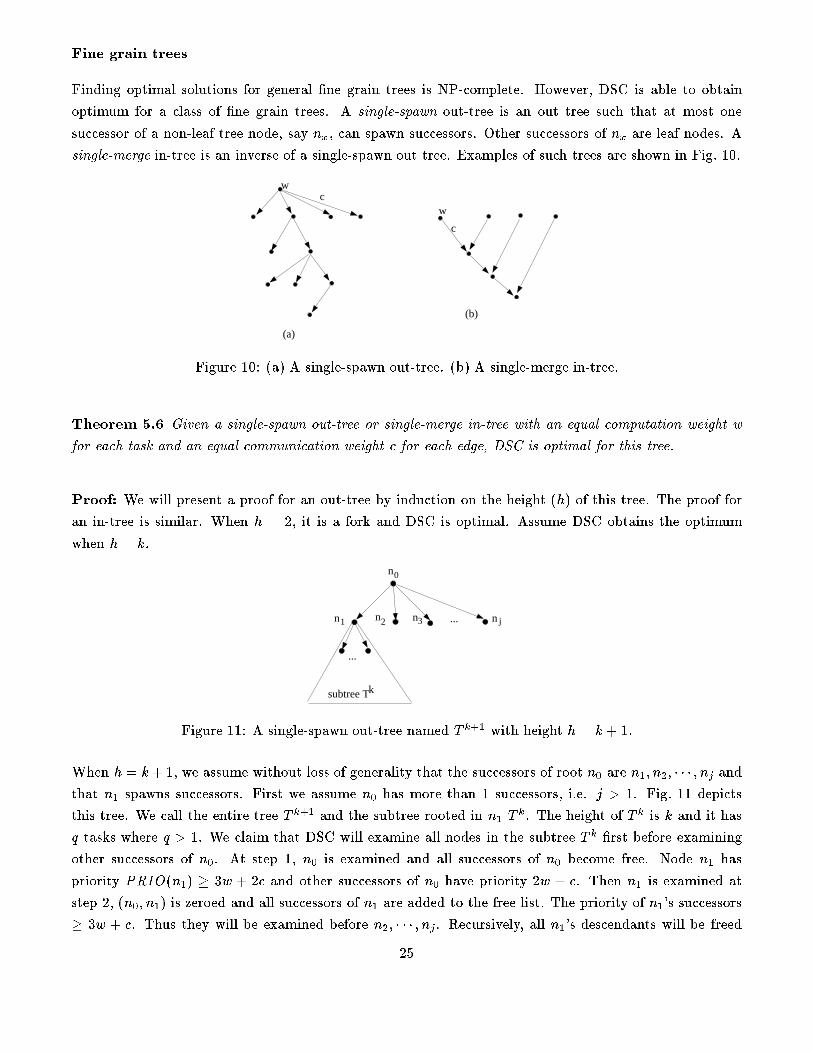
Fine grain trees
Finding optimal solutions for general �ne grain trees is NP-complete. However, DSC is able to obtain
optimum for a class of �ne grain trees. A single-spawn out-tree is an out tree such that at most one
successor of a non-leaf tree node, say n
x
, can spawn successors. Other successors of n
x
are leaf nodes. A
single-merge in-tree is an inverse of a single-spawn out tree. Examples of such trees are shown in Fig. 10.
(a)
(b)
wc
w
c
Figure 10: (a) A single-spawn out-tree. (b) A single-merge in-tree.
Theorem 5.6 Given a single-spawn out-tree or single-merge in-tree with an equal computation weight w
for each task and an equal communication weight c for each edge, DSC is optimal for this tree.
Proof: We will present a proof for an out-tree by induction on the height (h) of this tree. The proof for
an in-tree is similar. When h = 2, it is a fork and DSC is optimal. Assume DSC obtains the optimum
when h = k.
n1 n3n2 n j
n0
...
...
subtree Tk
Figure 11: A single-spawn out-tree named T
k+1
with height h = k + 1.
When h = k+ 1, we assume without loss of generality that the successors of root n
0
are n
1
; n
2
; � � � ; n
j
and
that n
1
spawns successors. First we assume n
0
has more than 1 successors, i.e. j > 1. Fig. 11 depicts
this tree. We call the entire tree T
k+1
and the subtree rooted in n
1
T
k
. The height of T
k
is k and it has
q tasks where q > 1. We claim that DSC will examine all nodes in the subtree T
k
�rst before examining
other successors of n
0
. At step 1, n
0
is examined and all successors of n
0
become free. Node n
1
has
priority PRIO(n
1
) � 3w + 2c and other successors of n
0
have priority 2w + c. Then n
1
is examined at
step 2, (n
0
; n
1
) is zeroed and all successors of n
1
are added to the free list. The priority of n
1
's successors
� 3w + c. Thus they will be examined before n
2
; � � � ; n
j
. Recursively, all n
1
's descendants will be freed
25
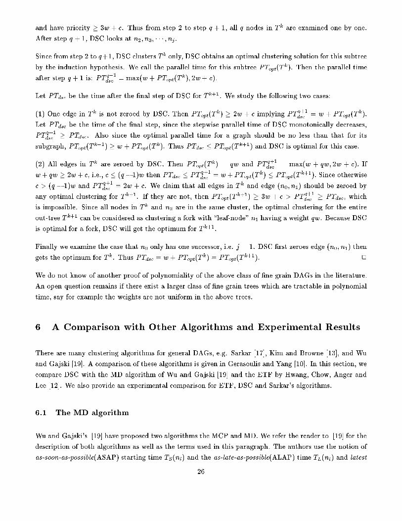
and have priority � 3w + c. Thus from step 2 to step q + 1, all q nodes in T
k
are examined one by one.
After step q + 1, DSC looks at n
2
; n
3
; � � � ; n
j
.
Since from step 2 to q+1, DSC clusters T
k
only, DSC obtains an optimal clustering solution for this subtree
by the induction hypothesis. We call the parallel time for this subtree PT
opt
(T
k
). Then the parallel time
after step q + 1 is: PT
q+1
dsc
= max(w + PT
opt
(T
k
); 2w+ c):
Let PT
dsc
be the time after the �nal step of DSC for T
k+1
. We study the following two cases:
(1) One edge in T
k
is not zeroed by DSC. Then PT
opt
(T
k
) � 2w + c implying PT
q+1
dsc
= w + PT
opt
(T
k
):
Let PT
dsc
be the time of the �nal step, since the stepwise parallel time of DSC monotonically decreases,
PT
q+1
dsc
� PT
dsc
. Also since the optimal parallel time for a graph should be no less than that for its
subgraph, PT
opt
(T
k+1
) � w + PT
opt
(T
k
). Thus PT
dsc
� PT
opt
(T
k+1
) and DSC is optimal for this case.
(2) All edges in T
k
are zeroed by DSC. Then PT
opt
(T
k
) = qw and PT
q+1
dsc
= max(w + qw; 2w + c): If
w+ qw � 2w+ c, i.e., c � (q� 1)w then PT
dsc
� PT
q+1
dsc
= w+ PT
opt
(T
k
) � PT
opt
(T
k+1
): Since otherwise
c > (q � 1)w and PT
q+1
dsc
= 2w + c. We claim that all edges in T
k
and edge (n
0
; n
1
) should be zeroed by
any optimal clustering for T
k+1
. If they are not, then PT
opt
(T
k+1
) � 3w + c > PT
q+1
dsc
� PT
dsc
, which
is impossible. Since all nodes in T
k
and n
0
are in the same cluster, the optimal clustering for the entire
out-tree T
k+1
can be considered as clustering a fork with \leaf-node" n
1
having a weight qw. Because DSC
is optimal for a fork, DSC will get the optimum for T
k+1
.
Finally we examine the case that n
0
only has one successor, i.e. j = 1. DSC �rst zeroes edge (n
0
; n
1
) then
gets the optimum for T
k
. Thus PT
dsc
= w + PT
opt
(T
k
) = PT
opt
(T
k+1
): 2
We do not know of another proof of polynomiality of the above class of �ne grain DAGs in the literature.
An open question remains if there exist a larger class of �ne grain trees which are tractable in polynomial
time, say for example the weights are not uniform in the above trees.
6 A Comparison with Other Algorithms and Experimental Results
There are many clustering algorithms for general DAGs, e.g. Sarkar [17], Kim and Browne [13], and Wu
and Gajski [19]. A comparison of these algorithms is given in Gerasoulis and Yang [10]. In this section, we
compare DSC with the MD algorithm of Wu and Gajski [19] and the ETF by Hwang, Chow, Anger and
Lee [12]. We also provide an experimental comparison for ETF, DSC and Sarkar's algorithms.
6.1 The MD algorithm
Wu and Gajski's [19] have proposed two algorithms the MCP and MD. We refer the reader to [19] for the
description of both algorithms as well as the terms used in this paragraph. The authors use the notion of
as-soon-as-possible(ASAP) starting time T
S
(n
i
) and the as-late-as-possible(ALAP) time T
L
(n
i
) and latest
26
�nishing time, T
F
(n
i
). The relative mobility of a node is de�ned by (T
L
(n
i
)� T
S
(n
i
))=w(n
i
) where w(n
i
)
is the task weight.
The MCP algorithm uses T
L
(n
i
) as a node priority. It then selects the free node with the smallest node
priority, which is equivalent to selecting the node with the largest blevel(n
i
), and schedules it to a processor
that allows its earliest starting time.
The MD algorithm uses the relative mobility as a node priority and at each step of scheduling, it identi�es
a task n
p
using the smallest relative mobility. It then examines the available processors starting from PE
0
and it schedules n
p
to the �rst processor that satis�es a condition called Fact 1 [19], pp. 336
4
. An intuitive
explanation for Fact 1 is that scheduling a task n
p
to a processor m should not increase the length of the
current critical path (DS).
The complexity of the original algorithm is O(v
3
) as shown in [19], pp. 337. The corrected version of MD
has a better performance but slightly higher complexity. This is because of the recomputation of T
S
and
T
F
for each scanned processor. For each scheduling step, the complexity of MD is O(p(v + e)) where p is
the number of scanned processors and O(v + e) for the mobility information and checking Fact 1 for each
processor, and since there are v steps the total complexity for the revised MD is O(pv(v+ e)).
The idea of identifying the important tasks in DSC is the same as in MD, i.e. the smallest relative mobility
identi�es DS nodes which have the maximum tlevel + blevel. However, the way to identify DS nodes is
di�erent. The DSC uses a priority function with an O(log v) computing scheme, while MD uses the relative
mobility function with a computing cost of O(v+ e). Another di�erence is that when DSC picks a DS task
n
p
to schedule, it uses the minimization procedure to reduce the tlevel of this task and thus decrease the
length of DS going through this task. On the other hand, the MD scans the processors from the left to
right to �nd the �rst processor satisfying Fact 1. Even though Fact 1 guarantees the non-increase of the
current critical path, it does not necessarily make the path length shorter.
For a fork or join, MD picks up the DS node at each step and we can show that it produces an optimal
solution. For a coarse grain tree, as we saw in our optimality proof, the tlevel must be reduced at each
step. Since the MD schedules a task to a processor which does not necessarily decrease the tlevel at each
step, the MD may not produce the optimum in general. A summary of this comparison is given in Table 2.
6.2 The ETF algorithm
ETF [12] is a scheduling algorithm for a bounded number of processors with arbitrary network topologies.
At each scheduling step, ETF �nds a free task whose starting time is the smallest and then assigns this
task to a processor in which the task execution can be started as early-as-possible. If there is a tie then
4
In a recent personal communication [20], the authors have made the following corrections to the MD algorithm presented
in [19]: (1) For Fact 1 when considering processor m, the condition \for each k" should change to \there exists k", [19], pp.
336. (2) The T
F
and T
S
computation [19], pp. 336, should assume that task n
p
is scheduled on processor m. (3) When n
p
is
scheduled to processor m, n
p
is inserted before the �rst task in the task sequence of processor m that satis�es the inequality
listed in Fact 1.
27
the task with the highest blevel is scheduled and this heuristic is called the ETF/CP in [12].
ETF is designed for scheduling on a bounded number of processors. Thus to compare the performance of
DSC and ETF we �rst apply DSC to determine the number of processors(clusters), which we then use as
an input to the ETF algorithm.
We discuss the di�erences and similarities of DSC and ETF as follows. For a node priority DSC uses
tlevel + blevel, and then selects the largest node priority. On the other hand, the ETF uses the earliest-
task-�rst which is similar to using tlevel as node priority and then selecting the smallest node priority
for scheduling. For the scheduling step DSC and ETF use the same idea, i.e. try to reduce tlevel by
scheduling to a processor that can start a task as early as possible. However, the technique for choosing
a processor is di�erent. ETF places a task to the processor that allows the earliest starting time without
re-scheduling its predecessors, while DSC uses the minimization procedure that could re-schedule some of
the predecessors. It should be mentioned that the MCP [19] algorithm also schedules a task to a processor
that allows its earliest starting time as in ETF. However, the node priority for MCP is blevel as opposed
to tlevel used by ETF.
The complexity of ETF is higher than DSC. Since at each step ETF examines all free tasks on all possible
processors to �nd the minimum starting time, the complexity of ETF is O(pw) where p is the number of
processors used, w is the maximum size of the free task list. For v tasks, the total complexity is O(pwv).
In our case, p = O(v), w = O(v), thus the worst complexity is O(v
3
). We have used the balanced searching
tree structure for the ETF algorithm in �nding the values of a clock variable, NM, [12], pp. 249-250.
However, the complexity of ETF for �nding the earliest task at each step cannot be reduced since the
earliest starting time of a task depends on the location of processors to be assigned. In practice, the
average complexity of ETF could be lower than O(v
3
). For the Choleski decomposition DAG described
in section 6.3, p = O(
p
v) and w = O(
p
v), thus the actual complexity is O(v
2
). In section 6.3, we will
compare the CPU time spent for DSC and ETF on a SUN 4 workstation.
For a join DAG, ETF does not use a minimization procedure such as DSC, and it may not be optimal.
For a fork, ETF may pick up a task with the earliest starting time but this task may not be in a DS and
thus ETF may not give the optimum. For a coarse grain in-tree, ETF places a task to the processor of its
successor which allows the earliest starting time for this task. We can use a similar approach as in DSC to
prove the optimality of ETF for coarse grain in-trees.
A summary of the comparison is described in Table 2. Notice the similarities and di�erences between MCP
and ETF and between MD and DSC. For a detailed comparison of MCP and DSC, see [10].
6.3 Random DAGs
Due to the NP-completeness of this scheduling problem, heuristic ideas used in DSC cannot always lead
to an optimal solution. Thus it is necessary to compare the average performance of di�erent algorithms
using randomly generated graphs. Since both the MD and DSC are using the DS to identify the important
28
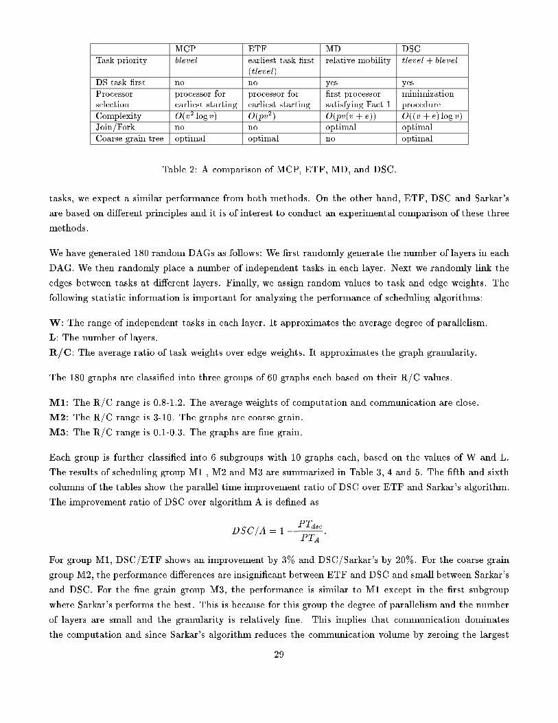
MCP ETF MD DSC
Task priority blevel earliest task �rst relative mobility tlevel + blevel
(tlevel)
DS task �rst no no yes yes
Processor processor for processor for �rst processor minimization
selection earliest starting earliest starting satisfying Fact 1 procedure
Complexity O(v
2
logv) O(pv
2
) O(pv(v + e)) O((v + e) log v)
Join/Fork no no optimal optimal
Coarse grain tree optimal optimal no optimal
Table 2: A comparison of MCP, ETF, MD, and DSC.
tasks, we expect a similar performance from both methods. On the other hand, ETF, DSC and Sarkar's
are based on di�erent principles and it is of interest to conduct an experimental comparison of these three
methods.
We have generated 180 random DAGs as follows: We �rst randomly generate the number of layers in each
DAG. We then randomly place a number of independent tasks in each layer. Next we randomly link the
edges between tasks at di�erent layers. Finally, we assign random values to task and edge weights. The
following statistic information is important for analyzing the performance of scheduling algorithms:
W: The range of independent tasks in each layer. It approximates the average degree of parallelism.
L: The number of layers.
R/C: The average ratio of task weights over edge weights. It approximates the graph granularity.
The 180 graphs are classi�ed into three groups of 60 graphs each based on their R/C values.
M1: The R/C range is 0.8-1.2. The average weights of computation and communication are close.
M2: The R/C range is 3-10. The graphs are coarse grain.
M3: The R/C range is 0.1-0.3. The graphs are �ne grain.
Each group is further classi�ed into 6 subgroups with 10 graphs each, based on the values of W and L.
The results of scheduling group M1 , M2 and M3 are summarized in Table 3, 4 and 5. The �fth and sixth
columns of the tables show the parallel time improvement ratio of DSC over ETF and Sarkar's algorithm.
The improvement ratio of DSC over algorithm A is de�ned as
DSC=A = 1�
PT
dsc
PT
A
:
For group M1, DSC/ETF shows an improvement by 3% and DSC/Sarkar's by 20%. For the coarse grain
group M2, the performance di�erences are insigni�cant between ETF and DSC and small between Sarkar's
and DSC. For the �ne grain group M3, the performance is similar to M1 except in the �rst subgroup
where Sarkar's performs the best. This is because for this group the degree of parallelism and the number
of layers are small and the granularity is relatively �ne. This implies that communication dominates
the computation and since Sarkar's algorithm reduces the communication volume by zeroing the largest
29
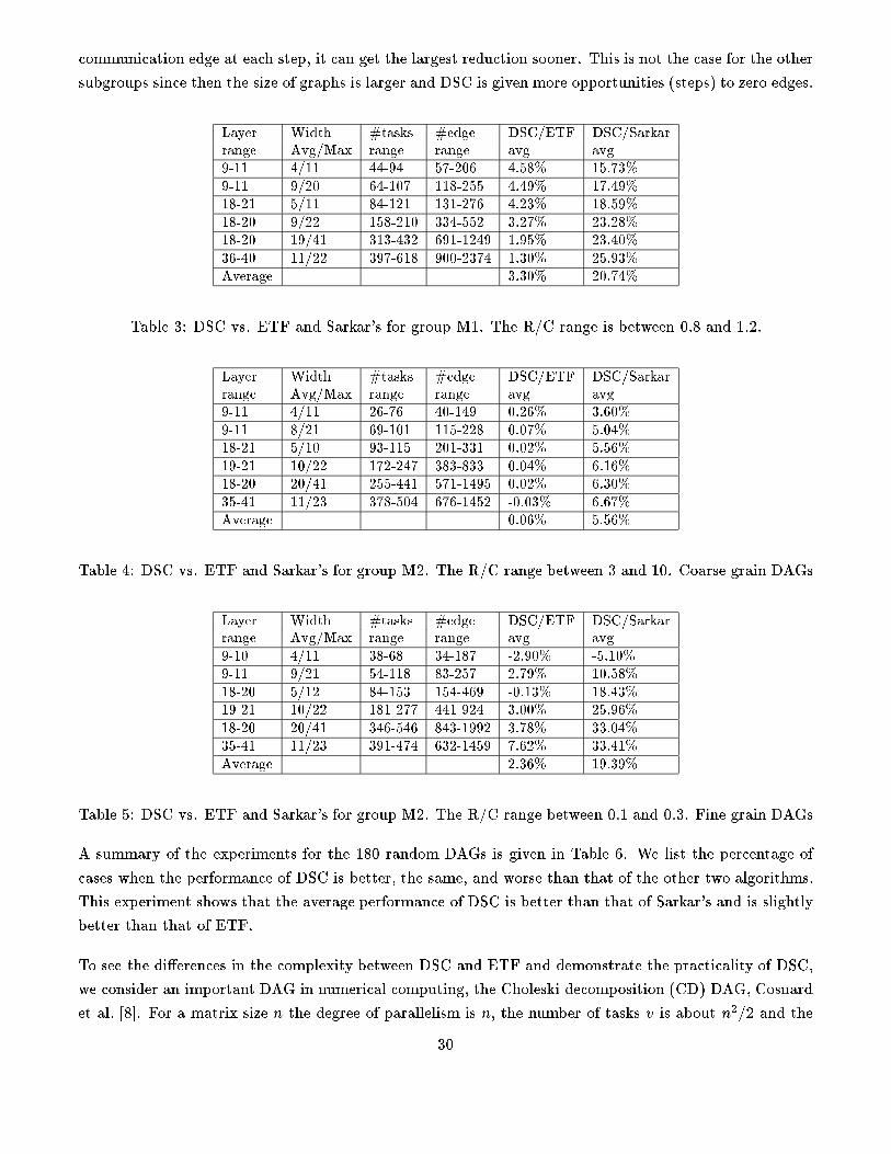
communication edge at each step, it can get the largest reduction sooner. This is not the case for the other
subgroups since then the size of graphs is larger and DSC is given more opportunities (steps) to zero edges.
Layer Width #tasks #edge DSC/ETF DSC/Sarkar
range Avg/Max range range avg avg
9-11 4/11 44-94 57-206 4.58% 15.73%
9-11 9/20 64-107 118-255 4.49% 17.49%
18-21 5/11 84-121 131-276 4.23% 18.59%
18-20 9/22 158-210 334-552 3.27% 23.28%
18-20 19/41 313-432 691-1249 1.95% 23.40%
36-40 11/22 397-618 900-2374 1.30% 25.93%
Average 3.30% 20.74%
Table 3: DSC vs. ETF and Sarkar's for group M1. The R/C range is between 0.8 and 1.2.
Layer Width #tasks #edge DSC/ETF DSC/Sarkar
range Avg/Max range range avg avg
9-11 4/11 26-76 40-149 0.26% 3.60%
9-11 8/21 69-101 115-228 0.07% 5.04%
18-21 5/10 93-115 201-331 0.02% 5.56%
19-21 10/22 172-247 383-833 0.04% 6.16%
18-20 20/41 255-441 571-1495 0.02% 6.30%
35-41 11/23 378-504 676-1452 -0.03% 6.67%
Average 0.06% 5.56%
Table 4: DSC vs. ETF and Sarkar's for group M2. The R/C range between 3 and 10. Coarse grain DAGs
Layer Width #tasks #edge DSC/ETF DSC/Sarkar
range Avg/Max range range avg avg
9-10 4/11 38-68 34-187 -2.90% -5.10%
9-11 9/21 54-118 83-257 2.79% 10.58%
18-20 5/12 84-153 154-469 -0.13% 18.43%
19-21 10/22 181-277 441-924 3.00% 25.96%
18-20 20/41 346-546 843-1992 3.78% 33.04%
35-41 11/23 391-474 632-1459 7.62% 33.41%
Average 2.36% 19.39%
Table 5: DSC vs. ETF and Sarkar's for group M2. The R/C range between 0.1 and 0.3. Fine grain DAGs
A summary of the experiments for the 180 random DAGs is given in Table 6. We list the percentage of
cases when the performance of DSC is better, the same, and worse than that of the other two algorithms.
This experiment shows that the average performance of DSC is better than that of Sarkar's and is slightly
better than that of ETF.
To see the di�erences in the complexity between DSC and ETF and demonstrate the practicality of DSC,
we consider an important DAG in numerical computing, the Choleski decomposition (CD) DAG, Cosnard
et al. [8]. For a matrix size n the degree of parallelism is n, the number of tasks v is about n
2
=2 and the
30
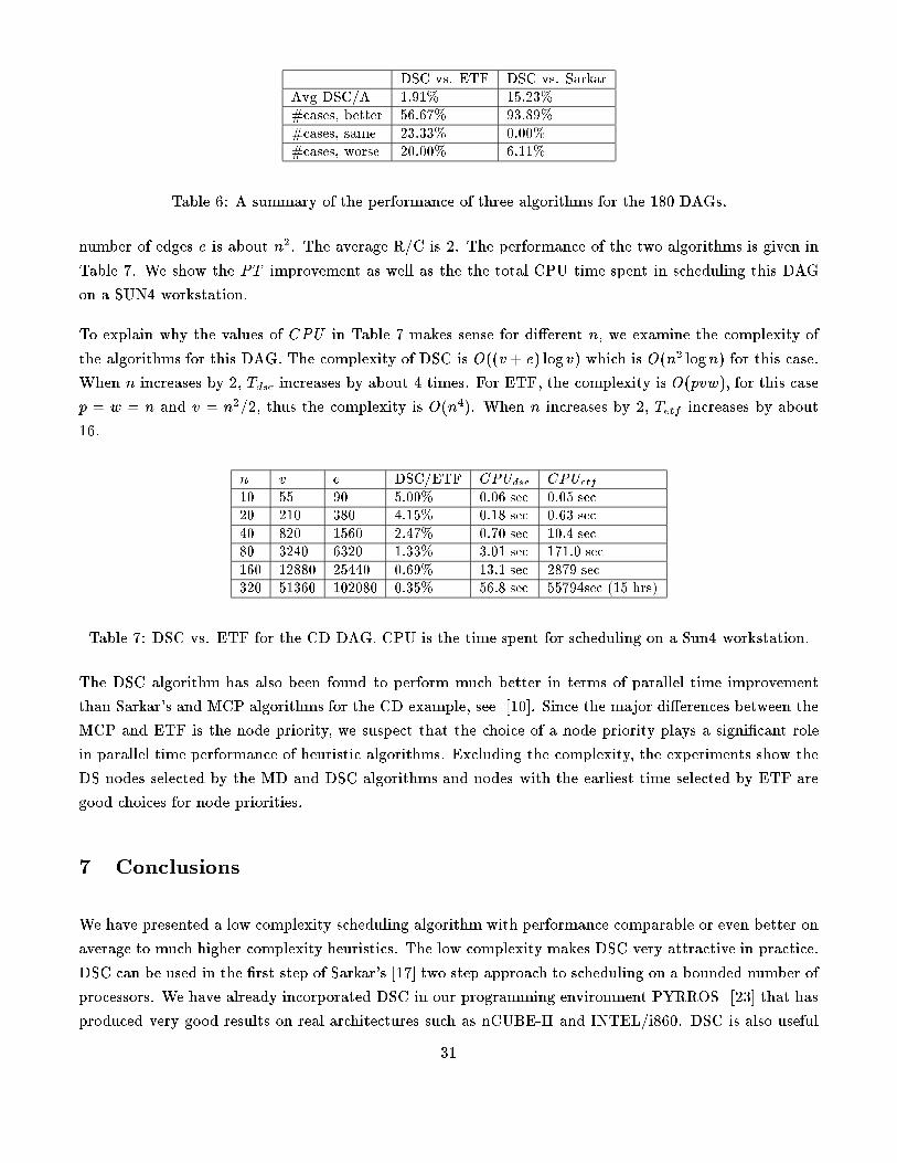
DSC vs. ETF DSC vs. Sarkar
Avg DSC/A 1.91% 15.23%
#cases, better 56.67% 93.89%
#cases, same 23.33% 0.00%
#cases, worse 20.00% 6.11%
Table 6: A summary of the performance of three algorithms for the 180 DAGs.
number of edges e is about n
2
. The average R/C is 2. The performance of the two algorithms is given in
Table 7. We show the PT improvement as well as the the total CPU time spent in scheduling this DAG
on a SUN4 workstation.
To explain why the values of CPU in Table 7 makes sense for di�erent n, we examine the complexity of
the algorithms for this DAG. The complexity of DSC is O((v+ e) logv) which is O(n
2
logn) for this case.
When n increases by 2, T
dsc
increases by about 4 times. For ETF, the complexity is O(pvw), for this case
p = w = n and v = n
2
=2, thus the complexity is O(n
4
). When n increases by 2, T
etf
increases by about
16.
n v e DSC/ETF CPU
dsc
CPU
etf
10 55 90 5.00% 0.06 sec 0.05 sec
20 210 380 4.15% 0.18 sec 0.63 sec
40 820 1560 2.47% 0.70 sec 10.4 sec
80 3240 6320 1.33% 3.01 sec 171.0 sec
160 12880 25440 0.69% 13.1 sec 2879 sec
320 51360 102080 0.35% 56.8 sec 55794sec (15 hrs)
Table 7: DSC vs. ETF for the CD DAG. CPU is the time spent for scheduling on a Sun4 workstation.
The DSC algorithm has also been found to perform much better in terms of parallel time improvement
than Sarkar's and MCP algorithms for the CD example, see [10]. Since the major di�erences between the
MCP and ETF is the node priority, we suspect that the choice of a node priority plays a signi�cant role
in parallel time performance of heuristic algorithms. Excluding the complexity, the experiments show the
DS nodes selected by the MD and DSC algorithms and nodes with the earliest time selected by ETF are
good choices for node priorities.
7 Conclusions
We have presented a low complexity scheduling algorithm with performance comparable or even better on
average to much higher complexity heuristics. The low complexity makes DSC very attractive in practice.
DSC can be used in the �rst step of Sarkar's [17] two step approach to scheduling on a bounded number of
processors. We have already incorporated DSC in our programming environment PYRROS [23] that has
produced very good results on real architectures such as nCUBE-II and INTEL/i860. DSC is also useful
31
for partitioning and clustering of parallel programs [17, 21]. A particular area that DSC could be useful is
scheduling irregular task graphs. Pozo [16] has used DSC to investigate the performance of sparse matrix
methods for distributed memory architectures. Wolski and Feo [18] have extended the applicability of DSC
to program partitioning for NUMA architectures.
Acknowledgments
We are very grateful to Vivek Sarkar for providing us with the programs of his system in [17] and his
comments and suggestions, to Min-You Wu for his help in clarifying the MD algorithm. We also thank
referees for their useful suggestions in improving the presentation of this paper. We thank Weining Wang
for programming the random graph generator, Richard Wolski and Alain Darte for their comments on this
work. The analysis for a �ne grain tree was inspired by a conversation with Theodora Varvarigou.
References
[1] M. A. Al-Mouhamed, Lower Bound on the Number of Processors and Time for Scheduling Precedence
Graphs with Communication Costs, IEEE Trans. on Software Engineering, vol. 16, no. 12, pp. 1390-
1401, 1990.
[2] F.D. Anger, J. Hwang, and Y. Chow, Scheduling with Su�cient Loosely Coupled Processors, Journal
of Parallel and Distributed Computing, vol. 9, pp. 87-92, 1990.
[3] Ph. Chretienne, Task Scheduling over Distributed Memory Machines, Proc. of the Inter. Workshop on
Parallel and Distributed Algorithms, (North Holland, Ed.), 1989.
[4] Ph. Chretienne, A Polynomial Algorithm to Optimially Schedule Tasks over an ideal Distributed Sys-
tem under Tree-like Presedence Constraints, European Journal of Operational Research, 2:43 (1989),
pp225-230.
[5] Ph. Chretienne, Complexity of Tree Scheduling with Interprocessor Communication Delays, Tech.
Report, M.A.S.I. 90.5, Universite Pierre et Marie Curie, 1990.
[6] J. Y. Colin and Ph. Chretienne, C.P.M. Scheduling with Small Communication Delays and Task
Duplication, Report, M.A.S.I. 90.1, Universite Pierre et Marie Curie, 1990.
[7] T. H. Cormen, C. E. Leiserson,and R. L. Rivest, Introduction to algorithms, MIT Press and McGraw-
Hill, 1990.
[8] M. Cosnard, M. Marrakchi, Y. Robert, and D. Trystram, Parallel Gaussian Elimination on an MIMD
Computer, Parallel Computing, vol. 6, pp. 275-296, 1988.
[9] A. Gerasoulis and T. Yang, On the Granularity and Clustering of Directed Acyclic Task Graphs, TR-
153, Dept. of Computer Science, Rutgers Univ., 1990. To appear in IEEE Trans. on Parallel and
Distributed Systems.
32
[10] A. Gerasoulis and T. Yang, A Comparison of Clustering Heuristics for Scheduling DAGs on Mul-
tiprocessors , Journal of Parallel and Distributed Computing, special issue on scheduling and load
balancing, Vol. 16, No. 4, pp. 276-291 (1992).
[11] M. Girkar and C. Polychronopoulos, Partitioning Programs for Parallel Execution, Proc. of the 1988
ACM Inter. Conf. on Supercomputing, St. Malo, France, July 4-8, 1988.
[12] J. J. Hwang, Y. C. Chow, F. D. Anger, and C. Y. Lee, Scheduling Precedence Graphs in Systems with
Interprocessor Communication times, SIAM J. Comput., pp. 244-257, 1989.
[13] S.J. Kim and J.C Browne, A General Approach to Mapping of Parallel Computation upon Multipro-
cessor Architectures, Int'l Conf. on Parallel Processing, vol 3, pp. 1-8, 1988.
[14] B. Kruatrachue B. and T. Lewis, Grain Size Determination for Parallel Processing, IEEE Software,
pp. 23-32, Jan. 1988.
[15] C. Papadimitriou and M. Yannakakis, Towards on an Architecture-Independent Analysis of Parallel
Algorithms, SIAM J. Comput., vol. 19, pp. 322-328, 1990.
[16] R. Pozo, Performance modeling of sparse matrix methods for distributed memory architectures, in
Lecture Notes in Computer Science, No. 634, Parallel Processing: CONPAR 92 { VAPP V, Springer-
Varlag, 1992, pp. 677-688.
[17] V. Sarkar, Partitioning and Scheduling Parallel Programs for Execution on Multiprocessors, The MIT
Press, 1989.
[18] R. Wolski and J. Feo, Program Parititoning for NUMA Multiprocessor Computer Systems, Tech.
Report, Lawrence Livermore Nat. Lab., 1992.
[19] M. Y. Wu and D. Gajski, Hypertool: A Programming Aid for Message-Passing Systems, IEEE Trans.
on Parallel and Distributed Systems, vol. 1, no. 3, pp.330-343, 1990.
[20] M. Y. Wu, Personal Communications, Feb. 1993.
[21] J. Yang, L. Bic and A. Nicolau, A Mapping Strategy for MIMD Computers, Proc. of 1991 Inter. Conf.
on Parallel Processing, vol I, pp. 102-109.
[22] T. Yang and A. Gerasoulis, A Fast Scheduling Algorithm for DAGs on an Unbounded Number of
Processors, Proc. of IEEE Supercomputing '91, Albuquerque, NM, 1991, pp. 633-642.
[23] T. Yang and A. Gerasoulis, PYRROS: Static Task Scheduling and Code Generation for Message-
Passing Multiprocessors, Proc. of 6th ACM Inter. Conf. on Supercomputing, Washington D.C., July,
1992, pp. 428-437.
33