Hyperboloidal layers for hyperbolic equationson unbounded domains

Anıl Zenginoglu

Laboratoire Jacques-Louis Lions, Universite Pierre et Marie Curie (Paris VI), Paris, France, andTheoretical Astrophysics, California Institute of Technology, Pasadena, CA, USA

Abstract

We show how to solve hyperbolic equations numerically on unbounded domains by compactifi-cation, thereby avoiding the introduction of an artificial outer boundary. The essential ingredientis a suitable transformation of the time coordinate in combination with spatial compactification.We construct a new layer method based on this idea, called the hyperboloidal layer. The methodis demonstrated on numerical tests including the one dimensional Maxwell equations using fi-nite differences and the three dimensional wave equation with and without nonlinear source termsusing spectral techniques.

Keywords: Transparent (nonreflecting, absorbing) boundary conditions, perfectly matchedlayers, hyperboloidal layers, hyperboloidal compactification, wave equations, Maxwellequations.

1. Introduction

Hyperbolic equations typically admit wavelike solutions that oscillate infinitely many timesin an unbounded domain. Take a plane wave in one spatial dimension with frequency ω andwave number k,

u(x, t) = e2πi(kx−ωt) . (1)

Any mapping of such an oscillatory solution from an infinite domain to a finite domain results ininfinitely many oscillations near the domain boundary, which can not be resolved numerically.We refer to this phenomenon as the compactification problem [1]. It is commonly stated thathyperbolic partial differential equations are not compatible with compactification, and thereforecan not be solved on unbounded domains accurately.

A suitable transformation of the time coordinate, however, leads to a finite number of oscil-lations in an infinite spatial domain. Introduce

τ(x, t) = t −kω

(x +

C1 + x

), (2)

where C is a finite, positive constant. The plane wave (1) becomes

u(x, τ) = e−2πi(kC/(1+x)+ωτ) . (3)

This representation of the plane wave has only k C cycles along a constant time hypersurface inthe unbounded space x ∈ [0,∞), and is therefore compatible with compactification.

Preprint submitted to Journal of Computational Physics December 30, 2010

arX

iv:1

008.

3809

v2 [

mat

h.N

A]

25

Dec

201

0

The simple idea just described has far reaching consequences. In numerical calculations ofhyperbolic equations one typically truncates the unbounded solution domain by introducing anartificial outer boundary that is not part of the original problem. Boundary conditions, calledtransparent, absorbing, radiative, or nonreflecting, are constructed to simulate transparency ofthis artificial outer boundary. There has been significant developments in the treatment of ar-tificial outer boundaries since the 70s, but there is no consensus on an optimal method [2, 3].Especially the construction of boundary conditions for nonlinear problems is difficult [4]. A suc-cessful technique for numerical calculations on unbounded domains resolves this problem forsuitable hyperbolic equations and provides direct quantitative access to asymptotic properties ofsolutions.

Furthermore, the numerical construction of oscillatory solutions as (3) can be very efficient.Numerical accuracy requirements for hyperbolic equations are typically given in terms of num-bers of grid points per wavelength. In the example presented above, the free parameter C de-termines the number of cycles to be resolved, which can be chosen small. This suggests thathigh order numerical discretizations requiring a few points per wavelength can be very efficientin combination with time transformations of the type (2).

The rest of the paper is devoted to the discussion of time transformation and compactifica-tion for hyperbolic equations. The theoretical part of the paper (sections 2 and 3) includes adetailed description of the method. We discuss the compactification problem (section 2.1) andits resolution (section 2.2) for the advection equation in one dimension. In section 2.3 we discussthe wave equation with incoming and outgoing characteristics. We show that the method worksalso for systems of equations (section 2.4). Hyperboloidal layers are introduced in section 2.5in analogy to absorbing layers. In multiple spatial dimensions, compactification is performedin the outgoing direction in combination with rescaling to take care of the asymptotic behavior(sections 3.1 and 3.2). The layer strategy in multiple dimensions allows us to employ arbitrarycoordinates in an inner domain, where sources or scatterers with irregular shapes may be present(section 3.3). We finish the theoretical part discussing possible generalizations of the method tononspherical coordinate systems (section 3.4). Section 4 includes numerical experiments in oneand three spatial dimensions. In one dimension, we solve the Maxwell equations using finitedifference methods (section 4.1). A stringent test of the method is the evolution of off-centeredinitial data for the wave equation in three spatial dimensions with and without nonlinear sourceterms (section 4.2). We conclude with a discussion and an outlook in section 5.

2. Compactification in one spatial dimension

2.1. Spatial compactificationConsider the initial boundary value problem for the advection equation

∂tu + ∂xu = 0, u(x, 0) = u0(x), u(0, t) = b(t). (4)

The problem is posed on the unbounded domain x ∈ [0,∞). We transform the infinite domain inx to a finite domain by introducing the compactifying coordinate ρ via

ρ(x) =x

1 + x, x(ρ) =

ρ

1 − ρ. (5)

The advection equation becomes

∂tu + (1 − ρ)2∂ρu = 0 . (6)

2

0.0 0.2 0.4 0.6 0.8 1.0Ρ

1

2

3

4

5

6

7t

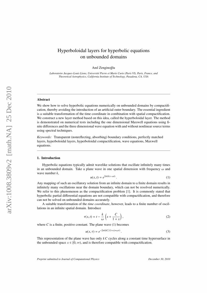
Figure 1: Characteristic diagram for the advection equation after spatial compactification. The characteristic speedapproaches zero near spatial infinity at ρ = 1 causing loss of numerical resolution: this is the compactification problem.

The spatial domain is now given by ρ ∈ [0, 1]. Characteristics of this equation are solutions tothe ordinary differential equation

dρ(t)dt

= −(1 − ρ(t))2.

They are plotted in figure 1. The compactification problem is clearly visible: the coordinate speedof characteristics approaches zero near a neighborhood of the point that corresponds to spatialinfinity. The advection equation has a finite speed of propagation, therefore its characteristicscan not reach infinity in finite time.

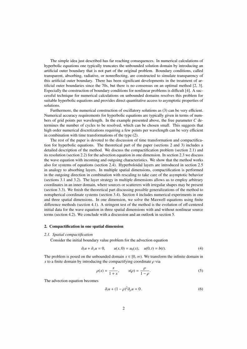
A concrete example illustrates the problem for oscillatory solutions. Set initial data u0(x) =

sin(2πx) and boundary data b(t) = − sin(2πt) in (4). We obtain the solution

u(x, t) = sin(2π(x − t)), (7)

which reads in the compactifying coordinate (5)

u(ρ, t) = sin(2π

(ρ

1 − ρ− t

)). (8)

The solution is depicted in figure 2 at t = 0 on x ∈ [0, 10] in the original coordinate and on

2 4 6 8 10x

-1.0

-0.5

0.5

1.0u

0.2 0.4 0.6 0.8 1.0Ρ

-1.0

-0.5

0.0

0.5

1.0u

Figure 2: The solution (7) at time t = 0 is plotted on the left panel. The same solution in the compactifying coordinategiven in (8) plotted on the right panel illustrates infinite blueshift in frequency.

ρ ∈ [0, 10/11] in the compactifying coordinate. The oscillations can not be resolved in thecompactifying coordinate near infinity due to infinite blueshift in spatial frequency.

Mapping infinity to a finite coordinate seems to require infinite resolution. However, a suit-able time transformation discussed in the next section provides a clean solution to this problem.

3

2.2. Hyperboloidal compactificationThe idea is to transform the time coordinate as in (2). We introduce

τ = t −(x +

C1 + x

), (9)

With the compactification (5) we get the Jacobian

∂τ = ∂t, ∂x = (−1 + C Ω2)∂τ + Ω2 ∂ρ ,

where we define Ω := 1 − ρ. The advection equation in the new coordinates (ρ, τ) reads

∂τu +1C∂ρu = 0 .

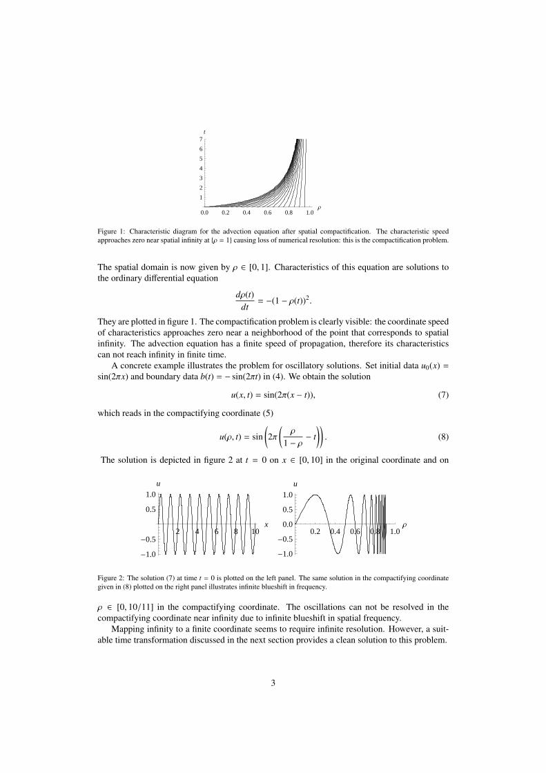
This equation has the same form, up to an additional free parameter, as the advection equationin the original coordinates (4), but the meaning of the coordinates is different. Solutions to theabove equation in the bounded domain ρ ∈ [0, 1] correspond to solutions to the original advectionequation in the unbounded domain x ∈ [0,∞). The free parameter C expresses the freedom toprescribe the characteristic speed in the compactifying coordinate and the number of cycles in aninfinite domain. To see this, we write the solution (7) in the new coordinates

u(ρ, τ) = − sin (2π(C Ω + τ)) . (10)

The solution is depicted in figure 3 at τ = 0 for two values of C. The number of cycles onthe domain is finite and depends on C. The wave is resolved evenly through the compactifieddomain. In such representations of the solution it should be kept in mind that lines of constant τdo not correspond to lines of constant t.

0.2 0.4 0.6 0.8 1.0Ρ

-1.0

-0.5

0.5

1.0u

0.2 0.4 0.6 0.8 1.0Ρ

-1.0

-0.5

0.5

1.0u

Figure 3: The solution (10) at time τ = 1 is plotted for two values of C. On the left panel we have C = 1 and on theright panel C = 5. The number of oscillations, and therefore the wavelength of the solution, can be influenced by the freeparameter C.

The idea to introduce a coordinate transformation of time in combination with compactifi-cation comes from general relativity [5]. The time function (2) approaches characteristics ofthe advection equation asymptotically. In general relativity, infinity along characteristic direc-tions is called null infinity. Time functions whose level sets approach null infinity are calledhyperboloidal because their asymptotic behavior is similar to the asymptotic behavior of stan-dard hyperboloids [6, 7]. To see this, consider the rectangular hyperbola on the (x, t) plane,t2 − x2 = C2, with a free parameter C. Shifting the hyperbola along the t direction by τ gives(t − τ)2 − x2 = C2. Introducing τ as the new time coordinate we write

τ = t −√

C2 + x2. (11)

4

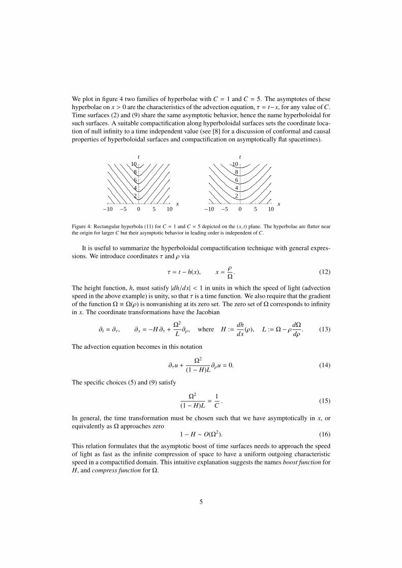
We plot in figure 4 two families of hyperbolae with C = 1 and C = 5. The asymptotes of thesehyperbolae on x > 0 are the characteristics of the advection equation, τ = t−x, for any value of C.Time surfaces (2) and (9) share the same asymptotic behavior, hence the name hyperboloidal forsuch surfaces. A suitable compactification along hyperboloidal surfaces sets the coordinate loca-tion of null infinity to a time independent value (see [8] for a discussion of conformal and causalproperties of hyperboloidal surfaces and compactification on asymptotically flat spacetimes).

-10 -5 0 5 10x

2468

10t

-10 -5 0 5 10x

2468

10t

Figure 4: Rectangular hyperbola (11) for C = 1 and C = 5 depicted on the (x, t) plane. The hyperbolae are flatter nearthe origin for larger C but their asymptotic behavior in leading order is independent of C.

It is useful to summarize the hyperboloidal compactification technique with general expres-sions. We introduce coordinates τ and ρ via

τ = t − h(x), x =ρ

Ω. (12)

The height function, h, must satisfy |dh/dx| < 1 in units in which the speed of light (advectionspeed in the above example) is unity, so that τ is a time function. We also require that the gradientof the function Ω ≡ Ω(ρ) is nonvanishing at its zero set. The zero set of Ω corresponds to infinityin x. The coordinate transformations have the Jacobian

∂t = ∂τ, ∂x = −H ∂τ +Ω2

L∂ρ, where H :=

dhdx

(ρ), L := Ω − ρdΩ

dρ. (13)

The advection equation becomes in this notation

∂τu +Ω2

(1 − H)L∂ρu = 0. (14)

The specific choices (5) and (9) satisfy

Ω2

(1 − H)L=

1C. (15)

In general, the time transformation must be chosen such that we have asymptotically in x, orequivalently as Ω approaches zero

1 − H ∼ O(Ω2). (16)

This relation formulates that the asymptotic boost of time surfaces needs to approach the speedof light as fast as the infinite compression of space to have a uniform outgoing characteristicspeed in a compactified domain. This intuitive explanation suggests the names boost function forH, and compress function for Ω.

5

2.3. Wave equation

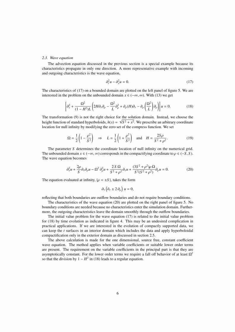
The advection equation discussed in the previous section is a special example because itscharacteristics propagate in only one direction. A more representative example with incomingand outgoing characteristics is the wave equation,

∂2t u − ∂2

xu = 0. (17)

The characteristics of (17) on a bounded domain are plotted on the left panel of figure 5. We areinterested in the problem on the unbounded domain x ∈ (−∞,∞). With (13) we get[

∂2τ +

Ω2

(1 − H2)L

(2H∂τ∂ρ −

Ω2

L∂2ρ + ∂ρ(H)∂τ − ∂ρ

(Ω2

L

)∂ρ

)]u = 0. (18)

The transformation (9) is not the right choice for the solution domain. Instead, we choose theheight function of standard hyperboloids, h(x) =

√S 2 + x2. We prescribe an arbitrary coordinate

location for null infinity by modifying the zero set of the compress function. We set

Ω =12

(1 −

ρ2

S 2

)⇒ L =

12

(1 +

ρ2

S 2

)and H =

2S ρS 2 + ρ2 . (19)

The parameter S determines the coordinate location of null infinity on the numerical grid.The unbounded domain x ∈ (−∞,∞) corresponds in the compactifying coordinate to ρ ∈ (−S , S ).The wave equation becomes

∂2τu +

2ρS∂τ∂ρu −Ω2 ∂2

ρu +2 S Ω

S 2 + ρ2 ∂τu +(3S 2 + ρ2)ρΩ

S 2(S 2 + ρ2)∂ρu = 0. (20)

The equation evaluated at infinity, ρ = ±S , takes the form

∂τ(∂τ ± 2 ∂ρ

)u = 0,

reflecting that both boundaries are outflow boundaries and do not require boundary conditions.The characteristics of the wave equation (20) are plotted on the right panel of figure 5. No

boundary conditions are needed because no characteristics enter the simulation domain. Further-more, the outgoing characteristics leave the domain smoothly through the outflow boundaries.

The initial value problem for the wave equation (17) is related to the initial value problemfor (18) by time evolution as indicated in figure 4. This may be an undesired complication inpractical applications. If we are interested in the evolution of compactly supported data, wecan keep the t surfaces in an interior domain which includes the data and apply hyperboloidalcompactification only in the exterior domain as discussed in section 2.5.

The above calculation is made for the one dimensional, source free, constant coefficientwave equation. The method applies when variable coefficients or suitable lower order termsare present. The requirement on the variable coefficients in the principal part is that they areasymptotically constant. For the lower order terms we require a fall off behavior of at least Ω2

so that the division by 1 − H2 in (18) leads to a regular equation.

6

-10 -5 0 5 10x

2

4

6

8

10t

-10 -5 0 5 10Ρ

2

4

6

8

10Τ

Figure 5: On the left panel we plot the characteristics for the standard wave equation (17) on the bounded domainx ∈ [−10, 10]. On the right panel hyperboloidal compactification has been applied with infinity located at ρ = S = ±10.The standard wave equation on a bounded domain requires boundary conditions for the incoming characteristics fromboth boundaries. There are no incoming characteristics with hyperboloidal compactification.

2.4. Hyperbolic systemsConsider the linear, homogeneous system of partial differential equations with variable coef-

ficients∂tu = A∂xu, (21)

where u = (u1(x, t), u2(x, t), . . . , un(x, t))T , and A is an n × n matrix that may depend on x. Thetransformation (12) with Jacobian (13) leads to

(1 + HA)∂τu =Ω2

LA∂ρu. (22)

Assuming that the time transformation has been chosen to satisfy (16), we require that the poly-nomial remainder of det(1 + HA) by 1 − H vanishes asymptotically. This is a condition on theasymptotic form of the elements of A. For example, taking n = 2 we write

A =

(a11 a12a21 a22

).

The asymptotic condition for the applicability of hyperboloidal compactification reads

1 + a11 + a22 − a12a21 + a11a22 = 0. (23)

A typical example is the wave equation (17) written as a first order symmetric hyperbolicsystem. The wave equation takes the form (21) in the auxiliary variables v = ∂tu and w = ∂xu,with

u =

(vw

), A =

(0 11 0

). (24)

The condition (23) is satisfied. The transformed system reads

∂τu =Ω2

(1 − H2)L

(−H 11 −H

)∂ρu. (25)

Note that this equation is not the first order symmetric hyperbolic form of the transformed waveequation (18). The particular choice (19) leads to the regular system

∂τu =1

2 S 2

(−2S ρ S 2 + ρ2

S 2 + ρ2 −2S ρ

)∂ρu.

7

The outer boundaries at ρ = ±S are pure outflow boundaries.As a further example consider the one dimensional Maxwell equations for the electric and

magnetic fields (E, H)

∂tE = −1ε∂xH, ∂tH = −

1µ∂xE,

The electric permittivity ε and the magnetic permeability µ may be point-dependent. The equa-tions have the form (21) with

u =

(EH

), and A = −

1εµ

(0 µε 0

).

We get after hyperboloidal compactification

∂τu = −Ω2

(εµ − H2)L

(H µε H

)∂ρu. (26)

In vacuum outside a compact domain we have ε = ε0 and µ = µ0, where ε0 and µ0 are theelectric and the magnetic constants. We need to choose the asymptotic behavior of H such that√ε0µ0 − H ∼ O(Ω2). Then the Maxwell equations behave similarly to the wave equation (25)

near null infinity.The example of Maxwell equations suggests that including lower order terms or variable

characteristic speeds in a compact domain are straightforward in the hyperboloidal method aslong as the asymptotic form of the equations are suitable. The asymptotic characteristic speedsneed to be constant and lower order terms need to have compact support or fall off sufficientlyfast. Hyperboloidal compactification can then be applied outside a compact domain as discussedin the next section.

2.5. Hyperboloidal layers

It may be desirable to employ specific coordinates in a compact domain without the timetransformation or the compactification required by the hyperboloidal method. One reason istechnical. Elaborate numerical techniques to deal with shocks, scatterers, and media assumepredominantly specific coordinates. It may be impractical to modify these methods to work withhyperboloidal compactification throughout the simulation domain. Another reason is initial data.One may be interested in the evolution of certain (compactly supported) initial data prescribedon a level set of t. Therefore, it may be favorable to restrict the hyperboloidal compactificationto a layer.

We discuss briefly the perfectly matched layer (PML) by Berenger [9] to set the stage forhyperboloidal layers. In the PML method one attaches an absorbing medium—a layer— to thedomain of interest such that the interface between the interior domain and the exterior mediumis transparent independent from the frequency and the angle of incidence of the outgoing wave.Inside the layer the solution decays exponentially in the direction perpendicular to the interface.As a consequence, the solution is close to zero at the outer boundary of the layer where any stableboundary condition may be applied. The reflections from the outer boundary may be ignored ifthe layer is sufficiently wide.

The success of the PML method lies in the transparency of the interface between the interiordomain and the layer. This property finds explanation in the interpretation of Chew and Weedonof the PML as the analytic continuation of the equations into complex coordinates [10]. The

8

challenge is then to find suitable choices of the equations and the free parameters that lead toexponential damping of the solution in a stable way, which may be difficult depending on theproblem [11, 12, 13].

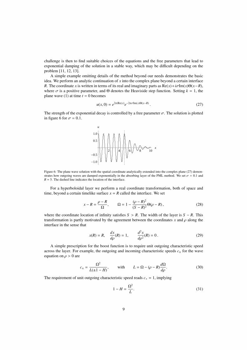
A simple example omitting details of the method beyond our needs demonstrates the basicidea. We perform an analytic continuation of x into the complex plane beyond a certain interfaceR. The coordinate x is written in terms of its real and imaginary parts as Re(x)+ iσIm(x)Θ(x−R),where σ is a positive parameter, and Θ denotes the Heaviside step function. Setting k = 1, theplane wave (1) at time t = 0 becomes

u(x, 0) = e2πiRe(x)e−2πσIm(x)Θ(x−R) . (27)

The strength of the exponential decay is controlled by a free parameter σ. The solution is plottedin figure 6 for σ = 0.1.

2 4 6 8 10x

-1.0

-0.5

0.5

1.0

u

Figure 6: The plane wave solution with the spatial coordinate analytically extended into the complex plane (27) demon-strates how outgoing waves are damped exponentially in the absorbing layer of the PML method. We set σ = 0.1 andR = 5. The dashed line indicates the location of the interface.

For a hyperboloidal layer we perform a real coordinate transformation, both of space andtime, beyond a certain timelike surface x = R called the interface. We set

x − R =ρ − R

Ω, Ω = 1 −

(ρ − R)2

(S − R)2 Θ(ρ − R) , (28)

where the coordinate location of infinity satisfies S > R. The width of the layer is S − R. Thistransformation is partly motivated by the agreement between the coordinates x and ρ along theinterface in the sense that

x(R) = R,dxdρ

(R) = 1,d2xdρ2 (R) = 0 . (29)

A simple prescription for the boost function is to require unit outgoing characteristic speedacross the layer. For example, the outgoing and incoming characteristic speeds c± for the waveequation on ρ > 0 are

c± =Ω2

L(±1 − H), with L = Ω − (ρ − R)

dΩ

dρ. (30)

The requirement of unit outgoing characteristic speed reads c+ = 1, implying

1 − H =Ω2

L. (31)

9

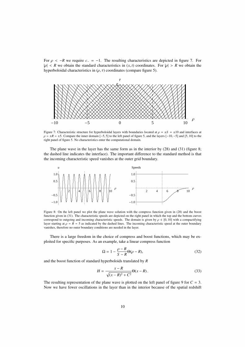
For ρ < −R we require c− = −1. The resulting characteristics are depicted in figure 7. For|ρ| < R we obtain the standard characteristics in (x, t) coordinates. For |ρ| > R we obtain thehyperboloidal characteristics in (ρ, τ) coordinates (compare figure 5).

-10 -5 0 5 10Ρ

5Τ

Figure 7: Characteristic structure for hyperboloidal layers with boundaries located at ρ = ±S = ±10 and interfaces atρ = ±R = ±5. Compare the inner domain [−5, 5] to the left panel of figure 5, and the layers [−10,−5] and [5, 10] to theright panel of figure 5. No characteristics enter the computational domain.

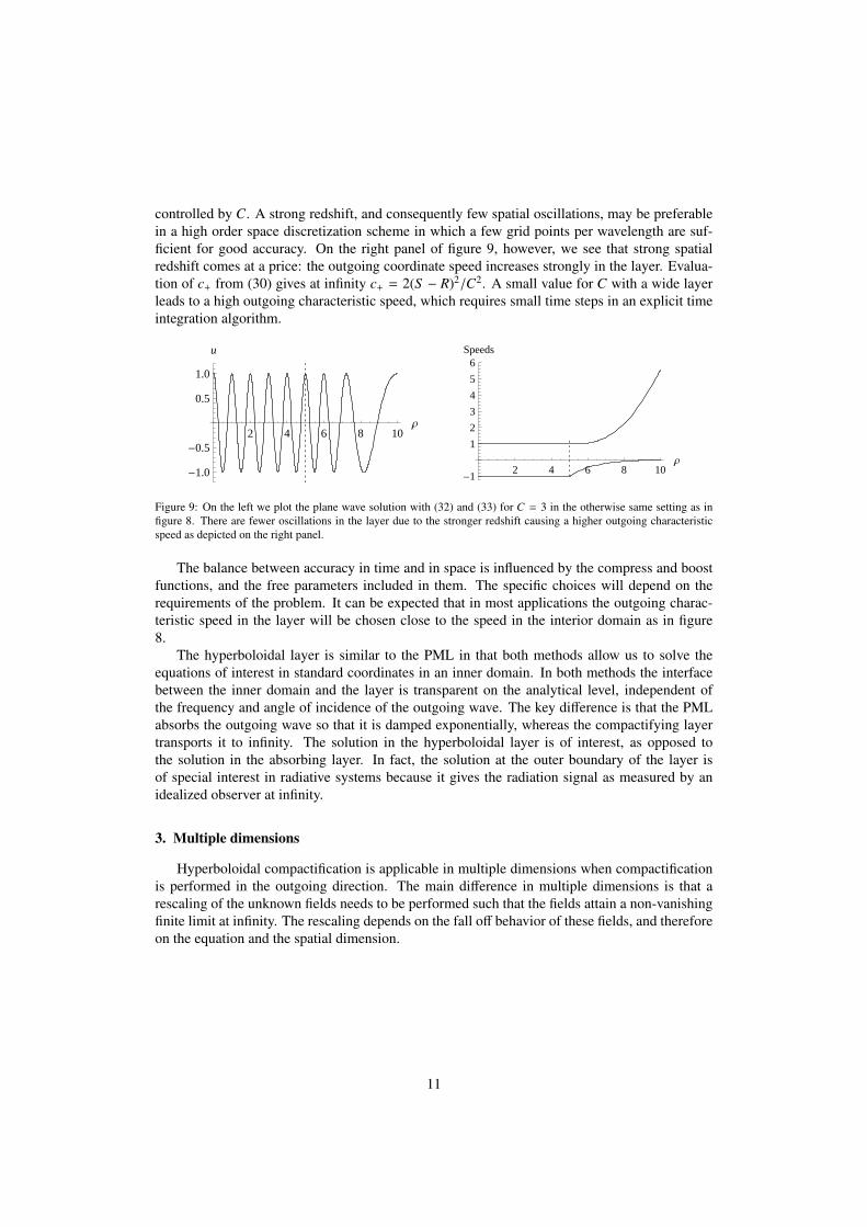
The plane wave in the layer has the same form as in the interior by (28) and (31) (figure 8;the dashed line indicates the interface). The important difference to the standard method is thatthe incoming characteristic speed vanishes at the outer grid boundary.

2 4 6 8 10Ρ

-1.0

-0.5

0.5

1.0

u

2 4 6 8 10Ρ

-1.0

-0.5

0.5

1.0

Speeds

Figure 8: On the left panel we plot the plane wave solution with the compress function given in (28) and the boostfunction given in (31). The characteristic speeds are depicted on the right panel in which the top and the bottom curvescorrespond to outgoing and incoming characteristic speeds. The domain is given by ρ ∈ [0, 10] with a compactifyinglayer starting at ρ = R = 5 as indicated by the dashed lines. The incoming characteristic speed at the outer boundaryvanishes, therefore no outer boundary conditions are needed in the layer.

There is a large freedom in the choice of compress and boost functions, which may be ex-ploited for specific purposes. As an example, take a linear compress function

Ω = 1 −ρ − RS − R

Θ(ρ − R), (32)

and the boost function of standard hyperboloids translated by R

H =x − R√

(x − R)2 + C2Θ(x − R) . (33)

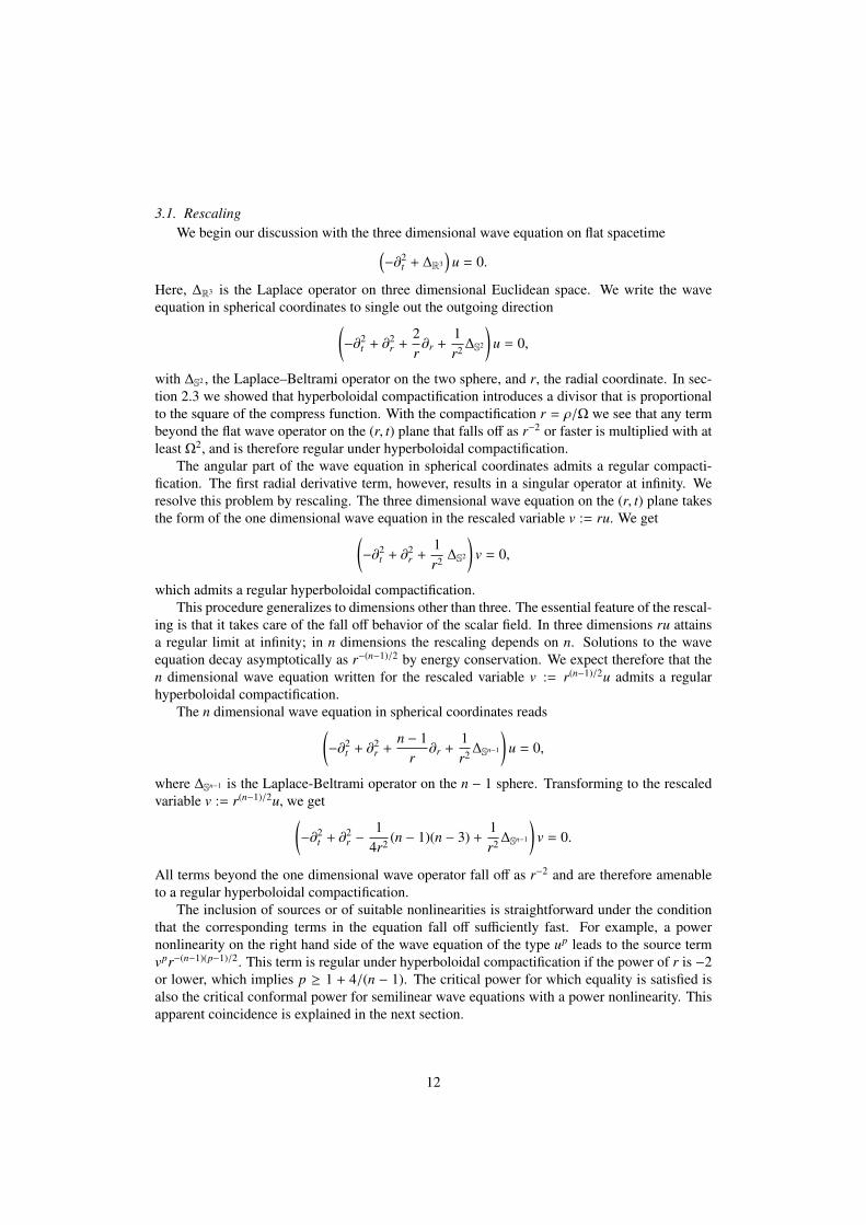
The resulting representation of the plane wave is plotted on the left panel of figure 9 for C = 3.Now we have fewer oscillations in the layer than in the interior because of the spatial redshift

10

controlled by C. A strong redshift, and consequently few spatial oscillations, may be preferablein a high order space discretization scheme in which a few grid points per wavelength are suf-ficient for good accuracy. On the right panel of figure 9, however, we see that strong spatialredshift comes at a price: the outgoing coordinate speed increases strongly in the layer. Evalua-tion of c+ from (30) gives at infinity c+ = 2(S − R)2/C2. A small value for C with a wide layerleads to a high outgoing characteristic speed, which requires small time steps in an explicit timeintegration algorithm.

2 4 6 8 10Ρ

-1.0

-0.5

0.5

1.0

u

2 4 6 8 10Ρ

-1

1

2

3

4

5

6Speeds

Figure 9: On the left we plot the plane wave solution with (32) and (33) for C = 3 in the otherwise same setting as infigure 8. There are fewer oscillations in the layer due to the stronger redshift causing a higher outgoing characteristicspeed as depicted on the right panel.

The balance between accuracy in time and in space is influenced by the compress and boostfunctions, and the free parameters included in them. The specific choices will depend on therequirements of the problem. It can be expected that in most applications the outgoing charac-teristic speed in the layer will be chosen close to the speed in the interior domain as in figure8.

The hyperboloidal layer is similar to the PML in that both methods allow us to solve theequations of interest in standard coordinates in an inner domain. In both methods the interfacebetween the inner domain and the layer is transparent on the analytical level, independent ofthe frequency and angle of incidence of the outgoing wave. The key difference is that the PMLabsorbs the outgoing wave so that it is damped exponentially, whereas the compactifying layertransports it to infinity. The solution in the hyperboloidal layer is of interest, as opposed tothe solution in the absorbing layer. In fact, the solution at the outer boundary of the layer isof special interest in radiative systems because it gives the radiation signal as measured by anidealized observer at infinity.

3. Multiple dimensions

Hyperboloidal compactification is applicable in multiple dimensions when compactificationis performed in the outgoing direction. The main difference in multiple dimensions is that arescaling of the unknown fields needs to be performed such that the fields attain a non-vanishingfinite limit at infinity. The rescaling depends on the fall off behavior of these fields, and thereforeon the equation and the spatial dimension.

11

3.1. RescalingWe begin our discussion with the three dimensional wave equation on flat spacetime(

−∂2t + ∆R3

)u = 0.

Here, ∆R3 is the Laplace operator on three dimensional Euclidean space. We write the waveequation in spherical coordinates to single out the outgoing direction(

−∂2t + ∂2

r +2r∂r +

1r2 ∆S2

)u = 0,

with ∆S2 , the Laplace–Beltrami operator on the two sphere, and r, the radial coordinate. In sec-tion 2.3 we showed that hyperboloidal compactification introduces a divisor that is proportionalto the square of the compress function. With the compactification r = ρ/Ω we see that any termbeyond the flat wave operator on the (r, t) plane that falls off as r−2 or faster is multiplied with atleast Ω2, and is therefore regular under hyperboloidal compactification.

The angular part of the wave equation in spherical coordinates admits a regular compacti-fication. The first radial derivative term, however, results in a singular operator at infinity. Weresolve this problem by rescaling. The three dimensional wave equation on the (r, t) plane takesthe form of the one dimensional wave equation in the rescaled variable v := ru. We get(

−∂2t + ∂2

r +1r2 ∆S2

)v = 0,

which admits a regular hyperboloidal compactification.This procedure generalizes to dimensions other than three. The essential feature of the rescal-

ing is that it takes care of the fall off behavior of the scalar field. In three dimensions ru attainsa regular limit at infinity; in n dimensions the rescaling depends on n. Solutions to the waveequation decay asymptotically as r−(n−1)/2 by energy conservation. We expect therefore that then dimensional wave equation written for the rescaled variable v := r(n−1)/2u admits a regularhyperboloidal compactification.

The n dimensional wave equation in spherical coordinates reads(−∂2

t + ∂2r +

n − 1r

∂r +1r2 ∆Sn−1

)u = 0,

where ∆Sn−1 is the Laplace-Beltrami operator on the n − 1 sphere. Transforming to the rescaledvariable v := r(n−1)/2u, we get(

−∂2t + ∂2

r −1

4r2 (n − 1)(n − 3) +1r2 ∆Sn−1

)v = 0.

All terms beyond the one dimensional wave operator fall off as r−2 and are therefore amenableto a regular hyperboloidal compactification.

The inclusion of sources or of suitable nonlinearities is straightforward under the conditionthat the corresponding terms in the equation fall off sufficiently fast. For example, a powernonlinearity on the right hand side of the wave equation of the type up leads to the source termvpr−(n−1)(p−1)/2. This term is regular under hyperboloidal compactification if the power of r is −2or lower, which implies p ≥ 1 + 4/(n − 1). The critical power for which equality is satisfied isalso the critical conformal power for semilinear wave equations with a power nonlinearity. Thisapparent coincidence is explained in the next section.

12

3.2. Conformal method

Compactification of spacetimes with a suitable time transformation as proposed by Penrosein [5] as well the hyperboloidal initial value problem as proposed by Friedrich [7] employ confor-mal methods. The conformal language is prevalent in studies of spacetimes in general relativity[14]. In this section we discuss the hyperboloidal compactification using conformal techniques.This viewpoint is of theoretical and practical interest because it reveals the interplay of confor-mal geometry, partial differential equations, and numerical methods within the hyperboloidalapproach, and also simplifies the implementation of the method for certain problems.

In general, a hyperboloidal time transformation with a spatial compactification leads to asingular metric. Consider the Minkowski metric in spherical coordinates

η = −dt2 + r2dr2 + r2dσ2, (34)

where dσ2 is the standard metric on the unit sphere. Introducing new coordinates τ and ρ as in(12) gives [8]

η = −dτ2 −2HLΩ2 dτdρ +

1 − H2

Ω4 L2dρ2 +ρ2

Ω2 dσ2.

This representation of the Minkowski metric is singular at infinity. The singularity is removedby conformally rescaling the metric,

g = Ω2η = −Ω2 dτ2 − 2HL dτdρ +1 − H2

Ω2 L2dρ2 + ρ2 dσ2. (35)

The conformal metric g is regular at null infinity by (16), and can be extended beyond null infinityin a process referred to as conformal extension [5, 14, 15]. In this context, the function Ω is calledthe conformal factor. The zero set of the conformal factor corresponds to null infinity where ithas a non-vanishing gradient. These properties of the conformal factor underlie our choices forthe compress function in the previous sections.

Partial differential equations within the conformal framework have first been studied forfields with vanishing rest mass, such as scalar, electromagnetic, and gravitational fields [15].The key observation is that the complicated asymptotic analysis of solutions to these partial dif-ferential equations is replaced with local differential geometry by considering the conformallytransformed equations in a conformally extended, regular spacetime [16, 17].

We discuss the wave equation on Minkowski spacetime as an example. Under a conformalrescaling of the Minkowski metric, g = Ω2 η, the wave equation transforms as [14, 15](

g −n − 1

4nR[g]

)v = Ω−(n+3)/2 η u, with v := Ω(1−n)/2u. (36)

Here, g := gµν∇µ∇ν is the d’Alembert operator with respect to g, R[g] is the Ricci scalar ofg, and n is the spatial dimension of the spacetime. The rescaling with Ω in the definition of thevariable v is asymptotically equivalent to the rescaling in Section 3.1, where we factor out thefall off behavior of u such that the rescaled variable v has a non-vanishing limit at null infinity.To see this, consider a specific choice for Ω from previous sections, say Ω(ρ) = 1 − ρ as in (5).In terms of the coordinate r = ρ/Ω, the conformal factor reads Ω(r) = (1 + r)−1, which behavesasymptotically as r−1. Therefore the definition of v in (36) corresponds asymptotically to thedefinition of v in section 3.1.

13

We can also explain the observation made at the end of section 3.1 concerning the agreementbetween the critical conformal power and the critical power for which hyperboloidal compact-ification leads to a regular equation. Using ηu = up and the definition of v in (36) we get atthe right hand side of the conformally invariant wave equation Ω((n−1)p−(n+3))/2vp. Regularity ofthis term at infinity, where the conformal factor vanishes, requires (n − 1)p ≥ n + 3, which is thecondition of Section 3.1. Equality is obtained for pc = 1 + 4/(n − 1) for which the semilinearwave equation is conformally invariant, hence pc is called the critical conformal power.

The conformal approach may be useful for various reasons. It extends directly to asymp-totically flat backgrounds with non-vanishing curvature [8, 18]. It also helps identifying thetransformation behavior of the equations independent of coordinates. For example, Yang-Millsand Maxwell equations are conformally invariant, and therefore do not require a rescaling of thevariables (the specific variables in which the covariant equations are written may not be confor-mally invariant and may require a rescaling).

Hyperboloidal compactification with rescaling, as presented in section 3.1, seems numer-ically feasible in any spatial dimension. In even spatial dimensions, however, the notion ofconformal infinity may not be feasible [19]. It is an open question whether the hyperboloidaltechnique applies to this case. If the method fails in even dimensions, it should be interesting tounderstand whether this failure is related to the violation of Huygens’ principle.

3.3. Hyperboloidal layers in multiple dimensions

In multiple dimensional problems, the layer technique is employed along the outgoing direc-tion r. We employ a compactifying coordinate ρ defined via r = ρ/Ω. The compress functionneeds to be unity in a compact domain bounded by radius R, be sufficiently smooth across theinterface at r = ρ = R, and vanish at a coordinate location S > R with non-vanishing gradient. Asuitable choice is

Ω = 1 −(ρ − RS − R

)4

Θ(ρ − R), L = 1 +(ρ − R)3(3ρ + R)

(S − R)4 Θ(ρ − R) .

The coordinates r and ρ coincide up to second order along the interface (compare (29)). Theheight function in the new time coordinate depends only on the radial coordinate: τ = t − h(r).The boost function is given by H = dh/dr. It may be set such that the outgoing characteristicspeed through the layer is unity. For the wave equation this corresponds to

1 − H =Ω2

L,

as in (31). Finally, the rescaling of the variable is performed with the compress function notingthat asymptotically Ω ∼ r−1. Further details are presented in section 4.2 in which the layertechnique is applied to solve the wave equation numerically in three spatial dimensions.

The extension of the hyperboloidal method from one dimension to multiple dimensions isfairly straightforward in spherical coordinates, which may be, however, too restrictive for thegrid geometry in applications. The discussion of the conformal regularity of the Minkowskimetric suggests that the method can also be applied in nonspherical coordinates as discussed inthe next section.

14

3.4. Nonspherical coordinate systems

Spherical coordinates are suitable for hyperboloidal compactification because cuts of nullinfinity have spherical topology [15]. The coordinate shape of null infinity, however, does nothave to be a sphere. We can employ any coordinate system with a unique outgoing direction forthe compactification.

An example for a nonspherical coordinate system, useful especially in electromagnetism, isthe prolate spheroidal coordinate system. The relation between Cartesian coordinates x, y, z andprolate spheroidal coordinates µ, ν, φ reads

x = sinh µ sin ν cosϕ, y = sinh µ sin ν sinϕ, z = cosh µ cos ν.

We have r2 = sinh2 µ + cos2 ν. Here, µ is the outgoing direction that has closed coordinatesurfaces. Compactification is performed along µ. Using the conformal method, we argue thatif conformal compactification of Minkowski spacetime in these coordinates leads to a regularmetric, the equations we solve on that background will be regular. The Minkowski metric reads

η = −dt2 + dx2 + dy2 + dz2 = −dt2 + (sinh2 µ + sin2 ν) (dµ2 + dν2) + sinh2 µ sin2 ν dϕ2.

We introduce a new time coordinate by setting

τ = t −√

1 + sinh2 µ.

The metric becomes

η = −dτ2 − 2 sinh µ dµdτ + sin2 ν dµ2 + (sinh2 µ + sin2 ν)dν2 + sinh2 µ sin2 νdϕ2.

Compactification along µ is performed via

sinh µ =2ρ

1 − ρ2 =ρ

Ω, dµ =

dρΩ.

The conformal metric g = Ω2η becomes

g = −Ω2dτ2 − 2ρ dρ dτ + sin2 ν dρ2 + (ρ2 + Ω2 sin2 ν)dν2 + ρ2 sin2 ν dϕ2.

The qualitative behavior of this metric near infinity is similar to the conformal Minkowski metricgiven in (35); the only difference is the coordinate representation. Therefore we conclude thathyperboloidal compactification of suitable hyperbolic equations in prolate spheroidal coordinatesleads to regular equations as for spherical or oblate spheroidal coordinates.

It is an open question whether the hyperboloidal method applies to Cartesian or cylindricalcoordinates. The difficulty is to ensure regularity of the equations at corners and along edgeswith respect to limits to infinity. This requirement implies a restriction on the geometry of boththe interface boundary and the numerical outer boundary. Even with the requirement of smoothcoordinate surfaces, it would be useful to extend the method such that the layer has an arbitraryshape in coordinate space. This generalization would increase the efficiency of the method whendealing with scatterers with irregular shape.

15

4. Numerical experiments

The aim of this chapter is to demonstrate numerical implementations of hyperboloidal com-pactification on simple examples in one and three spatial dimensions. The application of themethod in two dimensions is an open question as discussed in 3.2 and is left for future work.Also left for future work is an in-depth numerical analysis of the method in comparison withother boundary treatments, such as absorbing boundary conditions or perfectly matched layers.

In previous sections, we have seen that we may employ an arbitrary coordinate system in aninterior domain restricting compactification to a layer outside that domain. This idea is basedon the matching method with a transition zone presented in [8]. Numerical applications of thematching, however, are inefficient due to a blueshift in frequency in the matching region andmany arbitrary parameters for the transition function [20, 21]. A hyperboloidal layer gives asufficiently smooth interface without a transition function.

In this section, we compare the numerical accuracy of solutions with and without the layerin one dimension. In three dimensions we focus on the application of hyperboloidal layers forthe wave equation. Calculations using hyperboloid foliations, that is, constant mean curvaturesurfaces without the layer, have been presented in [21].

4.1. One spatial dimension

4.1.1. Analytical setupConsider the Maxwell equations (26). Assume that the electric permittivity and the magnetic

permeability are constant and have unit value. The transformed Maxwell system for the unknownvector u = (E, H)T reads

∂τu = −Ω2

(1 − H2)L

(H 11 H

)∂ρu. (37)

The characteristic speeds are c± = −Ω2/((±1+ H)L). This system is similar to the wave equationwritten in first order symmetric hyperbolic form (25), so our results apply both to Maxwell andwave equations in one dimension.

We experiment with two sets of the compress and boost functions. First we employ thehyperboloid foliation everywhere in the simulation domain. We set as in (19)

Ω =12

(1 −

ρ2

S 2

)and H =

2S ρS 2 + ρ2 .

The characteristic speeds read c± = ±(1± ρ/S )2/2. The minus sign corresponds to the incomingspeed at the right boundary, which vanishes at ρ = S . The plus sign corresponds to the incomingspeed at the left boundary, which vanishes at ρ = −S . The qualitative behavior of the charac-teristics is the same as depicted on the right panel of figure 5. The time step in an explicit timeintegration scheme is restricted by the maximum absolute value of the characteristic speed whichreads |c|max = 2.

The second set of compress and boost functions are for hyperboloidal layers. We set thecompress function as in (28)

Ω = 1 −(ρ − R)2

(S − R)2 Θ(ρ − R).

16

We determine the boost function from the requirement of unit outgoing characteristic speedsthrough the layers. We set

H = 1 −Ω2

Lfor ρ > R , and H = −1 −

Ω2

Lfor ρ < −R .

The characteristic structure for the resulting equations are depicted in figure 7.

4.1.2. Numerical setupThe hyperboloidal method is essentially independent of numerical details due to its geometric

origin. We discretize (37) employing common methods: an explicit 4th order Runge–Kutta timeintegrator and finite differencing in space with 4th, 6th, and 8th order accurate centered operators.At the boundaries we apply one-sided stencils of the same order as the inner operator. We useKreiss–Oliger type artificial dissipation to suppress numerical high-frequency waves [22]. For a2p − 2 accurate scheme we choose a dissipation operator Ddiss of order 2p as

Ddiss = ε (−1)p h2p−1

2p Dp+Dp−,

where h is the grid size, D± are forward and backward finite differencing operators and ε is thedissipation parameter.

Both for the hyperboloid foliation and the layer we set S = 10. The simulation domain isthen given by ρ ∈ [−10, 10], which corresponds to the unbounded domain x ∈ (−∞,∞). Theinterface for the layer is at R = ±5. Hyperboloidal coordinates (ρ, τ) coincide with standardcoordinates (x, t) within the domain |ρ| ≤ 5.

We solve the initial value problem for (37) with a Gaussian wave packet centered at the originfor the electric field and vanishing data for the magnetic field. We set at the initial time surface

E(ρ, 0) = e−ρ2, H(ρ, 0) = 0 .

The solutions with respect to the hyperboloid foliation and the hyperboloidal layer correspondto different initial value problems due to the different time surfaces. The solution constructedusing the hyperboloidal layer corresponds, however, to the solution that we would obtain usingthe standard coordinates (x, t).

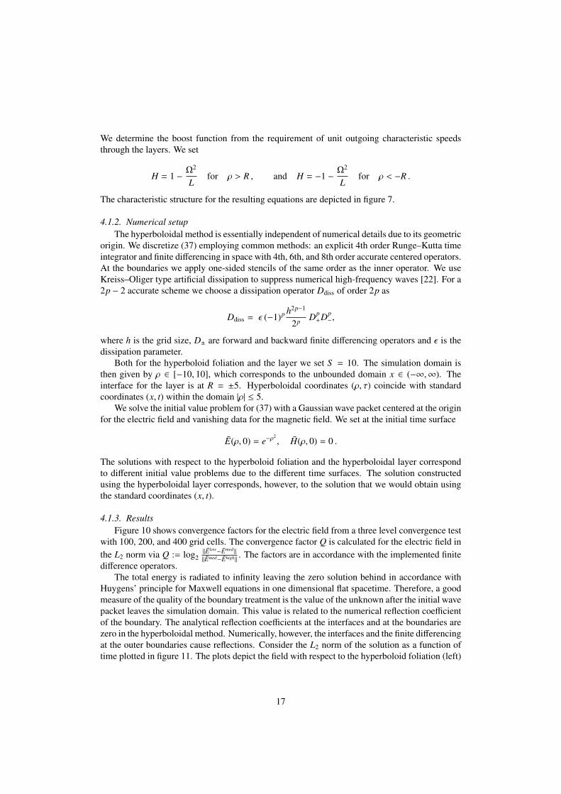
4.1.3. ResultsFigure 10 shows convergence factors for the electric field from a three level convergence test

with 100, 200, and 400 grid cells. The convergence factor Q is calculated for the electric field inthe L2 norm via Q := log2

‖Elow−Emed‖

‖Emed−Ehigh‖. The factors are in accordance with the implemented finite

difference operators.The total energy is radiated to infinity leaving the zero solution behind in accordance with

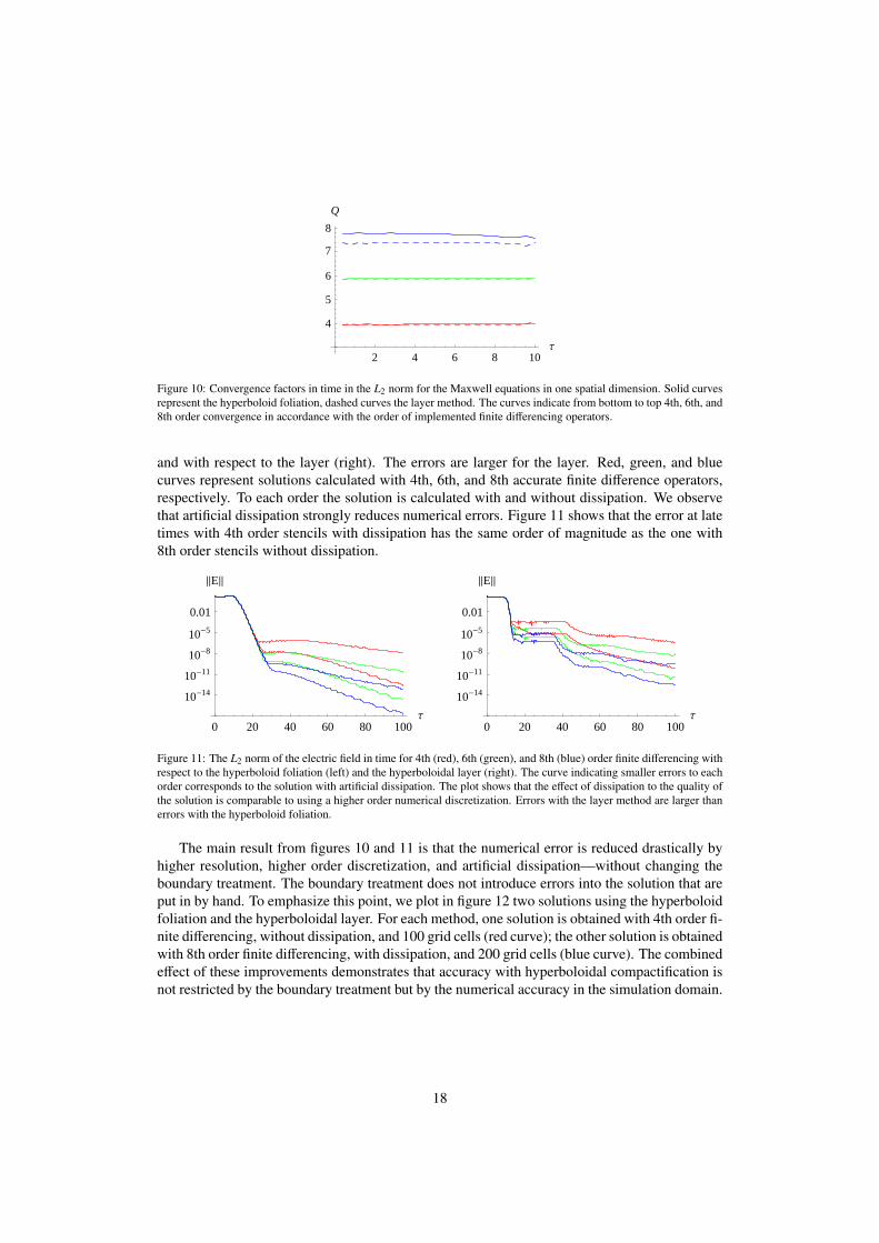
Huygens’ principle for Maxwell equations in one dimensional flat spacetime. Therefore, a goodmeasure of the quality of the boundary treatment is the value of the unknown after the initial wavepacket leaves the simulation domain. This value is related to the numerical reflection coefficientof the boundary. The analytical reflection coefficients at the interfaces and at the boundaries arezero in the hyperboloidal method. Numerically, however, the interfaces and the finite differencingat the outer boundaries cause reflections. Consider the L2 norm of the solution as a function oftime plotted in figure 11. The plots depict the field with respect to the hyperboloid foliation (left)

17

2 4 6 8 10Τ

4

5

6

7

8

Q

Figure 10: Convergence factors in time in the L2 norm for the Maxwell equations in one spatial dimension. Solid curvesrepresent the hyperboloid foliation, dashed curves the layer method. The curves indicate from bottom to top 4th, 6th, and8th order convergence in accordance with the order of implemented finite differencing operators.

and with respect to the layer (right). The errors are larger for the layer. Red, green, and bluecurves represent solutions calculated with 4th, 6th, and 8th accurate finite difference operators,respectively. To each order the solution is calculated with and without dissipation. We observethat artificial dissipation strongly reduces numerical errors. Figure 11 shows that the error at latetimes with 4th order stencils with dissipation has the same order of magnitude as the one with8th order stencils without dissipation.

0 20 40 60 80 100Τ

10-14

10-11

10-8

10-5

0.01

°E´

0 20 40 60 80 100Τ

10-14

10-11

10-8

10-5

0.01

°E´

Figure 11: The L2 norm of the electric field in time for 4th (red), 6th (green), and 8th (blue) order finite differencing withrespect to the hyperboloid foliation (left) and the hyperboloidal layer (right). The curve indicating smaller errors to eachorder corresponds to the solution with artificial dissipation. The plot shows that the effect of dissipation to the quality ofthe solution is comparable to using a higher order numerical discretization. Errors with the layer method are larger thanerrors with the hyperboloid foliation.

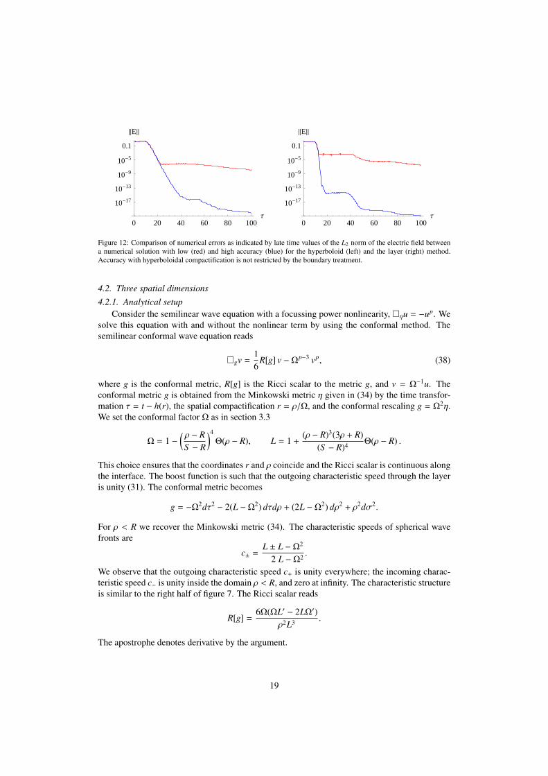
The main result from figures 10 and 11 is that the numerical error is reduced drastically byhigher resolution, higher order discretization, and artificial dissipation—without changing theboundary treatment. The boundary treatment does not introduce errors into the solution that areput in by hand. To emphasize this point, we plot in figure 12 two solutions using the hyperboloidfoliation and the hyperboloidal layer. For each method, one solution is obtained with 4th order fi-nite differencing, without dissipation, and 100 grid cells (red curve); the other solution is obtainedwith 8th order finite differencing, with dissipation, and 200 grid cells (blue curve). The combinedeffect of these improvements demonstrates that accuracy with hyperboloidal compactification isnot restricted by the boundary treatment but by the numerical accuracy in the simulation domain.

18

0 20 40 60 80 100Τ

10-17

10-13

10-9

10-5

0.1

°E´

0 20 40 60 80 100Τ

10-17

10-13

10-9

10-5

0.1

°E´

Figure 12: Comparison of numerical errors as indicated by late time values of the L2 norm of the electric field betweena numerical solution with low (red) and high accuracy (blue) for the hyperboloid (left) and the layer (right) method.Accuracy with hyperboloidal compactification is not restricted by the boundary treatment.

4.2. Three spatial dimensions4.2.1. Analytical setup

Consider the semilinear wave equation with a focussing power nonlinearity, ηu = −up. Wesolve this equation with and without the nonlinear term by using the conformal method. Thesemilinear conformal wave equation reads

gv =16

R[g] v −Ωp−3 vp, (38)

where g is the conformal metric, R[g] is the Ricci scalar to the metric g, and v = Ω−1u. Theconformal metric g is obtained from the Minkowski metric η given in (34) by the time transfor-mation τ = t − h(r), the spatial compactification r = ρ/Ω, and the conformal rescaling g = Ω2η.We set the conformal factor Ω as in section 3.3

Ω = 1 −(ρ − RS − R

)4

Θ(ρ − R), L = 1 +(ρ − R)3(3ρ + R)

(S − R)4 Θ(ρ − R) .

This choice ensures that the coordinates r and ρ coincide and the Ricci scalar is continuous alongthe interface. The boost function is such that the outgoing characteristic speed through the layeris unity (31). The conformal metric becomes

g = −Ω2dτ2 − 2(L −Ω2) dτdρ + (2L −Ω2) dρ2 + ρ2dσ2.

For ρ < R we recover the Minkowski metric (34). The characteristic speeds of spherical wavefronts are

c± =L ± L −Ω2

2 L −Ω2 .

We observe that the outgoing characteristic speed c+ is unity everywhere; the incoming charac-teristic speed c− is unity inside the domain ρ < R, and zero at infinity. The characteristic structureis similar to the right half of figure 7. The Ricci scalar reads

R[g] =6Ω(ΩL′ − 2LΩ′)

ρ2L3 .

The apostrophe denotes derivative by the argument.

19

4.2.2. Numerical setupWe apply similar numerical techniques as those that have been used to test constant mean

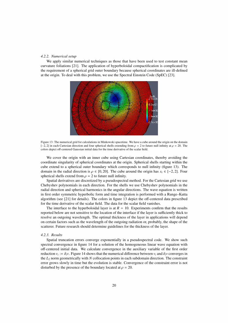
curvature foliations [21]. The application of hyperboloidal compactification is complicated bythe requirement of a spherical grid outer boundary because spherical coordinates are ill-definedat the origin. To deal with this problem, we use the Spectral Einstein Code (SpEC) [23].

Figure 13: The numerical grid for calculations in Minkowski spacetime. We have a cube around the origin on the domain[−2, 2] in each Cartesian direction and four spherical shells extending from ρ = 2 to future null infinity at ρ = 20. Thecolors depict off-centered Gaussian initial data for the time derivative of the scalar field.

We cover the origin with an inner cube using Cartesian coordinates, thereby avoiding thecoordinate singularity of spherical coordinates at the origin. Spherical shells starting within thecube extend to a spherical outer boundary which corresponds to null infinity (figure 13). Thedomain in the radial direction is ρ ∈ [0, 20]. The cube around the origin has xi ∈ [−2, 2]. Fourspherical shells extend from ρ = 2 to future null infinity.

Spatial derivatives are discretized by a pseudospectral method. For the Cartesian grid we useChebyshev polynomials in each direction. For the shells we use Chebyshev polynomials in theradial direction and spherical harmonics in the angular directions. The wave equation is writtenin first order symmetric hyperbolic form and time integration is performed with a Runge–Kuttaalgorithm (see [21] for details). The colors in figure 13 depict the off-centered data prescribedfor the time derivative of the scalar field. The data for the scalar field vanishes.

The interface to the hyperboloidal layer is at R = 10. Experiments confirm that the resultsreported below are not sensitive to the location of the interface if the layer is sufficiently thick toresolve an outgoing wavelength. The optimal thickness of the layer in applications will dependon certain factors such as the wavelength of the outgoing radiation or, probably, the shape of thescatterer. Future research should determine guidelines for the thickness of the layer.

4.2.3. ResultsSpatial truncation errors converge exponentially in a pseudospectral code. We show such

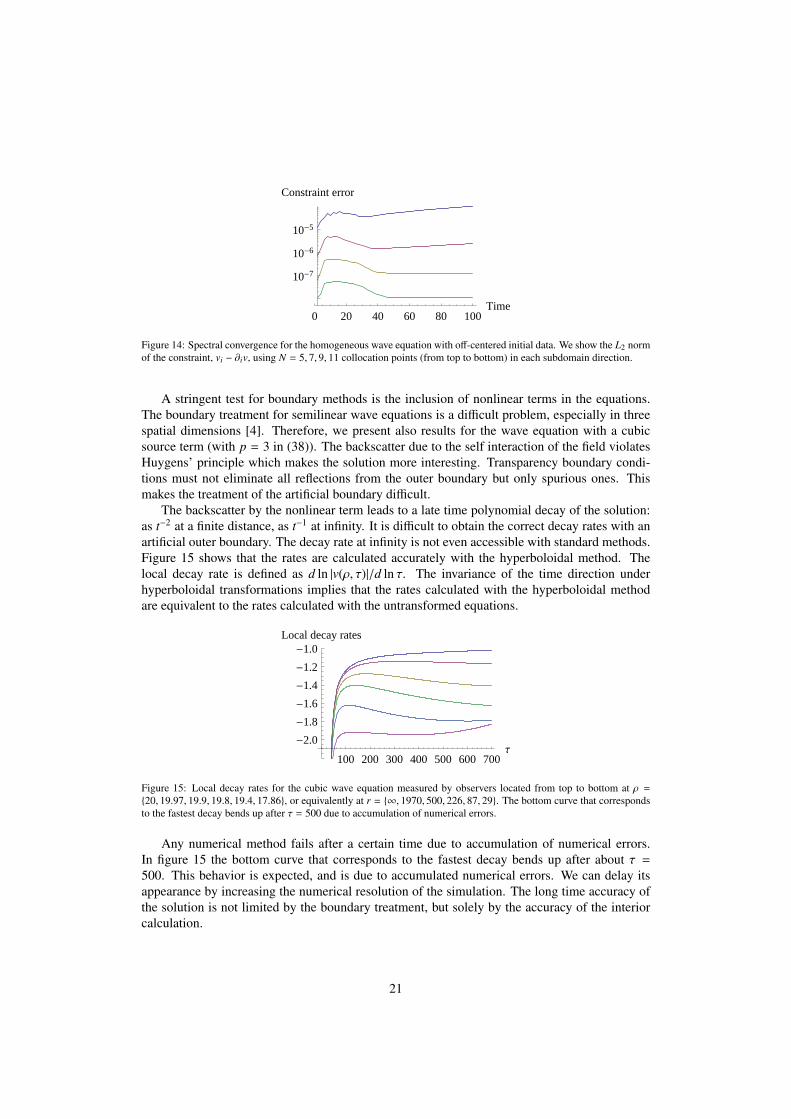
spectral convergence in figure 14 for a solution of the homogeneous linear wave equation withoff-centered initial data. We calculate convergence in the auxiliary variable of the first orderreduction vi := ∂iv. Figure 14 shows that the numerical difference between vi and ∂iv converges inthe L2 norm geometrically with N collocation points in each subdomain direction. The constrainterror grows slowly in time but the evolution is stable. Convergence of the constraint error is notdisturbed by the presence of the boundary located at ρ = 20.

20

0 20 40 60 80 100Time

10-7

10-6

10-5

Constraint error

Figure 14: Spectral convergence for the homogeneous wave equation with off-centered initial data. We show the L2 normof the constraint, vi − ∂iv, using N = 5, 7, 9, 11 collocation points (from top to bottom) in each subdomain direction.

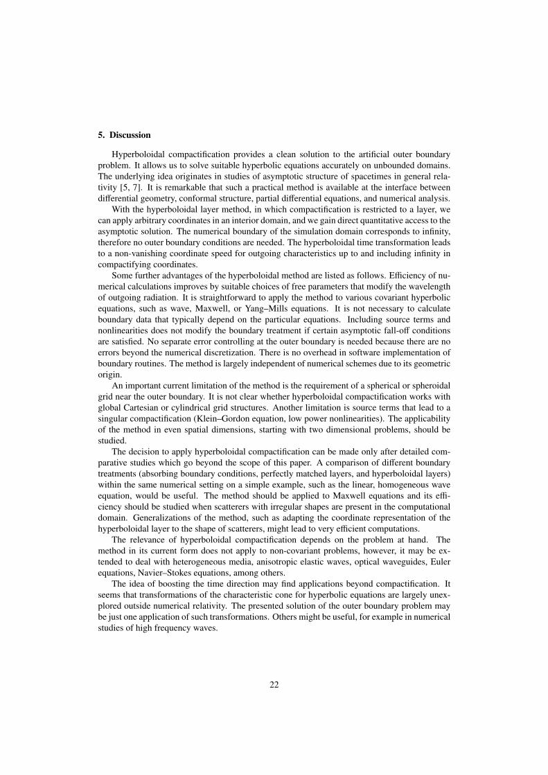
A stringent test for boundary methods is the inclusion of nonlinear terms in the equations.The boundary treatment for semilinear wave equations is a difficult problem, especially in threespatial dimensions [4]. Therefore, we present also results for the wave equation with a cubicsource term (with p = 3 in (38)). The backscatter due to the self interaction of the field violatesHuygens’ principle which makes the solution more interesting. Transparency boundary condi-tions must not eliminate all reflections from the outer boundary but only spurious ones. Thismakes the treatment of the artificial boundary difficult.

The backscatter by the nonlinear term leads to a late time polynomial decay of the solution:as t−2 at a finite distance, as t−1 at infinity. It is difficult to obtain the correct decay rates with anartificial outer boundary. The decay rate at infinity is not even accessible with standard methods.Figure 15 shows that the rates are calculated accurately with the hyperboloidal method. Thelocal decay rate is defined as d ln |v(ρ, τ)|/d ln τ. The invariance of the time direction underhyperboloidal transformations implies that the rates calculated with the hyperboloidal methodare equivalent to the rates calculated with the untransformed equations.

100 200 300 400 500 600 700Τ

-2.0

-1.8

-1.6

-1.4

-1.2

-1.0Local decay rates

Figure 15: Local decay rates for the cubic wave equation measured by observers located from top to bottom at ρ =

20, 19.97, 19.9, 19.8, 19.4, 17.86, or equivalently at r = ∞, 1970, 500, 226, 87, 29. The bottom curve that correspondsto the fastest decay bends up after τ = 500 due to accumulation of numerical errors.

Any numerical method fails after a certain time due to accumulation of numerical errors.In figure 15 the bottom curve that corresponds to the fastest decay bends up after about τ =

500. This behavior is expected, and is due to accumulated numerical errors. We can delay itsappearance by increasing the numerical resolution of the simulation. The long time accuracy ofthe solution is not limited by the boundary treatment, but solely by the accuracy of the interiorcalculation.

21

5. Discussion

Hyperboloidal compactification provides a clean solution to the artificial outer boundaryproblem. It allows us to solve suitable hyperbolic equations accurately on unbounded domains.The underlying idea originates in studies of asymptotic structure of spacetimes in general rela-tivity [5, 7]. It is remarkable that such a practical method is available at the interface betweendifferential geometry, conformal structure, partial differential equations, and numerical analysis.

With the hyperboloidal layer method, in which compactification is restricted to a layer, wecan apply arbitrary coordinates in an interior domain, and we gain direct quantitative access to theasymptotic solution. The numerical boundary of the simulation domain corresponds to infinity,therefore no outer boundary conditions are needed. The hyperboloidal time transformation leadsto a non-vanishing coordinate speed for outgoing characteristics up to and including infinity incompactifying coordinates.

Some further advantages of the hyperboloidal method are listed as follows. Efficiency of nu-merical calculations improves by suitable choices of free parameters that modify the wavelengthof outgoing radiation. It is straightforward to apply the method to various covariant hyperbolicequations, such as wave, Maxwell, or Yang–Mills equations. It is not necessary to calculateboundary data that typically depend on the particular equations. Including source terms andnonlinearities does not modify the boundary treatment if certain asymptotic fall-off conditionsare satisfied. No separate error controlling at the outer boundary is needed because there are noerrors beyond the numerical discretization. There is no overhead in software implementation ofboundary routines. The method is largely independent of numerical schemes due to its geometricorigin.

An important current limitation of the method is the requirement of a spherical or spheroidalgrid near the outer boundary. It is not clear whether hyperboloidal compactification works withglobal Cartesian or cylindrical grid structures. Another limitation is source terms that lead to asingular compactification (Klein–Gordon equation, low power nonlinearities). The applicabilityof the method in even spatial dimensions, starting with two dimensional problems, should bestudied.

The decision to apply hyperboloidal compactification can be made only after detailed com-parative studies which go beyond the scope of this paper. A comparison of different boundarytreatments (absorbing boundary conditions, perfectly matched layers, and hyperboloidal layers)within the same numerical setting on a simple example, such as the linear, homogeneous waveequation, would be useful. The method should be applied to Maxwell equations and its effi-ciency should be studied when scatterers with irregular shapes are present in the computationaldomain. Generalizations of the method, such as adapting the coordinate representation of thehyperboloidal layer to the shape of scatterers, might lead to very efficient computations.

The relevance of hyperboloidal compactification depends on the problem at hand. Themethod in its current form does not apply to non-covariant problems, however, it may be ex-tended to deal with heterogeneous media, anisotropic elastic waves, optical waveguides, Eulerequations, Navier–Stokes equations, among others.

The idea of boosting the time direction may find applications beyond compactification. Itseems that transformations of the characteristic cone for hyperbolic equations are largely unex-plored outside numerical relativity. The presented solution of the outer boundary problem maybe just one application of such transformations. Others might be useful, for example in numericalstudies of high frequency waves.

22

Acknowledgments

I thank Daniel Appelo, Eliane Becache, and Frederic Nataf for discussions, Larry Kidderfor his help with SpEC, and Piotr Bizon, Philippe LeFloch, and Eitan Tadmor for support. Thisresearch was supported by the National Science Foundation (NSF) grant 07-07949 in Maryland,by the Marie Curie Transfer of Knowledge contract MTKD-CT-2006-042360 in Krakow, by theAgence Nationale de la Recherche (ANR) grant 06-2-134423 entitled ”Mathematical Methodsin General Relativity” in Paris, by the NSF grant PHY-0601459 and by a Sherman FairchildFoundation grant to Caltech in Pasadena.

References

[1] C. E. Grosch and S. A. Orszag, Numerical solution of Problems in Unbounded Regions: Coordinate Transforms,J. Comput. Phys. 25 (1977) 273–296.

[2] D. Givoli, High-order local non-reflecting boundary conditions: a review, Wave Motion 39 (2004) 319–326.[3] T. Hagstrom and S. Lau, Radiation boundary conditions for Maxwell’s equations: A review of accurate time-

domain formulations, J. Comput. Math. 25 (2007) 305–336.[4] J. Szeftel, A nonlinear approach to absorbing boundary conditions for the semilinear wave equation, Math. Comput.

75 (2006) 565–594.[5] R. Penrose, Asymptotic properties of fields and space-times, Phys. Rev. Lett. 10 (1963) 66–68.[6] D. M. Eardley and L. Smarr, Time functions in numerical relativity: Marginally bound dust collapse, Phys. Rev. D

19 (1979) 2239–2259.[7] H. Friedrich, Cauchy problems for the conformal vacuum field equations in general relativity, Comm. Math. Phys.

91 (1983) 445–472.[8] A. Zenginoglu, Hyperboloidal foliations and scri-fixing, Class. Quant. Grav. 25 (2008) 145002.[9] J.-P. Berenger, A perfectly matched layer for the absorption of electromagnetic waves, J. Comput. Phys. 114 (1994)

185–200.[10] W. C. Chew and W. H. Weedon, A 3D perfectly matched medium from modified Maxwell’s equations with stretched

coordinates, Microwave and Optical Technology Letters 7 (1994) 599–604.[11] S. Abarbanel and D. Gottlieb, A mathematical analysis of the PML method, J. Comput. Phys. 134 (1997) 357–363.[12] D. Appelo, T. Hagstrom, and G. Kreiss, Perfectly matched layers for hyperbolic systems: General formulation,

well-posedness, and stability, SIAM Journal on Applied Mathematics 67 (1) (2006) 1–23.[13] E. Becache, S. Fauqueux, and P. Joly, Stability of perfectly matched layers, group velocities and anisotropic waves,

J. Comput. Phys. 188 (2003) 399–433.[14] R. M. Wald, General relativity, The University of Chicago Press, Chicago, 1984.[15] R. Penrose, Zero rest-mass fields including gravitation: Asymptotic behaviour, Proc. Roy. Soc. Lond. A284 (1965)

159–203.[16] R. Geroch, Asymptotic structure of space-time, in: F. Esposito, L. Witten (Eds.), Asymptotic Structure of Space-

Time, Plenum Press, 1977, pp. 1–105.[17] H. Friedrich, Conformal Einstein evolution, Lect. Notes Phys. 604 (2002) 1–50.[18] A. Zenginoglu, A hyperboloidal study of tail decay rates for scalar and Yang-Mills fields, Class. Quant. Grav. 25

(2008) 175013.[19] S. Hollands and R. M. Wald, Conformal null infinity does not exist for radiating solutions in odd spacetime dimen-

sions, Class. Quant. Grav. 21 (2004) 5139.[20] A. Zenginoglu, Asymptotics of Schwarzschild black hole perturbations, Class. Quant. Grav. 27 (2010) 045015.[21] A. Zenginoglu and L. E. Kidder, Hyperboloidal evolution of test fields in three spatial dimensions, Phys. Rev. D81

(2010) 124010.[22] H. O. Kreiss and J. Oliger, Methods for the approximate solution of time dependent problems, International Council

of Scientific Unions, World Meteorological Organization, Geneva, 1973.[23] L. Kidder, H. Pfeiffer, and M. Scheel, SpEC: Spectral Einstein Code.

URL http://www.black-holes.org/SpEC.html

23