IEICE TRANS. INF. & SYST., VOL.E101–D, NO.6 JUNE 20181581

PAPER

Domain Adaptation Based on Mixture of Latent Words LanguageModels for Automatic Speech Recognition

Ryo MASUMURA†a), Taichi ASAMI†, Takanobu OBA†∗, Hirokazu MASATAKI†, Sumitaka SAKAUCHI†,and Akinori ITO††, Members

SUMMARY This paper proposes a novel domain adaptation methodthat can utilize out-of-domain text resources and partially domain matchedtext resources in language modeling. A major problem in domain adap-tation is that it is hard to obtain adequate adaptation effects from out-of-domain text resources. To tackle the problem, our idea is to carry out modelmerger in a latent variable space created from latent words language mod-els (LWLMs). The latent variables in the LWLMs are represented as spe-cific words selected from the observed word space, so LWLMs can sharea common latent variable space. It enables us to perform flexible mix-ture modeling with consideration of the latent variable space. This paperpresents two types of mixture modeling, i.e., LWLM mixture models andLWLM cross-mixture models. The LWLM mixture models can perform alatent word space mixture modeling to mitigate domain mismatch problem.Furthermore, in the LWLM cross-mixture models, LMs which individuallyconstructed from partially matched text resources are split into two elementmodels, each of which can be subjected to mixture modeling. For the ap-proaches, this paper also describes methods to optimize mixture weightsusing a validation data set. Experiments show that the mixture in latentword space can achieve performance improvements for both target domainand out-of-domain compared with that in observed word space.key words: domain adaptation, mixture modeling, latent words languagemodels, latent variable space, automatic speech recognition

1. Introduction

Language models (LMs) are invaluable for natural lan-guage processing tasks such as automatic speech recogni-tion (ASR) and statistical machine translation [1], [2]. LMperformance strongly depends on the quantity and quality ofthe training data sets. Superior performance is usually ob-tained by using enormous domain-matched data sets to con-struct LMs [3]. Unfortunately, in practical ASR tasks, largeamounts of domain-matched data sets are not available.

Therefore, LMs demand domain adaptation techniquesto allow the use of multiple out-of-domain text resources [4],[5]. In language modeling, one of the most popular ap-proaches to domain adaptation is based on mixture model-ing [6], [7]. An adapted model can be constructed by com-bining LMs that are individually constructed from out-of-domain text resources with mixture weighting [8]. The mix-

Manuscript received July 3, 2017.Manuscript revised January 5, 2018.Manuscript publicized February 26, 2018.†The authors are with NTT Media Intelligence Laboratories,

NTT Corporation, Yokosuka-shi, 239–0847 Japan.††The author is with the Graduate School of Engineering,

Tohoku University, Sendai-shi, 980–8579 Japan.∗Presently, with NTT Docomo Corporation, Yokosuka-shi,

239–8536 Japan.a) E-mail: masumura.ryo@lab.ntt.co.jp

DOI: 10.1587/transinf.2017EDP7210

ture weights are optimized using a small amount of targetdomain text.

Previously, observed word space mixture modeling,i.e., n-gram mixture modeling, has been used in variouscases [9]–[11]. Also, mixture modeling of recurrent neuralnetwork LMs (RNNLMs) was performed in the observedword space [12]–[14]. However, mixtures in the observedword space do not support flexible domain adaptation ifdomain-related data sets are hardly obtained. In the ob-served word space, a word directly represents a state in amixture. It can be considered that effective state sharingis not available by merging LMs individually constructedfrom out-of-domain text resources since words are not over-lapped.

In order to conduct flexible domain adaptation usingthe LMs constructed from out-of-domain text resources, thispaper develops methods in which model merging is con-ducted in a latent variable space. In the latent variable space,a word is mapped into a latent variable space, so it can beexpected to perform more flexible state sharing than is pos-sible in the observed word space. To this end, this paperintroduces latent words language models (LWLMs) to themixture modeling [15]–[18]. The latent variables in usualclass based n-gram LMs are only model-dependent indices,so each model has a different latent variable space [19], [20].Therefore, conventional class-based n-gram mixture model-ing have to be performed in the observed word space [21],[22]. On the other hand, latent variables in LWLMs are rep-resented as specific latent word, multiple LWLMs can sharethe common latent variable space.

In addition, this paper also focuses on the fact that anyLWLM can be split into two elements, a transition probabil-ity model and an emission probability model, and each ofwhich can be mixed independently. This concept of mix-ture modeling yields flexibility in that both elements are theintersections of different data sources. It is assumed thateach element model has a different role, i.e., the transitionprobability model captures the sentence pattern in the la-tent variable space, while the emission probability modelcaptures the lexical pattern in the observed word space. Infact, most available out-of-domain text resources in practi-cal ASR tasks will partially match either the sentence pat-tern or the lexical pattern. It can be expected that a domainmatched model will become available by optimizing bothelements independently.

In this paper, two types of mixture modeling meth-

Copyright c© 2018 The Institute of Electronics, Information and Communication Engineers

1582IEICE TRANS. INF. & SYST., VOL.E101–D, NO.6 JUNE 2018

ods using multiple LWLMs are proposed. One is LWLMmixture models that can merge multiple LWLM in the la-tent word space with mixture weights. The other is LWLMcross-mixture models in which two elements in LWLMs areindependently combined with mixture weights. Althoughthe proposed models have complex model structure, theycan be implemented into ASR decoder using n-gram ap-proximation method, which randomly generates a lot of textdata according to a stochastic process and a simple n-grammodel is constructed from the generated data [16], [18].

For domain adaptation, this paper also presents theiroptimization method using a validation data set. In the ob-served word space mixture, the maximum likelihood (ML)criterion can be used because generative probabilities ofeach word of the validation data set can be directly calcu-lated [23]. Unfortunately, this advantage is offset by the factthe latent word sequence of the validation data set cannotbe determined uniquely. In order to estimate optimal mix-ture weights of the LWLM mixture models and the LWLMcross-mixture models, we introduce Bayesian criterion. TheBayesian criterion can be flexibly applied to various modelstructures, and sampling techniques can be used. In this pa-per, Gibbs sampling is introduced for estimating the latentword sequence and model index sequence underlying thevalidation data set [24].

In fact, this paper is an extended study of our pre-vious work in which LWLM mixture models were onlypresented [25]. In this paper, we additionally formulatethe LWLM cross-mixture modeling and its optimizationmethod, and clarify relationships to each mixture model.Our evaluation examines two kinds of setups. The first ex-periment employs in-domain training data set and out-of-domain training data set for constructing a target domainLM, and shows effectiveness of the LWLM-mixture mod-els. The second experiment employs two types of par-tially matching training data sets on the assumption of apractical spontaneous speech recognition task, and showsthe LWLM-cross mixture model yields additional adapta-tion effects which cannot be obtained by the LWLM-mixturemodel.

The rest of this paper is organized as follows. Sec-tion 2 overviews LWLMs and n-gram mixture models. Sec-tion 3 describes definitions of LWLM mixture models andLWLM cross-mixture models. In addition, optimizationmethods for domain adaptation and implementation meth-ods for ASR tasks are detailed. Sections 4 and 5 presentautomatic speech recognition experiments. Section 6 con-cludes this paper with a summary of key points.

2. Previous Work

2.1 Latent Words Language Models

LWLMs are generative models that employ a latent variablecalled latent word [15]. An LWLM has a soft clusteringstructure, and a latent word is a specific word that can beselected from the entire vocabulary. Thus, the number of la-

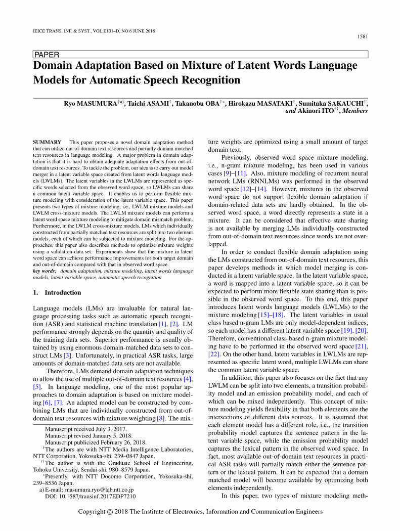
Fig. 1 Model structure of LWLMs.

tent words equals the number of observed words, and mul-tiple LWLMs can share a common latent variable space.

In the generative process of an LWLM, a latent wordht is generated on the basis of a transition probability modeland its context lt = ht−n+1, · · · , ht−1. An observed word wt isgenerated on the basis of an emission probability model anda latent word ht. A graphic rendering of LWLM is shown inFig. 1. The gray circles denote observed words and the whitecircles denote latent variables. The LWLM produces thegenerative probability of the observed word sequence w =w1, · · · , wT . The probability is approximately calculated bythe following point estimation:

P(w) �T∏

t=1

∑

ht∈VP(wt |ht,Θlw)P(ht |lt,Θlw), (1)

where Θlw indicates a model parameter of the LWLM,and V is the vocabulary. The transition probability modelP(ht |lt,Θlw) is expressed as an n-gram model for latentwords; it can capture the sentence pattern on the basis ofa latent variable sequence. The emission probability modelP(wt |ht,Θlw) is expressed as a unigram model for each latentword and can capture the lexical pattern. Usually a hierar-chical Pitman-Yor prior is used as the transition probabilitymodel, and a Dirichlet prior is used as the emission prob-ability model. More details are provided in previous stud-ies [15]–[18].

2.2 N-gram Mixture Models

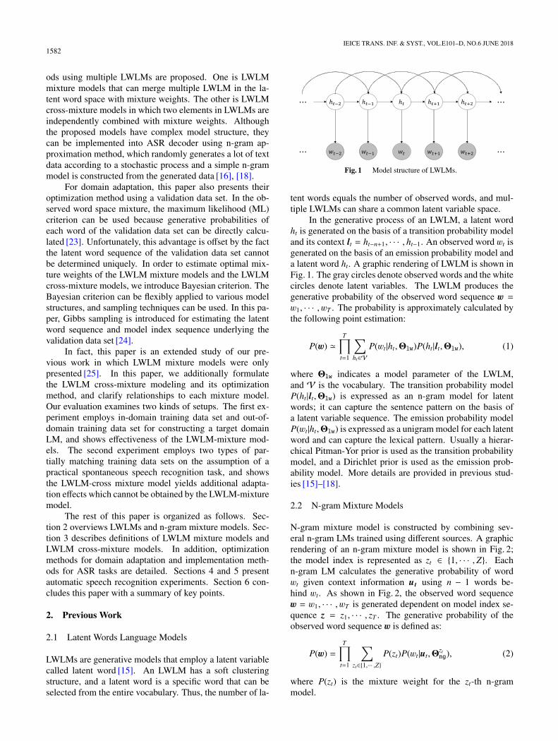
N-gram mixture model is constructed by combining sev-eral n-gram LMs trained using different sources. A graphicrendering of an n-gram mixture model is shown in Fig. 2;the model index is represented as zt ∈ {1, · · · ,Z}. Eachn-gram LM calculates the generative probability of wordwt given context information ut using n − 1 words be-hind wt. As shown in Fig. 2, the observed word sequencew = w1, · · · , wT is generated dependent on model index se-quence z = z1, · · · , zT . The generative probability of theobserved word sequence w is defined as:

P(w) =T∏

t=1

∑

zt∈{1,··· ,Z}P(zt)P(wt |ut,Θ

ztng), (2)

where P(zt) is the mixture weight for the zt-th n-grammodel.

MASUMURA et al.: DOMAIN ADAPTATION BASED ON MIXTURE OF LATENT WORDS LANGUAGE MODELS FOR AUTOMATIC SPEECH RECOGNITION1583

Fig. 2 Model structure of n-gram mixture models.

In practice, direct implementation of the n-gram mix-ture model to ASR is not ideal because it does not havea back-off n-gram structure. Actually, the n-gram mixturemodel can be approximately represented as a single back-off n-gram structure [26].

For domain adaptation of n-gram mixture models, mix-ture weights are optimized using a validation data set.The expectation maximization algorithm, which is basedon maximum likelihood (ML) criterion, can be used forthe optimization [23]. Given a validation data set W =

w1, · · · , w|W|, the optimized mixture weight P̂(z) is esti-mated in an iterative manner as:

P̂(z) =1|W|

|W|∑

t=1

P(wt |ut,Θzng)P(z)

∑z′ ∈{1,··· ,Z} P(wt |ut,Θ

z′ng)P(z′)

. (3)

After iterations, the optimized weight P̂(z) is used in Eq. (2).

3. Proposed Method

3.1 LWLM Mixture Models

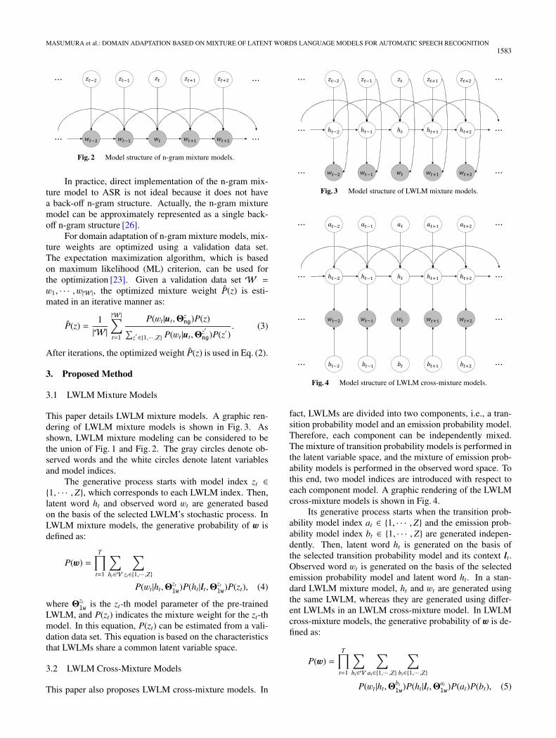
This paper details LWLM mixture models. A graphic ren-dering of LWLM mixture models is shown in Fig. 3. Asshown, LWLM mixture modeling can be considered to bethe union of Fig. 1 and Fig. 2. The gray circles denote ob-served words and the white circles denote latent variablesand model indices.

The generative process starts with model index zt ∈{1, · · · ,Z}, which corresponds to each LWLM index. Then,latent word ht and observed word wt are generated basedon the basis of the selected LWLM’s stochastic process. InLWLM mixture models, the generative probability of w isdefined as:

P(w) =T∏

t=1

∑

ht∈V

∑

zt∈{1,··· ,Z}P(wt |ht,Θ

zt

lw)P(ht |lt,Θzt

lw)P(zt), (4)

where Θzt

lwis the zt-th model parameter of the pre-trained

LWLM, and P(zt) indicates the mixture weight for the zt-thmodel. In this equation, P(zt) can be estimated from a vali-dation data set. This equation is based on the characteristicsthat LWLMs share a common latent variable space.

3.2 LWLM Cross-Mixture Models

This paper also proposes LWLM cross-mixture models. In

Fig. 3 Model structure of LWLM mixture models.

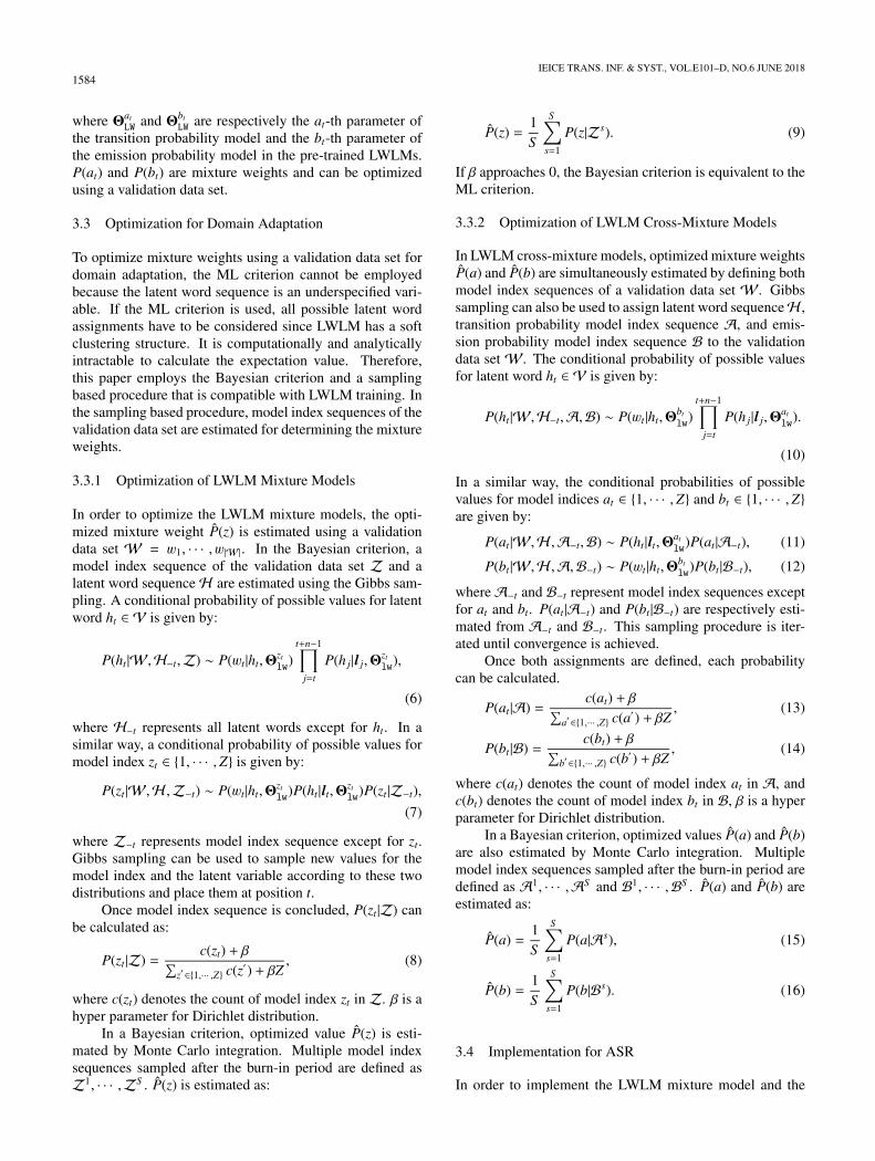
Fig. 4 Model structure of LWLM cross-mixture models.

fact, LWLMs are divided into two components, i.e., a tran-sition probability model and an emission probability model.Therefore, each component can be independently mixed.The mixture of transition probability models is performed inthe latent variable space, and the mixture of emission prob-ability models is performed in the observed word space. Tothis end, two model indices are introduced with respect toeach component model. A graphic rendering of the LWLMcross-mixture models is shown in Fig. 4.

Its generative process starts when the transition prob-ability model index at ∈ {1, · · · ,Z} and the emission prob-ability model index bt ∈ {1, · · · ,Z} are generated indepen-dently. Then, latent word ht is generated on the basis ofthe selected transition probability model and its context lt.Observed word wt is generated on the basis of the selectedemission probability model and latent word ht. In a stan-dard LWLM mixture model, ht and wt are generated usingthe same LWLM, whereas they are generated using differ-ent LWLMs in an LWLM cross-mixture model. In LWLMcross-mixture models, the generative probability of w is de-fined as:

P(w) =T∏

t=1

∑

ht∈V

∑

at∈{1,··· ,Z}

∑

bt∈{1,··· ,Z}P(wt |ht,Θ

bt

lw)P(ht |lt,Θat

lw)P(at)P(bt), (5)

1584IEICE TRANS. INF. & SYST., VOL.E101–D, NO.6 JUNE 2018

where ΘatLW and Θbt

LW are respectively the at-th parameter ofthe transition probability model and the bt-th parameter ofthe emission probability model in the pre-trained LWLMs.P(at) and P(bt) are mixture weights and can be optimizedusing a validation data set.

3.3 Optimization for Domain Adaptation

To optimize mixture weights using a validation data set fordomain adaptation, the ML criterion cannot be employedbecause the latent word sequence is an underspecified vari-able. If the ML criterion is used, all possible latent wordassignments have to be considered since LWLM has a softclustering structure. It is computationally and analyticallyintractable to calculate the expectation value. Therefore,this paper employs the Bayesian criterion and a samplingbased procedure that is compatible with LWLM training. Inthe sampling based procedure, model index sequences of thevalidation data set are estimated for determining the mixtureweights.

3.3.1 Optimization of LWLM Mixture Models

In order to optimize the LWLM mixture models, the opti-mized mixture weight P̂(z) is estimated using a validationdata set W = w1, · · · , w|W|. In the Bayesian criterion, amodel index sequence of the validation data set Z and alatent word sequenceH are estimated using the Gibbs sam-pling. A conditional probability of possible values for latentword ht ∈ V is given by:

P(ht |W,H−t,Z) ∼ P(wt |ht,Θzt

lw)

t+n−1∏

j=t

P(h j|l j,Θzt

lw),

(6)

where H−t represents all latent words except for ht. In asimilar way, a conditional probability of possible values formodel index zt ∈ {1, · · · ,Z} is given by:

P(zt |W,H ,Z−t) ∼ P(wt |ht,Θzt

lw)P(ht |lt,Θzt

lw)P(zt |Z−t),

(7)

where Z−t represents model index sequence except for zt.Gibbs sampling can be used to sample new values for themodel index and the latent variable according to these twodistributions and place them at position t.

Once model index sequence is concluded, P(zt |Z) canbe calculated as:

P(zt |Z) =c(zt) + β∑

z′ ∈{1,··· ,Z} c(z′) + βZ, (8)

where c(zt) denotes the count of model index zt in Z. β is ahyper parameter for Dirichlet distribution.

In a Bayesian criterion, optimized value P̂(z) is esti-mated by Monte Carlo integration. Multiple model indexsequences sampled after the burn-in period are defined asZ1, · · · ,ZS . P̂(z) is estimated as:

P̂(z) =1S

S∑

s=1

P(z|Zs). (9)

If β approaches 0, the Bayesian criterion is equivalent to theML criterion.

3.3.2 Optimization of LWLM Cross-Mixture Models

In LWLM cross-mixture models, optimized mixture weightsP̂(a) and P̂(b) are simultaneously estimated by defining bothmodel index sequences of a validation data set W. Gibbssampling can also be used to assign latent word sequenceH ,transition probability model index sequence A, and emis-sion probability model index sequence B to the validationdata setW. The conditional probability of possible valuesfor latent word ht ∈ V is given by:

P(ht |W,H−t,A,B) ∼ P(wt |ht,Θbt

lw)

t+n−1∏

j=t

P(h j|l j,Θat

lw).

(10)

In a similar way, the conditional probabilities of possiblevalues for model indices at ∈ {1, · · · ,Z} and bt ∈ {1, · · · ,Z}are given by:

P(at |W,H ,A−t,B) ∼ P(ht |lt,Θat

lw)P(at |A−t), (11)

P(bt |W,H ,A,B−t) ∼ P(wt |ht,Θbt

lw)P(bt |B−t), (12)

whereA−t and B−t represent model index sequences exceptfor at and bt. P(at |A−t) and P(bt |B−t) are respectively esti-mated from A−t and B−t. This sampling procedure is iter-ated until convergence is achieved.

Once both assignments are defined, each probabilitycan be calculated.

P(at |A) =c(at) + β∑

a′ ∈{1,··· ,Z} c(a′ ) + βZ, (13)

P(bt |B) =c(bt) + β∑

b′ ∈{1,··· ,Z} c(b′ ) + βZ, (14)

where c(at) denotes the count of model index at in A, andc(bt) denotes the count of model index bt in B, β is a hyperparameter for Dirichlet distribution.

In a Bayesian criterion, optimized values P̂(a) and P̂(b)are also estimated by Monte Carlo integration. Multiplemodel index sequences sampled after the burn-in period aredefined as A1, · · · ,AS and B1, · · · ,BS . P̂(a) and P̂(b) areestimated as:

P̂(a) =1S

S∑

s=1

P(a|As), (15)

P̂(b) =1S

S∑

s=1

P(b|Bs). (16)

3.4 Implementation for ASR

In order to implement the LWLM mixture model and the

MASUMURA et al.: DOMAIN ADAPTATION BASED ON MIXTURE OF LATENT WORDS LANGUAGE MODELS FOR AUTOMATIC SPEECH RECOGNITION1585

Algorithm 1 Random sampling based on LWLM mixturemodel.Input: Model parameters Θ1

lw, · · · ,ΘM

lw, number of sampled words T

Output: Sampled words w1: l1 = <s>2: for t = 1 to T do3: zt ∼ P(zt)4: ht ∼ P(ht |lt ,Θzt

lw)

5: wt ∼ P(wt |ht ,Θztlw

)6: end for7: return w = w1, · · · , wT

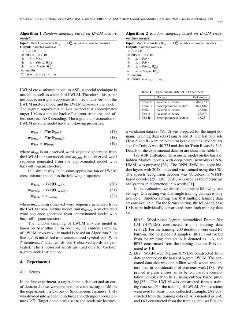
LWLM cross-mixture model to ASR, a special technique isneeded as well as a standard LWLM. Therefore, this paperintroduces an n-gram approximation technique for both theLWLM mixture model and the LWLM cross-mixture model.The n-gram approximation is a method that approximatestarget LM as a simple back-off n-gram structure, and of-fers one-pass ASR decoding. The n-gram approximation ofLWLM mixture model has the following properties:

wlwm ∼ P(w|Θlwm), (17)

wlwmng ∼ P(w|Θlwmng), (18)

wlwm � wlwmng, (19)

where wlwm is an observed word sequence generated fromthe LWLM mixture model, and wlwmng is an observed wordsequence generated from the approximated model withback-off n-gram structure.

In a similar way, the n-gram approximation of LWLMcross-mixture model has the following properties:

wlwcm ∼ P(w|Θlwcm), (20)

wlwcmng ∼ P(w|Θlwcmng), (21)

wlwcm � wlwcmng, (22)

where wlwcm is an observed word sequence generated fromthe LWLM cross-mixture model, and wlwcmng is an observedword sequence generated from approximated model withback-off n-gram structure.

The random sampling of LWLM mixture model isbased on Algorithm 1. In addition, the random samplingof LWLM cross-mixture model is based on Algorithm 2. Inline 1, l1 is initialized as a sentence head symbol <s>. WithT iterations, T latent words, and T observed words are gen-erated. The T observed words are used only for back-offn-gram model estimation.

4. Experiment 1

4.1 Setups

In the first experiment, a target domain data set and an out-of-domain data set were prepared for constructing an LM. Inthe experiment, the Corpus of Spontaneous Japanese (CSJ)was divided into academic lectures and extemporaneous lec-tures [27]. Target domain was set to the academic lectures;

Algorithm 2 Random sampling based on LWLM cross-mixture model.Input: Model parameters Θ1

lw, · · · ,ΘM

lw, number of sampled words T

Output: Sampled words w1: l1 = <s>2: for t = 1 to T do3: at ∼ P(at)4: bt ∼ P(bt)5: ht ∼ P(ht |lt ,Θat

lw)

6: wt ∼ P(wt |ht ,Θbtlw

)7: end for8: return w = w1, · · · , wT

Table 1 Experimental data set in Experiment 1.

Domain # of words

Train A Academic lecture 3,468,133Train B Extemporaneous lecture 3,847,816Valid Academic lecture 28,046Test A Academic lecture 27,907Test B Extemporaneous lecture 18,251

a validation data set (Valid) was prepared for the target do-main. Training data sets (Train A and B) and test data sets(Test A and B) were prepared for both domains. Vocabularysize for Train A was 40,725 and that for Train B was 64,543.Details of the experimental data set are shown in Table 1.

For ASR evaluation, an acoustic model on the basis ofhidden Markov models with deep neural networks (DNN-HMM) was prepared [28]. The DNN-HMM had eight hid-den layers with 2048 nodes and was trained using the CSJ.The speech recognition decoder was VoiceRex, a WFST-based decoder [29], [30]. JTAG was used as the morphemeanalyzer to split sentences into words [31].

In the evaluation, we aimed to compare following twosettings. One setting was that single training data set is onlyavailable. Another setting was that multiple training datasets are available. For the former setting, the following baseLMs were individually constructed from each training dataset.

1. HPY3: Word-based 3-gram hierarchical Pitman-YorLM (HPYLM) constructed from a training dataset [32]. For the training, 200 iterations were used forburn-in, and collected 10 samples. HPY3 constructedfrom the training data set A is denoted as 1-A, andHPY3 constructed from the training data set B is de-noted as 1-B

2. LW3: Word-based 3-gram HPYLM constructed fromdata generated on the basis of 3-gram LWLM. The gen-erated data size was one billion words which was de-termined in consideration of previous work [18]. Wepruned n-gram entries as to be comparable compu-tation complexity to HPY3 using entropy based prun-ing [33]. The LWLM was constructed from a train-ing data set. For the training of LWLM, 500 iterationswere used for burn-in and collected a sample. LW3 con-structed from the training data set A is denoted as 2-A,and LW3 constructed from the training data set B is de-

1586IEICE TRANS. INF. & SYST., VOL.E101–D, NO.6 JUNE 2018

Table 3 Perplexity and word error rate [%] results in Experiment 1.

Valid (Target domain) Test A (Target domain) Test B (Out-of-domain)PPL WER PPL WER PPL WER

1-A. Base model A HPY3 70.57 20.80 62.85 21.98 183.38 32.512-A. (Target domain training set) LW3 70.02 20.72 62.34 21.85 165.87 31.433-A. HPY3+LW3 65.30 19.27 58.25 21.09 156.45 30.26

1-B. Base model B HPY3 180.02 30.76 127.26 32.24 88.48 24.222-B. (Out-of-domain training set) LW3 174.84 30.25 122.44 31.45 90.71 24.303-B. HPY3+LW3 161.60 29.20 115.57 30.68 83.20 23.02

4. Adapted model HPYM3 71.68 18.78 64.19 20.34 178.71 26.565. ALWM3 72.83 18.56 64.57 20.22 178.48 26.386. LWM3 72.72 18.45 64.39 20.10 162.87 25.297. HPYM3+ALWM3 67.52 17.88 60.45 19.62 178.53 26.258. HPYM3+LWM3 67.38 17.64 60.19 19.36 164.46 25.34

Table 2 Out-of-vocabulary rate [%] in Experiment 1.

OOV rateVocabulary size Valid Test A Test B

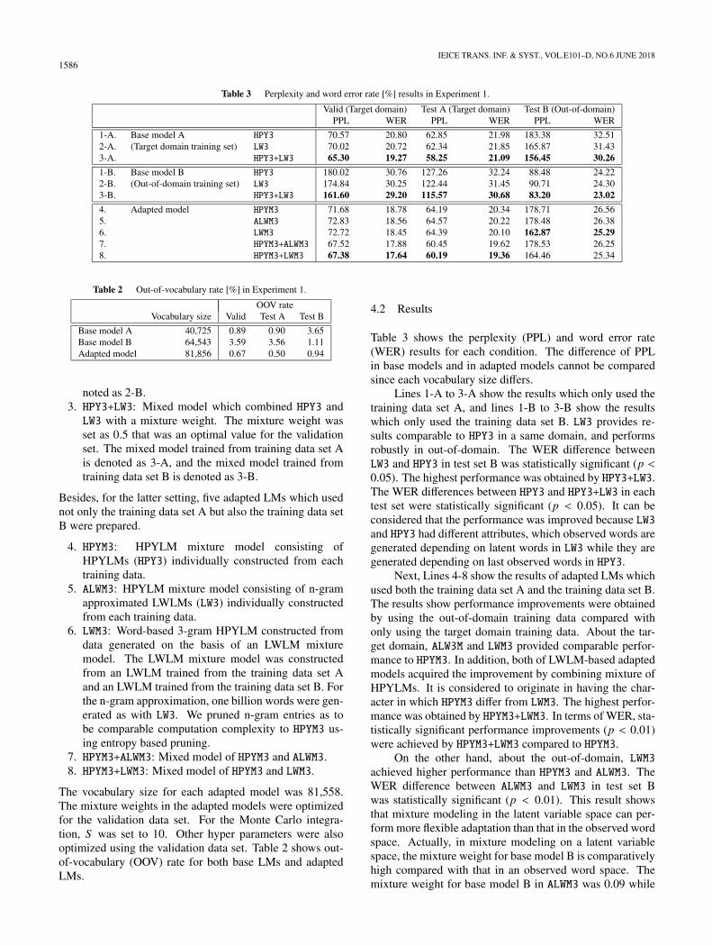
Base model A 40,725 0.89 0.90 3.65Base model B 64,543 3.59 3.56 1.11Adapted model 81,856 0.67 0.50 0.94

noted as 2-B.3. HPY3+LW3: Mixed model which combined HPY3 andLW3 with a mixture weight. The mixture weight wasset as 0.5 that was an optimal value for the validationset. The mixed model trained from training data set Ais denoted as 3-A, and the mixed model trained fromtraining data set B is denoted as 3-B.

Besides, for the latter setting, five adapted LMs which usednot only the training data set A but also the training data setB were prepared.

4. HPYM3: HPYLM mixture model consisting ofHPYLMs (HPY3) individually constructed from eachtraining data.

5. ALWM3: HPYLM mixture model consisting of n-gramapproximated LWLMs (LW3) individually constructedfrom each training data.

6. LWM3: Word-based 3-gram HPYLM constructed fromdata generated on the basis of an LWLM mixturemodel. The LWLM mixture model was constructedfrom an LWLM trained from the training data set Aand an LWLM trained from the training data set B. Forthe n-gram approximation, one billion words were gen-erated as with LW3. We pruned n-gram entries as tobe comparable computation complexity to HPYM3 us-ing entropy based pruning.

7. HPYM3+ALWM3: Mixed model of HPYM3 and ALWM3.8. HPYM3+LWM3: Mixed model of HPYM3 and LWM3.

The vocabulary size for each adapted model was 81,558.The mixture weights in the adapted models were optimizedfor the validation data set. For the Monte Carlo integra-tion, S was set to 10. Other hyper parameters were alsooptimized using the validation data set. Table 2 shows out-of-vocabulary (OOV) rate for both base LMs and adaptedLMs.

4.2 Results

Table 3 shows the perplexity (PPL) and word error rate(WER) results for each condition. The difference of PPLin base models and in adapted models cannot be comparedsince each vocabulary size differs.

Lines 1-A to 3-A show the results which only used thetraining data set A, and lines 1-B to 3-B show the resultswhich only used the training data set B. LW3 provides re-sults comparable to HPY3 in a same domain, and performsrobustly in out-of-domain. The WER difference betweenLW3 and HPY3 in test set B was statistically significant (p <0.05). The highest performance was obtained by HPY3+LW3.The WER differences between HPY3 and HPY3+LW3 in eachtest set were statistically significant (p < 0.05). It can beconsidered that the performance was improved because LW3and HPY3 had different attributes, which observed words aregenerated depending on latent words in LW3 while they aregenerated depending on last observed words in HPY3.

Next, Lines 4-8 show the results of adapted LMs whichused both the training data set A and the training data set B.The results show performance improvements were obtainedby using the out-of-domain training data compared withonly using the target domain training data. About the tar-get domain, ALW3M and LWM3 provided comparable perfor-mance to HPYM3. In addition, both of LWLM-based adaptedmodels acquired the improvement by combining mixture ofHPYLMs. It is considered to originate in having the char-acter in which HPYM3 differ from LWM3. The highest perfor-mance was obtained by HPYM3+LWM3. In terms of WER, sta-tistically significant performance improvements (p < 0.01)were achieved by HPYM3+LWM3 compared to HPYM3.

On the other hand, about the out-of-domain, LWM3achieved higher performance than HPYM3 and ALWM3. TheWER difference between ALWM3 and LWM3 in test set Bwas statistically significant (p < 0.01). This result showsthat mixture modeling in the latent variable space can per-form more flexible adaptation than that in the observed wordspace. Actually, in mixture modeling on a latent variablespace, the mixture weight for base model B is comparativelyhigh compared with that in an observed word space. Themixture weight for base model B in ALWM3 was 0.09 while

MASUMURA et al.: DOMAIN ADAPTATION BASED ON MIXTURE OF LATENT WORDS LANGUAGE MODELS FOR AUTOMATIC SPEECH RECOGNITION1587

that in LWM3 was 0.13. In terms of WER, statistically sig-nificant performance improvements (p < 0.01) were alsoachieved by HPYM3+LWM3 compared to HPYM3. It turned outthat LWM3 can achieve improvement for both the target do-main and the out-of-domain compared with HPYM3.

5. Experiment 2

5.1 Setups

In the second experiment, two types of partially matchedtraining data sets were prepared for constructing an LM. Thetarget domain was set to academic lecture speech; its styleis spontaneous speech and the topic is related to acoustics.A validation data set (Valid) and a test data set (Test) for thetarget domain were prepared from CSJ [27]. Each data sethad about 30K words.

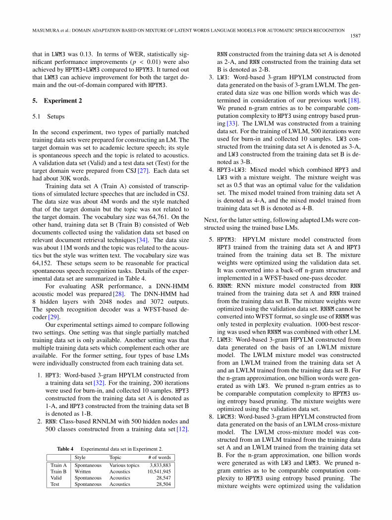
Training data set A (Train A) consisted of transcrip-tions of simulated lecture speeches that are included in CSJ.The data size was about 4M words and the style matchedthat of the target domain but the topic was not related tothe target domain. The vocabulary size was 64,761. On theother hand, training data set B (Train B) consisted of Webdocuments collected using the validation data set based onrelevant document retrieval techniques [34]. The data sizewas about 11M words and the topic was related to the acous-tics but the style was written text. The vocabulary size was64,152. These setups seem to be reasonable for practicalspontaneous speech recognition tasks. Details of the exper-imental data set are summarized in Table 4.

For evaluating ASR performance, a DNN-HMMacoustic model was prepared [28]. The DNN-HMM had8 hidden layers with 2048 nodes and 3072 outputs.The speech recognition decoder was a WFST-based de-coder [29].

Our experimental settings aimed to compare followingtwo settings. One setting was that single partially matchedtraining data set is only available. Another setting was thatmultiple training data sets which complement each other areavailable. For the former setting, four types of base LMswere individually constructed from each training data set.

1. HPY3: Word-based 3-gram HPYLM constructed froma training data set [32]. For the training, 200 iterationswere used for burn-in, and collected 10 samples. HPY3constructed from the training data set A is denoted as1-A, and HPY3 constructed from the training data set Bis denoted as 1-B.

2. RNN: Class-based RNNLM with 500 hidden nodes and500 classes constructed from a training data set [12].

Table 4 Experimental data set in Experiment 2.

Style Topic # of words

Train A Spontaneous Various topics 3,833,883Train B Written Acoustics 10,541,945Valid Spontaneous Acoustics 28,547Test Spontaneous Acoustics 28,504

RNN constructed from the training data set A is denotedas 2-A, and RNN constructed from the training data setB is denoted as 2-B.

3. LW3: Word-based 3-gram HPYLM constructed fromdata generated on the basis of 3-gram LWLM. The gen-erated data size was one billion words which was de-termined in consideration of our previous work [18].We pruned n-gram entries as to be comparable com-putation complexity to HPY3 using entropy based prun-ing [33]. The LWLM was constructed from a trainingdata set. For the training of LWLM, 500 iterations wereused for burn-in and collected 10 samples. LW3 con-structed from the training data set A is denoted as 3-A,and LW3 constructed from the training data set B is de-noted as 3-B.

4. HPY3+LW3: Mixed model which combined HPY3 andLW3 with a mixture weight. The mixture weight wasset as 0.5 that was an optimal value for the validationset. The mixed model trained from training data set Ais denoted as 4-A, and the mixed model trained fromtraining data set B is denoted as 4-B.

Next, for the latter setting, following adapted LMs were con-structed using the trained base LMs.

5. HPYM3: HPYLM mixture model constructed fromHPY3 trained from the training data set A and HPY3trained from the training data set B. The mixtureweights were optimized using the validation data set.It was converted into a back-off n-gram structure andimplemented in a WFST-based one-pass decoder.

6. RNNM: RNN mixture model constructed from RNN

trained from the training data set A and RNN trainedfrom the training data set B. The mixture weights wereoptimized using the validation data set. RNNM cannot beconverted into WFST format, so single use of RNNMwasonly tested in perplexity evaluation. 1000-best rescor-ing was used when RNNMwas combined with other LM.

7. LWM3: Word-based 3-gram HPYLM constructed fromdata generated on the basis of an LWLM mixturemodel. The LWLM mixture model was constructedfrom an LWLM trained from the training data set Aand an LWLM trained from the training data set B. Forthe n-gram approximation, one billion words were gen-erated as with LW3. We pruned n-gram entries as tobe comparable computation complexity to HPYM3 us-ing entropy based pruning. The mixture weights wereoptimized using the validation data set.

8. LWCM3: Word-based 3-gram HPYLM constructed fromdata generated on the basis of an LWLM cross-mixturemodel. The LWLM cross-mixture model was con-structed from an LWLM trained from the training dataset A and an LWLM trained from the training data setB. For the n-gram approximation, one billion wordswere generated as with LW3 and LWM3. We pruned n-gram entries as to be comparable computation com-plexity to HPYM3 using entropy based pruning. Themixture weights were optimized using the validation

1588IEICE TRANS. INF. & SYST., VOL.E101–D, NO.6 JUNE 2018

Table 6 Perplexity and word error rate [%] results in Experiment 2.

Valid (Target domain) Test (Target domain)PPL WER PPL WER

1-A. Base model A HPY3 247.73 31.42 186.11 35.942-A. (Training set A) RNN 244.73 - 184.16 -3-A. LW3 239.91 31.09 179.83 35.454-A. HPY3+LW3 223.68 29.86 169.93 34.16

1-B. Base model B HPY3 235.91 30.68 273.09 37.332-B. (Training set B) RNN 275.23 - 326.31 -3-B. LW3 207.91 30.05 240.08 36.474-B. HPY3+LW3 200.90 28.82 232.93 34.88

5. Adapted model HPYM3 130.30 25.24 119.22 30.336. RNNM 126.35 - 118.45 -7. LWM3 121.60 24.47 113.76 29.848. LWCM3 133.85 25.50 123.55 30.489. HPYM3+RNNM3 114.15 24.32 106.49 29.4010. LWM3+LWCM3 116.54 24.06 108.44 29.3711. HPYM3+LWM3 115.72 24.27 109.26 29.5512. HPYM3+LWM3+LWCM3 111.90 23.88 105.74 29.2013. HPYM3+LWM3+LWCM3+RNNM 105.81 23.42 100.82 28.64

Table 5 Out-of-vocabulary rate [%] in Experiment 2.

OOV rate (%)Vocabulary size Valid Test

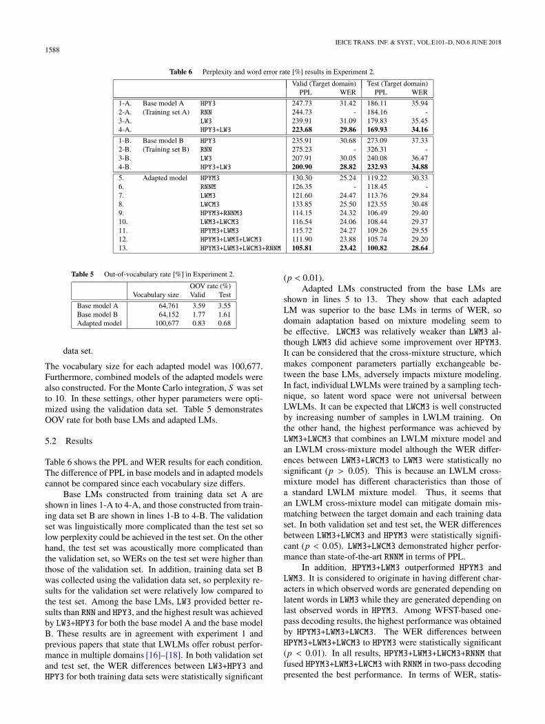
Base model A 64,761 3.59 3.55Base model B 64,152 1.77 1.61Adapted model 100,677 0.83 0.68

data set.

The vocabulary size for each adapted model was 100,677.Furthermore, combined models of the adapted models werealso constructed. For the Monte Carlo integration, S was setto 10. In these settings, other hyper parameters were opti-mized using the validation data set. Table 5 demonstratesOOV rate for both base LMs and adapted LMs.

5.2 Results

Table 6 shows the PPL and WER results for each condition.The difference of PPL in base models and in adapted modelscannot be compared since each vocabulary size differs.

Base LMs constructed from training data set A areshown in lines 1-A to 4-A, and those constructed from train-ing data set B are shown in lines 1-B to 4-B. The validationset was linguistically more complicated than the test set solow perplexity could be achieved in the test set. On the otherhand, the test set was acoustically more complicated thanthe validation set, so WERs on the test set were higher thanthose of the validation set. In addition, training data set Bwas collected using the validation data set, so perplexity re-sults for the validation set were relatively low compared tothe test set. Among the base LMs, LW3 provided better re-sults than RNN and HPY3, and the highest result was achievedby LW3+HPY3 for both the base model A and the base modelB. These results are in agreement with experiment 1 andprevious papers that state that LWLMs offer robust perfor-mance in multiple domains [16]–[18]. In both validation setand test set, the WER differences between LW3+HPY3 andHPY3 for both training data sets were statistically significant

(p < 0.01).Adapted LMs constructed from the base LMs are

shown in lines 5 to 13. They show that each adaptedLM was superior to the base LMs in terms of WER, sodomain adaptation based on mixture modeling seem tobe effective. LWCM3 was relatively weaker than LWM3 al-though LWM3 did achieve some improvement over HPYM3.It can be considered that the cross-mixture structure, whichmakes component parameters partially exchangeable be-tween the base LMs, adversely impacts mixture modeling.In fact, individual LWLMs were trained by a sampling tech-nique, so latent word space were not universal betweenLWLMs. It can be expected that LWCM3 is well constructedby increasing number of samples in LWLM training. Onthe other hand, the highest performance was achieved byLWM3+LWCM3 that combines an LWLM mixture model andan LWLM cross-mixture model although the WER differ-ences between LWM3+LWCM3 to LWM3 were statistically nosignificant (p > 0.05). This is because an LWLM cross-mixture model has different characteristics than those ofa standard LWLM mixture model. Thus, it seems thatan LWLM cross-mixture model can mitigate domain mis-matching between the target domain and each training dataset. In both validation set and test set, the WER differencesbetween LWM3+LWCM3 and HPYM3 were statistically signifi-cant (p < 0.05). LWM3+LWCM3 demonstrated higher perfor-mance than state-of-the-art RNNM in terms of PPL.

In addition, HPYM3+LWM3 outperformed HPYM3 andLWM3. It is considered to originate in having different char-acters in which observed words are generated depending onlatent words in LWM3 while they are generated depending onlast observed words in HPYM3. Among WFST-based one-pass decoding results, the highest performance was obtainedby HPYM3+LWM3+LWCM3. The WER differences betweenHPYM3+LWM3+LWCM3 to HPYM3 were statistically significant(p < 0.01). In all results, HPYM3+LWM3+LWCM3+RNNM thatfused HPYM3+LWM3+LWCM3 with RNNM in two-pass decodingpresented the best performance. In terms of WER, statis-

MASUMURA et al.: DOMAIN ADAPTATION BASED ON MIXTURE OF LATENT WORDS LANGUAGE MODELS FOR AUTOMATIC SPEECH RECOGNITION1589

tically significant performance improvements (p < 0.05)were achieved by HPYM3+LWM3+LWCM3+RNNM compared toHPYM3+RNNM in validation set and test set. This indicatesthat LWM3+LWCM3 could improve the state-of-the-art domainadapted systems that combines n-gram language modelingand RNN language modeling.

6. Conclusions

In this paper, LWLM mixture models and LWLM cross-mixture models were reported to enhance domain adapta-tion using out-of-domain text resources. Latent variablesin LWLMs are represented as specific words that can beselected from the observed word space, so we can realizemixture modeling with consideration of the latent variablespace. The LWLM mixture models can perform latent wordspace mixture that can mitigate a domain mismatch betweena target domain and training data sets. Besides, the LWLMcross mixture models that construct a mixture model foreach component in LWLMs can utilize partially matchedtext resources. The proposed models can be optimized usinga small amount of target domain data as well as n-gram mix-ture modeling. Detailed experiments showed that LWLMmixture modeling outperformed n-gram mixture modeling.In addition, combination of the LWLM cross-mixture modeland the LWLM mixture model yielded performance im-provements, while using an LWLM cross-mixture model byitself offers little benefit.

References

[1] R. Rosenfeld, “Two decades of statistical language modeling:Where do we go from here?,” Proceedings of the IEEE, vol.88,pp.1270–1278, 2000.

[2] J.T. Goodman, “A bit of progress in language modeling,” ComputerSpeech & Language, vol.15, no.4, pp.403–434, 2001.

[3] T. Brants, A.C. Popat, P. Xu, F.J. Och, and J. Dean, “Large languagemodels in machine translation,” Proc. ACL, pp.858–867, 2007.

[4] J.R. Bellegarda, “Statistical language model adaptation: Reviewand perspectives,” Speech Communication, vol.42, no.1, pp.93–108,2004.

[5] P. Koehn and J. Schroeder, “Experiments in domain adaptation forstatistical machine translation,” Proc. Second Workshop on Statisti-cal Machine Translation, pp.224–227, 2007.

[6] S. Katz, “Estimation of probabilities from sparse data for the lan-guage model component of a speech recognizer,” IEEE Transac-tions on Audio, Speech and Language Processing, vol.35, no.3,pp.400–401, 1987.

[7] R.M. Iyer and M. Ostendorf, “Modeling long distance depen-dence in language: topic mixtures versus dynamic cache models,”IEEE Transactions on Speech and Audio Processing, vol.7, no.1,pp.30–39, 1999.

[8] R. Iyer, M. Ostendorf, and H. Gish, “Using out-of-domain data toimprove in-domain language models,” IEEE Signal Process. Lett.,vol.4, no.8, pp.221–223, 1997.

[9] G. Foster and R. Kuhn, “Mixture-model adaptation for SMT,” Proc.Second Workshop on Statistical Machine Translation, pp.128–135,2007.

[10] B.-J. Hsu, “Generalized linear interpolation of language models,”Proc. ASRU, pp.136–140, 2007.

[11] X. Liu, M.J.F. Gales, and P.C. Woodland, “Context dependent lan-guage model adaptation,” Proc. INTERSPEECH, pp.837–840, 2008.

[12] T. Mikolov, S. Kombrink, L. Burget, J. Cernocky, and S. Khudanpur,“Extensions of recurrent neural network language model,” Proc.ICASSP, pp.5528–5531, 2011.

[13] Y. Shi, M. Larson, and C.M. Jonker, “K-component recurrent neuralnetwork language models using curriculum learning,” Proc. ASRU,pp.1–6, 2013.

[14] Y. Shi, M. Larson, and C.M. Jonker, “Recurrent neural networklanguage model adaptation with curriculum learning,” ComputerSpeech & Language, vol.33, no.1, pp.136–154, 2015.

[15] K. Deschacht, J.D. Belder, and M.-F. Moens, “The latent wordslanguage model,” Computer Speech & Language, vol.26, no.5,pp.384–409, 2012.

[16] R. Masumura, H. Masataki, T. Oba, O. Yoshioka, and S. Takahashi,“Use of latent words language models in ASR: a sampling-basedimplementation,” Proc. ICASSP, pp.8445–8449, 2013.

[17] R. Masumura, T. Oba, H. Masataki, O. Yoshioka, and S. Takahashi,“Viterbi decoding for latent words language models using Gibbssampling,” Proc. INTERSPEECH, pp.3429–3433, 2013.

[18] R. Masumura, T. Adami, T. Oba, H. Masataki, S. Sakauchi, and S.Takahashi, “N-gram approximation of latent words language modelsfor domain robust automatic speech recognition,” IEICE Transac-tion. on Information and Systems, vol.E99-D, no.10, pp.2462–2470,2016.

[19] S. Goldwater and T. Griffiths, “A fully Bayesian approach to unsu-pervised part-of-speech tagging,” Proc. ACL, pp.744–751, 2007.

[20] P. Blunsom and T. Cohn, “A hierarchical Pitman-Yor process HMMfor unsupervised part of speech induction,” Proc. ACL, pp.865–874,1996.

[21] T.R. Niesler and P.C. Woodland, “Combination word-based and cat-egory-based language models,” Proc. ICSLP, vol.1, pp.220–223,1996.

[22] R.C. Moore and W. Lewis, “Intelligent selection of language modeltraining data,” Proc. ACL, pp.220–224, 2010.

[23] F. Jelinek and R.L. Mercer, “Interpolated estimation of Markovsource parameters from sparse data,” pattern Recognition in Prac-tice, pp.381–397, 1980.

[24] G. Casella and E.I. George, “Explaining the Gibbs sampler,” TheAmerican Statistician, vol.46, no.3, pp.167–174, 1992.

[25] R. Masumura, T. Asami, T. Oba, H. Masataki, and S. Sakauchi,“Mixture of latent words language models for domain adaptation,”Porc. INTERPSEECH, pp.1425–1429, 2014.

[26] A. Stolcke, “SRILM – an extensible language modeling toolkit,” InProc. ICSLP, vol.2, pp.901–904, 2002.

[27] K. Maekawa, H. Koiso, S. Furui, and H. Isahara, “Spontaneousspeech corpus of Japanese,” Proc. LREC, pp.947–952, 2000.

[28] G. Hinton, L. Deng, D. Yu, G.E. Dahl, A. Mohamed, N. Jaitly, A.Senior, V. Vanhoucke, P. Nguyen, T.N. Sainath, and B. Kingsbury,“Deep Neural Networks for Acoustic Modeling in Speech Recogni-tion: The Shared Views of Four Research Groups,” Signal Process-ing Magazine, vol.29, no.6, pp.82–97, 2012.

[29] T. Hori, C. Hori, Y. Minami, and A. Nakamura, “EfficientWFST-based one-pass decoding with on-the-fly hypothesis rescor-ing in extremely large vocabulary continuous speech recognition,”IEEE transactions on Audio, Speech and Language Processing,vol.15, no.4, pp.1352–1365, 2007.

[30] H. Masataki, D. Shibata, Y. Nakazawa, S. Kobashikawa, A. Ogawa,and K. Ohtsuki, “VoiceRex spontaneous speech recognition technol-ogy for contact-center conversations,” NTT Technical Review, vol.5,no.1, pp.22–27, 2007.

[31] T. Fuchi and S. Takagi, “Japanese morphological analyzer usingword co-occurrence: JTAG,” Proc. COLING/ACL, pp.409–413,1998.

[32] S. Huang and S. Renals, “Hierarchical Pitman-Yor language modelsfor ASR in meetings,” Proc. ASRU, pp.124–129, 2007.

[33] A. Stolcke, “Entropy-based pruning of backoff language models,”In Proc. DARPA Broadcast News Transcription and UnderstandingWorkshop, pp.270–274, 1998.

1590IEICE TRANS. INF. & SYST., VOL.E101–D, NO.6 JUNE 2018

[34] R. Masumura, S. Hahm, and A. Ito, “Language model expansion us-ing webdata for spoken document retrieval,” Proc. INTERSPEECH,pp.2133–2136, 2011.

Ryo Masumura received B.E., M.E., andPh.D. degrees in engineering from Tohoku Uni-versity, Sendai, Japan, in 2009, 2011, 2016, re-spectively. Since joining Nippon Telegraph andTelephone Corporation (NTT) in 2011, he hasbeen engaged in research on speech recogni-tion, spoken language processing, and naturallanguage processing. He received the StudentAward and the Awaya Kiyoshi Science Promo-tion Award from the Acoustic Society of Japan(ASJ) in 2011 and 2013, respectively, the Sendai

Section Student Awards The Best Paper Prize from the Institute of Elec-trical and Electronics Engineers (IEEE) in 2011, the Yamashita SIG Re-search Award from the Information Processing Society of Japan (IPSJ) in2014, the Young Researcher Award from the Association for Natural Lan-guage Processing (NLP) in 2015, and the ISS Young Researcher’s Award inSpeech Field from the Institute of Electronic, Information and Communi-cation Engineers (IEICE) in 2015. He is a member of the ASJ, the IPSJ, theNLP, the IEEE, and the International Speech Communication Association(ISCA).

Taichi Asami received B.E. and M.E. de-grees in computer science from Tokyo Instituteof Technology, Tokyo, Japan, in 2004 and 2006,respectively. Since joining Nippon Telegraphand Telephone Corporation (NTT) in 2006, hehas been engaged in research on speech recog-nition and spoken language processing. He re-ceived the Awaya Kiyoshi Science PromotionAward and the Sato Prize Paper Award from theAcoustic Society of Japan (ASJ) in 2012 and2014, respectively. He is a member of the ASJ,

the Institute of Electronics, Information and Communication Engineers(IEICE), Institute of Electrical and Electronics Engineers (IEEE), and theInternational Speech Communication Association (ISCA).

Takanobu Oba received B.E. and M.E. de-grees from Tohoku University, Sendai, Japan,in 2002 and 2004, respectively. In 2004, hejoined Nippon Telegraph and Telephone Cor-poration (NTT), where he was engaged in theresearch and development of spoken languageprocessing technologies including speech recog-nition at the NTT Communication Science Lab-oratories, Kyoto, Japan. In 2012, he startedthe research and development of spoken appli-cations at the NTT Media Intelligence Labora-

tories, Yokosuka, Japan. Since 2015, he has been engaged in developmentof spoken dialogue services at the NTT Docomo Corporation, Yokosuka,Japan. He received the Awaya Kiyoshi Science Promotion Award from theAcoustical Society of Japan (ASJ) in 2007. He received Ph. D. (Eng.) de-gree from Tohoku University in 2011. He is a member of the Institute ofElectrical and Electronics Engineers (IEEE), the Institute of Electronics,Information, and Communication Engineers (IEICE) and the ASJ.

Hirokazu Masataki received B.E., M.E.,and Ph.D. degrees from Kyoto University in1989, 1991, and 1999, respectively. From1995 to 1998, he worked with ATR Inter-preted Telecommunications Research Labora-tories, where specialized in statistical lan-guage modeling for large vocabulary contin-uous speech recognition. He joined NipponTelegraph and Telephone Corporation (NTT) in2004 and has been engaged in the practical useof speech recognition. He received the Maejima

Hisoka Award from the Tsushin-bunko Association in 2013, and the 54-thSato Prize Paper Award from the Acoustic Society of Japan (ASJ) in 2014.He is a member of the Institute of Electronics, Information and Communi-cation Engineers (IEICE) and the ASJ.

Sumitaka Sakauchi received M.S. degreefrom Tohoku University in 1995 and Ph.D. de-gree from Tsukuba University in 2005. Sincejoining Nippon Telegraph and Telephone Cor-poration (NTT) in 1995, he has been engagedin research on acoustics, speech and signal pro-cessing. He is now Senior Manager in the Re-search and Development Planning Departmentof NTT. He received the Paper Award from theInstitute of Electronics, Information and Com-munication Engineers (IEICE) in 2001, and

Awaya Kiyoshi Science Promotion Award from the Acoustic Society ofJapan (ASJ) in 2003. He is a member of the IEICE and the ASJ.

Akinori Ito received B.E., M.E., and Ph.D.degrees from Tohoku University, Sendai, Japan.Since 1992, he has worked with Research Cen-ter for Information Sciences and Education Cen-ter for Information Processing, Tohoku Univer-sity. He was with the Faculty of Engineering,Yamagata University, from 1995 to 2002. From1998 to 1999, he worked with the College ofEngineering, Boston University, MA, USA, asa Visiting Scholar. He is now a Professor of theGraduate School of Engineering, Tohoku Uni-

versity. He is engaged in spoken language processing, statistical text pro-cessing, and audio signal processing. He is a member of the Acoustic So-ciety of Japan, the Information Processing Society of Japan, and the IEEE.