linear latent structure analysis: mixture distribution models with linear constraints
TRANSCRIPT
arX
iv:m
ath/
0507
025v
1 [
mat
h.PR
] 1
Jul
200
5
LINEAR LATENT STRUCTURE ANALYSIS: MIXTURE
DISTRIBUTION MODELS WITH LINEAR CONSTRAINTS
MIKHAIL KOVTUN, IGOR AKUSHEVICH, KENNETH G. MANTON,AND H. DENNIS TOLLEY
Abstract. A new method for analyzing high-dimensional categorical data,Linear Latent Structure (LLS) analysis, is presented. LLS models belong tothe family of latent structure models, which are mixture distribution modelsconstrained to satisfy the local independence assumption. LLS analysis explic-itly considers a family of mixed distributions as a linear space and LLS modelsare obtained by imposing linear constraints on the mixing distribution.
LLS models are identifiable under modest conditions and are consistentlyestimable. A remarkable feature of LLS analysis is the existence of a high-performance numerical algorithm, which reduces parameter estimation to asequence of linear algebra problems. Preliminary simulation experiments witha prototype of the algorithm demonstrated a good quality of restoration ofmodel parameters.
1. Introduction
We present a new statistical method, Linear Latent Structure (LLS) analysis,which belongs to a domain of latent structure analysis. In presentation of themethod and in investigation of its properties we follow a new understanding oflatent structure models as mixture distribution models (Bartholomew, 2002).
The latent structure analysis considers a number of categorical variables mea-sured on each individual in a sample, and it is aimed to discover properties of a pop-ulation as well as properties of individuals composing a population. The main as-sumption of the latent structure analysis is the local independence assumption. Be-ing formulated in a more contemporary way, this means that the observed joint dis-tribution of categorical random variables is a mixture of independent distributions(see section 2 for more detail). The mixing distribution is considered as a distribu-tion of latent variable(s), which is thought of as containing hidden information re-garding the phenomenon under consideration. The goal of the latent structure anal-ysis is to discover properties of latent variables; different approaches to this prob-lem are described in Lazarsfeld (1950b,a); Lazarsfeld and Henry (1968); Goodman(1978); Langeheine and Rost (1988); Clogg (1995); Heinen (1996); Bartholomew and Knott(1999); Marcoulides and Moustaki (2002).
The various branches of latent structure analysis differ in additional assumptionsregarding latent variables—or, equivalently, regarding mixing distribution. Latent
2000 Mathematics Subject Classification. Primary 62G05; Secondary 62H25.Key words and phrases. Mixed distributions, latent structure analysis, principal component
analysis.This work was supported in part by NIH grants P01-AG17937-05 and R01-AG01159-28.This article was submitted for publication in Statistical Methodology.
1
2 M.KOVTUN, I.AKUSHEVICH, K.G.MANTON, AND H.D.TOLLEY
class analysis assumes that the mixing distribution is concentrated in a finite num-ber of points (called “latent classes”). Latent trait analysis (LTA) tries to representmixed distributions as a function of a latent trait, which in most cases is assumed tobe one-dimensional parameter. In the 1990s, multidimensional latent traits were in-vestigated (Hoijtink and Molenaar, 1997; Reckase, 1997). However, the applicationof multidimensional LTA is not as broad as one-dimensional LTA, since estimatingparameters in multidimensional case requires additional assumptions.
The novelty of our approach lies in consideration of the space of mixed distri-butions as a linear space. This allows us to employ geometric intuition and clearlyformulate the main additional assumption of LLS that the mixed distribution issupported by a linear subspace of the space of independent distributions.
Models arising from this approach are identifiable under modest conditions andare consistently estimable. Further, there exists a high-performance numerical al-gorithm, which reduces estimation of model parameters to a sequence of linearalgebra problems. Preliminary simulation experiments with a prototype of thealgorithm (presented in section 6) demonstrated a good quality of restoration ofmodel parameters.
The word “linear” in the name of the method reflects at least three aspects ofour method: first, the model is obtained by imposing linear constraints on themixing distribution; second, the algorithm for model construction uses methodsof linear algebra; and third, the most interesting ideas of our approach arise fromconsideration of a space of distributions as a linear space.
Historically, the predecessor of LLS analysis was Grade of Membership (GoM)analysis, which was introduced in Woodbury and Clive (1974); see also Manton et al.(1994) for detailed exposition and additional references. Our work on LLS analysisoriginated from attempts to find conditions for consistency of GoM estimators. Thedevelopment eventually lead to a new class of models, which differ from GoM mod-els in a way how the model is formulated, methods of model estimation, meaningof estimators and their interpretation. We present here this new class of modelsunder the name “linear latent structure analysis.”
The present article concentrates on the exposition of main ideas of the LLSanalysis and investigation of its statistical properties. Section 2 describes the basicsof LLS analysis. A new procedure for parameter estimation is explained in Section 3.Sections 4 and 5 answer the questions concerning identifiability of LLS models andconsistency of the estimators. Section 6 gives results of preliminary experimentswith a prototype of the algorithm implemented by the authors. The article isconcluded by section 7, where we discuss some interesting properties of LLS analysisand compare it with other kinds of latent structure analysis.
2. LLS models
The input to LLS analysis is outcome of J categorical measurements, each madeon N individuals.
Mathematically, we consider J categorical random variables X1, . . . , XJ . The setof possible values of random variable Xj is {1, . . .Lj}. This structure is describedby an integer vector L = (L1, . . . , LJ). Two numbers, which are used frequently inthe rest of the article, are associated with that structure: |L| = L1 + . . . + LJ and|L∗| = L1 · . . . · LJ .
LINEAR LATENT STRUCTURE ANALYSIS 3
To denote response patterns, we use integer vectors ℓ = (ℓ1, . . . , ℓJ). The jth
component, ℓj , represents the value of random variable Xj (thus, ℓj ∈ [1..Lj]).Note that there are |L∗| different vectors ℓ.
The joint distribution of random variables X1, . . . , XJ is given by |L∗| elementaryprobabilities
(1) pℓ = P(X1 = ℓ1 and . . . and XJ = ℓJ)
In general, no restrictions other than pℓ ≥ 0 for all ℓ and∑
ℓ pℓ = 1 are imposedon the family of elementary probabilities; thus, one needs |L∗| − 1 parameters todescribe a joint distribution of X1, . . . , XJ .
Note that probabilities pℓ are directly estimable from the observed data: fre-quencies fℓ = Nℓ
N(where N is the total number of individuals in the sample and Nℓ
is the number of individuals who responded with response pattern ℓ) are consistentand efficient estimators for pℓ.
Among all joint distributions one can distinguish independent distributions, i.e.distributions, in which random variables X1, . . . , XJ are mutually independent.This means that for every set of indices j1, . . . , jp and for every response pattern ℓ
the relation
(2) P(Xj1 = ℓj1 and . . . and Xjp= ℓjp
) = P(Xj1 = ℓj1) · . . . · P(Xjp= ℓjp
)
holds. Equation (2) allows us to describe an independent distribution using fewerparameters. Namely, let βjl = P(Xj = l). Then for every response pattern ℓ,
(3) pℓ =
J∏
j=1
βjℓj
Thus, every independent distribution can be identified with a point β = (βjl)jl ∈
R|L|. Not every point β ∈ R
|L| corresponds to a probability distribution; to describea distribution, β must satisfy the conditions:
(4)
{
∑Lj
l=1 βjl = 1 for every j
βjl ≥ 0 for every j and l
Conditions (4) define a convex (|L| − J)-dimensional polyhedron in R|L|, which
we denote SL.
Now we are ready to formulate the first assumption of the LLS analysis:
(G1) The observed distribution is a mixture of independent distributions, i.e.there exist a probabilistic measure µβ, supported by S
L, such that for everyresponse pattern ℓ
(5) pℓ =
∫
(
∏J
j=1 βjℓj
)
µβ(dβ)
Remark 2.1. Here and later, we use measures instead of probability density func-tions or cumulative distribution functions, as this allows us to avoid discussion ofpossible singularities and specifics of the space on which probability distributionis defined. This is just a matter of convenience; the above integral can be written
4 M.KOVTUN, I.AKUSHEVICH, K.G.MANTON, AND H.D.TOLLEY
as∫
(
∏Jj=1 βjℓj
)
dF (β), where F (β) is the cumulative distribution function of the
mixing distribution.
Assumption (G1) is a cornerstone of latent structure analysis (often, it is calledthe local independence assumption). There are a lot of excellent books and articlesdevoted to latent structure analysis; we refer to Lazarsfeld (1950b,a); Lazarsfeld and Henry(1968); Goodman (1978); Langeheine and Rost (1988); Clogg (1995); Heinen (1996);Bartholomew and Knott (1999); Marcoulides and Moustaki (2002) for discussion ofthe meaning and applicability of this assumption.
Mathematically, the assumption (G1) alone does not imply much. For almosteach distribution (pℓ)ℓ there exist infinitely many mixing distributions µβ thatproduce the same observed distribution. Thus, one needs more assumptions to makethe model identifiable. In latent structure analysis, such assumptions are usuallyformulated in the form of restrictions on the support of the mixing distribution µβ.
The specific assumption of LLS analysis is:
(G2) The mixing distribution µβ is supported by a linear subspace Q of R|L|.
For comparison, the corresponding assumption of latent class analysis is that µβ
is supported by a finite number of points (latent classes).When dimensionality of Q is sufficiently smaller than |L|, LLS model is almost
surely identifiable and consistently estimable from data. It is discussed in subse-quent sections.
Informally, the existence of low-dimensional support of measure µβ means thatall measurements reflect the same underlying hidden entity. In Kovtun et al. (2005)we have shown that the existence of low-dimensional support is equivalent to theexistence of a K-dimensional random vector G such that regressions of all indicatorrandom vectors Yj on G are linear. (Yj = (Yj1, . . . , YjLj
); Yjl = 1, if Xj = l;otherwise, Yjl = 0.)
Distributions satisfying the condition (G2) may be expected when random vari-ables X1, . . . , XJ represent responses to survey or exam questions. Here, ques-tions are intentionally chosen to discover a single (potentially multidimensional)quantity—like “quality of life” or “mathematical knowledge”. This is the naturaldomain of applications of latent structure analysis in general, and LLS analysis inparticular.
We say that a distribution is generated by a K-dimensional LLS model, if it canbe represented as a mixed distribution satisfying (G2) with dim(Q) = K.
3. Estimation of LLS model
“To define a LLS model” means to define mixing distribution µβ, which, in turn,means specifying the supporting subspace Q and the distribution over it.
The supporting subspace may be consistently estimated from the observed data,i.e. the estimated subspace converges to the true one when sample size tends toinfinity. The identifiability conditions are rather straightforward: if the dimen-
sionality of supporting subspace is of order of(
|L|−J
2 − maxLj
)
or smaller, the
supporting subspace is almost surely identifiable (theorem 4.4).LLS analysis uses nonparametric approach to description of the mixing distribu-
tion. Thus, the knowledge about the mixing distribution is expressed in the formof a family of conditional moments of order up to J . Using these moments, the
LINEAR LATENT STRUCTURE ANALYSIS 5
mixing distribution may be approximated as an empirical distribution. The exam-ples given in section 6 demonstrate the goodness of such approximation; see alsosection 7 for discussion of properties of this approximation.
The technical details of what follows are given in Kovtun et al. (2005). Here weformulate the most important facts and pay more attention to the most significantstatistical properties such as identifiability of the model and consistency of theestimates.
Let K be the dimensionality of Q and let λ1 = (λ1jl)jl, . . . , λ
K = (λKjl )jl be
a basis of Q. Let g = (g1, . . . , gK) be coordinates of points of Q written in thebasis λ1, . . . , λK . This means that for points contained in Q coordinates β and g
connected as:
(6) βjl =∑K
k=1 λkjl · gk
or, in matrix form, β = Λg, where Λ is |L| × K matrix, Λ = (λkjl)
kjl.
Recall that the support of mixing measure µβ is also restricted to SL (a polyhe-
dron defined by conditions (4)), i.e. µβ is supported by intersection of Q and SL.
We consider only bases in which all λk belong to SL. In this case, coordinates g of
points belonging to the support of µβ satisfy g1 + · · · + gK = 1; thus, g are homo-geneous coordinates of points from Q∩S
L. It is possible to exclude any coordinateg1, . . . , gK and use the remaining K − 1 coordinates to denote points of Q ∩ S
L;however, we prefer to use the redundant set of coordinates to preserve symmetryof equations.
Let µg be the measure µβ written in coordinates g. This means that for everyfunction φ defined on Q one has
∫
φ(β)µβ(dβ) =∫
φ(Λg)µg(dg). In particular,
(7) pℓ =
∫
(
∏Jj=1 βjℓj
)
µβ(dβ) =
∫
(
∏Jj=1
∑Kk=1 λk
jl · gk
)
µg(dg)
Every probabilistic measure on n-dimensional euclidean space may be consideredas a distribution law of an n-dimensional random vector. Let B = (Bjl)jl be arandom vector corresponding to measure µβ and let G = (Gk)k be a random vectorcorresponding to measure µg. In fact, B and G are the same random vector, butwritten in different coordinates.
It might be shown that X1, . . . , XJ and G (or B) have a joint distribution; thus,one can speak about conditional probabilities and conditional expectations.
Some moments of order J of B coincide with elementary probabilities (1). Name-ly, due to (5),
(8) Mℓ(B) =
∫
(
∏J
j=1 βjℓj
)
µβ(dβ) = pℓ
The above equation may be extended to moments of order lower than J . Toproceed, we need to extend ℓ-notation. From now, we allow 0’s in some positions ofvector ℓ. Such 0’s mean that we “do not care” about values of corresponding randomvariables. A vector ℓ with some components equal to 0 may be also thought of asa set of all response patterns, which have arbitrary values on “do not care” places
6 M.KOVTUN, I.AKUSHEVICH, K.G.MANTON, AND H.D.TOLLEY
and coincide with ℓ on all other places. Then pℓ will be a marginal probability, andthe corresponding moments of B will be:
(9) Mℓ(B) =
∫ (
∏
j : ℓj 6=0
βjℓj
)
µβ(dβ) = pℓ
The set of moments Mℓ(B) for all ℓ (including ℓ with zeros) is all what is directlyestimable from the observation.
Another set of values of interest is the set of conditional moments of order v =(v1, . . . , vK) of random vector G:
(10) gvℓ = E(Gv1
1 · . . . · GvK
K | X = ℓ)
Here E denotes the expectation, and X = ℓ is an abbreviation for conjunction ofconditions Xj = ℓj for all j such that ℓj 6= 0. Note that the values gv
ℓ depend onthe choice of the basis λ1, . . . , λK .
These conditional moments express the knowledge regarding individuals thatcan be obtained from the measurements. In particular, conditional expectations(equation (11) below) may be considered as estimators of individual coordinates instate space (see also section 7).
Among all conditional moments, moments of order 1, or conditional expectations,have special importance, and we use special notation for them:
gℓ1def= g
(1,0,...,0)ℓ = E(G1 | X = ℓ)
. . .(11)
gℓKdef= g
(0,...,0,1)ℓ = E(GK | X = ℓ)
The above values satisfy the following equation (Kovtun et al., 2005, section6.2):
(12) Mℓ(B) ·(
λ1jl · g
v1
ℓ + · · · + λKjl · g
vK
ℓ
)
= Mℓ′(B) · gvℓ′
Here: (a) vk denotes a vector v with kth component increased by 1 (for example,if v = (1, 3, 2, 1), then v3 = (1, 3, 3, 1)), (b) response pattern ℓ must have 0 at jth
position, (c) ℓ′ denotes the response pattern obtained from ℓ by replacing 0 at jth
position by l (for example, if ℓ = (1, 0, 0, 2, 1) and j = 3, then ℓ′ = (1, 0, l, 2, 1)).Equation (12) holds for every j, l, v, and every ℓ containing 0 at jth place.
A special case of equation (12) when v = (0, . . . , 0) is:
(13) Mℓ(B) ·(
λ1jl · gℓ1 + · · · + λK
jl · gℓK
)
= Mℓ′(B)
The right-hand side of this equation does not involve gvℓ because g
(0,...,0)ℓ = 1.
By combining all equations (12) for all possible v and ℓ with normalization equa-tions (like
∑
k gℓk = 1) one obtains the main system of equations (see Kovtun et al.,2005, section 7).
The important property of the main system of equations is given by the following
LINEAR LATENT STRUCTURE ANALYSIS 7
Theorem 3.1. Let Mℓ(B) be moments of a distribution generated by K-dimensio-nal LLS model. Let λ1, . . . , λK be any basis of the supporting subspace Q and letgv
ℓ be conditional moments calculated with respect to this basis.Then λk and gv
ℓ give a solution of the main system of equation with coefficientsMℓ(B).
Moreover, for almost all (in the strict mathematical sense) distributions everysolution of the main system of equations is a basis of the supporting subspace andconditional moments, calculated with respect to this basis. This implies that LLSmodel is almost surely identifiable; we discuss this fact in more detail in the nextsection.
Note that equations (12) are linear with respect to variables gvℓ . Thus, if one
knows a basis of Q, it is sufficient to solve a linear system of equations to find theconditional moments.
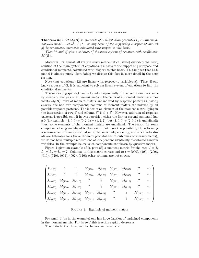
The supporting space Q can be found independently of the conditional momentsby means of analysis of a moment matrix. Elements of a moment matrix are mo-ments Mℓ(B); rows of moment matrix are indexed by response patterns ℓ havingexactly one non-zero component; columns of moment matrix are indexed by allpossible response patterns. The index of an element of the moment matrix lying inthe intersection of row ℓ′ and column ℓ′′ is ℓ′ + ℓ′′. However, addition of responsepatterns is possible only if in every position either the first or second summand hasa 0 (for example, (1, 0, 0) + (0, 2, 1) = (1, 2, 2), but (1, 0, 0) + (2, 0, 1) is undefined);thus, some elements of the moment matrix are undefined. The reason for somecomponents being undefined is that we do not have the possibility of performinga measurement on an individual multiple times independently, and since individu-als are heterogeneous (have different probabilities of outcomes of measurements),we do not have multiple realizations of independent identically distributed randomvariables. In the example below, such components are shown by question marks.
Figure 1 gives an example of (a part of) a moment matrix for the case J = 3,L1 = L2 = L3 = 2. Columns in this matrix correspond to ℓ = (000), (100), (200),(010), (020), (001), (002), (110); other columns are not shown.
M(100) ? ? M(110) M(120) M(101) M(102) ? · · ·
M(200) ? ? M(210) M(220) M(201) M(202) ? · · ·
M(010) M(110) M(210) ? ? M(011) M(012) ? · · ·
M(020) M(120) M(220) ? ? M(021) M(022) ? · · ·
M(001) M(101) M(201) M(011) M(021) ? ? M(111) · · ·
M(002) M(102) M(202) M(012) M(022) ? ? M(112) · · ·
Figure 1. Example of moment matrix
For small J (as in the example) one has large fraction of undefined componentsin the moment matrix. For large J this fraction rapidly decreases.
The main fact with respect to the moment matrix is:
8 M.KOVTUN, I.AKUSHEVICH, K.G.MANTON, AND H.D.TOLLEY
Theorem 3.2. If a distribution is generated by K-dimensional LLS model withsupporting subspace Q, then the moment matrix has a completion such that everyone of its columns belongs to Q.
We show below that a completion of a moment matrix is almost surely deter-mined by its available part. Thus, the main system of equations almost surely hasa unique solution.
Here we need to clarify what we mean when we say “uniqueness of solution.”The supporting subspace Q and the identifiable properties of mixing distributionon this subspace are defined uniquely. One way to describe the subspace Q is topresent its basis, and this can be done in infinitely many ways. The coordinateexpression of the mixing distribution does depend on the choice of basis, and itscharacteristics (like moments) also do depend on this choice. Such dependenciesare governed by tensor laws (Kovtun et al., 2005, section 6.4).
The existence of infinitely many bases does not mean that we have infinitelymany solutions; rather, we can describe a unique solution by infinitely many means.Various bases of Q provide different points of view on the same underlying picture.The ability to choose a basis may benefit the applied researcher, as it may help topresent phenomenon under consideration more clearly.
The phase of finding the supporting subspace in LLS analysis is tightly relatedto the principal component analysis of the mixing distribution. In fact, the sub-matrix of the moment matrix consisting of columns from 2 to |L| + 1 is (moduloincompleteness) a shifted covariance matrix of the mixing distribution. Theorem3.2 corresponds to the fact that a multidimensional distribution is supported bym-dimensional linear manifold if and only if the rank of covariance matrix is m.
Theorem 3.2 also provides a method for determining whether an LLS modelexists for a particular dataset. One has to find the largest computational rank(Forsythe et al., 1977) of minors of the moment matrix containing no questionmarks; if it is sufficiently smaller than |L|, LLS model exists (the exact criterion ofidentifiability of LLS model is given by theorem 4.4).
Now we are ready to describe a method for estimation of parameters of LLSmodel.
First, the supporting subspace is estimated from the moment matrix. Themethod of estimation is very similar to the one used in the principal componentanalysis, adopted to handle incompleteness of the moment matrix. The detaileddescription of the numerical procedure is a subject of another article.
Second, a basis of the supporting subspace is chosen and conditional momentsgv
ℓ are estimated by (approximately) solving the main system of equations. Notethat moments can be found only for ℓ having sufficiently many 0’s (to guaranteethat there are sufficiently many equations (12)). Moments for other ℓ’s can beestimated as an average of directly estimable moments (for example, g(ℓ1,...,ℓJ ) =1J
(
g(0,ℓ2,...,ℓJ ) + · · · + g(ℓ1,...,ℓJ−1,0)
)
).This is a nonparametric approach, i.e. inference of properties of a (mixing) dis-
tribution is made without any additional assumptions about the structure of thedistribution. If the nature of the applied problem justifies an assumption that themixing distribution belongs to some parametric family (say, a mixing distributionis a Dirichlet distribution), the parameters of such distribution may be easily esti-mated by the moment method.
LINEAR LATENT STRUCTURE ANALYSIS 9
The mixed distribution in LLS analysis can be estimated in style of empiricdistribution, by letting the estimate of the mixing distribution be concentrated inpoints gℓ with weights Mℓ(B) (where bars mean estimates of corresponding values).It might be shown that this estimated distribution converges to the true one whenboth size of the sample and number of measurements tend to infinity, but the proofis outside the scope of the present paper.
4. Identifiability of LLS models
Identifiability of a parameter of a model means that the value of the parameteris uniquely determined by the distribution of the observed variables (Gabrielsen,1978). In our case, the observed distribution is given by moments Mℓ(B). Thus,identifiability means that the values of other parameters (i.e., supporting subspaceand conditional moments) are uniquely determined by the values Mℓ(B).
We start with the discussion of identifiability of supporting subspace Q. Thecovariance matrix of the mixing distribution uniquely defines Q (Q is spanned by thevector of expectations of βjl, which is the first column of the moment matrix, andeigenvectors of covariance matrix corresponding to non-zero eigenvalues). Thus, thesupporting subspace is identifiable, if the covariance matrix (which is incompletefor the same reasons as the moment matrix) can be uniquely restored from theavailable moments.
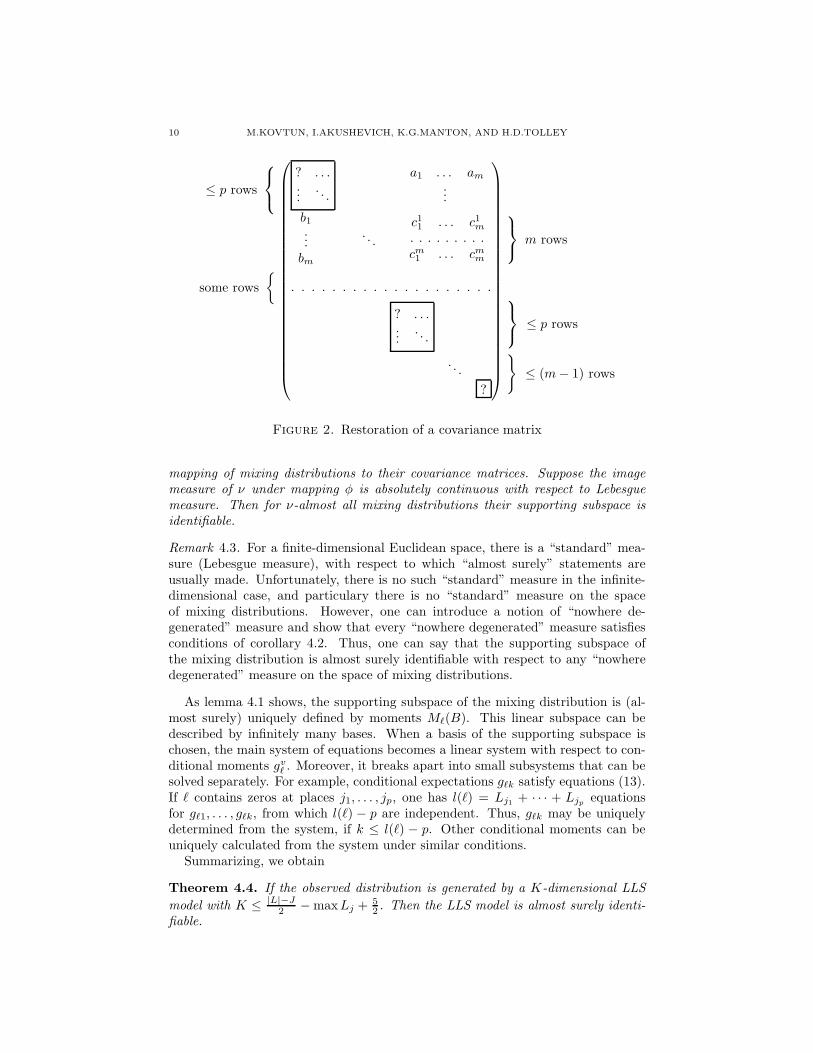
Lemma 4.1. Let Cm be a class of covariance matrices of n-dimensional distribu-tions of rank m. Let, for arbitrary A ∈ Cm, A denote the matrix A with missingdiagonal blocks of maximal size p. Let also assume that inequality 2m + 2p− 1 ≤ n
holds.Then, for arbitrary A, B ∈ Cm, the equality A = B almost surely implies A = B.
Outline of the proof. Figure 2 demonstrates how an incomplete covariance matrixcan be restored. If the minor (ci
j)ij is nondegenerate, there exist a unique linear
combination of columns c1, . . . , cm that yields column b; let bj =∑
i γicij for all j.
Then, as the rank of the whole matrix is m, the element in the top left corner ofthe matrix must be
∑
i γiai. Other elements denoted by question marks may berestored by applying similar procedure.
The picture also illustrates the necessity of condition 2m + 2p− 1 ≤ n.Thus, to complete a proof of the theorem, it is sufficient to show that all minors
of a covariance matrix are almost surely nondegenerate.Every covariance matrix A of rank m is nonnegative definite and symmetric;
thus, it can be represented in form A = OT DO, where O is an orthogonal matrixand D is a diagonal matrix with exactly m nonzero elements. Further, almost everyorthogonal matrix may be represented as O = (I + V )(I − V )−1, where I is theunit matrix and V is a skew-symmetric matrix (Cayley parametrization; see Satake,1975, IV.6). Thus, elements of covariance matrix can be represented as ratios of
polynomials of n(n−1)2 + m variables (n(n−1)
2 elements of skew-symmetric matrixand m elements of matrix D). Consequently, all minors of order m are ratios ofpolynomials of these variables, and they are not identically 0 (as it is possible togive an example of covariance matrix of rank m with all minors of order m beingnon-degenerate). But a set of 0’s of a polynomial has measure 0, q.e.d. �
Corollary 4.2. Let M be a family of mixing distributions supported by K-dimen-sional linear subspaces and let ν be a Borel measure on M. Let φ : µ 7→ Cµ be a
10 M.KOVTUN, I.AKUSHEVICH, K.G.MANTON, AND H.D.TOLLEY
≤ p rows
some rows
{
? . . ....
. . .
a1 . . . am
...
b1
...bm
. . .
c11 . . . c1
m
. . . . . . . . .
cm1 . . . cm
m
. . . . . . . . . . . . . . . . . . . .
? . . ....
. . .
. . .
?
m rows
≤ p rows
}
≤ (m − 1) rows
Figure 2. Restoration of a covariance matrix
mapping of mixing distributions to their covariance matrices. Suppose the imagemeasure of ν under mapping φ is absolutely continuous with respect to Lebesguemeasure. Then for ν-almost all mixing distributions their supporting subspace isidentifiable.
Remark 4.3. For a finite-dimensional Euclidean space, there is a “standard” mea-sure (Lebesgue measure), with respect to which “almost surely” statements areusually made. Unfortunately, there is no such “standard” measure in the infinite-dimensional case, and particulary there is no “standard” measure on the spaceof mixing distributions. However, one can introduce a notion of “nowhere de-generated” measure and show that every “nowhere degenerated” measure satisfiesconditions of corollary 4.2. Thus, one can say that the supporting subspace ofthe mixing distribution is almost surely identifiable with respect to any “nowheredegenerated” measure on the space of mixing distributions.
As lemma 4.1 shows, the supporting subspace of the mixing distribution is (al-most surely) uniquely defined by moments Mℓ(B). This linear subspace can bedescribed by infinitely many bases. When a basis of the supporting subspace ischosen, the main system of equations becomes a linear system with respect to con-ditional moments gv
ℓ . Moreover, it breaks apart into small subsystems that can besolved separately. For example, conditional expectations gℓk satisfy equations (13).If ℓ contains zeros at places j1, . . . , jp, one has l(ℓ) = Lj1 + · · · + Ljp
equationsfor gℓ1, . . . , gℓk, from which l(ℓ) − p are independent. Thus, gℓk may be uniquelydetermined from the system, if k ≤ l(ℓ) − p. Other conditional moments can beuniquely calculated from the system under similar conditions.
Summarizing, we obtain
Theorem 4.4. If the observed distribution is generated by a K-dimensional LLS
model with K ≤ |L|−J
2 − maxLj + 52 . Then the LLS model is almost surely identi-
fiable.
LINEAR LATENT STRUCTURE ANALYSIS 11
5. Consistency of LLS estimators
The consistency of LLS estimators is almost a straightforward corollary of thewell-known statistical fact that frequencies are consistent and efficient estimatorsof probabilities.
The supporting subspace is estimated as a K-dimensional subspace closest tocolumns of the frequency matrix (more precisely, closest to the subspaces spannedby incomplete columns). This estimate continuously depends on the elements of thefrequency matrix; thus, it converges to the true supporting subspace when elementsof the frequency matrix converge to the true moments.
Similarly, estimators for conditional moments gvℓ are (approximate) solutions of
a linear system with coefficients depending on frequencies. Again, these estimatorscontinuously depend on frequencies and converge to the true conditional momentswhen frequencies converge to the true moments.
The consistency of LLS estimators may be formulated as follows. Suppose wehave a distribution generated by LLS model with mixing distribution supportedby subspace Q and having conditional moments gv
ℓ . Then estimators Q and gvℓ ,
obtained by the procedure described above, converge to Q and gvℓ , respectively,
when the size of a sample tends to infinity. Thus, we have:
Theorem 5.1. If LLS model is identifiable, it is consistently estimable.
6. Simulation studies
We have developed a prototype of the algorithm for estimation of LLS param-eters and performed preliminary experiments with it. The implementation of thealgorithm follows the ideas described above, though differring in detail needed toprovide computational stability.
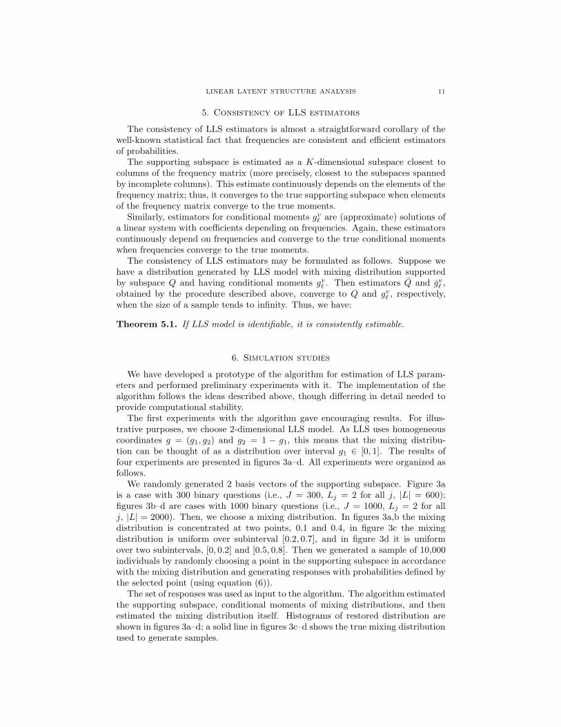
The first experiments with the algorithm gave encouraging results. For illus-trative purposes, we choose 2-dimensional LLS model. As LLS uses homogeneouscoordinates g = (g1, g2) and g2 = 1 − g1, this means that the mixing distribu-tion can be thought of as a distribution over interval g1 ∈ [0, 1]. The results offour experiments are presented in figures 3a–d. All experiments were organized asfollows.
We randomly generated 2 basis vectors of the supporting subspace. Figure 3ais a case with 300 binary questions (i.e., J = 300, Lj = 2 for all j, |L| = 600);figures 3b–d are cases with 1000 binary questions (i.e., J = 1000, Lj = 2 for allj, |L| = 2000). Then, we choose a mixing distribution. In figures 3a,b the mixingdistribution is concentrated at two points, 0.1 and 0.4, in figure 3c the mixingdistribution is uniform over subinterval [0.2, 0.7], and in figure 3d it is uniformover two subintervals, [0, 0.2] and [0.5, 0.8]. Then we generated a sample of 10,000individuals by randomly choosing a point in the supporting subspace in accordancewith the mixing distribution and generating responses with probabilities defined bythe selected point (using equation (6)).
The set of responses was used as input to the algorithm. The algorithm estimatedthe supporting subspace, conditional moments of mixing distributions, and thenestimated the mixing distribution itself. Histograms of restored distribution areshown in figures 3a–d; a solid line in figures 3c–d shows the true mixing distributionused to generate samples.
12 M.KOVTUN, I.AKUSHEVICH, K.G.MANTON, AND H.D.TOLLEY
0
50
100
150
200
250
300
350
400
0 0.1 0.2 0.3 0.4 0.5 0.6 0.7 0.8 0.90
100
200
300
400
500
600
700
0 0.1 0.2 0.3 0.4 0.5 0.6 0.7 0.8 0.9
0
50
100
150
200
250
300
350
400
450
0 0.1 0.2 0.3 0.4 0.5 0.6 0.7 0.8 0.90
100
200
300
400
500
0 0.1 0.2 0.3 0.4 0.5 0.6 0.7 0.8 0.9
Figure 3. Restored mixing distribution (see text for further explanations).
Experiments with different choices of supporting subspace and other randomlygenerated samples give similar results.
Figures 3c–d demonstrate a good quality of restoration of the mixing distributionunder various conditions. Figures 3a–b show that the precision of restoration ofthe mixing distribution increases with the increase of the number of variables.
It is interesting to compare the results of LLS model with the results of latentclass model (LCM). In the cases 3a and 3b, LCM would restore the same picture asLLS does, and thus, it can be an alternative to LLS model. However, in the cases3c and 3d, LCM may be used only as approximation, and it might be shown thatLCM may involve approximately 1,000 (number of measurements) latent classes inthese cases.
7. Discussion
In the present paper we described a new class of models for analyzing high-dimensional categorical data, which belongs to a family of latent structure models.We established conditions for identifiability of models and consistency of parameter
LINEAR LATENT STRUCTURE ANALYSIS 13
estimators. The essence of our approach is in the consideration of a space of inde-pendent distributions (which is a space of distributions being mixed in the case oflatent structure analysis) as a linear space. This allows us, first, to formulate modelassumptions in the language of linear algebra, and second, to reduce a method forestimating model parameters to a sequence of linear algebra problems. The verymodest identifiability conditions (theorem 4.4) allow application of these models toa wide range of practical datasets.
This linear-algebra approach allows us to clarify relationship between variousbranches of latent structure analysis. Consider, for example, relation between LLSmodels and latent class models (LCM). In geometric language, latent classes arepoints in the space of independent distributions. If an LCM with classes c1, . . . , cm
exists for a particular dataset, then an LLS model also exists, and its supportingsubspace is the linear subspace spanned by vectors c1, . . . , cm. Thus, dimensionalityof LLS model never exceeds the number of classes in LCM. These numbers are equalif and only if LCM classes are points in general position (i.e., vectors c1, . . . , cm donot belong to a subspace of dimensionality smaller than m). If LCM classes are notin general position, however, the dimensionality of LLS model may be significantlysmaller. For example, it is possible to construct a mixing distribution such that (a)it is supported by a line (i.e., dimensionality of LLS model is 2); (b) there existsLCM with J (number of variables) classes; (c) there is no LCM with smaller numberof classes. (A rigorous proof of the last fact will be given in another paper.) Onthe other hand, LLS can be used to evaluate applicability of LCM: if the mixingdistribution in LLS model has pronounced modality, then an LCM is more likelyto exist (with the number of classes equal to number of modes).
Maybe, the most important question regarding any kind of model is its interpre-tation. The interpretation heavily depends on application domain, so we are ableto give here only very general guidelines. If the application domain supports anassumption that individuals in a population may be described by points in a statespace and probabilities of outcomes of measurements depend on individual coor-dinates in the state space, this state space can be recovered by LLS analysis, andcoordinates of an individual in the state space can be estimated from the outcomesof measurements. However, the “physical meaning” of the state space, what does itmean “to be in a particular region of the state space”, etc. may be discussed onlyin terms of the application domain.
There is one interesting property of LLS models, which can be characterizedas a partial identifiability. Our method gives consistent estimates for supportingsubspace of the mixing distribution and for conditional moments gv
ℓ of maximalorder v satisfying |v| = v1 + · · ·+ vK ≤ J . This is not, however, a limitation of themodel; rather, it is limitation of the problem itself: if two mixing distributions aresupported by the same subspace and have the same conditional moments of order|v| ≤ J , they will produce the same observed moments Mℓ; thus, these two mixingdistributions are indistinguishable based on available data. On the other hand,two mixing distributions, which have the same moments of order up to J cannotbe significantly different: it might be shown that distance between them convergesto 0 when J tends to infinity. This means that the recovered knowledge aboutmixing distribution can be made more and more precise by increasing number ofmeasurements. This fact is well recognized in practice; for example, a mathematical
14 M.KOVTUN, I.AKUSHEVICH, K.G.MANTON, AND H.D.TOLLEY
test based on multiple-choice questions would include several questions regarding,say, the addition of fractions to judge student performance on this topic.
The above problem may also be considered from another side. As it was men-tioned in the end of section 3, the mixing distribution can be estimated in style ofempirical distribution, by letting the estimate of the mixing distribution be con-centrated in points gℓ with weights Mℓ(B). One can ask how this estimate relatesto the true mixing distribution? The answer is: the estimate of the mixing dis-tribution converges to the true one when both size of a sample and number ofmeasurements tend to infinity. This fact may be considered as an analogue of theGlivenko-Cantelli theorem. The fact that estimate of the individual position inthe state space becomes more and more precise with the increase of the number ofmeasurements is an analogue of the Bernoulli’s law of large numbers. The fact thatone needs more and more measurements performed on each individual to increaseprecision of restoration of the mixing distribution does not diminish the usefulnessof LLS analysis. It is well recognized that to achieve a required precision in statisti-cal inference one needs to perform sufficiently many measurements. The differencehere is in that one needs not only to repeat the same measurement on different in-dividuals, but also to perform sufficiently many measurements on each individual.The proof of the above convergence and estimation of the rate of the convergenceis subject of forthcoming papers.
References
Bartholomew, D. J. (2002). Old and new approaches to latent variable modeling.In Marcoulides, G. A. and Moustaki, I., editors, Latent Variable and LatentStructure Models, pages 1–14, Mahwah, NJ. Lawrence Erlbaum Associates.
Bartholomew, D. J. and Knott, M. (1999). Latent Variable Models and FactorAnalysis. Oxford University Press, New York, 2 edition.
Clogg, C. C. (1995). Latent Class Models, pages 311–360. Handbook of StatisticalModeling for the Social and Behavioral Sciences. Plenum Press, New York.
Forsythe, G. E., Malcolm, M. A., and Moler, C. B. (1977). Computer Methods forMathematical Computations. Prentice-Hall, Inc., Englewood Cliffs, NJ.
Gabrielsen, A. (1978). Consistency and identifiability. Journal of Econometrics,8(2):261–263.
Goodman, L. A. (1978). Analyzing Qualitative/Categorical Data: Log-linear Modelsand Latent-Structure Analysis. Abt Books, Cambridge, MA.
Heinen, T. (1996). Latent Class and Discrete Latent Trait Models: Similarities andDifferences. SAGE Publications, Thousand Oaks.
Hoijtink, H. and Molenaar, I. W. (1997). A multidimensional item response model:Constrained latent class analysis using gibbs sampler and posterior predictivechecks. Psychometrika, 63(2):171–189.
Kovtun, M., Akushevich, I., Manton, K. G., and Tolley, H. D. (2005). Grade ofMembership Analysis: One Possible Approach to Foundations. Focus on Proba-bility Theory. Nova Science Publishers, New York. Available from e-Print archivearXiv.org at http://www.arxiv.org, arXiv code math.PR/0403373.
Langeheine, R. and Rost, J., editors (1988). Latent Trait and Latent Class Models.Plenum Press, New York.

LINEAR LATENT STRUCTURE ANALYSIS 15
Lazarsfeld, P. F. (1950a). The Interpretation and Computation of some LatentStructures, volume IV of Studies in Social Psychology in World War II, chap-ter 11, pages 413–472. Princeton University Press, Princeton, NJ.
Lazarsfeld, P. F. (1950b). The Logical and Mathematical Foundations of LatentStructure Analysis, volume IV of Studies in Social Psychology in World War II,chapter 10, pages 362–412. Princeton University Press, Princeton, NJ.
Lazarsfeld, P. F. and Henry, N. W. (1968). Latent Structure Analysis. HoughtonMifflin Company, Boston, MA.
Manton, K. G., Woodbury, M. A., and Tolley, H. D. (1994). Statistical applicationsusing fuzzy sets. John Wiley and Sons, New York.
Marcoulides, G. A. and Moustaki, I., editors (2002). Latent Variable and LatentStructure Models. Methodology for Business and Management. Lawrence Erl-baum Associates, Mahwah, NJ.
Reckase, M. D. (1997). The past and future of multidimensional item responsetheory. Applied Psychological Measurements, 21(1):25–36.
Satake, I. (1975). Linear Algebra, volume 29 of Pure and Applied Mathematics.Marcel Dekker, New York.
Woodbury, M. and Clive, J. (1974). Clinical pure types as a fuzzy partition. Journalof Cybernetics, 4:111–121.
Duke University, CDS, 2117 Campus Dr., Durham, NC, 27708
E-mail address: [email protected]
Duke University, CDS, 2117 Campus Dr., Durham, NC, 27708
E-mail address: [email protected]
Duke University, CDS, 2117 Campus Dr., Durham, NC, 27708
E-mail address: [email protected]
Brigham Young University, Department of Statistics, 206 TMCB, Provo, UT, 84602
E-mail address: [email protected]