clustering of variables around latent components

COMMUNICATIONS lN STATISTICS

Simulation and Computation@Vol. 32, No. 4, pp. 1131-1150,2003

Clustering of Variables AroundLatent Components

E. Vigneau* and E. M. Qannari

Laboratoire de Sensométrie et de Chimiométrie,ENITIAAjINRA, Nantes, France

ABSTRACT

Clustering of variables around latent components is investigated as ameans to organize multivariate data into meaningful structures. Thecoverage incIudes (i) the case where it is desirable to lump togethercorrelated variables no matter whether the correlation coefficient

is positive or negative; (ii) the case where negative correlationshows high disagreement among variables; (iii) an extension ofthe cIustering techniques which makes it possible to explain thecIustering of variables taking account of external data. The strategybasically consists in performing a hierarchical cIuster analysis,followed by a partitioning algorithm. Both algorithms aim atmaximizing the same criterion which reflects the extent to whichvariables in each cIuster are related to the latent variable associatedwith this cIuster. Illustrations are outlined using real data sets fromsensory studies.

*Correspondence: E. Vigneau, Laboratoire de Sensométrie et de Chimiométrie,ENITIAAjINRA, rue de la Géraudière, BP 82 225, 44 322, Nantes Cedex 03,France; Fax: +33-2-51-78-54-38; E-mail: [email protected].

1131

DOI: 1O.1081jSAC-120023882CoPyright @2003 by Marcel Dekker, Inc.

0361-0918 (Print); 1532-4141 (On line)www.dekker.com

1132 Vigneau and Qannari

Key Words: Clustering of variables; Principal component analysis;Sensory data; Preference data.

1. INTRODUCTION

Principal Components Analysis (PCA) is an appealing statistical toolfor data inspection and dimensionality reductioD.. Rotated principal com-ponents fulfill the need for practitioners to have more interpretable linearcombinations of the original variables. Cluster analysis of variables is analternative technique as it makes it possible to organize the data intomeaningful structures. Moreover, once the variables are arranged intohomogeneous clusters, further investigations may be undertaken. Forinstance, it is possible to associate with each c1uster of variables a syn-thetic component. These synthetic components may be easier to interpretthan the rotated principal components as they exc1usivelyrefer to differ-

. ent groups of variables pertaining to various facets of the problem underinvestigation. Another advantage which may be gained from the cluster-ing of variables relates to the selection of a subset of variables.Procedures for discarding or selecting variables based on a statisticalcriterion have been proposed by Jolliffe (1972), McCabe (1984),KrzanO\ysJei(1987), AI-Kandari and Jollife (2001) or Guo et al. (2002)among many others. Clustermg of variables gives the advantage overthese methods of allowing the practitioner of actually choosing one vari-able from each c1uster taking account, in addition to statistical considera-tions, of such aspects as cost, easiness of measurement, practicability,interpretability. .. .

ln articles from Qannari et al. (1997, 1998), Abdallah and Saporta(1998) ~nd Soffritti (1999), procedures of c1ustering of variables based onthe definition of similarity (or dissimilarity) measures between variableshave been discussed. The approach discussed herein consists in c1usteringvaria~es around latent components. More precisely, the aim is to deter-mine simultaneously K c1usters of variables and K latent componentssuch that the variables in each c1uster are strongly related to the corre-sponding latent component. A solution to this problem is given by aniterative partitioning algorithm which involves, as a first step, the choiceof K initial c1usters. ln order to help the practitioner in choosing anappropriate number of c1usters and the initial partition, a hierarchicalc1ustering procedure is proposed. This hierarchical approach has thesame rationale as the partitioning algorithm as both techniques aim atmaximizing the same criterion.

Clustering of Variables 1133

ln practice, two cases have to be considered:

1. The first case applies to situations where the aim is to lumptogether correlated variables regardless of the sign of the correla-tion coefficients. Such situation can typically be encountered insensory studies when reduction of a list of attributes issought (Gains et al., 1988).The second case applies when a negative correlation coefficientbetween two variables shows disagreement between them.Panel segmentation in consumer studies illustrates this case asdiscussed in Sec. 5.2.

2.

ln both cases, the following aims are of interest:

(a) To achieve clustering of variables around latent componentsthus exhibiting their redundancy.

(b) To cluster the variables around latent components that areexpressed as linear combinations of external variables thusshowing how the various clusters may be interpreted in termsof these external data. For instance, it may be of interest tocluster a set of sensory attributes while investigating how thevarious clusters relate to chemical measurements. Performed

on preference data, the approach which consists in clusteringvariables (consumers) while taking account of external datasuch as sensory profiles provides an alternative to the so-calledExternal Preference Mapping (PrefMap) (see for instanceGreenhoff and MacFie (1994)).

It should be pointed out that the procedure Varclus in SASpackage SAS/STAT (1990) answers both the issues 1 and 2 raisedabove without, however, considering the situation where external dataare available.

The next two sections are dedicated to the presentation of the meth-ods of clustering of variables. Extensions of these approaches by takingaccount of external data are discussed in Sec. 4. Finally, the techniquesare illustrated using real data sets from sensory studies and hedonicscoring experiments.

Throughout this article, matrices are represented- with boldcapital letters, e.g., X. A vector is written with a lower case boldletter, e.g., x.


2. CLUSTERING OF VARIABLES WHEN POSITIVEAND NEGATIVE CORRELATIONS

IMPL Y AGREEMENT

Consider the case where the aim is to lump together correlatedvariables regardless of the sign of the correlation coefficients. For thispurpose, we seek to determine K (supposed to be fixed) clusters ofvariables and K latent components by maximizing a criterion whichexpresses the extent to which the variables in each cluster are colinearwith a latent component associated with this cluster.

Consider a set of p variables Xl, Xz,. . ., Xpmeasured on n individuals.These variables, are assumed to be centered, but not necessarilystandardized.

Let us denote by Gl> Gz,..., GK the K clusters of variables and byCI, Cz,. . ., CKthe K latent components (i.e., synthetic variables) associatedrespectively with the K clusters. We seek to maximize the quantity:

K p

T = nLL °kj Covz(Xj, Ck) under the constraint C~Ck= 1k=l j=l

(2.1)

where °kj = 1 if the jth variable belongs to cluster Gk and °kj = 0, other-wise, and Cov(Xj,Ck)stands for the covariance between Xj and Ck'

T cân also be written as:

K1"" 1 1

T = - .i J CkXkXkCkn k=l

(2.2)

where Xk is the matrix whose columns are formed with the variablesbelonging to group Gk.

A solution to this problem is given by an iterative algorithm in thecourse, of which the variables are allowed to move in and out of thegrou~s at the different stages of the algorithm achieving at each stagean increase of criterion T. This partitioning algorithm mns as follows:

Step 1. Start with K groups of variables which may be obtained byrandom allocation of the variables into K groups, or preferably, fromthe hierarchical clustering method discussed below.

Step 2. ln cluster Gb the latent component Ck is defined as thefirst standardized eigenvector of XkX~. ln other words, Ck is the firststandardized principal component of Xk.


Step 3. New clusters of variables are formed by assigninga variable to agroup if its squared coefficient of covariance with the latent component ofthis group is higher than with any other latent component.

ln further steps, the process starting from Step 2 is continuediteratively until stability is achieved.

We propose to complement this partitioning algorithm by ahierarchical clustering method. ln practice, both methods should beperformed in order to gain benetit of each. The hierarchical clusteringstrategy is based on the same criterion T discussed above (2.1) whichhighlights the complementarity of both approaches. It is an agglomera-tive technique which proceeds sequentiaIly from the stage in which eachvariable is considered to form a cluster by itself to the stage where there isa single cluster containing aIl variables. At each stage, the number ofclusters is reduced by one by aggregating two groups.

Let us consider criterion T. From Eq. (2.2), it can be easily shownthat T can be written as foIlows:

K

T = LÀ~k)k=1

(2.3)

where À~k)denotes the largest eigenvalue ofmatrix ~XkX~or, equivalently~X~Xk which is the covariance matrix between the variables in class Gk.This form of criterion T suggests the foIlowing hierarchical procedure:

At the tirst stage, each variable forms a cluster by itself. T is thenequal to:

p

Ta = L var(xÛj=1

(2.4)

At stage i, the merging of two clusters of variables A and B results ina variation of criterion T given by:

1:1= T- 1 - T - 1 (A) + 1 (B) 1 (AUB)1- 1 -11.1 11.1 -11.1 (2.5)

where À~A), À~B) and À~AUB)are the largest eigenvalues associatedwith the covariance matrices of the variables in cluster A, B and A U B,respectively.

We can prove (see Appendix) that:

À(AUB) < À(A) + À(B)1 - 1 1 (2.6)


which implies that the merging of two clusters at each step results in adecrease in criterion T. Therefore, the strategy of aggregation consists inmerging those clusters A and B that result in the smallest decrease incriterion T.

3. CLUSTERING OF VARIABLES WHEN NEGATIVECORRELATIONS SHOW DISAGREEMENT

There are situations in which the practitioner wishes to take accountof the strength of the correlation and also of the sign of the correlationbetween variables. For instance, suppose that P consumers are asked torate their acceptability of n products. A negative covariance between thescores of two consumers emphasizes their different views of the products.

The clustering procedure discussed herein is based on the followingprinciple: find K groups of variables Gh G2,.. ., GK (with K supposed tobe fixed) and K latent components, CI,Cz,. . ., CKsuch that the quantity Sis maximized:

K P

S = ..;n L L ÔkjCOV(Xj,Ck) under the constraint C~Ck= 1k=1 j=1

(3.1)

with Ôkj= 1 ifthejth variable belongs to cluster Gk and Ôkj= 0, otherwise.A solution to this problem is given by a partitioning algorithm which

follows the same pattern as in Sec. 2 with the following adaptations:

Step 2.;In cluster Gk(k = 1,2,..., K), component Ckis set to:

Xk

Ck = JX~Xk(3.2)

where Xk is the variable which represents the centroid of cluster Gk,defined by:

"" Pk- Lj=l XkjXk =

Pk

with Xkjdenoting the jth variable in group Gk and Pb the total number ofvariables in this group.

(3.3)

Step 3. New clusters are formed by moving each variable to a new groupif its covariance with the standardized centroid of this group is higherthan with any other standardized centroid.


As in Sec. 2, we suggest to complement the partitioning algorithm bya hierarchical clustering method. The strategy of hierarchical algorithmstems from the following form of criterion S:

K

S = LPko-(Xk)k=l

(3.4)

where o-(Xk)is the standard deviation of xk.At stage i, consider two clusters of variables A and Band denote by

XAand XBtheir respective centroids. If A and B are merged this will resultin a variation of criterion S as measured by:

fj. = Si-l - Si = PAo-(XA)+ PBo-(XB)- (PA + PB)o-(XAUB) (3.5)

where PA, PB are respectively the number of variables in group A andgroup B. It is easy to verify (see Appendix) that:

(PA + PB)o-(XAUB) :S PAo-(XA) + PBo-(XB) (3.6)

Therefore the merging of two c1usters leads to a decrease in criterionS. The strategy of aggregation consists in merging at each stage thosec1usters A and B that result in the smallest decrease in S.

4. EXTENSION: CLUSTERING OF VARIABLESWITHRESPECT TO EXTERNAL DATA

The extension in this section deals with the problem of c1ustering aset of variables while at the same time exploring how this c1ustering maybe explained using external variables.

ln addition to the variables x., X2,. . ., xP' we consider a data set Zformed with q external variables, z., Z2,. . ., Zq,which refer to the same nindividuals.

Firstly, consider the case where it is assumed that both positive andnegative correlations imply agreement. We seek to maximize criterion fgiven by:

K P

f = nL L OkjCov2(Xj,Ck) under the constraintsk=l j=l

Ck = Z ak and a~ak = 1 (4.1)

L.


we have:

- 1~ " ,T = - ~ akZ XkXkZak

n k=l(4.2)

Xk being the matrix whose columns are formed with the variablesbelonging to group Gk.

The maximiza tion of T under the considered constraints leads to apartitioning algorithm similar to the algorithm that was used for max-imizing T, except that in this case, the latent component in group Gk isgiven by Ck= Zak with 3k being the first standardized eigenvector of~ Z'XkX~Z associated with the largest eigenvalue f.L~k).

The hierarchical clustering approach may also be used in order togive a starting point for the partitioning algorithm and a hint about howmany clusters should be considered. As previously, the strategy stemsfrom the following form of T:

K

T = L f.L~k)k=l

(4.3)

This suggests an agglomerative procedure which consists in merging,at eacll 'step, those two clusters that result in the smallest decrease in T.~he fact that the merging of two clusters results in a decrease of criterionT can be proven in a very similar way as for criterion T (see Appendix).

If we consider the case where negative correlations imply disagree-ment, the objective becomes to maximize the criterion:

K p

S = ..jiiL L DlçjCOV(Xj,Ck) under the constraintsk=l j=l

<4k = Zak and a~ak = 1 (4.4)

This optimization problem is solved by means of the same kindof iterative partitioning algorithm as previously, except that the latentcomponents are now defined by:

Z'Xk

Ck= Zak with 3k = JXkZZ 'Xk(4.5)

The partitioning algorithm may, once again, be complemented bya hierarchical clustering algorithm according to the same principle asdiscussed above.


5. WORKING EXAMPLES

5.1. Clustering of Sensory Attributes

The case where positive and negative correlations imply agreementis illustrated by a descriptive sensory analysis of 18 fish mousses. Themousses were elaborated with different emulsifying and textural agents.The analysis was carried out, at the ADRIA Center of Quimper (France),by a trained panel. Seventeen attributes describing the textures of theproducts were listed (Table 1).Panelists were first asked to feel the textureof each sample with their fingers, then evaluate the products using a knifeand finally assess the texture in their mouths. Each panelist scored eachproduct for each attribute on a 9 point scale. The data considered for thesubsequent study consist in the average scores over assessors and give thedescription of the 18 fish mousses by the 17 attributes. The attributes arecentered, but not standardized.

The objective of this case study is to examine the redundancy amongvariables in order to select a subset of attributes to be used in further

studies thus saving fatigue for the panelists. Should only few variables beretained then, for obvious practical reasons, it would be preferable toselect those attributes involving the use of a knife or the finger ratherthan the mouth. The objective is also to investigate the sensory charac-terization of the fish mousses. These objectives were achieved by usinga clustering approach around latent components which aims atlumping together redundant attributes. ln this context, twovariables are considered as redundant if the magnitude of their coefficientof correlation is high no matter whether it is positive or negative.Therefore, the latent components which constitute the hard core of the

Table 1. List of the sensory attributes. K refers to anassessment using a knife, F refers to finger, M refers to mouth.

K-firmK-tacky

F-smoothF-moistF-tackyF-firmF-cohesionF-fractureF-fat

M-moistM-oilyM-fatM-foamM-firm

M-particleM-roughM-tacky

1140

100.!!!Q50

Vigneau and Qannari

180

160

140

120

80

60

40

20

016 15 14 13 12 11 10 9 8 7 6 5

number of clusters after aggregation4 3 2

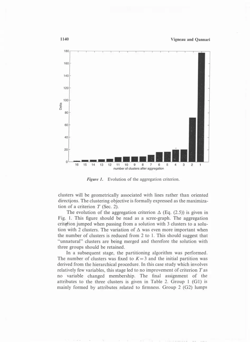
Figure 1. Evolution of the aggregation criterion.

clusters will be geometrically associated with lines rather than orienteddirectjûns. The clustering objective is formally expressed as the maximiza-tion of a criterion T (Sec. 2).

The evolution of the aggregation criterion !:l (Eq. (2.5» is given inFig. 1. This figure should be read as a scree-graph. The aggregationcritqfion jumped when passing from a solution with 3 clusters to a solu-tion with 2 clusters. The variation of !:l was even more important whenthe number of clusters is reduced from 2 to 1. This should suggest that"unnatural" clusters are being merged and therefore the solution withthree groups should be retained.

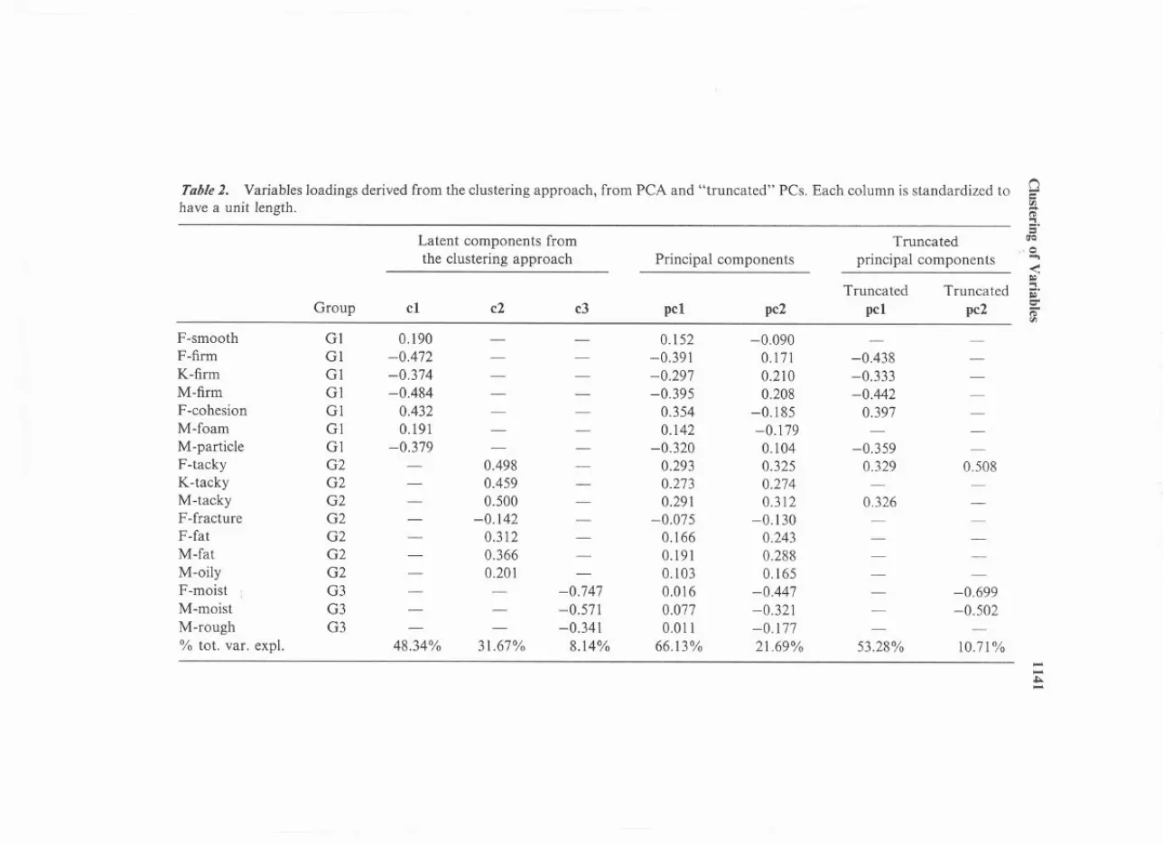
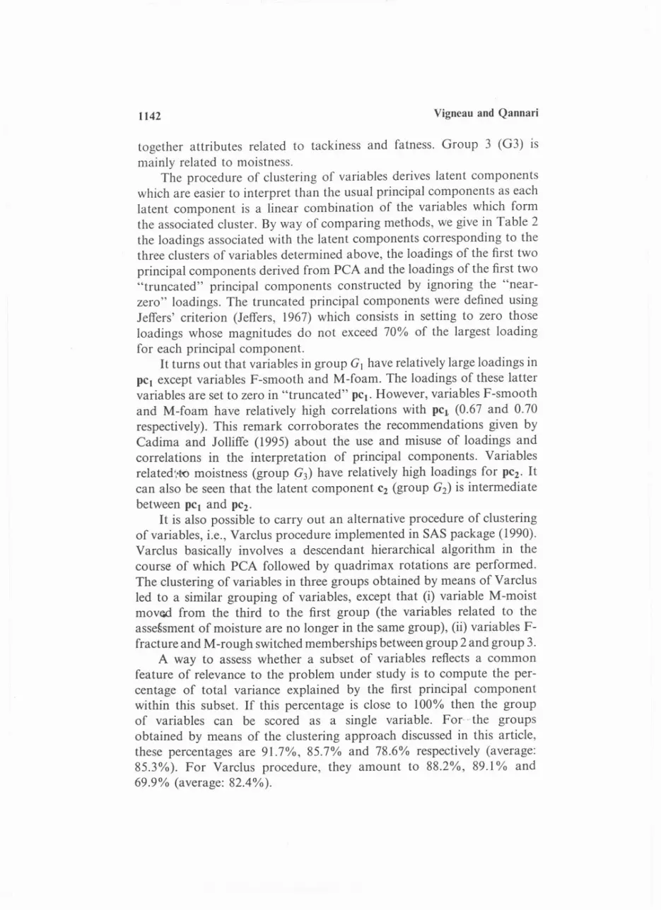
ln a subsequent stage, the partitioning algorithm was performed.The number of clusters was fixed to K = 3 and the initial partition wasderived from the hierarchical procedure. ln this case study which involvesrelatively few variables, this stage led to no improvement of criterion Tasno variable changed membership. The final assignment of theattributes to the three clusters is given in Table 2. Group 1 (G 1) ismainly formed by attributes related to firmness. Group 2 (G2) lumps

TaMe 2. Variables 10adings derived from the c1ustering approach, from PCA and "truncated" PCs. Each column is standardized to(j=

have a unit length.(IJ.......5s

Latent components from Truncated C1Q

.0

the c1ustering approach Principal components principal components -.-<

Truncated Truncated'"tï

Group el e2 e3 pet pe2 pet pc2C'"

;-(IJ

F-smooth G1 0.190 - - 0.152 -0.090 -F-firm Gl -0.472 - - -0.391 0.171 -0.438K-firm G1 -0.374 - - -0.297 0.210 -0.333M-firm G1 -0.484 - - -0.395 0.208 -0.442F-cohesion G1 0.432 - - 0.354 -0.185 0.397M-foam G1 0.191 - - 0.142 -0.179M-partic1e G1 -0.379 - - -0.320 0.104 -0.359F-tacky G2 - 0.498 - 0.293 0.325 0.329 0.508K-tacky G2 - 0.459 - 0.273 0.274 -

M-tacky G2 - 0.500 - 0.291 0.312 0.326F-fracture G2 - -0.142 - -0.075 -0.130F-fat G2 - 0.312 - 0.166 0.243M-fat G2 - 0.366 - 0.191 0.288M-oily G2 - 0.201 - 0.103 0.165F-moist G3 - - -0.747 0.016 -0.447 - -0.699M-moist G3 - - -0.571 0.077 -0.321 - -0.502M-rough G3 - - -0.341 0.011 -0.177 - -

% tot. var. expl. 48.34% 31.67% 8.14% 66.13% 21.69% 53.28% 10.71% --.1:;0.-


together attributes related to tackiness and fatness. Group 3 (G3) ismainly related to moistness.

The procedure of clustering of variables derives latent componentswhich are easier to interpret than the usual principal components as eachlatent component is a linear combination of the variables which formthe associated cluster. By way of comparing methods, we give in Table 2the loadings associated with the latent components corresponding to thethree clusters of variables determined above, the loadings of the first two

principal components derived from PCA and the loadings of the first two"truncated" principal components constructed by ignoring the "near-zero" loadings. The truncated principal components were defined usingJeffers' criterion (Jeffers, 1967) which consists in setting to zero thoseloadings whose magnitudes do not exceed 70% of the largest loadingfor each principal component.

It turns out that variables in group G1have relatively large loadings inpc. except variables F-smooth and M-foam. The loadings of these lattervariables are set to zero in "truncated" pc.. However, variables F-smoothand M-foam have relatively high correlations with pc.. (0.67 and 0.70respectively). This remark corroborates the recommendations given byCadima and Jolliffe (1995) about the use and misuse of loadings andcorrelations in the interpretation of principal components. Variablesre1atedi;.t'Cmoistness (group G3) have relatively high loadings for PC2.Itcan also be seen that the latent component C2(group G2) is intermediatebetween pc. and PC2.

It is also possible to carry out an alternative procedure of clusteringof variables, i.e., Varclus procedure implemented in SAS package (1990).Varclus basically involves a descendant hierarchical algorithm in thecourse of which PCA followed by quadrimax rotations are performed.The clustering of variables in three groups obtained by means of Varclusled to a similar grouping of variables, except that (i) variable M-moistmovoo from the third to the first group (the variables related to theasse§sment of moisture are no longer in the same group), (ii) variables F-fracture and M-rough switched memberships between group 2 and group 3.

A way to assess whether a subset of variables reflects a commonfeature of relevance to the problem under study is to compute the per-centage of total variance explained by the first principal componentwithin this subset. If this percentage is close to 100% then the groupof variables can be scored as a single variable. For--the groupsobtained by means of the clustering approach discussed in this article,these percentages are 91.7%, 85.7% and 78.6% respectively (average:85.3%). For Varclus procedure, they amount to 88.2%, 89.1% and69.9% (average: 82.4%).


5.2. PANEL SEGMENTATION lNPREFERENCE STUDIES

ln this experiment pertaining to preference analysis, consumers areasked to score a set of products, expressing their degree of acceptability.The data used are part of a large study undertaken by the EuropeanSensory Network (1996). The primary data table X is formed by n=8rows referring to the varieties of coffee and p= 160 columns referring toFrench consumers. Beside these preference data, sensory characterizationof the products, assessed by a trained panel using the list of q=18 attri-butes given in Table 3, is available. The initial sensory data were averagedover assessors leading to a data table Z whose rows refer to products andcolumns to sensory attributes.

The method generally used to analyze these data is ExternalPreference Mapping (PrefMap). PrefMap mainly consists in regressingthe scores of each consumer on the two (or three) first principal compo-nents derived from the sensory data (matrix Z). The main displays result-ing from this appraoch are provided in Figs. 2 and 3. Figure 2 gives thebiplot of products and sensory attributes on the first two factorial axesderived from PCA of Z along with the proportion of the total varianceexplained by each principal component. Figure 3 illustrates vectors asso-ciated with consumers which are obtained by projection of the scoresgiven by these consumers onto the plane spanned by the two first princi-pal components of sensory data (vector model in PrefMap terminology).Examination of the preference vectors reveals that a majority of respon-dents (left side of the plot) prefer products with less spicy, less burnt andless bitter taste. Few respondents are situated to the right side of the plotand seem to react positively to coffees with relatively strong taste.Therefore, this analysis gives useful information about the preference

Tahle 3. List of the 18 sensory attributes.

Odor Taste ln mouth After-taste

o-intensityo-chocolateo-greeno-roastedo-mouldo-sweeto-flavoredo-toffee

t-intensityt-spicyt-burntt-sourt-chocolatet-metallict-bittert-sweet

m-thin/thick aft -in tensity


aft-intensi

t-bitter

P2'"

t-spicy

-sour

0 0.1 0.2axis 1 : 82.39%

0.50.3 OA

FigUl'e 2, PCA of sensory data. Biplot display of products and attributes on thefirst two axes. .

Q.25

0.2

0.15

0.1

o'i-

~ 0.05.,;N(/)

'xco

0

-{).05

-{).1

-{).15

-{).20.08 0.06 0.04 0.02 0 0.02

axis 1 : 82.39 %0.04 0.06 0.08 0.1

Figure 3, Consumer vectors fitted onto the sensory space spanned by the firsttwo principal components.

OA

0.3

0.2

"r

o'i-..... 0 P5-<t

",'P10;

N

'5!1-{).1al

-{).2

-{).3

-{)A

-{).5-{).3 -{).2 -{).1


12000

0

10000

8000

'"~ 60000

4000

2000

16 15 14 13 12 11 10 9 8 7 6 5number of elusters alter aggregation

4 3 2

Figure 4. Evolution of the aggregation criterion.

of the consumers but the segmentation of the panel is only suggestedfrom the configuration of the consumers in Fig. 3 and not clearly defined.Moreover, by retaining only the first principal components, there is a riskto omit relevant information for explaining consumer preferences. Theaim of the approach investigated in this paper is to directly segment thepanel of consumers, exhibit the underlying preference dimensions andexpress these dimensions in terms of the sensory attributes in order toallow further improvement of the products.

The hierarchical algorithm and the partitioning algorithm of cluster-ing of variables which aim at maximizing criterion S (Eq. (4.4)) werecarried out in order to determine groups of variables, i.e. consumers.Figure 4 which shows the evolution of the merging criterion ~ suggestsa partition of the consumers into two clusters. The first cluster contains120 consumers, whereas the second cluster contains 40 consumers.

By construction, the two latent components respectively associatedwith the two clusters are expressed as linear combinations oLthe sensoryattributes. The coefficients of these linear combinations are depicted inFig. 5. It turns out that the main distinction between the two clusters lies

in appreciations related to taste. Consumers of the dominant group (75%


aft-intensity

t-bifter

0m-thinthick

t-sweet 0

0

1

t-metallic

t-chocolate

t-sour

t-bumt 0

t-spicy 0

t-intensity 0

o-toffee 0

0o-flavoure<!

o-sweel 0

o-mould

o-roasted

o-green

o-chocolate

o-intensity 0

-0.5 -0.4 -0.3 -0.2 -0.1 0 0.1 0.2 0.3 0.4 0.5

Figure 5. Coefficients (loadings) of the latent components associated with group1 and group 2.

of the panel) prefer soft products with low intensity taste, without burnttaste nor after-taste. Only 25% of the panel seem to like coffees withstrong taste. Odor descriptors of the products are less important in seg-menting the preferences of the panel. Latent components CI and C2, ingroup 1 and 2 respectively, are plotted in Fig. 6. It appears that whereasproducis P6 and Pg are similarly scored by the two segments of consu-mers, P2 is the most segmenting product as it is appreciated by consumersin segment 2 and rejected by consumers in segment 1.

F#'üm this study, it is then possible to set up a marketing strategy. Bychoosing a target segment in the population of consumers, a productprototype could be identified, i.e., PI or Ps for segment 1. The optimiza-tion of this prototype could also be investigated by softing at best thesensory characteristics which are not appreciated by the consumers of thissegment, Le., the bitterness, burnt taste, spicy taste and the after-taste.

It is worth noting that, in this case study, the outcomes of the clus-tering of variables approach seem to tally to a large ext~nt with those ofPrefMap. This stems from the fact that the first principal component ofsensory data contains the most relevant information for explaining thepreference of consumers. This was retrieved by our approach which


60

I~C110 C2

40

-20

0 0

0

0

--40

-60P1 P2 P3 P4 P5 P6 Pl P8

Figure 6. Latent components associated with the two groups.

exhibited two opposite latent components which are, as a matter of fact,almost collinear with this principal component. However, it should bestressed that the advantage of the c1ustering approach around latentcomponents over PrefMap is three folds:

1.2.

It directly provides segments of consumers.ln each segment, it gives a (single) model which relates prefer-ence to sensory data, whereas PrefMap derives a model perconsumer.

It captures the most relevant information for explaining prefer-ence data even if this information is not contained in the first

principal components of sensory data.

3.

6. CONCLUSION

The examples presented in Sec. 5 show the potential of c1uster ana-lysis of variables around latent components (CAVALC, for short). Wealso stressed how this approach complements existing methods.


The strategy CAVALC-l is based on the magnitudes and not thesigns of the covariances between variables. It may be used as a comple-ment or an alternative to PCA, especially when simplification of principalcomponents is wished. The main difference between this approachand other simplification schemes of principal components (Jeffers,1967; Vines, 2000) is that individual variables can not appear in morethan one latent component. CAVALC-l may also be used to select asubset of variables by choosing one variable from each cluster. Whenexternal data are available, CAVALC-l offers an alternative to PLSapproach (Garthwaite, 1994) as it involves the computation of latentcomponents, linear combinations of external data, that explain the vari-ables under study. For this purpose, CAVALC-l splits these variablesinto several groups according to how they relate to the external data.Further research is indicated in order to investigate more deeply therespective advantages of CAVALC-l and PLS.

CA VALC-2 which considers that two negatively correlated variablespresent high disagreement may be used in preference studies. By segment-ing the panel of consumers, CA VALC-2 exhibits one dominant directionof preference in each segment. When external data are available,CAVALC-2 provides an alternative to External Preference Mapping(PrefMap) and leads to a small number of models linking preferencedata to e)\:ternal data. Moreover, it directly captures the information inthese external data which are relevant for explaining the preferences ofconsumers.

Research will also be undertaken in order to set up a hypothesistesting framework for the choice of the number of clusters. Monte-Carlosimulation may be useful in this context.

APPENDIX

Pr00f of inequality (2.6):

À(AUB)1{

I, '}

= max - c XAUBXAUBCIIcll=1 n

{

I" 1 1 '

}= max -c XAXAc + -c XBXBC

11c1l=1n n

{

I"

} {

l, '

}.:Smax -c XAXAC + max -c XBXBC

11c1l=1n IIcll=1n

= À~A)+ À~B)


With XA denoting the matrix whose columns are formed with thevariables belonging to group A and maxllcll=1standing for the maximumover the standardized components c.

Proof of inequality (3.6):

(PA +PB)CJ(XAUB)= (PA +PB) .)n"XAUBI1 -

= .j1iIIpAxA+ PBxBII1 - 1-

:SPA .j1i"XAIi+PB .j1i"xBII

= PACJ(XA) + PBCJ(XB)

where Il.11 denotes the usual Euclidean norm.

REFERENCES

Abdallah, H., Saporta, G. (1998). Classification d'un ensemble de vari-ables qualitatives. Revue de Statistique Appliquée XLVI(4):5-26.

AI-Kandari, N. M., Jolliffe, 1. T. (2001). Variable selection and interpre-tation of covariance principal components. Communications inStatistics: Simulation and Computation 30:339-354.

Cadima, J., Jolliffe, 1. T. (1995). Loadings and correlations in the inter-pretation of principal components. Journal of Applied Statistics22:203-214.

ESN. (1996). A European Sensory and Consumer Study: A Case Studyon Coffee. Published by the European Sensory Network.

Gains, N., Krzanowski, J., Thomson, M. H. (1988). A comparison ofvariable reduction techniques in a attitudinal investigation of meatproducts. Journal of Sensory Studies. 3:37-48.

Garthwaite, P. H. (1994). An interpretation of partial least squares.Journal of the American Statistical Association 89:122-127.

Greenhoff, K., MacFie, H. J. H. (1994). Preference mapping in practice.Measurement of Food Preferences; ln: Macfie, H. J. H.,Thomson, D. M. H., eds. Blackie Academie & Professional:London, pp. 137-166.

Guo, Q., Wu, W., Massart, D. L., Boucon, c., de Jong, S. (2002).Feature selection in principal component analysis- of analyticaldata. Chemometrics and Intelligent Laboratory Systems 61:123-132.

Jeffers, J. N. R. (1967). Two case studies in the application of PrincipalComponent Analysis. Applied Statistics 16:225-236.


Jolliffe, 1. T. (1972). Discarding variables in a principal componentanalysis. i: artificial data. Applied Statistics 21:160-173.

Krzanowski, W. J. (1987). Selection of variables to preserve multivariatedata structure, using principal components. Applied Statistics.36:22-33.

McCabe, G. P. (1984). Principal variables. Technometrics 26:137-144.Qannari, E. M., Vigneau, E., Courcoux, P. (1997). Clustering of variables,

application in consumer and sensory studies. Food Quality andPreference 8:423-428.

Qannari, E. M., Vigneau, E., Courcoux, P. (1998). Une nouvelle distanceentre variables; application en classification. Revue de StatistiqueAppliquée XLVI(2):21- 32.

SAS/STAT. (1990). The VARCLUS procedure. User's Guide, Version 6,Vol. 2. Cary, North Carolina: SAS Institute Inc., pp. 1641-1659.

Soffritti, G. (1999). Hierarchical clustering of variables: a comparisonamong strategies of analysis. COlnmunications in Statistics:Simulation and Computation 28:977-999.

Vines, S. K. (2000). Simple principal components. Applied Statistics49:441-451.

clustering of variables around latent components

Documents