does distance make good neighbors? the role of spatial externalities and income in residential...
TRANSCRIPT

1
Does Distance Make Good Neighbors? The Role of Spatial Externalities and Income in Residential
Development Patterns
Rocio Moreno-Sanchez Graduate Student
Dept. of Agricultural, Environmental, and Developmental Economics Ohio State University
2120 Fyffe Rd, Columbus, OH 43210 Telephone: 614-688-9197
Fax: 614-292-0078 Email: [email protected]
Elena G. Irwin Assistant Professor
Dept. of Agricultural, Environmental, and Developmental Economics Ohio State University
2120 Fyffe Rd, Columbus, OH 43210 Telephone: 614-292-6449
Fax: 614-292-0078 Email: [email protected]
Paper prepared for the American Agricultural Economics Association Annual Meeting, Denver, CO, August 1-4, 2004. Short Abstract: Scattered residential development is explained using a theoretical model of residential location in which household interactions generate externalities that determine location choices. Results demonstrate the role of income and heterogeneous preferences in generating this form of sprawl. Among our findings is that rising income generates only temporary increases in sprawl. Copyright 2004 by Rocio Moreno-Sanchez and Elena Irwin. All rights reserved. Readers may make verbatim copies of this document for non-commercial purposes by any means, provided that this copyright notice appears on all such copies.
1
Introduction
Urban sprawl is a catch-all phrase that is often used to refer to various aspects of changing urban
form characterized by low density, scattered, or mixed use development. Within economics,
sprawl has been largely conceived of and analyzed as two complementary urban land use
patterns: decentralization of cities and leapfrog (or scattered) development.1 Rising household
incomes, along with population growth and declining transportation costs, have been
hypothesized to be a primary driving force of decentralization (Mieszkowski and Mills). With
increasing incomes, households are hypothesized to consume more housing services, which
leads to an expansion of the overall city size (Brueckner). In addition, to the extent that
households substitute land consumption for proximity to the city, rising incomes will redistribute
population towards the suburbs and away from the central city. Finally, because suburbs are
often perceived as having superior public goods and services, increases in income are
hypothesized to spur households to engage in Tieboutian moves to suburban locations in search
of these superior goods and services (O’Sullivan). Empirical evidence supports these theoretical
hypotheses. For example, Brueckner and Fansler find that sprawl, as proxied by city size, is
positively influenced by average household income levels. Based on empirical results from a
model of household location, Margo estimates that about 40% of the increase in suburbanization
between 1950 and 1980 is attributable to increases in household income.
While evidence supports a broad connection between rising incomes and sprawl in terms of
population decentralization, theoretical motivations and empirical evidence regarding the role of
income in generating sprawl at a finer spatial scale, e.g., in the form of scattered or leapfrog
development, are much more limited. The standard income effect that links rising incomes to
increased consumption of housing and land, both normal goods, implies that increases in income
will lead to a more dispersed or scattered pattern of development. Other than this hypothesis,
which is implicit in Brueckner’s discussion of sprawl and city size, the closest explanation linking 1 Both trends capture relevant aspects of sprawl, but at different spatial scales. Decentralization (or suburbanization) is typically used to refer to metropolitan-wide shifts in population away from central cities towards suburban locations whereas leapfrog (or scattered) development typically refers to a finer scale pattern of development that is characterized by intervening plots of vacant land.

2
income and leapfrogging is from Mills. He extends the basic intertemporal efficiency model of
leapfrog development (e.g., Ohls and Pines) by incorporating economic growth into a two-period
model of land development. He shows how uncertainty over future returns and heterogeneity
among land developers’ expectations can lead to permanent scattered and mixed use patterns of
development. More recent explanations of leapfrogging focus on the role externalities, e.g.,
externalities from public parks that attract residents (Wu and Plantinga) and, for the case of
scattered development, externalities from neighboring land uses (Irwin and Bockstael, 2002;
Parker and Metersky, Turner).
To explore the role of income in generating sprawl at a finer spatial scale, we develop a
theoretical model of scattered residential development,2 in which spatial interactions among
households generate a set of locational features that are hypothesized to be the primary
determinants of household location. For example, spatial clustering of households can generate
both local benefits, e.g., the provision of public infrastructure and the availability of neighborhood
networks, as well as costs, e.g., neighborhood congestion and the loss of open space amenities.
Thus, rather than defining space exogenously in terms of distance to an exogenously located
central city, space is defined endogenously by the relative proximity of households to each other
and the spatial externalities that result are treated as the primary determinant of a household’s
location choice. This approach is consistent with some of the more recent models of scattered
development (Parker and Metersky, Turner), in which endogenous land use externalities from
neighboring plots of land influence household choice, and is similar in spirit to the approach taken
by some theoretical models of suburban subcenter formation (e.g., Fujita and Ogawa). In
addition, it is consistent with the empirical evidence on spatial externalities and residential
patterns, which indicates that such local externalities are a significant determinant of these
patterns (Carrion-Flores and Irwin, Irwin and Bockstael, 2002, 2004). This approach is in contrast
2 By scattered development we mean low-density, dispersed development with intervening vacant land that is typical of urban-rural fringe landscapes in the U.S. and refer interchangeably to this as scattered development, leapfrog development, or sprawl. While some researchers associate leapfrog development explicitly with an urban distance gradient, we treat is as a more generic land use pattern that is not necessarily defined with respect to the city center.

3
to the majority of theoretical models of leapfrog development, which have been developed within
the framework of the monocentric model and explain leapfrogging as the result of distance to the
city center, as well as heterogeneous expectations among landowners (Mills, 1981) or publicly
provided open space (Wu and Plantinga).
In developing such a model, we depart from the traditional monocentric framework and define
space as the average distance between a household and neighboring households. Thus, this
approach is applicable for describing residential patterns for cases in which distance to a central
location is not a primary factor.3 Both positive and negative spatial externalities are assumed to
decay continuously with average distance to a maximum point, at which point they disappear.
Positive externalities generate benefits to nearby households and encourage agglomeration, e.g.,
people may find it beneficial to live close enough to others so as to reap social benefits from
neighbors. In addition, there may be positive effects associated with a critical density of residents
in an area that attracts public or private services. Negative externalities create disutility among
neighboring households and encourage dispersion, e.g., due to congestion of local public goods,
including environmental goods, lack of neighboring open space, pollution, or simply the desire of
living in relative isolation from others. By incorporating these effects into a model of household
location choice, we are able to describe the household’s bid curve as a function of the optimal
average distance between a household and its neighbors. From this we derive the household’s
demand for distance and examine the effects of spatial externalities and household preferences
and income on the regional pattern of scattered development. Results show that increases in
household income will increase the optimal distance among households, but that this effect
diminishes with further increases in income and eventually goes to zero. This is due to the fact
that distance to other households is not always a normal good and thus income effects in a model
of spatial externalities are not always positive. The result is that continual increases in household
3 For example, this approach is applicable for describing patterns within a smaller area, e.g., a neighborhood, for which all locations are relatively equi-distant from the employment center or for areas located relatively far from the urban center (e.g., exurban areas), such that differences in distance to the city are small across locations. Alternatively, this model applies to cases in which transportation costs are sufficiently low or employment is more uniformly distributed throughout the region such that distance to a single employment center is not a primary factor.
4
income over time are predicted to generate only temporary increases in scattered residential
development. We also consider the influence of heterogeneous households, as distinguished by
their preferences over the spatial externalities, on the effect of income on scattered development.
Although the total amount of scattered development is clearly increasing in the proportion of
households that have strong preferences for more isolated locations, we find that the rate of
increase in scattered development due to rising household incomes is greater the higher the
proportion of “average” households4 in the region.
Explaining Scattered Residential Development
Theoretical models of leapfrog or scattered development have suggested different causes of
leapfrogging, including efficient intertemporal decisionmaking, heterogeneous expectations
among land developers under uncertainty, heterogeneous preferences among households, and
spatial externalities. The traditional explanation of leapfrogging is that it is a temporary process
that results from intertemporal efficient decisionmaking by land developers. For instance, Ohls
and Pines develop a two period model in which households trade-off living space and
accessibility and demonstrate that under certain conditions, discontinuous development will be
efficient. They argue that if households prefer lower densities (or if lower costs are associated
with lower densities), then lower density housing further from city center will be built initially to
accommodate this desire for low density, while leaving the skipped-over land to be filled with
higher-density residential buildings during later stages of development. Fujita (1976) uses a
dynamic version of the monocentric model to compare the efficiency of the competitive outcome,
in which vacant land is skipped over for a period of time, with the optimal equilibrium growth path
and finds that the competitive path with leapfrog development is efficient. In a later work, Fujita
(1983) differentiates households by income in which differences in incomes drive differences in
buildings and activity types. He shows that, under conditions of perfect foresight, a “sprawl-
fashioned urbanization” process is more efficient. The spatial growth of the city is characterized
4 Average households are defined as those that have moderated preferences over the positive and negative externalities that are generated by proximity of a household to others.
5
by a pattern of leapfrog and mixed development, which is shown to be an intertemporal efficient
process of land development.
Mills develops an extension of these models by incorporating multiple types of development
(residential and industrial) and alternative assumptions about economic growth relative to
landowners’ expectations in a two-period analysis. When landowners are uncertain about future
returns, they must speculate in the first period because they cannot know for certain how much
land to be withheld and preserved for future industrial expansion. A permanent pattern of leapfrog
development results when actual growth is insufficient to fill the vacant land with industrial
expansion. When extending his model to include heterogeneous expectations, Mills finds that
either scattered development occurs if actual growth in the second period is less than
landowners’ expectations or mixed development occurs if actual growth in the second period is
greater than expected growth.
Alternatively, Bar-Ilan and Strange explain leapfrogging as the result of uncertainty combined with
temporal lags in development. As described by Capozza and Helsley (1989), uncertainty over
future returns to development introduces an option value to delaying development (i.e., a growth
premium). Findings from Capozza and Helsley’s (1990) model show that, although the presence
of uncertainty and irreversibility delay development, they cannot cause leapfrogging. Bar-Ilan and
Strange consider the role of development lags in this model. They find that in a non-lag scenario,
uncertainty increases with distance and thus so does the option value. Therefore, leapfrogging
does not occur as landowners at the edge of a city will exhibit more caution than central owners
and wait. However, when development lags are incorporated into the model, leapfrog
development can occur because lags reduce the option value and thus uncertainty is less a
deterrent to development.
Heterogeneity in agent preferences or incomes has been shown to generate leapfrog
development. Fujita (1982) develops a model to examine the spatial dynamics of residential
6
development and shows that, while leapfrog development does not occur when all households
have homogeneous income levels, it is the general development pattern in the suburbs if there
are multiple income classes and housing is a non-neutral good. Page analyzes city formation
using an agent location model where agents’ preferences depend on location’s population and its
separation (its average distance from other agents). Given their preferences on population at
their own location and the average distance from their location to other agents, individual agent’s
decision about where to locate result in different “macro” spatial configurations.
Leapfrog or scattered pattern of residential development has also been explained as an outcome
of public policies, e.g., zoning, public open space preservation, or publicly provided infrastructure,
e.g., roads and sewer lines. Turnbull examines the effect of zoning on the pace and pattern of
residential development using a dynamic open city model. Zoning, which is specified as a
minimum lot size restriction, is shown to temporarily halt development at some locations while
inducing leapfrog development at others, both phenomena that in the absence of zoning would
not occur. Wu and Plantinga, investigate the impact of public open space on residential land use
patterns in a city. They use an open city monocentric model, but, in contrast to the traditional
model, residential sites are differentiated by their proximity to open space, which generates
distance-dependent amenities for residents. After solving for the spatial market equilibrium, they
use a series of simulations to examine the conditions under which public open space causes
leapfrog development when placed outside the city by spurring development of nearby land
before land closer to the city is developed.
Finally, leapfrog development has been explained as the result of spatial externalities that arise
from interactions among households that cause households to locate apart from each other.
Turner develops a game theoretic model of residential location choice in which people choose to
immigrate to a city and derive utility from their proximity to open space. In a static framework, the
equilibrium development outcome consists of three regions: An urban region near to the old city
that is solidly occupied, a more extreme suburban region where only alternate spaces are

7
occupied, and an unoccupied frontier. Any immigrant at a suburban location who does not obtain
open space benefits is strictly better off in an alternate city and therefore, no adjacent occupied
spaces are possible in the suburbs. When incorporating a dynamic component, Turner finds that
an equilibrium location profile has the same basic form as the static games. In addition he show
that if proximity to open space is sufficiently valuable and player are sufficiently patient, then at
least some suburban locations must be occupied before all urban locations are occupied,
generating leapfrog development. In both the static and dynamic games, he finds that the
competitive equilibrium is not efficient: it will contain too many people too close together because
the external open space effects are not considered. In addition, in the dynamic game, the
equilibrium development path deviates from the optimum because suburban locations are
developed earlier than they should be and thus generate leapfrog development. Parker and
Meteresky develop an agent-based model of urban and agricultural land use in which transport
costs pull urban uses to the center of the city, negative externalities between agricultural and
urban users encourage separation and negative externalities between urban users encourage
dispersal of urban activity. They simulate this model and show that the negative externalities
associated with urban land generate a fragmented pattern of development on the urban fringe,
which surrounds a contiguous urban core.
The vast majority of the papers reviewed above explain leapfrog development within the
framework of the monocentric model, which assumes that proximity to the city center is a primary
determinant of urban land use patterns. Leapfrog development is explained either as the result of
dynamic efficiency decisions, made under conditions of either perfect foresight or uncertainty, that
are driven by the urban land rent gradient or as the result of additional sources of exogenous
heterogeneity. A limitation of this approach is that it fails to consider how leapfrog development
may arise endogenously from a process of interdependent household decisionmaking about
location or land use. In contrast are the models by Turner and Parker and Meteresky, in which
leapfrogging is posited as the result of spatial externalities generated by other households’
location or land use decisions. However, both these papers focus only on externalities that
8
create repelling effects that cause development to disperse. Positive externalities that cause
residential land to cluster are of course also quite plausible. Such household interaction effects
have been incorporated into previous urban economic models that have explained urban spatial
structure as the result of social interactions (e.g., Beckman, Page) and there is some empirical
evidence of both positive and negative effects associated with neighboring residential
development (e.g., Carrion-Flores and Irwin, Irwin and Bockstael, 2002, 2004). Thus a more
general model would consider the role of both agglomerative and repelling effects that are
generated from proximity of households to each other and how the tension between these effects
influences leapfrog or scattered development.
A Model of Household Location with Spatial Externalities
We begin with a model in which households are assumed to maximize utility by choosing
residential location and the amount of a composite good. To focus on the role of endogenous
interactions among households, we assume that residential location is defined solely in terms of
the location of households relative to one another. Proximity of households to one another
generate externalities that yield both positive (agglomerative) and negative (repelling) spatial
externalities. Households have preferences over these effects and thus, in choosing a location,
households choose the optimal levels of positive and negative externalities generated by the
relative proximity of neighboring households. To simplify a measure of neighboring household
proximity, we assume that all nearest neighbors (i.e., houses on lots that share a common
border) are equi-distant, so that the distance between a house and its nearest neighbor is the
same for all nearest neighbors and thus is equal to the average distance the nearest neighbors.5
To capture the effects of heterogeneous households, we allow for different types of households
who vary in their preferences over the agglomerative and repelling effects. As a result, a
household’s optimal distance to neighbors will characterize and distinguish each type of
household; some households enjoy living in neighborhoods that are within close proximity to
5 Because we assume a lattice structure, this distance measure corresponds exactly to a measure of residential density around each house and thus we refer interchangeably to average distance and neighborhood density.
9
others (i.e., higher density neighborhoods) while others prefer to live in much more isolated
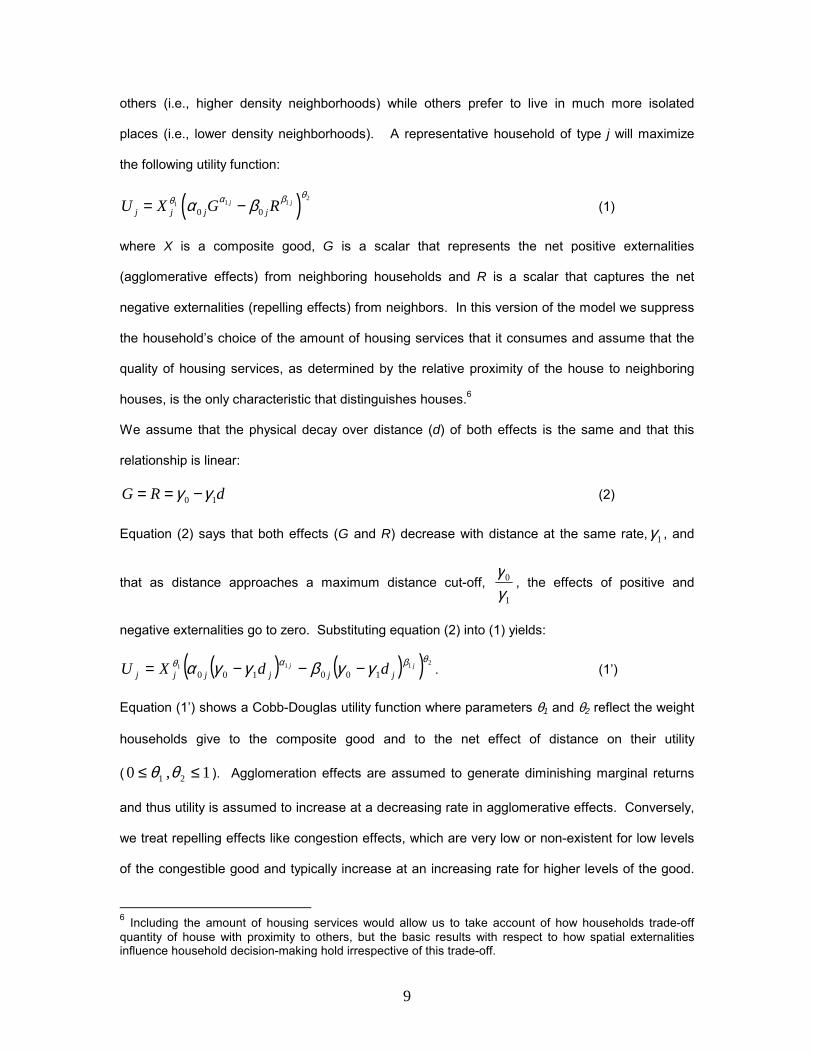
places (i.e., lower density neighborhoods). A representative household of type j will maximize
the following utility function:
( ) 21 11
0 0j j
j j j jU X G Rθα βθ α β= − (1)
where X is a composite good, G is a scalar that represents the net positive externalities
(agglomerative effects) from neighboring households and R is a scalar that captures the net
negative externalities (repelling effects) from neighbors. In this version of the model we suppress
the household’s choice of the amount of housing services that it consumes and assume that the
quality of housing services, as determined by the relative proximity of the house to neighboring
houses, is the only characteristic that distinguishes houses.6
We assume that the physical decay over distance (d) of both effects is the same and that this
relationship is linear:
0 1G R dγ γ= = − (2)
Equation (2) says that both effects (G and R) decrease with distance at the same rate, 1γ , and
that as distance approaches a maximum distance cut-off, 1
0
γγ
, the effects of positive and
negative externalities go to zero. Substituting equation (2) into (1) yields:
( ) ( )( ) 2111100100
θβαθ γγβγγα jjjjjjjj ddXU −−−= . (1’)
Equation (1’) shows a Cobb-Douglas utility function where parameters θ1 and θ2 reflect the weight
households give to the composite good and to the net effect of distance on their utility
( 1,0 21 ≤≤ θθ ). Agglomeration effects are assumed to generate diminishing marginal returns
and thus utility is assumed to increase at a decreasing rate in agglomerative effects. Conversely,
we treat repelling effects like congestion effects, which are very low or non-existent for low levels
of the congestible good and typically increase at an increasing rate for higher levels of the good.
6 Including the amount of housing services would allow us to take account of how households trade-off quantity of house with proximity to others, but the basic results with respect to how spatial externalities influence household decision-making hold irrespective of this trade-off.

10
Thus repelling effects are assumed to generate disutility at an increasing rate. These
assumptions imply that 10 1 ≤≤ α and 11 ≥β . Household types are distinguished by their
preferences over agglomerative and repelling effects and thus by the specific values assigned to
α0 and β0, both of which are assumed to be non-negative. These assumptions guarantee the
following concavity conditions for the households’ utility function:
0≥j
j
dXdU
; 0≥dGdU j
; 0≤dR
dU j
; 0≤jdddG ; 0≤jdd
dR
02
2
≤dX
Ud; 02
2
≤dG
Ud; 02
2
≤dR
Ud
Taken together with the linear distance-decay process specified in (2), these assumptions imply
that utility is affected non-linearly by distance due to the trade-off that households make between
agglomerative and repelling forces when choosing their optimal distance.
Households are assumed to maximize utility subject to their budget constraint:
)(* drpXI jj += , (3)
where I is income, r*(d) is the market price of a house at distance d, and p is the price of the
composite good. Housing price r*(d) it is determined in the market by both the distributions of
consumer tastes and producer costs and thus is exogenous to individual households. Because it
is a function of housing characteristics (in this case, average distance to neighboring houses), we
treat r*(d) as a hedonic price function from which the implicit price for distance can be derived
(Rosen).7 The household’s maximization process yields the following first order conditions:
( ) ( )( ) 21 11 11 0 0 0j j
j j jdL X G R pdX
θα βθθ α β µ−= − − = , (4)
( ) ( )( ) ( ) ( )( ) 0*110
110
1
0012112111 =−−−= −−−
µϕααβββαγθ αβθβαθ GRRGXdddL
jjjjjjjj
jj , (5)
7 The hedonic price function is a double envelope of households bid curves and developers offer curves and therefore it depends on the determinants of demand and supply. For all firms and households to be in equilibrium, all bid and offer curves for distance, for each participant in the market, must be tangent to the hedonic price function. For more details, see Rosen or Freeman.
11
where L represents the Lagrangian and ( )
jj dd
ddr ** =ϕ is the marginal implicit price for distance.
Equations (4) and (5) indicate that at the optimum households will equate the marginal utilities
and marginal costs of the composite good and distance respectively. Interpreted jointly they say
that at the optimum, the marginal utility of the last dollar spent in the composite good should be
equal to the marginal utility from the last dollar spent in distance:
( ) ( )1 1 1 11 11 0 0 2 1 0 1 0 1
*
j jj j j j j j j
j
G R X R Gp
α β β αθ α β θ γ β β α αϕ
− −− −= . (6)
Considering the household’s optimal choice of distance, d*, it is clear that the household will
never choose values of d for which the net spatial externality effect is negative. This is because
the household can always choose to locate at d ≥ 1
0
γγ
, at which point the spatial externality effect
is zero. Thus for any d*, it will always be the case that 01100 ≥− βα βα RG . Given this, the
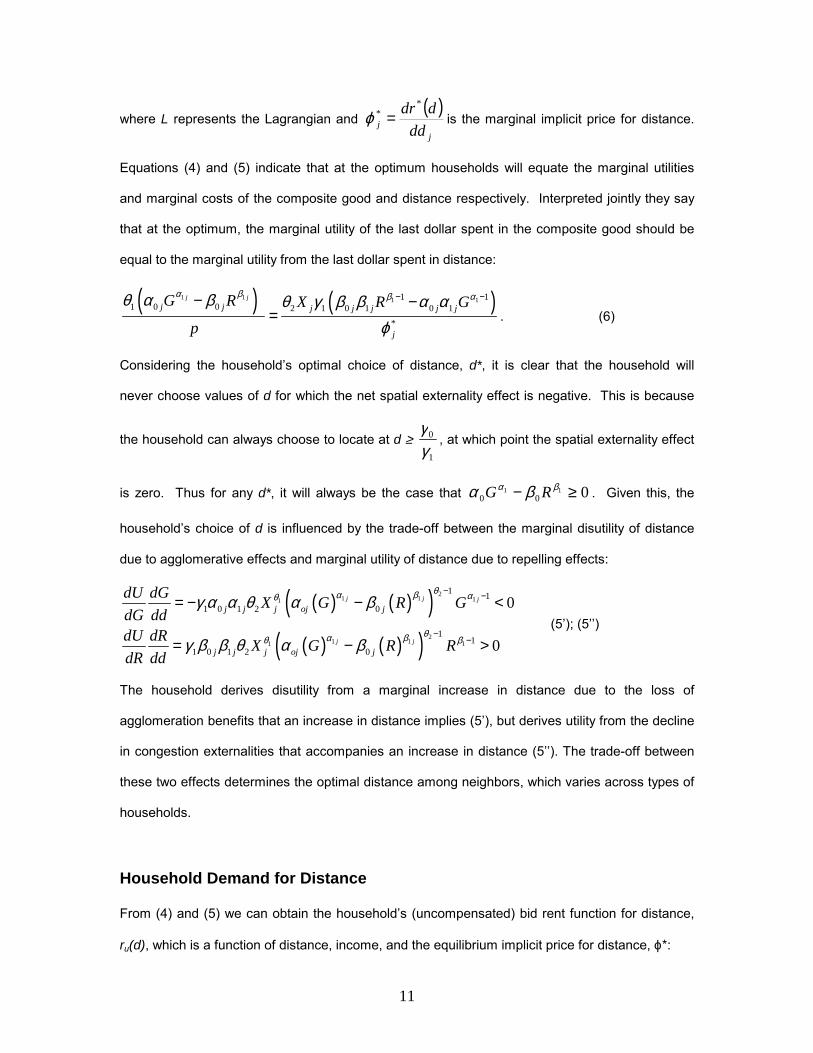
household’s choice of d is influenced by the trade-off between the marginal disutility of distance
due to agglomerative effects and marginal utility of distance due to repelling effects:
( ) ( )( )( ) ( )( )
21 1 11
21 11 1
1 11 0 1 2 0
11
1 0 1 2 0
0
0
j j j
j j
j j j oj j
j j j oj j
dU dG X G R GdG dddU dR X G R RdR dd
θα β αθ
θα βθ β
γ α α θ α β
γ β β θ α β
− −
−−
= − − <
= − > (5’); (5’’)
The household derives disutility from a marginal increase in distance due to the loss of
agglomeration benefits that an increase in distance implies (5’), but derives utility from the decline
in congestion externalities that accompanies an increase in distance (5’’). The trade-off between
these two effects determines the optimal distance among neighbors, which varies across types of
households.
Household Demand for Distance
From (4) and (5) we can obtain the household’s (uncompensated) bid rent function for distance,
ru(d), which is a function of distance, income, and the equilibrium implicit price for distance, ϕ*:
12
( ) ( )( )( ) ( )( )1
10101
101012
*1001001
11
11
−− −−−
−−−−=
jj
jj
dddd
Irjjjj
jjjuj αβ
βα
γγααγγββγθϕγγβγγαθ
. (7)
The household’s bid rent function reflects the household’s willingness to pay for a house at every
distance, while the hedonic price function, r*(d), is the minimum price that households must pay in
the market. Thus household utility is maximized at the point at which the household’s bid equals
the market price: ( ) ( )*** ,, jjujjj Idrdr ϕ= , where d* is the optimal distance. At this optimal
point, the bid curves have the same slope and are tangent to the hedonic price function and thus
the marginal bid and the marginal implicit price of distance are equal:
ujj ϕϕ =* . (8)
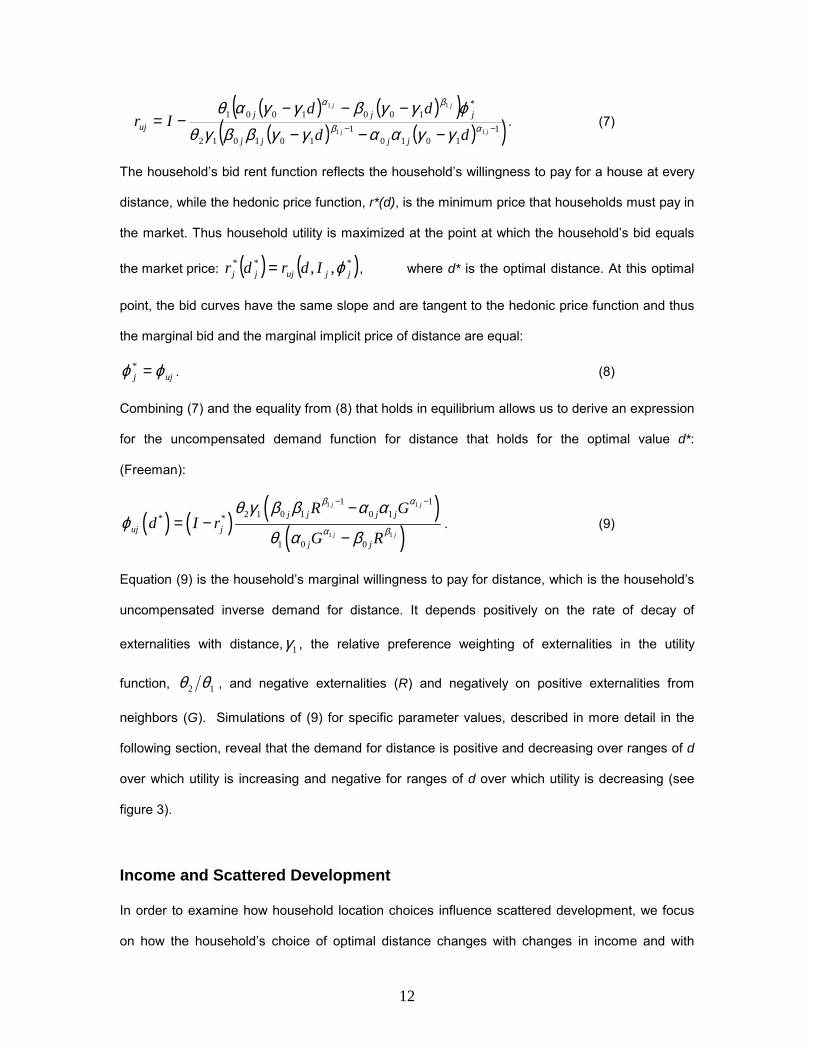
Combining (7) and the equality from (8) that holds in equilibrium allows us to derive an expression
for the uncompensated demand function for distance that holds for the optimal value d*:
(Freeman):
( ) ( ) ( )( )
1 1
1 1
1 12 1 0 1 0 1* *
1 0 0
j j
j j
j j j juj j
j j
R Gd I r
G R
β α
α β
θ γ β β α αϕ
θ α β
− −−= −
−. (9)
Equation (9) is the household’s marginal willingness to pay for distance, which is the household’s
uncompensated inverse demand for distance. It depends positively on the rate of decay of
externalities with distance, 1γ , the relative preference weighting of externalities in the utility
function, 12 θθ , and negative externalities (R) and negatively on positive externalities from
neighbors (G). Simulations of (9) for specific parameter values, described in more detail in the
following section, reveal that the demand for distance is positive and decreasing over ranges of d
over which utility is increasing and negative for ranges of d over which utility is decreasing (see
figure 3).
Income and Scattered Development
In order to examine how household location choices influence scattered development, we focus
on how the household’s choice of optimal distance changes with changes in income and with
13
heterogeneity in households’ preferences over the agglomerative and repelling effects generated
by proximity to neighbors. As a household’s choice of optimal distance from its neighbors
increases, so does the degree of scattered or leapfrog development in the region and thus factors
that increase optimal distance will increase this form of sprawl. Given this, we are interested in
testing whether this form of sprawl is increasing in income, as is suggested by previous models,
and whether increases in income affect heterogeneous households differentially in terms of their
optimal location decision. The latter allows us to investigate the interaction between
heterogeneous preferences and income and whether the income effect associated with
households that have stronger preferences for more isolated locations contributes more to sprawl
than the income effect associated with those with weaker preferences for isolated locations.
The effect of income changes on optimal distance
Comparative statics is used to examine the effect of an exogenous change in income on the
household’s equilibrium bid function (equation 7), where the marginal implicit price of distance,
ϕ*, is equal to the household’s marginal willingness to pay for distance, ϕuj, at the equilibrium
point:
jujj
j
ZdIdd
1
2
θϕθ
= , (10)
where ( ) ( ) ( )( )
( ) 011
1 2110
110
2110
211000
11
1111
>−
−−−−+=
−−
−−
jj
jjjj
GR
GRRGZ
jjjj
jjjjjjjjj αβ
αββα
ααββ
αααββββα for
any positive value of utility function.8 Therefore, the sign of j
j
dIdd
depends on the sign of ϕuj. From
equation (9) we know that the sign of ϕuj changes with distance such that, for jjj ddd ˆ0 << , ϕuj
8 Remember that dRG 10 γγ −== .

14
> 0 and 0>j
j
dIdd
, where jj
j
jjd
11
1
0
0
11
00
1 αβ
βα
γγγ −
−= , which is the minimum distance that
generates a positive utility for household j and jj
jj
jjjd
11
1
10
10
11
0 1ˆαβ
ββαα
γγγ −
−= , which is the
distance at which household j maximizes its utility. Thus, for jjj ddd ˆ0 << , utility is positive and
increasing over dj and distance behaves as a normal good. On the other hand, for
jjj ddd 1ˆ << , ϕuj < 0 and 0<
j
j
dIdd
, where 1
01 γ
γ=jd is the distance at which agglomerative
and repelling effects vanish. In this case, utility is positive and decreasing over dj and distance
behaves as an inferior good.
As discussed earlier, the market equilibrium is defined by a set of tangencies between the
households’ bid functions and the offer curves of the sellers (in this case assumed to be housing
developers). Although we refrain from developing an explicit model of the supply side, we
assume that developers can achieve economics of scale in housing production when houses are
within sufficient proximity of each other and thus, that developers’ offer curves are non-
decreasing over distance. On the other hand, as discussed above, household bid functions are
increasing over distance only for distances that are less than or equal to their unconstrained
optimal distance, jdK
, and are decreasing with distances that are greater than this. Given these
conditions, a market equilibrium implies that households will be located at distances that are less
than or equal to jdK
since an offer curve can only be tangent to that portion of the bid curve that
correspond to this distance range. In this case, increases in income will cause a household to
increase its optimal distance from neighbors so long as households are not already located at
their unconstrained optimum (i.e., so long as j*j d̂d < ). However, once a household reaches
jd̂ , further increases in income will have no effect on distance decisions and additional income
15
will be allocated to the consumption of other goods, ceteris paribus. These results lead us to
conclude that, keeping population constant, scattered development that is driven by spatial
externalities is a process that is driven only temporarily by increases in income. This process is
the result of households looking, over time, for a location that satisfies their preferences over
proximity to others. Once households have reached their unconstrained optimum, jd̂ , increases
in income will not be reflected in greater distances, ceteris paribus, because distance becomes
an inferior good over the range jjj ddd 1ˆ << . If we accept that income increases over time, we
can assert that distance among households reaches a static equilibrium point and that increases
in income only generate temporary increases in scattered development due to spatial
externalities, other things equal.
Income effects with heterogeneous households
While the comparative statics tell us something about how the household’s optimal distance
changes with income, we cannot readily compare the magnitude of this change across different
household types (as differentiated by their preferences over proximity to neighbors). To obtain
this, we compute household type j’s income elasticity of demand for distance:
( )( )
1 1
11
1 10 02
1 1 0 1 0 1
j j
j
j jjj j
uj j j j j
G RrZ
d R G
α β
αβ
α βθη
θ ϕ γ β β α α
+ + − = − −
, (11)
where Zj is defined as in equation (10). The sign of income elasticity depends of the sign of ϕuj.
Household j’s income elasticity is positive for jd d<K
and negative for jd d>K
, where jdK
is the
optimal distance to neighbors for household type j. The magnitude of the percentage change in
distance due to a change in income varies among households and depends, among other things,
on the values of the parameters governing preferences over proximity to neighbors.
To further examine how heterogeneous preferences influence the income elasticity of demand for
distance, a simulation is performed for three types of households that have identical incomes, but
16
heterogeneous preferences over their proximity to neighbors. We refer to these three types as
gregarious, average, and loner households. Gregarious households value the benefits from living
within close proximity to their neighbors, but also perceive some of the negative effects from
congestion. Average households perceive a relatively balanced mix of benefits and costs
associated with proximity to neighbors and thus do not like locating too close or too far from
others. Loner households primarily perceive the costs from congestion generated by neighbors
and only a few of the potential benefits from proximity and thus try to locate relatively far from
neighbors. To define each type of household, variations in the values of some parameters are
allowed (namely, we vary α0 and β0), while the other parameters remain constant across
households.9
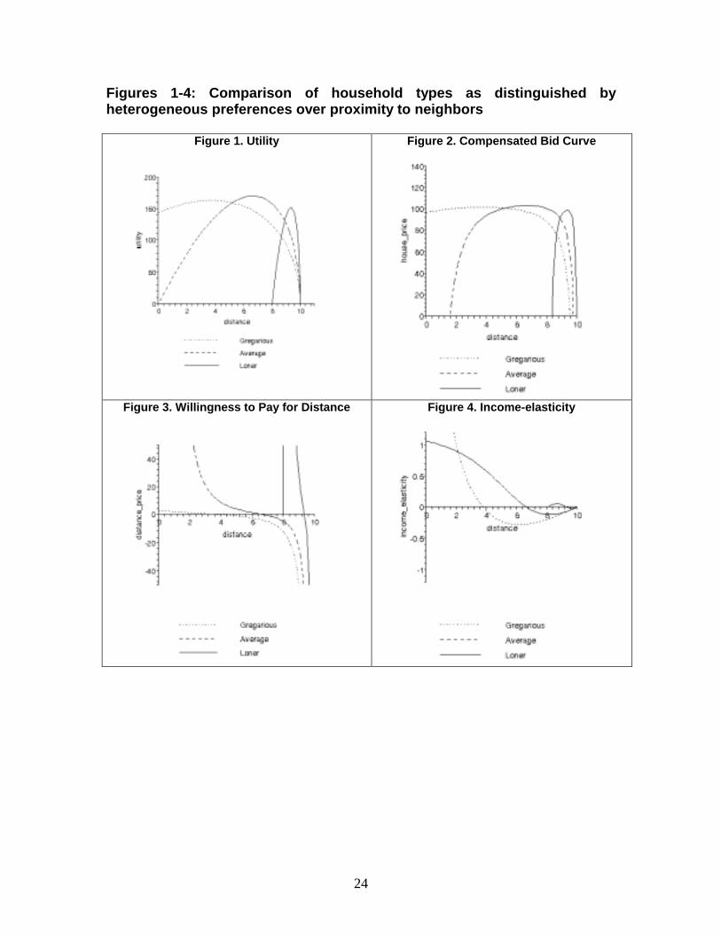
Figures 1 to 4 report the results of the simulation, including the optimal distance, compensated
bid function,10 uncompensated marginal willingness to pay for distance, and income elasticity of
demand for distance for each type of household. We use these results to discuss the optimal
choices of each household type and the implications of this heterogeneity for scattered residential
development. Gregarious households have a positive utility over the relevant distance range
(from zero to γ0/γ1), but their utility is increasing only for a portion of this range, 0 gd d< <K
(figure
1). Their maximum willingness to pay for a house is at 0gd d= >K
(figure 2) and their demand
for distance is positive only for the range gg d̂d <≤0 (figure 3). On the other hand, the range
of distances for which average households’ utility is increasing is much greater than the
gregarious households (figure 1) and therefore, its marginal willingness to pay for distance is
positive for a greater range of d (figure 3). Lastly, loner households maximize utility at ld d=�
,
which is very close to the distance at which agglomerative and repelling effects vanishes, γ0/γ1.
9 Specifically, we vary the following parameters as follows for the gregarious, average, and loner households: α0 = 14, 20, and 40 respectively and β0 = 0.75, 2, and 20 respectively. The following parameters are held constant at the following values: θ1 = 0.5; θ2 = 1; α1 = 0.5; β1 = 1.5; γ0 = 10; and γ1 = 1. 10 We graph the compensated bid function since the uncompensated function in (9) is a function of the marginal implicit price of distance, ϕ*, which is an endogenous variable. The compensated bid function is derived by substituting (3) into (1’), holding utility constant and solving for r(d) as a function of distance.
17
This type of household faces a small distance range for which their utility is positive and small
range for which it is increasing (figure 1). Its willingness to pay for a house within its relevant
distance range is the steepest of all types of households (figure 2) and these households have
the highest demand for housing that is located at further distances (figure 3).
Figure 4 illustrates the differences in the income elasticity of demand for distance across
household types. In each case, households’ demand for distance is more or less income elastic
depending on distance. Households’ income elasticity of demand for distance is zero at the
household’s unconstrained optimum and is the most inelastic and positive (negative) for
distances that are just less than (greater than) this value. Thus, at the unconstrained optimum,
income changes do not alter the household’s optimal choice of distance. For all households, the
income elasticity goes to zero at distances that are at or beyond the maximum distance for which
externalities are generated (d = γ0/γ1).
Households’ income elasticity varies in sign and magnitude by household type. Gregarious and
average households exhibit an income elasticity of demand for distance that is positive and highly
elastic for distances that are substantially less than their respective unconstrained optimal
distances. Distances that are farther than this point reduce utility and therefore the income
elasticity is negative for these distances. The gregarious households’ demand for distance is
highly income elastic for shorter distances, but their income elasticity is positive only for a
relatively narrow range of distances before reaching their unconstrained optimum. On the other
hand, the income elasticity for average households is less elastic, but is positive for a greater
range of distances. Finally, loner households are the most inelastic of all types as the range of
distances for which their utility (as well as their demand for distance) is positive and increasing is
very short and close to the distance at which the externalities vanish.
Taken together, these results indicate that the effect of income on household location will depend
on both the household’s initial location and their particular set of preferences over the spatial
18
externalities generated by proximity to neighbors. As discussed earlier, the market equilibrium
will force households to locate at distances that are either less than or equal to their
unconstrained optimal distance, jdK
. If j*j d̂d < , then increases in income will increase the
optimal distance, but the magnitude of this effect will depend on the household’s preferences over
distance.11 Gregarious households’ demand for distance is highly elastic to income, but at the
same time they only consider a small range of plausible locations. Thus, increases in income will
generate relatively little increase in the amount of scattered development among these
households. On the other hand, the demand for distance among loner households is the most
inelastic to income changes. In addition, because they choose a location that is relatively far
away (but not beyond the point at which the externalities vanish), they also have a small range of
plausible distances from which they are willing to choose. In contrast, the average households’
demand for distance is moderately elastic and these households have the greatest range of
distances over which they are willing to choose. Consequently, changes in income are likely to
affect these households the most in terms of the magnitude of their increase in optimal distance
and thus, the rate at which scattered development increases as a result of rising incomes. This
leads us to conclude that, while the absolute amount of scattered development obviously
increases in the proportion of loner households in the region that have strong preferences for
more isolated locations, the rate at which scattered development increases as the result of rising
incomes will be driven by the proportion of average households in the region. Holding population
constant, the rate at which scattered development increases due to rising incomes will be greater
the higher the proportion of average households in the region.
Summary and Conclusions We develop a theoretical model to explain scattered development at the urban fringe, as
characterized by dispersed development with intervening vacant land. The central feature of the
model is a set of spatial externalities that arise from the relative proximity of neighboring
11 It will also depend on the nature of the economies of scale that determine the developers’ offer curves, but we abstract from this consideration here.
19
residential development and that influence households’ location decisions. Both positive and
negative externalities are hypothesized to exist that generate benefits (agglomerative effects) and
costs (repelling effects) respectively, which influence a household’s decision regarding its optimal
average distance from nearest neighbors. The cumulative result of households’ location choices
determines the extent of scattered development or sprawl in the region.
Based on a utility-maximizing framework in which households choose distance and a composite
good, we derive the household’s bid rent function and their demand for distance, which describes
the households’ implicit price of distance as a function of distance. We use the basic model to
examine the impact of economic growth on the scattered development that results from the
externalities. Our two main findings are that (1) rising household income generates only
temporary increases in scattered development due to spatial externalities, holding population
constant and (2) the rate at which scattered development increases due to rising incomes will be
greater the higher the proportion of average households in the region. The first result is driven by
the fact that distance behaves as a normal good only up to a certain distance threshold, the
household’s unconstrained optimal distance, jd̂ . Beyond this point, distance is an inferior good
and thus further increases in income once the household has reached jd̂ will not be reflected in
greater distances, ceteris paribus. The second result is due to the fact that, given our
assumptions about the heterogeneous preferences of households over distance, households with
moderated preferences over the positive and negative externalities that are generated by
distance (i.e., average households), are the most responsive to income changes in terms of
having both a moderately elastic income elasticity of demand and a relatively large range of
distances over which their utility is increasing. Thus, while the absolute amount of scattered
development will depend on the proportion of households that have strong preferences for more
isolated locations (loner households), the rate at which scattered development increases as the
result of rising incomes is driven by the proportion of average households in the region.
20
These results are subject to several important caveats. First, this model ignores the household’s
choice over the amount of housing or land that is consumed and thus we do not account for the
standard income effect associated with housing and land consumption. Assuming that housing
and land are both normal goods, this effect would generate an ever-increasing amount of
scattered development, which is in contrast to the income effect associated with distance that we
analyze here. Because the consumption of both the quantity of housing (or land) and its location
(in terms of distance) are likely to drive observed household behavior, the net effect of these two
income effects is an empirical question. Second, we assume that population and preferences
over spatial externalities are constant. Clearly the amount of scattered development will increase
with population as additional households locate in a region. If the population is homogeneous in
their preferences, then additional population will simply increase in the geographical extent of the
developed area in the region. However, if new households entering the region have different
preferences—namely, stronger preferences for proximity to neighbors—or if the preferences of
the existing population change such that there is a larger proportion of more gregarious
households, then this “temporary” process of increasing sprawl could easily become permanent.
For example, as new households with stronger preferences for proximity fill up intervening vacant
land, then these locations will become sub-optimal for existing residents with stronger
preferences for more distant locations. In a dynamic setting, such households would choose to
relocate to more distant locations, thus expanding the geographical extent of sprawl in the region.
So, with increases in population or even with a constant population, but heterogeneous and
changing preferences, a stationary state may never be reached.
Despite these limitations, our results are of interest in terms of highlighting the role of spatial
externalities in generating scattered development and have implications for the efficiency of
development patterns. Contrary to the traditional models of leapfrogging, a model in which
scattered development is driven by spatial externalities implies that the competitive outcome is
unlikely to be efficient. In our case, household are both the victims and generators of externalities
as their location decisions are driven by externalities that are generated by others, but these

21
decisions also generate externalities that impact others’ utility and cause a divergence between
the private and social optima. This is akin to Turner’s result that the competitive outcome is
characterized by not enough intervening open space since individual agents do not take into
account the impact on others’ utilities of the loss of open space that is generated by their action.
Here we hypothesize that household interactions lead to both positive and negative externalities
and thus, depending on the net effects, the competitive outcome will be characterized either by
houses that are too close (if the net externality is negative) or not close enough (if the net
externality is positive). Thus, unlike Turner’s results in which the competitive process always
leads to overdevelopment of a given area, the competitive outcome in our model may lead to
either too much or too little development for a given area, depending on the net effect.
Our results have potential implications for the evolution of scattered residential development and
policies that seek to manage this form of sprawl. To the extent that spatial externalities drive
household location, policies that seek to make this form of development more efficient are
warranted. However, because both positive and negative externalities may exist, it is unclear
what the desired policy goal should be. If there are net positive externalities generated by
household interactions, then policies that seek to encourage more spatially clustered
development are warranted. On the other hand, if negative externalities are stronger, then this
would suggest that policies should seek to spread development out further and to retain larger
areas of intervening open space. Thus, to draw more substantial policy implications from such a
model, a better understanding is needed of the types of externalities that are generated from
household proximity, their magnitudes and spatial extents, and the underlying processes that
generate these effects.
22
References
Bar-Ilan, A., and W.C. Strange. “Urban Development with Lags.” Journal of Urban Economics 39
(1996): 87-113.
Beckmann, Martin. “Spatial Equilibrium in the Dispersed City” In Mathematical Land Use, George
J. Papageorgiou, ed., Lexington, MA: Lexington Books, 1976.
Brueckner, J.K. “Urban Sprawl: Diagnosis and Remedies” International Regional Science Review
23 (April 2000): 160-171.
Brueckner, J.K., and D. Fansler. “The Economics of Urban Sprawl: Theory and Evidence on the
Spatial Sizes of Cities.” The Review of Economics and Statistics 65 (August 1983): 479-
482.
Capozza, D. R., and R.W. Helsley. “The Fundamentals of Land Prices and Urban Growth.”
Journal of Urban Economics 26 (1989): 295-306.
Capozza, D. R., and R.W. Helsley. “The Stochastic City.” Journal of Urban Economics 28 (1990):
187-203.
Carrion-Flores, C., and E.G. Irwin. “Determinants of Residential Land Use Conversion and Sprawl
at the Rural-Urban Fringe.” American Journal of Agricultural Economics., in press.
Freeman, A.M. The Measurement of Environmental and Resource Values. Theory and Methods.
Washington: Resources for the Future., 1993.
Fujita, M. “Spatial Patterns of Residential Development.” Journal of Urban Economics 12 (1982):
22-52.
___. “Spatial Patterns of Urban Growth: Optimum and Market.” Journal of Urban Economics 3
(1976): 209-241.
___. “Urban Spatial Dynamics: A Review.” Sistemi Urbani 3 (1983): 411-475
Fujita, M., and H. Ogawa. “Multiple Equilibria and Structural Transition of Non-Monocentric Urban
Configurations.” Regional Science and Urban Economics 12 (1982): 161-196.
Irwin, E.G., and N.E. Bockstael. “Interacting Agents, Spatial Externalities and the Endogenous
Evolution of land Use Patterns.” Journal of Economic Geography 2 (2002): 31-54.
23
___. "Land Use Externalities, Growth Management Policies, and Urban Sprawl." Regional
Science and Urban Economics, 34(November 2004), in press.
Mieszkowski, P., and E.S. Mills. “The Causes of Metropolitan Suburbanization.” Journal of
Economic Perspectives 7 (1993): 135-147
Mills, D. E. “Growth, Speculation and Sprawl in a Monocentric City.” Journal of Urban Economics
10 (1981): 201-226.
Mills, E.S. “The Measurement and Determinants of Suburbanization.” Journal of Urban
Economics 32 (November 1992): 377-387.
Margo, R.A. “Explaining the Postwar Suburbanization of Population in the United-States- The
Role of Income.” Journal of Urban Economics 31 (May, 1992): 301-310.
O’Sullivan, A. Urban Economics. New York: McGraw Hill Book Co., 2003.
Ohls, J.C., and D. Pines. “ Discontinuous Urban Development and Economic Efficiency.” Land
Economics 3 (1975): 224-234.
Page, S.E. “On the Emergence of Cities.” Journal of Urban Economics 45 (1999): 184-208.
Parker, D.C., and V. Meretsky. “Measuring Patterns outcomes in an Agent-Based Model of Edge-
Effect Externalities Using Spatial Econometrics.” Agriculture, Ecosystems and Environment
101 (February 2004): 233-250.
Rosen, S. “Hedonic Prices and Implicit Markets: Product Differentiation in Pure Competition.”
The Journal of Political Economy 82 (January-February 1974): 34-55.
Turnbull, G.K. “A Comparative Dynamic Analysis of Zoning in a Growing City.” Journal of Urban
Economics 29(1991): 235-248.
Turner, M.A. “Landscape Preferences and Patterns of Residential Development.” Working paper,
Dept of Economics, University of Toronto, 2003.
Wu, J., and A.J. Plantinga. “The Influence of Public Open Space on Urban Spatial Structure.”
Journal of Environmental Economics and Management 46 (September 2003): 288-309.
24
Figures 1-4: Comparison of household types as distinguished by heterogeneous preferences over proximity to neighbors
Figure 1. Utility Figure 2. Compensated Bid Curve
Figure 3. Willingness to Pay for Distance Figure 4. Income-elasticity