Northeast Fisheries Science Center Reference Document 06-15

Documentation for the Energy Modeling and Analysis eXercise (EMAX)

Jason S. Link, Carolyn A. Griswold, Elizabeth T. Methratta, and Jessie Gunnard, Editors

August 2006

Recent Issues in This Series

05-14 41st SAW Assessment Report, by the 41st Northeast Regional Stock Assessment Workshop. September 2005.

05-15 Economic Analysis of Alternative Harvest Strategies for Eastern Georges Bank Haddock [5Zjm; 551, 552, 561, 562], by EM Thunberg, DSK Liew, CM Fulcher, and JKT Brodziak. October 2005.

05-16 Northeast Fisheries Science Center Publications, Reports, and Abstracts for Calendar Year 2004, by L Garner. October 2005.

05-17 Modification of Defined Medium ASP12 for Picoplankter Aureococcus anophagefferens, with Limited Com-parison of Physiological Requirements of New York and New Jersey Isolates, by JB Mahoney. November 2005.

05-18 Program Planning and Description Documents for the Northeast Fisheries Science Center, Its Component Laboratories, and Their Predecessors during 1955-2005, by JA Gibson. December 2005.

05-19 Seasonal Management Area to Reduce Ship Strikes of Northern Right Whales in the Gulf of Maine, by RL Merrick. December 2005.

06-01 42nd SAW Assessment Summary Report, by the 42nd Northeast Regional Stock Assessment Workshop. January 2006.

06-02 The 2005 Assessment of the Gulf of Maine Atlantic Cod Stock, by RK Mayo and LA Col. March 2006.

06-03 Summer Abundance Estimates of Cetaceans in US North Atlantic Navy Operating Areas, by DL Palka. March 2006.

06-04 Mortality and Serious Injury Determinations for Baleen Whale Stocks along the Eastern Seaboard of the United States, 2000-2004, by TVN Cole, DL Hartley, and M Garron. April 2006.

06-05 A Historical Perspective on the Abundance and Biomass of Northeast Complex Stocks from NMFS and Massachusetts Inshore Bottom Trawl Surveys, 1963-2002, by KA Sosebee and SX Cadrin. April 2006.

06-06 Report of the GoMA GOOS Workshop on Objectives of Ecosystem Based Fisheries Management in the Gulf of Maine Area, Woods Hole, Massachusetts, 11-13 May 2004, by S Gavaris, WL Gabriel,and TT Noji, Co-Chairs. April 2006.

06-07 Vida de los Pescadores Costeros del Pacífico desde México a Perú y su Dependencia de la Recolecta de Conchas (Anadara spp.), Almejas (Polymesoda spp.), Ostiones (Crassostrea spp., Ostreola spp.), Camarones (Penaeus spp.), Cangrejos (Callinectes spp.), y la Pesca de Peces de Escama en Los Manglares [The Fishermen’s Lives in Pacific Coast Villages from Mexico to Peru, Supported by Landings of Mangrove Cockles (Anadara spp.), Clams (Polymesoda spp.), Oysters (Crassostrea spp., Ostreola spp.), Shrimp (Penaeus spp.), Crabs (Callinectes spp.), and Finfish], by CL MacKenzie Jr and RJ Buesa. April 2006.

06-08 Bloom History of Picoplankter Aureooccus anophagefferens in the New Jersey Barnegat Bay-Little Egg Harbor System and Great Bay, 1995-1999, by JB Mahoney, PS Olsen, and D Jeffress. May 2006.

06-09 42nd Northeast Regional Stock Assessment Workshop (42nd SAW) Stock Assessment Report, by the Northeast Fisheries Science Center. May 2006.

06-10 Assessment of the Georges Bank Atlantic Cod Stock for 2005, by L O’Brien, N Shepherd, and L Col. June 2006.

06-11 Stock Assessment of Georges Bank Haddock, 1931-2004, by J Brodziak, M Traver, L Col, and S Sutherland. June 2006.

06-12 Report from the Atlantic Surfclam (Spisula solidissima) Aging Workshop Northeast Fisheries Science Cen-ter, Woods Hole, MA, 7-9 November 2005, by L Jacobson, S Sutherland, J Burnett, M Davidson, J Harding, J Normant, A Picariello, and E Powell. July 2006.

06-13 Estimates of Cetacean and Seal Bycatch in the 2004 Northeast Sink Gillnet and Mid-Atlantic Coastal Gillnet Fisheries, by DL Belden, CD Orphanides, MC Rossman, and DL Palka. July 2006.

06-14 43rd SAW Assessment Summary Report, by the 43rd Northeast Regional Stock Assessment Workshop. July 2006.

Northeast Fisheries Science Center Reference Document 06-15

U.S. DEPARTMENT OF COMMERCENational Oceanic and Atmospheric Administration

National Marine Fisheries ServiceNortheast Fisheries Science Center

Woods Hole, Massachusetts

August 2006

Documentation for the Energy Modeling and Analysis eXercise (EMAX)

Jason S. Link1,6, Carolyn A. Griswold2,7, Elizabeth T. Methratta1, and Jessie Gunnard1, Editors

with contributions from (listed alphabetically): Jon K.T. Brodziak3, Laurel A. Col1, David D. Dow1, Steven F. Edwards2, Michael J. Fogarty1,

Steven A. Fromm4, John R. Green2, Carolyn A. Griswold2, Vincent G. Guida4, Donna L. Johnson4, Joseph M. Kane2, Christopher M. Legault1, Jason S. Link1,

John E. O’Reilly2, William J. Overholtz1, Debra L. Palka1, William T. Stockhausen5, Joseph J. Vitaliano4, and Gordon T. Waring1

EMAX Group membership (listed alphabetically):Jon K.T. Brodziak, Laurel A. Col, David D. Dow, Steven F. Edwards, Michael J. Fogarty,

Steven A. Fromm, Ronald Goldberg, John R. Green, Carolyn A. Griswold, Vincent G. Guida, Jack W. Jossi, Joseph M. Kane, Nancy E. Kohler, Christopher M. Legault, Jason S. Link, Cami McCandless, Clyde L. MacKenzie Jr., Elizabeth T. Methratta, David G. Mountain,

John E. O’Reilly, William J. Overholtz, Debra L. Palka, Tim D. Smith, William T. Stockhausen, Joseph J. Vitaliano, and Gordon T. Waring

Postal addresses: 1National Marine Fisheries Service, 166 Water St., Woods Hole MA 02543 2National Marine Fisheries Service, 28 Tarzwell Drive, Narragansett RI 02882 3National Marine Fisheries Service, 2570 Dole St., Honolulu HI 96822 4National Marine Fisheries Service, 74 Magruder Rd, Highlands NJ 07732 5National Marine Fisheries Service, 7600 Sand Point Way NE, Seattle WA 98115

Email addresses: 6Jason.Link@noaa.gov 7Carolyn.Griswold@noaa.gov

Northeast Fisheries Science Center Reference Documents

This series is a secondary scientific series designed to assure the long-term documentation and to enable the timely transmission of research results by Center and/or non-Center researchers, where such results bear upon the research mission of the Center (see the outside back cover for the mission statement). These documents receive internal scientific review but no technical or copy editing. The National Marine Fisheries Service does not endorse any proprietary material, process, or product mentioned in these documents. All documents issued in this series since April 2001, and several documents issued prior to that date, have been copublished in both paper and electronic versions. To access the electronic version of a document in this series, go to http://www.nefsc.noaa.gov/nefsc/publications/series/crdlist.htm. The electronic version will be available in PDF format to permit printing of a paper copy directly from the Internet. If you do not have Internet access, or if a desired document is one of the pre-April 2001 documents available only in the paper version, you can obtain a paper copy by contacting the senior Center author of the desired document. Refer to the title page of the desired document for the senior Center author’s name and mailing address. If there is no Center author, or if there is corporate (i.e., non-individualized) authorship, then contact the Center’s Woods Hole Laboratory Library (166 Water St., Woods Hole, MA 02543-1026).

This document’s publication history is as follows: manuscript submitted for review -- Sep-tember 16, 2005; manuscript accepted through technical review -- August 7, 2006; manuscript accepted through policy review -- August 7, 2006; and final copy submitted for publication -- August 7, 2006. This document may be cited as:

Link JS, Griswold CA, Methratta ET, Gunnard J, Editors. 2006. Documentation for the Energy Modeling and Analysis eXercise (EMAX). US Dep. Commer., Northeast Fish. Sci. Cent. Ref. Doc. 06-15; 166 p. Available from: National Marine Fisheries Service, 166 Water Street, Woods Hole, MA 02543-1026.

iii

TABLE OF CONTENTS Abstract .......................................................................................................................................... iv Preface............................................................................................................................................. v List of Acronyms ........................................................................................................................... vi 1. Introduction................................................................................................................................. 1 BIOMASS ESTIMATES 2. Phytoplankton and Primary Production...................................................................................... 8 3. Bacteria ..................................................................................................................................... 15 4. Microzooplankton..................................................................................................................... 21 5. Copepods (large and small) ...................................................................................................... 26 6. Gelatinous Zooplankton............................................................................................................ 30 7. Micronekton.............................................................................................................................. 34 8. Macrobenthos (polychaetes, crustaceans, mollusks, other) ...................................................... 37 9. Megabenthos - Filterers ............................................................................................................ 47 10. Megabenthos - Other............................................................................................................... 53 11. Shrimp and Similar Species .................................................................................................... 60 12. Larval and Juvenile Fish ......................................................................................................... 64 13. Small Pelagics (commercial, other, squid, anadromous) and Mesopelagics .......................... 67 14. Demersals (benthivores, omnivores, piscivores) and Medium Pelagics................................. 72 15. Large Pelagics (coastal sharks, pelagic sharks, and highly migratory species)...................... 83 16. Pinnipeds................................................................................................................................. 87 17. Baleen Whales and Odontocetes............................................................................................. 93 18. Seabirds................................................................................................................................. 104 19. Detritis - Particulate Organic Carbon (POC) and Dissolved Organic Carbon (DOC) ......... 107 RATE ESTIMATES AND MODEL PROTOCOLS 20. Fishery Removals (pelagic fisheries, demersal fisheries, discards)...................................... 113 21. Other Removals .................................................................................................................... 116 22. Consumption and Diet Composition Matrix......................................................................... 120 23. Respiration ............................................................................................................................ 144 24. Model Protocols .................................................................................................................... 145 25. Discussion ............................................................................................................................. 155 26. EMAX Glossary.................................................................................................................... 159 27. Appendix A – Preliminary Networks for Each Region ........................................................ 163

iv

Abstract

The Northeast U.S. (NEUS) Continental Shelf Ecosystem is a dynamic environment. In order to evaluate the response of this ecosystem to numerous human-induced perturbations and to explore possible future scenarios, the Northeast Fisheries Science Center (NEFSC) instituted the Energy Modeling and Analysis eXercise (EMAX). The primary goal of EMAX was to establish an ecological network model (i.e., a nuanced energy budget) of the entire NEUS Ecosystem food web. The highly interdisciplinary EMAX work focused on four contemporary(1996-2000) subregions of the ecosystem; designated 36 network nodes (biomass state variables)across a broad range of the biological hierarchy; and incorporated a wide range of key rateprocesses. The emphasis of EMAX was to explore the particular role of small pelagic fishesin the ecosystem, and various model configurations were constructed and psuedo-dynamic scenarios evaluated to explore how potential changes to this group can affect the rest of the food web. Preliminary results show that small pelagic fishes are clearly keystone species in the ecosystem. There are some differences across the four EMAX regions reflective of the local biology, but major patterns of network properties are similar over space. EMAX will continue to play a critical role in the further development of an ecosystem approach to fisheries (EAF) by acting as a catalogue of information and data; identifying major fluxes among biotic components of the ecosystem; serving as a basis for further analytical models; developing a way to evaluate biomass tradeoffs; and acting as a backdrop for a suite of other relevant management and research questions.

v

Preface

This document serves to capture the methodologies we used in the Energy Modeling and Analysis eXercise (EMAX) to present the parameter values across all taxa (biomass, consumption, production, respiration, other rate estimates, diet compositions, etc.). The intent is not to provide particular scenarios or detailed analyses of the networks modeled, nor to present results of any particular group, as many of these are reported in other venues. Rather, we wanted to document the methodological approaches we used in one place for future reference.

Each subject matter expert or group of experts is noted as the lead for each section, and references are kept within each section for proximity to the subject matter.

The document is organized into four main sections. First is an introduction which provides the background context and rationale for why we undertook this exercise. A list of acronyms is provided here.

The second and largest section is a series of chapters outlining how biomasses were estimated for each of the network nodes. The format of each generally follows the same outline. First, any relevant background information is provided, including a species list. Next is an annotation (with references) of the data sources from which biomass estimates were obtained. Following that is a section noting the quantitative approaches for estimatation, and finally, any germane example results are presented to help clarify the methodology. We also include the major rate values where appropriate.

The third section treats respiration, consumption, diet composition, fisheries and other removals separately. These parameters are common across nodes and as such are presented distinct from any particular node. This section also includes the modeling protocols and how we constructed, balanced, and utilized the network.

Finally there is a discussion section which includes a glossary and appendix of the input matrices. The discussion reports on key data gaps and lessons learned from EMAX; the glossary defines some key terms used in the model; and the appendix presents the prebalanced data matrices.

Nearly twenty researchers worked to bring information together for this reference document, and we hope it will well serve future EMAX efforts.

Jason S. Link, Ph.D. EMAX Chair

vi

List of Acronyms

AVHRR Advanced Very High Resolution Radiometer AE assimilation efficiency BCD bacterial carbon demand BENCAT Benthic Survey Catch (Database) BGE bacterial growth efficiency BTS bottom trawl survey BW body weight CETAP Cetacean and Turtle Assessment Program CFDBS Commercial Fisheries Database System CV coefficient of variation DOC dissolved organic carbon DW dry weight EAF ecosystem approach to fisheries EBFM ecosystem-based fisheries management EE ecotrophic efficiency EMAX Energy Modeling and Analysis eXercise ERSEM European Regional Seas Ecosystem Model ESSG Ecosystem Status Steering Group ESWG Ecosystem Status Working Group FEP Fisheries Ecosystem Plan GARM Groundfish Assessment Review Meeting GB Georges Bank GGE gross growth efficiency GOM Gulf of Maine GUI graphical user interface HNLC high nitrogen, low chlorophyll IBP International Biological Program ICCAT International Commission for the Conservation of Atlantic Tunas MAB Mid-Atlantic Bight MARMAP Marine Resources Monitoring Assessment and Prediction Program MCMC Monte Carlo Markov Chain MCSST Multi-Channel Sea Surface Temperature MRFSS Marine Recreational Fisheries Statistics Survey LMR Living Marine Resource NABE North Atlantic Bloom Experiment NEFSC Northeast Fisheries Science Center NEPA National Environmental Policy Act NEUS Northeast United States NTS non-target species PAR photosynthetically active radiation PER percent extracellular release PETS Protected, Endangered and Threatened Species POC particulate organic carbon PS protected species SAW Stock Assessment Workshop SeaWiFS Sea-viewing Wide Field-of-view Sensor SNE Southern New England SST sea surface temperature TS target species US EEZ United States Exclusive Economic Zone VGPM Vertically Generalized Productivity Model VPA virtual population analysis WW wet weight

1

1. Introduction Why Do EMAX?

The Northeast U.S. (NEUS) Continental Shelf Ecosystem is a dynamic environment.

The general observation is that it has shifted from a vertical to a horizontal system due to the resurgence of small pelagic fishes, namely herring and mackerel. With regard to this resurgence, the question is: How important have these small pelagics become to the success of other commercial fish stocks; protected, endangered and threatened species (PETS); National Environmental Policy Act (NEPA) species; and the overall functioning of the ecosystem? This issue has become increasingly important as multiple stakeholders have begun exploring potential tradeoffs in the NEUS Ecosystem.

More broadly, there have been numerous recent calls to adopt an ecosystem approach to fisheries (EAF, or Ecosystem-based Fisheries Management [EBFM]. Here EAF and EBFM are used synonymously). There are many rationales for why EAF is an emerging approach, such as competing stake-holders and legislation; debate over the importance of different processes (fishing, environment, predation, etc.); the need for explicit consideration of non-targeted species, protected species, habitats, etc.; and the need to directly assess tradeoffs among and within sectors and across biomass allocation. Central to these considerations is taking a more holistic look at an ecosystem and simultaneously evaluating tradeoffs among component biomass or user sectors.

To evaluate the response of this ecosystem to numerous human-induced perturbations and to explore possible future scenarios, the Northeast Fisheries Science Center (NEFSC) instituted the Energy Modeling and Analysis eXercise (EMAX). The primary goal of EMAX was to establish an ecological network model (i.e., a nuanced energy budget) of the entire NEUS Ecosystem food web.

The highly interdisciplinary EMAX work focused on four subregions of the ecosystem from contemporary times (1996-2000), had 36 network nodes (biomass state variables) across a broad range of the biological hierarchy, and incorporated a wide range of key rate processes. The emphasis of EMAX was to explore the particular role of small pelagic fishes in the ecosystem. Various model configurations were constructed and psuedo-dynamic scenarios were evaluated to explore how potential changes to the small pelagic fishes can affect the rest of the food web. Why Do an Energy Budget and Network Analysis? There are a wide range of approaches one could take to answer the question about the role of small pelagics. One way to explore holistic ecosystem perspectives and examine biomass tradeoffs is to use ecosystem models. Within the wide variety of possible ecosystem models, energy budgets and network analyses provide useful tools to evaluate relative biomass, system properties, and fluxes within an ecosystem. Many of these models allow one to explore the fate and flux of production within a system by explicitly tracking how the energy flows among various components of the system. Of the many network models available, we chose to use Ecopath and EcoNetwrk to evaluate various spatial, temporal, and hypothetical scenarios.

Key to our selection of a network analysis was the need to evaluate multiple processes and factors simultaneously and holistically. Further, the relative importance of any particular

2

process or biological group is hard to capture without a broader context of energy flows and standing stock biomass in an ecosystem. Additionally, we wanted to compile information as a catalogue for future endeavors, and constructing an energy budget for the entire ecosystemwas an excellent way to integrate such information. There are many other rationales for doingan energy budget and network analysis, but the major consideration we kept returning to wasthat evaluating scenarios and tradeoffs cannot correctly be done in a vacuum. A broader context of ecosystem structure and dynamics is truly required to evaluate the issue of tradeoffs among component biomass or user sectors. Background of the Working Group

The core of our Working Group (hereafter, WG) started out in mid-1998 as a reading

group for interested staff at the Northeast Fisheries Science Center who wanted to keep abreast of current issues in fisheries science and management. After reading and discussing material on the subject (including Steve Hall’s 1999 book) the WG realized it could make a positive contribution toward the implementation of EBFM. Since the NEFSC has some of the world’s premier time series of fisheries-independent data on subjects such as fish, mammal, and bivalve species abundance, zooplankton biomass, and food habits and temperature, the WG thought it would be useful to assemble these data and document the current status and recent history of the NEUS Ecosystem. The WG became the Ecosystem Status Working Group (ESWG) from 2000-2002 and produced a report on the status of the NEUS Ecosystem (Link and Brodziak 2002). The WG had a vast array of personnel from a wide range of disciplines covering physics, biology, and social sciences. As 2002 ended, the core of the WG recognized a need to do more than simply compile a catalog of information. Several factors external to the NEFSC were influencing the prominence of ecosystem considerations and were expected to continue. Such factors included a global increase in calls for ecosystem-based approaches to fisheries management; potential changes to key U.S. legislation; two high-level Commission reports on the world’s oceans; continuing conflicts across living marine resource (LMR) user sectors; important initiatives within NOAA and NMFS; and a regional recognition of LMR management complexity.

The ESWG morphed into the Ecosystem Status Steering Group (ESSG), which proposed multiple options for helping the NEFSC deal with these external considerations of mutual interest to the NEFSC’s priorities, stakeholders, and the members of the WG itself. The ESSG set out to identify and develop a project that would form the basis for a fishery ecosystem plan. In developing EMAX, the ESSG decided it required:

� Broad Center involvement � An interdisciplinary perspective � A high degree of management relevancy � The ability to serve as a pilot project, meaning that it would be short term in nature but

designed with long term perspective in mind � Be in the context of ultimately supporting a fisheries ecosystem plan (FEP)

After discussions with senior NEFSC staff during 2002-2003, an internal proposal was

accepted and there began more formal analysis and examination of the region’s ecosystems as a whole.

3

A network analysis-energy budget approach was determined a logical place to start for the construction and piecing together of relevant, interdisciplinary data across the NEFSC’s programs. It was recognized that after the assembly of a network, multiple questions could be addressed, but it was difficult to address questions beforehand. Thus, in late 2003 the Energy Modeling and Analysis eXercise (EMAX) was formed from the core WG. Emphasis of EMAX

The following outlines our original question and terms of reference. Some of the major products and deliverables proposed for this project are also listed. Specific Question

What is the role of small pelagic fish in the NEUS Ecosystem as determined by a recent

network analysis? Why emphasize small pelagics as a pilot project? These organisms are keystone species,

are found at mid trophic levels, interact with a large number of other species, are currently highly abundant, and have a minimal fisheries prosecuted on them (i.e., it was a relatively non-controversial issue). Terms of Reference 1. For the NEUS Ecosystem, what are the annual, seasonally-resolved values for the

following for each of the major sub-ecosystem regions over the past 5 years or so (1996 – 2000)?

A. Primary production B. Secondary production (both zooplankton and benthos, as data permits) C. Fish production D. Marine mammal and bird production E. Fishery production (in terms of catch, landings, etc.)

2. What is the transfer efficiency between trophic levels or black boxes (i.e., develop an integrated and balanced energy budget)?

3. What is the role of small pelagics relative to other species in the ecosystem? Proposed Key Deliverables • Understanding the relative role of small pelagic species simultaneously with other

organisms (target species [TS], non-target species [NTS], and protected species [PS]) • Examining how changes to small pelagics could potentially affect management of these

and other interacting species • A compiled set of integrated information and data • Basis for further FEP efforts • Basis for further modeling • Identification of information gaps

4

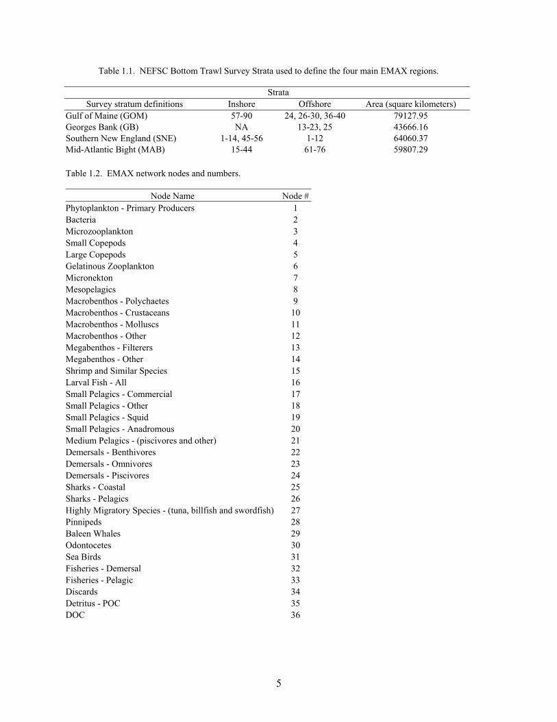
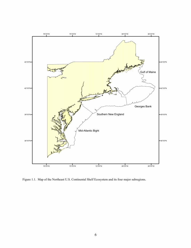
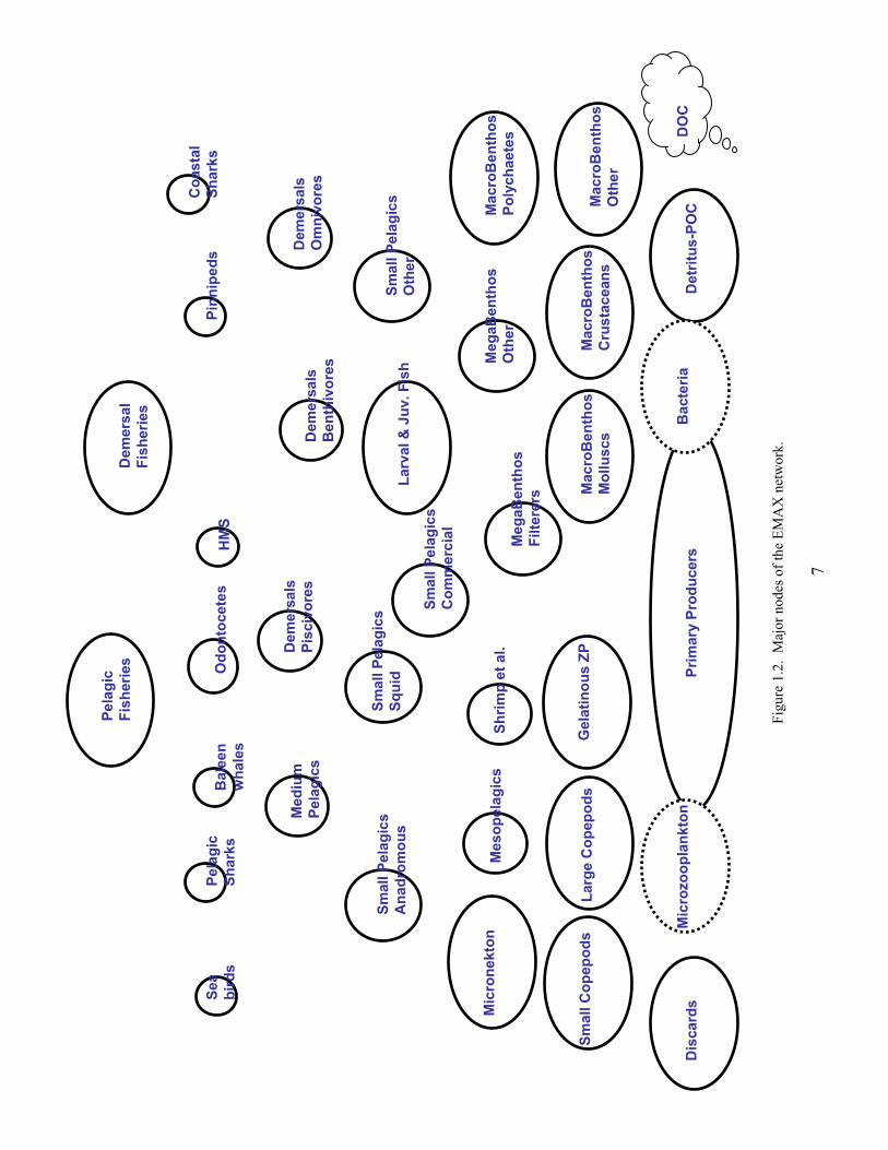
Spatial and Temporal Extent Our analyses cover 1996 to 2000. The choice was made to produce annualized estimates integrated across the appropriate seasonality for each taxa group. We separated the NEUS Ecosystem into four main subregions (ecoregions): Gulf of Maine (GOM), Georges Bank (GB), Southern New England (SNE), and Mid-Atlantic Bight (MAB) (Figure 1.1). These principally correspond to the major regions of the Center’s bottom trawl survey (BTS; Table 1.1) according to a commonly-defined strata set, but also account for key oceanographic, sediment, and bathymetric considerations. Network Nodes In network parlance, a node is analogous to a box, group, etc., and this usage was adopted for EMAX. The current network configuration has 36 nodes, representing a wide amalgamation of species (Table 1.2). Each node can potentially interact with other nodes, and the network configuration is shown in Figure 1.2. Each node was not necessarily represented in each ecoregion (e.g., there are no pinnipeds on Georges Bank), but the vast majority were. A glossary of terms (see Section 26) provides further information about common network and energy budget concepts. References Hall, SJ. 1999. The effects of fishing on marine ecosystems and communities. Oxford, UK: Blackwell Publishing

Ltd; 274 p. Link, J; Brodziak, J, eds. 2002. Report on the Status of the NE US Continental Shelf Ecosystem. NEFSC

Ecosystem Status Working Group. Northeast Fish. Sci. Cent. Ref. Doc. 02-11; 245 p.

5

Table 1.1. NEFSC Bottom Trawl Survey Strata used to define the four main EMAX regions.

Strata Survey stratum definitions Inshore Offshore Area (square kilometers)

Gulf of Maine (GOM) 57-90 24, 26-30, 36-40 79127.95 Georges Bank (GB) NA 13-23, 25 43666.16 Southern New England (SNE) 1-14, 45-56 1-12 64060.37 Mid-Atlantic Bight (MAB) 15-44 61-76 59807.29 Table 1.2. EMAX network nodes and numbers.

Node Name Node #Phytoplankton - Primary Producers 1 Bacteria 2 Microzooplankton 3 Small Copepods 4 Large Copepods 5 Gelatinous Zooplankton 6 Micronekton 7 Mesopelagics 8 Macrobenthos - Polychaetes 9 Macrobenthos - Crustaceans 10 Macrobenthos - Molluscs 11 Macrobenthos - Other 12 Megabenthos - Filterers 13 Megabenthos - Other 14 Shrimp and Similar Species 15 Larval Fish - All 16 Small Pelagics - Commercial 17 Small Pelagics - Other 18 Small Pelagics - Squid 19 Small Pelagics - Anadromous 20 Medium Pelagics - (piscivores and other) 21 Demersals - Benthivores 22 Demersals - Omnivores 23 Demersals - Piscivores 24 Sharks - Coastal 25 Sharks - Pelagics 26 Highly Migratory Species - (tuna, billfish and swordfish) 27 Pinnipeds 28 Baleen Whales 29 Odontocetes 30 Sea Birds 31 Fisheries - Demersal 32 Fisheries - Pelagic 33 Discards 34 Detritus - POC 35 DOC 36

6

Gulf of Maine

Georges Bank

Southern New England

Mid-Atlantic Bight

78°0'0"W

78°0'0"W

75°0'0"W

75°0'0"W

72°0'0"W

72°0'0"W

69°0'0"W

69°0'0"W

66°0'0"W

66°0'0"W

36°0'0"N 36°0'0"N

39°0'0"N 39°0'0"N

42°0'0"N 42°0'0"N

45°0'0"N 45°0'0"N

Figure 1.1. Map of the Northeast U.S. Continental Shelf Ecosystem and its four major subregions.

Med

ium

Pela

gics

Smal

l Pel

agic

sC

omm

erci

al

Odo

ntoc

etes

Larg

e C

opep

ods

Gel

atin

ous

ZP

Mic

rone

kton

Mes

opel

agic

s

Pinn

iped

sB

alee

n w

hale

s

Prim

ary

Prod

ucer

s

Mac

roB

enth

osPo

lych

aete

s

Dem

ersa

l Fi

sher

ies

Sea

bird

sPe

lagi

c Sh

arks

HM

S

Smal

l Cop

epod

s

Coa

stal

Shar

ks

Mac

roB

enth

osM

ollu

scs

Mac

roB

enth

osC

rust

acea

nsM

acro

Ben

thos

Oth

er

Meg

aBen

thos

Filte

rers

Meg

aBen

thos

Oth

er

Larv

al &

Juv

. Fis

h

Pela

gic

Fish

erie

s

Smal

l Pel

agic

sO

ther

Smal

l Pel

agic

sA

nadr

omou

sSm

all P

elag

ics

Squi

d

Dem

ersa

lsB

enth

ivor

es

Dem

ersa

lsPi

sciv

ores

Shrim

p et

al.

Dem

ersa

lsO

mni

vore

s

Dis

card

sD

etrit

us-P

OC

DO

CB

acte

riaM

icro

zoop

lank

ton

7

Fi

gure

1.2

. M

ajor

nod

es o

f the

EM

AX

net

wor

k.

8

2. Phytoplankton and Primary Production John E. O’Reilly and David D. Dow (node #1) Background/Data Sources

Biomass The broad-scale patterns in the spatial and seasonal distribution of phytoplankton

biomass in the NEUS Ecosystem were described by O'Reilly and Zetlin (1998). These patterns were derived from 57,088 measurements of chlorophyll a made during 78 NEFSC MARMAP (Marine Resources Monitoring, Assessment, and Prediction Program) surveys conducted between 1977 and 1988. Additionally, we have developed a comprehensive time series of surface chlorophyll concentration for the NEUS based on SeaWiFS (Sea-viewing Wide Field-of-view Sensor) ocean color data collected since September 1997.

Production

Phytoplankton primary productivity measurements (14C uptake rate) made during

MARMAP surveys between 1977 and 1982 revealed that the Northeast shelf is among the most productive shelf ecosystems in the world (O'Reilly et al. 1987). While the in situ 14C uptake method provides precise estimate of primary productivity, this method is expensive and labor-intensive, and therefore it is difficult to obtain sufficient spatial and temporal coverage to assess annual variability and long-term trends. At present, combining remotely-sensed data from satellites with productivity algorithms (Campbell et al. 2002) represents the only feasible method for resolving seasonal, annual, and climate-related variability of primary productivity throughout large marine ecosystems. Quantitative Approach for Biomass Estimates

Estimates of standing stocks of phytoplankton biomass in the water column were based

on chlorophyll a (Chl) concentrations and two approaches. The first approach used MARMAP vertical profiles of chlorophyll a pigment which were vertically integrated over the water column to a depth of 75 m (or bottom if < 75m) to yield mg Chl m-2. Vertically-integrated chlorophyll (mg Chl m-2) was averaged by standard stations/tiles (O’Reilly and Zetlin 1998) and by six bimonthly seasons. The annual mean (mg Chl m-2) was computed for each station/tile from the six seasonal means. The annual means for each station/tile were then weighted by the area of each tile to generate the average phytoplankton standing stock (mg Chl m-2) for the GOM (Gulf of Maine), SNE (Southern New England), GB (Georges Bank), and MAB (Mid-Atlantic Bight) regions.

The second approach used remotely sensed estimates of near surface Chl from 1,450 high-resolution SeaWiFS scenes of the region and the vertical profile model of Morel and Berthon (1989) to derive mg Chl m-2 for the euphotic layer from surface estimates. For these analyses, satellite data were processed according to the methods of Fu et al. (1998) and were mapped using a standard projection with an image size of 1024 x 1024 pixels and a resolution of 1.25 x 1.25 km per pixel. Annual mean integral chlorophyll (mg Chl m-2) values for each pixel

9

were constructed from monthly means, and these were averaged to yield regional estimates of phytoplankton standing stocks (mg Chl m-2). Biomass Results

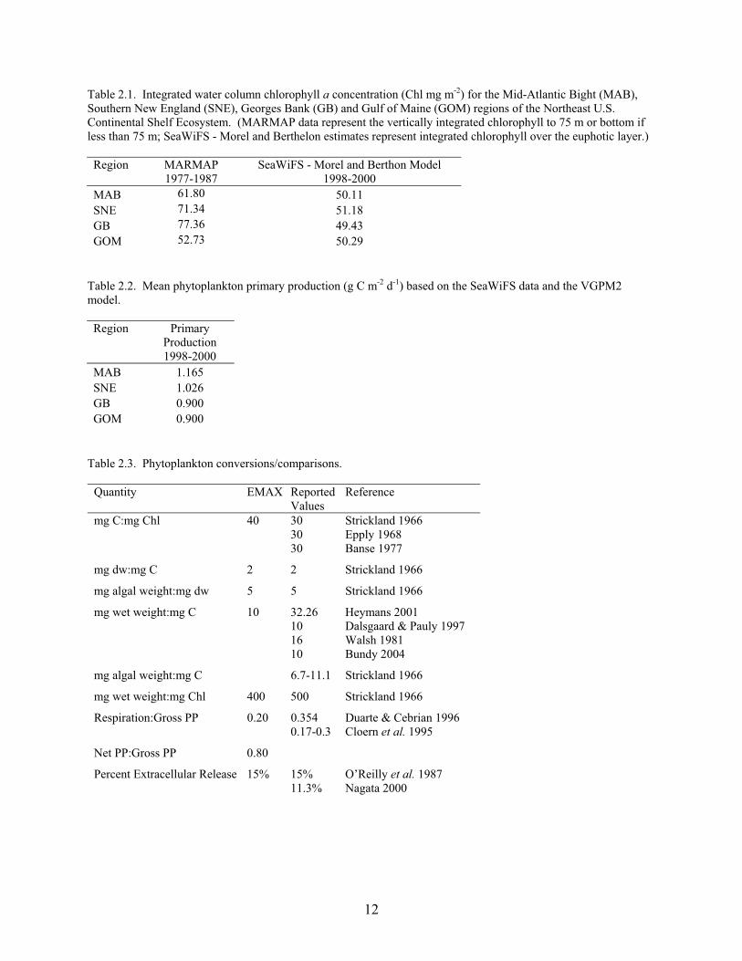
Table 2.1 compares estimates of phytoplankton biomass made by vertically integrating insitu data from MARMAP surveys with those based on SeaWiFS satellite estimates in Table 2.1. Since the SeaWiFS/Morel and Berthon Model estimates represent integral stocks in the euphotic layer and the MARMAP estimates are integrated standing stocks in the upper 75 m of the water column, we expect the latter estimates to be greater than the former. The MARMAP estimates are slightly higher than the satellite model-based estimates in the GOM but significantly higher in the other three regions. Quantitative Approach for Estimates of Production

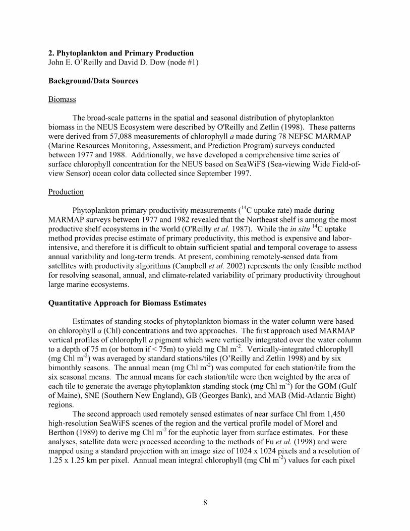
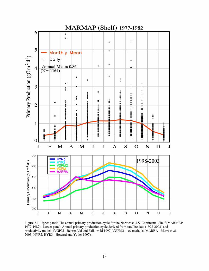
The Vertically Generalized Productivity Model (VGPM, Behrenfeld and Falkowski 1997) was used to estimate primary production. The VGPM incorporates remotely-sensed estimates of surface chlorophyll concentration and photosynthetically active radiation (PAR) from SeaWiFS and sea surface temperature (SST) from the NOAA AVHRR sensor (Advanced Very High Resolution Radiometer). In the VGPM, the optimal rate of productivity (Pbopt: optimal water column carbon fixation [mg C {mg chlorophyll a}-1 h-1]) is modeled as a 7th order polynomial function of SST. In our application of the VGPM, which we designate VGPM2, the relationship between Pbopt and SST follows the exponential relationship by Eppley (1972), as modified by Antoine et al. (1996). A trial of the VGPM, VGPM2 and three other productivity models revealed that the VGPM2 yielded the best agreement with the MARMAP seasonal productivity cycle for the NEUS Ecosystem (O'Reilly and Ducas 2004) (Figure 2.1).

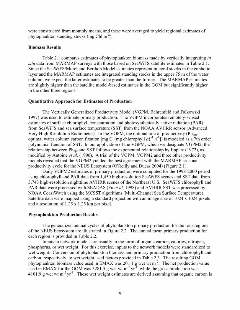
Daily VGPM2 estimates of primary production were computed for the 1998-2000 period using chlorophyll and PAR data from 1,450 high-resolution SeaWiFS scenes and SST data from 3,743 high-resolution nighttime AVHRR scenes of the Northeast U.S. SeaWiFS chlorophyll and PAR data were processed with SEADAS (Fu et al. 1998) and AVHRR SST was processed by NOAA CoastWatch using the MCSST algorithms (Multi-Channel Sea Surface Temperature). Satellite data were mapped using a standard projection with an image size of 1024 x 1024 pixels and a resolution of 1.25 x 1.25 km per pixel. Phytoplankton Production Results The generalized annual cycles of phytoplankton primary production for the four regions of the NEUS Ecosystem are illustrated in Figure 2.2. The annual mean primary production for each region is provided in Table 2.2. Inputs to network models are usually in the form of organic carbon, calories, nitrogen, phosphorus, or wet weight. For this exercise, inputs to the network models were standardized to wet weight. Conversion of phytoplankton biomass and primary production from chlorophyll and carbon, respectively, to wet weight used factors provided in Table 2.3. The resulting GOM phytoplankton biomass value used in EMAX was 20.11 g wet wt m-2. The net production value used in EMAX for the GOM was 3281.5 g wet wt m-2 yr-1, while the gross production was 4101.9 g wet wt m-2 yr-1. These wet weight estimates are derived assuming that organic carbon is

10

50% of the dry weight and the dry weight is 20% of the wet weight for phytoplankton, resulting in an overall conversion factor of 10 mg wet weight:mg carbon (Table 2.3). This is less than the 32.26 mg wet weight:mg carbon value used by Heymans (2001) (who assumed 3.23 mg dry weight:mg C and 10:1 wet weight:dry weight) for input to their model. Other studies employing the Ecopath model, such as that of Dalsgaard and Pauly (1997), used a conversion factor of 10 mg wet weight:mg carbon, within the range for algal weight:carbon indicated by Strickland (1966) in Table 2.3. It should be noted that there is some confusion in the literature regarding the appropriate conversion factor to convert phytoplankton organic carbon to wet weight. It is worthwhile to quote Strickland’s distinction between algal weight and wet weight (1966, p.15):

Two “wet weights” must be recognized, the true wet weight of the cells themselves with no extraneous water and the experimental wet weight obtained after draining the cells in some standard manner. The first weight is obtained from algal cell volumes, as measured microscopically, and a specific gravity value which, for all practical purposes, may be taken as unity. To avoid confusion this quantity should be called, simply, algal weight. The experimental “wet weight” will vary considerably according to the technique employed and will rarely, if ever, be less than twice the true algal weight, due to the presence of interstitial water. The confusion of these two weight figures by some authors has caused serious errors when computing, for example, chlorophyll:carbon ratios from cell volumes.

From the foregoing, it appears that the 10-12 mg algal weight:mg C is the most suitable factor for estimating phytoplankton biomass as “wet weight”.

The EcoNetwrk software requires estimates of gross production. Conversion of primary production values for input to EMAX assumes that our estimates of primary production based on the VGPM2 and 14C methods represent net primary production and that net primary production and phytoplankton respiration are respectively 80% and 20% of gross primary production. Marra and Barber (2004) estimated daily plankton respiration as twice the dark uptake of carbon-14, where the dark uptake averaged 20-25% of the uptake during the light. Gross primary production can be calculated directly using the oxygen change method over a 24 hour period with light and dark bottles. Marra and Barber (2004) found good correlation between their carbon-14 estimate of phytoplankton respiration and the respiration from the oxygen change method during the North Atlantic Bloom Experiment (NABE). During this experiment the heterotrophic and phytoplankton respiration contributed equally to the total water column respiration. For comparison, Duarte and Cebrian (1996) estimate that phytoplankton respiration is 35% of gross primary production.

We assumed that the percent extracellular release (PER) of dissolved organic carbon by phytoplankton is 15% of the net primary production, based on 14C-uptake results from O’Reilly et al. 1987 (Table 2.3). For comparison, Nagata (2000) reported PER values ranging from 5%-30% and an average value of 11.3% for samples from the Gulf of Maine.

11

References Antoine, D; Andre, JM; Morel, A. 1996. Oceanic primary production. 2. Estimation at global scale from satellite

(coastal zone color scanner) chlorophyll. Global Biogeochem. Cycles 10:57-69. Banse, K. 1977. Determining the carbon-to-chlorophyll ratio of natural phytoplankton. Mar. Biol. 41:199-212. Behrenfeld, MJ, et al. 2001. Temporal variations in the photosynthetic biosphere. Science 291:2594-2597. Behrenfeld, MJ; Falkowski, PG. 1997. Photosynthetic rates derived from satellite-based chlorophyll concentration.

Limnol. Oceanogr. 42(1):1-20. Bundy, A.. 2004. Mass balance models of the eastern Scotian Shelf before and after the cod collapse and other

ecosystem changes. Can. Tech. Rep. Fish. Aquat. Sci. 2520: xii-193. Campbell, J; Antoine, D; Armstrong, R; Arrigo, K; Balch,W; Barber, R; Behrenfeld, M; Bidigare, R; Bishop, J;

Carr, ME; Esaias,W; Falkowski, PG; Hoepffner, N; Iverson, R; Kiefer, D; Lohrenz, S; Marra, J; Morel, A; Ryan, J; Vedernikov, V; Waters, K; Yentsch, C; Yoder, J. 2002. Comparison of algorithms for estimating ocean primary production from surface chlorophyll, temperature, and irradiance. Global Biogeochemical Cycles 16 (3).

Cloern, J; Grenz, C; Vidergar-Lucas, L. 1995. An empirical model of the phytoplankton chlorophyll : carbon ratio - the conversion factor between productivity and growth rate. Limnol. Oceanogr. 40(7):1313-1321.

Dalsgaard, J; Pauly, D. 1997. Preliminary mass-balance model of Prince William Sound, Alaska, for the pre-spill period, 1980-1989. Fisheries Centre Research Report 5(2); 34p.

Duda, AM; Sherman, K. 2002. A new imperative for improving management of large marine ecosystems. Ocean & Coastal Management 45: 797-833.

Eppley, RW. 1968. An incubation method for estimating the carbon content of phytoplankton in natural samples. Limnol.Oceanogr. 13:574-582.

Eppley, RW. 1972. Temperature and phytoplankton growth in the sea. Fish. Bull. 70: 1063-1085. Fu, G; Baith, KS; McClain, CR. 1998. SeaDAS: The SeaWiFS Data Analysis System, Proceedings of The 4th

Pacific Ocean Remote Sensing Conference, Qingdao, China, July 28-31, 1998, 73-79. Heymans, JJ. 2001. The Gulf of Maine, 1977-1986. In: Guénette, S; Christensen, V; Pauly, D, eds. Fisheries

impacts on North Atlantic ecosystems: Models and analyses. FCRR 9(4); p.128-150. Howard, KL; Yoder, JA. 1997. Contribution of the subtropical ocean to global primary production. In: Liu, CT, ed.

Space Remote Sensing of the Subtropical Oceans. New York: Pergamon; p.157-168. Jones, R. 1984. Some Observations on energy transfer through the North Sea and Georges Bank food webs. Rapp.

P.-V. Réun. Cons. Int. Explor. Mer 183: 204-217. Marra, J; Barber, RT. 2004. Phytoplankton and heterotrophic respiration in the surface layer of the ocean. JGR,

Geophysical Research Letters 31(9):L09314. Marra, J; Ho, C; Trees, CC. 2003. An alternative algorithm for the calculation of primary productivity from remote

sensing data. LDEO Technical Report 2003-1; 27p. Morel, A; Berthon, JF. 1989. Surface pigments, algal biomass profiles, and potential production of the euphotic

layer: relationships reinvestigated in view of remote-sensing applications. Limnol. Oceanogr. 34: 1545-1562.

Nagata, T. 2000. Production mechanisms of dissolved organic matter. In: Kirchman, DL, ed. Microbial ecology of the ocean. New York: Wiley-Liss; p. 121-152.

O'Reilly, JE; Evans-Zetlin, C; Busch, DA. 1987. Primary Production. Chapter 21. In: Backus, RH, ed. Georges Bank. Cambridge, MA: MIT Press; p. 220-233.

O’Reilly, JE; Zetlin, C. 1998. Seasonal, Horizontal, and Vertical Distribution of Phytoplankton Chlorophyll a in the Northeast U.S. Continental Shelf Ecosystem. NOAA Tech. Rep. NMFS 139; 120 p.

O’Reilly, JE; Ducas, T. 2004. Seasonal and annual variability in primary production in the Northeast U.S. Large Marine Ecosystem. [Abstr.; oral pres.] Prepared for: NASA Ocean Color Research Team Meeting; Washington, DC; April, 2004; np.

Parsons, TR; Takahashi, M; Hargrave, B. 1977. Biological Oceanographic Processes. Oxford, UK: Pergamon; 332 p.

Strickland, JDH. 1966. Measuring the production of marine phytoplankton. Bulletin No. 122. Fisheries Research Board of Canada, Ottowa, Canada.

Walsh, JJ. 1981. A carbon budget for overfishing off Peru. Nature 290: 300-304.

12

Table 2.1. Integrated water column chlorophyll a concentration (Chl mg m-2) for the Mid-Atlantic Bight (MAB), Southern New England (SNE), Georges Bank (GB) and Gulf of Maine (GOM) regions of the Northeast U.S. Continental Shelf Ecosystem. (MARMAP data represent the vertically integrated chlorophyll to 75 m or bottom if less than 75 m; SeaWiFS - Morel and Berthelon estimates represent integrated chlorophyll over the euphotic layer.) Region MARMAP

1977-1987 SeaWiFS - Morel and Berthon Model

1998-2000 MAB 61.80 50.11 SNE 71.34 51.18 GB 77.36 49.43 GOM 52.73 50.29

Table 2.2. Mean phytoplankton primary production (g C m-2 d-1) based on the SeaWiFS data and the VGPM2 model. Region Primary

Production 1998-2000

MAB 1.165 SNE 1.026 GB 0.900 GOM 0.900

Table 2.3. Phytoplankton conversions/comparisons.

Quantity EMAX ReportedValues

Reference

mg C:mg Chl 40 30 Strickland 1966 30 Epply 1968 30 Banse 1977

mg dw:mg C 2 2 Strickland 1966

mg algal weight:mg dw 5 5 Strickland 1966

mg wet weight:mg C 10 32.26 Heymans 2001 10 Dalsgaard & Pauly 1997 16 Walsh 1981 10 Bundy 2004

mg algal weight:mg C 6.7-11.1 Strickland 1966

mg wet weight:mg Chl 400 500 Strickland 1966

Respiration:Gross PP 0.20 0.354 Duarte & Cebrian 1996 0.17-0.3 Cloern et al. 1995

Net PP:Gross PP 0.80

Percent Extracellular Release 15% 15% O’Reilly et al. 1987 11.3% Nagata 2000

13

Figure 2.1. Upper panel: The annual primary production cycle for the Northeast U.S. Continental Shelf (MARMAP 1977-1982). Lower panel: Annual primary production cycle derived from satellite data (1998-2003) and productivity models (VGPM - Behrenfeld and Falkowski 1997; VGPM2 - see methods; MARRA - Marra et al. 2003; HYR2, HYR3 - Howard and Yoder 1997).

14

Figure 2.2. Annual cycle of primary production (g C m-2 d-1) for the Mid-Atlantic Bight (MAB), Southern New England (SNE), Georges Bank (GB) and Gulf of Maine (GOM) regions (1998-2000).

15

3. Bacteria David D. Dow and John E. O’Reilly (node #2) Background/Data Sources

In the past two decades numerous studies have reported on the quantitative significance

of energy and matter flows through the “microbial loop”, particularly studies by biological oceanographers interested in nutrient cycling (Pomeroy 2004). While there have been numerous surveys and studies of the phytoplankton primary producers in the NEUS Ecosystem, spatially and temporally comprehensive surveys of the distribution, abundance and metabolic rates of heterotrophic bacterioplankton have not been conducted. Consequently, our estimates of bacterioplankton metabolic rates must be based on indirect methods and on studies and knowledge derived from comparable ecosystems. The primary grazers of bacterioplankton, the microzooplankton, are also poorly characterized for this shelf ecosystem. Together, the bacterioplankton and microzooplankton feeding guilds link dissolved primary production and detritus (particulate organic carbon) to the mesozooplankton. Subsequently, it is available to the living marine resources at higher trophic levels.

Network models such as Ecopath frequently use the detritus compartment to accumulate heterotrophic egestion/excretion energy and sedimented primary production not utilized in the surface mixed layer. In order to process this accumulation of detritus, we added bacteria and microzooplankton guilds (consumption followed by respiration) and transferred a component (secondary production of microzooplankton) to the grazing food chain via mesozooplankton ingestion (mesozooplankton are assumed to be omnivores).

In the EMAX network models the detritus node is particulate organic carbon (POC) processed by vertebrate/invertebrate detritivores which consume the POC and attached bacteria/protozoa. Since bacteria utilize labile and semilabile dissolved organic carbon (DOC), the tacit assumption is that bacterial extracellular enzymes convert the POC to DOC before it is taken up by the bacteria. Even though DOC represents a large nonliving organic carbon pool in the water column, much of it is refractory, and since we do not know its bioavailability to bacteria, the EMAX network models did not explicitly model a node for DOC. Moreover, the operational definition of DOC is the organic matter which passes through a 0.7 μm glass fiber filter, and includes small particles and colloidal organic carbon, making it difficult to distinguish POC and DOC assimilation efficiencies.

In the EMAX networks, bacteria utilize and respire POC. The photoassimilated dissolved organic carbon released by phytoplankton and bacterioplankton are fed upon by microzooplankton prior to a transfer pathway to mesozooplankton. This is obviously a simplification of what occurs in the “microbial loop” which has multiple transfer steps between different size classes of phytoplankton and a variety of microbial heterotrophs (Calvet and Saiz 2005). There is a debate in the literature about whether the “microbial loop” is a sink for POC and DOC (respiration of primary production and storage of carbon in inactive microbial cells) or a source of carbon to the grazing food chain through mesozooplankton acting as omnivores (Ducklow 1994). The assimilation efficiency of bacteria for DOC and POC is often assumed to be 50%, but it may be lower due to the refractory nature of much of the DOC and components of the POC (Pomeroy 2001).

16

Quantitative Approach for Estimates Since we had estimates of the phytoplankton biomass and primary production from

satellite data for the four subregions of the NEUS Ecosystem, it was assumed that bacterial secondary production (BP) should be roughly 10% of the primary production (PP). We adjusted the consumption of the bacterioplankton node so that the BP:PP ratio = 0.10 (Table 3.1). This is lower than the commonly assumed BP:PP range of 0.15 to 0.30 (Pomeroy 1979; Cole et al. 1988; Pomeroy 2001). The outcome of this adjustment was that bacterial consumption was roughly 40% of the net production (PP). This is similar to the value reported in Calbet (2001) for the consumption of primary production by micro- and mesozooplankton in coastal waters. Bacterioplankton have a critical role in processing the excretion (DOC) and egestion (POC) from the other living nodes in the EMAX network. The resultant transfer of recycled carbon from the microbial loop to the grazing food chain improves the overall transfer efficiency of the network energy flow. Given this important trophic role for bacterioplankton, the fact that they might consume 40% of PP via either direct or indirect energy pathways in the EMAX model is not unreasonable.

The other key assumptions were: bacterial gross growth efficiency (GGE) = 0.24; growth rate (P:B) = 0.25 per day; Assimilation Efficiency (AE) = 0.80 and carbon x 10 = wet weight (Bratbak and Dundas, 1984). These assumptions permitted the estimate of the bacterial biomass from BP and growth rate, while the various energy flow ratios (C:B, R:B, R:P, etc.) can be computed using the GGE and AE values. Ducklow (2000) reported an average bacterial growth rate of 0.3 d-1 for the eastern North Atlantic spring phytoplankton bloom, and lower rates (0.05-0.25 d-1) for other open sea regions. Reinthaler and Herndl (2005) reported a mean bacterioplankton growth rate of 0.2 ± 0.3 d-1 for the southern North Sea. Assuming an average bacterial growth rate of 0.25 d-1 applies to the NEUS Ecosystem, then the standing stocks of bacterioplankton biomass in the GOM would be estimated at 0.345g C m-2. This equates to approximately 17% of the phytoplankton standing stock (2.011 g C m-2), based on an average vertically integrated chlorophyll value of 52.73 mg Chl m-2 and a phytoplankton carbon:chlorophyll ratio of 40:1.

Del Giorgio and Cole (2000) summarize estimates of bacterial net growth efficiency for a variety of marine systems, reporting a mean value of 0.27. This net growth efficiency (NGE) is slightly lower than our value of 0.30. The growth rate assumption yields an annual P:B = 91.2 which is slightly lower than the value of 100 for bacteria given in Pomeroy (2001). EMAX doesn’t use DOC as a food source for bacterioplankton, but Ducklow and Shia (1992) estimate a bacterial conversion efficiency of 20% for DOC and 50% of bioavailable organic matter (like algal exudate). Since the continental shelves have a greater percentage of bacteria attached to particles (POC) than the free living bacteria which dominate the open ocean, we assumed that bacterial enzymes convert the POC to DOC which is consumed by the bacterioplankton. Since EMAX has the bacterioplankton consuming detritus from egestion by the other living nodes, algal exudate and the phytoplankton that sediment out of the euphotic zone, we assumed that the AE = 0.80. The quality of the available POC and DOC seems to determine the AE value and the assimilation efficiency differs between the carbon (used for respiration) and nitrogen (used for growth and cell division). Thus the literature had a broad range of values for AE. The AE for the different heterotrophic nodes determines the rates at which this POC flows into detritus and is shown by the Lindeman Spine in the network output. Our balanced network flow models had high AE values which minimized this POC production.

17

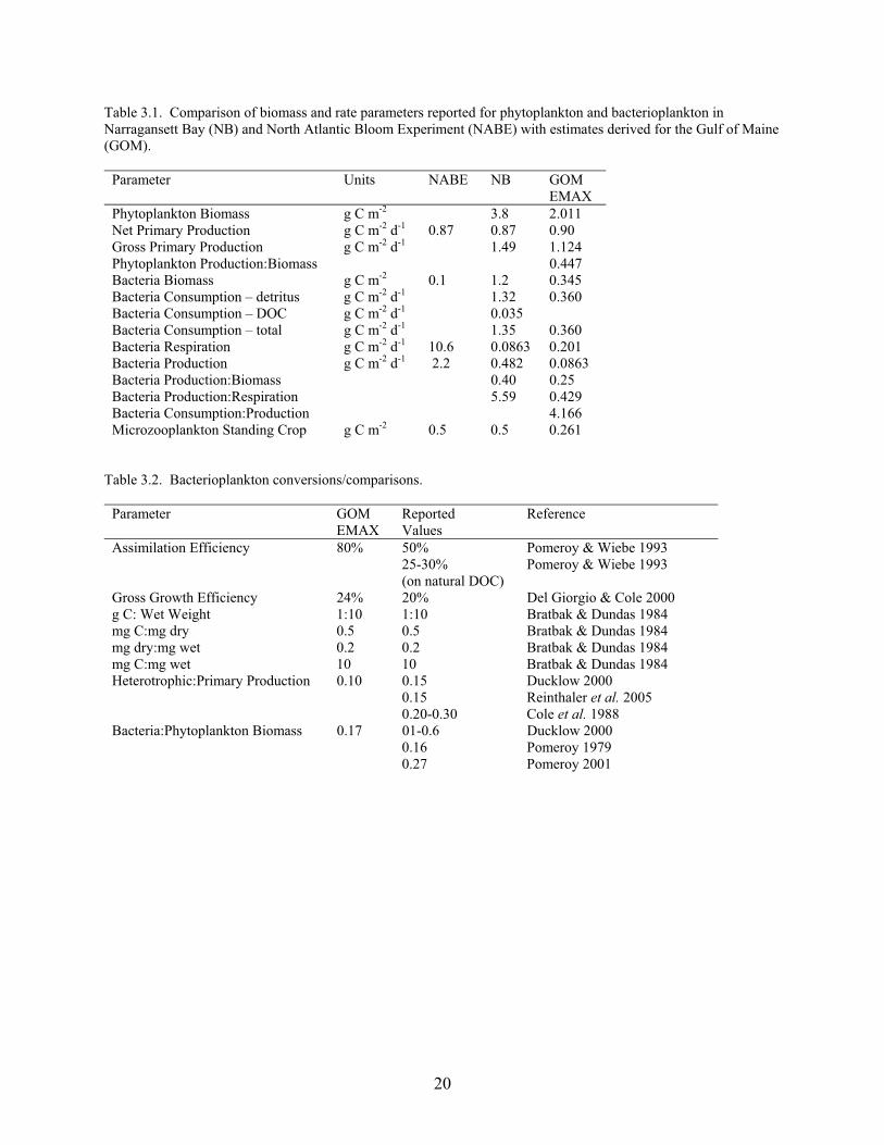
The resulting biomass of bacterioplankton was 0.345 g C m-2 with a production of 0.0863g C m-2 d-1 for the Gulf of Maine (GOM). The carbon values were converted to wet weight (see Table 3.2) based on the following conversion factors: carbon x 0.5 = dry weight; and dry weight x 0. 20 = wet weight (or carbon wt. x 10 = wet weight). The estimated wet weight biomass is 3.452 g m-2 and annual production is 315.026 g m-2 y-1. This implies that the annual P:B ratio = 91.3 (which lies between the 163 for phytoplankton and 72 for microzooplankton). Given the GGE and AE assumptions, the net growth efficiency (NGE) is 0.30 which implies that respiration is 70% of the assimilated energy, with the other 30% going to secondary production. NGE values in the literature generally lie between 0.20 and 0.40 (Reinthaler and Herndl, 2005). The choice of the NGE value has a major role in determining whether the microbial loop is a sink for primary production or a link to the grazing food chain. The bacterioplankton consumption was 0.360 g C m-2 d-1 with respiration representing 0.201 g C m-2 d-1 and production 0.086 g C m-2 d-1. The energetic ratios were: C:B = 1.042; P:B = 0.250 (assumption); R:B = 0.583; and P:R = 0.429. Table 3.1 provides values reported for some other oceanic systems: coastal embayment (Narragansett Bay, NB) and open ocean (North Atlantic Bloom Experiment, NABE). Most of the information on the structure/function of the bacterioplankton community is from studies in estuaries and the open ocean. We assumed that the metabolic activity of bacterioplankton in continental shelf water lies somewhere between the extremes of this gradient. Table 3.1 provides an overview of the underlying assumptions used to estimate bacterial production and biomass, plus the diagnostic energy flow ratios used in the EMAX network model.

In NB the reported gross primary production is 1.49 g C m-2 d-1 and phytoplankton biomass is 3.8 g C m-2. NB net primary production (0.87 g C m-2 d-1) is comparable to our estimate for GOM (0.9 g C m-2 d-1), while the standing crop biomass is higher than our estimate for the GOM (2.01 g C m-2 d-1). The NABE model is based on values averaged over a 20 day spring bloom/post-bloom period, and we presume that these daily values do not represent the yearly average which is lower in the open ocean than on continental shelves. In NB the standing crops (g C m-2) are 1.2 for pelagic bacteria and 0.5 for microzooplankton, compared to NABE values of 0.1 for bacteria and 0.5 for microzooplankton. The bacterioplankton biomass in the GOM is 0.345 g C m-2 which lies along the gradient between NB and the NABE.

In EMAX we partitioned assimilated energy 70% to respiration and 30% to secondary production, which is much different than that reported for the open ocean where respiration is 90% and secondary production is 10% (Ducklow and Carlson, 1992). Our values were chosen to have the bacterioplankton be a link through microzooplankton to the grazing food chain, while the oceanic values assume that the microbial loop is a sink for DOC with most of the carbon being respired. In order to eliminate POC accumulation from the egestion emanating from the other living nodes in EMAX, we assumed that the 70% respiration component would remove this detritus. The secondary production component (30%) provides the link to the grazing food chain.

Del Giorgio and Cole (2000) summarized measurements of bacterial growth efficiency (BGE) for a number of marine systems. In their work, BGE is the ratio of bacterial production to bacterial respiration plus production (BGE = BP/[BR+BP]), and they reported a mean BGE value of 0.27 for coastal areas. This value implies that 73% of the carbon uptake is respired and 27% is retained as organic carbon production, yielding a respiration:production ratio of 2.7 and a consumption:production ratio of 3.7. The bacterial carbon demand (BCD) is BP:BGE and provides an estimate of the heterotrophic consumption in relation to the net primary production.

18

Since we ignored the DOC component of bacterial consumption, our BCD estimates will be biased high. An exception is bacterial uptake of phytoplankton dissolved production, for which we assumed 100% assimilation efficiency.

Only a portion of the POC is bioavailable to bacteria, but we assumed that all the dissolved primary production was utilized by them. Since we did not know the percentage of POC bioavailability, we adjusted the bacterial respiration rate in order to consume the “apparent detritus production” to prevent it from accumulating or having to export a large faction out of our system boundaries. Since the network models we used balance the flows through the detritus component, one has to develop a way to consume the “apparent detritus production”. We decided not to explicitly incorporate the DOC pool in the energy flow pathway, even though it represents a large non-living carbon pool (15 times the POC and 75 times the phytoplankton carbon) of unknown bioavailability in the “microbial loop”. We incorporated POC in the EMAX energy flow, since it was a component of the diet matrix for a number of feeding guilds (or nodes) in the network. All of the material egested in the different heterotrophic nodes contributes to the POC pool.

Results The GOM data in Table 3.1 shows the estimates that were used in EMAX. We assumed a gross growth efficiency of 24% for EMAX (Table 3.2), noting that Del Giorgio and Cole (2000) reported 20%. The ratio of heterotrophic secondary production:primary production in EMAX is 0.10 (assumption), whereas Ducklow (2000) and Reinthaler et al. (2005) report a value of 0.15 and Cole et al. (1988) report a range between 0.20-0.30.

As shown in Table 3.2, EMAX used fairly high values of Assimilation Efficiency (AE, 80%) and Gross Growth Efficiency (GGE, 24%) since we wanted to prevent the accumulation of detritus or its export out of the system. We assumed that net primary production is approximately balanced by the heterotrophic community respiration on the NEUS Continental Shelf Ecosystem. If one used the values suggested in the literature (AE < 50% and GGE = 20%), then the bacterioplankton would consume the net primary production and none would be available for transfer to the grazing food chain that supports living marine resources (LMRs). EMAX assumed that the microbial food web was a link to the grazing food chain. Using these lower values for AE and GGE would lead to the ecosystem being net heterotrophic (P<<R) and runs counter to field observations, but supports the notion of the “microbial loop” being a carbon sink. This issue is discussed at greater length by Williams (2000) who estimated that bacteria provide 40% of the heterotrophic community respiration. The implications of bacterial GGE values on bacterial consumption of DOC is explored by Ducklow (2000) and Del Giorgio and Cole (2000). Nagata (2000) estimated that bacterial consumption of DOC corresponded to 42% of net primary production, while Williams (2000) estimated that this value was 50%. The issue of the P versus R balance in the water column is discussed by Del Giorgio and Williams (2005).

The EMAX bacteria/phytoplankton biomass and productivity ratios listed in Table 3.1 are similar to those in the literature. Therefore, even if there are some problems with our carbon to wet weight conversions, our scaling between bacteria and phytoplankton seems to be reasonable. Since a significant fraction of the bacterial biomass in oligotrophic, oceanic areas is metabolically inactive, there is much variation in the C:B, R:B, and P:B ratios in the literature, with a wide range of values as one moves from estuarine to open ocean regions. We did not have

19

the regional data necessary to estimate the metabolically active bacterial biomass, so we used an approach based on literature values to bound the bacterial biomass and rates.

References Baretta-Bekker, JG; Baretta, JW; Rasmussen, EK. 1995. The microbial food web in the European Regional Seas

Ecosystem Model. Neth. J. Sea Res. 33:363-379. Baretta-Bekker, JG; Reimann, B; Baretta, J; Rasmussen, EK. 1994. Testing the microbial loop concept by

comparing mesocosm data with results from a dynamical simulation model. Mar. Ecol. Prog. Ser. 106:187-198.

Bratbak, G; Dundas, I. 1984. Bacterial dry matter content and biomass estimates. Appl. Envir. Microbiol. 48:755-757.

Calbet, A; Saiz, E. 2005. The ciliate-copepod link in marine ecosystems. Aquat. Microb. Ecol. 38:157-167. Calbet, A. 2001. Mesozooplankton grazing effect on primary production: a global comparative analysis of marine

systems. Limnol. Oceanogr. 46: 1824-1830. Cianelli, L; Robson, BW; Francis, RC; Aydin, K; Brodeur, RD. 2004. Boundaries of open marine ecosystems: an

application to the Pribilof Archipelago, southeast Bering Sea. Ecolog. Applicat. 14:942-953. Del Giorgio, PA; Cole, JJ. 2000. Bacterial energetics and growth efficiency. In: Kirchman, DL, ed. Microbial

Ecology of the Ocean. New York, NY: Wiley-Liss; p. 289-325. Del Giorgio, PA; Williams, PJ le B, eds. 2005. Respiration in Aquatic Ecosystems. New York, N.Y.: Oxford Univ.

Press; 315 p. Ducklow, HW. 1994. Modeling the microbial food web. Microb. Ecol. 28: 303-319. Ducklow, HW. 2000. Bacterial production and biomass in the oceans. In: Kirchman, DL, ed. Microbial Ecology

of the Ocean. New York, NY: Wiley-Liss; p. 85-120. Ducklow, HW; Shiah, F-K. 1992. Estuarine bacterial production. In: Ford, T., ed. Aquatic Microbiology:an

Ecological Approach. Cambridge, Ma: Blackwell; p. 261-287. Ducklow, HW; Carlson, DA. Oceanic bacterial production. In: Marshall, KC, ed. Advances in Microbial Ecology.

New York, NY: Plenum Press;p. 113-181. Fasham, MJR; Boyd, PW; Savidge, G. 1999. Modeling the relative contributions of autotrophs and heterotrophs to

carbon flow at a Lagrangian JGOFS station in the Northeast Atlantic. The importance of DOC. Limnol. Oceanogr. 44:80-94.

Lee S; Fuhrman, J. 1987. Relationships between biovolume and biomass of naturally derived marine bacterioplankton. Appl. Envir. Microbiol. 53:1298-1303.

Monaco, ME; Ulanowicz, RE. 1997. Comparative ecosystem trophic structure of three U.S. mid-Atlantic estuaries. Mar. Ecol. Prog. Ser. 161:239-254.

Nagata, Toshi. 2000. Production mechanisms of dissolved organic matter. In: Kirchman, DL, ed. Microbial Ecology of the Ocean. New York, NY: Wiley-Liss; p. 121-152.

Newell, RC; Turley, CM. 1987. Carbon and nitrogen flow through pelagic microheterotrophic communities. In: Payne, AIL; Gulland, JA; Brink, KH, eds. The Benguela and Comparable Ecosystems, S.Afr. J. Mar. Sci. 5:717-734.

Peterson, BJ. 1984. Synthesis of carbon stocks and flows in the open ocean mixed layer. In: Hobbie, JE; Williams, PJ le B, eds. Heterotrophic Activity in the Sea. New York, NY: Plenum Press; p. 547-554.

Pomeroy, LR. 1979. Secondary production mechanisms of continental shelf communities. In: Livingston, RJ, ed. Ecological Processes in Coastal and Marine Systems. New York, NY: Plenum Press; p. 163-186.

Pomeroy, LR. 2001. Caught in the food web: complexity made simple? Sci. Mar. 65 (Suppl. 2): 31-40. Pomeroy, L R. 2004. Building bridges across subdisciplines in marine ecology. Sci. Mar. 68 (Suppl. 1):5-12. Pomeroy, LR; Wiebe, WJ. 1993. Energy sources for microbial food webs. Marine Microb. Food Webs 7:101-118. Sherr, BF; Sherr, EB. 1984. Role of heterotrophic protozoa in carbon and energy flow in aquatic ecosystems. In:

Klugg, MJ; Reddy, CA, eds. Current Perspectives in Microbial Ecology. Washington, DC: American Society for Microbiology; p. 412-423.

Williams, Peter J. le B. 2000. Heterotrophic bacteria and the dynamics of dissolved organic material. In: Kirchman, DL, ed. Microbial Ecology of the Ocean. New York, NY: Wiley-Liss; p. 153-198.

20

Table 3.1. Comparison of biomass and rate parameters reported for phytoplankton and bacterioplankton in Narragansett Bay (NB) and North Atlantic Bloom Experiment (NABE) with estimates derived for the Gulf of Maine (GOM).

Parameter Units NABE NB GOM EMAX

Phytoplankton Biomass g C m-2 3.8 2.011 Net Primary Production g C m-2 d-1 0.87 0.87 0.90 Gross Primary Production g C m-2 d-1 1.49 1.124 Phytoplankton Production:Biomass 0.447 Bacteria Biomass g C m-2 0.1 1.2 0.345 Bacteria Consumption – detritus g C m-2 d-1 1.32 0.360 Bacteria Consumption – DOC g C m-2 d-1 0.035 Bacteria Consumption – total g C m-2 d-1 1.35 0.360 Bacteria Respiration g C m-2 d-1 10.6 0.0863 0.201 Bacteria Production g C m-2 d-1 2.2 0.482 0.0863 Bacteria Production:Biomass 0.40 0.25 Bacteria Production:Respiration 5.59 0.429 Bacteria Consumption:Production 4.166 Microzooplankton Standing Crop g C m-2 0.5 0.5 0.261

Table 3.2. Bacterioplankton conversions/comparisons.

Parameter GOM EMAX

Reported Values

Reference

Assimilation Efficiency 80% 50% Pomeroy & Wiebe 1993 25-30%

(on natural DOC) Pomeroy & Wiebe 1993

Gross Growth Efficiency 24% 20% Del Giorgio & Cole 2000 g C: Wet Weight 1:10 1:10 Bratbak & Dundas 1984 mg C:mg dry 0.5 0.5 Bratbak & Dundas 1984 mg dry:mg wet 0.2 0.2 Bratbak & Dundas 1984 mg C:mg wet 10 10 Bratbak & Dundas 1984 Heterotrophic:Primary Production 0.10 0.15 Ducklow 2000 0.15 Reinthaler et al. 2005 0.20-0.30 Cole et al. 1988 Bacteria:Phytoplankton Biomass 0.17 01-0.6 Ducklow 2000 0.16 Pomeroy 1979 0.27 Pomeroy 2001

21

4. Microzooplankton David D. Dow, John E. O’Reilly and John R. Green (node #3) Background/Data Sources The microzooplankton group includes holoplankton (protozoa, ciliates, flagellates, copepod nauplii, etc.) and meroplankton (larval stages of benthic invertebrates: trochophores, veligers, etc.). This diverse assemblage has a range of biomass and rate values. For example, in the southeast Bering Sea the protozoan component had a biomass of 10 Mg km-2, a P:B ratio of 72 and a C:B ratio of 144, while the other holoplankton/meroplankton biomass was 13.3 Mg km-

2, P:B was 9 and C:B was 27 (Ciannelli et al. 2004). In EMAX it was assumed that the microzooplankton were primarily composed of protozoans which have a boom and bust life history strategy that tracks the abundance of their prey (Reid et al. 1993). The microzooplankton in the EMAX model feed on bacteria (40% of diet), small phytoplankton (15%), detritus (35%) and other microzooplanton (10%). This diet composition reflects the reality that in nature they consume a wide variety of microautotrophs/heterotrophs (and cannibalize one another). Stimulated by new nitrogen, the spring phytoplankton bloom is often dominated by net plankton (diatoms) which are consumed primarily by mesozooplankton (large and small copepods). Microzooplankton grazing also occurs as a minor component. During the summer stratified period when recycled nitrogen maintains primary productivity, the phytoplankton is dominated by smaller nanoplankton (i.e., dinoflagellates, microflagellates, non-colonial diatoms, etc.) which are grazed by microzooplankton. Microzooplankton grazing of bacteria is the primary link between the microbial loop and grazing food chain. Quantitative Approach for Estimates The microzooplankton (MZ) biomass fluctuates seasonally like the phytoplankton biomass, since it is controlled by food resources and grazing. In the EMAX model the food resources are small planktonic autotrophs/heterotrophs and the grazers are mesozooplankton (three nodes). Since we didn’t have any independent data on protozoan biomass and rates on the Northeast Continental Shelf, we decided to relate the MZ biomass (in carbon units) to that of phytoplankton (in carbon units) based on Figure 3 in Caron et al. (1990) which showed a relationship (log-log) between ciliate and phytoplankton biomass. We assumed that MZ biomass was 0.13 of the phytoplankon biomass, similar to values for unfertilized North Sea mesocosms (Baretta-Bekker, 1994) and Narragansett Bay (Monaco, 1997). Given the boom and bust life history strategy of protozoans, we assumed that their annual biomass would be a relatively small fraction of the annual phytoplankton biomass. As described in the Phytoplankton Section of this document, we had satellite data available to estimate phytoplankton biomass (conversion from chlorophyll a to carbon) in the euphotic zone. The phytoplankton biomass was revised to include its distribution throughout the water column, so that it could be used to estimate the MZ biomass. The phytoplankton biomass was 2.0114 g C m-2 which resulted in a microzooplankton biomass of 0.2615 g C m-2. These values are shown in Table 4.1. We converted from carbon to dry weight and then to weight wet using the conversion factors in Sherr and Sherr (1984). The dry/wet weight conversion factor was 0.18, while the dry weight/carbon conversion factor was 0.46, yielding a carbon/wet weight conversion factor of 0.0828. Thus the

22

estimated wet weight biomass for phytoplankton was 20.1144 g m-2 and 3.158 g m-2 for microzooplankton. We estimated the ratios of the rates (C:P, P:B, R:P) in carbon units on a daily basis and then converted these to wet weight values on an annual basis. The conversion factors and literature sources for these are shown in Table 4.2. The estimated rates of consumption and respiration shown in Table 4.1 are based on a net growth efficiency of 33% (Straile, 1997; Muren et al., 2005); assimilation efficiency of 90%; and P:B ratio of 72 (Pomeroy, 2001). Using these assumptions, 67% of the assimilated energy goes to respiration and 33% to secondary production. Consumption for the microzooplankton is 0.1737 g C m-2 d-1 and the assimilation value is 0.1563 g C m-2 d-1. Of the assimilated energy, the respiration is 0.1047 and the secondary production is 0.0516. The growth rate (0.197 per day) was based on the assumption that the MZ biomass turns over every 5 days. The growth rate for microzooplankton was assumed to be much slower than that of phytoplankton and slightly slower than that of bacterioplankton. Table 4.1 compares the consumption, respiration and production rates for EMAX GOM (Gulf of Maine) with that of the southeast Bering Sea (BS), North Atlantic Bloom Experiment (NABE), and Narragansett Bay (NB). The NABE values come from a bloom in the open ocean and thus don’t represent daily means from a yearly perspective. In theory continental shelf values should fall somewhere along the gradient from inshore waters (NB) to open ocean (BS and NABE). In general the EMAX GOM P:B, P:R, and C:P ratios lie along this inshore/open ocean gradient. Unfortunately most of the literature values that we found came from either inshore waters or the open ocean, so that we had to assume the continental shelf values lies somewhere between the extreme ends of this gradient. The European Regional Seas Ecosystem Model (ERSEM) lists the assimilation efficiency (AE) for microzooplankton as 50%, even though the value for heterotrophic nanoflagellates is lower at 20% (Baretta-Bekker et al. 1995). The bacterial AE is usually assumed to be 50%, even though it can range as low as 25-30% on natural substrates. The AE is related to the mode of feeding, food quality, and the extent of DOC excretion. Protozoa can have significant excretion losses as DOC (Nagata 2000), which explains the range of variation in the AE values. The EMAX AE value was taken as 90% to reflect Protozoa feeding on bacteria attached to detritus (POC), but not DOC, which can be an important pathway (Nagata 2000). The Gross Growth Efficiency (GGE) for microzooplankton is often taken as 40% (McManus 1991), but in EMAX we used 30% (Straile, 1997; Muren et al., 2005). Thus the GGE lies between that of bacteria (24%) and phytoplankton (80%). The microzooplankton secondary production:primary production ratio varies from 7% (ERSEM Model for North Sea, Baretta-Bekker et al. 1995) to 14% (English Channel in August, Newell and Linley 1984). The EMAX P:B ratio was assumed to be 72 (Pomeroy, 2001). The EMAX C:B ratio (daily) was assumed to be 0.66 based on an AE of 90%, which is higher than the English Channel C:B value (0.33 per day, Araujo et al., 2005), but is lower than the Baltic Sea value (1.49 per day, Harvey et al. 2003). The EMAX R:B ratio was assumed to be 0.40 per day and should lie somewhere between P:B (0.197 per day) and C:B (0.664 per day). Since DOC release can be a significant component for microzooplankton, our R is actually respiration + excretion (where we don't know the magnitude of E). Thus the R:B ratio might differ from 0.40 (58 per yr) if DOC were addressed in the EMAX network model. The factor for converting microzooplankton carbon weight to wet weight is a multiplier of 12, based on a g C:g dry weight ratio of 0.46 and g dry:wet weight ratio of 0.18 (Table 4.2). As explained in other Sections, we used slightly different carbon to wet weight conversion factors for phytoplankton, bacterioplankton, and detritus (multiplier of 10). Table 4.1 expresses

23

the P:B, P:R, and C:P ratios on a daily basis, since microzooplankton have a rapid turnover time. We discuss these as yearly values in the text in order to make the values comparable to those reported for other EMAX nodes, which deal with biota with much longer population turnover times. Results It is commonly found that when one compares photosynthesis to respiration in the oceanic water column, the ocean appears to be net heterotrophic (P < R; Pomeroy and Wiebe 1993; del Giorgio and Williams 2005). This suggests that either there are methodological problems in measuring primary production and community respiration, or the spatial/temporal coupling is offset and results in biases as one goes from seasonal samples to estimating annual averages. Network analysis balances inputs and outputs from a node so that secondary production of the prey node or food assimilated by the predator node is artificially balanced by respiration, secondary production, net exports/imports, biomass accumulation and harvest removal. Ecopath with Ecosim computes respiration by difference, since it is based on production from the donor node driving the consumption in the receiving node. EcoNetwrk, on the other hand, incorporates respiration as a parameter and is consumption driven. Thus in network models there is a relationship between C:B, R:B, and P:B such that in the balanced models they are different from the input values. Table 4.2 indicates that the GGE and microzooplankton:phytoplankton biomass (0.13) and productivity (0.07) ratios used in EMAX are similar to those from the literature. This suggests that we got the scaling right in extrapolating from phytoplankton to microzooplankton. We choose a high AE (90%) in EMAX to help transfer the bacterial production efficiently to copepods for transfer up the grazing food chain. Since EMAX did not include DOC as a node, a lot of the bacterial production stems from DOC use beyond just the phytoplankton dissolved production. Therefore, we used higher assimilation efficiencies as compensation to link the microbial food web to the grazing food chain. Our microzooplankton secondary production:phytoplankton production ratio is slightly lower than those reported in the literature. In EMAX the mesozooplankton biomass (108.4 g wet wet m-2) is much larger than the microzooplankton biomass (3.2 g wet wet m-2), but this is partly compensated for by a higher P:B ratio (72) in microzooplankton compared to the 3 mesozooplankton nodes (P:B range from 20-40). It is assumed that the nauplii and copepodites stages of mesozooplankton reside in the small copepod node and thus the microzooplankton are primarily protozoans. Protozoans can grow almost as rapidly as their bacterial prey which leads to a high P:B ratio, but their boom and bust life history strategy probably results in a much lower average biomass than that of mesozoplankton. Unfortunately traditional zooplankton sampling nets destroy the fragile protozoans, so we lack a monitoring database to evaluate the ecological importance of this microzooplankton group.

24

References Araujo, JN; Mackinson, S; Ellis, JR; Hart, PJB. 2005. An Ecopath model of the Western English Channel ecosystem

with an exploration of its dynamic properties. IN: Lowestoft, England: Centre for Environment, Fisheries & Aquaculture Science; Science Series technical Report No. 125; 45 p.

Baretta-Bekker, JG; Baretta, JW; Rasmussen, EK. 1995. The microbial food web in the European Regional Seas Ecosystem Model. Neth. J. Sea Res. 33:363-379.

Baretta-Bekker, JG; Reimann, B; Baretta, J; Rasmussen, EK. 1994. Testing the microbial loop concept by comparing mesocosm data with results from a dynamical simulation model. Mar. Ecol. Prog. Ser. 106:187-198.

Calbet, A; Saiz, E. 2005. The ciliate-copepod link in marine ecosystems. Aquat. Microb. Ecol. 38:157-167. Caron, DA; Goldman, JC; Fenchel, T. 1990. Protozoan respiration and metabolism. In: Capriulo, GM, ed. Ecology

of Marine Protozoa. New York, NY: Oxford University Press; p. 307-322. Cianelli, L; Robson, BW; Francis, RC; Aydin, K; Brodeur, RD. 2004. Boundaries of open marine ecosystems: an

application to the Pribilof Archipelago, southeast Bering Sea. Ecolog. Applicat. 14:942-953. Del Giorgio, PA; Williams, PJ le B, eds. 2005. Respiration in Aquatic Ecosystems. New York, N.Y.: Oxford Univ.

Press; 315 p. Harvey, CJ; Cox, SP; Essington, TE; Hansson, S.; Kitchell, JF. 2003. An ecosystem model of food web and

fisheries interactions in the Baltic Sea. ICES Jour. Mar. Sci. 60:939-950. McManus, GB. 1991. Flow analysis of a planktonic microbial food web model. Marine Microb. Food Webs

5(1):145-160. Monaco, ME; Ulanowicz, RE. 1997. Comparative ecosystem trophic structure of three U.S. mid-Atlantic estuaries.

Mar. Ecol. Prog. Ser. 161:239-254. Muren, H.; Berglund, J; Samuelsson; Andersson, A.. 2005. Potential effects of elevated sea-water temperature on

pelagic food webs. Hydrobiologia 545: 153-166. Nagata, Toshi. 2000. Production mechanisms of dissolved organic matter. In: Kirchman, DL, ed. Microbial

Ecology of the Ocean. New York, NY: Wiley-Liss; p. 121-152. Newell, RC; Turley, CM. 1987. Carbon and nitrogen flow through pelagic microheterotrophic communities. In:

Payne, AIL; Gulland, JA; Brink, KH, eds. The Benguela and Comparable Ecosystems, S.Afr. J. Mar. Sci. 5:717-734.

Reid, PC; Turley, CM; Burkhill, PH, eds. 1993. Protozoa and Their Role in Marine Processes. New York, NY: Springer-Verlag; 506 p.

Pomeroy, LR. 2001. Caught in the food web: complexity made simple? Sci. Mar. 65 (Suppl. 2): 31-40. Pomeroy, LR; Wiebe, WJ. 1993. Energy sources for microbial food webs. Marine Microb. Food Webs 7:101-118. Sherr, BF; Sherr, EB. 1984. Role of heterotrophic protozoa in carbon and energy flow in aquatic ecosystems. In:

Klugg, MJ; Reddy, CA, eds. Current Perspectives in Microbial Ecology. Washington, DC: American Society for Microbiology; p. 412-423.

Straile, D. 1997. Gross growth efficiencies of protozoan and metazoan zooplankton and their dependence on food concentration, predaor-prey weight ratio, and taxonomic group. Limnol. Oceanogr. 42: 1375-1385.

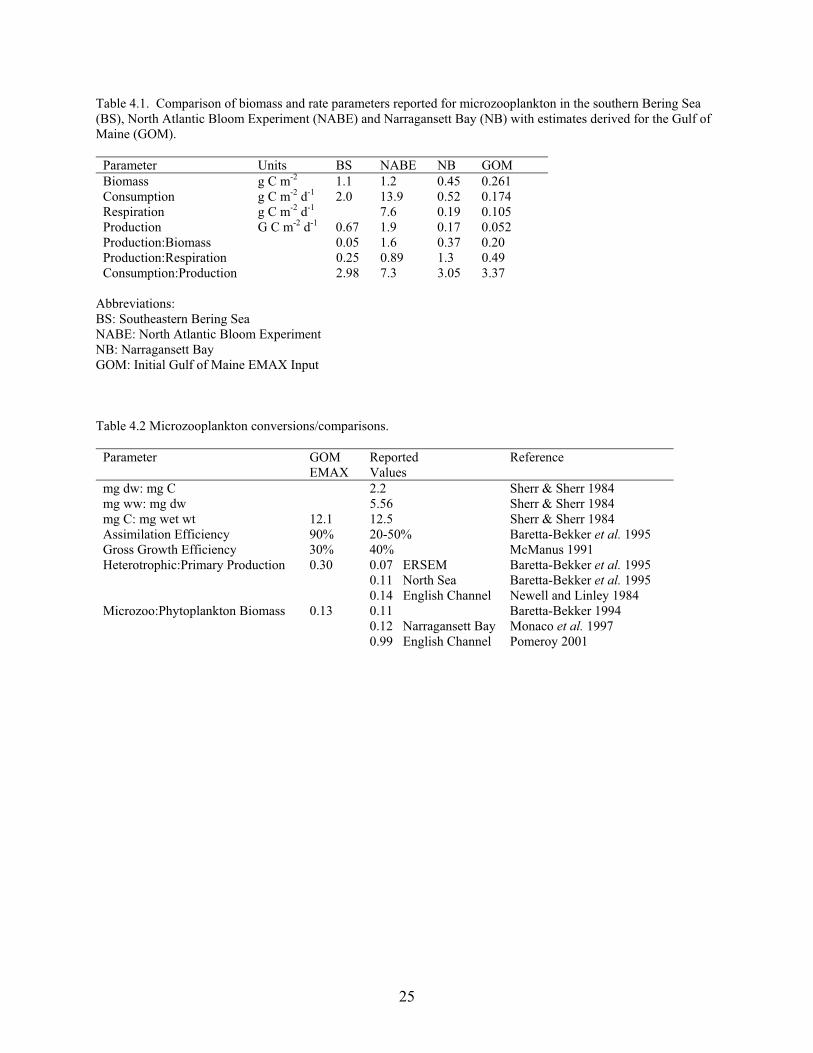
25

Table 4.1. Comparison of biomass and rate parameters reported for microzooplankton in the southern Bering Sea (BS), North Atlantic Bloom Experiment (NABE) and Narragansett Bay (NB) with estimates derived for the Gulf of Maine (GOM).

Parameter Units BS NABE NB GOM Biomass g C m-2 1.1 1.2 0.45 0.261 Consumption g C m-2 d-1 2.0 13.9 0.52 0.174 Respiration g C m-2 d-1 7.6 0.19 0.105 Production G C m-2 d-1 0.67 1.9 0.17 0.052 Production:Biomass 0.05 1.6 0.37 0.20 Production:Respiration 0.25 0.89 1.3 0.49 Consumption:Production 2.98 7.3 3.05 3.37

Abbreviations: BS: Southeastern Bering Sea NABE: North Atlantic Bloom Experiment NB: Narragansett Bay GOM: Initial Gulf of Maine EMAX Input Table 4.2 Microzooplankton conversions/comparisons.

Parameter GOM EMAX

Reported Values

Reference

mg dw: mg C 2.2 Sherr & Sherr 1984 mg ww: mg dw 5.56 Sherr & Sherr 1984 mg C: mg wet wt 12.1 12.5 Sherr & Sherr 1984 Assimilation Efficiency 90% 20-50% Baretta-Bekker et al. 1995 Gross Growth Efficiency 30% 40% McManus 1991 Heterotrophic:Primary Production 0.30 0.07 ERSEM Baretta-Bekker et al. 1995 0.11 North Sea Baretta-Bekker et al. 1995 0.14 English Channel Newell and Linley 1984 Microzoo:Phytoplankton Biomass 0.13 0.11 Baretta-Bekker 1994 0.12 Narragansett Bay Monaco et al. 1997 0.99 English Channel Pomeroy 2001

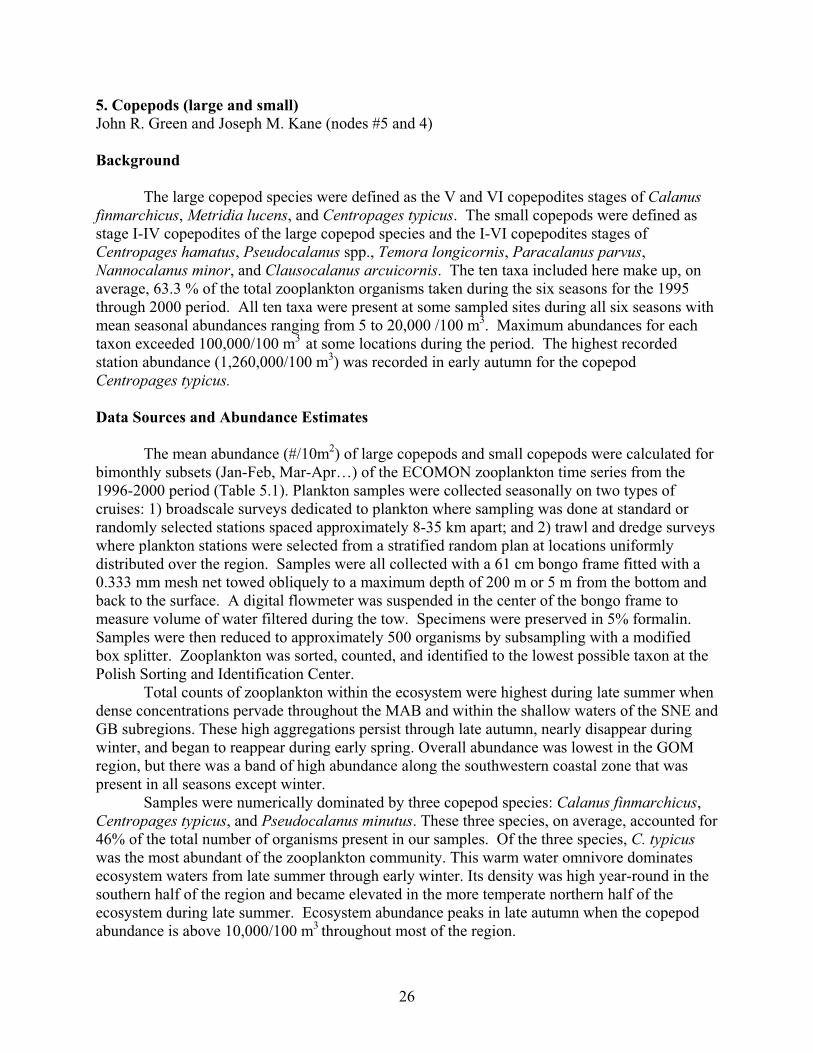
26

5. Copepods (large and small) John R. Green and Joseph M. Kane (nodes #5 and 4) Background

The large copepod species were defined as the V and VI copepodites stages of Calanusfinmarchicus, Metridia lucens, and Centropages typicus. The small copepods were defined as stage I-IV copepodites of the large copepod species and the I-VI copepodites stages of Centropages hamatus, Pseudocalanus spp., Temora longicornis, Paracalanus parvus, Nannocalanus minor, and Clausocalanus arcuicornis. The ten taxa included here make up, on average, 63.3 % of the total zooplankton organisms taken during the six seasons for the 1995 through 2000 period. All ten taxa were present at some sampled sites during all six seasons with mean seasonal abundances ranging from 5 to 20,000 /100 m3. Maximum abundances for eachtaxon exceeded 100,000/100 m3 at some locations during the period. The highest recordedstation abundance (1,260,000/100 m3) was recorded in early autumn for the copepodCentropages typicus. Data Sources and Abundance Estimates

The mean abundance (#/10m2) of large copepods and small copepods were calculated for bimonthly subsets (Jan-Feb, Mar-Apr…) of the ECOMON zooplankton time series from the 1996-2000 period (Table 5.1). Plankton samples were collected seasonally on two types of cruises: 1) broadscale surveys dedicated to plankton where sampling was done at standard or randomly selected stations spaced approximately 8-35 km apart; and 2) trawl and dredge surveys where plankton stations were selected from a stratified random plan at locations uniformly distributed over the region. Samples were all collected with a 61 cm bongo frame fitted with a 0.333 mm mesh net towed obliquely to a maximum depth of 200 m or 5 m from the bottom and back to the surface. A digital flowmeter was suspended in the center of the bongo frame to measure volume of water filtered during the tow. Specimens were preserved in 5% formalin. Samples were then reduced to approximately 500 organisms by subsampling with a modified box splitter. Zooplankton was sorted, counted, and identified to the lowest possible taxon at the Polish Sorting and Identification Center.

Total counts of zooplankton within the ecosystem were highest during late summer when dense concentrations pervade throughout the MAB and within the shallow waters of the SNE and GB subregions. These high aggregations persist through late autumn, nearly disappear during winter, and began to reappear during early spring. Overall abundance was lowest in the GOM region, but there was a band of high abundance along the southwestern coastal zone that was present in all seasons except winter.

Samples were numerically dominated by three copepod species: Calanus finmarchicus, Centropages typicus, and Pseudocalanus minutus. These three species, on average, accounted for 46% of the total number of organisms present in our samples. Of the three species, C. typicus was the most abundant of the zooplankton community. This warm water omnivore dominates ecosystem waters from late summer through early winter. Its density was high year-round in the southern half of the region and became elevated in the more temperate northern half of the ecosystem during late summer. Ecosystem abundance peaks in late autumn when the copepod abundance is above 10,000/100 m3 throughout most of the region.

27

The herbivores Calanus finmarchicus and Pseudocalanus minutus utilize the spring phytoplankton bloom and dominate early and late spring samples. Both species have similar annual abundance cycles but differ in their spatial distribution. Pseudocalanus spp. abundance rises sharply in early spring when it concentrates in coastal areas of the MAB, throughout SNE, and the western and eastern margins of the GOM. Peak seasonal abundances occurred in late spring with high values found throughout SNE, in the more shallow waters of GB, and along coastal GOM. C. finmarchicus abundance was high year-round in the GOM and on GB from early spring through late summer. Dense concentrations of this copepod were also found in the offshore waters of SNE and the MAB in late spring and late summer. Abundance was low year-round in the coastal waters of these latter two regions. The annual abundance cycle and spatial distribution of Metridia lucens was very similar to Calanus finmarchicus, though overall abundance levels were much lower. Density is highest during late spring and the largest concentrations were usually found in the western GOM and along the outer shelf of the MAB and SNE subregions. Abundance was low year-round in southern coastal waters and within the central shoals of GB.

The copepod Centropages hamatus reached peak abundance during the late summer when dense concentrations formed in the central shoals region of GB and persisted there through late autumn. High levels were also found in MAB and SNE coastal waters during early and late spring. The copepod was sparsely distributed year-round in the GOM and during the latter half of the year in the MAB and SNE subregions. Mean abundance of Acartia spp. peaked during late summer when they concentrated in shallow coastal waters throughout the ecosystem. Numbers remained high inshore through late autumn in the southern half of the ecosystem. They became scarce in the GOM during winter and early spring. Temora longicornis mean abundance also peaked during late summer when high concentrations of the copepod were found scattered in shallow waters throughout the ecosystem. It also was very scarce in the GOM during the colder months. Oithona spp. were captured year round in nearly all samples from the ecosystem. However, there was no strong seasonal cycle and only relatively large concentrations were found scattered throughout the MAB and SNE regions. It should be noted that the abundance levels of this comparatively small copepod species is underestimated because it is not quantitatively caught with the nets used in our surveys. Paracalanus parvus abundance was at its maximum during late autumn when high concentrations were found across SNE and GB. It was present year-round in the SNE and MAB subregions and became very rare in GOM and GB waters during the spring seasons. Biomass Estimates

Copepod abundance by size group was converted to biomass using the length to wet weight (W) equation given by Pearre (1980): (EQ. 5.1) W=0.08810L2.8514 This equation is based on Petipa (1957) and others using prosome lengths (L) of various copepod species obtained from the literature (Table 5.1).

28

Production

Copepod production was calculated according to Huntley and Lopez (1992) using the formula: (EQ. 5.2) P = B 0.0445e0.111T where P is production; B is copepod biomass-m2; and T is mean temperature. Mean temperatures are derived from integrated CTD temperature profiles taken at each station (Table 5.2). Consumption

Feeding rates were derived from Pafenhofer (1976) based on the daily weight-specific filtering rate for a calanoid copepod, Calanus helgolandicus. This rate, 0.20 times biomass/day, was scaled to an annual consumption rate for both copepod size groups. Thus, both groups were assumed to have the same consumption rates relative to body size. References Huntley, M; Lopez, M. 1992. Temperature dependent production of marine copepods: a global synthesis. Am. Nat.

140(2):201–242. Pafenhofer, GA.. 1976. Feeding growth and food conversion of the marine planktonic copepod Calanus

helgolandicus. Limnol Oceanog 21(1):39-50. Pearre, S Jr. 1980. The copepod width-weight relation and its utility in food chain research. Can J Zool. 58:1884-

1891. Petipa, TS. 1957. On the average weight of common forms of zooplankton in the Black Sea. Tr. Sevastopol Stn.

Akad. Nauk. Ukr. SSR, 9, 39-57 (in Russian) Shmeleva, AA; 1965. Weight characteristics of the Adriatic Sea. Bull. Inst Oceanogr. (Monaco) 65(1351):1-24.

Studenikina, YI; Cherepakhina, MM. 1996. Average weight of the main forms of zooplankton in the Sea of Azov. Hydrobiol. J. 5:74-76.

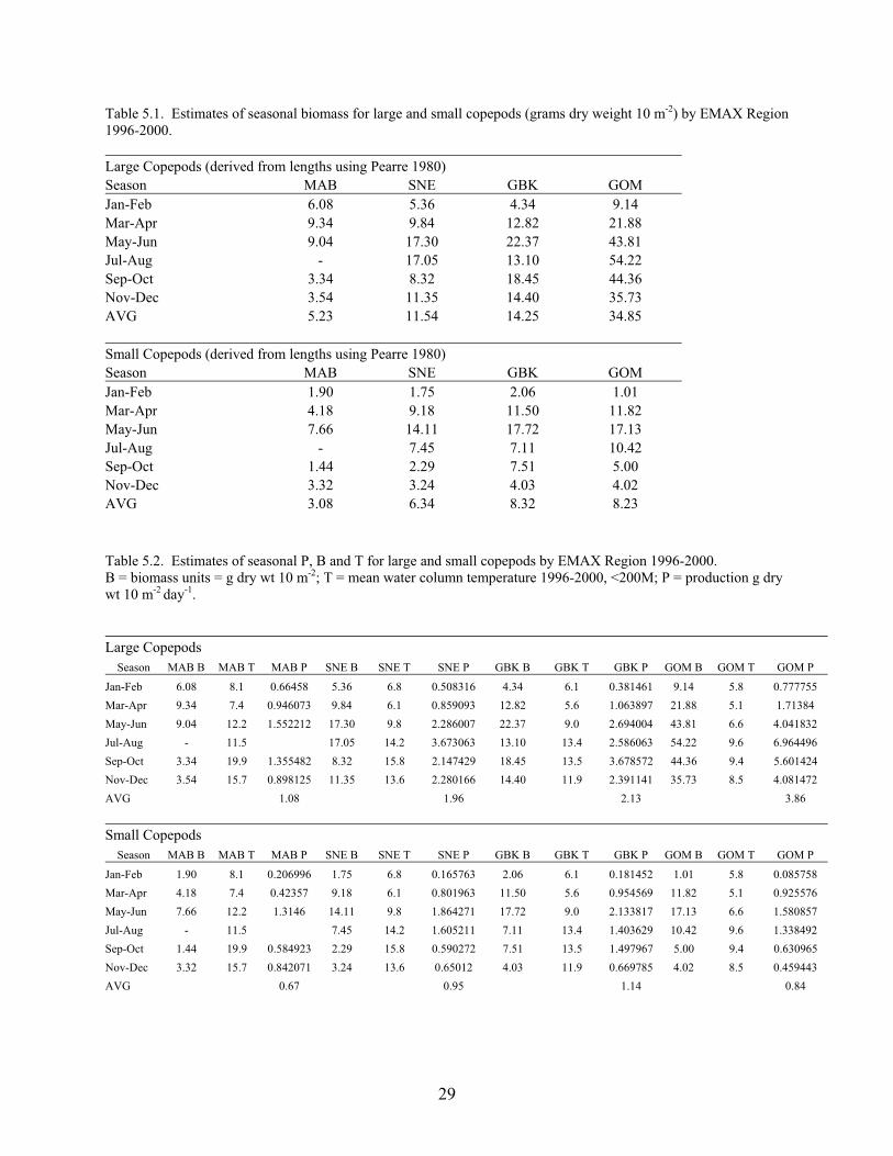
29

Table 5.1. Estimates of seasonal biomass for large and small copepods (grams dry weight 10 m-2) by EMAX Region 1996-2000. Large Copepods (derived from lengths using Pearre 1980) Season MAB SNE GBK GOM Jan-Feb 6.08 5.36 4.34 9.14 Mar-Apr 9.34 9.84 12.82 21.88 May-Jun 9.04 17.30 22.37 43.81 Jul-Aug - 17.05 13.10 54.22 Sep-Oct 3.34 8.32 18.45 44.36 Nov-Dec 3.54 11.35 14.40 35.73 AVG 5.23 11.54 14.25 34.85 Small Copepods (derived from lengths using Pearre 1980) Season MAB SNE GBK GOM Jan-Feb 1.90 1.75 2.06 1.01 Mar-Apr 4.18 9.18 11.50 11.82 May-Jun 7.66 14.11 17.72 17.13 Jul-Aug - 7.45 7.11 10.42 Sep-Oct 1.44 2.29 7.51 5.00 Nov-Dec 3.32 3.24 4.03 4.02 AVG 3.08 6.34 8.32 8.23 Table 5.2. Estimates of seasonal P, B and T for large and small copepods by EMAX Region 1996-2000. B = biomass units = g dry wt 10 m-2; T = mean water column temperature 1996-2000, <200M; P = production g dry wt 10 m-2 day-1. Large Copepods

Season MAB B MAB T MAB P SNE B SNE T SNE P GBK B GBK T GBK P GOM B GOM T GOM P

Jan-Feb 6.08 8.1 0.66458 5.36 6.8 0.508316 4.34 6.1 0.381461 9.14 5.8 0.777755 Mar-Apr 9.34 7.4 0.946073 9.84 6.1 0.859093 12.82 5.6 1.063897 21.88 5.1 1.71384 May-Jun 9.04 12.2 1.552212 17.30 9.8 2.286007 22.37 9.0 2.694004 43.81 6.6 4.041832 Jul-Aug - 11.5 17.05 14.2 3.673063 13.10 13.4 2.586063 54.22 9.6 6.964496 Sep-Oct 3.34 19.9 1.355482 8.32 15.8 2.147429 18.45 13.5 3.678572 44.36 9.4 5.601424 Nov-Dec 3.54 15.7 0.898125 11.35 13.6 2.280166 14.40 11.9 2.391141 35.73 8.5 4.081472 AVG 1.08 1.96 2.13 3.86 Small Copepods

Season MAB B MAB T MAB P SNE B SNE T SNE P GBK B GBK T GBK P GOM B GOM T GOM P

Jan-Feb 1.90 8.1 0.206996 1.75 6.8 0.165763 2.06 6.1 0.181452 1.01 5.8 0.085758 Mar-Apr 4.18 7.4 0.42357 9.18 6.1 0.801963 11.50 5.6 0.954569 11.82 5.1 0.925576 May-Jun 7.66 12.2 1.3146 14.11 9.8 1.864271 17.72 9.0 2.133817 17.13 6.6 1.580857 Jul-Aug - 11.5 7.45 14.2 1.605211 7.11 13.4 1.403629 10.42 9.6 1.338492 Sep-Oct 1.44 19.9 0.584923 2.29 15.8 0.590272 7.51 13.5 1.497967 5.00 9.4 0.630965 Nov-Dec 3.32 15.7 0.842071 3.24 13.6 0.65012 4.03 11.9 0.669785 4.02 8.5 0.459443 AVG 0.67 0.95 1.14 0.84

30

6. Gelatinous Zooplankton John R. Green (node #6) Background

Gelatinous zooplankton are common constituents of plankton samples. They can be locally very abundant and have significant predatory impact on the composition of the plankton community (Reeve and Walter, 1978). As considered here, gelatinous zooplankton are a taxonomically diverse group that includes the Cnidaria (both the medusae and hydrozoans); the Ctenophores (comb jellies); the colonial Siphonophores; and the colonial Salpidae. All are characterized by a high water content in body tissues that causes significant distortion and shrinkage upon preservation, and by delicate structures that can be fragmented or extruded during capture, making identification and enumeration for abundance estimates extremely difficult and uncertain. Biomass Estimates

Gelatinous zooplankton biomass was estimated from 60 cm bongo tows with 333 mm mesh nets taken on NEFSC monitoring cruises from 1996-2000. Mean abundances per m3 for each station are the calculated mean of the abundance for each stratum sampled. These were done for six 2-month periods for all the main gelatinous zooplankton groups (Table 6.1). Mean station abundance was multiplied by the sampling depth to calculated no./m2.

Individual group biomasses were calculated using the following relationship (Reeve and Walter 1976):

(EQ. 6.1) Log DW = 2.65 * Log L

Where DW is dry weight (g) and L is length (mm). This relationship was established for

ctenophores and is assumed to be similar enough for all other gelatinous zooplankton groups such that we used it for all these zooplankton taxa. A mean length of 1.3 mm was assumed for this calculation. Total biomass for all groups was then integrated into an annual average, summed across all gelatinous zooplankton taxa, and then converted to g wet weight per m-2. Conversion to wet weight from dry weight was approximated from Pages (1997), with DW = 4.48% of WW. Estimates for all four regions are given in Table 6.2. Production Estimates

Gelatinous zooplankton production was scaled from estimates derived from a study of Ctenophore trophodynamics from the Caribbean (Persad et al. 2003). Rates from that study were adjusted for EMAX purposes using a Q10 rule of 2 (i.e., temperature correction of rate processes, with a halving or doubling for each change in temperature of 10oC) to approximate the difference in temperature conditions and the seasonal cycle of prey abundance found in the coastal Northeast Atlantic Ocean.

Upon further reflection, these production estimates were slightly modified to account for depth patchiness, vertical stratification of distribution, seasonality, and the bloom nature of these

31

organisms. To do so, we adjusted the production value to fall within the range of previously reported (literature) gelatinous zooplankton P:B ratios, resulting in a P:B ratio of ~ 40. Consumption Estimates

Gelatinous zooplankton consumption rates were scaled to the results of Reeve and Walter (1976). As with production, these estimates were modified to account for depth patchiness, vertical stratification of distribution, seasonality, and the bloom nature of these organisms. Reeve and Walter (1976) estimate a clearance rate of approximately 17% body weight per day. Scaling to other nodes and the Reeve and Walter estimate, our calculations assumed an adjusted clearance rate of approximately 40% body weight per day, which was then annualized. This gives a C:B ratio value of ~146, well within the range of other reported values for similar organisms. This also gives a C:P of 3.5-3.7, a reasonable value and consistent with similar nodes at this trophic level. References Persad, G; Hopcroft, R.; Webber, M.; Roff, J. 2003. Abundance biomass and production of ctenophores and

medusae off Kingston, Jamaica. Bull. Mar. Sci. 73(2):379-396. Reeve. M; Walter, M. 1976. A large scale experiment on the growth and predation potential of ctenophore

populations. In: Mackie, G, ed. Coelenterate ecology and behavior. New York, NY: Plenum Pubcorp.; p. 187-199.

Reeve.M; Walter, M. 1978. Nutritional ecology of ctenophores-a review of recent research. In Russel, FS; Yonge, M, eds. Advances in Marine Biology New York, NY; Academic Press; Vol. 15 p. 249-287.

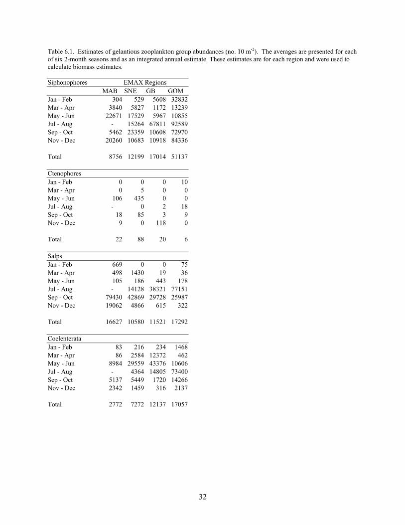
32

Table 6.1. Estimates of gelantious zooplankton group abundances (no. 10 m-2). The averages are presented for each of six 2-month seasons and as an integrated annual estimate. These estimates are for each region and were used to calculate biomass estimates. Siphonophores EMAX Regions MAB SNE GB GOM Jan - Feb 304 529 5608 32832Mar - Apr 3840 5827 1172 13239May - Jun 22671 17529 5967 10855Jul - Aug - 15264 67811 92589Sep - Oct 5462 23359 10608 72970Nov - Dec 20260 10683 10918 84336 Total 8756 12199 17014 51137 Ctenophores Jan - Feb 0 0 0 10Mar - Apr 0 5 0 0May - Jun 106 435 0 0Jul - Aug - 0 2 18Sep - Oct 18 85 3 9Nov - Dec 9 0 118 0 Total 22 88 20 6 Salps Jan - Feb 669 0 0 75Mar - Apr 498 1430 19 36May - Jun 105 186 443 178Jul - Aug - 14128 38321 77151Sep - Oct 79430 42869 29728 25987Nov - Dec 19062 4866 615 322 Total 16627 10580 11521 17292 Coelenterata Jan - Feb 83 216 234 1468Mar - Apr 86 2584 12372 462May - Jun 8984 29559 43376 10606Jul - Aug - 4364 14805 73400Sep - Oct 5137 5449 1720 14266Nov - Dec 2342 1459 316 2137 Total 2772 7272 12137 17057

33

Table 6.2. Total estimate of gelatinous zooplankton biomass for the different EMAX regions. Values are in g m-2. EMAX Region Biomass (g m-2) MAB 3.6 SNE 3.9 GB 5.2 GOM 11.0

34

7. Micronekton John R. Green (node #7) Background

Micronekton are the largest sized animals taken in plankton nets, typically having body lengths of 5-10 mm or more. For this study, the micronekton group is considered inclusive of the crustacean groups amphipoda, euphausiacea, mysidacea and similar decapoda captured in plankton nets. Chaetognatha are also included in this group. Compared to copepods, abundance estimates of micronekton from plankton net sampling are relatively low. There are, however, instances of swarming behavior, particularly of gammarid amphipods and euphausiids, when they can dominate plankton biomass. Such events occur on small temporal and spatial scales. It is possible that bongo nets under-sample micronekton due to net avoidance (Angel and Pugh 2000). Biomass

Micronekton biomass was estimated from abundance estimates from the ECOMON zooplankton time series for the 1996-2000 period. The mean abundances (no./ 10 m2) of micronekton were calculated for bimonthly subsets (Jan - Feb, Mar - Apr…) distinctly for each of the groups listed above.

These estimates of mean abundance were then converted to biomass based upon established size-biomass relationships. Here we assume that most micronekton were roughly equivalent to a common micronekton taxa, the amphipod Gamarrus sp. Mean abundance was converted to dry weight from the relationship established in Avery et al. (1996), using a mean length of 6 mm which produced a dry weight estimate of 1.2 mg. This average weight was then multiplied by the abundance estimates to obtain a total biomass for each group (Table 7.1).

However, for the chaetogaths group, dry weight was calculated based on the relationship in Sameoto (1971) for the species Sagitta elegans. This formula is: (EQ 7.1) DW = 0.00097 l 2.2365,

where DW is dry weight (mg) and l = length. A mean length of 4 mm was used based on laboratory observations, giving a mean dry weight of 0.026 mg. S. elegans is the most abundant chaetognath in these plankton samples.

After conversions to biomass were done for each micronekton group, the values were then converted to biomass and integrated into an annual estimate. This was then converted to g wet weight per m-2. Estimates for all four regions are given in Table 7.2.

Production and Consumption Estimates

Growth was estimated at 0.04 day-1 and consumption at 0.10 day-1 based on an assumption growth similar to that of juvenile cod of approximately the same size (Peck et al. 2003). These values were then scaled to provide an annual estimate.

35

References Angel, MV; Pugh, PR. 2000. Quantification of diel vertical migration by micronekton taxa the northeast Atlantic.

Hydrobiologia 440:161-179. Avery, D; Green, J; Durbin E. 1996. Distribution and abundance of pelagic gammarid amphipods in Georges Bank

and Nantucket Shoals. Deep Sea Res. II 43(7-8):1521-1532. Peck, M; Buckley, L; Caldarone, E; Bengston D. 2003. Effects of food consumption and temperature on growth

rate and biochemical based indicators of growth in early juvenile Atlantic cod (Gadus morhua) and haddock (Melanogrammus aeglifinus). Mar. Ecol. Prog. Ser. 251:233-243.

Sameoto, D. 1971. Life history ecological production and empirical mathematical model of the population of Sagitta elegans in St. Margaret’s Bay Nova Scotia. J. Fish. Res. Board. Can. 28:971-985.

36

Table 7.1. Estimates of micronekton abundance. Units are in Number 10 m-2 unless otherwise noted. The averages are presented for each of six 2-month seasons and as an integrated annual estimate. DW = dry weight, WW = wet weight. EMAX Region MAB SNE GB GOM Amphipods Jan - Feb 4432.8 5555.8 1869.9 3413.0 Mar - Apr 2790.7 5198.8 11370.2 9887.2 May - Jun 6294.8 25473.3 33448.5 17289.2 Jul - Aug - 22783.8 14086.5 48310.7 Sep - Oct 14493.9 39336.3 9717.8 13922.2 Nov - Dec 19212.3 26938.8 11983.4 12563.8 Euphausids Jan - Feb 2052.2 1276.6 800.4 334.2 Mar - Apr 4009.8 8424.2 13991.4 24019.8 May - Jun 4347.9 5128.1 4984.4 24726.6 Jul - Aug - 5722.6 5928.9 8204.9 Sep - Oct 1718.3 4088.6 2625.4 5671.0 Nov - Dec 3135.9 7751.4 2773.6 2251.2 Mysids Jan - Feb 131.5 101.9 265.3 12.2 Mar - Apr 60.4 65.1 152.5 5.0 May - Jun 0.0 0.0 907.4 62.8 Jul - Aug - 118.9 839.0 45.6 Sep - Oct 752.4 371.7 5814.2 12.3 Nov - Dec 170.4 545.7 4466.0 90.6 Decapoda Jan - Feb 6381.2 240.2 219.9 50.0 Mar - Apr 309.7 804.6 2903.6 190.2 May - Jun 9237.0 7767.5 15529.2 1551.3 Jul - Aug - 3461.8 7562.5 2712.4 Sep - Oct 13269.6 1949.2 4336.6 726.4 Nov - Dec 5965.4 882.0 650.9 2582.6 Avg. of all Crustacean Micronekton 4938.3 7249.5 6551.2 7443.1 Avg. Biomass (mg) 5926.0 8699.3 7861.4 8931.8 Avg. DW Biomass (g/10m2) 5.93 8.70 7.86 8.93 WW g/10 m2 55.11 80.90 73.11 83.07

Chaetognaths Dry Weight (mg/10m2) Jan - Feb 122.8 91.5 39.8 14.7 Mar - Apr 75.1 85.9 132.5 7.8 May - Jun 234.8 315.1 440.5 36.1 Jul - Aug - 479.4 449.8 25.8 Sep - Oct 585.4 408.7 258.8 80.3 Nov - Dec 549.1 488.0 168.5 84.08 Avg. Chaetognath DW (mg) 313.5 311.4 248.3 41.5 Avg. WW (dw/0.082) 3776.8 3752.0 2991.7 499.6 WW g/10 m2 3.8 3.8 3.0 0.5

37

8. Macrobenthos (polychaetes, crustaceans, mollusks, other) Joseph J. Vitaliano, Steven A. Fromm, and Vincent G. Guida (nodes #9-12) Background

Macrobenthos are defined as invertebrates living in or on the sediments that are quantitatively sampled by a 0.1 m2 Smith McIntyre grab and are retained on a 1.0 mm or 0.5 mm sieve. In the NEFSC, a 1.0 mm sieve was used until the middle of 1979 and a 0.5 mm sieve was used thereafter. Wet weight biomasses were determined for each species in a sample by blot-drying the species collections on absorbent paper towels for about three minutes and weighing them to the nearest mg (Holme and McIntyre 1984). Wet weight biomasses include the shell in molluscs, the carapaces in crustaceans, and the tests in echinoderms. For EMAX, the macrobenthos were separated into four major taxonomic groups (polychaetes, crustaceans, molluscs, and other) that will occupy separate network compartments. The macrobenthos group “other” contains the echinoderms, nemerteans, tunicates, and coelenterates.

The specific feeding mechanisms for many benthic invertebrates in nature are uncertain. For example, polychaetes with well-developed jaws and eyes were found in field surveys to have their fecal matter packed with algal cells and enzymes in their gut capable of digesting cellulose (Warwick et al. 1979). Many spionid polychaetes are surface deposit feeders under low flow conditions but switch to filter feeding under high flow conditions (Dauer et al. 1981). In general, the polychaetes on the Northeast U.S. Continental Shelf Ecosystem are deposit feeders, filter feeders, omnivores and carnivores. The bivalve molluscs such as Arctica islandica, Spisula solidissima, and Pitar morrhuanus are filter feeders but the bivalves Nucula proxima and Tellinaagilis are deposit feeders. Gastropod molluscs are generally carnivores and scavengers. The crustaceans are carnivores, scavengers, deposit feeders, filter feeders and omnivores. The nemerteans are generally carnivores, while the tunicates are filter feeders. Although the coelenterates are mostly carnivores, the smaller Cerianthids (a dominant coelenterate in our collections) are considered suspension feeders on live and dead material. Sand dollars are a dominant echinoderm in the NEUS Ecosystem and are deposit and suspension feeders. The sea cucumber, Molpadia oolitica, is locally abundant in the GOM and is a deposit feeder. Brittle stars are particle feeders and sea stars are carnivores (Caracciolo and Steimle 1983). Species Lists

Over 2,000 benthic invertebrate species have been identified in the NEFSC surveys in the

NEUS Ecosystem and their individual biomasses have contributed to the total biomass of the taxonomic groups in the four EMAX regions. The species listed in Table 8.1 include the 10 dominant taxa in terms of total biomass from each of the taxonomic groups in each geographic region.

Data Sources

Since no benthic data were available for the EMAX regions between 1996 and 2000, we

used historical data contained in the Oracle table BENCAT (Benthic Survey Catch database, NEFSC) to estimate biomass for the four macrobenthos taxonomic groups in the EMAX regions. BENCAT includes grab data from a number of surveys conducted by the NEFSC in the NEUS coastal and shelf waters over the past 40 years. These included Wigley and Theroux benthic

38

sampling between 1956 – 1964; Ocean Pulse and Northeast Monitoring Program 1979-1985; and the 12 Mile Dump Site Study 1986-1989 (Wigley and Theroux 1981; Steimle 1990; Reid et al. 1991; Theroux and Wigley, 1998). Quantitative Approach for Biomass Estimates

The total wet weight biomass for each taxonomic group (polychaetes, crustaceans,

molluscs, and others) within a grab sample was summed for all grab samples within a specific geographic region (GOM, GB, SNE and MAB) over all years. This value was divided by the total number of grab samples taken within the specific geographic region over all years. Only those grabs where biomass data were available were used to calculate this total. This result is an estimate of the average wet weight biomass in g 0.1 m-2 for the specific taxonomic group in the specific geographic region over all years. This value was multiplied by 10 to extrapolate the estimate from the area of the grab (0.1 m-2) to a square meter. Example Results

The biomass estimates for the taxonomic groups in each of the EMAX regions (Figure 8.1) are comparable to previously published biomass estimates for the same regions, e.g., Wigley and Theroux benthic sampling between 1956 – 1964 (Wigley and Theroux 1981; Theroux and Wigley 1998) and Ocean Pulse (Steimle 1990).

The biomass estimates for macrobenthos on the NEUS Continental Shelf Ecosystem (Figure 8.1) are subject to a number of possible errors. There were differences among the four geographic regions in the total number of data points (grab samples) that were used to estimate biomass values for the entire geographic region. The total number of Smith McIntyre grab samples taken from each of the geographic regions break down as follows: GOM = 330, GB = 344, SNE = 1,648, and MAB = 487. There were also differences in the temporal and spatial distribution of the grab samples within each of the geographic regions. It is well known that the abundances and biomasses of individual marine benthic invertebrate species can be highly variable in both time and space. Thus it cannot be certain if the biomass values (Figure 8.1) are an accurate estimate of the biomasses for the entire geographic region or are representative of the biomasses for the four taxonomic groups between 1996 and 2000 (the time period being modeled in EMAX). However, Steimle (1990) suggests a long-term stability in overall biomass on the NEUS Ecosystem based on data from the Ocean Pulse surveys. Another source of error was the use of different sieve sizes to process the samples in the various surveys. Theroux and Wigley (1998) used a 1.0 mm sieve and Reid et al. (1991) used a 0.5 mm sieve. The Ocean Pulse monitoring surveys (Steimle 1990) used a 1.0 mm sieve from 1978 until the first half of 1979 and a 0.5 mm sieve thereafter. Steimle (1990) compared the retention efficiency between the 1.0 mm and 0.5 mm sieves. On average, the 0.5 mm sieve retained only 4% greater biomass than the 1.0 mm sieve. Since this difference is low, no adjustments were made to the biomass estimates.

A number of other possible errors were identified in the macrobenthos biomass estimates. For a number of invertebrate species on the NEUS Ecosystem, there was overlap in the biomass data between the macrobenthos, sampled by Smith McIntyre grab, and the megabenthos, sampled by scallop dredge, otter trawl, and the Campbell grab. Since the Smith McIntyre grab does not quantitatively sample larger mobile invertebrates very well, we made the following adjustments to the macrobenthos biomass estimates to eliminate this overlap. The biomasses for

39

decapod crabs were subtracted out of the biomass estimate for macrobenthos - crustaceans, the biomasses of Arctica islandica and Spisula solidissima were subtracted out of the biomass estimate for macrobenthos - molluscs, and the biomasses for the asteroids (starfish) were subtracted out of the biomass estimate for macrobenthos - other. The biomass data for all these taxa will be included in the megabenthos compartments. In another situation, the total biomass for an unknown bivalve species in one grab sample from the MAB was 0.5 the total biomass for all molluscs in all 487 grab samples in that region. This one grab contained 12,000 bivalve individuals with a biomass of 3,242 grams. It is unknown if these data are real or if there is a data entry error. Since the data from this one grab collected from the offshore waters near the Chesapeake Bay would have heavily influenced the biomass estimate for molluscs over the entire MAB region, we decided to eliminate the data from this grab in the biomass calculation. Method for Estimating Annual Macrobenthos Production A number of studies (Wildish 1984; Collie 1985; Steimle 1989; Steimle et al. 1990; Maurer et al. 1992; Seitz and Schaffner 1995; Sarda et al. 2000) have directly measured the production of benthic invertebrate species populations along the NEUS coast. Of these studies, Collie (1985); Steimle (1989); and Steimle et al. (1990) have measured production in the open waters of the NEUS Ecosystem within the EMAX geographic regions. The species for which production estimates have been made represent a small fraction of the important species in terms of biomass in the four EMAX geographic regions (see Table 8.1). Direct production measurements are costly and labor intensive. Since production data are not available even for the most common species of the NEUS Ecosystem, the general relationship between production and biomass, the P:B ratio, was used to estimate production for each of the taxonomic groups (polychaetes, crustaceans, molluscs, and others) in each of the geographic regions. To help with the decision regarding the best P:B ratios to use for the EMAX network, we relied extensively on Steimle (1985; 1987), the studies listed in the first paragraph, and Brey (1990), Cartes et al. (2002), Steimle et al. (2002) and others. Steimle (1985; 1987) determined the most appropriate P:B ratios to use for a number of taxonomic groups on Georges Bank and the NY Bight based on published P:B ratios from the direct production studies of species from the NEUS Ecosystem and on production studies of similar species at similar latitudes from around the world. The specific P:B ratios used to calculate production for the macrobenthos compartments in the EMAX network (Table 8.2) were determined based on the dominant species in each taxonomic group within each geographic region (Table 8.1). The use of P:B ratios to estimate production is subject to a number of general errors as well as errors specific to its use in the EMAX network. The production of a given invertebrate population at a given site is dependent on the annual temperature regime, the quality and quantity of food influx, the size of the individuals in the population, life span, and most likely other environmental and biological variables. The P:B ratio does not account for these variables (Steimle 1990; Brey et al., 1996; and Sarda 2000). In the EMAX network, the P:B ratio is applied to all species in a given taxonomic group and all habitats within a wide geographic region to estimate production over that entire region.

40

Consumption Background Consumption rates have been measured for only a few benthic invertebrate species, and most measurements have been conducted under laboratory conditions and for filter feeding bivalves. There are no measurements of consumption rates for the benthic invertebrates in the four EMAX regions. Both Valiela (1995) and Dame (1996) estimated ecological efficiency (P:C) at approximately 10% based on literature values for invertebrates and bivalves, respectively. Quantitative Approach for Estimates We used P:C = 0.10 to estimate consumption from our production estimates for the macrobenthos nodes in the four EMAX regions. These are crude estimates since consumption rates for benthic invertebrates in the field are dependant on temperature, size, age, and food supply (Valiela, 1995; Velasco and Navarro, 2005). Example Results

Table 8.3 shows the estimates for production and consumption of the macrobenthos nodes. Production was calculated from the biomass estimates (Figure 8.1) and the derived P:B ratios (Table 8.2). Consumption was calculated using the production estimates for each macrobenthos node and an assumed ecological efficiency of 10 percent. Macrobenthos (polychaetes, crustaceans, molluscs, other) respiration estimates Background There is considerable literature on respiration rates among benthos. Most published work falls into two basic categories: benthic system respiration (e.g., Hopkinson et al. 2001) and respiration of selected benthic animal species (e.g., Emerson et al. 1988). Neither of these categories provided data directly applicable to the current study. Most benthic system studies do not treat functional grouping (like our nodes) separately, and data on such factors as size distributions, feeding status, activity level, and life history stage and temperature responses are inadequately known for all but a few of the nearly 2,000 benthic species of the NEUS Ecosystem (Theroux and Wigley 1998). One study in which system respiration was built up from individual species data and partitioned into functional groupings (Piepenberg et al. 1995) is from an arctic system whose species composition, temperature and depth regimes are so different from ours that comparison is questionable. Quantitative Approach for Respiration Estimates For the reasons described above, we chose to estimate respiration values for the macrobenthic nodes from other composite parameters for the same groups:

41

(EQ. 8.1) R = C � EA � 0.65, Where R is respiration, C is consumption, EA is assimilation efficiency, and 0.65 represents the fraction of assimilated energy that is typically respired by ectotherms (Parry 1983). Values for assimilation efficiencies for this purpose were derived from Valiela (1995). Example Results

Table 8.4 shows the estimates for respiration of the macrobenthos nodes. Respiration was calculated using Equation 8.1 and the specific assimilation efficiency.

Acknowledgments

We thank Patti Jones, Alan Kohuth, and Joan Palmer of DMS for providing the data for estimating macrobenthos biomass. References Brey, T. 1990. Estimating productivity of macrobenthic invertebrates from biomass and mean individual weight.

Meeresforsch. 32:329-343. Brey, T; Jarre-Teichmann, A; Borlich, O. 1996. Artificial neural network versus multiple linear regression:

Predicting P/B ratios from empirical data. Mar. Ecol. Prog. Ser. 140 (1-3):251-256. Caracciolo, JV; Steimle, FW. 1983. An atlas of the distribution and abundance of the dominant benthic

invertebrates in the New York Bight Apex with reviews of their life histories. NOAA Tech. Rept. NMFS SSRF-766; 58 p.

Cartes, JE; Brey, T; Sorbe, JC; Maynou, F. 2002. Comparing production-biomass ratios of benthos and suprabenthos in macrofaunal marine crustaceans. Can. J. Fish.

Aquat. Sci. 59(10):1616-1625. Collie, JS. 1985. Life history and production of three amphipod species on Georges Bank. Mar. Ecol. Prog. Ser.

22:229-238. Dame, RF. 1996. Ecology of marine bivalves: An ecological approach. Boca Raton, Florida: CRC Press; 254 p. Dauer, DM; Maybury, CA; Ewing, RM. 1981. Feeding behavior and general ecology of several spionid

polychaetes from the Chesapeake Bay. J. Exp. Mar. Biol. Ecol. 54(1):21-38. Emerson, CW; Minchinton, TE; Grant, J. 1988. Population structure, biomass, and respiration of Mya arenaria L.

on temperate sandflat. J. Exp. Mar. Biol. Ecol. 115(2):99-111. Holme, NA; McIntyre, DA, eds. 1984. Methods for the Study of Marine Benthos. 2nd Ed. ISP Handbook 16.

Oxford, UK: Blackwell Scientific Publications; 387 p. Hopkinson, CS Jr.; Giblin, AE; Tucker, J. 2001. Benthic metabolism and nutrient regeneration on the continental

shelf of eastern Massachusetts, USA. Mar. Ecol. Prog. Ser. 224:1-19. Maurer, D; Howe, S; Leathem, W. 1992. Secondary production of macrobenthic invertebrates from Delaware Bay

and coastal waters. Int. Rev. Gesamt. Hydrobiol. 77(2):187-201. Parry, GD. 1983. The influence of the cost of growth on ectotherm metabolism. J. Theor. Biol. 101:453-477. Piepenburg, D; Blackburn, TH; von Dorrien, CF; Gutt, J; Hall, POJ; Hulth, S; Kendall MA; Opalinski, KW;

Rachor, E; Schmid, M.K. 1995. Partitioning of benthic community respiration in the Arctic (northwestern Barents Sea). Mar. Ecol. Prog. Ser. 118:199-213.

Reid, RN; Radosh, DJ; Frame, AB; Fromm, SA. 1991. Benthic macrofauna of the New York Bight, 1979-1989. NOAA Tech. Rept. NMFS-103; 50 p.

Sarda, R; Pinedo, S; Dueso, A. 2000. Estimating secondary production in natural populations of polychaetes: Some general constraints. Bull. Mar. Sci. 67(1):433-447.

Seitz, RD; Schaffner, LC. 1995. Population ecology and secondary production of the polychaete Loimia medusa (Terebellidae). Mar. Biol. 121(4):701-711.

42

Steimle, FW Jr. 1985. Biomass and estimated productivity of the benthic macrofauna in the New York Bight: A stressed coastal area. Estuar. Coast. Shelf Sci. 21:539-554.

Steimle, FW Jr. 1987. Benthic fuanal production. In: Backus, RH, ed. Georges Bank. Cambridge, MA: MIT Press; p. 310-314.

Steimle, FW Jr. 1989. Population dynamics, growth and production estimates for the sand dollar, Echinarachnius parma. Fish. Bull. 88:179-189.

Steimle, FW Jr. 1990. Benthic macrofauna and habitat monitoring on the continental shelf of the Northeastern United States. 1. Biomass. NOAA Tech. Rept. NMFS-86; 28 p.

Steimle, F; Foster, K; Kropp, R; Conlin, B. 2002. Benthic macrofauna productivity enhancement by an artificial reef in Delaware Bay, USA. ICES J. Mar. Sci. 59: S100-S105.

Steimle, FW Jr.; Kinner, P; Howe, S; Leathem, W. 1990. Polychaete population dynamics and production in the New York Bight associated with variable levels of sediment contamination. Ophelia 31(2):105-123.

Theroux, RB; Wigley, RI. 1998. Quantitative composition and distribution of macrobenthic invertebrate fauna of the continental shelf ecosystems of the Northeastern United States. NOAA Tech. Rept. NMFS-140; 240 p.

Valiela, I. 1995. Marine ecological processes. New York, NY: Springer-Verlag Inc.; 686 p. Velasco, LA; Navarro, JM. 2005. Feeding physiology of two bivalves under laboratory and field conditions in

response to variable food concentrations. Mar. Ecol. Prog. Ser. 291:115-124. Warwick, RM; Joint, IR; Radford, PJ. 1979. Secondary Production of the benthos in an estuarine environment. In:

Jefferies, RL; Davy, AJ, eds. Ecological Processes in Coastal Environments. Oxford, UK: Blackwell Scientific Publications.

Wigley, RI; Theroux, RB. 1981. Macrobenthic fauna from the Middle Atlantic Bight region. Faunal composition and quantitive distribution. U.S. Dept. Int., Geol. Serv. Prof. Pap. 529 N; 198 p.

Wildish, DJ. 1984. Secondary production of four sublitoral amphipod populations in the Bay of Fundy. Can. J. Zoo. 62:1027-1033.

43

Tabl

e 8.

1. D

omin

ant b

enth

ic ta

xa in

bio

mas

s for

the

EMA

X re

gion

s. TA

XO

NO

MIC

GR

OU

P G

OM

G

B

SNE

MA

B

C

RU

STA

CEA

NS

Am

phip

oda

unid

ent.

Am

phip

oda

unid

ent.

Am

phip

oda

unid

ent.

Ampe

lisca

aga

ssiz

i

Pagu

rus p

ubes

cens

C

orop

hium

cra

ssic

orne

Am

pelis

ca a

gass

izi

Pagu

rus p

ollic

aris

Lept

oche

irus p

ingu

is

Ampe

lisca

aga

ssiz

i Le

ptoc

heiru

s pin

guis

U

ncio

la ir

rora

ta

Po

litol

ana

impr

essa

Le

ptoc

heir

us p

ingu

is

Unc

iola

iner

mis

Rh

epox

yniu

s hud

soni

Meg

anyc

tipha

nes s

p.

Pagu

rus s

p.

Unc

iola

irro

rata

Pa

guru

s aca

dian

us

Pa

ndal

us p

ropi

nquu

s By

blis

serr

ata

Gam

mar

us a

nnul

atus

Am

pelis

ca v

ador

um

Is

opod

a un

iden

t. D

iast

ylis

qua

dris

pino

sa

Cir

olan

a po

lita

Unc

iola

iner

mis

Polit

olan

a po

lita

Unc

iola

irro

rata

By

blis

serr

ata

Pagu

rus l

ongi

carp

us

U

ncio

la sp

. U

ncio

la sp

. Ed

otea

acu

ta

Cra

ngon

sept

emsp

inos

a

Cir

olan

a sp

. U

ncio

la in

erm

is

Cra

ngon

sept

emsp

inos

a Ps

eudu

ncio

la o

bliq

ua

POLY

CH

AET

ES

Spio

filic

orni

s Fi

logr

ana

impl

exa

Pher

usa

affin

is

Poly

chae

ta u

nide

nt.

Po

lych

aeta

uni

dent

. Po

lych

aeta

uni

dent

. N

epht

ys in

cisa

Lu

mbr

iner

is a

cicu

laru

m

N

epht

ys in

cisa

N

epht

ys sp

.Po

lych

aeta

uni

dent

. G

lyce

ra d

ibra

nchi

ata

St

erna

spis

foss

or

Ster

nasp

is sc

utat

a St

rebl

osom

a sp

. Sp

ioph

anes

bom

byx

N

epht

ys sp

. N

inoe

nig

ripes

Lu

mbr

iner

is a

cicu

laru

m

Cho

ne in

fund

ibul

iform

is

M

alda

ne sa

rsi

Agla

opha

mus

cir

cina

ta

Nin

oe n

igrip

es

Lum

brin

eris

heb

es

O

nuph

is o

palin

a Sc

alib

regm

a in

flatu

m

Spio

seto

sa

Asab

ellid

es o

cula

ta

An

obot

hrus

gra

cilis

Lu

mbr

iner

is m

agal

haen

sis

Cap

itelli

dae

Amph

aret

e ar

ctic

a

Lum

brin

eris

sp.

Nep

htys

buc

era

Spio

phan

es b

omby

x N

epht

ys p

icta

Aphr

odita

sp.

Spio

phan

es b

omby

x G

lyce

ra d

ibra

nchi

ata

Aphr

odita

has

tata

MO

LLU

SCS

- B

IVA

LVES

C

yclo

card

ia b

orea

lis

Biv

alvi

a un

iden

t. Pi

tar m

orrh

uanu

s N

ucul

a pr

oxim

a

Asta

rte

cren

ata

Cyc

loca

rdia

bor

ealis

N

ucul

a pr

oxim

a M

ytilu

s edu

lis

M

ytilu

s edu

lis

Asta

rte

unda

ta

Biv

alvi

a un

iden

t. C

yclo

card

ia b

orea

lis

B

ival

via

unid

ent.

Mod

iolu

s mod

iolu

s As

tarte

und

ata

Ensi

s dir

ectu

s

Nuc

ula

sp.

Anom

ia a

cule

ata

Mod

iolu

s mod

iolu

s As

tart

e un

data

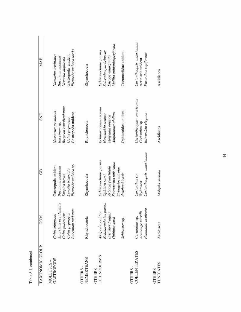
44

Tabl

e 8.

1, c

ontin

ued.

TA

XO

NO

MIC

GR

OU

P G

OM

G

B

SNE

MA

B

MO

LLU

SCS

- G

AST

RO

POD

S C

olus

stim

pson

i G

astro

poda

uni

dent

. N

assa

rius

triv

ittat

us

Nas

sari

us tr

ivitt

atus

Apor

rhai

s occ

iden

talis

Bu

ccin

um u

ndat

um

Bucc

inum

sp.

Bucc

inum

und

atum

Col

us p

ubes

cens

Eu

spir

a he

ros

Busy

con

cana

licul

atum

N

ever

ita d

uplic

ata

C

olus

pyg

mae

us

Luna

tia tr

iser

iata

C

olus

pyg

mae

us

Gas

tropo

da u

nide

nt.

Bu

ccin

um u

ndat

um

Pleu

robr

anch

aea

sp.

Gas

tropo

da u

nide

nt.

Pleu

robr

anch

aea

tard

a

O

THER

S -

NEM

ERTE

AN

S R

hync

hoco

ela

Rhy

ncho

coel

a R

hync

hoco

ela

Rhy

ncho

coel

a

OTH

ERS

- EC

HIN

OD

ERM

S M

olpa

dia

oolit

ica

Echi

nara

chni

us p

arm

a Ec

hina

rach

nius

par

ma

Echi

nara

chni

us p

arm

a

Echi

nara

chni

us p

arm

a O

phiu

ra sa

rsi

Hav

eloc

kia

scab

ra

Scle

roda

ctyl

a br

iare

us

Br

isas

ter f

ragi

lis

Arba

cia

punc

tula

ta

Mol

padi

a oo

litic

a En

cope

em

argi

nata

Oph

iura

sars

i St

erod

erm

a un

isem

ita

Amph

iopl

us a

bditu

s M

ellit

a qu

inqu

iesp

erfo

rata

Sc

hiza

ster

sp.

Stro

ngyl

ocen

trot

us

droe

bach

iens

is

Oph

iuro

idea

uni

dent

. C

ucum

ariid

ae u

nide

nt.

O

THER

S -

CO

ELEN

TER

ATE

S C

eria

nthu

s sp.

C

eria

nthu

s sp.

C

eria

nthe

opsi

s am

eric

anus

C

eria

nthe

opsi

s am

eric

anus

Actin

auge

ver

rilli

H

ydro

zoa

C

eria

nthu

s sp.

Act

inia

ria u

nide

nt.

Pe

nnat

ula

acul

eata

C

eria

nthe

opsi

s am

eric

anus

Ed

war

dsia

ele

gans

Pa

rant

hus r

apifo

rmis

O

THER

S -

TUN

ICA

TES

Asc

idia

cea

M

olgu

la a

rena

ta

Asc

idia

cea

A

scid

iace

a

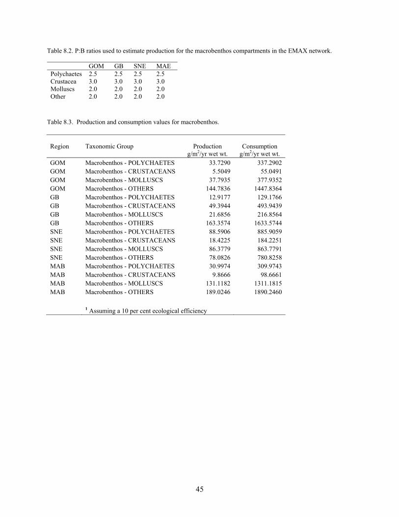
45

Table 8.2. P:B ratios used to estimate production for the macrobenthos compartments in the EMAX network.

GOM GB SNE MAE Polychaetes 2.5 2.5 2.5 2.5 Crustacea 3.0 3.0 3.0 3.0 Molluscs 2.0 2.0 2.0 2.0 Other 2.0 2.0 2.0 2.0

Table 8.3. Production and consumption values for macrobenthos.

Region Taxonomic Group

Production g/m2/yr wet wt.

Consumption

g/m2/yr wet wt. GOM Macrobenthos - POLYCHAETES 33.7290 337.2902 GOM Macrobenthos - CRUSTACEANS 5.5049 55.0491 GOM Macrobenthos - MOLLUSCS 37.7935 377.9352 GOM Macrobenthos - OTHERS 144.7836 1447.8364 GB Macrobenthos - POLYCHAETES 12.9177 129.1766 GB Macrobenthos - CRUSTACEANS 49.3944 493.9439 GB Macrobenthos - MOLLUSCS 21.6856 216.8564 GB Macrobenthos - OTHERS 163.3574 1633.5744 SNE Macrobenthos - POLYCHAETES 88.5906 885.9059 SNE Macrobenthos - CRUSTACEANS 18.4225 184.2251 SNE Macrobenthos - MOLLUSCS 86.3779 863.7791 SNE Macrobenthos - OTHERS 78.0826 780.8258 MAB Macrobenthos - POLYCHAETES 30.9974 309.9743 MAB Macrobenthos - CRUSTACEANS 9.8666 98.6661 MAB Macrobenthos - MOLLUSCS 131.1182 1311.1815 MAB Macrobenthos - OTHERS 189.0246 1890.2460 1 Assuming a 10 per cent ecological efficiency

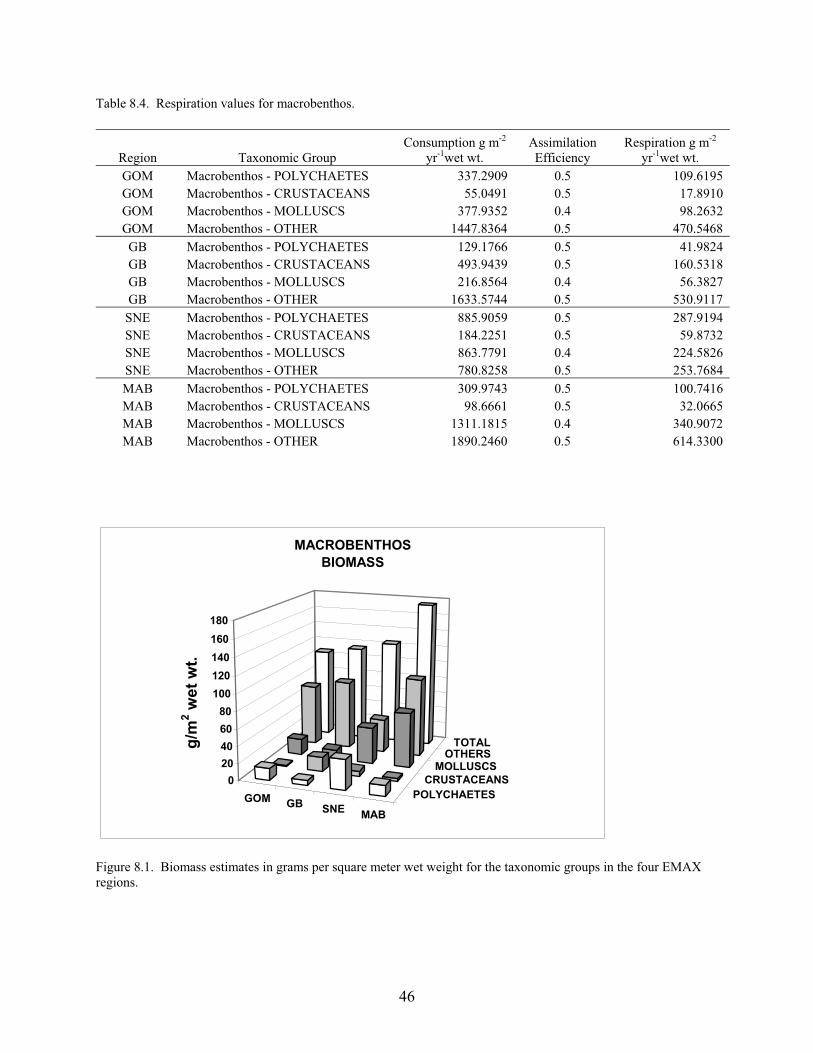
46

Table 8.4. Respiration values for macrobenthos.

Region Taxonomic Group Consumption g m-2

yr-1wet wt. Assimilation Efficiency

Respiration g m-2 yr-1wet wt.

GOM Macrobenthos - POLYCHAETES 337.2909 0.5 109.6195 GOM Macrobenthos - CRUSTACEANS 55.0491 0.5 17.8910 GOM Macrobenthos - MOLLUSCS 377.9352 0.4 98.2632 GOM Macrobenthos - OTHER 1447.8364 0.5 470.5468 GB Macrobenthos - POLYCHAETES 129.1766 0.5 41.9824 GB Macrobenthos - CRUSTACEANS 493.9439 0.5 160.5318 GB Macrobenthos - MOLLUSCS 216.8564 0.4 56.3827 GB Macrobenthos - OTHER 1633.5744 0.5 530.9117

SNE Macrobenthos - POLYCHAETES 885.9059 0.5 287.9194 SNE Macrobenthos - CRUSTACEANS 184.2251 0.5 59.8732 SNE Macrobenthos - MOLLUSCS 863.7791 0.4 224.5826 SNE Macrobenthos - OTHER 780.8258 0.5 253.7684 MAB Macrobenthos - POLYCHAETES 309.9743 0.5 100.7416 MAB Macrobenthos - CRUSTACEANS 98.6661 0.5 32.0665 MAB Macrobenthos - MOLLUSCS 1311.1815 0.4 340.9072 MAB Macrobenthos - OTHER 1890.2460 0.5 614.3300

GOM GB SNE MAB

POLYCHAETESCRUSTACEANS

MOLLUSCSOTHERS

TOTAL

020406080

100120140160180

g/m

2 wet

wt.

MACROBENTHOS BIOMASS

Figure 8.1. Biomass estimates in grams per square meter wet weight for the taxonomic groups in the four EMAX regions.

47

9. Megabenthos - Filterers William T. Stockhausen and Vincent G. Guida (node #13) Background

Although not strictly defined in terms of size, the largest benthic invertebrates are often

referred to as “megabenthos”. For the purposes of this modeling exercise, we defined megabenthos filter feeders to include three species of large, commercially exploited bivalves: ocean quahog, Arctica islandica; Atlantic surf clam, Spisula solidissima; and sea scallop,Placopecten magellanicus. Other kinds of bivalves, including mussels (e.g., Mytilus edulis and Modiolus modiolus), numerous species of small clams, cockles, jingle shells, and others are included in the macrobenthos (polychaetes, crustaceans, mollusks, and others) node (Section 8 of this document).

The ocean quahog is a large, temperate to boreal, infaunal clam with an amphi-Atlantic distribution (Weinberg 1995). It is widely distributed across the continental shelf in medium- to fine-grained sand from the Delmarva Penninsula to Georges Bank (Cargnelli et al. 1999a), including nearshore waters in the Gulf of Maine (Wigley and Theroux 1998). It has low recruitment and slow growth rates (Kennish et al. 1994; Kennish and Lutz 1995). The Atlantic surf clam is another large infaunal clam found in fine sand to gravel, ranging from the Gulf of St. Lawrence to Cape Hatteras (Merrill and Ropes 1969; Cargnelli et al. 1999b). The sea scallop is an epifaunal bivalve living in coarse gravelly or shelly sand to gravel and rock, whose range is similar to that of the surf clam. Sea scallops are moderately abundant only in nearshore waters in the Gulf of Maine (Packer et al. 1999). Data Sources

Fisheries independent survey data from the NEFSC Clam and Scallop Surveys were used to estimate biomass density (g meat weight m-2). The surveys do not sample in the Gulf of Maine (GOM) since biomass densities are low for the three species of bivalves in this node outside state waters in this region. Therefore, data for the GOM subregion was derived from grab sample values (Theroux and Wigley 1998). Quantitative Approach for Biomass Estimates

Ocean Quahogs and Atlantic Surfclams Survey data from the NEFSC Clam Surveys for 1997 and 1999 were used to estimate

biomass densities of ocean quahogs and Atlantic surfclams in each EMAX region. For each tow, reported shell lengths were converted to meat weights using species- and region-specific length-meat weight regressions (Table 9.1; NEFSC 2003, 2004). Total meat weight caught in a tow was calculated by summing over the individual weights for each species. Area-stratified mean catch per tow was then calculated for each EMAX region and species combination using the total meat weights from stations in survey strata contained within the EMAX region. Efficiency-corrected estimates of species biomass density in EMAX region r and survey year y, dry (g meat weight m-

2), were calculated from the corresponding area-stratified mean catch per tow, cry, using the formula

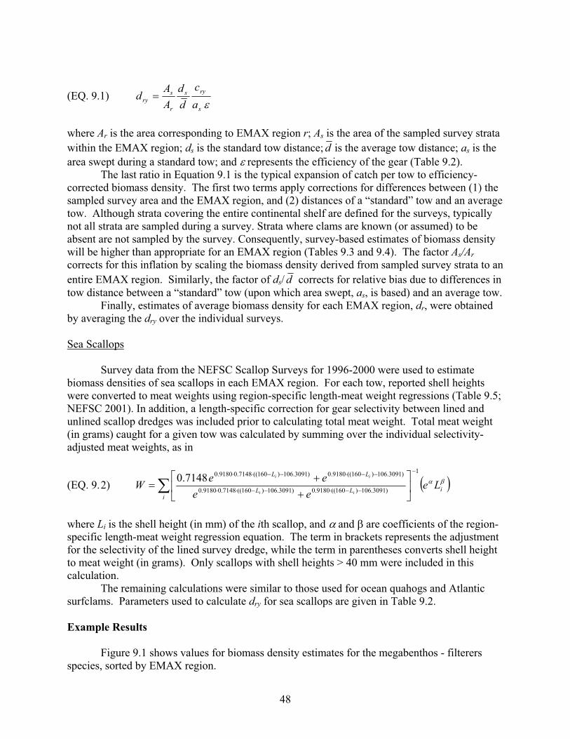
48

(EQ. 9.1) �s

rys

r

sry a

cdd

AA

d �

where Ar is the area corresponding to EMAX region r; As is the area of the sampled survey strata within the EMAX region; ds is the standard tow distance; d is the average tow distance; as is the area swept during a standard tow; and � represents the efficiency of the gear (Table 9.2).

The last ratio in Equation 9.1 is the typical expansion of catch per tow to efficiency-corrected biomass density. The first two terms apply corrections for differences between (1) the sampled survey area and the EMAX region, and (2) distances of a “standard” tow and an average tow. Although strata covering the entire continental shelf are defined for the surveys, typically not all strata are sampled during a survey. Strata where clams are known (or assumed) to be absent are not sampled by the survey. Consequently, survey-based estimates of biomass density will be higher than appropriate for an EMAX region (Tables 9.3 and 9.4). The factor As/Ar corrects for this inflation by scaling the biomass density derived from sampled survey strata to an entire EMAX region. Similarly, the factor of ds/ d corrects for relative bias due to differences in tow distance between a “standard” tow (upon which area swept, as, is based) and an average tow.

Finally, estimates of average biomass density for each EMAX region, dr, were obtained by averaging the dry over the individual surveys.

Sea Scallops

Survey data from the NEFSC Scallop Surveys for 1996-2000 were used to estimate

biomass densities of sea scallops in each EMAX region. For each tow, reported shell heights were converted to meat weights using region-specific length-meat weight regressions (Table 9.5; NEFSC 2001). In addition, a length-specific correction for gear selectivity between lined and unlined scallop dredges was included prior to calculating total meat weight. Total meat weight (in grams) caught for a given tow was calculated by summing over the individual selectivity-adjusted meat weights, as in

(EQ. 9. 2) � ���i

iLL

LL

Leee

eeWii

ii1

)3091.106)160((9180.0)3091.106)160((7148.09180.0

)3091.106)160((9180.0)3091.106)160((7148.09180.07148.0

� �

���

��

��

where Li is the shell height (in mm) of the ith scallop, and � and � are coefficients of the region-specific length-meat weight regression equation. The term in brackets represents the adjustment for the selectivity of the lined survey dredge, while the term in parentheses converts shell height to meat weight (in grams). Only scallops with shell heights > 40 mm were included in this calculation.

The remaining calculations were similar to those used for ocean quahogs and Atlantic surfclams. Parameters used to calculate dry for sea scallops are given in Table 9.2. Example Results

Figure 9.1 shows values for biomass density estimates for the megabenthos - filterers species, sorted by EMAX region.

49

Production/Growth/Reproduction

No published data were available for any of the three target species. Production values

for this node were therefore based on the use of a P:B ratio of 0.8. This value is well within the published range for bivalves (0.28 to 2.91; based on compilation of preexisting data by Dame 1996), and is below the median value, reflecting the slow growth rate of the dominant ocean quahog. No published data was available for any of the three target species. Consumption

Here again, no published consumption data were available for the target species. Values

were based on the use of a C:B ratio of 10. This value is well within values calculated from the compilation of Dame (1.9 to 54.3; 1996), and approaches the value for the American oyster (9.48; Dame 1976). Respiration

We have chosen to estimate respiration values for the megabenthic nodes from other

composite parameters for the same groups: (EQ. 9.3) R = C � EA � 0.65, where R is respiration, C is consumption, EA is assimilation efficiency, and 0.65 represents the fraction of assimilated energy that is typically respired by ectotherms (Parry 1983). Values for assimilation efficiencies for this purpose were derived from Valiela (1995). Example Results

Table 9.6 shows values for biomass density, production, consumption, and respiration for megabenthos - filterers in each of the four ecoregions.

50

References Cargnelli, LM; Griesbach, SJ; Packer, DB; Weissberger E. 1999a. Ocean quahog, Arctica islandica, life history

and habitat characteristics. NOAA Tech. Memo. NMFS-NE-148; 12 p. Cargnelli, LM; Griesbach, SJ; Packer, DB; Weissberger E. 1999b. Atlantic surfclam, Spissula solidissima, life

history and habitat characteristics. NOAA Tech. Memo. NMFS-NE-142; 13 p. Dame, RF Jr. 1976. Energy flow in an intertidal oyster population. Estuarine Coastal Mar. Sci. 4(3):243-253. Dame, RF Jr. 1996. Ecology of marine bivalves, and ecosystem approach. Boca Raton, FL: CRC Press; 254 p. Kennish, MJ; Lutz, RA. 1995. Assessment of the ocean quahog, Arctica islandica (Linnaeus, 1767), in the New

Jersey fishery. J. Shellfish Res. 14(1):45-52. Kennish, MJ; Lutz, RA; Dobarro JA; Fritz LW. 1994. In situ growth rates of the ocean quahog, Arcitca islandica

(Linnaeus, 1767), in the Middle Atlantic Bight. J. Shellfish Res. 13(2):473-478. Merrill, AS; Ropes, JW. 1969. The general distribution of the surf clam and ocean quahog. Proc. Nat. Shellfish.

Assoc. 59(1):40-45. NEFSC. 2001. 32nd Northeast Regional Stock Assessment Workshop (32nd SAW) Public Review Workshop B. Sea

scallop advisory report. Northeast Fish. Sci. Cent. Ref. Doc. 01-04:15-22. NEFSC. 2003. 37th Northeast Regional Stock Assessment Workshop (37nd SAW) Public Review Workshop C.

Atlantic surf clam advisory report. Northeast Fish. Sci. Cent. Ref. Doc. 03-16:284-433. NEFSC. 2004. 38th Northeast Regional Stock Assessment Workshop (38th SAW) Public Review Workshop A.

Ocean quahog advisory report. Northeast Fish. Sci. Cent. Ref. Doc. 04-04:10-20. Packer, DB; Cargnelli, LM; Griesbach, SJ; Shumway, SE. 1999. Sea scallop, Placopecten magellanicus, life

history and habitat characteristics. NOAA Tech. Memo. NMFS-NE-134; 21 p. Parry, GD. 1983. The influence of the cost of growth on ectotherm metabolism. J. Theor. Biol. 101(3):453-477. Valiela, I. 1995. Marine ecological processes. New York, NY: Springer-Verlag Inc.; 686 p. Weinberg, J. 1995. Ocean quahog. In: Conservation and Utilization Division. Northeast Fisheries Science Center,

eds. Status of the fishery resources off the northeastern United States for 1994. NOAA Tech. Memo. NMFS-NE-108:121-122.

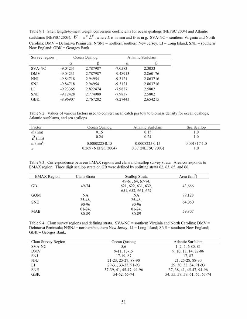
51

Table 9.1. Shell length-to-meat weight conversion coefficients for ocean quahogs (NEFSC 2004) and Atlantic surfclams (NEFSC 2003). �� LeW � , where L is in mm and W is in g. SVA-NC = southern Virginia and North Carolina; DMV = Delmarva Peninsula; N/SNJ = northern/southern New Jersey; LI = Long Island; SNE = southern New England; GBK = Georges Bank.

Ocean Quahog Atlantic Surfclam Survey region � � � �

SVA-NC -9.04231 2.787987 -7.0583 2.3033 DMV -9.04231 2.787987 -9.48913 2.860176 NNJ -9.84718 2.94954 -9.3121 2.863716 SNJ -9.84718 2.94954 -9.3121 2.863716 LI -9.23365 2.822474 -7.9837 2.5802 SNE -9.12428 2.774989 -7.9837 2.5802 GBK -8.96907 2.767282 -8.27443 2.654215

Table 9.2. Values of various factors used to convert mean catch per tow to biomass density for ocean quahogs, Atlantic surfclams, and sea scallops.

Factor Ocean Quahog Atlantic Surfclam Sea Scallop ds (nm) 0.15 0.15 1.0 d (nm) 0.24 0.24 1.0 as (nm2) 0.00082250.15 0.00082250.15 0.0013171.0 � 0.269 (NEFSC 2004) 0.37 (NEFSC 2003) 1.0

Table 9.3. Correspondence between EMAX regions and clam and scallop survey strata. Area corresponds to EMAX region. Three digit scallop strata on GB were defined by splitting strata 62, 63, 65, and 66.

EMAX Region Clam Strata Scallop Strata Area (km2)

GB 49-74 49-61, 64, 67-74,

621, 622, 631, 632, 651, 652, 661, 662

43,666

GOM NA NA 79,128

SNE 25-48, 90-96

25-48, 90-96 64,060

MAB 01-24, 80-89

01-24, 80-89 59,807

Table 9.4. Clam survey regions and defining strata. SVA-NC = southern Virginia and North Carolina; DMV = Delmarva Peninsula; N/SNJ = northern/southern New Jersey; LI = Long Island; SNE = southern New England; GBK = Georges Bank.

Clam Survey Region Ocean Quahog Atlantic Surfclam SVA-NC 5,6 1, 2, 5, 6 80, 81 DMV 9-11, 13-15 9, 10, 13, 14, 82-86 SNJ 17-19, 87 17, 87 NNJ 21-23, 25-27, 88-90 21, 25-28, 88-90 LI 29-31, 33-35, 91-93 29, 30, 33, 34, 91-93 SNE 37-39, 41, 45-47, 94-96 37, 38, 41, 45-47, 94-96 GBK 54-62, 65-74 54, 55, 57, 59, 61, 65, 67-74

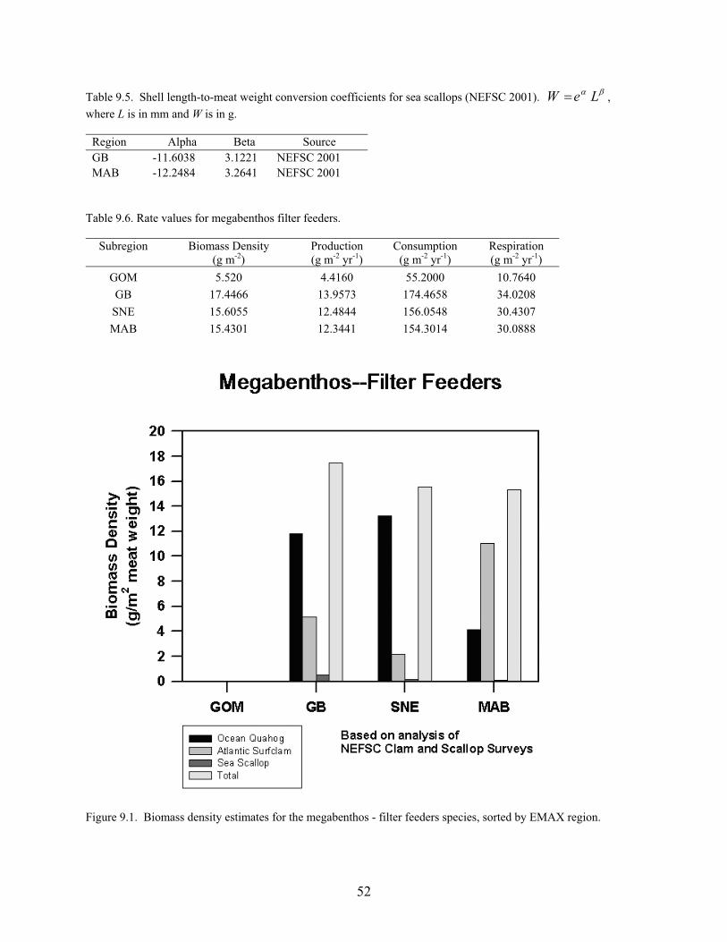
52

Table 9.5. Shell length-to-meat weight conversion coefficients for sea scallops (NEFSC 2001). �� LeW � , where L is in mm and W is in g.

Region Alpha Beta Source GB -11.6038 3.1221 NEFSC 2001 MAB -12.2484 3.2641 NEFSC 2001

Table 9.6. Rate values for megabenthos filter feeders.

Subregion Biomass Density (g m-2)

Production (g m-2 yr-1)

Consumption (g m-2 yr-1)

Respiration (g m-2 yr-1)

GOM 5.520 4.4160 55.2000 10.7640 GB 17.4466 13.9573 174.4658 34.0208

SNE 15.6055 12.4844 156.0548 30.4307 MAB 15.4301 12.3441 154.3014 30.0888

Figure 9.1. Biomass density estimates for the megabenthos - filter feeders species, sorted by EMAX region.

53

10. Megabenthos - Other William T. Stockhausen and Vincent G. Guida (node #14) Background

Although not strictly defined in terms of size, the largest benthic invertebrates are often

referred to as “megabenthos”. Aside from large filter-feeding bivalves (megabenthos filterers), there are a variety of mostly predators and scavengers that may fit this description. We have chosen to include two groups: large Arthropods and Asteroid Echinoderms. All other large invertebrates, even if of comparable size, have been consigned to macrobenthos (see Section 8 for a list).

Megabenthic species have been assessed by a number of methods: trawls, dredges, grabs, submersible, towed camera sled, and divers (Uzmann et al. 1977; Franz et al. 1981; Miller 1989; Stehlik et al. 1991; Theroux and Wigley 1998). However, no one study has treated all such organisms comprehensively in this region and no one method is suitable for all of them. Therefore, for purposes of biomass quantification, we have divided the megabenthos biomass in this node into two separate elements, defined by the efficiency of various gear types used to collect them: sea stars (Echinodermata: Asteroidea) and large Arthropods. The latter element includes horseshoe crabs (Merostomata), mantis shrimp (Crustacea: Stomatopoda), crabs (Crustacea: Decapoda: Brachyura and Anomura other than hermit crabs) and lobsters (Decapoda: Astacidea).

Twenty-five species of commonly-occurring Asteroids, including sub-tropical, wide ranging, boreal and subarctic-boreal groups, have been identified from NEFSC groundfish survey data (Franz et al. 1981). Species listed in Table 10.1 are dominants from among that list. However, comparison of NEFSC Bottom Trawl Survey data with data from bottom video and still photographs and catches with a small-mesh 2 m beam trawl suggest that these Survey Trawl data greatly underestimate sea star (Asteroid) abundance. Asteroid biomass from grab sampling data (Wigley and Theroux 1981, Theroux and Wigley 1998) more closely resembles estimates based on visual assessments and beam trawl catches that ranged from about 0.5 to 5.0 g m-2 (Guida, unpublished).

Decapod biomasses from these grab sampling sources were substantially larger than from NEFSC Bottom Trawl Survey data, but were not comparable because they were heavily dominated by small Decapods (e.g., crangonid shrimps and hermit crabs), which are included in the macrobenthos (Section 8) in this document. Larger Decapods were admittedly underrepresented in grab samples (Theroux and Wigley 1998). The species list is given in Table 10.1. Data Sources

Fisheries-independent survey data from the NEFSC Bottom Trawl Survey were used to estimate biomass density (g wet weight m-2) for large arthropods. Comparison of NEFSC Bottom Trawl Survey data with data from bottom video and still photographs and catches with a small-mesh 2 m beam trawl net suggest that while these Trawl Survey data provide reasonable estimates for large arthropods, they greatly underestimate Asteroid density (Guida, unpublished). Sea star biomass was derived from comprehensive regional benthic grab data (Wigley and Theroux 1981; Theroux and Wigley 1998).

54

Quantitative Approach for Biomass Estimates

Large Arthropods For each species and EMAX region, mean catch per tow (in kg tow-1) was first calculated

on a per-survey basis over survey strata contained within the EMAX region (Table 10.2, see also Table 1.1) using both spring and fall surveys during the period 1996-2000. If fewer than two stations were completed in a stratum during a given survey, that stratum was dropped from calculations of mean catch per tow. Mean catch per tow in season s and year y, csy, was then converted to biomass density (dsy) using the formula

(EQ. 10.1) a

cfd sy

sy �

where a is the area swept by the bottom trawl in a standard tow (0.01 nm2 for the Bottom Trawl Survey) and f is a conversion factor from kg naut. mi-2 to g m-2 (f = [1000 g/kg]/[1852 m/naut. mi]2). Finally, biomass density estimates were averaged over season and year using the formula

(EQ. 10.2) � ����

���

�y s

sydd 6121

51

where equal weight was given to spring and fall survey results (Figure 10.1). Except in the Mid-Atlantic Bight, American lobster (Homarus americanus) comprised

the major component of “other” biomass (Figure 10.1). In the Mid-Atlantic Bight, horseshoe crabs (Limulus polyphemus) comprised the major component, with American lobster as the second largest component. The mean lobster value for the four subregions calculated here (0.025 g m-2) closely approximates the 1996 NEFSC autumn bottom trawl survey biomass index for lobster: 1.3 kg tow-1 = 0.027 g m-2 (Idoine 1996). Comparative sampling of the same set of stations using 36’ Yankee otter trawl (as used in the NEFSC Bottom Trawl Survey), 2 m beam trawl with 6.4 mm (1/4”) mesh, and video drift vehicle (Guida, unpublished) indicated that a catchability factor was needed for data on large Arthropods other than the American lobster. Table 10.3 compares catches of Cancer spp. crabs (C. borealis and C. irroratus could not be distinguished in the video images) taken from the same stations during three NEFSC Benthic Habitat cruises conducted near Hudson Canyon (SNE Region). Biomass densities for net catches were calculated by dividing total wet weight by the estimated area swept out by the respective trawl gears. Video biomass densities were calculated by multiplying counts of individuals seen in the video by the mean individual weight as determined from the beam trawl catch and dividing by the area of the video drift transect. Although not all methods were employed during each cruise, it is clear that 36’ Yankee estimates were about two orders of magnitude smaller than densities based on either beam trawl catches or bottom video counts. Assuming the bottom video biomass represents the actual crab density, a catchability of about 50% for the beam trawl and 1% for 36’ Yankee for these large Arthropods is suggested by the mean values and by the data from August 2004, when all three methods were employed. Therefore, NEFSC survey values for all large Arthropods other than the American lobster will be multiplied by 100 to obtain realistic estimates. Unlike Cancer spp., the American lobster was too rarely caught in the beam trawl or in video images to be able to assess its biomass density by those means for comparison with 36’

55

Yankee values. Thus, no unique catchability factor could be assigned. From behavioral observation, it appears that catchability factor for lobsters might be far higher than for Cancer spp. crabs because the former, unlike the latter, tends to propel itself off the bottom with “tail thrusts” when disturbed, making otter trawl capture more likely. On the other hand, lobsters are more likely than Cancer crabs to be found in rocky areas (Hudon and Lamarche 1989), where capture by mobile gear is not possible. This may be disproportionately true of juveniles (Steneck et al. 1991). Choosing to err on the side of conservatism, lobsters have therefore been assigned a catchability of 100%, which probably greatly underestimates their abundance and biomass. Asteroids General comments provided for macrobenthos (Section 8) regarding biomass estimates from grab sample data apply to our estimates of the Asteroid element of the megabenthos as well. Example Results

Figures 10.1 and 10.2 show estimated biomass for megabenthos - other sampled from the two survey methodologies, with a single focus on large arthopods (10.1) and all species combined (10.2). Production/Growth/Reproduction

Production was estimated using a P:B ratio of 1.5 based on the assumption that as large,

active invertebrates, P:B should resemble that of squid and shrimp. Consumption

Consumption was estimated using a C:B ratio of 13.5 based again on the assumption that

shrimp should resemble other large benthic invertebrates. We estimated consumption by multiplying the C:B ratio by biomass for the megabenthos - other node in the four EMAX regions. These are crude estimates since consumption rates for benthic invertebrates in the field are dependant on temperature, size, age, and food supply (Valiela 1995; Velasco and Navarro 2005). Respiration

We chose to estimate respiration values for the macrobenthic nodes from other composite

parameters for the same groups: (EQ. 10.3) R = C � EA � 0.65, where R is respiration, C is consumption, EA is assimilation efficiency, and 0.65 represents the fraction of assimilated energy that is typically respired by ectotherms (Parry 1983). Values for assimilation efficiencies for this purpose were derived from Valiela (1995).

56

Example Results

Values for biomass density, production, consumption, and respiration for megabenthos - other in each of the four subregions are summarized in Table 10.4. References Franz, DR, Worley, EK; Merrill, AS. 1981. Distribution patterns of common seastars of the middle Atlantic

continental shelf of the northwest Atlantic (Gulf of Maine to Cape Hatteras). Biol.Bull.160(3):394-418. Guida, VG. Unpublished data from NEFSC Benthic Habitat cruises DE01-11, OC02-12, and DE04-12. Hudon, C; Lamarche, G. 1989. Niche segregation between American lobster Homarus americanus and rock crab

Cancer irroratus. Mar. Ecol. Prog. Ser. 52(2):155-168. Idoine, J. 1996. American lobster. In: NEFSC. 1996. 22nd Northeast Regional Stock Assessment Workshop (22nd

SAW). Northeast Fish. Sci. Cent. Ref. Doc. 96-13:47-134. Miller, RJ. 1989. Catchability of American lobster (Homarus americanus) and rock crabs (Cancer irroratus) by

traps. Can. J. Fish. Aquat. Sci. 46(10):1652-1657. Parry, GD. 1983. The influence of the cost of growth on ectotherm metabolism. J. Theor. Biol. 101(3):453-477. Stehlik, LL; MacKenzie, CL Jr.; Morse, WW. 1991. Distribution and abundance of four brachyuran crabs on the

northwest Atlantic shelf. Fish. Bull. 89(3):473-492. Steneck, RS; Wahle, RA; Incze, LS; Belknap, DF. 1991. Patterns of distribution and abundance of lobsters in the

Gulf of Maine: Ideas on the carrying capacity of their environment. J. Shellfish Res.10(1):1-300. Theroux, R; Wigley R. 1998. Quantitative composition and distribution of macrobenthic invertebrate fauna of the

continental shelf ecosystems of the northeastern United States. NOAA Tech. Rep. NMFS 140; 240 p. Uzmann, JR, Cooper, RA; Theroux RB; Wigley, RL. 1977. Synoptic comparison of three sampling techniques for

estimating abundance and distribution of selected megafuana: submersible vs. camera sled vs. otter trawl. Mar. Fish. Rev. 39(12):11-19.

Valiela, I. 1995. Marine ecological processes. New York, NY: Springer-Verlag Inc.; 686 p. Wigley, R; Theroux R. 1981. Macrobenthic invertebrate fauna of the middle Atlantic Bight region: faunal

composition and quantitative distribution. US Geol. Surv. Prof. Pap. 529-N; 198 p.

57

Table 10.1. Species defined as megabenthos - other. Scientific name Common Name NEFSC Species Code Limulus polyphemus Horseshoe crab 318 Homarus americanus American lobster 301 Scyllarides nodifer Ridged slipper lobster 302 Scyllarides aequinoctialis Spanish slipper lobster 303 Panulirus argus Caribbean spiny lobster 304 Geryon fenneri Golden deepsea crab 308 Geryon affinis White crab 309 Geryon quinquedens Red deepsea crab 310 Cancridae Cancer crabs, unclassified 311 Cancer borealis Jonah crab 312 Cancer irroratus Atlantic rock crab 313 Callinectes sapidus Blue crab 314 Ovalipes sp Calico crabs, unclassified 315 Majidae Spider crabs, unclassified 317 Galatheidae Galatheids, unclassified 319 Portunidae Swimming crabs, unclassified 320 Ovalipes stephensoni Coarsehand lady crab 321 Ovalipes ocellatus Lady crab 322 Stomatopoda Mantis shrimps, unclassified 323 Lithodes maja Northern stone crab 324 Chionoecetes opilio Snow crab 325 Carcinus maenas Green crab 326 Hepatus epheliticus Calico box crab 327 Calappa flammea Flame box crab 328 Calappa sulcata Yellow box crab 329 Calappidae Box crabs, unclassified 339 Asterias forbesii Common sea star 332 Asterias vulgaris Boreal asterias 333 Astropecten spp. Margined sea stars 334 Leptasterias sp. Slender-armed and polar sea stars 332 Solaster sp. Sun stars 332 Ctenodiscus crispatus Mud star 332

Table 10.2. EMAX Regions and NEFSC Bottom Trawl Survey strata.

EMAX Region NEFSC Strata Area (km2)

GB 01130-01230, 01250 43,666

GOM 24,26-30,36-40 03570-03900 79,128

SNE 01010-01120; 03010-03140,03450-03560 64,060

MAB 01610-01760; 03150-03440 59,807

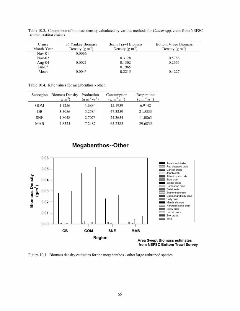
58

Table 10.3. Comparison of biomass density calculated by various methods for Cancer spp. crabs from NEFSC Benthic Habitat cruises.

Cruise Month-Year

36 Yankee Biomass Density (g m-2)

Beam Trawl Biomass Density (g m-2)

Bottom Video Biomass Density (g m-2)

Nov-01 0.0066 Nov-02 0.3128 0.5788 Aug-04 0.0021 0.1302 0.2665 Jan-05 0.1965 Mean 0.0043 0.2215 0.4227

Table 10.4. Rate values for megabenthos - other.

Subregion Biomass Density (g m-2)

Production (g m-2 yr-1)

Consumption (g m-2 yr-1)

Respiration (g m-2 yr-1)

GOM 1.1256 1.6884 15.1959 6.9142 GB 3.5056 5.2584 47.3259 21.5333

SNE 1.8048 2.7073 24.3654 11.0863 MAB 4.8325 7.2487 65.2385 29.6835

Megabenthos--Other

RegionGB GOM SNE MAB

Bio

mas

s D

ensi

ty(g

/m2 )

0.00

0.01

0.02

0.03

0.04

0.05

0.06American lobster Red deepsea crab Cancer crabs Jonah crab Atlantic rock crab Blue crab Spider crabs Horseshoe crab Galatheids Swimming crabs Coarsehand lady crab Lady crab Mantis shrimps Northern stone crab Snow crab Hermit crabs Box crabs Total

Area Swept Biomass estimatesfrom NEFSC Bottom Trawl Survey

Figure 10.1. Biomass density estimates for the megabenthos - other large arthropod species.

59

0.00

0.50

1.00

1.50

2.00

2.50

3.00

3.50

4.00

4.50

5.00

Biomass (g/sq m)

GOM GB SNE MAB

Subregion

Asteroids Non-lobster Arthropods Lobsters

Figure 10.2. Combined biomass density estimates for various elements of the megabenthos - other: Large Non-lobster Arthropods (modified for catchability) from NEFSC Trawl Survey; Lobsters (unmodified) from NEFSC Trawl Survey; and Asteroids from grab sample data (Wigley and Theroux 1981, Theroux and Wigley 1998).

60

11. Shrimp and Similar Species Christopher M. Legault, John R. Green, Vincent G. Guida, and Joseph J. Vitaliano (node #15) Background

The northern shrimp, Pandalus borealis, has a discontinuous distribution throughout the

North Atlantic, North Pacific, and Arctic Oceans. In the Gulf of Maine, northern shrimp populations comprise a single stock (Clark and Anthony 1980), which is concentrated in the southwestern region of the Gulf (Haynes and Wigley 1969). P. borealis occurs as far south as New Jersey on the continental slope (William 1984). Dichelopandalus leptocerus can be found from Newfoundland to North Carolina, from estuaries to the continental slope (Williams 1984). While D. leptocerus is not exploited commercially, is an important forage item for a number of fisheries species including monkfish, spiny dogfish, various skate species, red hake, silver hake, and black sea bass (Bowman and Michaels 1984; Bowman et al. 2000; Steimle et al. 2000). It is the principal non-crangonid shrimp species in the region outside of the Gulf of Maine. Pasiphaea multidentata, a circumpolar bathypelagic species largely restricted to the Gulf of Maine in our area, may also play a substantial role as a forage species and consumer of zooplankton and micronekton along with D. leptocerus (Cartes 1993, Frank and Widder 1997). Additional caridean and penaeid shrimp species (e.g., Lebbeus spp., Spirontocaris spp., Parapenaeus politus) occur at depths approaching 200 m and beyond in all subregions and in shallower waters of the Gulf of Maine (Williams 1984), but are probably not in sufficient numbers to be important in terms of the system energy budget. The same is likely true of southern penaeids (white, pink, brown, and rock shrimp: Litopenaeus setiferus, Farfantepenaeus duodorum, F. aztecus, and Sicyonia brevirostris, respectively) that may occur in small numbers as far north as southern New England (Williams 1984). Unlike most other decapod shrimps, the very abundant and widespread crangonids (e.g., Crangon septemspinosa, Pontophilus spp.) are readily captured and assessed by grab sampling, and are therefore included with other such species in the macrobenthos - crustaceans node (Section 8 of this document) rather than here. The species we categorized as shrimp are given in Table 11.1. Data Sources

Stock assessment for Gulf of Maine northern shrimp reviewed in SARC 36 (SARC 2003)

used commercial landings data, Northern Shrimp Technical Committee summer shrimp survey data, and unpublished data from NEFSC Benthic Habitat cruises. Quantitative Approach for Biomass Estimates

A Collie-Sissenwine analysis was used to estimate biomass of northern red shrimp (P.

borealis) in the Gulf of Maine. This analysis is based on relating the annual changes in survey abundance for both recruiting shrimp and fully recruited shrimp to the annual catches in order to estimate biomass of northern shrimp in the Gulf of Maine for years 1985 to 2003. The assessment was confirmed using surplus production, a different modeling approach which produced qualitatively similar results. The Collie-Sissenwine model biomass estimates for years 1996-2000 were averaged and then multiplied by 1.5 to account for other species of shrimp. The

61

resulting total shrimp biomass (mt) was divided by the area of Gulf of Maine (km2) to produce a total shrimp biomass value in units of g m-2 (Table 11.2). Biomass Results

As shrimp are not harvested commercially outside of the Gulf of Maine in the NEUS Ecosystem, this type of analysis could not be used for biomass estimates of shrimp in other subregions (principally D. leptocerus). A mean density estimate for D. leptocerus was made (0.0171 g m-2 or 0.0075 individuals m-2, Guida unpublished) from 2 m beam trawl catches at 38 stations during summer and fall cruises to the outer shelf near Hudson Canyon, along the border between the Mid-Atlantic and Southern New England subregions. While this density is based upon a very limited dataset from a very small portion of the entire region, it is comparable in magnitude to the only published density for this species in the NEUS Ecosystem: 0.0035 individuals m-2 (no biomass data provided) calculated from data on a year-round study performed in Penobscot Bay, Gulf of Maine (Stevenson and Pierce 1984). Semiquantitative data from epibenthic sled collections in nearshore waters off New York Harbor also indicate densities in the range of 10-3 to 10-2 individuals m-2 (Guida, unpublished). We have therefore chosen to adopt 0.0171 g m-2 as an estimate of shrimp biomass for Georges Bank, Southern New England, and the Mid-Atlantic Bight subregions. Production/Growth/Reproduction

Production was estimated using a P:B ratio of 1.5 based on the assumption that as large,

active invertebrates, P:B should resemble that of squid and megabenthos - other. Production was estimated to be 0.1695 * 1.5 = 0.254214 g m-2 yr-1 in the case of the GOM. Consumption

Consumption was estimated using a C:B ratio of 13.5 based again on the assumption that

shrimp should resemble other large benthic invertebrates. Consumption was estimated to be 0.1695 * 13.5 = 2.2883 g m-2 yr-1 in the case of the GOM. Respiration

We have chosen to estimate respiration values for the macrobenthic nodes from other

composite parameters for the same groups: (EQ. 11.1) R = C � EA � 0.65, where R is respiration, C is consumption, EA is assimilation efficiency, and 0.65 represents the fraction of assimilated energy that is typically respired by ectotherms (Parry 1983). Values for assimilation efficiencies for this purpose were derived from Valiela (1995). Thus, respiration was estimated to be 2.2883 * 0.7 * 0.65 = 1.0412 g m-2 yr-1 in the case of the GOM (Table 11.3).

62

Example Results Values for biomass density, production, consumption, and respiration for shrimp and shirmp-like species in each of the four subregions are summarized in Table 11.3. References Bowman, RE; Michaels, WL. 1984. Food of seventeen species of Northwest Atlantic fish. NOAA Tech. Memo.

NMFS-F/NEC-28; 183 p. Bowman, RE; Stillwell, CE; Michaels, WL; Grosslein, MD. 2000. Food of northwest Atlantic fishes and two

common species of squid. NOAA Tech. Memo. NMFS-NE-155; 137 p. Cartes, JE. 1993. Feeding habits of pasiphaeid shrimps close to the bottom on the western Mediterranean slope.

Mar. Biol.117(3):459-468. Clark, SH; Anthony, VC. 1980. An assessment of the Gulf of Maine northern shrimp resource. Proceedings of the

International Pandalid Shrimp Symposium. Univ. Alaska Sea Grant Rep. 81-3:207-224. Frank, TM; Widder, EA. 1997. The correlation of downwelling irradiance and staggered vertical migration patterns

of zooplankton in Wilkinson Basin, Gulf of Maine. J. Plankton Res. 19(12):1975-1992. Guida, VG. Unpublished data from NEFSC Benthic Habitat cruises OC02-12, and DE04-12 and Oceanic-Estuarine

Linkages program. Haynes, EB; Wigley, RL. 1969. Biology of the northern shrimp, Pandalus borealis, in the Gulf of Maine. Trans.

Am. Fish. Soc. 98(1): 60-76. NEFSC. 2001. 36th Northeast Regional Stock Assessment Workshop (36th SAW) Public Review Workshop C.

Northern Shrimp advisory report. Northeast Fish. Sci. Cent. Ref. Doc. 03-04:42-47. Parry, GD. 1983. The influence of the cost of growth on ectotherm metabolism. J. Theor. Biol. 101(3):453-477. Steimle, FW; Pikanowski, RA; McMillan, DG; Zetlin CA; Wilk. SJ. 2000. Demersal fish and American lobster

diets in the lower Hudson - Raritan Estuary. NOAA Tech. Memo. NMFS-NE-161; 106 p. Stevenson, DK; Pierce, F. 1984. Life history characteristics of Pandalus montagui and Dichelopandalus leptocerus

in Penobscot Bay, Maine. Fish. Bull. 83(3):219-233. Valiela, I. 1995. Marine ecological processes. New York, NY: Springer-Verlag Inc.; 686 p. Williams, AB. 1984. Shrimp, lobsters, and crabs of the Atlantic coast of the eastern United States, Maine to

Florida. Washington DC: Smithsonian Institution Press; 550 p.

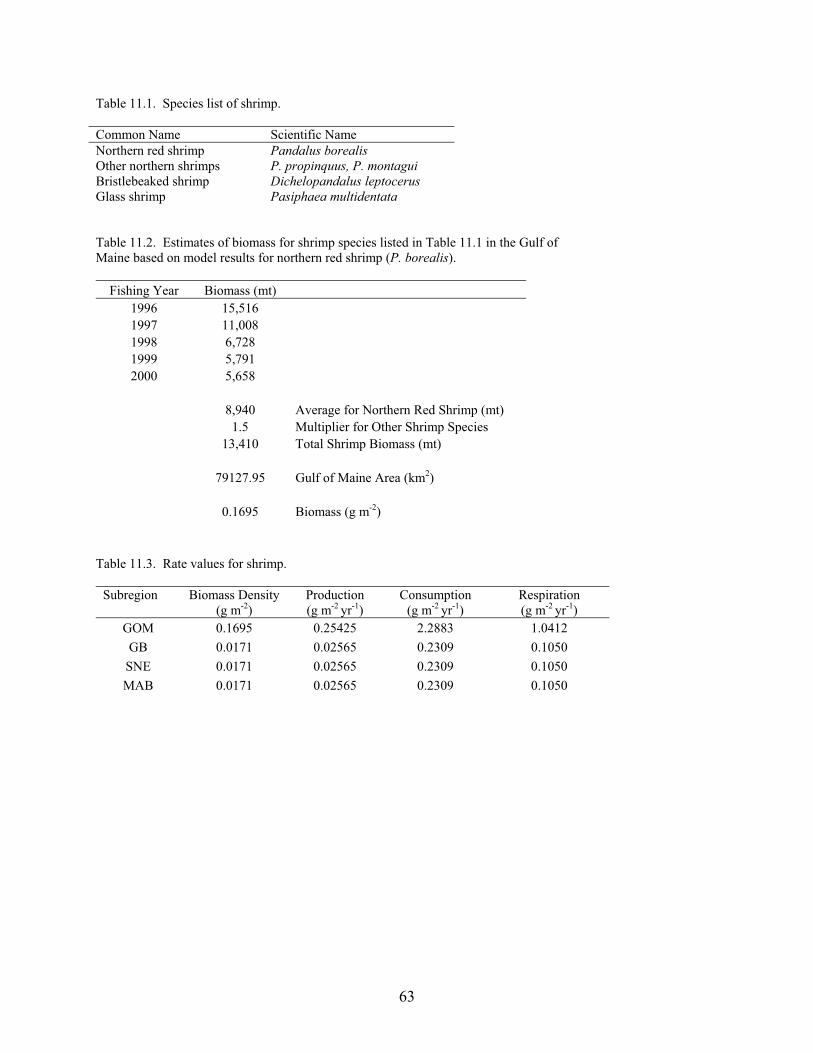
63

Table 11.1. Species list of shrimp. Common Name Scientific Name Northern red shrimp Pandalus borealis Other northern shrimps P. propinquus, P. montagui Bristlebeaked shrimp Dichelopandalus leptocerus Glass shrimp Pasiphaea multidentata Table 11.2. Estimates of biomass for shrimp species listed in Table 11.1 in the Gulf of Maine based on model results for northern red shrimp (P. borealis).

Fishing Year Biomass (mt) 1996 15,516 1997 11,008 1998 6,728 1999 5,791 2000 5,658

8,940 Average for Northern Red Shrimp (mt) 1.5 Multiplier for Other Shrimp Species 13,410 Total Shrimp Biomass (mt) 79127.95 Gulf of Maine Area (km2) 0.1695 Biomass (g m-2)

Table 11.3. Rate values for shrimp.

Subregion Biomass Density (g m-2)

Production (g m-2 yr-1)

Consumption (g m-2 yr-1)

Respiration (g m-2 yr-1)

GOM 0.1695 0.25425 2.2883 1.0412 GB 0.0171 0.02565 0.2309 0.1050

SNE 0.0171 0.02565 0.2309 0.1050 MAB 0.0171 0.02565 0.2309 0.1050

64

12. Larval and Juvenile Fish John R. Green and Donna L. Johnson (node #16) Background Larval fish included in this study represent a wide variety of taxonomic groups and growth forms that change with season and location. Although fish larvae are present in all seasons, abundances decrease in fall and winter when the most numerous larvae are elongated clupeid types. During the spring and early summer gadiform and flatfish larvae are at their most numerous. Larval myctophids are numerous and sometimes dominant, although the adults are distributed in deeper water off the continental shelf. Data Sources & Sampling Procedures

Larval fish biomass was derived from the Marine Resources Monitoring, Assessment and Prediction (MARMAP) sampling program conducted from 1977-87 on the U.S. continental shelf from Cape Hatteras, North Carolina to the Gulf of Maine (Sherman 1980, Morse 1982, Sherman 1986). Double-oblique 61 cm bongo ichthyoplankton and zooplankton sampling tows were taken from the surface to a maximum depth of 200 m or from within 5 meters of the bottom. The sampler was fitted with 0.505 mm mesh nets for ichthyoplankton and 0.333 mm nets for zooplankton. The flowmeter was used as a measure of filtration efficiency for each sample. Ichthyoplankton samples were sorted, identified, and enumerated according to the procedures outlined by Jossi and Marak (1983). Larval fish were identified to the lowest taxon possible and measured to the nearest 0.1 mm standard length (SL). For a summary of MARMAP operations see Sibunka and Silverman (1984, 1989). Mean-Abundance Procedures The number of larvae caught was transformed to the number of individuals under 10 m2 of sea-surface area based on the maximum tow depth and volume filtered by the bongo net: (EQ. 12.1) N = 10 * C * M * B-1 * D-1 where N represents the standardized abundance; C represents the number of larvae collected in the sample; M represents the maximum tow depth (meters); B represents the aperture of the bongo frame; and D represents the total distance the net was towed in meters from the calibrated flowmeter (Smith and Richardson 1977). The mean abundance and its variance were calculated by Pennington’s (1983) method based on the Delta (Δ) distribution. For each station, catch values were standardized to the number of individuals under 10 m2 surface area. The Delta distribution of catch frequencies (Aitchison 1955) was used to provide unbiased estimates of sample means from mean catch calculations and its variance using zero tows (Berrien, et al. 1981; Pennington 1983).

65

Larval Fish Biomass

Delta mean abundances (number/10 m2) of all larvae were extracted by 1 mm SL increments. Dry weight was estimated for each 1 mm abundance group averaged over all seasons of sampling using the length to weight relationship: (EQ 12.2) LogDW = -4.152LogSL 1.186

where DW is dry weight in ug and SL is standard length in mm. The coefficient of SL (1.186) and the intercept are the means of the those parameters from length weight relationships in Laurence (1979) based on laboratory-reared larvae of seven species of fish including a variety of growth forms. Larval weights are rarely given in the literature as wet weight, thus dry weight was assumed to be equal to 10% of wet weight, as were other planktonic forms. Production and Consumption

For purposes of this study, consumption rates used for larvae are based on the average growth rate observed for larval gadids taken from laboratory studies at the NMFS Narragansett laboratory (Laurence, 1978) and unpublished field observations. Growth (i.e., production) was estimated at 0.04 day-1 based on an assumption of growth consistent with that of juvenile cod (Peck et al. 2003). These values were then scaled to provide an annual estimate. This produced a P:B ratio of 15, similar to micronekton. References Aitchison, J. 1955. On the distribution of a positive random variable having a discrete probability mass at the

origin. J. Amer. Statis. Assoc. 50:901-908. Berrien, P; Naplin, NA.; Pennington, M. 1981. Atlantic mackerel, Scomber scombrus, egg production and

spawning population estimates for 1977 in the Gulf of Maine, Georges Bank, and Middle Atlantic Bight. Rapp. P-v. Reun. Cons. int. Explor. Mer. 178:278-288.

Buckley, LJ; Lough, RG. 1987. Recent growth ,biochemincal composition, and prey field of larval haddock (Melanogrammus aeglifinus ) and Atlantic cod ( Gadus morhua) on Georges Bank. Can.J. Fish Aquat. Sci. 44:14-25.

Jossi, JW; Marak RR. 1983. MARMAP plankton survey manual. U.S. Dept. Com., NOAA Tech. Memo., NMFS-F/NEC-21. 258 p.

Laurence G. 1979. Larval length weigh relationships for seven species of northwest Atlantic fishes reared in the laboratory. Fish. Bull. 76(4)890-895.

Morse, W. 1982. Spawning stock biomass estimates of sand lance, Ammodytes sp. off northeastern United States determined from MARMAP plankton surveys, 1974- 1980. Int. Coun. Explor. Sea Demersal Fish Comm. C.M. 1982/G:59.

Peck, M; Buckley, L; Caldarone, E; Bengston D. 2003. Effects of food consumption and temperature on growth rate and biochemical based indicators of growth in early juvenile Atlantic cod (Gadus morhua) and haddock (Melanogrammus aeglifinus). Mar. Ecol. Prog. Ser. 251:233-243.

Pennington, M. 1983. Efficient estimators of abundance, for fish and plankton surveys. Biometrics. 39:81-286. Sherman, K. 1980. MARMAP, a fisheries ecosystem study in the NW Atlantic: Fluctuations in ichthyoplankton-

zooplankton components and their potential for impact on the system. In: Diemer, FP, Vernberg, FJ, Mirkes, DZ, eds. Advance concepts in ocean measurements for marine biology. Belle W. Baruch Institute for Marine Biology and Coastal Research, Univ. South Carolina Press, Berkeley, p. 9-37.

66

Sherman, K. 1986. Measurements strategies for monitoring and forecasting variability in large marine ecosystems. In: Sherman, K and Alexander, LM (eds). Variability and management of marine ecosystems. AAAS Selected Symposium, 99:203-236.

Sibunka, JD; Silverman, MJ. 1984. MARMAP surveys of the continental shelf from Cape Hatteras, North Carolina, to Cape Sable, Nova Scotia (1977-1983). Atlas No. 1, summary of operations. NOAA Tech. Mem., NMFS-F/NEC-33, 306 p.

Sibunka, JD; Silverman, MJ. 1989. MARMAP surveys of the continental shelf from Cape Hatteras, North Carolina, to Cape Sable, Nova Scotia (1984-1987). Atlas No. 3, summary of operations. U.S. Dept. Com., NOAA Tech. Mem., NMFS-F/NEC-68, 197 p.

Smith, PE; Richardson, SL. 1977. Standard techniques for pelagic fish egg and larva surveys. FAO Fish. Tech. Pap., No. 175, 100 p.

67

13. Small Pelagics (commercial, other, squid, anadromous) and Mesopelagics William J. Overholtz, Jon K.T. Brodziak, Christopher M. Legault, and Laurel A. Col (nodes #17-20, 8) Background and Estimation Approach

Five categories of small pelagic fish were assessed using a survey swept area biomass

expansion approach. Categories included small pelagics – commercial; small pelagics – other; squid, anadromous, and mesopelagic fishes (Table 13.1). Time series of spring and autumn research bottom trawl survey swept area biomass were produced for the 1996-2000 period. Informative gamma priors for weighting coefficients were developed from sources in the literature for the various categories by using available values (Table 13.2; Edwards 1968; Harley et al. 2001). Specific priors were developed for herring, mackerel, butterfish, sand lance, and anadromous, while general priors were developed for the squid, mesopelagic, and pelagic - other categories (Table 13.2). In addition, species-specific weighting coefficients were developed from stock assessments for herring, mackerel, and butterfish to be used as maximum likelihood estimates for these species. Linear regressions of spring and autumn survey swept area biomass on stock biomass were used to estimate the coefficient for each of the three stocks.

Priors used in the analysis were based on a gamma distribution where:

(EQ. 13.1) )()(1

rxF exu uxrr

��

; x>0

where u is the mean and r is a shape parameter.

Priors for herring and mackerel were developed from weighting coefficients provided in Edwards (1968) for herring and argentine. The value for butterfish was taken as the average for butterfish and redfish from the same source. The prior for sand lance was available from Harley et al. (2001) and for the anadromous category from Edwards (1968) for alewife. A general prior was developed for the rest of the categories, taken as the average for herring, argentine, butterfish, and alewife (Edwards 1968). A Bayesian model framework was developed for each pelagic category, a CV of 25% was assumed for the r and u parameters of the gamma distributions for each category, and informative priors were calculated (Figure 13.1 and Table 13.3). In the case of herring, mackerel, and butterfish, recent estimates of weighting coefficients from the linear regression analysis were additionally provided as specific maximum likelihoods used to modify priors. Biomass estimates for all other categories were calculated based only on priors.

A WinBUGS (Spiegelhalter et al. 2003) model was produced for each pelagic category or for each single stock of pelagic fish, and average values (1996-2000) of swept area biomass for spring and autumn for each ecoregion were input. Two MCMC chains (Monte Carlo Markov Chains) were initiated for each run with a 10,000 iteration burn in period and a 100,000 iteration output period. Total biomass for each ecoregion was produced (Table 13.4), along with summary statistics including mean, sd, median, quartiles, and 80% and 95% CI’s. In addition, trajectories for each variable and posterior distributions were output as cross checks on model performance. Results for herring, mackerel, and butterfish were summed to produce total biomass estimates for the pelagic - commercial category, and sand lance and the pelagic - other category were summed to produce the total for the pelagic - other category.

68

Production

Production for herring and mackerel was estimated from age-based data. Instantaneous

growth rates were estimated from mean weight at age data, multiplied by average biomass, and summed across ages to obtain estimates of total production for 1996-2000. These values were annualized and converted to g m-2 (Table 13.4). The values were divided by annual biomass to obtain P:B ratios for mackerel and herring. Butterfish production was estimated from surplus production methods. Production to biomass ratios were used to calculate production for the other small pelagic categories. The butterfish P:B ratio (0.95) was used to calculate production for the pelagic - other, mesopelagic, and squid groups. The herring P:B ratio (0.42) was used for the anadromous group (Table 13.4). Consumption

Consumption to biomass ratios for small pelagic and demersal fish were investigated by

exploring the approach used in Sissenwine et al. (1984). In this study C:B ratios for six Georges Bank species were calculated based on theoretical considerations, ranging between 3.2 and 4.9 (Sissenwine et al. 1984). New calculations for GOM fishes suggest that these estimates may be too high; Palomares and Pauly’s (1998) estimates ranged between 1.2 and 3.9 (Table 13.5). Ratios for pelagic and demersal fish used to balance the GOM Ecopath and EcoNetwrk models were based on estimates from the NEFSC food habits database. These estimates utilized the Eggers (1977) equation for consumption, and all the ratios were less than those in the Sissenwine et al. (1984) and Palomares and Pauly (1998) approaches. References Edwards, RL. 1968. Fishery resources of the North Atlantic area. In: De Witt, G, ed. The Future of the Fishing

Industry of the United States. University of Washington Publication in Fisheries. 4:52-60. Eggers, DM. 1977. Factors in interpreting data obtained by diel sampling of fish stomachs. Fish. Res. Board of

Can. 34:290-294. Harley, SJ; Myers, R; Barrowman, N; Bowen, K; Admiro, R. 2001. Estimation of research trawl survey

catchability for biomass reconstruction of the eastern Scotian Shelf. Can. Sci. Advis. Sec. Res. Doc. 2001/084; 54 p.

Palomares, MLD; Pauley, D. 1998. Predicting food consumption of fish populations as functions of mortality, food type, morphometrics, temperature and salinity. Mar. Freshw. Res. 49:447-453.

Sissenwine, MP; Cohen, EB; Grosslein, MD. 1984. Structure of the Georges Bank ecosystem. Rapp. P.-v. Reun. Cons. Int. Explor. Mer. 183:243-254.

Spiegelhalter, DA; Thomas, NB; Lunn, D. 2003. WinBUGS User Manuel. http//www.mrc.bsu.carn.ac.uk/bugs.

69

Table 13.1. List of species in the pelagic category.

Pelagics Pelagic-Commercial Squid Anadromous Pelagic-Other

Clupea harengus Cephalopoda Alosa pseudoharengus Etrumeus teres Scomberesox saurus Scomber scombrus Illex illecebrosus Alosa aestivalis Brevoortia tyrannus Decapterus macarellus Peprilus triacanthus Loligo pealeii Alosa sapidissima Osmerus mordax Selar crumenophthalmus

Alosa mediocris Argentina silus Decapterus punctatus Meso-Pelagic Menidia menidia Trachurus lathami

Myctophidae Ammodytes dubius Ariomma bondi Maurolicus sp. Anchoa mitchilli Opisthonema oglinum Anchoa hepsetus Sardinella aurita Ablennes hians Hemiramphus brasiliensis Scomber japonicus Mugil cephalus Selene setapinnis Mugil curema

Table 13.2. Values for weighting coefficients from Edwards (1968) and Harley et al. (2001) and average values used for developing priors for each category. Category Species Coefficient Average Pelagic - commercial Herring and mackerel Argentine 0.018 Herring 0.01 0.014 Butterfish Butterfish 0.07 Redfish 0.27 0.17 Pelagic - other Herring 0.01 Argentine 0.018 Butterfish 0.07 Alewife 0.22 0.08 Sand lance 0.00087 0.00087 Squid Herring 0.01 Argentine 0.018 Butterfish 0.07 Alewife 0.22 0.08 Anadromous Alewife 0.22 0.22 Meso-pelagic Herring 0.01 Argentine 0.018 Butterfish 0.07 Alewife 0.22 0.08

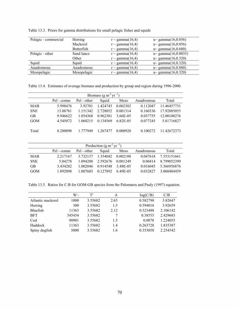
70

Table 13.3. Priors for gamma distributions for small pelagic fishes and squids

Herring r ~ gamma(16,4) u~ gamma(16,0.056) Mackerel r ~ gamma(16,4) u~ gamma(16,0.056)

Pelagic - commercial

Butterfish r ~ gamma(16,4) u~ gamma(16,0.680) Sand lance r ~ gamma(16,4) u~ gamma(16,0.0035) Pelagic - other Other r ~ gamma(16,4) u~ gamma(16,0.320)

Squid Squid r ~ gamma(16,4) u~ gamma(16,0.320) Anadromous Anadromous r ~ gamma(16,4) u~ gamma(16,0.880) Mesopelagic Mesopelagic r ~ gamma(16,4) u~ gamma(16,0.320)

Table 13.4. Estimates of average biomass and production by group and region during 1996-2000.

Biomass (g m-2 yr -1) Pel - comm Pel - other Squid Meso Anadromous Total

MAB 5.998476 3.92701 1.424743 0.002302 0.112047 11.46457731 SNE 13.88781 1.151342 2.728052 0.001314 0.160336 17.92885055 GB 9.946622 1.054368 0.962301 3.66E-05 0.037755 12.00108276 GOM 4.545072 1.060215 0.134569 6.82E-05 0.077245 5.81716827 Total 8.280098 1.777949 1.267477 0.000928 0.100272 11.42672373 Production (g m-2 yr -1)

Pel - comm Pel - other Squid Meso Anadromous Total MAB 2.217167 3.732137 1.354042 0.002188 0.047618 7.353151661 SNE 5.04278 1.094208 2.592676 0.001249 0.06814 8.799052399 GB 3.434282 1.002046 0.914548 3.48E-05 0.016045 5.366956876 GOM 1.892098 1.007603 0.127892 6.49E-05 0.032827 3.060484459

Table 13.5. Ratios for C:B for GOM-GB species from the Palomares and Pauly (1997) equation.

W~ T' A log(C/B) C/B Atlantic mackerel 1000 3.55682 2.65 0.582798 3.82647 Herring 300 3.55682 1.5 0.594016 3.92659 Bluefish 11363 3.55682 2.12 0.323488 2.106142 BFT 545454 3.55682 7 0.38555 2.429683 Cod 90901 3.55682 1.5 0.0878 1.224053 Haddock 11363 3.55682 1.4 0.263728 1.835387 Spiny dogfish 5000 3.55682 1.6 0.353058 2.254542

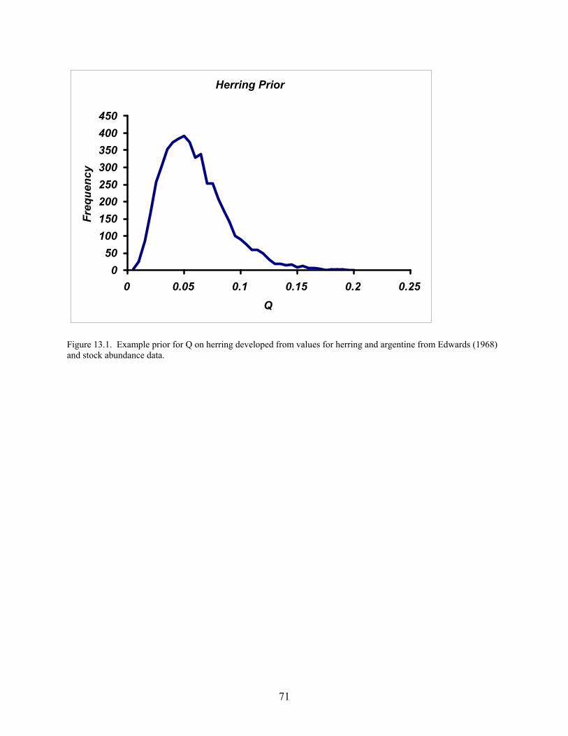
71

Herring Prior

050

100150200250300350400450

0 0.05 0.1 0.15 0.2 0.25Q

Freq

uenc

y

Figure 13.1. Example prior for Q on herring developed from values for herring and argentine from Edwards (1968) and stock abundance data.

72

14. Demersals (benthivores, omnivores, piscivores) and Medium Pelagics Jon K.T. Brodziak, Christopher M. Legault, and Laurel A. Col (nodes #22-24, 21) Background

Three groups of demersal species were formed based on feeding preferences described in

Collette and Klein-MacPhee (2002). These are: benthivores, piscivores, and omnivores (includes all others). The demersal benthivore group was composed of species that primarily feed on benthic prey. This group included gadiformes, elasmobranchs, pleuronectiformes, perciformes, scorpaeniformes, and other benthivores (Table 14.1). The demersal piscivore group included species that feed primarily on fishes. This group included gadiformes, elasmobranchs, and other piscivores (Table 14.2). The unclassified demersals was a large group composed of either omnivorous species that fed opportunistically on both benthos and fish (Table 14.3), or unclassified southern demersal species whose food habits were not reported in Collette and Klein-MacPhee (2002; Table 14.4).

Data Sources

Annual research survey data were collected from 1968-2003 to estimate demersal and

pelagic biomasses using a stratified random sampling design (Azarovitz 1981). Quantitative Approach for Biomass Estimates

Survey Catchability

Research survey catchability varies among species and groups of species. If it were known for a given species or group, survey catchability (Q) would provide a direct estimate of absolute biomass (B) based on the survey index value (I):

(EQ. 14.1) QIB �

We assumed that the average survey catchability for each demersal or pelagic species

group was constant and estimable. Seasonal estimates of average survey catchability were made for each species group during spring and autumn using the Bayesian estimation approach described below. The seasonal estimates of Q were then applied to spring and autumn survey swept-area biomass indices during 1968-2003 to produce an estimate of absolute biomass for each species group and season using Equation 14.1. The seasonal estimates of absolute biomass were then averaged to produce an estimate of average annual biomass for each species group during 1968-2003. Bayesian Estimation Approach

A priori, it was recognized that there were few direct observations to estimate the average

catchability of many species groups. Given this lack of information, we chose to use a Bayesian estimation approach to incorporate information on catchability from previous studies. This

73

enabled us to use both prior information and observed data to estimate seasonal catchabilities for species groups. A probability model (likelihood) was developed for observed catchability data where both model parameters and observed data were assumed to be random variables. The joint probability distribution for model-based catchability estimate (Q) and catchability data (D), denoted by p(Q, D), depended on the prior distribution of model parameters (see Informative Priors below), denoted by p(Q) , and the likelihood of observing the data (see Likelihood of Catchability Observations below), denoted by p(D | Q)�L(D | Q). (EQ. 14.2) p(Q | D) = p(Q)p(D | Q)

Applying Bayes’ rule for the conditional probability of model parameters given the data, the posterior distribution of model parameters was p(Q | D)

(EQ. 14.3) � � � �

� �� � � �

� �p Q Dp Q D

p Dp Q p D Q

p D|

, |� �

where the integrated likelihood p(D) was the constant

(EQ. 14.4)� � � � � �p D p Q p D Q dQ� � |

Since p(D) was constant with respect to the model parameters (which have been integrated out of the expression), the posterior distribution of model parameters is proportional to the product of the (informative) prior and the likelihood

(EQ. 14.5) � � � � � �p Q D p Q p D Q| |�

Markov Chain Monte Carlo (MCMC) simulation (Gilks et al. 1996) was applied to numerically generate posterior samples from Equation. 14.5. MCMC simulates a random walk through the set of possible catchability values that converges to a stationary distribution that is exactly the posterior distribution of Q. This simulation was equivalent to numerically integrating Equation 14.3. We used the WINBUGS 1.4 software for performing the MCMC calculations (Spiegelhalter et al. 2003). For each species group, two simulated chains of length 110,000 posterior samples of Q were generated. In the first chain the coefficient of variation (CV) for Q was 50% while CV[Q] = 75% in the second chain. The first 10,000 samples of both chains were discarded to burn them in (i.e., to eliminate dependence on the initial value of Q). Of the remaining 100,000 samples in each chain, every other sample was discarded to eliminate the possibility of autocorrelation. This left 100,000 posterior samples of Q for inference (50,000 from each chain). Inferences about the estimated absolute biomasses of species groups were based on this numerical integration of p(Q | D). For example, the expected value of biomass of the jth species group (Bj) in a given year was calculated from N=100,000 posterior samples of the survey catchability of the jth species group (Q1, Q2, Q3 ,...) as

74

(EQ. 14.6) � � � �E B D

NB Qj j

T

T

N

| ���1

1 Informative Priors

Prior information on NEFSC research survey catchabilities was available from two

sources: Edwards (1968) and Clark and Brown (1977). In the former study, Edwards developed estimates of NEFSC survey catchability for 27 species based on their seasonal availability within the survey region and their vulnerability to the survey trawl gear. These survey catchability estimates were scaled to adjust survey swept-area biomass indices to absolute biomasses. In Clark and Brown’s study, estimates of NEFSC autumn survey catchability were developed for several species using estimates of fishing mortality, total catch and stock size, and relative survey abundance indices. These catchability estimates were appropriate for scaling survey mean catch biomass per tow and were rescaled to swept-area values for comparison with Edwards’ results.

The informative prior for catchabilities of demersal species groups was assumed to be a gamma distribution with shape (r) and scale (μ) parameters.

(EQ. 14.7) � � � � � �p Q r Gamma r Q

er

for Qr rQ

| , ~ ,� � ��

�

1 0�

This choice provided a flexible positive distribution with mean equal to E[Q] = r/μ and coefficient of variation equal to CV[Q] = r -0.5.

For the demersal species groups, the expected value of the informative catchability prior was determined from Edwards’ (1968) catchability estimate for the “all others” species group (Q = 0.16) and Clark and Brown’s (1977) untransformed catchability estimate for “other finfish” (Q = 0.13, CV = 31%). These two values were chosen because they represented general groups of species that were not actively targeted by commercial fisheries at that time. We set the expected value of the catchability prior to equal the average of the two catchability estimates so that E[Q] = 0.145. Given the expected value of Q, the CV[Q] was assumed to be 50%. This implied that the informative prior was more variable than Clark and Brown’s estimate of survey Q.

The shape and scale parameters of the informative prior for demersal species groups were also parameters in the estimation model. Both were assumed to be distributed as a gamma random variable with parameters chosen to match the values of E[Q] and CV[Q]. In particular, the hyperprior for the shape parameter r was distributed as Gamma(16, 4). This implied that the expected value of r was E[r] = 4, with CV[r] = 25%. The hyperprior for the scale parameter μ was distributed as Gamma(16, 0.58). This implied that the expected value of μ was E[μ] = 27.6 with CV[μ] = 25%. These choices led to E[r]/E[μ] = E[Q] = 0.145 and CV[Q] = 50%. Observed Catchability Data

There were two sources of survey catchability observations (QOBS) for the demersal

species groups: Edwards (1968); and catchability observations derived from stock assessment data. Edwards (1968) provided survey catchability data for a total of 23 species (Table 14.2). Of these, the same catchability data was used for benthivore and omnivore elasmobranchs given the

75

similarity in their benthic habitats and body shapes. These catchabilities were used as average values for autumn and spring since Edwards included seasonal availability as a calculation factor. There were a total of 12 catchability observations derived from assessment data (Table 14.2). All of these were derived from age-structured assessment information (NEFSC 2002, NEFSC 2003a, NEFSC 2003b, Terceiro 2003), with the exception of spiny dogfish (Squalusacanthias, NEFSC 2003b). Separate catchability values for autumn and spring were derived by regressing survey swept-area biomass (thousand mt) on stock biomass (thousand mt) over the assessment time period. The slopes of these regressions were the observed survey catchabilities. This approach was used for 11 stocks. Seasonal differences in catchability were apparent for some stocks (e.g., American plaice, Hippoglossoides platessoides), but not for others. For spiny dogfish, the assessment-based catchability was derived as the ratio of total spring survey swept-area biomass during 1990-2002 to total biomass estimated using the minimum trawl herding assumption (NEFSC 2003b, Tables B6.2 and B7.3) during the same period. Likelihood of Catchability Observations

The likelihood of a single catchability observation was a gamma distribution (Equation

14.3) with shape and scale parameters set by the informative priors. Seven demersal subgroups did not have any catchability observations (Table 14.2). These were: other benthivores, other omnivores, and the five unclassified southern demersal species subgroups. For the pelagic groups, only the pelagic commercial finfish group had catchability observations (Table 14.2). Catchabilities of the remaining groups that had no catchability observations were determined by their informative priors. The joint likelihood of a total of n catchability observations (Qi) was

(EQ. 14.8) � � � �L D

rQ e

r n

ir Q

i

ni|!

� ��"#$

%&'

�(�

1

1 Average Biomass Production

Average biomass production per unit area was computed for each species group, region,

and year. There were some obvious outliers due to variability in survey catches. These outliers had a disproportionate influence on average biomass. To identify outliers in an objective manner we computed biomass production anomalies (BANOM) for each group and region using the median (B0.5) and standard deviation (σB) of the observed values (BOBS)

(EQ. 14.9) B

B BANOMOBS

B�

0 5.

)

We removed outliers based on the biomass production anomalies. For demersal species groups, an observed value was an outlier if BANOM > 3. Applying this criterion led to removal of 10 outliers out of a total of 864 observed values (�1%).

Average biomass production per unit area (grams per square meter) was computed for each species group and region over the period 1968-2003. This was done to see if there were regional differences in biomass production by individual species groups. Average total biomass production for demersal species groups was also computed along with the percent contribution of

76

each group to the total. This was expected to show whether the production of demersal biomass differed among regions. Last, the average total production of demersal biomass was computed for each region to determine differences in total biomass production among regions. Example Results Average biomass production

Total demersal biomass production differed among regions (Figure 14.1). On average,

Georges Bank had the highest demersal biomass (14 g m-2) while the Gulf of Maine had the lowest (10 g m-2). The Mid-Atlantic Bight had the most variability in demersal biomass and the Gulf of Maine had the least variability. Overall, total demersal biomass was less variable than biomass for the individual demersal groups.

Biomass production by the individual demersal groups also differed among regions (Figure 14.1). The highest average benthivore biomass was in the Mid-Atlantic Bight (5 g m-2) while the lowest was in Southern New England (2 g m-2). Average piscivore biomass ranged from a low of 6 g m-2 in the Mid-Atlantic Bight and Georges Bank to a high of 8 g m-2 in Southern New England. The highest average omnivore biomass was on Georges Bank (5 g m-2). In comparison, omnivore biomass was only 1 g m-2 in the Gulf of Maine and the Mid-Atlantic. Benthivore biomass varied substantially in each region with CVs ranging from 35-50%. Piscivore and omnivore biomasses were also highly variable, with CVs of 40-65%. The exception was the Gulf of Maine piscivore biomass which was the least variable of all the groups (CV=23%).

Individual demersal groups contributed differing percentages to the total demersal biomass by region (Figure 14.1). The piscivore group was the dominant group in each region. Its contribution to total demersal biomass ranged from a low of 37% for Georges Bank to a high of over 60% in the Gulf of Maine and Southern New England. The benthivore group was the 2nd dominant group in the Gulf of Maine (31%) and Mid-Atlantic Bight (41%). These regions also had the lowest percent composition of omnivores (9%). In comparison, the omnivore group was 2nd dominant on Georges Bank (34%) and in Southern New England (20%). Production/Growth/Reproduction

Production for demersals and medium pelagics was estimated using age-based data for a

small number of assessed stocks to confirm literature values for the P:B ratio (Cohen et al. 1982; Sissenwine 1987; Savenkoff et al. 2004). Two approaches were used to estimate the P:B ratios from virtual population analysis results: age-based growth and a production model. The age-based growth approach computed the change in weight at age for each cohort in a given year and multiplied these values by the average biomass for that age. Summing these values produced an estimate of production which was then divided by the beginning of the year biomass to generate an estimate of the P:B ratio. The production model approach calculated production as the total catch plus the change in biomass each year and then divided that by the biomass to produce a P:B ratio. Results for Georges Bank cod, haddock and yellowtail flounder ranged from 0.34 to 0.48 for the age-based growth approach and ranged from 0.35 to 0.59 for the production model approach. These results agreed in general with the literature values for demersals and medium

77

pelagics. The selected values for the P:B ratio varied by group: demersal benthivores and omnivores had a ratio of 0.45 while demersal piscivores and medium pelagics had a ratio of 0.55. Consumption

Consumption was estimated using the methods described in Section 22: Consumption

and Diet Composition Matrix, based on NEFSC research survey observations. Resulting C:B ratios for the Gulf of Maine ecoregion were on the order of 0.6 to 3.0. References Azarovitz, TR. 1981. A brief historical review of the Woods Hole Laboratory trawl survey time series. In: Bottom

Trawl Surveys. Can. Spec. Sci. Pub. Fish. Aquat. Sci. 58:62-67. Brodziak, JKT; and W.K. Macy., III.. 1996. Growth of long-finned squid, Loligo pealei, in the northwest Atlantic.

Fish. Bull. 94:212-236. Brodziak, J; Link, J. 2002. Ecosystem-based fishery management: What is it and how can we do it? Bull. Mar. Sci.

70(2):589-611. Brown, JH; Gillooly, JF; Allen, AP; West, GB. 2004. Towards a metabolic theory of ecology. Ecol. 85(7):1771-

1789. Choi, JS; Frank, KT; Leggett, WC; Drinkwater, K. 2004. Transition to an alternate state in a continental shelf

ecosystem. Can. J. Fish. Aqua. Sci. 61:505-510. Clark, SH; Brown, BE. 1977. Changes in biomass of finfishes and squids from the Gulf of Maine to Cape Hatteras,

1963-74, as determined from research vessel survey data. Fish. Bull. 75(1):1-21. Cohen, EB; Grosslein, MD; Sissenwine, MP; Steimle, F; Wright, WR. 1982. Energy budget of Georges Bank.

Canadian Special Publication of Fisheries and Aquatic Sciences. Workshop on Multispecies Approaches to Fisheries Management Advice, St. John's, Newfoundland.

Collette, BB; Klein-MacPhee, G, eds. 2002. Bigelow and Schroeder’s Fishes of the Gulf of Maine, 3rd Ed. Washington, D.C.: Smithsonian Institution Press; 748 p.

Edwards, RL. 1968. Fishery resources of the North Atlantic area. In: Gilbert, DW, ed. The future of the fishing industry of the United States. Univ. of Washington Publications in Fisheries. 4:52-60.

Fogarty, MJ; Cohen, EB; Michaels, WL; Morse, WW. 1991. Predation and the regulation of sand lance populations: an exploratory analysis. ICES Mar. Sci. Symp. 193:120-124.

Fogarty, MJ; Murawski, SA. 1998. Large-scale disturbance and the structure of marine ecosystems: fishery impacts on Georges Bank. Ecol. Appl. 8(1) Suppl. S6-S22 p.

Gilks, WR; Richardson, S; Spiegelhalter, DG, eds. 1996. Markov chain monte carlo in practice. London, UK: Chapman and Hall; 486 p.

Harley, SJ; Myers, R; Barrowman, N; Bowenand, K; Admiro, R. 2001. Estimation of research trawl survey catchability for biomass reconstruction of the eastern Scotian Shelf. Can. Sci. Advis. Sec. Res. Doc. 2001/084; 54 p.

Hatfield, EMC; Hanlon, RT; Forsythe, JW; Grist, EPM. 2001. Laboratory testing of a growth hypothesis for juvenile squid Loligo pealeii (Cephalopoda: Loliginidae). Can. J. Fish. Aquat. Sci. 58:845-857.

Link, J. 1999. (Re)Constructing food webs and managing fisheries. In: Ecosystem approaches for fisheries management. Univ. Of Alaska Sea Grant, AK-99-01, Fairbanks; p. 571-588.

Link, JS; Garrison, LP. 2002. Changes in piscivory associated with fishing induced changes to the finfish community on Georges Bank. Fish. Res. 55:71-86.

Mayo, RK; Fogarty, MJ; Serchuk, FM. 1992. Aggregate fish biomass and yield on Georges Bank, 1960-87. J.Northw. Atl. Fish. Sci. 14:59-78.

Mountain, DG; Holzwarth, TJ. 1989. Surface and bottom temperature distribution for the northeast continental shelf. NOAA Technical Memorandum. NMFS-F/NEC-73; 32 p. Available from NEFSC Library, 166 Water St., Woods Hole, MA 02543.

Mountain, DG; Taylor, MH; Bascuñán, C. 2004. Revised Procedures for Calculating Regional Average Water Properties for Northeast Fisheries Science Center Cruises. Woods Hole, MA. Northeast Fish. Sci. Cent. Ref. Doc. 04-08; 62 p.

Murawski, SA; Brown, R; Lai, H-L; Rago, PJ; Hendrickson, L. 2000. Large-scale closed areas as a fishery-

78

management tool in temperate marine ecosystems: the Georges Bank experience. Bull. Mar. Sci. 66(3):775-798.

New England Fishery Management Council (NEFMC). 2003. Final Amendment 13 to the Northeast Multispecies Fishery Management Plan including a Final Supplemental Environmental Impact Statement and an Initial Regulatory Flexibility Analysis. NEFMC, Newburyport, MA 01950; 1659 p. Available at: http://www.nefmc.org/nemulti/index.html

NEFSC (Northeast Fisheries Science Center). 2000. Atlantic Mackerel. 30th Northeast Regional Stock Assessment Workshop (30th SAW). Woods Hole, MA. Northeast Fish. Sci. Cent. Ref. Doc. 00-03; 37 p.

NEFSC. 2002. Assessment of 20 northeast groundfish stocks through 2001. A report of the Groundfish Assessment Review Meeting. Woods Hole, MA. Northeast Fish. Sci. Cent. Ref. Doc. 02-16; 478 p.

NEFSC. 2003. 37th Northeast Regional Stock Assessment Workshop (37th SAW) Stock Assessment Review Committee (SARC) Consensus Summary of Assessments. Woods Hole, MA. Northeast Fish. Sci. Cent. Ref. Doc. 03-16; 603 p.

NEFSC. 2004. Atlantic Butterfish. 38th Northeast Regional Stock Assessment Workshop (38th SAW). Woods Hole, MA. Northeast Fish. Sci. Cent. Ref. Doc. 04-03; 72 p.

O’Reilly, J; Evans-Zetlin, C; Busch, D. 1987. Primary production. In: Backus, R; Price, R; Bourne, D, eds. Georges Bank. Cambridge, MA: MIT Press; p. 220-233.

Overholtz, WJ; Friedland, KD. 2002. Recovery of the Gulf of Maine-Georges Bank Atlantic herring (Clupea harengus) complex: perspectives based on bottom trawl survey data. Fish. Bull. 100:593-608.

Overholtz, WJ; Jacobson, LD; Melvin, GD; Cieri, M; Power, M; Libby, D; Clark, K. 2004. Stock assessment of the Gulf of Maine-Georges Bank Atlantic herring complex, 2003. Woods Hole, MA. Northeast Fish. Sci. Cent. Ref. Doc. 04-06; 290 p.

Savenkoff, C; Castonguay, M; Despatie, S-P; Chabot, D; Hammill, MO. 2004. Inverse modelling of trophic flows through an entire ecosystem: the northern Gulf of St. Lawrence in the mid-1980s. Can. J. Fish. Aquat. Sci. 61: 2194–2214.

Sissenwine, MP. 1987. Fish and squid production. In: Backus, R; Price, R; Bourne, D, eds. Georges Bank. Cambridge, MA: MIT Press; p. 347-350.

Spiegelhalter, D; Thomas, A; Best, N; Lunn, D. 2003. WinBUGS User Manual. Available at: http://www.mrc.bsu.carn.ac.uk/bugs

Terceiro, M. 2003. Stock Assessment of Summer Flounder for 2003. Wood Hole, MA. Fish. Sci. Cent. Ref. Doc. 03-09. 190 p.

Wigley, S; Brodziak, JKT; Col, L. 2003. Assessment of the Gulf of Maine and Georges Bank witch flounder stock for 2003. Wood Hole, MA. Fish. Sci. Cent. Ref. Doc. 03-14; 194 p.

79

Table 14.1. List of species in the demersal benthivore category.

Demersal Benthivores Gadiformes Elasmobranchs Perciformes Scorpaeniformes Others

Melanogrammus aeglefinus Dasyatis centroura Macrorhamphosus scolopax Pontinus longispinis Myxine glutinosa Urophycis chuss Etmopterus princeps Synagrops bellus Sebastes fasciatus Antigonia capros Urophycis regia Dasyatis say Micropogonias undulatus Helicolenus dactylopterus Opsanus tau Antimora rostrata Myliobatis freminvillei Synagrops spinosus Helicolenus maderensis Dibranchus atlanticus Enchelyopus cimbrius Torpedo nobiliana Orthopristis chrysoptera Artediellus sp. Ogcocephalus corniger Brosme brosme Raja eglanteria Stenotomus chrysops Cottidae Chlorophthalmus sp Gaidropsarus ensis Leucoraja garmani Epigonus pandionis Triglops murrayi Chlorophthalmus agassizi Macrouridae Malacoraja senta Menticirrhus saxatilis Myoxocephalus scorpius Gonostoma bathyphilum Nezumia bairdi Dasyatis americana Pogonias cromis Myoxocephalus

octodecemspinosusGonostoma atlanticum

Macrourus berglax Rhinoptera bonasus Bairdiella chrysoura Hemitripterus americanus Gonostoma elongatum

Coelorhynchus carminatus Leiostomus xanthurus Aspidophoroides monopterygius Vinciguerria sp

Otophidium omostigmum Howella sherborni Myoxocephalus aenaeus Polymetme thaeocoryla Ophidion marginatum Pleuronectiformes Lopholatilus chamaeleonticeps Liparis inquilinus Chauliodus danae Lepophidium profundorum Poecilopsetta beani Tautogolabrus adspersus Eumicrotremus spinosus Parasudis truculenta Malacocephalus occidentalis Hippoglossoides platessoides Tautoga onitis Prionotus carolinus Xenodermichthys copeiOphidion grayi Paralichthys oblongus Astroscopus guttatus Prionotus evolans Polymixia lowei Ophidion welshi Limanda ferruginea Lumpenus lumpretaeformis Peristedion miniatum Polymixia nobilis

Pseudopleuronectes americanus Lumpenus maculatus Triglidae Hoplostethus occidentalis Glyptocephalus cynoglossus Ulvaria subbifurcata Careproctus ranula Gephyroberyx darwini Scophthalmus aquosus Mullus auratus Prionotus paralatus Saurida brasiliensis Citharichthys arctifrons Lycodes reticulatus Bagre marinus Monolene sessilicauda Lycenchelys verrilli Opsanus pardus Etropus microstomus Cryptacanthodes maculatus Porichthys plectrodon Trinectes maculatus Anarhichas lupus

Macrozoarces americanus Nesiarchus nasutus

Table 14.2. List of species in the demersal piscivore category.

Demersal Piscivores Gadiformes Elasmobranchs Others

Merluccius albidus Carcharhinus obscurus Reinhardtius hippoglossoides Merluccius bilinearis Centroscyllium fabricii Hippoglossus hippoglossus Gadus morhua Carcharhinus plumbeus Paralichthys dentatus Pollachius virens Carcharias taurus Trichiurus lepturus Urophycis tenuis Mustelus canis Lophius americanus Urophycis chesteri Scyliorhinus retifer Gadidae Squalus acanthias Merluccius sp. Squatina dumeril

Table 14.3. List of species in the demersal omnivore category.

Demersal Omnivores Elasmobranchs Others

Dipturus laevis Centropristis striata Leucoraja ocellata Leucoraja erinacea Amblyraja radiata

80

Table 14.4. List of species in the unclassified southern demersal category.

Unclassified Southern Demersal Species Perciformes Perciformes (Cont.) Perciformes (Cont.) Tetradontiformes

Schultzea beta Epinephelus mystacinus Halichoeres caudalis Balistidae Mycteroperca interstitialis Apogon aurolineatus Halichoeres poeyi Parahollardia lineata Centropristis ocyurus Rypticus subbifrenatus Halichoeres radiatus Aluterus heudeloti Centropristis philadelphica Eucinostomus gula Hemipteronotus novacula Aluterus monoceros Epinephelus inermis Gerreidae Lachnolaimus maximus Aluterus schoepfi Diplectrum bivittatum Archosargus probatocephalus Labridae Aluterus scriptus Diplectrum formosum Perciformes Chaetodontidae Balistes vetula Epinephelus adscensionis Calamus bajonado Chaetodon aculeatus Canthidermis sufflamen Epinephelus drummondhayi Calamus calamus Cryptotomus roseus Monacanthus ciliatus Epinephelus flavolimbatus Calamus leucosteus Nicholsina usta Lactophrys bicaudalis Epinephelus guttatus Calamus nodosus Scarus coeruleus Lactophrys polygonia Epinephelus morio Calamus penna Sparisoma radians Lactophrys quadricornis Epinephelus nigritus Calamus proridens Scaridae Lactophrys trigonus Epinephelus niveatus Diplodus argenteus Mugil liza Lactophrys triqueter Epinephelus striatus Diplodus holbrooki Mugil gyrans Canthigaster rostrata Hemanthias vivanus Lagodon rhomboides Sphyraena barracuda Sphoeroides dorsalis Mycteroperca bonaci Pagrus sedecim Sphyraena borealis Sphoeroides nephelus Mycteroperca microlepis Stenotomus caprinus Sphyraena guachancho Sphoeroides spengleri Mycteroperca phenax Sparidae Opistognathus lonchurus Sphoeroides testudineus Mycteroperca venenosa Cynoscion arenarius Opistognathus maxillosus Chilomycterus antillarum Holanthias martinicensis Cynoscion nebulosus Bembrops gobioides Chilomycterus atinga Paranthias furcifer Cynoscion nothus Astroscopus y-graecum Diodon holocanthus Hemanthias aureorubens Equetus acuminatus Xenocephalus egregius Diodon hystrix Serraniculus pumilio Equetus lanceolatus Kathetostoma albigutta Tetraodontidae Serranus annularis Equetus punctatus Clinidae Sphoeroides pachygaster Serranus atrobranchus Equetus umbrosus Hypsoblennius ionthas Serranus baldwini Larimus fasciatus Blenniidae Serranus notospilus Menticirrhus americanus Ammodytes americanus Serranus phoebe Menticirrhus littoralis Foetorepus agassizi Serranus subligarius Sciaenops ocellatus Dormitator maculatus Serranidae Stellifer lanceolatus Bathygobius soporator Rypticus bistrispinus Sciaenidae Gobiosoma bosc Priacanthus cruentatus Eucinostomus argenteus Gobiidae Pristigenys alta Pseudupeneus maculatus Uranoscopidae Apogon maculatus Upeneus parvus Anisotremus virginicus Apogon pseudomaculatus Kyphosus sectatrix Haemulon aurolineatum Caulolatilus cyanops Chaetodipterus faber Haemulon carbonarium Lutjanus analis Chaetodon aya Haemulon plumieri Lutjanus apodus Chaetodon capistratus Haemulidae Lutjanus buccanella Chaetodon ocellatus Acanthurus bahianus Lutjanus campechanus Chaetodon sedentarius Acanthurus chirurgus Lutjanus griseus Chaetodon striatus Acanthurus coeruleus Lutjanus jocu Holacanthus bermudensis Ariomma regulus Lutjanus synagris Holacanthus ciliaris Peprilus alepidotus Lutjanus vivanus Holacanthus tricolor Stromateidae Ocyurus chrysurus Pomacanthus arcuatus Trichiuridae Pristipomoides aquilonaris Abudefduf saxatilis Ruvettus pretiosus Rhomboplites aurorubens Chromis enchrysurus Lepidocybium flavobrunneum Lutjanidae Chromis insolata Pomacentrus variabilis Lobotes surinamensis Pomacentrus leucostictus Scombridae Cookeolus japonicus Bodianus pulchellus Gempylus serpens Caulolatilus microps Clepticus parrae Cubiceps pauciradiatus Caulolatilus chrysops Decodon puellaris Seriola fasciata Caulolatilus intermedius Halichoeres bathyphilus Haemulon striatum Malacanthus plumieri Halichoeres bivittatus Ariomma melanum Paralepidae Uraspis secunda Parablennius marmoreus Chasmodes bosquianus Hypleurochilus geminatus Hypsoblennius hentz

81

Table 14.4, continued. Pleuronectiformes Elasmobranchs Scorpaeniformes Gadiformes

Ancylopsetta dilecta Narcine brasiliensis Neomerinthe hemingwayi Laemonema barbatulum Ancylopsetta quadrocellata Raja ackleyi Pontinus rathbuni Ophidion beani Bothus lunatus Dipturus olseni Scorpaena agassizi Ophidion selenops Bothus ocellatus Bathyraja spinicauda Scorpaena brasiliensis Chascanopsetta lugubris Raja texana Scorpaena calcarata Citharichthys arenaceus Dasyatis sabina Scorpaena dispar Others Citharichthys cornutus Dasyatis violacea Scorpaena grandicornis Citharichthys macrops Gymnura altavela Scorpaena plumieri Xenolepidichthys dalgleishi Citharichthys spilopterus Gymnura micrura Scorpaenidae Engraulidae Cyclopsetta fimbriata Urolophus jamaicensis Bellator brachychir Synodontidae Engyophrys senta Myliobatis goodei Bellator egretta Argentina striata Etropus crossotus Squalidae Bellator militaris Anchoa lyolepis Etropus rimosus Etmopterus gracilispinis Peristedion gracile Chaunax stigmaeus Gastropsetta frontalis Etmopterus hillianus Prionotus alatus Gymnothorax saxicola Paralichthys albigutta Centroscymnus coelolepis Prionotus ophryas Harengula jaguana Paralichthys lethostigma Breviraja plutonia Prionotus roseus Echiophis punctifer Paralichthys squamilentus Alopias vulpinus Prionotus longispinosus Gobiesox strumosus Syacium gunteri Alopias superciliosus Prionotus rubio Ogcocephalus radiatus Syacium micrurum Isurus paucus Prionotus scitulus Syacium papillosum Carcharhinus isodon Prionotus tribulus Etropus sp Carcharhinus altimus Myoxocephalus quadricornis Bothidae Carcharhinus longimanus Prionotus stearnsi Paralichthys sp. Carcharhinus brevipinna Trachyscorpia cristulata Citharichthys sp. Carcharhinus porosus Bothus robinsi Carcharhinus perezii Pleuronectiformes Carcharhinus signatus Citharichthys gymnorhinus Mustelus norrisi Pleuronectidae Triakis semifasciata Gymnachirus melas Sphyrna media Symphurus civitatus Symphurus diomedianus Symphurus minor Symphurus marginatus Symphurus plagiusa Symphurus pusillus Symphurus urospilus

82

2

4

6

8

10

12

14

Gul

f of M

aine

2

4

6

8

10

0.5

1.0

1.5

2.0

2.5

3.0

3.5

4.0

Geo

rges

Ban

k

2

4

6

8

10

5

10

15

20

2468

101214161820

Biomass per area (g/m

2)

1

2

3

4

5

6

5

10

15

20

25

2

4

6

8

1965 1970 1975 1980 1985 1990 1995 2000 2005

Mid

-Atla

ntic

Big

ht

0

2

4

6

8

10

12

14

16

Year

1965 1970 1975 1980 1985 1990 1995 2000 200502468

101214161820

1965 1970 1975 1980 1985 1990 1995 2000 20050.0

0.5

1.0

1.5

2.0

2.5

3.0

3.5

4.0

Sou

ther

n N

ew E

ngla

nd

Benthivores Piscivores Unclassified

Figure 14.1. Time series of annual demersal biomass production (g m-2) by benthivores, piscivores, and unclassified species in four regions of the Northeast United States Continental Shelf Ecosystem (Gulf of Maine, Georges Bank, Southern New England, and Mid-Atlantic Bight) during 1968-2003.

83

15. Large Pelagics (coastal sharks, pelagic sharks, and highly migratory species) William J. Overholtz (nodes #25-27) Background and Estimation Approaches

Bluefin tuna Virtual Population Analysis (VPA) estimates of stock size and biomass were

obtained from a recent ICCAT (International Commission for the Convservation of Atlantic Tunas) stock assessment (ICCAT 2003). For bluefin tuna we assumed that 50% of the age 3+ VPA biomass occupies the New England region during July-October. This approach produced a biomass of 9,067 mt during July-October and an annual average biomass of 3,022 for the entire region (Table 15.1). Combining subjective information about the distribution of bluefin tuna during their residency period from the Mid-Atlantic region to the Gulf of Maine with some information in the literature (Chase 2002), we assumed that 45% of the regional contingent was found in both the Gulf of Maine and Georges Bank ecoregions and 10% in the SNE region. Biomass in the 4 ecoregions was the product of the regional proportions and the average annual biomass (Table 15.1).

Since no stock abundance information is available for yellowfin, bigeye, albacore, swordfish, and white-blue marlin, we developed a ratio method with Japanese longline ICCAT data (1978-1988, 5,640 sets) for the United States Exclusive Economic Zone (US EEZ) (Hoey etal. 2002). We used the ratio between catch rates for these species and bluefin tuna from Hoey etal. (2002) to produce a raising factor to scale tuna-billfish numbers during 1996-2000 to bluefin tuna numbers for the same period. We used ICCAT SCRS reports for each species to obtain mean weight data, and this was used to estimate biomass during each year. An assumption concerning the relative proportion of each stock in the 4 ecoregions was also made with distribution maps available in the ICCATR SCRS reports for each species. Average biomass for the 1996-2000 period was calculated for bluefin tuna, yellowfin tuna, bigeye tuna, albacore tuna, swordfish, and a white-blue marlin aggregate group.

Annual production for bluefin and bigeye tuna was calculated from VPA results for these species obtained from ICCAT SCRS Reports. Production data for these two species were used to calculate P:B ratios (bluefin tuna = 0.316, bigeye = 0.558). Production for albacore was calculated from the P:B ratio for bluefin tuna and yellowfin by using the P:B ratio for bigeye tuna. We assumed that swordfish and white-blue marlin are less productive, so a P:B ratio of 0.2 was used for these species. Consumption was calculated by assuming that the daily ration for the tunas was the same as for bluefin tuna (3%) and multiplying this value by the biomass during 1996-2000. Swordfish and white-blue marlin were assumed to have a daily ration of 1% body weight (BW). Landings for these species were obtained from ICCAT SCRS Reports, and it was assumed that only 10% of the average landings during 1996-2000 occurred on the continental shelf for albacore, yellowfin, bigeye, swordfish, and white-blue marlin (5% for yellowfin tuna) (Table 15.2). United States Bluefin tuna landings were averaged for 1996-2000 and scaled to account for residency time (Table 15.2). Data for all the tuna and billfish were summed for each ecoregion for biomass, production, consumption, and landings and converted to g m-2 (Table 15.3).

To estimate blue shark abundance, we used the ratio between blue shark and bluefin tuna catch rates from Hoey et al. (2002) to produce a raising factor to scale blue shark numbers during 1996-2000 to bluefin tuna numbers for the same period. This exercise produced a ratio of 1.5. Next a weighted average mean weight (drawn) was calculated from recreational mean weight

84

data (24.59 kg) collected during MRFSS interviews and a factor of 1.96 round:drawn ratio was used to convert to round weight (48.19 kg) (Cortez 2002). Biomass in the region was estimated by assuming that 50% of the stock (Kohler 1988) is found in the SNE-GOM area during May-October. This yielded a calculated biomass of 7,950 mt for the six month period and an annual average of 3,975 mt (Table 15.4). We further assumed that the biomass was equally distributed (Kohler 1988) over the SNE-GOM ecoregions, with 1,325 mt in each region (Table 15.4).

For the other sharks (hammerhead, shortfin mako, thresher, dusky, porbeagle, sandbar, and other) we used the ratio between the catch rates of these sharks and blue shark from Hoey etal. (2002) to produce a raising factor to scale numbers during 1996-2000 to blue shark numbers for the same period. Next a weighted average mean weight (drawn) was calculated from recreational mean weight data collected during MRFSS interviews for blue, mako, thresher, and porbeagle shark. The average weight for mako shark was used for sandbar and dusky, while the average weight for blue shark was used for hammerhead shark because no information for these species was available. A factor of 1.96 round:drawn ratio was used to convert to round weight for each species (Cortez 2002). We further assumed that the biomass was unequally distributed over the MA-GOM ecoregions on a seasonal basis. Production and Consumption

Consumption by sharks in the four regions was estimated from daily ration estimates for

blue (0.056) and mako (0.010) shark available from the literature (Stillwell and Kohler 1982; Kohler 1988). An average of these two values (0.008) was used to estimate consumption for the other shark species. Production for all sharks was estimated by assuming a P:B ratio of 0.1. This ratio was used with average biomass to calculate production for each species. Recreational and commercial landings of sharks were averaged during 1996-2000, scaled down to account for the percentage landed in the region, and scaled to an annual basis since sharks are only present during about half the year. Data for biomass, production, consumption, and landings were further scaled to g m-2 for each ecoregion and combined into a pelagic group (thresher, mako, blue, porbeagle, and hammerhead) and a coastal group (dusky, sandbar, other) (Table 15.5). References Chase, B.C. 2002. Differences in diet of Atlantic bluefin tuna (Thunnus thynnus) at five seasonal feeding grounds

on the New England continental shelf. Fisheries Bulletin. 100:168-180. Cortes, E. 2002. Catches and catch rates of pelagic sharks from the Northwestern Atlantic, Gulf of Mexico, and

Caribbean. Collected Volumes Scientific Papers. ICCAT. 54(4): 1164-1181. Hoey, J.J, E. Pritchard, C. Brown, and M. Showell. 2002. Pelagic shark abundance indices based on fishery-

dependent and fishery-independent data from the western North Atlantic. Collected Volumes Scientific Papers. ICCAT. 54(4): 1199-1211.

ICCAT. 2003. Report of the 2002 Atlantic bluefin tuna stock assessment session. Col. Vol. Sci. Pap. ICCAT. 55(4):1289-1415.

Kohler, N.F. 1988. Aspects of the feeding ecology of the blue shark, Prionace glauca in the Western North Atlantic. PhD. Dissertation, University of Rhode Island. UMI Ann Arbor, MI. 163 pp.

Stillwell, C.E., and N.E. Kohler. 1982, Food, feeding habits, and estimates of daily ration of the shortfin mako (Isurus oxyrinchus) in the Northwest Atlantic. Canadian Journal of Fisheries and Aquatic Sciences. 39:407-414.

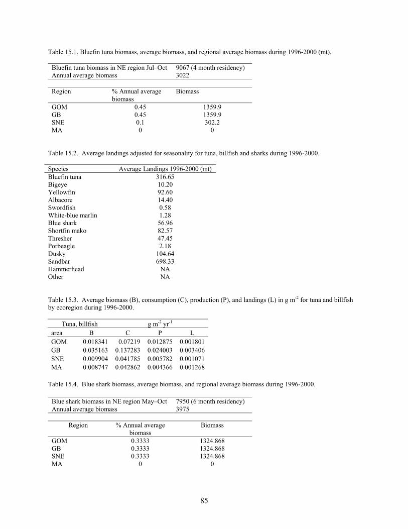
85

Table 15.1. Bluefin tuna biomass, average biomass, and regional average biomass during 1996-2000 (mt).

Bluefin tuna biomass in NE region Jul–Oct 9067 (4 month residency) Annual average biomass 3022 Region % Annual average

biomass Biomass

GOM 0.45 1359.9 GB 0.45 1359.9 SNE 0.1 302.2 MA 0 0

Table 15.2. Average landings adjusted for seasonality for tuna, billfish and sharks during 1996-2000. Species Average Landings 1996-2000 (mt) Bluefin tuna 316.65 Bigeye 10.20 Yellowfin 92.60 Albacore 14.40 Swordfish 0.58 White-blue marlin 1.28 Blue shark 56.96 Shortfin mako 82.57 Thresher 47.45 Porbeagle 2.18 Dusky 104.64 Sandbar 698.33 Hammerhead NA Other NA Table 15.3. Average biomass (B), consumption (C), production (P), and landings (L) in g m-2 for tuna and billfish by ecoregion during 1996-2000.

Tuna, billfish g m-2 yr-1 area B C P L GOM 0.018341 0.07219 0.012875 0.001801 GB 0.035163 0.137283 0.024003 0.003406 SNE 0.009904 0.041785 0.005782 0.001071 MA 0.008747 0.042862 0.004366 0.001268

Table 15.4. Blue shark biomass, average biomass, and regional average biomass during 1996-2000.

Blue shark biomass in NE region May–Oct 7950 (6 month residency) Annual average biomass 3975

Region % Annual average biomass

Biomass

GOM 0.3333 1324.868 GB 0.3333 1324.868 SNE 0.3333 1324.868 MA 0 0

86

Table 15.5. Average biomass (B), consumption (C), production (P), and landings (L) in g m-2 for pelagic and coastal sharks by ecoregion during 1996-2000.

Pelagic sharks g m-2 yr-1 Area B C P L GOM 0.013014 0.013513 0.001301 0.00023 GB 0.024358 0.025903 0.002436 0.000794 SNE 0.019873 0.022623 0.001987 0.001153 MA 0.010237 0.012939 0.001024 0.001044

Coastal sharks g m-2 yr-1 Area B C P L

GOM 0 0 0 0 GB 0 0 0 0 SNE 0.015858 0.023153 0.001586 0.005451 MA 0.016986 0.024799 0.001699 0.005838

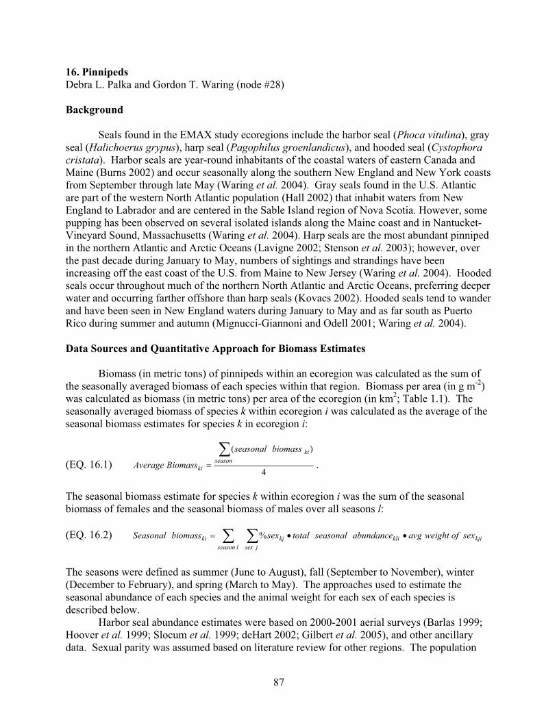
87

16. Pinnipeds Debra L. Palka and Gordon T. Waring (node #28) Background

Seals found in the EMAX study ecoregions include the harbor seal (Phoca vitulina), gray

seal (Halichoerus grypus), harp seal (Pagophilus groenlandicus), and hooded seal (Cystophoracristata). Harbor seals are year-round inhabitants of the coastal waters of eastern Canada and Maine (Burns 2002) and occur seasonally along the southern New England and New York coasts from September through late May (Waring et al. 2004). Gray seals found in the U.S. Atlantic are part of the western North Atlantic population (Hall 2002) that inhabit waters from New England to Labrador and are centered in the Sable Island region of Nova Scotia. However, some pupping has been observed on several isolated islands along the Maine coast and in Nantucket-Vineyard Sound, Massachusetts (Waring et al. 2004). Harp seals are the most abundant pinniped in the northern Atlantic and Arctic Oceans (Lavigne 2002; Stenson et al. 2003); however, over the past decade during January to May, numbers of sightings and strandings have been increasing off the east coast of the U.S. from Maine to New Jersey (Waring et al. 2004). Hooded seals occur throughout much of the northern North Atlantic and Arctic Oceans, preferring deeper water and occurring farther offshore than harp seals (Kovacs 2002). Hooded seals tend to wander and have been seen in New England waters during January to May and as far south as Puerto Rico during summer and autumn (Mignucci-Giannoni and Odell 2001; Waring et al. 2004). Data Sources and Quantitative Approach for Biomass Estimates

Biomass (in metric tons) of pinnipeds within an ecoregion was calculated as the sum of

the seasonally averaged biomass of each species within that region. Biomass per area (in g m-2) was calculated as biomass (in metric tons) per area of the ecoregion (in km2; Table 1.1). The seasonally averaged biomass of species k within ecoregion i was calculated as the average of the seasonal biomass estimates for species k in ecoregion i:

(EQ. 16.1) 4

)(�� season

ki

ki

biomassseasonal

BiomassAverage .

The seasonal biomass estimate for species k within ecoregion i was the sum of the seasonal biomass of females and the seasonal biomass of males over all seasons l: (EQ. 16.2) �� ���

jsexkjiklikj

lseasonki sexofweightavgabundanceseasonaltotalsexbiomassSeasonal %

The seasons were defined as summer (June to August), fall (September to November), winter (December to February), and spring (March to May). The approaches used to estimate the seasonal abundance of each species and the animal weight for each sex of each species is described below.

Harbor seal abundance estimates were based on 2000-2001 aerial surveys (Barlas 1999; Hoover et al. 1999; Slocum et al. 1999; deHart 2002; Gilbert et al. 2005), and other ancillary data. Sexual parity was assumed based on literature review for other regions. The population

88

age structure was assumed to be 30% ages 1-3 and 70% ages 4+. Age 7 mean weights (kg) for males (80.791) and females (68.796) (M. Hammill, pers. comm., DFO, Mont-Joli, Quebec) were used to estimate Gulf of Maine biomass. Age 6 weights (76.450 males, 66.023 females) were used for the Southern New England and Mid-Atlantic Bight regions.

Gray seal abundance estimates were derived from 2000-2003 surveys (Barlas 1999; S. Wood pers. comm., UMass Boston) and other ancillary data. A 50:50 sex ratio was assumed. Age 9 weights (kg) for males (208.0) and females (153.0) (Mohn and Bowen 1996) were used to estimate biomass in all ecoregions.

Harp seal abundance estimates were based on strandings and bycatch data (Waring et al. 2004). A 50:50 sex ratio was assumed. Juvenile harp seals comprise the bycatch and strandings data; therefore, age 4 weights (kg) were used to estimate biomass. Female and male age 4 weights were derived from the following equations (Chabot et al. 1996):

(EQ. 16.3) Female: mass = (98.6 e(-1.325e-0.383*age));

(EQ. 16.4) Male: mass = (103.3 e(-1.326e-0.352*age)).

Hooded seal abundance estimates were based on strandings and bycatch data (Waring etal. 2004). The stranding network saw primarily juvenile hooded seals (at ~ 120 cm / 27 kg with about 6-12 adults a year at ~215 cm / 136 kg; B. Rubinstein, pers. comm., New England Aquarium). Most were under 14 months because they were bluebacks, which have a distinct coloration until they molt at 14 months of age. Mean weight was calculated as (0.95 * 27 kg + 0.05 * 136kg) = 32.45 kg. Quantitative Approach for Production Estimates

Net production biomass (in metric tons) within an ecoregion was calculated as the sum of

the net production of species found in that ecoregion. Net production biomass per area (in g m-2) was calculated as biomass (in metric tons) per area of the ecoregion (in km2; Table 1.1). Net production biomass of species k within ecoregion i was calculated as the product of the seasonally-averaged biomass of species k within ecoregion i (eq. 16.1) and the net production rate for species k:

(EQ. 16.5) 1000/)( kkiki rateproductionnetbiomassavgseasonalbiomassproductionnet �� .

The net production rate of harbor seals was assumed to be 6.5%, which is the percentage the harbor seal population in Maine increased between 1981 and 2001 (J. Gilbert, pers. comm.). In general, a net maximum production rate of 12% has been recognized as a default value for pinnipeds. This is based on theoretical modeling showing that pinniped populations may not grow at rates much greater than 12% given the constraints of their reproductive history (Barlow et al. 1995). Because the number of breeding gray seals in U.S. waters is expanding, a 12% net production rate was assumed. This is comparable to the rate of increase observed on Sable Island (Lesage and Hammill 2001). However, for both harp and hooded seals, a 6.5% value was assumed because these populations are not breeding in U.S. waters and the animals found in U.S. waters are essentially stragglers at the outskirts of their range.

89

Quantitative Approach for Consumption Estimates Consumption biomass (in metric tons) within an ecoregion was calculated as the sum of

the annual consumption biomass of species found in that region. Consumption biomass per area (in g m-2) was calculated as consumption biomass (in metric tons) per area of the ecoregion (in km2; Table 1.1). The annual consumption biomass (in metric ton) for species k within ecoregion i was estimated by:

(EQ. 16.6) 1000

)/(�� �

� sindaysiksks

sseasonik

daybiomassratefeedingdaily

biomassnConsumptio ,

where the (daily feeding rate)ks (in kg day-1) is the daily feeding rate of species k for season s and the (biomass day-1)iks (in kg) is the biomass of species k within ecoregion i and within season s. The feeding rate per individual per day is defined as a percentage of its biomass. There is an inverse relation between feeding rate and body weight (Sargeant 1969). The daily feeding rate of pinnipeds was estimated using Innes et al. (1987):

(EQ. 16.7) .068.0 78.0

i

ii wtavg

wtavgratefeedingDaily

��

The average body weights (avg wt) for each species are in the biomass section above. Example Results Biomass Estimates

The seasonal movements of pinnipeds between and outside the EMAX ecoregions are

substantial, particularly for the southern two regions (Southern New England and Mid-Atlantic Bight) (Table 16.1), where there are only a few pinnipeds found in the summer. Pinnipeds primarily inhibit the Gulf of Maine region, and rarely use the Georges Bank region (Figure 16.1). Thus, it was assumed there were no seals in the Georges Bank area. Harbor seals contribute the most biomass to the pinniped mode in these U.S. waters. Production Estimates

The patterns of production biomass (g m-2) are similar to the patterns in biomass (Figure

16.1) because production biomass is simply the product of biomass and net production rate, which was assumed to be 6.5% for all species except gray seals (12%). Consumption Estimates

Using equation 16.7, the daily feeding rate of pinnipeds ranged from 2.2% of the grey

seal’s body weight to 3.2% of the hooded seal’s body weight, where the daily feeding rate of harbor and harp seals was 2.6% of its body weight.

90

The consumption biomass per area (g m-2) is the highest in the Gulf of Maine and lowest in the Georges Bank and Mid-Atlantic Bight ecoregions (Figure 16.2). Harbor seals contribute most of the biomass in this node, so harbor seals contribute the most to the consumption biomass. References Barlas, ME. 1999. The distribution and abundance of harbor seals (Phoca vitulina concolor) and gray seals

(Halichoerus grypus) in southern New England, winter 1998 – summer 1999. MA Thesis, Boston University, Graduate School of Arts and Sciences, Boston, MA; 52 p.

Barlow, J; Swartz, SL; Eagle, TC; Wade, PR. 1995. U.S. marine mammal stock assessment: guidelines for preparation, background, and a summary of the 1995 assessments. NOAA Technical Memorandum NMFS-OPR-6. 73 p. http://www.nmfs.noaa.gov/prot_res/readingrm/hqtechm.pdf

Burns, JJ. 2002. Harbor seal and spotted seal. In: Perrin, WE; Wursig, B; Thewissen, JGM, eds. Encyclopedia of Marine Mammals. New York, NY: Academic Press; p. 552-560.

Chabot, D; Stenson, GB; Cadigan, NB. 1996. Short-and long-term fluctuations in the size and condition of harp seal (Phoca groenlandica) in the Northwest Atlantic. NAFO Sci. Coun. Stud. 26:15-32.

DeHart, PAP. 2002. The distribution and abundance of harbor seals (Phoca vitulina color) in the Woods Hole region. MA Thesis, Boston University, Graduate School of Arts and Sciences, Boston, MA; 88 p.

Gilbert, JR; Waring, GT; Wynne, KM; Guldager, N. 2005. Changes in abundance of harbor seals in Maine, 1981-2001. Mar. Mamm. Sci. 21(3):519-535.

Hall, A. 2002. Gray seal. In: Perrin, WE; Wursig, B; Thewissen, JGM, eds. Encyclopedia of Marine Mammals. New York, NY: Academic Press; p. 522-524.

Hoover, KS; Sadove, S; Forestell, P. 1999. Trends of harbor seal, Phoca vitulina, abundance from aerial surveys in New York waters: 1985-1999. In: Proceedings of the 13th Biennial Conference on the Biology of Marine, Wailea, Hawaii, Nov. 28 – Dec 3, 1999. (Abstract).

Innes, S; Lavigne, DM; Earle, WM; Kovacs, KM. 1987. Feeding rates of seals and whales. Journal of Animal Ecology 56:115-130.

Lavigne, DM. 2002. Harp seal. In: Perrin, WE; Wursig, B; Thewissen, JGM, eds. Encyclopedia of Marine Mammals. New York, NY: Academic Press; p. 560-562.

Lesage, V; Hammill, MO. 2001. The status of the grey seal, Halichoerus grypus, in the Northwest Atlantic. Can. Field-Naturalist 115(4):653-662.

Mignucci-Giannoni, AA; Odell, DK. 2001. Tropical and subtropical records of hooded seals (Cystophora cristata) dispel the myth of extant Caribbean Monk Seals (Monachus tropicalis). Bull. Mar. Sci. 68(1):47-58.

Mohn, R; Bowen, WD. 1996. Grey seal predation on the eastern Scotian Shelf: Modeling the impact on Atlantic cod. Can. J. Fish. Aquat. Sci. 53:2722-2738.

Sergeant, DE. 1969. Feeding rates of Cetacea. Fiskeridirektoratets Slorifter Serie Havundersokelser 15:246-258. Slocum, CJ; Schoelkopf, R; Tulevech, S; Stevens, M; Evert, S; Moyer, M. 1999. Seal populations wintering in

New Jersey (USA) has increased in abundance and diversity. In: Proceedings of the 13th Biennial Conference on the Biology of Marine, Wailea, Hawaii, Nov. 28 – Dec 3, 1999. (Abstract).

Stenson, GB; Rivest, LP; Hammill, MO; Gosselin, JF; Sjare, B. 2003. Estimating pup production of harp seals, Pagophilus groenlandicus, in the Northwest Atlantic. Mar. Mamm. Sci.19(1):141-160.

Waring, G; Pace, RM; Quintal, JM; Fairfield, CP; Maze-Foley, K, eds. 2004. U.S. Atlantic and Gulf of Mexico marine mammal stock assessments – 2003. NOAA Technical Memorandum NMFS-NE-182. www.nefsc.noaa.gov/nefsc/publications/tm/tm182

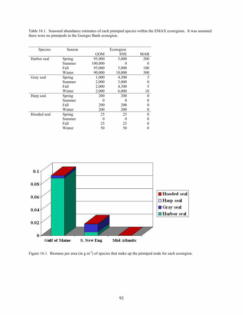
91

Table 16.1. Seasonal abundance estimates of each pinniped species within the EMAX ecoregions. It was assumed there were no pinnipeds in the Georges Bank ecoregion.

Species Season Ecoregion GOM SNE MAB Harbor seal Spring 95,000 5,000 200 Summer 100,000 0 0 Fall 95,000 5,000 100 Winter 90,000 10,000 300 Gray seal Spring 1,000 4,500 5 Summer 2,000 3,000 0 Fall 2,000 4,500 5 Winter 2,000 6,000 10 Harp seal Spring 200 200 0 Summer 0 0 0 Fall 200 200 0 Winter 200 200 0 Hooded seal Spring 25 25 0 Summer 0 0 0 Fall 25 25 0 Winter 50 50 0

Figure 16.1. Biomass per area (in g m-2) of species that make up the pinniped node for each ecoregion.

92

Figure 16.2. Consumption biomass per area (in g m-2) of species that make up the pinniped node for each ecoregion.

93

17. Baleen Whales and Odontocetes Debra L. Palka (nodes #29 and 30) Background

Cetaceans (whales, dolphins and porpoises) inhabiting the EMAX study ecoregions

migrate between the four regions and also go outside them. A general description of the distribution and habit of cetaceans in the North Atlantic is found in Waring and Palka (2002). More detailed descriptions for each species are found in Waring et al. (2004). Cetaceans that have teeth (odontocetes) that utilize at least one of the EMAX ecoregions for some part of the year include: bottlenose dolphins (Tursiops truncatus), common dolphins (Delphinus delphis), beaked whales (Ziphius or Mesoplodon spp.), Risso’s dolphins (Grampus griseus), harbor porpoise (Phocena phocena), dwarf sperm or pygmy sperm whale (Kogia spp.), long-fin and short-fin pilot whales (Globicephala spp.), sperm whales (Physeter macrocephalus), spotted dolphins (Stenella frontalis), striped dolphins (S. coeruleoalba), and white-sided dolphins (Lagenorhynchus acutus). Cetaceans with baleen that utilize some part of the EMAX ecoregions for some part of the year include: fin whales (Balaenoptera physalus), sei whales (B. borealis), humpback whales (Megaptera novaeangliae), minke whales (B. acutorostrata), and right whales (Eubalaena glacialis). Data Sources

The biomass data are based on abundance shipboard and aerial sighting surveys

conducted by the NMFS/NEFSC during the summers of 1998 and 1999. The 1999 survey was used to estimate abundance within the Gulf of Maine ecoregion, while the 1998 survey covered the other ecoregions (Figure 17.1). The 1998 shipboard survey was conducted from 6 July to 6 September, and two teams of observers searched for marine mammals using line transect field data collection methods. These data were analyzed using the direct duplicate line transect analysis method (Palka 1995; Palka 2005a). The 1998 aerial survey was conducted from 18 July to 21 August using standard 1-team line transect methods (Palka 2005b). The 1999 shipboard and aerial surveys were conducted during 28 July to 31 August using methods similar to those used in the 1998 surveys (Palka 2000). Quantitative Approach for Biomass Estimates

Biomass (in metric tons) of baleen whales and odontocetes within an ecoregion was

calculated as the sum of the seasonally averaged biomass of each baleen or odontocetes species within that ecoregion. Biomass per area (in g m-2) was calculated as biomass (in metric tons) per area of the region (in km2; Table 1.1). The seasonally averaged biomass of species k within ecoregion i was calculated as the product of the seasonal average abundance estimate for species k in ecoregion i and the average weight (in kg; Table 17.1) of an individual of species k:

(EQ. 17.1) 10004

)(kseason

ki

kiweightavg

abundanceseasonal

BiomassAverage ���

.

94

The seasonal average abundance estimate was defined as the average of the abundance for each season weighted by the length of the season. The seasons were defined as summer (June to August), fall (September to November), winter (December to February), and spring (March to May). Average weights of individuals were based on values in Trites and Pauly (1998) and Kenney et al. (1997).

Abundance estimates were derived from shipboard and aerial line transect surveys conducted by the NEFSC in the summers (July and August) of 1998 and 1999 (Figure 17.1). The EMAX Gulf of Maine abundance estimate was derived from the 1999 survey data and the abundance estimates for the rest of the ecoregions were derived from the 1998 data. Shipboard and aerial abundance estimates within an EMAX ecoregion were derived from the length of track lines (L), number of sightings (n), and average group size ( s ) within each EMAX region and the estimates of the effective strip width (esw) and g(0) derived from the entire survey. Thus, the abundance for a species k within ecoregion i on platform j (ship or plane) was:

(EQ. 17.2) ijkjkjij

kijkijkij A

geswLsn

Abundance ����

��

)0(2,

where Aij was the area within EMAX ecoregion i that was surveyed by platform j. The total abundance for species k within a region was the sum of the aerial and shipboard abundance estimates for that species.

Abundance estimates from these surveys represent the summer season. Since each species migrates up and down the U.S. Atlantic coast in different ways and at different times, a seasonal abundance estimate for each species within each EMAX ecoregion was calculated separately. That is, the seasonal abundance estimate within each ecoregion was defined as a proportion of the summer population within that region using expert opinion and general patterns documented in the Cetacean and Turtle Assessment Program (CETAP) (1982) and Department of Navy (2005).

Note that the estimate of g(0), the probability of detecting a group on the track line, was defined as 1.0 for these aerial surveys, while g(0) was estimated for the shipboard data. This means the abundance estimates presented here are negatively biased, because not all whales and dolphins were seen on the track line from an airplane flying at 600 ft altitude as was assumed when g(0)=1. During 2004, methods developed to estimate g(0) for aerial survey data indicate g(0) for large whales as about 0.2 and for smaller cetaceans about 0.6 to 0.7 (Palka 2005). Consequentially, if g(0) was included in the calculation, the abundance estimates would be 50-500% higher than what is presented here, depending on the species. Quantitative Approach for Production Estimates

Net production biomass (in metric tons) within an ecoregion was calculated as the sum of

the net production of species found in that region. Net production biomass per area (in g m-2) was calculated as biomass (in metric tons) per area of the ecoregion (in km2; Table 1.1). Net production biomass of species k within ecoregion i was calculated as the product of the seasonally averaged biomass of species k (eq. 17.1) within ecoregion i and the net production rate for species k:

(EQ. 17.3) 1000/)( kkiki rateproductionnetbiomassavgseasonalbiomassproductionnet �� .

95

The net production rate of cetaceans is poorly understood because only a few studies

have calculated a species-specific rate. However, a value of 4% is recognized as a default value for both baleen and odontocetes. This is based on theoretical modeling showing that cetacean populations may not grow at rates much greater than 4% given the constraints of their reproductive history (Barlow et al. 1995). Thus, 4% was used as the net production rate for all baleen and odontocetes, except if there was a species-specific estimate available. The only species-specific estimate of the net reproductive rate that was available and differed from 4% was for right whales (0%; Fujiwara and Caswell 2001). Quantitative Approach for Consumption Estimates

Consumption biomass (in metric tons) within an EMAX region was calculated as the sum

of the annual consumption biomass of species found in that region. Consumption biomass per area (in g m-2) was calculated as consumption biomass (in metric tons) per area of the region (in km2; Table 1.1). The annual consumption biomass (in metric ton) for species k within ecoregioni was estimated by:

(EQ. 17.4) 1000

)/(�� �

� sindaysiksks

sseasonik

daybiomassratefeedingdaily

biomassnConsumptio

where the (daily feeding rate)ks (in kg day-1) is the daily feeding rate of species k for season s and the (biomass day-1)iks (in kg) is the biomass of species k within ecoregion i and within season s. The feeding rate per individual per day is defined as a percentage of its biomass.

There is an inverse relationship between feeding rate and body weight (Sargeant 1969). Thus, for large whales (baleen whales and sperm whales) the daily feeding rate (in kg day-1) for species i was estimated using (Innes et al. 1987):

(EQ. 17.5) .042.0 67.0

i

ii wtavg

wtavgratefeedingDaily

��

Because baleen whales do not feed while migrating and mating in the winter, it was

assumed the daily feeding rate for baleen whales in winter was 0%; all other seasons followed Equation 17.5.

The range of daily feeding rates for odontocetes is 4-11% (Table 17.2). For this study it was assumed the daily feeding rate for harbor porpoises was 8.3% of body weight, and for other odontocetes (excluding sperm whales) it was assumed to be 4.2% of body weight. Example Results Biomass Estimates

The seasonal distribution of baleen and odontocetes varies greatly by species (Table

17.3). Cetacean biomass per area (in g m-2) is dominated by baleen whales, even though there are fewer species of baleen whales than odontocetes (Figure 17.2). The cetacean biomass per area is highest in the Gulf of Maine and Georges Bank, and the lowest in the Mid-Atlantic Bight.

96

Among the baleen whales, the most common species are fin and humpback whales (Figure 17.2A). Within the odontocetes, most of the biomass is from pilot whales (long and short fin), common dolphins, and white-sided dolphins (Figure 17.2B). The Gulf of Maine region has the lowest number of species but the most biomass. The Georges Bank and Southern New England regions have the most diverse composition of species. Note that all the species found in the ecoregions south of the Gulf of Maine are also found offshore of the EMAX ecoregions. For some species, the abundance offshore is much greater than that estimated for the EMAX regions. Production Estimates

Little is known about cetacean reproduction rates, so the default value of 4% annual

reproduction rate was used for all species except right whales (0%). Thus the patterns of production (g m-2 yr-1) are the same as those for biomass (Figure 17.2). The magnitude, however, is 4% of the biomass. Consumption Estimates

Using equation 17.5, the daily feeding rate of baleen whales during seasons other than

winter ranged from 1.2% of a fin or sei whale’s body weight to 2.3% of a minke whale’s body weight. It was assumed baleen whales did not eat during winter (January to March). It was also assumed the daily feeding rate of harbor porpoises was 8.3% of its body weight, odontocetes (except sperm whales) were 4.2% of their body weight, and sperm whales (using equation 17.5) was 1.6% of its body weight.

The consumption rate per area (g m-2 yr-1) is the highest in the Gulf of Maine and lowest in the Mid-Atlantic Bight (Figure 17.3). Baleen whales consume more than the odontocetes. Of the odontocetes, those on Georges Bank contribute the most biomass (Figure 17.2) and the most consumption biomass (Figure 17.3).

97

References Barlow, J; Swartz, SL; Eagle, TC; Wade, PR. 1995. U.S. marine mammal stock assessment: guidelines for

preparation, background, and a summary of the 1995 assessments. NOAA Technical Memorandum NMFS-OPR-6. 73 p. http://www.nmfs.noaa.gov/prot_res/readingrm/hqtechm.pdf

CETAP. 1982. A characterization of marine mammals and turtles in the mid- and north Atlantic areas of the U.S. outer continental shelf. Cetacean and Turtle Assessment Program, University of Rhode Island. Final Report, Contract AA51-C78-48, Bureau of Land Management, Washingon, D.C.; 538 p.

Cheal, A.J; Gales, NJ. 1991. Body mass and food intake in captive breeding bottlenose dolphin, Tursiops truncates. Zoo. Biol. 10(6):451-456.

Department of the Navy. 2005. Marine resource assessment for the northeast operating areas: Atlantic City, Narragansett Bay, and Boston. Naval Facilities Engineering Command, Atlantic; Norfolk, Virginia. Contract Number N62470-02-D-9997, Task Order Number 0018. Prepared by Geo-Marine, Inc., Newport News, Virginia.

Fujiwara, M; Caswell, H. 2001. Demography of the endangered North Atlantic right whale. Nature 414:537:41. Innes, S.; Lavigne, DM; Earle, WM; Kovacs, KM. 1987. Feeding rates of seals and whales. Journal of Animal

Ecology 56:115-130. Kenney, RD; Scott, GP; Thompson, TJ; Winn, HE. 1997. Estimates of prey consumption and trophic impacts of

cetaceans in the USA northeast continental shelf ecosystem. J. Northw. Atl. Fish. Sci. 22:155-171. Ohizumi, H; Miyakaki, N. 1998. Feeding rate and daily energy intake of Dall’s propoise in the northeastern Sea of

Japan. Proc. NIPR Symp. Polar Biol. 11:74-81. Palka, D. 1995. Abundance estimate of Gulf of Maine harbor porpoise. Rep. int. Whal. Commn Special Issue 16 -

The Biology of Phocoenidae. p. 28-50. Palka, D. 2000. Abundance of the Gulf of Maine/Bay of Fundy harbor porpoise stock based on shipboard and

aerial surveys in 1999. Northeast Fish. Sci. Cent. Ref. Doc. 00-07; 29 p. Palka, D. 2005a. Shipboard surveys in the northwest Atlantic: estimation of g(0). In: Thomsen, F; Ugarte, F;

Evans, PGH, eds. Proceedings of the workshop on Estimation of g(0) in line-transect surveys of cetaceans. ECS Newletter No. 44 – Special Issue. April 2005; p. 32-37.

Palka, D. 2005b. Aerial surveys in the northwest Atlantic: estimation of g(0). In: Thomsen, F; Ugarte, F; Evans, PGH, eds. Proceedings of the workshop on Estimation of g(0) in line-transect surveys of cetaceans. ECS Newletter No. 44 – Special Issue. April 2005; p. 12-17.

San Miguel, A. 1977. Feeding habits of the dolphin, Tursiops truncatus. Rev. Parque Zool. Barc. 28:12-13. Sergeant, DE. 1969. Feeding rates of Cetacea. Fiskeridirektoratets Slorifter Serie Havundersokelser 15:246-258. Trites, AW; Pauly, D. 1998. Estimating mean body masses of marine mammals from maximum body lengths.

Canadian Journal of Zoology 76:886-896. Waring, GT; Palka, DL. 2002. North Atlantic marine mammals. In: Perrin, WE; Wursig, B; Thewissen, JGM, eds.

Encyclopedia of Marine Mammals. New York, NY: Academic Press; p. 802-805. Waring, G; Pace, RM; Quintal, JM; Fairfield, CP; Maze-Foley, K, eds. 2004. U.S. Atlantic and Gulf of Mexico

marine mammal stock assessments – 2003. NOAA Technical Memorandum NMFS-NE-182. www.nefsc.noaa.gov/nefsc/publications/tm/tm182

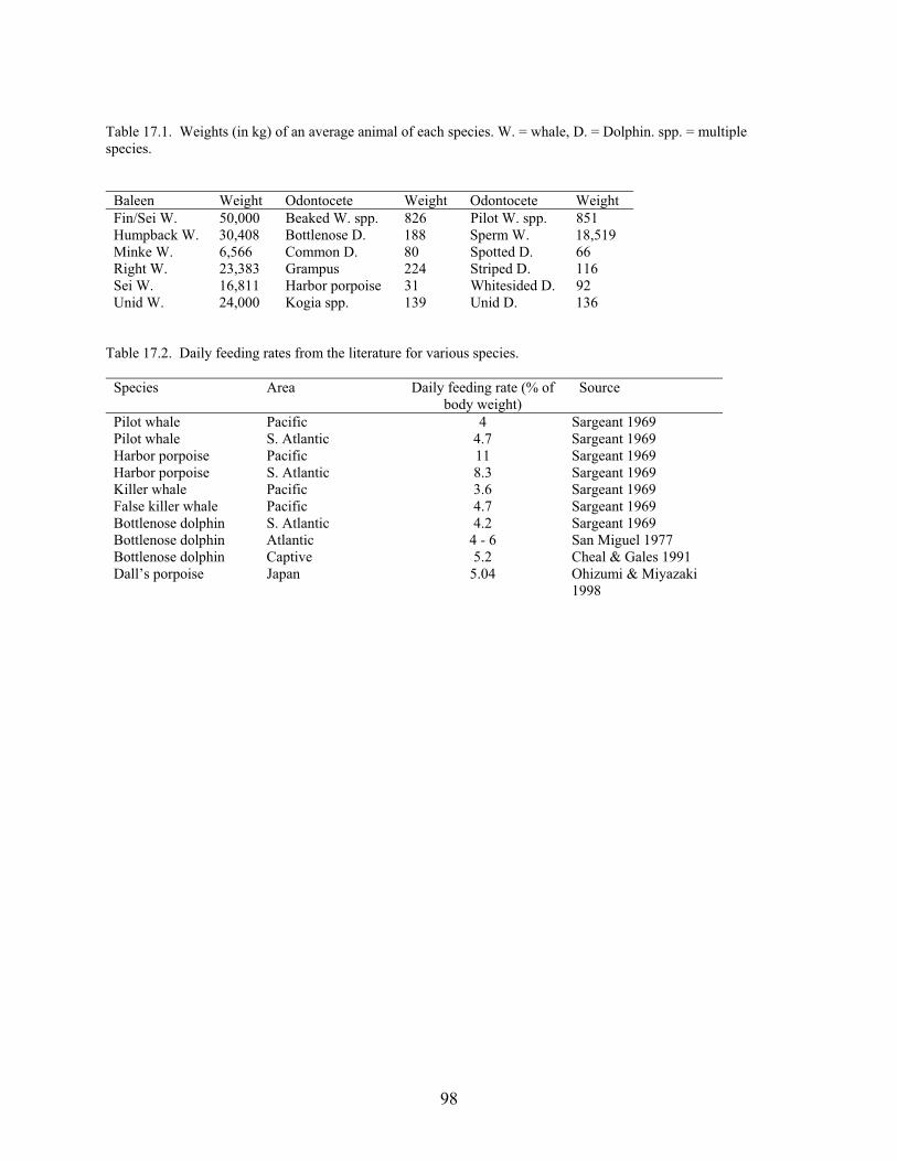
98

Table 17.1. Weights (in kg) of an average animal of each species. W. = whale, D. = Dolphin. spp. = multiple species.

Baleen Weight Odontocete Weight Odontocete Weight Fin/Sei W. 50,000 Beaked W. spp. 826 Pilot W. spp. 851 Humpback W. 30,408 Bottlenose D. 188 Sperm W. 18,519 Minke W. 6,566 Common D. 80 Spotted D. 66 Right W. 23,383 Grampus 224 Striped D. 116 Sei W. 16,811 Harbor porpoise 31 Whitesided D. 92 Unid W. 24,000 Kogia spp. 139 Unid D. 136

Table 17.2. Daily feeding rates from the literature for various species.

Species Area Daily feeding rate (% of body weight)

Source

Pilot whale Pacific 4 Sargeant 1969 Pilot whale S. Atlantic 4.7 Sargeant 1969 Harbor porpoise Pacific 11 Sargeant 1969 Harbor porpoise S. Atlantic 8.3 Sargeant 1969 Killer whale Pacific 3.6 Sargeant 1969 False killer whale Pacific 4.7 Sargeant 1969 Bottlenose dolphin S. Atlantic 4.2 Sargeant 1969 Bottlenose dolphin Atlantic 4 - 6 San Miguel 1977 Bottlenose dolphin Captive 5.2 Cheal & Gales 1991 Dall’s porpoise Japan 5.04 Ohizumi & Miyazaki

1998

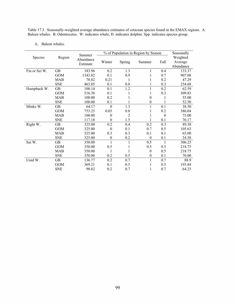
99

Table 17.3. Seasonally-weighted average abundance estimates of cetacean species found in the EMAX regions. A. Baleen whales. B. Odontocetes. W. indicates whale, D. indicates dolphin. Spp. indicates species group.

A. Baleen whales.

% of Population in Region by Season Species

Region Summer

Abundance Estimate Winter Spring Summer Fall

Seasonally Weighted Average

Abundance Fin or Sei W. GB 183.96 0.2 1.3 1 0.4 133.37 GOM 1343.82 0.1 0.9 1 0.7 907.08 MAB 78.82 0.21 1 1 0.2 47.29 SNE 463.05 0.1 0.8 1 0.3 254.68 Humpback W. GB 100.14 0.1 1.2 1 0.2 62.59 GOM 516.38 0.1 1 1 0.3 309.83 MAB 100.00 0.2 1 0 1 55.00 SNE 100.00 0.1 1 0 1 52.50 Minke W. GB 64.17 0 1.3 1 0.1 38.50 GOM 753.25 0.05 0.8 1 0.2 386.04 MAB 100.00 0 2 1 0 75.00 SNE 117.18 0 1.5 1 0.1 76.17 Right W. GB 325.00 0.2 0.4 0.2 0.3 89.38 GOM 325.00 0 0.1 0.7 0.5 105.63 MAB 325.00 0.3 0.3 0.1 0.1 65.00 SNE 325.00 0 0.2 0 0.1 24.38 Sei W. GB 350.00 1 1 0.5 1 306.25 GOM 350.00 0.5 1 0.5 0.5 218.75 MAB 350.00 1 1 0 0.5 218.75 SNE 350.00 0.2 0.5 0 0.1 70.00 Unid W. GB 136.77 0.2 0.7 1 0.7 88.9 GOM 369.21 0.1 0.5 1 0.5 193.84 SNE 98.82 0.2 0.7 1 0.7 64.23

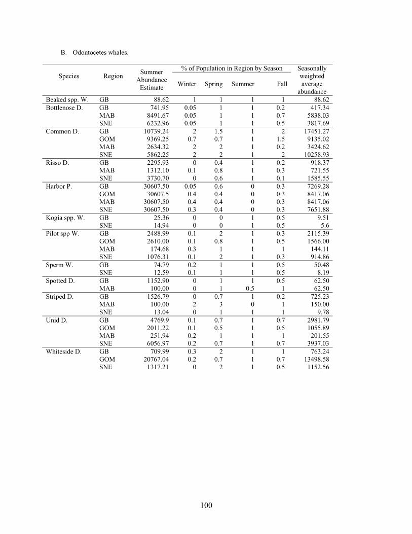
100

B. Odontocetes whales.

% of Population in Region by Season Species

Region Summer

Abundance Estimate Winter Spring Summer Fall

Seasonally weighted average

abundance Beaked spp. W. GB 88.62 1 1 1 1 88.62 Bottlenose D. GB 741.95 0.05 1 1 0.2 417.34 MAB 8491.67 0.05 1 1 0.7 5838.03 SNE 6232.96 0.05 1 1 0.5 3817.69 Common D. GB 10739.24 2 1.5 1 2 17451.27 GOM 9369.25 0.7 0.7 1 1.5 9135.02 MAB 2634.32 2 2 1 0.2 3424.62 SNE 5862.25 2 2 1 2 10258.93 Risso D. GB 2295.93 0 0.4 1 0.2 918.37 MAB 1312.10 0.1 0.8 1 0.3 721.55 SNE 3730.70 0 0.6 1 0.1 1585.55 Harbor P. GB 30607.50 0.05 0.6 0 0.3 7269.28 GOM 30607.5 0.4 0.4 0 0.3 8417.06 MAB 30607.50 0.4 0.4 0 0.3 8417.06 SNE 30607.50 0.3 0.4 0 0.3 7651.88 Kogia spp. W. GB 25.36 0 0 1 0.5 9.51 SNE 14.94 0 0 1 0.5 5.6 Pilot spp W. GB 2488.99 0.1 2 1 0.3 2115.39 GOM 2610.00 0.1 0.8 1 0.5 1566.00 MAB 174.68 0.3 1 1 1 144.11 SNE 1076.31 0.1 2 1 0.3 914.86 Sperm W. GB 74.79 0.2 1 1 0.5 50.48 SNE 12.59 0.1 1 1 0.5 8.19 Spotted D. GB 1152.90 0 1 1 0.5 62.50 MAB 100.00 0 1 0.5 1 62.50 Striped D. GB 1526.79 0 0.7 1 0.2 725.23 MAB 100.00 2 3 0 1 150.00 SNE 13.04 0 1 1 1 9.78 Unid D. GB 4769.9 0.1 0.7 1 0.7 2981.79 GOM 2011.22 0.1 0.5 1 0.5 1055.89 MAB 251.94 0.2 1 1 1 201.55 SNE 6056.97 0.2 0.7 1 0.7 3937.03 Whiteside D. GB 709.99 0.3 2 1 1 763.24 GOM 20767.04 0.2 0.7 1 0.7 13498.58 SNE 1317.21 0 2 1 0.5 1152.56

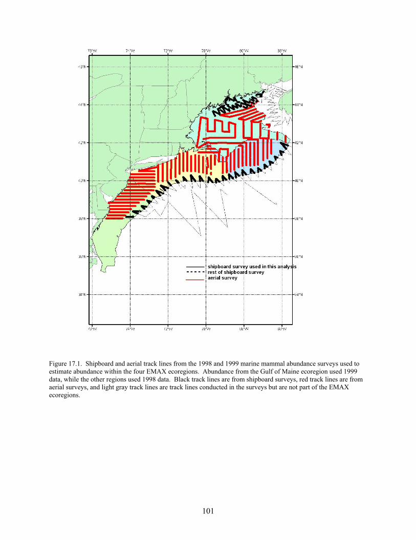
101

Figure 17.1. Shipboard and aerial track lines from the 1998 and 1999 marine mammal abundance surveys used to estimate abundance within the four EMAX ecoregions. Abundance from the Gulf of Maine ecoregion used 1999 data, while the other regions used 1998 data. Black track lines are from shipboard surveys, red track lines are from aerial surveys, and light gray track lines are track lines conducted in the surveys but are not part of the EMAX ecoregions.

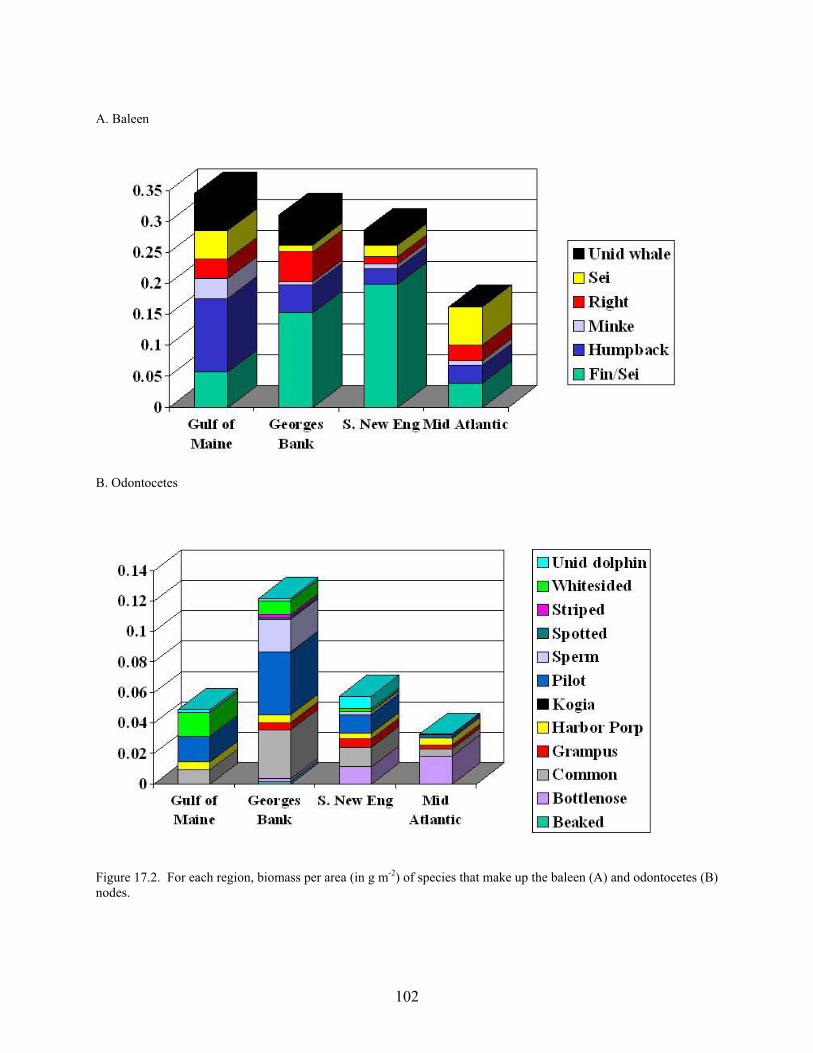
102

A. Baleen B. Odontocetes Figure 17.2. For each region, biomass per area (in g m-2) of species that make up the baleen (A) and odontocetes (B) nodes.

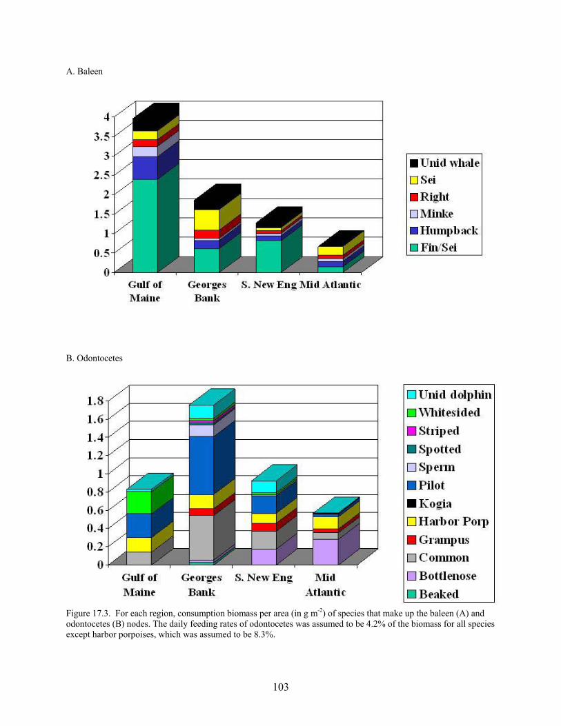
103

A. Baleen B. Odontocetes Figure 17.3. For each region, consumption biomass per area (in g m-2) of species that make up the baleen (A) and odontocetes (B) nodes. The daily feeding rates of odontocetes was assumed to be 4.2% of the biomass for all species except harbor porpoises, which was assumed to be 8.3%.

104

18. Seabirds William J. Overholtz (node #31) Background and Estimation Approaches

Marine birds are represented by 20 species in the Northeast U.S. Continental Shelf

Ecosystem and are moderately abundant, especially on Georges Bank (Schneider and Heinemann 1996). There have been no large scale surveys of marine bird populations conducted in the region since 1988. The region is generally thought of as a seasonal feeding area with few species actually nesting locally. Eleven species were chosen as important offshore predators to include in the energy budgets of the four EMAX ecoregions (Table 18.1).

Schneider and Heinemann (1996) provide the mean and standard deviation for various seabirds during 1978-1988 as well as abundance data (deviations for the mean) for the same period. Since no current seasonal abundance data are available for the region, the information for quarterly abundance during 1978-1980 in Powers (1983; Appendix 5 in that publication) was used. These data were standardized to the highest quarterly value and used with the mean, standard deviation, and yearly deviation for each species to calculate quarterly numbers of birds during 1978-1988, assuming that the seasonal distribution of seabirds has not changed over time. Since the three species of shearwaters are similar in size and greater shearwaters are by far the most abundant, their abundance was combined.

The proportion of seabirds in each ecoregion was calculated from seasonal and regional abundance data provided in Powers (1983; Appendix 1 in that publication). Quarterly abundance by region was summed and divided by the total abundance in all regions for that species. Since there are no estimates of abundance for the 1996-2000 period, the average abundance during 1984-1988 was calculated for each quarter and converted to biomass with estimates of average species specific weight from Powers and Bachus (1987). Quarterly biomass estimates were averaged and the proportions by region used to partition biomass into the four ecoregions (Table 18.2). Production and Consumption

Consumption by seabirds was estimated from quarterly numbers of birds and estimates of

daily ration (kg day-1) from an energetics equation (Innes 1987). The daily consumption by each species was estimated and expanded to a quarterly basis (91.5 days). Quarterly consumption was summed and a yearly average was calculated (Table 18.3). Production was estimated with a P:B ratio (0.275) obtained from Savonkoff et al. (2004) and applied to the average biomass. Quarterly estimates were summed and averaged for the year (Table 18.3). Results for all species were summed and apportioned into each ecoregion (Table 18.4)

105

References Powers, K.D. 1983. Pelagic distributions of marine birds off the Northeastern United States. U.S. Department of

Commerce. NOAA Technical Memorandum NMFS-F/NEC-27. 201 pp. Powers, K.D., and E.H. Bachus. 1987. Energy transfer to birds. In R.H. Backus and D. W. Bourne (eds), Georges

Bank, Cambridge, MA: MIT Press, pp. 372-375. Schneider, D.C., and D.W. Heinemann. 1996. The state of marine bird populations from Cape Hatteras to the Gulf

of Maine. Chapter 11 in K. Sherman, N.A. Jaworski, and T.J. Smayda (eds), The Northeast Shelf Ecosystem Assessment, Sustainability, and Management. Blackwell Science, Cambridge, MA, pp. 197-216.

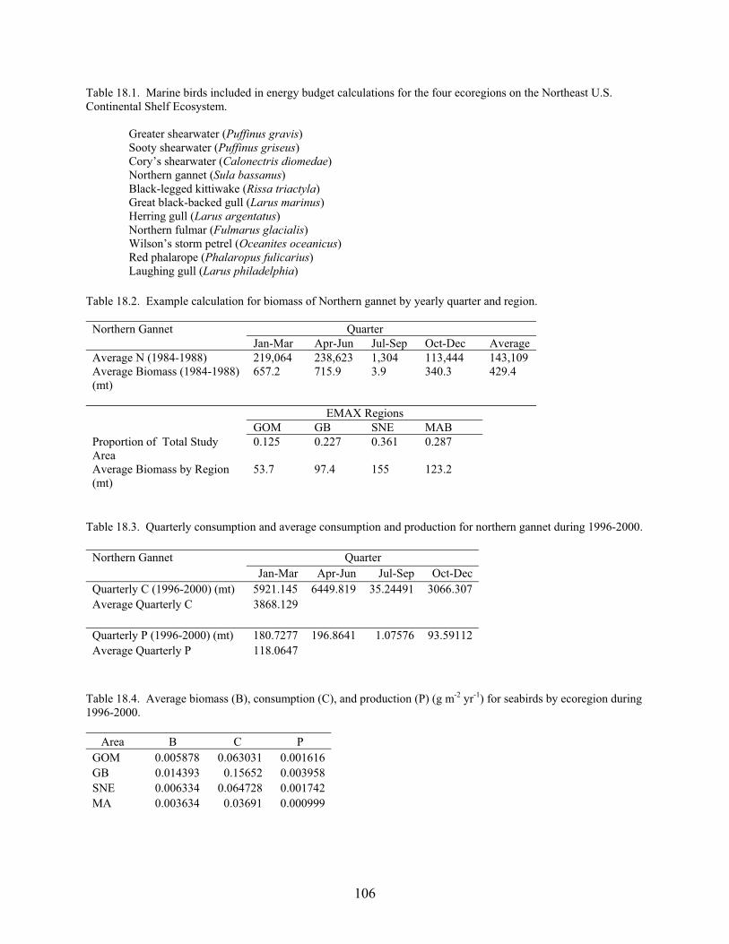
106

Table 18.1. Marine birds included in energy budget calculations for the four ecoregions on the Northeast U.S. Continental Shelf Ecosystem. Greater shearwater (Puffinus gravis) Sooty shearwater (Puffinus griseus) Cory’s shearwater (Calonectris diomedae) Northern gannet (Sula bassanus) Black-legged kittiwake (Rissa triactyla) Great black-backed gull (Larus marinus) Herring gull (Larus argentatus) Northern fulmar (Fulmarus glacialis) Wilson’s storm petrel (Oceanites oceanicus) Red phalarope (Phalaropus fulicarius) Laughing gull (Larus philadelphia) Table 18.2. Example calculation for biomass of Northern gannet by yearly quarter and region.

Northern Gannet Quarter Jan-Mar Apr-Jun Jul-Sep Oct-Dec Average Average N (1984-1988) 219,064 238,623 1,304 113,444 143,109 Average Biomass (1984-1988) (mt)

657.2 715.9 3.9 340.3 429.4

EMAX Regions GOM GB SNE MAB Proportion of Total Study Area

0.125 0.227 0.361 0.287

Average Biomass by Region (mt)

53.7 97.4 155 123.2

Table 18.3. Quarterly consumption and average consumption and production for northern gannet during 1996-2000.

Northern Gannet Quarter Jan-Mar Apr-Jun Jul-Sep Oct-Dec Quarterly C (1996-2000) (mt) 5921.145 6449.819 35.24491 3066.307 Average Quarterly C 3868.129 Quarterly P (1996-2000) (mt) 180.7277 196.8641 1.07576 93.59112 Average Quarterly P 118.0647

Table 18.4. Average biomass (B), consumption (C), and production (P) (g m-2 yr-1) for seabirds by ecoregion during 1996-2000.

Area B C P GOM 0.005878 0.063031 0.001616 GB 0.014393 0.15652 0.003958 SNE 0.006334 0.064728 0.001742 MA 0.003634 0.03691 0.000999

107

19. Detritis - Particulate Organic Carbon (POC) and Dissolved Organic Carbon (DOC) John E. O’Reilly and David D. Dow (nodes #35 and 36) Background/Data Sources

Organic carbon bound in a dissolved form (DOC) represents the largest pool of organic

matter in the ocean, exceeding standing stocks of particulate organic carbon (POC) and phytoplankton carbon by approximately one and two orders of magnitude, respectively. For example, Kepkay (2000) partitioned the carbon pools for the world ocean (in Gt C) as: DOC (200-700); POC (20); phytoplankton (1-11); and other biota (0.4). He further partitioned the DOC pool into a refractory low molecular weight component (120-630) and a bioavailable colloidal component (20-280). The combined DOC + POC is often referred to as “detritus” and represents a major source of carbon for the microbial food web.

In oceanic waters, the concentration of DOC generally decreases with depth from the surface to the level of the seasonal or permanent thermocline. In the MAB, Vlahos et al. (2002) and Del Vecchio and Blough (2004) found that DOC concentrations generally decreased from the coast to the shelf break. Quantitative Approach for Estimates

Our estimation of the standing stocks of DOC is based on two steps. The first involves

the construction of a generalized vertical profile of DOC, using the data from Guo et al. (1985) supplemented by near surface measurements of DOC made by Aluwihare et al. (1997) and by Vlahos et al. (2002). The second step involves the vertical integration of our generalized DOC profile from surface to bottom, using high resolution bathymetry data (1 km).

Guo et al. (1985) measured the vertical profile of DOC at a station in the MAB southeast of Chesapeake Bay during May 1993 (Figure 19.1). We have redrawn the data from Guo and Santschi in Figure 19.2 and show our estimates of DOC concentrations for sampling depths between 25 m and 2,500 m below the surface.

Aluwihare et al. (1997) measured DOC in surface waters of the MAB, on Georges Bank, and near shore waters near Woods Hole, MA (Figure 19.3). The mean DOC measured in these seven surface samples is 97.0 μM C.

Kepkay (2000) reported that DOC concentrations for the MAB ranged between 45 and 102 μM C. Vlahos et al. (2002) measured DOC in the MAB during surveys in April 1994, March 1996 and August 1996 (Figure 19.4) and reported that DOC concentrations ranged from 60 to 165 μM C in surface waters and converged to 49 μM C at depths below 200 m. The mean DOC in 137 samples from the upper 10 meters of the water column is 97.0 μM C, based on Table 3 in Vlahos et al. (2002). From these two studies, we assume a value of 97 μM C represents a typical DOC concentration in surface water in our region. Our generalized vertical profile of DOC is illustrated in Figure 19.5.

The standing stocks of DOC were estimated for each region by combining the generalized DOC profile with a highly resolved map of bottom depth for the ecosystem (developed from the SRTM30 Plus bathymetry data set of Becker and Sandwell 2004). A frequency distribution of bottom depths was constructed for each region at a resolution of 1 meter and a spatial resolution of 1.25 x 1.25 km per pixel. (For the purpose of illustrating the bathymetric differences among the four regions, a less resolved frequency distribution is shown

108

in Figure 19.6.). For each bottom depth interval in increments of 1 meter, the generalized DOC profile was integrated from surface to bottom depth and these results were summed to yield the total and mean DOC concentration for each region (Table 19.1). Results

Our estimate of average standing stocks of DOC in the MAB (44.5 g C m-2) is in good agreement with the mean value 43.9 g C m-2 which we computed from the MAB shelf surveys reported by Vlahos et al. (2002; their Table 1).

Our estimates of particulate organic carbon (POC) standing stocks for the GOM (8.1 g C m-2) assume an approximate 15:1 ratio between DOC and POC (Millero 1996; Kepkay 2000; Ogawa 2000). If we also apply a 5:1 ratio for POC:planktonic C ratio (Volkman and Tanoue 2002; Valiela 1995), then our estimated ratio of DOC:POC:Phytoplankton Carbon is 75:5:1, compared to the traditional oceanic water assumption of 100:10:1 (Parsons et al. 1984). The modern perspective on this ratio suggests that continental shelf waters are proportionally richer in POC and phytoplankton carbon than the oceanic water column, since coastal waters receive nutrient inputs from coastal land use which increases the rate of primary production and also receive inputs of POC from estuaries/bays. The planktonic carbon based on this simple proportionality scheme is 1.61 g C m-2. This value is somewhat lower than our estimate of 2.01 g C m-2 for phytoplankton biomass derived from water column integrated chlorophyll concentrations (see in this document Section 2: Phytoplankton and Primary Production).

Given the operational separation of POC and DOC by filtration on glass fiber filters (nominal pore size 0.7 μm), a portion of the POC is living, while there are small particles (viruses and some bacteria) in the “dissolved” DOC fraction. Some biological oceanographers analyze either ATP (adenosine triphosphate) or chlorophyll a and its degradation products (pheaophytin or phaeophorbide) to estimate the living portion of POC. For example, off the California coast, the living fraction of POC varies from 14% to 79% in the upper 100 meters of the water column, decreasing to 6% at intermediate depths and below 3% at 500 to 1,000 meters below surface. Direct chemical composition of POC suggests that it is primarily carbohydrate and protein with small amounts of fat (Parsons et al. 1984). The water-soluble carbohydrate fraction disappears between 50 and 300 m, so that below 300-1000 m only the water-insoluble fraction persists. A variable fraction of the particulate detritus is calcium carbonate which can be mistaken for the non-living organic carbon component of POC (Parsons et al. 1984). The chemical and biological degradation of POC tends to decrease with depth (becomes more refractory). Bacteria and protozoa colonize some of these particles and their enzymatic activities convert POC to DOC. This colonization by microbes increases the nutritional value of POC for vertebrate/invertebrate detritivores.

In EMAX we assumed that 10% of the net primary production (Pnet) was exported out of the mixed layer and transferred to the detritus compartment (noted as an assimilation efficiency of 90% in the EMAX spreadsheet). Cebrian (2002) utilized a value of 17% for the export of primary production out of the mixed layer. Net primary production is conventionally divided into recycled production (based on using ammonia) and new production (based on nitrate). In theory the new production in the euphotic zone is balanced by export production out of the mixed layer. The export ratio (ef) values range between 0.25 and 0.5 (Falkowski et al. 2003; Muller-Karger etal. 2005). A number of models have been developed to relate net production, temperature and/or depth to the ef value (Falkowski et al. 2003; Muller-Karger et al. 2005). We do not know how

109

much of the Pnet value estimated from ocean color satellite measurements is new versus recycled production, so we assumed that export was 15% of Pnet.

The DOC node was not explicitly incorporated as a food source for the microbial loop in the EMAX network given the uncertainty on its bioavailability to bacteria and microzooplankton (see discussion in those chapters). The POC node inputs include: phytoplankton dissolved production; phytoplankton that sediments out of the euphotic zone; and the detritus produced by egestion from each living node (since the assimilation efficiency is less than 100% of the consumption). The output from the POC node is consumed by bacteria, microzooplankton, mesozooplankton and various other larger benthic/pelagic filter feeders (see diet matrix in spread sheets). The microbial loop increases the efficiency of the grazing food chain by recycling the DOC excreted by phytoplankton and the POC egested from other nodes and linking it back to the grazing food chain through the use of POC as a food source. This recycled carbon passes through the indirect flow pathways in network models with the consequence that at the higher trophic levels (fish and marine mammals) much of the carbon received is via indirect pathways. This tendency is reflected in the recycling index parameter. The recycled carbon from the lower trophic levels allows the marine food web to be longer (more trophic levels) than that in lakes/estuaries. This is reflected to a degree in the average trophic level parameter for each node. References Aluwihare, L; Repeta, D; Chen, R. 1997. A major biopolymeric component to dissolved organic carbon in surface

sea water. Nature 387:166-169. Becker, JJ; Sandwell, DT. 2004. SRTM30_PLUS: Data fusion of SRTM land topography with measured and

estimated seafloor topography. Scripps Inst. Oceanography, Univ. California San Diego, 9500 Gilman Drive, La Jolla, CA.

Del Vecchio, R.; Blough, N. 2004. Spatial and seasonal distribution of chromophoric dissolved organic matter and dissolved organic carbon in the Middle Atlantic Bight. Marine Chemistry 89:169-187.

Guo, L; Santschi, PH; Warren, KH. 1995. Dynamics of dissolved organic carbon (DOC) in oceanic environments. Limnol. Oceanogr. 40:1392-1403.

Guo, L; Santschi, PH. 1997. Composition and cycling of colloids in the marine environment. Rev. Geophys. 35:17-40.

Kepkay, PF. 2000. Colloids and the ocean carbon cycle. In: Wangersky, P, ed. The Handbook of Environmental Chemistry Vol 5, Part D, Marine Chemistry. Berlin, Germany: Springer-Verlag; p. 536-560.

Millero, FJ. 1996. Chemical Oceanography. Second Edition; Boca Raton, Fl: CRC Press; 469 p. Valiela, I. 1995. Marine Ecological Processes. New York, NY: Springer-Verlag; 686 p. Vlahos, P; Chen, R; Repeta, J. 2002. Dissolved organic carbon in the Mid-Atlantic Bight. Deep-Sea Research II

49:4369-4385.

110

Table 19.1. Average standing stocks of DOC for the MAB, SNE, GB and GOM ecoregions.

REGION AREA (m2) DOC (g region-1) Avg. DOC (g C m-2) MAB 5.73E+10 2.55E+12 44.5 SNE 6.46E+10 3.83E+12 59.2 GB 4.43E+10 3.29E+12 74.4 GOM 7.92E+10 9.66E+12 121.9

Figure 19.1. Location of station where Guo and Santschi (1997) measured the vertical profile of DOC.

Figure 19.2. Vertical profile of DOC measured in the MAB, redrawn from Guo et al. (1995), showing our estimates of depth and DOC derived from the graph.

111

Figure 19.3. Sampling locations for DOC measurements made by Aluwihare et al. 1997.

Figure 19.4. Sampling locations for DOC measurements made by Vlahos et al. 2002.

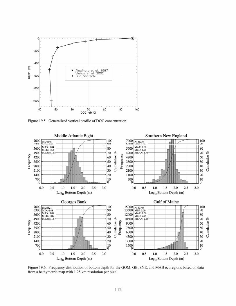
112

Figure 19.5. Generalized vertical profile of DOC concentration.

Figure 19.6. Frequency distribution of bottom depth for the GOM, GB, SNE, and MAB ecoregions based on data from a bathymetric map with 1.25 km resolution per pixel.

113

20. Fishery Removals (pelagic fisheries, demersal fisheries, discards) Steven F. Edwards, Christopher M. Legault, Jon K.T. Brodziak, William J. Overholtz, and Laurel A. Col (nodes #32-34) Landings

Commercial Landings Data on U.S. and (where appropriate) Canadian landings (live weight in metric tons) of

demersal and pelagic managed species from the years 1996-2000 were obtained from five general sources. Priority was given to sources that already compiled data into the ecoregion geographic classification. In some cases, various Stock Assessment Workshop (SAW) documents (http://www.nefsc.noaa.gov/nefsc/saw) and the related Groundfish Assessment Review Meeting (GARM) report (NEFSC 2002) provided data in the exact form necessary (e.g., Atlantic sea scallop from the 39th SAW and American plaice from the GARM report). In most cases, however, the available information was reported either for combinations of ecoregions (GARM [2002] and SAW documents) or for spatial units other than ecoregions (i.e., by Statistical Region or by State in the NMFS commercial database, including the small pelagic species, squids, and the remainder of the megabenthos). In either case, expert opinion from staff in the Population Dynamics Branch was used to allocate the values to the ecoregions. When only total regional landings were available, the expert opinion of one of the team members was relied on to allocate landings (bluefish, cusk, red hake, silver hake, white hake, offshore hake, river herring, black sea bass, American shad, striped bass, tilefish, Atlantic wolfish, and red crab). Landings for squid and the pelagic commercial group were obtained from NMFS data sources (CFDBS). These estimates were averaged over 1996-2000 and apportioned to the four areas by using area fished from the NMFS database. Commercial landings of large pelagic species were obtained from International Commision for the Conservation of Atlantic Tunas Standing Committee on Research and Statistics (ICCAT SCRS) reports. These data were apportioned by using distribution maps and making some assumptions about the percentage landed on the continental shelf. Recreational Landings

Annual data (1996-2000) on the Type A (number of fish landed), Type B1 (number of

fish discarded), and combined weight of both these categories were downloaded from the Marine Recreational Fisheries Statistics Survey (MRFSS) (http://www.st.nmfs.gov/st1/recreational) for the “all ocean combined” area of the Northeast Region (i.e., excluding bays and inland waters which lie outside the ecoregions). Given an assumption of equal size fish in both categories, Type A landings in weight (metric tons) were approximated by species. Species landings were allocated to the Gulf of Maine, Southern New England, and Mid-Atlantic Bight ecoregions in proportion to the length of each state’s contiguous shoreline. These results were aggregated by taxa.

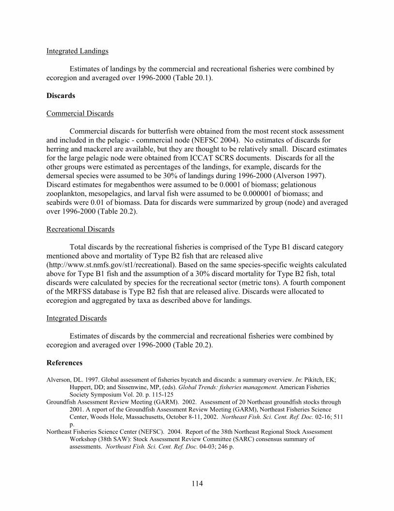
114

Integrated Landings Estimates of landings by the commercial and recreational fisheries were combined by

ecoregion and averaged over 1996-2000 (Table 20.1). Discards

Commercial Discards Commercial discards for butterfish were obtained from the most recent stock assessment

and included in the pelagic - commercial node (NEFSC 2004). No estimates of discards for herring and mackerel are available, but they are thought to be relatively small. Discard estimates for the large pelagic node were obtained from ICCAT SCRS documents. Discards for all the other groups were estimated as percentages of the landings, for example, discards for the demersal species were assumed to be 30% of landings during 1996-2000 (Alverson 1997). Discard estimates for megabenthos were assumed to be 0.0001 of biomass; gelationous zooplankton, mesopelagics, and larval fish were assumed to be 0.000001 of biomass; and seabirds were 0.01 of biomass. Data for discards were summarized by group (node) and averaged over 1996-2000 (Table 20.2). Recreational Discards

Total discards by the recreational fisheries is comprised of the Type B1 discard category

mentioned above and mortality of Type B2 fish that are released alive (http://www.st.nmfs.gov/st1/recreational). Based on the same species-specific weights calculated above for Type B1 fish and the assumption of a 30% discard mortality for Type B2 fish, total discards were calculated by species for the recreational sector (metric tons). A fourth component of the MRFSS database is Type B2 fish that are released alive. Discards were allocated to ecoregion and aggregated by taxa as described above for landings. Integrated Discards

Estimates of discards by the commercial and recreational fisheries were combined by

ecoregion and averaged over 1996-2000 (Table 20.2). References Alverson, DL. 1997. Global assessment of fisheries bycatch and discards: a summary overview. In: Pikitch, EK;

Huppert, DD; and Sissenwine, MP, (eds). Global Trends: fisheries management. American Fisheries Society Symposium Vol. 20. p. 115-125

Groundfish Assessment Review Meeting (GARM). 2002. Assessment of 20 Northeast groundfish stocks through 2001. A report of the Groundfish Assessment Review Meeting (GARM), Northeast Fisheries Science Center, Woods Hole, Massachusetts, October 8-11, 2002. Northeast Fish. Sci. Cent. Ref. Doc. 02-16; 511 p.

Northeast Fisheries Science Center (NEFSC). 2004. Report of the 38th Northeast Regional Stock Assessment Workshop (38th SAW): Stock Assessment Review Committee (SARC) consensus summary of assessments. Northeast Fish. Sci. Cent. Ref. Doc. 04-03; 246 p.

115

Table 20.1. Average annual landings (mt) for nodes used in the Ecopath-EcoNetwrk analysis.

Landings in mt Node GOM GB SNE MAB

Shrimp et al. 4924 0 0 0 Mesopelagics 0 0 0 0 Macrobenthos - polychaetes 0 0 0 0 Macrobenthos - crustaceans 0 0 0 0 Macrobenthos - molluscs 0 0 0 0 Macrobenthos - other 0 0 0 0 Megabenthos - filterers 7255 28287 106876 177728 Megabenthos - other 27320 1443 9788 860 Larval fish - all 0 0 0 0 Small Pelagics - commercial 69171 13056 28218 10770 Small Pelagics - other 1 0 1951 54770 Small Pelagics -anadromous 444 148 445 1377 Small Pelagics - squid 1095 1430 15865 12509 Medium Pelagics - (piscivores and other) 800 443 4137 3549 Demersals - benthivores 11274 11535 5336 1933 Demersals - omnivores 569 232 935 1680 Demersals - piscivores 23831 23206 18656 21297 Sharks - coastal 0 0 777 1460 Sharks - pelagics 19 35 74 62 Highly Migratory Species 144 149 487 607

Table 20.2. Average annual discards (mt) for nodes used in the Ecopath-Econetwrk analysis.

Discards in mt Node GOM GB SNE MAB

Gelatinous ZP <1 <1 <1 <1 Shrimp et al. 1540 0 616 561 Mesopelagics <1 <1 <1 <1 Macrobenthos- polychaetes 11 2 23 7 Macrobenthos- crustaceans 1 7 4 0 Macrobenthos- molluscs 15 5 28 0 Macrobenthos- other 57 36 25 0 Megabenthos- filterers 2387 8486 33280 54192 Megabenthos- other 8199 433 3358 524 Larval fish- all <1 <1 <1 0 Small Pelagics- commercial 10369 1306 10556 2919 Small Pelagics - other 12 0 1808 5556 Small Pelagics -anadromous 44 15 45 138 Small Pelagics- squid 1322 143 2540 1347 Medium Pelagics (piscivores and other) 240 133 1241 1106 Demersals- benthivores 3401 3460 1625 734 Demersals- omnivores 180 70 643 1100 Demersals- piscivores 7149 6962 5597 6389 Sharks-coastal 0 0 233 438 Sharks-pelagics 6 10 22 19 Highly Migratory Species 43 45 146 182 Sea Birds 5 6 4

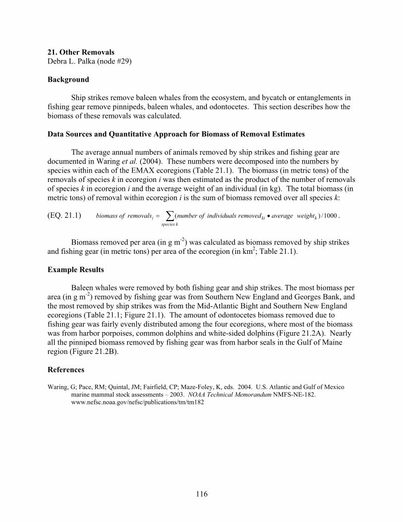
116

21. Other Removals Debra L. Palka (node #29) Background

Ship strikes remove baleen whales from the ecosystem, and bycatch or entanglements in

fishing gear remove pinnipeds, baleen whales, and odontocetes. This section describes how the biomass of these removals was calculated. Data Sources and Quantitative Approach for Biomass of Removal Estimates

The average annual numbers of animals removed by ship strikes and fishing gear are

documented in Waring et al. (2004). These numbers were decomposed into the numbers by species within each of the EMAX ecoregions (Table 21.1). The biomass (in metric tons) of the removals of species k in ecoregion i was then estimated as the product of the number of removals of species k in ecoregion i and the average weight of an individual (in kg). The total biomass (in metric tons) of removal within ecoregion i is the sum of biomass removed over all species k:

(EQ. 21.1) � ��kspecies

kkii weightaverageremovedsindividualofnumberremovalsofbiomass 1000/)( .

Biomass removed per area (in g m-2) was calculated as biomass removed by ship strikes

and fishing gear (in metric tons) per area of the ecoregion (in km2; Table 21.1). Example Results

Baleen whales were removed by both fishing gear and ship strikes. The most biomass per

area (in g m-2) removed by fishing gear was from Southern New England and Georges Bank, and the most removed by ship strikes was from the Mid-Atlantic Bight and Southern New England ecoregions (Table 21.1; Figure 21.1). The amount of odontocetes biomass removed due to fishing gear was fairly evenly distributed among the four ecoregions, where most of the biomass was from harbor porpoises, common dolphins and white-sided dolphins (Figure 21.2A). Nearly all the pinniped biomass removed by fishing gear was from harbor seals in the Gulf of Maine region (Figure 21.2B).

References

Waring, G; Pace, RM; Quintal, JM; Fairfield, CP; Maze-Foley, K, eds. 2004. U.S. Atlantic and Gulf of Mexico

marine mammal stock assessments – 2003. NOAA Technical Memorandum NMFS-NE-182. www.nefsc.noaa.gov/nefsc/publications/tm/tm182

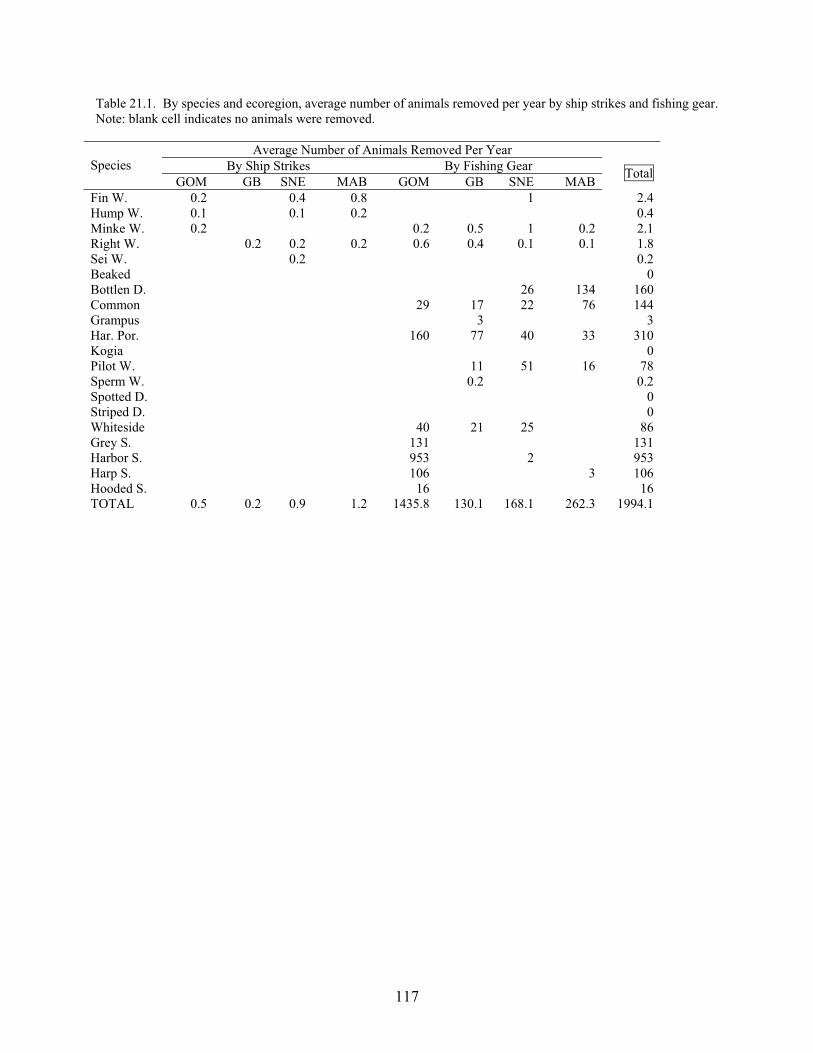
117

Table 21.1. By species and ecoregion, average number of animals removed per year by ship strikes and fishing gear. Note: blank cell indicates no animals were removed.

Average Number of Animals Removed Per Year

By Ship Strikes By Fishing Gear Species

GOM GB SNE MAB GOM GB SNE MAB

Total

Fin W. 0.2 0.4 0.8 1 2.4 Hump W. 0.1 0.1 0.2 0.4 Minke W. 0.2 0.2 0.5 1 0.2 2.1 Right W. 0.2 0.2 0.2 0.6 0.4 0.1 0.1 1.8 Sei W. 0.2 0.2 Beaked 0 Bottlen D. 26 134 160 Common 29 17 22 76 144 Grampus 3 3 Har. Por. 160 77 40 33 310 Kogia 0 Pilot W. 11 51 16 78 Sperm W. 0.2 0.2 Spotted D. 0 Striped D. 0 Whiteside 40 21 25 86 Grey S. 131 131 Harbor S. 953 2 953 Harp S. 106 3 106 Hooded S. 16 16 TOTAL 0.5 0.2 0.9 1.2 1435.8 130.1 168.1 262.3 1994.1

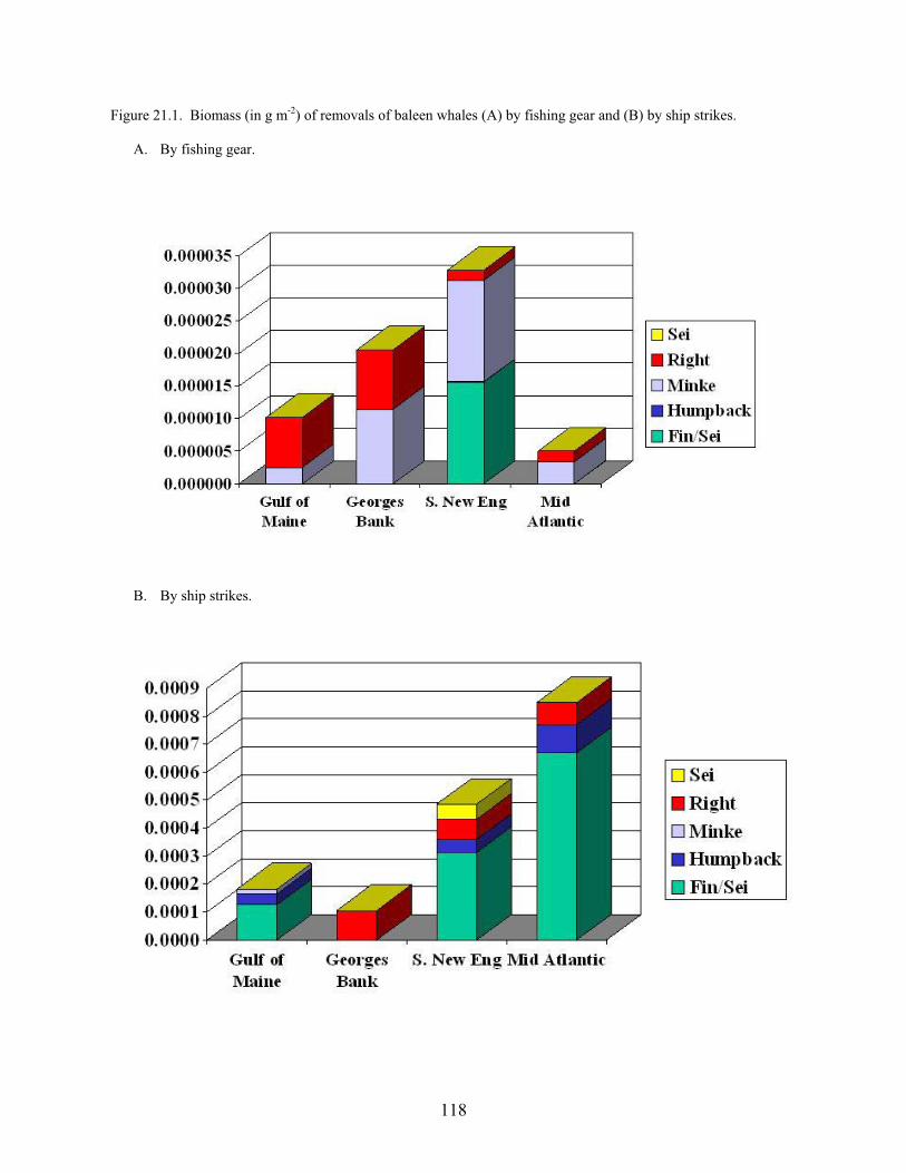
118

Figure 21.1. Biomass (in g m-2) of removals of baleen whales (A) by fishing gear and (B) by ship strikes.

A. By fishing gear.

B. By ship strikes.

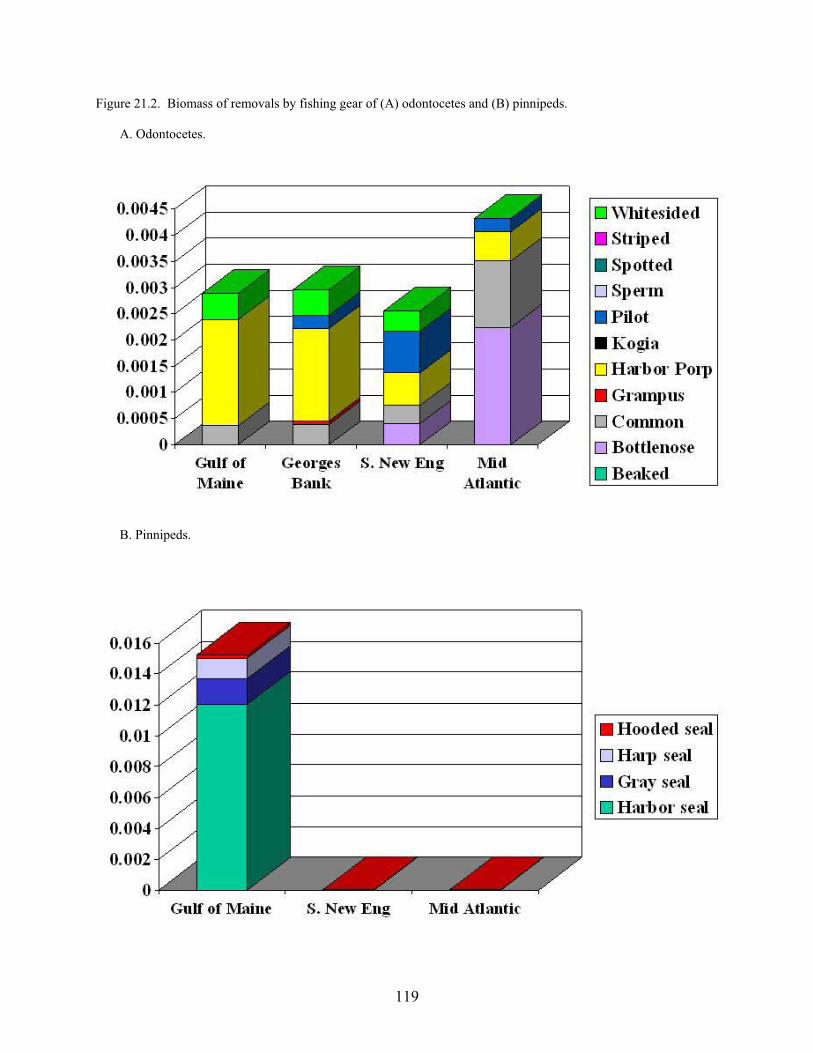
119

Figure 21.2. Biomass of removals by fishing gear of (A) odontocetes and (B) pinnipeds.

A. Odontocetes.

B. Pinnipeds.

120

22. Consumption and Diet Composition Matrix Jason S. Link Interaction Matrix - Fish The standard Northeast Fisheries Science Center (NEFSC) bottom trawl survey program has been executed annually since 1963 (Grosslein 1969; Azarovitz 1981; NEFC 1988). During these surveys, food habits data are collected from a variety of species. These multi-species surveys were designed to monitor trends in abundance and distribution and to provide samples to study the ecology of the large number of fish and invertebrate species inhabiting the region. The surveys have generally utilized a 36’ Yankee otter trawl towed at approximately 3.5 knots for 30 minutes at each station. Trawl stations were selected using a stratified random design. Within each stratum, stations were assigned randomly, and the number of stations allotted to a stratum was in proportion to its area. Station allotments were approximately one station per 200 square nautical miles. The surveys were conducted at depths of 27 m to 366 m; however, greater depths were occasionally sampled in the deep canyons along the continental shelf break. Once onboard, predators were sorted to species, weighed to the nearest 0.1 kg and measured to the nearest cm. Sex and maturity were determined, and subsamples of key species were eviscerated for feeding ecology studies. The NEFSC has collected fish food habits data for over 30 years. Starting in 1973, individual stomach samples for selected species were preserved at sea in 10% buffered formalin for later prey identification. Individual stomach preservation was continued until 1981 for an expanding list of species. Prey weight (to 0.01 g), number, percent composition, total stomach weight (to 0.01 g), and lengths of fish prey (mm) were determined upon examination in the laboratory. Prey identification was to the lowest taxon feasible. In 1981 the stomachs of major species such as Atlantic cod, haddock, silver hake, yellowtail flounder, winter flounder, Atlantic herring, and Atlantic mackerel continued to be individually preserved, but prey of all other species were examined and identified at sea. In addition, a conversion from mass (g) to volumetric measurement of prey (to 0.1 cm3) was initiated. Data on prey composition (%), numbers, and lengths were also collected shipboard. Since 1985, all stomach samples have been processed and prey identified at sea. To account for potential differences in the resolution of prey taxonomy between in-lab and at-sea sampling, we grouped most prey, particularly invertebrates, into broad prey categories (i.e., Class or Order). The exception was fish prey, which were maintained at the lowest feasible level. A conversion factor of 1.1 was used to convert prey volumes to weights based upon regression analyses (Link and Almeida 2000) similar to other studies (Bowman, unpublished manuscript; Tanasichuk et al. 1991; Garrison and Link 2000). For further details of the food habits data, see Link and Almeida (2000). We estimated mean stomach contents (to 0.01 g) and diet composition (as a percentage of weight) for each EMAX predator node category by EMAX prey node category. Interaction Matrix - Other Nodes

For those nodes for which we did not have direct diet information, we assumed that the

values for each EMAX predator’s diet composition fell within the range described for similar species in the literature. These percentages were adapted based on a suite of criteria (including

121

suitability and known feeding patterns from local species of similar biology) so that each predator’s diet summed to 100%. Examples of values can be found in the subject literature for each node or in food web compilations (e.g., Kenny et al. 1985, Overholtz et al. 1991, Pauly etal. 1995, Hammill et al. 1997, Kenny et al. 1997, Sigurjonsson and Vikingsson 1997, Stenson etal. 1997, Barros and Clarke 2002, Link 2002,). Values for the EMAX interaction matrix are in Table 22.1. We also show the connections for each node in Figure 22.1. Fish Consumption

We calculated the percent composition by weight of each major EMAX prey category in relation to the total amount consumed by each EMAX fish predator. Using a two-stage cluster method we weighted these values by the number of tows and the number of fish in a tow (see equations below). Link and Almeida (2000) provide a more thorough discussion of the statistics behind these methods and their calculation.

Based on an evacuation rate model (Eggers 1977; Elliot and Persson 1978), daily consumption estimates (Cd) were calculated for an average predator in each of the EMAX fish groups as

(EQ. 22.1) C E Sd i ii� 24 *

, where 24 is the number of hours in a day, i is the species of fish, γ is a constant (usually assumed to be equal to 1). The evacuation rate E is

(EQ. 22.2) E eiTp� � �

, where α and β are both fitted constants and T is temperature. Based on literature values and sensitivity analyses, we set α and β to 0.004 and 0.115, respectively (Durbin et al. 1983; Overholtz et al. 1999). We used a mean temperature for two (approximately semiannual) time periods (p) per year: 1) winter and spring surveys combined, and 2) summer and fall surveys combined (D. Mountain and M. Taylor; NEFSC, Woods Hole, Massachusetts, unpublished data). From Equation 22.1 above, S i

is the mean total stomach contents (g), such that

(EQ. 22.3) S

n S

ni

it itt

n

t

t

�

��

1

, where nt is the number of tows for all strata sampled, nit is the number of predator stomachs within a tow, and

(EQ. 22.4) S

S

nit

itkk

n

it

it

� ��

1

is the mean stomach weight of predator i in tow t, where k represents an individual fish. The daily consumption rates from both semiannual time periods were combined into a total, annual population level consumption rate (C):

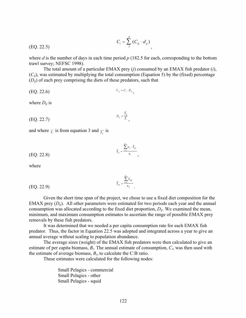
122

(EQ. 22.5) C C di d p

p

i� � ( )

1 , where d is the number of days in each time period p (182.5 for each, corresponding to the bottom trawl survey; NEFSC 1998). The total amount of a particular EMAX prey (j) consumed by an EMAX fish predator (i), (Cij), was estimated by multiplying the total consumption (Equation 5) by the (fixed) percentage (Dij) of each prey comprising the diets of these predators, such that (EQ. 22.6) C C Dij i ij� , where Dij is

(EQ. 22.7) D

SSij

ij

i�

, and where S i

is from equation 3 and S ij is

(EQ. 22.8) S

n S

nij

it ijtt

n

t

t

�

��

1

, where

(EQ. 22.9) S

S

nijt

ijtkk

n

it

it

� ��

1

.

Given the short time span of the project, we chose to use a fixed diet composition for the EMAX prey (Dij). All other parameters were estimated for two periods each year and the annual consumption was allocated according to the fixed diet proportion, Dij. We examined the mean, minimum, and maximum consumption estimates to ascertain the range of possible EMAX prey removals by these fish predators.

It was determined that we needed a per capita consumption rate for each EMAX fish predator. Thus, the factor in Equation 22.5 was adopted and integrated across a year to give an annual average without scaling to population abundance.

The average sizes (weight) of the EMAX fish predators were then calculated to give an estimate of per capita biomass, Bi. The annual estimate of consumption, Ci, was then used with the estimate of average biomass, Bi, to calculate the C:B ratio.

These estimates were calculated for the following nodes:

Small Pelagics - commercial Small Pelagics - other Small Pelagics - squid

123

Small Pelagics - anadromous Medium Pelagics - (piscivores and other) Demersals - benthivores Demersals - omnivores Demersals – piscivores

For examples of where this approach has been previously used see Link et al. (2002), Link and Garrison (2002), and Overholtz et al. (1999, 2000).

For all other EMAX nodes, literature values of C:B were used to estimate consumption. Further details are given in sections in this volume specific to each group. Integrating Consumptive Removals

For each EMAX node, the total consumption was multiplied by the diet composition

vector (Equation 22.6) to allocate the amount removed via consumption by each predator node for all EMAX prey nodes. These vectors were then summed across the cross-vector (or row) for each prey item to calculate a total amount of biomass removed per year for each EMAX node.

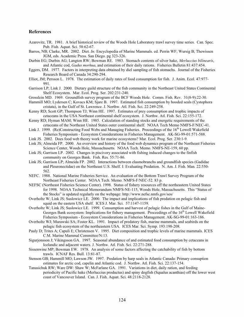
124

References Azarovitz, TR. 1981. A brief historical review of the Woods Hole Laboratory trawl survey time series. Can. Spec.

Pub. Fish. Aquat. Sci. 58:62-67. Barros, NB; Clarke, MR. 2002. Diet. In: Encyclopedia of Marine Mammals. ed. Perrin WF; Wursig B; Thewissen

JGM, eds. Academic Press. San Diego. pg 323-326. Durbin EG; Durbin AG; Langton RW; Bowman RE. 1983. Stomach contents of silver hake, Merluccius bilinearis,

and Atlantic cod, Gadus morhua, and estimation of their daily rations. Fisheries Bulletin 81:437:454. Eggers, DM. 1977. Factors in interpreting data obtained by diel sampling of fish stomachs. Journal of the Fisheries

Research Board of Canada 34:290-294. Elliot, JM; Persson L. 1978. The estimation of daily rates of food consumption for fish. J. Anim. Ecol. 47:977-

991. Garrison LP; Link J. 2000. Dietary guild structure of the fish community in the Northeast United States Continental

Shelf Ecosystem. Mar. Ecol. Prog. Ser. 202:231-240. Grosslein MD. 1969. Groundfish survey program of the BCF Woods Hole. Comm. Fish. Rev. 31(8-9):22-30. Hammill MO; Lydersen C; Kovacs KM; Sjare B. 1997. Estimated fish consumption by hooded seals (Cystophora

cristata), in the Gulf of St. Lawrence. J. Northw. Atl. Fish. Sci. 22:249-258. Kenny RD; Scott GP; Thompson TJ; Winn HE. 1997. Estimates of prey consumption and trophic impacts of

cetaceans in the USA Northeast continental shelf ecosystem. J. Northw. Atl. Fish. Sci. 22:155-172. Kenny RD; Hyman MAM; Winn HE. 1985. Calculation of standing stocks and energetic requirements of the

cetaceans of the Northeast United States outer continental shelf. NOAA Tech Memo NMFS-F/NEC-41. Link J. 1999. (Re)Constructing Food Webs and Managing Fisheries. Proceedings of the 16th Lowell Wakefield

Fisheries Symposium - Ecosystem Considerations in Fisheries Management. AK-SG-99-01:571-588. Link JS. 2002. Does food web theory work for marine ecosystems? Mar. Ecol. Prog. Ser. 230:1-9. Link JS; Almeida FP. 2000. An overview and history of the food web dynamics program of the Northeast Fisheries

Science Center, Woods Hole, Massachusetts. NOAA Tech. Memo. NMFS-NE-159, 60 pp. Link JS; Garrison LP. 2002. Changes in piscivory associated with fishing induced changes to the finfish

community on Georges Bank. Fish. Res. 55:71-86. Link JS; Garrison LP; Almeida FP. 2002. Interactions between elasmobranchs and groundfish species (Gadidae

and Pleuronectidae) on the Northeast U.S. Shelf. I: Evaluating Predation. N. Am. J. Fish. Man. 22:550-562.

NEFC. 1988. National Marine Fisheries Service. An evaluation of the Bottom Trawl Survey Program of the Northeast Fisheries Center. NOAA Tech. Memo. NMFS-F/NEC-52. 83 p.

NEFSC (Northeast Fisheries Science Center). 1998. Status of fishery resources off the northeastern United States for 1998. NOAA Technical Memorandum NMFS-NE-115, Woods Hole, Massachusetts. This “Status of the Stocks” is updated regularly on the webpage: http://www.nefsc.nmfs.gov/sos/

Overholtz W; Link JS; Suslowicz LE. 2000. The impact and implications of fish predation on pelagic fish and squid on the eastern USA shelf. ICES J. Mar. Sci. 57:1147-1159.

Overholtz W; Link JS; Suslowicz LE. 1999. Consumption and harvest of pelagic fishes in the Gulf of Maine-Georges Bank ecosystem: Implications for fishery management. Proceedings of the 16th Lowell Wakefield Fisheries Symposium - Ecosystem Considerations in Fisheries Management. AK-SG-99-01:163-186.

Overholtz WJ; Murawski SA; Foster KL. 1991. Impact of predatory fish, marine mammals, and seabirds on the pelagic fish ecosystem of the northeastern USA. ICES Mar. Sci. Symp. 193:198-208.

Pauly D; Trites A; Capuli E; Christensen V. 1995. Diet composition and trophic levels of marine mammals. ICES C.M. Marine Mammal Committee/N:13.

Sigurjonsson J; Vikingsson GA. 1997. Seasonal abundance of and estimated food consumption by cetaceans in Icelandic and adjacent waters. J. Northw. Atl. Fish. Sci. 22:271-288.

Sissenwine MP; Bowman EW. 1978. An analysis of some factors affecting the catchability of fish by bottom trawls. ICNAF Res. Bull. 13:81-87.

Stenson GB; Hammill MO; Lawson JW. 1997. Predation by harp seals in Atlantic Canada: Primary consuption estimates for arctic cod, capelin and Atlantic cod. J. Northw. Atl. Fish. Sci. 22:137-154.

Tanasichuk RW; Ware DW: Shaw W; McFarlane GA. 1991. Variations in diet, daily ration, and feeding periodicity of Pacific hake (Merluccius productus) and spiny dogfish (Squalus acanthias) off the lower west coast of Vancouver Island. Can. J. Fish. Aquat. Sci. 48:2118-2128.

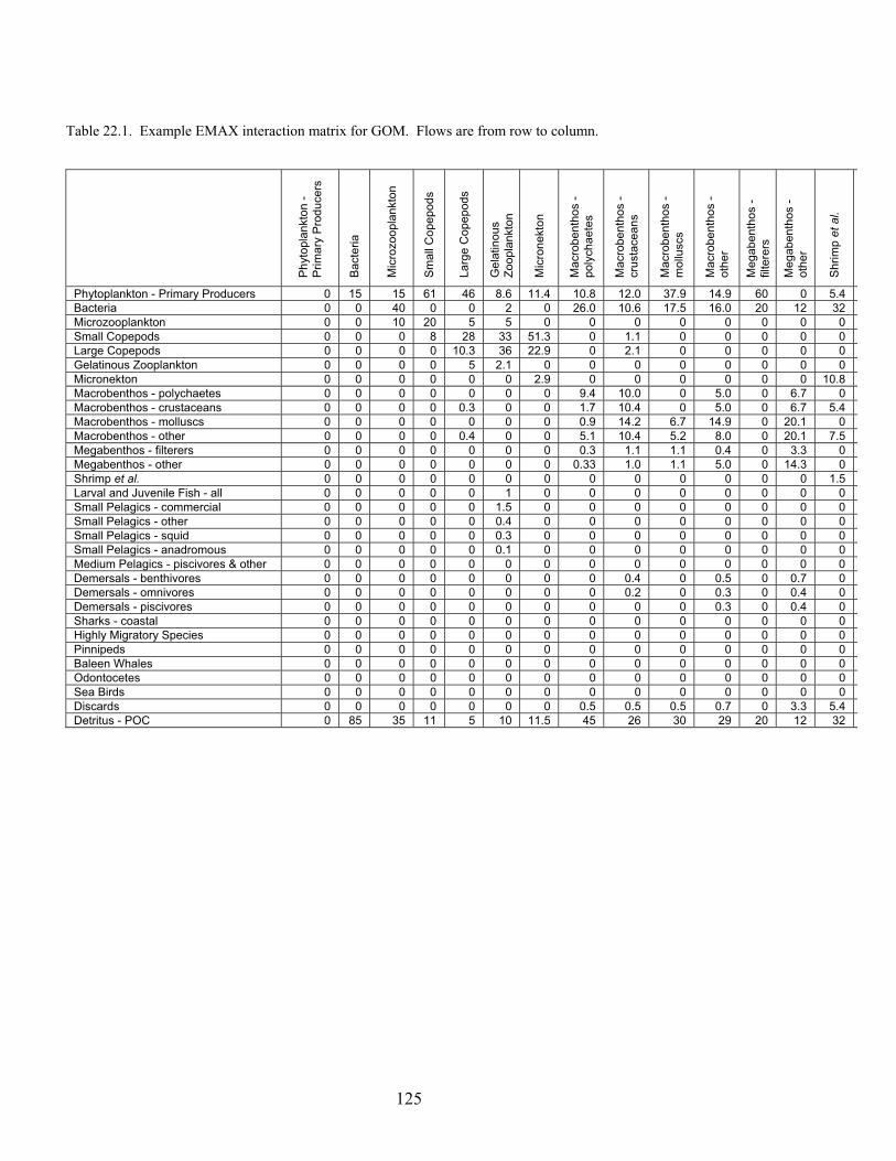
125

Table 22.1. Example EMAX interaction matrix for GOM. Flows are from row to column.

Phy

topl

ankt

on -

Prim

ary

Pro

duce

rs

Bac

teria

Mic

rozo

opla

nkto

n

Sm

all C

opep

ods

Larg

e C

opep

ods

Gel

atin

ous

Zoop

lank

ton

Mic

rone

kton

Mac

robe

ntho

s -

poly

chae

tes

Mac

robe

ntho

s -

crus

tace

ans

Mac

robe

ntho

s -

mol

lusc

s

Mac

robe

ntho

s -

othe

r

Meg

aben

thos

- fil

tere

rs

Meg

aben

thos

- ot

her

Shr

imp

et a

l.

Phytoplankton - Primary Producers 0 15 15 61 46 8.6 11.4 10.8 12.0 37.9 14.9 60 0 5.4 Bacteria 0 0 40 0 0 2 0 26.0 10.6 17.5 16.0 20 12 32 Microzooplankton 0 0 10 20 5 5 0 0 0 0 0 0 0 0 Small Copepods 0 0 0 8 28 33 51.3 0 1.1 0 0 0 0 0 Large Copepods 0 0 0 0 10.3 36 22.9 0 2.1 0 0 0 0 0 Gelatinous Zooplankton 0 0 0 0 5 2.1 0 0 0 0 0 0 0 0 Micronekton 0 0 0 0 0 0 2.9 0 0 0 0 0 0 10.8 Macrobenthos - polychaetes 0 0 0 0 0 0 0 9.4 10.0 0 5.0 0 6.7 0 Macrobenthos - crustaceans 0 0 0 0 0.3 0 0 1.7 10.4 0 5.0 0 6.7 5.4 Macrobenthos - molluscs 0 0 0 0 0 0 0 0.9 14.2 6.7 14.9 0 20.1 0 Macrobenthos - other 0 0 0 0 0.4 0 0 5.1 10.4 5.2 8.0 0 20.1 7.5 Megabenthos - filterers 0 0 0 0 0 0 0 0.3 1.1 1.1 0.4 0 3.3 0 Megabenthos - other 0 0 0 0 0 0 0 0.33 1.0 1.1 5.0 0 14.3 0 Shrimp et al. 0 0 0 0 0 0 0 0 0 0 0 0 0 1.5 Larval and Juvenile Fish - all 0 0 0 0 0 1 0 0 0 0 0 0 0 0 Small Pelagics - commercial 0 0 0 0 0 1.5 0 0 0 0 0 0 0 0 Small Pelagics - other 0 0 0 0 0 0.4 0 0 0 0 0 0 0 0 Small Pelagics - squid 0 0 0 0 0 0.3 0 0 0 0 0 0 0 0 Small Pelagics - anadromous 0 0 0 0 0 0.1 0 0 0 0 0 0 0 0 Medium Pelagics - piscivores & other 0 0 0 0 0 0 0 0 0 0 0 0 0 0 Demersals - benthivores 0 0 0 0 0 0 0 0 0.4 0 0.5 0 0.7 0 Demersals - omnivores 0 0 0 0 0 0 0 0 0.2 0 0.3 0 0.4 0 Demersals - piscivores 0 0 0 0 0 0 0 0 0 0 0.3 0 0.4 0 Sharks - coastal 0 0 0 0 0 0 0 0 0 0 0 0 0 0 Highly Migratory Species 0 0 0 0 0 0 0 0 0 0 0 0 0 0 Pinnipeds 0 0 0 0 0 0 0 0 0 0 0 0 0 0 Baleen Whales 0 0 0 0 0 0 0 0 0 0 0 0 0 0 Odontocetes 0 0 0 0 0 0 0 0 0 0 0 0 0 0 Sea Birds 0 0 0 0 0 0 0 0 0 0 0 0 0 0 Discards 0 0 0 0 0 0 0 0.5 0.5 0.5 0.7 0 3.3 5.4 Detritus - POC 0 85 35 11 5 10 11.5 45 26 30 29 20 12 32

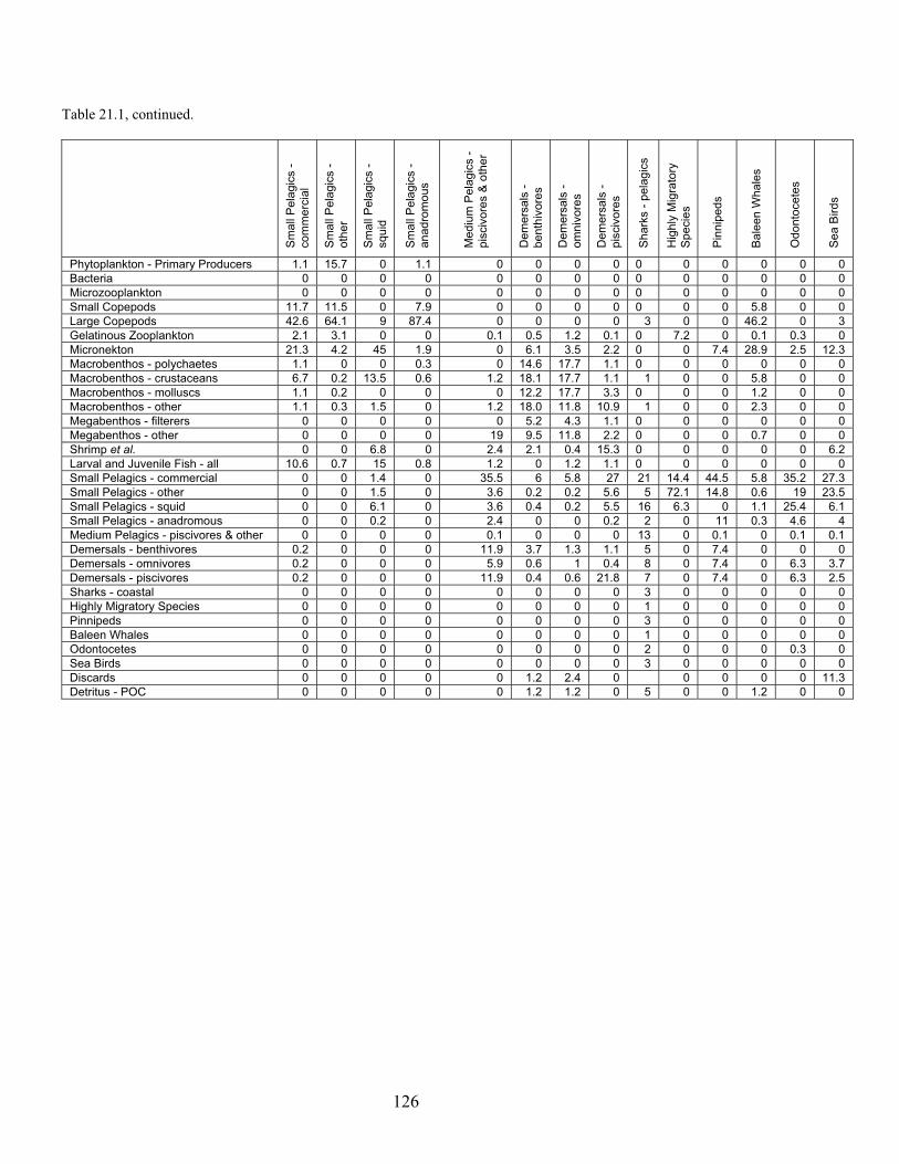
126

Table 21.1, continued.

Sm

all P

elag

ics

- co

mm

erci

al

Sm

all P

elag

ics

- ot

her

Sm

all P

elag

ics

- sq

uid

Sm

all P

elag

ics

- an

adro

mou

s

Med

ium

Pel

agic

s -

pisc

ivor

es &

oth

er

Dem

ersa

ls -

bent

hivo

res

Dem

ersa

ls -

omni

vore

s

Dem

ersa

ls -

pisc

ivor

es

Sha

rks

- pel

agic

s

Hig

hly

Mig

rato

ry

Spe

cies

Pin

nipe

ds

Bal

een

Wha

les

Odo

ntoc

etes

Sea

Bird

s

Phytoplankton - Primary Producers 1.1 15.7 0 1.1 0 0 0 0 0 0 0 0 0 0 Bacteria 0 0 0 0 0 0 0 0 0 0 0 0 0 0 Microzooplankton 0 0 0 0 0 0 0 0 0 0 0 0 0 0 Small Copepods 11.7 11.5 0 7.9 0 0 0 0 0 0 0 5.8 0 0 Large Copepods 42.6 64.1 9 87.4 0 0 0 0 3 0 0 46.2 0 3 Gelatinous Zooplankton 2.1 3.1 0 0 0.1 0.5 1.2 0.1 0 7.2 0 0.1 0.3 0 Micronekton 21.3 4.2 45 1.9 0 6.1 3.5 2.2 0 0 7.4 28.9 2.5 12.3 Macrobenthos - polychaetes 1.1 0 0 0.3 0 14.6 17.7 1.1 0 0 0 0 0 0 Macrobenthos - crustaceans 6.7 0.2 13.5 0.6 1.2 18.1 17.7 1.1 1 0 0 5.8 0 0 Macrobenthos - molluscs 1.1 0.2 0 0 0 12.2 17.7 3.3 0 0 0 1.2 0 0 Macrobenthos - other 1.1 0.3 1.5 0 1.2 18.0 11.8 10.9 1 0 0 2.3 0 0 Megabenthos - filterers 0 0 0 0 0 5.2 4.3 1.1 0 0 0 0 0 0 Megabenthos - other 0 0 0 0 19 9.5 11.8 2.2 0 0 0 0.7 0 0 Shrimp et al. 0 0 6.8 0 2.4 2.1 0.4 15.3 0 0 0 0 0 6.2 Larval and Juvenile Fish - all 10.6 0.7 15 0.8 1.2 0 1.2 1.1 0 0 0 0 0 0 Small Pelagics - commercial 0 0 1.4 0 35.5 6 5.8 27 21 14.4 44.5 5.8 35.2 27.3 Small Pelagics - other 0 0 1.5 0 3.6 0.2 0.2 5.6 5 72.1 14.8 0.6 19 23.5 Small Pelagics - squid 0 0 6.1 0 3.6 0.4 0.2 5.5 16 6.3 0 1.1 25.4 6.1 Small Pelagics - anadromous 0 0 0.2 0 2.4 0 0 0.2 2 0 11 0.3 4.6 4 Medium Pelagics - piscivores & other 0 0 0 0 0.1 0 0 0 13 0 0.1 0 0.1 0.1 Demersals - benthivores 0.2 0 0 0 11.9 3.7 1.3 1.1 5 0 7.4 0 0 0 Demersals - omnivores 0.2 0 0 0 5.9 0.6 1 0.4 8 0 7.4 0 6.3 3.7 Demersals - piscivores 0.2 0 0 0 11.9 0.4 0.6 21.8 7 0 7.4 0 6.3 2.5 Sharks - coastal 0 0 0 0 0 0 0 0 3 0 0 0 0 0 Highly Migratory Species 0 0 0 0 0 0 0 0 1 0 0 0 0 0 Pinnipeds 0 0 0 0 0 0 0 0 3 0 0 0 0 0 Baleen Whales 0 0 0 0 0 0 0 0 1 0 0 0 0 0 Odontocetes 0 0 0 0 0 0 0 0 2 0 0 0 0.3 0 Sea Birds 0 0 0 0 0 0 0 0 3 0 0 0 0 0 Discards 0 0 0 0 0 1.2 2.4 0 0 0 0 0 11.3 Detritus - POC 0 0 0 0 0 1.2 1.2 0 5 0 0 1.2 0 0

127

Figure 22.1. Network connections for each node, showing the flows from one node to its consumer nodes.

EMAX

MediumPelagics

Small PelagicsCommercial

Odontocetes

Large Copepods Gelatinous ZP

Micronekton Mesopelagics

PinnipedsBaleen whales

Primary Producers

MacroBenthosPolychaetes

Demersal Fisheries

Sea birds

Pelagic Sharks HMS

Small Copepods

CoastalSharks

MacroBenthosMolluscs

MacroBenthosCrustaceans MacroBenthos

Other

MegaBenthosFilterers

MegaBenthosOther

Larval & Juv. Fish

PelagicFisheries

Small PelagicsOther

Small PelagicsAnadromous

Small PelagicsSquid

DemersalsBenthivores

DemersalsPiscivores

Shrimp et al.

DemersalsOmnivores

Discards Detritus-POC DOCBacteriaMicrozooplankton

EMAX

MediumPelagics

Small PelagicsCommercial

Odontocetes

Large Copepods Gelatinous ZP

Micronekton Mesopelagics

PinnipedsBaleen whales

Primary Producers

MacroBenthosPolychaetes

Demersal Fisheries

Sea birds

Pelagic Sharks HMS

Small Copepods

CoastalSharks

MacroBenthosMolluscs

MacroBenthosCrustaceans MacroBenthos

Other

MegaBenthosFilterers

MegaBenthosOther

Larval & Juv. Fish

PelagicFisheries

Small PelagicsOther

Small PelagicsAnadromous

Small PelagicsSquid

DemersalsBenthivores

DemersalsPiscivores

Shrimp et al.

DemersalsOmnivores

Discards Detritus-POC DOCBacteriaMicrozooplankton

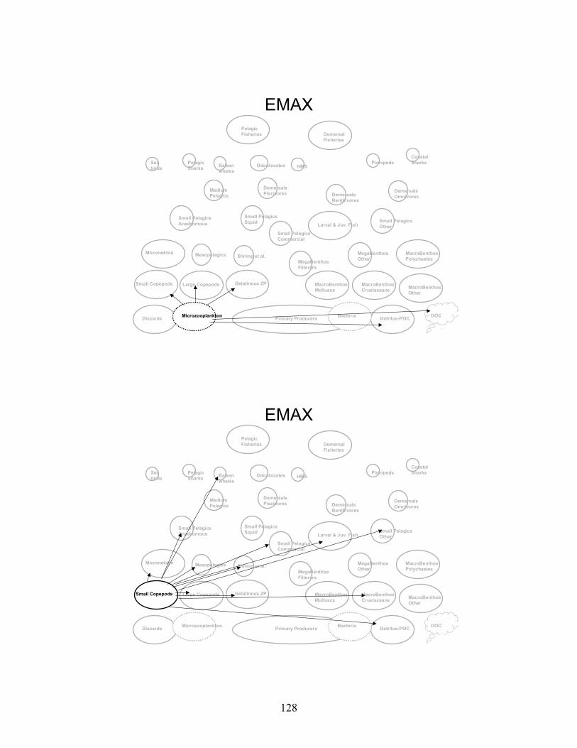
128

EMAX

MediumPelagics

Small PelagicsCommercial

Odontocetes

Large Copepods Gelatinous ZP

Micronekton Mesopelagics

PinnipedsBaleen whales

Primary Producers

MacroBenthosPolychaetes

Demersal Fisheries

Sea birds

Pelagic Sharks HMS

Small Copepods

CoastalSharks

MacroBenthosMolluscs

MacroBenthosCrustaceans MacroBenthos

Other

MegaBenthosFilterers

MegaBenthosOther

Larval & Juv. Fish

PelagicFisheries

Small PelagicsOther

Small PelagicsAnadromous

Small PelagicsSquid

DemersalsBenthivores

DemersalsPiscivores

Shrimp et al.

DemersalsOmnivores

Discards Detritus-POC DOCBacteriaMicrozooplankton

EMAX

MediumPelagics

Small PelagicsCommercial

Odontocetes

Large Copepods Gelatinous ZP

Micronekton Mesopelagics

PinnipedsBaleen whales

Primary Producers

MacroBenthosPolychaetes

Demersal Fisheries

Sea birds

Pelagic Sharks HMS

Small Copepods

CoastalSharks

MacroBenthosMolluscs

MacroBenthosCrustaceans MacroBenthos

Other

MegaBenthosFilterers

MegaBenthosOther

Larval & Juv. Fish

PelagicFisheries

Small PelagicsOther

Small PelagicsAnadromous

Small PelagicsSquid

DemersalsBenthivores

DemersalsPiscivores

Shrimp et al.

DemersalsOmnivores

Discards Detritus-POC DOCBacteriaMicrozooplankton

129

EMAX

MediumPelagics

Small PelagicsCommercial

Odontocetes

Large Copepods Gelatinous ZP

Micronekton Mesopelagics

PinnipedsBaleen whales

Primary Producers

MacroBenthosPolychaetes

Demersal Fisheries

Sea birds

Pelagic Sharks HMS

Small Copepods

CoastalSharks

MacroBenthosMolluscs

MacroBenthosCrustaceans MacroBenthos

Other

MegaBenthosFilterers

MegaBenthosOther

Larval & Juv. Fish

PelagicFisheries

Small PelagicsOther

Small PelagicsAnadromous

Small PelagicsSquid

DemersalsBenthivores

DemersalsPiscivores

Shrimp et al.

DemersalsOmnivores

Discards Detritus-POC DOCBacteriaMicrozooplankton

EMAX

MediumPelagics

Small PelagicsCommercial

Odontocetes

Large Copepods Gelatinous ZP

Micronekton Mesopelagics

PinnipedsBaleen whales

Primary Producers

MacroBenthosPolychaetes

Demersal Fisheries

Sea birds

Pelagic Sharks HMS

Small Copepods

CoastalSharks

MacroBenthosMolluscs

MacroBenthosCrustaceans MacroBenthos

Other

MegaBenthosFilterers

MegaBenthosOther

Larval & Juv. Fish

PelagicFisheries

Small PelagicsOther

Small PelagicsAnadromous

Small PelagicsSquid

DemersalsBenthivores

DemersalsPiscivores

Shrimp et al.

DemersalsOmnivores

Discards Detritus-POC DOCBacteriaMicrozooplankton

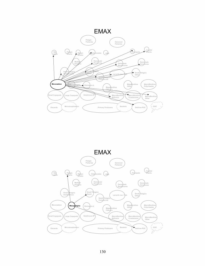
130

EMAX

MediumPelagics

Small PelagicsCommercial

Odontocetes

Large Copepods Gelatinous ZP

Micronekton Mesopelagics

PinnipedsBaleen whales

Primary Producers

MacroBenthosPolychaetes

Demersal Fisheries

Sea birds

Pelagic Sharks HMS

Small Copepods

CoastalSharks

MacroBenthosMolluscs

MacroBenthosCrustaceans MacroBenthos

Other

MegaBenthosFilterers

MegaBenthosOther

Larval & Juv. Fish

PelagicFisheries

Small PelagicsOther

Small PelagicsAnadromous

Small PelagicsSquid

DemersalsBenthivores

DemersalsPiscivores

Shrimp et al.

DemersalsOmnivores

Discards Detritus-POC DOCBacteriaMicrozooplankton

EMAX

MediumPelagics

Small PelagicsCommercial

Odontocetes

Large Copepods Gelatinous ZP

Micronekton Mesopelagics

PinnipedsBaleen whales

Primary Producers

MacroBenthosPolychaetes

Demersal Fisheries

Sea birds

Pelagic Sharks HMS

Small Copepods

CoastalSharks

MacroBenthosMolluscs

MacroBenthosCrustaceans MacroBenthos

Other

MegaBenthosFilterers

MegaBenthosOther

Larval & Juv. Fish

PelagicFisheries

Small PelagicsOther

Small PelagicsAnadromous

Small PelagicsSquid

DemersalsBenthivores

DemersalsPiscivores

Shrimp et al.

DemersalsOmnivores

Discards Detritus-POC DOCBacteriaMicrozooplankton

131

EMAX

MediumPelagics

Small PelagicsCommercial

Odontocetes

Large Copepods Gelatinous ZP

Micronekton Mesopelagics

PinnipedsBaleen whales

Primary Producers

MacroBenthosPolychaetes

Demersal Fisheries

Sea birds

Pelagic Sharks HMS

Small Copepods

CoastalSharks

MacroBenthosMolluscs

MacroBenthosCrustaceans MacroBenthos

Other

MegaBenthosFilterers

MegaBenthosOther

Larval & Juv. Fish

PelagicFisheries

Small PelagicsOther

Small PelagicsAnadromous

Small PelagicsSquid

DemersalsBenthivores

DemersalsPiscivores

Shrimp et al.

DemersalsOmnivores

Discards Detritus-POC DOCBacteriaMicrozooplankton

EMAX

MediumPelagics

Small PelagicsCommercial

Odontocetes

Large Copepods Gelatinous ZP

Micronekton Mesopelagics

PinnipedsBaleen whales

Primary Producers

MacroBenthosPolychaetes

Demersal Fisheries

Sea birds

Pelagic Sharks HMS

Small Copepods

CoastalSharks

MacroBenthosMolluscs

MacroBenthosCrustaceans MacroBenthos

Other

MegaBenthosFilterers

MegaBenthosOther

Larval & Juv. Fish

PelagicFisheries

Small PelagicsOther

Small PelagicsAnadromous

Small PelagicsSquid

DemersalsBenthivores

DemersalsPiscivores

Shrimp et al.

DemersalsOmnivores

Discards Detritus-POC DOCBacteriaMicrozooplankton

132

EMAX

MediumPelagics

Small PelagicsCommercial

Odontocetes

Large Copepods Gelatinous ZP

Micronekton Mesopelagics

PinnipedsBaleen whales

Primary Producers

MacroBenthosPolychaetes

Demersal Fisheries

Sea birds

Pelagic Sharks HMS

Small Copepods

CoastalSharks

MacroBenthosMolluscs

MacroBenthosCrustaceans MacroBenthos

Other

MegaBenthosFilterers

MegaBenthosOther

Larval & Juv. Fish

PelagicFisheries

Small PelagicsOther

Small PelagicsAnadromous

Small PelagicsSquid

DemersalsBenthivores

DemersalsPiscivores

Shrimp et al.

DemersalsOmnivores

Discards Detritus-POC DOCBacteriaMicrozooplankton

EMAX

MediumPelagics

Small PelagicsCommercial

Odontocetes

Large Copepods Gelatinous ZP

Micronekton Mesopelagics

PinnipedsBaleen whales

Primary Producers

MacroBenthosPolychaetes

Demersal Fisheries

Sea birds

Pelagic Sharks HMS

Small Copepods

CoastalSharks

MacroBenthosMolluscs

MacroBenthosCrustaceans MacroBenthos

Other

MegaBenthosFilterers

MegaBenthosOther

Larval & Juv. Fish

PelagicFisheries

Small PelagicsOther

Small PelagicsAnadromous

Small PelagicsSquid

DemersalsBenthivores

DemersalsPiscivores

Shrimp et al.

DemersalsOmnivores

Discards Detritus-POC DOCBacteriaMicrozooplankton

133

EMAX

MediumPelagics

Small PelagicsCommercial

Odontocetes

Large Copepods Gelatinous ZP

Micronekton Mesopelagics

PinnipedsBaleen whales

Primary Producers

MacroBenthosPolychaetes

Demersal Fisheries

Sea birds

Pelagic Sharks HMS

Small Copepods

CoastalSharks

MacroBenthosMolluscs

MacroBenthosCrustaceans MacroBenthos

Other

MegaBenthosFilterers

MegaBenthosOther

Larval & Juv. Fish

PelagicFisheries

Small PelagicsOther

Small PelagicsAnadromous

Small PelagicsSquid

DemersalsBenthivores

DemersalsPiscivores

Shrimp et al.

DemersalsOmnivores

Discards Detritus-POC DOCBacteriaMicrozooplankton

EMAX

MediumPelagics

Small PelagicsCommercial

Odontocetes

Large Copepods Gelatinous ZP

Micronekton Mesopelagics

PinnipedsBaleen whales

Primary Producers

MacroBenthosPolychaetes

Demersal Fisheries

Sea birds

Pelagic Sharks HMS

Small Copepods

CoastalSharks

MacroBenthosMolluscs

MacroBenthosCrustaceans MacroBenthos

Other

MegaBenthosFilterers

MegaBenthosOther

Larval & Juv. Fish

PelagicFisheries

Small PelagicsOther

Small PelagicsAnadromous

Small PelagicsSquid

DemersalsBenthivores

DemersalsPiscivores

Shrimp et al.

DemersalsOmnivores

Discards Detritus-POC DOCBacteriaMicrozooplankton

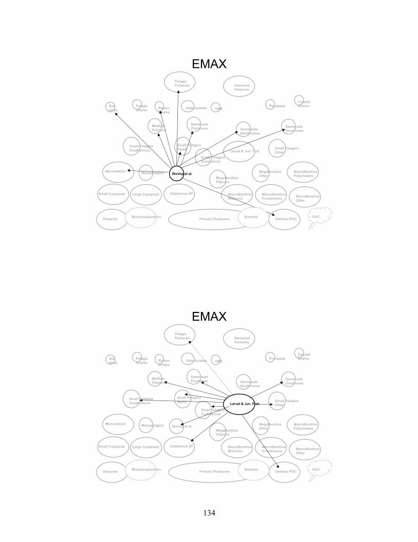
134

EMAX

MediumPelagics

Small PelagicsCommercial

Odontocetes

Large Copepods Gelatinous ZP

Micronekton Mesopelagics

PinnipedsBaleen whales

Primary Producers

MacroBenthosPolychaetes

Demersal Fisheries

Sea birds

Pelagic Sharks HMS

Small Copepods

CoastalSharks

MacroBenthosMolluscs

MacroBenthosCrustaceans MacroBenthos

Other

MegaBenthosFilterers

MegaBenthosOther

Larval & Juv. Fish

PelagicFisheries

Small PelagicsOther

Small PelagicsAnadromous

Small PelagicsSquid

DemersalsBenthivores

DemersalsPiscivores

Shrimp et al.

DemersalsOmnivores

Discards Detritus-POC DOCBacteriaMicrozooplankton

EMAX

MediumPelagics

Small PelagicsCommercial

Odontocetes

Large Copepods Gelatinous ZP

Micronekton Mesopelagics

PinnipedsBaleen whales

Primary Producers

MacroBenthosPolychaetes

Demersal Fisheries

Sea birds

Pelagic Sharks HMS

Small Copepods

CoastalSharks

MacroBenthosMolluscs

MacroBenthosCrustaceans MacroBenthos

Other

MegaBenthosFilterers

MegaBenthosOther

Larval & Juv. Fish

PelagicFisheries

Small PelagicsOther

Small PelagicsAnadromous

Small PelagicsSquid

DemersalsBenthivores

DemersalsPiscivores

Shrimp et al.

DemersalsOmnivores

Discards Detritus-POC DOCBacteriaMicrozooplankton

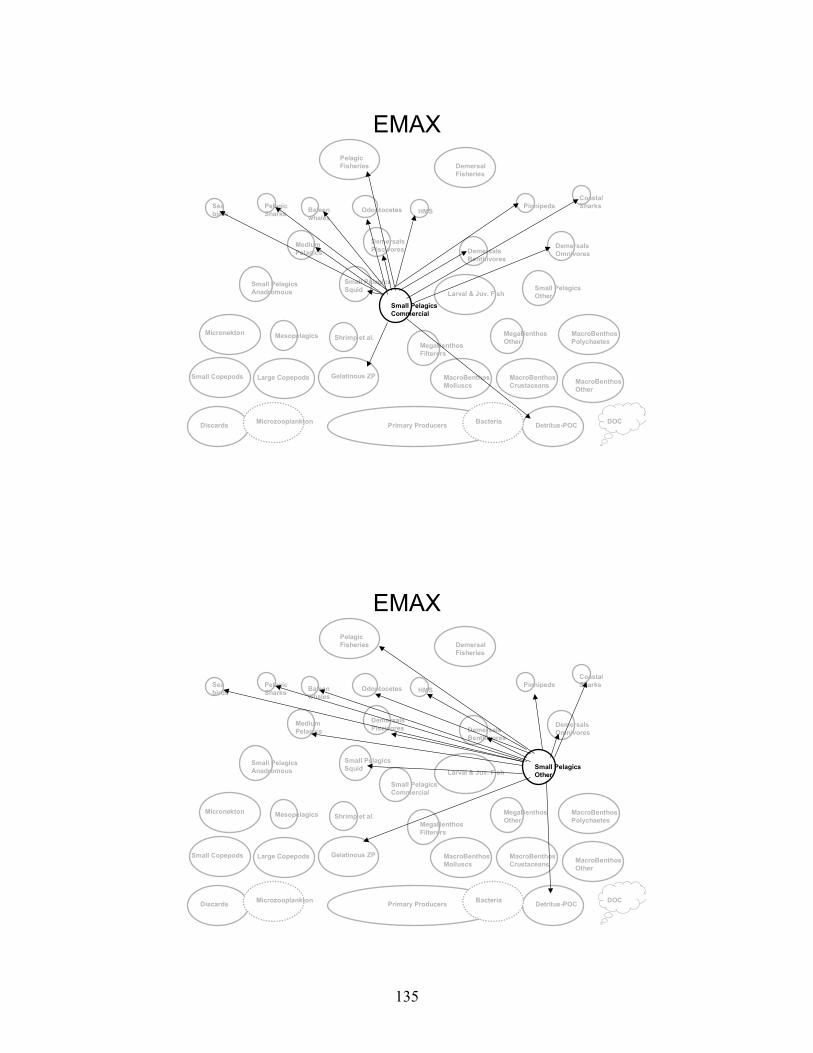
135

EMAX

MediumPelagics

Small PelagicsCommercial

Odontocetes

Large Copepods Gelatinous ZP

Micronekton Mesopelagics

PinnipedsBaleen whales

Primary Producers

MacroBenthosPolychaetes

Demersal Fisheries

Sea birds

Pelagic Sharks HMS

Small Copepods

CoastalSharks

MacroBenthosMolluscs

MacroBenthosCrustaceans MacroBenthos

Other

MegaBenthosFilterers

MegaBenthosOther

Larval & Juv. Fish

PelagicFisheries

Small PelagicsOther

Small PelagicsAnadromous

Small PelagicsSquid

DemersalsBenthivores

DemersalsPiscivores

Shrimp et al.

DemersalsOmnivores

Discards Detritus-POC DOCBacteriaMicrozooplankton

EMAX

MediumPelagics

Small PelagicsCommercial

Odontocetes

Large Copepods Gelatinous ZP

Micronekton Mesopelagics

PinnipedsBaleen whales

Primary Producers

MacroBenthosPolychaetes

Demersal Fisheries

Sea birds

Pelagic Sharks HMS

Small Copepods

CoastalSharks

MacroBenthosMolluscs

MacroBenthosCrustaceans MacroBenthos

Other

MegaBenthosFilterers

MegaBenthosOther

Larval & Juv. Fish

PelagicFisheries

Small PelagicsOther

Small PelagicsAnadromous

Small PelagicsSquid

DemersalsBenthivores

DemersalsPiscivores

Shrimp et al.

DemersalsOmnivores

Discards Detritus-POC DOCBacteriaMicrozooplankton

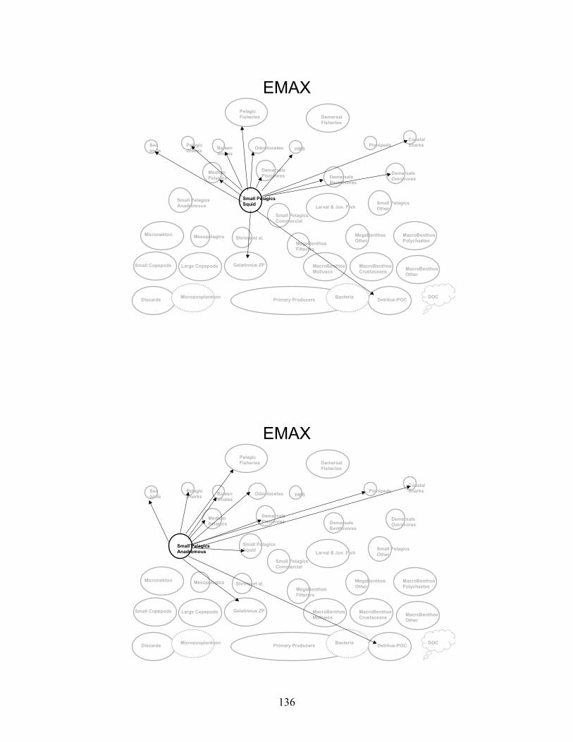
136

EMAX

MediumPelagics

Small PelagicsCommercial

Odontocetes

Large Copepods Gelatinous ZP

Micronekton Mesopelagics

PinnipedsBaleen whales

Primary Producers

MacroBenthosPolychaetes

Demersal Fisheries

Sea birds

Pelagic Sharks HMS

Small Copepods

CoastalSharks

MacroBenthosMolluscs

MacroBenthosCrustaceans MacroBenthos

Other

MegaBenthosFilterers

MegaBenthosOther

Larval & Juv. Fish

PelagicFisheries

Small PelagicsOther

Small PelagicsAnadromous

Small PelagicsSquid

DemersalsBenthivores

DemersalsPiscivores

Shrimp et al.

DemersalsOmnivores

Discards Detritus-POC DOCBacteriaMicrozooplankton

EMAX

MediumPelagics

Small PelagicsCommercial

Odontocetes

Large Copepods Gelatinous ZP

Micronekton Mesopelagics

PinnipedsBaleen whales

Primary Producers

MacroBenthosPolychaetes

Demersal Fisheries

Sea birds

Pelagic Sharks HMS

Small Copepods

CoastalSharks

MacroBenthosMolluscs

MacroBenthosCrustaceans MacroBenthos

Other

MegaBenthosFilterers

MegaBenthosOther

Larval & Juv. Fish

PelagicFisheries

Small PelagicsOther

Small PelagicsAnadromous

Small PelagicsSquid

DemersalsBenthivores

DemersalsPiscivores

Shrimp et al.

DemersalsOmnivores

Discards Detritus-POC DOCBacteriaMicrozooplankton

137

EMAX

MediumPelagics

Small PelagicsCommercial

Odontocetes

Large Copepods Gelatinous ZP

Micronekton Mesopelagics

PinnipedsBaleen whales

Primary Producers

MacroBenthosPolychaetes

Demersal Fisheries

Sea birds

Pelagic Sharks HMS

Small Copepods

CoastalSharks

MacroBenthosMolluscs

MacroBenthosCrustaceans MacroBenthos

Other

MegaBenthosFilterers

MegaBenthosOther

Larval & Juv. Fish

PelagicFisheries

Small PelagicsOther

Small PelagicsAnadromous

Small PelagicsSquid

DemersalsBenthivores

DemersalsPiscivores

Shrimp et al.

DemersalsOmnivores

Discards Detritus-POC DOCBacteriaMicrozooplankton

EMAX

MediumPelagics

Small PelagicsCommercial

Odontocetes

Large Copepods Gelatinous ZP

Micronekton Mesopelagics

PinnipedsBaleen whales

Primary Producers

MacroBenthosPolychaetes

Demersal Fisheries

Sea birds

Pelagic Sharks HMS

Small Copepods

CoastalSharks

MacroBenthosMolluscs

MacroBenthosCrustaceans MacroBenthos

Other

MegaBenthosFilterers

MegaBenthosOther

Larval & Juv. Fish

PelagicFisheries

Small PelagicsOther

Small PelagicsAnadromous

Small PelagicsSquid

DemersalsBenthivores

DemersalsPiscivores

Shrimp et al.

DemersalsOmnivores

Discards Detritus-POC DOCBacteriaMicrozooplankton

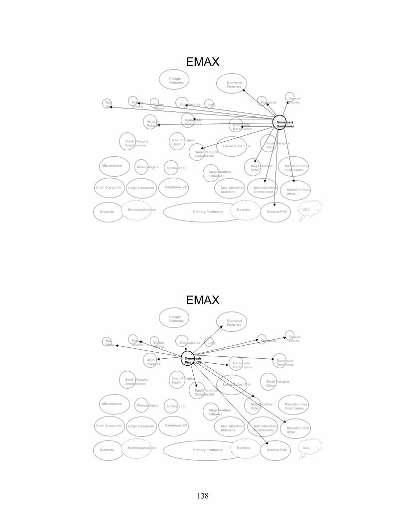
138

EMAX

MediumPelagics

Small PelagicsCommercial

Odontocetes

Large Copepods Gelatinous ZP

Micronekton Mesopelagics

PinnipedsBaleen whales

Primary Producers

MacroBenthosPolychaetes

Demersal Fisheries

Sea birds

Pelagic Sharks HMS

Small Copepods

CoastalSharks

MacroBenthosMolluscs

MacroBenthosCrustaceans MacroBenthos

Other

MegaBenthosFilterers

MegaBenthosOther

Larval & Juv. Fish

PelagicFisheries

Small PelagicsOther

Small PelagicsAnadromous

Small PelagicsSquid

DemersalsBenthivores

DemersalsPiscivores

Shrimp et al.

DemersalsOmnivores

Discards Detritus-POC DOCBacteriaMicrozooplankton

EMAX

MediumPelagics

Small PelagicsCommercial

Odontocetes

Large Copepods Gelatinous ZP

Micronekton Mesopelagics

PinnipedsBaleen whales

Primary Producers

MacroBenthosPolychaetes

Demersal Fisheries

Sea birds

Pelagic Sharks HMS

Small Copepods

CoastalSharks

MacroBenthosMolluscs

MacroBenthosCrustaceans MacroBenthos

Other

MegaBenthosFilterers

MegaBenthosOther

Larval & Juv. Fish

PelagicFisheries

Small PelagicsOther

Small PelagicsAnadromous

Small PelagicsSquid

DemersalsBenthivores

DemersalsPiscivores

Shrimp et al.

DemersalsOmnivores

Discards Detritus-POC DOCBacteriaMicrozooplankton

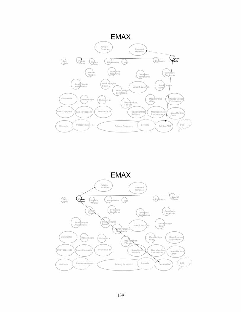
139

EMAX

MediumPelagics

Small PelagicsCommercial

Odontocetes

Large Copepods Gelatinous ZP

Micronekton Mesopelagics

PinnipedsBaleen whales

Primary Producers

MacroBenthosPolychaetes

Demersal Fisheries

Sea birds

Pelagic Sharks HMS

Small Copepods

CoastalSharks

MacroBenthosMolluscs

MacroBenthosCrustaceans MacroBenthos

Other

MegaBenthosFilterers

MegaBenthosOther

Larval & Juv. Fish

PelagicFisheries

Small PelagicsOther

Small PelagicsAnadromous

Small PelagicsSquid

DemersalsBenthivores

DemersalsPiscivores

Shrimp et al.

DemersalsOmnivores

Discards Detritus-POC DOCBacteriaMicrozooplankton

EMAX

MediumPelagics

Small PelagicsCommercial

Odontocetes

Large Copepods Gelatinous ZP

Micronekton Mesopelagics

PinnipedsBaleen whales

Primary Producers

MacroBenthosPolychaetes

Demersal Fisheries

Sea birds

Pelagic Sharks HMS

Small Copepods

CoastalSharks

MacroBenthosMolluscs

MacroBenthosCrustaceans MacroBenthos

Other

MegaBenthosFilterers

MegaBenthosOther

Larval & Juv. Fish

PelagicFisheries

Small PelagicsOther

Small PelagicsAnadromous

Small PelagicsSquid

DemersalsBenthivores

DemersalsPiscivores

Shrimp et al.

DemersalsOmnivores

Discards Detritus-POC DOCBacteriaMicrozooplankton

140

EMAX

MediumPelagics

Small PelagicsCommercial

Odontocetes

Large Copepods Gelatinous ZP

Micronekton Mesopelagics

PinnipedsBaleen whales

Primary Producers

MacroBenthosPolychaetes

Demersal Fisheries

Sea birds

Pelagic Sharks HMS

Small Copepods

CoastalSharks

MacroBenthosMolluscs

MacroBenthosCrustaceans MacroBenthos

Other

MegaBenthosFilterers

MegaBenthosOther

Larval & Juv. Fish

PelagicFisheries

Small PelagicsOther

Small PelagicsAnadromous

Small PelagicsSquid

DemersalsBenthivores

DemersalsPiscivores

Shrimp et al.

DemersalsOmnivores

Discards Detritus-POC DOCBacteriaMicrozooplankton

EMAX

MediumPelagics

Small PelagicsCommercial

Odontocetes

Large Copepods Gelatinous ZP

Micronekton Mesopelagics

PinnipedsBaleen whales

Primary Producers

MacroBenthosPolychaetes

Demersal Fisheries

Sea birds

Pelagic Sharks HMS

Small Copepods

CoastalSharks

MacroBenthosMolluscs

MacroBenthosCrustaceans MacroBenthos

Other

MegaBenthosFilterers

MegaBenthosOther

Larval & Juv. Fish

PelagicFisheries

Small PelagicsOther

Small PelagicsAnadromous

Small PelagicsSquid

DemersalsBenthivores

DemersalsPiscivores

Shrimp et al.

DemersalsOmnivores

Discards Detritus-POC DOCBacteriaMicrozooplankton

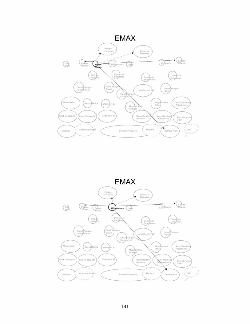
141

EMAX

MediumPelagics

Small PelagicsCommercial

Odontocetes

Large Copepods Gelatinous ZP

Micronekton Mesopelagics

PinnipedsBaleen whales

Primary Producers

MacroBenthosPolychaetes

Demersal Fisheries

Sea birds

Pelagic Sharks HMS

Small Copepods

CoastalSharks

MacroBenthosMolluscs

MacroBenthosCrustaceans MacroBenthos

Other

MegaBenthosFilterers

MegaBenthosOther

Larval & Juv. Fish

PelagicFisheries

Small PelagicsOther

Small PelagicsAnadromous

Small PelagicsSquid

DemersalsBenthivores

DemersalsPiscivores

Shrimp et al.

DemersalsOmnivores

Discards Detritus-POC DOCBacteriaMicrozooplankton

EMAX

MediumPelagics

Small PelagicsCommercial

Odontocetes

Large Copepods Gelatinous ZP

Micronekton Mesopelagics

PinnipedsBaleen whales

Primary Producers

MacroBenthosPolychaetes

Demersal Fisheries

Sea birds

Pelagic Sharks HMS

Small Copepods

CoastalSharks

MacroBenthosMolluscs

MacroBenthosCrustaceans MacroBenthos

Other

MegaBenthosFilterers

MegaBenthosOther

Larval & Juv. Fish

PelagicFisheries

Small PelagicsOther

Small PelagicsAnadromous

Small PelagicsSquid

DemersalsBenthivores

DemersalsPiscivores

Shrimp et al.

DemersalsOmnivores

Discards Detritus-POC DOCBacteriaMicrozooplankton

142

EMAX

MediumPelagics

Small PelagicsCommercial

Odontocetes

Large Copepods Gelatinous ZP

Micronekton Mesopelagics

PinnipedsBaleen whales

Primary Producers

MacroBenthosPolychaetes

Demersal Fisheries

Sea birds

Pelagic Sharks HMS

Small Copepods

CoastalSharks

MacroBenthosMolluscs

MacroBenthosCrustaceans MacroBenthos

Other

MegaBenthosFilterers

MegaBenthosOther

Larval & Juv. Fish

PelagicFisheries

Small PelagicsOther

Small PelagicsAnadromous

Small PelagicsSquid

DemersalsBenthivores

DemersalsPiscivores

Shrimp et al.

DemersalsOmnivores

Discards Detritus-POC DOCBacteriaMicrozooplankton

EMAX

MediumPelagics

Small PelagicsCommercial

Odontocetes

Large Copepods Gelatinous ZP

Micronekton Mesopelagics

PinnipedsBaleen whales

Primary Producers

MacroBenthosPolychaetes

Demersal Fisheries

Sea birds

Pelagic Sharks HMS

Small Copepods

CoastalSharks

MacroBenthosMolluscs

MacroBenthosCrustaceans MacroBenthos

Other

MegaBenthosFilterers

MegaBenthosOther

Larval & Juv. Fish

PelagicFisheries

Small PelagicsOther

Small PelagicsAnadromous

Small PelagicsSquid

DemersalsBenthivores

DemersalsPiscivores

Shrimp et al.

DemersalsOmnivores

Discards Detritus-POC DOCBacteriaMicrozooplankton

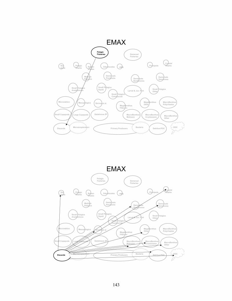
143

EMAX

MediumPelagics

Small PelagicsCommercial

Odontocetes

Large Copepods Gelatinous ZP

Micronekton Mesopelagics

PinnipedsBaleen whales

Primary Producers

MacroBenthosPolychaetes

Demersal Fisheries

Sea birds

Pelagic Sharks HMS

Small Copepods

CoastalSharks

MacroBenthosMolluscs

MacroBenthosCrustaceans MacroBenthos

Other

MegaBenthosFilterers

MegaBenthosOther

Larval & Juv. Fish

PelagicFisheries

Small PelagicsOther

Small PelagicsAnadromous

Small PelagicsSquid

DemersalsBenthivores

DemersalsPiscivores

Shrimp et al.

DemersalsOmnivores

Discards Detritus-POC DOCBacteriaMicrozooplankton

EMAX

MediumPelagics

Small PelagicsCommercial

Odontocetes

Large Copepods Gelatinous ZP

Micronekton Mesopelagics

PinnipedsBaleen whales

Primary Producers

MacroBenthosPolychaetes

Demersal Fisheries

Sea birds

Pelagic Sharks HMS

Small Copepods

CoastalSharks

MacroBenthosMolluscs

MacroBenthosCrustaceans MacroBenthos

Other

MegaBenthosFilterers

MegaBenthosOther

Larval & Juv. Fish

PelagicFisheries

Small PelagicsOther

Small PelagicsAnadromous

Small PelagicsSquid

DemersalsBenthivores

DemersalsPiscivores

Shrimp et al.

DemersalsOmnivores

Discards Detritus-POC DOCBacteriaMicrozooplankton

144

23. Respiration David Dow Background and Approach

Two approaches were used to estimate metabolism in the EMAX project. Unless

otherwise noted in each previous section, the default values for respiration were 65% of the assimilated consumption. Otherwise, where appropriate, values or formulae from the literature were used for the network nodes.

When appropriate literature values were lacking we assumed that assimlated energy was divided: 65% to respiration and 35% to secondary production (Parry 1983). The assimilated energy was estimated using the International Biological Program (IBP) approach where C - E = Assimlation = P + R. C represents consumption, E is egestion + excretion, P is secondary production and R represents respiration. There is a vast literature on the respiratory metabolism of individual organisms and many review papers with regressions or allometric equations which relate respiration to body size and temperature. Since field respiration values are influenced by feeding status, activity level, life history stage, body size, water tempreature, etc., this extrapolation process generates a crude estimate. Since we did not have any respiration measurements for many of the nodes, and many of the nodes represent a composite of species, we decided to utilize this indirect approach to estimate the metabolic energy loss in most instances.

The EMAX network energy budget was interested in linking secondary production of the prey to either harvest or consumption by predators, so we did not focus on the metabolic energy losses from the system. The secondary production estimates were done independently and thus provided a reasonable estimate of the ecological transfer efficiency. Since the majority of the metabolic losses in the pelagic and benthic communities occur in the smaller size classes, this influences the base of the food web, leading to living marine resources (LMRs) and not the energy transfer effciency within this chain. References

Del Giorgio, PA; Williams, PJ leB, eds. 2005. Respiration in Aquatic Ecosystems. New York, NY: Oxford

University Press; 315 p. Parry, GD. 1983. The influence of the cost of growth on ectotherm metabolism. J. Theor. Biol. 101:453-477. Pomeroy, LR; Wiebe, WJ. 1993. Energy sources for microbial food webs. Mar. Microb. Food Webs 7:101-118.

145

24. Model Protocols

Jason S. Link, John E. O’Reilly, Vincent G. Guida, William J. Overholtz, Christopher M. Legault, Michael J. Fogarty, Jon K.T. Brodziak, Debra L. Palka, John R. Green, Joseph J. Vitaliano, andDavid D. Dow

In this section we describe the software selection process, balancing exercises, diagnostics protocols and scenarios applied in the Energy Modeling and Analysis eXercise (EMAX). A Primer on Energy Budgets and Network Models

Network models are based on the concept of a steady state ecosystem in which the energy inputs to a node are balanced by the outputs. Ecosystem network models trace the flows of energy or materials among compartments of the system. At steady state, the flows into a compartment exactly equal flows out of the compartment:

(EQ. 24.1) 011

�''&

%$$#

"�� ��

��

n

jijii

n

jij EFIF

where Fij is the flux from compartment j to compartment I; Ii is import to compartment i from outside the system; and Ei is export from compartment i to outside the system. The estimates of production, consumption, and respiration described in earlier sections for each compartment are used in determining the flows among compartments. Under the assumption of steady-state conditions, these initial estimates of the flows are checked to see if the mass-balance criteria are met. If the system is not in steady-state, iterative adjustments are made to the flows in an attempt to achieve mass-balance.

Typically, all parameters necessary to determine the flows are not known and must be estimated. In general, there is not a unique solution to the system of linear equations (the problem is under-determined) and several alternative approaches were used to obtain solutions. We explored two alternative modeling approaches to examine solutions to this problem, the details of which are below. Caveats and Assumptions

For the purposes of this exercise, we assumed steady state equilibrium. We acknowledge that there are dynamic elements of what we modeled, but averaging estimates over a five-year period mitigates some of the inter-annual dynamics.

For EMAX we assumed no movement of animals across regions (captured by proportionality of distributions spatially and seasonally). Thus, Ii was set to 0 and Ei was treated as fishery removals, bycatch, and ship-strikes for each appropriate node. That is, the network models didn't consider any potential transfer of matter or energy between the different subregions (Gulf of Maine; Georges Bank; Southern New England and Mid-Atlantic Bight) on the Northeast Continental Shelf, so that each system was treated in isolation.

We recognize the potential for a wide range of results depending upon which units are used. Although network models have been constructed using energy, biomass, or elemental units, we chose to execute our model in units of biomass (wet weight) per unit area.

146

Given that the carbon turnover of phytoplankton and bacteria is roughly 3 days, and that of fish varies over a range of 300 - 450 days (Hakanson and Gyllenhammar, 2005), it appears that the carbon formed in photosynthesis is recycled many times before reaching fish and marine mammals. This brings into question the assumption that this recycled carbon has the same qualitative value or embodied chemical energy at different trophic levels. Schneider and Sagan (2005) discuss the importance of distinguishing between carbon which cycles and energy which flows from sources to sinks. Direct carbon flow follows the pathways of energy, while the recycled carbon flow goes along the indirect pathways. It is important to distinguish between “cycles” (indirect flows) and “network connections” (direct flows) in carbon-based networks.

In classical energy flow models where joules or kilocalories are the measure of exchange between compartments, energy flows from sources (sunlight and resultant primary production) to sinks (higher trophic levels) with a large respiratory dissipation of energy at each trophic level. This highlights the need to resolve the apparent paradox between nutrients which cycle throughout the nodes within a network and energy which flows from sources to sinks with a large respiratory tax at each trophic level. In most network models, recycled energy is implicitly modeled as flows through indirect pathways.

The EMAX network budget was based on wet weight which lies at an intermediate point on the gradient between budgets based on carbon (which explicitly consider turnover time differences between compartments) and the classical energy flow budgets (j or kcal transported from sources to sinks). Software and Modeling Approaches

We explored a broad selection of energy budget models, network models, and associated

software packages for use in EMAX. First we examined EcoNetwrk and constructed a preliminary model for the Gulf of Maine

region. This approach uses reconstructed flows as the state variables (see Ulanowicz 2004 for an overview). Balancing the network proved to be challenging, as this model balances mainly by constraining respiration and consumption, and is a statistical minimization rather than a true optimization solution. Assumptions about primary production and detrital processing were key. We also explored Netwrk, the precursor to EcoNetwrk, which we decided was not likely to be an improvement over EcoNetwrk, particularly because it did not reside in a graphical user interface (GUI) environment.

We also constructed a preliminary model for Ecopath. This approach uses estimates of standing stocks as the state variables (see Christensen and Pauly 1992, Walters et al. 1997). Although initial balance was achieved, we were uncertain how much was due to detritus. This model balances primarily off ecotrophic efficiencies and uses a true optimization protocol.

Other software packages we investigated were WAND, WAND Balance, DR. LOOP, and SIMULOOP. They may be useful for additional analyses once balanced budgets are formed using the two primary software packages, because they feature some useful cybernetic metrics. However, they are not likely to provide a balancing package of any improvement over the first two programs. Many packages provide useful information and analytical capabilities, but are not readily amenable for balancing a budget or easily translatable into the fisheries management context. Other models we evaluated as potentially very useful but rejected were redundant; focused on more qualitative network properties; were less user-friendly; or obfuscated their underlying model structure.

147

We also noted the potential for using some of the outputs from a concurrent GLOBEC Phase IV project, which could provide some MATLAB software to conduct energy budget balancing. Additionally, we made explorations into AD Model Builder and At-Risk/Excel, tools used to build models from scratch. Neither option, however, could be implemented in a timely manner.

After several iterations, we settled on using EcoPath (Christensen and Pauly 1992; Walters et al. 1997) and EcoNetwrk (Ulanowicz and Kay 1991; Ulanowicz 2004) as our primary tools. The pros and cons of each have been noted elsewhere (e.g., Walters et al. 1997; Heymans and Baird 2000; Hollowed et al. 2000; Whipple et al. 2000; Allesina and Bondavalli 2003; Kavanagh et al. 2004; Ulanowicz 2004). There is a subtle difference in the underlying philosophy and numerical solutions between the two programs (Heymans and Baird 2000).

The production (flows) for the heterotrophic compartments in EcoNetwrk can be expressed as:

(EQ. 24.2) ERCP �

where P is production; C is consumption; R is respiration; and E is egestion (unassimilated food). The autotrophic compartment(s) considers respiration losses to gross primary production (GPP) to yield net primary production. Fishery yields are treated as exports from the system.

The mass balance EcoPath model can be expressed as: (EQ. 24.3) ijj

jjiiii DCBQBCEEBPB )/()/( ���

where Bi is the biomass in the compartment; (P/B)i is the production to biomass ratio; EEi is the ecotrophic efficiency (fraction of total production consumed by predators or exported from the system); Ci is the catch for compartment i; Bj is the biomass for predator j; (Q/B)j is the consumption to biomass ratio for predator j; and DCij is the diet composition of predator j (fraction of biomass comprising prey i in the diet of predator j).

The benefit of using the two packages instead of choosing one is that their strengths and weaknesses can be played off against one another. The detritus box is the main weakness of Ecopath, while in EcoNetwrk it is egestion. Ecopath is an optimization program, whereas EcoNetwrk is a minimization procedure. These programs use two different methods to arrive at working, balanced solutions: Ecopath emphasizes P, while EcoNetwrk emphasizes R. Both use convergence of values with repeated (auto) balancing as the main way to verify model finalization. Even though the two models have a conceptually different approach (Ecopath is more top-down while EcoNetwrk is more bottom-up), both have highlighted the same deficiencies in our data matrix. A positive outcome of using both software packages is that we improve our input data and systemic understanding more than we would have by changing the model parameters using only one package. This also suggests that our results are robust to model choice. Balancing Protocols

We made an initial calculation of the difference between the inflows and outflows from

each compartment according to the specification of the input variables. For compartments exhibiting large discrepancies, we reexamined the input information for consistency, made

148

comparisons with similar inputs from other systems, and made adjustments as necessary. We then employed balancing options in both software packages to provide estimates of the steady-state flows. EcoNetwrk employs a manual balancing procedure in which an extended matrix comprising elements for the exchanges among compartments, respiration, imports, and exports is adjusted using successive transformations of this structural matrix (see Allesina and Bondavalli 2003). EcoNetwrk allows for “locking” estimates thought to be well determined and therefore provides an implicit weighting procedure. EcoPath employs a statistical balancing procedure using Singular Value Decomposition to constrain the estimates for the underdetermined system of equations. EcoPath allows the specification of an index of reliability (or “pedigree”) for each element to provide weighting options for estimation. Following each balancing procedure, we reevaluated inputs showing large deviations from mass balance or unrealistic estimates for certain diagnostic measures such as the ratio of production to consumption and respiration to consumption in EcoNetwrk, and the ecotrophic efficiency in EcoPath. Adjustments were made to the inputs to obtain more realistic estimates and the balancing protocols were repeated until stable estimates were obtained.

One of the benefits of this exercise and approach is that we identified major information/data gaps for the GOM (and generally NEUS) ecosystem (Table 24.1). Ecopath Considerations

For the EcoPath model we initially investigated entering uncertainties globally rather

than using the pedigree of data option on individual nodes. We used a 50% coefficient of variation (CV) on diet and Q:B values, and a 10% CV on biomass and P:B values.

The EcoPath model provided a range of options for autobalancing based either on minimizing maximum ecotrophic efficiencies, minimizing the sum of excess EEs, or minimizing the current EE. We chose the first two options simultaneously. Additionally, we used the Ecopath pedigree table to set confidence values for biomass, P:B, Q:B, diet and catch for autobalancing (Table 24.1). After examining several runs, the group decided that the pedigree approach was more desirable since it provided a way to weight the data sources with their relative degree of confidence.

Next, we began an iterative process whereby we modified the input/initial matrix and attempted to rebalance the network, primarily keying off EE < 1. For the initial Ecopath runs, P:C anomalies (P:C >0.5) appeared to be the result of low consumption values rather than high production values. Using autobalancing based on ecotrophic efficiencies (EEs) worked well without causing major changes to network structure.

Large-scale changes were necessary to for gelatinous zooplankton, squid, demersal omnivores, macrobenthos - other, and shrimp. We reduced the C:B ratio, diet composition, and B for gelantinous zooplankton; C:B and P:B of demersal ominivores; C:B of macrobenthos mollusks; B and C:B of macrobenthos – other; diet composition of predators of small pelagics; and P:B and B of shrimp.

Since the balancing approach was iterative, we had to ask: When do we have a balanced model? The model was considered sufficiently balanced when we reran it starting at the solution and verified that it provided the same solution, conditioned upon minimizing EE via several numerical solution methodologies.

149

EcoNetwrk Considerations For the EcoNetwrk model, we used an iterative approach similar to the one used for

Ecopath. Repeated use of the balancing protocol (DATBAL, similar to AUTOBAL in Ecopath) was required to find a more global solution that would be responsive to input parameter changes.

The major consideration was to “close the loop” in EcoNetwrk by ensuring that the detrital node received unassimilated consumption from the other nodes in the network. We took the unassimilated fractions of all the consumptive flows (portions relegated to detritus), summed them and made microbial respiration equal to that sum. We also added 15% of primary production (phytoplankton direct contribution to detritus) to that sum to account for that flow, and the model then seemed to be more solvable.

Once these solutions were implemented, we carried out an iterative balancing process. For this we modified the input data matrix and attempted to rebalance the network primarily by keying off the R:C ratio. As a caveat, biomasses and C:B ratios seemed reasonable, but assimilation efficiencies (AE) were all >0.9. Again, the R:C ratio was a useful constraint in solving these multiple concerns.

Significant changes to gelatinous zooplankton (B, C:B); macrobenthos - other (B, R:B, C:B); larval fish (B); and shrimp (B, C:B, R:B) were initially required before we even came close to achieving network balance. These are similar to network nodes requiring similar changes in the EcoPath model version, our prebalance, and are noted as groups with lower datacertainty (Table 24.1). We then modified megabenthos filterers, macrobenthos mollusks, medium pelagics, demersal omnivores, small pelagics anadromous, and small copepods. Diagnostics

The input matrices and some diagnostic measures we used are provided in Appendix 1.

Foremost is that once we identified a major constraining factor based upon the underlying assumption of the model software (i.e., EE or R:C), other key ratios were then examined. These model outputs must make sense relative to expert knowledge among EMAX personnel, and be consistent with literature values. In this way our exercise was unique; the large amount of extant, reasonable quality data allowed for a model reality check.

Many of these diagnostics (e.g., mean trophic level, ascendancy, input-output analysis, size spectra metrics, imbalance sum, pyramidal structure, connectance, etc.) might form the basis for indicators to be translated and incorporated into ecosystem approaches to fisheries management.

Scenarios

Once a balanced, baseline model was obtained for both software packages, various changes were made to the network (e.g., multiplying key nodes by various scalars such as 1/100th, ½, 10, 100, singularly and in various combinations), which was then rebalanced. Although we have preliminary balanced networks for all four subregions, we chose to initially evaluate the various scenarios for only one of them, the Gulf of Maine. We executed the scenario rebalancing as a psuedo-dynamic modeling process to see where the perturbed system would redistribute biomass and production after the changes were imposed. We executed all scenarios in both model packages.

150

For comparisons across regions and across scenarios, we examined a set of network, cybernetic, and ecological statistics common to both software packages. However, to highlight the role of small pelagics in particular, we primarily evaluated a set of biomass ratios and similar indicators (Link 2005).

The bulk of the results and interpretation of these (and other) scenarios and the model balancing exercise are intended for presentation in other venues, but the main highlights are:

� Overall changes to major fish groups resulted in compensating changes to other fishes. � The upper trophic levels (TLs) had minimal impact on the rest of the network. � Changes to marine mammals sometimes had a counterintuitive effect on fish. � Categorically across all scenarios, gelatinous zooplankton and macrobenthos decreased

whereas most other zooplankton increased. Could that be a possible hardwiring artifact of the network structure?

� In terms of biomass, production, energy flows, and importance for upper trophic levels, small pelagics are a keystone group in this ecosystem.

151

References and Bibliography Allesina, S; Bondavalli, C. 2003. Steady state of ecosystem flow networks: a comparison between balancing

procedures. Ecol. Model. 165:221-229. Allesina, S; Bondavalli, C. 2004. WAND: an Ecological Network Analysis user-friendly tool. Env. Model.

Software 19:337-340. Allesina, S; Bodini, A. 2004. Who dominates whom in the ecosystem? Energy flow bottlenecks and cascading

exctinctions. J. Theor. Biol. 230(3);351-358. Allesina, S; Ulanowicz, RE. 2004. Cycling in ecological networks: Finn's index revisited. Comput. Biol. Chem.

28(3):227-233. Baird, D; Glade, JM: Ulanowicz, RE. 1991. The comparative ecology of six marine ecosystems. Philos. Trans. R.

Soc. Lond. 333:15-29. Baird, D; Ulanowicz, RE. 1989. The seasonal dynamics of the Chesapeake Bay ecosystem. Ecol. Monogr. 59:329-

364. Baird, D; Ulanowicz, RE. 1993. Comparative study on the trophic structure, cycling and ecosystem properties of

four tidal estuaries. Mar. Ecol. Prog. Ser. 99:221-237. Bax, NJ. 1991. A comparison of the fish biomass flow to fish, fisheries, and mammals on six marine ecosystems.

ICES (Int. Counc. Explor. Sea) Mar. Sci. Symp. 193:217-224. Brown, MT. 2004. A picture is worth a thousand words: energy systems language and simulation. Ecol. Model.

178: 83-100. Brown, MT; Buranakarn, V. 2003. Energy indices and ratios for sustainable material cycles and recycle options.

Resources Conserv. Recycl. 38:1-22. Brown, MT; Herendeen, RA. 1996. Embodied energy analysis and energy analysis: a comparative view. Ecol.

Econ. 19:219-235. Brown, MT; McClanahan, TR. 1996. Energy analysis perspectives of Thailand and Mekong River dam proposals.

Ecol. Model. 91(1-3):105-130. Brown, MT; Ulgiati, S. 1999. Energy evaluation of the biosphere and natural capital. Ambio 28(6):486-493. Brown, MT; Ulgiati, S. 2004a. Energy quality, energy, and transformity: H.T. Odum’s contributions to quantifying

and understanding systems. Ecol. Model. 178:201-213. Brown, MT; Ulgiati, S. 2004b. Energy analysis and environmental accounting. Encyclopedia of Energy, Volume 2.

New York, NY: Elsevier. Bodini, A. 1991. What is the role of predation on stability of natural communities? A theoretical investigation.

BioSys. 26:21-30. Bodini, A. 1996. Uncertainty and resource exploitation: exploration based on qualitative modeling. Statist. Appl. 8

(1):185-199. Bodini, A. 1998. Representing ecosystem structure through signed digraphs. Model reconstruction, qualitative

predictions and management: the case of a freshwater ecosystem. Oikos 83:93-106. Bodini, A. 2000. Reconstructing trophic interactions as a tool for understanding and managing ecosystems:

application to a shallow eutrophic lake. Can. J. Fish. Aq. Sci. 57:1999-2009. Bodini, A; Bondavalli, C. 2002. Toward a sustainable use of water resources. A whole-ecosystem approach using

network analysis. Int. J. Env. Pollut. 15:463-485. Bodini, A; Giavelli, G. 1989. The qualitative approach in investigating the role of species interactions on stability

of natural communities. Biosys. 22:289-299. Bodini, A; Giavelli, G. 1992. Multicriteria analysis as a tool to investigate the compatibility between conservation

and development on Salina Island, Aeolian Archipelago, Italy. Env. Manag. 16:633-652. Bodini, A; Giavelli, G; Rossi, O. 1994. The qualitative analysis of community food webs: implications for wildlife

management and conservation. J. Env. Manag. 41:49-65. Bodini, A; Puccia, CJ; Giavelli, G. 1990. Understanding resource management strategies under different ecological

constraints: the case of oligotrophic and eutrophic lakes. In: Ravera, O. ed. Terrestrial and Aquatic Ecosystems: Perturbation and Recovery. London, UK: Ellis Horwood; p. 583-592.

Bodini, A; Ricci, A; Viaroli, P. 2000. A multi-methodological approach for the sustainable management of perifluvial wetlands of the Po river (Italy). Env. Manag. 26:59-72.

Bondavalli, C; Naldi, M; Christian, RR. 1998. Cs-137 circulation in an eutrophic lagoon: a modeling approach. Ver. Internat. Verein. Limnol. 26:1422-1425.

152

Bondavalli, C; Ulanowicz, RE. 1999. Unexpected effects of predators upon their prey: the case of the American alligator. Ecosys. 2: 49-63.

Bondavalli, C; Ulanowicz, RE; Bodini, A. 2000. Insights into the processing of carbon in the South Florida Cypress Wetlands: a whole-ecosystem approach using network analysis. J. Biogeog. 27:697-710.

Bundy, A. 2005. Structure and functioning of the eastern Scotian Shelf ecosystem before and after the collapse of groundfish stocks in the early 1990s. Can. J. Fish. Aquat. Sci. 62:1453-1473.

Christensen, V; Pauly, D. 1992. On steady-state modeling of ecosystems. In: Christensen, V; Pauly, D eds. Trophic models of aquatic ecosystems. ICLARM (Int. Center Liv. Aq. Resour. Manag.) Conf. Proc. 26:14-19.

Christensen, V; Pauly, D. 2004. Placing fisheries in their ecosystem context, an introduction. Ecol. Model. 172:103-107.

Cohen, EB; Grosslein, MD; Sissenwine, MP. 1982. Energy budget of Georges Bank. Can. Spec. Publ. Fish. Aquat. Sci. 59:95-107.

Fogarty, MJ; Murawski, SA. 1998. Large-scale disturbance and the structure of marine systems: Fishery impacts on Georges Bank. Ecol. Appl. 8(S1):S6-S22.

Giavelli, G; Bodini, A. 1990 Plant-ant-fungus communities investigated through qualitative modeling. Oikos 57: 357-365.

Giavelli, G; Bodini, A; Rossi, O. 1990. An extension of the complexity concept derived from the analysis of colonisation processes in small island environments. Coenoses 5: 1-5.

Grosslein, M; Langton, R; Sissenwine, MP. 1980. Recent fluctuations in pelagic fish stocks of the northwest Atlantic, Georges Bank region, in relation to species interactions. Rapports et Proces-Verbaux des Reunions du Conseil International pour l’Exploration de la Mer. 177:374-404.

Heymans, JJ; Baird, D. 2000. Network analysis of the northern Benguela ecosystem by means of NETWRK and ECOPATH. Ecol. Model. 131:97-119.

Heymans, JJ; Ulanowicz, RE; Bondavalli, C. 2002. Network analysis of the South Florida Everglades graminoid marshes and comparison with nearby cypress ecosystems. Ecol. Model. 149:5-23.

Hollowed, AB; Bax, N; Beamish, R; Collie, J; Fogarty, M; Livingston, P; Pope, J; Rice, JC. 2000. Are multispecies models an improvement on single-species models for measuring fishing impacts on marine ecosystems? ICES (Int. Counc. Explor. Sea) J. Mar. Sci. 57:707-719.

Jollands, N; Lermit, J; Patterson, M. 2004. Aggregate eco-efficiency indices for New Zealand--a principal components analysis. J. Env. Manag. 73:293-305.

Jorgensen, SE. 1992. Exergy and ecology. Ecol. Model. 63:185-214. Kang, D; Park, SS. 2002. Energy evaluation perspectives of a multipurpose dam proposal in Korea. J. Env. Manag.

66:293-306. Kavanagh, P; Newlands, N; Christensen, V; Pauly, D. 2004. Automated parameter optimization for Ecopath

ecosystem models. Ecol. Model. 172:141-149. Larkin, PA. 1996. Concepts and issues in marine ecosystem management. Rev. Fish Biol. Fish. 6:139-164. Lindeman, RL. 1942. The trophic-dynamic aspect of ecology. Ecol. 23:399-418. Link, JS. 2005. Translation of ecosystem indicators into decision criteria. ICES ICES (Int. Counc. Explor. Sea) J.

Mar. Sci. 62:569-576. Mageau, MT ; Constanza, R; Ulanowicz, RE. 1998. Quantifying the trends expected in developing ecosystems.

Ecol. Model. 112:1-22. Monaco, M; Ulanowicz, RE. 1997. Comparative ecosystem trophic structure of three U.S. mid-Atlantic estuaries.

Mar. Ecol. Prog. Ser. 161:239-254. Morisette, L; Despatie, S-P; Savenkoff, C; Hammill, MO; Bourdages, H; Chabot, D. 2003. Data gathering and

input parameters to construct ecosystem models for the northern Gulf of St. Lawrence (mid-1980s). Can.Tech. Rep. Fish. Aquat. Sci. no. 2497; 100 p.

Odum, E. 2004. Energy analysis of shrimp mariculture in Ecuador: a review. Ecol. Model. 178:239-240. Odum, HT. 1988a. Energy, environment and public policy: a guide to the analysis of systems. UNEP (United

Nations Environment Program) Regional Seas Report; Study #95. Odum, HT. 1988b. Self organization, transformity, and information. Science 242:1132-1139. Odum, HT. 1996. Environmental Accounting: Energy and Environmental Decision Making. New York, NY: John

Wiley & Sons. Odum, HT. 2000. Energy of Global Processes (Folio#2). Gainesville, FL: Univ. of Florida Center Env. Pol.; 30 p. Odum, HT; Arding, JE. 1991. Energy Analysis of Shrimp Mariculture in Ecuador. Narragansett, RI: University of

Rhode Island Coastal Resources Center; 114 p.

153

Odum, HT; Brown, MT; Brandt-Williams, S. 2000. Introduction and Global Budget (Folio#1). Gainesville, FL: Univ. of Florida Center Env. Pol.; 16 p.

Odum, HT; Odum, EC. 2000. Modeling for All Scales: An Introduction of Systems Simulation. San Diego, CA: Academic Press.

Odum, HT; Odum, EP. 2000. The energetic basis for valuation of ecosystem services. Ecosys. 3:21-23. Savenkoff, C; Bourdages, H; Swain, DP; Despatie, S-P; Hanson, JM; Methot, R; Morissette, L; Hammill, MO.

2004. Input data and parameter estimates for ecosystem models of the southern Gulf of St. Lawrence (mid-1980s and mid-1990s). Can. Tech. Rep. Fish. Aquat. Sci. no. 2529; 111 p.

Savenkoff, C; Castonguay, M; Vezina, AF; Despatie, S-P; Chabot, D; Morisette, L; Hammill, MO. 2004. Inverse modelling of trophic flow through an entire ecosystem: the northern Gulf of St. Lawrence in the mid-1980s. Can. J. Fish. Aquat. Sci. 61:2194-2214.

Savenkoff, C; Vezina, AF; Bundy, A. 2001. Inverse analysis of the structure and dynamics of the whole Newfoundland-Labrador Shelf ecosystem. Can. Tech. Rep. Fish. Aquat. Sci. no. 2354; 64 p.

Savenkoff, C; Vezina, AF; Roy, S; Klein, B; Lovejoy, C; Therriault, J-C; Legendre, L; Rivkin, R; Berube, C; Tremblay, J-E; Silverberg, N. 2000. Export of biogenic carbon and structure and dynamics of the pelagic food web in the Gulf of St. Lawrence Part 1. Seasonal variations. Deep-Sea Res. II 47(3-4):585-607.

Savenkoff, C; Vezina, AF; Smith, PC; Han, G. 2001. Summer transports of nutrients in the Gulf of St. Lawrence estimated by inverse modelling. Estuar. Coast. Shelf Sci. 52: 565-587.

Schneider, ED; Sagan, D. 2005. Into the Cool: Energy Flow, Thermodynamics and Life. University of Chicago Press; Chicago, Il.; 378 p.

Ulanowicz, RE. 1986. Growth and development: ecosystems phenomenology. New York, NY: Springer-Verlag. Ulanowicz, RE. 1995. Trophic flow networks as indicators of ecosystem stress. In: Polis, GA; Winemiller, KO.

eds. Food webs: integration of patterns and dynamics. New Yor, NY: Chapman and Hall; p. 358-368. Ulanowicz, RE. 2000. Toward the measurement of ecological integrity. In: Pimentel, D; Westra, L; Noss, RF. eds.

Ecological Integrity: Integrating Environment, Conservation and Health. Washington, DC: Island Press; p. 102-113.

Ulanowicz, RE. 2004. Quantitative methods for ecological network analysis. Comput. Biol. Chem. 28(5-6):321-339.

Ulanowicz, RE; Kay, JJ. 1991. A package for the analysis of ecosystem flow networks. Environ. Software 6:131-142.

Ulanowicz, RE; Platt, TC. 1985. Ecosystem theory for biological oceanography. Can Bull. Fish. Aquatic Sci. no. 213; 260 p.

Ulanowicz, RE; Wulff, F. 1991. Comparing ecosystem structures: the Chesapeake Bay and the Baltic Sea. In: Cole, J; Lovett, G; Findlay, S. eds. Comparative analysis of ecosystems, pattern, mechanism, and theories. New York, NY: Springer-Verlag.

Vezina, AF; Savenkoff, C. 1999. Inverse modeling of carbon and nitrogen flows in the pelagic food web of the northeast subarctic Pacific. Deep-Sea Res. II 46(11-12): 2909-2939.

Vezina, AF; Savenkoff, C; Roy, S; Klein, B; Rivkin, R; Therriault, J-C; Legendre, L. 2000. Export of biogenic carbon and structure and dynamics of the pelagic food web in the Gulf of St. Lawrence Part 2. Inverse analysis. Deep-Sea Res. II 47(3-4): 609-635.

Walters, CJ; Christensen, V; Pauly, D. 1997. Structuring dynamic models of exploited ecosystems from trophic mass-balance assessments. Rev. Fish Biol. Fish. 7:139-172.

Whipple, SJ; Link, JL; Garrison, LP; Fogarty, MJ. 2000. Models of predation and fishing mortality in aquatic ecosystems. Fish. Fish. 1:22-40.

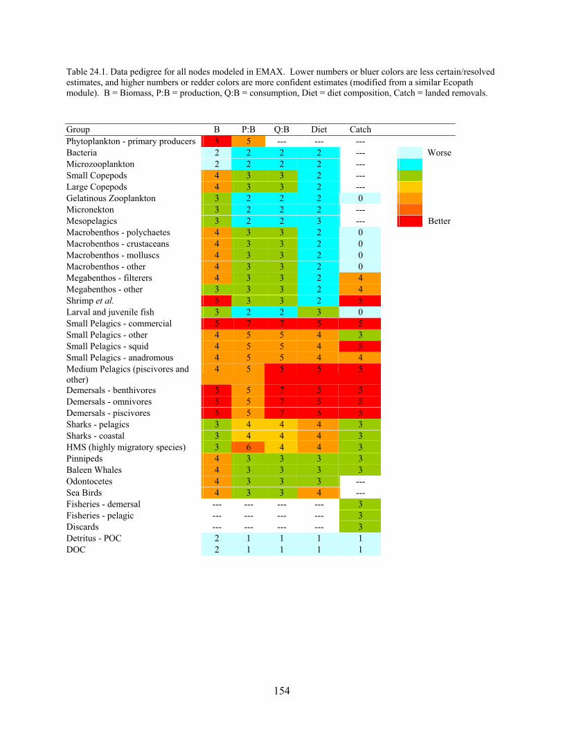
154

Table 24.1. Data pedigree for all nodes modeled in EMAX. Lower numbers or bluer colors are less certain/resolved estimates, and higher numbers or redder colors are more confident estimates (modified from a similar Ecopath module). B = Biomass, P:B = production, Q:B = consumption, Diet = diet composition, Catch = landed removals. Group B P:B Q:B Diet Catch Phytoplankton - primary producers 5 5 --- --- --- Bacteria 2 2 2 2 --- Worse Microzooplankton 2 2 2 2 --- Small Copepods 4 3 3 2 --- Large Copepods 4 3 3 2 --- Gelatinous Zooplankton 3 2 2 2 0 Micronekton 3 2 2 2 --- Mesopelagics 3 2 2 3 --- Better Macrobenthos - polychaetes 4 3 3 2 0 Macrobenthos - crustaceans 4 3 3 2 0 Macrobenthos - molluscs 4 3 3 2 0 Macrobenthos - other 4 3 3 2 0 Megabenthos - filterers 4 3 3 2 4 Megabenthos - other 3 3 3 2 4 Shrimp et al. 5 3 3 2 5 Larval and juvenile fish 3 2 2 3 0 Small Pelagics - commercial 5 7 7 5 5 Small Pelagics - other 4 5 5 4 3 Small Pelagics - squid 4 5 5 4 5 Small Pelagics - anadromous 4 5 5 4 4 Medium Pelagics (piscivores and other)

4 5 5 5 5

Demersals - benthivores 5 5 7 5 5 Demersals - omnivores 5 5 7 5 5 Demersals - piscivores 5 5 7 5 5 Sharks - pelagics 3 4 4 4 3 Sharks - coastal 3 4 4 4 3 HMS (highly migratory species) 3 6 4 4 3 Pinnipeds 4 3 3 3 3 Baleen Whales 4 3 3 3 3 Odontocetes 4 3 3 3 --- Sea Birds 4 3 3 4 --- Fisheries - demersal --- --- --- --- 3 Fisheries - pelagic --- --- --- --- 3 Discards --- --- --- --- 3 Detritus - POC 2 1 1 1 1 DOC 2 1 1 1 1

155

25. Discussion The EMAX exercise and process of model balancing were informative in many respects.

Paramount was highlighting areas where our perceptions or understanding may merit revision or reexamination in light of this holistic view of the data, relative magnitudes of different nodes, or combined model outputs.

Answering the Original Question- Evaluating the Role of Small Pelagics Specific question:

What is the role of small pelagic fish in the Northeast United States (NEUS) Continental

Shelf Ecosystem, as determined by a recent network analysis?

Answer:

Small pelagics are an extremely important part of the NEUS Ecosystem, and it is likely that they will continue to be for the foreseeable future. A majority of energy in the system flows through these nodes (commercial, squid, anadromous and other). An increasingly important issue is how other species, especially commercially or ecologically important ones, respond to herring, mackerel, squid, and similar organisms. It appears that when the amount of small pelagics in the system changes, there are trickle-through effects to other network nodes. In terms of biomass, production, energy flows, and importance for upper trophic levels, small pelagics are a keystone group of species in this ecosystem.

Overall, the pelagic community is more prominent than the benthic community. More fluxes pass through pelagic nodes than benthic or demersal ones. In particular, consumptive demand (C:P) is quite high for small pelagics, which indicate that these are keystone species groups. Summary of Other Results

Total system production is less than primary production when one accounts for

respiration, trophic transfer efficiencies, etc. This leads to the question of whether we have optimized biomass for all groups simultaneously. This is a key question for global fisheries management and should be addressed in additional exercises. The system appears to be driven more from bottom-up than top-down factors. The NEUS Ecosystem is one of the most productive marine ecosystems on the planet, and that assessment is reinforced by this study. As a proportion of primary production, most of the events at upper trophic levels (particularly fisheries catches) are an extremely small fraction. More telling is that total fisheries catch is a low proportion of overall energy flow. Even when we increase the biomass of small pelagics by two orders of magnitude, the effects on the next lower trophic level down (zooplankton) are minimal. Further, given the connectedness of all the species in this ecosystem, it appears that if one energy pathway is altered, another pathway compensates such that overall changes in standing stock biomass at a given trophic level are minimized. These are all symptomatic of a highly productive and highly resilient system.

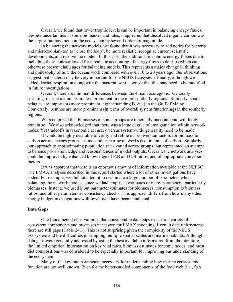
156

Overall, we found that lower trophic levels can be important in balancing energy fluxes. Despite uncertainties in some biomasses and rates, it appeared that dissolved organic carbon was the largest biomass node in the ecosystem by several orders of magnitude.

In balancing the network models, we found that it was necessary to add nodes for bacteria and microzooplankton to “close the loop”, be more realistic, recognize current scientific developments, and resolve the model. In this case, the additional metabolic energy fluxes due to including these nodes allowed for a realistic accounting of energy flows to detritus which can otherwise present challenges for balancing models. This represents a major change in thinking and philosophy of how the oceans work compared with even 10 to 20 years ago. Our observations suggest that bacteria may be very important for the NEUS Ecosystem. Finally, although we added detrital respiration along with the bacteria, we recognize that this may need to be modified in future investigations

Overall, there are minimal differences between the 4 main ecoregions. Generally speaking, marine mammals are less prominent in the more southerly regions. Similarly, small pelagics are important (more prominent, higher standing B, etc.) in the Gulf of Maine. Conversely, benthos are more prominent (in terms of overall system functioning) in the southerly regions.

We recognized that biomasses of some groups are inherently uncertain and will likely remain so. We also acknowledged that there was a large degree of amalgamation within network nodes. Yet tradeoffs in taxonomic accuracy versus system-wide generality need to be made.

It would be highly desirable to verify and refine our conversion factors for biomass to carbon across species groups, as most other marine networks deal in units of carbon. Similarly, our approach to approximating population rates varied across groups, but represented an attempt to balance prior knowledge and reasonableness of model outputs. Overall, the network analyses could be improved by enhanced knowledge of P:B and C:B ratios, and of appropriate conversion factors.

It was apparent that there is an enormous amount of information available at the NEFSC. The EMAX analyses described in this report started where a lot of other investigations have ended. For example, we did not attempt to reestimate a large number of parameters when balancing the network models, since we had empirical estimates of many parameters, particularly biomasses. Instead, we used input parameter estimates for biomasses, consumption to biomass ratios, and other parameters as consistency checks. This approach differs from how many other energy budget investigations with fewer data have been conducted. Data Gaps

One fundamental observation is that considerable data gaps exist for a variety of

ecosystem components and processes necessary for EMAX modeling. Even in data rich systems there are still gaps (Table 24.1). This is not surprising given the complexity of the NEUS Ecosystem and the difficulties in sampling multiple spatial scales and marine habitats. Although data gaps were generally addressed by using the best available information from the literature, the limited empirical information on key vital rates, biomass estimates for some nodes, and most diet compositions was considered to be especially important for improving our understanding of the ecosystem.

Many of the key rate parameters necessary for understanding how marine ecosystems function are not well known. Even for the better-studied components of the food web (i.e., fish

157

and marine mammals), population rates such as production, consumption and respiration are not commonly estimated. As a result, our EMAX analyses relied on literature values or simple approximations for many species groups. Imputting such rates created the danger of propagating potential errors from past studies, as well as not accounting for potential changes through time. We recommend a suite of process-oriented studies and complementary laboratory work to directly estimate production, consumption, and respiration rates for the individual species and species groups examined.

Another primary data gap was the lack of direct estimates of standing stock biomass for several groups of species. In particular, the biomasses of the following species groups were not well known: mesopelagic fishes*, macro- and mega-benthos*, micronekton, shrimp*, bacteria, microzooplankton, gelatinous zooplankton*, and larval fish*. For these species groups, we used historical estimates, expansion of density estimates taken from the literature, or expert opinion based on the relative abundances of other groups with biomass estimates. Several of these groups are very difficult to sample using existing technologies (e.g., micronekton, bacteria, and microzooplankton). Biomasses of the other groups, however, could probably be estimated if modified sampling gears or technologies were deployed in research surveys (* in list above). Regardless, the biomasses of these groups warrant further investigation, because they consistently emerge as pivotal species groups in modeling energy fluxes and balancing energy flows. For example, in one sensitivity analysis we found that a halving of the estimate of gelatinous zooplankton substantially altered the biomasses of other zooplankton, larval fish, and micronekton. These changes, in turn, transferred up the food web to affect commercially important and protected species groups.

Some species groups are always going to be problematic or inherently underdetermined. Until clear advances in sampling and monitoring technology are developed and become routine, we may have to simply recognize that many of our efforts for estimating parameters associated with these types of groups simply provide a bounding of possible magnitudes.

Diet composition of most species groups was limited, with the exception of mid-trophic level fishes which have been reasonably well sampled in this ecosystem. In particular, the feeding ecology of upper trophic level species warrants further investigation to characterize diet composition and consumption. Novel approaches to use sampling of isotopic signatures, fattyacids, protein structures, bioassays, etc., via tissue plugs can provide non-lethal means of assessing the diets of the larger, charismatic megafauna. Direct measurement of the feeding ecology of lower trophic level organisms (e.g., benthos, zooplankton) is also important andwe recommend that research be conducted to improve the estimates of diet composition for these organisms. Even those species groups for which we have a relatively significant amount of information (e.g., demersal fishes), seasonal data collections of diet data would help to estimate energy fluxes among groups.

The effect of fisheries on the NEUS Ecosystem has been relatively well investigated through ongoing long-term fishery data collection programs. Nonetheless, an accurate accounting of fishery removals (both landings and discards) by location is needed to measure regional fisheries effects on ecosystem processes. Partitioning catches to area using current logbook and dealer data was complicated for some species. Creating a more spatially explicit reporting scheme for fisheries landings and discards in the NEUS Ecosystem would help to reduce uncertainty about estimates of regional fisheries effects.

158

Model Considerations While estimating parameters of the network models, we found that diet composition and

consumption rates were very important to achieving balanced energy budgets. In this context, getting the flows right is critical and it is important to iteratively refit the models to achieve balance. We also found that species groups with relatively small biomasses pose unique balancing problems.

Approximation or estmation approaches have varied, but literature ranges proved to be a helpful way to address and scale the magnitude of those estimates that were undetermined locally. There may be better ways to estimate many of our parameters, as the approaches we used often represent a compromise for the sake of simplicity.

We found that there was value in using multiple modeling approaches. While the differences among the software packages we examined were not trivial, the overall results were similar for the ones we used (Ecopath and EcoNetwrk). This concordance suggests that the underlying data, rather than the structural equations used in the particular models, had a dominant influence on the results.

Summary and Conclusions

Small pelagics clearly are and will likely remain a critical part of this ecosystem for the

foreseeable future. Changes to the biomass and vital rates of these species could have major impacts on other components of the ecosystem. Currently, however, there does not appear to be a shortage of biomass of this group available for other groups. In addition, most small pelagic predators do have some capacity to switch prey. Thus, the strong trophic linkages seen in other ecosystems may not be of as much concern here.

Obviously there is a lot more we could elaborate on from this work. In particular, future efforts should initially consist of more detailed examinations of a broader set of cybernetic and systems metrics. Comparing the results of the contemporary study to some historical energy budgets from this region will also be valuable. Comparative studies exploring the differences and similarities across other marine ecosystems will better elucidate key marine and fisheries processes, patterns, and theories. We will also be able to even further elucidate the key dynamics of the ecosystem with further comparisons across the four ecoregions; more detailed analyses between the two (and perhaps other) model outputs; exploration of other statistics; and testing scenarios more rigorously and formally.

There is an ever-increasing need for holism in marine and fisheries science. One of the values of an exercise like this is gaining a better sense of the relativity of concurrent processes. That the dynamics of this and likely most marine ecosystems are dominated by the first two trophic levels is a sober reminder that the relative magnitude of important events and processes may often be beyond human control. Yet at the same time, our ability to even detect changes in network nodes that are often highly influenced by human events in marine systems (e.g., fishing) is critical. Being able to evaluate such events in the context of an entire system is going to be an increasingly important task as we move toward ecosystem-based fisheries management.

159

26. EMAX Glossary Carolyn A. Griswold Assimilation Efficiency (AE) - In an animal, the percentage of energy content of ingested food absorbed across the gut wall. In primary producers, the percentage of solar visible light fixed by photosynthesis. Biomass (B) - Living weight, including stored food; the amount of living matter as in a unit area or volume of habitat. Measure of the quantity of a stock at a given time, usually by weight in pounds or metric tons (2,205 pounds = 1 metric ton). Bycatch - Many fishers are catching more unwanted species, juveniles, and other marine wildlife than they intend. These non-target species are known as bycatch. Annually, 30 million metric tons - more than 25 per cent of all fish caught - is being thrown over the side of fishing boats, dead or dying. Catch - Fishery removal which is considered fishing mortality. The catch can consist of targeted species and bycatch or discards. Chlorophyll - Using satellite sensors, we can measure chlorophyll concentrations in oceans, lakes and seas to indicate the distribution and abundance of phytoplankton. Phytoplankton are the base of the marine food chain and, therefore, are a good indicator of the abundance of life in a body of water. Consumption (C) - The process of taking food into an organism (eating, ingestion, intake, uptake, etc.). Reported as a rate. Consumption:Biomass (C:B) - A ratio. Consumption:Production (C:P) - A ratio. Consumptive flows - The amount of biomass flowing into a network node from other sources (typically predation). Consumptive removals - The sum of removals via predation from all sources. Diet composition - Any matter or combination of matter ingested by an indiviual or defined group of organisms for any given time period. Usually expressed as a percentage. Discards - The portion of a catch not used and thrown away at sea. Dry weight (dw) – Mass of tissue minus the weight of free water. Ecological efficiency - A mathematical statement of the ratio between the energy available to an organism or group or group processes, and the energy actually expended. A 10 % gain is average, 20 % is very good, and 5 % is typical of the top of the food chain.

160

Ecotrophic Efficiency (EE) - The fraction of production (P= B*[P:B]) consumed or caught within the system (including net migration and biomass accumulation). EE can be for one species or a species guild. Egestion - Expulsion of non-assimilated matter (excess and/or unused food) from the body. Excretion - Discharge or elimination of an absorbed or endogenous substance or of a waste product, and/or their metabolites, through some tissue of the body and its appearance in urine, feces, or other products normally leaving the body. Also the act or process of discharging waste or other matter from the blood, tissues, or organs. Fishery removal - The sum of fishing mortality. Added together with natural mortality, they equal total mortality. Gross Growth Efficiency (GGE) - Secondary Production (P)/Consumption (C), where P is composed of growth + reproduction, while C is the food ingested. Consumption = Secondary Production (P) + Respiration (R) + Egestion (E). The EcoNetwrk program uses P = Production + Egestion (E), where E represents unassimilated consumption, which is an important parameter in Ecopath with Ecosim (EwE). P:C is sometimes referred to as k1. Gross primary production/productivity - The total amount of organic matter produced by autotrophs. Gross production - The total rate of photosynthesis including the organic matter used up in respiration during the measurement period. This is also known as total photosynthesis or total assimilation and can be expressed as g C m-2 day-1. Growth - A change in size over time (a rate). A value is obtained by dividing the change by the period of time elapsed during the change. Input – In the model, parameters (C:B, P:B, R:B, diet composition matrix, etc.) or external forcing used to initialize the model. Interaction matrix - A table in which the cell elements are rankings. In the context of a fisheries ecosystem, the table would indicate who ate whom. Landings - The amount of fish or shellfish by weight (expressed as live weight or equivalents) that is brought ashore (or to a factory ship), usually for sale. Nominal catches do not include unreported discards. Mass balance - These equations are based on an assumption of steady state equilibrium of biomass, and formulate that for any given group its production can be described as:

Production = Catches + Predation + Biomass Accumulation + Net Migration + Other Mortality

161

And further, that

Consumption = Production + Unassimilated Food + Respiration At steady state (EMAX), the consumptive flows = productive flows. Ecopath can be operated in a non-steady state mode which allows biomass to accumulate in a compartment. Since Ecopath is not a dynamic simulation model, it provides a static picture of the biomass and flows within the ecosystem at one point in time (usually yearly average). Net Growth Efficiency (NGE) - Secondary Production (P)/Assimilation (A), where A = C - E or C x Assimilation Efficiency (AE) = A. Assimilated energy is composed of P + R (Respiration). P:A is sometimes referred to as k2. Net production - The amount of organic matter produced by plants and remaining after subtracting the matter consumed by respiration. Other removals - The amount of biomass removed from other sources. In EMAX this refers to ship strikes of large marine mammals. Output - Generated by the model and can be either biotic or abiotic. This information is used to evaluate model performance, network balance, and scenario outcome. Primary production/productivity - The photosynthesis and production of organic matter by plants from inorganic material and sunlight energy. Net primary production/productivity - The energy remaining after respiratory needs have been met, i.e., Net Primary Production = Gross Primary Production – Respiration, expressed as grams of carbon fixed per squre meter of sea surface per unit of time. Production:biomass (P:B) - A ratio. Production:respiration (P:R) - A ratio. Productive flows - The allocation of biological production from one compartment to a set of recipient compartments. Reproduction - The process by which a new organism is produced. Respiration (R) - The bodily processes involved in exchange of oxygen and carbon dioxide between an organism and the environment. Respiration:biomass (R:B) - A ratio. Respiration:consumption (R:C) - A ratio.

162

Sloppy feeding - Loss of material due to inefficient feeding. For example, when prey is large relative to a copepod (e.g., during a bloom of large cells), copepods are not an efficient link to higher trophic levels. They lose significant amounts of what they clear to the surroundings as

dissolved material (DOC). Total production (P) - The total amount of biomass produced, including any respiratory losses. Transfer efficiency - The fraction of energy that is usefully transferred, usually expressed as a percentage. Wet weight (ww) – Mass of tissue including water content.

16

3

27. A

ppen

dix

A –

Pre

limin

ary

Net

wor

ks fo

r E

ach

Reg

ion

Mid

-Atla

ntic

Big

ht n

etw

ork

inpu

t dat

a.

Uni

ts fo

r Bio

mas

s are

in g

m-2

; uni

ts fo

r Pro

duct

ion,

Byc

atch

, Tar

gete

d Fi

sher

y/N

avig

atio

n R

emov

als,

Con

sum

ptio

n an

d R

espi

ratio

n ar

e in

g m

-2 y

r-1.

Taxa

Biomass

Production

P/B

Bycatch

TargetedFishery/Navigation

Removals

Consumption

C/B

Assimilation Efficiency

Unassimilated Consumption

Respiration

R/B

C/P

P/R

R/C

Living or Dead

Phy

topl

ankt

on -

Prim

ary

Pro

duce

rs

20.0

455

4251

.874

21

2.11

0

0 0

0 1

0 10

62.9

68

53.0

3 0

4.00

0

L

Bac

teria

4.

4732

0 40

8.17

99

91.2

5 0

0 17

00.7

49

380.

21

0.8

0.2

952.

4196

21

2.92

4.

17

0.43

0.

56

L

Mic

rozo

opla

nkto

n 3.

1472

4 22

6.60

13

72.0

0 0

0 76

2.96

73

242.

42

0.9

0.1

460.

0693

14

6.18

3.

37

0.49

0.

60

L

Sm

all C

opep

ods

3.70

002

246.

1677

1 66

.53

0 0

472.

6771

0 12

7.75

0.

75

0.25

23

0.43

009

62.2

8 1.

92

1.07

0.

49

L

Larg

e C

opep

ods

5.22

595

395.

4024

5 75

.66

0 0

572.

2419

4 10

9.5

0.75

0.

25

278.

9679

4 53

.38

1.45

1.

42

0.49

L

G

elat

inou

s Zo

opla

nkto

n 3.

6348

9 14

5.39

579

40

8.41

3E-0

7 0

530.

6946

2 14

6 0.

65

0.35

22

4.21

848

61.6

9 3.

65

0.65

0.

42

L

Mic

rone

kton

5.

8888

4 83

.916

03

14.2

5 0.

0093

8 0

854.

1826

7 14

5.05

0.

75

0.25

41

6.41

405

70.7

1 10

.18

0.20

0.

49

L

Mes

opel

agic

s 0.

0023

0 0.

0021

9 0.

95

2.30

2E-1

0 0

0.00

420

1.83

0.

85

0.15

0.

0023

2 1.

01

1.92

0.

94

0.55

L

M

acro

bent

hos

- pol

ycha

etes

12

.398

97

30.9

9743

2.

5 0.

0001

2 0

216.

9820

3 17

.5

0.5

0.5

70.5

1916

5.

69

7 0.

44

0.33

L

M

acro

bent

hos

- cru

stac

eans

3.

2888

7 9.

8666

1 3

3.28

9E-0

5 0

69.0

6628

21

0.

5 0.

5 22

.446

54

6.83

7

0.44

0.

33

L

Mac

robe

ntho

s - m

ollu

scs

15.5

7963

31

.159

26

2 0.

0006

6 0

218.

1148

0 14

0.

4 0.

6 56

.709

85

3.64

7

0.55

0.

26

L

Mac

robe

ntho

s - o

ther

94

.512

30

189.

0246

0 2

0.00

095

0 17

01.2

2140

18

0.

5 0.

5 55

2.89

695

5.85

9

0.34

0.

33

L

Meg

aben

thos

- fil

tere

rs

3.63

356

30.5

8 8.

42

0.90

612

2.97

168

36.3

3555

10

0.

3 0.

7 7.

0854

3 1.

95

1.19

4.

32

0.20

L

M

egab

enth

os -

othe

r 6.

5319

6 13

.042

17

2.00

0.

0087

6 0.

0143

8 11

7.57

522

18

0.7

0.3

53.4

9673

8.

19

9.02

0.

24

0.46

L

S

hrim

p et

al.

0.06

177

0.06

177

1 0.

0093

8 0.

0300

1 0.

5558

9 9

0.7

0.3

0.25

293

4.10

9

0.24

0.

46

L

Larv

al a

nd J

uven

ile F

ish

- all

0.51

699

10.8

5677

21

5.

315E

-09

0 23

.264

51

45

0.85

0.

15

12.8

5364

24

.86

2.14

0.

84

0.55

L

S

mal

l Pel

agic

s - c

omm

erci

al

5.99

848

2.21

717

0.37

0.

0488

2 0.

1800

8 11

.996

95

2 0.

85

0.15

6.

6283

2 1.

11

5.41

0.

33

0.55

L

S

mal

l Pel

agic

s - o

ther

3.

9270

1 3.

7321

4 0.

95

0.09

290

0.91

578

7.85

402

2 0.

65

0.35

3.

3183

2 0.

85

2.10

1.

12

0.42

L

S

mal

l Pel

agic

s - s

quid

1.

4247

4 1.

3540

4 0.

95

0.00

232

0.02

303

3.91

804

2.75

0.

85

0.15

2.

1647

2 1.

52

2.89

0.

63

0.55

L

S

mal

l Pel

agic

s - a

nadr

omou

s 0.

1120

5 0.

0476

2 0.

42

0.02

252

0.20

916

0.22

409

2 0.

85

0.15

0.

1238

1 1.

11

4.71

0.

38

0.55

L

M

ediu

m P

elag

ics

- pis

civo

res

& o

ther

0.

9075

8 0.

4084

1 0.

45

0.01

849

0.05

935

1.85

147

2.04

0.

85

0.15

1.

0229

4 1.

13

4.53

0.

40

0.55

L

Dem

ersa

ls -

bent

hivo

res

5.50

998

2.47

949

0.45

0.

0122

8 0.

0323

2 3.

4878

2 0.

63

0.7

0.3

1.58

696

0.29

1.

41

1.56

0.

46

L

Dem

ersa

ls -

omni

vore

s 1.

4998

0 0.

6749

1 0.

45

0.01

840

0.02

810

1.19

984

0.8

0.65

0.

35

0.50

693

0.34

1.

78

1.33

0.

42

L

Dem

ersa

ls -

pisc

ivor

es

6.28

162

2.82

673

0.45

0.

1068

3 0.

3560

9 7.

2238

7 1.

15

0.85

0.

15

3.99

119

0.64

2.

56

0.71

0.

55

L

Sha

rks

- coa

stal

0.

0169

9 0.

0017

0 0.

1 0.

0073

2 0.

0244

1 0.

0248

0 1.

46

0.85

0.

15

0.01

370

0.81

14

.6

0.12

0.

55

L

Sha

rks

- pel

agic

s 0.

0102

4 0.

0010

2 0.

1 0.

0003

1 0.

0010

4 0.

0135

1 1.

32

0.85

0.

15

0.00

747

0.73

13

.20

0.14

0.

55

L

Hig

hly

Mig

rato

ry S

peci

es

0.00

875

0.00

437

0.50

0.

0030

5 0.

0101

5 0.

0721

9 8.

25

0.85

0.

15

0.03

989

4.56

16

.53

0.11

0.

55

L

Bal

een

Wha

les

0.16

264

0.00

619

0.04

8.

814E

-09

0.00

085

0.67

494

4.15

0.

8 0.

2 4.

2371

2 26

.05

109.

07

0.00

6.

28

L

Odo

ntoc

etes

0.

0328

9 0.

0013

2 0.

04

1.28

4E-0

8 0

0.57

102

17.3

6 0.

8 0.

2 0.

5292

0 16

.09

434

0.00

0.

93

L

Sea

Bird

s 0.

0036

3 0.

0010

0 0.

28

3.63

4E-0

5 0

0.06

303

17.3

4 0.

85

0.15

0.

0348

2 9.

58

63.0

6 0.

03

0.55

L

D

isca

rds

1.26

865

N/A

-

0 0

- -

- -

- -

- -

- D

Det

ritus

- P

OC

30

42

51.8

7356

-

0 0

- -

- -

- -

- -

- D

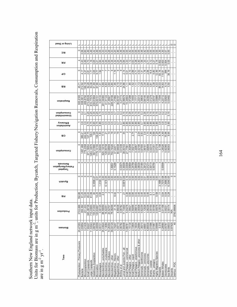
16

4

Sout

hern

New

Eng

land

net

wor

k in

put d

ata.

U

nits

for B

iom

ass a

re in

g m

-2; u

nits

for P

rodu

ctio

n, B

ycat

ch, T

arge

ted

Fish

ery/

Nav

igat

ion

Rem

oval

s, C

onsu

mpt

ion

and

Res

pira

tion

are

in g

m-2

yr-1

.

Taxa

Biomass

Production

P/B

Bycatch

Targeted Fishery/Navigation

Removals

Consumption

C/B

Assimilation Efficiency

Unassimilated Consumption

Respiration

R/B

C/P

P/R

R/C

Living or Dead

Phy

topl

ankt

on -

Prim

ary

Pro

duce

rs

20.4

7293

37

43.6

66

182.

86

0 0

0 0

1 0

935.

9165

45

.71

0 4

0 L

B

acte

ria

3.93

854

359.

392

91.2

5 0

0 14

97.4

66

380.

21

0.8

0.2

838.

5813

21

2.92

4.

17

0.43

0.

56

L

Mic

rozo

opla

nkto

n 3.

2143

5 23

1.43

3 72

.00

0 0

779.

2358

24

2.42

0.

9 0.

1 46

9.87

92

146.

18

3.37

0.

49

0.60

L

S

mal

l Cop

epod

s 7.

6022

7 34

5.38

738

45.4

3 0

0 97

1.19

054

127.

75

0.75

0.

25

473.

4553

9 62

.28

2.81

0.

73

0.49

L

La

rge

Cop

epod

s 11

.535

43

715.

0395

5 61

.99

0 0

1263

.129

76

109.

5 0.

75

0.25

61

5.77

576

53.3

8 1.

77

1.16

0.

49

L

Gel

atin

ous

Zoop

lank

ton

3.88

780

155.

5120

0 40

6.

359E

-07

0 56

7.61

880

146

0.65

0.

35

239.

8189

4 61

.69

3.65

0.

65

0.42

L

M

icro

nekt

on

8.46

559

120.

6346

7 14

.25

0.01

0

1179

.141

55

139.

29

0.75

0.

25

574.

8315

1 67

.90

9.77

0.

21

0.49

L

M

esop

elag

ics

0.00

131

0.00

125

0.95

1.

314E

-10

0 0.

0024

0 1.

83

0.85

0.

15

0.00

133

1.01

1.

92

0.94

0.

55

L

Mac

robe

ntho

s - p

olyc

haet

es

35.4

3624

88

.590

59

2.5

0.00

0

620.

1341

6 17

.5

0.5

0.5

201.

5436

0 5.

69

7 0.

44

0.33

L

M

acro

bent

hos

- cru

stac

eans

6.

1408

4 18

.422

51

3 6.

141E

-05

0 12

8.95

758

21

0.5

0.5

41.9

1122

6.

83

7 0.

44

0.33

L

M

acro

bent

hos

- mol

lusc

s 10

.263

54

20.5

2707

2

0.00

0

143.

6894

9 14

0.

4 0.

6 37

.359

27

3.64

7

0.55

0.

26

L

Mac

robe

ntho

s - o

ther

39

.041

29

78.0

8258

2

0.00

1.

6683

7 70

2.74

326

18

0.5

0.5

228.

3915

6 5.

85

9 0.

34

0.33

L

M

egab

enth

os -

filte

rers

3.

7024

7 31

.16

8.42

0.

52

0.15

280

37.0

2471

10

0.

3 0.

7 7.

2198

2 1.

95

1.19

4.

32

0.20

L

M

egab

enth

os -

othe

r 4.

4971

9 8.

9943

8 2

0.05

0

80.9

4938

18

0.

7 0.

3 36

.831

97

8.19

9

0.24

0.

46

L

Shr

imp

et a

l.0.

0678

2 0.

0678

2 1

0.01

0.

0307

6 0.

6103

9 9

0.7

0.3

0.27

773

4.10

9

0.24

0.

46

L

Larv

al a

nd J

uven

ile F

ish

- all

0.84

448

17.7

3400

21

8.

681E

-09

0.44

049

38.0

0143

45

0.

85

0.15

20

.995

79

24.8

6 2.

14

0.84

0.

55

L

Sm

all P

elag

ics

- com

mer

cial

13

.887

81

5.04

278

0.36

0.

16

0.03

046

27.7

7561

2

0.85

0.

15

15.3

4603

1.

11

5.51

0.

33

0.55

L

S

mal

l Pel

agic

s - o

ther

1.

1513

4 1.

0942

1 0.

95

0.03

0.

0069

4 2.

3026

8 2

0.65

0.

35

0.97

288

.85

2.10

1.

12

0.42

L

S

mal

l Pel

agic

s - s

quid

2.

7280

5 2.

5926

8 0.

95

0.00

0.

2476

6 7.

5021

4 2.

75

0.85

0.

15

4.14

493

1.52

2.

89

0.63

0.

55

L

Sm

all P

elag

ics

- ana

drom

ous

0.16

034

0.06

814

0.42

0.

04

0.06

459

0.32

067

2 0.

85

0.15

0.

1771

7 1.

11

4.71

0.

38

0.55

L

M

ediu

m P

elag

ics

- pis

civo

res

& o

ther

0.

2068

4 0.

0930

8 0.

45

0.02

0.

0833

0 0.

4219

5 2.

04

0.85

0.

15

0.23

313

1.13

4.

53

0.40

0.

55

L

Dem

ersa

ls -

bent

hivo

res

1.38

310

0.62

239

0.45

0.

03

0.01

460

0.87

550

0.63

0.

7 0.

3 0.

3983

5 0.

29

1.41

1.

56

0.46

L

D

emer

sals

- om

nivo

res

2.48

951

1.12

028

0.45

0.

01

0.29

123

1.99

161

0.8

0.65

0.

35

0.84

145

0.34

1.

78

1.33

0.

42

L

Dem

ersa

ls -

pisc

ivor

es

6.80

530

3.06

238

0.45

0.

09

0.01

214

7.82

609

1.15

0.

85

0.15

4.

3239

2 0.

64

2.56

0.

71

0.55

L

S

hark

s - c

oast

al

0.01

586

0.00

159

0.1

0.00

0.

0011

5 0.

0231

5 1.

46

0.85

0.

15

0.01

279

0.81

14

.6

0.12

0.

55

L

Sha

rks

- pel

agic

s 0.

0198

7 0.

0019

9 0.

1 0.

00

0.00

760

0.01

351

0.68

0.

85

0.15

0.

0074

7 0.

38

6.80

0.

27

0.55

L

H

ighl

y M

igra

tory

Spe

cies

0.

0099

0 0.

0057

8 0.

58

0.00

0

0.07

219

7.29

0.

85

0.15

0.

0398

9 4.

03

12.4

9 0.

14

0.55

L

P

inni

peds

0.

018

0.00

19

.11

3.16

8E-1

1 0

0.15

8 8.

78

0.8

0.2

1.17

049

65.0

3 83

.16

0.00

2 3.

30

L

Bal

een

Wha

les

0.28

580

0.01

158

0.04

1.

707E

-08

0.00

049

1.28

326

4.49

0.

8 0.

2 4.

2371

2 14

.83

110.

81

0.00

3 3.

30

L

Odo

ntoc

etes

0.

0578

7 0.

0023

1 0.

04

1.30

6E-0

8 0

0.92

360

15.9

6 0.

8 0.

2 0.

5292

0 9.

14

399

0.00

4 0.

57

L

Sea

Bird

s 0.

0063

3 0.

0017

4 0.

28

6.33

4E-0

5 0

0.06

303

9.95

0.

85

0.15

0.

0348

2 5.

50

36.1

9 0.

05

0.55

L

D

isca

rds

0.97

425

N/A

-

0 0

- -

- -

- -

- -

- D

Det

ritus

- P

OC

40

37

43.6

6606

-

0 0

- -

- -

- -

- -

- D

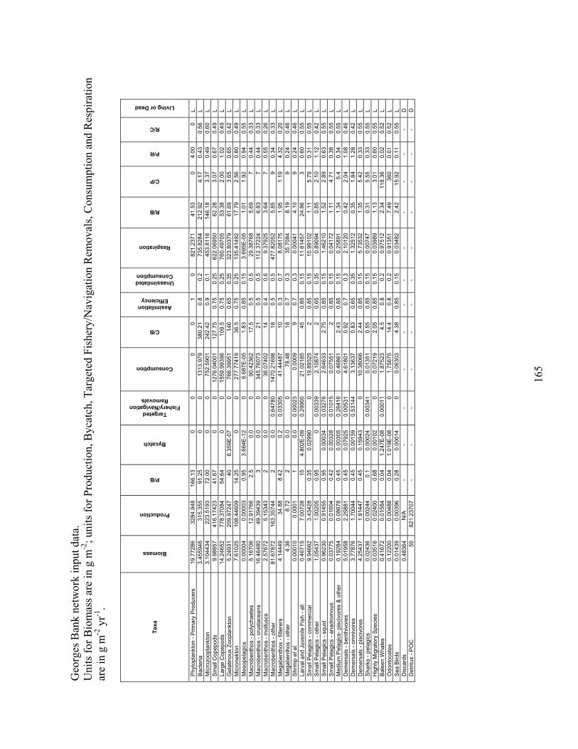
16

5

Geo

rges

Ban

k ne

twor

k in

put d

ata.

U

nits

for B

iom

ass a

re in

g m

-2; u

nits

for P

rodu

ctio

n, B

ycat

ch, T

arge

ted

Fish

ery/

Nav

igat

ion

Rem

oval

s, C

onsu

mpt

ion

and

Res

pira

tion

are

in g

m-2

yr-1

.

Taxa

Biomass

Production

P/B

Bycatch

Targeted Fishery/Navigation

Removals

Consumption

C/B

Assimilation Efficiency

Unassimilated Consumption

Respiration

R/B

C/P

P/R

R/C

Living or Dead

Phy

topl

ankt

on -

Prim

ary

Pro

duce

rs

19.7

7286

32

84.9

48

166.

13

0 0

0 0

1 0

821.

2371

41

.53

0 4.

00

0 L

Bac

teria

3.45

5946

31

5.35

5 91

.25

0 0

1313

.979

38

0.21

0.

8 0.

2 73

5.82

84

212.

92

4.17

0.

43

0.56

L

Mic

rozo

opla

nkto

n 3.

1044

34

223.

5193

72

.00

0 0

752.

5901

24

2.42

0.

9 0.

1 45

3.81

18

146.

18

3.37

0.

49

0.60

L

Sm

all C

opep

ods

9.98

857

416.

1742

3 41

.67

0 0

1276

.040

01

127.

75

0.75

0.

25

622.

0695

0 62

.28

3.07

0.

67

0.49

L

Larg

e C

opep

ods

14.2

4652

77

8.37

084

54.6

4 0

0 15

59.9

9396

10

9.5

0.75

0.

25

760.

4970

5 53

.38

2.00

1.

02

0.49

L

Gel

atin

ous

Zoop

lank

ton

5.24

931

209.

9724

7 40

6.

359E

-07

0 76

6.39

951

146

0.65

0.

35

323.

8037

9 61

.69

3.65

0.

65

0.42

L

Mic

rone

kton

7.

6102

5 10

8.44

609

14.2

5 0

0 27

7.77

419

36.5

0.

75

0.25

13

5.41

492

17.7

9 2.

56

0.80

0.

49

LM

esop

elag

ics

0.00

004

0.00

003

0.95

3.

664E

-12

0 6.

687E

-05

1.83

0.

85

0.15

3.

695E

-05

1.01

1.

92

0.94

0.

55

LM

acro

bent

hos

- pol

ycha

etes

5.

1670

6 12

.917

66

2.5

0.0

0 90

.423

62

17.5

0.

5 0.

5 29

.387

68

5.69

7

0.44

0.

33

LM

acro

bent

hos

- cru

stac

eans

16

.464

80

49.3

9439

3

0.0

0 34

5.76

073

21

0.5

0.5

112.

3722

4 6.

83

7 0.

44

0.33

L

Mac

robe

ntho

s - m

ollu

scs

2.57

672

5.15

343

2 0.

0 0

36.0

7402

14

0.

4 0.

6 9.

3792

5 3.

64

7 0.

55

0.26

L

Mac

robe

ntho

s - o

ther

81

.678

72

163.

3574

4 2

0.0

0.64

780

1470

.216

98

18

0.5

0.5

477.

8205

2 5.

85

9 0.

34

0.33

L

Meg

aben

thos

- fil

tere

rs

4.14

449

34.8

8 8.

42

0.2

0.03

305

41.4

4487

10

0.

3 0.

7 8.

0817

5 1.

95

1.19

4.

32

0.20

L

Meg

aben

thos

- ot

her

4.36

8.

72

2 0.

0 0

78.4

8 18

0.

7 0.

3 35

.708

4 8.

19

9 0.

24

0.46

L

Shr

imp

et a

l.0.

0001

0 0.

0001

1

0.0

0.00

023

0.00

09

9 0.

7 0.

3 0.

0004

1 4.

10

9 0.

24

0.46

L

Larv

al a

nd J

uven

ile F

ish

- all

0.46

715

7.00

728

15

4.80

2E-0

9 0.

2990

0 21

.021

85

45

0.85

0.

15

11.6

1457

24

.86

3 0.

60

0.55

L

Smal

l Pel

agic

s - c

omm

erci

al

9.94

662

3.43

428

0.35

0.

0299

0 0

19.8

9325

2

0.85

0.

15

10.9

9102

1.

11

5.79

0.

31

0.55

L

Sm

all P

elag

ics

- oth

er

1.05

437

1.00

205

0.95

0

0.00

339

2.10

874

2 0.

65

0.35

0.

8909

4 0.

85

2.10

1.

12

0.42

L

Sm

all P

elag

ics

- squ

id

0.96

230

0.91

455

0.95

0.

0003

4 0.

0327

6 2.

6463

3 2.

75

0.85

0.

15

1.46

210

1.52

2.

89

0.63

0.

55

LS

mal

l Pel

agic

s - a

nadr

omou

s 0.

0377

5 0.

0160

4 0.

42

0.00

328

0.01

015

0.07

551

2 0.

85

0.15

0.

0417

2 1.

11

4.71

0.

38

0.55

L

Med

ium

Pel

agic

s- p

isci

vore

s &

oth

er

0.19

284

0.08

678

0.45

0.

0030

5 0.

2641

6 0.

4686

1 2.

43

0.85

0.

15

0.25

891

1.34

5.

4 0.

34

0.55

L

Dem

ersa

ls -

bent

hivo

res

5.01

958

2.25

881

0.45

0.

0792

5 0.

0053

1 4.

6180

1 0.

92

0.7

0.3

2.10

120

0.42

2.

04

1.08

0.

46

LD

emer

sals

- om

nivo

res

3.77

876

1.70

044

0.45

0.

0015

9 0.

5314

4 3.

1363

7 0.

83

0.65

0.

35

1.32

512

0.35

1.

84

1.28

0.

42

LD

emer

sals

- pi

sciv

ores

4.

2543

7 1.

9144

7 0.

45

0.15

943

0 10

.380

66

2.44

0.

85

0.15

5.

7353

2 1.

35

5.42

0.

33

0.55

L

Sha

rks

- pel

agic

s 0.

0243

6 0.

0024

4 0.

1 0.

0002

4 0.

0034

1 0.

0135

1 0.

55

0.85

0.

15

0.00

747

0.31

5.

55

0.33

0.

55

LH

ighl

y M

igra

tory

Spe

cies

0.

0351

6 0.

0240

0 0.

68

0.00

102

0 0.

0721

9 2.

05

0.85

0.

15

0.03

989

1.13

3.

01

0.60

0.

55

LB

alee

n W

hale

s 0.

4167

2 0.

0158

4 0.

04

1.24

7E-0

8 0.

0001

1 1.

8752

3 4.

5 0.

8 0.

2 0.

9751

2 2.

34

118.

36

0.02

0.

52

LO

dont

ocet

es

0.12

200

0.00

488

0.04

1.

019E

-08

0 1.

7567

5 14

.4

0.8

0.2

0.91

351

7.49

36

0 0.

01

0.52

L

Sea

Bird

s 0.

0143

9 0.

0039

6 0.

28

0.00

014

0 0.

0630

3 4.

38

0.85

0.

15

0.03

482

2.42

15

.92

0.11

0.

55

LD

isca

rds

0.48

364

N/A

-

- -

- -

- -

- -

- -

- D

Det

ritus

- P

OC

50

82

1.23

707

- -

- -

- -

- -

- -

- -

D

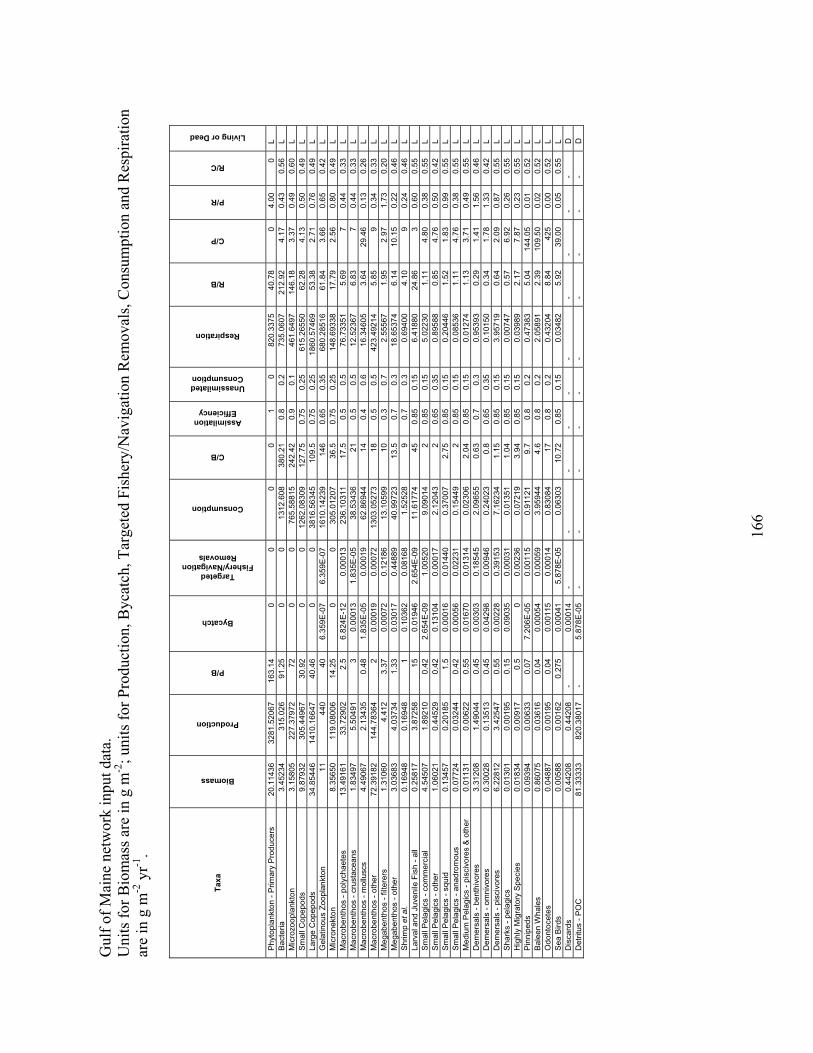
16

6

Gul

f of M

aine

net

wor

k in

put d

ata.

U

nits

for B

iom

ass a

re in

g m

-2; u

nits

for P

rodu

ctio

n, B

ycat

ch, T

arge

ted

Fish

ery/

Nav

igat

ion

Rem

oval

s, C

onsu

mpt

ion

and

Res

pira

tion

are

in g

m-2

yr-1

.

Taxa

Biomass

Production

P/B

Bycatch

Targeted Fishery/Navigation

Removals

Consumption

C/B

Assimilation Efficiency

Unassimilated Consumption

Respiration

R/B

C/P

P/R

R/C

Living or Dead

Phy

topl

ankt

on -

Prim

ary

Pro

duce

rs

20.1

1436

32

81.5

2067

16

3.14

0

0 0

0 1

0 82

0.33

75

40.7

8 0

4.00

0

L

Bac

teria

3.

4523

4 31

5.02

6 91

.25

0 0

1312

.608

38

0.21

0.

8 0.

2 73

5.06

07

212.

92

4.17

0.

43

0.56

L

M

icro

zoop

lank

ton

3.15

805

227.

3797

2 72

0

0 76

5.58

815

242.

42

0.9

0.1

461.

6497

14

6.18

3.

37

0.49

0.

60

L

Sm

all C

opep

ods

9.87

932

305.

4496

7 30

.92

0 0

1262

.083

09

127.

75

0.75

0.

25

615.

2655

0 62

.28

4.13

0.

50

0.49

L

La

rge

Cop

epod

s 34

.854

46

1410

.166

47

40.4

6 0

0 38

16.5

6345

10

9.5

0.75

0.

25

1860

.574

69

53.3

8 2.

71

0.76

0.

49

L

Gel

atin

ous

Zoop

lank

ton

11

440

40

6.35

9E-0

7 6.

359E

-07

1610

.142

39

146

0.65

0.

35

680.

2851

6 61

.84

3.66

0.

65

0.42

L

M

icro

nekt

on

8.35

650

119.

0800

6 14

.25

0 0

305.

0120

7 36

.5

0.75

0.

25

148.

6933

8 17

.79

2.56

0.

80

0.49

L

M

acro

bent

hos

- pol

ycha

etes

13

.491

61

33.7

2902

2.

5 6.

824E

-12

0.00

013

236.

1031

1 17

.5

0.5

0.5

76.7

3351

5.

69

7 0.

44

0.33

L

M

acro

bent

hos

- cru

stac

eans

1.

8349

7 5.

5049

1 3

0.00

013

1.83

5E-0

5 38

.534

36

21

0.5

0.5

12.5

2367

6.

83

7 0.

44

0.33

L

M

acro

bent

hos

- mol

lusc

s 4.

4906

7 2.

1343

5 0.

48

1.83

5E-0

5 0.

0001

9 62

.869

44

14

0.4

0.6

16.3

4605

3.

64

29.4

6 0.

13

0.26

L

M

acro

bent

hos

- oth

er

72.3

9182

14

4.78

364

2 0.

0001

9 0.

0007

2 13

03.0

5273

18

0.

5 0.

5 42

3.49

214

5.85

9

0.34

0.

33

L

Meg

aben

thos

- fil

tere

rs

1.31

060

4.41

2 3.

37

0.00

072

0.12

186

13.1

0599

10

0.

3 0.

7 2.

5556

7 1.

95

2.97

1.

73

0.20

L

M

egab

enth

os -

othe

r 3.

0368

3 4.

0373

4 1.

33

0.03

017

0.44

889

40.9

9723

13

.5

0.7

0.3

18.6

5374

6.

14

10.1

5 0.

22

0.46

L

S

hrim

p et

al.

0.16

948

0.16

948

1 0.

1036

2 0.

0816

8 1.

5252

8 9

0.7

0.3

0.69

400

4.10

9

0.24

0.

46

L

Larv

al a

nd J

uven

ile F

ish

- all

0.25

817

3.87

258

15

0.01

946

2.65

4E-0

9 11

.617

74

45

0.85

0.

15

6.41

880

24.8

6 3

0.60

0.

55

L

Sm

all P

elag

ics

- com

mer

cial

4.

5450

7 1.

8921

0 0.

42

2.65

4E-0

9 1.

0052

0 9.

0901

4 2

0.85

0.

15

5.02

230

1.11

4.

80

0.38

0.

55

L

Sm

all P

elag

ics

- oth

er

1.06

021

0.44

529

0.42

0.

1310

4 0.

0001

7 2.

1204

3 2

0.65

0.

35

0.89

588

0.85

4.

76

0.50

0.

42

L

Sm

all P

elag

ics

- squ

id

0.13

457

0.20

185

1.5

0.00

016

0.01

440

0.37

007

2.75

0.

85

0.15

0.

2044

6 1.

52

1.83

0.

99

0.55

L

S

mal

l Pel

agic

s - a

nadr

omou

s 0.

0772

4 0.

0324

4 0.

42

0.00

056

0.02

231

0.15

449

2 0.

85

0.15

0.

0853

6 1.

11

4.76

0.

38

0.55

L

M

ediu

m P

elag

ics

- pis

civo

res

& o

ther

0.

0113

1 0.

0062

2 0.

55

0.01

670

0.01

314

0.02

306

2.04

0.

85

0.15

0.

0127

4 1.

13

3.71

0.

49

0.55

L

Dem

ersa

ls -

bent

hivo

res

3.31

208

1.49

044

0.45

0.

0030

3 0.

1854

5 2.

0965

5 0.

63

0.7

0.3

0.95

393

0.29

1.

41

1.56

0.

46

L

Dem

ersa

ls -

omni

vore

s 0.

3002

8 0.

1351

3 0.

45

0.04

298

0.00

946

0.24

023

0.8

0.65

0.

35

0.10

150

0.34

1.

78

1.33

0.

42

L

Dem

ersa

ls -

pisc

ivor

es

6.22

812

3.42

547

0.55

0.

0022

8 0.

3915

3 7.

1623

4 1.

15

0.85

0.

15

3.95

719

0.64

2.

09

0.87

0.

55

L

Sha

rks

- pel

agic

s 0.

0130

1 0.

0019

5 0.

15

0.09

035

0.00

031

0.01

351

1.04

0.

85

0.15

0.

0074

7 0.

57

6.92

0.

26

0.55

L

H

ighl

y M

igra

tory

Spe

cies

0.

0183

4 0.

0091

7 0.

5 0

0.00

236

0.07

219

3.94

0.

85

0.15

0.

0398

9 2.

17

7.87

0.

23

0.55

L

P

inni

peds

0.

0939

4 0.

0063

3 0.

07

7.20

6E-0

5 0.

0011

5 0.

9112

1 9.

7 0.

8 0.

2 0.

4738

3 5.

04

144.

05

0.01

0.

52

L

Bal

een

Wha

les

0.86

075

0.03

616

0.04

0.

0005

4 0.

0005

9 3.

9594

4 4.

6 0.

8 0.

2 2.

0589

1 2.

39

109.

50

0.02

0.

52

L

Odo

ntoc

etes

0.

0488

7 0.

0019

5 0.

04

0.00

115

0.00

014

0.83

084

17

0.8

0.2

0.43

204

8.84

42

5 0.

00

0.52

L

S

ea B

irds

0.00

588

0.00

162

0.27

5 0.

0004

1 5.

878E

-05

0.06

303

10.7

2 0.

85

0.15

0.

0348

2 5.

92

39.0

0 0.

05

0.55

L

D

isca

rds

0.44

208

0.44

208

- 0.

0001

4 -

- -

- -

- -

- -

- D

D

etrit

us -

PO

C

81.3

3333

82

0.38

017

- 5.

878E

-05

- -

- -

- -

- -

- -

D

Procedures for Issuing Manuscriptsin the

Northeast Fisheries Science Center Reference Document (CRD) Series

Clearance: All manuscripts submitted for issuance as CRDs must have cleared the NEFSC ‘s manuscript/abstract/web-page review process. If any author is not a federal employee, he/she will be required to sign an “NEFSC Release-of-Copyright Form.” If your manuscript includes material lifted from another work which has been copyrighted, then you will need to work with the NEFSC’s Editorial Office to arrange for permission to use that material by securing release signatures on the “NEFSC Use-of- Copyrighted-Work Permission Form.”

Organization: Manuscripts must have an abstract and table of contents, and — if applicable — lists of figures and tables. As much as possible, use traditional scientific manuscript organization for sections: “Introduction,” “Study Area”/”Experimental Apparatus,” “Methods,” “Results,” “Discussion” and/or “Conclusions,” “Acknowledgments,” and “Literature/References Cited.”

Style: The CRD series is obligated to conform with the style contained in the current edition of the United States Government Printing Office Style Manual. That style manual is silent on many aspects of scientific manuscripts. The CRD series relies more on the CBE/CSE Style Manual. Manuscripts should be prepared to conform with these style manuals. The CRD series uses the American Fisheries Society’s guides to names of fishes, mollusks, and decapod crusta-ceans, the Society for Marine Mammalogy’s guide to names of marine mammals, the Biosciences Information Service’s guide to serial title abbreviations, and the International Standardization Organization’s guide to statistical terms. For in-text citation, use the name-date system. A special effort should be made to ensure that all necessary biblio-graphic information is included in the list of cited works. Personal communications must include date, full name, and full mailing address of the contact.

Preparation: The document must be paginated continuously from beginning to end and must have a “Table of Contents.” Begin the preliminary pages of the document -- always the “Table of Contents” -- with page “iii.” Begin the body of the document -- normally the “Introduction” -- with page “1,” and continuously paginate all pages including tables, figures, appendices, and indices. You can insert blank pages as appropriate throughout the document, but account for them in your pagination (e.g., if your last figure ends on an odd-numbered/right-hand page such as “75,” and if your next page is the first page of an appendix, then you would normally insert a blank page after the last figure, and paginate the first page of the appendix as “77” to make it begin on an odd-numbered/right-hand page also). Forward the final version to the Editorial Office as both a paper copy and electronically (i.e., e-mail attachment, 3.5-inch floppy disk, high-density zip disk, or CD). For purposes of publishing the CRD series only, the use of Microsoft Word is preferable to the use of Corel WordPerfect.

Production and Distribution: The Editorial Office will develop the inside and outside front covers, the inside and outside back covers, and the title and bibliographic control pages (pages “i” and “ii”) of the document, then combine those covers and preliminary pages with the text that you have supplied. The document will then be issued online. Paper copies of the four covers and two preliminary pages will be sent to the sole/senior NEFSC author should he/she wish to prepare some paper copies of the overall docu-ment as well. The Editorial Office will only produce three paper copies (i.e., two copies for the NEFSC’s libraries and one copy for its own archives) of the overall document. A number of organizations and individuals in the North-east Region will be notified by e-mail of the availability of the online version of the document. The sole/senior NEFSC author of the document will receive a list of those so noti-fied.

Research Communications BranchNortheast Fisheries Science Center

National Marine Fisheries Service, NOAA166 Water St.

Woods Hole, MA 02543-1026

Publications and Reportsof the

Northeast Fisheries Science CenterThe mission of NOAA’s National Marine Fisheries Service (NMFS) is “stewardship of living marine resources for the benefit of the nation through their science-based conservation and management and promotion of the health of their environment.” As the research arm of the NMFS’s Northeast Region, the Northeast Fisheries Science Center (NEFSC) supports the NMFS mission by “conducting ecosystem-based research and assess-ments of living marine resources, with a focus on the Northeast Shelf, to promote the recovery and long-term sustainability of these resources and to generate social and economic opportunities and benefits from their use.” Results of NEFSC research are largely reported in primary scientific media (e.g., anonymously-peer-reviewed scientific journals). However, to assist itself in providing data, information, and advice to its constituents, the NEFSC occasionally releases its results in its own media. Currently, there are three such media:

NOAA Technical Memorandum NMFS-NE -- This series is issued irregularly. The series typically includes: data reports of long-term field or lab studies of important species or habitats; synthesis reports for important species or habitats; annual reports of overall assessment or monitoring programs; manuals describing program-wide surveying or experimental techniques; literature surveys of important species or habitat topics; proceedings and collected papers of scientific meetings; and indexed and/or annotated bibliographies. All issues receive internal scientific review and most issues receive technical and copy editing.

Northeast Fisheries Science Center Reference Document -- This series is issued irregularly. The series typically includes: data reports on field and lab studies; progress reports on experiments, monitoring, and assessments; background papers for, collected abstracts of, and/or summary reports of scientific meetings; and simple bibliographies. Issues receive internal scientific review, but no technical or copy editing.

Resource Survey Report (formerly Fishermen’s Report) -- This information report is a quick-turnaround report on the distribution and relative abundance of selected living marine resources as derived from each of the NEFSC’s periodic research vessel surveys of the Northeast’s continental shelf. There is no scientific review, nor any technical or copy editing, of this report.

OBTAINING A COPY: To obtain a copy of a NOAA Technical Memorandum NMFS-NE or a Northeast Fisheries Science Center Reference Document, or to subscribe to the Resource Survey Report, either contact the NEFSC Editorial Office (166 Water St., Woods Hole, MA 02543-1026; 508-495-2350) or consult the NEFSC webpage on “Reports and Publications” (http://www.nefsc.noaa.gov/nefsc/publications/).

ANY USE OF TRADE OR BRAND NAMES IN ANY NEFSC PUBLICATION OR REPORT DOES NOT IMPLY EN-DORSEMENT.

MEDIA MAIL