Do Americans Consume Too Little Natural Gas?

An Empirical Test of Marginal Cost Pricing

Lucas W. Davis Erich Muehlegger∗

March 2010

Abstract

This article measures the extent to which prices exceed marginal costs in the U.S. natural

gas distribution market during the period 1991-2007. We find large departures from marginal

cost pricing in all 50 states, with residential and commercial customers facing average markups

of over 40%. Based on conservative estimates of the price elasticity of demand these distortions

impose hundreds of millions of dollars of annual welfare loss. Moreover, current price schedules

are an important pre-existing distortion which should be taken into account when evaluating

carbon taxes and other policies aimed at addressing external costs.

Key Words: Efficient Pricing, Marginal Cost Pricing, Natural Gas

JEL: D42, L50, L95, Q48, Q54

∗(Davis) Haas School of Business, University of California, Berkeley and National Bureau of Economic Research.email: ldavis@haas.berkeley.edu. (Muehlegger) John F. Kennedy School of Government, Harvard University andNational Bureau of Economic Research. email: Erich Muehlegger@hks.harvard.edu. We thank Soren Anderson, Sev-erin Borenstein, Judith Chevalier, Meredith Fowlie, Ed Glaeser, Ryan Kellogg, Erzo Luttmer, Peter Reiss, CatherineWaddams, Matt White, two anonymous referees and seminar participants at Columbia, Duke, the University ofCalifornia Energy Institute and the University of Michigan for helpful comments.

1 Introduction

Energy plays a central role in determining our overall economic well-being, from heating and

cooling our homes and businesses to determining the cost and composition of goods and services

produced in the economy. It is crucial that energy be priced appropriately to correctly encourage

efficient choices within and across different energy sources. These choices are particularly important

given recent increased attention to the external costs of energy. In the United States, 81% of

greenhouse gas emissions are derived directly from the production and consumption of energy.1

There is a great deal of public interest, therefore, in making energy prices accurately reflect both

private and social costs.

The standard approach for addressing externalities is to use a Pigouvian tax, or similarly, a

cap-and-trade program. In the standard case, a tax works by increasing prices to reflect marginal

damages. Adding marginal damages on top of private marginal costs gives social marginal costs,

leading to the socially optimal level of production. This solution is predicated on the idea that, in

the absence of the tax, prices are equal to private marginal cost. This is a reasonable assumption

in perfectly competitive markets. However, this assumption may be less reasonable for markets

served by regulated natural monopolies, which include the vast majority of retail natural gas and

electricity sales in the United States. For these markets, the welfare consequences of a tax depend

on how regulated prices compare to private marginal cost. If regulated prices are not set equal to

marginal cost, the standard Pigouvian solution will not work and may actually exacerbate existing

market distortions.

We focus, in particular, on natural gas distribution in the United States. This is a clear

natural monopoly with high fixed costs and low marginal costs. Like other monopolies, natural gas

distributors would, if left unregulated, maximize profit by pricing above marginal cost. A standard

result in regulation is that it is possible to achieve the efficient solution by using a two-part tariff.

By setting marginal price equal to marginal cost, the regulator increases the level of production

and eliminates the deadweight loss associated with the monopoly. The regulator can then allow

the monopolist to recoup its fixed costs by charging fixed fees that do not depend on the level

of production. Two-part tariffs are commonly used in regulating natural gas distributors, with

customers paying both a fixed monthly fee and a price per unit of consumption.

In this article, we measure the extent to which actual two-part tariffs for natural gas differ from

1U.S. Department of Energy, Energy Information Administration, “Emissions of Greenhouse Gases in the UnitedStates 2008”, DOE/EIA-0573, released December 2009.

1

the theoretical ideal of marginal cost pricing. We find that markups differ dramatically by customer

class. While industrial customers face prices that are close to marginal cost, most residential and

commercial customers face prices closer to average cost, with most revenues coming from per-unit

charges rather than through fixed monthly fees. Based on conservative estimates of the price

elasticity of demand, our results imply that the current pricing system yields annual welfare losses

of $2.7 billion compared to marginal cost pricing. This represents approximately 3 percent of the

$92 billion of total expenditures on natural gas in the United States in 2008.

On average, we estimate that residential and commercial customers face markups of over 40%

above marginal cost. The average markups for residential and commercial customers ($3.38 and

$3.05 per McF, respectively) are equivalent to taxes of over $55 per ton of carbon dioxide ($200

per metric ton of carbon).2 This is substantially higher than the level of a carbon tax envisioned

by most economists. As a point of comparison, Nordhaus (2007) calculates a baseline optimal tax

of $10 per ton of carbon dioxide.3 Thus, residential and commercial customers may already be

facing a marginal price that is above the social marginal cost of natural gas. If this is the case

then imposing a Pigouvian tax would move consumption in the wrong direction, further reducing

consumption below the efficient level. The broader policy lesson from our analysis is that pre-

existing distortions from regulated natural monopolies are important to consider when evaluating

carbon taxes and other policies that would increase the marginal price of energy products.

We then discuss possible explanations for the observed rate structures. Cost recovery is a

central feature of the current regulatory environment, but cost recovery alone cannot explain why

per-unit charges tend to be marked up considerably while fixed monthly fees are consistently very

low across states and customer classes. In part, this preference for low fixed fees may reflect

efforts by regulated companies to maximize the total number of customers and thus the total

rate base (see Sherman and Visscher, 1982). Distributional considerations provide an additional

and complementary explanation. Under current price schedules, high-volume customers pay a

disproportionately large share of fixed costs and attempts to “levelize” price schedules typically face

substantial political opposition because higher fixed fees would result in increased expenditures for

low-volume customers.

2U.S. Department of Energy, Energy Information Administration, “Documentation for Emissions of GreenhouseGases in the United States (2005)”, October 2007, DOE/EIA-0638, Table 6-4. There are .0543 metric tons of carbondioxide (CO2) per thousand cubic feet (McF) of natural gas.

3A carbon tax of $35 per ton from Nordhaus (2007) implies a tax of $10 per ton of CO2 because the atomic weightof carbon is 12 atomic mass units, whereas the weight of CO2 is 44, so one ton of carbon equals 44/12 tons of CO2.To avoid confusion we use CO2 throughout.

2

Finally, the article considers available policy approaches for addressing these departures from

marginal cost pricing. One alternative is public ownership. Comparing revenues from municipally-

owned and investor-owned distribution companies, we find that approximately 25 percent of a

municipally-owned utility’s fixed costs are borne by taxpayers rather than consumers of natural gas.

Lower revenue requirements could allow municipally-owned companies to charge marginal prices

which are closer to marginal cost, reducing deadweight loss. Of course, these subsidies must be

financed through taxes. Because the government cannot collect non-distortionary taxes, the welfare

effects of public provision are ambiguous - welfare for natural gas consumers rises if subsidies lower

marginal prices, but tax collection introduces distortions in other parts of the economy.

The article proceeds as follows. Section 2 describes relevant background information about the

organization of the natural gas market. Section 3 describes the seventeen-year state-level panel

of prices and quantities assembled for the analysis. Section 4 presents the results of our test of

marginal cost pricing and measures of the total welfare loss compared to marginal cost pricing.

Section 5 discusses the causes and consequences of the current rate structure with emphasis on

implications for carbon policy. Section 6 compares regulated prices for municipally-owned and

investor-owned distribution companies and section 7 concludes.

2 Background

This section provides a brief description of the organization of the U.S. natural gas market,

highlighting the features of the market that are relevant for the analysis and providing a bridge to

a substantial theoretical literature in industrial organization on the optimal regulation of natural

monopoly. For more information about the organization and regulatory history of the U.S. natural

gas market see Viscusi, Hamilton, and Vernon (2005) and U.S. Department of Energy (2010).

The natural gas market in the United States consists of gas producers, interstate pipeline

operators, and local distribution companies (“LDCs”). This article focuses on LDCs and on the

price schedules faced by residential, commercial, and industrial customers. The costs in this market

are widely understood. The main fixed cost for the LDC is the installation and maintenance of the

pipeline network. In addition, LDCs incur costs installing and maintaining gas meters, processing

bills, and taking customer service calls. These costs depend critically on the total number of

customers, and the “marginal customer cost”, i.e. the cost of adding an additional customer to

the network is substantial. In addition, LDCs purchase natural gas. Commodity cost for LDCs

3

is measured by the “city gate price”, the price at which the LDC receives natural gas.4 The

marginal cost of distributing gas through the local pipeline network is virtually zero for all classes

of consumers. Our conversations with industry participants and examinations of industry filings

confirm that line losses are negligible, representing a tiny fraction of total costs. Thus the marginal

cost of providing an additional unit of natural gas to an existing customer is well-approximated by

the city gate price.

LDCs are regulated by state utility commissions which set tariff schedules for each customer

class using traditional rate-of-return techniques.5 Regulators create price schedules to equate total

revenues from all customer classes with total operating costs plus an allowed rate of return on

the firm’s capital expenditures. There are many different price schedules which would satisfy the

zero profit condition and several previous studies have considered the question of which schedule

yields the highest level of utility. If constrained to use linear prices, Boiteux (1956) shows that

the welfare-maximizing price markup is proportional to the inverse of the elasticity of demand.

Specifically, if a monopolist produces N goods (or serves N different customer classes) with total

cost function C(x1, x2, ..., xI) and faces inverse demand function pi(xi) for good i, a social planner

constrained to using linear prices can maximize social surplus by setting prices

pi −∂C(X)

∂xi

pi

= −

(

∂pi

∂xi

xi

pi

)(

λ

1 + λ

)

,

where λ is a non-negative constant. These prices are called “Ramsey-Boiteux” prices because

the problem considered by Boiteux (1956) is formally identical to the constrained maximization

problem solved by Ramsey (1927).

When nonlinear prices can be used the regulator has more flexibility. This is the case in practice

with natural gas distribution, where the dominant price schedule is a two-part tariff.6 First, LDCs

typically charge customers a fixed fee, typically levied monthly, that does not depend on the level

4From a research perspective, a significant advantage of natural gas distribution compared to many other markets isthat marginal costs are observed. This is important because although an extensive literature in industrial organizationhas been developed for inferring marginal cost based on pricing behavior, this approach is problematic for studies ofregulated firms because prices for these firms are established by regulators, causing the key identification assumptionto fail. Not only do we observe marginal costs, but they are observed for all 50 states and at a monthly frequencygoing back to 1991.

5Price controls on wellhead prices were a major feature of the U.S. natural gas market for much of the post-warperiod (see e.g. Davis and Kilian, 2009) but were terminated in 1989 before the beginning of our sample period.

6Typically LDCs use simple two-part tariffs, although multiple-part tariffs are not uncommon. We examined the2007 tariff schedules of the twelve largest investor-owned distribution companies and the six largest municipally-owneddistribution companies. Two-part tariffs are the dominant price schedule throughout. For the LDCs we surveyed,ten of the eighteen companies use multiple-part tariffs for at least one category of customers.

4

of consumption. This fee varies by customer class - typically, industrial customers pay a higher

monthly fee than residential or commercial customers. In some cases, the fixed fee also varies

within customer class - for example, residential customers who use natural gas for heating may be

charged a different fee than residential customers who do not use natural gas for heating. Second,

customers pay a per-unit charge for each unit of natural gas that is consumed. This price includes

a commodity charge for natural gas purchased on their behalf by the local distribution company.

Commodity costs change throughout the year with the LDCs procurement costs and typically

changes in commodity costs are passed on relatively quickly to final customers.7 In addition to

commodity costs, most companies also charge customers a per unit “transportation charge” per

unit of natural gas consumed. This is typically a price per unit, though in some cases commodity

costs are marked up by a fixed percentage. As we illustrate in Section 4, these per unit fees imply

that LDC revenues are highly seasonal with LDCs collecting a large share of their total annual

revenue during cold, high-demand winter months.

In theory, with two-part tariffs a regulator can set marginal prices equal to marginal costs. As

first suggested by Coase (1946), two-part tariffs can be adjusted such that the per-unit charge is

equal to marginal cost and the fixed fee set to cover fixed costs. For the relevant case with declining

average costs and constant marginal costs, this implies that the fixed fee would be set equal to each

customer’s share of the LDC’s fixed costs. Ng and Weisser (1974) and Sherman and Visscher

(1982) extend the analysis of two-part tariffs, solving for optimal tariffs with and without revenue

constraints. If this efficient two-part tariff is not sufficient to cover the monopolist’s fixed costs,

then both prices are marked up by an amount inversely proportional to the elasticity of demand

for that margin.

In summary, this study examines the regulation of natural gas LDCs. A standard result in

regulation is that efficiency requires that marginal prices be set equal to marginal costs. The

availability of two-part tariffs makes it possible to use marginal cost pricing while still allowing the

LDC to recuperate fixed costs. How marginal prices compare to marginal costs in practice is an

empirical question to which we turn in the following section.

7Friedman (1991, Section 3) provides a fascinating description of electricity and natural gas ratemaking in Cal-ifornia under the California Public Utility Commission. Typically every three years there is a rate case with morefrequent rate adjustments for commodity cost changes. “Substantively, each case proceeds in the same way. First, theutility’s revenue requirement and marginal costs are determined. Second, the commission comes to a broad decisionabout how to allocate that revenue among customer classes. Finally, actual rates within classes are set to raise theallotted revenue. See also Kahn (1994, Chapter 4) for additional description of the rate making process including adetailed example from Pacific Gas and Electric.”

5

3 Data

To measure the extent to which regulated prices differ from marginal cost pricing, we assembled

a seventeen-year panel of natural gas sales and prices at the state-level. Our sample includes the

entire period for which data are available, January 1991 through December 2007. Natural gas sales

and prices come from the U.S. Department of Energy, Energy Information Administration, “Natural

Gas Navigator”. The Department of Energy constructs these data using a monthly survey (EIA

Form-857) of natural gas distribution companies. These data describe natural gas sales separately

for residential, commercial, industrial, and electric utility customers. See Department of Energy,

Energy Information Administration, “Definitions, Sources and Explanatory Notes” for details.

In states with active retail choice programs such as Georgia, Maryland, New York, Ohio, Penn-

sylvania, and Virginia, the Energy Information Administration calculates natural gas sales and

prices come from both the monthly survey of LDCs (EIA Form-857) and a monthly survey of

natural gas marketers (EIA Form-910). In these states customers have a choice between buying

natural gas from their LDC and buying natural gas from independent natural gas marketers. The

LDC provides and is reimbursed for transportation services but marketers perform the financial

transactions, procuring natural gas in the wholesale market and then selling it to final customers.

For states with retail choice programs, our panel describes total sales and average prices for all

customers by state, month, and customer class.

In this article, we focus on sales to residential, commercial and industrial customers. We omit

electric utility consumers. These facilities consume sufficiently large amounts of natural gas such

that it is often profitable to build a dedicated line directly to an interstate pipeline, contract with

suppliers directly and bypass the LDC. Consequently, LDCs have little bargaining power with

respect to electric utility customers and they tend to face very different price schedules from other

customers. Similarly, among commercial and industrial customers, we exclude what are called

“non-core” customers.8 Whereas “core” customers must buy from the LDC, “non-core” customers

by virtue of their size or other factors can buy from third parties and then contract with the LDCs

for transportation services only. Much like electric utility customers, non-core customers have

negotiating power which allows them to typically obtain price schedules that are different from the

schedules faced by most customers. Both the prices and quantities used in the analysis exclude

8While a relatively high proportion of commercial demand comes from “core” customers, most industrial customerscontract with wholesaler natural gas providers directly. From 2002 to 2007, approximately, 79% of commercial naturalgas demand came from “core” customers. For industrial demand, approximately 23% of demand came from “core”customers.

6

non-core customers.

Prices are available by state, month, and customer class and include all charges paid by end-

users including transportation costs as well as all federal, state and local taxes. Also available by

state and month are city gate prices, the price paid by the LDC when they receive deliveries at

the entrance to the distribution network. Table 1 presents descriptive statistics for the monthly

data: consumption and average delivered prices by customer class, city gate prices, the spot price

for North Sea crude oil (Brent Crude Spot Price), and heating degree days. All dollar values in

the article have been normalized to reflect year 2007 prices. In addition to the monthly survey

data from EIA Form-857, we assembled annual utility-level data for the universe of distribution

companies delivering natural gas to end users from EIA Form-176. The EIA does not release any

utility-level data at the monthly level. In the annual data we observe sales, revenues, and number

of customers for each LDC. In addition, we know firm ownership, which allows us to compare

regulated prices of investor-owned and municipally-owned distribution companies in Section 6.

In regulated natural gas markets, marginal prices change in two ways. First, the underlying

commodity cost for the LDCs may change if natural gas prices rise nationally. Second, regulators

may change the fixed monthly fees and per-unit markups as a result of a rate case. Natural gas

commodity prices change from month to month with national production and consumption. Fixed

monthly fees and per-unit markups, on the other hand, adjust infrequently - they are periodically

set during rate cases and held constant until the following review, which could be anywhere from

one to several years later. Although both of these are likely to be exogenous with respect to local

demand conditions, our empirical framework emphasizes within-year changes. Consequently, our

results are less likely to be driven by spurious changes in regulated prices.

City gate prices play a critical role in the analysis that follows because they represent the

marginal cost of natural gas for LDCs. Our primary source of city gate prices is the Platts’ GASdat

database which describes daily natural gas spot prices from 131 different locations throughout the

United States.9 Platts obtains these prices via surveys of trades made at each location and they

represent true natural gas spot prices. We aggregate these city gate prices to the monthly level and

then calculate state averages across all locations in a given state. For states without Platts survey

9In practice LDCs procure natural gas both on the spot market and in a forward market called the “bidweekmarket” in which the LDC purchases a specified volume of natural gas every day over the course of a month.Participating in this forward market reduces the volatility of expenditures but not the marginal cost of natural gasbecause at the margin, LDCs always have the option to buy (or sell) natural gas on the spot market. See Borenstein,Busse, and Kellogg (2009) for a detailed description of how LDCs procure natural gas.

7

locations, prices from the closest available location are used.10

We also perform our empirical test of marginal cost pricing using an alternative set of city gate

prices derived from an entirely independent source. These alternative prices come from EIA Form-

857 and represent, the city gate prices reported by LDCs including, ‘commodity charges, monthly

minimum bill and/or take-or-pay charges, surcharges, refunds in the form of reduced charges,

charges incidental to underground storage of company-owned gas, and transportation charges paid

or incurred to deliver gas to your distribution area.” Although many of these costs indeed reflect

the true marginal cost of natural gas to the LDC, one might be concerned, for example, by the

monthly minimum bill charges which should be correctly thought of as a fixed fee rather than as a

marginal cost. In addition, LDCs enter long-term contracts and engage in hedging transactions so

costs in a particular month may be a poor proxy for marginal commodity costs. These concerns lead

us to focus primarily on our measure of city gate prices from Platts. Nonetheless, it is reassuring

that the results are generally very similar using both measures.

Table 1 reports summary statistics for both measures of the city gate price. The price from

the EIA tends to be somewhat higher, consistent with including additional non-marginal costs.

Overall, however, the two prices track each other fairly accurately and the correlation between the

two monthly price series is 78.1%.11

The analysis which follows is performed at the monthly level. Although there is daily variation

in city gate prices, short-run variation in natural gas prices is mitigated by the ability of natural gas

suppliers to store natural gas. In the United States total natural gas storage capacity exceeds eight

trillion cubic feet, enough to meet total consumption for several months. In addition, natural gas

transmission lines themselves are a form of storage as they can accommodate a range of different

levels of pressurization. With access to storage, natural gas suppliers are able to arbitrage within-

month price differences, and on average across states in our sample the month-to-month variation

represents 94% of the total variation in city gate prices whereas the within-month variation rep-

resents only 6%. Our deadweight loss estimates in Section 4.2 calculate the gain in welfare that

could be realized by moving to a system of monthly marginal cost pricing. Additional gains could

10When performing the test with Platts data we exclude Alaska and Hawaii as there are no Platts survey locationsin or near these states.

11The largest deviation between EIA and Platts prices occurs in California in December 2000 following the El Pasopipeline explosion that severely curtailed natural gas shipments. The Platts city gate price of $25.61 per McF issubstantially higher than the EIA city gate price of $8.75 per McF. We do not see the extremely high spot pricesbeing passed through to consumers; average revenues from residential customers in California in December 2000 were$12.56 per McF. The difference arises because the Platts price is based on spot transactions whereas the EIA pricereflects the use of long-term contracts and other hedging strategies by the LDCs. Because of the substantial differencein this month, when conducting our test of marginal cost pricing, we drop the data for December 2000 in California.

8

be realized by moving to marginal cost pricing where prices vary daily. Still, the monthly-level

counterfactual makes most sense from a policy standpoint. Current metering technology does not

record daily consumption levels, so a change to daily pricing would require large changes in meter-

ing infrastructure along the same lines currently being observed in electricity. Moreover, utilities

have been historically very resistant to more dynamic-forms of pricing, even in electricity markets

where cost-effective storage is not available so the potential welfare gains are considerably larger.

4 Results

4.1 A Test of Marginal Cost Pricing

This section describes our test of marginal cost pricing and our estimation of per-unit markups.

Efficiency requires per-unit prices to be equal to the marginal commodity cost of natural gas. Or,

equivalently, efficiency requires that revenue net of commodity costs should not be a function of the

level of consumption. For each state, month, and customer class we calculate “net revenue”, the

total revenue collected by LDCs net of commodity costs. Next, we test if net revenue is a function

of the level of natural gas consumption.

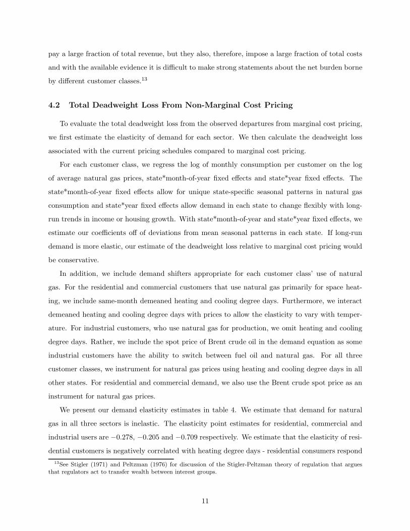
The best way to understand our test is by example. Figure 1 plots consumption and net revenue

by month for residential natural gas customers in Massachusetts in 2006. Natural gas consumption

varies substantially throughout the year with per capita consumption increasing by a factor of five

between summer and winter months as more natural gas is used for home heating. Net revenue

follows a similar pattern, increasing substantially with per capita consumption and peaking in the

winter. In addition to the monthly observations, the figure also plots fitted values from the following

regression equation:

NRt = α0 + α1qt + ǫt, t ∈ 1, 2, ..., 12 (1)

where monthly net revenue from residential sales per customer, NRt, is regressed on monthly gas

consumption per customer, qt.

The variation in consumption during the course of the year traces the price schedule. The

intercept, α0, is the average amount paid in fixed monthly fees and the slope, α1 is the average

per-unit markup over the city gate price. The price schedule for Massachusetts in 2006 indicates

that revenues tend to be collected from per-unit charges rather than from the fixed monthly fee. As

a result, net revenue in winter months is many times higher than net revenue in summer months.

9

For our test of marginal cost pricing we estimate equation (1), allowing α0 and α1 to vary by state,

year, and customer class. The null hypothesis of marginal cost pricing is α1 = 0.

Table 2 presents the main results of our test of marginal cost pricing. Panel A reports F-

statistics by state over all years and customer classes, panel B reports F-statistics by year over

all states and customer classes, and panel C reports F-statistics by customer class over all states

and years. For all 48 states (Alaska and Hawaii excluded), all years and for all three customer

classes, we reject marginal cost pricing with p-values less than 0.001. Overall, the tests provide

strong evidence of departures from marginal cost pricing.12 Our conclusions do not change if we use

the alternative city gate prices from EIA as our measure of marginal cost. Using this alternative

measure of marginal cost, we reject marginal cost pricing for all 50 states, all years, and all customer

classes.

Table 3 summarizes the per-unit markups borne by each customer class. On average, residential

consumers paid a 47.9% per-unit markup over the city gate price, equivalent to a $3.38 transporta-

tion fee per-unit. The per-unit markup for commercial customers is slightly lower, a 43.0% markup

equivalent to a $3.05 transportation fee per-unit. Markups are much lower for industrial customers

- industrial customers pay a 2.5% markup over the city gate on average, equivalent to a $0.16 trans-

portation fee per-unit. Overall, the results imply an average markup across all customer classes

of 38.4%. Using the EIA city gate prices, we find similar markups - we estimate that the average

per-unit markup across all customer classes is 38.4%, equivalent to a $2.70 per-unit markup. In

the sections which follow we attempt to put these results in context, for example comparing our

estimated markups to the increase that would be implied by proposed carbon legislation.

In addition to markups, table 3 reports the fraction of total revenues collected from each cus-

tomer class. The results indicate that residential consumers were responsible for 71.1% of total

net revenues while receiving 54.1% of total core deliveries. In contrast, industrial customers were

responsible for 3.7% of total net revenues while receiving 18.4% of total core deliveries. Although

the pattern of revenues is interesting, these results should be interpreted with caution because it

is not clear how these collected revenues compare to marginal customer costs. For example, the

residential market is characterized by a large number of customers, each consuming a relatively

small amount of natural gas. For each customer the LDC must build and maintain an additional

connection, purchase and maintain metering equipment, and process bills. Residential customers

12In related work, Naughton (1982) tests the efficiency of price schedules for a sample of electric utilities in 1980.After estimating marginal costs using a translog cost function, Naughton finds that the per-unit prices faced by allcustomer classes exceed marginal costs.

10

pay a large fraction of total revenue, but they also, therefore, impose a large fraction of total costs

and with the available evidence it is difficult to make strong statements about the net burden borne

by different customer classes.13

4.2 Total Deadweight Loss From Non-Marginal Cost Pricing

To evaluate the total deadweight loss from the observed departures from marginal cost pricing,

we first estimate the elasticity of demand for each sector. We then calculate the deadweight loss

associated with the current pricing schedules compared to marginal cost pricing.

For each customer class, we regress the log of monthly consumption per customer on the log

of average natural gas prices, state*month-of-year fixed effects and state*year fixed effects. The

state*month-of-year fixed effects allow for unique state-specific seasonal patterns in natural gas

consumption and state*year fixed effects allow demand in each state to change flexibly with long-

run trends in income or housing growth. With state*month-of-year and state*year fixed effects, we

estimate our coefficients off of deviations from mean seasonal patterns in each state. If long-run

demand is more elastic, our estimate of the deadweight loss relative to marginal cost pricing would

be conservative.

In addition, we include demand shifters appropriate for each customer class’ use of natural

gas. For the residential and commercial customers that use natural gas primarily for space heat-

ing, we include same-month demeaned heating and cooling degree days. Furthermore, we interact

demeaned heating and cooling degree days with prices to allow the elasticity to vary with temper-

ature. For industrial customers, who use natural gas for production, we omit heating and cooling

degree days. Rather, we include the spot price of Brent crude oil in the demand equation as some

industrial customers have the ability to switch between fuel oil and natural gas. For all three

customer classes, we instrument for natural gas prices using heating and cooling degree days in all

other states. For residential and commercial demand, we also use the Brent crude spot price as an

instrument for natural gas prices.

We present our demand elasticity estimates in table 4. We estimate that demand for natural

gas in all three sectors is inelastic. The elasticity point estimates for residential, commercial and

industrial users are −0.278, −0.205 and −0.709 respectively. We estimate that the elasticity of resi-

dential customers is negatively correlated with heating degree days - residential consumers respond

13See Stigler (1971) and Peltzman (1976) for discussion of the Stigler-Peltzman theory of regulation that arguesthat regulators act to transfer wealth between interest groups.

11

less to exogenous shifts in price during cold months. We estimate that a one standard deviation

increase in monthly heating degree days (419 degree days) increases the residential elasticity point

estimate by 0.115. In addition, we find that the cross-price elasticity of industrial demand with

respect to the crude oil price is 0.333.

Table 5 reports deadweight loss generated by using existing pricing tariffs relative to marginal

cost prices. We separately report deadweight loss for each customer class as well as block boot-

strapped standard errors.14 In total, we estimate that the existing price schedules create $2.7 billion

annually in deadweight loss, relative to marginal cost pricing. In the United States total expendi-

ture on natural gas in 2008 by core customers was $92 billion so this represents approximately 3%

of the total market.

These estimates provide a valuable preliminary assessment of the welfare consequences of the

observed departures from marginal cost pricing. However, it is important to emphasize that the

magnitude of the deadweight loss is sensitive to the elasticity of demand for natural gas. The

estimates from Table 4 provide a starting point but there is sampling variation in these estimates.

Moreover, the relevant demand elasticity for these calculations is the long-run demand elasticity

which is likely to be larger than the short-run elasticity because agents may employ additional

margins of adjustment. For example, in the long-run, consumers may purchase new heating equip-

ment and new appliances that uses natural gas. Because the stock of equipment turns over slowly,

the full long-run impact of a price change may not be realized for many years and estimating such

long-run effects using historical data is extremely challenging. In order to assess sensitivity, Table

5 reports deadweight loss estimates for two alternative sets of demand elasticities. The magnitude

of the implied deadweight loss varies predictably with the choice of elasticities, but even under the

most conservative assumption (-.20 for all customers), total deadweight loss exceeds $1.6 billion

annually.

It is important to note that is a partial equilibrium analysis and that these estimates of dead-

weight loss ignore any effects that a change in natural gas pricing would have on other markets.

In our thought experiment the price per unit of natural gas is decreased and set equal to marginal

cost, while the monthly fixed fees are increased. This may lead some consumers to switch between

natural gas and alternative energy sources such as electricity and oil. If prices for these other

14When calculating the deadweight loss, we assume that the number of customers using natural gas does not change.If firms can accurately estimate consumer willingness to pay based on observable and non-mutable characteristics (e.g.heating / non-heating residential) and price discriminate on fixed fees, shifting to marginal cost pricing will create awelfare gain along the extensive margin as well. Consequently, our estimates likely understate the true deadweightloss.

12

energy sources differ from marginal cost, these changes could have additional welfare consequences.

A more comprehensive analysis would consider the complete set of available energy sources, the

costs and pricing in all sectors, and model substitution patterns both across and within energy

categories.

5 Discussion of Possible Explanations

The results in the previous section provide strong evidence of departure from marginal cost

pricing in the U.S. natural gas distribution market. In this section, we consider several possible

explanations for the observed rate structure, all of which likely play a role in distorting prices away

from the theoretical ideal. We then discuss the implications of the current rate structure for carbon

policy and other public efforts aimed at addressing the external costs of energy consumption.

5.1 Profit Maximization by LDCs

One possible explanation for the current price schedules lies in the incentives created by rate-

of-return regulation. As described in the previous section, the central idea behind rate-of-return

regulation is that a firm’s revenues must equal its costs so that economic profit is zero. In theory,

the firm’s allowed rate of return on capital investments should be set equal to the firm’s market

rate of return on capital for a riskless asset. In practice, however, the firm’s market rate of return

is imperfectly observed by regulators and face a difficult tradeoff. If they set the allowed rate of

return too low, the ability of the firm to raise capital can be threatened. If they set the allowed rate

of return too high, this yields positive profits for the firm. Trying to balance these two objectives

and under pressure from regulated firms, the conventional wisdom is that in practice allowed rates

of return typically exceeds the market rate.15

When the allowed rate of return exceeds the market rate, the regulated firm has an incentive to

maximize the rate base. As pointed out by Sherman and Visscher (1982), the price schedule that

best allows the firm to increase the rate base depends on whether adding customers or increasing

output requires marginally the most capital. For natural gas distribution, capital depends most

importantly on the number of customers. More customers means more miles of network, more

connections, more metering equipment, etc. Although a large number of potential rate structures

satisfy the zero profit condition, from the regulated firm’s perspective the optimal rate structure is

15See, e.g. Averch and Johnson (1962), Baumol and Klevorick (1970), and Joskow (1974).

13

one with low fixed monthly fees that will induce as many customers as possible to enter the market.16

Of course, low fixed fees also mean high per-unit charges. However, decreased consumption along

the intensive margin is not costly from the regulated firm’s perspective because the rate base does

not depend on the level of natural gas consumption per customer. In short, under traditional rate-

of-return regulation a regulated firm attempts to maximize the rate base, and this creates incentive

for firms to lobby regulators for low fixed fees.

In adjusting per-unit charges and fixed monthly fees, the LDC faces a tradeoff between small and

large customers. Small customers are sensitive to fixed fees whereas large customers are sensitive

to the price per unit. Consider for example, a decrease in the fixed fee that is offset by an increase

in the price per unit. Such a change attracts small customers while potentially leading some large

consumers to switch to other energy sources. Whether or not such a change leads to a net increase or

decrease in the number of customers depends on the distribution of customers of different sizes and

the ease with which they can substitute across fuels. For the rate-base maximizing explanation to

make sense, it must be the case that the current price schedules with low fixed fees tend to increase

the customer base relative to alternative schedules. There would seem to be some support for this.

Particularly in the commercial and residential sectors there are a large number of smaller customers

who may indeed be sensitive to the fixed fee. Moreover, there tend to be fewer large customers

and the largest customers (e.g. non-core industrial and commercial customers) are typically able

to negotiate alternative rate structures rather than switch to other energy sources.

From an efficiency standpoint, the important question in this context is how existing fixed fees

compare to marginal connection costs. To add an additional customer requires connecting the

customer to the central distribution network. This connection cost depends on the distance from

the customer to the central network. In addition, LDCs incur costs installing and maintaining

meters, processing bills and providing customer service. Much of these additional costs should

be considered marginal connection costs. Our study reveals very low fixed fees across states and

customer classes. Thus there would appear to be scope to improve efficiency by increasing fixed

fees up to the level of marginal connection costs.

16These incentives could also help explain the fact that monthly fees sometimes vary within customer class. Forexample, some companies charge monthly fees for industrial customers that vary by historical consumption levels andsome companies charge different monthly fees for residential customers depending on whether or they use natural gasfor heating. This price discrimination could be seen as a mechanism for inducing as many customers as possible intothe market.

14

5.2 Distributional Considerations

Distributional considerations provide an alternative and complementary explanation for the

observed rate structure. With low fixed fees the existing rates imply that within customer classes

high-demand customers pay a disproportionately large share of fixed costs. Where monthly fees

are exactly zero, for example, a customer consuming 100 McF annually pays twice as much as a

customer consuming 50 McF despite the fact that the cost of providing distribution service to these

two customers is nearly identical. This structure may have progressive distributional consequences.

If high-income households own large homes and consume high levels of natural gas, they will also

pay a large share of total costs. This distributional argument is highlighted in a recent rate case for

Bay State Gas before the Massachusetts Department of Telecommunications and Energy (emphasis

added).

The Attorney General also takes issue with the Company’s proposed residential delivery

rates (id. at 116-117). While the Company’s proposed block rates for the residential

rate classes, the Attorney General requests that the Company provide a flat rate design

(i.e., no block charges) for the residential rate classes (id. at 117). The Attorney General

argues that a flat rate design for the residential rate classes not only would simplify rate

design but would also provide lower bill impacts for all but those customers with higher

than average use.17

These distributional concerns make it politically difficult to implement rate changes that would

increase fixed fees. Although state and federal programs exist aimed at providing assistance to low-

income households with energy bills, there are concerns that these programs may not do enough for

vulnerable populations.18 Moreover, enrollment in means-tested subsidy programs is rarely high.

As an example, Borenstein (2010) cites an upper-bound of 78 percent for the take-up rate of the

CARE program, a heavily promoted, means-tested electricity subsidy in California.

More broadly, fixed fees are salient to consumer protection groups and they are perceived as sub-

stantially impacting energy bills for low-income groups and small businesses. Absent accompanying

subsidies, lowering per-unit markups and increasing fixed fees would shift the burden of fixed costs

from high-usage to low-usage customers. As Reiss and White (2005) finds for electricity, non-linear

17Massachusetts Department of Telecommunications and Energy, DTE 05-27, p. 325.18The largest such program, the Low Income Home Energy Assistance Program (LIHEAP) has been in operation

since 1982 and operates in all 50 states with a $4.5 billion dollar budget in 2009. Eligible household must meet incomerequirements and typically assistance is awarded on a first come first serve basis.

15

tariffs that increase the marginal price for high-usage customers may be preferable for distributional

reasons. In addition, they estimate that high-income households are less price-sensitive than low-

income households, strengthening the distributional argument for non-linear residential electricity

tariffs. Although no previous work to our knowledge has performed a similar distributional analysis

for natural gas demand or tariffs, many state boards cite distributional reasons when setting low

monthly fees and high or increasing marginal prices.

5.3 Environmental Externalities

Environmental externalities provide a third possible explanation for the observed departures

from marginal cost pricing. Could it be the case that whether intended or unintended, the current

system of price schedules serves to effectively internalize the external costs of energy? In this

section we consider this possibility, but conclude that the markups are considerably higher than

most available estimates in the literature for the external damages from natural gas consumption.

Section 4 showed that most customers face large per-unit charges for natural gas. The average

customer markup ($2.70 per McF) is equivalent to a tax of $50 per metric ton of CO2. Average

markups vary substantially across customer classes ranging from 2.5% for industrial customers to

47.9% for residential customers. For industrial customers, the average markup ($0.16) is equivalent

to a $3 tax per metric ton of CO2. In contrast, for residential and commercial customers the

average markups ($3.38 and $3.05, respectively) are equivalent to a tax of $62 and $56 per metric

ton of CO2. Interestingly, these markups straddle markups implied by the range of carbon taxes

envisioned by most economists. For example, Nordhaus (2007) calculates a baseline optimal tax

of $10 and Metcalf (2007) calls for a $15 tax. Regardless of one’s views on the marginal external

costs of CO2 emissions, it is critical that carbon policy take into account pre-existing distortions

in the market. Based on $10 or $15 taxes, for example, the current per-unit price of natural gas

for residential and commercial customers already exceeds marginal social costs.19

Given recent attention to the issue of climate change it makes sense to consider the implications

of current pricing schedules for carbon. However, it also makes sense to consider local pollutants

such as nitrogen oxides and particulates.20 Natural gas combustion releases .09 pounds of nitrogen

19In related work, Buchanan (1969), Barnett (1980), and Oates and Strassman (1984) consider Pigouvian taxes inthe context of an unregulated monopoly.

20There may also be negative externalities from emerging forms of natural gas production. There is currently agreat deal of excitement in the natural gas market about shale gas. Natural gas producers have long known thatshale and other rock deposits contain large amounts of natural gas. It was not until recently, however, that horizontaldrilling and hydraulic fracturing technology improved enough to make these supplies accessible at reasonably low cost.See e.g., D. Rotman “Natural Gas Changes the Energy Map,” MIT Technology Review, November 2009. See also

16

oxides and .007 pounds of particulates per McF.21 Using estimates from Muller and Mendelsohn

(2009), the external costs of these emissions are less than 3 cents per McF, equivalent to a markup

over average residential prices of about one fifth of one percent. Of course, marginal damages from

local pollutants depend on the proximity between the location of emissions and population centers.

However, even the 99% percentile estimates from Muller and Mendelsohn imply markups of less

than 1% over average residential prices.22 Thus with neither carbon emissions nor with emissions

of local pollutants would it appear that external costs justify the size of markups that are currently

observed.

Nevertheless, the presence of external costs imply that the deadweight loss estimates in Table

5 may somewhat overstate the total welfare cost of the observed departures from marginal cost

pricing. In Table 6, we present deadweight loss estimates that take into account that, due to

external costs, the socially optimal level of natural gas consumption is lower than what would be

implied by pricing at private marginal cost. We present results for three different values of the

marginal cost of CO2 emissions: $0 per ton, $10 per ton, and $15 per ton. In each case, we use

our elasticity estimates from Table 4. As a point of reference, $10 per ton of CO2 is equivalent

to a markup of $0.54 per Mcf, $15/ton of CO2 is equivalent to a markup of $0.81 per Mcf. The

first column is identical to the results reported in Table 5. Without incorporating the cost of CO2

emissions, we estimate total deadweight losses of $2.7 billion dollars per year. Using a cost of

$10/ton of CO2, our deadweight loss estimate falls to $2.5 billion dollars per year. Using a cost of

$15/ton of CO2, our deadweight loss estimate falls further to $2.4 billion dollars per year.

Again, it is important to note that this analysis is partial equilibrium. In this thought experi-

“America’s Natural Gas Revolution” Wall Street Journal, 11/3/2009 and “Has Natural Gas’s Moment Come?” Wall

Street Journal, 12/16/2009. These developments suggest that natural gas is going to continue to be an importantpart of the energy portfolio in the United States for many years to come. These technologies also, however, raisepotential environmental concerns and in particular concerns about water consumption, though these potential costsare still poorly understood.

21U.S. Department of Energy, Energy Information Administration, ‘Natural Gas 1998: Issues and Trends”, DOE-EIA-0560(1998), released April 1999, Chapter 2: Natural Gas and the Environment, Table 2. See also U.S. De-partment of Energy, Energy Information Administration, “Annual Energy Review”, DOE/EIA-0384(2007), releasedJune 2008, Table 12.7a. Natural gas is the cleanest of all major fossil fuels. Per unit of energy, natural gas combus-tion releases 80% less nitrogen oxides, 90% less particulates, and over 99% less sulfur dioxide and mercury than oilcombustion.

22Muller and Mendelsohn (2009), use an integrated assessment model to track and value emissions from 10,000point and aggregated non-point sources in the United States. Average marginal damages from Table 1 are $1.61 perpound of particulates (PM2.5) and $.13 per pound of nitrogen oxides. The 99th percentile of marginal damages is$6.20 per pound of particulates (PM2.5) and $.55 per pound of nitrogen oxides. Alternative, and somewhat largerestimates of the marginal damages of nitrogen oxide emissions come from Muller, Tong, and Mendelsohn (2009)using the Community Multi-scale Air Quality model (CMAQ) rather than the reduced-form Air Pollution EmissionExperiments and Policy (APEEP) model used in Muller and Mendelsohn (2009). With CMAQ, marginal damagesfrom ground-level nitrogen oxide emissions from nine locations in and around Atlanta (Table 1) average $.27 perpound with a maximum of $.55.

17

ment the marginal price of natural gas is decreased and set equal to social marginal cost. We are

ignoring the implications that this change would have for other markets. Lowering the marginal

price of natural gas accompanied by an increase in the monthly fixed fees would affect demand for

alternative energy sources such as electricity and oil. These changes could have additional welfare

consequences if prices in these other markets differ from marginal cost. Moreover, these estimates

of deadweight loss ignore externalities from the production, processing, transmission, storage, and

distribution of natural gas. U.S. Environmental Protection Agency (2010) reports that emissions

from these sources in 2008 represented 9.3% of total greenhouse gas emissions from natural gas.

Incorporating these additional external costs would modestly reduce the estimated total deadweight

loss estimates in Tables 5 and 6.

6 Ownership Structure and Efficiency

There are several available approaches for addressing these departures from marginal cost pric-

ing. There are many alternative rate structures which could improve efficiency while allowing LDCs

to recoup their investments. In the conclusion we discuss rate “levelization”, which would increase

fixed fees while decreasing per unit prices.

An alternative approach for lowering per-unit prices is public provision. Energy utilities in the

United States operate under one of two types of institutional arrangements: (1) privately-owned

companies regulated by state public utility commissions, and (2) publicly-owned or “municipally-

owned” companies that are directly under public control. In both cases, the public sector controls

rate setting. However, unlike privately-owned companies which must recoup fixed costs from end

users of natural gas, municipally-owned companies can recoup fixed costs through government

subsidies, thereby shifting the burden of fixed costs from natural gas consumers to taxpayers.

Consequently, a municipally-owned LDC may offer a price schedule with lower per-unit markups.

Still, as we discuss in this section the welfare effects of public provision are ambiguous because

subsidies must be financed through distortionary taxes.

Municipal ownership is common in natural gas distribution. In 2007, approximately two-thirds

of LDCs were municipally-owned (848 out of a total of 1,229). On average, municipally-owned

LDCs are much smaller than investor-owned LDCs. In total, municipally-owned LDCs delivered

only eight percent of the natural gas to end-users in 2007. Despite differences in mean deliver-

ies, the size distributions of municipally-owned and investor-owned LDCs overlap substantially.

18

Approximately 45 percent of municipal utilities and 34 percent of investor-owned utilities deliver

between 100 million cubic feet of gas a year and 10 billion cubic feet of gas per year. Municipal util-

ities and investor-owned utilities are comparable on other observable dimensions. For the average

municipally-owned distribution company, 41 percent, 25 percent and 33 percent of deliveries are

made to residential, commercial and industrial customers. In comparison, 42 percent, 26 percent

and 30 percent of deliveries of investor-owned utilities go to residential, commercial and industrial

customers.

To estimate the proportion of municipal utility fixed costs borne by taxpayers, we calculate

annual net revenues for each distribution company using the utility-level data from 1997 to 2007.

In total, we observe 9,426 company-years of municipal data and 3,755 company-years of investor-

owned data. In this case, we calculate net revenues for each LDC using the city-gate prices reported

by the EIA rather than the Platts spot price data. The city-gate averages reported by the EIA

measure the average natural gas procurement cost by state, including both spot transactions as

well as long-term contracts. Thus, net revenues calculated using the EIA data provide the best

proxy for the amount of fixed costs covered by the regulated price schedule.

We compare the net revenues earned by comparably-sized municipally-owned and investor-

owned distribution companies. Table 7 presents the results from regressing annual net revenues for

each firm on total deliveries (as a proxy for firm size), the proportion of deliveries made to indus-

trial or electric customers (to account for differences in the composition of end users), population

density, and a dummy variable corresponding to whether the distribution company is municipally-

owned. In each specification, we include state fixed effects and year fixed effects. Controlling for

size and customer composition, we expect municipal utilities and investor-owned utilities to have

similar fixed costs. Absent the ability of the government to fiscally subsidize a municipal utility,

the firms should require similar net revenues. Specifications (1) and (2) include all firms, whereas

specifications (3) and (4) restrict the sample to the portion of the firm size distribution where sub-

stantial overlap between municipally-owned and investor-owned LDCs exists - between 100 million

and 5 billion cubic feet of delivered gas per year. Restricting the sample to mid-sized distribution

companies does not substantially affect the results. In all four regressions we estimate a positive

coefficient on annual deliveries between 0.805 and 0.950 - in all cases, the estimates are statistically

distinguishable from 1 - consistent with a natural monopoly exhibiting economies of scale. We

estimate that a 10 percentage point increase in the share of deliveries to large (industrial/electric)

customers is associated with a 12-13 percent reduction in net revenues. Finally, we estimate that,

19

conditional on observables, municipally-owned distribution companies collect approximately 25 to

30 percent less net revenues through their service rates than investor-owned utilities. This is consis-

tent with substantial direct subsidies to municipally-owned LDCs that allow these LDCs to collect

considerably less revenue from natural gas customers. Without monthly utility-level data it is

impossible to say whether this comes in the form of lower markups, lower fixed fees (or both). 23

The overall welfare impact of direct subsidies depends, therefore, on the marginal cost of public

funds. While subsidies increase the welfare of natural gas users, these gains are offset by tax

distortions in other parts of the economy. As a thought exercise, we calculate the threshold cost of

public funds which lead a 25 percent subsidy of fixed costs to be welfare neutral. We estimate that

a 25 percent subsidy of the per unit transportation fee requires $5.85 billion per year to cover lost

revenues and is associated with a welfare gain of $733 million to natural gas users. Consequently,

the welfare-neutral threshold cost of public funds is roughly 12 cents per dollar. If a jurisdiction can

collect taxes which introduce less than 12 cents of deadweight loss per dollar of revenue generated

(and the cost of public versus private provision are similar), public subsidization of the fixed costs

of operation may improve welfare if used to reduce per-unit markups.

Of course, there are other advantages and disadvantages of private ownership. A large literature

in economics examines the effect of firm ownership on operating efficiency. See, e.g., Olley and

Pakes (1996), Joskow (1997), Ng and Seabright (2001) and Fabrizio, Rose and Wolfram (2007).

Privately-owned LDCs typically have more incentive than publicly-owned LDCs to reduce costs.

Rate-of-return regulation guarantees privately-owned LDCs a certain rate of return on investments,

but because of regulatory lag these firms have an incentive for cost-reduction between rate cases.

Moreover, managers of privately-owned LDC may be more motivated because of the threat that they

would be replaced by a disappointed regulator whereas management in publicly-owned LDCs face

less threat of takeover. On the other hand, effective regulation of privately-owned LDCs is difficult

because the regulatory agency needs detailed information about the firm’s costs and the regulatory

proceedings used to elicit this information require time and resources. In addition, regulation of

privately-owned LDCs may introduce additional inefficiencies such as overcapitalization (Averch

and Johnson, 1962).

23An alternative explanation is that regulators allow investor-owned or privately-owned utilities to earn substan-tially higher profit than those earned by a municipally-owned LDC. To check, we examined the 2007 annual reportsof the six largest municipally-owned LDCs. In 2007, the six municipally-owned LDCs examined received direct andindirect subsidies. Subsidies took the form of government grants to cover operation, repairs and construction, accessto subsidized government and cooperative natural gas supplies, and the ability to issue tax-exempt government bondsand commercial paper.

20

7 Concluding Remarks

Our analysis of the U.S. natural gas distribution market supports the following conclusions.

First, we strongly reject marginal cost pricing. This result holds individually and jointly for all 50

states, all seventeen years and for residential and commercial customer classes. Second, markups

above marginal cost are largest for residential and commercial customers, averaging 47.9% and

45.0%, respectively. Markups for industrial customers are much lower, averaging only 2.5%. Third,

for conservative estimates of the price elasticity of demand, these distortions impose large aggregate

welfare losses compared to marginal cost pricing. In short, the current system with low fixed fees

and high per unit prices implies that there are too many natural gas customers, each consuming

too little natural gas.

The most natural approach to addressing these departures from marginal cost pricing would

be to have regulators work with LDCs to “levelize” rate structures, increasing monthly fees and

lowering the price charged per unit. There is some precedent for this. For example, in May 2008 a

new rate structure was approved for Duke Energy Ohio in which the monthly fixed delivery charge

increased from $4.50 to $10.00 with an offsetting reduction in per-unit prices. The Public Utilities

Commission of Ohio (PUCO) argued that the new “levelized” rate structure is more equitable,

“making sure that each customer pays only their share of the costs Duke must cover to deliver gas

to their home.” According to PUCO, the costs of natural gas distribution including installing and

maintaining pipelines, reading gas meters, processing bills, and taking customer service calls is the

same “whether a customer uses a little natural gas each month, or a lot.”

Carbon taxes could then be added to the “levelized” rates to ensure that customers pay the

socially efficient price. Proceeding in this way would ensure that carbon policy works as it is

designed. Levelized rates combined with a carbon tax or cap-and-trade program would make

natural gas prices accurately reflect both private and social cost. If prices in other energy sectors

also accurately reflect both private and social costs, this will encourage efficient choices across

energy sources. Adding a carbon tax on top of the “levelized” rates would also create appropriate

incentives for reducing carbon emissions from natural gas production, processing, transmission,

storage and distribution.

Natural gas is cleaner than other fossil fuels, but less clean than energy from renewables so

some policymakers have argued that natural gas can serve as a bridge to a less carbon-intensive

economy. Moreover, many industry observers believe that recent developments in horizontal drilling

21

and hydraulic fracturing technology have ensured that natural gas will continue to play an important

role in the United States’ energy portfolio. It is crucial that natural gas be priced appropriately

if these new sources are to be developed efficiently, and if energy consumers are to make efficient

consumption and capital choices.

22

References

[1] Averch, H. and Johnson, L. “Behavior of the Firm Under Regulatory Constraint.” AmericanEconomic Review, Vol. 52 (1962), pp. 1052-1069.

[2] Baumol, W. and Bradford, D. “Optimal Departures from Marginal Cost Pricing.” AmericanEconomic Review, Vol. 60 (1970), pp. 265-283.

[3] Baumol, W. and Klevorick, A. “Input Choices and Rate-of-Return Regulation: An Overviewof the Discussion.” Bell Journal of Economics and Management Science, Vol. 1 (1970), pp.162-190.

[4] Barnett, A. “A Pigouvian Tax Rule Under Monopoly.” American Economic Review, Vol. 70(1980), pp. 1037-1041.

[5] Boiteux, M. “Sur la Gestion des Monopoles Publics Astreints a L’equilibre Budgetaire.” Econo-metrica, Vol. 24 (1956), pp. 22-40.

[6] Borenstein, S. “The Redistributional Impact of Nonlinear Electricity Pricing.” Energy Institute@ Haas Working Paper 204, University of California Berkeley, (2010).

[7] Borenstein, S., Busse, M. and Kellogg, R. “Principal-Agent Incentives, Excess Caution, andMarket Inefficiency: Evidence from Utility Regulation.” NBER Working Paper 13679, (2009).

[8] Buchanan, J. “External Diseconomies, Corrective Taxes, and Market Structure.” AmericanEconomic Review, Vol 59 (1969), pp. 174-177.

[9] Coase, R. “The Marginal Cost Controversy.” Economica, Vol 13 (1946), pp. 169-182.

[10] Davis, L. and Kilian, L. “The Allocative Cost of Price Ceilings in the U.S. Residential Marketfor Natural Gas.” NBER Working Paper 14030, (2008).

[11] Fabrizio, K., Rose, N., and Wolfram, C. “Do Markets Reduce Costs? Assessing the Impact ofRegulatory Restructuring on U.S. Electric Generation Efficiency.”American Economic Review,Vol. 97 (2007), pp. 1250-1277.

[12] Feldstein, M. “Equity and Efficiency in Public Sector Pricing: The Optimal Two-Part Tariff.”Quarterly Journal of Economics, Vol. 86 (1972), pp. 175-187.

[13] Friedman, L. “Energy Utility Pricing and Customer Response: The Recent Record in Cali-fornia.” Regulatory Choices Ed. Richard J. Gilbert. Berkeley: University of California Press,(1991)

[14] Joskow, P. “Inflation and Environmental Concern: Change in the Process of Public UtilityPrice Regulation.” Journal of Law and Economics, Vol. 2 (1974), pp. 291-327.

[15] Joskow, P. “Restructuring, Competition and Regulatory Reform in the U.S. Electricity Sector.”Journal of Economic Perspectives, Vol. 11 (1997), pp. 119-138.

[16] Kahn, E. Electric Utility Planning and Regulation, Washington D.C.: American Council foran Energy-Efficient Economy, 2nd Edition, (1994).

[17] Knittel, C. “Market Structure and the Pricing of Electricity and Natural Gas.” Journal ofIndustrial Economics, Vol. 60 (2003), pp. 167-191.

23

[18] Klein, C. and Sweeney, G. “Regulator Preferences and Utility Prices: Evidence from NaturalGas Distribution Utilities.” Energy Economics, Vol. 21 (1999), pp. 1-15.

[19] Metcalf, G. “A Proposal for a U.S. Carbon Tax Swap.” Brookings Institution Discussion Paper2007-12, (2007).

[20] Muller, N. and Mendelsohn, R. “Efficient Pollution Regulation: Getting the Prices Right.”American Economic Review, Vol. 99 (2009), pp. 1714-1739.

[21] Muller, N., Tong, D. and Mendelsohn, R. “Regulating NOx and SO2 Emissions in Atlanta.”The B.E. Journal of Economic Analysis and Policy, Vol. 9 (2009), Article 3.

[22] Naughton, M. “The Efficiency and Equity Consequences of Two-Part Tariffs in ElectricityPricing.” Review of Economics and Statistics,Vol. 68 (1982), pp. 406-414.

[23] Nelson, R. “An Empirical Test of the Ramsey Theory and Stigler-Peltzman Theory of PublicUtility Pricing.” Economic Inquiry, Vol. 20 (1982), pp. 277-290.

[24] Ng, C. and Seabright, P. “Competition, Privatisation and Productive Efficiency: Evidencefrom the Airline Industry.”Economic Journal Vol. 111 (2001), pp. 591-619.

[25] Ng, Y. and Weisser, M. “Optimal Pricing with a Budget Constraint-The Case of the Two-partTariff.” Review of Economic Studies Vol. 41 (1974), pp. 337-345.

[26] Nordhaus, W. “A Review of the Stern Review on the Economics of Global Warming.” Journalof Economic Literature, Vol. 45 (2007), pp 686-702.

[27] Oates, W. and Strassman, D. “Effluent Fees and Market Structure.” Journal of Public Eco-nomics, Vol. 24 (1984), pp. 29-46.

[28] Olley, S. and Pakes, A. “The Dynamics of Productivity in the Telecommunications EquipmentIndustry.” Econometrica, Vol. 64 (1996), pp. 1263-1297.

[29] Peltzman, S. “Toward a More General Theory of Regulation.” Journal of Law and Economics,Vol. 19 (1976), pp. 211-240.

[30] Ramsey, F. “A Contribution to the Theory of Taxation.” Economic Journal, Vol. 37 (1927),pp. 47-61.

[31] Ramsey, F. “A Contribution to the Theory of Taxation.” Economic Journal, Vol. 37 (1927),pp. 47-61.

[32] Reiss, P. and White, M. “Household Electricity Demand, Revisited.” Review of EconomicStudies, Vol. 72 (2005), pp. 853-883.

[33] Schmalensee, R. “Monopolistic Two-Part Pricing Arrangements.”Bell Journal of Economics,Vol. 12 (1981), pp. 445-466.

[34] Sherman, R. and Visscher, M. “Rate-of-Return Regulation and Two-Part Tariffs.”QuarterlyJournal of Economics, Vol. 96 (1982), pp. 27-42.

[35] U.S. Department of Energy, Energy Information Administration, “Natural Gas Annual 2008”,DOE/EIA-0131, March 2010.

24

[36] U.S. Environmental Protection Agency, “Inventory of U.S. Greenhouse Gas Emissions andSinks: 1990-2008”, EPA 430-R-10-006, April 15, 2010.

[37] Viscusi, W. Kip, Harrington, J., and Vernon, J. Economics of Regulation and Antitrust, Cam-bridge, Massachusetts: MIT Press, 2005.

25

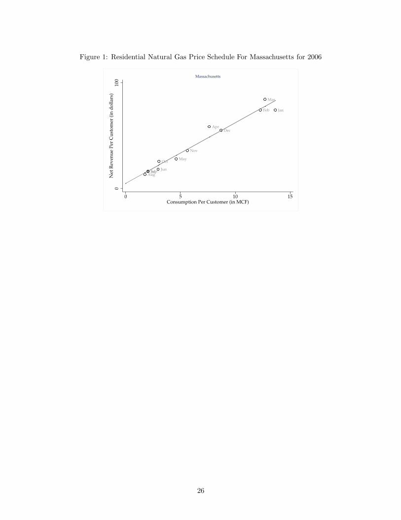
Figure 1: Residential Natural Gas Price Schedule For Massachusetts for 2006

AugJulSep

Jun

OctMay

Nov

AprDec

Feb

Mar

Jan

010

0N

et R

even

ue

Per

Cu

sto

mer

(in

do

llar

s)

0 5 10 15Consumption Per Customer (in MCF)

Massachusetts

26

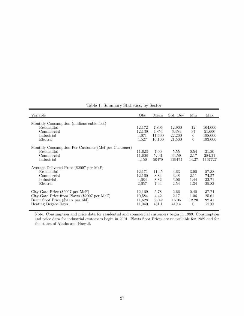
Table 1: Summary Statistics, by Sector

Variable Obs Mean Std. Dev Min Max

Monthly Consumption (millions cubic feet)Residential 12,172 7,806 12,900 12 104,000Commercial 12,139 4,854 6,454 37 51,600Industrial 4,671 11,600 22,200 0 198,000Electric 4,527 10,100 21,500 0 193,000

Monthly Consumption Per Customer (Mcf per Customer)Residential 11,623 7.00 5.55 0.54 31.30Commercial 11,608 52.31 34.59 2.17 284.31Industrial 4,150 50478 159474 14.27 1167727

Average Delivered Price ($2007 per McF)Residential 12,171 11.45 4.63 3.00 57.38Commercial 12,160 8.84 3.48 2.11 74.57Industrial 4,684 8.82 3.06 1.44 32.71Electric 2,657 7.44 2.54 1.34 25.83

City Gate Price ($2007 per McF) 12,169 5.78 2.66 0.40 37.74City Gate Price from Platts ($2007 per McF) 10,584 4.42 2.17 1.06 25.61Brent Spot Price ($2007 per bbl) 11,628 33.42 16.05 12.20 92.41Heating Degree Days 11,040 431.1 419.4 0 2109

Note: Consumption and price data for residential and commercial customers begin in 1989. Consumptionand price data for industrial customers begin in 2001. Platts Spot Prices are unavailable for 1989 and forthe states of Alaska and Hawaii.

27

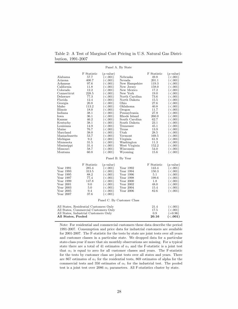
Table 2: A Test of Marginal Cost Pricing in U.S. Natural Gas Distri-bution, 1991-2007

Panel A. By State

F Statistic (p-value) F Statistic (p-value)Alabama 57.7 (<.001) Nebraska 49.8 (<.001)Arizona 400.7 (<.001) Nevada 201.1 (<.001)Arkansas 97.6 (<.001) New Hampshire 119.3 (<.001)California 11.8 (<.001) New Jersey 158.0 (<.001)Colorado 12.2 (<.001) New Mexico 17.2 (<.001)Connecticut 228.5 (<.001) New York 19.0 (<.001)Delaware 77.3 (<.001) North Carolina 73.6 (<.001)Florida 12.4 (<.001) North Dakota 15.5 (<.001)Georgia 20.8 (<.001) Ohio 27.6 (<.001)Idaho 113.2 (<.001) Oklahoma 40.8 (<.001)Illinois 18.0 (<.001) Oregon 11.7 (<.001)Indiana 38.1 (<.001) Pennsylvania 27.9 (<.001)Iowa 36.1 (<.001) Rhode Island 260.0 (<.001)Kansas 46.2 (<.001) South Carolina 62.7 (<.001)Kentucky 38.1 (<.001) South Dakota 23.1 (<.001)Louisiana 14.9 (<.001) Tennessee 45.1 (<.001)Maine 76.7 (<.001) Texas 13.9 (<.001)Maryland 38.0 (<.001) Utah 28.5 (<.001)Massachusetts 53.7 (<.001) Vermont 169.5 (<.001)Michigan 9.2 (<.001) Virginia 61.9 (<.001)Minnesota 31.5 (<.001) Washington 11.3 (<.001)Mississippi 31.4 (<.001) West Virginia 152.2 (<.001)Missouri 58.7 (<.001) Wisconsin 54.0 (<.001)Montana 60.8 (<.001) Wyoming 15.6 (<.001)

Panel B. By Year

F Statistic (p-value) F Statistic (p-value)Year 1991 285.4 (<.001) Year 1992 143.4 (<.001)Year 1993 313.5 (<.001) Year 1994 150.3 (<.001)Year 1995 88.2 (<.001) Year 1996 5.1 (<.001)Year 1997 77.4 (<.001) Year 1998 199.6 (<.001)Year 1999 147.8 (<.001) Year 2000 1.8 (<.001)Year 2001 9.0 (<.001) Year 2002 48.0 (<.001)Year 2003 5.0 (<.001) Year 2004 15.4 (<.001)Year 2005 9.4 (<.001) Year 2006 82.6 (<.001)Year 2007 37.6 (<.001)

Panel C. By Customer Class

All States, Residential Customers Only 21.4 (<.001)All States, Commercial Customers Only 17.5 (<.001)All States, Industrial Customers Only 0.9 (=0.96)All States, Pooled 20.16 (<.001)

Note: For residential and commercial customers these data describe the period1991-2007. Consumption and price data for industrial customers are availablefor 2001-2007. The F-statistic for the tests by state are joint tests over all yearsand customer classes in a particular state. We dropped data for a particularstate-class-year if more that six monthly observations are missing. For a typicalstate there are a total of 41 estimates of α1 and the F-statistic is a joint testthat α1 is equal to zero for all customer classes and years. The F-statisticfor the tests by customer class are joint tests over all states and years. Thereare 867 estimates of α1 for the residential tests, 869 estimates of alpha for thecommercial tests and 350 estimates of α1 for the industrial test. The pooledtest is a joint test over 2086 α1 parameters. All F-statistics cluster by state.

28

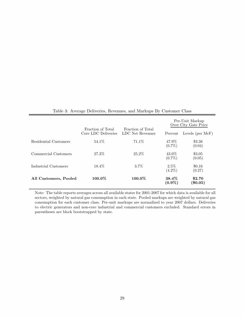
Table 3: Average Deliveries, Revenues, and Markups By Customer Class

Per-Unit MarkupOver City Gate Price

Fraction of Total Fraction of TotalCore LDC Deliveries LDC Net Revenues Percent Levels (per McF)

Residential Customers 54.1% 71.1% 47.9% $3.38(0.7%) (0.04)

Commercial Customers 27.3% 25.2% 43.0% $3.05(0.7%) (0.05)

Industrial Customers 18.4% 3.7% 2.5% $0.16(4.2%) (0.27)

All Customers, Pooled 100.0% 100.0% 38.4% $2.70(0.9%) ($0.05)

Note: The table reports averages across all available states for 2001-2007 for which data is available for allsectors, weighted by natural gas consumption in each state. Pooled markups are weighted by natural gasconsumption for each customer class. Per-unit markups are normalized to year 2007 dollars. Deliveriesto electric generators and non-core industrial and commercial customers excluded. Standard errors inparentheses are block bootstrapped by state.

29

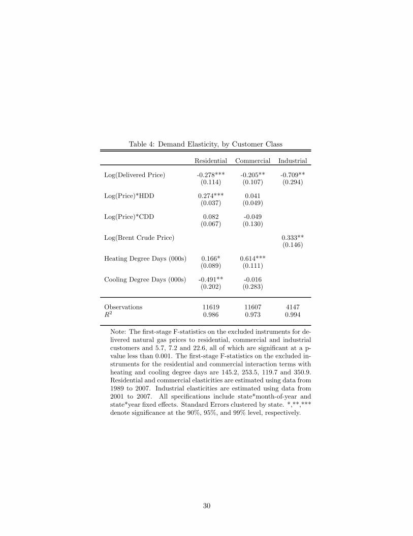
Table 4: Demand Elasticity, by Customer Class

Residential Commercial Industrial

Log(Delivered Price) -0.278*** -0.205** -0.709**(0.114) (0.107) (0.294)

Log(Price)*HDD 0.274*** 0.041(0.037) (0.049)

Log(Price)*CDD 0.082 -0.049(0.067) (0.130)

Log(Brent Crude Price) 0.333**(0.146)

Heating Degree Days (000s) 0.166* 0.614***(0.089) (0.111)

Cooling Degree Days (000s) -0.491** -0.016(0.202) (0.283)

Observations 11619 11607 4147R2 0.986 0.973 0.994

Note: The first-stage F-statistics on the excluded instruments for de-livered natural gas prices to residential, commercial and industrialcustomers and 5.7, 7.2 and 22.6, all of which are significant at a p-value less than 0.001. The first-stage F-statistics on the excluded in-struments for the residential and commercial interaction terms withheating and cooling degree days are 145.2, 253.5, 119.7 and 350.9.Residential and commercial elasticities are estimated using data from1989 to 2007. Industrial elasticities are estimated using data from2001 to 2007. All specifications include state*month-of-year andstate*year fixed effects. Standard Errors clustered by state. *,**,***denote significance at the 90%, 95%, and 99% level, respectively.

30

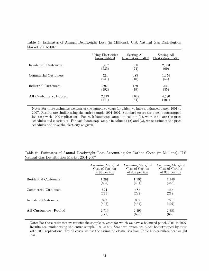
Table 5: Estimates of Annual Deadweight Loss (in Millions), U.S. Natural Gas DistributionMarket 2001-2007

Using Elasticities Setting All Setting AllFrom Table 4 Elasticities = -0.2 Elasticities = -0.5

Residential Customers 1,297 968 2,683(535) (24) (69)

Commercial Customers 524 485 1,354(241) (18) (54)

Industrial Customers 897 189 543(492) (19) (55)

All Customers, Pooled 2,719 1,642 4,580(771) (34) (101)

Note: For these estimates we restrict the sample to years for which we have a balanced panel, 2001 to2007. Results are similar using the entire sample 1991-2007. Standard errors are block bootstrappedby state with 1000 replications. For each bootstrap sample in column (1), we re-estimate the priceschedules and elasticities. For each bootstrap sample in columns (2) and (3), we re-estimate the priceschedules and take the elasticity as given.

Table 6: Estimates of Annual Deadweight Loss Accounting for Carbon Costs (in Millions), U.S.Natural Gas Distribution Market 2001-2007

Assuming Marginal Assuming Marginal Assuming MarginalCost of Carbon Cost of Carbon Cost of Carbonof $0 per ton of $35 per ton of $55 per ton

Residential Customers 1,297 1,197 1,146(535) (491) (468)

Commercial Customers 524 485 465(241) (222) (212)

Industrial Customers 897 809 770(492) (434) (407)

All Customers, Pooled 2,719 2,491 2,381(771) (696) (659)

Note: For these estimates we restrict the sample to years for which we have a balanced panel, 2001 to 2007.Results are similar using the entire sample 1991-2007. Standard errors are block bootstrapped by statewith 1000 replications. For all cases, we use the estimated elasticities from Table 4 to calculate deadweightloss.

31

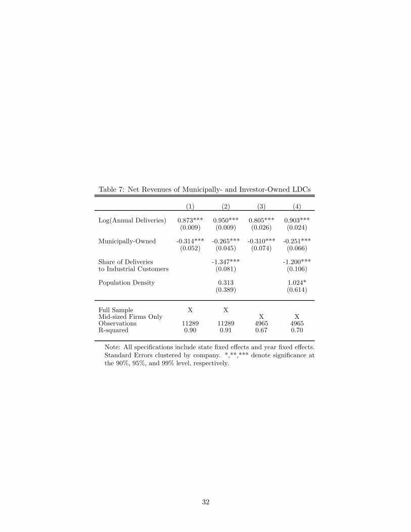
Table 7: Net Revenues of Municipally- and Investor-Owned LDCs

(1) (2) (3) (4)

Log(Annual Deliveries) 0.873*** 0.950*** 0.805*** 0.903***(0.009) (0.009) (0.026) (0.024)

Municipally-Owned -0.314*** -0.265*** -0.310*** -0.251***(0.052) (0.045) (0.074) (0.066)

Share of Deliveries -1.347*** -1.200***to Industrial Customers (0.081) (0.106)

Population Density 0.313 1.024*(0.389) (0.614)

Full Sample X XMid-sized Firms Only X XObservations 11289 11289 4965 4965R-squared 0.90 0.91 0.67 0.70

Note: All specifications include state fixed effects and year fixed effects.Standard Errors clustered by company. *,**,*** denote significance atthe 90%, 95%, and 99% level, respectively.

32