distributed resource allocation optimization for user-centric
TRANSCRIPT
arX
iv:2
110.
0815
4v1
[cs
.IT
] 1
5 O
ct 2
021
1
Distributed Resource Allocation Optimization for
User-Centric Cell-Free MIMO NetworksHussein A. Ammar∗, Student Member, IEEE, Raviraj Adve∗, Fellow, IEEE, Shahram Shahbazpanahi†∗, Senior
Member, IEEE, Gary Boudreau‡, Senior Member, IEEE, and Kothapalli Venkata Srinivas‡, Member, IEEE
Abstract—We develop two distributed downlink resource allo-cation algorithms for user-centric, cell-free, spatially-distributed,multiple-input multiple-output (MIMO) networks. In such net-works, each user is served by a subset of nearby transmitters thatwe call distributed units or DUs. The operation of the DUs in aregion is controlled by a central unit (CU). Our first scheme isimplemented at the DUs, while the second is implemented at theCUs controlling these DUs. We define a hybrid quality of servicemetric that enables distributed optimization of system resourcesin a proportional fair manner. Specifically, each of our algorithmsperforms user scheduling, beamforming, and power controlwhile accounting for channel estimation errors. Importantly, ouralgorithm does not require information exchange amongst DUs(CUs) for the DU-distributed (CU-distributed) system, while alsosmoothly converging. Our results show that our CU-distributedsystem provides 1.3- to 1.8-fold network throughput comparedto the DU-distributed system, with minor increases in complexityand front-haul load - and substantial gains over benchmarkschemes like local zero-forcing. We also analyze the trade-offsprovided by the CU-distributed system, hence highlighting thesignificance of deploying multiple CUs in user-centric cell-freenetworks.
Index Terms—Distributed resource allocation, user scheduling,user-centric clustering, cell-free MIMO, cooperative cellular net-works, distributed antenna system, scalable resource allocation,fairness.
I. INTRODUCTION
Scalability requires a system to accommodate growing de-
mands gracefully [1]. Scalability is critical motivation for user-
centric, cell-free, spatially-distributed, multiple-input multiple-
output (MIMO) networks [2], [3] , where users can be served
by many transmitters [4], [5], denoted herein as distributed
units (DUs). In these networks, a serving cluster of DUs is
defined for each user based on a metric, e.g., channel power [5]
or serving distance [6]; each user is effectively located at the
center of its serving cluster, thereby eliminating conventional
cell edges.
Designing flexible distributed resource allocation schemes
for cell-free networks is still an open issue [7] due to the
This work was supported in part by the Natural Sciences and EngineeringResearch Council (NSERC) of Canada and in part by Ericsson Canada.∗H. A. Ammar and R. Adve are with the Edward S. Rogers Sr. De-
partment of Electrical and Computer Engineering, University of Toronto,Toronto, ON M5S 3G4, Canada (e-mail: [email protected];[email protected]).†S. Shahbazpanahi is with the Department of Electrical, Computer, and
Software Engineering, University of Ontario Institute of Technology, Oshawa,ON L1H 7K4, Canada. He also holds a Status-Only position with the EdwardS. Rogers Sr. Department of Electrical and Computer Engineering, Universityof Toronto.‡G. Boudreau and K. V. Srinivas are with Ericsson Canada, Ottawa, ON
K2K 2V6, Canada.
difficulties arising from the lack of a regular cell structure and
the overlapping serving clusters for the users. Theoretically,
centralized resource allocation, wherein all transmissions are
jointly optimized, provides the performance upper bound.
However, such a scheme implies an enormous overhead in
terms of real-time exchange of channel state information (CSI)
and computation load. Furthermore, since the optimization
problems involved are usually non-convex, even effective
solutions may not lead to the global optimum.
A distributed system, on the other hand, provides a trade-
off between performance and scalability. Compared to a
centralized scheme, it provides an advantage due to lower
front-haul load as well as lower computational and stor-
age complexity per network node. Importantly, it allows for
lower communication overhead with limited exchange of CSI.
Hence, a distributed system is more practical to deploy than
a centralized one [8]. On the other hand, such an approach
may provide worse performance than a centralized scheme [9],
because the resource allocation is performed without a global
view of the network and with limited coordination.
A major challenge in designing a distributed resource
allocation scheme is that the crucial signal-to-interference-
plus-noise ratio (SINR) metric is coupled between all the
transmitters. Hence, SINR-based approaches, like in [10], [11],
are not suitable for distributed resource allocation. One alter-
native is to use metrics like the signal-to-leakage-plus-noise
ratio (SLNR) [12] which decouples the allocation problem
between the different transmitters. However, SLNR does not
allow for effective power allocation because the beam power
scales equally in both the signal and leakage terms. Here, we
modify the approach proposed for cellular networks [13] based
on a mix of of inter-cell leakage and intra-cell interference.
Specifically, for the cell-free MIMO network at hand, the com-
binatorial approach to user scheduling in [13] is not possible.
Additionally, unlike most works in distributed processing, we
include fairness as a key criterion for user-scheduling, thereby
avoiding repeatedly serving the same users with strongest
channels.
The available efforts to implement a distributed resource
allocation scheme in cell-free networks have been based on
algorithms that require iterative exchange of signals between
the base stations [14]. The investigation in [15] studies a
distributed framework for cooperative precoding in cell-free
MIMO requiring over-the-air signaling between the base sta-
tions instead of front-haul\back-haul signaling. Similarly, the
work in [16] maximizes the weighted sum rate (WSR) within
joint transmission clusters without centralized beamformer
2
processing. However, the problem is solved through an equiva-
lent minimum square error-based problem that requires a feed-
back channel to update weights during algorithm iterations.
The authors in [17] maximize the uplink minimum SINR
by decoupling the problem into two sub-problems, one that
designs the receiver filter and another that optimizes the power
allocation, using an alternating optimization. The study in [18]
propose two distributed variants of zero-forcing (ZF); however,
this work does not consider user scheduling. The authors
of [19] optimize the energy efficiency in the uplink of cell-
free massive MIMO networks under different scenarios of
signal quantization. The investigations in [2] and [20] study a
suboptimal but scalable power control policy that uses large-
scale fading decoding. Moreover, the study in [21] uses dual
decomposition and the gradient method for resource alloca-
tion in a relaying system by relaxing the binary scheduling
variables. Furthermore, the work in [8] analyzes the uplink
spectral efficiencies under four different levels of cooperation
in cell-free implementations. However, this work does not
optimize resource allocation, but rather numerically studies
the performance under minimum mean-square error (MMSE)
combining.
Distributed resource allocation can also be tackled through
a game-theoretic framework. The studies in [22], [23] use
a distributed form of auction theory for user scheduling in
conventional networks. Briefly, the users compete for the
resources through bidding and assignment phases [24]. One
disadvantage of such approaches is the considerable com-
munications required between the network nodes before an
allocation occurs, hence leading to a substantial overhead.
Furthermore, these have been developed for simple schemes
like carrier sense multiple access.
The DUs that connect to users are, themselves, controlled
by central units (CUs). While some models use a single CU to
control all DUs [9], [20], this would limit the scalability of the
network. As in [18], we consider a system of multiple central
units (CUs), each controlling the DUs in its region. Under
the user-centric cell-free MIMO scheme at hand, a serving
cluster of DUs is defined specifically for each user. In contrast
to the schemes available in the literature, we develop two
totally distributed resource allocation schemes that perform
user scheduling, beamforming, and implicit power control in a
user-centric MIMO network. The first solution is implemented
on the DUs, while the second one is deployed on the CUs1. We
acquire local CSI between each DU and its users, an approach
shown to be scalable [26]. We then define a weighted pseudo-
rate function that depends on a hybrid leakage and intra-
(DU\CU) interference; the weights implement user fairness.
Our objective decouples the problem between the different
network nodes, with each node making decisions independent
of the other nodes in the network.
To solve our formulated problem, we employ tools such
as block coordinate descent, fractional programming, and
1Although this study is not concerned with the core-network protocols thatshould be used to deploy a distributed CU system under the user-centric cell-free network architecture, the authors note that distributed software definednetwork (SDN) [25] is a promising avenue to implement the flexible networkarchitecture suggested in this paper.
compressive sensing to develop an algorithm that converges
smoothly in a non-decreasing manner. In addition to standard
CSI estimation, we further propose using either statistical
CSI or the spatial traffic distribution to compute the leakage
needed to construct our objective function. These alternative
approaches further reduce any required information exchange
amongst processing nodes. Notably, our results show that the
proposed methods to compute the leakage are very effective
with a dense distribution of users.
To the best of the authors’ knowledge, this work is one
of the first studies to consider fully distributed resource
allocation, and is the first study which investigates fully
distributed user-scheduling and beamforming (not only power
control) for user-centric cell-free MIMO networks. In most
of the literature, user scheduling is neglected and the users
are assumed pre-selected. Hence, our work fills two gaps
by focusing on distributed schemes and on user scheduling.
Our scheme is different from the literature, e.g., [15], in
the sense that it conducts resource allocation without using
feedback channels between the network entities. Additionally,
to maintain scalability, we use a network with distributed
CUs [9], [20].
A few works in the literature focus on scalability. The
study in [9] proposes a simple sub-optimal power allocation
using conjugate beamforming (to be able to perform a dis-
tributed beamforming), but this study does not optimize user
scheduling or beamforming. In [2] the authors study the uplink
of a single-CU network, using large-scale fading decoding
and power control; however, the scheme is not distributed.
The authors of [27] employ a combinatorial search for user-
association based on the position of the access points. The
system uses conjugate beamforming and maximizes the sum
rate, however, this scheme is also not distributed. The scheme
sacrifices performance to enable a low fronthaul load. Thus,
our developed schemes are fundamentally different from those
found in literature.
The theory developed here sets the foundation for deploy-
ment of an optimized resource allocation scheme. Specifically,
the contributions of our paper are:
• Developing two distributed resource allocation schemes
that optimize resources, including user scheduling and
beamforming (not only power allocation) in a cell-free,
user-centric, MIMO network. These schemes are based
on a hybrid leakage and interference metric that elimi-
nates the need for information exchange and implements
fairness amongst users.
• Proposing and testing three approaches to calculate the
leakage term in the metric. These approaches require
different levels of computational complexity and required
real-time information while producing comparable perfor-
mance, especially at high user densities.
• Analyzing the computation complexity of our two pro-
posed approaches, illustrating the substantial reduction in
complexity compared to a centralized resource allocation
scheme, with, in some cases, improved performance.
• Highlighting the importance of a multiple-CU user-
centric cell-free network by illustrating trade-offs in
performance and front-haul load provided by the CU-
3
distributed system compared to DU-distributed and cen-
tralized systems.
The rest of the paper is organized as follows. Section II
presents the system model. Section III formulates the resource
allocation problem in a DU-distributed system and develops
the steps required to solve this problem. Section IV casts the
problem as a CU-distributed system and develops an approach
to perform the resource allocation. Section V proposes further
methods to enhance the scalability of calculating the leakage
term. Section VI reports on our numerical results and findings.
Finally, Section VII concludes our discussion.
Notation: a lower or upper case letter, e.g., a or A, repre-
sents a scalar, a bold lower case letter, e.g., a, represents a
vector, while a bold upper case letter, e.g., A, represents a
matrix. The term [A]ij is the (i, j)th entry of matrix A. The
operators (·)−1, (·)T and (·)H , used as superscripts, denote the
inverse, transpose, and conjugate transpose, respectively. ‖ ·‖2and | · | are the vector and scalar Euclidean norms (ℓ2 norm),
‖ · ‖p is the ℓp norm, and Im is the m-dimensional identity
matrix. Calligraphic letters, e.g., A, are used to indicate sets
with its cardinality represented by |A|. We use A = [A] to
construct a matrix or vector using the elements of set A.
The spaces B, Cm, and Cm×n represent the set of binary
numbers, complex m×1 column vectors, and complex m×nmatrices, respectively. E· is the expectation operator, and
x ∼ CN (m,R) indicates that x is a complex Gaussian
random vector with mean m and covariance R.
II. SYSTEM MODEL
A. Network and Signal Model
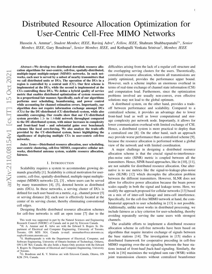
We consider a user-centric cell-free MIMO network, which
operates in time-division duplex (TDD) mode. Our network,
illustrated in Fig. 1, comprises Q CUs, each controlling
N DUs represented by the set Bq. We denote the region
containing the DUs in Bq as a virtual cell. Accordingly,
we have a total of NQ DUs represented by the set of sets
B = B1, B2, . . . ,BQ. Each DU is equipped with Mantennas, while each user is equipped with a single antenna.
We use U to represent the set of users that need to be
served, where |U| is a random number, but is much larger
than the number of available resources. The DUs serve users
coherently2.
Based on this model, for each user u, we define a serving
cluster Cu comprising the DUs that can potentially serve the
user. Specifically, here we define Cu based on the criterion
ψruβ(dru) ≥ ρ : r ∈ B, where the term ψru accounts for
the (lognormal) shadowing, β(dru) accounts for the path loss,
which depends on the distance dru between DU r and user
u. If no DU can meet this connection criterion, Cu comprises
the DU providing the highest average received power, i.e.,
largest ψruβ(dru). Based on this scheme, we can formally
2Coherent transmission requires phase synchronization across the DUs,which can be achieved through synchronization protocols like the IEEE1588v2 (Precision Time Protocol PTP) [28]. The system can achieve thissynchronization by properly choosing the serving clusters and the use of acyclic prefix [6]. We note that synchronization issues are out of the scope ofthis paper; they need to be studied in a dedicated work using different toolsfrom those used in this paper.
DU
User
Servingcluster
CU
Fronthaul
Backhaul
Network core
Fig. 1: User-centric cell-free network with either DU-
distributed or CU-distributed processing.
define Cu = r : ψruβ(dru) ≥ ρ ∪ arg maxr ψruβ(dru).
The set Cu, therefore excludes DUs that cannot contribute
significantly to the user’s useful signal while also limiting the
number of users each DU serves. We assume a low-mobility
profile for the users and hence we use the popular block
fading model for the channel. Hence, the channel (small-scale
and large-scale fading) is assumed static within each channel
coherence interval. The large-scale fading also changes much
more slowly than the small-scale fading, and hence stays
constant for many coherence intervals. The block fading model
is widely accepted and used in the literature when high-
mobility scenarios are not being studied [4] as the case of
this paper.
We develop two different distributed algorithms for resource
allocation. The first variant runs on the DUs, while the second
variant runs on the CUs. The developed algorithms pro-
vide user scheduling and perform resource allocation. These
procedures include channel estimation, formation of serving
clusters, user scheduling, beamforming, and fairness control
for the users. Finally, it is worth noting that we will be using
the global indices q, r, and u to, respectively, refer to the CUs,
DUs and users found in the network.
In the downlink, the signal received by user u ∈ U can be
written as
yu =∑
r∈Cu
√sruh
Hruwruxu
+∑
u′∈U ,u′ 6=u
∑
r′∈Cu′
√sr′u′hH
r′uwr′u′xu′ + zu. (1)
The first term in (1) is the useful signal, the second term is
the interference, and the third is the additive white Gaussian
noise (AWGN) zu ∼ CN (0, σ2z). The scalar sru ∈ B is the
scheduling decision at DU r for user u (that is, when sru = 1,
DU r schedules user u, otherwise sru = 0), hru ∈ CM×1
is the channel vector between the two peers, wru is the
beamforming weight or the transmit precoder used by DU rto serve the user with an overall power budget of p for the
DU, and xu is the zero-mean data symbol intended for user
u with E|xu|2 = 1.
We model the channel between DU r and user u as hru =√ψruβ(dru)gru ∈ CM×1, where the term gru ∼ CN (0, IM )
accounts for the small-scale fading, and as noted earlier, ψru
4
and β(dru) account for lognormal shadowing and path loss,
respectively. We define the set Er representing the users that
need to be served by DU r. These sets Er : r ∈ B can
obtained directly from the sets Cu : u ∈ U. Crucially,
because of user-centric clustering, each Er can partially or
totally overlap with other Er′ , for r′ 6= r; similarly, the same
user may “belong” to multiple CUs.
B. Channel Estimation
For a TDD system, channel estimation is performed in the
uplink and the estimated channel is used in downlink assuming
channel reciprocity. In the pilot-training phase of length τp, the
signal Yr ∈ CM×τp observed at DU r can be written as
Yr =∑
u∈U
√puhruφu + Zr, (2)
where φu ∈ C1×τp is the unit norm (φuφHu = 1) pilot
sequence used by user u, pu is the transmit power, and Zr
is the noise with entries distributed as CN(0, σ2
Z
). Following
the assumptions in [4], [5], we assume the knowledge of the
the large-scale fading and the transmit power used.
Unfortunately, using pilots that are orthogonal among the
users, i.e., φuφHu′ = 0, ∀u′ 6= u, requires having τp ≥ |U|
which is unlikely to be feasible. We assume that the users
are grouped such that the pilot sequences inside each group
are orthogonal, while the same pilot sequences are used
across groups. Specifically, as in [29], we use the hierarchical
agglomerative clustering (HAC) algorithm to cluster the users
into subsets each containing a number of users less than or
equal to τp, the length of the pilot sequence. The available
orthogonal pilot sequences are randomly assigned to the users
inside each subset. The intuition is to keep users sharing the
same pilot sequence as far as possible from each other, thus
minimizing pilot contamination in our user-centric cell-free
network [30]. Additionally, the choice of HAC is based on
its consistency and its lack of sensitivity to the choice of the
distance-metric used to construct the subsets [31].
We can extract the channel of user u at DU r by first
defining yru = 1√puYrφ
Hu , hence eliminating all users’
contributions other than the ones using the same pilot sequence
φu. The channel hru : u ∈ U can then be estimated using
linear MMSE as [32]
hru = Dru
(∑
u′∈Uu
Dru′ +σ2Z
puIM
)−1
yru, (3)
where Dru ∈ CM×M is a diagonal matrix with entries
[Dru]mm , ψruβ(dru), and Uu are the users using the same
pilot sequence as user u (including user u).
Remark 1. Due to path loss, each DU r only needs to estimate
the channel vectors of nearby users. In Section V, we show
that each DU need only estimate the channels to users u ∈ Er,
i.e., its own users and it can use large-scale fading statistics or
a traffic distribution model for the other users, thus enhancing
the scalability of the required channel estimation.
The estimated channel hru is distributed according to
CN (0,Ψru), with Ψru defined as
Ψru , Dru
(∑
u′∈Uu
Dru′ +σ2Z
puIM
)−1
Dru. (4)
It is known from the theory of MMSE estimation that the
channel estimation error eru = hru − hru is distributed as
CN (0,Θru), where Θru , Dru −Ψru [32].
Based on this, the model for the signal received at user ucan be written as
yu =∑
r∈Cu
√sruh
Hruwruxu +
∑
r∈Cu
√srue
Hruwruxu
+∑
u′∈U ,u′ 6=u
∑
r′∈Cu′
√sr′u′ hH
r′uwr′u′xu′
+∑
u′∈U ,u′ 6=u
∑
r′∈Cu′
√sr′u′eHr′uwr′u′xu′ + zu. (5)
Including the random estimation error, eru, in (5) allows
us to implement robust beamforming that exploits the error
covariance matrix Θru and hence compensate for some of the
error.
We now define hybrid expressions that account for both
the leakage and intra-(DU\CU) interference. For distributed
implementation, these expressions use locally constructed
beamformers.
III. DU-DISTRIBUTED SYSTEM
A. Hybrid Leakage-Interference
Let U−r = U\Er, represent the set of users that do not
belong to Er, i.e., U−r = u | u /∈ Er. We define an
expression for the average power (leakage) experienced by
the users U−r from DU r by serving user u. Averaged over
the random channel estimation error this power is given by
Lru (wru)
= Ee
∑
u′∈U−r
tr,u′
∣∣∣hHru′wru
∣∣∣2
+∑
u′∈U−r
tr,u′
∣∣eHru′wru
∣∣2
=∑
u′∈U−r
tr,u′
∣∣∣hHru′wru
∣∣∣2
+∑
u′∈U−r
tr,u′wHruΘru′wru. (6)
The vector hru′ for u′ ∈ U−r is the estimated leakage channel
between DU r and user u′ ∈ U−r. The term tr,u′ ∈ B is
defined at DU r and represents the assumption about user
u′ ∈ U−r being scheduled by at least one of its serving DUs
r′ ∈ Cu′ .
We also define our optimization variables as the ma-
trix Wr = [wru : u ∈ Er] ∈ CM×|Er|, and sr =[sru : u ∈ Er]T ∈ B|Er|×1 the beamformers and scheduling
variables used by DU r. For each pair of DU r and user
u, we now define a hybrid signal-to-leakage-and-intra-DU-
interference-and-noise ratio (SLINR-D) as
ξru ,sruw
Hruhruh
Hruwru
Aru (sr,Wr), (7)
where Aru (sr,Wr), used to simplify the notation, is the
5
leakage plus intra-DU interference and noise averaged over
the unknown random channel estimation error, and it is defined
in (8).
In (7) we treat channel estimation error eru as additional
noise with covariance Θru as defined earlier. The first term
in (8) is the power leakage to the users not served by DU
r, the second is the self-interference resulting from imperfect
CSI of the serving channel, the third and fourth terms are the
intra-DU interference experienced by user u, and the final term
is the noise power.
Remark 2. It is worth commenting on the role of self-
interference in (8). Previous works based on leakage, do
not mix in interference. However, from (7) and (8), using
purely leakage means that the beam power (||wru||2) would
effectively cancel out in all but the noise term. This effectively
takes away the role of power allocations, to the detriment of
performance [13].
Remark 3. Even for a user served by a cluster of DUs, we
can still define an SLINR-D for each DU-user pair. Also, (7)
is still indirectly coupled across the scheduling decisions
of the other DUs through the terms tr,u′ : u′ ∈ U−r.
In centralized resource allocation, the scheduling of users
is performed by a single entity, hence we can simply set
tr,u = min(1,∑
r′∈Cusr′u
). However, in a DU-distributed
system, a DU cannot know which users are scheduled by
the other DUs, complicating the development of a distributed
scheduling algorithm. In Section V, we address this issue by
introducing different methods to calculate the leakage.
Based on (7), we define a weighted pseudo-rate between
each DU r and its user u ∈ Er as
WPSru , δu log (1 + ξru) . (9)
As the name suggests, the weighted pseudo-rate employs the
SLINR-D metric in a rate-like function while providing for
fairness. We will optimize this pseudo-rate. Here, δu is a term
that accounts for the proportional fairness of user u. At time
slot i+1, these weights are the inverse of the long-term expo-
nentially averaged achieved data rate, i.e., δ(i+1)u = 1
R(i)u
[33],
where R(i)u = ηR
(i)u +(1−η)R(i−1)
u is the user’s exponentially
weighted rate averaged over the previous time slots. Here,
0 < η < 1 acts as a forgetting factor, and R(i)u is the data
rate at time slot i.
The motivation to optimize the weighted pseudo-rate is, in
fact, two-fold. First, by only using local variables, it allows
for the development of a DU-distributed system. Second, it
acknowledges that maximizing the useful signal while min-
imizing the leakage and intra-DU interference is a prudent
practice. Although the SLINR lacks an operational meaning
(from an engineering viewpoint) still it can be interpreted as
a proxy to enhance the performance [12]. Specifically, when
a DU r minimizes the leaked interference to users U−r, it
minimizes the interference terms experienced by these users,
and hence it enhances the SINR for these users. The same
applies for the intra-DU interference experienced by users Er.
The mix between the leakage and the intra-DU interference
instead of using the leakage only prevents the power of the
beam of the DU from scaling equally in both the signal and
leakage terms when it is being optimized. In our numerical
results, we compare our approach to an SINR-based approach
which, unfortunately, requires centralized deployment, and we
show that our approach is effective.
B. Problem Definition
For each DU r, we define the following optimization
problem:
(P1)(r) maxWr,sr
∑
u∈Er
δu log (1 + ξru) (10a)
s.t.∑
u∈Er
sru ≤M (10b)
∑
u∈Er
||wru||22 ≤ p (10c)
ξru =sruw
Hruhruh
Hruwru
Aru (sr,Wr), u ∈ Er
(10d)
sru ∈ 0, 1, u ∈ Er.(10e)
The term Aru (sr,Wr) is defined in (8). We note that, in
(10d), tr,u′ : u′ ∈ U−r are not decision variables, but
rather they represent the assumptions of DU r about the
scheduled users served by other DUs. When this knowledge is
not available by any means, tr,u′ : u′ ∈ U−r are simply set
to 1. In Section V, we evaluate alternative methods to handle
this important issue.
The aim in (10) is to optimize, at DU r, the decision
variables sr and Wr, respectively the user scheduling and
beamforming vectors. The constraint in (10b) restricts the
number of users served by DU r to the number of antennas
M , (10c) specifies the power budget of DU r, (10d) treats the
SLINR-D expression as an auxiliary variable, and (10e) shows
that a user may be either scheduled or not. It is well established
that problems having the form of (10) are NP-hard [34], thus
obtaining the global optimum is computationally prohibitive,
and only a local optimum can be obtained. The problem is
mixed-integer and non-convex due to the binary variables and
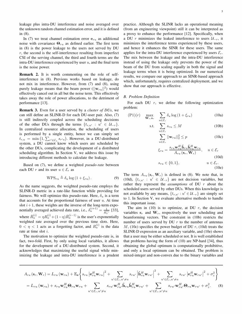
Aru (sr,Wr) = Lru (wru) + Ee
sru∣∣eHruwru
∣∣2 +∑
u′∈Er,u′ 6=u
sru′
∣∣∣hHruwru′
∣∣∣2
+∑
u′∈Er,u′ 6=u
sru′
∣∣eHruwru′
∣∣2 + σ2z
= Lru (wru) + sruwHruΘruwru +
∑
u′∈Er,u′ 6=u
sru′wHru′hruh
Hruwru′ +
∑
u′∈Er,u′ 6=u
sru′wHru′Θruwru′ + σ2
z . (8)
6
their presence in both the numerator and denominator of the
utility function.
Using fractional programming, the problem in (10) can be
reformulated and written as
(P2)(r) maxWr,sr,ξr,ζr
f2 (sr,Wr, ξr, ζr) (11a)
s.t.∑
u∈Er
sru ≤M (11b)
∑
u∈Er
||wru||22 ≤ p (11c)
sru ∈ 0, 1, u ∈ Er. (11d)
with the function f2 (sr,Wr, ξr, ζr) found in (11a) is de-
fined as
f2 (sr,Wr, ξr, ζr) =∑
u∈Er
δu (log (1 + ξru)− ξru)
+∑
u∈Er
(2Re
ζ∗ru√δu (1 + ξru)sruw
Hruhru
− |ζru|2(sruw
Hruhruh
Hruwru +Aru (sr,Wr)
)). (12)
where ζr ∈ C|Er|×1 is a new auxiliary variable vector
introduced by fractional programming [10]. Fractional pro-
gramming refers to optimizing functions composed of ratios.
The function can be composed of a single ratio, or, as in
our case, a sum of ratios. The numerator and denominator
can be nonlinear. Techniques used to obtain local optimum
for such optimization problems include the Charnes-Cooper
method [35], Dinkelbach’s method [36], and quadratic trans-
form [10].
The reformulation in (11) is based on the Lagrangian formu-
lation and fractional programming. Please refer to Appendix A
for details.
In what follows, we obtain optimal expressions for the
optimization variables, one set of variables at a time, i.e.,
we use block coordinate descent. As for the scheduling vari-
ables sr, we optimize them using a combinatorial search as
described below.
When the variables other than ζru are fixed, the first
optimality condition of (12) with respect to ζru results in the
optimal value as
ζru =sru√δu (1 + ξru)w
Hruhru
sruwHruhruhH
ruwru +Aru (sr,Wr). (13)
We write the Lagrangian formulation of (11), and when vari-
ables (sr, ξr, ζr) are fixed, we derive the optimality condition
to obtain the optimal expression for the transmit precoder wru
as shown in (14).
The variable µr denotes the Lagrange multiplier for the
power budget constraint (11c), and is inversely related to the
beamformers’ power at DU r; µr can be determined through
the complementary slackness condition for the power budget.
Specifically, let wru(µr) denote the right-hand side of (14).
If∑
u∈Er‖wru(0)‖22 ≤ p, then µr = 0, otherwise the value
of µr can be determined through a bisection search to satisfy∑u∈Er
‖wru(µr)‖22 = p.
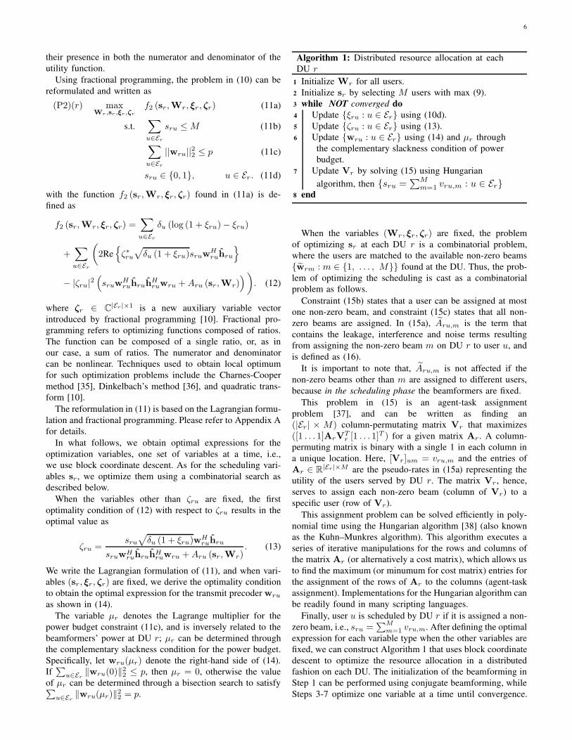
Algorithm 1: Distributed resource allocation at each
DU r
1 Initialize Wr for all users.
2 Initialize sr by selecting M users with max (9).
3 while NOT converged do
4 Update ξru : u ∈ Er using (10d).
5 Update ζru : u ∈ Er using (13).
6 Update wru : u ∈ Er using (14) and µr through
the complementary slackness condition of power
budget.
7 Update Vr by solving (15) using Hungarian
algorithm, then sru =∑M
m=1 vru,m : u ∈ Er8 end
When the variables (Wr, ξr, ζr) are fixed, the problem
of optimizing sr at each DU r is a combinatorial problem,
where the users are matched to the available non-zero beams
wrm : m ∈ 1, . . . , M found at the DU. Thus, the prob-
lem of optimizing the scheduling is cast as a combinatorial
problem as follows.
Constraint (15b) states that a user can be assigned at most
one non-zero beam, and constraint (15c) states that all non-
zero beams are assigned. In (15a), Aru,m is the term that
contains the leakage, interference and noise terms resulting
from assigning the non-zero beam m on DU r to user u, and
is defined as (16).
It is important to note that, Aru,m is not affected if the
non-zero beams other than m are assigned to different users,
because in the scheduling phase the beamformers are fixed.
This problem in (15) is an agent-task assignment
problem [37], and can be written as finding an
(|Er| × M) column-permutating matrix Vr that maximizes
([1 . . . 1]ArVTr [1 . . . 1]
T ) for a given matrix Ar. A column-
permuting matrix is binary with a single 1 in each column in
a unique location. Here, [Vr]um = vru,m and the entries of
Ar ∈ R|Er|×M are the pseudo-rates in (15a) representing the
utility of the users served by DU r. The matrix Vr, hence,
serves to assign each non-zero beam (column of Vr) to a
specific user (row of Vr).
This assignment problem can be solved efficiently in poly-
nomial time using the Hungarian algorithm [38] (also known
as the Kuhn–Munkres algorithm). This algorithm executes a
series of iterative manipulations for the rows and columns of
the matrix Ar (or alternatively a cost matrix), which allows us
to find the maximum (or minumum for cost matrix) entries for
the assignment of the rows of Ar to the columns (agent-task
assignment). Implementations for the Hungarian algorithm can
be readily found in many scripting languages.
Finally, user u is scheduled by DU r if it is assigned a non-
zero beam, i.e., sru =∑M
m=1 vru,m. After defining the optimal
expression for each variable type when the other variables are
fixed, we can construct Algorithm 1 that uses block coordinate
descent to optimize the resource allocation in a distributed
fashion on each DU. The initialization of the beamforming in
Step 1 can be performed using conjugate beamforming, while
Steps 3-7 optimize one variable at a time until convergence.
7
We will analyze convergence in our section on numerical
results.
IV. CU-DISTRIBUTED SYSTEM
The previous section designed an algorithm that allows
each DU to perform its own allocation decisions. However,
if a CU can coordinate the DUs under its control, we can
include the intra-CU interference, i.e., inside the virtual cell
of each CU. A CU-distributed algorithm would, therefore,
provide a balance between some coordination (and information
exchange) and the completely centralized case where all CUs
are jointly optimized. Additionally, the CU would decide
on user scheduling for all the DUs under its control. We
emphasize, however, that a user may be associated with DUs
under the control of different CUs (user-centric clustering).
A user may, therefore, be scheduled by one CU, but not
by the other. For each CU q, we define the set of users
Uq , ∪r′∈Bq
Er′ that includes all the users connected to at
least one DU under the control of CU q. Due to user-centric
clustering, the different sets UqQq=1 overlap.
For each user u ∈ Uq and DUs Dqu = (Cu ∩ Bq), we
define the concatenation of beamformers, estimated channels,
channel estimation error and scheduling variables as
wqu =[wT
ru : r ∈ Dqu
]T ∈ CM|Dqu|×1 (17)
hqu,u′ =[
hTru′ : r ∈ Dqu
]T∈ C
M|Dqu|×1 (18)
equ,u′ =[eTru′ : r ∈ Dqu
]T ∈ CM|Dqu|×1 (19)
Squ = (diag (sru : r ∈ Dqu)⊗ IM ) ∈ BM|Dqu|×M|Dqu|
(20)
We note that (18) and (19) represent the estimated channel and
estimation error, respectively, between user u′ and the serving
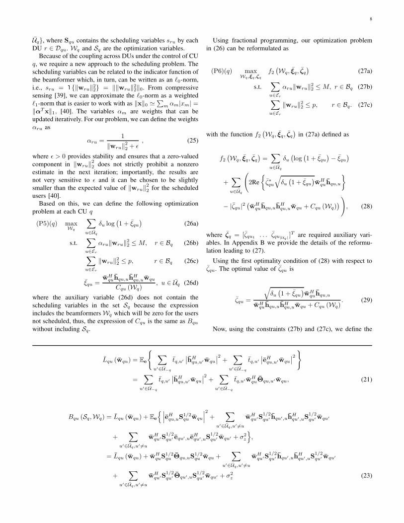
DUs Dqu for user u. As in the previous section, we define an
expression for the power leakage experienced by the users in
U−q = U\Uq from all the DUs due to serving user u. Averaged
over the random channel estimation error this leakage is given
by (21), where the term Eequ,u′ eHqu,u′
= Θqu,u′ in (21)
represents the covariance of the channels’ estimation error
obtained from treating the unknown random Gaussian error
as additional noise.
As before, we define the hybrid signal-to-leakage-and-intra-
CU-interference-and-noise-ratio (SLINR-C) between each CU
q and user u ∈ Uq as
ξqu ,wH
quS1/2qu hqu,uh
Hqu,uS
1/2qu wqu
Bqu (Sq,Wq), (22)
where the leakage plus intra-CU interference and noise, av-
eraged over the random estimation error, is defined as (23).
Here in (23), Squ is defined in (20) with diagonal entries
sru ∈ B denoting the scheduling variable of user u at DU r,and tq,u ∈ B is defined at CU q to represent the assumption
for user u being scheduled by at least one of its serving DUs
r′ /∈ Bq not under the control of CU q.
Similar to the previous section, for each CU q we can opti-
mize the pseudo-rates as (24). The set Wq = Wr : r ∈ Bqin (24) represents the matrix of beamformers used by the
DUs Bq , where, as noted earlier, Wr = [wru : u ∈ Er] ∈CM×|Er| are the beamformers used by each DU r to serve its
users. Similarly, the scheduling variables Sq = Squ : u ∈
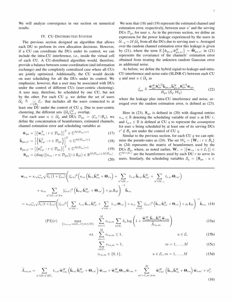
wru = sruζ∗ru
√δu (1 + ξru)
(|ζru|2
(sru
(hruh
Hru +Θru
)+
∑
u′∈U−r
tr,u′hru′ hHru′ +
∑
u′∈U−r
tr,u′Θru′
)
+ sru∑
u′∈Er,u′ 6=u
|ζru′ |2(hru′hH
ru′ +Θru′
)+ µrIM
)−1
hru
= sruζ∗ru
√δu (1 + ξru)
(|ζru|2
( ∑
u′∈U−r
tr,u′ hru′hHru′ +
∑
u′∈U−r
tr,u′Θru′
)+ sru
∑
u′∈Er
|ζru′ |2(hru′hH
ru′ +Θru′
)+ µrIM
)−1
hru, (14)
(P3)(r) maxvru,m:u∈Er,1≤m≤M
M∑
m=1
vru,m∑
u∈Er
δu log
(1 +
wHrmhruh
Hruwrm
Aru,m
)(15a)
s.t.
M∑
m=1
vru,m ≤ 1, u ∈ Er (15b)
∑
u∈Er
vru,m = 1, m = 1, . . . ,M (15c)
vru,m ∈ 0, 1, u ∈ Er,m = 1, . . . ,M (15d)
Aru,m =∑
u′∈U ,u′ /∈Er
tr,u′wHrm
(hru′ hH
ru′ +Θru′
)wrm + wH
rmΘruwrm +M∑
m′=1,m′ 6=m
wHrm′
(hruh
Hru +Θru
)wrm′ + σ2
z .
(16)
8
Uq, where Squ contains the scheduling variables sru by each
DU r ∈ Dqu. Wq and Sq are the optimization variables.
Because of the coupling across DUs under the control of CU
q, we require a new approach to the scheduling problem. The
scheduling variables can be related to the indicator function of
the beamformer which, in turn, can be written as an ℓ0-norm,
i.e., sru = 1‖wru‖22 = ‖‖wru‖22‖0. From compressive
sensing [39], we can approximate the ℓ0-norm as a weighted
ℓ1-norm that is easier to work with as ‖x‖0 ≃∑m αm|xm| =‖αTx‖1, [40]. The variables αm are weights that can be
updated iteratively. For our problem, we can define the weights
αru as
αru =1
‖wru‖22 + ǫ, (25)
where ǫ > 0 provides stability and ensures that a zero-valued
component in ‖wru‖22 does not strictly prohibit a nonzero
estimate in the next iteration; importantly, the results are
not very sensitive to ǫ and it can be chosen to be slightly
smaller than the expected value of ‖wru‖22 for the scheduled
users [40].
Based on this, we can define the following optimization
problem at each CU q
(P5)(q) maxWq
∑
u∈Uq
δu log(1 + ξqu
)(26a)
s.t.∑
u∈Er
αru‖wru‖22 ≤M, r ∈ Bq (26b)
∑
u∈Er
‖wru‖22 ≤ p, r ∈ Bq (26c)
ξqu =wH
quhqu,uhHqu,uwqu
Cqu (Wq), u ∈ Uq (26d)
where the auxiliary variable (26d) does not contain the
scheduling variables in the set Sq because the expression
includes the beamformers Wq which will be zero for the users
not scheduled, thus, the expression of Cqu is the same as Bqu
without including Sq.
Using fractional programming, our optimization problem
in (26) can be reformulated as
(P6)(q) maxWq,ξq,ζq
f2(Wq, ξq, ζq
)(27a)
s.t.∑
u∈Er
αru‖wru‖22 ≤M, r ∈ Bq (27b)
∑
u∈Er
‖wru‖22 ≤ p, r ∈ Bq. (27c)
with the function f2(Wq, ξq, ζq
)in (27a) defined as
f2(Wq, ξq, ζq
)=∑
u∈Uq
δu(log(1 + ξqu
)− ξqu
)
+∑
u∈Uq
(2Re
ζ∗qu
√δu(1 + ξqu
)wH
quhqu,u
− |ζqu|2(wH
quhqu,uhHqu,uwqu + Cqu (Wq)
)), (28)
where ζq = [ζqu1 . . . ζqu|Uq |]T are required auxiliary vari-
ables. In Appendix B we provide the details of the reformu-
lation leading to (27).
Using the first optimality condition of (28) with respect to
ζqu. The optimal value of ζqu is
ζqu =
√δu(1 + ξqu
)wH
quhqu,u
wHquhqu,uhH
qu,uwqu + Cqu (Wq). (29)
Now, using the constraints (27b) and (27c), we define the
Lqu (wqu) = Ee
∑
u′∈U−q
tq,u′
∣∣hHqu,u′wqu
∣∣2 +∑
u′∈U−q
tq,u′
∣∣eHqu,u′wqu
∣∣2
=∑
u′∈U−q
tq,u′
∣∣hHqu,u′wqu
∣∣2 +∑
u′∈U−q
tq,u′wHquΘqu,u′wqu, (21)
Bqu (Sq,Wq) = Lqu (wqu) + Ee
∣∣∣eHqu,uS1/2qu wqu
∣∣∣2
+∑
u′∈Uq,u′ 6=u
wHqu′S
1/2qu′ hqu′,uh
Hqu′,uS
1/2qu′ wqu′
+∑
u′∈Uq,u′ 6=u
wHqu′S
1/2qu′ equ′,ue
Hqu′,uS
1/2qu′ wqu′ + σ2
z
,
= Lqu (wqu) + wHquS
1/2qu Θqu,uS
1/2qu wqu +
∑
u′∈Uq,u′ 6=u
wHqu′S
1/2qu′ hqu′,uh
Hqu′,uS
1/2qu′ wqu′
+∑
u′∈Uq,u′ 6=u
wHqu′S
1/2qu′ Θqu′,uS
1/2qu′ wqu′ + σ2
z (23)
9
following Lagrangian function
f3(Wq,µq,λq) = −∑
r∈Bq
λr
(∑
u∈Er
αru‖wru‖22 −M
)
−∑
r∈Bq
µr
(∑
u∈Er
‖wru‖22 − p
)
(a)= −
∑
u∈Uq
∑
r∈Dqu
λrαru‖wru‖22 +M∑
r∈Bq
λr
−∑
u∈Uq
∑
r∈Dqu
µr‖wru‖22 + p∑
r∈Bq
µr
= −∑
u∈Uq
∑
r∈Dqu
ωru‖wru‖22 +∑
r∈Bq
(pµr +Mλr) , (30)
where ωru = µr + λrαru, and (a) follows from∑r∈Bq
∑u∈Er
(·) =∑u∈Uq
∑r∈Dqu
(·).When the variables other than Wq are fixed, using the
Lagrangian formulation of (27), we can write the correspond-
ing expression for the optimal beamformer wru as (31),
where Ωqu = (diag (ωru : r ∈ Cu)⊗ IM ). Note that the
beamformer wru is obtained from wqu using (17).
The Lagrangian multipliers µr ≥ 0 and λr ≥ 0 found in
Ωqu and (30) can be determined using their power budget
in (27c) and capacity (27b) constraints, respectively. Impor-
tantly, both constraints are related to the power used at DU
r, where constraint (27b) can be seen as a weighted power
constraint. Hence, both cannot be tight simultaneously; from
complementary slackness, one of these Lagrangian multipliers
needs to be zero. Unfortunately, we do not know, a priori,
which constraint will remain tight. Therefore, we propose
a heuristic that, at each iteration, the algorithm checks for
whether the capacity constraint is satisfied (allowing λr = 0);
if it is not satisfied, we update λr to a small value. As fo
µr, we update it using the bisection search method as was
discussed in the previous section for a DU-distributed system.
It is worth noting that the off-diagonal entries of the terms
of the inverse term in (31) are very small compared to the
diagonal entries; this directly follows from summing up a
large number of multiplied independent zero-mean random
elements. Hence, in practice, changing µr has little effect on
the other beamformers wr′u : r′ ∈ Dqu\r in (31) (see (17)).
Finally, we implement Algorithm 2 on each CU to perform
the resource allocation and the user scheduling. The discussion
Algorithm 2: Distributed resource allocation at each
CU q
1 Initialize W and αru for all users.
2 while NOT converged do
3 Update ξqu : u ∈ Uq using (26d).
4 Update ζqu : u ∈ Uq using (29).
5 Update W using (31).
6 Update λr, µr : r ∈ Bq as described using
complementary slackness.
7 Update weights α using (25).
8 end
of Algorithm 2 is similar to that in the DU-distributed system
and is omitted for brevity.
V. SCALABILITY OF CALCULATING THE LEAKAGE
The main issue in calculating the leakage expressions in (6)
or (21), is that each DU needs to estimate the channels to
all the users in the network. This is, likely, impractical and
not scalable. Another issue is that in a distributed algorithm, a
DU in the DU-distributed system (or CU in the CU-distributed
system) cannot know which users will be scheduled by other
DUs (or CUs), i.e., does not know the value of the terms sr,u′
(or sq,u′ ) to accurately choose tr,u′ (or tq,u′ ). As such, for a
practical implementation, alternative methods to calculate the
leakage are needed.
In this section, we exploit the fact that leakage is a conve-
nience we use to estimate the impact a DU (CU) has on other
DUs (CUs). We propose here three methods to calculate this
impact:
• Standard CSI estimation: assume all the users U−r in
DU-distributed system (or U−q in CU-distributed system)
are scheduled and estimate the CSI to all of them. This
means that for each DU r, we set tr,u = 1 : u ∈ U−r;
similarly for tq,u for the CU-distributed system. This
technique is already used above in the development of
our algorithms.
• Statistical CSI: similar to the first method, except using
only the large-scale fading statistics to calculate the
leakage, eliminating the need for continual training of
the leakage channels.
(P4)(q) maxWq,Sq
∑
u∈Uq
δu log(1 + ξqu
)(24a)
s.t.∑
u∈Er
sru ≤M, r ∈ Bq (24b)
∑
u∈Er
||wru||22 ≤ p, r ∈ Bq (24c)
ξqu =wH
quS1/2qu hqu,uh
Hqu,uS
1/2qu wqu
Bqu (Sq,Wq), r ∈ Bq, u ∈ Er (24d)
sru ∈ 0, 1, r ∈ Bq, u ∈ Er (24e)
10
• Traffic distribution: use traffic distribution to calculate the
leakage. Based on the statistical distribution of traffic,
this completely eliminates the need for real-time leakage
information.
Statistical CSI: Each DU r uses the large-scale fading
statistics to calculate the leakage to all the users u′ ∈ U−r
other than the ones it serves. This means that the leakage term
in the DU-distributed system can be alternatively defined as
Lru (wru) =∑
u′∈U−r
wHruΛru′wru,
where Λru′ = ψru′β(dru′)IM . (32)
Similarly, for the CU-distributed system, we define the leakage
in the CU-distributed system as
Lqu (wqu) =∑
u′∈U−Uq
wHquΛqu,u′wqu,
where Λqu,u′ = (diag (ψru′β(dru′ ) : r ∈ Dqu)⊗ IM ) .(33)
Traffic distribution: Instead of calculating the leakage to all
the users that may or may not be scheduled, each node in the
network can use a spatial traffic distribution for the network
region around it. Such an approach can be easily based
on a simple traffic survey, resulting in a traffic probability
density function (PDF), Υn(xu, yu) at location (xu, yu). we
can redefine the leakage terms found in (8) and (23) to use the
PDF of the traffic distribution in the region around the node
instead of calculating the leakage to the users in these regions.
Hence, for the DU-distributed system, the leakage term can be
written as
Lru (wru) = Exu,yu
wH
ruΛruwru
=
∫∫
xu,yu∈ιr
wHruΛruwruΥ(xu, yu) dxu dyu, (34)
where ιr is the boundary of the region considered to calculate
the leakage. Essentially, (34) calculates the average leakage
power weighted by the traffic PDF, i.e., it emphasizes the
regions with hotspots. The term Λru =(β(dru + dexcl)
)IM ,
with dru =
√(xr − xu)
2+ (yr − yu)
2written as a function
of the location of the DU (xr, yr) and the point (xu, yu)used to calculate the leakage, and dexcl is an exclusion region
around the DU, which is chosen to be larger than the reference
distance of the path loss.
Parameter Value
Cell con-fig.
Q, N , M , density of PPPλusers when no hotspots exist
7, 10, 8, 200 users/km2
Power,pilots
p, pu, τd, τp 30 dBm, 20 dBm, 200,(32 or 64)
Noise noise spectral efficiency Sz ,noise figure Fz , Bandwidth
−174 dBm/Hz,8 dBm, 180 KHz
Fading σshadowing, ρ 4 dB, β(0.4)
TABLE I: Simulation parameters.
Similarly, in the CU-distributed system, the leakage term
can be defined as
Lqu (wqu) = Exu,yu
wH
quΛquwqu
=
∫∫
xu,yu∈ιq
wHquΛquwquΥ(xu, yu) dxu dyu, (35)
where Λqu =(diag
(β(dru + dexcl
): r ∈ Dqu
)⊗ IM
)
is the concatenated path loss between the serving cluster of
user u found in cell q, i.e., Dqu, and locations (xu, yu) ∈ ιq .
We emphasize that the traffic distribution eliminates the need
for any inter-node information exchange.
VI. NUMERICAL RESULTS
In this section, we illustrate the efficacy of the proposed
algorithms. We simulate a network of 7 hexagonal virtual
cells, i.e., 7 CUs, each has a radius of 500 meters. We assume
that the N DUs in each virtual cell are uniformly distributed
inside the cell boundaries. We use wraparound to eliminate
the network border effect. As stated in the system model, the
user-centric clustering is applied, thus the concept of cells is
only applicable on the front-haul, hence the term “virtual”.
We use an exclusion region of radius 20 m around each DU
and model the user locations as a Poisson point process (PPP)
with local density determined by the traffic model.
In this paper, we model the traffic distribution as a mix of
a uniform distribution, chosen with a probability Ph, and a
number (Nh) of hotspots. The hotspot traffic is modeled as
bivariate normal distributions. Based on this, we define the
PDF of the traffic used to calculate the leakage on a node n(DU or CU) as [41]
Υn(xu, yu) , fh
(Ph
(1
an
)+ (1− Ph)
× 1
Nh2πσ2h
Nh∑
i=1
(exp
(− (xk − xhi
)2+ (yk − yhi
)2
2σ2h
)))
(36)
wqu = ζ∗qu
√δu(1 + ξqu
)(|ζqu|2
(hqu,uh
Hqu,u + Θqu,u +
∑
u′∈U−q
tq,u′
(hqu,u′ hH
qu,u′ + Θqu,u′
) )
+∑
u′∈Uq,u′ 6=u
|ζqu′ |2(hqu,u′ hH
qu,u′ + Θqu,u′
)+Ωqu
)−1
hqu,u
= ζ∗qu
√δu(1 + ξqu
)(|ζqu|2
∑
u′∈U−q
tq,u′
(hqu,u′ hH
qu,u′ + Θqu,u′
)+∑
u′∈Uq
|ζqu′ |2(hqu,u′ hH
qu,u′ + Θqu,u′
)+Ωqu
)−1
hqu,u,
(31)
11
0 10 208
10
12
14
16
18
20
22
24
26O
bjec
tive
Func
tion
0 10 20
Number of iterations
10
15
20
25
0 10 2012
14
16
18
20
22
24
26
28
p = 64
p = 32
(a) On typical DUs in the DU distributed system.
0 10 2060
80
100
120
140
160
180
200
220
Obj
ectiv
e Fu
nctio
n
0 10 20
Number of iterations
60
80
100
120
140
160
180
200
220
0 10 2060
80
100
120
140
160
180
200
p = 64
p = 32
(b) On typical CUs in the CU distributed system.
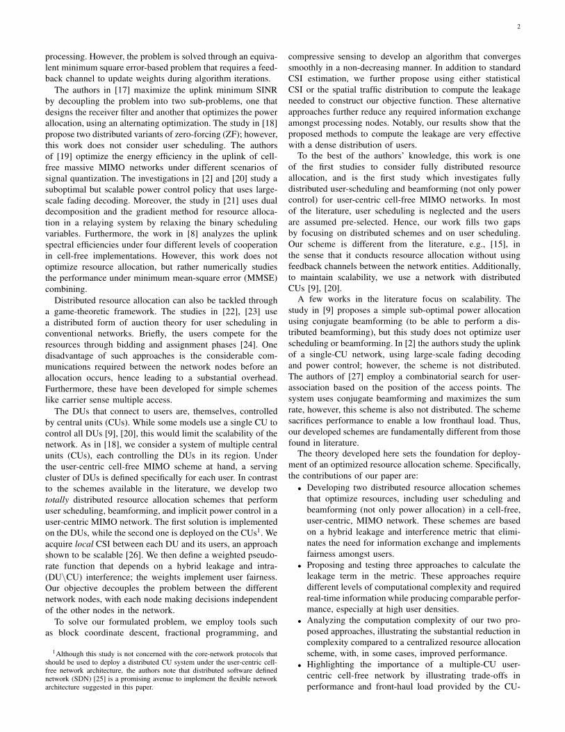
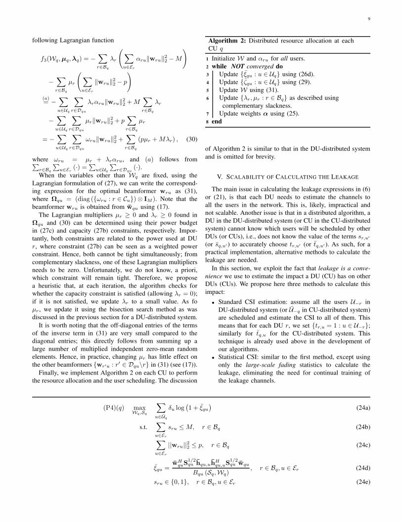
Fig. 2: Evolution of objection function. Subplots in each system: (Left) standard CSI est. case, (center) statistical CSI for
out-of-cluster users case, (right) traffic distribution case.
The value of Ph can be used to control the density of
the hotspots that are centered at locations [xh, yh] =[[xh1 , . . . , xhNh
]T,[yh1 , . . . , yhNh
]T]∈ RNh×2. These
hotspots have equal variances σ2h in both x and y dimensions.
The term an is the area of the considered region around each
node, and fh is a normalizing factor that can be calculated
numerically to normalize the PDF.
We simulate path loss using the COST231 Walfisch-Ikegami
model [42], at carrier frequency f = 1800 MHz, in a
typical urban environment, where we define β(dru) (dB) =−112.4271−38 log10 (dru) with dru in km. We use τd = 200symbols as the length of the downlink transmission phase, and
we simulate the cases of pilot lengths τp = 32 and 64. We
average our results using Monte Carlo simulations over both
network realizations and time slots.
Simulating multiple time slots captures the effect of the
fairness on user scheduling. In this regard, we simulate 30 time
slots and average the results over the last 20 time slots after
the transient in the fairness weights. These results represent the
network steady state performance and is denoted as the long-
term performance. In Table I, we summarize the parameters
used in all simulations unless specified otherwise.
In Fig. 2, we plot the evolution of the objective func-
tion in the DU-distributed system (Fig. 2(a)) and the CU-
distributed one (Fig. 2(b)) for different realizations of channels
and networks. For each system, we show as subplots the
three different methods proposed to calculate the leakage.
Additionally, we plot many runs for each case different choices
of the pilot length, τp. As is clear, the results show that the
algorithms converge in a smooth, non-decreasing, pattern.
To test the efficacy of our developed approaches and to
benchmark them, we compare our results with three schemes
defined as follows.
• Centralized [29]: we use a similar approach to the CU-
distributed system but with some differences that include
the use of the weighted sum rate objective function, i.e.,
SINR-based. The implication of this is the need for a
centralized unit to gather all the information about the
network and run the algorithm, which means that the
scheme is not as scalable as the distributed schemes.
In theory, a centralized solution should outperform a
distributed solution. However, since the optimization
problem is non-convex, any solution is a local optimum. It
is, therefore, not guaranteed that the centralized solution
outperforms the distributed solution in practice.
• Local zero-forcing (ZF): we use ZF constructed locally
on each DU with round-robin scheduling for the users.
Note that the ZF matrix needs to be constructed locally
at the DUs, because the sets of users to be served by the
DUs overlap with each other. Hence, no disjoint regions
can be defined to construct a ZF matrix across multiple
DUs.
• Conjugate: we use conjugate beamforming with round-
robin scheduling.
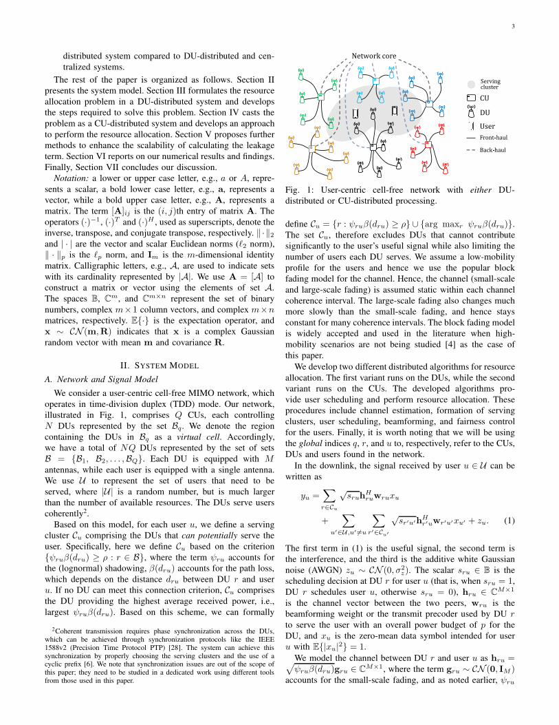
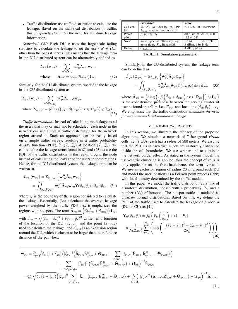
Sum Rate: In Fig. 3(a), we plot the network sum of
spectral efficiency (SE) averaged over network realizations for
a single time slot when the fairness weights are equal for
all the users (max sum rate). As expected, the CU-distributed
system provides better performance than the DU-distributed
system because it implements more coordination. Compared
to a centralized approach, the CU-system provides comparable
performance, with only a slight loss in network sum SE. This
is a very important result because it illustrates the importance
of deploying multiple CUs in the cell-free MIMO scheme.
Note that unlike the DU- and CU-distributed systems, the
centralized scheme is not scalable because it requires gathering
all the CSI, including inter-CU CSI, at a central node in the
network to perform the optimization.
Clearly, round-robin scheduling and the benchmark beam-
forming systems provide poor performance due to scheduling
the users irrespective of their channel conditions and without
any consideration of interference cancellation. Compared to
the benchmark schemes, our proposed approaches provide
a huge gain. Moreover, the results show the efficacy of
the different methods of calculating the leakage, denoted as
12
DU-system,p=64 CU-system,
p=64 DU-system,
p=32 CU-system,
p=32
0
100
200
300
400
500
600
700
800
900N
etw
ork
Sum
SE
(na
ts/s
/Hz)
Standard CSI est.Statistical CSITraffic dist.
p=64
p=32
CentralizedLocal ZFConjugate
(a) At equal fairness weights (max sum rate).
DU-system,p=64 CU-system,
p=64 DU-system,
p=32 CU-system,
p=32
0
100
200
300
400
500
600
700
Lon
g-te
rm N
etw
ork
Sum
SE
(na
ts/s
/Hz)
Standard CSI est.Statistical CSITraffic dist.
p=64
p=32
CentralizedLocal ZFConjugate
(b) Long-term with evolving fairness weights.
Fig. 3: Network sum SE for the two distributed systems under
different techniques to calculate leakage.
standard CSI, statistical CSI and traffic distribution; these three
approaches provide approximately equal performance. One
note though is that using the traffic distribution to calculate
the leakage is more reasonable when the number of users
requesting access is very large, which is the main theme for
this study. When the number of users requesting access is
small, using the traffic distribution will lead to some loss in
performance.
In Table II, we compare the gains of our proposed schemes
to the benchmark schemes, where our two distributed systems
are able to provide different degrees of performance. Note
that the CU-distributed system provides a 1.28- and 1.77-
fold performance gain compared to the DU-distributed system
using τp = 32 and τp = 64, respectively.
Including Fairness: In Fig. 3(b), we plot the long-term
network sum SE, averaged over both network realizations and
time slots. The importance of this figure is in capturing the
effect of the evolution of fairness weights and steady state
algorithm performance. The results show that on the long-term,
using the statistical CSI provides the best performance among
the other methods used to calculate the leakage. Also, the
CU-distributed system provides a 1.3-fold performance gain
over the long-term compared to the DU-distributed system.
Furthermore, the results show that over the long-term the CU-
distributed system can outperform the centralized scheme.
As mentioned, both the centralized scheme and the ones
proposed here result in local optima; given the complexity of
the objective function and constraints, it is impossible to bound
the distance from the optimal solution. However, as in the
DU-distributed system CU-distributed systemτp = 64 τp = 32 τp = 64 τp = 32
Centralized 0.64-fold 0.72-fold 0.88-fold 0.9-fold
Local ZF 9-fold 7.6-fold 12.5-fold 9.5-fold
Conjugate 12.7-fold 12-fold 17.5-fold 15-fold
TABLE II: Performance of our proposed systems compared to
different schemes at equal fairness weights.
proposed distributed schemes, fewer variables are optimized at
each DU/CU. We speculate that the fewer variables required
for the CU-distributed system lead to a solution closer to the
global optimum. This is consistent with results for a traditional
cellular network [43]. Another possible reason for this is
that the fairness weights of the users are different in each
system, after the allocation of time slots, which may affect
the set of users being scheduled concurrently in the latter time
slots. For the DU-distributed system, the centralized scheme
still provides a better performance in any scenario. This is
also reasonable because the DU-distributed sytem restricts its
performance to the knowledge found at the DU, so it is less
cooperative than the CU-distributed system.
All in all, the results show that both schemes are very
efficient in performing the resource allocation, though, as
expected, the CU-distributed system provides substantially
better performance. Our results highlight the importance of
deploying multiple CUs in the user-centric cell-free network
while the DU-distributed system can still be used if the front-
haul is overloaded.
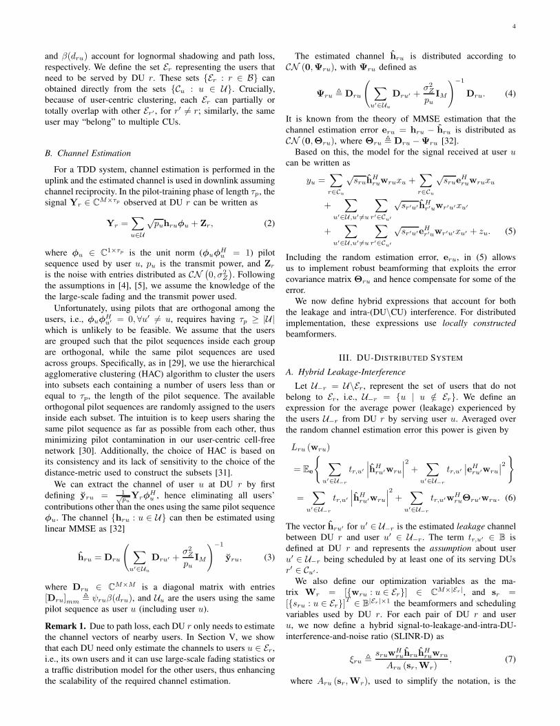
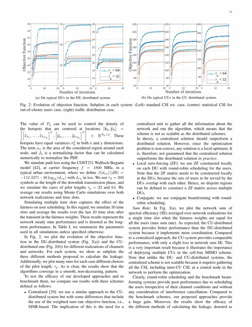
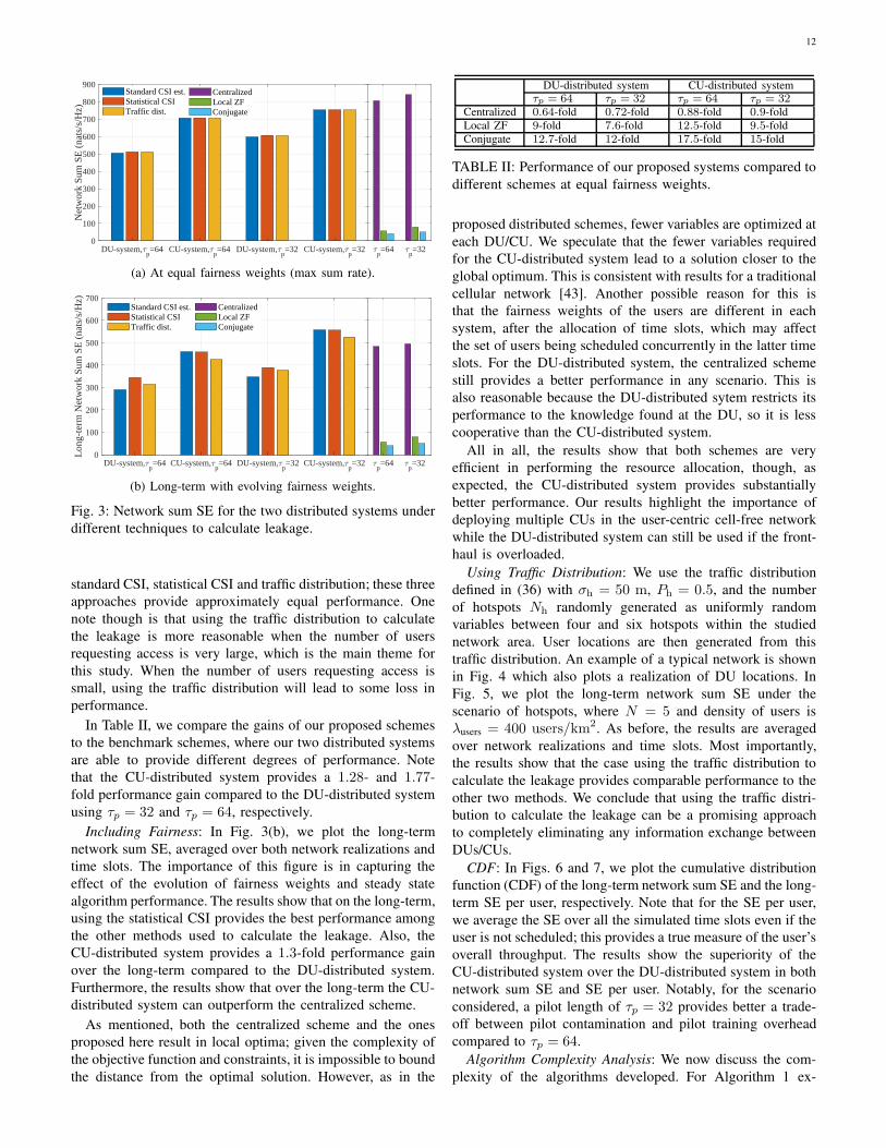
Using Traffic Distribution: We use the traffic distribution
defined in (36) with σh = 50 m, Ph = 0.5, and the number
of hotspots Nh randomly generated as uniformly random
variables between four and six hotspots within the studied
network area. User locations are then generated from this
traffic distribution. An example of a typical network is shown
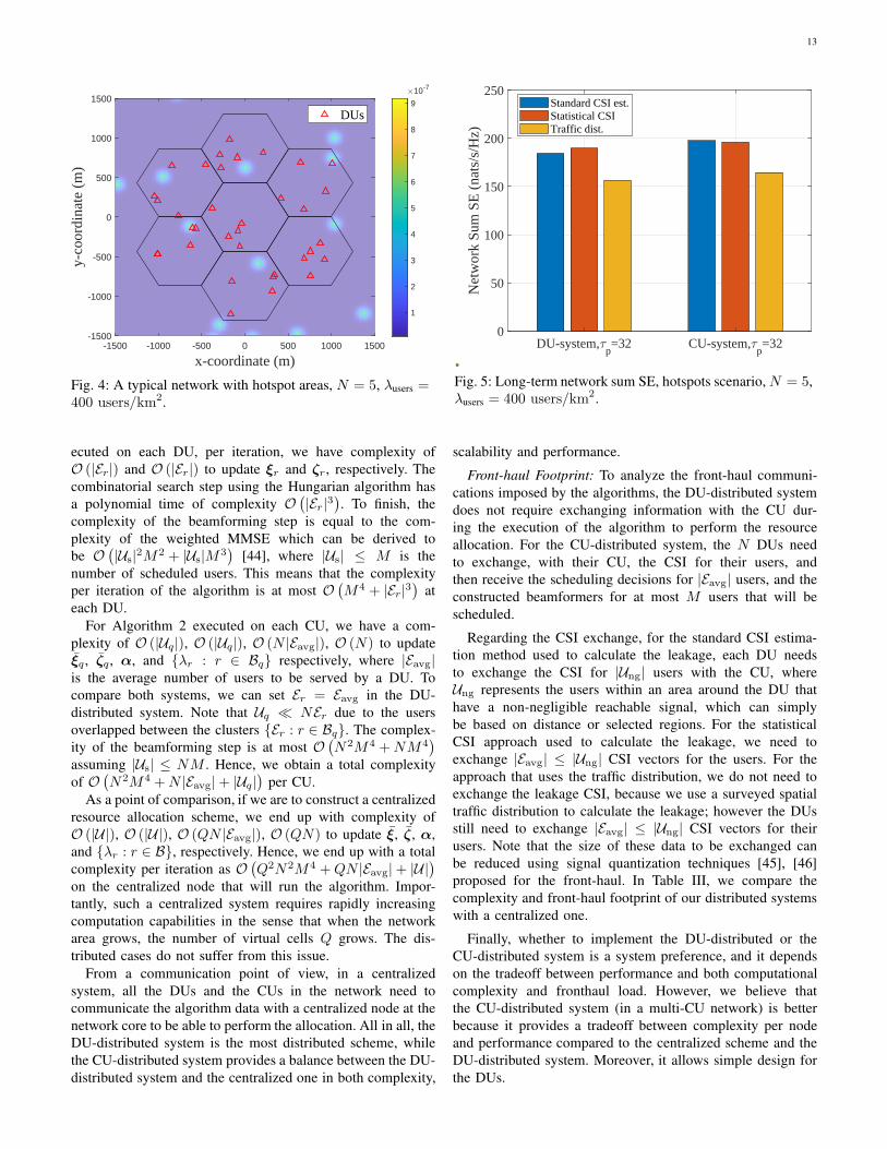
in Fig. 4 which also plots a realization of DU locations. In
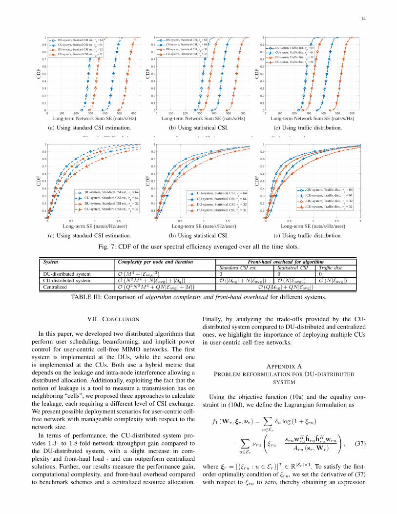
Fig. 5, we plot the long-term network sum SE under the
scenario of hotspots, where N = 5 and density of users is
λusers = 400 users/km2. As before, the results are averaged
over network realizations and time slots. Most importantly,
the results show that the case using the traffic distribution to
calculate the leakage provides comparable performance to the
other two methods. We conclude that using the traffic distri-
bution to calculate the leakage can be a promising approach
to completely eliminating any information exchange between
DUs/CUs.
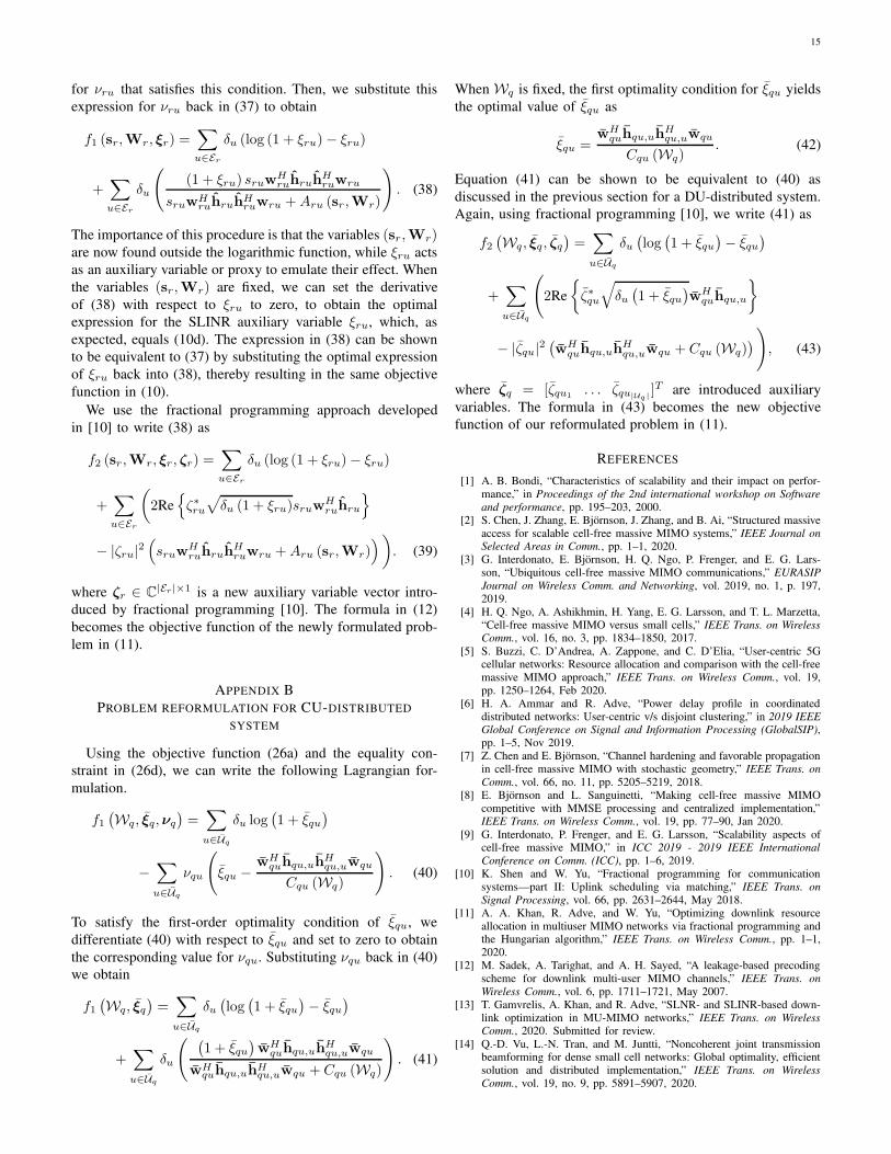
CDF: In Figs. 6 and 7, we plot the cumulative distribution
function (CDF) of the long-term network sum SE and the long-
term SE per user, respectively. Note that for the SE per user,
we average the SE over all the simulated time slots even if the
user is not scheduled; this provides a true measure of the user’s
overall throughput. The results show the superiority of the
CU-distributed system over the DU-distributed system in both
network sum SE and SE per user. Notably, for the scenario
considered, a pilot length of τp = 32 provides better a trade-
off between pilot contamination and pilot training overhead
compared to τp = 64.
Algorithm Complexity Analysis: We now discuss the com-
plexity of the algorithms developed. For Algorithm 1 ex-
13
-1500 -1000 -500 0 500 1000 1500
x-coordinate (m)
-1500
-1000
-500
0
500
1000
1500
y-co
ordi
nate
(m
)
1
2
3
4
5
6
7
8
9
10-7
DUs
Fig. 4: A typical network with hotspot areas, N = 5, λusers =400 users/km2.
DU-system,p=32 CU-system,
p=32
0
50
100
150
200
250
Net
wor
k Su
m S
E (
nats
/s/H
z)
Standard CSI est.Statistical CSITraffic dist.
Fig. 5: Long-term network sum SE, hotspots scenario,N = 5,
λusers = 400 users/km2.
ecuted on each DU, per iteration, we have complexity of
O (|Er|) and O (|Er|) to update ξr and ζr, respectively. The
combinatorial search step using the Hungarian algorithm has
a polynomial time of complexity O(|Er|3
). To finish, the
complexity of the beamforming step is equal to the com-
plexity of the weighted MMSE which can be derived to
be O(|Us|2M2 + |Us|M3
)[44], where |Us| ≤ M is the
number of scheduled users. This means that the complexity
per iteration of the algorithm is at most O(M4 + |Er|3
)at
each DU.
For Algorithm 2 executed on each CU, we have a com-
plexity of O (|Uq|), O (|Uq|), O (N |Eavg|), O (N) to update
ξq , ζq , α, and λr : r ∈ Bq respectively, where |Eavg|is the average number of users to be served by a DU. To
compare both systems, we can set Er = Eavg in the DU-
distributed system. Note that Uq ≪ NEr due to the users
overlapped between the clusters Er : r ∈ Bq. The complex-
ity of the beamforming step is at most O(N2M4 +NM4
)
assuming |Us| ≤ NM . Hence, we obtain a total complexity
of O(N2M4 +N |Eavg|+ |Uq|
)per CU.
As a point of comparison, if we are to construct a centralized
resource allocation scheme, we end up with complexity of
O (|U|), O (|U|), O (QN |Eavg|), O (QN) to update ξ, ζ, α,
and λr : r ∈ B, respectively. Hence, we end up with a total
complexity per iteration as O(Q2N2M4 +QN |Eavg|+ |U|
)
on the centralized node that will run the algorithm. Impor-
tantly, such a centralized system requires rapidly increasing
computation capabilities in the sense that when the network
area grows, the number of virtual cells Q grows. The dis-
tributed cases do not suffer from this issue.
From a communication point of view, in a centralized
system, all the DUs and the CUs in the network need to
communicate the algorithm data with a centralized node at the
network core to be able to perform the allocation. All in all, the
DU-distributed system is the most distributed scheme, while
the CU-distributed system provides a balance between the DU-
distributed system and the centralized one in both complexity,
scalability and performance.
Front-haul Footprint: To analyze the front-haul communi-
cations imposed by the algorithms, the DU-distributed system
does not require exchanging information with the CU dur-
ing the execution of the algorithm to perform the resource
allocation. For the CU-distributed system, the N DUs need
to exchange, with their CU, the CSI for their users, and
then receive the scheduling decisions for |Eavg| users, and the
constructed beamformers for at most M users that will be
scheduled.
Regarding the CSI exchange, for the standard CSI estima-
tion method used to calculate the leakage, each DU needs
to exchange the CSI for |Ung| users with the CU, where
Ung represents the users within an area around the DU that
have a non-negligible reachable signal, which can simply
be based on distance or selected regions. For the statistical
CSI approach used to calculate the leakage, we need to
exchange |Eavg| ≤ |Ung| CSI vectors for the users. For the
approach that uses the traffic distribution, we do not need to
exchange the leakage CSI, because we use a surveyed spatial
traffic distribution to calculate the leakage; however the DUs
still need to exchange |Eavg| ≤ |Ung| CSI vectors for their
users. Note that the size of these data to be exchanged can
be reduced using signal quantization techniques [45], [46]
proposed for the front-haul. In Table III, we compare the
complexity and front-haul footprint of our distributed systems
with a centralized one.
Finally, whether to implement the DU-distributed or the
CU-distributed system is a system preference, and it depends
on the tradeoff between performance and both computational
complexity and fronthaul load. However, we believe that
the CU-distributed system (in a multi-CU network) is better
because it provides a tradeoff between complexity per node
and performance compared to the centralized scheme and the
DU-distributed system. Moreover, it allows simple design for
the DUs.
14
0 100 200 300 400 500 600
Long-term Network Sum SE (nats/s/Hz)
0
0.1
0.2
0.3
0.4
0.5
0.6
0.7
0.8
0.9
1C
DF
DU-system, Standard CSI est., p = 64
CU-system, Standard CSI est., p = 64
DU-system, Standard CSI est., p = 32
CU-system, Standard CSI est., p = 32
(a) Using standard CSI estimation.
0 100 200 300 400 500 600
Long-term Network Sum SE (nats/s/Hz)
0
0.1
0.2
0.3
0.4
0.5
0.6
0.7
0.8
0.9
1
CD
F
DU-system, Statistical CSI, p = 64
CU-system, Statistical CSI, p = 64
DU-system, Statistical CSI, p = 32
CU-system, Statistical CSI, p = 32
(b) Using statistical CSI.
0 100 200 300 400 500 600
Long-term Network Sum SE (nats/s/Hz)
0
0.1
0.2
0.3
0.4
0.5
0.6
0.7
0.8
0.9
1
CD
F
DU-system, Traffic dist., p = 64
CU-system, Traffic dist., p = 64
DU-system, Traffic dist., p = 32
CU-system, Traffic dist., p = 32
(c) Using traffic distribution.
Fig. 6: CDF of the network sum of spectral efficiency averaged over all the time slots.
0 0.5 1 1.5 2
Long-term SE (nats/s/Hz/user)
0
0.1
0.2
0.3
0.4
0.5
0.6
0.7
0.8
0.9
1
CD
F
DU-system, Standard CSI est., p = 64
CU-system, Standard CSI est., p = 64
DU-system, Standard CSI est., p = 32
CU-system, Standard CSI est., p = 32
(a) Using standard CSI estimation.
0 0.5 1 1.5 2
Long-term SE (nats/s/Hz/user)
0
0.1
0.2
0.3
0.4
0.5
0.6
0.7
0.8
0.9
1C
DF
DU-system, Statistical CSI, p = 64
CU-system, Statistical CSI, p = 64
DU-system, Statistical CSI, p = 32
CU-system, Statistical CSI, p = 32
(b) Using statistical CSI.
0 0.5 1 1.5 2
Long-term SE (nats/s/Hz/user)
0
0.1
0.2
0.3
0.4
0.5
0.6
0.7
0.8
0.9
1
CD
F
DU-system, Traffic dist., p = 64
CU-system, Traffic dist., p = 64
DU-system, Traffic dist., p = 32
CU-system, Traffic dist., p = 32
(c) Using traffic distribution.
Fig. 7: CDF of the user spectral efficiency averaged over all the time slots.
System Complexity per node and iteration Front-haul overhead for algorithmStandard CSI est. Statistical CSI Traffic dist.
DU-distributed system O(
M4 + |Eavg|3)
0 0 0
CU-distributed system O(
N2M4 +N |Eavg|+ |Uq|)
O (|Ung|+N |Eavg |) O (N |Eavg |) O (N |Eavg|)Centralized O
(
Q2N2M4 +QN |Eavg|+ |U|)
O (Q|Ung|+QN |Eavg|)
TABLE III: Comparison of algorithm complexity and front-haul overhead for different systems.
VII. CONCLUSION
In this paper, we developed two distributed algorithms that
perform user scheduling, beamforming, and implicit power
control for user-centric cell-free MIMO networks. The first
system is implemented at the DUs, while the second one
is implemented at the CUs. Both use a hybrid metric that
depends on the leakage and intra-node interference allowing a
distributed allocation. Additionally, exploiting the fact that the
notion of leakage is a tool to measure a transmission has on
neighboring “cells”, we proposed three approaches to calculate
the leakage, each requiring a different level of CSI exchange.
We present possible deployment scenarios for user-centric cell-
free network with manageable complexity with respect to the
network size.
In terms of performance, the CU-distributed system pro-
vides 1.3- to 1.8-fold network throughput gain compared to
the DU-distributed system, with a slight increase in com-
plexity and front-haul load - and can outperform centralized
solutions. Further, our results measure the performance gain,
computational complexity, and front-haul overhead compared
to benchmark schemes and a centralized resource allocation.
Finally, by analyzing the trade-offs provided by the CU-
distributed system compared to DU-distributed and centralized
ones, we highlight the importance of deploying multiple CUs
in user-centric cell-free networks.
APPENDIX A
PROBLEM REFORMULATION FOR DU-DISTRIBUTED
SYSTEM
Using the objective function (10a) and the equality con-
straint in (10d), we define the Lagrangian formulation as
f1 (Wr, ξr,νr) =∑
u∈Er
δu log (1 + ξru)
−∑
u∈Er
νru
(ξru − sruw
Hruhruh
Hruwru
Aru (sr,Wr)
), (37)
where ξr = [ξru : u ∈ Er]T ∈ R|Er|×1. To satisfy the first-
order optimality condition of ξru, we set the derivative of (37)
with respect to ξru to zero, thereby obtaining an expression
15
for νru that satisfies this condition. Then, we substitute this
expression for νru back in (37) to obtain
f1 (sr,Wr, ξr) =∑
u∈Er
δu (log (1 + ξru)− ξru)
+∑
u∈Er
δu
((1 + ξru) sruw
Hruhruh
Hruwru
sruwHruhruhH
ruwru +Aru (sr,Wr)
). (38)
The importance of this procedure is that the variables (sr,Wr)are now found outside the logarithmic function, while ξru acts
as an auxiliary variable or proxy to emulate their effect. When
the variables (sr,Wr) are fixed, we can set the derivative
of (38) with respect to ξru to zero, to obtain the optimal
expression for the SLINR auxiliary variable ξru, which, as
expected, equals (10d). The expression in (38) can be shown
to be equivalent to (37) by substituting the optimal expression
of ξru back into (38), thereby resulting in the same objective
function in (10).
We use the fractional programming approach developed
in [10] to write (38) as
f2 (sr,Wr, ξr, ζr) =∑
u∈Er
δu (log (1 + ξru)− ξru)
+∑
u∈Er
(2Re
ζ∗ru√δu (1 + ξru)sruw
Hruhru
− |ζru|2(sruw
Hruhruh
Hruwru +Aru (sr,Wr)
)). (39)
where ζr ∈ C|Er|×1 is a new auxiliary variable vector intro-
duced by fractional programming [10]. The formula in (12)
becomes the objective function of the newly formulated prob-
lem in (11).
APPENDIX B
PROBLEM REFORMULATION FOR CU-DISTRIBUTED
SYSTEM
Using the objective function (26a) and the equality con-
straint in (26d), we can write the following Lagrangian for-
mulation.
f1(Wq, ξq,νq
)=∑
u∈Uq
δu log(1 + ξqu
)
−∑
u∈Uq
νqu
(ξqu − wH
quhqu,uhHqu,uwqu
Cqu (Wq)
). (40)
To satisfy the first-order optimality condition of ξqu, we
differentiate (40) with respect to ξqu and set to zero to obtain
the corresponding value for νqu. Substituting νqu back in (40)
we obtain
f1(Wq, ξq
)=∑
u∈Uq
δu(log(1 + ξqu
)− ξqu
)
+∑
u∈Uq
δu
( (1 + ξqu
)wH
quhqu,uhHqu,uwqu
wHquhqu,uhH
qu,uwqu + Cqu (Wq)
). (41)
When Wq is fixed, the first optimality condition for ξqu yields
the optimal value of ξqu as
ξqu =wH
quhqu,uhHqu,uwqu
Cqu (Wq). (42)
Equation (41) can be shown to be equivalent to (40) as
discussed in the previous section for a DU-distributed system.
Again, using fractional programming [10], we write (41) as
f2(Wq, ξq, ζq
)=∑
u∈Uq
δu(log(1 + ξqu
)− ξqu
)
+∑
u∈Uq
(2Re
ζ∗qu
√δu(1 + ξqu
)wH
quhqu,u
− |ζqu|2(wH
quhqu,uhHqu,uwqu + Cqu (Wq)
)), (43)
where ζq = [ζqu1 . . . ζqu|Uq |]T are introduced auxiliary
variables. The formula in (43) becomes the new objective
function of our reformulated problem in (11).
REFERENCES
[1] A. B. Bondi, “Characteristics of scalability and their impact on perfor-mance,” in Proceedings of the 2nd international workshop on Software
and performance, pp. 195–203, 2000.[2] S. Chen, J. Zhang, E. Bjornson, J. Zhang, and B. Ai, “Structured massive
access for scalable cell-free massive MIMO systems,” IEEE Journal onSelected Areas in Comm., pp. 1–1, 2020.
[3] G. Interdonato, E. Bjornson, H. Q. Ngo, P. Frenger, and E. G. Lars-son, “Ubiquitous cell-free massive MIMO communications,” EURASIP
Journal on Wireless Comm. and Networking, vol. 2019, no. 1, p. 197,2019.
[4] H. Q. Ngo, A. Ashikhmin, H. Yang, E. G. Larsson, and T. L. Marzetta,“Cell-free massive MIMO versus small cells,” IEEE Trans. on WirelessComm., vol. 16, no. 3, pp. 1834–1850, 2017.
[5] S. Buzzi, C. D’Andrea, A. Zappone, and C. D’Elia, “User-centric 5Gcellular networks: Resource allocation and comparison with the cell-freemassive MIMO approach,” IEEE Trans. on Wireless Comm., vol. 19,pp. 1250–1264, Feb 2020.
[6] H. A. Ammar and R. Adve, “Power delay profile in coordinateddistributed networks: User-centric v/s disjoint clustering,” in 2019 IEEEGlobal Conference on Signal and Information Processing (GlobalSIP),pp. 1–5, Nov 2019.
[7] Z. Chen and E. Bjornson, “Channel hardening and favorable propagationin cell-free massive MIMO with stochastic geometry,” IEEE Trans. on
Comm., vol. 66, no. 11, pp. 5205–5219, 2018.[8] E. Bjornson and L. Sanguinetti, “Making cell-free massive MIMO
competitive with MMSE processing and centralized implementation,”IEEE Trans. on Wireless Comm., vol. 19, pp. 77–90, Jan 2020.
[9] G. Interdonato, P. Frenger, and E. G. Larsson, “Scalability aspects ofcell-free massive MIMO,” in ICC 2019 - 2019 IEEE International
Conference on Comm. (ICC), pp. 1–6, 2019.[10] K. Shen and W. Yu, “Fractional programming for communication
systems—part II: Uplink scheduling via matching,” IEEE Trans. on
Signal Processing, vol. 66, pp. 2631–2644, May 2018.[11] A. A. Khan, R. Adve, and W. Yu, “Optimizing downlink resource
allocation in multiuser MIMO networks via fractional programming andthe Hungarian algorithm,” IEEE Trans. on Wireless Comm., pp. 1–1,2020.
[12] M. Sadek, A. Tarighat, and A. H. Sayed, “A leakage-based precodingscheme for downlink multi-user MIMO channels,” IEEE Trans. on
Wireless Comm., vol. 6, pp. 1711–1721, May 2007.[13] T. Gamvrelis, A. Khan, and R. Adve, “SLNR- and SLINR-based down-
link optimization in MU-MIMO networks,” IEEE Trans. on WirelessComm., 2020. Submitted for review.
[14] Q.-D. Vu, L.-N. Tran, and M. Juntti, “Noncoherent joint transmissionbeamforming for dense small cell networks: Global optimality, efficientsolution and distributed implementation,” IEEE Trans. on Wireless
Comm., vol. 19, no. 9, pp. 5891–5907, 2020.
16
[15] I. Atzeni, B. Gouda, and A. Tolli, “Distributed precoding design viaover-the-air signaling for cell-free massive MIMO,” IEEE Trans. onWireless Comm., vol. 20, no. 2, pp. 1201–1216, 2021.
[16] J. Kaleva, A. Tolli, M. Juntti, R. A. Berry, and M. L. Honig, “Decen-tralized joint precoding with pilot-aided beamformer estimation,” IEEE
Trans. on Signal Processing, vol. 66, no. 9, pp. 2330–2341, 2018.
[17] M. Bashar, K. Cumanan, A. G. Burr, M. Debbah, and H. Q. Ngo, “Onthe uplink max–min SINR of cell-free massive MIMO systems,” IEEE
Trans. on Wireless Comm., vol. 18, no. 4, pp. 2021–2036, 2019.
[18] G. Interdonato, M. Karlsson, E. Bjornson, and E. G. Larsson, “Localpartial zero-forcing precoding for cell-free massive MIMO,” IEEE Trans.
on Wireless Comm., pp. 1–1, 2020.
[19] M. Bashar, H. Q. Ngo, K. Cumanan, A. G. Burr, P. Xiao, E. Bjornson,and E. G. Larsson, “Uplink spectral and energy efficiency of cell-freemassive MIMO with optimal uniform quantization,” IEEE Trans. on
Comm., pp. 1–1, 2020.
[20] E. Bjornson and L. Sanguinetti, “Scalable cell-free massive MIMOsystems,” IEEE Trans. on Comm., pp. 1–1, 2020.
[21] Z. Chen, E. Bjornson, and E. G. Larsson, “Dynamic resource allocationin co-located and cell-free massive MIMO,” IEEE Trans. on GreenComm. and Networking, pp. 1–1, 2019.
[22] A. Zappone, E. Jorswieck, and A. Leshem, “Distributed resource alloca-tion for energy efficiency in MIMO OFDMA wireless networks,” IEEEJournal on Selected Areas in Comm., vol. 34, no. 12, pp. 3451–3465,2016.
[23] O. Naparstek and A. Leshem, “Fully distributed optimal channel as-signment for open spectrum access,” IEEE Trans. on Signal Processing,vol. 62, no. 2, pp. 283–294, 2014.
[24] D. P. Bertsekas, “A distributed algorithm for the assignment problem,”Lab. for Inf. Decis. Sys. Working Paper, MIT, 1979.
[25] F. Bannour, S. Souihi, and A. Mellouk, “Distributed SDN control:Survey, taxonomy, and challenges,” IEEE Comm. Surveys Tutorials,vol. 20, no. 1, pp. 333–354, 2018.
[26] E. Bjornson, R. Zakhour, D. Gesbert, and B. Ottersten, “Cooperativemulticell precoding: Rate region characterization and distributed strate-gies with instantaneous and statistical CSI,” IEEE Trans. Sig. Process.,vol. 58, no. 8, 2010.
[27] C. D’Andrea and E. G. Larsson, “User association in scalable cell-freemassive MIMO systems,” arXiv preprint arXiv:2103.05321, 2021.
[28] “IEEE standard for a precision clock synchronization protocol fornetworked measurement and control systems,” IEEE Std 1588-2019
(Revision of IEEE Std 1588-2008), pp. 1–499, 2020.
[29] H. A. Ammar, R. Adve, S. Shahbazpanahi, G. Boudreau, and K. V.Srinivas, “Downlink resource allocation in multiuser cell-free MIMOnetworks with user-centric clustering,” IEEE Transactions on Wireless
Communications, pp. 1–1, 2021.
[30] M. Attarifar, A. Abbasfar, and A. Lozano, “Random vs structured pilotassignment in cell-free massive MIMO wireless networks,” in 2018 IEEE
International Conference on Comm. Workshops (ICC Workshops), pp. 1–6, 2018.
[31] M. G. Karypis, V. Kumar, and M. Steinbach, “A comparison of documentclustering techniques,” in TextMining Workshop at KDD2000 (May
2000), 2000.
[32] S. M. Kay, Fundamentals of statistical signal processing. Prentice HallPTR, 1993.
[33] W. Yu, T. Kwon, and C. Shin, “Adaptive resource allocation in coopera-tive cellular networks,” Cooperative cellular wireless networks, pp. 233–256, 2011.
[34] Z. Luo and S. Zhang, “Dynamic spectrum management: Complexity andduality,” IEEE Journal of Selected Topics in Signal Processing, vol. 2,pp. 57–73, Feb 2008.
[35] S. Schaible, “Parameter-free convex equivalent and dual programs offractional programming problems,” Zeitschrift fur Operations Research,vol. 18, no. 5, pp. 187–196, 1974.
[36] W. Dinkelbach, “On nonlinear fractional programming,” Managementscience, vol. 13, no. 7, pp. 492–498, 1967.
[37] S. H. Bokhari, Assignment problems in parallel and distributed comput-
ing. Springer Science & Business Media, 2012.
[38] H. W. Kuhn, “The Hungarian method for the assignment problem,”Naval research logis. quarterly, vol. 2, no. 1-2, pp. 83–97, 1955.
[39] D. L. Donoho, “Compressed sensing,” IEEE Trans. on Information
Theory, vol. 52, pp. 1289–1306, April 2006.
[40] E. J. Candes, M. B. Wakin, and S. P. Boyd, “Enhancing sparsity byreweighted ℓ1 minimization,” Journal of Fourier analysis and applica-
tions, vol. 14, no. 5-6, pp. 877–905, 2008.
[41] A. Minasian, R. S. Adve, S. Shahbazpanahi, and G. Boudreau, “On RRHplacement for multi-user distributed massive MIMO systems,” IEEEAccess, vol. 6, pp. 70597–70614, 2018.
[42] J. Walfisch and H. L. Bertoni, “A theoretical model of UHF propagationin urban environments,” IEEE Trans. on Antennas and Propagation,vol. 36, pp. 1788–1796, Dec 1988.
[43] A. A. Khan and R. S. Adve, “Centralized and distributed deep rein-forcement learning methods for downlink sum-rate optimization,” IEEE
Trans. on Wireless Comm., vol. 19, no. 12, pp. 8410–8426, 2020.[44] Q. Shi, M. Razaviyayn, Z. Luo, and C. He, “An iteratively weighted
MMSE approach to distributed sum-utility maximization for a MIMO in-terfering broadcast channel,” IEEE Trans. on Signal Processing, vol. 59,pp. 4331–4340, Sep. 2011.
[45] M. Bashar, K. Cumanan, A. G. Burr, H. Q. Ngo, M. Debbah, andP. Xiao, “Max–min rate of cell-free massive MIMO uplink with optimaluniform quantization,” IEEE Trans. on Comm., vol. 67, no. 10, pp. 6796–6815, 2019.
[46] M. Bashar, K. Cumanan, A. G. Burr, H. Q. Ngo, E. G. Larsson, andP. Xiao, “Energy efficiency of the cell-free massive MIMO uplink withoptimal uniform quantization,” IEEE Trans. Green Comm. and Net.,vol. 3, no. 4, pp. 971–987, 2019.