distributed hydrological modeling of total dissolved phosphorus transport in an agricultural...

Hydrol. Earth Syst. Sci., 10, 245–261, 2006www.hydrol-earth-syst-sci.net/10/245/2006/© Author(s) 2006. This work is licensedunder a Creative Commons License.

Hydrology andEarth System

Sciences

Distributed hydrological modelling of total dissolvedphosphorus transport in an agricultural landscape,part I: distributed runoff generation

P. Gerard-Marchant 1, W. D. Hively2, and T. S. Steenhuis1

1Department of Biological and Environmental Engineering, Cornell University, Ithaca, NY 14853, USA2Department of Natural Resources, Cornell University, Ithaca, NY 14853, USA

Received: 30 June 2005 – Published in Hydrol. Earth Syst. Sci. Discuss.: 22 August 2005Revised: 30 November 2005 – Accepted: 21 February 2006 – Published: 26 April 2006

Abstract. Successful implementation of best managementpractices for reducing non-point source (NPS) pollution re-quires knowledge of the location of saturated areas that pro-duce runoff. A physically-based, fully-distributed, GIS-integrated model, the Soil Moisture Distribution and Rout-ing (SMDR) model was developed to simulate the hydrologicbehavior of small rural upland watersheds with shallow soilsand steep to moderate slopes. The model assumes that grav-ity is the only driving force of water and that most overlandflow occurs as saturation excess. The model uses availablesoil and climatic data, and requires little calibration.

The SMDR model was used to simulate runoff produc-tion on a 164-ha farm watershed in Delaware County, NewYork, in the headwaters of New York City water supply.Apart from land use, distributed input parameters were de-rived from readily available data. Simulated hydrographscompared reasonably with observed flows at the watershedoutlet over a eight year simulation period, and peak timingand intensities were well reproduced. Using off-site weatherinput data produced occasional missed event peaks. Sim-ulated soil moisture distribution agreed well with observedhydrological features and followed the same spatial trend asobserved soil moisture contents sampled on four transects.Model accuracy improved when input variables were cali-brated within the range of SSURGO-available parameters.The model will be a useful planning tool for reducing NPSpollution from farms in landscapes similar to the Northeast-ern US.

Correspondence to:T. S. Steenhuis([email protected])

1 Introduction

Reducing agricultural non-point source (NPS) pollution hasbecome a focus for watershed management programs thatmaintain and improve water quality. Significant NPS pollu-tion originates from hydrologically active areas where runoffis generated, and that also have high soil nutrient concentra-tions (Gburek et al., 1996). Successful implementation ofbest management practices for reducing NPS pollution re-quires the knowledge of the location of frequently-saturatedareas prone to overland flow generation, termed hydrologi-cally sensitive areas (HSAs) (Walter et al., 2000).

Overland flow generation can occur by two mechanisms.Infiltration-excess runoff (also called Hortonian overlandflow) takes place when precipitation rate exceeds soil infiltra-tion capacity (Horton, 1933, 1940). This mechanism is pre-dominant on low organic matter arid and semiarid soils thatare prone to crusting and on compacted areas during high-intensity rainfall events. In contrast, saturation-excess over-land flow occurs when precipitation falls on saturated soil.Location of saturation-excess overland flow generation doesnot depend on rainfall intensity but on topography, soil prop-erties, and local hydrological conditions, such as high watertable (Hewlett and Hibbert, 1967; Dunne and Black, 1970;Hewlett and Nutter, 1970; Dunne et al., 1975; Beven andKirby, 1979).

Either infiltration- or saturation-excess processes may pre-dominate at different times and different locations within awatershed. When Hortonian flow dominates, the volumeof surface runoff is a function of soil type, land cover andrainfall intensity. Semi distributed models such as SWAT(Arnold et al., 1993, 1994; Di Luzio and Arnold, 2004;Neisch et al., 2002), HSPF (Donigian et al., 1995; Bicknell

Published by Copernicus GmbH on behalf of the European Geosciences Union.

246 P. Gerard-Marchant et al.: Phosphorus transport in an agricultural landscape

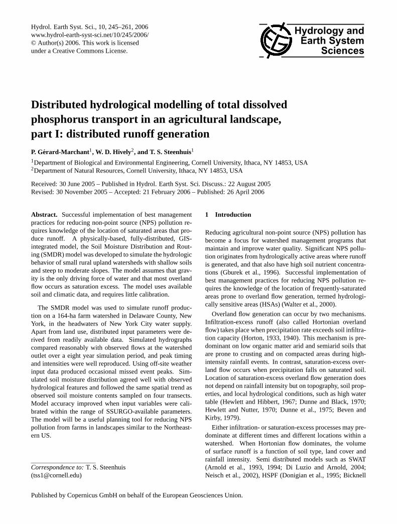
Fig. 1. Schematic representation of the water balance componentsover one cell.

et al., 1997; Srinivasan et al., 1998) or GWLF (Haith andShoemaker, 1987; Haith et al., 1992; Schneidermannet al.,2002) are usually based on Hortonian overland flow genera-tion mechanisms. With these models, topographical informa-tion is not an important predictor of total runoff and nutrientloads to the streams. However, when overland flow is gen-erated by saturation- excess mechanisms, landscape positionis a determining factor, and the temporal distribution of vari-able source areas must be estimated. Therefore, only modelsthat preserve the spatial information during the simulationcan accurately simulate saturation-excess overland flow.

Typical fully-distributed spatial models include theSysteme Hydrologic Europeen, SHE (Abbott et al., 1986a,b; Refsgaard and Storm, 1995); TOPMODEL (Beven, 1997;Beven and Kirkby, 1979; Saulnieret al., 1998); DistributedHydrology Soil Vegetation Model, DHSVM (Wigmosta etal., 1994; Wigmosta et al., 2002; Wigmosta and Perkins,2001) and the Soil Moisture Distribution and Routing model,SMDR. The SMDR model is based on a soil moisture bal-ance calculation initially developed by Steenhuis and vander Molen (1986), later modified and integrated into theGeographic Resources Analysis Support System (GRASS)Geographic Information System (GIS) (US Army C.E.R.L.,1991; Neteler and Mitasova, 2002) by Zollweg et al. (1996),Frankenberger et al. (1999) and Kuo et al. (1999). Thismodel is currently maintained by the Soil and Water Labora-tory, Cornell University (Soil and Water Laboratory, 2003).SMDR was specifically designed for application on small ru-ral watersheds of the Northeastern United States, character-ized by soils overlying slowly permeable layers at shallowdepths and moderate to steep slopes. It differs from othermodels such as SHE or DHVSM in that it uses only readilyavailable input data. Unlike TOPMODEL, it does not assumea water table underlying the whole watershed, but uses soildata on depth to restrictive layer to determine the lower soilboundary.

In the recent years, SMDR has been successfully ap-plied to predict discharge data in several watersheds of theCatskills Mountain region, New York (Frankenberger et al.,1999; Mehta et al., 2004), in Central New York (Kuo etal., 1999; Johnson et al., 2003), and in Pennsylvania (Srini-vasanet al., 2005). Validation of the model distributed out-puts has been limited due to the difficulty of collecting accu-rate distributed data.

The objective of this paper is, therefore, to validate SDMRintegrated (i.e. runoff at the watershed outlet) and distributedresults. The study watershed is a 164-ha dairy farm, locatedin the northern Catskills region of Delaware County, NY,within the headwaters of Cannonsville reservoir, the thirdlargest reservoir of the New York City water supply system.Streamflows and streamwater nutrient concentrations havebeen measured at the watershed outlet since 1993 (Bishopet al., 2003, 2005). Detailed management records are alsoavailable, and this farm provides an ideal context for appli-cation of the model and verification of results.

2 Description of the SMDR model

The purpose of SMDR is to identify the location and evo-lution of variable source areas for overland flow generationand to estimate water fluxes to streams and groundwater. TheSMDR is intended as a tool for planners or groups interestedin watershed management. Therefore, it does not require ex-tensive calibration and is designed to use data that are read-ily available in electronic form: (i) a digital elevation map,(ii) a soil type map and the associated table of soil hydro-logic properties, (iii) a land use and land cover map, and (iv)weather data (temperature, precipitation and potential evap-otranspiration). Details of input data requirements are givenin a following section.

Use of SMDR is limited to upland, well-vegetated water-sheds, where soils have a high infiltration capacity and slopesover 3%. In many cases, a low permeability layer, such asbedrock or fragipan, is present at a relatively shallow depth.Watersheds of this type occur not only in the NortheasternUnited States, but also in many other parts of the world.

The SMDR divides the watershed in square gridcells, withtypical cell dimensions ranging from 5 to 30 m. Larger di-mensions tend to misrepresent the landscape curvatures andlead to unreasonably high estimates of soil water content(Kuo et al., 1999). In practice, the minimum grid size de-pends on the resolution of the DEM. Within each cell, soilproperties are assumed to be homogeneous. Soil horizonsabove the low-conductivity restricting layer are grouped intoa single surface soil layer. This surface soil layer is thendecomposed into two functional sublayers, corresponding tothe rooting zone and a transmission zone.

A soil water mass balance is computed for the surfacesoil of each cell at each time step. A constant dailytime step is usually chosen as a good compromise between

Hydrol. Earth Syst. Sci., 10, 245–261, 2006 www.hydrol-earth-syst-sci.net/10/245/2006/

P. Gerard-Marchant et al.: Phosphorus transport in an agricultural landscape 247

computational speed, accuracy of results, and data availabil-ity. Daily water inputs to the top soil layer of each cell aredaily precipitation and lateral flow from surrounding ups-lope cells. Outputs are lateral flow to surrounding downslopecells, percolation through the restrictive layer, and evapotran-spiration. A schematic representation of the water balance isillustrated Fig. 1. The water mass balance equation can beexpressed for each cell as:

zW2|θ(t) − θ(t − 1t)| = |RF(t) + SM(t)|

+ Qi(t) − Qo(t)

− ET (t) − P(t) − SE(t)

(1)

where z is the thickness of the surface soil (m),W the(square) grid size (m),θ the cell average water content(cm3.cm−3), 1t the time step (d), RF andSM the rainfalland snowmelt volumes, respectively,Qi the volume of wa-ter received through lateral flow from surrounding upslopecells,Qo the volume of water lost through lateral flow to sur-rounding downslope cells,ET the volume of water lost byevapotranspiration,P the volume of water lost by percola-tion through the bounding layer, andSE the saturation excessrunoff. Volumes are expressed in (m3). Although the massbalance components are tightly coupled, they are estimatedseparately for computational simplicity. They are presentedhereafter in the order in which they are calculated for eachtime step.

2.1 Precipitation

Daily precipitation is first partitioned into rain or snow, de-pending on the observed daily mean air temperature (◦C),corrected as necessary for local elevation by the adiabaticlapse rate of 6.5×10−3 C.m−1 (Boll et al., 1998). Rain-fall RF is identified with precipitation on cells where airtemperature is greater than−1◦C. SnowmeltSM is com-puted following a simple land-cover dependent temperatureindex method (US Army Corps of Engineers, 1960). Rainfalland snowmelt occurring on impervious areas, e.g. roads andbuildings, are converted directly to overland flow.

2.2 Moisture redistribution

Water inputs are assumed to infiltrate and are added to thewater already stored in the surface layer. After infiltration,three characteristic moistureθf , θm and θs are considered,corresponding to field capacity, macroporous drainage limitand saturation, respectively. Field capacity is defined as themoisture content below which no drainage takes place. Themacroporous drainage limit corresponds to the minimum wa-ter content required to activate macropore flows, and is re-lated to the depth to the slowly permeable layer: the shal-lower the slowly permeable layer, the larger the drainagelimit (Boll et al., 1998). The moisture content at saturation isidentified with effective porosity (i.e. porosity corrected byrock fragment and organic matter content).

When the average soil water contentθ is less than themacroporous drainage limit, the moisture profile is assumeduniform throughout the top layer of soil. Otherwise, a sat-urated layer of thicknesszs is formed, with average watercontentθ , so that

zθ = (z − zs)θm + zsθs (2)

2.3 Lateral flows

Lateral outflows are calculated by integrating Darcy’s lawover soil depth, grid width and time step. After identify-ing the hydraulic gradient with the local surface slopeσ

(m.m−1), and assuming that the hydraulic conductivity doesnot vary significantly with position or time during one timestep, it comes eventually:

Qo = − κ K(θ) z W σ 1t (3)

whereK is the average hydraulic conductivity of the layer(m.day−1), κ a depth-dependent multiplier (typical range of2 to 10) introduced to correct transmissivities for preferen-tial flows in macropores (Boll et al., 1998). The average hy-draulic conductivityK is defined as:

K(θ) = 0 for θ < θf

K(θ) = Ks exp[−α θs−θ

θs−θf

]for θf ≤ θ < θm

K(θ) = Km + Ksθ−θm

θs−θmfor θm ≤ θ

(4)

whereKs=K(θs) andKm=K(θm) are the hydraulic conduc-tivity at saturation and at macroporous drainage limit, respec-tively, andα is an universal constant equal to 13 for a largerange of soils (Bresler et al., 1978; Steenhuis and van derMolen, 1986).

Lateral outflows from each cell are then distributed ac-cording to local aspect between one cardinal and one diag-onal downslope neighboring cells, following theD∞ algo-rithm (Tarboton, 1997). On each cell, the lateral inflowQi

is defined as the sum of the contributions received from theupslope surrounding cells.

2.4 Evapotranspiration

EvapotranspirationET is calculated by solving the differen-tial equation:

zr

dθ

dt= −Kc E (5)

wherezr is the depth of the rooting zone (m),Kc a basalevapotranspiration coefficient introduced to reflect differ-ences among vegetation types (−) (Allen et al., 1998), andE the evapotranspiration rate (m.day−1). Following Thorn-thwaite and Mather (1955), it is assumed thatE varieslinearly with water content, from 0 at permanent wiltingpoint, θp (cm3.cm−3), to the potential evapotranspiration

www.hydrol-earth-syst-sci.net/10/245/2006/ Hydrol. Earth Syst. Sci., 10, 245–261, 2006


rate,Eref, when soil moisture exceeds a given “evapotran-spiration limit” θl , usually set to field capacity. The po-tential evapotranspiration rateEref is calculated daily fromtemperature data, following the Hargreaves and Samani’s(1985) method or a simplified Priestley and Taylor (1972)method. Rooting depthszr and basal coefficientsKc are cal-culated for each vegetative cover, depending on its develop-ment stage. Vegetative development is calculated as a func-tion of cumulative growing degree-days, i.e. the cumulativedifference of daily average temperatures and a vegetation-type dependent basal temperatureTb (◦C). Five developmentstages are defined, according to cumulative growing degree-day thresholds and a final winter cutoff condition (Jensen etal., 1990). Growing degree-days accumulation starts whenaverage daily air temperature is larger than the basal temper-atureTb for five consecutive days (Goudriaan and van Laar,1994). Data for the basal coefficients and growing-degreeday threshold are compiled from literature or estimated fromlocal records.

2.5 Percolation

Percolation of water through the fractures and cracks in thebedrock and, to a lesser extent, through the dense fragipan(Soren, 1963), is computed for each cell as:

P = min[K(θ);Ksub]W21t (6)

whereKsub is the conductivity at saturation of the cell sub-stratum, (m.day−1), and where the hydraulic conductivityKis given by Eq. (4). Percolation stops when the average watercontent of the bottom structural layer is less than field capac-ity.

Identification of percolation pathways requires someknowledge of the geometry of the fractures. Unfortunately,such data are scarce. Therefore, it is assumed that at eachtime step, only a fractionr of the total percolating volumeflows to the streams, with the remainder lost to regional flow.Percolation to the stream constitutes the stream baseflowBF

(m3), such as

BF = r∑

i

Pi (7)

wherePi is the percolation volume simulated on cell (i) (m3),and where the summation domain is the entire watershed.Conceptually, this does not mean that a drop of water thatpercolates in the substratum becomes immediately baseflow.Water, as in previous versions of the model, enters into a sub-surface reservoir. In the current implementation, the reser-voir volume is fixed so that for each quantity of water thatenters the reservoir, a similar quantity becomes baseflow. Al-though for the water balance the distinction of what waterenters the stream as baseflow is immaterial, it becomes im-portant when nutrient transport is considered.

2.6 Overland flow and streamflow generation

At the end of each time step, any water in excess of saturationbecomes saturation excess overland flowSE (m3). Overlandflow is routed directly to the watershed outlet. Re-infiltrationand interaction of overland flow with downslope soils are notconsidered.

3 Input data

Refsgaard and Strom (1996) stress that for a rigorousparametrization of hydrological systems, only the parame-ters that are pertinent to modeling and that can be directlymeasured or derived from field data should be selected. InSMDR, computation of the water balance requires, in ad-dition to climatic input, the knowledge of several parame-ters on each cell:z, θp, θl , θf , θm, θs , κ, Ks , zr , Kc, andKsub. Another parameter, the percolation coefficientr, hasto be estimated on the watershed scale. To limit the risk ofoverparameterisation (Beven, 1996), parameters are actuallygrouped in generic classes reflecting only significant spatialvariations. Typical classes consist of soil units, soil horizons,vegetative types and land covers. Parameter classes for thestudy watershed are defined in a following section.

3.1 Weather information

Daily minimum and maximum temperatures were obtainedfrom a nearby weather station located at Delhi, New York,438.9 m.s.l., (National Weather Service (USDC NOAA) co-operative observer station #302036, “Delhi 2 SE”), locatedabout 20 km SW of the site (NCDC, 2000). Temperatureswere corrected by−1.2◦C to account for the difference ofelevation with the study watershed. Potential evapotranspira-tion ratesEref were calculated from daily temperature data,following the Priestley and Taylor (1972) method. Precipi-tation was recorded at a 10-min interval, and integrated overone day. Onsite precipitation records were available from1998 to 1999 only, for air temperatures greater than 1◦C.When onsite information was not available, daily precipita-tion records from the Delhi weather station were used in-stead. Daily stream flows were recorded on a 10-min basisby a gauge at the watershed outlet, and integrated over oneday (Bishop et al., 2003).

3.2 Parameter classes

3.2.1 Topographic map

Elevation data were obtained from the USGS as a 1:24 000,10-m×10-m horizontal, 0.1-m vertical resolution digital ele-vation map (USGS, 1998). The watershed boundary was firstderived using the Arcview Basins extension (ESRI, 2002),then was modified to reflect the effect of a farm access road



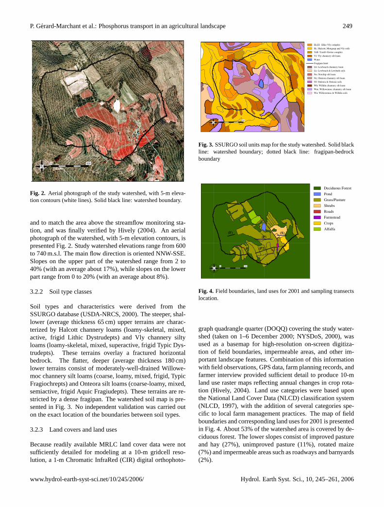
N0 500

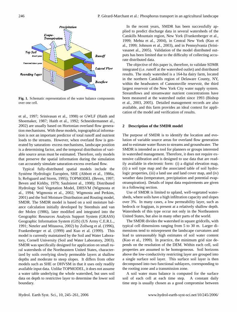
Fig. 2. Aerial photograph of the study watershed, with 5-m eleva-tion contours (white lines). Solid black line: watershed boundary.

and to match the area above the streamflow monitoring sta-tion, and was finally verified by Hively (2004). An aerialphotograph of the watershed, with 5-m elevation contours, ispresented Fig. 2. Study watershed elevations range from 600to 740 m.s.l. The main flow direction is oriented NNW-SSE.Slopes on the upper part of the watershed range from 2 to40% (with an average about 17%), while slopes on the lowerpart range from 0 to 20% (with an average about 8%).

3.2.2 Soil type classes

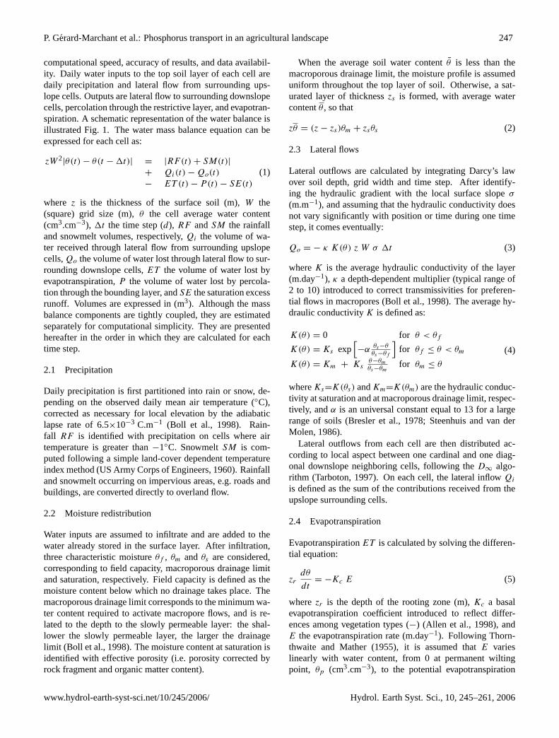
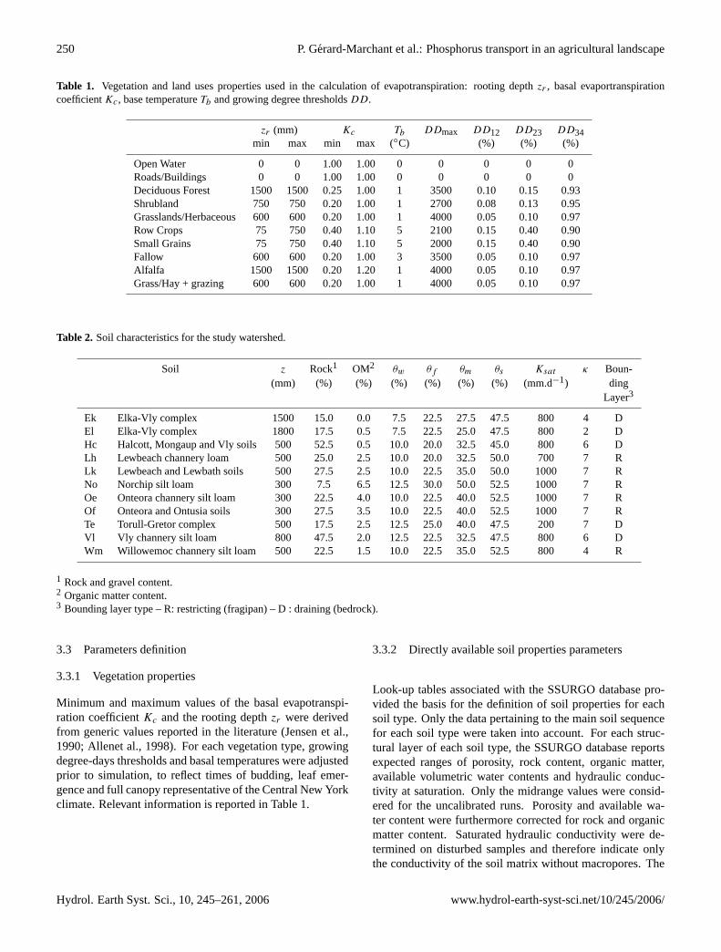
Soil types and characteristics were derived from theSSURGO database (USDA-NRCS, 2000). The steeper, shal-lower (average thickness 65 cm) upper terrains are charac-terized by Halcott channery loams (loamy-skeletal, mixed,active, frigid Lithic Dystrudepts) and Vly channery siltyloams (loamy-skeletal, mixed, superactive, frigid Typic Dys-trudepts). These terrains overlay a fractured horizontalbedrock. The flatter, deeper (average thickness 180 cm)lower terrains consist of moderately-well-drained Willowe-moc channery silt loams (coarse, loamy, mixed, frigid, TypicFragiochrepts) and Onteora silt loams (coarse-loamy, mixed,semiactive, frigid Aquic Fragiudepts). These terrains are re-stricted by a dense fragipan. The watershed soil map is pre-sented in Fig. 3. No independent validation was carried outon the exact location of the boundaries between soil types.

3.2.3 Land covers and land uses

Because readily available MRLC land cover data were notsufficiently detailed for modeling at a 10-m gridcell reso-lution, a 1-m Chromatic InfraRed (CIR) digital orthophoto-

N

Ek,El: Elka−Vly complex Hc: Halcott, Mongaup and Vly soils TeB: Torull−Gretor complex Vl: Vly channery silt loam Water Fragipan limit Lh: Lewbeach channery loam Lk: Lewbeach & Lewbath soils No: Norchip silt loam Oe: Onteora channery silt loam Of: Onteora & Ontusia soils Wh: Willdin channery silt loam Wm: Willowemoc channery silt loam Wn: Willowemoc & Willdin soils

0 500

Fig. 3. SSURGO soil units map for the study watershed. Solid blackline: watershed boundary; dotted black line: fragipan-bedrockboundary

N

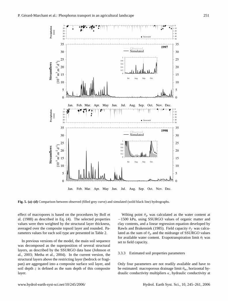
(P2)

(P)(S)(F)

Deciduous Forest Pond Grass/Pasture Shrubs Roads Farmstead Crops Alfalfa

0 500

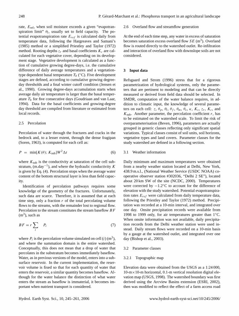
Fig. 4. Field boundaries, land uses for 2001 and sampling transectslocation.

graph quadrangle quarter (DOQQ) covering the study water-shed (taken on 1–6 December 2000; NYSDoS, 2000), wasused as a basemap for high-resolution on-screen digitiza-tion of field boundaries, impermeable areas, and other im-portant landscape features. Combination of this informationwith field observations, GPS data, farm planning records, andfarmer interview provided sufficient detail to produce 10-mland use raster maps reflecting annual changes in crop rota-tion (Hively, 2004). Land use categories were based uponthe National Land Cover Data (NLCD) classification system(NLCD, 1997), with the addition of several categories spe-cific to local farm management practices. The map of fieldboundaries and corresponding land uses for 2001 is presentedin Fig. 4. About 53% of the watershed area is covered by de-ciduous forest. The lower slopes consist of improved pastureand hay (27%), unimproved pasture (11%), rotated maize(7%) and impermeable areas such as roadways and barnyards(2%).



Table 1. Vegetation and land uses properties used in the calculation of evapotranspiration: rooting depthzr , basal evaportranspirationcoefficientKc, base temperatureTb and growing degree thresholdsDD.

zr (mm) Kc Tb DDmax DD12 DD23 DD34min max min max (◦C) (%) (%) (%)

Open Water 0 0 1.00 1.00 0 0 0 0 0Roads/Buildings 0 0 1.00 1.00 0 0 0 0 0Deciduous Forest 1500 1500 0.25 1.00 1 3500 0.10 0.15 0.93Shrubland 750 750 0.20 1.00 1 2700 0.08 0.13 0.95Grasslands/Herbaceous 600 600 0.20 1.00 1 4000 0.05 0.10 0.97Row Crops 75 750 0.40 1.10 5 2100 0.15 0.40 0.90Small Grains 75 750 0.40 1.10 5 2000 0.15 0.40 0.90Fallow 600 600 0.20 1.00 3 3500 0.05 0.10 0.97Alfalfa 1500 1500 0.20 1.20 1 4000 0.05 0.10 0.97Grass/Hay + grazing 600 600 0.20 1.00 1 4000 0.05 0.10 0.97

Table 2. Soil characteristics for the study watershed.

Soil z Rock1 OM2 θw θf θm θs Ksat κ Boun-(mm) (%) (%) (%) (%) (%) (%) (mm.d−1) ding

Layer3

Ek Elka-Vly complex 1500 15.0 0.0 7.5 22.5 27.5 47.5 800 4 DEl Elka-Vly complex 1800 17.5 0.5 7.5 22.5 25.0 47.5 800 2 DHc Halcott, Mongaup and Vly soils 500 52.5 0.5 10.0 20.0 32.5 45.0 800 6 DLh Lewbeach channery loam 500 25.0 2.5 10.0 20.0 32.5 50.0 700 7 RLk Lewbeach and Lewbath soils 500 27.5 2.5 10.0 22.5 35.0 50.0 1000 7 RNo Norchip silt loam 300 7.5 6.5 12.5 30.0 50.0 52.5 1000 7 ROe Onteora channery silt loam 300 22.5 4.0 10.0 22.5 40.0 52.5 1000 7 ROf Onteora and Ontusia soils 300 27.5 3.5 10.0 22.5 40.0 52.5 1000 7 RTe Torull-Gretor complex 500 17.5 2.5 12.5 25.0 40.0 47.5 200 7 DVl Vly channery silt loam 800 47.5 2.0 12.5 22.5 32.5 47.5 800 6 DWm Willowemoc channery silt loam 500 22.5 1.5 10.0 22.5 35.0 52.5 800 4 R

1 Rock and gravel content.2 Organic matter content.3 Bounding layer type – R: restricting (fragipan) – D : draining (bedrock).

3.3 Parameters definition

3.3.1 Vegetation properties

Minimum and maximum values of the basal evapotranspi-ration coefficientKc and the rooting depthzr were derivedfrom generic values reported in the literature (Jensen et al.,1990; Allenet al., 1998). For each vegetation type, growingdegree-days thresholds and basal temperatures were adjustedprior to simulation, to reflect times of budding, leaf emer-gence and full canopy representative of the Central New Yorkclimate. Relevant information is reported in Table 1.

3.3.2 Directly available soil properties parameters

Look-up tables associated with the SSURGO database pro-vided the basis for the definition of soil properties for eachsoil type. Only the data pertaining to the main soil sequencefor each soil type were taken into account. For each struc-tural layer of each soil type, the SSURGO database reportsexpected ranges of porosity, rock content, organic matter,available volumetric water contents and hydraulic conduc-tivity at saturation. Only the midrange values were consid-ered for the uncalibrated runs. Porosity and available wa-ter content were furthermore corrected for rock and organicmatter content. Saturated hydraulic conductivity were de-termined on disturbed samples and therefore indicate onlythe conductivity of the soil matrix without macropores. The



Jan. Feb. Mar. Apr. May Jun. Jul. Aug. Sep. Oct. Nov. Dec.

0

5

10

15

20

25

30

35

[10-3

m3 .m

-2.d

-1]

ObservedSimulated


0

5

10

15

20

25

30

35

[10-3

m3 .m

-2.d

-1]

0

5

10

15

20

25

30

35

Stre

amflo

ws

1997

Jul. Aug. Sep. Oct.

0

0.2

0.4

0.6

0.8

1

50403020100

Snowmelt50403020100

Prec

ipita

tion

[mm

]


0

5

10

15

20

25

30

35

[10-3

m3 .m

-2.d

-1]

ObservedSimulated


0

5

10

15

20

25

30

35

[10-3

m3 .m

-2.d

-1]

0

5

10

15

20

25

30

35

Stre

amflo

ws

1998

Jul. Aug. Sep. Oct.

0

0.2

0.4

0.6

0.8

1

50403020100

Snowmelt50403020100

Prec

ipita

tion

[mm

]

Fig. 5. (a)–(d)Comparison between observed (filled grey curve) and simulated (soild black line) hydrographs.

effect of macropores is based on the procedures by Boll etal. (1988) as described in Eq. (4). The selected propertiesvalues were then weighted by the structural layer thickness,averaged over the composite topsoil layer and rounded. Pa-rameters values for each soil type are presented in Table 2.

In previous versions of the model, the main soil sequencewas decomposed as the superposition of several structurallayers, as described by the SSURGO data base (Johnson etal., 2003; Metha et al., 2004). In the current version, thestructural layers above the restricting layer (bedrock or fragi-pan) are aggregated into a composite surface soil layer, andsoil depthz is defined as the sum depth of this compositelayer.

Wilting point θp was calculated as the water content at−1500 kPa, using SSURGO values of organic matter andclay contents, and a linear regression equation developed byRawls and Brakensiek (1985). Field capacityθf was calcu-lated as the sum ofθp and the midrange of SSURGO valuesfor available water content. Evapotranspiration limitθl wasset to field capacity.

3.3.3 Estimated soil properties parameters

Only four parameters are not readily available and have tobe estimated: macroporous drainage limitθm, horizontal hy-draulic conductivity multipliersκ, hydraulic conductivity at




0

5

10

15

20

25

30

35

[10-3

m3 .m

-2.d

-1]

ObservedSimulated


0

5

10

15

20

25

30

35

[10-3

m3 .m

-2.d

-1]

0

5

10

15

20

25

30

35

Stre

amflo

ws

2000

Jul. Aug. Sep. Oct.

0

0.2

0.4

0.6

0.8

1

50403020100

Snowmelt50403020100

Prec

ipita

tion

[mm

]


0

5

10

15

20

25

30

35

[10-3

m3 .m

-2.d

-1]

ObservedSimulated


0

5

10

15

20

25

30

35

[10-3

m3 .m

-2.d

-1]

0

5

10

15

20

25

30

35

Stre

amflo

ws

2001

Jul. Aug. Sep. Oct.

0

0.2

0.4

0.6

0.8

1

50403020100

Snowmelt50403020100

Prec

ipita

tion

[mm

]

Fig. 5. Continued.

saturation of the bounding layerKsub, and percolation frac-tion delivered to streamflow,r.

In previous versions of the model, decreasing values ofthe multipliersκ were allocated from the top structural layerto the bottom one (Mehta et al., 2004). In the current ver-sion, the multipliers were assumed to decrease exponentiallywith topsoil thickness, from 10 for the shallowest soils of thewatershed to 2 for the deepest ones. The values were ini-tially chosen to reproduce field observations that hydraulicconductivities derived from bore hole measurements were upto one order of magnitude larger than those reported in theSSURGO database, for which conductivities are determinedon disturbed samples (unpublished data).

The macroporous drainage limit,θm, is a key parametercontrolling subsurface lateral flows and percolation. Prelimi-nary investigations indicated that ifθm was set to a low value,simulated percolation would last for too long a period forwet soils, as compared with observed baseflows, and wouldrestart after a too short period for dry soils, leading to over-estimated baseflows at the beginning and end of the summerperiod. Eventually, for soils with a restrictive layer of lessthan 3 m, the parameter was estimated from field capacityand soil depth, through the relation:

θm = θf |3/z|1/4 (8)

with the soil depthz expressed in (m). This relation relieson the hypotheses that under hydrostatic conditions, the soil



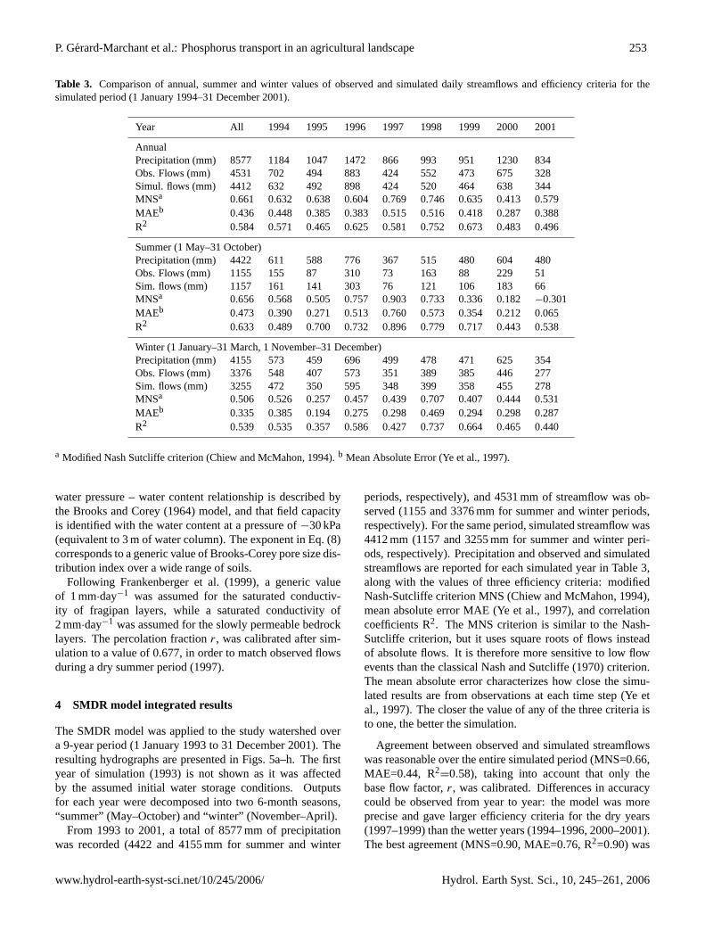
Table 3. Comparison of annual, summer and winter values of observed and simulated daily streamflows and efficiency criteria for thesimulated period (1 January 1994–31 December 2001).

Year All 1994 1995 1996 1997 1998 1999 2000 2001

AnnualPrecipitation (mm) 8577 1184 1047 1472 866 993 951 1230 834Obs. Flows (mm) 4531 702 494 883 424 552 473 675 328Simul. flows (mm) 4412 632 492 898 424 520 464 638 344MNSa 0.661 0.632 0.638 0.604 0.769 0.746 0.635 0.413 0.579MAEb 0.436 0.448 0.385 0.383 0.515 0.516 0.418 0.287 0.388R2 0.584 0.571 0.465 0.625 0.581 0.752 0.673 0.483 0.496

Summer (1 May–31 October)Precipitation (mm) 4422 611 588 776 367 515 480 604 480Obs. Flows (mm) 1155 155 87 310 73 163 88 229 51Sim. flows (mm) 1157 161 141 303 76 121 106 183 66MNSa 0.656 0.568 0.505 0.757 0.903 0.733 0.336 0.182−0.301MAEb 0.473 0.390 0.271 0.513 0.760 0.573 0.354 0.212 0.065R2 0.633 0.489 0.700 0.732 0.896 0.779 0.717 0.443 0.538

Winter (1 January–31 March, 1 November–31 December)Precipitation (mm) 4155 573 459 696 499 478 471 625 354Obs. Flows (mm) 3376 548 407 573 351 389 385 446 277Sim. flows (mm) 3255 472 350 595 348 399 358 455 278MNSa 0.506 0.526 0.257 0.457 0.439 0.707 0.407 0.444 0.531MAEb 0.335 0.385 0.194 0.275 0.298 0.469 0.294 0.298 0.287R2 0.539 0.535 0.357 0.586 0.427 0.737 0.664 0.465 0.440

a Modified Nash Sutcliffe criterion (Chiew and McMahon, 1994).b Mean Absolute Error (Ye et al., 1997).

water pressure – water content relationship is described bythe Brooks and Corey (1964) model, and that field capacityis identified with the water content at a pressure of−30 kPa(equivalent to 3 m of water column). The exponent in Eq. (8)corresponds to a generic value of Brooks-Corey pore size dis-tribution index over a wide range of soils.

Following Frankenberger et al. (1999), a generic valueof 1 mm·day−1 was assumed for the saturated conductiv-ity of fragipan layers, while a saturated conductivity of2 mm·day−1 was assumed for the slowly permeable bedrocklayers. The percolation fractionr, was calibrated after sim-ulation to a value of 0.677, in order to match observed flowsduring a dry summer period (1997).

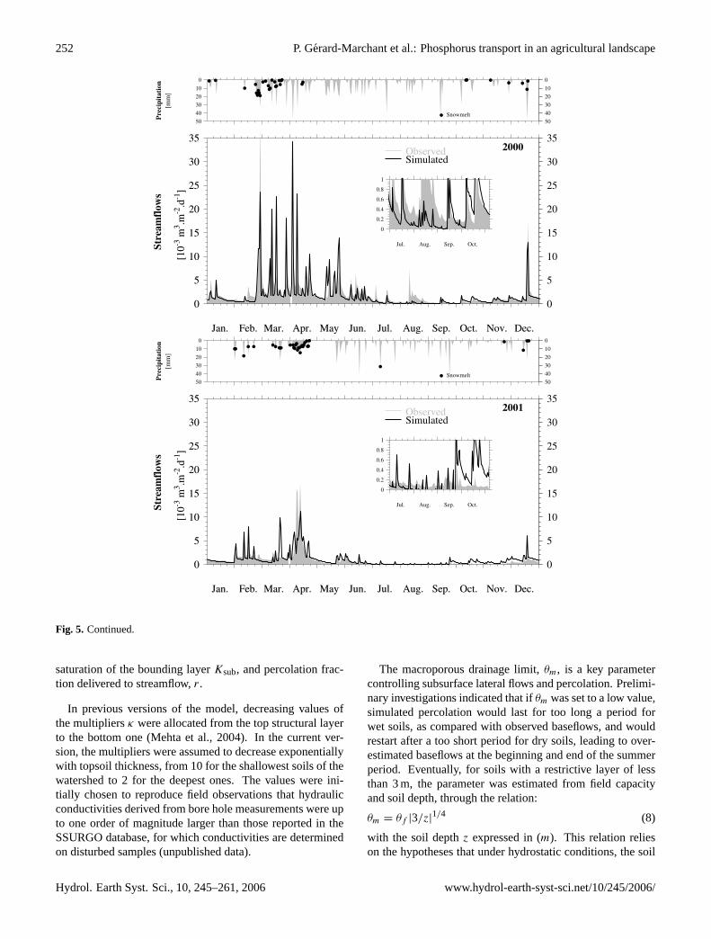
4 SMDR model integrated results

The SMDR model was applied to the study watershed overa 9-year period (1 January 1993 to 31 December 2001). Theresulting hydrographs are presented in Figs. 5a–h. The firstyear of simulation (1993) is not shown as it was affectedby the assumed initial water storage conditions. Outputsfor each year were decomposed into two 6-month seasons,“summer” (May–October) and “winter” (November–April).

From 1993 to 2001, a total of 8577 mm of precipitationwas recorded (4422 and 4155 mm for summer and winter

periods, respectively), and 4531 mm of streamflow was ob-served (1155 and 3376 mm for summer and winter periods,respectively). For the same period, simulated streamflow was4412 mm (1157 and 3255 mm for summer and winter peri-ods, respectively). Precipitation and observed and simulatedstreamflows are reported for each simulated year in Table 3,along with the values of three efficiency criteria: modifiedNash-Sutcliffe criterion MNS (Chiew and McMahon, 1994),mean absolute error MAE (Ye et al., 1997), and correlationcoefficients R2. The MNS criterion is similar to the Nash-Sutcliffe criterion, but it uses square roots of flows insteadof absolute flows. It is therefore more sensitive to low flowevents than the classical Nash and Sutcliffe (1970) criterion.The mean absolute error characterizes how close the simu-lated results are from observations at each time step (Ye etal., 1997). The closer the value of any of the three criteria isto one, the better the simulation.

Agreement between observed and simulated streamflowswas reasonable over the entire simulated period (MNS=0.66,MAE=0.44, R2

=0.58), taking into account that only thebase flow factor,r, was calibrated. Differences in accuracycould be observed from year to year: the model was moreprecise and gave larger efficiency criteria for the dry years(1997–1999) than the wetter years (1994–1996, 2000–2001).The best agreement (MNS=0.90, MAE=0.76, R2=0.90) was



obtained for the dry summer 1997 on which the calibrationof the percolation rater was performed. This was expectedsince it was assumed, for lack of better data, that the fractionof the watershed contributing to percolation was constant. Inreality it is not and because of the many springs in the water-shed, it could even be affected by the previous year’s rainfall.Therefore, more complex reservoir models requiring moreparameters were also considered. However, they did not sig-nificantly improved baseflow simulations. It was finally de-cided to use the simplest model as presented above. Notethat the lack of knowledge of the complicated undergroundflow paths is a limitation for any hydrology model applied towatersheds in the Catskills.

It is also of interest to evaluate the model’s performanceby comparing the timing and intensities of simulated peakflows with observed data. Unlike watersheds where Horto-nian overland flow is the dominant process and where peakflows have a short duration (of a few minutes to a few hours),watershed where runoff is generated by saturation excess ex-hibit broader flow peaks. These peaks occur when a majorportion of the watershed contributes to runoff, during peri-ods when total rainfall amounts exceeds evaporation greatly.Moreover, since precipitation data was available on a dailybasis only, observed and simulated peak flows were com-pared at the same daily time step.

Peak flow timing, intensities and hydrograph recessionwere usually well simulated. Occasionally peaks were not re-produced in winter (e.g. 25 January 1996, 6 February 1997,17 January 1998, 15 Feburary 2000 in Figs. 5c–g, respec-tively), while some peaks were incorrectly simulated duringobserved low winter flows (e.g. 23 January 1997, 22 March1999 in Figs. 5d and f, respectively). This discrepancy wasattributed to the use of off-site climate data, as described be-low.

Agreement between observed and simulated flows wasbetter during summer (MNS=0.66, MAE=0.47, R2

=0.63)than during winter (MNS=0.51, MAE=0.33, R2=0.54). Hereagain, peak timing and intensities were generally well pre-dicted, with a slight underestimation of peakflows. A signif-icant underestimation of peakflows was observed in August2000 (Fig. 5g), when precipitation occurred late in the sea-son, as short-duration, high-intensity summer thunderstormsover dry soils. Low flows were usually underestimated (e.g.August 1998 and July 1999).

Three main sources can explain the occasional poormatches between observed and predicted hydrographs.First, water balance components are not perfectly mod-eled. Snowmelts are only crudely estimated by thetemperature-index method currently implemented. More re-alistic snowmelt routines involve calculation of a radiationbalance, even simplified (Walteret al., 2005), but requireddata were not readily available. Soil freezing and interactionsbetween rainfall and snow cover should also be taken intoaccount. Moreover, infiltration-excess overland flow duringsummer months is modeled on impervious areas only and

not on other soils, which for high rainfall intensity summerstorms will likely cause the underestimation of peakflowssuch as were observed in August 2000. Also, SMDR takesinto account perched water tables only, and regional ground-water only indirectly. The latter is a direct consequence ofthe lack of information about the subsoil structure and thelocation of subsurface flow paths.

An additional source of errors comes from non-optimal pa-rameter calibration. For example, an overestimation of thesoil drainage properties would lead to too rapid a depletionof the water storage by lateral flows, causing an underestima-tion of percolation during summer months. This hypothesiscan explain the simulation of lower summer flows than wereobserved.

Finally, weather data were obtained from an offsite stationabout 20 km from the site. In the summer, thunderstormsare localized, and precipitation measured at Delhi, NY maynot equal precipitation occurring onsite. For example, on 7August 2000, 18 mm of rain (as recorded in Delhi) producedonly 0.7 mm of streamflow at the watershed outlet, whilethree days later, 15 mm of rain produced 7.3 mm of stream-flows. It is likely that the actual precipitation for the stormthat hit Delhi on 7 August 2000 was in fact much less on thestudy watershed. Model results may improve substantiallywith the use of on-site climatic data. Similarly, the use ofoff-site temperature data may have contributed to the imper-fect reproduction of snowmelt events.

5 SMDR model distributed results

Alone, comparison of observed and simulated hydrographsis not a sufficient check of the distributed accuracy of hy-drological models. For example, Refsgaard and Knud-sen (1996) observed that after proper calibration, a con-ceptual lumped model (NAM) and a physically-based dis-tributed model (MIKE-SHE) predicted streamflows equallywell. Similarly, Johnson et al. (2003) compared SMDR re-sults with outputs simulated by HSPF, an infiltration-excessbased semi-distributed conceptual model. Both models gaveequally accurate hydrographs despite their different runoffgeneration mechanisms (Johnson et al., 2003).

A classical approach to assess the efficiency of a dis-tributed model such as SMDR consists in the quantitativecomparison of observed and simulated moisture contents atvarious locations throughout the watershed. Such a methodis intrinsically limited by its local character, as samples aretaken at specific locations, on particular dates. Even if thisapproach provides valuable information about the hydro-dynamic characteristics of the soils where the samples aretaken, it usually fails to identify variable source areas on alarger scale and to capture their dynamics.

A complementary validation consists in using direct in-formation about the location of springs, ephemeral streampaths and saturated areas, as obtained with GPS and mapping



(Mehta et al., 2001, 2004), or indirect information about theposition of hydrological features in the landscape. For exam-ple, diversion ditches and tile drains are usually installed tointercept overland flow and subsurface lateral flows, respec-tively, thus indicating the regular occurrence of runoff gener-ating areas upslope of these installations. In a related way,certain vegetation types, such as ferns and marsh grasses,grow preferentially in wet areas, and could be used as anindicator of the location of areas prone to generate runoff.Both direct and indirect validation approaches are presentedbelow.

5.1 Transect sampling

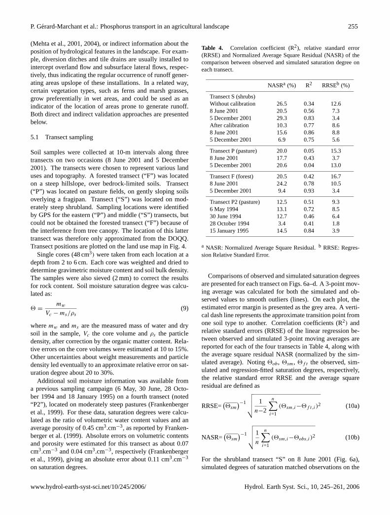
Soil samples were collected at 10-m intervals along threetransects on two occasions (8 June 2001 and 5 December2001). The transects were chosen to represent various landuses and topography. A forested transect (“F”) was locatedon a steep hillslope, over bedrock-limited soils. Transect(“P”) was located on pasture fields, on gently sloping soilsoverlying a fragipan. Transect (“S”) was located on mod-erately steep shrubland. Sampling locations were identifiedby GPS for the eastern (“P”) and middle (“S”) transects, butcould not be obtained the forested transect (“F”) because ofthe interference from tree canopy. The location of this lattertransect was therefore only approximated from the DOQQ.Transect positions are plotted on the land use map in Fig. 4.

Single cores (48 cm3) were taken from each location at adepth from 2 to 6 cm. Each core was weighted and dried todetermine gravimetric moisture content and soil bulk density.The samples were also sieved (2 mm) to correct the resultsfor rock content. Soil moisture saturation degree was calcu-lated as:

2 =mw

Vc − ms/ρs

(9)

wheremw andms are the measured mass of water and drysoil in the sample,Vc the core volume andρs the particledensity, after correction by the organic matter content. Rela-tive errors on the core volumes were estimated at 10 to 15%.Other uncertainties about weight measurements and particledensity led eventually to an approximate relative error on sat-uration degree about 20 to 30%.

Additional soil moisture information was available froma previous sampling campaign (6 May, 30 June, 28 Octo-ber 1994 and 18 January 1995) on a fourth transect (noted“P2”), located on moderately steep pastures (Frankenbergeret al., 1999). For these data, saturation degrees were calcu-lated as the ratio of volumetric water content values and anaverage porosity of 0.45 cm3.cm−3, as reported by Franken-berger et al. (1999). Absolute errors on volumetric contentsand porosity were estimated for this transect as about 0.07cm3.cm−3 and 0.04 cm3.cm−3, respectively (Frankenbergeret al., 1999), giving an absolute error about 0.11 cm3.cm−3

on saturation degrees.

Table 4. Correlation coefficient (R2), relative standard error(RRSE) and Normalized Average Square Residual (NASR) of thecomparison between observed and simulated saturation degree oneach transect.

NASRa (%) R2 RRSEb (%)

Transect S (shrubs)Without calibration 26.5 0.34 12.68 June 2001 20.5 0.56 7.35 December 2001 29.3 0.83 3.4After calibration 10.3 0.77 8.68 June 2001 15.6 0.86 8.85 December 2001 6.9 0.75 5.6

Transect P (pasture) 20.0 0.05 15.38 June 2001 17.7 0.43 3.75 December 2001 20.6 0.04 13.0

Transect F (forest) 20.5 0.42 16.78 June 2001 24.2 0.78 10.55 December 2001 9.4 0.93 3.4

Transect P2 (pasture) 12.5 0.51 9.36 May 1994 13.1 0.72 8.530 June 1994 12.7 0.46 6.428 October 1994 3.4 0.41 1.815 January 1995 14.5 0.84 3.9

a NASR: Normalized Average Square Residual.b RRSE: Regres-sion Relative Standard Error.

Comparisons of observed and simulated saturation degreesare presented for each transect on Figs. 6a–d. A 3-point mov-ing average was calculated for both the simulated and ob-served values to smooth outliers (lines). On each plot, theestimated error margin is presented as the grey area. A verti-cal dash line represents the approximate transition point fromone soil type to another. Correlation coefficients (R2) andrelative standard errors (RRSE) of the linear regression be-tween observed and simulated 3-point moving averages arereported for each of the four transects in Table 4, along withthe average square residual NASR (normalized by the sim-ulated average). Noting2ob, 2sm, 2f t the observed, sim-ulated and regression-fitted saturation degrees, respectively,the relative standard error RRSE and the average squareresidual are defined as

RRSE=(2sm

)−1

√√√√ 1

n−2

n∑i=1

(2sm,i−2f t,i)2 (10a)

NASR=(2sm

)−1

√√√√1

n

n∑i=1

(2sm,i−2obs,i)2 (10b)

For the shrubland transect “S” on 8 June 2001 (Fig. 6a),simulated degrees of saturation matched observations on the



0 20 40 60 80 100 120 140 160 1800

0.2

0.4

0.6

0.8

1

0 20 40 60 80 100 120 140 160 1800

0.2

0.4

0.6

0.8

1

Position from base of transect [m]

Satu

ratio

n de

gree

Observed

Simulated [w/o cal.]

Simulated [w/ cal.] 06/08/2001

0

0.2

0.4

0.6

0.8

1

0

0.2

0.4

0.6

0.8

1

Satu

ratio

n de

gree

Observed

Simulated [w/o cal.]

Simulated [w/ cal.] 12/05/2001

610

620

630

Ele

vatio

n [m

]

Shrubland transect ’S’

0 20 40 60 80 100 120 140 160 180 200 220 240 260 280 300 320 3400

0.2

0.4

0.6

0.8

1

0 20 40 60 80 100 120 140 160 180 200 220 240 260 280 300 320 3400

0.2

0.4

0.6

0.8

1


Satu

ratio

n de

gree

Observed

Simulated 06/08/2001

0

0.2

0.4

0.6

0.8

1

0

0.2

0.4

0.6

0.8

1

Satu

ratio

n de

gree

Observed


610

620

630

640

650

Ele

vatio

n [m

]

Pasture transect ’P’

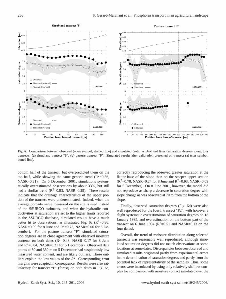
Fig. 6. Comparison between observed (open symbol, dashed line) and simulated (solid symbol and lines) saturation degrees along fourtransects,(a) shrubland transect “S”,(b) pasture transect “P”. Simulated results after calibration presented on transect (a) (star symbol,dotted line).

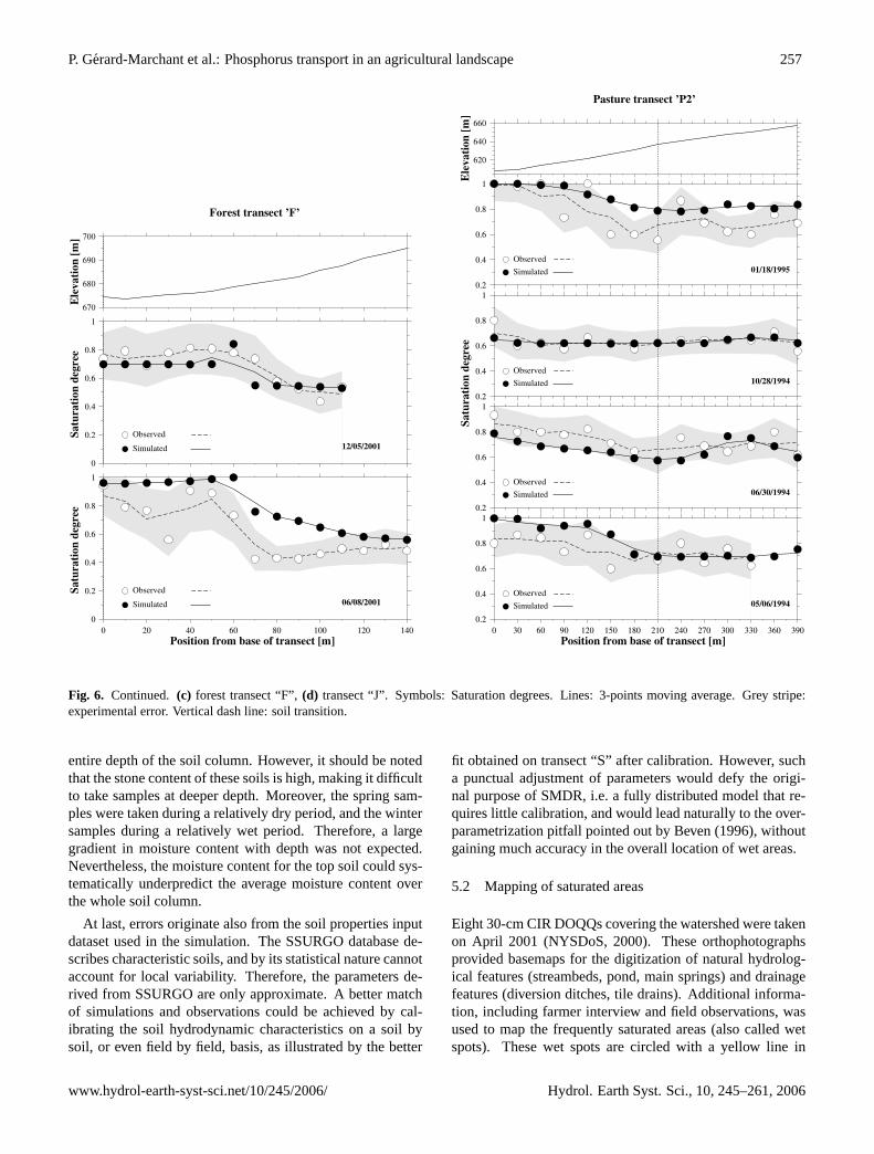
bottom half of the transect, but overpredicted them on thetop half, while showing the same generic trend (R2=0.56,NASR=0.21). On 5 December 2001, simulations system-atically overestimated observations by about 33%, but stillhad a similar trend (R2=0.83, NASR=0.29). These resultsindicate that the drainage characteristics of the upper por-tion of the transect were underestimated. Indeed, when theaverage porosity value measured on the site is used insteadof the SSURGO estimates, and when the hydraulic con-ductivities at saturation are set to the higher limits reportedin the SSURGO database, simulated results have a muchbetter fit to observations, as illustrated Fig. 6a (R2=0.86,NASR=0.09 for 8 June and R2=0.75, NASR=0.06 for 5 De-cember). For the pasture transect “P”, simulated satura-tion degrees are in close agreement with observed moisturecontents on both dates (R2=0.43, NASR=0.17 for 8 Juneand R2=0.04, NASR=0.21 for 5 December). Observed datapoints at 30 and 330 m on 5 December had suspiciously lowmeasured water content, and are likely outliers. These out-liers explain the low values of theR2. Corresponding errormargins were adapted in consequence. Results were also sat-isfactory for transect “F” (forest) on both dates in Fig. 6c,

correctly reproducing the observed greater saturation at theflatter base of the slope than on the steeper upper section(R2=0.78, NASR=0.24 for 8 June and R2=0.93, NASR=0.09for 5 December). On 8 June 2001, however, the model didnot reproduce as sharp a decrease in saturation degree withslope change as was observed at 70 m from the bottom of theslope.

Finally, observed saturation degrees (Fig. 6d) were alsowell reproduced for the fourth transect “P2”, with however aslight systematic overestimation of saturation degrees on 18January 1995, and overestimation on the bottom part of thetransect on 6 June 1994 (R2=0.51 and NASR=0.13 on thefour dates).

Overall, the trend of moisture distribution along selectedtransects was reasonably well reproduced, although simu-lated saturation degrees did not match observations at somelocations at some dates. Discrepancies between observed andsimulated results originated partly from experimental errorsin the determination of saturation degrees and partly from thepotential lack of representativity of the samples. Thus, someerrors were introduced by using only relatively shallow sam-ples for comparison with moisture contact simulated over the



0 20 40 60 80 100 120 1400

0.2

0.4

0.6

0.8

1

0 20 40 60 80 100 120 1400

0.2

0.4

0.6

0.8

1


Satu

ratio

n de

gree

Observed


0

0.2

0.4

0.6

0.8

1

0

0.2

0.4

0.6

0.8

1

Satu

ratio

n de

gree

Observed


670

680

690

700

Ele

vatio

n [m

]

Forest transect ’F’

0 30 60 90 120 150 180 210 240 270 300 330 360 3900.2

0.4

0.6

0.8

1

0 30 60 90 120 150 180 210 240 270 300 330 360 3900.2

0.4

0.6

0.8

1


ObservedSimulated 05/06/1994

0.2

0.4

0.6

0.8

1

0.2

0.4

0.6

0.8

1

Satu

ratio

n de

gree


0.2

0.4

0.6

0.8

1

0.2

0.4

0.6

0.8

1


0.2

0.4

0.6

0.8

1

0.2

0.4

0.6

0.8

1


620

640

660

Ele

vatio

n [m

]

Pasture transect ’P2’

Fig. 6. Continued. (c) forest transect “F”,(d) transect “J”. Symbols: Saturation degrees. Lines: 3-points moving average. Grey stripe:experimental error. Vertical dash line: soil transition.

entire depth of the soil column. However, it should be notedthat the stone content of these soils is high, making it difficultto take samples at deeper depth. Moreover, the spring sam-ples were taken during a relatively dry period, and the wintersamples during a relatively wet period. Therefore, a largegradient in moisture content with depth was not expected.Nevertheless, the moisture content for the top soil could sys-tematically underpredict the average moisture content overthe whole soil column.

At last, errors originate also from the soil properties inputdataset used in the simulation. The SSURGO database de-scribes characteristic soils, and by its statistical nature cannotaccount for local variability. Therefore, the parameters de-rived from SSURGO are only approximate. A better matchof simulations and observations could be achieved by cal-ibrating the soil hydrodynamic characteristics on a soil bysoil, or even field by field, basis, as illustrated by the better

fit obtained on transect “S” after calibration. However, sucha punctual adjustment of parameters would defy the origi-nal purpose of SMDR, i.e. a fully distributed model that re-quires little calibration, and would lead naturally to the over-parametrization pitfall pointed out by Beven (1996), withoutgaining much accuracy in the overall location of wet areas.

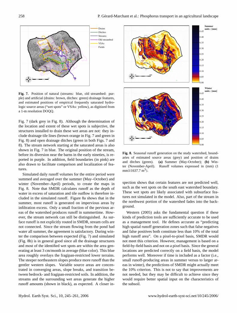
5.2 Mapping of saturated areas

Eight 30-cm CIR DOQQs covering the watershed were takenon April 2001 (NYSDoS, 2000). These orthophotographsprovided basemaps for the digitization of natural hydrolog-ical features (streambeds, pond, main springs) and drainagefeatures (diversion ditches, tile drains). Additional informa-tion, including farmer interview and field observations, wasused to map the frequently saturated areas (also called wetspots). These wet spots are circled with a yellow line in



N

Drains Ditches Streams Old streambed VSAs Fields

0 500

Fig. 7. Position of natural (streams: blue, old streambed: pur-ple) and artificial (drains: brown, ditches: green) drainage features,and estimated positions of empirical frequently saturated hydro-logic source areas (“wet spots” or VSAs: yellow), as digitized froma 1-m resolution DOQQ.

Fig. 7 (dark grey in Fig. 8). Although the determination ofthe location and extent of these wet spots is subjective, thestructures installed to drain these wet areas are not: they in-clude drainage tile lines (brown orange in Fig. 7 and green inFig. 8) and open drainage ditches (green in both Figs. 7 and8). The stream network starting at the saturated areas is alsoshown in Fig. 7 in blue. The original position of the stream,before its diversion near the barns in the early nineties, is re-ported in purple. In addition, field boundaries (in pink) arealso drawn to facilitate comparison and localization of fea-tures.

Simulated daily runoff volumes for the entire period weresummed and averaged over the summer (May–October) andwinter (November–April) periods, to create the maps inFig. 8. Note that SMDR calculates runoff as the depth ofwater in excess of saturation and tile outflow is therefore in-cluded in the simulated runoff. Figure 8a shows that in thesummer, most runoff is generated on impervious areas byinfiltration excess. Only a small fraction of the pervious ar-eas of the watershed produces runoff in summertime. How-ever, the stream network can still be distinguished. As sur-face runoff is not explicitly routed in SMDR, stream cells arenot connected. Since the stream flowing from the pond hadwater all summer, the agreement is satisfactory. During win-ter the comparison between expected (Fig. 7) and simulated(Fig. 8b) is in general good since all the drainage structuresand most of the identified wet spots are within the area gen-erating at least 3 cm/month in average (blue color). This bluearea roughly overlays the fragipan-restricted lower terrains.The steeper northeastern slopes produce more runoff than thegentler western slopes. Variable source areas are concen-trated in converging areas, slope breaks, and transition be-tween bedrock- and fragipan-restricted soils. In addition, thestreams and the surrounding wet areas generate the higherrunoff amounts (shown in black), as expected. A closer in-

N

N

0 500

0.00

0.05

0.10

0.15

0.20

0.25

0.30

0.35

0.40

0.45

Summer units : [mm]

N

N

0 500

0.00

0.05

0.10

0.15

0.20

0.25

0.30

0.35

0.40

0.45

Winter units : [mm]

Fig. 8. Seasonal runoff generation on the study watershed, bound-aries of estimated source areas (grey) and position of drainsand ditches (green). (a) Summer (May-October);(b) Win-ter (November-April). Runoff volumes expressed in (mm) (1mm∼=1637.7 m3).

spection shows that certain features are not predicted well,such as the wet spots on the south east watershed boundary.These wet spots are likely associated with subsurface fea-tures not simulated in the model. Also, part of the stream inthe northwest portion of the watershed fades into the back-ground.

Western (2005) asks the fundamental question if thesekinds of prediction tools are sufficiently accurate to be usedas a management tool. He defines accurate as “predictinghigh spatial runoff generation zones such that false negativesand false positives both constitute less than 10% of the totalhigh runoff area”. On a pixel-to-pixel basis, SMDR wouldnot meet this criterion. However, management is based on afield-by-field basis and not on a pixel basis. Since the generallocations are predicted correctly on a field basis, the modelperforms well. Moreover if time is included as a factor (i.e.,small runoff-producing areas in summer versus to larger ar-eas in winter), the predictions of SMDR might actually meetthe 10% criterion. This is not to say that improvements arenot needed, but they may be difficult to achieve since theywould require better spatial input on the characteristics ofthe subsoil.



6 Conclusions

Results of the hydrological model were good considering theminimal calibration. Hydrographs were generally properlysimulated, both in terms of timing and intensity of peaks,although summer baseflows were often underestimated, andsome winter peakflows were improperly reproduced. Agree-ment between observed and simulated saturation degreesalong four transects at different dates were usually correct.Visual comparison of seasonal cumulative runoff maps anddigitized hydrological features was also very encouraging.Improvements should focus on a better representation ofsnowmelt and soil freezing during winter periods, baseflowgeneration mechanisms during summer periods, and simpleestimation rules for some of the hydrodynamic properties(macroporous drainage limit and horizontal hydraulic con-ductivity). However, given the limited information aboutspatially distributed nature of soils, the question remains howthe suggested improvements can best be implemented to ob-tain more accurate simulated distributed moisture contents.

Acknowledgements.The United States Department of Agriculture,through the National Research Initiative funding, and Departmentof Interior provided primary funding for this study. The grant ofthe Department of Interior was administered by the New York StateWater Resources Institute. Additional funding was provided by theUnited States Department of Environmental Protection under theSafe Drinking Water Act, administered by the Watershed Agricul-tural Council (WAC). The data for validation was obtained fromP. Bishop of the New York State Department of EnvironmentalConservation (NYSDEC). M. R. Rafferty, J. L. Lojpersbergerof NYSDEC and S. Pacenka of WRI are acknowledged for thecollecting and/or modification of this data. In addition, we wouldlike to thank the members of the Town Brook Research Group,Watershed Agricultural Program Planners and Landowners for theirinvaluable discussions and insights regarding watershed processesin the Catskill Mountains. Specifically we would like to thank thecollaborating farm family for their willingness to participate in theresearch effort and their patience in dealing with us.

Edited by: N. Romano

References

Abbott, M. B., Bathurst, J. C., Cunge, J. A., O’Connell, P. E., andRasmussen, J.: An introduction to the European hydrologicalsystem – Systeme Hydrologique Europeen, “SHE”, 1. historyand philosophy of a physically based, distributed modeling sys-tem, J. Hydrol., 87, 45–59, 1986a.

Abbott, M. B., Bathurst, J. C., Cunge, J. A., O’Connell, P. E., andRasmussen, J.: An introduction to the European hydrologicalsystem – Systeme Hydrologique Europeen, “SHE”, 2. structureof a physically based, distributed modeling system, J. Hydrol.,87, 61–77, 1986b.

Allen, R. G., Pereira, L. S., Raes, D., and Smith, M.: Crop evap-otranspiration - Guidelines for computing crop water require-ments – FAO Irrigation and drainage paper 56, FAO – Food

and Agriculture Organization of the United Nations, Rome, IT,http://www.fao.org/docrep/X0490E/X0490E00.htm, 1998.

Arnold, J. G., Allen, P. M., and Bernhardt, G.: A comprehensivesurface-groundwater flow model, J. Hydrol., 142, 47–69, 1993.

Arnold, J. G., Williams, J. R., Srinivasan, R., King, K. W., andGriggs, R. H.: SWAT, Soil and Water Assessment Tool, USDA,Agriculture Research Service, Temple, TX 76502, 1994.

Beven, K. J.: A discussion of distributed hydrological modelling,in: Distributed Hydrological Modelling, edited by: Abbott, M.B. and Refsgaard, J. C., Kluwer, Dordrecht, NL, 255–277, 1996.

Beven, K. J. (Ed.): Distributed modeling in hydrology: Applica-tions of the TOPMODEL Concept, Adv. Hydrol. Proc. Wiley,Chichester, 1997.

Beven, K. J. and Kirkby, M. J.: A physically based, variable con-tributing area model of basin hydrology, Hydrol. Sci. Bull., 24,43–69, 1979.

Bicknell, B. R., Imhoff, J. C., Kittle Jr, J. L., Donigian, A. S.,and Johanson, R. C.: Hydrological Simulation Program-Fortran:User’s manual for version 11, US Environmental ProtectionAgency, National Exposure Research Laboratory, Athens, GA,1997.

Bishop, P. L., Hively, W. D., Stedinger, J. R., Bloomfield, J. A.,Rafferty, M. R., and Lojpersberger, J. L.: Multivariate analysisof paired watershed data to evaluate agricultural BMP effects onstream water phosphorus, J. Env. Qual., 34, 1087–1101, 2005.

Bishop, P. L., Rafferty, M., and Lojpersberger, J.: Event based wa-ter quality monitoring to determine effectiveness of agriculturalBMPs, Proceedings of the American Water Resources Associa-tion, International Congress on Watershed Management for Wa-ter Supply Systems, 29 June–2 July, 2003.

Boll, J., Brooks, E. S., Campbell, C. R., Stockle, C. O., Young, S.K., Hammel, J. E., and McDaniel, P. A.: Progress toward de-velopment of a GIS based water quality management tool forsmall rural watersheds: modification and application of a dis-tributed model, ASAE Annual International Meeting, Orlando,FL., ASAE paper 982230, 1998.

Bresler, E., Russo, D., and Miller, R. D.: Rapid estimate of unsat-urated hydraulic conductivity function, Soil Sci. Soc. Amer. J.,42, 170–177, 1978.

Brooks, R. H., and Corey, A. T.: Hydraulic properties of porousmedia, Colorado State Univ., Colorado, 1964.

Chiew, F. H. S. and McMahon, T. A.: Application of the dailyrainfall-runoff model MODHYDROLOG to 28 Australian catch-ments, J. Hydrol., 153, 383–416, 1994.

DiLuzio, M. D. and Arnold, J. G.: Formulation of a hybrid cali-bration approach for a physically based distributed model withNEXRAD data input, J. Hydrol., 298, 136–154, 2004.

Donigian, A. S., Bicknell, B. R., and Imhoff, J. C.: HydrologicalSimulation Program – Fortran (HSPF), Water Resour. Pubs., Col-orado, 1995.

Dunne, T. and Black, R.: Partial area contributing to storm run offin a small New-England watershed, Water Resour. Res., 6, 1296–1311, 1970.

Dunne, T., Moore, T. R., and Taylor, C. H.: Recognition and pre-diction of runoff-producing zones in humid regions, Hydrol. Sci.Bull., 20, 305–327, 1975.

ESRI: ArcView GIS 3.3, India, 2002.Frankenberger, J. R., Brooks, E. S., Walter, M. T., Walter, M. F., and

Steenhuis, T. S.: A GIS-based variable source area hydrology


http://www.fao.org/docrep/X0490E/X0490E00.htm


model, Hydrol. Processes, 13, 805–822, 1999.Gburek, W. J., Sharpley, A. N., and Pionke, H.: Identification

of critical source areas for phosphorus export from agriculturalcatchments, in: Advances in Hillslope Processes, edited by: An-derson, M. and Brookes, S., John Wiley & Sons, Chichester, UK,263–282, 1996.

Goudriaan, J. and van Laar, H.H.: Modelling Potential Crop GrowthProcesses, Textbook with Exercises, Kluwer Academic Publish-ers, 1994.

Haith, D. A., Mandel, R., and Wu, R. S.: Generalized watershedloading functions version 2.0: User’s manual, Tech. rep., Dept.of Agricultural and Biological Engineering, Cornell University,New York, 1992.

Haith, D. A. and Shoemaker, L. L.: Generalized watershed loadingfunctions for stream flow nutrients, Water Resour. Bull., 23, 471–478, 1987.

Hargreaves, G. H. and Samani, Z. A.: Reference crop evapotranspi-ration from temperature, Appl. Eng. Agric., 1, 96–99, 1985.

Hewlett, J. D. and Hibbert, A. R.: Factors affecting the responseof small watersheds to precipitation in humid regions, in: Foresthydrology, edited by: Sopper W. E. and Lull, H. W., PergamonPress, Oxford, UK, 275–290, 1967.

Hewlett, J.D. and Nutter, W.L.: The varying source area of stream-flow from upland basins, Proc. of the Symp. on Interdisciplinar-ity Aspects of Watershed Mgmt. 08/06/1970, ASCE, Montana,1970.

Hively, W. D.: Phosphorus loading from a monitored dairy farmlandscape, Ph.D. dissertation, Cornell University, Ithaca, NY,2004.

Horton, R. E.: The role of infiltration in the hydrological cycle,Transactions of the American Geophysical Union, 14, 446–460,1933.

Horton, R. E.: An approach toward a physical interpretation of in-filtration capacity, Soil Sci. Soc. Amer. Proc., 4, 399–418, 1933.

Jensen, M. E., Burman, R. D., and Allen, R. G. (Eds.): Evapotran-spiration and Irrigation Water Requirements, Vol. 70 of ASCEManuals and Reports on Engineering Practice, American Soci-ety of Civil Engineers, New York, 1990.

Johnson, M. S., Coon, W. F., Mehta, V. K., Steenhuis, T. S., Brooks,E. S., and Boll, J.: Application of two hydrologic models withdifferent runoff mechanisms to a hillslope dominated watershedin the Northeastern US: a comparison of HSPF and SMR, J. Hy-drol., 284, 57–76, 2003.

Kuo, W.-L., Steenhuis, T. S., McCulloch, C. E., Mohler, C. L., We-instein, D. A., DeGloria, S. D., and Swaney, D. P.: Effect ofgrid size on runoff and soil moisture for a variable-source-areahydrology model, Water Resour. Res., 35, 3419–3428, 1999.

Mehta, V. K., Johnson, M. S., Gerard-Marchant, P. G. F., Wal-ter, M. T., and Steenhuis, T. S.: Testing a variable source GIS-based hydrology model for watersheds in the northeastern US,the Soil Moisture Routing model, EOS Trans. AGU, 82, FallMeet. Suppl., Abstract H22I-05, 2001.

Mehta, V. K, Walter, M. T., Brooks, E. S., Steenhuis, T. S., Walter,M. F., Johnson, M. S., Boll, J., and Thongs, D.: Applicationof smr to modeling watersheds in the Catskills mountains, Env.Model. Assess., 9, 77–89, 2004.

Nash, J. E. and Sutcliffe, J. V.; River flow forecasting through con-ceptual models, part I – a discussion of principles, J. Hydrol., 10,238–250, 1970.

NCDC: Climatalogical data annual summary – New York, NationalClimate Data Center (NCDC), North Carolina, 2000.

Neitsch, S. L., Arnold, J. G., Kiniry, J. R., William, J. R., and King,K. W.: SWAT- Soil and Water Assessment Tool, 2000 – Theoret-ical documentation, Texas, 2002.

Neteler, M. and Mitasova, H.: Open Source GIS: A GRASS GISApproach, Kluwer Academic Publishers, Massachusetts, 2002.

NLCD: New York Land Cover Data Set,http://landcover.usgs.gov/nlcd/showdata.asp?code=NY&state=NewYork, US GeologicalSurvey (USGS), South Dakota, 1997.

NYSDoS: Digitally Enhanced Ortho Imagery Online Linkhttp://www.nysgis.state.ny.us/gateway/mg/napphtmls/f7.htm, Meta-data: http://www.nysgis.state.ny.us/gis3/data/dos.doqqorthos.html, NYS Department of State Division of Coastal Resources,GIS Unit, New York State, 2000.

Priestley, C. H. B. and Taylor, R. J.: On the assessment of surfaceheat fluxes and evaporation using large-scale parameters, Mon.Wea. Rev., 100, 81–92, 1972.

Rawls, W. and Brakensiek, D.: Prediction of soil water propertiesfor hydrologic modeling, Watershed Management in the Eight-ies, ASCE, 293–299, 1985.

Refsgaard, J. C. and Knudsen, J.: Operational validation and in-tercomparison of different types of hydrological models, WaterResour. Res., 32, 2189–2202, 1996.

Refsgaard, J. C. and Storm, B.: Computer Models of WatershedHydrology, edited by: She, M. and Singh, V., Water ResourcePublications, Colorado, 1995.

Saulnier, G.-M., Beven, K. J., and Obled, Ch.: Including spatiallyvariable soil depths in TOPMODEL, J. Hydrol., 202, 158–172,1998.

Schneiderman, E. M., Pierson, D. C., Lounsbury, D. G., and Zion,M. S.: Modeling the hydrochemistry of the Cannonsville water-shed with Generalized Watershed Loading Functions (GWLF),J. Amer. Water Resour. Assoc., 38, 1323–1347, 2002.

Soil and Water Laboratory: SMDR, the Soil Moisture Distribu-tion and Routing model version 2.0 – Documentation, Dept. ofBiological and Environmental Engineering, Cornell University,Ithaca, NY, 2003.

Soren, J.: The groundwater resources of Delaware County, NewYork, Tech. Rep. Water Res. Comm. Bull. GW-50., USGS, NewYork, 1963.

Srinivasan, M. S., Hamlett, J. M., Day, R. L., Sams, J. I., and Pe-tersen, G. W.: Hydrologic modeling in two subwatersheds ofLake Wallenpaupack, Pennsylvania, J. Amer. Water Resour. As-soc., 34, 963–978, 1998.

Srinivasan, M. S., Gerard-Marchant, P., Veith, T. L., Gburek, W.J., and Steenhuis, T. S.: Watershed-scale modeling of critical-source-areas of runoff generation and phosphorus transport, J.Amer. Water Resour. Assoc., 41, 361–375, 2005.

Steenhuis, T. S. and van der Molen, W. M.: The Thornthwaite-Mather method procedure as a simple engineering method to pre-dict recharge, J. Hydrol., 84, 221–229, 1986.

Tarboton, D. G.: A new method for the determination of flow direc-tions and upslope areas in grid digitale elevation models, WaterResour. Res., 33, 309–319, 1997.

Thornthwaite, C. W. and Mather, J. R.: The water balance, Tech.Rep. Publ. No. 8, Laboratory of Climatology, New Jersey, 1955.

US Army C.E.R.L.: GRASS 4.1 users’ manual, Tech. rep., USArmy Construction Engineering Research Laboratory, Illinois,


http://landcover.usgs.gov/nlcd/show_data.asp?code=NY&state=New_York

http://landcover.usgs.gov/nlcd/show_data.asp?code=NY&state=New_York

http://www.nysgis.state.ny.us/gateway/mg/napphtmls/f7.htm

http://www.nysgis.state.ny.us/gateway/mg/napphtmls/f7.htm

http://www.nysgis.state.ny.us/gis3/data/dos.doqq_orthos.html

http://www.nysgis.state.ny.us/gis3/data/dos.doqq_orthos.html


1991.US Army Corps of Engineers: Engineering and design: Runoff

from snowmelt, Tech. Rep. EM 1110-2-1406, US Army Corpsof Engineers, Govt. Printing Office, District of Columbia, 1960.

US Department of Agriculture, N.R.C.S.: Soil Survey Geographic(SSURGO) database for Delaware County, New York,http://www.ncgc.nrcs.usda.gov/products/datasets/ssurgo/, 2000.

US Geographical Survey (USGS): New York State Digital ElevationModels (DEM), Davenport quadrangle, Online through CornellUniversity Geographic Information Resources (CUGIR), Cor-nell University, New York,http://new-gis.mannlib.cornell.edu/CUGIR Data/data1/u40elu.dem.gz, 1998.

Walter, M. T., Brooks, E. S., McCool, D. K., King, L. G., Mol-nau, M., and Boll, J.: Process-based snowmelt modeling: doesit require more input data than temperature-index modeling?, J.Hydrol., 300(1–4), 65–75, 2005.

Walter, M. T., Walter, M. F., Brooks, E. S., Steenhuis, T. S., Boll,J., and Weiler, K. R.: Hydrologically sensitive areas: Variablesource area hydrology implications for water quality risk assess-ment, J. Soil Water Conserv., 3, 277–284, 2000.

Western, A.: Comments on “Distributed hydrological modeling oftotal dissolved phosphorus transport in an agricultural landscape,part 1: Distributed runoff generation” by Gerard-Marchant et al.,2005”, Hydrol. Earth Syst. Sci. Discuss., 2, 1537–1579 RC S780,available online:http://www.cosis.net/copernicus/EGU/hessd/2/S780/hessd-2-S780.pdf, 2005.

Wigmosta, M. S., Nijssen, B., Storck, P., and Lettenmaier, D.:The Distributed Hydrology Soil Vegetation Model, MathematicalModels of Small Watershed Hydrology and Applications, WaterResource Publications, Colorado, 2002.

Wigmosta, M. S. and Perkins, W. A.: Simulating the effects of for-est roads on watershed hydrology, Land Use and Watersheds:Human Influence on Hydrology and Geomorphology in Urbanand Forest Areas, Vol. 2 of Water Science and Application, AGU,2001.

Wigmosta, M. S., Vail, L., and Lettenmaier, D. P.: A distributedhydrology-vegetation model for complex terrain, Water Resour.Res., 30, 1665–1679, 1994.

Ye, W., Bates, B. C., Viney, N. R., Silvapan, M., and Jakeman, A. J.:Performance of conceptual rainfall-runoff models in low yieldingephemeral catchments, Water Resour. Res., 33, 153–166, 1997.

Zollweg, J. A., Gburek, W. J., and Steenhuis, T. S.: SMoRMod - agis-integrated rainfall-runoff model, Transactions of the ASAE,39, 1299–1307, 1996.


http://www.ncgc.nrcs.usda.gov/products/datasets/ssurgo/

http://www.ncgc.nrcs.usda.gov/products/datasets/ssurgo/

http://new-gis.mannlib.cornell.edu/CUGIR_Data/data1/u40elu.dem.gz

http://new-gis.mannlib.cornell.edu/CUGIR_Data/data1/u40elu.dem.gz

http://www.cosis.net/copernicus/EGU/hessd/2/S780/hessd-2-S780.pdf

http://www.cosis.net/copernicus/EGU/hessd/2/S780/hessd-2-S780.pdf

distributed hydrological modeling of total dissolved phosphorus transport in an agricultural...

Documents