distributed actuation requirements of piezoelectric structures under servoconstraints
TRANSCRIPT
Distributed actuation requirements of piezoelectric
structures under servoconstraints
T. M. Seigler, A. H. Ghasemi
University of Kentucky, Lexington, KY 40506-0503
and
A. Salehian
University of Waterloo, Waterloo, Ontario, N2L 3G1, Canada
January 16, 2011
Abstract
This article is concerned with the analysis of actuation requirements for dynamic
shape control of a piezoelectric structure. A general procedure is given for determining
the distributed actuation input required to satisfy a partially specified displacement
field for a generic piezoelectric shell structure. It is shown that under certain conditions
a servoconstraint that defines a finite number algebraic relations on the motion of
the material points of the structure can be satisfied in steady-state by an equivalent
number of independent actuators. Application examples are developed to demonstrate
application of the theory and its potential usefulness in the analysis and design of
advanced engineering structures.
1
1 Introduction.
One of the primary advantages piezoelectric actuators and sensors in the control of de-
formable structures is that they can be directly integrated into the structure and distributed
throughout it. As discussed in the review of Crawley [1], this in situ distribution of sens-
ing and control is extremely useful for the design and realization of “intelligent” structures.
However, one of the primary disadvantages of piezoelectrics is that the induced strains are
severely limited (on the order of 1000 µstrain), consequentially limiting the amount of force
that can be applied. Thus, an important consideration in the evaluation of piezoelectric
actuators for a given application is whether they can supply sufficient input to achieve the
desired objective. A general technique suggested here for evaluating piezoelectric actuators
is to specify a desired motion that should be achieved, whether it be zero motion due to
an external disturbance such as with vibration control or non-zero motion such as with ac-
tive shape control, and subsequently determine whether a distributed array of actuators is
capable of supplying the required input.
In mechanics, a specified motion is called a servoconstraint (or program constraint) [2]. The
simplest type of constraint is when the entire displacement field is specified; assuming that
this motion is a solution to the equations of motion and the boundary conditions, the required
forcing can be found by the direct inverse solution. The more interesting circumstance is
when the servoconstraint is such that only part of the displacement field is defined. Such
a circumstance might arise for example when trying to control the trailing edge angle of a
morphing wing [3], or localized vibration mitigation [4].
For a finite-dimensional square system (equal number of inputs and outputs) there are at
least two ways to solve for the input that satisfies a given servoconstraint. Perhaps the most
well-known is a common technique of nonlinear control called input-output linearization.
Another method, perhaps less well-known, is the projection technique of Parciwizki and
Blajer [5, 2]. Both methods ultimately require solving a set of ordinary differential equations.
Here we consider the servoconstraint problem for a deformable shell structure with a
2
number of discrete piezoelectric actuators attached to its surface. As outlined in Sec. 2,
the model used for the piezoelectric shell structure is based on Tzou’s form of Love’s theory
[6]. The particular servoconstraint considered is one for which the motion of a finite number
of material points of a structure is of interest. This servoconstraint is to be satisfied by at
least an equal number of piezoelectric actuators, the dimensions and location of which are
assumed known. Following modal expansion of the solution the dynamic equations takes
the form of a square input-output system, a form which differs from previous approaches to
dynamic shape control [7, 8].
The main results of the article are contained in Sec. 3, where a solution method is de-
veloped for computing the distributed actuation voltage that satisfies a periodic constraint.
Unlike the time domain methods cited above, the problem is here cast in the frequency
domain, which is particularly convenient for vibration analysis. To demonstrate the formal
application of this analysis procedure and its potential usefulness toward structural control
problems, two examples are developed in Sec. 4: the first considers free-end motion control
of a cantilevered beam, and the second investigates the application of localized vibration
mitigation.
2 Piezoelectric shell model.
We consider the vibration of an elastic shell structure with a distributed array of m piezo-
electric actuators. The undeflected mean plane of the shell is characterized by the curvilinear
coordinates α1 and α2. The position of a material point P of the mean plane relative to its
initial location (α1, α2) is quantified by the vector
u(P, t) =3∑
i=1
ui(α1, α2, t)ei (1)
3
where the ei are orthogonal unit vectors, e3 being normal to the mean surface . It is assumed
that the ui can be written in the standard separated form
ui(α1, α2, t) =∞∑
k=1
ηk(t)Uik(α1, α2), (2)
where the Uik are known mode shape functions, and the ηk are unknown modal participation
factors each governed by a second-order ordinary differential equation of the form
ηk(t) + 2ζkΩkηk(t) + Ω2
kηk(t) = Fk(t) + F ak (t), (3)
where Ωk is the natural frequency, ζk is the modal damping coefficient, and Fk and F ak are
the modal forces due to the external mechanical excitations and distributed piezoelectric
actuation, respectively. The modal forces due to external excitation is of the form [Soedel]
Fk(t) =1
ρhNk
∫
α1
∫
α2
(
3∑
i=1
FiUik
)
A1A2 dα1dα2, (4)
where Fi(α1, α2, t) accounts for external distributed mechanical disturbance on the surface
in the ei-direction, A1 and A2 are Lame parameters, ρ is the mass density, h the thickness,
and
Nk =
∫
α1
∫
α2
(
3∑
i=1
U2
ik
)
A1A2 dα1dα2.
The disturbance Fi(α1, α2, t) is decomposed as the product of a spatial function that quan-
tifies the location of the disturbance, and a time-dependent function. The modal force can
then be written in the general form
Fk(t) =∞∑
i=1
Dkiwi(t), (5)
4
where Dki is a constant that depends on the location of the disturbance, and wi(t) quantifies
the time-history of the disturbance.
Following the work of Tzou [6] the modal force due to piezoelectric actuation is
F ak (t) =
1
ρhNk
∫
α1
∫
α2
(
3∑
i=1
Lci(φ3)Uik
)
A1A2 dα1dα2, (6)
where φ3(α1, α2, t) is the distributed transverse applied voltage, and Lci is Love’s control
operator given by
Lc1φ3 = − 1
A1A2
∂
∂α1
(N c11
A2) − N c22
∂
∂α1
A2 +1
R1
[
∂
∂α1
(M c11
A2) − M c22
∂
∂α1
A2
]
Lc2φ3 = − 1
A1A2
∂
∂α2
(N c22
A1) − N c11
∂
∂α2
A1 +1
R2
[
∂
∂α2
(M c22
A1) − M c11
∂
∂α2
A1
]
Lc3φ3 = − 1
A1A2
∂
∂α1
(
1
A1
∂(M c11
A2)
∂α1
− M c22
A1
∂A2
∂α1
)
+∂
∂α2
(
1
A2
∂(M c22
A1)
∂α2
− M c11
A2
∂A2
∂α2
)
− A1A2
(
N c11
R1
+N c
22
R2
)
.
The actuator induced forces and moments, respectively N cii and M c
ii, are
M cii = riid3iEpφ3(α1, α2, t)
N cii = d3iEpφ3(α1, α2, t),
where Ep is the elastic modulus of the actuator, d3i is the actuator constant, and rii is the
moment arm measured from the plate neutral surface to the actuator mid-surface.
For a set of M actuators, the distributed control input φ3 is decomposed as
φ3(α1, α2, t) =M∑
i=1
φai (t)bi(α1, α2), (7)
where φai is the voltage input of the i-th actuator and the spatial function bi(α1, α2) quantifies
5
its size and placement. The actuation input thus takes the general form
F ak (t) =
M∑
i=1
Bkiφai (t) (8)
where Bki is a constant that is dependent on the placement, size, and electromechanical
properties of the i-th actuator. With Eq. (5) and (8), the m + n differential relations of Eq.
(3) can be written in the infinite-dimensional matrix form as
η(t) + ΛDη(t) + ΛKη(t) = Bv(t) + Dw(t) (9)
where η = [η1 η2 · · · ]T , ΛD = diag2ζ1ω1, 2ζ2ω2, · · · , ΛK = diagω1, ω2, · · · , w =
[w1 w2 · · · ]T , v = [φa1
· · · φam]T , and D and B contain the Dki and Bki components of
Eqs. (5) and (8), respectively.
3 Actuation of servoconstraints
Let u denote the mathematical vector function u = [u1 u2 u3]T . Define a set of material
points P1, ..., Ps for which desired steady-state motion is specified by the relation
limt→∞
E[ uT (P1, t) · · · uT (Ps, t) ]T = y(t), (10)
where E is a constant M × 3s matrix, and y is a time-dependent m-vector. It is noted
that the number of program constraints is equal to the number of actuators. The relation
of Eq. (10) is called the servoconstraint (or program constraint). We seek the distributed
piezoelectric actuation voltage v that enforces this constraint.
To further develop Eq. (10), the modal expansion of Eq. (2) is written in matrix form as
u(P, t) = [ U1(P ) U2(P ) U3(P ) ]T η(t). (11)
6
where, and Ui = [Ui1 Ui2 · · · ]T , i = 1, 2, 3. Letting U = [U1 U2 U3], an ∞ × 3 matrix
function, Eq. (7) can be further simplified as
u(P, t) = UT (P )η(t). (12)
It then follows that Eq. (12) can be written
limt→∞
E[ U(P1) · · · U(Ps) ]T η(t) = y(t). (13)
or concisely
limt→∞
Cη(t) = y(t), (14)
where C = E[U(P1) · · · U(Ps)]T .
Since we are interested in the steady-state response, it is convenient to work in the fre-
quency domain. The equations of motion, Eq. (9), together with the servoconstraint, Eq.
(14), are expressed in the frequency domain as
α(ω)η(ω) = Bv(ω) + Dw(ω) (15)
Cη(ω) = y(ω), (16)
where η(ω) denotes the frequency domain representation of η(t), etc., I is the identity matrix,
and
α(ω) = (ΛK − ω2I − iωΛD)−1
is called the admittance.
Given that Eqs. (15) and (16) are in general complex equations, it is sometimes convenient
to work with an equivalent real form of the equations of motion. By definition, the frequency
7
domain transformation assumes that the inputs are of the form v(t) = vc cos ωt + vs sin ωt,
and w(t) = wc cos ωt + ws sin ωt. Given that the system is linear it follows that in steady
state, the response is of the form η(t) = ηc cos ωt + ηs sin ωt. Substituting these into the
equations of motion thus gives
ΛK − ω2I −ωΛD
ωΛD ΛK − ω2I
ηc(ω)
ηs(ω)
=
B 0
0 B
vc(ω)
vs(ω)
+
D 0
0 D
wc(ω)
ws(ω)
.
(17)
Similarly, the output equation is
C 0
0 C
ηc(ω)
ηs(ω)
=
yc(ω)
ys(ω)
. (18)
The complex relations of Eqs. (15) and (16) will be used for subsequent development;
however, since they contain the same structure as Eqs. (17) and (18), the two are considered
interchangeable.
We now seek the input v, given r and Dw, such that Eq. (15) satisfies Eq. (16). Solving
Eq. (15) for η and substituting into Eq. (16) gives
(CαB)v + (CαD)w = y. (19)
Letting Gv = CαB and Gw = CαD, it follows that the control input that satisfies the
servoconstraint is
v = G−1
v (y − Gww). (20)
In steady state the actuation input of Eq. (20) is equivalent to any input provided by a
measurement based feedback control algorithm satisfying the servoconstraint of Eq. (14).
8
Hence, given known limits on the magnitude of v(t), the solution to Eq. (20) indicates
whether a given motion is possible under the defined actuation scheme. Note that the static
shape control solution is also contained in Eq. (20), corresponding to ω = 0.
Special case 1: non-zero motion constraint with zero disturbance.
Suppose that w = 0, and y 6= 0, in which case Eq. (20) reduces to
v = G−1
v y. (21)
The natural frequencies of the system are contained in the admittance matrix, α, which
show up as poles of the component transfer functions of Gv; the kl component is
(Gv)kl =∞∑
j=1
CkjBjl
Ω2
j − ω2 − 2iζjΩjω=
Zkl(ω)
Π∞
j=1(Ω2
j − ω2 − 2iζjΩjω)
where the Zkl are complex algebraic expressions in ω; assuming the series of Eq. (2) is
truncated at i = n, the order of Zkl in ω is less than n, implying that the magnitude of the
response “rolls off” for large ω. The frequency ω at which Zkl = 0 is a zero of Zkl, meaning
that the input vj does not affect the output yi at that frequency. The contribution of each
pole to the actuation input is scaled by the components of C and B.
Now we have important point, although perhaps an obvious one, that the poles and zeros
of G−1
v are not in general equal to those of Gv; and also, the poles of G−1
v are dependent on
the matrices C and B. For example, the inverse for a system with two independent actuators
is
G−1
v =Π∞
j=1(Ω2
j − ω2 − 2iζjΩjω)
Z11(ω)Z22(ω) − Z12(ω)Z21(ω)
Z22(ω) −Z12(ω)
−Z21(ω) Z11(ω)
.
Thus, the natural frequencies of the system show up as zeros of the inverse response, which
9
can potentially be canceled by a pole of G−1
v . The significance is that one can not expect
that the actuation input is the smallest for servoconstraints near the natural frequencies of
the system, nor necessarily that actuating a node of a natural frequency requires substantial
input magnitudes. Generally speaking, for a given placement, the actuation input is the
smallest when the motion to be controlled is close to the natural response of the structure.
These matters will be discussed further in the application example of Sec. 4.
Special case 2: zero motion constraint with non-zero disturbance.
Suppose now that y = 0 and w 6= 0, in which case Eq. (20) reduces to
v = G−1
v Gww. (22)
Similar to the previous special case, the poles of G−1
v Gw are affected by the choice of C and
B, and do not necessarily coincide with the natural frequencies of the system. Thus, it may
not be that the actuation requirements are the greatest when the disturbance w(t) is at one
of the natural frequencies of the system. If, for example, a material point to be actuated is
near a node of the natural frequency the input will decrease (assuming the actuator is placed
at a node).
The most apparent purpose for this constraint is the desire to suppress motion of certain
material elements in the presence of an external disturbance (i.e., localized vibration control).
However, the complete suppression of motion is potentially a very restrictive constraint. A
less restrictive constraint is yT y ≤ ǫ2, where ǫ can be taken as a function of ω. There are an
infinite number of inputs v(ω) that satisfy this constraint; we seek the one such that v(ω)
is a minimum. To solve the optimization problem, define the cost function
J =1
2vT v, (23)
10
and the equality constraint
yT y − ǫ2 = 0. (24)
Using the method of Lagrange multipliers, with Eq. (22) the function for which we seek a
minimum is
L =1
2(G−1
v y − G−1
v Gww)T (G−1
v y − G−1
v Gww) + λ(yT y − ǫ2). (25)
Taking the partial derivative of L with respect to y, and setting it equal to zero results in
y(ǫ) = (2λI + G−Tv G−1
v )−1G−Tv G−1
v Gww, (26)
where (·)−T indicates the transpose of the inverse (or vice versa). Substituting this into the
equality constraint gives
[(2λI + G−Tv G−1
v )−1G−Tv G−1
v Gww]T [(2λI + G−Tv G−1
v )−1G−Tv G−1
v Gww] − ǫ2 = 0 (27)
This equation can be solved numerically for λ, which gives y per Eq. (26), and subsequently
the minimum control input per Eq. (20).
Note that the smallest J independent of the constraint is J = 0, which corresponds to the
unactuated response: y = Gww. The value of ǫ corresponding to the uncatuated response,
denoted ǫ∗, is thus
ǫ∗ = [wTGTwGww]1/2.
Since J is a quadratic function in y, it follows that J decreases as ǫ decreases from 0 to
ǫ∗. Further increase of ǫ above ǫ∗ results an increase J . Hence, choosing 0 < ǫ < ǫ∗ ensures
that the actuation input is less than that corresponding to y = 0. Setting ǫ > ǫ∗ means that
11
the desired motion is greater than the nominal response due to the disturbance input, and
is thus not an appropriate constraint.
4 Applications
To demonstrate the application of the results of the previous sections, here two application
examples are presented corresponding to the two special cases of Sec. 2. The first example is a
thin cantilever plate for which it is desired to control material elements of the free edge. In the
second example, we consider localized vibration attenuation of a half-cylindrical shell. The
equations of motion for these examples are derived in the Appendix from the piezoelectric
shell theory of Sec. 2.
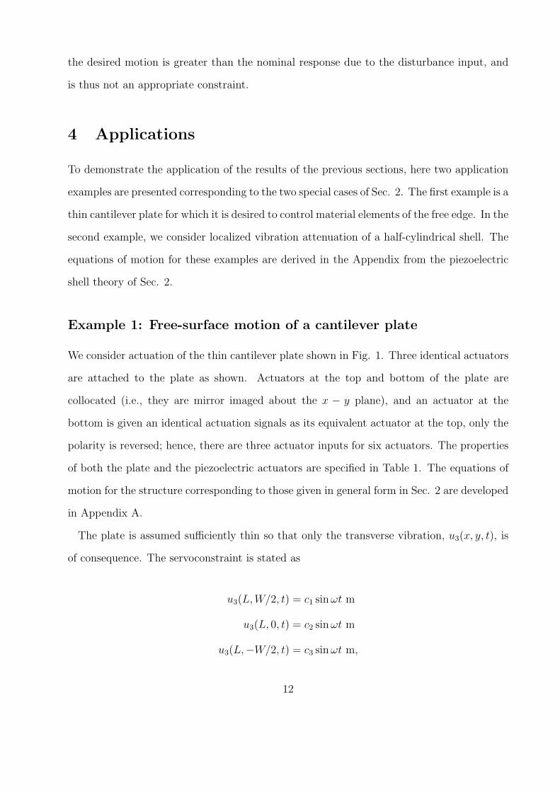
Example 1: Free-surface motion of a cantilever plate
We consider actuation of the thin cantilever plate shown in Fig. 1. Three identical actuators
are attached to the plate as shown. Actuators at the top and bottom of the plate are
collocated (i.e., they are mirror imaged about the x − y plane), and an actuator at the
bottom is given an identical actuation signals as its equivalent actuator at the top, only the
polarity is reversed; hence, there are three actuator inputs for six actuators. The properties
of both the plate and the piezoelectric actuators are specified in Table 1. The equations of
motion for the structure corresponding to those given in general form in Sec. 2 are developed
in Appendix A.
The plate is assumed sufficiently thin so that only the transverse vibration, u3(x, y, t), is
of consequence. The servoconstraint is stated as
u3(L,W/2, t) = c1 sin ωt m
u3(L, 0, t) = c2 sin ωt m
u3(L,−W/2, t) = c3 sin ωt m,
12
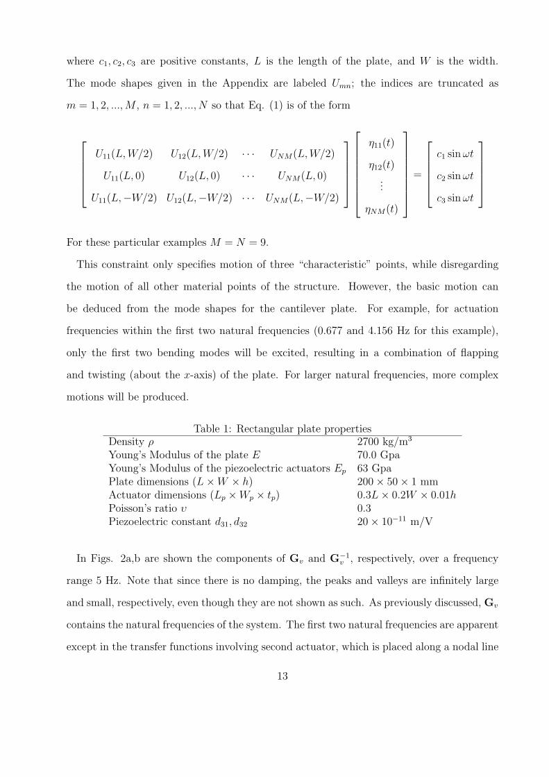
where c1, c2, c3 are positive constants, L is the length of the plate, and W is the width.
The mode shapes given in the Appendix are labeled Umn; the indices are truncated as
m = 1, 2, ...,M , n = 1, 2, ..., N so that Eq. (1) is of the form
U11(L,W/2) U12(L,W/2) · · · UNM(L,W/2)
U11(L, 0) U12(L, 0) · · · UNM(L, 0)
U11(L,−W/2) U12(L,−W/2) · · · UNM(L,−W/2)
η11(t)
η12(t)
...
ηNM(t)
=
c1 sin ωt
c2 sin ωt
c3 sin ωt
For these particular examples M = N = 9.
This constraint only specifies motion of three “characteristic” points, while disregarding
the motion of all other material points of the structure. However, the basic motion can
be deduced from the mode shapes for the cantilever plate. For example, for actuation
frequencies within the first two natural frequencies (0.677 and 4.156 Hz for this example),
only the first two bending modes will be excited, resulting in a combination of flapping
and twisting (about the x-axis) of the plate. For larger natural frequencies, more complex
motions will be produced.
Table 1: Rectangular plate propertiesDensity ρ 2700 kg/m3
Young’s Modulus of the plate E 70.0 GpaYoung’s Modulus of the piezoelectric actuators Ep 63 GpaPlate dimensions (L × W × h) 200 × 50 × 1 mmActuator dimensions (Lp × Wp × tp) 0.3L × 0.2W × 0.01hPoisson’s ratio υ 0.3Piezoelectric constant d31, d32 20 × 10−11 m/V
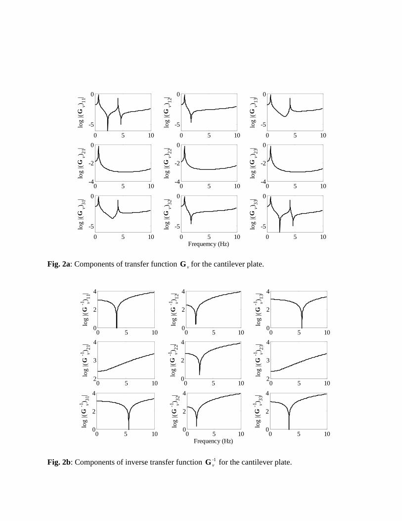
In Figs. 2a,b are shown the components of Gv and G−1
v , respectively, over a frequency
range 5 Hz. Note that since there is no damping, the peaks and valleys are infinitely large
and small, respectively, even though they are not shown as such. As previously discussed, Gv
contains the natural frequencies of the system. The first two natural frequencies are apparent
except in the transfer functions involving second actuator, which is placed along a nodal line
13
of the second mode (i.e., twisting about the x-axis). The zeros of G−1
v for this case are not
the natural frequencies of the system. Hence, as previously discussed, actuation of specified
motions at the natural frequencies does not necessarily require a “smaller” actuation input.
This will depend on the shape of the actuation and location of the actuators.
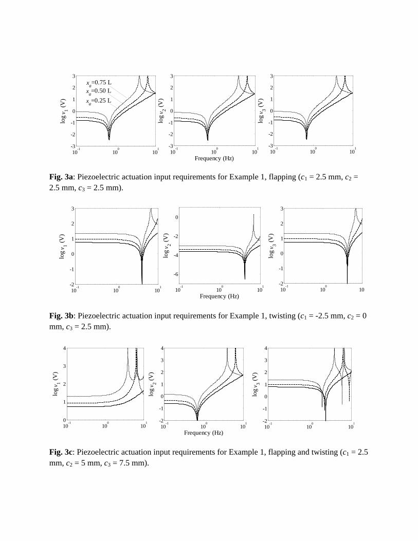
Based on the computations outlined in Sec. 3, Figs. 3a-c show the steady-state actua-
tor magnitude requirements for three different specifications of c1, c2, and c3, and for three
different locations of xa (cf. Fig. 1). The specifications of the constants respectively corre-
spond to actuation of flapping (Fig. 3a), twisting (Fig. 3b), and flapping with twisting (Fig.
3c). For the first two cases (Figs. 3a,b) it is not possible to produce pure flapping or pure
twisting since only three points are being controlled; however, the motions can be described
as “mostly flapping” and “mostly twisting”, respectively. As shown in Fig. 3a, the least
input is required to actuate flapping motion at around 0.7 Hz, slightly above the first natu-
ral frequency. It becomes more difficult to actuate the flapping motion as the frequency is
increased above 0.7 Hz (the maximum is dependent on the placement xa), which is expected
since the plate naturally wants to twist at these frequencies.
The twisting motion of Fig. 3b requires the least input at the second natural frequency,
which is also expected, since we are simply actuating a natural mode shape. Note that at the
first natural frequency and below the plate wants to solely flap, while we are commanding
twisting. However, the actuation input does not have a peak at the first natural frequency.
This is because the first mode is not excited due to the symmetry of both the material points
and actuator placements.
As shown in Fig. 3c, the input requirements to actuate both flappping and twisting become
substantially larger at higher frequencies. To limit the maximum voltage of each actuator to
less than 100V, the maximum frequency that this motion can be actuated is around 3 Hz.
14
Example 2: Localized vibration attenuation
The second application example examines local vibration attenuation of the shell structure
depicted in Fig. 4, with coordinates (α1, α2) = (x, β) For the servoconstraint three material
points (P1, P2, P3) are chosen, and it is desired that these points have zero transverse motion
in the presence of a point disturbance, w(t) =√
20 × 103 sin ωt N, located at (x, β) =
(0.75L, 0.75π). The servoconstraint is thus
u3(P1, t) = u3(P2, t) = u3(P3, t) = 0.
where P1 = (0.85L, 0.25π), P2 = (0.80L, 0.3π), P3 = (0.75L, 0.35π). These points could
represent for example a localized defect such as a crack, in which case it would be desirable
to limit their motion to prevent propagation. The source of the disturbance that must be
attenuated is located at a single point. Similar to the previous example, there are six actu-
ators (three sets collocated at the top and bottom of the structure) with three independent
voltage inputs. Properties of the shell and the piezoelectric actuators are listed in Table 2.
The equations of motion for this example are derived in Appendix B.
Table 2: Shell propertiesYoung Modulus of the Shell, E 70 GpaYoung Modulus of the piezoelectric patch, Ep 63 GpaDensity, ρ 2700 kg/m3
Shell Length, L 0.1 mShell Thickness, h 1 mmModal damping, ζi 0.01 %Piezoelectric Thickness, hs 0.01 hRadius of Curvature, R 0.5 mShell Curvature Angle πPoisson Ratio, υ 0.3Piezoelectric Constant, d3i 20 × 10−11 m/V
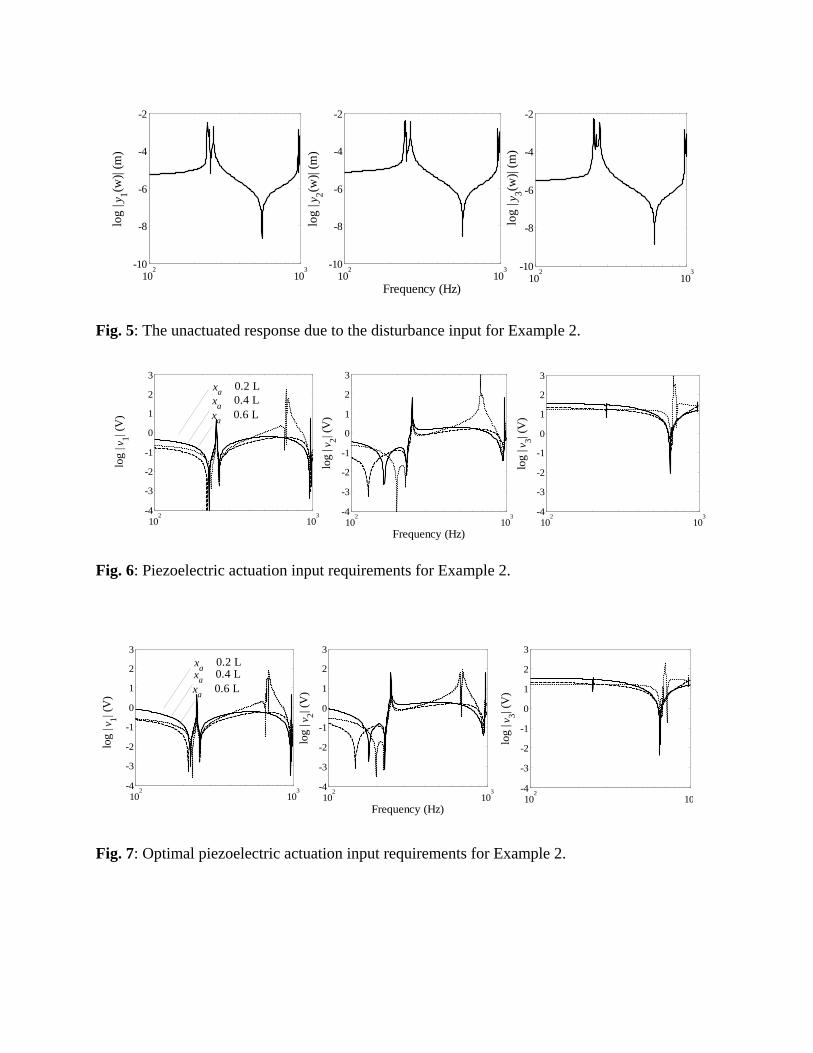
The unactuated response due to the disturbance input is shown in Fig. 5 for three different
locations of xa. The system has five natural frequencies between 240-270 Hz, and five more
between 970-1000 Hz. In Fig. 6 are shown the actuator inputs required to completely
15
suppress the motion of the three points. There is peak in all of the actuation inputs at 246
Hz and 970 Hz, the second and sixth natural frequency, for all actuator placements. Note
that there are several natural frequencies for which there is no substantial increase in the
actuator input.
As discussed in Sec. 3, the constraint that the motion of all point be completely suppressed
is a potentially restrictive constraint. For example, for the actuator placement of xa = 0.6L
there is a large peak on the order of 1000V at approximately 680 Hz. To relax this constraint
we set ǫ = 0.1 µm in the constraint of Eq. (24). The optimal results per the minimization
of Eq. (25) are shown in Fig. 7; here the actuator voltages for any placement is less than
260 V over the entire frequency range.
5 Concluding remarks.
It has been shown that a servoconstraint that takes the form a finite number of algebraic
relations on the motion of a piezoelectric shell structure can be satisfied by an equivalent
number of independent actuators. Such an analysis procedure is thought to be useful in
evaluating the applicability of piezoelectric actuators for active structures. The examples
that were developed demonstrated the analysis for potential applications involving static and
dynamic shape control, and localized vibration control. There are several interesting aspects
of the problem that has been left unexplored, particularly with regards to optimization. It is
clear that the actuator placement substantially effects the input requirements, and thus this
placement can be optimized. Further, there is the matter of defining the servoconstraint. For
the examples shown, the servoconstraint was based on actuating defined motion of a number
of material points. However, the constraint can involve any number of material points; it is
just that the number of constraints must be limited to the number of independent actuators.
Thus, while this type of servoconstraint can not be made equivalent to every given continuous
motion constraint, the two can be made “close”.
16
References
[1] E. F. Crawley. Intelligent stuctures for aerospace: a technology overview and assessment.
AIAA Journal, 32(8):1689–1699, 1994.
[2] W. Blajer. Dynamics and control of mechanical systems in partly specified motion.
Journal of the Franklin Institute, 334B:407–426, 1997.
[3] B. Sanders, F. E. Eastep, and E. Foster. Aerodynamic and aeroelastic considerations
of wings with conformal control surfaces for morphing aircraft. Journal of Aircraft,
40:94–99, 2007.
[4] J. H. Su and C. E. Ruckman. Aerodynamic and aeroelastic considerations of wings
with conformal control surfaces for morphing aircraft. Journal of Intelligent Material
Systems and Structures, 6:801–808, 1995.
[5] J. Parczewski and W. Blajer. On realization of program constraints: Part I - theory,
part II - practical implications. Journal of Applied Mechanics, 56:676–684, 1989.
[6] H. S. Tzou. Piezoelectric Shells: Distributed Sensing and Control of Continua. Springer,
1993.
[7] D. B. Koconis, L. P. Kollar, and G. S. Springer. Shape control of composite plates
and shells with embedded actuators. ii. desired shape specified. Journal of Composite
Materials, 28(5):459–482, 1994.
[8] S. S. Na and L. Librescu. Oscillation control of cantilevers via smart material technology
and optimal feedback control: actuator location and power consumption issues. Smart
Materials and Structures, 7(6):833–842, 1998.
[9] L. Meirovitch. Principles and Techniques of Vibrations. Prentice-Hall Inc.Uppers., 1997.
[10] A.W. Leissa. Vibration of plates. U.S. Government Printing Office, 1969.
17

[11] W. Sodel. Vibrations of shells and plates. Marcel Dekker, 2004.
18
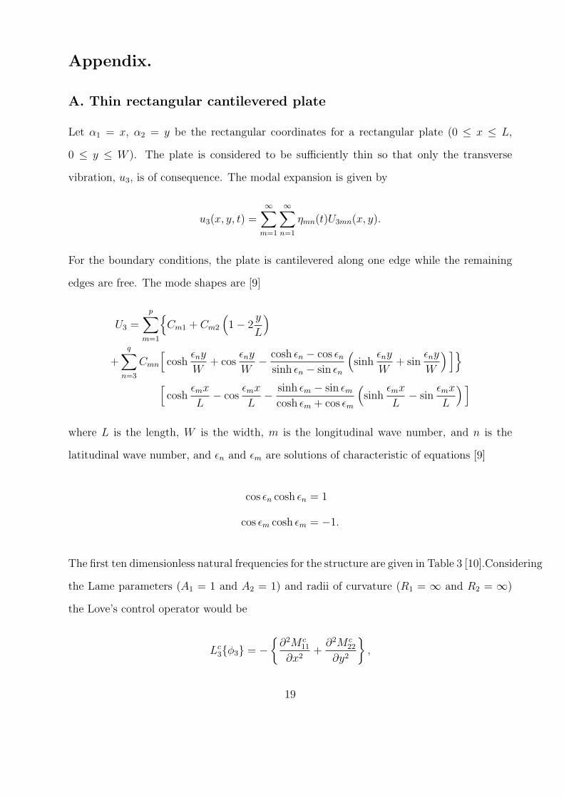
Appendix.
A. Thin rectangular cantilevered plate
Let α1 = x, α2 = y be the rectangular coordinates for a rectangular plate (0 ≤ x ≤ L,
0 ≤ y ≤ W ). The plate is considered to be sufficiently thin so that only the transverse
vibration, u3, is of consequence. The modal expansion is given by
u3(x, y, t) =∞∑
m=1
∞∑
n=1
ηmn(t)U3mn(x, y).
For the boundary conditions, the plate is cantilevered along one edge while the remaining
edges are free. The mode shapes are [9]
U3 =
p∑
m=1
Cm1 + Cm2
(
1 − 2y
L
)
+
q∑
n=3
Cmn
[
coshǫny
W+ cos
ǫny
W− cosh ǫn − cos ǫn
sinh ǫn − sin ǫn
(
sinhǫny
W+ sin
ǫny
W
) ]
[
coshǫmx
L− cos
ǫmx
L− sinh ǫm − sin ǫm
cosh ǫm + cos ǫm
(
sinhǫmx
L− sin
ǫmx
L
) ]
where L is the length, W is the width, m is the longitudinal wave number, and n is the
latitudinal wave number, and ǫn and ǫm are solutions of characteristic of equations [9]
cos ǫn cosh ǫn = 1
cos ǫm cosh ǫm = −1.
The first ten dimensionless natural frequencies for the structure are given in Table 3 [10].Considering
the Lame parameters (A1 = 1 and A2 = 1) and radii of curvature (R1 = ∞ and R2 = ∞)
the Love’s control operator would be
Lc3φ3 = −
∂2M c11
∂x2+
∂2M c22
∂y2
,
19
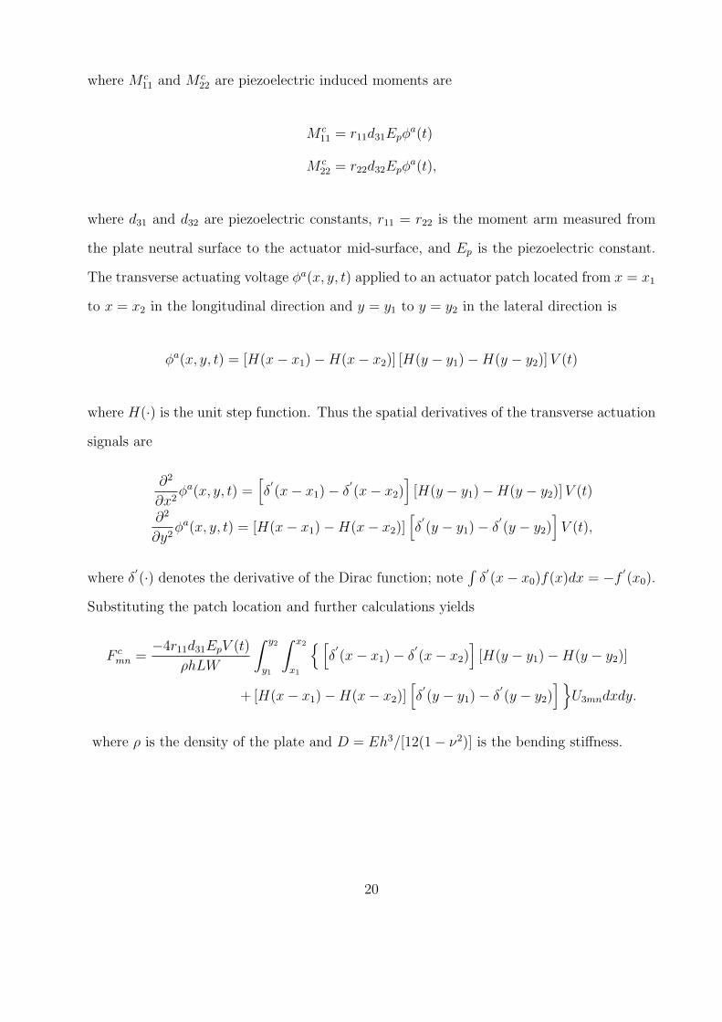
where M c11
and M c22
are piezoelectric induced moments are
M c11
= r11d31Epφa(t)
M c22
= r22d32Epφa(t),
where d31 and d32 are piezoelectric constants, r11 = r22 is the moment arm measured from
the plate neutral surface to the actuator mid-surface, and Ep is the piezoelectric constant.
The transverse actuating voltage φa(x, y, t) applied to an actuator patch located from x = x1
to x = x2 in the longitudinal direction and y = y1 to y = y2 in the lateral direction is
φa(x, y, t) = [H(x − x1) − H(x − x2)] [H(y − y1) − H(y − y2)] V (t)
where H(·) is the unit step function. Thus the spatial derivatives of the transverse actuation
signals are
∂2
∂x2φa(x, y, t) =
[
δ′
(x − x1) − δ′
(x − x2)]
[H(y − y1) − H(y − y2)] V (t)
∂2
∂y2φa(x, y, t) = [H(x − x1) − H(x − x2)]
[
δ′
(y − y1) − δ′
(y − y2)]
V (t),
where δ′
(·) denotes the derivative of the Dirac function; note∫
δ′
(x − x0)f(x)dx = −f′
(x0).
Substituting the patch location and further calculations yields
F cmn =
−4r11d31EpV (t)
ρhLW
∫ y2
y1
∫ x2
x1
[
δ′
(x − x1) − δ′
(x − x2)]
[H(y − y1) − H(y − y2)]
+ [H(x − x1) − H(x − x2)][
δ′
(y − y1) − δ′
(y − y2)]
U3mndxdy.
where ρ is the density of the plate and D = Eh3/[12(1 − ν2)] is the bending stiffness.
20
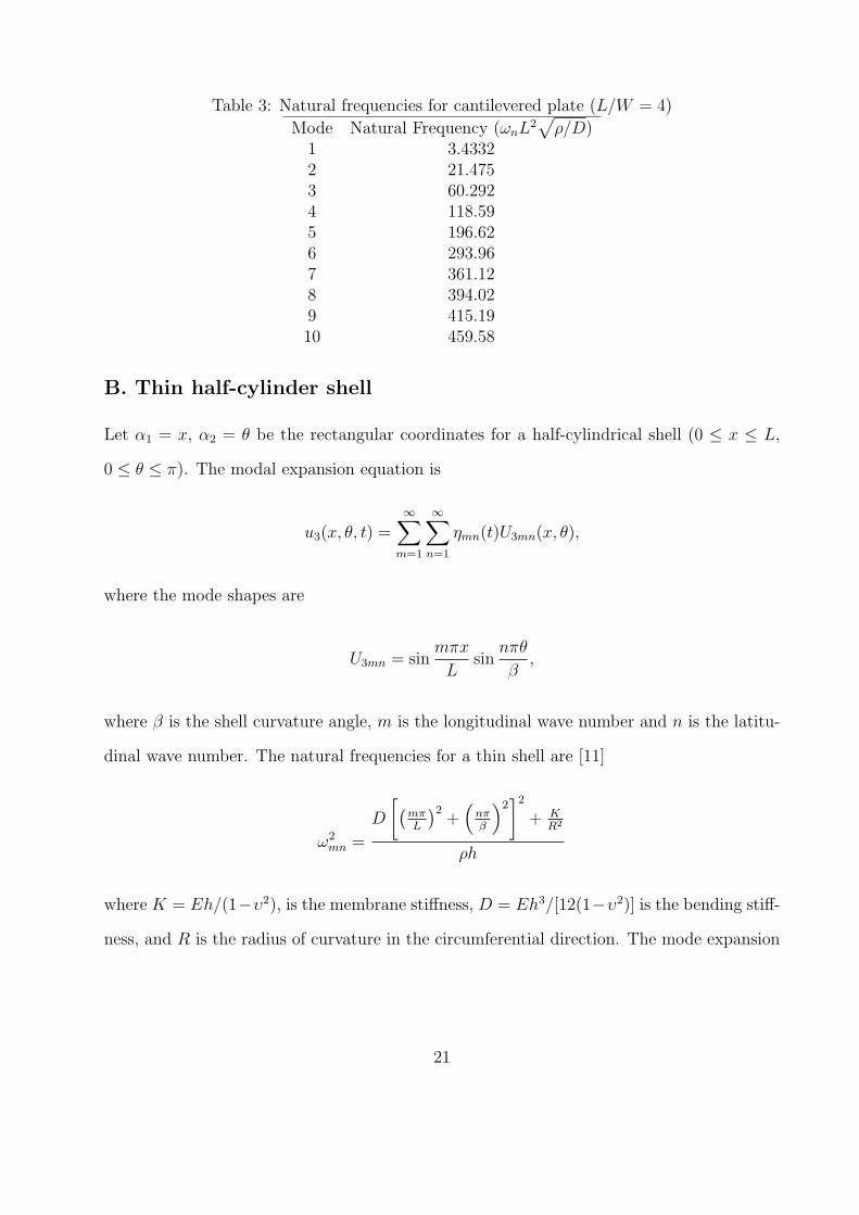
Table 3: Natural frequencies for cantilevered plate (L/W = 4)
Mode Natural Frequency (ωnL2√
ρ/D)1 3.43322 21.4753 60.2924 118.595 196.626 293.967 361.128 394.029 415.1910 459.58
B. Thin half-cylinder shell
Let α1 = x, α2 = θ be the rectangular coordinates for a half-cylindrical shell (0 ≤ x ≤ L,
0 ≤ θ ≤ π). The modal expansion equation is
u3(x, θ, t) =∞∑
m=1
∞∑
n=1
ηmn(t)U3mn(x, θ),
where the mode shapes are
U3mn = sinmπx
Lsin
nπθ
β,
where β is the shell curvature angle, m is the longitudinal wave number and n is the latitu-
dinal wave number. The natural frequencies for a thin shell are [11]
ω2
mn =
D
[
(
mπL
)2
+(
nπβ
)2]2
+ KR2
ρh
where K = Eh/(1−υ2), is the membrane stiffness, D = Eh3/[12(1−υ2)] is the bending stiff-
ness, and R is the radius of curvature in the circumferential direction. The mode expansion
21
used for the thin shell is
ηmn + Cmnη + Ω2
mnηmn = Fmn(t)
where Cmn is the constant damping matrix(Cmn = 0.001Ω2
mn), Fmn(t) is the modal force
which consists two components of mechanical force(q3(t)) and control force (Lc3φ3).
FMmn =
1
ρhNmn
∫
x
∫
θ
q3U3mnA1A2dα1dα2
F cmn =
1
ρhNmn
∫
x
∫
θ
Lc3φ3U3mnA1A2dα1dα2
and
Nmn =
∫
x
∫
θ
U2
3mndα1dα2
where ρ is the mass density, h is the thickness of the shell, A1 and A2 are Lame parameters,
α1 and α2, respectively denote the directions of x and θ. Substituting the Lame parameters
(i.e., A1 = 1 and A2 = R), radii of curvature (i.e., R1 = ∞ and R2 = R) and the two
principle directions α1 = x and α2 = θ and also assuming the external force,q3(t), is a point
force at (x∗, θ∗) the mechanical force and the generic control force are
FMmn =
4
ρhRLβ
∫
x
∫
θ
q3δ(x − x∗)δ(θ − θ∗) sinmπx
Lsin
nπθ
βdxRdθ
=4q3
ρhLβsin
mπx∗
Lsin
nπθ∗
β
Lc3φ3 = −
∂2M cxx
∂x2+
1
R2
∂2M cθθ
∂θ2− 1
RN c
θθ
22
where N and M , induced forces and moments by piezoelectric actuator with an applied
voltage φa, are
Nii = d3iEpφa(x, θ, t)
Mii = riid3iEpφa(x, θ, t)
where d3i is piezoelectric constant, (for a hexagonal structure it is assumed d3x = d3θ),
rii = rxx = rθθ is the moment arm measured from the shell neutral surface to the actuator
mid-surface and Ep is the piezoelectric constant. The transverse actuating voltage φa(x, θ, t)
applied to an actuator patch defined from x = x1 to x = x2 in longitudinal direction and
θ = θ1 and θ = θ2 in the circumferential direction can be expressed by a spatial distribution
part and time dependent part
φa(x, θ, t) = [H(x − x1) − H(x − x2)] [H(θ − θ1) − H(θ − θ2)] V (t)
where H(.) is the unit step function Thus the spatial derivatives of the transverse actuation
signals is
∂2
∂x2φa(x, θ, t) =
[
δ′
(x − x1) − δ′
(x − x2)]
[H(θ − θ1) − H(θ − θ2)] V (t)
∂2
∂θ2φa(x, θ, t) = [H(x − x1) − H(x − x2)]
[
δ′
(θ − θ1) − δ′
(θ − θ2)]
V (t)
23
where δ′
(.) is the derivative of a Dirac function:∫
δ′
(x − x0)f(x)dx = −f′
(x0). Substituting
the patch definition and further calculations yields
F cmn = −4d31EpV (t)
ρhLβ
∫ x2
x1
∫ θ2
θ1
rxx
[
δ′
(x − x1) − δ′
(x − x2)]
[H(θ − θ1) − H(θ − θ2)]
+rθθ
R2[H(x − x1) − H(x − x2)]
[
δ′
(θ − θ1) − δ′
(θ − θ2)]
+1
R[H(x − x1) − H(x − x2)] [H(θ − θ1) − H(θ − θ2)]
(
sinmπx
Lsin
nπθ
β
)
dxdθ
F cmn =
4d31EpV (t)
ρhLβ
[
rxx
(mπ
L
)
(
β
nπ
)
(
cosmπx1
L− cos
mπx2
L
)
(
cosnπθ2
β− cos
nπθ1
β
)]
+
[
rθθ
R2
(
L
mπ
)(
nπ
β
)
(
cosmπx2
L− cos
mπx1
L
)
(
cosnπθ1
β− cos
nπθ2
β
)]
+
[
1
R
(
L
mπ
)(
β
nπ
)
(
cosmπx2
L− cos
mπx1
L
)
(
cosnπθ2
β− sin
nπθ1
β
)]
24
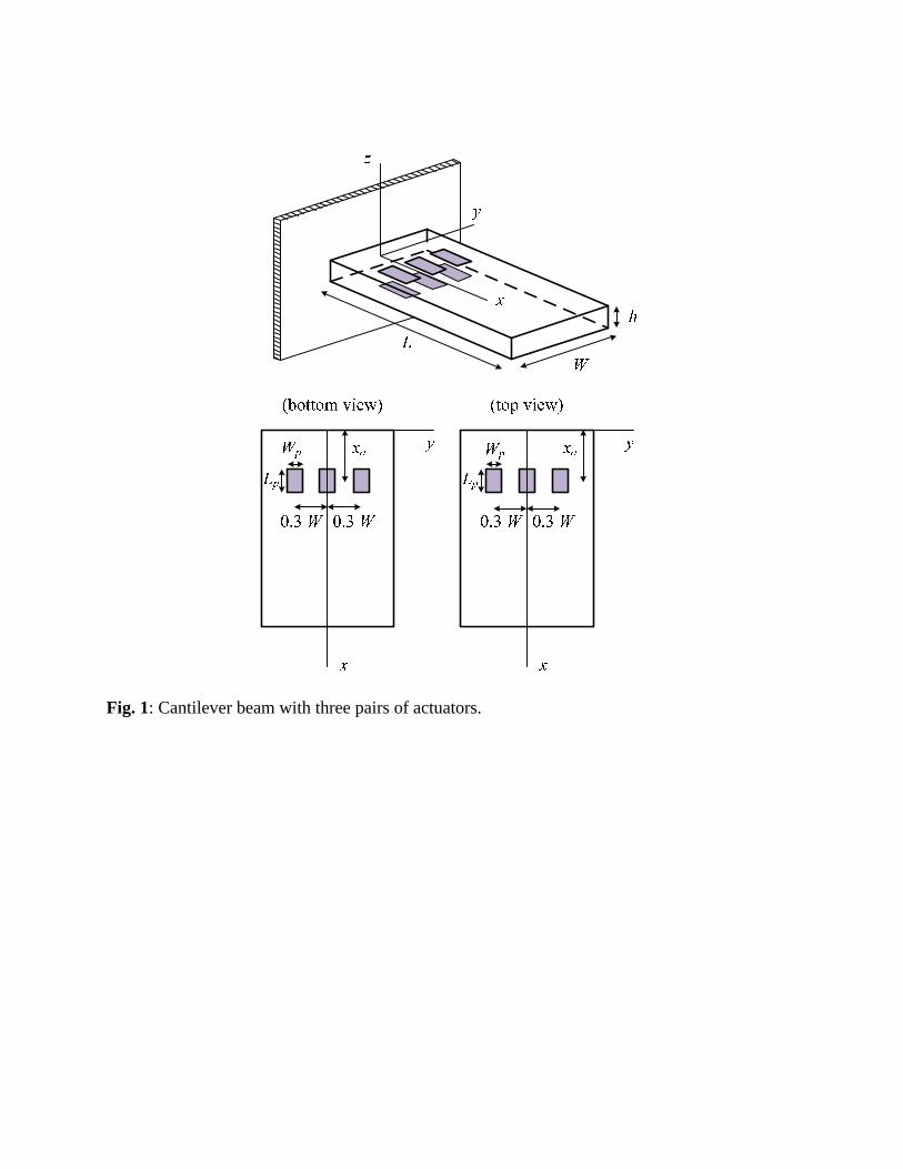
Fig. 1: Cantilever beam with three pairs of actuators.
0 5 10
-5
0
log
|( G v
) 11|
0 5 10
-5
0
log
|( G v
) 12|
0 5 10
-5
0
log
|( G v
) 13|
0 5 10-4
-2
0
log
|( G v
) 21|
0 5 10-4
-2
0
log
|( G v
) 22|
0 5 10-4
-2
0
log
|( G v
) 23|
0 5 10-5
0
log
|( G v
) 31|
0 5 10-5
0
log
|( G v
) 32|
Frequemcy (Hz)0 5 10
-5
0
log
|( G v
) 33|
Fig. 2a: Components of transfer function vG for the cantilever plate.
0 5 100
2
4
log
|( G -1 v
) 11|
0 5 100
2
4
log
|( G -1 v
) 12|
0 5 100
2
4
log
|( G -1 v
) 13|
0 5 102
3
4
log
|( G -1 v
) 21|
0 5 100
2
4
log
|( G -1 v
) 22|
0 5 102
3
4
log
|( G -1 v
) 23|
0 5 100
2
4
log
|( G -1 v
) 31|
0 5 100
2
4
log
|( G -1 v
) 32|
Frequency (Hz)0 5 10
0
2
4
log
|( G -1 v
) 33|
Fig. 2b: Components of inverse transfer function 1-vG for the cantilever plate.
10-1
100
101-3
-2
-1
0
1
2
3
log
v 1 (V)
10-1
100
101-3
-2
-1
0
1
2
3
Frequency (Hz)lo
g v 2 (V
)10
-110
010
1-3
-2
-1
0
1
2
3
log
v 3 (V)
xa=0.75 L xa=0.50 L xa=0.25 L
Fig. 3a: Piezoelectric actuation input requirements for Example 1, flapping (c1 = 2.5 mm, c2 = 2.5 mm, c3 = 2.5 mm).
10-1
100
101-2
-1
0
1
2
3
log
v 1 (V)
10-1
100
101
-6
-4
-2
0
Frequency (Hz)
log
v 2 (V)
10-1
100
10-2
-1
0
1
2
3
log
v 3 (V)
Fig. 3b: Piezoelectric actuation input requirements for Example 1, twisting (c1 = -2.5 mm, c2 = 0 mm, c3 = 2.5 mm).
10-1
100
1010
1
2
3
4
log
v 1 (V)
10-1
100
101-2
-1
0
1
2
3
4
Frequency (Hz)
log
v 2 (V)
10-1
100
101-2
-1
0
1
2
3
4
log
v 3 (V)
Fig. 3c: Piezoelectric actuation input requirements for Example 1, flapping and twisting (c1 = 2.5 mm, c2 = 5 mm, c3 = 7.5 mm).
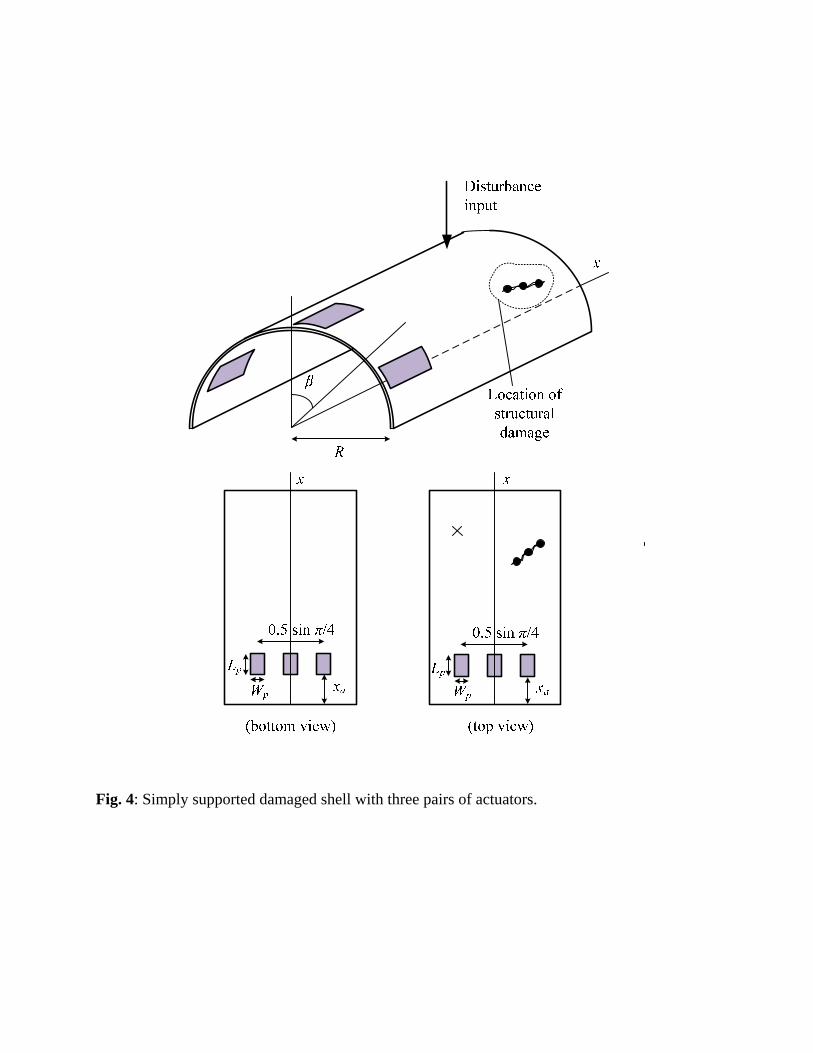
Fig. 4: Simply supported damaged shell with three pairs of actuators.
102
103-10
-8
-6
-4
-2lo
g | y
1(w)|
(m)
102
103-10
-8
-6
-4
-2
Frequency (Hz)
log
| y2(w
)| (m
)
102
103-10
-8
-6
-4
-2
log
| y3(w
)| (m
)
Fig. 5: The unactuated response due to the disturbance input for Example 2.
102
103-4
-3
-2
-1
0
1
2
3
102
103-4
-3
-2
-1
0
1
2
3
Frequency (Hz)
log
| v2| (
V)
log
| v1| (
V)
102
103-4
-3
-2
-1
0
1
2
3
log
| v3| (
V)
xa 0.2 L xa 0.4 L xa 0.6 L
Fig. 6: Piezoelectric actuation input requirements for Example 2.
102
103-4
-3
-2
-1
0
1
2
3
102
103-4
-3
-2
-1
0
1
2
3
Frequency (Hz)
log
| v2| (
V)
log
| v1| (
V)
102
10-4
-3
-2
-1
0
1
2
3
log
| v3| (
V)
xa 0.2 L xa 0.4 L xa 0.6 L
Fig. 7: Optimal piezoelectric actuation input requirements for Example 2.