did deregulation affect aircraft engine maintenance? an empirical policy analysis

RAND Journalof EconomicsVol. 24. No.4, Winter 1993

Did deregulation Meet aircraft enginemaintenance? an empirical policy analysis

D. Mark Kennet *

Examination of aircraft engine histories provided by Pratt & Whitney, Inc., indicates asignificant increase in the number of engine hours between major overhauls in the periodfollowing deregulation. Parametric analysis of times between overhauls, which controls forother variables affecting the length of the shop visit cycle, suggests that deregulation is asignificant factor in the change. Logit analysis, however, shows that engine ‘~ailures” (asmeasured by in-jlight shutdowns) have not increasedas a result of deregulation. These,findingssuggest that airlines have responded to competitive pressures by optimizing scheduled servicetimes and perhaps by improving the quality of service performed bul paying less atten~ionto minor problems between scheduled shop visits,

1. Introduction

■ A major focus of popular media attention to the airline deregulation] issue has beenon the question of aircraft safety. While economists have devoted journal space to otheraspects of deregulation, safety has been a major concern in academic circles as well.

Economists agreed that deregulation would bring down the average price of airlinetravel, but there was less certainty surrounding the effect on quality of service, Theoristsposited that during the regulated era, airlines competed in quality—since price competitionwas not available to them (see Douglas and Miller ( 1974 ))—and there has been theoreticaltreatment of the notion that deregulation would bring a reduction in quality (Moses and

* U.S. Bureau of Labor Statistics.Acknowledgments are due to Arthur Wegner, Edward Cowles, and Robert Weiss of Pratt & Whitney, Inc.,

for permission to use their data; and to Charlie Walters, Roy Ftfe, and Johnny Townsley of Federal Express, Inc.,for helping to explain them. The Monterey Merit Scholarship Fund at the University of Wisconsin providedfinancial support and enabled me to pay Mary Pat O’Donnell to enter data. Three anonymous referees, as well asSteve Berry, Coedilur Tim Bresnahan, Zvi Eckstein, Noel Gaston, Keith Heyen, Jonathan Pritchett, John Rust,Jim Schmitz, George Slotsve, Jay Stewart, Mark Stone, Insan Tunali, Dan Vincent, Len Weiss, and seminarparticipants at the University of California, Santa Cruz, the University of California, Davis, University of NewCJr]eans, Tel Aviv University, the Antitrust Division of the U.S. Department of Justice, the Bureau of LaborStatistics Office of Research, and the Econometric Society/Social Systems Research Institute Conference on EmpiricalApplications of Structural Models, read earlier drafts and made useful comments. Remaining errors maybe attributed

to faulty inspection procedures on the part of the author.1For this analysis, deregulation is taken to have occurred in 1978, the year Congress passed the Airline

Deregulation Act. Of course, actions taken by the Civil Aeronautics Board (CAB) before 1978 (as well as airlines’expectations ) could support an argument for an earlier cutoff date, and that the Act did not abolish the CAB until1982 could support a later cutoff date. In using 1978 as the cutoff, I am following the examples of Morrison andWinston ( 1988) and Borenstein and Zimmerman ( 1988).

542

KENNET / 543

Savage, 1990; Kamien and Vincent, 1990; Panzar and Savage, 1987; Stiglitz and Arnott,1987; and Braeutigam, 1987) as well as empirical treatment of the notion that airlines havemoved sharply to control costs (for example, Card ( 1986, 1989) on the decline of wagespaid airline employees since deregulation ). A key component of quality of service is aircraftsafety.

There is direct evidence that aggregate safety has not declined since deregulation (seeRose ( 1992) and Morrison and Winston ( 1988 )), and that airlines’ safety records were notaffected by profitability either before (see Golbe ( 1986)) or after (see Rose ( 1990)) dereg-ulation. Borenstein and Zimmerman ( 1988) provide evidence that the reverse does nothold: airlines experiencing accidents do suffer financial losses, although not nearly at thelevel of the social costs.

These empirical studies share one important feature: The number of observations inwhich an accident is present is quite small. Statistical analysis of rare events is problematic,and it is not inconceivable that results could be driven by airlines’ “lucky” or “unlucky”draws. One way of getting around this difficulty is to analyze the actions taken by airlinesto enhance safety, and one such action is aircraft engine maintenance.

This article looks at two questions: Did deregulation lead airlines to reduce enginemaintenance effort? And if there was a reduction in effort, has it led to deterioration inengine performance?

This study differs from previous ones in two important ways. First, this article is largelyan analysis of “effort” as opposed to “performance.” I measure effort by the preventivemaintenance performed on aircraft engines. Engine maintenance occurs quite frequently,and because its purpose is to prevent engine failures and, hence, accidents, analysis ofmaintenance effort is a valid approach to the study of safety.

Second, this study employs a unique and rich dataset not previously available to re-searchers. Data were collected at the level of an individual aircraft engine, enabling anexamination of micro-level decision making in the maintenance process. The data take theform of 42 complete engine histories covering the years 1964 to 1988 provided by Pratt &Whitney, Inc.2 A major advantage of this dataset is the relatively large number of events to

be analyzed (engine shutdowns and shop visits) compared to the infrequent occurrence ofaccidents and what the National Transportation Safety Board terms “incidents” analyzedin the other studies.

2. Background

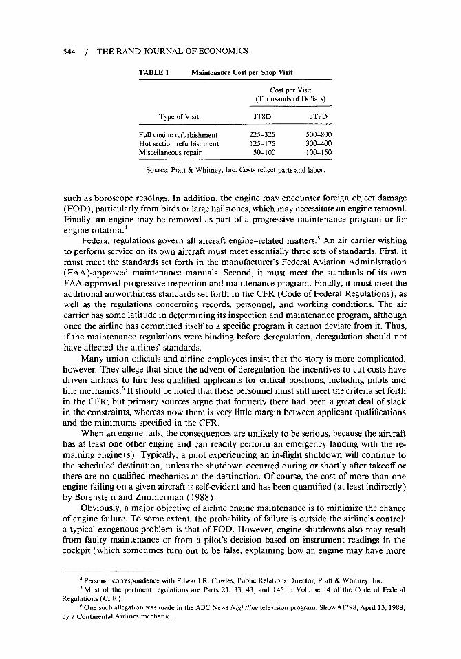
■ Before describing the data, methodology, and results, it is worthwhile to discuss aircraftengines, maintenance, and regulations briefly. A mechanic described the operation of a jetengine succinctly as “suck, squeeze, bang, and blow.” 3 This expression offers a fair repre-sentation of major engine processes: Air is pulled into the engine, compressed, and mixedwith fuel, The explosion of this mixture and its exhaust propels the plane forward. The hightemperatures and intense pressures take a heavy toll on the engine’s components, andmaintenance and repair can be costly (Table 1). Much of the cost is labor.

The decision to remove and overhaul an engine depends heavily on information gatheredby both the pilot and the ground crew during service checks. Some critical measures, likeoil pressure, are readily observable from the cockpit. The ground crew collects other data,

2 Because I wished to address the question of how deregulation affected the treatment of individual engines,the sample was drawn from engines whose service lives covered a substantial period both before and stir deregulation.1 argue below that the fact that the engines are overhauled means that they are “renewed” at each shop visit andmay therefore be considered new enginey this renewal puts the engines on an approximate y equal footing withother renewed engines,

3 Personal interview with Charlie Walters and Roy Fife, aircrafi mechanics with Federal Express, Inc., Madkon,APril 9, 1988.

544 / THE RAND JOURNAL OF ECONOMICS

TABLE1 MaintenanceCost per Shop Visit

Cost per Visit(Thousands of Dollars)

Type of Visit JT8D JT9D

Full engine refurbishment 225-325 500-800Hot section refurbishment 125-175 300-400

Miscellaneous repair 50-100 100-150

Source: Pratt & Whitney, Inc. Costs reflect parts and labor.

such as horoscope readings. In addition, the engine may encounter foreign object damage(FOD ), particularly from birds or large hailstones, which may necessitate an engine removal.Finally, an engine may be removed as part of a progressive maintenance program or forengine rotation.4

Federal regulations govern all aircraft engine-related matters.5 An air earner wishingto perform service on its own aircraft must meet essentially three sets of standards. First, itmust meet the standards set forth in the manufacturer’s Federal Aviation Administration(FAA )-approved maintenance manuals. Second, it must meet the standards of its ownFAA-approved progressive inspection and maintenance program. Finally, it must meet theadditional airworthiness standards set forth in the CFR (Code of Federal Regulations), aswell as the regulations concerning records, personnel, and working conditions. The aircarrier has some latitude in determining its inspection and maintenance program, althoughonce the airline has committed itself to a specific program it cannot deviate from it. Thus,if the maintenance regulations were binding before deregulation, deregulation should nothave affected the airlines’ standards.

Many union officials and airline employees insist that the story is more complicated,however. They allege that since the advent of deregulation the incentives to cut costs havedriven airlines to hire less-qualified applicants for critical positions, including pilots andline mechanics.6 It should be noted that these personnel must still meet the criteria set forthin the CFR; but primary sources argue that formerly there had been a great deal of slackin the constraints, whereas now there is very little margin between applicant qualificationsand the minimums specified in the CFR.

When an engine fails, the consequences are unlikely to be serious, because the aircrafthas at least one other engine and can readily perform an emergency landing with the re-maining engine (s). Typically, a pilot experiencing an in-flight shutdown will continue tothe scheduled destination, unless the shutdown occurred during or shortly after takeoff orthere are no qualified mechanics at the destination. Of course, the cost of more than oneengine failing on a given aircraft is self-evident and has been quantified (at least indirectly)by Borenstein and Zimmerman ( 1988).

Obviously, a major objective of airline engine maintenance is to minimize the chanceof engine failure. To some extent, the probability of failure is outside the airline’s control;a typical exogenous problem is that of FOD. However, engine shutdowns also may resultfrom faulty maintenance or from a pilot’s decision based on instrument readings in thecockpit (which sometimes turn out to be false, explaining how an engine may have more

4 Personal correspondence with Edward R. Cowles, Public Relations Director, Pratt & Whitney, Inc.5Most of the pertinent regulations are Parts 21, 33, 43, and 145 in Volume 14 of the Code of Federal

Regulations (CFR ).6 One such allegation was made in the ABC News Nighlline television program, Show-# 1798, April 13, 1988,

by a Continental Airlines mechanic.

KENNET / 545

than one shutdown during one shop visit cycle ). The engine work in this dataset also reflectsthe installation of upgrade kits, designed to improve an engine’s performance.

3. Preliminary analysis

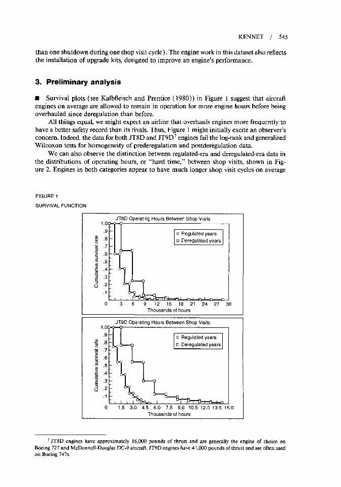
■ Survival plots (see Kalbfleisch and Prentice ( 1980)) in Figure 1 suggest that aircraftengines on average are allowed to remain in operation for more engine hours before beingoverhauled since deregulation than before.

All things equal, we might expect an airline that overhauls engines more frequently tohave a better safety record than its rivals. Thus, Figure 1 might initially excite an observer’sconcern. Indeed, the data for both JT8D and JT9D 7engines fail the log-rank and generalizedWilcoxon tests for homogeneity of prederegulation and postderegulation data.

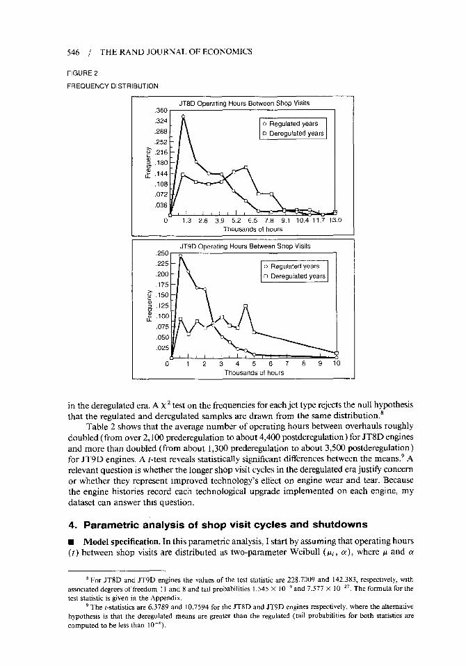
We can also observe the distinction between regulated-era and deregulated-era data inthe distributions of operating hours, or “hard time,” between shop visits, shown in Fig-ure 2. Engines in both categories appear to have much longer shop visit cycles on average

FIGURE 1

SURVIVAL FUNCTION

T8D Operating Hours Between Shop Visits

Ei5zEl~<)

1 ,0369 12 15 18 21 24 27 :

Thousands of hours

JT9D Operating Hours Between Shop Visits1,OB

.9 –~~ 8 :- m

o 1,5 3,0 4.5 6.0 7.5 9.0 10.5 12.0 13.5 15.0Thousands of hours

7JT8D engines have approximately 16,000 pounds of thrust and are generally the engine of choice onBoeing 727 and McDonnell-Douglas DC-9 aircraft. JT9D engines have 41,000 pounds of thrust and are often usedon Boeing 747s.


FIGURE 2

FREQUENCY DISTRIBUTION

JT8D Operating Hours Between Shop Visits.360 -

.324 –

.288 –

.252 –

~ .216 –al2 ,180 —

,108

.072

.036

0 1.3 2.6 3.9 5.2 6.5 7,8 9,1 10,4 11.7 13.0Thousands of hours

JT9D Operating Hours Between Shop Visits.250

.225 –

.200 –

.175 –

.075 -

.050

.025

01234567 891OThousands of hours

in the deregulated era. A X2test on the frequencies for each jet type rejects the null hypothesisthat the regulated and deregulated samples are drawn from the same distribution.8

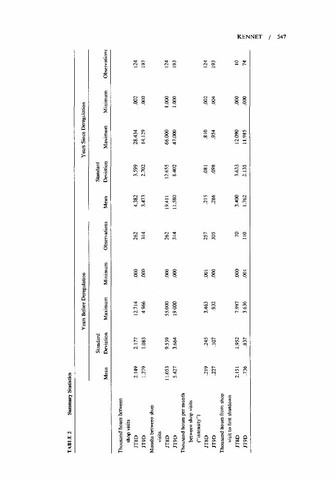
Table 2 shows that the average number of operating hours between overhauls roughlydoubled (from over 2,100 prederegulation to about 4,400 postderegulation ) for JT8D enginesand more than doubled (from about 1,300 prederegulation to about 3,500 postderegulation )

for JT9D engines. A t-test reveals statistically significant differences between the means.g A

relevant question is whether the longer shop visit cycles in the deregulated era justify concern

or whether they represent improved technology’s effect on engine wear and tear. Because

the engine histories record each technological upgrade implemented on each engine, my

dataset can answer this question.

4. Parametric analysis of shop visit cycles and shutdowns

■ Model specification. In this parametric analysis, I start by assuming that operating hours(t) between shop visits are distributed as two-parameter Weibull ( ~i, a), where Mand a

*For JT8D and JT9D engines the values of the test statistic are 228.7009 and 142.383, respectively, withassociated degrees of freedom I 1 and 8 and tail probabilities 1.545 x 10’9 and 7.577 X 10-27. The formula for thetest statistic is given in the Appendix.

9 The t-statistics are 6.3789 and 10.7594 for the JT8D and JT9D engines respectively, where the alternativehypothesis is that the deregulated means are greater than the regulated (tail probabilities for both statistics are

computed to be less than 10-4).


are, respectively, the location and scale parameters. Subscript i indexes a “renewal’’ -that

is, a shop visit cycle. This particular parametrization of the Weibull maximum likelihood

estimator is due to Lancaster ( 1979).

Letting t[ denote the ( hard) time between shop visits i – 1 and i, the Weibull probabilitydensity function is given by’0

~(t,) = IZ,OZ;-l exp(–p, t;) (1)

with

#i = exp(~’xi), (2)

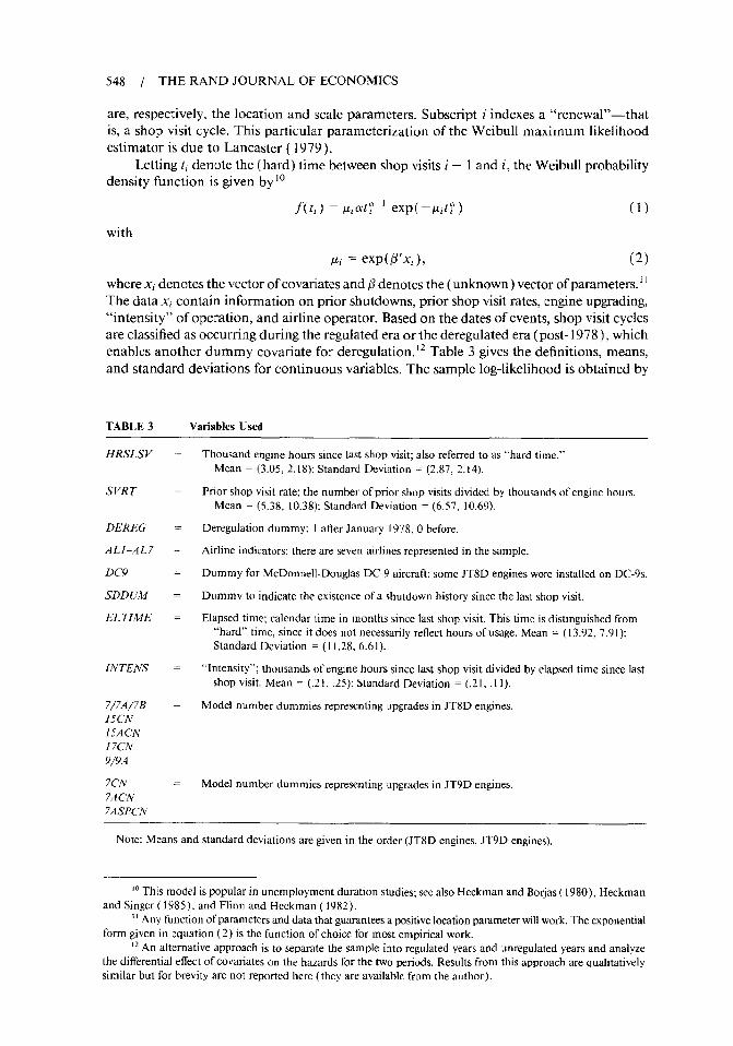
where xi denotes the vector of covariates and ~ denotes the ( unknown ) vector of parameters. 11The data xi contain information on prior shutdowns, prior shop visit rates, engine upgrading,“intensity” of operation, and airline operator. Based on the dates of events, shop visit cyclesare classified as occurring during the regulated era or the deregulated era ( post- 1978), which

12 Table 3 givesthedefinitions, means>enables another dummy covariate for deregulation.and standard deviations for continuous variables. The sample log-likelihood is obtained by

T.ABLE3 VariablesUsed

HRSLSV

SVRT

DEREG

AL1-AL7

DC9

SDDUJ4

EL 17ME

INTENS

7/7A/7BIJCN

15ACN17CN9/9A

7CN

7AC,V7ASPCN

——

——

——

——

——

——

——

——

—

——

Thousand engine hours since last shop visit; also referred to as “hard time.”Mean = (3.05, 2. 18); Standard Deviation = (2.87, 2. 14).

Prior shop visit rate; the number of prior shop visits divided by thousands of engine hours.Mean = (5.38, 10.38): Standard Deviation = (6,57, 10.69).

Deregulation dummy; I after January 1978, 0 before.

Airline indicators; there are seven airlines represented in the sample.

Dummy for McDonnell-Douglas DC-9 aircraft; some JT8D engines were installed on DC-9S,

Dummy to indicate the existence of a shutdown history since the last shop visit.

Elapsed time; calendar time in months since last shop visit. This time is distinguished from“hard’ time, since it does not necessarily reflect hours of usage. Mean = ( 13.92, 7.9 1):Standard Deviation = (11 .28, 6.61).

“Intensity”; thousands of engine hours since last shop visit divided by elapsed time since lastshop visit, Mean = (.21, ,25): Standard Deviation = (.21, 11),

Model number dummies representing upgrades in JT8D engines.

Model number dummies representing upgrades in JT9D engines.

Note: Means and standard deviations are given in the order (JT8D engines, JT9D engines).

‘0 This model is popular in unemployment duration studies; see also Heckman and Borjas ( 1980), Heckmanand Singer ( 1985), and Flinn and Heckman ( 1982),

II Anv function of pmameter~ and data that guarantees a positive location parameterwillWork.Theexponential

form given ‘in equation (2) is the function of choice for most empirical work.12,+n alternative approach is to separate the sample into regulated years and um’ewlatedwan and anahze

the differential effect of covariates on the hazards for the two periods. Results from this approach are qualitativelysimilar but for brevity are not reported here (they are available from the author),

KENNET / 549

taking the natural logarithm of equation ( 1) and summing over i for each engine; a isrestricted to a >0 by estimating in (a).

My priors on the coefficients were as follows. If we are to believe the story of, say,Kamien and Vincent ( 1990) that airlines overprovided quality before deregulation, thederegulation dummy (DEREG ) should negatively influence the hazard, since firms wouldhave scaled back their maintenance effort in the face of fierce rivalry.

Prior shop visit rate (NZRT), which indicates the number of times the engine visitedthe shop per thousand hours of hard time prior to the current shop visit cycle, can play tworoles. First, it may signal the seriousness of the airline’s maintenance program: a highershop visit rate is equivalent to more maintenance and thus will lead to a lower hazard rate.Alternatively, the shop visit rate may indicate engines with more problems requiring shopattention, in which case the effect on the hazard rate will be positive. Thus, I will not specifya prior on shop visit rate; the data are permitted to choose which of the two hypothesesapplies. i3

The shutdown dummy ( SDDUM) should have a negative effect on the hazard rate,because this indicator conveys the information that an engine has experienced trouble ofsome sort during its current cycle.

Intensity of use ( INTENS) should have a positive effect on the hazard rate, assumingthat it is accurately measured, because a more intensely used engine can be expected towear out (and therefore require shop attention ) more quickly. I must note, though, thatthe intensity measure here is quite problematic: it simply relates hard time to elapsed time,and does not take into account (for example) takeoffs and landings, when engines undergothe greatest portion of their stress. A useful measure of the intensity of operation wouldhave been engine “cycles,” or hours of operation at full throttle; unfortunately, these werevery inconsistently recorded in the dataset. Conceivably, an engine with a higher intensityunder the measure I use may be one that is used on longer, but fewer, flights, and may thusaffect hazard negatively.

The upgrade dummies (see Table 3) should proxy technical improvements in the enginesand should thus have a negative effect on the hazard rate, since an improved engine is lesslikely to require service.

I will take no position on airline dummies (All to AI,7), because I do not know theactual airlines involved and thus have no way of discovering their safety records. However,I will venture to assert that as factors leading to the deterioration of an engine are controlledfor, a positive coefficient for a given airline is suggestive of a greater willingness to performmaintenance (as opposed to a response to a more problematic collection of engines). Theassertion is strengthened by noting that an airline fixed effect applies to all engines operatedby the airline, and that it is unlikely that all of an airline’s engines in the sample are “lemons.”

The DC9 dummy for JT8D engines should have a positive effect on the hazard ratebecause the DC-9 is a two-engine underwing aircraft. The fact that there are two (versusthree for the Boeing 727 ) suggests that the engines are stressed more. Also, mechanics

indicated to me that although underwing engines are somewhat easier to service, they seem

to have more maintenance problems, possibly because of wing vibration and because nothing

is in front of the engines to keep out FOD.The data suffer from neither right nor left censoring because each shop visit cycle—

except for the first installation—is preceded by a shop visit and is followed by another shopvisit. Thus, no correction is required. Even though a given engine goes through many cycles(of uptime, shop visit ), following the example of Amemiya ( 1985) and others I treat theuptimes as independent events. In other words, I am assuming that an engine returning to

13lt ~hou]d be pointed out that the shopvisitrate as measured here does not include contemPo~neous shop

visits, but only those that occurred up to the time of the last shop visit. Thus, this specification should not sufferfrom any problems of endogeneity.


TABLE4 Weibull and Least Squares ResultsDependent Variable: Engine Hours Between ShopVkhs

Weibull Models OLS Mndels

Variable JT8D Engines JT9D Engines JT8D En~nes JT9D Engines

Primary variables

Constant

Shop visit rate

Deregulation dummy

Shutdown dummy

Intensity

Engine upgradedummies

7/7A/717

15CN

15ACN

17CN

9/9.4

7CN

7ACN

7ASPL’N

Airline dummies

AL2

AL3

AL4

.379(.258).177

.030(,005).014

–.307(.138)

–.136

–.386(.240)

–. I52

-6.77 I(1.259)

-3.156

–.476(.146)

– .222

–.580(.244)

–.217

–.529(.492)

–.193

–.124(.430)

–.246

–,862(1.161)–,270

-,188(,196),081

–.260(.240)

-.109

-.534(.317)

–.197

–.954(.114)

–,016

.036(.004).001

-.298(. 140)

–.005

–.282(,220)–.004

–.579(.133)

–.010

–.642(.209)

-.c09

–.460(.290)

–.006

–.800(,408)

-.010

-3.023(I .054)–.017

–.100(.187)

–.002

–.350(.230)

–.005

–.510(.2c0)

–.007

2.233(.186)1.849

,00i(l e-04)

.001

–.398(,185)

–.317

–,200(.164)

–.153

–11.801(.963)

–9.77

–.292(.133)

–,226

–.261(,198)

–,209

–.351(.504)

-.246

.080(.212).069

–,134(,157)

–.105

–,130(.163)

–.102

.004(.077)

1*O4

.00I( le-04)

.000

–.534(.185)

–.013

–.176(,152)

–.004

–.606(.128)

–.013

–.820(.197)

–.019

-1.143(.489)

–.017

-,236(,198)

–005

–.218(.118)

–.005

–.210(.134)

–.005

–1.430(.272)

.031

(.013)

–.986(.347)

–1.035(.546)

–3.004(.645)

–1.119(.309)

–1.450(.549)

–,907(1.103)

–1.142(.952)

–24.528

(2.469)

–.685(.430)

–,429

(.540)

–1.332(,620)

–2.068(.242)

.035(.013)

–.911(.356)

–.937(.560)

–1.212(.316)

–1.558(.564)

–.984(1133)

–1 365( 977)

-25,839(2520)

–.538(.441)

–.510(.554)

–1.2L39(.636)

-.532(.158)

le-04(2e-04)

–1.432(.322)

–.287(.288)

–2.051(.348)

–.720(.230)

–,912(.343)

-2.034(.874)

.118(.375)

–.284(,278)

–,524(,289)

-.900(,150)

2e-04(2e-04)

–1.304(.332)

–.277(.297)

–.750(.238)

–1.156(.352)

-2,379(.902)

–.346(.379)

–.324(.287)

–.533(.299)

KENNET / 551

TABLE4 Continued

Weitrull Models OLS Models

Variable JT8D Engines JT9D Engines JT8D Engines JT9D Engines

AL5 .146(,243),073

.876[.62[)

1.218(.634)(,262)

,013

AL6 –.049(.277)

–.022

–,015(,108)

–2e-04

–.343(.593)

–.369(,609)

AL? ,131(.259).065

,147(.237).003

.338(.549)

,418(.564)

DC9 .311(.237).163

.522(.216).011

.754(.512)

,978(.523)

1.240(,053)

1.[60[.050)

1.346 1.107 —(.050) (.043)

732,8 814.7 856.2— — ,395— — 15,047

495 496 369

a

–Log-likelihoodR-squaredF statisticDegrees of freedom

— — —

738.2 762. I—

867.2 1006.0 1023.0.359 .317 .269

13.829 22.980 20.287370 496 497

——368 369

Notes Standard errors in parentheses. WeibuO hazard derivatives under standard errors. OLS results relate to the negative ofduration to facilitate comparison.

service from the shop is essentially a new engine, having been certified as meeting airwor-thiness standards. 14

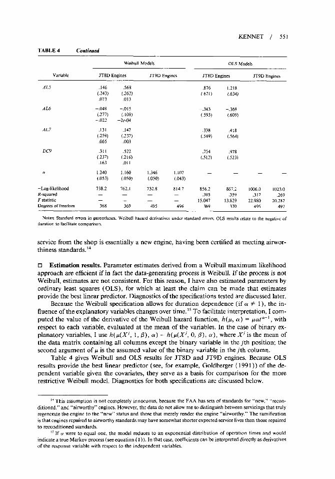
❑ Estimation results. Parameter estimates derived from a Weibull maximum likelihoodapproach are efficient if in fact the data-generating process is Weibull. If the process is notWeibull, estimates are not consistent. For this reason, I have also estimated parameters byordinary least squares ( OLS ), for which at least the claim can be made that estimatesprovide the best linear predictor. Diagnostics of the specifications tested are discussed later.

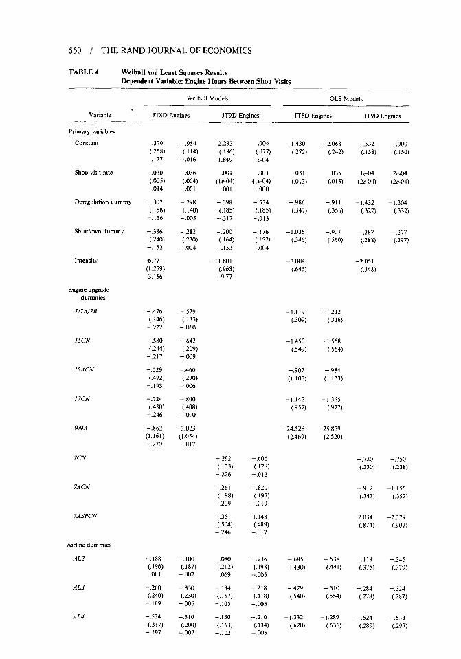
Because the Weibull specification allows for duration dependence (if a # 1), the in-fluence of the explanatory variables changes over time. ]5To facilitate interpretation, I com-puted the value of the derivative of the Weibull hazard function, rf(p, a) = I.Lata-’,withrespect to each variable, evaluated at the mean of the variables. In the case of binary ex-planatory variables, I use L( p(X~, 1, B), a) – II(~(X~, O, f?), a), where Xj is the mean ofthe data matrix containing all columns except the binary variable in the jth position; thesecond argument of ~ is the assumed value of the binary variable in the jth column.

Table 4 gives Weibull and OLS results for JT8D and JT9D engines. Because OLSresults provide the best linear predictor (see, for example, Goldberger ( 1991)) of the de-pendent variable given the covariates, they serve as a basis for comparison for the morerestrictive Weibull model. Diagnostics for both specifications are discussed below.

‘4This assumption is not completely innocuous, because the FAA has sets of standards for “new,” “recon-

ditioned,” and “airworthy” engines. However, the data do not allow me to distinguish between servicing that trulyregenerate the engine to the “new” status and those that merely render the engine “airworthy.” Tbe ramificationis that engines repaired to airworthy standards may have somewhat shorter expected service lives than those repairedto reconditioned standards.

‘3If a were to equal one, the model reduces to an exponential distribution of operation times and wouldindicate a true Markov process (see equation ( 1)). In that case, coefficients can be interpreted direct] y as derivativesof the response variable with respect to the independent variables.


Deregulation is distinguishable as a separate effect negatively influencing the shop visithazard rate in the Weibull specification and significantly increasing the length of the shopvisit cycle in the OLS specification. lb The result stands for both engines at the 10170significance

level whether or not the intensity measure is included.Table 2 shows that while the intensity measure rose significantly since deregulation for

JT9D engines, it has not changed significantly for JT8D engines.’7 Because the intensityratio is a less-than-perfect proxy, I also report Weibull results with the intensity measurenot present in Table 4. The data, however, reject this restriction. 18

Table 4 reveals that intensity has both positive and significant effects on the WeibuIlhazard rates for both engine types. That result seems to indicate that as intensity of useincreases (operating hours per month increase ), the likelihood of an engine requiring ashop visit increases. OLS estimates of the intensity coefficient are significant as well. Thedata seem to support the hypothesis that the more intensively used engines are employedon longer trips and have relatively fewer takeoffs and landings.

Prior shop visit rate has a positive and significant effect on the hazard rate for bothengine types. That result most likely comes about because engines with weaker prior historiestend to break down more easily. This explanation is consistent with the OLS results forJT8D but not JT9D engines.

Engine upgrade packages had negative and significant effects on the Weibull hazard inthe 7/7A/7B, 15CN, and 17C’N cases for JT8D engines and in the case of 7CN for JT9Dengines. That is to say, these particular upgrade packages led to increased service lives forthe engines on which they were installed. When intensity is excluded, upgrade packagesexcept Model 15ACN exhibit statistically significant effects relative to Model 1/1A/1 B (theoriginal JT8D model); the statistically significant coefficients all reflect reductions in thehazard rate. All the engine updates applied to the JT9D engines reduce the hazard raterelative to Model 3A, the original JT9D model, when intensity is excluded. OLS results areslightly different: in the JT8D case, 7/7A/ 7B, 15CIV, and 9/9A have significant coefficients,while in the JT9D case, all three upgrades appear to have significant coefficients.

Only airline 4 (AL4) in the JT8D case has significant ( negative ) effects on the Weibullshop visit hazard when intensity is included. Without intensity, airlines 4 and 5 are significantfor JT8D engines ( negatively and positively, respectively, with respect to the hazard rate).It follows based on the earlier reasoning that airline 4 is less safety-conscious than its peers,and airline 5 more so. If the intensity measure is excluded, only airline 3 behaves significantlydifferently-it seems to be less safety-conscious. The OLS results are roughly consistentwith the Weibull for JT8D engines; airlines 4 and 5 have significant coefficients with thesigns consistent with the Weibull results. The JT9D OLS results show a significant effectfor airline 4.

The JT9D engines were installed on only one aircraft type, the Boeing 747, so noaircraft dummy was included. The JT8D engines in the sample were installed on bothBoeing 727 and Douglas DC-9 aircraft. The Weibull results indicate that the fact that agiven engine is installed on a DC-9 had a positive and significant effect on the hazard ratewhen intensity is excluded, but no significant effect when intensity is included. The DC-9efiect is significant in both OLS specifications. This result may reflect more intense usagewhen the JT8Ds are installed on the DC-9, which is a two-engine aircraft as opposed to thethree-engine 727.

IC&.cau~e weib~ll ~~timates refer to the influence on the hazard, I report the nesative of estimated ON

coefficients in Table 4 to make the coefficients comparable across the two models.17The f-statistic for the difference in mean “intensity” for JT8D engines is .236, while that for JT9Ds iS6.315.

ISThe likelihood ratio for the JTgD engines is 47.8 ( x 2 distribution tail probatillity is 1.5 X 10’9 ), and that

for JT9D engines is 163.8 (tail probability also 1.5 X 10-9),

KENNET / 553

TABLE5 BinaryLogitResultsMonthlyProbabilityof EngineShutdown

JT8D Engines JT9D Engines

Variable Model 1 Model2 Model 1 Model2

Primary variables

Constant

Hours since last shop visit

Prior shop visit rate

Deregulation dummy

Engine upgrade dummies

7/7A/7B

15CN

15ACN

17CN

9/9A

7CN

7ACN

7ASPCN

Airline dummies

AL2

AL3

AL4

AL5

AL6

AL7

DC9

–Log-likelihood

Degrees of freedom

-2.7127(.2955)

.0214(.0610)

–.1037(.0499)

–,7837(.4099)

– 1.20S7(.2790)

-2.7130( 1.0760)

–.8216( 1.0968)

–13.6910(236.7088)

–13.2838(424.5485)

–.1707(.4847)

–1.1148(.5585)

–.7484(.5361)

–.2821(1.0465)

.4846(.4490)

–.8823(.7286)

.2782

(.5127)

378.22

5372

–3.2132(.1958)

– 1.9048(.2002)

-2.1193(.1314)

–.06 14(.0444)

–.0448(.3107)

–.2704(.2005)

--.7893(.3224)

–1.9375(1.0618)

–.7859(.3706)

–.095 1(.2309)

-1,6860(.4579)

826.78

4092

.0595(.0572)

–.0695(,0450)

–.1065(.0125)

–.7426(.4096)

–.0650(.3114)

–1.1872(.2773)

–2.7542(1.0760)

–.8212(1.0966)

–22.2733

(289.5752)

–22.3762

(629.1351)

–.3270(.2031)

–.8585(.3257)

–2.0166( 1.0623)

–.3480(.4762)

–.8491(.3728)

-.9771(.5570)

–.1561(.2347)

–.8016(.5354)

–1.6759(.4578)

–.7203(1.0275)

.3331(.4408)

–.75 14[.7264)

.2210(.5110)

380.68

5373

825.57

4091

Note: Standard errors in parentheses.


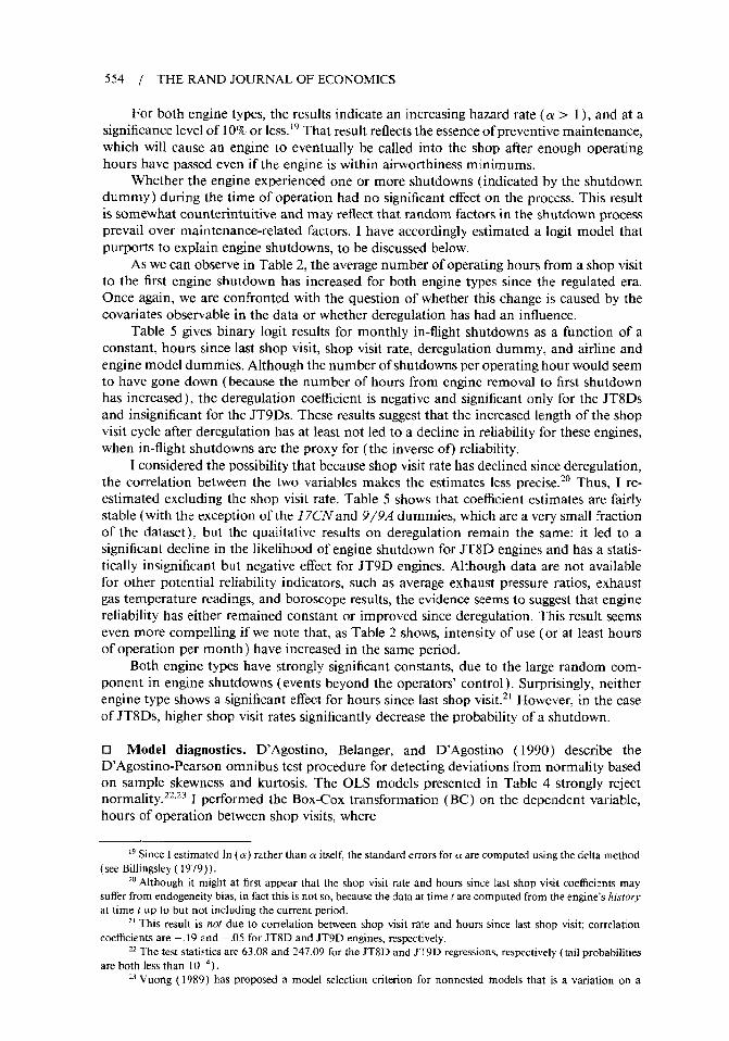
For both engine types, the results indicate an increasing hazard rate ( a > 1), and at asignificance level of 1070or less. I9 That ~e~ult reflects the essence of preventive maintenance>

which will cause an engine to eventually be called into the shop after enough operating

hours have passed even if the engine is within airworthiness minimums.

Whether the engine experienced one or more shutdowns (indicated by the shutdown

dummy ) during the time of operation had no significant effect on the process. This result

is somewhat counterintuitive and may reflect that random factors in the shutdown process

prevail over maintenance-related factors, I have accordingly estimated a logh model that

purports to explain engine shutdowns, to be discussed below.

As we can observe in Table 2, the average number of operating hours from a shop visit

to the first engine shutdown has increased for both engine types since the regulated era.

Once again, we are confronted with the question of whether this change is caused by the

covariates observable in the data or whether deregulation has had an influence.

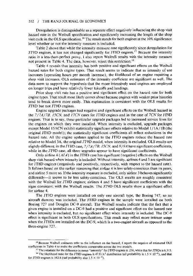
Table 5 gives binary logit results for monthly in-flight shutdowns as a function of a

constant, hours since last shop visit, shop visit rate, deregulation dummy, and airline and

engine model dummies. Although the number of shutdowns per operating hour would seemto have gone down (because the number of hours from engine removal to first shutdownhas increased ), the deregulation coefficient is negative and significant only for the JT8Dsand insignificant for the JT9Ds. These results suggest that the increased length of the shopvisit cycle after deregulation has at least not led to a decline in reliability for these engines,when in-flight shutdowns are the proxy for (the inverse of) reliability.

I considered the possibility that because shop visit rate has declined since deregulation,the correlation between the two variables makes the estimates less precise.20 Thus, I re-estimated excluding the shop visit rate. Table 5 shows that coefficient estimates are fairlystable (with the exception of the 17CN and 9\9A dummies, which are a very small fractionof the dataset ), but the qualitative results on deregulation remain the same: it led to asignificant decline in the likelihood of engine shutdown for JT8D engines and has a statis-tically insignificant but negative effect for JT9D engines. Although data are not availablefor other potential reliability indicators, such as average exhaust pressure ratios, exhaustgas temperature readings, and horoscope results, the evidence seems to suggest that enginereliabilityy has either remained constant or improved since deregulation. This result seemseven more compelling if we note that, as Table 2 shows, intensity of use (or at least hoursof operation per month) have increased in the same period.

Both engine types have strongly significant constants, due to the large random com-ponent in engine shutdowns (events beyond the operators’ control). Surprisingly, neitherengine type shows a significant effect for hours since last shop visit.z 1However, in the caseof JT8Ds, higher shop visit rates significantly decrease the probability of a shutdown.

❑ Model diagnostics. D’Agostino, Belanger, and D’Agostino ( 1990) describe theD’Agostino-Pearson omnibus test procedure for detecting deviations from normality basedon sample skewness and kurtosis. The OLS models presented in Table 4 strongly rejectnormality. **,231 performed the BOX.COX transformation ( BC ) on the dependent variable,

hours of operation between shop visits, where

19 since I ~~t]m~ted ]n (a) rather than a itself, the standard errors for a are cOmputed using the delta methOd

(see Bdlingsley ( 1979)).ZOAlthough it might at first appear that the shop visit rate and hours S’hCe laS’t shop visit coefficients maY

sutTer from endogeneity bias, in fact this is not so, because the data at time t are computed from the engine’s Iustoryat time [ up to but not including the current period.

2 I This result is ~0~ due to ~or~elatio~ between shop visit rate and hours Since lmt shop visk correlation

coefficients are –. 19 and – .05 for JT8D and JT9D engines, respective y.u The test statistics are 63.08 and 247.09 for the JT8D and JT9D regressions, resPcctivelY (~il PrObabilities

are both less than 10’4 ).m Vuong ( 1989) has proposed a model selection criterion for nonnested models that is a vtiation on a

ILENNET / 555

{

Xc-le+o

Bc(x; e) = e

in (x), e=o”

Performing a grid search for the e that maximizes the log-likelihood of the sample underthe assumption of normality did not alter the significance of the D’Agostino-Pearson sta-tistic 24Thus the OLS results, while lending credence to the results because the techniquedoes provide the best linear predictor, cannot be regarded as efficient estimates.

Lancaster ( 1979) noted that the inclusion of more explanatory variables in his modelcaused the value of a to rise. That observation is consistent with my finding for both enginetypes, and quite possibly the conclusion that he draws— heterogeneity caused by omittedvariables may be responsible for the nonconstant hazard rate—may apply. Lancaster ( 1990 )provides Jests for unobserved heterogeneity and a nonmonotone hazard. The models do

25 however, there is strong rejection ofnot seem to suffer from unobserved heterogeneity;the monotone hazard specification.26

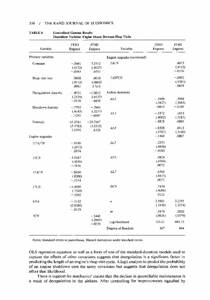
One way to address the nonmonotone hazard problem parametrically is to estimate ageneralized gamma model, which fits an additional shape parameter. The generalized gammalog-likelihood is

N

L= ~ {ln(a)+m~’xi -t-(am– l)ln(~i) –y~e~’x’ –ln (r’(m))},i- I

where m is the additional shape parameter (note that if m = 1, the model is identical to theWeibull ). Results from this specification are reported in Table 6; the results reject the nullhypothesis that m = 1, and the likelihood ratio test rejects a restriction of setting m to unity.Other results are qualitatively similar to the Weibull and OLS results.

A possible specification error in the logit model is unobserved heterogeneity .27 Thereappears to be no omnibus specification test for unobserved heterogeneity in the logit frame-work, so I considered a possible source arising from the engines themselves. The likelihoodratio test did not reject the null hypothesis that the coefficients of the engine fixed effectsare all zero for both JT8D and JT9D engines.28

5. Conclusion

■ The dataset containing complete Pratt & Whitney aircraft engine histories exhibits aclear distinction between maintenance behavior before and after airline deregulation. An

likelihood ratio test, The formula for the test statistic in this case is given in the AppendLx. The &ta overwhelmingly

reject the null hypothesis that the Weibull and OLS models are equivalent in favor of the Weibull being better.The Vuong statistic for the unrestricted (intensity included as a covanate ) JT8D model is 4.958, with associatedsignificance 3.6 X 10’7. The Vuong statistic for the unrestricted JT9D model is 4.459, with associated significance4.1 X 10-’. For the restricted case, Vuong statistic vahres are 6.403 and 7.211, both with significance 7.7 X 10-7,for JT8D and JT9D models, respectively.

24“Optimal” EOX-COXparameters ranged from .2077 to .3375 for the four specifications in Table 4; DAgostino-Pearson statistics ranged from 28.43 to 60.21, with associated tail probabilities less than 10’4.

2s The normaIIy distributed, fight.tailed test statistic is –4.0024 (tail probability .9999) for JT8D en.@res and

–9.47 16 (tail probability 1.0000) for JT9D engines.M Test Statistic values for JTSD and JT9D models are 496.1399 and 4051.5056, respectively, with a~ociat~

tail probabilities both less than 10‘“.27 Another ptentia] problem is heteroskedasticity. Davidson and MacKinnon ( 1984 ) proposed a hetero-

skedasticity test for a probit model in which the heteroskedasticity arises in the underlying ( normal ) latent variablemodel. However, as Greene ( 1990) points out (and the authors also suggest), their test does not apply to a Iogitframework because the logit model is not derived from a latent variable fkamework (except in the special case ofrandom utility models ).

28The likelihood ratio test statistics for the JT8D and JT9D engines are 25.67 and 10.59,re5PeCtive1Y,with

associated tail probabilities .1771 and .9562, Degrees of freedom in both cases are 20.


TABLE6 GeneralizedGammaResultsDependentVariable Engine Hours Between shop Visits

JT8D JT9D JT8D JT9DVariable Engines Engines Variable Engines Engines

Primary variables

Constant –.5601(.6 122)

–.0565

Shop visit rate .0608(.0112).0061

Deregulation dummy –.4551(.2539)

–.0538

Shutdown dummy –.7703(.4145)

–.1295

Intensity –16,~54]

(3.3783)– 1.6392

Engine upgrades

7/7A/7B

15CN

l.iACN

17CN

9/9A

–,9!86(.2672)

–.0874

– 1.0267(.4350)

–.1816

–.8450(.8200)

–.1514

– 1.4990(.7328)

–.3202

–.1132(2,0380)–.0129

3.5312(,4627).0751

.0018(.0003)3.7e-5

–1.0612(.4137)

–.0439

–.7043(.3257)

–.0587

-29,7467(3,5222)– ,6326

7CN –.5440(.2660)

–.0276

Engine upgrades (continued)

7ACIV

7ASPCN

Airline dummies

AL2

AL3

AL4

AL j

AL6

AL7

DC9

a

m

–Log-likelihood

Degrees of freedom

-.4913(.4152)

–.0176

–.0902(.9381)

–. f)()~9

–,5489 .3908(.3427) (.3983)

–,0815 –.0105

–.5572 .1653(.4082) (.3187)

–.0828 .0005

–.8388 .0413(,4787) (.3140)

–,1468 .0007

–.2253(.4856)

–,0280

.0824(.4504).0075

,6506(,4415)

,0071

,7434(,4066),0122

2.5661 3.2195(,3430) (.3274)

.3474 .2820(.0626) (.0379)

723.21 685.75

367 494

Notes: Standard errors in parentheses. Hazard derivatives under standard errors,

OLS regression equation as well as a form of one of the standard-duration models used tocapture the effects of other covariates suggests that deregulation is a significant factor inpredicting the length of an engine’s shop visit cycle. A logit analysis to predict the probabilityof an engine shutdown uses the same covanates but suggests that deregulation does notaffect that likelihood.

There is support for mechanics’ claims that the decline in quantifiable maintenance isa result of deregulation in the airlines. After controlling for improvements signalled by

KENNET / 557

model upgrades in the engines, heterogeneity in airline maintenance practices, unobservedairline heterogeneity, heterogeneity in aircraft types, and the incidence of shutdowns, de-regulation seems to have resulted in a lower probability that an engine gets a shop visit.This finding is robust to inclusion of usage intensity as an explanatory variable; however,the intensity variable is a noisy signal that may not adequately proxy the desired effect.Despite the increased time between engine overhauls, there is no evidence of reduced enginereliability as measured by in-flight shutdowns, suggesting that the counterarguments ofairline managers may also be correct: safety performance has not suffered since the adventof deregulation. These results verify machinists’ union claims that maintenance policieshave substantially changed in the deregulated environment, but also back corporate claimsthat reliability has not suffered.

One way of reconciling these conflicting views is to recognize that quite possibly, newmaintenance policies are at variance with the older notions of good maintenance practice—thereby leading to the unions’ discomfort-but are in fact optimal from the safety standpoint.Some empirical support for this interpretation is found in Kennet ( 1988 ), where an estimatedstructural model (based on Rust ( 1987)) incorporating a dynamic programming model ofmaintenance decision making into a statistical model suggests that maintenance prior to1978 was not dynamically optimized but was optimal after 1978.

The results strengthen existing literature on air safety in the deregulated environment,which has unanimously found little cause for concern, but provide the extra reassurancethat comes from microdata at the level of the decision makers.

Appendix

9 The X2 statistic in footnote 8 is computed by determining the expected frequency for each of k ranges ofvalues under the null hypothesis that the regulated-era distribution would apply to the deregulated era, fij, andinserting the observed frequencies, O,, from the deregulated era in tbe following formula (Kenkel, 1989 ):

~, = <. (Oj– E,)z&

,--1 E,

Degrees of freedom are then k – 1.n n

The test statistic for footnote 23 is V(f~, /$) = n-1/2( Z ~~[b) – Z lY(?))/~, where 1: is the vector of,=, i=1

observation log-likelihoods evaluated under the Weibull likelihood function assumption at ~, the associated maximumlikelihood estimator for the model; 1$ is the vector of observation log-likelihoods evaluated under the competingGaussian normal functional assumption at ?, its associated maximum likelihood estimator; n isthe number ofobservations 1~( o) and /~(. ) are observation log-likelihoods, and

{J*=: \ {r(g) –1;(+)}2– ::1[r(~) –1:(?)1]2.

!– ,–

Vuong ( 1989 ) shows that this statistic is asymptotically standard normally distributed

References

AM EMIYA, T. Advanced Econometric.~. Cambridge, Mass.: Harvard University Press, 1985.BILLINGSLEY, P. Probnbilit.v urrd Measure. New York: Wiley. 1979.BORENSTEIN, S. AND ZIMMERMAN, M.B. “Market Incentives for Safe Commercial Airline Operation.” American

Economic Review, Vol. 78 ( 1988), pp. 913-935.BRAEUTIGAM, R. “Airline Deregulation and Safety: A Comment.” Conference Proceedings, Transportation De-

regulation and Safety Conference, Northwestern University, June 23-25, 1987.CARD, D, “The Impact of Deregulation on the Employment and Wages of Airline Mechanics. ” Industrial and

Labor Relations Rtwiew, Vol. 39 ( 1986), pp. 527-538.—. “Deregulation and Labor Earnings in the Airline Industry.” Working Paper no. 247, Industrial Relations

Section, Princeton University, January 1989.DAGOSTINO, R. B., BELANGER, A., AND DAGOSTINO, R. B., JR. “A Suggestion for Using Powerful and Informative

Tests of Normality.” .4nrerican ,!Jalistician, Vol. 44 ( 1990 ), pp. 316-321.


DAVIDSON,R. AND MACKINNON, J.G. “Convenient Specification Tests for Logit and Probit Models.” Journal ofEccmormvrics, Vol. 25 ( 1984), pp. 241-262.

DOUGLAS, G.W. AND MILLER, J. C., 111. Economic Regulation qf Domestic Air Transporl; Theory and policy.Washington: Brookings Institution, 1974.

FLINN, C. AND HECKMAN, J. “Models for the Analysis of Labor Force Dynamics.” Advances in Econometrics,Vol. 1 ( 1982), pp. 35-95.

GOLBE, D. “Safety and Profits in the Airline Industry.” Journal ofIndrcstrial Economics, Vol. 34( 1986), PP. 305-

318.GOLDBERCER, A.S. A Course in Econometrics. Cambridge, Mass.: Harvard University Press, 1991.GREENE, W, H. Econometric Analysis. New York: Macmillan, 1990.HECKMAN, J,J. AND BORJAS, G,J. “flues Unemployment Cause Future Unemployment’? Definitions, Questions

and Answers from a Continuous Time Model of Heterogeneity and State Dependence.” Economics, Vol. 47( 1980), pp. 247-283.

AND SINGER, B. “Social Science Duration Analysis. ” In J.J. Heckman and B, Singer, eds., Longitudinal

Ana/y.ri.s qf Labor A4arke/ Data. Cambridge: Cambridge University Press, 1985.KALBFLEISCH, J.D. AND PRENTICE, RL. The S[alistica/ Arralysis of Failure Time Data. New York: Wiley, 1980.KAMIEN, M.I. AND VINCENT, D. “The Effects of Price Regulation and Consumer Ignorance on Quality of Service.”

Mimeo, Department of Managerial Economics and Decision Sciences, Kellogg School of Business, NorthwesternUniversity, 1990.

KENKEL, J.L. Irtlroductory Slatisflc~forManagement and Economics. 3d ed, Boston: PWi-Kent Publishing Company,1989.

KENNET, D,M. “Airline Investment and Maintenance During Deregulation.” Ph.D. dissertation, Economics De-partment, University of Wisconsin-Madison, 1988.

LANCASTER, T. “Econometric Methods for the Duration of Unemployment.” Economezrica, Vol. 47 ( 1979), pp.939-956

The Economeo’ic Analysis of Transiliorr Data. Cambridge: Cambridge University Press, 1990.MORRISON, S.A. AND WINSTON, C. “Air Safety, Deregulation, and Public Policy.” Brookings Review, Vol. 6

(1988), pp. 10-15.MOSES, L.N, AND SAVAGE, 1, “Aviation Deregulation and Safety: Theory and Evidence.” Journal of Transport

Economics and Po/ic)’. VOL 24( 1990). PP. 171-188.

PANZAR, J.C. AND SAVAGE, 1. “Transportation Deregulation and Safety: An Economic Analysis.” ConferenceProceedings, Transportation Deregulation and Safety Conference, Northwestern University, June 23-25, 1987.

ROSE, N. L. “Financial Influences on Airline Safety.” In L.N. Moses and I. Savage, eds., Trarrspor’laf ~on Safety inan Age of Dercgu/a[ion. New York: Oxford University Press, 1989.

“Profitability and Product Quality: Economic Determinants of Airline .%fety Performance.” Journa/ ofPolitical Economy, Vol. 98 ( 1990), pp. 944-964.

—, “Fear of Ffying? Economic Analyses of Airline Safety.” Journal of Economic Perspectives, Vol. 6 ( 1992),

pp. 75–94.RUST, J. “Optimal Replacement of CIMC Bus Engines: An Empirical Model of Harold Zurcher.” Econometrics,

Vol. 55 ( 1987), pp. 999-1034.STIGLITZ, J.E. AND ARNOTT, R.J. “Safety, User Fees, and Public Infrastructure. ” Conference Proceedings, Trans-

poflation Deregulation and Safety Conference, Northwestern University, June 23-25, 1987.VUONG, Q.H. “Likelihood Ratio Tests for Model Selection and Non-Nested Hypotheses.” Economelrica, Vol. 57

( 1989), pp. 307-334.

did deregulation affect aircraft engine maintenance? an empirical policy analysis

Documents