di-jet production in photon-photon colisions at $\\sqrt{s_{ee}}$ from 189 to 209 gev
TRANSCRIPT

EUROPEAN ORGANIZATION FOR NUCLEAR RESEARCH
CERN-EP-2002-09320 December 2002
Di-Jet Production in Photon-PhotonCollisions at
√see from 189 to 209 GeV
The OPAL Collaboration
Abstract
Di-jet production is studied in collisions of quasi-real photons at e+e− centre-of-mass ener-gies
√see from 189 to 209 GeV at LEP. The data were collected with the OPAL detector.
Jets are reconstructed using an inclusive k⊥-clustering algorithm for all cross-section mea-surements presented. A cone jet algorithm is used in addition to study the different struc-ture of the jets resulting from either of the algorithms. The inclusive di-jet cross-section ismeasured as a function of the mean transverse energy Ejet
T of the two leading jets, and as afunction of the estimated fraction of the photon momentum carried by the parton enteringthe hard sub-process, xγ, for different regions of Ejet
T . Angular distributions in di-jet eventsare measured and used to demonstrate the dominance of quark and gluon initiated pro-cesses in different regions of phase space. Furthermore the inclusive di-jet cross-section asa function of |ηjet| and |∆ηjet| is presented, where ηjet is the jet pseudo-rapidity. Differentregions of the x+
γ -x−γ -space are explored to study and control the influence of an underlyingevent. The results are compared to next-to-leading order perturbative QCD calculationsand to the predictions of the leading order Monte Carlo generator PYTHIA.
To be submitted to Eur. Phys. J.

The OPAL Collaboration
G.Abbiendi2, C.Ainsley5, P.F. Akesson3, G.Alexander22, J. Allison16, P.Amaral9,G.Anagnostou1, K.J.Anderson9, S.Arcelli2, S.Asai23, D.Axen27, G.Azuelos18,a,I. Bailey26, E. Barberio8,p, R.J. Barlow16, R.J. Batley5, P. Bechtle25, T.Behnke25,
K.W.Bell20, P.J. Bell1, G.Bella22, A.Bellerive6, G.Benelli4, S. Bethke32, O.Biebel31,I.J. Bloodworth1, O.Boeriu10, P. Bock11, D.Bonacorsi2, M.Boutemeur31, S. Braibant8,
L. Brigliadori2, R.M.Brown20, K.Buesser25, H.J. Burckhart8, S. Campana4,R.K.Carnegie6, B.Caron28, A.A.Carter13, J.R.Carter5, C.Y.Chang17, D.G.Charlton1,b,
A.Csilling8,g , M.Cuffiani2, S.Dado21, S.Dallison16, A.De Roeck8, E.A.De Wolf8,s,K.Desch25, B.Dienes30, M.Donkers6, J.Dubbert31, E.Duchovni24, G.Duckeck31,
I.P.Duerdoth16, E. Elfgren18, E. Etzion22, F. Fabbri2, L. Feld10, P. Ferrari8, F. Fiedler31,I. Fleck10, M.Ford5, A. Frey8, A. Furtjes8, P.Gagnon12, J.W.Gary4, G.Gaycken25,
C.Geich-Gimbel3, G.Giacomelli2, P.Giacomelli2, M.Giunta4, J.Goldberg21, E.Gross24,J.Grunhaus22, M.Gruwe8, P.O.Gunther3, A.Gupta9, C.Hajdu29, M.Hamann25,
G.G.Hanson4, K.Harder25, A.Harel21, M.Harin-Dirac4, M.Hauschild8, J. Hauschildt25,C.M.Hawkes1, R.Hawkings8, R.J.Hemingway6, C.Hensel25, G.Herten10, R.D.Heuer25,J.C.Hill5, K.Hoffman9, R.J.Homer1, D.Horvath29,c, R.Howard27, P. Igo-Kemenes11,
K. Ishii23, H. Jeremie18, P. Jovanovic1, T.R. Junk6, N.Kanaya26, J.Kanzaki23,G.Karapetian18, D.Karlen6, V.Kartvelishvili16, K.Kawagoe23, T.Kawamoto23,
R.K.Keeler26, R.G.Kellogg17, B.W.Kennedy20, D.H.Kim19, K.Klein11,t, A.Klier24,S.Kluth32, T.Kobayashi23, M.Kobel3, S.Komamiya23, L.Kormos26, T.Kramer25,
T.Kress4, P.Krieger6,l, J. von Krogh11, D.Krop12, K.Kruger8, T.Kuhl25, M.Kupper24,G.D. Lafferty16, H. Landsman21, D. Lanske14, J.G. Layter4, A. Leins31, D. Lellouch24,
J. Lettso, L. Levinson24, J. Lillich10, S.L. Lloyd13, F.K. Loebinger16, J. Lu27, J. Ludwig10,A.Macpherson28,i, W.Mader3, S.Marcellini2, T.E.Marchant16, A.J.Martin13,
J.P.Martin18, G.Masetti2, T.Mashimo23, P.Mattigm, W.J.McDonald28, J.McKenna27,T.J.McMahon1, R.A.McPherson26, F.Meijers8, P.Mendez-Lorenzo31, W.Menges25,F.S.Merritt9, H.Mes6,a, A.Michelini2, S.Mihara23, G.Mikenberg24, D.J.Miller15,
S.Moed21, W.Mohr10, T.Mori23, A.Mutter10, K.Nagai13, I. Nakamura23, H.A.Neal33,R.Nisius32, S.W.O’Neale1, A.Oh8, A.Okpara11, M.J.Oreglia9, S.Orito23, C. Pahl32,
G. Pasztor4,g, J.R. Pater16, G.N.Patrick20, J.E. Pilcher9, J. Pinfold28, D.E. Plane8, B. Poli2,J. Polok8, O. Pooth14, M.Przybycien8,n, A.Quadt3, K.Rabbertz8,r, C.Rembser8,
P.Renkel24, H.Rick4, J.M.Roney26, S. Rosati3, Y.Rozen21, K.Runge10, K. Sachs6,T. Saeki23, O. Sahr31, E.K.G. Sarkisyan8,j , A.D. Schaile31, O. Schaile31, P. Scharff-Hansen8,
J. Schieck32, T. Schorner-Sadenius8, M. Schroder8, M. Schumacher3, C. Schwick8,W.G. Scott20, R. Seuster14,f , T.G. Shears8,h, B.C. Shen4, P. Sherwood15, G. Siroli2,A. Skuja17, A.M. Smith8, R. Sobie26, S. Soldner-Rembold10,d, F. Spano9, A. Stahl3,K. Stephens16, D. Strom19, R. Strohmer31, S. Tarem21, M.Tasevsky8, R.J. Taylor15,R.Teuscher9, M.A.Thomson5, E.Torrence19, D.Toya23, P.Tran4, T.Trefzger31,
A.Tricoli2, I. Trigger8, Z. Trocsanyi30,e, E.Tsur22, M.F.Turner-Watson1, I. Ueda23,B.Ujvari30,e, B.Vachon26, C.F.Vollmer31, P.Vannerem10, M.Verzocchi17, H.Voss8,q,J. Vossebeld8,h, D.Waller6, C.P.Ward5, D.R.Ward5, P.M.Watkins1, A.T.Watson1,
N.K.Watson1, P.S.Wells8, T.Wengler8, N.Wermes3, D.Wetterling11 G.W.Wilson16,k,J.A.Wilson1, G.Wolf24, T.R.Wyatt16, S.Yamashita23, D. Zer-Zion4, L. Zivkovic24
1

1School of Physics and Astronomy, University of Birmingham, Birmingham B15 2TT, UK2Dipartimento di Fisica dell’ Universita di Bologna and INFN, I-40126 Bologna, Italy3Physikalisches Institut, Universitat Bonn, D-53115 Bonn, Germany4Department of Physics, University of California, Riverside CA 92521, USA5Cavendish Laboratory, Cambridge CB3 0HE, UK6Ottawa-Carleton Institute for Physics, Department of Physics, Carleton University, Ot-tawa, Ontario K1S 5B6, Canada8CERN, European Organisation for Nuclear Research, CH-1211 Geneva 23, Switzerland9Enrico Fermi Institute and Department of Physics, University of Chicago, Chicago IL60637, USA10Fakultat fur Physik, Albert-Ludwigs-Universitat Freiburg, D-79104 Freiburg, Germany11Physikalisches Institut, Universitat Heidelberg, D-69120 Heidelberg, Germany12Indiana University, Department of Physics, Bloomington IN 47405, USA13Queen Mary and Westfield College, University of London, London E1 4NS, UK14Technische Hochschule Aachen, III Physikalisches Institut, Sommerfeldstrasse 26-28, D-52056 Aachen, Germany15University College London, London WC1E 6BT, UK16Department of Physics, Schuster Laboratory, The University, Manchester M13 9PL, UK17Department of Physics, University of Maryland, College Park, MD 20742, USA18Laboratoire de Physique Nucleaire, Universite de Montreal, Montreal, Quebec H3C 3J7,Canada19University of Oregon, Department of Physics, Eugene OR 97403, USA20CLRC Rutherford Appleton Laboratory, Chilton, Didcot, Oxfordshire OX11 0QX, UK21Department of Physics, Technion-Israel Institute of Technology, Haifa 32000, Israel22Department of Physics and Astronomy, Tel Aviv University, Tel Aviv 69978, Israel23International Centre for Elementary Particle Physics and Department of Physics, Uni-versity of Tokyo, Tokyo 113-0033, and Kobe University, Kobe 657-8501, Japan24Particle Physics Department, Weizmann Institute of Science, Rehovot 76100, Israel25Universitat Hamburg/DESY, Institut fur Experimentalphysik, Notkestrasse 85, D-22607Hamburg, Germany26University of Victoria, Department of Physics, P O Box 3055, Victoria BC V8W 3P6,Canada27University of British Columbia, Department of Physics, Vancouver BC V6T 1Z1, Canada28University of Alberta, Department of Physics, Edmonton AB T6G 2J1, Canada29Research Institute for Particle and Nuclear Physics, H-1525 Budapest, P O Box 49, Hun-gary30Institute of Nuclear Research, H-4001 Debrecen, P O Box 51, Hungary31Ludwig-Maximilians-Universitat Munchen, Sektion Physik, Am Coulombwall 1, D-85748Garching, Germany32Max-Planck-Institute fur Physik, Fohringer Ring 6, D-80805 Munchen, Germany33Yale University, Department of Physics, New Haven, CT 06520, USA
a and at TRIUMF, Vancouver, Canada V6T 2A3b and Royal Society University Research Fellowc and Institute of Nuclear Research, Debrecen, Hungaryd and Heisenberg Fellow
2

e and Department of Experimental Physics, Lajos Kossuth University, Debrecen, Hungaryf and MPI Muncheng and Research Institute for Particle and Nuclear Physics, Budapest, Hungaryh now at University of Liverpool, Dept of Physics, Liverpool L69 3BX, U.K.i and CERN, EP Div, 1211 Geneva 23j now at University of Nijmegen, HEFIN, NL-6525 ED Nijmegen,The Netherlands, onNWO/NATO Fellowship B 64-29k now at University of Kansas, Dept of Physics and Astronomy, Lawrence, KS 66045,U.S.A.l now at University of Toronto, Dept of Physics, Toronto, Canadam current address Bergische Universitat, Wuppertal, Germanyn and University of Mining and Metallurgy, Cracow, Polando now at University of California, San Diego, U.S.A.p now at Physics Dept Southern Methodist University, Dallas, TX 75275, U.S.A.q now at IPHE Universite de Lausanne, CH-1015 Lausanne, Switzerlandr now at IEKP Universitat Karlsruhe, Germanys now at Universitaire Instelling Antwerpen, Physics Department, B-2610 Antwerpen, Bel-giumt now at RWTH Aachen, Germany
3

1 Introduction
We have studied the production of di-jets in the collisions of two quasi-real photons at ane+e− centre-of-mass energy
√see from 189 to 209 GeV, with a total integrated luminosity
of 593 pb−1 collected by the OPAL detector at LEP. Di-jet events are of particular interest,as the two jets can be used to estimate the fraction of the photon momentum participatingin the hard interaction, which is a sensitive probe of the structure of the photon. Thetransverse energy of the jets provides a hard scale that allows such processes to be calculatedin perturbative QCD. Fixed order calculations at next-to-leading order (NLO) in the strongcoupling constant αs for di-jet production are available and are compared to the data,providing tests of the theory. Leading order Monte Carlo (MC) generators are used toestimate the importance of soft processes not included in the NLO calculation.
Inclusive jet cross-sections in photon-photon collisions have previously been measuredat
√see = 58 GeV at TRISTAN [1, 2] and at
√see from 130 to 172 GeV at LEP [3, 4]. This
paper extends the latter analysis to higher e+e− centre-of-mass energies, and provides anapproximately thirty-fold increase in integrated luminosity. The k⊥-clustering algorithm [5]is used as opposed to the cone algorithm [6] in [3, 4] for the measurement of the differentialcross-sections, because of the advantages of this algorithm in comparing to theoreticalcalculations [7]. The cone jet algorithm is used to demonstrate the different structure of thecone jets compared to jets defined by the k⊥-clustering algorithm. The large amount of dataallows us to measure the cross-section for di-jet production in photon-photon interactionsas a function of the mean transverse jet energy Ejet
T , the jet pseudo-rapidity |ηjet| and theabsolute difference in pseudo-rapidity |∆ηjet| of the jets, with ηjet = − ln tan(θjet/2) 1. Forthe first time, the differential cross-section is also measured as a function of the estimatedfraction of the photon momentum carried by the parton entering the hard sub-process, xγ ,with full unfolding for detector effects. Angular distributions in di-jet events are measuredand used to demonstrate the dominance of quark and gluon initiated processes in differentregions of phase space.
At e+e− colliders the photons are emitted by the beam electrons2. Most of these photonscarry only a small negative four-momentum squared, Q2, and can be considered quasi-real(Q2 ≈ 0). The electrons are hence scattered with very small polar angles and are notdetected. Events where one or both scattered electrons are detected are not consideredin the present analysis. Three processes contribute to di-jet production in photon-photoncollisions: the direct process where two bare photons interact, the single-resolved processwhere a bare photon picks out a parton (quark or gluon) of the other photon, and thedouble-resolved process where partons of both photons interact [8]. This separation isonly unambiguous at leading order. At higher orders it becomes dependent on the processscales.
1The coordinate system of OPAL has the z axis along the electron beam direction, the y axis pointingupwards and x towards the center of the LEP ring. The polar angle θ and the azimuthal angle φ aredefined relative to the +z-axis and +x-axis, respectively.
2Positrons are also referred to as electrons.
4

2 The OPAL detector
A detailed description of the OPAL detector can be found in [9]. Only the main featuresrelevant to the present analysis will be given here.
The central tracking system is located inside a solenoidal magnet which provides auniform axial magnetic field of 0.435 T along the beam axis. The magnet is surrounded inthe barrel region (| cos θ| < 0.82) by a lead glass electromagnetic calorimeter (ECAL) and ahadronic sampling calorimeter (HCAL). Outside the HCAL, the detector is surrounded bymuon chambers. There are similar layers of detectors in the endcaps (0.82 < | cos θ| < 0.98).The small angle region from 47 to 140 mrad around the beam pipe on both sides of theinteraction point is covered by the forward calorimeters (FD) and the region from 33 to59 mrad by the silicon tungsten luminometers (SW).
Starting with the innermost components, the tracking system consists of a high precisionsilicon micro-vertex detector, a vertex drift chamber, a large volume jet chamber with 159layers of axial anode wires and a set of z chambers measuring the track coordinates alongthe beam direction.
The barrel and endcap sections of the ECAL are both constructed from lead glassblocks with a depth of 24.6 radiation lengths in the barrel region and more than 22 radiationlengths in the endcaps. The HCAL consists of streamer tubes and thin multiwire chambersinstrumenting the gaps in the iron yoke of the magnet, which provides the absorber materialof 4 or more interaction lengths.
The FD consists of two cylindrical lead-scintillator calorimeters with a depth of 24radiation lengths divided azimuthally into 16 segments. The SW detectors consist of 19layers of silicon detectors and 18 layers of tungsten, corresponding to a total of 22 radiationlengths.
3 Monte Carlo simulation
The MC generators PYTHIA 5.722 [10, 11] and PHOJET 1.10 [12] are used to study de-tector effects. PYTHIA is based on leading order (LO) QCD matrix elements for masslessquarks with added parton showers and hadronisation. PHOJET also simulates hard in-teractions through perturbative QCD in LO, but includes soft interactions through Reggephenomenology before the partons are hadronised. The probability of finding a partonin the photon is taken from parametrisations of the parton distribution functions. Thedefault choices of SaS 1D [13] for PYTHIA and LO GRV [14] for PHOJET are taken forthe samples used to study detector effects.
An increased flow of transverse energy, ET, apparently not directly related to the hardsubprocess has been observed in photon-hadron scattering [15], and has been labeled theunderlying event. Both PHOJET and PYTHIA include a model of multiple parton inter-actions (MIA) to simulate such effects. In PYTHIA the amount of MIA added to the event
5

is controlled by a lower cutoff parameter pmit , which describes the transverse momentum of
the parton involved. Following the studies carried out in [3, 4], pmit is set to 1.4 GeV for
the SaS 1D parton densities. In PHOJET the default setting for MIA is used.
Three non-signal processes are important: hadronic decays of the Z0, where initial statephoton radiation has reduced the centre-of-mass energy of the hadronic final state to beclose to the Z0 mass, γγ → ττ reactions, and photon-photon collisions where one of thephotons is virtual (γ?γ) but the scattered electron is not detected. The hadronic Z0 decaysare simulated using PYTHIA. The pair-production of τ -leptons in photon-photon collisionsis simulated using BDK [16]. Deep-inelastic electron-photon scattering events are studiedwith the HERWIG 5.9 [17] generator.
All signal and background MC samples were generated with the full simulation of theOPAL detector [18]. They are analysed using the same reconstruction algorithms as areapplied to the data.
4 Definition of di-jet observables
All cross-section measurements use jets reconstructed with the inclusive k⊥-clustering al-gorithm as proposed in [5] with R0 = 1. In addition, a cone jet algorithm [6] with a conesize of 1.0 in η-φ-space is employed to study the dependence of the jet structure on thealgorithm used. A di-jet event is defined as an event with at least two jets fulfilling therequirements detailed below. In events with more than two jets, only the two jets with thehighest Ejet
T values are taken.
The primary intentions of this analysis are to study the ability of QCD theory todescribe jet production in photon-photon collisions, and to explore the photon structurerevealed in these hadronic interactions. The most advanced theoretical predictions todate are provided by fixed order perturbative calculations up to NLO for the productionof di-jets. These calculations need as input a scale that is in principle arbitrary, butcommonly set to a value related to the hardness of the interaction. Possible choices fordi-jet production are for example the mean transverse energy Ejet
T or the maximum EjetT of
the di-jet system.
The separation of quasi-real and virtual photons is somewhat arbitrary and thereforeneeds to be defined. For this analysis we choose values of Q2 < 4.5 GeV2 to define quasi-real photons. It is the same value as used in previous analyses [3, 4], motivated by theacceptance of the low angle calorimeters. The median Q2 resulting from this definitioncannot be determined with the data since the scattered electrons are not tagged. For thekinematic range of this analysis both PHOJET and PYTHIA predict the median Q2 to beof the order 10−4 GeV2.
6

4.1 Properties of di-jet events
In LO QCD, neglecting multiple parton interactions, two hard parton jets are producedin γγ interactions. In single- or double-resolved interactions, these jets are expected to beaccompanied by one or two remnant jets. A pair of variables, x+
γ and x−γ , can be defined [19]that estimate the fraction of the photon’s momentum participating in the hard scattering:
x+γ ≡
∑jets=1,2
(Ejet + pjetz )
∑hfs
(E + pz)and x−γ ≡
∑jets=1,2
(Ejet − pjetz )
∑hfs
(E − pz), (1)
where pz is the momentum component along the z axis of the detector and E is theenergy of the jets or objects of the hadronic final state (hfs). In LO, for direct events,all energy of the event is contained in two jets, i.e., x+
γ = 1 and x−γ = 1, whereas forsingle-resolved or double-resolved events one or both values are smaller than 1. The di-jetdifferential cross-section as a function of xγ is therefore particularly well suited to studythe structure of the photon, since it separates predominantly direct events at high xγ
(xγ > 0.75) from predominantly resolved events at low xγ (xγ < 0.75). The fraction ofdirect, single-resolved and double-resolved events as a function of xγ predicted by PYTHIAis shown in Figure 1 (a)-(c). The dominance of resolved events for xγ < 0.75 is clearlyvisible. In these distributions and in the definitions below, xγ indicates that each evententers the distribution twice, at the value of x+
γ and the value of x−γ .
Due to the different nature of the underlying partonic process one expects differentdistributions of the angle Θ∗ between the jet axis and the axis of the incoming partonsor direct photons in the di-jet centre-of-mass frame. The leading order direct processγγ → qq proceeds via the t-channel exchange of a spin- 1
2quark, which leads to an angular
dependence ∝ (1 − cos2Θ∗)−1. In double resolved processes the sum of all matrix elements,
including a large contribution from spin-1 gluon exchange, leads to an approximate angu-lar dependence ∝ (1 − |cosΘ∗|)−2 [20]. The contribution of the different processes to allresolved events depends on the parton distribution functions of the photon. An estimatorof the angle Θ∗ can be formed from the pseudo-rapidities of the two jets as
cosΘ∗ = tanh
(ηjet
1 − ηjet2
2
), (2)
where it is assumed that the jets are collinear in φ and have equal transverse energy.Only |cos Θ∗| can be measured, as the ordering of the jets in the detector is arbitrary.To obtain an unbiased distribution of |cos Θ∗| the measurement needs to be restricted to
the region where the di-jet invariant mass Mjj = 2EjetT /√
1 − |cos Θ∗|2 is not influenced
by the cuts on EjetT [4]. In the present analysis a cut of Mjj > 15 GeV ensures that the
|cos Θ∗| distribution is not biased by the restrictions on EjetT for the range |cos Θ∗|<0.8 and
|ηjet| = |(ηjet
1 + ηjet2
)/2| < 1 confines the measurement to the region where the detector
resolution on |cos Θ∗| is good.
7

4.2 Differential di-jet cross-sections
The following differential cross-sections are measured, where the labels 1 and 2 refer to thetwo jets with highest Ejet
T in the event, defined by the k⊥ algorithm:
dσdijet
dEjetT
with EjetT ≡ Ejet
T,1 + EjetT,2
2and Ejet
T > 5 GeV (3)
dσdijet
dxγin 3 bins of Ejet
T [5 − 7 − 11 − 25] GeV (4)
dσdijet
dlog10 (xγ)for 5 GeV < Ejet
T < 7 GeV (5)
dσdijet
d|ηjetcntr|
,dσdijet
d|ηjetfwd|
,dσdijet
d|∆ηjet| for EjetT > 5 GeV (6)
dσdijet
d|cos Θ∗| for EjetT > 5 GeV, |ηjet| < 1, Mjj > 15 GeV (7)
with in all cases
|ηjet1,2| < 2 and
|EjetT,1 − Ejet
T,2|Ejet
T,1 + EjetT,2
<1
4(8)
Here, |ηjetcntr| and |ηjet
fwd| denote the jet with the smaller and larger value of |ηjet| respectively,and |∆ηjet| is defined to be the absolute distance in pseudo-rapidity between the two leadingjets.
The combination of the second condition in Equation (8) with the minimum EjetT re-
quirement defines asymmetric EjetT thresholds for the two jets of the di-jet system, which
is important in comparisons to NLO QCD calculations [21]. This method of definingasymmetric thresholds has previously been used in [22].
Four regions in x+γ -x−γ -space are considered (see Figure 1 (d)): (A) the complete x+
γ -x−γ -space (full x±γ range), (B) both x+
γ and x−γ larger than 0.75 (x±γ > 0.75), (C) either x+γ or
x−γ smaller than 0.75 (x+γ or x−γ < 0.75), (D) both x+
γ and x−γ smaller than 0.75 (x±γ < 0.75).
The cross-sections (3), (4) and (5) are measured in regions (A), (C) and (D). For thecross-sections in (6) regions (C) and (D) are considered. The cross-section as a function of|cos Θ∗| in (7) is measured in regions (B) and (D).
4.3 Jet structure in di-jet events
The internal structure of jets is studied using the jet shape, which is defined as the fractionaltransverse jet energy contained in a subcone of radius r concentric with the jet axis,
8

averaged over all jets of the event sample:
ψ(r) ≡ 1
Njets
∑jets
EjetT (r)
EjetT (r = 1.0)
with r =√
(∆η)2 + (∆φ)2. (9)
Njet is the total number of jets analysed. Both k⊥ and cone jets are analysed in this way.As proposed in [23], only particles assigned to the jet by the jet finders are considered.Events entering the jet shape distributions are required to have at least two jets with atransverse energy 3 GeV < Ejet
T < 20 GeV and a pseudo-rapidity |ηjet| < 2. The cone jetalgorithm is used in addition to the k⊥-clustering algorithm to demonstrate the differentstructure of the cone jets with respect to those defined by the k⊥-clustering algorithm.
The jet shape is measured in the two regions of x+γ -x−γ - space, x±γ < 0.75 and x±γ > 0.75,
in four bins of EjetT with bin boundaries at 3, 6, 9, 12 and 20 GeV and four bins of |ηjet|
between 0 and 2, each bin 0.5 units wide.
5 Event selection
In this analysis, a sum over all particles in the event or in a jet means a sum over twokinds of objects: tracks and calorimeter clusters, including the FD and SW calorimeters.A track is required to have a minimum transverse momentum of 120 MeV and at least20 hits in the central jet chamber. The point of closest approach to the origin must havea distance of less than 25 cm in z and a radial distance of less than 2 cm to the z-axis.Calorimeter clusters have to pass an energy threshold of 100 MeV in the barrel section or250 MeV in the endcap section for the ECAL, 600 MeV for the barrel and endcap sectionsof the HCAL, 1 GeV for the FD, and 2 GeV for the SW. An algorithm is applied toavoid double-counting of particle momenta in the central tracking system and their energydeposits in the calorimeters [3]. The measured hadronic final state for each event consistsof all objects thus defined.
Di-jet events are preselected using the k⊥ algorithm by requiring at least two jetswith |ηjet| < 2 and a transverse energy Ejet
T > 3 GeV. Photon-photon scattering events areselected using the requirements detailed below. The corresponding distributions in Figure 2compare the sum of the simulated signal and background processes to the data, uncorrectedfor detector effects. For each distribution shown, all selection criteria are applied except theone on the quantity plotted. The signal MC generators PHOJET and PYTHIA are foundto underestimate the cross-section by about 20% in these comparisons, and are scaled upaccordingly. Of all non-signal processes studied, only those listed in Section 3 contributesignificantly. Comparisons of the rate of di-jet events in photon-photon collisions whereone of the photons is virtual (see for example [24]) show that the prediction of the MCgenerator used is too low by about a factor of two. The prediction of the contribution fromγ?γ events has been scaled up accordingly.
All distributions are sufficiently well described by the sum of signal and backgroundcontributions. The total contribution of non-signal processes to the selected event sampleis about 5% after the following selection criteria have been applied:
9

• The sum of all energy deposits in the ECAL and HCAL (Figure 2 (a)) has to beless than 55 GeV to remove background from hadronic Z0-decays in events with aradiative return to the Z0-peak.
• The visible invariant mass measured in the ECAL, WECAL, has to be greater than3 GeV to suppress low energy events.
• The missing transverse momentum of the event, PT,MISS, calculated from the mea-sured hadronic final state, has to be less than 0.05 ·EBEAM.
• At least 7 tracks must have been found in the tracking chambers. This cut re-duces mostly the contamination from γγ → ττ events. The distribution of the trackmultiplicity is shown in Figure 2 (b). The discrepancy in shape between data andsimulation is not present when using PYTHIA instead of PHOJET as signal MCgenerator, and is addressed in the study of model dependencies in Section 8.
• To remove events with scattered electrons in the FD or in the SW calorimeters,the total sum of the energy measured in the FD has to be less than 0.25 · EBEAM
and the total sum of the energy measured in the SW calorimeter has to be less than0.18 · EBEAM. These cuts also reduce the contamination from hadronic Z0-decays withtheir thrust axis close to the beam direction. The energy sum in the FD calorimeterscaled by the beam energy is shown in Figure 2 (c).
• The z position of the primary vertex is required to satisfy |z| < 5 cm and the netcharge Q of the event calculated from adding the charges of all tracks is required tobe |Q| ≤ 5 to reduce background due to beam-gas interactions.
• To remove events originating from interactions between beam electrons and the beam-pipe the radial distance of the primary vertex from the beam axis has to be less than3 cm.
• To further reject background from hadronic Z0-decays and from deep-inelastic electron-photon scattering an invariant mass, MJ1H2, is calculated from the jet with highestEjet
T in the event and the four-vector sum of all hadronic final state objects in thehemisphere opposite to the direction defined by this jet. The quantity MJ1H2 is asimple reconstruction of the Z0-mass in case of background from hadronic Z0-decays,and will therefore be larger on average for this type of background than for signalevents. Events with MJ1H2 > 55 GeV are rejected. The distribution of MJ1H2 isshown in Figure 2 (d).
We use data at centre-of-mass energies√see from 189 GeV to 209 GeV. For the purpose
of this analysis, the difference between the data taken at the various values of√see is small
and therefore the distributions for all energies have been added. The luminosity weightedaverage centre-of-mass energy
√see is approximately 198.5 GeV. The efficiency to trigger
di-jet events in the region of phase space considered in this analysis has been shown to beclose to 100% [4].
10

6 Transverse energy flow in di-jet events
NLO QCD calculations do not take into account the possibility of an underlying eventwhich leads to an increased ET-flow and therefore to an increased jet cross-section abovea given threshold of Ejet
T . In PYTHIA and PHOJET the underlying event is simulatedby multiple parton interactions. The contribution from multiple parton interactions is notknown a priori, but has to be adjusted to give a good description of the data. In thisanalysis the size of this contribution is taken from our previous study of di-jet events in [4].The transverse energy flow from an underlying event is expected to be small compared tothe transverse energy of the leading jets, and it is not correlated to the direction of thejet axes. The energy flow outside the jets will therefore be most sensitive to the presenceof an underlying event [25]. Additional energy outside the leading jets will shift the xγ
distributions towards lower values.
To study the performance of the MC generators in describing the energy flow severaluncorrected distributions are used. The average ET-flow per event is measured with respectto the jet axis as a function of ∆φ and ∆η. The variable η is equivalent to η, except that itis signed positively if x+
γ is greater than or equal x−γ , and signed negatively otherwise. Thedefinition of η ensures that the energy flow associated with the “more resolved” photon,i.e., the smaller value of xγ , will always appear on the left hand side of the plots. Theprofiles in ∆φ consider a range of |∆η| = 1 around the jet-axis, while a |∆φ|-range of π/2around the jet-axis is considered for the profiles in ∆η. The two leading jets in Ejet
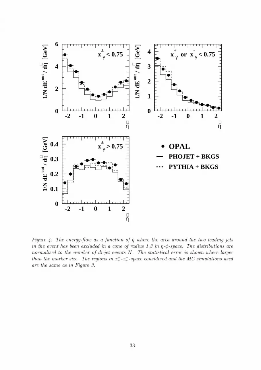
T in eachevent are considered. Another sensitive variable is the energy flow with the leading twojets in the event removed, Eout, as a function of η . All objects are excluded inside a coneof radius 1.3 in η-φ around the two leading jets.
Multiple parton interactions are important in interactions where the photon is resolved.It is therefore interesting to study separately the three cases of (a) two resolved photons,(b) one resolved photon, or (c) no resolved photon in the interaction. Experimentally thesesituations can be approximated by choosing events with x±γ < 0.75, x+
γ or x−γ < 0.75, orx±γ > 0.75, i.e. regions (D), (C) and (B) defined in Section 4.
Figures 3 and 4 show the jet profiles and the energy flow outside the leading jets. Thedata are compared to a mixture of signal (PHOJET or PYTHIA) and background MCsimulation. The contributions of signal and background are weighted according to theircross-section in each region of phase space. The background MC generators used are thesame as in Figure 2.
For the φ-profiles in Figure 3 it is evident that both PHOJET and PYTHIA are ableto describe the data in the region of the high ET jets around zero. Moving away fromthe jet axis PHOJET predicts an energy flow which is too low compared to the data,especially for x±γ < 0.75. This corresponds to the area where effects from an underlyingevent are expected to be most prominent. PHOJET improves towards higher xγ . PYTHIAreproduces the data reasonably well. Such differences between PHOJET and PYTHIA arenot evident in the η-profiles. Here in the case of resolved photons the ET-flow is dominatedby the photon remnant(s), and is reasonably well described by both generators. The jetsentering Figure 3 are selected from the range 10 < Ejet
T < 25 GeV. No significant deviation
11

from the behaviour just described is observed when selecting EjetT < 10 GeV.
The energy-flow outside the two leading jets is shown in Figure 4. Again PYTHIAdescribes the data well, while PHOJET is somewhat low. With both models used tounfold the data as a systematic check, we conclude that the details of the energy flowaround the two leading jets are sufficiently well under control and remaining influences areincluded in the systematic uncertainty of the cross-section and jet shape measurements.
7 Data corrections
An example of the uncorrected distributions as a function of xγ including the contributionof the remaining background events is shown in Figure 5. To obtain jet cross-sectionswhich can be compared to theoretical calculations, we use MC simulations to correct forthe selection cuts, the resolution effects of the detector and the background from non-signal processes. Backgrounds are first subtracted bin-by-bin from all distributions. Forthe differential cross-sections as a function of Ejet
T and xγ , sizable migration and resolutioneffects are to be expected. We therefore apply a matrix unfolding method, as implementedin the GURU program [26], for these distributions. The results are cross checked usinga bin-by-bin correction. By definition xγ can only take values between zero and unity.At either extremity no adjacent bins are available. To avoid instabilities expected fromthe smoothing procedures in the unfolding for the first and last bin, the central valuesfor these bins are taken from the bin-by-bin correction method. The |cos Θ∗|, |ηjet| and|∆ηjet| distributions are corrected bin-by-bin, as only small migrations are expected here.PHOJET is used as the default signal MC generator for the unfolding.
The correction method employed for the jet shapes is a bin-by-bin correction using theMC simulations to correct for detector effects. The contribution of the same backgroundprocesses as for the cross-section measurements was studied. The influence on the signalwas found to be less than 1%. Therefore the subtraction of the background was omittedin this analysis. Both PYTHIA and PHOJET were used to estimate the correction factorsto study their model dependence.
8 Systematic uncertainties
The overall systematic uncertainty is determined from the sources listed below added inquadrature. The same sources are considered for the measurement of the differential cross-sections and the jet shapes, with the exception of the background, which has been neglectedfor the jet shapes as discussed in Section 7.
• To assess the uncertainty associated with the subtraction of background events, thepredictions for hadronic decays of the Z0 and for γγ → ττ reactions are conserva-tively varied by 10% without contributing significantly to the systematic error. The
12

prediction of the contribution from γ?γ events has been scaled up by a factor of twoas described above. By comparing the predictions to the data for large EFD/EBEAM
and MJ1H2 (see Figure 2), where this background dominates, we determine that thisscaling factor can be varied by no more than about 30% in order to keep a gooddescription of the data. The scaling factor is varied accordingly. The uncertaintyfrom all the background subtraction is typically 2-4%.
• To estimate the systematic error arising from the specific model used for the un-folding, both PYTHIA and PHOJET are used to unfold the data. The estimateduncertainty derived from this study is typically 10%, and up to 20% in some casesfor the differential cross-sections, and 1-2% for the jet shapes.
• The absolute energy scale of the ECAL calorimeter is known to about 3% [27] for therange of jet energies in this analysis. To estimate the influence on the observables theenergy scale is varied by this amount and the analysis is repeated. The cross-sectionschange by 5-10% due to this variation. The estimated uncertainty for the jet shapesis about 1%.
• The selection criteria described in Section 5 are varied simultaneously both to be morerestrictive and to allow more events into the analysis to exclude a strong dependenceon the event selection. Selection criteria based on energy measurements are varied by10% of their central value, which is considered conservative given the uncertainty inthe energy scale and the energy resolution of the calorimeter. The number of tracksrequired and the maximum net charge of the event are changed by ±1. The allowedradial distance and z position of the primary vertex are varied by 0.5 cm and 1 cmrespectively. The uncertainty on the cross-section derived from all these variations istypically 5-10%, and up to 20% in some cases for the differential cross-section, andabout 2-4% for the jet shapes.
The uncertainty on the determination of the integrated luminosity is much less than 1%,and is neglected. For the differential cross-sections the systematic uncertainties evaluatedfor each bin were averaged with the results from its two neighbours (single neighbour forendpoints) to reduce the effect of bin-to-bin fluctuations.
9 Hadronisation corrections
The differential di-jet cross-sections measured are compared to NLO QCD calculationswhich predict jet cross-sections for partons, whereas the experimental jet cross-sections arepresented for hadrons. Effects due to the modelling of the hadronisation process are nottaken into account in the NLO calculation. Because the partons in the MC generators andthe partons in the NLO calculations are defined in different ways there is as yet no rigorousprocedure to use the MC generators to correct the data so that they can be compared to theNLO parton level predictions. However, as the MC generators are the only available optionso far, they are used to study the approximate size of these hadronisation corrections. Forthis purpose the prediction of the MC generators at the level of the partonic final state
13

is calculated and divided by the prediction obtained from the hadronic final state. Theresulting correction factor is labeled (1 + δhadr). The partonic final state consists of allpartons at the end of the parton shower. The hadronic final state utilises all charged andneutral particles with lifetimes greater than 3 × 10⁻¹⁰ s, which are treated as stable.
Examples of hadronisation corrections estimated by PYTHIA 6.161 and HERWIG 6.1for the observables defined in Section 4 are shown in Figure 6. The numerical values canbe found in [28]. In PYTHIA the partonic final state is hadronised according to the stringfragmentation model, while HERWIG uses cluster fragmentation. In all plots the full x+
γ -x−γ -range is considered. The theoretical calculations are corrected bin-by-bin using themean of the hadronisation corrections estimated using PYTHIA and HERWIG.
Figure 6 (a) shows (1 + δhadr) as a function of EjetT . The correction is less than 10% for
EjetT greater than about 10 GeV, but rises to about 25% for PYTHIA and 15% for HERWIG
towards small EjetT . The corrections for observbles involving the jet pseudo-rapidities are
dominated by the low EjetT region. They are essentially flat and around 20% for PYTHIA.
HERWIG estimates these corrections to be around 10%.
Figure 6 (b) shows (1 + δhadr) as a function of xγ for the lowest bin in EjetT defined
in Section 4. From the figure it is evident that hadronisation causes large corrections forxγ > 0.75. The effect is reduced for higher values of Ejet
T , as can be seen in Figure 6 (c) and(d). The large corrections for xγ > 0.75 are mainly due to the large influence hadronisationhas on the distribution of direct events, which are peaked at xγ = 1 for the partonicfinal state of the LO calculation, but are much more smeared out at the level of stablehadrons (see Figure 1 (a)-(c)). While both the measurement and the NLO calculation areperfectly valid for the presented bin sizes, the hadronisation corrections needed for thecomparison introduces a large migration between the two bins above xγ = 0.75. For asensible comparison in this region one should therefore consider the sum of the two binsabove xγ = 0.75 and compare it to the corresponding sum for the data.
10 Results
10.1 Jet structure in di-jet events
In Figure 7 (a) the jet shape, Ψ(r), is shown for the k⊥ algorithm for both x±γ > 0.75 andx±γ < 0.75. The first sample is dominated by direct photon-photon interactions and henceby quark-initiated jets. As is demonstrated in the figure, jets in this sample are morecollimated than for small values of x±γ , where the cross-section is dominated by resolvedprocesses and hence has a large contribution from gluon-initiated jets. In both cases thejets become more collimated with increasing transverse energy, as is shown in Figure 7 (c).There is no significant dependence on the jet pseudo-rapidity (Figure 7 (d)). Both PHOJETand PYTHIA give an adequate description of the jet shapes as can be seen in Figures 7 (b),(c), and (d).
Figure 8 compares the shapes of jets defined by the cone algorithm and the k⊥ algorithm,
14

in each case compared to the shape as obtained from PYTHIA. As for the k⊥-jets, thejets defined by the cone algorithm are more collimated in the quark-dominated sampleand always become more collimated for increasing transverse energy, while there is nodependence on the jet pseudo-rapidity. The cone-jets are significantly broader than the jetsdefined by the k⊥ algorithm at low Ejet
T . With increasing EjetT , jets become more collimated
and the two jet algorithms give similar results. While the k⊥-jets are well described byPYTHIA and PHOJET, the jet shapes obtained for the cone-jets are somewhat broaderthan in the data.
10.2 Differential di-jet cross-sections
Only the k⊥ jet algorithm is used for the measurement of the differential di-jet cross-sections. The experimental results are compared to a perturbative QCD calculation atNLO [29] which uses the GRVHO parametrisation of the parton distribution functions ofthe photon [14], and was repeated for the kinematic conditions of the present analysis. Therenormalisation and factorisation scales are set to the maximum Ejet
T in the event. The
calculation was performed in the MS-scheme with five light flavours and Λ(5)QCD = 130 MeV.
The average of the hadronisation corrections estimated by PYTHIA and HERWIG havebeen applied to the calculation for this comparison.
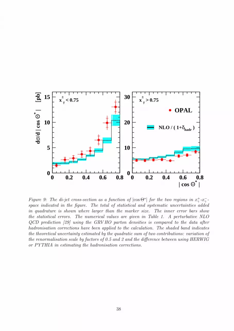
Figure 9 and Table 1 show the differential di-jet cross-section as a function of |cos Θ∗|for both x±γ > 0.75 and x±γ < 0.75. The steeper rise with increasing |cosΘ∗| from thedominating spin-1 gluon exchange in the second sample is clearly visible (see Section 4).The shape of both samples is well described by NLO QCD. For x±γ < 0.75 the NLOcalculation is about 20% below the data. It should be noted that in this region thecontribution from the underlying event, not included in the calculation, is expected to belargest, as discussed in more detail below. For x±γ > 0.75 the NLO QCD prediction is about20% above the data. While here the contribution from MIA is small, this region is affectedby rather large hadronisation corrections as discussed in Section 9, which translates intoan uncertainty of the normalisation in comparing the theoretical prediction to the data.
The differential di-jet cross-section as a function of the mean transverse energy EjetT
of the di-jet system is shown in Figure 10 and Table 2. At high EjetT the cross-section
is expected to be dominated by direct processes, associated with the region x±γ > 0.75.Consequently we observe a significantly softer spectrum for the case x±γ < 0.75 than forthe full x+
γ -x−γ -space. The calculation is in good agreement with the data for the full x+γ -
x−γ -range and for x+γ or x−γ < 0.75. The cross-section predicted for x±γ < 0.75 is again below
the measurement. PYTHIA 6.161 is in good agreement with the measured distributionsusing the SaS 1D parton densities.
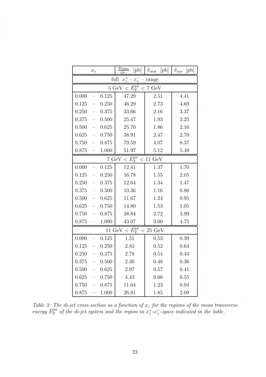
Figure 11 and Tables 3 and 6 show the di-jet cross-section as a function of xγ andlog10(xγ). The cross-section for the lowest values of Ejet
T shows the largest fraction ofevents at xγ < 0.75 of the three ranges considered, and is hence most sensitive to gluon-initiated processes. The di-jet cross-section logarithmic in xγ emphasises the region oflowest accessible xγ , which extends down to approximately 0.02.
15

As EjetT increases, the fraction of events with xγ > 0.75 increases. In MC simulations
these are predominantly direct events. The sensitivity to the gluon density in the photon ishence expected to decrease with increasing Ejet
T . On the other hand, NLO QCD predictionswhich use Ejet
T as the process-relevant scale are expected to become more reliable as thisscale increases. It is hence important to provide measurements at both low and high valuesof Ejet
T , to study all aspects of the theory.
PYTHIA using SaS 1D is in good agreement with the measured distributions, with atendency to be too low for small values of xγ . The shaded histogram at the bottom of eachplot indicates the MIA contribution to the PYTHIA prediction. The numerical values ofthis contibution can be found in [28]. NLO QCD predicts the shape of the cross-sectionswell for xγ < 0.75, but is too low by about 10-20% especially at low Ejet
T . As MIA arenot included in this calculation it is interesting to note that the MIA contribution to thecross-section as obtained from PYTHIA is similar in size to the discrepancy.
The region of xγ > 0.75 suffers from large hadronisation corrections as discussed inSection 9. The uncertainty for the data-theory comparison associated with these largecorrections can be reduced by considering the sum of the two bins above xγ = 0.75, forwhich NLO QCD indeed gives an adequate description of the data.
Figure 12 demonstrates the effect of using different parton distribution functions of thephoton on the NLO QCD prediction. AFG HO [30] and GS96 HO [31] are used in additionto the default GRVHO. The sensitivity of the cross-section to the different gluon densityin each case is clearly visible for the gg-contribution (Figure 12 (b)), but is less pronouncedfor the full cross-section as can be seen in Figure 12 (a), due to compensating effects fromprocesses involving the quark densities (Figures 12 (c) and (d)). A global analysis, beyondthe scope of this paper, using for example F γ
2 measurements to constrain simultaneouslythe quark densities hence promises to yield the highest sensitivity to the gluon density inthe photon.
In Figure 13 (Tables 4 and 6) the same cross-sections as in Figure 11 are shown for thecase x+
γ or x−γ < 0.75. Here the cross-section is dominated by interactions where one ofthe two incident photons is resolved. The multiple parton interactions used in PYTHIAto model an underlying event are much suppressed in this case, and NLO QCD describesboth the shape and normalisation of the data well. The opposite effect can be observedin Figure 14 (Tables 5 and 6), where for the case x±γ < 0.75 one expects a large influenceof multiple parton interactions, as demonstrated again by the shaded histogram at thebottom of each plot. The cross-sections change by as much as 50% in the low Ejet
T region,when MIA are switched on. For higher Ejet
T the influence is not as strong. Even with MIAswitched on, PYTHIA using SaS 1D is too low. The deficit visible in the normalisation ofthe NLO calculation is again of similar size as the MIA contribution to the cross-sectionobtained from PYTHIA.
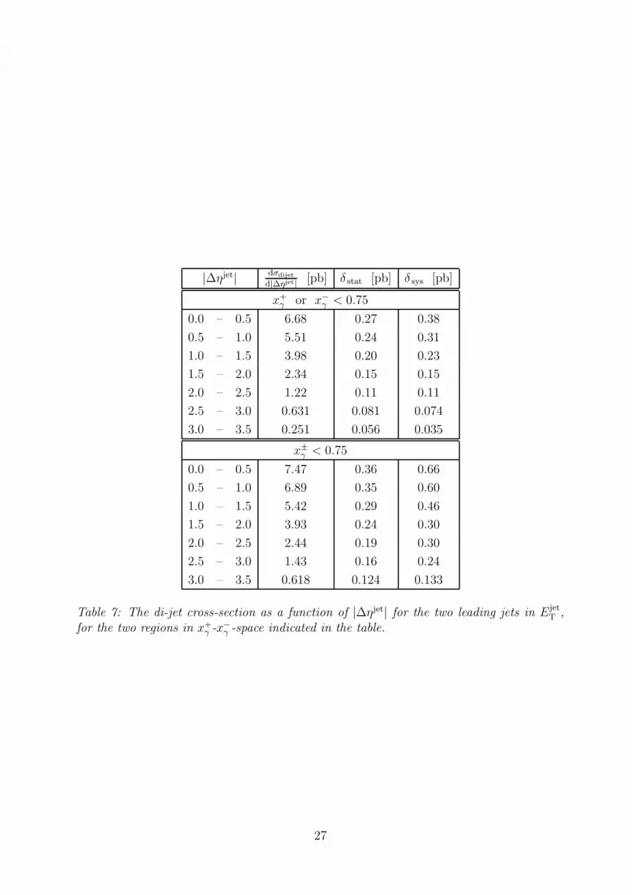
Complementary information can be obtained by measuring the angular distributions ofthe two highest Ejet
T jets in di-jet events. The |ηjet| and |∆ηjet| dependence of the di-jetcross-section is dominated by the low Ejet
T events. The cross-sections measured are listedin Tables 7, 8 and 9. In Figure 15 the di-jet cross-sections as a function of |∆ηjet|, |ηjet
cntr|and |ηjet
fwd| are shown for the case x+γ or x−γ < 0.75. Again the multiple parton interactions
16
used in PYTHIA to model an underlying event are much suppressed in this case. PYTHIAusing SaS 1D is about 20% too low. The prediction of NLO QCD is in good agreementwith the data in both shape and normalisation.
In Figure 16 the same cross-sections are presented for the case of x±γ < 0.75. Asexpected, the effect of including MIA in PYTHIA is again sizable. When multiple partoninteractions are switched on, the prediction obtained from PYTHIA reproduces the datareasonably well. Again the prediction of NLO QCD is too low by about the size of theMIA contribution to the cross-section obtained by PYTHIA.
11 Conclusions
We have studied di-jet production in photon-photon interactions with the OPAL detectorat e+e− centre-of-mass energies
√see from 189 to 209 GeV with an integrated luminosity
of 593 pb−1. The data are combined into one sample with a luminosity weighted averagecentre-of-mass energy of approximately
√see = 198.5 GeV. Jets are reconstructed using an
inclusive k⊥-clustering algorithm for the measurement of differential di-jet cross-sections,and using both the inclusive k⊥ and a cone algorithm for the study of jet structure.
Jet shapes, Ψ(r), have been studied in two separate samples: x±γ > 0.75, which is dom-inated by direct processes and hence by quark-initiated jets, and x±γ < 0.75, dominated byresolved events and therefore by gluon-initiated jets. As expected from QCD the jets inthe first sample are significantly more collimated than for x±γ < 0.75. Jets in both sam-ples become more collimated with increasing transverse energy, but show no significantdependence on the jet pseudo-rapidity. Jets defined by the cone algorithm are substan-tially broader than those defined by the k⊥ algorithm at low Ejet
T . However the differencedecreases with increasing Ejet
T . The shape of k⊥-jets is well described by PYTHIA andPHOJET. The jet shapes obtained for the cone-jets are somewhat broader in PYTHIAand PHOJET than in the data.
Inclusive differential di-jet cross-sections have been measured as a function of |cos Θ∗|,Ejet
T , |ηjet| and |∆ηjet| and, for the first time, as a function of xγ in several bins of EjetT .
Different regions of the x+γ -x−γ -space are explored to separate experimentally direct from
resolved interactions and to study and control the influence of an underlying event. Bymeasuring the cross-sections for events in which either x+
γ or x−γ is smaller than 0.75 we haveisolated a region of phase space in which resolved photon processes dominate, and whichat the same time is much less sensitive to multiple parton interactions. By performing themeasurement also for x±γ < 0.75, observables are made available which are sensitive to theamount of multiple parton interactions added in the prediction, and which can be used tostudy these effects in detail.
A strong rise with increasing |cos Θ∗| is observed for the differential di-jet cross-sectionfor x±γ < 0.75, as expected from QCD for a sample with a significant contribution fromspin-1 gluon exchange. The flatter distribution for direct events is also in good agreementwith the QCD calculation.
17

The differential di-jet cross-sections as a function of EjetT , |ηjet|, |∆ηjet| and xγ are in
good agreement with the next-to-leading order perturbative QCD calculation except forx±γ < 0.75, where the calculation is too low. As this calculation does not include a modelfor the underlying event that is expected to be largest in this region, it is interesting to notethat the discrepancy is of similar size to the contribution of multiple parton interactionsto the PYTHIA prediction. The sensitivity of the results presented to the gluon density inthe photon is clearly visible in NLO QCD predictions using different parton distributionfunctions, but is compensated to some extent by anti-correlated differences in the respectivequark-densities. A global analysis using additional data sets to simultaneously constrainthe quark densities hence promises to yield the highest sensitivity to the gluon density inthe photon.
The measurements carried out for events in which only either x+γ or x−γ is smaller than
0.75 are a unique data set. While this region is almost insensitive to multiple partoninteractions, the fraction of events at small xγ is still sizable, which indicates a significantcontribution of resolved processes and hence a good sensitivity to the hadronic structure ofthe photon. The good agreement of data and theory in this region in particular confirmsthat perturbative QCD in next-to-leading order is able to describe correctly the inclusiveproduction of di-jets in photon-photon collisions.
Acknowledgements
We thank M.Klasen and collaborators for providing the NLO QCD calculations andD.Berge and S.Konig for their contribution to the analysis of jet shapes presented inthis paper.
We particularly wish to thank the SL Division for the efficient operation of the LEPaccelerator at all energies and for their close cooperation with our experimental group. Inaddition to the support staff at our own institutions we are pleased to acknowledge theDepartment of Energy, USA,National Science Foundation, USA,Particle Physics and Astronomy Research Council, UK,Natural Sciences and Engineering Research Council, Canada,Israel Science Foundation, administered by the Israel Academy of Science and Humanities,Benoziyo Center for High Energy Physics,Japanese Ministry of Education, Culture, Sports, Science and Technology (MEXT) and agrant under the MEXT International Science Research Program,Japanese Society for the Promotion of Science (JSPS),German Israeli Bi-national Science Foundation (GIF),Bundesministerium fur Bildung und Forschung, Germany,National Research Council of Canada,Hungarian Foundation for Scientific Research, OTKA T-029328, and T-038240,The NWO/NATO Fund for Scientific Reasearch, the Netherlands.
18

References
[1] AMY Collaboration, B.J.Kim et al., Phys. Lett. B325 (1994) 248.
[2] TOPAZ Collaboration, H.Hayashii et al., Proceedings of Photon ’95, Sheffield, UK,8-13 April 1995, edited by D.J.Miller, S.L.Cartwright and V.Khoze, World Scientific(Singapore) 1995, p133;TOPAZ Collaboration, H.Hayashii et al., Phys. Lett. B314 (1993) 149.
[3] OPAL Collaboration, K.Ackerstaff et al., Z. Phys. C73 (1997) 433.
[4] OPAL Collaboration, G.Abbiendi et al., Eur. Phys. J. C10 (1999) 547.
[5] S. Catani, Yu.L.Dokshitzer, M.H. Seymour and B.R.Webber, Nucl. Phys. B406 (1993)187;S.D.Ellis, D.E. Soper, Phys. Rev. D48 (1993) 3160.
[6] OPAL Collaboration, R.Akers et al., Z. Phys. C63 (1994) 197.
[7] M.Wobisch and T.Wengler, hep-ph/9907280;M.H. Seymour, hep-ph/9707349;S.D.Ellis, Z.Kunszt and D.E. Soper, Phys. Rev. Lett. 69 (1992) 3615.
[8] C.H. Llewellyn Smith, Phys. Lett. B79 (1978) 83.
[9] OPAL Collaboration, K.Ahmet et al., Nucl. Instrum. Methods A305 (1991) 275;S.Anderson et al., Nucl. Instrum. Methods A403 (1998) 326;OPAL Collaboration, G.Abbiendi et al., Eur. Phys. J. C14 (2000) 373.
[10] T. Sjostrand, Comp. Phys. Comm. 82 (1994) 74;T. Sjostrand, LUND University Report, LU-TP-95-20 (1995).
[11] G.A. Schuler and T. Sjostrand, Z. Phys. C73 (1997) 677;G.A. Schuler and T. Sjostrand, Nucl. Phys. B407 (1993) 539.
[12] R.Engel, Z. Phys. C66 (1995) 203;R.Engel and J.Ranft, Phys. Rev. D54 (1996) 4244.
[13] G.A. Schuler and T. Sjostrand, Z. Phys. C68 (1995) 607.
[14] M.Gluck, E.Reya and A.Vogt, Phys. Rev. D45 (1992) 3986;M.Gluck, E.Reya and A.Vogt, Phys. Rev. D46 (1992) 1973.
[15] H1 Collaboration, C.Adloff et al., Eur. Phys. J. C1 (1998) 97;ZEUS Collaboration, J. Breitweg et al., Eur. Phys. J. C1 (1998) 109;ZEUS Collaboration, J. Breitweg et al., Eur. Phys. J. C4 (1998) 591;ZEUS Collaboration, J. Breitweg et al., Eur. Phys. J. C11 (1999) 35.
[16] F.A.Berends, P.H.Daverveldt and R.Kleiss, Nucl. Phys. B253 (1985) 421;F.A.Berends, P.H.Daverveldt and R.Kleiss, Comp. Phys. Comm. 40 (1986) 271, 285and 309.
19
[17] G.Marchesini et al., Comp. Phys. Comm. 67 (1992) 465;G.Corcella et al., JHEP 0101 (2001) 010.
[18] J.Allison et al., Nucl. Instrum. Methods A317 (1992) 47.
[19] L. Lonnblad and M. Seymour (convenors), γγ Event Generators, in “Physics at LEP2”,CERN 96-01, eds. G.Altarelli, T. Sjostrand and F. Zwirner, Vol. 2 (1996) 187.
[20] for example: H.Kolanoski, Two-Photon Physics at e+e− Storage Rings, Springer-Verlag (1984);B.L.Combridge, J.Kripfganz and J.Ranft, Phys. Lett. B70 (1977) 234;D.W.Duke and J.F.Owens, Phys. Rev. D26 (1982) 1600.
[21] M.Klasen and G.Kramer, Phys. Lett. B366 (1996) 385;S. Frixione and G.Ridolfi, Nucl. Phys. B507 (1997) 315.
[22] H1 Collaboration, C. Adloff et al., Eur. Phys. J. C1 (1998) 97.
[23] M.H. Seymour, Nucl. Phys. B513 (1998) 269.
[24] A.M.Rooke (for the OPAL collaboration), Proceedings of Photon ’97, Egmond aanZee, The Netherlands, 10-18 May 1997, edited by A.Buijs and F.C.Erne, World Sci-entific (Singapore) 1997, p465;A.M.Rooke, University of London, PhD Thesis, September 1998.
[25] H1 Collaboration, S.Aid et al., Z. Phys. C70 (1996) 17.
[26] A.Hocker, V.Kartvelishvili, Nucl. Instrum. Methods A372 (1996) 469.
[27] OPAL Collaboration, G.Abbiendi et al., Eur. Phys. J. C14 (2000) 199.
[28] HEPDATA: The Durham RAL Databases, Durham Database Group, at DurhamUniversity(UK), http://www-spires.dur.ac.uk/HEPDATA.
[29] M.Klasen, T.Kleinwort and G.Kramer, Eur. Phys. J. Direct C1 (1998) 1;B.Potter, Eur. Phys. J. Direct C5 (1999) 1.
[30] P.Aurenche, J.P.Guillet and M.Fontannaz, Z. Phys. C64 (1994) 621.
[31] L.E.Gordon and J.K. Storrow, Nucl. Phys. B489 (1997) 405.
20

|cos Θ∗| dσdijet
d|cos Θ∗| [pb] δ stat [pb] δ sys [pb]
x±γ > 0.75
0.0 – 0.1 5.04 0.49 0.32
0.1 – 0.2 4.96 0.49 0.34
0.2 – 0.3 5.22 0.49 0.32
0.3 – 0.4 5.35 0.48 0.38
0.4 – 0.5 4.90 0.45 0.32
0.5 – 0.6 6.73 0.56 0.47
0.6 – 0.7 7.09 0.54 0.43
0.7 – 0.8 8.42 0.61 0.51
x±γ < 0.75
0.0 – 0.1 1.50 0.31 0.24
0.1 – 0.2 2.63 0.46 0.36
0.2 – 0.3 2.91 0.50 0.41
0.3 – 0.4 3.73 0.62 0.43
0.4 – 0.5 4.36 0.61 0.62
0.5 – 0.6 6.52 0.80 0.74
0.6 – 0.7 9.90 0.92 1.07
0.7 – 0.8 13.05 0.96 1.02
Table 1: The di-jet cross-section as a function of |cos Θ∗| for the two regions in x+γ -x−γ -
space indicated in the table. The total uncertainty for each bin is the quadratic sum of thestatistical and systematic uncertainty given in the table.
21

EjetT [GeV]
dσdijet
dEjetT
[pb/GeV] δ stat [pb/GeV] δ sys [pb/GeV]
full x+γ - x−γ – range
5.00 – 6.54 11.54 0.36 0.59
6.54 – 8.55 4.16 0.16 0.25
8.55 – 11.18 1.45 0.07 0.09
11.18 – 14.62 0.543 0.036 0.044
14.62 – 19.12 0.176 0.020 0.020
19.12 – 25.00 0.0607 0.0117 0.0087
x+γ or x−γ < 0.75
5.00 – 6.54 3.56 0.21 0.22
6.54 – 8.55 1.32 0.09 0.10
8.55 – 11.18 0.475 0.045 0.037
11.18 – 14.62 0.190 0.025 0.024
14.62 – 19.12 0.0518 0.0127 0.0073
x±γ < 0.75
5.00 – 6.54 5.94 0.41 0.66
6.54 – 8.55 1.84 0.16 0.23
8.55 – 11.18 0.461 0.060 0.071
11.18 – 14.62 0.0781 0.0192 0.0130
Table 2: The di-jet cross-section as a function of the mean transverse energy EjetT of the
di-jet system, for the three regions in x+γ -x−γ -space indicated in the table.
22
xγdσdijet
dxγ[pb] δ stat [pb] δ sys [pb]
full x+γ - x−γ – range
5 GeV < EjetT < 7 GeV
0.000 – 0.125 47.29 2.51 4.41
0.125 – 0.250 46.29 2.73 4.69
0.250 – 0.375 33.66 2.16 3.37
0.375 – 0.500 25.47 1.93 2.25
0.500 – 0.625 25.70 1.86 2.16
0.625 – 0.750 38.91 2.47 2.70
0.750 – 0.875 79.59 4.07 8.37
0.875 – 1.000 51.97 5.12 5.49
7 GeV < EjetT < 11 GeV
0.000 – 0.125 12.41 1.37 1.70
0.125 – 0.250 16.78 1.55 2.05
0.250 – 0.375 12.64 1.34 1.47
0.375 – 0.500 10.36 1.16 0.86
0.500 – 0.625 11.67 1.24 0.95
0.625 – 0.750 14.80 1.53 1.05
0.750 – 0.875 38.84 2.72 3.99
0.875 – 1.000 43.07 3.00 4.75
11 GeV < EjetT < 25 GeV
0.000 – 0.125 1.51 0.53 0.39
0.125 – 0.250 2.83 0.52 0.64
0.250 – 0.375 2.78 0.54 0.43
0.375 – 0.500 2.30 0.48 0.36
0.500 – 0.625 2.97 0.57 0.41
0.625 – 0.750 4.43 0.66 0.55
0.750 – 0.875 11.04 1.23 0.94
0.875 – 1.000 26.81 1.85 2.09
Table 3: The di-jet cross-section as a function of xγ for the regions of the mean transverseenergy Ejet
T of the di-jet system and the region in x+γ -x−γ -space indicated in the table.
23

xγdσdijet
dxγ[pb] δ stat [pb] δ sys [pb]
x+γ or x−γ < 0.75
5 GeV < EjetT < 7 GeV
0.000 – 0.125 12.47 0.96 1.18
0.125 – 0.250 8.87 0.74 1.16
0.250 – 0.375 7.00 0.69 0.83
0.375 – 0.500 5.12 0.58 0.65
0.500 – 0.625 5.99 0.69 0.56
0.625 – 0.750 12.36 1.27 0.98
0.750 – 0.875 38.50 1.92 4.19
0.875 – 1.000 11.80 1.72 1.30
7 GeV < EjetT < 11 GeV
0.000 – 0.125 5.44 0.73 0.62
0.125 – 0.250 4.84 0.52 0.48
0.250 – 0.375 3.45 0.44 0.31
0.375 – 0.500 2.91 0.41 0.21
0.500 – 0.625 3.28 0.48 0.25
0.625 – 0.750 5.38 0.76 0.39
0.750 – 0.875 15.03 1.17 1.94
0.875 – 1.000 8.63 1.19 1.31
Table 4: The di-jet cross-section as a function of xγ for the regions of the mean transverseenergy Ejet
T of the di-jet system and the region in x+γ -x−γ -space indicated in the table.
24

xγdσdijet
dxγ[pb] δ stat [pb] δ sys [pb]
x±γ < 0.75
5 GeV < EjetT < 7 GeV
0.000 – 0.125 42.37 2.94 4.71
0.125 – 0.250 37.66 2.44 4.32
0.250 – 0.375 26.87 1.99 2.66
0.375 – 0.500 19.63 1.88 1.49
0.500 – 0.625 17.84 1.55 1.10
0.625 – 0.750 26.71 3.86 1.73
7 GeV < EjetT < 11 GeV
0.000 – 0.125 8.81 1.08 1.54
0.125 – 0.250 11.00 1.00 1.72
0.250 – 0.375 10.30 0.96 1.24
0.375 – 0.500 8.10 0.81 0.76
0.500 – 0.625 7.49 0.94 0.64
0.625 – 0.750 8.51 1.58 0.72
Table 5: The di-jet cross-section as a function of xγ for the regions of the mean transverseenergy Ejet
T of the di-jet system and the region in x+γ -x−γ -space indicated in the table.
25

log10(xγ)dσdijet
dlog10(xγ)[pb] δ stat [pb] δ sys [pb]
5 GeV < EjetT < 7 GeV
full x+γ - x−γ – range
-1.65 – -1.32 4.00 0.42 0.42
-1.32 – -0.99 9.54 0.76 1.07
-0.99 – -0.66 16.55 1.12 1.83
-0.66 – -0.33 27.51 1.39 2.35
-0.33 – 0.00 76.87 1.69 5.05
x+γ or x−γ < 0.75
-1.65 – -1.32 1.29 0.18 0.18
-1.32 – -0.99 2.38 0.24 0.32
-0.99 – -0.66 3.64 0.30 0.44
-0.66 – -0.33 4.87 0.38 0.47
-0.33 – 0.00 25.87 0.99 2.16
x±γ < 0.75
-1.65 – -1.32 3.08 0.44 0.41
-1.32 – -0.99 7.81 0.63 1.02
-0.99 – -0.66 13.95 0.92 1.55
-0.66 – -0.33 19.39 1.13 1.78
-0.33 – 0.00 18.01 1.53 1.36
Table 6: The di-jet cross-section as a function of log10(xγ) for the region of the meantransverse energy Ejet
T of the di-jet system and the regions in x+γ -x−γ -space indicated in the
table.
26
|∆ηjet| dσdijet
d|∆ηjet| [pb] δ stat [pb] δ sys [pb]
x+γ or x−γ < 0.75
0.0 – 0.5 6.68 0.27 0.38
0.5 – 1.0 5.51 0.24 0.31
1.0 – 1.5 3.98 0.20 0.23
1.5 – 2.0 2.34 0.15 0.15
2.0 – 2.5 1.22 0.11 0.11
2.5 – 3.0 0.631 0.081 0.074
3.0 – 3.5 0.251 0.056 0.035
x±γ < 0.75
0.0 – 0.5 7.47 0.36 0.66
0.5 – 1.0 6.89 0.35 0.60
1.0 – 1.5 5.42 0.29 0.46
1.5 – 2.0 3.93 0.24 0.30
2.0 – 2.5 2.44 0.19 0.30
2.5 – 3.0 1.43 0.16 0.24
3.0 – 3.5 0.618 0.124 0.133
Table 7: The di-jet cross-section as a function of |∆ηjet| for the two leading jets in EjetT ,
for the two regions in x+γ -x−γ -space indicated in the table.
27

|ηjetcntr| dσdijet
d|ηjetcntr|
[pb] δ stat [pb] δ sys [pb]
x+γ or x−γ < 0.75
0.00 – 0.25 11.48 0.50 0.65
0.25 – 0.50 9.25 0.44 0.55
0.50 – 0.75 7.19 0.38 0.46
0.75 – 1.00 5.30 0.32 0.31
1.00 – 1.25 3.49 0.26 0.23
1.25 – 1.50 2.60 0.24 0.25
1.50 – 1.75 1.49 0.21 0.17
x±γ < 0.75
0.00 – 0.25 14.93 0.67 1.24
0.25 – 0.50 13.38 0.65 1.17
0.50 – 0.75 10.83 0.60 0.96
0.75 – 1.00 7.17 0.47 0.60
1.00 – 1.25 5.59 0.46 0.54
1.25 – 1.50 3.20 0.41 0.41
1.50 – 1.75 2.01 0.41 0.32
Table 8: The di-jet cross-section as a function of |ηjetcntr| for the two regions in x+
γ -x−γ -spaceindicated in the table.
28

|ηjetfwd| dσdijet
d|ηjetfwd|
[pb] δstat [pb] δsys [pb]
x+γ or x−γ < 0.75
0.00 – 0.25 0.906 0.137 0.065
0.25 – 0.50 2.68 0.23 0.18
0.50 – 0.75 4.30 0.29 0.26
0.75 – 1.00 5.65 0.33 0.33
1.00 – 1.25 6.18 0.34 0.33
1.25 – 1.50 6.86 0.36 0.34
1.50 – 1.75 7.27 0.40 0.48
1.75 – 2.00 7.03 0.44 0.55
x±γ < 0.75
0.00 – 0.25 1.03 0.17 0.16
0.25 – 0.50 4.11 0.38 0.54
0.50 – 0.75 5.64 0.40 0.60
0.75 – 1.00 6.71 0.41 0.51
1.00 – 1.25 8.40 0.47 0.74
1.25 – 1.50 10.72 0.62 0.94
1.50 – 1.75 11.30 0.68 1.18
1.75 – 2.00 9.86 0.72 0.96
Table 9: The di-jet cross-section as a function of |ηjetfwd| for the two regions in x+
γ -x−γ -spaceindicated in the table.
29

0
0.2
0.4
0.6
0.8
1
0 0.2 0.4 0.6 0.8 1xγ
frac
tion
PYTHIA 6.1 (SaS1D)directsingle - res.double - res.
5 < E jet
T < 7 GeV−
7 < E jet
T < 11 GeV−
11 < E jet
T < 25 GeV−
0
0.2
0.4
0.6
0.8
1
0 0.2 0.4 0.6 0.8 1xγ
frac
tion
0
0.2
0.4
0.6
0.8
1
0 0.2 0.4 0.6 0.8 1xγ
frac
tion
0
1
0 1xγ
-
x γ +
C
C
B
D
(a) (b)
(c) (d)
0.75
0.75
Figure 1: (a)-(c): The relative contribution of direct, single-resolved, and double-resolvedprocesses according to PYTHIA at the hadron level for the cross-sections as a functionof xγ for the full x+
γ -x−γ -range (see Section 4). In (d) the regions in x+γ -x−γ -space used in
addition to the full x+γ -x−γ -range (referred to as (A)) are illustrated: (B) both x+
γ and x−γlarger than 0.75 (x±γ > 0.75), (C) either x+
γ or x−γ smaller than 0.75 (x+γ or x−γ < 0.75),
(D) both x+γ and x−γ smaller than 0.75 (x±γ < 0.75).
30

10
10 2
10 3
10 4
0 20 40 60
EECAL + EHCAL [GeV]
Eve
nts
0 20 40 6010
10 2
10 3
10 4
10
10 2
10 3
10 4
10 20 30 40
NTRK
Eve
nts
10 20 30 40
10
10 2
10 3
10 4
1
10
10 2
10 3
10 4
10 5
0 0.1 0.2 0.3 0.4
EFD / EBEAM
Eve
nts
0 0.1 0.2 0.3 0.41
10
10 2
10 3
10 4
10 5
10
10 2
10 3
10 4
0 20 40 60 80
MJ1H2 [GeV]
Eve
nts
0 20 40 60 80
10
10 2
10 3
10 4
OPAL MC PHOJETMC γ*γ
MC γγ → ττMC Z/ γ* → qq
_
(a)(b)
(c) (d)
↓
↓
↓ ↓
Figure 2: Comparison of event quantities for uncorrected data with the simulation for thedi-jet sample including contributions from background processes. (a) shows the sum ofenergy measured in the electromagnetic and hadronic calorimeter, (b) the number of tracksin the event, (c) is the sum of energy in the FD detector scaled by the beam energy, and(d) the invariant mass of the jet with the highest Ejet
T in the event and the four-vectorcalculated from all objects in the opposite hemisphere as seen from this jet. The statisticalerror is shown where larger than the marker size. The label γ?γ stands for simulatedphoton-photon collision events in which one of the photons has a virtuality larger than4.5 GeV 2 as discussed in Section 4.
31

1
10
-2 0 2
∆φ
1/N
jet d
ET /
d(∆Φ
) [
GeV
]
10-1
1
10
-2 -1 0 1 2
∆η∧
1/N
jet d
ET /
d(∆η
∧)
[GeV
]
1
10
10 2
-2 0 2
∆φ
1/N
jet d
ET /
d(∆Φ
) [
GeV
]
10-1
1
10
10 2
-2 -1 0 1 2
∆η∧
1/N
jet d
ET /
d(∆η
∧)
[GeV
]
10-1
1
10
-2 0 2
∆φ
1/N
jet d
ET /
d(∆Φ
) [
GeV
]
10-1
1
10
-2 -1 0 1 2
∆η∧
1/N
jet d
ET /
d(∆η
∧)
[GeV
]
x± γ < 0.75
x+ γ or x
- γ < 0.75
x± γ > 0.75
x± γ < 0.75
x+ γ or x
- γ < 0.75
x± γ > 0.75
OPAL
PHOJET + BKGSPYTHIA + BKGS
Figure 3: Jet profiles: The ET-flow normalised to the number of jets Njet as a functionof the distance from the jet axis in φ and η. Jets are selected from the range 10 < Ejet
T <25 GeV. The statistical error is shown where larger than the marker size. The data arecompared to a mixture of signal (PHOJET or PYTHIA) and background MC simulation.The background MC simulations used are the same as in Figure 2.
32
0
2
4
6
-2 -1 0 1 2
η∧
1/N
dE
out
/ dη∧
[G
eV]
0
1
2
3
4
-2 -1 0 1 2
η∧
1/N
dE
out
/ dη∧
[G
eV]
0
0.1
0.2
0.3
0.4
-2 -1 0 1 2
η∧
1/N
dE
out
/ dη∧
[G
eV]
x± γ < 0.75 x
+ γ or x
- γ < 0.75
x± γ > 0.75 OPAL
PHOJET + BKGS
PYTHIA + BKGS
Figure 4: The energy-flow as a function of η where the area around the two leading jetsin the event has been excluded in a cone of radius 1.3 in η-φ-space. The distributions arenormalised to the number of di-jet events N . The statistical error is shown where largerthan the marker size. The regions in x+
γ -x−γ -space considered and the MC simulations usedare the same as in Figure 3.
33

10
10 2
10 3
10 4
0 0.2 0.4 0.6 0.8 10 0.2 0.4 0.6 0.8 1
10
10 2
10 3
10 4
xγ
Eve
nts
OPAL MC PHOJETMC γ*γ
MC γγ → ττMC Z/ γ* → qq
_
5 < E jet
T < 7 GeV−
5 < E jet
T < 7 GeV−
7 < E jet
T < 11 GeV−
11 < E jet
T < 25 GeV−
10
10 2
10 3
10 4
-1.5 -1 -0.5 0-1.5 -1 -0.5 0
10
10 2
10 3
10 4
log10( xγ)
Eve
nts
10
10 2
10 3
10 4
0 0.2 0.4 0.6 0.8 10 0.2 0.4 0.6 0.8 1
10
10 2
10 3
10 4
xγ
Eve
nts
10
10 2
10 3
0 0.2 0.4 0.6 0.8 10 0.2 0.4 0.6 0.8 1
10
10 2
10 3
xγ
Eve
nts
Figure 5: The uncorrected xγ distributions in the data compared to the sum of signal andbackground processes in the simulation. The statistical error is shown where larger thanthe marker size. The MC simulations used are the same as in Figure 2.
34

0.6
0.8
1
1.2
1.4
5 10 15 20 25
E– jet
T [GeV]
1+δ ha
dr
0
1
2
3
0 0.2 0.4 0.6 0.8 1xγ
1+δ ha
dr
0
1
2
3
0 0.2 0.4 0.6 0.8 1xγ
1+δ ha
dr
0
1
2
3
0 0.2 0.4 0.6 0.8 1xγ
1+δ ha
dr
5 < E jet
T < 7 GeV−
7 < E jet
T < 11 GeV−
11 < E jet
T < 25 GeV−
PYTHIAHERWIG
(a) (b)
(c) (d)
Figure 6: Hadronisation corrections estimated by PYTHIA and HERWIG for (a) EjetT and
(b)-(d) xγ for the regions of EjetT given in the figure. In all cases the full x+
γ -x−γ -space isconsidered.
35

0
0.2
0.4
0.6
0.8
1
0.2 0.4 0.6 0.8 1r
ψ(r
)
OPAL, k ⊥ algor.
x± γ > 0.75
x± γ < 0.75
r
ψ(r
)
0
0.2
0.4
0.6
0.8
1
0.2 0.4 0.6 0.8 1r
ψ(r
)PHOJET
PYTHIA
PYTHIAPYTHIA
(a) (b)
(c) (d)
0.5
0.6
0.7
0.8
0.9
5 10 15 20E
jet
T [ GeV ]
ψ(r
=0.
4)
0.5
0.6
0.7
0.8
0.9
0 0.5 1 1.5 2| ηjet|
ψ(r
=0.
4)
x± γ < 0.75
Figure 7: The jet shape, Ψ(r), for the two regions of x+γ -x−γ -space indicated in the figure (a),
and Ψ(r) for x±γ < 0.75 compared to the predictions of the LO MC generators PHOJETand PYTHIA (b). Figures (c) and (d) show the value of Ψ(r = 0.4) as a function ofthe transverse energy and pseudo-rapidity of the jet respectively, compared to the PYTHIAprediction. The total of statistical and systematic uncertainties added in quadrature isshown where larger than the marker size. The inner error bars show the statistical errors.
36

0.5
0.6
0.7
0.8
5 10 15 20E
jet
T [ GeV ]
ψ(r
=0.
4)
OPALk ⊥ algorithm
cone algorithm
PYTHIAk ⊥ algorithm
cone algorithm
(a) x± γ < 0.75
(b) x± γ > 0.75
(c) x± γ < 0.75
(d) x± γ > 0.75
0.5
0.6
0.7
0.8
5 10 15 20E
jet
T [ GeV ]
ψ(r
=0.
4)
0.5
0.6
0.7
0.8
0 0.5 1 1.5 2| ηjet|
ψ(r
=0.
4)
0.5
0.6
0.7
0.8
0 0.5 1 1.5 2| ηjet|
ψ(r
=0.
4)
Figure 8: The value of the jet shape Ψ(r) at r = 0.4 as a function of the jet transverseenergy for x±γ < 0.75 (a) and x±γ > 0.75 (b), and as a function of the jet pseudo-rapidityfor x±γ < 0.75 (c) and x±γ > 0.75 (d). In each figure the results obtained using the inclusivek⊥ and the cone jet algorithm are shown and compared to the PYTHIA prediction. Thetotal of statistical and systematic uncertainties added in quadrature is shown where largerthan the marker size. The inner error bars show the statistical errors.
37
0
5
10
15
0 0.2 0.4 0.6 0.80 0.2 0.4 0.6 0.80
5
10
15
dσ/d
| co
s Θ* |
[p
b]
0
10
20
30
0 0.2 0.4 0.6 0.80 0.2 0.4 0.6 0.80
10
20
30
| cos Θ* |
OPAL
x± γ > 0.75x
± γ < 0.75
NLO / ( 1+δhadr )
Figure 9: The di-jet cross-section as a function of |cos Θ∗| for the two regions in x+γ -x−γ -
space indicated in the figure. The total of statistical and systematic uncertainties addedin quadrature is shown where larger than the marker size. The inner error bars showthe statistical errors. The numerical values are given in Table 1. A perturbative NLOQCD prediction [29] using the GRV HO parton densities is compared to the data afterhadronisation corrections have been applied to the calculation. The shaded band indicatesthe theoretical uncertainty estimated by the quadratic sum of two contributions: variation ofthe renormalisation scale by factors of 0.5 and 2 and the difference between using HERWIGor PYTHIA in estimating the hadronisation corrections.
38

10-2
10-1
1
10
10 2
5 7.5 10 12.5 15 17.5 20 22.5 25 27.5 305 7.5 10 12.5 15 17.5 20 22.5 25 27.5 30
10-2
10-1
1
10
10 2
E– jet
T [GeV]
f •
dσ
/dE–
jet
T
[pb
/GeV
]
OPAL
full x± γ range
x+ γ or x
- γ < 0.75
x± γ < 0.75
f = 10.0
f = 1.0
f = 0.1
PYTHIA SaS 1D
NLO / ( 1+δhadr )
Figure 10: The di-jet cross-section as a function of the mean transverse energy EjetT of the
di-jet system, for the three regions in x+γ -x−γ -space given in the figure. The factor f is used
to separate the three measurements in the figure more clearly. The total of statistical andsystematic uncertainties added in quadrature is shown where larger than the marker size.The inner error bars show the statistical errors. The numerical values are given in Table 2.The prediction of the LO program PYTHIA using the parton distribution function SaS 1Dis compared to the data. The NLO calculation is the same as in Figure 9.
39

0
20
40
60
80
100
0 0.2 0.4 0.6 0.8 10 0.2 0.4 0.6 0.8 10
20
40
60
80
100
xγ
dσ/d
x γ [p
b]
OPALfull x
± γ range
NLO / ( 1+δhadr )
PYTHIA SaS 1D
PYTHIA MIAcontribution
5 < E jet
T < 7 GeV−
5 < E jet
T < 7 GeV−
7 < E jet
T < 11 GeV−
11 < E jet
T < 25 GeV−
10
10 2
-1.5 -1 -0.5 0-1.5 -1 -0.5 0
10
10 2
log10( xγ)
dσ/d
log 10
(xγ)
[p
b]
0
10
20
30
40
50
60
70
0 0.2 0.4 0.6 0.8 10 0.2 0.4 0.6 0.8 10
10
20
30
40
50
60
70
xγ
dσ/d
x γ [p
b]
0
5
10
15
20
25
30
0 0.2 0.4 0.6 0.8 10 0.2 0.4 0.6 0.8 10
5
10
15
20
25
30
xγ
dσ/d
x γ [p
b]
Figure 11: The di-jet cross-section as a function of xγ and log10 (xγ) for the regions ofthe mean transverse energy Ejet
T of the di-jet system indicated in the figures. The totalof statistical and systematic uncertainties added in quadrature is shown where larger thanthe marker size. The inner error bars show the statistical errors. The numerical valuesare given in Tables 3 and 6. The prediction of the LO MC generator PYTHIA using theparton distribution function SaS 1D is compared to the data. The shaded histogram at thebottom of each plot indicates the MIA contribution to the PYTHIA prediction. The NLOcalculation is the same as in Figure 9.
40
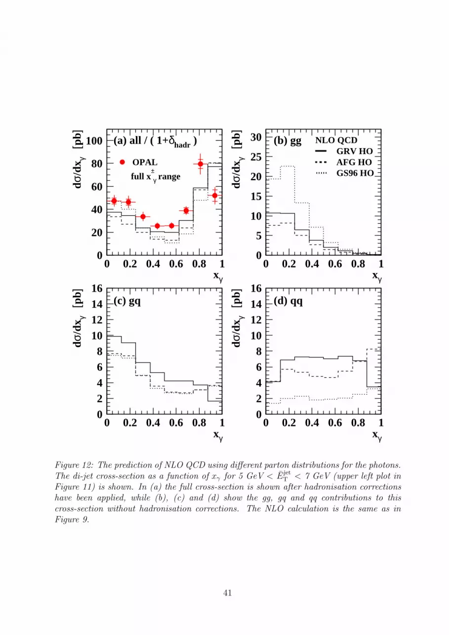
0
20
40
60
80
100
0 0.2 0.4 0.6 0.8 1xγ
dσ/d
x γ [p
b]
0
5
10
15
20
25
30
0 0.2 0.4 0.6 0.8 1xγ
dσ/d
x γ [p
b]
02468
10121416
0 0.2 0.4 0.6 0.8 1xγ
dσ/d
x γ [p
b]
02468
10121416
0 0.2 0.4 0.6 0.8 1xγ
dσ/d
x γ [p
b]
OPAL
full x± γ range
NLO QCDGRV HOAFG HOGS96 HO
(a) all / ( 1+δhadr ) (b) gg
(c) gq (d) qq
Figure 12: The prediction of NLO QCD using different parton distributions for the photons.The di-jet cross-section as a function of xγ for 5 GeV < Ejet
T < 7 GeV (upper left plot inFigure 11) is shown. In (a) the full cross-section is shown after hadronisation correctionshave been applied, while (b), (c) and (d) show the gg, gq and qq contributions to thiscross-section without hadronisation corrections. The NLO calculation is the same as inFigure 9.
41

0
20
40
0 0.2 0.4 0.6 0.8 10 0.2 0.4 0.6 0.8 10
20
40
xγ
dσ/d
x γ [p
b]
OPAL
x+ γ or x
- γ < 0.75
PYTHIA SaS 1D
PYTHIA MIAcontribution
NLO / ( 1+δhadr )
5 < E jet
T < 7 GeV−
5 < E jet
T < 7 GeV−
7 < E jet
T < 11 GeV−
1
10
-1.5 -1 -0.5 0-1.5 -1 -0.5 0
1
10
log10( xγ)
dσ/d
log 10
(xγ)
[p
b]
0
5
10
15
20
0 0.2 0.4 0.6 0.8 10 0.2 0.4 0.6 0.8 10
5
10
15
20
xγ
dσ/d
x γ [p
b]
Figure 13: The di-jet cross-section as a function of xγ and log10 (xγ) for the regions ofthe mean transverse energy Ejet
T of the di-jet system indicated in the figures and for x+γ or
x−γ < 0.75 . The total of statistical and systematic uncertainties added in quadrature isshown where larger than the marker size. The inner error bars show the statistical errors.The numerical values are given in Tables 4 and 6. The NLO calculation and MC simulationare the same as in Figure 11.
42

0
20
40
60
0 0.2 0.4 0.6 0.8 10 0.2 0.4 0.6 0.8 10
20
40
60
xγ
dσ/d
x γ [p
b]
OPAL
x± γ < 0.75
PYTHIA SaS 1D
PYTHIA MIAcontribution
NLO / ( 1+δhadr )
5 < E jet
T < 7 GeV−
5 < E jet
T < 7 GeV−
7 < E jet
T < 11 GeV−
1
10
-1.5 -1 -0.5 0-1.5 -1 -0.5 0
1
10
log10( xγ)
dσ/d
log 10
(xγ)
[p
b]
0
5
10
15
0 0.2 0.4 0.6 0.8 10 0.2 0.4 0.6 0.8 10
5
10
15
xγ
dσ/d
x γ [p
b]
Figure 14: The di-jet cross-section as a function of xγ and log10 (xγ) for the regions of themean transverse energy Ejet
T of the di-jet system indicated in the figures. For these cross-sections x±γ < 0.75 is required. The total of statistical and systematic uncertainties addedin quadrature is shown where larger than the marker size. The inner error bars show thestatistical errors. The numerical values are given in Tables 5 and 6. The NLO calculationand MC simulation are the same as in Figure 11.
43

0
2
4
6
8
0 0.5 1 1.5 2 2.5 3 3.5 40 0.5 1 1.5 2 2.5 3 3.5 40
2
4
6
8
| ∆ηjet |
dσ/d
| ∆η
jet |
[p
b]
0
5
10
0 0.5 1 1.5 20 0.5 1 1.5 20
5
10
| ηcntr
jet |
dσ/d
| η cn
tr
jet
| [
pb]
0
2
4
6
8
0 0.5 1 1.5 20 0.5 1 1.5 20
2
4
6
8
| ηfwd
jet |
dσ/d
| η fw
d
jet |
[
pb]
OPALx
+ γ or x
- γ < 0.75
NLO / ( 1+δhadr )
PYTHIA SaS 1D
PYTHIA MIAcontribution
Figure 15: The di-jet cross-section as a function of |∆ηjet| for the two leading jets in EjetT
and separately for the central and the forward jet, for x+γ or x−γ < 0.75. The total of
statistical and systematic uncertainties added in quadrature is shown where larger than themarker size. The inner error bars show the statistical errors. The numerical values aregiven in Tables 7, 8 and 9. The NLO calculation and MC simulation are the same as inFigure 11.
44
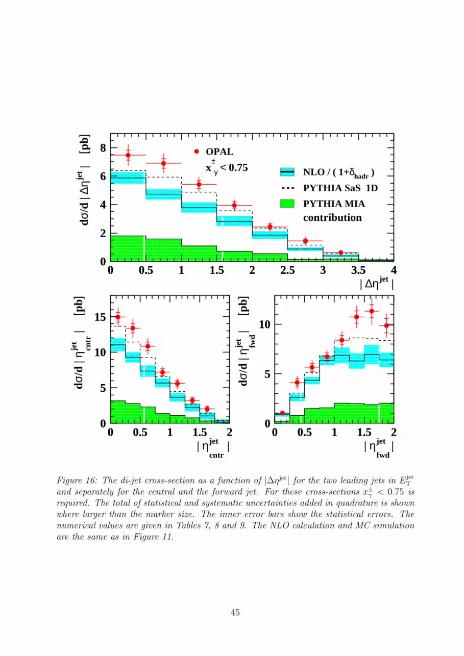
0
2
4
6
8
0 0.5 1 1.5 2 2.5 3 3.5 40 0.5 1 1.5 2 2.5 3 3.5 40
2
4
6
8
| ∆ηjet |
dσ/d
| ∆η
jet |
[p
b]
0
5
10
15
0 0.5 1 1.5 20 0.5 1 1.5 20
5
10
15
| ηcntr
jet |
dσ/d
| η cn
tr
jet
| [
pb]
0
5
10
0 0.5 1 1.5 20 0.5 1 1.5 20
5
10
| ηfwd
jet |
dσ/d
| η fw
d
jet |
[
pb]
OPAL
x± γ < 0.75 NLO / ( 1+δhadr )
PYTHIA SaS 1D
PYTHIA MIAcontribution
Figure 16: The di-jet cross-section as a function of |∆ηjet| for the two leading jets in EjetT
and separately for the central and the forward jet. For these cross-sections x±γ < 0.75 isrequired. The total of statistical and systematic uncertainties added in quadrature is shownwhere larger than the marker size. The inner error bars show the statistical errors. Thenumerical values are given in Tables 7, 8 and 9. The NLO calculation and MC simulationare the same as in Figure 11.
45