développement de méthodes numériques et étude des
TRANSCRIPT
HAL Id: tel-01639797https://tel.archives-ouvertes.fr/tel-01639797
Submitted on 20 Nov 2017
HAL is a multi-disciplinary open accessarchive for the deposit and dissemination of sci-entific research documents, whether they are pub-lished or not. The documents may come fromteaching and research institutions in France orabroad, or from public or private research centers.
L’archive ouverte pluridisciplinaire HAL, estdestinée au dépôt et à la diffusion de documentsscientifiques de niveau recherche, publiés ou non,émanant des établissements d’enseignement et derecherche français ou étrangers, des laboratoirespublics ou privés.
Développement de méthodes numériques et étude desphénomènes couplés d’écoulement, de rayonnement, etd’ablation dans les problèmes d’entrée atmosphérique
James Scoggins
To cite this version:James Scoggins. Développement de méthodes numériques et étude des phénomènes couplésd’écoulement, de rayonnement, et d’ablation dans les problèmes d’entrée atmosphérique. Autre. Uni-versité Paris Saclay (COmUE), 2017. Français. NNT : 2017SACLC048. tel-01639797
Development of numerical methods and study
of coupled flow, radiation, and ablation phenomena for atmospheric entry
Thèse de doctorat de l'Université Paris-Saclay, préparée au von Karman Institute for Fluid Dynamics, Aeronautics and Aerospace
Department, et à CentraleSupélec, Laboratoire EM2C
École doctorale n°579 Sciences mécaniques et énergétiques, matériaux et géosciences (SMEMAG)
Spécialité de doctorat: Energétique
Thèse présentée et soutenue à Paris, le 29 septembre 2017, par
M. James B. Scoggins Composition du Jury : M. Marc Massot Professeur, École Polytechnique (Laboratoire CPAM) Président M. Yann Cressault Maître de conférences, Université Toulouse III (Laboratoire LAPLACE) Rapporteur M. Sergey Timofeevich Surzhikov Directeur de recherche, Ishlinsky Institute for Problems in Mechanics Rapporteur M. Philippe Rivière Chargé de recherche CNRS, CentraleSupélec (Laboratoire EM2C) Examinateur M. Nagi Mansour Branch Chief, NASA ARC (NAS Supercomputing Branch) Examinateur M. Anouar Soufiani Directeur de recherche CNRS, CentraleSupélec (Laboratoire EM2C) Directeur de thèse M. Thierry Magin Associate professor, von Karman Institute for Fluid Dynamics Co-Directeur de thèse
NN
T : 2
017S
AC
LC04
8


i
To my parents, James and Susan,who taught me the most important lessons.

Abstract
This thesis focuses on the coupling between flow, ablation, and radiation phenomena encounteredin the stagnation region of atmospheric entry vehicles with carbon-phenolic thermal protectionsystems (TPS). The research is divided into three parts: 1) development of numerical methodsand tools for the simulation of hypersonic, non equilibrium flows over blunt bodies, 2) implemen-tation of a new radiation transport model for calculating nonequilibrium radiative heat transfer inatmospheric entry flows, including ablation contaminated boundary layers, and 3) application ofthese tools to study real flight conditions.
A review of the thermochemical nonequilibrium models and governing equations for atmosphericentry flows is made, leading to a generalized framework, able to encompass most popular modelsin use today. From this, a new software library called MUlticomponent Thermodynamic AndTransport properties for IONized gases, written in C++ (MUTATION++) is developed, providingthermodynamic, transport, chemistry, and energy transfer models, data, and algorithms, relevantto nonequilibrium flows. In addition, the library implements a novel method, developed in thiswork, for the robust calculation of linearly constrained, multiphase equilibria, which is guaranteedto converge for all well posed constraints, a crucial component of many TPS response codes.
The steady-state flow along the stagnation line of an atmospheric entry vehicle is computedusing a one-dimensional, finite-volume tool, based on the dimensionally reduced Navier-Stokesequations. Coupling with ablation is achieved through a steady-state ablation boundary conditionusing finite-rate heterogeneous reactions at the surface and imposed equilibrium compositions ofpyrolysis outgassing.
The High Temperature Gas Radiation (HTGR) database provides accurate line-by-line (LBL)spectral coefficients. From a review of the major mechanisms contributing to the radiative heat fluxfor atmospheric entry vehicles, several contributions are added to the HTGR database, includingH lines, C3 Swings and UV electronic systems, and photoionization of H, H2, and CH. TheHybrid Statistical Narrow Band (HSNB) model is implemented to reduce the CPU time requiredto compute accurate radiative heating calculations when many species are present. New SNBparameters are computed for the H2 Lyman and Werner systems, by adjusting the Doppler andLorentz overlap parameters to fit curves of growth for each narrow band. Comparisons with band-averaged LBL transmissivities show excellent agreement with the SNB parameters. It’s shown thatthe HSNB method provides a speedup of two orders of magnitude and can accurately predict wallradiative fluxes to within 5% of LBL results. A novel spectral grid adaptation is developed foratomic lines and is shown to provide nearly identical results compared to the high-resolution HSNBmethod with a 20-fold decrease in CPU time. The HSNB model yields greater accuracy comparedto the Smeared-Rotational-Band model in the case of Titan entry, dominated by optically thickCN radiation.
The effects of coupled ablation and radiation are studied for Earth entries. It’s shown thatablation products in the boundary layer can increase the radiation blockage to the surface of thevehicle. In particular, the C3 UV and CO 4+ band systems and photoionization of C contributesignificantly to absorption when enough carbon is present. An analysis of the Apollo 4 peakheating condition shows coupled radiation and ablation effects reduce the conducted heat flux byas much as 35% for a fixed wall temperature of 2500 K. Comparison with the radiometer datashows excellent agreement, partially validating the coupling methodology and radiation database.The importance of accurately modeling the amount of carbon blown into the boundary layer isdemonstrated by contrasting the results of other researchers.

Résumé
Cette thèse est centrée sur le couplage entre les phénomènes d’écoulement, d’ablation et de rayon-nement au voisinage du point d’arrêt de véhicules d’entrée atmosphérique pourvus d’un systèmede protection thermique de type carbone-phénolique. La recherche est divisée en trois parties :1) le développement de méthodes numériques et d’outils pour la simulation d’écoulements hyper-soniques hors équilibre autour de corps émoussés, 2) la mise en œuvre d’un nouveau modèle detransport du rayonnement hors équilibre dans ces écoulements, y compris dans les couches limitescontaminées par les produits d’ablation, et 3) l’application de ces outils à des conditions réelles devol.
La librairie MUTATION++ a été développée en C++ sur la base d’une formulation généraleenglobant les modèles hors équilibre thermo-chimique les plus couramment utilisés pour fermerles équations gouvernant les écoulements hypersoniques. Les propriétés thermodynamiques et detransport de gaz ionisés multi-composants sont calculés, ainsi que les taux de production chim-ique et de transfert d’énergie. Un nouvel algorithme permet un calcul robuste de la compositiond’équilibre de mélanges multiphasiques sous contraintes linéaires, garantissant la convergence dela méthode pour les problèmes contraints bien posés, une composante essentielle aux nombreuxcodes de réponse pour les matériaux.
L’écoulement stationnaire le long de la ligne d’arrêt de l’écoulement autour d’un véhicule spatialest simulé à l’aide d’une méthode de volumes finis appliquée aux équations de Navier-Stokes réduitesà une dimension. Le couplage avec l’ablation est réalisé à l’aide d’une condition aux limites utilisantun modèle de chimie hétérogène avec des taux de réaction surfaciques finis et une compositiond’équilibre des gaz de pyrolyse.
La base de données de rayonnement des gaz à haute température (HTGR) fournit des propriétésradiatives spectrales précises de type raie-par-raie (LBL). Après évaluation des principaux mécan-ismes contribuant au flux radiatif à la paroi, plusieurs contributions ont été ajoutées dans HTGR: les raies atomiques de H, les systèmes électroniques de C3 Swings et UV, et la photoionisation deH, H2 et CH. Le modèle hybride statistique à bande étroite (HSNB) est mis en œuvre pour réduirele coût CPU nécessaire au calcul précis du transfert par rayonnement en présence de nombreusesespèces. De nouveaux paramètres SNB sont calculés pour les systèmes H2 Lyman et Werner, enajustant les paramètres de chevauchement Doppler et Lorentz de façon à reproduire les courbes decroissance pour chaque bande étroite. Les comparaisons avec les transmittivités LBL moyennéespar bande montrent un excellent accord avec les résultats SNB. La méthode HSNB fournit une ac-célération de deux ordres de grandeur avec une précision de 5% sur les flux radiatifs pariétaux parrapport aux résultats LBL. Une nouvelle méthode d’adaptation de la grille spectrale est développéepour les raies atomiques, fournissant des résultats très proches de ceux obtenus par la méthodeHSNB à haute résolution tout en réduisant d’un facteur 20 le coût CPU. Le modèle HSNB apporteaussi une précision accrue par rapport au modèle de gaz gris par bandes dans l’étude d’une entréedans l’atmosphère de Titan, dominée par le rayonnement optiquement épais de CN.
Les effets du couplage entre l’ablation et le rayonnement sont étudiés pour les rentrées terrestres.Il est démontré que les produits d’ablation dans la couche limite peuvent augmenter le blocageradiatif à la surface du véhicule. Pour les conditions de flux maximum d’Apollo 4, les effets decouplage entre le rayonnement et l’ablation réduisent le flux conductif de 35%. L’accord avec lesdonnées radiométriques est excellent, ce qui valide partiellement la méthode de couplage et la basede données radiatives. L’importance d’une modélisation précise du soufflage du carbone dans lacouche limite est également établie.

Acknowledgements
It’s probably a bit cliché to recall the famous metaphor Isaac Newton wrote in a letter to RobertHooke, “If I have seen further, it is because I have stood on the shoulders of Giants.” However,looking back over the last years, I am inclined to paraphrase Newton by saying that if I have beensuccessful, it is only because I have stood on the toes of Giants and strained to see further. Ihave been extremely fortunate to boast a large network of mentors and friends, willing and able toprop me up and give me guidance throughout my academic and personal journeys. I am sincerelyindebted to a host of individuals, without whom I could not have accomplished this work.
Thesis committeeFirst and foremost, I cannot thank enough Dr. Thierry Magin who has been a wonderful adviser,mentor, and friend throughout these last years at VKI. Beyond the obvious technical wizardry,which he graciously imparted unto me (at least as much as I could understand), he was alwaysavailable to discuss and provide guidance on all aspects of the Ph.D. Since we first met at NASAAmes Research Center to discuss the “von Carbon” institute, he has pushed me to tackle problemsthat I would never have considered on my own, which greatly expanded both my expertise and theavailable career options moving forward. He provided me with endless opportunities to collaboratewith others and travel to many conferences to discuss with experts in the field. In addition, he wasalways careful to strike a balance between letting me chart my own scientific path and preventingme from wasting time on the more hopeless or unimportant avenues of research. It is for all ofthese reasons and more that I have him to thank for making this thesis a success and I am reallylooking forward to continuing our shared research interests in the future.
I would like to sincerely thank Dr. Anouar Soufiani and Dr. Philippe Rivière for being trulyexcellent advisers at CentraleSupélec (previously at Ecole Centrale Paris). I’m not sure they wouldhave agreed had they realized how much I needed to learn about radiation! However, regardlessof the learning curve I had ahead of me at the start, they were very patient and helpful along theway and I am very grateful to all of their hard work and generous efforts, without which I cansafely say this thesis would have been impossible. I have learned a great deal from both of them,not only because of their expertise in the field, but also from their attention to detail and scientificrigor, qualities which I think will be invaluable to me as I begin the rest of my career. I wouldalso like to thank Dr. Soufiani for all that he did to guide me through the bureaucratic web of aFrench university, which was quite daunting for a boy from North Carolina, struggling to speakthe language.
I would like to wholeheartedly express my gratitude to Dr. Nagi Mansour for not only travelingall the way from San Francisco to Paris for my defense, or for his remarks which followed, but forall of the guidance, encouragement, mentoring, and support he gave me over the last several yearsthat we have worked together. What started as a summer internship at NASA Ames ResearchCenter quickly turned into a very productive and satisfying collaboration, which I hope to continuein the future.
Finally, I want to sincerely thank the other thesis committee members for their honest and help-ful feedback, which served to elevate the quality of this thesis beyond what I was capable of onmy own. Dr. Sergey Surzhikov and Dr. Yann Cressault have my utmost gratitude for agreeingto review the manuscript and for providing their extremely detailed comments and insights. Iwould also like to thank Dr. Marc Massot for agreeing to chair the committee and for his helpfulquestions and comments during the defense.
North Carolina State UniversityStories are often best told from the beginning and I would be remiss if I did not mention mytime at NCSU where I received my B.Sc. and M.Sc. degrees in Aerospace Engineering and where

viii
the groundwork for this thesis was actually laid. During my time at NCSU, I was fortunate tolearn from some exceptional professors. In particular I want to thank Dr. Hall, Dr. Luo, and Dr.Edwards for their enlightening courses and guidance throughout my senior and graduate years atNCSU. I would also like to especially acknowledge Dr. Hassan Hassan for plucking me up as asenior and convincing me to begin a graduate research project with him on the modeling of thermalprotection systems for atmospheric entry vehicles. This was the real start of my journey towardscompleting a Ph.D. and I am very grateful for the trust he put in me and for his tutorship duringthe early years of my graduate education.
At N.C. State, I found a real home on the NCSU Aerial Robotics Team, which undoubtedlyshaped my career and personal life for the better. In particular, I want to thank Dan, Dave,Cheng, and Jonathan for being excellent mentors and friends during my early days on the team. Itwasn’t until I was a senior myself, with the massive workload, which that entails, before I realizedhow incredibly generous they were with their time and patience for the “newbs” like me. I alsowant to thank Matt, Alan, Trent, Tim, Lars, Michael, and the rest of the ARC members for allthe great times we had, for being roommates and friends, and for being there when I needed youmost.
I also want to thank my other NCSU family, which suffered with me through the late nights,project deadlines, and homework assignments of grad school while being the source of endlesslaughs and good times. In particular, thanks to Evan, Judy, Jeff, Ilya, Amar, Ghosh, and Jesse.
NASA Ames Research CenterI was extremely lucky to spend several summers at NASA Ames Research Center during the firstyears of grad school. NASA was pivotal during my Masters and Ph.D., providing funding througha N.C. Space Grant and a Graduate Student Research Program fellowship. Above all, I want tothank NASA Ames for allowing me to get to know some incredible scientists and mentors. Forexample, it was there I met Dr. Jean Lachaud who taught me a great deal about thermal pro-tection system modeling and fostered the idea to create the Mutation++ library, a key elementof this thesis. Since our first encounter, I have enjoyed a fantastic collaboration with Jean, whichI hope to continue in the future. I would also like to thank Dr. David Hash for all of his hardwork over the years to provide outstanding internship experiences at Ames. I also want to thankall of the other members of the Aerothermodynamics branch who helped make my internshipsextremely rewarding through enlightening discussions and advice. In particular, thanks to Drs.Aaron Brandis, Brett Cruden, Grant Palmer, Richard Jaffe, Dinesh Prahbu, and Mike Wright.And finally, thanks to all the other interns that shared the summers with me at Ames. Thanks forall the pool parties, BBQ’s, and late night antics!
von Karman Institute for Fluid DynamicsWhen I first moved to Belgium to start a Ph.D. at VKI, I was pretty nervous that I might havemade a mistake. After all, I was moving to a country that was quite different from my own. Ididn’t know anybody and I didn’t speak French (or Dutch, or “VKI English”). I wasn’t sure howit would affect my career to move from a university in the U.S. to a small research institute inBrussels. However, looking back on those early fears, I couldn’t be happier with the result. I wouldlike to thank all of the people at VKI who have made my time here so rewarding. I have trulymade lifelong friends and learned a great deal from others.
I want to start by thanking the members of our research group: Bernd, Alessandro M., AlessandroT., Erik, Pierre, Aurélie, George, Bruno, Federico, Laurent, and Vincent. There is a little bit (anda lot for some) of each of you in this thesis. Thank you for all the discussions, advice, and data,which you gave me over the last five years. In particular, I want to thank the core ablation group- Bernd, Alessandro, and Pierre - for all the collaborations, which helped me so much during thePh.D. Laurent, you were absolutely crucial to the success of this thesis. I really enjoyed workingwith you during your postdoc and I owe a significant amount of the results in this thesis to you.Vincent, thanks for showing me “proper” coding and version control techniques and for how to killscores of zombies. Thank you to Andrea Lani for all the helpful discussions about the design ofMutation++, especially early on in the Ph.D. I also had the pleasure to mentor several students

ix
along the way. Brad, Bruno, George, Benjamin Barros Fernandez, Gabriele, Dinesh, Alexandre,Claudio, Michele, and Benjamin Terschanski - I hope you have learned as much from me as Ilearned from you.
Apart from the excellent working relationships I have built at VKI, I am extremely grateful toall the other amazing friends I have made along the way, who made this experience so enjoyable.Alejandro, Marina, Chiara, Sophia, Bariş, Işıl, Clara, Jorge, Fabrizio, Alessia, Laura, Francesco,and everyone else, it is a pleasure to know you. Thanks for all the great times we’ve had and forall that are left to come!
Lastly, I want to thank the hardworking and dedicated staff in the VKI computer center andlibrary who keep VKI running and made my own experience here possible. In particular, thankyou Raimondo, Nathalie, Christelle, and Evelyne.
FamilyI want to thank my family for supporting me and being a constant source of love and encouragementthroughout my life. To my brothers, aunts and uncles, cousins, and grand parents, thank you forbelieving in me. I owe everything to my parents, James and Susan, who sacrificed more than I’msure I’ll ever really know to allow me to follow my passion. I have never been torn between doingwhat I love and getting a “real job” because you were always there, backing me up and giving methe freedom to choose. I recognize this was a huge privilege, and will forever be grateful to you forthat.
And finally, to my best friend and companion, Anabel - looking back, I have no idea how Iwas supposed to get through these last years without you. Thank you for all the words of en-couragement, the endless trips back and forth to test the Belgian health care system, the amazingexperiences we’ve had traveling the world, for picking me up every time I was down, and for beingmy biggest fan. Through everything, you kept me laughing and you kept me inspired. Thanks forbeing you.
J.B. ScogginsBrussels, 2017

Contents
List of Publications xv
List of Figures xviii
List of Tables xix
Nomenclature xxiConstants . . . . . . . . . . . . . . . . . . . . . . . . . . . . . . . . . . . . . . . . . . . . xxiRoman Symbols . . . . . . . . . . . . . . . . . . . . . . . . . . . . . . . . . . . . . . . . xxiGreek Symbols . . . . . . . . . . . . . . . . . . . . . . . . . . . . . . . . . . . . . . . . . xxiiiAcronyms . . . . . . . . . . . . . . . . . . . . . . . . . . . . . . . . . . . . . . . . . . . . xxiv
1. Introduction 11.1. Historical Perspective on Space Exploration . . . . . . . . . . . . . . . . . . . . . . 11.2. Entry, Descent, and Landing . . . . . . . . . . . . . . . . . . . . . . . . . . . . . . 11.3. Atmospheric Entry Phenomena . . . . . . . . . . . . . . . . . . . . . . . . . . . . . 4
1.3.1. Shock Layer Physics . . . . . . . . . . . . . . . . . . . . . . . . . . . . . . . 41.3.2. Material Response . . . . . . . . . . . . . . . . . . . . . . . . . . . . . . . . 71.3.3. Flow, Material, Radiation Coupling . . . . . . . . . . . . . . . . . . . . . . 9
1.4. State-of-the-Art Flow-Radiation Tools . . . . . . . . . . . . . . . . . . . . . . . . . 91.5. Objectives and Outline of the Thesis . . . . . . . . . . . . . . . . . . . . . . . . . . 11
2. Governing Equations for Hypersonic Flows 132.1. Introduction . . . . . . . . . . . . . . . . . . . . . . . . . . . . . . . . . . . . . . . . 132.2. Review of Energy Partitioning Models . . . . . . . . . . . . . . . . . . . . . . . . . 13
2.2.1. Thermal Equilibrium . . . . . . . . . . . . . . . . . . . . . . . . . . . . . . . 142.2.2. Multitemperature Models . . . . . . . . . . . . . . . . . . . . . . . . . . . . 152.2.3. State-Specific Models . . . . . . . . . . . . . . . . . . . . . . . . . . . . . . 172.2.4. State-to-State Models . . . . . . . . . . . . . . . . . . . . . . . . . . . . . . 182.2.5. Coarse-Grain and Energy Binning Models . . . . . . . . . . . . . . . . . . . 18
2.3. Governing Equations . . . . . . . . . . . . . . . . . . . . . . . . . . . . . . . . . . . 192.3.1. Preliminaries . . . . . . . . . . . . . . . . . . . . . . . . . . . . . . . . . . . 192.3.2. Thermochemical Nonequilibrium . . . . . . . . . . . . . . . . . . . . . . . . 212.3.3. Local Thermodynamic Equilibrium . . . . . . . . . . . . . . . . . . . . . . . 24
2.4. Thermodynamics . . . . . . . . . . . . . . . . . . . . . . . . . . . . . . . . . . . . . 252.4.1. Thermodynamics of Pure Gases . . . . . . . . . . . . . . . . . . . . . . . . . 262.4.2. Formation Enthalpies . . . . . . . . . . . . . . . . . . . . . . . . . . . . . . 282.4.3. Mixture Thermodynamic Properties . . . . . . . . . . . . . . . . . . . . . . 28
2.5. Transport . . . . . . . . . . . . . . . . . . . . . . . . . . . . . . . . . . . . . . . . . 292.5.1. Stress Tensor . . . . . . . . . . . . . . . . . . . . . . . . . . . . . . . . . . . 292.5.2. Diffusion Fluxes . . . . . . . . . . . . . . . . . . . . . . . . . . . . . . . . . 302.5.3. Heat Flux . . . . . . . . . . . . . . . . . . . . . . . . . . . . . . . . . . . . . 31
2.6. Chemical Kinetics . . . . . . . . . . . . . . . . . . . . . . . . . . . . . . . . . . . . 322.6.1. Homogeneous Chemistry (Gas Phase) . . . . . . . . . . . . . . . . . . . . . 322.6.2. Effect of thermal nonequilibrium on reaction rates . . . . . . . . . . . . . . 352.6.3. Heterogeneous Chemistry (Gas-Surface Interaction) . . . . . . . . . . . . . 38
2.7. Energy Transfer Mechanisms . . . . . . . . . . . . . . . . . . . . . . . . . . . . . . 402.7.1. Energy relaxation processes . . . . . . . . . . . . . . . . . . . . . . . . . . . 41
xii Contents
2.7.2. Chemical energy exchange processes . . . . . . . . . . . . . . . . . . . . . . 432.8. Concluding Remarks . . . . . . . . . . . . . . . . . . . . . . . . . . . . . . . . . . . 45
3. Radiative Transfer for Atmospheric Entry 473.1. Introduction . . . . . . . . . . . . . . . . . . . . . . . . . . . . . . . . . . . . . . . . 473.2. Radiative Transfer in Participating Media . . . . . . . . . . . . . . . . . . . . . . . 47
3.2.1. Radiative Processes in Gases . . . . . . . . . . . . . . . . . . . . . . . . . . 473.2.2. The Radiative Transport Equation . . . . . . . . . . . . . . . . . . . . . . . 493.2.3. Boundary Conditions . . . . . . . . . . . . . . . . . . . . . . . . . . . . . . 493.2.4. Coupling to Fluid Dynamics . . . . . . . . . . . . . . . . . . . . . . . . . . 50
3.3. High Temperature Gas Radiation Database . . . . . . . . . . . . . . . . . . . . . . 513.3.1. Bound-Bound Transitions . . . . . . . . . . . . . . . . . . . . . . . . . . . . 513.3.2. Bound-Free Processes . . . . . . . . . . . . . . . . . . . . . . . . . . . . . . 563.3.3. Free-Free Processes . . . . . . . . . . . . . . . . . . . . . . . . . . . . . . . . 59
3.4. The Hybrid Statistical Narrow Band Model . . . . . . . . . . . . . . . . . . . . . . 593.4.1. Optically Thick Molecular Systems . . . . . . . . . . . . . . . . . . . . . . . 603.4.2. Optically Thin Molecular Systems and Continua . . . . . . . . . . . . . . . 633.4.3. Atomic Lines . . . . . . . . . . . . . . . . . . . . . . . . . . . . . . . . . . . 653.4.4. Putting It All Together: The HSNB Database . . . . . . . . . . . . . . . . . 68
3.5. Concluding Remarks . . . . . . . . . . . . . . . . . . . . . . . . . . . . . . . . . . . 71
4. Development of Mutation++ 734.1. Introduction . . . . . . . . . . . . . . . . . . . . . . . . . . . . . . . . . . . . . . . . 734.2. Object Oriented Software Design in C++ . . . . . . . . . . . . . . . . . . . . . . . 744.3. Overview of the Library . . . . . . . . . . . . . . . . . . . . . . . . . . . . . . . . . 75
4.3.1. Generalized System of Governing Equations . . . . . . . . . . . . . . . . . . 764.3.2. The State Model . . . . . . . . . . . . . . . . . . . . . . . . . . . . . . . . . 774.3.3. High-level Design . . . . . . . . . . . . . . . . . . . . . . . . . . . . . . . . . 77
4.4. Thermodynamics . . . . . . . . . . . . . . . . . . . . . . . . . . . . . . . . . . . . . 784.4.1. The Rigid-Rotor and Harmonic Oscillator Model . . . . . . . . . . . . . . . 784.4.2. NASA Thermodynamic Polynomials . . . . . . . . . . . . . . . . . . . . . . 784.4.3. Object-Oriented Design . . . . . . . . . . . . . . . . . . . . . . . . . . . . . 80
4.5. Transport Fluxes . . . . . . . . . . . . . . . . . . . . . . . . . . . . . . . . . . . . . 824.5.1. Collision Integrals . . . . . . . . . . . . . . . . . . . . . . . . . . . . . . . . 824.5.2. Transport Algorithms . . . . . . . . . . . . . . . . . . . . . . . . . . . . . . 904.5.3. Object-Oriented Design . . . . . . . . . . . . . . . . . . . . . . . . . . . . . 934.5.4. Transport Properties . . . . . . . . . . . . . . . . . . . . . . . . . . . . . . . 95
4.6. Chemical Kinetics . . . . . . . . . . . . . . . . . . . . . . . . . . . . . . . . . . . . 1014.6.1. Automatic Reaction Type Recognition . . . . . . . . . . . . . . . . . . . . . 1024.6.2. Efficient Evaluation of MT Reaction Rates . . . . . . . . . . . . . . . . . . 1034.6.3. Stoichiometric Operations . . . . . . . . . . . . . . . . . . . . . . . . . . . . 106
4.7. Concluding Remarks . . . . . . . . . . . . . . . . . . . . . . . . . . . . . . . . . . . 106
5. Linearly Constrained Multiphase Equilibria 1095.1. Introduction . . . . . . . . . . . . . . . . . . . . . . . . . . . . . . . . . . . . . . . . 1095.2. Constrained Chemical Equilibrium . . . . . . . . . . . . . . . . . . . . . . . . . . . 110
5.2.1. Free Energy Minimization . . . . . . . . . . . . . . . . . . . . . . . . . . . . 1105.2.2. Constraint Potentials . . . . . . . . . . . . . . . . . . . . . . . . . . . . . . . 1115.2.3. Coordinate Transfer and Matrix-Vector Representation . . . . . . . . . . . 113
5.3. Multiphase Gibbs Function Continuation . . . . . . . . . . . . . . . . . . . . . . . 1135.3.1. Initial Conditions . . . . . . . . . . . . . . . . . . . . . . . . . . . . . . . . . 1145.3.2. Computing the Tangent Vector . . . . . . . . . . . . . . . . . . . . . . . . . 1155.3.3. Newton’s Method . . . . . . . . . . . . . . . . . . . . . . . . . . . . . . . . . 1175.3.4. Inclusion of Condensed Phases . . . . . . . . . . . . . . . . . . . . . . . . . 117
Contents xiii
5.4. Practical Implementation . . . . . . . . . . . . . . . . . . . . . . . . . . . . . . . . 1185.4.1. Solution Algorithm . . . . . . . . . . . . . . . . . . . . . . . . . . . . . . . . 1185.4.2. Some Examples . . . . . . . . . . . . . . . . . . . . . . . . . . . . . . . . . . 120
5.5. Mole Fraction Derivatives . . . . . . . . . . . . . . . . . . . . . . . . . . . . . . . . 1245.6. Concluding Remarks . . . . . . . . . . . . . . . . . . . . . . . . . . . . . . . . . . . 124
6. Numerical Methods and Codes 1276.1. Introduction . . . . . . . . . . . . . . . . . . . . . . . . . . . . . . . . . . . . . . . . 1276.2. Stagnation Line Flow . . . . . . . . . . . . . . . . . . . . . . . . . . . . . . . . . . . 127
6.2.1. Dimensionally Reduced Navier-Stokes Equations . . . . . . . . . . . . . . . 1276.2.2. Discretization . . . . . . . . . . . . . . . . . . . . . . . . . . . . . . . . . . . 1306.2.3. Boundary Conditions . . . . . . . . . . . . . . . . . . . . . . . . . . . . . . 133
6.3. 1D Radiative Transfer . . . . . . . . . . . . . . . . . . . . . . . . . . . . . . . . . . 1346.3.1. LBL Tangent Slab . . . . . . . . . . . . . . . . . . . . . . . . . . . . . . . . 1356.3.2. HSNB Tangent Slab . . . . . . . . . . . . . . . . . . . . . . . . . . . . . . . 136
6.4. Coupling Strategies . . . . . . . . . . . . . . . . . . . . . . . . . . . . . . . . . . . . 1396.5. Concluding Remarks . . . . . . . . . . . . . . . . . . . . . . . . . . . . . . . . . . . 140
7. Applications and Results 1417.1. Introduction . . . . . . . . . . . . . . . . . . . . . . . . . . . . . . . . . . . . . . . . 141
7.1.1. Vehicles and Flight Conditions . . . . . . . . . . . . . . . . . . . . . . . . . 1417.2. Accuracy and Efficiency of HSNB Model . . . . . . . . . . . . . . . . . . . . . . . . 144
7.2.1. Adaptive HSNB . . . . . . . . . . . . . . . . . . . . . . . . . . . . . . . . . 1447.2.2. Curtis-Godson versus Lindquist-Simmons . . . . . . . . . . . . . . . . . . . 1497.2.3. Comparison with Smeared Rotational Band Model . . . . . . . . . . . . . . 1507.2.4. Comparison with literature results . . . . . . . . . . . . . . . . . . . . . . . 152
7.3. Flow-Radiation Coupling . . . . . . . . . . . . . . . . . . . . . . . . . . . . . . . . 1537.3.1. Fire II (1634 s) . . . . . . . . . . . . . . . . . . . . . . . . . . . . . . . . . . 1547.3.2. Fire II (1642.66 s) . . . . . . . . . . . . . . . . . . . . . . . . . . . . . . . . 1557.3.3. Huygens (191 s) . . . . . . . . . . . . . . . . . . . . . . . . . . . . . . . . . 158
7.4. Ablation-Flow-Radiation Coupling . . . . . . . . . . . . . . . . . . . . . . . . . . . 1587.4.1. Radiative Absorption by Ablation Products . . . . . . . . . . . . . . . . . . 1587.4.2. Apollo 4 Peak Radiative Heating Analysis . . . . . . . . . . . . . . . . . . . 160
7.5. Concluding Remarks . . . . . . . . . . . . . . . . . . . . . . . . . . . . . . . . . . . 167
8. Conclusions and Perspectives 1698.1. Contributions of This Work . . . . . . . . . . . . . . . . . . . . . . . . . . . . . . . 1698.2. Future Work and Perspectives . . . . . . . . . . . . . . . . . . . . . . . . . . . . . . 171
Appendices 173
A. Transport Systems 175
B. MPGFC M Matrix Properties 179
C. Stagnation Line Jacobians 181C.1. Convective Flux Jacobian and Eigensystem . . . . . . . . . . . . . . . . . . . . . . 181C.2. Positive-Negative Split Jacobians . . . . . . . . . . . . . . . . . . . . . . . . . . . . 184C.3. Convective Source Term Jacobian . . . . . . . . . . . . . . . . . . . . . . . . . . . . 185C.4. Diffusive Flux Jacobian . . . . . . . . . . . . . . . . . . . . . . . . . . . . . . . . . 185C.5. Diffusive Source Term Jacobian . . . . . . . . . . . . . . . . . . . . . . . . . . . . . 187C.6. Kinetic Source Term Jacobian . . . . . . . . . . . . . . . . . . . . . . . . . . . . . . 188
D. Mixtures and Data 191D.1. Mixtures . . . . . . . . . . . . . . . . . . . . . . . . . . . . . . . . . . . . . . . . . . 191D.2. Reaction Mechanisms . . . . . . . . . . . . . . . . . . . . . . . . . . . . . . . . . . 192

xiv Contents
D.3. Collision Integrals . . . . . . . . . . . . . . . . . . . . . . . . . . . . . . . . . . . . 195
Bibliography 199
List of Publications
The following publications have contributed directly or indirectly to this thesis. The author wouldalso like to gratefully acknowledge the opportunities to present unpublished work at various interna-tional meetings, including the Ablation Workshops, IPPW, and the ESA TPS and Hot StructuresWorkshops. These meetings have significantly contributed to this thesis through collaboration anddiscussion with experts in the field.
Journal articles
1. J. B. Scoggins, J. Rabinovitch, B. Barros-Fernandez, A. Martin, J. Lachaud, R. L. Jaffe,N. N. Mansour, G. Blanquart, T. E. Magin. Thermodynamic properties of equilibriumcarbon-phenolic gas mixtures. Aerospace Science and Technology, 66:177-192, 2017.
2. J. Lachaud, J. B. Scoggins, T. E. Magin, M. G. Meyer, N. N. Mansour. A generic localthermal equilibrium model for porous reactive materials submitted to high temperatures.International Journal of Heat and Mass Transfer, 108:1406-1417, 2017.
3. B. Helber, A. Turchi, J. B. Scoggins, A. Hubin, T. E. Magin. Experimental investigation ofablation and pyrolysis processes of carbon-phenolic ablators in atmospheric entry plasmas.International Journal of Heat and Mass Transfer, 100:810-824, 2016.
4. L. Soucasse, J. B. Scoggins, P. Rivière, T. E. Magin, A. Soufiani. Flow-radiation coupling foratmospheric entries using a Hybrid Statistical Narrow Band model. Journal of QuantitativeSpectroscopy and Radiative Transfer, 180:55-56, 2016.
5. J. B. Scoggins, T. E. Magin. Gibbs function continuation for linearly constrained multiphaseequilibria. Combustion and Flame, 162(12):4514-4522, 2015.
6. J. Lachaud, T. van Eekelen, J. B. Scoggins, T. E. Magin, N. N. Mansour. Detailed equilib-rium model for porous ablative materials. International Journal of Heat and Mass Transfer,90:1034-1045, 2015.
Conference proceedings
Publications after the start of the thesis:
1. J. B. Scoggins, A. Lani, P. Rivière, A. Soufiani, T. E. Magin. 3D Radiative Heat TransferCalculations using Monte Carlo Ray Tracing and the Hybrid Statistical Narrow Band Modelfor Hypersonic Vehicles. AIAA Paper 2017-4536. 47th AIAA Thermophysics Conference,Denver, CO, June 2017.
2. J. B. Scoggins, P. Knisely, T. E. Magin. Crossed contributions to electron and heavy-particletransport fluxes for magnetized plasmas in the continuum regime. AIP Conference Proceed-ings, 1786(130002), 2016.
3. J. B. Scoggins, L. Soucasse, P. Rivière, A. Soufiani, T. E. Magin. Coupled flow, radiation,and ablation simulations of atmospheric entry vehicles using the Hybrid Statistical NarrowBand model. AIAA Paper 2015-3112. 45th AIAA Thermophysics Conference, Dallas, TX,June 2015.
4. J. B. Scoggins, L. Soucasse, P. Rivière, A. Soufiani, T. E. Magin. An adaptive HybridStatistical Narrow Band model for coupled radiative transfer in atmospheric entry flows.Proc. of the 8th European Symposium on Aerothermodynamics for Space Vehicles, Lisbon,Portugal, March 2015.
xvi Chapter 0. List of Publications
5. L. Soucasse, J. B. Scoggins, T. E. Magin, P. Rivière, A. Soufiani. Radiation calculationsalong the stagnation line of atmospheric entry flows using a Hybrid Statistical Narrow Bandmodel. Proc. of the 6th International Workshop on Radiation of High Temperature Gases inAtmospheric Entry, St. Andrews, United Kingdom, November 2014.
6. J. B. Scoggins, T. E. Magin. Development of Mutation++: multicomponent thermodynamicand transport properties for ionized plasmas written in C++. AIAA Paper 2014-2966. 11th
AIAA/ASME Joint Thermophysics and Heat Transfer Conference, Atlanta, GA, June 2014.
7. J. B. Scoggins, T. E. Magin, A. A. Wray, N. N. Mansour. Multi-group reductions of LTEair plasma radiative transfer in cylindrical geometries. AIAA Paper 2013-3142. 44th AIAAThermophysics Conference, San Diego, CA, June 2013.
Publications before the start of the thesis:
8. J. B. Scoggins, N. N. Mansour, H. A. Hassan. Development of a reduced kinetic mech-anism for PICA pyrolysis products. AIAA Paper 2011-3126. 42nd AIAA ThermophysicsConference, Honolulu, HI, June 2011.
9. J. B. Scoggins, H. A. Hassan. Pyrolysis mechanism of PICA. AIAA Paper 2010-4655. 10th
AIAA/ASME Joint Thermophysics and Heat Transfer Conference, Chicago, IL, June 2010.
VKI PhD Symposium reports
1. J. B. Scoggins, A. Soufiani, T. E. Magin. Fast Hybrid Statistical Narrow Band model forradiative transfer in atmospheric entry flows. Proc. of the 6th VKI PhD Symposium, Sint-Genesius Rode, Belgium, March 2015.
2. J. B. Scoggins, A. Soufiani, T. E. Magin. An extension of the Gibbs function continuationmethod for linearly constrained multiphase equilibria. Proc. of the 5th VKI PhD Symposium,Sint-Genesius Rode, Belgium, March 2014.
3. J. B. Scoggins, A. Soufiani, T. E. Magin. Development of Mutation++: multicomponentthermodynamics and transport properties in ionized gases library in C++. Proc. of the 4th
VKI PhD Symposium, Sint-Genesius Rode, Belgium, March 2013.
List of Figures
1.1. EDL sequence for the MSL. . . . . . . . . . . . . . . . . . . . . . . . . . . . . . . . 21.2. Flight regimes in Earth’s atmosphere. . . . . . . . . . . . . . . . . . . . . . . . . . 31.3. Diagram of Galileo probe and TPS thickness. . . . . . . . . . . . . . . . . . . . . . 41.4. TPS mass fraction for several atmospheric entry vehicles. . . . . . . . . . . . . . . 51.5. Phenomenology of atmospheric entry. . . . . . . . . . . . . . . . . . . . . . . . . . 51.6. Phenomenology of thermal protection material response. . . . . . . . . . . . . . . . 8
2.1. Potential energy curves for selected electronic states of N2. . . . . . . . . . . . . . 142.2. Idealized gas-surface interactions. . . . . . . . . . . . . . . . . . . . . . . . . . . . . 40
3.1. Types of atomic bound-bound transitions. . . . . . . . . . . . . . . . . . . . . . . . 483.2. Description of Voigt, Doppler, and Lorentz line shapes. . . . . . . . . . . . . . . . . 543.3. Photoionization absorption cross-sections of CH, H, and H2. . . . . . . . . . . . . . 583.4. LTE hydrogen absorption spectrum at 6000K and 0.3 bar. . . . . . . . . . . . . . . 593.5. Absorption spectrum of N, O, N+, and O+ at 1 bar. . . . . . . . . . . . . . . . . . 653.6. Comparison of adaptive meshes from 10 000 cm−1 to 12 000cm−1. . . . . . . . . . . 673.7. Comparison of adaptive meshes from 75 000 cm−1 to 77 000cm−1. . . . . . . . . . . 673.8. Adaptive mesh characteristics for example flow. . . . . . . . . . . . . . . . . . . . . 683.9. LBL and SNB transmissivities for H2 Werner system. . . . . . . . . . . . . . . . . 703.10. Molecular and continuum processes in SNB database. . . . . . . . . . . . . . . . . 72
4.1. Example UML class diagram. . . . . . . . . . . . . . . . . . . . . . . . . . . . . . . 764.2. Relational dependence between Mutation++ and a CFD solver. . . . . . . . . . . 774.3. Overview of the Mutation++ library. . . . . . . . . . . . . . . . . . . . . . . . . . 774.4. Contributions to species enthalpies using the RRHO model. . . . . . . . . . . . . . 794.5. Mixture thermodynamic properties of equilibrium air. . . . . . . . . . . . . . . . . 814.6. UML diagram of Mutation++ thermodynamics module. . . . . . . . . . . . . . . 824.7. Reduced collision integrals for various types of interactions. . . . . . . . . . . . . . 884.8. Reduced temperature used for Coulomb interactions. . . . . . . . . . . . . . . . . . 894.9. Coulomb collision integrals for equilibrium air mixture. . . . . . . . . . . . . . . . . 894.10. Comparison of Q(1,s) recurrence relations. . . . . . . . . . . . . . . . . . . . . . . . 904.11. Comparison of shear viscosity algorithms. . . . . . . . . . . . . . . . . . . . . . . . 914.12. UML diagram for the design of the transport module. . . . . . . . . . . . . . . . . 934.13. UML diagram for the design of the collision integral database. . . . . . . . . . . . . 944.14. Equilibrium compositions of selected mixtures at 1 atm. . . . . . . . . . . . . . . . 964.15. Viscosities of selected mixtures at 1 atm. . . . . . . . . . . . . . . . . . . . . . . . . 974.16. Equilibrium ambipolar electric field per temperature gradient. . . . . . . . . . . . . 984.17. Species diffusion fluxes for equilibrium mixtures. . . . . . . . . . . . . . . . . . . . 994.18. Components of thermal conductivity for equilibrium air at 1 atm. . . . . . . . . . . 1004.19. Electron thermal conductivity of equilibrium air at 1 atm. . . . . . . . . . . . . . . 1014.20. Thermal conductivity of equilibrium air at 1 atm. . . . . . . . . . . . . . . . . . . . 1024.21. Simplified UML diagram of the kinetics module. . . . . . . . . . . . . . . . . . . . 1034.22. Classification tree for non-STS reactions. . . . . . . . . . . . . . . . . . . . . . . . . 1044.23. Order of operations for efficient evaluation of MT rate coefficients. . . . . . . . . . 105
5.1. Solution procedure for the MPGFC method. . . . . . . . . . . . . . . . . . . . . . . 1205.2. Equilibrium water mixture with constrained total moles. . . . . . . . . . . . . . . . 1215.3. Global mole fractions of equilibrium C6H5OH–Si mixture. . . . . . . . . . . . . . . 122
xviii List of Figures
5.4. Eigenvalues of the matrix PT BΛy. . . . . . . . . . . . . . . . . . . . . . . . . . . . 1235.5. Mole fraction derivatives with respect to T and P . . . . . . . . . . . . . . . . . . . 125
6.1. Hypersonic flow around a spherical body. . . . . . . . . . . . . . . . . . . . . . . . 1286.2. Diagram of the tangent slab approximation. . . . . . . . . . . . . . . . . . . . . . . 1346.3. Selected exponential integrals En(x). . . . . . . . . . . . . . . . . . . . . . . . . . . 1366.4. Angular integration convergence study. . . . . . . . . . . . . . . . . . . . . . . . . . 1386.5. Coupling strategies. . . . . . . . . . . . . . . . . . . . . . . . . . . . . . . . . . . . 139
7.1. Schematic of Fire II entry vehicle. . . . . . . . . . . . . . . . . . . . . . . . . . . . 1437.2. Simulated temperature profiles along the SL of the Fire-II vehicle. . . . . . . . . . 1457.3. Radiative heat fluxes for the Fire II 1634 s case. . . . . . . . . . . . . . . . . . . . 1467.4. Radiative heat fluxes for the Fire II 1645 s case. . . . . . . . . . . . . . . . . . . . 1477.5. Comparison of Curtis-Godson and Lindquist-Simmons. . . . . . . . . . . . . . . . . 1507.6. Fire II 1634 s: LBL, HSNB-Weak and HSNB models. . . . . . . . . . . . . . . . . . 1527.7. Huygens 191 s: LBL, HSNB-Weak and HSNB models. . . . . . . . . . . . . . . . . 1527.8. Huygens 189 s: stagnation line flow field. . . . . . . . . . . . . . . . . . . . . . . . . 1537.9. Huygens 189 s: CN red and violet radiation. . . . . . . . . . . . . . . . . . . . . . . 1537.10. Fire II 1634 s: temperatures and composition. . . . . . . . . . . . . . . . . . . . . . 1567.11. Fire II 1634 s: total radiative source term. . . . . . . . . . . . . . . . . . . . . . . . 1577.12. Fire II 1642.66 s: temperatures and composition. . . . . . . . . . . . . . . . . . . . 1577.13. Huygens 191 s: temperature and CN mole fraction. . . . . . . . . . . . . . . . . . . 1587.14. Huygens 191 s: total radiative source term. . . . . . . . . . . . . . . . . . . . . . . 1597.15. Species mole fractions versus α. . . . . . . . . . . . . . . . . . . . . . . . . . . . . . 1607.16. Average BL transmissivities for different mixing ratios. . . . . . . . . . . . . . . . . 1627.17. Apollo 4 30 032 s: temperature profiles vs coupling strategy. . . . . . . . . . . . . . 1637.18. Apollo 4 30 032 s: species number densities. . . . . . . . . . . . . . . . . . . . . . . 1647.19. Apollo 4 30 032 s: wall directed intensities. . . . . . . . . . . . . . . . . . . . . . . . 1657.20. Apollo 4 30 032 s: comparison with radiometer data. . . . . . . . . . . . . . . . . . 166
D.1. Collision integral data for air mixture. . . . . . . . . . . . . . . . . . . . . . . . . . 195D.2. Collision integral data for Titan mixture. . . . . . . . . . . . . . . . . . . . . . . . 196D.3. Collision integral data for air-ablation mixture. . . . . . . . . . . . . . . . . . . . . 196
List of Tables
2.1. Summary of homogeneous chemical processes in hypersonics. . . . . . . . . . . . . 36
3.1. Radiative mechanisms in the HTGR database. . . . . . . . . . . . . . . . . . . . . 523.2. Relations of black equivalent line widths for uniform paths. . . . . . . . . . . . . . 623.3. Relations of black equivalent line widths for non-uniform paths. . . . . . . . . . . . 643.4. Description of SNB database. . . . . . . . . . . . . . . . . . . . . . . . . . . . . . . 69
4.1. Internal contributions to RRHO thermodynamic properties. . . . . . . . . . . . . . 794.2. Summary of required collision integral data. . . . . . . . . . . . . . . . . . . . . . . 844.3. Ratios of Q(l,s)
ij /Q(1,1)ij for the Langevin potential. . . . . . . . . . . . . . . . . . . . 86
5.1. Example constraint matrices B and P. . . . . . . . . . . . . . . . . . . . . . . . . . 112
7.1. Conditions for the considered vehicle trajectory points. . . . . . . . . . . . . . . . . 1427.2. CPU and error statistic comparison for adaptive HSNB methods. . . . . . . . . . . 1487.3. LBL, HSNB-Weak and HSNB models: flux and CPU times. . . . . . . . . . . . . . 1517.4. Fire II 1634 s: standoff distances, flux, and intensity. . . . . . . . . . . . . . . . . . 1547.5. Fire II 1642.66 s: standoff distances, flux, and intensity. . . . . . . . . . . . . . . . 1557.6. Elemental mass fractions of simulated boundary layer. . . . . . . . . . . . . . . . . 1597.7. Apollo 4 30 032 s: components of stagnation point heat flux. . . . . . . . . . . . . . 161
A.1. Heavy particle transport subsystems. . . . . . . . . . . . . . . . . . . . . . . . . . . 176A.2. Heavy-electron and electron-electron transport subsystems. . . . . . . . . . . . . . 177
D.1. Summary of the three mixtures used in Chapter 7. . . . . . . . . . . . . . . . . . . 191D.2. Reaction mechanism used for air simulations. . . . . . . . . . . . . . . . . . . . . . 192D.3. Reaction mechanism used for air-ablation simulations. . . . . . . . . . . . . . . . . 193D.4. Reaction mechanism used for Titan simulations. . . . . . . . . . . . . . . . . . . . 194D.5. Interaction potential parameters used in this work. . . . . . . . . . . . . . . . . . . 197


Nomenclature
Symbols with multiple definitions should be clear from the context in which they are used.
Constants
c Speed of light
h Planck’s constant
kB Boltzmann constant
NA Avogadro number
Ru universal gas constant, Ru = kBNA
Ry Rydberg constant
σ Stefan-Boltzmann constant
Roman Symbols
a speed of sound
a degeneracy of a particular energy state
Aul spontaneous emission Einstein coefficient of bound-bound transi-tion ul
Blu absorption Einstein coefficient of bound-bound transition ul
Bul induced emission Einstein coefficient of bound-bound transitionul
Be Elemental stoichiometry coefficient matrix
B magnetic field
cp specific heat at constant pressure
cv specific heat at constant volume
D binary diffusion coefficient
e energy
E energy of a particle or energy level
E electric field
E′ electric field in hydrodynamic velocity frame
fab absorption spectral line profile

xxii Roman Symbols
f ie induced emission spectral line profile
f se spontaneous emission spectral line profile
f oscillator strength
g relative velocity between two particles
g species pure Gibbs function
g species non-dimensionalized pure Gibbs function
G mixture Gibbs function
G mixture normalized Gibbs function
h enthalpy
H set of heavy species
I identity matrix
I radiant intensity
Ib Planck function
J diffusive mass flux
j conduction current
k mean absorption coefficient per partial pressure of absorbingspecies
L set of energy levels
M molecular weight
m particle mass
n number density
nH number of heavy species
nP number of phases
nS number of species
N species moles
N species mole vector
N phase moles
N phase moles vector
p pressure
P radiative power
P set of phases indices
P phase summation function
P phase summation matrix
Greek Symbols xxiii
q charge
q convective heat flux
qr radiative heat flux
Q partition function
Q reduced collision integral
R specific gas constant, Rj = Ru/Mj
R reaction rate of progress
R set of reaction indices
s entropy
Sse spontaneous emission cross-section for bound-free process
Sie induced emission cross-section for bound-free process
Sabs absorption cross-section for bound-free process
S set of species indices
T temperature
Te free electron translational temperature
Tel electronic temperature
Th heavy particle translational temperature
Tr rotational temperature of molecules
Tv vibrational temperature of molecules
u hydrodynamic velocity
V diffusion velocity
V set of vibrating molecules
W mean black equivalent line width
x mole fraction
y mass fraction
Greek Symbols
α absorptivity or absorptance
β line overlap parameter for narrow band
χe free electron thermal diffusion ratio
χh heavy particle thermal diffusion ratio
χneq non-equilibrium coefficient used for bound-free processes
ϵ emittance or emissivity
η emission coefficient

xxiv Acronyms
η shear viscosity
κ absorption coefficient
κ bulk viscosity
λ thermal conductivity
λe free-electron thermal conductivity
λh heavy particle thermal conductivity
µ reduced mass of two particles
Π viscous stress tensor
ω mass production rate due to chemical reactions
Ω collision integral
ΩCV chemical-vibrational energy coupling term
ΩET heavy-electron translational energy relaxation rate
ΩEV electron-vibrational energy relaxation rate
ΩI thermal energy lost provided by electrons during electron impactreactions
ΩVT vibrational-translational energy relaxation rate
ΩVV vibrational-vibrational energy relaxation rate
φ mass production rate due to photochemical reactions
ρ mass density
ρ molar density
ρ reflectivity or reflectance
σ wavenumber
τ transmissivity
τET heavy-electron translational energy relaxation time
τVT vibrational-translational energy relaxation time
θB non-Boltzmann equilibrium parameter
ν′
forward stoichiometry coefficient
ν′′
backard stoichiometry coefficient
Acronyms
ANL Argonne National Laboratory
ATcT Active Thermochemical Tables
BRVC Boltzmann rovibrational collisional
CEA Chemical Equilibrium with Applications
Acronyms xxv
CFD Computational Fluid Dynamics
CFL Courant-Friedrichs-Lewy
CG Conjugate-Gradient
CR Collisional-Radiative
DNRS Dimensionally Reduced Navier Stokes
EDC Eddy Dissipation Concept
EDL Entry, Descent, and Landing
EPE Element Potential Equations
ESA European Space Agency
FV Finite Volume
GFC Gibbs function continuation
GMRES Generalized minimum residual
GSI gas-surface interactions
HSNB Hybrid Statistical Narrow Band
HTGR High Temperature Gas Radiation
HWHM half-width at half-maximum
LBL line-by-line
LHTS Local Heat Transfer Simulation
LTE local thermodynamic equilibrium
MPGFC multiphase Gibbs function continuation
MT multi-temperature
MUSCL Monotone Upstream Centered Schemes for Conservation Laws
NASA National Aeronautics and Space Administration
NIST National Institute for Standards and Technology
OOP Object-Oriented Programming
ODE Ordinary Differential Equation
PAH Polycyclic Aromatic Hydrocarbons
PES potential energy surface
QCT quasi-classical trajectory
RCCE Rate-Controlled Chemical Equilibrium
RCCE-GALI RCCE using greedy algorithm with local improvement
RRHO Rigid-Rotor Harmonic-Oscillator
RRM Relaxa tion-Redistribution method

xxvi Acronyms
RTE Radiative Transport Equation
RVC rovibrational collisional
SNB Statistical Narrow-Band
SRE Specified Reaction Efficiency
STANJAN Stanford-JANAF
STS State-to-State
TN Thermochemical Network
TOPBASE The Opacity Project atomic database
TPS Thermal Protection System
TRC Thermochemical Research Center
UML Unified Modeling Language
VC vibronic-specific collisional
XML eXtensible Markup Language
CHAPTER 1
Introduction
“At first they thought the steam was escaping somewhere, but, looking upwards, they sawthat the strange noise proceeded from a ball of dazzling brightness, directly over their heads,and evidently falling towards them with tremendous velocity. Too frightened to say a word,they could only see that in its light the whole ship blazed like fireworks and the wholesea glittered like a silver lake. Quicker than tongue can utter, or mind can conceive, itflashed before their eyes for a second, an enormous [meteor] set on fire by friction with theatmosphere, and gleaming in its white heat like a stream of molten iron gushing straightfrom the furnace."
— Jules Verne, (translated from Autour de la lune)
1.1. Historical Perspective on Space Exploration
In his 1870 novel, Autour de la lune (Around the moon), the prolific French writer Jules Vernedescribes the reentry of his fictitious spacecraft, a Columbiad projectile, from the viewpoint ofthe sailors aboard the recovery ship. Apart from a few physical inaccuracies – for instance, youcan’t hear an object moving towards you faster than the speed of sound – Verne had no way ofknowing that he had imagined the scene that would take place nearly one hundred years later asthe sailors aboard the USS Hornet (and indeed the rest of the world) awaited the return of theworld’s first lunar explorers: Neil Armstrong, Buzz Aldrin, and Michael Collins, aboard the Apollo11 Command Module, Columbia. The space race, which began as a cold war struggle between theUnited States and the Soviet Union in the late 1950’s, had culminated in the successful completionof the most daunting technological challenge in human history. Human exploration of the lunarsurface returned a wealth of scientific knowledge concerning the geological formation of the Moon aswell as clues regarding the early history of our own planet. Beyond the scientific and technologicaladvancements, the lunar program served to fuel our collective curiosity about our place in theuniverse through images like the ones broadcast aboard Apollo 8 on Christmas Eve, 1968, of thelunar Earthrise.
Unlike those early days of space exploration, the bulk of the space missions in the proceedingdecades have been largely robotic in nature, with the notable exception of the more than 16years of continuous human presence in space aboard the international space station. However, thetechnological and scientific achievements of these missions are no less important or awe inspiring.Notable scientific advancements from these missions include the discovery of liquid hydrocarbonlakes on the surface of Saturn’s moon Titan by the joint NASA/ESA Cassini-Huygens mission andthe recent discoveries of organic matter on the surface of Mars and in the coma of the Wild 2comet by the NASA Mars Science Laboratory and Stardust missions, respectively.
1.2. Entry, Descent, and Landing
A common feature of most planetary exploration or sample return missions, is the need to enterinto the atmosphere of a celestial body at high velocity. Atmospheric entry is the first phase of a
2 Chapter 1. Introduction
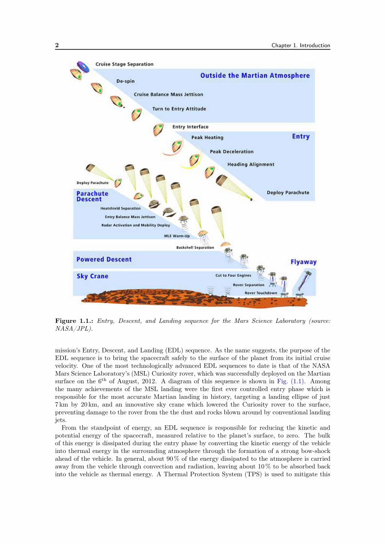
Figure 1.1.: Entry, Descent, and Landing sequence for the Mars Science Laboratory (source:NASA/JPL).
mission’s Entry, Descent, and Landing (EDL) sequence. As the name suggests, the purpose of theEDL sequence is to bring the spacecraft safely to the surface of the planet from its initial cruisevelocity. One of the most technologically advanced EDL sequences to date is that of the NASAMars Science Laboratory’s (MSL) Curiosity rover, which was successfully deployed on the Martiansurface on the 6th of August, 2012. A diagram of this sequence is shown in Fig. (1.1). Amongthe many achievements of the MSL landing were the first ever controlled entry phase which isresponsible for the most accurate Martian landing in history, targeting a landing ellipse of just7 km by 20 km, and an innovative sky crane which lowered the Curiosity rover to the surface,preventing damage to the rover from the the dust and rocks blown around by conventional landingjets.
From the standpoint of energy, an EDL sequence is responsible for reducing the kinetic andpotential energy of the spacecraft, measured relative to the planet’s surface, to zero. The bulkof this energy is dissipated during the entry phase by converting the kinetic energy of the vehicleinto thermal energy in the surrounding atmosphere through the formation of a strong bow-shockahead of the vehicle. In general, about 90% of the energy dissipated to the atmosphere is carriedaway from the vehicle through convection and radiation, leaving about 10% to be absorbed backinto the vehicle as thermal energy. A Thermal Protection System (TPS) is used to mitigate this
1.2. Entry, Descent, and Landing 3
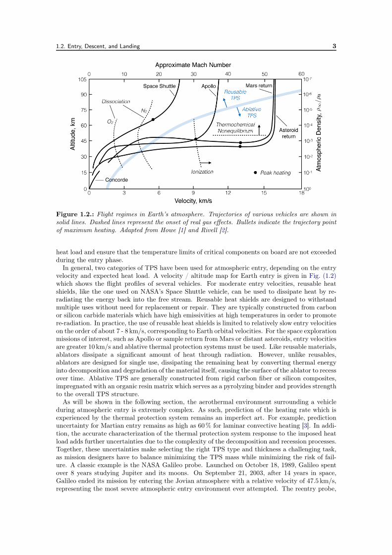
Figure 1.2.: Flight regimes in Earth’s atmosphere. Trajectories of various vehicles are shown insolid lines. Dashed lines represent the onset of real gas effects. Bullets indicate the trajectory pointof maximum heating. Adapted from Howe [1] and Rivell [2].
heat load and ensure that the temperature limits of critical components on board are not exceededduring the entry phase.
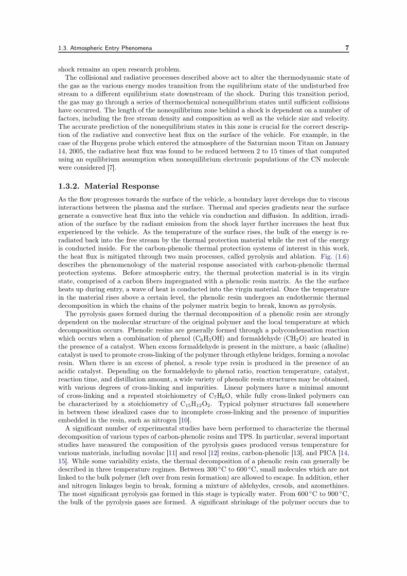
In general, two categories of TPS have been used for atmospheric entry, depending on the entryvelocity and expected heat load. A velocity / altitude map for Earth entry is given in Fig. (1.2)which shows the flight profiles of several vehicles. For moderate entry velocities, reusable heatshields, like the one used on NASA’s Space Shuttle vehicle, can be used to dissipate heat by re-radiating the energy back into the free stream. Reusable heat shields are designed to withstandmultiple uses without need for replacement or repair. They are typically constructed from carbonor silicon carbide materials which have high emissivities at high temperatures in order to promotere-radiation. In practice, the use of reusable heat shields is limited to relatively slow entry velocitieson the order of about 7 - 8 km/s, corresponding to Earth orbital velocities. For the space explorationmissions of interest, such as Apollo or sample return from Mars or distant asteroids, entry velocitiesare greater 10 km/s and ablative thermal protection systems must be used. Like reusable materials,ablators dissipate a significant amount of heat through radiation. However, unlike reusables,ablators are designed for single use, dissipating the remaining heat by converting thermal energyinto decomposition and degradation of the material itself, causing the surface of the ablator to recessover time. Ablative TPS are generally constructed from rigid carbon fiber or silicon composites,impregnated with an organic resin matrix which serves as a pyrolyzing binder and provides strengthto the overall TPS structure.
As will be shown in the following section, the aerothermal environment surrounding a vehicleduring atmospheric entry is extremely complex. As such, prediction of the heating rate which isexperienced by the thermal protection system remains an imperfect art. For example, predictionuncertainty for Martian entry remains as high as 60% for laminar convective heating [3]. In addi-tion, the accurate characterization of the thermal protection system response to the imposed heatload adds further uncertainties due to the complexity of the decomposition and recession processes.Together, these uncertainties make selecting the right TPS type and thickness a challenging task,as mission designers have to balance minimizing the TPS mass while minimizing the risk of fail-ure. A classic example is the NASA Galileo probe. Launched on October 18, 1989, Galileo spentover 8 years studying Jupiter and its moons. On September 21, 2003, after 14 years in space,Galileo ended its mission by entering the Jovian atmosphere with a relative velocity of 47.5 km/s,representing the most severe atmospheric entry environment ever attempted. The reentry probe,
4 Chapter 1. Introduction
Deceleration Module Aft Cover
Descent Module
Deceleration Module Aeroshell
Mortar CoverAccess Cover
Communicating Antenna
Lightning Detector Antenna
Separation FittingMass Spectrometer Inlet
Guide Rail
Payload Ring
Heat Shield
Drogue Parachute Mortar
Main Parachute Pack
Spin Vane
Temperature Sensor
Thermal Control Radioisotope Heaters
1.26 m
152 kg
Before Entry
14.6 cm
5.4 cm
After Entry
Ablated material
70 kg
10 cm
1 cm
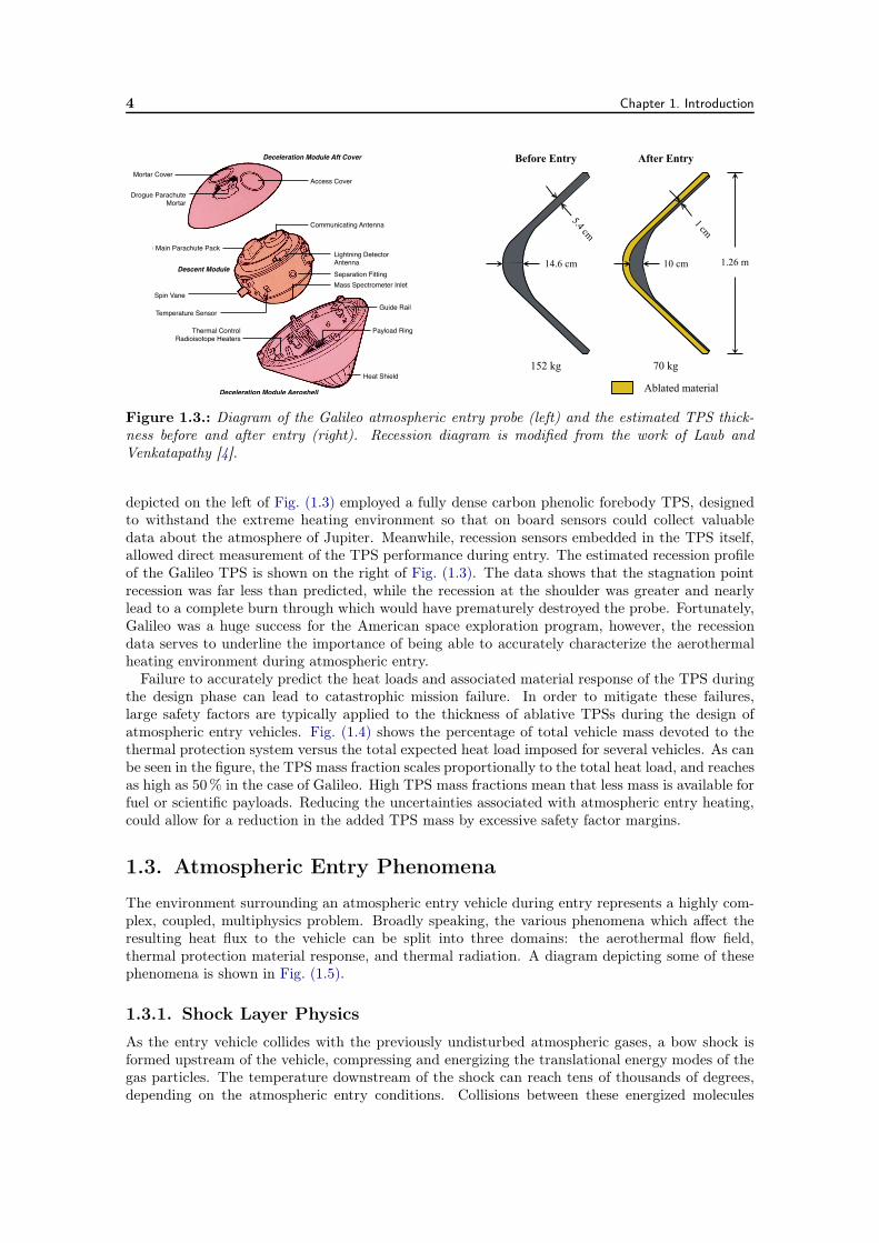
Figure 1.3.: Diagram of the Galileo atmospheric entry probe (left) and the estimated TPS thick-ness before and after entry (right). Recession diagram is modified from the work of Laub andVenkatapathy [4].
depicted on the left of Fig. (1.3) employed a fully dense carbon phenolic forebody TPS, designedto withstand the extreme heating environment so that on board sensors could collect valuabledata about the atmosphere of Jupiter. Meanwhile, recession sensors embedded in the TPS itself,allowed direct measurement of the TPS performance during entry. The estimated recession profileof the Galileo TPS is shown on the right of Fig. (1.3). The data shows that the stagnation pointrecession was far less than predicted, while the recession at the shoulder was greater and nearlylead to a complete burn through which would have prematurely destroyed the probe. Fortunately,Galileo was a huge success for the American space exploration program, however, the recessiondata serves to underline the importance of being able to accurately characterize the aerothermalheating environment during atmospheric entry.
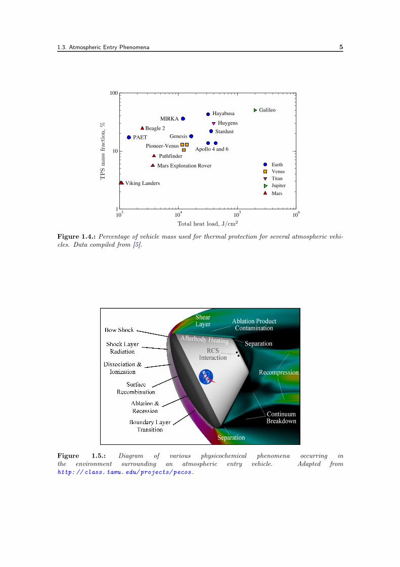
Failure to accurately predict the heat loads and associated material response of the TPS duringthe design phase can lead to catastrophic mission failure. In order to mitigate these failures,large safety factors are typically applied to the thickness of ablative TPSs during the design ofatmospheric entry vehicles. Fig. (1.4) shows the percentage of total vehicle mass devoted to thethermal protection system versus the total expected heat load imposed for several vehicles. As canbe seen in the figure, the TPS mass fraction scales proportionally to the total heat load, and reachesas high as 50% in the case of Galileo. High TPS mass fractions mean that less mass is available forfuel or scientific payloads. Reducing the uncertainties associated with atmospheric entry heating,could allow for a reduction in the added TPS mass by excessive safety factor margins.
1.3. Atmospheric Entry Phenomena
The environment surrounding an atmospheric entry vehicle during entry represents a highly com-plex, coupled, multiphysics problem. Broadly speaking, the various phenomena which affect theresulting heat flux to the vehicle can be split into three domains: the aerothermal flow field,thermal protection material response, and thermal radiation. A diagram depicting some of thesephenomena is shown in Fig. (1.5).
1.3.1. Shock Layer Physics
As the entry vehicle collides with the previously undisturbed atmospheric gases, a bow shock isformed upstream of the vehicle, compressing and energizing the translational energy modes of thegas particles. The temperature downstream of the shock can reach tens of thousands of degrees,depending on the atmospheric entry conditions. Collisions between these energized molecules
1.3. Atmospheric Entry Phenomena 5
103 104 105 1061
10
100
EarthVenusTitanJupiterMars
Apollo 4 and 6
PAET Genesis
MIRKA
Stardust
Hayabusa
Pioneer-Venus
Huygens
Galileo
Viking Landers
Beagle 2
Pathfinder
Mars Exploration Rover
Total heat load, J/cm2
TP
Sm
ass
frac
tion
,%
Figure 1.4.: Percentage of vehicle mass used for thermal protection for several atmospheric vehi-cles. Data compiled from [5].
Figure 1.5.: Diagram of various physicochemical phenomena occurring inthe environment surrounding an atmospheric entry vehicle. Adapted fromhttp:// class.tamu. edu/projects/pecos .
6 Chapter 1. Introduction
transfer some of the translational energy into the internal energy modes of the gas causing thetranslational energy to relax. In general, rotational and vibrational mode excitation is inducedbefore excitation of the electronic modes.
Once the vibrational modes of the molecules become sufficiently energetic, additional collisionsprovide the energy necessary to break their inter-nuclear bonds, leading to dissociation. In air, forexample, dissociation leads to the formation of atomic nitrogen and oxygen from N2 and O2. At thesame time, Zelodvich exchange reactions between atoms and molecules form NO which can thendissociate as well. In the Martian atmosphere, on the other hand, dissociation of CO2 creates COand O2 molecules and finally O atoms. Further collisional excitation of the atoms and moleculesexcites the bound electrons to higher electronic states. If the electrons become sufficiently excited,they may be stripped from their parent species, forming a plasma. In air, this process beginswith the associative ionization of the NO molecule (N + O −−−− NO+ + e– ), producing a singlyionized NO+ and a free electron. The positive molecule is then typically neutralized through acharge exchange reaction with N or O, stripping an electron from one of those atoms to formionized N+ or O+. Over time, the associative ionization reactions build up the concentration offree electrons until a critical mass is formed. At this point, electron impact ionization reactions,create a chain reaction and the level of ionization increases dramatically. This process is calledthe electron avalanche. A similar process is also found during Martian entries, starting from theassociative ionization of CO. However, Martian entries typically occur at a slower velocities thanthose on Earth, leading to far less ionization in general.
In addition to dissociation and ionization, collisional excitation may lead to thermal radiationas excited atoms and molecules spontaneously emit a photon and drop to a lower energy state.The radiant energy can then be absorbed by other atoms and molecules in the flow field, causingparticles to jump to higher energy levels, or directly absorbed by the surface of the vehicle. Emissionand absorption from bound levels to other bound levels is referred to as bound-bound radiation.The emission and absorption spectra of bound-bound processes is highly oscillatory in nature due tothe many transitions between discrete internal energy levels of atoms and molecules. For sufficientlyenergetic atoms and molecules, absorption of a photon may lead to dissociation or ionization. Inparticular, the photo-dissociation of O2 and photo-ionization of N and O are common in air.These processes are called bound-free since the particles in question begin the process bound toone another and are separate or “free” at the end. The reverse processes are likewise termed free-bound. Finally, free electrons may also contribute to radiation. As an electron passes throughthe electric field of another charged particle, it may undergo a deceleration and emit a photonwith energy equal to the difference between the kinetic energy of the electron before and after thecollision. This process is known as Bremsstrahlung from the german words bremsen for “to brake”and strahlung for “radiation”. Bremsstrahlung is also called free-free radiation, since transitionsoccur between two unbound electrons. Bound-free and free-free processes exhibit a continuousspectrum, since the energy transitions are not limited to discrete jumps.
A significant portion of the energy emitted is radiated out of the shock layer into the free stream,reducing the temperature of the shock layer gas. This process is referred to as radiative cooling.For cases in which radiation is a significant source of heat transfer, radiative cooling may introducea strong coupling mechanism between the flow and radiation fields and must be taken into accountin order to accurately predict the heat flux reaching the surface of the vehicle. Assessing theimportance of this coupling mechanism for a given entry is typically done by considering theso-called Goulard number Γ [6],
Γ =2qrad
0.5ρ∞u3∞
, (1.1)
which is the ratio of the adiabatic (uncoupled) radiative flux, approximated as twice the surfaceflux, to the total energy flux. As a general rule of thumb radiation coupling can be neglectedfor conditions in which Γ < 0.01 . For higher values of the Goulard number, radiation couplingshould be considered. In addition, for strongly radiating shock layers, the internal energy modesof the free stream ahead of the shock may be sufficiently excited by absorption processes to causephoto-ionization leading to the generation of free electrons. The effect of this precursor ionizationon the shock structure and the ensuing thermochemical relaxtion processes downstream of the
1.3. Atmospheric Entry Phenomena 7
shock remains an open research problem.The collisional and radiative processes described above act to alter the thermodynamic state of
the gas as the various energy modes transition from the equilibrium state of the undisturbed freestream to a different equilibrium state downstream of the shock. During this transition period,the gas may go through a series of thermochemical nonequilibrium states until sufficient collisionshave occurred. The length of the nonequilibrium zone behind a shock is dependent on a number offactors, including the free stream density and composition as well as the vehicle size and velocity.The accurate prediction of the nonequilibrium states in this zone is crucial for the correct descrip-tion of the radiative and convective heat flux on the surface of the vehicle. For example, in thecase of the Huygens probe which entered the atmosphere of the Saturnian moon Titan on January14, 2005, the radiative heat flux was found to be reduced between 2 to 15 times of that computedusing an equilibrium assumption when nonequilibrium electronic populations of the CN moleculewere considered [7].
1.3.2. Material Response
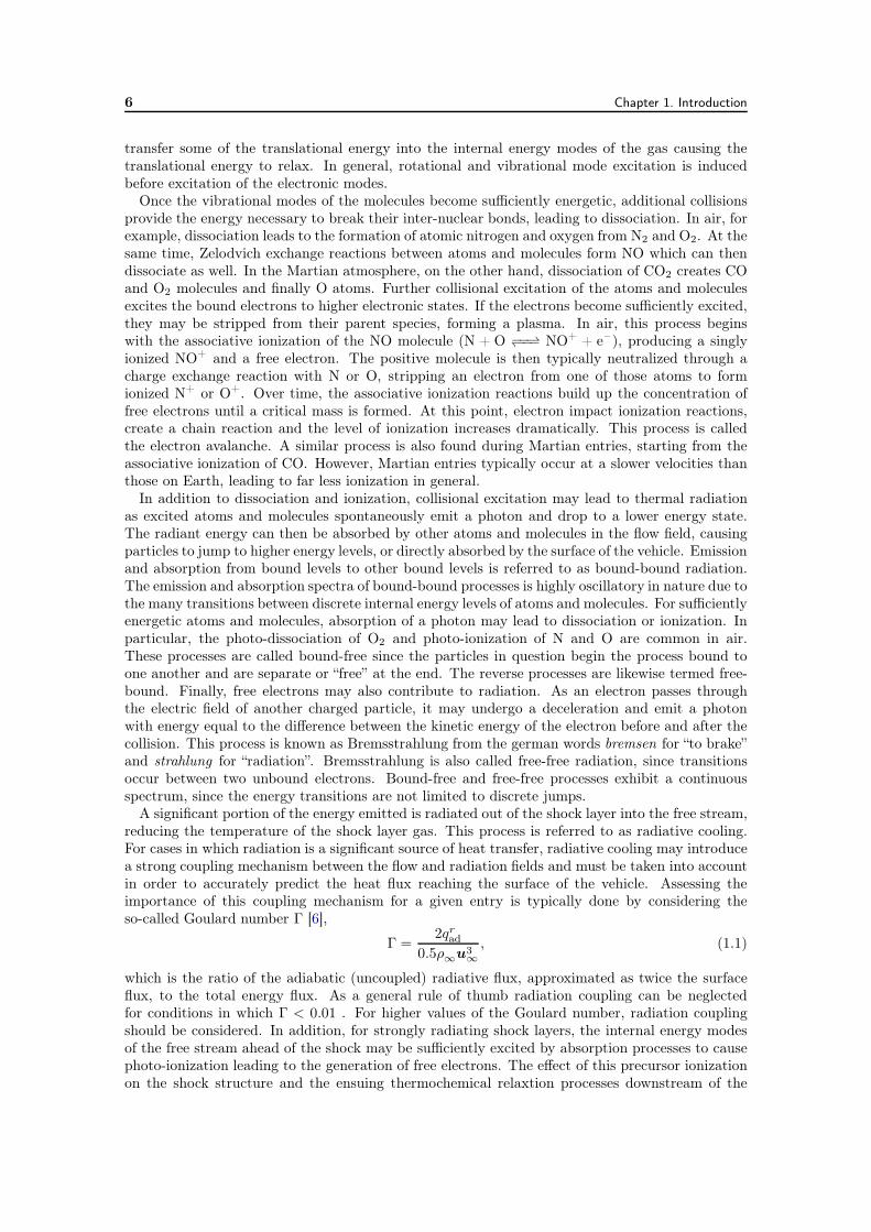
As the flow progresses towards the surface of the vehicle, a boundary layer develops due to viscousinteractions between the plasma and the surface. Thermal and species gradients near the surfacegenerate a convective heat flux into the vehicle via conduction and diffusion. In addition, irradi-ation of the surface by the radiant emission from the shock layer further increases the heat fluxexperienced by the vehicle. As the temperature of the surface rises, the bulk of the energy is re-radiated back into the free stream by the thermal protection material while the rest of the energyis conducted inside. For the carbon-phenolic thermal protection systems of interest in this work,the heat flux is mitigated through two main processes, called pyrolysis and ablation. Fig. (1.6)describes the phenomenology of the material response associated with carbon-phenolic thermalprotection systems. Before atmospheric entry, the thermal protection material is in its virginstate, comprised of a carbon fibers impregnated with a phenolic resin matrix. As the the surfaceheats up during entry, a wave of heat is conducted into the virgin material. Once the temperaturein the material rises above a certain level, the phenolic resin undergoes an endothermic thermaldecomposition in which the chains of the polymer matrix begin to break, known as pyrolysis.
The pyrolysis gases formed during the thermal decomposition of a phenolic resin are stronglydependent on the molecular structure of the original polymer and the local temperature at whichdecomposition occurs. Phenolic resins are generally formed through a polycondensation reactionwhich occurs when a combination of phenol (C6H5OH) and formaldehyde (CH2O) are heated inthe presence of a catalyst. When excess formaldehyde is present in the mixture, a basic (alkaline)catalyst is used to promote cross-linking of the polymer through ethylene bridges, forming a novolacresin. When there is an excess of phenol, a resole type resin is produced in the presence of anacidic catalyst. Depending on the formaldehyde to phenol ratio, reaction temperature, catalyst,reaction time, and distillation amount, a wide variety of phenolic resin structures may be obtained,with various degrees of cross-linking and impurities. Linear polymers have a minimal amountof cross-linking and a repeated stoichiometry of C7H6O, while fully cross-linked polymers canbe characterized by a stoichiometry of C15H12O2. Typical polymer structures fall somewherein between these idealized cases due to incomplete cross-linking and the presence of impuritiesembedded in the resin, such as nitrogen [10].
A significant number of experimental studies have been performed to characterize the thermaldecomposition of various types of carbon-phenolic resins and TPS. In particular, several importantstudies have measured the composition of the pyrolysis gases produced versus temperature forvarious materials, including novolac [11] and resol [12] resins, carbon-phenolic [13], and PICA [14,15]. While some variability exists, the thermal decomposition of a phenolic resin can generally bedescribed in three temperature regimes. Between 300 C to 600 C, small molecules which are notlinked to the bulk polymer (left over from resin formation) are allowed to escape. In addition, etherand nitrogen linkages begin to break, forming a mixture of aldehydes, cresols, and azomethines.The most significant pyrolysis gas formed in this stage is typically water. From 600 C to 900 C,the bulk of the pyrolysis gases are formed. A significant shrinkage of the polymer occurs due to
8 Chapter 1. Introduction
Figure 1.6.: Phenomenology of thermal protection material response. Top two micrographs aretaken from [8] while the bottom is taken from [9].
1.4. State-of-the-Art Flow-Radiation Tools 9
the creation of carbon-carbon bonds between aromatic rings, forming a polyaromatic char. Severalgases may be formed in this range, such as H2, CH4, H2O, CO, CO2, and volatile aromatics suchas phenol (C6H5OH) and benzene (C6H6). Finally, above about 900 C, dehydrogenation furthershrinks the polymer forming mostly H2 and other small noncarbonacious molecules.
Once formed, the pyrolysis gases are convected and diffused through the porous material, drivenby a pressure gradient originating in the pyrolysis zone. As the gases flow towards the surface theymay react with one another to form new compounds or dissociate further. Closer to the surface,the gas passes through a char layer, leftover from the completion of the pyrolysis processes. In somecases, the presence of carbonaceous pyrolysis gases leads to coking, in which some of the carbonin the gas is redeposited onto the polyaromatic char. At the surface of the thermal protectionsystem, the pyrolysis gases generated inside are convected into the boundary layer. Atmosphericgases, diffusing to the surface, interact with the carbon fibers and carbonaceous char. In air, forexample, nitrogen and oxygen atoms may undergo a catalytic recombination at the surface to formN2 and O2. In addition, oxidation and nitridation reactions may remove carbon from the surface,causing the surface to recess and generating CO, CO2, and CN. At temperatures above about3000K, the carbon surface begins to sublimate, generating carbonaceous species such as C, C2,and C3, and increasing the surface recession rate. In extreme cases, surface spallation can alsooccur, in which large particles are ejected from the surface due to mechanical and thermal loads.Spallation is highly undesirable since it can dramatically increase the recession rate with littlethermodynamic benefit. When combined, the processes which remove material from the surfaceare collectively known as ablation.
1.3.3. Flow, Material, Radiation Coupling
The gaseous products of ablation and pyrolysis are blown into the boundary layer where they mayreact with the atmospheric gases coming from the shock layer. For strong mass blowing rates,the boundary layer can be blown off of the surface, significantly reducing the thermal gradients atthe surface and decreasing the convective heat flux. Depending on their type and concentration,ablation and pyrolysis gases may block a significant amount of the incoming radiation as well,through absorption. This process, known as radiation blockage, is still not fully characterized, dueto the complexity of the phenomena leading to the creation of the ablation and pyrolsyis gases. Tofurther complicate matters, certain ablation products such as CO, CN, and C3 are known to bestrong radiators, leading to the possibility that ablation may actually increase the radiative flux tothe vehicle through spontaneous emission of these species as they are heated in the boundary layer.For example, Johnston et al. [16] have shown for a simplified boundary layer in air, contaminationwith ablation products may block radiation in the vacuum ultraviolet through increased absorption,while increasing it in the infrared and visible regions of the spectrum due to emission from CO,C2, and CN.
Finally, as the flow moves across the surface of the ablator, the boundary layer thickness tendsto grow. For larger vehicles, the laminar boundary layer flow can transition to turbulent, whichmay significantly increase the convective heating rate to the surface. As the flow wraps around theleading corner of the vehicle, a significant decompression and separation occurs, generating a large,turbulent wake. As the wake cools, previously dissociated atmospheric gases and ablation productsmay recombine. For Martian entries, a significant radiative heat flux can occur on the backshellof the vehicle due recombination of CO2 which is a strong emitter in the infrared region. Thisphenomena may become increasingly important for future missions aiming to send increasinglylarge vehicles to Mars.
1.4. State-of-the-Art Flow-Radiation Tools
In this section, the current state-of-the-art of numerical prediction and modeling of atmosphericentry flows is briefly reviewed with a focus on topics relevant to this thesis. A more detailed reviewof the relevant literature is made throughout the thesis, as necessary. For a review of experimental
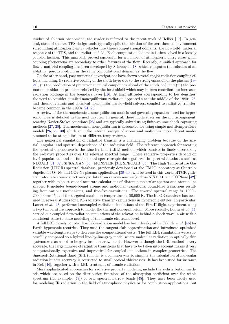
10 Chapter 1. Introduction
studies of ablation phenomena, the reader is referred to the recent work of Helber [17]. In gen-eral, state-of-the-art TPS design tools typically split the solution of the aerothermal environmentsurrounding atmospheric entry vehicles into three computational domains: the flow field, materialresponse of the TPS, and the radiation field. Each computational domain is then solved in a looselycoupled fashion. This approach proved successful for a number of atmospheric entry cases whencoupling phenomena are secondary to other features of the flow. Recently, a unified approach forflow / material coupling has been developed by Schrooyen [18] which computes the solution of anablating, porous medium in the same computational domain as the flow.
On the other hand, past numerical investigations have shown several major radiation coupling ef-fects, including (i) radiative cooling of the shock layer due to the strong emission of the plasma [19–21], (ii) the production of precursor chemical compounds ahead of the shock [22], and (iii) the pro-motion of ablation products released by the heat shield which may in turn contribute to increasedradiation blockage in the boundary layer [16]. At high altitudes corresponding to low densities,the need to consider detailed nonequilibrium radiation appeared since the middle of the 1980s [23]and thermodynamic and chemical nonequilibrium flowfield solvers, coupled to radiative transfer,became common in the 1990s [24, 25].
A review of the thermochemical nonequilibrium models and governing equations used for hyper-sonic flows is detailed in the next chapter. In general, these models rely on the multicomponent,reacting Navier-Stokes equations [26] and are typically solved using finite-volume shock capturingmethods [27, 28]. Thermochemical nonequilibrium is accounted for using simple multitemperaturemodels [26, 29, 30] which split the internal energy of atoms and molecules into different modesassumed to be at equilibrium at different temperatures.
The numerical simulation of radiative transfer is a challenging problem because of the spa-tial, angular, and spectral dependence of the radiation field. The reference approach for treatingthe spectral dependence is the Line-By-Line (LBL) method which consists in finely discretizingthe radiative properties over the relevant spectral range. These radiative properties depend onlevel populations and on fundamental spectroscopic data gathered in spectral databases such asNEQAIR [31, 32], SPRADIAN [33], MONSTER [34], SPECAIR [35]. The High Temperature GasRadiation (HTGR) spectral database, previously developed at the EM2C laboratory at Centrale-Supélec for O2-N2 and CO2-N2 plasma applications [36–40], will be used in this work. HTGR gath-ers up-to-date atomic spectroscopic data from various sources (such as NIST [41] and TOPbase [42])together with exhaustive and accurate calculations of diatomic molecular spectra and atomic lineshapes. It includes bound-bound atomic and molecular transitions, bound-free transitions result-ing from various mechanisms, and free-free transitions. The covered spectral range is [1000 -200,000 cm−1] and the targeted maximum temperature is 50,000 K. The HTGR database has beenused in several studies for LBL radiative transfer calculations in hypersonic entries. In particular,Lamet et al. [43] performed uncoupled radiation simulations of the Fire II flight experiment usinga two-temperature approach to model the thermal nonequilibrium. More recently, Lopez et al. [44]carried out coupled flow-radiation simulations of the relaxation behind a shock wave in air with aconsistent state-to-state modeling of the atomic electronic levels.
A full LBL closely coupled flowfield-radiation model has been developed by Feldick et al. [45] forEarth hypersonic reentries. They used the tangent slab approximation and introduced optimizedvariable wavelength steps to decrease the computational costs. The full LBL simulations were suc-cessfully compared to a hybrid line-by-line-gray model where molecular radiation in optically thinsystems was assumed to be gray inside narrow bands. However, although the LBL method is veryaccurate, the large number of radiative transitions that have to be taken into account makes it verycomputationally expensive and impractical for coupled simulations in complex geometries. TheSmeared-Rotational-Band (SRB) model is a common way to simplify the calculation of molecularradiation but its accuracy is restricted to small optical thicknesses. It has been used for instancein Ref. [46], together with a LBL treatment of atomic radiation.
More sophisticated approaches for radiative property modeling include the k-distribution meth-ods which are based on the distribution functions of the absorption coefficient over the wholespectrum (for example, [47]) or over spectral narrow bands [48]. They have been widely usedfor modeling IR radiation in the field of atmospheric physics or for combustion applications, but
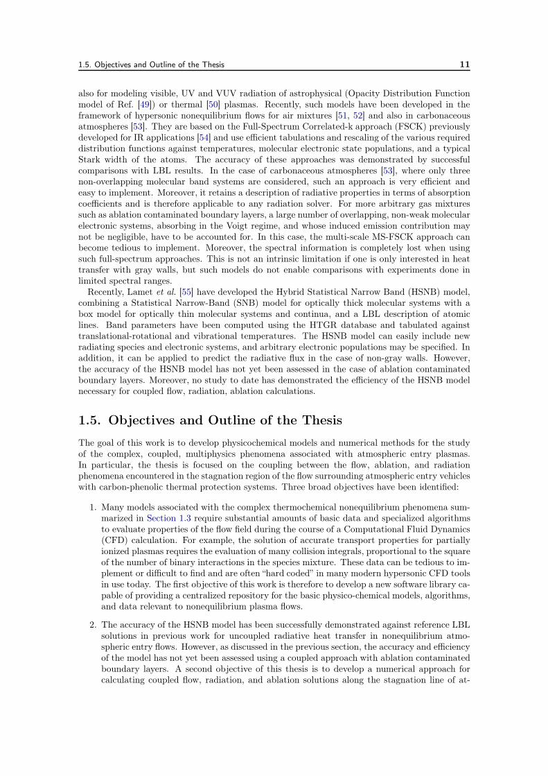
1.5. Objectives and Outline of the Thesis 11
also for modeling visible, UV and VUV radiation of astrophysical (Opacity Distribution Functionmodel of Ref. [49]) or thermal [50] plasmas. Recently, such models have been developed in theframework of hypersonic nonequilibrium flows for air mixtures [51, 52] and also in carbonaceousatmospheres [53]. They are based on the Full-Spectrum Correlated-k approach (FSCK) previouslydeveloped for IR applications [54] and use efficient tabulations and rescaling of the various requireddistribution functions against temperatures, molecular electronic state populations, and a typicalStark width of the atoms. The accuracy of these approaches was demonstrated by successfulcomparisons with LBL results. In the case of carbonaceous atmospheres [53], where only threenon-overlapping molecular band systems are considered, such an approach is very efficient andeasy to implement. Moreover, it retains a description of radiative properties in terms of absorptioncoefficients and is therefore applicable to any radiation solver. For more arbitrary gas mixturessuch as ablation contaminated boundary layers, a large number of overlapping, non-weak molecularelectronic systems, absorbing in the Voigt regime, and whose induced emission contribution maynot be negligible, have to be accounted for. In this case, the multi-scale MS-FSCK approach canbecome tedious to implement. Moreover, the spectral information is completely lost when usingsuch full-spectrum approaches. This is not an intrinsic limitation if one is only interested in heattransfer with gray walls, but such models do not enable comparisons with experiments done inlimited spectral ranges.
Recently, Lamet et al. [55] have developed the Hybrid Statistical Narrow Band (HSNB) model,combining a Statistical Narrow-Band (SNB) model for optically thick molecular systems with abox model for optically thin molecular systems and continua, and a LBL description of atomiclines. Band parameters have been computed using the HTGR database and tabulated againsttranslational-rotational and vibrational temperatures. The HSNB model can easily include newradiating species and electronic systems, and arbitrary electronic populations may be specified. Inaddition, it can be applied to predict the radiative flux in the case of non-gray walls. However,the accuracy of the HSNB model has not yet been assessed in the case of ablation contaminatedboundary layers. Moreover, no study to date has demonstrated the efficiency of the HSNB modelnecessary for coupled flow, radiation, ablation calculations.
1.5. Objectives and Outline of the Thesis
The goal of this work is to develop physicochemical models and numerical methods for the studyof the complex, coupled, multiphysics phenomena associated with atmospheric entry plasmas.In particular, the thesis is focused on the coupling between the flow, ablation, and radiationphenomena encountered in the stagnation region of the flow surrounding atmospheric entry vehicleswith carbon-phenolic thermal protection systems. Three broad objectives have been identified:
1. Many models associated with the complex thermochemical nonequilibrium phenomena sum-marized in Section 1.3 require substantial amounts of basic data and specialized algorithmsto evaluate properties of the flow field during the course of a Computational Fluid Dynamics(CFD) calculation. For example, the solution of accurate transport properties for partiallyionized plasmas requires the evaluation of many collision integrals, proportional to the squareof the number of binary interactions in the species mixture. These data can be tedious to im-plement or difficult to find and are often “hard coded” in many modern hypersonic CFD toolsin use today. The first objective of this work is therefore to develop a new software library ca-pable of providing a centralized repository for the basic physico-chemical models, algorithms,and data relevant to nonequilibrium plasma flows.
2. The accuracy of the HSNB model has been successfully demonstrated against reference LBLsolutions in previous work for uncoupled radiative heat transfer in nonequilibrium atmo-spheric entry flows. However, as discussed in the previous section, the accuracy and efficiencyof the model has not yet been assessed using a coupled approach with ablation contaminatedboundary layers. A second objective of this thesis is to develop a numerical approach forcalculating coupled flow, radiation, and ablation solutions along the stagnation line of at-
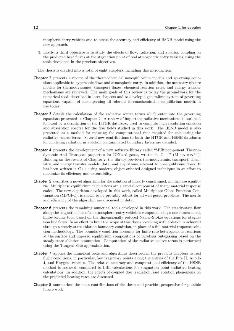
12 Chapter 1. Introduction
mospheric entry vehicles and to assess the accuracy and efficiency of HSNB model using thenew approach.
3. Lastly, a third objective is to study the effects of flow, radiation, and ablation coupling onthe predicted heat fluxes at the stagnation point of real atmospheric entry vehicles, using thetools developed in the previous objectives.
The thesis is divided into a total of eight chapters, including this introduction.
Chapter 2 presents a review of the thermochemical nonequilibrium models and governing equa-tions applicable to hypersonic flows and atmospheric entry. In addition, the necessary closuremodels for thermodynamics, transport fluxes, chemical reaction rates, and energy transfermechanisms are reviewed. The main goals of this review is to lay the groundwork for thenumerical tools described in later chapters and to develop a generalized system of governingequations, capable of encompassing all relevant thermochemical nonequilibrium models inuse today.
Chapter 3 details the calculation of the radiative source terms which enter into the governingequations presented in Chapter 2. A review of important radiative mechanisms is outlined,followed by a description of the HTGR database, used to compute high resolution emissionand absorption spectra for the flow fields studied in this work. The HSNB model is alsopresented as a method for reducing the computational time required for calculating theradiative source terms. Several new contributions to both the HTGR and HSNB databasesfor modeling radiation in ablation contaminated boundary layers are detailed.
Chapter 4 presents the development of a new software library called “MUlticomponent Thermo-dynamic And Transport properties for IONized gases, written in C++” (Mutation++).Building on the results of Chapter 2, the library provides thermodynamic, transport, chem-istry, and energy transfer models, data, and algorithms, relevant to nonequilibrium flows. Ithas been written in C++ using modern, object oriented designed techniques in an effort tomaximize its efficiency and extensibility.
Chapter 5 describes a novel algorithm for the solution of linearly constrained, multiphase equilib-ria. Multiphase equilibrium calculations are a crucial component of many material responsecodes. The new algorithm developed in this work, called Multiphase Gibbs Function Con-tinuation (MPGFC), is shown to be provably robust for all well posed problems. The meritsand efficiency of the algorithm are discussed in detail.
Chapter 6 presents the remaining numerical tools developed in this work. The steady-state flowalong the stagnation line of an atmospheric entry vehicle is computed using a one-dimensional,finite-volume tool, based on the dimensionally reduced Navier-Stokes equations for stagna-tion line flows. In an effort to limit the scope of this thesis, coupling with ablation is achievedthrough a steady-state ablation boundary condition, in place of a full material response solu-tion methodology. The boundary condition accounts for finite-rate heterogeneous reactionsat the surface and imposed equilibrium compositions of pyrolysis out-gassing based on thesteady-state ablation assumption. Computation of the radiative source terms is performedusing the Tangent Slab approximation.
Chapter 7 applies the numerical tools and algorithms described in the previous chapters to realflight conditions, in particular, key trajectory points along the entries of the Fire II, Apollo4, and Huygens vehicles. The relative accuracy and computational efficiency of the HSNBmethod is assessed, compared to LBL calculations for stagnation point radiative heatingcalculations. In addition, the effects of coupled flow, radiation, and ablation phenomena onthe predicted heating rates are discussed.
Chapter 8 summarizes the main contributions of the thesis and provides perspective for possiblefuture work.
CHAPTER 2
Governing Equations for Hypersonic Flows
2.1. Introduction
Atmospheric entry vehicles operate in the hypersonic flow regime due to their extreme velocitiesrelative to the atmosphere in which they enter. Hypersonic flight is characterized by velocitytimescales on the same order of magnitude as the chemical and kinetic timescales of the shockedgas. Under such conditions, thermal and chemical nonequilibrium may dominate the aerothermalenvironment surrounding the entry vehicle. In addition, radiative heating becomes important asatoms and molecules are excited to higher internal energy levels. These phenomena have substantialeffects on vehicle heating and aerodynamic forces affecting its trajectory and must be accuratelycharacterized during the design phase.
This chapter reviews the approaches typically used to model thermochemical nonequilibrium andradiative heat transfer in hypersonic flow fields for atmospheric entry. In particular, the variousspecies internal energy partitioning models are discussed as well as the closure models employedto compute the necessary thermodynamic, transport, and chemistry properties required to closethe governing equations. One contribution of this chapter is to formulate the governing equationsusing a generalized notation, valid for most thermochemical models of interest in the literature.As will be shown, this framework represents a powerful tool for abstracting away the physico-chemical models from the governing equations for hypersonic flows and forms the basis of theMutation++ library presented in Chapter 4.
2.2. Review of Energy Partitioning Models
Quantum mechanics dictates that atoms and molecules are permitted only discrete energy lev-els [56]. For atoms, this energy is contained within translational and electronic energy modes.Molecules have two additional energy storage modes via rotation and vibration of the molecule.In general, all energy modes are coupled. For weakly interacting particles (dilute gases), however,translational energy may be considered decoupled from the internal energy. Note that this use of“internal energy” should not be confused with the typical fluid dynamic description of the internalenergy of a gas, which includes translational energy. Here, internal energy is meant to differentiatebetween energy associated with the translation of the center of mass of a particle and the energyassociated with the relative motion of its constituents (nuclei and electrons). While translationalenergy levels are discrete, the spacing between levels is extremely small. For all practical purposes,this permits a semi-classical approach in which translational energy is assumed continuous whileinternal energy is left discrete. Furthermore, it is assumed that the populations of internal energylevels satisfy Maxwell-Boltzmann statistics, such that the quantum effects differentiating bosons(Bose-Einstein statistics) and fermions (Fermi-Dirac statistics) are negligible [56].
Fig. (2.1) provides potential energy curves of N2 for selected electronic energy states of themolecule. Energy levels are measured from the zero point energy of the molecule (energy of theground state at 0K). Vibrational energy levels are denoted with tick marks for each electronic state.Rotational levels are spaced even closer together between vibrational levels. Individual particlesmay jump from one state to another through collisional or radiative (de)excitation processes orreact with other particles to form an entirely different species.
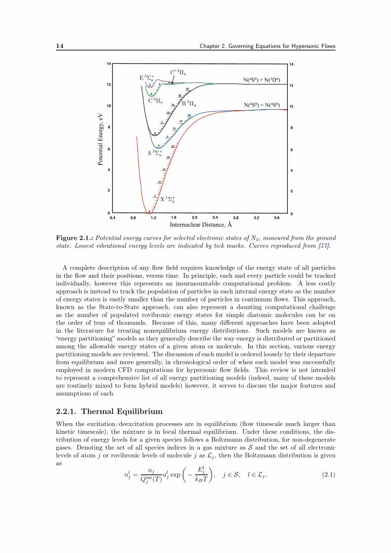
14 Chapter 2. Governing Equations for Hypersonic Flows
0
5
10
15
20
250
5
10
15
20
0
5
10
15
20
25
0
4 00
14
12
10
8
6
4
2
0
14
12
10
8
6
4
2
00.4 0.8 1.2 1.6 2.0 2.4 2.8 3.2 3.6
Internuclear Distance, !
Pote
ntia
l Ene
rgy,
eV
N(4S0) + N(4S0)
N(4S0) + N(2D0)
X1Σ
+g
A3Σ
+u
B3Πg
C3Πu
C′ 3Πu
E3Σ
+g
Figure 2.1.: Potential energy curves for selected electronic states of N2, measured from the groundstate. Lowest vibrational energy levels are indicated by tick marks. Curves reproduced from [57].
A complete description of any flow field requires knowledge of the energy state of all particlesin the flow and their positions, versus time. In principle, each and every particle could be trackedindividually, however this represents an insurmountable computational problem. A less costlyapproach is instead to track the population of particles in each internal energy state as the numberof energy states is vastly smaller than the number of particles in continuum flows. This approach,known as the State-to-State approach, can also represent a daunting computational challengeas the number of populated rovibronic energy states for simple diatomic molecules can be onthe order of tens of thousands. Because of this, many different approaches have been adoptedin the literature for treating nonequilibrium energy distributions. Such models are known as“energy partitioning” models as they generally describe the way energy is distributed or partitionedamong the allowable energy states of a given atom or molecule. In this section, various energypartitioning models are reviewed. The discussion of each model is ordered loosely by their departurefrom equilibrium and more generally, in chronological order of when each model was successfullyemployed in modern CFD computations for hypersonic flow fields. This review is not intendedto represent a comprehensive list of all energy partitioning models (indeed, many of these modelsare routinely mixed to form hybrid models) however, it serves to discuss the major features andassumptions of each.
2.2.1. Thermal Equilibrium
When the excitation/deexcitation processes are in equilibrium (flow timescale much larger thankinetic timescale), the mixture is in local thermal equilibrium. Under these conditions, the dis-tribution of energy levels for a given species follows a Boltzmann distribution, for non-degenerategases. Denoting the set of all species indices in a gas mixture as S and the set of all electroniclevels of atom j or rovibronic levels of molecule j as Lj , then the Boltzmann distribution is givenas
nlj =
nj
Qintj (T )
alj exp
(
−El
j
kBT
)
, j ∈ S, l ∈ Lj , (2.1)
2.2. Review of Energy Partitioning Models 15
where nlj is the number density of species j with energy level l, nj =
∑
l nlj is the total number
density of species j, Elj is the internal energy of level (j, l) relative to the zero point energy of
species j, and alj is the degeneracy of the level. The quantity Qintj is called the internal partition
function for species j and is given by
Qintj (T ) =
∑
l∈Lj
alj exp
(
−El
j
kBT
)
, j ∈ S. (2.2)
Note that the only unknowns present in Eq. (2.1) are the number density of species j, nj , andthe mixture temperature T . These quantities must be determined through suitable governingequations which are discussed in the next section.
When thermal equilibrium is no longer valid, a suitable energy partitioning model must be usedto provide the distribution of energy levels for each species. The following subsections review themost common models found in the literature.
2.2.2. Multitemperature Models
The thermal nonequilibrium models which are still used today for aerospace engineering applica-tions can be attributed to the works of Park [58–60] and Lee [29, 61] in the mid to late 1980’swho developed so-called multi-temperature models. The main idea behind multi-temperature(MT) models is that the energy associated with any internal level can be separated into vari-ous energy modes. When the fine structure is neglected, all internal energy levels of a diatomicmolecule may be enumerated by the electronic, rotational, and vibrational quantum numbers, n, J ,ν, respectively. Electronic states may be characterized by the label 2S+1Λ where 2S+1 is the spinmultiplicity and Λ is the absolute value of the electronic orbital momentum on the internuclearaxis. Under this notation, the electronic degeneracy is then given as ael
j = (2−δ0,Λ)(2S+1), whereδ is the Kronecker delta. The rotational degeneracy is simply ar
j = 2J + 1. Vibrational states arenot degenerate (av
j = 1).Assuming that each energy mode is decoupled from the others, a rovibronic energy level l =
(n, J, ν) of a diatomic molecule j, could be split according to [61], such that
Elj ≡ Ej(n, J, ν) = Eel
j (n) + Erj(J) + Ev
j (ν), (2.3)
where Eelj , Er
j , and Evj are the electronic, rotational, and vibrational contributions to energy level
l. Each energy mode is then assumed to represent a thermal bath in equilibrium at a separatetemperature, yielding
nlj =
nj
Qintj (Tel, Tr, Tv)
alj exp
(
−Eel
j (n)
kBTel−
Erj(J)
kBTr−
Evj (ν)
kBTv
)
, (2.4)
where alj = aelj a
rja
vj and Qint
j (Tel, Tr, Tv) is the multitemperature internal partition function ofspecies j,
Qintj (Tel, Tr, Tv) =
∑
l∈Lj
alj exp
(
−Eel
j (n)
kBTel−
Erj(J)
kBTr−
Evj (ν)
kBTv
)
= Qelj (Tel)Q
rj(Tr)Q
vj (Tv).
(2.5)
The assumption of perfect separability of the energy modes allows the internal partition functionto be split into a product of partition functions for each mode as is shown on the second line ofEq. (2.5), where the partition function for mode m can be written generically as
Qmj (Tm) =
∑
k∈Lmj
amj (k) exp
(
−Em
j (k)
kBTm
)
, (2.6)
16 Chapter 2. Governing Equations for Hypersonic Flows
where Lmj is the set of pure energy levels for mode m.
Eqs. (2.4) and (2.5) drastically reduce the number of unknowns required to model thermalnonequilibrium as compared to those required for State-to-State (STS) models. However, decou-pling of the internal degrees of freedom as in Eq. (2.3) is a strong assumption and may introducesignificant errors in the thermodynamic properties of the gas. Based on the Born-Oppenheimerapproximation, electronic motion may be decoupled from the nuclear motion above relatively lowtemperatures, below the range of interest for atmospheric entry simulations [62]. Unfortunately,this is not the case for rotation and vibration due to a strong coupling caused by centrifugal forcescreated by rotation and the dependence of the moment of inertia of a vibrating molecule on theinternuclear distances between its constituent nuclei. In addition, since the rotational and vibra-tional spectroscopic constants depend on the electronic states, the rovibrational energy may exhibita strong coupling with the electronic energy of a molecule, even when the Born-Oppenheimer ap-proximation is appropriate.
Jaffe [63] first introduced a “general” MT model which takes into account rovibrational energycoupling in a consistent way for diatomic molecules by introducing the following energy splitting,
Elj ≡ Ej(n, J, ν) = Eel
j (n) + Erj′(n, J, ν) + Ev
j′(n, J, ν), (2.7)
where Eelj (n) is the pure electronic energy for electronic state n and
Erj′(n, J, ν) = Er
j(n, J) + Ervj (n, J, ν) (1− α), (2.8)
Evj′(n, J, ν) = Ev
j (n, ν) + Ervj (n, J, ν) α, (2.9)
where Erj(n, J) and Ev
j (n, ν) are the pure rotational and vibrational energies for electronic level nand Erv
j (n, J, ν) is the rotation-vibration interaction energy. The parameter 0 ≤ α ≤ 1 in Jaffe’smodel is used to distribute the rovibrational interaction energy into rotational and vibrationalmodes. There is no physical basis for this distribution, however it has been shown that thisparameter has little effect on thermodynamic properties for diatomic air species [43, 63].
When all of the interaction energy is added to the vibrational mode (α = 1), the followinggeneric MT distribution is obtained for diatomic molecules,
nlj =
njaljQint
j
exp
(
−Eel
j (n)
kBTel−
Erj(n, J)
kBTr−
Evj (n, ν) + Erv
j (n, J, ν)
kBTv
)
, (2.10)
where the internal partition function may be written as
Qintj =
∑
n
(2 − δ0,Λ(n))(2S(n) + 1) exp
(
−Eel
j (n)
kBTel
)
×
∑
J
(2J + 1) exp
(
−Er
j(n, J)
kBTr
)
×
∑
ν
exp
(
−Ev
j (n, ν) + Ervj (n, J, ν)
kBTv
)
(2.11)
Eqs. (2.10) and (2.11) provide a consistent, general MT model for describing nonequilibrium statedistributions. Like the Park and Lee models in Eqs. (2.4) and (2.5), the general model significantlyreduces the number of parameters required to describe nonequilibrium flows. However, it is im-portant to note that the partition function in Eq. (2.11) cannot be split into separable modes asin Eq. (2.5) due to the coupled summation over the level quantum numbers.
The MT models presented in this section may be easily adapted to polyatomic species with moredegrees of freedom [64, 65]. In general, any polyatomic species j with na
j nuclei have 3naj − (Lj +3)
normal vibrational modes, where Lj = 2 for linear molecules and Lj = 3 for nonlinear molecules.Each new vibrational mode can be enumerated with an additional vibrational quantum numberand the corresponding energy partitioning updated. It should also be noted that the models shown
2.2. Review of Energy Partitioning Models 17
here all assumed a single temperature for each energy mode, however it is common for example tohave separate vibrational temperatures for each vibrational mode in each molecule. The separableand nonseparable MT models presented above can be easily generalized by appending a speciessubscript to the temperatures (e.g., Tvj for a vibrational mode of species j).
MT models have been used with great success since the late 1980’s for a variety of CFD applica-tions [26, 27, 29, 43, 58–61, 66–71]. However, because they are based on Boltzmann distributions,these models are valid for only small departures from equilibrium [72]. With recent advancementsin computational efficiency and multiprocessor computer architectures, collisional models have be-come more feasible. In particular, state-specific and energy binning models are discussed in thenext sections.
2.2.3. State-Specific Models
State-specific models attempt to increase the validity range of MT models beyond small departuresfrom equilibrium by modeling some states as pseudo-species [7, 73, 74]. In general, the energy of aparticular molecular state is split into two categories: 1) modes assumed to be in full nonequilibriumand must be treated as pseudo-species, and 2) those which follow a Boltzmann distribution withall the modeling possibilities presented in Section 2.2.2.
Cambier [73] introduced an electronic-specific Collisional-Radiative (CR) model for molecularplasmas, in which each electronic mode of a given molecule is treated as a separate pseudo-species.We will denote this species with the subscript j(n) for the nth electronic state of species j. Thenumber of particles of species j at the electronic state n is given by
nj(n) =∑
νJ
nnJνj . (2.12)
The rovibrational levels in each electronic state are then populated according to a Boltzmanndistribution at the species rotation and vibration temperature, such that for diatomic molecules,
nlj ≡ nnJν
j =nj(n)a
nJνj
Qintj(n)
exp
(
−Eel
j (n)
kBTel−
Erj(n,J)
kBTrj−
Evj′(n,J,ν)
kBTvj
)
, (2.13)
where the rovibrational partition function for electronic state n is given by
Qintj(n) = exp
(
−Eel
j (n)
kBTel
)
∑
νJ
anJνj exp
(
−Er
j(n,J)
kBTrj−
Evj′(n,J,ν)
kBTvj
)
, (2.14)
and Evj′(n, J, ν) represents the energy partitioned into the vibrational mode as was done in Eq. (2.9).
Notice that the term anj exp(−Eelj (n)/kBTel) (with arbitrary Tel) in Eq. (2.13) is canceled out when
the rovibrational partition function is substituted into the equation, however we have opted to in-clude this term in the definition of the partition function in order to obtain a general relation forthermodynamic properties later on (see Section 2.4).
When applied to atoms, electronic-specific models, like the one above, represent the most rigorousnonequilibrium model possible. In this case, the approach is typically referred to as a full STS modelwhich is discussed in Section 2.2.4. Under some conditions, a large number of atomic and molecularelectronic states may be populated, requiring many pseudo-species to be retained in the energypartitioning model. To reduce the system size, some researchers propose to group close electronicstates [73] into a single pseudo-species. Relations similar to Eqs. (2.13) and (2.14) can then beobtained by summing over all electronic levels in each group. Care should be taken when groupingelectronic levels to take into account the distribution of energy accross the levels, major radiativetransitions, and chemistry coupling [73, 75]. As an example, consider the electronic states of N2shown in Fig. (2.1). The low lying states in the figure will dissociate to two N(4S0) atoms whilethe upper states will dissociate to N(4S0) and N(2D0). Based on this observation, grouping lowerelectronic states of N2 with higher states will introduce errors in the dissociation of N2 and shouldbe avoided if possible.
18 Chapter 2. Governing Equations for Hypersonic Flows
Vibronic-specific collisional (VC) models have also been widely used in the literature [74]. Here,all vibrational-electronic (vibronic) states are treated as a pseudo-species by summing over allrotational levels,
nj(nν) =∑
J
nnJνj , (2.15)
and appropriate relationships are derived for the number densities and state-specific internal par-tition functions as was done for the electronic-specific case. VC models are important for studyingpreferential dissociation rates of high-lying vibrational levels [74], among other things. In generalhowever, the large number of vibronic states of a given molecule, make VC models impractical inmultidimensional CFD simulations.
2.2.4. State-to-State Models
The most rigorous energy partitioning models are the so-called STS or collisional models whichtreat all internal energy levels as pseudo-species [76–78]. When all collisional processes are takeninto account and assuming that the corresponding rate coefficients are correct, collisional modelsaccurately capture all nonequilibrium phenomena occuring in the flow field.
The STS approach makes no assumption on the distribution of energy states and thus no tem-perature has been introduced into the expression for the number densities of individual levels.However, it is still useful to define a partition function for the internal energy of a single en-ergy state in order to correctly evaluate the thermodynamics associated with each level. Thiswill become more clear when the thermodynamics associated with such models are developed inSection 2.4.1. The partition function for a single energy state l for species j is thus given by,
Qlj(T ) = alj exp
(
−El
j
kBT
)
, (2.16)
where the choice of T is arbitrary.With the advancement of computational resources, accurate STS collision cross sections and
reaction rates can now be computed with quasi-classical trajectory (QCT) methods using potentialenergy surfaces (PESs) obtained from detailed ab initio quantum chemistry calculations [79]. Forexample, Panesi et al. [78] have recently developed a rovibrational collisional (RVC) model for theN2(1Σg
+)–N(4Su) system based on STS rate coefficients developed at NASA Ames Research Center[80–83]. The NASA Ames database provides consistent thermodynamic and kinetic data for 9390rovibrational levels of the N2 ground electronic state. Such models allow us to study nonequilbriumchemistry and energy exchange processes with an unprecedented level of detail and remove muchof the empiricism involved in the energy partitioning methods previously discussed. However,because of the large number of unknowns, molecular STS models are currently relegated to 0Dreactors or simple 1D flows [76–78, 84–95]. In addition, when radiative heat transfer is considered,the electronically excited states of molecules like N2 must also be accounted for, significantlyincreasing the size and complexity of STS models.
2.2.5. Coarse-Grain and Energy Binning Models
The reduced nonequilibrium models presented thus far have all made use of the concept of separableinternal energy modes (e.g., Eq. (2.3)). However, these approaches do not have a physical basisbecause energy modes are in fact coupled. Coarse-grained models [72, 75, 96, 97] provide analternative approach which attempts to decrease the resolution of STS models by grouping closeenergy levels into bins. For a species j with energy levels l ∈ Lj , the levels are ordered and groupedinto bins labeled with index b ∈ Bj. We will denote the set of level indices belonging to bin b forspecies j as Ibj . Each bin is then treated as a pseudo-species, requiring a mass conservationequation to be solved for the population of the bin.
Various strategies have been proposed for which parameter to conserve [96], including the totalnumber density of all levels in each bin or the number density of the lowest level in the bin. The
2.3. Governing Equations 19
levels in each bin can then be populated according to a particular distribution function. In thecase of a uniform distribution, levels are populated according to
nlj =
aljab
nb, (2.17)
where ab =∑
l∈Ibjalj and nb are the bin degeneracy and number density, respectively. Levels may
also be populated using a Boltzmann distribution at the translational temperature of the heavyparticles. In that case,
nlj =
alj
Qintb
exp
(
−∆El
bj
kBTh
)
, (2.18)
where ∆Elbj ≡ El
j − Eb, Eb is the energy of the lowest level in bin b, and the bin partition functionis
Qintb =
∑
l∈Ibj
alj exp
(
−∆El
bj
kBTh
)
. (2.19)
The uniform distribution above does not retrieve equilibrium and thus a Boltzmann distributionis typically preferred [72].
While still relatively young, coarse-grained models show a great deal of promise for the efficientcomputation of nonequilibrium phenomena. For example, Munafò et al. [72, 97] have performed abin convergence study for the relaxation of shock-heated nitrogen using a Boltzmann rovibrationalcollisional (BRVC) model based on the NASA Ames nitrogen STS database [80–83] and haveshown that accurate relaxation times and post-shock conditions are obtained with just 20 bins. Inthat work, bins were formed using uniform energy discretizations of 9390 rovibrational levels ofthe N2 ground electronic state. The resulting size of the system of conservation equations is onpar with the number of equations typically solved in the state-specific models. However, coarse-grain models make no assumptions on the nature of the nonequilibrium phenomena, except forthe intrabin distribution, and can be generated to any level of resolution from detailed ab initioSTS data obtained from accurate quantum chemistry calculations.
2.3. Governing Equations
The nonequilibrium models presented in the previous sections provide relationships for individuallevel populations as functions of independent mass and energy variables. Additional conservationequations are required to relate these parameters to the flow field. Before proceeding with thedescription of these equations, a few preliminary assumptions and notations are introduced, defin-ing the framework around which general governing equations are written, valid for any energypartitioning model. Following this setup, the necessary equations to model both thermochemicalequilibrium and nonequilibrium, hypersonic, plasma flows are presented.
2.3.1. Preliminaries
We begin by considering a partially ionized gas phase mixture composed of nS distinct chemicalspecies, including neutral and ionized atoms and molecules, and free electrons. The set of speciesindices which enumerate each species in the mixture is denoted as S = e ∪ H = 1, . . . , nS,where the set of heavy species H has been defined for convenience and e represents the index offree electrons. In addition, the set of chemical elements which combine to form the species set Sis denoted as E = 1, . . . , nE, where nE ≤ nS is the number of elements considered. Followingconvention [65], E contains the electron as well, in order to track the electric charge of each species.An elemental stoichiometry matrix Be
ji defines the number of atoms (or electrons) i ∈ E used toform the species j ∈ S. From purely stoichiometric arguments, the species masses and charges are
20 Chapter 2. Governing Equations for Hypersonic Flows
then written as
mj =∑
i∈E
meiB
eji, ∀ j ∈ S, (2.20)
qj = −qeBeje, ∀ j ∈ S, (2.21)
where mj and mei are the particle masses of species j and element i, while qj and qe are the
elemental charge of species j and free electrons, respectively.Following the discussion of Section 2.2, each species is assigned an energy partitioning model,
requiring the definition of at least one pseudo-species per species in the mixture. The set of pseudo-species indices which belong to a species j ∈ S is denoted S∗
j such that the set of all pseudo-speciesin the mixture is given as S∗ = e ∪H∗ = ∪j∈SS∗
j = 1, . . . , nS∗
, where nS∗
≥ nS is the totalnumber of pseudo-species defined by the species energy partitioning models. Pseudo-species, bydefinition, share the same mass and charge as the physical species which they model. Thus, thedensity of a species j ∈ S is given as
ρj =∑
k∈S∗j
ρk = mj
∑
k∈S∗j
nk, (2.22)
where ρk and nk are the mass and number densities, respectively, of pseudo-species k ∈ S∗j . Apart
from the pseudo-species themselves, species energy partitioning models also define the separationof energy modes belonging to each pseudo-species. It is now assumed that each energy mode δ,in the set of nM
k separable modes Mk belonging to each pseudo-species k ∈ S∗, represents anenergy bath with average specific energy ekδ = ekδ(Tkδ), characterized by suitable thermodynamicrelations in terms of a partition function Qδ
k = Qδk(Tkδ) and temperature Tkδ. Upon careful
review, it can be seen that this assumption encompasses all of the partitioning models described inSection 2.2, except the generalized MT model of Jaffe which defines a multitemperature partitionfunction. The generalized MT model is convenient for approximating nonequilibrium molecularenergy level populations, necessary for the calculation of molecular radiative spectra [55]. However,to the author’s knowledge, no rigorous theory for the conservation of energy in a multitemperaturethermal bath has yet been developed. Therefore, no penalty has been paid by this restriction interms of developing the necessary governing equations. Furthermore, from the separability of theenergy modes, the total energy of a pseudo-species k ∈ S∗ can be written as
ek =∑
δ∈Mk
ekδ(Tkδ) + ek0, (2.23)
where ek0 is the zero-point energy of the species.Finally, a set of global energy modes are now defined which represent collections of thermal
baths, in equilibrium with one another and characterized by a single temperature. The set of allnM global energy modes is denoted M = 1, . . . , nM. The set of separate energy modes belongingto a pseudo-species k ∈ S∗ which are assigned to a global mode m ∈ M is then defined as Mm
k ,such that Mk = ∪m∈MMm
k . In addition, for each global mode m ∈ M, a temperature Tm is alsodefined, such that
Tkδ = Tm, ∀ δ ∈ Mmk ,m ∈ M, k ∈ S∗. (2.24)
Following these definitions, the total specific energy of the global mode m ∈ M is given by
em =1
ρ
∑
k∈S∗
ρkemk (Tm), (2.25)
where ρ =∑
k∈S∗ ρk is the total density of the mixture and the specific energy of pseudo-speciesk ∈ S∗ associated with global mode m ∈ M is
emk (Tm) =∑
δ∈Mmk
ekδ(Tm). (2.26)

2.3. Governing Equations 21
Note that the specific energy emk is defined per mass of pseudo-species k, while em is per massof the mixture. Furthermore, when the energy em for m ∈ M and the mixture composition areknown, Eq. (2.25) represents an implicit relation for the solution of the temperature Tm.
In summary, a full thermochemical model is described by the list of species considered (char-acterized by Be
ji for j ∈ S and i ∈ E), the species energy partitioning models (characterized byekδ(Tkδ) for δ ∈ Mk, k ∈ S∗
j , and j ∈ S), and the global thermal nonequilibrium model (charac-terized by Tkδ = Tm for δ ∈ Mm
k , k ∈ S∗, and m ∈ M). When nM = 1, thermal equilibrium isenforced. Conversely, when nM > 1, thermal nonequilibrium is envisaged in the thermochemicalmodel. With this framework in place, a generic set of governing equations may be written, validfor all thermochemical models expressible with this notation. Two particular cases are considered:1) multicomponent, partially ionized, plasma flows in thermochemical nonequilibrium (nM ≥ 1),and 2) flows in local thermodynamic equilibrium (LTE) (nM = 1). In both cases, the effects of anelectromagnetic field and thermal radiation are taken into account.
In principle, the governing equations should be derived from a suitable kinetic theory basedon a generalized Chapmann-Enskog perturbative solution of the Boltzmann equation [56, 98, 99]accounting for 1) thermal nonequilibrium of translational energy, 2) the influence of the electro-magnetic field, 3) excitation of internal energy modes through inelastic collisions and radiativeprocesses, 4) reactive collisions, and 5) photochemical processes. However, no such uniform theory,incorporating all of these phenomena, currently exists. While significant progress has been made inthis direction [100–102], current state-of-the-art models rely instead on the principle of generalizedbalancing to describe the evolution of extensive flow field quantities, namely the conservation of to-tal or partial mass, momentum, and energy [65]. The resulting governing equations derived in thisway for the two cases considered here are presented in the next sections. Closure of the governingequations in terms of thermodynamic, transport, and chemical properties, are then presented.
2.3.2. Thermochemical Nonequilibrium
This section presents the necessary equations to model flows in thermochemical nonequilibriumusing the general thermochemical model introduced in the previous section. In general, these con-sist of nS∗
mass, 1 momentum, and nM energy conservation equations. Chemical nonequilibriumis described by a set of elementary chemical reactions involving the nS∗
pseudo-species in S∗. Forconvenience, it is assumed that heavy species translation thermalizes to the same temperature Th
and electrons thermalize to Te, which may be different than Th. In addition, the semi-classicalapproach in which translational energy is treated as continuous while internal energy is discreteaccording to quantum mechanics, is recalled from Section 2.2.
Pseudo-species mass conservation
Conservation of mass for each pseudo-species k is written as
∂
∂t(ρk) +∇ · (ρku) +∇ · (ρkV k) = ωk + φk, ∀ k ∈ S∗ (2.27)
where u is the mass-averaged mixture velocity,
ρu =∑
k∈S∗
ρkuk, (2.28)
and uk is the average velocity for the pseudo-species k. Diffusion velocities are defined as Vk ≡uk − u and are linearly dependent, such that
∑
k∈S∗
ρkVk = 0. (2.29)
The source terms on the right-hand-side of Eq. (2.27) account for the mass production of species kdue to elementary homogeneous chemical reactions, ωk, and radiative processes, φk, respectively.
22 Chapter 2. Governing Equations for Hypersonic Flows
Note that the species mass production due to ablation and pyrolysis has been entirely neglectedin Eq. (2.27), as only the flow and radiative fields are considered here, sufficiently far from thethermal protection system. When modeling the flow near and inside a charring, porous ablator,these terms must be taken into account. All chemical and photochemical processes satisfy elementand charge conservation, leading to
∑
k∈S∗
ωk = 0, and (2.30)
∑
k∈S∗
φk = 0. (2.31)
The evaluation of chemical production rates are detailed in Section 2.6.1, while photochemicalprocesses are discussed in Chapter 3.
Total mass continuity
Summing Eq. (2.27) over all species and energy levels and substituting in Eqs. (2.28 - 2.31) yieldsthe total mass conservation, or continuity, equation,
∂
∂t(ρ) +∇ · (ρu) = 0. (2.32)
Note that Eq. (2.32) remains valid regardless of the thermochemical model employed and is adirect consequence of conservation of mass. In practice two options are possible for the solution ofthe nS∗
pseudo-species densities: 1) solution of nS∗
pseudo-species mass balance equations, or 2)the solution of nS∗ − 1 pseudo-species mass balance equations supplied with the total continuityequation. In the first option, the total density can be found from the sum of the pseudo-speciesdensities, while in the second, the missing pseudo-species density is found from the total densityminus the known species densities. In practice, this choice is generally a matter of preference.
Momentum conservation
Conservation of total momentum yields
∂
∂t(ρu) +∇ · (ρu⊗ u) = −∇p+∇ · Π+ nqE′ + j ×B, (2.33)
where n =∑
k∈S∗ nk is the mixture number density, q =∑
k∈S∗ xkqk is the mixture charge, xk =nk/n the mole fraction of pseudo-species k, j =
∑
k∈S∗ jk is the mixture conduction current,jk = nkqkVk is the conduction current for species k, E′ = E + u ×B is the electric field in thehydrodynamic velocity frame, E is the electric field, and B is the magnetic field. The terms onthe right-hand-side of Eq. (2.33) account for pressure, viscous, and electric forces, respectively. Forelectrically neutral gas mixtures, the term nqE′ vanishes. The radiation pressure is neglected andthe static pressure is given by the combination of the perfect gas and Dalton’s laws,
p =∑
k∈H∗
ρkRkTh + ρeReTe, (2.34)
where Rk = kB/mk is the specific gas constant for species k. The exact form of the viscousstress tensor Π is determined by the type of energy partitioning model used and is discussed inSection 2.5.1.
Total energy conservation
The total energy of the system is also conserved. Total energy conservation is written as
∂
∂t(ρE) +∇ · (ρHu) = ∇ · (Πu)−∇ · q + P + j ·E′, (2.35)
2.3. Governing Equations 23
where the specific total energy of the gas E is the sum of mixture “internal" and kinetic energies,
E = e+1
2u · u, (2.36)
with the specific “internal” energy written as
e =1
ρ
∑
k∈S∗
ρkek =∑
m∈M
em(Tm). (2.37)
The word “internal” is written in quotes here to indicate the conventional thermodynamic definitionof internal energy, including the translational modes. Likewise, the total specific enthalpy is givenas
H = E +p
ρ. (2.38)
The four terms on the right-hand-side of Eq. (2.35) account for work done on the fluid due toviscous forces, heating due to conduction and diffusion, energy emitted or absorbed through thermalradiation, and the total Joule heating, respectively. The total heat flux vector q is described inSection 2.5.3 while the calculation of the radiative power P is detailed in Chapter 3.
Free-electron energy conservation
Conservation of free electron energy is expressed as,
∂
∂t(ρeee) +∇ · (ρeeeu+ peu) = u ·∇pe −∇ · qe + Ωe + je ·E′ + Pe. (2.39)
The second term in Eq. (2.39) accounts for the convection of the enthalpy of free electrons, whilethe third term represents the work done on electrons by an electric field induced from an electronpressure gradient. Typically, these two terms are combined, resulting in
∂
∂t(ρeee) +∇ · (ρeeeu) = −pe∇ · u−∇ · qe + Ωe + je ·E′ + Pe. (2.40)
Eq. (2.40) is usually preferred over Eq. (2.39) as it simplifies the resulting Eigen system for theconvective flux, necessary in various upwind schemes [26], when the non conservative term −pe∇·uis discretized as a source term. This pragmatic choice remains questionable at best, however thecorrect treatment of the electron energy equation is beyond the scope of this thesis and will not beaddressed here. The last four terms in Eq. (2.40) account for conduction and diffusion of electronenergy, electron energy exchanged from other energy modes, Joule heating, and electron energyabsorbed or emitted through radiative processes. Note that electrons do not contribute to theviscous shear stress due to their small mass compared to heavy particles, thus there is no workdone on electrons by viscous forces. The electron heat flux vector qe is detailed in Section 2.5.3.
The electron energy transfer source Ωe is split into several components,
Ωe =∑
n∈M
Ωen + ΩCe, (2.41)
where Ωen accounts for exchange between electrons and heavy particles due to elastic and inelasticcollisions while ΩCe accounts for energy provided to the free electron thermal bath through chemicalreactions. These terms are detailed in Section 2.7. Lastly, the radiative source term is discussedin Chapter 3.
24 Chapter 2. Governing Equations for Hypersonic Flows
Internal energy conservation
Finally, conservation of any purely internal energy mode m may be written as
∂
∂t(ρem) +∇ · (ρemu) = −∇ · qm + Ωm + Pm. (2.42)
The expression of the heat flux vector for an internal energy mode qm is given in Section 2.5.3.The remaining two source terms in Eq. (2.42) account for energy exchanged from another mode tomode m through collisional and radiative processes, respectively. The collisional source term Ωm
is generally written asΩm =
∑
n∈Mn=m
Ωmn + ΩCm, (2.43)
where the first term accounts for relaxation with translation and internal energy modes throughelastic and inelastic collisions and ΩCm accounts for energy gained (or lost) through reactivecollisions.
Conservation of mass and energy leads to the following constraints on the energy transfer terms,∑
m∈M
ΩCm = 0, (2.44)
Ωnm + Ωmn = 0, m, n ∈ M. (2.45)
Two popular energy MT models are the so called two temperature (2T) and three temperature(3T) models [26, 92]. The 3T model splits the energy into three groups, namely heavy translational-rotational energy, vibrational energy, and electronic-electron energy. The 2T model combines thevibrational energy and electronic-electron energy into a single thermal bath. In both cases, thetotal energy conservation equation is solved in conjunction with two or one additional energyequations. The corresponding energy equations for the 3T model are given as
∂
∂t(ρev) +∇ · (ρevu) = −∇ · qv + ΩVT − ΩEV + ΩCV + Pv, (2.46)
∂
∂t(ρee) +∇ · (ρeeu) = −pe∇ · u−∇ · qe + ΩET + ΩEV − ΩI + Pe, (2.47)
where ΩVT accounts for vibration-translation energy exchange, ΩEV accounts for energy exchangebetween electronic-electron and vibrational modes, ΩCV accounts for vibrational energy gainedthrough chemical processes, ΩET is the energy transferred from heavy particle to electron transla-tional modes through elastic collisions, and ΩI is the energy lost by the electron thermal bath dueto electron impact reactions (ionization, excitation, dissociation, etc.). Summing the two equationsabove yields the 2T model internal energy equation,
∂
∂t(ρeve) +∇ · (ρeveu) = −pe∇ · u−∇ · qev + ΩVT + ΩET + ΩCV − ΩI + Pve. (2.48)
The treatment of the radiative source terms in the 3T and 2T models remains unclear. In practice,for the 2T model, a practical choice is to neglect radiative energy transfer to the rotational modesuch that all radiant power is converted to vibration and electronic energy. See Chapter 3 for ain-depth discussion of this topic.
2.3.3. Local Thermodynamic Equilibrium
So far, the main emphasis of this chapter was to establish the thermochemical nonequilibriummodels and conservation equations used to simulate hypersonic flows. Such models are necessarywhen characteristic time scales of the flow match or fall below the kinetic time scales, causingsignificant departures from equilibrium. However, it is often necessary to simulate flows relevantto hypersonics which fall in the LTE regime, such that the thermochemical equilibrium can be
2.4. Thermodynamics 25
assumed. Examples include flow field rebuilding of plasma torch test facilities [103] and Marsreturn vehicle entry simulations [16].
Under LTE conditions, all energy states of every species are assumed to be in equilibrium at asingle mixture temperature T (nM = 1). Species densities ρj are an implicit function of elementaldensities ρei and the mixture energy,
ρj = f(ρei ∀ i ∈ E ; ρe(T )), (2.49)
where the mass density of element i is given by
ρei =∑
j∈S
Bejime
i
mjρj , ∀ i ∈ E . (2.50)
The unspecified function f in Eq. (2.49) may represent the minimization of the system-wide Gibbsfree energy or equivalently, the simultaneous solution of nS formation reaction equations. Thereader is referred to Chapter 5 for an in-depth discussion on this topic.
Eqs. (2.49) and (2.50) may be used to significantly reduce the number of conservation equationsrequired to simulate flows in LTE. The following subsections describe the conservation of mass,momentum, and energy for LTE flows.
Elemental mass conservation
Summing Eq. (2.27) over all species and weighting by Bejim
ei /mj , nE elemental mass conservation
equations are obtained, yielding
∂
∂t(ρei ) +∇ · (ρeiu) +∇ · Je
i = 0 ∀ i ∈ E , (2.51)
where element mass diffusion fluxes are,
Jei = ρeiV
ei =
∑
j∈S
Bejime
i
mjρjV j , ∀ i ∈ E . (2.52)
Element diffusion velocities are readily obtained from Eqs. (2.50) and (2.52) and can be expressedas
V ei =
Jei
ρei=
1
xei
∑
j∈S
xjBejiVj ,
∑
i∈E
ρeiVei = 0, (2.53)
where xei is the elemental mole fraction for element i. The linear dependence of the element
diffusion velocities makes use of the relation mj =∑
i Bejim
ei .
Momentum and total energy conservation
Momentum and total energy conservation for equilibrium flows remains identical to Eq. (2.33) andEq. (2.35) shown for nonequilibrium flows.
2.4. Thermodynamics
The governing equations described in the previous section require the evaluation of mixture andspecies thermodynamic properties. In particular, energy and enthalpy are explicitly necessitatedby the conservation of energy. As will be shown in the proceeding sections, other thermodynamicproperties are also required for the evaluation of the transport, chemistry, and energy transferterms. This section provides general descriptions of the necessary thermodynamic properties interms of the species partition functions detailed in Section 2.2.
26 Chapter 2. Governing Equations for Hypersonic Flows
2.4.1. Thermodynamics of Pure Gases
Relations for the thermodynamic properties of pure gases are derived from statistical mechanics[56]. Recall from Eq. (2.23) that the energy of a given species or pseudo-species k ∈ S∗ is thesum of the energy attributed from each separable energy mode (or thermal bath) δ ∈ Mk, wherethe energy of each mode is a function of a separate temperature Tkδ. Following the semi-classicalapproach described in Section 2.2, it is convenient to organize these modes into translational andinternal energy, such that
ek = ekt(Tkt) +∑
δ∈Mintk
ekδ(Tkδ) + ek0 (2.54)
where ekt is the translational energy of pseudo-species k and Mintk denotes the set of all other
energy modes which contribute to the internal energy, such that Mk = t ∪Mintk . Furthermore,
the energy in each internal mode δ ∈ Mintk is split into a set of discrete energy levels l ∈ Lδ
kaccording to quantum mechanics and the temperature describes the distribution of these level inthe Boltzmann limit,
nlkδ
nk=
alkδQkδ(Tkδ)
exp
(
−El
kδ
kBTkδ
)
, (2.55)
Qkδ =∑
l∈Lδk
alkδ exp
(
−El
kδ
kBTkδ
)
, (2.56)
where alkδ and Elkδ are the degeneracy and energy of level l ∈ Lδ
k, respectively, and Qkδ is thepartition function for pseudo-species k ∈ S∗ and internal mode δ ∈ Mint
k . Note that all of theenergy partitioning models discussed in Section 2.2, except for the MT model of Jaffe, can bedescribed by Eqs. (2.55) and (2.56). Recall that, in the case of the STS model, the partitionfunction is written for a single energy level only. It this case, Eq. (2.55) reduces to nl
kδ = nk asexpected. From these assumptions, the translational and internal energies are now readily givenas
ekt =3
2RkTkt, (2.57)
ekδ =1
ρk
∑
l∈Lδk
nlkδE
lkδ = RkT
2kδ
∂
∂Tkδ
(
lnQkδ
)
, ∀ δ ∈ Mintk (2.58)
where Tkt = Th, k ∈ H∗ and Tkt = Te, k = e, according to the assumptions made in Section 2.3.2.The first expression given in Eq. (2.58) is simply the definition of the average energy of a distributionof energy states. The second expression is easily derived by substitution of Eqs. (2.55) and (2.56).The benefit of defining a STS partition function in Eq. (2.16) is now clear, since it allows theinclusion of the STS model under the general notation of Eq. (2.58).
Pseudo-species enthalpies hk and entropies sk for k ∈ S∗ are likewise split into translational andinternal modes, such that
hk = hkt +∑
δ∈Mintk
hkδ + ek0, (2.59)
sk = skt +∑
δ∈Mintk
skδ, (2.60)
where hkδ ≡ ekδ + pkδ/ρk, pkδ, and skδ are the enthalpy, pressure, and entropy associated witheach thermal bath δ ∈ Mk. The thermodynamic pressure is zero for all but the translational
2.4. Thermodynamics 27
modes, permitting the enthalpies to be written as
hkt = ekt +RkTkt, (2.61)
hkδ = ekδ, ∀ δ ∈ Mintk . (2.62)
The translational and internal entropies for pseudo-species k ∈ S∗ are found to be
skt = Rk
[
5
2+ lnQkt − lnnk
]
, (2.63)
skδ = Rk
[
Tkδ∂
∂Tkδ
(
lnQkδ
)
+ lnQkδ
]
, ∀ δ ∈ Mintk , (2.64)
where the volumetric translational partition function is evaluated as
Qkt =
(
2πmkkBTkt
h2
)3/2
. (2.65)
When computing the entropy of free electrons, it is important to take into account their spin. Theelectron spin yields a degeneracy of 2 in the “internal” partition function such that Qint
e = 2 (zeroenergy of electron “ground state” measured from zero point energy).
Species Gibbs free energies are necessary for the computation of equilibrium constants, as willbe shown in Section 2.6. The Gibbs energy for a pseudo-species k ∈ S∗ is defined as
gk =∑
δ∈Mk
gkδ, (2.66)
gkδ ≡ hkδ − Tkδskδ. (2.67)
In Section 2.3.1, a generic set of global energy modes, representing collections of thermal bathsin thermal equilibrium with one another, was also defined. It is necessary to derive the thermody-namic properties of these global modes as well for the solution of the governing equations whichnecessitates the formulation of the contribution of each species or pseudo-species to these proper-ties. Since each of the modes δ ∈ Mk are assumed to be separable for a pseudo-species k ∈ S∗,the contribution of species k to any extensive thermodynamic property of the mixture αm for theglobal mode m ∈ M is readily given by
αmk =
∑
δ∈Mmk
αkδ(Tm). (2.68)
Eq. (2.68) is a generalization of Eq. (2.26) to any extensive thermodynamic property of interest.Finally, species specific heats are required for the evaluation of transport properties as well as in
the solution of temperatures from given energies. Using Eq. (2.68), pseudo-species specific heatsare defined per constant pressure and volume for each global energy mode m ∈ M and speciesk ∈ S∗ as
cpmk =
(
∂hk
∂Tm
)
p
=∑
δ∈Mmk
d hkδ
d Tm, (2.69)
cvmk =
(
∂ek∂Tm
)
V
=∑
δ∈Mmk
d ekδd Tm
, (2.70)
where hkδ and ekδ are evaluated at the global temperature Tm corresponding to δ ∈ Mmk .
28 Chapter 2. Governing Equations for Hypersonic Flows
2.4.2. Formation Enthalpies
In general, it is not possible to calculate or measure species zero-point energies. Fortunately, theyare not necessary since only the change in enthalpy is important for modeling thermochemicalprocesses. In particular, the governing equations require the enthalpy gradient to be known andchemical equilibrium constants are based on enthalpy changes across a reaction (see Section 2.6).The heat of formation or formation enthalpy ∆hf,i(T ) of any substance i is the energy requiredto create one mole of that substance from its elements in their standard conditions. The standardcondition of an element is the form in which it naturally exists at the standard state temperatureand pressure (298.15K and 1 atm). For example, the formation enthalpy of carbon dioxide is thechange in enthalpy across the formation reaction
C(graphite) + O2 −−→ CO2,
where C(graphite) and O2 are the natural forms of carbon and oxygen atoms at the standard stateconditions.
It is trivial to show that the change in formation enthalpies across any reaction is equal to thechange in zero-point energies across the same reaction [104]. Therefore, in practice, the zero-pointenergies ek0 in Eqs. (2.54) and (2.59) are replaced with species formation enthalpies at standardstate conditions computed relative to reference species with defined formation enthalpies of zero.Reference species are chosen based on the elements in their natural state at standard conditions(i.e.,: N2, O2, C(graphite), H2, Ar, etc.). Note that this is a practical convention used in muchof the literature, however using a different convention would not change the underlying equationsgoverning the transport of mass, momentum, and energy.
2.4.3. Mixture Thermodynamic Properties
Mixture thermodynamic quantities are derived from pure species quantities through mixing rules.For a perfect gas, mixture thermodynamic properties are simply the sum of pure species propertiesweighted by the composition of the mixture. Thus, mixture energies, enthalpy, entropy, and specificheats are given as
e =1
ρ
∑
k∈S∗
ρkek, (2.71)
em =1
ρ
∑
k∈S∗
ρkemk , ∀ m ∈ M, (2.72)
h =1
ρ
∑
k∈S∗
ρkhk, (2.73)
s =1
ρ
∑
k∈S∗
ρk(sk −Rk lnxk), (2.74)
g =1
ρ
∑
k∈S∗
ρk(gk −Rk lnxk), (2.75)
cmp =1
ρ
∑
k∈S∗
ρkcmpk, ∀ m ∈ M, (2.76)
cmv =1
ρ
∑
k∈S∗
ρkcmvk, ∀ m ∈ M, (2.77)
where the −Rk lnxk term in Eqs. (2.74) and (2.75) accounts for the entropy of mixing.For flows in LTE, the mixture composition is a function of a single temperature T , pressure p, and
elemental mole fractions. Under these conditions, the composition’s dependence on temperaturemust be taken into account in the formulation of specific heats. The equilibrium specific heat at
2.5. Transport 29
constant pressure is thus
cp,eq ≡(
∂h
∂T
)
p
=∑
k∈S∗
[
ykcpk + hk
(
∂yk∂T
)
p
]
, (2.78)
where yk = ρk/ρ is the mass fraction of species k, evaluated at equilibrium. The first term inthe sum of Eq. (2.78) is call the “frozen” specific heat since it matches the specific heat of a non-LTE mixture in which the composition is taken as constant or frozen. The second term is calledthe “reactive” specific heat as it accounts for chemical reactions in equilibrium. The equilibriumspecific heat at constant volume is similarly written as
cv,eq ≡(
∂e
∂T
)
V
=∑
k∈S∗
[
ykcvk + ek
(
∂yk∂T
)
V
]
(2.79)
= cp,eq +
[
p
ρ2−(
∂e
∂p
)
T
(
∂p
∂ρ
)
T
](
∂ρ
∂T
)
p
,
where the second relation in terms of cp,eq is provided for convenience. Note that for an ideal gas,ρ = pMmix/(RuT ), and thus at equilibrium
∂ρ
∂p=
ρ
Mmix
∑
i∈S∗
Mi∂xi
∂p+ρ
p. (2.80)
The equilibrium mole and mass fraction derivatives in Eqs. (2.78) and (2.80) may be easily obtainedfrom the solution of the equilibrium mole fractions. See Chapter 5 for more details.
2.5. Transport
Closure of the transport fluxes is achieved through a multiscale Chapman-Enskog perturbativesolution of the Boltzmann equation [98, 105]. Graille et al. [100] have derived a rigorous kineticmodel for multicomponent plasmas accounting for the influence of the electromagnetic field andthermal nonequilibrium between free electrons and heavy particles. They showed through a dimen-sional analysis that the correct scaling of the Boltzmann equation is obtained by using a scalingparameter equal to the square-root of the ratio between the electron mass and a characteristicheavy-particle mass. Magin et al. [106] have provided explicit expressions for the transport co-efficients in terms of binary collision integrals based on the approach in [107] for weakly ionizedand unmagnetized plasmas. These works have neglected the treatment of internal energy in thetransport systems. Treatment of internal energy is presented in the book of Giovangigli [99]. Inaddition, Nagnibeda and Kustova [101] have proposed a transport theory accounting for internalenergy and thermal nonequilibrium effects. In this work, the transport of internal energy is treatedsimply by neglecting inelastic collisions.
2.5.1. Stress Tensor
The viscous stress tensor in Eq. (2.33) is defined as
Π = η[
∇u+ (∇u)T −2
3∇ · uI
]
+ κ∇ · uI − preacI. (2.81)
where η and κ are the dynamic (shear) and bulk (volume) mixture viscosities and preac is called thechemical pressure. For STS models, the bulk viscosity is zero. Bruno and Giovangigli [108] providean important discussion of the various effects contributing to the bulk viscosity in nonequilibriumplasmas. This term is nearly always neglected in hypersonic flow calculations under the assumptionthat κ/η ≪ 1. However, Giovangigli et al. [109] have shown that this assumption is not always
30 Chapter 2. Governing Equations for Hypersonic Flows
valid for larger polyatomic gases. The chemical pressure is given by
preac =∑
r∈R
yrRr, (2.82)
where yr and Rr are the chemical pressure coefficient and the net rate of progress for reactionr, respectively. For gases in the Maxwellian regime, the chemical pressure term vanishes in theviscous stress tensor and is generally thought to be small in comparison to the other terms. In thiswork, both bulk viscosity and chemical pressure effects are neglected.
The dynamic viscosity η is obtained from the first Laguerre-Sonine polynomial approximationof the Chapman-Enskog expansion. The resulting expression requires the solution of the linearsystem
η =∑
i∈H∗
αηi xi,
∑
j∈H∗
Gηijα
ηj = xi ∀ i ∈ H∗,
(2.83)
where Gηij is the viscosity transport matrix depending on the species mole fractions and binary
collision integrals, detailed in Appendix A. Notice that electrons do not contribute to mixtureviscosity due to the mass disparity with heavy particles.
2.5.2. Diffusion Fluxes
Species diffusion velocities can be obtained from the multicomponent diffusion coefficient matrixDij by
Vi = −∑
j∈S∗
Dij
(
dj + χhj∇ lnTh + χe
j∇ lnTe
)
, (2.84)
where dj are the species specific driving forces defined as
dj =∇pj
nkBTh−
yjp
nkBTh∇ ln p− κjE (2.85)
with κj ≡ xjqj/(kBTh) − yjq/(kBTh), q =∑
i∈S xiqi is the mixture charge, and E is the electricfield. The species diffusion fluxes, Ji = ρiVi, satisfy the mass conservation constraint, such that∑
i∈S∗ Ji = 0. Furthermore, the driving forces and κi values are linearly dependent, namely∑
i∈S∗ di = 0 and∑
i∈S∗ κi = 0.An equivalent formulation of the species diffusion velocities are found from the solution of the
generalized Stefan-Maxwell equations [110],∑
j∈S∗
GVijVj = −d′
i + κiE, ∀ i ∈ H∗, (2.86)
∑
j∈S∗
GVejVj = − (d′
e + κeE)Th
Te, (2.87)
where the modified driving forces are
d′j =
∇pjnkBTh
−yjp
nkBTh∇ ln p+ χh
j∇ lnTh + χej∇ lnTe. (2.88)
The multicomponent diffusion coefficient matrix Dij and the diffusion transport system matrixGV
ij are functions of the species binary collision integrals and compositions. The exact expressionsfor these matrices are given in Appendix A.
2.5. Transport 31
2.5.3. Heat Flux
The heat flux vector in Eq. (2.35) accounts for the energy transferred through diffusion, thermaldiffusion, and conduction, such that
q =∑
k∈S∗
ρkhkVk + nkBTh
∑
k∈S∗
(
χhk + χe
k
)
Vk −∑
m∈M
λm∇Tm, (2.89)
where χhk and χe
k are heavy particle thermal diffusion ratios for pseudo-species k ∈ S∗ and λm =λtm + λint
m is the effective thermal conductivity of the global energy mode m ∈ M which can besplit into translational λtm and internal λint
m components. From the assumption in Section 2.3.2that heavy particles thermalize at temperature Th and electrons at Te, the translational thermalconductivities can be written as
λtm = αhmλh + αe
mλe, (2.90)
where λh and λe are the thermal conductivities associated with translation of heavy particles andelectrons, respectively, and the constants αh
m and αem indicate whether or not the global mode
m ∈ M includes translational energy of heavy particles and electrons, respectively. Thus, αhm = 1
when heavy particle translational energy is included in the thermal bath m, and αhm = 0 otherwise.
Likewise, αem = 1 when free-electron translational energy is included in the thermal bath m, and
αem = 0 otherwise.The electron heat flux from Eqs. (2.39) and (2.40) and internal energy heat flux from Eq. (2.42)
are given as,
qe = ρeheV e + nkBTh
∑
k∈S∗
χek V k − λe∇Te, (2.91)
qm =∑
k∈S∗
ρkhmk Vk − λm∇Tm, (2.92)
where the flux qm in Eq. (2.92) is valid only for purely internal energy modes (αhm = αe
m = 0).The heavy particle translational thermal conductivity is obtained from the second order Laguerre-
Sonine polynomial approximation of the Chapman-Enskog expansion. The resulting expressionrequires the solution of the linear system similar to that of the dynamic viscosity,
λh =∑
i∈H∗
αλh
i xi,
∑
j∈H∗
Gλhij α
λhj = xi ∀ i ∈ H∗.
(2.93)
The transport matrix Gλh
ij is given in Appendix A and is a function of species mole fractions andbinary collision integrals.
Heavy particle thermal diffusion ratios may then be computed via
χhi =
5
2
∑
j∈H∗
Λ01ij α
λhj , ∀i ∈ H∗ (2.94)
χhe = 0, (2.95)
where Λ01ij is another transport matrix based on binary collision integrals and αλh is obtained from
the solution of the linear system in Eq. (2.93). Heavy particle thermal diffusion ratios satisfy theexpression
∑
i∈H∗ χhi = 0. Note that free electrons do not contribute to the mixture viscosity,
heavy particle thermal conductivity, or the heavy particle thermal diffusion ratios.Expressions for the electron thermal conductivity, λe, and thermal diffusion ratios, χe
i , may beobtained from second or third order Laguerre-Sonine approximations (denoted by (2) or (3)) and
32 Chapter 2. Governing Equations for Hypersonic Flows
are given by
λe(2) =x2e
Λ11ee, (2.96)
λe(3) =x2eΛ
22ee
Λ11eeΛ
22ee −
(
Λ12ee
)2 , (2.97)
and
χei (2) =
5
2
Te
Thxe
Λ01ie
Λ11ee
∀ i ∈ S∗, (2.98)
χei (3) =
5
2
Te
Thxe
Λ01ieΛ
22ee − Λ02
ieΛ12ee
Λ11eeΛ
22ee − (Λ12
ee)2 ∀ i ∈ S∗. (2.99)
The Λlkie and Λlk
ee matrices are complex functions of the binary collision integrals for heavy-electron and electron-electron interactions. The electron thermal diffusion ratios satisfy the relation∑
i∈H∗ χei +χe
eTe/Th = 0. Magin et al. [106] have studied the convergence of the λe and χei due to
the Laguerre-Sonine order and found that differences can exist in the levels of approximation evenin plasmas with relatively low degrees of ionization. Therefore, the third order expressions shouldbe used in practice.
Finally, the thermal conductivity associated with the internal energy of mode m ∈ M, is givenby the so called Euken corrections, such that
λintm =
∑
k∈H∗
ρicm,intpk
∑
j∈H∗ xj/Dkj, (2.100)
where Dkj is the binary diffusion coefficient for pseudo-species k and j, defined in Appendix A,and the internal specific heat for mode m has been defined as
cm,intpk =
∑
δ∈Mm,int
k
(
∂hkδ
∂Tkδ
)
p
, (2.101)
where Mm,intk = Mm
k ∩Mintk indicates the intersection of sets Mk and Mint
k . It can be shownthat the Euken corrections are exact when the internal energy modes are separable and inelasticcollisions are neglected [107].
2.6. Chemical Kinetics
Chemistry plays a major role in the accurate description of hypersonic flows. This section detailsthe important chemical kinetic models relevant to hypersonics and how they fit into the governingequations described in Section 2.3. In the first subsection, a description of the species productionrates for flows in thermal equilibrium is presented. The effects of thermal nonequilibrium are thendiscussed. Finally, the relevant models used to simulate heterogeneous chemistry at the surface ofan ablating heat shield are briefly introduced.
2.6.1. Homogeneous Chemistry (Gas Phase)
The chemical production source term found in Eq. (2.27) accounts for the production and destruc-tion of individual species through elementary chemical reactions. Every elementary (single-step)chemical reaction r, in the set of reactions R, can be described through the general formula,
∑
k∈S∗
ν′
krAk ∑
k∈S∗
ν′′
krAk,
2.6. Chemical Kinetics 33
where ν′
kr and ν′′
kr are the forward and reverse stoichiometric coefficients for species Ak in reactionr. As an example, for the water-gas shift reaction,
CO+H2O −−→ CO2 +H2,
the forward stoichiometric coefficients of CO and H2O and the reverse stoichiometric coefficientsof CO2 and H2 are all equal to unity, while all other stoichiometric coefficients are zero. Forelementary reactions, the overall order of a reaction is the sum of the reactant stoichiometriccoefficients.
A rigorous derivation of the chemical production rate from kinetic theory yields an expressionof the form,
ωk = ω0k + ω1
k, (2.102)
where ω0k is the zero-order Maxwellian production rate and ω1
k is a first-order perturbation [111].The structure of the first-order term has been studied by Giovangigli [99] for general reactingmixtures in the strong reaction regime and is found to be a sum of quadratics in the forward andbackward rates of progress for each reaction plus a linear term in the rates of progress multiplied bythe velocity divergence. Estimates for several simplified cases has shown ω1
k to be small compared tothe zero-order term [112–116] and it is typically neglected in CFD calculations. In the Maxwellianregime, ω1
k is exactly zero.
Law of Mass Action
Zero-order production rates are compatible with the Law of Mass Action which states that the rateof production of a reaction product is proportional to the product of the reactant densities raisedto their stoichiometric coefficients [117]. For example, the rate of change of the number density ofcarbon dioxide in the water-gas shift reaction, may be written as
∂
∂t(nCO2
) = kf nCO nH2O,
where the proportionality constant kf is called the reaction rate coefficient and is not a functionof the reactant densities. The subscript f denotes that the rate coefficient is for the “forward”process.
In general, reactions are reversible and the reverse process must be taken into account. Themolar rate-of-progress for any homogeneous reaction r is given as
Rr = kf,r∏
j∈S∗
ρjν′
jr − kb,r∏
j∈S∗
ρjν′′
jr , (2.103)
which represents the net rate of moles of reactants which are destroyed to form products with unitsof mol/m3s. ρj = ρj/Mj is the molar density or concentration of species j and kb,r represents thebackward reaction rate coefficient for reaction r. At equilibrium, the rate-of-progress of all reactionsis zero, which yields the following relationship between the forward and backward rate coefficients,
kf,rkb,r
≡ Keq,r =∏
j∈S∗
(ρ∗j )(ν
′′
jr−ν′
jr), (2.104)
where Keq,r is called the equilibrium constant for reaction r and the superscript ∗ on the speciesconcentrations is used to denote equilibrium quantities. The equilibrium constant is related to thechange in Gibbs free energy across a reaction ∆G
r by
Keq,r =
(
p
RuT
)∆νr
exp
(
−∆G
r
RuT
)
, (2.105)
where ∆νr =∑
j∈S∗(ν′′
jr − ν′
jr) is the difference in reaction orders in the forward and reverse
34 Chapter 2. Governing Equations for Hypersonic Flows
directions and ∆Gr =
∑
j∈S∗(ν′′
jr − ν′
jr)Gj is the change in Gibbs energy across the reaction, where
Gj is the standard state molar Gibbs energy of species j, and Ru is the universal gas constant.
The left-hand-side of Eq. (2.104) is only a function of temperature while the right-hand-side is onlya function species concentrations. Therefore, Eq. (2.104) remains valid under all conditions, notjust at chemical equilibrium.
Using Eq. (2.103), the total mass production rate for a species k due to all reactions consideredis readily given by
ωk = Mk
∑
r∈R
(ν′′
kr − ν′
kr) Rr, k ∈ S∗. (2.106)
The difference in backward and forward stoichiometry coefficients in Eq. (2.106) relates the numberof moles of species k created or destroyed by the reaction r to the molar rate-of-progress for thatreaction.
Rate coefficients
For second- and third-order reactions, the rate coefficient depends on
1. the frequency of collisions between reactants,
2. the fraction of such collisions with sufficient energy for the reaction, and
3. the fraction of those collisions which actually react.
First-order reactions, such as predissociation (for example N2 −−→ 2 N), do not depend on thecollision rate as these reactions occur spontaneously. Instead, the rate coefficients depend onthe energy of the reactant above some threshold energy. For example, predissociation occurswhen a molecule in a quasi-bound vibrational energy state, above the dissociation energy level,spontaneously dissociates.
For the majority of reactions of interest in hypersonics, the reaction rate coefficients may beexpressed as
kf (T ) = AT β exp
(
−Ea
RuT
)
, (2.107)
where the pre-exponential term represents the temperature dependence of the collision frequencyand the exponential term, called the Boltzmann factor, specifies the fraction of collisions withenergy greater than the activation energy of the reaction, Ea. Eq. (2.107) is called the (modified)Arrhenius rate law after the Swedish physicist Svante Arrhenius who originally proposed the de-pendence of the reaction rate on the activation energy of the reaction. While the formula has sometheoretical basis, the rate constants A, β, and Ea are usually determined experimentally as theirtheoretical values often do not provide sufficient accuracy. This is largely due to the difficulty indescribing the third dependency of the rate coefficient listed above, namely the fraction of collisionswith sufficient energy that actually cause a reaction (embedded in the constant A). This fractionis called the steric factor and depends on the collision dynamics and relative orientation of thereacting species.
A promising alternative to the experimentally determined rate coefficients are those integratedfrom effective reaction cross sections, based on QCT calculations using accurate PESs from quan-tum mechanics. For example, statistical mechanics provides the following expression for the state-to-state rate coefficient kf for a reaction going from initial state i to final state j [79],
kf (Th) =1
3(2RuTh)
32 (µπ)−
12
∫ ∞
0σij(Ei)Ei exp
(
−Ei
RuTh
)
dEi, (2.108)
where σij is the effective cross section of reaction as a function of the translational energy of theinitial state Ei. Rate coefficients computed in this way could be tabulated versus temperature orfitted to an Arrhenius form for efficient use in hypersonic CFD codes.
2.6. Chemical Kinetics 35
Third-body reactions
Some reactions require an additional species to provide or remove energy from the reactants,though the species remains inert. Consider, for example, the heavy-particle impact dissociation ofthe nitrogen molecule by collisions with N and O atoms,
N2 +N −−−− N+N+N,
N2 +O −−−− N+N+O.
In this case, N and O are called third bodies and provide the necessary energy for N2 to overcomeits dissociation energy and dissociate. Likewise, in the reverse direction, the third-body speciesremove sufficient energy from the two N atoms and allow them to recombine. It is common todenote a generic third-body species in a chemical reaction with the letter M, such that
N2 +M −−−− N+N+M
represents all heavy-particle impact nitrogen dissociation reactions.Each third body considered in a third-body reaction represents a unique elementary chemical
pathway. However, the activation energy required in a given third-body reaction is the same,regardless of which third-body provides that energy. It is therefore common to assume that therate coefficients associated with the reactions of different third bodies differ only by a constantfactor. Upon simple review of Eqs. (2.103) and (2.104), this allows the net rate-of-progress for athird-body reaction, considering all third bodies, to be written as
Rr =
[
kf,r∏
j∈S∗
ρjν′
jr − kb,r∏
j∈S∗
ρjν′′
jr
]
∑
j∈S∗
αjr ρj , (2.109)
where the stoichiometric coefficients are only assigned to non third-body species. The constant αjr
parameters are called third-body efficiency factors and represent the ratio of the forward reactionrate coefficient associated with the third body j to the reference rate coefficient kf,r. Evaluatingthe rates-of-progress for third-body reactions in this way can significantly decrease the size of agiven reaction mechanism as well as the time necessary to compute the species chemical productionrates.
2.6.2. Effect of thermal nonequilibrium on reaction rates
For strong nonequilibrium flows, the distribution of internal energy states can play an importantrole in the description of kinetic rates. The most accurate method for treating nonequilibriumrates is with a full STS model, like those described in Section 2.2.4. However, since such modelsremain prohibitively expensive from a computational standpoint, most hypersonic CFD codes relyon MT models. For this reason, an extensive literature exists on the study of nonequilibriumreaction kinetics and many models have been proposed, in particular for the dissociation of oxygenand nitrogen molecules (i.e., [58, 60, 90, 91, 118–127]).
In general, nonequilibrium models multiply the equilibrium rate coefficient by a nonequilibriumfactor Φ,
kf (Tf , Tint) = keqf (Tf ) Φ(Tf , Tint), (2.110)
where keqf (Tf ) represents the forward rate coefficient in thermal equilibrium as discussed in the
previous section, evaluated at the heat-bath temperature Tf , and Φ is a function of Tf and aninternal temperature Tint. At thermal equilibrium, Φ = 1. Classically, the temperature Tf repre-sents the temperature of the thermal bath which provides the energy for the reaction to proceed.For third-body reactions, the translational energy of the inert particle is typically chosen as thethermal bath. Thus, for heavy-particle impact reactions, generally Tf = Th, while for electron-impact reactions the convention is Tf = Te. For some reactions, the choice of Tf remains an activearea of research. The dependence of Eq. (2.110) on an internal temperature Tint relies on the typeof reaction considered and in some cases, Tint may represent more than one temperature.
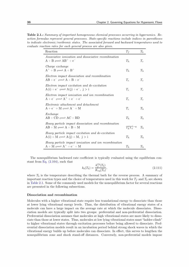
36 Chapter 2. Governing Equations for Hypersonic Flows
Table 2.1.: Summary of important homogeneous chemical processes occurring in hypersonics. Re-action formulas represent general processes. State-specific reactions include indices in parenthesesto indicate electronic/rovibronic states. The associated forward and backward temperatures used toevaluate reaction rates for each general process are also given.
Reaction Tf Tb
Associative ionization and dissociative recombinationA + B −−−− AB+ + e– Th Te
Charge exchangeA+ + B −−−− A + B+ Th Th
Electron impact dissociation and recombinationAB + e– −−−− A + B + e– Te Te
Electron impact excitation and de-excitationA(i) + e– −−−− A(j) + e– , j > i Te Te
Electron impact ionization and ion recombinationA + e– −−−− A+ + e– + e– Te Te
Electronic attachment and detachmentA + e– + M −−−− A– + M Te Th
ExchangeAB + CD −−−− AC + BD Th Th
Heavy particle impact dissociation and recombinationAB + M −−−− A + B + M T q
hT1−qv Th
Heavy particle impact excitation and de-excitationA(i) + M −−−− A(j) + M, j > i Th Th
Heavy particle impact ionization and ion recombinationA + M −−−− A+ + e– + M Th Th
The nonequilibrium backward rate coefficient is typically evaluated using the equilibrium con-stant from Eq. (2.104), such that
kb(Tb) =keqf (Tb)
Keq(Tb), (2.111)
where Tb is the temperature describing the thermal bath for the reverse process. A summary ofimportant reaction types and the choice of temperatures used in this work for Tf and Tb are shownin Table 2.1. Some of the commonly used models for the nonequilibrium factor for several reactionsare presented in the following subsections.
Dissociation and recombination
Molecules with a higher vibrational state require less translational energy to dissociate than thoseat lower lying vibrational energy levels. Thus, the distribution of vibrational energy states of amolecule can have a large impact on the average rate at which the molecule dissociates. Disso-ciation models are typically split into two groups: preferential and non-preferential dissociation.Preferential dissociation assumes that molecules at high vibrational states are more likely to disso-ciate than those at lower states. Thus, molecules at low lying vibrational states must “ladder-climb”to higher vibrational states through excitation processes before being allowed to dissociate. Pref-erential dissociation models result in an incubation period behind strong shock waves in which thevibrational energy builds up before molecules can dissociate. In effect, this serves to lengthen thenonequilibrium zone and shock stand-off distances. Conversely, non-preferential models impose
2.6. Chemical Kinetics 37
the same likelihood that a molecule will dissociate from all vibrational levels. Three importantnonequilibrium models for dissociation and recombination are presented here.
Marrone and Treanor [119], building on the work on Hammerling et al. [118] for non-preferentialdissociation, derived an expression for the nonequilibrium factor assuming that higher vibrationalenergy levels were more likely to dissociate. The resulting expression may be written as
Φ(Th, Tv) =Qv
j (Th) Qvj (TF )
Qvj (Tv) Qv
j (−U), (2.112)
1
TF=
1
Tv−
1
Th−
1
U, (2.113)
where U is a fictitious temperature used to adjust the probability of dissociation from a givenvibrational energy level and is usually taken to be U = D/3kB and D is the dissociation energyof the molecule. Under thermal equilibrium, Tv = Th and TF = −U such that Φ(Th, Tv) = 1 asexpected. When U = ∞, the non-preferential model of Hammerling is obtained. Qv
j representsthe partition function for a truncated harmonic-oscillator. According to Marrone and Treanor,the negative value −U represents the “vibrational temperature” at which molecules are formed byrecombination.
Park [58, 60] developed a simple phenomenological model to describe the nonequilibrium dis-sociation of nitrogen which remains widely used today. When applied to the Arrhenius rate law,Eq. (2.107), Park’s model is given as
Φ(Th, Tv) = T βa Th
−β exp
(
Ea
RuTh−
Ea
RuTa
)
, (2.114)
where Ta = ThqTv
1−q, for 0 ≤ q ≤ 1, is an “average” temperature. Park originally suggested to usea geometric mean such that q = 0.5, though this was later improved by Sharma [120] to q = 0.7 inorder to better match experimental data. Typically, this model is implemented by treating Φ = 1and simply evaluating the equilibrium rate coefficient with Tf = Ta. It is well known that Park’smodel substantially under predicts dissociation rates when Tv ≪ Th, however it remains a popularchoice in hypersonic CFD codes because of its simplicity.
Finally, Macheret [123, 124, 127] derived a model based on the assumption of impulsive collisionsand rigid-rotor harmonic oscillators. The resulting expression for the nonequilibrium factor maybe written as
Φ(Th, Tr, Tv) =1
keqf (Th)
[
kl(Th, Tr, Tv) + kh(Tv)
]
, (2.115)
kl(Th, Tr, Tv) ∝ exp
[
−D
Ta+ 6α2D
(
1
Ta−
1
Th
)]
, (2.116)
kh(Tv) ∝ exp
(
−D
Tv
)
, (2.117)
where kl and kh represent the contribution of low and high vibrational energy levels of the dissoci-ating molecule to the dissociation rate coefficient, Ta = αTv+(1−α)Tk is an “average” temperature,Tk = (Th +
√αTr)/(1 +
√α) is the “kinetic” temperature, and α is a simple factor related to the
masses of the colliding species. The proportionality factors which complete the expressions for thelow and high rate coefficients depend on the type of collision partners involved (diatom-diatomor diatom-atom) and are described in detail in [124]. Macheret’s model has been shown to accu-rately describe nitrogen dissociation rates under nonequilibrium conditions as compared to thoseobtained to detailed STS rates [128]. Furthermore, the model does not require any tuned or empir-ically derived parameters, which represents a major advantage to the models of Park and Treanorand Marrone.
38 Chapter 2. Governing Equations for Hypersonic Flows
Other reactions
The effect of internal energy on nonequilibrium reaction rates is typically modeled for dissociationreactions only due to the important role they play behind strong shock waves. However, modelsalso exist for other types of reactions as well. For example, Knab et al. [122, 125] have developedexpressions similar to those described above for dissociation reactions which model the nonequi-librium factor for exchange, associative ionization, and electron impact ionization and dissociationreactions. These expressions are not given here for the sake of brevity.
2.6.3. Heterogeneous Chemistry (Gas-Surface Interaction)
As with homogeneous chemistry mechanisms, heterogeneous chemistry plays an important role inthe description of the thermochemical environment surrounding hypersonic vehicles. In particular,an accurate prediction of the heat flux to the surface of a vehicle may depend strongly on thecorrect solution of catalysis and ablation processes occurring at the gas-surface interface, knownin general as gas-surface interactions (GSI). These processes may strongly affect the compositionof the boundary layer, which in turn may alter the convective or radiative heating at or near thevehicle surface. For Martian entries, these effects have also been shown to be important downstream as ablated species radiate and increase the radiative flux to the back-shell of the vehicle.Typically, GSI models are implemented as boundary conditions along the vehicle surface. Inthis section, the relevant heterogeneous chemical processes and the corresponding models used tosimulate them are reviewed.
For non-ablating thermal protection systems, catalysis may play an important role in the heatingto the surface of the TPS. In particular, for Earth entries, catalytic recombination of the N2, O2,and NO at the surface,
N+N −−−− N2,
O+O −−−− O2,
N+O −−−− NO,
are well known. Catalytic reactions do not participate in the surface mass balance but can promotesubstantial heat transfer. As an example, the reactions shown above release approximately 950,500, and 630 kJ per mole of product, respectively [129].
Surface participating reactions involve both heat and mass transfer between the surface andsurrounding gas. As such, these reactions always include reactants originating from the TPSmaterial. Examples include the nitridation or oxidation of solid carbon C(s),
C(s) + N −−−− CN,
C(s) + O −−−− CO,
C(s) + O2 −−−− CO2,
the passive and active oxidation of silicon carbide,
SiC(s) + 2O2 −−−− SiO2(s) + CO2,
SiC(s) + 3O −−−− SiO2(s) + CO,
SiC(s) + O2 −−−− SiO + CO,
SiC(s) + 2O −−−− SiO + CO,
and the sublimation of solid carbon to form C, C2, or C3. In general, there are two types of modelswhich are used to describe surface chemistry and these are discussed below.
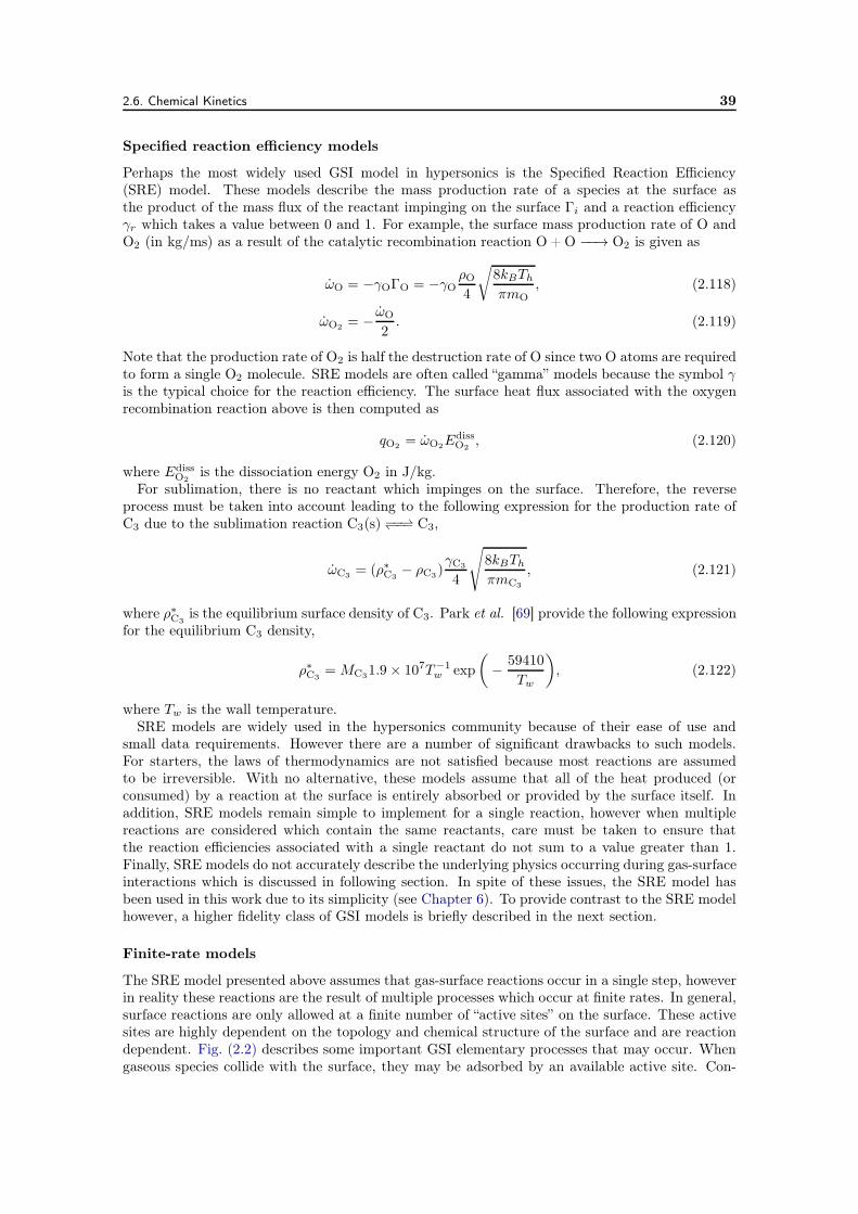
2.6. Chemical Kinetics 39
Specified reaction efficiency models
Perhaps the most widely used GSI model in hypersonics is the Specified Reaction Efficiency(SRE) model. These models describe the mass production rate of a species at the surface asthe product of the mass flux of the reactant impinging on the surface Γi and a reaction efficiencyγr which takes a value between 0 and 1. For example, the surface mass production rate of O andO2 (in kg/ms) as a result of the catalytic recombination reaction O + O −−→ O2 is given as
ωO = −γOΓO = −γOρO4
√
8kBTh
πmO, (2.118)
ωO2= −
ωO
2. (2.119)
Note that the production rate of O2 is half the destruction rate of O since two O atoms are requiredto form a single O2 molecule. SRE models are often called “gamma” models because the symbol γis the typical choice for the reaction efficiency. The surface heat flux associated with the oxygenrecombination reaction above is then computed as
qO2= ωO2
EdissO2
, (2.120)
where EdissO2
is the dissociation energy O2 in J/kg.For sublimation, there is no reactant which impinges on the surface. Therefore, the reverse
process must be taken into account leading to the following expression for the production rate ofC3 due to the sublimation reaction C3(s) −−−− C3,
ωC3= (ρ∗C3
− ρC3)γC3
4
√
8kBTh
πmC3
, (2.121)
where ρ∗C3is the equilibrium surface density of C3. Park et al. [69] provide the following expression
for the equilibrium C3 density,
ρ∗C3= MC3
1.9× 10⁷T−1w exp
(
−59410
Tw
)
, (2.122)
where Tw is the wall temperature.SRE models are widely used in the hypersonics community because of their ease of use and
small data requirements. However there are a number of significant drawbacks to such models.For starters, the laws of thermodynamics are not satisfied because most reactions are assumedto be irreversible. With no alternative, these models assume that all of the heat produced (orconsumed) by a reaction at the surface is entirely absorbed or provided by the surface itself. Inaddition, SRE models remain simple to implement for a single reaction, however when multiplereactions are considered which contain the same reactants, care must be taken to ensure thatthe reaction efficiencies associated with a single reactant do not sum to a value greater than 1.Finally, SRE models do not accurately describe the underlying physics occurring during gas-surfaceinteractions which is discussed in following section. In spite of these issues, the SRE model hasbeen used in this work due to its simplicity (see Chapter 6). To provide contrast to the SRE modelhowever, a higher fidelity class of GSI models is briefly described in the next section.
Finite-rate models
The SRE model presented above assumes that gas-surface reactions occur in a single step, howeverin reality these reactions are the result of multiple processes which occur at finite rates. In general,surface reactions are only allowed at a finite number of “active sites” on the surface. These activesites are highly dependent on the topology and chemical structure of the surface and are reactiondependent. Fig. (2.2) describes some important GSI elementary processes that may occur. Whengaseous species collide with the surface, they may be adsorbed by an available active site. Con-
40 Chapter 2. Governing Equations for Hypersonic Flows
Figure 2.2.: Idealized gas-surface interactions.
versely, atoms may desorb from occupied sites to form gaseous species. Adsorbed species may alsodiffuse along the surface between active sites. A Langmuir-Hinshelwood reaction occurs betweentwo adsorbed species or atoms in the bulk phase which combine and are released as a gaseousmolecule. Recombination may also occur through an Eley-Rideal mechanism in which a gaseousspecies reacts with an adsorbed or bulk species, which is then released from the surface.
Finite-rate surface chemistry models describe the net surface reactions as a series of the ele-mentary processes shown in Fig. (2.2). For example, Marschall et al. [129] describe the catalyticrecombination of oxygen atoms on a silica surface through the following elementary processes,
O+ (s) −−−− O(s),
O2 + (s) −−−− O2(s),
O+O(s) −−−− O2(s),
O+O(s) −−−− O2 + (s),
O+O2(s) −−−− O2 +O(s),
where (s), O(s), and O2(s) represent active sites in the bulk phase and absorbed oxygen atomand molecule, respectively. The first two reactions account for the adsorption of oxygen atomsand molecules onto the bulk surface. Each reaction converts an active site in the bulk phase toactive sites on adsorbed oxygen atoms. The third reaction represents adsorption of an oxygenatom onto an active O site to form an O2 site. Finally, the last two reactions represent theEley-Rideal recombination of oxygen. Each of these processes may occur at different temperaturedependent rates. Furthermore, the reverse processes are related to the forward reaction through anequilibrium constant. The heat flux to the surface of a material is then related to the rate of changein the density of active sites. Thus, a finite-rate surface chemistry model ensures the conservationof mass and energy at the surface. However, as can be seen by this simple example, finite-ratemodels require significantly more data than that required in the SRE models. In addition, theinitial distribution of active sites on a surface remains a difficult parameter to determine for mostapplications. Some finite-rate models assume that the active site density follows a steady-statesolution, allowing for this parameter to be determined analytically. A detailed analysis of finite-rate surface chemistry models is beyond the scope of this thesis and thus only this simple discussionis provided.
2.7. Energy Transfer Mechanisms
As previously discussed, nonequilibrium kinetics are most accurately described by full STS models.However, as these models are extremely costly, most CFD codes resort to the use of MT modelsinstead. For such models, the energy transferred between different energy modes is not explicitlydetermined through the reaction mechanism and must therefore be modeled by the various energytransfer source terms presented in Section 2.3.2. In general, energy transfer mechanisms fall intotwo categories: energy relaxation processes and chemical energy exchange processes. Both are
2.7. Energy Transfer Mechanisms 41
described in detail in the following subsections.
2.7.1. Energy relaxation processes
Energy relaxation is the process in which two distributions of energy states exchange energy throughelastic and inelastic collisions and “relax” to a final equilibrium distribution. For the MT models,relaxation processes describe the exchange of energy between different energy modes with Boltz-mann distributions described by separate temperatures. In general, we are interested in how theaverage or total energy of one mode equilibrates with another.
Vibration-translation energy exchange
Vibration-translation energy exchange plays a major role in the relaxation behind strong shockwaves. We first consider a harmonic-oscillator interacting with a single heat bath of translationalenergy. The rate of change for this harmonic-oscillator’s vibrational energy, measured from theground state, is written
∂
∂t(ρje
vj ) = hνj
∞∑
i=1
i∂
∂t(ni
j), (2.123)
where νj represents the characteristic frequency of vibration for species j and ∂nij/∂t is the rate
of change of the number density of vibrational level i due to (de)excitation processes.For weak binary interactions [56], transitions may be assumed to occur only between neighboring
vibrational states. Under these conditions, the following rate equation is then easily derived,
∂
∂t(ni
j) = −ki,i+1j ni
j + ki+1,ij ni+1
j − ki,i−1j ni
j + ki−1,ij ni−1
j , (2.124)
where ka,bj represents the rate coefficient for the transition from vibrational state a to b for speciesj. The rate coefficients depend primarily on a) the number of collisions between oscillators andmolecules of the heat bath with sufficient energy to cause transition and b) the probability that sucha collision results in a transition. For harmonic-oscillators, the rate coefficients are proportional tothe vibrational quantum number, ki,i−1
j = ik1,0j [30]. Thus, using detailed balancing to relate theexcitation and deexcitation rate coefficients, Eq. (2.124) may be rewritten as
∂
∂t(ni
j) = k1,0j
− inij + (i + 1)ni+1
j + exp
(
θvjTh
)[
− (i + 1)nij + ini−1
j
]
, (2.125)
where θvj = hνj/kB is the characteristic vibrational temperature for species j.Substituting Eq. (2.125) in Eq. (2.123) and simplifying the summation over states yields the
Landau-Teller form [130] for vibrational energy relaxation,
∂
∂t(ρje
vj ) = ρj
ev∗j (Th)− evjτVTj
, (2.126)
where ev∗j (Th) denotes the vibrational energy for a Boltzmann distribution at temperature Th andτVTj = [k1,0j (1− exp(−θvj /Th)]−1 is the relaxation time. Physically, the relaxation time represents
the time in seconds required for the difference (ev∗j (Th)−evj ) to fall to 1/e of its original magnitudein a constant heat bath. Eq. (2.126) shows that the vibrational energy tends to equilibrate withthe translational heat bath at a linear rate which is proportional to the degree of nonequilibrium.It is important to note that no assumptions were made on the distribution of vibrational statesin the derivation of Eq. (2.126) or the degree of nonequilibrium. However, the assumption ofharmonic-oscillators is only valid for low vibrational states, limiting the validity of the formulationto small departures from equilibrium and relatively low vibrational temperatures.
The theoretical treatment of the relaxation time present in Eq. (2.126) is very difficult. Millikanand White [131] have shown that many diatomic collision systems can be described by the simple
42 Chapter 2. Governing Equations for Hypersonic Flows
phenomenological formula at low temperatures (< 8000K),
(1− xe) p τMWj [atm s] =
∑
s∈H
xs exp[
ajs(T− 1
3 − bjs)− 18.42]
(2.127)
where ajs = 1.16× 10⁻³ µ12
js θvj
43 , bjs = 0.015µ
14
js, and µjs is the reduced molecular weight of thevibrator j and heat bath species s. At high temperatures, the Millikan and White model under-predicts the relaxation time because it does not take into account the limiting of excitation ratesdue to the finiteness of elastic collision cross-sections. Park [67] proposed the simple formula forthe relaxation time at high temperatures,
τPj =
(
nj
√
8kBTh
πmjσvj
)−1
, (2.128)
where σvj is an effective cross-section for vibrational relaxation. In addition, at high temperatures,
the kinetic energy of the gas becomes much greater than the vibrational energy gap between excitedvibrational levels. In this regime, vibrational excitation and deexcitation behave classically and thevibrational energy may be treated as continuously distributed, leading to a diffusion-like equationfor the rate of change in the density of a vibrational state [30]. In order to combine the diffusionand Landau-Teller models, Park [60] has suggested a correction to the relaxation time for shockheated flows, such that
τVTj =
(
τMWj + τP
j )
∣
∣
∣
∣
Ts − Tvs
Ts − Tvj
∣
∣
∣
∣
s−1
, (2.129)
where Ts and Tvs are the heavy-particle translational and vibrational temperatures immediatelybehind the normal shock wave. The parameter s = 3.5 exp(−5000/Ts) acts as a bridging functionbetween the high and low temperature regimes. For one-dimensional problems, the high tempera-ture correction is straight forward to implement. For two- and three-dimensional flows, the shockwave location should be based on a streamwise trace from the local point to the shock front, thoughin practice the average post shock temperature is typically used instead [26].
When separate vibrational temperatures are used to describe the vibrational energy distributionsof each vibrating molecule, the resulting energy transfer terms for each vibrator j are easily derivedfrom Eq. (2.126), such that
ΩVTj = ρj
evj (Th)− evj (Tvj)
τVTj
, (2.130)
where the superscript ∗ has been dropped because the vibrational energy is assumed to follow aBoltzmann distribution. If all vibrators have the same vibrational temperature, then the sourceterm is simply the net energy transfer due to each molecule,
ΩVT =∑
j∈V
ΩVTj =
∑
j∈V
ρjevj (Th)− evj (Tv)
τVTj
. (2.131)
The Landau-Teller form for vibration-translation energy exchange has several limitations, whichmay severely limit its accuracy. For example, anharmonicity, rovibration coupling effects, andreal collision dynamics are not taken into account. Nikitin and Troe [132] provide a historicalreview of energy transfer models developed since the landmark paper of Landau and Teller in 1936[130]. In general, these models build on the original Landau-Teller formulation by incorporating amore detailed Master equation than Eq. (2.124) and using higher fidelity collision dynamics suchas those obtained through QCT calculations. Despite the many advances, Eqs. (2.127 - 2.131)remain widely used in the field of hypersonics due to their ease of implementation and small datarequirements.
2.7. Energy Transfer Mechanisms 43
Free electron-vibration energy exchange
Electron-impact vibrational (de)excitation processes play an important role in the energy exchangebetween electrons and molecules. In particular, the resonant electron impact nitrogen excitationreaction
N2(X1Σg
+; v) + e− −−→ N2−(2Πg) −−→ N2(X
1Σg+; w) + e−, w > v
is known to be very efficient. Electron impact excitation reactions for other air molecules arenegligible [27]. Studies of electron-vibration energy exchange for nitrogen plasmas suggest thatthis process may be modeled with a Landau-Teller rate equation [133–135], where
ΩEVj = ρj
evj (Te)− evj (Tvj)
τEVj
. (2.132)
Laporta and Bruno [135] have developed analytical expressions for the relaxation time τEVj based
on STS calculations using accurate theoretical cross sections.
Vibration-vibration energy exchange
When separate vibrational energy equations are attributed to each vibrating molecule, the vibra-tional energy exchanged between each of these vibrators should be taken into account. Knab etal. [122] have proposed the following consistent model for vibrational energy exchange,
ΩVVj = NA
√
8RuTh
π
∑
s∈V
σjsPjsρsMs
ρj
[
evj (Th)
evs(Th)evs(Tvs)− evj (Tvj)
]
, (2.133)
where Pjs is the exchange probability, taken to be 0.01 [122]. Panesi [128] has shown vibration-vibration energy exchange to be of secondary importance for nonequilibrium air flows.
Elastic energy exchange between free electrons and heavy particles
Elastic energy exchange between free electrons and heavy particles has been studied in-depth forpartially ionized nonequilibrium plasmas based on kinetic theory [100, 107]. This energy exchangefollows the Landau-Teller form, such that
ΩET = ρeee(Th)− ee(Te)
τET =3
2ρeRe
Th − Te
τET . (2.134)
The average relaxation time is derived directly from kinetic theory as
1
τET =∑
i∈H
8
3
me
mini
√
8kBTe
πmeQ(1,1)
ei , (2.135)
where Q(1,1)ei is the reduced collision integral for the electron-heavy interaction.
2.7.2. Chemical energy exchange processes
Chemical energy exchange processes result from reactive collisions between particles in which en-ergy is transferred in order to promote the reaction. Important coupling mechanisms are describedbelow.
Electron-impact ionization
Electron-impact ionization reactions result in a lowering of the overall electron translational energysince the free-electrons provide the energy necessary to ionize the heavy particle. It is important
44 Chapter 2. Governing Equations for Hypersonic Flows
to take this energy transfer mechanism into account, in particular to accurately describe electronavalanche. The amount of energy lost from the electron bath is modeled as
ΩI =∑
r∈I
∆hrRr, (2.136)
where I is the set of electron impact ionization reactions and ∆hr and Rr are the molar reactionenthalpy and rate of progress for the ionization reaction r. The reaction enthalpy represents theaverage energy required to ionize the heavy particle in reaction r and the rate of progress is equalto the rate of electron impact ionization reactions. Note that this model assumes that all theenergy required to ionize a given species comes from the free-electrons which may overestimate therate of electron energy loss.
Vibration-chemistry-vibration coupling
When molecules are created or destroyed through chemical reactions, vibrational energy is addedor removed from the gas. This creates an important coupling mechanism between the vibrationalenergy distribution of a given molecule and the rate of creation or destruction of that molecule,which in turn effects the net vibrational energy exchange of the gas. Vibration-chemistry-vibrationcoupling is strongly related to the vibrational chemical nonequilibrium model in use. As such, themodels are split again into preferential and non-preferential dissociation categories.
Preferential dissociation leads to the following general expression for the vibration-chemistryenergy transfer source term,
ΩCVm = Mm
∑
r∈R
Rr
[
ν′′
mG′′
rm − ν′
mG′
rm
]
, (2.137)
where G′
rm and G′′
rm are the average vibrational energy gained or lost per mass of molecule massociated with the forward and reverse process of reaction r. The actual form of these parametersmust be consistent with the vibration-chemistry model being employed. For example, in the caseof the Treanor and Marrone model [119] discussed in Section 2.6.2, these average energies become
G′
rm =Rmθvm
exp(−θvm/U)− 1−
RmθDmexp(−θDm/U)− 1
, (2.138)
G′′
rm =Rmθvm
exp(−θvm/TF )− 1−
RmθDmexp(−θDm/TF )− 1
, (2.139)
where θDm is the dissociation energy of molecule m (associated with the dissociation reaction r) andTF and U were defined in Eq. (2.113).
Non-preferential models assign equal probability to a molecule dissociating from any vibrationalenergy state. Therefore, the average vibrational energy lost or gained by a molecule which dissoci-ates or recombines is equal to the average vibrational energy of the molecule itself, evm (regardlessof energy distribution). Therefore, for non-preferential dissociation Eq. (2.137) readily assumesthe form proposed by Candler and MacCormack [27],
ΩCVm = c1e
vmωm, (2.140)
where the factor c1 is introduced as a preferential dissociation factor. For c1 = 1, Eq. (2.140)represents a non-preferential dissociation model while for c1 > 1, a simple preferential model isobtained.
2.8. Concluding Remarks 45
2.8. Concluding Remarks
The goal of this chapter was to present the general governing equations for hypersonic, atmosphericentry flows. Hypersonic flows are characterized by flow time scales on the order of chemical andrelaxation time scales which result in significant thermal and chemical nonequilibrium phenomena.Thermal nonequilibrium is treated through the use of so-called energy partitioning models in whichassumptions are made on the relative distribution of populated energy states for each componentof the flow. Various energy partitioning models have been reviewed in this chapter and their role inthe governing fluid equations has been detailed. In particular, both thermochemical nonequilibriumand LTE flows have been considered.
Closure models for the thermodynamic, transport, and chemistry properties, whose evaluation isrequired to solve the governing equations, have also been presented. In general, all properties havebeen shown to be functions of the local state of the fluid. General relations for thermodynamicproperties were provided, based on the a statistical mechanics description of individual speciesenergy partitioning models and associated partition functions. Transport properties were presentedbased on a perturbative Chapmann-Enskog solution of the scaled Boltzmann equation, whichresults in linear transport systems defined in terms of temperature dependent collision integralsand species concentrations. Chemical production rates were formulated in terms of the Law of MassAction. The effect of thermal nonequilibrium was also considered and several common models fornonequilibrium rate coefficients were presented. In addition, several important energy transfermodels were discussed in the context of a MT approach.
Radiation was largely ignored in this chapter, except in the presentation of the governing equa-tions. The computation of radiative source terms represents a significant numerical and theoreticaleffort. In addition, the treatment of radiation in the governing equations alters the general natureof the equations from differential to integro-differential. For these reasons, the discussion of radi-ation has been postponed until Chapter 3. Finally, it is worth noting that this chapter presentedthe governing equations in a general manner. The specific models and data used in this work arepresented in Chapter 4.

CHAPTER 3
Radiative Transfer for Atmospheric Entry
3.1. Introduction
The radiative heat flux, energy source, and photochemical source terms required to couple radiativetransfer to the fluid dynamic conservation equations, were presented in Chapter 2. As will beevident from the following sections, the accurate calculation of these quantities involves a significantmodeling and numerical effort. This chapter is broken into three distinct sections. Section 3.2provides an introduction to radiation for atmospheric entry applications. Section 3.3 details theHTGR database, used in this work to compute high resolution emission and absorption spectra.Finally, Section 3.4 derives the so-called hybrid statistical narrow band model, used in this workto significantly improve the performance of radiative transfer calculations.
3.2. Radiative Transfer in Participating Media
This section provides a short introduction to the basics of modeling radiative transfer in partici-pating media, in particular, gases. The various radiative processes which occur in gases are firstoutlined, followed by a description of the governing equations for radiation transport includingthe radiative boundary conditions typically used for atmospheric entry applications. Finally, theradiative surface heat flux, energy source, and species mass production rates due to photochemicalprocesses are detailed.
3.2.1. Radiative Processes in Gases
Radiative processes in gaseous media can be grouped into three categories, namely bound-bound,bound-free or free-bound, and free-free processes. Each one is discussed below.
Bound-bound
Bound-bound processes are radiative transitions between bound electronic states of atoms or rovi-bronic states of molecules. Bound-bound transitions can occur through absorption,
A(l) + hcσ −−→ A(u),
spontaneous emission,A(u) −−→ A(l) + hcσ,
and induced emission,A(u) + hcσ −−→ A(l) + 2 hcσ.
Each process is depicted graphically in Fig. (3.1). Spontaneous emission occurs when an atom ormolecule at an upper energy state u with energy Eu spontaneously emits a photon with energyhcσ and falls to a lower energy state l with energy El = Eu − hcσ. Absorption is the oppositeprocess, in which a photon with energy hcσ is absorbed to raise the energy from El to Eu. Apart
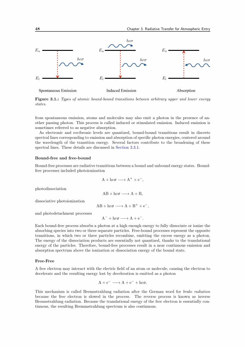
48 Chapter 3. Radiative Transfer for Atmospheric Entry
Eu
El
hcσ
Eu
El
hcσ
hcσ
Eu
El
hcσ
Induced EmissionSpontaneous Emission Absorption
Figure 3.1.: Types of atomic bound-bound transitions between arbitrary upper and lower energystates.
from spontaneous emission, atoms and molecules may also emit a photon in the presence of an-other passing photon. This process is called induced or stimulated emission. Induced emission issometimes referred to as negative absorption.
As electronic and rovibronic levels are quantized, bound-bound transitions result in discretespectral lines corresponding to emission and absorption of specific photon energies, centered aroundthe wavelength of the transition energy. Several factors contribute to the broadening of thesespectral lines. These details are discussed in Section 3.3.1.
Bound-free and free-bound
Bound-free processes are radiative transitions between a bound and unbound energy states. Bound-free processes included photoionization
A+ hcσ −−→ A+ + e−,
photodissociationAB+ hcσ −−→ A+ B,
dissociative photoionizationAB+ hcσ −−→ A+ B+ + e−,
and photodetachment processesA− + hcσ −−→ A+ e−.
Each bound-free process absorbs a photon at a high enough energy to fully dissociate or ionize theabsorbing species into two or three separate particles. Free-bound processes represent the oppositetransitions, in which two or three particles recombine, emitting the excess energy as a photon.The energy of the dissociation products are essentially not quantized, thanks to the translationalenergy of the particles. Therefore, bound-free processes result in a near continuous emission andabsorption spectrum above the ionization or dissociation energy of the bound state.
Free-Free
A free electron may interact with the electric field of an atom or molecule, causing the electron todecelerate and the resulting energy lost by deceleration is emitted as a photon
A+ e− −−→ A+ e− + hcσ.
This mechanism is called Bremsstrahlung radiation after the German word for brake radiationbecause the free electron is slowed in the process. The reverse process is known as inverseBremsstrahlung radiation. Because the translational energy of the free electron is essentially con-tinuous, the resulting Bremmstrahlung spectrum is also continuous.
3.2. Radiative Transfer in Participating Media 49
3.2.2. The Radiative Transport Equation
Each radiative mechanism discussed in the previous section contributes to the net emission andabsorption of photons. The energy carried by a photon at wavenumber σ is given hcσ. Therefore,emission and absorption of photons results in a net energy transfer between points in the flow field,or from the flow field to the vehicle surface.
The radiant intensity Iσ(x, s) is defined as the photon energy flux per unit area, per elementarysolid angle, per wavenumber, in the direction s at wavenumber σ and position x. In the absenceof scattering, the steady Radiative Transport Equation (RTE) describes the variation of spectralintensity Iσ along a ray with length parameter s as
dIσds
= s ·∇Iσ(s) = ησ − κσIσ(s), (3.1)
where ησ and κσ are the local emission and absorption coefficients at point s along the ray.Photons may be emitted in any direction. Therefore, the spectral emission coefficient is inde-
pendent of direction and represents the total photon energy emitted per volume, per time, perwavenumber, and per elementary solid angle. The absorption coefficient represents the fraction ofphoton energy absorbed by the gas over a unit distance, and is independent of direction as well.In general, these coefficients are functions of the local energy level populations of the participatinggaseous species. They will be described in more detail in Section 3.3.
Under radiative equilibrium conditions, the intensity follows Planck’s law such that
Iσ = Ibσ ≡ 2hc2σ3[
exp( hcσ
kBT
)
− 1]−1
, (3.2)
and the emission and absorption coefficients are related through Kirchhoff’s law by ησ = Ibσκσ.This relation is also satisfied for flows in thermo-chemical equilibrium.
The formal solution of Eq. (3.1) may be written as
Iσ(s) = Iσ(0)τσ(0, s) +
∫ s
0ησ(s
′)τσ(s′, s)ds′, (3.3)
where the spectral transmissivity τσ between points s′ and s is given by Beer’s law,
τσ(s′, s) = exp
(
−∫ s
s′κσ(s
′′) ds′′)
. (3.4)
The integral inside the exponential is called the optical thickness of the gas. When the opticalthickness is large, the transmissivity approaches zero, indicating that no radiation is transmittedthrough the gas. Conversely, for optically thin media, the transmissivity approaches unity and allradiation is transmitted.
3.2.3. Boundary Conditions
Eq. (3.3) represents an integral equation for the solution of the radiant intensity at a given pointin space, in the direction defined by the ray. This equation may be solved by integrating along theray from a known boundary condition, Iσ(0). Two types of boundaries will be considered in thiswork.
Diffuse surfaces
Vehicle surfaces are assumed to be diffuse, and opaque, such that
Iσ(xw, s) = ϵσIbσ(Tw) +
ρσπ
∫
n·s′<0Iσ(xw, s
′) |n · s′| dΩ′, n · s > 0, (3.5)
50 Chapter 3. Radiative Transfer for Atmospheric Entry
where ϵσ and ρσ are the local spectral emittance and reflectance of the surface and n is the outwardfacing surface normal. Emittance represents the fraction of black body radiation emitted by thesurface, while reflectance represents the fraction of incoming intensity that is reflected away fromthe wall. For an opaque surface, the reflectance is related to the absorptance ασ of the surface by
ρσ = 1− ασ, (3.6)
where the absorptance represents the fraction of incoming energy absorbed by the material at thesurface. Also, for a diffuse surface, the emittance and absorptance are independent of direction,leading to ϵσ = ασ.
The integral in Eq. (3.5) represents the spectral irradiation, or incoming spectral flux, onto thesurface. For partially reflecting boundaries (ϵ < 1), the reflective term in Eq. (3.5) imposes acoupling between the incoming and outgoing intensities at the boundaries.
Free-stream boundaries
It is assumed that free-stream boundaries are sufficiently far from the shock layer to ensure that alltemperatures associated with the flow field are equal and relatively low. Under these assumptions,the domain boundaries may be treated as black walls at the local temperature, such that
Iσ(x∞, s) = Ibσ(T∞), (3.7)
where the subscript ∞ represents the free-stream quantity.
3.2.4. Coupling to Fluid Dynamics
Once the intensity field is known, the solution must be coupled back to the mass and energytransport equations derived in Chapter 2 via the radiative surface heat flux, power, and speciesmass production rates due to photochemical processes.
Heat flux and its divergence
The total radiative flux at any location in the flow field is given by the integral of intensity overall wavenumbers and directions,
qr =
∫ ∞
0
∫
4πIσ(s) s dΩ dσ. (3.8)
We may also construct the total radiative energy fluxes going into and out of a wall with surfacenormal n, respectively as
qrin =
∫ ∞
0
∫
n·s<0Iσ(xw, s) |n · s| dΩ dσ, (3.9)
qrout =
∫ ∞
0
∫
n·s>0Iσ(xw, s) |n · s| dΩ dσ. (3.10)
Using Eq. (3.5), the total radiative heat flux on a gray, diffuse, and opaque surface is then given as
qrw = qrout − qrin = ϵ(σT 4w − qrin). (3.11)
Finally, the heat flux itself is not a particularly useful parameter within the flow field. Instead,the radiative power, defined by the negative divergence of the heat flux is required to determinethe amount of radiant energy being deposited or emitted at any given point. Using Eqs. (3.1) and
3.3. High Temperature Gas Radiation Database 51
(3.8), the radiative power may be written as
−∇ · qr =−∇ ·∫ ∞
0
∫
4πIσ(s) s dΩ dσ
=
∫ ∞
0κσGσ − 4πησ dσ,
(3.12)
where Gσ is called the spectral incident radiation,
Gσ ≡∫
4πIσ(s) dΩ. (3.13)
Photochemical source terms
The bound-bound and bound-free processes described in Section 3.2.1 alter the chemical compo-sition of the gas through emission or absorption of photons and are known collectively as pho-tochemical processes. The net rate of production of photons at wavenumber σ from a reversiblephotochemical process is equal to the net photon energy emitted by that process, divided by theenergy of a single photon, hcσ. Using the definition of the emission and absorption coefficients fora single photochemical process, it is then plain to see that the net production rate of a species (orpseudo-species) j is given as
φj =mj
hc
∑
p
νpj
∫ ∞
0
1
σ
∫
4π
(
κpσIσ − ηpσ)
dΩ dσ
=mj
hc
∑
p
νpj
∫ ∞
0
κpσGσ − 4πηpσσ
dσ,
(3.14)
where the sum over p represents the sum over all photochemical processes and νpj is the stoichiom-etry difference of species j across process p.
3.3. High Temperature Gas Radiation Database
The emission and absorption coefficients required in the solution of the RTE presented in theprevious section are taken from the HTGR spectroscopic database [36, 37, 39, 40]. An overview ofthe database is presented in this section. In addition, new mechanisms which have been added inthis work are highlighted. Contributions to the emission and absorption coefficients are split intobound-bound transitions and bound-free and free-free continua. Total emission and absorptioncoefficients are obtained by summing each contribution. All radiative mechanisms included in thedatabase are summarized in Table 3.1.
3.3.1. Bound-Bound Transitions
Radiative transitions between bound energy levels of an arbitrary species A follow the generalform,
A(l) + hcσ −−−− A(u), El < Eu. (3.15)
The emission and absorption coefficients for all such transitions are given by
ησ =∑
ul
nuAul
4πhcσf se
ul(σ − σul) (3.16)
κσ =∑
ul
[
nlBlufabul (σ − σul)− nuBulf
ieul(σ − σul)
]
hσ (3.17)
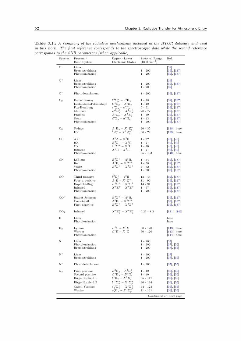
52 Chapter 3. Radiative Transfer for Atmospheric Entry
Table 3.1.: A summary of the radiative mechanisms included in the HTGR database and usedin this work. The first reference corresponds to the spectroscopic data while the second referencecorresponds to the SNB parameters (when applicable).
Species Process / Upper - Lower Spectral Range Ref.Band System Electronic States [1000 cm−1]
C Lines [39]Bremsstrahlung 1 - 200 [39], [137]Photoionization 1 - 200 [39], [137]
C+ Lines [39]Bremsstrahlung 1 - 200 [39], [137]Photoionization 1 - 200 [39]
C– Photodetachment 1 - 200 [39], [137]
C2 Balik-Ramsay b3Σ−g − a3Πu 1 - 48 [39], [137]
Deslandres-d’Azambuja C1Σg − A1Πu 1 - 42 [39], [137]Fox-Herzberg e3Σg − a3Πu 5 - 51 [39], [137]Mulliken D1Σ+
u − X1Σ+g 28 - 77 [39], [137]
Phillips A1Σg − X1Σ+g 1 - 49 [39], [137]
Swan d3Σg − a3Πu 1 - 43 [39], [137]Photoionization 1 - 200 [39], [137]
C3 Swings A1Πu − X1Σ+g 20 - 35 [138], here
UV 1Σ+u − X1Σ+
g 30 - 74 [139], here
CH AX A2∆ − X2Π 1 - 37 [40], [40]BX B2Σ− − X2Π 1 - 27 [40], [40]CX C2Σ+ − X2Π 1 - 40 [40], [40]Infrared X2Π − X2Π 1 - 27 [40], [40]Photoionization 85 - 193 [140], here
CN LeBlanc B2Σ+ − A2Πi 1 - 54 [39], [137]Red A2Πi − X2Σ+ 1 - 58 [39], [137]Violet B2Σ+ − X2Σ+ 4 - 62 [39], [137]Photoionization 1 - 200 [39], [137]
CO Third positive b3Σ+g − a3Π 13 - 43 [39], [137]
Fourth positive A1Π − X1Σ+ 11 - 90 [39], [137]Hopfield-Birge B1Σ+ − X1Σ+ 14 - 91 [39], [137]Infrared X1Σ+ − X1Σ+ 1 - 77 [39], [137]Photoionization 1 - 200 [39], [137]
CO+ Baldet-Johnson B2Σ+ − A2Πi [39], [137]Comet-tail A2Πi − X2Σ+ [39], [137]First negative B2Σ+ − X2Σ+ [39], [137]
CO2 Infrared X1Σ+g − X1Σ+
g 0.25 - 8.3 [141], [142]
H Lines herePhotoionization here
H2 Lyman B1Σ − X1Σ 60 - 120 [143], hereWerner C1Π − X1Σ 60 - 120 [143], herePhotoionization [144], here
N Lines 1 - 200 [37]Photoionization 1 - 200 [37], [55]Bremsstrahlung 1 - 200 [37], [55]
N+ Lines 1 - 200 [37]Bremsstrahlung 1 - 200 [37], [55]
N– Photodetachment 1 - 200 [37], [55]
N2 First positive B3Πg − A3Σ+u 1 - 42 [36], [55]
Second positive C3Πu − B3Πg 1 - 40 [36], [55]Birge-Hopfield 1 b1Πu − X1Σ+
g 55 - 117 [36], [55]Birge-Hopfield 2 b
′1Σ+u − X1Σ+
g 36 - 124 [36], [55]
Caroll-Yoshino c′14 Σ+
u − X1Σ+g 54 - 123 [36], [55]
Worley o13Πu − X1Σ+g 71 - 121 [36], [55]
Continued on next page
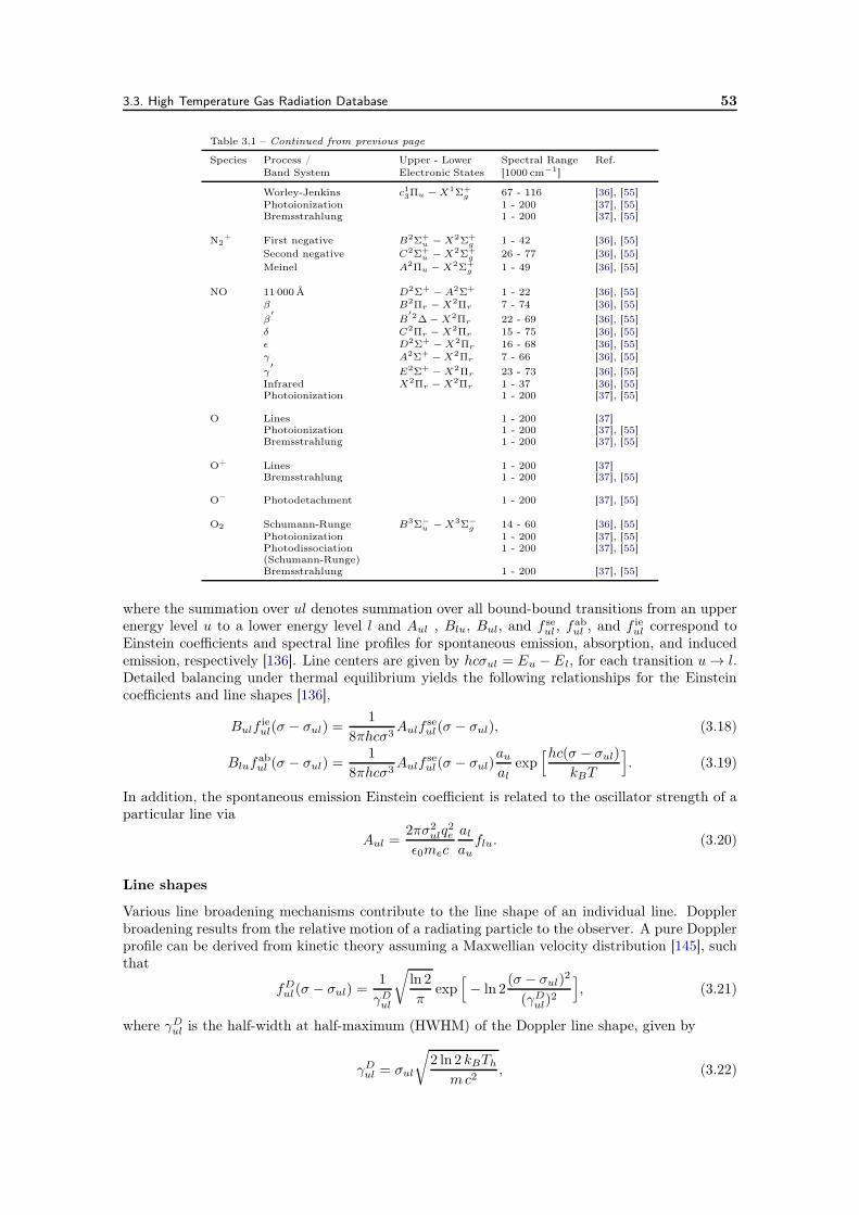
3.3. High Temperature Gas Radiation Database 53
Table 3.1 – Continued from previous page
Species Process / Upper - Lower Spectral Range Ref.Band System Electronic States [1000 cm−1]
Worley-Jenkins c13Πu − X1Σ+g 67 - 116 [36], [55]
Photoionization 1 - 200 [37], [55]Bremsstrahlung 1 - 200 [37], [55]
N2+ First negative B2Σ+
u − X2Σ+g 1 - 42 [36], [55]
Second negative C2Σ+u − X2Σ+
g 26 - 77 [36], [55]Meinel A2Πu − X2Σ+
g 1 - 49 [36], [55]
NO 11 000Å D2Σ+ − A2Σ+ 1 - 22 [36], [55]β B2Πr − X2Πr 7 - 74 [36], [55]β′
B′2∆− X2Πr 22 - 69 [36], [55]
δ C2Πr − X2Πr 15 - 75 [36], [55]ϵ D2Σ+ − X2Πr 16 - 68 [36], [55]γ A2Σ+ − X2Πr 7 - 66 [36], [55]γ′
E2Σ+ − X2Πr 23 - 73 [36], [55]Infrared X2Πr − X2Πr 1 - 37 [36], [55]Photoionization 1 - 200 [37], [55]
O Lines 1 - 200 [37]Photoionization 1 - 200 [37], [55]Bremsstrahlung 1 - 200 [37], [55]
O+ Lines 1 - 200 [37]Bremsstrahlung 1 - 200 [37], [55]
O– Photodetachment 1 - 200 [37], [55]
O2 Schumann-Runge B3Σ−u − X3Σ−
g 14 - 60 [36], [55]Photoionization 1 - 200 [37], [55]Photodissociation 1 - 200 [37], [55](Schumann-Runge)Bremsstrahlung 1 - 200 [37], [55]
where the summation over ul denotes summation over all bound-bound transitions from an upperenergy level u to a lower energy level l and Aul , Blu, Bul, and f se
ul , fabul , and f ie
ul correspond toEinstein coefficients and spectral line profiles for spontaneous emission, absorption, and inducedemission, respectively [136]. Line centers are given by hcσul = Eu −El, for each transition u → l.Detailed balancing under thermal equilibrium yields the following relationships for the Einsteincoefficients and line shapes [136],
Bulfieul(σ − σul) =
1
8πhcσ3Aulf
seul(σ − σul), (3.18)
Blufabul (σ − σul) =
1
8πhcσ3Aulf
seul(σ − σul)
aual
exp[hc(σ − σul)
kBT
]
. (3.19)
In addition, the spontaneous emission Einstein coefficient is related to the oscillator strength of aparticular line via
Aul =2πσ2
ulq2e
ϵ0mec
alau
flu. (3.20)
Line shapes
Various line broadening mechanisms contribute to the line shape of an individual line. Dopplerbroadening results from the relative motion of a radiating particle to the observer. A pure Dopplerprofile can be derived from kinetic theory assuming a Maxwellian velocity distribution [145], suchthat
fDul(σ − σul) =
1
γDul
√
ln 2
πexp
[
− ln 2(σ − σul)2
(γDul)2
]
, (3.21)
where γDul is the half-width at half-maximum (HWHM) of the Doppler line shape, given by
γDul = σul
√
2 ln 2 kBTh
mc2, (3.22)
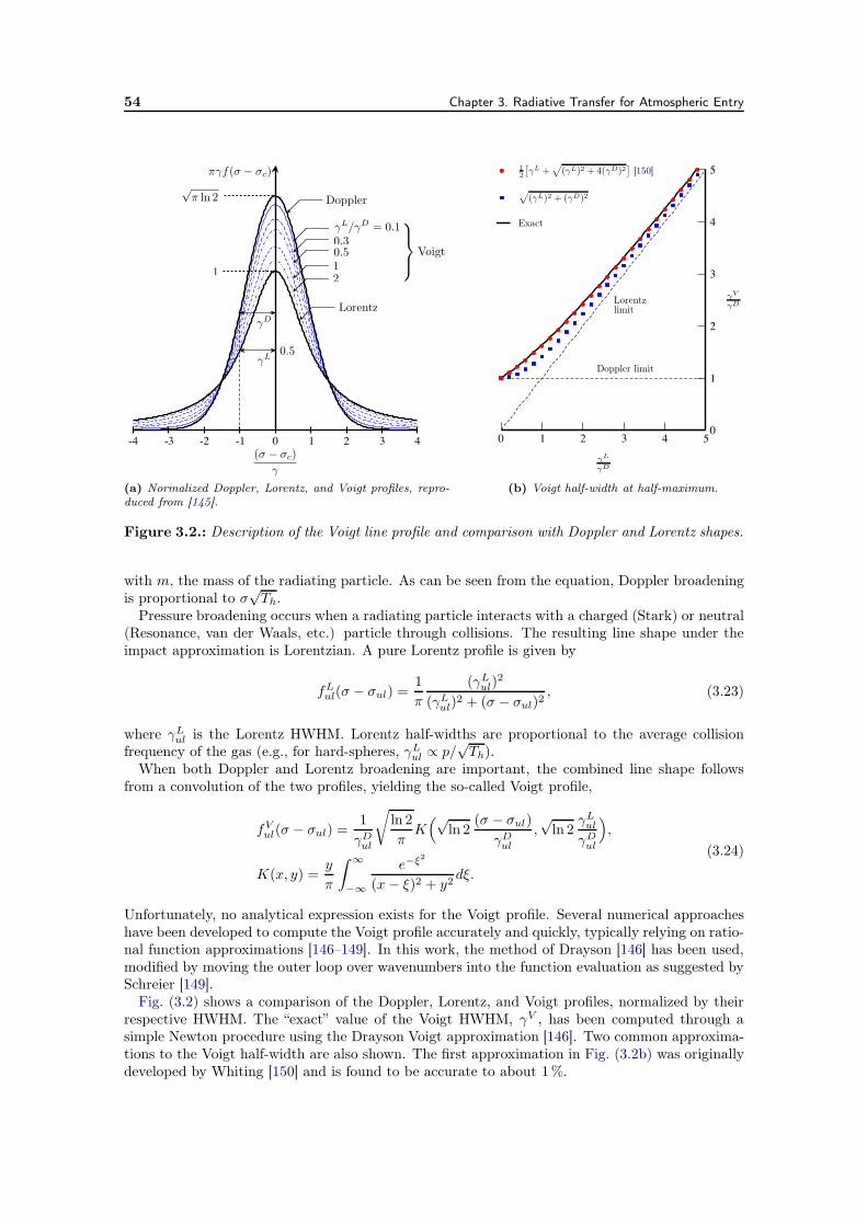
54 Chapter 3. Radiative Transfer for Atmospheric Entry
-4 -3 -2 -1 0 1 2 3 4
0.5
γD
γL
πγf(σ − σc)
(σ − σc)
γ
Doppler
Lorentz
γL/γD= 0.1
0.3
0.5
1
2
!
Voigt
√
π ln 2
1
(a) Normalized Doppler, Lorentz, and Voigt profiles, repro-duced from [145].
0 1 2 3 4 50
1
2
3
4
5
γL
γD
γV
γD
Exact
√
(γL)2 + (γD)2
12
[
γL +√
(γL)2 + 4(γD)2]
[150]
Lorentzlimit
Doppler limit
(b) Voigt half-width at half-maximum.
Figure 3.2.: Description of the Voigt line profile and comparison with Doppler and Lorentz shapes.
with m, the mass of the radiating particle. As can be seen from the equation, Doppler broadeningis proportional to σ
√Th.
Pressure broadening occurs when a radiating particle interacts with a charged (Stark) or neutral(Resonance, van der Waals, etc.) particle through collisions. The resulting line shape under theimpact approximation is Lorentzian. A pure Lorentz profile is given by
fLul(σ − σul) =
1
π
(γLul)2
(γLul)2 + (σ − σul)2
, (3.23)
where γLul is the Lorentz HWHM. Lorentz half-widths are proportional to the average collisionfrequency of the gas (e.g., for hard-spheres, γLul ∝ p/
√Th).
When both Doppler and Lorentz broadening are important, the combined line shape followsfrom a convolution of the two profiles, yielding the so-called Voigt profile,
fVul(σ − σul) =
1
γDul
√
ln 2
πK(√
ln 2(σ − σul)
γDul,√ln 2
γLulγDul
)
,
K(x, y) =y
π
∫ ∞
−∞
e−ξ2
(x− ξ)2 + y2dξ.
(3.24)
Unfortunately, no analytical expression exists for the Voigt profile. Several numerical approacheshave been developed to compute the Voigt profile accurately and quickly, typically relying on ratio-nal function approximations [146–149]. In this work, the method of Drayson [146] has been used,modified by moving the outer loop over wavenumbers into the function evaluation as suggested bySchreier [149].
Fig. (3.2) shows a comparison of the Doppler, Lorentz, and Voigt profiles, normalized by theirrespective HWHM. The “exact” value of the Voigt HWHM, γV , has been computed through asimple Newton procedure using the Drayson Voigt approximation [146]. Two common approxima-tions to the Voigt half-width are also shown. The first approximation in Fig. (3.2b) was originallydeveloped by Whiting [150] and is found to be accurate to about 1%.
3.3. High Temperature Gas Radiation Database 55
Atomic lines
It is convenient to express electronic energy level populations of atoms in terms of Boltzmannpopulations at an electronic temperature Tel. Introducing a non-Boltzmann parameter θBk ≡ nk/nB
kfor an arbitrary electronic level k of atom A, the number density of level k can be expressed as
nk = θBknA
QintA (Tel)
ak exp(
−EA
k
kBTel
)
, (3.25)
where nBk represents the Boltzmann number density of level k and nA is the total number density
for the atom. QintA (Tel) is the atomic internal (electronic) partition function evaluated at Tel.
Inserting Eq. (3.25) along with Eqs. (3.18 - 3.20) into Eqs. (3.16) and (3.17), the emission andabsorption coefficients associated with a single transition u → l for an atom A are given as
ηAσ,ul =hσq2e2ϵ0me
θBunA
QintA
exp( −EA
u
kBTel
)
alflu σ2ul f
seul(σ − σul), (3.26)
κAσ,ul =1
2hc2σ3
[θBlθBu
exp( hcσ
kBTel
)
− 1]
ηAσ,ul. (3.27)
The total emission and absorption coefficients associated with atomic lines are obtained by summingEqs. (3.26) and (3.27) over all considered atoms and transitions. Note that in equilibrium, the non-Boltzmann parameters are equal to unity and Eq. (3.27) is simply a statement of Kirchhoff’s law.
Previous compilations of the necessary line data (alflu, EAu , and σul) for N, O, N+, O+ [37] as well
as C and C+ [39] have been made using the NIST atomic line database [41]. Line shapes associatedwith spontaneous emission are assumed to be Voigt to account for Doppler and neutral collisionalbroadening at a temperature Th and Stark broadening at temperature Te. Stark broadeningparameters for these lines are computed based on a semi-classical approach using line oscillatorstrengths of The Opacity Project atomic database (TOPBASE) [42] and compiled in [37, 39, 151].
H transitions have also been added in this work using the NIST database for line positions andstrengths. The simple approximation of Zoby et al. [152] is retained for Stark broadening, basedon [153], expressing the Lorentz half-width of hydrogen lines as
γLul [eV] = 1.05× 10⁻¹⁵ (n2 −m2) n2/3e−
0.642 n = m+ 1
1 otherwise, (3.28)
where n and m are the principle quantum numbers of the upper and lower electronic states andm = n+1 indicates the first line in each series. The hydrogen electronic partition function is givensimply as
QintH (Tel) =
40∑
k=1
2k2 exp[ Ry
kBTel
( 1
k2− 1)]
, (3.29)
where the level cutoff of 40 has been used in order to match the maximum level retained in theNIST line database. Ry is the Rydberg constant, defined as the ionization energy of the hydrogenground state.
Molecular electronic systems
The HTGR database contains the necessary line information for several air and carbonaceousmolecules. Chauveau et al. [36] have included 19 electronic systems of N2, N2
+, NO, and O2 forhigh temperature air radiation calculations for atmospheric reentry and electric arc applications.Babou et al. [39] extended the database to include 16 electronic systems of C2, CN, CO, and CO+.In addition, 4 electronic systems of CH have been presented by Soufiani et al. [40]. CO2 infraredtransitions have been included based on the CDSD-4000 spectroscopic database [141]. Prasanna etal. [143] have recently compiled line data for the H2 Lyman and Werner bands based on the workof Abgrall et al. [154] and Dabrowski et al. [155].
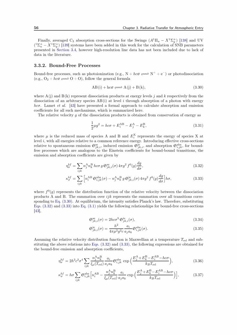
56 Chapter 3. Radiative Transfer for Atmospheric Entry
Finally, averaged C3 absorption cross-sections for the Swings (A1Πu − X1Σ+g ) [138] and UV
(1Σ+u −X1Σ+
g ) [139] systems have been added in this work for the calculation of SNB parameterspresented in Section 3.4, however high-resolution line data has not been included due to lack ofdata in the literature.
3.3.2. Bound-Free Processes
Bound-free processes, such as photoionization (e.g., N + hcσ −−−− N+ + e– ) or photodissociation(e.g., O2 + hcσ −−−− O + O), follow the general formula
AB(i) + hcσ −−−− A(j) + B(k), (3.30)
where A(j) and B(k) represent dissociation products at energy levels j and k respectively from thedissociation of an arbitrary species AB(i) at level i through absorption of a photon with energyhcσ. Lamet et al. [43] have presented a formal approach to calculate absorption and emissioncoefficients for all such mechanisms, which is summarized here.
The relative velocity g of the dissociation products is obtained from conservation of energy as
1
2µg2 = hcσ + EAB
i − EAj − EB
k , (3.31)
where µ is the reduced mass of species A and B and EXi represents the energy of species X at
level i, with all energies relative to a common reference energy. Introducing effective cross-sectionsrelative to spontaneous emission Sse
jk,i, induced emission Siejk,i, and absorption Sabs
i,jk, for bound-free processes which are analogous to the Einstein coefficients for bound-bound transitions, theemission and absorption coefficients are given by
ηbfσ =∑
ijk
nAj n
Bk hcσ gSse
jk,i(σ) 4πg2 f0(g)
dg
dσ, (3.32)
κbfσ =∑
ijk
[
nABi Sabs
i,jk(σ)− nAj n
Bk gSie
jk,i(σ) 4πg2 f0(g)
dg
dσ
]
hσ, (3.33)
where f0(g) represents the distribution function of the relative velocity between the dissociationproducts A and B. The summation over ijk represents the summation over all transitions corre-sponding to Eq. (3.30). At equilibrium, the intensity satisfies Planck’s law. Therefore, substitutingEqs. (3.32) and (3.33) into Eq. (3.1) yields the following relationships for bound-free cross-sections[43],
Ssejk,i(σ) = 2hcσ3 Sie
jk,i(σ), (3.34)
Siejk,i(σ) =
h2
4πµ2g2c
aiajak
Sabsi,jk(σ). (3.35)
Assuming the relative velocity distribution function is Maxwellian at a temperature Trel and sub-stituting the above relations into Eqs. (3.32) and (3.33), the following expressions are obtained forthe bound-free emission and absorption coefficients,
ηbfσ = 2h2c2σ4∑
ijk
nAj n
Bk
ξµ(Trel)
aiajak
Sabsi,jk exp
(EAj +EB
k −EABi −hcσ
kBTrel
)
, (3.36)
κbfσ = hσ∑
ijk
Sabsi,jk
[
nABi −
nAj n
Bk
ξµ(Trel)
aiajak
exp(EA
j +EBk −EAB
i −hcσ
kBTrel
)]
, (3.37)
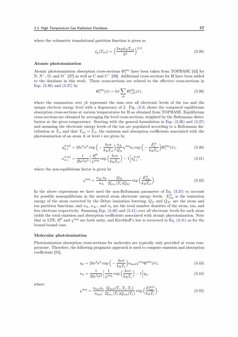
3.3. High Temperature Gas Radiation Database 57
where the volumetric translational partition function is given as
ξµ(Trel) =(2πµkBTrel
h2
)3/2. (3.38)
Atomic photoionization
Atomic photoionization absorption cross-sections Sabsi have been taken from TOPBASE [42] for
N, N+, O, and O+ [37] as well as C and C+ [39]. Additional cross-sections for H have been addedto the database in this work. These cross-sections are related to the effective cross-sections inEqs. (3.36) and (3.37) by
Sabsi (σ) = hσ
∑
jk
Sabsi,jk(σ), (3.39)
where the summation over jk represents the sum over all electronic levels of the ion and theunique electron energy level with a degeneracy of 2. Fig. (3.3) shows the computed equilibriumabsorption cross-sections at various temperatures for H as obtained from TOPBASE. Equilibriumcross-sections are obtained by averaging the level cross-sections, weighted by the Boltzmann distri-bution at the given temperature. Starting with the general formulation in Eqs. (3.36) and (3.37)and assuming the electronic energy levels of the ion are populated according to a Boltzmann dis-tribution at Tel and that Trel = Tel, the emission and absorption coefficients associated with thephotoionization of an atom A at level i are given by
ηA,bfσ,i = 2hc2σ3 exp
(
−hcσ
kBTel
) nA
QAχneqai exp
(
−EA
i
kBTel
)
Sabsi (σ), (3.40)
κA,bfσ,i =
1
2hc2σ3
[ θBiχneq exp
( hcσ
kBTel
)
− 1]
ηA,bfσ,i , (3.41)
where the non-equilibrium factor is given by
χneq =nA+ne
nA
QA
2ξme(Te)QA+
exp( EA
ion
kBTel
)
. (3.42)
In the above expressions we have used the non-Boltzmann parameter of Eq. (3.25) to accountfor possible nonequilibrium in the neutral atom electronic energy levels. EA
ion is the ionizationenergy of the atom corrected by the Debye ionization lowering, QA and QA+ are the atom andion partition functions, and nA, nA+ , and ne are the total number densities of the atom, ion, andfree electrons respectively. Summing Eqs. (3.40) and (3.41) over all electronic levels for each atomyields the total emission and absorption coefficients associated with atomic photoionization. Notethat in LTE, θBi and χneq are both unity, and Kirchhoff’s law is recovered in Eq. (3.41) as for thebound-bound case.
Molecular photoionization
Photoionization absorption cross-sections for molecules are typically only provided at room tem-perature. Therefore, the following pragmatic approach is used to compute emission and absorptioncoefficients [55],
ησ = 2hc2σ3 exp(
−hcσ
kBTe
)
nmolχneqSabs(σ), (3.43)
κσ =1
2hc2σ3
[ 1
χneq exp( hcσ
kBTe
)
− 1]
ησ, (3.44)
where
χneq =nionne
nmol
Qmol(Te, Te, Te)
2ξme(Te)Qion(Te)exp
(Emolion
kBTe
)
. (3.45)
58 Chapter 3. Radiative Transfer for Atmospheric Entry
The database includes appropriate molecular photoionization absorption cross-sections for C2, CN,CO, N2, NO, and O2 [37, 39]. The cross-sections for N2, NO, and O2 actually correspond to globalabsorption cross-sections, including dissociative photoionization, however these contributions areat least an order of magnitude less than photoionization [37] and are therefore treated as purephotoionization in this work. In addition, photoionization of CH and H2 have been added in thiswork using absorption cross-sections taken from [140] and [144, 156], respectively, and are plottedin Fig. (3.3). The sharp drop-offs in the CH and H2 cross-sections correspond to the ionizationenergy of those molecules. For example, the ionization energy of H2 is approximately 15.6 eV orabout 126 000cm−1. Therefore, only photons with at least that much energy can ionize H2.
An example hydrogen absorption spectrum is shown in Fig. (3.4) for a pure hydrogen plasma inLTE, at a temperature and pressure of 6000K and 0.3 bar respectively. Under these conditions, H2accounts for just 0.1% of the mixture by volume, however the Lyman and Werner bands dominatethe absorption spectrum. Photoionization of H2 is the dominate contribution to the absorptionspectrum for wavenumbers above the ionization energy.
0 5 10 15 20 25 3010-4
10-3
10-2
10-1
100
101
102
Photon energy, eV
Pho
toio
niza
tion
cros
sse
ctio
ns,M
b
CH
H2
H, 10 000K
H, 15 000K
H, 20 000K
Figure 3.3.: Equilibrium photoionization absorption cross-sections of CH, H, and H2, used in thiswork. Data for each species has been taken from [140], [42], and [144, 156], respectively.
Other bound-free mechanisms
The HTGR databse includes photodetachment of the C– , N– , and O– anions [37, 39]. In general,these processes are not well understood. The database relies on simple absorption cross-sectionsrelated to the most dominate contributions to the photodetachment of each species. Typically,these species are not included in CFD calculations for atmospheric entry flows. In this case, thepopulations of the negative ions are computed assuming a Saha equilibrium at Te.
Schumann-Runge photodissociation of O2 is also considered, using LTE absorption cross-sectionscompiled in [37]. The extension to a MT approach is presented by Lamet et al. [43].
3.4. The Hybrid Statistical Narrow Band Model 59
0 50000 100000 150000 20000010-8
10-7
10-6
10-5
10-4
10-3
10-2
10-1
100
101
102
Wavenumber, cm−1
Abs
orpt
ion
Coe
ffici
ent,cm
−1 H
H
H2 (Lyman, Werner)
H2 photoionization
Hphotoion.
Figure 3.4.: LTE hydrogen absorption spectrum at T = 6000K and p = 0.3 bar.
3.3.3. Free-Free Processes
Free-free transitions, known as Bremsstrahlung radiation, occur when an electron emits a photonafter passing through the electric field of a neutral or ionic species. Bremsstrahlung radiation ofthe atomic ions C+, N+, and O+ is considered using Kramers’ formula [157] corrected by a Gauntfactor [37, 39]. Inverse Bremsstrahlung radiation of C [39], and N, O, N2, and O2 [37] is alsoincluded through estimated absorption cross-sections obtained from the literature.
3.4. The Hybrid Statistical Narrow Band Model
It is evident from the previous sections that the accurate solution of the radiant intensity fieldrequires a massive computational undertaking. To solidify this fact, recall that the RTE mustbe integrated along lines of sight passing through each point in the flow field, in every direction,and at every wavenumber. The emission and absorption coefficients, required to solve the RTE,are dependent on the local energy level populations of each species which may change rapidlythroughout the flow field, thanks to the strong thermochemical nonequilibrium that is characteristicof hypersonic flows. In addition, because of the quantized nature of bound-bound transitions, theemission and absorption coefficients have strong spectral variations, requiring millions of spectralpoints to accurately resolve the spectral intensity for typical atmospheric entry problems. Thecomputational complexity is further increased when coupled solutions are needed, as a new intensityfield is required for each update of the radiative source terms.
In this section, the HSNB model is described which significantly reduces the computational com-plexity of computing the radiative intensity by decreasing spectral detail of the resulting solution.To begin, we recall that contributions of each radiative mechanism to the spectral emission andabsorption coefficients are additive, allowing Eq. (3.3) to be rewritten as
Iσ(s) = Iσ(0)∏
k∈R
τkσ (0, s) +∑
k∈R
∫ s
0ηkσ(s
′)∏
k′∈R
τk′
σ (s′, s) ds′, (3.46)
60 Chapter 3. Radiative Transfer for Atmospheric Entry
where R is the set of all considered radiative mechanisms (atomic lines, molecular systems, and con-tinuum processes) and the superscripts k and k′ represent contributions to the emission coefficientand transmissivities of an individual radiative mechanism.
Using X∆σ
to denote the band-averaged quantity
X∆σ ≡
1
∆σ
∫ σ2
σ1
X dσ, (3.47)
for a spectral narrow-band ∆σ, ranging from σ1 to σ2, integration of Eq. (3.46) over a narrow-bandyields
Iσ(s)∆σ
= Iσ(0)∆σ ∏
k∈R
τkσ (0, s)∆σ
+∑
k∈R
Ikσ(s)∆σ
, (3.48)
where the band-averaged intensity associated with contribution k is given as
Ikσ(s)∆σ
=
∫ s
0ηkσ(s
′)τkσ (s′, s)
∆σ ∏
k′∈Rk′ =k
τk′
σ (s′, s)∆σ
ds′. (3.49)
The following assumptions have been made to arrive at Eqs. (3.48) and (3.49):
1. absorption is statistically uncorrelated from the band-averaged boundary intensity over anarrow-band, and
2. only self absorption is correlated with emission for a narrow-band.
The first assumption is generally valid because only highly emissive boundaries are considered inthis work, and thus
Iσ(0)∆σ
≈ ϵ∆σ Ibσ(Twall)∆σ
. (3.50)
The second assumption is more subtle, but is likely valid as there are no physical reasons for theabsorption of one mechanism to be significantly correlated to the emission of another.
Lamet et al. [55] have proposed to separate the set of radiative mechanisms into three groups: 1)optically thick molecular systems, 2) optically thin molecular systems and continua, and 3) atomiclines. The band-averaged quantities required in Eq. (3.48) can then be computed using a specificmodel, depending on which of the three groups the contribution belongs. This allows the totalintensity to be split according to
Iσ∆σ
= Iboundσ
∆σ+ Ithick
σ
∆σ+ Ibox
σ
∆σ+ Iat
σ∆σ
, (3.51)
where Iboundσ
∆σ, Ithick
σ
∆σ, Ibox
σ
∆σ, and Iat
σ∆σ
correspond to the band-averaged intensities fromthe boundaries and the three groups listed above, respectively. Optically thick systems are treatedusing a statistical narrow band approach, detailed in Section 3.4.1, while thin systems and continuaare treated with a simple box model presented in Section 3.4.2. Due to the relatively small numberof lines associated with electronic transitions of atoms, atomic lines are treated using a full line-by-line (LBL) approach, discussed in Section 3.4.3. When the groups are coupled together, theresulting method is called the Hybrid Statistical Narrow Band model [55].
3.4.1. Optically Thick Molecular Systems
The molecular systems presented in Section 3.3 are considered thick if the optical depth of thesystem maxσ(κkσl) is greater than 0.1 for a homogeneous slab of pure gas in thermal equilibriumat T = 8000K, p = 2atm, and l = 10 cm. This criterion represents a conservative estimate fortypical atmospheric entry conditions.
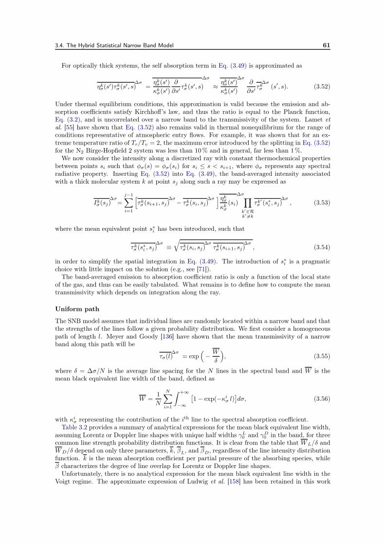
3.4. The Hybrid Statistical Narrow Band Model 61
For optically thick systems, the self absorption term in Eq. (3.49) is approximated as
ηkσ(s′)τkσ (s′, s)∆σ
=ηkσ(s′)
κkσ(s′)
∂
∂s′τkσ (s′, s)
∆σ
≈ηkσ(s′)
κkσ(s′)
∆σ∂
∂s′τkσ
∆σ(s′, s). (3.52)
Under thermal equilibrium conditions, this approximation is valid because the emission and ab-sorption coefficients satisfy Kirchhoff’s law, and thus the ratio is equal to the Planck function,Eq. (3.2), and is uncorrelated over a narrow band to the transmissivity of the system. Lamet etal. [55] have shown that Eq. (3.52) also remains valid in thermal nonequilibrium for the range ofconditions representative of atmospheric entry flows. For example, it was shown that for an ex-treme temperature ratio of Tr/Tv = 2, the maximum error introduced by the splitting in Eq. (3.52)for the N2 Birge-Hopfield 2 system was less than 10% and in general, far less than 1%.
We now consider the intensity along a discretized ray with constant thermochemical propertiesbetween points si such that φσ(s) = φσ(si) for si ≤ s < si+1, where φσ represents any spectralradiative property. Inserting Eq. (3.52) into Eq. (3.49), the band-averaged intensity associatedwith a thick molecular system k at point sj along such a ray may be expressed as
Ikσ(sj)∆σ
=j−1∑
i=1
[
τkσ (si+1, sj)∆σ
− τkσ (si, sj)∆σ] ηkσκkσ
(si)
∆σ∏
k′∈Rk′ =k
τk′
σ (s∗i , sj)∆σ
, (3.53)
where the mean equivalent point s∗i has been introduced, such that
τkσ (s∗i , sj)
∆σ≡√
τkσ (si, sj)∆σ
τkσ (si+1, sj)∆σ
, (3.54)
in order to simplify the spatial integration in Eq. (3.49). The introduction of s∗i is a pragmaticchoice with little impact on the solution (e.g., see [71]).
The band-averaged emission to absorption coefficient ratio is only a function of the local stateof the gas, and thus can be easily tabulated. What remains is to define how to compute the meantransmissivity which depends on integration along the ray.
Uniform path
The SNB model assumes that individual lines are randomly located within a narrow band and thatthe strengths of the lines follow a given probability distribution. We first consider a homogeneouspath of length l. Meyer and Goody [136] have shown that the mean transmissivity of a narrowband along this path will be
τσ(l)∆σ
= exp(
−W
δ
)
, (3.55)
where δ = ∆σ/N is the average line spacing for the N lines in the spectral band and W is themean black equivalent line width of the band, defined as
W =1
N
N∑
i=1
∫ +∞
−∞
[
1− exp(−κiσ l)]
dσ, (3.56)
with κiσ representing the contribution of the ith line to the spectral absorption coefficient.Table 3.2 provides a summary of analytical expressions for the mean black equivalent line width,
assuming Lorentz or Doppler line shapes with unique half widths γL0 and γD0 in the band, for threecommon line strength probability distribution functions. It is clear from the table that WL/δ andWD/δ depend on only three parameters, k, βL, and βD, regardless of the line intensity distributionfunction. k is the mean absorption coefficient per partial pressure of the absorbing species, whileβ characterizes the degree of line overlap for Lorentz or Doppler line shapes.
Unfortunately, there is no analytical expression for the mean black equivalent line width in theVoigt regime. The approximate expression of Ludwig et al. [158] has been retained in this work
62
Chap
ter3.Rad
iative
Tra
nsf
erfo
rAtm
osp
her
icEntr
y
Table 3.2.: Summary of analytical relationships for mean black equivalent line widths for a uniform path of length l, corresponding to differentprobability distribution functions P (S) of line strength S. k is the mean absorption coefficient per partial pressure pa of species a.
P (S) k Lorentz profile Doppler profile
βL WL/δ βD WD/δ
Uniformδ(S − S0) S0
δγL0
δ2πβLL
! palk
2πβL
"a γD0
δ
#
πln 2
βDD!palk
βD
"b
Goody exponential1S0
exp!
−SS0
" S0
δγL0
δpalk
$
1 + palk
4βL
γD0
δ
#
πln 2
βDE!palk
βD
"c
Malkmus tail inverse-exponential
exp%
− SSm
&
− exp%
− RSSm
&
S lnR
Sm
δ lnRπγL
0
δ lnR 2βL
!
'
1 +palk
βL
− 1"
γD0
δ lnR
#
πln 2
βDH!palk
βD
"d
aL(x) = xe−x[I0(x) + I1(x)]bD(x) = 1√
π
(∞−∞[1− exp(−xe−ξ2)]dξ
cE(x) = 1√π
(∞−∞
xe−ξ2
1+xe−ξ2dξ
dH(x) = 1√π
(∞−∞ ln(1 + xe−ξ2)dξ
3.4. The Hybrid Statistical Narrow Band Model 63
for computing the Voigt width as
WV
δ= palk
√
1− Ω−1/2,
Ω =
[
1−(
1
palk
WD
δ
)2]−2
+
[
1−(
1
palk
WL
δ
)2]−2
− 1.
(3.57)
The Ludwig formula has the advantage that the correct solution is obtained in a pure Lorentzianor Doppler regime.
Non-uniform path
Both the classical Curtis-Godson and Lindquist-Simmons approaches [159] are considered for com-puting W/δ along a non-uniform path. The Curtis-Godson method assumes that non-uniformpaths may be treated the same as a uniform path, using path-averaged properties. The pressurepath length u, mean absorption coefficient k
∗per partial pressure pa of the absorbing species, and
mean overlap parameter β∗
are defined as
u =
∫ s
s′pa(s
′′)ds′′, (3.58)
k∗=
1
u
∫ s
s′pa(s
′′)k(s′′)ds′′, (3.59)
β∗=
1
uk∗
∫ s
s′pa(s
′′)k(s′′)β(s′′)ds′′. (3.60)
The expressions given in Table 3.2 and Eq. (3.57) can then be reused along a non-homogeneouspath by replacing pal with u, k with k
∗, and βL,D with β
∗
L,D. The resulting expressions for theLorentz and Doppler mean black equivalent line widths are given in Table 3.3 for the line strengthdistributions of interest in this work and Eq. (3.57) is updated accordingly,
WV
δ= uk
∗√
1− Ω−1/2,
Ω =
[
1−(
1
uk∗
WD
δ
)2]−2
+
[
1−(
1
uk∗
WL
δ
)2]−2
− 1.
(3.61)
The Lindquist-Simmons approach consists in finding a suitable expression for the local spa-tial derivative of the mean black equivalent width in the Lorentz and Doppler regimes and thencomputing W/δ through numerical integration,
W
δ(s′, s) = −
∫ s
s′
1
δ
∂
∂s′′W (s′′, s)ds′′, (3.62)
where the derivative ∂W/∂s′′ is a function of both local and averaged parameters. Table 3.3provides the expressions necessary to compute the mean black equivalent width derivatives for bothLorentz and Doppler regimes [160]. The Voigt mean black equivalent widths are then obtainedusing Eq. (3.61) as in the Curtis-Godson approximation.
3.4.2. Optically Thin Molecular Systems and Continua
The band-averaged intensity associated with optically thin systems and continua may be expressedas
Ikσ(sj)∆σ
=j−1∑
i=1
ηkσ(si)∆σ ∏
k′∈R
τk′
σ (s∗i , sj)∆σ
, (3.63)
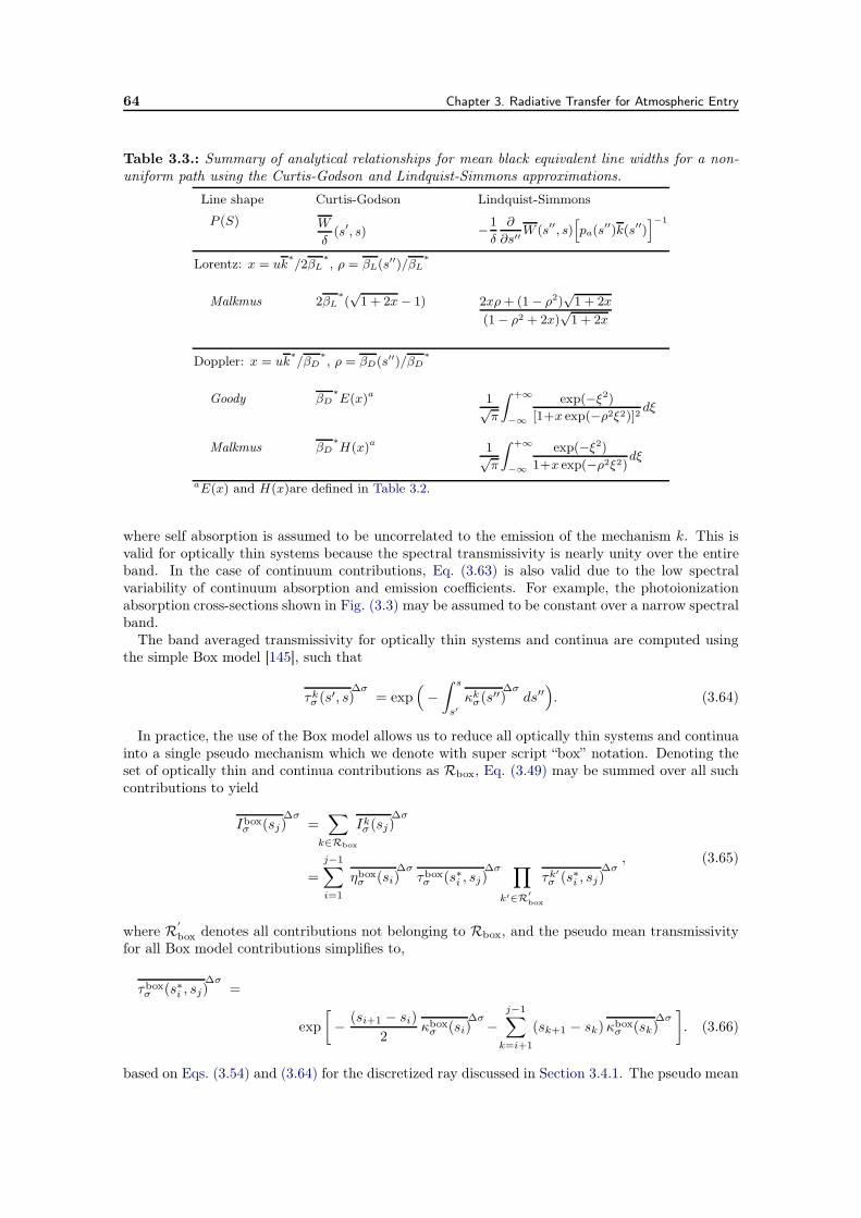
64 Chapter 3. Radiative Transfer for Atmospheric Entry
Table 3.3.: Summary of analytical relationships for mean black equivalent line widths for a non-uniform path using the Curtis-Godson and Lindquist-Simmons approximations.
Line shape Curtis-Godson Lindquist-Simmons
P (S) Wδ(s′, s) −
1δ
∂∂s′′
W (s′′, s))
pa(s′′)k(s′′)
*−1
Lorentz: x = uk∗/2βL
∗, ρ = βL(s
′′)/βL∗
Malkmus 2βL∗(√1 + 2x− 1) 2xρ+ (1− ρ2)
√1 + 2x
(1− ρ2 + 2x)√1 + 2x
Doppler: x = uk∗/βD
∗, ρ = βD(s′′)/βD
∗
Goody βD∗E(x)a 1√
π
+ +∞
−∞
exp(−ξ2)[1+x exp(−ρ2ξ2)]2
dξ
Malkmus βD∗H(x)a 1√
π
+ +∞
−∞
exp(−ξ2)
1+x exp(−ρ2ξ2)dξ
aE(x) and H(x)are defined in Table 3.2.
where self absorption is assumed to be uncorrelated to the emission of the mechanism k. This isvalid for optically thin systems because the spectral transmissivity is nearly unity over the entireband. In the case of continuum contributions, Eq. (3.63) is also valid due to the low spectralvariability of continuum absorption and emission coefficients. For example, the photoionizationabsorption cross-sections shown in Fig. (3.3) may be assumed to be constant over a narrow spectralband.
The band averaged transmissivity for optically thin systems and continua are computed usingthe simple Box model [145], such that
τkσ (s′, s)
∆σ= exp
(
−∫ s
s′κkσ(s
′′)∆σ
ds′′)
. (3.64)
In practice, the use of the Box model allows us to reduce all optically thin systems and continuainto a single pseudo mechanism which we denote with super script “box” notation. Denoting theset of optically thin and continua contributions as Rbox, Eq. (3.49) may be summed over all suchcontributions to yield
Iboxσ (sj)
∆σ=∑
k∈Rbox
Ikσ(sj)∆σ
=j−1∑
i=1
ηboxσ (si)
∆στboxσ (s∗i , sj)
∆σ ∏
k′∈R′
box
τk′
σ (s∗i , sj)∆σ
, (3.65)
where R′
box denotes all contributions not belonging to Rbox, and the pseudo mean transmissivityfor all Box model contributions simplifies to,
τboxσ (s∗i , sj)
∆σ=
exp
[
−(si+1 − si)
2κboxσ (si)
∆σ−
j−1∑
k=i+1
(sk+1 − sk)κboxσ (sk)
∆σ]
. (3.66)
based on Eqs. (3.54) and (3.64) for the discretized ray discussed in Section 3.4.1. The pseudo mean
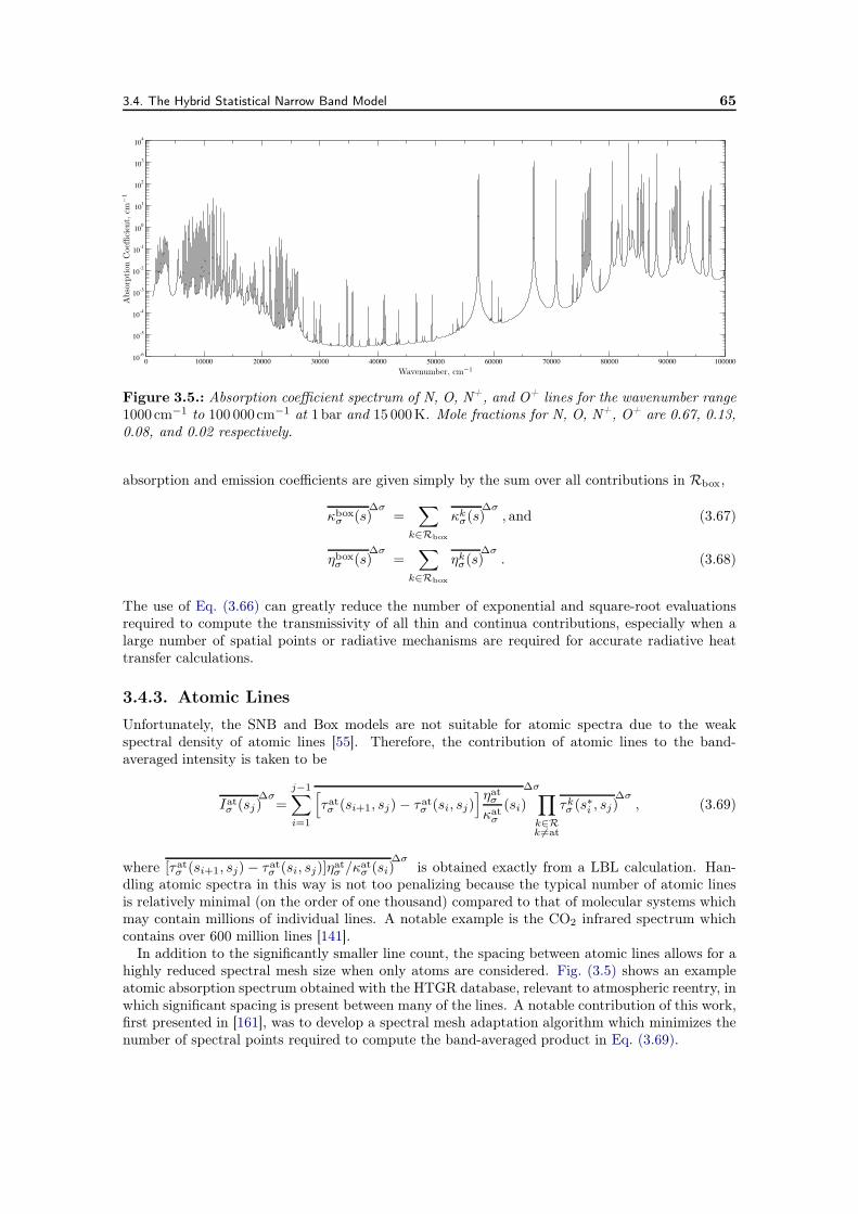
3.4. The Hybrid Statistical Narrow Band Model 65
0 10000 20000 30000 40000 50000 60000 70000 80000 90000 10000010-6
10-5
10-4
10-3
10-2
10-1
100
101
102
103
104
Wavenumber, cm−1
Abs
orpt
ion
Coe
ffici
ent,cm
−1
Figure 3.5.: Absorption coefficient spectrum of N, O, N+, and O+ lines for the wavenumber range1000 cm−1 to 100 000cm−1 at 1 bar and 15 000K. Mole fractions for N, O, N+, O+ are 0.67, 0.13,0.08, and 0.02 respectively.
absorption and emission coefficients are given simply by the sum over all contributions in Rbox,
κboxσ (s)
∆σ=
∑
k∈Rbox
κkσ(s)∆σ
, and (3.67)
ηboxσ (s)
∆σ=
∑
k∈Rbox
ηkσ(s)∆σ
. (3.68)
The use of Eq. (3.66) can greatly reduce the number of exponential and square-root evaluationsrequired to compute the transmissivity of all thin and continua contributions, especially when alarge number of spatial points or radiative mechanisms are required for accurate radiative heattransfer calculations.
3.4.3. Atomic Lines
Unfortunately, the SNB and Box models are not suitable for atomic spectra due to the weakspectral density of atomic lines [55]. Therefore, the contribution of atomic lines to the band-averaged intensity is taken to be
Iatσ (sj)
∆σ=
j−1∑
i=1
[
τatσ (si+1, sj)− τat
σ (si, sj)]ηat
σ
κatσ
(si)
∆σ∏
k∈Rk =at
τkσ (s∗i , sj)
∆σ, (3.69)
where [τatσ (si+1, sj)− τat
σ (si, sj)]ηatσ /κat
σ (si)∆σ
is obtained exactly from a LBL calculation. Han-dling atomic spectra in this way is not too penalizing because the typical number of atomic linesis relatively minimal (on the order of one thousand) compared to that of molecular systems whichmay contain millions of individual lines. A notable example is the CO2 infrared spectrum whichcontains over 600 million lines [141].
In addition to the significantly smaller line count, the spacing between atomic lines allows for ahighly reduced spectral mesh size when only atoms are considered. Fig. (3.5) shows an exampleatomic absorption spectrum obtained with the HTGR database, relevant to atmospheric reentry, inwhich significant spacing is present between many of the lines. A notable contribution of this work,first presented in [161], was to develop a spectral mesh adaptation algorithm which minimizes thenumber of spectral points required to compute the band-averaged product in Eq. (3.69).
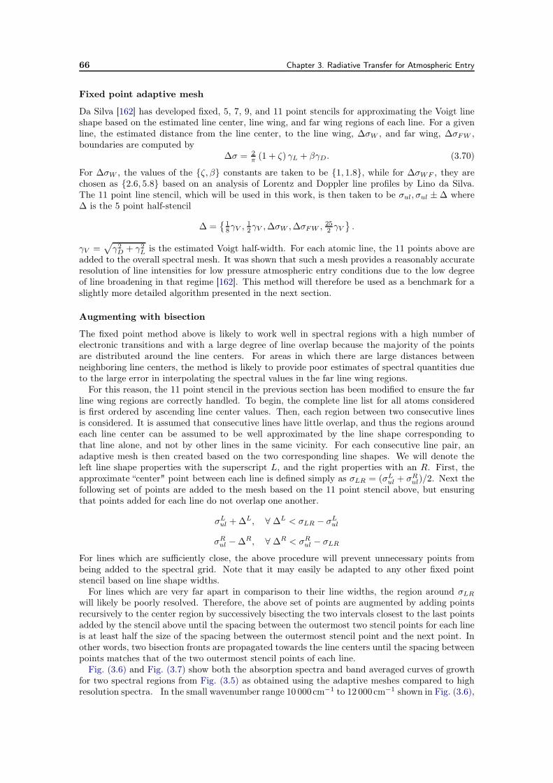
66 Chapter 3. Radiative Transfer for Atmospheric Entry
Fixed point adaptive mesh
Da Silva [162] has developed fixed, 5, 7, 9, and 11 point stencils for approximating the Voigt lineshape based on the estimated line center, line wing, and far wing regions of each line. For a givenline, the estimated distance from the line center, to the line wing, ∆σW , and far wing, ∆σFW ,boundaries are computed by
∆σ = 2π (1 + ζ) γL + βγD. (3.70)
For ∆σW , the values of the ζ,β constants are taken to be 1, 1.8, while for ∆σWF , they arechosen as 2.6, 5.8 based on an analysis of Lorentz and Doppler line profiles by Lino da Silva.The 11 point line stencil, which will be used in this work, is then taken to be σul,σul ±∆ where∆ is the 5 point half-stencil
∆ =
18γV ,
12γV ,∆σW ,∆σFW , 25
2 γV
.
γV =√
γ2D + γ2L is the estimated Voigt half-width. For each atomic line, the 11 points above areadded to the overall spectral mesh. It was shown that such a mesh provides a reasonably accurateresolution of line intensities for low pressure atmospheric entry conditions due to the low degreeof line broadening in that regime [162]. This method will therefore be used as a benchmark for aslightly more detailed algorithm presented in the next section.
Augmenting with bisection
The fixed point method above is likely to work well in spectral regions with a high number ofelectronic transitions and with a large degree of line overlap because the majority of the pointsare distributed around the line centers. For areas in which there are large distances betweenneighboring line centers, the method is likely to provide poor estimates of spectral quantities dueto the large error in interpolating the spectral values in the far line wing regions.
For this reason, the 11 point stencil in the previous section has been modified to ensure the farline wing regions are correctly handled. To begin, the complete line list for all atoms consideredis first ordered by ascending line center values. Then, each region between two consecutive linesis considered. It is assumed that consecutive lines have little overlap, and thus the regions aroundeach line center can be assumed to be well approximated by the line shape corresponding tothat line alone, and not by other lines in the same vicinity. For each consecutive line pair, anadaptive mesh is then created based on the two corresponding line shapes. We will denote theleft line shape properties with the superscript L, and the right properties with an R. First, theapproximate “center" point between each line is defined simply as σLR = (σL
ul + σRul)/2. Next the
following set of points are added to the mesh based on the 11 point stencil above, but ensuringthat points added for each line do not overlap one another.
σLul +∆L, ∀ ∆L < σLR − σL
ul
σRul −∆R, ∀ ∆R < σR
ul − σLR
For lines which are sufficiently close, the above procedure will prevent unnecessary points frombeing added to the spectral grid. Note that it may easily be adapted to any other fixed pointstencil based on line shape widths.
For lines which are very far apart in comparison to their line widths, the region around σLR
will likely be poorly resolved. Therefore, the above set of points are augmented by adding pointsrecursively to the center region by successively bisecting the two intervals closest to the last pointsadded by the stencil above until the spacing between the outermost two stencil points for each lineis at least half the size of the spacing between the outermost stencil point and the next point. Inother words, two bisection fronts are propagated towards the line centers until the spacing betweenpoints matches that of the two outermost stencil points of each line.
Fig. (3.6) and Fig. (3.7) show both the absorption spectra and band averaged curves of growthfor two spectral regions from Fig. (3.5) as obtained using the adaptive meshes compared to highresolution spectra. In the small wavenumber range 10 000cm−1 to 12 000cm−1 shown in Fig. (3.6),
3.4. The Hybrid Statistical Narrow Band Model 67
10000 10500 11000 11500 1200010-4
10-3
10-2
10-1
100
101
102
Hi-Res11 PointBisect
Wavenumber, cm−1
Abs
orpt
ion
Coe
ffici
ent,cm
−1
(a) Absorption coefficients.
10-4 10-3 10-2 10-1 100 10110-5
10-4
10-3
10-2
10-1
100
Hi-Res11 PointBisect
l, cm
−lnτ
at σ∆σ(l)
10,000 - 11,000 cm−1
11,000 - 12,000 cm−1
(b) Curves of growth.
Figure 3.6.: Atomic absorption coefficients and curves of growth using adaptive spectral grids,compared to a high-resolution mesh, for the spectral range 10 000cm−1 to 12 000cm−1. Sameconditions as in Fig. (3.5).
75000 75500 76000 76500 7700010-3
10-2
10-1
100
101
102
103
Hi-Res11 PointBisect
Wavenumber, cm−1
Abs
orpt
ion
Coe
ffici
ent,cm
−1
(a) Absorption coefficients.
10-4 10-3 10-2 10-1 100 10110-4
10-3
10-2
10-1
100
101
Hi-Res11 PointBisect
l, cm
−lnτ
at σ∆σ(l)
75,000 - 76,000 cm−1
76,000 - 77,000 cm−1
(b) Curves of growth.
Figure 3.7.: Atomic absorption coefficients and curves of growth using adaptive spectral grids,compared to a high-resolution mesh, for the spectral range 75 000cm−1 to 77 000cm−1. Sameconditions as in Fig. (3.5).
both adaptive methods work well. This is largely due to the fact that there are many spectrallines close to one another, and while some of them are very weak, they still contribute grid pointsin the wing regions of stronger lines. The differences become much more apparent in the largerwavenumber range 75 000cm−1 to 77 000cm−1 as in Fig. (3.7). Here, the atomic lines are farenough apart such that the 11 point stencil is not wide enough to encompass the far wing regionsof some lines. Therefore, large interpolation errors are clearly visible in the absorption spectrumusing only these points, while the points augmented with the bisection algorithm represent thetrue spectrum well. The affect this interpolation error has on the computed curves of growth isalso clearly visible, with a significant error shown even at a column length of 1mm for both bandregions.
Conditions for line width calculations
A careful reader will note that the conditions for calculating the line widths in the previous sub-sections were not specified. In general, the spectral mesh should remain constant for all points inthe flow field in order to integrate along each ray. However, the above mesh adaptation scheme
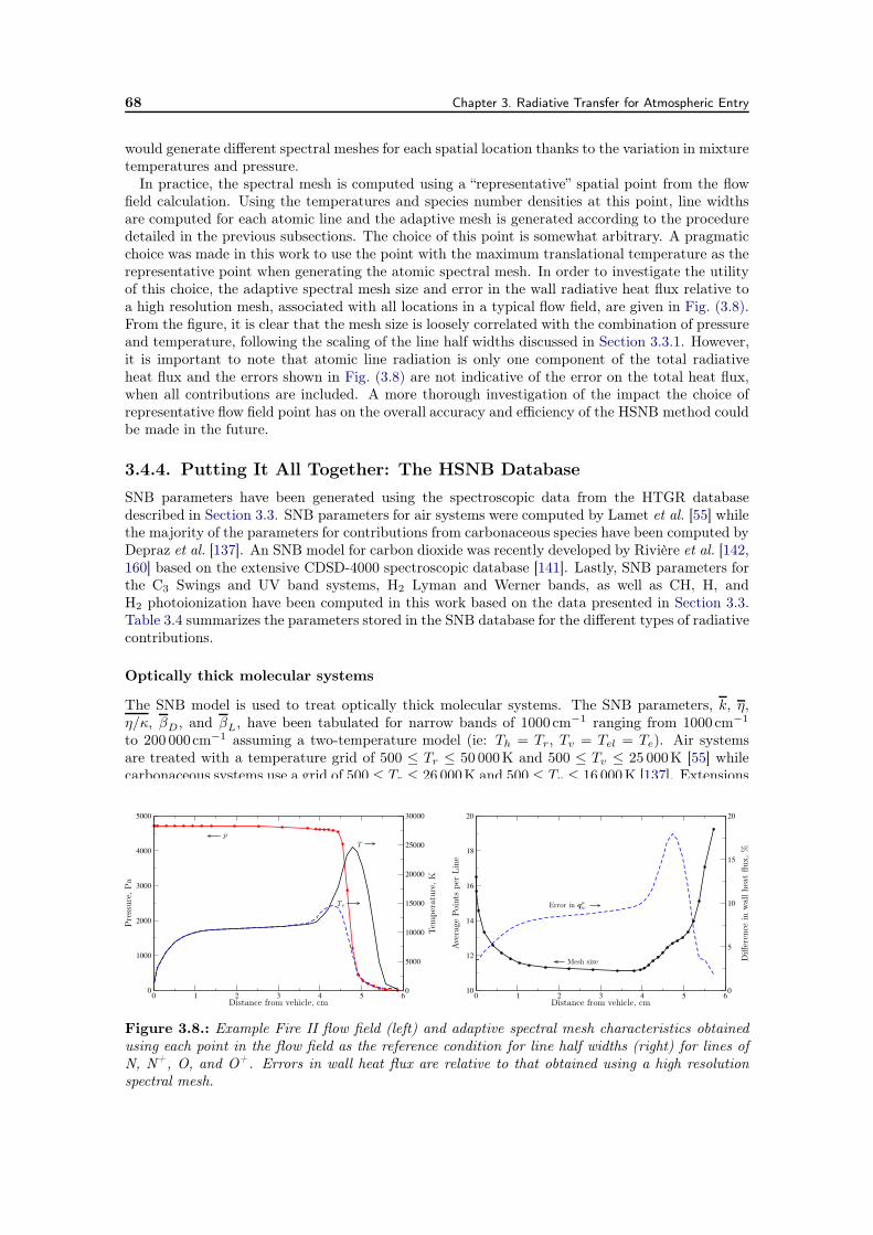
68 Chapter 3. Radiative Transfer for Atmospheric Entry
would generate different spectral meshes for each spatial location thanks to the variation in mixturetemperatures and pressure.
In practice, the spectral mesh is computed using a “representative” spatial point from the flowfield calculation. Using the temperatures and species number densities at this point, line widthsare computed for each atomic line and the adaptive mesh is generated according to the proceduredetailed in the previous subsections. The choice of this point is somewhat arbitrary. A pragmaticchoice was made in this work to use the point with the maximum translational temperature as therepresentative point when generating the atomic spectral mesh. In order to investigate the utilityof this choice, the adaptive spectral mesh size and error in the wall radiative heat flux relative toa high resolution mesh, associated with all locations in a typical flow field, are given in Fig. (3.8).From the figure, it is clear that the mesh size is loosely correlated with the combination of pressureand temperature, following the scaling of the line half widths discussed in Section 3.3.1. However,it is important to note that atomic line radiation is only one component of the total radiativeheat flux and the errors shown in Fig. (3.8) are not indicative of the error on the total heat flux,when all contributions are included. A more thorough investigation of the impact the choice ofrepresentative flow field point has on the overall accuracy and efficiency of the HSNB method couldbe made in the future.
3.4.4. Putting It All Together: The HSNB Database
SNB parameters have been generated using the spectroscopic data from the HTGR databasedescribed in Section 3.3. SNB parameters for air systems were computed by Lamet et al. [55] whilethe majority of the parameters for contributions from carbonaceous species have been computed byDepraz et al. [137]. An SNB model for carbon dioxide was recently developed by Rivière et al. [142,160] based on the extensive CDSD-4000 spectroscopic database [141]. Lastly, SNB parameters forthe C3 Swings and UV band systems, H2 Lyman and Werner bands, as well as CH, H, andH2 photoionization have been computed in this work based on the data presented in Section 3.3.Table 3.4 summarizes the parameters stored in the SNB database for the different types of radiativecontributions.
Optically thick molecular systems
The SNB model is used to treat optically thick molecular systems. The SNB parameters, k, η,η/κ, βD, and βL, have been tabulated for narrow bands of 1000 cm−1 ranging from 1000 cm−1
to 200 000cm−1 assuming a two-temperature model (ie: Th = Tr, Tv = Tel = Te). Air systemsare treated with a temperature grid of 500 ≤ Tr ≤ 50 000K and 500 ≤ Tv ≤ 25 000K [55] whilecarbonaceous systems use a grid of 500 ≤ Tr ≤ 26 000K and 500 ≤ Tv ≤ 16 000K [137]. Extensions
65432100
1000
2000
3000
4000
5000
0
5000
10000
15000
20000
25000
30000
Distance from vehicle, cm
Pre
ssur
e,Pa
Tem
pera
ture
,K
pT
Tv
654321010
12
14
16
18
20
0
5
10
15
20
Distance from vehicle, cm
Ave
rage
Poi
nts
per
Lin
e
Diff
eren
cein
wal
lhea
tflu
x,%
Mesh size
Error in qrw
Figure 3.8.: Example Fire II flow field (left) and adaptive spectral mesh characteristics obtainedusing each point in the flow field as the reference condition for line half widths (right) for lines ofN, N+, O, and O+. Errors in wall heat flux are relative to that obtained using a high resolutionspectral mesh.
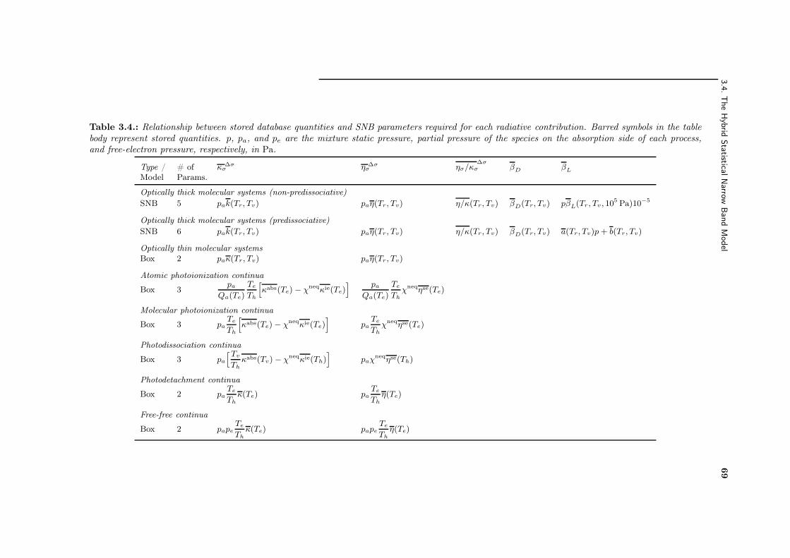
3.4
.T
he
Hyb
ridStatistical
Narrow
Ban
dM
odel
69
Table 3.4.: Relationship between stored database quantities and SNB parameters required for each radiative contribution. Barred symbols in the tablebody represent stored quantities. p, pa, and pe are the mixture static pressure, partial pressure of the species on the absorption side of each process,and free-electron pressure, respectively, in Pa.
Type / # of κσ∆σ ησ
∆σ ησ/κσ∆σ
βD βL
Model Params.
Optically thick molecular systems (non-predissociative)SNB 5 pak(Tr, Tv) paη(Tr, Tv) η/κ(Tr, Tv) βD(Tr, Tv) pβL(Tr, Tv, 10
5 Pa)10−5
Optically thick molecular systems (predissociative)SNB 6 pak(Tr, Tv) paη(Tr, Tv) η/κ(Tr, Tv) βD(Tr, Tv) a(Tr, Tv)p+ b(Tr, Tv)
Optically thin molecular systemsBox 2 paκ(Tr, Tv) paη(Tr, Tv)
Atomic photoionization continua
Box 3pa
Qa(Te)Te
Th
)
κabs(Te)− χneqκie(Te)* pa
Qa(Te)Te
Thχneqηse(Te)
Molecular photoionization continua
Box 3 paTe
Th
)
κabs(Te)− χneqκie(Te)*
paTe
Thχneqηse(Te)
Photodissociation continua
Box 3 pa)Tv
Thκabs(Tv)− χneqκie(Th)
*
paχneqηse(Th)
Photodetachment continua
Box 2 paTe
Thκ(Te) pa
Te
Thη(Te)
Free-free continua
Box 2 papeTe
Thκ(Te) pape
Te
Thη(Te)
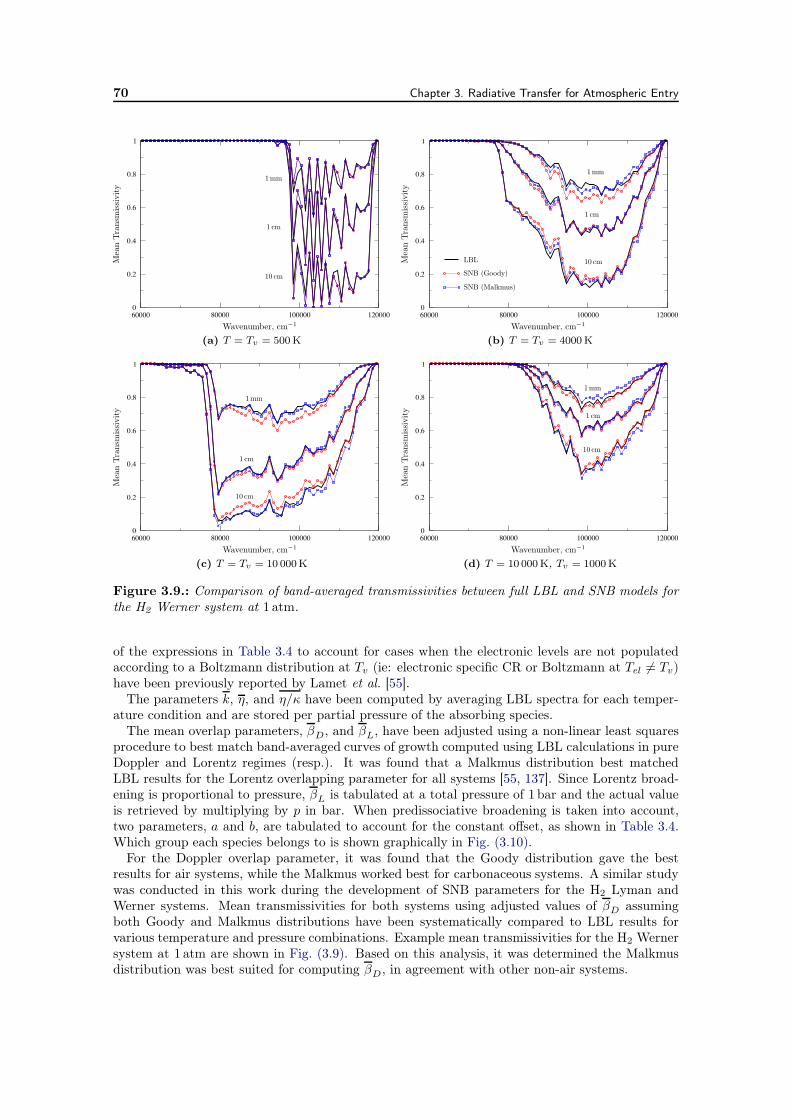
70 Chapter 3. Radiative Transfer for Atmospheric Entry
60000 80000 100000 1200000
0.2
0.4
0.6
0.8
1
Wavenumber, cm−1
Mea
nTra
nsm
issi
vity
1mm
1 cm
10 cm
(a) T = Tv = 500K
60000 80000 100000 1200000
0.2
0.4
0.6
0.8
1
Wavenumber, cm−1
Mea
nTra
nsm
issi
vity
1mm
1 cm
10 cmLBL
SNB (Goody)
SNB (Malkmus)
(b) T = Tv = 4000K
60000 80000 100000 1200000
0.2
0.4
0.6
0.8
1
Wavenumber, cm−1
Mea
nTra
nsm
issi
vity
1mm
1 cm
10 cm
(c) T = Tv = 10 000K
60000 80000 100000 1200000
0.2
0.4
0.6
0.8
1
Wavenumber, cm−1
Mea
nTra
nsm
issi
vity
1mm
1 cm
10 cm
(d) T = 10 000K, Tv = 1000K
Figure 3.9.: Comparison of band-averaged transmissivities between full LBL and SNB models forthe H2 Werner system at 1 atm.
of the expressions in Table 3.4 to account for cases when the electronic levels are not populatedaccording to a Boltzmann distribution at Tv (ie: electronic specific CR or Boltzmann at Tel = Tv)have been previously reported by Lamet et al. [55].
The parameters k, η, and η/κ have been computed by averaging LBL spectra for each temper-ature condition and are stored per partial pressure of the absorbing species.
The mean overlap parameters, βD, and βL, have been adjusted using a non-linear least squaresprocedure to best match band-averaged curves of growth computed using LBL calculations in pureDoppler and Lorentz regimes (resp.). It was found that a Malkmus distribution best matchedLBL results for the Lorentz overlapping parameter for all systems [55, 137]. Since Lorentz broad-ening is proportional to pressure, βL is tabulated at a total pressure of 1 bar and the actual valueis retrieved by multiplying by p in bar. When predissociative broadening is taken into account,two parameters, a and b, are tabulated to account for the constant offset, as shown in Table 3.4.Which group each species belongs to is shown graphically in Fig. (3.10).
For the Doppler overlap parameter, it was found that the Goody distribution gave the bestresults for air systems, while the Malkmus worked best for carbonaceous systems. A similar studywas conducted in this work during the development of SNB parameters for the H2 Lyman andWerner systems. Mean transmissivities for both systems using adjusted values of βD assumingboth Goody and Malkmus distributions have been systematically compared to LBL results forvarious temperature and pressure combinations. Example mean transmissivities for the H2 Wernersystem at 1 atm are shown in Fig. (3.9). Based on this analysis, it was determined the Malkmusdistribution was best suited for computing βD, in agreement with other non-air systems.
3.5. Concluding Remarks 71
Optically thin molecular systems
Optically thin molecular systems are treated using the Box model as shown in Section 3.4.2. Therequired averaged quantities, κ and η, have been tabulated using the same procedure as for thethick systems. Which systems are considered thick or thin is shown in Fig. (3.10).
Continua
Continua are also treated using the Box model. However, for each continuum process detailed inSections. (3.3.2) and (3.3.3), the band-averaged parameters are only functions of a single tempera-ture. Therefore, parameters for all continuum processes are tabulated using a single temperature.Nonequilibrium values can then be retrieved using the expressions in Table 3.4.
3.5. Concluding Remarks
In this chapter, the necessary ingredients for coupling radiation with the fluid conservation equa-tions have been detailed. In particular the radiative heat flux, power, and photochemical massproduction terms were given as integral functions of the radiant intensity field. The solution ofthe RTE for the intensity was also given, including appropriate boundary conditions typical ofatmospheric entry problems.
The various bound-bound, bound-free, and free-free radiative mechanisms which contribute tothe spectral emission and absorption coefficients of the gas have been summarized. These coeffi-cients are computed with the HTGR database which has also been summarized in this chapter.In particular, a focus was placed on the implementation of nonequilibrium spectral emission andabsorption coefficients for each type of radiative mechanism. The data required and their sourcesfor each mechanism have been carefully enumerated, including mechanisms added to the databasein this work. The new contributions include hydrogen lines, C3 Swings and UV systems, as wellas the photoionization of H, H2, and CH.
The HSNB model has been described in detail, which combines the statistical narrow band, box,and adaptive line-by-line models as an efficient and accurate alternative to the full line-by-linesolution of the intensity field. The narrow band parameters required for the model implementa-tion have been thoroughly presented for each radiative mechanism. SNB parameters have beencomputed in this work for the H2 Lyman and Werner systems, by adjusting the Doppler andLorentz overlap parameters to fit curves of growth for each narrow band. Comparisons with band-averaged transmissivities computed with the line-by-line approach show excellent agreement withthe resulting SNB parameters for these systems.
Lastly, a new adaptive mesh algorithm tailored to the spectra of atomic lines has also beenpresented in this work. The algorithm combines a simple fixed point stencil designed to accuratelycapture line centers with an adaptive bisection algorithm for the placement of spectral points inthe far line wing regions of atomic lines. The computational benefits of this method as comparedto conventional line-by-line approaches will be demonstrated in Chapter 7.
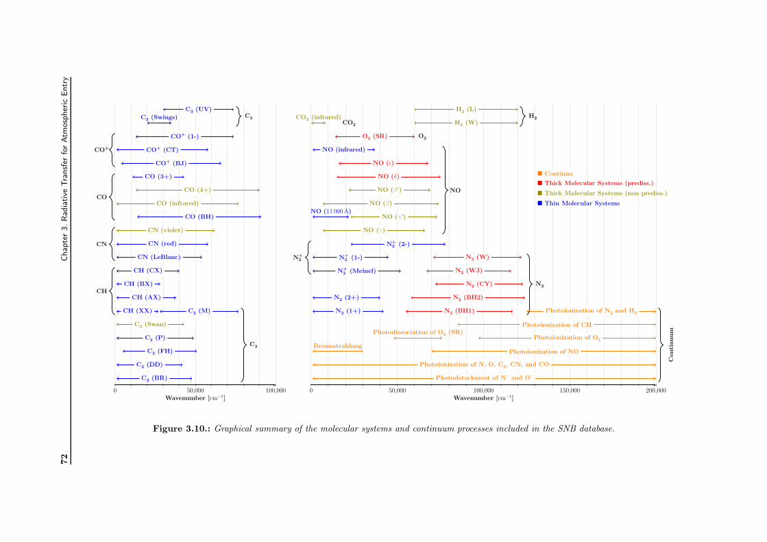
72
Chap
ter3.Rad
iative
Tra
nsf
erfo
rAtm
osp
her
icEntr
y
0 50,000 100,000
C2 (BR)
C2 (DD)
C2 (FH)
C2 (P)
C2 (Swan)
C2 (M)
C2
CH (XX)
CH (AX)
CH (BX)
CH (CX)
CH
CN (LeBlanc)
CN (red)
CN (violet)
CN
CO (BH)
CO (infrared)
CO (4+)
CO (3+)
CO
CO+ (BJ)
CO+ (CT)
CO+ (1-)
CO+
C3 (Swings)C3 (UV)
C3
Wavenumber [cm−1]0 50,000 100,000 150,000 200,000
Photodetachment of N– and O–
Photoionization of N, O, C2, CN, and CO
BremsstrahlungPhotoionization of NO
Photodissociation of O2 (SR)Photoionization of O2
Photoionization of CH
Photoionization of N2 and H2
Continuum
N2 (1+) N2 (BH1)
N2 (2+) N2 (BH2)
N2 (CY)
N2 (WJ)
N2 (W)
N2
N+2 (Meinel)
N+2 (1-)
N+2 (2-)
N+2
NO (γ)
NO (γ’)NO (11 000 A)
NO (β)
NO (β’)
NO (δ)
NO (ϵ)
NO (infrared)
NO
O2 (SR) O2
H2 (W)
H2 (L)H2CO2 (infrared)
CO2
! Continua
! Thick Molecular Systems (prediss.)
! Thick Molecular Systems (non prediss.)
! Thin Molecular Systems
Wavenumber [cm−1]
Figure 3.10.: Graphical summary of the molecular systems and continuum processes included in the SNB database.

CHAPTER 4
Development of Mutation++
“The best computer is a man, and it’s the only one that can be mass-produced by unskilledlabor."
— Wernher von Braun
4.1. Introduction
As was shown in Chapter 2, several different thermochemical models can be used for hypersonicflows depending on the problem of interest and the level of fidelity required in the solution. Thethermochemical model used has a direct effect on the evaluation of physicochemical propertiesnecessary to solve the governing equations. These include thermodynamic and transport properties,chemical production rates, and energy transfer rates. The evaluation of each of these propertiesfurther depends on the selection of a variety of specialized algorithms and physicochemical dataincluding species partition functions, transport collision integrals, and reaction rate coefficients.The implementation, testing, and maintenance of all of the physicochemical models, algorithms,and data required to simulate hypersonic flows represent a significant cost in terms of humanresources and time necessary to develop a hypersonic CFD tool. Furthermore, as newer models,algorithms, or data become available, a significant amount of work is typically needed to updateexisting CFD codes when the thermochemical model is embedded directly in the code.
These observations have led to the desire to reduce the work necessary to implement new modelsand algorithms and centralize their development into a single software library which may be usedby multiple CFD codes to maximize code reuse and testing. As a result, one outcome of thisthesis was the development of a new software library called “MUlticomponent ThermodynamicAnd Transport properties for IONized gases, written in C++” (Mutation++). The library wasdesigned with several goals in mind, including
1. provide accurate thermodynamic, transport, and chemical kinetic properties for multicom-ponent, partially ionized gases,
2. ensure the efficient evaluation of these properties using state-of-the-art algorithms and datastructures,
3. be easily extendable to incorporate new data or algorithms as they become available,
4. interface to any CFD tool through a consistent and logical interface,
5. use self-documenting database formats to decrease data transcription errors and increasereadability, and
6. be open source to promote code and data sharing among different research groups.
Solutions to the first three goals have been previously developed by Bottin et al. [103] in thePEGASE library and more recently by Magin [163] in the MUTATION library. These predecessorswere developed in the procedural Fortran programming language and were primarily aimed at the
74 Chapter 4. Development of Mutation++
accurate and efficient evaluation of thermodynamic and transport properties for a few mixturesrelevant to atmospheric entry. Mutation++ builds on these works, using the C++ language andadvanced Object-Oriented Programming (OOP) programming techniques. In particular, startingfrom about 50 species in MUTATION, this work extends the reach of the thermodynamic datato over 1200 species through the incorporation of new databases. An advanced equilibrium solverhas also been developed as part of the library for computing linearly constrained, multiphaseequilibria. This algorithm is presented in Chapter 5. A new collision integral database has alsobeen developed which accepts user-defined collision integral formats and provides an extensibleway to manage the default behavior for missing data. In addition, the library successfully providesa level of abstraction between any generic CFD tool and the thermochemical models employed byexploiting the structure of generalized governing equations for hypersonic flows, combined withmodern OOP techniques.
It is worth noting that some of the features in Mutation++ already exist in other libraries, suchas Cantera [164], Chemkin [165], CEA [166], and EGlib [167]. However, these libraries tend tofocus either on combustion related problems in thermal equilibrium or are specialized in providingonly certain types of properties. The Mutation++ library is designed from the ground up withhypersonic plasma flows and nonequilibrium effects in mind.
In the context of this thesis, the library has been coupled with the numerical tools describedin Chapter 6 to provide the solutions obtained in Chapter 7. This chapter presents the object-oriented design and validation of Mutation++. In the next section, a short introduction toOOP concepts in C++ is presented in order to define the vocabulary used throughout the restof the chapter. Section 4.3 gives a brief overview of the design of the library including how itinterfaces with a generic CFD code. The next three sections provide a more detailed discussionof the thermodynamic, transport, and chemical kinetics data and algorithms used. Finally, someconcluding remarks are presented in Section 4.7.
4.2. Object Oriented Software Design in C++
C++ is a general-purpose programming language, supporting (among others) procedural, objected-oriented, and generic programming paradigms [168]. Procedural languages such as C or Fortranrely on blocks of code, known as procedures (also known as functions or subroutines), which arerun in serial to complete a task. In contrast, OOP languages break the description of a task into acollection of objects which each have specific attributes and functionality. The task is then solvedthrough the interaction of different objects. In C++, the definition of a type of object is called aclass. Classes represent the prototypes from which objects are created and describe the attributesa type of object has and what methods the objects can perform to modify those attributes (knownas member variables in C++). For example, a class could be used to describe a person. The personclass will be denoted as Person. A Person has attributes such as their name and gender andcan perform actions such as walking or talking. Several Person objects can then be created tomodel a collection of people.
A brief review of a few important C++ concepts used in the design and implementation ofMutation++ is presented below. This is by no means a complete or thorough review of the topic.For more detailed information, the reader is referred to dedicated works on the C++ languagesuch as [168–170].
Data encapsulation
Data encapsulation is a central feature of OOP in which data about specific objects are encapsulatedin those objects. From a design standpoint, data encapsulation allows users of a class to ignorethe implementation of the class and instead focus on how it should be used.
4.3. Overview of the Library 75
Polymorphism and abstraction
Polymorphism allows classes to inherit or extend the attributes and functionality of another classor classes. A class which extends another class is called the child class or subclass and the classwhich is extended is called the parent or base class. Base classes can also be abstract, meaningthat they do not fully implement all of their methods, instead forcing child classes to provide theappropriate implementation. Polymorphism and abstraction are very important components inOOP. They provide the ability to have a collection of objects which share the same interface butmay have different behaviors.
Templates and metaprogramming
C++ supports generic programming through templates. A templated class or method is a genericprogram unit which acts on a general type. A simple example would be an Array type whichconsists of an ordered collection of numbers. In C++, a “number” can be represented by a varietyof different types such as integers or floating point decimal numbers. Instead of creating multipleclasses which provide exactly the same behavior for each numeric type, such as IntegerArrayand FloatArray, a templated class could be used to write a generic array type. The templatedversion is written as Array<T>, where <T> denotes the Array class excepts a generic templateparameter T. Then, in order to create an array of integers, one simply writes Array<int>.
Templates are evaluated at compile-time, meaning that all generic template classes in C++ be-come specific classes when compiled. For example, the compiler will actually create two separatearray classes when it sees Array<int> and Array<float>. Compile-time template evaluationprovides an extremely powerful programming technique to be used in C++, known as metapro-gramming. Template metaprogramming allows certain methods or algorithms to be evaluated atcompile-time, which can provide significant performance improvements over conventional program-ming techniques.
Self registration
Self registration is a programming pattern in which concrete child classes can be instantiated asa base class using a given name represented as a string. In short, self registration allows a userto select a particular implementation of a base class, without needing to know how to createthat specific type of object. As will be shown in this chapter, self registration has been used inMutation++ to enable a variety of interchangeable models and algorithms to be selected by a userthrough a string loaded from an input file. For a more detailed discussion of the self registrationpattern, see the work of Lani [171].
Class diagrams
Finally, the remainder of the chapter makes use of a diagram style, known as a class diagram,in order to convey certain aspects of the design of the Mutation++ library. Class diagrams arepart of the Unified Modeling Language (UML) which provides structural and behavior diagramformats for representing object-oriented software designs. In particular, they represent the staticrelationship between individual classes which form a software solution. Fig. (4.1) provides a genericexample of a UML class diagram, depicting the format used here for representing class attributesand methods, composition, aggregation, abstract classes, inheritance, templated classes, and theself registration pattern.
4.3. Overview of the Library
This section provides a general overview of the Mutation++ library. To begin, a general set ofgoverning equations is presented, encompassing all of the energy partitioning and thermochemicalnonequilibrium models discussed in Chapter 2. A separation between the solution of the governing
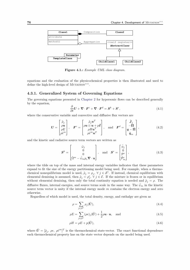
76 Chapter 4. Development of Mutation++
Parameter
Class1
attribute
method()AbstractClass
<<self register>>
ChildClass1 ChildClass2
Composition Class2
Aggregation
TemplateClass
Figure 4.1.: Example UML class diagram.
equations and the evaluation of the physicochemical properties is then illustrated and used todefine the high-level design of Mutation++.
4.3.1. Generalized System of Governing Equations
The governing equations presented in Chapter 2 for hypersonic flows can be described generallyby the equation,
∂
∂tU +∇ · F c +∇ · F d = Sk + Sr, (4.1)
where the conservative variable and convective and diffusive flux vectors are
U =
⎡
⎢
⎢
⎣
ρjρuρEρem
⎤
⎥
⎥
⎦
, F c =
⎡
⎢
⎢
⎣
ρjuT
ρu⊗ u+ pIρHuT
ρemuT
⎤
⎥
⎥
⎦
, and F d =
⎡
⎢
⎢
⎣
Jj
−Π
q − Π
qm
⎤
⎥
⎥
⎦
, (4.2)
and the kinetic and radiative source term vectors are written as
Sk =
⎡
⎢
⎢
⎣
ωj
00
Ωm − ψmpe∇ · u
⎤
⎥
⎥
⎦
, and Sr =
⎡
⎢
⎢
⎣
φj0Pr
Prm
⎤
⎥
⎥
⎦
, (4.3)
where the tilde on top of the mass and internal energy variables indicates that these parametersexpand to fit the size of the energy partitioning model being used. For example, when a thermo-chemical nonequilibrium model is used, ρj = ρj , ∀ j ∈ S∗. If instead, chemical equilibrium withelemental demixing is assumed, then ρj = ρej , ∀ j ∈ E . If the mixture is frozen or in equilibriumwithout elemental demixing, then only the total continuity equation is needed and ρj = ρ. Thediffusive fluxes, internal energies, and source terms scale in the same way. The ψm in the kineticsource term vector is unity if the internal energy mode m contains the electron energy and zerootherwise.
Regardless of which model is used, the total density, energy, and enthalpy are given as
ρ =∑
j∈S∗
ρj(U ), (4.4)
ρE =∑
j∈S∗
(ρe)j(U) +1
2ρu · u, and (4.5)
ρH = ρE + p(U), (4.6)
where U = [ρj , ρe, ρem]T is the thermochemical state-vector. The exact functional dependence
each thermochemical property has on the state vector depends on the model being used.
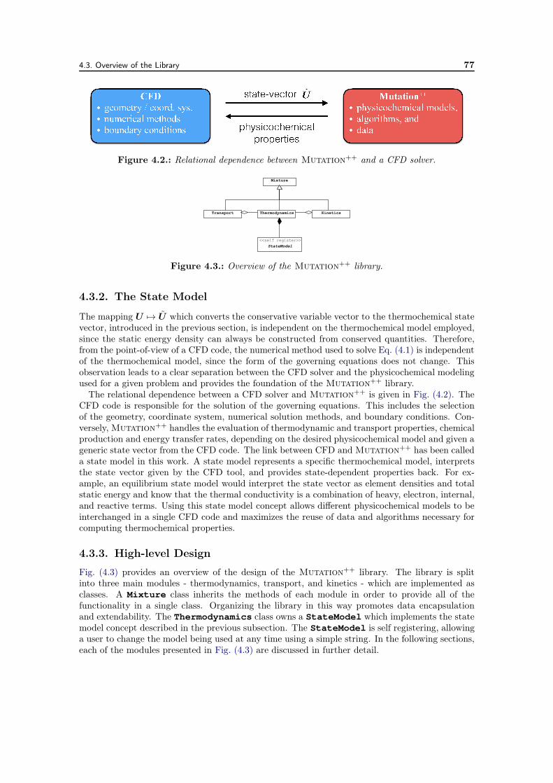
4.3. Overview of the Library 77
Figure 4.2.: Relational dependence between Mutation++ and a CFD solver.
Mixture
ThermodynamicsTransport Kinetics
StateModel<<self register>>
Figure 4.3.: Overview of the Mutation++ library.
4.3.2. The State Model
The mapping U 3→ U which converts the conservative variable vector to the thermochemical statevector, introduced in the previous section, is independent on the thermochemical model employed,since the static energy density can always be constructed from conserved quantities. Therefore,from the point-of-view of a CFD code, the numerical method used to solve Eq. (4.1) is independentof the thermochemical model, since the form of the governing equations does not change. Thisobservation leads to a clear separation between the CFD solver and the physicochemical modelingused for a given problem and provides the foundation of the Mutation++ library.
The relational dependence between a CFD solver and Mutation++ is given in Fig. (4.2). TheCFD code is responsible for the solution of the governing equations. This includes the selectionof the geometry, coordinate system, numerical solution methods, and boundary conditions. Con-versely, Mutation++ handles the evaluation of thermodynamic and transport properties, chemicalproduction and energy transfer rates, depending on the desired physicochemical model and given ageneric state vector from the CFD code. The link between CFD and Mutation++ has been calleda state model in this work. A state model represents a specific thermochemical model, interpretsthe state vector given by the CFD tool, and provides state-dependent properties back. For ex-ample, an equilibrium state model would interpret the state vector as element densities and totalstatic energy and know that the thermal conductivity is a combination of heavy, electron, internal,and reactive terms. Using this state model concept allows different physicochemical models to beinterchanged in a single CFD code and maximizes the reuse of data and algorithms necessary forcomputing thermochemical properties.
4.3.3. High-level Design
Fig. (4.3) provides an overview of the design of the Mutation++ library. The library is splitinto three main modules - thermodynamics, transport, and kinetics - which are implemented asclasses. A Mixture class inherits the methods of each module in order to provide all of thefunctionality in a single class. Organizing the library in this way promotes data encapsulationand extendability. The Thermodynamics class owns a StateModel which implements the statemodel concept described in the previous subsection. The StateModel is self registering, allowinga user to change the model being used at any time using a simple string. In the following sections,each of the modules presented in Fig. (4.3) are discussed in further detail.
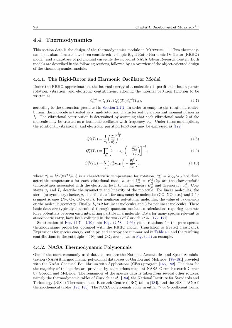
78 Chapter 4. Development of Mutation++
4.4. Thermodynamics
This section details the design of the thermodynamics module in Mutation++. Two thermody-namic database formats have been considered: a simple Rigid-Rotor Harmonic-Oscillator (RRHO)model, and a database of polynomial curve-fits developed at NASA Glenn Research Center. Bothmodels are described in the following sections, followed by an overview of the object-oriented designof the thermodynamics module.
4.4.1. The Rigid-Rotor and Harmonic Oscillator Model
Under the RRHO approximation, the internal energy of a molecule i is partitioned into separaterotation, vibration, and electronic contributions, allowing the internal partition function to bewritten as
Qinti = Qr
i(Tr)Qvi (Tv)Q
eli (Tel), (4.7)
according to the discussion presented in Section 2.2.2. In order to compute the rotational contri-bution, the molecule is treated as a rigid-rotor and characterized by a constant moment of inertiaIi. The vibrational contribution is determined by assuming that each vibrational mode k of themolecule may be treated as a harmonic-oscillator with frequency νki. Under these assumptions,the rotational, vibrational, and electronic partition functions may be expressed as [172]
Qri(Tr) =
1
σi
(
Tr
θri
)
Li2
, (4.8)
Qvi (Tv) =
∏
k
[
1− exp
(
−θvkiTv
)]−1
, (4.9)
Qeli (Tel) =
∑
k
aelki exp
(
−θelkiTel
)
, (4.10)
where θri = h2/(8π2IikB) is a characteristic temperature for rotation, θvki = hνki/kB are char-acteristic temperatures for each vibrational mode k, and θelki = Eel
ki/kB are the characteristictemperatures associated with the electronic level k, having energy Eel
ki and degeneracy aelki. Con-
stants σi and Li describe the symmetry and linearity of the molecule. For linear molecules, thesteric (or symmetry) factor, σi, is defined as 1 for unsymmetric molecules (CO, NO, etc.) and 2 forsymmetric ones (N2, O2, CO2, etc.). For nonlinear polyatomic molecules, the value of σi dependson the molecule geometry. Finally, Li is 2 for linear molecules and 3 for nonlinear molecules. Thesebasic data are typically determined through quantum mechanics calculations requiring accurateforce potentials between each interacting particle in a molecule. Data for many species relevant toatmospheric entry, have been collected in the works of Gurvich et al. [172–177].
Substitution of Eqs. (4.7 - 4.10) into Eqs. (2.58 - 2.66) yields relations for the pure speciesthermodynamic properties obtained with the RRHO model (translation is treated classically).Expressions for species energy, enthalpy, and entropy are summarized in Table 4.1 and the resultingcontributions to the enthalpies of N2 and CO2 are shown in Fig. (4.4) as example.
4.4.2. NASA Thermodynamic Polynomials
One of the more commonly used data sources are the National Aeronautics and Space Adminis-tration (NASA)thermodynamic polynomial databases of Gordon and McBride [178–181] providedwith the NASA Chemical Equilibrium with Applications (CEA) program [166, 182]. The data forthe majority of the species are provided by calculations made at NASA Glenn Research Centerby Gordon and McBride. The remainder of the species data is taken from several other sources,namely the thermodynamic tables of Gurvich et al. [183], the National Institute for Standards andTechnology (NIST) Thermochemical Research Center (TRC) tables [184], and the NIST-JANAFthermochemical tables [185, 186]. The NASA polynomials come in either 7- or 9-coefficient forms.
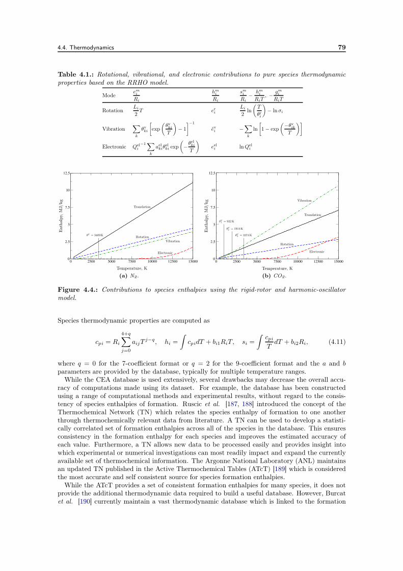
4.4. Thermodynamics 79
Table 4.1.: Rotational, vibrational, and electronic contributions to pure species thermodynamicproperties based on the RRHO model.
ModeemiRi
hmi
Ri
smiRi
−hmi
RiT, −
gmiRiT
RotationLi
2T er
iLi
2ln
(
T
θri
)
− lnσi
Vibration∑
k
θvki
[
exp
(
θvkiT
)
− 1
]−1
evi −
∑
k
ln
[
1− exp
(
−θvikT
)]
Electronic Qeli−1∑
k
aelkiθ
elki exp
(
−θelkiT
)
eeli lnQel
i
0 2500 5000 7500 10000 12500 150000
2.5
5
7.5
10
12.5
Temperature, K
Ent
halp
y,MJ/
kg
Translation
RotationVibration
Electronic
θV = 3409K
(a) N2.
0 2500 5000 7500 10000 12500 150000
2.5
5
7.5
10
12.5
Temperature, K
Ent
halp
y,MJ/
kg
Translation
Rotation
Vibration
Electronic
θV1 = 932K
θV2 = 1914K
θV3 = 3374K
(b) CO2.
Figure 4.4.: Contributions to species enthalpies using the rigid-rotor and harmonic-oscillatormodel.
Species thermodynamic properties are computed as
cpi = Ri
4+q∑
j=0
aijTj−q, hi =
∫
cpidT + bi1RiT, si =
∫
cpiT
dT + bi2Ri, (4.11)
where q = 0 for the 7-coefficient format or q = 2 for the 9-coefficient format and the a and bparameters are provided by the database, typically for multiple temperature ranges.
While the CEA database is used extensively, several drawbacks may decrease the overall accu-racy of computations made using its dataset. For example, the database has been constructedusing a range of computational methods and experimental results, without regard to the consis-tency of species enthalpies of formation. Ruscic et al. [187, 188] introduced the concept of theThermochemical Network (TN) which relates the species enthalpy of formation to one anotherthrough thermochemically relevant data from literature. A TN can be used to develop a statisti-cally correlated set of formation enthalpies across all of the species in the database. This ensuresconsistency in the formation enthalpy for each species and improves the estimated accuracy ofeach value. Furthermore, a TN allows new data to be processed easily and provides insight intowhich experimental or numerical investigations can most readily impact and expand the currentlyavailable set of thermochemical information. The Argonne National Laboratory (ANL) maintainsan updated TN published in the Active Thermochemical Tables (ATcT) [189] which is consideredthe most accurate and self consistent source for species formation enthalpies.
While the ATcT provides a set of consistent formation enthalpies for many species, it does notprovide the additional thermodynamic data required to build a useful database. However, Burcatet al. [190] currently maintain a vast thermodynamic database which is linked to the formation
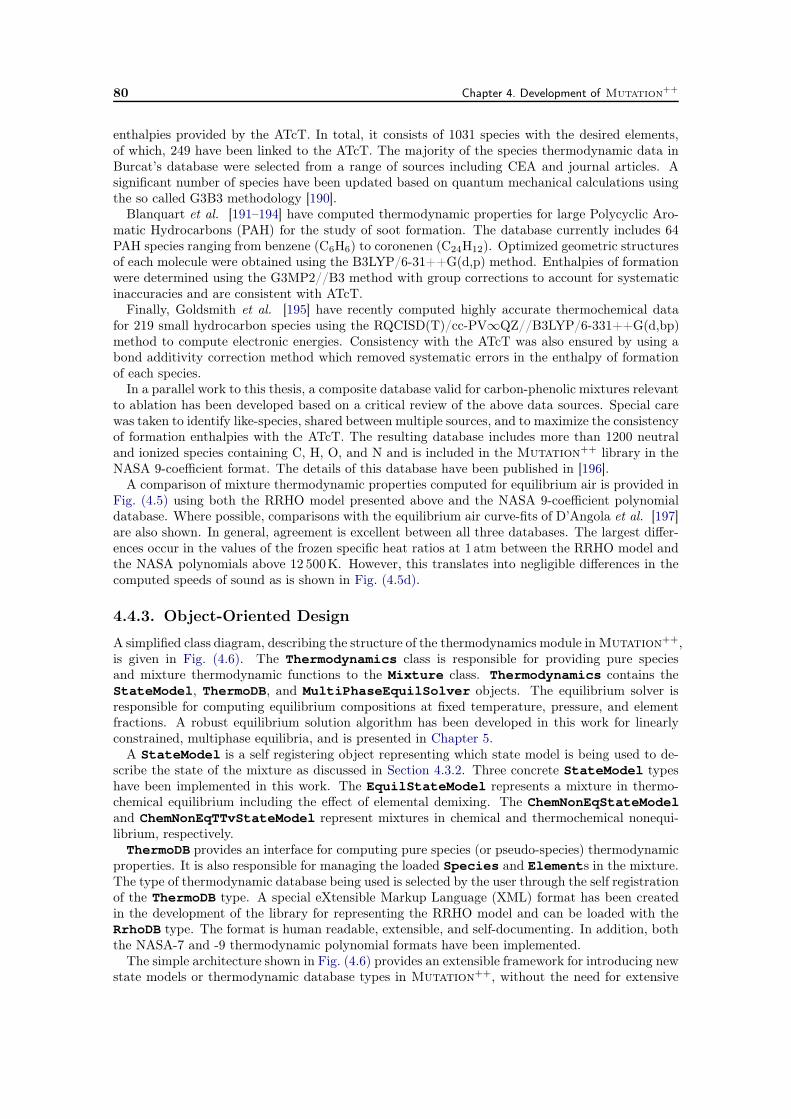
80 Chapter 4. Development of Mutation++
enthalpies provided by the ATcT. In total, it consists of 1031 species with the desired elements,of which, 249 have been linked to the ATcT. The majority of the species thermodynamic data inBurcat’s database were selected from a range of sources including CEA and journal articles. Asignificant number of species have been updated based on quantum mechanical calculations usingthe so called G3B3 methodology [190].
Blanquart et al. [191–194] have computed thermodynamic properties for large Polycyclic Aro-matic Hydrocarbons (PAH) for the study of soot formation. The database currently includes 64PAH species ranging from benzene (C6H6) to coronenen (C24H12). Optimized geometric structuresof each molecule were obtained using the B3LYP/6-31++G(d,p) method. Enthalpies of formationwere determined using the G3MP2//B3 method with group corrections to account for systematicinaccuracies and are consistent with ATcT.
Finally, Goldsmith et al. [195] have recently computed highly accurate thermochemical datafor 219 small hydrocarbon species using the RQCISD(T)/cc-PV∞QZ//B3LYP/6-331++G(d,bp)method to compute electronic energies. Consistency with the ATcT was also ensured by using abond additivity correction method which removed systematic errors in the enthalpy of formationof each species.
In a parallel work to this thesis, a composite database valid for carbon-phenolic mixtures relevantto ablation has been developed based on a critical review of the above data sources. Special carewas taken to identify like-species, shared between multiple sources, and to maximize the consistencyof formation enthalpies with the ATcT. The resulting database includes more than 1200 neutraland ionized species containing C, H, O, and N and is included in the Mutation++ library in theNASA 9-coefficient format. The details of this database have been published in [196].
A comparison of mixture thermodynamic properties computed for equilibrium air is provided inFig. (4.5) using both the RRHO model presented above and the NASA 9-coefficient polynomialdatabase. Where possible, comparisons with the equilibrium air curve-fits of D’Angola et al. [197]are also shown. In general, agreement is excellent between all three databases. The largest differ-ences occur in the values of the frozen specific heat ratios at 1 atm between the RRHO model andthe NASA polynomials above 12 500K. However, this translates into negligible differences in thecomputed speeds of sound as is shown in Fig. (4.5d).
4.4.3. Object-Oriented Design
A simplified class diagram, describing the structure of the thermodynamics module in Mutation++,is given in Fig. (4.6). The Thermodynamics class is responsible for providing pure speciesand mixture thermodynamic functions to the Mixture class. Thermodynamics contains theStateModel, ThermoDB, and MultiPhaseEquilSolver objects. The equilibrium solver isresponsible for computing equilibrium compositions at fixed temperature, pressure, and elementfractions. A robust equilibrium solution algorithm has been developed in this work for linearlyconstrained, multiphase equilibria, and is presented in Chapter 5.
A StateModel is a self registering object representing which state model is being used to de-scribe the state of the mixture as discussed in Section 4.3.2. Three concrete StateModel typeshave been implemented in this work. The EquilStateModel represents a mixture in thermo-chemical equilibrium including the effect of elemental demixing. The ChemNonEqStateModel
and ChemNonEqTTvStateModel represent mixtures in chemical and thermochemical nonequi-librium, respectively.ThermoDB provides an interface for computing pure species (or pseudo-species) thermodynamic
properties. It is also responsible for managing the loaded Species and Elements in the mixture.The type of thermodynamic database being used is selected by the user through the self registrationof the ThermoDB type. A special eXtensible Markup Language (XML) format has been createdin the development of the library for representing the RRHO model and can be loaded with theRrhoDB type. The format is human readable, extensible, and self-documenting. In addition, boththe NASA-7 and -9 thermodynamic polynomial formats have been implemented.
The simple architecture shown in Fig. (4.6) provides an extensible framework for introducing newstate models or thermodynamic database types in Mutation++, without the need for extensive
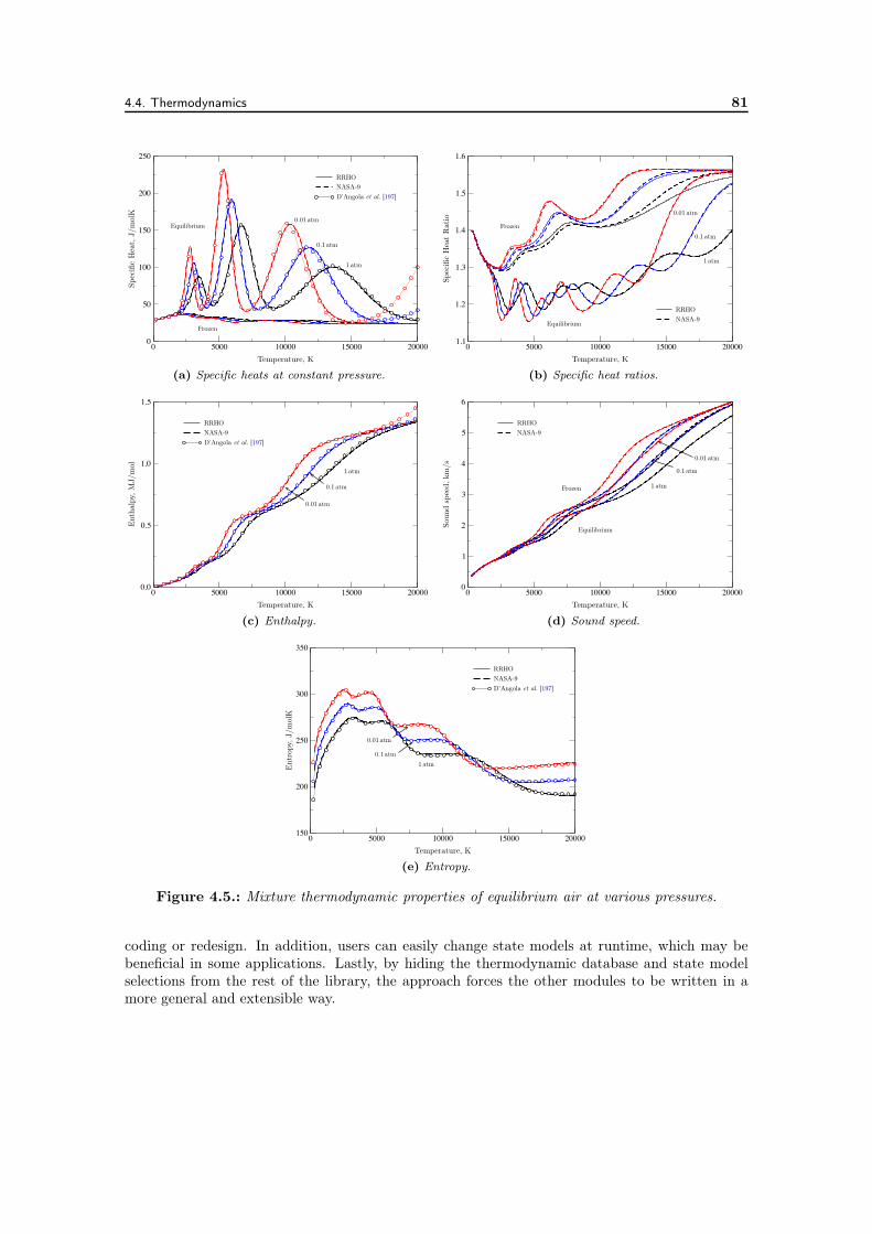
4.4. Thermodynamics 81
0 5000 10000 15000 200000
50
100
150
200
250
Temperature, K
Equilibrium
Frozen
RRHONASA-9D’Angola et al. [197]
0.01 atm
0.1 atm
1 atm
Spec
ific
Hea
t,J/
molK
(a) Specific heats at constant pressure.
0 5000 10000 15000 200001.1
1.2
1.3
1.4
1.5
1.6
Temperature, K
Equilibrium
Frozen
RRHONASA-9
0.01 atm
0.1 atm
1 atm
Spec
ific
Hea
tR
atio
(b) Specific heat ratios.
0 5000 10000 15000 200000.0
0.5
1.0
1.5
Temperature, K
RRHONASA-9D’Angola et al. [197]
0.01 atm
0.1 atm
1 atm
Ent
halp
y,MJ/
mol
(c) Enthalpy.
0 5000 10000 15000 200000
1
2
3
4
5
6
Temperature, K
Equilibrium
Frozen
RRHONASA-9
0.01 atm
0.1 atm
1 atm
Soun
dsp
eed,
km/s
(d) Sound speed.
0 5000 10000 15000 20000150
200
250
300
350
Temperature, K
RRHONASA-9D’Angola et al. [197]
1 atm
0.01 atm
0.1 atm
Ent
ropy
,J/m
olK
(e) Entropy.
Figure 4.5.: Mixture thermodynamic properties of equilibrium air at various pressures.
coding or redesign. In addition, users can easily change state models at runtime, which may bebeneficial in some applications. Lastly, by hiding the thermodynamic database and state modelselections from the rest of the library, the approach forces the other modules to be written in amore general and extensible way.
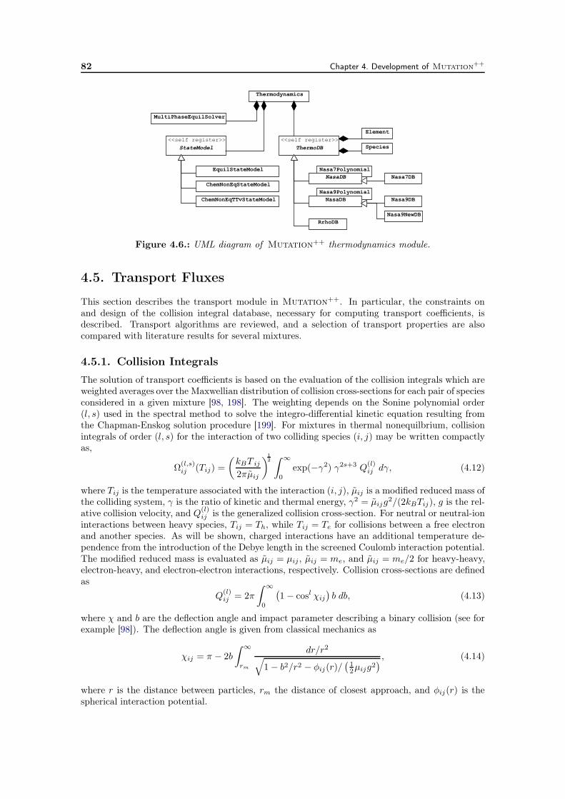
82 Chapter 4. Development of Mutation++
Nasa9Polynomial
Nasa7Polynomial
Thermodynamics
ThermoDB<<self register>>
MultiPhaseEquilSolver
StateModel<<self register>>
Element
Species
RrhoDB
NasaDB Nasa7DB
NasaDB Nasa9DB
Nasa9NewDB
EquilStateModel
ChemNonEqStateModel
ChemNonEqTTvStateModel
Figure 4.6.: UML diagram of Mutation++ thermodynamics module.
4.5. Transport Fluxes
This section describes the transport module in Mutation++. In particular, the constraints onand design of the collision integral database, necessary for computing transport coefficients, isdescribed. Transport algorithms are reviewed, and a selection of transport properties are alsocompared with literature results for several mixtures.
4.5.1. Collision Integrals
The solution of transport coefficients is based on the evaluation of the collision integrals which areweighted averages over the Maxwellian distribution of collision cross-sections for each pair of speciesconsidered in a given mixture [98, 198]. The weighting depends on the Sonine polynomial order(l, s) used in the spectral method to solve the integro-differential kinetic equation resulting fromthe Chapman-Enskog solution procedure [199]. For mixtures in thermal nonequilbrium, collisionintegrals of order (l, s) for the interaction of two colliding species (i, j) may be written compactlyas,
Ω(l,s)ij (Tij) =
(
kBT ij
2πµij
)12∫ ∞
0exp(−γ2) γ2s+3 Q(l)
ij dγ, (4.12)
where Tij is the temperature associated with the interaction (i, j), µij is a modified reduced mass ofthe colliding system, γ is the ratio of kinetic and thermal energy, γ2 = µijg2/(2kBTij), g is the rel-ative collision velocity, and Q(l)
ij is the generalized collision cross-section. For neutral or neutral-ioninteractions between heavy species, Tij = Th, while Tij = Te for collisions between a free electronand another species. As will be shown, charged interactions have an additional temperature de-pendence from the introduction of the Debye length in the screened Coulomb interaction potential.The modified reduced mass is evaluated as µij = µij , µij = me, and µij = me/2 for heavy-heavy,electron-heavy, and electron-electron interactions, respectively. Collision cross-sections are definedas
Q(l)ij = 2π
∫ ∞
0
(
1− cosl χij
)
b db, (4.13)
where χ and b are the deflection angle and impact parameter describing a binary collision (see forexample [98]). The deflection angle is given from classical mechanics as
χij = π − 2b
∫ ∞
rm
dr/r2√
1− b2/r2 − φij(r)/(
12µijg2
)
, (4.14)
where r is the distance between particles, rm the distance of closest approach, and φij(r) is thespherical interaction potential.
4.5. Transport Fluxes 83
It is convenient to express collision integrals in terms of dimensional, reduced collision integralsQ(l,s)
ij [200], defined as
Q(l,s)ij = πσ2
HSΩ(l,s)∗ij
=4(l+ 1)
(s+ 1)![2l+ 1− (−1)l]
∫ ∞
0exp(−γ2) γ2s+3 Q(l)
ij dγ,(4.15)
where Ω(l,s)∗ij are the standard reduced collision integrals normalized by the corresponding hard-
sphere values [198] and πσ2HS is the hard-sphere cross-section. Reduced collision integrals represent
the deviation from the rigid-sphere values and are often used since they have a weaker dependenceon temperature than Eq. (4.12), making them easier to represent with curve-fits. Notice that thehard-sphere cross-section is not actually needed to evaluate the reduced collision integrals. Thefollowing ratios also occur frequently enough in the calculation of transport properties, that theyare explicitly defined as
A∗ij = Q(2,2)
ij /Q(1,1)ij , (4.16)
B∗ij =
(
5Q(1,2)ij − 4Q(1,3)
ij
)
/Q(1,1)ij , (4.17)
C∗ij = Q(1,2)
ij /Q(1,1)ij , (4.18)
E∗ij = Q(2,3)
ij /Q(2,2)ij , (4.19)
F ∗ij = Q(3,3)
ij /Q(1,1)ij , (4.20)
G∗ij = Q(4,4)
ij /Q(2,2)ij . (4.21)
Tables A.1 and A.2 provide practical expressions for the linear transport systems in terms ofreduced collision integrals and ratios based on the derivation of Magin and Degrez [107] for par-tially ionized and unmagnetized plasmas. The derivation is based on a modified Chapman-Enskogperturbative solution of the scaled Boltzmann equation, using the electron to heavy particle massratio as the scaling parameter. The effects of chemistry and internal energy on the transport sys-tems are neglected. Instead, the Euken corrections for internal energy have been used. Only onenon-vanishing Sonine polynomial order is retained for heavy-heavy interactions. Two non-vanishingorders are retained for interactions involving electrons. A summary of the required collision in-tegral data necessary to compute each transport coefficient based the expressions of Magin andDegrez is provided in Table 4.2. As is shown by last row in the table, the total number of collisionintegrals required to compute all of the transport coefficients scales with the number of speciessquared, since all collision pairs must be taken into account. As an example, the 11-species airmixture, consisting of 5 neutrals (N, O, N2, O2, and NO) and their first ions and free electrons,has 66 unique collision pairs and requires the evaluation of 273 collision integrals, based on Ta-ble 4.2. Thus, the data requirements for transport properties grows significantly faster than forthermodynamics, which grows linearly with the number of species.
The preferred method to computed collision integrals is to numerically integrate from accurateab initio potential energy surfaces. Such data is available for several important collision systems.Recent reviews of available collision integral data for neutral-neutral interactions are providedby Wright et al. [201, 202] for air, Mars, and Venus mixtures and collision integrals have beentabulated versus temperature up to 20 000K. The review of Bruno et al. [203] has been usedfor Jupiter mixtures and provides accurate curve-fits suitable for collision integral calculationsup to 50 000K. When potential energy surfaces are not available, collision integrals are typicallyintegrated from model interaction potentials. The evaluation of these potentials is typically splitinto four groups: neutral-neutral, ion-neutral, electron-neutral, and charged interactions. Thefollowing subsections review commonly used potentials for each type of interaction and present thedata sources for collision integrals required in this work.
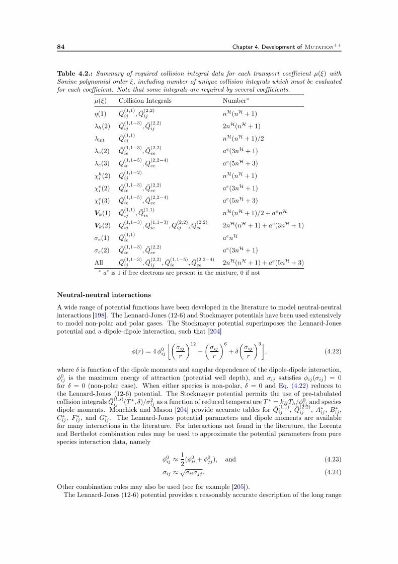
84 Chapter 4. Development of Mutation++
Table 4.2.: Summary of required collision integral data for each transport coefficient µ(ξ) withSonine polynomial order ξ, including number of unique collision integrals which must be evaluatedfor each coefficient. Note that some integrals are required by several coefficients.
µ(ξ) Collision Integrals Number∗
η(1) Q(1,1)ij , Q
(2,2)ij nH(nH + 1)
λh(2) Q(1,1−3)ij , Q
(2,2)ij 2nH(nH + 1)
λint Q(1,1)ij nH(nH + 1)/2
λe(2) Q(1,1−3)ie , Q
(2,2)ee ae(3nH + 1)
λe(3) Q(1,1−5)ie , Q
(2,2−4)ee ae(5nH + 3)
χhi (2) Q
(1,1−2)ij nH(nH + 1)
χei (2) Q
(1,1−3)ie , Q
(2,2)ee ae(3nH + 1)
χei (3) Q
(1,1−5)ie , Q
(2,2−4)ee ae(5nH + 3)
Vk(1) Q(1,1)ij , Q
(1,1)ie nH(nH + 1)/2 + aenH
Vk(2) Q(1,1−3)ij , Q
(1,1−3)ie , Q
(2,2)ij , Q
(2,2)ee 2nH(nH + 1) + ae(3nH + 1)
σe(1) Q(1,1)ie aenH
σe(2) Q(1,1−3)ie , Q
(2,2)ee ae(3nH + 1)
All Q(1,1−3)ij , Q
(2,2)ij , Q
(1,1−5)ie , Q
(2,2−4)ee 2nH(nH + 1) + ae(5nH + 3)
∗ ae is 1 if free electrons are present in the mixture, 0 if not
Neutral-neutral interactions
A wide range of potential functions have been developed in the literature to model neutral-neutralinteractions [198]. The Lennard-Jones (12-6) and Stockmayer potentials have been used extensivelyto model non-polar and polar gases. The Stockmayer potential superimposes the Lennard-Jonespotential and a dipole-dipole interaction, such that [204]
φ(r) = 4φ0ij
[(
σijr
)12
−(
σijr
)6
+ δ
(
σijr
)3]
, (4.22)
where δ is function of the dipole moments and angular dependence of the dipole-dipole interaction,φ0ij is the maximum energy of attraction (potential well depth), and σij satisfies φij(σij) = 0for δ = 0 (non-polar case). When either species is non-polar, δ = 0 and Eq. (4.22) reduces tothe Lennard-Jones (12-6) potential. The Stockmayer potential permits the use of pre-tabulatedcollision integrals Q(l,s)
ij (T ∗, δ)/σ2ij as a function of reduced temperature T ∗ = kBTh/φ0ij and species
dipole moments. Monchick and Mason [204] provide accurate tables for Q(1,1)ij , Q(2,2)
ij , A∗ij , B
∗ij ,
C∗ij , F ∗
ij , and G∗ij . The Lennard-Jones potential parameters and dipole moments are available
for many interactions in the literature. For interactions not found in the literature, the Lorentzand Berthelot combination rules may be used to approximate the potential parameters from purespecies interaction data, namely
φ0ij ≈1
2(φ0ii + φ0jj), and (4.23)
σij ≈√σiiσjj . (4.24)
Other combination rules may also be used (see for example [205]).The Lennard-Jones (12-6) potential provides a reasonably accurate description of the long range
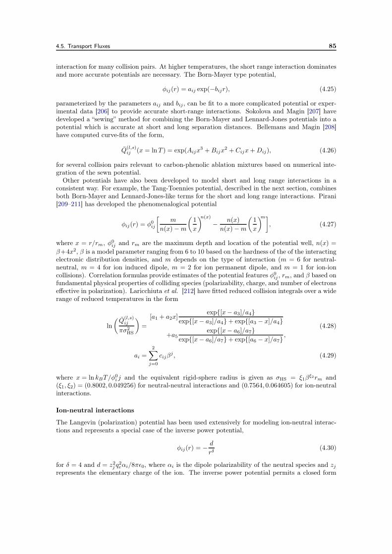
4.5. Transport Fluxes 85
interaction for many collision pairs. At higher temperatures, the short range interaction dominatesand more accurate potentials are necessary. The Born-Mayer type potential,
φij(r) = aij exp(−bijr), (4.25)
parameterized by the parameters aij and bij , can be fit to a more complicated potential or exper-imental data [206] to provide accurate short-range interactions. Sokolova and Magin [207] havedeveloped a “sewing” method for combining the Born-Mayer and Lennard-Jones potentials into apotential which is accurate at short and long separation distances. Bellemans and Magin [208]have computed curve-fits of the form,
Q(l,s)ij (x = lnT ) = exp(Aijx
3 +Bijx2 + Cijx+Dij), (4.26)
for several collision pairs relevant to carbon-phenolic ablation mixtures based on numerical inte-gration of the sewn potential.
Other potentials have also been developed to model short and long range interactions in aconsistent way. For example, the Tang-Toennies potential, described in the next section, combinesboth Born-Mayer and Lennard-Jones-like terms for the short and long range interactions. Pirani[209–211] has developed the phenomenalogical potential
φij(r) = φ0ij
[
m
n(x) −m
(
1
x
)n(x)
−n(x)
n(x)−m
(
1
x
)m]
, (4.27)
where x = r/rm, φ0ij and rm are the maximum depth and location of the potential well, n(x) =β+4x2, β is a model parameter ranging from 6 to 10 based on the hardness of the of the interactingelectronic distribution densities, and m depends on the type of interaction (m = 6 for neutral-neutral, m = 4 for ion induced dipole, m = 2 for ion permanent dipole, and m = 1 for ion-ioncollisions). Correlation formulas provide estimates of the potential features φ0ij , rm, and β based onfundamental physical properties of colliding species (polarizability, charge, and number of electronseffective in polarization). Laricchiuta et al. [212] have fitted reduced collision integrals over a widerange of reduced temperatures in the form
ln
(
Q(l,s)ij
πσ2HS
)
=
[a1 + a2x]exp[x− a3]/a4
exp[x− a3]/a4+ exp[a3 − x]/a4
+a5exp[x− a6]/a7
exp[x− a6]/a7+ exp[a6 − x]/a7,
(4.28)
ai =2∑
j=0
cijβj , (4.29)
where x = ln kBT/φ0i j and the equivalent rigid-sphere radius is given as σHS = ξ1βξ2rm and(ξ1, ξ2) = (0.8002, 0.049256) for neutral-neutral interactions and (0.7564, 0.064605) for ion-neutralinteractions.
Ion-neutral interactions
The Langevin (polarization) potential has been used extensively for modeling ion-neutral interac-tions and represents a special case of the inverse power potential,
φij(r) = −d
rδ(4.30)
for δ = 4 and d = z2j q2eαi/8πϵ0, where αi is the dipole polarizability of the neutral species and zj
represents the elementary charge of the ion. The inverse power potential permits a closed form
86 Chapter 4. Development of Mutation++
Table 4.3.: Ratios of Q(l,s)ij /Q(1,1)
ij for the Langevin potential.
l,s 2 3 4 51 0.833 0.729 0.656 0.6022 0.870 0.761 0.6853 0.842
solution of the collision integrals, such that
Q(l,s)ij =
4π(l + 1)
(s+ 1)![2l+ 1− (−1)l]A(l)(δ)
√
d δ
kBThΓ
(
s+ 2−2
δ
)
, (4.31)
where A(1)(4) = 0.5523, A(2)(4) = 0.3846, A(3)(4) = 0.6377, and Γ is the gamma function for realnumbers. Using the parameters for the Langevin potential, the diffusion integral is given as,
Q(1,1)ij = 424.443zjπ
√
αi
Th. (4.32)
Other integrals are constant ratios of the above. These ratios are given in Table 4.3 for thenecessary integrals. The Langevin potential is useful when no data is available for a given collisionas it only requires the polarizability of the neutral species, which may be found easily for most gases.Polarizabilities for neutral species considered in this work are provided in Appendix D. Levin andWright [213] have compared this potential with accurate collision data for some important ion-neutral collisions in air and found the accuracy to be about 40% over the temperature range ofinterest. Capitelli [214] has shown that this error can be as high as 100% for the K+-Ne andK+-Xe collisions, suggesting that care should be taken when using this potential.
Levin and Wright [213] have proposed to use an effective Tang-Toennies potential for ion-neutralcollisions,
φij(r) = φ0ij exp(−r/β)−∞∑
n=2
[
1− exp(−r/β)2n∑
k=0
(r/β)k
k!
]
C2n
r2n, (4.33)
which combines an exponential repulsion term, dominate at short-range, with damped dispersionand polarization terms for the long-range interaction. For n > 5, the dispersion coefficients C2n
are given by the recursive relation
C2n+4 = C2n−2(C2n+2/C2n)3. (4.34)
The lower order dispersion coefficients and the short-range coefficients φ0 and β may be estimatedgiven C6 and the dipole, quadrupole, and octopole polarizabilities of the ion and neutral speciesas discussed in [213].
For collisions between ions and their parent neutral, resonant charge transfer can significantlyincrease the momentum-transfer cross-section and should be taken into account for collision in-tegrals with odd l. Charge transfer does not affect the viscosity cross-section due to symmetry.Typically, resonant charge transfer is considered through the simple mixing rule [215], such that
Q(l,s)ij =
√
(
Q(l,s)ij,ex
)2+(
Q(l,s)ij,el
)2, odd l, (4.35)
where Q(l,s)ij,ex and Q(l,s)
ij,el are the collision integrals computed with pure charge transfer and elasticmomentum-transfer cross-sections, respectively.
Collision integral data for ion-neutral collisions have been taken from several sources. Levinand Wright [213] provide tabulated diffusion and viscosity integrals for air interactions based onintegrated Tang-Toennies potentials. In addition, Wright et al. [201] suggest that constant valuesof 1.2 and 0.85 are sufficient for the ratios B∗ and C∗ which has been used as a default for all
4.5. Transport Fluxes 87
ion-neutral interactions when no other data is available. In a second work, Wright et al. [202]have also computed ion-neutral integrals for Mars and Venus mixtures, based on a combination ofLangevin and Tang-Toennies models. Bruno et al. [203] provide accurate collision integral datafor Jupiter species as well. Finally, the Langevin potential has been used for all other ion-neutralinteractions required in this work.
Electron-neutral interactions
Unfortunately, it is difficult to use engineering approximations when computing electron-neutralcollision integrals, due to the complexity of the interactions. Often these data are assembled fromelastic or momentum cross sections as functions of energy, as determined from beam scatteringor swarm measurements [201]. The most accurate method for computing collision integrals forelectron-neutral interactions is through numerical integration of the differential elastic cross sec-tions, dσ/dΩ. Differential cross sections can be integrated over all scattering angles to provideintegral cross sections versus energy,
Q(l)ei (E) = 2π
∫ π
0
dσ
dΩ(1− cosl χ) sinχdχ. (4.36)
The resulting cross sections can then be integrated over energy, assuming a Boltzmann energydistribution, to determine the required collision integrals versus temperature.
Wright et al. [201, 202] provide tables for Air, Mars, and Venus, electron-neutral collisionintegrals based on integrated differential cross sections, obtained from a careful review of theliterature. A selection of these integrals are plotted in Fig. (4.7).
Charged interactions
Collisions between charged particles can be accurately modeled using the screened Coulomb po-tential shielded by the Debye length (Debye-Hückel potential),
φij(r) =zizjr
q2e4πϵ0
exp
(
−r
λD
)
, (4.37)
where zi and zj are the elementary charges of colliding species. The Debye length (radius) rep-resents the characteristic length over which charged particles in a plasma are shielded from othercharged particles. When both electrons and ions are considered in the shielding, the Debye lengthis given as
λ2D =ϵ0kB/q2e
ne/Te +∑
j∈H z2jnj/Th. (4.38)
It is not clear whether ions should be included in the shielding or not. When they are neglected,the sum in the denominator should be removed. For neutral plasmas with Te = Th, the Debyelength simplifies to
λ2D =ϵ0kBTe
2q2ene. (4.39)
Mason, Munn, and Smith [216] have accurately integrated the Coulomb potential and providetabulated attractive and repulsive diffusion and viscosity integrals, as well as the ratios A∗, B∗,C∗, E∗, F ∗, and G∗ versus a reduced temperature,
T ∗ =λDkBT
q2e/(4πϵ0). (4.40)
Devoto [200] later extended these tabulations to include Q(1,4)ij , Q(1,5)
ij , and Q(2,4)ij which are neces-
sary for the third-order electron transport coefficients, as shown in Table 4.2. From Eq. (4.40), thereduced temperature is a function of the electron temperature and number density through the de-pendence on the Debye length. The tables provided by Devoto are valid for reduced temperatures
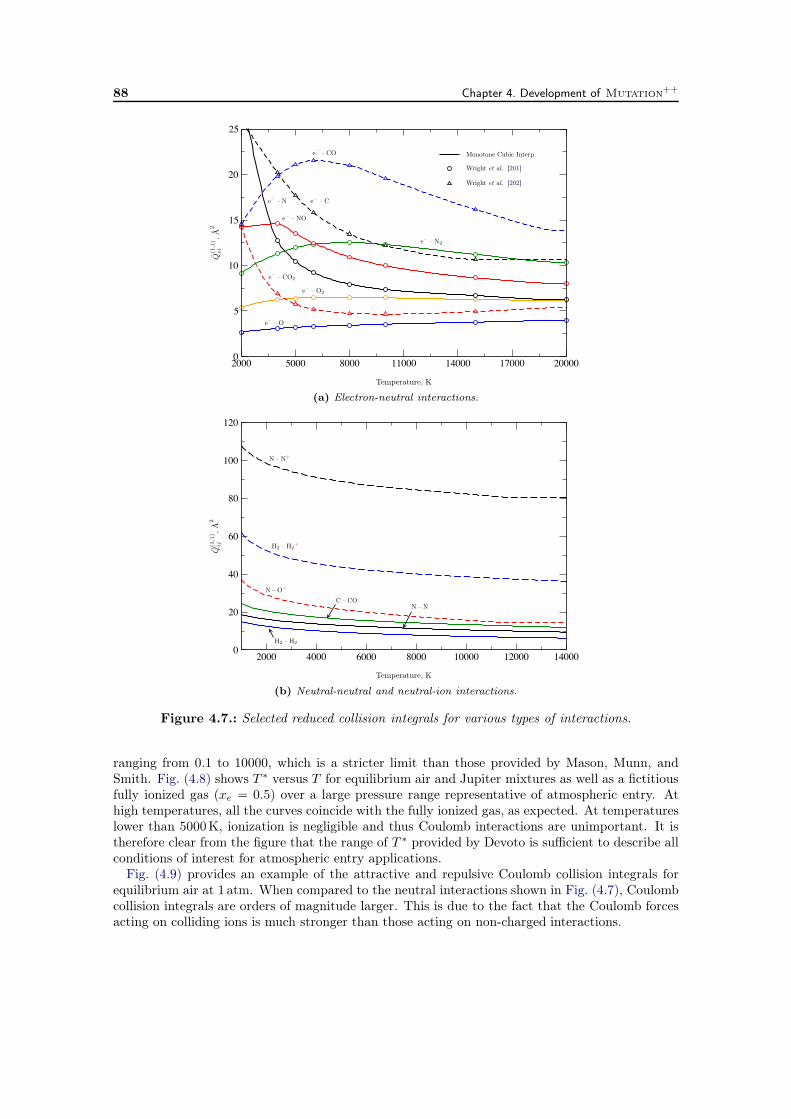
88 Chapter 4. Development of Mutation++
2000 5000 8000 11000 14000 17000 200000
5
10
15
20
25
Temperature, K
Q(1
,1)
ei
,Å2
e– – N
e– – N2
e– – O
e– – O2
e– – NO
e– – CO
e– – CO2
e– – C
Monotone Cubic Interp.
Wright et al. [201]
Wright et al. [202]
(a) Electron-neutral interactions.
2000 4000 6000 8000 10000 12000 140000
20
40
60
80
100
120
Temperature, K
Q(1
,1)
ij,Å
2
N – N+
N – N
H2 – H2+
H2 – H2
N – O+
C – CO
(b) Neutral-neutral and neutral-ion interactions.
Figure 4.7.: Selected reduced collision integrals for various types of interactions.
ranging from 0.1 to 10000, which is a stricter limit than those provided by Mason, Munn, andSmith. Fig. (4.8) shows T ∗ versus T for equilibrium air and Jupiter mixtures as well as a fictitiousfully ionized gas (xe = 0.5) over a large pressure range representative of atmospheric entry. Athigh temperatures, all the curves coincide with the fully ionized gas, as expected. At temperatureslower than 5000K, ionization is negligible and thus Coulomb interactions are unimportant. It istherefore clear from the figure that the range of T ∗ provided by Devoto is sufficient to describe allconditions of interest for atmospheric entry applications.
Fig. (4.9) provides an example of the attractive and repulsive Coulomb collision integrals forequilibrium air at 1 atm. When compared to the neutral interactions shown in Fig. (4.7), Coulombcollision integrals are orders of magnitude larger. This is due to the fact that the Coulomb forcesacting on colliding ions is much stronger than those acting on non-charged interactions.
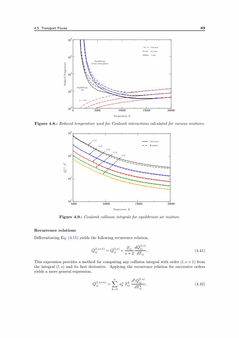
4.5. Transport Fluxes 89
0 5000 10000 15000 20000100
102
104
106
108
Temperature, K
Red
uced
Tem
pera
ture
EquilibriumAir
EquilibriumJovian Atmosphere
xe = 0.5
0.01 atm
0.1 atm
1 atm
Figure 4.8.: Reduced temperature used for Coulomb interactions calculated for various mixtures.
5000 10000 15000 20000101
102
103
104
Temperature, K
Q(l,s)
ij,Å
2
Attractive
Repulsive
(1,1)
(1,2)
(1,3)(1,4)
(1,5)
Figure 4.9.: Coulomb collision integrals for equilibrium air mixture.
Recurrence relations
Differentiating Eq. (4.15) yields the following recurrence relation,
Q(l,s+1)ij = Q(l,s)
ij +Tij
s+ 2
dQ(l,s)ij
dTij. (4.41)
This expression provides a method for computing any collision integral with order (l, s+ 1) fromthe integral (l, s) and its first derivative. Applying the recurrence relation for successive ordersyields a more general expression,
Q(l,s+n)ij =
n∑
k=0
ank T kij
dkQ(l,s)ij
dT kij
, (4.42)
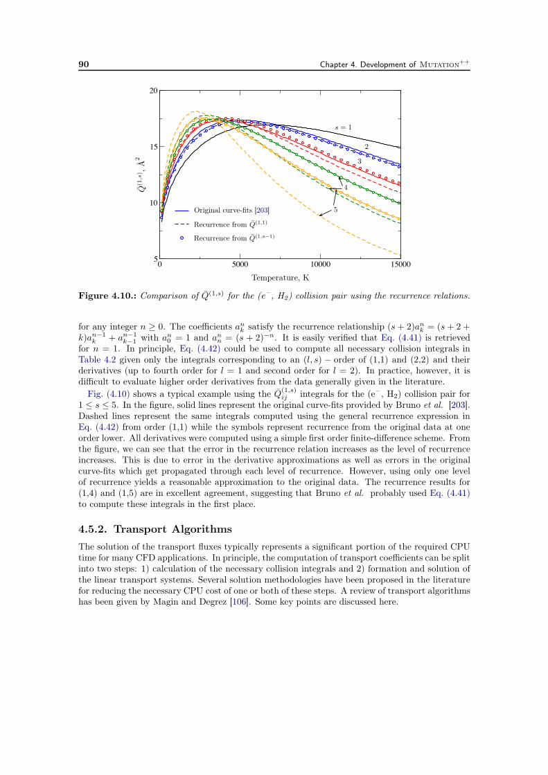
90 Chapter 4. Development of Mutation++
0 5000 10000 150005
10
15
20
Temperature, K
Q(1
,s) ,
Å2
s = 1
2
3
4
5Original curve-fits [203]
Recurrence from Q(1,1)
Recurrence from Q(1,s−1)
Figure 4.10.: Comparison of Q(1,s) for the (e– , H2) collision pair using the recurrence relations.
for any integer n ≥ 0. The coefficients ank satisfy the recurrence relationship (s+ 2)ank = (s + 2 +k)an−1
k + an−1k−1 with an0 = 1 and ann = (s + 2)−n. It is easily verified that Eq. (4.41) is retrieved
for n = 1. In principle, Eq. (4.42) could be used to compute all necessary collision integrals inTable 4.2 given only the integrals corresponding to an (l, s) − order of (1,1) and (2,2) and theirderivatives (up to fourth order for l = 1 and second order for l = 2). In practice, however, it isdifficult to evaluate higher order derivatives from the data generally given in the literature.
Fig. (4.10) shows a typical example using the Q(1,s)ij integrals for the (e– , H2) collision pair for
1 ≤ s ≤ 5. In the figure, solid lines represent the original curve-fits provided by Bruno et al. [203].Dashed lines represent the same integrals computed using the general recurrence expression inEq. (4.42) from order (1,1) while the symbols represent recurrence from the original data at oneorder lower. All derivatives were computed using a simple first order finite-difference scheme. Fromthe figure, we can see that the error in the recurrence relation increases as the level of recurrenceincreases. This is due to error in the derivative approximations as well as errors in the originalcurve-fits which get propagated through each level of recurrence. However, using only one levelof recurrence yields a reasonable approximation to the original data. The recurrence results for(1,4) and (1,5) are in excellent agreement, suggesting that Bruno et al. probably used Eq. (4.41)to compute these integrals in the first place.
4.5.2. Transport Algorithms
The solution of the transport fluxes typically represents a significant portion of the required CPUtime for many CFD applications. In principle, the computation of transport coefficients can be splitinto two steps: 1) calculation of the necessary collision integrals and 2) formation and solution ofthe linear transport systems. Several solution methodologies have been proposed in the literaturefor reducing the necessary CPU cost of one or both of these steps. A review of transport algorithmshas been given by Magin and Degrez [106]. Some key points are discussed here.
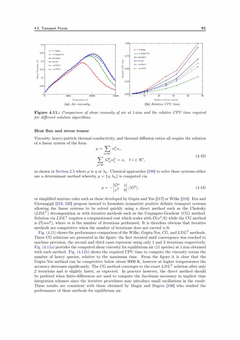
4.5. Transport Fluxes 91
0 5000 10000 150000
0.05
0.1
0.15
0.2
0.25
0.3
Wilke
Gupta-Yos
LDLT
CG
CG(1)
CG(2)
Temperature, K
Shea
rV
isco
sity
,cP
(a) Air viscosity.
0 10 20 30 40 500.00
0.25
0.50
0.75
1.00
Wilke
Gupta-Yos
LDLT
CG
CG(1)
CG(2)
Number of heavy species
Rel
ativ
eC
PU
tim
e
(b) Relative CPU time.
Figure 4.11.: Comparison of shear viscosity of air at 1 atm and the relative CPU time requiredfor different solution algorithms.
Heat flux and stress tensor
Viscosity, heavy-particle thermal conductivity, and thermal diffusion ratios all require the solutionof a linear system of the form
µ =∑
i∈H∗
αµi xi,
∑
j∈H∗
Gµijα
µj = xi ∀ i ∈ H∗,
(4.43)
as shown in Section 2.5 where µ is η or λh. Classical approaches [198] to solve these systems eitheruse a determinant method whereby µ = η,λh is computed via
µ = −∣
∣
∣
∣
Gµ xxT 0
∣
∣
∣
∣
/|Gµ|, (4.44)
or simplified mixture rules such as those developed by Gupta and Yos [217] or Wilke [218]. Ern andGiovangigli [219, 220] propose instead to formulate symmetric positive definite transport systemsallowing the linear systems to be solved quickly using a direct method such as the Cholesky(LDLT ) decomposition or with iterative methods such as the Conjugate-Gradient (CG) method.Solution via LDLT requires a computational cost which scales with O(n3/6) while the CG methodis O(mn2), where m is the number of iterations performed. It is therefore obvious that iterativemethods are competitive when the number of iterations does not exceed n/6.
Fig. (4.11) shows the performance comparison of the Wilke, Gupta-Yos, CG, and LDLT methods.Three CG solutions are presented in the figure: the first iterated until convergence was reached tomachine precision, the second and third cases represent using only 1 and 2 iterations respectively.Fig. (4.11a) provides the computed shear viscosity for equilibrium air (11 species) at 1 atm obtainedwith each method. Fig. (4.11b) shows the required CPU time to compute the viscosity versus thenumber of heavy species, relative to the maximum time. From the figure it is clear that theGupta-Yos method can be competitive below about 9000 K, however at higher temperatures theaccuracy decreases significantly. The CG method converges to the exact LDLT solution after only2 iterations and is slightly faster, as expected. In practice however, the direct method shouldbe prefered when finite-differences are used to compute the Jacobians necessary in implicit timeintegration schemes since the iterative procedures may introduce small oscillations in the result.These results are consistent with those obtained by Magin and Degrez [106] who studied theperformance of these methods for equilibrium air.
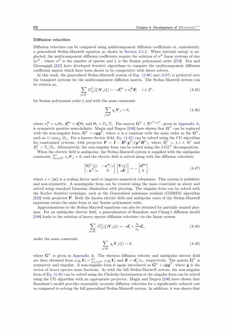
92 Chapter 4. Development of Mutation++
Diffusion velocities
Diffusion velocities can be computed using multicomponent diffusion coefficients or, equivalently,a generalized Stefan-Maxwell equation as shown in Section 2.5.2. When internal energy is ne-glected, the multicomponent diffusion coefficients require the solution of nS linear systems of sizeξnS , where nS is the number of species and ξ is the Sonine polynomial order [219]. Ern andGiovangigli [221] have developed iterative algorithms to compute the multicomponent diffusioncoefficient matrix which have been shown to be competitive with direct solvers.
In this work, the generalized Stefan-Maxwell system of Eqs. (2.86) and (2.87) is preferred overthe transport systems for the multicomponent diffusion matrix. The Stefan-Maxwell system canbe written as,
∑
j∈S∗
GVij(ξ)V j(ξ) = −dΘ
i′ + κΘi E, i ∈ S∗, (4.45)
for Sonine polynomial order ξ and with the mass constraint∑
j∈S∗
yjV j = 0, (4.46)
where κΘi = κiΘi, dΘi′ = d′
iΘi and Θi = Th/Ti. The matrix GV ∈ RnS×nS
, given in Appendix A,is symmetric positive semi-definite. Magin and Degrez [106] have shown that GV can be replacedwith the non-singular form, GV + αyyT , where α is a constant with the same order as the GV ,such as 1/maxij Dij . For a known electric field, Eq. (4.45) can be solved using the CG algorithmfor constrained systems, with projector P = I − RV yT /(yTRV ), where RV
i = 1, i ∈ H∗ andRV
e = Te/Th. Alternatively, the non-singular form can be solved using the LDLT decomposition.When the electric field is ambipolar, the Stefan-Maxwell system is supplied with the ambipolar
constraint,∑
j∈S∗ κjV j = 0, and the electric field is solved along with the diffusion velocities,
[
GV (ξ) −κΘ/s−κT /s 0
] [
V (ξ)sE
]
= −[
dΘ′
0
]
, (4.47)
where s = ∥κ∥ is a scaling factor used to improve numerical robustness. This system is indefiniteand non-symmetric. A nonsingular form can be created using the mass constraint as above andsolved using standard Gaussian elimination with pivoting. The singular form can be solved withthe Krylov iterative technique, such as the Generalized minimum residual (GMRES) algorithm[222] with projector P. Both the known electric field and ambipolar cases of the Stefan-Maxwellequations retain the same form at any Sonine polynomial order.
Approximations to the Stefan-Maxwell equations can also be obtained for partially ionized plas-mas. For an ambipolar electric field, a generalization of Ramshaw and Chang’s diffusion model[106] leads to the solution of heavy species diffusion velocities via the linear system
∑
j∈H∗
GVij(ξ)V j(ξ) = −d′
i +κiκe
d′e, (4.48)
under the mass constraint∑
j∈H∗
yjV j(ξ) = 0, (4.49)
where GV is given in Appendix A. The electron diffusion velocity and ambipolar electric fieldare then obtained from xeqeVe =
∑
j∈H∗ xjqjVj and E = d′e/κe, respectively. The matrix GV is
symmetric and singular. A non-singular form is again introduced as GV + ayyT , where y is thevector of heavy-species mass fractions. As with the full Stefan-Maxwell system, the non-singularform of Eq. (4.48) can be solved using the Cholesky factorization or the singular form can be solvedusing the CG algorithm with an appropriate projector. Magin and Degrez [106] have shown thatRamshaw’s model provides reasonably accurate diffusion velocities for a significantly reduced costas compared to solving the full generalized Stefan-Maxwell system. In addition, it was shown that
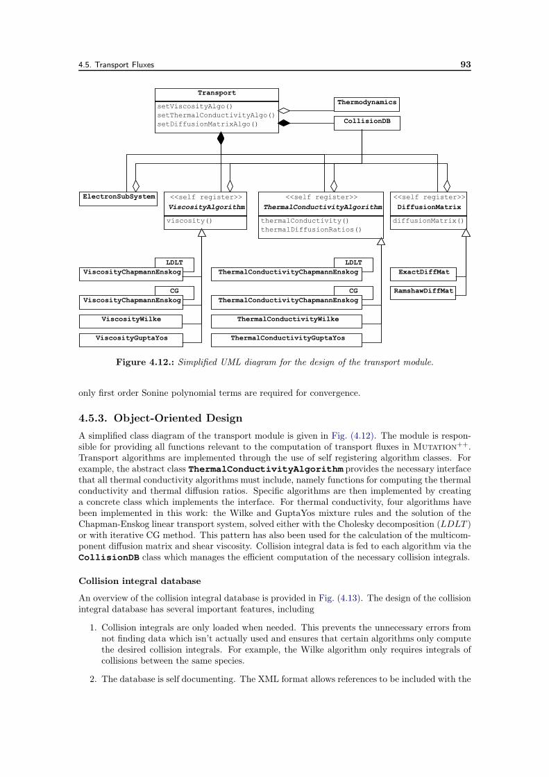
4.5. Transport Fluxes 93
LDLTLDLT
CGCG
Transport
setViscosityAlgo()setThermalConductivityAlgo()setDiffusionMatrixAlgo()
Thermodynamics
CollisionDB
ElectronSubSystemViscosityAlgorithm<<self register>>
viscosity()
ThermalConductivityAlgorithm<<self register>>
thermalConductivity()thermalDiffusionRatios()
DiffusionMatrix<<self register>>
diffusionMatrix()
ViscosityWilke
ViscosityChapmannEnskog
ViscosityGuptaYos
ThermalConductivityChapmannEnskog
ThermalConductivityWilke
ThermalConductivityGuptaYos
ExactDiffMat
RamshawDiffMat
ViscosityChapmannEnskog ThermalConductivityChapmannEnskog
Figure 4.12.: Simplified UML diagram for the design of the transport module.
only first order Sonine polynomial terms are required for convergence.
4.5.3. Object-Oriented Design
A simplified class diagram of the transport module is given in Fig. (4.12). The module is respon-sible for providing all functions relevant to the computation of transport fluxes in Mutation++.Transport algorithms are implemented through the use of self registering algorithm classes. Forexample, the abstract class ThermalConductivityAlgorithm provides the necessary interfacethat all thermal conductivity algorithms must include, namely functions for computing the thermalconductivity and thermal diffusion ratios. Specific algorithms are then implemented by creatinga concrete class which implements the interface. For thermal conductivity, four algorithms havebeen implemented in this work: the Wilke and GuptaYos mixture rules and the solution of theChapman-Enskog linear transport system, solved either with the Cholesky decomposition (LDLT )or with iterative CG method. This pattern has also been used for the calculation of the multicom-ponent diffusion matrix and shear viscosity. Collision integral data is fed to each algorithm via theCollisionDB class which manages the efficient computation of the necessary collision integrals.
Collision integral database
An overview of the collision integral database is provided in Fig. (4.13). The design of the collisionintegral database has several important features, including
1. Collision integrals are only loaded when needed. This prevents the unnecessary errors fromnot finding data which isn’t actually used and ensures that certain algorithms only computethe desired collision integrals. For example, the Wilke algorithm only requires integrals ofcollisions between the same species.
2. The database is self documenting. The XML format allows references to be included with the
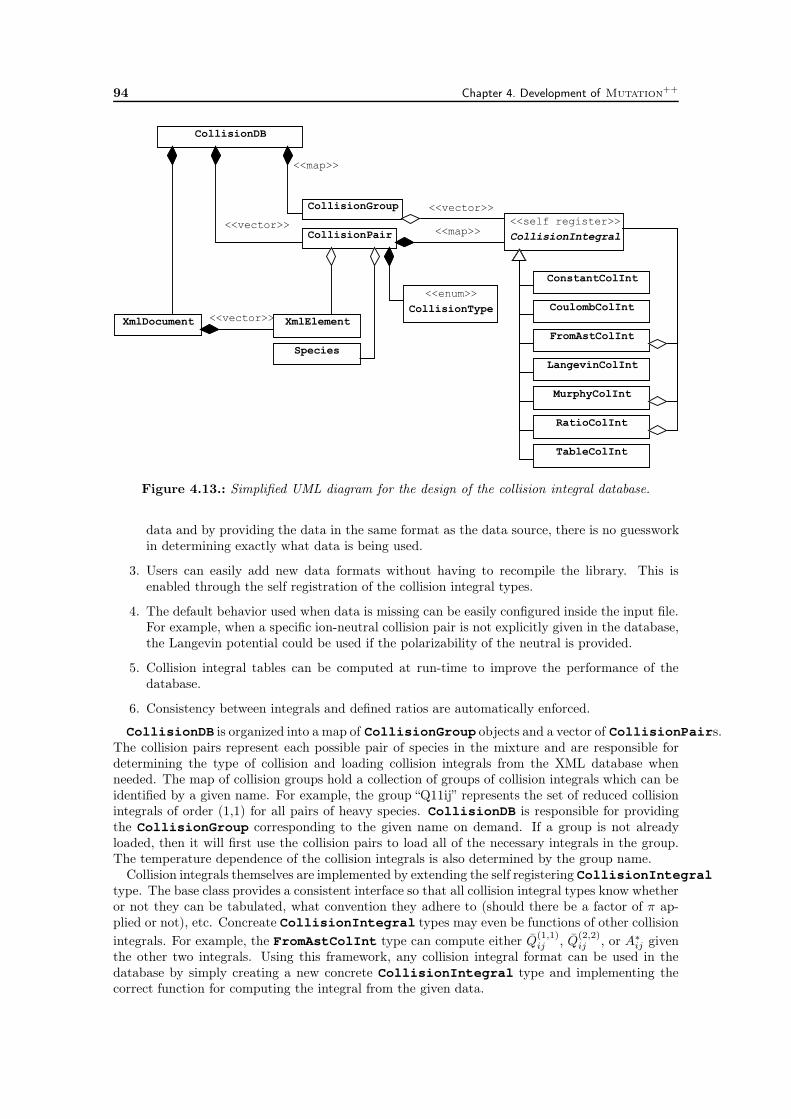
94 Chapter 4. Development of Mutation++
CollisionDB
CollisionPair<<vector>>
CollisionGroup
<<map>>
CollisionType<<enum>>
TableColInt
ConstantColInt
FromAstColInt
MurphyColInt
RatioColInt
CoulombColInt
LangevinColInt
CollisionIntegral<<self register>>
<<map>>
<<vector>>
Species
XmlDocument XmlElement<<vector>>
Figure 4.13.: Simplified UML diagram for the design of the collision integral database.
data and by providing the data in the same format as the data source, there is no guessworkin determining exactly what data is being used.
3. Users can easily add new data formats without having to recompile the library. This isenabled through the self registration of the collision integral types.
4. The default behavior used when data is missing can be easily configured inside the input file.For example, when a specific ion-neutral collision pair is not explicitly given in the database,the Langevin potential could be used if the polarizability of the neutral is provided.
5. Collision integral tables can be computed at run-time to improve the performance of thedatabase.
6. Consistency between integrals and defined ratios are automatically enforced.
CollisionDB is organized into a map of CollisionGroup objects and a vector of CollisionPairs.The collision pairs represent each possible pair of species in the mixture and are responsible fordetermining the type of collision and loading collision integrals from the XML database whenneeded. The map of collision groups hold a collection of groups of collision integrals which can beidentified by a given name. For example, the group “Q11ij” represents the set of reduced collisionintegrals of order (1,1) for all pairs of heavy species. CollisionDB is responsible for providingthe CollisionGroup corresponding to the given name on demand. If a group is not alreadyloaded, then it will first use the collision pairs to load all of the necessary integrals in the group.The temperature dependence of the collision integrals is also determined by the group name.
Collision integrals themselves are implemented by extending the self registering CollisionIntegraltype. The base class provides a consistent interface so that all collision integral types know whetheror not they can be tabulated, what convention they adhere to (should there be a factor of π ap-plied or not), etc. Concreate CollisionIntegral types may even be functions of other collisionintegrals. For example, the FromAstColInt type can compute either Q(1,1)
ij , Q(2,2)ij , or A∗
ij giventhe other two integrals. Using this framework, any collision integral format can be used in thedatabase by simply creating a new concrete CollisionIntegral type and implementing thecorrect function for computing the integral from the given data.
4.5. Transport Fluxes 95
4.5.4. Transport Properties
This section serves to both demonstrate and validate the calculation of transport coefficients forseveral equilibrium, partially ionized mixtures. For reference, Fig. (4.14) shows the equilibriumcompositions of the three mixtures considered here. The first mixture represents equilibriumair, considering the eleven species comprised of N, N2, O, O2, NO, and their first ions plus freeelectrons. The second mixture is equilibrium carbon-dioxide. Eight species are considered: CO2,CO, O2, O, C, O+, C+, and e– . The last mixture is equilibrium Jovian atmosphere consisting ofthe nine species H2, H2
+, H, H+, H– , He, He+, He++, and e– . The equilibrium compositions havebeen computed using the Gibbs energy minimization procedure detailed in Chapter 5 at constantpressure of 1 atm.
Viscosity
The equilibrium shear viscosities of each of the mixtures shown in Fig. (4.14) are presented inFig. (4.15). In addition, the viscosity of several frozen mixtures corresponding to the equilib-rium compositions at specified temperatures are also shown. For the air and CO2 cases, thesetemperatures are 300K, 5000K, 10 000K, 15 000K, and 20 000K. For the Jupiter mixture, thetemperatures are taken to be 300K, 3500K, 13 000K, 30 000K, and 50 000K in order to accom-modate the larger temperature range.
Two general trends can be seen in Fig. (4.15). The first is that viscosity tends to increase withtemperature for a fixed mixture composition as is visible from the frozen cases. The second isthat viscosity decreases with increasing levels of ionization. Both trends are easily predicted byconsidering the viscosity of a pure gas i (given in Appendix A),
ηi =5
16
√πkBTmi
Q(2,2)ii
, (4.50)
where mi and Q(2,2)ii are the mass and reduced collision integral of the gas. As was noted in
Section 4.5.1, the collision integrals for resonant charge transfer and charged interactions are sig-nificantly larger than other collisions due to Coulomb forces. Thus, as the level of ionizationincreases, these interactions dominate and the viscosity decreases due to the inverse proportional-ity with Q(2,2)
ii .Fig. (4.15) includes comparisons with literature results for both the air and Jupiter mixtures. For
air, the computed viscosity is compared to the result obtained by D’Angola et al. [197] who havedeveloped a set of accurate curve-fits for equilibrium air thermodynamic and transport properties.The Jupiter result is compared with the calculations of Bruno et al. [203] based on a review ofaccurate collision integral data for Jupiter mixtures. Only minor differences can be seen in bothcases. In the air case, the differences can be attributed small differences in the collision integraldata used in this work compared to [197], while in the Jupiter case, the differences are a result ofslightly different equilibrium compositions as a result of the thermodynamic data used in [203].
Diffusion fluxes
For a mixture in thermochemical equilibrium with constant pressure and element fractions, speciesdiffusion velocities may be expressed from Eqs. (2.84) and (2.85) as,
Vi = −∑
j∈S
Dij
[
∂xj
∂T+
(χhj + χe
j)
T
]
∇T +E∑
j∈S
Dijκj , ∀ i ∈ S, (4.51)
where ∂xj/∂T are the derivatives of equilibrium species mole fractions with respect to tempera-ture. It will be shown in Chapter 5 that these derivatives can be evaluated cheaply during thesolution of the equilibrium compositions. In principle, when element fractions are assumed con-stant, the mole fraction derivatives should be constrained to prevent elemental demixing [224, 225]through the diffusion of elements. The electric field E can either be specified in Eq. (4.51), or
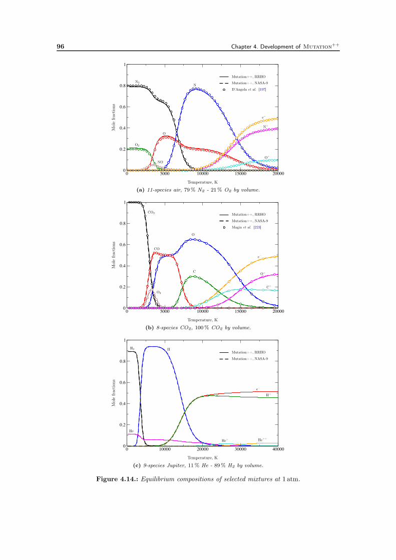
96 Chapter 4. Development of Mutation++
0 5000 10000 15000 200000
0.2
0.4
0.6
0.8
1
Temperature, K
Mol
efr
action
s
Mutation++, RRHO
Mutation++, NASA-9
D’Angola et al. [197]N
N2
O
O2
NO
N+
O+
e–
(a) 11-species air, 79% N2 - 21% O2 by volume.
0 5000 10000 15000 200000
0.2
0.4
0.6
0.8
1
Temperature, K
Mol
efr
action
s
Mutation++, RRHO
Mutation++, NASA-9
Magin et al. [223]
O
O2
O+
e–
CO
CO2
C
C+
(b) 8-species CO2, 100% CO2 by volume.
0 10000 20000 30000 400000
0.2
0.4
0.6
0.8
1
Temperature, K
Mol
efr
action
s
Mutation++, RRHO
Mutation++, NASA-9
e–
H2 H
H+
He
He+ He++
(c) 9-species Jupiter, 11% He - 89% H2 by volume.
Figure 4.14.: Equilibrium compositions of selected mixtures at 1 atm.
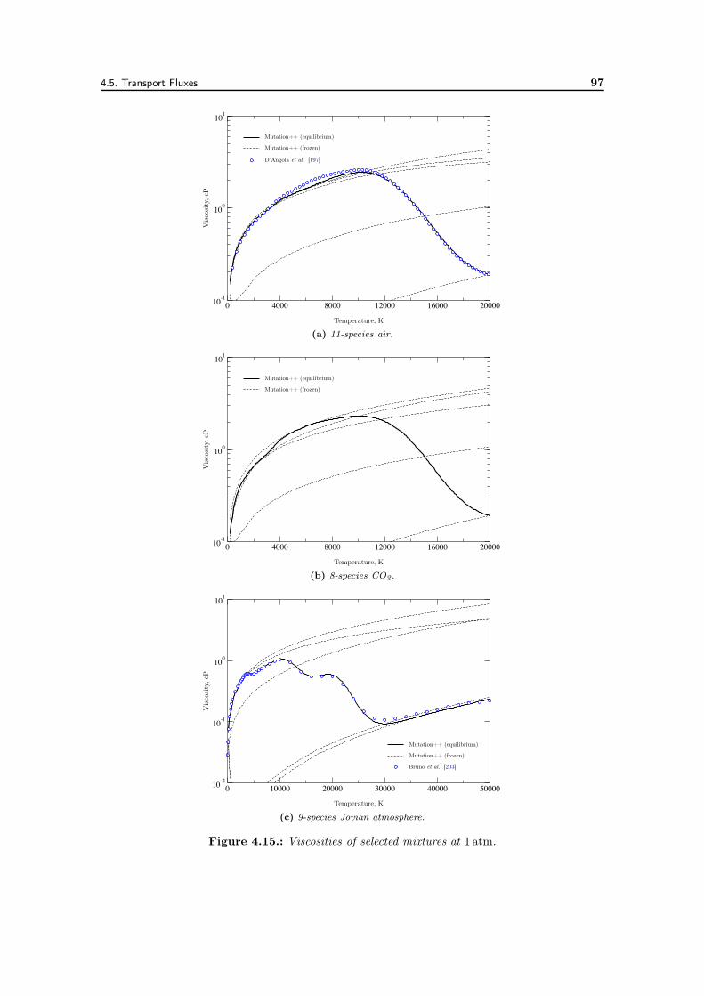
4.5. Transport Fluxes 97
0 4000 8000 12000 16000 2000010-1
100
101
Temperature, K
Vis
cosi
ty,c
P
Mutation++ (equilibrium)
D’Angola et al. [197]
Mutation++ (frozen)
(a) 11-species air.
0 4000 8000 12000 16000 2000010-1
100
101
Temperature, K
Vis
cosi
ty,c
P
Mutation++ (equilibrium)
Mutation++ (frozen)
(b) 8-species CO2.
0 10000 20000 30000 40000 5000010-2
10-1
100
101
Temperature, K
Vis
cosi
ty,c
P
Mutation++ (equilibrium)
Bruno et al. [203]
Mutation++ (frozen)
(c) 9-species Jovian atmosphere.
Figure 4.15.: Viscosities of selected mixtures at 1 atm.
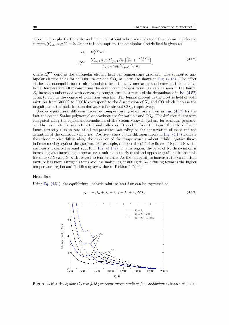
98 Chapter 4. Development of Mutation++
determined explicitly from the ambipolar constraint which assumes that there is no net electriccurrent,
∑
i∈S niqiVi = 0. Under this assumption, the ambipolar electric field is given as
Ea = E∇Ta ∇T
E∇Ta =
∑
i∈S niqi∑
j∈S Dij
[∂xj
∂T +(χh
j +χej )
T
]
∑
i∈S niqi∑
j∈S Dijκj,
(4.52)
where E∇Ta denotes the ambipolar electric field per temperature gradient. The computed am-
bipolar electric fields for equilibrium air and CO2 at 1 atm are shown in Fig. (4.16). The effectof thermal nonequilibrium is also simulated by artificially increasing the heavy particle transla-tional temperature after computing the equilibrium compositions. As can be seen in the figure,Ea increases unbounded with decreasing temperature as a result of the denominator in Eq. (4.52)going to zero as the degree of ionization vanishes. The bumps present in the electric field of bothmixtures from 5000K to 8000K correspond to the dissociation of N2 and CO which increase themagnitude of the mole fraction derivatives for air and CO2, respectively.
Species equilibrium diffusion fluxes per temperature gradient are shown in Fig. (4.17) for thefirst and second Sonine polynomial approximations for both air and CO2. The diffusion fluxes werecomputed using the equivalent formulation of the Stefan-Maxwell system, for constant pressure,equilibrium mixtures, neglecting thermal diffusion. It is clear from the figure that the diffusionfluxes correctly sum to zero at all temperatures, according to the conservation of mass and thedefinition of the diffusion velocities. Positive values of the diffusion fluxes in Fig. (4.17) indicatethat those species diffuse along the direction of the temperature gradient, while negative fluxesindicate moving against the gradient. For example, consider the diffusive fluxes of N2 and N whichare nearly balanced around 7000K in Fig. (4.17a). In this region, the level of N2 dissociation isincreasing with increasing temperature, resulting in nearly equal and opposite gradients in the molefractions of N2 and N, with respect to temperature. As the temperature increases, the equilibriummixture has more nitrogen atoms and less molecules, resulting in N2 diffusing towards the highertemperature region and N diffusing away due to Fickian diffusion.
Heat flux
Using Eq. (4.51), the equilibrium, isobaric mixture heat flux can be expressed as
q = −(λh + λe + λint + λr + λs)∇T, (4.53)
2500 5000 7500 10000 12500 15000 17500 200000
2
4
6
8
Te, K
Ele
ctri
cFie
ld,mV/K
Air
CO2
Th = Te
Th = Te + 5000K
Th = Te + 10 000K
Figure 4.16.: Ambipolar electric field per temperature gradient for equilibrium mixtures at 1 atm.
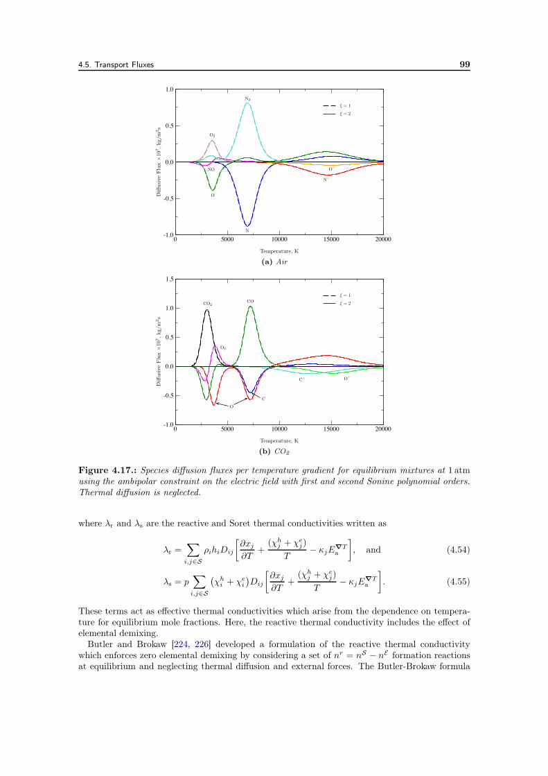
4.5. Transport Fluxes 99
0 5000 10000 15000 20000-1.0
-0.5
0.0
0.5
1.0
Temperature, K
Diff
usiv
eFlu
x×10
7,kg
/m2s
ξ = 1
ξ = 2
N
N2
O
O2
NO
N+
O+
(a) Air
0 5000 10000 15000 20000-1.0
-0.5
0.0
0.5
1.0
1.5
Temperature, K
Diff
usiv
eFlu
x×10
7,kg
/m2s
ξ = 1
ξ = 2COCO2
O
O2
C
C+ O+
(b) CO2
Figure 4.17.: Species diffusion fluxes per temperature gradient for equilibrium mixtures at 1 atmusing the ambipolar constraint on the electric field with first and second Sonine polynomial orders.Thermal diffusion is neglected.
where λr and λs are the reactive and Soret thermal conductivities written as
λr =∑
i,j∈S
ρihiDij
[
∂xj
∂T+
(χhj + χe
j)
T− κjE
∇Ta
]
, and (4.54)
λs = p∑
i,j∈S
(
χhi + χe
i
)
Dij
[
∂xj
∂T+
(χhj + χe
j)
T− κjE
∇Ta
]
. (4.55)
These terms act as effective thermal conductivities which arise from the dependence on tempera-ture for equilibrium mole fractions. Here, the reactive thermal conductivity includes the effect ofelemental demixing.
Butler and Brokaw [224, 226] developed a formulation of the reactive thermal conductivitywhich enforces zero elemental demixing by considering a set of nr = nS − nE formation reactionsat equilibrium and neglecting thermal diffusion and external forces. The Butler-Brokaw formula
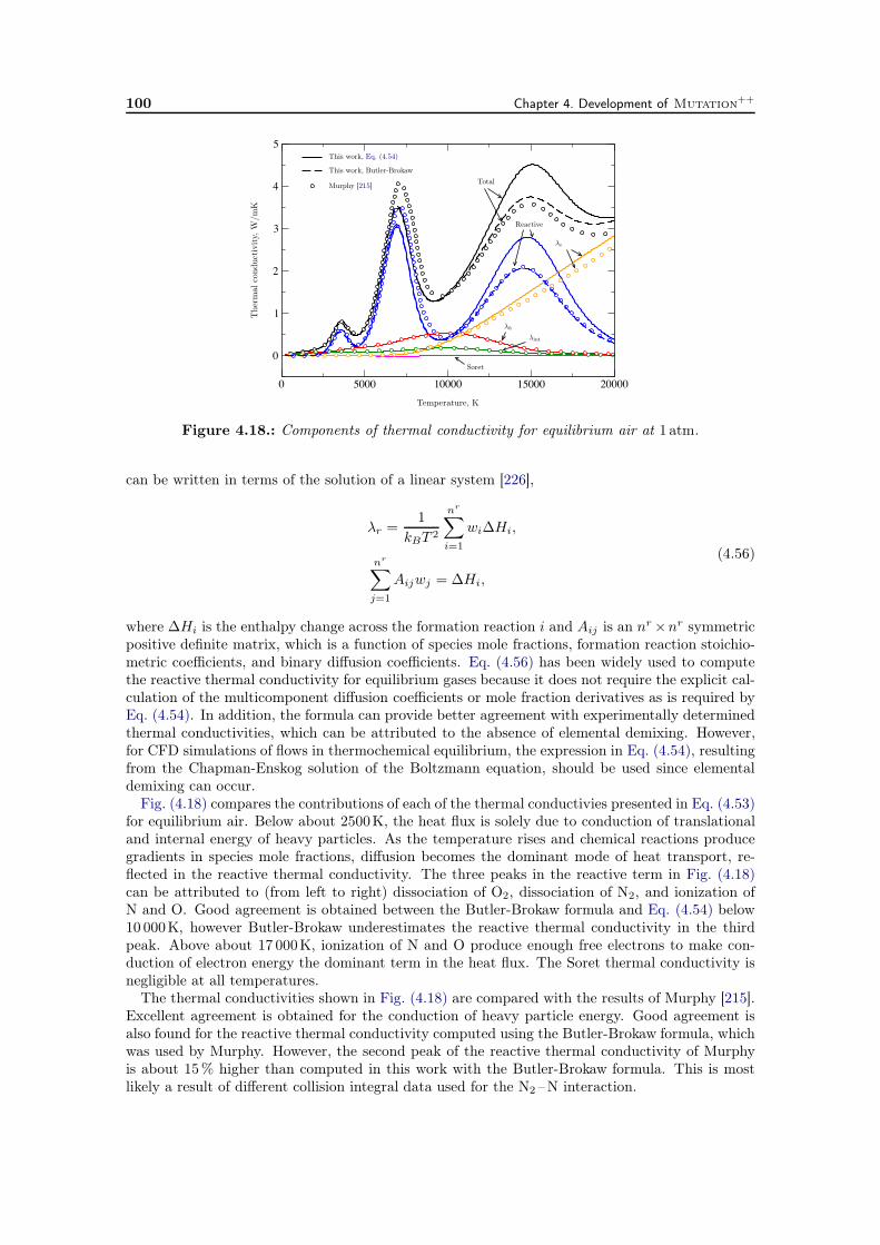
100 Chapter 4. Development of Mutation++
0 5000 10000 15000 20000
0
1
2
3
4
5
Temperature, K
The
rmal
cond
uctivi
ty,W
/mK
λh
λe
λint
Reactive
Soret
Total
This work, Eq. (4.54)
This work, Butler-Brokaw
Murphy [215]
Figure 4.18.: Components of thermal conductivity for equilibrium air at 1 atm.
can be written in terms of the solution of a linear system [226],
λr =1
kBT 2
nr∑
i=1
wi∆Hi,
nr∑
j=1
Aijwj = ∆Hi,
(4.56)
where ∆Hi is the enthalpy change across the formation reaction i and Aij is an nr ×nr symmetricpositive definite matrix, which is a function of species mole fractions, formation reaction stoichio-metric coefficients, and binary diffusion coefficients. Eq. (4.56) has been widely used to computethe reactive thermal conductivity for equilibrium gases because it does not require the explicit cal-culation of the multicomponent diffusion coefficients or mole fraction derivatives as is required byEq. (4.54). In addition, the formula can provide better agreement with experimentally determinedthermal conductivities, which can be attributed to the absence of elemental demixing. However,for CFD simulations of flows in thermochemical equilibrium, the expression in Eq. (4.54), resultingfrom the Chapman-Enskog solution of the Boltzmann equation, should be used since elementaldemixing can occur.
Fig. (4.18) compares the contributions of each of the thermal conductivies presented in Eq. (4.53)for equilibrium air. Below about 2500K, the heat flux is solely due to conduction of translationaland internal energy of heavy particles. As the temperature rises and chemical reactions producegradients in species mole fractions, diffusion becomes the dominant mode of heat transport, re-flected in the reactive thermal conductivity. The three peaks in the reactive term in Fig. (4.18)can be attributed to (from left to right) dissociation of O2, dissociation of N2, and ionization ofN and O. Good agreement is obtained between the Butler-Brokaw formula and Eq. (4.54) below10 000K, however Butler-Brokaw underestimates the reactive thermal conductivity in the thirdpeak. Above about 17 000K, ionization of N and O produce enough free electrons to make con-duction of electron energy the dominant term in the heat flux. The Soret thermal conductivity isnegligible at all temperatures.
The thermal conductivities shown in Fig. (4.18) are compared with the results of Murphy [215].Excellent agreement is obtained for the conduction of heavy particle energy. Good agreement isalso found for the reactive thermal conductivity computed using the Butler-Brokaw formula, whichwas used by Murphy. However, the second peak of the reactive thermal conductivity of Murphyis about 15% higher than computed in this work with the Butler-Brokaw formula. This is mostlikely a result of different collision integral data used for the N2 –N interaction.
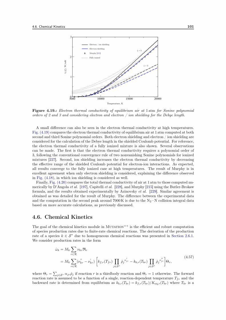
4.6. Chemical Kinetics 101
5000 10000 15000 200000
1
2
3
Temperature, K
λe(ξ),
W/m
K
Murphy [215]
Electron / ion shielding
Electron shielding
Fully ionized
ξ = 2
ξ = 3
Figure 4.19.: Electron thermal conductivity of equilibrium air at 1 atm for Sonine polynomialorders of 2 and 3 and considering electron and electron / ion shielding for the Debye length.
A small difference can also be seen in the electron thermal conductivity at high temperatures.Fig. (4.19) compares the electron thermal conductivity of equilibrium air at 1 atm computed at bothsecond and third Sonine polynomial orders. Both electron shielding and electron / ion shielding areconsidered for the calculation of the Debye length in the shielded Coulomb potential. For reference,the electron thermal conductivity of a fully ionized mixture is also shown. Several observationscan be made. The first is that the electron thermal conductivity requires a polynomial order of3, following the conventional convergence rule of two nonvanishing Sonine polynomials for ionizedmixtures [227]. Second, ion shielding increases the electron thermal conductivity by decreasingthe effective range of the shielded Coulomb potential for electron-ion interactions. As expected,all results converge to the fully ionized case at high temperatures. The result of Murphy is inexcellent agreement when only electron shielding is considered, explaining the difference observedin Fig. (4.18), in which ion shielding is considered as well.
Finally, Fig. (4.20) compares the total thermal conductivity of air at 1 atm to those computed nu-merically by D’Angola et al. [197], Capitelli et al. [228], and Murphy [215] using the Butler-Brokawformula, and the results obtained experimentally by Azinovsky et al. [229]. Similar agreement isobtained as was detailed for the result of Murphy. The difference between the experimental dataand the computation in the second peak around 7000K is due to the N2 –N collision integral databased on more accurate calculations, as previously discussed.
4.6. Chemical Kinetics
The goal of the chemical kinetics module in Mutation++ is the efficient and robust computationof species production rates due to finite-rate chemical reactions. The derivation of the productionrate of a species k ∈ S∗ due to homogeneous chemical reactions was presented in Section 2.6.1.We consider production rates in the form
ωk = Mk
∑
r∈R
νkrRr
= Mk
∑
r∈R
(ν′′
kr − ν′
kr)
[
kf,r(Tfr)∏
j∈S∗
ρjν′
jr − kb,r(Tbr)∏
j∈S∗
ρjν′′
jr
]
Θr,(4.57)
where Θr =∑
j∈S∗ αjrρj if reaction r is a thirdbody reaction and Θr = 1 otherwise. The forwardreaction rate is assumed to be a function of a single, reaction-dependent temperature Tfr and thebackward rate is determined from equilibrium as kb,r(Tbr) = kf,r(Tbr)/Keq,r(Tbr) where Tbr is a
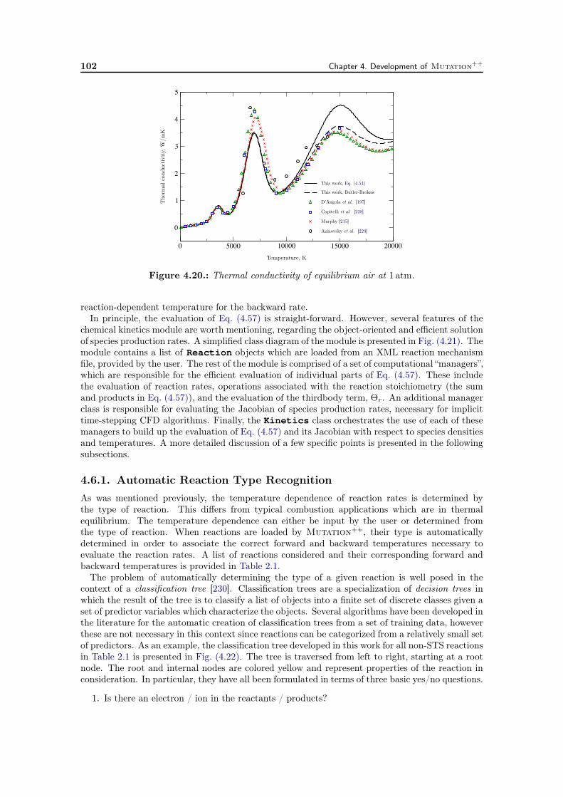
102 Chapter 4. Development of Mutation++
0 5000 10000 15000 20000
0
1
2
3
4
5
Temperature, K
The
rmal
cond
uctivi
ty,W
/mK
This work, Eq. (4.54)
This work, Butler-Brokaw
Murphy [215]
Capitelli et al. [228]
D’Angola et al. [197]
Azinovsky et al. [229]
Figure 4.20.: Thermal conductivity of equilibrium air at 1 atm.
reaction-dependent temperature for the backward rate.In principle, the evaluation of Eq. (4.57) is straight-forward. However, several features of the
chemical kinetics module are worth mentioning, regarding the object-oriented and efficient solutionof species production rates. A simplified class diagram of the module is presented in Fig. (4.21). Themodule contains a list of Reaction objects which are loaded from an XML reaction mechanismfile, provided by the user. The rest of the module is comprised of a set of computational “managers”,which are responsible for the efficient evaluation of individual parts of Eq. (4.57). These includethe evaluation of reaction rates, operations associated with the reaction stoichiometry (the sumand products in Eq. (4.57)), and the evaluation of the thirdbody term, Θr. An additional managerclass is responsible for evaluating the Jacobian of species production rates, necessary for implicittime-stepping CFD algorithms. Finally, the Kinetics class orchestrates the use of each of thesemanagers to build up the evaluation of Eq. (4.57) and its Jacobian with respect to species densitiesand temperatures. A more detailed discussion of a few specific points is presented in the followingsubsections.
4.6.1. Automatic Reaction Type Recognition
As was mentioned previously, the temperature dependence of reaction rates is determined bythe type of reaction. This differs from typical combustion applications which are in thermalequilibrium. The temperature dependence can either be input by the user or determined fromthe type of reaction. When reactions are loaded by Mutation++, their type is automaticallydetermined in order to associate the correct forward and backward temperatures necessary toevaluate the reaction rates. A list of reactions considered and their corresponding forward andbackward temperatures is provided in Table 2.1.
The problem of automatically determining the type of a given reaction is well posed in thecontext of a classification tree [230]. Classification trees are a specialization of decision trees inwhich the result of the tree is to classify a list of objects into a finite set of discrete classes given aset of predictor variables which characterize the objects. Several algorithms have been developed inthe literature for the automatic creation of classification trees from a set of training data, howeverthese are not necessary in this context since reactions can be categorized from a relatively small setof predictors. As an example, the classification tree developed in this work for all non-STS reactionsin Table 2.1 is presented in Fig. (4.22). The tree is traversed from left to right, starting at a rootnode. The root and internal nodes are colored yellow and represent properties of the reaction inconsideration. In particular, they have all been formulated in terms of three basic yes/no questions.
1. Is there an electron / ion in the reactants / products?
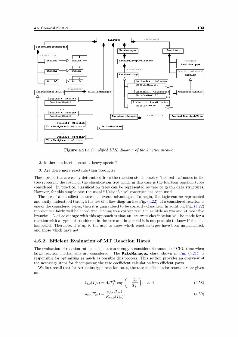
4.6. Chemical Kinetics 103
Stoich
Stoich
Stoich Stoich
StoichArrhen ector
Arrhen eSelector
Arrhen Selector
cs
ReactionStoichiometryManager
RateManager
ager
anManager
RateLaw<<self register>>
Reacti<<enum>>
ArrheniusRat
<<vector>>
RateLa Collection
RateLawGroup
<<vector>>
RateLa
RateLa
RateLa
<<vector>>
StoichStoich
<<vector>>
Stoich Stoich
Stoich Stoich
ReactionStoi<<vector>>
ReactionStoich
ReactionStoich
ectionStoich
...
ctionStoich
Figure 4.21.: Simplified UML diagram of the kinetics module.
2. Is there an inert electron / heavy species?
3. Are there more reactants than products?
These properties are easily determined from the reaction stoichiometry. The red leaf nodes in thetree represent the result of the classification tree which in this case is the fourteen reaction typesconsidered. In practice, classification trees can be represented as tree or graph data structures.However, for this simple case the usual “if/else if/else” construct has been used.
The use of a classification tree has several advantages. To begin, the logic can be representedand easily understood through the use of a flow diagram like Fig. (4.22). If a considered reaction isone of the considered types, then it is guaranteed to be correctly classified. In addition, Fig. (4.22)represents a fairly well balanced tree, leading to a correct result in as little as two and at most fivebranches. A disadvantage with this approach is that an incorrect classification will be made for areaction with a type not considered in the tree and in general it is not possible to know if this hashappened. Therefore, it is up to the user to know which reaction types have been implemented,and those which have not.
4.6.2. Efficient Evaluation of MT Reaction Rates
The evaluation of reaction rate coefficients can occupy a considerable amount of CPU time whenlarge reaction mechanisms are considered. The RateManager class, shown in Fig. (4.21), isresponsible for optimizing as much as possible this process. This section provides an overview ofthe necessary steps for decomposing the rate coefficient calculation into efficient parts.
We first recall that for Arrhenius type reaction rates, the rate coefficients for reaction r are givenas
kf,r(Tfr) = ArTβr
fr exp
(
−θrTfr
)
, and (4.58)
kb,r(Tbr) =kf,r(Tbr)
Keq,r(Tbr), (4.59)
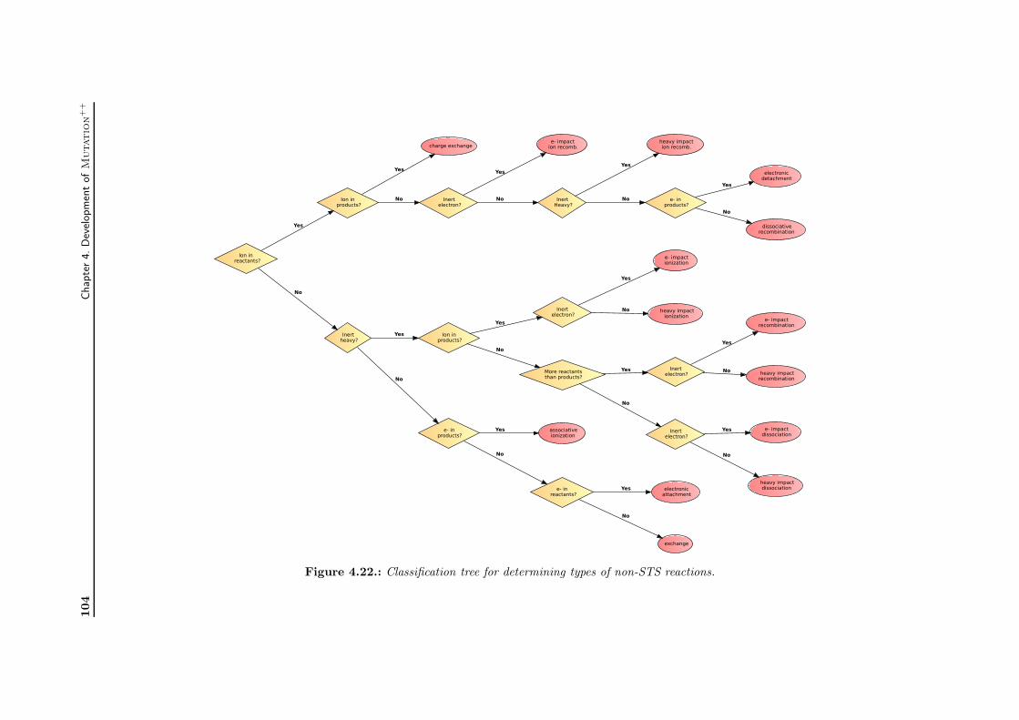
104
Chap
ter4.D
evel
opm
ent
ofM
utatio
n++
Ion in reactants?
Ion in products?
Yes
Inertheavy?
No
charge exchange
Yes
Inertelectron?
No
e- impact ion recomb.
Yes
InertHeavy?
No
heavy impact ion recomb.
Yes
e- in products?
No
electronicdetachment
Yes
dissociativerecombination
No
Ion inproducts?
Yes
e- inproducts?
No
Inertelectron?
Yes
More reactantsthan products?
No
e- impactionization
Yes
heavy impactionization
No
Inertelectron?
Yes
Inertelectron?
No
e- impactrecombination
Yes
heavy impactrecombination
No
e- impactdissociation
Yes
heavy impactdissociation
No
associativeionization
Yes
e- in reactants?
No
electronicattachment
Yes
exchange
No
Figure 4.22.: Classification tree for determining types of non-STS reactions.
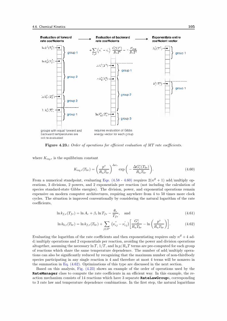
4.6. Chemical Kinetics 105
Figure 4.23.: Order of operations for efficient evaluation of MT rate coefficients.
where Keq,r is the equilibrium constant
Keq,r(Tbr) =
(
p
RuTbr
)∆νr
exp
(
−∆G
r(Tbr)
RuTbr
)
. (4.60)
From a numerical standpoint, evaluating Eqs. (4.58 - 4.60) requires 2(nS + 1) add/multiply op-erations, 3 divisions, 2 powers, and 2 exponentials per reaction (not including the calculation ofspecies standard-state Gibbs energies). The division, power, and exponential operations remainexpensive on modern computer architectures, requiring anywhere from 4 to 50 times more clockcycles. The situation is improved conventionally by considering the natural logarithm of the ratecoefficients,
ln kf,r(Tfr) = lnAr + βr lnTfr −θrTfr
, and (4.61)
ln kb,r(Tbr) = ln kf,r(Tbr) +∑
j∈S∗
(
ν′′
rj − ν′
rj
)
[
Gj
RuTbr− ln
(
p
RuTbr
)]
. (4.62)
Evaluating the logarithm of the rate coefficients and then exponentiating requires only nS + 4 ad-d/multiply operations and 2 exponentials per reaction, avoiding the power and division operationsaltogether, assuming the necessary lnT , 1/T , and ln p/RuT terms are pre-computed for each groupof reactions which share the same temperature dependence. The number of add/multiply opera-tions can also be significantly reduced by recognizing that the maximum number of non-thirdbodyspecies participating in any single reaction is 4 and therefore at most 4 terms will be nonzero inthe summation in Eq. (4.62). Optimizations of this type are discussed in the next section.
Based on this analysis, Fig. (4.23) shows an example of the order of operations used by theRateManager class to compute the rate coefficients in an efficient way. In this example, the re-action mechanism consists of 14 reactions which have 3 separate RateLawGroups, correspondingto 3 rate law and temperature dependence combinations. In the first step, the natural logarithms
106 Chapter 4. Development of Mutation++
of the forward rate coefficients are computed, including those used in the backward rate coeffi-cient evaluation. Note that for Arrhenius rate laws, Eq. (4.61) can be efficiently evaluated for awhole group using a matrix-vector product in order to minimize the effect of cache thrashing. Inthe example, groups 2 and 3 share the same rate law and temperature dependence in both theforward and backward directions, therefore the forward coefficient at the backward temperature isnot reevaluated. In a second step, the logarithm of the backward rate coefficients are evaluatedusing Eq. (4.62). Finally, the entire vector of forward and backward rate coefficients are exponen-tiated. Evaluating the entire vector at once allows for additional compiler optimizations, such asvectorization.
4.6.3. Stoichiometric Operations
The result of the summations and products in Eqs. (4.57) and (4.62) are functions of the stoichio-metric coefficients for all species in the species set for a given reaction. An important observationhowever, is that at most four species can have non-zero stoichiometric coefficients for any givenreaction. It is therefore inefficient to evaluate these summations and products by looping explic-itly over all species. The class StoichiometryManager shown in Fig. (4.21) is responsible forevaluating these operations in an efficient way by keeping track of species indices which contributeto each reaction and providing suitable stoichiometric operations.
4.7. Concluding Remarks
This chapter detailed the design of Mutation++, a new software library written in C++ forproviding physicochemical models, data, and algorithms for use in hypersonic CFD codes. Thelibrary has been designed using modern OOP techniques in an effort to maximize its extendabilityand efficiency. The driving principle behind Mutation++ is the ability to separate the underlyingthermochemical model from the set of governing equations solved by the CFD tool. A genericset of governing equations was presented which encompasses all of the energy partitioning andthermochemical nonequilibrium models presented in Chapter 2. The concept of a state model wasalso introduced to provide the link between CFD and Mutation++. At a high level, the libraryis organized into three modules: thermodynamics, transport, and chemical kinetics.
Two separate thermodynamic databases were presented in the framework of the thermodynamicsmodule: one based on the RRHO energy partitioning model and the other based on the NASAthermodynamic polynomials. Pure species thermodynamic properties were derived based on theRRHO assumption and a summary of the resulting analytical expressions for these properties waspresented using fundamental properties of the molecules. Using an object-oriented approach, bothdatabases are seamlessly integrated and can be selected by the user at run-time. A comparisonof mixture thermodynamic properties for equilibrium air, using both databases and the work ofD’Angola et al. [197], serves to validate the implementation of the module.
The transport module was split roughly into the calculation of transport collision integrals anda discussion of transport algorithms. The collision integrals were defined for a multitemperaturegas in which heavy species and free electrons thermalize at different temperatures. A summary ofthe necessary collision integrals required to compute all of the transport properties presented inChapter 2 was provided. In addition, an extensive review of common interaction potentials used tocompute collision integrals was made for neutral-neutral, ion-neutral, electron-neutral, and chargedparticle interactions. It was shown that collision integral data comes in a wide variety of formats inthe literature and that the OOP approach used in the design of the Mutation++ collision integraldatabase allows for each of these formats to be integrated in a simple and efficient way. Transportalgorithms were also reviewed in this chapter based on a previous work by Magin and Degrez [107].Transport properties for equilibrium air, CO2, and Jupiter were compared with relevant literatureresults in order to validate the transport module.
A few important aspects of the chemical kinetics module were also presented in this chapterincluding an object-oriented approach for the efficient calculation of species chemical productionrates. In addition, a classification tree was developed to enable the automatic classification of

4.7. Concluding Remarks 107
chemical reactions in order to determine the correct temperature dependence of individual reactionrates in a multitemperature context.
The Mutation++ library has been coupled to the computational tools presented in Chapter 6and applied to several atmospheric entry simulations in Chapter 7. Apart from the direct con-tribution to this thesis, it is worth mentioning that Mutation++ has contributed to a numberof other applications as well. These include the study of biomass pyrolysis [231], state-to-statecatalytic recombination of nitrogen flows, [232], transport properties of carbon-phenolic ablationmixtures [208], atmospheric entry of meteors [233, 234], and uncertainty quantification for highenthalpy, plasma wind tunnels [235]. Finally, the library is available for download, open source, athttps://sync.vki.ac.be/mpp/mutationpp.

CHAPTER 5
Linearly Constrained Multiphase Equilibria
“Gibbs is the greatest mind in American history."
— Albert Einstien, (c. 1925)
5.1. Introduction
The efficient and robust computation of multiphase, constrained equilibrium compositions is animportant topic over a wide range of fields including combustion, aerospace and (bio)chemical engi-neering, metallurgy, paper processes, and the design of thermal protection systems for atmosphericentry vehicles (e.g., [236–241]). For a detailed history and list of applications, the reader is referredto the treatises by van Zeggeren and Storey [242] or Smith and Missen [243].
Prior to the work of White et al. [244], the equilibrium constant formulation was primarilyused to compute equilibrium compositions for ideal, gas phase mixtures. The equilibrium constantformulation works by assigning formation reactions to each species based on a set of base orcomponent species which are chosen a priori for the given reaction system. Kuo [117] cites severaldisadvantages that hindered researches using this method including difficulties in extending themethod to non ideal equations of state, testing for the presence of condensed species and numericalcomplications with the use of component species.
In 1958, White, Johnson, and Dantzig [244] introduced the concept of free-energy minimizationand proposed a numerical solution technique using the method of steepest decent. White [245]later elaborated on the advantages of free-energy minimization and the use of element potentialsin the solution of equilibrium compositions, including the possibility to treat any general chemicalsystem without the necessity of specifying the formation reactions. In addition, the use of elementpotentials allowed for the solution of linear systems whose size scaled with the number of elementsrather than species, present in the mixture. This fact alone offers a significant computationaladvantage when considering large chemical systems.
Today, both the equilibrium constant formulation and the free-energy minimization methodsare widely used. Most commercial and general purpose research codes implement various numer-ical methods for solving the free-energy minimization problem, however the equilibrium constantformulation is still used in certain applications [103, 239]. Perhaps one of the most widely used equi-librium codes today is the Stanford-JANAF (STANJAN) code by Reynolds [246] who popularizedthe element potential method for constrained Gibbs free-energy minimization by developing a nu-merical solution procedure to the minimization problem which solves the so-called “dual problem.”Part of the success of the STANJAN method lies in its powerful initialization and preconditioningprocedures which help make STANJAN extremely robust for most problems. The CEA code devel-oped by Gordon and McBride [166, 182] is also used heavily, helped by the success of the detailedthermodynamic database developed at NASA Glenn Research Center [181], which it employs.
In addition to the normal mass balance constraints, so called “generalized constraints” [247] onthe equilibrium solution have been used in a wide range of applications [238] and in particular, arean integral component of the Rate-Controlled Chemical Equilibrium (RCCE) [247–261] method.Some important examples of constraints used in the RCCE method include constraints on the
110 Chapter 5. Linearly Constrained Multiphase Equilibria
total number of moles, the number of free valence electrons, and the number of O–O bonds,among many others [238, 260]. Bishnu et al. [262, 263] added the ability to include general linearconstraints on the equilibrium solutions to both STANJAN and CEA. They found that, undercertain conditions, both the constrained versions of STANJAN and CEA failed to converge toa solution. In general, these situations arise when the linear constraints force the equilibriumcomposition near the boundary of the feasible region imposed by the hyperplane defined by theconstraints.
In an effort to provide a provably robust, constrained equilibrium solver, Pope [264, 265] devel-oped the Gibbs function continuation (GFC) method which solves the element potential equationsfor an ideal gas mixture under general linear constraints. Since its development, the GFC methodhas been successfully embedded into a variety of more complex turbulent combustion modelingalgorithms, including the Eddy Dissipation Concept (EDC) [266, 267], RCCE using greedy algo-rithm with local improvement (RCCE-GALI) [259], and the Relaxa tion-Redistribution method(RRM) [268]. One drawback of the GFC method however, is that it is only capable of computingequilibrium compositions of gas phase mixtures.
The purpose of this chapter is to present a generalization of the GFC method to mixtureswith multiple ideal phases and to provide a more rigorous mathematical analysis of its robust-ness and stability. The new method is referred to as the multiphase Gibbs function continuation(MPGFC) method. This work was recently published in [269]. In Section 5.2, the necessary equa-tions to describe constrained chemical equilibrium for any number of ideal phases are reviewed.Section 5.3 develops the mathematical basis of the MPGFC method, followed by a detailed overviewof a practical implementation of the algorithm in Section 5.4.1. Finally, two numerical test caseswill be presented to demonstrate some key features of the algorithm in Section 5.4.2.
5.2. Constrained Chemical Equilibrium
5.2.1. Free Energy Minimization
Consider a chemical system composed of any number of ideal phases. The set of indices whichdenote all species in this system is S =
1, . . . , nS
= ∪m∈PSm where nS is the total numberof species considered, P =
1, . . . , nP
is the set of phase indices with nP the number of phases,and Sm denotes the set of species indices belonging to phase m. Note that each species belongsto a single phase. If a particular chemical species occurs in (for example) three phases, then it istreated as three different species. Since all phases are ideal, the normalized Gibbs function for thissystem is
G ≡G
RuT=∑
m∈P
∑
j∈Sm
N j
(
gj + lnN j − ln Nm
)
, (5.1)
where N j is the number of moles of species j and gj(T , p) is the non-dimensional Gibbs function ofpure species j at the system temperature T and pressure p, Ru is the molar universal gas constant,and Nm is the total moles in phase m, sometimes referred to as the phase moles of phase m.
Nm =∑
j∈Sm
N j , ∀ m ∈ P . (5.2)
The vector of nP phase moles, N , can thus be expressed as
N = PTN , (5.3)
where N ∈ RnS
is the vector of species moles and P ∈ RnS×nP
is a “phase summation matrix”whose elements are defined as
P jm ≡ δpjm. (5.4)
The symbol δpjm is the familiar Kronecker Delta function and the subscript pj is used to denotethe index of the phase in P to which the species j belongs. In other words, for all m in P and all
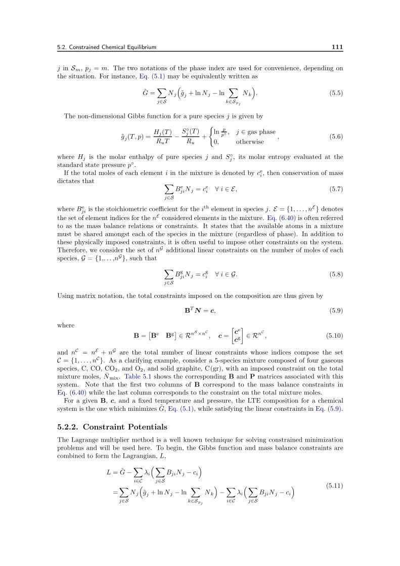
5.2. Constrained Chemical Equilibrium 111
j in Sm, pj = m. The two notations of the phase index are used for convenience, depending onthe situation. For instance, Eq. (5.1) may be equivalently written as
G =∑
j∈S
N j
(
gj + lnN j − ln∑
k∈Spj
Nk
)
. (5.5)
The non-dimensional Gibbs function for a pure species j is given by
gj(T , p) =Hj(T )
RuT−
Sj (T )
Ru+
ln pp , j ∈ gas phase
0, otherwise, (5.6)
where Hj is the molar enthalpy of pure species j and Sj , its molar entropy evaluated at the
standard state pressure p.If the total moles of each element i in the mixture is denoted by cei , then conservation of mass
dictates that∑
j∈S
BejiN j = cei ∀ i ∈ E , (5.7)
where Beji is the stoichiometric coefficient for the ith element in species j. E = 1, . . . , nE denotes
the set of element indices for the nE considered elements in the mixture. Eq. (6.40) is often referredto as the mass balance relations or constraints. It states that the available atoms in a mixturemust be shared amongst each of the species in the mixture (regardless of phase). In addition tothese physically imposed constraints, it is often useful to impose other constraints on the system.Therefore, we consider the set of nG additional linear constraints on the number of moles of eachspecies, G = 1,. . . ,nG, such that
∑
j∈S
BgjiN j = cgi ∀ i ∈ G. (5.8)
Using matrix notation, the total constraints imposed on the composition are thus given by
BTN = c, (5.9)
where
B =[
Be Bg]
∈ RnS×nC
, c =
[
ce
cg
]
∈ RnC
, (5.10)
and nC = nE + nG are the total number of linear constraints whose indices compose the setC = 1, . . . , nC. As a clarifying example, consider a 5-species mixture composed of four gaseousspecies, C, CO, CO2, and O2, and solid graphite, C(gr), with an imposed constraint on the totalmixture moles, Nmix. Table 5.1 shows the corresponding B and P matrices associated with thissystem. Note that the first two columns of B correspond to the mass balance constraints inEq. (6.40) while the last column corresponds to the constraint on the total mixture moles.
For a given B, c, and a fixed temperature and pressure, the LTE composition for a chemicalsystem is the one which minimizes G, Eq. (5.1), while satisfying the linear constraints in Eq. (5.9).
5.2.2. Constraint Potentials
The Lagrange multiplier method is a well known technique for solving constrained minimizationproblems and will be used here. To begin, the Gibbs function and mass balance constraints arecombined to form the Lagrangian, L,
L = G−∑
i∈C
λi(
∑
j∈S
BjiN j − ci)
=∑
j∈S
N j
(
gj + lnN j − ln∑
k∈Spj
Nk
)
−∑
i∈C
λi(
∑
j∈S
BjiN j − ci) (5.11)
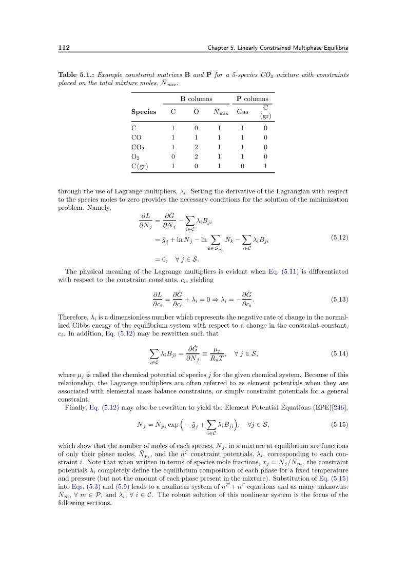
112 Chapter 5. Linearly Constrained Multiphase Equilibria
Table 5.1.: Example constraint matrices B and P for a 5-species CO2 mixture with constraintsplaced on the total mixture moles, Nmix.
B columns P columns
Species C O Nmix Gas C(gr)
C 1 0 1 1 0CO 1 1 1 1 0CO2 1 2 1 1 0O2 0 2 1 1 0C(gr) 1 0 1 0 1
through the use of Lagrange multipliers, λi. Setting the derivative of the Lagrangian with respectto the species moles to zero provides the necessary conditions for the solution of the minimizationproblem. Namely,
∂L
∂N j=
∂G
∂N j−∑
i∈C
λiBji
= gj + lnN j − ln∑
k∈Spj
Nk −∑
i∈C
λiBji
= 0, ∀ j ∈ S.
(5.12)
The physical meaning of the Lagrange multipliers is evident when Eq. (5.11) is differentiatedwith respect to the constraint constants, ci, yielding
∂L
∂ci=∂G
∂ci+ λi = 0 ⇒ λi = −
∂G
∂ci. (5.13)
Therefore, λi is a dimensionless number which represents the negative rate of change in the normal-ized Gibbs energy of the equilibrium system with respect to a change in the constraint constant,ci. In addition, Eq. (5.12) may be rewritten such that
∑
i∈C
λiBji =∂G
∂N j≡
µj
RuT, ∀ j ∈ S, (5.14)
where µj is called the chemical potential of species j for the given chemical system. Because of thisrelationship, the Lagrange multipliers are often referred to as element potentials when they areassociated with elemental mass balance constraints, or simply constraint potentials for a generalconstraint.
Finally, Eq. (5.12) may also be rewritten to yield the Element Potential Equations (EPE)[246],
N j = Npj exp(
− gj +∑
i∈C
λiBji
)
, ∀j ∈ S, (5.15)
which show that the number of moles of each species, N j , in a mixture at equilibrium are functionsof only their phase moles, Npj , and the nC constraint potentials, λi, corresponding to each con-straint i. Note that when written in terms of species mole fractions, xj = N j/Npj , the constraintpotentials λi completely define the equilibrium composition of each phase for a fixed temperatureand pressure (but not the amount of each phase present in the mixture). Substitution of Eq. (5.15)into Eqs. (5.3) and (5.9) leads to a nonlinear system of nP +nC equations and as many unknowns:Nm, ∀ m ∈ P, and λi, ∀ i ∈ C. The robust solution of this nonlinear system is the focus of thefollowing sections.
5.3. Multiphase Gibbs Function Continuation 113
5.2.3. Coordinate Transfer and Matrix-Vector Representation
The following sections make use of a coordinate transformation which simplifies the developmentof the multiphase Gibbs function continuation method. This transformation is similar to the onemade by Pope in the original development of the single-phase method. Instead of dealing directlywith species moles, it is convenient to use their square-root,
yi ≡√
N i. (5.16)
The purpose of this change of variables will become evident later. Using Eq. (5.15), the vectory ∈ RnS
may be expressed in matrix-vector notation as a function of the element potential vector,λ ∈ RnC
, and phase mole vector N ∈ RnP
by
y = exp(
−g +Bλ+P ln N)
12 . (5.17)
Here, the exponential, logarithm, and square-root operators act element-wise on their vector argu-ment. Note also that P in Eq. (5.17) is used to transform the nP -sized vector ln N into a nS-sizedvector with repeated values depending on the phase of each species. This construction will be usedthroughout the paper. Finally, the matrices Y ∈ RnS×nS
, B ∈ RnS×nC
, and P ∈ RnS×nP
aredefined as
Y ≡ diag (y) , B ≡ YB, P ≡ YP. (5.18)
Using the above notation, the constrained chemical equilibrium problem defined in Eqs. (5.3) and(5.9) may be written as
PTy = N (5.19)
BTy = c (5.20)
5.3. Multiphase Gibbs Function Continuation
Newton’s method, or a variant thereof, is the most common method for solving nonlinear equationssuch as Eqs. (5.19) and (5.20)). In general, the convergence of Newton’s method for a Lipshitzcontinuous, nonlinear system, F (x) = 0, is q-quadratic when the initial iterate, x0, is close enoughto a root of F , x∗, and the system Jacobian within the region around the root is nonsingular [270].In fact, quadratic convergence is only guaranteed when the initial guess, x0, is close enough to thereal solution, x∗, to satisfy the condition
∥x0 − x∗∥2 <∥F′(x∗)∥2γκ(F′(x0))
, (5.21)
where F′(x) is the system Jacobian evaluated at x, γ is the Lipschitz constant for F′, and κ(F′(x))is the condition number of F′(x). The condition number is a measure of how close a matrix isto being singular, increasing to infinity when the matrix is singular. Thus, as the Jacobian of thesystem approaches a singular matrix, the corresponding bound on the initial guess’s proximity tothe actual solution becomes nearly zero. For the equilibrium problem of Eqs. (5.19) and (5.20),situations often arise in which the system Jacobian approaches a singular matrix causing theNewton convergence to stagnate.
The MPGFC method avoids the above difficulties by converting Eqs. (5.19) and (5.20) into aninitial value problem which may be integrated robustly through the use of a continuation parameter.To begin, the multiphase residual vector, R ∈ RnC+nP
, is formally expressed as a function of thesolution vector, x, and the Gibbs vector, g(T , p), such that
R (x, g) =
[
BT
PT
]
y −[
cN
]
, and x ≡[
λln N
]
, (5.22)
114 Chapter 5. Linearly Constrained Multiphase Equilibria
where B, P, and y are implicit functions of x as shown in Eqs. (5.17) and (5.18). Eqs. (5.19) and(5.20) may now be written in terms of the residual vector as R(x∗, g) = 0, which implicitly definesthe equilibrium point x∗ for a fixed T and p. The solution of this nonlinear system via Newton’smethod is not guaranteed to succeed, based on the arguments made above. Instead, we define anew Gibbs energy vector g, linearly parameterized by a continuation parameter s, such that
g(s) = g(0) + s [g − g(0)] , (5.23)
where g(0) denotes g at s = 0. Replacing g with g, the equation R(x, g(s)) = 0 now implicitlydefines a path of pseudo-equilibrium points x(s), parameterized by s, where x(1) = x∗. As g(0) isarbitrary, there are an infinite number of such paths, however, given a set of initial values of g(0)and x(0) which satisfy R(x(0), g(0)) = 0, the equilibrium point can be determined by tracing thepath of pseudo-equilibrium points from s = 0 to s = 1, via
x∗ = x(1) =
∫ 1
0
dx
dsds+ x (0) , (5.24)
where the tangent vector, dx/ds = [dλ/ds, d ln N/ds]T , can be derived from the implicit relationdR(x, g(s))/ds = 0. Note that the ‘hat’ symbol is left off of λ and N for convenience but theirdependence on s will be clear based on the context. Given a g(0), the path x(s) is smooth andunique because g(s) is linear from Eq. (5.23) and the existence and uniqueness of the equilibriumproblem is well known (see for example [271]).
In its most basic form, the MPGFC method solves for the equilibrium point x∗ by numericallyintegrating the initial value problem of Eq. (5.24) using a simple Euler scheme.The derivatives,dλ/ds and d ln N/ds, can be computed robustly by exploiting a feature of least-squares solutions.In addition, special care must be taken to ensure that the correct condensed phases are included inthe equilibrium solution. Further improvements to the efficiency and global accuracy of the methodare obtained by using an adaptive step-size, ∆s, as well as Newton’s method (when possible) toreduce errors in the numerical integration. The mathematical basis for each of these issues arepresented in the following subsections while Section 5.4.1 will detail the exact MPGFC solutionalgorithm.
5.3.1. Initial Conditions
The initial conditions, g(0), λ(0), and ln N (0), must satisfy the constraint R(x(0), g(0)) = 0.Therefore, the initial species moles vector, N(0), must satisfy Eqs. (5.19) and (5.20). There are aninfinite number of species mole vectors which can satisfy the underdetermined constraint systemin Eq. (5.20). The vector space of all such vectors will be denoted by
B =
N ∈ RnS
: BTN = c, N j ≥ 0
. (5.25)
We now define two species compositions contained in this vector space. The Min-G composition,
Nmin-g = argminN∈B
NT g, (5.26)
minimizes the sum of species Gibbs energies while satisfying the constraints in Eq. (5.20), ap-proximating the minimization of Eq. (5.1) without regard to the energy of mixing. The Max-Mincomposition,
Nmax-min = argmaxN∈B
(
minj∈S
N j
)
, (5.27)
is the composition which maximizes the smallest single species moles and still satisfies Eq. (5.20).Both compositions can be formulated as the solution to a linear programming problem which canbe easily solved via the Simplex algorithm [272]. The Min-G composition is useful because itestimates the equilibrium moles of the major species. However, at most nC species in Nmin-g will
5.3. Multiphase Gibbs Function Continuation 115
be non-zero, while the rest are exactly zero. The Max-Min composition is strictly positive but farfrom the equilibrium composition as it does nothing to minimize G. Therefore, Pope [264] hassuggested that a linear combination of the Min-G and Max-Min compositions,
N(0) = Nmin-g(1− α) +Nmax-minα, (5.28)
provides a good approximation of the major equilibrium species while ensuring that all speciesmoles are strictly positive and that Eq. (5.20) is satisfied. The value of α is typically taken tobe 0.01 such that the Min-G composition dominates, and the major species moles are still wellapproximated by the initial solution.
The Gibbs phase rule [273] says that, for a fixed temperature and pressure, the maximum numberof phases allowed in an equilibrium solution are the total number of constraints imposed on it, nC .In order to ensure that the initial conditions satisfy the phase rule, only the phases which havenon-zero moles in the Min-G solution are kept for the Max-Min solution. As the maximum numberof non zero species in the Min-G solution is equal to the number of constraints, this is sufficient toensure the phase rule is satisfied.
Eq. (5.19) is then directly satisfied by taking
ln N(0) = ln(
PTN(0)
)
. (5.29)
Note the necessity of having a strictly positive N(0) in order for the logarithm above to be welldefined.
Eqs. (5.28) and (5.29) ensure that R = 0 (recall that y =√N from Eq. (5.16)). All that remains
is to determine g(0) and λ(0) which are consistent with N(0) through the EPE, Eq. (5.17). First,λ(0) is computed as the least-squares solution of the EPE using the Gibbs energy vector, g.
λ(0) = argminλ
∥
∥Bλ− lnN (0) +P ln N (0)− g∥
∥
2(5.30)
Finally, g(0) is chosen such that Eq. (5.17) is exactly satisfied.
g(0) = Bλ(0)− lnN(0) +P ln N(0) (5.31)
5.3.2. Computing the Tangent Vector
The derivatives, dλ/ds and d ln N/ds, at constant R, are obtained from the implicit relationsfound when the residual is differentiated with respect to s and set equal to zero, such that
dR
ds=
d
ds
[
BTy
PTy − N
]
= 0. (5.32)
From Eq. (5.17), the following relationship can be easily determined.
d
ds(Yy) = Y
2
[
Bdλ
ds−
dg
ds+P
d
ds(ln N)
]
= Y
[
Bdλ
ds−Y
dg
ds+ P
d
ds(ln N )
] (5.33)
Note that dg/ds is a known function from Eq. (5.23), namely dg/ds = g− g(0). Using Eq. (5.33),the first term in Eq. (5.32) can be written as
d
ds
(
BTy)
= BT
[
Bdλ
ds−Y
dg
ds+ P
d
ds(ln N)
]
. (5.34)
We now seek a dλ/ds such that d(BTy)/ds = 0 is satisfied regardless of the value of d ln N/ds.
116 Chapter 5. Linearly Constrained Multiphase Equilibria
To begin, dλ/ds, is decomposed into two components,
dλ
ds= λg − Λ
y d
ds(ln N), (5.35)
where λg ∈ RnC
and Λy ∈ RnC×nP
are obtained via the minimum-norm solutions to the followingleast-squares problems
λg = argminλ
∥
∥
∥
∥
Bλ−Ydg
ds
∥
∥
∥
∥
2
, (5.36)
Λy = argmin
Λ
∥
∥
∥BΛ− P
∥
∥
∥
2. (5.37)
The solutions of Eqs. (5.36) and (5.37) may be stably computed using the singular value decom-position of B, regardless of its rank. In addition, their residuals reside in the null space of BT ,based on a general property of least squares solutions. Thus,
BT(
Bλg −Ydg
ds
)
= 0, (5.38)
BT(
BΛy − P
)
= 0. (5.39)
Using this fact and substituting Eq. (5.35) into Eq. (5.34) and rearranging, we then have
BT
[
Bλg −Ydg
ds−(
BΛy − P
) d
ds(ln N)
]
= 0. (5.40)
The usefulness of the decomposition of dλ/ds in Eq. (5.35) is now evident because it ensures thatthe first term in Eq. (5.32) is always satisfied, regardless of the value of d ln N/ds.
The phase moles derivatives, d ln N/ds, are determined from the second implicit relation definedin Eq. (5.32), namely
d
ds
(
PTy − N
)
= PT
(
Pd
ds(ln N )−Y
dg
ds+ B
dλ
ds
)
−dN
ds= 0 (5.41)
Making use of the following relationship for d ln N/ds when R = 0,
d
ds(ln N) = diag(N)−1 dN
ds=(
PTP
)−1 dN
ds, (5.42)
and substituting in Eq. (5.35) for dλ/ds, Eq. (5.41) may be written as
PTBΛ
y d
ds(ln N) = P
T
(
Bλg −Ydg
ds
)
. (5.43)
Eq. (5.43) represents a linear system of equations for the solution of d ln N/ds. We now introducethe matrix M ≡ PT BΛy ∈ RnP×nP
for convenience. The structure of this matrix is studied indetail in Appendix B. In particular, M is symmetric and positive definite when the phase molesare non zero. In fact, the eigenvalues of M, denoted β1 ≥ βm ≥ βnP , have the following upper andlower bounds:
Nm ≥ βm(M) ≥βm(CTC)
∥B∥22≥ 0, ∀ m ∈ P , (5.44)
where C ≡ BT P ∈ RnC×nP
has column vectors, cm, which represent the amount of elements orconstraint constants which are associated with the phase m. It is trivial to show that
∑
m∈P cm = c.For the single phase case, M becomes a scalar M and the bounds on the eigenvalues given inEq. (5.44) become the bounds on M itself. In this special case, the lower bound on M is readily
5.3. Multiphase Gibbs Function Continuation 117
given as M ≥ ∥c∥22/∥B∥22, which is strictly positive. In the development of the single phaseGFC method, Pope [265] derived a similar equation as Eq. (5.43) (divided by the total moles ofthe mixture) and placed an identical lower bound on the scalar quotient (D in Pope’s notation)through other means. In Pope’s derivation, the physical meaning of the scalar was unknown,and furthermore, the proof of positivity cannot be readily extended to consider multiple phases.However, the eigenvalue analysis given in Appendix B, and whose result is given by the bounds inEq. (5.44), directly relates the eigenvalues of M to the moles in each phase and is applicable toany number of phases (including the single phase case). Furthermore, the upper bound of Nm onthe eigenvalues of M informs a practical method for determining when M approaches a positivesemidefinite matrix.
With a careful treatment of nearly empty phases, Eq. (5.43) can be solved in a robust andefficient manner using the Cholesky factorization for symmetric positive definite systems, ensuringthat the derivatives dλ/ds and d ln N/ds can be determined in a fully robust way.
5.3.3. Newton’s Method
As the Euler integration scheme approximates the pseudo-equilibrium path in a linear way, errorsmay accumulate during the course of the numerical integration. Therefore, after each new solutionis obtained in the numerical integration of Eq. (5.24), Newton’s method is used to attempt to reducethe residual below a specified global error tolerance for a fixed value of s (fixed g). Newton’s methodcorresponds to solving the following linear system for successive updates in the pseudo-equilibriumsolution,
J(
xk+1 − xk)
= −R(xk, g), (5.45)
where the superscript k denotes the kth solution iterate and the system Jacobian, J, is determinedto be
J ≡∂R
∂x=
[
BT B BT P
PT B PT P
]
−[
0 0
0 diag(
N)
]
. (5.46)
Note that the parentheses on the right hand side of Eq. (5.45) denote that the residual is evaluatedat (xk, g), while those on the left simply distribute the matrix vector product to both xk+1 andxk.
In some situations, the above system may be singular, making it impossible to converge thesolution further after taking a continuation step. In such cases, the Newton iterations are aban-doned and the residual is reduced by reducing the step-size used for the numerical integration andretaking the step.
5.3.4. Inclusion of Condensed Phases
The initialization procedure presented in Section 5.3.1 typically does a good job of predictingwhich condensed phases should be present in the equilibrium mixture through the Min-G solution.However, it is possible that the phases present in the initial solution are not the correct oneswhich minimize the Gibbs free energy. Furthermore, it is also possible that some phases, whichare correctly included in the initial solution, are removed during the course of the integration ofEq. (5.24). Therefore, at the end of the integration of Eq. (5.24), a check must be performed todetermine whether or not a previously neglected phase can in fact minimize the system Gibbs energyfurther. Since the equilibrium solution represents a stationary point of the Lagrange function(∂L = 0), Eq. (5.12) yields the necessary condition for a new phase to be included. Namely, if
gc −∑
i∈C
λ∗iBci < 0, (5.47)
for any condensed species c, which has not yet been included in the equilibrium solution, thenadding the phase to which species c belongs will decrease the overall Gibbs energy at equilibrium.This is sometimes referred to as the vapor pressure test. When multiple phases meet this criteria,the one with the most negative change in the Gibbs energy is added.
118 Chapter 5. Linearly Constrained Multiphase Equilibria
When it is determined that a new phase should be included, a phase redistribution procedure isperformed which distributes moles of the largest (in terms of quantity) species into the new phasewhile satisfying the mass balance constraint of Eq. (5.20). This is done in the following way. First,the current solution of the species moles vector, N , is extended by the number of species in thenew phase. If the new phase has index m, then the extended species vector, denoted by N ext, iscomputed as
N extj =
N j , j ∈ SNm/nS
m, j ∈ Sm. (5.48)
where Nm is the desired number of initial moles in the phase m, and nSm denotes the number of
species in that phase. The constraint matrix B, the phase summation matrix P, and the speciesindex set are also extended accordingly.
We then search for an update in the nC largest species of N ext which will satisfy the massbalance constraints through the solution of the linear system,
BT∆Nmax = c−B
TN ext, (5.49)
where the vector ∆Nmax is defined to be a vector of zeros except for the elements representingthe nC largest species. Note that Eq. (5.49) represents a linear system with nC equations and nC
unknowns. Furthermore, a suitable update can always be obtained by using the singular valuedecomposition of the sub matrix of BT representing the nC maximum species, even when thatmatrix is rank deficient.
Finally, a new initial species moles vector is computed by applying the update to N ext,
N(0) = N ext +∆Nmax. (5.50)
It is easy to verify that that this new N(0) vector satisfies Eq. (5.20). With a new N (0), thesolution is then reinitialized and the integration procedure is repeated to solve Eq. (5.24). Thiswhole process must be repeated until all necessary phases are included in the equilibrium mixtureaccording to Eq. (5.47).
5.4. Practical Implementation
5.4.1. Solution Algorithm
The previous section detailed the mathematical basis for the MPGFC method. However, in orderto create an efficient and robust equilibrium solver, several algorithmic details must be developed.An overview of the full MPGFC algorithm is presented in this section.
For a fixed temperature, pressure, and constraint vector, the initial moles of each species aredetermined using Eqs. (5.26 - 5.28). Following initialization, the proceeding steps are then used tocompute the integral in Eq. (5.24).
1. The initial solution x(0) and Gibbs energy vector g(0) are computed according to Eqs. (5.29 - 5.31).The continuation parameter and step size are also initialized as s = 0 and ∆s = 1.
2. Compute the tangent vector of the pseudo-equilibrium path, dx/ds at s using Eqs. (5.35 - 5.37),and Eq. (5.43).
3. Next, integrate the solution forward along the pseudo-equilibrium path with an Euler inte-gration over ∆s,
x0(s+∆s) = x(s) +dx
ds∆s. (5.51)
The superscript 0 is used to denote the initial iterate for the Newton iteration procedure.The Gibbs energy vector is also updated via Eq. (5.23) at s+∆s.
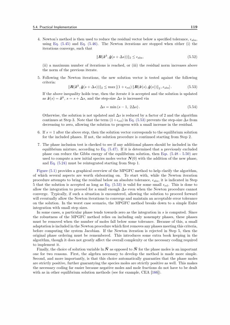
5.4. Practical Implementation 119
4. Newton’s method is then used to reduce the residual vector below a specified tolerance, ϵabs,using Eq. (5.45) and Eq. (5.46). The Newton iterations are stopped when either (i) theiterations converge, such that
∥R(xk, g(s+∆s))∥2 ≤ ϵabs, (5.52)
(ii) a maximum number of iterations is reached, or (iii) the residual norm increases abovethe norm of the previous iterate.
5. Following the Newton iterations, the new solution vector is tested against the followingcriteria:
∥R(xk, g(s+∆s))∥2 ≤ max [(1 + ϵrel) ∥R(x(s), g(s))∥2 , ϵabs] . (5.53)
If the above inequality holds true, then the iterate k is accepted and the solution is updatedas x(s) = xk, s = s+∆s, and the step-size ∆s is increased via
∆s = min (s− 1, 2∆s) . (5.54)
Otherwise, the solution is not updated and ∆s is reduced by a factor of 2 and the algorithmcontinues at Step 3. Note that the term (1+ϵrel) in Eq. (5.53) prevents the step-size ∆s fromdecreasing to zero, allowing the solution to progress with a small increase in the residual.
6. If s = 1 after the above step, then the solution vector corresponds to the equilibrium solutionfor the included phases. If not, the solution procedure is continued starting from Step 2.
7. The phase inclusion test is checked to see if any additional phases should be included in theequilibrium mixture, according to Eq. (5.47). If it is determined that a previously excludedphase can reduce the Gibbs energy of the equilibrium solution, then Eqs. (5.48 - 5.50) areused to compute a new initial species moles vector N(0) with the addition of the new phase,and Eq. (5.24) must be reintegrated starting from Step 1.
Figure (5.1) provides a graphical overview of the MPGFC method to help clarify the algorithm,of which several aspects are worth elaborating on. To start with, while the Newton iterationprocedure attempts to bring the residual below an absolute tolerance, ϵabs, it is indicated in Step5 that the solution is accepted as long as Eq. (5.53) is valid for some small ϵrel. This is done toallow the integration to proceed for a small enough ∆s even when the Newton procedure cannotconverge. Typically, if such a situation is encountered, allowing the solution to proceed forwardwill eventually allow the Newton iterations to converge and maintain an acceptable error toleranceon the solution. In the worst case scenario, the MPGFC method breaks down to a simple Eulerintegration with small step sizes.
In some cases, a particular phase tends towards zero as the integration in s is computed. Sincethe robustness of the MPGFC method relies on including only nonempty phases, these phasesmust be removed when the number of moles fall below some tolerance. Because of this, a smalladaptation is included in the Newton procedure which first removes any phases meeting this criteria,before computing the system Jacobian. If the Newton iteration is rejected in Step 5, then theoriginal phase ordering must be remembered. This introduces some extra book keeping in thealgorithm, though it does not greatly affect the overall complexity or the necessary coding requiredto implement it.
Finally, the choice of solution variable ln N as opposed to N for the phase moles is an importantone for two reasons. First, the algebra necessary to develop the method is made more simple.Second, and more importantly, is that this choice automatically guaranties that the phase molesare strictly positive, further guarantying the species moles are strictly positive as well. This makesthe necessary coding far easier because negative moles and mole fractions do not have to be dealtwith as in other equilibrium solution methods (see for example, CEA [166]).
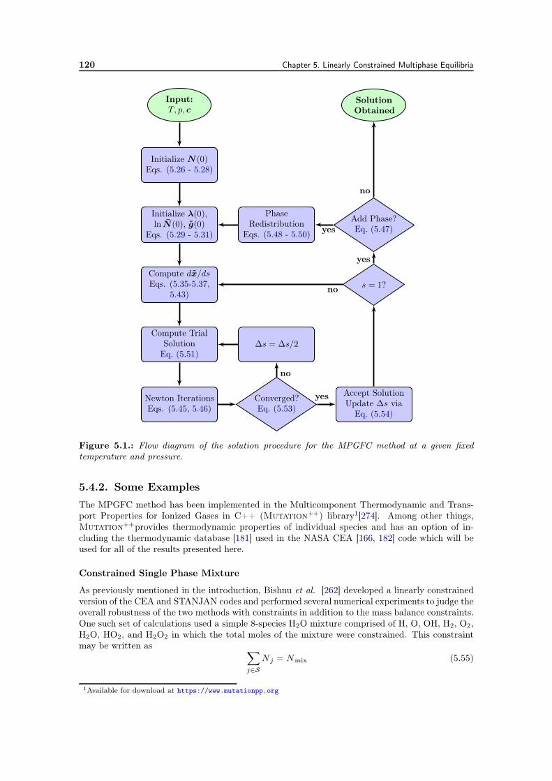
120 Chapter 5. Linearly Constrained Multiphase Equilibria
Input:T, p, c
Initialize N (0)Eqs. (5.26 - 5.28)
Initialize λ(0),ln N(0), g(0)
Eqs. (5.29 - 5.31)
Compute dx/dsEqs. (5.35-5.37,
5.43)
Compute TrialSolution
Eq. (5.51)
Newton IterationsEqs. (5.45, 5.46)
Converged?Eq. (5.53)
∆s = ∆s/2
Accept SolutionUpdate ∆s via
Eq. (5.54)
s = 1?
Add Phase?Eq. (5.47)
PhaseRedistribution
Eqs. (5.48 - 5.50)
SolutionObtained
yes
no
yes
yes
no
no
Figure 5.1.: Flow diagram of the solution procedure for the MPGFC method at a given fixedtemperature and pressure.
5.4.2. Some Examples
The MPGFC method has been implemented in the Multicomponent Thermodynamic and Trans-port Properties for Ionized Gases in C++ (Mutation++) library1[274]. Among other things,Mutation++provides thermodynamic properties of individual species and has an option of in-cluding the thermodynamic database [181] used in the NASA CEA [166, 182] code which will beused for all of the results presented here.
Constrained Single Phase Mixture
As previously mentioned in the introduction, Bishnu et al. [262] developed a linearly constrainedversion of the CEA and STANJAN codes and performed several numerical experiments to judge theoverall robustness of the two methods with constraints in addition to the mass balance constraints.One such set of calculations used a simple 8-species H2O mixture comprised of H, O, OH, H2, O2,H2O, HO2, and H2O2 in which the total moles of the mixture were constrained. This constraintmay be written as
∑
j∈S
N j = Nmix (5.55)
1Available for download at https://www.mutationpp.org
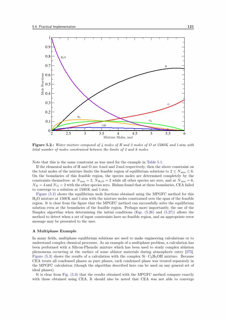
5.4. Practical Implementation 121
2 2.5 3 3.5 4 4.5 5 5.5 60
0.1
0.2
0.3
0.4
0.5
0.6
0.7
0.8
0.9
1
Mixture Moles, mol
Mol
eFr
action
s
H2O
H2
O2
OH
H
O
Figure 5.2.: Water mixture composed of 4 moles of H and 2 moles of O at 1500K and 1 atm withtotal number of moles constrained between the limits of 2 and 6 moles.
Note that this is the same constraint as was used for the example in Table 5.1.If the elemental moles of H and O are 4mol and 2mol respectively, then the above constraint on
the total moles of the mixture limits the feasible region of equilibrium solutions to 2 ≤ Nmix ≤ 6.On the boundaries of this feasible region, the species moles are determined completely by theconstraints themselves: at Nmix = 2, NH2O = 2 while all other species are zero, and at Nmix = 6,NH = 4 and NO = 2 with the other species zero. Bishnu found that at these boundaries, CEA failedto converge to a solution at 1500K and 1 atm.
Figure (5.2) shows the equilibrium mole fractions obtained using the MPGFC method for thisH2O mixture at 1500K and 1 atm with the mixture moles constrained over the span of the feasibleregion. It is clear from the figure that the MPGFC method can successfully solve the equilibriumsolution even at the boundaries of the feasible region. Perhaps more importantly, the use of theSimplex algorithm when determining the initial conditions (Eqs. (5.26) and (5.27)) allows themethod to detect when a set of input constraints have no feasible region, and an appropriate errormessage may be presented to the user.
A Multiphase Example
In many fields, multiphase equilibrium solutions are used to make engineering calculations or tounderstand complex chemical processes. As an example of a multiphase problem, a calculation hasbeen performed with a Silicon-Phenolic mixture which has been used to study complex ablationphenomena occurring at the surface of some ablator materials during atmospheric entry [275].Figure (5.3) shows the results of a calculation with the complex Si–C6H5OH mixture. BecauseCEA treats all condensed phases as pure phases, each condensed phase was treated separately inthe MPGFC calculation (though the algorithm described here can be used on any general set ofideal phases).
It is clear from Fig. (5.3) that the results obtained with the MPGFC method compare exactlywith those obtained using CEA. It should also be noted that CEA was not able to converge
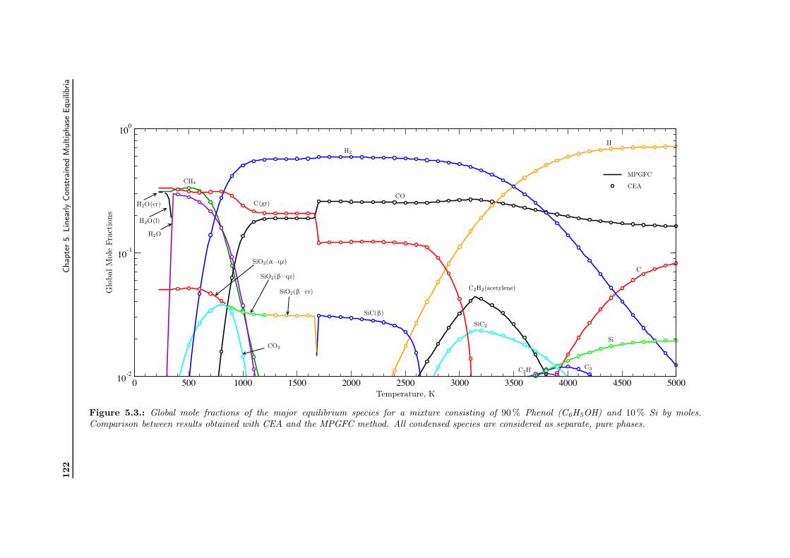
122
Chap
ter5.Lin
early
Const
rain
edM
ultip
has
eEquili
bria
0 500 1000 1500 2000 2500 3000 3500 4000 4500 500010-2
10-1
100
Temperature, K
Glo
balM
ole
Frac
tion
s
MPGFC
CEA
C(gr)
SiO2(α–qz)
SiO2(β–qz)
SiO2(β–cr)
SiC(β)
H2O(cr)
H2O(l)
H2O
CO2
CH4
SiC2
C2H2(acetylene)
C2H C3
H
C
CO
H2
Si
Figure 5.3.: Global mole fractions of the major equilibrium species for a mixture consisting of 90% Phenol (C6H5OH) and 10% Si by moles.Comparison between results obtained with CEA and the MPGFC method. All condensed species are considered as separate, pure phases.
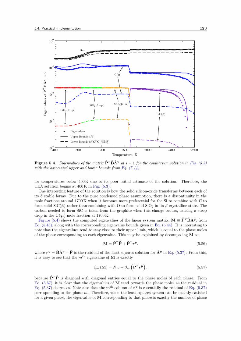
5.4. Practical Implementation 123
400 800 1200 1600 2000 2400 280010-4
10-3
10-2
10-1
100
Temperature, K
Eig
enva
lues
ofP
TBΛ
y,mol
Eigenvalues
Lower Bounds (β(CTC)/∥B∥22)
Upper Bounds (N )
Gas
C(gr)
SiO2(α–qz)
SiO2(β–qz) SiO2(β–cr)
SiC(β)
Figure 5.4.: Eigenvalues of the matrix PT BΛy at s = 1 for the equilibrium solution in Fig. (5.3)with the associated upper and lower bounds from Eq. (5.44).
for temperatures below 400K due to its poor initial estimate of the solution. Therefore, theCEA solution begins at 400K in Fig. (5.3).
One interesting feature of the solution is how the solid silicon-oxide transforms between each ofits 3 stable forms. Due to the pure condensed phase assumption, there is a discontinuity in themole fractions around 1700K when it becomes more preferential for the Si to combine with C toform solid SiC(β) rather than combining with O to form solid SiO2 in its β-crystalline state. Thecarbon needed to form SiC is taken from the graphite when this change occurs, causing a steepdrop in the C(gr) mole fraction at 1700K.
Figure (5.4) shows the computed eigenvalues of the linear system matrix, M ≡ PT BΛy, fromEq. (5.43), along with the corresponding eigenvalue bounds given in Eq. (5.44). It is interesting tonote that the eigenvalues tend to stay close to their upper limit, which is equal to the phase molesof the phase corresponding to each eigenvalue. This may be explained by decomposing M as,
M = PTP+ P
Try. (5.56)
where ry = BΛy − P is the residual of the least squares solution for Λy in Eq. (5.37). From this,it is easy to see that the mth eigenvalue of M is exactly
βm (M) = Nm + βm(
PT ry
)
, (5.57)
because PT P is diagonal with diagonal entries equal to the phase moles of each phase. FromEq. (5.57), it is clear that the eigenvalues of M tend towards the phase moles as the residual inEq. (5.37) decreases. Note also that the mth column of ry is essentially the residual of Eq. (5.37)corresponding to the phase m. Therefore, when the least squares system can be exactly satisfiedfor a given phase, the eigenvalue of M corresponding to that phase is exactly the number of phase
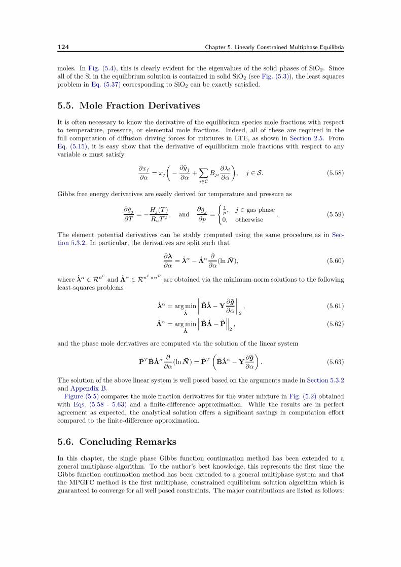
124 Chapter 5. Linearly Constrained Multiphase Equilibria
moles. In Fig. (5.4), this is clearly evident for the eigenvalues of the solid phases of SiO2. Sinceall of the Si in the equilibrium solution is contained in solid SiO2 (see Fig. (5.3)), the least squaresproblem in Eq. (5.37) corresponding to SiO2 can be exactly satisfied.
5.5. Mole Fraction Derivatives
It is often necessary to know the derivative of the equilibrium species mole fractions with respectto temperature, pressure, or elemental mole fractions. Indeed, all of these are required in thefull computation of diffusion driving forces for mixtures in LTE, as shown in Section 2.5. FromEq. (5.15), it is easy show that the derivative of equilibrium mole fractions with respect to anyvariable α must satisfy
∂xj
∂α= xj
(
−∂gj∂α
+∑
i∈C
Bji∂λi∂α
)
, j ∈ S. (5.58)
Gibbs free energy derivatives are easily derived for temperature and pressure as
∂gj∂T
= −Hj(T )
RuT 2, and
∂gj∂p
=
1p , j ∈ gas phase0, otherwise
. (5.59)
The element potential derivatives can be stably computed using the same procedure as in Sec-tion 5.3.2. In particular, the derivatives are split such that
∂λ
∂α= λα − Λ
α ∂
∂α(ln N), (5.60)
where λα ∈ RnC
and Λα ∈ RnC×nP
are obtained via the minimum-norm solutions to the followingleast-squares problems
λα = argminλ
∥
∥
∥
∥
Bλ−Y∂g
∂α
∥
∥
∥
∥
2
, (5.61)
Λα = argmin
Λ
∥
∥
∥BΛ− P
∥
∥
∥
2, (5.62)
and the phase mole derivatives are computed via the solution of the linear system
PTBΛ
α ∂
∂α(ln N ) = P
T
(
Bλα −Y∂g
∂α
)
. (5.63)
The solution of the above linear system is well posed based on the arguments made in Section 5.3.2and Appendix B.
Figure (5.5) compares the mole fraction derivatives for the water mixture in Fig. (5.2) obtainedwith Eqs. (5.58 - 5.63) and a finite-difference approximation. While the results are in perfectagreement as expected, the analytical solution offers a significant savings in computation effortcompared to the finite-difference approximation.
5.6. Concluding Remarks
In this chapter, the single phase Gibbs function continuation method has been extended to ageneral multiphase algorithm. To the author’s best knowledge, this represents the first time theGibbs function continuation method has been extended to a general multiphase system and thatthe MPGFC method is the first multiphase, constrained equilibrium solution algorithm which isguaranteed to converge for all well posed constraints. The major contributions are listed as follows:
5.6. Concluding Remarks 125
0 1000 2000 3000 4000 5000 6000-1e-3
-5e-4
0
5e-4
1e-3
H2O
H2
O2
OH
H
O
Analytical
Finite-Difference
Temperature, K
∂x/∂
T,K
−1
(a) With respect to temperature.
0 1000 2000 3000 4000 5000 6000-2e-6
-1e-6
0
1e-6
2e-6
H2O
H2
O2OH
H
O
Temperature, K
∂x/∂
p,Pa−
1
(b) With respect to pressure.
Figure 5.5.: Mole fraction derivatives with respect to temperature and pressure for the watermixture from Fig. (5.2). The expressions in Eqs. (5.58 - 5.63) were used to compute the analyticalresults and are compared against results obtained using a finite-difference approximation.
• The phase moles have been added to the solution vector with the necessary mathematicaladjustments developed for the GFC methodology.
• A procedure to ensure that the Gibbs phase rule is satisfied has been included in the ini-tialization procedure along with a phase redistribution technique to ensure all phases arecorrectly included.
• Strictly positive (upper and lower) bounds have been placed on the eigenvalues of the linearsystem matrix necessary for computing the tangent vector of the pseudo-equilibrium path ina robust manner.
• Furthermore, it was shown that the eigenvalues tend toward the moles of each included phaseas the residual of the least squares solution for Λy decreases.
• The eigenvalue analysis has been used to develop a sensible procedure for removing phasesfrom the equilibrium solution, namely when the moles in a phase drop below a specifiedtolerance.
The above points were demonstrated on two numerical test cases which serve to highlight someof the features of the method. A single phase case demonstrated the use of constraints on theequilibrium mixture and the robustness of the method when the solution lies on the edge of thefeasible region. A multiphase example was used to show, first and foremost, that the methodprovides the correct solution when compared to the well established CEA code, and secondly thatthe underlying eigenvalue analysis is correct.
Finally, the MPGFC method is shown to be a reliable and robust algorithm for computinglinearly constrained, multiphase, chemical equilibrium solutions. The method has been includedin the Mutation++ library, presented in Chapter 4, which is available as a free, open source,software package.

CHAPTER 6
Numerical Methods and Codes
6.1. Introduction
The purpose of this chapter is to present the numerical tools developed in this thesis which are usedin the following chapter to study coupled flow, radiation, and ablation phenomena for atmosphericentry vehicles. Unsteady, three-dimensional, coupled simulations of atmospheric entry vehicles withablative heat shields remain extremely costly undertakings due to the large number of species,chemical reactions, and physical phenomena involved. As a result, these types of simulationsare often performed with lower fidelity modeling and approximate coupling strategies betweenradiation, ablation, and flow solutions.
Since the primary focus of this work is to study these complex interactions, only the steady-statestagnation stream line is considered. As will be shown, considering only the stagnation line of anatmospheric entry vehicle substantially reduces the cost in terms of CPU time required to obtainmeaningful solutions. These savings can then be reinvested by using higher fidelity physicochemicalmodels and coupling strategies. In addition, this approach provides the ability to make accurateengineering predictions of stagnation point heating in a relatively short time. A few drawbacks ofthis approach is that 3D and unsteady effects are not considered. However, such effects are out ofthe scope of this thesis.
The chapter is organized as follows. Section 6.2 details the derivation and discretization of thegoverning equations for the flow field along the stagnation line of an atmospheric entry vehicle.Coupling with the material response is approximately modeled through a steady-state ablativeboundary condition. Section 6.3 presents the development of two numerical tools which are usedin this work for the solution of radiative transport along the stagnation line using the LBL andHSNB methodologies. Finally, Section 6.4 discusses the strategies used to compute coupled simu-lations.
6.2. Stagnation Line Flow
This section details the code developed for modeling the stagnation line flow field. The governingequations, numerical methods, and boundary conditions used in this work are summarized inthe following sections. The two-temperature thermochemical nonequilibrium model presented inChapter 2 is used to illustrate the governing equations derived for the stagnation line. In principle,however, any thermochemical nonequilibrium model could be used with this approach.
6.2.1. Dimensionally Reduced Navier-Stokes Equations
We follow the methodology of Klomfass and Müller [276] for deriving a 1D plasma flow model alongthe stagnation-line of a spherical body with radius R0 as shown in Fig. (6.1). Non-spherical bodiesare modeled using an equivalent sphere radius R0 which correctly reproduces certain desired flowfeatures. For example, Turchi et al. [277] have shown that the Local Heat Transfer Simulation(LHTS) methodology can be used to define an equilivalent sphere radius to match subsonic plasmawind tunnel conditions with actual flight conditions, through appropriate similarity conditions. Inthis work, equivalent sphere radii have been determined in order to match expected shock standoff
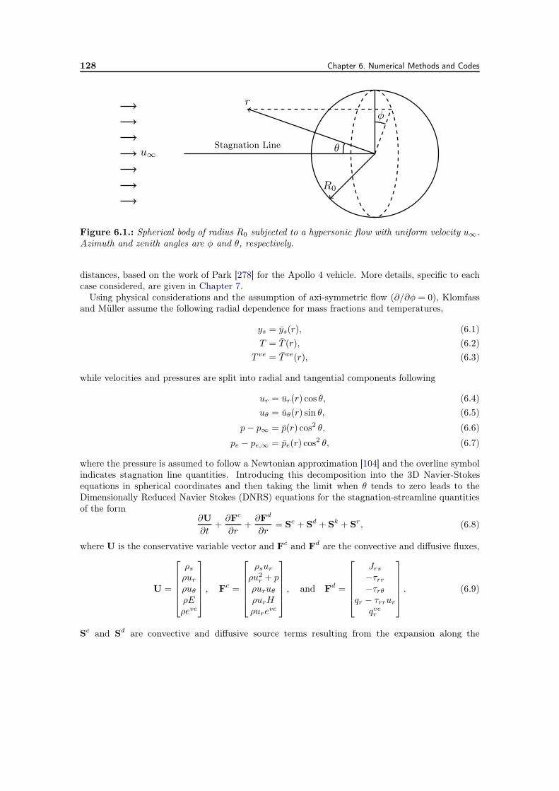
128 Chapter 6. Numerical Methods and Codes
Stagnation Line
R0
r
θ
φ
u∞
Figure 6.1.: Spherical body of radius R0 subjected to a hypersonic flow with uniform velocity u∞.Azimuth and zenith angles are φ and θ, respectively.
distances, based on the work of Park [278] for the Apollo 4 vehicle. More details, specific to eachcase considered, are given in Chapter 7.
Using physical considerations and the assumption of axi-symmetric flow (∂/∂φ = 0), Klomfassand Müller assume the following radial dependence for mass fractions and temperatures,
ys = ys(r), (6.1)T = T (r), (6.2)
T ve = T ve(r), (6.3)
while velocities and pressures are split into radial and tangential components following
ur = ur(r) cos θ, (6.4)uθ = uθ(r) sin θ, (6.5)
p− p∞ = p(r) cos2 θ, (6.6)
pe − pe,∞ = pe(r) cos2 θ, (6.7)
where the pressure is assumed to follow a Newtonian approximation [104] and the overline symbolindicates stagnation line quantities. Introducing this decomposition into the 3D Navier-Stokesequations in spherical coordinates and then taking the limit when θ tends to zero leads to theDimensionally Reduced Navier Stokes (DNRS) equations for the stagnation-streamline quantitiesof the form
∂U
∂t+∂Fc
∂r+∂Fd
∂r= Sc + Sd + Sk + Sr, (6.8)
where U is the conservative variable vector and Fc and Fd are the convective and diffusive fluxes,
U =
⎡
⎢
⎢
⎢
⎢
⎣
ρsρur
ρuθ
ρEρeve
⎤
⎥
⎥
⎥
⎥
⎦
, Fc =
⎡
⎢
⎢
⎢
⎢
⎣
ρsur
ρu2r + p
ρuruθ
ρurHρureve
⎤
⎥
⎥
⎥
⎥
⎦
, and Fd =
⎡
⎢
⎢
⎢
⎢
⎣
Jrs−τrr−τrθ
qr − τrrur
qver
⎤
⎥
⎥
⎥
⎥
⎦
. (6.9)
Sc and Sd are convective and diffusive source terms resulting from the expansion along the
6.2. Stagnation Line Flow 129
stagnation-line and are written as
Sc = −(ur + uθ)
r
⎡
⎢
⎢
⎢
⎢
⎣
2ρs2ρur
3ρuθ − 2 p−p∞
ur+uθ
2ρH2ρeve
⎤
⎥
⎥
⎥
⎥
⎦
, and (6.10)
Sd = −1
r
⎡
⎢
⎢
⎢
⎢
⎣
2Jrs2(τθθ − τrr + τrθ)
τθθ − 3τrθ2(qr − τrrur − τrθur − τθθuθ)
2qver
⎤
⎥
⎥
⎥
⎥
⎦
. (6.11)
Finally Sk and Sr are the internal kinetic and energy transfer and radiative source term vectors,respectively, where
Sk =
⎡
⎢
⎢
⎢
⎢
⎣
ωs
000
Ωve
⎤
⎥
⎥
⎥
⎥
⎦
, and Sr =
⎡
⎢
⎢
⎢
⎢
⎣
φs00PPve
⎤
⎥
⎥
⎥
⎥
⎦
. (6.12)
The overline symbol introduced in Eqs. (6.1 - 6.7) to designate stagnation-line quantities has beenomitted for the sake of clarity. The DNRS equations are supplied with appropriate boundaryconditions at the free-stream radius r = R∞ and the vehicle surface r = R0. The boundaryconditions used in this work are discussed in Section 6.2.3.
The total energy and the vibrational-electronic-electron energy per unit volume are defined asρE =
∑
s ρses+ρu2r/2 and ρeve =
∑
s ρseves . Only the radial velocity component contributes to the
kinetic energy due to the ansatz Eqs. (6.4 - 6.7). Note that the formation energy is not includedin eve. This point is important for the source terms described below. The total enthalpy is definedas usual by H = E + p/ρ.
The radial species diffusion fluxes Jrs are obtained by solving the approximate Stefan-Maxwellequations for heavy species with an ambipolar electric field as discussed in Section 4.5.2. Theradial heat fluxes are defined by
qr =∑
s
Jrshs − λtr∂T
∂r− λve
∂T ve
∂r, (6.13)
qver =∑
s
Jrshves − λve
∂T ve
∂r, (6.14)
where λtr and λve are the thermal conductivities of the energy modes in equilibrium with thetemperatures T and T ve respectively, hs = es + ps/ρs, hve
s = eves for s = e and hvee = evee + pe/ρe.
The components of the viscous stress tensor τrr, τrθ and τθθ are given by
τrr =4
3η
(
∂ur
∂r−
ur + uθ
r
)
, (6.15)
τrθ = η
(
∂uθ
∂r−
ur + uθ
r
)
, (6.16)
τθθ = −1
2τrr, (6.17)
where η is the shear viscosity.In Eq. (6.12) ωs are the collisional species mass production rates. Reaction rate constants are
assumed to follow an Arrhenius law (see Section 2.6.1). Forward reaction constants are taken fromthe literature depending on the mixture considered. Backward reaction constants are computed
130 Chapter 6. Numerical Methods and Codes
such that equilibrium relations are satisfied [7]. The nonequilibrium temperatures used for the for-ward and backward rates in this work have already been presented in Table 2.1. Ωve represents therate of translational energy being converted to vibration-electronic-electron energy and is writtenas
Ωve = −pe
(
∂ur
∂r+ 2
ur + uθ
∂r
)
+∑
s∈M
ρsev0s − evsτV Ts
+ ρeet0e − eteτET
+∑
s
eves ωs −∑
p∈R
∆HpRp. (6.18)
The first term on the right-hand-side of Eq. (6.18) represents the internal work done by the electronpressure. The second term represents vibration-translation energy exchange where ev0s and evs arevibrational energies of species s at the temperature T and T ve, respectively. The third term corre-sponds to electron-heavy translation energy exchange where et0e and ete are translational energiesof electrons at the temperature T and T ve, respectively. The expressions shown in Eq. (2.129) andEq. (2.135) are used in this work for the associated relaxation times τV T
s and τETs , respectively.
The fourth term represents the coupling between chemistry and vibrational-electronic energy. Fi-nally, the fifth term accounts for the energy removed from the electron bath due to the set Rof electron impact ionization and dissociation reactions, where Rp is the molar rate of progressand ∆Hp =
∑
s νspefs/Ms is the chemical heat released per unit mole (νsp is the stoichiometric
coefficient for reaction p and Ms is the molar mass of species s) of reaction p.Lastly, φs represents the mass production rate of species s due to photochemical reactions, P is
the total radiative energy source term and Pve is the radiative energy source term for the energymodes in equilibrium with T ve. The numerical solution of the radiative source terms is presentedin Section 6.3.
6.2.2. Discretization
The numerical solution of the DNRS stagnation-line equations derived in the previous section hasbeen developed by Munafò [97] for nitrogen STS flows. This implementation has been extendedin this work to general thermochemical non-equilibrium models, however the numerical methodsremain unchanged from the original work of Munafò. The stagnation-line equations of Eq. (6.8) aresolved via the method-of-lines. The spatial and temporal discretizations are summarized below.
Spatial Discretization
The stagnation-line equations are discretized in space between the surface radius R0 and free-stream radius R∞ using the Finite Volume (FV) method. The resulting discretization yields thefollowing Ordinary Differential Equation (ODE) for the temporal variation of the cell-averagedconservative variables in cell i,
∂Ui
∂t∆ri + F
ci+ 1
2− F
ci− 1
2+ Fd
i+ 12− Fd
i− 12=(
Sci + Sd
i + Ski + Sr
i
)
∆ri, (6.19)
where ∆ri = ri+ 12− ri− 1
2is length of cell i. The numerical inviscid flux F
ci+ 1
2is computed using
Roe’s approximate Riemann solver [279], such that
Fci+ 1
2=
1
2
[
Fc(Ui+1) + Fc(Ui)]
−1
2
∣
∣A(U)∣
∣
[
Ui+1 − Ui
]
. (6.20)
∣
∣A(U)∣
∣ is the dissipation matrix, defined as∣
∣A(U)∣
∣ = R(U)∣
∣Λ(U)∣
∣L(U), where R, L, and Λ arethe right eigenvector, left eigenvector, and diagonal eigenvalue matrices associated with the inviscidflux Jacobian A = ∂Fc/∂U = RΛL. The exact expressions used for the eigensystem matrices areprovided in Appendix C. The hat symbol on the conservative variable vector in Eq. (6.20) denotesthe Roe averaged state, evaluated using the linearization of Prabhu [280] with the entropy fix ofHarten and Hyman [281] in order to prevent the occurrence of expansion shocks.
6.2. Stagnation Line Flow 131
Second-order accuracy in space is achieved by reconstructing upwind variables at the cell inter-face. For robustness, the reconstruction is performed on primitive variables, P = [ρs, ur, uθ, T, T ve]T , s ∈ S∗
[27]. For a generic primitive variable p, the reconstructed “left” (L) and “right” (R) values at aninterface i+ 1/2 are computed using the Monotone Upstream Centered Schemes for ConservationLaws (MUSCL) scheme [282],
pLi+1/2 = pi +1
2φ(rLi )(pi − pi−1), (6.21)
pRi+1/2 = pi+1 −1
2φ(1/rRi+1)(pi+2 − pi+1), (6.22)
where φ(r) is a slope limiter function. Here, r represents the ratios of consecutive differences, suchthat
rLi =pi+1 − pipi − pi−1
, (6.23)
rRi+1 =pi+2 − pi+1
pi+1 − pi. (6.24)
The van Albada limiter [283] has been used in this work, following the implementation of Munafò[97]. Conservative variables are then built from reconstructed primitive variables and the second-order numerical flux is computed according to F
ci+1/2 = F
ci+1/2(U
Li+1/2,U
Ri+1/2).
The diffusive fluxes and source terms are computed using primitive variables. Primitive variablesare computed at the face i+ 1
2 for the diffusive fluxes using a simple weighted average, such thatfor a generic primitive variable p
pi+ 12=
pi+1∆ri+1 + pi∆ri∆ri+1 +∆ri
. (6.25)
Likewise, primitive variable gradients are computed using a central difference scheme at the face,(
∂p
∂r
)
i+ 12
= 2
(
pi+1 − pi∆ri+1 +∆ri
)
. (6.26)
Cell-centered gradients are computed using a two point central finite difference for the diffusiveflux source term, such that
(
∂p
∂r
)
i
= 2
(
pi+1 − pi−1
∆ri+1 + 2∆ri +∆ri−1
)
. (6.27)
Temporal Discretization
Eq. (6.19) is integrated in time from an initial time level of n = 0 using the implicit Backward-Eulermethod,
δUni
∆ti∆ri + F
c n+1i+ 1
2− F
c n+1i− 1
2+ Fd n+1
i+ 12
− Fd n+1i− 1
2
=(
Sc n+1i + Sd n+1
i + Sk n+1i + Sr k
i
)
∆ri, (6.28)
where δUni = Un+1
i − Uni and ∆ti is the local time-step based on the Courant-Friedrichs-Lewy
(CFL) number according to Blazek [284],
∆ti =CFL∆ri
[
|ur|+ a+ 1∆r max
(
43ηρ ,
λcv
)]
i
, (6.29)
where a is the numerical speed of sound presented in Appendix C. In practice, the CFL number
132 Chapter 6. Numerical Methods and Codes
is typically ramped up from about 0.01 to 100 by multiplying by 10 every 1000 iterations or so.For simplicity, the initial solution for uncoupled simulations is taken as the free-stream conditions.Coupled simulations are discussed in Section 6.4. The radiative source term in Eq. (6.28) is treatedexplicitly at a lagged time level k = n − (n mod nr) where nr is the number of flow time-stepscomputed between updates to the radiative source term and (n mod nr) represents the modulusof the integer division of n by nr.
The numerical inviscid flux is linearized using the method of Liou and van Leer [285],
Fc n+1i+ 1
2≈ F
c ni+ 1
2+A
+i δU
ni +A
−i+1δU
ni+1, (6.30)
where the positive-negative split Jacobians are A± = RΛ±L. Their expressions are provided inAppendix C. The diffusive fluxes and source term are linearized in two steps. In the first step, thefluxes and source terms are rewritten as a sum of the terms which are linearly dependent on thegradient of conservative variables plus those which are not, such that
Fd ni+ 1
2= A
d ni+ 1
2
(
∂U
∂r
)n
i+ 12
+Bd ni+ 1
2
, (6.31)
Sd ni = A
d ns i
(
∂U
∂r
)n
i
+Bd ns i . (6.32)
To simplify the linearization procedure, the matrices Ad and Ads are computed assuming a Fickian
diffusion model using the self-consistent effective diffusion coefficients of Ramshaw and Chang [286].Expressions for the matrices Ad, Ad
s , Bd, and Bds are provided in Appendix C. In the second step,
the gradients in Eqs. (6.31) and (6.32) are computed according to Eqs. (6.26) and (6.27) and theresulting expressions are linearized around time-level n, such that
Fd n+1i+ 1
2
≈ Fd ni+ 1
2+ 2Ad n
i+ 12
(
δUi+1 − δUi
∆ri+1 +∆ri
)
+∂Bd n
i+1/2
∂Uni
δUni +
∂Bd ni+1/2
∂Uni+1
δUni+1, (6.33)
Sd n+1i ≈ Sd n
i + 2Ad ns i
(
δUi+1 − δUi
∆ri+1 + 2∆ri +∆ri−1
)
+∂Bd n
s i
∂Uni
δUni , (6.34)
where the matrices Ad and Ads have been assumed constant during the linearization. For simplicity,
the last two Jacobians in Eq. (6.33) are approximated as
∂Bd ni+1/2
∂Uni
≈∂Bd n
i
∂Uni
, (6.35)
∂Bd ni+1/2
∂Uni+1
≈∂Bd n
i+1
∂Uni+1
, (6.36)
where the expressions for ∂Bd/∂U and ∂Bds/∂U are given in Appendix C.
Finally, the convective and kinetic source terms are linearized through a simple Taylor seriesexpansion, such that
Sc n+1i ≈ Sc n
i +∂Sc n
i
∂Uni
δUni , (6.37)
Sk n+1i ≈ Sk n
i +∂Sk n
i
∂Uni
δUni . (6.38)
The source term Jacobians are computed analytically to increase stability and the resulting ex-pressions are presented in Appendix C.
The substitution of Eqs. (6.30 - 6.38) into Eq. (6.28) leads to a block-tridiagonal linear systemof equations which is solved at each time-step using the Thomas algorithm [281] for the update inthe conservative variables. This procedure is repeated until a steady-state solution is reached.
6.2. Stagnation Line Flow 133
6.2.3. Boundary Conditions
Boundary conditions are imposed using primitive variables at ghost-cells [281]. The differentboundary conditions used in this work are described below. The wall boundary conditions areimposed at a radius r = R0, while free-stream conditions are imposed at r = R∞.
Isothermal, non-catalytic, no-slip wall
When ablation coupling is neglected, the wall of the vehicle is assumed to be non-ablative, non-catalytic, and isothermal at T = T ve = Tw for a prescribed wall temperature Tw. A no-slipcondition for the velocity is prescribed, where (ρur)w = (ρuθ)w = 0. Finally, species partialpressures are assumed constant across the wall.
Isothermal, steady-state ablation
Coupling with ablation and pyrolysis phenomena is obtained by way of a steady-state ablationboundary condition using the procedure detailed by Turchi et al. [287]. A detailed species massbalance at the surface yields the following relationship,
(ρiur)w + (Jri)w = mc,i + mg,i, ∀ i ∈ S, (6.39)
in which the first two terms are the convective and diffusive mass fluxes of species i at the surfaceand mc,i and mg,i represent the char and pyrolysis gas blowing rates respectively at the surfacefor species i. Summing the species mass balance over all species, we have
(ρur)w = mc + mg, (6.40)
where mc =∑
i∈S mc,i and mg =∑
i∈S mg,i. The recession rate of the surface, sc, and the virginlayer, sv, are given as
sc =mc
ρc, sv =
mg
ρv − ρc(6.41)
where ρc and ρv are the densities of the char and virgin materials respectively. Under the steady-state ablation assumption, the surface and virgin layer recess at the same rate, leading to thefollowing expression for the pyrolysis blowing rate:
mg =
(
ρvρc
− 1
)
mc. (6.42)
The ratio ρv/ρc is by definition greater than one and may be determined experimentally for a givenTPS material. Substituting Eqs. (6.40) and (6.42) into Eq. (6.39), we have
ρvρc
mc
(
ρiρ
)
w
+ (Jri)w = mc,i +
(
ρvρc
− 1
)
yg,imc, ∀ i ∈ S, (6.43)
where yg,i is the mass fraction of species i in the pure pyrolysis gas. When equilibrium is assumedfor the pyrolysis gas composition, yg,i is fixed based on the surface temperature, pressure, and thegiven elemental composition of the pyrolysis gas. The char mass blowing rate is determined fromthe following four elementary reactions considered at a pure carbon surface.
C(s) + O −−→ CO (6.44)2C(s) + O2 −−→ 2CO (6.45)C(s) + N −−→ CN (6.46)3C(s) −−−− C3 (6.47)
The reaction probabilities for the two oxidation reactions and the sublimation reaction have beentaken from Park [69], while the nitridation reaction probability is taken from Suzuki [288] based
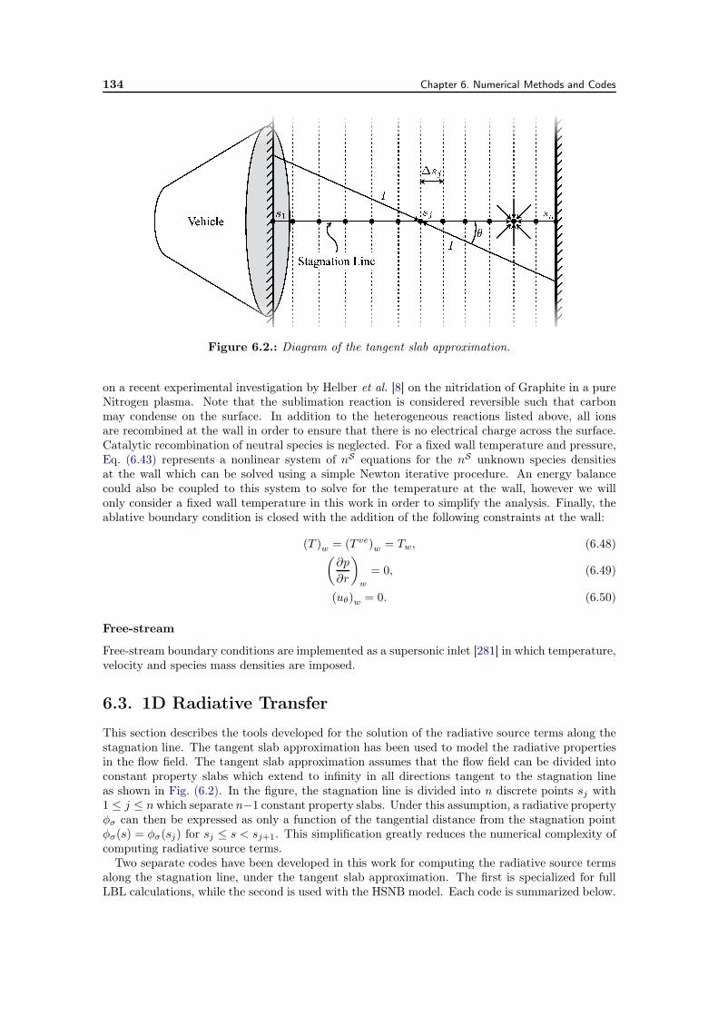
134 Chapter 6. Numerical Methods and Codes
Figure 6.2.: Diagram of the tangent slab approximation.
on a recent experimental investigation by Helber et al. [8] on the nitridation of Graphite in a pureNitrogen plasma. Note that the sublimation reaction is considered reversible such that carbonmay condense on the surface. In addition to the heterogeneous reactions listed above, all ionsare recombined at the wall in order to ensure that there is no electrical charge across the surface.Catalytic recombination of neutral species is neglected. For a fixed wall temperature and pressure,Eq. (6.43) represents a nonlinear system of nS equations for the nS unknown species densitiesat the wall which can be solved using a simple Newton iterative procedure. An energy balancecould also be coupled to this system to solve for the temperature at the wall, however we willonly consider a fixed wall temperature in this work in order to simplify the analysis. Finally, theablative boundary condition is closed with the addition of the following constraints at the wall:
(T )w = (T ve)w = Tw, (6.48)(
∂p
∂r
)
w
= 0, (6.49)
(uθ)w = 0. (6.50)
Free-stream
Free-stream boundary conditions are implemented as a supersonic inlet [281] in which temperature,velocity and species mass densities are imposed.
6.3. 1D Radiative Transfer
This section describes the tools developed for the solution of the radiative source terms along thestagnation line. The tangent slab approximation has been used to model the radiative propertiesin the flow field. The tangent slab approximation assumes that the flow field can be divided intoconstant property slabs which extend to infinity in all directions tangent to the stagnation lineas shown in Fig. (6.2). In the figure, the stagnation line is divided into n discrete points sj with1 ≤ j ≤ n which separate n−1 constant property slabs. Under this assumption, a radiative propertyφσ can then be expressed as only a function of the tangential distance from the stagnation pointφσ(s) = φσ(sj) for sj ≤ s < sj+1. This simplification greatly reduces the numerical complexity ofcomputing radiative source terms.
Two separate codes have been developed in this work for computing the radiative source termsalong the stagnation line, under the tangent slab approximation. The first is specialized for fullLBL calculations, while the second is used with the HSNB model. Each code is summarized below.
6.3. 1D Radiative Transfer 135
6.3.1. LBL Tangent Slab
The tangent slab geometry depicted in Fig. (6.2) allows the RTE given in Eq. (3.1) to be greatlysimplified to,
cos θ∂
∂sIσ(s, θ) = ησ(s)− κσ(s)Iσ(s, θ), (6.51)
where θ is the angle between the ray direction and the stagnation line and s is the normal coordinatebetween the two walls in Fig. (6.2) or along the stagnation line in this work. Note that this s isdistinctly different than the s used in Eq. (3.1) which is the coordinate along the ray. Writingµ = cos θ, the formal solution to Eq. (6.51) is given by
Iσ(s, µ) = Iσ(b, µ) τσ(b, s, µ) +1
µ
∫ s
bησ(s
′) τσ(s′, s, µ) ds′, (6.52)
where b represents the tangential coordinate of the boundary from which a ray with angle cosineµ starts from. The spectral transmissivity is given as
τσ(s′, s, µ) = exp
(
−∫ s
s′
κσ(s′′)
µds′′)
. (6.53)
Using the formalism of Section 3.4.1, the intensity at a point sj in the direction µ for the constantproperty slab geometry in Fig. (6.2) is found to be
Iσ(sj , µ) = Iσ(s1, µ) τ(s1, sj , µ) +j−1∑
i=1
η
κ(si)[
τ(si+1, sj , µ)− τ(si, sj , µ)]
, 0 ≤ µ ≤ 1, (6.54)
and
Iσ(sj , µ) = Iσ(sn, µ) τ(sn, sj , µ) +n−1∑
i=j
η
κ(si)[
τ(si, sj , µ)− τ(si+1, sj , µ)]
, −1 ≤ µ < 0. (6.55)
The radiative heat flux can then be computed as
qrσ(sj) = 2π
∫ 1
−1Iσ(sj , µ)µ dµ. (6.56)
Assuming black walls, the integrals over the angle cosine may be computed analytically, resultingin the final expression for the tangent slab heat flux,
qrσ(sj) = 2π
Ibσ(T1)E3
( j−1∑
i=1
κi∆si
)
− Ibσ(T2)E3
( n−1∑
i=j
κi∆si
)
+j−1∑
i=1
ησκσ
∣
∣
∣
∣
i
[
E3
( j−1∑
k=i+1
κk∆sk
)
− E3
( j−1∑
k=i
κk∆sk
)]
−n−1∑
i=j
ησκσ
∣
∣
∣
∣
i
[
E3
( i−1∑
k=j
κk∆sk
)
− E3
( i∑
k=j
κk∆sk
)]
,
(6.57)
where κi and ηi are respectively the spectral absorption and emission coefficients for slab i, T1 andT2 are the temperatures of the boundaries at s1 and sn, and ∆si = si+1 − si is the thickness of
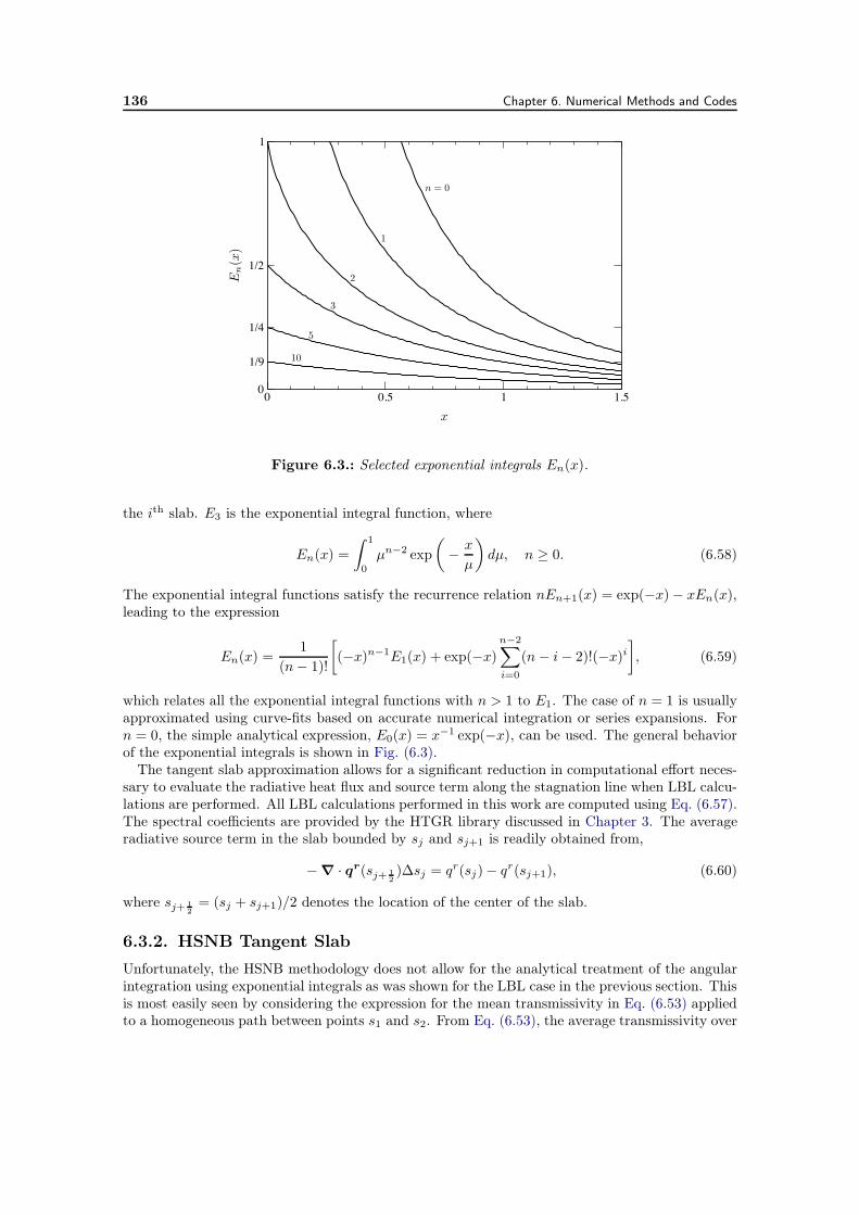
136 Chapter 6. Numerical Methods and Codes
0 0.5 1 1.50
1/9
1/4
1/2
1
x
En(x)
n = 0
1
2
3
5
10
Figure 6.3.: Selected exponential integrals En(x).
the ith slab. E3 is the exponential integral function, where
En(x) =
∫ 1
0µn−2 exp
(
−x
µ
)
dµ, n ≥ 0. (6.58)
The exponential integral functions satisfy the recurrence relation nEn+1(x) = exp(−x)− xEn(x),leading to the expression
En(x) =1
(n− 1)!
[
(−x)n−1E1(x) + exp(−x)n−2∑
i=0
(n− i− 2)!(−x)i]
, (6.59)
which relates all the exponential integral functions with n > 1 to E1. The case of n = 1 is usuallyapproximated using curve-fits based on accurate numerical integration or series expansions. Forn = 0, the simple analytical expression, E0(x) = x−1 exp(−x), can be used. The general behaviorof the exponential integrals is shown in Fig. (6.3).
The tangent slab approximation allows for a significant reduction in computational effort neces-sary to evaluate the radiative heat flux and source term along the stagnation line when LBL calcu-lations are performed. All LBL calculations performed in this work are computed using Eq. (6.57).The spectral coefficients are provided by the HTGR library discussed in Chapter 3. The averageradiative source term in the slab bounded by sj and sj+1 is readily obtained from,
−∇ · qr(sj+ 12)∆sj = qr(sj)− qr(sj+1), (6.60)
where sj+ 12= (sj + sj+1)/2 denotes the location of the center of the slab.
6.3.2. HSNB Tangent Slab
Unfortunately, the HSNB methodology does not allow for the analytical treatment of the angularintegration using exponential integrals as was shown for the LBL case in the previous section. Thisis most easily seen by considering the expression for the mean transmissivity in Eq. (6.53) appliedto a homogeneous path between points s1 and s2. From Eq. (6.53), the average transmissivity over
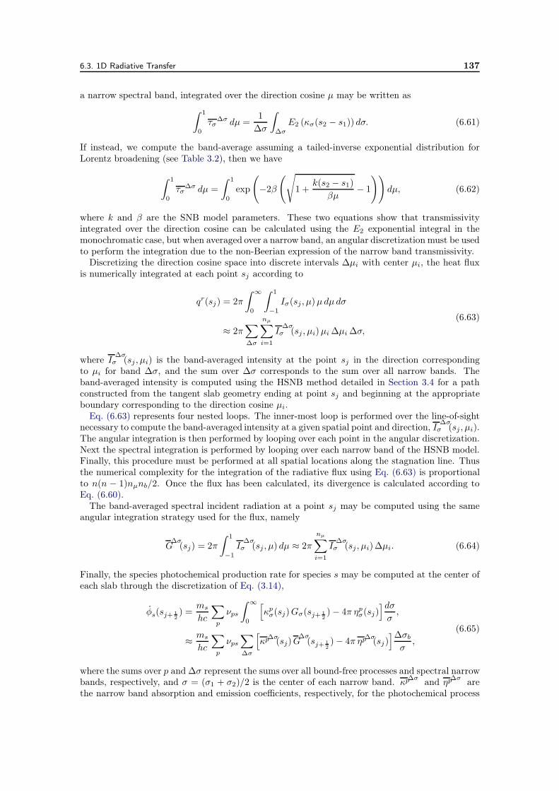
6.3. 1D Radiative Transfer 137
a narrow spectral band, integrated over the direction cosine µ may be written as∫ 1
0τσ
∆σ dµ =1
∆σ
∫
∆σE2 (κσ(s2 − s1)) dσ. (6.61)
If instead, we compute the band-average assuming a tailed-inverse exponential distribution forLorentz broadening (see Table 3.2), then we have
∫ 1
0τσ
∆σ dµ =
∫ 1
0exp
(
−2β
(
√
1 +k(s2 − s1)
βµ− 1
))
dµ, (6.62)
where k and β are the SNB model parameters. These two equations show that transmissivityintegrated over the direction cosine can be calculated using the E2 exponential integral in themonochromatic case, but when averaged over a narrow band, an angular discretization must be usedto perform the integration due to the non-Beerian expression of the narrow band transmissivity.
Discretizing the direction cosine space into discrete intervals ∆µi with center µi, the heat fluxis numerically integrated at each point sj according to
qr(sj) = 2π
∫ ∞
0
∫ 1
−1Iσ(sj , µ)µ dµ dσ
≈ 2π∑
∆σ
nµ∑
i=1
Iσ∆σ(sj , µi)µi ∆µi ∆σ,
(6.63)
where Iσ∆σ(sj , µi) is the band-averaged intensity at the point sj in the direction corresponding
to µi for band ∆σ, and the sum over ∆σ corresponds to the sum over all narrow bands. Theband-averaged intensity is computed using the HSNB method detailed in Section 3.4 for a pathconstructed from the tangent slab geometry ending at point sj and beginning at the appropriateboundary corresponding to the direction cosine µi.
Eq. (6.63) represents four nested loops. The inner-most loop is performed over the line-of-sightnecessary to compute the band-averaged intensity at a given spatial point and direction, Iσ
∆σ(sj , µi).
The angular integration is then performed by looping over each point in the angular discretization.Next the spectral integration is performed by looping over each narrow band of the HSNB model.Finally, this procedure must be performed at all spatial locations along the stagnation line. Thusthe numerical complexity for the integration of the radiative flux using Eq. (6.63) is proportionalto n(n − 1)nµnb/2. Once the flux has been calculated, its divergence is calculated according toEq. (6.60).
The band-averaged spectral incident radiation at a point sj may be computed using the sameangular integration strategy used for the flux, namely
G∆σ(sj) = 2π
∫ 1
−1Iσ
∆σ(sj , µ) dµ ≈ 2π
nµ∑
i=1
Iσ∆σ(sj , µi)∆µi. (6.64)
Finally, the species photochemical production rate for species s may be computed at the center ofeach slab through the discretization of Eq. (3.14),
φs(sj+ 12) =
ms
hc
∑
p
νps
∫ ∞
0
[
κpσ(sj)Gσ(sj+ 12)− 4π ηpσ(sj)
]dσ
σ,
≈ms
hc
∑
p
νps∑
∆σ
[
κp∆σ(sj)G
∆σ(sj+ 1
2)− 4π ηp
∆σ(sj)
]∆σbσ
,
(6.65)
where the sums over p and ∆σ represent the sums over all bound-free processes and spectral narrowbands, respectively, and σ = (σ1 + σ2)/2 is the center of each narrow band. κp∆σ and ηp
∆σ arethe narrow band absorption and emission coefficients, respectively, for the photochemical process
138 Chapter 6. Numerical Methods and Codes
1 10 100 10000
1
2
3
4
5
Size of angular discretization
Rel
ativ
edi
ffere
nce,
%
Figure 6.4.: Difference in computed wall radiative flux versus different sizes of the angular dis-cretization with 1000 angular points taken as reference. Flow field taken from the Fire II 1634 scase presented in Section 7.3.1.
p as provided by the HSNB database. The incident radiation is approximated at the slab centerby averaging, G
∆σ(sj+ 1
2) = (G
∆σ(sj) +G
∆σ(sj+1))/2.
The treatment of the angular discretization and boundary conditions are discussed in the fol-lowing subsections.
Angular discretization
A uniform angular discretization is constructed via
µi = 1− (i − 0.5)∆µi, (6.66)
∆µi =2
nµ, (6.67)
where 1 ≤ i ≤ nµ and nµ is number of angular points. A total of 20 points over the range−1 ≤ µ ≤ 1 has been used for all calculations presented in this work. This choice is based on anangular grid convergence study for typical flow fields. An example convergence result is shown inFig. (6.4) for the Fire II 1634 s case presented in Section 7.3.1. The relative precision loss on thewall radiative flux with 20 angular points is about 0.3% when compared to a reference solutionwith 1000 points. This is about one order of magnitude smaller than the accuracy that can beexpected with the HSNB method compared to full LBL results. Thus, 20 points is a reasonablechoice for the angular discretization.
Reflecting boundaries
The boundary condition in Eq. (3.5) is discretized as
Iσ∆σ(s1, µj) = ϵ1Ibσ
∆σ(T1) +
1− ϵ1π
∑
µi<0
Iσ∆σ(s1, µi) |µi|∆µi, µj > 0, (6.68)
Iσ∆σ(sn, µj) = ϵ2Ibσ
∆σ(T2) +
1− ϵ2π
∑
µi>0
Iσ∆σ(sn, µi) |µi|∆µi, µj < 0, (6.69)
where ϵ1 and ϵ2 are the emissivities of the first and second wall respectively. These equationsrepresent a coupling between the outgoing intensity of each wall through reflection of the incoming
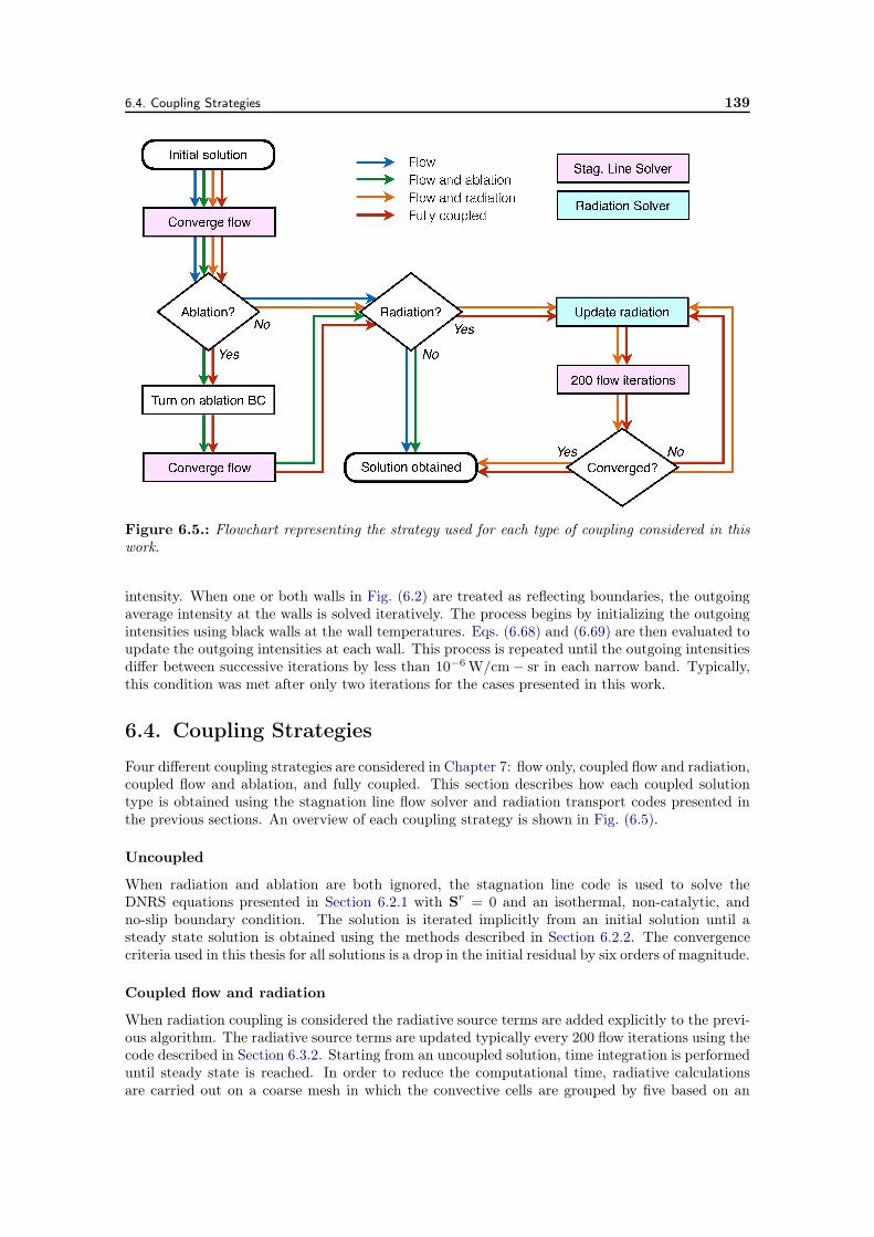
6.4. Coupling Strategies 139
Figure 6.5.: Flowchart representing the strategy used for each type of coupling considered in thiswork.
intensity. When one or both walls in Fig. (6.2) are treated as reflecting boundaries, the outgoingaverage intensity at the walls is solved iteratively. The process begins by initializing the outgoingintensities using black walls at the wall temperatures. Eqs. (6.68) and (6.69) are then evaluated toupdate the outgoing intensities at each wall. This process is repeated until the outgoing intensitiesdiffer between successive iterations by less than 10−6W/cm− sr in each narrow band. Typically,this condition was met after only two iterations for the cases presented in this work.
6.4. Coupling Strategies
Four different coupling strategies are considered in Chapter 7: flow only, coupled flow and radiation,coupled flow and ablation, and fully coupled. This section describes how each coupled solutiontype is obtained using the stagnation line flow solver and radiation transport codes presented inthe previous sections. An overview of each coupling strategy is shown in Fig. (6.5).
Uncoupled
When radiation and ablation are both ignored, the stagnation line code is used to solve theDNRS equations presented in Section 6.2.1 with Sr = 0 and an isothermal, non-catalytic, andno-slip boundary condition. The solution is iterated implicitly from an initial solution until asteady state solution is obtained using the methods described in Section 6.2.2. The convergencecriteria used in this thesis for all solutions is a drop in the initial residual by six orders of magnitude.
Coupled flow and radiation
When radiation coupling is considered the radiative source terms are added explicitly to the previ-ous algorithm. The radiative source terms are updated typically every 200 flow iterations using thecode described in Section 6.3.2. Starting from an uncoupled solution, time integration is performeduntil steady state is reached. In order to reduce the computational time, radiative calculationsare carried out on a coarse mesh in which the convective cells are grouped by five based on an
140 Chapter 6. Numerical Methods and Codes
extensive grid convergence analysis. Finally, radiative source terms are linearly interpolated fromthe cell centers of the radiation mesh to the cell centers of the flow mesh.
Coupled flow and ablation
Ablation coupling is obtained via the steady-state ablation boundary condition described in Sec-tion 6.2.3. Starting from an uncoupled solution, a new solution is converged with the updatedboundary condition. The uncoupled flow solution is first obtained considering only the speciesrelevant to the shock layer chemistry. Once converged, the additional products of ablation and py-rolysis are added to the mixture and initialized with negligible densities. The chemical mechanismis also updated accordingly. This solution is then used as the initial conditions for coupled flowand ablation calculation.
Fully coupled
Fully coupled solutions are obtained using a mix of the partially coupled methods described above.An uncoupled solution is first obtained and used as initial conditions for a coupled ablation solution.This solution is then used as the initial conditions for the fully coupled solution. Computingintermediate solutions in this way helps to avoid numerical difficulties associated with trying tocompute the radiative source terms and ablation boundary condition before the shock and boundarylayers have developed.
6.5. Concluding Remarks
This chapter presented the numerical tools developed to study coupled flow, radiation, and ablationeffects for atmospheric entry flows. The focus was placed on modeling the stagnation streamlinein an effort to maximize the fidelity of the phyiscochemical models and coupling strategies. Threecodes have been developed to model flow and radiative transfer along the stagnation line.
The dimensionally reduced Navier-Stokes equations for multicomponent, reacting, and radiatingflows along the stagnation streamline were presented. The equations have been discretized in spaceusing a second-order FV method and their steady-state solution via the method-of-lines was alsopresented. Ablation coupling is achieved through a steady-state ablation boundary condition.
Radiation coupling is treated explicitly. Two treatments of the RTE have been considered: 1) afull LBL solution using spectra produced by the HTGR database discussed in Chapter 3, and 2)solution via the HSNB methodology. Both solutions make use of the tangent-slab approximationfor the three-dimensional geometry of the radiation field ahead of the vehicle. An analyticaltreatment of the angular integration via exponential integrals is used for the LBL case in order tosignificantly reduce the solution cost. It was shown that this is not possible when the HSNB modelis used, due to the non-Beerian nature of the SNB approximation. Instead, numerical integrationis performed on a discretized angular domain and it was shown that 20 angular points providessufficient accuracy, based on a grid convergence study.
Finally, four coupling strategies are envisaged: no coupling, coupled flow and ablation, coupledflow and radiation, and fully coupled. The methodology used for each strategy has been presented.While it was not discussed in this chapter, it is important to mention that the codes developed inthis work have been verified against other numerical solutions [72, 289]. The tools developed inthis chapter are used in Chapter 7 to study several atmospheric entry vehicles.
CHAPTER 7
Applications and Results
7.1. Introduction
Previous chapters have been dedicated to the description of the physico-chemical models and algo-rithms developed in this thesis for atmospheric entry simulations. In this chapter, several applica-tions are presented in which the HSNB methodology is analyzed in terms of its overall accuracy andefficiency. The model is then used to study the effects of flow-radiation and flow-radiation-ablationcoupling on the predicted convective and radiative heating to different atmospheric vehicles usingthe numerical tools developed in the previous chapter.
Two key questions regarding the use of the HSNB method are addressed, namely
1. How does the HSNB model compare to LBL results for flight conditions relevant to atmo-spheric entry?
2. What is the cost/benefit analysis in terms of speed and accuracy of the adaptive HSNB methodpresented in Chapter 3 as compared to the high-resolution HSNB method?
The effects of coupled flow, radiation, and ablation are discussed, based on stagnation line simula-tions of real flight vehicles. Finally, the various conclusions drawn in this chapter are summarizedin the last section.
7.1.1. Vehicles and Flight Conditions
This section details the various vehicles and flight conditions considered in the rest of the chapter.A summary of the different flight conditions is presented in Table 7.1 for each vehicle. In addition,the specific thermodynamic, transport, and chemistry data used for each of the mixtures presentedin the following sections is summarized in Appendix D.
Fire II
The Fire II vehicle was the second of two early successful reentry flight tests conducted duringthe Apollo era in order to help reduce uncertainties in the predicted aerothermal environmentsurrounding the Apollo reentry capsule. Launched on May 22, 1965, Fire II reentered Earth’satmosphere with a velocity of 11.35km/s at a flightpath angle of −14.7. The Fire reentry packageconsisted of a blunt spherical forebody with a conical afterbody as shown in Fig. (7.1) and flewwith a nominal 0 angle of attack. The forebody was constructed of three beryllium calorimetershields designed to be ejected before reaching their melting point. Each shield was sandwichedbetween phenolic-asbestos insulation layers for protection until the desired exposure times. Thus,Fire II data is split into three distinct data-gathering periods, each with a different nose radius. Aseries of sensor plugs embedded with thermocouples provided in-depth temperature profiles of eachberyllium shield allowing estimation of the surface temperature of the stagnation region during eachdata-gathering period [290]. In addition, three total radiometers provided integrated intensitiesover a wavelength range of 0.2µm to 4.0µm at the stagnation point and two off-axis locations [291].A spectral radiometer was also located at the stagnation point, providing a 0.004µm wavelengthresolution from 0.3µm to 0.6µm.
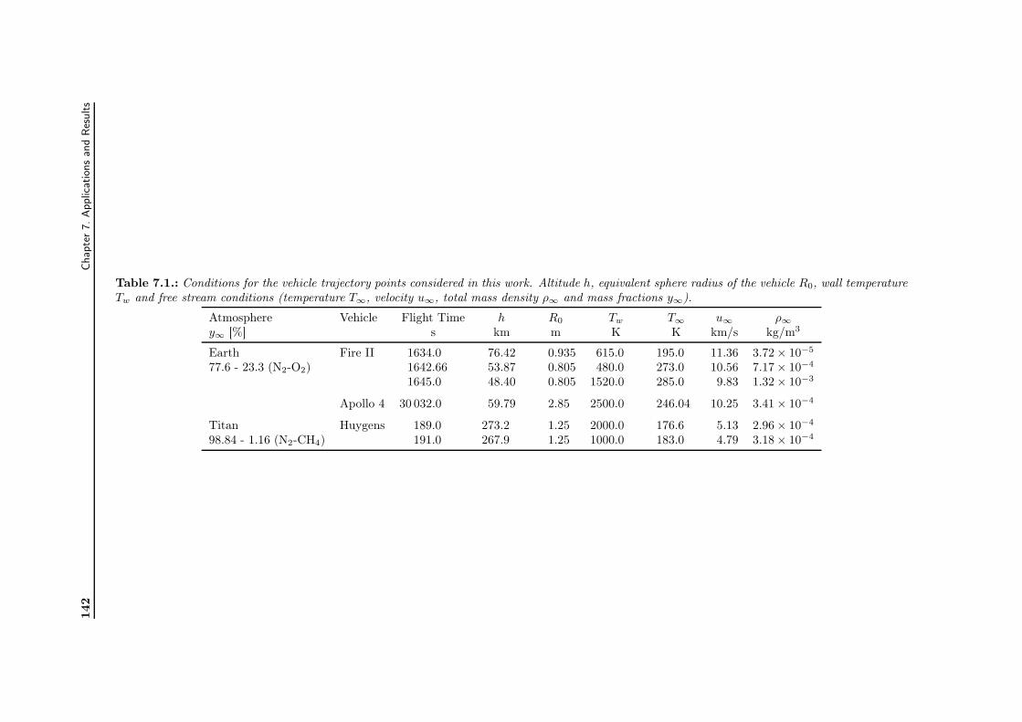
142
Chap
ter7.Applic
atio
ns
and
Res
ults
Table 7.1.: Conditions for the vehicle trajectory points considered in this work. Altitude h, equivalent sphere radius of the vehicle R0, wall temperatureTw and free stream conditions (temperature T∞, velocity u∞, total mass density ρ∞ and mass fractions y∞).
Atmosphere Vehicle Flight Time h R0 Tw T∞ u∞ ρ∞y∞ [%] s km m K K km/s kg/m3
Earth Fire II 1634.0 76.42 0.935 615.0 195.0 11.36 3.72× 10⁻⁵
77.6 - 23.3 (N2-O2) 1642.66 53.87 0.805 480.0 273.0 10.56 7.17× 10⁻⁴
1645.0 48.40 0.805 1520.0 285.0 9.83 1.32× 10⁻³
Apollo 4 30 032.0 59.79 2.85 2500.0 246.04 10.25 3.41× 10⁻⁴
Titan Huygens 189.0 273.2 1.25 2000.0 176.6 5.13 2.96× 10⁻⁴
98.84 - 1.16 (N2-CH4) 191.0 267.9 1.25 1000.0 183.0 4.79 3.18× 10⁻⁴
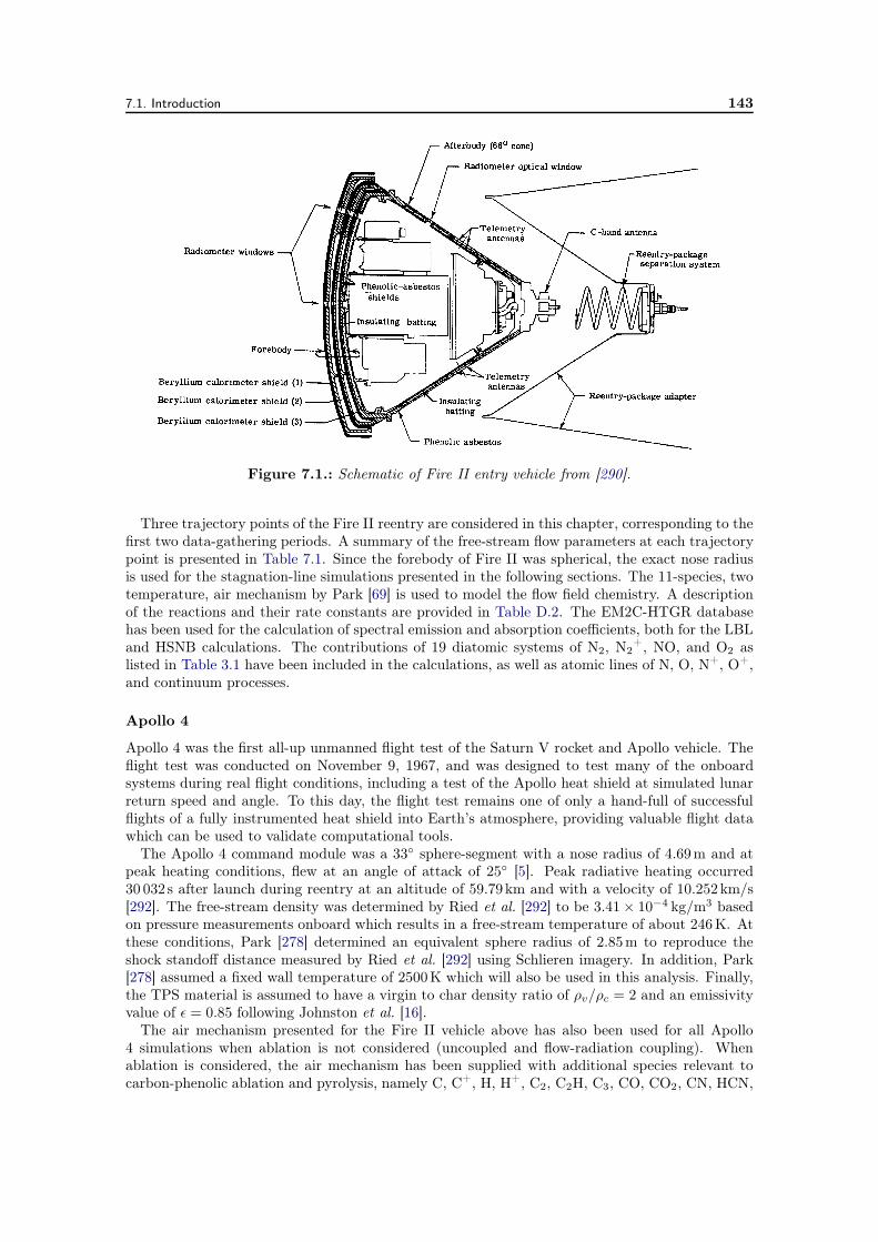
7.1. Introduction 143
Figure 7.1.: Schematic of Fire II entry vehicle from [290].
Three trajectory points of the Fire II reentry are considered in this chapter, corresponding to thefirst two data-gathering periods. A summary of the free-stream flow parameters at each trajectorypoint is presented in Table 7.1. Since the forebody of Fire II was spherical, the exact nose radiusis used for the stagnation-line simulations presented in the following sections. The 11-species, twotemperature, air mechanism by Park [69] is used to model the flow field chemistry. A descriptionof the reactions and their rate constants are provided in Table D.2. The EM2C-HTGR databasehas been used for the calculation of spectral emission and absorption coefficients, both for the LBLand HSNB calculations. The contributions of 19 diatomic systems of N2, N2
+, NO, and O2 aslisted in Table 3.1 have been included in the calculations, as well as atomic lines of N, O, N+, O+,and continuum processes.
Apollo 4
Apollo 4 was the first all-up unmanned flight test of the Saturn V rocket and Apollo vehicle. Theflight test was conducted on November 9, 1967, and was designed to test many of the onboardsystems during real flight conditions, including a test of the Apollo heat shield at simulated lunarreturn speed and angle. To this day, the flight test remains one of only a hand-full of successfulflights of a fully instrumented heat shield into Earth’s atmosphere, providing valuable flight datawhich can be used to validate computational tools.
The Apollo 4 command module was a 33 sphere-segment with a nose radius of 4.69m and atpeak heating conditions, flew at an angle of attack of 25 [5]. Peak radiative heating occurred30 032 s after launch during reentry at an altitude of 59.79km and with a velocity of 10.252km/s[292]. The free-stream density was determined by Ried et al. [292] to be 3.41× 10⁻⁴ kg/m3 basedon pressure measurements onboard which results in a free-stream temperature of about 246K. Atthese conditions, Park [278] determined an equivalent sphere radius of 2.85m to reproduce theshock standoff distance measured by Ried et al. [292] using Schlieren imagery. In addition, Park[278] assumed a fixed wall temperature of 2500K which will also be used in this analysis. Finally,the TPS material is assumed to have a virgin to char density ratio of ρv/ρc = 2 and an emissivityvalue of ϵ = 0.85 following Johnston et al. [16].
The air mechanism presented for the Fire II vehicle above has also been used for all Apollo4 simulations when ablation is not considered (uncoupled and flow-radiation coupling). Whenablation is considered, the air mechanism has been supplied with additional species relevant tocarbon-phenolic ablation and pyrolysis, namely C, C+, H, H+, C2, C2H, C3, CO, CO2, CN, HCN,
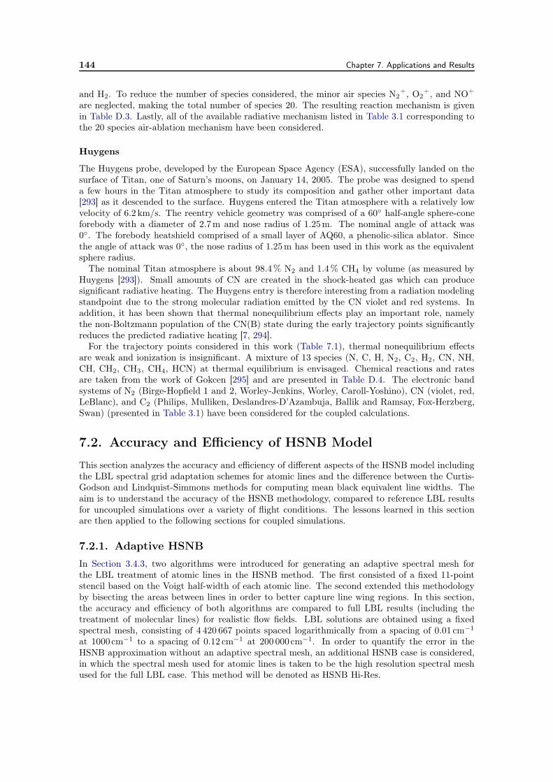
144 Chapter 7. Applications and Results
and H2. To reduce the number of species considered, the minor air species N2+, O2
+, and NO+
are neglected, making the total number of species 20. The resulting reaction mechanism is givenin Table D.3. Lastly, all of the available radiative mechanism listed in Table 3.1 corresponding tothe 20 species air-ablation mechanism have been considered.
Huygens
The Huygens probe, developed by the European Space Agency (ESA), successfully landed on thesurface of Titan, one of Saturn’s moons, on January 14, 2005. The probe was designed to spenda few hours in the Titan atmosphere to study its composition and gather other important data[293] as it descended to the surface. Huygens entered the Titan atmosphere with a relatively lowvelocity of 6.2 km/s. The reentry vehicle geometry was comprised of a 60 half-angle sphere-coneforebody with a diameter of 2.7m and nose radius of 1.25m. The nominal angle of attack was0. The forebody heatshield comprised of a small layer of AQ60, a phenolic-silica ablator. Sincethe angle of attack was 0, the nose radius of 1.25m has been used in this work as the equivalentsphere radius.
The nominal Titan atmosphere is about 98.4% N2 and 1.4% CH4 by volume (as measured byHuygens [293]). Small amounts of CN are created in the shock-heated gas which can producesignificant radiative heating. The Huygens entry is therefore interesting from a radiation modelingstandpoint due to the strong molecular radiation emitted by the CN violet and red systems. Inaddition, it has been shown that thermal nonequilibrium effects play an important role, namelythe non-Boltzmann population of the CN(B) state during the early trajectory points significantlyreduces the predicted radiative heating [7, 294].
For the trajectory points considered in this work (Table 7.1), thermal nonequilibrium effectsare weak and ionization is insignificant. A mixture of 13 species (N, C, H, N2, C2, H2, CN, NH,CH, CH2, CH3, CH4, HCN) at thermal equilibrium is envisaged. Chemical reactions and ratesare taken from the work of Gokcen [295] and are presented in Table D.4. The electronic bandsystems of N2 (Birge-Hopfield 1 and 2, Worley-Jenkins, Worley, Caroll-Yoshino), CN (violet, red,LeBlanc), and C2 (Philips, Mulliken, Deslandres-D’Azambuja, Ballik and Ramsay, Fox-Herzberg,Swan) (presented in Table 3.1) have been considered for the coupled calculations.
7.2. Accuracy and Efficiency of HSNB Model
This section analyzes the accuracy and efficiency of different aspects of the HSNB model includingthe LBL spectral grid adaptation schemes for atomic lines and the difference between the Curtis-Godson and Lindquist-Simmons methods for computing mean black equivalent line widths. Theaim is to understand the accuracy of the HSNB methodology, compared to reference LBL resultsfor uncoupled simulations over a variety of flight conditions. The lessons learned in this sectionare then applied to the following sections for coupled simulations.
7.2.1. Adaptive HSNB
In Section 3.4.3, two algorithms were introduced for generating an adaptive spectral mesh forthe LBL treatment of atomic lines in the HSNB method. The first consisted of a fixed 11-pointstencil based on the Voigt half-width of each atomic line. The second extended this methodologyby bisecting the areas between lines in order to better capture line wing regions. In this section,the accuracy and efficiency of both algorithms are compared to full LBL results (including thetreatment of molecular lines) for realistic flow fields. LBL solutions are obtained using a fixedspectral mesh, consisting of 4 420 667 points spaced logarithmically from a spacing of 0.01 cm−1
at 1000cm−1 to a spacing of 0.12 cm−1 at 200 000cm−1. In order to quantify the error in theHSNB approximation without an adaptive spectral mesh, an additional HSNB case is considered,in which the spectral mesh used for atomic lines is taken to be the high resolution spectral meshused for the full LBL case. This method will be denoted as HSNB Hi-Res.
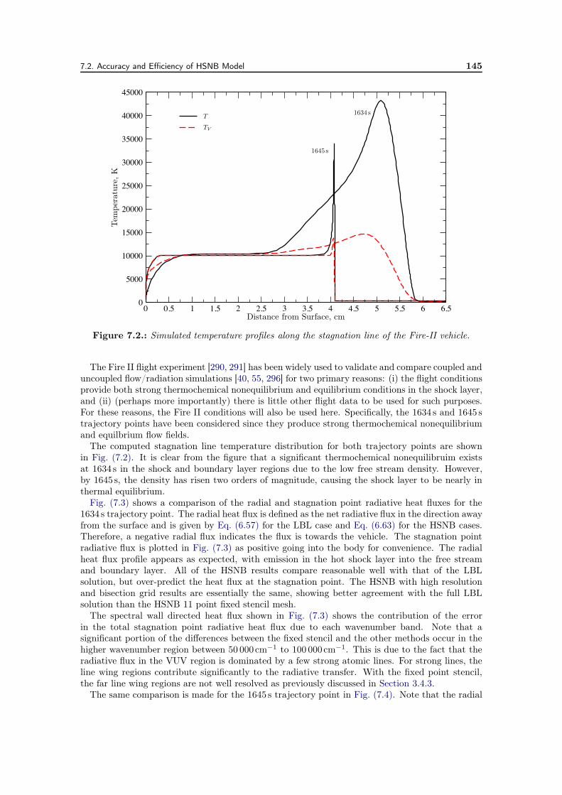
7.2. Accuracy and Efficiency of HSNB Model 145
0 0.5 1 1.5 2 2.5 3 3.5 4 4.5 5 5.5 6 6.50
5000
10000
15000
20000
25000
30000
35000
40000
45000
T
TV
Distance from Surface, cm
Tem
pera
ture
,K1634 s
1645 s
Figure 7.2.: Simulated temperature profiles along the stagnation line of the Fire-II vehicle.
The Fire II flight experiment [290, 291] has been widely used to validate and compare coupled anduncoupled flow/radiation simulations [40, 55, 296] for two primary reasons: (i) the flight conditionsprovide both strong thermochemical nonequilibrium and equilibrium conditions in the shock layer,and (ii) (perhaps more importantly) there is little other flight data to be used for such purposes.For these reasons, the Fire II conditions will also be used here. Specifically, the 1634 s and 1645 strajectory points have been considered since they produce strong thermochemical nonequilibriumand equilbrium flow fields.
The computed stagnation line temperature distribution for both trajectory points are shownin Fig. (7.2). It is clear from the figure that a significant thermochemical nonequilibruim existsat 1634 s in the shock and boundary layer regions due to the low free stream density. However,by 1645 s, the density has risen two orders of magnitude, causing the shock layer to be nearly inthermal equilibrium.
Fig. (7.3) shows a comparison of the radial and stagnation point radiative heat fluxes for the1634 s trajectory point. The radial heat flux is defined as the net radiative flux in the direction awayfrom the surface and is given by Eq. (6.57) for the LBL case and Eq. (6.63) for the HSNB cases.Therefore, a negative radial flux indicates the flux is towards the vehicle. The stagnation pointradiative flux is plotted in Fig. (7.3) as positive going into the body for convenience. The radialheat flux profile appears as expected, with emission in the hot shock layer into the free streamand boundary layer. All of the HSNB results compare reasonable well with that of the LBLsolution, but over-predict the heat flux at the stagnation point. The HSNB with high resolutionand bisection grid results are essentially the same, showing better agreement with the full LBLsolution than the HSNB 11 point fixed stencil mesh.
The spectral wall directed heat flux shown in Fig. (7.3) shows the contribution of the errorin the total stagnation point radiative heat flux due to each wavenumber band. Note that asignificant portion of the differences between the fixed stencil and the other methods occur in thehigher wavenumber region between 50 000cm−1 to 100 000cm−1. This is due to the fact that theradiative flux in the VUV region is dominated by a few strong atomic lines. For strong lines, theline wing regions contribute significantly to the radiative transfer. With the fixed point stencil,the far line wing regions are not well resolved as previously discussed in Section 3.4.3.
The same comparison is made for the 1645 s trajectory point in Fig. (7.4). Note that the radial
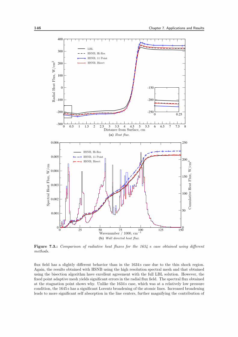
146 Chapter 7. Applications and Results
0 0.5 1 1.5 2 2.5 3 3.5 4 4.5 5 5.5 6 6.5 7 7.5 8-300
-200
-100
0
100
200
300
400
0 0.25-250
-200
-150
LBL
HSNB, Hi-Res
HSNB, 11 Point
HSNB, Bisect
Distance from Surface, cm
Rad
ialH
eat
Flu
x,W
/cm
2
(a) Heat flux.
0 25 50 75 100 125 1500
0.001
0.002
0.003
0.004
0.005
0.006
0
50
100
150
200
250
HSNB, Hi-Res
HSNB, 11 Point
HSNB, Bisect
Wavenumber / 1000, cm−1
Spec
tral
Hea
tFlu
x,W
/cm
Cum
ulat
ive
Hea
tFlu
x,W
/cm
2
(b) Wall directed heat flux.
Figure 7.3.: Comparison of radiative heat fluxes for the 1634 s case obtained using differentmethods.
flux field has a slightly different behavior than in the 1634 s case due to the thin shock region.Again, the results obtained with HSNB using the high resolution spectral mesh and that obtainedusing the bisection algorithm have excellent agreement with the full LBL solution. However, thefixed point adaptive mesh yields significant errors in the radial flux field. The spectral flux obtainedat the stagnation point shows why. Unlike the 1634 s case, which was at a relatively low pressurecondition, the 1645 s has a significant Lorentz broadening of the atomic lines. Increased broadeningleads to more significant self absorption in the line centers, further magnifying the contribution of
7.2. Accuracy and Efficiency of HSNB Model 147
0 0.5 1 1.5 2 2.5 3 3.5 4 4.5 5 5.5 6 6.5-600
-400
-200
0
200
400
600
800
1000
0 0.25-550
-500
-450
-400
-350
LBL
HSNB, Hi-Res
HSNB, 11 Point
HSNB, Bisect
Distance from Surface, cm
Rad
ialH
eat
Flu
x,W
/cm
2
(a) Heat flux.
0 25 50 75 100 125 1500
0.01
0.02
0.03
0.04
0 50 100 1500
100
200
300
400
500
600
HSNB, Hi-Res
HSNB, 11 Point
HSNB, Bisect
Wavenumber / 1000, cm−1
Spec
tral
Hea
tFlu
x,W
/cm
Cum
ulat
ive
Hea
tFlu
x,W
/cm
2
(b) Wall directed heat flux.
Figure 7.4.: Comparison of radiative heat fluxes for the 1645 s case obtained using differentmethods.
the line wings to the radiative transfer. Thus, poorly resolved line wings with the fixed point meshresults in significant errors in the radiative flux.
Table 7.2 summarizes the results for each of the methods at both trajectory points, includingerrors in the calculated wall heat flux, and the CPU time required to compute the radiative flux,relative to the time with the bisection method. The CPU time required for the full flux calculationis two orders of magnitude less for the adaptive HSNB methods compared to the LBL solution,while the high-resolution HSNB model allows a one order of magnitude reduction. In practice,
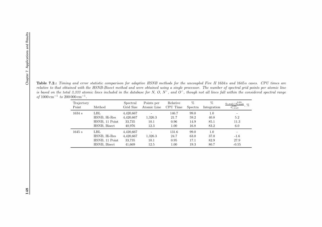
148
Chap
ter7.Applic
atio
ns
and
Res
ults
Table 7.2.: Timing and error statistic comparison for adaptive HSNB methods for the uncoupled Fire II 1634 s and 1645 s cases. CPU times arerelative to that obtained with the HSNB-Bisect method and were obtained using a single processor. The number of spectral grid points per atomic lineis based on the total 3,333 atomic lines included in the database for N, O, N+, and O+, though not all lines fall within the considered spectral rangeof 1000 cm−1 to 200 000cm−1.
Trajectory Spectral Points per Relative % % qr,wall−qLBLr,wall
qLBLr,wall
, %Point Method Grid Size Atomic Line CPU Time Spectra Integration
1634 s LBL 4,420,667 - 146.7 99.0 1.0 -HSNB, Hi-Res 4,420,667 1,326.3 21.7 59.2 40.8 5.2HSNB, 11 Point 33,735 10.1 0.96 14.9 85.1 11.3HSNB, Bisect 40,976 12.3 1.00 16.8 83.2 6.0
1645 s LBL 4,420,667 - 131.6 99.0 1.0 -HSNB, Hi-Res 4,420,667 1,326.3 24.7 63.0 37.0 -1.6HSNB, 11 Point 33,735 10.1 0.95 17.1 82.9 27.9HSNB, Bisect 41,669 12.5 1.00 19.3 80.7 -0.55
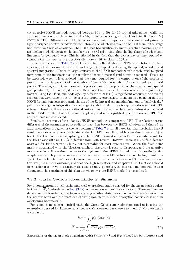
7.2. Accuracy and Efficiency of HSNB Model 149
the adaptive HSNB methods required between 60 s to 90 s for 30 spatial grid points, while theLBL solution was completed in about 2.5 h, running on a single core of an Intel(R) Core(TM)i7-4770K CPU. Differences in CPU times for the different trajectory points are caused primarilyby the assigned spectral window for each atomic line which was taken to be 10 000 times the Voigthalf-width for these calculations. The 1645 s case has significantly more Lorentz broadening of theatomic lines, which increases the number of spectral grid points that the line shape of each atomicline must be computed over. This is reflected in the fact that the percentage of time required tocompute the line spectra is proportionally more at 1645 s than at 1634 s.
It can also be seen in Table 7.2 that for the full LBL calculations, 99% of the total CPU timeis spent just generating the spectra, and only 1% is spent performing the spatial, angular, andspectral integration. This is in large contrast to the HSNB methods which clearly tend to spendmore time in the integration as the number of atomic spectral grid points is reduced. This is tobe expected, when it is considered that the time required for the computation of the spectra isproportional to the product of the number of lines with the number of spectral and spatial gridpoints. The integration time, however, is proportional to the product of the spectral and spatialgrid points only. Therefore, it is clear that since the number of lines considered is significantlylowered using the HSNB methodology (by a factor of ≈ 1000), a significant amount of the overallreduction in CPU time is due to the spectral property calculation. It should also be noted that theHSNB formulation does not permit the use of the En integral exponential functions to “analytically"perform the angular integration in the tangent slab formulation as is typically done in most RTEsolvers. Therefore, there is an additional cost required to compute the angular integration includedin the HSNB results. This additional complexity and cost is justified when the overall CPU costrequirements are considered.
Finally, the accuracy of the adaptive HSNB methods are compared to LBL. The relative percentdifference of the stagnation point radiative heat flux between the HSNB solutions and that of theLBL calculations are given in the last column of Table 7.2. In all cases the high resolution HSNBresult provides a very good estimate of the full LBL heat flux, with a maximum error of just5.2%. For the fixed point adaptive grid, the HSNB formulation provides a reasonable result forthe 1634 s case with an 11.3% difference from LBL results. However, there is a 27.9% differenceobserved for 1645 s, which is likely not acceptable for most applications. When the fixed pointmesh is augmented with the bisection method, this error is seen to disappear, and the adaptivemesh provides a flux estimate close to the high resolution HSNB formulation. Interestingly, thisadaptive approach provides an even better estimate to the LBL solution than the high resolutionspectral mesh for the 1645 s case. However, since the total error is less than 1%, it is assumed thatthis was just a lucky outcome, and that the high resolution and adaptive HSNB methods shouldbe considered to provide essentially the same results. Therefore, the bisection method will be usedthroughout the remainder of this chapter where ever the HSNB method is considered.
7.2.2. Curtis-Godson versus Lindquist-Simmons
For a homogeneous optical path, analytical expressions can be derived for the mean black equiva-lent width W/δ introduced in Eq. (3.55) for mean transmissivity calculations. These expressionsdepend on the broadening mechanism and a prescribed distribution law for line intensities withinthe narrow band and are functions of two parameters: a mean absorption coefficient k and anoverlapping parameter β.
For a non homogeneous optical path, the Curtis-Godson approximation consists in using theexpressions derived for homogeneous media with averaged parameters ku∗ and β∗ that we defineaccording to
ku∗ =
∫ s
s′p(s′′)k(s′′)ds′′, (7.1)
β∗ =1
ku∗
∫ s
s′β(s′′)p(s′′)k(s′′)ds′′. (7.2)
Expressions of the mean black equivalent width WL(s′, s)/δ and WD(s′, s)/δ for both Lorentz and
150 Chapter 7. Applications and Results
0 0.02 0.04 0.06 0.08 0.1
-500
-400
-300
-200
-100
0
-2
0
2
Distance from wall, m
Rad
iative
pow
er,W
/cm
3
LBL
Curtis-Godson
Linquist-Simmons
Figure 7.5.: Radiative power comparison between Curtis-Godson and Lindquist-Simmons approx-imations for the Fire II 1634 s test case.
Doppler broadening are given in Table 3.2. Eq. (3.57) is used to obtain the mean black equivalentwidth in the Voigt broadening regime, as proposed by Ludwig et al. [158].
An alternative approach for treating non-uniform optical paths is the Lindquist-Simmons ap-proximation [159]. It consists in finding an expression for the space derivative of the mean blackequivalent width and then integrating it over the path in order to get the mean transmissivity
τσ(s′, s)∆σ
= exp
(
1
δ
∫ s
s′
∂W (s′′, s)
∂s′′ds”
)
. (7.3)
The expressions of ∂WL(s′′, s)/∂s′′ and ∂WD(s′′, s)/∂s′′ for Lorentz and Doppler broadening usedin this work are given in Table 3.3. They involve both local parameters k(s′′), β(s′′) and aver-aged parameters ku∗, β∗. After the spatial integration, Eq. (3.57) is used to get the mean blackequivalent width in the Voigt regime, as is done in the Curtis-Godson approach.
A comparison between the HSNB Curtis-Godson and the HSNB Lindquist-Simmons is given inFig. (7.5) for the Fire II (1634 s) test case. The difference between the two approximations isvery tiny and for most of the points is much lower than the difference between HSNB Lindquist-Simmons and LBL calculations. However, we can see a much larger discrepancy in the free stream,where the radiative power predicted by the HSNB Curtis-Godson model becomes negative whileit remains positive for the HSNB Lindquist-Simmons and LBL models. A negative energy sourceterm in this cold region is a major computational issue for coupling as negative temperatures canbe predicted after a few iterations. Therefore, the Lindquist-Simmons approximation has beenchosen for all coupled simulations presented in this work, though it requires around three timesmore computational time.
7.2.3. Comparison with Smeared Rotational Band Model
In order to assess the accuracy and the efficiency of the HSNB model, a comparison with therigorous Line-By-Line (LBL) method is carried out. In LBL calculations, radiative properties ofthe plasma are computed from the spectroscopic HTGR database, presented in Chapter 3, on a
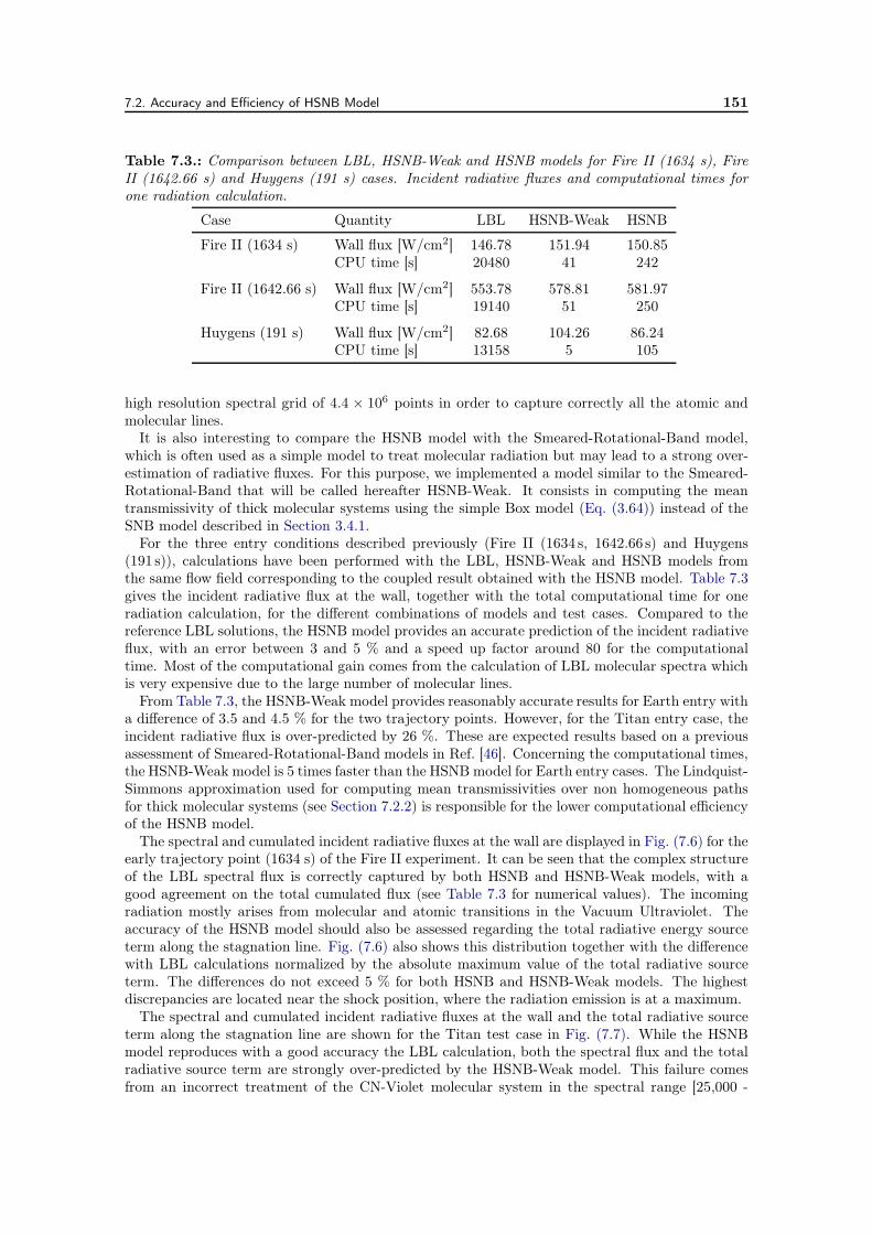
7.2. Accuracy and Efficiency of HSNB Model 151
Table 7.3.: Comparison between LBL, HSNB-Weak and HSNB models for Fire II (1634 s), FireII (1642.66 s) and Huygens (191 s) cases. Incident radiative fluxes and computational times forone radiation calculation.
Case Quantity LBL HSNB-Weak HSNB
Fire II (1634 s) Wall flux [W/cm2] 146.78 151.94 150.85CPU time [s] 20480 41 242
Fire II (1642.66 s) Wall flux [W/cm2] 553.78 578.81 581.97CPU time [s] 19140 51 250
Huygens (191 s) Wall flux [W/cm2] 82.68 104.26 86.24CPU time [s] 13158 5 105
high resolution spectral grid of 4.4 × 10⁶ points in order to capture correctly all the atomic andmolecular lines.
It is also interesting to compare the HSNB model with the Smeared-Rotational-Band model,which is often used as a simple model to treat molecular radiation but may lead to a strong over-estimation of radiative fluxes. For this purpose, we implemented a model similar to the Smeared-Rotational-Band that will be called hereafter HSNB-Weak. It consists in computing the meantransmissivity of thick molecular systems using the simple Box model (Eq. (3.64)) instead of theSNB model described in Section 3.4.1.
For the three entry conditions described previously (Fire II (1634 s, 1642.66 s) and Huygens(191 s)), calculations have been performed with the LBL, HSNB-Weak and HSNB models fromthe same flow field corresponding to the coupled result obtained with the HSNB model. Table 7.3gives the incident radiative flux at the wall, together with the total computational time for oneradiation calculation, for the different combinations of models and test cases. Compared to thereference LBL solutions, the HSNB model provides an accurate prediction of the incident radiativeflux, with an error between 3 and 5 % and a speed up factor around 80 for the computationaltime. Most of the computational gain comes from the calculation of LBL molecular spectra whichis very expensive due to the large number of molecular lines.
From Table 7.3, the HSNB-Weak model provides reasonably accurate results for Earth entry witha difference of 3.5 and 4.5 % for the two trajectory points. However, for the Titan entry case, theincident radiative flux is over-predicted by 26 %. These are expected results based on a previousassessment of Smeared-Rotational-Band models in Ref. [46]. Concerning the computational times,the HSNB-Weak model is 5 times faster than the HSNB model for Earth entry cases. The Lindquist-Simmons approximation used for computing mean transmissivities over non homogeneous pathsfor thick molecular systems (see Section 7.2.2) is responsible for the lower computational efficiencyof the HSNB model.
The spectral and cumulated incident radiative fluxes at the wall are displayed in Fig. (7.6) for theearly trajectory point (1634 s) of the Fire II experiment. It can be seen that the complex structureof the LBL spectral flux is correctly captured by both HSNB and HSNB-Weak models, with agood agreement on the total cumulated flux (see Table 7.3 for numerical values). The incomingradiation mostly arises from molecular and atomic transitions in the Vacuum Ultraviolet. Theaccuracy of the HSNB model should also be assessed regarding the total radiative energy sourceterm along the stagnation line. Fig. (7.6) also shows this distribution together with the differencewith LBL calculations normalized by the absolute maximum value of the total radiative sourceterm. The differences do not exceed 5 % for both HSNB and HSNB-Weak models. The highestdiscrepancies are located near the shock position, where the radiation emission is at a maximum.
The spectral and cumulated incident radiative fluxes at the wall and the total radiative sourceterm along the stagnation line are shown for the Titan test case in Fig. (7.7). While the HSNBmodel reproduces with a good accuracy the LBL calculation, both the spectral flux and the totalradiative source term are strongly over-predicted by the HSNB-Weak model. This failure comesfrom an incorrect treatment of the CN-Violet molecular system in the spectral range [25,000 -
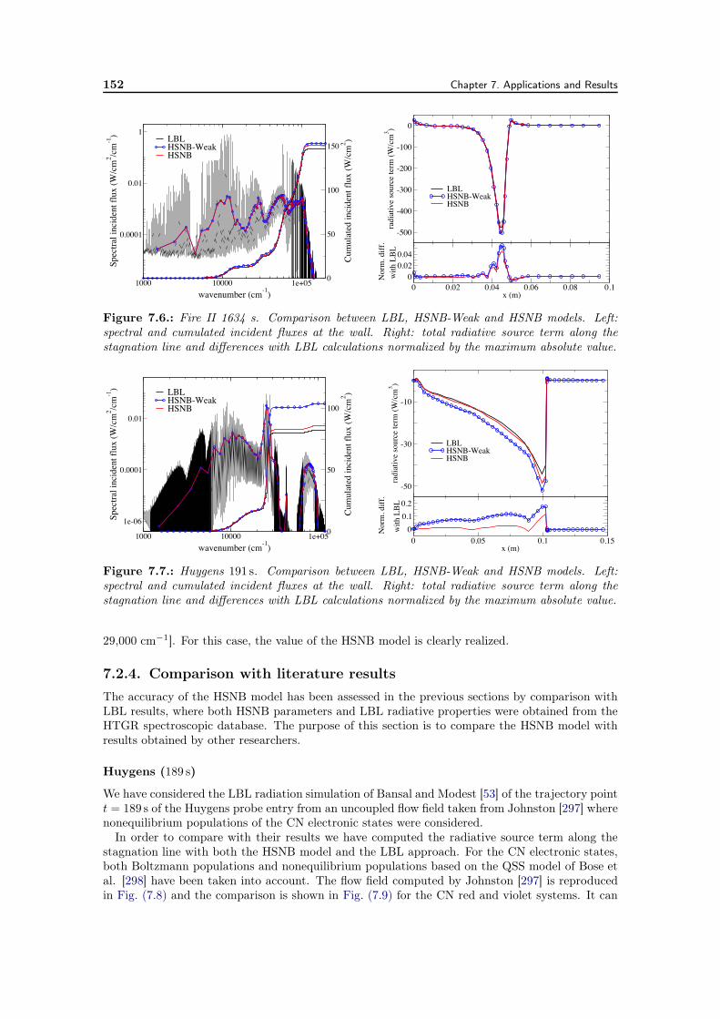
152 Chapter 7. Applications and Results
1000 10000 1e+05wavenumber (cm-1)
0.0001
0.01
1
Spec
tral i
ncid
ent f
lux
(W/c
m2 /c
m-1
)
0
50
100
150
Cum
ulat
ed in
cide
nt fl
ux (W
/cm
2 )LBLHSNB-WeakHSNB
-500
-400
-300
-200
-100
0
radi
ativ
e so
urce
term
(W/c
m3 )
LBLHSNB-WeakHSNB
0 0.02 0.04 0.06 0.08 0.1x (m)
00.020.04
with
LB
LN
orm
. diff
.
Figure 7.6.: Fire II 1634 s. Comparison between LBL, HSNB-Weak and HSNB models. Left:spectral and cumulated incident fluxes at the wall. Right: total radiative source term along thestagnation line and differences with LBL calculations normalized by the maximum absolute value.
1000 10000 1e+05wavenumber (cm-1)
1e-06
0.0001
0.01
Spec
tral i
ncid
ent f
lux
(W/c
m2 /c
m-1
)
0
50
100
Cum
ulat
ed in
cide
nt fl
ux (W
/cm
2 )LBLHSNB-WeakHSNB
-50
-30
-10ra
diat
ive
sour
ce te
rm (W
/cm
3 )
LBLHSNB-WeakHSNB
0 0.05 0.1 0.15x (m)
00.10.2
with
LB
L
Nor
m. d
iff.
Figure 7.7.: Huygens 191 s. Comparison between LBL, HSNB-Weak and HSNB models. Left:spectral and cumulated incident fluxes at the wall. Right: total radiative source term along thestagnation line and differences with LBL calculations normalized by the maximum absolute value.
29,000 cm−1]. For this case, the value of the HSNB model is clearly realized.
7.2.4. Comparison with literature results
The accuracy of the HSNB model has been assessed in the previous sections by comparison withLBL results, where both HSNB parameters and LBL radiative properties were obtained from theHTGR spectroscopic database. The purpose of this section is to compare the HSNB model withresults obtained by other researchers.
Huygens (189 s)
We have considered the LBL radiation simulation of Bansal and Modest [53] of the trajectory pointt = 189 s of the Huygens probe entry from an uncoupled flow field taken from Johnston [297] wherenonequilibrium populations of the CN electronic states were considered.
In order to compare with their results we have computed the radiative source term along thestagnation line with both the HSNB model and the LBL approach. For the CN electronic states,both Boltzmann populations and nonequilibrium populations based on the QSS model of Bose etal. [298] have been taken into account. The flow field computed by Johnston [297] is reproducedin Fig. (7.8) and the comparison is shown in Fig. (7.9) for the CN red and violet systems. It can
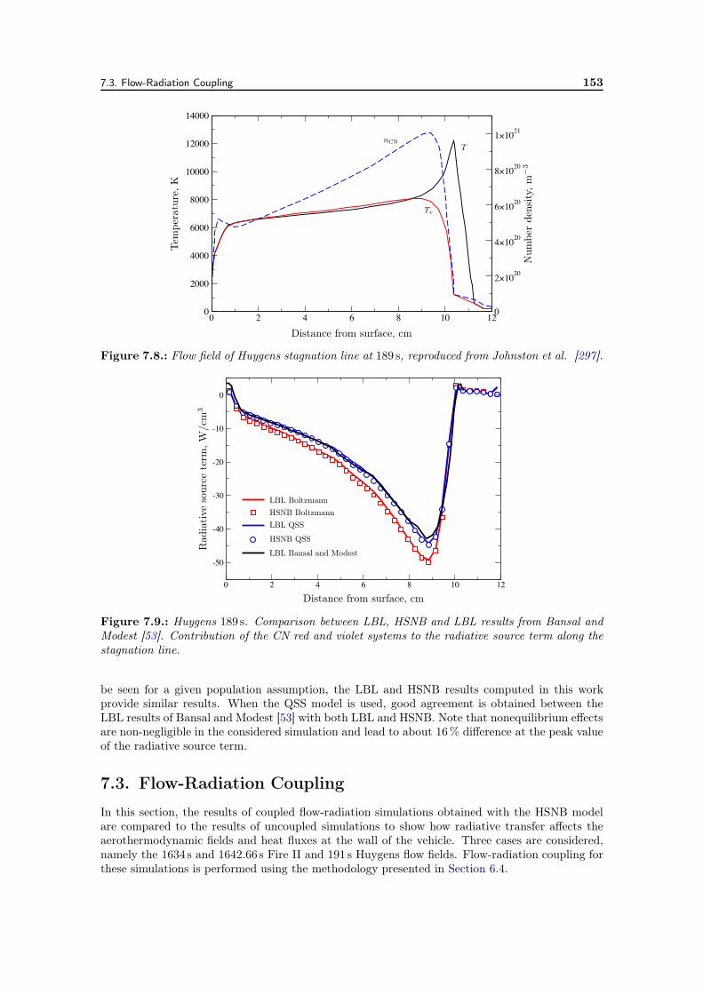
7.3. Flow-Radiation Coupling 153
0
2000
4000
6000
8000
10000
12000
14000
121086420 0
2×10²⁰
4×10²⁰
6×10²⁰
8×10²⁰
1×10²¹
Tem
pera
ture
,K
Num
ber
dens
ity,
m−3
Distance from surface, cm
nCNT
Tv
Figure 7.8.: Flow field of Huygens stagnation line at 189 s, reproduced from Johnston et al. [297].
0 2 4 6 8 10 12
-50
-40
-30
-20
-10
0
Rad
iative
sour
cete
rm,W
/cm
3
Distance from surface, cm
LBL BoltzmannHSNB BoltzmannLBL QSS
HSNB QSS
LBL Bansal and Modest
Figure 7.9.: Huygens 189 s. Comparison between LBL, HSNB and LBL results from Bansal andModest [53]. Contribution of the CN red and violet systems to the radiative source term along thestagnation line.
be seen for a given population assumption, the LBL and HSNB results computed in this workprovide similar results. When the QSS model is used, good agreement is obtained between theLBL results of Bansal and Modest [53] with both LBL and HSNB. Note that nonequilibrium effectsare non-negligible in the considered simulation and lead to about 16% difference at the peak valueof the radiative source term.
7.3. Flow-Radiation Coupling
In this section, the results of coupled flow-radiation simulations obtained with the HSNB modelare compared to the results of uncoupled simulations to show how radiative transfer affects theaerothermodynamic fields and heat fluxes at the wall of the vehicle. Three cases are considered,namely the 1634 s and 1642.66 s Fire II and 191 s Huygens flow fields. Flow-radiation coupling forthese simulations is performed using the methodology presented in Section 6.4.
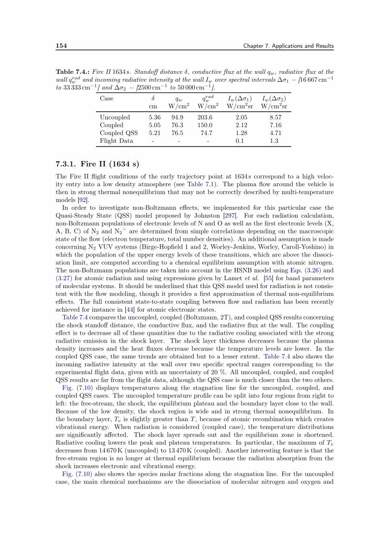
154 Chapter 7. Applications and Results
Table 7.4.: Fire II 1634 s. Standoff distance δ, conductive flux at the wall qw, radiative flux at thewall qradw and incoming radiative intensity at the wall Iw over spectral intervals ∆σ1 = [16 667 cm−1
to 33 333 cm−1] and ∆σ2 = [2500 cm−1 to 50 000cm−1].
Case δ qw qradw Iw(∆σ1) Iw(∆σ2)cm W/cm2 W/cm2 W/cm2sr W/cm2sr
Uncoupled 5.36 94.9 203.6 2.05 8.57Coupled 5.05 76.3 150.0 2.12 7.16Coupled QSS 5.21 76.5 74.7 1.28 4.71Flight Data - - - 0.1 1.3
7.3.1. Fire II (1634 s)
The Fire II flight conditions of the early trajectory point at 1634 s correspond to a high veloc-ity entry into a low density atmosphere (see Table 7.1). The plasma flow around the vehicle isthen in strong thermal nonequilibrium that may not be correctly described by multi-temperaturemodels [92].
In order to investigate non-Boltzmann effects, we implemented for this particular case theQuasi-Steady State (QSS) model proposed by Johnston [297]. For each radiation calculation,non-Boltzmann populations of electronic levels of N and O as well as the first electronic levels (X,A, B, C) of N2 and N2
+ are determined from simple correlations depending on the macroscopicstate of the flow (electron temperature, total number densities). An additional assumption is madeconcerning N2 VUV systems (Birge-Hopfield 1 and 2, Worley-Jenkins, Worley, Caroll-Yoshino) inwhich the population of the upper energy levels of these transitions, which are above the dissoci-ation limit, are computed according to a chemical equilibrium assumption with atomic nitrogen.The non-Boltzmann populations are taken into account in the HSNB model using Eqs. (3.26) and(3.27) for atomic radiation and using expressions given by Lamet et al. [55] for band parametersof molecular systems. It should be underlined that this QSS model used for radiation is not consis-tent with the flow modeling, though it provides a first approximation of thermal non-equilibriumeffects. The full consistent state-to-state coupling between flow and radiation has been recentlyachieved for instance in [44] for atomic electronic states.
Table 7.4 compares the uncoupled, coupled (Boltzmann, 2T), and coupled QSS results concerningthe shock standoff distance, the conductive flux, and the radiative flux at the wall. The couplingeffect is to decrease all of these quantities due to the radiative cooling associated with the strongradiative emission in the shock layer. The shock layer thickness decreases because the plasmadensity increases and the heat fluxes decrease because the temperature levels are lower. In thecoupled QSS case, the same trends are obtained but to a lesser extent. Table 7.4 also shows theincoming radiative intensity at the wall over two specific spectral ranges corresponding to theexperimental flight data, given with an uncertainty of 20 %. All uncoupled, coupled, and coupledQSS results are far from the flight data, although the QSS case is much closer than the two others.
Fig. (7.10) displays temperatures along the stagnation line for the uncoupled, coupled, andcoupled QSS cases. The uncoupled temperature profile can be split into four regions from right toleft: the free-stream, the shock, the equilibrium plateau and the boundary layer close to the wall.Because of the low density, the shock region is wide and in strong thermal nonequilibrium. Inthe boundary layer, Tv is slightly greater than T , because of atomic recombination which createsvibrational energy. When radiation is considered (coupled case), the temperature distributionsare significantly affected. The shock layer spreads out and the equilibrium zone is shortened.Radiative cooling lowers the peak and plateau temperatures. In particular, the maximum of Tv
decreases from 14 670K (uncoupled) to 13 470K (coupled). Another interesting feature is that thefree-stream region is no longer at thermal equilibrium because the radiation absorption from theshock increases electronic and vibrational energy.
Fig. (7.10) also shows the species molar fractions along the stagnation line. For the uncoupledcase, the main chemical mechanisms are the dissociation of molecular nitrogen and oxygen and
7.3. Flow-Radiation Coupling 155
Table 7.5.: Fire II 1642.66 s. Standoff distance δ, conductive flux at the wall qw, radiative fluxat the wall qradw and incoming radiative intensity at the wall Iw over spectral intervals ∆σ1 =[16 667 cm−1 to 33 333 cm−1] and ∆σ2 = [2500 cm−1 to 50 000cm−1].
Case δ qw qradw Iw(∆σ1) Iw(∆σ2)cm W/cm2 W/cm2 W/cm2sr W/cm2sr
Uncoupled 4.06 635.6 791.3 11.65 71.01Coupled 4.01 617.0 581.7 9.28 53.63Flight Data - - - 10.5 63.0
the ionization of atomic nitrogen and oxygen through the shock. A significant amount of nitrogenmonoxide is also produced in the shock region. The ionization level is quite important in the plateauas the electron molar fraction reaches 0.15. In the boundary layer, the ionization level drops downand atomic nitrogen starts recombining. For the coupled case, the fall of the two temperatures slowsdown the ionization reactions and the electron molar fraction reaches a maximum of 0.08. The free-stream region ahead of the shock becomes chemically reacting under the effect of radiation: atomicoxygen is produced by photodissociation and electrons are produced mainly by photoionization ofmolecular oxygen.
These coupling effects on temperature and composition are also noticeable in Fig. (7.10) forthe coupled QSS case, however they are much weaker. In order to understand this behavior, theradiative source term along the stagnation line is plotted in Fig. (7.11) and split according to theatomic, molecular, and continua emission contributions. From uncoupled to coupled calculations,the peak of the radiative source term is decreased by a factor two due to radiative cooling. Fromcoupled to coupled QSS calculations, the peak of the radiative source term is further reduced andatomic contribution almost vanishes at the shock location. The reason is that the Tv Boltzmanndistribution leads to an overestimation of the population of the highest electronic energy levels ofatomic N and O, as well as N2 and N2
+. In particular, for the N2 VUV systems, the dissocia-tion equilibrium assumption makes the population of the upper electronic energy level associatedwith these systems close to zero and thus cancels their contribution to radiation. The remainingmolecular emission peak in Fig. (7.11) comes mostly from NO radiation, of which electronic energylevels are assumed to be populated according to the temperature Tv. An incorrect treatment ofthe thermal state of NO might be responsible of the remaining discrepancies between the coupledQSS results and the flight data.
7.3.2. Fire II (1642.66 s)
The Fire 2 flight conditions of the trajectory point t = 1642.66 s correspond to a quasi-thermalequilibrium situation. Due to the higher density, the kinetic energy transfer between the internalenergy modes is much faster than for the trajectory point t = 1634 s. Thus, the QSS model hasnot been considered in this case.
Table 7.5 shows the computed shock standoff distance and conductive and radiative flux at thewall for the coupled and uncoupled simulations. As can be seen, the standoff distance and theconductive flux slightly decrease and the radiative flux diminishes by around 25% when radiationis coupled to the flow. In addition, coupled results are in fair agreement with flight data whichare given with an uncertainty of 20%. Temperatures and composition along the stagnation lineare shown in Fig. (7.12). For the uncoupled case, the flow is in thermal equilibrium everywhereexcept in the shock region. A chemical equilibrium zone with flat molar fraction profiles is clearlydistinguishable between the boundary layer and the shock. The electron molar fraction is around0.07 in this zone. When radiation is considered, as for the previous trajectory point, the vibration-electronic-electron temperature Tv increases and a slight fraction of O, e– and O2
+ are producedin the free stream by photodissociation and photoionization of O2. The temperature is slightlydecreased in the shock layer, leading to a lower ionization level.
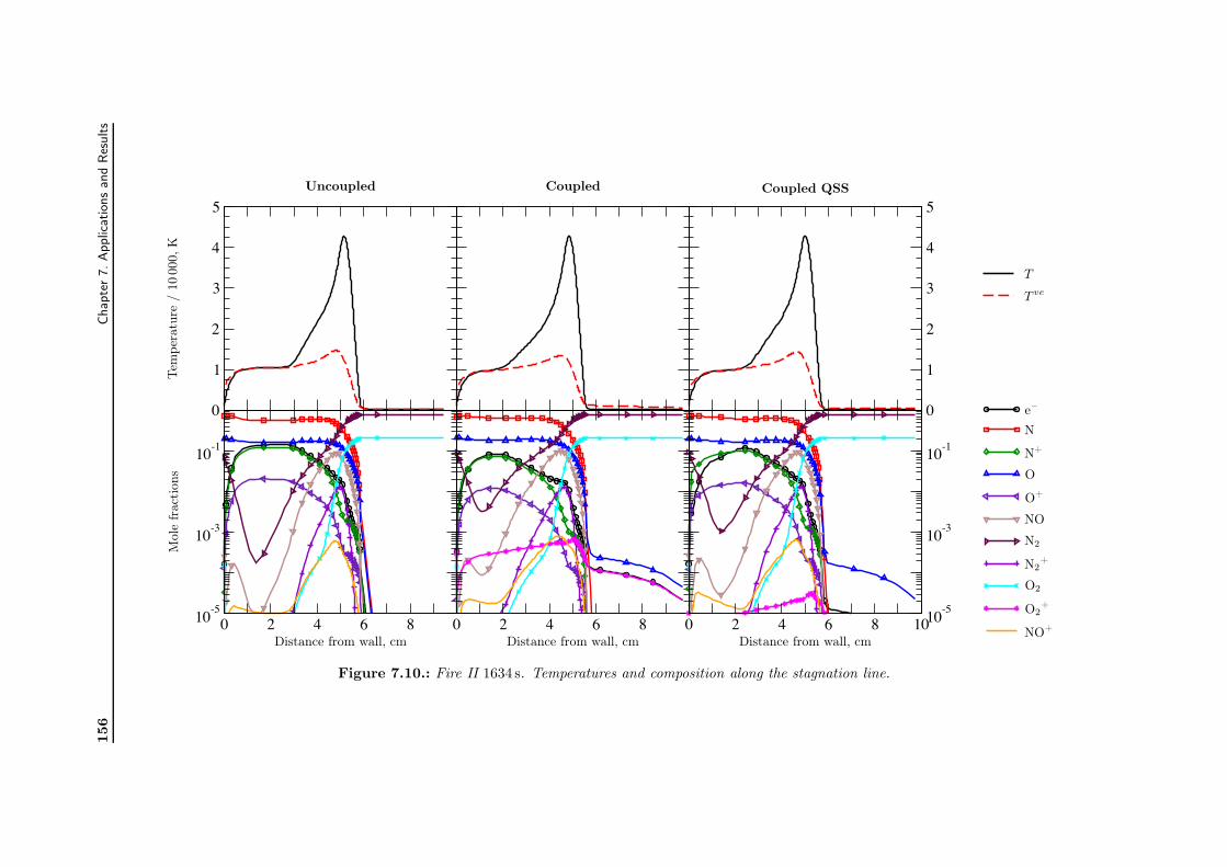
156
Chap
ter7.Applic
atio
ns
and
Res
ults
0
1
2
3
4
5
0
1
2
3
4
5
0 2 4 6 810-5
10-3
10-1
0 2 4 6 8 0 2 4 6 8 1010-5
10-3
10-1
Distance from wall, cmDistance from wall, cmDistance from wall, cm
Tem
pera
ture
/10
000,
KM
ole
frac
tion
s
e–
N
N+
O
O+
NO
NO+
N2
N2+
O2
O2+
T
T ve
Uncoupled Coupled Coupled QSS
Figure 7.10.: Fire II 1634 s. Temperatures and composition along the stagnation line.
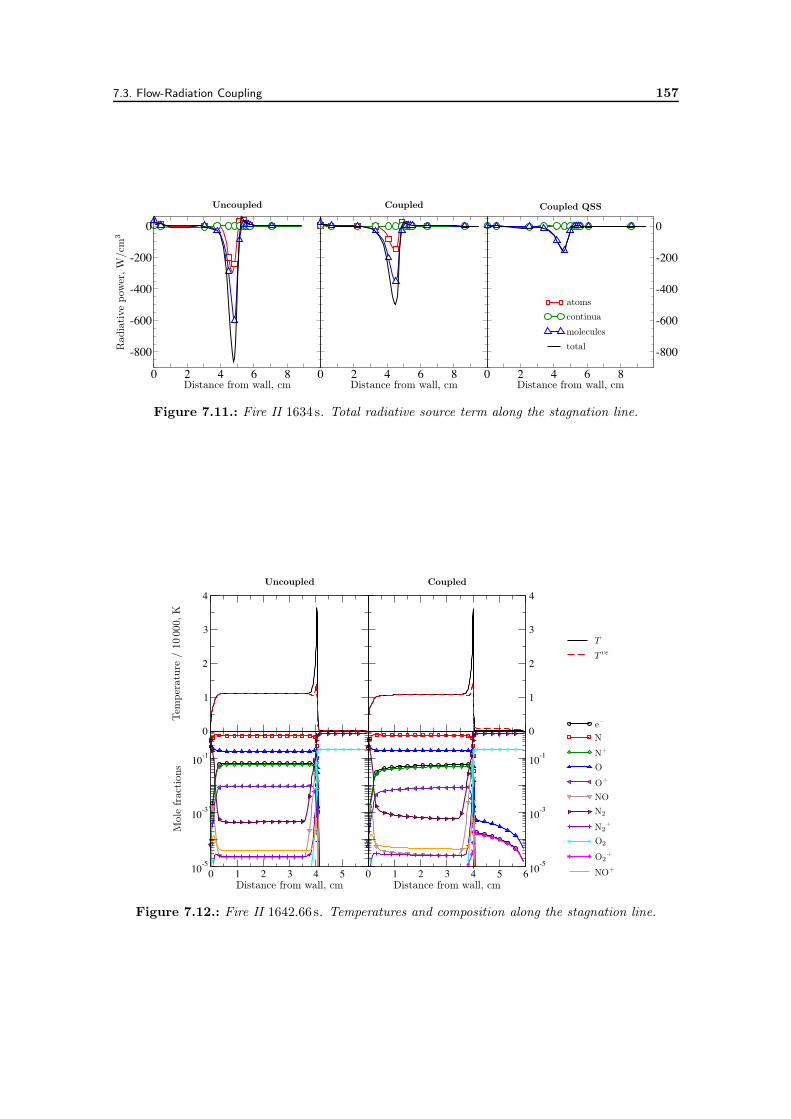
7.3. Flow-Radiation Coupling 157
0 2 4 6 8
-800
-600
-400
-200
0
0 2 4 6 8 0 2 4 6 8
-800
-600
-400
-200
0
Distance from wall, cmDistance from wall, cmDistance from wall, cm
Rad
iative
pow
er,W
/cm
3
Uncoupled Coupled Coupled QSS
atoms
continua
molecules
total
Figure 7.11.: Fire II 1634 s. Total radiative source term along the stagnation line.
0
1
2
3
4
0
1
2
3
4
0 1 2 3 4 5 610-5
10-3
10-1
0 1 2 3 4 510-5
10-3
10-1
Distance from wall, cm Distance from wall, cm
Tem
pera
ture
/10
000,
KM
ole
frac
tion
s
e–
N
N+
O
O+
NO
NO+
N2
N2+
O2
O2+
T
T ve
Uncoupled Coupled
Figure 7.12.: Fire II 1642.66 s. Temperatures and composition along the stagnation line.
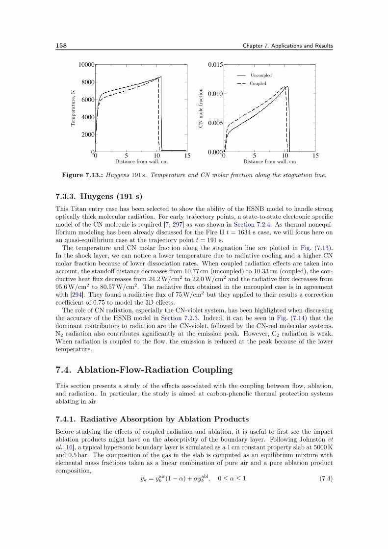
158 Chapter 7. Applications and Results
0 5 10 150
2000
4000
6000
8000
10000
0 5 10 150.000
0.005
0.010
0.015
Distance from wall, cmDistance from wall, cm
Tem
pera
ture
,K
CN
mol
efr
action
Uncoupled
Coupled
Figure 7.13.: Huygens 191 s. Temperature and CN molar fraction along the stagnation line.
7.3.3. Huygens (191 s)
This Titan entry case has been selected to show the ability of the HSNB model to handle strongoptically thick molecular radiation. For early trajectory points, a state-to-state electronic specificmodel of the CN molecule is required [7, 297] as was shown in Section 7.2.4. As thermal nonequi-librium modeling has been already discussed for the Fire II t = 1634 s case, we will focus here onan quasi-equilibrium case at the trajectory point t = 191 s.
The temperature and CN molar fraction along the stagnation line are plotted in Fig. (7.13).In the shock layer, we can notice a lower temperature due to radiative cooling and a higher CNmolar fraction because of lower dissociation rates. When coupled radiation effects are taken intoaccount, the standoff distance decreases from 10.77 cm (uncoupled) to 10.33 cm (coupled), the con-ductive heat flux decreases from 24.2W/cm2 to 22.0W/cm2 and the radiative flux decreases from95.6W/cm2 to 80.57W/cm2. The radiative flux obtained in the uncoupled case is in agreementwith [294]. They found a radiative flux of 75W/cm2 but they applied to their results a correctioncoefficient of 0.75 to model the 3D effects.
The role of CN radiation, especially the CN-violet system, has been highlighted when discussingthe accuracy of the HSNB model in Section 7.2.3. Indeed, it can be seen in Fig. (7.14) that thedominant contributors to radiation are the CN-violet, followed by the CN-red molecular systems.N2 radiation also contributes significantly at the emission peak. However, C2 radiation is weak.When radiation is coupled to the flow, the emission is reduced at the peak because of the lowertemperature.
7.4. Ablation-Flow-Radiation Coupling
This section presents a study of the effects associated with the coupling between flow, ablation,and radiation. In particular, the study is aimed at carbon-phenolic thermal protection systemsablating in air.
7.4.1. Radiative Absorption by Ablation Products
Before studying the effects of coupled radiation and ablation, it is useful to first see the impactablation products might have on the absorptivity of the boundary layer. Following Johnston etal. [16], a typical hypersonic boundary layer is simulated as a 1 cm constant property slab at 5000Kand 0.5 bar. The composition of the gas in the slab is computed as an equilibrium mixture withelemental mass fractions taken as a linear combination of pure air and a pure ablation productcomposition,
yk = yairk (1− α) + αyabl
k , 0 ≤ α ≤ 1. (7.4)
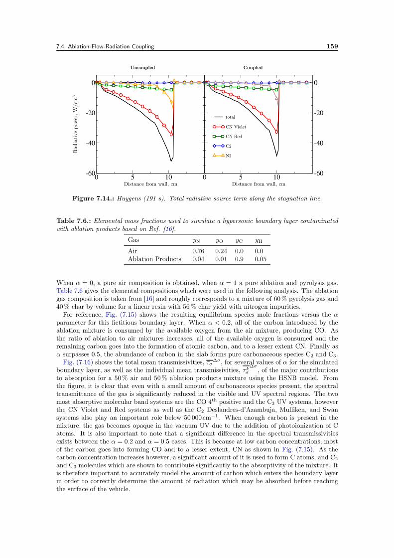
7.4. Ablation-Flow-Radiation Coupling 159
0 5 10-60
-40
-20
0
0 5 10 -60
-40
-20
0
Distance from wall, cmDistance from wall, cm
Rad
iative
pow
er,W
/cm
3
total
CN Violet
CN Red
C2
N2
Uncoupled Coupled
Figure 7.14.: Huygens (191 s). Total radiative source term along the stagnation line.
Table 7.6.: Elemental mass fractions used to simulate a hypersonic boundary layer contaminatedwith ablation products based on Ref. [16].
Gas yN yO yC yH
Air 0.76 0.24 0.0 0.0Ablation Products 0.04 0.01 0.9 0.05
When α = 0, a pure air composition is obtained, when α = 1 a pure ablation and pyrolysis gas.Table 7.6 gives the elemental compositions which were used in the following analysis. The ablationgas composition is taken from [16] and roughly corresponds to a mixture of 60% pyrolysis gas and40% char by volume for a linear resin with 56% char yield with nitrogen impurities.
For reference, Fig. (7.15) shows the resulting equilibrium species mole fractions versus the αparameter for this fictitious boundary layer. When α < 0.2, all of the carbon introduced by theablation mixture is consumed by the available oxygen from the air mixture, producing CO. Asthe ratio of ablation to air mixtures increases, all of the available oxygen is consumed and theremaining carbon goes into the formation of atomic carbon, and to a lesser extent CN. Finally asα surpasses 0.5, the abundance of carbon in the slab forms pure carbonaceous species C2 and C3.
Fig. (7.16) shows the total mean transmissivities, τσ∆σ, for several values of α for the simulatedboundary layer, as well as the individual mean transmissivities, τkσ
∆σ, of the major contributions
to absorption for a 50% air and 50% ablation products mixture using the HSNB model. Fromthe figure, it is clear that even with a small amount of carbonaceous species present, the spectraltransmittance of the gas is significantly reduced in the visible and UV spectral regions. The twomost absorptive molecular band systems are the CO 4th positive and the C3 UV systems, howeverthe CN Violet and Red systems as well as the C2 Deslandres-d’Azambuja, Mulliken, and Swansystems also play an important role below 50 000cm−1. When enough carbon is present in themixture, the gas becomes opaque in the vacuum UV due to the addition of photoionization of Catoms. It is also important to note that a significant difference in the spectral transmissivitiesexists between the α = 0.2 and α = 0.5 cases. This is because at low carbon concentrations, mostof the carbon goes into forming CO and to a lesser extent, CN as shown in Fig. (7.15). As thecarbon concentration increases however, a significant amount of it is used to form C atoms, and C2and C3 molecules which are shown to contribute significantly to the absorptivity of the mixture. Itis therefore important to accurately model the amount of carbon which enters the boundary layerin order to correctly determine the amount of radiation which may be absorbed before reachingthe surface of the vehicle.
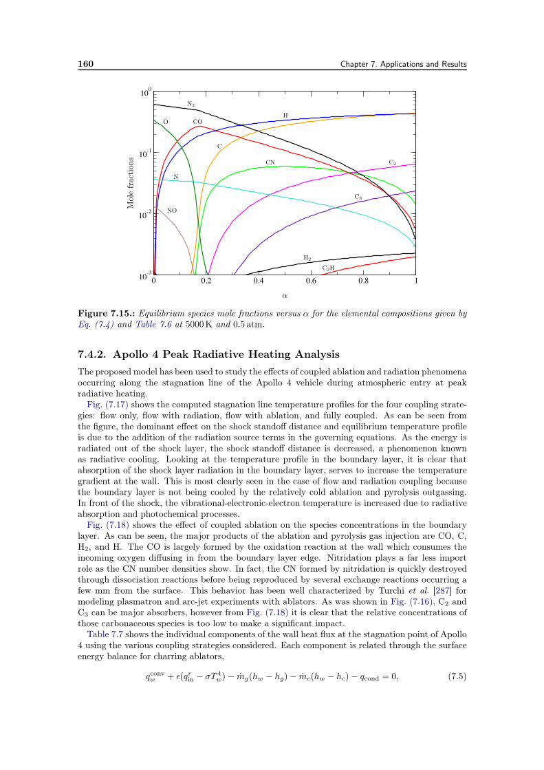
160 Chapter 7. Applications and Results
0 0.2 0.4 0.6 0.8 110-3
10-2
10-1
100
α
Mol
efr
action
s
N2
O CO
N
NO
C
H
CN C2
C3
H2
C2H
Figure 7.15.: Equilibrium species mole fractions versus α for the elemental compositions given byEq. (7.4) and Table 7.6 at 5000K and 0.5 atm.
7.4.2. Apollo 4 Peak Radiative Heating Analysis
The proposed model has been used to study the effects of coupled ablation and radiation phenomenaoccurring along the stagnation line of the Apollo 4 vehicle during atmospheric entry at peakradiative heating.
Fig. (7.17) shows the computed stagnation line temperature profiles for the four coupling strate-gies: flow only, flow with radiation, flow with ablation, and fully coupled. As can be seen fromthe figure, the dominant effect on the shock standoff distance and equilibrium temperature profileis due to the addition of the radiation source terms in the governing equations. As the energy isradiated out of the shock layer, the shock standoff distance is decreased, a phenomenon knownas radiative cooling. Looking at the temperature profile in the boundary layer, it is clear thatabsorption of the shock layer radiation in the boundary layer, serves to increase the temperaturegradient at the wall. This is most clearly seen in the case of flow and radiation coupling becausethe boundary layer is not being cooled by the relatively cold ablation and pyrolysis outgassing.In front of the shock, the vibrational-electronic-electron temperature is increased due to radiativeabsorption and photochemical processes.
Fig. (7.18) shows the effect of coupled ablation on the species concentrations in the boundarylayer. As can be seen, the major products of the ablation and pyrolysis gas injection are CO, C,H2, and H. The CO is largely formed by the oxidation reaction at the wall which consumes theincoming oxygen diffusing in from the boundary layer edge. Nitridation plays a far less importrole as the CN number densities show. In fact, the CN formed by nitridation is quickly destroyedthrough dissociation reactions before being reproduced by several exchange reactions occurring afew mm from the surface. This behavior has been well characterized by Turchi et al. [287] formodeling plasmatron and arc-jet experiments with ablators. As was shown in Fig. (7.16), C2 andC3 can be major absorbers, however from Fig. (7.18) it is clear that the relative concentrations ofthose carbonaceous species is too low to make a significant impact.
Table 7.7 shows the individual components of the wall heat flux at the stagnation point of Apollo4 using the various coupling strategies considered. Each component is related through the surfaceenergy balance for charring ablators,
qconvw + ϵ(qrin − σT 4
w)− mg(hw − hg)− mc(hw − hc)− qcond = 0, (7.5)
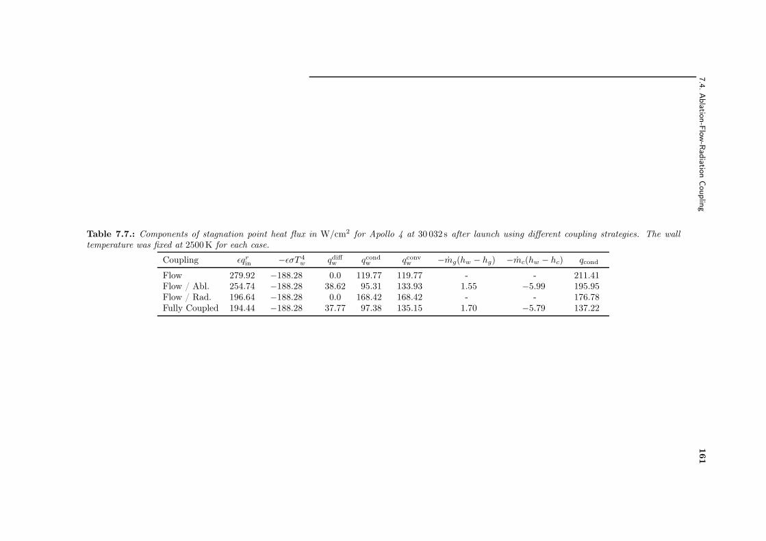
7.4
.Ablatio
n-F
low-R
adiatio
nCouplin
g161
Table 7.7.: Components of stagnation point heat flux in W/cm2 for Apollo 4 at 30 032 s after launch using different coupling strategies. The walltemperature was fixed at 2500K for each case.
Coupling ϵqrin −ϵσT 4w qdiff
w qcondw qconv
w −mg(hw − hg) −mc(hw − hc) qcond
Flow 279.92 −188.28 0.0 119.77 119.77 - - 211.41Flow / Abl. 254.74 −188.28 38.62 95.31 133.93 1.55 −5.99 195.95Flow / Rad. 196.64 −188.28 0.0 168.42 168.42 - - 176.78Fully Coupled 194.44 −188.28 37.77 97.38 135.15 1.70 −5.79 137.22
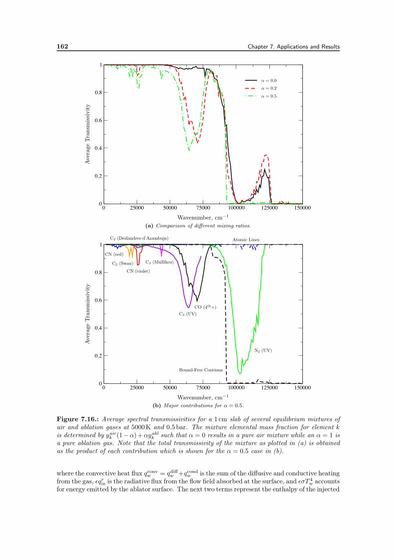
162 Chapter 7. Applications and Results
0 25000 50000 75000 100000 125000 1500000
0.2
0.4
0.6
0.8
1
Wavenumber, cm−1
Ave
rage
Tra
nsm
issi
vity
α = 0.0
α = 0.2
α = 0.5
(a) Comparison of different mixing ratios.
0 25000 50000 75000 100000 125000 1500000
0.2
0.4
0.6
0.8
1
Wavenumber, cm−1
Ave
rage
Tra
nsm
issi
vity
C2 (Deslandres-d’Azambuja)
C2 (Swan) C2 (Mulliken)
CN (red)
CN (violet)
C3 (UV)CO (4th+)
N2 (UV)
Atomic Lines
Bound-Free Continua
(b) Major contributions for α = 0.5.
Figure 7.16.: Average spectral transmissivities for a 1 cm slab of several equilibrium mixtures ofair and ablation gases at 5000K and 0.5 bar. The mixture elemental mass fraction for element kis determined by yair
k (1−α)+αyablk such that α = 0 results in a pure air mixture while an α = 1 is
a pure ablation gas. Note that the total transmissivity of the mixture as plotted in (a) is obtainedas the product of each contribution which is shown for the α = 0.5 case in (b).
where the convective heat flux qconvw = qdiff
w +qcondw is the sum of the diffusive and conductive heating
from the gas, ϵqrin is the radiative flux from the flow field absorbed at the surface, and ϵσT 4w accounts
for energy emitted by the ablator surface. The next two terms represent the enthalpy of the injected
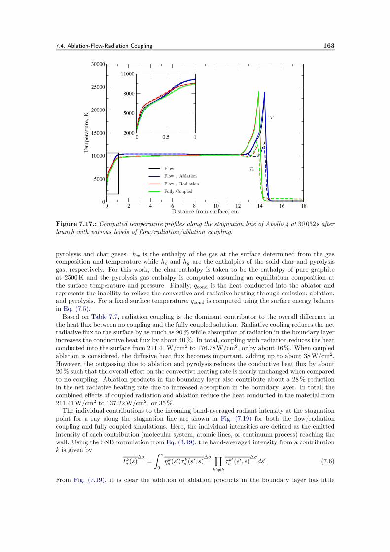
7.4. Ablation-Flow-Radiation Coupling 163
0 2 4 6 8 10 12 14 16 180
5000
10000
15000
20000
25000
30000
0 0.5 12000
5000
8000
11000
Distance from surface, cm
Tem
pera
ture
,K T
TvFlow
Flow / Ablation
Flow / Radiation
Fully Coupled
Figure 7.17.: Computed temperature profiles along the stagnation line of Apollo 4 at 30 032 s afterlaunch with various levels of flow/radiation/ablation coupling.
pyrolysis and char gases. hw is the enthalpy of the gas at the surface determined from the gascomposition and temperature while hc and hg are the enthalpies of the solid char and pyrolysisgas, respectively. For this work, the char enthalpy is taken to be the enthalpy of pure graphiteat 2500K and the pyrolysis gas enthalpy is computed assuming an equilibrium composition atthe surface temperature and pressure. Finally, qcond is the heat conducted into the ablator andrepresents the inability to relieve the convective and radiative heating through emission, ablation,and pyrolysis. For a fixed surface temperature, qcond is computed using the surface energy balancein Eq. (7.5).
Based on Table 7.7, radiation coupling is the dominant contributor to the overall difference inthe heat flux between no coupling and the fully coupled solution. Radiative cooling reduces the netradiative flux to the surface by as much as 90% while absorption of radiation in the boundary layerincreases the conductive heat flux by about 40%. In total, coupling with radiation reduces the heatconducted into the surface from 211.41W/cm2 to 176.78W/cm2, or by about 16%. When coupledablation is considered, the diffusive heat flux becomes important, adding up to about 38W/cm2.However, the outgassing due to ablation and pyrolysis reduces the conductive heat flux by about20% such that the overall effect on the convective heating rate is nearly unchanged when comparedto no coupling. Ablation products in the boundary layer also contribute about a 28% reductionin the net radiative heating rate due to increased absorption in the boundary layer. In total, thecombined effects of coupled radiation and ablation reduce the heat conducted in the material from211.41W/cm2 to 137.22W/cm2, or 35%.
The individual contributions to the incoming band-averaged radiant intensity at the stagnationpoint for a ray along the stagnation line are shown in Fig. (7.19) for both the flow/radiationcoupling and fully coupled simulations. Here, the individual intensities are defined as the emittedintensity of each contribution (molecular system, atomic lines, or continuum process) reaching thewall. Using the SNB formulation from Eq. (3.49), the band-averaged intensity from a contributionk is given by
Ikσ(s)∆σ
=
∫ s
0ηkσ(s
′)τkσ (s′, s)
∆σ ∏
k′ =k
τk′
σ (s′, s)∆σ
ds′. (7.6)
From Fig. (7.19), it is clear the addition of ablation products in the boundary layer has little
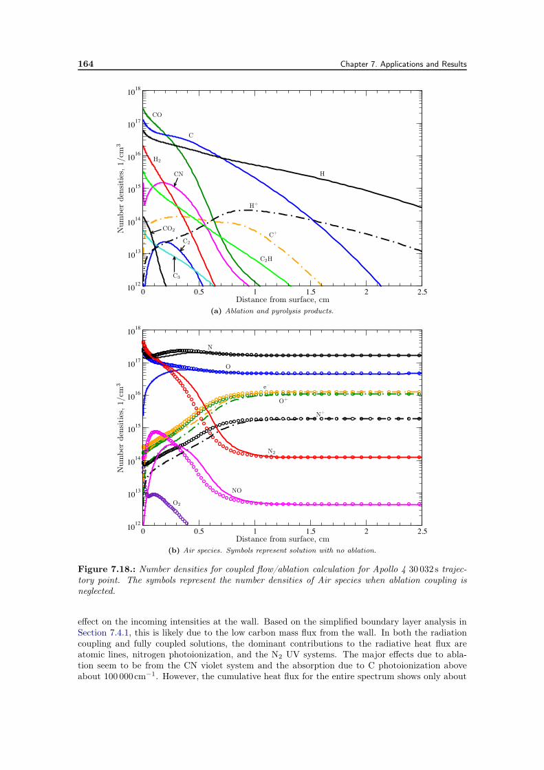
164 Chapter 7. Applications and Results
0 0.5 1 1.5 2 2.51012
1013
1014
1015
1016
1017
1018
Distance from surface, cm
Num
ber
dens
itie
s,1/
cm3
CO
H2
CN H
H+
CO2
C2
C3
C2H
C
C+
(a) Ablation and pyrolysis products.
0 0.5 1 1.5 2 2.51012
1013
1014
1015
1016
1017
1018
Distance from surface, cm
Num
ber
dens
itie
s,1/
cm3
N
O
N+
O+
e–
N2
O2
NO
(b) Air species. Symbols represent solution with no ablation.
Figure 7.18.: Number densities for coupled flow/ablation calculation for Apollo 4 30 032 s trajec-tory point. The symbols represent the number densities of Air species when ablation coupling isneglected.
effect on the incoming intensities at the wall. Based on the simplified boundary layer analysis inSection 7.4.1, this is likely due to the low carbon mass flux from the wall. In both the radiationcoupling and fully coupled solutions, the dominant contributions to the radiative heat flux areatomic lines, nitrogen photoionization, and the N2 UV systems. The major effects due to abla-tion seem to be from the CN violet system and the absorption due to C photoionization aboveabout 100 000cm−1. However, the cumulative heat flux for the entire spectrum shows only about
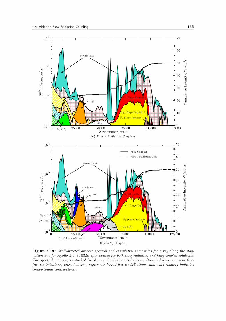
7.4. Ablation-Flow-Radiation Coupling 165
0 25000 50000 75000 100000 12500010-5
10-4
10-3
10-2
0
10
20
30
40
50
60
70
Wavenumber, cm−1
Ik σ
∆σ,W
cm/cm
2sr
Cum
ulat
ive
Inte
nsity,
W/cm
2sr
atomic lines
N2 (Carol-Yoshino)
N2 (1+)
N2 (2+)
N2 (Birge-Hopfield 1)
N2 (Birge-Hopfield 2)
N
N
N
N+
O+
O
other
(a) Flow / Radiation Coupling.
0 25000 50000 75000 100000 12500010-5
10-4
10-3
10-2
0
10
20
30
40
50
60
70
Wavenumber, cm−1
Ik σ
∆σ,W
cm/cm
2sr
Cum
ulat
ive
Inte
nsity,
W/cm
2sr
Fully Coupled
Flow / Radiation Only
atomic lines
CN (red)
CO (4+)
CN (violet)
N2 (Carol-Yoshino)N2 (1+)
N2 (2+) N2 (Birge-Hopfield 1)
N2 (Birge-Hopfield 2)
O2 (Schuman-Runge)
NN
N
N+
O+
O
other
(b) Fully Coupled.
Figure 7.19.: Wall-directed average spectral and cumulative intensities for a ray along the stag-nation line for Apollo 4 at 30 032 s after launch for both flow/radiation and fully coupled solutions.The spectral intensity is stacked based on individual contributions. Diagonal bars represent free-free contributions, cross-hatching represents bound-free contributions, and solid shading indicatesbound-bound contributions.
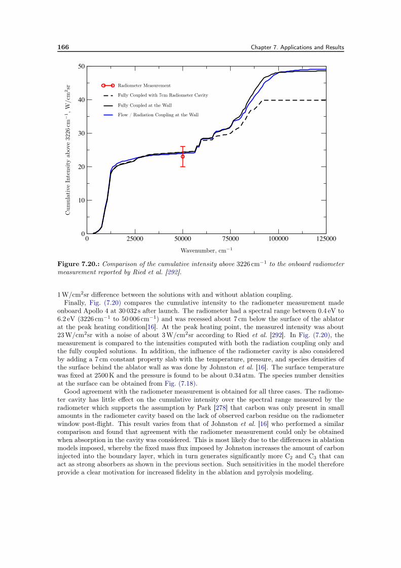
166 Chapter 7. Applications and Results
0 25000 50000 75000 100000 1250000
10
20
30
40
50
Wavenumber, cm−1
Cum
ulat
ive
Inte
nsity
abov
e32
26cm
−1,W
/cm
2sr Radiometer Measurement
Fully Coupled with 7cm Radiometer Cavity
Fully Coupled at the Wall
Flow / Radiation Coupling at the Wall
Figure 7.20.: Comparison of the cumulative intensity above 3226 cm−1 to the onboard radiometermeasurement reported by Ried et al. [292].
1W/cm2sr difference between the solutions with and without ablation coupling.Finally, Fig. (7.20) compares the cumulative intensity to the radiometer measurement made
onboard Apollo 4 at 30 032 s after launch. The radiometer had a spectral range between 0.4 eV to6.2 eV (3226 cm−1 to 50 006 cm−1) and was recessed about 7 cm below the surface of the ablatorat the peak heating condition[16]. At the peak heating point, the measured intensity was about23W/cm2sr with a noise of about 3W/cm2sr according to Ried et al. [292]. In Fig. (7.20), themeasurement is compared to the intensities computed with both the radiation coupling only andthe fully coupled solutions. In addition, the influence of the radiometer cavity is also consideredby adding a 7 cm constant property slab with the temperature, pressure, and species densities ofthe surface behind the ablator wall as was done by Johnston et al. [16]. The surface temperaturewas fixed at 2500K and the pressure is found to be about 0.34 atm. The species number densitiesat the surface can be obtained from Fig. (7.18).
Good agreement with the radiometer measurement is obtained for all three cases. The radiome-ter cavity has little effect on the cumulative intensity over the spectral range measured by theradiometer which supports the assumption by Park [278] that carbon was only present in smallamounts in the radiometer cavity based on the lack of observed carbon residue on the radiometerwindow post-flight. This result varies from that of Johnston et al. [16] who performed a similarcomparison and found that agreement with the radiometer measurement could only be obtainedwhen absorption in the cavity was considered. This is most likely due to the differences in ablationmodels imposed, whereby the fixed mass flux imposed by Johnston increases the amount of carboninjected into the boundary layer, which in turn generates significantly more C2 and C3 that canact as strong absorbers as shown in the previous section. Such sensitivities in the model thereforeprovide a clear motivation for increased fidelity in the ablation and pyrolysis modeling.
7.5. Concluding Remarks 167
7.5. Concluding Remarks
This chapter has proven the ability of the HSNB model to accurately and efficiently predict ra-diation effects on hypersonic entry flows. In general, the method provides a speedup of at leasttwo orders of magnitude and can accurately predict wall radiative heat fluxes to within 5% com-pared to LBL calculations. The novel spectral grid adaptation method developed in this thesisfor atomic lines was shown to provide nearly identical results with 20 times speedup comparedto the original high-resolution HSNB method. This significant improvement is possible due tothe small amount of atomic lines as compared to those typically treated for molecular systems.Concerning molecular radiation, the HSNB model provides a significant improvement compared tothe Smeared-Rotational-Band model in the case of Titan entry dominated by optically thick CNradiation.
The Lindquist-Simmons and Curtis-Godson approximations to the mean black equivalent linewidth for non-uniform media were also compared in this chapter. The Lindquist-Simmons methodwas found to be about three times slower than the Curtis-Godson method for Fire II. It was alsoshown that the Curtis-Godson approach can provide small negative radiative source terms in thefree-stream region, causing numerical instabilities in coupled calculations. For this reason, allcoupled cases were computed using the Lindquist-Simmons approach.
Taking into account the coupling with radiation, both convective and radiative heat fluxes atthe wall decrease. The standoff distance is reduced due to radiative cooling of the shock layer. ForEarth entry cases, we observed slower ionization levels as well as the appearance of O, e− and O+
2in the free stream produced by the photodissociation and the photoionization of O2.
The analysis of the first trajectory point of the Fire II experiment has shown that the two temper-ature approach was not satisfactory to model the thermal nonequilibrium state of the plasma. Theresults obtained using non-Boltzmann electronic populations provided by the QSS model of John-ston [297] were closer to the flight data even if discrepancies still remain. For such entry conditions(high velocity, low density), a self-consistent electronic specific collisional-radiative model shouldbe developed. The HSNB model could be used since it is compatible with arbitrary populations ofelectronic states.
Finally, the effects of coupled ablation and radiation were studied for Earth entries. It was shownthat for a simulated boundary layer, ablation products in the boundary layer can significantlyincrease the radiation blockage to the surface of the vehicle. In particular, the C3 UV and COfourth positive band systems as well as photoionization of C atoms contribute significantly toabsorption when enough carbon is present. An analysis of the Apollo 4 peak heating conditionshowed that coupled radiation and ablation effects can reduce the conducted heat flux by as much as35% for a fixed wall temperature of 2500K. Comparison with the radiometer data taken during theApollo 4 flight showed excellent agreement for the peak heating condition, partially validating thecoupling methodology and radiation database. In addition, the importance of accurately modelingthe amount of carbon which is blown into the boundary layer was demonstrated by contrastingthe results of this study to those obtained by Johnston et al. [16].

CHAPTER 8
Conclusions and Perspectives
This thesis presented the development of physicochemical models and numerical methods for thestudy of the complex, coupled, multiphysics phenomena associated with atmospheric entry flows.In particular, the research focused on the coupling between the flow, ablation, and radiationphenomena encountered in the stagnation region of atmospheric entry vehicles with carbon-phenolicthermal protection systems. Broadly speaking, the following objectives have been achieved, basedon the goals outlined in Chapter 1.
1. Development of a new software library capable of providing a centralized repository for thebasic physicochemical models, algorithms, and data relevant to nonequilibrium plasma flows.
2. Development of a numerical approach for calculating coupled flow, radiation, and ablationsolutions along the stagnation line of atmospheric entry vehicles and to assess the accuracyand efficiency of HSNB model using the tools developed.
3. Application of these tools to study real flight conditions of interest in an effort to gain agreater understanding of the coupled flow, radiation, and ablation phenomena occurring inatmospheric entry flows.
In the next section, the specific conclusions and contributions of this thesis are summarized inmore detail. Lastly, some perspectives on future work are given in Section 8.2.
8.1. Contributions of This Work
In Chapter 2, a review of the thermochemical nonequilibrium models and the corresponding gov-erning equations used to simulate hypersonic flows was made. From this review, a generalizednotation was developed, capable of describing most of the popular nonequilibrium models in usetoday, including state-to-state, multitemperature, and local thermodynamic equilibrium models.Using this notation, a general set of governing equations were derived from the standard conserva-tion of mass, momentum, and energy equations for multicomponent, reacting, radiating, partiallyionized and weakly magnetized plasmas. The thermodynamic, transport, chemical kinetic, andenergy transfer models necessary to close the governing equations were then presented, consistentwith the generalized notation. While the models presented in Chapter 2 are not original, the de-velopment of a consistent notation capable of encompassing most thermochemical nonequilibriummodels of interest is a valuable contribution for a number of reasons. For starters, a vast literatureis available describing numerous thermochemical nonequilibrium models relevant to atmosphericentry. As was shown in Chapter 2, these models can be derived from many different assump-tions with varying levels of fidelity and are often inconsistent with one another. By placing eachmodel into a consistent mathematical framework, the similarities and differences between themcan be readily assessed. Perhaps more importantly, the generalized model presented in this workprovides the machinery needed to abstract the physicochemical models used in modern hyper-sonic CFD tools away from the implementation of the discretization and solution of the governingequations.
This concept was demonstrated through the development of the Mutation++ software library,presented in Chapter 4. Written using modern, objected oriented programming techniques in C++,
170 Chapter 8. Conclusions and Perspectives
Mutation++ provides thermodynamic, transport, chemistry, and energy transfer models, data,and algorithms, relevant to flows in thermochemical nonequilibrium as well as LTE flows. The driv-ing principle behind Mutation++ is the ability to separate the underlying thermochemical modelfrom the set of governing equations solved by CFD tools, using the framework from Chapter 2.The library builds on previous Fortran libraries developed at the von Karman Institute for theefficient computation of accurate thermodynamic [103] and transport [163] properties for partiallyionized gas mixtures. In particular, the scope of the thermodynamic and transport data has beenvastly expanded through implementation of the NASA thermodynamic polynomial databases andthe creation of a specialized XML format for the storage of binary collision integrals. In addi-tion, Mutation++ implements a novel method for the robust calculation of linearly constrained,multiphase equilibria, a crucial component of many thermal protection material response codes.To the author’s best knowledge, the MPGFC algorithm presented in Chapter 5, is the first suchalgorithm guaranteed to converge for all well-posed constraints. While it was originally developedto improve the robustness of multiphase equilibrium routines required in certain ablation models,the MPGFC algorithm has wide ranging applications.
Chapter 6 presented the other numerics tools developed in this work. The steady-state flowalong the stagnation line of an atmospheric entry vehicle is computed using a one-dimensional,finite-volume code, based on the dimensionally reduced Navier-Stokes equations for stagnationline flows. The flow solver was developed in a previous thesis for modeling STS nitrogen flows[72] and has been extended in this work to general thermochemical nonequilibrium mixtures, bycoupling with the Mutation++ library. Coupling with ablation is achieved through a steady-stateablation boundary condition using finite-rate heterogeneous reactions at the surface and imposedequilibrium compositions of pyrolysis outgassing.
Concerning radiation coupling, the HTGR database from the laboratory EM2C at Centrale-Supélec has been used to provide accurate LBL spectra. Based on a review of the major radiativemechanisms contributing to the radiative heat flux for atmospheric entry vehicles, several contri-butions were added to the HTGR database in this work, including hydrogen lines, C3 Swings andUV systems, as well as the photoionization of H, H2, and CH. The HSNB model has also beenimplemented in this work in order to significantly reduce the computational resources required tocompute accurate radiative heating calculations when many species are present in the flow field.SNB parameters have been computed for the H2 Lyman and Werner systems, by adjusting theDoppler and Lorentz overlap parameters to fit curves of growth for each narrow band. Comparisonswith band-averaged transmissivities computed with the LBL approach show excellent agreementwith the resulting SNB parameters for these systems. In general, the method provides a speedupof at least two orders of magnitude and can accurately predict wall radiative heat fluxes to within5% compared to LBL calculations. In addition, a novel spectral grid adaptation method has beendeveloped for atomic lines and was shown to provide nearly identical results as compared to theoriginal high-resolution HSNB method with a 20-fold decrease in the computational time. Con-cerning molecular radiation, the HSNB model provides a significant improvement compared tothe Smeared-Rotational-Band model in the case of Titan entry, dominated by optically thick CNradiation.
Finally, the effects of coupled ablation and radiation have been studied for Earth entries inChapter 7. It was shown that for a simulated boundary layer, ablation products in the boundarylayer can significantly increase the radiation blockage to the surface of the vehicle. In particular,the C3 UV and CO fourth positive band systems as well as photoionization of C atoms contributesignificantly to absorption when enough carbon is present. This is the first time that the HSNBmodel has been used to simulate ablation contaminated boundary layer flows. An analysis of theApollo 4 peak heating condition showed that coupled radiation and ablation effects can reducethe conducted heat flux by as much as 35% for a fixed wall temperature of 2500K. Comparisonwith the radiometer data taken during the Apollo 4 flight showed excellent agreement for thepeak heating condition, partially validating the coupling methodology and radiation database. Inaddition, the importance of accurately modeling the amount of carbon which is blown into theboundary layer was demonstrated by contrasting the results of other researchers.
8.2. Future Work and Perspectives 171
8.2. Future Work and Perspectives
This work represents a first step in the direction of understanding fully coupled flow, radiation,and ablation phenomena for atmospheric entry vehicles. The effectiveness of the HSNB model foraccurately and efficiently computing radiative heating in highly nonhomogeneous, nonequilibriumflow fields has been clearly demonstrated. However, the steady-state ablation boundary conditionused in this work is not sufficient to gain a complete picture of the possible radiation-ablationcoupling mechanisms at work in real atmospheric entry flows. In addition, the effects of a 3-dimensional flow field have been completely ignored in an effort to limit the scope of the thesisto a manageable workload. Using the tools developed in this work only, it is not possible todraw conclusions regarding the interaction of ablation products and the radiative heating on thebackshell of an entry vehicle. A reasonable step in this direction could be the use of a 3D radiationtransport code based on the Monte Carlo Ray Tracing (MCRT) technique and the HSNB method,coupled with a single domain flow / material response solver like the one recently developed bySchrooyen [18]. For example, Rouzaud et al. have developed MCRT/SNB code for studying theradiative heating on a Martian orbiter [299]. This tool was later extended to use the full HSNBmodel for nonequilibrium air flows by Lamet et al. [300], however the presence of ablation productshas not yet been studied.
As discussed in Chapter 4, the Mutation++ library has already been used by other researchersfor a variety of applications related to hypersonics and ablation. These include the study ofbiomass pyrolysis [231], state-to-state catalytic recombination of nitrogen flows, [232], transportproperties of carbon-phenolic ablation mixtures [208], atmospheric entry of meteors [233, 234], anduncertainty quantification for high enthalpy, plasma wind tunnels [235]. However, the library isuseful for many other applications which are not directly obvious upon first glance. One interestingexample is the study of the Sun’s chromosphere which shares many of the phenomena experiencedduring atmospheric entry, including thermochemical nonequilibrium and strong radiation coupling.A major difference however, is the presence of strong electromagnetic fields which dominate theSun’s landscape. Under such conditions, transport properties are no longer isotropic for ionizedplasmas due to the gyroscopic motion of free electrons (and to a lesser extent, ions) around themagnetic field lines. Current approaches for the simulation of the solar chromosphere use simplifiedmodels like the one of Braginskii [301] for computing anisotropic transport coefficients [302, 303].Recently, Graille, Magin, and Massot developed a unified fluid model for multicomponent plasmasin thermal nonequilibrium accounting for the influence of the electromagnetic field [100]. While notpresented in this thesis, explicit expressions for asymptotic solutions of the anisotropic transportproperties have recently been derived using a spectral Galerkin projection, supplied with Laguerre-Sonine polynomial basis functions, and implemented in Mutation++ [304]. Coupling this newmodel with the tools used in solar chromosphere studies is a straight forward avenue for futureresearch which may lead to a better understanding of the complex processes involved in that regionof our star.


173
Appendices

APPENDIX A
Transport Systems
This appendix describes the evaluation of the linear transport systems necessary for computingthe multicomponent transport properties shown in Chapter 2. For the most part, these equationssummarize the results of [106], and are reproduced here for completeness.
Binary diffusion coefficients are given as
nDij =3
16
√
2πkBTh(mi +mj)
mimj
1
Q(1,1)ij
, i, j ∈ H, (A.1)
nDie =3
16
√
2πkBTe
me
1
Q(1,1)ie
, i ∈ H, (A.2)
nDee =3
8
√
πkBTe
me
1
Q(1,1)ee
. (A.3)
Shear viscosity coefficients for heavy particles read
ηi =5
16
√πkBThmi
Q(2,2)ii
, i ∈ H. (A.4)
As discussed in Chapter 2, the transport systems result from Laguerre-Sonine polynomial approx-imations of the Chapmann-Enskog approximation to the nondimensionalized Boltzmann equation.The resulting systems are summarized in Table A.1 and Table A.2 for heavy-heavy interactionsand all electron interactions, respectively. The correction functions for heavy-heavy interactions,φij , i, j ∈ H, are given in first and second order approximations as
φij(1) = 0, (A.5)
φij(2) = −25
8kB
nDij
xixj
∑
k∈H
Λ01ikβkj , (A.6)
∑
k∈H
Gλh
ik βkj = −2Λ01ji , i, j ∈ H, (A.7)
and for heavy-electron interactions, φie, i ∈ H, as
φie(1) = 0, (A.8)
φie(2) = −25
8kB
nDie
xixe
Λ01eeΛ
01ie
Λ11ee
. (A.9)
Only first order solutions have been used in this work.
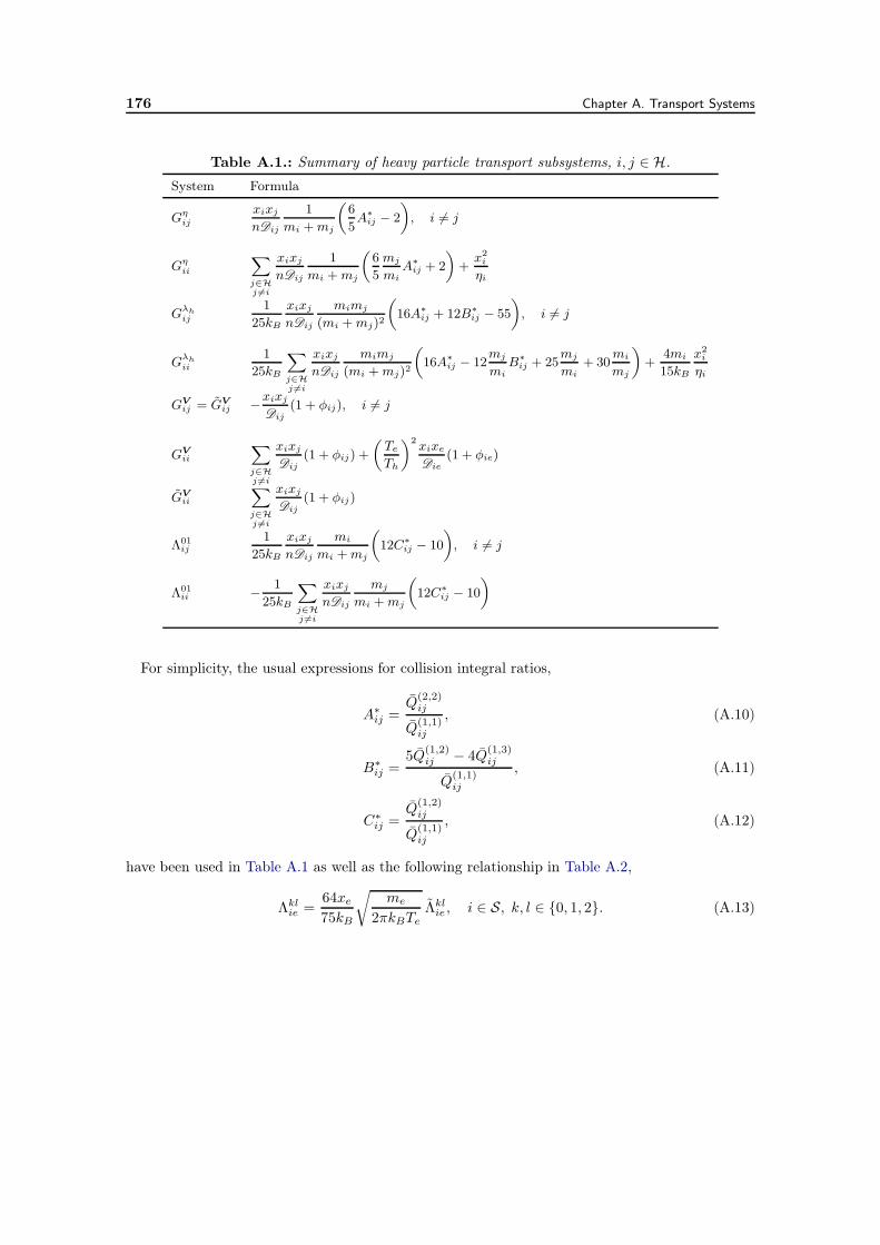
176 Chapter A. Transport Systems
Table A.1.: Summary of heavy particle transport subsystems, i, j ∈ H.
System Formula
Gηij
xixj
nDij
1mi +mj
,
65A∗
ij − 2
-
, i = j
Gηii
.
j∈Hj =i
xixj
nDij
1mi +mj
,
65mj
miA∗
ij + 2
-
+x2i
ηi
Gλhij
125kB
xixj
nDij
mimj
(mi +mj)2
,
16A∗ij + 12B∗
ij − 55
-
, i = j
Gλhii
125kB
.
j∈Hj =i
xixj
nDij
mimj
(mi +mj)2
,
16A∗ij − 12
mj
miB∗
ij + 25mj
mi+ 30
mi
mj
-
+4mi
15kB
x2i
ηi
GVij = GV
ij −xixj
Dij(1 + φij), i = j
GVii
.
j∈Hj =i
xixj
Dij(1 + φij) +
,
Te
Th
-2 xixe
Die(1 + φie)
GVii
.
j∈Hj =i
xixj
Dij(1 + φij)
Λ01ij
125kB
xixj
nDij
mi
mi +mj
,
12C∗ij − 10
-
, i = j
Λ01ii −
125kB
.
j∈Hj =i
xixj
nDij
mj
mi +mj
,
12C∗ij − 10
-
For simplicity, the usual expressions for collision integral ratios,
A∗ij =
Q(2,2)ij
Q(1,1)ij
, (A.10)
B∗ij =
5Q(1,2)ij − 4Q(1,3)
ij
Q(1,1)ij
, (A.11)
C∗ij =
Q(1,2)ij
Q(1,1)ij
, (A.12)
have been used in Table A.1 as well as the following relationship in Table A.2,
Λklie =
64xe
75kB
√
me
2πkBTeΛklie , i ∈ S, k, l ∈ 0, 1, 2. (A.13)
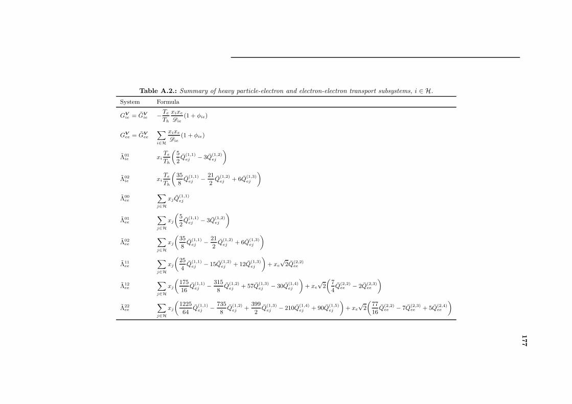
177
Table A.2.: Summary of heavy particle-electron and electron-electron transport subsystems, i ∈ H.
System Formula
GVie = GV
ie −Te
Th
xixe
Die(1 + φie)
GVee = GV
ee
.
i∈H
xixe
Die(1 + φie)
Λ01ie xi
Te
Th
,
52Q(1,1)
ej − 3Q(1,2)ej
-
Λ02ie xi
Te
Th
,
358Q(1,1)
ej −212Q(1,2)
ej + 6Q(1,3)ej
-
Λ00ee
.
j∈H
xjQ(1,1)ej
Λ01ee
.
j∈H
xj
,
52Q(1,1)
ej − 3Q(1,2)ej
-
Λ02ee
.
j∈H
xj
,
358Q(1,1)
ej −212Q(1,2)
ej + 6Q(1,3)ej
-
Λ11ee
.
j∈H
xj
,
254Q(1,1)
ej − 15Q(1,2)ej + 12Q(1,3)
ej
-
+ xe
√2Q(2,2)
ee
Λ12ee
.
j∈H
xj
,
17516
Q(1,1)ej −
3158
Q(1,2)ej + 57Q(1,3)
ej − 30Q(1,4)ej
-
+ xe
√2
,
74Q(2,2)
ee − 2Q(2,3)ee
-
Λ22ee
.
j∈H
xj
,
122564
Q(1,1)ej −
7358
Q(1,2)ej +
3992
Q(1,3)ej − 210Q(1,4)
ej + 90Q(1,5)ej
-
+ xe
√2
,
7716
Q(2,2)ee − 7Q(2,3)
ee + 5Q(2,4)ee
-

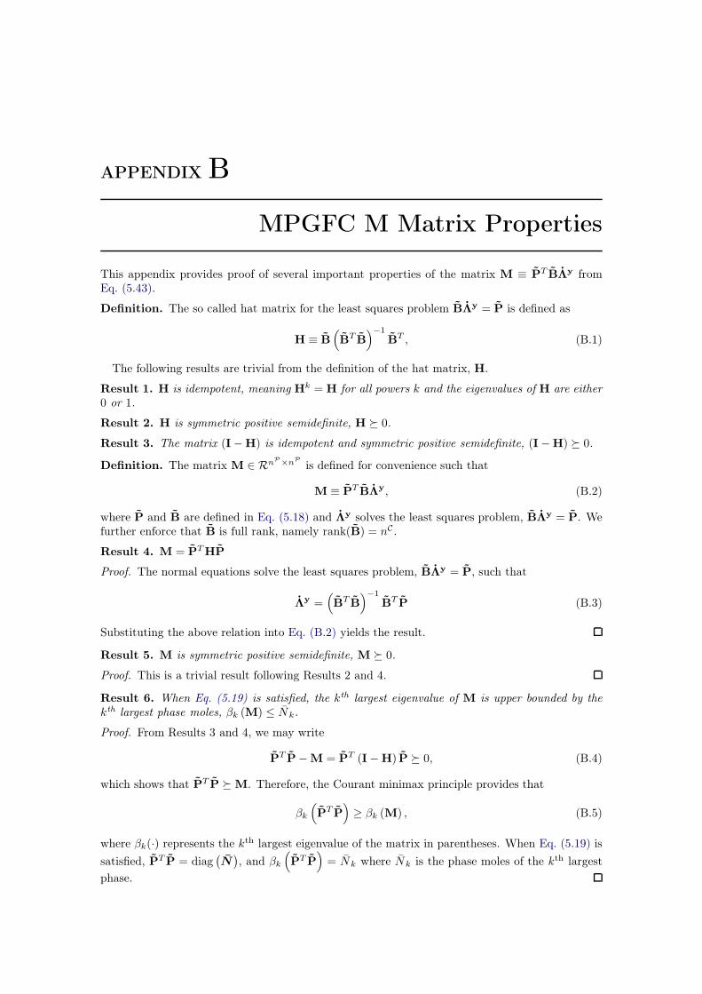
APPENDIX B
MPGFC M Matrix Properties
This appendix provides proof of several important properties of the matrix M ≡ PT BΛy fromEq. (5.43).
Definition. The so called hat matrix for the least squares problem BΛy = P is defined as
H ≡ B
(
BTB
)−1B
T , (B.1)
The following results are trivial from the definition of the hat matrix, H.
Result 1. H is idempotent, meaning Hk = H for all powers k and the eigenvalues of H are either0 or 1.
Result 2. H is symmetric positive semidefinite, H ≽ 0.
Result 3. The matrix (I−H) is idempotent and symmetric positive semidefinite, (I−H) ≽ 0.
Definition. The matrix M ∈ RnP×nP
is defined for convenience such that
M ≡ PTBΛ
y, (B.2)
where P and B are defined in Eq. (5.18) and Λy solves the least squares problem, BΛy = P. Wefurther enforce that B is full rank, namely rank(B) = nC .
Result 4. M = PTHP
Proof. The normal equations solve the least squares problem, BΛy = P, such that
Λy =
(
BTB
)−1B
TP (B.3)
Substituting the above relation into Eq. (B.2) yields the result.
Result 5. M is symmetric positive semidefinite, M ≽ 0.
Proof. This is a trivial result following Results 2 and 4.
Result 6. When Eq. (5.19) is satisfied, the kth largest eigenvalue of M is upper bounded by thekth largest phase moles, βk (M) ≤ Nk.
Proof. From Results 3 and 4, we may write
PTP−M = P
T (I−H) P ≽ 0, (B.4)
which shows that PT P ≽ M. Therefore, the Courant minimax principle provides that
βk(
PTP
)
≥ βk (M) , (B.5)
where βk(·) represents the kth largest eigenvalue of the matrix in parentheses. When Eq. (5.19) issatisfied, PT P = diag
(
N)
, and βk(
PT P
)
= Nk where Nk is the phase moles of the kth largestphase.
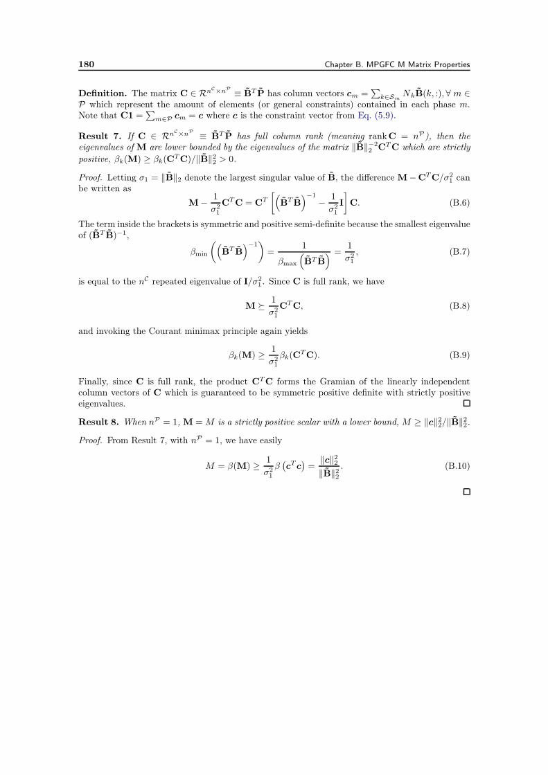
180 Chapter B. MPGFC M Matrix Properties
Definition. The matrix C ∈ RnC×nP ≡ BT P has column vectors cm =∑
k∈SmNkB(k, :), ∀ m ∈
P which represent the amount of elements (or general constraints) contained in each phase m.Note that C1 =
∑
m∈P cm = c where c is the constraint vector from Eq. (5.9).
Result 7. If C ∈ RnC×nP ≡ BT P has full column rank (meaning rankC = nP), then theeigenvalues of M are lower bounded by the eigenvalues of the matrix ∥B∥−2
2 CTC which are strictlypositive, βk(M) ≥ βk(CTC)/∥B∥22 > 0.
Proof. Letting σ1 = ∥B∥2 denote the largest singular value of B, the difference M−CTC/σ21 can
be written as
M−1
σ21
CTC = C
T
[
(
BTB
)−1−
1
σ21
I
]
C. (B.6)
The term inside the brackets is symmetric and positive semi-definite because the smallest eigenvalueof (BT B)−1,
βmin
(
(
BTB
)−1)
=1
βmax
(
BT B
) =1
σ21
, (B.7)
is equal to the nC repeated eigenvalue of I/σ21 . Since C is full rank, we have
M ≽1
σ21
CTC, (B.8)
and invoking the Courant minimax principle again yields
βk(M) ≥1
σ21
βk(CTC). (B.9)
Finally, since C is full rank, the product CTC forms the Gramian of the linearly independentcolumn vectors of C which is guaranteed to be symmetric positive definite with strictly positiveeigenvalues.
Result 8. When nP = 1, M = M is a strictly positive scalar with a lower bound, M ≥ ∥c∥22/∥B∥22.
Proof. From Result 7, with nP = 1, we have easily
M = β(M) ≥1
σ21
β(
cT c)
=∥c∥22∥B∥22
. (B.10)
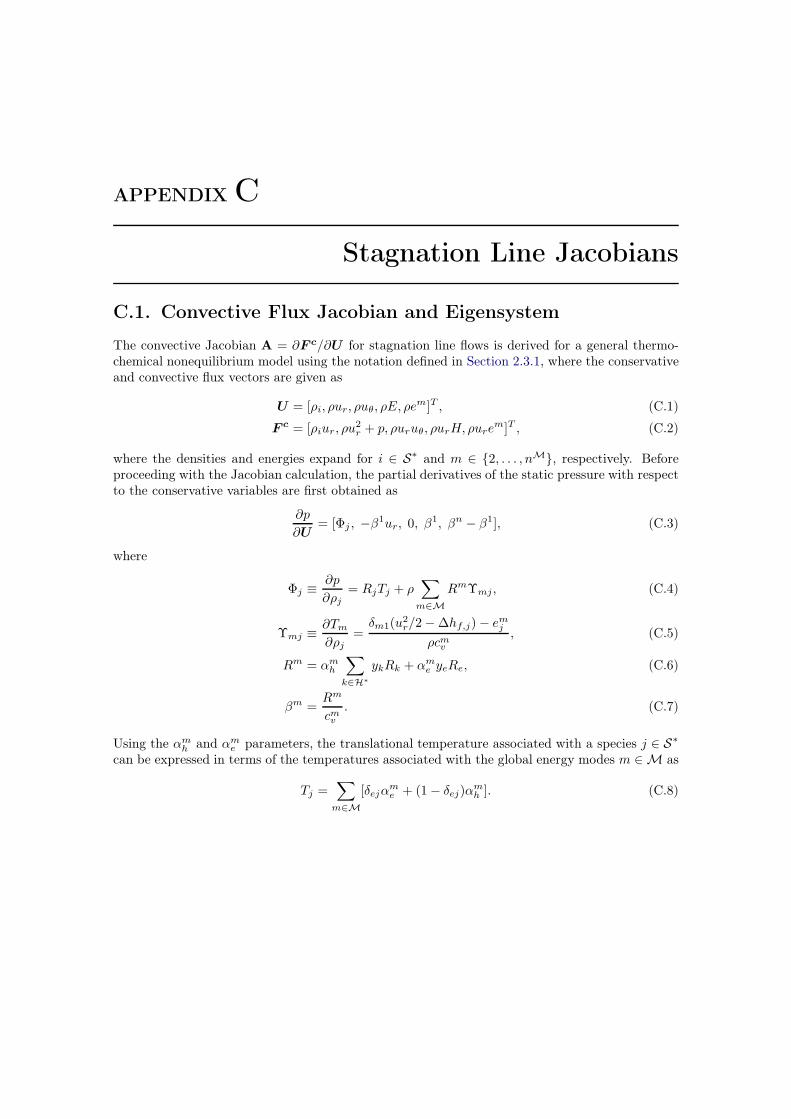
APPENDIX C
Stagnation Line Jacobians
C.1. Convective Flux Jacobian and Eigensystem
The convective Jacobian A = ∂F c/∂U for stagnation line flows is derived for a general thermo-chemical nonequilibrium model using the notation defined in Section 2.3.1, where the conservativeand convective flux vectors are given as
U = [ρi, ρur, ρuθ, ρE, ρem]T , (C.1)
F c = [ρiur, ρu2r + p, ρuruθ, ρurH, ρure
m]T , (C.2)
where the densities and energies expand for i ∈ S∗ and m ∈ 2, . . . , nM, respectively. Beforeproceeding with the Jacobian calculation, the partial derivatives of the static pressure with respectto the conservative variables are first obtained as
∂p
∂U= [Φj , −β1ur, 0, β
1, βn − β1], (C.3)
where
Φj ≡∂p
∂ρj= RjTj + ρ
∑
m∈M
RmΥmj, (C.4)
Υmj ≡∂Tm
∂ρj=δm1(u2
r/2−∆hf,j)− emjρcmv
, (C.5)
Rm = αmh
∑
k∈H∗
ykRk + αme yeRe, (C.6)
βm =Rm
cmv. (C.7)
Using the αmh and αm
e parameters, the translational temperature associated with a species j ∈ S∗
can be expressed in terms of the temperatures associated with the global energy modes m ∈ M as
Tj =∑
m∈M
[δejαme + (1− δej)α
mh ]. (C.8)
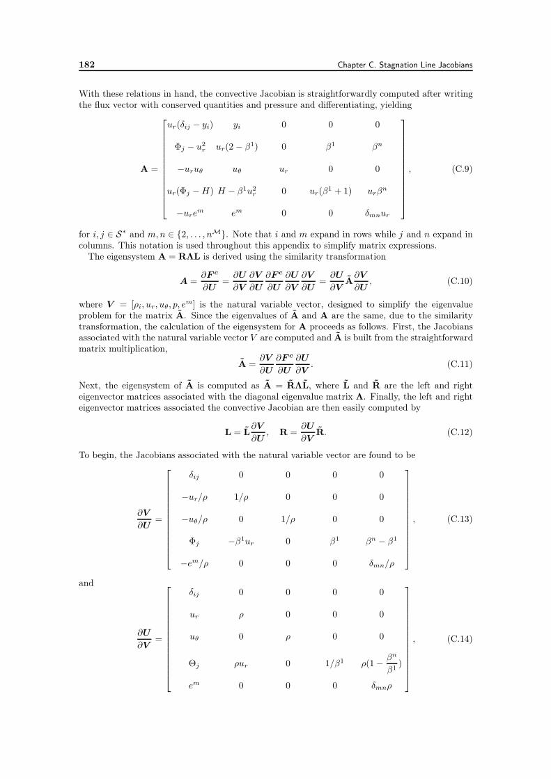
182 Chapter C. Stagnation Line Jacobians
With these relations in hand, the convective Jacobian is straightforwardly computed after writingthe flux vector with conserved quantities and pressure and differentiating, yielding
A =
⎡
⎢
⎢
⎢
⎢
⎢
⎢
⎢
⎢
⎢
⎢
⎢
⎢
⎣
ur(δij − yi) yi 0 0 0
Φj − u2r ur(2 − β1) 0 β1 βn
−uruθ uθ ur 0 0
ur(Φj −H) H − β1u2r 0 ur(β1 + 1) urβn
−urem em 0 0 δmnur
⎤
⎥
⎥
⎥
⎥
⎥
⎥
⎥
⎥
⎥
⎥
⎥
⎥
⎦
, (C.9)
for i, j ∈ S∗ and m,n ∈ 2, . . . , nM. Note that i and m expand in rows while j and n expand incolumns. This notation is used throughout this appendix to simplify matrix expressions.
The eigensystem A = RΛL is derived using the similarity transformation
A =∂F c
∂U=∂U
∂V
∂V
∂U
∂F c
∂U
∂U
∂V
∂V
∂U=∂U
∂VA∂V
∂U, (C.10)
where V = [ρi, ur, uθ, p, em] is the natural variable vector, designed to simplify the eigenvalueproblem for the matrix A. Since the eigenvalues of A and A are the same, due to the similaritytransformation, the calculation of the eigensystem for A proceeds as follows. First, the Jacobiansassociated with the natural variable vector V are computed and A is built from the straightforwardmatrix multiplication,
A =∂V
∂U
∂F c
∂U
∂U
∂V. (C.11)
Next, the eigensystem of A is computed as A = RΛL, where L and R are the left and righteigenvector matrices associated with the diagonal eigenvalue matrix Λ. Finally, the left and righteigenvector matrices associated the convective Jacobian are then easily computed by
L = L∂V
∂U, R =
∂U
∂VR. (C.12)
To begin, the Jacobians associated with the natural variable vector are found to be
∂V
∂U=
⎡
⎢
⎢
⎢
⎢
⎢
⎢
⎢
⎢
⎢
⎢
⎢
⎢
⎣
δij 0 0 0 0
−ur/ρ 1/ρ 0 0 0
−uθ/ρ 0 1/ρ 0 0
Φj −β1ur 0 β1 βn − β1
−em/ρ 0 0 0 δmn/ρ
⎤
⎥
⎥
⎥
⎥
⎥
⎥
⎥
⎥
⎥
⎥
⎥
⎥
⎦
, (C.13)
and
∂U
∂V=
⎡
⎢
⎢
⎢
⎢
⎢
⎢
⎢
⎢
⎢
⎢
⎢
⎢
⎢
⎣
δij 0 0 0 0
ur ρ 0 0 0
uθ 0 ρ 0 0
Θj ρur 0 1/β1 ρ(1−βn
β1)
em 0 0 0 δmnρ
⎤
⎥
⎥
⎥
⎥
⎥
⎥
⎥
⎥
⎥
⎥
⎥
⎥
⎥
⎦
, (C.14)
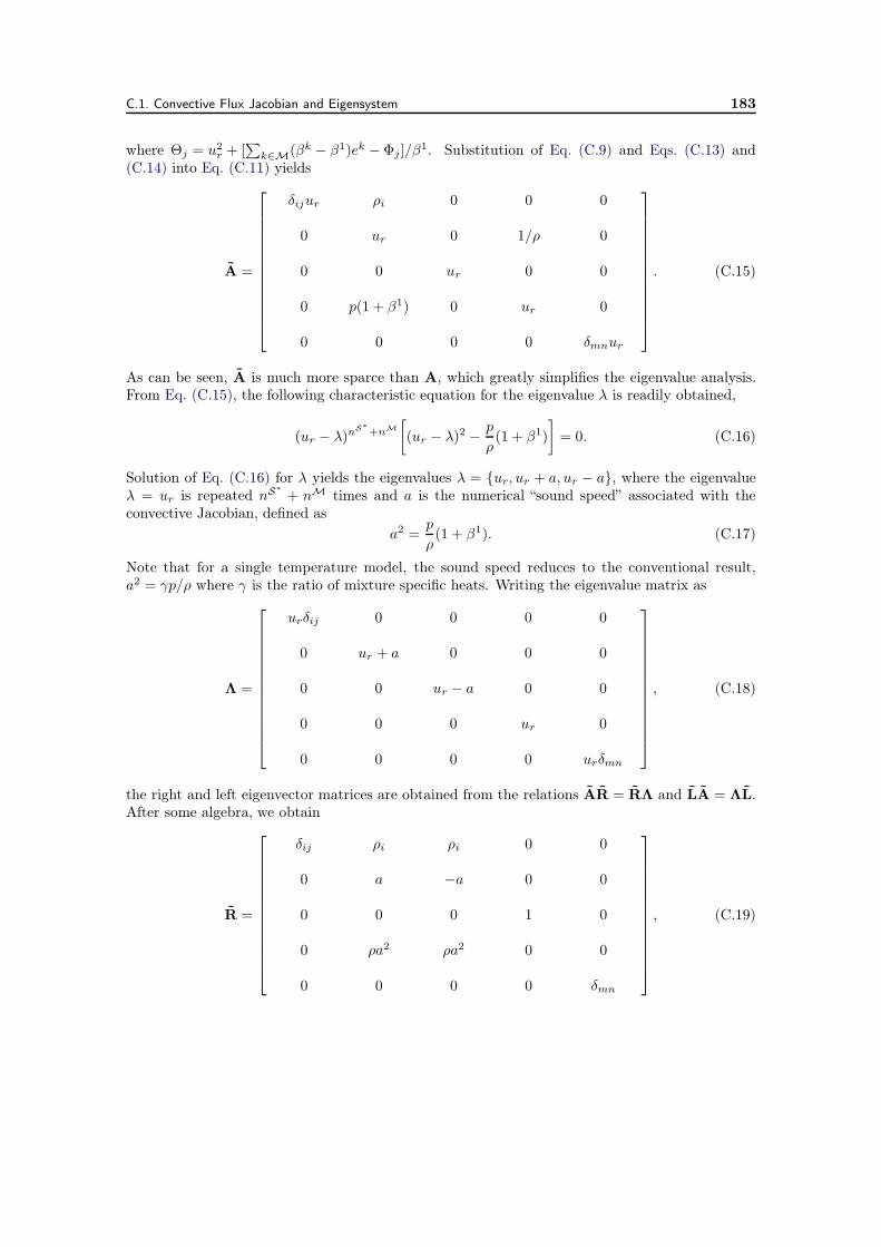
C.1. Convective Flux Jacobian and Eigensystem 183
where Θj = u2r + [
∑
k∈M(βk − β1)ek − Φj ]/β1. Substitution of Eq. (C.9) and Eqs. (C.13) and(C.14) into Eq. (C.11) yields
A =
⎡
⎢
⎢
⎢
⎢
⎢
⎢
⎢
⎢
⎢
⎢
⎢
⎢
⎣
δijur ρi 0 0 0
0 ur 0 1/ρ 0
0 0 ur 0 0
0 p(1 + β1) 0 ur 0
0 0 0 0 δmnur
⎤
⎥
⎥
⎥
⎥
⎥
⎥
⎥
⎥
⎥
⎥
⎥
⎥
⎦
. (C.15)
As can be seen, A is much more sparce than A, which greatly simplifies the eigenvalue analysis.From Eq. (C.15), the following characteristic equation for the eigenvalue λ is readily obtained,
(ur − λ)nS∗
+nM
[
(ur − λ)2 −p
ρ(1 + β1)
]
= 0. (C.16)
Solution of Eq. (C.16) for λ yields the eigenvalues λ = ur, ur + a, ur − a, where the eigenvalueλ = ur is repeated nS∗
+ nM times and a is the numerical “sound speed” associated with theconvective Jacobian, defined as
a2 =p
ρ(1 + β1). (C.17)
Note that for a single temperature model, the sound speed reduces to the conventional result,a2 = γp/ρ where γ is the ratio of mixture specific heats. Writing the eigenvalue matrix as
Λ =
⎡
⎢
⎢
⎢
⎢
⎢
⎢
⎢
⎢
⎢
⎢
⎢
⎢
⎣
urδij 0 0 0 0
0 ur + a 0 0 0
0 0 ur − a 0 0
0 0 0 ur 0
0 0 0 0 urδmn
⎤
⎥
⎥
⎥
⎥
⎥
⎥
⎥
⎥
⎥
⎥
⎥
⎥
⎦
, (C.18)
the right and left eigenvector matrices are obtained from the relations AR = RΛ and LA = ΛL.After some algebra, we obtain
R =
⎡
⎢
⎢
⎢
⎢
⎢
⎢
⎢
⎢
⎢
⎢
⎢
⎢
⎣
δij ρi ρi 0 0
0 a −a 0 0
0 0 0 1 0
0 ρa2 ρa2 0 0
0 0 0 0 δmn
⎤
⎥
⎥
⎥
⎥
⎥
⎥
⎥
⎥
⎥
⎥
⎥
⎥
⎦
, (C.19)
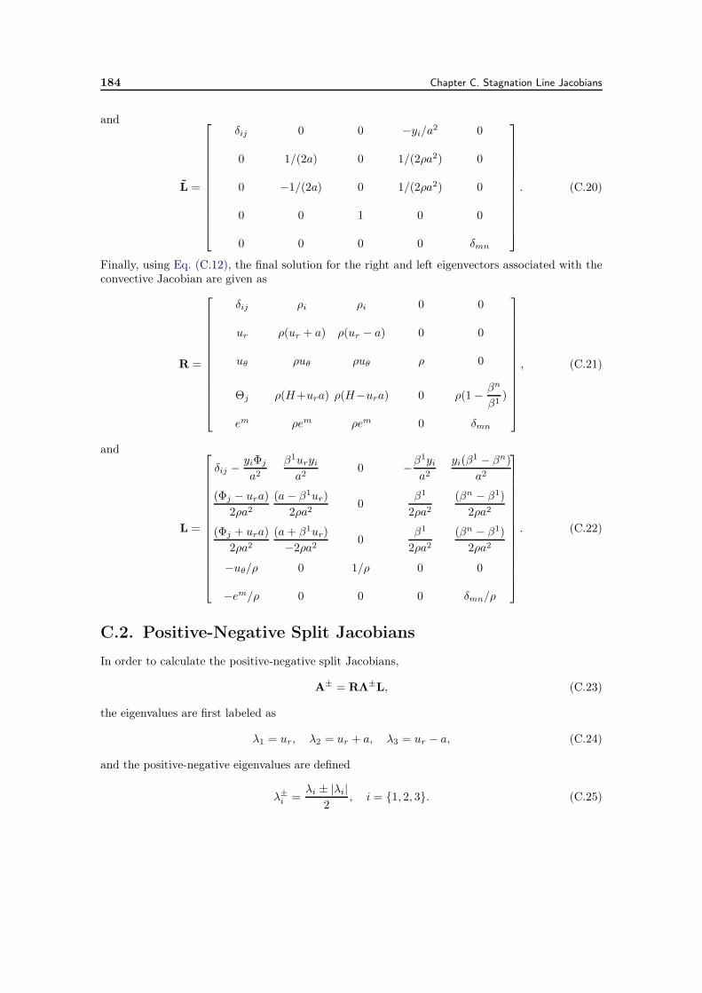
184 Chapter C. Stagnation Line Jacobians
and
L =
⎡
⎢
⎢
⎢
⎢
⎢
⎢
⎢
⎢
⎢
⎢
⎢
⎢
⎣
δij 0 0 −yi/a2 0
0 1/(2a) 0 1/(2ρa2) 0
0 −1/(2a) 0 1/(2ρa2) 0
0 0 1 0 0
0 0 0 0 δmn
⎤
⎥
⎥
⎥
⎥
⎥
⎥
⎥
⎥
⎥
⎥
⎥
⎥
⎦
. (C.20)
Finally, using Eq. (C.12), the final solution for the right and left eigenvectors associated with theconvective Jacobian are given as
R =
⎡
⎢
⎢
⎢
⎢
⎢
⎢
⎢
⎢
⎢
⎢
⎢
⎢
⎢
⎣
δij ρi ρi 0 0
ur ρ(ur + a) ρ(ur − a) 0 0
uθ ρuθ ρuθ ρ 0
Θj ρ(H+ura) ρ(H−ura) 0 ρ(1−βn
β1)
em ρem ρem 0 δmn
⎤
⎥
⎥
⎥
⎥
⎥
⎥
⎥
⎥
⎥
⎥
⎥
⎥
⎥
⎦
, (C.21)
and
L =
⎡
⎢
⎢
⎢
⎢
⎢
⎢
⎢
⎢
⎢
⎢
⎢
⎢
⎢
⎢
⎢
⎣
δij −yiΦj
a2β1uryia2
0 −β1yia2
yi(β1 − βn)
a2
(Φj − ura)
2ρa2(a− β1ur)
2ρa20
β1
2ρa2(βn − β1)
2ρa2
(Φj + ura)
2ρa2(a+ β1ur)
−2ρa20
β1
2ρa2(βn − β1)
2ρa2
−uθ/ρ 0 1/ρ 0 0
−em/ρ 0 0 0 δmn/ρ
⎤
⎥
⎥
⎥
⎥
⎥
⎥
⎥
⎥
⎥
⎥
⎥
⎥
⎥
⎥
⎥
⎦
. (C.22)
C.2. Positive-Negative Split Jacobians
In order to calculate the positive-negative split Jacobians,
A± = RΛ
±L, (C.23)
the eigenvalues are first labeled as
λ1 = ur, λ2 = ur + a, λ3 = ur − a, (C.24)
and the positive-negative eigenvalues are defined
λ±i =λi ± |λi|
2, i = 1, 2, 3. (C.25)
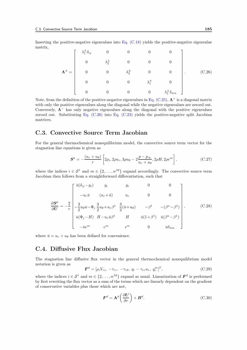
C.3. Convective Source Term Jacobian 185
Inserting the positive-negative eigenvalues into Eq. (C.18) yields the positive-negative eigenvaluematrix,
Λ± =
⎡
⎢
⎢
⎢
⎢
⎢
⎢
⎢
⎢
⎢
⎢
⎢
⎢
⎣
λ±1 δij 0 0 0 0
0 λ±2 0 0 0
0 0 λ±3 0 0
0 0 0 λ±1 0
0 0 0 0 λ±1 δmn
⎤
⎥
⎥
⎥
⎥
⎥
⎥
⎥
⎥
⎥
⎥
⎥
⎥
⎦
. (C.26)
Note, from the definition of the positive-negative eigenvalues in Eq. (C.25), Λ+ is a diagonal matrixwith only the positive eigenvalues along the diagonal while the negative eigenvalues are zeroed out.Conversely, Λ− has only negative eigenvalues along the diagonal with the positive eigenvalueszeroed out. Substituting Eq. (C.26) into Eq. (C.23) yields the positive-negative split Jacobianmatrices.
C.3. Convective Source Term Jacobian
For the general thermochemical nonequilibrium model, the convective source term vector for thestagnation line equations is given as
Sc = −(ur + uθ)
r
[
2ρi, 2ρur, 3ρuθ − 2p− p∞ur + uθ
, 2ρH, 2ρem]
, (C.27)
where the indices i ∈ S∗ and m ∈ 2, . . . , nM expand accordingly. The convective source termJacobian then follows from a straightforward differentiation, such that
∂Sc
∂U= −
2
r
⎡
⎢
⎢
⎢
⎢
⎢
⎢
⎢
⎢
⎢
⎢
⎢
⎢
⎣
u(δij−yi) yi yi 0 0
−uru (ur+u) ur 0 0
−3
2uθu−Φj
3
2uθ+urβ1 3
2(u+uθ) −β1 −(βn−β1)
u(Φj−H) H−uruβ1 H u(1+β1) u(βn−β1)
−uem em em 0 uδmn
⎤
⎥
⎥
⎥
⎥
⎥
⎥
⎥
⎥
⎥
⎥
⎥
⎥
⎦
, (C.28)
where u = ur + uθ has been defined for convenience.
C.4. Diffusive Flux Jacobian
The stagnation line diffusive flux vector in the general thermochemical nonequilibrium modelnotation is given as
F d = [ρiVri, −τrr, −τrθ, qr − τrrur, qmr ]T , (C.29)
where the indices i ∈ S∗ and m ∈ 2, . . . , nM expand as usual. Linearization of F d is performedby first rewriting the flux vector as a sum of the terms which are linearly dependent on the gradientof conservative variables plus those which are not,
F d = Ad
(
∂U
∂r
)
+Bd. (C.30)
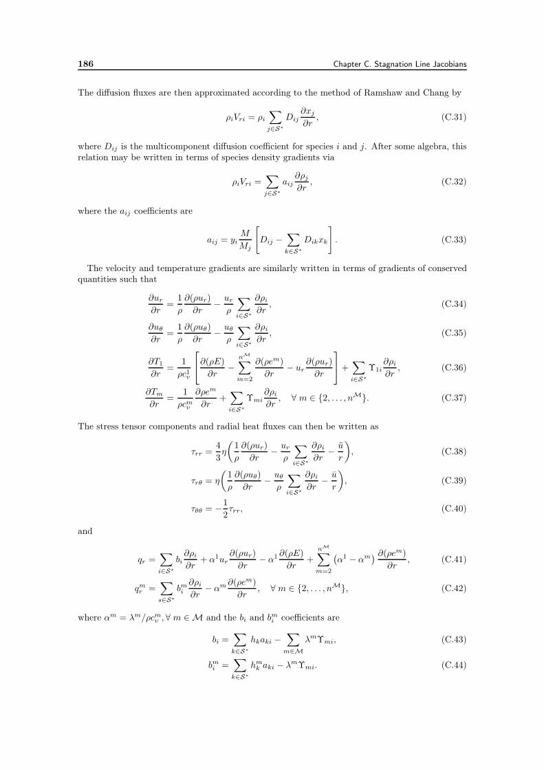
186 Chapter C. Stagnation Line Jacobians
The diffusion fluxes are then approximated according to the method of Ramshaw and Chang by
ρiVri = ρi∑
j∈S∗
Dij∂xj
∂r, (C.31)
where Dij is the multicomponent diffusion coefficient for species i and j. After some algebra, thisrelation may be written in terms of species density gradients via
ρiVri =∑
j∈S∗
aij∂ρj∂r
, (C.32)
where the aij coefficients are
aij = yiM
Mj
[
Dij −∑
k∈S∗
Dikxk
]
. (C.33)
The velocity and temperature gradients are similarly written in terms of gradients of conservedquantities such that
∂ur
∂r=
1
ρ
∂(ρur)
∂r−
ur
ρ
∑
i∈S∗
∂ρi∂r
, (C.34)
∂uθ
∂r=
1
ρ
∂(ρuθ)
∂r−
uθ
ρ
∑
i∈S∗
∂ρi∂r
, (C.35)
∂T1
∂r=
1
ρc1v
⎡
⎣
∂(ρE)
∂r−
nM
∑
m=2
∂(ρem)
∂r− ur
∂(ρur)
∂r
⎤
⎦+∑
i∈S∗
Υ1i∂ρi∂r
, (C.36)
∂Tm
∂r=
1
ρcmv
∂ρem
∂r+∑
i∈S∗
Υmi∂ρi∂r
, ∀ m ∈ 2, . . . , nM. (C.37)
The stress tensor components and radial heat fluxes can then be written as
τrr =4
3η
(
1
ρ
∂(ρur)
∂r−
ur
ρ
∑
i∈S∗
∂ρi∂r
−u
r
)
, (C.38)
τrθ = η
(
1
ρ
∂(ρuθ)
∂r−
uθ
ρ
∑
i∈S∗
∂ρi∂r
−u
r
)
, (C.39)
τθθ = −1
2τrr, (C.40)
and
qr =∑
i∈S∗
bi∂ρi∂r
+ α1ur∂(ρur)
∂r− α1 ∂(ρE)
∂r+
nM
∑
m=2
(
α1 − αm) ∂(ρem)
∂r, (C.41)
qmr =∑
s∈S∗
bmi∂ρi∂r
− αm ∂(ρem)
∂r, ∀ m ∈ 2, . . . , nM, (C.42)
where αm = λm/ρcmv , ∀ m ∈ M and the bi and bmi coefficients are
bi =∑
k∈S∗
hkaki −∑
m∈M
λmΥmi, (C.43)
bmi =∑
k∈S∗
hmk aki − λmΥmi. (C.44)
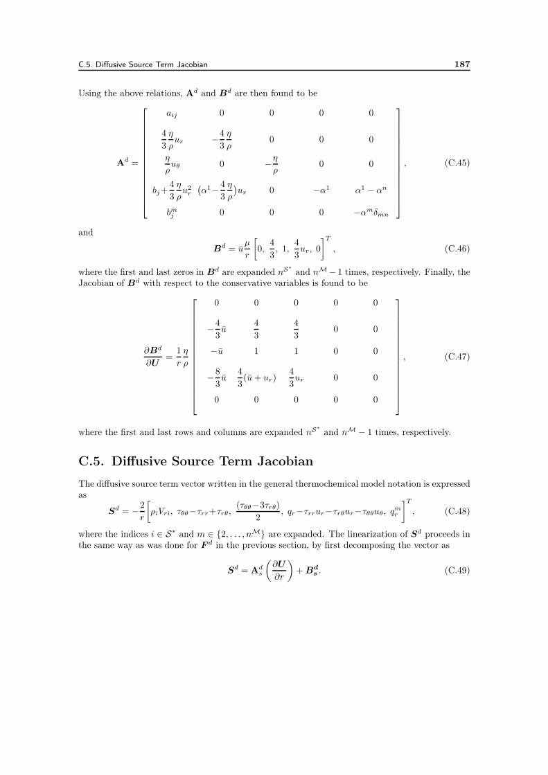
C.5. Diffusive Source Term Jacobian 187
Using the above relations, Ad and Bd are then found to be
Ad =
⎡
⎢
⎢
⎢
⎢
⎢
⎢
⎢
⎢
⎢
⎢
⎢
⎢
⎢
⎢
⎣
aij 0 0 0 0
4
3
η
ρur −
4
3
η
ρ0 0 0
η
ρuθ 0 −
η
ρ0 0
bj+4
3
η
ρu2r
(
α1−4
3
η
ρ
)
ur 0 −α1 α1 − αn
bmj 0 0 0 −αmδmn
⎤
⎥
⎥
⎥
⎥
⎥
⎥
⎥
⎥
⎥
⎥
⎥
⎥
⎥
⎥
⎦
, (C.45)
and
Bd = uµ
r
[
0,4
3, 1,
4
3ur, 0
]T
, (C.46)
where the first and last zeros in Bd are expanded nS∗
and nM− 1 times, respectively. Finally, theJacobian of Bd with respect to the conservative variables is found to be
∂Bd
∂U=
1
r
η
ρ
⎡
⎢
⎢
⎢
⎢
⎢
⎢
⎢
⎢
⎢
⎢
⎢
⎢
⎢
⎢
⎢
⎣
0 0 0 0 0
−4
3u
4
3
4
30 0
−u 1 1 0 0
−8
3u
4
3(u+ ur)
4
3ur 0 0
0 0 0 0 0
⎤
⎥
⎥
⎥
⎥
⎥
⎥
⎥
⎥
⎥
⎥
⎥
⎥
⎥
⎥
⎥
⎦
, (C.47)
where the first and last rows and columns are expanded nS∗
and nM − 1 times, respectively.
C.5. Diffusive Source Term Jacobian
The diffusive source term vector written in the general thermochemical model notation is expressedas
Sd = −2
r
[
ρiVri, τθθ−τrr+τrθ,(τθθ−3τrθ)
2, qr−τrrur−τrθur−τθθuθ, q
mr
]T
, (C.48)
where the indices i ∈ S∗ and m ∈ 2, . . . , nM are expanded. The linearization of Sd proceeds inthe same way as was done for F d in the previous section, by first decomposing the vector as
Sd = Ads
(
∂U
∂r
)
+Bds . (C.49)
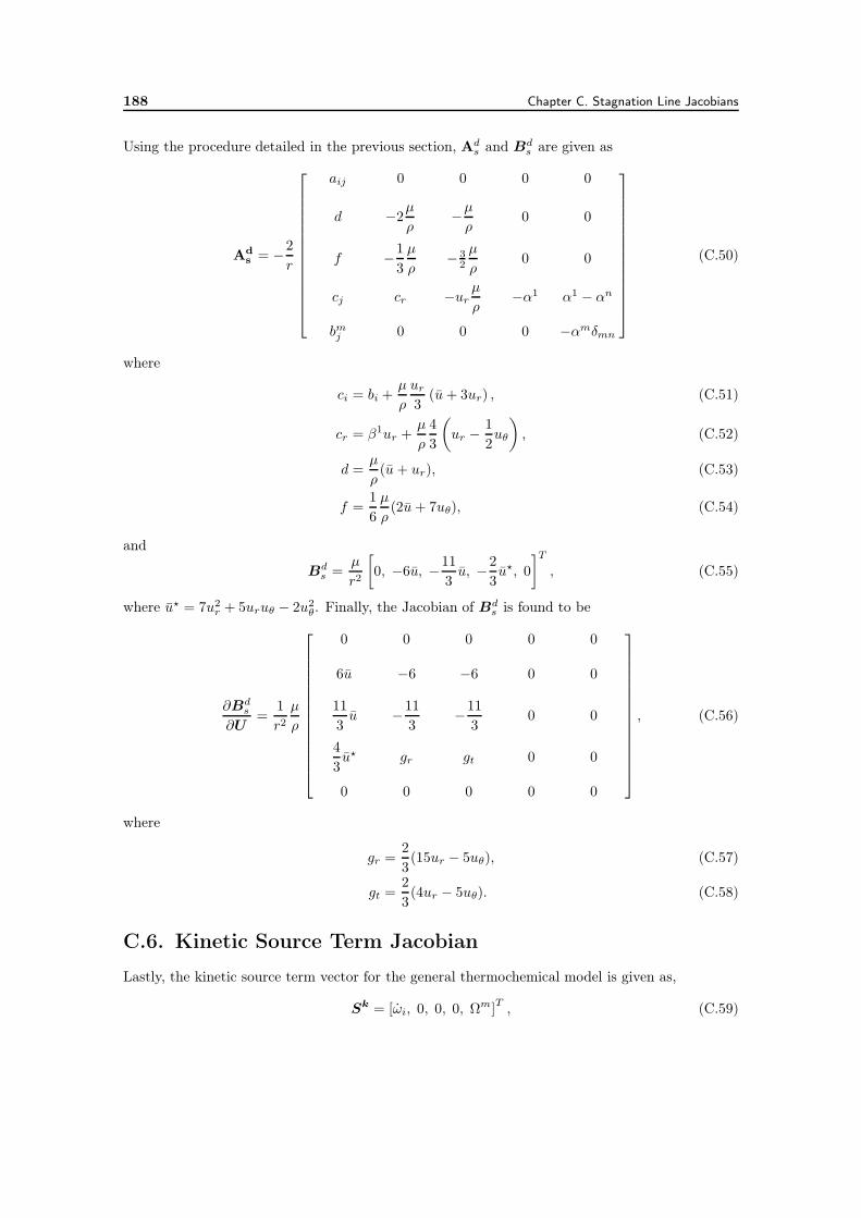
188 Chapter C. Stagnation Line Jacobians
Using the procedure detailed in the previous section, Ads and Bd
s are given as
Ads = −
2
r
⎡
⎢
⎢
⎢
⎢
⎢
⎢
⎢
⎢
⎢
⎢
⎢
⎢
⎢
⎣
aij 0 0 0 0
d −2µ
ρ−µ
ρ0 0
f −1
3
µ
ρ− 3
2
µ
ρ0 0
cj cr −urµ
ρ−α1 α1 − αn
bmj 0 0 0 −αmδmn
⎤
⎥
⎥
⎥
⎥
⎥
⎥
⎥
⎥
⎥
⎥
⎥
⎥
⎥
⎦
(C.50)
where
ci = bi +µ
ρ
ur
3(u+ 3ur) , (C.51)
cr = β1ur +µ
ρ
4
3
(
ur −1
2uθ
)
, (C.52)
d =µ
ρ(u + ur), (C.53)
f =1
6
µ
ρ(2u+ 7uθ), (C.54)
and
Bds =
µ
r2
[
0, −6u, −11
3u, −
2
3u⋆, 0
]T
, (C.55)
where u⋆ = 7u2r + 5uruθ − 2u2
θ. Finally, the Jacobian of Bds is found to be
∂Bds
∂U=
1
r2µ
ρ
⎡
⎢
⎢
⎢
⎢
⎢
⎢
⎢
⎢
⎢
⎢
⎢
⎢
⎢
⎣
0 0 0 0 0
6u −6 −6 0 0
11
3u −
11
3−11
30 0
4
3u⋆ gr gt 0 0
0 0 0 0 0
⎤
⎥
⎥
⎥
⎥
⎥
⎥
⎥
⎥
⎥
⎥
⎥
⎥
⎥
⎦
, (C.56)
where
gr =2
3(15ur − 5uθ), (C.57)
gt =2
3(4ur − 5uθ). (C.58)
C.6. Kinetic Source Term Jacobian
Lastly, the kinetic source term vector for the general thermochemical model is given as,
Sk = [ωi, 0, 0, 0, Ωm]T , (C.59)
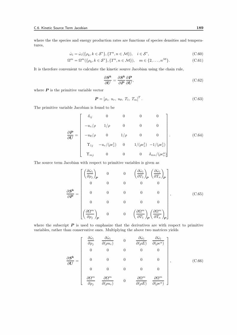
C.6. Kinetic Source Term Jacobian 189
where the the species and energy production rates are functions of species densities and tempera-tures,
ωi = ωi(ρk, k ∈ S∗, T n, n ∈ M), i ∈ S∗, (C.60)
Ωm = Ωm(ρk, k ∈ S∗, T n, n ∈ M), m ∈ 2, . . . , nM. (C.61)
It is therefore convenient to calculate the kinetic source Jacobian using the chain rule,
∂Sk
∂U=∂Sk
∂P
∂P
∂U, (C.62)
where P is the primitive variable vector
P = [ρi, ur, uθ, T1, Tm]T . (C.63)
The primitive variable Jacobian is found to be
∂P
∂U=
⎡
⎢
⎢
⎢
⎢
⎢
⎢
⎢
⎢
⎢
⎢
⎢
⎢
⎣
δij 0 0 0 0
−ur/ρ 1/ρ 0 0 0
−uθ/ρ 0 1/ρ 0 0
Υ1j −ur/(ρc1v) 0 1/(ρc1v) −1/(ρc1v)
Υmj 0 0 0 δmn/(ρcnv )
⎤
⎥
⎥
⎥
⎥
⎥
⎥
⎥
⎥
⎥
⎥
⎥
⎥
⎦
. (C.64)
The source term Jacobian with respect to primitive variables is given as
∂Sk
∂P=
⎡
⎢
⎢
⎢
⎢
⎢
⎢
⎢
⎢
⎢
⎢
⎢
⎢
⎢
⎢
⎢
⎣
(
∂ωi
∂ρj
)
P
0 0
(
∂ωi
∂T1
)
P
(
∂ωi
∂Tn
)
P
0 0 0 0 0
0 0 0 0 0
0 0 0 0 0
(
∂Ωm
∂ρj
)
P
0 0
(
∂Ωm
∂T1
)
P
(
∂Ωm
∂Tn
)
P
⎤
⎥
⎥
⎥
⎥
⎥
⎥
⎥
⎥
⎥
⎥
⎥
⎥
⎥
⎥
⎥
⎦
, (C.65)
where the subscript P is used to emphasize that the derivatives are with respect to primitivevariables, rather than conservative ones. Multiplying the above two matrices yields
∂Sk
∂U=
⎡
⎢
⎢
⎢
⎢
⎢
⎢
⎢
⎢
⎢
⎢
⎢
⎢
⎢
⎢
⎣
∂ωi
∂ρj
∂ωi
∂(ρur)0
∂ωi
∂(ρE)
∂ωi
∂(ρen)
0 0 0 0 0
0 0 0 0 0
0 0 0 0 0
∂Ωm
∂ρj
∂Ωm
∂(ρur)0
∂Ωm
∂(ρE)
∂Ωm
∂(ρen)
⎤
⎥
⎥
⎥
⎥
⎥
⎥
⎥
⎥
⎥
⎥
⎥
⎥
⎥
⎥
⎦
, (C.66)

190 Chapter C. Stagnation Line Jacobians
where the derivatives with respect to conservative variables are found to be
∂X
∂ρj=
(
∂X
∂ρj
)
P
+∑
l∈M
Υlj
(
∂X
∂Tl
)
P
, (C.67)
∂X
∂(ρur)= −
ur
ρc1v
(
∂X
T1
)
P
, (C.68)
∂X
∂(ρE)=
1
ρc1v
(
∂X
T1
)
P
, (C.69)
∂X
∂(ρen)=
1
ρcnv
(
∂X
Tn
)
P
−1
ρc1v
(
∂X
T1
)
P
, (C.70)
for X = ωi, Ωm.

APPENDIX D
Mixtures and Data
This appendix details the various mixtures and data used for the simulations presented in Chap-ter 7, including the the species involved, specific reactions considered, as well as the collisionintegral data necessary to compute the transport coefficients.
D.1. Mixtures
The three mixtures described in Section 7.1.1 are summarized in Table D.1. The table providesa list of species included in each mixture, the thermal nonequilibrium model employed, and thenumber of species, reactions, and collision pairs. Species thermodynamic properties were computedusing the RRHO model as described in Section 4.4.1 using the rotational, vibrational, and electroniccharacteristic temperatures and degeneracies provided by Gurvich et al. [173, 175]. The reactionmechanisms and rate constants employed for each mixture are detailed in the proceeding sectionfollowed by the collision integral data required to compute transport coefficients for each mixture.
Table D.1.: Summary of the three mixtures used in Chapter 7.
Mixture Species Noneq. # Species / # CollisionName Model Reactions Pairs
air e– N+ O+ NO+ N2+ O2
+ T , T ve 11 / 22 66N O NO N2 O2
air-ablation e– N+ O+ N O NO N2 T , T ve 20 / 25 210O2 C C+ H H+ C2
C2H C3 CO CO2 CNHCN H2
Titan N C H N2 C H CN NH T 13 / 27 91CH CH2 CH3 CH4 HCN
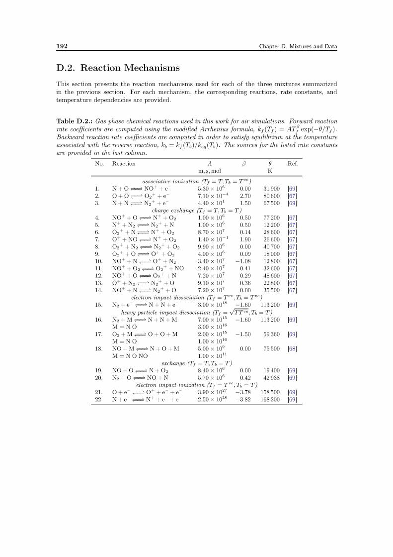
192 Chapter D. Mixtures and Data
D.2. Reaction Mechanisms
This section presents the reaction mechanisms used for each of the three mixtures summarizedin the previous section. For each mechanism, the corresponding reactions, rate constants, andtemperature dependencies are provided.
Table D.2.: Gas phase chemical reactions used in this work for air simulations. Forward reactionrate coefficients are computed using the modified Arrhenius formula, kf (Tf ) = AT β
f exp(−θ/Tf).Backward reaction rate coefficients are computed in order to satisfy equilibrium at the temperatureassociated with the reverse reaction, kb = kf (Tb)/keq(Tb). The sources for the listed rate constantsare provided in the last column.
No. Reaction A β θ Ref.m, s,mol K
associative ionization (Tf = T, Tb = T ve)1. N + O −−−− NO+ + e– 5.30× 10⁶ 0.00 31 900 [69]2. O + O −−−− O2
+ + e– 7.10× 10⁻⁴ 2.70 80 600 [67]3. N + N −−−− N2
+ + e– 4.40× 101 1.50 67 500 [69]charge exchange (Tf = T, Tb = T )
4. NO+ + O −−−− N+ + O2 1.00× 10⁶ 0.50 77 200 [67]5. N+ + N2 −−−− N2
+ + N 1.00× 10⁶ 0.50 12 200 [67]6. O2
+ + N −−−− N+ + O2 8.70× 10⁷ 0.14 28 600 [67]7. O+ + NO −−−− N+ + O2 1.40× 10⁻¹ 1.90 26 600 [67]8. O2
+ + N2 −−−− N2+ + O2 9.90× 10⁶ 0.00 40 700 [67]
9. O2+ + O −−−− O+ + O2 4.00× 10⁶ 0.09 18 000 [67]
10. NO+ + N −−−− O+ + N2 3.40× 10⁷ −1.08 12 800 [67]11. NO+ + O2 −−−− O2
+ + NO 2.40× 10⁷ 0.41 32 600 [67]12. NO+ + O −−−− O2
+ + N 7.20× 10⁷ 0.29 48 600 [67]13. O+ + N2 −−−− N2
+ + O 9.10× 10⁷ 0.36 22 800 [67]14. NO+ + N −−−− N2
+ + O 7.20× 10⁷ 0.00 35 500 [67]electron impact dissociation (Tf = T ve, Tb = T ve)
15. N2 + e– −−−− N + N + e– 3.00× 10¹⁸ −1.60 113 200 [69]heavy particle impact dissociation (Tf =
√TT ve, Tb = T )
16. N2 + M −−−− N + N + M 7.00× 10¹⁵ −1.60 113 200 [69]M = N O 3.00× 10¹⁶
17. O2 + M −−−− O + O + M 2.00× 10¹⁵ −1.50 59 360 [69]M = N O 1.00× 10¹⁶
18. NO + M −−−− N + O + M 5.00× 10⁹ 0.00 75 500 [68]M = N O NO 1.00× 10¹¹
exchange (Tf = T, Tb = T )19. NO + O −−−− N + O2 8.40× 10⁶ 0.00 19 400 [69]20. N2 + O −−−− NO + N 5.70× 10⁶ 0.42 42 938 [69]
electron impact ionization (Tf = T ve, Tb = T )21. O + e– −−−− O+ + e– + e– 3.90× 1027 −3.78 158 500 [69]22. N + e– −−−− N+ + e– + e– 2.50× 1028 −3.82 168 200 [69]
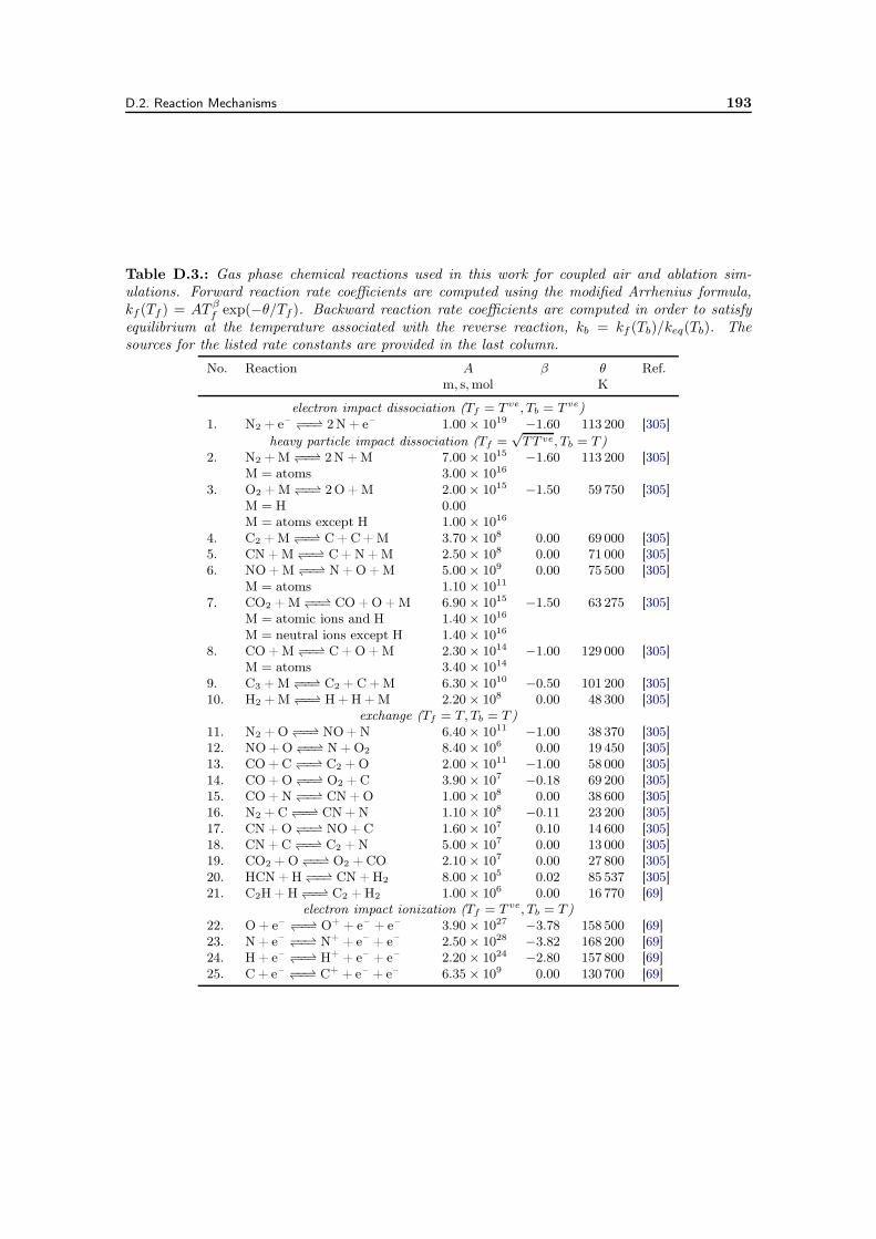
D.2. Reaction Mechanisms 193
Table D.3.: Gas phase chemical reactions used in this work for coupled air and ablation sim-ulations. Forward reaction rate coefficients are computed using the modified Arrhenius formula,kf (Tf ) = AT β
f exp(−θ/Tf). Backward reaction rate coefficients are computed in order to satisfyequilibrium at the temperature associated with the reverse reaction, kb = kf (Tb)/keq(Tb). Thesources for the listed rate constants are provided in the last column.
No. Reaction A β θ Ref.m, s,mol K
electron impact dissociation (Tf = T ve, Tb = T ve)1. N2 + e– −−−− 2N + e– 1.00× 10¹⁹ −1.60 113 200 [305]
heavy particle impact dissociation (Tf =√TT ve, Tb = T )
2. N2 + M −−−− 2N + M 7.00× 10¹⁵ −1.60 113 200 [305]M = atoms 3.00× 10¹⁶
3. O2 + M −−−− 2O + M 2.00× 10¹⁵ −1.50 59 750 [305]M = H 0.00M = atoms except H 1.00× 10¹⁶
4. C2 + M −−−− C + C + M 3.70× 10⁸ 0.00 69 000 [305]5. CN + M −−−− C + N + M 2.50× 10⁸ 0.00 71 000 [305]6. NO + M −−−− N + O + M 5.00× 10⁹ 0.00 75 500 [305]
M = atoms 1.10× 10¹¹
7. CO2 + M −−−− CO + O + M 6.90× 10¹⁵ −1.50 63 275 [305]M = atomic ions and H 1.40× 10¹⁶
M = neutral ions except H 1.40× 10¹⁶
8. CO + M −−−− C + O + M 2.30× 10¹⁴ −1.00 129 000 [305]M = atoms 3.40× 10¹⁴
9. C3 + M −−−− C2 + C + M 6.30× 10¹⁰ −0.50 101 200 [305]10. H2 + M −−−− H + H + M 2.20× 10⁸ 0.00 48 300 [305]
exchange (Tf = T, Tb = T )11. N2 + O −−−− NO + N 6.40× 10¹¹ −1.00 38 370 [305]12. NO + O −−−− N + O2 8.40× 10⁶ 0.00 19 450 [305]13. CO + C −−−− C2 + O 2.00× 10¹¹ −1.00 58 000 [305]14. CO + O −−−− O2 + C 3.90× 10⁷ −0.18 69 200 [305]15. CO + N −−−− CN + O 1.00× 10⁸ 0.00 38 600 [305]16. N2 + C −−−− CN + N 1.10× 10⁸ −0.11 23 200 [305]17. CN + O −−−− NO + C 1.60× 10⁷ 0.10 14 600 [305]18. CN + C −−−− C2 + N 5.00× 10⁷ 0.00 13 000 [305]19. CO2 + O −−−− O2 + CO 2.10× 10⁷ 0.00 27 800 [305]20. HCN + H −−−− CN + H2 8.00× 10⁵ 0.02 85 537 [305]21. C2H + H −−−− C2 + H2 1.00× 10⁶ 0.00 16 770 [69]
electron impact ionization (Tf = T ve, Tb = T )22. O + e– −−−− O+ + e– + e– 3.90× 1027 −3.78 158 500 [69]23. N + e– −−−− N+ + e– + e– 2.50× 1028 −3.82 168 200 [69]24. H + e– −−−− H+ + e– + e– 2.20× 1024 −2.80 157 800 [69]25. C + e– −−−− C+ + e– + e– 6.35× 10⁹ 0.00 130 700 [69]
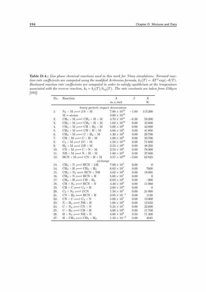
194 Chapter D. Mixtures and Data
Table D.4.: Gas phase chemical reactions used in this work for Titan simulations. Forward reac-tion rate coefficients are computed using the modified Arrhenius formula, kf (T ) = AT β exp(−θ/T ).Backward reaction rate coefficients are computed in order to satisfy equilibrium at the temperatureassociated with the reverse reaction, kb = kf (T )/keq(T ). The rate constants are taken from Gökçen[295].
No. Reaction A β θm, s,mol K
heavy particle impact dissociation1. N2 + M −−−− 2 N + M 7.00× 10¹⁵ −1.60 113 200
M = atoms 3.00× 10¹⁶
2. CH4 + M −−−− CH3 + H + M 4.70× 1041 −8.20 59 2003. CH3 + M −−−− CH2 + H + M 1.02× 10¹⁰ 0.00 45 6004. CH3 + M −−−− CH + H2 + M 5.00× 10⁹ 0.00 42 8005. CH2 + M −−−− CH + H + M 4.00× 10⁹ 0.00 41 8006. CH2 + M −−−− C + H2 + M 1.30× 10⁸ 0.00 29 7007. CH + M −−−− C + H + M 1.90× 10⁸ 0.00 33 7008. C2 + M −−−− 2C + M 1.50× 10¹⁰ 0.00 71 6009. H2 + M −−−− 2 H + M 2.23× 10⁸ 0.00 48 35010. CN + M −−−− C + N + M 2.53× 10⁸ 0.00 78 00011. NH + M −−−− N + H + M 1.80× 10⁸ 0.00 37 60012. HCN + M −−−− CN + H + M 3.57× 10²⁰ −2.60 62 845
exchange13. CH3 + N −−−− HCN + 2H 7.00× 10⁷ 0.00 014. CH3 + H −−−− CH2 + H2 6.03× 10⁷ 0.00 760015. CH2 + N2 −−−− HCN + NH 4.82× 10⁶ 0.00 18 00016. CH2 + N −−−− HCN + H 5.00× 10⁷ 0.00 017. CH2 + H −−−− CH + H2 6.03× 10⁶ 0.00 −90018. CH + N2 −−−− HCN + N 4.40× 10⁶ 0.00 11 06019. CH + C −−−− C2 + H 2.00× 10⁸ 0.00 020. C2 + N2 −−−− 2CN 1.50× 10⁷ 0.00 21 00021. CN + H2 −−−− HCN + H 2.95× 10⁻¹ 0.00 113022. CN + C −−−− C2 + N 5.00× 10⁷ 0.00 13 00023. N + H2 −−−− NH + H 1.60× 10⁸ 0.00 12 65024. C + N2 −−−− CN + N 5.24× 10⁷ 0.00 22 60025. C + H2 −−−− CH + H 4.00× 10⁸ 0.00 11 70026. H + N2 −−−− NH + N 3.00× 10⁶ 0.50 71 40027. H + CH4 −−−− CH3 + H2 1.32× 10⁻² 3.00 4045
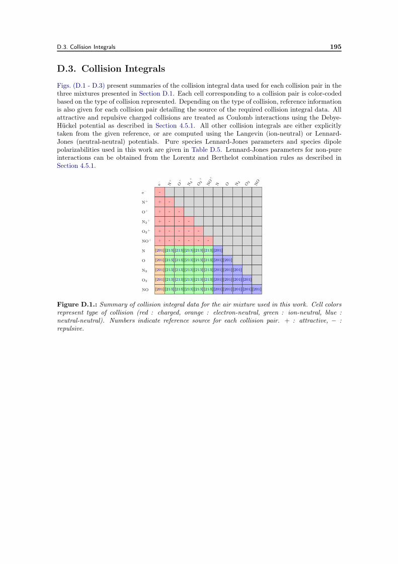
D.3. Collision Integrals 195
D.3. Collision Integrals
Figs. (D.1 - D.3) present summaries of the collision integral data used for each collision pair in thethree mixtures presented in Section D.1. Each cell corresponding to a collision pair is color-codedbased on the type of collision represented. Depending on the type of collision, reference informationis also given for each collision pair detailing the source of the required collision integral data. Allattractive and repulsive charged collisions are treated as Coulomb interactions using the Debye-Hückel potential as described in Section 4.5.1. All other collision integrals are either explicitlytaken from the given reference, or are computed using the Langevin (ion-neutral) or Lennard-Jones (neutral-neutral) potentials. Pure species Lennard-Jones parameters and species dipolepolarizabilities used in this work are given in Table D.5. Lennard-Jones parameters for non-pureinteractions can be obtained from the Lorentz and Berthelot combination rules as described inSection 4.5.1.
e–
N+
O+
N2
+
O2
+
NO
+
N O N2
O2
NO
e– -
N+ + -
O+ + - -
N2+ + - - -
O2+ + - - - -
NO+ + - - - - -
N [201] [213] [213] [213] [213] [213] [201]
O [201] [213] [213] [213] [213] [213] [201] [201]
N2 [201] [213] [213] [213] [213] [213] [201] [201] [201]
O2 [201] [213] [213] [213] [213] [213] [201] [201] [201] [201]
NO [201] [213] [213] [213] [213] [213] [201] [201] [201] [201] [201]
Figure D.1.: Summary of collision integral data for the air mixture used in this work. Cell colorsrepresent type of collision (red : charged, orange : electron-neutral, green : ion-neutral, blue :neutral-neutral). Numbers indicate reference source for each collision pair. + : attractive, − :repulsive.
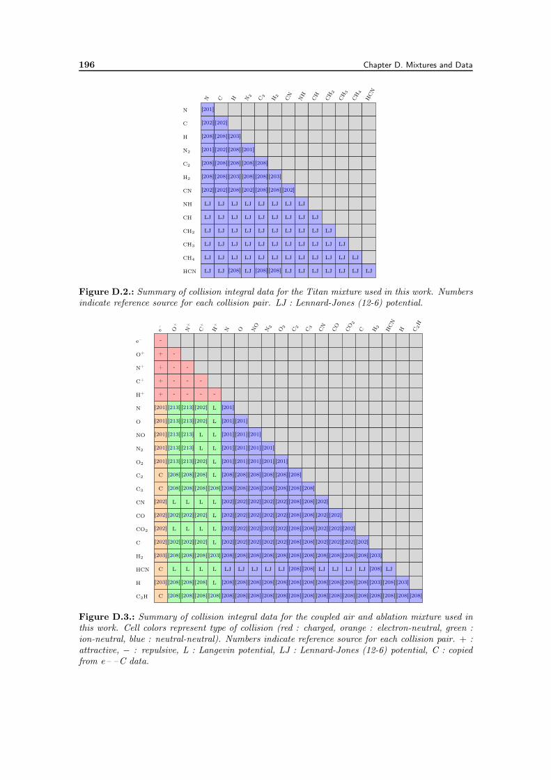
196 Chapter D. Mixtures and Data
N C H N2
C2
H2
CN
NH
CH
CH
2
CH3
CH
4
HCN
N [201]
C [202] [202]
H [208] [208] [203]
N2 [201] [202] [208] [201]
C2 [208] [208] [208] [208] [208]
H2 [208] [208] [203] [208] [208] [203]
CN [202] [202] [208] [202] [208] [208] [202]
NH LJ LJ LJ LJ LJ LJ LJ LJ
CH LJ LJ LJ LJ LJ LJ LJ LJ LJ
CH2 LJ LJ LJ LJ LJ LJ LJ LJ LJ LJ
CH3 LJ LJ LJ LJ LJ LJ LJ LJ LJ LJ LJ
CH4 LJ LJ LJ LJ LJ LJ LJ LJ LJ LJ LJ LJ
HCN LJ LJ [208] LJ [208] [208] LJ LJ LJ LJ LJ LJ LJ
Figure D.2.: Summary of collision integral data for the Titan mixture used in this work. Numbersindicate reference source for each collision pair. LJ : Lennard-Jones (12-6) potential.
e–
O+
N+
C+
H+
N O NO
N2
O2
C2
C3
CN
CO
CO
2
C H2
HCN
H C2H
e– -
O+ + -
N+ + - -
C+ + - - -
H+ + - - - -
N [201] [213] [213] [202] L [201]
O [201] [213] [213] [202] L [201] [201]
NO [201] [213] [213] L L [201] [201] [201]
N2 [201] [213] [213] L L [201] [201] [201] [201]
O2 [201] [213] [213] [202] L [201] [201] [201] [201] [201]
C2 C [208] [208] [208] L [208] [208] [208] [208] [208] [208]
C3 C [208] [208] [208] [208] [208] [208] [208] [208] [208] [208] [208]
CN [202] L L L L [202] [202] [202] [202] [202] [208] [208] [202]
CO [202] [202] [202] [202] L [202] [202] [202] [202] [202] [208] [208] [202] [202]
CO2 [202] L L L L [202] [202] [202] [202] [202] [208] [208] [202] [202] [202]
C [202] [202] [202] [202] L [202] [202] [202] [202] [202] [208] [208] [202] [202] [202] [202]
H2 [203] [208] [208] [208] [203] [208] [208] [208] [208] [208] [208] [208] [208] [208] [208] [208] [203]
HCN C L L L L LJ LJ LJ LJ LJ [208] [208] LJ LJ LJ LJ [208] LJ
H [203] [208] [208] [208] L [208] [208] [208] [208] [208] [208] [208] [208] [208] [208] [208] [203] [208] [203]
C2H C [208] [208] [208] [208] [208] [208] [208] [208] [208] [208] [208] [208] [208] [208] [208] [208] [208] [208] [208]
Figure D.3.: Summary of collision integral data for the coupled air and ablation mixture used inthis work. Cell colors represent type of collision (red : charged, orange : electron-neutral, green :ion-neutral, blue : neutral-neutral). Numbers indicate reference source for each collision pair. + :attractive, − : repulsive, L : Langevin potential, LJ : Lennard-Jones (12-6) potential, C : copiedfrom e– –C data.
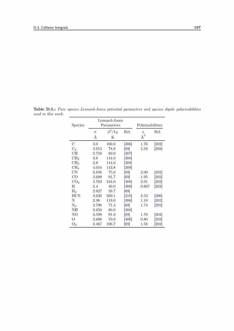
D.3. Collision Integrals 197
Table D.5.: Pure species Lennard-Jones potential parameters and species dipole polarizabilitiesused in this work.
Lennard-JonesSpecies Parameters Polarizabilities
σ φ0/kB Ref. α Ref.Å K Å
3
C 3.0 100.0 [306] 1.76 [202]C2 3.913 78.8 [69] 5.58 [208]CH 2.750 80.0 [307]CH2 3.8 144.0 [308]CH3 3.8 144.0 [308]CH4 4.010 143.8 [309]CN 3.856 75.0 [69] 2.00 [202]CO 3.690 91.7 [69] 1.95 [202]CO2 3.763 244.0 [308] 2.91 [202]H 2.4 40.0 [306] 0.667 [203]H2 2.827 59.7 [69]HCN 3.630 569.1 [310] 2.53 [306]N 2.98 119.0 [306] 1.10 [202]N2 3.798 71.4 [69] 1.74 [202]NH 2.650 80.0 [308]NO 3.599 91.0 [69] 1.70 [202]O 2.660 70.0 [306] 0.80 [202]O2 3.467 106.7 [69] 1.58 [202]

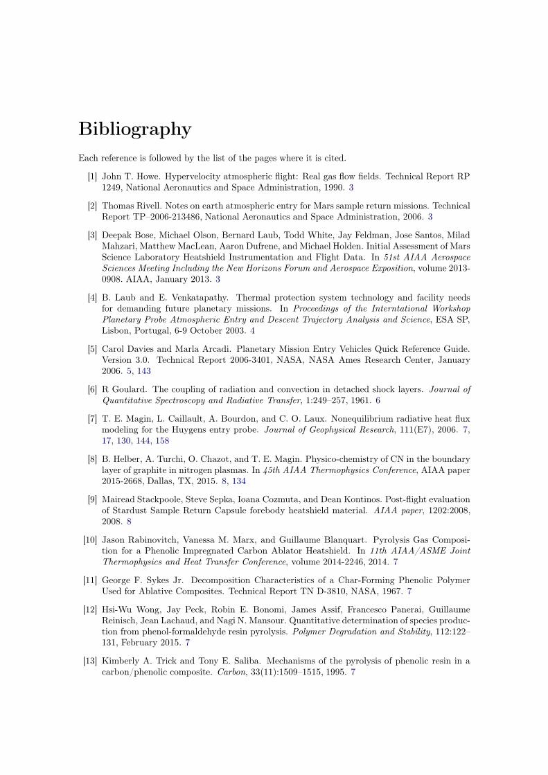
Bibliography
Each reference is followed by the list of the pages where it is cited.
[1] John T. Howe. Hypervelocity atmospheric flight: Real gas flow fields. Technical Report RP1249, National Aeronautics and Space Administration, 1990. 3
[2] Thomas Rivell. Notes on earth atmospheric entry for Mars sample return missions. TechnicalReport TP–2006-213486, National Aeronautics and Space Administration, 2006. 3
[3] Deepak Bose, Michael Olson, Bernard Laub, Todd White, Jay Feldman, Jose Santos, MiladMahzari, Matthew MacLean, Aaron Dufrene, and Michael Holden. Initial Assessment of MarsScience Laboratory Heatshield Instrumentation and Flight Data. In 51st AIAA AerospaceSciences Meeting Including the New Horizons Forum and Aerospace Exposition, volume 2013-0908. AIAA, January 2013. 3
[4] B. Laub and E. Venkatapathy. Thermal protection system technology and facility needsfor demanding future planetary missions. In Proceedings of the Interntational WorkshopPlanetary Probe Atmospheric Entry and Descent Trajectory Analysis and Science, ESA SP,Lisbon, Portugal, 6-9 October 2003. 4
[5] Carol Davies and Marla Arcadi. Planetary Mission Entry Vehicles Quick Reference Guide.Version 3.0. Technical Report 2006-3401, NASA, NASA Ames Research Center, January2006. 5, 143
[6] R Goulard. The coupling of radiation and convection in detached shock layers. Journal ofQuantitative Spectroscopy and Radiative Transfer, 1:249–257, 1961. 6
[7] T. E. Magin, L. Caillault, A. Bourdon, and C. O. Laux. Nonequilibrium radiative heat fluxmodeling for the Huygens entry probe. Journal of Geophysical Research, 111(E7), 2006. 7,17, 130, 144, 158
[8] B. Helber, A. Turchi, O. Chazot, and T. E. Magin. Physico-chemistry of CN in the boundarylayer of graphite in nitrogen plasmas. In 45th AIAA Thermophysics Conference, AIAA paper2015-2668, Dallas, TX, 2015. 8, 134
[9] Mairead Stackpoole, Steve Sepka, Ioana Cozmuta, and Dean Kontinos. Post-flight evaluationof Stardust Sample Return Capsule forebody heatshield material. AIAA paper, 1202:2008,2008. 8
[10] Jason Rabinovitch, Vanessa M. Marx, and Guillaume Blanquart. Pyrolysis Gas Composi-tion for a Phenolic Impregnated Carbon Ablator Heatshield. In 11th AIAA/ASME JointThermophysics and Heat Transfer Conference, volume 2014-2246, 2014. 7
[11] George F. Sykes Jr. Decomposition Characteristics of a Char-Forming Phenolic PolymerUsed for Ablative Composites. Technical Report TN D-3810, NASA, 1967. 7
[12] Hsi-Wu Wong, Jay Peck, Robin E. Bonomi, James Assif, Francesco Panerai, GuillaumeReinisch, Jean Lachaud, and Nagi N. Mansour. Quantitative determination of species produc-tion from phenol-formaldehyde resin pyrolysis. Polymer Degradation and Stability, 112:122–131, February 2015. 7
[13] Kimberly A. Trick and Tony E. Saliba. Mechanisms of the pyrolysis of phenolic resin in acarbon/phenolic composite. Carbon, 33(11):1509–1515, 1995. 7
200 Chapter 8. Bibliography
[14] Hsi-Wu Wong, Jay Peck, James Assif, Jean Lachaud, and Nagi N. Mansour. Quantitativedetermination of species production from the pyrolysis of the Phenolic Impregnated CarbonAblator (PICA). In AIAA Science and Technology Forum and Exposition, volume 2015-1447.AIAA, January 2015. 7
[15] Brody K. Bessire, Sridhar A. Lahankar, and Timothy K. Minton. Pyrolysis of PhenolicImpregnated Carbon Ablator (PICA). ACS Applied Materials & Interfaces, 7(3):1383–1395,January 2015. 7
[16] Christopher O. Johnston, Peter A. Gnoffo, and Kenneth Sutton. Influence of ablation onradiative heating for earth entry. Journal of Spacecraft and Rockets, 46(3):481–491, 2009. 9,10, 25, 143, 158, 159, 166, 167
[17] Bernd Helber. Material Response Characterization of Low-density Ablators in AtmophericEntry Plasmas. PhD thesis, von Karman Institute for Fluid Dynamics and Vrije UniversiteitBrussel, Brussels, Belgium, January 2016. 10
[18] Pierre Schrooyen. Numerical simulation of aerothermal flows through ablative thermal pro-tection systems. PhD thesis, von Karman Institute for Fluid Dynamics and UniversitéCatholique de Louvain, Belgium, November 2015. 10, 171
[19] T. Gökçen and C. Park. The coupling of radiative transfer to quasi-1d flows with thermo-chemical nonequilibrium. In AIAA 29th aerospace sciences meeting, page 570, 1991. 10
[20] Lin C. Hartung, Robert A. Mitcheltree, and Peter A. Gnoffo. Coupled radiation effects inthermochemical nonequilibrium shock-capturing flowfield calculations. Journal of Thermo-physics and Heat Transfer, 8(2):244–250, 1994.
[21] Michael J. Wright, Deepak Bose, and Joe Olejniczak. Impact of flowfield-radiation couplingon aeroheating for titan aerocapture. Journal of Thermophysics and Heat Transfer, 19(1):17–27, 2005. 10
[22] Scott A. Stanley and Leland A. Carlson. Effects of shock wave precursors ahead of hypersonicentry vehicles. Journal of Spacecraft and Rockets, 29(2):190–197, 1992. 10
[23] C. Park. Radiation enhancement by nonequilibrium in earth’s atmosphere. Journal of Space-craft and Rockets, 22(1):27–36, 1985. 10
[24] Lin C. Hartung. Development of a nonequilibrium radiative heating prediction method forcoupled flowfield solutions. Journal of Thermophysics and Heat Transfer, 6(4):618–625, 1992.10
[25] S. Sharma. Modeling of nonequilibrium radiation phenomena: an assessment. Journal ofThermophysics and Heat Transfer, 10:85âĂŞ396, 1996. 10
[26] Peter A. Gnoffo, Roop N. Gupta, and Judy L. Shinn. Conservation equations and physicalmodels for hypersonic air flows in thermal and chemical nonequilibrium. Technical Paper2867, NASA, February 1989. 10, 17, 23, 24, 42
[27] Graham V. Candler and Robert W. Maccormack. Computation of weakly ionized hyper-sonic flows in thermochemical nonequilibrium. Journal of Thermophysics and Heat Transfer,5(3):266–273, July 1991. 10, 17, 43, 44, 131
[28] Graham V. Candler, Pramod K. Subbareddy, and Ioannis Nompelis. Decoupled ImplicitMethod for Aerothermodynamics and Reacting Flows. AIAA Journal, 51(5):1245–1254,May 2013. 10
[29] Jong-Hun Lee. Basic governing equations for the flight regimes of aeroassisted orbital transfervehicles. In 19th Thermophysics Conference, AIAA paper 84-1729, Snowmass, CO, 1984. 10,15, 17

Chapter 8. Bibliography 201
[30] Chul Park. Nonequilibrium Hypersonic Aerothermodynamics. Wiley, New York, 1990. LCCB:TL571.5 .P37 1990. 10, 41, 42
[31] Ellis E. Whiting, Chul Park, James O. Arnold, and John A. Paterson. NEQAIR96, nonequi-librium and equilibrium radiative transport and spectra program: User’s manual. TechnicalReport NASA-RP-1389, NASA Ames Research Center, 1996. 10
[32] Brett A. Cruden and Aaron M. Brandis. Updates to the NEQAIR radiation solver. In Pro-ceedings of the 6th High Temperature Gas Radiation Workshop, St. Andrews, UK, November2014. ESA. 10
[33] K. Fujita and T. Abe. SPRADIAN, structural package for radiation analysis: theory andapplication. ISAS Report No 669, 1997. 10
[34] L. Kuznetsova and S. Surzhikov. Absorption cross sections of diatomic molecules for problemsof radiative heat transfer in low-temperature plasma. High Temperature, 37(3):374–385, 1999.10
[35] C. Laux. Radiation and nonequilibrium collisinal-radiative models. VKI special course onphysico-chemical models for high enthalpy and plasma flows modeling, 2002. 10
[36] S. Chauveau, M.-Y. Perrin, Ph Rivière, and A. Soufiani. Contributions of diatomic molecularelectronic systems to heated air radiation. Journal of Quantitative Spectroscopy and RadiativeTransfer, 72(4):503–530, 2002. 10, 51, 52, 53, 55
[37] Sophie Chauveau, Christine Deron, Marie-Yvonne Perrin, Philippe Rivière, and AnouarSoufiani. Radiative transfer in LTE air plasmas for temperatures up to 15,000 K. Jour-nal of Quantitative Spectroscopy and Radiative Transfer, 77:113–130, 2003. 51, 52, 53, 55,57, 58, 59
[38] Y. Babou, Ph. Rivière, M.Y. Perrin, , and A. Soufiani. High-temperature and nonequilibriumpartition function and thermodynamic data of diatomic molecules. International Journal ofThermophysics, 30(2):416–438, 2009.
[39] Y. Babou, Ph. Rivière, M.Y. Perrin, , and A. Soufiani. Spectroscopic data for the prediction ofradiative transfer in CO2âĂŞN2 plasmas. Journal of Quantitative Spectroscopy and RadiativeTransfer, 110:89–108, 2009. 51, 52, 55, 57, 58, 59
[40] A. Soufiani, Ph. Rivière, and M.Y. Perrin. High temperature gas radiation (HTGR) databaseand models. Von Karman Institute Lecture Series, STO-EN-AVT-218, 2013. 10, 51, 52, 55,145
[41] A. Kramida, Yu Ralchenko, J. Reader, and NIST ASD Team. NIST Atomic Spectra Database(version 5.2), 2014. 10, 55
[42] W. Cunto, C. Mendoza, F. Ochsenbein, and C. J. Zeippen. TOPbase at the CDS. Astronomyand Astrophysics, 275, 1993. 10, 55, 57, 58
[43] Jean-Michel Lamet, Yacine Babou, Philippe Rivière, Marie-Yvonne Perrin, and Anouar Soufi-ani. Radiative transfer in gases under thermal and chemical nonequilibrium conditions: Ap-plication to earth atmospheric re-entry. Journal of Quantitative Spectroscopy and RadiativeTransfer, 109(2):235–244, January 2008. 10, 16, 17, 56, 58
[44] Bruno Lopez, Marie Yvonne Perrin, Philippe Rivière, and Anouar Soufiani. Coupled Nonequi-librium Flowfield–Radiative Transfer Calculation Behind a Shock Wave. Journal of Ther-mophysics and Heat Transfer, 27(3):404–413, 2013. 10, 154
[45] A. M. Feldick, M. F. Modest, and D. A. Levin. Closely Coupled Flowfield-Radiation Interac-tions During Hypersonic Reentry. Journal of Thermophysics and Heat Transfer, 25(4):481–492, October 2011. 10
202 Chapter 8. Bibliography
[46] C.O. Johnston, B.R. Hollis, and K. Sutton. Spectrum modeling for air shock-layer radiationat lunar-return conditions. Journal of Spacecraft and Rockets, 45(5):865–878, 2008. 10, 151
[47] M. K. Denison and B. W. Webb. The spectral-line-based weighted-sum-of-gray-gases modelin nonisothermal nonhomogeneous media. Journal of Heat Transfer, 117:359–365, 1995. 10
[48] R. Goody, R. West, L. Chen, and D. Crisp. The correlated-k method for radiation calcula-tions in nonhomogeneous atmospheres. Journal of Quantitative Spectroscopy and RadiativeTransfer, 42:539–550, 1989. 10
[49] D. Mihalas and B. Weibel-Mihalas. Foundations of radiation hydrodynamics. Dover Publi-cations, INC, Mineloa, 1999. 11
[50] Ph. Rivière, A. Soufiani, M. Y. Perrin, H. Riad, and A. Gleizes. Air mixture radiativeproperty modelling in the temperature range 10,000-40,000 K. Journal of Quantitative Spec-troscopy and Radiative Transfer, 56(1):29–45, 1996. 11
[51] A. Bansal and M. F. Modest. Multiscale Part-Spectrum k-Distribution Database for AtomicRadiation in Hypersonic Nonequilibrium Flows. Journal of Heat Transfer, 133(12):122701–122701, 2011. 11
[52] A. Bansal, M. F. Modest, and D. A. Levin. Multi-scale k-distribution model for gas mixturesin hypersonic nonequilibrium flows. Journal of Quantitative Spectroscopy and RadiativeTransfer, 112:1213–1221, 2011. 11
[53] Ankit Bansal and M. F. Modest. Modeling of Radiative Heat Transfer in CarbonaceousAtmospheres Using k-Distribution Models. Journal of Thermophysics and Heat Transfer,27(2):217–225, April 2013. 11, 152, 153
[54] M. F. Modest. Radiative heat transfer. Academic Press, third edition, 2013. 11
[55] Jean-Michel Lamet, Philippe Rivière, Marie-Yvonne Perrin, and Anouar Soufiani. Narrow-band model for nonequilibrium air plasma radiation. Journal of Quantitative Spectroscopyand Radiative Transfer, 111(1):87–104, January 2010. 11, 20, 52, 53, 57, 60, 61, 65, 68, 70,145, 154
[56] W. G. Vincenti and Charles H. Kruger. Introduction to Physical Gas Dynamics. KriegerPub Co, 1975. 13, 21, 26, 41
[57] Forrest R. Gilmore. Potential energy curves for N2, NO, O2 and corresponding ions. Journalof Quantitative Spectroscopy and Radiative Transfer, 5:369–390, 1965. 14
[58] C. Park. Assessment of two-temperature kinetic model for dissociating and weakly-ionizingnitrogen. In 4th Thermophysics and Heat Transfer Conference, Boston, MA, June 1986.AIAA. 15, 17, 35, 37
[59] Chul Park. Convergence of Computation of Chemical Reacting Flows. In Thermophysical As-pects of Re-Entry Flows, pages 478–513. American Institute of Aeronautics and Astronautics,New York, January 1986.
[60] Chul Park. Assessment of two-temperature kinetic model for ionizing air. In 22nd Thermo-physics Conference, AIAA paper 87-1574, Honolulu, Hawaii, 1987. 15, 35, 37, 42
[61] Jong-Hun Lee. Basic Governing Equations for the Flight Regimes of Aeroassisted OrbitalTransfer Vehicles. In H. F. Nelson, editor, Thermal Design of Aeroassisted Orbital Trans-fer Vehicles, pages 3–53. American Institute of Aeronautics and Astronautics, New York,January 1985. 15, 17
[62] M. Born and R. Oppenheimer. Zur Quantentheorie der Molekeln. Annalen der Physik,389(20):457–484, 1927. 16
Chapter 8. Bibliography 203
[63] Richard L. Jaffe. The calculation of high-temperature equilibrium and nonequilibrium specificheat data for N2, O2 and NO. In 22nd AIAA Thermophysics Conference, AIAA paper 87-1633, Honolulu, HI, 1987. 16
[64] Thomas L. Eddy and K. Y. Cho. A multitemperature model for plasmas in chemical nonequi-librium. In HTD, volume 161, pages 195–210. ASME, 1991. 16
[65] D. Giordano. Hypersonic-flow governing equations with electromagnetic fields. In Non-Equilibrium Gas Dynamics - From Physical Models to Hypersonic Flights, volume EN-AVT-162, pages 1–68, Rhode St. Genèse, Belgium, 2009. NATO-STO/VKI Lecture Series. 16, 19,21
[66] Chul Park and Seung-Ho Lee. Validation of multi-temperature nozzle flow code NOZNT. In28th Therrnophysics Conference, volume 93–2862. AIAA, 1993. 17
[67] Chul Park. Review of chemical-kinetic problems of future NASA missions, I: Earth entries.Journal of Thermophysics and Heat Transfer, 7(3):385–398, July-Sept. 1993. 42, 192
[68] Chul Park, John T. Howe, Richard L. Jaffe, and Graham V. Candler. Review of Chemical-Kinetic Problems of Future NASA Missions, II: Mars Entries. Journal of Thermophysics andHeat Transfer, 8(1):9–23, 1994. 192
[69] Chul Park, Richard L. Jaffe, and Harry Partridge. Chemical-Kinetic Parameters of Hyper-bolic Earth Entry. Journal of Thermophysics and Heat Transfer, 15(1):76–90, 2001. 39, 133,143, 192, 193, 197
[70] Andrea Lani, Marco Panesi, and Herman Deconinck. Conservative Residual DistributionMethod for Viscous Double Cone Flows in Thermochemical Nonequilibrium. Communica-tions in Computational Physics, 2012.
[71] Laurent Soucasse, James B. Scoggins, Thierry E. Magin, Philippe Rivière, and Anouar Soufi-ani. Flow-radiation coupling for atmospheric entries using a Hybrid Statistical Narrow Bandmodel. Journal of Quantitative Spectroscopy and Radiative Transfer, 2016. in press. 17, 61
[72] A. Munafò, M. Panesi, and T. E. Magin. Boltzmann rovibrational collisional coarse-grainedmodel for internal energy excitation and dissociation in hypersonic flows. Physical ReviewE, 89(2), February 2014. 17, 18, 19, 140, 170
[73] Jean-Luc Cambier and Stephane Moreau. Simulations of a molecular plasma in collisional-radiative nonequilibrium. In AIAA 24th Plasmadynamics & Lasers Conference, AIAA paper93-3196, Orlando, FL, 1993. 17
[74] Laurent C. Pierrot, Christophe O. Laux, and Charles H. Kruger. Vibrationally-specificcollisional-radiative model for nonequilibrium nitrogen plasmas. In 29th AIAA Plasmady-namics and Lasers Conference, AIAA paper 98-2664, Albuquerque, NM, 1998. 17, 18
[75] Thierry E. Magin, Marco Panesi, Anne Bourdon, Richard L. Jaffe, and David W. Schwenke.Coarse-grain model for internal energy excitation and dissociation of molecular nitrogen.Chemical Physics, 398:90–95, April 2012. 17, 18
[76] M. G. Kapper and J.-L. Cambier. Ionizing shocks in argon. Part II: Transient and multi-dimensional effects. Journal of Applied Physics, 109(11):113309, 2011. 18
[77] M. G. Kapper and J.-L. Cambier. Ionizing shocks in argon. Part I: Collisional-radiativemodel and steady-state structure. Journal of Applied Physics, 109(11):113308, 2011.
[78] Marco Panesi, Richard L. Jaffe, David W. Schwenke, and Thierry E. Magin. Rovibrationalinternal energy transfer and dissociation of N2(1Σg+)-N(4Su) system in hypersonic flows.The Journal of Chemical Physics, 138(4):044312, 2013. 18
204 Chapter 8. Bibliography
[79] Richard L. Jaffe, David W. Schwenke, and Marco Panesi. First principles calculations ofheavy particle rate coefficients. In Timothy C. Lieuwen, editor, Hypersonic NonequilibriumFlows: Fundamentals and Recent Advances, volume 247 of Progress in Astronautics andAeronautics, pages 103–158. American Institute of Aeronautics and Astronautics, Reston,Virginia, 2015. 18, 34
[80] Galina Chaban, Richard Jaffe, David Schwenke, and Winifred Huo. Dissociation cross sec-tions and rate coefficients for nitrogen from accurate theoretical calculations. In 46th AIAAAerospace Sciences Meeting and Exhibit, AIAA paper 2008-1209, Reno, NV, 2008. 18, 19
[81] Galina Chaban, Richard Jaffe, David Schwenke, and Winifred Huo. Dissociation cross sec-tions and rates for nitrogen. In Non-Equilibrium Gas Dynamics - from Physical Models toHypersonic Flights, NATO-STO/VKI LS RTO-EN-AVT-162, Rhode-Saint-Genèse, Belgium,2009.
[82] Richard Jaffe, David Schwenke, and Galina Chaban. Theoretical analysis of N2 collisionaldissociation and rotation-vibration energy transfer. In 47th AIAA Aerospace Sciences Meet-ing including The New Horizons Forum and Aerospace Exposition, AIAA paper 2009-1569,Orlando, FL, 2009.
[83] Richard Jaffe, David Schwenke, and Galina Chaban. Vibration-rotation excitation and dis-sociation in N2-N2 collisions from accurate theoretical calculations. In 10th AIAA/ASMEJoint Thermophysics and Heat Transfer Conference, AIAA paper 2010-4517, Chicago, IL,2010. 18, 19
[84] Gert Due Billing and Edward R. Fisher. VV and VT rate coefficients in H2 by a quantum-classical model. Chemical Physics, 18:225–232, 1976. 18
[85] Gert Due Billing and E. R. Fisher. VV and VT rate coefficients in N2 by a quantum-classicalmodel. Chemical Physics, 43(3):395–401, 1979.
[86] Kenneth Haug, Donald G. Truhlar, and Normand C. Blais. Monte Carlo trajectoryand master equation simulation of the nonequilibrium dissociation rate coefficient forAr+H2→Ar+2H at 4500 K. The Journal of Chemical Physics, 86(5):2697, 1987.
[87] David W. Schwenke. A theoretical prediction of hydrogen molecule dissociation-recombination rates including an accurate treatment of internal state nonequilibrium effects.The Journal of Chemical Physics, 92(12):7267, 1990.
[88] Eswar Josyula and William F. Bailey. Vibration-Dissociation Coupling Using Master Equa-tions in Nonequilibrium Hypersonic Blunt-Body Flow. Journal of Thermophysics and HeatTransfer, 15(2):157–167, April 2001.
[89] Eswar Josyula, William F. Bailey, and Stephen M. Ruffin. Reactive and nonreactive vibra-tional energy exchanges in nonequilibrium hypersonic flows. Physics of Fluids, 15(10):3223,2003.
[90] F. Esposito, I. Armenise, and M. Capitelli. N–N2 state to state vibrational-relaxation anddissociation rates based on quasiclassical calculations. Chemical Physics, 331(1):1–8, Decem-ber 2006. 35
[91] Fabrizio Esposito, Iole Armenise, Giulia Capitta, and Mario Capitelli. O–O2 state-to-statevibrational relaxation and dissociation rates based on quasiclassical calculations. ChemicalPhysics, 351(1-3):91–98, July 2008. 35
[92] Marco Panesi, Thierry Magin, Anne Bourdon, Arnaud Bultel, and O. Chazot. Fire II flightexperiment analysis by means of a collisional-radiative model. Journal of thermophysics andheat transfer, 23(2):236–248, April-June 2009. 24, 154
Chapter 8. Bibliography 205
[93] Marco Panesi, T. E. Magin, A. Bourdon, A. Bultel, and O. Chazot. Electronic Excitationof Atoms and Molecules for the FIRE II Flight Experiment. Journal of Thermophysics andHeat Transfer, 25(3):361–374, July 2011.
[94] Christophe O. Laux, Laurent Pierrot, and Richard J. Gessman. State-to-state modeling ofa recombining nitrogen plasma experiment. Chemical Physics, 398:46–55, April 2012.
[95] Jae Gang Kim and Iain D. Boyd. State-resolved thermochemical nonequilibrium analysis ofhydrogen mixture flows. Physics of Fluids, 24(8):086102, 2012. 18
[96] Hai P. Le, Ann R. Karagozian, and Jean-Luc Cambier. Complexity reduction of collisional-radiative kinetics for atomic plasma. Physics of Plasmas, 20(12):123304, December 2013.18
[97] A. Munafò and T. E. Magin. Modeling of stagnation-line nonequilibrium flows by means ofquantum based collisional models. Physics of Fluids, 26(9):097102, September 2014. 18, 19,130, 131
[98] J. H. Ferziger and H. G. Kaper. Mathematical Theory of Transport Processes in Gases.North-Holland Publishing Company, 1972. 21, 29, 82
[99] Vincent Giovangigli. Multicomponent Flow Modeling. Birkhäuser, Boston, 1999. 21, 29, 33
[100] Benjamin Graille, Thierry E. Magin, and Marc Massot. Kinetic theory of plasmas: Transla-tional energy. Mathematical Models and Methods in Applied Sciences, 19(04):527–599, 2009.21, 29, 43, 171
[101] Ekaterina Nagnibeda and Elena Kustova. Non-Equilibrium Reacting Gas Flows: KineticTheory of Transport and Relaxation Processes. Heat and mass transfer. Springer, Berlin,2009. OCLC: 382400436. 29
[102] Raymond Brun. Introduction to reactive gas dynamics. Oxford University Press, New York,2009. 21
[103] B. Bottin, D. Vanden Abeele, M. Carbonaro, G. Degrez, and G.S.R. Sarma. Thermodynamicand transport properties for inductive plasma modeling. Journal of Thermophysics and HeatTransfer, 13(3):343–350, 1999. 25, 73, 109, 170
[104] John D. Anderson. Hypersonic and High Temperature Gas Dynamics. McGraw-Hill BookCompany, New York, 1989. 28, 128
[105] M. Mitchner and H. Kruger Charles Jr. Partially Ionized Gases. John Wiley and Sons, Inc,1973. 29
[106] Thierry E. Magin and Gérard Degrez. Transport algorithms for partially ionized and un-magnetized plasmas. Journal of Computational Physics, 198(2):424–449, August 2004. 29,32, 90, 91, 92, 175
[107] Thierry Magin and Gérard Degrez. Transport properties of partially ionized and unmagne-tized plasmas. Physical Review E, 70(4), October 2004. 29, 32, 43, 83, 106
[108] Domenico Bruno and Vincent Giovangigli. Relaxation of internal temperature and volumeviscosity. Physics of Fluids, 23(9):093104, 2011. 29
[109] V Giovangigli, B Graille, T Magin, and M Massot. Multicomponent transport in weaklyionized mixtures. Plasma Sources Science and Technology, 19(3):034002, June 2010. 29
[110] A. F. Kolesnikov. The equations of motion of a multicomponent partially ionized two-tempertaure mixture of gases in an electromagnetic field with transport coefficients in higherapproximations. Technical Report 1556, Moscow State University, 1974. in Russian. 30
206 Chapter 8. Bibliography
[111] Vincent Giovangigli and Benjamin Graille. Kinetic theory of partially ionized reactive gasmixtures. Physica A: Statistical Mechanics and its Applications, 327(3-4):313–348, September2003. 33
[112] I. Prigogine and E. Xhrouet. On the Perturbation of Maxwell Distribution Function byChemical Reactions in Gases. Physica, 15(11-12):913–932, 1949. 33
[113] Ilya Prigogine and M. Mahieu. Sur la perturbation de la distribution de Maxwell par desréactions chimiques en phase gazeuse. Physica, 16(1):51–64, 1950.
[114] B. Shizgal and M. Karplus. Nonequilibrium Contributions to the Rate of Reaction. I. Pertur-bation of the Velocity Distribution Function. The Journal of Chemical Physics, 52(8):4262,1970.
[115] B. Shizgal and M. Karplus. Nonequilibrium Contributions to the Rate of Reactions. II.Isolated Multicomponent Systems. The Journal of Chemical Physics, 54(10):4345, 1971.
[116] B. Shizgal and M. Karplus. Nonequilibrium Contribution to the Rate of Reaction. III.Isothermal Multicomponent Systems. The Journal of Chemical Physics, 54(10):4357, 1971.33
[117] Kenneth K. Kuo. Principles of Combustion. John Wiley and Sons, Inc, second editionedition, 2005. 33, 109
[118] P. Hammerling, J. D. Teare, and B. Kivel. Theory of Radiation from Luminous Shock Wavesin Nitrogen. Physics of Fluids, 2(4):422, 1959. 35, 37
[119] Paul V. Marrone and Charles E. Treanor. Chemical Relaxation with Preferential Dissociationfrom Excited Vibrational Levels. Physics of Fluids, 6(9):1215, 1963. 37, 44
[120] Surendra P. Sharma, Winifred M. Huo, and Chul Park. The rate parameters for coupledvibration-dissociation in a generalized SSH approximation. AIAA paper, 2714:1988, 1988. 37
[121] D. I. Ford and R. E. Johnson. Dependence of rate constants on vibrational temperatures: AnArrhenius description. In AIAA Paper 88-0461, AIAA 26 Th Aerospace Sciences Meeting,1988.
[122] O. Knab, H. H. Fruhauf, and S. Jonas. Multiple temperature descriptions of reaction rateconstants with regard to consistent chemical-vibrational coupling. In 27th ThermophysicsConference, Nashville, TN, July 6-8, 1992. 38, 43
[123] S. O. Macheret and J. W. Rich. Theory of nonequilibrium dissociation rates behind strongshock waves. In AIAA 28th Thermophysics Conference, volume AIAA 93-2860, Orlando,Florida, July 6-9, 1993. 37
[124] S. O. Macheret, A. A. Fridman, I. V. Adamovich, J. W. Rich, and C. E. Treanor. Mechanismsof nonequilibrium dissociation of diatomic molecules. In 6th Joint Thermophysics and HeatTransfer Conference, AIAA paper 94-1984, Colorado Springs, CO, 1994. 37
[125] O. Knab, T. H. Gogel, H.-H. Fruhauf, and E. W. Messerschmid. CVCV-Model Validation byMeans of Radiative Heating Calculations. In 33rd Aerospace Sciences Meeting and Exhibit,volume AIAA 95-0623, Reno, Nevada, January 9-12, 1995. 38
[126] S. Kanne, O. Knab, H. H. Frühauf, and E. W. Messerschmid. The influence of rotationalexcitation on vibration-chemistry-vibration-coupling. AIAA-Paper 96-1802, pages 18–21,1996.
[127] Sergey O. Macheret. Molecular dissociation at high temperatures. In 32nd ThermophysicsConference, volume AIAA 97–2501, Atlanta, Georgia, 1997. 35, 37
Chapter 8. Bibliography 207
[128] Marco Panesi. Physical Models for Nonequilibrium Plasma Flow Simulations at High SpeedRe-Entry Conditions. Ph.d. thesis, von Karman Institute for Fluid Dynamics and Universitadegli Studi di Pisa, July 2009. 37, 43
[129] Jochen Marschall, Matthew MacLean, Paul E. Norman, and Thomas E. Schwartzentruber.Surface Chemistry in Non-equilibrium Flows. In Hypersonic Nonequilibrium Flows: Fun-damentals and Recent Advances, volume 247 of Progress in Astronautics and Aeronautics,pages 239–327. American Institute of Aeronautics and Astronautics, Reston, Virginia, 2015.38, 40
[130] L. Landau and E. Teller. Theory of sound dispersion. Physikalische Zeitschrift der Sowjetu-nion, 10:34, 1936. 41, 42
[131] Roger C. Millikan and Donald R. White. Systematics of Vibrational Relaxation. The Journalof Chemical Physics, 39(12):3209, 1963. 41
[132] E. E. Nikitin and J. Troe. 70 years of Landau–Teller theory for collisional energy trans-fer. Semiclassical three-dimensional generalizations of the classical collinear model. PhysicalChemistry Chemical Physics, 10(11):1483, 2008. 42
[133] Jong-Hun Lee. Electron-Impact Vibrational Relaxation in High Temperature Nitrogen. In30th Aerospace Sciences Meeting & Exhibit, Reno, Nevada, 1992. AIAA Paper 92-0807. 43
[134] A. Bourdon and P. Vervisch. Electron-vibration energy exchange models in nitrogen plasmaflows. Physical Review E, 55(4):4634–4641, April 1997.
[135] V. Laporta and D. Bruno. Electron-vibration energy exchange models in nitrogen-containingplasma flows. The Journal of Chemical Physics, 138(10):104319, 2013. 43
[136] R. M. Goody and Y. L. Yung. Atmospheric Radiation: Theoretical Basis. Oxford Univ.Press, New York, 2nd ed edition, 1995. 53, 61
[137] Sébastien Depraz, Philippe Rivière, Marie-Yvonne Perrin, and Anouar Soufiani. Band modelsfor radiative transfer in non-LTE diatomic molecules of CO2-N2 plasmas. In Proceedings ofthe 14th International Heat Transfer Conference, page 6, Washington, USA, August 8-13,2010. ASME. 52, 68, 70
[138] D. M. Cooper. An experimental determination of the cross section of the swings band systemof C3. Journal of Quantitative Spectroscopy and Radiative Transfer, 22:201–208, 1979. 52,56
[139] Laurent C. Pierrot, Christophe O. Laux, and Charles H. Kruger. Optical absorption ofcarbon and hydrocarbon species from shock heated acetylene and methane in the 135-220nm wavelength range. In AIAA 16th Thermophysics Conference, AIAA paper 81-1189, PaloAlto, CA, 1981. 52, 56
[140] T. E. H. Walker and H. P. Kelly. The Photoionization Cross Section for Diatomic CH*.Chemical Physics Letters, 16(3), October 1972. 52, 58
[141] S.A. Tashkun and V.I. Perevalov. CDSD-4000: High-resolution, high-temperature carbondioxide spectroscopic databank. Journal of Quantitative Spectroscopy and Radiative Transfer,112(9):1403–1410, June 2011. 52, 55, 65, 68
[142] Philippe Rivière, Marie-Yvonne Perrin, and Anouar Soufiani. New developments for CO2IR radiation: Comparison between experiments and spectroscopic database predictions, andupdated band model parameters. In 5th International Workshop on Radiation of High Tem-perature Gases in Atmospheric Entry, Barcelona, Spain, 16-19 October 2012. ESA. 52, 68
208 Chapter 8. Bibliography
[143] S Prasanna, Ph Rivière, and A Soufiani. Modelling radiative properties of participatingspecies in a microwave plasma reactor for diamond deposition. Journal of Physics: Confer-ence Series, 550:012050, November 2014. 52, 55
[144] M. Yan, H. R. Sadeghpour, and A. Dalgarno. Photoionization cross sections of He and H2.The Astrophysical Journal, 496(2):1044, 1998. Erratum - [156]. 52, 58
[145] Michael F. Modest. Radiative Heat Transfer. Academic Press, 2. ed edition, 2003. 53, 54, 64
[146] S. Roland Drayson. Rapid computation of the Voigt profile. Journal of Quantitative Spec-troscopy and Radiative Transfer, 16(7):611–614, 1976. 54
[147] J. Humlíček. Optimized computation of the voigt and complex probability functions. Journalof Quantitative Spectroscopy and Radiative Transfer, 27(4):437–444, April 1982.
[148] Kendra L. Letchworth and D. Chris Benner. Rapid and accurate calculation of the Voigt func-tion. Journal of Quantitative Spectroscopy and Radiative Transfer, 107(1):173–192, Septem-ber 2007.
[149] Franz Schreier. Optimized implementations of rational approximations for the Voigt andcomplex error function. Journal of Quantitative Spectroscopy and Radiative Transfer,112(6):1010–1025, April 2011. 54
[150] E.E. Whiting. An empirical approximation to the Voigt profile. Journal of QuantitativeSpectroscopy and Radiative Transfer, 8(6):1379–1384, June 1968. 54
[151] Ph. Rivière. Systematic semi-classical calculations of Stark broadening parameters of NI, OI,NII, OII multiplets for modelling the radiative transfer in atmospheric air mixture plasmas.Journal of Quantitative Spectroscopy and Radiative Transfer, 73:91–110, 2002. 55
[152] E. V. Zoby, K. Sutton, W. B. Olstand, and J. N. Moss. An approximate inviscid radiatingflowfield analysis for outer planet entry probes. In 16th Aerospace Sciences Meeting, AIAApaper 78-189, Huntsville, AL, 1978. 55
[153] R. Vaillon, M. Lallemand, and C. Stehle. Specific frequency integration method appliedto thermally nonhomogeneous hydrogen-helium gas mixture. Journal of Quantitative Spec-troscopy and Radiative Transfer, 58(3):301–328, 1997. 55
[154] Hervé Abgrall, Evelyne Roueff, Françoise Launay, Jean-Yves Roncin, and Jean-Louis Sub-til. The Lyman and Werner band systems of molecular hydrogen. Journal of MolecularSpectroscopy, 157:512–523, 1993. 55
[155] I. Dabrowski. The Lyman and Werner bands of H2. Canadian Journal of Physics,62(12):1639–1664, December 1984. 55
[156] M. Yan, H. R. Sadeghpour, and A. Dalgarno. Photoionization cross sections of He and H2 -Erratum. The Astrophysical Journal, 559:1194, 2001. 58, 208
[157] H. A. Kramers. XCIII. On the theory of X -ray absorption and of the continuous X -rayspectrum. Philosophical Magazine Series 6, 46(275):836–871, November 1923. 59
[158] Claus B. Ludwig, W. Malkmus, J. E. Reardon, and J. A. L. Thomson. Handbook of infraredradiation from combustion gases. Technical Report NASA SP-3080, Marshall Space FlightCenter, 1973. 61, 150
[159] Stephen J. Young. Nonisothermal band model theory. Journal of Quantitative Spectroscopyand Radiative Transfer, 18:1–28, 1977. 63, 150
[160] Philippe Rivière and Anouar Soufiani. Generalized Malkmus line intensity distribution forCO2 infrared radiation in Doppler broadening regime. Journal of Quantitative Spectroscopyand Radiative Transfer, 112(3):475–485, February 2011. 63, 68
Chapter 8. Bibliography 209
[161] James B. Scoggins, Laurent Soucasse, Philippe Riviere, Anouar Soufiani, and Thierry E.Magin. An adaptive hybrid statistical narrow band model for coupled radiative transferin atmospheric entry flows. In 8th European Symposium on Aerothermodynamics of SpaceVehicles, Lisbon, Portugal, March, 2-6, 2015. 65
[162] M. Lino da Silva. An adaptive line-by-line—statistical model for fast and accurate spectralsimulations in low-pressure plasmas. Journal of Quantitative Spectroscopy and RadiativeTransfer, 108(1):106–125, November 2007. 66
[163] Thierry E. Magin. A Model for Inductive Plasma Wind Tunnels. PhD thesis, UniversitéLibre de Bruxelles and von Karman Institute for Fluid Dynamics, Belgium, June 2004. 73,170
[164] David G. Goodwin, Harry K. Moffat, and Raymond L. Speth. Cantera: An object-orientedsoftware toolkit for chemical kinetics, thermodynamics, and transport processes, 2017. Ver-sion 2.3.0. 74
[165] R. J. Kee, F. M. Rupley, J. A. Miller, M. E. Coltrin, J. F. Grcar, E. Meeks, H. K. Moffat, A. E.Lutz, G. Dixon-Lewis, M. D. Smooke, J. Warnatz, G. H. Evans, R. S. Larson, R. E. Mitchell,L. R. Petzold, W. C. Reynolds, M. Caracotsios, W. E. Stewart, P. Glarborg, C. Wang, andO. Adigun. CHEMKIN collection, 2000. 74
[166] Sanford Gordon and Bonnie J. McBride. Computer program for calculation of complexchemical equilibrium compositions and applications: I. Analysis. Technical Report RP 1311,NASA, October 1994. 74, 78, 109, 119, 120
[167] A. Ern and V. Giovangigli. EGLIB: A General-Purpose Fortran Library for MulticomponentTransport Property Evaluation. Technical report, CERMICS, 1996. 74
[168] Bjarne Stroustrup. The C++ Programming Language. Addison-Wesley, Reading, Mass, 3rded edition, 1997. LCCB: QA76.73.C153 S77 1997. 74
[169] Erich Gamma, editor. Design Patterns: Elements of Reusable Object-Oriented Software.Addison-Wesley professional computing series. Addison-Wesley, Reading, Mass, 1995. LCCB:QA76.64 .D47 1995.
[170] Paul J. Deitel and Harvey M. Deitel. C++ How to Program. How to program series. Pearson,Boston, ninth edition edition, 2014. LCCB: QA76.73.C153 D45 2014. 74
[171] Andrea Lani. An Object Oriented and High Performance Platform for AerothermodynamicsSimulation. PhD thesis, Universite Libre de Bruxelles and von Karman Institute for FluidDynamics, April 2009. 75
[172] L. V. Gurvich, I. V. Veyts, and C. B. Alcock, editors. Thermodynamic Properties of IndividualSubstatnces, volume 1, Elements O, H(D, T), F, Cl, Br, I, He, Ne, Ar, Kr, Xe, Rn, S, N,P, and Their Compounds. Part One. Methods and Computation. Hemisphere PublishingCorporation, fourth edition, 1989. 78
[173] L. V. Gurvich, I. V. Veyts, and C. B. Alcock, editors. Thermodynamic Properties of IndividualSubstatnces, volume 1, Elements O, H(D, T), F, Cl, Br, I, He, Ne, Ar, Kr, Xe, Rn, S, N,P, and Their Compounds. Part Two. Tables. Hemisphere Publishing Corporation, fourthedition, 1989. 191
[174] L. V. Gurvich, I. V. Veyts, and C. B. Alcock, editors. Thermodynamic Properties of Indi-vidual Substatnces, volume 2, Elements C, Si, Ge, Sn, Pb, and Their Compounds. Part One.Methods and Computation. Hemisphere Publishing Corporation, fourth edition, 1991.
[175] L. V. Gurvich, I. V. Veyts, and C. B. Alcock, editors. Thermodynamic Properties of IndividualSubstatnces, volume 2, Elements C, Si, Ge, Sn, Pb, and Their Compounds. Part Two. Tables.Hemisphere Publishing Corporation, fourth edition, 1991. 191
210 Chapter 8. Bibliography
[176] L. V. Gurvich, I. V. Veyts, and C. B. Alcock, editors. Thermodynamic Properties of IndividualSubstatnces, volume 3, Elements B, Al, Ga, In, Tl, Be, Mg, Ca, Sr, Ba and Their Compounds.Part One. Methods and Computation. CRC Press, Inc., 1994.
[177] L. V. Gurvich, I. V. Veyts, and C. B. Alcock, editors. Thermodynamic Properties of IndividualSubstatnces, volume 3, Elements B, Al, Ga, In, Tl, Be, Mg, Ca, Sr, Ba and Their Compounds.Part Two. Tables. CRC Press, Inc., 1994. 78
[178] B. J. McBride, S. Gordon, and M. J. Reno. Thermodynamic Data for Fifty ReferenceElements. Technical Report TP 3287, NASA, 1993. 78
[179] Bonnie J. McBride, S. Gordon, and M. J. Reno. Coefficients for Calculating Thermodynamicand Transport Properties of Individual Species. Technical Report TM 4513, NASA, 1993.
[180] S. Gordon and B. J. McBride. Thermodynamic Data to 20 000 K for Monatomic Gases.Technical Report TP 208523, NASA, 1999.
[181] Bonnie J. McBride, Michael J. Zehe, and Sanford Gordon. NASA Glenn Coefficients forCalculating Thermodynamic Properties of Individual Species. Technical Report 211556,NASA, 2002. 78, 109, 120
[182] Bonnie J. McBride and Sanford Gordon. Computer program for calculation of complex chem-ical equilibrium compositions and applicaitons: II. Users Manual and Program Description.Technical Report RP 1311, NASA, June 1996. 78, 109, 120
[183] L. V. Gurvich, I. V. Veyts, and C. B. Alcock. Thermodynamic Properties of IndividualSubstances. Hemisphere Pub. Corp., 4th edition, 1989. 78
[184] TRC. TRC Thermodynamic Tables, Non-Hydrocarbons and TRC Thermodynamic Tables,Hydrocarbons, extent 2001 (loose-leaf tables with individual dates). 78
[185] M. W. Chase and National Institute of Standards and Technology (U.S.), editors. NIST-JANAF Thermochemical Tables. American Chemical Society: American Institute of Physicsfor the National Institute of Standards and Technology, Washington, DC : New York, 4thed edition, 1998. 78
[186] O. V. Dorofeeva, Vladimir P. Novikov, and David B. Neumann. NIST-JANAF thermochem-ical tables. I. Ten organic molecules related to atmospheric chemistry. Journal of Physicaland Chemical Reference Data, 30(2):475–513, 2001. 78
[187] Branko Ruscic, Reinhardt E. Pinzon, Melita L. Morton, Gregor von Laszevski, Sandra J.Bittner, Sandeep G. Nijsure, Kaizar A. Amin, Michael Minkoff, and Albert F. Wagner. Intro-duction to Active Thermochemical Tables: Several “Key” Enthalpies of Formation Revisited.The Journal of Physical Chemistry A, 108(45):9979–9997, November 2004. 79
[188] Branko Ruscic, Reinhardt E Pinzon, Gregor von Laszewski, Deepti Kodeboyina, AlexanderBurcat, David Leahy, David Montoy, and Albert F Wagner. Active Thermochemical Tables:Thermochemistry for the 21st century. Journal of Physics: Conference Series, 16:561–570,January 2005. 79
[189] B. Ruscic. Active Thermochemical Tables (ATcT) values based on ver. 1.112 of the Thermo-chemical Network, 2013. 79
[190] Alexander Burcat and Branko Ruscic. Third millenium ideal gas and condensed phase ther-mochemical database for combustion with updates from active thermochemical tables. Tech-nical Report ANL-05/20, Argonne National Laboratory, 2005. 79, 80
[191] Guillaume Blanquart and Heinz Pitsch. Thermochemical Properties of Polycyclic AromaticHydrocarbons (PAH) from G3MP2B3 Calculations. The Journal of Physical Chemistry A,111(28):6510–6520, July 2007. 80
Chapter 8. Bibliography 211
[192] G. Blanquart, P. Pepiot-Desjardins, and H. Pitsch. Chemical mechanism for high temperaturecombustion of engine relevant fuels with emphasis on soot precursors. Combustion and Flame,156(3):588–607, March 2009.
[193] K. Narayanaswamy, G. Blanquart, and H. Pitsch. A consistent chemical mechanism for oxi-dation of substituted aromatic species. Combustion and Flame, 157(10):1879–1898, October2010.
[194] Guillaume Blanquart. Effects of spin contamination on estimating bond dissociation en-ergies of polycyclic aromatic hydrocarbons. International Journal of Quantum Chemistry,115(12):796–801, June 2015. 80
[195] C. Franklin Goldsmith, Gregory R. Magoon, and William H. Green. Database ofSmall Molecule Thermochemistry for Combustion. The Journal of Physical Chemistry A,116(36):9033–9057, September 2012. 80
[196] James B. Scoggins, Jason Rabinovich, Benjamin Barros-Fernandez, Alexandre Martin, JeanLachaud, Richard L. Jaffe, Nagi N. Mansour, Guillaume Blanquart, and Thierry E. Ma-gin. Thermodynamic properties of carbon-phenolic gas mixtures. Aerospace Science andTechnology, March 2017. 80
[197] A. D’Angola, G. Colonna, C. Gorse, and M. Capitelli. Thermodynamic and transport prop-erties in equilibrium air plasmas in a wide pressure and temperature range. The EuropeanPhysical Journal D, 46(1):129–150, January 2008. 80, 81, 95, 96, 97, 101, 102, 106
[198] Joseph O. Hirschfelder, Charles F. Curtiss, and R. Byron Bird. Molecular Theory of Gasesand Liquids. John Wiley & Sons, Inc., 1954. 82, 83, 84, 91
[199] Sydney Chapman and T. G. Cowling. The Mathematical Theory of Non-Uniform Gases: AnAccount of the Kinetic Theory of Viscosity, Thermal Conduction and Diffusion in Gases.Cambridge mathematical library. Cambridge Univ. Press, Cambridge, 3. ed., transferred todigital printing edition, 1998. OCLC: 246384286. 82
[200] R. S. Devoto. Transport coefficients of ionized argon. Physics of Fluids, 16(5):616, 1973. 83,87
[201] Michael J. Wright, Deepak Bose, Grant E. Palmer, and Eugene Levin. Recommended col-lision integrals for transport property computations part 1: Air species. AIAA journal,43(12):2558–2564, 2005. 83, 86, 87, 88, 195, 196
[202] Michael J. Wright, Helen H. Hwang, and David W. Schwenke. Recommended CollisionIntegrals for Transport Property Computations Part II: Mars and Venus Entries. AIAAJournal, 45(1):281–288, January 2007. 83, 87, 88, 196, 197
[203] D. Bruno, C. Catalfamo, M. Capitelli, G. Colonna, O. De Pascale, P. Diomede, C. Gorse,A. Laricchiuta, S. Longo, D. Giordano, and F. Pirani. Transport properties of high-temperature Jupiter atmosphere components. Physics of Plasmas, 17(11):112315, November2010. 83, 87, 90, 95, 97, 196, 197
[204] Louis Monchick and E. A. Mason. Transport properties of polar gases. The Journal ofChemical Physics, 35(5):1676–1697, 1961. 84
[205] Chang Lyoul Kong. Combining rules for intermolecular potential parameters. II. Rules for theLennard-Jones (12–6) potential and the Morse potential. The Journal of Chemical Physics,59(5):2464–2467, September 1973. 84
[206] Adolf A. Abrahamson. Born-Mayer-type interatomic potential for neutral ground-state atomswith Z= 2 to Z= 105. Physical Review, 178(1):76, 1969. 85
212 Chapter 8. Bibliography
[207] I. Sokolova and Thierry Magin. Potential models for transport property calculations ofdissociated and ionized mixtures for Mars atmosphere. Technical note, von Karman Institutefor Fluid Dynamics, 2002. 85
[208] Aurélie Bellemans and Thierry Magin. Calculation of collision integrals for ablation species.In 8th European Conference on Aerodynamics for Space Vehicles, Lisbon, Portugal, March,2-6, 2015. 85, 107, 171, 196, 197
[209] F. Pirani, M. Albertı, A. Castro, M. Moix Teixidor, and D. Cappelletti. Atom–bond pair-wise additive representation for intermolecular potential energy surfaces. Chemical PhysicsLetters, 394(1-3):37–44, August 2004. 85
[210] Fernando Pirani, Glauciete S. Maciel, David Cappelletti, and Vincenzo Aquilanti. Exper-imental benchmarks and phenomenology of interatomic forces: Open-shell and electronicanisotropy effects. International Reviews in Physical Chemistry, 25(1-2):165–199, January2006.
[211] M. Capitelli, D. Cappelletti, G. Colonna, C. Gorse, A. Laricchiuta, G. Liuti, S. Longo, andF. Pirani. On the possibility of using model potentials for collision integral calculations ofinterest for planetary atmospheres. Chemical Physics, 338(1):62–68, September 2007. 85
[212] A. Laricchiuta, G. Colonna, D. Bruno, R. Celiberto, C. Gorse, F. Pirani, and M. Capitelli.Classical transport collision integrals for a Lennard-Jones like phenomenological model po-tential. Chemical Physics Letters, 445(4-6):133–139, September 2007. 85
[213] Eugene Levin and Michael J. Wright. Collision integrals for ion-neutral interactions of ni-trogen and oxygen. Journal of Thermophysics and Heat Transfer, 18(1):143–147, 2004. 86,195, 196
[214] M. Capitelli. Transport properties of partially ionized gases. Le Journal de Physique Collo-ques, 38(C3):C3–227–C3–237, August 1977. 86
[215] A. B. Murphy. Transport coefficients of air, argon-air, nitrogen-air, and oxygen-air plasmas.Plasma Chemistry and Plasma Processing, 15(2):279–307, 1995. 86, 100, 101, 102
[216] E. A. Mason, R. J. Munn, and Francis J. Smith. Transport Coefficients of Ionized Gases.Physics of Fluids, 10(8):1827, 1967. 87
[217] Roop N. Gupta, Jerrold M. Yos, Richard A. Thompson, and Kam-Pui Lee. A review ofreaction rates and thermodynamic and transport properties for an 11-species air model forchemical and thermal nonequilibrium calculations to 3000K. Reference Publication RP-1232,NASA, 1990. 91
[218] C. R. Wilke. A Viscosity Equation for Gas Mixtures. The Journal of Chemical Physics,18(4):517, 1950. 91
[219] Alexandre Ern and Vincent Giovangigli. Fast and accurate multicomponent transport prop-erty evaluation. Journal of Computational Physics, 120:105–116, 1995. 91, 92
[220] Vincent Giovangigli. Multicomponent transport algorithms for partially ionized mixtures.Journal of Computational Physics, 229(11):4117–4142, June 2010. 91
[221] Alexandre Ern and Vincent Giovangigli. Projected iterative algorithms with application tomulticomponent transport. Linear Algebra and its Applications, 250:289–315, 1997. 92
[222] Youcef Saad and Martin H. Schultz. GMRES: A generalized minimal residual algorithm forsolving nonsymmetric linear systems. SIAM Journal on scientific and statistical computing,7(3):856–869, 1986. 92
Chapter 8. Bibliography 213
[223] Thierry Magin, Gérard Degrez, and Irina Sokolova. Thermodynamics and transport proper-ties of Martian atmosphere for space entry application. In 33rd Plasmadynamics and LasersConference, Maui, Hawaii, 2002. AIAA. 96
[224] James N. Butler and Richard S. Brokaw. Thermal Conductivity of Gas Mixtures in ChemicalEquilibrium. The Journal of Chemical Physics, 26(6):1636–1643, June 1957. 95, 99
[225] Andrea Lani, Janos Molnar, D. Vanden Abeele, Pietro Rini, Thierry Magin, and Gérard De-grez. Numerical Study of Elemental Demixing in Atmospheric Entry Flow Regimes near LocalThermodynamic Equilibrium. In ECCOMAS CFD 2006: Proceedings of the European Con-ference on Computational Fluid Dynamics, Egmond aan Zee, The Netherlands, September5-8, 2006. Delft University of Technology; European Community on Computational Methodsin Applied Sciences (ECCOMAS). 95
[226] Richard S. Brokaw. Thermal Conductivity of Gas Mixtures in Chemical Equilibrium. II. TheJournal of Chemical Physics, 32(4):1005–1006, April 1960. 99, 100
[227] G. A. Tirsky. Up-to-date gasdynamic models of hypersonic aerodynamics and heat transferwith real gas properties. Annual Review of Fluid Mechanics, 25:151–181, 1993. 101
[228] M. Capitelli, C. Gorse, S. Longo, and D. Giordano. Collision integrals of high-temperatureair species. Journal of Thermophysics and Heat Transfer, 14(2):259–268, 2000. 101, 102
[229] E. I. Asinovsky, A. V. Kirillin, E. P. Pakhomov, and V. I Shabashov. Experimental inves-tigation of transport properties of low-temperature plasma by means of electric arc. IEEEProc, 69(4):592–601, 1971. 101, 102
[230] Wei-Yin Loh. Classification and regression trees. Wiley Interdisciplinary Reviews: DataMining and Knowledge Discovery, 1(1):14–23, January 2011. 102
[231] J. Lachaud, J.B. Scoggins, T.E. Magin, M.G. Meyer, and N.N. Mansour. A Generic LocalThermal Equilibrium Model for Porous Reactive Materials Submitted to High Temperatures.International Journal of Heat and Mass Transfer, 108:1406–1417, May 2017. 107, 171
[232] G. Bellas-Chatzigeorgis, P. F. Barbante, and T. E. Magin. Development of Detailed Chem-istry Models for Boundary Layer Catalytic Recombination. In 8th European Symposium onAerothermodynamics for Space Vehicles, Lisbon, Portugal, 2015. 107, 171
[233] Bruno Dias, Alessandro Turchi, and Thierry E. Magin. Stagnation-line simulations of meteorablation. In 45th AIAA Thermophysics Conference, AIAA paper 2015-2349, Dallas, TX,2015. 107, 171
[234] Bruno Dias, Federico Bariselli, Alessandro Turchi, Aldo Frezzotti, Philippe Chatelain, andThierry Magin. Development of a melting model for meteors. In AIP Conference Proceedings,1786, page 160004, 2016. 107, 171
[235] Ana Isabel del Val Benıtez, Thierry E. Magin, Bruno Dias, and Olivier Chazot. Characteriza-tion of Ground Testing Conditions in High Enthalpy and Plasma Wind Tunnels for AerospaceMissions. In 8th European Symposium on Aerothermodynamics for Space Vehicles, Lisbon,Portugal, 2015. 107, 171
[236] S. H. Chan and C. C. Tan. Complex equilibrium calculations by Simplex and Duality theorieswith applications to liquid metal fuel propulsion systems. Combustion and Flame, 88(2):123–136, 1992. 109
[237] Risto Pajarre, Peter Blomberg, and Pertti Koukkari. Thermochemical multi-phase modelsapplying the constrained gibbs energy method. Comput.-Aided Chem. Eng., 25:883–888,2008.
214 Chapter 8. Bibliography
[238] Pertti Koukkari and Risto Pajarre. A Gibbs energy minimization method for constrainedand partial equilibria. Pure Appl. Chem., 83(6):1243–1254, 2011. 109, 110
[239] F. S. Milos and Y. K. Chen. Comprehensive model for multi-component ablation thermo-chemistry. In 35th Aerospace Sciences Meeting and Exhibit, volume 97-0141. AIAA, 1997.109
[240] Ben F. Blackwell and Micah A. Howard. An Element Potential Based Chemical EquilibriumSolver for Gas/Surface Thermochemistry. In 50th AIAA Aerospace Sciences Meeting Includ-ing the New Horizons Forum and Aerospace Exposition. American Institute of Aeronauticsand Astronautics, January 2012.
[241] Jason Rabinovitch. Advancing EDL Technologies for Future Space Missions: From GroundTesting Facilities to Ablative Heatshields. PhD thesis, California Institute of Technology,2014. 109
[242] F. Van Zeggeren and S. H. Storey. The Computation of Chemical Equilibria. Cambridge atthe University Press, 1970. 109
[243] W. R. Smith and R. W. Missen. Chemical Reaction Equilibrium Analysis: Theory andAlgorithms. Krieger, Malabar, FL, 1991. 109
[244] W. B. White, S. M. Johnson, and G. B. Dantzig. Chemical Equilibrium in Complex Mixtures.The Journal of Chemical Physics, 28(5):751, 1958. 109
[245] W. B. White. Numerical Determination of Chemical Equilibrium and the Partitioning ofFree Energy. The Journal of Chemical Physics, 46(11):4171, 1967. 109
[246] W. C. Reynolds. The element potential method for chemical equilibrium analysis: Imple-mentation in the interactive program STANJAN version 3. Technical report, Department ofMechanical Engineering, Stanford University, January 1986. 109, 112
[247] James C. Keck and David Gillespie. Rate-controlled partial-equilibrium method for treatingreacting gas mixtures. Combustion and Flame, 17(2):237–241, 1971. 109
[248] A.R. Morr and J.B. Heywood. Partial equilibrium model for predicting concentration of COin combustion. Acta Astronautica, 1(7-8):949–966, July 1974.
[249] M. Delichatsios and J. C. Keck. Rate-controlled constrained-equilibrium calculations of COand NO freezing in internal combustion engines. In ACS Division of Petroleum ChemistrySymposium on Chemistry of Combustion in Engines, volume 20, pages 105–113, Philadelphia,PA, April 1975.
[250] Robert Law, Mohamad Metghalchi, and James C. Keck. Rate-controlled constrained equi-librium calculation of ignition delay times in hydrogen-oxygen mixtures. Symposium (Inter-national) on Combustion, 22(1):1705–1713, January 1989.
[251] James C. Keck. Rate-controlled constrained-equilibrium theory of chemical reactions incomplex systems. Prog. Energy Combust. Sci., 16:125–154, 1990.
[252] V. Yousefian. A rate-controlled constrained-equilibrium thermochemistry algorithm for com-plex reacting systems. Combustion and Flame, 115(1-2):68–80, 1998.
[253] Djamel Hamiroune, Partha Bishnu, Mohamad Metghalchi, and James C. Keck. Rate-controlled constrained-equilibrium method using constraint potentials. Combustion Theoryand Modelling, 2:81–94, 1998.
[254] Q. Tang and S. B. Pope. A more accurate projection in the rate-controlled constrained-equilibrium method for dimension reduction of combustion chemistry. Combust. There.Model, 8:255–279, 2004.
Chapter 8. Bibliography 215
[255] W.P. Jones and Stelios Rigopoulos. Rate-controlled constrained equilibrium: Formulationand application to nonpremixed laminar flames. Combustion and Flame, 142(3):223–234,August 2005.
[256] Mohammad Janbozorgi, Sergio Ugarte, Hameed Metghalchi, and James. C. Keck. Combus-tion modeling of mono-carbon fuels using the rate-controlled constrained-equilibrium method.Combustion and Flame, 156(10):1871–1885, October 2009.
[257] Mohammad Janbozorgi and Hameed Metghalchi. Rate-controlled constrained-equilibriumtheory applied to expansion of combustion products in the power stroke of an internal com-bustion engine. Int. J. Thermodyn, 12(1):44–50, 2009.
[258] Varun Hiremath, Zhuyin Ren, and Stephen B. Pope. A greedy algorithm for species selec-tion in dimension reduction of combustion chemistry. Combustion Theory and Modelling,14(5):619–652, September 2010.
[259] Varun Hiremath, Zhuyin Ren, and Stephen B. Pope. Combined dimension reduction andtabulation strategy using ISAT–RCCE–GALI for the efficient implementation of combustionchemistry. Combustion and Flame, 158(11):2113–2127, November 2011. 110
[260] Gian Paolo Beretta, James C. Keck, Mohammad Janbozorgi, and Hameed Metghalchi. TheRate-Controlled Constrained-Equilibrium Approach to Far-From-Local-Equilibrium Ther-modynamics. Entropy, 14(12):92–130, January 2012. 110
[261] Salem Elbahloul and Stelios Rigopoulos. Rate-Controlled Constrained Equilibrium (RCCE)simulations of turbulent partially premixed flames (Sandia D/E/F) and comparison withdetailed chemistry. Combustion and Flame, 162(5):2256–2271, 2015. 109
[262] Partha S. Bishnu, Djamel Hamiroune, Mohamad Metghalchi, and James C. Keck.Constrained-equilibrium calculations for chemical systems subject to generalized linear con-straints using the NASA and STANJAN equilibrium programs. Combustion Theory andModelling, 1(3):295–312, 1997. 110, 120
[263] P. S. Bishnu, D. Hamiroune, and M. Metghalchi. Development of constrained equilibriumcodes and their applications in nonequilibrium thermodynamics. J. Energy Resour. Technol.,123(3):214–220, 2001. 110
[264] Stephen B. Pope. The computation of constrained and unconstrained equilibrium composi-tions of ideal gas mixtures using Gibbs function continuation. FDA03-02, Cornell University,http://eccentric. mae. cornell. edu/∼ pope/Reports/CEQ_FDA. pdf, 2003. 110, 115
[265] S Pope. Gibbs function continuation for the stable computation of chemical equilibrium.Combustion and Flame, 139(3):222–226, November 2004. 110, 117
[266] Zhuyin Ren, Graham M. Goldin, Varun Hiremath, and Stephen B. Pope. Simulations ofa turbulent non-premixed flame using combined dimension reduction and tabulation forcombustion chemistry. Fuel, 105:636–644, March 2013. 110
[267] Jian Cai, Masato Handa, and Michael F. Modest. Eulerian-eulerian multi-fluid methods forpulverized coal flames with nongray radiation. Combustion and Flame, 162(4):1550–1565,April 2015. 110
[268] Mahdi Kooshkbaghi, Christos E. Frouzakis, Eliodoro Chiavazzo, Konstantinos Boulouchos,and Iliya V. Karlin. The global relaxation redistribution method for reduction of combustionkinetics. The Journal of Chemical Physics, 141(4):044102, July 2014. 110
[269] James B. Scoggins and Thierry E. Magin. Gibbs function continuation for linearly constrainedmultiphase equilibria. Combustion and Flame, 162(12):4514–4522, December 2015. 110
216 Chapter 8. Bibliography
[270] T. C. Kelley. Iterative Methods for Linear and Nonlinear Equations. Society for Industrialand Applied Mathematics, 1995. 113
[271] David B. Shear. Stability and Uniqueness of the Equilibrium Point in Chemical ReactionSystems. The Journal of Chemical Physics, 48(9):4144, 1968. 114
[272] William H. Press, Saul A. Teukolsky, William T. Vetterling, and Brian P. Flannery. NumericalRecipes in C: The Art of Scientific Computing. Cambridge University Press, 2nd edition,1992. 114
[273] J. W. Gibbs. The equilibrium of heterogeneous substances. Transactions of the ConnecticutAcademy of Arts and Sciences, 111:198–248, 1874-1879. 115
[274] James B. Scoggins and Thierry E. Magin. Development of Mutation++: Multicompo-nent thermodynamic and transport properties for ionized plasmas written in C++. In 11thAIAA/ASME Joint Thermophysics and Heat Transfer Conference, AIAA paper 2014-2966,Atlanta, GA, 2014. 120
[275] B. Helber, C. O. Asma, Y. Babou, A. Hubin, O. Chazot, and T. E. Magin. Material responsecharacterization of a low-density carbon composite ablator in high-enthalpy plasma flows. J.Mater. Sci., 49(13):4530 – 4543, 2014. 121
[276] Arno Klomfass and Siegfried Müller. Calculation of stagnation streamline quantities in hy-personic blunt body flows. Shock Waves, 7(1):13–23, 1997. 127
[277] Alessandro Turchi, J. J. Matesanz Saiz, Thierry E. Magin, and Olivier Chazot. On theFlight Extrapolation of Stagnation-Point Ablative Material Plasma Wind Tunnel Tests. InProceedings of 8th European Symposium on Aerothermodynamics for Space Vehicles, 2015.127
[278] Chul Park. Stagnation-Point Radiation for Apollo 4. Journal of Thermophysics and HeatTransfer, 18(3):349–357, July-September 2004. 128, 143, 166
[279] P. L. Roe. Approximate Riemann solvers, parameter vectors and difference schemes. Journalof Computational Physics, 43(2):357–372, 1981. 130
[280] Ramadas K. Prabhu. An approximate Riemann solver for thermal and chemical nonequilib-rium flows. Contractor Report 195003, NASA, 1994. 130
[281] C. Hirsch. Numerical Computation of Internal and External Flows. John Wiley & Sons, Inc.,New York, NY, 1990. 130, 132, 133, 134
[282] B. van Leer. Towards the ultimate conservative difference scheme. Journal of ComputationalPhysics, 32(1):101–136, 1979. 131
[283] G. D. van Albada, B. van Leer, and W. W. Roberts. A comparative study of computationalmethods in cosmic gasdynamics. Astronomy and Astrophysics, 108(1):76–84, 1982. 131
[284] J. Blazek. Computational Fluid Dynamics: Principles and Applications. Elsevier, Amster-dam, 2. ed., 6. reprint edition, 2008. 131
[285] M.-S Liou and B. van Leer. Choice of implicit and explicit operators for the upwind differ-encing method. In 26th AIAA Aerospace Sciences Meeting, volume AIAA Paper 1988-624,Reno, Nevada, 1988. 132
[286] J. D. Ramshaw and C. H. Chang. Friction-weighted self-consistent effective binary diffusionapproximation. Journal of Non-Equilibrium Thermodynamics, 21(3):223–232, 1996. 132
Chapter 8. Bibliography 217
[287] Alessandro Turchi, Bernd Helber, Alessandro Munafò, and Thierry E. Magin. Develop-ment and testing of an ablation model based on plasma wind tunnel experiments. In 11thAIAA/ASME Joint Thermophysics and Heat Transfer Conference, AIAA paper 2014-2125,Atlanta, GA, 2014. 133, 160
[288] Toshiyuki Suzuki, Masahito Mizuno, Kazuhisa Fujita, and Takeharu Sakai. Experimentaland numerical study of thermal response of ablator in an arc-jet facility. In 45th AerospaceSciences Meeting and Exhibit, Reno, 2007. 133
[289] James B. Scoggins, Laurent Soucasse, Philippe Rivière, Anouar Soufiani, and Thierry Magin.Coupled flow, radiation, and ablation simulations of atmospheric entry vehicles using thehybrid statistical narrow band model. In 45th AIAA Thermophysics Conference, AIAApaper 2015-3112, Dallas, TX, 2015. 140
[290] Elden S. Cornette. Forebody temperatures and calorimeter heating rates measured duringproject fire ii reentry at 11.35 kilometers per second. Technical Report NASA TM X-1305,NASA Langley Research Center, 1966. 141, 143, 145
[291] Dona L. Cauchon. Radiative heating results from the Fire II flight experiment at a reentryvelocity of 11.4 kilometers per second. Technical Report TM X-1402, National Aeronauticsand Space Administration, Washington, D.C., July 1967. 141, 145
[292] R. C. Ried Jr., W. C. Rochelle, and J. D. Milhoan. Radiative heating to the Apollo commandmodule: Engineering prediction and flight measurement. Technical Report TM X-58091,NASA, 1972. 143, 166
[293] H. B. Niemann, S. K. Atreya, S. J. Bauer, G. R. Carignan, J. E. Demick, R. L. Frost,D. Gautier, J. A. Haberman, D. N. Harpold, D. M. Hunten, G. Israel, J. I. Lunine, W. T.Kasprzak, T. C. Owen, M. Paulkovich, F. Raulin, E. Raaen, and S. H. Way. The abundancesof constituents of Titan’s atmosphere from the GCMS instrument on the Huygens probe.Nature, 438(7069):779–784, December 2005. 144
[294] L. Caillault, L. Walpot, T. E. Magin, A. Bourdon, and C. O. Laux. Radiative heatingpredictions for Huygens entry. Journal of Geophysical Research, 111(E9), 2006. 144, 158
[295] Tahir Gokcen. N2-CH4-Ar Chemical Kinetic Model for Simulations of Atmospheric Entryto Titan. Journal of Thermophysics and Heat Transfer, 21(1):9–18, January 2007. 144, 194
[296] Grant E. Palmer, Todd White, and Alexander Pace. Direct coupling of the NEQAIR radiationand DPLR CFD codes. Journal of Spacecraft and Rockets, 48(5):836–845, 2011. 145
[297] Christopher O. Johnston. Nonequilibrium Shock-Layer Radiative Heating for Earth and TitanEntry. PhD thesis, Virginia Polytechnic Institute and State University, 2006. 152, 153, 154,158, 167
[298] Deepak Bose, Michael Wright, David Bogdanoff, George Raiche, and Gary A. Allen. Modelingand Experimental Assessment of CN Radiation Behind a Strong Shock Wave. Journal ofThermophysics and Heat Transfer, 20(2):220–230, April 2006. 152
[299] Olivier Rouzaud, Anouar Soufiani, Philippe Rivière, and David Zeitoun. Influence of radiativeheating on a martian orbiter. Journal of Thermophysics and Heat Transfer, 22(1):10–19,2008. 171
[300] J.M. Lamet, Ph. Rivière, L. Tessé, A. Soufiani, and M.Y. Perrin. Radiation modellingof air plasma in nonequilibrium conditions: application to earth atmospheric re-entry. InProceedings of the 3rd International Workshop on Radiation of High Temperature Gases inAtmospheric Entry, Heraklion, Greece, 30 September-3 October 2008. 171
[301] S. I. Braginskii. Transport processes in plasma. Reviews of Plasma Physics, 1:205, 1965. 171
218 Chapter 8. Bibliography
[302] A. Alvarez Laguna, A. Lani, H. Deconinck, N.N. Mansour, and S. Poedts. A fully-implicitfinite-volume method for multi-fluid reactive and collisional magnetized plasmas on unstruc-tured meshes. Journal of Computational Physics, 318:252–276, August 2016. 171
[303] Yana G. Maneva, Alejandro Alvarez Laguna, Andrea Lani, and Stefaan Poedts. Multi-fluidModeling of Magnetosonic Wave Propagation in the Solar Chromosphere: Effects of ImpactIonization and Radiative Recombination. The Astrophysical Journal, 836(2):197, February2017. 171
[304] James B. Scoggins, Carleton P. Knisely, and Thierry E. Magin. Crossed contributions toelectron and heavy-particle transport fluxes for magnetized plasmas in the continuum regime.AIP Conference Proceedings, 1786:130002, 2016. 171
[305] David Olynick, Y.-K. Chen, and Michael E. Tauber. Aerothermodynamics of the StartdustSample Return Capsule. Journal of Spacecraft and Rockets, 36(3):442–462, 1999. 193
[306] P. André, J. Aubreton, S. Clain, M. Dudeck, E. Duffour, M. F. Elchinger, B. Izrar, D. Ro-chette, R. Touzani, and D. Vacher. Transport coefficients in thermal plasma. Applications toMars and Titan atmospheres. The European Physical Journal D, 57(2):227–234, April 2010.197
[307] Mechanical San Diego Mechanism web page and University of California at San DiegoAerospace Engineering (Combustion Research). Chemical-kinetic mechanisms for combustionapplications. http://combustion.ucsd.edu. 197
[308] Gregory P. Smith, David M. Golden, Michael Frenklach, Nigel W. Moriarty, Boris Eit-eneer, Mikhail Goldenberg, C. Thomas Bowman, Ronald K. Hanson, Soonho Song,William C. Gardiner, Jr., Vitali V. Lissianski, and Zhiwei Qin. GRI-Mech 3.0.http://www.me.berkeley.edu/gri_mech. 197
[309] F. Cuadros, I. Cachadiña, and W. Ahumada. Determination of lennard-jones interactionparameters using a new procedure. Molecular Engineering, 6:319–325, 1996. 197
[310] Chun Yang, Jeanna Buldyreva, Iouli E. Gordon, François Rohart, Arnaud Cuisset, GaëlMouret, Robin Bocquet, and Francis Hindle. Oxygen, nitrogen and air broadening of hcnspectral lines at terahertz frequencies. Journal of Quantitative Spectroscopy & RadiativeTransfer, 109:2857–2868, 2008. 197

!
Université Paris-Saclay Espace Technologique / Immeuble Discovery Route de l’Orme aux Merisiers RD 128 / 91190 Saint-Aubin, France
Titre : Développement de méthodes numériques et étude des phénomènes couplés d’écoulement, de rayonnement, et d’ablation dans les problèmes d’entrée atmosphérique
Mots clés : entrée atmosphérique, hypersonique, aerothermodynamique, rayonnement, ablation, équilibre multiphase
Résumé : Cette thèse est centrée sur le couplage entre les phénomènes d’écoulement, d’ablation et de rayonnement au voisinage du point d’arrêt de véhicules d’entrée atmosphérique pourvus d’un système de protection thermique de type carbone- phénolique. La recherche est divisée en trois parties : 1) le développement de méthodes numériques et d’outils pour la simulation d’écoulements hypersoniques hors équilibre autour de corps émoussés, 2) la mise en œuvre d’un nouveau modèle de transport du rayonnement hors équilibre dans ces écoulements, y compris dans les couches limites contaminées par les produits d’ablation, et 3) l’application de ces outils à des conditions réelles de vol.
Les effets du couplage entre l’ablation et le rayonnement sont étudiés pour les rentrées terrestres. Il est démontré que les produits d’ablation dans la couche limite peuvent augmenter le blocage radiatif à la surface du véhicule. Pour les conditions de flux maximum d’Apollo 4, les effets de couplage entre le rayonnement et l’ablation réduisent le flux conductif de 35%. L’accord avec les données radiométriques est excellent, ce qui valide partiellement la méthode de couplage et la base de données radiatives. L’importance d’une modélisation précise du soufflage du carbone dans la couche limite est également établie.
Title : Development of numerical methods and study of coupled flow, radiation, and ablation phenomena for atmospheric entry
Keywords : atmospheric entry, hypersonics, aerothermodynamics, radiation, ablation, coupling, multiphase equilibrium
Abstract : This thesis focuses on the coupling between flow, ablation, and radiation phenomena encountered in the stagnation region of atmospheric entry vehicles with carbon-phenolic thermal protection systems. The research is divided into three parts : 1) development of numerical methods and tools for the simulation of hypersonic, non equilibrium flows over blunt bodies, 2) implementation of a new radiation transport model for calculating nonequilibrium radiative heat transfer in atmospheric entry flows, including ablation contominated boundary layers, and 3) application of these tools to study real flight conditions. The effects of coupled ablation and radiation are studied for Earth entries. It’s shown that
ablation products in the boundary layer can increase the radiation blockage to the surface of the vehicle. An analysis of the Apollo 4 peak heating condition shows coupled radiation and ablation effects reduce the conducted heat flux by as much as 35% for a fixed wall temperature of 2500 K. Comparison with the radiometer data shows excellent agreement, partially validating the coupling methodology and radiation database. The importance of accurately modeling the amount of carbon blown into the boundary layer is demonstrated by contrasting the results of other researchers.