This content has been downloaded from IOPscience. Please scroll down to see the full text.

Download details:

This content was downloaded by: lorin2007

IP Address: 134.117.21.160

This content was downloaded on 02/03/2015 at 18:46

Please note that terms and conditions apply.

Development of nonperturbative nonlinear optics models including effects of high order

nonlinearities and of free electron plasma: Maxwell–Schrödinger equations coupled with

evolution equations for polarization effects, and the SFA-like nonlinear optics model

View the table of contents for this issue, or go to the journal homepage for more

2015 J. Phys. A: Math. Theor. 48 105201

(http://iopscience.iop.org/1751-8121/48/10/105201)

Home Search Collections Journals About Contact us My IOPscience

Development of nonperturbative nonlinearoptics models including effects of highorder nonlinearities and of free electronplasma: Maxwell–Schrödinger equationscoupled with evolution equations forpolarization effects, and the SFA-likenonlinear optics model

E Lorin1,2, M Lytova2, A Memarian2 and A D Bandrauk1,3

1 Centre de Recherches Mathématiques, Université de Montréal, Montréal, H3T 1J4,Canada2 School of Mathematics and Statistics, Carleton University, Ottawa, K1S 5B6, Canada3 Laboratoire de Chimie Théorique, Faculté des Sciences, Université de Sherbrooke,Sherbrooke, J1K 2R1, Canada

E-mail: elorin@math.carleton.ca, MariannaLytova@cmail.carleton.ca, ashkan.memarian@gmail.com and andre.bandrauk@usherbrooke.ca

Received 2 October 2014, revised 18 December 2014Accepted for publication 22 December 2014Published 12 February 2015

AbstractThis paper is dedicated to the exploration of non-conventional nonlinear opticsmodels for intense and short electromagnetic fields propagating in a gas. Whenan intense field interacts with a gas, usual nonlinear optics models, such ascubic nonlinear Maxwell, wave and Schrödinger equations, derived by per-turbation theory may become inaccurate or even irrelevant. As a consequence,and to include in particular the effect of free electrons generated by laser–molecule interaction, several heuristic models, such as UPPE, HOKE models,etc, coupled with Drude-like models [1, 2], were derived. The goal of thispaper is to present alternative approaches based on non-heuristic principles.This work is in particular motivated by the on-going debate in the fila-mentation community, about the effect of high order nonlinearities versusplasma effects due to free electrons, in pulse defocusing occurring in laserfilaments [3–9]. The motivation of our work goes beyond filamentationmodeling, and is more generally related to the interaction of any externalintense and (short) pulse with a gas. In this paper, two different strategies are

Journal of Physics A: Mathematical and Theoretical

J. Phys. A: Math. Theor. 48 (2015) 105201 (47pp) doi:10.1088/1751-8113/48/10/105201

1751-8113/15/105201+47$33.00 © 2015 IOP Publishing Ltd Printed in the UK 1

developed. The first one is based on the derivation of an evolution equation onthe polarization, in order to determine the response of the medium (polariza-tion) subject to a short and intense electromagnetic field. Then, we derive acombined semi-heuristic model, based on Lewenstein’s strong field approx-imation model and the usual perturbative modeling in nonlinear optics. Theproposed model allows for inclusion of high order nonlinearities as well asfree electron plasma effects.

Keywords: nonlinear optics, nonperturbative models, lasers

(Some figures may appear in colour only in the online journal)

1. Introduction

1.1. Introductory remarks

This paper is devoted to the derivation of non-standard nonperturbative nonlinear opticsmodels for intense electromagnetic fields propagating in a gas. This work is stronglymotivated by the recurrent debate in the nonlinear optics community, regarding appropriatechoice of nonlinear optics models for modeling laser filaments, in particular appropriatemodels for high order nonlinearities and plasma of free electrons. These issues were alreadydiscussed in the celebrated papers [10, 11]. Over the years, several models were proposedand the interested reader can refer to several complete review papers [1, 2, 12]. Although,some elaborated models (HOKE, UPPE [13, 14]) allow for accurate simulations and ana-lysis of laser filamentation in several physical frameworks [7, 9, 13, 15–17] at high intensityaccurate modeling of the generation and evolution of plasma of free electron and non-perturbative nonlinearities, is still an open problem, which is in particular studied in[3, 4, 6, 8, 18–20].

The first approach which is proposed here, consists of an extension of a micro–macromodel constituted by Maxwell’s equations, MEs, and Schrödinger equations, TDSEs,modeling the nonlinear response of a gas to an electromagnetic field, see [21–23]. From apractical point of view, this model confronts a major issue, which is the huge computa-tional cost for estimating the polarization using TDSEs. As a consequence realisticsimulations are only possible on very short propagation distances, which makes thisab initio model irrelevant for filamentation for instance. In order to reduce the overallcomputational complexity, a model is then proposed which is based on a transportequation, modeling the time evolution of polarization. This additional equation allows fora drastic reduction of the number of TDSEs to be solved, and then of the overall com-putational complexity of the numerical model. Although we still do not expect the modelto be efficient enough for simulating filamentation, it may be a good candidate for afundamental understanding of this phenomenon [1, 2]. This strategy is first developed indetails for circularly polarized pulses and is valid for ultrashort pulses. Other strategiesbased on geometrical optics or Kirchoff’s formula are also proposed for more generalpulses.

In the second part of the paper, we propose to derive from the strong field approximation(SFA) model [24], for intense laser–molecule interaction, a macroscopic nonperturbativenonlinear optics model. As first order nonlinearities play an important role in field

J. Phys. A: Math. Theor. 48 (2015) 105201 E Lorin et al

2

propagation, Lewenstein’s SFA model, which cannot be treated by 1D models, is coupledwith a traditional perturbative nonlinear optics model [25]. We will also show how far we cango in the explicit and rigorous derivation of the dipole moment including bound and con-tinuous states, using the density matrix formalism.

1.2. Maxwell–Schrödinger model

We recall that the Maxwell–Schrödinger model developed in [21–23] is based on thecoupling of the 3D macroscopic MEs with many TDSEs under the dipole approximation(electric field is supposed to be constant in space at the molecular scale). This is valid whenthe smallest internal wavelengths λmin of the electromagnetic field are much larger than themolecule size ℓ, that is λ≪ℓ min (typically λ ≈ 800 nmmin , where ≈ℓ 0.1 nm). We thendefine MEs on a bounded space domain with a boundary Γ, and ′ = ′ ′ ′x y zx ( , , )T denotesthe electromagnetic field space variable. At the molecular scale, and working under theBorn–Oppenheimer approximation, we will denote by = x y zx ( , , )T the TDSE spacevariable (for electrons). The molecular density is supposed to be constant in time, con-tinuous in space, and is denoted by ′ x( ). The equations we consider are the followingones:

π

π

∂ ′ = − × ′∂ ′ = × ′ − ∂ ′

′ =′ + ′ = − ( )

( )t c t

t c t t

t

t t e

B x E x

E x B x P x

B x

E x P x

( , ) ( , ),

( , ) ( , ) 4 ( , ) ,

· ( , ) 0,

· ( ( , ) 4 ( , )) .

(1)

t

t t

I e

⎧

⎨⎪⎪

⎩⎪⎪

Polarization-TDSE is written as:

∫∑ ∑ χ ψ ψ

ψ ψ ψ

ψ

′ = ′ ′ = ′ ′

∂ = − +

+ ∀ ∈

′

Ω= =

{ }

t t t t

t t t t

V t i m

P x x P x x x x x x x

x x x E x

x x

( , ) ( ) ( , ) ( ) ( ) ( , ) ( , )d ,

i ( , )2

( , ) · ( ) ( , )

( ) ( , ) 1 ,.., ,

(2)i

m

i

i

m

i i

t i i i

c i

xx

1 1

*

2

i

i

3

⎧

⎨⎪⎪⎪

⎩⎪⎪⎪

where Vc denotes the ‘Coulomb’ potential. Computation of the TDSE provides completewavefunctions, including ionization, that is a continuum spectrum of free electronspropagating in a laser pulse. Such electrons can recombine with the parent ion withmaximum energy +I U3.17p p, where Ip is the ionization potential and ω=U E m4p

2 2, theponderomotive energy acquired by a particle of mass m in a field E and frequency ω or withneighbours with energies exceeding 3Up [26, 27]. In (1), Ωi denotes the macroscopic spatialdomain containing a molecule of reference associated to a wavefunction ψi, and Pi denotes themacroscopic polarization in this domain. In other words, Domain Ωi contains Ω′ x( )vol( )i

molecules represented by one single eigenfunction ψi (under the assumption of a unique purestate). Naturally we have ∪ Ω Ω==i

mi1 . We now assume that the spatial support of ψi is

included in a domain ω ⊂ i3, which is supposed to be sufficiently large. We allow free

electrons to reach the boundary ωi and we impose absorbing boundary conditions on ω∂ i. Werefer to [23, 26] for a complete description of the geometry of this model. Functions χΩi

are

defined by χ ⨂ Ω1 i, where χ is a plateau function and Ω1 i is the characteristic function of Ωi.Finally ′Exi

denotes the electric field (supposed constant in space) in Ωi.

J. Phys. A: Math. Theor. 48 (2015) 105201 E Lorin et al

3

The overall complexity of this model is huge due to the very large number of TDSEswhich must be solved in order to get an accurate description of the medium response.Details can again be found in [26, 27]. In this paper we propose some models to reduceconsiderably the complexity of the ME–TDSE model. The principle is based on the deri-vation of a transport equation satisfied by the polarization vector, which will be coupled toMEs. Although the model still contains TDSEs, the evolution equation for the polarization,P, allows to reduce drastically the number of TDSEs involved in the model. The mostsimple polarization evolution equation is an homogeneous transport equation. Moreaccurate models are then proposed, including, in particular, the electric field variations.Models for circularly polarized electric pulses, Gaussian beams, as well as general electricfields are presented.

1.3. SFA model

The second strategy is based on the estimation of the medium polarization P, modeling theresponse of a medium to an electromagnetic field, from molecular dipole moments, as acombination of contributions derived from Lewenstein’s SFA model [24], and from usualperturbative modeling [25]. Classical nonlinear optics models are derived from MEs coupledwith field-molecule TDSEs. The TDSEs are mathematically solved using perturbation theory,allowing for explicit expressions of molecule dipole moments, then of the polarization.Although, this approach gives accurate nonlinear models for not too intense electromagneticfields, when ionization occurs, these models can fail for precise description of all the complexnonperturbative nonlinear phenomena occurring during laser–molecule interactions (ATI,HHG, plasma of free electron generation, etc). Heuristic models are then derived [1, 2], inorder to include, free electron contributions. The SFA model is derived from the transitionsfrom free to ground states:

∫ψ ϕ= +( )t b tx x v v v( , ) e ( ) d ( , )LI ti

03p

for a ground state ϕ0 and ionization potential Ip. It allows for an accurate modeling of laser–molecule interaction for intense pulses. The second part of this paper is then devoted to thederivation of a combined model, including the features of both the SFA model and theclassical nonlinear optics perturbative models.

1.4. Organization of the paper

The paper is organized as follows. Section 2 is devoted to the modeling of the polar-ization, based on an evolution equation. More specifically, in section 2.1 transport-likeequations modeling the polarization vector evolution, are derived and are coupled to theMEs, for circularly ultrashort polarized pulses. The case of general 3D electric fields isproposed in section 2.2. In the appendix, other extensions are proposed, including anevolution equation of the polarization for Gaussian beams. Then, the methodology isextended for long pulses in section 3, under the paraxial and slowly varying envelopeapproximations section 3.1. Section 3.2 is dedicated to geometrical optics techniques forderiving a polarization equation. In section 4, a combined SFA and perturbationapproach is then presented. First, section 4.1 is dedicated to the derivation of a Liouville-like equation for free and bound states. However, the complexity of the derivedequations does not allow for an explicit computation of the matrix density, and of the

J. Phys. A: Math. Theor. 48 (2015) 105201 E Lorin et al

4

dipole moment without using perturbation theory. Then section 4.2 is devoted to SFA-like models including high order nonlinearities. Concluding remarks are proposed insection 5.

2. Polarization evolution equation for very short pulses

2.1. Evolution equation on the dipole moment: circularly polarized field

We assume first that the external electromagnetic field is circularly polarized, which satisfiesin vacuum, the following equations:

∂ ′ = − ∂ ′

∂ ′ = + ∂ ′∂ ′ = +∂ ′∂ ′ = −∂ ′

′ ′ ′

′ ′ ′

′ ′ ′

′ ′ ′

E z t c B z t

E z t c B z t

B z t E z t

B z t E z t

( , ) ( , ),

( , ) ( , ),

( , ) ( , ),

( , ) ( , ).

(3)

t x z y

t y z x

t x z y

t y z x

2

2

⎧

⎨⎪⎪

⎩⎪⎪

A solution to these (Maxwell) equations is

ω ωω ω

ω ωω ω

′ = ′ − ′ −′ = − ′ − ′ −

′ = − ′ − ′ −′ = ′ − ′ −

′

′

′

′

( ) ( )( ) ( )( ) ( )( ) ( )

E z t E f kz t kz t

E z t E f kz t kz t

B z t B f kz t kz t

B z t B f kz t kz t

( , ) sin ,

( , ) cos ,

( , ) cos ,

( , ) sin ,

x

y

x

y

0 0 0

0 0 0

0 0 0

0 0 0

⎧

⎨⎪⎪

⎩⎪⎪

where f is the envelope of the initial electromagnetic field, ω=k c0 . In figure 1, we illustratean example of a pulse we will consider, where we use atomic units:

= × −E (a.u.) 5 10 V cm09 1 corresponding to π= = × −I cE 8 3.5 10 W cm0

2 16 2,

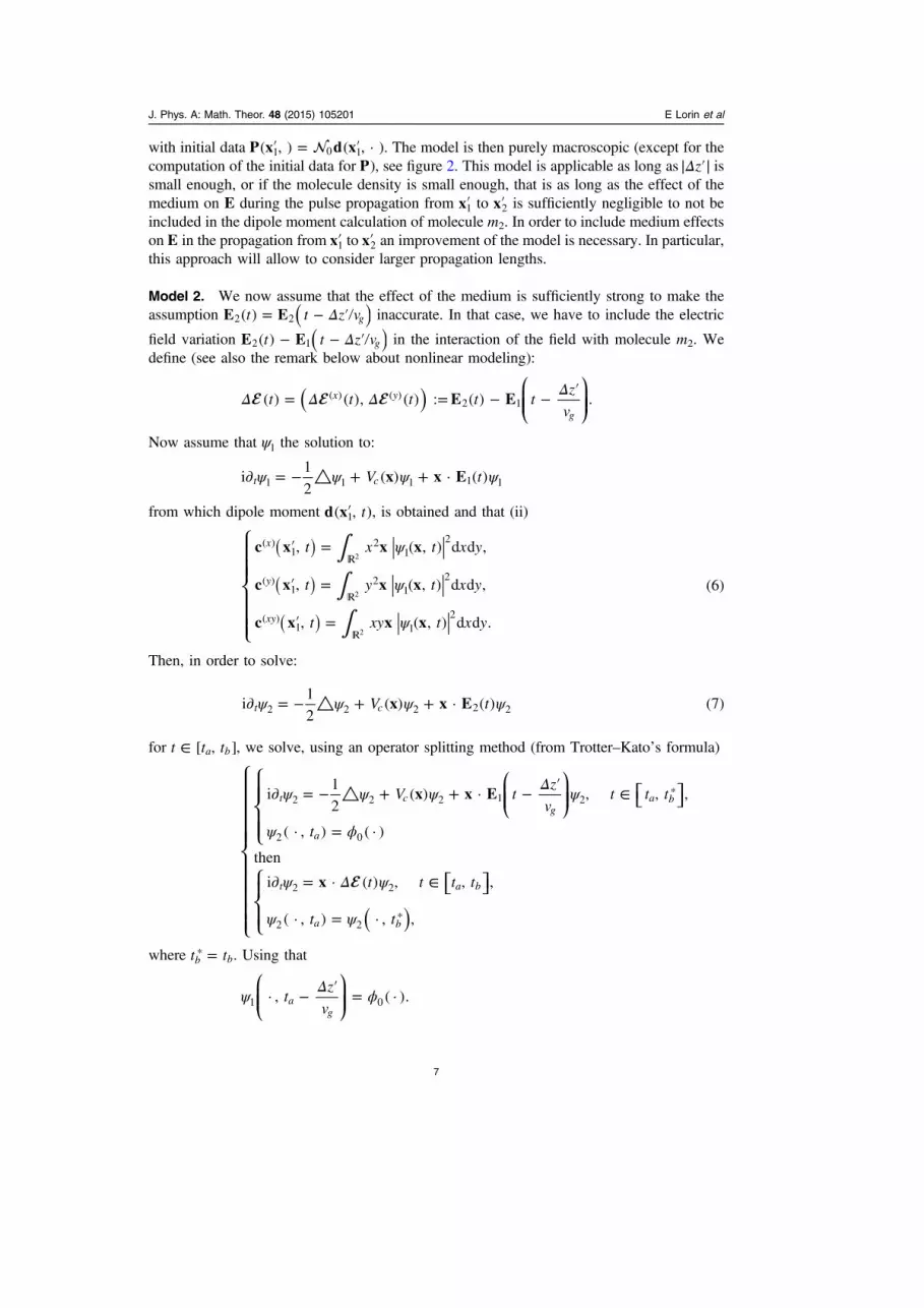
Figure 1. A circularly polarized pulse, ′ ′x y tE( , , ).

J. Phys. A: Math. Theor. 48 (2015) 105201 E Lorin et al

5

= × =−T (a.u.) 24 10 s 24 asec18 , =a 0.0529 nm0 , = = =e m 1e . Within the ME-TDSEmodel, interaction with a molecule requires the solution to TDSE:

ψ ψ ψ ψ∂ = − △ + + ′V tx x Ei1

2( ) · ( )t c x

with x = (x, y), =′ ′ ′E EE ( , )x yx . In velocity gauge [28], this is written equivalently as:

ψ ψ ψ ψ ψ∂ = − △ + + +∥ ∥

′′V t

tx A

Ai

1

2( ) i ( ) ·

( )

4t c x

x2

with =′ ′ ′A AA ( , )x yx , = −∂′ ′E Atx x . The computation of the wavefunction ψ of a molecule‘located in ′x ’, allows to deduce the dipole moment d as follows

∫ ψ′ =

t t x yd x x x( , ) ( , ) d d .22

Following [29] and [30], we now derive an evolution equation for d. Assuming that thewavefunction of molecule m1 ‘located’ in ′ = ′ ′ ′x y zx ( , , )1 1 1 1 is known, a sequence of evolutionequations to estimate the dipole moment of molecule m2 ‘located’ in ′ = ′ ′ ′x y zx ( , , )2 1 1 2 with

′ > ′z z2 1 , can be derived as follows.

Model 1. If Δ∣ ′∣ = ∣ ′ − ′∣z z z: 2 1 is small enough, we may assume that a circularly polarizedelectromagnetic field interacting with molecule m2 is almost identical (up to a time delay) tothe one which molecule m1 is subject to. Note that overall, we obviously do not assume thatthe electromagnetic field propagates as in a linear medium (or vacuum) in Maxwell’sequations. In that case, let us define ψi the wavefunction of molecule mi

ψ ψ ψ ψ∂ = − △ + +V tx x Ei1

2( ) · ( )t i i c i i i

and ′ td x( , )i the corresponding dipole moment, with i = 1, 2. In addition = ′t tE E x( ) ( , )i i

denotes the electric field that molecule mi is subject to. The above assumption mathematicallyimplies: Δ= − ′( )t t z vE E( ) g2 1 and as a consequence

Δ′ = ′ − ′( )t tz

vd x d x, , , (4)

g2 1

⎛⎝⎜⎜

⎞⎠⎟⎟

where vg is the group velocity (c in vacuum). Then the polarization P satisfies for ′ ∈ ′ ′z z z[ , ]1 2the following transport equation

∂ ′ + ∂ ′ =′t v tP x P x 0( , ) ( , ) (5)t g z

Figure 2. Macroscopic model with initial data from TDSE.

J. Phys. A: Math. Theor. 48 (2015) 105201 E Lorin et al

6

with initial data ′ = ′P x d x( , ) ( , · )1 0 1 . The model is then purely macroscopic (except for thecomputation of the initial data for P), see figure 2. This model is applicable as long as Δ∣ ′∣z issmall enough, or if the molecule density is small enough, that is as long as the effect of themedium on E during the pulse propagation from ′x1 to ′x2 is sufficiently negligible to not beincluded in the dipole moment calculation of molecule m2. In order to include medium effectson E in the propagation from ′x1 to ′x2 an improvement of the model is necessary. In particular,this approach will allow to consider larger propagation lengths.

Model 2. We now assume that the effect of the medium is sufficiently strong to make theassumption Δ= − ′( )t t z vE E( ) g2 2 inaccurate. In that case, we have to include the electric

field variation Δ− − ′( )t t z vE E( ) g2 1 in the interaction of the field with molecule m2. Wedefine (see also the remark below about nonlinear modeling):

Δ Δ Δ Δ= = − − ′ ( )t t t t tz

vE E( ) ( ), ( ) : ( ) .x y

g

( ) ( )2 1

⎛⎝⎜⎜

⎞⎠⎟⎟

Now assume that ψ1 the solution to:

ψ ψ ψ ψ∂ = − △ + +V tx x Ei1

2( ) · ( )t c1 1 1 1 1

from which dipole moment ′ td x( , )1 , is obtained and that (ii)

∫∫∫

ψ

ψ

ψ

′ =

′ =

′ =

( )

( )

( )

t x t x y

t y t x y

t xy t x y

c x x x

c x x x

c x x x

, ( , ) d d ,

, ( , ) d d ,

, ( , ) d d .

(6)

x

y

xy

( )1

21

2

( )1

21

2

( )1 1

2

2

2

2

⎧

⎨⎪⎪⎪

⎩⎪⎪⎪

Then, in order to solve:

ψ ψ ψ ψ∂ = − △ + +V tx x Ei1

2( ) · ( ) (7)t c2 2 2 2 2

for ∈t t t[ , ]a b , we solve, using an operator splitting method (from Trotter–Kato’s formula)

ψ ψ ψ Δ ψ

ψ ϕ

ψ Δ ψ

ψ ψ

∂ = − △ + + − ′ ∈

=

∂ = ∈

=

( )

V tz

vt t t

t

t t t t

t t

x x E

x

i1

2( ) · , , ,

( · , ) ( · )

then

i · ( ) , , ,

( · , ) · , ,

t cg

a b

a

t a b

a b

2 2 2 1 2*

2 0

2 2

2 2*

⎧

⎨

⎪⎪⎪⎪⎪

⎩

⎪⎪⎪⎪⎪

⎧⎨⎪⎪

⎩⎪⎪

⎛⎝⎜⎜

⎞⎠⎟⎟ ⎡⎣ ⎤⎦

⎧⎨⎪⎩⎪

⎡⎣ ⎤⎦

where =t tb b* . Using that

ψ Δ ϕ− ′ =tz

v· , ( · ).a

g1 0

⎛⎝⎜⎜

⎞⎠⎟⎟

J. Phys. A: Math. Theor. 48 (2015) 105201 E Lorin et al

7

The solution to this equation is approximated by:

ψ ψ Δ Δ Δ≈ − ′ − ( )t tz

vT tx x x( , ) , 1 i · ( ) ,b b

ga2 1

⎛⎝⎜⎜

⎞⎠⎟⎟

where Δ = −T t tb a. Note that the choice of approximating Δ at ta, is arbitrary (anytime timet in t t[ , ]a b would be acceptable, in principle). That is

ψ ψ Δ Δ Δ≈ − ′ + ( )( )t tz

vT tx x x( , ) , 1 · ( ) . (8)b b

ga2

21

2

2 2⎛⎝⎜⎜

⎞⎠⎟⎟

So that

Δ Δ Δ Δ

Δ Δ

Δ Δ Δ

′ ≈ ′ − ′ + ′ − ′

+ ′ − ′

+ ′ − ′

( )

( )

( )t tz

vT t t

z

v

t tz

v

t t tz

v

d x d x c x

c x

c x

, , ( ) ,

( ) ,

2 ( ) ( ) , (9)

b bg

xa

xb

g

ya

yb

g

xa

ya

xyb

g

2 12 ( ) 2 ( )

1

( ) 2 ( )1

( ) ( ) ( )1

⎛⎝⎜⎜

⎞⎠⎟⎟

⎛⎝⎜⎜

⎛⎝⎜⎜

⎞⎠⎟⎟

⎛⎝⎜⎜

⎞⎠⎟⎟

⎛⎝⎜⎜

⎞⎠⎟⎟

⎞⎠⎟⎟

and from which we can evaluate ′ = ′ ′t tP x x d x( , ) ( ) ( , )b b2 0 2 2 .

The operator splitting used above induces an error between the approximate ψ t( · , )ab2

( )

(computed in (8)), and exact wavefunction ψ t( · , )eb2

( ) solution to

ψ ψ ψ ψ∂ = − △ + +V tx x Ei1

2( ) · ( )t c2 2 2 2 2

is of the form Δ ψ− △ ( )t t t tx( ) · ( ) ( · , )b a a a2 . As a consequence, we can evaluate the

error between the exact polarization ′ tP x( , )eb

( )2

∫ ψ′ = ′ ′ = ′

( ) ( ) ( )t t t x yP x x d x x x x, ( , ) ( , ) d deb

e e( )2 0 2 2

( )0 2 2

( ) 2

2

and approximate polarization ′ tP x( , )ab

( )2 computed from (9).

Note that from a practical point of view this approximation is accurate in principle, for−t t( )b a small enough, as the splitting error leads to

Δ′ − ′ = ′ − ∞ ( )( ) ( ) ( )t t t tP x P x x, , ( ) .eb

ab b a

( )2

( )2 0 2

4 2

In practice however, −t tb a is large, corresponding to the overall computational time forTDSE. Typically for a Nc-cycle pulse of wavelength λ, as λ− ≈t t N v( )b a c g

λΔ′ − ′ = ′ ∞ ( ) ( ) ( )t t

N

vP x P x x, , . (10)e

ba

bc

g

( )2

( )2 0 2

4

2⎛

⎝⎜⎜

⎡⎣⎢⎢

⎤⎦⎥⎥

⎞

⎠⎟⎟

This makes, in practice, this approximation only relevant for very short pulses, or for Δ∣ ∣∞small enough.

J. Phys. A: Math. Theor. 48 (2015) 105201 E Lorin et al

8

We deduce from this estimate that the polarization computed above is accurate as long as

Δ Δ′ ∞ ( )z vx( ) g0 24 2 is small enough. This means that: for low density medium and/or

short enough propagation length, and/or small electric field variation approximation′ tP x( , )a

b( )

2 is accurate.Under the above assumptions, a macroscopic model can then be derived from the above

calculus. We set

= t tQ c( · , ) : ( · ) ( · , )x y xy x y xy( , , )0

( , , )

and

∫ Δ Δ∂ ′ + ∂ ′ = ′ ′ ′ ′ ′

∂ ′ + ∂ ′ =

t v t s s s

t v t

P x P x x x

Q x Q x 0

( , ) ( , ) [ ( , ), ( , )] d ,

( , ) ( , ) ,(11)

t g z

t

t g z

Q0

⎧⎨⎪⎩⎪

where for Ω ∈ M ( )42 such that

Ω Ω ΩΩ Ω

=x xy

xy y

( ) ( )

( ) ( )

⎛⎝⎜

⎞⎠⎟

with Ω x y xy( , , ) in M ( )21 , × →Ω M M M[ · , · ] : ( ) ( ) ( )21 21 21 is defined as follows. ForΓ Δ ∈ M, ( ):21

Γ Δ Ω Ω ΩΔ Γ Δ Γ Δ Γ Δ Γ= + + +Ω ( )[ , ] .x xx

y yy

x y y xxy( ) ( ) ( )

The initial data (at t = ta) satisfies

′ = ′ −′ − ′

′ = ′ −′ − ′

( )

( )

t tz z

v

t tz z

v

P x P x

Q x Q x

, , ,

, ,

(12)

a ag

a ag

11

11

⎧

⎨⎪⎪⎪

⎩⎪⎪⎪

⎛⎝⎜⎜

⎞⎠⎟⎟

⎛⎝⎜⎜

⎞⎠⎟⎟

with Q matrix function with values in M ( )42

′ =′ ′′ ′

tt t

t tQ x

Q x Q x

Q x Q x( , )

( , ) ( , )

( , ) ( , )

x xy

xy y

( ) ( )

( ) ( )

⎛⎝⎜⎜

⎞⎠⎟⎟

and

Δ Δ′ = ′ − ′ − ′ t t tz

vx E x E x( , ) ( , ) , .

g

⎛⎝⎜⎜

⎞⎠⎟⎟

This set of equations is then coupled to MEs (only): (11), (12), (1). From ′x1 to ′x2, the model isthen purely macroscopic. Schrödinger’s equation is only solved to determine the initial dataof P and Q at ′x1. This approach allows to take into account variations (including linear,nonlinear medium effects as well as diffraction) of electromagnetic field which may occurduring the propagation from ′x1 to ′x2. Note that the rhs of (11), can in particular be interpretedas the polarization change due to diffraction, and medium nonlinear effects.

The evolution equation for P is then coupled to MEs (1) for modeling the propagation ofthe laser pulse over ′ ′z z( , )1 2 . Polarization at ′ ′ ′x y z( , , ) for ′ > ′z z2, is then computed againusing the TDSE from (2). More specifically, the domain is decomposed in subdomains in thez′ direction, and only at certain locations of each sudomain, the TDSEs are computed to

J. Phys. A: Math. Theor. 48 (2015) 105201 E Lorin et al

9

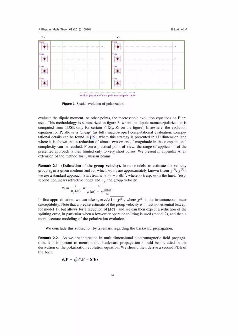
evaluate the dipole moment. At other points, the macroscopic evolution equations on P areused. This methodology is summarized in figure 3, where the dipole moment/polarization iscomputed from TDSE only for certain z′ (Za, Zb on the figure). Elsewhere, the evolutionequation for P, allows a ‘cheap’ (as fully macroscopic) computational evaluation. Compu-tational details can be found in [29], where this strategy is presented in 1D dimension, andwhere it is shown that a reduction of almost two orders of magnitude in the computationalcomplexity can be reached. From a practical point of view, the range of application of thepresented approach is then limited only to very short pulses. We present in appendix A, anextension of the method for Gaussian beams.

Remark 2.1 (Estimation of the group velocity). In our models, to estimate the velocitygroup vg in a given medium and for which n0, n2 are approximately known (from χ (1), χ (3)),we use a standard approach. Start from ≈ + ∣ ∣n n n E0 2

2, where n0 (resp. n2) is the linear (resp.second nonlinear) refractive index and ng, the group velocity

ω ω ω= =

+ ωω

∂∂

vc

n

c

n( ) ( ).g

gn ( )

In first approximation, we can take χ≈ +v c 1g(1) , where χ (1) is the instantaneous linear

susceptibility. Note that a precise estimate of the group velocity is in fact not essential (exceptfor model 1), but allows for a reduction of Δ ∞ and we can then expect a reduction of thesplitting error, in particular when a low-order operator splitting is used (model 2), and then amore accurate modeling of the polarization evolution.

We conclude this subsection by a remark regarding the backward propagation.

Remark 2.2. As we are interested in multidimensional electromagnetic field propaga-tion, it is important to mention that backward propagation should be included in thederivation of the polarization evolution equation. We should then derive a second PDE ofthe form

∂ − △ =vP P S E( )tt g2

Figure 3. Spatial evolution of polarization.

J. Phys. A: Math. Theor. 48 (2015) 105201 E Lorin et al

10

with initial data to determine from quantum TDSE. This is possible by extending thearguments developed above. This time, we will use: χ χ≈ +P E E(1) (3) 3, where χ (1) and χ (3)

are estimates of the first and third instantaneous susceptibilities. That is

χ χχχ

≈+

= −χχ

EP

E

PE

1

11 . (13)

(1) 2 (1)

(3)

(1)2

(3)

(1)

⎛⎝⎜

⎞⎠⎟

Then substituting E from (13), in the wave equation, and including the current density J:

π∂ − △ = − ∂ + ∂( )cE E P J4 .t t t2 2 2

Note that J satisfies the following evolution equation [2, 21], where νe is the collisionfrequency:

ν ρ∂ + = e

mJ J E.t e

e

2

Thus, we get a general equation for P, which writes:

χχ πχ

πχπχ

∂ − △ = −+

△ − ∂ −+

∂( ) ( ) ( )v

c

cP P P E P E J

1 4

1 4

1 4.(14)t g t t

2 22 (3)

(1) (1)2

22 2

(1)

(1)

⎡⎣⎢

⎤⎦⎥

This equation is then coupled to the usual wave equation, and the initial data P(·,0), ∂ P( · , 0)t

are computed from TDSEs, following a similar approach as above. Note that (14) is a generalwave equation for P from which we can derive for instance (5) or (11).

To illustrate this model, its strengths and its limits, we propose a numerical examplewhich consists of the comparison of harmonics spectrum of an electric field solution to a non-homogeneous 1D MEs, coupled with Schrödinger equations. Molecules are supposed to bealigned, and we compare the electric field spectra, when the response (polarization) of themedium is computed from, respectively, 1024, 256, 64, 16, 4 and 2 TDSEs. The physical dataare as follows:

• = × − 1.2 1005 mol ·(volume unit)−1 in atomic unit.

• Number of cycles ≈7, and wavelength 800 nm.• The total propagation length is μ≈30 m, including μ≈10 m in the gas.

As expected the spectra are quite close, even when the polarization is computed from 4TDSEs versus 1024, see figure 4. In figure 5, we represent in logscale, the L2-norm of theerror with respect to the spectrum of reference (computed from 1024 TDSEs), as well as theestimation of the CPU/storage gain. Roughly, we can estimate that dividing by a factor N thenumber of the TDSE to solve (compared to a full Maxwell–Schrödinger model), allows toreduce by a factor N the overall computational complexity and data storage.

We now propose the same example (same data) except that the medium is 5 times denserthat in the previous example. In that case, we expect that nonlinearities will deteriorate thenumerical solution, see figure 6. In that case, a good representation of the medium requiresmore TDSEs, which increases the overall complexity of the simulation. More advancedmodels should then derived to include nonlinearities.

J. Phys. A: Math. Theor. 48 (2015) 105201 E Lorin et al

11

2.2. Generalization

This section is devoted to a generalization of the methodology which was developed abovefor circularly polarized and Gaussian fields (see the appendix). We consider the full 3DMaxwell equations coupled with TDSEs. We are first interested in computing the dipolemoment of molecule αm , located in ′αx at time t. In this goal we have to evaluate thewavefunction ψα, solution to the following TDSE

ψ ψ∂ = − △ + +α α αt V t tx x x E xi ( , )1

2( ) · ( ) ( , )t c⎜ ⎟⎛

⎝⎞⎠

Figure 4. Electric field harmonic spectrum comparison for 4, 16, 64, 256 and 1024TDSEs.

Figure 5. CPU/storage gain and L2-norm error, as function of TDSEs.

J. Phys. A: Math. Theor. 48 (2015) 105201 E Lorin et al

12

and deduce the corresponding dipole moment ′ =α αt td x d( , ) ( ). We assume thatα≈ ∑ −α =t t TE E( ) ( )i

Li i1 , where T is some positive real number such that − ⩾t T 0. This

approximation comes typically from Kirchhoff’s formula:

∫ ∫πξ

πξ′ = ∂

∂′ + − + ∂ ′ + −α

ξα ξ

ξα ξ

= =( ) ( ) ( )t

tt c t T S

tc t T SE x E x E x,

1

4( ) d

4( ) d .t

1 1

⎛⎝⎜

⎞⎠⎟

We set χ α ϕ= ∑ −t t T( · , ) : ( · , )jL

j j for ⩾t T , where ϕ j is solution to

ϕ ϕ∂ = − △ + +t V t tx x x E xi ( , )1

2( ) · ( ) ( , )t j c j j

⎜ ⎟⎛⎝

⎞⎠

which are assumed known at time t − T, as well as −t Td ( )j . These are wavefunctions ofmolecules ‘located’ on the sphere of radius −c t T( ) and center x′ according to Kirchhoff’sformula. Thus

∑χ χ α ϕ∂ = − △ + + − −=

t V t t T t Tx x x x E xi ( , )1

2( ) ( , ) · ( ) ( , )t c

j

L

j j j1

⎜ ⎟⎛⎝

⎞⎠

that we rewrite

χ χ∂ = − △ + + +αt V t t F tx x x E x xi ( , )1

2( ) · ( ) ( , ) ( , ),t c⎜ ⎟⎛

⎝⎞⎠

where

∑α ϕ= − − −α=

( )F t t T t t Tx x E E x( , ) · ( ) ( ) ( , ).j

L

j j j1

Figure 6. Electric field harmonic spectrum comparison, for 4, 16, 64, 256 and 1024TDSE’s.

J. Phys. A: Math. Theor. 48 (2015) 105201 E Lorin et al

13

We denote

ψ ψ∂ = − △ + +α α αt V t tx x x E xi ( , )1

2( ) · ( ) ( , ).t c⎜ ⎟⎛

⎝⎞⎠

We denote β td ( ) the dipole moment associated to a virtual molecule of wavefunction χ, thatis:

∫ ∫∑χ α α ϕ ϕ= = − −β=

t t x y z t T t T x y zd x x x x x( ) ( , ) d d d ( , ) ¯ ( , ) d d d .

i j

L

i j i j2

, 13 3

Now we introduce β td ( )c( ) , β td ( )u( ) such that

= +β β βt t td d d( ) ( ) ( )c u( ) ( )

with

∫

∑

∑

α

α α ϕ ϕ

= −

= − −

β

β

=

≠ =

t t T

t t T t T x y z

d d

d x x x

( ) ( ),

( ) ( , ) ¯ ( , ) d d d .

c

j

L

j j

u

i j i j

L

i j i j

( )

1

2

( )

; , 13

We also have

ψ χ ϵ= +α αt t tx x x( , ) ( , ) ( , ),

where ϵα satisfies the equation

ϵ ϵ∂ = − △ + + −α α αt V t t F tx x x E x xi ( , )1

2( ) · ( ) ( , ) ( , )t c⎜ ⎟⎛

⎝⎞⎠

with null initial condition.

∫ ∫ϵ ϵ= − − △ + + +α α αt V s s s F s sx x x E x x( , ) i1

2( ) · ( ) ( , ) d i ( , )d .

T

t

cT

t⎜ ⎟

⎡⎣⎢

⎛⎝

⎞⎠

⎤⎦⎥

In the following, we denote

∫η ϕ= − − −α( )t s T s s T sx E E x( , ) : i ( ) ( ) ( , )djT

t

j j

so that

∫ ∑α η==

F s s tx x x( , )d · ( , ).T

t

j

L

j j1

We now use the approximation

∑ψ χ α η≈ +α=

t t tx x x x( , ) ( , ) · ( , )j

L

j j1

J. Phys. A: Math. Theor. 48 (2015) 105201 E Lorin et al

14

and

∫

∫

∑

∑

η η

η η

α α

α χ χ

=

− +

=

=

( )

( )

( )t t t x y z

t t t t x y z

x x x x x x

x x

( ) · ( , ) · ¯ ( , ) d d d

· ( ) ¯ ( ) ¯ ( ) ( ) d d d

i j

L

i j j i

j

L

j j j

, 1

1

3

3

which is again justified by the assumption of non-interaction of electrons attached to distinctmolecules

= + +α β βt t t td d d x( ) ( ) ( ) ( ).c u( ) ( )

Now we argue that in first approximation x and βd u( ) can be neglected. Indeed, the Maxwell–Schrödinger model is derived assuming that molecules mi and mj for ≠i j, do not interact,that is ϕ ϕ η η⟨ ⟩ = ⟨ ⟩ =, , 0i j i j . That is

∑α≈ = −α β=

t t t Td d d( ) ( ) ( ).c

j

L

j i( )

1

2

This equation leads to an expression of the polarization of the form

∑α′ ≈ ′ −α=

( ) ( )t t TP x d x, , ,j

L

j i1

2

where the xi’s lie on a sphere of radius cT and center ′αx . From a practical point of view, thisrelation is of little interest, as the dipole moment computation in one single location requirescomputations in several loci. However, from a more theoretical view point, it gives interestinginformation about the global picture.

3. Polarization evolution equation for longer pulses

The next two subsections are dedicated to the derivation of an evolution equation for thepolarization under the paraxial and slowly varying envelope approximations. We then nomore assume that the pulse duration is ultrashort.

3.1. General model under the paraxial approximation

The interaction of the laser field with the medium breaks the possible symmetry of theincoming pulse. We here propose an extension of section 2.1, when paraxial approximation isassumed [31]. We write the electric field propagation in direction ′ez as

′ ′ = ′ ′ ′ ′ω

⊥ ⊥−′( ) ( ) ( )z t A z tE x x e, , , , e .k z t

zi z

Say at time ta and in ′ ′⊥ zx( , ),1 1 , the initial polarization ′⊥ tP x( , )a,1 and its derivative∂ ′⊥ tP x( , )t a,1 , will be computed from a TDSE

ψ ψ ψ ψ∂ = − △ + +V tx x Ei1

2( ) · ( )t c1 1 1 1

with initial data ψ ϕ= =t t( )a1 . Now we seach for an evolution equation for P starting from(14) but under the paraxial approximation. In this goal we search for P and J in the form

J. Phys. A: Math. Theor. 48 (2015) 105201 E Lorin et al

15

Π′ ′ = ′ ′ ′ ′ω

⊥ ⊥−′( ) ( ) ( )z t z tP x x e, , , , e , (15)k z t

zi z

Λ′ ′ = ′ ′ ′ ′ω

⊥ ⊥−′( ) ( ) ( )z t z tJ x x e, , , , e , (16)k z t

zi z

where Π ΛA, , are the slowly varying complex amplitudes. We intend to rewrite the waveequation coupled with (14) under the SVAE. We first get

ω ω

△ = △ + ∂ + ∂ − ′

∂ = ∂ − ∂ − ′

′ ′ ′ ′ ′

′

ω

ω

⊥−

−

′

′

( )( )

( )

( )

A A k A k A

A A A

E e

E e

2i e ,

2i e .

z z z zk z t

z

t t tk z t

z

2 2 i

2 2 2 i

z

z

⎧⎨⎪⎩⎪

Now as

Λ ωΛ∂ = ∂ − ′ ′ω−′( ) ( )J ei et t

k z tz

i z

the continuity equation can be rewritten

Λ ω ν Λ ρ∂ = − +( ) e

mAi .t e

e

2

Thus we also have

ν Λ ρ∂ = − + ′ ′ω−′( )e

mAJ ee .t e

e

k z tz

2i z

⎛⎝⎜

⎞⎠⎟

We now rewrite the nonlinearity in (14) (rhs), as follows

Π Π

Π

∂ − △ = ∂ ′ − △ ′

− ∂ ′′ ′

ω ω

ω

−⊥

−

−

′ ′

′

( )( )

( )( ) ( )( ) ( )

( )

c A c A

c A

P E

e

e e

e .

t tk z t k z t

zk z t

z

2 2 2 2 i 2 2 2 i

2 2 i 2

z z

z

⎜

⎟

⎛⎝

⎞⎠

Now we rewrite

Π Π Π Π

Π Π Π Π

Π Π Π

Π ω Π ω Π ωΠ

Π Π Π

△ = △ + △ +

∂ ′ = ′ − + ∂ + ∂

+ ∂ ∂ + ∂ + ∂

∂ ′ = ′ − − ∂ − ∂

+ ∂ ∂ + ∂ + ∂

′ ′ ′

′ ′ ′ ′

ω ω

ω ω

⊥ ⊥ ⊥ ⊥ ⊥

− −

− −

′ ′

′ ′

( )

( ))

)

( )(

( )(

( )

( )

( )

( ) ( )

( ) ( )

A A A A

A k A k A k A

A A A

A A A A

A A A

2 · ,

e e 2i 2i

2 ,

e e 2i 2i

2 .

zk z t k z t

z z

z z z z

tk z t k z t

t t

t t t t

2 2 2 2

2 i 2 i 2 2 2 2

2 2 2 2 2

2 i 2 i 2 2 2 2

2 2 2 2 2

z z

z z

⎧

⎨

⎪⎪⎪⎪⎪

⎩

⎪⎪⎪⎪⎪We now apply the SVEA that is

Π Π Π

ω ω

Π ω Π ω Π

∂ ≪ ∂ ≪

∂ ≪ ∂ ≪

∂ ≪ ∂ ≪

∂ ≪ ∂ ≪

′ ′ ′ ′

′ ′ ′ ′

A k A k A

k k

A A A

,

,

,

.

z z z z

z z z z

t t

t t

2 2

2 2

2 2

2 2

⎧

⎨

⎪⎪⎪

⎩

⎪⎪⎪

J. Phys. A: Math. Theor. 48 (2015) 105201 E Lorin et al

16

Then, we get a full model

π Π Πνω

Λ ρω

Ππχ

Ππχ

πχ Π

πχ νπχ

Λ πχ ρπχ

πχχχ

Π

Π Π

χχ πχ

Π Π

Π

Λ ω ν Λ ρ

∂ + ∂ = △ + −∂ + + −

∂ ++

∂ =+

△ −

++

−+

−+

△

+ △ +

−+

∂ + ∂

+ ∂ + ∂

∂ = − +

′′

′

′′

′ ′

′

′

′

⊥

⊥

⊥

⊥ ⊥ ⊥

( )

( ) ( )

( )( )

( )( )

( )

( )

( )

A c Ac

kA

k cA

c c

kA

ck ckA

c

kA

A A

A c

A c A

A

i

24

i

2

i

2

i,

1 4

i

2 1 44

2i

1 4

2i

1 4

2i

1 4

2 ·

1 4

,

i .

(17)

t zz

tz e

t zz

e

z z

z

t z

t z

t e

(1) (1)(1)

(1)

(1)

(1)

(1)

(1)

(3)

(1)2

2 2

(3)

(1) (1)2

2 2

⎧

⎨

⎪⎪⎪⎪⎪⎪⎪⎪⎪⎪⎪

⎩

⎪⎪⎪⎪⎪⎪⎪⎪⎪⎪⎪

⎛⎝⎜

⎞⎠⎟

⎡⎣⎤⎦

⎡⎣⎤⎦

To close the model, we need an evolution equation on ρ, which naturally is ∂ + ∂ =ρ ρV 0t g z .The interest of this model is that it gives an accurate description of the polarization envelope(then of the electric field envelope). Again, the evolution equation on Π is used, only in alocalized spatial region, and from initial data tP( · , )a , ∂ tP( · , )t a , computed from TDSEsfollowing the same technique as the one described in section 2, except that we can nowconsider much larger propagation distances. Naturally from (17) it is possible to derive moresimple models neglecting certains terms of the rhs.

3.2. Geometrical optics approach (two-dimensional case)

We here discuss an approach based on the geometrical optics techniques which allows toderive a more simple model than (17). We will follow strategy and notation from [32], inorder to reduce TDSE computations. Starting first from

′ = ′ ′ ω−′t A tE x x e( , ) Re ( , )e k S t

zxi( ( )E0⎡⎣ ⎤⎦ then working in the moving frame ′ ← ′z z and

′ ← ′ − ′t t z vg, allows to get ride of the time dependence in the envelope calculation, with′ = ′ ′x zx ( , )

′ = ′ ′ ′AE x x e( ) ( )e k Sz

xi ( )E0

which satisfies the following Helmholtz equation

′ + ′ ′ =kE x x E x 0( ) ( ) ( )2 2

with ′ = + ∣ ′ ∣( )k k F Ux x( ) 1 ( ( ) )202 2 , and F a function, modeling to the medium response to

the electric field. Note that F null corresponds to a pulse propagation in vacuum. The eikonaland transport equations which follow, by identifying terms in k0 and k0

2, are

J. Phys. A: Math. Theor. 48 (2015) 105201 E Lorin et al

17

′ ′ = + ′

′ ′ + ′ ′ =

( )S S F A

S A A S

x x x

x x x x

( ) · ( ) 1 ( ) ,

2 ( ) · ( ) ( ) ( ) 0.

E E

E E

2

2

⎪⎪

⎧⎨⎩

Then, under the paraxial approximation, the envelope can be rewritten′ = ′ ′U Ax x( ) ( )e ,k S xi ( )U0 assuming ≫k 10 and = − ′S S zU E , where ′ = ∣ ∣ ′( )S F U zx( )U 0

2 .Ray trajectories are given by σ σ σ′ ∈ x{( ( ), ), }, where

σ

σ σ′ = ′Sx

xd

d( ) ( ( )).U

According again to [32], we can assume σ′ ≈z (high power beam) so that we canparameterize the rays in z′ (direction of propagation of the pulse. See figure 7.

The main idea is now to use rays in order to reduce the TDSE computations.

(1) The starting point is to model ′ = ′ + ∣ ′ ∣( )S z F Ux x( ) ( )U2 , where F is a medium

dependent function, modeling the Kerr effect (self-focusing), such that:

χ=( )F U U .2 (3) 2

The susceptibility χ (3) is medium, as well as time and space dependent. In firstapproximation χ (3) can be taken constant. However, it is possible to more preciselydetermine its value via TDSE computation [3]. We can rewrite αF , such that

χ=α α( )F U U ,2 (3) 2

where χα(3) is computed from a TDSE for a molecule ‘located’ at ′αx( , 0). In vacuum, F is

set to zero.(2) Determine the ray trajectories assuming that σ′ ≈z :

′′

′ = − ∂ ′ ′ ′′x

zz S x z z

d

d( )

1

2( ( ), ) (18)x U

with ′ = ′x x(0) 0 given.(3) Determine A along the rays, from the transport equation

′′ ′ = − ′ ′ ∂ ′ ′ ′′

A

zx z A x z S x z z

d

d( ( ))

1

2( ( )) ( ( ), ). (19)x U

From there, U is deduced along the rays: ′ ′ ′ = ′ ′ ′ ′ ′ ′U x z z A x z z( ( ), ) ( ( ), )e k S x z zi ( ( ), )U0 . Inpractice, the electric field will be computed from ME. However, this information isrelevant from a practical point of view, in order to estimate the polarization.

Figure 7. Ray path.

J. Phys. A: Math. Theor. 48 (2015) 105201 E Lorin et al

18

(4) We assume that for a molecule ‘located’ at ′αx , there exists a trajectory σ σ′ ⩾α{ }x ( ), 0 ,passing through that point. Except in vacuum, σ′ = ′ ≠ ′α α( ) ( )U U U xx x( ) ( ) , 0) . In themoving frame, the electric field the molecule is subject to, is identical to the one appliedto a molecule ‘located’ at ′βz(0, ), with ′ ⩽ ′β αz z . More specifically, there exists a level setdenoted by σα ( ), of normal vector σS ( ( ))U and passing though ′αx , which intersectsthe line ′ =x 0, at say ′βz . Along this curve, the electric field is constant, and in particular:

σ′ = ′α β( )( ) zE x E( ) 0, as well as σ′ = ′α β( )( ) zP x P( ) 0, . We may assume that ′β( )zP 0,was evaluated from a direct TDSE computation. From this remark, we can construct acontinuous equation, modeling the time evolution of the polarization. As along σα ( ), thepolarization is constant, we obviously get:

σ∂ =σ P 0{ ( ( ))} .

By assumption σ′ ≈z , so that

∂ ′ = ′′

′ =′ zz

zzP P 0{ ( ( ))}

d ( )

d· ( ( ))z

or equivalently in the moving frame

∂ ′ +′

′∂ ′ =′

′′ z

z

zzP P 0( ( ))

d ( )

d( ( )) .z

xx

In the fixed frame we get

∂ ′ + ∂ ′ +′

′∂ ′ =′

′′ z t v z t v

z

zz tP P P 0( ( ), ) ( ( ), )

d ( )

d( ( ), ) . (20)t g z g

xx

The equation models, along the level sets, the evolution of the polarization, taken intoaccount, the propagation and nonlinear effects. Diffraction effects are here assumednegligible.

From the above analysis we can then determine the rays, σ′x ( ), as well as σ′U x( ( )) andσ′S x( ( ))U (U and SU along the rays), starting from any ′⊥x( , 0). We denote by σ′αx ( ) the ray:

σ

σ σ′

= ′ ′ = ′αα α⊥( )S

xx x x

d

d( ) ( ( )), (0) , 0 .U ,

At for any ′x such that σ′ = ′αx x ( ), a molecule located at ′x , will be subject to the field

σ ω σ′ = ′ − ′ ′α α( )( ) ( )t U t t k SE x x x e( , ) ( ), cos ( ) .U z0

For ′βz(0, ), such that σ′ = ′α β( )( )U t U z tx ( ), (0, ), , then

ω′ = ′ − ′ ′β β( )( ) ( )( ) ( )t U z t k S zE x e( , ) , 0 cos 0, .U z0

From a practical view point, it is then necessary to evaluate the level sets σ ( ), in orderto solve (20). In conclusion, geometrical optics is not used here to directly update theelectric field, but (only) to determine the nonlinear response of the medium in the waveequation, without a direct TDSE computation. Note that in vacuum, F = 0,

σ σ′ ≈A xd ( ( )) d 0, that is A is constant along the ray ( = ′A x( (0))) and only the phaseσ′S x( ( ))U evolves.

3.3. Polarization reconstruction

Polarization is often deduced from TDSE in the hypothesis of a unique pure state, that is at′ tx( , ), polarization is given by

J. Phys. A: Math. Theor. 48 (2015) 105201 E Lorin et al

19

′ = ′ ′t tP x x d x( , ) ( ) ( , ),0

where ′ td x( , ) is the dipole moment of a molecule ‘located’ in ′x . A natural extension to ppure states consists of setting

∑′ = ′ ′=

t tP x x d x( , ) ( ) ( , ),l

pl

0

1

( )

where ψ ψ′ = ⟨ ∣ ∣ ⟩td x x( , )l l l( ) ( ) ( ) and ψ l( ) is solution to

ψ ψ ψ ϕ∂ = + =α( )t H t tx x E x x xi ( , ) · ( ) ( , ), ( , 0) ( )t l0

with ϕ ϵ ϕ=H l l l0 . From a practical point of view, solving this p TDSEs can easily beimplemented in parallel as each TDSE computation is done independently.

4. SFA nonlinear optics models

The method which is developed in this section consists of coupling bound and free statesin the solving of TDSE, in order to determine molecule dipole moments. More speci-fically, the overall strategy is to determine the bound state contribution combining theusual perturbative approach for weak fields, and a Lewenstein’s SFA approach for thefree state contribution, as well as the bound–continuous state interactions; however wedo not limit the interaction to free states of the continuum with the ground state like in[24]. In fine, we determine an explicit approximate solution to the TDSE, and of thedipole moment allowing to accurately model the polarization in Maxwell’s equations.We refer mainly to [25] for the notation and derivation of perturbative nonlinear opticsmodeling and [24] for the SFA model. Before presenting this model, we first derive ageneral Liouville equation, section 4.1, including bound and continuous states, fromwhich, in principle we could derived macroscopic polarization. However, due to thecomplexity of the derived model, it is expected of poor interest from a practical pointof view.

4.1. General non-perturbative approach. How far can we go?

In this subsection, we consider the general situation:

ψ ψ ψ ϕ∂ = + =( )H tx E xi · ( ) , ( , 0) .t 0 0

We consider the case a unique pure state. We search for a wavefunction in the general form:

∫∑ψ ϕ η ϕ η ρ η η= +σ

t c t c tx x x( , ) ( ) ( ) ( , ) ( , ) ( )d , (21)n

n n c cc

where (i) σc denotes the continuous spectrum of H0, (ii) ρc denotes the spectral density in σc,(iii) ϕc satisfies ϕ λ λϕ λ=H x x( , ) ( , )c c0 (where ‘ ϕ λ∥ ∥ =+∞( · , )c L2 ’, and finally (iv)

λ ϕ λ ψ= ⟨ ∣ ⟩c t t( , ) : ( · , ) ( · , ) . Assuming that the full spectrum (including eigenelements) isknown, we have to determine ( )c t( )n n

, λ λc t( ( , )) as well as ρ λ( ). In the following, thediscrete spectrum elements of H0 are denoted ϵn. For any ∈ n :

ψ ϕ ψ ϕ∂ = +( )H tx Ei · ( )t n n0

J. Phys. A: Math. Theor. 48 (2015) 105201 E Lorin et al

20

and for any λ σ∈ c

ψ ϕ λ ψ ϕ λ∂ = +( )H tx Ei ( · , ) · ( ) ( · , ) .t c c0

We set

ϕ ϕ

λ ϕ ϕ λ

λ ϕ λ ϕ

λ μ ϕ λ ϕ μ

λ μ ϕ λ ϕ μ

=

=

=

=

=

H t

H t

K t

H t

D

E x

E x

E x

E x

( ) · ,

( ) ( ) · ( · , ) ,

( ) ( ) · ( · , ) ,

( , ) ( ) · ( · , ) ( · , ) ,

( , ) ( · , ) ( · , )

nm n m

n n c

n c n

c c

c c

⎧

⎨

⎪⎪⎪⎪

⎩

⎪⎪⎪⎪and

ρ ρ λ ρ λ ρ λ μ= = = =λ λ λμt c t c t t c t c t t c t c t c t c t( ) ( ) ( ), ( ) ( ) ( , ), ( ) *( , ) , ( ) *( , ) ( , ).mn m n m m m m* *

We prove in appendix B, that for all m, n, λ, μ:

∫

∫

∫

∑

∑

∑

ρ ρ ρ ρ η ρ η ρ η ρ η η

ρ ρ ρ λ

η ρ η ρ η λ ρ η ρ η

ρ ρ λ ρ μ

η λ ρ η ρ η μ ρ η ρ η

= − + −

= −

+ −

= −

+ −

νν ν ν ν

σ η η

λ λ

σ ηλ η

λμ μ λ

σ ημ λη

( )t H t t H t K t K

t t H t H

K t H t

t t H t H

H t H t

˙ ( ) i ( ) ( ) i ( ) ( ) ( ) ( ) ( ) ( ) d ,

˙ ( ) i ( ) ( ) ( )

i ( ) ( ) ( ) ( , ) ( ) ( ) d ,

˙ ( ) i ( ) ( ) ( ) ( )

i *( , ) ( ) ( ) ( , ) ( ) ( ) d .

mn m n m n m c m n

mn

n nm mn n

n c c m

nn n n n

c c

* *

*

* *

*

*

c

c

c

⎧

⎨

⎪⎪⎪⎪⎪⎪

⎩

⎪⎪⎪⎪⎪⎪

⎡⎣ ⎤⎦⎡⎣ ⎤⎦

⎡⎣ ⎤⎦⎡⎣ ⎤⎦

Remark 4.1. This system is a Liouville-like equation which is comparable to the usual one,which does not include the continuum of the Hamiltonian spectrum and which writes

ρ ρ= −ℏ

H˙i ˆ , ˆmn mn

⎡⎣ ⎤⎦from which is deduced ρTr x( ˆ ˆ) = ρ∑ xnm nm mn in the classical theory.

The above equation contains, in principle, all the state transitions. However, from apractical point of view, it is of moderate interest, due to its complexity. The following sectionis devoted to an analogue approach, except that the integral over the continuum in (21), isapproximated by SFA.

4.2. SFA-like nonlinear optics model: unique continuous state

The principle of the following model is to include perturbative and nonperturbative con-tribution, using in particular on Lewenstein’s SFA model, which has the ability to accuratelycapture phenomena such as ionization and high order harmonic generation. We search for awavefunction ψ solution to

J. Phys. A: Math. Theor. 48 (2015) 105201 E Lorin et al

21

ψ ψ ψ ϕ∂ = + =( )H V tx x xi ( , ) , ( , 0) ( ),t 0 0

where H0 denotes the laser-free Hamiltonian and V the electric potential, as the sum of boundand bound-free state contributions:

ψ ψ ψ= +t t tx x x( , ) ( , ) ( , )B L

and where the purely bound part is of the form

∑ψ λ ψ=∈

t tx x( , ) ( , )Bl

lB

l( )

with

∑ψ ϕ= ω

∈

−

t a tx x( , ) ( ) ( )e ,Bl

kk

lk

t( ) ( ) i k

where we have denoted ϕk the eigenvectors of the field-free Hamiltonian: ϕ ϵ ϕ=H k k k0 andω ϵ=k k . We assume that

ψ α ϕ= − ω−( )t tx x( , ) 1 ( )e ( )e ,BI t t(0) i

0ip 0

where α t( ) is a time-dependent complex. The bound-continuous part is of the form of a SFA:

∫ψ α ϕ= +( )t t b tx x p p( , ) e ( ) ( ) d ( , )eLI t p xi

03 i ·p

with Ip the ionization potential and where ψ α ϕ=x x( , 0) ( )L 0 0 and =b p( , 0) 0. A naturalchoice for α is then the depletion coefficient. According to [24], uncoupling the equation in αand the TDSE, α can be modeled by the following equation

α γ α α α= − = ∈t t t˙ ( ) ( ) ( ), (0) (0, 1),0

where γ is defined by (52) in [24] and is naturally maximal at the electric field peaks. Inpractice, and as proposed in that paper γ will be approximated by its average γ ∈ ¯ withpositive real part, so that

α α≈ γ−t( ) e .t0¯

Now, we set

δ γ= − I: ¯ i p

so that

α α≈ δ−te ( ) e . (22)I t ti0

p

The unknowns of the problem are ⩾a( )l l 1 and b. Now by linearity, we have

ψ ψ∂ = +( )H V txi ( , ) .t B L B L, 0 ,

Parameter α is chosen such that initially

ψ ψ ψ α ϕ α ϕ ϕ= + = − + =( )x x x x x x( , 0) ( , 0) ( , 0) 1 ( ) ( ) ( ).B L 0 0 0 0 0

Naturally, we first have:

ψ α ϕ≈ − δ ω− −( )tx x( , ) 1 e ( )e . (23)Bt t(0)

0 0i 0

Coefficients ⩾a( )l l 1 will be searched following the usual perturbative method as presented in[25]. Denoting ω ϵ=l l , for all l

J. Phys. A: Math. Theor. 48 (2015) 105201 E Lorin et al

22

∫∑= ′ ′ ′ω

∈ −∞− ′

a t V t a t t( )1

i( ) ( )e d ,m

N

l

t

ml lN t( ) ( 1) i ml

where

∫ϕ ϕ ϕ ϕ= =V t t tx E x E x( ) · ( ) · ( ) dml m l m l* 3

and the transition frequencies are denoted ω ω ω= −mg m g. We deduce that for

ω= ∑ ω∈

−tE E( ) ( )ep p

ti p , and using (22)

∑μ ωω ω

αω ω δ

≈−

−− +

ω ω

∈

−

a tt

E( )1

· ( )1 ( )e

iem

pmg p

mg p

I t

mg p

t(1)i

i( )p

mg p⎪ ⎪

⎪ ⎪

⎧⎨⎩

⎫⎬⎭

then am(2) , etc, see [25] for details.

Remark 4.2 (Important remark on the contribution of χ l( ) in Lewenstein’s SFA). As itis well-known, Lewenstein’s SFA model contributes to χ l( ). Then, it is important to separatethe contribution of the susceptibility tensors from the bound states and from Lewenstein’sSFA function. In this goal, we will sum a( )n n only over the bound states, omitting thecontribution from ‘bound-continuum’ from the usual perturbative approach, as thiscontribution is already present in SFA. We denote the corresponding indices by (sumover the bound states only).

For instance

∑ ∑ μ μω ω

ω ω ω ω ω

αω ω δ ω ω ω δ

≈

×− − −

−− + − − +

ω ω ω

∈ ∈

− −

( )( )

( )( )

a t

t

E E( )1

· ( ) · ( )

1

( )( )

( )e

i ie

np q m

mg p nm q

ng p q mg p

I t

mg p ng p q

t

(2)2

( , )

ii( )

png p q

2

⎪⎪

⎪

⎪

⎧⎨⎩

⎫⎬⎭

and similarly

∑ ∑ μ μ μω ω ω

ω ω ω ω ω ω ω ω ω

αω ω ω ω δ ω ω ω δ ω ω δ

≈

×− − − − − −

−− − − + − − + − +

×

ν ν

ν

ν

ω ω ω ω

∈ ∈

− − −

( )( )

( )( )( )

( )a t

t

E E E( )1

· ( ) · ( ) · ( )

1

( )( )( )

( )e

i i i

e .

p q r m nn r nm q mg p

g p q r ng p q mg p

I t

g p q r ng p q mg p

t

(3)3

( , , ) ( , )

i

i( )

p

ng p q r

3 2

⎪⎪

⎪

⎪

⎧⎨⎩

⎫⎬⎭

In the above formula, if ⩾m 1 (recall that in atomic unit the electronic charge is e = 1):

∫μ ϕ ϕ= − x x¯ ˆ d .mg m 03

J. Phys. A: Math. Theor. 48 (2015) 105201 E Lorin et al

23

We deduce:

∑

∑ ∑

∑ ∑

∑ ∑

μ

μ μ

μ μ μ

ψ ϕ

ωω ω

αω ω δ

ϕ

ψ ω ω

ω ω ω ω ω

αω ω δ ω ω ω δ

ϕ

ψ ω ω ω

ω ω ω ω ω ω ω ω ω

αω ω δ ω ω ω δ ω ω ω ω δ

ϕ

=

=−

−− +

=

×− − −

−− + − − +

=

×− − − − − −

−− + − − + − − − +

×

ω

ω ω

ω ω ω

νν

ν

ν

νω ω ω ω

∈

−

∈ ∈

− +

∈ ∈

− + +

∈ ∈

− + + +

( )

( )

( )

( )

( )( )( )

( )( )( )

( )

( )

( )

( )

t a

t

t

t

t

t

x x

E

x

x E E

x

x E E E

x

( , ) ( )e

· ( )1

( )e

i( )e ,

( , ) · ( ) · ( )

1

( )( )

( )e

i i( )e ,

( , ) · ( ) · ( ) · ( )

1

( )( )( )

( )e

i i i

( )e .

Bm

m mt

m pmg p

mg p

I t

mg pm

t

Bm n p q

nm q mg p

mg p ng p q

I t

mg p ng p qn

t

Bm n p q r

n r nm q mg p

mg p ng p q g p q r

I t

mg p ng p q g p q r

t

(1) (1) i

ii

(2)

( , ) ( , )

ii

(3)

( , , ) ( , , )

i

i

m

pp

pp q

p

p q r

0

2 2

0

3 3

0

⎧

⎨

⎪⎪⎪⎪⎪⎪⎪⎪⎪⎪⎪⎪⎪⎪⎪⎪

⎩

⎪⎪⎪⎪⎪⎪⎪⎪⎪⎪⎪⎪⎪⎪⎪⎪

⎡⎣⎢⎢

⎤⎦⎥⎥

⎡⎣⎢⎢

⎤

⎦⎥⎥

⎡⎣⎢⎢

⎤

⎦⎥⎥

Now regarding the continuum, we have

α∂ = − + − −b t I b t t b t t tpp

p E p E d p( , ) i2

( , ) ( ) · ( , ) i ( ) ( ) ( ),t p gp

2⎛⎝⎜

⎞⎠⎟

where ϕ= ⟨ ∣ ∣ ⟩d p x p( )g 0 . We can then show (see [24], and method of characteristics) that

∫∫

α= − ′ ′ − − ′

× − ″ − − ″ +′

b t t t t t t

t t t I

p E d p A A

p A A

( , ) i d ( ) ( ) · ( ( ) ( ))

exp i d ( ( ) ( )) 2 .

t

g

t

t

p

0

2⎜ ⎟⎛⎝

⎞⎠

From there, we can give an approximate expansion of the overall dipole moment defined as

μψ ψ=td( ) ˆ

using that

μ μ μ μψ ψ ψ ψ ψ ψ ψ ψ= + + += + +

t

t t t

d

d d d

( ) ˆ ˆ ˆ ˆ

( ) ( ) ( )B B L L B L L B

BB LL BL

J. Phys. A: Math. Theor. 48 (2015) 105201 E Lorin et al

24

with

∑λ=∈

t td d( ) ( ). (24)BB

l

lBBl( )

In order to simplify the presentation, we will assume that damping phenomena are notincorporated in the model, which allows to deal with real transition frequencies. Extension tocomplex transitions is possible following [25]. We then get

=td ( ) 0 (25)BB(0)

then

μ μψ ψ ψ ψ= +td ( ) ˆ ˆ (26)BB B B B B(1) (0) (1) (1) (0)

leading, from ω ω= −E E*( ) ( )p p to

∑ ∑ μ μ

μ μ

ω

αω ω

α α

ω ω δ

ω αω ω

α α

ω ω δ

=

× −−

−−

− +

+ −−

−−

− −

ω

ω

∈ ∈

−−

−

−

( ){ ( )

( ) ( )

t

t t t

t t t

d E

E

( )1

· ( )

1 *( )e ( )e 1 *( )e

ie

( ) * 1 ( )e *( )e 1 ( )e

i *e . (27)

BBm p

gm mg p

I t

mg p

I t I t

mg p

t

mg p mg

I t

mg p

I t I t

mg p

t

(1)

ii i

i

i i ii

pp p

p

pp p

p

⎛

⎝

⎜⎜⎜

⎞

⎠

⎟⎟⎟⎛

⎝⎜⎜

⎞

⎠⎟⎟

⎫⎬⎪⎭⎪

This can be rewritten

∑ ∑ μ μ

μ μ

ω

αω ω

α α

ω ω δ

ω αω ω

α α

ω ω δ

=

× −−

−−

− +

+ −+

−−

+ −ω

∈ ∈

−−

−−

( ){ ( )

( ) ( )

t

t t t

t t t

d E

E

( )1

· ( )

1 *( )e ( )e 1 *( )e

i

· ( )1 ( )e *( )e 1 ( )e

i *e . (28)

BBm p

gm mg p

I t

mg p

I t I t

mg p

gm p mg

I t

mg p

I t I t

mg p

t

(1)

ii i

i i ii

pp p

pp p

p

⎛

⎝

⎜⎜⎜

⎞

⎠

⎟⎟⎟⎛

⎝⎜⎜

⎞

⎠⎟⎟

⎫⎬⎪⎭⎪

Similarly

μ μ μψ ψ ψ ψ ψ ψ= + +td ( ) ˆ ˆ ˆ . (29)BB B B B B B B(2) (0) (2) (2) (0) (1) (1)

J. Phys. A: Math. Theor. 48 (2015) 105201 E Lorin et al

25

From above, we deduce that

∑ ∑μ μ μ μψ ψ ω ω

αω ω ω ω ω

α α

ω ω δ ω ω ω δ

=

× −− − −

−−

− + − − +ω ω

∈ ∈

−

−− +

( )

( )( )

( )( )( )

t

t t

E Eˆ1

· ( ) · ( )

1 *( )e

( )( )

1 *( )e ( )e

i ie

B Bp q m n

gn nm q mg p

I t

ng p q mg p

I t I t

mg p ng p q

t

(0) (2)2

( , ) ( , )

i

i i

i

p

p p

p q

2 2

⎪

⎪

⎧⎨⎩

⎫⎬⎪

⎭⎪

and

∑ ∑μ μ μ μψ ψ ω ω

ω ωα

ω ω δ ω ωα

ω ω δ

=

×−

−− + −

−− −

× ω ω

∈ ∈

−

− −

( ) ( )

t t

E Eˆ1

· ( ) * · ( )

1 ( )e

i

1 *( )e

i *

e .

B Bp q m n

ng q nm mg q

mg p

I t

mg p ng q

I t

ng q

t

(1) (1)2

( , ) ( , )

i i

i( )

p p

p q

2 2

⎛⎝⎜⎜

⎞⎠⎟⎟

⎛

⎝⎜⎜

⎞

⎠⎟⎟

So that:

∑ ∑

∑ ∑

μ μ μ

μ μ μ

ω ω

αω ω ω ω ω

α α

ω ω δ ω ω ω δ

ω ω

ω ωα

ω ω δ ω ωα

ω ω δ

=

× −− − −

−−

− + − − +

+

×−

−− + −

−− −

ω ω

ω ω

∈ ∈

−− +

∈

−− −

( )

( )

( ) ( )

( )

( )( )( )

t

t

t t

t t

d E E

E E

( )2

Re · ( ) · ( )

1 *( )

( )( )

1 *( )e ( )e

i ie

1· ( ) * · ( )

1 ( )e

i

1 *( )e

i *e (30)

BBp q m n

gn nm q mg p

ng p q mg p

I t I t

mg p ng p q

t

p q m nng q nm mg q

mg p

I t

mg p ng q

I t

ng q

t

(2)2

( , ) ( , )

i i

i

2( , ) ( , )

i ii( )

p p

p q

p pp q

2 2

2 2

⎧⎨⎪

⎩⎪⎛

⎝

⎜⎜⎜⎞

⎠

⎟⎟⎟

⎫⎬⎪

⎭⎪

⎛⎝⎜⎜

⎞⎠⎟⎟

⎛

⎝⎜⎜

⎞

⎠⎟⎟

or written similarly

∑ ∑ μ

μ μ

α

ω ω

= −

×

∈ ∈

−

{ ( )( )( )

t td

E E

( )1

1 *( )e

· ( ) · ( )

BBm n p q

gnI t

nm q mg p

(2)2

( , ) ( , )

i p

2 2

J. Phys. A: Math. Theor. 48 (2015) 105201 E Lorin et al

26

μ μ μ

μ μ μ

ω ω ω ω ωα

ω ω δ ω ω ω δ

ω ωω ω

α

ω ω δ

ω ωα

ω ω δ

α ω ω

ω ω ω ω ω

α

ω ω δ ω ω ω δ

×− − −

−− + − − +

++

−+ −

×−

−− +

+ −

×+ + +

−+ − + + −

ω ω

−

−− +

( )( )

( )( )

( )( )

( )( )

( )

( )( )

( )

t

t

t

t

t

E E

E E

1

( )( )

( )e

i i

· ( ) · ( )1 *( )e

i *

1 ( )e

i

1 ( )e · ( ) · ( )

1

*( )e

i * i *e .

mg p ng p q

I t

mg p ng p q

nm gn q mg png q

I t

ng q

mg p

I t

mg p

ngI t

mn q gm p

mg p ng p q

I t

mg p ng p q

t

i

i

i

i

ii

p

p

p

p

pp q

⎛

⎝⎜⎜

⎞

⎠⎟⎟

⎛⎝⎜⎜

⎞⎠⎟⎟

⎫⎬⎪

⎭⎪

Similarly, one can deduce dBB(3) , from

μ μ μ μψ ψ ψ ψ ψ ψ ψ ψ= + + +td ( ) ˆ ˆ ˆ ˆ , (31)BB B B B B B B B B(3) (0) (3) (3) (0) (1) (2) (2) (1)

where

∑ ∑μ μ

μ μ μ

ψ ψ α

ω ω ω

ω ω ω ω ω ω ω ω ω

αω ω δ ω ω ω δ ω ω ω ω δ

= −

×

×− − − − − −

−− + − − + − − − +

×

νν

ν

ν

ν

ω ω ω

∈ ∈

−

− + +

( )

( )( )

( )( )( )

( )

( )

t

t

E E E

ˆ 1 *( )e

. ( ) · ( ) · ( )

1

( )( )( )

( )e

i i i

e

m n p q rg

I t

n r nm q mg p

mg p ng p q g p q r

I t

mg p ng p q g p q r

t

(0) (3)

( , , ) ( , , )

i

i

i

p

p

q p r

3 3

⎛⎝⎜⎜

⎞

⎠⎟⎟

and

∑ ∑μ μ μ

μ μ

ψ ψ ω

ω ω

ω ωα

ω ω δ ω ω ω ω ω

αω ω δ ω ω ω δ

=

×

×+

−+ − − − −

−− + − − +

νν

ν ν

ω ω ω

∈ ∈

−

− + +

( )

( )( )

( )( )( )

t

t

E

E E

ˆ · ( )

· ( ) · ( )

1 *( )e

i *

1

( )( )

( )e

i ie

m n p q rmn g r

nm q mg p

g r

I t

g r mg p ng p q

I t

mg p ng p q

t

(1) (2)

( , , ) ( , , )

i

ii

p

pp q r

3 3

⎛

⎝⎜⎜

⎞

⎠⎟⎟

⎛⎝⎜⎜

⎞

⎠⎟⎟

J. Phys. A: Math. Theor. 48 (2015) 105201 E Lorin et al

27

and

∑ ∑μ μ μ

μ μ

ψ ψ ω

ω ω

ω ωα

ω ω δ ω ω ω ω ω

α

ω ω δ ω ω ω δ

=

×

×−

−− + + + +

−+ − + + −

νν

ν ν

ω ω ω

∈ ∈

−− + +

( )( )

( )

( )( )

( )( )

( )

t

t

E

E E

ˆ · ( )

· ( ) · ( )

1 ( )e

i

1

*( )e

i * i *e

m n p q rnm g r

mn q gm p

g r

I t

g r mg p ng p q

I t

mg p ng p q

t

(2) (1)

( , , ) ( , , )

i

ii

p

pp q r

3 3

⎛⎝⎜⎜

⎞⎠⎟⎟

⎛

⎝⎜⎜

⎞

⎠

⎟⎟⎟

and

∑ ∑μ

μ

μ μ μ

ψ ψ

α

ω ω ω

ω ω ω ω ω ω ω ω ω

α

ω ω δ ω ω ω δ ω ω ω ω δ

= −

×

×+ + + + + +

−+ − + + − + + + −

×

νν

ν

ν

ν

ω ω ω

∈ ∈

−

− + +

( )( )( )

( )

( )

( )

( )( )( )

( )

( )

t

t

E E E

ˆ

1 ( )e

. ( ) · ( ) · ( )

1

*( )e

i * i * i *

e .

m n p q rg

I t

n r mn q gm p

mg p ng p q g p q r

I t

mg p ng p q g p q r

t

(3) (0)

( , , ) ( , , )

i

i

i

p

p

q p r

3 3

⎪⎪

⎧⎨⎩

⎫⎬⎪

⎭⎪

Now from [24] and denoting ϕ= ⟨ ∣ ∣ ⟩td p x( )g 0 , we have

∫ ∫ μτ τ τ= − − − − τ δ δ τ− − − −t t t td vE d v A v A( ) i d d ( ) · ( ( )) (( ( ))e , (32)*LL

t

g gS t t tv

0

3 * i ( , , ) ( )

where

∫τ = − +τ

S t ss

Ivv A

( , , ) : d ( ( ))2

t

p

2⎡⎣⎢

⎤⎦⎥

Naturally (29) and (32) are trivially deduced from the usual theory. We have now to evaluate

μ μψ ψ ψ ψ= +td ( ) ˆ ˆ .BL B L L B

In this goal, we will follow a strategy close the one developed by [24]. That is:

∑λ=∈

t td d( ) ( ) (33)BL

l

lBLl( )

with

μψ ψ= { }t t td x x( ) 2Re ( , ) ˆ ( , ) , (34)BLl

Bl

L( ) ( )

J. Phys. A: Math. Theor. 48 (2015) 105201 E Lorin et al

28

where

∫

∫

∑μ μψ ψ ϕ

α ϕ

=

× +

ω

∈

( )t t a t

t b t

x x x x

x p p

( , ) ˆ ( , ) d ( ) * ( )e e

( ) ( ) d ( , )e

Bl

Lm

ml

mt I t

p x

( ) 3 ( ) i i

03 i .

m p

3

3⎜ ⎟⎛⎝

⎞⎠

and

∫

∑ μ α=

+

ω

ω

∈

+

+

( )

( )

( )

( )

t a t t

a t b t

d

p p d p

( ) 2Re ( ) *e ( )

d ( ) * ( , )e ( ) , (35)

BLl

mml I t

mg

ml I t

m

( ) ( ) i

3 ( ) i

m p

m p

3

⎪

⎪

⎧⎨⎩

⎛⎝⎜

⎞⎠⎟

⎫⎬⎭where for all ⩾l 1

μϕ=d p p( ) ˆl l

and

∫

∫

τ τ

τ

= − + −

× − + − +τ

b t t t

t t sI s

p E d p A A

p A A

( , ) i cos( ) · ( ( ) ( ) ( ))

exp i( ( ) ( ) ( ))

2d d (36)

t

t

p

0

2⎛⎝⎜⎜

⎛⎝⎜

⎞⎠⎟

⎞⎠⎟⎟

with for ⩾l 1, d p( )l which is negligible. Indeed, as mentioned before, in the SFA model animplicit assumption is that the matrix elements of the Hamiltonian between bound states(except for the ground state) and free states are negligible. It is however possible to estimatethese contributions within our model. Moreover, a second model section 4.3, will bedeveloped to go beyond this assumption. Now for l = 0

∫ ∫ τ α τ τ= − − − −δ τ−( )t A t Ad v E d v d v( ) i d d 1 e ( ) · ( ( )) ( ( ))e . (37)*BL

tt

g gS t

R

v(0) 3

00 * i ( , , )

3

In addition, for the ⩾l 1 we have

∑ α= ω

∈

+

( ) ( ) dt a t td ( ) ( ) *e ( ). (38)BLl

mml I t

mg( ) ( ) i m p

We can now estimate the susceptibility tensors from bound-free state contribution. Morespecifically, for l = 1, we have

∑ ∑ μ

μ

ω

ω ωα

ω ω δα

=

×+

−+ −

∈ ∈

−

{

( )

( )

( )

t

tt

d E( ) · ( )

1 *( )e

i *( )

BLm p

gm p

mg p

I t

mg p

mg

(1)

i p

⎡⎣⎛

⎝

⎜⎜⎜

⎞

⎠

⎟⎟⎟

J. Phys. A: Math. Theor. 48 (2015) 105201 E Lorin et al

29

∫

∫

μ μ

μ

μ

ωω ω

αω ω δ

α

ωω ω

α

ω ω δ

ωω ω

αω ω δ

+−

−− +

++

−+ −

+−

−− +

ω

−

−

( )

( )

( )

( )

( )

( )

( )

tt

tb t

tb t

E

p E p d p

p E

p d p

· ( )1

( )

( )e

i( )

d · ( )1 *( )e

i *( , ) ( )

d · ( )1

( )

( )e

i*( , ) ( ) e . (39)

mg pmg p

I t

mg pgm

gm pmg p

I t

mg p

m

mg pmg p

I t

mg pm

t

i

3i

3

i* i

p

p

pp

3

3

⎛

⎝⎜⎜

⎞

⎠⎟⎟

⎛

⎝

⎜⎜⎜

⎞

⎠

⎟⎟⎟⎛⎝⎜⎜

⎞

⎠⎟⎟

⎤

⎦⎥⎥

⎫⎬⎪⎭⎪

For the 2nd order dipole moment we have

∫

∫

∑ ∑ μ μ

μ

μ μ

μ

μ μ

μ μ

ω ω

ω ω ω ω ω

α

ω ω δ ω ω ω δα

ω ωω ω ω ω ω

αω ω δ ω ω ω δ

α

ω ωω ω ω ω ω

α

ω ω δ ω ω ω δ

ω ωω ω ω ω ω

αω ω δ ω ω ω δ

=

×+ + +

−+ − + + −

+− − −

−− + − − +

++ + +

−+ − + + −

+− − −

−− + − − +

ω ω

∈ ∈

−

−

− +

{

( )( )

( )( )

( )

( )

( )

( )

( )

( )( )

( )

( )( )

( ) ( )( )

( )

( )( )( )

t

tt

tt

tb t

tb t

d E E

E E

p E E

p d p

p E E

p d p

( ) · ( ) · ( )

1

*( )e

i * i *( )

· ( ) · ( )1

( )( )

( )e

i i*( )

d · ( ) · ( )1

*( )e

i * i *( , ) ( )

d · ( ) · ( )1

( )( )

( )e

i i*( , ) ( ) e . (40)

BLm n p q

mn q gm p

mg p ng p q

I t

mg p ng p q

ng

nm q mg pmg p ng p q

I t

mg p ng p qn

mn q gm pmg p ng p q

I t

mg p ng p q

n

nm q mg pmg p ng p q

I t

mg p ng p qn

t

(2)

( , ) ( , )

i

i

0

3

i

3

i* i

p

p

p

pp q

2 2

3

3

⎡⎣⎡

⎣⎢⎢

⎤

⎦

⎥⎥⎥⎡⎣⎢⎢

⎤

⎦⎥⎥

⎡

⎣⎢⎢

⎤

⎦

⎥⎥⎥⎡⎣⎢⎢

⎤

⎦⎥⎥

⎤

⎦⎥⎥

⎫⎬⎪⎭⎪

J. Phys. A: Math. Theor. 48 (2015) 105201 E Lorin et al

30

Finally for the 3rd order bound-free dipole moment, we have

∫

∫

∑ ∑ μ

μ μ

μ μ μ μ

μ μ μ μ

μ μ μ

ω

ω ω

ω ω ω ω ω ω ω ω ω

α

ω ω δ ω ω ω δ ω ω ω ω δ

α ω ω ω

ω ω ω ω ω ω ω ω ω

αω ω δ ω ω ω δ ω ω ω ω δ

α ω ω ω

ω ω ω ω ω ω ω ω ω

α

ω ω δ ω ω ω δ ω ω ω ω δ

ω ω ω

ω ω ω ω ω ω ω ω ω

αω ω δ ω ω ω δ ω ω ω ω δ

=

×

×+ + + + + +

−+ − + + − + + + −

× +

×− − − − − −

−− + − − + − − − +

× +

×+ + + + + +

−+ − + + − + + + −

× +

×− − − − − −

−− + − − + − − − +

×

νσ

ν

ν

ν σ

ν

ν

ν σ

ν

ν

ν σ

ν

ν

νω ω ω

∈ ∈

−

−

− + +

}

( )( )( )

( )( )( )

{

( )

( )

( )

( )

( )

( )( )( )

( )

( )( )( )( )

( )( )( )

( )

( )( )( )

( )

( )

( )

( )

( )

t

t

t

t

t

t

b t

t

b t

d E

E E

E E E

p E E E

p d p p E E E

p d p

( ) . ( )

· ( ) · ( )

1

*( )e

i * i * i *

( ) · ( ) · ( ) · ( )

1

( )( )( )

( )e

i i i

( ) d . ( ) · ( ) · ( )

1

*( )e

i * i * i *

( , ) ( ) d · ( ) · ( ) · ( )

1

( )( )( )

( )e

i i i

*( , ) ( ) e . (41)

BLm n p q r

n r

mn q gm p

mg p ng p q g p q r

I t

mg p ng p q g p q r

g n r nm q mg p

mg p ng p q g p q r

I t

mg p ng p q g p q r

g n r mn q gm p

mg p ng p q g p q r

I t

mg p ng p q g p q r

n r nm q mg p

mg p ng p q g p q r

I t

mg p ng p q g p q r

t

(3)

( , , ) ( , , )

i

i

3

i

3

i

* i

p

p

p

p

p q r

3 3

3

3

⎡⎣

⎛

⎝⎜⎜

⎞

⎠

⎟⎟⎟

⎛⎝⎜⎜

⎞

⎠⎟⎟

⎛

⎝⎜⎜

⎞

⎠

⎟⎟⎟

⎛⎝⎜⎜

⎞

⎠⎟⎟

⎤⎦We then get

′ = ′ + ′ + ′t t t tP x P x P x P x( , ) ( , ) ( , ) ( , ) (42)BB BL LL

with

′ = ′ = ′ = t t t t t tP x d P x d P x d( , ) ( ), ( , ) ( ), ( , ) ( ),BB BB BL BL LL LL

where td ( )BB , td ( )BL and td ( )LL are approximated from (24), (27), (44) then (32) and finally(34), (40), (41). To conclude we take λ = 1. In fine, P has computed in (42) is used in (1).

J. Phys. A: Math. Theor. 48 (2015) 105201 E Lorin et al

31

Remark 4.3. The contribution dBL is estimated using [24], where transitions from‘continuum–continuum’ and ‘continuum-excited states’ are neglected. As a consequence,the contribution dBL

l( ) , for ⩾l 1 may be, in principle, neglected as by construction of SFAmodel, these transitions were neglected. In the next section, we will show how to improve themodeling, including contribution more ‘continuum-bound state’ transitions.

That is

∫ ∫

∫ ∫

∑ ∑

∑ ∑

∑

μ μ

μ μ

μ μ μ

μ μ

μ μ

ω

αω ω

α α

ω ω δ

ω αω ω

α α

ω ω δ

ω ω

αω ω ω ω ω

α α

ω ω δ ω ω ω δ

ω

αω ω

α α

ω ω δ

ω αω ω

α α

ω ω δ

τ τ τ

τ α τ

τ

′ ≈

× −−

−−

− +

+ −+

−−

+ −

+

× −− − −

−−

− + − − +

+

× −−

−−

− +

+ −+

−−

+ −

′ ≈ − − − −

×

′ ≈ − −

− −

ω

ω ω

ω

τ δ δ τ

δ

τ

∈ ∈

−−

−−

∈ ∈

−

− +

∈ ×

−

−−

− − − −

−

{ ( )

( )

( )

( )

{

{

{

( )

( )

( )

( )

( )

( )

( )

}

( )

( )( )( )

d

t

t t t

t t t

t

t t

t t t

t t t

t t t t

t

A t A

P x E

E

E E

E

E

P x pE d p A p A

P x v E

d v d v

( , ) · · ( )

1 *( )e ( ) 1 *( )e

i

· ( )1 ( ) *( )e 1 ( )e

i *e

2Re · ( ) · ( )

1 *( )e

( )( )

1 *( ) ( )e

i ie

· ( )

1 *( ) ( )e 1 *( )e

i

· ( ) ·1 ( ) *( )e 1 ( )e

i *e

( , ) i d d ( ) · ( ( )) (( ( ))

e

( , ) 2 Re i d d 1 e )( )

· ( ( )) ( ( ))e .

*

*

BB

m pmg mg p

I t

mg p

I t

mg p

gm p mgmg p

I t I t

mg p

t

p q m ngn nm q mg p

I t

ng p q mg p

I t

mg p ng p q

t

p m mg mg p

mg p

I t I t

mg p

gm p mgmg p

I t I t

mg p

t

LL

t

g g

S t t t

BL

tt

g gS t

p

R

v

ii

i ii

2( , ) ( , )

i

i

i

( , )

i i

i ii

0

3 *

i ( , , ) ( )

3

00

* i ( , , )

pp

p p

p

p

p

p q

p p

p p

p

2 2

3

⎧

⎨

⎪⎪⎪⎪⎪⎪⎪⎪⎪⎪⎪⎪⎪⎪⎪⎪⎪⎪⎪⎪⎪⎪⎪

⎩

⎪⎪⎪⎪⎪⎪⎪⎪⎪⎪⎪⎪⎪⎪⎪⎪⎪⎪⎪⎪⎪⎪⎪

⎛

⎝

⎜⎜⎜

⎞

⎠

⎟⎟⎟⎛

⎝⎜⎜

⎞

⎠⎟⎟

⎫⎬⎪⎭⎪

⎛⎝⎜⎜

⎞

⎠

⎟⎟⎟

⎫⎬⎪

⎭⎪

⎛

⎝

⎜⎜⎜

⎞

⎠

⎟⎟⎟⎛

⎝⎜⎜

⎞

⎠⎟⎟

⎫⎬⎪⎭⎪

Now a bit more detailed analysis is necessary to estimate the susceptibility tensors.

J. Phys. A: Math. Theor. 48 (2015) 105201 E Lorin et al

32

First, the linear susceptibility χBB(1) , is given through χ ω= ∑P E ( )BB i j ij BB j p,

(1),

(1) by

∑χ μ μ αω ω

α α

ω ω δ

μ μ αω ω

α α

ω ω δ

= −−

−−

− +

+ −+

− −

+ −

∈

( )t

t t t

t t t

( )1 *( ) ( ) 1 *( )

i

1 ( ) *( )(1 ( ))

i *.

BB ijm

mgi

mgj

mg p mg p

gmj

mgi

mg p mg p

,(1)

⎧⎨⎪

⎩⎪

⎛

⎝

⎜⎜⎜

⎞

⎠

⎟⎟⎟⎛

⎝⎜⎜

⎞

⎠⎟⎟

⎫⎬⎪⎭⎪

Assuming that α = 0, the linear susceptibility is the same usual (from perturbation theory).Next, using again [25]ʼs notations, and

∑∑ χ ω ω ω ω ω ω= +( )P E E, , ( ) ( )BB ijk pq

BB ijk p q q p j q k p,(2)

,(2)

the second-order susceptibility is given by

∑χ ω ω ω ω μ μ μ

α

ω ω ω ω ω

α α

ω ω δ ω ω ω δ

μ μ μω ω

α

ω ω δ ω ωα

ω ω δ

μ μ μ

α

ω ω ω ω ω

α α

ω ω δ ω ω ω δ

+ =

×−

− − −−

−

− + − − +

++

−+ − −

−− +

+

×−

+ + +−

−

+ − + + −

∈

− −

−

−

( ) ( )

( )( )

(

( ) ( )

( )

( )( )

( )( )

t t t

t t

t t t

, ,

1 *( )e

( )( )

( )e 1 *( )e

i i

1 *( )e

i *

1 ( )e

i

1 ( )e *( )e 1 ( )e

i * i *,

BB ijk p q q p I

m ngni

nmj

mgk

I t

mg p ng p q

I t I t

mg p ng p q

gnj

nmi

mgk

ng q

I t

ng q mg p

I t

mg p

gnj

nmk

mgi

I t

mg p ng p q

I t I t

mg p ng p q

,(2)

2( , )

i i i

i i

i i i

p p p

p p

p p p

2

⎛

⎝

⎜⎜⎜

⎞

⎠

⎟⎟⎟⎛

⎝⎜⎜

⎞

⎠⎟⎟

⎛⎝⎜⎜

⎞⎠⎟⎟

⎛

⎝

⎜⎜⎜

⎞

⎠

⎟⎟⎟

⎞

⎠

⎟⎟⎟

where I the intrindic permutation operator.Finally the expression of the third-order susceptibility χBB kjih,

(3) can be deduced from abovecalculation through:

∑∑ω ω ω χ ω ω ω ω ω ω ω ω ω+ + = + +( ) ( )P E E E, , , ( ) ( ) ( )BB k p q r

hij pqrBB kjih p q r r q p j r i q h p,

(3),

(3)

by

∑χ ω ω ω ω ω ω μ μ μ μ

α

ω ω ω ω ω ω ω ω ω

+ + =

×−

− − − − − −

νν ν

ν

∈

−

( )(( )

t

, , ,

1 *( )e

( )( )( )

BB kjih p q r r q p I

m ngk

nj

nmi

mgh

I t

mg p ng p q g p q r

,(3)

3( , , )

i p

3

⎛

⎝

⎜⎜⎜

J. Phys. A: Math. Theor. 48 (2015) 105201 E Lorin et al

33

α α

ω ω δ ω ω ω δ ω ω ω ω δ

μ μ μ μω ω

α

ω ω δ

ω ω ω ω ωα

ω ω δ ω ω ω δ

μ μ μ μω ω

αω ω δ

ω ω ω ω ωα

ω ω δ ω ω ω δ

μ μ μ μ

α

ω ω ω ω ω ω ω ω ω

α α

ω ω δ ω ω ω δ ω ω ω ω δ

−−

− + − − + − − − +

++

−+ −

×− − −

−− + − − +

++

−− +

×+ + +

−+ − + + −

+

×−

+ + + + + +

−−

+ − + + − + + + −

ν

ν νν ν

ν νν ν

ν ν

ν

ν

−

−

−

−

( )

( )( )

( )( )( )

( )

( )

( )( )( )

( )( )

( )( )

( )( )( )

t t

t

t

t

t

t

t t

1 *( )e ( )e

i i i

1 *( )e

i *

1

( )( )

( )e

i i

1 ( )e

i

1 *( )e

i * i *

1 ( )e

*( )e 1 ( )e

i * i * i *.

I t I t

mg p ng p q g p q r

gj

nk

nmi

mgh

g r

I t

g r

mg p ng p q

I t

mg p ng p q

gj

ni

nmk

mgh

g r

I t

g r

mg p ng p q

I t

mg p ng p q

gk

nj

nmi

mgh

I t

mg p ng p q g p q r

I t I t

mg p ng p q g p q r

i i

i

i

i

i

i

i i

p p

p

p

p

p

p

p p

⎞

⎠

⎟⎟⎟⎛

⎝⎜⎜

⎞

⎠⎟⎟

⎛

⎝⎜⎜

⎞

⎠⎟⎟

⎛⎝⎜⎜

⎞⎠⎟⎟

⎛

⎝

⎜⎜⎜

⎞

⎠

⎟⎟⎟

⎛

⎝⎜⎜

⎞

⎠

⎟⎟⎟

⎞

⎠

⎟⎟⎟

Now regarding the bound-free susceptibility tensors we have:

∫

∫

∑ ∑χ ωϵ

μ μω ω

α

ω ω δα

μ μω ω

αω ω δ

α

μω ω

α

ω ω δ

μω ω

αω ω δ

=+

−+ −

+−

−− +

++

−+ −

+−

−− +

∈ ∈

−

−

( )

( )

( )

( )

( )

( )

( )

tt

tt

dt

b t

dt

b t

p p p

p p p

( )1 *( )e

i *( )

1

( )

( )e

i*( )

d ( )1 *( )e

i *( , )

d ( ) * 1

( )

( )e

i*( , )

BL ij p

m pgmj

mgi

mg p

I t

mg p

mgj

gmi

mg p

I t

mg p

gmj

mi

mg p

I t

mg p

mgj

mi

mg p

I t

mg p

,(1)

0

i

i

3i

3i

p

p

p

p

3

3

⎡

⎣

⎢⎢⎢

⎛

⎝

⎜⎜⎜

⎞

⎠

⎟⎟⎟⎛

⎝⎜⎜

⎞

⎠⎟⎟

⎛

⎝

⎜⎜⎜

⎞

⎠

⎟⎟⎟⎛

⎝⎜⎜

⎞

⎠⎟⎟

⎤

⎦⎥⎥

J. Phys. A: Math. Theor. 48 (2015) 105201 E Lorin et al

34

then

∫

∫

∑χ ω ω ω μ μ μω ω ω ω ω

ω ω δ

α

ω ω ω δα

μ μ μω ω ω ω ω

αω ω δ ω ω ω δ

α

μ μω ω ω ω ω

α

ω ω δ ω ω ω δ

μ μω ω ω ω ω

αω ω δ ω ω ω δ

=+ + +

−+ − + + −

+− − −

−− + − − +

++ + +

−+ − + + −

+− − −

−− + − − +

∈

−

−

( ) ( )

( )( )( )

( ) ( )

( )( )

( )( )

( )( )

tt

tt

d

tb t

tb t

p p

p

p d p

p

( , , )1 1

1

i *

*( )e

i *( )

1

( )

1

( )

( )e

i i*( )

d ( )1

*( )e

i * i *( , )

d *( )1

( )( )

( )e

i i*( , )

BL ijk r q p

m nmnj

gmk

ngi

mg p ng p q

mg p

I t

ng p q

nmj

mgk

ni

mg p ng p q

I t

mg p ng p q

mnj

gmk

ni

mg p ng p q

I t

mg p ng p q

nmj

mgk

ni

mg p ng p q

I t

mg p ng p q

,(2)

( , )

i

0

i

3

i

3

i

p

p

p

p

2

3

3

⎡

⎣⎢⎢

⎡

⎣⎢⎢

⎤

⎦

⎥⎥⎥⎡⎣⎢⎢

⎤

⎦⎥⎥

⎡

⎣⎢⎢

⎤

⎦

⎥⎥⎥⎡⎣⎢⎢

⎤

⎦⎥⎥

⎤

⎦⎥⎥

and

∑ ∑χ ω ω ω ω μ μ μ μ

ω ω ω ω ω ω ω ω ω

α

ω ω δ ω ω ω δ ω ω ω ω δα

μ μ μ μω ω ω ω ω ω ω ω ω

αω ω δ ω ω ω δ ω ω ω ω δ

α

=

+ + + + + +

−+ − + + − + + + −

+− − − − − −

−− + − − + − − − +

σν

σ ν

ν

ν

σ νν

ν

∈ ∈

−

( )( )( )

( )( )( )

( )( )( )

tt

tt

( , , , )

1

*( )e

i * i * i *( )

1

( )( )( )

( )e

i i i( )

BL kjih r q p

m n p q rnj

mni

gmh

gk

mg p ng p q g p q r

I t

mg p ng p q g p q r

nj

nmi

mgh

gk

mg p ng p q g p q r

I t

mg p ng p q g p q r

,(3)

( , , ) ( , , )

i

i

p

p

3 3

⎡⎣⎢⎢

⎛

⎝⎜⎜

⎞

⎠

⎟⎟⎟⎛⎝⎜⎜

⎞

⎠⎟⎟

J. Phys. A: Math. Theor. 48 (2015) 105201 E Lorin et al

35

∫

∫

μ μ μω ω ω ω ω ω ω ω ω

ω ω δ ω ω ω δ

α

ω ω ω ω δ

μ μ μω ω ω ω ω ω ω ω ω

αω ω δ ω ω ω δ ω ω ω ω δ

++ + + + + +

−+ − + + − + + + −

+ ×− − − − − −

−− + − − + − − − +

σ νν

ν

σ νν

ν

−

( ) ( ) ( )( )

( )( )( )

( )( )( )

d

tb t

tb t

p p

p

p d p

p

d ( )1

1

i *

1

i *

*( )e

i *( , )

d *( )1

( )( )( )

( )e

i i i*( , )

nj

mni

gmh k

mg p ng p q g p q r

mg p ng p q

I t

g p q r

nj

nmi

mgh k

mg p ng p q g p q r

I t

mg p ng p q g p q r

3

i

3

i

p

p

3

3

⎛

⎝⎜⎜

⎞

⎠

⎟⎟⎟⎛⎝⎜⎜

⎞

⎠⎟⎟

⎤

⎦⎥⎥

and where ω ω ω ω= + +σ p q r.Interpretation and simplification of these tensors, such as the third harmonic generation

from χ ω(3 )(3) , will be analyzed is a forthcoming paper.

4.3. SFA-like nonlinear optics model: possible extension to multiple continuous states

The use of the SFA modeling implies (implicitly) that some transitions are (by construction)neglected: ‘continuum–continuum’ and ‘continuum-excited states’ transitions [24]. In thefollowing section, we propose to formally include more properly and accurately some of thesetransitions, which will allow us to model more accurately dBL and dLL. In this goal, we willsearch for ψ in the form:

ψ ψ ψ= +t t tx x x( , ) ( , ) ( , ),B L

where the purely bound part is of the form

∑ψ λ ψ=∈

t tx x( , ) ( , )Bl

lB

l( )

with

∑ψ ϕ= ω

∈

−

t a tx x( , ) ( ) ( )e ,Bl

kk

lk

t( ) ( ) i k

where we have denoted ϕk the eigenvectors of the field-free Hamiltonian: ϕ ϵ ϕ=H k k k0 . Thebound-continuous part is of the form of SFA:

∑ψ λ ψ=∈

t tx x( , ) ( , ),Ll

lL

l( )

where for ⩾l 0

∫ψ α ϕ= +( )t t b tx x p p( , ) e ( ) ( ) d ( , )eLl I t

l ll p x( ) i 3 ( ) i ·p

l( )

and with α t( )l a time-dependent parameter and IPl( ) is defined as a relative ionization potential,

from level l energy

ω ω ω= − − = −I I ( ) . (43)pl

p l l( )

0

In addition, we impose:

J. Phys. A: Math. Theor. 48 (2015) 105201 E Lorin et al

36

• for all ⩾l 0, =b p( , 0) 0l( ) ,• for l = 0, α ∈(0) (0, 1)0 and for ⩾l 1, α ≪(0) 1l .

μ μ μ μψ ψ ψ ψ ψ ψ ψ ψ= + + += + +

t

t t t

d

d d d

( ) ˆ ˆ ˆ ˆ

( ) ( ) ( )B B L L B L L B

BB BL LL

with

∑λ=∈

t td d( ) ( ) (44)BB

l

lBBl( )

which takes the same value as above (28), (30), (31). Then

∑ ∑λ λ= =∈

+

∈

+

t t t td d d d( ) ( ), ( ) ( ),BL

k l

k lBLkl

LL

k l

k lLLkl

( , )

( )

( , )

( )

2 2

where

∑ μ μψ ψ ψ ψ= +∈

( )td ( ) ˆ ˆ (45)BLkl

k lB

kL

lL

kB

l( )

( , )

( ) ( ) ( ) ( )

2

and

∑ μ μψ ψ ψ ψ= +∈

( )td ( ) ˆ ˆ . (46)LLkl

k lL

kL

lL

kL

l( )

( , )

( ) ( ) ( ) ( )

2

As dBL LL, is computed according to mathematical assumptions from [24], the following terms

are neglected: μψ ψ⟨ ∣ ∣ ⟩ ≈ˆ 0Bk

Ll( ) ( ) and μψ ψ⟨ ∣ ∣ ⟩ ≈ˆ 0L

kL

l( ) ( ) for ≠k l. Then for all l:

∑ ∑ μλ λ ψ ψ≈ =t td d( ) ( ) 2 Re ˆ ,BL

l

lBLll

l

lB

lL

l2 ( ) 2 ( ) ( )

where

∫

∑ α=

+

ω

ω

∈

+

+

( )

( )

( )

( )

t a t t

a t b t

d d

p p d p

( ) 2Re ( ) *e ( )

d ( ) * ( , )e ( ) , (47)

BLll

mml I t

mg l

ml l I t

m

( ) ( ) i

3 ( ) ( ) i

m pl

m pl

( )

3

( )

⎪

⎪

⎧⎨⎩

⎛⎝⎜

⎞⎠⎟

⎫⎬⎭where μ ϕ= ⟨ ∣ ∣ ⟩d p p( ) ˆl l . Regarding the continuum–continuum contribution

∑ ∑ μλ λ ψ ψ≈ =t td d( ) ( ) 2 Re ˆ .LL

l

lLLll

l

lL

lL

l2 ( ) 2 ( ) ( )

According to (32), we get

∫ ∫ τ τ τ= − − − − τ δ δ τ− − − −t t t td pE d p A d p A( ) i d d ( ) · ( ( )) (( ( ))e .*LLll

t

l LlS t t tp( )

0

3 * i ( , , ) ( )l l

J. Phys. A: Math. Theor. 48 (2015) 105201 E Lorin et al

37

We get a full description of macroscopic polarization

∫ ∫

∫

∑

∑ ∑

∑

∑

∑ ∑

μ μ

μ μ

μ μ

μ μ

ω

αω ω

α α

ω ω δ

ωα

ω ωα α

ω ω δ

μ

μ ω μ ω

αω ω ω ω ω

α α

ω ω δ ω ω ω δ

ω

αω ω

α α

ω ω δ

ωα

ω ωα α

ω ω δ

τ τ τ

α

′ ≈

×−

−−

−

− +

+−

+−

−

+ −

+

×

×−

− − −

−−

− + − − +

+

×−

−−

−

− +

+−

+−

−

+ −

′ ≈ − − − −

×

′ ≈

+

ω

ω ω

ω

τ δ δ τ

ω

ω

∈∈×

−

∈ ∈

− +

∈ ×

−

∈

− − − −

∈ ∈+

+

{

{

( )

( )

( )

{

( )

( )

( )

( )

( )

( )

( )

( )

)

( )( )

( )

( )

( )

( )

( )

d

t

t t t

t t t

t

t t

t t t

t t t

t t t t

t a t t

a t b t

P x E

E

E E

E

E

P x pE d p A p A

P x d

p p d p

( , ) · · ( )

1 ( ) ( ) 1 ( )

i

· ( ) ·1 ( ) ( ) 1 ( )

i *e

2Re

· ( ) · ( )

1 ( )

( )( )

1 ( ) ( )e

i ie

· · ( )

1 ( ) ( ) 1 ( )

i

· ( ) ·1 ( ) ( ) 1 ( )

i *e ,

( , ) i d d ( ) · ( ( )) (( ( ))

e ,

( , ) 2 Re ( ) *e ( )

d ( ) * ( , )e ( ) .

*

BBl

p m mg mg p

l

mg p

l l

mg p

gm p mgl

mg p

l l

mg p

t

p q m n gn

nm q mg p

l

ng p q mg p

l lI t

mg p ng p q

t

p m mg mg p

l

mg p

l l

mg p

gm p mgl

mg p

l l

mg p

t

LLl

l

t

l Ll

S t t t

BLl

l m ml I t

mg l

ml l I t

m

p

( , )

* *

*i

2 ( , ) ( , )

*

* ii

( , )

* *

*i

0

3 *

i ( , , ) ( )

( ) i

3 ( ) ( ) i

p

p

p q

p

l l

m pl

m pl

2 2

( )

3

( )

⎧

⎨

⎪⎪⎪⎪⎪⎪⎪⎪⎪⎪⎪⎪⎪⎪⎪⎪⎪⎪⎪⎪⎪⎪⎪

⎩

⎪⎪⎪⎪⎪⎪⎪⎪⎪⎪⎪⎪⎪⎪⎪⎪⎪⎪⎪⎪⎪⎪⎪

⎛

⎝⎜⎜

⎫⎬⎪⎭⎪

⎛

⎝⎜⎜

⎞

⎠⎟⎟

⎫⎬⎪⎭⎪

⎛

⎝⎜⎜

⎞

⎠⎟⎟

⎫⎬⎪⎭⎪

⎛

⎝⎜⎜

⎞

⎠⎟⎟

⎛

⎝⎜⎜

⎞

⎠⎟⎟

⎫⎬⎪⎭⎪

⎧⎨⎩⎛⎝⎜

⎞⎠⎟

⎫⎬⎭

Remark 4.4. One can also consider wavefunction of the type

∫ψ α ϕ α ϕ= + +

t t t b tr r r p p( , ) ( ) ( ) ( ) ( ) d ( , )e . (48)L m m n nmn p r3 ( ) i ·

3

By plugging this expression into the Schrödinger equation and taking the inner product withϕ∣ ⟩r( )m , ϕ∣ ⟩r( )n and ∣ ⟩p respectively, we get:

J. Phys. A: Math. Theor. 48 (2015) 105201 E Lorin et al

38

∫μα α α

ϕ

= +

+

t E t t t

b t x t

E

p p p E

i ˙ ( ) ( ) ( ) ( ) ·

d ( , ) · ( ), (49)

m m m n mn

mnm

3 ( )3

∫μα α α

ϕ

= +

+

t E t t t

b t x t

E

p p p E

i ˙ ( ) ( ) ( ) ( ) ·

d ( , ) · ( ), (50)

n n n m nm

mnn

3 ( )3

= +

− ∂

( )b t a t t a t

b t t b t

p E d p d p

pp E p

i ˙ ( , ) ( ) ( ) · ( ) ( ) ( )

2( , ) ( ) ( , ) (51)

m xm

n xn

mnp

mn

( ) ( )

2( ) ( )

x

assuming am(t) and an(t) are constant in time, can be solved using the method ofcharacteristics as shown above. Doing so implicitly means that the rate of change of am(t) andan(t) are much less than that of b tp( , )mn( ) . One acquires a coupled ODE with time dependentcoefficients.

Alternatively, we can propose a close approach, which may be cheaper numerically, asfollows: we search for ψL in the form of a discrete sum (which is then an approximation of theintegral over the continuum). Let us denote by the corresponding indices and including aswell, the ground state. That is

∑ψ ϕ ϕ= +∈

t c t c tx x x( , ) ( ) ( ) ( ) ( ).L g gm

m m

Plugging in the system in the TDSE gives:

∑ϵ ϕ ϕ

ϵ ϕ ϕ

= +

= +∈

c t c t t c t

c t c t t c t

E x x

E x x x

i ˙ ( ) ( ) ( ) · ( ) ( ),

i ˙ ( ) ( ) ( ) · ( ) ( ) ( )

g g g

mm g m

m m m m g g

⎧⎨⎪

⎩⎪

neglecting again the continuum–continuum transitions. Then ψL is combined with ψB areproposed in the above sections.

5. Conclusion

This paper was devoted to the derivation of two non-classical nonlinear optics models. In bothcases, contribution of bound–bound, bound-continuous and to a certain extent continuous–continuous state transitions are evaluated in order to determine the macroscopic polarizationin Maxwell’s equations. Although the first model, fully non-pertrubative, is an importantimprovement of the Maxwell–Schrödinger model in term of computational complexity, ithowever still contains microscopic components: TDSE computations have to be performed todetermined initial polarizations. In addition, from a practical point of view in this config-uration, it is valid only for very short pulses. The second model, although fully macroscopic,is however partially heuristic and perturbative.

In order to validate and to analyze these models, we plan, in a close future, to test themon realistic situations. In particular simple filamentation simulations will be performed. Theinclusion of nonlinearities coming from bound states as well as free electrons, is essential inorder to describe accurately filament dynamics [1, 2].

J. Phys. A: Math. Theor. 48 (2015) 105201 E Lorin et al

39

Appendix A. Gaussian beam

We consider the extension to Gaussian beams of the method developed above. Using [25]ʼsnotations (see also [33]), we denote by w0 the beam waist, λ its wavelength, and itsmaximal amplitude, see figure A1 , and [22] for details about this Gaussian pulse. We assumethat

′ = ′ ′ ′ω−t AE x x e( , ) ( )e ,kz t

zi( )

where ′ = ′ ′r zx ( , ) and

ξ ξ′ ′ =

+− ′

+

A r zr

w( , )

1 iexp

(1 i )

2

02

⎛⎝⎜

⎞⎠⎟

with ξ = ′z b2 and =b kw02. The beam power is given by

∫ πω= = nc

A n2

1

4.2

02

Assuming that the dipole moment ′ td x( , )1 at ′ = ′ ′r zx : ( , )1 1 1 for any ′r1 is known, from thesolution to

ψ ψ ψ ψ∂ = − △ + + ′V x Ei1

2·t c x1

we construct ′ td x( , )2 with ′ = ′ ′r zx : ( , )2 1 2 as follows. For Δ∣ ′∣ = ∣ ′ − ′∣z b z z b2 1 small enough,we next rewrite ′ ′A r z( , )1 2 as a function of ′ ′A r z( , )1 1

ξ ξξ′ ′ =

+−

′+

=′( )

( )A r z

r

w

z

b,

1 iexp

1 i,

21 2

2

12

02

22

2⎛⎝⎜⎜

⎞⎠⎟⎟

which can be rewritten, denoting Δξ Δ= ′z b2

ξ Δξ ξ Δξ′ ′ =

+ +−

′+ +

( )( )

A r zr

w,

1 i iexp

1 i i1 2

1

12

02

1

⎛⎝⎜⎜

⎞⎠⎟⎟

and

ξξ Δξ ω ξ Δξ ξ

ξξ Δξ ω ξ

ξξ Δξ

′ ′ = ′ ++ +

−′

+ +−

+

= ′ ++ +

−′+

++ +

−

( ) ( )

( )( )

A r z A r zr

A r zr

, ,1 i

1 i iexp

1

1 i i

1

1 i

,1 i

1 i iexp

1 iexp

1 i

1 i i1

1 2 11

1

12

02

1 1

11

1

12

02

1

1

1

⎛⎝⎜

⎛⎝⎜

⎞⎠⎟

⎞⎠⎟

⎛⎝⎜⎜

⎞⎠⎟⎟

⎛⎝⎜

⎞⎠⎟

Using Δξ∣ ∣ ≪ 1, we then have

ξξ Δξ

Δξξ

Δξξ

++ +

= −+

−+

+ ⋯( )

1 i

1 i i1

i

1 i 1 i

1

1 1

2

12

J. Phys. A: Math. Theor. 48 (2015) 105201 E Lorin et al

40

and as a consequence

Δξξ

Δξξ

ω ξΔξ

ξΔξ

ξ

′ ′ ≈ ′ −+

−+

× +′+ +

++

( ) ( )( )

( ) ( )

A r z A r z

r

, , 1i

1 i 1 i

11 i

i

1 i 1 i.

1 2 11

2

12

12

02

1 1

2

12

⎛⎝⎜⎜

⎞⎠⎟⎟

⎛

⎝⎜⎜

⎛⎝⎜⎜

⎞⎠⎟⎟

⎞

⎠⎟⎟

This gives a useful relation between ′ ′A r z( , )1 1 and ′ ′A r z( , )1 2 . Denoting, now

ϵ ξ Δ Δξξ

Δξ

ξ ωΔξ

ξ

Δξ

ξ ω′ ′ = −

++

′

+−

++

′

+( )

( ) ( ) ( )r z

r r, ,

i

1 i

i

1 i 1 i

2

1 i1 1

1

12

12

02

2

12

12 2

13

02

we obtain

ϵ ξ Δ′ ′ ≈ ′ ′ + ′ ′( )( ) ( ) ( )A r z A r z r z, , 1 , , .1 2 1 1 1 1

In general ∣ ′ ′ ∣≈∣ ′ ′ ∣A r z A r z( , ) ( , )1 2 1 1 , so that Δ′ ≈ ′ − ′( )t t z vd x d x( , ) , g2 1 . However, we candefine Δρ ′1 from

Δρ′ ′ ≈ ′ + ′ ′( )( )A r z A r z, , (52)1 2 1 1 1

so that ′ ≈ ′ − Δ ′t td x d x( , ) , z

v2 1g

⎜ ⎟⎛⎝

⎞⎠, where Δρ′ = ′ + ′ ′ r zx ( , )1 1 1 1 . In order to determine Δρ ′1 , we

expand

ΔρΔρ Δρ

ξ

Δρ Δρ

ξ

Δρ Δρ

ξ

′ + ′ ′ = ′ ′ −′ ′ +

+

≈ ′ ′ −′ ′ +

++

′ ′ +

+

′

′ ′( )

( ) ( )( )

( )( ) ( )

A r z A r zr

w

A r zr

w

r

w

, , exp2

1 i

, 12

1 i

2

2 1 i.

1 1 1 1 11 1 1

2

02

1

1 11 1 1

2

02

1

1 1 12 2

04

12

⎛⎝⎜⎜

⎞⎠⎟⎟

⎛

⎝⎜⎜⎜

⎞

⎠⎟⎟⎟

We set

δ ξ ΔρΔρ Δρ

ξ

Δρ Δρ

ξ′ = −

′ ′ +

++

′ ′ +

+

′ ′( )( )( ) ( )

r

w

r

w, :

2

1 i

2

2 1 i1 1

1 1 12

02

1

1 1 12 2

04

12

so that

Δρ δ ξ Δρ′ + ′ ′ ≈ ′ ′ + ′ ′( )( ) ( )( )A r z A r z r, , 1 , , .1 1 1 1 1 1 1 1

We now determine Δρ ′1 such that (52) holds, that is Δρ ′1 is such that

δ ξ Δρ ϵ ξ Δ′ ′ = ′ ′( ) ( )r r z, , , , .1 1 1 1 1

As a first approximation

Δρ Δ Γ ω′ ≈ ′ ′ ′( )z r z b, , , ,1 1 1 0

J. Phys. A: Math. Theor. 48 (2015) 105201 E Lorin et al

41

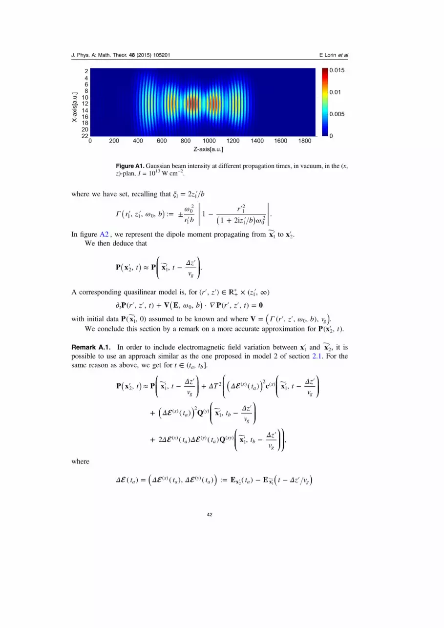
where we have set, recalling that ξ = ′z b21 1

Γ ωω

ω′ ′ = ±

′−

′+ ′

( )( )

r z br b

r

z b, , , : 1

1 2i.1 1 0

02

1

12

1 02

In figure A2 , we represent the dipole moment propagating from ′x1 to ′x2.We then deduce that

Δ′ ≈ ′ − ′( )t tz

vP x P x, , .

g2 1

⎛⎝⎜⎜

⎞⎠⎟⎟

A corresponding quasilinear model is, for ′ ′ ∈ × ′ ∞+r z z( , ) ( , )*1

ω∂ ′ ′ + ′ ′ =( )r z t b r z tP V E P 0( , , ) , , · ( , , )t 0

with initial data ′P x( , 0)1 assumed to be known and where Γ ω= ′ ′( )r z b vV ( , , , ), g0 .We conclude this section by a remark on a more accurate approximation for ′ tP x( , )2 .

Remark A.1. In order to include electromagnetic field variation between ′x1 and ′x2, it ispossible to use an approach similar as the one proposed in model 2 of section 2.1. For thesame reason as above, we get for ∈t t t( , ]a b .

Δ Δ Δ Δ

Δ Δ

Δ Δ Δ

′ ≈ ′ − ′ + ′ − ′

+ ′ − ′

+ ′ − ′

( )

( )

( )t tz

vT t t

z

v

t tz

v

t t tz

v

P x P x c x

Q x

Q x

, , ( ) ,

( ) ,

2 ( ) ( ) , ,

g

xa

x

g

xa

yb

g

xa

ya

xyb

g

2 12 ( ) 2 ( )

1

( ) 2 ( )1

( ) ( ) ( )1

⎛⎝⎜⎜

⎞⎠⎟⎟

⎛⎝⎜⎜

⎛⎝⎜⎜

⎞⎠⎟⎟

⎛⎝⎜⎜

⎞⎠⎟⎟

⎛⎝⎜⎜

⎞⎠⎟⎟

⎞⎠⎟⎟

where

Δ Δ Δ Δ= = − − ′′ ′ ( ) ( )t t t t t z vE E( ) ( ), ( ) : ( )ax

ay

a a gx x( ) ( )

2 1

2468101214161820220 200 400 600 800 1000 1200 1400 1600 1800

0.015

0.01

0.005

0

Z-axis[a.u.]

X-axis[a.u.]

Figure A1.Gaussian beam intensity at different propagation times, in vacuum, in the (x,z)-plan, I = 1013 W cm−2.

J. Phys. A: Math. Theor. 48 (2015) 105201 E Lorin et al

42

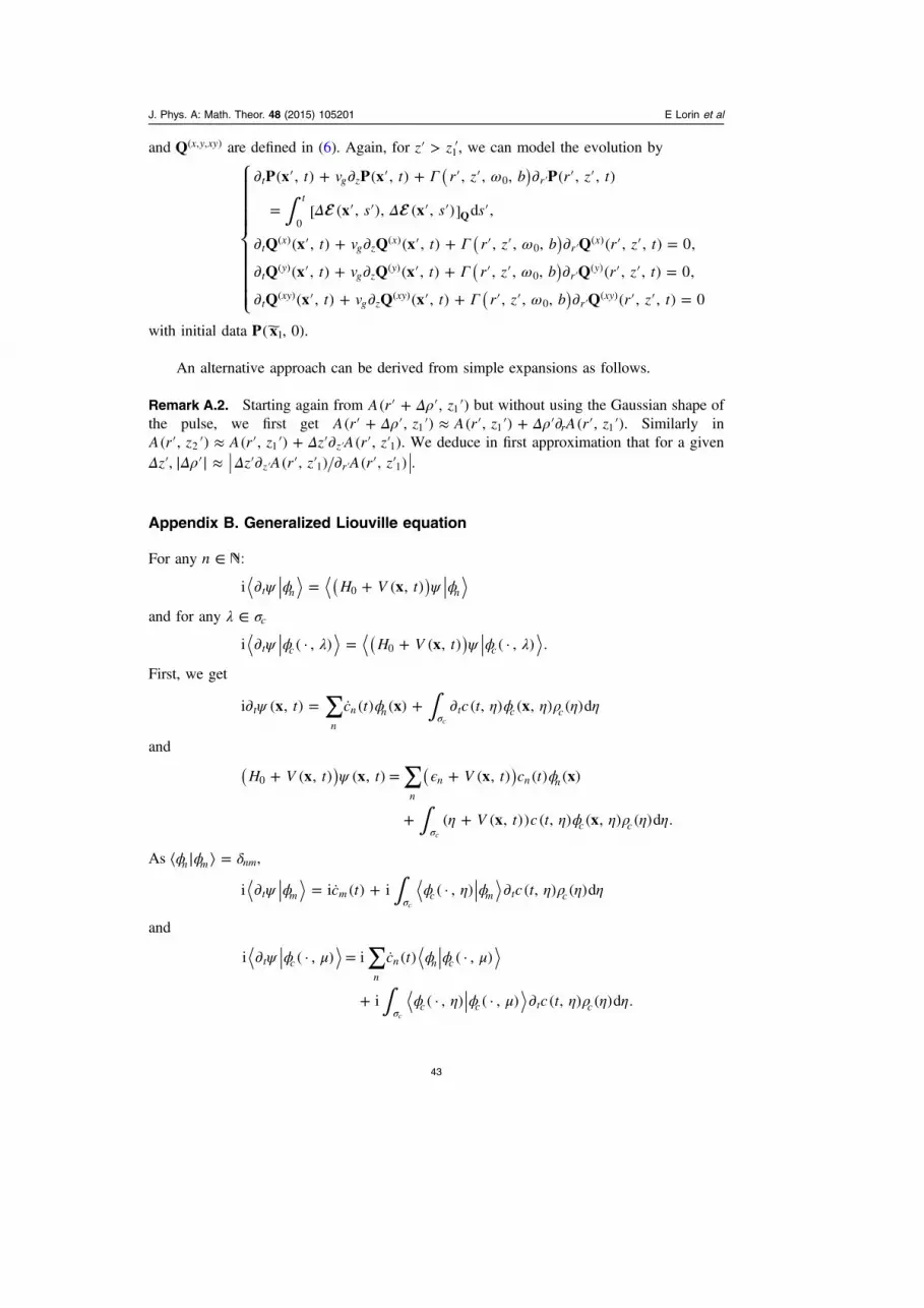
and Q x y xy( , , ) are defined in (6). Again, for ′ > ′z z1 , we can model the evolution by

∫Γ ω

Δ Δ

Γ ω

Γ ω

Γ ω

∂ ′ + ∂ ′ + ′ ′ ∂ ′ ′

= ′ ′ ′ ′ ′

∂ ′ + ∂ ′ + ′ ′ ∂ ′ ′ =

∂ ′ + ∂ ′ + ′ ′ ∂ ′ ′ =

∂ ′ + ∂ ′ + ′ ′ ∂ ′ ′ =

′

′

′

′

( )

( )( )

( )

t v t r z b r z t

s s s

t v t r z b r z t

t v t r z b r z t

t v t r z b r z t

P x P x P

x x

Q x Q x Q

Q x Q x Q

Q x Q x Q

( , ) ( , ) , , , ( , , )

[ ( , ), ( , )] d ,

( , ) ( , ) , , , ( , , ) 0,

( , ) ( , ) , , , ( , , ) 0,

( , ) ( , ) , , , ( , , ) 0

t g z r

t

tx

g zx

rx

ty

g zy

ry

txy

g zxy

rxy

Q

0

0

( ) ( )0

( )

( ) ( )0

( )

( ) ( )0

( )

⎧

⎨

⎪⎪⎪⎪

⎩

⎪⎪⎪⎪with initial data P x( , 0)1 .

An alternative approach can be derived from simple expansions as follows.

Remark A.2. Starting again from Δρ′ + ′ ′A r z( , )1 but without using the Gaussian shape ofthe pulse, we first get Δρ Δρ′ + ′ ′ ≈ ′ ′ + ′∂ ′ ′A r z A r z A r z( , ) ( , ) ( , )r1 1 1 . Similarly in

Δ′ ′ ≈ ′ ′ + ′∂ ′ ′′A r z A r z z A r z( , ) ( , ) ( , )z2 1 1 . We deduce in first approximation that for a givenΔ ′z , Δρ Δ∣ ′∣ ≈ ′∂ ′ ′ ∂ ′ ′′ ′z A r z A r z( , ) ( , )z r1 1 .

Appendix B. Generalized Liouville equation

For any ∈ n :

ψ ϕ ψ ϕ∂ = +( )H V txi ( , )t n n0

and for any λ σ∈ c

ψ ϕ λ ψ ϕ λ∂ = +( )H V txi ( · , ) ( , ) ( · , ) .t c c0

First, we get

∫∑ψ ϕ η ϕ η ρ η η∂ = + ∂σ

t c t c tx x xi ( , ) ˙ ( ) ( ) ( , ) ( , ) ( )dt

n

n n t c cc

and

∫

∑ψ ϵ ϕ

η η ϕ η ρ η η

+ = +

+ +σ

( ) ( )H V t t V t c t

V t c t

x x x x

x x

( , ) ( , ) ( , ) ( ) ( )

( ( , )) ( , ) ( , ) ( )d .

n

n n n

c c

0

c

As ϕ ϕ δ⟨ ∣ ⟩ =n m nm,

∫ψ ϕ ϕ η ϕ η ρ η η∂ = + ∂σ

c t c ti i ˙ ( ) i ( · , ) ( , ) ( )dt m m c m t cc

and

∫

∑ψ ϕ μ ϕ ϕ μ

ϕ η ϕ μ η ρ η η

∂ =

+ ∂σ

c t

c t

i ( · , ) i ˙ ( ) ( · , )

i ( · , ) ( · , ) ( , ) ( )d .

t cn

n n c

c c t cc

J. Phys. A: Math. Theor. 48 (2015) 105201 E Lorin et al

43

Similarly

∫

∑ψ ϕ ϵ ϕ ϕ

η η ϕ λ ϕ ρ λ λ

+ = +

+ +σ

( ) ( )H V t c t V t

c t V t

x x

x

( , ) ( ) ( , )

( , ) ( ( , )) ( · , ) ( )d

mn

n n n m

c m c

0

c

and

∫

∑ψ ϕ μ ϵ ϕ ϕ μ

η η ϕ η ϕ μ ρ η η

+ = +

+ +σ

( ) ( )H V t c t V t

V t c t

x x

x

( , ) ( · , ) ( ) ( , ) ( · , )

( ( , )) ( , ) ( · , ) ( · , ) ( )d .

cn

n n n c

c c c

0

c

We set

ϵ ϕ ϕ ϵ δ ϕ ϕ

λ ϵ ϕ ϕ λ ϕ ϕ λ

λ λ ϕ λ ϕ ϕ λ ϕ

λ μ λ ϕ λ ϕ μ ϕ λ ϕ μ

λ μ ϕ λ ϕ μ

μ ϕ ϕ μ

= + = +

= + =

= + =

= + =

=

=

( )( )

H V t V t

H V t V t

K V t V t

H V t V t

D

D

x x

x x

x x

x x

: ( , ) ( , ) ,

( ) : ( , ) ( · , ) ( , ) ( · , ) ,

( ) : ( ( , )) ( · , ) ( , ) ( · , ) ,

( , ) : ( ( , )) ( · , ) ( · , ) ( , ) ( · , ) ( · , ) ,

( , ) : ( · , ) ( · , ) ,

( ) : ( · , ) .

nm n n m n nm n m

n n n c n c

n c n c n

c c c c

c c

n n c

⎧

⎨

⎪⎪⎪⎪⎪

⎩

⎪⎪⎪⎪⎪

So that

∫∫

∫

∫

∑

∑

∑

η ρ η η η

η η ρ η η

μ η μ ρ η η η

μ η μ ρ η η η

+ ∂

= +

+ ∂

= +

σ

σ

σ

σ

c t D c t

c t H c t K

c t D D c t

c t H H c t

i ˙ ( ) i ( ) ( ) ( , )d

( ) ( , ) ( ) ( )d ,

i ˙ ( ) ( ) i ( , ) ( ) ( , )d

( ) ( ) ( , ) ( ) ( , )d .

m m c t

n

n nm n c

n

n n c t

n n n c

*

c

c

c

c

⎧

⎨

⎪⎪⎪⎪⎪

⎩

⎪⎪⎪⎪⎪

As the operator +H V tx( , )0 is self-adjoint, we deduce that: λ μ =D ( , ) 0 if λ μ≠ andλ =D ( ) 0n then

Figure A2. Dipole moment evolution.

J. Phys. A: Math. Theor. 48 (2015) 105201 E Lorin et al

44

∫∑ μ η μ ρ η η η μ+ ∂ = ∂σ

c t D D c t c ti ˙ ( ) ( ) i ( , ) ( ) ( , )d i ( , ).n

n n c t tc

This gives us a new set of equations:

∫∫

∑

∑

η η ρ η η

μ μ η μ ρ η η η

= +

∂ = +

σ

σ

c t c t H c t K

c t c t H H c t

i ˙ ( ) ( ) ( , ) ( ) ( )d ,

i ( , ) ( ) ( ) ( , ) ( ) ( , )d .

m n n nm n c

t n n n c

c

c

⎧⎨⎪⎪

⎩⎪⎪

As =V t tx x E( , ) · ( )

ϕ ϕ

λ ϕ ϕ λ

λ ϕ λ ϕ

λ μ ϕ λ ϕ μ

λ μ ϕ λ ϕ μ

=

=

=

=

=

H t

H t

K t

H t

D

E x

E x

E x

E x

( ) · ,

( ) ( ) · ( · , ) ,

( ) ( ) · ( · , ) ,

( , ) ( ) · ( · , ) ( · , ) ,

( , ) ( · , ) ( · , ) .

nm n m

n n c

n c n

c c

c c

⎧

⎨

⎪⎪⎪⎪

⎩

⎪⎪⎪⎪We are interested in ∫ ψ= ⟨ ⟩ = ∣ ∣t xd x x( ) d2 3 . In this goal, we set

ϕ ϕ ρ ρ λ ρ

λ ρ λ μ

= = =

= =

λ λ

λμ

t t c t c t t c t c t t

c t c t c t c t

d x( ) ˆ , ( ) ( ) ( ), ( ) ( ) ( , ), ( )

*( , ) , ( ) *( , ) ( , ).

mn m n mn m n m m m

m

* *

In order to compute d or equivalently Tr(ρxˆ ˆ ), we derive a system of differential equations.First, as

ρ = +t c t c t c t c t˙ ( ) ˙ ( ) ( ) ( ) ˙ ( )mn m n m n* *

then

∫∑ η η ρ η η= − −ν

ν νσ

c t c t c t c t H c t c t K( ) ˙ ( ) i ( ) ( ) i ( ) ( , ) ( ) ( )dn m n m n m c* * *

c

and

∫∑ η η ρ η η= +ν

ν νσ

c t c t c t c t H c t c t K˙ ( ) ( ) i ( ) ( ) i ( ) *( , ) ( ) *( )dn m m n m n* * *

c

so that

∫∑ρ ρ ρ ρ η ρ η ρ η ρ η η= − + −ν

ν ν ν νσ η η( )t H t t H t K t K˙ ( ) i ( ) ( ) i ( ) ( ) ( ) ( ) ( ) ( ) d .mn m n m n n n m c m n c

* *

c

Similarly, we have to evaluate ρ∂ λ μ t( )t , . From

ρ λ μ λ μ= ∂ + ∂λμ t c t c t c t c t˙ ( ) *( , ) ( , ) *( , ) ( , ).t t

We then get

∫∑ρ ρ λ ρ μ

η λ ρ η ρ η μ ρ η ρ η

= −

+ −

λμ μ λ

σ ημ λη

t t H t H

H t H t

˙ ( ) i ( ) ( ) ( ) ( )

i *( , ) ( ) ( ) ( , ) ( ) ( ) d .

n n n n n

c c

*

*

c

⎡⎣ ⎤⎦⎡⎣ ⎤⎦

J. Phys. A: Math. Theor. 48 (2015) 105201 E Lorin et al

45

Similarly

ρ λ λ= + ∂λ t c t c t c t c t˙ ( ) ˙ ( ) ( , ) ( ) ( , )m m m t* *

so that

∫∑ρ ρ ρ λ

η ρ η ρ η λ ρ η ρ η

= −

+ −

λ λ

σ ηλ η

t t H t H

K t H t

˙ ( ) i ( ) ( ) ( )

i ( ) ( ) ( ) ( , ) ( ) ( ) d .

m n n nm mn n

n c c m

*

* *

c

⎡⎣ ⎤⎦⎡⎣ ⎤⎦

That is, we get the following system, for all m, n, λ, μ:

∫

∫

∫

∑

∑

∑

ρ ρ ρ ρ η ρ η ρ η ρ η η

ρ ρ ρ λ

η ρ η ρ η λ ρ η ρ η

ρ ρ λ ρ μ

η λ ρ η ρ η μ ρ η ρ η

= − + −

= −

+ −

= −

+ −

ν ν ν ν νσ η η

λ λ

σ ηλ η

λμ μ λ

σ ημ λη

( )t H t t H t K t K

t t H t H

K t H t

t t H t H

H t H t

˙ ( ) i ( ) ( ) i ( ) ( ) ( ) ( ) ( ) ( ) d

˙ ( ) i ( ) ( ) ( )

i ( ) ( ) ( ) ( , ) ( ) ( ) d

˙ ( ) i ( ) ( ) ( ) ( )

i *( , ) ( ) ( ) ( , ) ( ) ( ) d .

mn m n m n m c m n

m n n nm mn n

n c c m

n n n n n

c c

* *

*

* *

*

*

c

c

c

⎧

⎨

⎪⎪⎪⎪⎪

⎩

⎪⎪⎪⎪⎪

⎡⎣ ⎤⎦⎡⎣ ⎤⎦

⎡⎣ ⎤⎦⎡⎣ ⎤⎦

References

[1] Couairon A and Mysyrowicz A 2007 Organizing multiple femtosecond filaments in air Phys. Rep.41 47–189

[2] Bergé L, Skupin S, Nuter R, Kasparian J and Wolf J-P 2007 Ultrashort filaments of light in weaklyionized, optically transparent media Rep. Prog. Phys. 70 1633–713

[3] Köhler C, Guichard R, Lorin E, Chelkowski S, Bandrauk A D, Bergé L and Skupin S 2013Saturation of the nonlinear refractive index in atomic gases Phys. Rev. A 87 043811

[4] Béjot P, Cormier E, Hertz E, Lavorel B, Kasparian J, Wolf J-P and Faucher O 2013 High-fieldquantum calculation reveals time-dependent negative Kerr contribution Phys. Rev. Lett. 110043902

[5] Loriot V, Hertz E, Faucher O and Lavorel B 2009 Measurement of high order Kerr refractive indexof major air components Opt. Express 17 13429

[6] Béjot P, Kasparian J, Henin S, Loriot V, Vieillard T, Hertz E, Faucher O, Lavorel B and Wolf J-P2010 Higher-order Kerr terms allow ionization-free filamentation in gases Phys. Rev. Lett. 104103903

[7] Kolesik M, Wright E M and Moloney J V 2010 Femtosecond filamentation in air and higher ordernonlinearities Opt. Express 35 2550

[8] Polynkin P, Kolesik M, Wright E M and Moloney J 2011 Experimental tests of the new paradigmfor laser filamentation in gases Phys. Rev. Lett. 106 153902

[9] Vinçotte A and Bergé L 2006 Atmospheric propagation of gradient-shaped and spinningfemtosecond light pulses Physica D 223 163–73

[10] Brabec T and Krausz F 2000 Intense few-cycle laser fields: frontiers of nonlinear optics Rev. Mod.Phys. 72 545–91

[11] Husakou A V and Hermann J 2001 Supercontinuum generation of higher-order solitons by fissionin photonic crystal fibers Phys. Rev. Lett. 87 203901

[12] Kolesik M and Moloney J V 2014 Modeling and simulation techniques in extreme nonlinearoptics of gaseous and condensed media Rep. Prog. Phys. 77 016401

[13] Babushkin I and Bergé L 2014 The fundamental solution of the unidirectional pulse propagationequation J. Math. Phys. 55 032903

J. Phys. A: Math. Theor. 48 (2015) 105201 E Lorin et al

46

[14] Kolesik M and Moloney J V 2004 Nonlinear optical pulse propagation simulation: fromMaxwellʼs to unidirectional equations Phys. Rev. E 70 036604

[15] Skupin S and Bergé L 2006 Self-guiding of femtosecond light pulses in condensed media: plasmageneration versus chromatic dispersion Physica D 220 14–30

[16] Champeaux S, Bergé L, Gordon D, Ting A, Peñano J and Sprangle P 2008 (3+1)-dimensionalnumerical simulations of femtosecond laser filaments in air: toward a quantitative agreementwith experiments Phys. Rev. E 77 036406

[17] Bergé L, Gouédard C, Schjodt-Eriksen J and Ward H 2003 Filamentation patterns in Kerr mediaversus beam shape robustness, nonlinear saturation and polarization states Physica D 176181–211

[18] Spott A, Jaroń-Becker A and Becker A 2014 Ab initio and perturbative calculations of the electricsusceptibility of atomic hydrogen Phys. Rev. A 90 013426

[19] Richter M, Patchkovskii S, Morales F, Smirnova O and Ivanov M 2013 The role of the Kramers–Henneberger atom in the higher-order Kerr effect New J. Phys. 15 083012

[20] Morishita T, Le A-T, Chen Z and Lin C D 2008 Accurate retrieval of structural information fromlaser-induced photoelectron and high-order harmonic spectra by few-cycle laser pulses Phys.Rev. Lett. 100 013903

[21] Lorin E, Chelkowski S and Bandrauk A 2011 The WASP model: a micro-macro system of Wave-Schrödinger-Plasma equations for filamentation Commun. Comput. Phys. 9 406–40

[22] Lorin E, Zaoui E, Chelkowsky S and Bandrauk A D 2011 Maxwell–Schroedinger–Plasma(MASP) model for laser–molecule interactions: towards quantum filamentation with intenseultrashort pulses Physica D 241 1059–71

[23] Lorin E, Chelkowski S and Bandrauk A 2007 A numerical Maxwell–Schrödinger model for laser–matter interaction and propagation Comput. Phys. Commun. 177 908–32

[24] Lewenstein M, Balcou P, Ivanov M Y, Huillier A and Corkum P B 1994 Theory of high-harmonicgeneration by low frequency laser fields Phys. Rev. A 49 2117–32

[25] Boyd R W 2003 Nonlinear Optics 2nd edn (New York: Academic)[26] Corkum P-B 1993 Plasma perspective on strong-field multiphoton ionization Phys. Rev. Lett.

71 1994[27] Bandrauk A D, Chelkowski S and Goudreau S 2005 Control of harmonic generation using two-

colour femtosecond-attosecond laser fields: quantum and classical perspectives bandraukJ. Mod. Opt. 52 411–28

[28] Bandrauk A D, Fillion-Gourdeau F and Lorin E 2013 Atoms and molecules in intense laser fields:Gauge invariance of theory and models J. Phys. B: At. Mol. Opt. Phys. 46 153001

[29] Lorin E and Bandrauk A D 2012 Efficient and accurate numerical modeling of a micro–macrononlinear optics model for intense and short laser pulses J. Comput. Sci. 3 159–68

[30] Nguyen H S, Suda A and Midorikawa K 1999 Generation and propagation of attosecond pulses inHe gas with sub-10-fs driver pulses Phys. Rev. A 60 2587

[31] Bidégaray-Fesquet B 2006 Hiérarchie de Modéles en Optique Quantique: De Maxwell–BlochSchrödinger Non-linéaire (Mathématiques et Applications vol 49) (Berlin: Springer)

[32] Gavish N, Fibich G, Vuong L T and Gaeta A L 2008 Predicting the filamentation of high-powerbeams and pulses without numerical integration: a nonlinear geometrical optics method Phys.Rev. A 78 043807

[33] Diels J C and Rudolph W 2006 Ultrashort Laser Pulse Phenomena (Optics and Photonics Series)2nd edn (New York: Academic)

J. Phys. A: Math. Theor. 48 (2015) 105201 E Lorin et al

47