arX

iv:h

ep-t

h/02

1102

6v2

10

Dec

200

2

Non-perturbative summation over 3D discrete topologies

Laurent Freidel∗

Perimeter Institute for Theoretical Physics

35 King street North, Waterloo N2J-2G9,Ontario, Canada

and

Laboratoire de Physique, Ecole Normale Superieure de Lyon

46 allee d’Italie, 69364 Lyon Cedex 07, France

David Louapre†

Laboratoire de Physique, Ecole Normale Superieure de Lyon

46 allee d’Italie, 69364 Lyon Cedex 07, France‡

(Dated: February 1, 2008)

Abstract

We construct a group field theory which realizes the sum of gravity amplitudes over all three di-mensional topologies trough a perturbative expansion. We prove this theory to be uniquely Borelsummable. This shows how to define a non-perturbative summation over triangulations includingall topologies in the context of three dimensional discrete gravity.

∗Electronic address: lfreidel@perimeterinstitute.ca†Electronic address: dlouapre@ens-lyon.fr‡UMR 5672 du CNRS

2

I. INTRODUCTION

In quantum gravity, we are interested in the computation of transition amplitudes between spatial geometries.These transition amplitudes are supposed to arise as a sum over spacetime ‘geometries’. In the classical realm whatis meant by geometries is clear, one usually means a smooth Lorentzian metric free of singularity on a manifold offixed topology, possibly satisfying some asymptotic conditions. In the quantum realm we obviously have much morefreedom in choosing which spacetime geometries should be included in the sum. Do we authorize the geometries toposses some singularities for instance? [1] Do we authorize topology change? One of the outstanding question in thiscontext is wether one should or not include a sum over topology in the sum over geometries. The next outstandingquestion is wether this is possible in a given framework. In this paper we are going to analyze this problem in thecontext of discrete approach to quantum gravity, i-e dynamical triangulation and spin foam models. In dynamicaltriangulation one first choose an equilateral triangulation ∆ of space-time with regular simplices and we assign toeach triangulation a statistical weight given by the exponential of the Regge action. In spin foam models one choosea triangulation of space time and assign to it certain representation labels of the Lorentz group. This representationlabels carry information on the geometry of the simplex. The transition amplitudes are constructed as a state sum,using sum over representations assigned to the geometrical building blocks of the triangulation. Historically, the firstspin foam model was proposed by Ponzano and Regge [2] for 3D Euclidian quantum gravity, and their work has beenrecently generalized to higher dimension to give birth to the spin foam approach for quantum gravity (see [3, 4] foran overview).

3D gravity is a topological theory. As a consequence, the transition amplitudes built in the Ponzano-Regge modeldo not depend on the choice of the triangulation. However this is no longer the case in 4D, and one has somehow toget rid of the choice of the triangulation in order to restore the infinite number of degrees of freedom of 4D gravity.A proposal to do this is to sum the discretized amplitude over all possible triangulations of the manifold. A moredrastic proposal is to sum over all possible triangulations regardless of the topology.

It is however commonly believed that there is no way to give sense to the sum over triangulations including alltopologies. The problem appears clearly in the context of dynamical triangulations [5]. In this context the amplitudeof a given 3-dimensional triangulation ∆ is given by

A[∆] =1

Sym[∆]λN3µN1 , (1)

where Sym[∆] is a symmetry factor, and N3 (resp. N1) denote the number of tetrahedra (resp. edges) of thetriangulation. The parameters λ, µ can be interpreted, if one uses the Regge action, in terms of the bare cosmologicalconstant Λ and the bare Newton constant 1/G

µ ∼ exp(1

G), (2)

λ ∼ exp(−Λ − c

G), (3)

where c is a geometrical constant. The sum over all triangulations is then

Z =∑

N3,N1

λN3µN1N (N3, N1), (4)

with N (N3, N1) being the number of triangulations with a fixed number of tetrahedra and edges. Since µ ≥ 1 thepartition function is bounded from below by

∑

N3λN3N (N3) where N (N3) is the total number of triangulations with

a fixed number of tetrahedra. This number grows factorially with the number of tetrahedra if there is no restrictionon the topology of the triangulation. Therefore a sum over triangulations does not seem to be possible in general,since this factorial growth can not be killed by any choice of λ, µ. The solution proposed in [5] is to restrict to a fixedtopology (as the 3-sphere), in order to get back to a case where the number of triangulations grows exponentially withthe number of 3-simplices. So the sum over simplicial manifold can be defined in the case of a restricted topology.However, since there is no general classification of the topologies in D > 2, we cannot expect to use this result tomake sense of a sum over topologies as in 2 dimensions. One conclusion that one can draw is that one should nottry to sum over topology when trying to solve quantum gravity. This is not completely satisfactory, since first, thereare argument in favor of classical topology change [1], but also one would expect in a theory of quantum gravity toresolve this issue dynamically and not a priori.

There is hopefully another point of view that can be taken on this problem. It is well known since Dyson [6]that physical quantities in interacting quantum theory are non-analytic functions of the coupling constant. Thistranslates into the fact that the perturbative expansion of any physical quantities in terms of the coupling constant

3

is a divergent series. This opens the possibility of giving a meaning to the sum over triangulations if we can interpretit as a perturbative expansion of a non-perturbative quantity.

These ideas have already been used in the context of 2D gravity, leading to the construction of the matrix models,which realize a sum over triangulations of 2D surfaces [7]. By considering three-indices tensors instead of matrices,Ambjorn et al. [5] tried to apply these ideas to obtain a dynamical triangulation model for three-dimensional quantumgravity. Later, Boulatov and Ooguri [8, 9] have generalized these models in the form of non local field theories overgroup manifold. The bottom line is that a space-time triangulation can naturally be interpreted as a Feynman graphof a Group Field Theory (GFT) [10]. Moreover, the specific gravity amplitude assigned to a given triangulation isexactly given by the Feynman graph evaluation of a group field theory GFT. This was shown in the context of 3Ddynamical triangulation [5], 3D Ponzano-Regge model [8] and even 4D spin foam model [11]. It is now understoodthat this is a general feature of spin foam models [12].

All these results lead to the conclusion that the sum over triangulations of a state sum amplitude is in fact a sumover Feynman graphs of a GFT,

∑

∆

AState sum(∆) =∑

Γ

AGFT(Γ). (5)

Therefore it is not a surprise that the sum over triangulations is divergent, since it is a perturbative expansion, itshould be understood as an asymptotic series. If we take for serious the fact that the sum over triangulations comesfrom a group field theory, this opens the possibility of giving a non perturbative meaning to the sum. This idea hasbeen already advocated in [12] and to some extent in [5].

However it is well known that in general, the asymptotic series does not determine uniquely the resummation. Oneneed additional non-perturbative inputs. In interacting quantum field theory, the large order behavior is determinedby non-perturbative information contained in the action and in some case [13] one is able to reconstruct a non-perturbative expression from the divergent series, in a uniquely defined manner. In such cases, the divergent seriesis said to be uniquely Borel-summable. Our main result in this paper is to prove that such a procedure can berealized for a particular type of GFT models associated with three dimensional gravity. If the Feynman expansionof a GFT model is Borel-summable, this means it could be related to a non perturbative expression in a uniquelydefined manner, giving a well-defined meaning to the equality

∑

Γ

AGFT(Γ) = ZNP . (6)

This result proves that a well-defined notion of a sum over all triangulations of all topologies is not unreasonable, asit could be achieved in particular cases.

In the context of dynamical triangulation the coupling constant λ of the group field theory has a physical meaning, itcan be interpreted as − exp(−Λ), where Λ is the cosmological constant. Since it is negative, the potential is unboundedfrom below and it was expected that the corresponding GFT is not uniquely Borel summable in the physical regime.Therefore one can think that the theories allowing non perturbative resummation will not be physical (at least inthe context of dynamical triangulations). In two dimension one can view this problem as the one preventing a nonperturbative definition of string theory via matrix models.

It was therefore for us a big surprise and a relief to find out that the modification of the Ambjorn et al. model [5]we propose is uniquely Borel summable in the physical region where λ > 0 (see sect. IV). In the context of threedimensional Ponzano-Regge models the value of the group field theory coupling constant model is not restricted byphysical requirement and we expect the Borel summable GFT to have physical meaning without restriction.

In section II of this paper we first review the definitions of several group field theory models related to 3 dimensionalgravity like the Boulatov or Ambjorn model. We present their Feynman expansions and show their relations with3 dimensional Ponzano-Regge models or dynamical triangulations. We also discuss their convergence properties. Insection III we review known facts and theorems concerning non perturbative resummation of a perturbative series.In section IV we propose a modification of the usual Ambjorn or Boulatov models in order to deal with positivepotential. We show that the perturbative expansion of this model can be related to the dynamical triangulation sumwith physical value of the parameters. In the last section V we finally prove the unique Borel summability of themodel we have defined. This give us an example of an unambiguous way to sum over all triangulations hence alltopologies.

II. 3D GROUP FIELD THEORY MODELS

In this part, we review various constructions of 3D group field theory (GFT) models : the Boulatov model, leadingto the Ponzano-Regge amplitude [8], a model on the non-commutative sphere, reproducing the 3D matrix model

4

of Ambjorn et al.[5], and some others models with improved convergence properties, analogous to those recentlyintroduced for 4D spin foam models [14, 15].

A. The Boulatov model

The Boulatov model is a field theory defined on the group manifold SO(3)3, with some invariances imposed on thefields. The fields are asked to be real (Φ = Φ), symmetric

Φ(gσ(1), gσ(2), gσ(3)) = (−1)|σ|Φ(g1, g2, g3), (7)

(where σ denotes a permutation of three elements and |σ| its signature), and (right-) SO(3) invariant

Φ(g1g, g2g, g3g) = Φ(g1, g2, g3). (8)

This last requirement allows us to see the Boulatov model as a field theory on the coset space SO(3)3/SO(3). Theaction is non-local and is given by

S[Φ] =1

2

∫

G3

dg1dg2dg3 Φ(g1, g2, g3)2

+λ

4!

∫

G6

dg1dg2dg3dg4dg5dg6 Φ(g1, g2, g3)Φ(g3, g5, g4)Φ(g4, g2, g6)Φ(g6, g5, g1) (9)

To compute the partition function of this model in perturbative expansion, one has to express the action in termsof the Fourier coefficients of the field Φ. In order to define a Fourier transform on the coset space, one first considersthe transform on SO(3)3, then requires the SO(3)-invariance. The representations of SO(3) are labelled by integerspin j, and a function on SO(3) can be expressed as a sum over the matrix elements of g in the spin j representationDjmn(g) (see appendix A)

Φ(g) =∑

j,m,n

djΦmnj Dj

mn(g), (10)

where dj = 2j + 1 and −j ≤ m,n ≤ j. The Fourier coefficient is

Φmnj =

∫

G

dg Φ(g)Djmn(g

∗), (11)

where g∗ denotes complex conjugation. The Fourier expansion on SO(3)3 is then

Φ(g1, g2, g3) =∑

~,~m,~n

d~Φ~m~n~ D~~m~n(~g), (12)

where ~j ≡ (j1, j2, j3) and D~~m~n(~g) ≡ Dj1m1,n1

(g1)Dj2m2,n2

(g2)Dj3m3,n3

(g3). The SO(3)-invariance is implemented by groupaveraging over the right diagonal action of SO(3)

Φ(g1, g2, g3) =

∫

dg Φ(g1g, g2g, g3g). (13)

Expanding the RHS using decomposition (12), then performing the integration on g using the relation (A6), we obtainthe Fourier decomposition of the field over SO(3)3/SO(3)

Φ(g1, g2, g3) =∑

~,~m,~n

A~m~

√

d~ D~~m~n(~g)C

~j~n, (14)

where we introduced the Fourier coefficient

A~m~ =

∑

~n

Φ~m~n~

√

d~ C~j~n, (15)

5

����������������

����������������

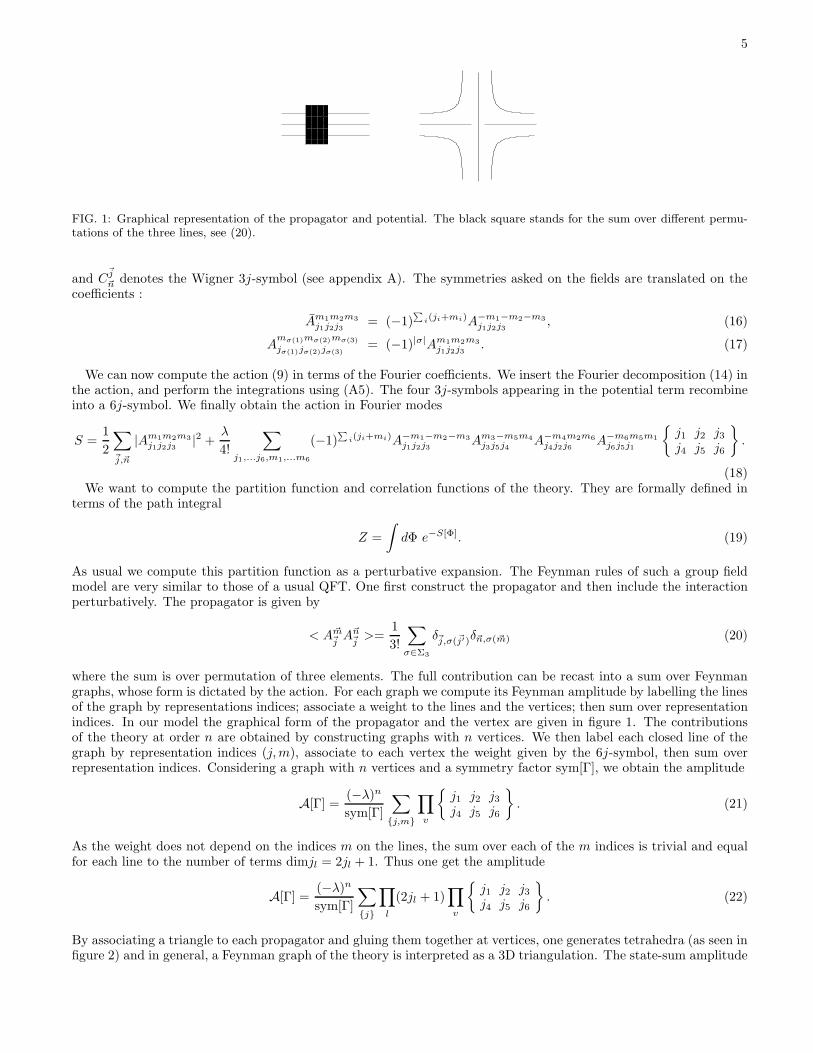
FIG. 1: Graphical representation of the propagator and potential. The black square stands for the sum over different permu-tations of the three lines, see (20).

and C~j~n denotes the Wigner 3j-symbol (see appendix A). The symmetries asked on the fields are translated on the

coefficients :

Am1m2m3

j1j2j3= (−1)

∑

i(ji+mi)A−m1−m2−m3

j1j2j3, (16)

Amσ(1)mσ(2)mσ(3)

jσ(1)jσ(2)jσ(3)= (−1)|σ|Am1m2m3

j1j2j3. (17)

We can now compute the action (9) in terms of the Fourier coefficients. We insert the Fourier decomposition (14) inthe action, and perform the integrations using (A5). The four 3j-symbols appearing in the potential term recombineinto a 6j-symbol. We finally obtain the action in Fourier modes

S =1

2

∑

~j,~n

|Am1m2m3

j1j2j3|2 +

λ

4!

∑

j1,...j6,m1,...m6

(−1)∑

i(ji+mi)A−m1−m2−m3

j1j2j3Am3−m5m4

j3j5j4A−m4m2m6

j4j2j6A−m6m5m1

j6j5j1

{

j1 j2 j3j4 j5 j6

}

.

(18)We want to compute the partition function and correlation functions of the theory. They are formally defined in

terms of the path integral

Z =

∫

dΦ e−S[Φ]. (19)

As usual we compute this partition function as a perturbative expansion. The Feynman rules of such a group fieldmodel are very similar to those of a usual QFT. One first construct the propagator and then include the interactionperturbatively. The propagator is given by

< A~m~jA~n~j >=

1

3!

∑

σ∈Σ3

δ~j,σ(~j′)δ~n,σ(~m) (20)

where the sum is over permutation of three elements. The full contribution can be recast into a sum over Feynmangraphs, whose form is dictated by the action. For each graph we compute its Feynman amplitude by labelling the linesof the graph by representations indices; associate a weight to the lines and the vertices; then sum over representationindices. In our model the graphical form of the propagator and the vertex are given in figure 1. The contributionsof the theory at order n are obtained by constructing graphs with n vertices. We then label each closed line of thegraph by representation indices (j,m), associate to each vertex the weight given by the 6j-symbol, then sum overrepresentation indices. Considering a graph with n vertices and a symmetry factor sym[Γ], we obtain the amplitude

A[Γ] =(−λ)nsym[Γ]

∑

{j,m}

∏

v

{

j1 j2 j3j4 j5 j6

}

. (21)

As the weight does not depend on the indices m on the lines, the sum over each of the m indices is trivial and equalfor each line to the number of terms dimjl = 2jl + 1. Thus one get the amplitude

A[Γ] =(−λ)nsym[Γ]

∑

{j}

∏

l

(2jl + 1)∏

v

{

j1 j2 j3j4 j5 j6

}

. (22)

By associating a triangle to each propagator and gluing them together at vertices, one generates tetrahedra (as seen infigure 2) and in general, a Feynman graph of the theory is interpreted as a 3D triangulation. The state-sum amplitude

6

����������������������������

FIG. 2: Triangulation generated by the Feynman diagrams

associated to a triangulation ∆ is thus

A[∆] =(−λ)nsym[∆]

∑

{j}

∏

e

(2je + 1)∏

t

{

j1 j2 j3j4 j5 j6

}

(23)

where e and t label the edges and tetrahedron of the triangulation. This amplitude is exactly the Ponzano-Reggepartition function associated to the triangulation ∆. Moreover, all the triangulations can be obtained as Feynmangraphs of the theory, thus the sum over Feynman graphs is indeed the sum over triangulations of the Ponzano-Reggeamplitude.

As in standard quantum field theory, the GFT are in general faced with two kind of divergences. The first onesare the analog of the UV/IR divergences, and arise when computing the value of a given graph by summing overrepresentation indices (momenta). The second ones are the large order divergences, arising when one try to sum allthe Feynman graphs, in order to get a non-perturbative expression of a physical quantity. In this paper we will mainlyconcentrate on the large order divergences, and we need somehow to get rid of the UV/IR divergences. For instance,it is well known that the weight (22) is divergent for some triangulations, the divergences being associated withthe vertices of the triangulation. This is a generalization of the usual fact that in standard field theory divergencesare associated with the loop of the Feynman graphs (for more details on loop divergences in group field models see[14, 15].) As we will see at the end of this section, one way to avoid these divergences is to define spin foam modelswith enhanced convergence properties, in analogy with the models introduced in [14, 15]. However the Ponzano-Reggeweight generated by the Boulatov model is not one of these enhanced models, and we feel that a full understanding ofthe notion of renormalisability for these theories should be developed. In this paper we will not dwell further on thisissue and we will ignore the UV problems by working with a fix regulator and concentrate on the problem of largeorder divergences.

The natural regularization to choose in this context, which respects the symmetry, is to project out modes of thefields carrying a spin j bigger than say N . So instead of the field Φ we use the projected field

ΦN (g1, g2, g3) =∑

~≤Nd~∑

~m,~n

Φ~m~n~ D~~m~n(~g). (24)

In this case the action expressed in Fourier mode is identical to (18), except that the sum over the spins are restrictedto be over j ≤ N . One can naturally interpret this projection as arising from a group field theory defined on thenon commutative sphere S3

N [16] (see [17] and the appendix B for non commutative 2-sphere S2N ). This leads to an

interpretation of the regularized group field theory model in terms of a generalized matrix models, since functions onthe non commutative sphere are matrices. Another natural way to get a regularization is to define this model with

the q-deformation of SU(2) for q a root of the unity q = ei√

Λ, where the cut off N in the representations is related tothe cosmological constant Λ by 2N + 1 = πΛ−1/2.

B. Group field model on the sphere and 3D matrix models

Keeping the action (9), one can define various models by requiring different kind of invariances on the fields. Forinstance by considering a real symmetric field on SO(3)3 with a SO(2)3-invariance,

Φ(g1h1, g2h2, g3h3) = Φ(g1, g2, g3) ∀(h1, h2, h3) ∈ SO(2)3 (25)

one obtains a group field model on the coset space [SO(3)/SO(2)]3. To implement the SO(2)3-invariance, one fixesan SO(2) subgroup of SO(3). In particular, we may consider SO(3) in its fundamental representation and choose a

7

unit vector v0; we then let H be the SO(2) subgroup which leaves v0 invariant. The space of the equivalence classes,SO(3)/SO(2), is diffeomorphic to the 2-sphere S2. Thus a GFT over the group manifold [SO(3)/SO(2)]3 is viewed asdefined over three copies of the 2-sphere S2. As in the case of the Boulatov model, one has to determine the Fouriertransform by requiring the invariance on the Fourier expansion. If the representation is of integer spin j there is aunique vector invariant under the action of the SO(2)-subgroup, we denote it v0. The SO(2)-group averaging of thematrices of representation gives the projector over this invariant vector

∫

SO(2)

dh Djmn(h) = v0

mv0n (26)

So if we define the Fourier coefficient

A~m~j

=√

d~∑

~n

Φ~m,~n~j

v0~n (27)

the field is expressed as

Φ(g1, g2, g3) =∑

~,~m,~n

A~~m√

d~ D~~m~n(~g)v

0~n. (28)

The reality conditions are translated on the coefficients

Aj1,j2,j3m1m2m3= (−1)

∑

i miAj1,j2,j3−m1−m2−m3(29)

The action is found to be

S =1

2

∑

j1,j2,j3,m1,m2,m3

∣

∣Am1m2m3

j1j2j3

∣

∣

2+λ

4!

∑

j1...j6,m1...m6

(−1)∑

i miA−m1−m2−m3

j1j2j3Am3−m5m4

j3j5j4A−m4m2m6

j4j2j6A−m6m5m1

j6j5j1(30)

The Feynman rules are the same than in the previous case, and the state sum amplitude associated to a graph isgiven by

(−λ)n∑

{j,i}1 = (−λ)n

∑

{j}

∏

e

(2je + 1). (31)

As before, this is interpreted as the amplitude associated to a 3D triangulation. This is a variant of the Ponzano-Reggemodel, with 1 as tetrahedron amplitude, instead of the 6j−symbol.

This partition function obviously diverges and has to be regularized. As before, an elegant way to regularize thismodel is to consider the original model to be defined on the non-commutative sphere S2

N instead of the 2-sphere. Thealgebras of function on S2

N is just the space of (N+1)×(N+1) matrices. This space carries naturally a representationof SU(2); if we decompose it in terms of spherical harmonics it can be written as a sum over spin j representationwhere j ≤ N (see appendix B). The amplitude associated to a graph becomes

A[Γ] =(−λ)nsym[Γ]

∑

{j≤N}

∏

e

(2je + 1) =(−λ)nsym[Γ]

[(N + 1)2](# edges), (32)

=1

sym[Γ](−λ)(# tetrahedra)µ(# edges). (33)

which is finite (we defined µ ≡ (N+1)2). This amplitude is the amplitude (1) obtained in 3D dynamical triangulations.However, we have to notice that to correctly interpret this GFT as defining a sum over triangulations of the 3Ddynamical triangulation model, we have to set λ negative, namely −λ ∼ exp(−Λ − c

G ), see (3).

C. Other group field theories

The two previous group field theories were the first ones introduced in the literature [5, 8]. There has been sincethen a resurgence of these models when it appeared that the Barrett-Crane amplitude, which was a candidate for a4D state sum model of quantum gravity, could be interpreted as a Feynman graph amplitude of a group field theory[11, 18].

8

Since then, different modifications of the original 4D model have been proposed first by Perez and Rovelli [14] (notealso the generalization in [19]). The purpose of these modified models was to improve the convergence properties ofthe Feynman graph amplitudes. We give here the 3D analogs of these models.

The general group field theory we will consider is defined on SO(3)3 for real symmetric fields, with the action

S[Φ] =1

2

∫

dg1dg2dg3 [PkinΦ(g1, g2, g3)]2

+λ

4!

∫

dg1dg2dg3dg4dg5dg6 [PpotΦ(g1, g2, g3)][PpotΦ(g3, g5, g4)][PpotΦ(g4, g2, g6)][PpotΦ(g6, g5, g1)], (34)

where Pkin, Ppot are operators acting on the space of fields and implementing some invariance property. For instancethe Boulatov model is recovered for Pkin = Ppot = PSO(3). Where PSO(3)Φ(g1, g2, g3) =

∫

SO(3) Φ(g1g, g2g, g3g)dg

is the projector on the space of SO(3) invariant fields. We denote by PRSO(2)3 the projector on the sphere, i-e

PRSO(2)3Φ(g1, g2, g3) =∫

SO(2)3Φ(g1h1, g2h2, g3h3)dh1dh2dh3. The Ambjorn model is recovered for Pkin = Ppot =

PRSO(2)3 . We can consider new group field theories that gives 3 dimensional analogs of the models introduced by Perez

and Rovelli, if we use

Pkin = PRSO(3), (35)

Ppot = (PRSO(3)PRSO(2)3)

pPkin. (36)

As the kinetic term is the same than in the Boulatov model, the Fourier coefficient will be the same. However,applying the projectors in Ppot leads to the following state sum amplitude

A[Γ] =∑

{j}

∏

f

(2jf + 1)∏

v

{

j1 j2 j3j4 j5 j6

}

Θp(j1, j2, j3)Θp(j3, j5, j4)Θ

p(j2, j4, j6)Θp(j1, j5, j6) (37)

where Θ is given by

Θ(j1, j2, j3) =[

C~j~nv

0~n

]2

=

∫

dg Dj100(g)D

j200(g)D

j300(g). (38)

One can use the following majoration of Θ

Θ(j1, j2, j3) = Cj1j2j3000 Cj1j2j3000

≤∑

m2m3

Cj1j2j30m2m3Cj1j2j30m2m3

(39)

This last term in the RHS is just 1/dj1 . Applying this uniformly for the three spins one gets the bound

Θ(j1, j2, j3) ≤1

(dj1dj2dj3)1/3

. (40)

III. NON-PERTURBATIVE RESUMMATION OF AN ASYMPTOTIC SERIES

In this section we review well known facts on divergent series in quantum theory. We recall the physical origin ofthese divergences, and how to deal with them from the perturbative and non-perturbative point of view. In particular,we explain how to obtain a non-perturbative resummation of a divergent perturbative series. We illustrate these ideason a one dimensional φ4 model and show the crucial role played by the instantons in this framework (see [13] for ageneral overview of the large order behavior in quantum field theory.)

It is known since Dyson [6] that physical quantities in interacting quantum theory are non analytic functions of thecoupling constant. This is easily related to the fact that for negative values of the coupling constant, the potential failsto be bounded from below and the theory becomes unstable. The consequence is that the perturbative expansion ofa physical quantity in terms of the coupling constant is a divergent series. A simple example is given by the followingaction

Sλ(φ) =1

2φ2 +

λ

4φ4, (41)

9

���������������������������������������������������������������������������������������������������������������������������������������������������������������������������

���������������������������������������������������������������������������������������������������������������������������������������������������������������������������

FIG. 3: Contour for the analytic continuation of Z(λ)

which is unbounded from below for negative λ. The partition function

Z(λ) =

∫ +∞

−∞dφ e−

12φ

2−λ4 φ

4

, (42)

can be perturbatively evaluated by first expanding the integrand in terms of λ, then inverting the integration and thesummation and integrating each term

∫ +∞

−∞dφ e−

12φ

2

φ4n = 22n+ 12 Γ(2n+

1

2). (43)

The exchange of integration and summation is in fact invalid, as a result the perturbative expansion of Z(λ)

Z(λ) =∑

n

√2(−1)n

λn

n!Γ(2n+

1

2), (44)

is a divergent series with the n-th term growing like C(−1)n4nn!.In general, the asymptotic behavior of perturbative divergent series can be analyzed by considering classical non-

perturbative objects of the theory called instantons. The instantons are complex valued solutions of the equationsof motion with finite action. For instance considering the action (41), its equations of motion have two non-trivial

complex solutions given by φ = ±i/√λ. The value of the action for these solutions is S(φ) = − 1

4λ . These quantitiesare expressed using the inverse of the coupling constant, showing the non-perturbative nature of these objects. Letus see how they play a role in the large order behavior of perturbative expansions.

Consider the previous partition function (42). First, we need to show that it can be analytically continued in the

complex plane, with a cut along the real negative axis. Let λ = ρeiθ be a complex number. We define Z(λ) by

Z(λ) =

∫

e−iθ/4R

dφ e−12φ

2−λ4 φ

4

(45)

First Z(λ) is well defined for all |θ| < π, second it is an analytic continuation of Z(λ). This is clear since for |θ| < π2 ,

the integral along e−iθ/4R is equal to the integral along R plus the circular contours which link these lines at infinity(see figure 3). Writing z = Reiα on these circular contours, the integral along them is equal to

limR→±∞

∫ 0

−θ/4dα e−

12R

2e2iα− ρ4 e

i(θ+4α)R4

(46)

which goes to zero when R → ±∞, provided that |θ| < π/2. Thus the contour of integration can be shifted frome−iθ/4R to R and the proposed expression defines the analytic continuation of Z(λ), which can be extended to thewhole complex plane, with a cut on the real negative axis. We can then define the discontinuity along this cut axis by

D(−ω) = Z(eiπω) − Z(e−iπω) (47)

10

FIG. 4: a) Original contour C for defining D(−ω); b) Deformed contour C′to apply the saddle point method.

for ω > 0. Thus D is given by the integral

D(−ω) =

∫

C

dφ e−12φ

2+ ω4 φ

4

(48)

where C is the contour eiπ/4R− e−iπ/4R pictured in figure 4. Now Z is related to this discontinuity by the dispersionrelation

Z(λ) =1

2iπ

∫ +∞

0

dωD(−ω)

ω + λ(49)

We can expand this dispersion relation

Z(λ) =∑

n

anλn (50)

with

an =(−1)n

2iπ

∫ +∞

0

dωD(−ω)

ωn+1(51)

We want to understand the large n behavior of the coefficients an of the series. For large n, the integrand in thedefinition of these coefficients is sharply peaked around z = 0. This shows that the large n behavior of an dependson the value of D(−ω) for small ω. We can change the variable of integration ψ ≡ √

ωφ.

D(−ω) =

∫

C

dφ e−12φ

2+ ω4 φ

4

=

∫

C

dψ√ωe

1ω (− 1

2ψ2+ 1

4ψ4) (52)

The value of the integral for small ω can be obtained by saddle point method. The saddle points equation is−ψ+ψ3 = 0, whose non-trivial solutions are ψ = ±1. We see that these solutions corresponds to instantons solutions,since if we rescale ψ by i

√ω, the saddle point equation becomes the equation of motion of the theory and the solutions

becomes the instantons. The contour C can be deformed into C′ (see figure 4) which contains these saddle points.Expanding around these points and integrating, one gets

D(−ω) ∝ e−1/4ω. (53)

which is the evaluation of the action for the instantons solutions. One gets

an ∝ C(−1)n∫ +∞

0

dω e−14ω

1

ωn+1∝ (−1)n

(

1

4

)−nn! (54)

which is in agreement with the asymptotic given for the exact computation (44). The value (1/4)−n arises from theevaluation −1/4z of the action on instantons solutions. This computation shows clearly how the instantons govern

11

the behavior of the asymptotic series. We will now see how they are related to the way of extracting perturbative andnon-perturbative information from the divergent expansions.

Even if interacting quantum theories lead to perturbative expansions which are divergent series one can use theseseries as approximation of the non-perturbative quantity by cutting them at an appropriate order. Consider a divergentseries

f(z) =

N−1∑

n=0

anzn +RN (z) (55)

with a rest bounded by

|RN (z)| < AS−NN !|z|N (56)

(as seen in the previous example, S arise from the integration (54) and is related to the evaluation of the action for firstinstantons solutions.) One can use the series truncated at order N as an approximation of the exact non-perturbativequantity f(z), the difference between them being given by the rest RN (z). One can study the variations of RN (z)with N (at fixed z) and show that the rest first decreases as N increases, reaches its minimum around N ∼ S/z, thenincreases and diverge to infinity. This means that the best estimation of f(z) by its truncated asymptotic series isobtained at order N ∼ S/z. One can define the accuracy of the expansion by

ǫ(z) = MinN RN (z). (57)

Evaluating the bound (56) for N ∼ S/z, one sees that ǫ(z) ∼ e−S/z.One thus know how to extract the best accurate physical information from a divergent perturbative series. However,

one would like to be able to extract exact finite non-perturbative information from the divergent perturbative expan-sions. In order to get non-perturbative quantities from perturbative expansions, one has to reconstruct the originalfunction Z(λ) from an asymptotic series. However, it is easy to see that the issue of unicity of such reconstruction isnot a trivial problem. For instance, if f(z) as an asymptotic series

∑

akzk, then f(z)+ e−S/z has the same one. This

is not a surprise since one expects an ambiguity arising from the fact that the accuracy function is not zero, whichmeans that the perturbative expansion does not contain all the information necessary to reconstruct the originalfunction. Thus without additional conditions on f , it remains this ambiguity, there is no way to reconstruct uniquelythe function from the asymptotic series. If one can find conditions on f to uniquely reconstruct it from its asymptoticseries, the asymptotic series is said to be uniquely Borel summable.

In that case, the unique function is recovered for instance by the Borel transform procedure. Let us consider anasymptotic series

∑

akzk. Assuming that the series

B(t) =∑ ak

k!zk, (58)

converges in some circle |t| < τ , and that its analytic continuation admits no singularity along the positive axis, onecan consider the function

f(z) =

∫ +∞

0

e−tB(zt)dt, (59)

whose perturbative expansion gives the asymptotic series∑

akzk. The possible ambiguity in the reconstruction is

manifest in the Borel transform procedure in the fact that the integral (59) can not be unambiguously performed ifthe Borel transform B(t) admits poles along the positive axis. In this case we will have to specify how we go aroundthe poles and different prescription will differ by terms of the type e−S/z.

The Sokal-Nevalinna’s improvement of Watson theorem [20] gives specific criteria on f in order for its asymptoticseries to be uniquely Borel summable.

Theorem 1 (Sokal-Nevalinna) Let f be analytic in the circle CR = {z|ℜ(z−1) > R−1} (see figure 5) and havingan asymptotic expansion

f(z) =

N−1∑

k=0

akzk +RN (z) (60)

with

|RN (z)| ≤ AS−NΓ(N + b)|z|N (61)

then the asymptotic series is uniquely Borel summable and f(z) can be uniquely reconstructed from it.

12

����������������������������������������������������������������������

����������������

����������������

��������������������������������������������������������������������

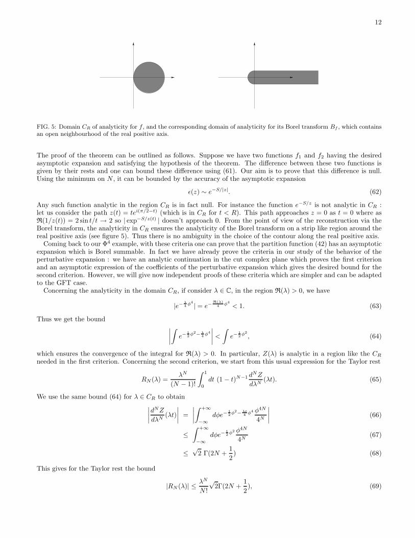
FIG. 5: Domain CR of analyticity for f , and the corresponding domain of analyticity for its Borel transform Bf , which containsan open neighbourhood of the real positive axis.

The proof of the theorem can be outlined as follows. Suppose we have two functions f1 and f2 having the desiredasymptotic expansion and satisfying the hypothesis of the theorem. The difference between these two functions isgiven by their rests and one can bound these difference using (61). Our aim is to prove that this difference is null.Using the minimum on N , it can be bounded by the accuracy of the asymptotic expansion

ǫ(z) ∼ e−S/|z|. (62)

Any such function analytic in the region CR is in fact null. For instance the function e−S/z is not analytic in CR :let us consider the path z(t) = tei(π/2−t) (which is in CR for t < R). This path approaches z = 0 as t = 0 where asR(1/z(t)) = 2 sin t/t → 2 so | exp−S/z(t) | doesn’t approach 0. From the point of view of the reconstruction via theBorel transform, the analyticity in CR ensures the analyticity of the Borel transform on a strip like region around thereal positive axis (see figure 5). Thus there is no ambiguity in the choice of the contour along the real positive axis.

Coming back to our Φ4 example, with these criteria one can prove that the partition function (42) has an asymptoticexpansion which is Borel summable. In fact we have already prove the criteria in our study of the behavior of theperturbative expansion : we have an analytic continuation in the cut complex plane which proves the first criterionand an asymptotic expression of the coefficients of the perturbative expansion which gives the desired bound for thesecond criterion. However, we will give now independent proofs of these criteria which are simpler and can be adaptedto the GFT case.

Concerning the analyticity in the domain CR, if consider λ ∈ C, in the region R(λ) > 0, we have

|e−λ4 φ

4 | = e−R(λ)

4 φ4

< 1. (63)

Thus we get the bound∣

∣

∣

∣

∫

e−12φ

2−λ4 φ

4

∣

∣

∣

∣

<

∫

e−12φ

2

, (64)

which ensures the convergence of the integral for R(λ) > 0. In particular, Z(λ) is analytic in a region like the CRneeded in the first criterion. Concerning the second criterion, we start from this usual expression for the Taylor rest

RN (λ) =λN

(N − 1)!

∫ 1

0

dt (1 − t)N−1 dNZ

dλN(λt). (65)

We use the same bound (64) for λ ∈ CR to obtain∣

∣

∣

∣

dNZ

dλN(λt)

∣

∣

∣

∣

=

∣

∣

∣

∣

∫ +∞

−∞dφe−

12φ

2−λt4 φ

4 φ4N

4N

∣

∣

∣

∣

(66)

≤∫ +∞

−∞dφe−

12φ

2 φ4N

4N(67)

≤√

2 Γ(2N +1

2) (68)

This gives for the Taylor rest the bound

|RN (λ)| ≤ λN

N !

√2Γ(2N +

1

2), (69)

13

Due to the multiplicative relation on the Γ-function Γ(2x) = 1√2π

22x−1/2Γ(x)Γ(x + 1/2), one can find a bound

Γ(2N + 12 )

N !< CANΓ(N + b), (70)

which leads a bound of the required form for the rest. The partition function satisfies the two Sokal criteria, henceits perturbative expansion is uniquely Borel summable.

IV. MODIFICATION OF THE GROUP FIELD THEORY MODEL

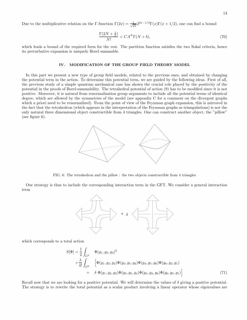
In this part we present a new type of group field models, related to the previous ones, and obtained by changingthe potential term in the action. To determine this potential term, we are guided by the following ideas. First of all,the previous study of a simple quantum mechanical case has shown the crucial role played by the positivity of thepotential in the proofs of Borel-summability. The tetrahedral potential of action (9) has to be modified since it is notpositive. Moreover, it is natural from renormalisation group arguments to include all the potential terms of identicaldegree, which are allowed by the symmetries of the model (see appendix C for a comment on the divergent graphswhich a priori need to be renormalized). From the point of view of the Feynman graph expansion, this is mirrored inthe fact that the tetrahedron (which appears in the interpretation of the Feynman graphs as triangulations) is not theonly natural three dimensional object constructible from 4 triangles. One can construct another object, the ”pillow”(see figure 6).

FIG. 6: The tetrahedron and the pillow : the two objects constructible from 4 triangles

Our strategy is thus to include the corresponding interaction term in the GFT. We consider a general interactionterm

+ δ

which corresponds to a total action

S[Φ] =1

2

∫

G3

Φ(g1, g2, g3)2

+λ

4!

∫

G6

[

Φ(g1, g2, g3)Φ(g3, g5, g4)Φ(g4, g5, g6)Φ(g6, g2, g1)

+ δ Φ(g1, g2, g3)Φ(g3, g5, g4)Φ(g4, g2, g6)Φ(g6, g5, g1)]

(71)

Recall now that we are looking for a positive potential. We will determine the values of δ giving a positive potential.The strategy is to rewrite the total potential as a scalar product involving a linear operator whose eigenvalues are

14

= +

j1j1j1 j2

j2j2

j3j3

j4j4j4

j5j5j5

j6j6 kk

FIG. 7: A pillow is obtained by the gluing of two tetrahedra along two common faces, introducing an additional internal edgek

under control. Let us define the object

A(g1, g2, g5, g4) =

∫

G

dg Φ(g1, g2, g)Φ(g, g5, g4) (72)

The pillow term is found to be

∫

G4

A(g1, g2, g5, g4)A(g1, g2, g5, g4) = 〈A,A〉 (73)

while the tetrahedron term can be written as∫

G4

A(g1, g2, g5, g4)[T A](g4, g2, g5, g1) = 〈A, T A〉 (74)

where T is the just the linear operator acting on A

T : A(g1, g2, g5, g4) → A(g4, g2, g5, g1). (75)

This operator T is a permutation, thus T 2 = Id and its eigenvalues are simply ±1. The total interaction term wedefined is thus

〈A, [Id+ δT ]A〉 (76)

whose eigenvalues are 1 ± δ. We obtained a positive potential for |δ| ≤ 1. This complete the construction of themodified potential term.

At first sight, one could say that such a modification of the potential term will lead to a drastic modificationof the models, first because we will sum over different kind of triangulations, second because the weights will bedifferent. We will see that the modification is not so drastic. We can first observe that geometrically, a pillow is nomore than the gluing of two tetrahedra, along two common faces (see figure 7). This allows us to relate in uniquemanner each ’generalized’ triangulation (made of pillows and tetrahedra) to a ’real’ triangulation (made only oftetrahedra) by replacing each pillow by a pair of tetrahedra glued along two common faces. The total sum generatedby the perturbative expansion can be reorganized by putting together the weights of all the generalized triangulationsrelated to a given real triangulation, and summing only over the real triangulations. The real triangulations containingpairs of tetrahedra glued along two common faces are called ’irregular’, while the other ones are called ’regular’. Wecan see that this reorganization concerns only the irregular triangulations.

Our results are the following. We consider the modifications of the Ambjorn and Boulatov GFT given by the action(71). In both cases the perturbative expansion of the partition function is uniquely Borel summable. In the case ofthe modified Ambjorn model, the perturbative expansion is written

Z(λ, µ) =∑

∆∈Treg

1

Sym[∆]λN3µN1 +

∑

∆∈Tirreg

1

Sym[∆]λN3−kµN1−k

(

µλ− 1

2

)k

, (77)

15

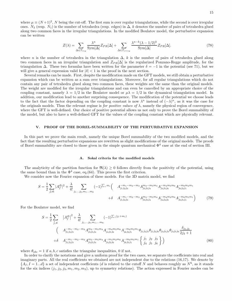
where µ ≡ (N+1)2, N being the cut-off. The first sum is over regular triangulations, while the second is over irregularones. N3 (resp. N1) is the number of tetrahedra (resp. edges) in ∆, k denotes the number of pairs of tetrahedra gluedalong two common faces in the irregular triangulations. In the modified Boulatov model, the perturbative expansioncan be written

Z(λ) =∑

∆∈Treg

λn

Sym[∆]ZPR[∆] +

∑

∆∈Tirreg

λn−k(λ− 1/2)k

Sym[∆]ZPR[∆]. (78)

where n is the number of tetrahedra in the triangulation ∆, k is the number of pairs of tetrahedra glued alongtwo common faces in an irregular triangulation and ZPR[∆] is the regularized Ponzano-Regge amplitude, for thetriangulation ∆. These two formulas have been written for the parameter δ = −1 in the potential (see 71), but wewill give a general expression valid for |δ| < 1 in the proof in the next section.

Several remarks can be made. First, despite the modification made on the GFT models, we still obtain a perturbativeexpansion which can be written as a sum over triangulations. Moreover, for all regular triangulations which do notcontain any pair of tetrahedra glued along two common faces, these weights are the same than the original models.The weight are modified for the irregular triangulations and can even be cancelled by an appropriate choice of thecoupling constant, namely λ = 1/2 in the Boulatov model or µλ = 1/2 in the dynamical triangulation model. Inaddition, our modification lead to another surprising consequence. The modification of the potential we choose leadsto the fact that the factor depending on the coupling constant is now λn instead of (−λ)n, as it was the case forthe originals models. Thus the relevant regime is for positive values of λ, namely the physical region of convergence,where the GFT is well-defined. Our choice of positive potential allows us not only to prove the Borel summability ofthe model, but also to have a well-defined GFT for the values of the coupling constant which are physically relevant.

V. PROOF OF THE BOREL-SUMMABILITY OF THE PERTURBATIVE EXPANSION

In this part we prove the main result, namely the unique Borel summability of the two modified models, and thefact that the resulting perturbative expansions are rewritten as slight modifications of the original models. The proofsof Borel summability are closed to those given in the simple quantum mechanical Φ4 case at the end of section III.

A. Sokal criteria for the modified models

The analyticity of the partition function for R(λ) ≥ 0 follows directly from the positivity of the potential, usingthe same bound than in the Φ4 case, eq.(64). This proves the first criterion.

We consider now the Fourier expansion of these models. For the 3D matrix model, we find

S =1

2

∑

~,~m

|A~m~ |2 +

λ

4!

∑

j1...j6,m1...m6

(−1)∑

i mi

(

A−m1−m2−m3

j1j2j3Am3−m5m4

j3j5j4A−m4m5m6

j4j5j6A−m6m2m1

j6j2j1

+δ A−m1−m2−m3

j1j2j3Am3−m5m4

j3j5j4A−m4m2m6

j4j2j6A−m6m5m1

j6j5j1

)

(79)

For the Boulatov model, we find

S =1

2

∑

~j,~n

∣

∣A~m~

∣

∣

2+λ

4!

∑

j1,...j6,m1,...m6

(−1)∑

i(ji+mi)

(

A−m1−m2−m3

j1j2j3Am3−m5m4

j3j5j4A−m4m5m6

j4j5j6A−m6m2m1

j6j2j1θj1j2j3θj1j2j6θj4j5j3θj4j5j6

δj3,j62j3 + 1

+δ A−m1−m2−m3

j1j2j3Am3−m5m4

j3j5j4A−m4m2m6

j4j2j6A−m6m5m1

j6j5j1

{

j1 j2 j3j4 j5 j6

}

)

(80)

where θabc = 1 if a, b, c satisfies the triangular inequalities, 0 if not.In order to clarify the notations and give a uniform proof for the two cases, we separate the coefficients into real and

imaginary parts. All the real coefficients we obtained are not independent due to the relations (16,17). We denote by{AI , I = 1...d} a set of independent coefficients (d is related to the cutoff N and behaves roughly as N6, as it standsfor the six indices (j1, j2, j3,m1,m2,m3), up to symmetry relations). The action expressed in Fourier modes can be

16

rewritten as

S =1

2

∑

I

A2I +

λ

4!

∑

IJKL

AIAJMIJKLAKAL (81)

with M IJKL a four indices matrix representing the potential, whose positivity is translated into

∑

IJKL

AIAJMIJKLAKAL ≥ 0 ∀AI (82)

The partition function is

Z(λ) =

∫

Rd

[

∏

I

dAI

]

exp

{

−1

2

∑

I

A2I −

λ

4!

∑

IJKL

AiAJMIJKLAKAL

}

(83)

We want to consider the asymptotic expansion of Z(λ)

Z(λ) =

n−1∑

p=0

apλp +Rn(λ) (84)

We use the expression (65) for the Taylor rest. Consider the expression for dnZdλn obtained by deriving n times the

original expression (83)

dnZ

dλn(λt) =

∫

Rd

[∏

I

dAI ] exp

[

−1

2

∑

I

A2I −

λt

4!

∑

IJKL

AIAJMIJKLAKAL

](

− 1

4!

∑

IJKL

AIAJMIJKLAKAL

)n

(85)

One look for a bound of the module of the integrand. The real part of the potential is positive for λ ∈ CR, thus

∣

∣

∣

∣

∣

exp

[

−1

2

∑

I

A2I −

λt

4!

∑

IJKL

AIAJMIJKLAKAL

]∣

∣

∣

∣

∣

< exp

[

−1

2

∑

I

A2I

]

(86)

Thus one obtains the following bound

∣

∣

∣

∣

dnZ

dλn(λt)

∣

∣

∣

∣

≤∫

Rd

[∏

I

dAI ] exp

[

−1

2

∑

I

A2I

] ∣

∣

∣

∣

∣

1

4!

∑

IJKL

AIAJMIJKLAKAL

∣

∣

∣

∣

∣

n

(87)

Let us denote

S = SupIJKL |M IJKL| (88)

One gets the bound

∣

∣

∣

∣

dnZ

dλn(λt)

∣

∣

∣

∣

≤ Sn

(4!)n

∫

Rd

[∏

I

dAI ] exp

[

−1

2

∑

I

A2I

](

∑

IJKL

|AIAJAKAL|)n

(89)

The RHS integral is symmetric over the AI , thus one can write it as d! times the integral over the domain A1 > A2 >... > Ad (recall that d denotes the total number of Fourier modes and depends polynomially on the cut-off N). Inthat case,

∑

IJKL

|AIAJAKAL| < d4|A1|4 (90)

Then we can decouple the integrals over the AI on LHS of (89) and extend the integral for I 6= 1 in order to get d− 1gaussian integrals. The integral over A1 gives a Γ−function

∣

∣

∣

∣

dnZ

dλn(λt)

∣

∣

∣

∣

≤ d!

(

S d4

4!

)n(∫

R

dA1 e− 1

2A21A4n

1

)(∫

R

dA e−12A

2

)d−1

(91)

17

and∣

∣

∣

∣

dnZ

dλn(λt)

∣

∣

∣

∣

≤(√

2 d! πd−12

)

(

S d4

3!

)n

Γ(2n+1

2) (92)

Coming back to the expression of the Taylor rest (65), one gets a bound

|Rn(λ)| ≤ C(

S d4

3!

)nΓ(2n+ 1

2 )

n!|λ|n (93)

which is of the required form, with constants depending on d, hence on the cut-off N . The perturbative expansion ofour model satisfies the two Sokal criteria and thus is uniquely Borel summable.

B. Reorganization of the perturbative expansion

We now analyze the consequences of the introduction of the pillow interaction term on the expression of the sumover triangulations. The perturbative expansions of modified GFT models give us a sum over triangulations madewith pillows and tetrahedra. However, we have seen that geometrically a pillow is obtained by gluing together twotetrahedra along two common faces.

In the matrix model case, the amplitude associated to a pillow is

Apillow = −λ (94)

while the amplitude for two tetrahedra glued along two common faces (see figure 7) is

A2tetra = (−δλ)2∑

k≤N(2k + 1) = (δλ)2(N + 1)2 (95)

Thus, if we compare the total amplitude for a (generalized) triangulation ∆ containing k pillows to the related realtriangulation ∆ obtained by replacing all the pillows by pairs of tetrahedra, we obtain (recall µ = (N + 1)2)

Z[∆] =

(

−1

2

1

λδ2µ

)k

Z[∆] (96)

The one-half factor comes from the fact that the symmetry factor for two tetrahedra is twice the symmetry factorfor one pillow. Consider a real triangulation ∆ made only with N3 tetrahedra and N1 edges, and such that 2k of itstetrahedra are glued by pair along two of their common faces. There are several generalized triangulations related toit : C1

k (binomial coefficients) triangulations with one pair of such tetrahedra replaced by a pillow, C2k triangulations

with two such pairs replaced by pillow etc...Counting together all their weights we obtain

Z[∆] = (−δλ)N3

(

1+(−2δ2λµ)−1C1k+(−2δ2λµ)−2C2

k+...+(−2δ2λµ)−kCkk

)

µN1 = (−δλ)N3(1−(2δ2λµ)−1)kµN1 (97)

This shows that one can reorganize our sum as a sum over real triangulations of the amplitude (−δλ)N3µN1 , exceptthe fact that an irregular triangulation containing k pairs of tetrahedra glued together along two common faces hasa weight modified by a factor (1 − (2δ2λµ)−1)k. Which gives

Z(λ, µ) =∑

∆

1

Sym[∆](−δλ)N3−kµN1−k

(

−δµλ+1

2δ

)k

. (98)

Recall that the positivity of the potential is valid for |δ| ≤ 1. For instance for δ = −1, we recover the result (77)announced in section IV.

The same reorganization can be performed on the perturbative expansion of the modified Boulatov model. Theamplitude associated to a pillow is

Apillow = −λ δj3,j62j3 + 1

(99)

18

The amplitude associated to the gluing of two tetrahedra along two common faces (see figure 7) is

A2tetra = (−δλ)2∑

k

(2jk + 1)

{

j1 j2 kj4 j5 j3

}{

j1 j2 kj4 j5 j6

}

= (δλ)2δj3,j6

2j3 + 1(100)

due to the orthogonality relation. As before, this means that a triangulation containing a pillow has an amplitudewhich is (1−2δ2λ)−1 times the amplitude of the same triangulation, with the pillow replaced by two tetrahedra gluedalong two common faces. We reorganize the sum in the same way than before and obtain

Z(λ) =∑

∆

1

Sym[∆](−δλ)n(1 − 1

2δ2λ)kZPR[∆] =

∑

∆

1

Sym[∆](−δλ)n−k(−δλ+

1

2δ)kZPR[∆]. (101)

The result (78) given in section IV is recovered for δ = −1.

VI. CONCLUSION

In this paper we have studied the possibility of defining the sum over topologies of three dimensional gravity inthe context of dynamical triangulation or spin foam models. We have provided an example of a group field theorymodel which is uniquely Borel summable in the physical regime of the theory. In order to do so we have used thefact that three dimensional triangulations are generated by a group field theory with a quartic potential and wehave shown that this potential can be naturally modified in order to be positive. Therefore, the message we wantedto convey here is that it is possible to resum the sum over triangulation if one accepts to take for serious the nonperturbative information provided to us by the GFT, namely the instantonic solutions. One can still question whatis the physical content of this non perturbative information. This is a direction of investigation we are following.Finally, 4 dimensional triangulations are generated by quintic potentials and we may think that there is no naturalmodification of this potential leading to a uniquely resummable theory. This is an issue that deserves to be studiedand could mean that we need more non-perturbative input in this case in order to give a meaning to the resummedseries.

Acknowledgments : We would like to thank J. Ambjorn for a discussion. D. L. is supported by a MENRT grantand Eurodoc program from Region Rhone-Alpes. L. F. is supported by CNRS and an ACI-Blanche grant.

APPENDIX A: REPRESENTATIONS OF SO(3) AND RACAH-WIGNER SYMBOLS

The irreducible unitary inequivalent representations of SU(2) are labelled by a half-integer j. The representations ofSO(3) are just the integer spin representation of SU(2). The space of representation is denoted Vj and has dimensiondimj = 2j+1. All the representations are self-dual V ∗

j = Vj . The matrix of representations are denoted Djmn(g). We

have the relation

Djmn(g) = (−1)m−nDj

−m−n(g) (A1)

Given three representations Vj1 , Vj2 , Vj3 , it exists only one (up to normalization) intertwiner ı : Vj1 ⊗ Vj2 ⊗ Vj3 → C.One can express it by using the Wigner 3j-symbol whose normalization is

∑

~m

C~j~mC

~j~m = 1 (A2)

The Racah-Wigner 6j symbol is defined by{

j1 j2 j3j4 j5 j6

}

=∑

mi

(−1)j4+j5+j6+m4+m5+m6Cj1j2j3m1m2m3Cj5j6j1m5−m6m1

Cj6j4j2m6−m4m2Cj4j5j3m4−m5m3

(A3)

It satisfies the orthogonality relation

∑

j6

(2j3 + 1)(2j6 + 1)

{

j1 j2 j3j4 j5 j6

}{

j1 j2 j′3j4 j5 j6

}

= δj3j′3θj1j2j3θj3j4j5 (A4)

19

where θabc = 1 if a, b, c satisfy the triangular inequalities, 0 in the contrary case. The fact that the integral of amatrix representation gives a projection on the space of invariant vectors leads to the following relations (using thenormalized Haar measure)

∫

SU(2)

dgDjmn(g)D

j′

m′n′(g) =1

djδjj

′

δmm′δnn′ , (A5)

and∫

dgDj1m1n1

(g)Dj2m2n2

(g)Dj3m3n3

(g) = C~j~mC

~j~n. (A6)

APPENDIX B: THE NON-COMMUTATIVE 2-SPHERE

A non-commutative space X is a space which is defined by specifying the (non-commutative) algebra of squareintegrable functions on it L2(X). In this part we recall some facts about the construction of the non-commutativesphere. The sphere S2 can be described by the algebra L2(S2). A basis of this algebra is given by polynomes of(x1, x2, x3) such that

x21 + x2

2 + x23 = 1 (B1)

Another possible basis is given the spherical harmonics Y lm and arises from the decomposition

L2(S2) =

+∞⊕

l=1

Vl. (B2)

where Vl is the spin j representation of SO(3). Let us construct the non-commutative sphere S2N (for a deformation

parameter 1/N) by giving its algebra of functions, obtained by starting from the first basis described for the sphere.Let us consider VN

2, the spin N/2 representation of the algebra su(2); DN/2 are the matrices of representation. Let

us define

Xi =1

NDN/2(Ji) (B3)

where the Ji are the generators of su(2). Xi is in VN2. Due to the Lie algebra relations of su(2), one gets

∑

i

XiXi = 1 (B4)

[Xi, Xj] =1

NǫijkXk (B5)

The first relation is the analogue of the relation (eq. B1), and the second one says that the Xi are commuting in thelarge N limit. This facts lead us to see the Xi as non-commuting spherical coordinates, and to define the algebra offunctions on the non-commutative sphere as the algebra of endomorphism of VN

2

L2(S2N ) = End(VN

2) ∼ VN

2⊗ V ∗

N2

(B6)

The right-hand side can be written as

N⊕

l=0

Vl, (B7)

which shows that the parameter N is nothing more than the cut-off in the decomposition of the functions overthe sphere into spherical harmonics. As the endomorphisms of VN

2are the non-commutative counterpart of the

polynomials over the sphere, a natural question is to ask what are the non-commutative counterpart of the sphericalharmonics basis. Indeed, each spherical harmonic Y l,m for l ≤ N can be represented as an endomorphism of VN

2by

Y l,m −→ [Y lm]ij = Cl N

2N2

m i j . (B8)

20

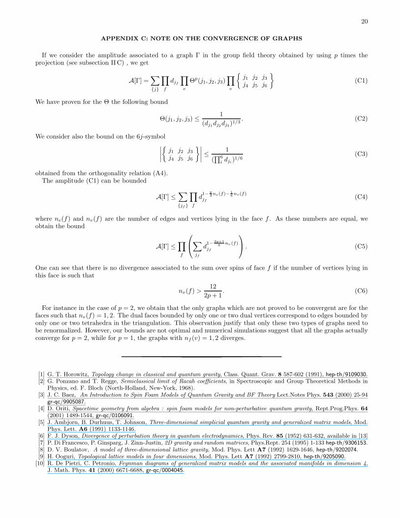
APPENDIX C: NOTE ON THE CONVERGENCE OF GRAPHS

If we consider the amplitude associated to a graph Γ in the group field theory obtained by using p times theprojection (see subsection II C) , we get

A[Γ] =∑

{j}

∏

f

djf∏

e

Θp(j1, j2, j3)∏

v

{

j1 j2 j3j4 j5 j6

}

(C1)

We have proven for the Θ the following bound

Θ(j1, j2, j3) ≤1

(dj1dj2dj3)1/3

. (C2)

We consider also the bound on the 6j-symbol∣

∣

∣

∣

{

j1 j2 j3j4 j5 j6

}∣

∣

∣

∣

≤ 1

(∏6i dji)

1/6(C3)

obtained from the orthogonality relation (A4).The amplitude (C1) can be bounded

A[Γ] ≤∑

{jf}

∏

f

d1− p

3ne(f)− 16nv(f)

jf(C4)

where ne(f) and nv(f) are the number of edges and vertices lying in the face f . As these numbers are equal, weobtain the bound

A[Γ] ≤∏

f

∑

jf

d1− 2p+1

6 nv(f)jf

. (C5)

One can see that there is no divergence associated to the sum over spins of face f if the number of vertices lying inthis face is such that

nv(f) >12

2p+ 1. (C6)

For instance in the case of p = 2, we obtain that the only graphs which are not proved to be convergent are for thefaces such that nv(f) = 1, 2. The dual faces bounded by only one or two dual vertices correspond to edges bounded byonly one or two tetrahedra in the triangulation. This observation justify that only these two types of graphs need tobe renormalized. However, our bounds are not optimal and numerical simulations suggest that all the graphs actuallyconverge for p = 2, while for p = 1, the graphs with nf (v) = 1, 2 diverges.

[1] G. T. Horowitz, Topology change in classical and quantum gravity, Class. Quant. Grav. 8 587-602 (1991), hep-th/9109030.[2] G. Ponzano and T. Regge, Semiclassical limit of Racah coefficients, in Spectroscopic and Group Theoretical Methods in

Physics, ed. F. Bloch (North-Holland, New-York, 1968).[3] J. C. Baez, An Introduction to Spin Foam Models of Quantum Gravity and BF Theory Lect.Notes Phys. 543 (2000) 25-94

gr-qc/9905087.[4] D. Oriti, Spacetime geometry from algebra : spin foam models for non-perturbative quantum gravity, Rept.Prog.Phys. 64

(2001) 1489-1544, gr-qc/0106091.[5] J. Ambjorn, B. Durhuus, T. Johnson, Three-dimensional simplicial quantum gravity and generalized matrix models, Mod.

Phys. Lett. A6 (1991) 1133-1146.[6] F. J. Dyson, Divergence of perturbation theory in quantum electrodynamics, Phys. Rev. 85 (1952) 631-632, available in [13][7] P. Di Francesco, P. Ginsparg, J. Zinn-Justin, 2D gravity and random matrices, Phys.Rept. 254 (1995) 1-133 hep-th/9306153.[8] D. V. Boulatov, A model of three-dimensional lattice gravity, Mod. Phys. Lett A7 (1992) 1629-1646, hep-th/9202074.[9] H. Ooguri, Topological lattice models in four dimensions, Mod. Phys. Lett A7 (1992) 2799-2810, hep-th/9205090.

[10] R. De Pietri, C. Petronio, Feynman diagrams of generalized matrix models and the associated manifolds in dimension 4,J. Math. Phys. 41 (2000) 6671-6688, gr-qc/0004045.

21

[11] R. De Pietri, L. Freidel, K. Krasnov, C. Rovelli, Barrett-Crane model from a Boulatov-Ooguri field theory over a homoge-

neous space, Nucl.Phys. B574 (2000) 785-806 hep-th/9907154.[12] M. P. Reisenberger, C. Rovelli, Spacetime as a Feynman diagram: the connection formulation, Class.Quant.Grav. 18

(2001) 121-140, gr-qc/0002095.[13] J. C. Le Guillou and J. Zinn-Justin, Eds, Large-order behaviour of perturbation theory, Current physics sources and

comments Vol. 7 (North-Holland, Amsterdam, 1990).[14] A. Perez, C. Rovelli, A spin foam model without bubble divergences, Nucl.Phys. B599 (2001) 255-282, gr-qc/0006107.[15] A. Perez, Finiteness of a spinfoam model for euclidean quantum general relativity, Nucl.Phys. B599 (2001) 427-434

gr-qc/0011058.[16] S. Ramgoolam, On spherical harmonics for fuzzy spheres in diverse dimensions, Nucl.Phys. B610 (2001) 461-488, hep-

th/0105006.[17] J. Madore, The fuzzy sphere, Class. Quant. Grav. 9 (1992) 69-87.[18] L. Freidel, K. Krasnov, Simple Spin Networks as Feynman Graphs, J.Math.Phys. 41 (2000) 1681-1690, hep-th/9903192.[19] D. Oriti, Boundary terms in the Barrett-Crane spin foam model and consistent gluing, Phys.Lett. B532 (2002) 363-372,

gr-qc/0201077.[20] A. D. Sokal, An improvement of Watson’s theorem on Borel summability, J. Math. Phys. 21 (1980) 261-263.