Inductively generated formal topologies

Thierry Coquand†, Giovanni Sambin‡,

Jan Smith†, Silvio Valentini‡

†Dept. of Computing Science ‡Dip. di Matematica Pura ed Applicata

Chalmers University Universita di Padova

S–41296 Goteborg, Swedish via Belzoni 7, I–35131 Padova, Italy

coquand,smith@cs.chalmers.se sambin,silvio@math.unipd.it

December 6, 2000

Abstract

Formal topology is today an established topic in the development of

constructive, that is intuitionistic and predicative, mathematics. Many

classical results of general topology have been already brought into the

realm of constructive mathematics by using formal topology and also new

light on basic topological notions was gained with this approach which

allows distinction which are not sensible in classical topology.

Here we give a systematic exposition of one of the main tools in formal

topology: inductive generation. In fact, many formal topologies can be

presented in a predicative way by an inductive generation and thus their

properties can be proved inductively.

Contents

1 The notion of formal topology 31.1 Concrete topological spaces . . . . . . . . . . . . . . . . . . . . . 41.2 Formal topologies . . . . . . . . . . . . . . . . . . . . . . . . . . . 5

2 Three problems and their solution 82.1 Formal topologies with pre-order . . . . . . . . . . . . . . . . . . 92.2 The problem of transitivity . . . . . . . . . . . . . . . . . . . . . 10

2.2.1 Fix-points and saturation . . . . . . . . . . . . . . . . . . 132.3 Dealing with the positivity predicate . . . . . . . . . . . . . . . . 16

3 Inductive generation 173.1 Set-based axioms and set-based relations . . . . . . . . . . . . . . 183.2 Inductive generation of formal topologies . . . . . . . . . . . . . . 193.3 Localizing the axioms . . . . . . . . . . . . . . . . . . . . . . . . 24

1

4 Some examples and one counter-example 254.1 The Cantor space . . . . . . . . . . . . . . . . . . . . . . . . . . . 264.2 The real numbers . . . . . . . . . . . . . . . . . . . . . . . . . . . 274.3 Cartesian product revisited . . . . . . . . . . . . . . . . . . . . . 284.4 All representable topologies have an axiom-set . . . . . . . . . . 294.5 Unitary and finitary formal topologies . . . . . . . . . . . . . . . 304.6 A covering which cannot be inductively defined . . . . . . . . . . 32

ForewordThe aim of formal topology is to develop topology in a constructive frame-

work where “constructive” is meant here to include both intuitionistic and pred-icative. We can fix, if desidered, such a foundational theory to be Martin-Lof’sconstructive set theory [ML84], but we actually often do not use its full strength.A monograph on formal topology is under construction; it will include all thepreliminaries on type theory which we are here compelled to skip, and moredetails on the basic notions.

Also other approaches to intuitionistic topology have been developed, no-tably the theory of locales, which is usually developed in topos theory. Working,as we do, with a foundational theory without power-sets brings to distinctionsbetween notions or methods which are irrelevant in a foundation like topos the-ory, and hence there neglected. The most striking example is that it does notseem possible to define predicatively the (co)product of two formal topologies,unless they are inductively generated. It also brings to new, sometime unex-pected connections, like that with inductive definitions, which constitute a keytool for proof theory (cfr. [BFPS81] and [Acz77]).

The paper is organized as follows. We first give a short introduction toformal topology by showing how to move from the classical and impredicativecase of a concrete topological space to the constructive and abstract notion offormal topology. Then the main topic of the paper is discussed, that is, theproblem of inductive generation of formal topologies. We will both show theproblems that must be solved to inductively generate a formal topology and wewill present our solutions of such problems. Finally, the last part of the paper isdevoted to show that most of the interesting formal topologies can be generatedinductively. But we will also show that there are formal topologies that cannotbe inductively generated; noticeably, we will also show that the example of non-inductively generated formal topology that we were able to build is classicallyequivalent to a formal topology which can be inductively generated.

Let us spend a few words to explain the contribution of the various authorsto the paper. The idea of an inductive generation of the mathematical struc-tures suitable for a constructive approach to topology can probably be tracedback to the works [FG82] (see their “postscript lemma”) and [Joh83] (see lemmaIV.1.1) or even to Brouwer, but an explicit mention of an inductive definitionof cover appeared in [Sam87]. After this, proof-theoretic methods in formaltopology was exploited more systematically. Nevertheless this first naive ap-proach to inductive generation of formal topologies payed little attention of thefoundational problems involved.

2

Then, adopting Johnstone’s definition of coverages, a simple and constructiveproof of Tychonoff’s theorem for locales was presented in [Coq92]. Readingthat paper, Sambin realized the need for an explicit inductive definition inthe framework of formal topologies. So he proposed an inductive definitionof (co)product of formal topologies, and he also suggested to look for a “proof-theoretic” proof of Tychonoff’s theorem in the framework of formal topologies.To this aim a theorem on the generation of formal topologies was proved incollaboration by Sambin and Valentini and it appeared in [NV97].

After knowing about the generation of the formal topology producing realnumbers as a formal space in [Sor95], Coquand and P. Dybjer arose the problemwith the impredicativity of that definition and Coquand provided a differentgeneration for real numbers which is undoubtable predicative. It was publishedin [CN96] and we present it now in section 4.2.

A key observation came then by Peter Aczel who pointed out that assum-ing the cover to be defined inductively is equivalent to existence of fixed pointsfor monotone operators; the latter is a well-known principle which has not yetfound a predicative justification. Soon after, Coquand and Sambin-Valentiniindependently obtained essentially the main theorem on inductive generationthat we present here. Coquand’s method was inspired by Dragalin’s definitionin [Dra87], while Sambin-Valentini combined previous work on localized transi-tivity (see section 3.2) with Coquand’s ideas for the inductive generation of theformal topology of real numbers.

More systematic collaboration started immediately after, and it producedall the extra results and applications. In particular, Valentini proved thatrepresentable and unitary formal topologies can be inductively generated andCoquand and Smith provided the proof that there are example of Dedekind-MacNeille cover which are not set-based.

In the whole paper we follow the notation introduced in [SV98]. We areconfident that the reader will understand the notation with no problem sincemost of the work in [SV98] was made purposely to be able to use standardmathematical notation and still remain completely within Martin-Lof construc-tive set theory. Anyhow it can be useful to stress at least one thing: we will usethe standard symbol ∈ to mean the membership relation between an elementand a set or a collection, while we switch to the symbol ε for the relation ofmembership between an element and a subset, since we want to stress on thefact that a subset is never a set but just a propositional function. It can beuseful to recall that, provided S is a set, a one of its elements and U one of itssubsets, a ∈ S is a judgement while aεU is a proposition such that aεU is trueif and only if U(a) is true; hence two subsets U and V of S are extensionallyequal, notation U =S V , if and only if (∀x ∈ S) (U(x) ↔ V (x)).

1 The notion of formal topology

We recall in this section some of the motivations which lead to the notionof formal topology, which is the central tool of the approach to constructive

3

topology adopted here.It is convenient to start from a short analysis of the traditional definition of

topological space, so that we can underline which steps are problematic from aconstructive point of view, and how they are solved.

1.1 Concrete topological spaces

The classical definition reads: (X,Ω(X)) is a topological space if X is a set andΩ(X) is a subset of P(X) which satisfies:

(Ω1) ∅, X ∈ Ω(X);

(Ω2) Ω(X) is closed under finite intersection;

(Ω3) Ω(X) is closed under arbitrary union.

Usually, elements of X are called points and elements of Ω(X) are called opens.The quantification implicitly used in (Ω3) is of the third order, since it says

(∀F ⊆ Ω(X))∪F ∈ Ω(X), that is (∀F ∈ P(P(X)))(F ⊆ Ω(X) → ∪F ∈ Ω(X)).The idea is that we can “go down” one step by thinking of Ω(X) as a familyof subsets indexed by a set S through a map N : S → P(X), since we can nowquantify on S rather than on Ω(X).

But we still have to say (∀U ∈ P(S))(∃c ∈ S) (∪aεUN(a) = N(c)), which isalso impredicative.

We can “go down” another step by defining opens to be of the form N(U) ≡∪aεUN(a) for an arbitrary subset U of S. In this way ∅ is open, becauseN(∅) = ∅, and closure under union is automatic, because obviously ∪i∈IN(Ui) =N(∪i∈IUi). So, all we have to do is to require N(S) to be the wholeX and closureunder finite intersections, that is, condition (Ω2). It is not difficult to realizethat this amounts to the standard definition saying that N(a) ⊆ X | a ∈ S isa base (see for instance [Eng77]). So we reach the following definition:

Definition 1.1 A concrete topological space is a triple X ≡ (X,S,N) where Xis a set of concrete points, S is a set of observables, N is a map from S intosubsets of X, called the neighborhood map, which satisfies

(B1) X = ∪a∈SN(a)

(B2) (∀a, b ∈ S)(∀x ∈ X) (xεN(a) ∩ N(b) →(∃c ∈ S) (xεN(c) & N(c) ⊆ N(a) ∩ N(b)))

Note that this definition re-establishes a balance between the side of points,which we call the concrete side, and the side of observables, or formal basicneighbourhoods, which we call the formal side.

Note that (B2) is just a rigorous writing of the usual condition stating thatif N(a) and N(b) are two neighbourhoods of x then there exists a neighborhoodN(c) of x which is contained both in N(a) and N(b) and this is all what we needto obtain closure under intersection.

4

Now, a map N : S → P(X) is a propositional function with two arguments,that is N(x)(a) prop [x : X, a : S], that is a binary relation. Then we write itmore suggestively as

x a prop [x : X, a : S]

and read it “x lies in a” or “x forces a”.It is convenient to use also a few abbreviations:

x U ≡ (∃bεU) x bext(a) ≡ x : X | x aext(U) ≡ ∪aεU ext(a)

Hence x a is the same as xεext(a) and x U is the same as xεext(U); thusthe map N coincides with ext.

Then (B1) and (B2) can be rewritten as

(B1) (∀x ∈ X)(∃a ∈ S) x a

(B2) (∀a, b ∈ S)(∀x ∈ X) ((x a) & (x b) →(∃c ∈ S) (x c & ext(c) ⊆ ext(a) & ext(c) ⊆ ext(b)))

We can make (B2) a bit shorter by introducing another abbreviation, that is

a ↓ b ≡ c : S| ext(c) ⊆ ext(a) & ext(c) ⊆ ext(b)

and by writing xεext(a) ∩ ext(b) for x a & x b, so that it becomes

(B2) (∀a, b ∈ S) ext(a) ∩ ext(b) ⊆ ext(a ↓ b)

which looks much better.Note that cεa ↓ b implies that ext(c) ⊆ ext(a) ∩ ext(b), so that ext(a ↓ b) ≡

∪cεa↓bext(c) ⊆ ext(a) ∩ ext(b). Then the definition of concrete topological spacecan be rewritten as follows:

Definition 1.2 A concrete topological space is a triple X ≡ (X,S, ) where Xand S are sets and is a binary relation from X to S satisfying:

(B1) (∀x ∈ X) x S

(B2) (∀a, b ∈ S) ext(a) ∩ ext(b) = ext(a ↓ b)

1.2 Formal topologies

The notion of formal topology arises by describing as well as possible the struc-ture induced by a concrete topological space on the formal side and then bytaking the result as an axiomatic definition. The reason for such a move is thatthe definition of concrete topological space is too restrictive, given that in themost interesting cases of topological space we do not have, from a constructive

5

point of view, a set of points to start with. Thus, we choose two primitives, thatis ⊳ and Pos, whose definition in the concrete case is

a ⊳ U ≡ (∀x ∈ X) (x a→ x U)

Pos(a) ≡ (∃x ∈ X) x a

and look for their properties which are expressible without mentioning X andits elements.

Given that x U ≡ (∃bεU) x b, the rule of ∃-introduction yields thatif aεU then a ⊳ U . Similarly, since (∀x ∈ X) (x U → x V ) is logicallyequivalent to (∀bεU)(∀x ∈ X) (x b → x V ), the rule of ∃-eliminationyields that if a ⊳ U and U ⊳ V then a ⊳ V , where U ⊳ V is a shorthand for(∀bεU) b ⊳ V which we will use from now on.

Similarly, properties of quantifiers bring to: if Pos(a) and a ⊳ U , then(∃bεU) Pos(b), which we will abbreviate by Pos(U) from now on.

To express (B1), namely that each point belongs to some neighbourhood(∀x ∈ X) x S, the naive translation into (∀a ∈ S) a ⊳ S is not enough, sinceit tells only that all basic neighbourhoods are covered by the whole S, whichfollows immediately from (aεU) → (a ⊳ U) required above. What we can do,however, is to require that only positive formal neigbourhoods contribute tocovers, or equivalently that a ⊳ U whenever a ⊳ U on the assumption Pos(a).Formally the condition is: if a ⊳ U [Pos(a)] then a ⊳ U , which is called positivity.In terms of points it would mean that, when it comes to coverings, we consideronly the subspace of X formed by the extension of the whole set S. Its validityamounts to the validity of (∃x.φ → ∀x.(φ→ ψ)) → ∀x.(φ → ψ) in intuitionisticlogic. For more details on positivity see [SVV96] where it is shown that it allowsproofs by cases on Pos(a) for deductions whose conclusion is of the form a ⊳ U .

To formulate (B2) completely within the formal side, what we can do is toweaken ext(a) ∩ ext(b) ⊆ ext(a ↓ b) into

ext(c) ⊆ ext(a) ∩ ext(b)

ext(c) ⊆ ext(a ↓ b)

that isc ⊳ a c ⊳ b

c ⊳ a ↓ b

where c ⊳ a and c ⊳ b are shorthand for c ⊳ a and c ⊳ b that we will usefrom now on.

But again, this is not enough: by definition c ⊳ a and c ⊳ b give cεa ↓ band hence c ⊳ a ↓ b. So, we would fail to express closure of open subsets underintersection. So, we first strengthen (B2) to arbitrary subsets, obtaining

ext(U) ∩ ext(V ) ⊆ ext(U ↓ V )

where U ↓ V ≡ ∪aεU,bεV a ↓ b. This holds by distributivity of P(X); in fact,

ext(U) ∩ ext(V ) ≡ ∪aεU ext(a) ∩ ∪bεV ext(b) = ∪aεU ∪bεV ext(a) ∩ ext(b)

6

So now by (B2) ext(U) ∩ ext(V ) ⊆ ∪aεU ∪bεV ext(a ↓ b) and hence the claimfollows since ext distributes unions.

Now, the preceding idea brings to

ext(c) ⊆ ext(U) ∩ ext(V )

ext(c) ⊆ ext(U ↓ V )

that isc ⊳ U c ⊳ V

c ⊳ U ↓ V

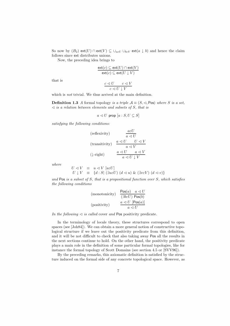
which is not trivial. We thus arrived at the main definition.

Definition 1.3 A formal topology is a triple A ≡ (S,⊳,Pos) where S is a set,⊳ is a relation between elements and subsets of S, that is

a ⊳ U prop [a : S,U ⊆ S]

satisfying the following conditions:

(reflexivity)aεU

a ⊳ U

(transitivity)a ⊳ U U ⊳ V

a ⊳ V

(↓-right)a ⊳ U a ⊳ V

a ⊳ U ↓ V

whereU ⊳ V ≡ u ⊳ V [uεU ]U ↓ V ≡ d : S| (∃uεU) (d ⊳ u) & (∃vεV ) (d ⊳ v)

and Pos is a subset of S, that is a propositional function over S, which satisfiesthe following conditions

(monotonicity)Pos(a) a ⊳ U

(∃bεU) Pos(b)

(positivity)a ⊳ U [Pos(a)]

a ⊳ U

In the following ⊳ is called cover and Pos positivity predicate.

In the terminology of locale theory, these structures correspond to openspaces (see [Joh84]). We can obtain a more general notion of constructive topo-logical structure if we leave out the positivity predicate from this definition,and it will be not difficult to check that also taking away Pos all the results inthe next sections continue to hold. On the other hand, the positivity predicateplays a main role in the definition of some particular formal topologies, like forinstance the formal topology of Scott Domains (see section 4.5 or [SVV96]).

By the preceding remarks, this axiomatic definition is satisfied by the struc-ture induced on the formal side of any concrete topological space. However, as

7

we explained above, its raison d’etre is that of gathering many more examples.We will show that lots of examples are provided by the method of inductivedefinitions, starting from given axioms for the cover relation.

Actually, this method is necessary also because otherwise we would not beable, as far as we can see, to define predicatively one of the simplest construc-tions, namely that of co-product of formal topologies (see [NV97]). In fact, letA ≡ (S,⊳A,PosA) and B ≡ (T,⊳B,PosB) be formal topologies. We want theco-product of A and B to be a formal topology

A + B ≡ (S × T,⊳A+B, PosA+B)

where S × T is the usual cartesian product of sets,

PosA+B((a, b)) ≡ PosA(a) & PosB(b)

and ⊳A+B is the minimal cover relation satisfying the axioms

(a, b) ⊳A+B U × b whenever b ∈ T and a ⊳A U,

(a, b) ⊳A+B a× V whenever a ∈ S and b ⊳B V

where of course U × b ≡ (u, b) : S × T | uεU and similarly for a× V .As it stands this is not a definition of ⊳A+B from a predicative point of view;

impredicatively, ⊳A+B would simply be the intersection of all covers containingthe required axioms. To solve this problem, we see no predicatively acceptableway other then that of an inductive definition.

2 Three problems and their solution

The conditions appearing in the definition of formal topology, though writtenin the shape of rules, must be understood as requirements of validity: if thepremises hold, also the conclusion must hold. As they stand, they are by nomeans acceptable rules to generate inductively a cover and a positivity predicate.This is obvious if one notes that the operation ↓ among subsets, which occursin the conclusion of ↓-right, is not even well defined unless we already have acomplete knowledge of the cover.

The second problem is that, as we will prove in detail, admitting transitivityas an acceptable rule for an inductive definition is equivalent to a well-known fix-point principle, which to our knowledge does not have a predicative justification.

Thirdly, one has to make up one’s mind whether the predicate Pos has toplay a role in the generation of the cover or has to be added on top of it. We willsee that the solution is a mixture. Monotonicity has an existential quantificationin its conclusion, and thus we cannot expect Pos to be generated inductively.Still positivity plays a role in the generation of the cover.

So, to transform the axiomatic definition into good inductive rules we need toface with three problems. We discuss them in detail in this section, together withthe solution we adopted, so that the reader can valuate correctly the methodand the main theorem in the next section.

8

2.1 Formal topologies with pre-order

As we reminded above, the definition of the operation ↓ among subsets dependson the covers and it requires the cover to be known. However, a crucial obser-vation is that only the trace of the cover on elements is sufficient. The idea isthen to separate covers between elements, that is a ⊳ b, from those a ⊳ U withan arbitrary subset U on the right, so that we can block the former, require ↓ onit and then generate the latter. So, we must add, to those of a formal topology,an extra primitive expressing what in the concrete case is ext(a) ⊆ ext(b). Wecan obtain this in two technically different ways. The easiest way is then toadd directly a pre-order relation a ≤ b among observables. The other is to adda binary operation • between observables, called combination, whose interpre-tation is that ext(a • b) = ext(a) ∩ ext(b), so that ext(a) ⊆ ext(b) correspondsto a • b = a. In this paper we will consider only the first solution, even if ananalogous development is possible for the second one.

Adopting a pre-order ≤ as a new primitive, the natural definition is:

Definition 2.1 A formal topology with pre-order, shortly a ≤-formal topology,is a quadruple A ≡ (S,≤,⊳,Pos) where S is a set, ≤ is a pre-order relationover S, that is ≤ is reflexive and transitive, ⊳ is a relation between elementsand subsets of S which satisfies the following conditions

(reflexivity)aεU

a ⊳ U

(transitivity)a ⊳ U U ⊳ V

a ⊳ V

(≤-left)a ≤ b b ⊳ U

a ⊳ U

(≤-right)a ⊳ U a ⊳ V

a ⊳↓ U∩ ↓ V

where ↓ U ≡ c : S| (∃uεU) c ≤ u and Pos is a positivity predicate with respectto ⊳.

The condition ≤-left is clearly equivalent to the fact that ≤ respects ⊳, thatis

a ≤ b

a ⊳ b

Of course, we must not require ≤ to coincide with ⊳ on elements, otherwise thiswould bring us back to the problem of the definition of U ↓ V .

Since ≤ respects ⊳, for any subset U we have ↓ U ⊆↓⊳ U , where ↓⊳ U ≡c : S| (∃uεU) c ⊳ u. Thus ↓ U∩ ↓ V ⊆↓⊳ U∩ ↓⊳ V ≡ U ↓ V , so that ≤-rightimplies ↓-right. Thus any ≤-formal topology is a formal topology. The converseis trivial: given any formal topology (S,⊳,Pos), all we need to do is to define

a ≤ b ≡ a ⊳ b

9

and we obviously obtain a ≤-formal topology with a cover and a positivitypredicate coinciding with the original ones.

Since we will deal almost exclusively with the operation ↓ U∩ ↓ V ratherthan ↓⊳ U∩ ↓⊳ V , in any ≤-formal topology we will abbreviate ↓ U∩ ↓ V

with U ↓ V . There is little danger of confusion with the previous definition ofU ↓ V , since in that case we can understand it as defined through the pre-ordera ≤ b ≡ a ⊳ b.

Other equivalent formulations are possible of the previous definition 2.1.Here we mention just one, to be used in the following.

Lemma 2.2 For any cover relation ⊳ closed under reflexivity, transitivity and≤-left the condition ≤-right is equivalent to the following

(localization)a ⊳ U

a ↓ b ⊳ U ↓ b

where a ↓ b ≡ c ∈ S| (c ≤ a) & (c ≤ b).

Proof. Immediate.

2.2 The problem of transitivity

An inductive definition of a cover will start from some axioms, which at themoment we assume to be given by means of any infinitary relation

R(a, U) prop [a : S,U ⊆ S]

We thus want to generate the least cover ⊳R which satisfies

(axioms)R(a, U)

a ⊳R U

As we will see, the task of forcing ⊳R to satisfy ≤-left and ≤-right is essentiallyonly technical and not too difficult, once it is clear that ⊳R satisfies reflexivityand transitivity. So we concentrate in this section on the conceptual problemof constructing the minimal infinitary relation ⊳R which satisfies reflexivity,transitivity and the axioms given by R.

From an impredicative point of view, ⊳R is easily obtained “from above”simply as the intersection of the collection CR of all the reflexive, transitiveinfinitary relations containing R. In fact, it is clear that the total relation is inCR and that the intersection preserves all such conditions. Even impredicatively,however, this is not enough to say that ⊳R is defined inductively; to be able toprove a property P by induction on the generation of ⊳R, that is by showingthat P contains R and is preserved by reflexivity and transitivity, one still needsa justification. In fact, one cannot a priori exclude that there is some rule whichis valid in all the infinitary relations in CR, but which is not derivable from theaxioms by means of reflexivity and transitivity.

10

From a classical point of view, one can easily prove that this is not the case.In fact, by using the axiom of choice one can construct a list of all of the subsetsof S and then one can “correct” it in such a way that any subset appears inthe list an infinite number of times, that is after any occurrence of a subset inthe list there is still another later. Let us denote this list by V1, V2, . . . , Vω, . . ..Now consider the following inductive definition of ⊳R:

⊳0 = R ∪ (a, U) : aεU⊳α+1 = ⊳α ∪(a, U) : a ⊳α Vα & Vα ⊳α U⊳β = ∪α<β ⊳α

and hence⊳R= ∪α<λ ⊳α

where λ is the ordinal of the set of P(S): what one has to do is to check aninfinite number of times all of the subsets of S. It is clear that the relation ⊳R

inductively defined in such a way satisfies all the conditions and nothing more.Note however that ordinals are not really necessary to prove the existence of

the minimal cover relation since, as we will see, it is possible to obtain the sameresult also for an impredicative set theory by using only intuizionistic logic.

Predicatively the method of defining ⊳R as the intersection CR is not ac-ceptable, since there is no way of producing CR above as a set-indexed familyand hence to define its intersection.

Therefore, we must obtain ⊳R “from below” by means of some introductoryrules. The first naive idea is that of using axioms, reflexivity and transitivity forthis purpose. But then a serious problem emerges: in the premises of transitivity,that is

a ⊳R V V ⊳R U

a ⊳R U

there is a subset V which does not appear in the conclusion. This means that thetree of possible premises to conclude that a ⊳R U has an unbounded branching:each subset V satisfying a ⊳R V and V ⊳R U would be enough to obtaina ⊳R U , and there is no way to survey them all. Also, a dangerous viciouscircle seems to be present: the subset V , whose existence would be enough toobtain a ⊳R U , could be defined by means of the relation ⊳R itself which we aretrying to construct. In this way, the instructions to try to build up ⊳R wouldnot be fixed in advance, but change along their application.

Some of us have tried for some time to eliminate transitivity, by reducingit to other less problematic rules. We convinced ourselves, however, that thisis an unrealistic expectation. In fact, ⊳ can be read as a logical consequencerelation on the axioms given by R, and then transitivity plays the role of cut,where what is cut is the subset V . So, a general method to eliminate transitivityfor any relation R would correspond to a general theorem of cut-elimination forall theories, and we know that this is impossible. In fact, we know how sensitivecut-elimination is to the way the theory, that is R, is presented; in this sense,the solution we will give in section 3 can be seen as a cut-elimination theoremof remarkable generality.

11

All these, though convincing, are not yet conclusive arguments. For thisreason, following a suggestion by P. Aczel, we now show in detail that theproblem of transitivity is reducible to that of the existence of the least fix-point for monotone operators, which is better known and seems to resist to apredicative justification.

We begin by reducing the problem of transitivity to its essence. The connec-tion with proof theory, in the form of the analogy between transitivity and cut,suggests a considerable reduction. Thinking of an application of transitivity asan application of cut, and hence the construction of ⊳R as a derivation in aproof-system (with our axioms, reflexivity and transitivity as the only inferencerules), one can see that transitivity can be lifted until all its applications areonly of the special form

R(a, V )

a ⊳R Vaxiom

V ⊳R U

a ⊳R Utrans.

which corresponds to cut on axioms. In fact, given a figure like

a ⊳R W W ⊳R V

a ⊳R Vtrans.

V ⊳R U

a ⊳R Utrans.

one can reduce it to

a ⊳R W

W ⊳R V V ⊳R U

W ⊳R Utrans.

a ⊳R Utrans.

where one application of transitivity has been moved from the left branch to theright branch. In this way, the number of application of transitivity in the leftbranch is lowered, and by iterating the reduction in the left branch we eitherreach a figure of the form

aεWa ⊳R W W ⊳R V

a ⊳R V

which, by definition of W ⊳R V , is immediately reduced to a ⊳R V with noapplication of transitivity, or an application of transitivity on axioms. Like withcut-elimination, by iterating such reduction on all applications of transitivity,we reach a proof were transitivity is applied only to the axioms.

Therefore one could think that a good strategy to get rid of transitivity wouldbe to adopt only

(reflexivity)aεU

a ⊳R U

(trax)R(a, V ) V ⊳R U

a ⊳R U

12

as introduction rules to generate⊳R. In fact, axioms would be derivable becauseobviously V ⊳R V holds by reflexivity and hence a ⊳R V follows from R(a, V )by trax, and by the above argument transitivity would be admissible in thisformal system.

To complete this argument into a proof, we should argue by induction onthe generation of ⊳R. However, one can see immediately that even adoptingtrax, rather then transitivity, does not change the conceptual essence of theproblem of justifying induction through the generation of ⊳R. The implicitquantification on subsets, and thus the unbounded branching and the viciouscircle, have remained, since we have passed simply from

(∃V ⊆ S) ((a ⊳R V & V ⊳R U)) → a ⊳R U

to(∃V ⊆ S) ((R(a, V ) & V ⊳R U)) → a ⊳R U

The idea of reducing to trax, however, allows to see more easily how the principleof the least fix-point for monotone operators comes in.

2.2.1 Fix-points and saturation

An operator on subsets is any function F : P(S) → P(S), that is a map bringingsubsets of S into subsets of S and respecting extensional equality of subsets. Fis called monotone if U ⊆ V → F (U) ⊆ F (V ).

First of all we need to recall the correspondence between infinitary relationsand operators on subsets. Given the infinitary relation

R(a, U) prop [a : S,U ⊆ S]

we define the operator FR : P(S) → P(S) by putting

FR(U) ≡ a ∈ S| R(a, U)

Conversely, given an operator F : P(S) → P(S), we define the relation RF byputting

RF (a, U) ≡ aεF (U)

Note that the correspondence is clearly biunivocal; actually, the move from R

to FR is simply abstraction on the variable a, and conversely the move from F

to RF is just application to a. So, infinitary relations and operators on subsetsare just two different notations for one and the same mathematical content, andwe call “rewriting” to pass from one to the other. Thus, if R is associated withF , we say that R(a, U) is a rewriting of aεF (U). Note that rewriting U ⊆ F (V )one obtains (∀aεU) R(a, V ); so, when F is associated with ⊳, U ⊆ F (V ) is arewriting of U ⊳ V .

By rewriting, we immediately see that an operator F is monotone if and onlyif, for the corresponding relation R, R(a, V ) and V ⊆ U yield R(a, U); thus wesay that in this case R is monotone.

13

Again by rewriting, we easily see that an infinitary relation ⊳ satisfies re-flexivity and transitivity if and only if the corresponding operator F is a closureoperator, that is U ⊆ F (U), U ⊆ V → F (U) ⊆ F (V ) and F (F (U)) ⊆ F (U)for any U, V ⊆ S. In fact, rewriting reflexivity gives U ⊆ F (U) and rewritingtransitivity gives U ⊆ F (V ) → F (U) ⊆ F (V ); together they are equivalent toF being a closure operator.

The connection with least fix-points of monotone operators is now easilyseen. First, let us recall that a subset Z is called the least fix-point for anoperator F if Z is a fix-point for F , that is F (Z) = Z, and any other fix-pointcontains Z, that is F (W ) = W yields Z ⊆W .

Theorem 2.3 Assume that for any infinitary relation R, a relation ⊳R canbe obtained inductively by closing R under reflexivity and trax, that is, assumethat a relation ⊳R exists which, for any subset U and any property P , satisfies:

(a)aεU

a ⊳R U

(b)R(a, V ) V ⊳R U

a ⊳R U

(c)a ⊳R U U ⊆ P xεP [R(x, V ), V ⊆ P ]

aεP

Then, for any monotone operator F , the least fix-point of F exists.

Proof. Given any monotone operator F , let R be the corresponding relation,that is R(a, V ) ≡ aεF (V ), and apply the assumption to such R to obtain ⊳R.Then Z ≡ a ∈ S| a ⊳R ∅ is the least fix-point of F . In fact

(1) F (Z) ⊆ Z

holds, because aεF (Z) ≡ R(a, Z) and Z ⊳R ∅ holds by definition, so that, by(b), also a ⊳R ∅, that is aεZ. Moreover

(2) F (W ) ⊆W → Z ⊆W

is easily proved by (c). In fact, assume F (W ) ⊆W and let aεZ, that is a ⊳R ∅.Trivially ∅ ⊆ W , so to obtain aεW by (c) it is enough to show that, for anyx ∈ S, xεW follows from R(x, V ) and V ⊆ W . Since F is monotone, V ⊆ W

gives F (V ) ⊆ F (W ) and hence F (V ) ⊆ W because F (W ) ⊆ W ; so fromR(x, V ) ≡ xεF (V ) it follows that xεW .

The proof is now quickly concluded. From (1) it follows that F (F (Z)) ⊆F (Z) by monotonicity of F , hence by (2) also Z ⊆ F (Z), which with (1) givesZ = F (Z). And (2) gives F (W ) = W → Z ⊆W a fortiori.

It is a fact that a predicative justification of the existence of least fix-pointsfor monotone operators has not been given yet, and some scholars believe thatactually it cannot be given. We agree with them. So, by the above proposi-tion, the same predicament applies to the expectation that ⊳R can be defined

14

inductively by closing under reflexivity and trax (or transitivity). The way outwe propose will be treated in section 3.

Here we continue our analysis of the relation between existence of least fix-points for monotone operators and inductive generation via transitivity. We willjustify, at least impredicatively, inductive generation via transitivity and we willimprove the understanding of theorem 2.3 above.

Given any infinitary relation R, we say that a subset U is R-saturated if itsatisfies

R(a, V ) V ⊆ U

aεU

We say that Z is the R-saturation of U if Z is the least R-saturated subsetcontaining U , that is, Z is R-saturated, U ⊆ Z and whenever U ⊆W , for someR-saturated subset W , then Z ⊆W .

Now, for any given relation R, assume that ⊳R exists which satisfies (a),(b) and (c) in theorem 2.3 and let R be the operator associated with ⊳R; byrewriting a ⊳R U as aεR(U), the conditions (a), (b) and (c) are immediatelyseen to be equivalent to

(a′) U ⊆ R(U)

(b′)R(a, V ) V ⊆ R(U)

aεR(U)

(c′)U ⊆ P xεP [R(x, V ), V ⊆ P ]

R(U) ⊆ P

Clearly (b′) says that R(U) is R-saturated, (a′) that it contains U , and (c′) thatit is the least such. Thus considering reflexivity and trax as good inductive rulesis equivalent to the

Principle of least R-saturationFor any infinitary relation R(a, V ) prop [a : S, V ⊆ S] and any subset U , thereexists a subset R(U) which is the least R-saturation of U .

Now, let R be any infinitary relation. Then by “monotonization” of R wemean the minimal infinitary relation R∗ which is monotone and contains R.From an impredicative point of view R∗ is defined by

R∗(a, U) ≡ (∃V ⊆ S) (R(a, V ) & V ⊆ U)

In fact, R∗ is obviously monotone and contains R. Moreover, it is clearly theleast monotone relation containing R. Of course, if R is a monotone relation noimpredicative definition is required to define R∗ and in this case all the resultsto follow will have a predicative proof. It is interesting to note that the coverrelation ⊳ generated by R and R∗ is exactly the same; in fact ⊳ is the minimalinfinitary relation obtained by closing R under reflexivity and transitivity andhence it is also a monotone relation; thus if ⊳ contains R then it also containsR∗ and the result follows by minimality.

15

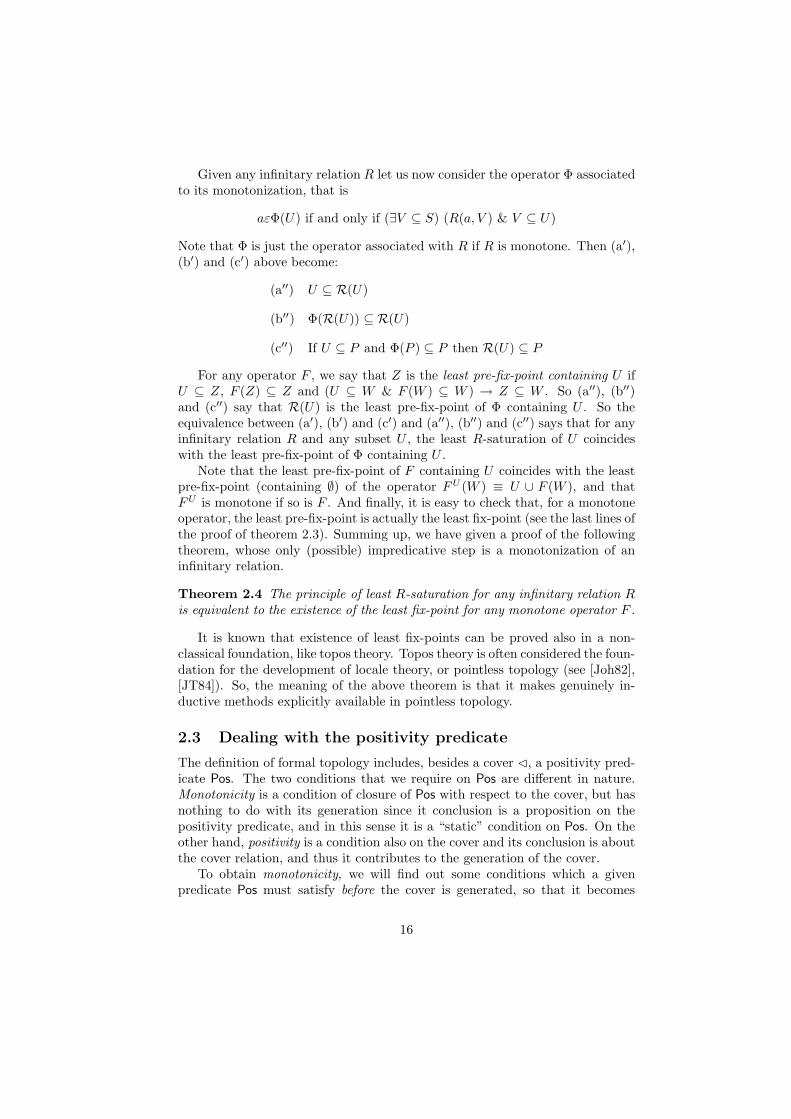
Given any infinitary relation R let us now consider the operator Φ associatedto its monotonization, that is

aεΦ(U) if and only if (∃V ⊆ S) (R(a, V ) & V ⊆ U)

Note that Φ is just the operator associated with R if R is monotone. Then (a′),(b′) and (c′) above become:

(a′′) U ⊆ R(U)

(b′′) Φ(R(U)) ⊆ R(U)

(c′′) If U ⊆ P and Φ(P ) ⊆ P then R(U) ⊆ P

For any operator F , we say that Z is the least pre-fix-point containing U ifU ⊆ Z, F (Z) ⊆ Z and (U ⊆ W & F (W ) ⊆ W ) → Z ⊆ W . So (a′′), (b′′)and (c′′) say that R(U) is the least pre-fix-point of Φ containing U . So theequivalence between (a′), (b′) and (c′) and (a′′), (b′′) and (c′′) says that for anyinfinitary relation R and any subset U , the least R-saturation of U coincideswith the least pre-fix-point of Φ containing U .

Note that the least pre-fix-point of F containing U coincides with the leastpre-fix-point (containing ∅) of the operator FU (W ) ≡ U ∪ F (W ), and thatFU is monotone if so is F . And finally, it is easy to check that, for a monotoneoperator, the least pre-fix-point is actually the least fix-point (see the last lines ofthe proof of theorem 2.3). Summing up, we have given a proof of the followingtheorem, whose only (possible) impredicative step is a monotonization of aninfinitary relation.

Theorem 2.4 The principle of least R-saturation for any infinitary relation Ris equivalent to the existence of the least fix-point for any monotone operator F .

It is known that existence of least fix-points can be proved also in a non-classical foundation, like topos theory. Topos theory is often considered the foun-dation for the development of locale theory, or pointless topology (see [Joh82],[JT84]). So, the meaning of the above theorem is that it makes genuinely in-ductive methods explicitly available in pointless topology.

2.3 Dealing with the positivity predicate

The definition of formal topology includes, besides a cover ⊳, a positivity pred-icate Pos. The two conditions that we require on Pos are different in nature.Monotonicity is a condition of closure of Pos with respect to the cover, but hasnothing to do with its generation since it conclusion is a proposition on thepositivity predicate, and in this sense it is a “static” condition on Pos. On theother hand, positivity is a condition also on the cover and its conclusion is aboutthe cover relation, and thus it contributes to the generation of the cover.

To obtain monotonicity, we will find out some conditions which a givenpredicate Pos must satisfy before the cover is generated, so that it becomes

16

monotonic with respect to the cover, after it is generated. To get an idea,assume that an infinitary relation R and a predicate Pos are given which satisfy

(monotonicity on axioms)Pos(a) R(a, V )

(∃bεV ) Pos(b)

If we could generate the cover by reflexivity and trax, we would easily provemonotonicity by induction. In fact, if Pos(a) and aεU , then trivially Pos(U).And if Pos(a), R(a, V ) and V ⊳ U then by monotonicity on axioms there existsbεV such that Pos(b) and, whatever b is, Pos(U) follows from V ⊳ U by inductivehypothesis.

After the results of the previous section 2.2, we know that we must use otherrules to generate covers; the idea to obtain monotonicity will however remainthe same, though some technical complications will be necessary.

Then there are conditions which depends on the particular presentation thatwe are going to use for formal topologies. For instance if we want to deal with≤-formal topologies it is clear that the following condition must hold, becausea ≤ b yields a ⊳ b:

(monotonicity on ≤)Pos(a) a ≤ b

Pos(b)

To impose positivity, we will simply put it among the rules generating thecover, that is we simply add the following rule

(positivity rule)a ⊳ U [Pos(a)]

a ⊳ U

We will see in section 3.2 that, as far as predicativity is concerned, it is as safeas the other rules that we will adopt.

3 Inductive generation

The problem concerning transitivity, also in its reduced form of transitivity onaxioms, is essentially due to the fact that it allows to infer a ⊳ U from R(a, V )and V ⊳ U , whatever the subset V is. Thus the possible premise of a ⊳ U

cannot be indexed by a set: the validity of a ⊳ U depends on an existentialquantification on P(S), namely (∃V ⊆ S) (R(a, V ) & V ⊳ U). The solution issimply to reduce it to a quantification over a set, so that the branching is undercontrol. The most general case we are able to devise is then to have a familyof sets I(a) set [a : S], so that the previous quantification over P(S) to infera ⊳ U will become a quantification over I(a), and for each i ∈ I(a) a subsetC(a, i) ⊂ S, which will play the role previously played by the subset V . So, thesubsets which are postulated to cover a given element a are not given as thoseV for which R(a, V ) holds, but directly as the family C(a, i) indexed on the setI(a). In this way the dependence on the general notion of subset is avoided, theaxioms are surely not affected by the process of generation and any danger ofvicious circles is stopped.

17

We will see in section 4 that the restriction is not too severe, since it is metby most of the known examples of formal topologies. Actually, proving that aspecific formal topology is not included is not simple: we do this in the end ofsection 4.

3.1 Set-based axioms and set-based relations

Let S be a set. We say that a set indexed family I(a) set [a : S] together witha family of subsets C(a, i) ⊆ S [a : S, i : I(a)] is an axiom-set. The intendedmeaning is that, for all a ∈ S, the subset C(a, i) is assumed to be a cover of a,for any i ∈ I(a). We can think of such axioms also as an infinitary relation R,linking a with C(a, i) for any i ∈ I(a), that is, the relation R(a, V ) holds if andonly if there exists i ∈ I(a) such that V =S C(a, i).

An application of the rule trax for such relation is particularly simple, sincethe assumption that a is related with any C(a, i) can be understood; so we reachthe rule

(infinity)i ∈ I(a) C(a, i) ⊳ U

a ⊳ U

Note that the previous implicit quantification over P(S) has now become aquantification over the family C(a, i) ⊆ S [i ∈ I(a)], which is reduced to aquantification over I(a). There remains the problem that the right premiseC(a, i) ⊳ U of infinity contains a subset at the left. We now must begin tobe more careful in the analysis of derivations, and thus we understand thatC(a, i) ⊳ U is an abbreviation for a derivation of x ⊳ U from xεC(a, i) withthe variable x free. So the expanded formulation of infinity is

(infinity)i ∈ I(a) x ⊳ U [xεC(a, i)]

a ⊳ U

and we use the previous formulation as an abbreviation of this. We understandthat a similar convention applies to all rules to follow, which contain a subsetat the left of ⊳.

Let us go back to the relation linked with an axiom-set. A bit more generally,we add monotonicity and say that an infinitary relation R is set-based if thereexist two families I and C as above such that, for all a ∈ S and V ⊆ S,

R(a, V ) if and only if (∃i ∈ I(a)) C(a, i) ⊆ V

We can now see immediately that the problem of closing under transitivity issolved for set-based relations. In fact, given any two families

I(a) set [a : S]

C(a, i) ⊆ S [a : S, i : I(a)]

we define ⊳ inductively by the rules

(reflexivity)aεU

a ⊳ U

(infinity)i ∈ I(a) C(a, i) ⊳ U

a ⊳ U

18

Such rules fall under a general scheme for which a predicative justification hasalready been given (see [Dyb94]); they are for instance an example of the Tree

type in [NPS90]. So we know that also the elimination rule

a ⊳ U U ⊆ P xεP [i : I(x), C(x, i) ⊆ P ]

aεP

is valid. This means that proofs by induction on reflexivity and infinity arejustified.

It is now easy to prove by induction that:

Theorem 3.1 For any infinitary relation R which is set-based on I and C

as above, the relation ⊳ defined inductively by reflexivity and infinity is theleast infinitary relation which contains R and is closed under reflexivity andtransitivity.

Proof. First, we show that the rules generating ⊳ are valid, in the sense thatthey hold for any relation ⊳′ which contains R and is closed under reflexivityand transitivity. Trivially reflexivity is valid. And if C(a, i) ⊳′ U for somei ∈ I(a), then also a ⊳′ U by transitivity on the axiom R(a, C(a, i)); this showsthat infinity is valid.

Then we show that they are complete, in the sense that they allow to derivea ⊳ U whenever it holds for each reflexive, transitive ⊳′ containing R. That is,we prove by induction that ⊳ is indeed closed under reflexivity and transitivityand that it contains R. Closure under reflexivity is built in the definition.Closure under transitivity is proved by induction on the derivation of the leftpremise a ⊳ U , the right premise being U ⊳ V . If a ⊳ U is obtained byreflexivity from aεU then a ⊳ V follows from U ⊳ V , since by definition U ⊳ Vmeans x ⊳ V [xεU ]. If a ⊳ U is obtained by infinity from C(a, i) ⊳ U forsome i ∈ I(a), then by inductive hypothesis C(a, i) ⊳ V , from which a ⊳ V byinfinity.

Finally, R(a, U) by assumption means that there exists i ∈ I(a) such thatC(a, i) ⊆ U ; then by reflexivity C(a, i) ⊳ U and hence a ⊳ U by infinity.

It is interesting to note that, as a corollary of a general theorem on deductivesystems by P. Aczel [Acz??], we have also the following result.

Theorem 3.2 If R is set-based, then also the least infinitary relation closedunder reflexivity and transitivity containing R is set-based.

We will recall the proof of this theorem and we will use it in section 4.6.

3.2 Inductive generation of formal topologies

In order to generate a cover inductively it is enough to modify the generationprocess of the previous section by forcing the resulting relation ⊳ to satisfy thecondition ↓-right. As shown in section 2.1, to this aim one must restrict toformal topologies with an extra primitive. We deal here with formal topologies

19

with a preorder ≤ and thus we have to force ≤-left and ≤-right to hold. Bylemma 2.2 we can equivalently force ≤-left and localization. Then the idea forthe solution comes from the following remark:

Localization LiftingEvery application of localization can be “lifted over” any application of reflex-ivity, transitivity and ≤-left.

The suitable proof transformations are shown by the following figures:

aεUa ⊳ U

refl.

a ↓ c ⊳ U ↓ cloc.

aεUa ↓ c ⊆ U ↓ c

a ↓ c ⊳ U ↓ crefl.

a ⊳ V V ⊳ Ua ⊳ U

trans.

a ↓ c ⊳ U ↓ cloc.

a ⊳ V

a ↓ c ⊳ V ↓ cloc.

V ⊳ U

V ↓ c ⊳ U ↓ cloc.

a ↓ c ⊳ U ↓ ctrans.

a ≤ b b ⊳ U

a ⊳ U≤-left

a ↓ c ⊳ U ↓ cloc.

a ≤ b

a ↓ c ⊆ b ↓ cb ⊳ U

b ↓ c ⊳ U ↓ cloc.

a ↓ c ⊳ U ↓ c

So, in a proof figure which contains only reflexivity, transitivity and ≤-left, lo-calization can be lifted until it is applied only under the axioms; thus to obtainclosure under localization we could either restrict its application or simply re-quire that the axioms are closed under localization. Because of the problemwith transitivity we cannot use this approach in an inductive process of gener-ation, but it suggests how to modify the inductive generation with reflexivityand infinity to obtain a relation ⊳ which is closed under localization. Applyingthe idea of loc-lifting to a figure of the form

i ∈ I(a) C(a, i) ⊳ V

a ⊳ Vinfinity

a ↓ c ⊳ V ↓ cloc.

we would apply localization to C(a, i) ⊳ V obtaining C(a, i) ↓ c ⊳ V ↓ c, butthen we could not apply infinity in its present form. However, we can modifyinfinity into a valid rule which includes localization on the left. We obtain

i ∈ I(a) C(a, i) ↓ c ⊳ V ↓ c

a ↓ c ⊳ V ↓ c

and thus we reach

(loc-infinity)i ∈ I(a) C(a, i) ↓ c ⊳ U

a ↓ c ⊳ U

which is still valid in any cover satisfying a ⊳ C(a, i). In fact, from a ⊳ C(a, i)one has a ↓ c ⊳ C(a, i) ↓ c by localization, and hence the premise C(a, i) ↓ c ⊳ U

20

gives a ↓ c ⊳ U by transitivity. It is easy to check that this rule permutes withlocalization. However, it has the drawback that a subset appears on the left ofits conclusion, and this could cause complications in a rigorous formalization ofproofs by induction. We can then write loc-infinity in the equivalent form

x ≤ c x ≤ a i ∈ I(a) C(a, i) ↓ c ⊳ U

x ⊳ U

which, when x is taken to be c itself, gives

c ≤ a i ∈ I(a) C(a, i) ↓ c ⊳ U

c ⊳ U

We can see that actually this special case is enough to give back the full ruleof loc-infinity. In fact, assume x ≤ c, x ≤ a and C(a, i) ↓ c ⊳ U . Since x ≤ c

implies ↓ x ⊆↓ c and hence C(a, i) ↓ x ⊆ C(a, i) ↓ c, we obtain C(a, i) ↓ x ⊳ U ;together with x ≤ a, this allows to obtain x ⊳ U by the special case.

We thus choose the special case, since it has one premise less then loc-infinity,and write it down as usual with a ⊳ U as a conclusion:

(≤-infinity)a ≤ b i ∈ I(b) C(b, i) ↓ a ⊳ U

a ⊳ U

We will show that ≤-infinity, together with reflexivity and ≤-left, is sufficientto generate the least cover satisfying the axioms. But if we wish to generatea formal topology, according to the present definition, we must have also apositivity predicate Pos. We remarked in section 2.3 that we must start froma given predicate Pos(a) prop [a : S] which is assumed to be monotonic withrespect to the axioms. But now the axioms are fitted in ≤-infinity, and hencewe are brought to require

(monotonicity on ≤-infinity)Pos(a) a ≤ b i ∈ I(b)

Pos(a ↓ C(b, i))

It is immediate to see that this condition has to hold if we want the positivitypredicate to be monotone. In fact from a ≤ b we can deduce a ⊳ a ↓ C(b, i)for any i ∈ I(b), by using ≤-left and ≤-right, and hence if Pos(a) it must alsobe Pos(a ↓ C(b, i)). We will prove that monotonicity of Pos with respect to thegenerated cover follows.

On the other hand, the condition of positivity is put in the process of gener-ation itself, that is we add

(positivity)a ⊳ U [Pos(a)]

a ⊳ U

to the rules generating ⊳. The premise of positivity is equivalent to

x ⊳ U [Pos(x) & x = a]

and hence, after putting

a+ ≡ x ∈ S| Pos(x) & x = a

21

also to a+ ⊳ U . So positivity can be formulated as

a+⊳ U

a ⊳ U

which shows that it falls under the same schema that we have chosen abovefor axioms. More precisely, if I and C are an axiom-set, we can define I ′ byadding a new element ♯ to each I(a) and C′ by putting C′(a, ♯) ≡ a+ andC′(a, i) ≡ C(a, i) for any i ∈ I(a). Then the cover generated by I ′ and C′

will be the least cover which satisfies positivity and which contains the covergenerated by I and C.

We are finally ready to state and prove the main theorem:

Theorem 3.3 (Inductive generation of formal topologies) Let S be anyset, ≤ any pre-order on S and let I(a) set [a : S] and C(a, i) ⊆ S [a : S, i : I(a)]be an axiom-set.

Then the infinitary relation ⊳0 defined inductively by the rules reflexivity,≤-left and ≤-infinity is the least cover satisfying a ⊳0 C(a, i) [a : S, i : I(a)].

Assume in addition that a predicate Pos(a) set [a : S] is given which satisfiesmonotonicity on ≤-infinity and monotonicity on ≤ and let ⊳ be the infinitaryrelation generated by the three rules above plus positivity.

Then A ≡ (S,≤,⊳,Pos) is a ≤-formal topology and ⊳ is the least amongthe covers ⊳′ satisfying a ⊳′ C(a, i) [a : S, i : I(a)] and making (S,≤,⊳′,Pos) aformal topology.

Proof. We already showed that all the rules that we use in the generationprocess are valid, thus we have only to show that they are complete, in thesense that they allow to derive a ⊳0 U (and a ⊳ U) whenever it holds for acover (formal topology) satisfying the axioms. This amounts to prove that ⊳0

(⊳) is closed under reflexivity, transitivity, ≤-left and ≤-right (and positivity)and that, for any a ∈ S and i ∈ I(a), a ⊳ C(a, i).

Closure under reflexivity, ≤-left and positivity: trivial.

Closure under transitivity: if a ⊳ U and U ⊳ W then a ⊳ W . The proofis by induction on the derivation of a ⊳ U , that is the property on whichwe apply induction is P (a) ≡ U ⊳W → a ⊳W .

reflexivity: a ⊳ U is derived from aεU . Then aεU and U ⊳ W givea ⊳W .

≤-left: a ⊳ U is derived from a ≤ b and b ⊳ U . Then, by inductivehypothesis, from b ⊳ U and U ⊳W we obtain b ⊳W , so that a ⊳Wby ≤-left.

≤-infinity: a ⊳ U is derived from a ≤ b and C(b, i) ↓ a ⊳ U . Weapply the inductive hypothesis to C(b, i) ↓ a ⊳ U and U ⊳ W toobtain C(b, i) ↓ a ⊳W , from which a ⊳W by ≤-infinity.

22

positivity: a ⊳ U is derived from a ⊳ U [Pos(a)]. Assume Pos(a); thena ⊳ U with a shorter derivation, so a ⊳ W by inductive hypothesisand hence a ⊳W by positivity.

Closure under ≤-right: if a ⊳ U and a ⊳ V then a ⊳ U ↓ V . To be ableto go through the inductive steps we prove by induction a stronger claim,that is

(stability)a ⊳ U b ⊳ V

a ↓ b ⊳ U ↓ V

Then the original ≤-right is obtained from the special case in which a = b,since aεa ↓ a. The proof of stability is by induction on the derivation ofa ⊳ U .

reflexivity: a ⊳ U is derived from aεU . The proof is by induction onthe derivation of b ⊳ V . If b ⊳ V is derived from bεV by reflexivity,then aεU and bεV give a ↓ b ⊆ U ↓ V by definition of ↓, and hencea ↓ b ⊳ U ↓ V by reflexivity. In all the other cases, the proof isexactly as the corresponding steps in the main induction.

≤-left: a ⊳ U is derived from a ≤ c and c ⊳ U . Then by inductivehypothesis c ↓ b ⊳ U ↓ V , but a ↓ b ⊆ c ↓ b because a ≤ c, and soa ↓ b ⊳ U ↓ V by using a bit of logic.

≤-infinity: a ⊳ U is derived from a ≤ c and C(c, i) ↓ a ⊳ U . Wehave to prove that a ↓ b ⊳ U ↓ V . Thus, let xεa ↓ b, that isx ≤ a and x ≤ b. The inductive hypothesis, and a bit of logic, give(C(c, i) ↓ a) ↓ b ⊳ U ↓ V , that is C(c, i) ↓ (a ↓ b) ⊳ U ↓ V ; hence, bylogic, also C(c, i) ↓ x ⊳ U ↓ V since xεa ↓ b. But x ≤ a and a ≤ c

give x ≤ c, and hence ≤-infinity can be applied to obtain x ⊳ U ↓ Vas wished.

positivity: a ⊳ U is derived from a ⊳ U [Pos(a)]. By the inductivehypothesis, a ↓ b ⊳ U ↓ V under the assumption Pos(a). Let xεa ↓ band Pos(x). Then x ≤ a and hence Pos(a) by monotonicity on ≤,so that x ⊳ U ↓ V under the assumption Pos(x). Then by positivityx ⊳ U ↓ V as wished.

Finally, we prove a ⊳ C(a, i), for any a ∈ S and i ∈ I(a). To this aim firstnote that, by reflexivity and ≤-left, ↓ C(a, i) ⊳ C(a, i) and hence a fortiori,C(a, i) ↓ a ≡↓ C(a, i)∩ ↓ a ⊳ C(a, i). Then a ⊳ C(a, i) follows by ≤-infinitysince a ≤ a.

Thus, we finished with the generation of the cover relation. To prove thesecond statement in the theorem we have to prove only monotonicity of Pos withrespect to the cover that we have generated by reflexivity, ≤-left, ≤-infinity andpositivity. So, let us assume that Pos(a) and a ⊳ U . Then the proof is byinduction on the derivation a ⊳ U .

reflexivity: a ⊳ U is derived from aεU . Then trivially Pos(U).

23

≤-left: a ⊳ U is derived from a ≤ b and b ⊳ U . Then, by monotonicityon ≤, we get Pos(b) and hence Pos(U) by inductive hypothesis.

≤-infinity: a ⊳ U is derived from a ≤ c and C(c, i) ↓ a ⊳ U , for some i inI(c). Then by monotonicity on ≤-infinity we obtain that Pos(C(c, i) ↓ a)and hence Pos(U) follows by inductive hypothesis (and a bit of logic).

positivity a ⊳ U is derived from a ⊳ U [Pos(a)]. By induction hypothesiswe obtain Pos(U) [Pos(a)] but Pos(a) is assumed, hence Pos(U).

3.3 Localizing the axioms

The main advantage of the approach above is that it is possible to choose theaxioms in a completely free way, that is without any condition, but the drawbackis the presence of a rule ad hoc, namely ≤-infinity. As we showed, the aim of≤-infinity is to be able to lift localization up to the axioms. But the axiomsare contained in the rule of infinity itself, and this is why we had to considerits localized form ≤-infinity. So, if some axioms are given which are alreadylocalized in a suitable sense, an expectation is that the infinity rule will beenough. We now prove that it is so.

Definition 3.4 (Localized axiom-set) Let I and C be an axiom-set. Thenwe say that it is localized if, for any a ≤ c and i ∈ I(c), there exists j ∈ I(a)such C(a, j) ⊆ a ↓ C(c, i).

Then, we can prove the following proposition.

Proposition 3.5 Provided the axiom-set is localized, an infinitary relation gen-erated by using reflexivity, ≤-left and infinity satisfies ≤-infinity.

Proof. Let us suppose that a ≤ c and C(c, i) ↓ a ⊳ U . Then, by assumption,there exists j ∈ I(a) such that C(a, j) ⊆ a ↓ C(c, i). So C(a, j) ⊳ U and hencea ⊳ U by infinity.

Thus, it is to be expected that it is possible to generate a formal topology alsoby using infinity instead of ≤-infinity, provided that the axiom-set is localized.In fact, we can prove the following theorem.

Theorem 3.6 Let S be any set, ≤ any pre-order on S and let I(a) set [a : S]and C(a, i) ⊆ S [a : S, i : I(a)] be a localized axiom-set. Assume in additionthat a predicate Pos(a) set [a : S] is given which satisfies monotonicity on ≤ andmonotonicity on infinity, that is, if Pos(a) and i ∈ I(a), then Pos(C(a, i)). Let ⊳be the infinitary relation generated by reflexivity, ≤-left, infinity and positivity.Then A ≡ (S,≤,⊳,Pos) is a ≤-formal topology and ⊳ is the least among thecovers ⊳′ satisfying a ⊳′ C(a, i) [a : S, i : I(a)] and making (S,≤,⊳′,Pos) aformal topology.

24

Proof. The proof is almost exactly the same as in theorem 3.3 except theinductive steps concerning the usage of ≤-infinity that we modify as follows:

transitivity: a ⊳ U is derived from C(a, i) ⊳ U by infinity. Then, suppos-ing U ⊳ V , C(a, i) ⊳ V follows by inductive hypothesis and hence a ⊳ Vby infinity.

stability: a ⊳ U is derived by C(a, i) ⊳ U by infinity. We want to provethat a ↓ b ⊳ U ↓ V . Then let xεa ↓ b, that is x ≤ a and x ≤ b. Theinductive hypothesis, and a bit of logic, give C(a, i) ↓ b ⊳ U ↓ V , andhence also C(a, i) ↓ x ⊳ U ↓ V since x ≤ b gives ↓ x ⊆↓ b. Since theaxiom-set is localized and we assumed that x ≤ a, there exists j ∈ I(x)such that C(x, j) ⊆ x ↓ C(a, i) and hence C(x, j) ⊳ U ↓ V which byinfinity gives x ⊳ U ↓ V as wished.

Also the axioms can be proved by using infinity instead of ≤-infinity, andwith a simpler proof. In fact, for any a ∈ S and any i ∈ I(a), C(a, i) ⊳ C(a, i)by reflexivity and hence a ⊳ C(a, i) by infinity.

Finally, we must give the inductive step to prove monotonicity when the ruleapplied to prove a ⊳ U is infinity. Hence we know C(a, i) ⊳ U for some i ∈ I(a);so by monotonicity on infinity Pos(a) gives Pos(C(a, i)) and hence Pos(U) byinductive hypothesis.

Given any axiom-set I, C we can always provide with a new axiom-set J , Dwhich is localized and generates the same cover relation. In fact, it is possibleto prove the following theorem.

Theorem 3.7 Let I(a) set [a : S] and C(a, i) ⊆ S [a : S, i : I(a)] be an axiom-set and define a new axiom-set by putting

J(a) ≡ 〈c, k〉| (a ≤ c) & k ∈ I(c)D(a, 〈c, k〉) ≡ a ↓ C(c, k)

Then, if a ≤ c and i ∈ J(c) there exists j ∈ J(a) such that D(a, j) ⊆ a ↓D(c, i), that is, the new axiom-set is localized. Moreover, the axiom-set J andD generates the same cover relation than the axiom-set I and C.

Its proof is almost immediate if one observe that, if a ≤ c and 〈d, k〉 ∈ J(c) then〈d, k〉 ∈ J(a) and D(a, 〈d, k〉) = a ↓ C(d, k) = a ↓ c ↓ C(d, k) = a ↓ D(c, 〈d, k〉).

4 Some examples and one counter-example

This section is devoted to show some examples of application of the generaltechnique that we exploited in the previous sections to inductively generateformal topologies. We will see that most of the standard topological spacesand topological constructions can indeed be inductively generated and hencethat almost nothing is lost by restricting to consider only inductively generated

25

formal topologies. Anyhow we will also show a remarkable example of formaltopology which cannot be inductively defined: this fact suggests to keep thevery definition of the notion of formal topology in its full generality instead torestrict to consider only inductively generated formal topologies.

4.1 The Cantor space

The first example that we want to show is the formal topology over binary trees,that is, Cantor space. To define such a formal topology we will use the set 22∗ ofbinary words, that is, finite sequences of 0 and 1. To obtain a ⊑-formal topologyfrom the set 22∗ we use the order relation ⊑ such that, for any two words σ andσ′, σ ⊑ σ′ holds if and only if σ′ is an initial segment of σ. The intendedmeaning of such an order relation can be understood if one thinks of a word asa partial information over an infinite sequence, which corresponds intuitively toa classical function from the set N of natural number into 22; thus a longer wordis a more precise information on the infinite sequence and hence there are lesswords that contains it than any of its initial segments. Finally the empty word,which is contained in all words, gives no information at all and is contained inall of the infinite sequences. In formal topology a representation of such infinitesequences can be obtained by using the collection of the formal points. Givenany formal topology (S,≤,⊳,Pos), a formal point is any non-empty subsets αof S such that, for any a, b ∈ S and U ⊆ S, both if aεα and bεα then thereexists cεα such that c ⊳ a and c ⊳ b, and if aεα and a ⊳ U then there existsuεU such that uεα. The collection of all the formal points will be indicatedby Pt(S). Then an infinite sequence f can be identified with the formal pointwhose elements are all the words σ such that for any natural number x, smallerthen the length of the word σ, f(x) is equal to σ[x], where σ[x] is the value inthe place x of σ.

With the same intuitive reading it is also easy to understand that σ ⊳ U

should means that the words which contain σ are all contained in the words thatcontain at least one of the words in U . But in order to inductively generate thiscover relation we have to state suitable axioms for it. Here we simply requirethat the word σ is covered by all its one-step successors, that is the only formof axiom is

σ ⊳ σ0, σ1

which is clearly an axiom-set. It is easy to prove that this axiom-set is localizedand hence the simple infinity rule is sufficient to generate this formal topology.Finally the positivity predicate is completely trivial since any word is positive,that is, we put

Pos(σ) ≡ true

For more information about this formal topology and the collection of its formalpoints see [Val99].

It can be useful to show directly an axiom-set for the full cover relation ofthis simple formal topology without making a reference to the proof of theorem

26

3.2. First note that

σ ⊳ U if and only if (∃n ∈ N)(∀σ′ ∈ 22∗(n))(∃uεU) σσ′ ⊑ u

where 22∗(n) is the set of the sequence of 0 and 1 of length n and σσ′ is theconcatenation of the two words σ and σ′. In fact, one direction can be provedby induction on the natural number n which is assumed to exist while the othercan be proved by induction on the length of the derivation of σ ⊳ U .

We can now use a choice principle, which is valid in constructive type theory,and obtain that

σ ⊳ U if and only if(∃n ∈ N)(∃f ∈ 22∗(n) → 22∗)(∀σ′ ∈ 22∗(n)) σσ′ ⊑ f(σ′) & f(σ′)εU

Then, by putting

I(σ) ≡ 〈n, f〉| n ∈ N, f ∈ 22∗(n) → 22∗, (∀σ′ ∈ 22∗(n)) σσ′ ⊑ f(σ′)C(σ, 〈n, f〉) ≡ Im[f ]

where Im[f ] ≡ σ ∈ 22∗| (∃σ′ ∈ 22∗(n)) σ = f(σ′) is the image of the functionf , we obtain

σ ⊳ U if and only if (∃〈n, f〉 ∈ I(σ)) C(σ, 〈n, f〉) ⊆ U

that is, I and C is an axiom-set for the Cantor formal topology.

4.2 The real numbers

Our second example of a formal topology which can be inductively generatedis the formal topology of real numbers. We can identify a real number with asuitable collection of open intervals on the rational line, that is, the collectionof all the intervals which contain such a real number (see for instance [Joh82,Ver86]). Thus, a real number can be identified with a formal point of a suitable≤-formal topology whose basic opens are the open intervals of the rational lineQ. We obtain such a ≤-formal topology (S,≤,⊳,Pos) by putting

S ≡ Q×Q

The order relation ≤ among these intervals is then simply defined by using thestandard order relation ≤ between rational numbers and putting

(p, q) ≤ (r, s) ≡ (r ≤ p) & (q ≤ s)

The intended meaning is that (p, q) ≤ (r, s) when the interval (p, q) is containedin the interval (r, s).

Let us note now that the interval (p, q) is meant to contain some point onlyif p < q and hence the positivity predicate can be defined by putting

Pos((p, q)) ≡ p < q

27

We can state now the axioms that we need:

(p, q) ⊳ (p, s), (r, q) for r < s

(p, q) ⊳ (r, s)| p < r < s < q

The geometrical meaning of these axioms should be clear. In fact, let us supposethat (p, q) is inhabited, then any axiom in the first family of axioms statesthat an interval (p, q) is covered by any pair of overlapping intervals which arecontained in (p, q) provided one covers the left part and the other the rightpart of (p, q). And the second axiom states that an interval is covered by thecollection of all the intervals that it contains properly. These axioms form anaxiom-set since for any couple (p, q) ∈ Q ×Q we can define I((p, q)) to be theset obtained by adding one element ∗ to the set of the ordered couple of rationalnumbers. In fact, we can now use any ordered couple (r, s) of rational numberssuch that r < s to index one of the axioms of the first family and the element∗ to index the only axiom of the second kind.

It is worth noting that also in this case the axiom-set that we are consideringis localized and hence this formal topology can be generated by using infinityinstead that the more complex ≤-infinity. This observation is useful to under-stand that to inductively generate this formal topology one can equivalently usethe following two rules

r < s (p, s), (r, q) ⊳ U

(p, q) ⊳ U

(r, s)| p < r < s < q ⊳ U

(p, q) ⊳ U

which ware indeed those one that Thierry Coquand proposed first in [CN96].Note that it can be shown that to prove (p, q) ⊳ U one needs to use the secondrule at most once at the end of the proof.

4.3 Cartesian product revisited

In this example we will go back to the problem of a predicative definition ofthe cartesian product of formal topologies. Indeed, in section 1 we observedthat we know no predicative way, apart inductive generation, to construct thecartesian product of formal topologies. After the previous sections we knowthat we can inductively generate a formal topology provided it has an axiom-set. Thus, we can present now our solution to the problem of the predicativedefinition of the cartesian product of formal topologies. In fact, if S and T aretwo formal topologies with an axiom-set then their cartesian product, like inthe definition at the end of section 1, is again a formal topology which has anaxiom-set. Indeed, it is sufficient to observe that if the axiom-set for the formaltopology S is the family of sets I(a) set [a : S] together with the family of subsetsC(a, i) ⊆ S [a : S, i : I(a)] and the axiom-set for the topology T is the family ofsets J(b) set [b : T ] together with the family of subsetsD(b, j) ⊆ T [b : T, j : J(b)]then the axiom-set for the cartesian product of S and T is the following

(a, b) ⊳ C(a, i) × b [a : S, b : T, i : I(a)](a, b) ⊳ a×D(b, j) [a : S, b : T, j : J(b)]

28

whereC(a, i) × b ≡ (z, b) ∈ S × T | zεC(a, i)a×D(b, j) ≡ (a,w) ∈ S × T | wεD(b, j)

It is clear that such an axiom-set can be indexed by using the following familyof sets:

K((a, b)) ≡ (I(a) × T ) + (S × J(b))

where A+B is the disjoint union of the two sets A and B.Note that the above definition of product of S and T works only if S and T

have an axiom-set. Since not all the formal topologies have an axiom-set (seesection 4.6) the problem of an unrestricted predicative definition of product offormal topologies is still open.

4.4 All representable topologies have an axiom-set

In the previous sections we have given single examples of formal topologies whichhave an axiom-set and this might suggest the idea that just a few, although im-portant, formal topologies have an axiom-set. Actually one can show that largeclasses of formal topologies have an axiom-set. Here we do this for representableformal topologies, in the next section for unitary and finitary formal topologies.1

We say that a formal topology A ≡ (S,⊳,Pos) is representable if there exista set X and a proposition x a prop [x : X, a : S] such that

a ⊳ U if and only if (∀x ∈ X) (x a→ (∃b ∈ S) x b & bεU)Pos(a) if and only if (∃x ∈ X) x a

That is, a formal topology is representable when it is the formal part of aconcrete topological space.

It is interesting to note that when a formal topology S is representable theset X of concrete points can be embedded into the collection Pt(S) of the formalpoints of S. In fact, it is possible to associate to the concrete point x in X theformal point αx ≡ a ∈ S| x a.

If we are dealing with a representable formal topology, we can apply a choiceprinciple, which is valid in constructive type theory, and obtain that

a ⊳ U

if and only if

(∃f ∈ g ∈ ext(a) → S| (∀xεext(a)) x g(x))(∀xεext(a)) f(x)εU

that is, the function f takes any point x contained in ext(a) and finds an elementb in S such that x is contained in ext(b) and b is an element of the subset U .Hence, we can put

I(a) ≡ g ∈ ext(a) → S| (∀xεext(a)) x g(x)C(a, f) ≡ Im[f ]

1The idea for the results in this section comes us from a conversation with Per Martin-Lof.

29

where Im[f ] is the image of f .Then we obtain

a ⊳ U if and only if (∃f ∈ I(a)) C(a, f) ⊆ U

that is, I and C is an axiom-set for ⊳. In fact, if a ⊳ U then by the above statedprinciple of choice we can find the suitable function in I(a). On the other hand,if (∃f ∈ I(a)) C(a, f) ⊆ U then we have a function such that for any point xcontained in ext(a) gives an element b of S such that xεext(b); thus, since thetopology is representable, a ⊳ Im[f ] holds; but also Im[f ] ⊆ U holds and hencea ⊳ U follows by transitivity.

Note that, as a consequence of the fact that all of the representable formaltopologies can be inductively generated and of the existence of a formal topologywhich cannot be generated, that we will present in section 4.6, we know thatnot all formal topologies are representable. Moreover, it is interesting to notethat there are formal topologies which can be inductively generated but arenot representable. For instance, in section 4.1 we proved that Cantor spaceis a formal topology inductively generated; on the other hand it cannot berepresentable, at least if we want to represent it by using the most naturalchoice, that is by using like set X the set 22N of the functions from the naturalnumbers into the two elements set 22. Indeed in this case the most naturaldefinition of the forcing relation would be

x σ ≡ (∀n < len(σ)) f(x) = σ[x]

where len(σ) is the length of the sequence σ and σ[x] is the value in the x-thposition of the sequence σ. Now, to state that X and can be used to representthe Cantor space is equivalent to the Brouwer’s fan theorem and hence it is notrecursively valid (see [JT84] and [FG82]).

4.5 Unitary and finitary formal topologies

In this section we will show that also two other classes of formal topologies havean axiom-set, namely Scott’s and the Stone’s formal topologies.

Let us first analyze the case of Stone’s, alias finitary, formal topologies sincethey are technically simpler than Scott’s topologies because they do not requirea detailed treatment of the positivity predicate. On the other hand, after Stone’stopologies will be understood, in order to deal with Scott’s topologies we willhave only to specialize the ideas that we used for the former to the latter andthus we will be able to work out the details which will allow us to deal with thepositivity predicate.

Let S be any set and Pω(S) be the set of the finite subsets of S2.Then we can give the following definition.

2We will not commit here with any particular implementation of this set to avoid to dealwith the problems that would arise (see for instance [Mai99]). In any case all of what we aredoing here can be formalize in Martin-Lof’s type theory by using the type List(S) of the listsof elements of S [NPS90].

30

Definition 4.1 A formal topology A ≡ (S,⊳,Pos) is finitary if a ⊳ U if andonly if (∃U0 ∈ Pω(S)) (U0 ⊆ U & a ⊳ U0).

Given any finitary formal topology (S,⊳,Pos) we will call trace of S therelation Tr(a, U0), where a is any element in S and U0 is any finite subset of S,which holds if and only if a ⊳ U0.

Then, supposing A ≡ (S,⊳,Pos) is a finitary formal topology whose trace isdefinible by the proposition Tr(a, U0), the axiom-set that one needs in order toinductively generate A is the following

I(a) ≡ U0 ∈ Pω(S)| Tr(a, U0)C(a, U0) ≡ U0

It is now possible to prove that

a ⊳ U if and only if (∃U0 ∈ I(a)) C(a, U0) ⊆ U

Both directions are trivial. Suppose that (∃U0 ∈ I(a)) C(a, U0) ⊆ U holds;then, U0 ∈ I(a) yields a ⊳ U0, that is, a ⊳ C(a, U0) and hence a ⊳ U follows bytransitivity, since C(a, U0) ⊆ U . To prove the other implication, let us assumethat a ⊳ U , that is, (∃U0 ∈ Pω(S)) (U0 ⊆ U & a ⊳ U0) since the cover isfinitary. Then U0 ∈ Pω(S) and Tr(a, U0), that is U0 ∈ I(a), and U0 ⊆ U , thatis C(a, U0) ⊆ U .

Let us analyze now the case of Scott, alias unitary, formal topologies. Thedefinition of unitary formal topology is the following:

Definition 4.2 The formal topology A ≡ (S,⊳,Pos) is unitary if a ⊳ U if andonly if Pos(a) → (∃b ∈ S) (bεU & a ⊳ b).

Also in this case there is a natural notion of trace Tr of the cover relation,that is, Tr(a, b), for any a, b ∈ S, is a relation which holds if and only if a ⊳ b.

The main novelty of unitary topologies with respect to the previous case offinitary topologies is the presence of the assumption on the positivity of a in thecondition on a ⊳ U which defines them, which is necessary to avoid reasoningby case, according to the positivity of a. This assumption will force us to changeall of the previous definitions to adapt them to this new setting. In particularit will be necessary to deal with the proofs of the proposition Pos(a). This isthe reason why, following the propositions as sets tradition, in the next proofswe will write x ∈ Pos(a) to mean that x is a proof of Pos(a).

Suppose A ≡ (S,⊳,Pos) is a unitary formal topology and that its trace isdefined by the proposition Tr(a, b) [a : S, b : S]; then we obtain an axiom-set forA by putting

I(a) ≡ g ∈ Pos(a) → S| (∀x ∈ Pos(a)) Tr(a, g(x))C(a, f) ≡ Im[f ]

Similarly to the previous case with finitary topologies, the intended meaningof the set I(a) is to denote the set whose elements are all the elements of S which

31

cover a but we had to move to this more complex definition because the setb ∈ S| a ⊳ b, which is equal to the set b ∈ S| Pos(a) → a ⊳ b because of thepositivity condition, is only classically equivalent to the set I(a) in our definitionand in the next proofs we will need exactly I(a). The intended meaning of thedefinition of the family of subset C(a, f) is to obtain, according to the fact thata is a positive element of S or not, a subset which is a singleton subset of S,whose only element is an element which covers a, or the empty subset; the waythe subset C(a, f) is defined, which can look a bit strange at a first sight, waschosen to guarantee the property above without requiring decidability of thepredicate Pos.

It is now possible to show that

a ⊳ U if and only if (∃f ∈ I(a)) C(a, f) ⊆ U

that is, any unitary formal topology with a definable trace has an axiom-set,and hence can be inductively generated.

Let us first suppose that (∃f ∈ I(a)) C(a, f) ⊆ U holds. Then f ∈ I(a) andhence, assuming x is a proof of Pos(a), we can deduce that a ⊳ f(x) and hencealso a ⊳ C(a, f) and finally a ⊳ U by transitivity, since f(x)εIm[f ] ≡ C(a, f)and C(a, f) ⊆ U . Then a ⊳ U without any assumption follows since theassumption Pos(a) can be discharged by positivity.

Now, let us suppose that a ⊳ U . Then Pos(a) → (∃b ∈ S) (bεU & a ⊳ b)follows because the formal topology is unitary. But then also

(∀x ∈ Pos(a))(∃b ∈ S) (bεU & a ⊳ b)

holds, and hence we can use a valid choice principle and obtain that

(∃f ∈ Pos(a) → S)(∀x ∈ Pos(a)) f(x)εU & a ⊳ f(x)

Thus we obtain both that f ∈ Pos(a) → S and (∀x ∈ Pos(a)) Tr(a, f(x)), thatis f ∈ I(a), and (∀x ∈ Pos(a)) f(x)εU , that is C(a, f) ≡ Im[f ] ⊆ U .

4.6 A covering which cannot be inductively defined

We want to finish this section by showing that not all of the formal topologiescan be obtained by inductive generation. To this aim let us introduce the notionof Dedekind-MacNeille cover. Let S be a set and ≤ be an order relation on theelements of S. Then, inspired by the Dedekind construction of the completionof the rational line, we can define an infinitary relation ⊳DM over S by putting,for any a ∈ S and any U ⊆ S,

a ⊳DM U ≡ aε⋂

U⊆↓y

↓ y

where ↓ y ≡ x ∈ S| x ≤ y. It is not difficult to prove that this relationsatisfies reflexivity, transitivity and ≤-left while to prove that also ≤-right holdssome more conditions on the order relation are required like, for instance, the

32

possibility of defining both an infimum operation between two elements of Sand its adjoint, namely implication (see [Sam89]). We will call such a cover theDedekind-MacNeille cover over S.

We want now to show that there are examples of a Dedekind-MacNeillecover which do not have an axiom-set. To this aim it is convenient to use anequivalent formulation of the notion of axiom-set. Thus in this section we willsay that a bunch of axioms for a cover relation on a set S is a family of setsB(a) set [a : S] and a family of sets C(a, b) set [a : S, b : B(a)] together witha function d(a, b, c) ∈ S [a : S, b : B(a), c : C(a, b)] whose intended meaning isthat, for all a ∈ S and b ∈ B(a), a ⊳ Im[λx. d(a, b, x)] where Im[λx. d(a, b, x)] ≡x ∈ S| (∃c ∈ C(a, b)) x =S d(a, b, c).

We know that a cover relation ⊳ on a set S is set-based when there is anaxiom-set I(a) set [a : S] and K(a, b) ⊆ S [a : S, b : I(a)] such that a ⊳ U ifand only if (∃b ∈ I(a)) K(a, b) ⊆ U . A similar condition can be used with abunch of axioms. We say that a cover relation is set-based if a ⊳ U if and onlyif (∃b ∈ B(a))(∀c ∈ C(a, b)) d(a, b, c)εU .

Then, it is possible to prove that the notion of bunch of axioms is equivalentto the notion of axiom-set. In fact, suppose a ∈ S and U ⊆ S and assumeto have a bunch of axioms B(a) set [a : S], C(a, b) set [a : S, b : B(a)] andd(a, b, c) ∈ S [a : S, b : B(a), c : C(a, b)]. Then we can define an equivalentaxiom-set by putting

I(a) ≡ B(a)K(a, b) ≡ Im[λx.d(a, b, x)]

In fact, it is now possible to prove that if (∃b ∈ B(a))(∀c ∈ C(a, b)) d(a, b, c)εUthen (∃b ∈ I(a)) K(a, b) ⊆ U . In fact by using the same element b that weknow to exist in I(a) ≡ B(a) from the hypothesis, we have just to show that,for all x ∈ S, if xεK(a, b) then xεU . But xεK(a, b) means that there is anelement c ∈ C(a, b)) such that x =S d(a, b, c) and then the hypothesis yieldsthat d(a, b, c)εU and hence xεU .

On the other hand, if we start with an axiom-set I(a) set [a : S] andK(a, b) ⊆S [a : S, b : I(a)] then we can define an equivalent bunch of axioms by putting

B(a) ≡ I(a)C(a, b) ≡ Σ(S,K(a, b))d(a, b, c) ≡ fst(c)

Indeed, it is now possible to prove that, if (∃b ∈ I(a)) K(a, b) ⊆ U , then(∃b ∈ B(a))(∀c ∈ C(a, b)) d(a, b, c)εU . In fact by using the same element bthat we know to exist in B(a) ≡ I(a) from the hypothesis, we have to showthat (∀c ∈ C(a, b)) d(a, b, c)εU . Thus, let us assume that c ∈ Σ(S,K(a, b)).Then snd(c) is a proof that fst(c)εK(a, b) and hence the hypothesis shows thatit belongs also to U ; thus d(a, b, c) belongs to U since d(a, b, c) ≡ fst(c).

Now, let S ∈ Set, B(x) ∈ Set [x ∈ S], C(x, y) ∈ Set [x ∈ S, y ∈ B(x)],d(x, y, z) ∈ S [x ∈ S, y ∈ B(x), z ∈ C(x, y)] be given.

33

We let ≺∈ S → (S → Set) → Set denote the infinitary relation inductivelydefined by the rules

a ǫ U

a ≺ U

b ∈ B(a) (∀z ∈ C(a, b)) (d(a, b, z) ≺ U)

a ≺ U

Intuitively, we can think of B(a) as the set of rules by which we can concludea ≺ U for a ∈ S. C(a, b) is then the set of indexes for the premisses of the rule:for each z in C(a, b), d(a, b, z) ≺ U is a premiss.

In general, ≺ is not a covering relation. However, given a partial order ≤,the rule

a′ ≺ U a ≤ a′

a ≺ U

is easily expressed by the schema above; hence, every inductively defined cover-ing relation can be obtained in this way.

For arbitrary a ∈ S, define the set Tree(a) of trees with root a by induction:

leaf tree(a) ∈ Tree(a)

b ∈ B(a) f ∈ (z ∈ C(a, b))Tree(d(a, b, z))

branch tree(a, b, f) ∈ Tree(a)

The set of branches Branch(a, t) of a tree t ∈ Tree(a) is defined by

Branch(a, leaf tree(a)) = N1

Branch(a, branch tree(a, y, f)) = (Σz ∈ C(a, y))(Branch(d(a, y, z), f(z)))

We also need the leaf of a branch u of a tree t:

lf br(a, leaf tree(a), u) = a

lf br(a, branch tree(a, y, f), (v, w)) = lf br(d(a, y, z), f(v), w)

We can now give an explicit description of covers by putting

cover(U, a, t) = (u ∈ Branch(a, t))U(lf br(a, t, u))

Theorem 4.3 a ≺ U holds if and only if there exists t ∈ Tree(a) such thatcover(U, a, t) holds.

Proof. The tree t is easily constructed by induction on the derivation of a ≺ U .That cover(U, a, t) implies a ≺ U is straightforwardly proved by induction t.

We now come to the topology which covering relation cannot be inductivelydefined. The base of the topology is Boole = 0, 1 with the natural ordering≤ and with the Dedekind-MacNeille cover

x U ⇔ (∀y)[(∀u ǫ U)u ≤ y] ⇒ x ≤ y

34

This covering relation can be redefined as

x U ⇔ x ǫ U ′′

where V ′ = x ∈ B | (∀u ǫ V )xu = 0 and the product is propositionalconjunction. Indeed, by taking z = ¬y in (∀y)[(∀u ǫ U)u ≤ y] ⇒ x ≤ y wesee that this proposition is equivalent to

∀z[(∀u ǫ U)uz = 0] ⇒ xz = 0

that is, U ′ ⊂ x′, which is equivalent to x ǫ U ′′.Assume that can be inductively defined. By theorem 4.3, we then have

a tree structure Tree(x) ∈ Set [x ∈ Boole], Branch(x, y) ∈ Set [x ∈ Boole, y ∈Tree(x)] such that

a ǫ U ′′ ⇔ (∃t ∈ Tree(a))(∀z ∈ Branch(a, t))U(lf br(a, t, z)) (1)

for all U ∈ (x ∈ Boole)Set because, as we have seen above, a U ⇔ a ǫ U ′′.Let V be an arbitrary subset of Boole, and let P1 denote the proposition 1 ǫ V .We then have V ′ = 0 ∪ 1 | ¬P1. Hence

V ′′ = 0 ∪ 1 | ¬¬P1 (2)

Let P be an arbitrary proposition and define UP by

x ǫ UP ⇔ [x = 0 ∨ (x = 1 & P )]

By (1) we have

1 ǫ U ′′P ⇔ (∃t ∈ Tree(1))(∀z ∈ Branch(1, t))UP (lf br(1, t, z)) (3)

Since 1 ǫ UP ⇔ P we get from (2) that 1 ǫ U ′′P ⇔ ¬¬P ; hence

¬¬P ⇔ (∃t ∈ Tree(1))(∀z ∈ Branch(1, t))U(lf br(1, t, z)) (4)

We claim that (4) is not valid in the ω-model [Hof97]. Indeed, if we takeP = Q ∨ ¬Q, (4) implies

(∃t ∈ Tree(1))(∀z ∈ Branch(1, t))UQ∨¬Q(lf br(1, t, z))

because ¬¬(Q ∨ ¬Q) is logically true. Hence, by the definition of UQ∨¬Q,

(∃t ∈ Tree(1))(∀z ∈ Branch(1, t))[lf br(1, t, z) = 0 ∨(lf br(1, t, z) = 1 & (Q ∨ ¬Q))]

(5)

Uniformity in the model gives the existence of t0 ∈ Tree(1) such that

(∀z ∈ Branch(1, t0))[lf br(1, t0, z) = 0 ∨ (lf br(1, t0, z) = 1 & (Q ∨ ¬Q))] (6)

for all propositions Q. Let br be an arbitrary element in Branch(1, t0). Iflf br(1, t, br) = 1 then, by (6), Q ∨ ¬Q for all Q, which is false in the ω-model.

35

So, lf br(1, t, br) = 0 for any br in Branch(1, t0)). Since UP (0) is true for all P ,we then obtain

(∃t ∈ Tree(1))(∀z ∈ Branch(1, t))UP (lf br(1, t, z)

Hence, by (3), 1 ǫ U ′′P and we get ¬¬P for all propositions P , which is false.

Since this topology cannot have an axiom-set, we don’t know a priori if theproduct topology of the space with itself is definable in type theory. This canbe formulated as the problem whether an explicitly given monotone operatoron subsets of S = 0, 1 × 0, 1 has a least fixed point in type theory. GivenU ⊆ S and z ∈ 0, 1 let pz(U) be the set of y such that (z, y) ∈ U and qz(U)be the set of x such that (x, z) ∈ U .

Open Problem 4.4 Let F (U) be the set of (x, y) such that y px(U) or x

qy(U). This is a monotone operator on P(S) which is definable by a first-orderformula, and which satisfies U ⊆ F (U). Can we define in type theory the leastfixed point of F containing U?

The operator F is positive but not strictly positive. Such operators havebeen analyzed in [BFPS81].

It is interesting to note that it is possible to give a formulation of theDedekind-MacNeille cover which is classically equivalent to the one above andfor which an axiom-set can be found. In particular, the example above of acover without an axiom-set has a classically equivalent formulation which hasan axiom-set. In fact, let us define a new infinitary relation ⊳′

DM over the setS by putting, for any a ∈ S and U ⊆ S,

a ⊳′DM U ≡ (∀y ∈ S) (¬(a ≤ y) → (∃uεU) ¬(u ≤ y))

This definition is clearly classically equivalent to the definition of the cover⊳DM

above since aε⋂

U⊆↓y ↓ y if and only if (∀y ∈ S) (((∀uεU) u ≤ y) → (a ≤ y)).Now, it is possible to prove in a straightforward way that ⊳′

DM satisfiesreflexivity and transitivity while to prove that it satisfies also ≤-left it is necessaryto use transitivity of ≤. Finally in order to prove the validity of ≤-right, somemore conditions must be required on the order relation. Indeed, according to thedefinition of ⊳′

DM , it is sufficient that if ¬(u ≤ y) and ¬(v ≤ y) then there existsz such that z ≤ u, z ≤ v and ¬(z ≤ y). This condition is for instance satisfiedif the pre-order relation ≤ is total, that is, for all x, y ∈ S, (x ≤ y) ∨ (y ≤ x)holds, as it was for the boolean algebra of two elements that we used above tobuild a formal topology which does not have an axiom-set.

After proving that ⊳′DM is a cover relation, the quickest way to see that it

has an axiom-set is to observe that by putting, for any a, y ∈ S,

y a ≡ ¬(a ≤ y)

the very definition of ⊳′DM shows that it is representable and hence, by the

results in section 4.4, it is inductively generable by using the following axiom-set:

I(a) ≡ g ∈ y ∈ S|¬(a ≤ y) → S| (∀x ∈ y ∈ S|¬(a ≤ y) ¬(g(x) ≤ x)C(a, f) ≡ Im[f ]

36

References

[Acz77] P. Aczel, An Introduction to Inductive Definitions, in “Handbook ofMathematical Logic”, J. Barwise ed., North-Holland, 1977, pp. 739-782.

[Acz??] P. Aczel, *** Something on set-based definitions ***, in ???.

[BFPS81] W. Buchholz, S. Feferman, W. Pohlers, W. Sieg. Iterated inductivedefinitions and subsystems of analysis: recent proof-theoretical studies.Lecture Notes in Mathematics, 897, Springer-Verlag, Berlin-New York,1981.

[Ced94] J. Cederquist, “A machine assisted formalization of pointfree topologyin type theory”, Chalmers University of Technology and University ofGoteborg, Sweden, Licentiate Thesis, 1994.

[CN96] J. Cederquist, S. Negri, A constructive proof of the Heine-Borel cover-ing theorem for formal reals, in S. Berardi and M. Coppo eds., TYPESfor Proofs and Programs, LNCS 1158, Springer-Verlag, 1996, pp. 62-75.

[Coq92] T. Coquand, An intuitionistic proof of Tychonoff’s theorem, The Jour-nal of Symbolic Logic vol. 57, no. 1, 1992, pp. 28-32.

[Dra87] A.G. Dragalin, A completeness theorem for higher-order intuitionisticlogic: an intuitionistic proof. in “Mathematical logic and its applica-tions”, D. Skordev ed., Plenum, 1987, pp. 107-124.

[Dyb94] P. Dybjer, Inductive Families, Formal Aspects of Computing 6, 1994,pp. 440-465.

[Eng77] R. Engelking, “General Topology”, Polish Scientific Publisher, War-sawa, 1977.

[FG82] M. P. Fourman, R.J. Grayson, Formal Spaces, in “The L. E. J. BrouwerCentenary Symposium”, A.S. Troelstra and D. van Dalen (eds), NorthHolland, Amsterdam, 1982, pp. 107-122.

[Hof97] M. Hofmann, Syntax and Semantics of Dependent Types, in “Semanticsand Logics of Computation”, A. Pitts and P. Dybjer (eds.), CambridgeUniversity Press, 1997, pp. 79-133.

[Joh82] P. T. Johnstone, “Stone Spaces”, Cambridge University Press, 1982.

[Joh83] P. T. Johnstone, The point of pointless topology, Bulletin of the Amer-ican Mathematical Society, vol. 8, 1983, pp. 41-43.

[Joh84] P. T. Johnstone, Open locales and exponentiation, Mathematical ap-plications of category theory (Denver, Col., 1983), Contemp. Math.,30, Amer. Math. Soc., Providence, R.I., 1984, pp. 84-116.

37

[JT84] A. Joyal, M. Tierney, An extension of the Galois theory of Grothen-dieck, Mem. Amer. Math. Soc. 51 (1984), no. 309.

[Mai99] M.E. Maietti, Quotient sets yield classical logic, proceedings of “Types’98”, T. Altenkirch and W. Naraschewski and B. Reus (eds.), SpringerLecture Notes in Computer Science, 1999, pp. 164-178.

[ML84] P. Martin-Lof, “Intuitionistic type theory”, June 1980, Bibliopolis,Naples, 1984.

[NV97] S. Negri, S. Valentini, Tychonoff’s theorem in the framework of formaltopologies, Journal of Symbolic Logic (62), 1997, pp. 1315-1332.

[NPS90] B. Nordstrom, K. Petersson, J. Smith, “Programming in Martin-Lof’sType Theory”, Oxford University Press, 1990.

[Sam87] G. Sambin, Intuitionistic formal spaces – a first communication, in“Mathematical logic and its applications”, D. Skordev ed., Plenum,1987, pp. 187-204.

[Sam89] G. Sambin, Intuitionistic formal spaces and their neighborhoods, in“Logic Colloquium 88”, Ferro, Bonotto, Valentini, Zanardo (eds),North-Holland, 1989, pp. 261-285.

[SG99] G. Sambin, S. Gebellato, A preview of the basic picture: a new perspec-tive on formal topology, proceedings of “Types ’98”, T. Altenkirch, W.Naraschewski and B. Reus (eds.), Springer Lecture Notes in ComputerScience, 1999, pp. 194-207.

[SV98] G. Sambin, S. Valentini, Building up a toolbox for Martin-Lof intuition-istic type theory: subset theory, in “Twenty-five years of ConstructiveType Theory”, G. Sambin e J. Smith (eds.), Oxford logic guides (36),1998, pp. 221-244.

[SVV96] G. Sambin, S. Valentini, P. Virgili, Constructive Domain Theory asa branch of Intuitionistic Pointfree Topology, Theoretical ComputerScience (159), 1996, pp. 319-341.

[Sor95] D. Soravia, “Numeri reali e analisi costruttiva nel contesto delle topolo-gie formali”, Tesi di Laurea in Matematica, Luglio 1995, Dipartimentodi Matematica, Universita di Padova, 1995.

[Val99] S. Valentini, On the formal points of the formal topology of the binarytree, to appear.

[Ver86] J. J. C. Vermeulen, “Constructive techniques in functional analysis”,Ph.D. Thesis, University of Sussex, 1986.

38