Comput. & Graphics Vol. 10, No. 2, pp. 171-176, 1986 0097-8493/86 $3.00 + .00 Printed in Great Britain. © 1986 Pergamon Journals Ltd.

DETERMINATION FOR TEXTURE

E u r o g r a p h i c s '85 A w a r d Pape r

OF LOCAL COORDINATE SYSTEMS SYNTHESIS ON 3-D SURFACESt

SONG DE MA and ANDRE GAGALOWlCZ INRIA, Domaine De Voluceau, B.P. 105-78153 Le Cbesnay Cedex, France

A b s t r a c t - - W e propose and compare three types of local coordinate systems and describe their geometric properties. Several results of texture synthesis on 3-D surfaces using these local coordinate systems are presented. The synthesis procedure is driven by a texture model including only a small amount of statistical parameters.

l . I N T R O D U C T I O N

Texture is an important surface feature which provides a great deal of information about the nature of the surface. Only a few algorithms for the replication of natural textures in computer shaded images have been presented till now in the literature. These algorithms are either t ime consuming or restricted to some par- ticular types of textures.

In our earlier publications, we have studied exten- sively texture modeling and have shown that it is pos- sible to generate planar homogeneous textures using a texture model (small set of statistical parameters) es- t imated from a training natural texture. The natural texture and the texture generated using our synthesis procedure are very similar visually.

The use of local coordinate systems (LCS) on 3-D surfaces gives us the possibility to extend our former work to the case of textures lying on a 3-D surface.

One of the advantages of using LCS is its flexibility, their computat ion is easy even for most general sur- faces. Comparatively, patches, used most commonly for texture mapping, may be difficult to construct and have some problems such as keeping the continuity of texture between the patches.

Relationships between LCS and texture models will be described in Section 2. Various types of LCS and their geometric properties are presented in Section 3. In Section 4, we present some results of texture syn- thesis using LCS and our texture model.

2. LOCAL COORDINATE SYSTEMS AND

TEXTURE M O D E L S

Second order statistics are very often used in the literature [ 1-4] to model homogeneous textures. As an example, we may use the autocovariance function M2(A) and the histogram p(1) of a texture field [2-4]. In the case of a planar texture, this model is obtained by:

t This paper is one of the award winning papers from EU- ROGRAPHICS '85, the annual Conference of the European Association for Computer Graphics. The paper is published here in a revised form, with permission of North Holland Publishing Company (Amsterdam), the Publisher of EU- ROGRAPHICS '85 Conference Proceedings.

171

N

M2(A) = ( l / N ) ~ ( X i - R ) (X i+ ,~ - X ) l a 2 i=1

N

p(1) = ( l / N ) ~ 6(Xi - 1) (1) i=1

where N is the number of points of the texture field plane, .~ and o -2 are its mean and variance, and 6 is the Kronecker function.

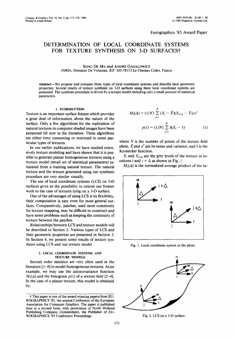
Xi and Xi+a are the grey levels of the texture at lo- cations i and i + A as shown in Fig. 1.

M2(A) is the normalized average product of the lu-

W

I W

A ~ j+A t

J

Fig. 1. Local coordinate system in the plane.

W

t

Fig. 2. LCS on a 3-D surface.

nsp

S. D. MA and A. GAGALOWICZ

ni w i • . _Ti

SP

° '

tsp

3 - D surface

geodesic curve joining SP. to i

Fig. 3. Parallel transport of LCS along geodesics.

minances of two points translated from one another by a vector A. p(1) is simply the proportion of grey levels 1 in the texture field.

Fig. 4. LCS defined by parallel planes.

i n t e r s e c t i o n curves

As shown in Fig. 1, A is defined at each location by a local coordinate system (t, w). In general, the LCS are parallel to each other, which corresponds to the homogeneous texture.

In the case of 3-D surfaces, the computation of such model can be extended in a straightforward way if the LCS are well defined (see Fig. 2).

The only constraint is that for each location i, i + A must belong to the surface.

Practically, the t, w vectors define the tangent plane at location i, and we suppose that the 3-D surface is smooth enough so it can be approximated by its tangent plane up to location i + A, for all translations consid- ered.

If the LCS are thus defined, we can use the same texture model for planar or 3-D texture because the M2(A) parameters are defined by the same planar translations.

The orientation of the t, w vectors on the tangent plane is specified by the LCS and defines the local ori- entation of the texture on the surface.

172

Fig. 5. Revolution surface.

Local coordinate systems for texture synthesis on 3-D surfaces 173

Fig. 6. Natural and synthesized planar SEISMIC texture.

Fig. 7. NAIL covered with SEISMIC texture.

Fig. 8. Cast-iron RENAULT car part covered with SEISMIC texture using two different LCS.

Local coordinate systems for texture synthesis on 3-D surfaces 175

3. LCS ON 3-I) SURFACES In this section, we propose several possible defini-

tions of LCS on a 3-D surface: (a) In the Computer Graphics Communi ty , a sur-

face is often described in a parametric form (2):

I x = x ( u , v)

y = y(U, V)

z = z (u , v)

(2)

the geodesics is the 3-D analog of parallelism of the local coordinate system on the plane.

In some special cases, for example, for a sphere, a geodesic is an arc of a great circle and on a cylinder, it is an arc of helix. In the general case ofcurved surfaces defined by a set of points whose x-y-z coordinates are given (may be measured by a 3-D sensor), we present an algorithm which allows us to compute rapidly the geodesics from a starting point SP to all the other points of the surface. We construct a graph G = (P, A) de- scribed as follows:

For each location i = (xi, y,, zi), a LCS can be derived immediately from (2). We may choose t and w on the tangent plane such that t is the tangent vector to the curve u = cst passing through i, and similarly, w is the tangent vector to the curve v = cst. n is the normal to the surface.

f u=ui t = (Ox/Ov, Oy/Ov, OzlOv)l . . . .

u~ui w = (Ox/Ou, Oy/Ou, Oz/Ou)l . . . .

n = t A w

(3)

Such local coordinate systems have some drawbacks. t and w are not orthogonal to each other, in general, so that it is preferable to replace the LCS (t, w, n) by (t, w', n) where w' -- t A n .

If the surface is only described by a set of discrete points (vertices of planar facets) then it is necessary to construct the surface with patches parametrized in the former way, which may be a very difficult task and is, in any case, time consuming.

(b) Another way to determine LCS is to use parallel transport along geodesics (see also [4]). A geodesic is the shortest path joining two different points of the surface. Tangent vectors to a geodesic at different points are related to one another by parallel propagation which is a natural extension of vectors moving along a straight line and remaining parallel to each other in the plane.

As shown in Fig. 3, we define a starting point SP on the surface and a local coordinate system (tsp, Wse, nse) associated to it. This initial LCS is transported along the geodesics to obtain the LCS for every points of the surface and we want to keep them parallel to each other in a certain sense.

(t~, w~, ni) define an orthonormal coordinate system at location i; n~ is the normal to the surface; t~ lies on the tangent plane• Let T~ be the tangent vector to the geodesic at location i, i fO is the angle between tse and Tse, we construct t~ such that the angle between t~ and 7",. is also O.

The LCS defined with the use of geodesics have some interesting properties. They assure that there is no local distortion of the textural information on the surface (local invariance of the topology).

A geodesic curve is the 3-D analog of a straight line on the plane and the parallel transport of LCS along

• P is the set of nodes in a graph G and, in our case, it is a set of points of the surface P = {P~,/'2 . . . . , Pm}.

• A is the set of arcs of G, A = {A~2, At3, . . . , Aij, • . . }. At each node of G, there are eight arcs (except at the boundary) which relate this node to its eight neighbors.

• Every arc A 0 has a length of do being the Euclidean distance between Pg and Pj.

We use the algorithm of Moore-Dijkstra [5] to find all the shortest paths from SP to Pi, i = 1 . . . . . m. These shortest paths will be taken as initial solutions for the research. A better solution will be obtained by a relaxation method.

The algorithm of Moore-Dijkstra can be explained briefly as follows:

Assume ~? is the length of the shortest path between SP and P~, giving at each point P~, i = l, • • • m a temporary value X~, the algorithm will make ),i con- verge to ~,* after a number of iterations.

At each iteration, we separate the set P in two subsets S and P-S:

S :a set of points in which we have )~ = ),* (e.g., for every point in S, we have found the shortest path with length h*).

P-S: in this set, we have not found the shortest path but we give a temporary value ~ for each point which is equal to:

hi = MIN(~k + dki). e~s

We can prove mathematically that there exists a point Pj in P-S and we have Xj = h* if:

Xj = MIN(),i). PiE P-S

Then we can put the point Pj in the set S after this iteration and systematically, with this procedure, S will converge to P and we can find all the shortest paths from S P t o any point of the surface. More information about this algorithm can be found in [5].

(c) The third type of LCS is the easiest to compute and is convenient for any type of surface description. As shown in Fig. 4, we compute the intersection curves between the 3-D surface and a set of parallel planes (parallel to the x, y plane for example).

176 S. D. MA and A. GAGALOWlCZ

The LCS at each location is defined by:

{w n~: the normal to the 3-D surface,

ti: the tangent to the intersection curve, and

i = Hi A t i .

If the surface is given by an analytical form, the intersection curve is obtained analytically using the surface equation and the plane equation in a straight- forward way.

Suppose that the surface is a surface of revolution, we can choose the parallel planes being orthogonal to the rotation axis of the surface. The intersection curves are simply circles as shown on Fig. 5.

A very current situation is that the surface data are given by a set of points measured by a 3-D laser sensor. In this case the intersection curves are automatically available from the data (each curve corresponds to a bloc of data: a line in a matrix) as the object is scanned line by line along these intersection curves.

The vector t may be approximated by the difference of two successive points on the curve.

Of course, with respect to LCS defined by parallel transport along the geodesics the computation is achieved much more rapidly, the inherent drawback being that the texture has undergone a spatial defor- mation on the surface which is also the case of (a).

The choice of LCS corresponds to a way of posi- tioning the texture on the surface. It is a structural information.

4. TEXTURE GENERATION AS we have pointed out in Section 2, the stochastic

parameters of the texture model can be defined by LCS in the case of 3-D surfaces. Using these parameters as input data, we can generate the texture field having exactly the same statistics by an optimization tech- nique. This method is a generalization of a planar method described in our previous papers [1, 3] and is presented in [4].

Some results of texture synthesis using various LCS are presented in Figs. 6 to 8.

Figure 6 displays the reproduction of natural SEIS- MIC TEXTURE in the planar case. The left image is a natural texture from which the model (1) is com- puted. The right image is generated by computer using the statistical parameters (1) described in Section 2 as input and our planar synthesis procedure [3].

In Fig. 7, we show the synthesis of SEISMIC TEX- TURE on a nail. In this particular situation (revolution surface), it is possible to find a parametrization (u, v) (case (a)), a starting point SP (summit of the cone) and a tangent tse (case (b)) such that these LCS obtained are the same as those obtained using parallel planes (orthogonal to the rotation axis of the object). Thus the result corresponds simultaneously to the synthesis achieved with the three possible choices of LCS.

Figure 8 displays the synthesis of the same texture on a cast-iron part of a RENAULT car. The left image corresponds to the use of parallel transport along geo- desics (case (b)) and the right image to the use of in- tersection curves of the 3-D object with horizontal planes (case (c)). The rendering of two images is dif- ferent, this time.

5. CONCLUSION Several possible LCS have been proposed as 3-D

surface descriptors. They are easy to compute and two of them can be used for any type of surface data. The LCS defined by parallel transport along geodesics are considered to be the best as they follow the geometrical deformation of the surface with no local distortion.

LCS defined by intersection curves with a set of par- allel planes can be computed very rapidly and are con- venient for any type of surface data.

The LCS allow the extension of the definition of texture models to the 3-D case and also give a very powerful tool for the reproduction of the textural in- formation in computer shaded images. Only a small data base is used for the textural information and the texture can be reproduced rather faithfully on any type of surface.

REFERENCES I. A. Gagalowicz and S. D. Ma, Synthesis of natural texture,

Sixth ICPR Conference, Munich, Germany (1982). 2. A. Gagalowicz and S. D. Ma, Synthesis of natural textures

on 3-D surfaces, Seventh ICPR Conference, Montreal, CANADA (1984).

3. S. D. Ma and A. Gagalowicz, Natural texture synthesis with the control of autocorrelation and histogram. Third Scandinavian Conference on Image Analysis, Copen- hagen, Denmark (1983).

4. A. Gagalowicz and S. D. Ma, Model driven synthesis of natural textures for 3-D scenes. Comput. & Graphics 10, 161-170.

5. M. Gondran and M. Minoux, Graphes et algorithmes. Erolles, Paris, France (1979).