Author's Accepted Manuscript

Determination of Cs-137 contamination depthdistribution in building structures using geos-tatistical modelling of ISOCS measurements

Sven Boden, Bart Rogiers, Diederik Jacques

PII: S0969-8043(13)00213-3DOI: http://dx.doi.org/10.1016/j.apradiso.2013.04.028Reference: ARI6251

To appear in: Applied Radiation and Isotopes

Received date: 4 September 2012Revised date: 21 March 2013Accepted date: 22 April 2013

Cite this article as: Sven Boden, Bart Rogiers, Diederik Jacques, Determinationof Cs-137 contamination depth distribution in building structures usinggeostatistical modelling of ISOCS measurements, Applied Radiation and Isotopes,http://dx.doi.org/10.1016/j.apradiso.2013.04.028

This is a PDF file of an unedited manuscript that has been accepted forpublication. As a service to our customers we are providing this early version ofthe manuscript. The manuscript will undergo copyediting, typesetting, andreview of the resulting galley proof before it is published in its final citable form.Please note that during the production process errors may be discovered whichcould affect the content, and all legal disclaimers that apply to the journalpertain.

www.elsevier.com/locate/apradiso

1

Determination of Cs-137 contamination depth distribution in building structures using geostatistical modelling of ISOCS measurements Sven Boden1, Bart Rogiers1,2 Diederik Jacques1 1 Institute for Environment, Health and Safety, Belgian Nuclear Research Centre (SCK•CEN), Boeretang 200, BE-2400 Mol, Belgium sven.boden@sckcen.be, Tel. +32 14 33 26 66, Fax /32 14 31 19 93; bart.rogiers@sckcen.be, Tel. +32 14 33 32 09, Fax +32 14 32 35 53 2 Dept. of Earth and Environmental Sciences, K.U.Leuven, Celestijnenlaan 200e - bus 2410, BE-3001 Heverlee, Belgium diederik.jacques@sckcen.be, Tel. +32 14 33 32 32, Fax +32 14 32 35 53 ABSTRACT Decommissioning of nuclear building structures usually leads to large amounts of low level radioactive waste. Using a reliable method to determine the contamination depth is indispensable prior to the start of decontamination works and also for minimizing the radioactive waste volume and the total workload. The method described in this paper is based on geostatistical modelling of in situ gamma-ray spectroscopy measurements using the multiple photo peak method. The method has been tested on the floor of the waste gas surge tank room within the BR3 (Belgian Reactor 3) decommissioning project and has delivered adequate results. Keywords: Facility decontamination and decommissioning, Site radiological characterization, Geostatistics, In situ gamma spectroscopy, ISOCS (In Situ Object Counting System)

1 Introduction In June 2012, 435 nuclear power reactors were in operation, 62 under construction and 140 in permanent shutdown (IAEA, 2012). According to the International Atomic Energy Agency (IAEA, 2011) as of December 2010, for only 5 reactors the license had been terminated, which is the legal act at the end of the decommissioning. The number of nuclear facility decommissioning projects is therefore increasing. Besides the nuclear installations to be dismantled, the building structures containing the installations take part of decommissioning as well. Contamination of the building structure, usually resulting from leakages during operation, releases due to maintenance works or even during dismantling operations, may result in large volumes of predominantly low level radioactive waste. In order to minimize the radioactive waste volume, it is indispensable to determine the contamination depth prior to initiate decontamination works. Some decommissioning projects use iterative cycles consisting of decontamination treatment steps and radiological control measurements until release levels are reached. The radiological control measurements are usually conducted with straightforward handheld equipment such as gas proportional or scintillation counters for surface contamination measurements. Despite being straightforward, this method might lead to multiple iterative cycles and is therefore not always practical and efficient. Most decommissioning projects also use sampling by core drilling and destructive analysis which is time consuming and costly. Moreover, it only provides information on small discrete spots and spatial extrapolation to the complete area of a structure might cause problems in case of an inappropriate sampling scheme. This could go from non-representativeness of the samples for the complete area or the absence of certain important small or narrow discrete features in the sampling scheme, to inaccurate estimation of the spatial variability and hence a misleading idea about the spatial continuity of the contamination. A second iteration of the decontamination might be required when important high contaminated spots or features are missed, while an erroneous estimate of the spatial continuity might heavily affect decontamination volumes. Therefore, the use of larger spatial supports (area/volume corresponding to a measurement location) is investigated in this paper as a possible methodology for optimizing a decommissioning project.

2

Determining the radionuclide depth in soil and concrete using Non Destructive Assay based on In-Situ Gamma Spectroscopy is a way to obtain prompt results and larger measurement supports. This has already been studied based on various principles (Whetstone et al, 2011):

• Using different special designed multiple collimators and/or shields (Whetstone et al, 2011) (Benke, Kearfott, 2002; Benke, Kearfott, 2001; Van Riper et al, 2002),

• Using the peak to valley ratio method (Zombori et al, 1992; Tyler, 1999), • Using the multiple photo peak method (Sowa et al, 1989; Beck et al, 1972; Karlberg, 1990) or the

primary photo peak and the X-ray lines (Rybacek et al, 1992). Each of these methods has its particular advantages and disadvantages. According to the most recent publication listed above (Whetstone et al, 2011), the first method seems to deliver the most accurate results. A drawback of this method is that one usually considers that the activity distribution in the horizontal direction is relatively homogeneous which is not always justified for example when hot spots are present. Moreover, multiple measurements on one spot are required to determine the radionuclide contamination depth. Therefore, based on experience from the remediation of the BR3 (Belgian Reactor 3) building structure at the Belgian Nuclear Research Centre (SCK•CEN, Mol, Belgium), we evaluated the third methodology using the In Situ Object Counting System (ISOCS) of Canberra (Canberra). In the case of a Pressurized Water Reactor such as the BR3, the key radionuclide to determine the contamination depth in building structures is Cs-137 (Boden, Cantrel, 2007). For the assessment and risk evaluation of surface contamination of an entire floor based on a limited number of measurements, the use of geostatistics could be envisaged. Geostatistics, based on the theory of regionalized variables (Goovaerts, 1997) provides algorithms to estimate expected values, uncertainties, and risk of exceeding a given threshold, based on a limited number of discrete sampling points. The basic notion is the covariance structure of the spatial random variable with the assumption that the correlation between two random variables depends only on their lag (separation) distance. This statistical method, originally applied in the mining industry (Krige, 1951), is applied in many areas where prediction of or uncertainty on regionalized variables is of importance, in particular, in environmental pollution studies (e.g. Goovaerts et al, 2008; Goovaerts, 2010; Zhang et al, 2009; Wu et al, 2009) and hydrology (e.g. De Marsily et al, 2005; El Idrysy, Smedt, 2007; Rogiers et al, 2012; Rogiers et al, 2010). Because radiological contamination is also expected to be correlated in space, several projects applied geostatistical methods for the evaluation of radiological contamination such as studies for sampling scheme optimization and for the spatial structure of extreme values (Jeannee et al, 2008; Desnoyers et al, 2011). These two studies focus on the surface activity, and use many small-scale measurements with uniform spatial support (0.03 m²). However, by varying the vertical placement of the ISOCS device, it is possible to perform measurements with different spatial supports at the same location which allows characterizing larger areas with a single measurement as well as smaller-scale details. Moreover, the focus in the present study is on the contamination depth which has a direct consequence on the radioactive waste volume, rather than the surface activity. The objective of this paper is to apply a new methodology for the decontamination of Cs-137 contaminated building structures with a view of minimizing the radioactive waste volume based on a geostatistical interpretation of a profound pre-treatment characterization programme using mainly Non Destructive Assay. The scope of the proposed methodology is oriented towards relatively high Cs-137 contamination levels, signifying building structures categorized as 2 and 3 (Cantrel, Boden, 2008). Building structures categorized as 2 are located at known contaminated areas where the contamination hazard mainly concerned aerosols and/or dust. In those areas only limited migration of Cs-137 is expected, with contamination depths limited to 5 mm. Contaminated areas where the contamination hazard concerns liquids as well are categorized as 3. In those areas contamination depths up to several hundreds of mm are expected. This paper describes a test case of the floor of the waste gas surge tank room within the BR3 decommissioning project (SCK•CEN), where ISOCS measurements combined with geostatistics have been applied in order to define the decontamination depth of Cs-137 and divide the floor into several decontamination areas. Results obtained are compared with the actual end result of the treatment and final release measurements.

2 Decontamination methodology and test case The floor of the waste gas surge tank room has been used to evaluate the decontamination methodology proposed.

3

2.1 Decontamination methodology The proposed process for the decontamination of Cs-137 contaminated building structures is presented in Figure 1 and consists of following steps:

(i) Pre-treatment characterization For clearly in-depth Cs-137 contaminated building structures, the pre-treatment characterization consists of the determination of the Cs-137 contamination depth by Non Destructive Assay using ISOCS.

(ii) Geostatistical analysis A proper analysis of the spatial distribution of the ISOCS measurement results is carried out, accounting for the different spatial supports (area represented by the measurement) that are used.

(iii) Probability maps and expected mean depth The risks are mapped using the spatial correlation characteristics from step (ii) and geostatistical simulations. Final risk maps are presented at the decontamination scale (scale on which the removal of material can be performed).

(iv) Check with cores Sampling by core drilling at step (i) is used to validate the results obtained in (iii) and to check the the building structure (composition and thicknesses of different layers).

(v) Decontamination plan Based on the results from (iii), previous experiences in the decontamination of rooms and input from the decontamination expert, the decommissioning plan is agreed upon.

(vi) Post-treatment characterization After the execution of the decontamination plan radiological control measurements are applied to demonstrate that the contamination has been completely removed.

Figure 1: Decontamination process: flow chart (left) and schematic view (right).

In order to evaluate the process proposed, potential remaining traces of Cs-137 contamination are determined using long term ISOCS measurements and the volume of removed material is determined by substracting the

Pre‐treatment characterization

Geostatistical analysis

Probability maps & expected mean depth

Decontamination plan& execution

Post‐treatment characterization

ISOCS Cores

Check

Evaluation

4

initial floor surface before decontamination, obtained by laser scanning, from the final floor surface after decontamination.

2.2 Description of the test case The surface of the floor of the waste gas surge tank room (Figure 2) is about 18.4 m² (4.6 m x 4.0 m). During operation of BR3, very limited access to this room was required (e.g. for maintenance purposes). Therefore, this well shielded isolated room had been used as temporary storage room for highly activated and contaminated components. This resulted in the contamination of the floor. Results of the cores showed that the distance between surface level and concrete foundation ranged from 34 up to 42 mm. Above the concrete foundation there is a layer of mortar and a surface epoxy layer, where the latter has a thickness between 5 and 11 mm. Pre-characterization of the floor using hand held scintillation counters was not feasible due to the relatively high radiation. Background radiation of several µGy.h-1and hotspots up to several hundreds of µGy.h-1 have been detected.

Figure 2: Waste gas surge tank before dismantling (left) and unfolded laser scanning picture of the waste gas surge tank room after dismantling and before floor treatment (right).

3 Determination of the Cs-137 depth distribution Firstly, the floor has been fully scanned using single circular surfaces of about 1 m² and partly using single circular surfaces of about 0.15 m² using the ISOCS. The data obtained in terms of Cs-137 surface activity concentration, relaxation depth and contamination depth were then statistically processed using geostatistical methods. Interpretation of the data obtained allowed the preparation of a decontamination plan.

3.1 ISOCS measurements For the determination of the Cs-137 depth, we used the multiple photo peak method (Rybacek et al, 1992). Cs-137 is considered as a multi-energy X-ray/gamma-ray emitting radionuclide, with energy lines at about 32, 36 and 662 keV (via its daughter Ba-137m). Various equations exist for the description of the vertical Cs-137 depth distribution (Dewey et al, 2011). Destructive sampling on more than 20 cores originating from various rooms in the BR3 building showed that an exponential depth distribution is a good approximation:

( ) (0)x

RLS SA x A e

−= × (1)

where x is the depth (mm), As(x) is the activity concentration (Bq.m-2), As(0) is the activity concentration at the surface (0 mm of depth) (Bq.m-2), and RL is the relaxation length (mm). The RL gives the depth at which the activity concentration falls by a factor of 1/e of its maximum value at the surface As(0). The averaged R-square with this exponential function to describe the measured Cs-137 depth profiles in BR3 is about 0.9. The depth of interest is the depth where the activity concentration As(x) is less than the release level (e.g. 10000 Bq.m-2 for Cs-137 according to (EC, 2000)):

x R= −

Assumi

• •

The relaenergy energy The meSystemwith shkeV. Atglobal udetectorsurface the ISO The ISOdistancemeasurecontamfor the cmeasuremeasurelocated to reach

Figure 3for the l

3.2The colthroughdifferenparameestimatethe bestdecontaupscalin

5

((0

S

s

A xRL lnA

⎛× ⎜

⎝

ing an exponendirectly propproportional to the total ac

axation length lines. The "corand the 662 ke

easurements anm (ISOCS) of C

ielding and colt that time, theuncertainty forrs was extendesources and of

OCS efficiency

OCS measuremes from the groements of a 0.1

mination depths contamination ements are in mements. On thejust outside th

h the detector, w

3: Layout of thelarge- (B) and s

2 Geostatisticalllected data without geostatistint spatial suppoters are the loge, a risk analyst estimates thatamination equipng is required.

)0)x ⎞⎟⎠

(2)

ntial depth distrportional to the

to the natural lctivity concent

can be determrrect" relaxatioeV energy linesnd interpretationCanberra. The s

llimators. The efficiency cali

r the depth calced from a minimf real surface ccalibration at R

ments have beeound level. We15 m² surface eat different locdepth are pres

many cases duee other hand, a he 90° collimatwhile the 32 k

e ISOCS measusmall-scale (C) I

l data analysisth ISOCS and ical analysis. Gorts). Furthermg10(activity), cosis based on get might be expepment (see fur

ribution of the count rate rati

logarithm of thtration).

mined on the baon length is thes. n of the resultsystem basicallrange of standibration curve

culation. In midmum of 45 keVcontaminated spRL = 0 mm.

n carried out ue performed abeach. This resucations for bothsented in Figure to local variabig overestim

ted view of the eV X-rays will

urements on theISOCS measure

s the planning o

Geostatistics allmore, a best estiontamination deostatistical simected. Since thrther-on), final

Cs-137 activitio of the 32 keVhe total activity

sis of the coune one where the

s have been cony consists of a

dard ISOCS calneeded to be e

d-2009 howeveV down to 10 kpots (no Cs-13

using a 90° collout 30 measur

ulted in Cs-137h sizes of spati

re 3. Differenceations which ar

mation of contamdetector. In th

l be blocked by

e floor plan of rements.

f the decontamlows an integraimate of the rel

depth and relaxmulation displahe decontamina

depth estimate

ty therefore meV and the 661.y concentration

nt rate ratio fore activity is ide

nducted usingcharacterized

librations used extrapolated doer, the standardkeV. Control m37 migration) s

limator placingements of a 1 m

7 activity conceial support. Thes in results forre generally avmination depthhis case still may a few mm of

oom 124 (A), an

mination benefiation of differelevant parametation length) is

ays the true varation depends oes are needed a

eans that the de6 keV energy l

n (instead of di

the 32 keV anentical when us

the In Situ Objhigh purity gerto be limited t

own to 32 keV.d calibration rameasurements oshowed a suffic

g the detector am² surface eachentrations, rela

he measuremenr the small- anderaged out in c

h can be made wany 662 keV phf lead shielding

nd estimated co

it in multiple went data types (mters (in this stus obtained. In ariability and theon the spatial sat the scale of i

epth is: line; and rectly proporti

d the 662 keV sing the 32 keV

ject Counting rmanium detecto a minimum o. This led to a lange of the Canof tailored madcient precision

at two differenth and about 40xation lengths

nt layout and red large-scale IScase of large scwhen a hotspothotons will be

g.

ontamination de

ways from a measurements

udy, relevant addition to thee uncertainty acale of the nterest, i.e.

ional

V

ctor of 45 large nberra de

for

t 0

and esults SOCS cale t is able

epths

with

best about

In a firswhich dcalculataccordivalues:

( )* hγ

Generalvariabilsemi-vapoints acalled th0.152 mFigure 4

Figure 4for the d

The incdistinctgradualgeostatisamplesTo estimeach povariograused forobtaineforms o

( )γ h =

( )γ h = where s(mm), aThe con

6

st step, the statidescribe the spting experimenng to their lag

1 2

gn

⎡= ⎣∑

lly, two points lity increases wariograms fromare too far awahe range. The

m²) ISOCS mea4.

4: Experimentadifferent spatia

crease of variabt maximum andl increase. Sincistics rather thas). mate or simulaossible lag distaam point set. Tr the depth andd by manually

of the spherical

( ) 3 2hs na

⎛= − ⎜⎜

⎝

( )( 1s n= − −

s is the total siland a is the ranntamination is

istical parametatial variability

ntal semi-variodistance h [L]

( ) (x g x h− +

close to each owith distance. Am smaller γ* vaay to be correlaexperimental sasurements for

al semi-variograal supports of th

bility with distad range in casece this illustratean classical sta

ate values at anance. This requ

The spherical md the relaxationy fitting the mol and exponent

312

h ha a

⎞⎛ ⎞− ⎟⎜ ⎟ ⎟⎝ ⎠ ⎠

( )exp /h a− −

ll or maximum nge (mm) that dnot expected to

ters (basically, y of the considgrams, γ*(h), b, and calculatin

2)h ⎤⎦ (4)

other are moreAs such, spatiaalues at small hated in space ansemi-variogramr the log10(activ

ams, total variahe obtained par

ance is clear foe of the log10(aces that the variatistical analyse

ny location in thuires a continumodel is used ton length to descdels to the expial models are,

n+ (5)

)) n+ (6)

semivariance,determines theo be stationary

mean, variancdered variables by grouping allng the average

e similar than pal correlation, ifh and larger valnd γ* becomes ms of the large-vity), contamin

nce (Var) fittedameters. A: log

or all three of thctivity), while tables are cleares (i.e. the ISO

he 2D space, thous semi-varioo describe the cribe the exper

perimental sem, respectively:

, n is the nuggee distance whery (meaning that

ce and the correare required. Il n possible samhalf squared d

points far awayf present, is evlues at larger hindependent o

-scale (1.057 mnation depth an

d semi-variograg10(activity); B:

he obtained ISthe depth and r

rly correlated inOCS measureme

he spatial variaogram model inlog10(activity),rimental semi-vi-variograms (

et or minimum re the semi varit the mean and

elation as a funIn geostatisticsmple pairs g(x)difference betw

y from each othvidenced from th. From a certaiof lag distance. m²) and the smand relaxation le

am models (VGMdepth; C: relax

OCS parameterelaxation lengn space, this juent do not form

ability needs tonstead of an ex, whereas the evariogram. Parsee Figure 4). T

variance, h is iance reaches i

d variance of th

nction of distan, this is done b) and g(x+h)

ween the variab

her, so the obsethe experimentin distance, theThis distance

all-scale (0.166ength are shown

M) xation length.

ers. There is a gth show a morustifies the use m independent

o be quantified xperimental semexponential morameters were The mathemat

the lag distancits maximum v

he random varia

nce) by

ble

erved tal e is

6 and n in

re of

for mi-odel is

ical

ce value. able

7

are constant in space) in the relatively small floor element, so the semi-variogram models are fitted without considering the total variance. The fitted model parameters are listed in Table 1. Table 1: Semi-variogram parameters and total variance of the data.

Variable Spatial support Type# Nugget Sill Variance

Effective Range (mm)

Depth Small Exp 0 70 48.9 3600 Depth Large Exp 0 65 54.7 3600 Relaxation length Small Exp 0 4 2.94 4000 Relaxation length Large Exp 0 2 1.68 4000 Log10(activity) Small Sph 0 0.8 0.60 3200 Log10(activity) Large Sph 0 0.6 0.43 3200

# Exp: Exponential model (Eq. ) and Sph: spherical model (Eq.) These parameters can however not be directly used in the estimation and simulation procedures because their support volumes (measured areas of 1 m2 and 0.15 m2) differ from the spatial scale of interest for the decontamination plan (300 x 300 mm2). The large-scale ISOCS measurements show consistently lower sills than the small-scale ones indicating the averaging properties of larger-scale measurements. To obtain a semi-variogram model at the point-scale, the sill has to be increased, to reflect the higher variability that might be expected for point-scale values. The range is not expected to change a lot, as indicated by the fitted ranges for the two measurement spatial supports. Several authors (e.g. Clark, 1977) give the following approximation to derive a point-scale exponential semi-variogram:

la a l= − (7)

( )2

/2/ 2 1 l a

la as s el l

−⎛ ⎞⎡ ⎤= − −⎜ ⎟⎢ ⎥⎜ ⎟⎣ ⎦⎝ ⎠

(8)

where l is a measure for spatial scale [mm], a and s are the point-scale range (mm) and sill [-] respectively, and al and sl are the equivalents at scale l. As an approximate value for l, the square root of the measurement area was used. The point scale parameters can be derived both from the large as the small scale ISOCS measurements. The most conservative values (i.e. highest sill and shortest range at the point scale) should however be taken in order to provide reliable risk maps. This leads to the conservative values of s = 74 and a = 2600 mm for the depth parameter which will be studied further-on.

3.3 Geostatistical simulation and risk mapping Since the amount of floor that has to be removed is the key to planning the decontamination methodology, estimations and simulations for risk assessment of the contamination depth are made in this section. Starting from the raw data and the obtained point support variogram, a point support prediction can be obtained for any point using kriging which is a weighted linear interpolation of the existing measurements, possibly with a different spatial support. A major difference with other interpolation techniques is that the spatial correlation structure in the data is taken into account to calculate the weights. Solving the linear kriging system to obtain these weights assures unbiased estimation with a minimal error variance (Rogiers et al, 2010). Data with a certain spatial support require the calculation of point to block covariances besides the standard point to point covariance. Several methods exist to implement this efficiently as is done within the BGeost algorithms (Liu, 2009). These algorithms allow for user-defined non-square supports and are available through the S-GeMS software (Remy et al, 2008; Bianchi, Zheng, 2009). To evaluate the uncertainty at the point-scale, the use of kriging is sufficient. However, since the final decisions for implementing a decontamination plan are made on a different scale (the decontamination scale), point support simulations need to be upscaled to get a proper risk assessment at the decontamination scale. Therefore, the block sequential simulation (BSSIM) algorithm within BGeost was used to make 50 different realizations of the contamination depth distribution at the point-scale, and all circular measurement supports were approximated by an icosagon (20-sided polygon). The block measurement error variance was initially set to 1% of the small ISOCS mean values. The numerical grid was chosen to be 150x150 mm, and the configuration is shown in Figure 5. Ordinary simulation is chosen which uses local mean values rather than a single mean value for the entire area. In this way, together with the non-stationary semi-variogram models, possible trends in the data can be detected and analysed. The block covariance computation approach that uses the traditional integration method was chosen (Liu, 2009) and both the small and large ISOCS measurements were used as primary data for the simulations.

Figure 5

Each ofmaps atblock. Aclear thplaces. (lower land upp

Figure 6contami

The decis a cleain space

8

5: Layout of the

f these point-sct the decontamA few examplehat the high val

There is howeleft quadrant) iper sides of the

6: Three realizaination depth).

contamination ar area with coe, and only a fe

e numerical sim

cale realizationmination scale. Nes of point-suppues, as well asver quite someis clearly contae room.

ations of the con

support risk montamination reew spots remai

mulation grids, t

ns was upscaledNext, several rport realization the areas with

e difference betaminated to a h

ntamination dep

maps are preseneaching beyondin with contam

the room bound

d using block krisk maps were ns are given inhout contaminatween the abso

higher degree th

pth, all conditio

nted in Figure 7d 10 mm depth

mination depths

daries and the r

kriging to a regmade using thFigure 6. From

ation seem to oolute values. Thhan the passag

oned on all the I

7, for depths ofh. The deeper ths exceeding 20

raw measureme

gular 300 x 300he 50 simulatedm the different ccur consistenthe area below t

ge way that was

ISOCS data (co

f 5, 10, 15, 20 ahan 15 mm aremm.

ent spatial supp

0 mm² grid to od values at eachrealizations, it

tly in the samethe waste surgs located at the

olor scale indica

and 25 mm. Theas are more iso

ports.

obtain h grid t is e e tank

e right

ates

here olated

Figure 7contamiprobabi

Subsequerrors, apatternsFinally,ISOCS measure8. Despexist in results oprovide

Figure 8(300 x 3ISOCS

3.4Core satraditionvalues rselectio

9

7: Risk maps atination depth leility).

uently, a sensitand the point-ss in the risk ma, besides the jomeasurementsements. Hence

pite the fact thathe risk maps

obtained with te the best overa

8: Comparison 300 mm²) for A:only, and 3) the

4 Comparison wamples were drnal method (IAresulting from

on was made pr

t the contaminaevel of A: 5 mm

tivity study wascale sill and raaps persisted inoint use of all ss was evaluatede the entire anaat both datasetsobtained usingthe combined uall picture of th

between the ob: 5 mm, B: 10 me small-scale IS

with core samprilled at 4 locatAEA, 1998; NErapid dose raterior to the exec

ation support scm, B: 10 mm, C:

as performed toange parametern all analyses (npatial supportsd for guiding fualysis was repeas (small and larg only one typeuse of all data.he contaminatio

btained contamimm, C: 15 mm, D

OCS only (colo

ples tions in the rooEA, 2011). Thee and surface acution of the IS

cale (300 x 300 m 15 mm, D: 20 m

o assess the infrs. Results shownot shown). s, the effect of future decisionsated twice, witrge ISOCS) aree of data. More Due to the fulon depth.

ination depth riD: 20 mm and E

or scale indicate

om, and the cone sampling locaactivity measurSOCS measure

mm²) showing tmm and E: 25 m

fluence of the swed very little

using only largs concerning thth less data, ane covering the eover, none of ll coverage of t

isk maps at the E: 25 mm, usines probability).

ntamination depations had beenrements using hements. The cor

the probability mm (color scale

specified block influence, and

ge-scale or onlyhe spatial suppod a comparisonentire room, clthem accuratelthe floor, the la

contaminationng 1) all data, 2)

pth was determn selected basehand held equipres were obtain

of exceeding a e indicates

k measurementd the important

y the small-scaort of the n is shown in Flear differencesly resemble thearge ISOCS see

support scale the large-scale

mined using theed on the highepment. The ned using a wa

t

ale

Figure s e em to

e

e est

ater

10

cooled Hilti diamond core drilling tool with a core bit diameter of 57 mm. Each core sample obtained was sliced, resulting in discs of a few mm thicknesses. Each disc was homogenized into powder using successively a jaw crusher and a planetary ball mill, both from Retch. The Cs-137 concentration of the homogenized powder samples is determined by high purity germanium gamma spectroscopy. The various measurements for each core resulted in the Cs-137 concentration depth profile and finally in the determination of the Cs-137 depth concentration. The results are displayed in Table 2. We observe relative large differences between the two methods, which could be explained by the standard uncertainty of each individual method and the big differences in the surfaces measured, even using the ISOCS "small" surface measurement results. For example, at sampling point 31, the core has been exactly taken at a small individual hotspot of 200 µGy.h-1, while the result of the ISOCS measurement is averaged out by including the neighboring surface. It is therefore difficult to identify the real reference value and compare results. However, sampling by core drilling is still indispensable to provide information regarding the composition and thicknesses of the different layers in the floor. Table 2: Cs-137 depth contamination (mm): Comparison between ISOCS (small area) and core samples.

Method Surface

measured (m²)

Depth Nr. 1 (mm)

Depth Nr. 11

(mm)

Depth Nr. 31 (mm)

Depth Nr. 34 (mm)

ISOCS – small area 0.166 21 18 16 12 Core samples 0.002 20 8 27 20 Ratio 1.1 2.3 0.6 0.6

In section 3.1 the use of an exponential depth distribution was proposed. In the specific case of the floor of the waste gas surge tank room this seems to be a good approximation as shown in Figure 9. The average R-square with this exponential function is 0.98, 0.95 and 0.92; respectively for sample number 1, 31 and 34. For sample number 11 insufficient subsamples were available.

Figure 9: ln[Cs-137 activity concentration] as a function of depth for sample number 31

4 Decontamination plan The main input for defining the decontamination plan were the 300 mm x 300 mm risk maps (Figure 7) and the mean depth distribution (Figure 10A). Apart from this, we used our return of experience from first attempts on an area in the controlled area of the BR3 auxiliary building (Cantrel, Boden, 2008). Highly important are the global uncertainty on the depth, the composition and thicknesses of the different layers (see 2.2) and the view of the concrete decontamination expert on the practicability. As a result of a meeting between experts from characterization, geostatistical analyses and decontamination discussing the various elements, we divided the floor into 3 areas (see also Figure 10B):

• Area I where the objective was to remove solely the epoxy coating corresponding to a depth of about 5 to 10 mm (blue zone in Figure 10B);

• Area II where the objective was to remove the epoxy layer and a part of the mortar layer corresponding to a total depth of about 20 to 25 mm (yellow zone in Figure 10B); and

R² = 0,95

‐4

‐2

0

2

4

6

8

10

0 10 20 30 40 50 60

ln [C

s‐13

7 activity con

centration

] (Bq

.g‐1)

depth (mm)

11

• Area III where the objective was to completely remove the epoxy coating and the mortar layer corresponding to a total depth of about 35 to 40 mm (red zone in Figure 10B).

An applied method in France consists of defining the maximum contamination depth within a certain area and add an additional safety margin (or factor) to compensate for uncertainties (e.g. see IAEA, 2010). In our test case, the ratio between the decontamination plan depths for the different areas and the mean (instead of maximum) depth values obtained from the geostatistical analysis, correspond to a safety factor between 1 and 2 in general.

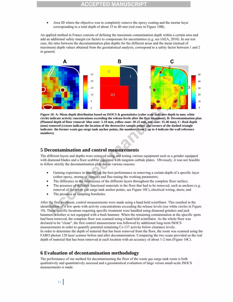
Figure 10: A: Mean depth distribution based on ISOCS & geostatistics (color scale indicates depth in mm; white circles indicate activity concentrations exceeding the release levels after the first treatment), B: Decontamination plan (Planned depth of floor removal: blue zone: 5-10 mm, yellow zone: 20-25 mm, red zone: 35-40 mm), C: Real depth (mm) removed (crosses indicate the location of the destructive sample points ,the corners of the dashed triangle indicates the former waste gas surge tank anchor points, the numbers from 1 up to 4 indicate the wall reference numbers).

5 Decontamination and control measurements The different layers and depths were removed using and testing various equipment such as a grinder equipped with diamond blades and a floor scabbler equipped with tungsten carbide plates. Obviously, it was not feasible to follow strictly the decontamination plan due to various reasons:

• Gaining experience in identifying the best performance in removing a certain depth of a specific layer (either epoxy, mortar or cement) and fine-tuning the working parameters;

• The difference in the thicknesses of the different layers throughout the complete floor surface; • The presence of different functional materials in the floor that had to be removed, such as anchors (e.g.

removal of the waste gas surge tank anchor points, see Figure 10C), electrical wiring, ducts; and • The presence of sampling boreholes.

After the first treatment, control measurements were made using a hand held scintillator. This resulted in the identification of a few spots with activity concentrations exceeding the release levels (see white circles in Figure 10). These specific locations requiring specific treatment were handled using diamond grinders and jack hammers whether or not equipped with a bush hammer. When the remaining contamination at the specific spots had been removed, the complete floor was scanned using a hand held scintillator. As the whole floor was declared to be "clean", the first control measurement was followed by additional long-term ISOCS measurements in order to quantify potential remaining Cs-137 activity below clearance levels. In order to determine the depth of material that has been removed from the floor, the room was scanned using the FARO photon 120 laser scanner before and after decontamination. Comparing the two scans provided us the real depth of material that has been removed at each location with an accuracy of about 1-2 mm (Figure 10C).

6 Evaluation of decontamination methodology The performance of our method for decontaminating the floor of the waste gas surge tank room is both qualitatively and quantitatively assessed and a geostatistical evaluation of large versus small-scale ISOCS measurements is made.

12

6.1 Qualitative assessment Figure 10 compares the mean of the depth realizations from the geostatistical analysis (A), the decontamination plan (B) and the removed volume after decontamination (C). The estimated spatial pattern of contamination depth does not correspond well to the real removed volume (Figure 10A and C). The zones from the decontamination plan are however clearly visible in the removed volume map. The rectangular yellow-red zone starting from the corner between wall 3 and 4 results from removing a duct between the waste gas surge tank room and the connecting room. The thin red zone starting at the top of wall 1 and following wall 2 and 3, is the result of the removal of electrical wiring. Apart from these special points, more material has been removed in contamination area I, mainly since the epoxy layer appeared to be thicker top right. In decontamination area II a little bit more material has been removed, mainly due to the presence of the crack underneath the epoxy coating (red spot and yellow-red diagonal bar top left), not visible before removing this coating, and additionally due to the fact that it is difficult to apply fine tune removal on a mortar layer. In the case of decontamination area III a little bit less material was removed compared to the decommissioning plan. Reason for the difference can be explained by the uncertainty of the thickness of the mortar layer throughout the area, since this zone was simply treated removing the whole of the mortar layer up to the concrete foundation. The full process of pre-characterization, decontamination, control measurements, treatment of specific spots and release measurements progressed smoothly without iterations. As shown on Figure 10A, the spots requiring additional decontamination after the first treatment are highly consistent with the results from the geostatistical analysis.

6.2 Quantitative evaluation No traces of contamination during the post-treatment characterization could be detected at most locations (release level Cs-137: 10000 Bq.m-2) conducting long term ISOCS measurements at the same locations and for the same sizes of spatial support as in the pre-treatment characterization. Minimum detectable activities usually ranged from 500 down to 50 Bq.m-2, depending on the measurement time and surface measured. Table 3 shows an estimation of the volume removed for various assumptions:

1. following the "traditional" method based on the maximum contamination depth found including a safety factor of 1.5 (see also section 4, IAEA, 2010);

2. exactly following the decontamination plan as defined in section 4; 3. the real volume removed based on the proposed method in this paper, including the material removed

due to other reasons than radiological contamination (see above); and 4. the real volume removed based on the proposed method in this paper, excluding the material removed

due to other reasons than radiological contamination.

Table 3: Estimation and comparison of volumes removed.

Assumption Volume removed

(m³)

Compared to traditional method

(%)

1 Max. contamination depth + SF 0.83

2 Decontamination plan 0.39 -53%

3 Geostatistics+ISOCS Incl. special points 0.60 -27%

4 Geostatistics+ISOCS Excl. special points 0.55 -34%

Following the proposed method in this paper, the estimated waste volume reduction was about 1/3 compared to a more traditional method. Moreover, the ratio between the clearance level and the potential remaining contamination is still more than a factor 5. The relaxation length can be calculated following equation (2) using the real depth of material removed, the initial activity concentration and the potential remaining Cs-137 traces. Where no traces of Cs-137 could be detected, only the maximum relaxation length was calculated. This is the case for area I. In a few locations in areas II and III remaining traces of Cs-137 contamination of a few hundred Bq.m-2 were detected. For those locations calculated post-treatment relaxation lengths can be compared with the pre-treatment relaxation lengths obtained by the initial ISOCS measurements (see also section 3.1). Table 4 shows the ratio between the pre- and post-treatment relaxation lengths; they vary between 0.5 and 2.0. The small-scale ISOCS measurements tend to have a ratio closer to 1. For future similar decontamination activities, starting from the mean depth distribution (Figure 10A) to define the decommissioning plan as has been done in this case, a safety factor between 1 and 2 should be considered and checked with the risk maps.

Table 4

6.3The biaframewdepth frscale IS11. Thefor the lboth cacases. Twhen uscale ISThe lattthe largcoveragspatial aNeverthlarge-scwhich iof conta

Figure 1ISOCS estimate

13

: Pre- and post-

3 Geostatisticalases introduced

work of planninrom the geostaSOCS support, e average misfilarge- and smases. A probabi

The use of smasing the large-

SOCS supportster is a result fr

ge-scale data. Tge of the contamaccuracy of theheless the correcale case (resp.indicates a highamination dept

11: Scatterplot data, versus thees are plotted, v

-treatment calc

Area

II II III III III III III III III

l evaluation: Ld by using eitheng future characatistical realizat

is compared toit amounts 0.3 all-scale ISOCSlty distribution

all-scale ISOCSscale supports.

s, while large urom the partial

To avoid such lminated area. Se predictions welations with th. 0.76 and 0.75hly significant th is retrieved b

of mean krigede misfit with thevisualising the p

ulated relaxatio

Nr Area

measure(m²)

29 0.16629 1.0572 0.1663 1.05712 0.16612 1.05713 0.16613 1.05719 1.057

Large- versus ser the large- orcterization in stions at the 300o the ‘true’ conand -0.2 mm, wS cases, respecn is also providS clearly result. Underestimat

underestimationl coverage of thlarge underestimSmall-scale me

within the largehe results from5; with p-valuelinear relationby both approa

d contaminatione results based

probability dens

on lengths.

ed

Post- treatment

RL (mm)

4.9 2.3 2.6 2.9 3.4 3.1 2.7 6.0 3.5

small-scale ISOr small-scale ISsimilarly contam0 x 300 mm² suntamination dewhile the averactively. This indded in Figure 1ts in more overtion of about 5 n of 10 to 20 mhe room for thimation, it is theasurements caer supports of th

m using all data s < 2.2 × 10-16,ship in both caaches.

n depth for the 3on all ISOCS dsity function of

Pre-treatment

RL (mm)

5.4 4.6 3.9 5.1 3.5 3.6 3.6 3.8 3.0

OCS measuremSOCS measureminated materiupport scale, u

epth using all dage absolute didicates that the1, using kernel

restimation of tmm seems to b

mm occurs mosis dataset, in co

hus recommendan be used as ahe large-scale are very simil

, using Pearsonases. This also

300 x 300 mm² data. Right of thf the misfit for b

Ratio

1.1 1.9 1.5 1.8 1.0 1.2 1.3 0.6 0.9

ments ments were tesial. The averagsing either the

data by plottingifference amoue predictions arl density estimthe contaminatbe more abund

stly with the smontrast with theded to try to achadditional meanISOCS. ar for both the n's product-moindicates that t

grid cells, for ahe scatterplot, tboth cases.

sted in the ge contaminatiosmall- or large

g the misfit in Funts 3.4 and 3.9re very similar

mation, for bothtion depth thandant for the largmall-scale suppe full coveragehieve a full ns to increase t

small-scale anment correlatiothe general pat

a single type of he kernel densi

on e-Figure 9 mm r for h n ge-

ports. e of

the

nd on), ttern

ity

14

7 Conclusions The method to determine Cs-137 depth contamination based on geostatistical modeling using ISOCS measurements delivered adequate results for the test case. Using geostatistics to downscale and upscale support volumes (from ISOCS support scales to point scale, and from point-scale to decontamination support scale, respectively) enabled us to subdivide the floor surface into several decontamination areas with different removal depths. The predicted depth distribution throughout the floor surface appears close to reality as inferred from the successful decontamination, and the spots where additional treatment was required. The actual removed floor volumes do however not correspond to the estimated contamination depths due to the practical limitations of the decontamination approach. The few locations where it was actually possible to compare calculated post-treatment relaxation lengths with calculated pre-treatment relaxation lengths showed that the accuracy aligns with the safety factor applied in the test case. However, one should be aware that all values are always averaged out on a certain surface, which implies the use of a safety factor. The size of the safety factor depends on the size of spatial support of the ISOCS measurements and the coverage (total surface versus surface measured). The ultimate goal of the proposed process for decontamination is to minimize the waste production, with an optimal amount of resources spent. For our test case, the estimated waste volume reduction is about 1/3 compared to a more traditional and conservative approach. Concerning the planning of future radiological characterization projects, it is recommended that a full coverage of the area is obtained with large-scale ISOCS. If high detail on depth and spatial location is needed, small-scale measurements should be performed additionally at the locations of interest. The use of geostatistics to provide risk maps is highly recommended since correct interpretation of the raw data with large spatial supports is very difficult.

Acknowledgements For the execution of measurements and discussion on the results, the authors gratefully acknowledge G. Verstrepen en B. Wuyts, in case of the ISOCS measurements and the sampling and destructive analysis; and W. Smolders in case of the Internal Safety Department hand held measurements. N. Mangelschots deserves recognition for selecting the company Argon that performed the laser scanning measurement and for further co-ordination and assistance during the performance and treatment of the laser scanning data. Discussion and consultation with R. Vandyck, responsible for the concrete decontamination, was indispensable to define and execute the decontamination plan. This test case was performed within a contract between Belgian Agency for Radioactive Waste and Enriched Fissile materials, NIRAS/ONDRAF and the SCK•CEN.

References Beck, H.L.,. DeCampo, J., Gogolak, C., 1972. In situ Ge(Li) and NaI(Tl) gamma-ray spectrometry, US Atomic

Energy Commission, New York, Report HASL-258. Benke, R.R., Kearfott, KT., 2001. An improved in situ method for determining depth distributions of gamma-ray

emitting radionuclides, Nuclear Instruments and Methods in Physics Research A 463 393-412. Benke, R.R., Kearfott, KJ., 2002. Demonstration of a collimated in situ method for determining depth

distributions using �-ray spectrometry, Nuclear Instruments and Methods in Physics Research A 482, pp. 814-831.

Bianchi, M., Zheng, C., 2009. SGeMS: A Free and Versatile Tool for Three-Dimensional Geostatistical Applications. Ground Water, 47(1), 8-12. doi:10.1111/j.1745-6584.2008.00522.x.

Boden, S., Cantrel, E., 2007. Pre-decommissioning radiological characterization of concrete, ICEM07-7044 Canberra, 2012, http://www.canberra.com/products/438244.asp Cantrel, E., Boden, S., 2008. Assainissement du génie civil du BR3: Etude de cas: les caves du BAN, 12ème

édition Séminaire Décontamination CEIDRE, Fontevraud. Clark, I., 1977. Regularization of a semivariogram. Computers & Geosciences, Vol. 3, pp. 341-346. Pergamon

Press. De Marsily, G., Delay, F., Goncalves, J., Renard, P., Teles, V., & Violette, S., 2005. Dealing with spatial

heterogeneity. Hydrogeology Journal, 13(1), pp. 161–183. Springer. doi:10.1007/s10040-004-0432-3. Desnoyers, Y., et al, 2011. Geostatistics for radiological evaluation: study of structuring of extreme values, Stoch

Environ Res Risk Assess. Dewey, S.C., et al., 2011. A method for determining the analytical form of a radionuclide depth distribution

using multiple gamma spectrometry measurements, Journal of Environmental Radioactivity. EC, 2000. European Commission - Radiation protection 113. Recommended radiological protection criteria for

the clearance of buildings and building rubble from the dismantling of nuclear installations. El Idrysy, E. H., & Smedt, F., 2007. A comparative study of hydraulic conductivity estimations using

geostatistics. Hydrogeology Journal, 15(3), pp. 459-470. doi:10.1007/s10040-007-0166-0.

15

Goovaerts, P., 1997. Geostatistics for Natural Resources Evaluation; Oxford University Press: New York. Goovaerts, P., Trinh, H. T., Demond, A., Franzblau, A., Garabrant, D., Gillespie, B., Lepkowski, J., et al., 2008.

Geostatistical modelling of the spatial distribution of soil dioxins in the vicinity of an incinerator. 1. Theory and application to Midland, Michigan. Environmental science & technology, 42(10), 3648-54.

Goovaerts, P., 2010. Combining Areal and Point Data in Geostatistical Interpolation: Applications to Soil Science and Medical Geography. Mathematical Geosciences, 42(5), pp. 535-554. doi:10.1007/s11004-010-9286-5.

IAEA, 1998. Technical Reports series No. 389, Radiological Characterization of Shut Down Nuclear Reactors for Decommissioning Purposes.

IAEA, 2010. Management of very low level radioactive waste in Europe – application of clearance (and the alternatives), Borrmann, F., 2010. The R²D² Project: Workshop 9, "Release of Sites and Building Structures", 27 September to 1 October, 2010, Karlsruhe, Germany.

IAEA, 2011. Nuclear Power Reactors in the world, IAEA reference data series n°2, 2011 edition, http://www-pub.iaea.org/books/IAEABooks/8752/Nuclear-Power-Reactors-in-the-World-2011-Edition.

IAEA, 2012. Power Reactor Information System (PRIS), http://www.iaea.org/PRIS/Home.aspx. Jeannee, N., et al, 2008. Geostatistical sampling optimization of contaminated premises,

http://www.geovariances.com/IMG/pdf/DEM08-Article-Geostatistics_Final-1.pdf. Karlberg, O., 1990. In situ gamma ray spectrometry of the Chernobyl fallout on urban and rural surfaces,

Nykoping, Sweden, Studsvik Nuclear, Report Studsvik/NP-89/109. Krige, D.G, 1951. A statistical approach to some mine valuations and allied problems at the Witwatersrand,

Master's thesis of the University of Witwatersrand. Liu, Y., Journel, A. G., 2009. A package for geostatistical integration of coarse and fine scale data. Computers &

Geosciences, 35(3), 527-547. doi:10.1016/j.cageo.2007.12.015. NEA, 2011. NEA/RWM/R1, JT03307286, The NEA co-operative programme on decommissioning,

Decontamination and demolition of concrete structures. Remy, N.N., Wu, J., Boucher, A., 2008. Applied Geostatistics with SGeMS: A User’s Guide. Cambridge, UK:

Cambridge University Press. Rogiers, B., Mallants, D., Batelaan, O., Gedeon, M., Huysmans, M., Dassargues, A. 2010. Geostatistical analysis

of primary and secondary data in a sandy aquifer at Mol/Dessel, Belgium. In Cockx, L., Van Meirvenne, M., Bogaert, P. and D'Or, D. (Eds.), Proceedings of the 8th International conference on Geostatistics for Environmental Applications, Ghent University, 13-15 September 2010, pp. 90-93.

Rogiers, B., Winters, P., Huysmans, M., Beerten, K., Mallants, D., Gedeon, M., Batelaan, O., Dassargues, A., 2012. Centimeter-scale secondary information on hydraulic conductivity using a hand-held air permeameter on borehole cores. Geophysical Research Abstracts, Vol. 14, EGU2012-1794-1, EGU General Assembly 2012, Vienna, 22-27 April 2012.

Rybacek, K., Jacop, P., Meckbach, R.,1992. In situ determination of deposited radionuclide activities: improved method using derived depth distributions from the measured photon spectra, Health Physics 62 (6), pp. 519-528.

SCK•CEN, 2012. http://www.sckcen.be/en/Our-Research/Research-facilities/BR3-Belgian-Reactor-3. Sowa, W., Martini, EK, Gehrcke, K., Marschner, P., Naziry, M.J., 1989. Uncertainties of in situ gamma

spectrometry for environmental monitoring, Radiation Protectopn Dosimetry 27, pp. 93-101. Tyler, A.N., 1999. Monitoring anthropogenic radioactivity in salt marsh environments through in situ gamma-

ray spectrometry, Journal of Environmental Radioactivity 45 (3), pp. 235-252. Van Riper, K.A., Metzger, R.L., and Kearfott, K.J., 2002. Radionuclide depth distribution by collimated

spectroscopy, Proceedings of the Topical Meeting on Radiation Serving Society, Santa Fe, NM. Whetstone, Z.D., Dewey, S.C., Kearfott, KJ., 2011. Simulation of a method for determining one-dimensional

137Cs distribution using multiple gamma spectroscopic measurements with an adjustable cylindrical collimator and center shield, Applied radiation and isotopes 69, pp. 790-802.

Wu, W., Xie, D.-T., & Liu, H.-B., 2009. Spatial variability of soil heavy metals in the three gorges area: multivariate and geostatistical analyses. Environmental monitoring and assessment, 157(1-4), pp. 63-71. doi:10.1007/s10661-008-0515-z.

Zhang, H., Huang, G.-he, & Zeng, G.-ming, 2009. Health risks from arsenic-contaminated soil in Flin Flon-Creighton, Canada: integrating geostatistical simulation and dose-response model. Environmental pollution, 157(8-9), 2413-20. doi:10.1016/j.envpol.2009.03.014.

Zombori, P., Andrasi, A., Nemeth, I., 1992. A new method for the determination of radionuclide distribution in the soil by gamma-ray spectroscopy. KFKI-1992-20/K. Budapest, Hungary, Central Research Institute for Physics, Institute for Atomic Energy Research.

16

Table 1: Semi-variogram parameters and total variance of the data.

Variable Spatial support Type# Nugget Sill Variance

Effective Range (mm)

Depth Small Exp 0 70 48.9 3600 Depth Large Exp 0 65 54.7 3600 Relaxation length Small Exp 0 4 2.94 4000 Relaxation length Large Exp 0 2 1.68 4000 Log10(activity) Small Sph 0 0.8 0.60 3200 Log10(activity) Large Sph 0 0.6 0.43 3200

# Exp: Exponential model (Eq. ) and Sph: spherical model (Eq.)

17

Table 2: Cs-137 depth contamination (mm): Comparison between ISOCS (small area) and core samples.

Method Surface

measured (dm²)

Depth Nr. 1 (mm)

Depth Nr. 11

(mm)

Depth Nr. 31 (mm)

Depth Nr. 34 (mm)

ISOCS – small area 16.6 21 18 16 12 Core samples 0.2 20 8 27 20 Ratio 1.1 2.3 0.6 0.6

18

Table 3: Estimation and comparison of volumes removed.

Assumption Volume removed

(m³)

Compared to traditional method

(%)

1 Max. contamination depth + SF 0.83

2 Decontamination plan 0.39 -53%

3 Geostatistics+ISOCS Incl. special points 0.60 -27%

4 Geostatistics+ISOCS Excl. special points 0.55 -34%

19

Table 4: Pre- and post-treatment calculated relaxation lengths.

Area Nr Area

measured (dm²)

Post- treatment

RL (mm)

Pre-treatment

RL (mm)

Ratio

II 29 16.6 4.9 5.4 1.1 II 29 105.7 2.3 4.6 1.9 III 2 16.6 2.6 3.9 1.5 III 3 105.7 2.9 5.1 1.8 III 12 16.6 3.4 3.5 1.0 III 12 105.7 3.1 3.6 1.2 III 13 16.6 2.7 3.6 1.3 III 13 105.7 6.0 3.8 0.6 III 19 105.7 3.5 3.0 0.9

HIGHLIGHTS

• Cs-137 depth contamination was determined using the multiple photo peak method. • Geostatistical modeling was used to determine treatment depth areas and perform risk analysis. • Results were evaluated using laser scanning and long term gamma-ray spectroscopy. • Waste volume reduction of about 1/3 compared to a more traditional approach.