Edith Cowan University Edith Cowan University

Research Online Research Online

Theses : Honours Theses

2003

Multivariate geostatistical analysis with application to a Western Multivariate geostatistical analysis with application to a Western

Australian nickel laterite deposit Australian nickel laterite deposit

Ellen Bandarian Edith Cowan University

Follow this and additional works at: https://ro.ecu.edu.au/theses_hons

Part of the Geology Commons

Recommended Citation Recommended Citation Bandarian, E. (2003). Multivariate geostatistical analysis with application to a Western Australian nickel laterite deposit. https://ro.ecu.edu.au/theses_hons/338

This Thesis is posted at Research Online. https://ro.ecu.edu.au/theses_hons/338

Edith Cowan University  

 

Copyright Warning      

You may print or download ONE copy of this document for the purpose 

of your own research or study.  

The University does not authorize you to copy, communicate or 

otherwise make available electronically to any other person any 

copyright material contained on this site.  

You are reminded of the following:  

Copyright owners are entitled to take legal action against persons who infringe their copyright. 

 

A reproduction of material that is protected by copyright may be a 

copyright infringement. Where the reproduction of such material is 

done without attribution of authorship, with false attribution of 

authorship or the authorship is treated in a derogatory manner, 

this may be a breach of the author’s moral rights contained in Part 

IX of the Copyright Act 1968 (Cth). 

 

Courts have the power to impose a wide range of civil and criminal 

sanctions for infringement of copyright, infringement of moral 

rights and other offences under the Copyright Act 1968 (Cth). 

Higher penalties may apply, and higher damages may be awarded, 

for offences and infringements involving the conversion of material 

into digital or electronic form.

USE OF THESIS

The Use of Thesis statement is not included in this version of the thesis.

MULTIVARIATE GEOSTATISTICALANALYSIS WITH

APPLICATION TO A WESTERN AUSTRALIAN NICKEL

LATERITE DEPOSIT

BY

ELLEN BANDARIAN

A Thesis Submitted to the

Faculty of Computing, Health and Science

Edith Cowan University

Perth, Western Australia

In Partial Fulfilment of the Requirements for the Degree of

Bachelor of Science Honours (Mathematics)

June 2003

Supervisors: Associate Professor Lyn Bloom

Dr Ute Mueller

ABSTRACT

Although it can be time consuming and computationaJiy more expensive to

work with multivariate data, it is often desirable to exploit the relationships among

and between the variables sampled across a study region. In most cases the

availability of this secondary information can enhance the estimation of the primary

vmiable(s). The aim of this research is to des<::ribe and then demonstrate the use of

multivariate statistical methods in gcostatistical analysis. The methods will be

illustrated by application to a multivariate data set from an actual mineralisation. The

data suite is known as MM22D and comes from the Murrin Murrin nickel mine near

Laverton in Western Australia. Two four variable subsets of the MM22D data suite

are used in the application. The first is MM22DHC4 and consists of nickel, cobalt,

iron and zinc, chosen for their high correlations with each other. The second is

MM22DTOP4 and consists of nickel, cobalt, magnesium and iron, chosen for their

economic importance to the mining company.

This thesis presents the theory and the process of the modelling and

estimation of multivariate data. We demonstrate the use of principal component

analysis in a geostatistical environment, in particular for the detection of intrinsic

correlation. We illustrate the modelling and estimation of an intrinsically correlated

data set (MM22DHC4) and estimate the variables in this data set using ordinary

cokriging, principal component kriging and ordinary kriging. In addition we illustrate

the derivation of a general linear model of coregionalisation and estimate the

variables of this data set (MM22DTOP4) using ordinary cokriging and ordinary

kriging. The grade control data from the MM22D data suite, which were considered

reality, were used as a comparison and assessment of the accuracy of all of the

estimates. As the data used in this study were isotopic it was anticipated that there

would be little difference in the estimates obtained which was i"'deed the case.

2

DECLARATION

I certify that this thesis docs not, to the best of my knowledge and belief:

(i) incorporate without acknowledgment any material previously submitted for a

degree or diploma in any institution of higher education;

(ii) contain any material previously published or written by another person except

where due reference is made in the text; or

(iii) contain any defamatory material.

3

ACKNOWLEDGEMENTS

I wish to thank the Faculty of Computing, Health and Science, in particular

Professor Patrick Garnett for the honour of receiving the Dean's Scholarship in 1997.

I would like to express my appreciation lo Anaconda Operations Pty Ltd for making

the Murrin Murrin data available to me. I would also like to extend my thanks to The

Statistical Society of Australia Inc for the privilege of being awarded the Honours

Scholarship 2003. My thanks go also to my supervisors Associate Professor Lyn

Bloom and Doctor Ute Mueller whose patience, motivation and support made this

project possible.

To my Mum and Maryann I convey my sincere appreciation ior all of the

extra babysitting they have done. Thanks also to Dad and Odette for tbir past and

ongoing encouragement. Finally and most importantly my heartfelt thanks goes to

my husband Nann and my two beautiful daughters Katherine and Emily. Their

support, encouragement and enthusiasm for my studies has been and continues to be

unwavering.

4

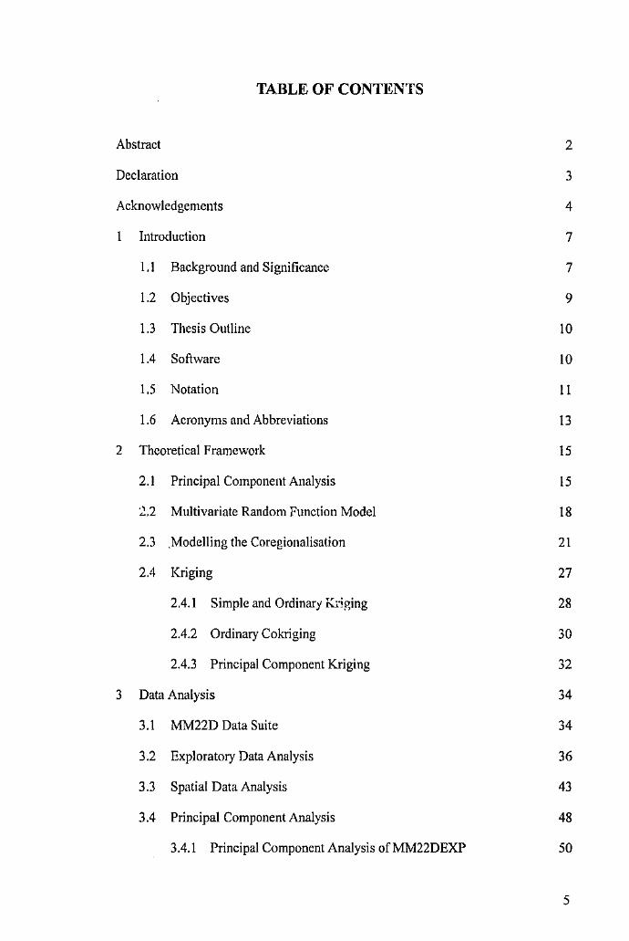
TABLE OF CONTENTS

Abstract 2

Declaration 3

Acknowledgements 4

1 Introduction 7

1.1 Background and Significance 7

1.2 Objectives 9

1.3 Thesis Outline 10

1.4 Software 10

1.5 Notation 11

1.6 Acronyms and Abbreviations 13

2 Theoretical Framework 15

2.1 Principal Component Analysis 15

:2.2 Multivariate Random Function Model 18

2.3 ,Modelling the Coregionalisation 21

2.4 Kriging 27

2.4.1 Simple and Ordinary Kriging 28

2.4.2 Ordinary Cokriging 30

2.4.3 Principal Component Kriging 32

3 Data Analysis 34

3.1 MM22D Data Suite 34

3.2 Exploratory Data Analysis 36

3.3 Spatial Data Analysis 43

3.4 Principal Component Analysis 48

3.4.1 Principal Component Analysis ofMM22DEXP 50

5

3.4.2 Principal Component Analysis ofMM22DHC4

3.4.3 Principal Component Analysis of Mlvl22DTOP4

4 Ordinary Cok:riging

4.1 Variography and Cokriging ofMM22DHC4

55

58

62

62

4.1.1 Variography and the Intrinsic Coregionalisation Model 62

4.1.2 Cross Validation for Cokriging of M1vl22DHC4 67

4.1.3 Cokriging Estimates of M:M22DHC4 70

4.2 Variography and Cokriging of MM22DTOP4 74

4.2.1 Variography and the Linear Model of Coregionalisation 75

4.2.2 Cross Validation for Cokriging of MM22DTOP4 79

4.2.3 Coktiging Estimates of MM22DTOP4 81

5 Principal Component K.tiging 84

5.1 Variography of the Principal Components 84

5.2 Cross Validation for Ordinary Kriging of the Principal Components 89

5.3 Principal component Kriging Estimates 92

6 Ordinary Kriging 97

6.1 Variography of Nickel, Cobalt, Magnesium, Iron and Zinc 97

6.2 Cross Validation for Ordinary Kriging 104

6.3 Ordinary Kriging Estimates of Nickel, Cobalt, Magnesium and Iron 107

7 Comparison of Estimates 109

8 Discussion and Conclusion 126

References 131

Appendices 133

Appendix A Principal Component Analysis of Transformed Data 134

Appendix B Cross Validation Results 139

Appendix C ISATIS Parameter Files 152

6

1 INTRODUCTION

1.1 Background and Significance

Geostatistics enables us to analyse spatially dependent data, that is, data

where location as well as value is important. Such data arise naturally in the earth,

mining, petroleum and environmental sciences. Geostatistics can be described as a

set 0f statistical tools that allow us to describe, interpret and model the spatial

continuity that is a fundamental feature of many natural phenomena. Furthennore

once we have a mathematical representation of the spatial continuity of the data we

can use this model to estimate values at unsampled locations across the study region.

Geostatistical methods generally provide better estimates than traditional methods

and most importantly provide us with a measure of the accuracy of the estimates.

This rapidly advancing area of applied mathematics has its origins in the

mining industry in South Africa in the 1950's. Mining engineer D. G. Krige and

statistician H. S. Sichel were among the first to implement new statistical methods

that did not rely on traditional methods based on normally distributed data. In the

1960's G. Matheron further developed and formalised these innovative ideas and

introduced the concept of a regionalised variable which he defined as a spatially

distributed phenomenon that exhibits a particular spatial structure consisting of both

random and structured aspects (Matheron, 1970, p. 5).

It is often the case that data collection in the earth sciences consists of

observations of many variables, some more densely sampled than others. While it is

more cumbersome and computationally more expensive to work with multivariate

data the availability of auxiliary information can enhance the interpretation and

estimation of a primary variable. Multivariate geostatistics takes into account the

relationships between and among the variables as well as incorporating their spatial

distribution across a region. The relationships between these variables can be

identified and summarised using methods of multivariate statistical analysis.

7

One classical, and probably the most commonly used, multivariate statistical

technique is principal component analysis which dates back to the early 1900's, in

particular to the work of Pearson (1901) and Hotelling (1933). Principal component

analysis involves the construction of linear combinations of correlated variables into

(preferably) fewer :.mcorrelated factors that account for the majority of the variation

in the original data (Afifi & Clarke, 1996, pp. 330-331). More specifically, principal

component analysis is concerned with explaining the variance-covariance structure

of a set of variables by means of a few linear combinations of these variables

(Johnson & Wichern, 2002, p. 426).

From a geostatistical perspective principal component analysis is a

particularly valuable tool as it can be used for reducing the number of variables in a

data set and for the detection of intrinsic correlation. One of the benefits of reducing

the number of variables in a multivariate data set is the practical advantage of

modelling fewer semivariograms. Furthermore, if the orthogonaiity of the principal

components extends to any separation vector h we may proceed with an intrinsic

coregionalisation model. Under this assumption we may perform cl~ssical kriging

individually on the principal components. This technique is known as principal

component kriging and is computationally less expensive than other methods such as

cokliging (Goovaerts, 1997, pp. 233-234).

When the data are not intrinsically correlated we must consider not only the

spatial variability of the individual variables but we must also take into account the

joint variability 0f each pair of variables. The linear model of coregionalisation is a

mathematical model that characterises the spatial variation of a multivariate system

at different spatial scales. The requirement of a linear model of coregionalisation is

that all direct and cross semivariograms or covariances are jointly modelled and

share a common set of basic structures. This then calls for the inference and

modelling of N/.Nv+l)/2 direct and cross semivariograms. While this can be a

tedious procedure the problem lies in whether the model fits adequately in the

mathematical sense (Goulard & Voltz, 1992, p. 269), more precisely the

coregionalisation matrices need to exhibit positive semi-definiteness in order for the

model to be permissible.

8

1.2 Objectives

The aim of this study was to describe and demonstrate the use of multivariate

statistical techniques in geostatistical analysis. The theory of principal component

analysis in a traditional multivariate statistical environment and the use of this

technique as it applies to geostatistics are presented. We examine also the theory of

the general form of the linear model of coregionalisation as well a particular case

known as the intrinsic coregionalisation model. In addition we discuss the theory of

the estimation techniques to be used, that is, ordinary kriging, ordinary cokliging and

principal component kriging.

For the application of the theory we had four main objectives. Firstly we

aimed to exhibit the use of principal component analysis in a geostatistical

environment, namely to determine whether the data were intrinsically correlated.

Secondly we wished to show examples of both the intrinsic coregionalisation model

and the linear model of coregionalisation. Thirdly we aimed to demonstrate the

estimation techniques of principal component kriging and ordinary co kriging. Finally

we wished to include a comparison of these multivariate techniques to the univariate

estimation method of ordinary kriging as well as with 'reality'.

To demonstrate these objectives we analysed a mineralisation (MM22D),

which comprises three dimensional grade and thickness measurements on eight

variables: nickel, cobalt, magnesium, iron, aluminium, chromium, zinc and

manganese. These data came from the Murrin Murrin nickel mine near Laverton in

Western Australia This data suite consists of two data sets: a grade control data set

:Mlvl22DGC and an exploration data set MM22DEXP. The set MM22DGC

comprises grade accumulations for each of the eight variables and will be considered

reality for assessment and comparative purposes. The set MM22DEXP is a subset of

MM22DGC and will be used to perform the analysis. This data set is isotopic and

comprises accumulations for each of the eight variables jointly sampled at 125

locations.

As the data were measured on different scales and have vastly different

ranges, means and variances we used the standardised values for the majority of the

analyses. Initially we performed a principal component analysis on the MM22DEXP

data set and determined that the data were not intrinsically correlated We then

9

investigated two four variable subsets of MM22DEXP, denoted as rvr:M:22DHC4 and

:M:M:22DTOP4. The fanner subset was intrinsically correlated; hence we used an

intrinsic coregionalisation model and prefonned the estimation using ordinary

cokriging. In addition we individually modelled the principal components from this

subset and perfonned the estimation using principal component kriging. For the latter

subset the variables were not intrinsically correlated hence we used a linear model of

coregionalisation and perfonned the estimation using ordinary cokriging. The

estimates were then compared to the grade control data, lvfl\.122DGC, and the

estimates obtained from ordinary kriging.

1.3 Thesis outline

Chapter two of this thesis discusses the theoretical framework relevant to this

study. This includes principal component analysis from both classical and

geostatistical perspectives, the multivariate random function model and the various

methods of kriging, namely ordinary kriging, ordinary cokriging and principal

component kriging. Chapter three presents a detailed exploratory data analysis of the

MM22D data suite. In chapter four we demonstrate the application of ordinary

cokriging using both the MM22DHC4 and MM22DTOP4 data sets. Chapter five

presents the application of principal component kriging using the principal

components extracted in the eigenanalysis of lv!M22DHC4. Chapter six presents

ordinary kriging of rhe nickel, cobalt, magnesium, iron and zinc variables. Chapter

seven presents a comparison of the estimation techniques used and chapter eight

presents a discussion and conclusions of the research.

1.4 Software

There are various software packages available to assist in geostatistical

analysis. My study has used primarily the packages listed below. It is appropriate at

this point to mention one package in particular, ISATIS, which is recognised as an

industry stanrlard. While ISATIS a relatively new package in the workplace, we are

in the fortunate position of having it available at this university.

10

I have taken this opportunity to familiarise myself with the capabilities of

ISATIS, to the point where I would now be considered proficient in implementing

this package in the workplace. ISATIS offers the geostatistician analytical features

and capabilities not previously available. Some of these features include

simultaneous modelling of direct and cross scmivariograms, sequential cokriging of

numerous variables, alternative measures of spatial variability and alternative kriging

methods.

3PLOT (Kanevski et al, 1998): post plots of data and estimates

ISATIS (Bleincs eta!, 2000): estimation

MATLAB 5.3 (1999): matrix manipulation and calculation

MICROSOFr EXCEL (2002): graphical representation of data;

spreadsheet calculations

MINITAB 12.1 (1998): summary statistics, principal component analysis,

residual analysis

V ARlO WIN 2.2 (Pannatier, 1996): semivariogram inference and modelling

1.5 Notation

The notation used throughout this study is a combination of that used by

Goovaerts ( 1997), Wackernagel (l998b) and Johnson and Wichern (2002).

V: forall

A: study region

a: range parameter

M: coefficient of the basic covariance model c,(h) or semivariogram

model g1(u) in the linear model of regionalisation of the random

variable Z(u)

b~: coefficient of the basic covariance model c1(h) or semivariogram

model g1(u) in the linear model of coregionalisation of the random

variables Zi(u) and 2j(u)

B,: corcgionalisation matrix including the coefficients b~ of the basic

II

covariance model t'!{h) or semivariogram model Rl(h) in the

' corresponding linear model of coregionalisation C(h) = L,S1c1(h) 1~o

'· or f(h) = :Ln,g,(h) c-o

C(O): covariance value at separation distance I hI= 0

C(h): stationary covariance of the random function Zfor lag vector h

C(h): covariance function matrix of size Nv x N\'

C;J(h); stationary cross covariance between the two random functions 2j

and 2j for a Jag vector h

Cov {.): covariance

q(h): /th basic covariance model in the linear model of (co)rcgionalisation

E{·): cxpcctcdvaluc

E: is an clement of

f(h): scmivariogram function matrix of size N,. x Nl'

g1(h): /th basic scmivariogram model m the linear model of

(co )regionalisation

Y(h): stationary scmivariogram of the random function Z for lag vector

h

f;;(h): stationary cross scmivariogram between the two random functions

~and -0" for a Jag vector h

h: separation vector

Aa(u): kriging weight associuted to z--datum at location Ua for estimation

of the attribute z at location u

Aulu): cokriging weight associated to z--datum at location Uu for estimation

of the attribute z at location u

m: stationary mean of the random function Z(u)

m: vector of stationary means

m(u): expected value of the random variable Z(u)

N,.: number of variables Z;

n: number of data values available over the study region A

12

n(u): number of data values z(ua) used for estimation of the attribute z at

location u

,1,(u): number of data values z1(uu) used for estimation of the attribute z at

location u

Q: matrix of eigenvectors extracted in the principal component analysis

rv: linear correlation coefficient between variables Z1 and Zj

u: coordinate •:ector

Uu: datum location

Var{·}: vanancc

f.1 (u): A1h region ali sed factor corresponding to the (/+ 1) basic covariance

Z(u):

Z:

Z:

z:

z(u):

z(ua):

Z;(Ua):

' model in the linear model of coregionalisation C11 (h) = ~)~c1 (h)

generic continuous random variable at location u

univariate random variable valued function

multivariate random variable valued function

continuous variable (attribute)

t111e valw! at unsampled location u

z-da!um value allocation Ua

z1-datum value at location Ua

1•0

1.6 Acronyms and Abbreviations

The following is a list of acronyms and abbreviations used in the Figures and

Tables throughout this thesis.

AL:

CO:

CR:

FE:

ICM:

LMC:

MAE:

aluminium

cobalt

chromium

iron

intrinsic coregionalisation model

linear model of corcgionalisation

mean absolute error

13

MG: magnesium

MN: manganese

MSE: mean square error

NI: nickel

OCK: ordinary co kriging

OK: ordinary kriging

PC: principal component

PCK; principal component kriging

PCK2: principal component kriging (two retained principal components)

ZN: zinc

14

2 THEORETICAL FRAMEWORK

) .1 this chapter we discuss the theory of principal component analysis from

both classical and geostatistical perspectives. We then introduce the multivariate

random function mcdel and the linear mode! of corcgionalisation. Finally we discuss

the vnrious kriging algorithms employed in this study: ordinary kriging, ordinary

cokriging and principal component kriging, The development of the theory and the

notation used follows that of Goovaerts (1997), Lay (1997) and Wackemagel

(1998a).

2.1 Principal Component Analysis

Almost any kind of data collection in the earth sciences involves

simultaneous measurements on many variables. Suppose that we are dealing with Nv

variables, that is Nv dimensional data, measured at n locations u in the region A

While multivariate gcostatistics gives us the tools to incorporate this additional

infonnation, in practice one seldom considers coregionalisations of N., greater than

three. The reasons for this include notational and computational complexity and

difficulties of statistical inference and modelling of the cross covariance or cross

semivariograms (Joumel & Huijbregts, 1978, p. 173).11 is often desirable to exploit

the interrelationships among and between the N., variables by representing them

through a few linear combinations of these variables.

One multivariate technique used to achieve this is known as principal

component analysis. This is one of the most commonly used methods of multivariate

analysis. It is simple to implement and interpretation of the results is often

straightforward. In its simplest form a principal component analysis consists of

defining a linear transformation that maps a set of N., correlated vmiables into Nv

uncorrelated principal components (Wackemagel, 1998a, p. 127). From a purely

mathematical perspective Johnson and Wichern (2002, p. 426) describe a principal

15

component analysis as a means of explaining the variance-covariance structure of a

set of variables by means of a few linear combinations of these variables.

Each principal component is a linear combination of the original variables

and the amount of information conveyed by each principal component is measured

by its variance (Afifi & Clarke, 1996, p. 330). The principal components are

arranged in order of decreasing variance, thus the first principal component is the

most infom1ativc and the least informative is the last principal component. One can

then choose to retain only the first few principal components that account for the

majority of the variability of the original data, making the subsequent analysis

simpler. A principal component analysis can also be used to test for normality of the

data; if a selected principal component is not normal then neither are the original

data. Other classical uses of principal component analysis are to identify outliers and

reveal relationships among and br:cween variables that may not have previously been

identified. One of the most important ge.ostatistical applications of principal

component analysis is to detect intrinsic correlation. This is done by examining the

cross corrclograms or cross scmivariograms of the first few principal components

and will be discussed fu1ther in section 2.3, Modelling the Coregionalisation.

The basic features of a principal component analysis consist of the extraction

of the eigenvalues and eigenvectors of a square, symmetric covariance or correlation

matrix. Principal component analysis does not require multivariate normality though

the interpretation and application are enhanced when this condition is met.

Algebraically the principal components arc specific linear combinations of the

random variables Zi(u) for i = 1, ... , N,,. Geometrically the linear combinations

represent the choice of a new coordinate system by rotating the original system with

Z,{u) as the coordinate axes (Johnson & Wichem, 2002, pp. 426~427).

If the variables have widely differing ranges, if they are measured on

differing scales or if the units of measurement arc not consistent, it is advisable to

standardise the variables. A principal component an1lysis performed on the

covariance matrix can be severely affected by large or inconsistent variances. Hence

by standardising the original data (or equivalently using the correlation matrix as

opposed to the covariance matrix) we ensure that the assigning of the weights in a

principal component analysis is not innuenced by variables with large variances. It is

16

important to note that all interpretations of a principal component analysis based on

the correlation matrix must be in tenns of the standardised variables.

Let R be the correlation matrix of the Nv random variables Z;(u) fori= 1, ... ,

Nv. The spectral decomposition of the Nv x Nv syrr'TI.etric matrix R is given by

(!)

where Jl,,~, ... ,I\.N are the eigenvalues of R and epe2 , ... ,eN are the associated ' '

nonnalised eigenvectors with eJe; = 1, i = 1, ... , N,. and eie1 = 0 when i :f. j. In matrix

notation the spectral decomposition of R then is

R=QAQ' (2)

where Q is the orthogonal matrix whose columns are the corresponding unit

eigenvectors epe2, ... ,eN, (note QQT = I) and A is the diagonal matrix [ltd of

eigenvalues of R fur k = 1, ... , Nv such that?,;::~~ ... ;::AN,. This orthogonal change

of variables does not change the total variance of the data. Furthermore the

eigenvalues determine~.! in the spectral decomposition are the variances of the

principal components.

The first principal component then is the eigenvector corresponding to the

largest eigenvalue of R, the second principal component is the eigenvector

corresponding to the second largest eigenvalue of R and so on. The kth principal

co.nponent is given by a linear combination of the set of Nv original variables:

The set of all Nv principal components are linear combinations of the set of Nv

original variables:

N

Y,(u)= !,q"Z,(u) (3)

for k = 1, ... , Nv. In matrix notation, Y(u)=QTZ(u) and has variance matrix

QTRQ =A. The total variance of Yk(u), k = 1, ... , Nv, is equal to the total variance of

Zi(u), i = 1, ... , Nv, and is given by tr(R)=tr(A)=/\.1 + k + ... + 1\.N =Nv. Hence the

variance of Yk(u) is Ak and the fraction of the total variance that is explained by Yk(u)

is measured by 1\.k/ tr(R).

17

J

The set of Nv principal component scores is computed at each datum location

Ua in A for a= 1, ... , n as linear combinations of the standardised sample values

Zi(Uu) at that location multiplied by the loading of variable Z,{u) or the kth principal

component Yk(u)

(4)

• fork= 1, ... , Nv with m; and 0'; being the mean and standard deviation respectively of

the Zi(u) data and qk; obtained from the matrix of eigenvectors Q in equation (2).

2.2 Multivariate Random Function Model

One of the fundamental aims of gcostatistics is to characterise the behaviour

of the population of a sampled attribute over a study region A In order to do this we

are required to model the statistical characteristics of the population using only the

available sample data. In essence geostatistics uses a probabilistic approach to model

the uncertainty about how the attribute behaves between the sample locations.

Consider a set of n sample data values denoted by z(ua), where o:=l, ... , n.

These observations may be considered as a subset of a larger, possibly infinite,

collection of observations. The value z(ua) can be thought of as one possible

realisation of a random variable Z(ua). Similarly the value z(u) at an unsampled

location can be thought of as a particular realisation of the random variable Z(u) for

each location u in the region A. The characterisation of a random variable Z(u) is

detennined completely by the cumulative distribution function, that is

F(u; z)=Prob{Z(u):5z)

for all z.

(5)

The set of random variables Z(u), denoted by Z, for all locations u in the

region A., { Z(u), u E A}, is called a random function and is characterised by the

set of all its N-variate cumulative distribution functions

(6)

18

•

for any locations uk, where k=:l, ... , N. In general it is impossible to infer the entire

spatial law of a random function so it is necessary to obtain an approximate solution

to most of the problems encountered. In the most commonly used geostatistical

procedures we assume that the random function is stationary, that is, the

characteristics of the random function remain invariant under translation. A random

function is said to be strictly stationary if for any set of N points u1, .•. ,UN and for

any vector h, the two vectors of random variables [Z(u1), ... , Z(uN)l and [Z(u 1 +h),

... , Z(uN +h)] have the same multivariate cumulative distribution function

F(u1, ... , UN; Zll'"' ZN) =F(U1 + h, ... , UN + h; Z1 , ... , ZN)

for all locations u,, ... , UN and any vector h.

(7)

As it is not possible to verify strict stationarity from experimental data we

usually require only second-order stationarity where the first two moments (mean

and covariance) are constant (Armstrong, 1998, p. 18). Hence we require, for all

locations u, that the mean exists and: is constant

E{Z(u)}=m

and the two-point covariance exists and depends only on the separation vector h

C(h)= E{Z(u)·Z(u +h)}-E{Z(u)} · E{Z(u +h)}

(8)

(9)

In many cases this assumption is not appropriate so we assume intrinsic stationarity

where the increments Z(u +h)- Z(u) are assumed to be second-order stationary.

E{Z(u+h)-Z(u)} =0 (10)

Var{Z(u +h)- Z(u)} = E{ [Z(u +h)-Z(u)]'} =2y(h) (11)

The function y(h) is called the semivatiogram and is the basic tool for the

interpretation of the spatial variability of the attribute being investigated.

The probabilistic approach to a coregionalisation (a regionalised phenomenon

that can be represented by several intercorrelated variables) is similar to that of the

requirements of a single variable whose concepts can be easily broadened to

incorporate a multivariate random function. The vector of unsampled values of Nv

variables [z1(u), ... , zN. (u)] can be considered as a particular realisation of the vector

of Nv random variables [Z1(u), ... , ZN, (u)] for all locations u over a region A.

Similarly this vector of random variables may be thought of as one particular

realisation of a multivariate random variable valued function:

19

([Z1(u), ... , Zv,Cn)]; UE A) denotedbythevector Z.

In order to define a cross covariance function that depends only on the

separation vector h the direct (auto) and cross Qoint) covariance functions Cu(h) of a

set of Nv continuous random functions are defined in the framework of joint second-

order stationarity. That is, for all locations u over the study region A the mean of

each variable Zi(u) exists and is constant and the covariance of a variable pair Zi(u)

and ZJ(u)~:-:::sts and is translation invariant

E[Z,(u)] = m,

C,1 (h)= E[(Z, (u) -m,) · (Z1 (u +h) -111, )]

(12)

(13)

for all i, j;:::; 1, ... , Nv. The mean-value vector of a random function Z is defined as:

m(u)=E[Z(u)] (14)

Hence the cross covariance functions Cu(h) may be written as the covariance matrix

C(h) = E{ [Z(u)- m] · [Z(u +h)- m]T), that is:

[

C,.(h)

C(h)= :

Cv;{h)

(15)

As with the univariate case it may be that in practice the covariance function

between any two locations u and u + h does not exist in which case it is necessary to

weaken the joint second-order stationarity hypothesis to the joint intrinsic hypothesis.

The assumption here is that there is only weak stationarity of the first two moments

(mean and variance) of the difference of a pair of values located at u and u + h, that

is

E[ z, (u+ h)-z, (h )}o (16)

Cav[ z, (u +h)- z, (h ),Z1 (u +h)- Z1 (h)]=2r, (h) (17)

for all i, j = 1, ... , Nv.

Hence the cross semivariogram functions y;j(h) may be written as the

semivariogram matrix r(h) = V2E{ [Z(u)- Z(u ·:·h)] · [Z(u)- Z(u + h)]T), that is:

20

(18)

It is important to note that while the cross variogram is symmetric in (h, -h),

this is not necessarily so for the cross covariance function, that is Cij(h) t- Cii(-h) and

Cij(h) :f; Cji(h). Goovaerts (1997, p. 73) states however that in practice this assumption

in ignored as the usual tools for description of the spatial variability are symmetric

and the verification of the presence of a lag effect is generally not possible as a result

of insufficient data.

2.3 Modelling the Coregionalisation

The regionalised variable possesses a local, random, erratic aspect which

accounts for local irregularities as well as a general structured aspect which reflects

large scale tendencies (Armstrong, 1998, p. 15). Both of these aspects need to be

taken into account in the process of developing a representation of the spatial

variability of the regionalised variable. Our goal when modelling the semivariogram

or covariance is to obtain a suitable interpretation of the spatial structure that

characterises the association and causal relationships and main features of the

corcgionalisation. Our need for a model of the coregionalisation arises from the fact

that it is likely that for estimation purposes we will require a semivariogram or

covariance value for some distance and/or direction for which we do not have 11. value

(lsaaks & Srivastava, 1989, p. 371). Inference of the scmivariogram or covariance

model provides a set of functions that allov.r us to compute semivarior,ram or

covariance values for any possible separation vector h.

Only certain functions may be used to model the cross covariance ;md cross

semivariogram. Let Z/u) fori::: 1, ... , Nv be a set of intercorrelated random functions,

Ua for a= 1, ... , n be a set of 11 data locations andY be a finite linear combination of

the random variables Zi(ua), where Ua. is a sample location in the study region A and

i = 1, ... , Nv. The variance of Y must be non-negative and can be written as the linear

combination of cross covariance values

21

(19)

where Cij(h) denotes the cross covariance at a lag distance h. The variance in terms

of the matrix C(h) is

" " Var[Yl=L~>:C(u,-u1 )Jc1 <eO (20) a~I P=I

where A.., =[A.aP···•A.aN, ]T and A! denotes the transpose of the vector Au. Thus the

matrix of covariances C(h) must be positive semi-definite to ensure that the

variances of Yare non-negative.

Using the relation C(h) = C(O)-f(h), the variance in terms of the matrix r(h)

is:

n n n n

Var[Y}=C(O) :L<!:LJc,- LLl.!r(h)Jc1 <eO (21) a"'l fl=l a=l p .. i

When a semivariogram is unbounded and has no covariance counterpart the variance

of Y is defined on a condition that the vectors of weights Aa sum to the null vector.

" " " Var[Y}=- LLJc!r(h)l.1 <eO with LA• =0 (22)

a=! P"I e>.=l

Thus the matrix of semivariograms f(h) must be conditionally negative semi-definite

to ensure that the variances of Yare non-negative.

Recognising whether a function is positive definite or conditionally negative

definite is not easy, nor is it simple to te'lt for positive definiteness. Hence it is

common practice to model a coregionalisation by using only a few basic structures

that are known to be admissible. The following list is not exhaustive but includes the

most commonly used admissible models in their standarised fonn.

' Nugget effect model

{0 if h=O

g(h) = 1 otherwise

• Spherical model with range a

if h;:;a g(h) = Sph( ~) = J 11 s ~ - o.s( H l otherwise

(23)

(24)

22

• Exponential model with practical range a

(-3h) g(h) =I - exp -;;- (25)

• Gaussian model with practical range a

( 3h') g(h) =I - exp T (26)

• Power model

g(h) = hw with 0 < w < 2 (27)

These models are considered to be the 'basic models' and are expressed in

their isotropic form, that is they are independent of direction (h =I h I). These basic

models can be modified to incorporate anisotropy if required.

The nugget effect model is a bounded transition model and is characterised

by its discontinuous behaviour at the origin. The spherical and exponential models

are also bounded transition models whose behaviour at small separation distances

near the origin is linear. The spherical model reaches its sill at the distance a, also

known as the actual range. The exponential model reaches its sill asymptotically with

a practical range a, the distance at which the semi-variogram value is 95% of the sill.

The Gaussian model is a bounded transition model with quadratic behaviour at the

origin and also reaches the sill asymptotically with practical ra:1ge a, the distance at

which the semi-variogram value is 95% of the sill (Isaaks & Srivastava, 1989, pp.

373-375). Finally the power model is an unbounded model and has no covariance

counterpart. The behaviour of the power model at the origin is dependent on the

value of the parameter ru, that is, linear when w = 1 and parabolic as w approaches

two.

The linear model of coregionalisation is a mathematical model that

characterises the spatial variation of a multivariate system at different spatial scales.

The requirement of a linear model of coregionalisation is that all direct and cross

semivariograms or covariances are jointly modelled and share a common set of basic

structures. The linear model of coregionalisation consists of :1 set of intercorrelated

random functions 2i so that their corresponding semivariogram matrix r or

covariance matrix C is by construction admissible. This means that each random

23

function 2i is a linear combination of (L+l) spatially uncorrelated components Y},

for l = 0, ... , L. Each of these componerts acts at a particular characteristic spatial

scale and has a covariance function c, ami· zero mean (Joumel & Huijbregts, 1978, p.

172).

(28)

for all i = 1, ... , Nv with

• E{Z,{u)} =m1 (a)

• E[ Y/(u))=O forallk=l, ... ,n1 andi=O, ... ,L (b)

. {c(h) ifk = k'andl Cov { Y/ (u), Yj. (u +h)) = ' .

0 othenvrse

= I' (c) •

If follows then that the cross covariance function associated with the spatial

components Z;(u) and ZJ(u + h) can be written as the linear combination of the cross

covadance between any two random variables Yl1 (u) and yl;· (u +h).

(29)

As the random variables Y/ (u) in equation (28c) are uncorrelated (orthogonal)

except when I = r and k = k' simultaneously, equation (29) reduces to a linear

combination of (L+l) basic covariance models c1(h). Hence we define the linear

model of coregionalisation as the set of Nv x Nv direct and cross covariance models

c,,(h)

' CIJ(h) = Lb~c1 (h) (30)

1~0

for all i, j = 1, ... , Nv, where the sill of the basic covariance model c1(h) is mattix­

valued and defined by

(31)

for all i, j = 1, ... , Nv and l = 0, ... , L. Similarly we can define the lineoar model of

coregionalisation in terms of the set of Nv x N.~ direct and cross semivariogram

models rv(h) such that:

24

' Y,(h)=~>:g,(h) (32)

'"' The coregionalisation matrix of size Nv x. Nv , Bt = [ b~ J, is by construction a

positive semi~definite matrix and is the variance-covariance matrix which describes

the multivariate correlation at each of the characteristic scales I for l = 0, ... , L

(Wackemagcl, 1998b, p. 27). Thus for a linear model of coregionalisation to be

admissible it must satisfy two conditions:

i) the functions c1(h) (gt(h)) are admissible covanance (semivariogram)

models and

ii) the (L + 1) corcgionalisation matrices 8 1 are positive semi-definite.

This second condition is readily checked by confirming that the eigenvalues of each

of the (L+ 1) coregionalisation matrices 8 1 is real and non-negative.

The multivariate nested covariance function model Cv(h) with positive semi­

definite coregionalisation matrices B1 expressed in matrix notation is ,_

C(h) = LB,c,(h) (33)

'"' with B1 = A1Af and A1 = [a~ J. Correspondingly, the multivariate nested model

associated with a linear model of coregionalisation of intrinsically stationary random

functions expressed in matrix notation is

' r(h) = LB,g,(h) (34) ,., where Bt arc positive semi-definite matrices and g1(h) are the semivariogram models.

If the multivariate correlation structure of a set of Nv variables is independent

of the spatial correlation the multivariate correlation is said to b~ intrinsic. According

to Chiles & Dclfiner (1999, p. 337) Matheron introduced the intrinsic

coregionalisation model in order to validate the use of the correlation coefficient

from a gcostatistical perspective. The problem arises with the fact that variance (or

covariance) of spatially correlated data within a finite domain A, depends on A

(Chiles & Dclfiner, 1999, p. 337). The intrinsic coregionalisation model may only be

implemented when the correlation riJ between the random functions 2/ and ~does

not depend on spatial scale, that is:

25

(35)

The intrinsic corcgionalisntion model is a special case of the linear model of

corcgionalisation where the coefficients (sills) of any basic structure c1(h) or g1(h)

that constitute the model are proportional to each other. That is, b,~ =rp,1

·b1 for

i, j = I. ... .md I= 0, ... , L. The intrinsic coregionalisation model is the simplest

multivariate model used in gcostatistics as all direct and cross covariance and

semivariogram models arc prof}Qr.f.t'nal to the basic standardised covariance,

£ L

C(h) = Lii c1 (h), or scmivariogram, y(h) = Lb1 g1 {h), functions

'

c,1 (h)=~,1 C(h)

Y,,(h)=~,y(h)

(36)

(37)

for all i, j = 1, ... , Nv and L.b' =I. In matrix notation the intrinsic coregionalisation /=0

model is written

l'(h)=<l>y(h)

C(h)=<I>C(h)

(38)

(39)

where the matrix of coefficients 4> = [tpuJ is equal to the variance-covariance matrix

under the assumption of second-order stationarity (Wackernagcl, l998b, p. lO).

While the intrinsic coregionalisation model is more restrictive than the linear

model of coregionalisation it is of particular benefit as this model reduces the

inference of Nv (N1• + 1)/2 covariance or semivariogram functions to the inference of

only one covariance or semivariogram model and N,. (N,. + 1)/2 coefficients. One

way of detecting whether variables are intrinsically correlated is by examining the

codispersion between the variables. This can be done by checking graphically

whether the codispersion coefficients

Jy,(h)y g(h)

are constant and equai to the .sample correlation coefficient. If they arc the

correlation of each pair of variables does not depend on spatial scale. This can

26

however become time consuming when the number of variables is large. An

alternative method is to perform a principal component analysis on the data and

compute the cross corre!ograms of the first few principal components which account

for the majority of variability in the original data. If the cross correlograms of the

principal components are zero for any separation vector h this implies that the

orthogonality of the principal components is not dependent on spatial scale. In other

words for the data to be intrinsically correlated we require the cross correlograms of

the principal components to be zero for any separation vector h.

2.4 Kriging

Once we have a mathematical representation of the spatial continuity of the

attributes of interest in the fonn of our random function model we are able to proceed

with the estimation of those attributes at unsampled locations across the study region.

There arc many traditional point estimation techniques available, such as polygonal,

Dclaunay triangulation, inverse distance squared and moving average methods. The

overriding problem with these techniques is that the 'best' one is dependent on one's

choice of criteria as to what is 'best'.

In the 1950's South African mining engineer Danie Krige developed a

technique of interpolation in an attempt to more accurately predict ore reserves.

Based on Kiige's work, Georges Matheron developed the Theory of Regionalized

Variables in the early 1960's in which he combined Krigc's pioneering work into a

single framework which was coined "krigeage" in recognition of Krige's

contlibution to the field (Chiles & Delfiner, 1999, p. 150). Fonnally, kriging now

refers to a family of least-squares linear regression algorithms that share the

objective of minimi~:ing the estimation (eiTOr) valiance subject to the constraint of

unbiasedness of the estimator (Deutsch & Joumel, 1998, p. 14). Over the past several

decade~ kriging has become a fundamental tool in the field of geostatistics as it has

established itself as a superior method of estimation.

27

2.4.1 Simple and Ordinary Kriging

Let Z be a second-order stationary random function with mean m. The

estimator Z*(u) of Z is given by a linear combination of random variables Z(ucr:) with

weights lta(u) r.hosen such that the estimator is unbiased tl.nd the estimation variance

is minimised. The basic generalised spatial least-squares regression estimator Z*(u)

is defined as

n(u)

Z*(u)-m(u) = L,!."(u)[Z(u.)-m(u.)] (40) a~l

where the quantities m(u) and m(ua) are the expected values of Z(u) and Z(ua)

respectively. By making the assumption that the both the sample value z(ucr:) and

unknown value z(u) are realisations of the random variables Z(ua) and Z(u)

respectively we are able to define an estimation error random variable Z*(u)- Z(u).

In order for the estimator to be unbiased we require that the expected value of the

estimation error be zero:

E{Z* (u)-Z(u)}=O (41)

The estimation error variance is then given by

"; (u )= V6r{Z* (u)- Z (u)} (42)

and is minimised under the constraint of unbiasedness of the estimator.

If we assume m(u) to be known and constant across the study region A the

linear estimator Z*(u) is known as the simple kriging (SK) estimator z;K(u) where

"'"' [ "'"' l z;K(u):::: ~1\..~"(u)Z(&a) + 1- ~1\.:K(U) m (43)

and the .AsK(u) are determined such that the error variance is minimised. The simple

kriging estimator automatically exhibits unbiasedncss as the m~an error is equal to

zero. The simple kriging system then becomes, in terms of the covariance function, a

system of normal equations

n(u)

L,!.:' (u)C(u, -u,l = C(u. -u) /l~l

for all a= 1, ... , n(u). The simple kriging minimum error variance is given by

(44)

28

n(u)

"L (u) = Var{z;, (u)-Z(u)}=C(O)- LJ;' (u)C(u" -u) (45) a=l

In most cases however it is not acce~table to assume that the mean is known

and globally constant. An alternative approach is ordinary kriging which assumes

that the mean is unknown but locally constant. Ordinary kriging then limits

stationarity of the mean to the local neighbourhood of the location u being estimated.

The linear estimator (40) is then modified to incorporate the constant local mean

m(u).

(46)

In order to filter the mean m(u) from equation (40) we must impose the constraint

that the sum of the weights be equal to one. This yields the ordinary kriging

estimator z;x (u) which again must be solved to obtain the optimal kriging weights

such that the estimation error is minimised under the unbiasedncss constraint.

n(u} n(u}

z~, (u) = "'}c OK (u)Z(u") with >A OK (u) = I L..J " • ....~ "

(47) a=! a •1

The ordinary kriging system involves n(u) weights ).~K (u) and the Lagrange

multiplier tloK(n), which accounts fur the unbiasedness constraint. Expressed in

tenns of the covariance function this system is

n(u}

L ).~K (u)C(ua -Up)+ Pox (u) = C(ua -·u) 11=1 n(u}

L?c:' (u) =I P=l

(48)

for all a= I, ... , n(u). Unlike the simple kriging system the ordinary la.iging system

may also be expressed in tenns of the semivariogram as

n(u)

L"~' (u )Y(u" -u, )- ~0, =y(u" -u) /1=1

I:,l~K (u) =I

(49)

/1=1

for all a= 1, ... , 11(0). The ordinary kriging minimum error variance is given by

29

a;"' (u)= = Var{z;K (u)-Z(u)}= C(O)- ~,!~K (u)C(u, -u)-PoK (u) (50) a"' I

2.4.2 Ordinary Cokriging

The linear estimator (40) is readily extended to the multivariate case where

we have available Nv c'Jntinuous random variables Zi(U). We consider Zi(u) as a

realisation of the random variable Z;(u), i = 1, ... , Nv, with Zi(ua) being the set of n

sample data located at ua, a= 1, ... , 11. Let Z1(u) be the primary random variable of

interest with E{ZJ(U)} = lllJ(U), E{Z1(u,,)}= mJua) and Aa, and Aa, being the

weights assigned to z1 (ua) and Zi(u,) respectively. 1n order to estimate a primary ' '

variable with Nv-1 auxiliary variables the linear estimator (40) is extended to

incorporate the additional information.

Analogous to the kriging paradigm the cokriging algorithm generally only

retains the data closest to the location u. Again we wish to determine the weights A" '

and A", sur:h that the estimation variance

a; (u )= Var{ z; (u)- z, (u )} (52)

is minimised under the unbiasedness constraint that the expected error is zero.

E{z; (u)-z, (u)}=O (53)

The three most commonly used types of cokriging are

i) Simple cokriging where the mean mJ(u) is known and constant throughout

the study region A

ii) Ordinary cokriging where the mean mJ(u) is unknown but constant

throughout the study region A and

iii) Cokriging with a trend where the mean mi(u) is unknown and varies as a

function of the spatial coordinates u.

Pertinent to this study is ordinary cokriging which limits stationarity of the

mean to the local neighbourhood of the location u being estimated, In order to filter

the means m 1(u) and m1(u), fmm equation (51) we must impose the constraints that

30

the sum of the weights of the primary variable be equal to one and the sum of the

weights of the secondary variable(s) be equal to zero. This yields the ordinary

cokriging estimator

(54)

which again must be solved for the kriging weights such that the estimation error is

minimised subject to the unbiasedness constraints fori= 2, ... , Nv.

~) l, .l~" (u )=1

The ordinary cokriging system can be expressed in tenns of the direct and cross

covariances as

(55)

for a 1 = 1, ... , n1(u) and i = 1, ... , Nv. As for the ordinary kriging case the ordinary

cokriging system can be expressed in terms of the direct and cross semivariograms as

(56)

for Clj = 1, ... , n1(u) and i = l, ... , Nv. The cokriging vmiance is given by

"~oc• (u) = Var{zg[, (u)- z, (u)}

= C, (0)-pf" (u)-ff ~" (u )C,, (uo, -u) (57)

i:l "'"']

As the cokriging systems (55) and (56) can become unstable if the variances of the

primary and secondary variables differ by several orders of magnitude it is advisable

to use standardised variables if this is likely to be a concern.

In general the benefit of incorporating secondary infonnation is fully

exploited when the primary variablc(s) of interest is undersampled. In the isotopic or

31

equally sampled case the estimates obtained from ordinary cokriging are likely to be

similar to those obtained by ordinary kriging. However one advantage of cokriging a

set of equally sampled variables is that we preserve the coherence of the estimators.

That is, the cokriging of a sum of variables is equal to the sum of the cokrigings of

each of the variables. Another advantage of cokriging in both the isotopic and

heterotopic cases is that the estimation variance is less than or equal to that of the

kriging estimator. In the particular case of the intrinsic coregionalisation model the

ordinary cokriging estimates will be equivalent to those obtained by ordinary kriging.

2.4.3 Principal Component Kriging

As we have discussed previously, a principal component analysis transforms

a set of correlated variables into a set of components that are uncorrelated at I hI= 0.

The advantage of principal component kriging is that it reduces the estimation

problem of cokriging N1• variables to the kriging of Nv principal compr,;nents. The

overriding assumption of principal component kriging is that ~he principal

components are mutually orthogonal for any separation vector h

Cov{Y, (u),Y,. (u +h)}= Cw (h)= 0 (58)

for all k 'f:. e. If the data aw intrinsically correlated condit.ion (48) is then satisfied.

This means that there is no benefit in incorporating seco.1dary infonnation as the

kriging and cokriging estimates will be identical. Hence the principal components

can be kriged independently. One of the drawbacks however of principal component

kriging is that the data must be isotopic, that is only those data that are jointly

measured can be considered.

Having determined the N,. principal components we calculate the principal

component scores Yk(Ua) as per equation (4) and model theN,. semivariograms yu(h)

from these scores. We then estimate the principal components separately at each

unsamp!ed location u in A As the mean of each principal component is zero, the

ordinary kriging estimator of the kth principal component at location u is of the fonn

Y~~· (u) = ~lc~,' (u )Y, (u.) (59) a=!

32

where the kriging weights are obtained from the ordinary kriging system as displayed

in expression (48). The estimate of z1(u) is then recalculated as a linear combination

of the principal component estimates at each location plus the mean m1 of each

attribute.

K

z~b~(u) = Lak;Yh~·(u)cr; +m; (60) k-1

The coefficients ak1 are obtained from the matrix A= [aH] = Q-1 = QT where Q is the

orthogonal matrix of eigenvectors calculated in the principal component analysis.

Should sufficient variability of the original data be explained by P principal

components (where Pis ideally significantly less than Nv), it is possible to retain only

these and yet simultaneously estimate all Nv original variables without the loss of too

much information. In this case the estimates are obtained by modifying equation (60)

as follows:

' ""' "' ·''''() ZPcKP = ~ap1YoK u a;+ m (61) p=l

33

3 DATA ANALYSIS

In this chapter we introduce the IVIM22D data suite used in this study. We

then proceed with an exploratory data analysis of the grade control and exploration

data sets contained in the data suite. We next discuss the principal component

analysis of the :rvt:M22DEXP data set and assess whether the data are intrinsically

con·elated. In addition we consider the principal component analysis and subsequent

assessment of intrinsic correlation of two four variable subsets of MM22DEXP

called MM22DHC4 and MM22DTOP4. The first subset consists of variables that are

highly cmrelated with nickel and cobalt. The second subset consists of variables that

are considered to be economically the most important to the mining company.

3.1 MM22D Data Suite

The data to be us~d in this study come from Anaconda's Murrin Murrin

nickel mine near the town of Laverton in Western Australia. The data have been

collected from an area within this mine known as MM2. Murphy, Bloom and

Mueller (2002) explain thai in this region "the laterite deposits are of the dry-Climate

type and occur as laterally extensive, undulating blankets of mineralisation with

strong vertical anisotropy and near normal nickel distrib•Jtions." The data suite

MM22D comprises three dimensional grade and thickness measurements on eight

variables: nickel, cobalt, magnesium, iron, aluminium, chromium, zinc and

manganese. For the purposes of this study the data have been transfonned to

accumulations (average grade multiplied by total thickness) hence are treated as two

dimensional.

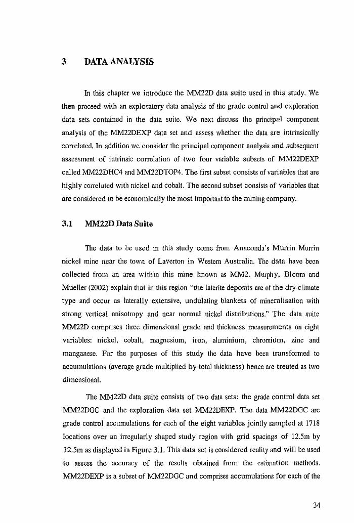
The :MM22D data suite consists of two data sets: the grade control data set

:rvt:M22DGC and the exploration data set r-.11vl22DEXP. The data 11I\1122DGC are

grade control accumulations for each of the eight variables jointly sampled at 1718

locations over an irregularly shaped study region with grid spacings of 12.5m by

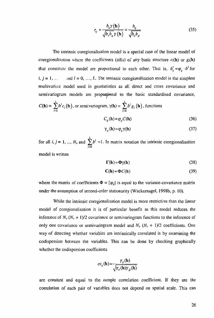
12.5m as displayed in Figure 3.1. This data set is considered reality and will be used

to assess the accuracy of the results obtained from the estimation methods.

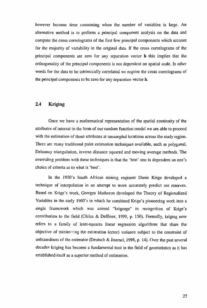
Mlvi22DEXP is a subset of :tv1M22DGC and comprises accumulations for each of the

34

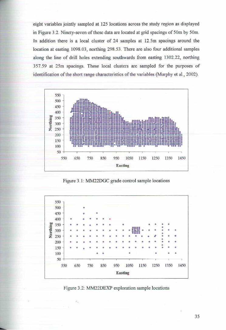
eight variables jointly sampled at 125 locations across the study region as displayed

in Figure 3.2. Ninety-seven of these data are located at grid spacings of 50m by 50m.

In addition there is a local cluster of 24 samples at 12.5m spacings around the

location at easting 1098.03, northing 298.53. There are also four additional samples

along the line of drill holes extending southwards from easting 1302.22, northing

357.59 at 25m spacings. These local clusters are sampled for the purposes of

identification of the short range characteristics of the variables (Murphy et al., 2002).

550 500 450

400 0.0 350 • . e l ~ 300 • <:> z 250

200 i 150 100 • • • 50

550 650 750 850 950 1050 1150 1250 1350 1450

Easting

Figure 3.1: MM22DGC grade control sample locations

550 500 • 450 • • 400 • • • • • •

0.0 350 • • • • • • • • • • • • . e ·mH· •

~ 300 • • • • • • • • • • • • • • 0 • z 250 • • • • • • • • • • • • • # • • • •

200 • • • • • • • • • • • • • • • • • • 150 • • • • • • • • • • • • • • • • •

100 • • • • • • 50

550 650 750 850 950 1050 1150 1250 1350 1450

Easting

Figure 3.2: MM22DEXP exploration sample locations

.·

35

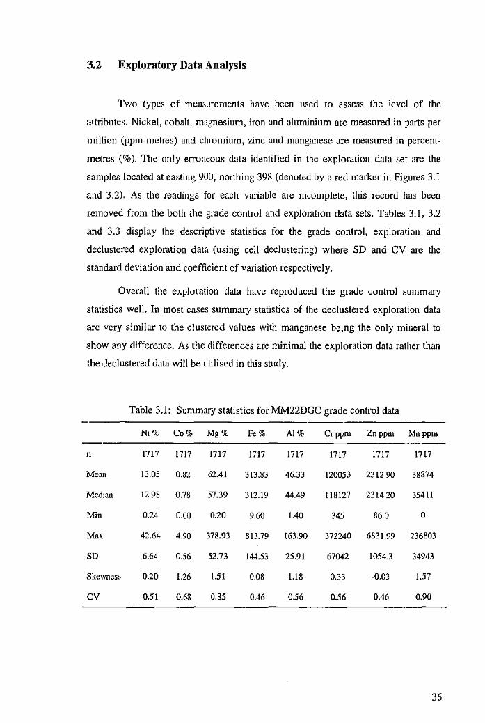
3.2 Exploratory Data Analysis

Two types of measurements have been used to assess the level of the

attributes. Nickel, cobalt, magnesium, iron and aluminium are measured in parts per

million (ppm-metres) and chromium, zinc and manganese are measured in percent­

metres (%). The only erroneous data identified in the exploration data set are the

samples located at casting 900, northing 398 (denoted by a red marker in Figures 3.1

and 3.2). As the readings for each variable are incomplete, this record has been

removed from the both i.he grade control and exploration data sets. Tables 3.1, 3.2

and 3.3 display the descriptive statistics for the grade control, exploration and

declustered exploration data (using cell declustering) where SD and CV are the

standard deviation and coefficient of variation respectively.

Overall the exploration data have reproduced the grade control sununary

statistics well. In most cases summary statistics of the declustered exploration data

are very similar to the clustered values with manganese being the only mineral to

show "~'Y difference. As the differences are minimal the exploration data rather than

the declustered data will be utilised in this study.

Table 3.1: Summary statistics for MM22DGC grade control data

Ni% Co% Mg% Fe% AI% Crppm Znppm Mnppm

n 1717 1717 1717 1717 1717 1717 1717 1717

Mean 13.05 0.82 62.41 313.83 46.33 120053 2312.90 38874

Median 12.98 0.78 57.39 312.19 44.49 118127 2314.20 35411

Min 0.24 0.00 0.20 9.60 1.40 345 86.0 0

Ma. 42.64 4.90 378.93 813.79 163.90 372240 6831.99 236803

SD 6.64 0.56 52.73 144.53 25.91 67042 1054.3 34943

Skewness 0.20 1.26 1.51 0.08 1.18 0.33 -0.03 1.57

cv 0.51 0.68 0.85 0.46 0.56 0.56 0.46 0.90

36

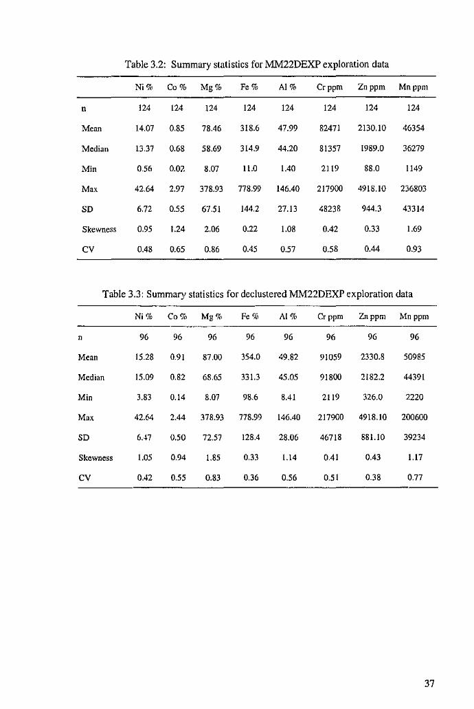
Table 3.2: Summary statistics for Mlvl22DEXP exploration data

Ni% Co% Mg% Fe% AI% Crppm Znppm Mnppm

n 124 124 124 124 124 124 124 124

Mean 14.07 0.85 78.46 318.6 47.99 82471 2130.10 46354

Median 13.37 0.68 58.69 314.9 44.20 81357 1989.0 36279

Min 0.56 0.0?. 8.07 11.0 1.40 2119 88.0 1149

M" 42.64 2.97 378.93 778.99 146.40 217900 4918.10 236803

so 6.72 0.55 67.51 144.2 27.13 48238 944.3 43314

Skewness 0.95 1.24 2.06 0.22 LOS 0.42 0.33 1.69

cv 0.48 0.65 0.86 0.45 0.57 0.58 0.44 0.93

Table 3.3: Summary statistics for declustered MM"22DEXP exploration data

Ni% Co% Mg% Fe% AI% Crppm Znppm Mn ppm

n 96 96 96 96 96 96 96 96

Mean 15.28 0.91 87.00 354.0 49.82 91059 2330.8 50985

Median 15.09 0.82 68.65 331.3 45.05 91800 2182.2 44391

Min 3.83 0.14 8.07 98.6 8.41 2119 326.0 2220

M" 42.64 2.44 378.93 778.99 146.40 217900 4918.10 200600

so 6A7 0.50 72.57 128.4 28.06 46718 881.10 39234

Skewness 1.05 0.94 1.85 0.33 Ll4 0.41 0.43 l.l7

cv 0.42 0.55 0.83 0.36 0.56 0.51 0.38 0.77

37

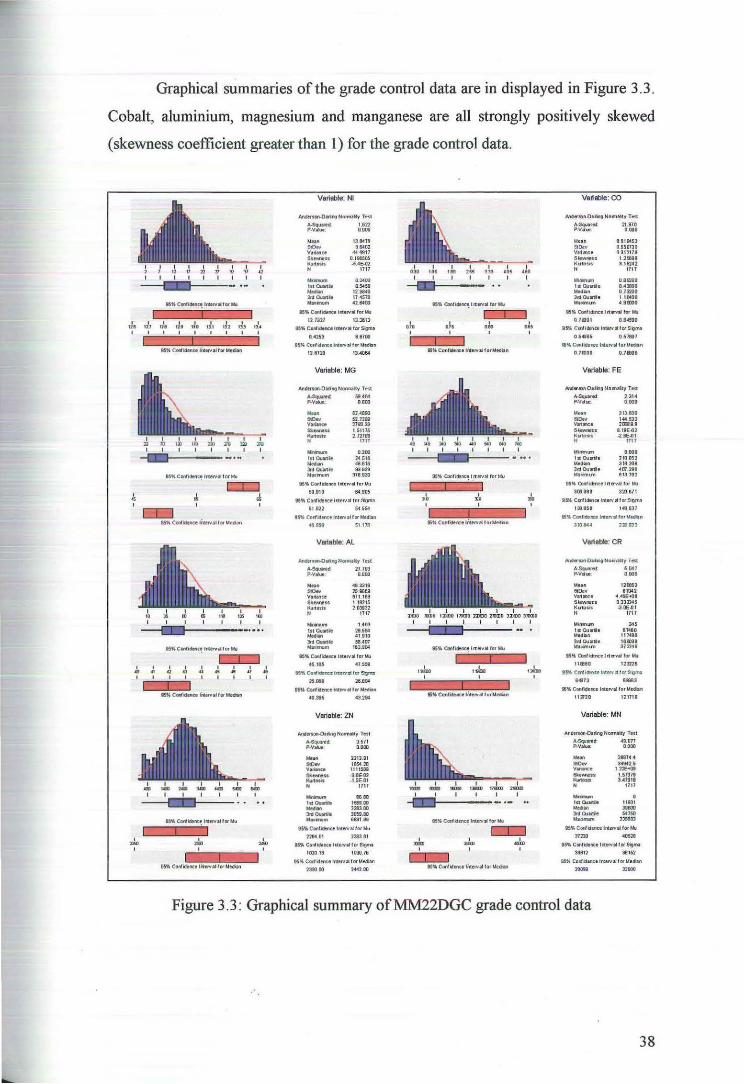
Graphical summaries of the grade control data are in displayed in Figure 3.3.

Cobalt, aluminium, magnesium and manganese are all strongly positively skewed

(skewness coefficient greater than 1) for the grade control data.

~ ~ ~ ~ . ~ ~ ~ ~ I I I I I I I I I

I .. I

I .. I

:J. I

11 I

f

.lo .\. .lo .lo I I I I

161Ao Confidtnc! l!l"eNIII I or Mu

t::J::J .1. .1

I

MtloCDnh~lnl.,.,lll l or t.\1

c::::r:::::::l I

" I ., ,\ I

" I .. I

q I • I I I I I I I

,1g, .,....,;....__,,.........,..-...., I

Va~able: Nl

AndfUCII'M>Mng NomuVy Tnt

o\o5Quwed 1.812 P-Y•.... oooo

"'"" 9Dw Vtnance ....... " Kunoli.s

" ......... llto...M .. -'"'""'" .. .........

130410

""' •lo4.0917 0.111650!1 -!i.4E-01

1117

Q_2<fllJ . ..... 12.184CJ ,.., 42.1400

IS'KCON~IRII'I'f'llifO'"IN

12,7U7 1:i.3LU~

I$"Confidt"CtiiUN'tllo.rSign'll

1 4153 UTOO

191. Co,.llhncellt(~tllar Median

178720 13.4084

Variable: MG

Ancleucw~ . .o•r~~ NollN!Iry ff:!; t

A-Sqlllmf 9.404 P.V•..._ OOCQ .... -y ...... Sl~n ~otis • Mftmu~t

htOuartle ·­lniDI••U•

"'•"""'

.,..,.. s1n• neo:o 1.51115 2.n18!J

1711

0.200 24.511 <48.616

""' 378930

iS'MoConlldluw::elnltrvtl for ~

59113 6481'6

IS" Collllclenu lruNII 101 S6grm

i l DU 5455-4

IS'K. COitidfl'll:t lntM'tl far.,ediH

4159 51 111

Varieblo:Al

AnO....OMnoHonnallv Tnt

A-Squated n1w P-v-.. a_ooo .... 413316 90w ,., .. VeiWK:e IIT U M 6k.W.ll 1. 18215 K.lftotis 2Ci31132

" 11 17

""""'m t .oiOO ISt OU:IItil: 29.5!M ..... • 1.810 ll'doartill 58.oi07 •-m 18U6C

IS'KCIIMide..:elrt.""'ll fDJ~

45 105 4l..5S.

tM~ C_.IOtfllt"e ltUf\oll l015$rN

.25..DIII 26.104

16K Cca'identfllrHNalfar"'edAn

40315 oiJ.2!M

vaneble: ZN

~ISort-0.-rilng NOifl'llllily Test

A-SQuattd 3.571 P·VIU. 0000

2l1U1 1"'28 111150& -U"'12 -ISE-Gt

UIT

... _ 11100

lsco.rta. ISOO WHW! 2313.00 lniOI.Jirlile 3tJ5.9.00 lotJII(rNPft tlttl1 81

16'K Confidence lnuwlll fot,.ll 77&401 23113.81

15~ Co,.IIHnc• lf•ttval tor stwna 10'10111 1000.18

IK~ CorldffiCelrteNIII f ar M~i.ln

'2'33000 1411100

I I I I 2§S llO j.OS dO I I I I

ts• Olnl•cl!ftet! lrtrv,." -" -' ·.,· .,.........,,

.lo ... .:.

as~ OlnfldtiK~ l rtsvll ror Mu

IS'!. CDnlldr:~l rtsvllfot llfu

t• I I

I"IDO l'rJCOO I I

I zmr ::a: t: sr»:: ts•COfttdtn:•lileNIIIfarWe.t•n

""" """ ci::::J I

es• Conlld~t~a tntttv• for Mect~t~

I I­I

Vanoble: co

MdwtDnOifingNom.Uy Tat

2Li70 .... IAUII 0 81 M53 ao.v 0558130 Vlri~e 0312171 s~u 1..2!MII l(uiD•s 3 .151.42

" 1117

"''*""" D.DaJOO I•C.,nle Q4l000 ..... O.ll:IID lMOYrie 1.10ta0

"'"""" 4.1mDD

tstlo CCWid!tl(:~rtrt8'VJI rw.., 071101 o..aao

UK C(Jihl'fttelt!UtVlllfOfS~""

054)115 Q_51tl)1

.,.CDnfiden::•lrterval. lor Medaf'l

01Ctl00 0 .78100

Va~ab le: FE

Md• mn.O.,i'lg Nomllty Tau

A-Sq~r.t Ul-i fWIII~ OJIIID

Nt•n SDiv v•--=• . ........ K1110th: • ..... ~ t•Oull1lle Med•n 31dQurie Wtwnun

313100 14U3l 1(81111

I.IIE42 -2..1E.OI

"" uoo 110152 lt8201 oi01211 81.3182

15,. Confld!rcel rtS'v .. for Nu

311111811 3:1)871

l mo\ Cftldenc;:elntervllllot!IQIN

191i11U 141$37

Z tlo Cenfrdtrn lrU:rvl!l forNMen

3 101114 318113

Variable: CR

....... tofttJ•U)g Na~.-lty Tat

~·- 5047 P.Vtl~. 0001

Mt~n nms:a !lOov """ Vwt.-.ce 4 49E:t0 1 S~u 03322-45 K111!1)1is .JOE41 N 1111

Minm1n1 ... I• Curie 11~10 Mltdr.n 117480 JldQ,urde llla:Jiilll .... JIW!IIIn 372'NO

liS'!. Oll'lfid!-rc:el rt rnl fot"' u••o 1237211

!5'A CII'Cid!:ntc lntuvd. tarSotm~

1473 IIIDIJ

15'K Confide.rc:t Irs eN• far WtODn

117120 121111

Venable: MN

AI\Oerson-Oalfrl; Notm11iry Ttsl

A-Sqund- 4U71 P.VaiUk OOCQ

Jlil87oi4 ,...,. I_,. 1-"311 3 47111

1111 - . lit O.... 11131 Mfdilft 308m )'dQJidik 54150 Umnun 23810:1

I$'K Coridtftt'e lnt.rt¥111 fat lll

nno 40528

IM4 CarM'iiMIKt lrternl far Sf;tm1

33812 38152

95'KCorj'ldeJ!ttlrteiVtlforMed.ln

29018 32800

Figure 3.3: Graphical summary of.MM22DGC grade control data

38

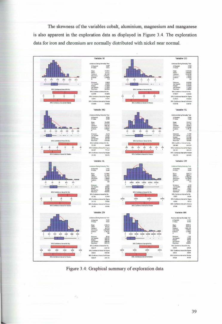
The skewness of the variables cobalt, aluminium, magnesium and manganese

1s also apparent in the exploration data as displayed in Figure 3.4. The exploration

data for iron and chromium are normally distributed with nickel near normal.

Variable: Nl Variable: CO

Ar!dtt~Of'ONIII'!Qt~TCSI AnteiS~N!rriUtyTI'• ...., ... ,,., ......... .... P.VIIIut o.o:n P.Va\le" '""' """ 140731

'···~ "''"' - 6_7191 """" ,....,., v ..... 4514B7 V..arct 01&QI&I

""""" OIH~~1 ........... I ""'

I - ,., .. I

..... .. 1ll""' .. , N I >I ,. N I >I

......, """' ......... 01121101

"'"""" u:~&s ,.~t OMIOJ ...... ,,... .... ~ ...... ........ '""" """"" 1111!0 M"Orttdl:f'Q...__b'WU ·~~

.,.., tw. ~Hen.lbMu """""' ....

115"0:1rf161nc•.lrt.,..,fo'.., ""'Cll'tim211*Mt b t.lu

I I ~ I ,.,.. 15.2tl15

I I I I IL7til1 OOWI

" " " ""Cbt1bnn h!MI ... Sqna .. " .. .. ""~tarwlbSi~ I I

517-'1 7.1781 I I

0.48552 '"""' M'KCotfidtrnoelfteN!IIflJ' Mt~bn UK ~~ trmw1 b MBhn 15~ CmlllefH W:fflll tar Mllbn 120l!D .. .,. ll!itl.~lrlfi\MbM.a~ 0617711 oamn

Variable: M8 Variable: FE

Andefson.ONI1119tbmJ!ityTut A~t«mdr-tT•• ........ ,,. ·- 021 P-V1h• 0000 p.v ... . .. ·- ,.,.... - 318111 - 8751J9 - ... 111 v ...... 455785 v-• ,., ... ......... 10511ol ......... 02tst8 - ,.,., ....... -llE-01

" "' N ... I I "'-•VI1 '"'" ......... OOCIUl - l«c:Md" '"" htDJril -znast ..... .. ... ..... 314ts9

:tlfo..o.tolf 11193 ~Q.Irie GI<B 15"-Qrllidtra herd b t.lu """"" 37UXI ~'K Oridlm:• lrl5'41 b !Au """""" 718892

Z%eo..tldttl<:elltfl'\&lfflhlu 9S"~Woldm:eldH<':IIbrl.tU

I ol I I ~. I ""' 90.458 ,/o I I .k .!o ,J., ,Jo

292 .9Sll "'"" .. .. " " "'' ~e\"'trMibr SIQI'D "" "' 95~0Yildtooe~~bSIIJnl

'""' 71141 I I I 1211191 IM153

{16-~ltttNlllktMfd-. ~~I'W..MIItlfiJotlbn liS" ~dett•"'mb Medii .. ..... 69374 15-.Conldn:.eW.II"ddfcrMniW'I

"'"' ,.,,.

Variable:~ Vaiable:CR

~fii'OIIi ... tmnlktTrsa 1-~Hom:Uylal - '"' - '"" P.V1fut 0000 P.v-..e oro

·- """' .... 82-4712 - 27.1252 - ..,.,, V"""'• 135n.:~ V•~ 2:nE•CIJ ·- I .... -- ....... """"" """'' I I I ' I """"" -UE~I N "' .... """' '"""' I""' """""

II "' l.lnrru n 1.<00 I

·~ 2119 ltlelMiM '"" 1-.Qlrie 45310 ..... 44.1(18 ""'"' ""' .. """ .. ..,.. JodO..r-1• . ~..,

IS'KCUltdencttuMibrt.IU ·- ...... II&Mo~Her.ettr Mu Mftmm "'"" li6~ Ccwtdtrnbt~kt t.lv 115'KQrir:lftnmfdbUu . .1, I I .,, .. ., ...

..loa ,.!., I ..lao """ ..... " .. " -~~b59n;o .... IWCMI~hrMib Sliflll

I I :.a us ..... I .... ""' e•~n.-truea;,., I!KClr*Sttlte~DMd!M ~0711d!tlceWt.wbt.ta:bn 31111 ..... ··~W.erwiiD't.IEd;n ..... """

Vllliable:ZN Variable: fVN

~Otiii'IQ~tyltu ~ruNo!m11t)'lm ......... !1.«169 """'""' , .,,

P-W~ ,,.. P-V~Ik ""' .... UD.13 ·- ....,., ..,., ... ,. ..,., qll43 ...... 891719 ...... l-......... 0:01859 -~ 183912 ·-- -1.3E.OZ I I I I I I

....... 1""" II .,. - """' t2mllO lmorD 2lOUlO :utiXI) N ,,. """""'

.,., """""' I Mil

Ill~ 1533_75 ··~ ""' ....... ...... ...... .,. ··-- ,.,..., .. """" 1110)7

~0711dlnc:e..,....A:Irt.lu ........ -491810 ""Qarfldsu h~ b Mu ·-- 2JOm

Z\lo~lf'UNIID'Uu ts%0wh:lerclr~bM\I

I I . I I I 11t171 ,., ..

I I , ,J., ..loa '''" ..... .... .... , .. , ?1'0 ""' "" Ht\~n..,.. lbrS9'f'IJ , ... .... IS%CcnDEricelrl ti'\DIIDI'9!JTB I I I I . I

llall 107808 I ,..., -15Mo~lrtl!Nifftt lotedian 9.5'~ Cort..ftrlta lr'ttlrui ID!"Mfit;n ti~ Ccrictfonce lrltfMi t~~ t.4edl.n lUI In 22~78

g~~lrUMb'Medi21 '27S'16 .. ~.

Figure 3.4: Graphical summary of exploration data

39

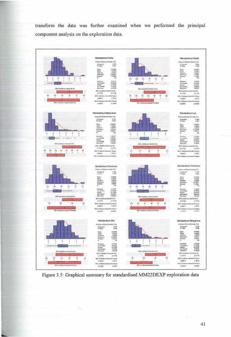
From the summary statistics displayed in Tables 3.1 and 3.2 it is evident that

the range, mean and variance of the auributes vary greatly. In order to make the

attributes comparable the data need to be standardised by subtracting the sample

mean and dividing by the sample standard deviation. Tab!.'! 3.4 displays the

standardised summary statistics for the exploration data (with the erroneous data

removed) and Figure 3.5 shows the graphical summary.

Table 3.4: Summary statistics for standardised MM22DEXP exploration data

Ni% Co% Mg% Fe% AI% CrPPM ZnPPM MnPPM

N 124 124 124 124 124 124 124 124

Mean 0.00 0.00 0.00 0.00 0.00 0.00 0.00 0.00

Median -0.10 -0.30 -0.29 -0.03 -0.14 -0.02 -0.15 -0.23

Min -2.01 -1.51 -1.04 -2.13 -1.72 -1.67 -2.16 -1.04

Max 4.25 3.89 4.45 3.19 3.63 2.81 2.95 4.40

SD 1.00 1.00 1.00 1.00 1.00 1.00 1.00 l.OO

Skewness 0.95 1:24 2.06 0.22 1.08 0.42 0.33 1.69

In many geostatistical and statistical procedures, we make the assumption of

second-order stationarity and normality. Although a principal component analysis

does not require normality of the data, the results are enhanced if this condition is

met. In many cases it is possible to transform the data in order to remove any trend,

stabilise the variance and achieve normality. However, one of the problems with

transforming data is that the estimation errors can become exaggerated when the

estimates arc back transfonncd. Hence, it is preferable to avoid transformation if

possible. Figure 3.6 displays the normal probability plots for each of the eight

variables. The plots for cobalt, magnesium, aluminium and manganese show strong

deviation from normality in the upper and lower tails. Figures 3.7 and 3.8 show the

lognormal and Weibull plots for these variables. While neither transformation

appears to have adequately removed the asymmetry of the raw data the lognormal

plots seem to have Jess deviation than the Wei bull plots. The decision of whether to

40

transform the data was further examined when we performed the principal

component analysis on the exploration data.

..:. I

I

I

~' I

-

I .0)3

..:.

I .. I

I I .02 00

I I

I D. I I

I

"

.~, I

I

"

.~, I

stendanised N ckel

A~Notmllcylut

~ OltJ P.v•w DOll - ...... - 1..., V•l3f"Ct- ltlOlO) 5~n O.MSI$1

"""'"' '''"" " 114

u ....... -201H4 1 ....... .-... u .. _

~~-........ ...... ........ 4251§1

amO:wlklerumrvllltrMu ~ITI7fl 0 17778

95'KQridcn:.e ......... ,..

o•13 tt.cn 8S1t~t ........ li:lfldtChll

.n:wn.1

stordortlsed Mlgno:Oun

Andc:n-cnOIII~fQn1kylta ~ ,.,. P-VM QDa)

..... ~"""' """' '"""' ·~ '"""' ......... 2~\W -- CI!I&M7

" "' MJnm.m -10i1Sl hiO..ll\l~ -OE&22 ·- .oam "'~ 021237 ......... ·-15%~h,..bMii

-0117'111 017Tll

IS'KQirl'ldence~tnbSI"""'

OEM13 1 1-4l77

t9K CcnlcPnoe lti{Nt lar ... ..._

.. _ '"' r.v•w .....

u ... ..... """ """" .... ~ '"""' 5ki'W'I!IU I Q&WI - ·· I!CXKl6

" 17<

MftnJm ·• r!J<IJ Itt CU.U. .A) 1on8 ~ -GilJel ~o...rtft 0 .. 5171 M~t<mJm :182812

iS" Ccr*krce ~ tw Mli ..om111 omn

M~IMIMI!w!iqnt

DEll 1 tq72

ts"~~lbtt.I«Urr ftM\)7

stlrdcrdsed Zinc

~~tam:nyTU

A·Sqvftd 04111 P.Vatue 024-;f ..... ....... ""'"' '"""' - I""" ......... 0.3Jit61 ... _

. , :E.-Qll

" "' M.rrm.m ~1 11257 l ltQnls!Je -tllliM ·- .. _ .. .,..,. Om>!

"""""" 201131

~Corf.dMcehH411bNv

.017776 01771!1

15~~1!11nt!r'1111fllr!lo'.t~ OIMIJ IIA2n

~ Ccrl\anc.-Jrtf!"'411tlt ... t6MI

-OVMD ~~

I .,

I

~' I

85%Co'IWetalttMIIiftrNu

E ~ ..II

I I

" " I I I

.~,

- --~

I

~· I

I

" I

stendcrdsed Cobalt

Ald!!SM~ Notnuity Tnt A.~ 2~11 P.v~ o.mo .... ~ ..... '"''' IJIOODIJ

""'""' lllllllll ......... 124262 -·· 171055 .. "' ....... -15\301 l$tcu.l .. ..07oQIO ·- ~-· ,..,..., ,,.,., """""' J895S7

95% Oridlrn lrtt!v.JI' b !.11.1

..o..tme otma IM5-~elrUMIIkrS!grN

0811113 ll4272

IS'K~t_,..b'Uftbrl

..0.40ll)4 ..0.0 15:1$"

stendlrdsed lrm

~~Tesa

A-Sq.J~ 0.38i p.v~..e 0 380 .. ....

'""""' '"""' G.lt!Dll .1fif41

110

Ri,.~r-.....~MII

..omra om7t 85% OJHidt!'Ce~ftr59ra

DBEilll 114212

ts'K~ ..... b~

stendaridsed OYOITiun

~~Test ........ 0470 P.V:i1L 01<1 . ... ~ .... so.. "'""" V~..-.c:e l(](l]OO] ,..,..,.,. 0 4 10047

"""'"' -19E..OI

" 12<

......... . . ...,. luQooM ~110311 ·- ~0Zl09

"'""" .. 0.81123

"'"""" 280753

95% Co(.Wm:e lrUMI b Mu

..o.m7& otm&

M~lllfHI:ftrs;g.n.

oa11n3 uczn ~~a.u..-Jbld.t<Url

A-S~d 442!1 P-VIIIIA!I """ y~ ODCXIOO

"""' I.IXDDD ....... """" ......... UHII

~· l.'fml N '" """"m -1.04368 1-R-OJM .. <l16104 ...... ~2mll

"""""" ...... """""" "''"' Z'tlo~tWtM'btUu

.otme oams A5!0 Griderc.•hlaMifaSIQII'D

DBIIU3 114212

~"carr-.. taM tlr t.l.e:brl

-.Q_UIJII -OG.m$

Figure 3.5: Graphical summary for standardised J.\.1M22DEXP exploration data

.·

41

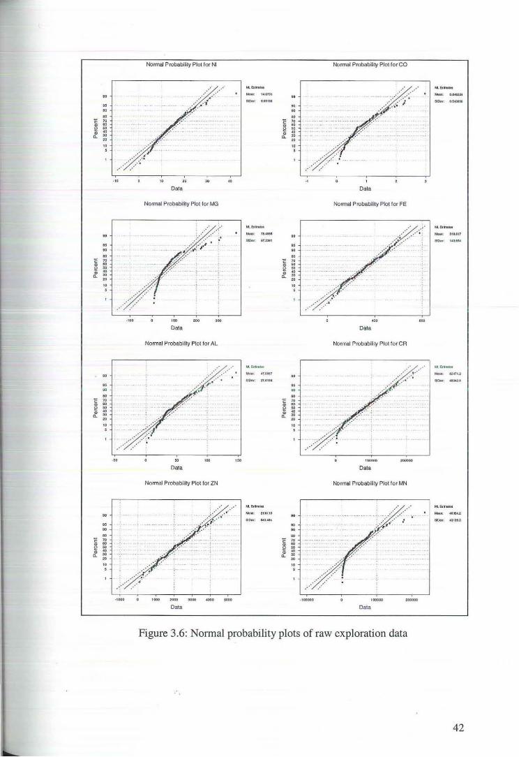
Nonnal Probabi~ty Plot for N1 Normal Probability Plot for CO

..... .._ ..._r .. m .. .. - .. .· . - O.l.Ull -· ._ .. , .. _ .. ~ ... ;: .. . """"

,...,.,. .. " I

00 .. eo ..

E 70 E "' " 10 " .. e 50 e 50

" ..

" ..

D. .. D. " 20 20

10 " 5 5

:

· 10 20 " ... Data Data

Normal Probability Plot for MG Nonnal ProbabiiHy Plot for FE

.. ..... _ t.t. &lim'N .. ...... , ....

" ._ 3tUtJ _,

"-"'1 _, 1 .....

" .. .. 10 .. .. E 70 E 70 .. .. " .. e 50 e 50

" .. 0) ..

D. 30 D. 30 20 20

" " s ..

·10 0 200 '" 400 100

Data Data

Nonnal Probability Plot lor AL Nonnal Probability Plot lor CA

t.t.r. ....... ... .. _

.. .... .,_ _, 12471.2 - l7.015f -· ...... .. t 5 .. .. .. ..

E 70 E 70 .. .. " .. e 50 11 50

" ..

" ..

D. 30 D. 30 20 20

" " s .. .-!

... 100 I SO ...... Data Data

Normal Probability Plot l or ZN Normal Probability Plot lor MN

.. M.(SIRio!IM K.&tt.iM .. .. · Mt!M: 2:1)1),13 . . ·' .• .....,, ....... .. ..,, NOM~

_, f31 3t,3

•• ., .. .. .. : E 70 .. E 70

" ..

" eo e 50 e 50 .. •• "

.. D. .. D. 30

20 20

" " • 5

.-

·1000 2000 3000 ... 0 5000 · 100000 100000

Data Data

Figure 3.6: Normal probability plots of raw exploration data

42

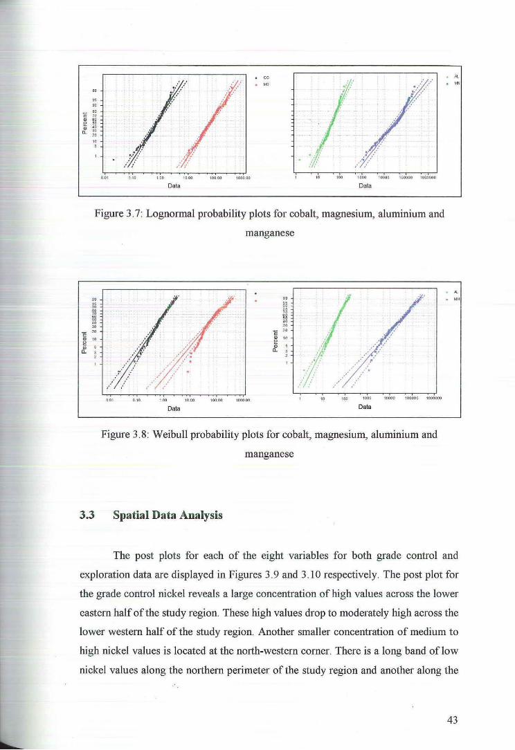
•• 95 90

- 80 c: 70 Q) 60 e so ., •o a. ;~

10

'

co • MG

Data

# . ..

10 100 1000 \0000 100000 1000000

Data

Figure 3.7: Lognormal probability plots for cobalt, magnesium, aluminium and

0.0 1 0. 10 I 00

Data

manganese

10 00 100 00 1000 00

99

Bo

u 30

- 20 c: Q) 10 e ~

10 100 1000 10000 100000 1000000

Data

Figure 3.8: Weibull probability plots for cobalt, magnesium, aluminium and

manganese

3.3 Spatial Data Analysis

. ""'

The post plots for each of the eight variables for both grade control and

exploration data are displayed in Figures 3.9 and 3.10 respectively. The post plot for

the grade control nickel reveals a large concentration of high values across the lower

eastern half of the study region. These high values drop to moderately high across the

lower western half of the study region. Another smaller concentration of medium to

high nickel values is located at the north-western comer. There is a long band of low

nickel values along the northern perimeter of the study region and another along the

43

eastern perimeter. The exploration nickel data reflect the spatial distribution of the

grade control nickel very well with only the low values on the eastern perimeter

under represented.

The cobalt grade control values seem to be predominately high in small

pockets across the southern half of the study region, along the western perimeter and

in the north-western comer. The entire south-western comer appears to have medium

to high levels of cobalt. There are low values along the northern perimeter of the

region as well as in the south-eastern corner. The exploration cobalt values also

reflect the spatial distribution of the grade contro1 Jata very well, although the low

values in the south-eastern comer and the high values in the north-western comer arc

not well represented.

The post plot of the grade control magnesium shows small pockets of high

values in the north-western corner, central eastern region, eastern perimeter, south­

eastern and the south-western comers. The concentratians of low values are located

predominately across the centre of the study area with pockets along the western and

northern perimeters. The spatial distribution of the exploration data is also very

representative of the grade control data with the only exception being an under

representation of low values along the south south-eastern and south south-western

perimeters of the study region.

The post plot of the grade control iron indicates that there is a large area of

high values across the central southern region extending across toward the south­

western corner and up along the western perimeter. There is also a small pocket of

high values in the north-western corner. The low values extend in a long band along

the northern perimeter of the region with a large area of low values in the south­

eastern corner. Overall the spatial distribution of the grade control iron is very well

represented by the exploration data, the only exception being an under representation

of low values in the south-eastern comer.

The post plot of the grade control aluminium shows two large areas of high

concentrations in the south-eastern and south-western regions of the study area.

There is also a pocket of high values in the north-western corner. The low values are

predominately located across the western side of the study region; in addition there

are small pockets of low values in the south-eastern corner. The spatial distribution

of the exploration data is also very representative of the grade control data with the

44

only exception being an under representation of high in the north-western corner of

the study region.

The post plot of the grade control chromium shows clear cut areas of high

and low concentrations with the high values along the south-eastern perimeter

extending across the central southern region into the lower western side. The low

values extend across the entire northem boundary extending down along the east

south-eastem perimeter. The spatial distribution of the exploration data is in this case

not very representative of the grade control data. The large regions of high

concentrations appear to be greatly under represented across the entire study region.

The post plot of the grade control zinc shows hi~h concentrations across the

entire southem half of the study region and in the north-western comer. The low

values are located along !he northem and south-eastern perimeters. The spatial

distribution of the exploration data is very representative of the grade control data

with all high and low values well represented across the entire study region.

The post plot of the grade control manganese shows a large concentration of

high values occupying the entire south-western region, extending east across the

lower southern half up into the south-eastern corner. There is also a pocket of high

values in the north-western comer of the study region. Three regions of low values

are evident, on the central north-western side, across the centre of the study area and

across the central south-eastern region. Again, the spatial distribution of the

exploration data is very representative of the grade control data with all high and low

values well represented across the entire study region.

45

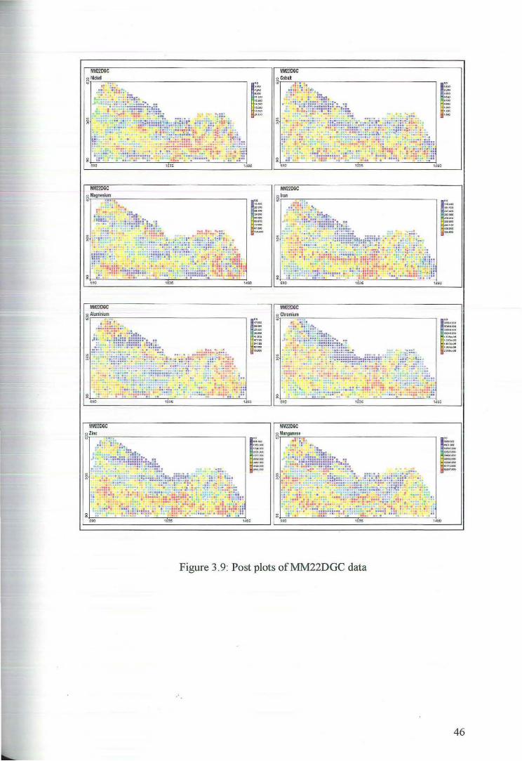
MMZ20GC ~ N'cktl

.

~

:::.:~ . ... ==· =!:·· :::·· '· :• . ._;:: ... ·-

r '~ "" "~ ,_ .. ~ uml:t

"""

I. :: --"' --·-

1~-·­,,.._ ··­-------~·-

MM220GC ~ Cobalt

~

MM220GC ~ion

MM220GC ~ Manginttt

·""• ..

r=:.•

Figure 3.9: Post plots ofl\1M22DGC data

.... .. r t.UQ ·-·-'"' ·~ ·-·-... ....

1

.. ttl ..

··~ =­-~~· _.,. -·­Q .. .....

1

.. _ .... ·-­-·­"u'~

UI:IOonCO ~.~ .. , .. " , ...... . 1* }_ •.. ~

1

.. ---.. ........ ...., .. ...... ----"""" --

""'

46

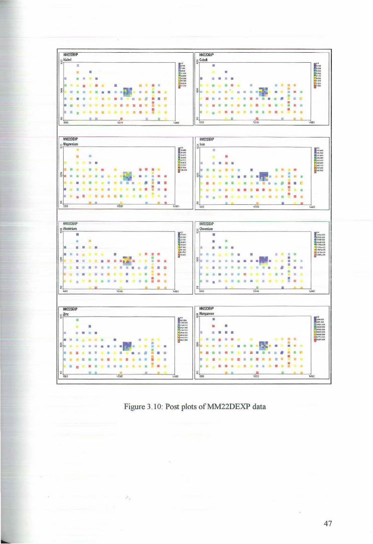
MM22DE>O' MM220EX!' ~t-icktl

r !:i Cobilt

r ·~ • .. .. '"' "" • • ·- • ,..,

..~ , _ •m • • • • .. .. • • • • • "" '"" "'' • • • • • • • • IUIO • • • • • • • • .... • • ~- • • '"' ~ I § • g • • • • • • • • • • • • • • • • • • • • • • • • • • • • • • • • • • • • • • • • • • ,., • • • • • • • • • • • • • •

'" . • • • • a • • • • • • • • • • • • • • • • • • • • • • • • • • • • • • • • • • • • • • • • • • • • • •

:i n n • ., .. ~ - " .. " " 590 10l5 1490 ... 1035 1460

MIIZ2cexP MMZZOEJO' a Magnesium

r !:i~ ••

r "~ ...... 3- ....

• • ~-»= ,.,. • • • • ~~

1'\ • .zl • • • • • .. ... -·~ • • • • • • • • • ...

" • • • • • . .... It ··- • • • • • ~~

~ • • ~ . • • • • • • • • • • • • • • ~ • • • • • • • • • • • • • • • • • • • • • • • • • • • • • • • • • • • • • • • • • • • • • • • • • • • • • • • • • • • • • • ] . • • • • • • • • • • • • • • • • • • • • • • • • .. • • • • • • • • • • •

g !" • .. • • g - - • ~ . ... 1036 ....so. ..., 1015 -IIM220EXI' IIM220EXI'

oAlunnwn ~Chromium ~

r r • "~ • -.. ~- --• • n.,. • • ---~ ..... ... 41M.

I• tii"·OS • • • • • '1101) • • • • UO'I'ul't

~·~ lj4hoCI$

• • • • • • • • • <>~- • • • • • • • • • Ull .. •<'f • • "., • , ...... ., .... • ~ • n • • . • • • • • • • • • • • • • • • • • • • . • • • • • • • • • • • • • • • • • • • • • • • • • • • .. • • • . • • • • I) • • • • • • • • • • • • • • • • • • • • • • • • • • • • • • • • • • • • • • • • • • • • • • • • • • • ~ • • • ~ h • ~ .. ~ .. " • ..

590 1035 , .. 60 "" 10:!5 14!!0

MM22DeXP MM220El<l'

~Zine ~ Manganm

r r • --.... .... • • • '"".m

~~-........ ......

• • • • _ ..

I • • • • ---- ·~-gfa -- • • . I • • -~-• • .. • • • • • • • -~~- • • • • --• § • • • • • • • • • • • • • • • • • • • • • • • • • • • • • I I • • • • • • • • • • • • • • • • • • • • • • • • • • • •

I ~ • • • • • • • • • • I • • • • • • • • • • • • • • • • • • • • • • • • • • ft • • • • • • • • • • • • g " " g .. ~ II ,. ~

••• 1035 1480 '"' 10lS 1460

Figure 3.10: Post plots of:MM22DEXP data

47

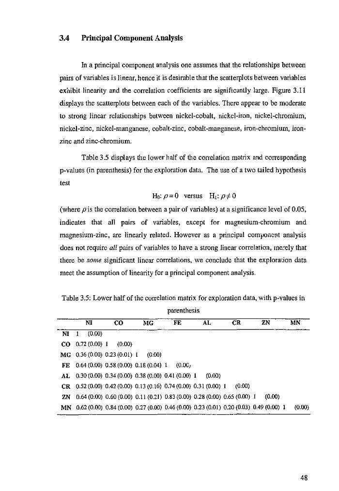
3.4 Principal Component Analysis

In a principal component analysis one assumes that the relationships between

pairs of variables is linear, hence it is desirable that the scatterplots between variables

exhibit linearity and the correlation coefficients are significantly large. Figure 3.11

displays the scatterplots between each of the variables. There appear to be moderate

to strong linear relationships between nickel-cobalt, nickel-iron, nickel-chromium,

nickel-zinc, nickel-manganese, cobalt-zinc, cobalt-manganese, iron-chromium, iron­

zinc and zinc-chromium.

Table 3.5 displays the lower half of the correlation matrix and corresponding

p-values (in parenthesis) for the exploration data. The use of a two tailed hypothesis

test

Ho:p;:::Q versus H1:p:f.O

(where pis the correlation between a pair of variables) at a significance level of 0.05,

indicates that all pairs of variables, except for magnesium-chromium and

magnesium-zinc, are linearly related. However as a principal compoGcnt analysis

does not require all pairs of variables to have a strong linear correlation, rne.~ely that

there be some significant linear correlations, we conclude that the explora'.jon data

meet the assumption of linearity for a principal component analysis.

Table 3.5: Lower half of the correlation matrix for exploration data, with p-values in

parenthesis

Nl

co

NI CO

1 (0.00)

0.72 (0.00) 1 (0.00)

MG

MG 0.36 (0.00) 0.23 (0.01) 1 (0.00)

FE

FE 0.64 (O.IJO) 0.58 (0.00) 0.18 (0.04) (0.0C)

AL

AL 0.30 (0.00) 0.34 (0.00) 0.38 (0.00) 0.41 (0.00) 1 (0.00)

CR

CR 0.52 (0.00) 0.42 (0.00) 0.13 (0.16) 0.74 (0.00) 0.31 (0.00) I (0.00)

ZN

ZN 0.64 (0.00) 0.60 (0.00) 0.11 (0.21) 0.83 (0.00) 0.28 (0.00) 0.65 (0.00) I (0.00)

MN

MN 0.62 (0.00) 0.84 (0.00) 0.27 (0.00) 0.46 (0.00) 0.23 (0.01) 0.20 (0.03) 0.49 (0.00) (0.00)

48

~ • .

~ • • • •

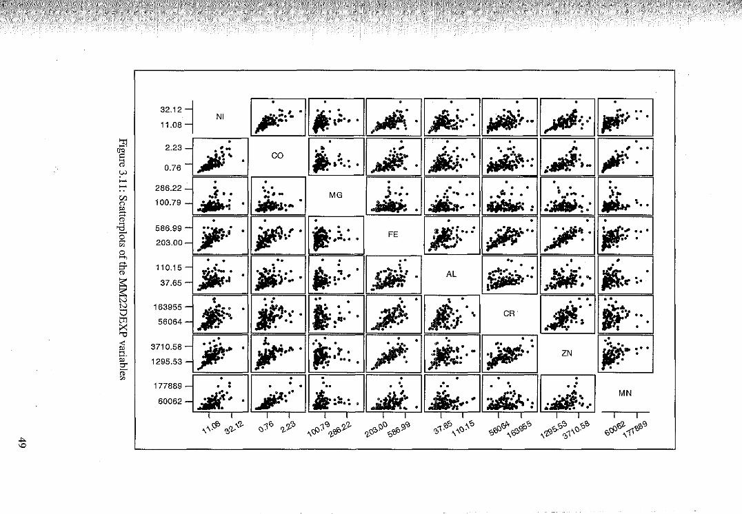
32.12 ,.= ... . It:' . ... . liM:~·· ;ria; :·. Nl . ,: .. ~ ... · ,)Aii·. ..... • •• 11.08 • • • • •

~ • . • • • . . 2.23 - '" ,,

A: JiA .. ~~·· ... ,.: . . ()Q

;#;' c co ... ;.: ;.#.:Jw d - • •• • 0.76 • • ' • • "" • ..... . • • . . • • ..... 286.22 - • •• • • • • • . . .. .. { .. ;,: ... MG ) ... . :: .... • ,.6 • . ·-·~ . ·':-C/:l 100.79 --= J/lllrJ:" •

~ ., .. "'~ ... ·'·· 0 - • • -~ .. · ~ • -xn: • • •

" • • • • • • • .a 586.99 -~· ~~r -· :It' . ~·· 7~· 0 ;.• • • . . . FE .... ~, ... .. .: .. • :. .. .

~ 203.00 -"' • 0 • "" • • .. . • .. •• • • ~ ::r 110.15 -

J~'T.; .

tr~~·· • • • .; lit: .. . .I.' ..&!.. • • lr." ._ • • " . AL

~~·· ;9/tl!f:· •.. -:C' : . ~ , ... • •

37.65 - -t •• •• • • • \ • • . . .. • • • N 163955 - $:. $1·,· ,. ~ Jf.'f • . .~!!·~ • If" 0 • • . .

• .. CR ~ .. ~ 56064 - •• " .. II•

• • • N • • •

"tt ••

~ ~· . .. . . •

~: < 3710.58 - j#r ,. <I> •••• .. .

§. • • :1' •• •• ~·:" _.I ••: • ~:· ZN g. 1295.53 - • • - .. .. • " "' . . . . . • .

177889 - • • • • • • .. • • .·. . • • • • • • •

.-iii' #:·· •= jj;: .. 'iitff,.'l.. . : J.~ MN 60062 - ·:, • ..... . .... • ... . ., . • :11 • •

l l I I I I I I I I I I I I I I

(§' \'I- ()~I) <z-'1-'b \ <:P ~'!!'I-'If" 'J-'~- '1-<:Jb "'\'If" 9>9! '!>1~\\()~"' <f:l'i}< rf>"' .;'!> .;'0 <:P"'I- 'If"'!! \ \· '!>'~-' "' ,<SO \ 'fl"'' '!>1\ (). " ,11

""" \0

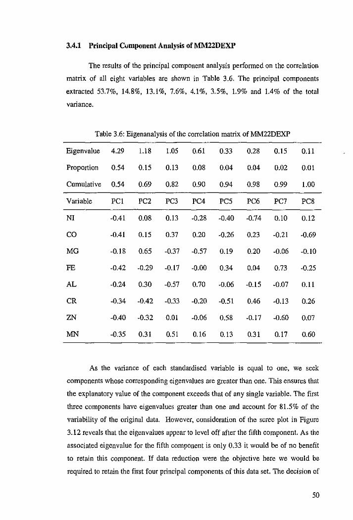
3.4.1 Principal Component Analysis of l\1M22DEXP

The results of the principal component analysis perfonned on the correlation

matrix of all eight variables are shown in Table 3.6. The principal components

extracted 53.7%, 14.8%, 13.1%, 7.6%, 4.1%, 3.5%, 1.9% and 1.4% of the total

variance.

Table 3.6: Eigenanalysis of the correlation matrix of :M:M22DEXP

Eigenvalue 4.29 1.18 1.05 0.61 0.33 0.28 0.15 0.11

Proportion 0.54 0.15 0.13 0.08 0.04 0.04 0.02 0.01

Cumulative 0.54 0.69 0.82 0.90 0.94 0.98 0.99 1.00

Variable PC! PC2 PC3 PC4 PC5 PC6 PC7 PCB

NI -0.41 0.08 0.13 -0.28 -0.40 -0.74 0.10 0.12

co -0.41 0.15 0.37 0.20 -0.26 0.23 -0.21 -0.69

MG -0.18 0.65 -0.37 -0.57 0.19 0.20 -0.06 -0.10

FE -0.42 -0.29 -0.17 -0.00 0.34 0.04 0.73 -0.25

AL -0.24 0.30 -0.57 0.70 -0.06 -0.15 -0.07 0.11

CR -0.34 -0.42 -0.33 -0.20 -0.51 0.46 -0.13 0.26

ZN -0.40 -0.32 0.01 -0.06 0.58 -0.17 -0.60 0.07

MN -0.35 0.31 0.51 0.16 0.13 0.31 0.17 0.60

As the variance of each standardised variable is equal to one, we seek

components whose corresponding eigenvalues are greater than one. This ensures that

the explanatory value of the component exceeds that of any single variable. The first

three components have eigenvalues greater than one and account for 81.5% of the

variability of the original data. However, consideration of the scree plot in Figure

3.12 reveals that the eigenvalues appear to level off after the fifth component. As the

associated eigenvalue for the fifth component is only 0.33 it would be of no benefit

to retain this component. If data reduction were the objective here we would be

required to retain the first four principal components of this data set. The decision of

50

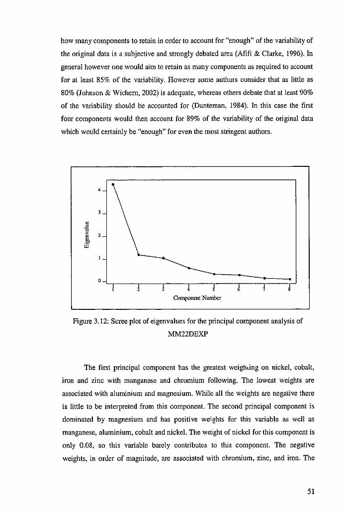
how many components to retain in order to account for "enough" of the variability of

the original data is a subjective and strongly debated area (Afifi & Clarke, 1996). In

general however one would aim to retain as many components as required to account

for at least 85% of the variability. However some authors consider that as little as

80% (Johnson & Wichern, 2002) is adequate, whereas others debate that at least 90%

of the variability should be accounted for (Dunteman, 1984). In this case the first

four componevts would then account for 89% of the variability of the original data

which would certainly be "enough" for even the most stringent authors.

'

l

Component Number

Figure 3.12: Scree plot of eigenvalues for the principal component analysis of

MM22DEXP

The first principal component has the greatest weighling on nickel, cobalt,

iron and zinc with manganese and chromium following. The lowest weights are

associated with aluminium and magnesium. While all the weights are negative there

is little to be interprei:ed from this component. The second principal component is

dominated by magnesium and has positive weights for this variable as well as

manganese, aluminium, cobalt and nickel. The weight of nickel for this component is

only 0.08, so this variable barely contributes to this component. The negative

weights, in order of magnitude, are associated with chromium, zinc, and iron. The

51

third principal component is composed of positively weighted manganese, cobalt,

nickel and zinc. The contribution of zinc to this principal component is negligible

with a weight of only 0.01. The negative weights are associated with aluminium,

magnesium, chromium and iron. The fourth principal component is dominated by

aluminium, whose weight is positive as are the weights for cobalt and manganese.

The negative contributors are magnesium, nickel, chromium, zinc and iron, with the

latter two being almost zero. There does not seem to br any clear interpretation for

any of the principal components from this data set.

Figure 3.13 displays the scatter plots of the scores of the first four principal

components. The plots between PC1-PC2, PC2-PC3 and PC3-PC4 reveal potential

outliers. The corresponding sample data was checked and it was ascertained that

these data were genuine, hence they could not be treated as erroneous and were left

in the data set.

There does appear to be some slight curvature in some of the scatter plots, in

particular those between PCSI, PCS2 and PCS3, suggesting that the strongly skewed

variables cobalt, magner.ium, aluminium and manganese, may benefit from a

transformation. These variables were transformed logarithmically and the principal

component analysis repeated. The results were compared to those obtained in the

principal component analysis of the raw data and are displayed in Appendix A. The

eigenvalues in each are case very close in value with the cumulative propmtion of

variability almost identical by the fourth component. The eigenvalues of the first and

second principal components are somewhat higher for the transformed data while the

third eigenvalue is somewhat lower. There have been numerous small changes in

some of the elements of the coefficient vectors, though they are all small.

52

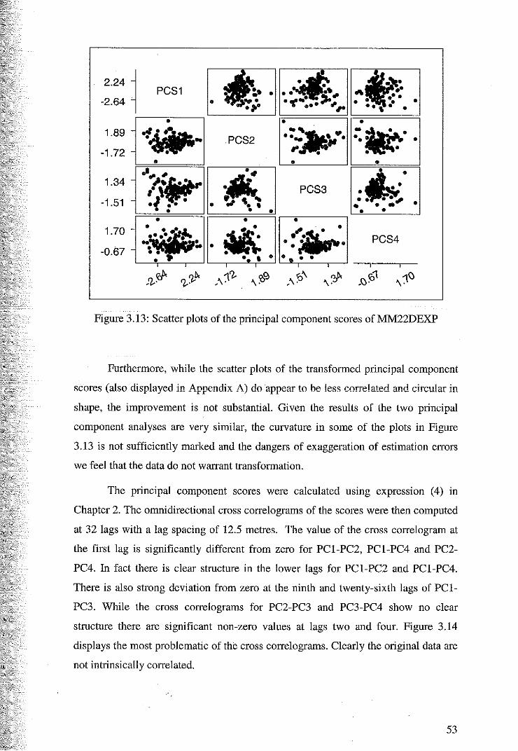
2.24

-2.64

1.89

-1.72

1.34

-1.51

1.70

-0.67

j -

-

-

-

-

PCS1

• A. . .. •

• .. ~ ~ ~·fit" ,., .I ••• • • • •• .. ····~~ . . . .. •• •

• ~:·. • • :to"

PCS2

. ., -If. ... • .., ..

• • •

• ~ •• • • -,- -,-

.. ~~~ ~-"' .. • ·-t·• • • ... ,,. ., . • • .. ... -.... ··~··· •• • • ,. , • • •

• • ... PCS3 : , . . - • • • •

·~ • • • • • •••

PCS4

-,-

Figure 3.13: Scatter plots of the principal component scores of MM22DEXP

Furthermore, while the scatter plots of the transformed principal component

scores (also displayed in Appendix A) do appear to be less correlated and circular in

shape, the improvement is not substantial. Given the results of the two principal

component analyses are very similar, the curvature in some of the plots in Figure

3.13 is not sufficiently marked and the dangers of exaggeration of estimation errors

we feel that the data do not warrant transformation.

The principal component scores were calculated usmg expression ( 4) in

Chapter 2. The omnidirectional cross correlograms of the scores were then computed

at 32 lags with a lag spacing of 12.5 metres. The value of the cross correlogram at

the first lag is significantly different from zero for PC1-PC2, PC1-PC4 and PC2-

PC4. In fact there is clear structure in the lower lags for PC1-PC2 and PC1-PC4.

There is also strong deviation from zero at the ninth and twenty-sixth lags of PC 1-

PC3. While the cross correlograms for PC2-PC3 and PC3-PC4 show no clear

structure there are significant non-zero values at lags two and four. Figure 3.14

displays the most problematic of the cross correlograms. Clearly the original data are

not intrinsically correlated.

53

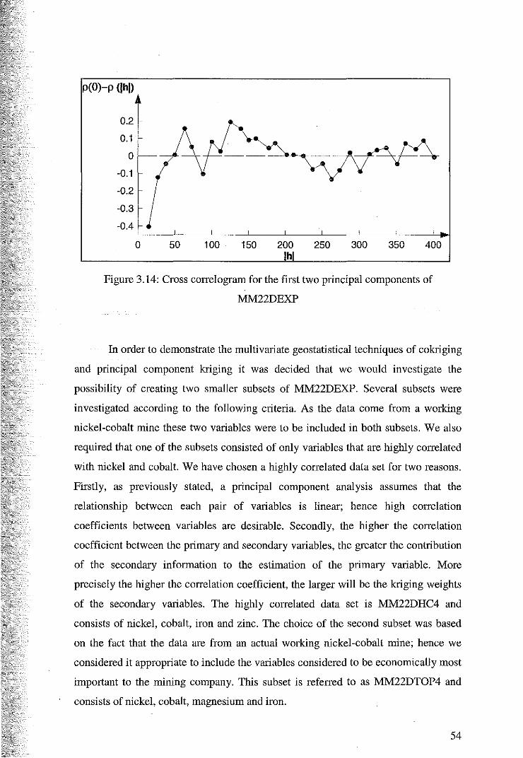
p(O)-p (lhl)

0.2

0.1

0

-0.1

-0.2

-0.3

-0.4

0 50 100 150 200 h

250 300 350 400

Figure 3.14: Cross correlogram for the first two principal components of

MM22DEXP

In order to demonstrate the multivariate geostatistical techniques of cokriging

and principal component kriging it was decided that we would investigate the

possibility of creating two smaller subsets of MM22DEXP. Several subsets were

investigated according to the following criteria. As the data come from a working

nickel-cobalt mine these two variables were to be included in both subsets. We also

required that one of the subsets consisted of only variables that are highly correlated

with nickel and cobalt. We have chosen a highly correlated data set for two reasons.

Firstly, as previously stated, a principal component analysis assumes that the

relationship between each pair of variables is linear; hence high correlation

coefficients between variables are desirable. Secondly, the higher the correlation

coefficient between the primary and secondary variables, the greater the contribution

of the secondary information to the estimation of the primary variable. More

precisely the higher the correlation coefficient, the larger will be the kriging weights

of the secondary variables. The highly correlated data set is MM22DHC4 and

consists of nickel, cobalt, iron and zinc. The choice of the second subset was based

on the fact that the data are from an actual working nickel-cobalt mine; hence we

considered it appropriate to include the variables considered to be economically most

important to the mining company. This subset is referred to as MM22DTOP4 and

consists of nickel, cobalt, magnesium and iron.

54

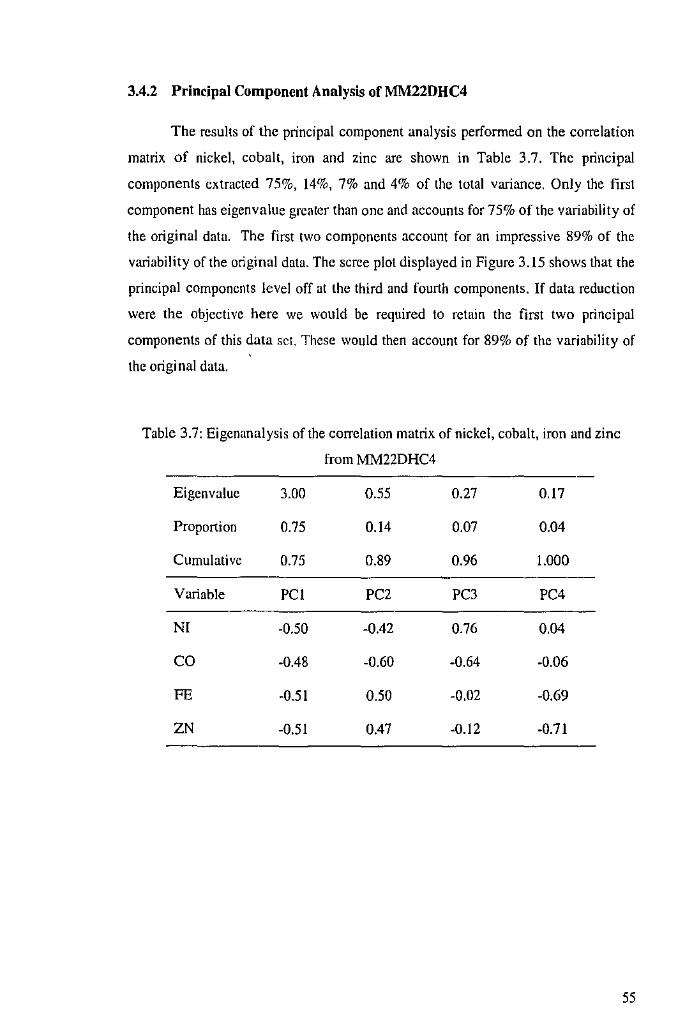
3.4.2 Principal Component Analysis of MM22DHC4

The results of the principal component analysis performed on the correlation

matrix of nickel, cobalt, iron and zinc are shown in Table 3.7. The principal

components extracted 75%, 14%, 7% and 4% of the total variance. Only the first

component has eigenvalue greater than one and accounts for 75% of the variability of

the original data. The first two components account for an impressive 89% of the

variability of the original data. The scree plot displayed in Figure 3.15 shows that the

principal components level off at the third and fourth components. If data reduction

were the objective here we would be required to retain the first two principal

components of this data set. These would then account for 89% of the variability of

the original data.

Table 3.7: Eigenanalysis of the correlation matrix of nickel, cobalt, iron and zinc

from MM22DHC4

Eigenvalue 3.00 0.55 0.27 0.17

Proportion 0.75 0.14 O.D7 0.04

Cumulative 0.75 0.89 0.96 1.000

Variable PC! PC2 PC3 PC4

NI -0.50 -0.42 0.76 0.04

co -0.48 -0.60 -0.64 -0.06

FE -0.51 0.50 -0.02 -0.69

ZN -0.51 0.47 -0.12 -0.71

55

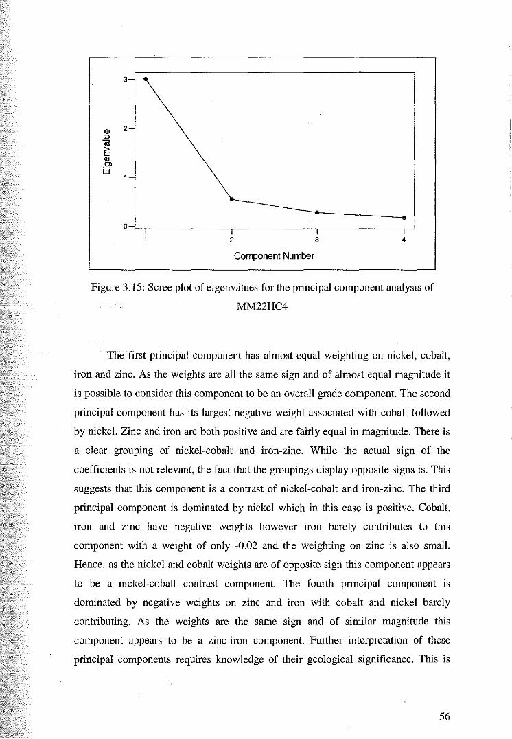
2 3 4

Component Number

Figure 3.15: Scree plot of eigenvalues for the principal component analysis of

MM22HC4

The first principal component has almost equal weighting on nickel, cobalt,

iron and zinc. As the weights are all the same sign and of almost equal magnitude it

is possible to consider this component to be an overall grade component. The second

principal component has its largest negative weight associated with cobalt followed

by nickel. Zinc and iron are both positive and are fair! y equal in magnitude. There is

a clear grouping of nickel-cobalt and iron-zinc. While the actual sign of the

coefficients is not relevant, the fact that the groupings display opposite signs is. This

suggests that this component is a contrast of nickel-cobalt and iron-zinc. The third

principal component is dominated by nickel which in this case is positive. Cobalt,

iron and zinc have negative weights however iron barely contributes to this

component with a weight of only -0.02 and the weighting on zinc is also small.

Hence, as the nickel and cobalt weights are of opposite sign this component appears

to be a nickel-cobalt contrast component. The fourth principal component is

dominated by negative weights on zinc and iron with cobalt and nickel barely

contributing. As the weights are the same sign and of similar magnitude this

component appears to be a zinc-iron component. Further interpretation of these

principal components requires knowledge of their geological significance. This is

56

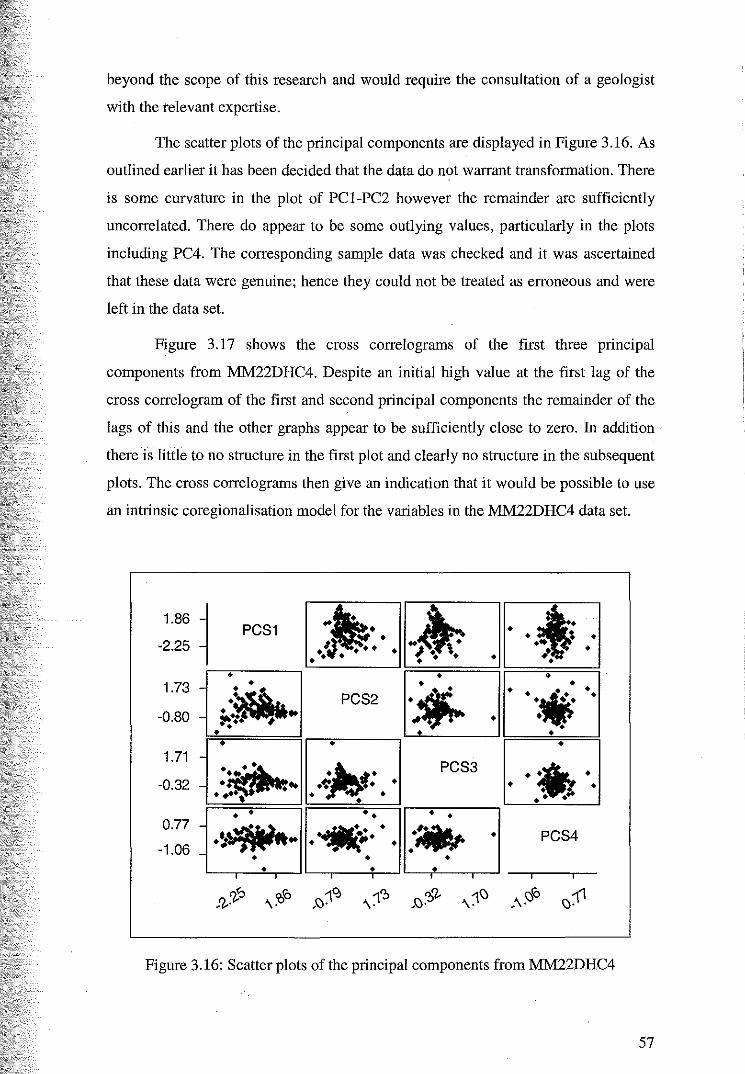
beyond the scope of this research and would require the consultation of a geologist

with the relevant expertise.

The scatter plots of the principal components are displayed in Figure 3.16. As

outlined earlier it has been decided that the data do not warrant transformation. There

is some curvature in the plot of PC1-PC2 however the remainder are sufficiently

uncorrelated. There do appear to be some outlying values, particularly in the plots

including PC4. The corresponding sample data was checked and it was ascertained

that these data were genuine; hence they could not be treated as erroneous and were

left in the data set.

Figure 3.17 shows the cross correlograms of the first three principal

components from MM22DHC4. Despite an initial high value at the first lag of the

cross correlogram of the first and second principal components the remainder of the

lags of this and the other graphs appear to be sufficiently close to zero. In addition

there is little to no structure in the first plot and clearly no structure in the subsequent

plots. The cross correlograms then give an indication that it would be possible to use

an intrinsic coregionalisation model for the variables in the MM22DHC4 data set.

1.86

-2.25

1.73

-0.80

1.71

-0.32

0.77

-1.06

i PCS1

• • -

:..~il-- •• • • - •• ... - . ..

• •••• •

- .'J ... •

'

• • !of • ·' • +. • • • •

PCS2

•

.~(: . • • •

•• . ,.. .... • • •

••• • -· ... J •• \. I • • • •

~ • • • ·~

• • • • • • • • •

PCS3 ·-· • • . . .:. • • .. ., • PCS4

• •

'

Figure 3.16: Scatter plots of the principal components from MM22DHC4

57

p(O}-p(lhD

-0.2

-0.3

p(O)-p (lfll) 0.4

0.3

0.2

0.1

-0.1

-0.2

-0.3

·0.4L...~-~~-~~-~~~~ -0.4 L....~-~~-~~-~~~--'-.1

0 • 100 1m - - - - - 0 • 100 1m - - - - -I~

PC1-PC2

p(O)-p ClhD 0.4

-0.1

-0.2

-0.3

lhl

PC1-PC3

-0.4'--~-~~-~~-~-~~

0 • 100 1m - - - - -~I

PC2-PC3

Figure 3.17: Cross correlograms of the first three principal components from

MM22DHC4

3.4.3 Principal Component Analysis of MM22DTOP4

The results of the principal component analysis performed on the correlation

matrix of nickel, cobalt, iron and magnesium are shown in Table 3.8. The principal

components extracted 61%, 22%, 11 %and 6% of the total variance. Only the first

component has eigenvalue greater than one and accounts for 61% of the variability of

the original data. The first two components account for 83% of the variability of the

original data. The scree plot displayed in Figure 3.18 shows that the principal

components do not level off at all. If data reduction were the objective here we

would be required to retain the first three principal components of this data set. These

would then account for 94% of the variability of the original data, however one

would question the utility of reducing a four variable data set to a three variable set.

58

Table 3.8: Eigenanalysis of the correlation matrix of nickel, cobalt, magnesium and

iron from tv1M22DTOP4

Eigenvalue 2.43 0.88 0.43 0.26

Proportion 0.61 0.22 0.11 0.06

Cumulative 0.61 0.83 0.94 1.00

Variable PC! PC2 PC3 PC4

NI -0.58 -0.03 -0.20 0.79

co -0.55 -0.20 -0.58 -0.56

MG -0.30 0.94 0.11 -0.16

FE -0.52 -0.29 0.78 -0.20

2.0

~ 1.5

l iii 1.0

0.5

2 3 4

Co1t1Jonent f\lurrber

Figure 3.18: Scree plot of eigenvalues for the principal component analysis of

MM22DTOP4

59

The first principal component has almost equal weighting on nickel, cobalt

and iron. While the weights are all the same sign magnesium is somewhat smaller in

magnitude than the others. Hence this component is not as easily interpreted as for

the previous case, although it could still be thought of as an overall grade component.

The second principal component is almost totally dominated by magnesium. Nickel

bare! y contributes to this component whereas cobalt and iron have similar weighting.

Again this component is not as easily interpreted, other than perhaps being a

magnesium component. The third principal component is dominated by iron. There is

a positive grouping of magnesium and iron, though the weights are by no means

close in value. Nickel and cobalt are both negative for this component, once again

the weighting is not equal. However as the weightings on nickel and magnesium are

quite small we could consider this a contrast component of cobalt and iron. The

fourth principal component is dominated by nickel with all the other weights being

negative. Magnesium and iron have fairly equal weighting but are relatively small in

magnitude. Hence this could be considered a nickel-cobalt contrast component. Once

again further interpretation of these principal components requires knowledge of

their geological significance and is beyond the scope of this research.

1.40 i -2.51 i PCS1 #· ...... ::~ ... ... ~s:

• • + •• I • • • • ..___.:._ __ ____, •• 1

• +\ • • • •

,---------,

2.79

-0.10 -

1.55-

-0.54

1.70-

-0.44-

• • •

:· ·;.,.,. • • 4 • :J.. PCS2 •• j v..~ .,· ••• • •

• • "··.-------, P==.~.~===l • • •

• .. ~fliL- k..~.: • • PCS3 • ~·.11 • ... ~~ ;P.! ~ + .• + ~~~:~·======~.---.---~L~·~·---~

.,....., ··.•:t .. ~.

• ' ' -·". • • •• .. , .

• '

PCS4

Figure 3.19: Scatter plots of the principal components from MM22DTOP4

60

The scatter plots of the principal components are displayed in Figure 3.19. As

outlined earlier it has been decided that the data do not warrant transformation. As

for the previous case there is some curvature in the plot of PC1-PC2 however the

remainder are sufficiently uncorrelated. There do appear to be some outlying values,

particularly in the plots including PC3 and PC4. The corresponding sample data was

checked and it was ascertained that these data were genuine; hence they could not be

treated as erroneous and were left in the data set.

Figure 3.20 shows the cross correlogram of the first two principal

components from MM22DTOP4. The first two lags have significantly non-zero

correlogram values. In addition there is definite structure at the lower lags which

indicates that the data are not intrinsically correlated. For this data set we will be

required to proceed with the linear model of coregionalisation and perform the

estimation using cokriging.

p(O)-p {lhl) 0.2

0.1

0

-0.1

-0.2

-0.3 L_ _ _j_ __ _j__ _ __l_ __ _j_ _ __l __ _l_ __ L___ _ ___j__~

0 50 100 150 200 h

250 300 350 400

Figure 3.20: Cross correlograms of the first two principal components from

MM22DTOP4

61

4 ORDINARY COKRIGING

In this chapter we demonstrate the estimation technique of ordinal"'; cokriging

using two data sets, Mlv122DHC4 and MM22DTOP4. To begin with v. e discuss the

variography of the MM22DHC4 and :tvnv122DTOP4 data sets. '.!.he former was

modelled using an intlinsic coregionalisation model; the latter was fitted with a linear

model of coregionalisation. All direct and cross semivariograms were calculated with

32 lags at a lag spacing of 12.5 metres and a lag tolerance of 6.25 metres. The

directional semivariograms were calculated with an angular tolerance of 45°. All

directional models were assessed for fit in the intermediate directions (with angular

tolerance set to 22.5°).

All models were cross validated using ordinary cokriging and performed

satisfactorily. The cokriging was perfonned using the software package ISATIS.

This package treats each variable nominated for estimation as the primary variable in

turn, using the other variables as secondary variables. 1717 estimates were obtainr:d

for each variable directly at the locations of the grade control data. The parameter

files for all kriging procedures are displayed in Appendix C. Comparisons of the

estimates obtained from the cokriging of each data set were made with the

MM22DGC grade control data.

4.1 V ARIOGRAPHY AND COKRIGING OF MM22DHC4

4.1.1 Variography and the Intrinsic Coregionaiisation Model

Recall that in the generic intrinsic correlation model the sills,b~, of any basic

structure g1(h) that constitute the model are proportional to each other. That is

b~ = fAj · b~ for all i,j and 1. As we are dealing with standardised data we require that

' Lb' = 1. Under the assumption of second-order stationarity the matrix of /•0

coefficients 4l = [!pij] is the positive semi-definite variance-covariance matrix C(O),

which in our case is the correlation matrix:

62

1 0.72 0.64 0.64

0.72 1 0.58 0.60 R= =<1>

0.64 0.58 1 0.83

0.64 0.60 0.83 1

The direct and cross semivariogram surfaces for nickel, cobalt, iron and zinc

are displayed in Figure 4.1. The semivariogram surface of nickel exhibits the

presence of two anisotropic structures, one short range and one long range. The

direction of maximum continuity of the short range structure is east-west (azimuth

90°). The direction of maximum continuity of the long range structure is

approximately azimuth 70°. Cobalt, iron and zinc also exhibit anisotropy with the

direction of maximum continuity being east-west. The east-west anisotropy is also

apparent in the cross semivariogram surfaces. Hence the semivariograms were

modelled with the direction of maximum continuity being east-west.

The semivariograms were fitted with an intrinsic correlation model consisting

of three basic structures, a nugget effect and two spherical structures. The first

spherical structure is omnidirectional with a range of 100 metres; the second is

modelled with east-west as the major direction with a range of 200 metres and an

anisotropy ratio of 0.5. This model can be expressed as:

1

0.72

0.64

0.72 0.64

1 0.58

0.58 1

0.64

0.60

0.83

0.64 0.60 0.83 1

where h'= = [1 0 ][ cos90' sin90'][h·] [ 0 1][1!·] 0 0.5 -sin90° cos90° hY -D.5 0 hY

Figures 4.2 and 4.3 display the direct and cross semivariograms fitted with this

model.

63

Nickel Cobalt y(h) y(h)

o= D "" .... ,.., r • ... ... . .. ._. .... ...

.... ·"'

0 .. .. Iron Zinc

y(h) Ylfll

0" 0" ~·

... .. .... ;r- •

'·' O. M .. ... o.o . ..

.... - 0 .. . .. ... ., .. ... . .. "' ,.,

~ .., .. ..

Nickel-Cobalt Nickel-Iron y(n) 'f(h)

u· 0" •n ... ... ...

,?- • r ... "' ... . ... " .

_..,

.. .. Nickel-Zinc Cobalt-Zinc

'I (n) 'I (h)

G" o· ... u '·'· .r • r .. uo

0 0 .,, . 0

..,. .... .... .. 0 - ... ... ... ... .. .. Iron-Zinc Cobalt-Iron

""' y(h) y(h)

0" u ... .... .... . ..

,?- • z-.. .., .,. .. .

Figure 4 .1: Direct and cross variogram surfaces for MM22DHC4

64

Nickel Cobalt YIP>D Direction 0 YIP'D Direction 0

2.1 2.4

1.8 2.1

1.5 1.8 .. 1.5 .. 1.2 .. --~ 1.2

0.9 .. ... . 0.9 ~ 0.8 . . . . . .. .. ..

0.8 0.3 0.3

50 100 150 200 250 300 "' 400 50 100 150 200 250 300 "' 400 1>1

~· YIP>Il Direction 90 YIP'D Direction 90

2.1 2.4

1.8 2.1 1.8

1.5 1.5 . .. •

. ... • -. . 50 100 150 200 250 300 350 400 50 100 150 200 250 300 "' 400

1>1 ~·

Zinc Iron YIP>Il Direction 0 y <P>D Direction 0

2.4 2.4

2.1 2.1

1.8 1.8

1.5 1.5

1.2 .. .. . • • . . . . . . . .. . . . . . -- -- . . ...

50 100 150 200 250 300 350 400 50 100 150 200 250 300 "' 400

~· ~· YQhD Direction 90 YIP'D Direction 90

2.4 2.4

2.1 2.1

1.8 1.8

1.5 . .. . ... .. . .. .. 50 100 150 200 250 300 "' 400 50 100 150 200 250 300 "' 400

1>1 ~·

Figure 4.2: Fitted direct semivariograms for MM22DHC4

65

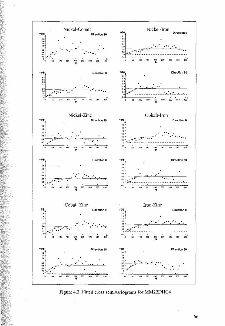
YlltO

'' '0 ,., '' ' . .

. .

Nickel-Cobalt

. . Direction 90

. . . . 100 150 200 250 300 350 400

I~

'0

'' ''

Direction 0

'~~b~ 1 ••• 0·' c"'r"~·"·~----~·s .. ~c:-c g:.: ::: ••• : . .. . . " .

0 ' ~

'~

'·' ,., '' 0.0

0.0

0.,

0 50 100 150 200 250 000 ow ~

I~

Nickel-Zinc

. . ..

Direction 90

..... 0~-=--~~~~~=--=~~~~ o • a 'w ""' • ooo "" •

, .. '' ,.0

'' 0.0

'~ '0 ,., '·' ' O.o 0.0 OA 0.,

'~ LO , .. " ' o.• 0.0 OA 0., 0

.. "'

--w

...

I"

. .

Direction 0

. . . . . . 100 150 200 250 300 350 400

I~

Cobalt -Zinc Direction 0

. . . . .. ... '"" 'w ""' 'w ""' ow ""' I~

Direction 90

. · ... 100 150 200 250 300 350 400

"

'~ " LO

" '' 0.0

0

, .. '' '' '' '' 0.0 0.0

...

Nickel-Iron Direction 0

.. ...... ..

Direction 90

.. .. 0.,

0 ----------------~~~~-~--~-

Cobalt-Iron YlltO

'' '' '' 0.0 . . . . .

Direction 0

... . . .

"' '"" "" ""' 'w •oo •w ""'

Yl!h()

'' '' ,.,

I.

Direction 90

0.9 •••

O.o 1--__,~~--"'.-'--''-~~------0.0 ...

0 ,._•.!---------------- .. ---·--~--O.s o'--".--,"oo:--:-,w~-~~. co-c,",c---cooo~-c,.,~---'-'•

YOlO

" ,., ,., '' 0.0

0.0 ...

I"

Iron-Zinc

. ... .. Direction 0

. . .... .. . o_~ -·~--------- ---------------

-0.3 0'--:,:--:,:00;:--o,.:o-o-~-:;;--:,o.,;:---;=~-o,.;;;--.,~o· I~

YOlO

'' '' ''

Direction 90

1.2 •• • • •• • •• ~:: r--., 3'---'-__,.~'--c.-'-'"-c:-~---~ 0.3 • • • •

0 --------------------------

-O.s o'--",---,,"oo:--:-"~o-ooo=-c,ce.,:---cooo~-'c""~-.,c'c'o· I"

Figure 4.3: Fitted cross semivariograms for MM22DHC4

66

4.1.2 Cross Validation for Cokriging of Ml\U2DHC4

/One method of assessing the suit~bility of a model is to use cross validation.

This technique allows us to compare estimates calculated from our chosen model

using the specified kriging algorithm with the actual data at each sample location.

The cross validation procedure removes one sample data from the data set, estimates

it using the specified model, replaces it then repeats the procedure for all other

sample data in tum. An analysis of the residuals is then carried out to check for

nonna1ity of the errors, presence of Outliers and suitability of the neighbourhood

parameters.

The cross validation was carried out for all of the variables in this data set

using ordinary cokriging to perfonn the estimation. We present here the results for

nickel, those for cobalt, iron and zinc are presented in Appendix B. There was little

difference in the cross validation results of several various search neighbourhoods

investigated. Figure 4.5 shows the cross validation residual analysis for the search

parameters displayed in Table 4.1 and Figure 4.4. The histogram of residuals appears

roughly nonnally distributed with a few extreme high and low values apparent.

These extreme values are also apparent in both the plots of the true values versus the

fits and the standardised estimates. The location of these values is exhibited in the

base map. These values were veritied and as no justification could be made for their

removal, they were left in the data set. The plot of estimates versus the true values is

reasonably well clustered around the 4SO bisector, once again with some deviations.

Finally the mean error and standardised error variance displayed in Table 4.2 are

sufficiently close to the optimal values of zero and one respectively (Bleines et. al,

2001, p. 126). All other neighbourhood search parameters tested failed to further

improve any of these results. Overall the model appears to have reproduced the

sample (exploration) values successfully for all variables.

67

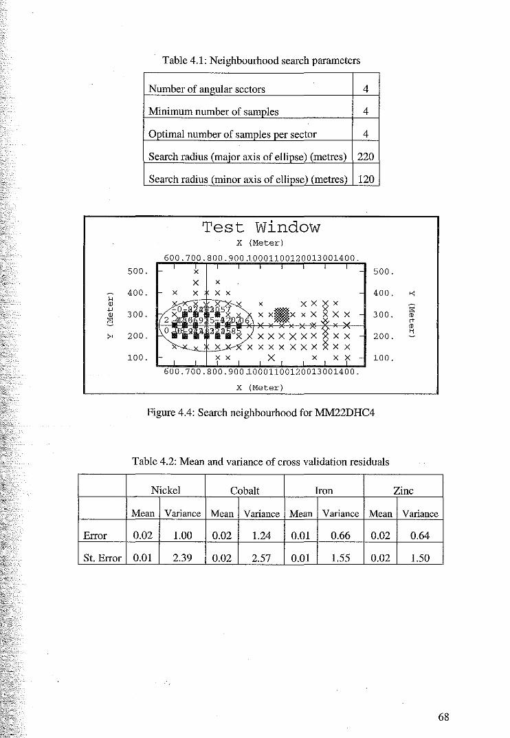
H (])

.j.) (]) ;.:

><

Error

St. Error

Table 4.1: Neighbourhood search parameters

Number of angular sectors 4

Minimum number of samples 4

Optimal number of samples per sector 4

Search radius (major axis of ellipse) (metres) 220

500.

400.

300.

200.

100.

Search radius (minor axis of ellipse) (metres)

Test Window X (Meter)

600.700.800.900l0001100120013001400.

X

X X

X X X X

X X X X X

600.700.800.900l0001100120013001400.

X (Meter)

120

500.

400.

300.

200.

100.

Figure 4.4: Search neighbourhood for MM22DHC4

Table 4.2: Mean and variance of cross validation residuals

Nickel Cobalt Iron

Mean Variance Mean Variance Mean Variance Mean

0.02 1.00 O.D2 1.24 0.01 0.66 0.02

0.01 2.39 0.02 2.57 0.01 1.55 0.02

>-<:

:;:: I]) rt I])

"

Zinc

Variance

0.64

1.50

68

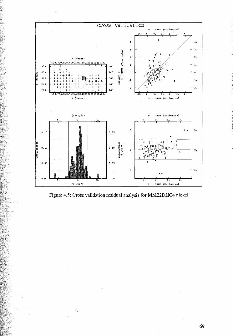
500.

400.

300.

200.

100.

0.15

• • ·o u 0.10 " • il • u •

0. 05

0.00

Cross Validation

X (Meter)

600 700.800 900 ~0001100120013001400

+ + + I + +-t r++•+ ' -t l-t+ 11-t++l>l++lltlh't-i •+ + f t I + f I + + + -~.-+ + !' ~ • 0 t f I ++++++t++++ l-+ ++tll-tl-f-tl++!l +-t

·1-+ + + +t 600.700 800.900 ~0001100120013001400.

X (Meter)

{Z*-Z) IS*

(Z*-Z) /S*

4.

3.

2.

500. 1.

400. 0.

300. -1.

200.

-2. 100.

5. 0.15

" "' ow 0.10 ~ ~ . " 0.

' ' u • e-" . -•

0. 05

-5.

0. 00

Z* : STNI (Estimates)

-2. -1. 0. 1. 2. 3.

•

++ + •

•

-2. -1. 0. 1. 2. 3.

Z* : STNI (Estimates)

Z* : STNI (Estimates)

-1 0

• 1- I I i+ I +

... -i"i'A:i':lt>~~"'~ t ' I •1- ,:'.11-'! ~ '"f + + +'t'lt,_l.l"'N+ +

+f_ ''tt-t+ + +4" I ·t+- .:,·+ + . . . +

•

• • -1. 0. 1. 2.

Z* STNI (Estimates)

4.

4.

• •

Figure 4.5: Cross validation residual analysis for MM22DHC4 nickel

4.

3.

2.

1.

0.

-1.

-2.

5.

0 •

-5.

69

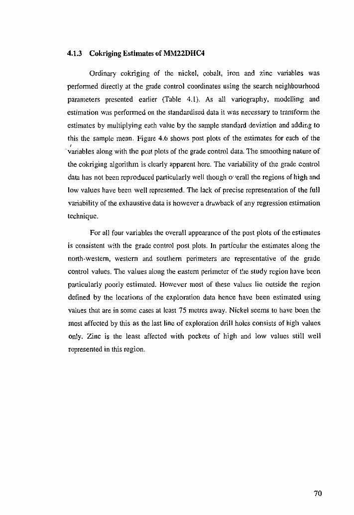
4.1.3 Cokriging Estimates of MM22DHC4

Ordinary cokriging of the nickel, cobalt, iron and zinc variables was

performed directly at the grade control coordinates using the search neighbourhood

parameters presented earlier (Table 4.1). As all vatiography, modelling and

estimation was performed on the standardised data it was necessary to transform the

estimates by multiplying eaGh value by the sample standard devir~tion and addir,g to

this the sample mean. Figure 4.6 shows post plots of the estimates for each of the ' ·variables along with the post plots of the grade control data. The smoothing nature of

the cokriging algorithm is clearly apparent here. The variability of the grade control

data has not been reproduced particularly well though o· 'era\1 the regions of high and

low values have been well represented. The lack of precise representation of the full

variability of the exhaustive data is however a drawback of any regression estimation

technique.

For all four variables the overall appearance of the post plots of the estimates

is consistent with the grade control post plots. In particular the estimates along the

north-western, western and southern perimeters arc representative of the grade

control values. The values along the eastern perimeter of t1,Ic study region have been

particularly poorly estimated. However most of these values lie outside the region

defined by the locations of the exploration data hence have been estimated using

values that are in some cases at least 75 metres away. Nickel seems to have been the

most affected by this as the last line of exploration drill hole!: consists of high values

only. Zinc is the least affected with pockets of high and low values still well

f4!presented in this region.

70

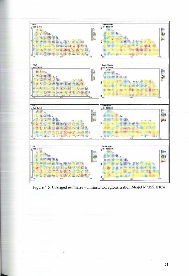
Nlcktl ~ Cradt Co~ol

... 1480

. . . . . . .. ~· ~ · .. . :~~:~~ j ::\1~1::

1

.. ··~ ·~ ·~ ·­·­""

I" ~-·-­·~-...... ~·­,,._ ~·-

Cobalt Estimates

~riC=M~·M~~~~~---------------------------------,

• I'

1

.. '""' "~

tt.ato

-~·

1

.. 0.110 ·­"" ·~ .... ·­.... ·-

1~-'*·* ·-­:·~­,., .. ,. .... ··­~""'

Figure 4.6: Cokriged estimates - Intrinsic Coregionalisation Model MM22DHC4

71

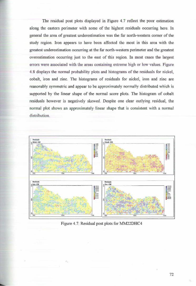
The residual post plots displayed in Figure 4.7 reflect the poor estimation

along the eastern perimeter with some of the highest residuals occurring here. In

general the area of greatest underestimation was the far north-western corner of the

study region. Iron appears to have been affected the most in this area with the

greatest underestimation occurring at the far north-western perimeter and the greatest

overestimation occurring just to the east of this region. In most cases the largest

errors were associated with the areas containing extreme high or low values. Figure

4.8 displays the normal probability plots and histograms of the residuals for nickel,

cobalt, iron and zinc. The histograms of residuals for nickel, iron and zinc are

reasonably symmetric and appear to be approximately normally distributed which is

supported by the linear shape of the normal score plots. The histogram of cobalt

residuals however is negatively skewed. Despite one clear outlying residual, the

normal plot shows an approximately· linear shape that is consistent with a normal

distribution.

Rtslduab ~Nt:kti· ICM

r _,,.. .,., ~ ...

~!..o

·= 11«0

~=

1

--~- ' ~-.. ·~"" ~­.... --

Residual a

~ Cobalt ·~CM

~

Residuals

~ Zinc · ICM

Figure 4.7: Residual post plots for MM22DHC4

..

r 4 -_, .. 4 ... _,,.. . .., .. ... "'"

14~--UlOOOO ·1~.w\l

•U)­.. , _ 09= ·=­--

72

250 20

200

"' '" 10 u !50 0: " " .,

" 100 ... 0 .,.. " " .t 00:

-10 50

0 -20 0

Residual Nickel Normal Score

2 350 0

300 I

"' 250

'" 0 u 0: 200 " -I "

., " !50 ... .,..

" -2 " 100 00: .t 50 -3

0 -4 • -4

Residual Cobalt Normal Score

250 500 • 200

"' u !50 '" 0:

" " " ., 0 .,.. 100 ~

"' " .t 50 00:

0 -500 0

5 0 Residual Iron N annal Score

300 3000 0

"' 200 2000

u 1000 0: '" " " 0 "

., .,.. 100 ~ -1000 " " .t 00: -2000

0 -3000 -4000

00

3000 Residual Zinc Normal Score

Figure 4.8: Residual histograms and normal probability plots for MM22DHC4

73

4.2 VARIOGRAPHY AND COKRIGING OF MM22DTOP4

4.2.1 Variography and the Linear Model of Coregionalisation

As the variables in the MM22DTOP4 data set arc not intrinsically correlated

it is necessary for us to jointly model the direct and cross semivariograms and build a

linear model of corcgionalisation. Goovaerts (1997, p. 114) identifies some practical

guidelines for selecting the basic structures in a linear model of coregionalisation.

These include that every basic structure incorporated in the cross semi varia gram

model 11_-fh) must be present in both direct semivariogram models }1;(h) and Jt(h).

Furthermore if a basic structure is not present on a direct semivariogram model it

cannot be incorporated on any cross semivariogram model involving this variable.

However it is not necessary for a cross semivariogr:im model Yu(h) to include every

structure that appears in both direct semivariogram models J1;(h) and i1J(h).

The procedure used for constructing our linear model of coregionalisation

was to model the direct semivariograms for each of the five variables then use these

basic structures to obtain the best possible fit for the cross semivariograms. In

addition to the direct and cross variograrn surfaces for nickel, cobalt and iron

displayed previously in Figure 4.1 those for magnesium are displayed in Figure 4.9.

The direct surface for magnesium is isotropic as is the surface for iron-magnesium.

i'-li£:\,·1·rr,agnesium and cobalt·magnesiurn are anisotropic with the direction of

maxhP·Fo continuity being east-west.

74

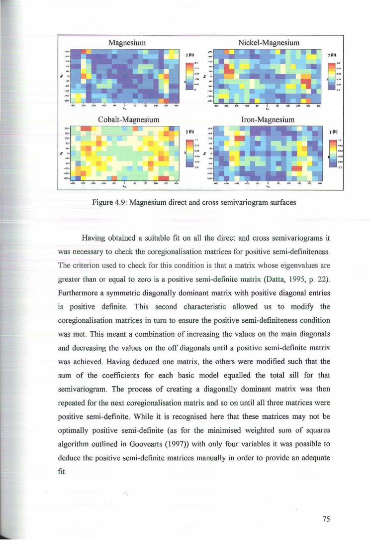
Magnesium y(h)

0: ... ... ... 0

....

Cobalt-Magnesium

Nickel-Magnesium

r •

Iron-Magnesium ~------ -----

., (h)

0·~ ., . .. . ... . .. ~·

y (h) y(h) ,,.

u on .. .r • :: r

~ .. . .. -tlD

0 .. ..... ... . .. . ... ~·

.. - ... ... ...

Figure 4.9: Magnesium direct and cross semivariogram surfaces

Having obtained a suitable fit on all the direct and cross semivariograms it

was necessary to check the coregionalisation matrices for positive semi-definiteness.

The criterion used to check for this condition is that a matrix whose eigenvalues are

greater than or equal to zero is a positive semi-definite matrix (Datta, 1995, p. 22).

Furthermore a symmetric diagonally dominant matrix with positive diagonal entries

is positive definite. This second characteristic allowed us to modify the

coregionalisation matrices in tum to ensure the positive semi-definiteness condition

was met. This meant a combination of increasing the values on the main diagonals

and decreasing the values on the off diagonals until a positive semi-definite matrix

was achieved. Having deduced one matrix, the others were modified such that the

sum of the coefficients for each basic model equalled the total sill for that

semivariogram. The process of creating a diagonally dominant matrix was then

repeated for the next coregionalisation matrix and so on until all three matrices were

positive semi-definite. While it is recognised here that these matrices may not be

optimally positive semi-definite (as for the minimised weighted sum of squares

algorithm outlined in Goovearts (1997)) with only four variables it was possible to

deduce the positive semi-definite matrices manually in order to provide an adequate

fit.

75

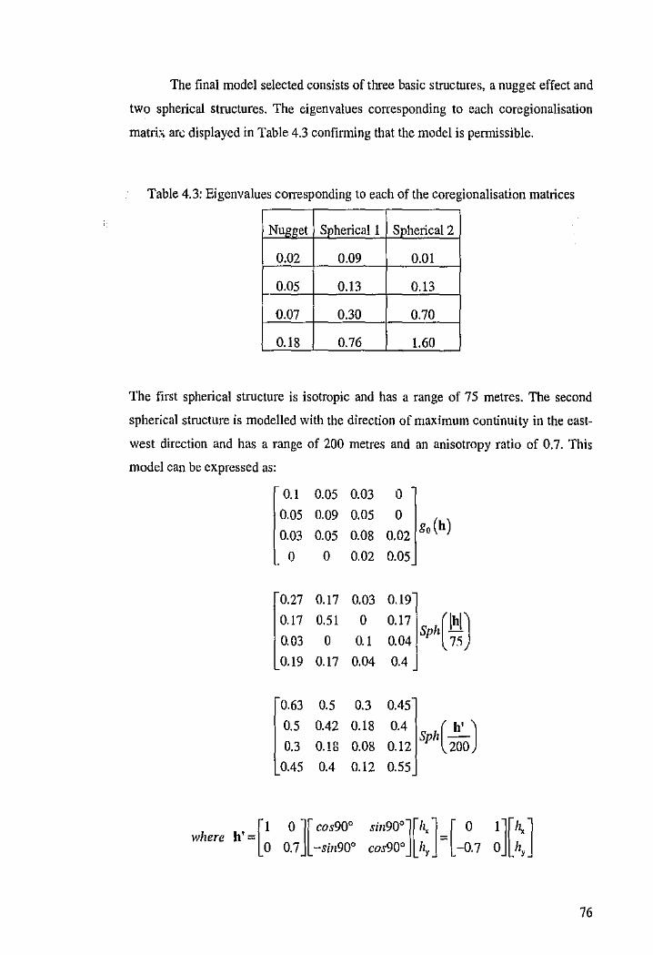
The final model selected consists of three basic structures, a nugget effect and

two spherical structures. The eigenvalues corresponding to each coregionalisation

matri:.> ar~ displayed in Table 4.3 confinning that the model is permissible.

Table 4.3: Eigenvalues corresponding to each of the coregionalisation matrices

Nue.et Svhericall Svherical2

0.02 0.09 O.oi

0.05 0.13 0.13

0.07 0.30 0.70

0.18 0.76 1.60

The first spherical structure is isotropic and has a range of 75 metres. The second

spherical structure is modelled with the direction of maximum continuity in the east-

west direction and has a range of 200 metres and an anisotropy ratio of 0.7. This

model can be expressed as:

0.1 0.05 0.03 0

0.05 0.09 0.05 0 g, (b)

0.03 0.05 0.08 0.02

0 0 0.02 0.05

0.27 0.17 0.03 0.19

0.17 0.51 0 0.17 Sph(ihi) 0.03 0 0.1 0.04 75

0.19 0.17 0.04 0.4

0.63 0.5 0.3 0.45

0.5 0.42 0.18 0.4 Sph( ~) 0.3 0.!8 0.08 0.12 200

0.45 0.4 0.12 0.55

where h'= = [I 0 ][ cos90° sin90°]["'] [ 0 ']["'] 0 0.7 -sin90° cos90° hy --Q.7 0 hy

76

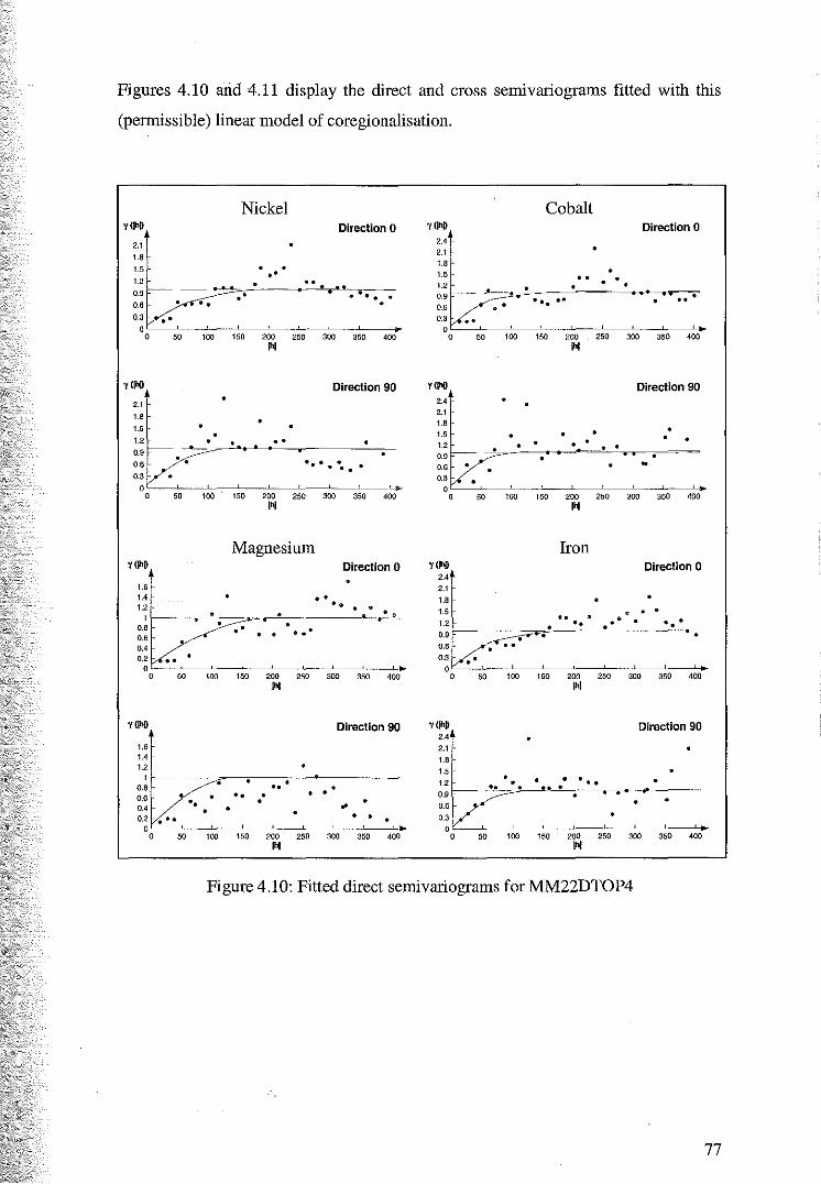
Figures 4.10 and 4.11 display the direct and cross semivariograms fitted with this

(permissible) linear model of coregionalisation.

Nickel Cobalt y(lhD Direction 0 Ylihll Direction 0

2.1 2.4

1.6 2.1

1.5 1.6

•• 1.5 .. 1.2 .. 1.2 --~ .... .. . ... .. .. .. 50 100 150 200 250 300 350 400 50 100 150 200 250 300 350 400

lhl lhl

yllhll Direction 90 Yllhll Direction 90

2.1 2.4

1.6 2.1

1.5 1.6 1.0 • 1.2 . .. 1.2 ~ .... . -..

--.~ ------'--~

50 100 150 200 250 300 350 400 50 100 150 200 250 300 350 400 lhl I~

Magnesium Iron YI~D Direction o Ylihll Direction 0

2.4 1.6 2.1 1.4 .. 1.6 1.2 .. • • ~ 1.5 .. •• ~ 1.2 .. . . . . . . . . . •

50 100 150 200 250 300 350 400 50 100 150 200 250 300 350 400

~I ~I

Yllhll Direction 90 Y(lhD Direction 90 2.4

1.6 2.1 1.4 1.6 1.2 1.5

1 1.2

. • . . ..

0.6 .. .. . • 0.6 .. . • •• . 0.4

, 0.2 ...

0 0 50 100 150 200 250 300 350 400 50 100 150 200 250 300 350 400

lhl lhl

Figure 4.10: Fitted direct semivariograms for MM22DTOP4

77

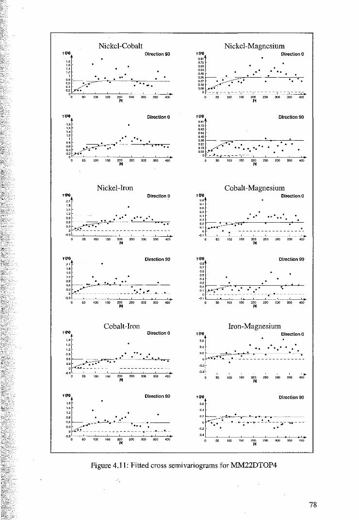
Yll~

'' '·' '' '·' '

'' '' '' ''

Yilt(! , ,, '' '' '' '' ''

"

Nickel-Cobalt Direction 90

.. . . .. ~

'"' '"' roo "" .,

'"' ~0

I~

Direction 0

.. .. ..

\00 150 200 250 300 350 400 I~

Nickel-Iron Direction 0

. .. ..... ~. . . . ..

0 _.__!------ - - - - - - - -------- -- -

~','---:.,c--,".,c---:,".,:---:,c,:--,c,=---:.,cCc-c,".,:-~~:· I~

vu .. , '' '' '' ..

Direction 90

.. . . . 0 ----------------~-~--~----

~.0 L_~OLO -~WLO-~,,~-c,::--c,.,::-~.,::-~,~OO::--.,.,c4-l~

Cobalt-Iron ,a,. Direction 0

'' " .., '' . ... ''

. '·' . . . . .. .

~------------------------~.,

0 "' '"' '"" = "" .,

"" ""' I~

ra,. Direction 90

'' '' '' '·' .. . '·' '·' ...

__. __ '!.._-

~' 0 "' '"' '"" "'' '"' = '"" "" I~

Y(ll(l

0.81 0.72

'·" 0.64

'·"

y(ll(l

'·' 0]

'·' '·' '' '·' 0.2 -

. .

Nickel-Magnesium

. .. . . Direction 0

.. · .

----------------------~

50 100 150 200 250 300 350 400

I"

Direction 90

. . . . .. . . . . . -~------------------------

100 150 200 250 300 350 400

I~

Cobalt-Magnesium Direction 0

.· . . . .

0 ----·--.--------------------

~.' "--~,L,--,",c,-c,~.,:---:,.,c0:--,c00c---:000cCc-c,".,:-~.,.,~ I~

'·' '·' '·' ~'

Direction 90

Iron-Magnesium Direction 0

.. - _._ ~--- !_ -------------------

~ 'L_---cc----c:c----::c---::c---::c---::c---::c----:~ 50 100 150 200 250 300 350 400

I~

Yllhf) Direction 90

''

~.,

~· L_-=--=--;O;--:-;O;---;::;:---;:'cc->;0;:-~~ 50 100 150 200 250 300 350 400

"

Figure 4.11: Fitted cross semivariograms for MM22DTOP4

78

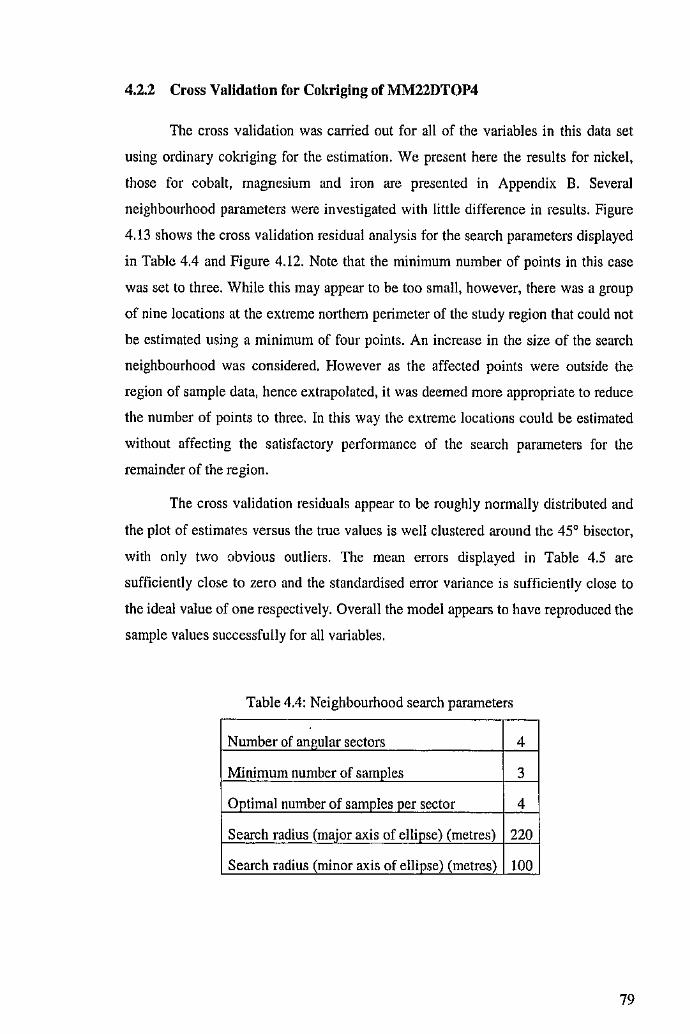
4.2.2 Cross Validation for Cokriging of MM22DTOP4

The cross validation was carried out for all of the variables in this data set

using ordinary cokriging for the estimation. We present here the results for nickel,

those for cobalt, magnesium and iron are presented in Appendix B. Several

neighbourhood parameters were investigated with little difference in results. Figure

4.13 shows the cross validation residual analysis for the search parameters displayed

in Table 4.4 and Figure 4.12. Note that the minimum number of points in this case

was set to three. While this may appear to be too small, however, there was a group

of nine locations at the extreme northem perimeter of the study region that could not

be estimated using a minimum of four points. An increase in the size of the search

neighbourhood was considered. However as the affected points were outside the

region of sample data, hence extrapolated, it was deemed more appropriate to reduce

the number of points to three. In this way the extreme locations could be estimated

without affecting the satisfactory perfonnance of the search parameters for the

remainder of the region.

The cross validation residuals appear to be roughly nonnally distributed and

the plot of estimates versus the true values is well clustered around the 45° bisector,

with only two obvious outliers. The mean errors displayed in Table 4.5 are

sufficiently close to zero and the standardised error variance is sufficiently close to

the ideal value of one respectively. Overall the model appears to have reproduced the

sample values successfully for all variables.

Table 4.4: Neighbourhood search parameters

Number of angular sectors 4

Minimum number of samples 3

Ootimal number of samples per sector 4

Search radius (maior axis of elliose) (metres) 220

Search radius (minor axis of elliose) (metres) 100

79

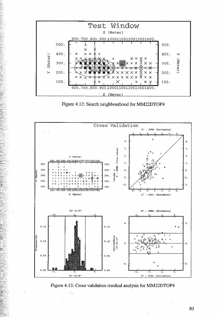
H

"' .w

"' ~ ><

500.

400.

300.

" 200.

100.

0.15

" l " 0.10 ' • g • " •

0. 05

0. 00

Test Window X (Meter)

600.700.800.900~0001100120013001400.

500. X 500. X

400. X X X X 400. XX 9 X

xlmx 300. X X X X X 300.

200. XX XXX X 200. X

xxxx * X X 100. X X X X 100.

600.700.800.900~0001100120013001400.

X

Figure 4.12: Search neighbourhood for MM22DTOP4

Cross Validation

X (Meter)

600 000 800 900 ~0001100120013001400.

+ • + I + + +

+++++•+ • ++f+ +·+++++·!·1·++,+++ :++ ++++++++++- ++-f •• ++++++++++++++ ++ + + ++++++ +++··!··++""'+ +

+ + + + t 600.700.800 900 l000110012 0013 001400.

X (Meter)

(Z*-Z) /S*

{Z*-Z)/S*

' ' e

' ' ' 0 500.

t H

400. "~ 300.

i .. ~-' 200. ~

100.

0.15

~ 0.10 ~

0.05

! e·

' •

,. STNI (Estimates)

-2. -1. 0. 1. 2. 3.

4.

3.

+'+ I· 2.

1. +

0.

-1. • -2.

-2. -1. 0. 1. 2. 3.

,. ' 'TN' {Estimates)

Z* STNI (Estimates)

-1. 0 1

5.

0 •

-5. • •

1. 0. 1.

Z* ; STNI (Estimates)

><

:;:: <D rt <D ~

4.

4.

• •

2.

Figure 4.13: Cross validation residual analysis for MM22DTOP4

4.

3.

2.

1.

0.

-1.

-2.

5.

-5 .

80

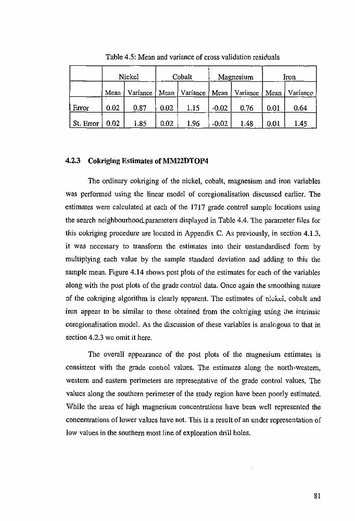
Table 4.5: Mean and variance of cross validation residuals

Nickel Cobalt Ma esium Iron

Mean Variance Mean Variance Mean Variance Mean Variancl~

Error 0.02 0.87 0.02 1.15 -0.02 0.76 0.01 0.64

St. Error 0.02 1.85 0.02 1.96 -0.02 1.48 O.DI 1.45

4.2.3 Co kriging Estimates of MM22DTOP4

The ordinary cokriging of the nickel, cobalt, magnesium and iron variables

was perfonned using the linear model of coregionalisation discussed earlier. The

estimates were calculated at each of the 1717 grade control sample locations using

the search neighbourhood.. parameters displayed in Table 4.4. The parameter files for

this cokriging procedure are located in Appendix C. As previously, in section 4.1.3,

it was necessary to transform the estimates into their unstandardised form by

multiplying each value by the sample standard deviation and adding to this the

sample mean. Figure 4.14 shows post plots of the estimates for each of the variables

along with the post plots of the grade control data. Once again the smoothing nature

of the cokriging algorithm is clearly apparent. The estimates of n:...:k.d, cob<llt and

iron appear to be similar to those obtained from the cokriging using ~he intrinsic

coregionalisation model. As the discussion of these variables is analogous to that in

section 4.2.3 we omit it here.

The overall appearance of the post plots of the magnesium estimates is

consistent with the grade contwl values. The estimates along the north~western,

western and eastern perimeters are representative of the grade control values. The

values along the southern perimeter of the study region have been poorly estimated.

While the areas of high magnesium concentrations have been well represented the

concentrations of lower values have not. This is a result of an under representation of

low values in the southern most line of exploration drill holes.

81

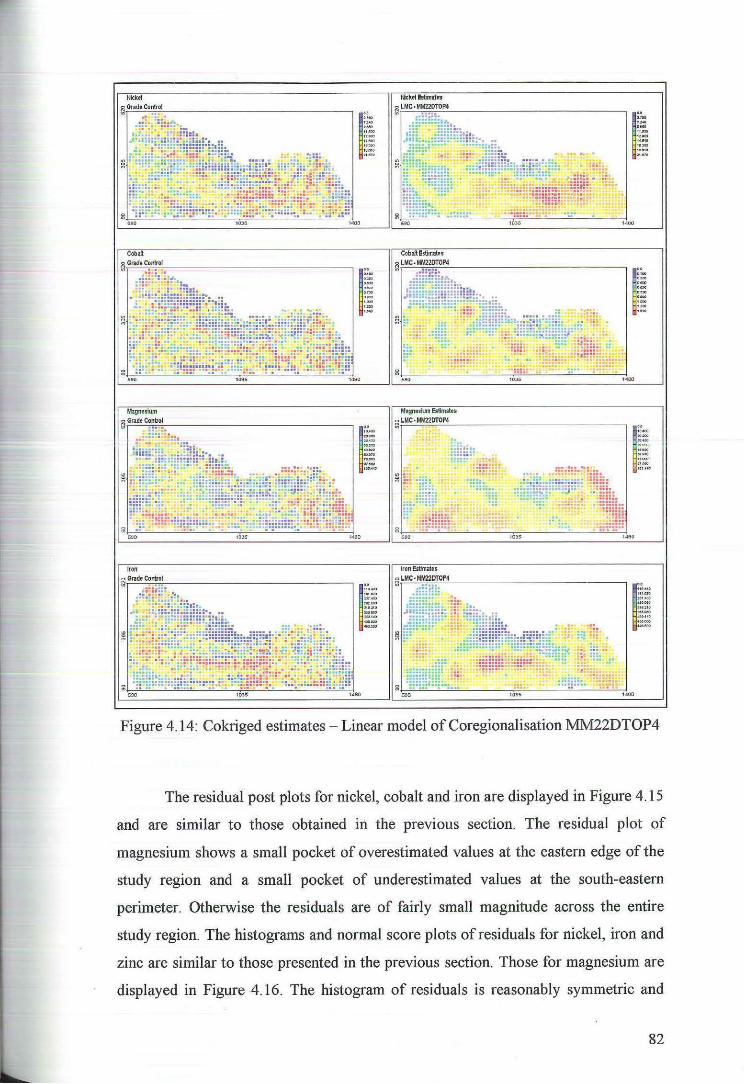
Nicktl

~GradeCo~ol

Magnesium o Grade Control

Iron a Grade Control (;j • • •

I" '"" "~ ,.., ..... ·­""" ···­,.~,0 ·-

1

... ·­·~

"" ·-

Magnesium Estimab:s:

~ LMC • MM22DTOP4

Iron Estimates

~ LMC • MM22DT0~4

....

I., .. ,_ ... ... ·­·~HOI

1400

Figure 4.14: Cokriged estimates - Linear model of Coregionalisation MM22DTOP4

The residual post plots for nickel, cobalt and iron are displayed in Figure 4.15

and are similar to those obtained in the previous section. The residual plot of

magnesium shows a small pocket of overestimated values at the eastern edge of the

study region and a small pocket of underestimated values at the south-eastern

perimeter. Otherwise the residuals are of fairly small magnitude across the entire

study region. The histograms and normal score plots of residuals for nickel, iron and

zinc are similar to those presented in the previous section. Those for magnesium are

displayed in Figure 4.16. The histogram of residuals is reasonably symmetric and

82

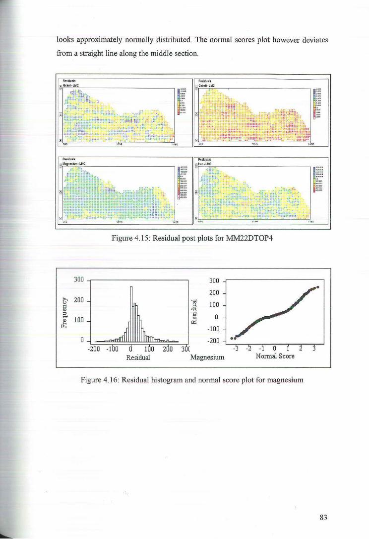
looks approximately normally distributed. The normal scores plot however deviates

from a straight line along the middle section.

Res idual' 1jl Jfckti•LMC

Residuals

~ Magnesium : ~~C

300

!>.. (.) 200 Q <1.1 ;::l 0" 100 11)

~

0

Ruiduab

~rc'=b~~·L=M~c --~--------------------.

1 ... . ..., , .. ..... ·•= .... ... ·~ ·­·­'"" ·­•• ••il

1

=-·l~b)(l

... ~ .. •w..,

-­~--­'"""

:< .: ...

Figure 4.15: Residual post plots for :MJ\122DTOP4

300

200 (0

100 ;::l "t3 .... "' 0 11)

0::: -100

-200 •

Residual Magnesium Normal Score

1

_ ... -"· •x:e.oct ... 00 • . .... '""" s.:,)~ -­==

•

Figure 4. 16: Residual histogram and normal score plot for magnesium

..

83

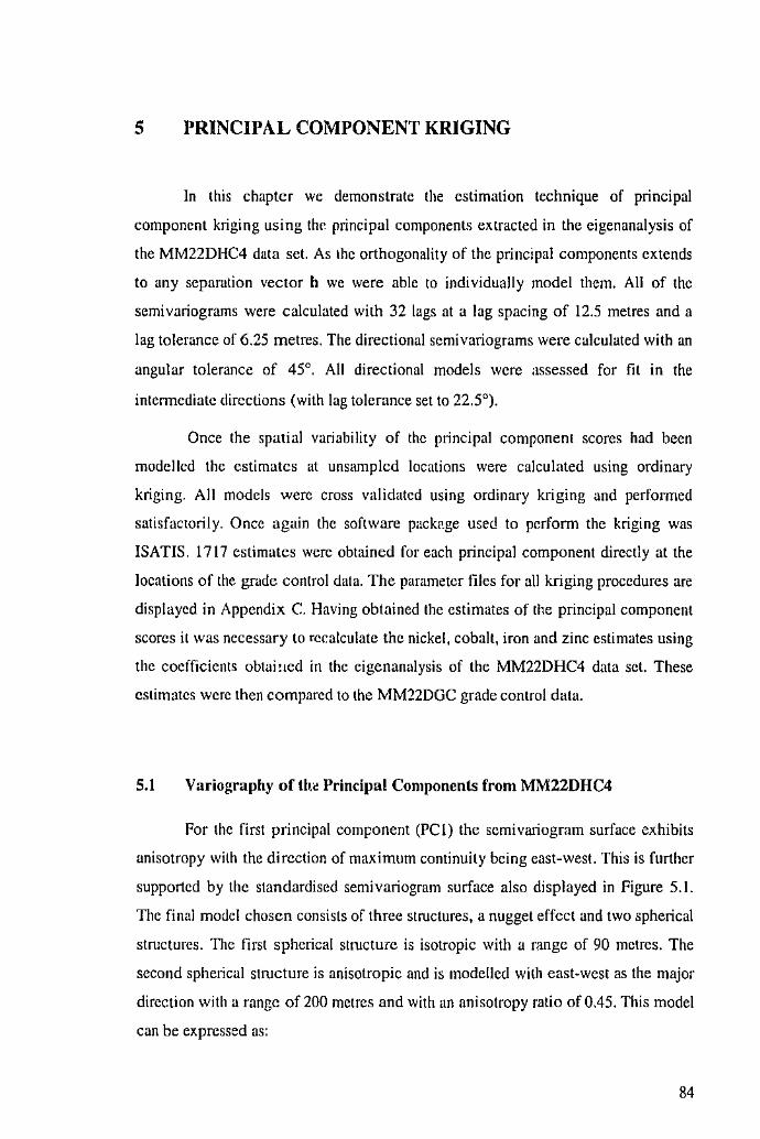
5 PRINCIPAL COMPONENT KRIGING

In this chapter we demonstrate the estimation technique of principal

component kriging using thr. principal components extracted in the eigenanalysis of

the MM22DHC4 data set. As the orthogonality of the principal components extends

to any separation vector h we were able to individually model them. All of the

semivariograms were calculated with 32 lags at a lag spacing of 12.5 metres and a

lag tolerance of 6.25 metres. The directional semivariograms were calculated with an

angular tolerance of 45°. All directional models were assessed for fit in the

intenncdiate directions (with lag tolerance set to 22.5°).

Once the spatial variability of the principal component scores had been

modelled the estimates at unsamplcd locations were calculated using ordinary

kriging. All models were cross validated using ordinary kriging and perfonned

satisfactorily. Once again the software pack<lge used to perform the kriging was

ISATIS. 1717 estimates were obtained for each principal component directly at the

locations of the grade control data. The parameter files for all kriging procedures are

displayed in Appendix C. Having obtained the estimates of the principal component

scores it was necessary to recalculate the nickel, cobalt, iron and zinc estimates using

the coefficients obtai!Jed in the eigenanalysis of the MM22DHC4 data set. These

estimates were then compared to the MM22DGC grade control data.

5.1 Variography of th.l! Principal Components from MM22DHC4

For the first principal component (PCl) the semivariogram surface exhibits

anisotropy with the direction of maximum continuity being east-west. This is further

supported by the standardised semivariogram surface also displayed in Figure 5.1.

The final model chosen consists of three structures, a nugget effect and two spherical

structures. The first spherical structure is isotropic with a range of 90 metres. The

second spherical structure is anisotropic and is modelled with cast-west as the major

direction with a range of 200 metres and with an anisotropy ratio of 0.45. This model

can be expressed as:

84

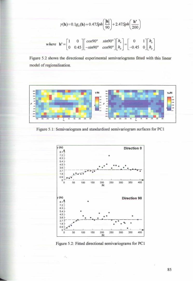
y(h) = 0.1g 0 (h)+ 0.4 7 Sph (M) + 2.4 7 Sph (~) 90 200

Figure 5.2 shows the directional experimental semivariograms fitted with this linear

model of regionalisation.

Y(hl Ys (hl

0:, u ... .l" • "'

~· ... IJ ... .., .. -

..... .. Figure 5.1: Semivariogram and standardised semivariogram surfaces for PC 1

~ (lhl) Direction 0 8.1 7.2 • 6.3 5 .4 4.5 •

• • • • ••• • 3.6 • • • _...__.

'''~·· . .

1.8 • • • •

0 .9 •• 0

0 50 100 150 200 250 300 350 400 I hi

y (lhl) Direction 90 8.1 • 7.2 6.3 5.4 • • • 4.5 • • • • 3.6 • • •

''V - • • 1.8 ... •

• • 0.9 • 0

0 50 100 150 200 250 300 350 400 I hi

Figure 5.2: Fitted directional semivariograms for PC1

85

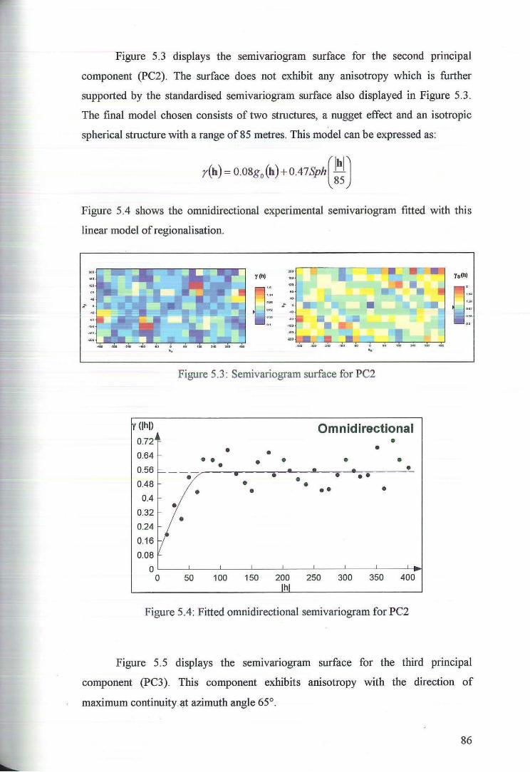
Figure 5.3 displays the semtvanogram surface for the second principal

component (PC2). The surface does not exhibit any anisotropy which is further

supported by the standardised semivariogram surface also displayed in Figure 5.3.

The final model chosen consists of two structures, a nugget effect and an isotropic

spherical structure with a range of85 metres. This model can be expressed as:

r(b)= 0.08g0 (h)+047Sphn;J

Figure 5.4 shows the omnidirectional experimental semivariogram fitted with this

linear model of regionalisation.

..

y(h)

0::: . .. .r- 0 .. , ·~ •..

- - - - 0 - - - - -.. Figure 5.3: Semivariogram surface for PC2

~ (lhl) Omnidirectional 0.72 •

• • 0.64 - • • • • • • • 0.56 • ... • - • t---- ... • • •• • • 0.48 • • • • •• •

0.4 • 0.32 •

0.24

0.16

0.08

0 . 0 50 100 150 200 250 300 350 400

I hi

Figure 5.4: Fitted omnidirectional semivariogram for PC2

Ys(h)

Figure 5. 5 displays the semivariogram surface for the third principal

component (PC3). This component exhibits anisotropy with the direction of

maximum continuity at azimuth angle 65°.

86

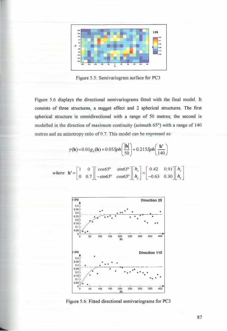
y(h)

DOG

00 .... .... 0 .. ...

Figure 5.5: Semivariogram surface for PC3

Figure 5.6 displays the directional semivariograms fitted with the final model. It

consists of three structures, a nugget effect and 2 spherical structures. The first

spherical structure is omnidirectional with a range of 50 metres; the second is

modelled in the direction of maximum continuity (azimuth 65°) with a range of 140

metres and an anisotropy ratio of0.7. This model can be expressed as:

r(h) = o. o 1g0 (h)+ o. o5Sph(MJ + o.215Sph(~) 50 140

where h' = [1 0 ][ cos6SO sin65°][hx] = [ 0.42 0.91][hx] 0 0.7 -sin65° cos65° hY -0.63 0.30 hY

lv <lhD Direction 25 0.4

0.35 • •• • • • 0.3 ••• • 0.25 v···.· • • • • 0.2 •

• • 0.15 • •• 0.1

0.05 • 0 0 50 100 150 200 250 300 350 400

lhl

lv (lhD Direction 115 • 0.4

0.35 • • • 0.3 . . . .

0.25 v· • .. • • • 0.2 • . • ••• •

0.15 • . •

0.1 •• • 0.05

0 0 50 100 150 200 250 300 350 400

lhl

Figur~ 5.6: Fitted directional semivariograms for PC3

87

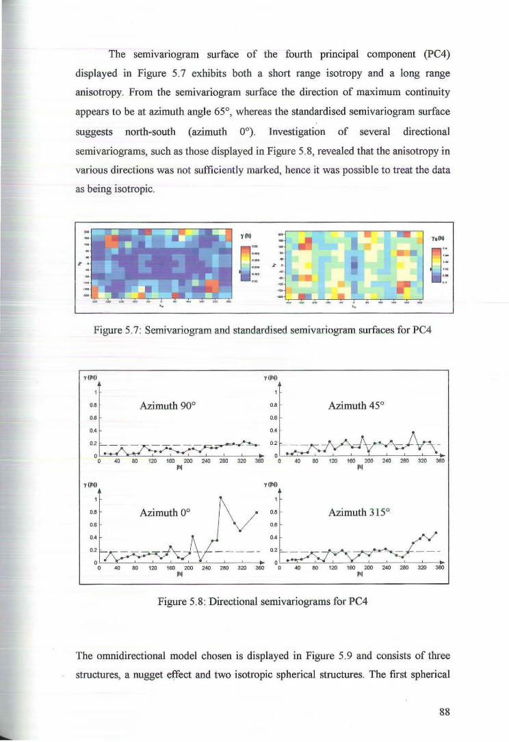
The semivariogram surface of the fourth principal component (PC4)

displayed in Figure 5. 7 exhibits both a short range isotropy and a long range

anisotropy. From the semivariogram surface the direction of maximum continuity

appears to be at azimuth angle 65°, whereas the standardised semivariogram surface

suggests north-south (azimuth 0°). Investigation of several directional

semivariograms, such as those displayed in Figure 5.8, revealed that the anisotropy in

various directions was not sufficiently marked, hence it was possible to treat the data

as being isotropic.

y (h)

0:: ·-·~ ~ D

O.iU ...

Js (h)

Figure 5.7: Semivariogram and standardised semivariogram surfaces for PC4

r <lhll r(lhll

0.8 Azimuth 90° 0.8 Azimuth 45° 0.6 0.6

0.4

0.2

40 80 120 160 200 240 280 320 360 40 80 120 160 200 240 280 320 360 lhl lhl

r<lhll r(lhll

0.8 Azimuth 0° 0.8 Azimuth 315° 0.6 0.6

0.4

0.2

o~~--~-L--L--L~L__L __ ~_.

0 ~ 80 w - 200 ~ ~ ~ 360 40 80 120 160 200 240 280 320 360 !hi lhl

Figure 5.8: Directional semivariograms for PC4

The omnidirectional model chosen is displayed in Figure 5.9 and consists of three

structures, a nugget e:tfect and two isotropic spherical structures. The ftrst spherical

88

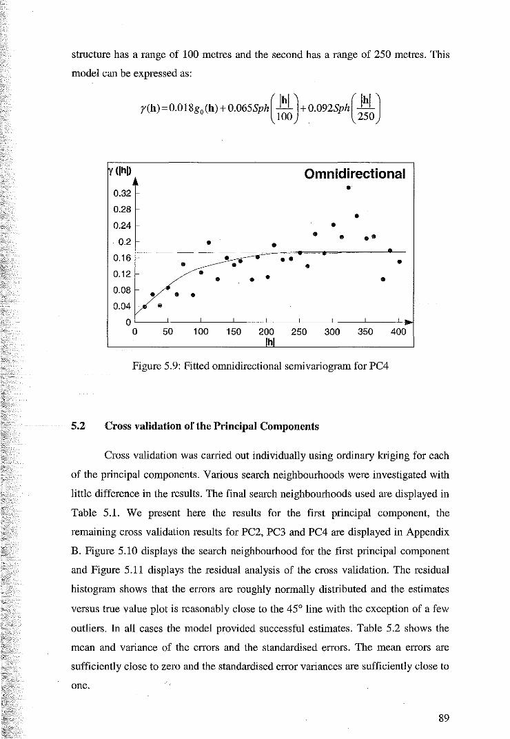
structure has a range of 100 metres and the second has a range of 250 metres. This

model can be expressed as:

y(h) =0.018g0 (h)+ 0.065Sph(11) + 0.092Sph(_M_) 100 250

~ (lhl) Omnidirectional 0.32 • 0.28 • 0.24 • • • • • 0.2 • • '------- • 0.16 • -. • • • •• • • 0.12 • • • • • 0.08- • • • 0.04 g

0 I I I I

0 50 100 150 200 250 300 350 400 I hi

Figure 5.9: Fitted omnidirectional semivariogram for PC4

5.2 Cross validation of the Principal Components

Cross validation was carried out individually using ordinary kriging for each

of the principal components. Various search neighbourhoods were investigated with

little difference in the results. The final search neighbourhoods used are displayed in

Table 5.1. We present here the results for the first principal component, the

remaining cross validation results for PC2, PC3 and PC4 are displayed in Appendix

B. Figure 5.10 displays the search neighbourhood for the first principal component

and Figure 5.11 displays the residual analysis of the cross validation. The residual

histogram shows that the errors are roughly normal! y distributed and the estimates

versus true value plot is reasonably close to the 45° line with the exception of a few

outliers. In all cases the model provided successful estimates. Table 5.2 shows the

mean and variance of the errors and the standardised errors. The mean errors are

sufficiently close to zero and the standardised error variances are sufficiently close to

one.

89

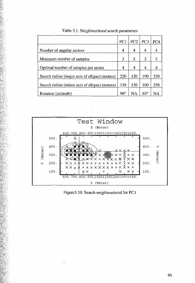
Table 5.1: Neighbourhood search parameters

PC1 PC2 PC3 PC4

Number of angular sectors 4 4 4 4

Minimum number of samples 3 3 3 3

Optimal number of samples per sector 4 4 4 4

Search radius (major axis of ellipse) (metres) 220 120 190 250

Search radius (minor axis of ellipse) (metres) llO 120 100 250

Rotation (azimuth) 90° NA 65° NA

Test Window X (Meter)

600

500. 500.

400. 400. e< H (j)

+' 300. (j)

~ X X 300.

::;:

" rt

" >< 200. 200. >i

100. X 100.

013001400.

X (Meter)

Figure5.10: Search neighbourhood for PC1

90

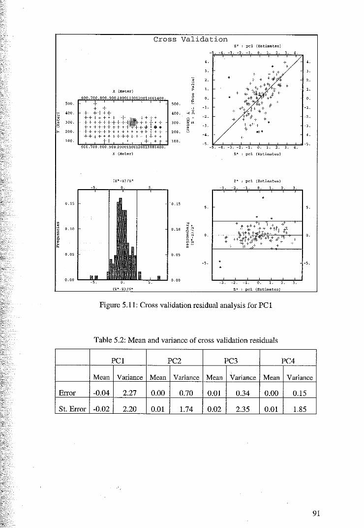
500.

" 400.

• " • "

300.

" 200.

100.

0 .1'5

• • ·K 0.10 u

' • il • u • 0. 05

0. 00

Error

Cross Validation

X {Meter)

600.700. 800.900 .1000110012 0013001400. .,+ + +

+ +++-1· +++++++ -·1- .++++ +++++++++-r - ++··--· + ++++++++++' +++···· ++++-t+++++++-t-+1+-t ++-t+++++++-t++-tt++

H + + j 600.700 800. 900 .10001100120013 001400.

X (Meter)

{Z*-Z)/S*

(Z*-Z) /S*

500.

400.

300 .

200.

100.

. 0.15

0.10

0. 05

0.00

.. 3.

.. "

2. rl

1. • , •

0. " ~ rl -1. u

" " ~~

-2.

-3. " • "--4.

-5.

5.

" K ' • • ~~ • " 0 •

' ' 0 • K· N • -•

-5.

Z* : pel (Estimates)

-5. -4. -3. -2. -1. 0. 1. 2. 3. 4.

•

•

+ +

4 .

3 .

2.

1.

0.

-1.

-2.

-3.

-4.

-5'" _:..._-f, _-_--,3'-. ~-21-.-_+1.--,iO-. ...,, ... _ -2+.-i-3 _ ___,, ....... _ -5.

Z* : pel (Estimates)

,. pel (Estimates)

3. 2. 1. 0. 1. 2. 3.

• 5.

• • + + +++ + + ,. -1~ .

-Jr\-t't+-..it-t ++** -~! * ++-f,yt-+~~-~+4-+ -tlr~·

0. + + it+. -i.l· + -H· + + + -tt-''' ~~+ +

-5.

3. 2. 1. 0. 1. 2. 3.

,. pel (Estimates)

Figure 5.11: Cross validation residual analysis for PCl

Table 5.2: Mean and variance of cross validation residuals

PC1 PC2 PC3 PC4

Mean Variance Mean Variance Mean Variance Mean Variance

-0.04 2.27 0.00 0.70 0.01 0.34 0.00 0.15

St. Error -0.02 2.20 0.01 1.74 0.02 2.35 0.01 1.85

91

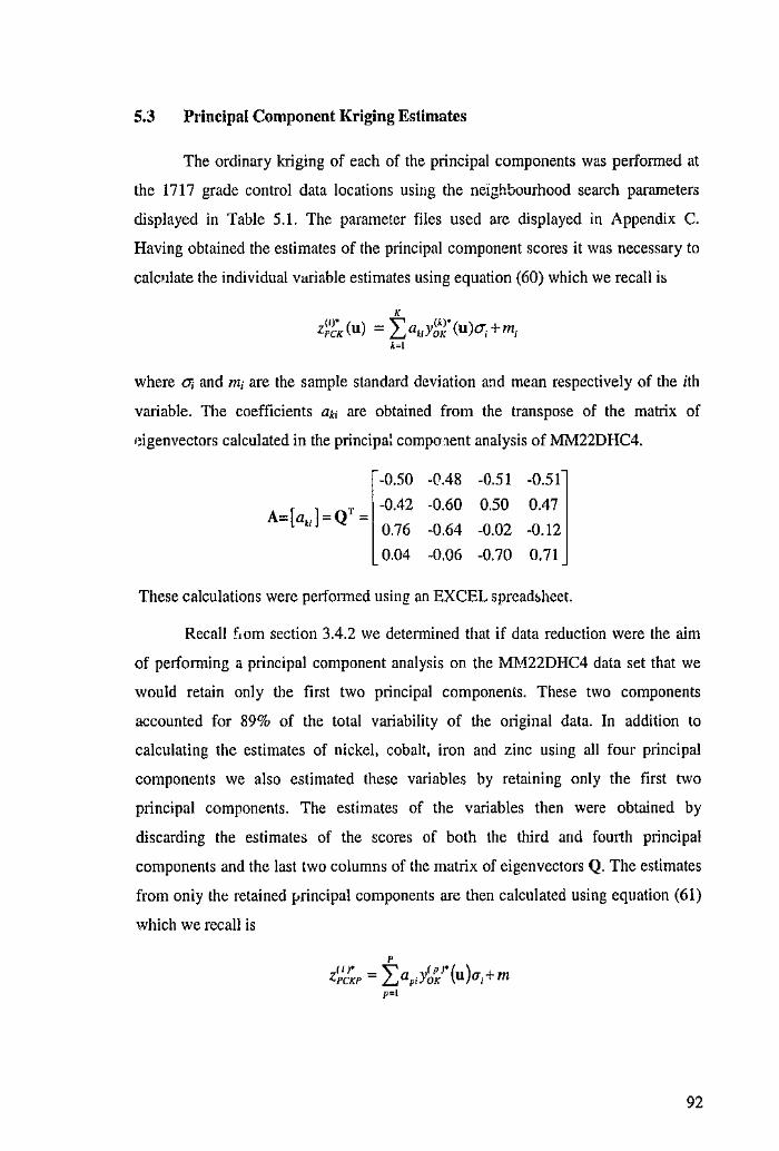
5.3 Principal Component Kriging Estimates

The ordinary kriging of each of the principal components was performed at

the 1717 grade control data locations using the neighbourhood search parameters

displayed in Table 5.1. The parameter files used are displayed in Appendix C.

Having obtained the estimates of the principal component scores it was necessary to

calcnlate the individual variable estimates using equation (60) which we recall is

where Oi and m; are the sample standard deviation and mean respectively of the ith

variable. The coefficients aki are obtained from the transpose of the matrix of

r'igenvectors calculated in the principa: cornpn1ent analysis of !vflv:[22DHC4.

-0.50 -Q.48 -0.51 -0.51

A=(a.,]=Q' = -0.42 -0.60 0.50 0.47

0.76 -0.64 -0.02 -0.12

0.04 -0.06 -0.70 0.71

These calculations were performed using an EXCEL spread~heet.

Recall f1om section 3.4.2 we determined that if data reduction were the aim

of performing a principal component analysis on the W.122DHC4 data set that we

would retain only the first two principal componenls. These two components

accounted for 89% of the total variability of the original data. In addition to

calculating the estimates of nickel, cobalt, iron and zinc using all four principal

components we also estimated these variables by retaining only the first two

principal components. The estimates of the variables then were obtained by

discarding the estimates of the scores of both the third and fourth principal

components and the last two columns of the matrix of eigenvectors Q. The estimates

from oniy the retained {.>rincipal components are then calculated using equation (61)

which we recall is

92

where Ol and mi are the sample standard deviation and mean respectively of the ith

variable and P is the number of principal components retained. The coefficients apt

for the truncated estimates are:

A- a -[ ] [-0.50

p- pi - -0.42 -0.51 -o.51 -0.51] -0.60 0.50 0.47

Figures 5.12 shows thr post plots of the nickel, cobalt, iron and zinc grade

control data and principal component kriging estimates (all four principal

components). Overall the estimates have reproduced the grade control samples well,

once again though the smoothing nature of the kriging process is apparent. The same

areas of over and underestimation are apparent as for the previous kriging methods.

In fact the post plots are almost identical to those we have alrearly seen. Figure 5.13

shows the post plots of the grade control data and the estimates obtained using only

the first two principal components. Clearly the grade control data have been

reasonably well reproduced with very little difference to those estimates obtained

using all four principal components. The histograms and normal score plots for the

residuals from both types of principal component kriging are very similar to those

presented earlier, hence are omitted here. Figures 5.14 and 5.15 display the residual

post plots for both type~: of principal component kriging. Both sets of plots are once

again very similar to those of the other kriging methods.

93

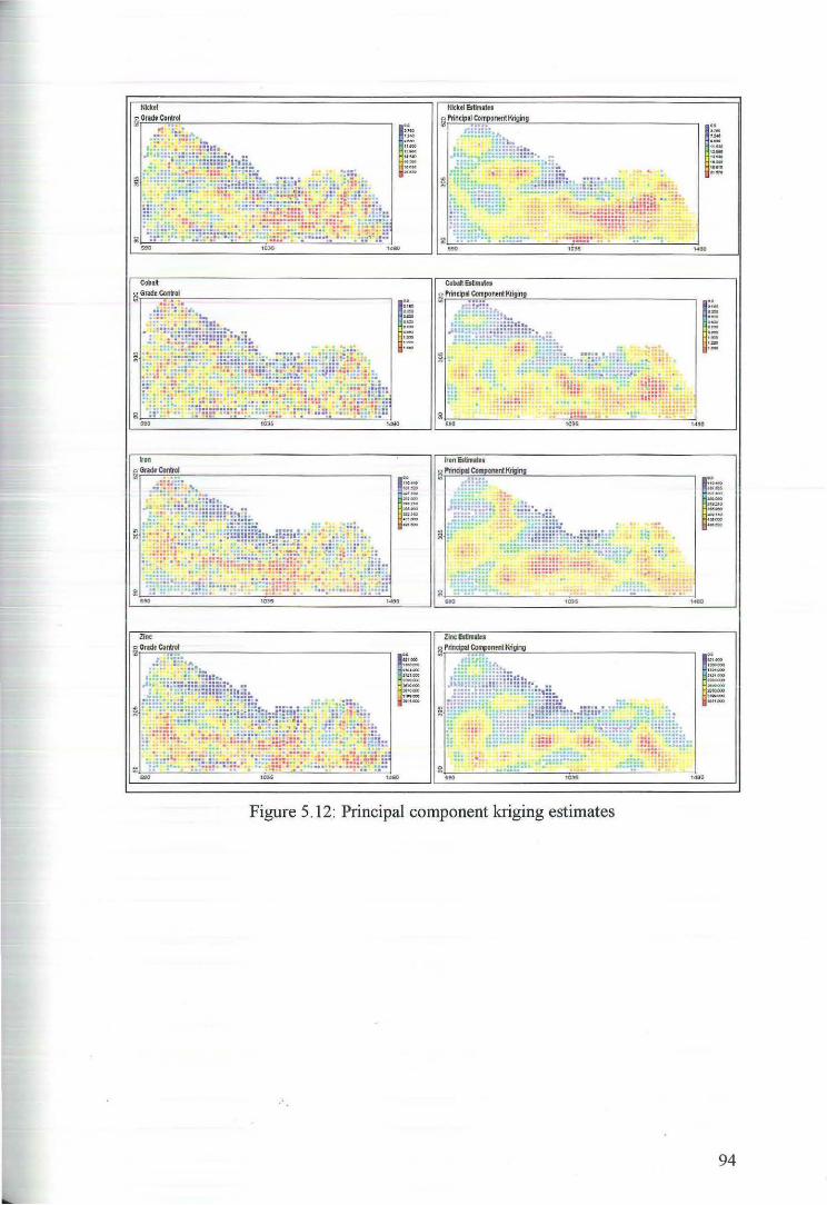
Nick~

g GrtdtCo~ol

Cob all

hn ~ Grade Conbot

·: . . .. :: 'i\ ..

·r!• ...

1

.. .,~ ,,., 11;1» ..... ,._ 1 ....

1~-·­·­·~ ·-

Zlnc;l!slinalts ~ ~rlncipal Compontnt ~glng

Figure 5.12: Principal component kriging estimates

1

.. ·­.... ·­..... ~2 .•

:::: ... " ·-

1

.. .... ... ·­·­·­·­'"" ·­·-

,,._

1

.. ..... ~­-.. , . ...... -·· :::

1~-·-­.... _ ··­----''""" ·-­~ ...

94

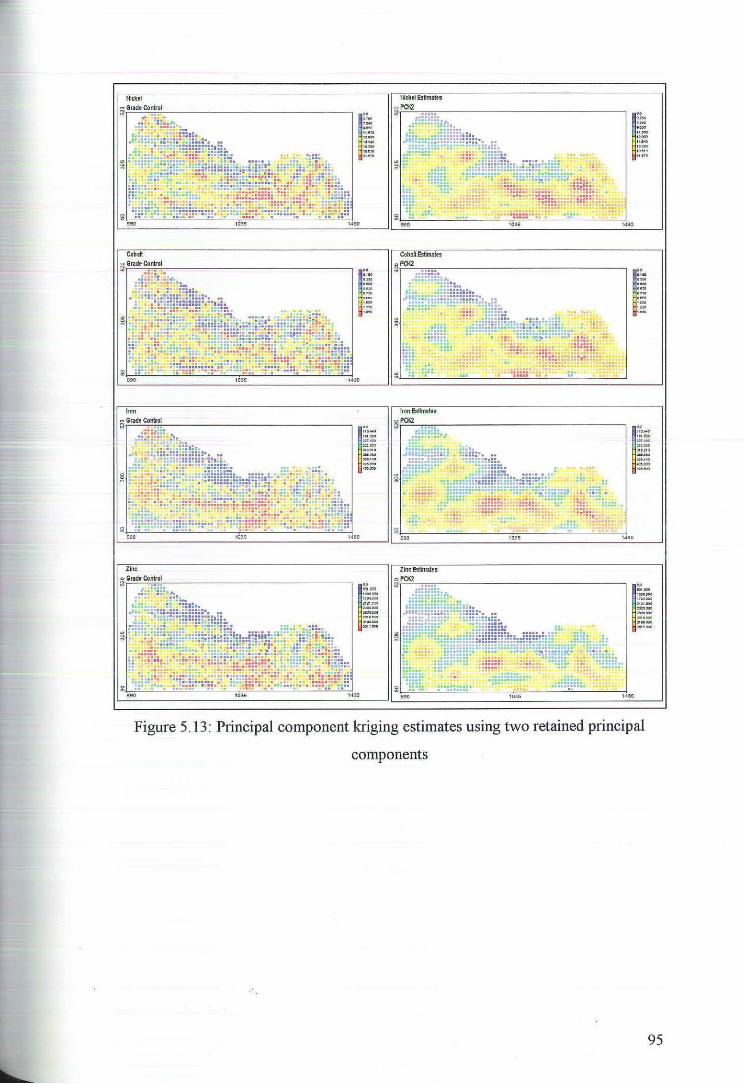
Cobalt

~ Grade C~n~ol

Iron ~ Grade Control

Zinc:

~ Gradt Control

.,;, : ~ : :·· .... . · ·!:-

:::· :::i::~~ni~::· ... ··:::·::::::::·::.::.

::. · .• ;; : .. : · ·~: !; ::::.: ........ .. g • : :=~== :: ;;~:; :·:;Eii1::: i;n;::::i~i~hi ~ ~ :: : · · ::~?;,; · ;=::

• .::"!!! . ' ; .... : .:· . : :;::::; ~ · ~: • .=-: .,; :.r :~ ~· .:; -~: ~ .. =·:::::: .. • ::.·.: :.f2 : E:·;~ ;~~~~~=~f:: ~ : · :~~;: -!:~::~:~~h ::

.. .. ,. .. ::; .. : .·=·.:· :.·i • • ":'f '.: ·· :: : .... :; .. . · :.:~· ::·:. . . . . ·:.::.~=~ :: :.: .. :~ • : !• :·· • • • . .•. ···. •· • ··· · .: ::··

1

.. ''"" ·-­,,~ (100'

ZI Z!.tm

_, ~·­~w-

,...ckel Estimates

~PCK2

Cobalt Estimates

~1'012

Iron Estimates

~ 1'012

I" .... "~ ·­,.., ! UIO ~~

1480

,_, U;lo<Q:>Q. ,.,.,

1

.. -­~0-.~ ... :l!IUOOO

Figure 5. 13: Principal component kriging estimates using two retained principal

components

.·

95

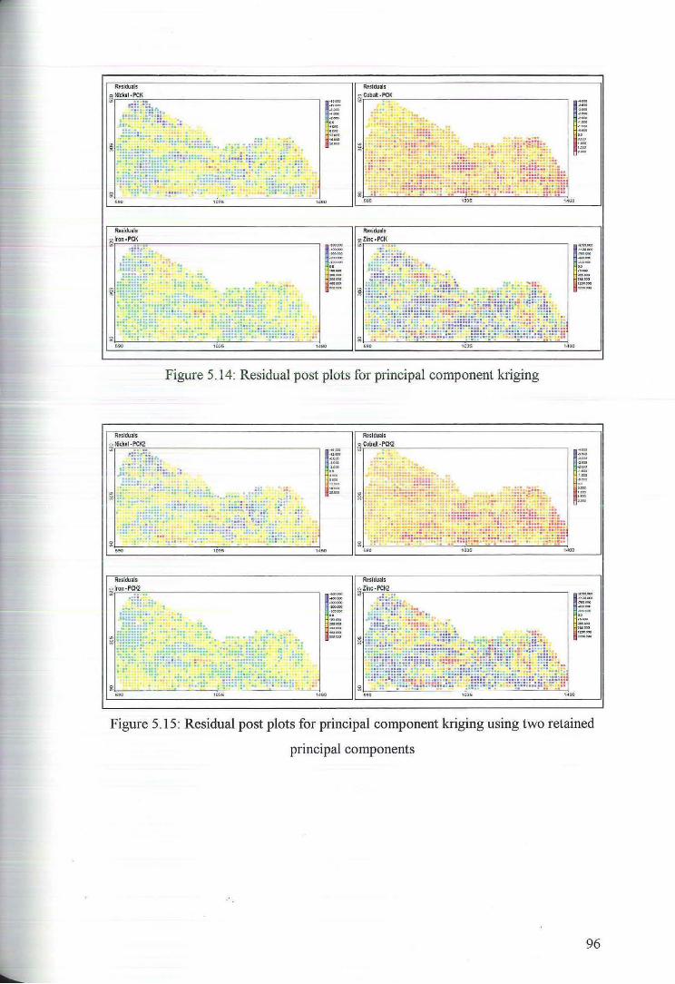
Rtsidu~ls

~ ~ckoi-PCK

Reskfuals

1---­~-··~­.. '""' M­..... --

Residuals

~ Cobillt -PCK

Residuals

~Zinc - PCK

Figure 5.14: Residual post plots for principal component kriging

r ·U-·~ ~-.. ·-,.., W#.'O

1

---­., ... --­·1(01100 .. '""" .... .. .., ... .,

~sidua!s

~ Cobilt·PCKZ

g

Residuals

~Zinc·~ . •

1

.,.,.., <~•:10 0100

'""" .. "­~-"'"' --

r ,.,,

··--H W

-·-.... ·-,, ·-

lmM_.-.,,.,fi<ICI ,,.,_ .. '""' .....

Figure 5.15: Residual post plots for principal component kriging using two retained

principal components

.·

96

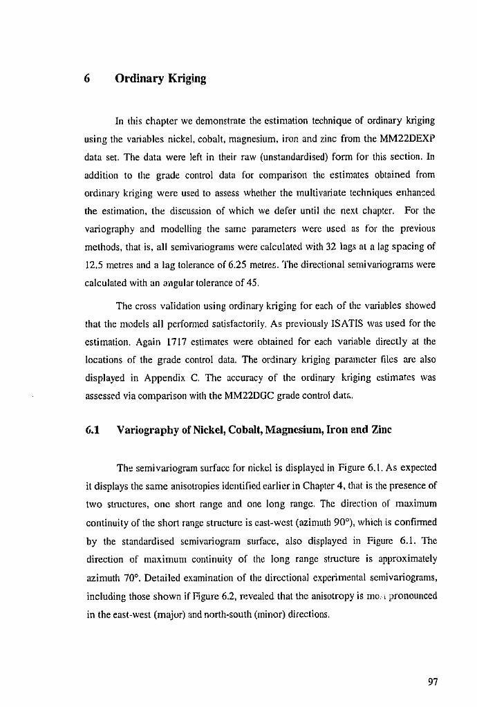
6 Ordinary Kriging

In this chapter we demomtrate the estimation technique of ordinary kriging

using the variables nickel. cobalt, magnesium, iron and zinc from the MM22DEXP

data set. The data were left in their raw (unstandardised) fonn for this section. In

addition to the grade control data for comparison the estimates obtained from

ordinary kriging were used to assess whether the multivariate techniques enhan-::ed

the estimation, the discussion of which we defer until the next chapter. For the

variography and modelling the same parameters were used as for the previous

methods, that is, all semivariograms were calculated with 32 lags at a Jag spacing of

12.5 metres and a lag tolerance of 6.25 metre.!>. The directional semivariograms were

calculated with an m1gular tolerance of 45.

The cross validation using ordinary kriging for each of the variables showed

that the models all performed satisfactorily. As previously IS A TIS was used for the

estimation. Again 1717 estimates were obtained for each variable directly at the

locations of the grade control data. The ordinary kriging parameter files are also

displayed in Appendix C. The accuracy of the ordinary kriging estimates was

assessed via comparison with the MM22DGC grade control dato..

6.1 Variography of Nickel, Cobalt, Magnesium, Iron end Zinc

The semivariogram surface for nickel is displayed in Figure 6.1. As expected

it displays the same anisotropies identified earlier in Chapter 4, that is the presence of

two structures, one short range and one long range. The direction of maximum

continuity of the short range structure is east~wcst (azimuth 90°), which is confirmed

by the standardised scmivariogram surface, also displayed in Figure 6.1. The

direction of maximum continuity of the long range structure is approximately

azimuth 70°. Detailed examination of the directional experimental scmivariograms,

including those shown if Figure 6.2, revealed that the anisotropy is mo.- l pronounced

in the east~west (major) and north~south (minor) directions.

97

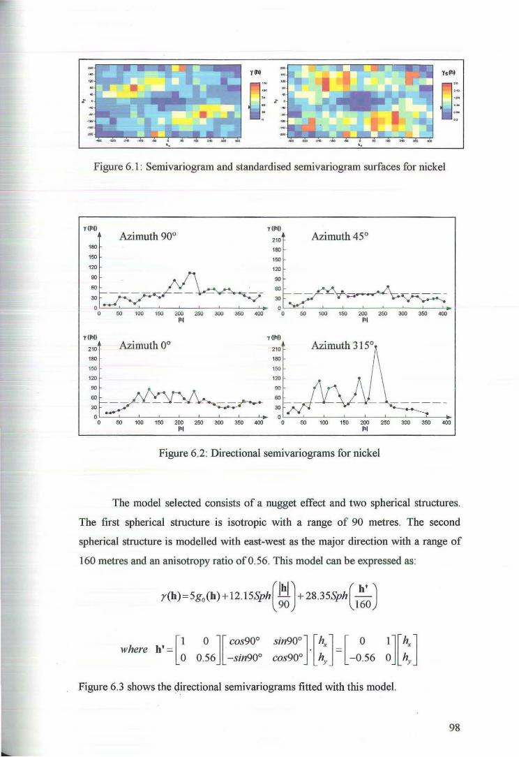
y(h) Ys(hl

0~ 0" ' "

,:- . ... .. ·-.,

Figure 6.1: Semivariogram and standardised semivariogram surfaces for nickel

Y (IIIII y(lhl)

Azimuth 90° 210 Azimuth 45° 180 180 150 150 120 120 90 90

60 60

30

50 100 150 200 250 300 350 400 60 100 150 200 250 300 350 400 lhl lhl

y(lhl) y(lhl)

210 Azimuth 0° 210 Azimuth 315° 180 180

150 150

120 120

90 90

60 60

30 -~ 30

0 50 100 150 200 250 300 350 400 0 50 100 150 200 2~0 300 350 400

I hi lhl

Figure 6.2: Directional semivariograms for nickel

The model selected consists of a nugget effect and two spherical structures.

The first spherical structure is isotropic with a range of 90 metres. The second

spherical structure is modelled with east-west as the major direction with a range of

160 metres and an anisotropy ratio of0.56. This model can be expressed as:

r(h) = 5 g0 (h)+ 12.15Sph(MJ + 28.3 5Sph (~) 90 160

Figure 6.3 shows the d~rectional semivariograms fitted with this model.

98

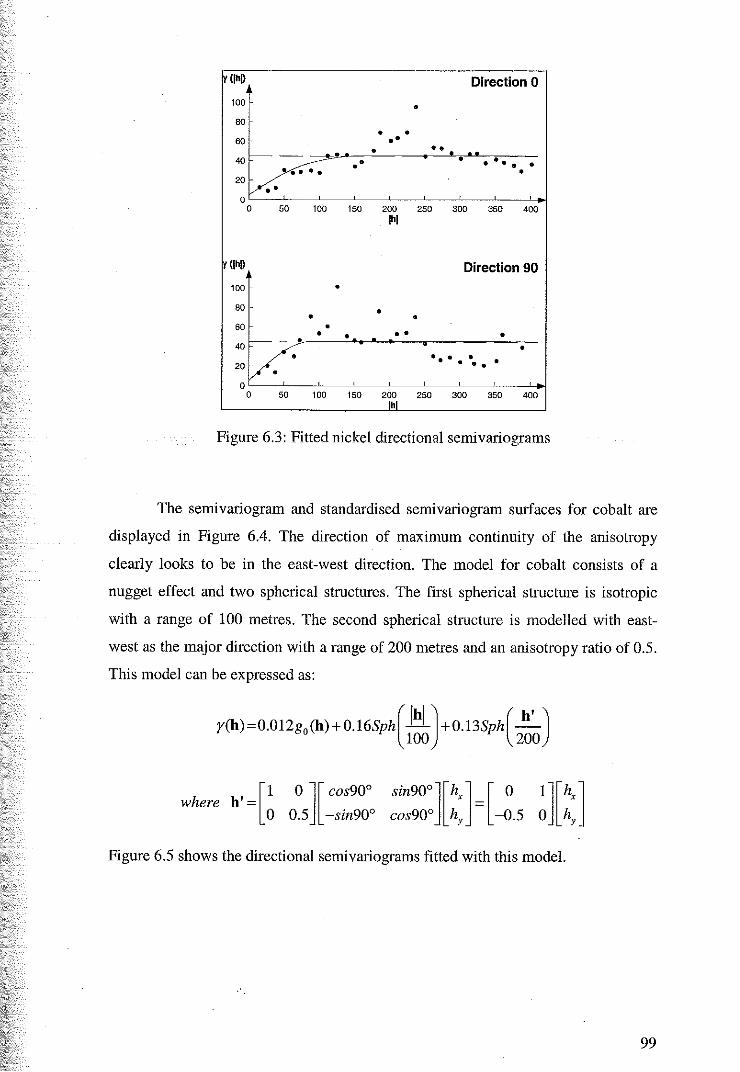
<I•D Direction 0 100 - • 80

• • 60 ••

?'~· • ••

40 • • • •• • • • • 20

• 0

0 50 100 150 200 250 300 350 400 lhl

<I•D Direction 90 100 • 80 • • • 60 • • • • • • v.· 40 ""T •

• • • • • • 20 •• 0

0 50 100 150 2<;;;,

250 300 350 400

Figure 6.3: Fitted nickel directional semivariograms

The semivariogram and standardised semivariogram surfaces for cobalt are

displayed in Figure 6.4. The direction of maximum continuity of the anisotropy

clearly looks to be in the east-west direction. The model for cobalt consists of a

nugget effect and two spherical structures. The first spherical structure is isotropic

with a range of 100 metres. The second spherical stmcture is modelled with east­

west as the major direction with a range of 200 metres and an anisotropy ratio of 0.5.

This model can be expressed as:

y(h)=0.012g0 (h)+0.16Sph(M_)+0.13Sph(~) 100 200

[1 0 ][ cos90° sin90°][hx] [ 0 l][hx] where h'= = 0 0.5 -sin90° cos90° hY -0.5 0 hY

Figure 6.5 shows the directional semivariograms fitted with this model.

99

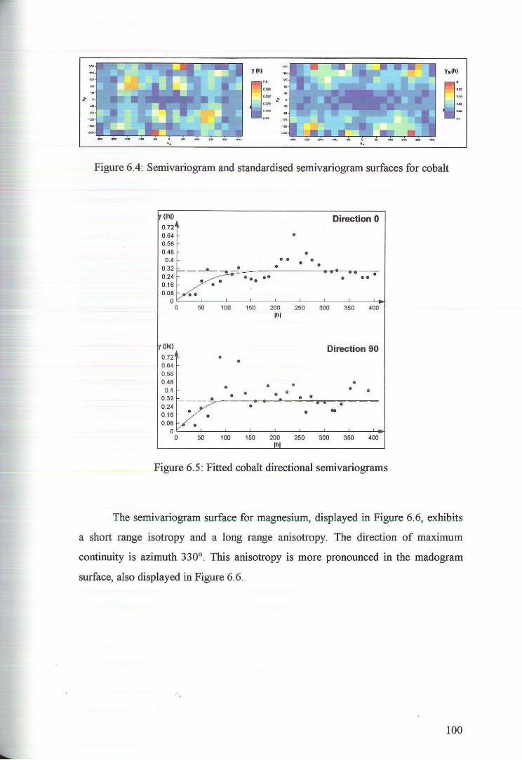
Ys(h)

0: .. >M

'M ,_

' ·'

Figure 6.4: Semivariogram and standardised semivariogram surfaces for cobalt

IY (lhl) Direction 0 0.72 0 .64 • 0.56 0.48 •

0.4 • • • • • '"7 • . • 0.24 • •• •• • • • 0.16 • • •

0.08 •• 0

0 50 100 150 200 250 300 350 400 I hi

y (lhl) Direction 90 0.72 • • 0 .64 0.56 0 .48 • • •

0.4 • • • • • • •

:::/ • • • . . •

0.16 • • • .. 0.08 •

0 0 50 100 150 200 250 300 350 400

I hi

Figure 6.5: Fitted cobalt directional semivariograms

The semivariogram surface for magnesium, displayed in Figure 6.6, exhibits

a short range isotropy and a long range anisotropy. The direction of maximum

continuity is azimuth 330°. This anisotropy is more pronounced in the madogram

surface, also displayed in Figure 6.6 .

..

100

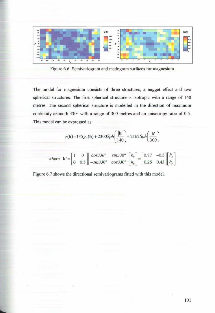
- t i!ltl ..., 0 ttl ltlO ~ :na -.. Figure 6.6: Semivariogram and madogram surfaces for magnesium

M(ll)

0:. ~·

"" ... ,

The model for magnesium consists of three structures, a nugget effect and two

spherical structures. The first spherical structure is isotropic with a range of 140

metres. The second spherical structure is modelled in the direction of maximum

continuity azimuth 330° with a range of 300 metres and an anisotropy ratio of 0.5.

This model can be expressed as:

r(h) = 13 5 g0 (h)+ 23oosph(!LJ + 2162Sph(~) 140 300

where h' = [ 1 0 ][ cos330° sin330°][hx] = [ 0.87 -0.5][hx] 0 0.5 -sin330° cos330° hY 0.25 0.43 hY

Figure 6. 7 shows the directional semivariograms fitted with this model.

101

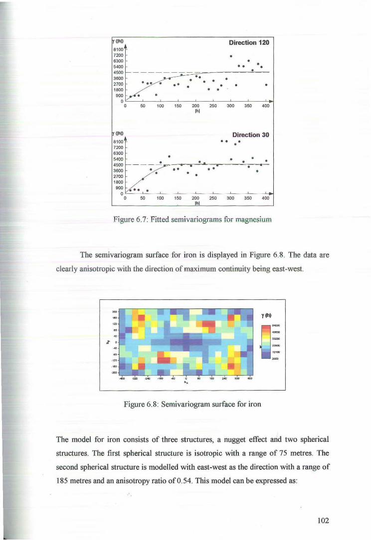
y (lhl) Direction 120 8100 7200 • 6300 • 5400 •• • •

:::~ ·· •

• 2700 • •• • • • • • • • • • • 1800 • • 900 • •

0 0 50 100 150 200 250 300 350 400

I hi

(I hi) Direction 30 8100 • • • • 7200 6300 5400 • • • :::::v • • •

• • . • • •

• • 2700 • 1800 900 • • •

0 0 50 100 150 200 250 300 350 400

JilL

Figure 6.7: Fitted semivariograms for magnesium

The semivariogram surface for iron is displayed in Figure 6.8. The data are

clearly anisotropic with the direction of maximum continuity being east-west.

""' , .. 120 .. "" .. .. 0

.... ... .... . , .. • :zoo - - - ~ ~ 0 ~ ~ ~ ~ -..

y (h)

Figure 6.8: Semivariogram surface for iron

The model for iron consists of three structures, a nugget effect and two spherical

structures. The first spherical structure is isotropic with a range of 75 metres. The

second spherical structure is modelled with east-west as the direction with a range of

185 metres and an anisotropy ratio of0.54. This model can be expressed as:

102

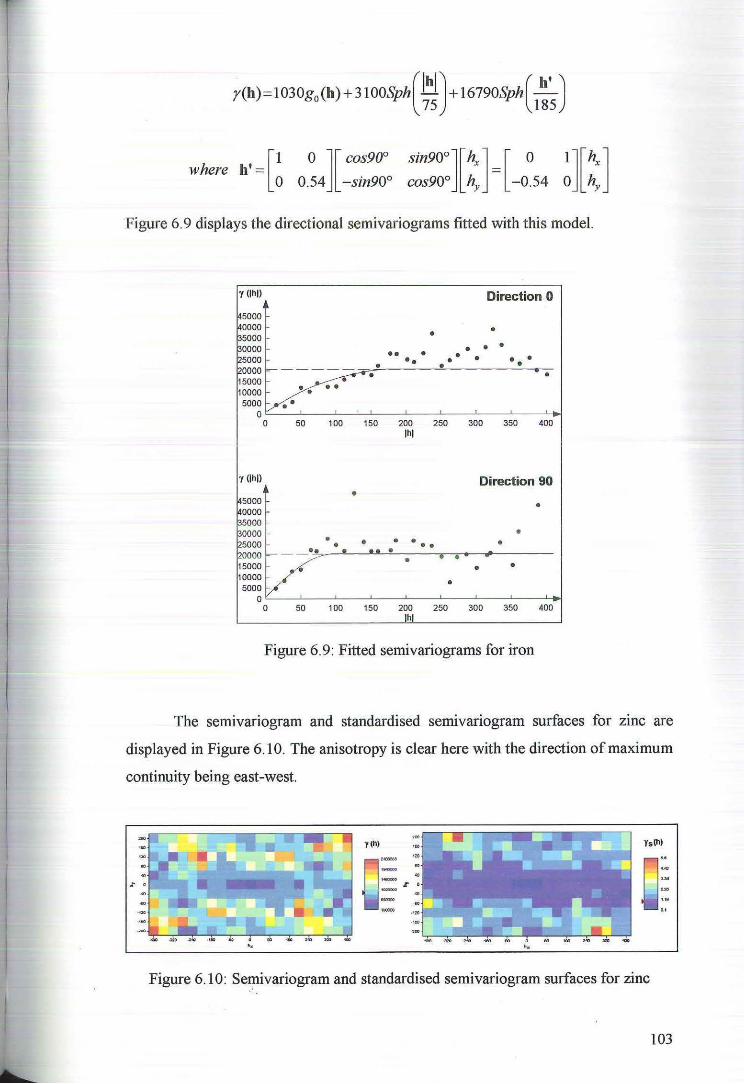
y(h) = 1 030g0 (h)+ 31 OOSph(MJ + 16790Sph (~) 75 185

where h'= · = · [1 0 ][ cos90° sin90°][h~J [ 0 1][hx] 0 0.54 -sin90° cos90° hY -0.54 0 hY

Figure 6.9 displays the directional semivariograms fitted with this model.

r !lhll Direction 0

~5000 ~0000 • • ~5000 poooo • • • •• • • ~5000 •• • • • • • P,ooo~.· • • 15000 •• 10000 • • •

5000 •• 0 .

0 50 100 150 200 250 300 350 400 I hi

1 (lhll Direction 90

~5000 • ~0000 • psooo ~0000 • ~5000 •• • • • •• • poooo ~ --•• • .. .

• • • '"00 / • • 10000 • 5000

0 0 50 100 150 200 250 300 350 400

I hi

Figure 6.9: Fitted semivariograms for iron

The semtvarwgram and standardised sennvanogram surfaces for zinc are

displayed in Figure 6.10. The anisotropy is clear here with the direction of maximum

continuity being east-west.

Ys(h)

0 .. ~ 0.1

Figure 6.10: Semivariogram and standardised semivariogram surfaces for zinc

103

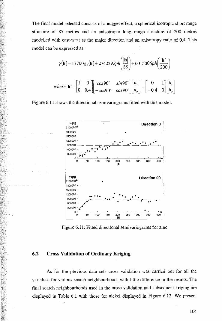
The final model selected consists of a nugget effect, a spherical isotropic short range

structure of 85 metres and an anisotropic long range structure of 200 metres

modelled with east-west as the major direction and an anisotropy ratio of 0.4. This

model can be expressed as:

y(h) = 17700g0 (h)+ 274239Sph(M)+ 601500Sph(~) 85 200

[1 0 ][ 90' h h ' cos were = 0 0.4 - sin90'

Figure 6.11 shows the directional semivariograms fitted with this model.

y(lhD 100000

1800000

1500000 •

Direction 0

1200000 • • • • • • •

I-- -~-=10~·~·--~·~·~·~·--·~·~ 900000 - • -

600000~· ••• • • 300000 • • OL_ __ L_ __ l_ __ ~.--~--~--_L---L---~~

0 50 100 150 200 250 300 350 400

Y(lhD 100000

1800000

1500000

1200000

300000

•

•• • • •

lhl

• • • • • •

• • • •

Direction 90

• • •• 900000/ 600000

• 0~--L_ __ l_ __ ~--~--~--_L __ _L __ _L., 0 50 100 150 300 350 400

Figure 6.11: Fitted directional semivariograms for zinc

6.2 Cross Validation of Ordinary Kriging

As for the previous data sets cross validation was carried out for all the

variables for various search neighbourhoods with little difference in the results. The

final search neighbourhoods used in the cross validation and subsequent kriging are

displayed in Table 6.1 with those for nickel displayed in Figure 6.12. We present

104

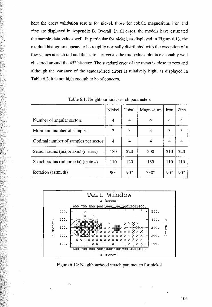
here the cross validation results for nickel, those for cobalt, magnesium, iron and

zinc are displayed in Appendix B. Overall, in all cases, the models have estimated

the sample data values well. In particular for nickel, as displayed in Figure 6.13, the

residual histogram appears to be roughly normally distributed with the exception of a

few values at each tail and the estimates versus the true values plot is reasonably well

clustered around the 45° bisector. The standard error of the mean is close to zero and

although the variance of the standardised errors is relatively high, as displayed in

Table 6.2, it is not high enough to be of concern.

Table 6.1: Neighbourhood search parameters

Nickel Cobalt Magnesium

Number of angular sectors 4 4

Minimum number of samples 3 3

Optimal number of samples per sector 4 4

Search radius (major axis) (metres) 180 220

Search radius (minor axis) (metres) 110 120

Rotation (azimuth) goo goo

Test Window

500.

400. H ID

'"' ID e 300.

>< 200.

100.

X (Meter)

013001400.

X

X X X

X X X X

XX XXXXXXXXXXX XX X

X (Meter)

4

3

4

300

160

330°

500.

400.

300.

200.

100.

Figure 6.12: Neighbourhood search parameters for nickel

Iron Zinc

4 4

3 3

4 4

210 220

110 110

goo goo

"' :;: ro " ro "

105

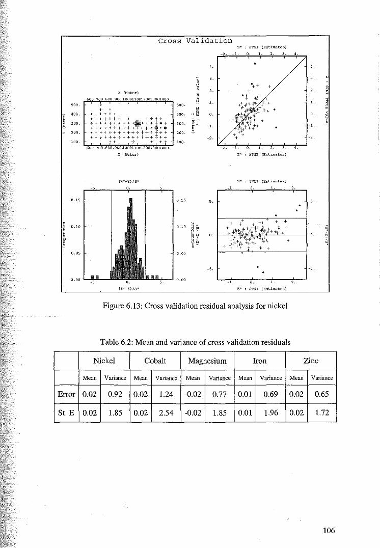
500.

;; 400.

~ • 3 300.

" 200.

100.

0.15

~ 0.10

l ~

0. 05

Error

St. E

Cross

X (Meter)

600.700.800.900 ~000110012001300.1400.

' 500.

+ + + + + + 400.

.... +,++ • ++r ++1·+++++++,+++ .. •+ 300. +-f-·1 ++++-1--t-+··+-t--fl •• +++-~+-+++++++++""'++ 200. ++++++++++++++--++

++ + + +t 100.

600.700 .800. 900 10001100120013001400.

X (Meter)

(Z*-Z) /S*

0.15

0.10

0.05

(Z*-Z)/S*

Validation

-2.

4.

• '. ' H : 2. • ' ~ 1.

"~ 0.

Iii .. ~" 0

-1.

!!. -2.

_,.

_,

5.

0.

-5.

,. ' STNI (Estimates)

-1. 0. 1. 2. '.

+

•

-1. 0. 1. '. '. ,. ' STNI (Estimates)

Z* : STNT (Estimates)

'

0. 1.

Z* : STNI (Estimates)

Figure 6.13: Cross validation residual analysis for nickel

4.

4.

3 • " ffi

2. " " 8 1. 2 0

0. ' • ' -1. ~

-2.

4.

2.

5.

0.

-5.

'.

Table 6.2: Mean and variance of cross validation residuals

Nickel Cobalt Magnesium Iron Zinc

Mean Variance Mean Variance Mean Variance Mean Variance Mean Variance

0.02 0.92 o.oz 1.24 -0.02 0.77 0.01 0.69 0.02 0.65

0.02 1.85 0.02 2.54 -0.02 1.85 0.01 1.96 0.02 1.72

106

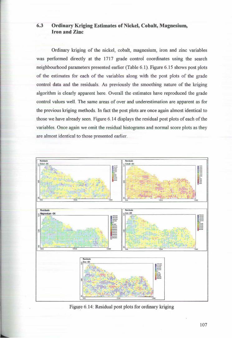
6.3 Ordinary Kriging Estimates of Nickel, Cobalt, Magnesium, Iron and Zinc

Ordinary kriging of the nickel, cobalt, magnesium, iron and zinc variables

was performed directly at the 1717 grade control coordinates using the search

neighbourhood parameters presented earlier (Table 6.1 ). Figure 6.15 shows post plots

of the estimates for each of the variables along with the post plots of the grade

control data and the residuals. As previously the smoothing nature of the kriging

algorithm is clearly apparent here. Overall the estimates have reproduced the grade

control values well . The same areas of over and underestimation are apparent as for

the previous kriging methods. In fact the post plots are once again almost identical to

those we have already seen. Figure 6.14 displays the residual post plots of each of the

variables. Once again we omit the residual histograms and normal score plots as they

are almost identical to those presented earlier.

R.,ldu~s

r ~ Cobillt·OK .. _ ... ·-.... .. "" ·-..... .... ""' ~

·- ... Rukfulls

~Iron ·OK_

r ·11~.000

-tOO .tOO --.. "'"" ·~-1110000 ...... .., ... ...... ....... ....... -

1480 .,

..... ......... .... ... . .:·: . ... . -:!:.:: .

. ;;· .. : ;.:~~z:::::u·=::~-: ··: ;;:-:;·:;~=~~t · ::= ~ : i:.

I~;. · <~ :~~~~:::::::: •:!~ ::;:::::~:= ; ;~=~~! : : ..... ~E=-~ :~: .. :: :~:: ... ~~ :; ~: : : ~~ ~ = · ·::::·: .. "i!::f;~z;! ·i=!:· o.::=.:::=::i-:i

£ .. ... '!':·· .•••••.•• ·:·· ······ •• • _ •.•.••. • - •• . ., 10)5

1···-----.. ..... ----

Figur.e 6.14: Residual post plots for ordinary kriging

r :·-. .. ·-. .. . .... _, ... ·-.. ~= ·-·-

. ...

r ...... --...... ·•to-.. ··-----: '::

107

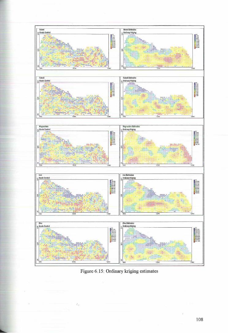
Cobalt ~Grade Control

Iron

~ Grade Control

Zinc o Grade Control

,.

1

.. a.•• ·­·~ ·~ ·­·­'"'

1480

1

.. ,..,.,a : t21DCZI ----=·-:111!1.«')

Magnesium Estimates

g Ordinuy Kriging

Zinc EsUmztes ~ Ordinary Kriging

Figure 6.15: Ordinary kriging estimates

1

.. ~·= '""'"' t ru~m .... -~ llllilDXl

1490

108

7 Comparison of Estimates

The post plots shown earlier in Figures 4.6, 4.14, 5.12, 5.13 and 6.15 show

that, as expected, the ordinary cokriging and ordinary kriging techniques used have

resulted in very similar estimates. The principal component kriging estimates are also

very similar to the other estimates. In addition the principal component estimates

using only the retained principal components arc very similar to all other estimates.

This indicates that very little infonnation has bee;n lost by retaining only two

principal components. Figures 7.1 to 7.5 and Tables 7.2 to 7.6 display the descriptive

statistics for each of the variables. Overall all of the kriging techniques used have

reproduced the grade control and exploration descriptive statistics reasonably well. In

all cases the mean and median of the estimates has over estimated that of the

exploration and grade control data. The only exception is zinc where the mean and

median of the estimates arc close in value to those of the grade control data. The

values obtained for the mean and median for each variable arc very close in value for

each kriging method.

The standard deviation of the estimates in all cases is considerably lower than

that of the grade control and exploration data, yet another indication of the

smoothing of the variability due to the kriging process. This is further supported by

the coefficient of variation which in all cases is lower for the estimates than that of

the grade control and exploration values. The standard deviation and coefficient of

variation obtained for each very is very similar for each kriging technique used. The

skewness of the histograms of the grade control data for each variable has been well

reproduced for all variables except cobalt. While the grade control cobalt is strongly

positively skewed the estimates are not, in fact the skewness of the estimates is

around one third of that of the grade control data.

Table 7.1 displays the mean square errors and mean absolute errors for each

variable and each kriging method used. The lowest mean square CITOr for each

variable is coloured red and the lowest mean absolute error is coloured blue. Overall

for the kriging methods used for each variable the values fo!" these measures are quite

similar. For nickel the lowest mean square error and mean absolute error were

109

associated with the principal component kriging estimates. The lowest mean square

error for cobalt is associated with the principal component kriging estimates using

only two principal components. Correct to two decimal places cobalt had identical

values for the mean absolute error for all methods. However correct to four decimal

places the principal component kriging estimates had the lowest value for this

measure. Both the mean square error and mean absolute error for magnesium were

lowest for the estimates obtained from cokriging. The iron mean square error and

mean absolute error were the lowest for the principal component kriging estimates

obtained using only two principal components. For zinc the lowest values for both

error measures were associated with principal component kriging.

Table 7.1: Mean square error and mean absolute error for each method

Nickel Cobalt Magnesium Iron Zinc

MSE 41.71 0.34 NA 20489.95 847999.31 OCK-ICM

MAE 4.88 0.43 NA 107.91 705 .32

MSE 41 .46 0.33 3269.59 20003 .96 NA OCK-LMC

MAE 4.86 0.43 39.51 106.59 NA

MSE 40.50 0.33 NA 20497.71 838231 .21 PCK

MAE 4.81 0.43 NA 107.92 699.99

MSE 42.51 0.32 NA 18568.06 884728.72 PCK2

MAE 5.05 0.43 NA 105.29 733 .77

MSE 41.56 0.34 3612.69 20365.44 843825.91 OK

MAE 4.87 0.43 41.09 107.32 701.78

,·

110

' ' " "' ., ' ' '

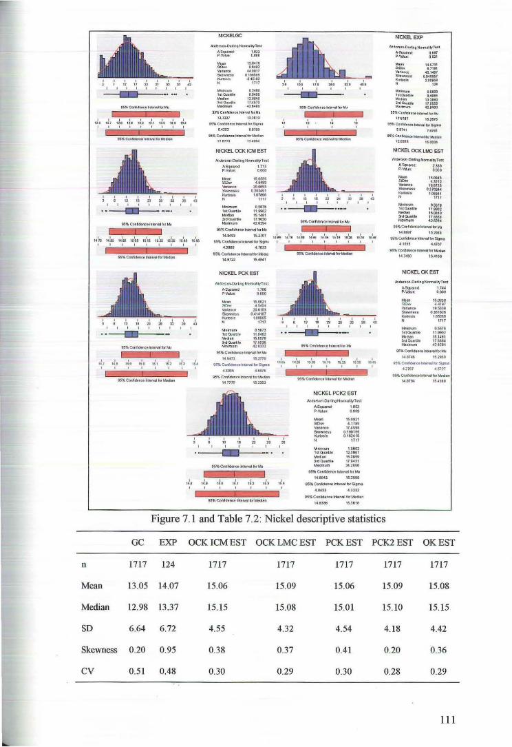
96tlConfldencelll'tiMIIforWu

I I I I I I I I I •z• 12.1 111 t:lJ t:s.o 11.1 t l..2 u' ''"

I I I I I I I I I

9511. Conftdtnn lnteMIIor MJ

' ' .,

I I I I I I I I I 141.5 t.c.tS 14M 1$0$ 11515 t5.7S 1$35 IH5 tU6

I I I I I I I I

r:~;ag~====~·~:::::::::J 95"JioCCWl~-MIIforM!dan

' ' I ' ' " ,.

" .. " ' ' ' -~".lio CcnlldtncelnltMII f« M#

' ' ' ' ' ,J, ' ' "' ... ... ... I" '" ... ' ' ' I '

»Sft ConftdencelnteMI for MK!t.n

I'ICKELGC

Nlden:o...Oatllng Notmaltt-(Tut

A.$quaf1!d I 122 P-Vatue. 0.000

-htClulttillt l.lrii;~n 3nf0t.i.mile Ma.limum

13.D470 11407

44 0117 0111!05 .f4E--O'l

1711

02400 ...... 12.1140 17AS70 41&400

SS%ConftdencetlteMI IorNu

12.1321 13.3113

95"- Cont.dli'~~ee .,.,_, h»f $itm• 1415l lllOO

t5'4Coftld•nu~IDfMidllft

n~t770 n<~AIW

I'ICKEL OCK ICM EST

llfld'llrsM-DarllngNonnallt{T-st

ASqu-.d 1713 FWIIIue. 0000

...... ISOSSS

""'"' ..... VarialK.e ,. ... , ,._, .. , 038:Htl

""'""" 10786t N t7H

Mnunum 05070 tstOw~ 119002 Maclan 151481 JrdOu•"- 179030 M!IJiimum 426N4

95~ Conlldon<e lnttMII« ldi

14.8403 152707

iS'Io CoMdence iniMWI for S9n1 4.3;88 4 7033

05~ Con~cSM~c•M*WitorMidla

14.8121 154841

NICKEL PCK EST

Jnderson-DorlingNorrnlflt,oTH t

ft.Scf.Jnd 1788 P-Va111.: 0000

...... 150821 - ·~ ""''""' 206153 -... 0414107 K"""h 100005 N 1717

Mnlmum 0 567:! 1<>10uertilt 11.&462 f>1adi~n 15007G lrdOUartile 1711038 M;t)l!mum 42.0332

85-J. Conlidlncelnr.tv.al lot,.,

t• 8A72 IS 2770

~ ConicNftc.ln ..... lor 59n• 4383S • 6876

95~ Confr.denw lnllfWf for Mtlhn

147270 153383

I I I I I 141 15.0 IS I 151 15.3

' 959f.Conldance tt•MIIQfMf(IJen

I I I I 12 II • t4 15

'c==='=r::~:':::::::~' 85'4 CoMff:na "*N.IIII!Dt t.t~~:ddn

' " " ' ' - ' ' ,. .. ' '

' ' . .,

I I I I I I 1 I I !Hill t<~~7t t•to 1.,1 1508 HUI 1$.2CI \5. ISC

I ~I=~·;;=.=' =;~' :;;~'::::;' =:'J I tiiJo CUII4tfKe ....... loiMdM

I I I I I I I IC85 1U5 15015 1515 15.25 1!35 1545

I I I I I I I

' 15_4

NICKEL PCK2 EST ,tnden;on-O.ilffin:o Normality Tall

ASQu..-d. 1 053 P..v.tue· 0009

15JI911 .. 1715

17,4581 0 111155 0 182415

1717

Mnlm~.m 1.9002 ISI OUI!Irtllt 12.0981 Ml dlao 15 0059 :SRIOUMit 17.9-4S1 Mmtnum 34.2800

as. Contdtnot rnteMtiiOf t.t~

14.8a43 ts.28tt

OS'4Conld..wt nlen'M IDr Sigml

4 0433 4 .32)2

OS!Mo Contderu ltUMI f« Mliditn

148386 15.3818

NICKEL EXP

AndtBon-OIIfttiQ NotmtlitfTtsl

,A,.Squtttd. Dill P.YI IUt 0021

We•n -.,.._ 14.0131 17111

4!.1411 $kt.Mes.t Kur!osis

o ... ,.,, 200151

" ,,. .......... 1$10ulfllt WediJn lrdCk.IJ1111t MI""Um

. .... ••oes

133110 IUOSS 41.1400

115 '4C:Otlftcfrnceln"rwiiDrWw

128711 15.2815 95'1iConlidtncetnll,.,..fofSiQtna

~..1741 1a11l

t 5'4 Cont4tnq '-'* w Mtdilln ll.Olll 110021

NICKEL OCK LMC EST

l<ndl>rson..o.ttngNcwmlljWTest

A-Squwtc~ 2360 P.Valua: 0.000

15.01M3 -43112

181723 .,_. I.OS941

1711

05676 11.0001 150810 17.8358 .,.,..

95% Conllt»ncalnltMllfot MJ

1-48807 1$.2181

95"'Confidtneal~ lorS9fta .tlt813 •U107

9~Con6dinct .,.,.lot ... cl ..

, .. _, .. so ts.ct60

NCKELOKEST

kldlnon-Daltlno Norm~~ Test

ASqu•ed I 744 PNIIut. 0000

Mnim1.1m 1S10ultfilt Mtdan 3tdQJ«t~la

""""""m

1500311 4 41117

19..5338 03151126

105288 171 7

0.5676 119902 15.1481 f1 8M4 426194

9St.4 Conac~tnc. NMl ror !vlJ

1• 1746 151i30

es~ C'oflldenw ll:l..,...lclt Sl9ft• •.2 181 4 5711

95"JG.ConlldtftwlnW't'IIIIOf~.a

1<4 871M 15 4169

Figure 7.1 and Table 7.2: Nickel descriptive statistics

GC EXP OCKICMEST OCKLMCEST PCKEST PCK2EST OK EST

n 1717 124 1717 1717 1717 1717 1717

Mean 13.05 14.07 15.06 15.09 15.06 15.09 15.08

Median 12.98 13.37 15.15 15.08 15.01 15.10 15.15

SD 6.64 6.72 4.55 4.32 4.54 4.18 4.42

Skewness 0.20 0.95 0.38 0.37 0.41 0.20 0.36

cv 0.51 0.48 0.30 0.29 0.30 0.28 0.29

Ill

'

' ...

.... '

' ... '

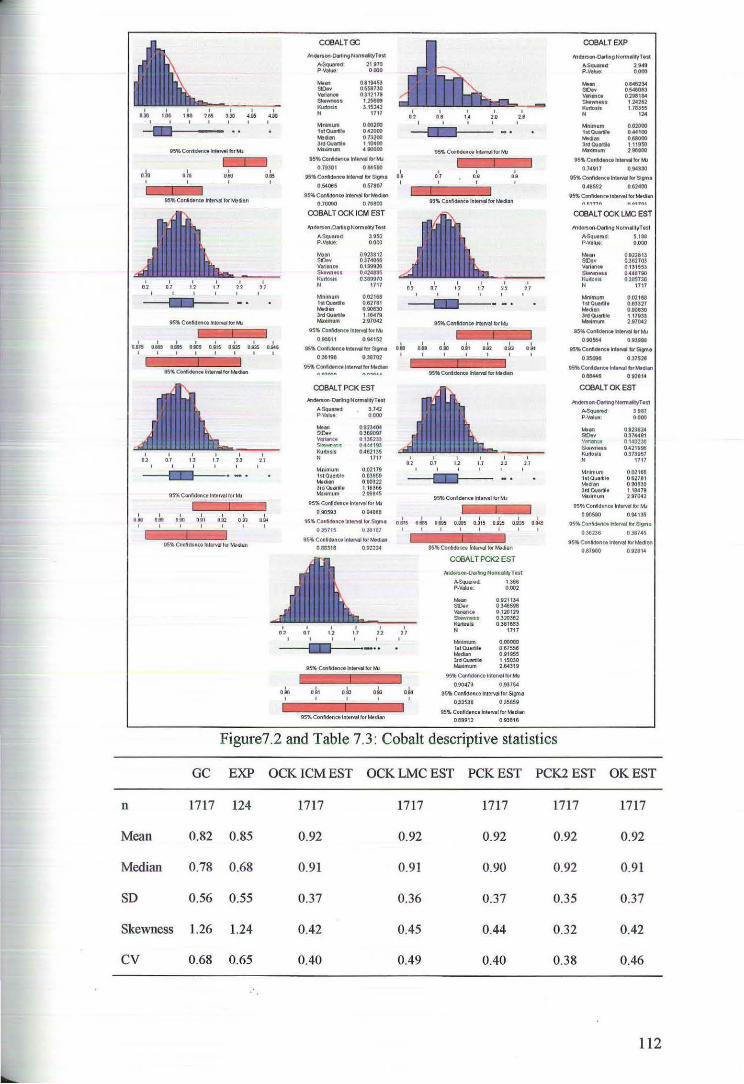
' lOS

' ' 3.30 ' .... ' ....

' -

' ... '

' 075 ' '"' '

2.2

DS'I.ConfMitncelnlltMlffofMJ

J ' ' ' '

'

'

j ' ... '

' "

' ·- .... 0815 ·= .... . .... ' ' ' ' ' 1::

IS'-Coni~ lni!MWI fOf Mlclan

' ' 22 ·a

U'll Confidence lnteMIIIorMJ

I I I I 080 011 Oil Oi'l

I I I I

j 05" Conlidtttc.lnleMII lor Mtdian

'

' .... '

'

o.lo

COBALT <X:

A""HMrson-a..t~ntNonnthtyTttl

~ 21970 P-Vtlut 0000

..... OltD-453 - 0551730 .......... 0312178 ........ 1.2SM9 ......... 315142 N 1117

M ....... 000200 11tou.tllt 042000 ....... 0 73200 3ntW .... 110400 .......... .......

85~ConfcMnct ~tiM' M.l

0 78301 014500 1

115~ Confldonc. t'lteMIII b' Sign• D I

0..54065 0 57807 I

85'M.Contellr'!Ctii'UMI torMtdien

0.70000 0.78800

COBALT OCK ICM EST

MellniOCI·O•hngNormllrtvTtll

ASQutttd 3 050 P-VtiUt 0 000

...... S10ov V•l.nce Sktwnen KurtOsis N

0123812 0.37110&8 0139920 0.42415$5 0,389970

1711

Mnlmum 0 02168 1s10Urie 06'2111 Mild... 0.80$30 3td ~-- 1 18418 Mwmum 2 t7f»'2

IIS .. ConfidWittln~IOtMJ

0..$10&11 0~15l

15'1. CoAMtnc:U'IIitMI f« Sto"na ' •• '

1 uo

'

' 07

' ' 0.8

'

' ,. '

' ,.

' OJ

95't. Conftdence lnteMIII f« 1\\llfan

' .... ' •• 1 ' . ., ' '

' .., '

' "

' ... ' c - ;::c 0 31tte 0.38702

IS. ConW.nc.tnse,_ fofh'ediM

COBALT PCK EST Jrndtr~on-OartingNomuMyTut

A-5Qvarecl 3 742 p.y.....,. 0000

...... o•134oc SIOov 0.3~007 -" 0 tl42U s.:.wneu 0444113 KurtoSlt 048'2135 N 1717

Mnlrnum 002171 tstOuettllt 0 &3850 ....... 090322 31d0Uiftllt 118366 M:IJimum 2 06845

95'4 Con~dencelntervel ror Ml

0.90513 0 ~088

1)5'1f. Conl!dancaln._MI lOt Sl~t

03$715 031187

ass Con~n<alm.Mtl ror Mtdr.n 0 88318 0 02224

ol1 a.b '

' 0 175

.:.. '

' ....

a5tloConldance hll:lmlllorMtlfan

' 22

95~ Conldance W.el\/81 b rM;

M"'Contdtnoe ~ t«Mld•n

COBALT PCK2 EST

Andenoon-051ing Normafit'/Tnl

ASIJiariiCl 1.366 P-Yafut_ 01102

..... 092113<4 SOO.v 0_3465'J8 \lllrianca 0120129 -... .. 0.320382

""""" 0~16S3 N 1111

Minimum ....... lstOUelfte 067556 ,.den 01U9S5 3u•OU•"IIe 1.15030 Mbllmum 2.&4319

95'!1o Coni"Kiance lntt!MIIIor t.t.1

0.90473 0 .9375-4

' "

D5'Jio Confidence Interval lor stgme

033538 O.!St59

QS'IIo Conrid$11(tlnterval fof t.;•den 089912 0 .938f8

' ....

CCBALTEXP

MdoBon·o.MgNonnelityTesf

.... Sqvttlld 2 948 P.V.tu. 0000

... .. -V«llnCI Sbwntu Kurtosis N

Mrumvm tstCkuwilt

""""' 3nt()J ...

""""'""'

0..02:)4 0548063 0.288184

12426? 178355

124

002000 04t100 ....... 111!iJ50 2te800

05'Ao~~in!wt111forMI

0 74817 0»4330

05'4 Confldtn<tln~MII tot Sgmt

0~552 062400

85t. Conlldlnc.tn•,.,., lot Mtdi-

COBALT OCK LMC EST

Mdtrson-Dtlf11ng Normel?lyTtst

A&lutnul 5.188 P·VtiUI 0.000

...... , SIOov v .. .... Slot .... . t<orsoslt N

0822813 0.381703 0 131553 0448700 038S73CI

1711

Mnlmum 0021S8 1st Ouertite O-'l327 Mtcl., 0 80030 lrdOu.... 117t3S Muiml.fl'l 297042

SIStloConld ..... ~tH'MJ

0805$-t 013998

a5'1Ct Conldtnte rnteMII b' S9'n a 035008 0375'21

IS..Cont~ Htnel .,..Midlln

0.18445 092814

COOALT OK EST

A'tdelSon~Normlfityl'est

~d am p.vatut 0000

.... .. 0123024 - OS74481 y..,.,ct 01 .. 023e SMawnen 0421$~ Kurto111 0373$57 N t717

Mnlmum 0.02158 l stO...-Itlla 061781 Mtd .. 0 00030 3ASOI.IIttllt 11~79 Mt»Mum 287().42

85 .. ContdtnOI ~ttMII br ~

Olil0590 0;.1135

OStlo Confl"ntt \'!!eMf tr Sfgme

038238 0387-'5

SIStloContdtnctlrCtP'o'ft t)rMtdtan

0 87900 0 .1211•

Figure7.2 and Table 7.3: Cobalt descriptive statistics

GC EXP OCKICMEST OCKLMCEST PCKEST PCK2EST OK EST

n 1717 124 1717 1717 1717 1717 1717

Mean 0.82 0.85 0.92 0.92 0.92 0.92 0.92

Median 0.78 0.68 0.91 0.91 0.90 0.92 0.91

SD 0.56 0.55 0.37 0.36 0.37 0.35 0.37

Skewness 1.26 1.24 0.42 0.45 0.44 0.32 0.42

cv 0.68 0.65 0.40 0.49 0.40 0.38 0.46

112

' "

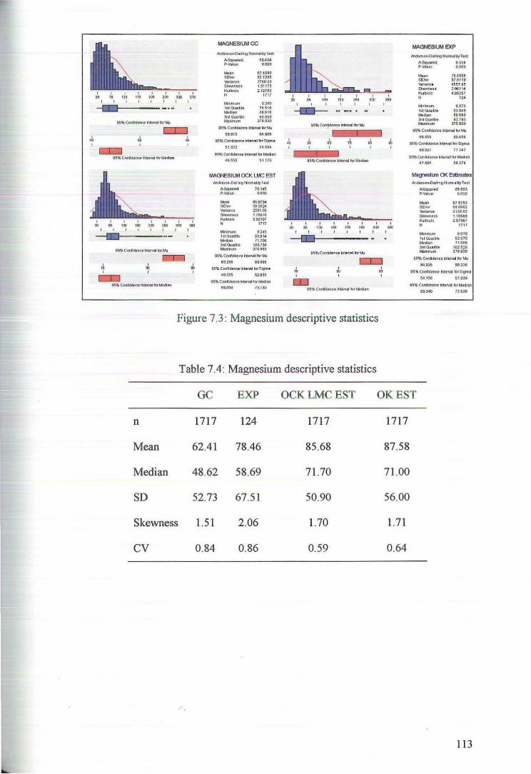
' 10

'

' ..

I I I I no 210 J2o :no

' ' '

' .. OS" Contdtnct ht.rval b' Modian

I I I I 731 18D DJ 310

' ' '

95~ Conft.c»nu tnleNIII for"'

' "' I

.:, '

MAGES1UMGC

Pndtrson-O.tngNormaM)'THI

.A.Squ.-ed S\)..404 P..V&Iut 0.000

Mttn 62.4090 sc... 52.7288 Valiance 2760.33 Skewness 1.511715 Kurtosis 2 .7278g N 1111

MnimLm 0100 1S10tutl111t 24.518 MJdi"lllt 48616 3tdou.r... 83~9 Ma:lomum 378.930

ts«.Cofltct.nc..-arvaJbrJ,t,, 5991:! G4.905

15,. ContMnce blel\'liJ tlrSigme

51022 54.5~

9S,.Conldtnce nt.MlforMt<Jian

•ruse su1e

MAGESIUM OCK lMC EST Mderscn.o..ung Nonnality Test

A-Squertct 78.145 P-V•tur 0000 ..... 85.6754 ..,.., 50902< -" 2SOI.tl$

""""'"' 170070 ........ 3.30107 N 1717

M n!Mum 1243 1A0u ..... 53.8\.4 Mod'" 71704 3fdOu~· 100734

""""'""' 378883

05'11. Conlldencelntarval for" t..tJ

83.288 88085

115% Confidtnc.lntff'llelfor Sigma

40255 5:ues

OS,._ ConlldtnttlnltMII tor M!tcfian

159.004 73.730

' .. ' .. '

' .. 1~ ~ ' '

9SW. Conldtnc. hteM! lcf Medum

~ ' • ' ' .I "' ' - ' ' 230 2111

I I

OS'M!Contden~ lnteMI brMJ

' ...

' 15

'

' ' ,,. ... '

CCl I

10 I

o::J ' "' '

os• Conldtnc• heM! tlt Mtdl"an

' .. I

MAGNESIUM EXP

Jtndefton-OarlingNonnabtyTest

..-..squ~~n~d. 1.334 P.V•kJe 0000

~an 7U556 StOliY (17,!5118 V.arianc:e 4557 as SkeWnt$$ 2.0811<4 KurtoSIS 4 .G52.57 N 12•

Mninnm 8.070 ts.t Quaflllt 33.545 Mtdian 58 888 lrd 0'*"- 92 713 Ms:JOmum 378..930

OS,. ContdtrM w.rvetlbf ~

66455 1NJ458

os• Contdet'ICt Htrvat * stom• 60027 17.147

111514 Conld•nce ht•rval for Mfdltn 47404 69.374

Magnesh.m ~ Estimates .And•JSon-Oartlng NonnalltlfT•st

ASquartd sa 863 P-Vatue. 0000 ..... 17'5752 ..,, ...... , ......... 3138.02 Sbwnns 170588 KudOS!$ 2.07187 N 1111

Mnimum 8070 bt0Jartile 52075 Mtdtan 1 \ 000 3rd0Ualtil• 102525 Mmmum 378 030

OS~ Conldenea htorval l:lr ~ 84 g, 90.226

OS" COt'lld&not hi& Milot Sigma

~ 188 '57.93t

95" Conldoncal'lleMI br~_, Ul-40 72.128

Figure 7.3: Magnesium descriptive statistics

Table 7.4 : Magnesium descriptive statistics

GC EXP OCKLMCEST OK EST

n 1717 124 1717 1717

Mean 62.41 78.46 85.68 87.58

Median 48.62 58.69 71.70 71.00

SD 52.73 67.51 50.90 56.00

Skewness 1.51 2.06 1.70 1.71

cv 0.84 0.86 0.59 0.64

113

' "'

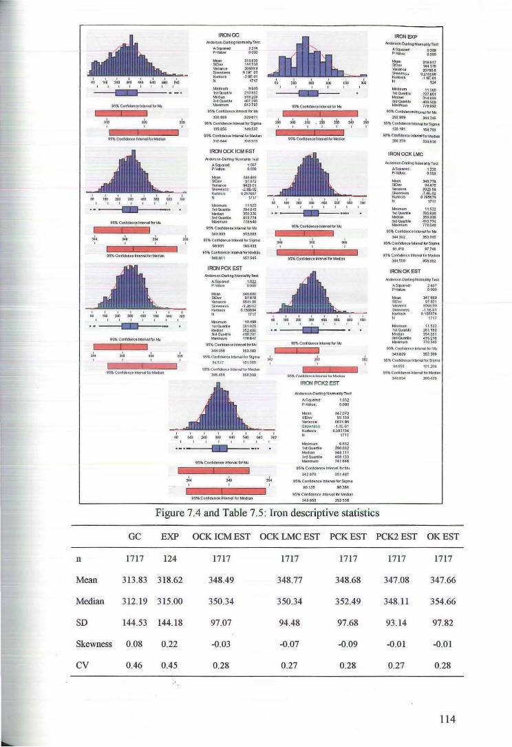
I

"'

I

"' I

,J, I

' I ,.. ... I I

I ... I

' ... '

I

"" '

95"4 Car\~tnce lntlrvallor MJ

I ... :J. I

IS~ConAOtnu: ln_....ku'Midt.en

' ... I

' '"

I

I ... I

,.,

I

"'

I 40

I

I

IRONGC kldftt:on.()ert~ngNonnllfity'Tes1

'"~·- 731-4 P-Y.We 0000 ..... ..,.... YIIIMCe Sl..•wn•ss Kurtosfl N

313.830 1-4-4.513 20889.9

8.19E-02 -28E-01

1717

Mr~lmum 9600 1st OUirile 210 852 Mechl'l 318.208 3rd Ou•ntte 41107.298 h'e»mum 813.792

85'11!>Cofti!dtnc.ln~larM.I

306.889 310671

ts'I'COflftdentelnlllmllforSigm•

131 156 140.SS7

9S'4Confldtnc.lnt«'4*-'r~"' ~,n.....,. ,.~,:\

IRONOCK ICMEST Mdtrlon.O.tllng No~malilyTo~t

A.$o.llfed. 1.067 P-YIIIue. 0008 ..... SlOe• V.tlenn Sbwntst ........ N

t.~lmum

I"OU-* -·· 3tdOuerwe ...........

348.488 97.072

9423.01 -1.8&02

0..2G7661 1717

11.521 284015 350336 413774 ns.540

05'1. Confidence Inti,.... I« MJ 343193 353033

li:SIJ. Confldenceltdorval rorSigma

8U31 100.433

$5'4 toniiO.nC'O intervllfort.ioeOIM

S48.011 357.545

IRONPCK EST Mct.rton-OerHng NonnefilyTest

~~!- ·~~ 348.680 17618 ......

-IUE-02 0.1508&11

1117

MnlmuM 104SI9 111 Ou~tt~l• 281.875 M$d'tn 352.486 Jrd Outllllt <1 18281 M;)idmum 178 647

95" Confidec~ttlnleMII for M..1

344 056 351.303

9S"' Confldenc.lnttMII fof ~a t.4SI7 1010W

IS .. Conadenc.tlnbiMII fDf Mediaft

348 .tSt 358399

' ,., I

I I 040 740 I I

85~ Conl dtnct lnlttvel br Medlen

0 I ... 1111 I

IRON PCK2 EST

.tnttmM-O•IIngNonnaldyTest

A-Squamlf· 1.332 P-Vtlue. 0.000

...... 347.079 SIOev 93139 Verience 8674.95 S~IUSS - 1.3f-01 Kurtosfs 0.352736 N 1117

.,.n~mum 6632 1st au.rtil• 290032 Median 348111 ~Ouar\Je -408.133 MlliiMUm 747.648

8S,Contdence IJUMI'I b"MJ

3<42170 3514t7

85"' Conldenu hltMII tor Slgm•

ao.12s a&,3S4

95' ConM•nc• lh~MIII br Median

3<43 658 353.536

IRONEXP Mderson.O,..,.gNOfl'l'lacittTetl

A.Squ•ed 0..381 P.VIlte· 0.!80

...... SOw

""'"''" S<twnu'l Kultosis N

318.617 144.176 20nea

0.215086 -U£-01 ...

Mnlmum 11.000 lstOUarote 221.851 ~i:an 3 14899 ltd ou.rru ~8.501 MD~moo. nu92

95'4Conld«tcelntMvattotMJ

202..18i 344246

1511. ConfldMce III'IRtNII tor Signa

128 191 1&4.763

15'4Conldttltto Nth!~~ lOt MlldiM

288271 "33481&

IRON OCK LMC

Hldtl'tOn.01111ing Norma 4ft Tut

A.Squate<J· 1.228 P-VI!ue: 0003 ..... SOw -" Sbwness Kilnosis N

311a.nc i<I 4 7S

mssa -7.4£02

0295871 1111

11..522 286.19!il 3503JG 413.774 na.S40

85!. Contdenctln!VfVall« MJ

344 302 353.245

t5"'Conll6ence lnteMli iOJSiO'fll

91<418 97.7<48

OS~ Confidence Interval lor Mtdl.n 344 5e9 3!5&.9&2

IRON OK EST

lnct.Ron--Oeding NonnUt(TMt

AScp•W 2.407 P.Vtklt 0.000

347659 978:11 .... ..

-1.1E-01 01D5378

1711

Mnlmum 11 522 Ill 0ul!lfDie 281.132 tw\)dan 354.6&1 3rd0uartilt 415216 Ml:ofmum ns 540

OS' Ccnlidlnce lntetv.!l lor Ml

30029 352-280 t511o ConldtnctlnleMif lOt SIOMI

suss 101208

8S'Io Con6dtnc-.lnteMIIIof ~lltl 3o48t84 360429

Figure 7.4 and Table 7.5: Iron descriptive statistics

GC EXP OCKICMEST OCKLMCEST PCKEST PCK2EST OK EST

n 17 17 124 1717 1717 1717 1717 1717

Mean 313.83 318.62 348.49 348.77 348.68 347.08 347.66

Median 312.19 315.00 350.34 350.34 352.49 348.11 354.66

SD 144.53 144.18 97.07 94.48 97.68 93.14 97.82

Skewness 0.08 0.22 -0.03 -0.07 -0.09 -0.01 -0.01

cv 0.46 0.45 0.28 0.27 0.28 0.27 0.28

114

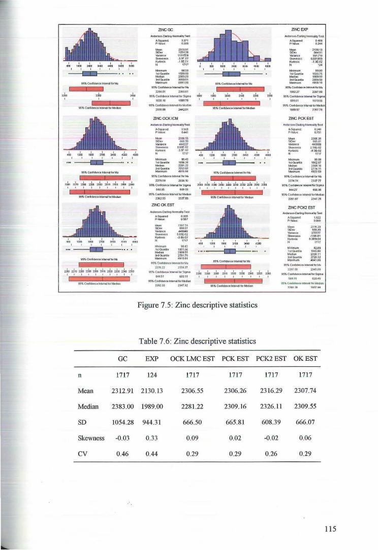
I I """ .. ,. I I

,-. 24~ I I

1- I

I I .,.. .... I I

riD .Jm ~ Jo 2~0 23110 ~ ~ ,k

I I I I I I I J

I I • 20o 4150 I I

ZINCOC

~·l•d 3.571 P~Yifue. 0.000

'"'"" '2313.91 - 1054.28 V.l'ian(e 1111509 SktwnHS -3.1£..02 KLirtosls -1~-01 N 1717

Mnlmum 8600 1st I:Aialtll• 1589.00 MedlM 238300 !kdau.... 305901 ~um 1831.99

85'4 Conld<Mc. lrfth31 roc MJ

2204.01 2363.81

85ft ConW.nu lntflmlllot sqna 1020 18 1090.78

951. COnedenctfn~ foth4t<lfln

2J)() 00 2442-01

ZJNCOCKICM

N!Otft Oft.O.IIU'IO Norme!Jiyltsl

A.$q,l•ed. 0363 P-YIIu.- 0.441

...... ..,, -· .......... -~ H

Mnlmum htOU ... ....... 3«10Ualllla Ms.limum

2300SS ... ,. 444227

88<E-02 -3..5E-02

1717

90.-42 1856.28 228122 2762..82 4915.84

$5'1. ConlldoncalnteMIIIor Ml

2.27500 2338 10

05'11. Coftlldtnte rnlfii'Val tor Sigma

844 »3 68958

85'1 ConlldencetntaMiforMN&n

126133 2331.88

ZINC OK EST

lndefs~o.lng Nonntittlest

ASquand 0305 P."AAtH 0567 - 1:30774 - 66607 ......... -443&116 Sktwn.st 5S3E-02 tQ.Inosls -lf£-02 N 1711

Mnlmum 9042 l iii t OUel1ilt 1851.56

""'"" 2309.55 3f'd0Uif01t :U8170

""""''m 4 915.84

05'1tConMenc.lttteM!lfforMJ

227$.22 233V2l

IS 'I. Coftlidtnct IM.....W b Sqna

144.51 8&913

f5"' COMdtn<'t kl.,. fofMfdan D81.3J 234732

IJ.o -d.. I I

~0 22.~0 2~ mo ~0 73110 TJ~ mo ~ Jso

I ... I

I

""' I

I I

I

'""'

06 .. COnfidence SnlliiMI IOt MJ

I I I I I I I -""' 2315 ""' ""' 1345 2355 I I I I I I I =­-- -~~-

I

""' I

ZINCEXP

/ftdtfSOftoo.lng Notmet.ty Test

AScaua""ct OMQ P.Yalua· 0.:2<4-4

..... so.. V.1Janc. SktwnHS t<tutosls N

Mnlmum tst OJaltlle -3rdOJri• -.um

2130.13 04431

891719 0.331 859 -1.3E.02

ll< .... 153375 1089.00 2859.50 .. 918. 10

OSII.CoMdMce~tort.\.1

1ge227 12i1.00

15,., Conldl-.lnlert'ill b-Si1Jn• 8l0.S1 107008

9s-4Confid..,('fln!01n'tJIOt._VIil

1869 &7 2287 78

ZINC PCK EST

Andlf&On-04111nQ NotmelltfT"I

A.$(JJ•ed. 02o48 P.V.rue 0.151 - 2308.20 ..,., &6581 -. ... .. 33011 Skewness 2.18E·D2 ........ -8.3E-02 N 1111

Mn.mllfl'l .... 1.510Jde 1862.17 -M 23091& ltd0UtJ'I1• 111.4111 Malmum .41912.69

95" Confidence Interval fOf MJ

2274.74 2337 71

os-.. Conftdonce lnuuval lor Sigma

&11427 688.86

95'4 Confidence kllent'lllor Mldi10

1261.87 :2347.16

ZINC PCK2 EST Mdtnoo.o.ting Nonne~a!r Test

ASQu.,.d' 1.122 p.v.tue 0000

..... -Vanence .......... Kurtosis N

hfnimum l t lOUaniil• ........ 3rd0u.-11le Mamum

2310.29 600.30 370137

·U!;.-01 028S42o4

1711

82.69 1~5.00 232611 17:2031 ~1.88

DS-1. ConMencelnteJWtlor Ml

2217 50 n45.09

iS'~. CGnldlnceMtw'tlltor SH}m•

51170 61845

ts,..Centctenulntttwt torMtOten ?111 :)11 ?:\57AA

Figure 7.5 : Zinc descriptive statistics

Table 7.6: Zinc descriptive statistics

GC EXP OCKLMCEST PCKEST PCK2EST OK EST

n 1717 124 1717 1717 1717 1717

Mean 2312.91 2130.13 2306.55 2306.26 2316.29 2307.74

Median 2383.00 1989.00 2281.22 2309.16 2326.11 2309.55

so 1054.28 944.31 666.50 665.81 608.39 666.07

Skewness -0.03 0.33 0.09 0.02 -0.02 0.06

cv 0.46 0.44 0.29 0.29 0.26 0.29

115

•

Next we consider the question of conditional bias by assessing the Q-Q plots

of the grade control data and estimates of each variable for each of the kriging

techniques used. These plots are displayed in Figures 7.6 to 7.10. It is clear from

these that the overe~timation of the mean for the nickel, cobalt, and iron variables has

resulted from significant overestimation of the low values and underestimation of the

high values. Overall nickel and iron appear to be the least affected by conditional

bias. As all of the kriging techniques produced similar estimates for each variable, as

was expected, there is little differellce in the Q-Q plots .

The underestimation of high values is not too marked for nickel for all

techniques except the principal component kriging where only two principal

components were retained. This technique has grossly underestimated the

particularly high values. The full principal component kriging has the best

performance with regard to underestimation of the high values. There has been

significant overestimation of the low values, particularly mound the 5111 to 201h

percentiles. There is little difference between the techniques in the overestimation of

low values although after the 251h percentile principal component kriging performs

marginally better than the others.

For cobalt the underestimation of the high values is significant regardless of

the kriging technique. In this case the principal component kriging (two principal

components) was the worst offender. There has been some overestimation of low

values for this variable, again particularly around the 5th to 20th percentiles. Overall

principal component kriging is marginally better than the other techniques here,

although all perform similarly.

Magnesium has suffered overestimation across all values although the

cokriging estimates perfonn somewhat better than the ordinary kriging estimates

from the 801h percentile. Magnesium was particularly difficult to model with very

erratic semivariograms. Little benefit was gained from examining the other measures

such as the madogram and pairwise relative semivariograms, though these measures

did assist in better detining the ranges of the model. The poor appearance of the Q·Q

plot for this variable indicates that the model has not ade.J.uately captured the erratic

behaviour of this vmiable.

The underestimation of high iron values is not as marked as for the other

variables discussed so far. In this case the principal component kriging method

116

obtained using ~mly two principal components is the worst offender, though certainly

not as significant as seen previously. Ordinary kriging has the best perfonnance from

the 95th percentile. The overestimation of lower values for iron follows a similar

pattem to nickel and cobalt with little difference in techniques.

For zinc the underestimation of the high values is significant regardless of the

kriging technique. Again the principal component kriging (two principal

components) was the worst offender, though only marginally. The best perfonner for

this variable was the ordinary cokriging using the intrinsic correlation model. There

has been some overestimation of iow values for this variable, particularly around the

5th to 15th percentiles. The only technique that differs from the others at the lower end

of the plot is principal componem kriging (two principal components) with

mru.ginally higher overestimation from the lOth to 35tl' percentiles.

117

...... ....... 00

5 10 15 20 25 30

Nickel Grade Control Data

-+- OCKICM

- OCKLMC

- PCK

- OK

--PCK2EST

35 40 45 50

......

...... \0

"l'1 ~-'"I (1)

-....)

-....)

10 I

10 "t:) -0 ..... Cl)

~ '"I

8 CJ E.. .....

~ .. ~

.§ .. rl.)

~ .. -~ ,.Q

= u

6

5

4 -+- OCKICM

--. QCKLMC

......_ PCK 3 --11 - OK

--+- PCK2 EST

2

1

0 ~------~------~----~------~-------,------,

0 1 2 3 4 5 6

Cobalt Grade Control Data

u ~ ~

~ 0

0

T

f

0 0

0 0

0 0

0 0

0 0

~

0 ~

0 ~

0 ~

0 ~

~ ~ ~ ~

N

N

""""" """""

s~ltnnps1[ mn!s~u~uw

Figure 7.8: Q

-Q plots for m

agnesium

0 0 ~

8 ~ 0 0 ~

0 0 N

0 0 """""

0

:3 =

Q -~ =

Q

u ~

"C

f: ~

~ .... riJ

~ ~ =

~ 120

d u ~

-~

f2 ~

~ ~

~ 8 0

0 ~

~

t ' f T

f

0 0

0 0

0 0

0 0

0 0

0 0

0 0

0 0

0\

00

t"'--

\0

l/') ~

M

N

S~JUUI!JS:i[ U

O.IJ

Figure 7.9: Q

-Q plots for iron 0

0 0 ~

0 0 0 ~

0 0 00

0 0 \0

0 0 N

0

121

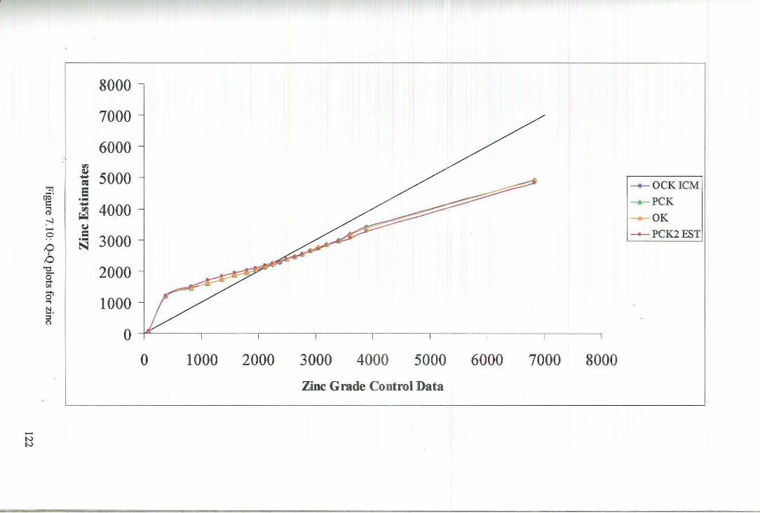
8000

7000

6000 f'-2 ~

"Tj ~ 5000

~- a ·-.., -Cll ~ 4000 :--l - (J

0 = /:) N 3000

I

---+- OCK ICM

---....-- PCK

- OK

- PCK2EST

/:)

'§- I - 2000 [/}

0> .., I 1000 ~-g

0

0 1000 2000 3000 4000 5000 6000 7000 8000

Zinc Grade Control Data

-N N

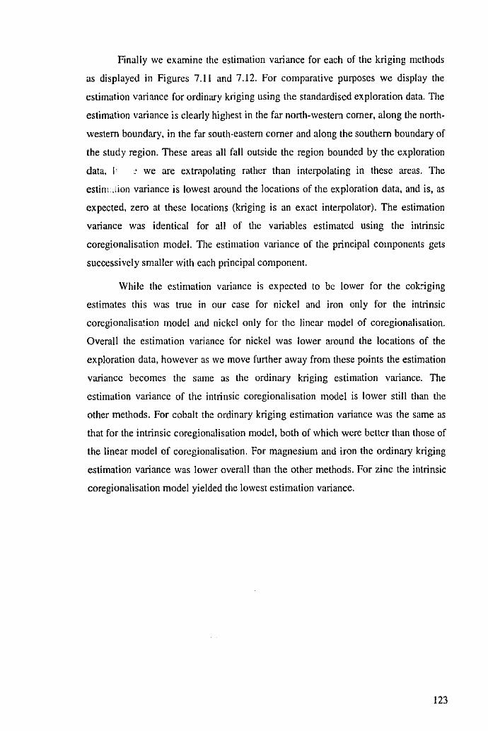
Finally we examine the estimation variance for each of the kriging methods

as displayed in Figures 7.11 and 7.12. For comparative purposes we display the

estimation variance for ordinary kriging using the standardised exploration data. The

estimation variance is clearly highest in the far north~westen comer, along the north­

western boundary, in the far south-eastern comer and along the southern boundary of

the study region. These areas all fall outside the region bounded by the exploration

data, 1· _. we are extmpolating rather than interpolating in these areas. The

estinuion variance is lowest around the locations of the exploration data, and is, as

expected, zero at these locations {kriging is an exact interpolator). The estimation

variance was identical for all of the variables estimated using the intrinsic

coregionalisation model. The estimation variance of the principal components gets

successively smaller with each principal component.

While the estimation variance is expected to be lower for the cok~ging

estimates this was true in our case for nickel and iron only for the intrinsic

coregionalisa!ion model and nickel only for the linear model of coregionalisation.

Overall the estimation variance for nickel was lower around the locations of the

exploration data, however as we move further away from these points the estimation

variance becomes the same as the ordinary kriging estimation variance. The

estimation variance of the intrinsic coregionalisation model is lower still than the

other methods. For cobalt the ordinary kriging estimation variance was the same as

that for the intrinsic coregionalisation model, both of which were belter than those of

the linear model of coregionalisation. For magnesium and iron the ordinary kriging

estimation variance was lower overall than the other methods. For zinc the intrinsic

coregionalisation model yielded the lowest estimation variance.

123

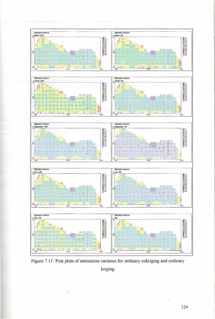
Estimation Variance

~ t-ac:kri·LMC

" . ·

!l '' " ....

E!tilmtionVJrfance ~ Cobalt·LMC

I ,.

EstlllllGon'hllanet o MagllfSIUm • LMC ll . .

Estimation Variance ~lrOn·LMC

:..

- ~ 1o

:;: .. . .. . ,.,

Estimation Variance E; Zinc-OK

•· ....

....

.. ··= · ..

l" w ·­·­·­... .... ,,.,., .... ·­...

. ...

,. --~ --.,

1480

Estimation Variance ~ lron·OK

...

Estimation Variance

!!.

.~ -

5: ...

·.:. : ::. ~ :::: . ~. . .: ..... . ~~ ~ : .. ..... .

1

.. '·'"" ... ·­·-·­·­·­.... ~ . .. ...

~.

~ -----·~ ..

.. ..,

1

.. .. ~ ·­·­... ·­... .... ·-

1

.. · ·~ ... ... . .. . ... ·­.. ~ . ..

....

1

.. .. .. ·­·­... ·­·­·-·­'""

Figure 7.11 : Post plots of estimation variance for ordinary co kriging and ordinary

kriging

124

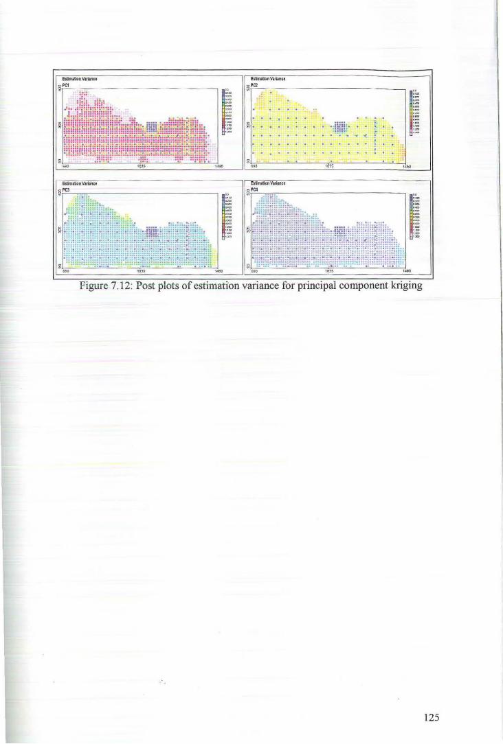
&Jtimlllion v.rtonn ~ PC1

eslimotion ""''"" ~ PCJ

r -·-·-"" ·~ ·-"~ ·-·-

....

r .. ~ ·-... ·-·-·-'"" ... "~ ·-

1400

Eltimalion VarilflCI

~ PC2

I . g.

~ 500

EsUmltion variance

~ PC4

~

'""

1

.. .. ~ ·­·­,.,. ... ·­... ·­... "~

1490

Figure 7.12: Post plots of estimation variance for principal component kriging

.·

125

8 DISCUSSION AND CONCLUSIONS

D~ta collection in the earth sciences is rarely limited to just one variable at

each location. Such is the case in mining, where it is common that each drill core

taken will be sampled for not just the primary variable of interest but also for other

attributes. These secondary variables are often spatidly cross correlated with the

primary variable as well as each other. Hence each of the variables sampled may

contain useful information about the others. Multivariate geostatistics allows us to

exploit the relationships among and between the variables with the aim of improving

their estimates at unsampled locations. This is particularly the case when the primary

variable of interest is undersampled in relation to the secondary variables.

This thesis presented the theory and the process of the modelling and

estimation of spatially dependent multivariate data. These methods were illustrated

by application to a multivariate data set from the Munin Murrin nickel mine near

Laverton in Western Australia. We have demonstrated the use of the classical

multivariate statistical technique principal component analysis in a geostatistical

environment. We have exhibited the development and application of three models of

spatial contin11ity, namely the intrinsic coregionalisation model, the linear model of

coregionalisation and the linear model of regionalisation. We have used each of these

models to estimate values of the attributes at unsampled locations using ordinary

cokriging, principal component kriging and ordinary kriging.

The data suite MM22D used in this study came from an actual mineralisation

and consisted of two data sets, a grade control (exhaustive) data set and an

exploration (sample) data set. As the data ai"e isotopic we did not have the case where

the primary variable is undersampled in relation to the secondary variables. This

would be unrealistic in a mining situation when all data are coming from the same

drill core sDmples. The data suite comprises three dimensional grade and thickness

measurements on eight variables: nickel, cobalt, magnesium, iron, aluminium,

chromium, zinc and manganese. For the purposes of this study the data were

transfonncd to accumulations, hence were considered two dimensional. In order to

demonstrate the different types of models of spatial variability yet remain within the

126

scope of an honours thesis we decided to limit the analysis to two four variable

subsets created from the exploration data. One subset consisted of highly correlated

variables (nickel, cobalt, iron and zinc), the other subset was chosen for the

economic importance of the variables (nickel, cobalt, magnesium and iron).

A detailed exploratory data analysis was carried out on each of the variables

in the MM22DGC and M:M:22DEXP data sets. Overall the exploration data

reproduced the grade control summary statistics well. Cobalt, aluminium,

magnesium and manganese were all strongly positively skewed for both the grade

control and exploration data. It was however decided that a transformation of these

variables was not wmTanted, A principal component analysis was performed on the

MM22DEXP data set and it wus determined (by examining the cross correlograms of

the principal components) that the data were not intrinsically correlated. We then

considered the principal component analysis of the two four variable subsets

M1v122DHC4 and MM22DTOP4. It was determined that the former subset was

intrinsically correlated. In both cases the principal components extracted could be

reasonably well interpreted.

The first estimation technique we investigated was ordinary cokriging. In

order to implement the cokriging algorithm we required a permissible model of the

spatial variability of the variables being estimated. The first model that we

demonstrated was the intrinsic coregionalisation model using the MM22DHC4 data

set. The intrinsic coregionalisation model is a particular example of the linear model

of coregionalisation where all of the sills of the basic scmivariogram models are

proportional to each other. Under the assumption of secondMorder stationarity the

matrix of coefficients was for our data set the correlation matrix. As we were dealing

with standardised data we required that the sills of the basic models summed to one.

The actual modelling process then for this data set was relatively simple in that it

consisted of identifying the basic structures that captured the spatial variability of the

variables and determining their corresponding sills. The conditions for this type of

model though are restrictive and in practice the intrinsic model rarely fits

experimental corcgionalisations (Gooevaerts, 1997, p. 117).

The second model we investigated was the more general linear model of

coregionalisation which was demonstrated using the MM22DTOP4 data set. The

difficulty with this type of model lies not only in the fact that each of the

127

Nv(Nv + 1)/2 (10 in our case) direct and cross semivariogram models must be jointly

inferred, but that each of the coregionalisation matrices must be positive semi­

definite. In order to ensure that the linear model of coregionalisation we were

building was indeed permissible it was necessary to first detennine jointly the basic

set of stn:ctures that best captured the characteristics of the direct semivariograms

(nickel, cobalt, magnesium and iron). It was then necessary to restrict our choice of

structures for the cross semivariograms to those used for the direct ones. Having

obtained a model with a suitable fit on all direct and dross semivariograms it was

necessary to make the coregionalisation matrices positive semi-definite. As we were

dealing with fairly small coregionalisation matrices we did this manually using the

property of diagonal dominance. This process can indeed be tedious, time consuming

and frustrating, and in addition may not be optimal, so for larger coregionalisation

matrices an iterative procedure, such as that outlined in Goovaerts (1997) is

recommended.

The estimates obtained from cokriging using both models were compared to

the grade control data, which we considered to be reality for this study. We

compared the postplots of the estimates with those of the grade control data. In both

cases the cokriging estimates captured the overall spatial distribution of the grade

control data. In addition we compared the descriptive statistics of the estimates

obtained for each variable with those of the grade control data. In all cases the mean

and median of the estimates has over estimated that of the exploration and grade

control data. The only exception is zinc where the mean and median of the estimates

were close in value to those of the grade control data. The standard deviation of the

estimates from both cokriging cases was considerably lower than that of the grade

control and exploration data, which is an indication of the smoothing of the

variability due to the cokriging process. The residual analysis for both cokriging

methods showed the residuals to be approximately nonnally distributed with the only

exception being cobalt. In both cases the histograms of the cobalt residuals were

negatively skewed.

The second estimation technique we investigated was principal component

kriging. The overriding assumption of this technique is that the data are intrinsically

correlated. Hence we used the principal components extracted from the MM22DHC4

data set for this method. In order to perfonn the ordinary kriging of the principal

128

component scores we were required individually model the spatial variability of the

principal component scores using a linear model of regionalisation. We then used

ordinary kriging to estimate the principal component scores at unsampled locations

and recalculated the estimates of the original variables using the corresponding

coefficients from the matrix of eigenvectors. In addition to estimating the variables

using all four principal components we krigccl only the first two (which accounted

for 89% of the total variability of the original data) and calculated our estimates

using only these.

The estimates obtained from both forms of principal component kriging were

compared with the grade control data. Overall, for all variables, the post plots of the

estimates in both cases have reproduced those of the grade control values reasonably

well. In addition the descriptive statistics of the estimates were compared to those of

the grade control data. Once again the mean and median of the nickel, cobalt and iron

estimates have overestimated those of the grade control data while those for zinc arc

close in value. The standard deviation is considerably lower for all four variables

estimated than for the grade control data. The residual analysis confirmed that the

residuals were approximately nonnally distributed with cobalt once again being the

only variable to not conform this. What is most significant here is that the estimates

obtained by using only the first two principal components are remarkably close in

value to those obtained using all four.

The ordinary kriging estimates were also obtained. for the nickel, cobalt,

magnesium, iron and zinc variables. As for the individual principal components this

involved obtaining a linear model of regionaHsation for each of the variables

individually. As the data we used were isotopic it was anticipated that the estimates

obtained in the ordinary kriging method would be similar to those obtained from the

other methods. This was indeed the case with all estimates for each variable being

almost identical. In particular in the case where the data are intrinsically correlated

the ordinary cokriging and ordinary kriging estimates are expected to be equivalent.

This was especially reflected in the Q·Q plots where the dark blue ordinary cokriging

(intrinsic coregionalisation model) line is completely covered by the orange ordinary

kriging line.

The only significant difference between methods was for magnesium where

the ordinary cokriging estimates slightly improved on the overestimation experienced

129

across all values for this variable. The only other major difference between methods

was that estimates obtained from the principal component kriging using only the first

two principal components consistently underestimated the higher values to a greater

extent than the other methods.

In conclusion then the estimates obtained from the various kriging methods

have confirmed that in the case of isotopic data, in particular when the data are

intrinsically correlated, there is little practical benefit to be obtained from cokriging.

The true benefits of cokriging are only fully appreciated when the primary variable is

undersamplcd in relation to the secondary variables and those secondary variables

are well correlated with the primary variable. A combination of technological

advances has lessened the practical and computational disadvantages of multivariate

geostatistical methods. There have been marked improvements in the development of

geostatistical software that allows interactive modelling simultaneously of both direct

and cross semivariograms. In addition there are now available automated iterative

procedures, such as those offered in the software package AGROMET, for

determining the positive semi-definite coregionalisation matrices. With increased

processing power the computational expense solving of large kriging matrices is

becoming less of an issue.

This study also raised the question as to the benefits of using principal

component kriging. As this technique relies on the data being intrinsically correl~ted

we are able to individually model and krige the principal components. However if

the data arc intrinsically correlated then there is no benefit in using cokriging as these

estimates are equivalent to the kriging estimates. Either way we are required to

individually model and krige either Nv variables or Nv principal components. From

the estimates obtained in this study using principal component kriging with both four

and two principal components there was little difference in the results. This would

suggest then that the renl benefit in using principal component kriging is when we

are able to reduce the number of principal components retained, effectively reducing

the number of variables to be modelled and estimated. To be of real benefit however

one would want the number of principal components to be retained to be

significantly less than the number of original variables, yet still account for the

majority of the variability of the original data.

!30

REFERENCES

Afifi, A. A., & Clarke, V. (1996). Computer-Aided Multivariate Analysis. Boca

Raton: Chapman & Hall.

Annstrong, M. (1998). Basic Linear Geostatistics. Berlin: Springer-Verlag.

Bleines, C., Deraisme, J., Geffroy, F., Jeannee, N., Perseval, S., Rambert, F., Renard,

D., & Touffait, Y. (2001). !SA TIS: Software Manual (3rd ed). Paris:

Geovariances.

Chiles, J.-P., & Delfiner, P. (1999). Geostatistics: Modelling Spatial Uncertainty.

New York: Wiley-Interscience.

Datta, B. N. (1995). Numerical Linear Algebra and Applications. Pacific Grove:

Brooks/Cole Publishing Company.

Deutsch, C. V.,& Journel, A. G. (1998). GSLIB: Geostatistical Software Library and

User's Guide (Seconded.). New York: Oxford University Press.

Dun ternan, G. H. (1984). Imroduction to Multivariate Anolysis. Beverley Hills: Sage

Publications, Inc.

Goovaerts, P. (1997). Geostatistics for Natural Resources Evaluation. New York:

Oxford University Press.

Goulard, M., & Voltz, M. (1992). LinearCoregionalization Model: Tools for

Estimation and Choice of CrossVariogram Matrix. Mathematical Geology, 24

(3), 269-286.

Hotel ling, H. (1933). Analysis of a complex of statistical variables into principal

component;;, Joumal of Educarional Psychology (24), 417-441.

Isaaks, R. M. & Srivastava, E. H. (1989). An Introduction to Applied Geostatistics.

New York: Oxford University Press.

131

Johnson, R. A. & Wichern, D. W. (2002). Applied Multivariate Statistical Analysis

(5th ed.). New Jersey: Prentice Hall.

Journel, A. G. & Huijbregts, C. J. (1978). Mining Geostatistics. London: Academic

Press Inc.

Kanevski, M., Chernov, S. & Demyanov, V. (1998). 3PLOT [Computer Software].

Moscow: ffiRAE.

Lay, D. C. (1997). Linear Algebra and its Applications. Reading: Addison-Wesley.

Matheron, G. (1970). The Theory of Regionalised Variables arzd its Applications.

Fasiscule 5, Les Cahiers du Centre Morphologic Mathematique, Ecole des

Mines de Paris, Fontainebleau.

Murphy, M., Bloom, L. M., & Mueller, U. A. (2002). Geostatistical Optimisation of

Mineral Resource Sampling Costs for a Western Australian Nickel Deposit.

IAMG 2002: Proceedings of the 8 11 Annual Conference of the International

Association for Mathematical Geology. (Volume I, pp. 105-110).

Pannatier, Y. (1996). VARIOWIN: Software for Spatial Data Analysis in 2D

[Computer software]. New York: Springer-Verlag.

Pearson, K. (1901). On lines and planes of closedst fit to systems of points in space.

Philosophical Maagazine, 6(2), 559-572.

Wackernagel, H. (1998a). Multivariate Geostatistics. Berlin: Springer-Verlag.

Wackemagel, H. ( 1998b ). Principal Component Analysis for autocorrelated data: a

geostatistical perspective. (N-22/98/G). Fontainebleau: Centre de

Geostatistique. Retdeved 5 November, 2002 from

http://citeseer.nj.nec.com/cache/papers/cs/5260/ftp:zSzzSzcg.ensmp.frzSzpub

zSzhanszSzpcaeof.pdf/wackcmagel98princip&l.pdf

132

APPENDICES

133

APPENDIX A: PRINCIPAL COMPONENT ANALYSIS OF

TRANSFORMED DATA

Here we consider the appropriateness of the transfonnation of the strongly

skewed variables cobalt, magnesium, aluminium and manganese. We firstly review

the eigenanalysis of the original data as covered in section 3.4.1

Table Al: Eigenanalysis of the correlation matrix of MM22DEXP

Eigenvalue 4.293 1.!84 1.047 0.607 0.326 0.279 0.154 0.109

Proportion 0.537 0.!48 0.131 0.076 0.041 0.035 0.019 0.014

Cumulative 0.537 0.685 0.815 0.892 0.932 0.967 0.986 1.000

Variable PC! PC2 PC3 PC4 PC5 PC6 PC7 PCB

Nl -0.409 0.082 0.133 -0.277 -0.401 -0.739 0.096 0.121

co -0.407 0.153 0.368 0.201 -0.258 0.233 -0.213 -0.685

MG -0.180 0.650 -0.365 -0.571 0.186 0.195 -0.063 -0.095

FE -0.416 -0.288 -0.168 -0.004 0,343 0.036 0.730 -0.253

AL -0.243 0.301 -0.565 0.698 -0.062 -0.154 -0.073 0.106

CR -0.340 -0.422 -0.331 -0.201 -0.510 0.459 -0.130 0.261

ZN -0.404 -0.320 0.007 -0.055 0.582 -0.172 -0.599 0.065

MN -0.351 0.305 0.507 0.162 0.130 0.308 0.169 0.600

134

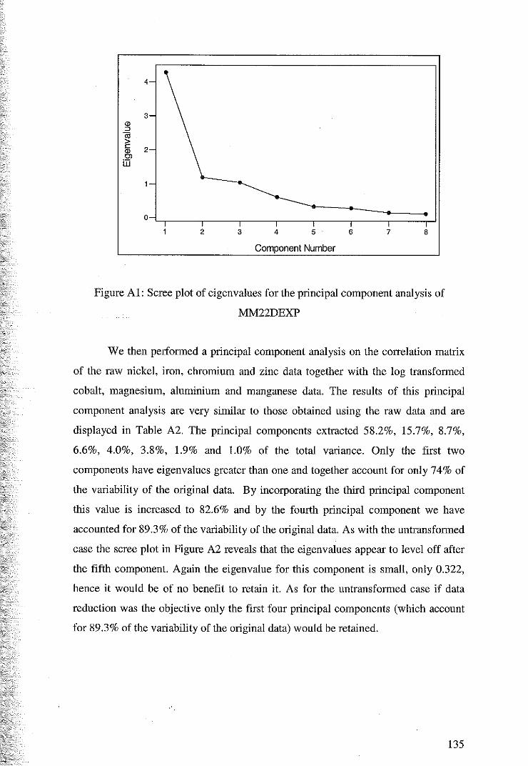
4-

3-<J) ::l

Cij > c 2-<J) O'l [j]

1-

0 I I

~ ~ ~ ~ ~ ~ 1 2

Component Number

Figure AI: Scree plot of eigenvalues for the principal component analysis of

MM22DEXP

We then performed a principal component analysis on the correlation matrix

of the raw nickel, iron, chromium and zinc data together with the log transformed

cobalt, magnesium, aluminium and manganese data. The results of this principal

component analysis are very similar to those obtained using the raw data and are

displayed in Table A2. The principal components extracted 58.2%, 15.7%, 8.7%,

6.6%, 4.0%, 3.8%, 1.9% and 1.0% of the total variance. Only the first two

components have eigenvalues greater than one and together account for only 74% of

the variability of the original data. By incorporating the third principal component

this value is increased to 82.6% and by the fourth principal component we have

accounted for 89.3% of the variability of the original data. As with the untransformed

case the scree plot in Figure A2 reveals that the eigenvalues appear to level off after

the fifth component. Again the eigenvalue for this component is small, only 0.322,

hence it would be of no benefit to retain it. As for the untransformed case if data

reduction was the objective only the first four principal components (which account

for 89.3% of the variability of tbe original data) would be retained.

135

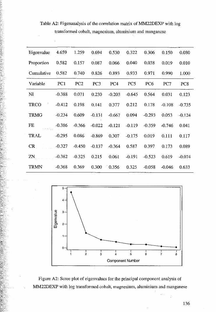
Table A2: Eigenanalysis of the correlation matrix of MM22DEXP with log

transformed cobalt, magnesium, aluminium and manganese

Eigenvalue 4.659 1.259 0.694 0.530 0.322 0.306 0.150 0.080

Proportion 0.582 0.157 0.087 0.066 0.040 0.038 0.019 0.010

Cumulative 0.582 0.740 0.826 0.893 0.933 0.971 0.990 1.000

Variable PC1 PC2 PC3 PC4 PC5 PC6 PC7 PC8

NI -0.388 0.071 0.230 -0.203 -0.645 0.564 0.031 0.123

TRCO -0.412 0.198 0.141 0.377 0.212 0.178 -0.108 -0.735

TRMG -0.234 0.609 -0.131 -0.667 0.094 -0.293 0.053 -0.124

FE -0.386 -0.366 -0.022 -0.121 -0.119 -0.359 -0.746 0.041

TRAL -0.295 0.086 -0.869 0.307 -0.175 0.019 0.111 0.117

CR -0.327 -0.450 -0.137 -0.364 0.587 0.397 0.173 0.089

ZN -0.382 -0.325 0.215 0.061 -0.191 -0.523 0.619 -0.074

TRMN -0.368 0.369 0.300 0.356 0.325 -0.058 -0.046 0.633

5

4-

(]) 3-::J (ij > c (]) Ol w 2-

1-

0-I I I l ~ 1 2 3 5 7 8

Component Number

Figure A2: Scree plot of eigenvalues for the principal component analysis of

MM22DEXP with log transformed cobalt, magnesium, aluminium and manganese

136

------------------------- -

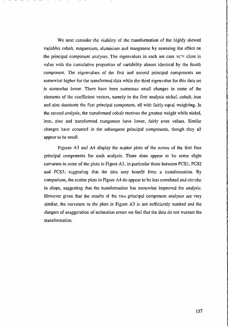
We next consider the viability of the transfonnation of the highly skewed

variables cobalt, magnesium, aluminium and manganese by assessing the effect on

the principal component analyses. The eigenvalues in each are case vcv close in

value with the cumulative proportion of variability almost identical by the fourth

component. The eigenvalues of the first and second principal components are

somewhat higher for the transfonned data while the third eigenvalue for this data set

is somewhat lower. There have been numerous small changes in some of the

elements of the coefficient vectors, namely in the first analysis nickel, cobalt, iron

and zinc dominate the first principal component, all with fairly equal weighting. In

the second analysis, the transfonned cobalt receives the greatest weight while nickel,

iron, zinc and transformed manganese have lower, fairly even values. Similar

changes have occurred in the subsequent principal components, though they all

appear to be small.

Figures A3 am! A4 display the scatter plots of the scores of the first four

principal components for each analysis. There does appear to be some slight

curvature in some of the plots in Figure A3, in particular those between PCS I, PCS2

and PCS3, suggesting that the data may benefit from a transfonnation. By

comparisor., the scatter plots in Figure A4 do appear to be less correlated and circular

in shape, suggesting that the transfonnation has somewhat improved the analysis.

However given that the results of the two principal component analyses are very

similar, the curvature in the plots in Figure A3 is not sufficiently marked and the

dangers of exaggeration of estimation errors we feel that the data do not warrant the

transfonnation.

137

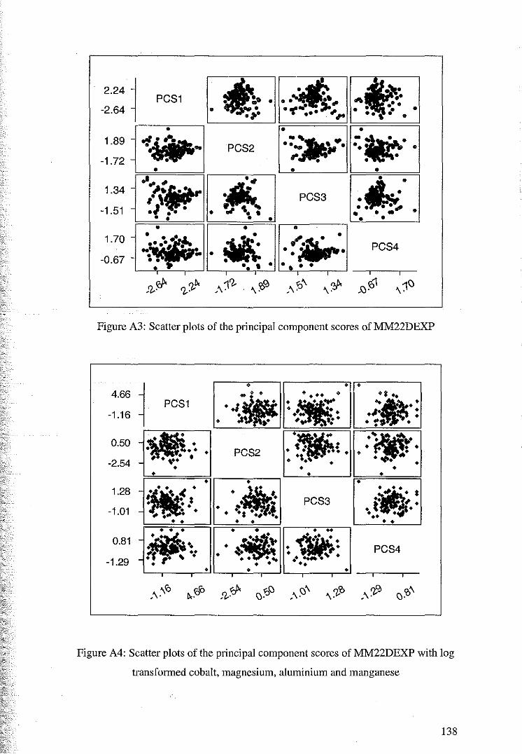
2.24

-2.64

1.89

-1.72

1.34

-1.51

1.70

-0.67

j

-

PCS1

0 ... . .. 0

0 .. "' "' ..... ~ ,., .I ...

• 0

• ... .... , . ... .. •• •

• •~·. .,.. PCS2

. ., -Aif.,

• .., .. • •

•

~-• •• •

4 ~0 "" .0 . . ;_., •• •<t• 0 "' 0 0 • oO ,. 0" •

• 0

-~ -~0 .... . •. •• • • ~ ,. • 0 0

• • •• PCS3 : , • • • • • •

0 . .... • • • • • •••

PCS4

'

Figure A3: Scatter plots of the principal component scores of MM22DEXP

~ • • •

4.66 ·J· ••• .: •.. PCS1 -1.16 . .... . .. .t• • • • • •• # ••• . :• . • •

·~ ·~· 0.50 -·· . •: . ~ • • • • • • PCS2 • •• -2.54 # • ~· • • •

., . . • •• • - . • • • • • • • • • •

1.28 --· ·~·· • ... • *

• • ·* l! .. PCS3 .i •. · -1.01 - ~ ...... • • •• +# ~ • • •• • • • • • •

• • • • • • .. -- ... • 0.81 • • •• ol . .,. . PCS4 #. •• -·! ,.. ~ . • . ....... ~. -1.29 .... ••• • • •

' ' ' ~.~ro 1J..roro ~().

,?,· \)~\) ~5J~ ~ './.-'0 ~'./.-~ '0~ \).

Figure A4: Scatter plots of the principal component scores of MM22DEXP with log

transformed cobalt, magnesium, aluminium and manganese

138

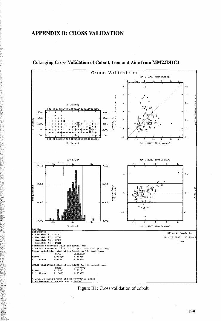
APPENDIX B: CROSS VALIDATION

Cokriging Cross Validation of Cobalt, Iron and Zinc from MM22DHC4

500.

400.

300.

200.

100.

0.15

0.10

0.05

0. 00

Isatis data/stexp

Variable

Cross Validation

X (Meter)

600 700. 800 900 ~0001100120013001400

+ ' .

+++++•~ + ++i·+-+ + r + r + + + + +il+ ... , r • + ++++++r+e ++~-t:t.•• +++++++++••+,+tl + +++++++·+++1 ~+ .... ,++

+ + • + t 600.700.800 900~0001100120013001400.

X (Meter)

{Z*-Z) /S*

(Z*-Z) /S*

" ""

500.

400.

3oo.

200.

100.

0.15

0.10

0. 05

0. 00

• " ' ' w ~::: ' " ' ' 0 ' e-" '~ '

4.

3.

2.

1.

0.

-1.

Z* : STCO (Estimates)

·'r·--~-~1-----"ot·----1~----"'r·----3~-----•'r·,

•

•

• ••

+

4.

3.

2.

1.

0.

-1.

-2 --2,'".----,1".--~0~-----~1".---,2"-----~3-.--~.·-.J-2 . Z* : STCO (Estimates)

Z* : STCO (Estimates)

-1. 0. 1

• 5. 5 .

• • •

0. 0.

• • I •

-5. -5 .

• 1. 0. 1. 2. 3.

Z* ; STCO (Estimates)

Ellen M. Bandarian

Variable " "co May 13 2003 13:29:45 - Variable " STFE - Variable " STZN Standard Parameter File for Model: hc4 Standard Parameter File for Neighborhood: neighborhood Cross validation statistics based on 124 test data

Me= Variance Error 01820 1.24065 Std. Error 01552 2. 56868

Cross validation statistics based on 112 robust data Mean Variance

Error 0.12837 0.63143 Std. Error 15833 1.25607

A data is robust when its Standardh;ed Error lies between -2.500000 and 2 500000

Figure B 1: Cross validation of cobalt

ellen

139

500.

" 400.

' " ~ 300.

" 200.

100.

I.satis

Cross Validation

X (Meter)

600 700 800. 900 .10001100120013001400.

' + +· + + + ·+ +++++++ -1- ++1_+-+ + + + + + -1- + + +:utli+ ++ + + ++++++++++·~~W++-4c •e. + + + + +++4111++++ ++ ··:+ + ++++++++++·~+++··-~·+

t+ + ' ++ 600.700.800 900 U001100120013001400.

X {Meter)

(Z*-Z)/S*

(Z*-Z)/S*

o;

' " • ' ~

500. /! • • 400. '~

300. " ~-0

200. ~

100.

0.15

0.10

0. 05

0. 00

Z* STFE (Estimates)

-2. -L o. L 2.

3.

2.

1.

0.

-1.

-2.

Z* STFE (Estimates)

Z* STFE (Estimates)

-2. -1. 0. L

5.

0.

-~H :· + ~ -f .~-~~~4!~-~ ++ ++

-5.

• -2. -1. 0. 1.

,. STFE (Estimates)

3.

3.

" 2.

• 8

L " " 0.

~ 0

• " -1. ' ,._

-2.

3.

-5.

2.

data/stexp Variable " STNI

Ellen M. Bandarian

Variable " STCO - Variable #3 STFE - variable " STZN Standard Parameter File for Model: hc4 Standard Parameter File for Neighborhood: neighborhood Cross validation statistics based on 124 test data

Error Std. Error

Mean 0.01315 0.01033

Variance 0. 65802 1. 54736

Cross validation statistics based on 118 robust data

Error Std. Error

Me~

0. 00384 0. 01486

Variance 0. 45980 0. 87059

A data is robust when its Standardized Error lies between -2.500000 and 2.500000

Figure B2: Cross validation of iron

May 13 2003 13 28:53

ellen

140

Cross Validation

X (Meter)

600 700.800 900 ~0001100120013001400.

500. t 500.

+ ;; 400. + + + + + 400.

• +H·++++ ' ++~+ " 300. + + + + + + + + + +~~t ++-: + + 300. ! +++++++++·I· ++-P--• 0 +++++++•++++++-++ ,. 200. 200.

+++++-~+·f-t+++++ ++ 100. +• + + +r 100.

600.700.800 900 ~0001100120013001400.

X (Meter)

(Z*-Z) /S*

0.125 0•.125

0.100 0.100

• • ., 0

0. 075 0. 075 ' • • • " • 0. 050 0. 050

0.025 0.025

0. 000 0. 000

(Z*-Z)/S* Isatis data/ste:xp - Variable " STNl - Variable " STCO - Variable " STFE - Variable " STZN Standard Parameter File for Model: hc4 Standard Parameter File for Neighborhood: neighborhood Cross validation statistics based on 124 test data

Error Std. Error

Mean 0. 01876 0.01526

Variance 0. 64322 1.50370

Cross validation statistics based on 119 robust data

Error Std. Error

Mean 0. 03477 0.04257

Variance 0.50105 0.97769

A data is robust when its standardized Error lies between -2.500000 and 2. 500000

-2.

3.

• 2.

" rl • ' • 1.

' ~ • 0.

" "~

" -1. ~" ' ~

-2.

-2.

5.

" " ' ' -~::: 0 • ' " ' '

"'" 0 '

""" + '~ ' +

-5.

,. STZN (Estimates)

-1. o. 1. 2. 3.

3.

• +

* 2. + + ·!'- + + ++ • o~*-Wt.t 1. + -1-- ++ :j::

-t:t:'nr-P~" ++ J,t ·1: 'I+ -1+

·> -~-4~f-~ + 0.

+ +· - . 'f- :t •

t '/'+, -1. ++11 * "+ ++

++ • ,. + +

" .. -2.

-1. 0. 1. 2. 3.

,. STZN (Estimates)

Z* STZN (Estimates)

1. 0. 1. 2

5.

• •

+ +· + + ++ + + +

+· r++-:tbt+ ++ + + t- '~ ~~-ttf.i'f ·t:l- + + .,

++ t "'!: '•+~; +/p + .. + -tfl.-~+ .. 1 + +~. ~~ --»t-+t * + +

+· +

o.

• '

. -5 .

-1. 0. 1. 2.

STZN (Estimates)

Ellen M. Bandarian

"

-8

" z 8 8 ' ' ' ' ~

" ' ' "

May 13 2003 13;29:18

ellen

Figure B3: Cross validation of zinc

141

Cokriging Cross Validation of Cobalt, Magnesium and Iron MM22DTOP4

Cross Validation

.. ' " • ,

X (Meter) • 600.700.800 900 j_Q0011001200 13001400. ' ~

500. 500. 0 + u

;; 400. + ' ' 400. ... ~

'. + + I·+· t+ • + + + + • .. " 300. ' l- + + + ·1- + + + +tl+ I ,+ • + -f. 300. ~ ~-++ + f + + + +. + + + + * i +. 0

" 200. ~+++++-f-++0+-f-++ ++ 200. ~ t+t+++++++++++,++

100. t• • + +t 100.

600.700 800. 900 j_QQ01100120013 001400.

X (Meter)

(Z*-Z)/S*

0.15 0.15

" • • 0.10 0.10 " . ·o 0 w

" ~::: ' • 0 " & ' ' • " e·" " 0 ~ • "

0. 05 0. 05

0. 00

(Z*-Z) /S* Is a tis data/stexp - Variable " '™' - Variable " STCO - Variable " STMG - variable " STFE Standard Parameter File for Model: top4 Standard Parameter File for Neighborhood: neighbourhood top4 Cross validation statistics based on 124 test data

Error Std. Error

Mean 0. 02044 0. 02028

Variance 1.14637 1.95856

Cross validation statistics based on 115 robust data

Error Std. Error

Mean 0.14843 0.17417

Variance 0. 60231 0.97074

A data is robust when its Standardized Error lies between -2.500000 and 2.500000

. . 3.

2.

1.

0.

-1.

-2

5.

0 .

-5.

-2 .

-2.

,. ' STCO (Estimates)

-1. 0. 1. 2. 3.

•

• .-+

.I":~+ + +

+ij.. '1{. '' +-++· ift.fH+

.;t t+ * + + +"' .+· +• + ... ;t;+~1i"* -· . +/It- + +

~-·ij<l- 4+ -t~~rf- ++

-1. 0. 1. 2. 3. ,. ' STCO (Estimates)

Z* : STCO (Estimates)

1. 0. 1. 2.

1-+ + + + t-·lf ·,;~1f-t "t ·tlf~~:t·l~. -~ .. . -tt +

?t•tot *{ + Ji,; ++-t "*+

+ t- ~.tt +

••• • • •

• 1. 0. 1. 2.

Z* : STCO (Estimates)

4.

4.

3.

•

. . 3.

2.

1.

0.

-1.

_,.

5.

"

-" n 0

;:; 2 0

• ~

' ~

N

' ' 0. ~

-5 .

Ellen M. Bandarian

May 19 2003 10 54:53

ellen

Figure B4: Cross validation of cobalt

142

Cross Validation Z* STMG (Estimates)

;;

' " • , X (Meter)

' 600 700 BOO 900 ~000H001200l3001400. ' ~ + 500. 500.

+ 0

• . 400 . "~ H H + ·• + • •+•· i: .. +• + + + + + + 1·-mtl+ + + t +e 300. ~" ++ . + • + . + +++-t,.l·+ ' ++ + • + ' • + +++++. 200 . ~

;; 400.

' " 300. ~

" 200. + ++++ • + + + ' + • + ,. t •

t + +; 100. 100.

600.700.800 900 ~0001100120013001400.

X (Meter)

(Z*-Z)/S*

0.15 0.15

' • ' 0.10 0.10 " . " ' m g ~::: ' ' " i\ ' ' 0 •

' e-N

" '~ • ' 0. 05 0. 05

0.00 0.00

(Z*-Z)/S* Isatis data/stexp

Variable " STN' Variable " STCO

. Variable N3 STMG - Variable .. STFE Standard Parameter File for Model: top4 Standard Parameter File for Neighborhood: neighbourhood top4 Cross validation statistics based on 124 test data

Error Std. Error

··~ -0.02439 -0.02089

Variance 0. 76237 1.48314

Cross validation statistics based on 116 robust data

Error Std. Error

Mean 0.02676 0.04236

Variance 0. 32645 0.76904

A data is robust when its Standardized Error lies between -2.500000 and 2. 500000

5.

4.

• 3.

8. .++

++ +

1.

;

0.

-1.

8' ' STMG

,. ' """G

1. 0.

5.

4.

3.

8. t + +-* + +

1. ·l:FI·~·W++

0. ~;;~!+ * +f~"'l.ll't

-1. "'+ ++ -2. ++ + +

-3. •• -4.

-5.

1. 0.

,. ' STMG

Figure B5: Cross validation of magnesium

5. . . "

3. m

~ " 8. ;:; 8 ' 1.

' ' ~ ' • 0. ~

• -1.

(Estimates)

(Estimates)

1. 8.

5. .. • • 3.

2. +

+ 1. 'i 0. ' ~

+ + -1. ~

+ -2.

-3.

-·. -5.

1. 2.

(Estimates)

Ellen M. Bandarian

May 19 2003 10:55 27

ellen

143

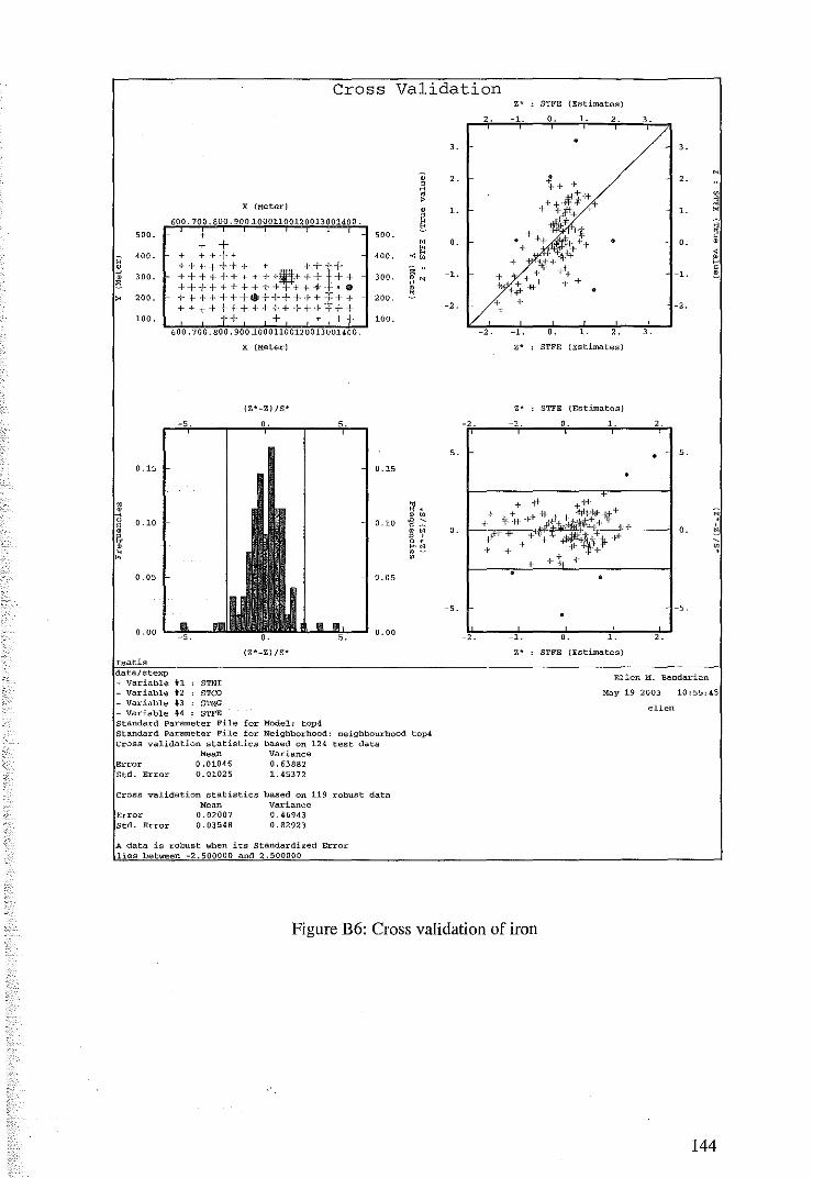
Cross Validation ,. STFE {Estimates)

-2. -1. 0. 1. 2. 3 .

• 3. 3.

' 2. {+ + 2. , H

~ ¥+* ~

++·i t + ~ X (Meter)

' 1. + +* - 1. " 600 000 800 900 ~0001100120013001400 ' "\'+ ;:; t 1!!11 +

500. + ' 500. + + 2 + • 0. ++~.l" • 0. ' + • + +

" 400. + ++++ 400. "~ +-4r:lt ~

+f+++H· • ++rl- + -~+ + e

' .. ' " 300. ++++++++++,+++ ++ 300. -1. + + ~ -!--+ + -1. ,.. ' ~" !'; ++++++++++ + -1--t:< •• ' #* + • " 200. ·i··++++++ID++++++ -++ 200. !!.

+ + + +--+ + + + -I-++ + + +. ~ + + -2. l· +· -2. + 100. ·i· ·I· + • + -i: 100.

600. 700. 800. 900..1000110012 0013 001400. -2. -1. 0. 1. 2. 3.

X (Meter) ,. STFE (Estimates)

(Z*-Z)/S* STFE (Estimates)

-2 - 1 1

' 5. • 5.

0.15 •

+ -!+- + +1-• ' " ~ 0.10

+ :If.~;-+ -{+ -itJol-+tf-iij:+

-I-+ Jl·~+tt;tttP.t+ + .. " ' ' N

!; ~

0.05

0. 00

Isatis data/stexp

Variable #1 STNI Variable #2 STCO

- Variable JlJ STMG - Variable #4 STFE

(Z*-Z) /S*

standard Parameter File for Model: top4 Standard Parameter File for Neighborhood: neighbourhood top4 cross validation statistics based on 124 test data

Error Std. Error

Mean 0.01046 0.01025

Variance 0. 63882 1.45372

Cross validation statistics based on 119 robust data

Error std. Error

Mean 0 02007 0 03548

Variance 0. 46943 0. 82923

A data is robust when its standardized Error lies between -2.500000 and 2.500000

0. ;f ·f·

-5.

2.

0. ~· +'''+ + .;iilili..)\.> } -f+

+ -11- '-1-+ + + + ~t- ·I· . •

- 5. . 1. 0. 3. 2

STFE (Estimates)

Ellen M. Bandarian

May 19 2003 10:55 45

ellen

Figure B6: Cross validation of iron

144

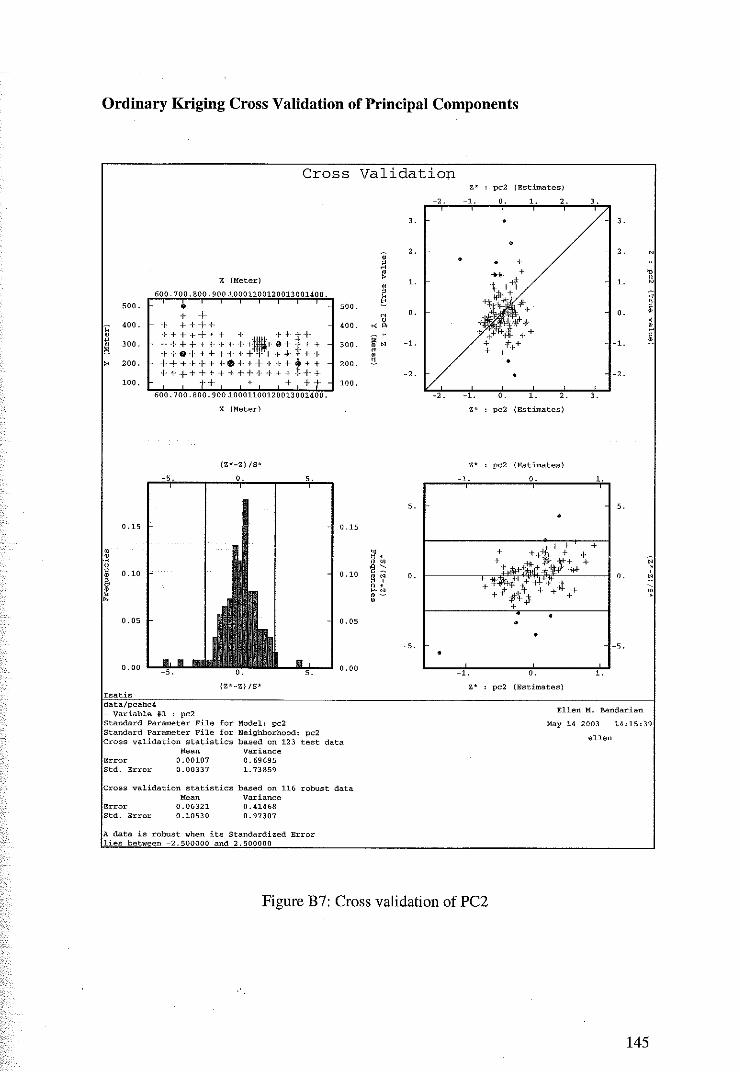
Ordinary Kriging Cross Validation of Principal Components

Cross Validation ,. pc2 (Estimates)

-2. -L 0. L 2.

3.

• .. 2 .

' " • X (Meter) >

' L

600 700.800 900 ~0001100120013001400. ' 500. • 500. ~

0. + + M 0

-,; 400. + ++++ 400. "" ' +++++· + I I f f f w~ " 300. +++++ f ' ' 1-+lt •+ + t 300. -L g; +·+•+ ·I " ++ 1+ +t-t- ~1 ' >< 200. ++++++ 1·0+ ++ +++t++ 200. "- • +·1·--f-++++++++ + + + . ·+ + -2. • 100. <-+ + + +t 100.

600.700. BOO 900 ~0001100120013001400. -2. -L 0. L 2.

X (Meter-) ,. pc2 (Estimates)

(Z*-Z) IS* Z* : pc2 (Estimates)

-L o.

5.

• 0.15 0.15

" . " ' w ~ '

0.10 • ;; 0. , ' 0 . e-" '-'

' ' '0 0 c 0.10 ' il ' k •

+ + . + ++) + + ' +1- t'\1'1+ + 'Ul+ j;\;;Jt:;; .. . . Jt+ ~~+ 'if., -~+ +"it + ... "!= + .. + +--~'f~-t- + +

+ 0. 05 0. 05 • •

• -5.

• 0. 00

L 0.

{Z*-Z) IS* pc2 (Estimates) Isatis

3.

3.

2.

L

0.

-L

-2.

3.

L

5.

+

0.

-5 .

L

" ~ ;; 2 ' ' e c ~

~ ' "

w .

data/pcahc4 - Variable il : pc2 Ellen M. Bandarian

Standard Parameter File for Model: pc2 Standard Parameter File for Neighborhood: pc2 Cross validation statistics based on 123 test data

Error Std. Error

Mean 0. 00107

00337

Variance 0.69695 1. 73859

Cross validation statistics based on 116 robust data

Error Std. Error

Mean 0. 06321 0.10530

Variance 0.41468 0. 97307

A data is robust when its Standardized Error lies between -2.500000 and 2.500000

Figure B7: Cross validation of PC2

May 14 2003 14 15:39

ellen

145

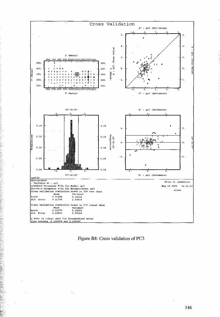
Cross

X (Meter)

600 700.800 900 ~0001100120013001400.

500. T ., 500.

+ +

" 400. + +· +· ++ 400.

• + f· +·++++ + ++ •• " 300. ++ ++++++++.,!-++.++ 300. • 1l + + ++++++++ +++ +$-

" 200. I· -1- + + + +· + + + • + + +·+. + + 200. + + + + ., f++++++·++ ; + +

100. '

·f· f· + ,+ •· ·f 100.

600.700 800.900 ~0001100120013001400.

X (Meter)

(Z*-Z) /S*

0. 20 0.20

• 0.15 • ·o 0.15

" ' • • • 0.10 H 0.10 •

0.05 0. 05

0. 00 0. 00

(Z*-Z) /S* Isatis data/pcahc4 - Variable #1 : pc3 Standard Parameter File for Model: pc3 Standard Parameter File for Neighborhood: pc3 Cross validation statistics based on 124 test data

Error Std. Error

Mean 0 01006 0 01740

Variance 0. 34312 2. 35414

cross validation statistics based on 114 robust data

Error std. Error

Mean 0. 01059 0. 03801

Variance 0.14802 0.93526

A data is robust when its Standardized Error lies between -2.500000 and 2. 500000

Validation

-1. 3.

2. • ' rl

' ' • 1.

' ~ • ~

><A 0.

~N " ' ~ -1.

-1.

5.

• " ' ' m

~ ' ' " 0.

' ' 0 ' e·" : ~

,. ' pc3 (Estimates)

0. 1. 2.

•

+

•

.. • •

0. 1. 2.

,. ' po3 (Esthuates)

Z* : pc3 (Estimates)

0.

++ + +"!j;l},

. .. +

... +

+ t

1.

3. 3.

2. " " ~

1. 8 2 ' ' 0. ' ' ~

-1.

3.

5.

0.

•• -5. -5.

• 1. 0. 1.

Z* : pc3 (Estimates)

Ellen M. Bandarian

May 19 2003 12:ll:U

ellen

Figure B8: Cross validation of PC3

146

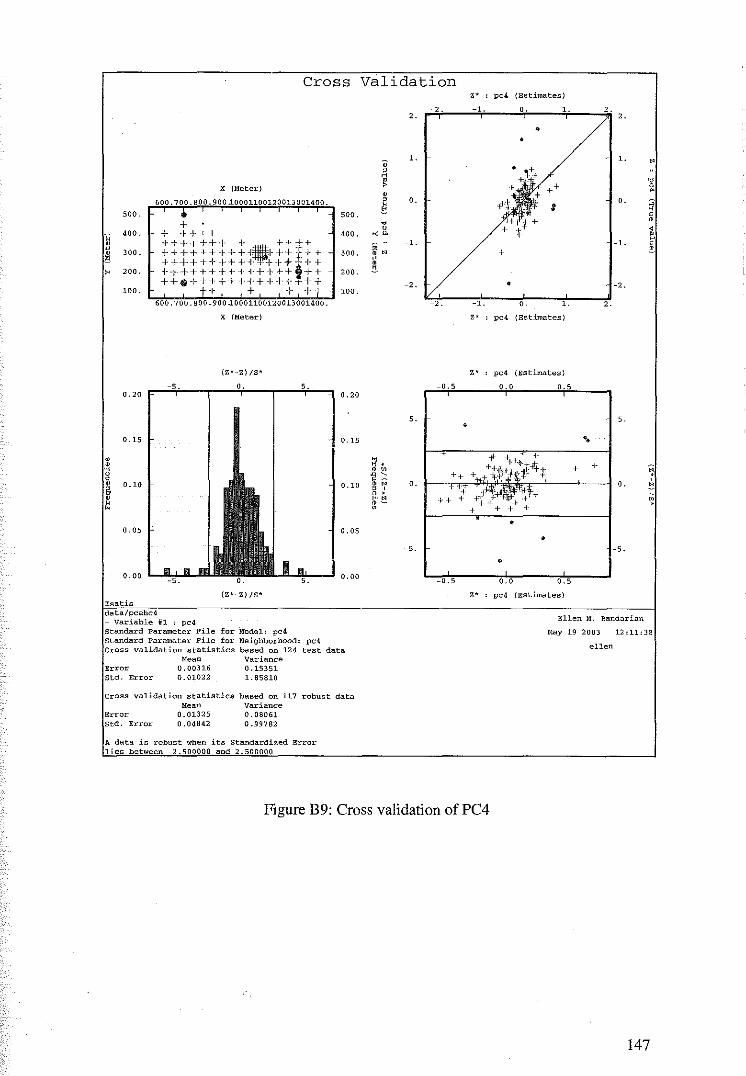
Cross

X (Meter)

600.700.800 900 j_QQ01100120013 001400.

500. ! 500.

" 400. + ·f·+ + + 400.

• +++++++ + ++I+ " 300. ++++ +++++·J,t++ ··+ + 300 . • 1l +++++++++·+- 1-+-t:·:+·+ " 200. ++++++++++++++ ++ 200.

++o+++++i-+++++ ++ 100. -t+ + + +-i- 100.

600.700 800.900 j_Q001100120013001400.

X (Meter)

(Z*-Z) /S*

0. 20

0.15

• • " g • 0.10 il • " •

0. OS

0.00 0.00

(Z*-Z}/S* Isatis data/pcahc4 - Variable Ill : pc4 standard Parameter File for Model: pc4 standard Parameter File for Neighborhood: pc4 Cross validation statistics based on 124 test data

Error Std. Error

Mean 0.00316 0 01022

Variance 0.15351 1. 85810

Cross validation statistics based on 117 robust data

Error std. Error

Mean 0. 01325 0.04842

Variance 0. 08061 0.99782

A data is robust when its Standardized Error lies between -2.500000 and 2. 500000

Validation ,. ' po4 (Estimates)

~2. ~1. 0. 1. 2. 2. 2.

•

.. 1. 1. "

' " ' " , 2 •

~ 0. 0.

~ ' • • u ' "" '

~"' ~1. ~1. ' + ".

rt • ~ ~2. ~2.

~2. ~1. o. 1. 2.

,. ' po4 (Estimates)

Z* : pc4 (Estimates)

~s. ~s.

• -0.5 0 0 0. 5

Z* , pc4 (Estimates)

Ellen M. Bandarian

May 19 2003 12:11:38

ellen

Figure B9: Cross validation of PC4

147

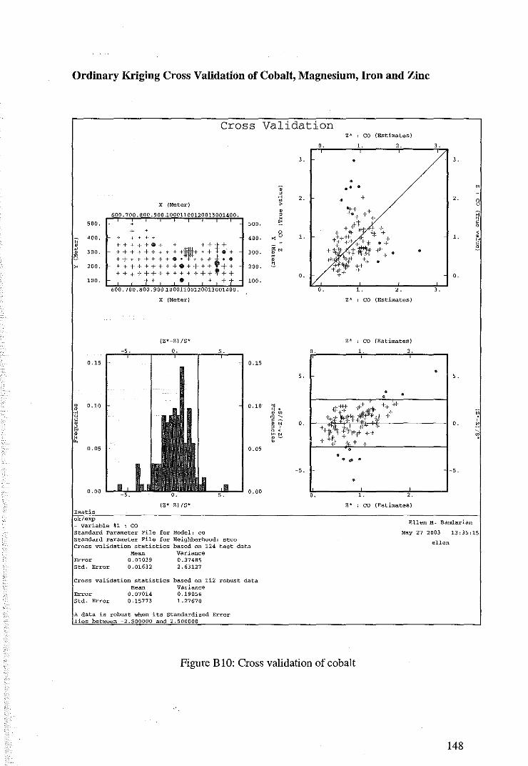
Ordinary Kriging Cross Validation of Cobalt, Magnesium, Iron and Zinc

Cross Validation z• ' co (Estimates)

0. 1. 2. 3.

3. • 3 .

• ., •• • " ~ 2. + 2 . • • n

X (Meter) > 0

• 'C+ ++ ;:; 600.700.800 900~0001100120013001400. , +•+ " .,. " 500. 500. "' + .[t:f:: ' + m + 0 + -it- -It + ' "

400. + . 400 . "0 1. ++_+t- + 1. ~ • + + + H>~ + ++t+ +t ++++·t •+ ' " 300. + +_ +_ I +_ ~ + + + +. + +_ .... 9 + 300. ~N +_· +t-6 -tJ • ~

#! + • " ·1+. oft-.tl· -l:l. ++++1++10•++++i•• m • " 200. +++++++++e++++ ++ 200. !!. +f•IJ!f ++

++++++++++++++,++ 0. +-~-~- +

0. 100. ++. ++-( 100.

600.700.800.900~0001100120013001400. 0. 1. 2. 3.

X (Meter) z• co (Estimates)

{Z*-Z)/S* Z* : CO (Estimates)

0. 2

0.15 0.15

• 5. 5 .

• • • • 0.10 0.10 " • " . ·< m ~ u ~::: " • m " o. g ,

' n + • ,. " " m~ • •

. rJ::~ -~1- +-r.:W·

+~4 1..:-!f'l ,#t,~c +' + J.:'l\ :t++ "" + +.;- '+. lfl-¥-_p- ++ +1r+:1f.++

'! 0 . N

;; •

0.05 0.05 • • . ~ • -5. . 5 .

• o.oo o.oo

0. 1. 2

(Z*-Z) /S* Z* : co (Estimates) I sa tis ok/exp Ellen M. Bandarian - variable nl : co Standard Parameter File for Model: co May 27 2003 13' 35' 15 Standard Parameter File for Neighborhood: stco Cross validation statistics based on 124 test data

Error Std. Error

0.01039 0.01632

Variance 0.37485 2. 63127

Cross validation statistics based on 112 robust data

Error Std. Error

Me= 0. 07014 0 15773

Variance 0.19056 1.27670

A data is robust when its standardized Error lies between -2.500000 and 2.500000

Figure BlO: Cross validation of cobalt

ellen

148

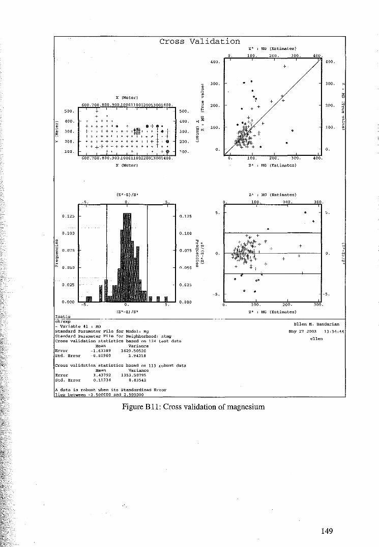
Cross Validation

X (Meter}

600 700. 800.900 ~0001100120013001400.

500. + soo. +

" 400. ' ' 400.

+ +·. + •+ • • • + + + " 300. +• + + + + +&+ + ' t •+ • ' 300. 1l t. + + + + + + + + + f + -!'" ,. 200. ., + + + + + + ' + + ++ t+e 200.

' ++++ + + + + + + + ·t t + 100. + • ,, 100.

600.700. 800.900 ~0001100120013 001400.

X {Meter)

(Z*-Z) IS*

0.125 0.125

0.100 0.100

• • ·rt

~ 0.075 0. 075

il • " • 0. 050 0.050

0.025 0. 025

o.ooo 0. 000

(Z*-Z) /S*

Isatis ok/exp - variable #1 ' MG Standard Parameter File for Model: mg Standard Parameter File for Neighborhood: stmg Cross validation statistics based on 124 test data

Error Std. Error

Mean -1.63389 -0.01960

Variance 3629.50520

1.94218

Cross validation statistics based on 113 robust data

Error Std. Error

Mean 3. 43792 0.11234

Variance 1353.50795

0.83542

A data is robust when its Standardized Error lies between -2.500000 and 2.500000

,. MG {Estimates)

400. 400. +

• 300. • 300. N

" • ~ • • ~ > • ~ + " 200. + 200. ;; " " t. • + ' •

~~ ' ~ ' ~~ 100. 100. "-• rt •

" • 0. o.

,. MG (Estimates)

Z* : MG (Estimates)

0. 100. 200. 300.

5. • 5 •

•

+., •. +

~ 0. N

• . + ?'~~-~- * " c"'t . , • 00 .:!·:+ -:lf-1- + ~ ~ +

• ;; o. . . '+ R ' 't~\ll)*t '+ , + P· N

·~ + ,_ • + t+

• .. • • -5. -5.

0' 100. 200. 300.

Z* : MG (Estimates)

Ellen M. Bandarian

May 27 2003 13:34:44

ellen

Figure Bll: Cross validation of magnesium

149

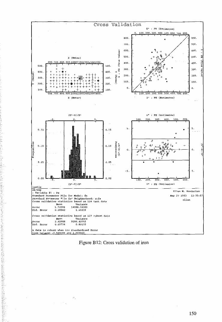
Cross Validation

800.

700.

• 600.

" ~ • 500. X {Meter) > • 600.700.800.900 .10001100120013001400. " 400. " 500. + soo. !0

+ + " 300. 400. + + + •• 400. ". ;;

+++++++ • ++t+ • *N 200. " • 300. ++++++++++,+++ ·+-+ 300. e + + + --1- + + + + + +' ·f· + .jlc ::·· • • " • 100.

" 200. ++ + + +++e+··i-++++ .... + + 200. !'. ++++++++++++++-·++ 0.

100. ++ + -1- +-t- 100.

600.700.800 900.10001100120013001400.

X (Meter)

(Z*-Z)/S*

0.15 0.15 5.

• • ' " . ·rl 0.10 u

' • il 0.10 • ~

~:: • N 0.

" ' 0 •

' e· N

" • -• • 0.05 0. 05

-5.

o.oo 0.00

(Z*-Z) IS* Isatis ok/exp - Variable #1 : FE

Z* : FE {Estimates)

0. 100. 200. 300. 400. 500. 600. 700. 800.

•

t +

• • +

+ + • +

• + +

0. 100.200.300.400.500.600.700.800.

Z'

100 200

#''+' + ++

' FE {Estimates)

FE (Estimates)

300 400. 500. 600.

•

• +

• •

• 100. 200. 300. 400. 500. 600.

z• FE (Estimates)

800 .

700.

600 .

soo.

400.

300.

200.

100 .

0.

5.

0 .

-5.

Ellen M. Bandarian

N

• " ;:; " ' • ' ' " ' ,._

N . ' N

standard Parameter File for Model: fe May 27 2003 13 35:57 Standard Parameter File for Neighborhood: stfe Cross validation statistics based on 124 test data

Error Std. Error

Mean 1. 72506 0.00942

Variance 14008.38280

1.65939

Cross validation statistics based on 117 robust data

Error Std. Error

Mean 2.82988 0.03734

Variance 9206.43755

0.89172

A data is robust when its Standardized Error lies between -2.500000 and 2.500000

Figure B 12: Cross validation of iron

ellen

150

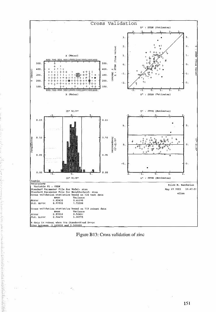
Cross Validation ,. ' STZN (Estimates)

-2. -1. 0. 1. '· 3.

3. • 3.

2. + ++ 2. " • + + ~ • • + ++ + ++ • p " X (Meter) • 1. +· :\\ -l~kt-t;t 1. ~

600 800. 9 00 ~0001100120013 001400. ~ _+· -++

700 !¢ +~++ * 8

± H 500. 500. 0. 0. ' + " " •""Jl•+ + ro

" +, 400. + f· I·++ 400. '~ "'' ++ ' -;; • ' +++++++ • ++;+ + * "'++ " • 1i .. -1. -1. ' " 300 . +++++++ + ++,+++ _++ 300. +·~ +it~ 'lt- ++ !'. • ro"

"' " ++. + + • ++++++++++ ++·tl---·· ro

" 200. +++++++0++++-~+--++ 200. !!. ++ ++++++++ +++-+++---:--1---+ -2. -.~ -2.

100. ++ + + ++ 100.

600.700.800.900~0001100120013001400. -2. -1. o. 1. 2. 3.

X (Meter) ,. STZN {Estimates)

(Z*-Z)/S* ,. STZN (Estimates)

-2. o . 2.

0.15 . 0.15

• 5. 5.

•

* ;;; ++

o. ' "

• 0.10 0.10 " ' H • ·H ro • ;I u ~:: ' • ro" 0 • fr " ' 0 •

~ • H· N

" ro-• • 0.05 0. 05 •

-5. -5.

• 0. 00 o.oo

2. 0 2.

{Z*-Z) /S* ,. STZN {Estimates) I sa tis data/stexp - Variable #1 : STZN Ellen M. Bandarian

Standard Parameter File for Model: stzn May 19 2003 10:42:51 Standard Parameter File for Neighborhood: stzn Cross validation statistics based on 124 test data

Error Std. Error

Me~

0. 02430 0.02022

Variance 0. 65195 1. 72399

Cross validation statistics based on 119 robust data

Error Std. Error

Mean 0.03916 0.04470

Variance 0.50497 1. 00775

A data is robust when its standardized Error lies between -2.500000 and 2.500000

Figure Bl3: Cross validation of zinc

ellen

151

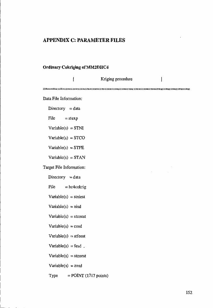
APPENDIX C: PARAMETER FILES

Ordinary Cokriging ofMM2DHC4

Kriging procedure

===---====================================================== Data File Information:

Directory = data

File =stexp

Variable(s) = STNI

Variable(s) = STCO

Variable(s) = STFE

Variable(s) = STA."'

Target File Information:

Directory =data

File = hc4cokrig

Variable(s) = stniest

Variable(s) = nisd

Variable(s) = stcoest

Variable(s) = cosd

Va.riable(s) = stfeest

Variable(s) = fesd _

Variable(s) = stznest

Variable(s) = znsd

Type =POINT (1717 points)

152

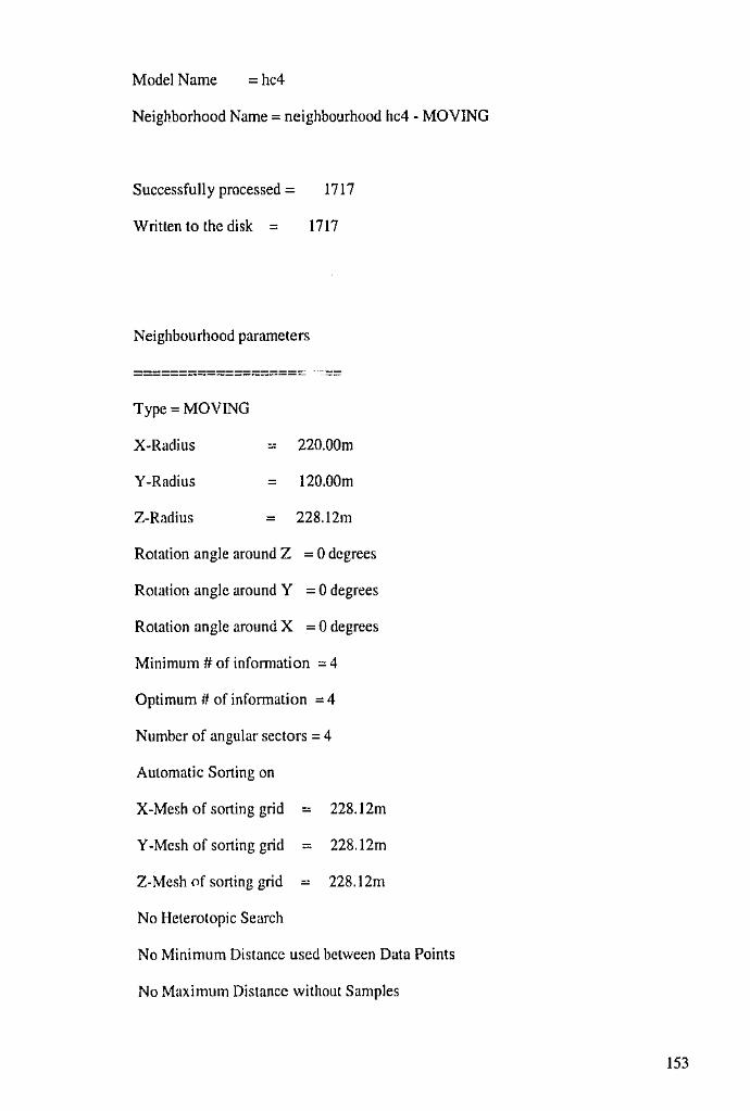
Model Name = hc4

Neighborhood Name= neighbourhood hc4- MOVING

Successfully processed= 1717

Writtentothedisk = 1717

Neighbourhood parameters

===================

Type= MOVING

X-Radius

Y-Radius

Z-Radius

=

=

220.00m

120.00m

228.12m

Rotation angle around Z = 0 degrees

Rotation angle around Y = 0 degrees

Rotation angle around X = 0 degrees

Minimum# of information = 4

Optimum# of information = 4

Number of angular sectors = 4

Automatic Sorting on

X-Mesh of sorting grid = 228.12m

Y -Mesh of sorting grid = 228.12m

Z-Mesh of sorting grid = 228.12m

No Heterotopic Search

No Minimum Distance used between Data Points

No Maximum Distance without Samples

153

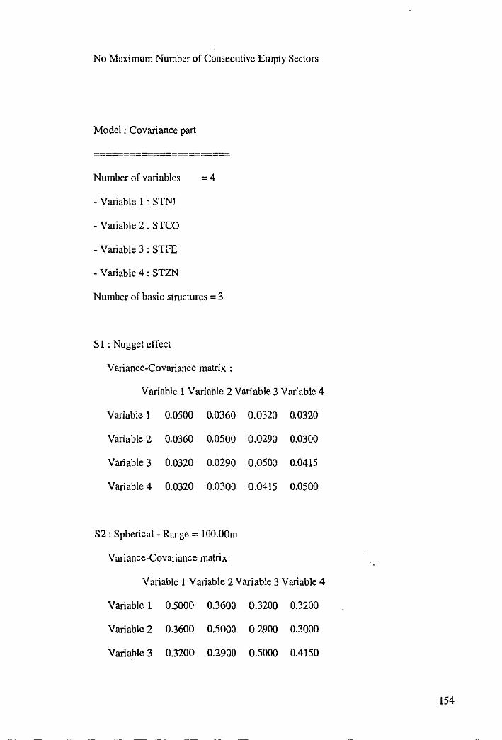
No Maximum Number of Consecutive Empty Sectors

Model : Covariance part

======================= Number of variables = 4

-Variable I : STI'J!

~Variable 2. srco

~ Variable 3 : STIT

~Variable 4 : STZN

Number of basic structures= 3

S l : Nugget effect

Variance~Covariance matrix :

Variable l Variable 2 Variable 3 Variable 4

Variable l 0.0500 0.0360

Variable 2 0.0360 0.0500

Variable 3 0.0320 0.0290

Variable 4 0.0320 0.0300

S2: Spherical- Range= lOO.OOm

Variance-Covariance matrix:

0.0320 0.0320

0.0290 0.0300

0.0500 0.0415

0.0415 0.0500

Variable 1 Variable 2 Variable 3 Variable 4

Variable 1 0.5000 0.3600 0.3200 0.3200

Variable 2 0.3600 0.5000 0.2900 0.3000

Variable 3 0.3200 0.2900 0.5000 0.4150

154

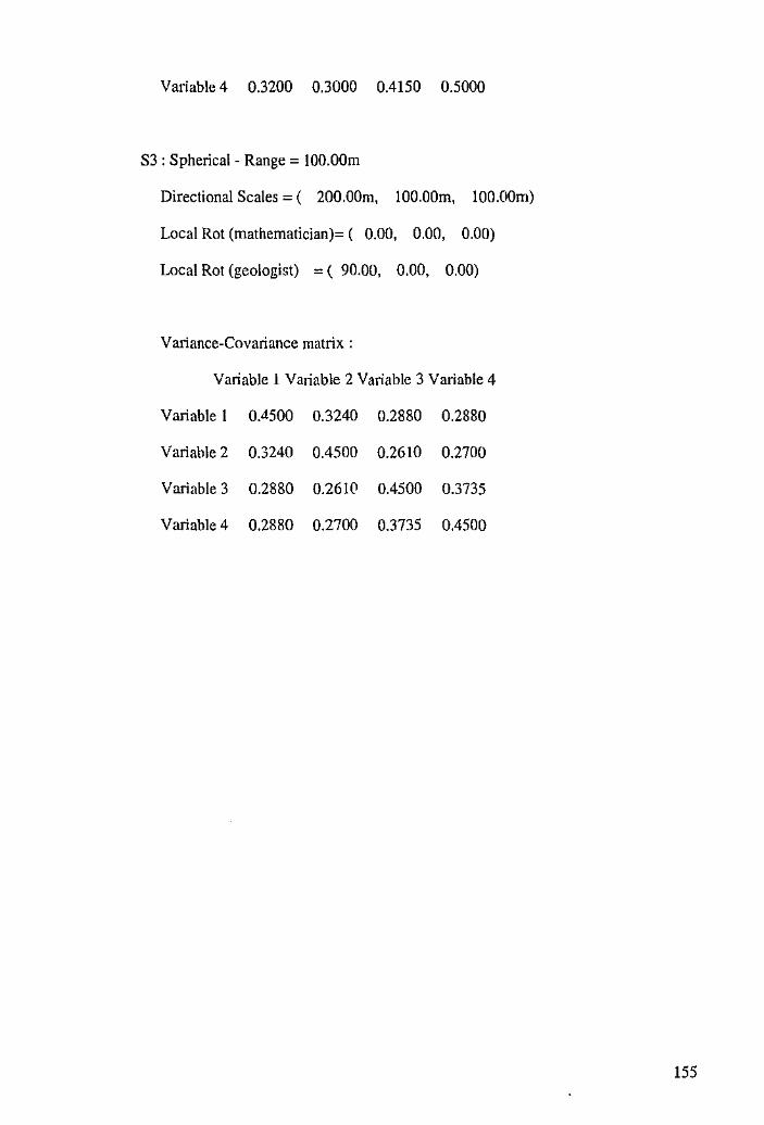
Variable 4 0.3200 0.3000 0.4150 0.5000

S3 : Spherical - Range= IOO.OOm

Directional Scales = ( 200.00m, IOO.OOm, IOO.OOm)

Local Rot (mathematician)= ( 0.00, 0.00, 0.00)

Local Rot (geologist) = ( 90.00, 0.00, 0.00)

Variance-Covariance matrix:

Variable 1 Variable 2 Variable 3 Variable 4

Variable I 0.4500 0.3240 0.2880 0.2880

Variable 2 0.3240 0.4500 0.2610 0.2700

Variable 3 0.2880 0.2610 0.4500 0.3735

Variable 4 0.2880 0.2700 0.3735 0.4500

!55

Ordinary Cokriging ofM,~22DTOP4

Kriging procedure

============================================================ Data File Infonnation:

Directory = data

File = stex.p

Variable(s) = STNI

Variable(s) = STCO

Variable(s) = STMG

Variable(s) = STFE

Target File Infonnation:

Directory = data

File = top4cokrig

Varlable(s) = stniest

Variable(s) = nisd

Variable(s) = stcoest

Variable(s) = cosd

Variable(s) = stmgest

Vnriable(s) = mgsd

Variable(s) = stfeest

Variable(s) = fesd

Type =POINT(I717points)

Model Name = top4

Neighborhood Name= neighbourhood top4- MOVING

156

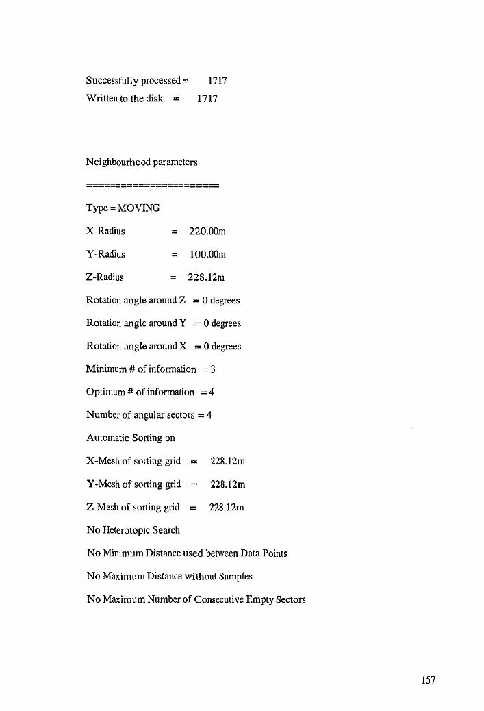
Successfully processed= 1717

Writtentothedisk = 1717

Neighbourhood parameters

=======================

Type= MOVING

X-Radius

Y-Radius

Z-Radius

= 220.00m

= IOO.OOm

= 228.12m

Rotation angle around Z = 0 degrees

Rotation angle around Y = 0 degrees

Rotation angle around X = 0 degrees

Minimum# of information = 3

Optimum # of information = 4

Number of angular sectors = 4

Automatic Sorting on

X-Mesh of sorting grid = 228.12m

Y -Mesh of sorting grid = 228.12m

Z-Mesh of sorting grid = 228.12m

No Heterotopic Search

No Minimum Distance used between Data Points

No Maximum Distance without Samples

No Maximum Number of Consecutive Empty Sectors

!57

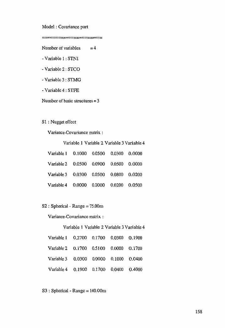
Model : Covariance part

======================= Number of variables = 4

-Variable 1: STNI

-Variable 2: STCO

- Variable 3 : STMG

- Variable 4 : STFE

Number of basic structures = 3

Sl :Nugget effect

Variance-Covariance matrix :

Variable 1 Variable2 Variable3Variable4

Variable 1 0.1000 0.0500 0.0300 0.0000

Variable 2 0.0500 0.0900 0.0500 0.0000

Variable 3 0.0300 0.0500 0.0800 0.0200

Variable4 0.0000 0.3000 0.0200 0.0500

S2 : Spherical - Range= 75.00m

Variance-Covariance matrix:

Variable 1 Variable 2 Vmiable 3 Variable 4

Variable 1 0.2700 0.1700 0.0300 0.1900

Variable 2 0.1700 0.5100 0.0000 0.1700

Variable 3 0.0300 0.0000 0.1000 0.0400

Variable 4 0.1900 0.1700 0.0400 0.4000

S3: Spherical- Range= 140.00m

158

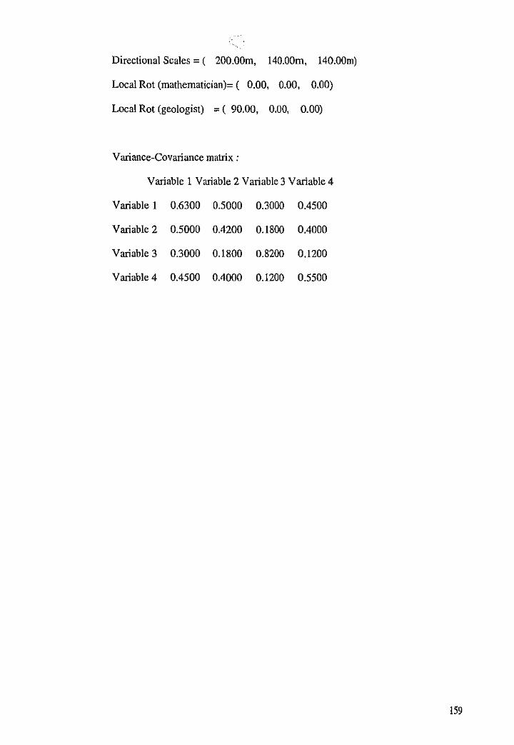
Directional Scales= ( 200.00m, 140.00m, 140.00m)

Local Rot (mathematician)= ( 0.00, 0.00, 0.00)

Local Rot (geologist) = ( 90.00, 0.00, 0.00)

Variance-Covariance matrix :

Variable 1 Variable 2 Variable 3 Variable 4

Variable 1 0.6300 0.5000 0.3000 0.4500

Variable 2 0.5000 0.4200 0.1800 0.4000

Variable 3 0.3000 0.1800 0.8200 0.1200

Variable 4 0.4500 OAOOO 0.1200 0.5500

159

Ordinary Kriging of the Principal Component Scores

Legend: pel (pc2) (pc3) (pc4)

Kriging procedure ·

Data File Information:

Directory = data (data) (data) (data)

File = pcahc4 (pcahc4) (pcahc4) (pcahc4)

Variable(s) =pel (pc2) (pc3) (pc4)

Target File Information:

Directory = pclest (pc2est) (pc3est) (pc4est)

File =pel est (pc2est) (pc3est) (pc4est)

Variable(s) =pel est (pc2cst) (pc3est) (pc4est)

Variable(s) = pclsd (pc2sd) (pc3sd) (pc4sd)

Type = POINT (1717 points) ( 1717 points) (1717 points) ( 1717 points)

Model Name = pel (pc2) (pc3) (pc4)

Neighborhood Name= pel (pc2) (pc3) (pc4) - MOVING

Successfully processed = 1717 (1717) ( 1717) ( 1717)

Written to the disk = 1717 (1717) (1717) ( 1717)

Neighbourhood parameters

Type= MOVING

160

X-Radius

Y-Radius

Z-Radius

220.00m (120.00m)(190.00m) (250.00m)

120.00m (120.00m) (1 OO.OOm) (250.00m)

228.12m ( 28. J 2m) (228.12m) (228.12m)

Rotation angle around Z = 0 degrees (?5 degrees) (0 degrees) (0 degrees)

Rotation angle around Y = 0 degrees (0 dcgrees)(O degrees) (0 degrees)

Rotation angle around X = 0 degrees (0 dcgrces)(O degrees) (0 degrees)

Minimum# of information = 3 (3) (3) (3)

Optimum# of information = 4 ( ) (4) (4)

Number of angular sectors= 4 (4) (4). (4)

Automatic Sorting on

X-Mesh of sorting grid

Y-Mesh of sorting grid

Z-Mesh of sorting grid

No Heterotopic Search

228.12m (?'2R 12m) (228 12m) ("'28 12m)

228.12m ( 28. 12m) (228.12m) (228 .12m)

228.12m ( 28 12m) (228 12m)(228. 12m)

No Minimum Distance used between Data Points

No Maximum Distance without Samples

No Maximum Number of Consecutive E mpty Sectors

Model : Covariance part

N umber of variables = 1

-Variable 1 : pel

Number of basic structures = 3

S 1 : Nugget effect

161

Sill = 0.1000

S2 : Spherical- Range= 90.00m

Sill = 0.4700

S3 : Spherical- Range= 90.00m

Sill = 2.4700

Directional Scales= ( 200.00m, 90.00m, 90.00m)

Local Rot (mathematician)= ( 0.00, 0.00, 0.00)

Local Rot (geologist) = ( 90.00, 0.00, 0.00)

Model : Drift part

Number of drift functions = 1

-Universality condition

Model : Covariance part

Number ofvariables = I

- Variable I : pc2

Number ofbasic structures= 2

S 1 Nugget effect

Sill = 0.0800

S2 : Spherical - Range= 85.00m

Sill = 0.4 700

Model : Drift patt

162

Number of drift fimctions = 1

- Universality condition

Model : Covariance part

Number of variables = 1

-Variable l : pc3

Number of basic structures = 3

S 1 : Nugget effect

Sill= 0.0100

S2 : Spherical- Range= 50 OOm

Sill= 0.0500

SJ : Spherical -Range= 98.00m

Sill 02150

Directional Scales= ( 140.00m, 98.00m, 98.00m)

Local Rot (mathematician)= ( 25.00, 0.00, 0.00)

Local Rot (geologist) = ( 65.00, 0.00, 0.00)

Model : Drift part

Number of drift functions = 1

- Universality condition

Model : Covariance pat1

Number of variables = I

163

- Variable I : pc4

Number of basic structures = 3

S I : Nugget effect

Sill = 0.0 180

S2 · Spherical - Range = I OO.OOm

Sill = 0.0650

S3 : Spherical - Range = 250.00m

Sill 0.0920

Model : Drift part

Numher of drift function'

- Universality condition

164

Ordinary Kriging of Nickel, Cobalt, Magnesium, Iron and Zinc

Legend: nickel (cobalt) (magnesium) (i11Jn) (zinc)

Kriging procedure

Data File Information:

Directory = ok (ok) (ok) (ok) (ok)

File = exp (exp) (exp) (exp) (exp)

Variable(s) = ni (co) (mg) (fc) (zn)

Target File Information:

Directory = ok (ok) (ok) (Clk) (ok)

File = niest (coest) (mgest) (lccst) (znest)

Variable(s) = niest (coest) (rngest) (fecst) (znest)

Variable(s) = nisd (co~d) (mgsd) (fesd} (znsd)

Type = POINT (1717 points) ( 1717 points) (1717 points) ( 1717 points} ( 1717

points)

Model Name = ni (co) (mg) (fc) (zn)

Neighborhood Name= ni (co) (mg) Ue) (zn) - MOVING

Successfully processed= 1717 (1717) (1717) ( 1717) (1717)

Written to the disk = 1717 (I 717) (1717) ( 1717) ( 1717)

Neighbourhood parameters

Type =MOVING

165

X-Radius

Y-Radius

Z-Radius

180.00m (220.00m)(300.00m) (210 00m)(220.00m)

llO.OOm (120.00m) (160.00m) (I 10.00m)(110.00m)

228.12m (228.12m) (228.12m) (228.12m)(228.12m)

Rotation angle around Z = 0 degrees (0 degrees) (120 degrees) (0 degrees) (0

degrees)

Rotation angle around Y = 0 degrees (0 degrees)(O degrees) (0 degrees) (0 degrees)

Rotation angle around X = 0 degrees (0 degrees)(O degrees) (0 degrees) (0 degrees)

Minimum# of information = 3 (3) (3) (1) (3)

Optimum# of information = 4 (4) (4) (4) (4)

Number of angular sectors = 4 (4) (4) (4) (4)

Automatic Sorting on

X-Mesh of sorting grid

Y -Mesh of sorting grid

Z-Mesh of sorting grid

No Heterotopic Search

228.12m (228 12m) (228 12m) (228. 12m)

228.12m (:28. l2m) (228.12m) (228. 12m)

228.12m (228. l2m) (228.12m) (228.12m)

No Minimum Distance used between Data Points

No Maximum Distance without Samples

No Maximum Number of Consecutive Empty Sectors

Model : Covariance part

Number ofvariables = 1

- Variable 1 : NI

Number ofbasic structures= 3

S 1 : Nugget effect

Sill = 5. 0000

S2 : Spherical - Range= 90.00m

166

Sill = 12.1500

S3 : Spherical -Range= 89.60m

Sill = 28.3500

Directional Scales= ( 160.00m, 89.60m, 89.60m)

Local Rot (mathematician)= ( 0.00, 0.00, 0.00)

Local Rot (geologist) = ( 90.00, 0.00, 0.00)

Model : Drift part

Number of drift functions = 1

- Universality condition

Model : Covariance part

Number ofvariables = 1

-Variable I : CO

Number of basic structures = 3

S I : Nugget effect

Sill= 0.0120

S2 : Spherical- Range= IOO.OOm

Sill- 0.1600

S3 : Spherical- Range= 1 OO.OOm

Sill = 0.1300

Directional Scales = ( 200.00m, 100.00m, I OO.OOm)

Local Rot (mathematician)= ( 0.00, 0.00, 0.00)

Local Rot (geologist) = ( 90.00, 0.00, 0.00)

Model : Drift part

Number of drift functions = I

-Universality condition

167

Model Covariance part

Number of variables = 1

- Variable 1 MG

Number of basic structures= 3

S 1 · Nugget effect

Sill = 135.0000

S2 : Spherical - Range = 140 OOm

Sill = 2300 0000

S3 : Spherical- Range= 150.00m

Sill = 2162.0000

Directional Scales= ( 300.00m, 150.00m, JSO.OOm)

Local Rot (mathematician)= ( 120.00, 0.00, 0.00)

Local Rot (geologist) = ( -30.00, 0.00, 0.00)

Model Drift part

Number of drift functions = 1

- Universality condition

Model : Covariance part

Number of variables = I

- Variable I : FE

Number ofbasic structures= 3

S I · Nugget efl'ect

Sill = 1030.0000

S2 : Spherical - Range = 75.00m

Sill - 3100.0000

S3 Spherical- Range= 99.90m

Si11 - 16790.0000

Diii.!Ciional Scales= ( 185.00m, 99 90m, 99 90m)

Local Rot (mathematician)- ( 0.00, 0.00, 0.00)

168

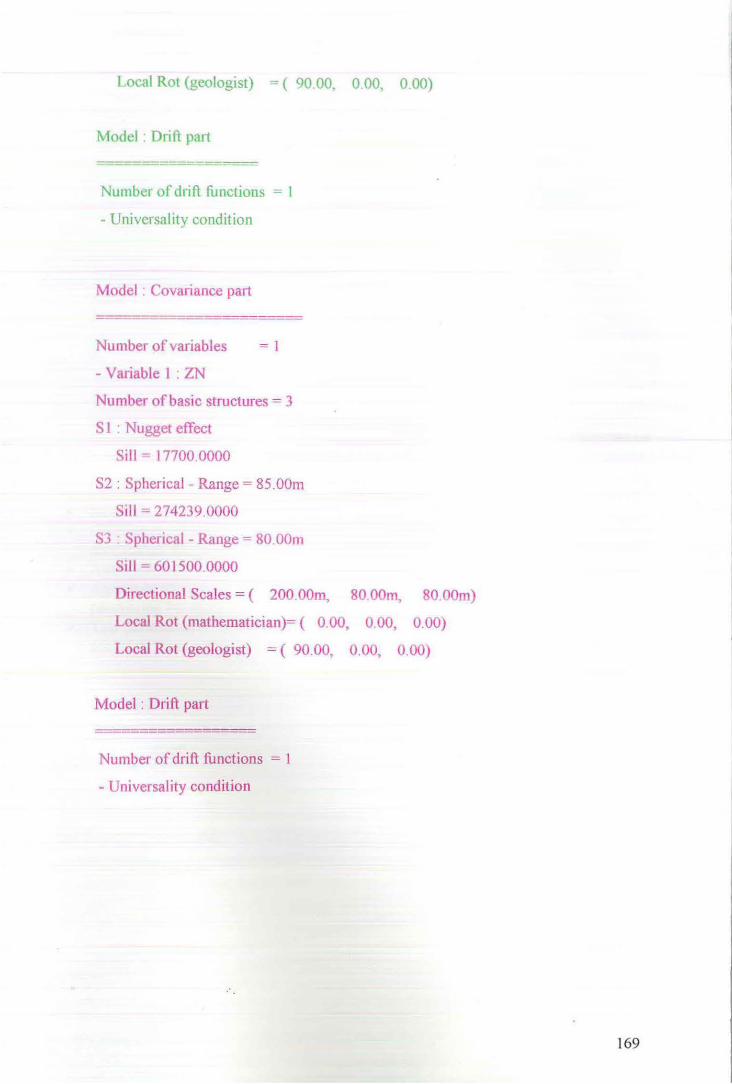
Local Rot (geologist) = ( 90.00, 0.00, 0.00)

Model : Drift part

Number of drift fi.mctions = I

- Universality condition

Model : Covariance part

Number of variables = 1

-Variable I : ZN

Number of basic structures = 3

S I · Nugget effect

Sill = I 7700.0000

S2 : Spherical - Range= 85.00m

Sill - 274239 0000

S3 : Spherical- Range = 80.00m

Sill= 60 I 500 0000

Directional Scales= ( 200 OOm, 80.00m, 80.00m)

Local Rot (mathematician)= ( 0.00, 0.00, 0.00)

Local Rot (geologist) = ( 90.00, 0.00, 0.00)

Model : Drift part

Number of drift functions = 1

-Universality condition

169

Date: l21h November 2002

David Selfe Anaconda Operations Locked Bag 4 Welshpool Delivery Centre Pilbara Street Welshpool, WA

Ute Mueller School of Engineering and Mathematics Edith Cowan University, WA

Dear Ute,

Re: Anaconda Multivariate Data Set

Anaconda

I refer to the e-mail sent by you on the jlh November 2002. Anaconda gives its permission for publication of research results on the data supplied to you by Mark Murphy on the following basis:

• Raw data is not published, • Original coordinate data will not be published and any published data will be made

anonymous by changing locations. • Anaconda will be informed and given a copy of any publications, • Anaconda will receive due acknowledgement ofit's support of the work, and it's

permission for the publication of the results, • This permission is only applicable to the studies of Ms Ellen Bandarian, any further

use of the data will require separate permission ~o be granted from Anaconda.

Yours Sincerely

David Selfe

Chief Production Geologist

An:u.::umJ~ Opcr~liuns Pry Llli ABNIACN 4J 076 717 505 L:vcl J 2, Qu~ys1lie Bldg 2 Mill Stn:el, Penh WA 6000

TeL 61892128500 Fa~: 61 89212 8501

M:Lil~ger or rhe Murrin Murrin Nickel CobJlt Project for

Anacondo Nickel l!d :Lilli Glencon: lnlcm,lional AG 1'0 Bo~ 7.'i 12. Perth W A 6850

l'crmi~soon lcllcr 112002.doc