detection of temporarily flooded vegetation using time series
TRANSCRIPT
Detection of temporarily flooded vegetation
using time series of dual polarised C-band
synthetic aperture radar data
Dissertation zur Erlangung des
Doktorgrades an der Fakultät für Geowissenschaften der Ludwig‐Maximilians‐Universität München
Vorgelegt von
Viktoriya Tsyganskaya
München, 23. September 2019

i
Supervisor: Prof. Dr. Ralf Ludwig, Department of Geography, Ludwig-Maximilians-
Universität, Munich
2nd Superviser: Prof. Dr. Günter Strunz, German Aerospace Center (DLR), German Remote
Sensing Data Center, Geo-Risks and Civil Security, Oberpfaffenhofen, Weßling
Tag der mündlichen Prüfung: 13.05.2020

ii
Acknowledgments
This work has been accomplished in the framework of the project Dykes under Pressure - Technical and ecological vulnerability and resilience of dyke landscapes at LMU Munich and in cooperation with the German Remote Sensing Data Center (DFD) of the German Aerospace Center (DLR) in Oberpfaffenhofen, Department for Civil Crisis Information and Georisks. The financial funding of the project by the Federal Ministry of Economics and Technology (BMWi) is gratefully acknowledged.
First of all, I would like to thank Prof. Dr. Ralf Ludwig and Dr. Philip Marzahn from the Department of Geography of the Ludwig-Maximilians-University Munich for giving me the opportunity to start this PhD project and been my supervisors during the whole period. Their passion for science inspired and motivated me constantly and their great and endless support helped me to find my own path and continue even in the most discouraging phases of PhD. Furthermore, I would like to especially thank Dr. Philip Marzahn for taking his time and for constructive very inspiring discussions about required methods and data analysis. I benefited a lot from his experience and his deep understanding of microwave remote sensing and geostatistics.
I want to sincerely thank Prof. Dr. Günter Strunz, Head of Department "Geo Risks and Civil Security" at the Earth Observation Centre of the German Aerospace Center (DLR), who agreed to become my second referee and encouraged me to write this work cumulatively from the beginning.
Special thanks to my supervisor at DLR, Dr. Sandro Martinis, Head of Research Group Natural Hazards at the Earth Observation Centre of the DLR, for the introduction to flood detection and the fruitful comments and suggestions for several aspects of my work.
I would also like to thank my colleagues (Prof. Dr. Andreas Schmitt, Dr. Simon Plank, Andre
Twele, Wenxi Coa, Dr. Marianne Jilge) at DLR for providing data sets, valuable exchange and mental support.
I am also very grateful to all the colleagues and friends from Deparment of Geography at the LMU for having a great time together and their helpful expertise and advices. I would like to thank Vera Erfurt for the organisational support of all doctoral students and for her open ear. My special thanks go to Dr. Janja Vrzel and Thomas Weiß for their unwavering faith, for the special moments and the unforgettable time. I would also like to thank my new colleagues at Cubert GmbH for their patience and understanding. Many thanks to all my important people, my family and friends. Thank you very much for your patience, the unconditional support during thesis-related crises and the cheering all the time. Special thanks go to Lukas for his support in implementing the methodology, but especially for his unlimited emotional support and always being there for me.
iii
Summary
The intense research of the last decades in the field of flood monitoring has shown that microwave
sensors provide valuable information about the spatial and temporal flood extent. The new
generation of satellites, such as the Sentinel-1 (S-1) constellation, provide a unique, temporally
high-resolution detection of the earth's surface and its environmental changes. This opens up new
possibilities for accurate and rapid flood monitoring that can support operational applications. Due
to the observation of the earth's surface from space, large-scale flood events and their spatio-
temporal changes can be monitored. This requires the adaptation of existing or the development of
new algorithms, which on the one hand enable precise and computationally efficient flood
detection and on the other hand can process a large amounts of data.
In order to capture the entire extent of the flood area, it is essential to detect temporary flooded
vegetation (TFV) areas in addition to the open water areas. The disregard of temporary flooded
vegetation areas can lead to severe underestimation of the extent and volume of the flood. Under
certain system and environmental conditions, Synthetic Aperture Radar (SAR) can be utilized to
extract information from under the vegetation cover. Due to multiple backscattering of the SAR
signal between the water surface and the vegetation, the flooded vegetation areas are mostly
characterized by increased backscatter values. Using this information in combination with a
continuous monitoring of the earth's surface by the S-1 satellites, characteristic time series-based
patterns for temporary flooded vegetation can be identified. This combination of information
provides the foundation for the time series approach presented here.
This work provides a comprehensive overview of the relevant sensor and environmental
parameters and their impact on the SAR signal regarding temporary open water (TOW) and TFV
areas. In addition, existing methods for the derivation of flooded vegetation are reviewed and their
benefits, limitations, methodological trends and potential research needs for this area are identified
and assessed. The focus of the work lies in the development of a SAR and time series-based
approach for the improved extraction of flooded areas by the supplementation of TFV and on the
provision of a precise and rapid method for the detection of the entire flood extent.
The approach developed in this thesis allows for the precise extraction of large-scale flood areas
using dual-polarized C-band time series data and additional information such as topography and
urban areas. The time series features include the characteristic variations (decrease and/or
increase of backscatter values) on the flood date for the flood-related classes compared to the
whole time series. These features are generated individually for each available polarization (VV,
VH) and their ratios (VV/VH, VV-VH, VV+VV). The generation of the time series features was
performed by Z-transform for each image element, taking into account the backscatter values on
the flood date and the mean value and standard deviation of the backscatter values from the non-
flood dates. This allowed the comparison of backscatter intensity changes between the image
elements. The time series features constitute the foundation for the hierarchical threshold method
for deriving flood-related classes. Using the Random Forest algorithm, the importance of the time
series data for the individual flood-related classes was analyzed and evaluated. The results showed
that the dual-polarized time series features are particularly relevant for the derivation of TFV.
However, this may differ depending on the vegetation type and other environmental conditions.
The analyses based on S-1 data in Namibia, Greece/Turkey and China during large-scale floods
show the effectiveness of the method presented here in terms of classification accuracy. The
iv
supplementary integration of temporary flooded vegetation areas and the use of additional
information resulted in a significant improvement in the detection of the entire flood extent. It
could be shown that a comparably high classification accuracy (~ 80%) was achieved for the flood
extent in each of study areas. The transferability of the approach due to the application of a single
time series feature regarding the derivation of open water areas could be confirmed for all study
areas. Considering the seasonal component by using time series data, the seasonal variability of the
backscatter signal for vegetation can be detected. This allows for an improved differentiation
between flooded and non-flooded vegetation areas. Simultaneously, changes in the backscatter
signal can be assigned to changes in the environmental conditions, since on the one hand a time
series of the same image element is considered and on the other hand the sensor parameters do
not change due to the same acquisition geometry. Overall, the proposed time series approach
allows for a considerable improvement in the derivation of the entire flood extent by
supplementing the TOW areas with the TFV areas.
v
Zusammenfassung
Die intensive Forschung der letzten Jahrzehnte in dem Bereich Hochwassermonitoring hat gezeigt,
dass mit Hilfe von Mikrowellensensoren wertvolle Informationen über die
Hochwasserausdehnung abgeleitet werden können. Die neuen Satelliten-Generationen, wie die S-
1 Konstellation, ermöglichen heutzutage eine in dieser Form neue, zeitlich hoch aufgelöste
Erfassung der Erdoberfläche und deren Umweltveränderungen. Dadurch eröffnen sich neue
Möglichkeiten für eine genaue und schnelle Hochwasserüberwachung, die den operationellen
Einsatz unterstützen können. Durch die Erfassung der Erdoberfläche aus dem Weltall können unter
anderem großflächige Hochwasserereignisse und ihre räumlich-zeitliche Veränderung beobachtet
werden. Dies erfordert die Anpassung bestehender oder die Entwicklung neuer Algorithmen,
welche zum einen eine präzise und rechnerisch effiziente Hochwassererkennung ermöglichen und
zum anderen große Datenmenge verarbeiten können.
Um die Gesamtausdehnung der Hochwasserfläche vollständig zu erfassen ist neben den offenen
Wasserflächen die Detektion von temporär unterfluteten Vegetation (TUV) erforderlich. Die
Nichtberücksichtigung der unterfluteten Vegetationsflächen kann zu gravierenden
Unterschätzungen des Hochwasserausmaßes und -volumens führen. Unter bestimmten System-
und Umweltbedingungen kann das Synthetic Aperture Radar (SAR) eingesetzt werden, um
Informationen unter der Vegetationsdecke zu extrahieren. Aufgrund von Mehrfachrückstreuungen
des SAR-Signals zwischen der Wasserfläche und der Vegetation sind die unterfluteten
Vegetationsflächen meist durch erhöhte Rückstreuwerte charakterisiert. Mit Hilfe dieser
Information in Kombination mit einer zeitlich hochaufgelösten Erfassung der Erdoberfläche durch
die S-1 Satelliten können charakteristische, zeitserienbasierte Muster für TUV identifiziert werden.
Diese Verknüpfung von Information dient als Grundlage für den hier vorgestellten
Zeitserienansatz.
Arbeit gibt einen umfangreichen Überblick über die relevanten Sensor- und Umweltparameter
sowie ihre Auswirkung auf das SAR-Signal in Bezug auf offene Wasserflächen und unterflutete
Vegetationsflächen. Zusätzlich werden bereits bestehenden Methoden für die Ableitung von
unterfluteter Vegetation untersucht und deren Nutzen, Limitierungen, methodische Trends und
der potenzielle Forschungsbedarfs für diesen Bereich aufgezeigt und bewertet. Der Schwerpunkt
der Arbeit liegt auf der Entwicklung eines zeitserienbasierten SAR Ansatzes zur verbesserten
Ableitung von Überschwemmungsflächen durch die Ergänzung von TUV und auf der zur Verfügung
stellen einer präzisen und schnellen Methode für Detektion des gesamten Überflutungsausmaßes.
Der in der vorliegenden Arbeit entwickelte Ansatz ermöglicht die präzise Ableitung von
großflächigen Überschwemmungsgebieten auf der Grundlage von dual-polarisierten C-Band
Zeitseriendaten und Zusatzinformationen, wie der Topographie und urbanen Flächen. Zu diesem
Zweck wurden mehrere Zeitserienfeatures entwickelt. Die Zeitreihenmerkmale beinhalten die
charakteristischen Variationen (Abfall und/oder Anstieg der Rückstreuwerte) für die
hochwasserrelevanten Klassen zum Hochwasserzeitpunkt im Vergleich zu der gesamten Zeitreihe.
Die Zeitserienmerkmale werden für jede verfügbare Polarisation (VV, VH) und deren Verhältnisse
(VV/VH, VV-VH, VV-VH, VV+VV) individuell generiert. Die Generierung der Zeitreihenmerkmale
erfolgte mittels Z-Transformation für jedes Bildelement unter Berücksichtigung der
Rückstreuungswerte zum Hochwasserzeitpunkt und des Mittelwerts und der Standardabweichung
der Rückstreuungswerte von Nicht-Hochwasserzeitpunkten. Dies ermöglichte die Vergleichbarkeit
von Rückstreuintensitätsänderungen zwischen den Bildelementen. Die Zeitserienfeatures

vi
fungieren als Grundlage für die hierarchische Schwellenwertmethode, durch die die flutbedingten
Klassen abgeleitet werden. Mit Hilfe des Random Forest Algorithmus wurde die Relevanz der
Zeitseriendaten für die individuellen flutbedingten Klassen untersucht und bewertet. Die
Ergebnisse zeigten, dass vor allem die dualpolarisierte Zeitserienfeatures für die Ableitung von
TUV relevant sind. Dies kann sich aber in Abhängigkeit von des Vegetationstyps und weiterer
Umweltbedingungen unterscheiden.
Die Untersuchungen auf der Grundlage von S-1 Daten in Namibia, Griechenland/Türkei und China
während großräumiger Überschwemmungen zeigen die Wirksamkeit der präsentierten Methode
in Bezug auf Klassifikationsgenauigkeit. Die ergänzende Integration von TUV und der Einsatz von
zusätzlichen Informationen, führten zu einer deutlichen Verbesserung in der Detektion der
gesamten Hochwasserausdehnung. Es konnte gezeigt werden, dass in allen Untersuchungsgebieten
eine vergleichsweise hohe Klassifikationsgenauigkeit (ca. 80 %) für die Hochwasserflächen
erreicht wurde. Die Übertragbarkeit des Ansatzes durch die Verwendung eines einzigen
Zeitserienfeatures bezüglich der Ableitung von offenen Wasserflächen konnte aber für alle
Untersuchungsgebiete bestätigt werden. Unter Berücksichtigung der saisonalen Komponente
durch den Einsatz von Zeitseriendaten kann die saisonale Variabilität des Rückstreusignals für
Vegetation erfasst werden. Dies ermöglicht eine verbesserte Unterscheidung zwischen gefluteten
und nicht gefluteten Vegetationsbereichen. Gleichzeitig können Veränderungen des
Rückstreusignals Veränderungen in den Umweltbedingungen zugeordnet werden, da zum einen
eine Zeitreihe desselben Bildelements betrachtet wird und zum anderen die Sensorparameter
aufgrund der gleichen Aufnahmegeometrie sich nicht verändern. Insgesamt ermöglicht der in
dieser Arbeit vorgestellte Zeitserienansatz eine erhebliche Verbesserung in der Ableitung der
gesamten Hochwasserausdehnung durch die Ergänzung der temporären offenen Wasserflächen
mit TUV.

vii
Contents
Acknowledgments............................................................................................................................................................. ii
Summary .............................................................................................................................................................................. iii
Zusammenfassung ............................................................................................................................................................. v
List of figures .................................................................................................................................................................... viii
List of tables........................................................................................................................................................................ ix
List of acronyms ................................................................................................................................................................ ix
1 Introduction ................................................................................................................................................................... 1
1.1 Relevance of TFV ................................................................................................................................................ 1
1.2 Potential of SAR and time series data for detection and extraction of the TFV ....................... 4
1.3 Scientific objectives .......................................................................................................................................... 5
1.4 Structure of the thesis...................................................................................................................................... 6
2 Theoretical basics ........................................................................................................................................................ 7
2.1 Physical fundamentals ..................................................................................................................................... 7
2.2 Basic principles of imaging radar systems .............................................................................................. 8
2.3 Sentinel-1 ............................................................................................................................................................ 16
3 Interactions between SAR signal and open and vegetation covered water bodies ....................... 17
3.1 Backscatter behavior of radar waves ...................................................................................................... 17
3.2 Open water ......................................................................................................................................................... 18
3.3 Temporary flooded vegetation .................................................................................................................. 19
4 Scientific publications.............................................................................................................................................. 21
4.1 Paper I: SAR-based detection of flooded vegetation – a review of characteristics and approaches ......................................................................................................................................................... 21
4.2 Paper II: Detection of temporary flooded vegetation using Sentinel-1 time series data ... 62
4.3 Paper III: Flood monitoring in vegetated areas using multitemporal Sentinel-1 data: Impact of time series features .................................................................................................................... 86
5 Conclusion and outlook ....................................................................................................................................... 120
Reference ......................................................................................................................................................................... 114

viii
List of figures
Figure 1: Global reported natural disasters including Floods (Ritchie and Roser 2019) ................... 2
Figure 2: Flood August 2002 of the Elbe river with a dyke breach, Germany ......................................... 2
Figure 3: Floodplain forest in Germany © Stefan Ellermann (LAU) (Natura 2000, 2019) ................ 3
Figure 4: The electromagnetic spectrum and the acquisition ranges of different sensors based on
Albertz 2007 ........................................................................................................................................................................ 8
Figure 5: Imaging geometry of a space-based SAR sensor ............................................................................... 9
Figure 6: Resolution in slant range and ground range .................................................................................... 10
Figure 7: Acquisition principle of a SAR sensor.................................................................................................. 11
Figure 8: Geometric and radiometric relief distortions .................................................................................. 13
Figure 9: Local imaging geometry ............................................................................................................................ 15
Figure 10: Radar reflection at a) smooth, b) moderately roughened and c) strongly roughened
surfaces modified after Lillesand et al. (2015) ................................................................................................... 15
Figure 11: Scattering mechanisms between microwaves and the land surface: a). specular
reflection, b) diffuse surface scattering, c) corner reflection (double bounce), d). diffuse volume
scattering ............................................................................................................................................................................ 18
Figure 12: The elements of the two-layer and three-layer model with sources of scattering for
non-woody vegetation and woody vegetation, respectively (modified after Kasischke and
Bourgeau-Chavez (1997)) ........................................................................................................................................... 20

ix
List of tables
Table 1: Characteristics of SM, IW and EW modes ............................................................................................ 17
Table 2: Acquisition resolution Level-1 SLC ........................................................................................................ 17
Table 3: High resolution Level-1 GRD ..................................................................................................................... 17
List of acronyms
EM Electromagnetic
ESA European Space Agency
EW Extra Wide Swath Mode
GMES Global Monitoring for Environment and Security
GRD Ground Range Detected
H Horizontal
IW Interferometric Wide Swath Mode
NCS Normalized Radar Cross Section
NDWI Normalized Difference Water Index
PRF Pulse Repetition Frequency
RAR Real Aperture Radar
S-1 Sentinel-1
S-2 Sentinel-2
SAR Synthetic Aperture Radar
SLAR Side Looking Airborn Radar
SLC Single Look Complex
SM Stripmap Mode
TFV Temporary Flooded Vegetation
TOW Temporary Open Water
V Vertical
1 Introduction
1
1 Introduction
The growing demand for information regarding the characteristics of flood events is a
fundamental motivation for ongoing research in various fields. The frequent and widespread
occurrence of floods worldwide causes high economic costs and also significant social and
environmental impact. Especially for various institutions such as aid organisations, first
rescuers, crisis management authorities, insurance companies or environmental agencies,
precise and timely information on the extent of the floods is essential for providing a foundation
for their decisions and actions. Besides, temporary open water, temporary flooded vegetation
(TFV) is an important component for the detection of the entire inundation area. TFV can be
described as areas in which water bodies occur temporary beneath vegetation. Thereby, an
important characteristic of TFV is that the vegetation is not completely covered by water.
In this thesis, temporary flooded vegetation areas are considered as an essential part of flood
detection. Floods are natural events that regularly occur at certain times of the year, depending
on the discharge regime. The causes of flooding are mostly continuous, extensive, large-scale
precipitation, often in combination with snowmelt (Vormoor et al. 2015). In addition, high
waves in coastal zones can be a natural cause of flood events. However, human intervention (e.g.
straightening of the river banks, large-area sealing and compaction of the soil, intensified land
use and forestry) in the water system is also a strong driver for the occurrence of flood events
(Bronstert 2003, Kundzewicz et al. 2018). Whether natural or anthropogenic, flood events are
highly variable in space and time. A snapshot is mostly insufficient to obtain a comprehensive
understanding of the hydrological process. The integration of the spatio-temporal component
along with TFV is essential for gaining an understanding of the dynamics of flood events and for
improving flood detection.
1.1 Relevance of TFV
In the context of flood detection, the relevance of TFVs can be particularly well demonstrated
by the diversity of the affected fields and the intensity with which they are affected. The
disregard of these areas has immense consequences from a hydrological, ecological and
economic point of view. The duration, frequency, intensity and magnitude of flood events
influence the intensity of the impacts.
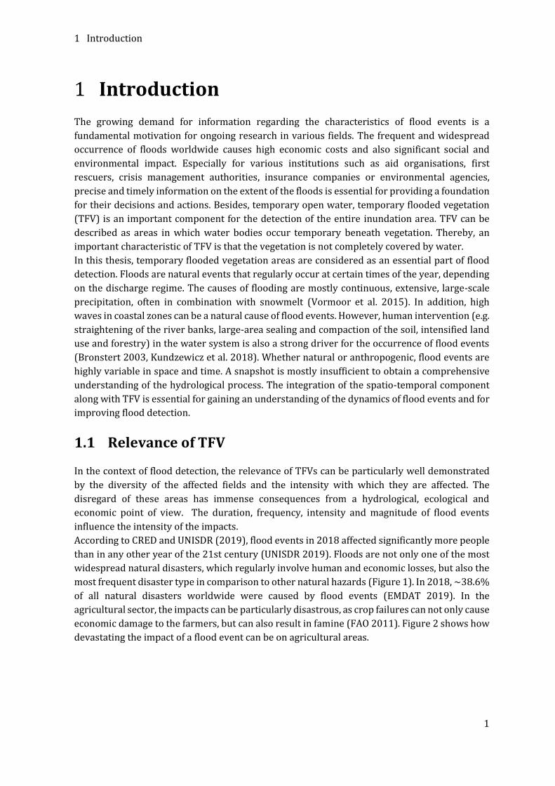
According to CRED and UNISDR (2019), flood events in 2018 affected significantly more people
than in any other year of the 21st century (UNISDR 2019). Floods are not only one of the most
widespread natural disasters, which regularly involve human and economic losses, but also the
most frequent disaster type in comparison to other natural hazards (Figure 1). In 2018, ~38.6%
of all natural disasters worldwide were caused by flood events (EMDAT 2019). In the
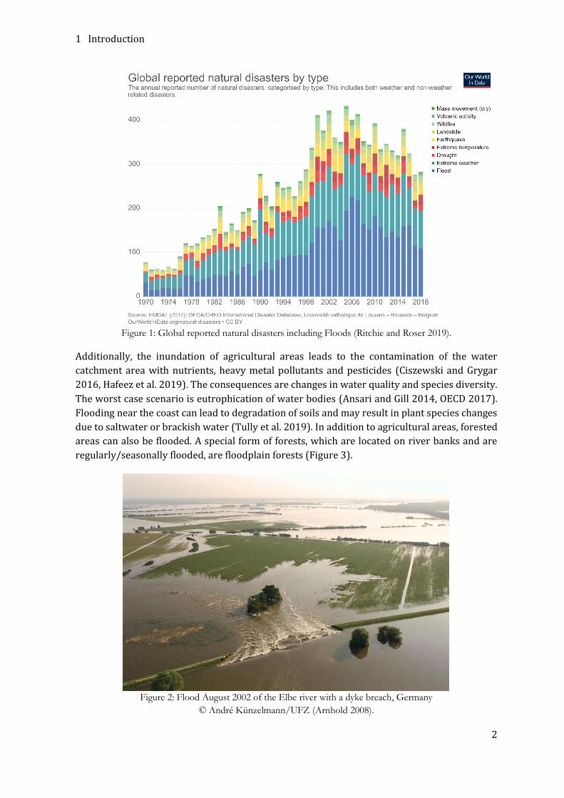
agricultural sector, the impacts can be particularly disastrous, as crop failures can not only cause
economic damage to the farmers, but can also result in famine (FAO 2011). Figure 2 shows how
devastating the impact of a flood event can be on agricultural areas.
1 Introduction
2
Figure 1: Global reported natural disasters including Floods (Ritchie and Roser 2019).
Additionally, the inundation of agricultural areas leads to the contamination of the water
catchment area with nutrients, heavy metal pollutants and pesticides (Ciszewski and Grygar
2016, Hafeez et al. 2019). The consequences are changes in water quality and species diversity.
The worst case scenario is eutrophication of water bodies (Ansari and Gill 2014, OECD 2017).
Flooding near the coast can lead to degradation of soils and may result in plant species changes
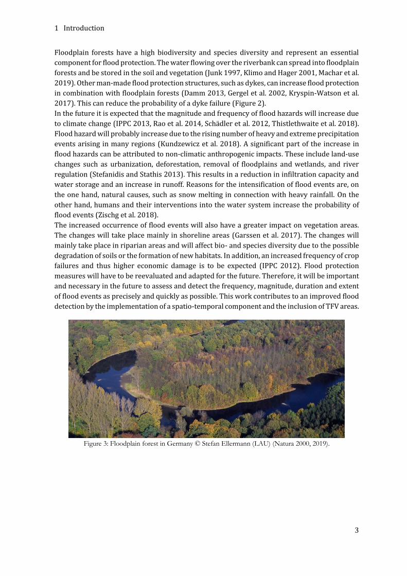
due to saltwater or brackish water (Tully et al. 2019). In addition to agricultural areas, forested
areas can also be flooded. A special form of forests, which are located on river banks and are
regularly/seasonally flooded, are floodplain forests (Figure 3).
Figure 2: Flood August 2002 of the Elbe river with a dyke breach, Germany
© André Künzelmann/UFZ (Arnhold 2008).
1 Introduction
3
Floodplain forests have a high biodiversity and species diversity and represent an essential
component for flood protection. The water flowing over the riverbank can spread into floodplain
forests and be stored in the soil and vegetation (Junk 1997, Klimo and Hager 2001, Machar et al.
2019). Other man-made flood protection structures, such as dykes, can increase flood protection
in combination with floodplain forests (Damm 2013, Gergel et al. 2002, Kryspin-Watson et al.
2017). This can reduce the probability of a dyke failure (Figure 2).
In the future it is expected that the magnitude and frequency of flood hazards will increase due
to climate change (IPPC 2013, Rao et al. 2014, Schädler et al. 2012, Thistlethwaite et al. 2018).
Flood hazard will probably increase due to the rising number of heavy and extreme precipitation
events arising in many regions (Kundzewicz et al. 2018). A significant part of the increase in
flood hazards can be attributed to non-climatic anthropogenic impacts. These include land-use
changes such as urbanization, deforestation, removal of floodplains and wetlands, and river
regulation (Stefanidis and Stathis 2013). This results in a reduction in infiltration capacity and
water storage and an increase in runoff. Reasons for the intensification of flood events are, on
the one hand, natural causes, such as snow melting in connection with heavy rainfall. On the
other hand, humans and their interventions into the water system increase the probability of
flood events (Zischg et al. 2018).
The increased occurrence of flood events will also have a greater impact on vegetation areas.
The changes will take place mainly in shoreline areas (Garssen et al. 2017). The changes will
mainly take place in riparian areas and will affect bio- and species diversity due to the possible
degradation of soils or the formation of new habitats. In addition, an increased frequency of crop
failures and thus higher economic damage is to be expected (IPPC 2012). Flood protection
measures will have to be reevaluated and adapted for the future. Therefore, it will be important
and necessary in the future to assess and detect the frequency, magnitude, duration and extent
of flood events as precisely and quickly as possible. This work contributes to an improved flood
detection by the implementation of a spatio-temporal component and the inclusion of TFV areas.
Figure 3: Floodplain forest in Germany © Stefan Ellermann (LAU) (Natura 2000, 2019).
1 Introduction
4
1.2 Potential of SAR and time series data for detection and
extraction of the TFV
Spaceborne remote sensing is a potential instrument for the acquisition of the entire flood
extent, which allows for the monitoring of large areas of the earth's surface. Since the use of
optical sensors during flood situations is often severely restricted by cloud cover, images taken
with microwave satellites are mostly used as a basis for operational flood detection due to their
independency towards weather and daylight. Therefore, this work focuses on microwave
remote sensing. Due to the characteristics of microwave radiation to penetrate into a medium
in dependence of the wavelength, microwave-based systems (radar, synthetic aperture radar
(SAR)) are suitable for the detection of standing water surfaces beneath the vegetation. This is
achieved by the capability of the radar signal to penetrate the vegetation canopy and the
interaction between the water surface and the lower areas of the vegetation. The latter can lead
to a strong backscatter signal, which is higher than under normal hydrological conditions (e.g.
(Richards et al. 1987, Townsend 2001). Despite the advantage regarding the detection of TFV
by SAR data, the interpretation of the backscatter signal from TFV is not always straightforward
because the interaction between system parameters and environmental conditions strongly
influences the backscatter signal. Therefore, essential statistical and on-site knowledge is
required in order to obtain accurate results.
Studies about the derivation of flood extent have grown steadily over the last decades (Brown
et al. 2016, Clement et al. 2017, Dellepiane et al. 2000, Schlaffer et al. 2015, Smith 1994).
However, there are only a small number of studies including the TFV area for flood monitoring
purposes (Long et al. 2014, Martinis et al. 2015, Pierdicca et al. 2008, Pulvirenti et al. 2010,
Pulvirenti et al. 2016, Zhao et al. 2014). This is primarily due to the limited availability of
appropriate SAR data. Despite the numerous operating microwave sensors, the availability of
the regularly acquired spaceborne microwave data is restricted. Therefore, the majority of the
analyzed studies used a single image or two images with flooded and non-flooded conditions.
However, the lack of information about the normal conditions of the environment and the
requirement of manual intervention can limit the reliability of results of the flood extent. With
the launched C-band S-1 satellite missiona new age of flood monitoring was initiated due to the
availability of high temporal resolution data with a revisit frequency of up to six days. The
regularity of the data acquisition over a longer period provides information about different
seasonal conditions of the vegetation and the corresponding backscatter signal.
The opportunity to include seasonal or annual fluctuations of backscatter using the free of
charge short revisit SAR time series data provide an opportunity to extract TFV and to improve
flood detection. However, the focus on the multi-temporal changes regarding TFV adds a new
level of complexity. Therefore, an in-depth analysis is required to exhibit the effects and changes
on the backscatter signal over time and during a flood event. To understand the effects regarding
TFV, the analysis of the multi-temporal characteristics and pattern of S-1 data is crucial. Besides
the SAR data, the integration of other data can be useful for obtaining an accurate extent of the
flood. Topographical data, optical data or specific layers obtained from this data can be
combined for a comprehensive analysis of inundation events and the extraction of special areas,
such as TFV.
Depending on the different tasks, the availability of SAR data, the polarization modes, the phase
information and the spatial or temporal resolution, various algorithms were applied to the

1 Introduction
5
different applications and thus inconsistency exists in the methods for the derivation of TFV
(Tsyganskaya et al. 2018b). Furthermore, there are a small number of papers in the literature
dealing with the automatic and rapid flood extraction from SAR data for operational use (e.g.
Martinis et al. 2009, Martinis and Twele 2010, Matgen et al. 2011, Pulvirenti et al. 2011,
Pulvirenti et al. 2012, Schumann et al. 2009). Due to its complexity, TFV is barely included in
flood detection approaches, as its transferability to different study areas is limited. Whenever
TFV was incorporated into a method, single image and change detection approaches were
mainly applied (Long et al. 2014, Martinis et al. 2015, Pierdicca et al. 2008, Pulvirenti et al. 2010,
Pulvirenti et al. 2016, Zhao et al. 2014). Very few studies have attempted to detect the
hydrological dynamics of flood events using time series data (Martinez and Le Toan 2007,
Pulvirenti et al. 2011a, Pulvirenti et al. 2012). Schlaffer et al. (2016) showed that based on a
multi-temporal image stack and using a harmonic model, the classification of wetland classes
can be achieved. This method shows the potential for the detection of TFV integrating temporal
and spatial variability. The use of frequently multi-temporal acquired S-1 data provide a
potential foundation for the development of a SAR based time series approach for the extraction
of TFV and improved flood detection. By incorporating seasonal or annual variations in
vegetation, the complexity of the TFV can be considered. However, the processing and analysis
of SAR time series data constitutes a challenge due to the large amounts of data. This requires
the development of an adapted algorithm allowing for the processing of dual-polarized SAR time
series data.
1.3 Scientific objectives
As shown in the previous Section 1.1, the detection of temporary flooded vegetation (TFV) is a
key component in many applications. However, at the current stage, the causes, states, impact
and implications of TFV are not sufficiently well characterized or understood. Furthermore, TFV
is not adequately considered in the current flood mapping products, as the focus mostly lies on
the extraction of temporary open water (TOW). Due to the lack of an appropriate data
foundation in the past, an adequate extraction of TFV areas is still underrepresented and widely
neglected. As the occurrence of TFV is a dynamic process, characterized by a spatio-temporal
variability, it is important to take into account and fully understand the drivers of this dynamic.
The use of SAR time series data has great potential for the detection and interpretation of TFV,
since the spatial and temporal variability can be considered (Section 1.2). Based on these
considerations, this thesis defines the following scientific objectives:
• Evaluation of the state of the art methods by providing an overview and comparison of
the data sets and classification algorithms with their advantages, limitations and
possible trends regarding the extraction of TFV.
• Analysis and evaluation of multitemporal characteristics and patterns regarding the
backscatter signal for flood related classes, such as TOW and TFV.
• Establishing the comparability between the TFV backscatter values of the image
elements and simplifying the complexity of multitemporal characteristics and patterns
of flood-relevant classes by developing polarization-dependent time series features.
• Development, assessment and validation of a new SAR time series-based method for
comprehensive and rapid mapping of entire flood extents using developed time series

1 Introduction
6
features with a focus on the increased quality of maps for flood detection by including
TFV.
• Demonstration of the transferability and the robustness of the methodology by
analyzing the impact of time series data and different polarization for various TFV types
in different study areas.
Based on the aforementioned scientific objectives, the following research questions have been
formulated:
• Research question 1: Does the comparison of the state of the art of the method provide an
identification of trends regarding the SAR based classification algorithms for the
extraction of TFV?
• Research question 2: Are the multitemporal characteristics and patterns of the SAR time
series data suitable for identifying flood-related classes (TOW and TFV)?
• Research question 3: Do the operational dual-polarized SAR systems have the potential to
provide time series features for the derivation of flood related classes (TOW and TVF)?
• Research question 4: Are dual-polarized Sentinel-1 time series data suitable for the
development of a robust classification approach for TFV extraction and improved flood
detection?
• Research question 5: Can the SAR time series approach be transferred to different study
areas and vegetation types using a single time series feature for the extraction of TFV and
thus be applied operationally?
1.4 Structure of the thesis
In Chapter 2 the basic principles of microwave remote sensing are presented. The focus lies on
the characteristics of SAR data. Furthermore, an overview of the S-1 sensors is provided, the
data of which is predominantly applied in this thesis.
Interactions of microwave signal with open water surfaces and water bodies covered by
vegetation are described in Chapter 3. Besides an explanation about the backscatter behavior of
radar waves in general, the particular characteristics of radar reflectance from open water
surfaces and flooded vegetation are also discussed.
In Chapter 4 an overview about the state of the art regarding SAR-based derivation of flooded
vegetation and the developed time series approach for the extraction of TFV with the
corresponding results are presented by three scientific peer-reviewed publications.
Section 4.1 presents the first paper reviewing the characteristics and approaches of SAR-based
detection of flooded vegetation. In addition, a comprehensive review of sensor- and object
parameters and their effects on the SAR signal regarding the detection of flooded vegetation is
provided. Furthermore, an overview of the data sets used and the state of the art for the applied
algorithms for the extraction of flooded vegetation is provided in the same publication, revealing
their benefits, limitations, methodological trends, and pointing out the potential research needs
for this field.
In Section 4.2 a SAR time series approach based on S-1 C-band data is proposed. For the
detection of the entire flood extent with the focus on TFV, the developed method combines dual-
polarized time series data with ancillary information. Based on the findings about

2 Theoretical basics
7
multitemporal characteristics and patterns (decrease and/or increase of the backscatter values
on the flood date), which indicate flood-related classes, time series features are derived. The
time series features were generated for each polarization and polarization combination by
performing a Z-transform over the time series for each image element. Thereby, a comparison
of the backscatter intensity change for the SAR signal between the pixels could be achieved. The
capabilities of the method are demonstrated for a flood event in Namibia that occurred in 2017.
Analyses regarding the impact of time series characteristics on the identification of flood related
classes and the transferability of the SAR time series approach are described in Section 4.3. An
analysis was carried out based on two independent study areas in Greece/Turkey and China
containing different vegetation types, such as high grassland and forested areas. In order to
demonstrate the transferability and the potential of the SAR time series approach for
operational use, time series features are compared simultaneously with respect to their
suitability for the extraction of TFV for all study areas.
The thesis concludes in Chapter 5 with an evaluation of the developed approach and discusses
improvement opportunities as well as an outlook for future analysis and synergetic use of SAR
data.
2 Theoretical basics
2.1 Physical fundamentals
The visualisation of the earth's surface in aerial and satellite images is defined by the properties
of the sensor in capturing the electromagnetic radiation that reaches the sensor during the
acquisition. The electromagnetic radiation serves as an information medium between the
observed object and the remote sensing sensor, which propagates as a harmonic wave with the
speed of light. The wave is detected as reflected or emitted radiation from the observed object
and contains information about its properties.
The electromagnetic radiation is represented in the electromagnetic spectrum. The entire
spectrum is divided into different areas, according to the origin and the effect of the radiations,
which fuse into each other without sharp boundaries. The different wavelength ranges, their
names, their transmissivity through the atmosphere and the most relevant recording methods
are shown in Figure 4. The electromagnetic radiation is characterized by the wavelength and
the frequency f (Lillesand et al. 2008). In comparison to the visible light about .4 to . m , which can be detected by optical sensors, the microwave radiation range is about between 1
mm and 1 m, which can be detected by radar methods. The detection of natural electromagnetic
radiation (solar radiation reflected from the earth's surface as well as heat radiation emitted
from the earth's surface itself) is called passive remote sensing, whereby artificially generated
radiation, e.g. by radar, is referred to as active remote sensing (Ulaby and Long 2015).

2 Theoretical basics
8
Figure 4: The electromagnetic spectrum and the acquisition ranges of different sensors
based on Albertz 2007.
2.2 Basic principles of imaging radar systems
In this work, data and methods of radar remote sensing were applied. Radar (radio detection
and ranging) is an active remote sensing method which uses the spectral range of microwaves.
Data acquisition using a radar sensor is largely daylight- and weather-independent, providing a
continuous temporal resolution in dependence on the orbit of the sensor. In addition, the
complex calibration and correction procedures for the reduction of atmospheric influences are
no longer necessary(Richards 2009).
Radar detection of the earth's surface is achieved by emitting microwave pulses at the pulse
repetition frequency (PRF) and by measuring the amount of energy or transit time reflected
back to the sensor by an antenna(Lillesand et al. 2008, Woodhouse 2006).The backscattering
properties are influenced by sensor-specific system parameters and the object properties.
Operational principle and properties of Synthetic Aperture Radar (SAR)
Radar remote sensing systems can be categorized into non-imaging and imaging systems. Non-
imaging systems include, for example, radar altimeters for determining heights on the land
surface. Imaging systems are e.g. the Side Looking Airborne Radar (SLAR) or the Synthetic
Aperture Radar (SAR) (Woodhouse 2006). Imaging radar systems provide a two-dimensional image of the Earth s surface after digital processing (Hein 2004).
For the remote sensing of the earth's surface from space, sensors are generally applied, which
use the Synthetic Aperture Radar (SAR) acquisition technique. The scanning process of the
earth's surface is carried out in a side-looking manner and perpendicular to the flight direction
(Figure 5), since the radar is a distance measuring method that uses the double travel time of
the microwave to spatially separate the received signals. Under optimal conditions, the sensor
moves in a straight line over a landscape and sends an impulse at fixed intervals, which
irradiates the area. Due to the relationship between antenna length and radiation
characteristics, i.e. primarily the antenna beam width, the geometric resolution of e.g. the SLAR

2 Theoretical basics
9
with real aperture is limited (Lillesand et al. 2008).In comparison, SAR systems have a short
antenna, but simulate a long antenna using the appropriate acquisition and processing
technology (Woodhouse 2006).This method is based on the Doppler effect, which is used to
generate a virtual antenna length that is a multiple larger than the physical antenna
(Lillesand et al. 2008). During the overflight, the same object is repeatedly illuminated by the
successive radar pulses. Thereby, the radar signal contributes several times to the received
signals, which are correlated in a complex way. During signal processing, however, the data is
treated as if it came from individual parts of a very long antenna. This reduces the effective radar
beam width and achieves a higher resolution in flight direction (azimuth direction) in the radar
image compared to a real beam width of the antenna.
Figure 5: Imaging geometry of a space-based SAR sensor.
Resolution in range and in azimuth
A SAR system is characterized by its resolution in range (across-track) and azimuth (along-
track). The range resolution can be described by the slant range or by the ground range
resolution. In order to distinguish two object points in the slant range, their signals must be
spatially separable from each other. For this purpose, their transit times (t1 and t2) must differ
from each other by at least the length of the pulse length t(|t2- t1| ≥τ). Thus, the resolution
(Figure 6) at slant range for Real Aperture Radar (RAR) and SAR is calculated with c for the
speed of light and pulse duration τ (Woodhouse 2006):

2 Theoretical basics
10
= ∗τ (1)
By projecting the slant range resolution with the angle of incidence θi on the ground, the
resolution in ground range resolution can be obtained (Wooshouse 2006):
𝑔 = ∗ τ𝑖 θi (2)
The slant range resolution remains constant, independent of the range. However, in ground
range coordinates, the ground resolution depends on the angle of incidence. The crucial
parameter for ground range resolution is not the height of the sensor above the ground, but the
length of the pulse duration τ.
Therefore, reducing the pulse duration increases the resolution in the range direction. The pulse
duration τ cannot be reduced arbitrarily in practice, since the energy to be sent increases with
a shortening. The amount of energy is limited by the hardware. Technically, this is achieved by
sending a much more extended, linear frequency-modulated signal instead of a short pulse. This
signal is called chirp. After receiving this signal, it is converted into an equivalent short signal by
the matched filter approach (Woodhouse 2006).
Figure 6: Resolution in slant range and ground range.
The azimuth resolution (ra) along the flight direction (along-track) corresponds with traditional
RAR approximately to the width of the footprint in flight direction. Using the RAR system, a
ground point is only acquired once. Therefore, two objects can only be distinguished if they are
not in the same footprint. The azimuth resolution depends on the beam width of the antenna
footprint 𝜑 (Figure 7), which is defined by the ratio between the wavelength of the transmitted
pulses and the physical antenna length L: 𝜑 = 𝜆𝐿 (3)
With this beam width, the geometric resolution of RAR results for a defined distance R on the
ground to:
2 Theoretical basics
11
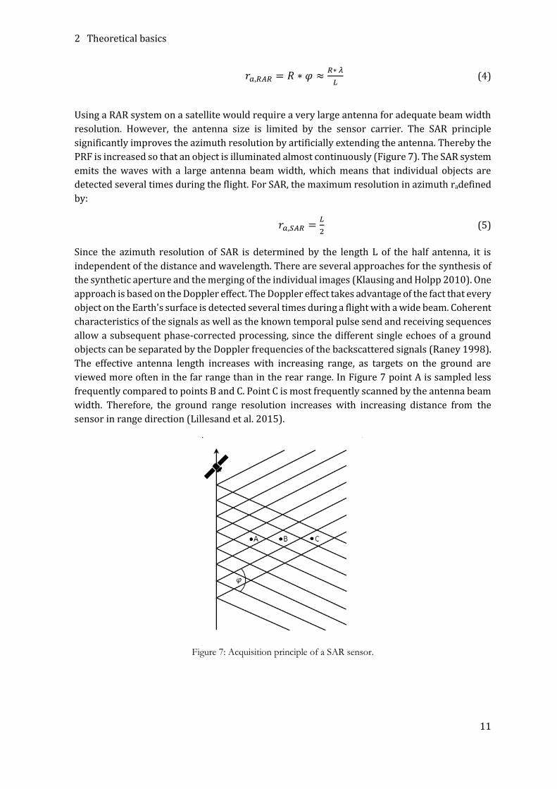
𝑎, 𝐴 = 𝑅 ∗ 𝜑 ≈ ∗ 𝜆𝐿 (4)
Using a RAR system on a satellite would require a very large antenna for adequate beam width
resolution. However, the antenna size is limited by the sensor carrier. The SAR principle
significantly improves the azimuth resolution by artificially extending the antenna. Thereby the
PRF is increased so that an object is illuminated almost continuously (Figure 7). The SAR system
emits the waves with a large antenna beam width, which means that individual objects are
detected several times during the flight. For SAR, the maximum resolution in azimuth radefined
by:
𝑎, 𝐴 = 𝐿 (5)
Since the azimuth resolution of SAR is determined by the length L of the half antenna, it is
independent of the distance and wavelength. There are several approaches for the synthesis of
the synthetic aperture and the merging of the individual images (Klausing and Holpp 2010). One
approach is based on the Doppler effect. The Doppler effect takes advantage of the fact that every
object on the Earth's surface is detected several times during a flight with a wide beam. Coherent
characteristics of the signals as well as the known temporal pulse send and receiving sequences
allow a subsequent phase-corrected processing, since the different single echoes of a ground
objects can be separated by the Doppler frequencies of the backscattered signals (Raney 1998).
The effective antenna length increases with increasing range, as targets on the ground are
viewed more often in the far range than in the rear range. In Figure 7 point A is sampled less
frequently compared to points B and C. Point C is most frequently scanned by the antenna beam
width. Therefore, the ground range resolution increases with increasing distance from the
sensor in range direction (Lillesand et al. 2015).
Figure 7: Acquisition principle of a SAR sensor.

2 Theoretical basics
12
Radar equation and backscatter coefficient
The received and recorded power (Pr) at the antenna of a SAR system can be transformed into
a two-dimensional image (Bamler and Schättler 1993, Curlander and MacDonough 1991,
Moreira et al. 2013). The power depends on the sensor and scattering properties of the
illuminated object. Both variables influence the backscatter signal and can be described
mathematically by the radar equation (Ulaby and Long 2015): 𝑃 = 𝑃𝑡𝐺 𝜆 σπ (6)
where Pt is s the emitted power, G is the antenna gain, the wavelength, R the distance to the target and σ represents the radar backscatter cross section. The radar cross-section σ[m2] is the backscattering of a discrete objects. This is a function of the
scattering properties or the reflection behavior of the target object on the earth's surface. For
the characterization of distributed targets in the context of Earth observation, the radar backscatter coefficient σ0 (normalized radar cross-section (NCS) or sigma naught) is used
(Woodhouse 2006): σ0 = σ𝐴 [ ] (7)
where A is the area over which the measurement is made. σ0 is usually expressed
logarithmically in decibel [dB]. For the description of imaging radar products, this parameter is
best suited to accurately estimate the normalized cross-sectional values for a given pixel. The
radar backscattering coefficient describes the scattering characteristics of an object (Hein
2004).
Speckle effect
A characteristic of radar images are the granular image structures, which also occur in
homogeneous surfaces - the so-called speckle effect (Lillesand et al. 2015, Woodhouse
2006). The occurrence of speckle is physically caused by a monochromatic imaging system,
due to the fact that the emitted coherent radiation is scattered differently at the objects
within the image pixel and reflected in different phases. Due to the backscatter at countless
particles (distributed target) on the ground, the individual waves overlap coherently and
thus interfere with each other. The recorded signal is thus a combination of different
individual signals with different phases (Raney 1998). Due to the speckle effect, the
backscatter intensity of a pixel is only slightly correlated with the physical conditions on the
ground. As a result, homogeneous surfaces are not homogeneously imaged, but appear
rather granular in the image.
Speckle can be reduced by various digital image processing techniques, e.g. speckle filtering,
which is crucial for adequate estimation of the backscattering coefficient σ0. Mostly, efforts
are made to reduce the influence of speckle by averaging the intensity and phase
information pixel by pixel. This can be achieved by so-called multi-look procedures during
SAR acquisition and processing. Thereby, the subdivision of the synthetic aperture into

2 Theoretical basics
13
several independent apertures (single looks) allows the detection of a terrain object by
multiple acquisitions, which are averaged to produce multi-looked image.This method
reduces the geometric resolution of the individual looks (Bähr and Vögtle 1998). For the
reduction of the speckle effect different filter methods are used (e.g. Frost et al. 1982, Lee
1981, Lee and Pottier 2009).
Geometric effects (Layover, Shadowing and foreshortening)
Using the SAR system, objects can only be distinguished if the reflected pulses arrive at the
sensor with a time delay. A resolution depending on the angle of incidence, as it is usual with
optical sensors, is not possible without a side looking antenna. Therefore, the SAR sensor can
never look down vertically (nadir), but has to look at the area diagonally from the side (side-
looking). This results in some effects that complicate the interpretation of a radar image. Figure
8 shows schematically the predominantly occurring geometric effects in a SAR system. Slopes
that face the sensor cause a shift from elevated terrain to the sensor. The side facing sensor
shrinks to a fragment of its actual length. This effect is called foreshortening. Thereby, the energy
of many scatters is compressed within few image pixels and the surface, which is directed
towards the sensor, appears bright in the SAR image. Layover is an extreme form of the
foreshortening effect, where the signal from the top of an object (mountain, building) reaches
the sensor before that of the base. Areas facing away from the sensor or located behind steep
walls or human buildings are not illuminated. Consequently, the objects hidden behind cannot
be displayed because no backscatter return is therefore received from that shadow region
(Ulaby and Long 2015).
Figure 8: Geometric and radiometric relief distortions.
As long as the landscape is quite flat, the distortions are hardly noticeable. However, if the
landscape has a strong relief, whether natural or man-made, the distortions occur (Woodhouse
2006).
The Foreshortening effect can be compensated with the help of an elevation model (Bayanudin
and Jatmiko 2016). The finer the resolution of the elevation model used, the more detailed the
geometric effects can be modeled. Layover can only be decomposed in exceptional cases if the
signatures of the overlapping objects are known. However, a shadow cannot be removed
mathematically due to a lack of information. In order to fill these gaps with image material,
further acquisitions from other angles are required.

2 Theoretical basics
14
System specific imaging parameters (wavelength, polarization, incidence angle)
The representation of the earth's surface in radar images depends on the interaction of various
individual factors. These are on the one hand the parameters of the acquisition system and on
the other hand parameters of the terrain surface. The system parameters (sensor parameters)
include the wavelength and frequency of the transmitted radiation, the polarization and the
incidence angle (Ulaby and Long 2015).
In radar remote sensing, the wavelength [cm] or frequency range [GHz] between 0.75 cm and
100.0 cm or 40.0 GHz and 0.3 GHz is used. Above a wavelength of approx. 2 cm, microwave
radiation can penetrate the atmosphere almost unaffected, even in cloudy conditions. Only
strong rain events can affect the transmissivity of the radar signal up to a wavelength of approx.
4 cm. The wavelength determines the percentage of different types of scattering on certain
object surfaces as well as the penetration depth of the waves and the signal attenuation in
media such as vegetation or soil (Ulaby and Long 2015). In general, radar signals of lower
frequencies are characterized by a higher capacity to penetrate media. Therefore, C-band
and X-band SAR are preferred for the analysis of surface structures, while L-band SAR is
preferred for the detection of structures below the surface (Lillesand et al. 2015).
The polarization of an electromagnetic wave is defined by the direction of the electric field
(Bhatta 2011). Radar systems have the ability to transmit and receive electromagnetic
waves in vertical (V) and horizontal (H) polarization planes. Like-polarised systems
transmit and receive in the same polarization (VV and HH). The cross-polarised systems
transmit in horizontal or vertical planes and receive the signals in the other plane (VH and
HV) (Bhatta 2011, Lillesand et al. 2015). Radar systems can be equipped with single,
multiple or fully polarized systems. A single polarized system captures information only in
one transmitted and received polarization combination, while a multiple system allows to
combine different channels. A fully polarized system is defined as a system in which the
polarimetric phase information is stored in addition to the backscatter intensity. It allows
the complete description of the scattering behavior of a terrain object by measuring a
complex scattering matrix containing the scattering mechanisms and the scattering
heterogeneity. The basics of polarimetry and its possible applications are discussed in Ulaby
et al. (2015) and in Lee and Pottier (2009). Depending on the object properties, such as
characteristic geometrical shape, different polarized radar beams are scattered differently
and thus show different backscattering behavior. The incidence angle θi is another relevant sensor parameter which is located between the
nadir and the incident radar beam (Figure 5). This is supplemented by the depression angle θd at 90°. While the incidence angle is defined for a plane earth, the local incidence angle θloc
takes the local terrain slope into account (Figure 9). This is defined as the angle between the radar beam and the surface normal. Since θloc depends on the orientation and slope of the
terrain surface as well as on the incidence angle, it can be regarded as a system parameter
as well as an object parameter. In addition, the interaction between the target and the
electromagnetic (EM) wave depends on the incidence angle. The sensitivity of the signal to
surface roughness or the contribution of the vegetation crown to the radar signal increases
with the angle of incidence (Townsend 2001).

2 Theoretical basics
15
Figure 9: Local imaging geometry.
Object-specific parameters
Due to the interaction of radar radiation with objects on the earth's surface, various object-
specific parameters influence the backscatter coefficient. The backscatter information can then
be used to draw conclusions about certain properties of the surfaces analyzed. Besides the
system parameters, the roughness characteristic and the dielectric properties of the object
are significant.
Roughness characteristics is one of the dominant factors influencing the visual representation
of a feature on radar images. In this context, roughness means the smoothness of the target in
terms of wavelength and incidence angle (Lewis et al. 1998, Woodhouse 2006). At different
frequencies and at different incidence angles the same surface shows different roughness.
When a smooth surface is hit by radiation, it is reflected away from the sensor by Snell's law
(Figure 10). As a result, it tends to appear very dark in radar images. With increasing roughness,
the proportion of diffuse scattering is greater. The incident energy is scattered in all directions
and a significant part is returned to the sensor. With increasing roughness of a surface, the
scattered element increases, while the reflected element of the signal decreases (Figure 10).
With a very rough (Lambertian) surface, the energy is evenly scattered in all directions (Ulaby
and Long 2015). In addition to the roughness itself, the wavelength ( ) and the incidence angle
(θi) or the local incidence angle (θloc) determine the intensity of backscattering to the sensor.
Figure 10: Radar reflection at a) smooth, b) moderately roughened and c) strongly roughened surfaces
modified after Lillesand et al. (2015).
The Rayleigh criterion describes the relationship between these parameters and also allows to
verify whether a surface is rough at a given wavelength and incidence angle. The Rayleigh
criterion is expressed as follows:
2 Theoretical basics
16
> λ8 θ𝑙𝑜𝑐 (8)
where s is the mean square height of the surface variations.
For natural surfaces, the Rayleigh criterion is often not strict enough, since the surfaces have a
roughness spectrum similar to the wavelength, which leads to more frequent scattering. A
stricter criterion, such as the Fraunhofer criterion proposed by Ulaby and Long (2015), is
required: > λ θ𝑙𝑜𝑐 (9)
According to Rayleigh and the Fraunhofer criteria, a surface is rough once the phase difference
ΔФ between two reflected waves is greater than π/2radiant or π/8 radiant (Woodhouse 2006).
The scattering and absorption of radar radiation through a medium is strongly dependent on its
dielectric properties. These are described by a complex dielectric constant ε, which is a measure
for the interaction of electromagnetic radiation with a material and for the polarizability of the
media, respectively (Raney 1998). It is mathematically described by a real component ε'' and
an imaginary or image component ε''. The real component defines the degree of reflection at the
transition of the radiation beams from one medium to another. The imaginary component
represents the loss factor and describes the attenuation of the signal in the respective medium.
The greater the contrast between the dielectric constants ε of two media, the stronger is the
interaction of electromagnetic waves at the boundary between the two media and thus the radar
backscattering (Bayer and Winter 1990). For the microwave range, most natural dry
materials have a low value of ε΄ between 3 and 8, while the dielectric constant of e.g. water
is very high (ε΄ = 80). Therefore materials with increased water content, but also metals,
have a much higher dielectric constant (Lillesand et al. 2015, Ulaby and Long 2015). The
dielectric properties of natural media are essentially determined by their water content
(Dobson et al. 1995). This means that variations in soil moisture and plant water content have
an effect on the dielectric properties and backscattering properties of these area. The dielectric
constant of the soil depends not only on the soil moisture but also on the soil type and the
frequency of the radar radiation (Ulaby and Long 2015). In general, the greater the roughness
and the dielectric constant of the detected object, the stronger the radar backscatter signal
(Kiage et al. 2005).
2.3 Sentinel-1
For this work spaceborne C-band (5.405 GHz) SAR data of the S-1 sensor were primarily used,
which belongs to the Sentinel satellite series. These are Earth observation satellites of the
Copernicus Program (formerly Global Monitoring for Environment and Security (GMES)) of
European Space Agency (ESA)(Copernicus 2018). The S-1 mission is designed as a two-satellite
constellation (Sentinel-1A and Sentinel-1B). The two satellites were launched on 3 April 2014
and 25 April 2016 respectively (ESA 2018b). Thereby, the two identical satellites operate in a
near-polar, sun-synchronous orbit plane with 180° orbital phasing difference and at an altitude
of almost 700 km. A single S-1 satellite is potentially able to map the global landmasses in the

3 Interactions between SAR signal and open and vegetation covered water bodies
17
Interferometric Wide Swath Mode (IW) once every 12 days, in a single pass (ascending or
descending). The configuration of two satellites optimizes coverage and provides a global
revision time of only six days. The Sentinel constellation is a dual polarised SAR system that also
preserves the phase information. The acquisition can be performed in single polarization (HH
or VV) mode as well as dual polarization (HH+HV or VV+VH) modes. The S-1 data is available
free of charge and can be downloaded via the Sentinel Data Hub (ESA 2018a). S-1 data products
acquired in Stripmap Mode (SM), IW mode, Extra Wide Swath Mode (EW), and Wave Mode (WV)
(Table 1). SM mode is only used for extraordinary situations such as emergency management or
for the detection of small islands. The monitoring of large-scale coastal areas, including shipping,
oil spills and sea ice, is primarily carried out in EW mode. The IW and the WV modes allow
conflict-free global coverage of the earth's surface via land with VV+VH and via open ocean with
VV polarization respectively. Doppler centroid estimated, single look complex focused S-1 data
are used in this work, additionally including image post-processing step for generation of the
products Single Look Complex (SLC) and Ground Range Detected (GRD). While the SLC products
(Table 2Fehler! Verweisquelle konnte nicht gefunden werden.) preserve the phase
information and maintain the natural pixel spacing, the GRD products (Table 3) contain only the
detected amplitude and are multi-looked to reduce the effects of speckle (ESA 2018b).
Table 1: Characteristics of SM, IW and EW modes.
SM IW EW Scene width 80 km 250 km 410 km Incidence angle range (full performance)
18.3° - 46.8° 29.1° - 46.0°
21.6° - 25.1° 34.8° - 38.0°
Polarization Dual HH+HV, VV+VH Single HH, VV
Dual HH+HV, VV+VH Single HH, VV
Single HH, VV
Table 2: Acquisition resolution Level-1 SLC.
Mode Resolution (rg x az) Pixel spacing (rg x az) SM 1.7 x 4.3 m to 3.6 x 4.9 m 1.5 x 3.6 m to 3.1 x 4.1 m IW 2.7 x 22.0 m to 3.5 x 22.0 m 2.3 x 14.1 m EW 7.9 x 43.0 m to 15.0 x 43.0 m 5.9 x 19.9 m
Table 3: High resolution Level-1 GRD.
Mode Resolution (rg x az) Pixel spacing (rg x az) SM 23x23 m 10x10 m IW 20x22 m 10x10 m EW 50x50 m 25x25 m
3 Interactions between SAR signal and
open and vegetation covered water bodies
3.1 Backscatter behavior of radar waves
The total radiation captured by the sensor is the sum of the various complex scattering
processes, which are dependent on the system and object parameters (Section 2.2) These

3 Interactions between SAR signal and open and vegetation covered water bodies
18
contribute differently to the backscatter coefficient (Figure 11). Two scattering mechanisms are
distinguished in the interaction of radiation at the surface. The first is surface scattering, which
takes place at the boundary layer of two media with different homogeneous dielectric properties
(Ulaby and Long 2015). Thereby, the microwaves are partly absorbed and reflected (specular
reflection) or diffusely scattered (diffuse surface scattering) depending on the properties of
the lower medium. The second main scattering mechanism is volume scattering, which occurs
in dielectrically inhomogeneous media, into which microwave radiation can penetrate. This is
particularly the case for vegetation (diffuse volume scattering). A special case of surface
scattering is corner reflection (double bounce), which occurs when a wave hits two flat
surfaces at a 90° angle to each other. Thereby, the emitted radiation is reflected back to the radar
sensor, which leads to a high backscatter value (Woodhouse 2006). These double or multiple
specular reflections occur, for example, between the ground/water surface and tree
trunks/vegetation stems or between streets and houses.
Figure 11: Scattering mechanisms between microwaves and the land surface: a). specular reflection, b) diffuse
surface scattering, c) corner reflection (double bounce), d). diffuse volume scattering.
3.2 Open water
The ideal condition for detecting open inland water surfaces is when the water surface is
smoother than the surrounding land surface in terms of wavelength and incidence angle. The
smooth open water surface (Figure 10) with a high dielectric constant can easily be detected
by the radar data, as it acts like a specular reflector reflecting the radar energy away from the
sensor (Ulaby and Long 2015). As a result, only a very small portion of the signal returns,
resulting in relatively dark pixels in the radar image. These provide a strong contrast to the
rougher land surfaces/non-water surfaces, which are dominated by diffuse scattering and have
higher backscattering values. With increasing incidence angle, the contrast between land and
water increases, as steep angles imply low backscatter values (Mouginis 2017). With longer
wavelengths, the sensitivity to diffuse scattering decreases and objects on land can appear
smoother, increasing the probability of confusion between land and water surfaces.
Furthermore, increased surface roughness of the water due to waves or precipitation reduces
the ability to distinguish between water and land surfaces. An increasing roughness causes a
higher backscatter signal and thus an increased backscatter intensity.
3 Interactions between SAR signal and open and vegetation covered water bodies
19
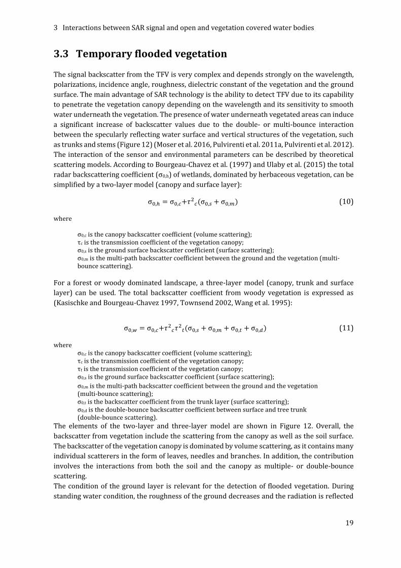
3.3 Temporary flooded vegetation
The signal backscatter from the TFV is very complex and depends strongly on the wavelength,
polarizations, incidence angle, roughness, dielectric constant of the vegetation and the ground
surface. The main advantage of SAR technology is the ability to detect TFV due to its capability
to penetrate the vegetation canopy depending on the wavelength and its sensitivity to smooth
water underneath the vegetation. The presence of water underneath vegetated areas can induce
a significant increase of backscatter values due to the double- or multi-bounce interaction
between the specularly reflecting water surface and vertical structures of the vegetation, such
as trunks and stems (Figure 12) (Moser et al. 2016, Pulvirenti et al. 2011a, Pulvirenti et al. 2012).
The interaction of the sensor and environmental parameters can be described by theoretical
scattering models. According to Bourgeau-Chavez et al. (1997) and Ulaby et al. (2015) the total
radar backscattering coefficient (σ0,h) of wetlands, dominated by herbaceous vegetation, can be
simplified by a two-layer model (canopy and surface layer): σ0,ℎ = σ0, +𝜏 σ0, + σ0, (10)
where σ0,c is the canopy backscatter coefficient (volume scattering); τc is the transmission coefficient of the vegetation canopy; σ0,s is the ground surface backscatter coefficient (surface scattering); σ0,m is the multi-path backscatter coefficient between the ground and the vegetation (multi-
bounce scattering).
For a forest or woody dominated landscape, a three-layer model (canopy, trunk and surface
layer) can be used. The total backscatter coefficient from woody vegetation is expressed as
(Kasischke and Bourgeau-Chavez 1997, Townsend 2002, Wang et al. 1995):
σ0,𝑤 = σ0, +𝜏 𝜏 σ0, + σ0, + σ0, + σ0, (11)
where σ0,c is the canopy backscatter coefficient (volume scattering); τc is the transmission coefficient of the vegetation canopy; τt is the transmission coefficient of the vegetation canopy; σ0,s is the ground surface backscatter coefficient (surface scattering); σ0,m is the multi-path backscatter coefficient between the ground and the vegetation
(multi-bounce scattering); σ0,t is the backscatter coefficient from the trunk layer (surface scattering); σ0,d is the double-bounce backscatter coefficient between surface and tree trunk (double-bounce scattering).
The elements of the two-layer and three-layer model are shown in Figure 12. Overall, the
backscatter from vegetation include the scattering from the canopy as well as the soil surface.
The backscatter of the vegetation canopy is dominated by volume scattering, as it contains many
individual scatterers in the form of leaves, needles and branches. In addition, the contribution
involves the interactions from both the soil and the canopy as multiple- or double-bounce
scattering.
The condition of the ground layer is relevant for the detection of flooded vegetation. During
standing water condition, the roughness of the ground decreases and the radiation is reflected

3 Interactions between SAR signal and open and vegetation covered water bodies
20
away from the sensor because of the specular smooth water surface. If this reflected radiation
hits vertical structures such as stems or tree trunks, this can lead to multi- or double bounce
scattering and thus to an increase in the backscattering values, which suggests the presence of
water underneath the vegetation. The ability to detect flood under the vegetation depends on
the transmittance τc and τt) of microwave energy through the canopy layer and also on the
canopy layer itself. In general, it should be noted that the factors leaf sizes, its shape and
orientation, spatial variations in tree heights, density, basal area and species composition can
cause significant spatial differences in the ability to detect inundation underneath the vegetation
(Townsend 2002). In addition, the transmittance depends strongly on the sensor parameters,
such as wavelength, polarization and incidence angle. The effects of sensor characteristics,
environmental conditions, and their interactions on the SAR signal regarding flooded vegetation
are described in detail in Section 4.1.
Figure 12: The elements of the two-layer and three-layer model with sources of scattering for non-woody vegetation and woody vegetation, respectively (modified after Kasischke and Bourgeau-Chavez (1997)).

4 Scientific publications
21
4 Scientific publications
This work is a collection of research results obtained in recent years regarding the temporary
flooded vegetation, which were published in several papers. The synthesis is carried out to
answer the research questions described in the previous section. The work consists of three
papers which have been published in relevant journals. Two of these papers were published in
international peer-review journals, while a further paper was submitted to a peer-review
journal and is currently under review. The first paper allows to situate the work within the
research context, shows the potential and limitation of SAR time series data for flood detection
with the focus on the derivation of TFV and points out the of future research needs. The second
paper presents the new methodology for flood area detection with a focus on TFV based on dual-
polarized S-1 C-band time series data and ancillary information. The method is applied to an
example study area. The last paper examines the transferability of the developed approach to
other study areas and different TFV types.
4.1 Paper I: SAR-based Detection of Flooded Vegetation – A
Review of Characteristics and Approaches
Tsyganskaya, V., Martinis S., Marzahn P., and Ludwig. R. 2018. 'SAR-based detection of flooded
vegetation – a review of characteristics and approaches'. In: International Journal of Remote
Sensing. 39 (8). 2255–2293.
For a fundamental understanding of the influence of sensor- and object parameters on the
backscatter coefficient regarding the flooded vegetation, a comprehensive review about the
effects of sensor characteristics, environmental conditions, and their interactions on the SAR
signal for the identification of flooded vegetation are described in Paper I. Furthermore, an
overview of the state of the art in relation to the data sets and algorithms for the extraction of
flooded vegetation is provided in the same publication showing their benefits, limitations and
methodological trends. Above all, this paper gives the state of the art of the used SAR data sets
and approaches regarding the detection of flooded vegetation and points out the potential
research needs in this field.
Author’s contributions: All authors contributed to the concept of the study, while all research,
information collection, analysis and evaluation were performed by V. Tsyganskaya. The first
version of the manuscript was written by V. Tsyganskaya, while all authors contributed with
valuable input and expertise to the final document.
Status: published
Journal: International Journal of Remote Sensing (Taylor & Francis)

REVIEW ARTICLE
SAR-based detection of flooded vegetation – a review ofcharacteristics and approaches
Viktoriya Tsyganskayaa,b, Sandro Martinis b, Philip Marzahna and Ralf Ludwiga
aDepartment of Geography, Ludwig-Maximilians-Universität München, Munich, Germany; bGermanRemote Sensing Data Center (DFD), German Aerospace Center (DLR), Wessling, Germany
ABSTRACT
The ability of synthetic aperture radar (SAR) to detect floodedvegetation (FV) (the temporary or permanent occurrence of water-bodies underneath vegetated areas) offers a great benefit in theresearch fields of flood and wetland monitoring. The growingdemand for near real-time information in flood monitoring andan increased awareness of the importance of wetland ecosystemsare strong drivers for the ongoing research in these fields, whereFV constitutes an essential part. This study reviewed 128 publica-tions summarizing the knowledge about the relationshipsbetween the SAR parameters and the environmental conditionsfor the detection of FV. An advanced review of 83 studies wascarried out to gain insights about applied classification techniquesand SAR data for the extraction of FV. Although some trendsemerged about which wavelengths, polarisations, or incidenceangles to use, there is variation in the application of differentclassification techniques or using SAR-derived informationdepending on the data sets and the study area. Notable through-out the analysed articles is the growing demand for unsupervisedand computationally efficient methods of higher accuracy for theextraction of FV. Based on the advances in SAR with regard tospatial and temporal resolution, the development of robustapproaches for the extraction of FV from various and complexenvironments has to be further pursued.
ARTICLE HISTORY
Received 28 March 2017Accepted 5 December 2017
1. Introduction
Detection and extraction of flooded vegetation (FV) is of particular importance for twoapplication fields: wetland and flood monitoring. Wetlands comprise open water areas,as well as different types of FV (e.g. emerging woody, herbaceous vegetation) (Whiteet al. 2015), which can be permanently or seasonally flooded. Wetlands are importantecosystems providing many essential services, such as flood control, sediment storage,wildlife habitat, filtering of contaminants, recreation, aesthetic value, and others(Millennium Ecosystem Assessment 2005). Despite these benefits, wetlands have beenextensively converted to agriculture areas worldwide (Asselen et al. 2013) and
CONTACT Viktoriya Tsyganskaya [email protected] Ludwig-Maximilians-Universität München, Department of Geography, Luisenstr. 37, Munich 37, 80333, Germany
INTERNATIONAL JOURNAL OF REMOTE SENSING, 2018
VOL. 39, NO. 8, 2255–2293
https://doi.org/10.1080/01431161.2017.1420938
© 2018 Informa UK Limited, trading as Taylor & Francis Group
Dow
nlo
aded
by [
89.1
5.1
45.1
16]
at 1
2:1
2 1
3 J
anuar
y 2
018

furthermore are endangered by climate change (Erwin 2009). Continuous monitoring ofchanges in wetlands contributes to their protection.
In comparison to wetland monitoring, detecting FV for flood monitoring is a relativelyyoung field. Besides the detection of open waterbodies, the focus lies on the extraction ofFV. The availability of detailed near real-time information about the extent of inundationareas at large scales is a significant data source for many institutions, such as humanitarianrelief organizations, decision makers for crisis management or insurance companies. Incontrast to open flood surfaces, there is little research on the detection of flooded areasunderneath vegetation. However, the disregard of FV can lead to an underestimation ofthe extent of an inundation, which may lead to higher risk to human lives and damage oftheir properties. Furthermore, flood affects agricultural areas worldwide, entailing enor-mous economic losses (Trujillo 2015). These possible impacts show the importance tocontinue the investigations in the field of FV as a part of wetland detection and floodmonitoring.
The terminology and definition of FV vary from survey to survey, depending on itsscope and study area. Terms such as partially submerged vegetation (Martinis und Rieke2015) or FV (e.g. Pierdicca et al. 2008; Pulvirenti et al. 2013; Pulvirenti et al. 2016; Martinezund Le Toan 2007; Martinis und Twele 2010) can be found in the corresponding literature.The designation FV is used to describe unspecified types of FV or as an umbrella term fordifferent vegetation types (e.g. standing water underneath forested or in between agri-cultural areas) (Betbeder et al. 2014; Schlaffer et al. 2016). In the scope of this review, theterm FV describes the temporary or permanent occurrence of a water surface beneath avegetation canopy; however, it does not consider vegetation areas, which are completelycovered by water. In agricultural or herbaceous areas, the leaves or stems of the plantsvisibly emerge above the water surface. In forests or tree stands, standing water can occurunderneath the vegetation canopy during flood conditions. FV summarizes different termsrelated to the aforementioned definition used in the reviewed literature.
Synthetic aperture radar (SAR) is a well-known and well-established tool for theextraction of FV from space due to numerous advantages. In comparison to opticalsensors, the SAR systems use longer wavelengths of the electromagnetic spectrum,allowing cloud penetration and therefore weather independent image acquisition.Furthermore, SAR systems are active sensors, transmitting and receiving their ownelectromagnetic impulses, which allows operations independent of daylight (Klemas2013; Betbeder et al. 2014). A relatively high energy supply is required for SAR observa-tions, which can be a restricting factor for the availability of SAR time series data andeven for the acquisition of single images in some regions in the world. However, therecently launched C-band Sentinel-1 and L-band ALOS-2 satellite missions may nowovercome this limitation and therefore provide a possibility for continuous monitoringof ground features and their changes over time with short revisit times (White et al.2015). The main advantage of SAR technology, however, is the ability to detect FV dueto its capability to penetrate the vegetation canopy to a certain extent depending onthe wavelength and its sensitivity to water underneath the vegetation. SAR backscatterintensity (BI) values can significantly increase during the presence of water underneathvegetated areas due to the double- or multi-bounce interaction between the specularlyreflecting water surface and vertical structures of the vegetation, such as trunks andstems (Moser et al. 2016; Pulvirenti et al. 2013; Pulvirenti et al. 2011a).
2256 V. TSYGANSKAYA ET AL.
Dow
nlo
aded
by [
89.1
5.1
45.1
16]
at 1
2:1
2 1
3 J
anuar
y 2
018
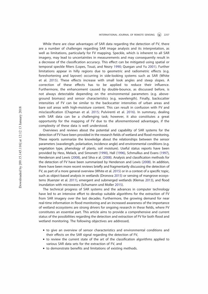
While there are clear advantages of SAR data regarding the detection of FV, thereare a number of challenges regarding SAR image analysis and its interpretation, aswell as limitations, particularly for FV mapping. Speckle, which is inherent to all SARimagery, may lead to uncertainties in measurements and may consequently result ina decrease of the classification accuracy. This effect can be mitigated using spatial ortemporal speckle filters (Lopes, Touzi, and Nezry 1990; Quegan und Yu 2001). Furtherlimitations appear in hilly regions due to geometric and radiometric effects (e.g.foreshortening and layover) occurring in side-looking systems such as SAR (Whiteet al. 2015). These effects increase with small look angles and steep slopes. Acorrection of these effects has to be applied to reduce their influence.Furthermore, the enhancement caused by double-bounce, as discussed before, isnot always detectable depending on the environmental parameters (e.g. above-ground biomass) and sensor characteristics (e.g. wavelength). Finally, backscatterintensities of FV can be similar to the backscatter intensities of urban areas andbare soil areas with high-moisture content. This can result in confusion with FV andmisclassification (Chapman et al. 2015; Pulvirenti et al. 2016). In summary, dealingwith SAR data can be a challenging task; however, it also constitutes a greatopportunity for the mapping of FV due to the aforementioned advantages, if thecomplexity of these data is well understood.
Overviews and reviews about the potential and capability of SAR systems for thedetection of FV have been provided in the research fields of wetland and flood monitoring.These reports summarize the knowledge about the relationships between the sensorparameters (wavelength, polarisation, incidence angle) and environmental conditions (e.g.vegetation type, phenology of plants, soil moisture). Useful status reports have beenprovided by Hess, Melack, and Simonett (1990), Hall (1996), Schmullius and Evans (1997),Henderson and Lewis (2008), and Silva e al. (2008). Analysis and classification methods forthe detection of FV have been summarized by Henderson and Lewis (2008). In addition,there have been more recent reviews briefly and fragmentarily discussing the detection ofFV, as part of a more general overview (White et al. 2015) or in a context of a specific topic,such as object-based analysis in wetlands (Dronova 2015) or sensing of mangrove ecosys-tems (Kuenzer et al. 2011), emergent and submerged wetlands (Klemas 2013), and floodinundation with microwaves (Schumann und Moller 2015).
The technical progress of SAR systems and the advances in computer technologyhave led to an intensive effort to develop suitable algorithms for the extraction of FVfrom SAR imagery over the last decades. Furthermore, the growing demand for nearreal-time information in flood monitoring and an increased awareness of the importanceof wetland ecosystems are strong drivers for ongoing research in these fields, where FVconstitutes an essential part. This article aims to provide a comprehensive and currentstatus of the possibilities regarding the detection and extraction of FV for both flood andwetland monitoring. The following objectives are addressed,
● to give an overview of sensor characteristics and environmental conditions andtheir effects on the SAR signal regarding the detection of FV,
● to review the current state of the art of the classification algorithms applied tovarious SAR data sets for the extraction of FV, and
● to demonstrate benefits and limitations of existing methods.
INTERNATIONAL JOURNAL OF REMOTE SENSING 2257
Dow
nlo
aded
by [
89.1
5.1
45.1
16]
at 1
2:1
2 1
3 J
anuar
y 2
018

The article is composed of five sections. Section 2 describes the literature selection onwhich the analyses are based. Section 3 provides an overview of the knowledge aboutthe relationship between SAR parameters (e.g. wavelength, polarisation, incidenceangle) and environmental parameters (e.g. aboveground biomass, water level) relatedto FV. Section 4 addresses various SAR data sets, the specifications of the classificationalgorithms including their different tasks and their respective benefits and limitations.Section 5 summarizes and concludes the aforementioned findings and illustrates futuretrends as well as needs for improved extraction of FV.
2. Methodology
For identification of relevant publications, a combination of key terms linked to FV, theirsynonyms, and related terms (Table 1) were applied as structured queries for the periodfrom 1 January 1985 to 26 July 2016 using Web of Science (http://apps.webofknowledge.com/) as a search engine. An initial gross selection of 547 results was determined after thesearch restriction to articles and reviews. Further selection was conducted based on theabstract of these articles. Studies were excluded where key terms were present, but thatdid not refer to any form of radar data application as data source alone or in combinationwith other information (e.g. optical data, elevation) for the analysis or/and detection of thetemporal or permanent occurrence beneath vegetated areas. Studies that did not addressany form of FV, e.g. studies on vegetation only or addressing open water alone, were alsoexcluded. The resulting set of studies containing 128 articles (Appendix 1) was then usedto give an overview about effects on the SAR signal by sensor characteristics (wavelength,polarisation, incidence angle), environmental parameters (e.g. aboveground biomass, soilmoisture, water depth), and their interaction.
An advanced selection was performed for the identification of studies, which appliedclassification algorithms for the extraction of FV. Based on this search, 83 studies weredetermined, published in the period from 1994 to July 2016 (Table 2). This new set ofarticles provides an overview of the diversity of applied data sets and classification algo-rithms aiming at the extraction of FV. The data sets include various SAR-derived informa-tion (BI, polarimetric parameters [PPs], and interferometric coherence [IC]). Furthermore,the classification algorithms differ regarding the level of classification (pixel or segmentbased) and the temporal frequency of the applied SAR data, which is investigated bycategorizing the studies into single date, change detection, order-independent multi-date,and time series approaches. The identified classification algorithms are categorized intovarious groups to demonstrate the diversity of applied methods, their number of occur-rences in the studies, and their requirements for preliminary information, such as trainingsamples (supervised or unsupervised approaches). Their benefits and limitations are
Table 1. Search key words applied to select studies for this review and the initial number of resultsfor each combination of key words.
Key words (topics)Number ofresults
Number of results (articlesand reviews)
(radar OR microwave* OR SAR*) AND (flood* OR inundat*) AND (‘floodedvegetation’ OR forest* OR agricultur*) AND (classif* OR mapp* OR extract*)
265 186
(radar OR microwave* OR SAR*) AND wetland* AND(classif* OR mapp* OR extract*)
483 361
2258 V. TSYGANSKAYA ET AL.
Dow
nlo
aded
by [
89.1
5.1
45.1
16]
at 1
2:1
2 1
3 J
anuar
y 2
018

Table
2.Eighty-threeselected
SARremote-sensingstudiesofFV.
Study
IDReference
Sensor
Wavelength
Polarization
Incidence
angle
PFV
types
Location
1Allen,Wang,andGore
(2013)
ALO
SPALSAR
LHH,HV
Unspecified
Wetland
Carolina,USA
2Arnesen
etal.( 2013)
ALO
SPALSAR
LHH
28°–35°
Flooded
forest
Brazil,South
America
3Augusteijn
andWarrender
(1998)
AirborneImagingRadar
SAR
C,L,P
HH,HV,
HV,VV
21°–34°
Forested
wetlands
Maryland,Canada
4Baghdadiet.al.(2001)
Airborne(SAR-580)ERS-2;RADARSA
T-1
CHH,HV,
HV,VV
10°–60°
Wetland
Ontario,Canada
5Betbeder
etal.( 2014)
TerraSAR-X
XHH,VV
37°
Forested
wetlands
France,Europe
6Betbeder
etal.(2015)
TerraSAR-X
XHH,VV
37°
Wetland
France,Europe
7Bianet
al.( 2016)
ALO
SPALSAR
LHH,HV
Unspecified
Flooded
forest
Changchun,China
8Bourgeau-Chavez
etal.(2001)
Shuttle
ImagingRadar-C,ERS-1,RADARSA
T-1,
JERS-1,EN
VISATASA
R,RADARSA
T-2
L,C
HH,HV,
HV,VV
25°
Forested
wetlands
Virginia,USA
9Bourgeau-Chavez
etal.( 2009)
JERS-1,RADARSA
T-1,
ERS-1,PALSAR
L,C
HH,VV,HV
35°,23°,47°
Wetland,flooded
forest
GreateLakes,Canada
10
Bourgeau-Chavez
etal.(2016)
ALO
SPALSAR,RADARSA
T-2
L,C
HH
34°,42°,19°,24°
Forested
wetlands
Michigan,USA
11
BouvetandLe
Toan
(2011)
ENVISAT
CHH
17°–42°
Ricepaddies
Vietnam
,Asian
12
Briscoet
al.( 2011)
Airborne(SAR-580),SimulatedRADARSA
T-2
CHH,HV,
HV,VV
45°–60°
Wetland
Manitoba,Canada
13
Briscoet
al.(2013b)
RADARSA
T-2
CHH,HV,
HV,VV
26°,36°,41°
Rice,Wetland
China,Asian
14
Bwangoyet
al.(2010)
JERS-1
LHH
37°
Wetland
Congo,Africa
15
Cazalset
al.( 2016)
Sentinel-1
CVV,VH
36°–42°
Flooded
vegetation
French,Europe
16
Chapman
etal.(2015)
ALO
SPALSAR
LHH
35°
Flooded
vegetation
South
America
17
Chen
etal.(2014)
ALO
SPALSAR
LHH,HV,
VH,VV
24°
Wetland
Yancheng,China
18
Corcoranet
al.(2012)
RADARSA
T-2
CHH,HV,
VH,VV
26°,28°
Wetland
Minnesota,USA
19
Cordeiro
andRossetti( 2015)
ALO
SPALSAR
LHH,VH
Unspecified
Wetland
Brazil,South
America
20
Costaet
al.( 1997)
RADARSA
T-1,JERS-1
C,L
HH
Unspecified
Flooded
forest
Brazil,South
America
21
Costaet
al.(2002)
RADARSA
T-1,JERS-1
C,L
HH
43°;35°
Flooded
forest
Brazilian,South
America
22
Costa( 2004)
RADARSA
T-1,JERS-1
C,L
HH
43°,35°
Flooded
forest
Brazil,South
America
23
CostaandTelmer
(2006)
RADARSA
T-1,JERS-1
C,L
HH
25°,50°,35°
Wetland
Brazilian,South
America
24
Cremon,Rossetti,Dilce,and
Zani(2014)
ALO
SPALSAR
LHH,HV
37°–41°
Flooded
forest
Brazil,South
America
25
DeGrandiet
al.(2000)
ERS-1
CVV
Unspecified
Flooded
forest
CentralAfrica
(Continued
)
INTERNATIONAL JOURNAL OF REMOTE SENSING 2259
Dow
nlo
aded
by [
89.1
5.1
45.1
16]
at 1
2:1
2 1
3 J
anuar
y 2
018

Table
2.(Continued).
Study
IDReference
Sensor
Wavelength
Polarization
Incidence
angle
PFV
types
Location
26
Dwivedi,Rao,and
Bhattacharya
( 1999)
ERS-1
CVV
Unspecified
Wetland
Bangladesh,Asian
27
Evanset
al.( 2010)
RADARSA
T-2,ALO
S(PALSAR)
C,L
HH,HV
18°–43°,20°–41°
Flooded
forest
Brazil,South
America
28
EvansandCosta(2013)
ALO
SPALSAR,RADARSA
T-2,EN
VISATASA
RL,C
HH,HV
34°–39°
Wetland
Brazil,South
America
29
Evanset
al.(2014)
Radarsat-2,ALO
SPALSAR
C,L
HH,HV
34°
Wetland
Brazil,South
America
30
Ferreira-Ferreiraet
al.(2015)
ALO
SPALSAR
LHH,HV
39°
Flooded
vegetation
Brazil,South
America
31
Frappartet
al.( 2005)
JERS-1
LHH
–Flooded
forest
Brazil,South
America
32
Furtado,Silva,andNovo
(2016)
RADARSA
T-2
CHH,HV,
HV,VV
25°,35°,45°
Wetland
Brazil,South
America
33
Gallantet
al.( 2014)
RADARSA
T-2
CHH,HV,
HV,VV
20°–33°
Flooded
vegetation
Minnesota,USA
34
Grenieret
al.( 2007)
RADARSA
T-1
CHH
20°–49°
Wetland
Quebec,Canada
35
Heine,Jagdhuber,andItzerott
(2016)
TerraSAR-X
XHH,VV
38°–42°
Flooded
vegetation
Germany,Europe
36
Hess( 2003)
JERS-1
LHH
34°–43°
Flooded
forest,
Wetland
Brazil,South
America
37
Hesset
al.(2015)
JERS-1
LHH
Unspecified
Flooded
forest
Brazil,South
America
38
Hidayat
etal.(2012)
ALO
SPALSAR
LHH
Unspecified
Flooded
forest
Indonesian,Asian
39
Karszenbaum,et
al.( 2000)
RADARSA
T-1,ERS-2
CHH,VV
20°–46°
Wetland
Argentina,South
America
40
LiandChen
(2005)
RADARSA
T-1
CHH
45°
Wetland
Ontario,Canada
41
Leeet
al.( 2015)
ALO
SPALSAR
LUnspecified
Unspecified
Wetland,
flooded
forest
Congo,
Africa
42
Long,Fatoyinbo,andPolicelli
(2014)
ENVISATASA
R,RADARSA
T-2
CHH
Unspecified
Flooded
vegetation
Nam
ibia,Africa
43
Maillard,Alencar-Silva,and
Clausi(2008)
RADARSA
T-1
CHH
24°–31°,41°–46°
Flooded
forest
Brazil,South
America
44
Martinez
andToan
( 2007)
JERS-1
LHH
34°–43°
Flooded
forest
Brazil,South
America
45
MartinisandTw
ele(2010)
TerraSAR-X
XHH
27°–36°
Flooded
shrubsand
grassland
Nam
ibia,Africa
46
Marti-Cardonaet
al.(2013)
ENVISATASA
RC
HH,VV
19°–45°
Flooded
vegetation
Spain,Europe
47
Mayauxet
al.( 2002)
ERS,JERS-1
L,C
VV,HH
19°–26°,
37°–42°
Flooded
forest
Congo,Africa
48
MelackandWang(1998)
JERS-1
LHH
35°
Flooded
forest
Brazil,South
America
49
Miranda,Fonseca,andCarr
( 1998)
JERS-1
LHH
Unspecified
Flooded
forest
Brazil,South
America
(Continued
)
2260 V. TSYGANSKAYA ET AL.
Dow
nlo
aded
by [
89.1
5.1
45.1
16]
at 1
2:1
2 1
3 J
anuar
y 2
018

Table
2.(Continued).
Study
IDReference
Sensor
Wavelength
Polarization
Incidence
angle
PFV
types
Location
50
Morandeira
etal.( 2016)
RADARSA
T-2
CHH,HV,
HV,VV
42°–44°,
26°–28°
Wetland
Paraguay,South
America
51
Moseret
al.( 2016)
TerraSAR-X
XHH,VV
27°–28°
Wetland
BurkinaFaso,
Africa
52
Mwitaet
al.(2012)
ALO
SPALSAR,EN
VISATASA
RL,C
HH,HV,HV,
VV;HH,HV
Unspecified
Wetland
Kenya,Africa
53
Naet
al.( 2013)
ENVISATASA
RC
HH,HV
19°–27°
Wetland
Heilongjiang,China
54
Naet
al.(2015)
RADARSA
T-2
CHH,HV
26–31°
Forested
wetlands
Heilongjiang,
China
55
Pierdicca
etal.( 2008)
ERS-1
CVV
Unspecified
Flooded
woodland
andgrassland
Italy,Europe
56
Pistolesi,Ni-Meister,and
McD
onald( 2015)
ALO
SPALSAR
LHH,HV
34°
Flooded
forest
New
York,USA
57
PodestandSaatchi(2002)
JERS-1
LHH
Unspecified
Flooded
vegetation
Brazil,South
America
58
Pope,Rey-Benayas,andParis
( 1994)
AIRSA
RC,L,P
HH,HV,
HV,VV
35°–50°
Wetland
Belize,Central
America
59
Pope,Rejmankova,andParis
(2001)
Endeavour(SIR-C)
C,L
HH,HV,
HV,VV
26°
Wetland,flooded
forest
Mexico,North
America
60
Pulvirenti,Pierdicca,andChini
( 2010)
COSM
O-SkyMed
XHH
Unspecified
Flooded
forest
Myanmar,Asian
61
Pulvirentiet
al.(2011a)
COSM
O-SkyMed
XHH
26°–51°
Flooded
agriculture
Italy,Europe
62
Pulvirentiet
al.( 2011b)
COSM
O-SkyMed
XHH
35°;22°
Flooded
agriculture,
flooded
forest
Albania,Europa
63
Pulvirentiet
al.(2013)
COSM
O-SkyMed
XHH
29°–47°
Flooded
agriculture,
flooded
forest
Italy,Europe
64
Pulvirentiet
al.(2016)
COSM
O-SkyMed
XHH
34°,40°
Flooded
agriculture
Italy,Europe
65
Rebelo,Senay,andMcCartney
(2012)
ALO
SPALSAR
LHH
Unspecified
Flooded
vegetation
South
Sudan,Africa
66
Robertson,King,andDavies
(2015)
RADARSA
T-2
CHH,HV,
HV,VV
18°–48°
Wetland
Ontario,Canada
67
Rodrigues
andSouza-Filho
( 2011)
RADARSA
T-2
CHH
20°–31°
Flooded
tropical
forest
Brazil,South
America
68
Schlaffer
etal.(2016)
ENVISATASA
RC
HH
15°–45°
Wetland
Zam
bia,Africa
69
Simard,Saatchi,andDe
Grandi(2000)
JERS-1
LHH
Unspecified
Flooded
tropical
forests
Gabun,Africa
70
Simardet
al.(2002)
JERS-1,ERS-1
L,C
HH,VV
Unspecified
Flooded
vegetation
CentralAfrica
(Continued
)
INTERNATIONAL JOURNAL OF REMOTE SENSING 2261
Dow
nlo
aded
by [
89.1
5.1
45.1
16]
at 1
2:1
2 1
3 J
anuar
y 2
018

Table
2.(Continued).
Study
IDReference
Sensor
Wavelength
Polarization
Incidence
angle
PFV
types
Location
71
Souza-Filhoet
al.( 2011)
SARR99BsensoroftheAmazonSurveillance
System
LHH,VV,VH
45°–53°
Flooded
tropical
forest
Brazil,South
America
72
Townsend( 2001)
RADARSA
T-1
CHH
23°–44°
Flooded
forest
Carolina,USA
73
Townsend(2002)
RADARSA
T-1,ERS-1
CHH,VV
23°
Flooded
forest
Carolina,USA
74
Töyrä,Pietroniro,andMartz
(2001)
RADARSA
T-1
CHH
24°–47°
Flooded
vegetation
Alberta,Canada
75
Töyräet
al.( 2002)
RADARSA
T-1
CHH
24°–46°
Flooded
vegetation
Alberta,Canada
76
Voorm
ansiket
al.(2014)
TerraSAR-X,
ENVISATASA
RX,C
HH
42°,24°
Flooded
forest
Estonia,Europe
77
Wanget
al.(1998)
ERS-1
CVV
23°
Wetland
Ontario,Canada
78
Wang( 2004)
JERS-1
LHH
Unspecified
Wetland,flooded
forest
Carolina,USA
79
Wardet
al.( 2014)
ALO
SPALSAR
LHH,HV
Unspecified
Flooded
forest
Carolina,USA
80
Westra(2010)
ENVISATASA
RC
HH,HV,
HV,VV
19°–36°
Wetland
Cam
eroon,Africa
81
Whitcombet
al.( 2009)
JERS-1
LHH
35°
Wetland
Alaska,USA
82
Zhao
etal.(2014)
RADARSA
T-2
CHH,HV,HV,
VV
37°–39°
Flooded
forest
NorthernInner
Mongolia,China
83
Zhanget
al.(2015)
ALO
SPALSAR,EN
VISATASA
RL,C
HH,HV
34°
Wetland
Liaoning,China
2262 V. TSYGANSKAYA ET AL.
Dow
nlo
aded
by [
89.1
5.1
45.1
16]
at 1
2:1
2 1
3 J
anuar
y 2
018
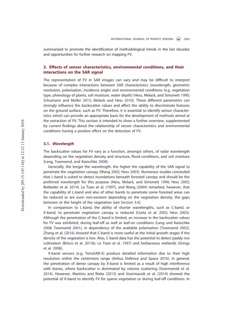
summarized to promote the identification of methodological trends in the last decadesand opportunities for further research on mapping FV.
3. Effects of sensor characteristics, environmental conditions, and their
interactions on the SAR signal
The representation of FV in SAR images can vary and may be difficult to interpretbecause of complex interactions between SAR characteristics (wavelength, geometricresolution, polarisation, incidence angle) and environmental conditions (e.g. vegetationtype, phenology of plants, soil moisture, water depth) (Hess, Melack, and Simonett 1990;Schumann and Moller 2015; Melack und Hess 2010). These different parameters canstrongly influence the backscatter values and affect the ability to discriminate featureson the ground surface, such as FV. Therefore, it is essential to identify sensor character-istics which can provide an appropriate basis for the development of methods aimed atthe extraction of FV. This section is intended to show a further overview, supplementedby current findings about the relationship of sensor characteristics and environmentalconditions having a positive effect on the detection of FV.
3.1. Wavelength
The backscatter values for FV vary as a function, amongst others, of radar wavelengthdepending on the vegetation density and structure, flood conditions, and soil moisture(Lang, Townsend, and Kasischke 2008).
Generally, the longer the wavelength, the higher the capability of the SAR signal topenetrate the vegetation canopy (Wang 2002; Hess 2003). Numerous studies concludedthat L-band is suited to detect inundations beneath forested canopy and should be thepreferred wavelength for this purpose (Hess, Melack, and Simonett 1990; Hess 2003;Betbeder et al. 2014). Le Toan et al. (1997), and Wang (2004) remarked, however, thatthe capability of L-band and also of other bands to penetrate some forested areas canbe reduced or are even non-existent depending on the vegetation density, the gapsbetween or the height of the vegetation (see Section 3.4).
In comparison to L-band, the ability of shorter wavelengths, such as C-band, orX-band, to penetrate vegetation canopy is reduced (Costa et al. 2002; Hess 2003).Although the penetration of the C-band is limited, an increase in the backscatter valuesfor FV was exhibited, during leaf-off as well as leaf-on conditions (Lang und Kasischke2008; Townsend 2001), in dependency of the available polarisation (Townsend 2002).Zhang et al. (2016) showed that C-band is more useful at the initial growth stages if thedensity of the vegetation is low. Also, C-band data has the potential to detect paddy ricecultivation (Brisco et al. 2013b; Le Toan et al. 1997) and herbaceous wetlands (Gringset al. 2008).
X-band sensors (e.g. TerraSAR-X) produce detailed information due to their highresolution within the centimetre range (Airbus Defence and Space 2016). In general,the penetration of dense canopy by X-band is limited as a result of high interferencewith leaves, where backscatter is dominated by volume scattering (Voormansik et al.2014). However, Martinis and Rieke (2015) and Voormansik et al. (2014) showed thepotential of X-band to identify FV for sparse vegetation or during leaf-off conditions. In
INTERNATIONAL JOURNAL OF REMOTE SENSING 2263
Dow
nlo
aded
by [
89.1
5.1
45.1
16]
at 1
2:1
2 1
3 J
anuar
y 2
018
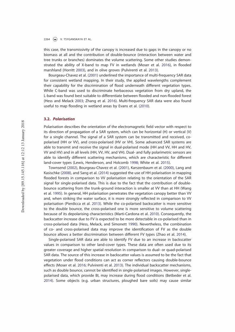
this case, the transmissivity of the canopy is increased due to gaps in the canopy or nobiomass at all and the contribution of double-bounce (interaction between water andtree trunks or branches) dominates the volume scattering. Some other studies demon-strated the ability of X-band to map FV in wetlands (Moser et al. 2016), in floodedmarshland (Horritt 2003), and in olive groves (Pulvirenti et al. 2013).
Bourgeau-Chavez et al. (2001) underlined the importance of multi-frequency SAR datafor consistent wetland mapping. In their study, the applied wavelengths complementtheir capability for the discrimination of flood underneath different vegetation types.While C-band was used to discriminate herbaceous vegetation from dry upland, theL-band was found best suitable to differentiate between flooded and non-flooded forest(Hess and Melack 2003; Zhang et al. 2016). Multi-frequency SAR data were also founduseful to map flooding in wetland areas by Evans et al. (2010).
3.2. Polarisation
Polarisation describes the orientation of the electromagnetic field vector with respect toits direction of propagation of a SAR system, which can be horizontal (H) or vertical (V)for a single channel. The signal of a SAR system can be transmitted and received, co-polarised (HH or VV), and cross-polarised (HV or VH). Some advanced SAR systems areable to transmit and receive the signal in dual-polarised mode (HH and VV, HH and HV,VV and HV) and in all levels (HH, VV, HV, and VH). Dual- and fully polarimetric sensors areable to identify different scattering mechanisms, which are characteristic for differentland-cover types (Lewis, Henderson, and Holcomb 1998; White et al. 2015).
Townsend (2002), Bourgeau-Chavez et al. (2001), Karszenbaum et al. (2000), Lang andKasischke (2008), and Sang et al. (2014) suggested the use of HH polarisation in mappingflooded forests in comparison to VV polarisation relating to the orientation of the SARsignal for single-polarised data. This is due to the fact that the contribution of double-bounce scattering from the trunk-ground interaction is smaller at VV than at HH (Wanget al. 1995). In general, HH polarisation penetrates the vegetation canopy better than VVand, when striking the water surface, it is more strongly reflected in comparison to VVpolarisation (Pierdicca et al. 2013). While the co-polarised backscatter is more sensitiveto the double bounce, the cross-polarised one is more sensitive to volume scatteringbecause of its depolarising characteristics (Marti-Cardona et al. 2010). Consequently, thebackscatter increase due to FV is expected to be more detectable in co-polarised than incross-polarised data (Hess, Melack, and Simonett 1990). Nevertheless, the combinationof co- and cross-polarised data may improve the identification of FV as the doublebounce allows a better discrimination between different FV types (Zhao et al. 2014).
Single-polarised SAR data are able to identify FV due to an increase in backscattervalues in comparison to other land-cover types. These data are often used due to itsgreater coverage and higher spatial resolution in comparison to dual- or quad-polarisedSAR data. The source of this increase in backscatter values is assumed to be the fact thatvegetation under flood conditions can act as corner reflectors causing double-bounceeffects (Moser et al. 2016; Pulvirenti et al. 2013). The individual backscatter mechanisms,such as double bounce, cannot be identified in single-polarised images. However, single-polarised data, which provide BI, may increase during flood conditions (Betbeder et al.2014). Some objects (e.g. urban structures, ploughed bare soils) may cause similar
2264 V. TSYGANSKAYA ET AL.
Dow
nlo
aded
by [
89.1
5.1
45.1
16]
at 1
2:1
2 1
3 J
anuar
y 2
018

backscatter intensities as FV. The similarity of SAR backscatter only constitutes a criticalissue when analysing single-polarised images (Schumann and Moller 2015; Martinis andRieke 2015; Pulvirenti et al. 2016). The use of ancillary data (e.g. land-cover map, opticaldata) may reduce the confusion between the aforementioned objects by exclusion ofnon-vegetated features. In the past, studies increasingly used single-polarised data forthe detection of different FV types, such as forested wetlands (Bourgeau-Chavez et al.2001; Pistolesi, Ni-Meister, and McDonald 2015), marshland (Horritt 2003), as well asagricultural areas (Pulvirenti et al. 2011b; Kasischke et al. 2003).
Single-polarised SAR data only provide BI and, according to White et al. (2015) andBetbeder et al. (2014), are not quite efficient enough to detect FV due to the restrictedinformation content about backscatter mechanism such as the double-bounce effect.SAR systems with multi-polarised SAR data (dual-polarised and fully polarised) havesignificant advantages in comparison to single-polarised SAR data, providing moreinformation about the presence of water underneath the vegetation canopy (Souza-Filho et al. 2011).
Dual-polarised SAR data are generally used to produce ratios between two polarisationtypes. Brisco et al. (2011) mentioned that polarisation ratios using horizontal polarisationare appropriate for mapping FV for a generalized land-cover map. Furthermore, Mouginet al. (1999) and the aforementioned study indicate the suitability of the HH/HV ratio inseparating FV from uplands. According to Le Toan et al. (1997) and Wang (2004), the ratiobetween HH and VV is higher for FV than that of most other land-cover classes, becausethe vertical polarised wave is more attenuated than the horizontally polarised one.Schmitt et al. (2012) designed an approach to identify FV by applying dual-polarised(HH-VV) data to distinguish between agricultural areas and swamp forest in wetlands. Arecently developed approach that enables the extraction of FV by the decomposition ofdual-polarised data was presented by Moser et al. (2016). The techniques for decomposi-tion of dual-polarised SAR data are quite young; however, according to aforementionedstudies, they produced promising results (see Section 4.1.2).
More known and common is the application of quad-polarised SAR data. The quad-polarised data have smaller area coverage in comparison to single- and dual-polarised SARdata. This can represent a drawback due to an inadequate coverage of the area of interest,depending on the study task. However, the quad-polarised data allow the application ofpolarimetric decomposition, which separates SAR signals into different scattering mechan-isms: volume, single-bounce (on specular or rough surface), and dihedral scattering(double-bounce). The volume scattering mechanism represents multiple scatterings andcan be found over forested and agricultural areas, where the SAR signal is diffuselybackscattered by tree crowns or vegetation canopy. In case of single-bounce scatteringon specular surfaces, the most of the SAR energy is reflected away from sensor. Forexample, these are flat open water surfaces, which often appear dark in a SAR image(Ulaby, Fung, and Moore 1986). Double- or multi-bounce scattering occurs between aspecularly reflecting water surface and vertical structures of the vegetation, such as trunksand stems (Moser et al. 2016; Pulvirenti et al. 2013; Pulvirenti et al. 2011a). This scatteringmechanism represents a key component for the detection of FV using SAR data.
The identification of scattering mechanisms enables the distinction of different covertypes and environmental conditions, such as flood. The most frequent application ofquad-polarised SAR data and decomposition techniques for detection of FV can be
INTERNATIONAL JOURNAL OF REMOTE SENSING 2265
Dow
nlo
aded
by [
89.1
5.1
45.1
16]
at 1
2:1
2 1
3 J
anuar
y 2
018

found in the field of wetland monitoring due to the capability of this data to distinguishflooded and non-flooded conditions, as well as individual FV types, such as marshes andwooded wetlands or rushes (Robertson, King, and Davies 2015; Gallant et al. 2014; Schmittund Brisco 2013; Morandeira et al. 2016; Betbeder et al. 2014). The individual decomposi-tion techniques and their successes for the extraction of FV are described in Section 4.1.2.
3.3. Incidence angle
The utility of SAR data to detect FV is significantly influenced by the incident angle. It isdefined as the angle between an imaginary line perpendicular to the Earth’s surface andthe radar signal. Depending on the satellite sensor, the incidence angles range between10° and 65°. Thereby, the larger incidence angles are declared as shallow and the smallerangles are termed steep. Several studies, focused on the vegetation type forest, addressan appropriate incidence angle for the differentiation between flooded and non-FV(Richards, Woodgate, and Skidmore 1987; Bourgeau-Chavez et al. 2001; Lang,Townsend, and Kasischke 2008). Previous investigations indicated that steeper incidenceangles are preferential for the distinction of non-flooded and flooded forest (Kanduset al. 2001; Bourgeau-Chavez et al. 2001; Hess, Melack, and Simonett 1990; Richards,Woodgate, and Skidmore 1987; Costa et al. 2002). This circumstance can be explained bythe SAR signal having a shorter path through the crown layer at steeper angles. As aresult, the transmissivity of the vegetation canopy for SAR energy is increased. This leadsto a potential increase in interaction between the surface water on the ground and thetree trunks. Shallow incidence angle signals are more influenced by the crown layer,resulting in increased volume scattering (Lang, Townsend, and Kasischke 2008; Hess2003; Townsend 2001; Costa et al. 2002). According to the results of Lang, Townsend,and Kasischke (2008), the ability to detect waterbodies underneath forested areas didnot decline as strongly as expected with increasing incidence angles, and less thanexpected at steeper incidence angles, in comparison to previous findings in the litera-ture. Lang, Townsend, and Kasischke (2008) also mentioned that the angular signaturesvaried between different forest types and the capability to detect flooded forest issimilar during the leaf-off and leaf-on conditions.
The backscatter signature of a target in two different images, acquired under similarenvironmental conditions, can vary in dependency of different incidence angles of theseimages. Depending on the task, the changes in backscatter due to different incidenceangles have to be considered. For instance, Pulvirenti et al. (2011a) applied a simplifiedcosine model (Ulaby und Dobson 1989) assuming that the variation of backscatter canbe approximated by cosine-squared function depending on the incidence angle itself.However, the use of multi-incident angle SAR images does not necessarily constitute adrawback. The results of Kandus et al. (2001) indicated that combinations of images withdifferent incidence angles can improve the discrimination of different FV types in wet-lands. In addition, Lang, Townsend, and Kasischke (2008) pointed out the benefits ofmulti-incident angle imagery for monitoring flood extent under forest canopies.Henderson and Lewis (2008) remarked that dense forest canopy can be appropriatelydetected by the combination of L-band, HH polarisation, and low-to-moderate incidenceangle imagery. However, low incident angle in C-band and HH or VV polarised data isalso suitable for a sparse canopy layer.
2266 V. TSYGANSKAYA ET AL.
Dow
nlo
aded
by [
89.1
5.1
45.1
16]
at 1
2:1
2 1
3 J
anuar
y 2
018

3.4. Environmental conditions
Besides sensor characteristics, the backscatter signature of FV is strongly affected by theenvironmental conditions and their characteristics, such as vegetative biomass over theground/water (vegetation type, phenology of plants), soil moisture, and water depth.Several theoretical microwave scattering models can be found in the literature, whichdescribe the interaction between the SAR transmitted microwave energy and vegetationor FV on the ground (Kasischke and Bourgeau-Chavez 1997; Wang et al. 1995). Lowvegetation (low/moderate stage of growth) and high vegetation (e.g. deciduous forests,coniferous forests) are often considered separately in the literature (e.g. Pulvirenti et al.2011b), because of the different effects that vegetation structure and density have onthe signal intensity.
Vegetative aboveground biomass has been found to have a great influence on thescattering of FV (Pope et al. 1997). The biomass is described in various studies as canopy orcrop density (e.g. Dwivedi, Rao, and Bhattacharya 1999; Grings et al. 2008) or as acombination between leafs and stems (Kasischke et al. 2003). Le Toan et al. (1997), Popeet al. (1997), Mougin et al. (1999), Sang et al. (2014), and Yu and Satschi (2016) found thatSAR backscatter is increasing as a function of biomass and they determined saturationpoints at which water beneath the canopy cannot be detected any longer. The saturationpoint can shift depending on sensor characteristics (wavelengths, incidence angle, andpolarisation) and environmental parameter (e.g. aboveground biomass) (Yu und Saatchi2016; Sang et al. 2014). Before the saturation point (lower level of biomass), the transmis-sivity of the microwaves radiation through the vegetation canopy is possible due to thesmall size and density of scattering elements. If the saturation point is reached, the volumescattering from the canopy completely superimposes the contribution of double bouncefrom the interaction between the water surface and vertical vegetation structure (e.g. treetrunk, stems volume) (Costa et al. 2002; Kasischke et al. 2003; Aziz und White 2003).Consequently, the phenology of plants or leaf-on/leaf-off conditions highly affect thedetection of FV depending on the sensor characteristics.
Beside the aboveground biomass, the contribution of the ground is another impor-tant environmental parameter influencing the backscatter signal of FV. Kasischke et al.(2003) showed an increase in backscatter through all biomass levels as soil moistureincreases, provided that the transmissivity of the biomass still exists (the saturation pointis not exceeded). In case of low soil moisture, as biomass increases, there is an increasedue to volume scattering from the canopy; however, there is a little or no contributionfrom multi-interaction scattering. When the surface is flooded, there is no contributionof energy from the ground surface and the backscatter signal is dominated by thedouble-bounce scattering and the volume scattering from the vegetation canopy(Kwoun und Lu 2009).
Pulvirenti et al. (2011a) investigated that the water depth fluctuations significantlyinfluence the backscatter intensities in FV areas due to the predominance of scatteringmechanisms for agricultural and herbaceous vegetation. Depending on the height of thevegetation and the water depth, the double-bounce scattering can become a predomi-nant effect and cause the increase in backscatter, while the volume scattering becomessubordinate (Bourgeau-Chavez et al. 2001; Bourgeau-Chavez, Kasischke, and Smith 1997;Grings et al. 2006; Kiage et al. 2005; Sang et al. 2014). If the emerging part of the plants
INTERNATIONAL JOURNAL OF REMOTE SENSING 2267
Dow
nlo
aded
by [
89.1
5.1
45.1
16]
at 1
2:1
2 1
3 J
anuar
y 2
018

becomes too small, no considerable double-bounce scattering can be produced and thebackscatter would not increase (Pulvirenti et al. 2011a). Consequently, the combinationof sensor parameters and the knowledge concerning environmental properties andconditions is a crucial point for the extraction of FV.
4. Overview of methods and their data sets for the extraction of FV
Based on 83 selected studies, an overview of the diversity of applied data sets andclassification algorithms aiming at the extraction of FV is given in this section.Furthermore, the classification algorithms are categorized and analysed based on thelevel of classification (pixel- or segment-based) and the temporal frequency of theapplied SAR data. A list of the studies is provided in Table 2. Each of these studiesincludes a unique ID, which serves as a reference within this section.
4.1. SAR-derived information for image classification
For the extraction of FV various SAR-derived image, information were used in the studiescomprising BI, PPs as well as IC. The number of occurrences of the SAR-derivedinformation in the analysed studies is demonstrated in Figure 1.
4.1.1. Backscatter intensity
The BI for each pixel in a SAR image represents the basic SAR-derived information andthe proportion of the SAR signal backscattered from the objects on the ground,depending on sensor characteristics (polarisation, frequency, incidence angle, and reso-lution) and environmental conditions of a target (e.g. size, shape, orientation, andmoisture content). The BI values are often converted to a normalized radar cross sectionor backscattering coefficient, which is measured in decibel (dB) units (Henderson undLewis 2008). Figure 1 shows that the majority of studies (69 of 83) used BI for theclassifications of FV vegetation (ID 1–12, 14–16, 19–31, 34, 36–49, 52–63, 65, 67–81).
Figure 1. SAR-related information on which classifications were conducted and their number ofoccurrences for the extraction of FV in the selected studies.
2268 V. TSYGANSKAYA ET AL.
Dow
nlo
aded
by [
89.1
5.1
45.1
16]
at 1
2:1
2 1
3 J
anuar
y 2
018
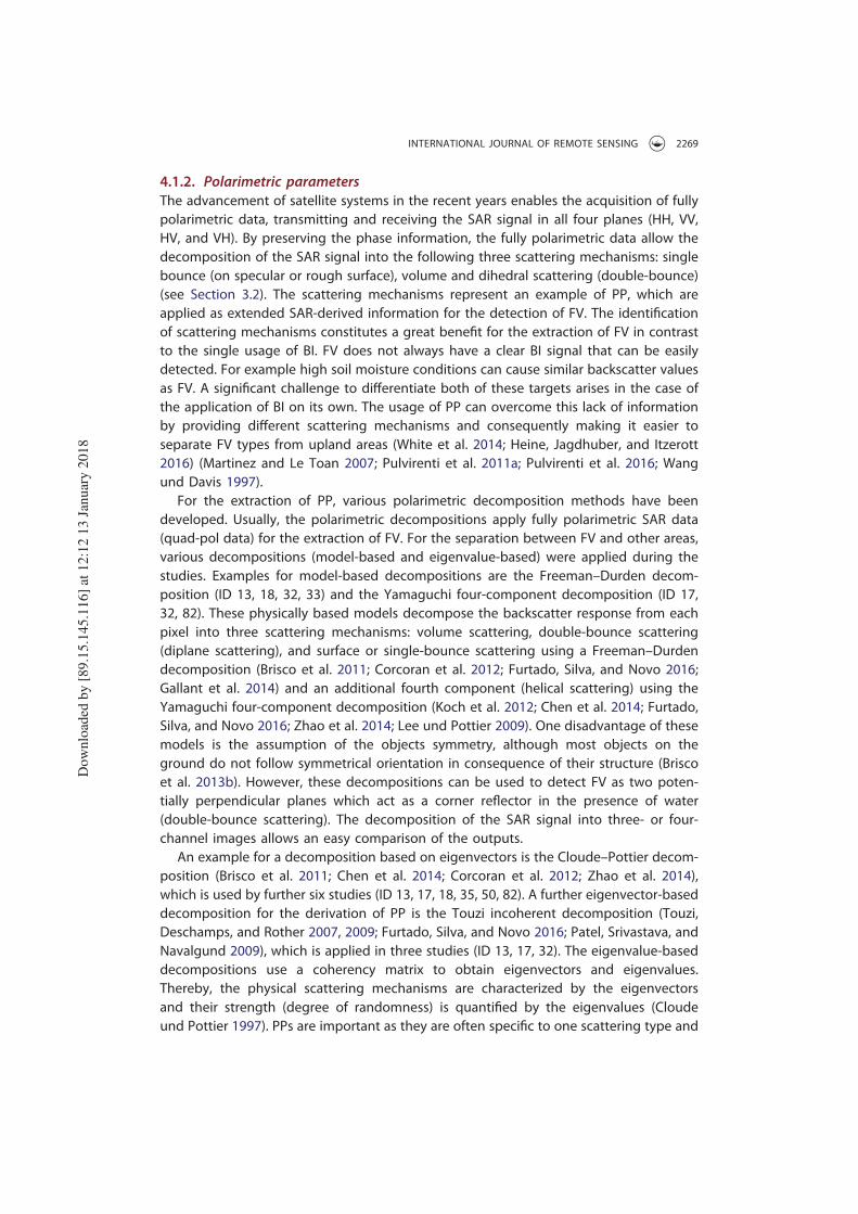
4.1.2. Polarimetric parameters
The advancement of satellite systems in the recent years enables the acquisition of fullypolarimetric data, transmitting and receiving the SAR signal in all four planes (HH, VV,HV, and VH). By preserving the phase information, the fully polarimetric data allow thedecomposition of the SAR signal into the following three scattering mechanisms: singlebounce (on specular or rough surface), volume and dihedral scattering (double-bounce)(see Section 3.2). The scattering mechanisms represent an example of PP, which areapplied as extended SAR-derived information for the detection of FV. The identificationof scattering mechanisms constitutes a great benefit for the extraction of FV in contrastto the single usage of BI. FV does not always have a clear BI signal that can be easilydetected. For example high soil moisture conditions can cause similar backscatter valuesas FV. A significant challenge to differentiate both of these targets arises in the case ofthe application of BI on its own. The usage of PP can overcome this lack of informationby providing different scattering mechanisms and consequently making it easier toseparate FV types from upland areas (White et al. 2014; Heine, Jagdhuber, and Itzerott2016) (Martinez and Le Toan 2007; Pulvirenti et al. 2011a; Pulvirenti et al. 2016; Wangund Davis 1997).
For the extraction of PP, various polarimetric decomposition methods have beendeveloped. Usually, the polarimetric decompositions apply fully polarimetric SAR data(quad-pol data) for the extraction of FV. For the separation between FV and other areas,various decompositions (model-based and eigenvalue-based) were applied during thestudies. Examples for model-based decompositions are the Freeman–Durden decom-position (ID 13, 18, 32, 33) and the Yamaguchi four-component decomposition (ID 17,32, 82). These physically based models decompose the backscatter response from eachpixel into three scattering mechanisms: volume scattering, double-bounce scattering(diplane scattering), and surface or single-bounce scattering using a Freeman–Durdendecomposition (Brisco et al. 2011; Corcoran et al. 2012; Furtado, Silva, and Novo 2016;Gallant et al. 2014) and an additional fourth component (helical scattering) using theYamaguchi four-component decomposition (Koch et al. 2012; Chen et al. 2014; Furtado,Silva, and Novo 2016; Zhao et al. 2014; Lee und Pottier 2009). One disadvantage of thesemodels is the assumption of the objects symmetry, although most objects on theground do not follow symmetrical orientation in consequence of their structure (Briscoet al. 2013b). However, these decompositions can be used to detect FV as two poten-tially perpendicular planes which act as a corner reflector in the presence of water(double-bounce scattering). The decomposition of the SAR signal into three- or four-channel images allows an easy comparison of the outputs.
An example for a decomposition based on eigenvectors is the Cloude–Pottier decom-position (Brisco et al. 2011; Chen et al. 2014; Corcoran et al. 2012; Zhao et al. 2014),which is used by further six studies (ID 13, 17, 18, 35, 50, 82). A further eigenvector-baseddecomposition for the derivation of PP is the Touzi incoherent decomposition (Touzi,Deschamps, and Rother 2007, 2009; Furtado, Silva, and Novo 2016; Patel, Srivastava, andNavalgund 2009), which is applied in three studies (ID 13, 17, 32). The eigenvalue-baseddecompositions use a coherency matrix to obtain eigenvectors and eigenvalues.Thereby, the physical scattering mechanisms are characterized by the eigenvectorsand their strength (degree of randomness) is quantified by the eigenvalues (Cloudeund Pottier 1997). PPs are important as they are often specific to one scattering type and
INTERNATIONAL JOURNAL OF REMOTE SENSING 2269
Dow
nlo
aded
by [
89.1
5.1
45.1
16]
at 1
2:1
2 1
3 J
anuar
y 2
018

thus improve the classification of specific classes, such as FV (Heine, Jagdhuber, andItzerott 2016).
The most common polarimetric decompositions can only be derived from fullypolarised (quad-polarised) SAR data. However, the availability of quad-pol data is morelimited (Moser et al. 2016; Schmitt et al. 2012). There are few decomposition approachesapplicable for quad- and dual-polarised data. One of them is the method of normalizedKennaugh elements, which is adapted for any wavelength (Moser et al. 2016; Schmitt,Wendleder, and Hinz 2015) and also for all SAR sensors (ID 51). By retaining the phaseinformation of dual-polarised data, the Kennaugh elements enable the interpretation ofphysical surface and double-bounce scattering mechanisms (Schmitt et al. 2012). Inaddition, the Shannon entropy (SE), which represents an eigenvector decomposition(Lee and Pottier 2009), can cope with dual-polarised data, too (ID 5, 6).
The compact polarimetric (CP) SAR system is configured to transmit only one polar-isation, while two linear polarisations, horizontal and vertical, are received. This techni-que enables the creation of pseudo quad-pol data from a dual-polarised SAR system(Brisco et al. 2013b; Dabboor et al. 2015; Nord et al. 2009). An important requirement ofCP is the maintenance of the relative phase between two received polarisations, which isnecessary to construct CP images. The reason for the application of CP are the benefitsof quad-pol data, such as improved classification through increased information content,while its drawbacks, such as reduced area coverage, are being avoided (Brisco et al.2013b). Within this technique, m-delta decomposition is a suitable method to decom-pose the CP data. It is comparable to the Freeman–Durden decomposition. The simu-lated CP was investigated by Brisco et al. (2013b) using the m-delta decomposition forFV classification in wetland areas (ID 8).
Decompositions allow the extraction of physical information (backscatter mechan-isms), but they do not represent a classification approach on their own. In theliterature, the classification of decompositions for FV was mostly performed bymachine-learning techniques (e.g. Support Vector Machine (ID 5, 6, 13), random forestclassification (ID 18, 32, 35, 66, 82)), followed by distance-based classification methods(e.g. maximum likelihood classification (ID 13, 51), k-nearest-neighbour classification(KNNC) (ID 5, 17). However, also a few decision tree classifiers (ID 5, 17), two Wishardclassifications (ID 17, 50), a single manual thresholding approach (MTA) (ID 33), and asingle ISODATA clustering technique (ID 59) were performed based on decomposedSAR data.
Only, 12 studies performed a classification applying PP (ID 5, 6, 13, 17, 18, 32, 33, 35, 50,51, 66, 82) (Figure 1). Several reasons for this uneven distribution can be assumed: (1) Theapplication of PP requires dual- or quad-polarised data, in which the phase information ismaintained. The advance in satellite systems during the last couple of years enables theextraction and application of the polarimetric information. (2) Based on different SARsensors, the advanced polarisation modes might not always be available. In comparisonto single-polarised data, reduced area coverage and resolution limit the usage of dual- orquad-polarised data. As a consequence, the application of polarimetric analysis for FV isrestricted in comparison to the usage of BI values. (3) The preprocessing effort for BI issignificantly lower in comparison to the derivation of PP (Betbeder et al. 2014; Morandeiraet al. 2016; Robertson, King, and Davies 2015). (4) The interpretation of PP is likely to bemore time consuming (e. g. interpretation of Pauli-Decomposition).
2270 V. TSYGANSKAYA ET AL.
Dow
nlo
aded
by [
89.1
5.1
45.1
16]
at 1
2:1
2 1
3 J
anuar
y 2
018

Figure 1 shows that exclusively PPs were applied in six different studies (ID 6, 13,17, 18, 33, 50). Seven further studies used BI along with PP (ID 5, 32, 35, 51, 59, 66,82). Thereby, the latter is used either as supplementary information to achievehigher accuracy for FV or as a comparison to BI-based results. Some of thesestudies performed comparisons of the accuracies for FV, which are described inthe following. The application of BI only (HH, VV, HH/VV) resulted in poor kappavalues (0.48, 0.33, 0.13) as reported by Betbeder et al. (2014). An improvement wasreached using SE (kappa: 0.85) showing an accuracy of 90% PA (producer’s accu-racy) and 75% UA (user’s accuracy) for FV. Furtado, Silva, and Novo (2016) reportedthat flooded forest had a 30–40% increase in PA and UA when polarimetricdescriptors were used instead of only BI. The highest accuracy, therefore, is situatedat 79% PA and 95% UA. Moser et al. (2016) demonstrated an increase in the PA(90%) and UA (90%) accuracy for FV extracted by PPs in comparison to the PA(79%) und UA (87%) based on BI. In addition, Robertson et al. (2016) applied BI andCloude–Pottier decomposition for the extraction of FV showing that the UA (83%)and PA (67%) based on the BI are similar to the PA (80%) and UA (68%) based onCloude–Pottier results. Overall, the application of PP constitutes an improvement ofthe accuracy for FV in comparison to results only achieved by using BI.
4.1.3. Interferometric coherence
A useful technique for the identification of FV constitutes the SAR interferometrythrough the usage of the IC, computable from two interferometric SAR images. Theapplication of interferometric SAR technology is relatively new in the research field ofthe extraction of FV and limited based on several requirements of certain conditions,such as maintained phase information in the SAR data or a short temporal baselinebetween an interferometric pair (Pulvirenti et al. 2016). Recently published studies usedIC information alone (ID 83) and in combination with the BI (ID 64) for the extraction ofFV (Figure 1). The coherence might help differentiating between vegetation and baresoil areas, where the latter has considerably higher coherency values. Consequently, thecoherence may replace the application of ancillary information, such as optical data orland-cover information, which is often used to separate between various objects withsimilar BI. The combination of both, BI values and associated phase coherence, enablesthe discrimination of non-flooded and FV (Alsdorf et al. 2000; Alsdorf, Smith, and Melack2001; Kwoun and Zhong 2009; Oliver-Cabrera und Wdowinski 2016; Xie et al. 2013;Zhang et al. 2015).
4.2. Specification and comparison of applied classification techniques
Based on 83 studies, a comprehensive review of the classification techniques applied forthe extraction of FV was conducted. The algorithms are placed in categories, due to theirsimilarity towards each other and in regard to their application fields. Thereby, thenumber of the applied approaches can exceed the number of the analysed studies asa single study can implement more than one of these approaches (overall 101 classifica-tion algorithms in 83 studies).
These classification techniques can be categorized into supervised and unsupervisedclassification techniques (Figure 2). In general, supervised classification uses reference
INTERNATIONAL JOURNAL OF REMOTE SENSING 2271
Dow
nlo
aded
by [
89.1
5.1
45.1
16]
at 1
2:1
2 1
3 J
anuar
y 2
018

classes obtained from training samples (reference data) to classify the image elements(Richards 2012). The majority of the performed classification algorithms in each study aresupervised (89 studies). The number of occurrences of unsupervised techniques for theextraction of FV in the studies is comparatively low (12 studies). Furthermore, unsuper-vised classification algorithms are mostly applied as a part of a processing chain, whichadditionally includes a supervised classification algorithm or manual interaction steps.
The range of classification algorithms applied for the extraction of FV is diverse(Figure 2). The distance-based classification methods constitute the majority of theapplied classification algorithms amongst the analysed studies (28 of 83). Whereby,algorithms are categorized as distance-based because they are using simple distancefunctions. Figure 3 shows the number of occurrences for distance-based classifications.Maximum likelihood classification (MLC) was identified as one of the most commonclassification techniques within the distance-based methods (15 of 29) applied for theextraction of FV (ID 8, 9, 12, 13, 23, 25, 49, 51, 53, 56, 57, 67, 71, 77, 80). The supervisedKNNC was applied four times for the extraction of FV (ID 5, 17, 54, 80). A parallelepipedclassification is one of the distance-based classification methods and was used in threestudies (ID 26, 44, 49). Three of the distance-based classifications used the Mahalanobisdistance (ID 43, 74, 75). Other two studies applied the Bhattacharyya distance (ID 20, 21,22). Due to their simplicity, availability, and statistical transparency (no black box), thesealgorithms are popular tools not only for classification in general but also for detectingFV. Furthermore, they can be easily adapted to other study sites or data sets (Martinezand Le Toan 2007). Especially MLC and KNNC are often used as a reference for theperformance of newly developed algorithms (Bourgeau-Chavez et al. 2001; Brisco et al.
Figure 2. Supervised and unsupervised classification techniques and their number of occurrences forthe extraction of FV in the selected studies.
2272 V. TSYGANSKAYA ET AL.
Dow
nlo
aded
by [
89.1
5.1
45.1
16]
at 1
2:1
2 1
3 J
anuar
y 2
018

2013b). However, Na et al. (2015) remarked that MLC and KNNC are in general notsuitable for the analysis of high dimensional data, which can constitute a drawback forthe extraction of FV.
The second most common approach used in the reviewed studies (25 of 83) is thedecision tree/rule-based classification (Figure 2), which includes decision tree classifica-tion (DTC) and hierarchical rule-based classification (HRBC).
Figure 4 shows the number of occurrences of both approaches, where the majority ofstudies (20) applied DTC for the extraction of FV (ID 2, 4, 5, 7, 9, 14, 17, 19, 40, 42, 44, 48,52, 60, 69, 70, 72, 73, 78, 79). A decision tree classifier is well adapted for SAR imageclassification, because it does not assume a special probability density distribution of thegiven input data (Baghdadi et al. 2001; Hess et al. 1995). This algorithm is based onhierarchical rules representing thresholds used to iteratively split data in more homoge-neous groups (Richards 2012), which can be easily refined after iterations (Martinez and LeToan 2007). The automatic boundary definition constitutes an advantage because manu-ally determining thresholds, especially for separation of FV to other classes, can be acomplex process. A further advantage of decision trees is their flexibility and robustnessregarding nonlinear and noisy relations among input features (Townsend 2002; Friedl undBrodley 1997; Na et al. 2015). This is a benefit for the detection of FV, because of the
Figure 3. Categorization of distance-based classifications and their number of occurrences for theextraction of FV in the selected studies.
Figure 4. Decision tree and hierarchical rule-based classifications and their number of occurrencesfor the extraction of FV in the selected studies.
INTERNATIONAL JOURNAL OF REMOTE SENSING 2273
Dow
nlo
aded
by [
89.1
5.1
45.1
16]
at 1
2:1
2 1
3 J
anuar
y 2
018

diversity of the applied input data for its extraction. Additionally, DTC requires less time fortraining in comparison to machine-learning algorithms (e.g. artificial neural networks[ANNs], Support Vector Machine) (Na et al. 2015).
Three studies used the HRBC for the extraction of FV (ID 27, 28, 29, 37, 47), in whichthe classification rules are designed by users based on their knowledge and expertiseand can be iteratively changed depending on the results of the classification process.Therefore, specific characteristics of FV can be systematically integrated into the rule set.The transparency of this approach ensures that this knowledge can be used as basis forfurther studies and decisions. Furthermore, HRBC allows adding new rules or data setswithout altering the predefined rules, while distance-based methods, such as MLC, maychange all classes’ rules due to additionally added information (Evans et al. 2010).
Several studies (15 of 83) used machine-learning techniques for the extraction of FV(Figure 2). Figure 5 shows various machine-learning techniques which were applied inthe reviewed studies and their number of occurrences.
The majority of these techniques (11 of 15) is represented by the Random forestclassification (RFC) (ID 10, 18, 24, 32, 35, 46, 53, 54, 66, 81, 82). RFC is an ensembleclassifier containing multiple decision trees and consequently, the aforementionedadvantages of DTC also shared by RFC. By averaging multiple decision trees, the usualoverfitting of each decision tree can be reduced (Richards 2012). This algorithm effi-ciently determines the contribution of diverse information to a classification. However,the application of different information types without the understanding of the truerelations within this information can also constitute a disadvantage. For instance, SARdata can be rated less important due to a better correlation of optical data with otherfeatures for the extraction of FV. In this particular case, RDF may ignore the context andset the priority to the highest correlated data. Furthermore, a large set of reference datais needed to mitigate misclassification caused by natural variability within FV (Robertson,King, and Davies 2015).
Support Vector Machine (SVM) classification, which is used in three studies (ID 5, 6,13), aims to separate two different classes by determining the maximum-margin hyper-planes for a given training set. SVMs are intended for the determination of the bestlinear separation between two categories within a new feature space. Moreover, theSVM classification is suitable for high-dimensional data even though limited trainingdata are available (Richards 2012), which is often the case when working with FV.
Figure 5. Machine-learning techniques and their number of occurrences for the extraction of FV inthe selected studies.
2274 V. TSYGANSKAYA ET AL.
Dow
nlo
aded
by [
89.1
5.1
45.1
16]
at 1
2:1
2 1
3 J
anuar
y 2
018
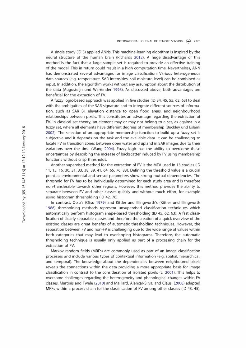
A single study (ID 3) applied ANNs. This machine-learning algorithm is inspired by theneural structure of the human brain (Richards 2012). A huge disadvantage of thismethod is the fact that a large sample set is required to provide an effective trainingof the model. This in return could result in a high computation time. Nevertheless, ANNhas demonstrated several advantages for image classification. Various heterogeneousdata sources (e.g. temperature, SAR intensities, soil moisture level) can be combined asinput. In addition, the algorithm works without any assumption about the distribution ofthe data (Augusteijn und Warrender 1998). As discussed above, both advantages arebeneficial for the extraction of FV.
A fuzzy logic-based approach was applied in five studies (ID 34, 45, 55, 62, 63) to dealwith the ambiguities of the SAR signature and to integrate different sources of informa-tion, such as SAR BI, elevation distance to open flood areas, and neighbourhoodrelationships between pixels. This constitutes an advantage regarding the extraction ofFV. In classical set theory, an element may or may not belong to a set, as against in afuzzy set, where all elements have different degrees of membership (Buckley und Eslami2002). The selection of an appropriate membership function to build up a fuzzy set issubjective and it depends on the task and the available data. It can be challenging tolocate FV in transition zones between open water and upland in SAR images due to theirvariations over the time (Wang 2004). Fuzzy logic has the ability to overcome theseuncertainties by describing the increase of backscatter induced by FV using membershipfunctions without crisp thresholds.
Another supervised method for the extraction of FV is the MTA used in 13 studies (ID11, 15, 16, 30, 31, 33, 38, 39, 41, 64, 65, 76, 83). Defining the threshold value is a crucialpoint as environmental and sensor parameters show strong mutual dependencies. Thethreshold for FV has to be individually determined for each study area and is thereforenon-transferable towards other regions. However, this method provides the ability toseparate between FV and other classes quickly and without much effort, for exampleusing histogram thresholding (ID 42, 76).
In contrast, Otsu’s (Otsu 1979) and Kittler and Illingworth’s (Kittler und Illingworth1986) thresholding methods represent unsupervised classification techniques whichautomatically perform histogram shape-based thresholding (ID 45, 62, 63). A fast classi-fication of clearly separable classes and therefore the creation of a quick overview of theexisting classes are great benefits of automatic thresholding techniques. However, theseparation between FV and non-FV is challenging due to the wide range of values withinboth categories that may lead to overlapping histograms. Therefore, the automaticthresholding technique is usually only applied as part of a processing chain for theextraction of FV.
Markov random fields (MRFs) are commonly used as part of an image classificationprocesses and include various types of contextual information (e.g. spatial, hierarchical,and temporal). The knowledge about the dependencies between neighboured pixelsreveals the connections within the data providing a more appropriate basis for imageclassification in contrast to the consideration of isolated pixels (Li 2001). This helps toovercome challenges regarding the heterogeneity and phenological changes within FVclasses. Martinis and Twele (2010) and Maillard, Alencar-Silva, and Clausi (2008) adaptedMRFs within a process chain for the classification of FV among other classes (ID 43, 45).
INTERNATIONAL JOURNAL OF REMOTE SENSING 2275
Dow
nlo
aded
by [
89.1
5.1
45.1
16]
at 1
2:1
2 1
3 J
anuar
y 2
018

Amongst the vast number of classification approaches to extract FV from SAR data,image clustering was used in seven studies (ID 1, 36, 52, 58, 59, 61, 68). The number ofoccurrences of different image clustering techniques in the reviewed studies is demon-strated in Figure 6. Image clustering is used to identify relationships within the datawithout any previous information (trainings sets) by dividing image elements into groupscontaining same or similar properties (spatial and/or temporal). Image clustering leads to areduction of the elements to be studied and therefore provides an appropriate basis forfurther analysis. Furthermore, grouping of elements constitutes an advantage for theextraction of FV by means of SAR data, because speckle noise can be compensated andvariation within FV as well as phenological changes can be considered.
k-Means (ID 61), k-medoids (ID 68), and ISODATA (ID 1, 52, 58, 59) are iterative,non-hierarchical clustering techniques of similar design. While k-means uses centroidsfor the determination of cluster centres, k-medoids uses medoids, which makes thisalgorithm more stable towards outliers. Both algorithms calculate a predefined num-ber of clusters, even though fewer clusters might describe the data more accurately(Park und Jun 2009; Richards 2012). This disadvantage is overcome by ISODATA,which automatically merges similar clusters and splits clusters with large standarddeviation during the iteration process. An iterative clustering algorithm based on theMahalanobis distance was performed by Hess (2003) for the extraction of floodedforest and wetland types (ID 36).
Wishart H/α and H/A/α unsupervised classifications were performed by two studies(ID 17, 50). These algorithms, especially designed for decomposed SAR data, require PP,which can be obtained by decomposition (see Section 4.1.2) of dual- or quad-polarisedSAR data. Morandeira et al. (2016) applied these classifications to increase expertise onthe backscatter response of herbaceous wetlands (ID 50).
A few studies provided a comparison of the accuracies of the results for differentclassification approaches, which were implemented based on the same constellation ofdata sets for each study. In order to give an idea of the range of performance statisticsand to demonstrate the accuracies for various algorithms, the corresponding accuraciesare summarized in the following. Chen et al. (2014) compared the accuracies of theresults for wetland vegetation of three different classification approaches: Wishard
Figure 6. Image clustering techniques and their number of occurrences for the extraction of FV inthe selected studies.
2276 V. TSYGANSKAYA ET AL.
Dow
nlo
aded
by [
89.1
5.1
45.1
16]
at 1
2:1
2 1
3 J
anuar
y 2
018
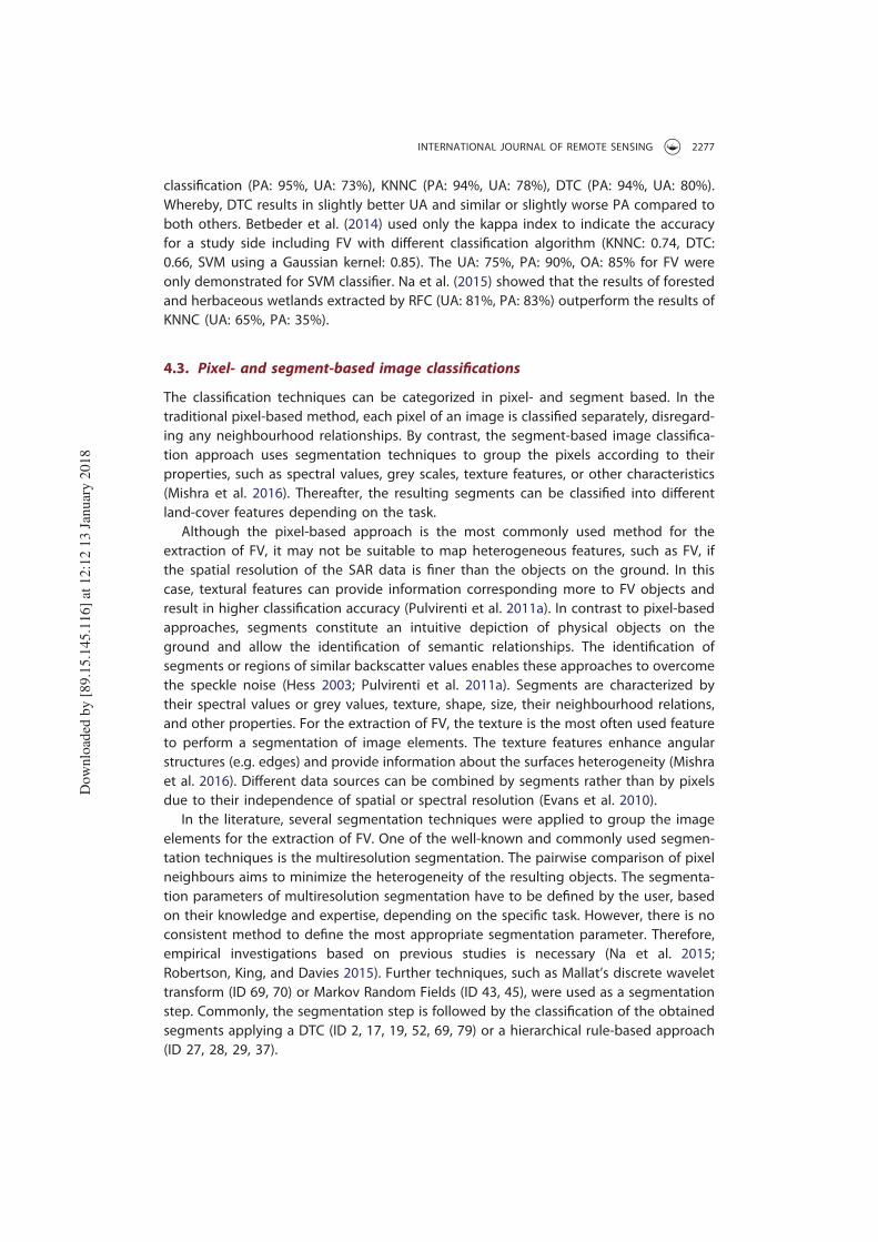
classification (PA: 95%, UA: 73%), KNNC (PA: 94%, UA: 78%), DTC (PA: 94%, UA: 80%).Whereby, DTC results in slightly better UA and similar or slightly worse PA compared toboth others. Betbeder et al. (2014) used only the kappa index to indicate the accuracyfor a study side including FV with different classification algorithm (KNNC: 0.74, DTC:0.66, SVM using a Gaussian kernel: 0.85). The UA: 75%, PA: 90%, OA: 85% for FV wereonly demonstrated for SVM classifier. Na et al. (2015) showed that the results of forestedand herbaceous wetlands extracted by RFC (UA: 81%, PA: 83%) outperform the results ofKNNC (UA: 65%, PA: 35%).
4.3. Pixel- and segment-based image classifications
The classification techniques can be categorized in pixel- and segment based. In thetraditional pixel-based method, each pixel of an image is classified separately, disregard-ing any neighbourhood relationships. By contrast, the segment-based image classifica-tion approach uses segmentation techniques to group the pixels according to theirproperties, such as spectral values, grey scales, texture features, or other characteristics(Mishra et al. 2016). Thereafter, the resulting segments can be classified into differentland-cover features depending on the task.
Although the pixel-based approach is the most commonly used method for theextraction of FV, it may not be suitable to map heterogeneous features, such as FV, ifthe spatial resolution of the SAR data is finer than the objects on the ground. In thiscase, textural features can provide information corresponding more to FV objects andresult in higher classification accuracy (Pulvirenti et al. 2011a). In contrast to pixel-basedapproaches, segments constitute an intuitive depiction of physical objects on theground and allow the identification of semantic relationships. The identification ofsegments or regions of similar backscatter values enables these approaches to overcomethe speckle noise (Hess 2003; Pulvirenti et al. 2011a). Segments are characterized bytheir spectral values or grey values, texture, shape, size, their neighbourhood relations,and other properties. For the extraction of FV, the texture is the most often used featureto perform a segmentation of image elements. The texture features enhance angularstructures (e.g. edges) and provide information about the surfaces heterogeneity (Mishraet al. 2016). Different data sources can be combined by segments rather than by pixelsdue to their independence of spatial or spectral resolution (Evans et al. 2010).
In the literature, several segmentation techniques were applied to group the imageelements for the extraction of FV. One of the well-known and commonly used segmen-tation techniques is the multiresolution segmentation. The pairwise comparison of pixelneighbours aims to minimize the heterogeneity of the resulting objects. The segmenta-tion parameters of multiresolution segmentation have to be defined by the user, basedon their knowledge and expertise, depending on the specific task. However, there is noconsistent method to define the most appropriate segmentation parameter. Therefore,empirical investigations based on previous studies is necessary (Na et al. 2015;Robertson, King, and Davies 2015). Further techniques, such as Mallat’s discrete wavelettransform (ID 69, 70) or Markov Random Fields (ID 43, 45), were used as a segmentationstep. Commonly, the segmentation step is followed by the classification of the obtainedsegments applying a DTC (ID 2, 17, 19, 52, 69, 79) or a hierarchical rule-based approach(ID 27, 28, 29, 37).
INTERNATIONAL JOURNAL OF REMOTE SENSING 2277
Dow
nlo
aded
by [
89.1
5.1
45.1
16]
at 1
2:1
2 1
3 J
anuar
y 2
018

Figure 7 shows the distribution of studies using either pixel- or segment-basedclassification. The majority of studies (58 of 83) applied the classification at the pixel-based scale (ID 1, 2–16, 18, 23–26, 31, 33, 35, 36, 38–42, 44, 47–51, 53–56, 58–60, 62, 64,65, 67, 68, 70–83). The segment-based classification was performed in 23 studies (ID 2,17, 19–22, 27–30, 32, 34, 37, 43, 45, 46, 52, 57, 61, 63, 66, 69, 79).
Three of these studies used both, pixel and segment level, to provide a comparisonbetween the classification accuracy of the classification results (ID 17, 54, 80). A slightincrease in the accuracy for FV in wetland areas was shown by Chen et al. (2014), by theapplication of an object-based approach (UA: 94%, PA: 81%) in comparison to a pixel-based approach (UA: 92%, PA: 77%). Na et al. (2015) demonstrated that the object-basedclassification (UA: 81%, PA: 83%) exceeds the pixel-based classification (UA: 67%, PA: 67%)for FV with the corresponding kappa index increasing from 0.7 to 0.8 (ID 54). Westra et al.(2010) presented the comparison between kappa values for pixel- (0.86) and for segment-based (0.83) approaches, which were carried out with different classification algorithms(MLC and KNNC). This may be the explanation for a decrease in kappa, which might notbe affected by the application of pixel- and segment-based approaches. Therefore, theseresults are not comparable. Overall, the presumption can be made that the trend istowards segment-based approaches due to their higher accuracies.
4.4. Approaches depending on the number of applied images in combination
with SAR-derived information
For the detection of FV, the aforementioned algorithms were applied on SAR data setswith a different number of images. Depending on the available number of SAR images,the selected studies can be categorized into four different approaches: single date,change detection, order-independent multi-date, and time-series approach (Figure 8),where more than one approach can occur in a single study. Furthermore, each categorycontains different SAR-derived information (BI, PP, and IC or their combination) (Section4.3). There is a huge difference in the amount of the studies that performed a single dateapproach in comparison to those that performed multi-date approaches (change detec-tion, order-independent multi-date, and time-series approach) using more than oneimage (52 vs 14, 52 vs 11, 52 vs six studies, respectively).
For the detection of FV, the single-date approach is a common method, in which theinformation of only one image for a current situation on the ground is considered. Despitethese restrictions, the single-date approach is applied in 52 studies (ID 2–4, 12–14, 16, 17,
Figure 7. Pixel- and segment-based classification techniques and their number of occurrences forthe extraction of FV in the selected studies.
2278 V. TSYGANSKAYA ET AL.
Dow
nlo
aded
by [
89.1
5.1
45.1
16]
at 1
2:1
2 1
3 J
anuar
y 2
018
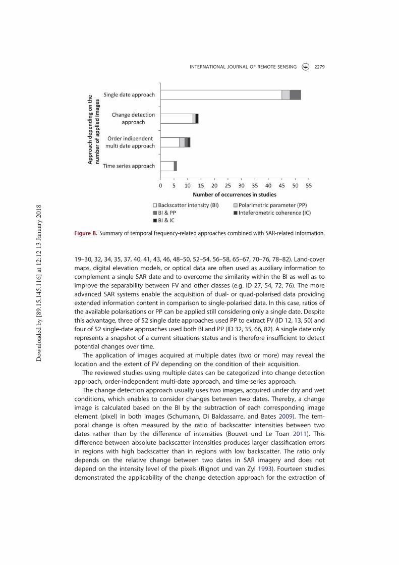
19–30, 32, 34, 35, 37, 40, 41, 43, 46, 48–50, 52–54, 56–58, 65–67, 70–76, 78–82). Land-covermaps, digital elevation models, or optical data are often used as auxiliary information tocomplement a single SAR date and to overcome the similarity within the BI as well as toimprove the separability between FV and other classes (e.g. ID 27, 54, 72, 76). The moreadvanced SAR systems enable the acquisition of dual- or quad-polarised data providingextended information content in comparison to single-polarised data. In this case, ratios ofthe available polarisations or PP can be applied still considering only a single date. Despitethis advantage, three of 52 single date approaches used PP to extract FV (ID 12, 13, 50) andfour of 52 single-date approaches used both BI and PP (ID 32, 35, 66, 82). A single date onlyrepresents a snapshot of a current situations status and is therefore insufficient to detectpotential changes over time.
The application of images acquired at multiple dates (two or more) may reveal thelocation and the extent of FV depending on the condition of their acquisition.
The reviewed studies using multiple dates can be categorized into change detectionapproach, order-independent multi-date approach, and time-series approach.
The change detection approach usually uses two images, acquired under dry and wetconditions, which enables to consider changes between two dates. Thereby, a changeimage is calculated based on the BI by the subtraction of each corresponding imageelement (pixel) in both images (Schumann, Di Baldassarre, and Bates 2009). The tem-poral change is often measured by the ratio of backscatter intensities between twodates rather than by the difference of intensities (Bouvet und Le Toan 2011). Thisdifference between absolute backscatter intensities produces larger classification errorsin regions with high backscatter than in regions with low backscatter. The ratio onlydepends on the relative change between two dates in SAR imagery and does notdepend on the intensity level of the pixels (Rignot und van Zyl 1993). Fourteen studiesdemonstrated the applicability of the change detection approach for the extraction of
Figure 8. Summary of temporal frequency-related approaches combined with SAR-related information.
INTERNATIONAL JOURNAL OF REMOTE SENSING 2279
Dow
nlo
aded
by [
89.1
5.1
45.1
16]
at 1
2:1
2 1
3 J
anuar
y 2
018
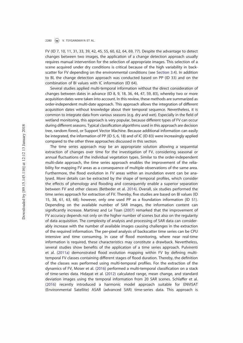
FV (ID 7, 10, 11, 31, 33, 39, 42, 45, 55, 60, 62, 64, 69, 77). Despite the advantage to detectchanges between two images, the application of a change detection approach usuallyrequires manual intervention for the selection of appropriate images. This selection of ascene acquired under dry conditions is critical because of the high variability in back-scatter for FV depending on the environmental conditions (see Section 3.4). In additionto BI, the change detection approach was conducted based on PP (ID 33) and on thecombination of BI values with IC information (ID 64).
Several studies applied multi-temporal information without the direct consideration ofchanges between dates in advance (ID 8, 9, 18, 36, 44, 47, 59, 83), whereby two or moreacquisition dates were taken into account. In this review, these methods are summarized asorder-independent multi-date approach. This approach allows the integration of differentacquisition dates without knowledge about their temporal sequence. Nevertheless, it iscommon to integrate data from various seasons (e.g. dry and wet). Especially in the field ofwetland monitoring, this approach is very popular, because different types of FV can occurduring different seasons. Typical classification algorithms used in this approach are decisiontree, random forest, or Support Vector Machine. Because additional information can easilybe integrated, the information of PP (ID 5, 6, 18) and of IC (ID 83) were increasingly appliedcompared to the other three approaches discussed in this section.
The time series approach may be an appropriate solution allowing a sequentialextraction of changes over time for the investigation of FV, considering seasonal orannual fluctuations of the individual vegetation types. Similar to the order-independentmulti-date approach, the time series approach enables the improvement of the relia-bility for mapping FV areas as a consequence of multiple observations of the same area.Furthermore, the flood evolution in FV areas within an inundation event can be ana-lysed. More details can be extracted by the shape of temporal profiles, which considerthe effects of phenology and flooding and consequently enable a superior separationbetween FV and other classes (Betbeder et al. 2014). Overall, six studies performed thetime series approach for extraction of FV. Thereby, five studies are based on BI values (ID15, 38, 61, 63, 68); however, only one used PP as a foundation information (ID 51).Depending on the available number of SAR images, the information content cansignificantly increase. Martinez and Le Toan (2007) remarked that the improvement ofFV accuracy depends not only on the higher number of scenes but also on the regularityof data acquisition. The complexity of analysis and processing of SAR data can consider-ably increase with the number of available images causing challenges in the extractionof the required information. The per-pixel analysis of backscatter time series can be CPUintensive and time consuming. In case of flood monitoring, where near real-timeinformation is required, these characteristics may constitute a drawback. Nevertheless,several studies show benefits of the application of a time series approach. Pulvirentiet al. (2011a) demonstrated flood evolution mapping within FV by defining multi-temporal FV classes containing different stages of flood duration. Thereby, the definitionof the classes was performed using multi-temporal profiles. For the extraction of thedynamics of FV, Moser et al. (2016) performed a multi-temporal classification on a stackof time-series data. Hidayat et al. (2012) calculated range, mean change, and standarddeviation images using the temporal information from 20 SAR scenes. Schlaffer et al.(2016) recently introduced a harmonic model approach suitable for ENVISAT(Environmental Satellite) ASAR (advanced SAR) time-series data. This approach is
2280 V. TSYGANSKAYA ET AL.
Dow
nlo
aded
by [
89.1
5.1
45.1
16]
at 1
2:1
2 1
3 J
anuar
y 2
018
appropriate for modelling seasonal backscatter value patterns induced by differentdynamics in wetlands, among others the flood evolution in vegetated areas. Theharmonic model approach requires a time-series length of at least one seasonal cyclefor clear classification of permanent or seasonal FV. This method represents an advancedtime series approach contributing to a more automatic extraction of FV.
A comparison of the accuracy between the single image and multi-temporal approachis provided in a few of the reviewed studies and is described in the following. Wang et al.(1998) compared the accuracy of a single-date (51% correctly classified pixels) wetlandclassification with different combination of dates (72–85% correctly classified pixels)showing a clear improvement with higher temporal resolution. Furtado, Silva, and Novo(2016) demonstrated that the use of dual-season imagery in comparison to a single imagebrought the largest improvements in accuracies for flooded forest, among other classes.PA increased from 49% to 79% and UA increased from 64% to 95%, respectively. Despitethe low accuracy performance reported by Heine, Jagdhuber, and Itzerott (2016), the bestaccuracy acquired from single-date classification (36% correctly classified proportion) wasimproved using multi-temporal data (45% correctly classified proportion). Zhao et al.(2014) showed that the accuracy classification of FV is improved by using multi date(PA: 97%, UA: 99%) in respect to single dates (PA: 80–92%, UA: 80–95%). Overall, anincrease in accuracy using multi-date data instead of single images is reported, which canbe explained by the increased information content including the seasonal stages of theplants. Thereby, the selection of specific dates constitutes the decisive factor and notnecessarily their increased number Martinez and Le Toan (2007).
5. Conclusion
This review provides the current state of the art regarding the detection and extractionof FV based on 128 studies. An overview of the interaction between sensor character-istics and environmental conditions, and their effects on the SAR signal, is given. Inaddition, various SAR data sets and classification algorithms, as well as their benefits andlimitations for the extraction of FV, are described.
As reported in earlier research reviews, longer wavelengths are still suggested for thedetection of flooded forests. However, L-band and C-band can be used, both combined orindividually, to separate between flooded forest, flooded herbaceous vegetation, and dry landclasses. Current research also demonstrates the ability of X-band to detect FV in case of lowbiomass or leaf-off conditions. For thedetectionof FV, HH is preferredover VV and co-polarisedin general over cross-polarised data. However, both are applied to discriminate betweendifferent FV types. Inhomogeneous statements were given about the application of polarisa-tion ratios. Nevertheless, multi-polarised data were found to be valuable due to enhancedinformation content in comparison to single polarised data. Steeper incidence angles are stillpreferred over shallow ones. However, a few studies suggest that the detection of floodbeneath forests with increasing incident angles is less limited than expected.
Besides sensor characteristics, the backscatter signature of FV is strongly affected by theenvironmental conditions and their characteristics. It was shown that the amount of theaboveground biomass is critical for the detection of FV. Therefore, saturation points of theSAR signal were determined, where the biomass increases and the water underneath thevegetation can no longer be detected. It was established that the location of the saturation
INTERNATIONAL JOURNAL OF REMOTE SENSING 2281
Dow
nlo
aded
by [
89.1
5.1
45.1
16]
at 1
2:1
2 1
3 J
anuar
y 2
018

point is strongly influenced by sensor characteristics and depends on the vegetation type.Furthermore, advanced analysis of the relation between the water depth and the height ofthe plants has been conducted and their importance for the detection of flood in agricul-tural and herbaceous areas has been emphasized in several studies.
With technological advances, an increase in the variety of SAR data sets and classi-fication algorithms has taken. BI using different polarisations is a proved basis for theextraction of FV. However, the application of PPs based on quad- or even dual-polarisedSAR data leads to promising results. This is because of their increased informationcontent and their ability to describe physical objects. Depending on the SAR data,various decomposition techniques were introduced for the extraction of PPs. In parti-cular, the decomposition of dual-polarised data, which constitutes a compromisebetween information content, calculation complexity, and general availability, will pro-vide a valuable foundation for future studies (Moser et al. 2016; Schmitt et al. 2012). IC iscomparatively novel SAR-derived information which, although limited by its demandingrequirements, can be beneficial as complementary information for BI (Pulvirenti et al.2016) and reduce the need for external data (Chini et al. 2016).
The reviewed studies show some inconsistency in the application of classificationalgorithms used for the extraction of FV. This can be explained by the wide variety of theunderlying data, which is often depending on the specific task but is mostly restricted byits availability. Thereby, the comparability of the results can be inhibited. A wide rangeof different classification techniques were applied in the studies, spanning from basicthresholding approaches to more complex algorithms like machine learning. A selectionof a suitable algorithm for a certain task can be crucial for a successful classification andstrongly depends on the applied data. With the increasing availability of data, due to amore continuous acquisition by SAR systems, such as Sentinel-1, current and prospectivealgorithms need to be examined in regards to their usability to extract FV. Although anincreased utilization of the random forest algorithm can be noticed for wetland obser-vations, no general trend was identified for the extraction of FV from SAR data. Eventhough unsupervised algorithms are applied within multiple process chains, still nocompletely unsupervised method exists that focuses on the extraction of FV.
The use of segmentation leads to more reliable results than pixel-based approaches,because it is less prone to speckle noise. Furthermore, segment-based approaches appearto be valuable alternatives, providing a depiction of real objects on the ground, mitigatingthe increasing heterogeneity of classes in high-resolution satellite imagery. Because of itspotential, the segment-based approach should be more utilized for the detection of FV.
Single-image approaches are still preferred and are mostly used in combination withancillary data, such as optical or elevation information, to describe land-cover types containingFV. The usage of multi-date SAR data sets seems to be attractive for wetland monitoringbecause it includes seasonal information. The comparisons between single and multi-dateapproaches within studies show an improvement in classification results. Short revisit timesand systematic data acquisitions by satellite missions, such as Sentinel-1 (Aulard-Macler 2011)and Tandem-L (German Aerospace Center 2017), pave the way for the application of timeseries approaches which are already implemented, especially for flood monitoring (Schlafferet al. 2016). Continuing efforts in the analysis of long-term profiles would expand the under-standing about the seasonal and annual variability and enable the development of fullyautomated and potentially transferable processes for the extraction of FV.
2282 V. TSYGANSKAYA ET AL.
Dow
nlo
aded
by [
89.1
5.1
45.1
16]
at 1
2:1
2 1
3 J
anuar
y 2
018
Disclosure statement
No potential conflict of interest was reported by the authors.
ORCID
Sandro Martinis http://orcid.org/0000-0002-6400-361X
References
Airbus Defence and Space. 2016. “TerraSAR-X Documentation.” Online verfügbar unter. Accessed25 October 2017. http://www.intelligence-airbusds.com/en/228-terrasar-x-technical-documents.
Allen, T., Y. Wang, and B. Gore. 2013. “Coastal Wetland Mapping Combining Multi-Date SAR andLiDAR.” Geocarto International 28 (7): 616–631. doi:10.1080/10106049.2013.768297.
Alsdorf, D. E., J. M. Melack, T. Dunne, L. A. K. Mertes, L. L. Hess, and L. C. Smith. 2000.“Interferometric Radar Measurements of Water Level Changes on the Amazon Flood Plain.”Nature 404 (6774): 174–177. doi:10.1038/35004560.
Alsdorf, D. E., L. C. Smith, and J. M. Melack. 2001. “Amazon Floodplain Water Level ChangesMeasured with Interferometric SIR-C Radar.” IEEE Transactions Geoscience Remote Sensing 39(2): 423–431. doi:10.1109/36.905250.
Arnesen, A. S., T. S. F. Silva, L. L. Hess, E. M. L. M. Novo, C. M. Rudorff, B. D. Chapman, and K. C. McDonald.2013. “Monitoring Flood Extent in the Lower Amazon River Floodplain Using ALOS/PALSARScanSAR Images.” Remote Sensing of Environment 130: 51–61. doi:10.1016/j.rse.2012.10.035.
Asselen, S., P. H. Verburg, J. E. Vermaat, and J. H. Janse. 2013. “Drivers of Wetland Conversion: AGlobal Meta-Analysis.” PloS One 8 (11): 1–13. doi:10.1371/journal.pone.0081292.
Augusteijn, M. F., and C. E. Warrender. 1998. “Wetland Classification Using Optical and Radar Dataand Neural Network Classification.” International Journal of Remote Sensing 19 (8): 1545–1560.doi:10.1080/014311698215342.
Aulard-Macler, M. 2011. Sentinel-1 Product Definition, MDA Technical Note Ref. S1-RS-MDA-52–7440.
MacDonald. Richmond, Canada: Dettwiler and Associates (MDA).Aziz, H. K., and K. White. 2003. “Using Mimics to Model L-Band SAR Mackscatter from a Peat
Swamp Forest.” Journal of Tropical Forest Science 15 (4): 546–556.Baghdadi, N., M. Bernier, R. Gauthier, and I. Neeson. 2001. “Evaluation of C-Band SAR Data for Wetlands
Mapping.” International Journal of Remote Sensing 22 (1): 71–88. doi:10.1080/014311601750038857.Betbeder, J., S. Rapinel, S. Corgne, E. Pottier, and L. Hubert-Moy. 2015. “TerraSAR-X Dual-Pol Time-
Series for Mapping of Wetland Vegetation.” ISPRS Journal of Photogrammetry and Remote
Sensing 107: 90–98. doi:10.1016/j.isprsjprs.2015.05.001.Betbeder, J., S. Rapinel, T. Corpetti, E. Pottier, S. Corgne, and L. Hubert-Moy. 2014. “Multitemporal
Classification of TerraSAR-X Data for Wetland Vegetation Mapping.” Journal Applications Remote
Sens 8 (1): 83648. doi:10.1117/1.JRS.8.083648.Bian, H., T. Yan, Z. Zhang, C. He, and L. Sheng. 2016. “MappingDeciduous Broad-Leaved Forested Swamps
UsingALOS/PalsarData.”ChineseGeographic Sciences26 (3): 352–365. doi:10.1007/s11769-016-0805-2.Bourgeau-Chavez, L., Y. Lee, M. Battaglia, S. Endres, Z. Laubach, and K. Scarbrough. 2016.
“Identification of Woodland Vernal Pools with Seasonal Change PALSAR Data for HabitatConservation.” Remote Sensing 8 (6): 490. doi:10.3390/rs8060490.
Bourgeau-Chavez, L. L., E. S. Kasischke, and K. Smith. 1997. “Using Satellite Radar Imagery toMonitor Flood Conditions in Wetland Ecoystems of Southern Florida.” In Proc. SPIE 2959, Remote
Sensing of Vegetation and Sea, edited by G. Cecchi, G. D’Urso, E. T. Engman, and P. Gudmandsen,Taormina, Italy, 139–148.
Bourgeau-Chavez, L. L., E. S. Kasischke, S. M. Brunzell, J. P. Mudd, K. B. Smith, and A. L. Frick. 2001.“Analysis of Space-Borne SAR Data for Wetland Mapping in Virginia Riparian Ecosystems.”International Journal of Remote Sensing 22 (18): 3665–3687. doi:10.1080/01431160010029174.
INTERNATIONAL JOURNAL OF REMOTE SENSING 2283
Dow
nlo
aded
by [
89.1
5.1
45.1
16]
at 1
2:1
2 1
3 J
anuar
y 2
018

Bourgeau-Chavez, L. L., K. Riordan, B. Richard, N. Miller, and M. Nowels. 2009. “Improving WetlandCharacterization with Multi-Sensor, Multi-Temporal SAR and Optical/Infrared Data Fusion.” InAdvances in Geoscience and Remote Sensing, edited by G. Jedlovec. Vukovar: Croatia: In-Teh.
Bouvet, A., and T. Le Toan. 2011. “Use of ENVISAT/ASAR Wide-Swath Data for Timely Rice FieldsMapping in the Mekong River Delta.” Remote Sensing of Environment 115 (4): 1090–1101.doi:10.1016/j.rse.2010.12.014.
Brisco, B., A. Schmitt, K. Murnaghan, S. Kaya, and A. Roth. 2013a. “SAR Polarimetric ChangeDetection for Flooded Vegetation.” International Journal of Digital Earth 6 (2): 103–114.doi:10.1080/17538947.2011.608813.
Brisco, B., L. Kun, B. Tedford, F. Charbonneau, S. Yun, and K. Murnaghan. 2013b. “CompactPolarimetry Assessment for Rice and Wetland Mapping.” International Journal of Remote
Sensing 34 (6): 1949–1964. doi:10.1080/01431161.2012.730156.Brisco, B., M. Kapfer, T. Hirose, B. Tedford, and J. Liu. 2011. “Evaluation of C-Band Polarization
Diversity and Polarimetry for Wetland Mapping.” Canadian Journal of Remote Sensing 37 (1): 82–92. doi:10.5589/m11-017.
Brisco, B., R. Touzi, J. J. van der Sanden, F. Charbonneau, T. J. Pultz, and M. D’Iorio. 2008. “WaterResource Applications with RADARSAT-2? A Preview.” International Journal of Digital Earth 1 (1):130–147. doi:10.1080/17538940701782577.
Brown, I., S. Mwansasu, and L.-O. Westerberg. 2016. “L-Band Polarimetric Target Decomposition ofMangroves of the Rufiji Delta, Tanzania.” Remote Sensing 8 (2): 140. doi:10.3390/rs8020140.
Buckley, J. J., and E. Eslami. 2002. An Introduction to Fuzzy Logic and Fuzzy Sets. Heidelberg:Physica-Verlag (Advances in soft computing).
Bwangoy, J.-R. B., M. C. Hansen, D. P. Roy, G. de Grandi, and C. O. Justice. 2010. “Wetland Mappingin the Congo Basin Using Optical and Radar Remotely Sensed Data and Derived TopographicalIndices.” Remote Sensing of Environment 114 (1): 73–86. doi:10.1016/j.rse.2009.08.004.
Cazals, C., S. Rapinel, P.-L. Frison, A. Bonis, G. Mercier, C. Mallet, S. Corgne, and J.-P. Rudant. 2016.“Mapping and Characterization of Hydrological Dynamics in a Coastal Marsh Using HighTemporal Resolution Sentinel-1A Images.” Remote Sensing 8 (7): 570. doi:10.3390/rs8070570.
Chapman, B., K. McDonald, M. Shimada, A. Rosenqvist, R. Schroeder, and L. Hess. 2015. “MappingRegional Inundation with Spaceborne L-Band SAR.” Remote Sensing 7 (5): 5440–5470.doi:10.3390/rs70505440.
Chen, Y., H. Xiufeng, J. Wang, and R. Xiao. 2014. “The Influence of Polarimetric Parameters and anObject-Based Approach on Land Cover Classification in Coastal Wetlands.” Remote Sensing 6(12): 12575–12592. doi:10.3390/rs61212575.
Chini, M., A. Papastergios, L. Pulvirenti, N. Pierdicca, P. Matgen, and I. Parcharidis. 2016. “SARCoherence and Polarimetric Information for Improving Flood Mapping. In: 2016 IEEEInternational Geoscience & Remote Sensing Symposium.” In Proceedings IGARSS 2016-2016
IEEE International Geoscience and Remote Sensing Symposium. Beijing, China, July 10-15, 2016,7577–7580. Piscataway, NJ: IEEE.
Cloude, S. R., and E. Pottier. 1997. “An Entropy Based Classification Scheme for Land Applications ofPolarimetric SAR.” IEEE Transactions Geoscience Remote Sensing 35 (1): 68–78. doi:10.1109/36.551935.
Corcoran, J., J. Knight, B. Brisco, S. Kaya, A. Cull, and K. Murnaghan. 2012. “The Integration ofOptical, Topographic, and Radar Data for Wetland Mapping in Northern Minnesota.” CanadianJournal of Remote Sensing 37 (5): 564–582. doi:10.5589/m11-067.
Cordeiro, C. L. D. O., and D. D. F. Rossetti. 2015. “Mapping Vegetation in a Late QuaternaryLandform of the Amazonian Wetlands Using Object-Based Image Analysis and Decision TreeClassification.” International Journal of Remote Sensing 36 (13): 3397–3422. doi:10.1080/01431161.2015.1060644.
Costa, F., M. Novo, E. Mantovani, V. Ballester, and F. Ahern. 1997. “Classification of FloodplainHabitats (Lago Grande, Brazilian Amazon) with RADARSAT and JERS-1 Data.” Presented aiGER’97 Conference, Ottawa, Canada, May 1997.
Costa, M. P. F. 2004. “Use of SAR Satellites for Mapping Zonation of Vegetation Communities in theAmazon Floodplain.” International Journal of Remote Sensing 25 (10): 1817–1835. doi:10.1080/0143116031000116985.
2284 V. TSYGANSKAYA ET AL.
Dow
nlo
aded
by [
89.1
5.1
45.1
16]
at 1
2:1
2 1
3 J
anuar
y 2
018

Costa, M. P. F., and K. H. Telmer. 2006. “Utilizing SAR Imagery and Aquatic Vegetation to Map Freshand Brackish Lakes in the Brazilian Pantanal Wetland.” Remote Sensing of Environment 105 (3):204–213. doi:10.1016/j.rse.2006.06.014.
Costa,M. P. F., O. Niemann, E. Novo, and F. Ahern. 2002. “Biophysical Properties andMappingof AquaticVegetation during the Hydrological Cycle of the Amazon Floodplain Using JERS-1 and Radarsat.”International Journal of Remote Sensing 23 (7): 1401–1426. doi:10.1080/01431160110092957.
Cremon, É., D. F. Rossetti, Dilce, and H. Zani. 2014. “Classification of Vegetation over a ResidualMegafan Landform in the Amazonian Lowland Based on Optical and SAR Imagery.” Remote
Sensing 6 (11): 10931–10946. doi:10.3390/rs61110931.Dabboor, M., L. White, B. Brisco, and F. Charbonneau. 2015. “Change Detection with Compact
Polarimetric SAR for Monitoring Wetlands.” Canadian Journal of Remote Sensing 41 (5): 408–417.doi:10.1080/07038992.2015.1104634.
de Grandi, G. F., P. Mayaux, J. P. Malingreau, A. Rosenqvist, S. Saatchi, and M. Simard. 2000. “NewPerspectives on Global Ecosystems from Wide-Area Radar Mosaics: Flooded Forest Mapping inthe Tropics.” International Journal of Remote Sensing 21 (6–7): 1235–1249. doi:10.1080/014311600210155.
Dronova, I. 2015. “Object-Based Image Analysis in Wetland Research: A Review.” Remote Sensing 7(5): 6380–6413. doi:10.3390/rs70506380.
Dwivedi, R. S., B. R. M. Rao, and S. Bhattacharya. 1999. “Mapping Wetlands of the Sundaban Deltaand It’s Environs Using ERS-1 SAR Data.” International Journal of Remote Sensing 20 (11): 2235–2247. doi:10.1080/014311699212227.
Erwin, K. L. 2009. “Wetlands and Global Climate Change. The Role of Wetland Restoration in aChanging World.” Wetlands Ecology Manage 17 (1): 71–84. doi:10.1007/s11273-008-9119-1.
Evans, T. L., and M. Costa. 2013. “Landcover Classification of the Lower Nhecolândia Subregion ofthe Brazilian Pantanal Wetlands Using ALOS/PALSAR, RADARSAT-2 and ENVISAT/ASAR Imagery.”Remote Sensing of Environment 128: 118–137. doi:10.1016/j.rse.2012.09.022.
Evans, T. L., M. Costa, K. Telmer, and T. S. F. Silva. 2010. “Using ALOS/PALSAR and RADARSAT-2 toMap Land Cover and Seasonal Inundation in the Brazilian Pantanal.” IEEE Journal Sel Topics
Applications Earth Observations Remote Sensing 3 (4): 560–575. doi:10.1109/JSTARS.2010.2089042.
Evans, T. L., M. Costa, W. M. Tomas, and A. R. Camilo. 2014. “Large-Scale Habitat Mapping of theBrazilian Pantanal Wetland. A Synthetic Aperture Radar Approach.” Remote Sensing of
Environment 155: 89–108. doi:10.1016/j.rse.2013.08.051.Ferreira-Ferreira, J., T. S. F. Silva, A. S. Streher, A. G. Affonso, A. Furtado, F. de Luiz, B. R. Forsberg,
et al. 2015. “Combining ALOS/PALSAR Derived Vegetation Structure and Inundation Patterns toCharacterize Major Vegetation Types in the Mamirau? Sustainable Development Reserve,Central Amazon Floodplain, Brazil.” Wetlands Ecology Manage 23 (1): 41–59. doi:10.1007/s11273-014-9359-1.
Frappart, F., F. Seyler, J.-M. Martinez, J. G. León, and A. Cazenave. 2005. “Floodplain Water Storagein the Negro River Basin Estimated from Microwave Remote Sensing of Inundation Area andWater Levels.” Remote Sensing of Environment 99 (4): 387–399. doi:10.1016/j.rse.2005.08.016.
Friedl, M. A., and C. E. Brodley. 1997. “Decision Tree Classification of Land Cover from Remotely SensedData.” Remote Sensing of Environment 61 (3): 399–409. doi:10.1016/S0034-4257(97)00049-7.
Furtado, L. F. D. A., T. S. F. Silva, and E. M. L. D. M. Novo. 2016. “Dual-Season and Full-Polarimetric CBand SAR Assessment for Vegetation Mapping in the Amazon várzea Wetlands.” Remote Sensing
of Environment 174: 212–222. doi:10.1016/j.rse.2015.12.013.Gallant, A., S. Kaya, L. White, B. Brisco, M. Roth, W. Sadinski, and J. Rover. 2014. “Detecting
Emergence, Growth, and Senescence of Wetland Vegetation with Polarimetric SyntheticAperture Radar (SAR) Data.” Water 6 (3): 694–722. doi:10.3390/w6030694.
German Aerospace Center. 2017. “Tandem-L. Satellite Mission Proposal for Monitoring DynamicProcesses on the Earth’s Surface. Cologne. Online Verfügbar Unter.” Accessed 27 August 2017.www.dlr.de/hr/en/Portaldata/32/Resources/dokumente/tdml/Tandem-L_Brochure_2017-05.pdf.
Grenier, M., A.-M. Demers, S. Labrecque, M. Benoit, R. A. Fournier, and B. Drolet. 2007. “An Object-Based Method to Map Wetland Using RADARSAT-1 and Landsat ETM Images. Test Case on Two
INTERNATIONAL JOURNAL OF REMOTE SENSING 2285
Dow
nlo
aded
by [
89.1
5.1
45.1
16]
at 1
2:1
2 1
3 J
anuar
y 2
018

Sites in Quebec, Canada.” Canadian Journal of Remote Sensing 33 (sup1): S28–S45. doi:10.5589/m07-048.
Grings, F. M., P. Ferrazzoli, H. Karszenbaum, M. Salvia, P. Kandus, J. C. Jacobo-Berlles, and P. Perna.2008. “Model Investigation about the Potential of C Band SAR in Herbaceous Wetlands FloodMonitoring.” International Journal of Remote Sensing 29 (17–18): 5361–5372. doi:10.1080/01431160802036409.
Grings, F. M., P. Ferrazzoli, J. C. Jacobo-Berlles, H. Karszenbaum, J. Tiffenberg, P. Pratolongo, and P.Kandus. 2006. “Monitoring Flood Condition in Marshes Using EM Models and Envisat ASARObservations.” IEEE Transactions Geoscience Remote Sensing 44 (4): 936–942. doi:10.1109/TGRS.2005.863482.
Hall, D. K. 1996. “Remote Sensing Applications to Hydrology; Imaging Radar.” Hydrological SciencesJournal 41 (4): 609–624. doi:10.1080/02626669609491528.
Heine, I., T. Jagdhuber, and S. Itzerott. 2016. “Classification and Monitoring of Reed Belts UsingDual-Polarimetric TerraSAR-X Time Series.” Remote Sensing 8 (7): 552. doi:10.3390/rs8070552.
Henderson, F. M., and A. J. Lewis. 2008. “Radar Detection of Wetland Ecosystems: A Review.”International Journal of Remote Sensing 29 (20): 5809–5835. doi:10.1080/01431160801958405.
Hess, L. L. 2003. “Dual-Season Mapping of Wetland Inundation and Vegetation for the CentralAmazon Basin.” Remote Sensing of Environment 87 (4): 404–428. doi:10.1016/j.rse.2003.04.001.
Hess, L. L., J. M. Melack, A. G. Affonso, C. Barbosa, M. Gastil-Buhl, and E. M. L. M. Novo. 2015.“Wetlands of the Lowland Amazon Basin. Extent, Vegetative Cover, and Dual-Season InundatedArea as Mapped with JERS-1 Synthetic Aperture Radar.” Wetlands 35 (4): 745–756. doi:10.1007/s13157-015-0666-y.
Hess, L. L., J. M. Melack, and D. S. Simonett. 1990. “Radar Detection of Flooding beneath the ForestCanopy. A Review.” International Journal of Remote Sensing 11 (7): 1313–1325. doi:10.1080/01431169008955095.
Hess, L. L., and J. M. Melack. 2003. “Remote Sensing of Vegetation and Flooding on Magela CreekFloodplain (Northern Territory, Australia) with the SIR-C Synthetic Aperture Radar.” In Aquatic
Biodiversity, edited by K. Martens, 65–82. Dordrecht: Springer Netherlands.Hess, L. L., J. M. Melack, S. Filoso, and Y. Wang. 1995. “Delineation of Inundated Area and
Vegetation along the Amazon Floodplain with the SIR-C Synthetic Aperture Radar.” IEEE
Transactions Geoscience Remote Sensing 33 (4): 896–904. doi:10.1109/36.406675.Hidayat, H., D. H. Hoekman, M. A. M. Vissers, and A. J. F. Hoitink. 2012. “Flood Occurrence Mapping
of the Middle Mahakam Lowland Area Using Satellite Radar.” Hydrology Earth Systems Sciences
16 (7): 1805–1816. doi:10.5194/hess-16-1805-2012.Horritt, M. 2003. “Waterline Mapping in Flooded Vegetation from Airborne SAR Imagery.” Remote
Sensing of Environment 85 (3): 271–281. doi:10.1016/S0034-4257(03)00006-3.Imhoff, M., M. Story, C. Vermillion, F. Khan, and F. Polcyn. 1986. “Forest Canopy Characterization
and Vegetation Penetration Assessment with Space-Borne Radar.” IEEE Transactions Geoscience
Remote Sensing GE-24 (4): 535–542. doi:10.1109/TGRS.1986.289668.Kandus, P., H. Karszenbaum, T. Pultz, G. Parmuchi, and J. Bava. 2001. “Influence of Flood Conditions
and Vegetation Status on the Radar Backscatter of Wetland Ecosystems.” Canadian Journal of
Remote Sensing 27 (6): 651–662. doi:10.1080/07038992.2001.10854907.Karszenbaum, H., P. Kandus, J. M. Martinez, T. Le Toan, J. Tiffenberg, and G. Parmuchi. 2000. ERS-2,
Radarsat SAR Backscattering Characteristics of the Parana River Delta Wetland, Argentina.Argentina: Special Publication SP-461.
Kasischke, E. S., K. B. Smith, L. L. Bourgeau-Chavez, E. A. Romanowicz, S. Brunzell, and C. J.Richardson. 2003. “Effects of Seasonal Hydrologic Patterns in South Florida Wetlands on RadarBackscatter Measured from ERS-2 SAR Imagery.” Remote Sensing of Environment 88 (4): 423–441.doi:10.1016/j.rse.2003.08.016.
Kasischke, E. S., and L. L. Bourgeau-Chavez. 1997. “Monitoring South Florida Wetlands Using ERS-1SAR Imagery.” Photogrammetric Engineering & Remote Sensing 63 (3): 281–291.
Kiage, L. M., N. D. Walker, S. Balasubramanian, A. Babin, and J. Barras. 2005. “Applications ofRadarsat? 1 Synthetic Aperture Radar Imagery to Assess Hurricane?Related Flooding of Coastal
2286 V. TSYGANSKAYA ET AL.
Dow
nlo
aded
by [
89.1
5.1
45.1
16]
at 1
2:1
2 1
3 J
anuar
y 2
018

Louisiana.” International Journal of Remote Sensing 26 (24): 5359–5380. doi:10.1080/01431160500442438.
Kittler, J., and J. Illingworth. 1986. “Minimum Error Thresholding.” Pattern Recognition 19 (1): 41–47.doi:10.1016/0031-3203(86)90030-0.
Klemas, V. 2013. “Remote Sensing of Emergent and Submerged Wetlands: An Overview.”International Journal of Remote Sensing 34 (18): 6286–6320. doi:10.1080/01431161.2013.800656.
Koch, M., T. Schmid, M. Reyes, and J. Gumuzzio. 2012. “Evaluating Full Polarimetric C- and L-BandData for Mapping Wetland Conditions in a Semi-Arid Environment in Central Spain.” IEEE JournalSel Topics Applications Earth Observations Remote Sensing 5 (3): 1033–1044. doi:10.1109/JSTARS.2012.2202091.
Kuenzer, C., A. Bluemel, S. Gebhardt, T. V. Quoc, and S. Dech. 2011. “Remote Sensing of MangroveEcosystems. A Review.” Remote Sensing 3 (12): 878–928. doi:10.3390/rs3050878.
Kwoun, O.-I., and L. Zhong. 2009. “Multi-Temporal RADARSAT-1 and ERS Backscattering Signaturesof Coastal Wetlands in Southeastern Louisiana.” Photogramm Eng Remote Sensing 75 (5): 607–617. doi:10.14358/PERS.75.5.607.
Lang, M. W., and E. S. Kasischke. 2008. “Using C-Band Synthetic Aperture Radar Data to MonitorForested Wetland Hydrology in Maryland’s Coastal Plain, USA.” IEEE Transactions Geoscience
Remote Sensing 46 (2): 535–546. doi:10.1109/TGRS.2007.909950.Lang, M. W., E. S. Kasischke, S. D. Prince, and K. W. Pittman. 2008. “Assessment of C-Band Synthetic
Aperture Radar Data for Mapping andMonitoring Coastal Plain ForestedWetlands in theMid-AtlanticRegion, U.S.A.” Remote Sensing of Environment 112 (11): 4120–4130. doi:10.1016/j.rse.2007.08.026.
Lang, M. W., P. A. Townsend, and E. S. Kasischke. 2008. “Influence of Incidence Angle on DetectingFlooded Forests Using C-HH Synthetic Aperture Radar Data.” Remote Sensing of Environment 112(10): 3898–3907. doi:10.1016/j.rse.2008.06.013.
Le Toan, T., F. Ribbes, L.-F. Wang, N. Floury, K.-H. Ding, J. A. Kong, M. Fujita, and T. Kurosu. 1997.“Rice Crop Mapping and Monitoring Using ERS-1 Data Based on Experiment and ModelingResults.” IEEE Transactions Geoscience Remote Sensing 35 (1): 41–56. doi:10.1109/36.551933.
Lee, H., T. Yuan, H. C. Jung, and E. Beighley. 2015. “Mapping Wetland Water Depths over theCentral Congo Basin Using PALSAR ScanSAR, Envisat Altimetry, and MODIS VCF Data.” Remote
Sensing of Environment 159: 70–79. doi:10.1016/j.rse.2014.11.030.Lee, J.-S., and E. Pottier. 2009. Polarimetric Radar Imaging. From Basics to Applications. Boca Raton:
CRC Press (Optical science and engineering, 142).Lewis, A. J., F. M. Henderson, and D. Holcomb. 1998. “Radar Fundamentals: The Geoscience
Perspective.” In Principles and Applications of Imaging Radar, 3rd ed. Vol. 2 edited by F. M.Henderson and A. J. Lewis, 131–181. New York: J. Wiley. (Manual of remote sensing).
Li, J., andW. Chen. 2005. “ARule-BasedMethod forMapping Canada’sWetlands UsingOptical, Radar andDEM Data.” International Journal of Remote Sensing 26 (22): 5051–5069. doi:10.1080/01431160500166516.
Li, S. Z. 2001. Markov Random Field Modeling in Image Analysis. Tokyo: Springer Japan (ComputerScience Workbench).
Long, S., T. E. Fatoyinbo, and F. Policelli. 2014. “Flood Extent Mapping for Namibia Using ChangeDetection and Thresholding with SAR.” Environment Researcher Letters 9 (3): 1–9. doi:10.1088/1748-9326/9/3/035002.
Lopes, A., R. Touzi, and E. Nezry. 1990. “Adaptive Speckle Filters and Scene Heterogeneity.” IEEETransactions Geoscience Remote Sensing 28 (6): 992–1000. doi:10.1109/36.62623.
Lu, Z., and O.-I. Kwoun. 2008. “Radarsat-1 and ERS InSAR Analysis over Southeastern CoastalLouisiana. Implications for Mapping Water-Level Changes beneath Swamp Forests.” IEEE
Transactions Geoscience Remote Sensing 46 (8): 2167–2184. doi:10.1109/TGRS.2008.917271.Maillard, P., T. Alencar-Silva, and D. A. Clausi. 2008. “An Evaluation of Radarsat-1 and ASTER Data for
MappingVeredas (PalmSwamps).” Sensors (Basel, Switzerland)8 (9): 6055–6076. doi:10.3390/s8096055.Marti-Cardona, B., C. Lopez-Martinez, J. Dolz-Ripolles, and E. Bladè-Castellet. 2010. “ASAR Polarimetric,
Multi-Incidence Angle and Multitemporal Characterization of Doñana Wetlands for Flood ExtentMonitoring.” Remote Sensing of Environment 114 (11): 2802–2815. doi:10.1016/j.rse.2010.06.015.
INTERNATIONAL JOURNAL OF REMOTE SENSING 2287
Dow
nlo
aded
by [
89.1
5.1
45.1
16]
at 1
2:1
2 1
3 J
anuar
y 2
018

Marti-Cardona, B., J. Dolz-Ripolles, and C. Lopez-Martinez. 2013. “Wetland Inundation Monitoringby the Synergistic Use of ENVISAT/ASAR Imagery and Ancilliary Spatial Data.” Remote Sensing of
Environment 139: 171–184. doi:10.1016/j.rse.2013.07.028.Martinez, J., and T. Le Toan. 2007. “Mapping of Flood Dynamics and Spatial Distribution of
Vegetation in the Amazon Floodplain Using Multitemporal SAR Data.” Remote Sensing of
Environment 108 (3): 209–223. doi:10.1016/j.rse.2006.11.012.Martinis, S., and A. Twele. 2010. “A Hierarchical Spatio-Temporal Markov Model for Improved Flood
Mapping Using Multi-Temporal X-Band SAR Data.” Remote Sensing 2 (9): 2240–2258. doi:10.3390/rs2092240.
Martinis, S., and C. Rieke. 2015. “Backscatter Analysis Using Multi-Temporal and Multi-FrequencySAR Data in the Context of Flood Mapping at River Saale, Germany.” Remote Sensing 7 (6): 7732–7752. doi:10.3390/rs70607732.
Mayaux, P., G. F. de Grandi, Y. Rauste, M. Simard, and S. Saatchi. 2002. “Large-Scale Vegetation MapsDerived from the Combined L-Band GRFM and C-Band CAMP Wide Area Radar Mosaics of CentralAfrica.” International Journal of Remote Sensing 23 (7): 1261–1282. doi:10.1080/01431160110092894.
Melack, J. M., and L. L. Hess. 2010. “Remote Sensing of the Distributions and Extent of Wetlands inthe Amazon Basin.” In Amazonian Flodplain Forests: Ecophysiology, Ecology, Biodiversity and
Sustainable Management: Ecological Studies, edited by W. J. Junk, M. Piedade, F. Wittmann, P.Parolin, and J. Schöngart, 43–59, Netherlands: Springer.
Melack, J. M., and Y. Wang. 1998. “Delineation of Flooded Area and Flooded Vegetation in BalbinaReservoir (Amazonas, Brazil) with Synthetic Aperture Radar.” Erhandlungen - Internationale
Vereinigung Fur Theoretische Und Angewandte Limnologie 26: 2374–2377.Millennium Ecosystem Assessment. 2005. Ecosystems and Human Well-Being: Synthesis. Washington, DC:
Island Press.Miranda, F. P., L. E. N. Fonseca, and J. R. Carr. 1998. “Semivariogram Textural Classification of JERS-1
(Fuyo-1) SAR Data Obtained over a Flooded Area of the Amazon Rainforest.” International
Journal of Remote Sensing 19 (3): 549–556. doi:10.1080/014311698216170.Mishra, D. R., S. Ghosh, C. Hladik, J. L. O’Connell, and H. J. Cho. 2016. “Wetland Mapping Methods
and Techniques Using Multisensor, Multiresolution Remote Sensing: Successes and Challenges.”In Remote Sensing of Water Resources, Disasters, and Urban Studies, edited by P. S. Thenkabail,191–220. Boca Raton: CRC Press (Remote sensing handbook).
Morandeira, N., F. Grings, C. Facchinetti, and P. Kandus. 2016. “Mapping Plant Functional Types inFloodplain Wetlands. An Analysis of C-Band Polarimetric SAR Data from RADARSAT-2.” Remote
Sensing 8 (3): 174. doi:10.3390/rs8030174.Moser, L., A. Schmitt, A. Wendleder, and A. Roth. 2016. “Monitoring of the Lac Bam Wetland Extent
Using Dual-Polarized X-Band SAR Data.” Remote Sensing 8 (4): 302. doi:10.3390/rs8040302.Mougin, E., C. Proisy, G. Marty, F. Fromard, H. Puig, J. L. Betoulle, and J. P. Rudant. 1999.
“Multifrequency and Multipolarization Radar Backscattering from Mangrove Forests.” IEEE
Transactions Geoscience Remote Sensing 37 (1): 94–102. doi:10.1109/36.739128.Mwita, E., G. Menz, S. Misana, and P. Nienkemper. 2012. “Detection of Small Wetlands with Multi
Sensor Data in East Africa.” ARS 01 (03): 64–73. doi:10.4236/ars.2012.13007.Na, X., S. Zang, L. Liu, and M. Li. 2013. “Wetland Mapping in the Zhalong National Natural Reserve,
China, Using Optical and Radar Imagery and Topographical Data.” Journal Applications Remote
Sens 7 (1): 73554. doi:10.1117/1.JRS.7.073554.Na, X. D., S. Y. Zang, C. S. Wu, and W. L. Li. 2015. “Mapping Forested Wetlands in the Great Zhan River
Basin through Integrating Optical, Radar, and Topographical Data Classification Techniques.”Environmental Monitoring and Assessment 187 (11): 696. doi:10.1007/s10661-015-4914-7.
Nord, M. E., T. L. Ainsworth, J.-S. Lee, and N. J. S. Stacy. 2009. “Comparison of Compact PolarimetricSynthetic Aperture Radar Modes.” IEEE Transactions Geoscience Remote Sensing 47 (1): 174–188.doi:10.1109/TGRS.2008.2000925.
Oliver-Cabrera, T., and S. Wdowinski. 2016. “InSAR-Based Mapping of Tidal Inundation Extent andAmplitude in Louisiana Coastal Wetlands.” Remote Sensing 8 (5): 393. doi:10.3390/rs8050393.
Otsu, N. 1979. “A Threshold Selection Method from Gray-Level Histograms.” IEEE Transactions on
Systems, Man, and Cybernetics 9: 62–66. doi:10.1109/TSMC.1979.4310076.
2288 V. TSYGANSKAYA ET AL.
Dow
nlo
aded
by [
89.1
5.1
45.1
16]
at 1
2:1
2 1
3 J
anuar
y 2
018

Park, H.-S., and C.-H. Jun. 2009. “A Simple and Fast Algorithm for K-Medoids Clustering.” ExpertSystems with Applications 36 (2): 3336–3341. doi:10.1016/j.eswa.2008.01.039.
Patel, P., H. Srivastava, and R. Navalgund. 2009. “Use of Synthetic Aperture Radar Polarimetry toCharacterize Wetland Targets of Keoladeo National Park, Bharatpur, India.” Current Science 97 (4):529–537.
Pierdicca, N., L. Pulvirenti, M. Chini, L. Guerriero, and L. Candela. 2013. “Observing Floods fromSpace: Experience Gained from COSMO-SkyMed Observations.” Acta Astronautica 84: 122–133.doi:10.1016/j.actaastro.2012.10.034.
Pierdicca, N., M. Chini, L. Pulvirenti, and F. Macina. 2008. “Integrating Physical and TopographicInformation into a Fuzzy Scheme to Map Flooded Area by SAR.” Sensors 8 (7): 4151–4164.doi:10.3390/s8074151.
Pistolesi, L. I., W. Ni-Meister, and K. C. McDonald. 2015. “Mapping Wetlands in the Hudson HighlandsEcoregion with ALOS PALSAR. An Effort to Identify Potential Swamp Forest Habitat for Golden-Winged Warblers.” Wetlands Ecology Manage 23 (1): 95–112. doi:10.1007/s11273-014-9381-3.
Podest, E., and S. Saatchi. 2002. “Application of Multiscale Texture in Classifying JERS-1 Radar Data overTropical Vegetation.” International Journal of Remote Sensing 23 (7): 1487–1506. doi:10.1080/01431160110093000.
Pope, K. O., E. Rejmankova, and J. F. Paris. 2001. “Spaceborne Imaging radar-C (SIR-C) Observationsof Groundwater Discharge and Wetlands Associated with the Chicxulub Impact Crater,Northwestern Yucatan Peninsula, Mexico.” Geological Society of America Bulletin 113 (3): 403–416. doi:10.1130/0016-7606(2001)113<0403:SIRCSC>2.0.CO;2.
Pope, K. O., E. Rejmankova, J. F. Paris, and R. Woodruff. 1997. “Detecting Seasonal Flooding Cyclesin Marshes of the Yucatan Peninsula with SIR-C Polarimetric Radar Imagery.” Remote Sensing of
Environment 59 (2): 157–166. doi:10.1016/S0034-4257(96)00151-4.Pope, K. O., J. M. Rey-Benayas, and J. F. Paris. 1994. “Radar Remote Sensing of Forest and Wetland
Ecosystems in the Central American Tropics.” Remote Sensing of Environment 48 (2): 205–219.doi: 10.1016/0034-4257(94)90142-2.
Pulvirenti, L., M. Chini, N. Pierdicca, and G. Boni. 2016. “Use of SAR Data for Detecting Floodwaterin Urban and Agricultural Areas: The Role of the Interferometric Coherence.” IEEE Transactions
Geoscience Remote Sensing 54 (3): 1532–1544. doi:10.1109/TGRS.2015.2482001.Pulvirenti, L., M. Chini, N. Pierdicca, L. Guerriero, and P. Ferrazzoli. 2011a. “Flood Monitoring Using
Multi-Temporal COSMO-SkyMed Data. Image Segmentation and Signature Interpretation.”Remote Sensing of Environment 115 (4): 990–1002. doi:10.1016/j.rse.2010.12.002.
Pulvirenti, L., N. Pierdicca, and M. Chini. 2010. “Analysis of Cosmo-SkyMed Observations of the2008 Flood in Myanmar.” ItJRS 79–90. doi:10.5721/ItJRS20104217.
Pulvirenti, L., N. Pierdicca, M. Chini, and L. Guerriero. 2011b. “An Algorithm for Operational FloodMapping from Synthetic Aperture Radar (SAR) Data Using Fuzzy Logic.” Natural Hazards EarthSystems Sciences 11 (2): 529–540. doi:10.5194/nhess-11-529-2011.
Pulvirenti, L., N. Pierdicca, M. Chini, and L. Guerriero. 2013. “Monitoring Flood Evolution in VegetatedAreas Using COSMO-SkyMed Data: The Tuscany 2009 Case Study.” IEEE Journal Sel Topics
Applications Earth Observations Remote Sensing 6 (4): 1807–1816. doi:10.1109/JSTARS.2012.2219509.Quegan, S., and J. Yu. 2001. “Filtering of Multichannel SAR Images.” IEEE Transactions Geoscience
Remote Sensing 39 (11): 2373–2379. doi:10.1109/36.964973.Rebelo, L.-M., G. B. Senay, and M. P. McCartney. 2012. “Flood Pulsing in the Sudd Wetland: Analysis of
Seasonal Variations in Inundation and Evaporation in South Sudan.” Earth Interact 16 (1): 1–19.doi:10.1175/2011EI382.1.
Richards, J. A. 2012. Remote Sensing Digital Image Analysis. An Introduction. 5th ed. Berlin, NewYork: Springer.
Richards, J. A., P. W. Woodgate, and A. K. Skidmore. 1987. “An Explanation of Enhanced RadarBackscattering from Flooded Forests.” International Journal of Remote Sensing 8 (7): 1093–1100.doi:10.1080/01431168708954756.
Rignot, E. J. M., and J. J. van Zyl. 1993. “Change Detection Techniques for ERS-1 SAR Data.” IEEETransactions Geoscience Remote Sensing 31 (4): 896–906. doi:10.1109/36.239913.
INTERNATIONAL JOURNAL OF REMOTE SENSING 2289
Dow
nlo
aded
by [
89.1
5.1
45.1
16]
at 1
2:1
2 1
3 J
anuar
y 2
018

Robertson, L. D., D. J. King, and C. Davies. 2015. “Object-Based Image Analysis of Optical and RadarVariables for Wetland Evaluation.” International Journal of Remote Sensing 36 (23): 5811–5841.doi:10.1080/01431161.2015.1109727.
Rodrigues, S. W. P., and P. W. M. Souza-Filho. 2011. “Use of Multi-Sensor Data to Identify and MapTropical Coastal Wetlands in the Amazon of Northern Brazil.” Wetlands 31 (1): 11–23.doi:10.1007/s13157-010-0135-6.
Rosenqvist, A., C. M. Finlayson, J. Lowry, and D. Taylor. 2007. “The Potential of Long-WavelengthSatellite-Borne Radar to Support Implementation of the Ramsar Wetlands Convention.” AquaticConservatin: Marine. Freshwater Ecosystem 17 (3): 229–244. doi:10.1002/aqc.835.
Sang, H., J. Zhang, H. Lin, and L. Zhai. 2014. “Multi-Polarization ASAR Backscattering from HerbaceousWetlands in Poyang Lake Region, China.” Remote Sensing 6 (5): 4621–4646. doi:10.3390/rs6054621.
Schlaffer, S., M. Chini, D. Dettmering, and W. Wagner. 2016. “Mapping Wetlands in Zambia UsingSeasonal Backscatter Signatures Derived from ENVISAT ASAR Time Series.” Remote Sensing 8: 5.doi:10.3390/rs8050402.
Schmitt, A., A. Wendleder, and S. Hinz. 2015. “The Kennaugh Element Framework for Multi-Scale,Multi-Polarized, Multi-Temporal and Multi-Frequency SAR Image Preparation.” ISPRS Journal of
Photogrammetry and Remote Sensing 102: 122–139. doi:10.1016/j.isprsjprs.2015.01.007.Schmitt, A., and B. Brisco. 2013. “Wetland Monitoring Using the Curvelet-Based Change Detection
Method on Polarimetric SAR Imagery.” Water 5 (3): 1036–1051. doi:10.3390/w5031036.Schmitt, A., B. Wessel, and A. Roth. 2010. “Curvelet-Based Change Detection on SAR Images for
Natural Disaster Mapping.” Photogrammetrie-Fernerkundung-Geoinformation 2010 (6): 463–474.doi:10.1127/1432-8364/2010/0068.
Schmitt, A., T. Leichtle, M. Huber, and A. Roth. 2012. “On the Use of Dual-Co-Polarized TerraSAR-XData for Wetland Monitoring.” International Archives Photogramm Remote Sens Spatial
Information Sciences XXXIX-B7: 341–344. doi:10.5194/isprsarchives-XXXIX-B7-341-2012.Schmullius, C. C., and D. L. Evans. 1997. “Review Article Synthetic Aperture Radar (SAR) Frequency
and Polarization Requirements for Applications in Ecology, Geology, Hydrology, andOceanography: A Tabular Status Quo after SIR-C/X-SAR.” International Journal of Remote
Sensing 18 (13): 2713–2722. doi:10.1080/014311697217297.Schumann, G., G. Di Baldassarre, and P. D. Bates. 2009. “The Utility of Spaceborne Radar to Render
Flood Inundation Maps Based on Multialgorithm Ensembles.” IEEE Transactions Geoscience
Remote Sensing 47 (8): 2801–2807. doi:10.1109/TGRS.2009.2017937.Schumann, G. J.-P., and D. K. Moller. 2015. “Microwave Remote Sensing of Flood Inundation.”
Physics and Chemistry of the Earth, Parts A/B/C 83-84: 84–95. doi:10.1016/j.pce.2015.05.002.Silva, T. S., F. Costa, P. F. Maycira, J. M. Melack, and E. M. L. M. Novo. 2008. “Remote Sensing of
Aquatic Vegetation: Theory and Applications.” Environmental Monitoring and Assessment 140 (1–3): 131–145. doi:10.1007/s10661-007-9855-3.
Simard, M., G. de Grandi, S. Saatchi, and P. Mayaux. 2002. “Mapping Tropical Coastal VegetationUsing JERS-1 and ERS-1 Radar Data with a Decision Tree Classifier.” International Journal of
Remote Sensing 23 (7): 1461–1474. doi:10.1080/01431160110092984.Simard, M., S. S. Saatchi, and G. de Grandi. 2000. “The Use of Decision Tree and Multiscale Texture
for Classification of JERS-1 SAR Data over Tropical Forest.” IEEE Transactions Geoscience Remote
Sensing 38 (5): 2310–2321. doi:10.1109/36.868888.Souza-Filho, P. W. M., W. R. Paradella, S. W. P. Rodrigues, F. R. Costa, J. C. Mura, and F. D. Gonçalves.
2011. “Discrimination of Coastal Wetland Environments in the Amazon Region Based on Multi-Polarized L-Band Airborne Synthetic Aperture Radar Imagery.” Estuarine, Coastal and Shelf
Science 95 (1): 88–98. doi:10.1016/j.ecss.2011.08.011.Touzi, R., A. Deschamps, and G. Rother. 2007. “Wetland Characterization Using Polarimetric RADARSAT-2
Capability.” Canadian Journal of Remote Sensing 33: S56–S67. doi:10.5589/m07-047.Touzi, R., A. Deschamps, and G. Rother. 2009. “Phase of Target Scattering for Wetland
Characterization Using Polarimetric C-Band SAR.” IEEE Transactions Geoscience Remote Sensing
47 (9): 3241–3261. doi:10.1109/TGRS.2009.2018626.Townsend, P. A. 2001. “Mapping Seasonal Flooding in Forested Wetlands Using Multi-Temporal
Radarsat SAR.” Photogrammetric Engineering & Remmote Sensing 67 (7): 857–864.
2290 V. TSYGANSKAYA ET AL.
Dow
nlo
aded
by [
89.1
5.1
45.1
16]
at 1
2:1
2 1
3 J
anuar
y 2
018

Townsend, P. A. 2002. “Relationships between Forest Structure and the Detection of FloodInundation in Forested Wetlands Using C-Band SAR.” International Journal of Remote Sensing
23 (3): 443–460. doi:10.1080/01431160010014738.Töyrä, J., A. Pietroniro, and L. W. Martz. 2001. “Multisensor Hydrologic Assessment of a Freshwater
Wetland.” Remote Sensing of Environment 75 (2): 162–173. doi:10.1016/S0034-4257(00)00164-4.Töyrä, J., A. Pietroniro, L. W. Martz, and T. D. Prowse. 2002. “A Multi-Sensor Approach to Wetland
Flood Monitoring.” Hydrology Processing 16 (8): 1569–1581. doi:10.1002/hyp.1021.Trujillo, M. 2015. “The impact of disasters on agriculture and food security.” Rome, Italy: Food and
Agriculture Organization of the United NationsUlaby, F. T., A. K. Fung, and R. K. Moore. 1986. Microwave Remote Sensing: Active and Passiv. Volume II:
Radar Remote Sensing and Surface Scattering and Emission Theory. Norwood, MA: Artech House(Remote sensing).
Ulaby, F. T., and M. C. Dobson. 1989. Handbook of Radar Scattering Statistics for Terrain. Norwood,MA: Artech House (The Artech House remote sensing library).
Voormansik, K., J. Praks, O. Antropov, J. Jagomagi, and K. Zalite. 2014. “Flood Mapping withTerraSAR-X in Forested Regions in Estonia.” IEEE Journal Sel Topics Applications Earth
Observations Remote Sensing 7 (2): 562–577. doi:10.1109/JSTARS.2013.2283340.Wang, J., J. Shang, B. Brisco, and R. J. Brown. 1998. “Evaluation of Multidate ERS-1 and Multispectral
Landsat Imagery for Wetland Detection in Southern Ontario.” Canadian Journal of Remote
Sensing 24 (1): 60–68. doi:10.1080/07038992.1998.10874692.Wang, Y. 2002. “Mapping Extent of Floods. What We Have Learned and How We Can Do Better.”
Natural Hazards Reviews 3 (2): 68–73. doi:10.1061/(ASCE)1527-6988(2002)3:2(68).Wang, Y. 2004. “Seasonal Change in the Extent of Inundation on Floodplains Detected by JERS-1
Synthetic Aperture Radar Data.” International Journal of Remote Sensing 25 (13): 2497–2508.doi:10.1080/01431160310001619562.
Wang, Y., and F. W. Davis. 1997. “Decomposition of Polarimetric Synthetic Aperture RadarBackscatter from Upland and Flooded Forests.” International Journal of Remote Sensing 18 (6):1319–1332. doi:10.1080/014311697218449.
Wang, Y., L. L. Hess, S. Filoso, and J. M. Melack. 1995. “Understanding the Radar Backscatteringfrom Flooded and Nonflooded Amazonian Forests. Results from Canopy Backscatter Modeling.”Remote Sensing of Environment 54 (3): 324–332. doi:10.1016/0034-4257(95)00140-9.
Ward, D. P., A. Petty, S. A. Setterfield, M. M. Douglas, K. Ferdinands, S. K. Hamilton, and S. Phinn.2014. “Floodplain Inundation and Vegetation Dynamics in the Alligator Rivers Region (Kakadu)of Northern Australia Assessed Using Optical and Radar Remote Sensing.” Remote Sensing of
Environment 147: 43–55. doi:10.1016/j.rse.2014.02.009.Wdowinski, S., W. Kim, F. Amelung, and T. Dixon. 2006. Wetland InSAR: A New Space-Based
Hydrological Monitoring Tool of Wetlands Surface Water Level Changes, SP–634. Frescati, Italy:European Space Agency, (Special Publication) ESA SP.
Westra, T. 2010. “Optimal Envisat Advanced Synthetic Aperture Radar Image Parameters forMapping and Monitoring Sahelian Floodplains.” Journal Applications Remote Sens 4 (1): 43511.doi:10.1117/1.3368722.
Whitcomb, J., M. Moghaddam, K. McDonald, J. Kellndorfer, and E. Podest. 2009. “MappingVegetated Wetlands of Alaska Using L-Band Radar Satellite Imagery.” Canadian Journal of
Remote Sensing 35 (1): 54–72. doi:10.5589/m08-080.White, L., B. Brisco, M. Dabboor, A. Schmitt, and A. Pratt. 2015. “A Collection of SAR Methodologies
for Monitoring Wetlands.” Remote Sensing 7 (6): 7615–7645. doi:10.3390/rs70607615.White, L., B. Brisco, M. Pregitzer, B. Tedford, and L. Boychuk. 2014. “RADARSAT-2 BeamMode Selection for
Surface Water and Flooded Vegetation Mapping.” Canadian Journal of Remote Sensing 40: 135–151.Xie, C., Y. Shao, X. Ji, Z. Wan, and L. Fang. 2013. “Analysis of ALOS PALSAR InSAR Data for Mapping
Water Level Changes in Yellow River Delta Wetlands.” International Journal of Remote Sensing 34(6): 2047–2056. doi:10.1080/01431161.2012.731541.
Yu, Y., and S. Saatchi. 2016. “Sensitivity of L-Band SAR Backscatter to Aboveground Biomass ofGlobal Forests.” Remote Sensing 8 (6): 522. doi:10.3390/rs8060522.
INTERNATIONAL JOURNAL OF REMOTE SENSING 2291
Dow
nlo
aded
by [
89.1
5.1
45.1
16]
at 1
2:1
2 1
3 J
anuar
y 2
018

Zhang, M., L. Zhen, B. Tian, J. Zhou, and P. Tang. 2016. “The Backscattering Characteristics ofWetland Vegetation and Water-Level Changes Detection Using Multi-Mode SAR. A Case Study.”International Journal of Applied Earth Observation and Geoinformation 45: 1–13. doi:10.1016/j.jag.2015.10.001.
Zhang, M., Z. Li, B. Tian, J. Zhou, and J. Zeng. 2015. “A Method for Monitoring HydrologicalConditions beneath Herbaceous Wetlands Using Multi-Temporal ALOS PALSAR CoherenceData.” International Archives Photogramm Remote Sensing Spatial Information Sciences XL-7/W4: 221–226. doi:10.5194/isprsarchives-XL-7-W4-221-2015.
Zhao, L., J. Yang, L. Pingxiang, and L. Zhang. 2014. “Seasonal Inundation Monitoring andVegetation Pattern Mapping of the Erguna Floodplain by Means of a RADARSAT-2 FullyPolarimetric Time Series.” Remote Sensing of Environment 152: 426–440. doi:10.1016/j.rse.2014.06.026.
Appendix 1.
1 Allen, Wang, and Gore (2013) 31 Cremon, Rossetti, Dilce,and Zani (2014)
61 Lee et al. (2015)
2 Alsdorf et al. (2000) 32 Dabboor et al. (2015) 62 Le Toan et al. (1997)3 Alsdorf, Smith, and Melack
(2001)33 De Grandi et al. (2000) 63 Li and Chen (2005)
4 Arnesen et al. (2013) 34 Dwivedi, Rao, andBhattacharya (1999)
64 Long, Fatoyinbo, and Policelli (2014)
5 Augusteijn and Warrender(1998)
35 Evans et al. (2010) 65 Lu and Kwoun (2008)
6 Aziz and White (2003) 36 Evans and Costa (2013) 66 Maillard, Alencar-Silva, and Clausi (2008)7 Baghdadi et al. (2001) 37 Evans et al. (2014) 67 Marti-Cardona et al. (2010)8 Betbeder et al. (2014) 38 Ferreira-Ferreira et al.
(2015)68 Marti-CardoMarti-Cardona, Dolz-Ripolles,
and Lopez-Martinez (2013)9 Betbeder et al. (2015) 39 Frappart et al. (2005) 69 Martinez and Le Toan (2007)10 Bian et al. (2016) 40 Furtado, Silva, and Novo
(2016)70 Martinis and Twele (2010)
11 Bourgeau-Chavez, Kasischke,and Smith (1997)
41 Gallant et al. (2014) 71 Martinis and Rieke (2015)
12 Bourgeau-Chavez et al. (2001) 42 Grenier et al. (2007) 72 Mayaux et al. (2002)13 Bourgeau-Chavez et al. (2009) 43 Grings et al. (2006) 73 Melack and Wang (1998)14 Bourgeau-Chavez et al. (2016) 44 Grings et al. (2008) 74 Miranda, Fonseca, and Carr (1998)15 (Bouvet and Le Toan 2011) 45 Heine, Jagdhuber, and
Itzerott (2016)75 Morandeira et al. (2016)
16 Brisco et al. (2008) 46 Hess et al. (1995) 76 Moser et al. (2016)17 Brisco et al. (2011) 47 Hess and Melack (2003) 77 Mougin et al. (1999)18 Brisco et al. (2013a) 48 Hess et al. (2003) 78 Mwita et al. (2012)19 Brisco et al. (2013b) 49 Hess et al. (2015) 79 Na et al. (2013)20 Brown, Mwansasu, and
Westerberg (2016)50 Hidayat et al. (2012) 80 Na et al. (2015)
21 Bwangoy et al. (2010) 51 Horritt (2003) 81 Oliver-Cabrera and Wdowinski (2016)22 Cazals et al. (2016) 52 Imhoff et al. (1986) 82 Patel, Srivastava, and Navalgund (2009)23 Chapman et al. (2015) 53 Kandus et al. (2001) 83 Pierdicca et al. (2008)24 Chen et al. (2014) 54 Karszenbaum et al.
(2000)84 Pierdicca et al. (2013)
25 Corcoran et al. (2012) 55 Kasischke and Bourgeau-Chavez (1997)
85 Pistolesi, Ni-Meister, and McDonald (2015)
26 Cordeiro and Rossetti (2015) 56 Kasischke et al. (2003) 86 Podest and Saatchi (2002)27 Costa et al. (1997) 57 Kiage et al. (2005) 87 Pope, Rey-Benayas, and Paris (1994)28 Costa et al. (2002) 58 Kwoun and Lu (2009) 88 Pope et al. (1997)29 Costa (2004) 59 Lang and Kasischke
(2008)89 Pope, Rejmankova, and Paris (2001)
30 Costa and Telmer (2006) 60 Lang et al. (2008) 90 Pulvirenti, Pierdicca, and Chini (2010)
(Continued )
2292 V. TSYGANSKAYA ET AL.
Dow
nlo
aded
by [
89.1
5.1
45.1
16]
at 1
2:1
2 1
3 J
anuar
y 2
018

(Continued).
91 Pulvirenti et al. (2011a) 110 Townsend (2002)92 Pulvirenti et al. (2011b) 111 Töyra et al. (2001)93 Pulvirenti et al. (2013) 112 Töyra et al. (2002)94 Pulvirenti et al. (2016) 113 Voormansik et al. (2014)95 Rebelo, Senay, and McCartney
(2012)114 Wang et al. (1995)
96 Richards et al. (1987) 115 Wang and Davis (1997)97 Robertson, King, and Davies (2015) 116 Wang et al. (1998)98 Rodrigues and Souza-Filho (2011) 117 Wang (2002)99 Rosenqvist et al. (2007) 118 Wang (2004)100 Sang et al. (2014) 119 Ward et al. (2014)101 Schlaffer et al. (2016) 120 Wdowinski et al. (2006)102 Schmitt, Wessel, and Roth (2010) 121 Westra (2010)103 Schmitt and Brisco (2013) 122 Whitcomb et al. (2009)104 Simard, Saatchi, and De Grandi
(2000)123 White et al. (2014)
105 Simard et al. (2002) 124 Xie et al. (2013)106 Souza-Filho et al. (2011) 125 Yu and Saatchi (2016)107 Touzi, Deschamps, and Rother
(2007)126 Zhang et al. (2015)
108 Touzi, Deschamps, and Rother(2009)
127 Zhang et al. (2016)
109 Townsend (2001) 128 Zhao et al. (2014)
List of studies (128 articles) analysed in this review.The IDs in Appendix 1 do not correspond to the study IDs in Table 2.
INTERNATIONAL JOURNAL OF REMOTE SENSING 2293
Dow
nlo
aded
by [
89.1
5.1
45.1
16]
at 1
2:1
2 1
3 J
anuar
y 2
018

4 Scientific publications
62
4.2 Paper II: Detection of Temporary Flooded Vegetation
using Sentinel-1 Time Series Data
Tsyganskaya, V., Martinis S., Marzahn P., and Ludwig. R. 2018. 'Detection of Temporary Flooded
Vegetation Using Sentinel-1 Time Series Data. Remote Sens'. Volume 8, pp. 1286
As a consequence of the high variability and low availability of the data sets and the resulting
large range of different approaches for the derivation of TFV in Paper I, a novel method using
globally and frequently available data sets of S-1 was developed. Paper II presents SAR time
series approach based on S-1 C-band data, which integrates dual-polarized time series data and
an ancillary information for the enhanced detection of the entire flood extent with the focus on
TFV. The analysis of C-band time series data showed that certain multitemporal characteristics
and patterns (increase and decrease during the flood period) are indicative for flood related
classes, such as open water and TFV. Based on these findings, time series features were
determined using VV, VH and their combinations. To ensure the comparability of the backscatter
values of the vegetation for each image element and thus the independency of the different
phenological development, a normalisation of backscatter values by Z-transform over the time
series was implemented. The developed approach was used to map a flood event that occurred
in spring 2017 in Namibia containing flooded high grass land as a temporary flooded vegetation
area. Results indicate reliable classification and demonstrate that the inclusion of TFV enhance
the extraction of flood extent.
Author’s contributions: All authors contributed to the concept of the study, while all
programming work, calculations, analysis, results generation, validation and interpretation of
the results were performed by V. Tsyganskaya. In addition, V. Tsyganskaya prepared the first
version of the manuscript. S. Martinis, P. Marzahn, and R. Ludwig commented on last version of
the manuscript.
Status: published
Journal: Remote Sensing (MDPI)

remote sensing
Article
Detection of Temporary Flooded Vegetation UsingSentinel-1 Time Series Data
Viktoriya Tsyganskaya 1,2,*, Sandro Martinis 2, Philip Marzahn 1 ID and Ralf Ludwig 1
1 Department of Geography, Ludwig Maximilian University of Munich, Luisenstr. 37, Munich 80333,
Germany; [email protected] (P.M.); [email protected] (R.L.)2 German Aerospace Center (DLR), German Remote Sensing Data Center (DFD), Oberpfaffenhofen,
82234 Wessling, Germany; [email protected]
* Correspondence: [email protected]; Tel.: +49-176-2221-3000
Received: 15 July 2018; Accepted: 12 August 2018; Published: 15 August 2018�����������������
Abstract: The C-band Sentinel-1 satellite constellation enables the continuous monitoring of the
Earth’s surface within short revisit times. Thus, it provides Synthetic Aperture Radar (SAR) time
series data that can be used to detect changes over time regardless of daylight or weather conditions.
Within this study, a time series classification approach is developed for the extraction of the flood
extent with a focus on temporary flooded vegetation (TFV). This method is based on Sentinel-1
data, as well as auxiliary land cover information, and combines a pixel-based and an object-oriented
approach. Multi-temporal characteristics and patterns are applied to generate novel times series
features, which represent a basis for the developed approach. The method is tested on a study area in
Namibia characterized by a large flood event in April 2017. Sentinel-1 times series were used for the
period between September 2016 and July 2017. It is shown that the supplement of TFV areas to the
temporary open water areas prevents the underestimation of the flood area, allowing the derivation
of the entire flood extent. Furthermore, a quantitative evaluation of the generated flood mask was
carried out using optical Sentinel-2 images, whereby it was shown that overall accuracy increased by
27% after the inclusion of the TFV.
Keywords: temporary flooded vegetation (TFV); SAR; Sentinel-1; time series data; classification;
flood mapping
1. Introduction
Flooding affects societies, economies, and ecosystems worldwide and can have a devastating
impacts. For the development of flood risk mitigation plans or disaster relief services, information
about the flood extent in affected regions is an important information source for many institutions
involved in crisis management, such as relief organizations, governmental authorities, and insurance
companies [1,2].
Numerous current studies focus on flood mapping using various algorithms that enable the
detection of temporary open water [3–5]. Besides these areas, the extraction of temporary flooded
vegetation (TFV) areas is essential for mapping the entire flood extent. TFV can be described as areas
where water bodies occur temporarily underneath vegetation [6]. The disregard of these areas can lead
to an underestimation of the whole flood extent. Ground-based observations or aerial vehicles are not
always sufficient for the mapping of large-scale floods due to weather conditions, technical limitations,
or high risks. Satellite remote sensing data, especially Synthetic Aperture Radar (SAR), allows one
to overcome these challenges and covers an extensive area of the Earth’s surface for a near-real time
detection of large-scale flood events independent of daylight and weather conditions [7,8] and is
suitable for the detection of water underneath the vegetation areas.
Remote Sens. 2018, 10, 1286; doi:10.3390/rs10081286 www.mdpi.com/journal/remotesensing

Remote Sens. 2018, 10, 1286 2 of 23
Smooth open water surfaces act as specular reflectors and are therefore characterized by low SAR
backscatter values. These areas can be well differentiated from non-water regions showing higher
backscatter values. In comparison, TFV shows highly complex backscatter behaviour, due to double-
or multi-bounce interactions between the smooth open water surfaces and the vertical structures of
the vegetation, such as trunks or stems. During the presence of water underneath vegetated areas,
the SAR backscatter intensity values can significantly increase [9–11].
SAR-based techniques for the detection of TFV include simple approaches like manual
thresholding [12,13] or automatic thresholding [11,14,15], distance-based classification methods [16,17],
clustering algorithms [18,19], decision tree [7,20], or rule-based classification [21,22]. Furthermore,
more advanced approaches based on machine learning [23–25], fuzzy logic [11,26], Markov Random Field
modelling [14], or wishart classifications [27–29] are applied in dependency on the task, the availability
of polarization modes, and phase information, as well as spatial or temporal resolution [6].
For the extraction of TFV, most of the approaches focus on a single-image, which represents only
a snapshot of a current flood situation [12,30,31]. Other classification approaches use change detection
techniques for the extraction of TFV, which allow one to detect potential changes in backscatter
intensities [25,26,32–35]. Thereby, the selection of the scenes acquired under dry and flood conditions
highly influences the classification results. Furthermore, the increase of backscatter intensities, which is
induced by TFV, may not clearly be separable from backscatter intensities from dry vegetation
depending on its phenological stage [36]. Time series approaches can be more appropriate for the
extraction of flood related classes by allowing the inclusion of seasonal or annual fluctuations of the
backscatter. Furthermore, as a consequence of multiple observations of the same area, multi-temporal
data can enable an improvement of the reliability for mapping TFV areas. The shape of multi-temporal
radar backscatter profiles can be used to derive multi-temporal features enabling a more detailed
extraction of flood-related classes [6,7]. Only few studies address the detection of TFV based on
multi-temporal satellite imagery, which either depends on the chronological order and regularity
of satellite images [19,37] or the use of a limited amount of SAR time steps [11,34]. Furthermore,
the application of multi-temporal approaches is limited due to the low availability of respective SAR
data in the past. SAR systematic and long-term data acquisition within short revisit times by satellite
missions such as Sentinel-1 finally enables the usage of multi-temporal data.
Although the pixel-based approach is the most commonly used method for the extraction
of TFV [6], object-based approaches are emerging as an effective method for complex image
classification [18,30,38,39]. On the one hand side, the objects are suitable to map heterogeneous
classes, such as TFV, if the spatial resolution of the SAR data is higher than the objects on the
ground [6]. On the other hand, the grouping of pixels to objects with similar backscatter values in
SAR images allows one to reduce speckle noise [10,40]. Furthermore, objects enable the consideration
of semantic or spatial contextual relationships, which helps to cope with heterogeneous feature such
as TFV [6,11]. Several segmentation techniques, which group pixels into meaningful or perceptual
regions (objects) for the extraction of TFV, can be found in the literature, including multiresolution
segmentation [24,41], Mallat’s discrete wavelet transform [42], Markov Random Fields [14,43],
and clustering approaches [10,11]. The combination of segmentation techniques with SAR time-series
data can be used to discover multi-temporal characteristics and patterns, allowing for the extraction of
useful information from enormous and complex data sets [44] and empowering the derivation of time
series features with the advantages of an object-based approach.
In contrast to methods for the extraction of open water surfaces for flood detection [4,45,46],
there is little research for the detection of the entire flood extent comprising TFV besides open water
areas [11,25,29]. An example for automatic flood detection of open water in near-real time (NRT) by
Sentinel-1 data is given by Twele et al. [47]. In the framework of the Center for Satellite Based Crisis
Information (ZKI) located at the German Aerospace Center (DLR), this method is designed to provide
a fully automatic web-based Sentinel-1 Flood Service (S-1FS) for rapid provision of open flood extent
information for humanitarian relief activities and civil security issues worldwide [48,49]. This S-1FS is

Remote Sens. 2018, 10, 1286 3 of 23
aimed to be extended and improved by the addition of TFV areas, which are derived by the developed
time series approach within this paper.
This article introduces a time series approach for the derivation of an entire flood extent with
a focus on the extraction of temporary open water (TOW) and temporary flooded vegetation (TFV)
using multi-temporal S-1 imagery. The objectives of this work are:
1. To investigate the characteristics and patterns of SAR time series data and to show their potential
regarding the detection of TOW and TFV;
2. To derive time series features, which are used as a basis for a time series approach focusing on
the detection of TOW and TFV;
3. To classify the entire flood extent, including TOW and TFV in the analysed study area;
4. To improve the results of external approach DLR’s S-1FS [47] by supplementing temporary open
water by TFV areas.
2. Materials
2.1. Study Area
The study area is located in the Caprivi Strip in the north-eastern part of Namibia, bordered
by the countries Zambia, Zimbabwe, and Botswana (Figure 1). The focus is on the Chobe-Sambesi
flood plain, which is formed by the Zambezi and Chobe river and is influenced by seasonal floods in
March and April [33,50]. Large areas of high grasslands dominate the landscape [51]. During flooding,
the area is therefore characterized not only by TOW areas but also by extensive TFV areas. The extent
of the study area is indicated by the red rectangle in Figure 1.
Remote Sens x FOR PEER REVIEW of
is imed to be extended nd improved by the ddition of TFV re s, which re derived by the
developed time series appro ch within this paper.
This rticle introduces time series ppro ch for the deriv tion of n entire flood extent with
focus on the extraction of temporary open water (TOW) nd temporary flooded veget tion (TFV)
using multi-temporal S- im gery. The objectives of this work re
To investigate the ch r cteristics nd patterns of SAR time series d t nd to show their potenti l
regarding the detection of TOW and TFV;
To derive time series features, which re used s b sis for time series ppro ch focusing on
the detection of TOW and TFV;
To cl ssify the entire flood extent, including TOW and TFV in the n lysed study re
To improve the results of external approach DLR s S- FS [ ] by supplementing temporary open
water by TFV are s.
t ri ls
Stud Area
The study re is located in the Caprivi Strip in the north-eastern part of Namibi bordered by
the countries Z mbi Zimbabwe nd Botsw n (Figure ) The focus is on the Chobe-S mbesi flood
pl in which is formed by the Z mbe i nd Chobe river nd is influenced by se son l floods in M rch
nd April [ ] L rge re s of high gr ssl nds domin te the l ndsc pe [ ] During flooding, the
re is therefore characteri ed not only by TOW re s but also by extensive TFV re s. The extent of
the study re is indicated by the red rectangle in Figure
Figure Loc tion m p of the study re (red rect ngle) in N mibia
Data Sets
A time series of Sentinel- (S- ) B im ges with identical orbit configuration (same im ge
geometry) was used to derive the flood-rel ted cl sses. The Sentinel- mission consists of two
satellites (Sentinel- A/B) equipped by C-band wavelengths [λ] = . cm sensors th t llow one to
monitor the E rth s surf ce t repe t frequency of six d ys The ch racteristics of the used im ges
nd the cquisition d tes are listed in Table Only im ges with n interval of d ys could be used
for the study re in the n lysed period since only one sensor (Sentinel- B) provided both
pol ri tions VV nd VH of the Interferometric Wide Swath (IW) mode nd was lre dy processed
by ESA s Ground R nge Detected High Resolution (GRDH) products. The flood event was covered
by three S- im ges, whereby the scene cquired on th of April was used s flood im ge for
further n lysis nd cl ssification This flood scene is chosen due to the temporal proximity of the
reference d ta The v lid tion of the developed ppro ch was carried out on the basis of km²
l rge extent in the study re Figure b shows the valid tion extent of the preprocessed S- im ge t
Figure 1. Location map of the study area (red rectangle) in Namibia.
2.2. Data Sets
A time series of 25 Sentinel-1 (S-1) B images with identical orbit configuration (same image
geometry) was used to derive the flood-related classes. The Sentinel-1 mission consists of two satellites
(Sentinel-1A/B) equipped by C-band (wavelengths [λ] = 5.6 cm) sensors that allow one to monitor
the Earth’s surface at a repeat frequency of six days. The characteristics of the used images and the
acquisition dates are listed in Table 1. Only images with an interval of 12 days could be used for the
study area in the analysed period, since only one sensor (Sentinel-1 B) provided both polarizations
VV and VH of the Interferometric Wide Swath (IW) mode and was already processed by ESA as
Ground Range Detected High Resolution (GRDH) products. The flood event was covered by three
S-1 images, whereby the scene acquired on 6th of April 2017 was used as a flood image for further
analysis and classification. This flood scene is chosen due to the temporal proximity of the reference

Remote Sens. 2018, 10, 1286 4 of 23
data. The validation of the developed approach was carried out on the basis of a 27 km2 large extent in
the study area. Figure 2b shows the validation extent of the preprocessed S-1 image at the flooding
event (6 April 2017) for VV polarization. The generation of the reference data was carried out by visual
interpretation and manual digitalisation of a high-resolution optical Sentinel-2 (S-2) image, which was
recorded on 8 April 2017. When the backscatter image and optical data were compered, no changes in
the flood extent could be observed within the span of two days. The digitised reference mask is shown
in Figure 2b.
Table 1. Characteristics and acquisition dates of the used S-1 satellite data. S-1 scenes are acquired
under the same orbit conditions. The scene acquired on 6 April 2017 was used within this study as
flood event image.
Characteristics of the Used Sentinel-1 Data No. Date No. Date
Wavelength 5.6 cm 1 2 September 2016 14 17 February 2017Mode Interferometric Wide Swath (IW) 2 26 September 2016 15 1 March 2017
Polarization VV, VH 3 08 October 2016 16 13 March 2017Frequency C-Band (GHz) 4 20 October 2016 17 25 March 2017
Resolution20 × 22 m (ground range and
azimuth)5 1 November 2016 18 6 April 20176 13 November 2016 19 18 April 2017
Pixel spacing 10 × 10 m 7 25 November 2016 20 30 April 2017Inc. angle 30.4◦–46.2◦ 8 7 December 2016 21 12 May 2017
Pass direction Ascending 9 19 December 2016 22 24 May 2017Relative orbit 116 10 31 December 2016 23 5 June 2017
Product levelLevel-1 (Ground Range Detected
High Resolution (GRDH))11 12 January 2017 24 29 June 201712 24 January 2017 25 23 July 201713 5 February 2017
Remote Sens x FOR PEER REVIEW of
the flooding event ( April ) for VV pol ri tion The generation of the reference d ta was carried
out by visual interpretation nd m nu l digitalisation of high-resolution optical Sentinel- (S- )
im ge, which w s recorded on April When the backscatter im ge nd optical d ta were
compered no changes in the flood extent could be observed within the span of two d ys The
digitised reference m sk is shown in Figure b
Table Char cteristics nd cquisition dates of the used S- satellite dat S- scenes re cquired
under the same orbit conditions The scene cquired on April w s used within this study s
flood event image.
Char ct ristics of the Us d S ntinel- D t No. D t No. D t
v l ngth cm September Febru ry
Mode Interferometric Wide Sw th (IW) September M rch
Pol ri tion VV VH October M rch
Frequ ncy C-Band (GH ) October M rch
Resolution m (ground r nge nd imuth)November April
November April
Pix l sp cing m November April
Inc ngl ° ° December M y
Pass dir ction Ascending December M y
Rel tiv orbit December June
Product l v lLevel- (Ground R nge Detected High
Resolution (GRDH))
J nu ry June
J nu ry July
Febru ry
Figure Valid tion extent of the preprocessed S- image t the flood event ( April ) for VV
polariz tion ( ). Digitized v lidation m sk b sed on S- d t ( April ) (b).
Urb n re s nd TFV re both char cteri ed by strong double-bounce nd multiple scattering
effects This m kes their separation consider bly more difficult. For the identification of urb n re s,
the Glob l Urb n Footprint (GUF) was therefore used s ddition l information which was derived
on the basis of Terr SAR-X nd T nDEM-X SAR d t [ ] The spati l resolution of the GUF is
rcseconds ( m) Figure shows the GUF for the study re In the developed ppro ch the GUF
l yer is used s the exclusion l yer Since the focus of the study is on the deriv tion of TFV re s,
urb n re s re excluded from the n lysis regarding flood nd re not considered in the
methodology
All regions th t lie below n elev tion of m bove the ne rest water network were defined s
flood-prone in order to prevent miscl ssifications in elev ted re s. For this purpose, the Height
bove ne rest drain ge (HAND) index [ ] h s been integr ted s bin ry m sk to exclude re s
bove the mentioned threshold of m before cl ssification [ ] The HAND index with bout m
resolution is b sed on the height nd flow direction information provided by the product
Hydrosheds [ ] Figure b shows the HAND m sk for the study re in N mibi
Figure 2. Validation extent of the preprocessed S-1 image at the flood event (6 April 2017) for VV
polarization (a). Digitized validation mask based on S-2 data (8 April 2017) (b).
Urban areas and TFV are both characterized by strong double-bounce and multiple scattering
effects. This makes their separation considerably more difficult. For the identification of urban areas,
the Global Urban Footprint (GUF) was therefore used as additional information, which was derived
on the basis of TerraSAR-X and TanDEM-X SAR data [52]. The spatial resolution of the GUF is
0.4 arcseconds (~12 m). Figure 3a shows the GUF for the study area. In the developed approach,
the GUF layer is used as the exclusion layer. Since the focus of the study is on the derivation of
TFV areas, urban areas are excluded from the analysis regarding flood and are not considered in
the methodology.
All regions that lie below an elevation of 20 m above the nearest water network were defined as
flood-prone in order to prevent misclassifications in elevated areas. For this purpose, the ‘Height above
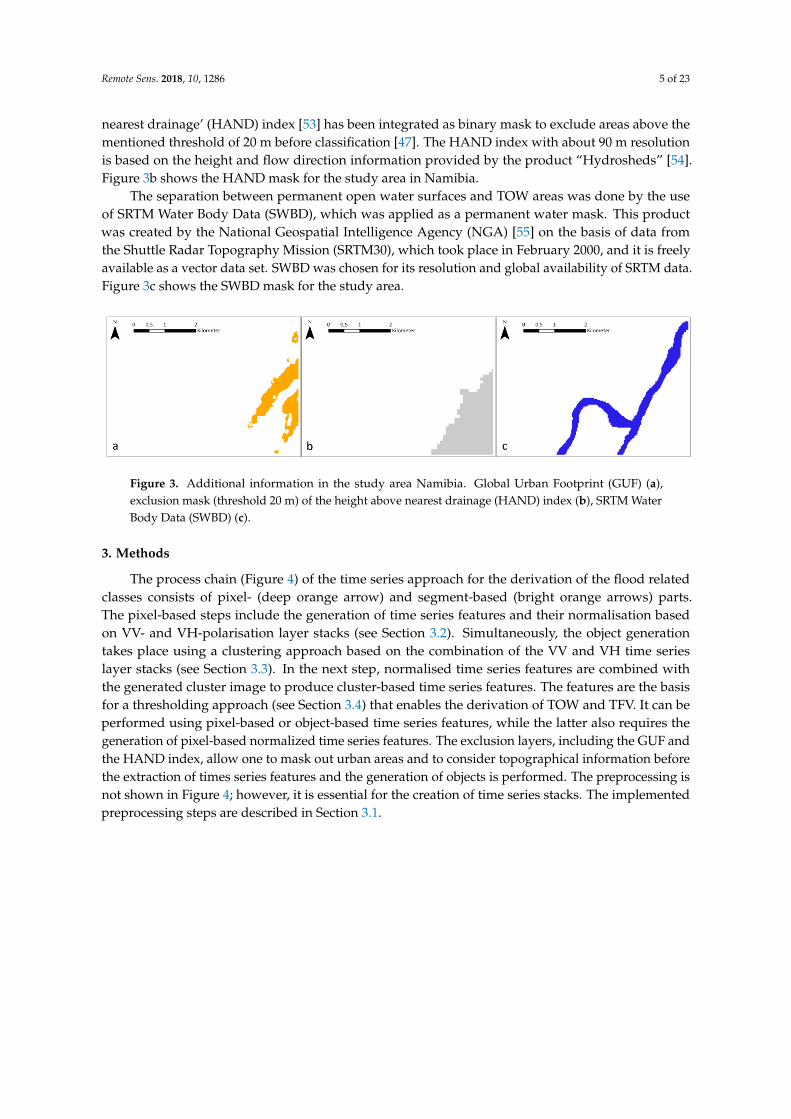
Remote Sens. 2018, 10, 1286 5 of 23
nearest drainage’ (HAND) index [53] has been integrated as binary mask to exclude areas above the
mentioned threshold of 20 m before classification [47]. The HAND index with about 90 m resolution
is based on the height and flow direction information provided by the product “Hydrosheds” [54].
Figure 3b shows the HAND mask for the study area in Namibia.
The separation between permanent open water surfaces and TOW areas was done by the use
of SRTM Water Body Data (SWBD), which was applied as a permanent water mask. This product
was created by the National Geospatial Intelligence Agency (NGA) [55] on the basis of data from
the Shuttle Radar Topography Mission (SRTM30), which took place in February 2000, and it is freely
available as a vector data set. SWBD was chosen for its resolution and global availability of SRTM data.
Figure 3c shows the SWBD mask for the study area.
Remote Sens x FOR PEER REVIEW of
The sep ration between perm nent open w ter surf ces nd TO re s w s done by the use of
SRTM ter Body Dat (SWBD), which was pplied s perm nent w ter m sk This product was
created by the N tion l Geospati l Intelligence Agency (NGA) [ ] on the b sis of d ta from the
Shuttle R d r Topography Mission (SRTM ) which took pl ce in Febru ry nd it is freely
v il ble s vector d ta set. SWBD was chosen for its resolution nd glob l v il bility of SRTM
d ta Figure c shows the SWBD m sk for the study rea
Figure Addition l inform tion in the study rea N mibia Glob l Urb n Footprint (GUF) ( ),
exclusion m sk (threshold m) of the height bove nearest dr in ge (HAND) index (b), SRTM ter
Body Dat (SWBD) (c).
thods
The process ch in (Figure ) of the time series ppro ch for the derivation of the flood rel ted
cl sses consists of pixel- (deep orange rrow) nd segment-based (bright orange rrows) parts. The
pixel-b sed steps include the generation of time series features nd their normalisation b sed on VV-
nd VH-pol risation l yer st cks (see Section ) Simultaneously, the object gener tion takes pl ce
using clustering ppro ch based on the combin tion of the VV nd VH time series l yer st cks (see
Section ) In the next step normalised time series features re combined with the generated cluster
im ge to produce cluster-based time series features. The features re the basis for thresholding
ppro ch (see Section ) th t en bles the derivation of TOW nd TFV. It c n be performed using
pixel-b sed or object-based time series features, while the l tter lso requires the gener tion of pixel-
based norm li ed time series features. The exclusion l yers, including the GUF nd the HAND index
llow one to m sk out urb n re s nd to consider topographical information before the extraction
of times series features nd the gener tion of objects is performed The preprocessing is not shown in
Figure however it is essenti l for the creation of time series st cks. The implemented preprocessing
steps are described in Section
Figure Cl ssific tion process ch in for the extr ction of tempor ry open w ter nd tempor ry
flooded veget tion b sed on SAR time series dat The deep or nge rrows represent the pixel-b sed
process part while bright or nge rrows show the object-b sed part of the process ch in * Glob l
Urb n Footprint (GUF), Height bove Nearest Dr in ge (HAND) index nd SRTM ter Body Dat
(SWBD) s exclusion l yers.
Figure 3. Additional information in the study area Namibia. Global Urban Footprint (GUF) (a),
exclusion mask (threshold 20 m) of the height above nearest drainage (HAND) index (b), SRTM Water
Body Data (SWBD) (c).
3. Methods
The process chain (Figure 4) of the time series approach for the derivation of the flood related
classes consists of pixel- (deep orange arrow) and segment-based (bright orange arrows) parts.
The pixel-based steps include the generation of time series features and their normalisation based
on VV- and VH-polarisation layer stacks (see Section 3.2). Simultaneously, the object generation
takes place using a clustering approach based on the combination of the VV and VH time series
layer stacks (see Section 3.3). In the next step, normalised time series features are combined with
the generated cluster image to produce cluster-based time series features. The features are the basis
for a thresholding approach (see Section 3.4) that enables the derivation of TOW and TFV. It can be
performed using pixel-based or object-based time series features, while the latter also requires the
generation of pixel-based normalized time series features. The exclusion layers, including the GUF and
the HAND index, allow one to mask out urban areas and to consider topographical information before
the extraction of times series features and the generation of objects is performed. The preprocessing is
not shown in Figure 4; however, it is essential for the creation of time series stacks. The implemented
preprocessing steps are described in Section 3.1.
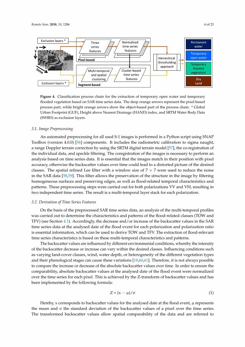
Remote Sens. 2018, 10, 1286 6 of 23
Remote Sens x FOR PEER REVIEW of
The sep ration between perm nent open w ter surf ces nd TO re s w s done by the use of
SRTM ter Body Dat (SWBD), which was pplied s perm nent w ter m sk This product was
created by the N tion l Geospati l Intelligence Agency (NGA) [ ] on the b sis of d ta from the
Shuttle R d r Topography Mission (SRTM ) which took pl ce in Febru ry nd it is freely
v il ble s vector d ta set. SWBD was chosen for its resolution nd glob l v il bility of SRTM
d ta Figure c shows the SWBD m sk for the study rea
Figure Addition l inform tion in the study rea N mibia Glob l Urb n Footprint (GUF) ( ),
exclusion m sk (threshold m) of the height bove nearest dr in ge (HAND) index (b), SRTM ter
Body Dat (SWBD) (c).
thods
The process ch in (Figure ) of the time series ppro ch for the derivation of the flood rel ted
cl sses consists of pixel- (deep orange rrow) nd segment-based (bright orange rrows) parts. The
pixel-b sed steps include the generation of time series features nd their normalisation b sed on VV-
nd VH-pol risation l yer st cks (see Section ) Simultaneously, the object gener tion takes pl ce
using clustering ppro ch based on the combin tion of the VV nd VH time series l yer st cks (see
Section ) In the next step normalised time series features re combined with the generated cluster
im ge to produce cluster-based time series features. The features re the basis for thresholding
ppro ch (see Section ) th t en bles the derivation of TOW nd TFV. It c n be performed using
pixel-b sed or object-based time series features, while the l tter lso requires the gener tion of pixel-
based norm li ed time series features. The exclusion l yers, including the GUF nd the HAND index
llow one to m sk out urb n re s nd to consider topographical information before the extraction
of times series features nd the gener tion of objects is performed The preprocessing is not shown in
Figure however it is essenti l for the creation of time series st cks. The implemented preprocessing
steps are described in Section
Figure Cl ssific tion process ch in for the extr ction of tempor ry open w ter nd tempor ry
flooded veget tion b sed on SAR time series dat The deep or nge rrows represent the pixel-b sed
process part while bright or nge rrows show the object-b sed part of the process ch in * Glob l
Urb n Footprint (GUF), Height bove Nearest Dr in ge (HAND) index nd SRTM ter Body Dat
(SWBD) s exclusion l yers.
Figure 4. Classification process chain for the extraction of temporary open water and temporary
flooded vegetation based on SAR time series data. The deep orange arrows represent the pixel-based
process part, while bright orange arrows show the object-based part of the process chain. * Global
Urban Footprint (GUF), Height above Nearest Drainage (HAND) index, and SRTM Water Body Data
(SWBD) as exclusion layers.
3.1. Image Preprocessing
An automated preprocessing for all used S-1 images is performed in a Python script using SNAP
Toolbox (version 4.0.0) [56] components. It includes the radiometric calibration to sigma naught,
a range Doppler terrain correction by using the SRTM digital terrain model [57], the co-registration of
the individual data, and speckle filtering. The coregistration of the images is necessary to perform an
analysis based on time series data. It is essential that the images match in their position with pixel
accuracy, otherwise the backscatter values over time could lead to a distorted picture of the desired
classes. The spatial refined Lee filter with a window size of 7 × 7 were used to reduce the noise
in the SAR data [58,59]. This filter allows the preservation of the structure in the image by filtering
homogeneous surfaces and preserving edges, as well as flood-related temporal characteristics and
patterns. These preprocessing steps were carried out for both polarizations VV and VH, resulting in
two independent time series. The result is a multi-temporal layer stack for each polarization.
3.2. Derivation of Time Series Features
On the basis of the preprocessed SAR time series data, an analysis of the multi-temporal profiles
was carried out to determine the characteristics and patterns of the flood-related classes (TOW and
TFV) (see Section 4.1). Accordingly, the decrease and/or increase of the backscatter values in the SAR
time series data at the analysed date of the flood event for each polarization and polarization ratio
is essential information, which can be used to derive TOW and TFV. The extraction of flood-relevant
time series characteristics is based on these multi-temporal characteristics and patterns.
The backscatter values are influenced by different environmental conditions, whereby the intensity
of the backscatter decrease or increase can vary within the desired classes. Influencing conditions such
as varying land-cover classes, wind, water depth, or heterogeneity of the different vegetation types
and their phenological stages can cause these variations [18,60,61]. Therefore, it is not always possible
to compare the increase or decrease of the absolute backscatter values over time. In order to ensure the
comparability, absolute backscatter values at the analysed date of the flood event were normalized
over the time series for each pixel. This is achieved by the Z-transform of backscatter values and has
been implemented by the following formula:
Z = (x − µ)/σ (1)
Hereby, x corresponds to backscatter values for the analysed date at the flood event, µ represents
the mean and σ the standard deviation of the backscatter values of a pixel over the time series.
The transformed backscatter values allow spatial comparability of the data and are referred to

Remote Sens. 2018, 10, 1286 7 of 23
hereinafter as Z-Score images. Because of the normalized description of the decrease or increase
of the backscatter values, and the Z-Score in connection with the respective polarizations, their ratio
(VV/VH) and their combinations (VV + VH, VV-VH) represent the essential time series features for
the derivation of TOW and TFV. Mean value, median, and the standard deviation over the time series
are considered as auxiliary information for the calculation of the Z-Score or as additional information
in the later classification.
A quantitative analysis of the time series features was carried out using the Random Forest (RF)
method to investigate the potential of those to derive the TOW and TFV. Therefore, training data for
two flood-related classes and a third class representing Dry Land areas were defined based on the
reference data and analysed by RF. RF is an ensemble learning method based on the construction
of a large number of decision trees using training data. The RF classifier is relatively robust against
outliers and noise, which is important for spatially variable SAR data [62]. Besides performing a
supervised classification, the application of RF algorithm allows one to derive the importance of
different features. By determining their importance, one can identify which time series feature has the
highest contribution to the classification results or is most reliable for the derivation of TOW and/or
TFV. In addition, RF was used to analyse whether a single time series characteristic or combination of
time series characteristics, and which one, allows for high classification accuracy for the two searched
classes. As a result, redundant information is sorted out, and the information essential for classification
is identified.
3.3. Clustering Approach for Segment Generation
The derivation of the TOW and TFV was done based on both pixels and segments. Among other
advantages, such as a reduction of speckle, the usage of segments allows for the reduction of intra-class
variability, which can be caused by the high spatial level of detail of the S-1 data. Clustering represents
a common method to perform image segmentation under consideration of multi-spectral and
multi-temporal data [63]. Cluster algorithms have already been used as segmentation methods
for the derivation of TFV [64–66]. The grouping of pixels into segments was implemented for the
study area using a k-means cluster algorithm. k-means is an iterative, unsupervised method that
assigns each pixel to a cluster using the minimum distance. This technique is widely used due to
its simple implementation. In addition, k-means produces relatively high-quality clusters with low
computational effort [67–69].
Segmentation by k-means was carried out in several steps. First, multi-temporal clustering
was performed. Therefore, a SAR time series data stack, containing the VV and VH polarizations,
is used. This allows one to integrate the temporal component and both polarizations for the
generation of clusters. Second, a spatial component was integrated by means of spatial clustering
based on the multi-polarised SAR image at the analysed date of the flood event. In order to
combine the multi-temporal and spatial information, both cluster images, multi-temporal and spatial,
were intersected with each other.
In contrast to other segmentation methods such as multiresolution segmentation [24,41], k-means
clustering requires the definition of only a single parameter: the number of clusters. In order to
determine this parameter for both the multi-temporal cluster and spatial cluster image, a range for the
number of clusters between 5 and 100 has been defined. Thereafter, all possible combinations of the
number of clusters for multi-temporal and spatial clustering were performed. Although all possible
combinations for the defined areas were tested, it turned out that the combination of 10 multi-temporal
clusters and 5 spatial clusters was the best cluster number combination in terms of classification
accuracy and computation efficiency. Finally, the combined clusters were examined for their spatial
independence and split into their spatially connected segments. The resulting segmented image was
used beside the pixel image as a basis for the classification of TOW and TFV.

Remote Sens. 2018, 10, 1286 8 of 23
3.4. Hierarchical Thresholding Approach
The last step in the classification process chain (Figure 4) is the hierarchical thresholding
approach, which is divided into three consecutive steps. First of all, the permanent open water
surfaces are identified using the SWBD mask (see Section 2) and excluded from further analysis.
In addition, GUF and HAND masks (see Section 2) were used as exclusion layers before the next
step. The other two steps are based on the remaining unclassified image elements using the derived
time series features (see Section 3.2). The threshold values for the corresponding time series features
are automatically generated by a decision tree classifier [62] using reference-based training data
(see Section 3.2). The automatic threshold definition represents a great advantage, since manually
determining thresholds, especially for separation of TFV to other classes, can be a complex process [6].
With the aid of the aforementioned time series features and corresponding threshold values, the class
TOW was derived firstly. Equivalent to TOW, the remaining unclassified image elements were
separated into TFV and Dry Land in the last step.
4. Results
4.1. Multi-Temporal Characteristics and Patterns of Backscatter Intensities
The analysis of multi-temporal characteristics and patterns was performed based on preprocessed
SAR time series data (see Section 3.1). For this purpose, pixels of the time series layer stacks were
combined into objects using clustering methods (see Section 3.3). Objects are less susceptible to noise
than pixels, and they can be used to create spatial contextual time series profiles, which allow one to
derive object-related characteristics and patterns. Examples of object-based time series profiles for
TOW and TFV, which were identified from the training data set acquired on 8 April 2017, are shown
in Figures 5 and 6. These objects contain 1148 pixels for TOW and 1054 pixels for TFV, respectively.
The box plots represent a range of the backscatter values within the segment for each date. The time
series are shown for the two single polarizations VV (Figures 5a and 6a), VH (Figures 5b and 6b),
and their ratio VV/VH (Figures 5c and 6c) for the same segment. In addition, the multi-temporal
behaviour of the NDVI and NDWI values for the same time-period is displayed in Figures 5d and 6d
and in Figures 5e and 6e, which serve as a comparison to the SAR time series data. These ratios are not
integrated in the methodology as a data set. The analysed flood event image (6 April 2017) is indicated
by a blue bar.
Figure 5 shows the multi-temporal characteristics and patterns of the backscatter values for TOW.
Compared to all other dates in the time series, a significant decrease of the backscatter values can be
observed at the analysed date during the flood event (blue bar) (Figure 5a,b). The ratio of the two
polarizations (Figure 5c) shows no change at the analysed date of the flood event. This indicates a
similar or equal change in both polarizations. As a comparison to the SAR time series data, NDVI values
were used, which were derived from the S-2 data sets. Despite the cloud-related data gap between
November 2016 and March 2017, there is a comparable reduction in the NDVI values for the analysed
date at the flood event. In combination with the decrease of the backscatter values, this confirms the
occurrence of water at the analysed date. In addition, the NDWI shows an increase in the values at the
date of flooding, which indicates the occurrence of water.

Remote Sens. 2018, 10, 1286 9 of 23
Remote Sens x FOR PEER REVIEW of
series profiles for TOW nd TFV, which were identified from the training d ta set cquired on April
re shown in Figures nd These objects contain pixels for TOW nd pixels for
TFV, respectively. The box plots represent range of the backscatter v lues within the segment for
each d te. The time series re shown for the two single pol ri tions VV (Figures nd ) VH
(Figures 5b nd b) nd their ratio VV/VH (Figures 5c nd c) for the same segment. In ddition the
multi-temporal beh viour of the NDVI nd NDWI values for the same time-period is displ yed in
Figures 5d nd d nd in Figures 5e nd 6e which serve s comparison to the SAR time series d t
These ratios re not integr ted in the methodology s d t set. The n lysed flood event im ge (
April ) is indicated by blue bar.
Figure shows the multi-temporal characteristics nd patterns of the backsc tter v lues for
TOW. Comp red to ll other d tes in the time series, significant decre se of the backscatter v lues
can be observed t the n lysed d te during the flood event (blue b r) (Figure b) The ratio of the
two pol ri tions (Figure c) shows no change t the n lysed d te of the flood event. This indicates
simil r or equ l change in both pol ri tions. As comparison to the SAR time series d t NDVI
values were used which were derived from the S- d t sets. Despite the cloud-rel ted d ta g p
between November nd M rch there is compar ble reduction in the NDVI v lues for the
n lysed d te t the flood event. In combin tion with the decre se of the b cksc tter v lues this
confirms the occurrence of water t the n lysed d te. In ddition the NDWI shows n incre se in
the v lues t the d te of flooding, which indicates the occurrence of water
Figure Multi-tempor l beh viour of the b ckscatter intensity for TOW reas for VV ( ) VH (b), the
r tio VV/VH (c), NDVI v lues (d) nd NDWI v lues ( ). The blue b rs m rk the n lysed d te t the
flood event
Figure shows n ex mple of multi-temporal characteristics nd patterns for TFV re s.
Compared to TO TFV is char cteri ed by n increase in the backsc tter values t the n lysed d te
in VV pol ri tion In contrast to the increase of the b ckscatter values in VV pol ris tion decre se
of the backscatter values occurs in VH pol risation during the flood event (Figure b) The ratio
between these two pol ri tions shows n increase for TFV t the n lysed d te (Figure c) As
comparison to the SAR time series d ta NDVI values for TFV were derived from the S- d ta nd
re displ yed for the same period (Figure d) At the n lysed d te, there is only very slight change
in the NDVI values. In ddition NDWI shows slight increase in v lues, which indicates the
occurrence of water in the veget ted re s. Nevertheless, the NDWI v lues rem in in the neg tive
range nd it seems th t there re no open water re s but mixture of st nding w ter nd vegetation
Accordingly, it can be confirmed th t the increase in backsc tter v lues in VV polari tion is caused
by flooding nd not by ny phenological changes. Over ll the increase in backsc tter v lues for TFV
Figure 5. Multi-temporal behaviour of the backscatter intensity for TOW areas for VV (a), VH (b),
the ratio VV/VH (c), NDVI values (d), and NDWI values (e). The blue bars mark the analysed date at
the flood event.
Figure 6 shows an example of multi-temporal characteristics and patterns for TFV areas. Compared
to TOW, TFV is characterized by an increase in the backscatter values at the analysed date in VV
polarization. In contrast to the increase of the backscatter values in VV polarisation, a decrease of the
backscatter values occurs in VH polarisation during the flood event (Figure 6b). The ratio between
these two polarizations shows an increase for TFV at the analysed date (Figure 6c). As a comparison
to the SAR time series data, NDVI values for TFV were derived from the S-2 data and are displayed
for the same period (Figure 6d). At the analysed date, there is only a very slight change in the NDVI
values. In addition, NDWI shows a slight increase in values, which indicates the occurrence of water in
the vegetated areas. Nevertheless, the NDWI values remain in the negative range, and it seems that
there are no open water areas but a mixture of standing water and vegetation. Accordingly, it can be
confirmed that the increase in backscatter values in VV polarization is caused by flooding and not by
any phenological changes. Overall, the increase in backscatter values for TFV in VV polarization is
significantly lower compared to the decrease in the backscatter values for TOW areas.
Remote Sens x FOR PEER REVIEW of
in VV pol ri tion is significantly lower compared to the decre se in the backsc tter v lues for TOW
re s.
Figure Multi-tempor l beh viour of the b ckscatter intensity for TFV reas for VV ( ), VH (b), the
r tio VV/VH (c), NDVI v lues (d) nd NDWI v lues ( ). The blue b rs m rk the n lysed d te t the
flood event
Rele ant Time Series Features
Relev nt time series features were determined for the deriv tion of the flood-rel ted cl sses
based on tr inings d ta which were taken from the reference d t The tot l number of training pixels
for each of the three cl sses is (TOW), (TFV) nd (Dry L nd) The importance of
time series features for each cl ss w s implemented by RF (see Section ) The n lysed time series
features include Z-Score for the VV nd VH pol ri tions, Z-Score for the ratio between VV nd VH
nd two Z-Score combin tions VV VH nd VV-VH.
The training d ta were used to visuali e the distribution nd separ bility of the cl sses with
respect to the derived time series features in histogram Figure shows histogram distributions of
the training d t for each aforementioned cl ss nd time series feature The separability between the
TOW nd other cl sses is clearly recogni ble for Z-Score VV nd Z-Score VV VH. The overl p
between the histograms of the cl sses TOW nd Dry L nd is strongly pronounced for Z-Score VV
VH nd Z-Score VV/VH. In ddition there is n overl p to TFV by using Z-Score VH. The sep rability
of TFV from other cl sses c n be observed for Z-Score VV, Z-Score VV-VH nd Z-Score VV/VH. In
particul r, Z-Score VV/VH ppe rs s suitable time series feature to distinguish the TFV from other
cl sses.
The RF lgorithm was used to qu ntify the importance of time series features for the TO nd
TFV classes (see Section ) Thereby the contribution of e ch time series feature was determined for
the deriv tion of the respective desired classes Taking into ccount the training d ta estim tors
nd m ximum tree depth of were defined to identify the importance These parameters were used
to exclude randomness from the results Figure shows the importance of time series fe tures for the
classes TOW nd TFV It can be observed th t for TO Z-Score VV nd Z-Score VV VH there re
time series features with the highest contributions of % nd % respectively The time series
fe ture with the highest contribution ( %) for the TFV class is Z-Score VV/VH
Figure 6. Multi-temporal behaviour of the backscatter intensity for TFV areas for VV (a), VH (b),
the ratio VV/VH (c), NDVI values (d), and NDWI values (e). The blue bars mark the analysed date at
the flood event.
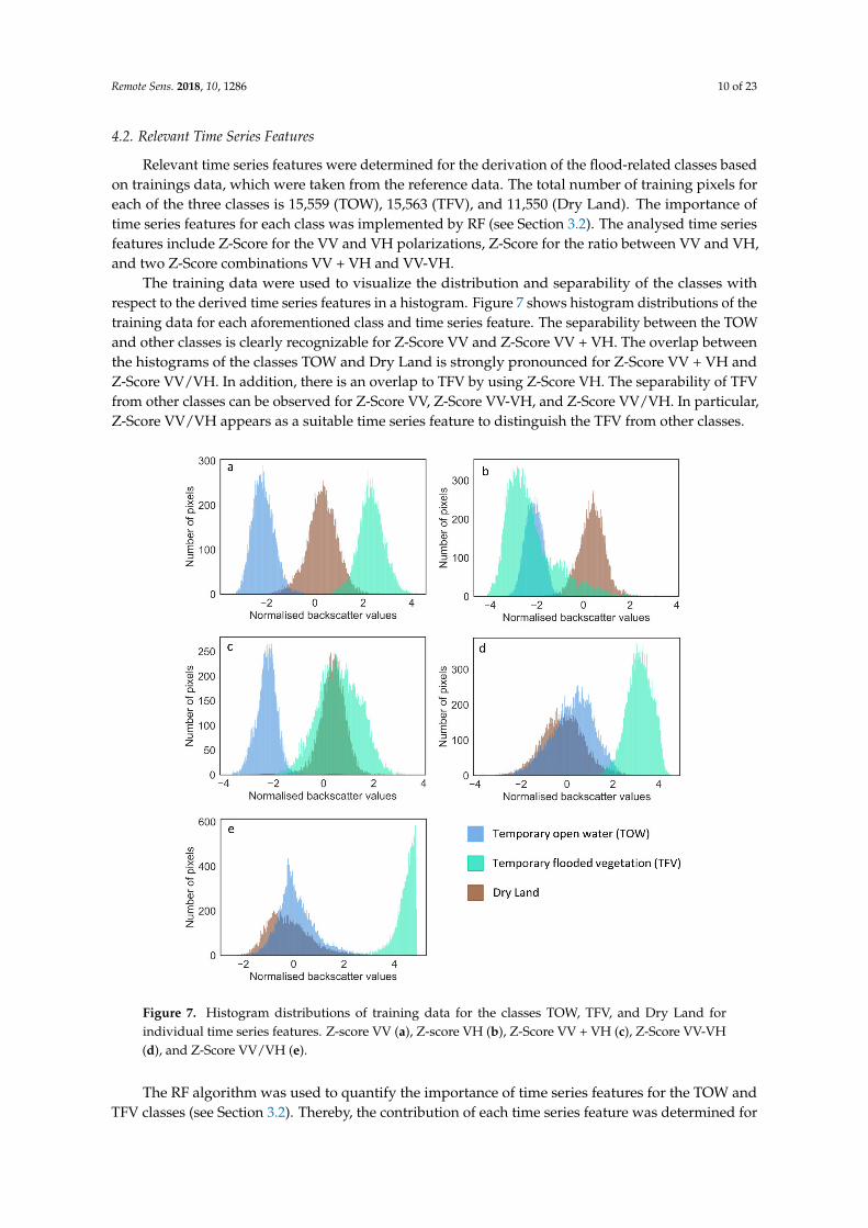
Remote Sens. 2018, 10, 1286 10 of 23
4.2. Relevant Time Series Features
Relevant time series features were determined for the derivation of the flood-related classes based
on trainings data, which were taken from the reference data. The total number of training pixels for
each of the three classes is 15,559 (TOW), 15,563 (TFV), and 11,550 (Dry Land). The importance of
time series features for each class was implemented by RF (see Section 3.2). The analysed time series
features include Z-Score for the VV and VH polarizations, Z-Score for the ratio between VV and VH,
and two Z-Score combinations VV + VH and VV-VH.
The training data were used to visualize the distribution and separability of the classes with
respect to the derived time series features in a histogram. Figure 7 shows histogram distributions of the
training data for each aforementioned class and time series feature. The separability between the TOW
and other classes is clearly recognizable for Z-Score VV and Z-Score VV + VH. The overlap between
the histograms of the classes TOW and Dry Land is strongly pronounced for Z-Score VV + VH and
Z-Score VV/VH. In addition, there is an overlap to TFV by using Z-Score VH. The separability of TFV
from other classes can be observed for Z-Score VV, Z-Score VV-VH, and Z-Score VV/VH. In particular,
Z-Score VV/VH appears as a suitable time series feature to distinguish the TFV from other classes.Remote Sens x FOR PEER REVIEW of
Figure Histogr m distributions of tr ining dat for the classes TOW, TFV nd Dry Land for
individual time series fe tures Z-score VV ( ), Z-score VH (b), Z-Score VV VH (c), Z-Score VV-VH
(d), nd Z-Score VV/VH ( ).
Figure Import nce of the time series features, which were determined by the Random Forest
lgorithm for TOW (blue b rs) nd TFV (green b rs) The fe tures re sorted by their highest to lowest
import nce.
The time series feature with the highest contribution does not necessarily represent the highest
possible cl ssification ccuracy. Therefore it is n lysed whether single feature or combin tion of
Figure 7. Histogram distributions of training data for the classes TOW, TFV, and Dry Land for
individual time series features. Z-score VV (a), Z-score VH (b), Z-Score VV + VH (c), Z-Score VV-VH
(d), and Z-Score VV/VH (e).
The RF algorithm was used to quantify the importance of time series features for the TOW and
TFV classes (see Section 3.2). Thereby, the contribution of each time series feature was determined for
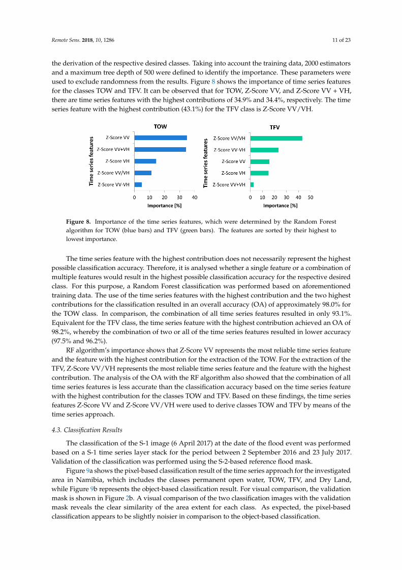
Remote Sens. 2018, 10, 1286 11 of 23
the derivation of the respective desired classes. Taking into account the training data, 2000 estimators
and a maximum tree depth of 500 were defined to identify the importance. These parameters were
used to exclude randomness from the results. Figure 8 shows the importance of time series features
for the classes TOW and TFV. It can be observed that for TOW, Z-Score VV, and Z-Score VV + VH,
there are time series features with the highest contributions of 34.9% and 34.4%, respectively. The time
series feature with the highest contribution (43.1%) for the TFV class is Z-Score VV/VH.
Remote Sens x FOR PEER REVIEW of
Figure Histogr m distributions of tr ining dat for the classes TOW, TFV nd Dry Land for
individual time series fe tures Z-score VV ( ), Z-score VH (b), Z-Score VV VH (c), Z-Score VV-VH
(d), nd Z-Score VV/VH ( ).
Figure Import nce of the time series features, which were determined by the Random Forest
lgorithm for TOW (blue b rs) nd TFV (green b rs) The fe tures re sorted by their highest to lowest
import nce.
The time series feature with the highest contribution does not necessarily represent the highest
possible cl ssification ccuracy. Therefore it is n lysed whether single feature or combin tion of
Figure 8. Importance of the time series features, which were determined by the Random Forest
algorithm for TOW (blue bars) and TFV (green bars). The features are sorted by their highest to
lowest importance.
The time series feature with the highest contribution does not necessarily represent the highest
possible classification accuracy. Therefore, it is analysed whether a single feature or a combination of
multiple features would result in the highest possible classification accuracy for the respective desired
class. For this purpose, a Random Forest classification was performed based on aforementioned
training data. The use of the time series features with the highest contribution and the two highest
contributions for the classification resulted in an overall accuracy (OA) of approximately 98.0% for
the TOW class. In comparison, the combination of all time series features resulted in only 93.1%.
Equivalent for the TFV class, the time series feature with the highest contribution achieved an OA of
98.2%, whereby the combination of two or all of the time series features resulted in lower accuracy
(97.5% and 96.2%).
RF algorithm’s importance shows that Z-Score VV represents the most reliable time series feature
and the feature with the highest contribution for the extraction of the TOW. For the extraction of the
TFV, Z-Score VV/VH represents the most reliable time series feature and the feature with the highest
contribution. The analysis of the OA with the RF algorithm also showed that the combination of all
time series features is less accurate than the classification accuracy based on the time series feature
with the highest contribution for the classes TOW and TFV. Based on these findings, the time series
features Z-Score VV and Z-Score VV/VH were used to derive classes TOW and TFV by means of the
time series approach.
4.3. Classification Results
The classification of the S-1 image (6 April 2017) at the date of the flood event was performed
based on a S-1 time series layer stack for the period between 2 September 2016 and 23 July 2017.
Validation of the classification was performed using the S-2-based reference flood mask.
Figure 9a shows the pixel-based classification result of the time series approach for the investigated
area in Namibia, which includes the classes permanent open water, TOW, TFV, and Dry Land,
while Figure 9b represents the object-based classification result. For visual comparison, the validation
mask is shown in Figure 2b. A visual comparison of the two classification images with the validation
mask reveals the clear similarity of the area extent for each class. As expected, the pixel-based
classification appears to be slightly noisier in comparison to the object-based classification.

Remote Sens. 2018, 10, 1286 12 of 23
Figure 10 shows the intersection between the validation data and the results based on pixel-based
(a) and object-based (b) classification, respectively. Areas of correspondence, as well as misclassified
areas, can be shown by this intersection. The orange areas, which are marked as TFV in the
classification, however, representing Dry Land in the validation data, can be visually identified
as largest misclassification areas. Another significant misclassification can be identified by yellow
areas. These areas represent the Dry Land class in the classification image and the TFV class in the
validation data, and are slightly larger in the pixel-based classification compared to the object-based
classification. Recognisable are also bright blue areas, which can be found at the transect zone between
Dry Land and TOW. While these areas represent Dry Land in the reference data, they are classified
as TOW. The visual comparison between pixel and object-based classification shows that the extent
of bright blue areas in both classifications is similar; this is also the case for all other remaining small
misclassified areas. A further difference between pixel- and object-based classification can be observed
in the red areas, which represent Dry Land in the classification and TOW in the validation data. Overall,
the comparison between pixel- and object-based classification shows that fewer misclassified areas
occur in the object-based classification.Remote Sens x FOR PEER REVIEW of
Figure Pixel-b sed classific tion result ( ) nd object-b sed classification result (b) for the study
rea in N mibia
Figure Are s of correspondence nd misclassific tions for the classes TOW, TFV, nd Dry L nd
using pixel-b sed ( ) nd object-b sed (b) classification which re gener ted by the intersection of
the classific tions nd the v lidation dat
The quantification of the classification ccuracy of TO TFV nd Dry L nd w s performed
using OA, producer ccuracy (PA) user ccur cy (UA) nd K pp index (K) The ccur cies for
pixel-b sed nd object-b sed cl ssification re shown in Figure The ccuracy values (UA nd PA)
for the TOW cl ss re % nd % for pixel-b sed cl ssification nd % (UA) nd % (PA)
for object-b sed cl ssification respectively. In comp rison the ccur cy of the cl ss TFV is lower,
with % (UA) nd % (PA) for pixel-b sed cl ssification nd % (UA) nd % (PA) for
object-based cl ssification For the cl ss Dry L nd the UA nd PA re % nd % for the pixel-
based cl ssification For the object-b sed cl ssification these re % (UA) nd % (PA)
respectively. The improvement w s m inly chieved in the UA re for TFV by % nd PA for Dry
L nd by %. Over ll the OA of object-based cl ssific tion is bout % higher compared to pixel-
based cl ssification The K pp index is lso higher for the object-b sed cl ssification In
ddition confidence interval was calcul ted for each of the ccur cy values [ ] For the pixel-based
Figure 9. Pixel-based classification result (a) and object-based classification result (b) for the study area
in Namibia.
Figure 10. Areas of correspondence and misclassifications for the classes TOW, TFV, and Dry Land
using pixel-based (a) and object-based (b) classification, which are generated by the intersection of the
classifications and the validation data.

Remote Sens. 2018, 10, 1286 13 of 23
The quantification of the classification accuracy of TOW, TFV, and Dry Land was performed using
OA, producer accuracy (PA), user accuracy (UA), and Kappa index (K). The accuracies for pixel-based
and object-based classification are shown in Figure 11. The accuracy values (UA and PA) for the TOW
class are 85.1% and 82.6% for pixel-based classification, and 85.8% (UA) and 85.5% (PA) for object-based
classification, respectively. In comparison, the accuracy of the class TFV is lower, with 67.9% (UA) and
86.32% (PA) for pixel-based classification, and 76.1% (UA) and 91.2% (PA) for object-based classification.
For the class Dry Land, the UA and PA are 74.8% and 59.0% for the pixel-based classification. For the
object-based classification, these are 80.8% (UA) and 67.0% (PA), respectively. The improvement was
mainly achieved in the UA area for TFV by 8.1% and PA for Dry Land by 8.0%. Overall, the OA of
object-based classification is about 5.0% higher compared to pixel-based classification. The Kappa
index is also 0.08 higher for the object-based classification. In addition, a confidence interval was
calculated for each of the accuracy values [70]. For the pixel-based classification, the largest confidence
interval lies at 0.38% for dry land producer accuracy. For object-based classification, the largest
confidence interval is 0.37% for the same class and accuracy.
Remote Sens x FOR PEER REVIEW of
cl ssification the l rgest confidence interv l lies t % for dry l nd producer ccuracy. For object-
based cl ssification the l rgest confidence interv l is 0 % for the same cl ss nd ccuracy.
Figure Accuracy ssessment results for pixel- nd object-b sed classific tion which re gener ted
by means of the time series ppro ch
In ddition to the cl ssification of the v lid tion extent, the cl ssification for the entire study re
was gener ted based on the same time series char cteristics and the corresponding threshold v lues
for the cl sses TOW nd TFV. Figure shows the pixel-b sed cl ssification nd Figure b the
object-based cl ssification A difference between both cl ssifications can be observed In particul r,
the Dry L nd re s of the pixel-b sed cl ssification ppe r to be noisier in comparison to the Dry
L nd re s of the object-based cl ssification nd show slightly higher overestim tion for ll re s,
especi lly for Dry L nd Both figures show th t the disregard of the TFV re s would result in n
enormous underestim tion of the flood extent.
Figure 11. Accuracy assessment results for pixel- and object-based classification, which are generated
by means of the time series approach.
In addition to the classification of the validation extent, the classification for the entire study
area was generated based on the same time series characteristics and the corresponding threshold
values for the classes TOW and TFV. Figure 12a shows the pixel-based classification and Figure 12b the
object-based classification. A difference between both classifications can be observed. In particular,
the Dry Land areas of the pixel-based classification appear to be noisier in comparison to the Dry Land
areas of the object-based classification and show slightly higher overestimation for all areas, especially
for Dry Land. Both figures show that the disregard of the TFV areas would result in an enormous
underestimation of the flood extent.

Remote Sens. 2018, 10, 1286 14 of 23Remote Sens x FOR PEER REVIEW of
Figure Pixel-based classific tion result for the entire study rea in N mibia ( ). Object-b sed
classific tion result for the entire study rea in N mibia (b).
Im rovement of t e Sentinel- Flood Ser ice
Figure shows the cl ssification result of the S- FS (see Section ) for the v lid tion re in
Namibi which initi lly only contains the open flood water re s [ ] For the extension nd
improvement of the S- FS the open flood re s were supplemented by TO nd TFV of the time
series ppro ch, in order to detect the entire flood extent. The object-based cl ssification result was
used s supplement since higher ccur cy could be chieved compared to pixel-b sed cl ssification
results
An ccur cy ssessment w s c rried out for both the cl ssification results of the S- FS nd the
supplemented cl ssification results of the S- FS The cl sses TFV nd TOW, both in the v lid tion
d ta nd in the supplemented cl ssification of the S- FS were combined into single cl ss flood
This represents the entire flood extent. The modified reference d t is shown in Figure d The
merging of the cl sses of TOW nd TFV provides more comprehensive cover ge of the flood extent
in the reference d ta compared to the results of the S- FS (Figure ) Figure b shows the
cl ssification result of the S- FS which re supplemented by TO nd Figure c represents the S-
FS cl ssification result simultaneously supplemented by TO nd TFV of the time series ppro ch.
Figure 12. Pixel-based classification result for the entire study area in Namibia (a). Object-based
classification result for the entire study area in Namibia (b).
4.4. Improvement of the Sentinel-1 Flood Service
Figure 13a shows the classification result of the S-1FS (see Section 1) for the validation area
in Namibia, which initially only contains the open flood water areas [47]. For the extension and
improvement of the S-1FS, the open flood areas were supplemented by TOW and TFV of the time
series approach, in order to detect the entire flood extent. The object-based classification result was used
as a supplement, since higher accuracy could be achieved compared to pixel-based classification results.
An accuracy assessment was carried out for both the classification results of the S-1FS and the
supplemented classification results of the S-1FS. The classes TFV and TOW, both in the validation
data and in the supplemented classification of the S-1FS, were combined into a single class: flood.
This represents the entire flood extent. The modified reference data is shown in Figure 13d. The merging
of the classes of TOW and TFV provides a more comprehensive coverage of the flood extent in the
reference data compared to the results of the S-1FS (Figure 13a). Figure 13b shows the classification
result of the S-1FS, which are supplemented by TOW, and Figure 13c represents the S-1FS classification

Remote Sens. 2018, 10, 1286 15 of 23
result simultaneously supplemented by TOW and TFV of the time series approach. The validation of
the S-1FS and the two supplemented S-1FS classification results were performed using OA, PA, UA,
and Kappa Index (Figure 14). A significant improvement in classification accuracy is observed for
PA Flood and UA Dry Land, which are 57.1% and 31.0%, respectively. This improvement is mainly
achieved by supplementing the S-1FS classification results with the TFV surfaces. Thereby, the OA
increases by 27.0% and the Kappa coefficient increases from 0.24 to 0.69.
4.5. Number of Images
Besides the sensor characteristics and environmental conditions, the number of images used for
the developed time series approach is another important element that can influence the accuracy of
the classification result. 25 S-1 images were used to derive flood-related classes for the study area
in Namibia. The time series was used to obtain the statistical multi-temporal distribution of the
backscatter values for the flood-related classes (see Section 3.2). For this purpose, it was analysed
whether a lower number of images in the time series has an effect on the classification results. In each
time series, fewer images were used starting with the original classification of 24 images decreasing
in increments of 1, whereby the analysed flood date image was included in each classification run.
Figure 15 shows the OAs and Kappa coefficients for 24 classification results, each based on time series
with a different number of applied images. In addition, a confidence interval was calculated for each
AO. The use of a single image, together with the image taken at the time of the flood results in the
lowest accuracy. The same classification resulted in the largest confidence interval 0.19%. Overall, it can
be observed that the fewer images are used in the time series, the lower is the OA and Kappa coefficient.
Remote Sens x FOR PEER REVIEW of
The v lid tion of the S- FS nd the two supplemented S- FS cl ssification results were performed
using OA, PA UA nd K ppa Index (Figure ) A significant improvement in cl ssification ccuracy
is observed for PA Flood nd UA Dry L nd which re % nd % respectively. This
improvement is m inly chieved by supplementing the S- FS cl ssification results with the TFV
surf ces. Thereby, the OA increases by 2 % nd the K pp coefficient increases from to
Number of Images
Besides the sensor char cteristics nd environmental conditions, the number of im ges used for
the developed time series ppro ch is nother important element th t c n influence the ccuracy of
the cl ssification result. S- im ges were used to derive flood-rel ted cl sses for the study re in
Namibi The time series was used to obt in the st tistical multi-temporal distribution of the
backsc tter values for the flood-rel ted cl sses (see Section ) For this purpose, it was n lysed
whether lower number of im ges in the time series h s n effect on the cl ssification results In each
time series, fewer im ges were used st rting with the origin l cl ssification of im ges decre sing
in increments of whereby the n lysed flood d te im ge was included in each cl ssification run.
Figure shows the OAs nd K pp coefficients for cl ssification results each b sed on time series
with different number of pplied im ges. In ddition confidence interval was calcul ted for each
AO. The use of single im ge together with the im ge taken t the time of the flood results in the
lowest ccuracy. The same cl ssification resulted in the l rgest confidence interval % Over ll it
can be observed th t the fewer im ges re used in the time series, the lower is the OA nd K pp
coefficient.
Figure Classific tion result of the S- FS ( ), cl ssific tion results of the S- FS supplemented by
TOW reas of the time series ppro ch (b), cl ssification results of the S- FS supplemented by TOW
nd TFV re s of the time series ppro ch (c) nd v lid tion image with merged flood reas (TOW
TFV) (d).
Figure 13. Classification result of the S-1FS (a), classification results of the S-1FS supplemented by TOW
areas of the time series approach (b), classification results of the S-1FS supplemented by TOW and TFV
areas of the time series approach (c), and validation image with merged flood areas (TOW + TFV) (d).

Remote Sens. 2018, 10, 1286 16 of 23Remote Sens x FOR PEER REVIEW of
Figure Accuracy ssessment results b sed on the S- FS nd its improvement (S- FS TOW nd S-
FS TOW TFV).
Figure Over ll Accuracy (AO) nd K ppa Coefficient for each classific tion run b sed on
decreasing number of images
Discussion
Multi-Tem oral Characteristics and Time Series Features
The n lysed ch r cteristics nd p tters of SAR time series d ta clearly show decre se in
backsc tter values for TOW nd n increase in backscatter v lues for TFV t the n lysed d te of the
flood event (Figures nd ) Thereby, the decre se indicates the occurrence of open w ter surf ces,
which re ch racteri ed by low b cksc tter values, in which the emitted sensor energy is reflected
w y by the specul r water surf ce [ ] The increase can be expl ined by the double- or multi-bounce
inter ctions between the specul r water surf ce nd the vertical structures of the veget tion [ ]
In m ny previous studies simil r beh viour of the backscatter v lues for the cl sses TO nd TFV
is described [ ] These char cteristics nd patters in backscatter v lues re prerequisite for
the detection of the flood-rel ted cl sses. The length of the decre se or increase of the b ckscatter
values depends on the dur tion of the flood the spati l extent nd the revisit time of the satellite.
It should lso be noted th t backscatter values can be strongly influenced by the environment l
conditions (see Section ) For ex mple, wind or heavy rainf ll can roughen the water surf ce nd
reduce or even er se the typical decre se in b cksc tter values during the flood event [ ] The
increase in backscatter t the d te of the flood can lso be strongly influenced by the inter ction
between sensor ch racteristics (wavelength ngle of incidence nd pol risation) [ ] nd
environment l conditions, such s boveground biom ss [ ] or the rel tion between w ter level
Figure 14. Accuracy assessment results based on the S-1FS and its improvement (S-1FS + TOW and
S-1FS + TOW + TFV).
Remote Sens x FOR PEER REVIEW of
Figure Accuracy ssessment results b sed on the S- FS nd its improvement (S- FS TOW nd S-
FS TOW TFV).
Figure Over ll Accuracy (AO) nd K ppa Coefficient for each classific tion run b sed on
decreasing number of images
Discussion
Multi-Tem oral Characteristics and Time Series Features
The n lysed ch r cteristics nd p tters of SAR time series d ta clearly show decre se in
backsc tter values for TOW nd n increase in backscatter v lues for TFV t the n lysed d te of the
flood event (Figures nd ) Thereby, the decre se indicates the occurrence of open w ter surf ces,
which re ch racteri ed by low b cksc tter values, in which the emitted sensor energy is reflected
w y by the specul r water surf ce [ ] The increase can be expl ined by the double- or multi-bounce
inter ctions between the specul r water surf ce nd the vertical structures of the veget tion [ ]
In m ny previous studies simil r beh viour of the backscatter v lues for the cl sses TO nd TFV
is described [ ] These char cteristics nd patters in backscatter v lues re prerequisite for
the detection of the flood-rel ted cl sses. The length of the decre se or increase of the b ckscatter
values depends on the dur tion of the flood the spati l extent nd the revisit time of the satellite.
It should lso be noted th t backscatter values can be strongly influenced by the environment l
conditions (see Section ) For ex mple, wind or heavy rainf ll can roughen the water surf ce nd
reduce or even er se the typical decre se in b cksc tter values during the flood event [ ] The
increase in backscatter t the d te of the flood can lso be strongly influenced by the inter ction
between sensor ch racteristics (wavelength ngle of incidence nd pol risation) [ ] nd
environment l conditions, such s boveground biom ss [ ] or the rel tion between w ter level
Figure 15. Overall Accuracy (AO) and Kappa Coefficient for each classification run based on a
decreasing number of images.
5. Discussion
5.1. Multi-Temporal Characteristics and Time Series Features
The analysed characteristics and patters of SAR time series data clearly show a decrease in
backscatter values for TOW and an increase in backscatter values for TFV at the analysed date of the
flood event (Figures 5 and 6). Thereby, the decrease indicates the occurrence of open water surfaces,
which are characterized by low backscatter values, in which the emitted sensor energy is reflected
away by the specular water surface [71]. The increase can be explained by the double- or multi-bounce
interactions between the specular water surface and the vertical structures of the vegetation [9–11].
In many previous studies, similar behaviour of the backscatter values for the classes TOW and TFV is
described [11,20,25]. These characteristics and patters in backscatter values are a prerequisite for the
detection of the flood-related classes. The length of the decrease or increase of the backscatter values
depends on the duration of the flood, the spatial extent, and the revisit time of the satellite.
It should also be noted that backscatter values can be strongly influenced by the environmental
conditions (see Section 4.2). For example, wind or heavy rainfall can roughen the water surface and
reduce or even erase the typical decrease in backscatter values during the flood event [4,9]. The increase
in backscatter at the date of the flood can also be strongly influenced by the interaction between sensor

Remote Sens. 2018, 10, 1286 17 of 23
characteristics (wavelength, angle of incidence, and polarisation) [6] and environmental conditions,
such as aboveground biomass [72–74] or the relation between water level and plant height [10].
Such external environmental conditions can have a limiting impact on the methodology presented here.
In previous studies, absolute backscatter values are applied for the extraction of flood-related
classes [10,37]. This can lead to underestimation or overestimation of the TFV areas and limits the
use of the method. These disadvantages can be compensated by the normalisation of backscatter
values over the time series, which ensure the comparability of the increase or decrease in backscatter
values for each image element independent of the different types of phenological development of the
vegetation. Moreover, the developed method enables simple management of SAR time series data
without the use of extensive methods to describe the seasonality or the typical vegetation conditions.
In comparison to other studies [19,37], which are based on the dependency of the sequential dates order
of the multi-temporal SAR data, the technique presented in this paper can deal with non-sequential
or irregular times series data. Sentinel-1 scenes acquired within a period of two years, which are
containing the flood event, the flood event made it possible to distinguish the natural range of variation
for the analysed vegetation from the changes induced by a flood event.
The decrease and the increase of the backscatter values in SAR time series data were used for
the extraction of time series features. Therefore, not only the polarizations VV and VH were applied,
but also their combination. By combining polarizations, the effects, such as different sensitivities
of the polarisations to objects, can also be intensified, e.g., by mathematically induced stretching of
the data [75–77]. The intensity of the amplification was quantified using the RF method (Figure 8).
For the extraction of TOW, Z-Score VV was determined by a RF classifier as the most reliable time
series feature, having the highest contribution in comparison to the VH based time series features.
While this finding matches the results of other studies [4,47], some studies [25,37] prefer VH as a basis
for the classification. This ambivalence can probably be explained by different sensor characteristics
and environmental conditions in the studies.
The time series feature Z-Score VV/VH proved to be most suitable for the derivation of TFV.
This can be explained by the different sensitivity of VV and VH for backscattering mechanisms [78],
which causes the backscatter values to increase for VV and decrease for VH. In case of TFV, the increase
of the backscatter values can usually be detected by VV polarization due to the double-bounce effect.
The double-bounce effect cannot be detected due to the depolarizing property of VH polarization,
and the increase of the backscatter values is not expected in VH. Because of the difference or ratio
between these two polarisations, the increase in VV is intensified, allowing a more effective derivation
of TFV compared to a simple use of VV polarisation.
In the example of Namibia, VV seems to be influenced by the double-bounce-effect indicating the
occurrence of TFV [60,79], whereby VH is not influenced by the interaction between water surface and
vegetation. Instead, VH is dominated by the specular reflection because of flooded soil in between the
vegetation, which consequently results in a decrease in backscatter values. According to the difference
in the backscatter between VV and VH for the analysed flood date, the time series feature Z-Score
VV/VH was successfully used for the extraction of the TFV.
5.2. Classification Results
The comparison of the time series approach results with the reference mask provides good
correspondence of 75.0% (OA, pixel-based) and 80.5% (OA, object-based) for the whole flood
extent, comprising both classes TOW and TFV. Cazals et al. [37] achieved a similar OA (82.0%)
using backscatter intensities of S-1 time series data for the detection of flooded areas, comprising
TOW and TFV. However, a sequential time series is necessary for this method. Furthermore,
the comparability of the validation results is limited by the differences between the study areas,
including the vegetation types, the sizes of the individual classes, and the ratio in size between these
classes and environmental conditions.

Remote Sens. 2018, 10, 1286 18 of 23
In the following, the classification results are discussed in comparison to the validation image
(Figure 10). It can be observed that the areas of the correctly classified classes (TOW = blue, TFV = green,
Dry Land = brown) predominate; however, misclassifications are present. The misclassifications occur
mostly for TFV in the classification image, which is marked as Dry Land in the validation image.
Indeed, in these areas the VV and VH polarisations of the time series features Z-Score VV/VH
have a significant difference during the flood event and are therefore classified as TFV. Nevertheless,
these areas are marked as Dry Land in the validation image. This contradiction can be explained by
the fact that the interpretation of optical data in relation to TFV is challenging, and water under the
vegetation cover cannot always be clearly identified in the validation image. In addition, the temporal
shift between the flood image (6 April 2017) and the validation image (8 April 2017) might also be
a reason for the aforementioned misclassifications. Even so, no change in the flood extend could be
observed; a receding flood extent (Figure 5) until the date of the S-2 acquisition could be possible.
Thus, misclassified areas can indeed represent Dry Land; however, they can also constitute TFV
areas in the S-1 flood image. Another significant misclassification is represented by yellow areas.
For these areas, the interaction between water surfaces and vegetation may not be strong enough
to cause an increase in the backscatter values in VV polarisation [10,80,81]. Accordingly, there is
no increase in the Z-Score VV/VH time series feature, so these areas were classified as Dry Land.
The light blue areas represent confusion between TOW in the classification results and Dry Land in the
validation image. These misclassifications may be caused by an insufficient decrease of the backscatter
values in the VV polarisation at the analysed date of the flood event, which could not be detected
by the generated threshold value. The transitional zones between TOW and dry areas have always
been challenging to detect [82], because of the rapidly changing conditions during the flood event.
Despite the misclassifications, the results show that for TOW 85.8% (UA) and 85.5% (PA) and for TFV
76.1% (UA) and 91.2% (PA) could be achieved.
In addition, it was shown that the object-based classification compared to pixel-based classification
can help to detect more precisely the areas affected by flood. This can be explained by the fact that
the heterogeneity of the TFV in S-1 imagery is reduced by grouping pixels into objects providing a
depiction of real objects on the ground. In the TOW area, misclassifications to Dry Land could also be
partially reduced. They may have been caused by environmental conditions such as wind, which only
affected a few pixels in an object. It also seems that speckle in the SAR data could also be reduced
by using objects for classification (Figure 10). However, it should be noted that an additional step to
calculate objects must be performed. The results of previous studies also confirm that object-based
classification reaches higher accuracies in comparison to pixel-based classifications [27,41].
The validation of the S-1FS results, which were supplemented with the results of the developed
SAR time series approach, show that this addition led to an improvement in the classification results
of the S-1FS. Although the results of the fully automatic near-real time S-1FS have been significantly
improved, it should be noted that the developed SAR time series approach requires training data for the
initialization, and that several images (time series) are used to derive the TFV. Thereby, preprocessing
is more time-consuming compared to the S-1FS and depends on the number of images used in the time
series, the classification basis applied (pixel- or object-based), and the duration for the extraction of
training data by an expert. Apart from the above-mentioned steps, the actual classification process only
takes a few seconds. A minimum number of data sets in the time series depends on the duration of the
flood and the number of S-1 images that have been acquired during the flood. The less non-flooded
dates used in the time series, the lower the classification accuracy. If available, it is recommended to
include at least one vegetation cycle in order to consider the entire seasonality or phenology. Thus,
the statistical distribution of the backscatter values over the entire vegetation cycle is considered [19].
Considering the above-mentioned prerequisite for the SAR time series approach, it was possible to
achieve a significant improvement in classification accuracy of S-1FS for PA Flood and UA Dry Land.
This was accomplished by supplementing the TOW of S-1FV with the TFV areas (Figure 13).
Remote Sens. 2018, 10, 1286 19 of 23
6. Conclusions
While most methods are aimed at the detection of temporary open water (TOW) areas, the
developed method especially focuses on the detection of temporarily flooded vegetation (TFV),
which allows the detection of flood areas without underestimating the flood extent. The developed
method is based on Sentinel-1 C-band time series data and on additional information taking into
account backscatter intensity, permanent water, and topographical and urban information, and uses a
hierarchical thresholding approach to combine this information. This approach was used to map a
flood event that occurred in spring 2017 in the Chobe-Sambesi flood plain in Namibia.
Normalized time series features were derived based on VV and VH polarisation and their
combinations. The time series feature using VV polarisation performed better for the derivation of
TOW than the composite of the derived time series features together. The time series feature using
the ratio between VV and VH performed best for the derivation of TFV. This demonstrated that both
polarizations, and especially their combination, are relevant for the detection of TFV. The classification
results showed that the developed SAR time series approach is well suited to map flood in vegetated
areas. By supplementing the TOW with the TFV areas, the accuracy of the classification results was
significantly improved, and the entire flood extent could be detected. This highlights the importance
of the extraction of TFV areas besides TOW for floodplain monitoring.
In the developed approach, the urban areas were not included; however, those will be integrated
in the future as a refinement of the methodology. The developed method can be used to monitor
future long-term flooding and flood dynamics. Furthermore, the classification results can serve as
supplement information in the evaluation of ground observations or as inputs to hydrological models.
In combination with the method developed here, the growing Sentinel-1 archive will be used in the
future to analyse different TFV types aiming at the continued improvement of the derivation of the
entire inundation area during flood events.
Author Contributions: V.T. designed the structure and contents of this article, acquired the data, carried outthe analysis and interpretation, developed the approach, and wrote all sections of this paper. The co-authorscontributed to the reflection of the ideas, the critical review of the methodology, the structure of the paper, and thereview of orthographic and grammatical correctness. The sequence of authors reflects their level of contribution.
Funding: This research was funded by the Federal ministry for Economic Affairs and Enegry (BMWi) grantnumber 50 EE1338.
Acknowledgments: The authors would like to thank the anonymous reviewers for their helpful comments andconstructive suggestions.
Conflicts of Interest: The authors declare no conflict of interest.
References
1. Smith, D.I. Flood Damage Estimation—A Review of Urban Stage Damage Curves and Loss Functions.
Water SA 1994, 20, 231–238.
2. Moel, H.D.; van Alphen, J.; Aerts, J.C.J.H. Flood maps in Europe–methods, availability and use. Nat. Hazards
Earth Syst. Sci. 2009, 9, 289–301. [CrossRef]
3. Li, Y.; Martinis, S.; Plank, S.; Ludwig, R. An automatic change detection approach for rapid flood mapping
in Sentinel-1 SAR data. Int. J. Appl. Earth Obs. Geoinf. 2018, 73, 123–135. [CrossRef]
4. Clement, M.A.; Kilsby, C.G.; Moore, P. Multi-temporal synthetic aperture radar flood mapping using change
detection. J. Flood Risk Manag. 2017, 39, 130. [CrossRef]
5. Dasgupta, A.; Grimaldi, S.; Ramsankaran, R.A.A.J.; Pauwels, V.R.N.; Walker, J.P. Towards operational
SAR-based flood mapping using neuro-fuzzy texture-based approaches. Remote Sens. Environ. 2018, 215,
313–329. [CrossRef]
6. Tsyganskaya, V.; Martinis, S.; Marzahn, P.; Ludwig, R. SAR-based detection of flooded vegetation—A review
of characteristics and approaches. Int. J. Remote Sens. 2018, 39, 2255–2293. [CrossRef]
7. Betbeder, J.; Rapinel, S.; Corpetti, T.; Pottier, E.; Corgne, S.; Hubert-Moy, L. Multitemporal Classification of
TerraSAR-X Data for Wetland Vegetation Mapping. J. Appl. Remote Sens. 2014, 8, 83648. [CrossRef]
Remote Sens. 2018, 10, 1286 20 of 23
8. Klemas, V. Remote Sensing of Emergent and Submerged Wetlands: An Overview. Int. J. Remote Sens. 2013,
34, 6286–6320. [CrossRef]
9. Moser, L.; Schmitt, A.; Wendleder, A.; Roth, A. Monitoring of the Lac Bam Wetland Extent Using
Dual-Polarized X-Band SAR Data. Remote Sens. 2016, 8, 302. [CrossRef]
10. Pulvirenti, L.; Chini, M.; Pierdicca, N.; Guerriero, L.; Ferrazzoli, P. Flood Monitoring using Multi-Temporal
COSMO-SkyMed Data: Image segmentation and signature interpretation. Remote Sens. Environ. 2011, 115,
990–1002. [CrossRef]
11. Pulvirenti, L.; Pierdicca, N.; Chini, M.; Guerriero, L. Monitoring Flood Evolution in Vegetated Areas Using
COSMO-SkyMed Data: The Tuscany 2009 Case Study. IEEE J. Sel. Top. Appl. Earth Obs. Remote Sens. 2012, 6,
1807–1816. [CrossRef]
12. Chapman, B.; McDonald, K.; Shimada, M.; Rosenqvist, A.; Schroeder, R.; Hess, L. Mapping Regional
Inundation with Spaceborne L-Band SAR. Remote Sens. 2015, 7, 5440–5470. [CrossRef]
13. Voormansik, K.; Praks, J.; Antropov, O.; Jagomagi, J.; Zalite, K. Flood Mapping with TerraSAR-X in Forested
Regions in Estonia. IEEE J. Sel. Top. Appl. Earth Obs. Remote Sens. 2014, 7, 562–577. [CrossRef]
14. Martinis, S.; Twele, A. A Hierarchical Spatio-Temporal Markov Model for Improved Flood Mapping Using
Multi-Temporal X-Band SAR Data. Remote Sens. 2010, 2, 2240–2258. [CrossRef]
15. Pulvirenti, L.; Pierdicca, N.; Chini, M.; Guerriero, L. An Algorithm for Operational Flood Mapping from
Synthetic Aperture Radar (SAR) Data using Fuzzy Logic. Nat. Hazards Earth Syst. Sci. 2011, 11, 529–540.
[CrossRef]
16. Brisco, B.; Schmitt, A.; Murnaghan, K.; Kaya, S.; Roth, A. SAR Polarimetric Change Detection for Flooded
Vegetation. Int. J. Digit. Earth 2011, 6, 103–114. [CrossRef]
17. Li, J.; Chen, W. A rule-based method for mapping Canada’s wetlands using optical, radar and DEM data.
Int. J. Remote Sens. 2005, 26, 5051–5069. [CrossRef]
18. Hess, L.L.; Melack, J.M. Remote Sensing of Vegetation and Flooding on Magela Creek Floodplain (Northern
Territory, Australia) with the SIR-C Synthetic Aperture Radar. Hydrobiologia 2003, 500, 65–82. [CrossRef]
19. Schlaffer, S.; Chini, M.; Dettmering, D.; Wagner, W. Mapping Wetlands in Zambia Using Seasonal Backscatter
Signatures Derived from ENVISAT ASAR Time Series. Remote Sens. 2016, 8, 402. [CrossRef]
20. Martinez, J.; Le Toan, T. Mapping of Flood Dynamics and Spatial Distribution of Vegetation in the Amazon
Floodplain using Multitemporal SAR Data. Remote Sens. Environ. 2007, 108, 209–223. [CrossRef]
21. Evans, T.L.; Costa, M.; Tomas, W.M.; Camilo, A.R. Large-Scale Habitat Mapping of the Brazilian Pantanal
Wetland: A synthetic aperture radar approach. Remote Sens. Environ. 2014, 155, 89–108. [CrossRef]
22. Hess, L.L.; Melack, J.M.; Affonso, A.G.; Barbosa, C.; Gastil-Buhl, M.; Novo, E.M.L.M. Wetlands of the
Lowland Amazon Basin: Extent, Vegetative Cover, and Dual-season Inundated Area as Mapped with JERS-1
Synthetic Aperture Radar. Off. Sch. J. Soc. Wetland Sci. 2015, 35, 745–756. [CrossRef]
23. Bourgeau-Chavez, L.; Lee, Y.; Battaglia, M.; Endres, S.; Laubach, Z.; Scarbrough, K. Identification of Woodland
Vernal Pools with Seasonal Change PALSAR Data for Habitat Conservation. Remote Sens. 2016, 8, 490.
[CrossRef]
24. Robertson, L.D.; King, D.J.; Davies, C. Object-Based Image Analysis of Optical and Radar Variables for
Wetland Evaluation. Int. J. Remote Sens. 2015, 36, 5811–5841. [CrossRef]
25. Zhao, L.; Yang, J.; Li, P.; Zhang, L. Seasonal inundation monitoring and vegetation pattern mapping of the
Erguna floodplain by means of a RADARSAT-2 fully polarimetric time series. Remote Sens. Environ. 2014,
152, 426–440. [CrossRef]
26. Pierdicca, N.; Chini, M.; Pulvirenti, L.; Macina, F. Integrating Physical and Topographic Information Into a
Fuzzy Scheme to Map Flooded Area by SAR. Sensors 2008, 8, 4151–4164. [CrossRef]
27. Chen, Y.; He, X.; Wang, J.; Xiao, R. The Influence of Polarimetric Parameters and an Object-Based Approach
on Land Cover Classification in Coastal Wetlands. Remote Sens. 2014, 6, 12575–12592. [CrossRef]
28. Morandeira, N.; Grings, F.; Facchinetti, C.; Kandus, P. Mapping Plant Functional Types in Floodplain
Wetlands: An Analysis of C-Band Polarimetric SAR Data from RADARSAT-2. Remote Sens. 2016, 8, 174.
[CrossRef]
29. Plank, S.; Jüssi, M.; Martinis, S.; Twele, A. Mapping of flooded vegetation by means of polarimetric Sentinel-1
and ALOS-2/PALSAR-2 imagery. Int. J. Remote Sens. 2017, 38, 3831–3850. [CrossRef]

Remote Sens. 2018, 10, 1286 21 of 23
30. Arnesen, A.S.; Silva, T.S.F.; Hess, L.L.; Novo, E.M.L.M.; Rudorff, C.M.; Chapman, B.D.; McDonald, K.C.
Monitoring flood extent in the lower Amazon River floodplain using ALOS/PALSAR ScanSAR images.
Remote Sens. Environ. 2013, 130, 51–61. [CrossRef]
31. Melack, J.M.; Wang, Y. Delineation of flooded area and flooded vegetation in Balbina Reservoir (Amazonas,
Brazil) with synthetic aperture radar. J. SIL Proc. 1998, 26, 2374–2377. [CrossRef]
32. Frappart, F.; Seyler, F.; Martinez, J.-M.; León, J.G.; Cazenave, A. Floodplain water storage in the Negro River
basin estimated from microwave remote sensing of inundation area and water levels. Remote Sens. Environ.
2005, 99, 387–399. [CrossRef]
33. Long, S.; Fatoyinbo, T.E.; Policelli, F. Flood Extent Mapping for Namibia using Change Detection and
Thresholding with SAR. Environ. Res. Lett. 2014, 3, 1–9. [CrossRef]
34. Pulvirenti, L.; Pierdicca, N.; Chini, M. Analysis of Cosmo-Sky Med observations of the 2008 flood in Myanmar.
Ital. J. Remote Sens. 2010, 42, 79–90. [CrossRef]
35. Pulvirenti, L.; Chini, M.; Pierdicca, N.; Boni, G. Use of SAR Data for Detecting Floodwater in Urban and
Agricultural Areas: The Role of the Interferometric Coherence. IEEE Trans. Geosci. Remote Sens. 2016, 54,
1532–1544. [CrossRef]
36. Martinis, S.; Rieke, C. Backscatter Analysis Using Multi-Temporal and Multi-Frequency SAR Data in the
Context of Flood Mapping at River Saale, Germany. Remote Sens. 2015, 7, 7732–7752. [CrossRef]
37. Cazals, C.; Rapinel, S.; Frison, P.-L.; Bonis, A.; Mercier, G.; Mallet, C.; Corgne, S.; Rudant, J.-P. Mapping and
Characterization of Hydrological Dynamics in a Coastal Marsh Using High Temporal Resolution Sentinel-1A
Images. Remote Sens. 2016, 8, 570. [CrossRef]
38. Costa, M.P.F. Use of SAR Satellites for Mapping Zonation of Vegetation Communities in the Amazon
Floodplain. Int. J. Remote Sens. 2004, 25, 1817–1835. [CrossRef]
39. Evans, T.L.; Costa, M.; Telmer, K.; Silva, T.S.F. Using ALOS/PALSAR and RADARSAT-2 to Map Land Cover
and Seasonal Inundation in the Brazilian Pantanal. IEEE J. Sel. Top. Appl. Earth Obs. Remote Sens. 2010, 3,
560–575. [CrossRef]
40. Hess, L. Dual-Season Mapping of Wetland Inundation and Vegetation for the Central Amazon Basin.
Remote Sens. Environ. 2003, 87, 404–428. [CrossRef]
41. Na, X.D.; Zang, S.Y.; Wu, C.S.; Li, W.L. Mapping Forested Wetlands in the Great Zhan River Basin through
Integrating Optical, Radar, and Topographical Data Classification Techniques. Environ. Monit. Assess. 2015,
187, 187–696. [CrossRef] [PubMed]
42. Maillard, P.; Alencar-Silva, T.; Clausi, D.A. An Evaluation of Radarsat-1 and ASTER Data for Mapping
Veredas (Palm Swamps). Sensors (Basel) 2008, 8, 6055–6076. [CrossRef] [PubMed]
43. Cremon, É.H.; Rossetti, D.D.F.; Zani, H. Classification of Vegetation over a Residual Megafan Landform in
the Amazonian Lowland Based on Optical and SAR Imagery. Remote Sens. 2014, 6, 10931–10946. [CrossRef]
44. Aghabozorgi, S.; Seyed, S.A.; Ying Wah, T. Time-series clustering—A decade review. Inf. Syst. 2015, 53,
16–38. [CrossRef]
45. Schlaffer, S.; Matgen, P.; Hollaus, M.; Wagner, W. Flood Detection from Multi-Temporal SAR data using
Harmonic Analysis and Change Detection. Int. J. Appl. Earth Obs. Geoinf. 2015, 38, 15–24. [CrossRef]
46. Martinis, S.; Kersten, J.; Twele, A. A fully automated TerraSAR-X based flood service. ISPRS J. Photogramm.
Remote Sens. 2015, 104, 203–212. [CrossRef]
47. Twele, A.; Cao, W.; Plank, S.; Martinis, S. Sentinel-1-based flood mapping: A fully automated processing
chain. Int. J. Remote Sens. 2016, 45, 2990–3004. [CrossRef]
48. Voigt, S.; Kemper, T.; Riedlinger, T.; Kiefl, R.; Scholte, K.; Mehl, H. Satellite Image Analysis for Disaster and
Crisis-Management Support. IEEE Trans. Geosci. Remote Sens. 2007, 45, 1520–1528. [CrossRef]
49. Martinis, S.; Twele, A.; Plank, S.; Zwenzner, H.; Danzeglocke, J.; Strunz, G.; Lüttenberg, H.-P.; Dech, S. The
International Charter ‘Space and Major Disasters’: DLR’s Contributions to Emergency Response Worldwide.
PFG–J. Photogramm. Remote Sens. Geoinf. Sci. 2017, 85, 317–325. [CrossRef]
50. Burke, J.; Pricope, N.; Blum, J. Thermal Imagery-Derived Surface Inundation Modeling to Assess Flood Risk
in a Flood-Pulsed Savannah Watershed in Botswana and Namibia. Remote Sens. 2016, 8, 676. [CrossRef]
51. Namibia Nature Foundation. Wetland Habitats in the Chobe-Zambezi River System. Available online:
http://www.nnf.org.na/RARESPECIES/InfoSys/IMAGES/WetlandGrazers/fig10habitatsChobeZam.gif
(accessed on 5 January 2018).
Remote Sens. 2018, 10, 1286 22 of 23
52. Esch, T.; Taubenböck, H.; Roth, A.; Heldens, W.; Felbier, A.; Thiel, M.; Schmidt, M.; Müller, A.; Dech, S.
TanDEM-X mission—New perspectives for the inventory and monitoring of global settlement patterns.
J. Appl. Remote Sens. 2012, 6, 061702. [CrossRef]
53. Rennó, C.D.; Nobre, A.D.; Cuartas, L.A.; Soares, J.V.; Hodnett, M.G.; Tomasella, J.; Waterloo, M.J. HAND,
a new terrain descriptor using SRTM-DEM: Mapping terra-firme rainforest environments in Amazonia.
Remote Sens. Environ. 2008, 112, 3469–3481. [CrossRef]
54. Lehner, B.; Verdin, K.; Jarvis, A. New Global Hydrography Derived from Spaceborne Elevation Data.
Eos Trans. AGU 2008, 89, 93. [CrossRef]
55. Farr, T.G.; Rosen, P.A.; Caro, E.; Crippen, R.; Duren, R.; Hensley, S.; Kobrick, M.; Paller, M.; Rodriguez, E.;
Roth, L.; et al. The Shuttle Radar Topography Mission. Rev. Geophys. 2007, 45, 1485. [CrossRef]
56. ESA. Sentinel-1 Toolbox (S1TBX): Version 4.0.0. Available online: https://sentinel.esa.int/web/sentinel/
toolboxes/sentinel-1 (accessed on 27 February 2018).
57. Jarvis, A.; Reuter, H.I.; Nelson, A.; Guevara, E. Hole-filled SRTM for the globe Version 4. Available online:
http://srtm.csi.cgiar.org (accessed on 27 February 2018).
58. Lee, J.-S. Refined filtering of image noise using local statistics. Comput. Graph. Image Process. 1981, 15,
380–389. [CrossRef]
59. Lee, J.-S.; Pottier, E. Polarimetric Radar Imaging: From basics to applications. In Optical Science and
Engineering; CRC Press: Boca Raton, FL, USA, 2009; Volume 142.
60. Hess, L.L.; Melack, J.M.; Simonett, D.S. Radar Detection of Flooding Beneath the Forest Canopy: A review.
Int. J. Remote Sens. 1990, 11, 1313–1325. [CrossRef]
61. Schumann, G.J.-P.; Moller, D.K. Microwave Remote Sensing of Flood Inundation. Phys. Chem. Earth 2015,
83–84, 84–95. [CrossRef]
62. Breiman, L. Random Forests. Mach. Learn. 2001, 45, 5–32. [CrossRef]
63. Fu, K.S.; Mui, J.K. A survey on image segmentation. Pattern Recognit. 1981, 13, 3–16. [CrossRef]
64. Allen, T.; Wang, Y.; Gore, B. Coastal wetland mapping combining multi-date SAR and LiDAR. J. Geocarto Int.
2013, 28, 616–631. [CrossRef]
65. Mwita, E.; Menz, G.; Misana, S.; Nienkemper, P. Detection of Small Wetlands with Multi Sensor Data in East
Africa. ARS 2012, 1, 64–73. [CrossRef]
66. Pope, K.O.; Rey-Benayas, J.M.; Paris, J.F. Radar remote sensing of forest and wetland ecosystems in the
Central American tropics. Remote Sens. Environ. 1994, 48, 205–219. [CrossRef]
67. Napoleon, D.; Ramaraj, E. An Efficient Segmentation of Remote Sensing Images for the Classification of
Satellite Data Using K-Means Clustering Algorithm. IJIRST–Int. J. Innov. Res. Sci. Technol. 2014, 1, 314–319.
68. Xu, E.; Jia, Z.; Wang, L.; Hu, Y.; Yang, J. Remote Sensing Image Segmentation Model Based on the Otsu Rule
and K-means Clustering Algorithm. Inf. Technol. J. 2014, 13, 690–696. [CrossRef]
69. Rekik, A.; Zribi, M.; Benjelloun, M.; Hamida, A.B. A k-Means Clustering Algorithm Initialization for
Unsupervised Statistical Satellite Image Segmentation. In Proceedings of the 2006 1ST IEEE International
Conference on E-Learning in Industrial Electronics, Hammamet, Tunisia, 18–20 December 2007; pp. 11–16.
70. Richards, J.A. Remote Sensing Digital Image Analysis: An Introduction, 5th ed.; Springer: Berlin, Germany, 2012.
71. Ulaby, F.T.; Fung, A.K.; Moore, R.K. Microwave Remote Sensing: Active and Passive. Volume II: Radar Remote
Sensing and Surface Scattering and Emission Theory; Remote Sensing Artech House: Norwood, MA, USA, 1986.
72. Kasischke, E.S.; Smith, K.B.; Bourgeau-Chavez, L.L.; Romanowicz, E.A.; Brunzell, S.; Richardson, C.J. Effects
of Seasonal Hydrologic Patterns in South Florida Wetlands on Radar Backscatter Measured from ERS-2 SAR
Imagery. Remote Sens. Environ. 2003, 88, 423–441. [CrossRef]
73. Costa, M.P.F.; Niemann, O.; Novo, E.; Ahern, F. Biophysical properties and mapping of aquatic vegetation
during the hydrological cycle of the Amazon floodplain using JERS-1 and Radarsat. Int. J. Remote Sens. 2002,
23, 1401–1426. [CrossRef]
74. Yu, Y.; Saatchi, S. Sensitivity of L-Band SAR Backscatter to Aboveground Biomass of Global Forests.
Remote Sens. 2016, 8, 522. [CrossRef]
75. Ulaby, F.T.; Long, D.G. Microwave Radar and Radiometric Remote Sensing; Artech House: Norwood, MA, USA, 2015.
76. Schmitt, A.; Wendleder, A.; Hinz, S. The Kennaugh Element Framework for Multi-Scale, Multi-Polarized,
Multi-Temporal and Multi-Frequency SAR Image Preparation. ISPRS J. Photogramm. Remote Sens. 2015, 102,
122–139. [CrossRef]
Remote Sens. 2018, 10, 1286 23 of 23
77. Moser, L.; Schmitt, A.; Wendleder, A. Automated Wetland Delineation from Multi-Frequency and
Multi-Polarized SAR Images in High Temporal and Spatial Resolution. ISPRS Ann. Photogramm. Remote
Sens. Spat. Inf. Sci. 2016, III-8, 57–64. [CrossRef]
78. Marti-Cardona, B.; Lopez-Martinez, C.; Dolz-Ripolles, J.; Bladè-Castellet, E. ASAR polarimetric,
multi-incidence angle and multitemporal characterization of Doñana wetlands for flood extent monitoring.
Remote Sens. Environ. 2010, 114, 2802–2815. [CrossRef]
79. Chini, M.; Papastergios, A.; Pulvirenti, L.; Pierdicca, N.; Matgen, P.; Parcharidis, I. SAR coherence and
polarimetric information for improving flood mapping. In Proceedings of the IEEE International Geoscience
& Remote Sensing Symposium, Beijing, China, 10–15 July 2016; pp. 7577–7580.
80. Bourgeau-Chavez, L.L.; Kasischke, E.S.; Brunzell, S.M.; Mudd, J.P.; Smith, K.B.; Frick, A.L. Analysis of
Space-Borne SAR data for Wetland Mapping in Virginia Riparian Ecosystems. Int. J. Remote Sens. 2001, 22,
3665–3687. [CrossRef]
81. Sang, H.; Zhang, J.; Lin, H.; Zhai, L. Multi-Polarization ASAR Backscattering from Herbaceous Wetlands in
Poyang Lake Region, China. Remote Sens. 2014, 6, 4621–4646. [CrossRef]
82. Malinowski, R.; Groom, G.; Schwanghart, W.; Heckrath, G. Detection and Delineation of Localized Flooding
from WorldView-2 Multispectral Data. Remote Sens. 2015, 7, 14853–14875. [CrossRef]
© 2018 by the authors. Licensee MDPI, Basel, Switzerland. This article is an open access
article distributed under the terms and conditions of the Creative Commons Attribution
(CC BY) license (http://creativecommons.org/licenses/by/4.0/).

4 Scientific publications
86
4.3 Paper III: Flood Monitoring in Vegetated Areas Using
Multitemporal Sentinel-1 data: Impact of Time Series
Features
Tsyganskaya V., Martinis S., and Marzahn P. 2018. 'Flood monitoring in vegetated areas using
multitemporal Sentinel-1 data: Impact of time series features'.
Paper III addresses the transferability of the developed approach in Paper II for further study
areas and different vegetation types. Based on two independent study areas in Greece/Turkey
and China containing different vegetation types, such as high grassland and forested areas, are
analyzed. The results confirm the findings of Paper II regarding the used time series features in
both studies. However, it was also shown that for the detection of different TFV types, such as
high grassland and forests, different time series features are relevant. Besides vegetation types,
other factors such as environmental conditions also have a strong influence on the radar signal.
This study shows the limitations of the transferability for the developed method due to different
vegetation types occurring in flood affected areas. Nevertheless, the visualization and
quantification of the results demonstrates that TFV can be reliably extracted with the proposed
approach in different study areas. This study laid a cornerstone for a global, automatic and
improved flood detection including TFV areas based on S-1 time series data.
Author’s contributions: The concept of this study was developed by V. Tsyganskaya, P.
Marzahn, and Sandro Martinis, while V. Tsyganskaya was responsible for the implementation,
which included the preparation of data, generation and validation of flood classification maps,
and methodological comparison of relevant features and their discussion.
Status: published
Journal: Remote Sensing (MDPI)

water
Article
Flood Monitoring in Vegetated Areas UsingMultitemporal Sentinel-1 Data: Impact of TimeSeries Features
Viktoriya Tsyganskaya 1,*, Sandro Martinis 2 and Philip Marzahn 1
1 Department of Geography, Ludwig Maximilian University of Munich, Luisenstr. 37, Munich 80333, Germany2 German Aerospace Center (DLR), German Remote Sensing Data Center (DFD), Oberpfaffenhofen,
82234 Wessling, Germany
* Correspondence: [email protected]
Received: 10 July 2019; Accepted: 12 September 2019; Published: 18 September 2019�����������������
Abstract: Synthetic Aperture Radar (SAR) is particularly suitable for large-scale mapping of
inundations, as this tool allows data acquisition regardless of illumination and weather conditions.
Precise information about the flood extent is an essential foundation for local relief workers,
decision-makers from crisis management authorities or insurance companies. In order to capture the
full extent of the flood, open water and especially temporary flooded vegetation (TFV) areas have to
be considered. The Sentinel-1 (S-1) satellite constellation enables the continuous monitoring of the
earths surface with a short revisit time. In particular, the ability of S-1 data to penetrate the vegetation
provides information about water areas underneath the vegetation. Different TFV types, such as high
grassland/reed and forested areas, from independent study areas were analyzed to show both the
potential and limitations of a developed SAR time series classification approach using S-1 data. In
particular, the time series feature that would be most suitable for the extraction of the TFV for all
study areas was investigated in order to demonstrate the potential of the time series approaches for
transferability and thus for operational use. It is shown that the result is strongly influenced by the TFV
type and by other environmental conditions. A quantitative evaluation of the generated inundation
maps for the individual study areas is carried out by optical imagery. It shows that analyzed study
areas have obtained Producer’s/User’s accuracy values for TFV between 28% and 90%/77% and 97%
for pixel-based classification and between 6% and 91%/74% and 92% for object-based classification
depending on the time series feature used. The analysis of the transferability for the time series
approach showed that the time series feature based on VV (vertical/vertical) polarization is particularly
suitable for deriving TFV types for different study areas and based on pixel elements is recommended
for operational use.
Keywords: flood mapping; temporary flooded vegetation (TFV); Sentinel-1; time series data; Synthetic
Aperture Radar (SAR)
1. Introduction
Flood events are the most frequent and widespread natural hazards worldwide and can have
devastating economic, social, and environmental impacts [1,2]. Precise and timely information
on the extent of flooding is therefore essential for various institutions such as relief organizations,
decision-makers of crisis management authorities or insurance companies [3].
Satellite Synthetic Aperture Radar (SAR) is particularly suitable for flood mapping, as this tool
supports the large-scale, cross-border detection of the affected area independent of illumination and
weather conditions [4–6]. The decisive advantage, however, is that in addition to open water surfaces,
Water 2019, 11, 1938; doi:10.3390/w11091938 www.mdpi.com/journal/water

Water 2019, 11, 1938 2 of 23
temporary flooded vegetation (TFV) can also be detected in dependency of system and environmental
parameters [7]. TFV are areas where water bodies temporarily occur underneath the vegetation [8]. To
avoid underestimations of the flooding, the derivation of both classes is essential to cover the entire
flood extent.
Smooth open water is characterized by low SAR backscatter values due to its specular surface. In
comparison, TFV shows a significant increase in backscatter, especially in the VV (vertical/vertical)
polarization, which is caused by the complex double- or multi-bounce interaction between smooth
open water surfaces and the structure of vegetation (e.g., tree trunks, stems) [8–10].
Most approaches are based on the backscatter intensity allowing the detection of TFV by the
identification of increased backscatter values compared to other objects (e.g., [4,11–15]). Others
utilize polarimetric decomposition and/or interferometric SAR (InSAR) coherence [7,16–19] to reduce
confusion with urban areas or to minimize the misclassification of shadowed regions as non-flooded
vegetation. Polarimetric decompositions, such as Freeman–Durden, Yamaguchi four-component,
Cloude–Pottier, or m-chi decompositions, have all been demonstrated to be suitable for the extraction
of TFV [7,20–28]. However, the availability of full polarimetric data is often limited regarding the
extent and temporal coverage.
In the literature, various methods for deriving the flood extent based on SAR data can be
found depending on the task, polarization modes, phase information, as well as spatial or temporal
resolution of the satellite sensor [29]. Some of them include, for example, visual interpretation [30],
histogram thresholding approaches [31,32], image texture-based methods [33], Markov Random Field
modeling [34], or Wishart classifications [17,35,36], which are mostly applied on single images. Change
detection techniques in combination with algorithms, such as manual or automatic thresholding [21,37]
and fuzzy logic [38,39], allow the extraction of potential changes between two images acquired under
dry and flood conditions. Change detection methods are often carried out by using absolute backscatter
values [40], which do not consider the chance intensity of backscatter values within vegetation. This
can lead to classification errors in regions with high vegetation growth variability or with different
vegetation types.
A few advanced techniques, among other machine learning techniques [11], decision tree [41], or
rule-based classification [13,42] use satellite time series [4,40,43–47] or multi-dates [11,38,48–52], which
allow the inclusion of multi-temporal, -polarized or/and ancillary information for the extraction of
temporary open water (TOW) and TFV classes. Thereby, seasonal or annual fluctuations of backscatter
and multiple observations of the same area can be used to improve the reliability of mapping the
flood extent or even the flood dynamics [43]. Moreover, the use of multitemporal approaches has been
in the past limited due to the low availability of corresponding SAR data. However, since October
2014, the Sentinel-1 (S-1) satellite constellation has continuously and systematically captured the earths
surface with C-band SAR data at short repetition time, enabling the use of SAR multi-temporal data for
systematic and operational flood monitoring. Using this data source, Tsyganskaya et al., [8] recently
showed a time series approach for the detection of TFV.
This study aims to show the potential of the SAR time series approach proposed in Tsyganskaya
et al., [8] regarding the extraction of the entire flood extent with the focus on TFV for two independent
study areas in Greece/Turkey and China. The main focus of the study is to demonstrate the impact of
the time series features on the classification results and to show their potential for operational use. The
objectives in detail are as follows:
• to investigate the relevance of polarization and time series features for the derivation of TFV with
respect to vegetation types in both study areas;
• to examine if the relevant time series features for the analyzed study areas correspond to the
relevant time series features of the previous study area (Namibia) in [8], despite the occurrence of
different vegetation types and

Water 2019, 11, 1938 3 of 23
• to identify a single time series feature that is relevant for the extraction of different TFV types and
for all study areas in order to demonstrate the potential for the transferability and operational use
of this time series approach.
2. Materials and Methods
2.1. Study Areas and Available Data Sets: Greece/Turkey and China
Besides the study area in Namibia described in [8], two further study areas with different vegetation
types were used for the impact analysis of time series features for the extraction of TFV. Compared
to [8] and to each other, both study areas have different vegetation types, which are described in this
section. One of the study areas is part of the Evros catchment, located at the border between Greece
and Turkey (Figure 1a) is one of the study areas.
Water , x FOR PEER REVIEW 3 of
t rials nd M thods
2.1 Stu Areas and Available Data Sets: Greece/Turke and C ina
Besides the study are in Namibia described in [8] two further study are s with different
veget tion types were used for the imp ct analysis of time series features for the extraction of TFV.
Compared to [ ] and to e ch other, both study are s h ve different vegetation types, which are
described in this section. One of the study areas is p rt of the Evros catchment located at the border
between Greece and Turkey (Figure 1a) is one of the study are s.
Figure 1. Overview map with the location of the study area (red rectangle) in Greece/Turkey ( ). Study
area in Greece/Turkey (Satellite data Esri, DigitalGlobe, GeoEye Earthstar Geographics,
CNES/Airbus DS, USDA USGS, AeroGRID, IGN, and the GIS Use Community) (b). The red
rectangles represent the reference mask extents for northern (c), and southern (d) areas. The reference
masks based on World-View 2 data (March 11, 2015) (c) and RapidEye (April 4, 2015) data (d).
With length of km and a b sin of bout km² the Evros river represents the second
l rgest river in E stern Europe The period of highest disch rge usually occurs between December
and April. Several severe, large-scale floods frequently hit the c tchment are p rticul rly in the
southern part. The focus of the study lies on a flood event in spring 2015. The flood-affected areas
consisted of farmland and forested are s where the water remained for over several weeks. For the
analysis and classific tion time series of dual-polari ed S-1 scenes w s used, which were
acquired under the same orbit l conditions between October 20 and December (Table 1) Five
S-1 images covered the flood event. Figure 1b shows the extent of the northern and southern areas of
interest, where two scenes acquired on M rch nd April 5 were considered for
classific tion as flood event images due to their temporal proximity to reference data for the two
different areas. The northern are is dominated by TFV consisting of deciduous forest, whereby the
m jority of gricultural fields are entirely inund ted during the flood event. In the southern p rt of
the study are , TFV occurs mostly in high grassland areas
Figure 1. Overview map with the location of the study area (red rectangle) in Greece/Turkey (a). Study
area in Greece/Turkey (Satellite data: Esri, DigitalGlobe, GeoEye, Earthstar Geographics, CNES/Airbus
DS, USDA, USGS, AeroGRID, IGN, and the GIS Use Community) (b). The red rectangles represent
the reference mask extents for northern (c), and southern (d) areas. The reference masks based on
World-View 2 data (March 11, 2015) (c) and RapidEye (April 4, 2015) data (d).
With a length of 515 km and a basin of about 52,900 km2, the Evros river represents the second
largest river in Eastern Europe. The period of highest discharge usually occurs between December and
April. Several severe, large-scale floods frequently hit the catchment area, particularly in the southern
part. The focus of the study lies on a flood event in spring 2015. The flood-affected areas consisted of
farmland and forested areas where the water remained for over several weeks. For the analysis and
classification, a time series of 60 dual-polarized S-1 scenes was used, which were acquired under the
same orbital conditions between October 2014 and December 2016 (Table 1). Five S-1 images covered
the flood event. Figure 1b shows the extent of the northern and southern areas of interest, where two
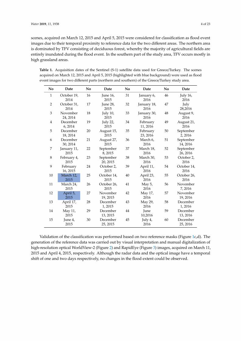
Water 2019, 11, 1938 4 of 23
scenes, acquired on March 12, 2015 and April 5, 2015 were considered for classification as flood event
images due to their temporal proximity to reference data for the two different areas. The northern area
is dominated by TFV consisting of deciduous forest, whereby the majority of agricultural fields are
entirely inundated during the flood event. In the southern part of the study area, TFV occurs mostly in
high grassland areas.
Table 1. Acquisition dates of the Sentinel (S-1) satellite data used for Greece/Turkey. The scenes
acquired on March 12, 2015 and April 5, 2015 (highlighted with blue background) were used as flood
event images for two different parts (northern and southern) of the Greece/Turkey study area.
No Date No Date No Date No Date
1 October 19,2014
16 June 16,2015
31 January 6,2016
46 July 16,2016
2 October 31,2014
17 June 28,2015
32 January 18,2016
47 July28,2016
3 November24, 2014
18 July 10,2015
33 January 30,2016
48 August 9,2016
4 December6, 2014
19 July 22,2015
34 February11, 2016
49 August 21,2016
5 December18, 2014
20 August 15,2015
35 February23, 2016
50 September2, 2016
6 December30, 2014
21 August 27,2015
36 March 6,2016
51 September14, 2016
7 January 11,2015
22 September8, 2015
37 March 18,2016
52 September26, 2016
8 February 4,2015
23 September20, 2015
38 March 30,2016
53 October 2,2016
9 February16, 2015
24 October 2,2015
39 April 11,2016
54 October 14,2016
10 March 12,2015
25 October 14,2015
40 April 23,2016
55 October 26,2016
11 March 24,2015
26 October 26,2015
41 May 5,2016
56 November7, 2016
12 April 5,2015
27 November19, 2015
42 May 17,2016
57 November19, 2016
13 April 17,2015
28 December1, 2015
43 May 29,2016
58 December1, 2016
14 May 11,2015
29 December13, 2015
44 June10,2016
59 December13, 2016
15 June 4,2015
30 December25, 2015
45 July 4,2016
60 December25, 2016
Validation of the classification was performed based on two reference masks (Figure 1c,d). The
generation of the reference data was carried out by visual interpretation and manual digitalization of
high-resolution optical WorldView-2 (Figure 2) and RapidEye (Figure 3) images, acquired on March 11,
2015 and April 4, 2015, respectively. Although the radar data and the optical image have a temporal
shift of one and two days respectively, no changes in the flood extent could be observed.

Water 2019, 11, 1938 5 of 23Water , x FOR PEER REVIEW 5 of
Figure 2. High-resolution false-color (NIR (near infrared), green, blue) WorldView2 image (March 11,
2015) (© European Space Imaging/DigitalGlobe) for northern Greece/Turkey containing temporary
flooded vegetation (TFV) ( ), temporary open water (TOW) (b), and dry land (DL) (c).
Figure 3. High-resolution false-color (NIR, green, blue) RapidEye image (April 04, 2015). (© Planet
Labs Inc.) for southern Greece/Turkey containing TOW ( ), DL (b) and TFV (c).
The second test case is the Dong Ting L ke, which is the second largest lake in China located in
the Hun n Province (Figure 4 ) It is flood-basin of the Yangt e River and thus varies seasonally in
size. During the annual floods, it c n expand to 91 km² three times its size compared to the dry
season. A flood event in summer 2017 (Figure 4b) w s chosen. For this study, dual-polarized S-1
scenes were used, which were cquired between October 201 nd February 2018 (T ble ). The scene
acquired on June is characterized by the l rgest flood extent In addition, the selection of the
analy ed flood image is c rried out due to the temporal proximity to the reference data. Comparable
to the study area in Greece/Turkey, the generation of the reference flood mask w s c rried out using
a high-resolution optical Sentinel- (S-2) image (Figure 5), which w s acquired on June 2 (Table
2). For the deriv tion of the reference m sk ll b nds with a resolution of 1 m and their combinations
of the S-2 scene were used The reference extent and the digitalized reference m sk is shown in Figure
4c. No changes in flood extent were observed between the analyzed flood image and the optic l scene.
Figure 2. High-resolution false-color (NIR (near infrared), green, blue) WorldView2 image (March 11,
2015) (© European Space Imaging/DigitalGlobe) for northern Greece/Turkey containing temporary
flooded vegetation (TFV) (a), temporary open water (TOW) (b), and dry land (DL) (c).
Water , x FOR PEER REVIEW 5 of
Figure 2. High-resolution false-color (NIR (near infrared), green, blue) WorldView2 image (March 11,
2015) (© European Space Imaging/DigitalGlobe) for northern Greece/Turkey containing temporary
flooded vegetation (TFV) ( ), temporary open water (TOW) (b), and dry land (DL) (c).
Figure 3. High-resolution false-color (NIR, green, blue) RapidEye image (April 04, 2015). (© Planet
Labs Inc.) for southern Greece/Turkey containing TOW ( ), DL (b) and TFV (c).
The second test case is the Dong Ting L ke, which is the second largest lake in China located in
the Hun n Province (Figure 4 ) It is flood-basin of the Yangt e River and thus varies seasonally in
size. During the annual floods, it c n expand to 91 km² three times its size compared to the dry
season. A flood event in summer 2017 (Figure 4b) w s chosen. For this study, dual-polarized S-1
scenes were used, which were cquired between October 201 nd February 2018 (T ble ). The scene
acquired on June is characterized by the l rgest flood extent In addition, the selection of the
analy ed flood image is c rried out due to the temporal proximity to the reference data. Comparable
to the study area in Greece/Turkey, the generation of the reference flood mask w s c rried out using
a high-resolution optical Sentinel- (S-2) image (Figure 5), which w s acquired on June 2 (Table
2). For the deriv tion of the reference m sk ll b nds with a resolution of 1 m and their combinations
of the S-2 scene were used The reference extent and the digitalized reference m sk is shown in Figure
4c. No changes in flood extent were observed between the analyzed flood image and the optic l scene.
Figure 3. High-resolution false-color (NIR, green, blue) RapidEye image (April 04, 2015). (© Planet
Labs Inc.) for southern Greece/Turkey containing TOW (a), DL (b), and TFV (c).
The second test case is the Dong Ting Lake, which is the second largest lake in China, located in
the Hunan Province (Figure 4a). It is a flood-basin of the Yangtze River and thus varies seasonally in
size. During the annual floods, it can expand to 2691 km2 three times its size compared to the dry
season. A flood event in summer 2017 (Figure 4b) was chosen. For this study, 38 dual-polarized S-1
scenes were used, which were acquired between October 2016 and February 2018 (Table 2). The scene
acquired on June 28, 2017 is characterized by the largest flood extent. In addition, the selection of the
analyzed flood image is carried out due to the temporal proximity to the reference data. Comparable
to the study area in Greece/Turkey, the generation of the reference flood mask was carried out using a
high-resolution optical Sentinel-2 (S-2) image (Figure 5), which was acquired on June 27, 2017 (Table 2).
For the derivation of the reference mask, all bands with a resolution of 10 m and their combinations of
the S-2 scene were used. The reference extent and the digitalized reference mask is shown in Figure 4c.
No changes in flood extent were observed between the analyzed flood image and the optical scene.
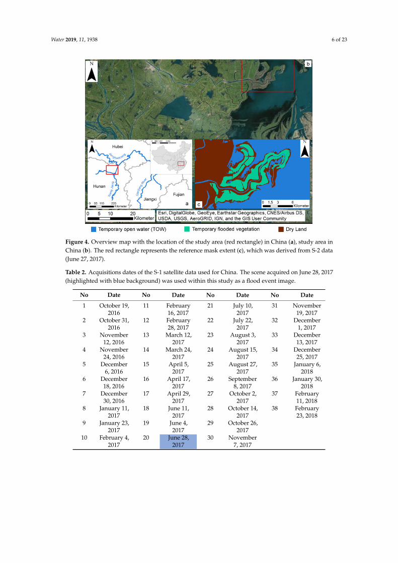
Water 2019, 11, 1938 6 of 23
Water , x FOR PEER REVIEW 6 of
Figure 4. Overview map with the location of the study area (red rectangle) in China ( ), study area in
China (b). The red rectangle represents the reference mask extent (c) which was derived from S-2
data (June 27, 2017).
Figure 5. High-resolution false-color (NIR, green, blue) Sentinel-2 image (June 27, 2017) for southern
Greece/Turkey containing DL (a), TFV (b) and TOW (c)
According to the ESA (European Space Agency) acquisition plan for S-1 constellation, dual-
polari ed images of the S-1A with an interv l of d ys were available for the study are s and the
analy ed acquisition period. These d ta sets are processed and provided by ESA as Ground Range
Detected High Resolution (GRDH) products. According to [ ] n autom ted preprocessing of the
time series d t for both reas and both polari tions VV and VH (vertic l/horizontal) w s c rried
out in sever l steps. The characteristics of all used S- data are listed in T ble
Figure 4. Overview map with the location of the study area (red rectangle) in China (a), study area in
China (b). The red rectangle represents the reference mask extent (c), which was derived from S-2 data
(June 27, 2017).
Table 2. Acquisitions dates of the S-1 satellite data used for China. The scene acquired on June 28, 2017
(highlighted with blue background) was used within this study as a flood event image.
No Date No Date No Date No Date
1 October 19,2016
11 February16, 2017
21 July 10,2017
31 November19, 2017
2 October 31,2016
12 February28, 2017
22 July 22,2017
32 December1, 2017
3 November12, 2016
13 March 12,2017
23 August 3,2017
33 December13, 2017
4 November24, 2016
14 March 24,2017
24 August 15,2017
34 December25, 2017
5 December6, 2016
15 April 5,2017
25 August 27,2017
35 January 6,2018
6 December18, 2016
16 April 17,2017
26 September8, 2017
36 January 30,2018
7 December30, 2016
17 April 29,2017
27 October 2,2017
37 February11, 2018
8 January 11,2017
18 June 11,2017
28 October 14,2017
38 February23, 2018
9 January 23,2017
19 June 4,2017
29 October 26,2017
10 February 4,2017
20 June 28,2017
30 November7, 2017

Water 2019, 11, 1938 7 of 23
Water , x FOR PEER REVIEW 6 of
Figure 4. Overview map with the location of the study area (red rectangle) in China ( ), study area in
China (b). The red rectangle represents the reference mask extent (c) which was derived from S-2
data (June 27, 2017).
Figure 5. High-resolution false-color (NIR, green, blue) Sentinel-2 image (June 27, 2017) for southern
Greece/Turkey containing DL (a), TFV (b) and TOW (c)
According to the ESA (European Space Agency) acquisition plan for S-1 constellation, dual-
polari ed images of the S-1A with an interv l of d ys were available for the study are s and the
analy ed acquisition period. These d ta sets are processed and provided by ESA as Ground Range
Detected High Resolution (GRDH) products. According to [ ] n autom ted preprocessing of the
time series d t for both reas and both polari tions VV and VH (vertic l/horizontal) w s c rried
out in sever l steps. The characteristics of all used S- data are listed in T ble
Figure 5. High-resolution false-color (NIR, green, blue) Sentinel-2 image (June 27, 2017) for southern
Greece/Turkey containing DL (a), TFV (b) and TOW (c).
According to the ESA (European Space Agency) acquisition plan for S-1 constellation,
dual-polarized images of the S-1A with an interval of 12 days were available for the study areas and
the analyzed acquisition period. These data sets are processed and provided by ESA as Ground Range
Detected High Resolution (GRDH) products. According to [8], an automated preprocessing of the time
series data for both areas and both polarizations VV and VH (vertical/horizontal) was carried out in
several steps. The characteristics of all used S-1 data are listed in Table 3.
Table 3. Characteristics of the S-1 data used.
Sensor Properties Values
Wavelength Mode Interferometric Wide Swath (IW)Polarization VV − VHFrequency C-band (GHz)Resolution 20 × 22 m (az. × gr. range)
Pixel spacing 10 × 10 m (az. × gr. range)Inc. angle 30.5◦–46.3◦
Orbit AscendingProduct-level Level-1 (Ground Range Detected High Resolution
(GRDH))
In addition to the satellite data, ancillary information was used to avoid misclassification of the
desired flood-related classes [8] in both study areas. Initially, permanent open water (POW) surfaces
were identified by the 30 m SRTM Water Body Data (SWBD) [53]. Besides POW, information regarding
urban areas and topography was integrated by using the Global Urban Footprint (GUF) and Height
Above Nearest Drainage (HAND) index. Urban areas, as well as TFV, are characterized by strong
double- and multiple-bounce backscattering effects. Therefore, the GUF [54] mask is used to identify
and exclude urban areas. In order to prevent misclassifications in elevated areas, the HAND index [55]
was used to identify and exclude areas with an elevation of greater than 20 m above the nearest water
network [56].

Water 2019, 11, 1938 8 of 23
2.2. Methodology
The foundation for the analysis of the impact of time series features on the flood extent derivation
is the SAR time series approach [8]. This method provides the opportunity to generate flood maps
including the classes TOW, TFV and Dry Land (DL) based on different time series features. The main
steps of the classification process for the generation of the flood maps are summarized below.
The S-1 time series data presented in Section 2.1 provide a foundation for the generation of
two independent multi-temporal layer stacks for each polarization and for each study area via an
image preprocessing step. In addition, three further multitemporal stacks are generated, including
the combinations of polarization (VV + VH, VV − VH, VV/VH). The ratio between VV and VH was
calculated by using linear units, whereby for the elimination of outliers (e.g., due to speckle) only the
values within the 5th and 95th percentiles were considered.
Based on findings about characteristics and patterns for TOW and TFV [8], the time series features
were determined using the z-transform of the backscatter values for each pixel over the time series
and for the available multi-temporal layer stack. The z-transform allows the normalization of the
backscatter values over the time series and ensures that the image elements of the analyzed flood scene
are comparable with each other when considering the individual seasonal fluctuation of vegetation.
The normalized time series features are termed as Z-Score. In relation to the polarizations, the time
series features are Z-Score VV, Z-Score VH, the combination of polarization, Z-Score VV + VH, Z-Score
VV − VH and the ratio Z-Score VV/VH, which represent the foundation for the derivation of TOW
and TFV [8]. Based on training data, two time series features with the highest contribution for the
derivation of the desired classes (TOW and TFV) were identified for each study area by using Random
Forest Algorithm. These features were used in the last step of the classification approach.
The classification of the flood-related classes was carried out based on pixels and objects. The
K-means clustering algorithm [57] was applied for the generation of clusters using SAR time series data
and the analyzed flood image. The resulting multitemporal and spatial cluster images were intersected
with each other to combine multi-temporal and spatial information. The time series features, which
are based on pixels, were merged with the segmented image by averaging the corresponding values
within each object.
The hierarchical thresholding approach is the last step in the classification process chain, which
allows a successive derivation of the desired classes based on the image elements (pixels or segments).
First of all, the permanent water surfaces are identified by the SWBD mask (see Section 2.1). On the
remaining image elements, the TOW, TFV and Dry Land (DL) are then derived consecutively using the
relevant time series features. The corresponding thresholds were determined automatically using the
decision tree classifier and the above-mentioned training data. For further details and an in-depth
explanation see [8]. The implementation of the entire approach was done in Python. The quantification
of the classification accuracy of TOW, TFV, and DL was carried out using overall accuracy (OA),
producer accuracy (PA), user accuracy (UA), and kappa index (K).
In order to investigate the impact of time series features for the derivation of TFV and to show
the potential of time series features for the transferability to different study areas and thus for the
operational use, a statistical comparison of the classification accuracies based on different study areas
and TFV types was performed. Thereby, a single time series feature was searched for, which allows the
extraction of different types of TFV with high accuracy for all study areas. Besides the study areas
described in Section 2.1, the study area in Namibia, which was analyzed in Tsyganskaya et al., [8], was
also used for the investigation.
In order to identify a single time series feature, which can then be used for all study areas, the
mean value and the coefficient of variation (CV) were determined based on user accuracy (UA) and
producer accuracy (PA) for each time series feature. The mean value represents the total accuracy
for the TFV classification of all study areas and for each time series feature. The higher the mean
value, the more relevant is the time series feature for all study areas. In addition, the CV was used
to quantify the variance of the data relative to the mean. The variance of the values is particularly
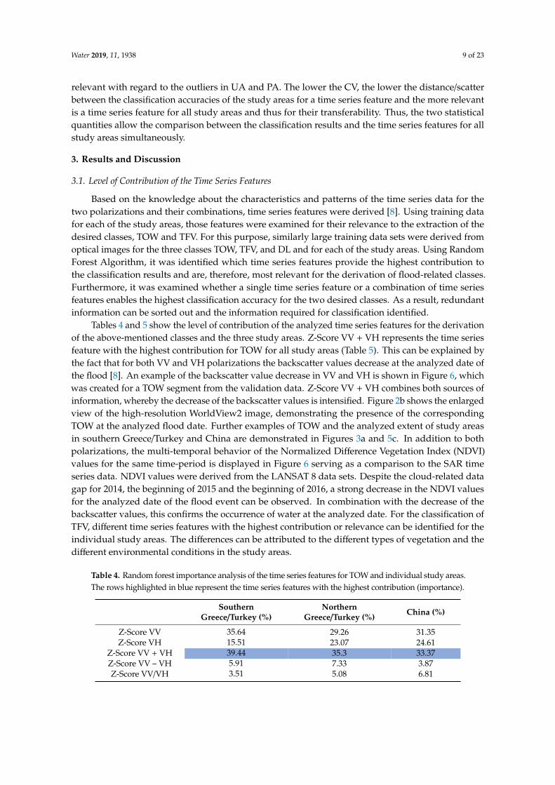
Water 2019, 11, 1938 9 of 23
relevant with regard to the outliers in UA and PA. The lower the CV, the lower the distance/scatter
between the classification accuracies of the study areas for a time series feature and the more relevant
is a time series feature for all study areas and thus for their transferability. Thus, the two statistical
quantities allow the comparison between the classification results and the time series features for all
study areas simultaneously.
3. Results and Discussion
3.1. Level of Contribution of the Time Series Features
Based on the knowledge about the characteristics and patterns of the time series data for the
two polarizations and their combinations, time series features were derived [8]. Using training data
for each of the study areas, those features were examined for their relevance to the extraction of the
desired classes, TOW and TFV. For this purpose, similarly large training data sets were derived from
optical images for the three classes TOW, TFV, and DL and for each of the study areas. Using Random
Forest Algorithm, it was identified which time series features provide the highest contribution to
the classification results and are, therefore, most relevant for the derivation of flood-related classes.
Furthermore, it was examined whether a single time series feature or a combination of time series
features enables the highest classification accuracy for the two desired classes. As a result, redundant
information can be sorted out and the information required for classification identified.
Tables 4 and 5 show the level of contribution of the analyzed time series features for the derivation
of the above-mentioned classes and the three study areas. Z-Score VV + VH represents the time series
feature with the highest contribution for TOW for all study areas (Table 5). This can be explained by
the fact that for both VV and VH polarizations the backscatter values decrease at the analyzed date of
the flood [8]. An example of the backscatter value decrease in VV and VH is shown in Figure 6, which
was created for a TOW segment from the validation data. Z-Score VV + VH combines both sources of
information, whereby the decrease of the backscatter values is intensified. Figure 2b shows the enlarged
view of the high-resolution WorldView2 image, demonstrating the presence of the corresponding
TOW at the analyzed flood date. Further examples of TOW and the analyzed extent of study areas
in southern Greece/Turkey and China are demonstrated in Figures 3a and 5c. In addition to both
polarizations, the multi-temporal behavior of the Normalized Difference Vegetation Index (NDVI)
values for the same time-period is displayed in Figure 6 serving as a comparison to the SAR time
series data. NDVI values were derived from the LANSAT 8 data sets. Despite the cloud-related data
gap for 2014, the beginning of 2015 and the beginning of 2016, a strong decrease in the NDVI values
for the analyzed date of the flood event can be observed. In combination with the decrease of the
backscatter values, this confirms the occurrence of water at the analyzed date. For the classification of
TFV, different time series features with the highest contribution or relevance can be identified for the
individual study areas. The differences can be attributed to the different types of vegetation and the
different environmental conditions in the study areas.
Table 4. Random forest importance analysis of the time series features for TOW and individual study areas.
The rows highlighted in blue represent the time series features with the highest contribution (importance).
SouthernGreece/Turkey (%)
NorthernGreece/Turkey (%)
China (%)
Z-Score VV 35.64 29.26 31.35Z-Score VH 15.51 23.07 24.61
Z-Score VV + VH 39.44 35.3 33.37Z-Score VV – VH 5.91 7.33 3.87Z-Score VV/VH 3.51 5.08 6.81

Water 2019, 11, 1938 10 of 23
Table 5. Random forest importance analysis of the time series features for TFV and individual study
areas. The rows highlighted in green represent the time series features with the highest contribution
(importance).
SouthernGreece/Turkey (%)
NorthernGreece/Turkey (%)
China (%)
Z-Score VV 32.61 28.39 33.21Z-Score VH 2.79 11.30 17.32
Z-Score VV + VH 18.66 21.53 33.84Z-Score VV – VH 41.57 16.37 8.56Z-Score VV/VH 4.38 22.41 7.10Water , x FOR PEER REVIEW 10 of
Figure 6. Multitemporal behavior of the backscatter intensity for TOW areas for VV (decibel (dB)),
VH (dB), VV/VH (linear scale), and Normalized Difference Vegetation Index (NDVI) values in
northern Greece/Turkey. The blue bars mark the analyzed d te at the flood event.
Table 4. Random forest importance analysis of the time series features for TOW and individual study
areas. The rows highlighted in blue represent the time series features with the highest contribution
(importance).
Southern
Greece/Turkey (%)
Northern
Greece/Turkey (%) China (%)
Z-Score VV
Z-Score VH
Z-Score VV + VH
Z-Score VV – VH
Z-Score VV/VH
Table 5. Random forest importance analysis of the time series features for TFV and individual study
areas. The rows highlighted in green represent the time series features with the highest contribution
(importance).
Southern
Greece/Turkey (%)
Northern
Greece/Turkey (%) China (%)
Z-Score VV
Z-Score VH
Z-Score VV + VH
Z-Score VV – VH
Z-Score VV/VH
The different behavior of both polarizations can be explained by the different sensitivity of VV and
VH to specific backsc ttering mechanisms, which caused an incre sed difference in the b ckscatter
v lues between the two polari tions t the analy ed date of the flood. In comp rison, the difference
Figure 6. Multitemporal behavior of the backscatter intensity for TOW areas for VV (decibel (dB)), VH
(dB), VV/VH (linear scale), and Normalized Difference Vegetation Index (NDVI) values in northern
Greece/Turkey. The blue bars mark the analyzed date at the flood event.
For the study area in southern Greece/Turkey, the Z-Score VV − VH is the most relevant time series
feature for the derivation of TFV (Table 5). This can be explained by the strong difference between the
polarizations VV and VH (Figure 7). Thereby, VV polarization shows a strong increase at the flood
date compared to the rest of the time series and VH polarization shows low or almost no increase at
the flood date.
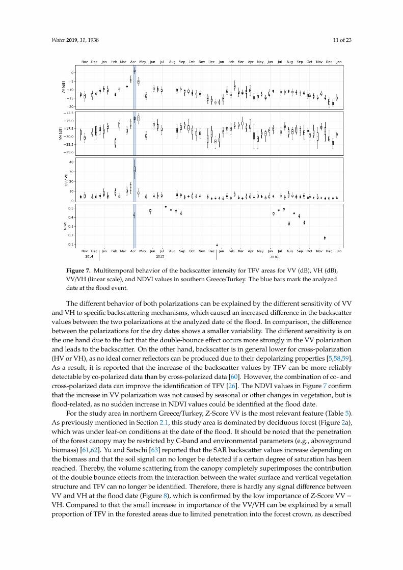
Water 2019, 11, 1938 11 of 23
Water , x FOR PEER REVIEW 11 of
between the polari tions for the dry d tes shows a smaller v riability. The different sensitivity is on
the one h nd due to the f ct th t the double-bounce effect occurs more strongly in the VV polarization
nd leads to the backscatter. On the other hand, backscatter is in general lower for cross-pol ri tion
(HV or VH), as no ide l corner reflectors c n be produced due to their depolarizing properties
[5 ]. As a result, it is reported th t the incre se of the b ckscatter v lues by TFV can be more
reliably detectable by co-polari ed d t than by cross-polari ed dat [ ] However, the combination
of co- and cross-polarized data can improve the identific tion of TFV [2 ]. The NDVI v lues in Figure
7 confirm that the incre se in VV pol ri tion w s not caused by seasonal or other ch nges in
veget tion, but is flood-related as no sudden incre se in NDVI values could be identified at the flood
date.
Figure 7. Multitemporal behavior of the backscatter intensity for TFV are s for VV (dB), VH (dB)
VV/VH (linear scale) and NDVI values in southern Greece/Turkey. The blue bars mark the analyzed
date at the flood event
For the study are in northern Greece/Turkey, Z-Score VV is the most relev nt fe ture (Table )
As previously mentioned in Section 2 this study are is domin ted by deciduous forest (Figure 2 )
which w s under le f-on conditions t the d te of the flood. It should be noted that the penetration
of the forest c nopy m y be restricted by C-b nd and environmental parameters (e.g., aboveground
biomass) [ ]. Yu and S tschi [ 3] reported th t the SAR b ckscatter v lues increase depending on
the biomass and that the soil signal can no longer be detected if a certain degree of s tur tion h s
been reached. Thereby, the volume scattering from the c nopy completely superimposes the
contribution of the double bounce effects from the interaction between the w ter surface and vertical
veget tion structure and TFV c n no longer be identified Therefore there is h rdly any signal
difference between VV and VH t the flood d te (Figure ) which is confirmed by the low importance
of Z-Score VV − VH Compared to that the small incre se in importance of the VV/VH can be
expl ined by a small proportion of TFV in the forested are s due to limited penetration into the forest
crown, as described above. In the c se of northern Greece/Turkey the importance incre ses, bec use
the outliers were eliminated by using the Z-Score VV/VH feature. For southern Greece/Turkey on the
contr ry, using the Z-Score VV/VH the outlier reduction caused also an elimination of extreme values
Figure 7. Multitemporal behavior of the backscatter intensity for TFV areas for VV (dB), VH (dB),
VV/VH (linear scale), and NDVI values in southern Greece/Turkey. The blue bars mark the analyzed
date at the flood event.
The different behavior of both polarizations can be explained by the different sensitivity of VV
and VH to specific backscattering mechanisms, which caused an increased difference in the backscatter
values between the two polarizations at the analyzed date of the flood. In comparison, the difference
between the polarizations for the dry dates shows a smaller variability. The different sensitivity is on
the one hand due to the fact that the double-bounce effect occurs more strongly in the VV polarization
and leads to the backscatter. On the other hand, backscatter is in general lower for cross-polarization
(HV or VH), as no ideal corner reflectors can be produced due to their depolarizing properties [5,58,59].
As a result, it is reported that the increase of the backscatter values by TFV can be more reliably
detectable by co-polarized data than by cross-polarized data [60]. However, the combination of co- and
cross-polarized data can improve the identification of TFV [26]. The NDVI values in Figure 7 confirm
that the increase in VV polarization was not caused by seasonal or other changes in vegetation, but is
flood-related, as no sudden increase in NDVI values could be identified at the flood date.
For the study area in northern Greece/Turkey, Z-Score VV is the most relevant feature (Table 5).
As previously mentioned in Section 2.1, this study area is dominated by deciduous forest (Figure 2a),
which was under leaf-on conditions at the date of the flood. It should be noted that the penetration
of the forest canopy may be restricted by C-band and environmental parameters (e.g., aboveground
biomass) [61,62]. Yu and Satschi [63] reported that the SAR backscatter values increase depending on
the biomass and that the soil signal can no longer be detected if a certain degree of saturation has been
reached. Thereby, the volume scattering from the canopy completely superimposes the contribution
of the double bounce effects from the interaction between the water surface and vertical vegetation
structure and TFV can no longer be identified. Therefore, there is hardly any signal difference between
VV and VH at the flood date (Figure 8), which is confirmed by the low importance of Z-Score VV −
VH. Compared to that the small increase in importance of the VV/VH can be explained by a small
proportion of TFV in the forested areas due to limited penetration into the forest crown, as described

Water 2019, 11, 1938 12 of 23
above. In the case of northern Greece/Turkey the importance increases, because the outliers were
eliminated by using the Z-Score VV/VH feature. For southern Greece/Turkey on the contrary, using the
Z-Score VV/VH the outlier reduction caused also an elimination of extreme values caused by TFV. This
led to a drop of the importance in VV/VH in comparison to the Z-Score VV − VH. Regarding the most
relevant time series feature Z-Score VV for the northern Greece/Turkey study area, it is assumed that
the backscatter in VV polarization is dominated by the contribution of the forest canopy and moreover
the volume scattering represents the main scattering mechanism. Due to the sensitivity of the VV
polarization for the double bounce effect, however, a slight increase in the backscattering values at the
flood date was detected, which can indicate TFV (Figure 8). The NDVI values were derived from the
LANDSAT 8 data and show that the slight increase of the backscatter values in both polarizations at
the date of flood can be attributed to the flood event and not to any change in vegetation.
Water , x FOR PEER REVIEW 12 of
c used by TFV This led to drop of the import nce in VV/VH in comparison to the Z-Score VV −VH. Regarding the most relev nt time series feature Z-Score VV for the northern Greece/Turkey
study rea, it is ssumed that the b ckscatter in VV polari tion is dominated by the contribution of
the forest canopy and moreover the volume scattering represents the main scattering mechanism.
Due to the sensitivity of the VV polari tion for the double bounce effect, however, a slight increase
in the b ckscattering v lues at the flood date was detected, which can indicate TFV (Figure 8). The
NDVI v lues were derived from the LANDSAT data and show th t the slight incre se of the
b cksc tter v lues in both polari tions at the date of flood c n be attributed to the flood event and
not to any change in vegetation.
Figure 8. Multitemporal behavior of the backscatter intensity for TFV are s for VV (dB), VH (dB)
VV/VH (linear scale) and NDVI values in northern Greece/Turkey. The blue bars mark the analyzed
date at the flood event
For the study re in Chin Z-Score VV VH represents the most relev nt time series fe ture
for the deriv tion of the TFV (Table ). The time series feature indic tes that in both pol ri tions an
incre se of the b cksc tter v lues h s occurred t the n ly ed d te of the flood This c n be
confirmed in Figure 9. Both polari tions incre se at the analy ed flood date, whereas the stronger
incre se c n be observed in VV polari tion. The sum of the two polarizations intensifies the increase
of the b ckscatter v lues t the same d te. Although only a few cloud-free optical Sentinel- images
are available that cover the study rea in China for the analyzed time period it can be observed th t
there is no increase in the NDVI v lues at the an lyzed flood date (Figure 9) This leads to the
deduction that the incre se in SAR time series d t is not rel ted to phenological changes Figure 5b
shows a high-resolution Sentinel-2 image demonstrating the presence of the corresponding TFV area
at the an ly ed flood d te.
Since the TFV type is high grassland and reed (Figure 5b) [ ], which is simil r to the structure
of some crops (rice, whe t) it is assumed that the veget tion can be penetrated by the C-b nd d ta
[10,65]. Therefore, it is expected th t the incre se in b cksc tter v lues will occur at the time of the
flood in the VV polarization due to their sensitivity to the double impact effect. However, the increase
in VH polarization cannot be confirmed by the depolarizing property mentioned above. Instead, the
Figure 8. Multitemporal behavior of the backscatter intensity for TFV areas for VV (dB), VH (dB),
VV/VH (linear scale), and NDVI values in northern Greece/Turkey. The blue bars mark the analyzed
date at the flood event.
For the study area in China, Z-Score VV + VH represents the most relevant time series feature
for the derivation of the TFV (Table 5). The time series feature indicates that in both polarizations an
increase of the backscatter values has occurred at the analyzed date of the flood. This can be confirmed
in Figure 9. Both polarizations increase at the analyzed flood date, whereas the stronger increase
can be observed in VV polarization. The sum of the two polarizations intensifies the increase of the
backscatter values at the same date. Although only a few cloud-free optical Sentinel-2 images are
available that cover the study area in China for the analyzed time period, it can be observed that there
is no increase in the NDVI values at the analyzed flood date (Figure 9). This leads to the deduction
that the increase in SAR time series data is not related to phenological changes. Figure 5b shows a
high-resolution Sentinel-2 image demonstrating the presence of the corresponding TFV area at the
analyzed flood date.

Water 2019, 11, 1938 13 of 23
Water , x FOR PEER REVIEW 13 of
latter incre se is result of the combination of environmental par meters. The contribution of the soil
under the vegetation plays a decisive role in this process. Due to of possible unevenness of the soil
(microtopography) and the low w ter level, it is possible th t a p rt of the soil surface beneath the
vegetation w s only p rtially flooded. In the flood-free are s underneath the vegetation, the soil
moisture may have increased at the date of the flood compared to non-flooded conditions.
Simultaneously, w ter could h ve accumul ted in the sinks, which could also le d to standing water
beneath vegetation in the s me region. Due to different sensitivities of VV and VH to the respective
conditions, the latter c n dominate the respective polari tion The analyses from the literature
confirm th t an incre se in soil moisture in both VV nd VH c uses n increase in the backscatter
values and c n be detected by the sensor depending on the biomass amount [ ] The TFV, which
is represented by the double-bounce effect, c n only be detected by VV polarization as the
depolarizing property of VH polarization does not allow sensitivity to double-bounce [ ]. The
mixture of these two cases by micro topographic l differences explains the incre se not only of
b cksc tter v lues for VV but lso for VH and, thus the relev nce of Z-Score VV + VH for the
derivation of TFV in the study are of China
Figure 9. Multitemporal behavior of the backscatter intensity for TFV are s for VV (dB), VH (dB)
VV/VH (linear scale) and NDVI values in China. The blue bars mark the analyzed date at the flood
event.
A comparison of the relev nt time series features with the results of the study of Tsygansk y
et al., [8] shows that for the class TOW, Z-Score VV + VH is also one of the time series features with
the highest contribution. For TFV, the most relev nt time series characteristic (Z-Score VV − VH) is
confirmed only for the study rea in the southern area of interest of Greece/Turkey In the other two
example are s, the algorithm determined different relev nt time series features due to different
environmental conditions (e.g., vegetation type topography soil moisture) and their interaction
Based on a previous analysis in Tsyganskaya et al., [ ], the time series feature with the highest
contribution can achieve a higher classification accuracy compared to the combination of all time
series features Therefore, a single time series feature with the highest contribution was used for the
classific tion for deriving the desired classes. This identific tion step is performed automatic lly by
Figure 9. Multitemporal behavior of the backscatter intensity for TFV areas for VV (dB), VH (dB),
VV/VH (linear scale), and NDVI values in China. The blue bars mark the analyzed date at the
flood event.
Since the TFV type is high grassland and reed (Figure 5b) [64], which is similar to the structure of
some crops (rice, wheat), it is assumed that the vegetation can be penetrated by the C-band data [10,65].
Therefore, it is expected that the increase in backscatter values will occur at the time of the flood
in the VV polarization due to their sensitivity to the double impact effect. However, the increase
in VH polarization cannot be confirmed by the depolarizing property mentioned above. Instead,
the latter increase is a result of the combination of environmental parameters. The contribution of
the soil under the vegetation plays a decisive role in this process. Due to of possible unevenness
of the soil (microtopography) and the low water level, it is possible that a part of the soil surface
beneath the vegetation was only partially flooded. In the flood-free areas underneath the vegetation,
the soil moisture may have increased at the date of the flood compared to non-flooded conditions.
Simultaneously, water could have accumulated in the sinks, which could also lead to standing water
beneath vegetation in the same region. Due to different sensitivities of VV and VH to the respective
conditions, the latter can dominate the respective polarization. The analyses from the literature confirm
that an increase in soil moisture in both VV and VH causes an increase in the backscatter values and
can be detected by the sensor depending on the biomass amount [66,67]. The TFV, which is represented
by the double-bounce effect, can only be detected by VV polarization, as the depolarizing property of
VH polarization does not allow sensitivity to double-bounce [68]. The mixture of these two cases by
micro topographical differences explains the increase not only of backscatter values for VV, but also for
VH and, thus, the relevance of Z-Score VV + VH for the derivation of TFV in the study area of China.
A comparison of the relevant time series features with the results of the study of Tsyganskaya
et al., [8] shows that for the class TOW, Z-Score VV + VH is also one of the time series features with
the highest contribution. For TFV, the most relevant time series characteristic (Z-Score VV − VH)
is confirmed only for the study area in the southern area of interest of Greece/Turkey. In the other

Water 2019, 11, 1938 14 of 23
two example areas, the algorithm determined different relevant time series features due to different
environmental conditions (e.g., vegetation type, topography, soil moisture) and their interaction.
Based on a previous analysis in Tsyganskaya et al., [8], the time series feature with the highest
contribution can achieve a higher classification accuracy compared to the combination of all time
series features. Therefore, a single time series feature with the highest contribution was used for the
classification for deriving the desired classes. This identification step is performed automatically by
the algorithm using training data. Moreover, these examples show that the use of both polarizations is
relevant for the derivation of flooded areas.
3.2. Classification Results
The classification of the study area in southern Greece/Turkey was carried out based on the S-1
time series stack (October 19, 2014–December 25, 2016) containing the flood image (April 4, 2015). This
classification was validated using the S-2-based reference mask (April 5, 2015). Figure 10a shows the
pixel-based classification result of the time series approach, which comprises the classes POW, TOW,
TFV, and DL, while Figure 10b shows the object-based classification result. For visual comparison, the
validation mask is shown in Figure 1d. It is noticeable that the areas of the classes TOW, TFV, and
DL contain more small structures of the other classes in the pixel-based classification compared to
the object-based classification. The usage of objects reduces this noise; however, it also can lead to
the loss of details and thus information. In general, the use of pixel- or object-based classification
depends strongly on the kind of the landscape under investigation. In the case of flooding in vegetated
areas, a single, isolated pixel could contain water ponds and so differ from its neighboring pixels. Due
to limited visibility in optical data, these areas could not be identified during the generation of the
validation mask.
Water , x FOR PEER REVIEW 14 of
the algorithm using training data. Moreover, these examples show that the use of both polarizations
is relev nt for the derivation of flooded areas.
Classification Results
The classification of the study area in southern Greece/Turkey was c rried out based on the S-1
time series stack (October 4–December 2 ) containing the flood image (April )
This classification was validated using the S-2-b sed reference m sk (April ). Figure shows
the pixel-based classification result of the time series approach, which comprises the classes POW,
TOW, TFV, and DL, while Figure b shows the object-b sed classific tion result For visual
comparison the valid tion mask is shown in Figure 1d It is noticeable th t the are s of the classes
TOW, TFV, and DL contain more small structures of the other classes in the pixel-based classification
compared to the object-based classific tion. The usage of objects reduces this noise; however it lso
can lead to the loss of details and thus information In gener l the use of pixel- or object-b sed
classific tion depends strongly on the kind of the landscape under investigation. In the c se of
flooding in veget ted reas, single, isol ted pixel could cont in water ponds and so differ from its
neighboring pixels Due to limited visibility in optic l data these areas could not be identified during
the gener tion of the v lid tion m sk
Figure 10. Pixel-based classification result ( ), object-based classification result (b) for the study area
in southern Greece/Turkey.
For the study are in northern Greece/Turkey the cl ssific tion is b sed on the S- time series
stack (October 19 December 25 6), with the flood im ge being cquired on March
Validation of this classific tion w s performed using the S-2-b sed reference m sk (March 2015).
Figure shows the pixel-based classification result for the study are of northern Greece/Turkey
which comprises the classes POW TOW, TFV, and DL, while Figure 11b shows the object-based
classific tion result. Compared to the v lidation m sk (Figure 1c), both pixel- and object-based
classific tion show only low representativity of the class TFV. This c n be explained by the low
penetration of the vegetation (deciduous forest (Figure 2 )) by the C-band d ta which is reduced in
this case [8]. In addition, occasional TFV areas in the classification can be identified in DL of the
validation mask, especially in the pixel-based classification. These could be small are s of water
(ponds or temporary water accumulations). In combin tion with vertical structures of the agricultural
are s or grassland, the double bounce effect c n lso be produced resulting in an incre se in the
b cksc tter v lues t the d te of the flood. These are s were lso classified s TFV, though they could
not, however, be identified during the generation of the v lid tion m sk due to limited visibility in
optic l data.
The classification for the study are in China w s performed using the S-1 time series st ck
(October February 23 ). The nalyzed date of the flood is June 28 . The v lidation
for this cl ssification was performed using the S-2-b sed reference mask (June 17). Figures 1
b show the pixel- and object-based classific tion results with POW TOW, TFV nd DL classes The
validation mask used is shown in Figure 4c.
The comparison between the classific tion results and the valid tion m sk reveals the
occurrence of TOW in DL. DL also occurs between the permanent w ter surfaces and the TO are s.
On the one h nd, the confusion between these two classes can rise due to small areas of water
occurring in the agricultural are s On the other h nd, the dur tion of a flood event c n le d to an
accumul tion of S- im ges, cont ining the inund tion and a decre se of images without flooding.
Figure 10. Pixel-based classification result (a), object-based classification result (b) for the study area in
southern Greece/Turkey.
For the study area in northern Greece/Turkey, the classification is based on the S-1 time series
stack (October 19, 2014–December 25, 2016), with the flood image being acquired on March 12, 2015.
Validation of this classification was performed using the S-2-based reference mask (March 15, 2015).
Figure 11a shows the pixel-based classification result for the study area of northern Greece/Turkey,
which comprises the classes POW, TOW, TFV, and DL, while Figure 11b shows the object-based
classification result. Compared to the validation mask (Figure 1c), both pixel- and object-based
classification show only a low representativity of the class TFV. This can be explained by the low
penetration of the vegetation (deciduous forest (Figure 2a)) by the C-band data, which is reduced
in this case [8]. In addition, occasional TFV areas in the classification can be identified in DL of the
validation mask, especially in the pixel-based classification. These could be small areas of water (ponds
or temporary water accumulations). In combination with vertical structures of the agricultural areas or
grassland, the double bounce effect can also be produced resulting in an increase in the backscatter
values at the date of the flood. These areas were also classified as TFV, though they could not, however,
be identified during the generation of the validation mask due to limited visibility in optical data.

Water 2019, 11, 1938 15 of 23
Water , x FOR PEER REVIEW 15 of
This can cause a higher fluctuation r nge and a lower mean value when gener ting the time series
features, which in p rticular c n lead to confusion with DL, s the are s between permanent water
and TOW demonstrate. The combination of these two conditions makes the above-mentioned
confusions between the cl sses possible Therefore the use of time series with t least one vegetation
cycle is recommended, as the st tistic l r nge of the b ckscatter v lues of the vegetation stages is
detected and thus sufficiently represented [ ]
Figure 11. Pixel-based classification result ( ) and object-based classification result (b) for the study
area in northern Greece/Turkey.
Figure 12. Pixel-based classification result ( ), object-based classification result (b) and validation
mask (c) for the study area in China.
The accur cy values for the pixel-based and object-based classific tions for the respective study
are s are shown in Table The OA for all study are s ranges between 8 % and 87%. In comparison,
in [8] the authors achieved similar or even slightly lower OA for the pixel-based (75%) and object-
based (82%) classific tion The accur cy assessment for the study are in northern Greece/Turkey
shows high values for the TOW class but strong misclassific tions for TFV (PA: 28% for pixel-based
and 6% for object-based) nd DL (UA: % for pixel-based and % for object-based). This indicates
signific nt confusion between these two classes and c n be explained by different environmental
conditions (see Section ) The accur cy values show no significant difference between pixel-b sed
and object-based classific tion, except for the PA values of TFV. When applying object-based
classific tion it should be noted that the sm ll-scale flood are s could be generalized by merging the
Figure 11. Pixel-based classification result (a) and object-based classification result (b) for the study
area in northern Greece/Turkey.
The classification for the study area in China was performed using the S-1 time series stack
(October 19, 2016–February 23, 2018). The analyzed date of the flood is June 28, 2017. The validation
for this classification was performed using the S-2-based reference mask (June 27, 2017). Figure 12a,
b show the pixel- and object-based classification results with POW, TOW, TFV, and DL classes. The
validation mask used is shown in Figure 4c.
Water , x FOR PEER REVIEW 15 of
This can cause a higher fluctuation r nge and a lower mean value when gener ting the time series
features, which in p rticular c n lead to confusion with DL, s the are s between permanent water
and TOW demonstrate. The combination of these two conditions makes the above-mentioned
confusions between the cl sses possible Therefore the use of time series with t least one vegetation
cycle is recommended, as the st tistic l r nge of the b ckscatter v lues of the vegetation stages is
detected and thus sufficiently represented [ ]
Figure 11. Pixel-based classification result ( ) and object-based classification result (b) for the study
area in northern Greece/Turkey.
Figure 12. Pixel-based classification result ( ), object-based classification result (b) and validation
mask (c) for the study area in China.
The accur cy values for the pixel-based and object-based classific tions for the respective study
are s are shown in Table The OA for all study are s ranges between 8 % and 87%. In comparison,
in [8] the authors achieved similar or even slightly lower OA for the pixel-based (75%) and object-
based (82%) classific tion The accur cy assessment for the study are in northern Greece/Turkey
shows high values for the TOW class but strong misclassific tions for TFV (PA: 28% for pixel-based
and 6% for object-based) nd DL (UA: % for pixel-based and % for object-based). This indicates
signific nt confusion between these two classes and c n be explained by different environmental
conditions (see Section ) The accur cy values show no significant difference between pixel-b sed
and object-based classific tion, except for the PA values of TFV. When applying object-based
classific tion it should be noted that the sm ll-scale flood are s could be generalized by merging the
Figure 12. Pixel-based classification result (a), object-based classification result (b) and validation mask
(c) for the study area in China.
The comparison between the classification results and the validation mask reveals the occurrence
of TOW in DL. DL also occurs between the permanent water surfaces and the TOW areas. On the one
hand, the confusion between these two classes can arise due to small areas of water occurring in the
agricultural areas. On the other hand, the duration of a flood event can lead to an accumulation of
S-1 images, containing the inundation and a decrease of images without flooding. This can cause a
higher fluctuation range and a lower mean value when generating the time series features, which in
particular can lead to confusion with DL, as the areas between permanent water and TOW demonstrate.
The combination of these two conditions makes the above-mentioned confusions between the classes
possible. Therefore, the use of a time series with at least one vegetation cycle is recommended, as

Water 2019, 11, 1938 16 of 23
the statistical range of the backscatter values of the vegetation stages is detected and thus sufficiently
represented [8].
The accuracy values for the pixel-based and object-based classifications for the respective study
areas are shown in Table 6. The OA for all study areas ranges between 80% and 87%. In comparison,
in [8] the authors achieved a similar or even slightly lower OA for the pixel-based (75%) and object-based
(82%) classification. The accuracy assessment for the study area in northern Greece/Turkey shows high
values for the TOW class but strong misclassifications for TFV (PA: 28% for pixel-based and 6% for
object-based) and DL (UA: 57% for pixel-based and 53% for object-based). This indicates a significant
confusion between these two classes and can be explained by different environmental conditions (see
Section 3.1). The accuracy values show no significant difference between pixel-based and object-based
classification, except for the PA values of TFV. When applying object-based classification, it should be
noted that the small-scale flood areas could be generalized by merging the pixels to objects. However,
object-based classification can help to exclude pixels which can be confused with a flood-related
increase in values due to dominant environmental conditions, such as soil moisture, topography, or
surface roughness, which can cause a small-scale increase or decrease in the backscatter. In addition,
objects are less susceptible to speckle noise than pixels [29].
Table 6. Accuracy assessment for the pixel- and object-based classification for the individual study
areas. Overall accuracy (OA) in %, Producer accuracy (PA) in %, User accuracy (UA) in %, and Kappa
index (K).
Southern Greece/Turkey(%)
Northern Greece/Turkey(%)
China (%)
Pixel-based Object-based Pixel-based Object-based Pixel-based Object-based
DL—UA 76.64 77.62 56.65 53.25 85.26 87.66TOW—UA 86.53 86.87 97.58 98.23 79.73 85.65TFV—UA 90.37 92.17 76.83 73.86 78.28 83.01DL—PA 77.86 79.61 91.67 96.60 69.89 78.95TOW—PA 85.94 86.38 91.02 91.67 90.47 91.14TFV—PA 89.52 90.09 28.18 6.32 90.09 91.23
OA 84.26 85.17 81.47 79.59 81.37 85.84Kappa 0.76 0.78 0.66 0.63 0.71 0.78
3.3. Time Series Features—Transferability Analysis
For the transferability analysis of the classification approach, several pixel-based and object-based
classification runs were carried out for each study area and its subareas using the individual time
series features. For each run, the most relevant time series feature (Z-Score VV + VH) was used for
the derivation of TOW (Section 3.1). Simultaneously, each time series feature was used in each study
area to derive the TFV, so that 20 pixel-based and 20 object-based classification products could be
generated. For each result, an accuracy assessment was performed. Since the analysis of the different
time series features refers to the TFV, the PA and UA of TFV were selected as indicators to represent
the classification accuracy of the TFV. The accuracy values PA and UA for the individual study areas
and the five analyzed time series features for pixel-based classification are shown in Table 7 and for
object-based classification in Table 8. The relevant time series features that were identified by the
Random Forest Algorithm (Section 3.1) are highlighted in dark green for the respective study areas
for the PA and UA values. These tables show that different time series features are relevant for the
individual study areas. The low PA values seen for northern Greece in both tables can be explained by
the specific TFV type that dominates this study area, namely flooded forest areas. In this case, the
penetration of the forest crown is limited by C-band data, whereby the water under the vegetation can
only be partially detected.
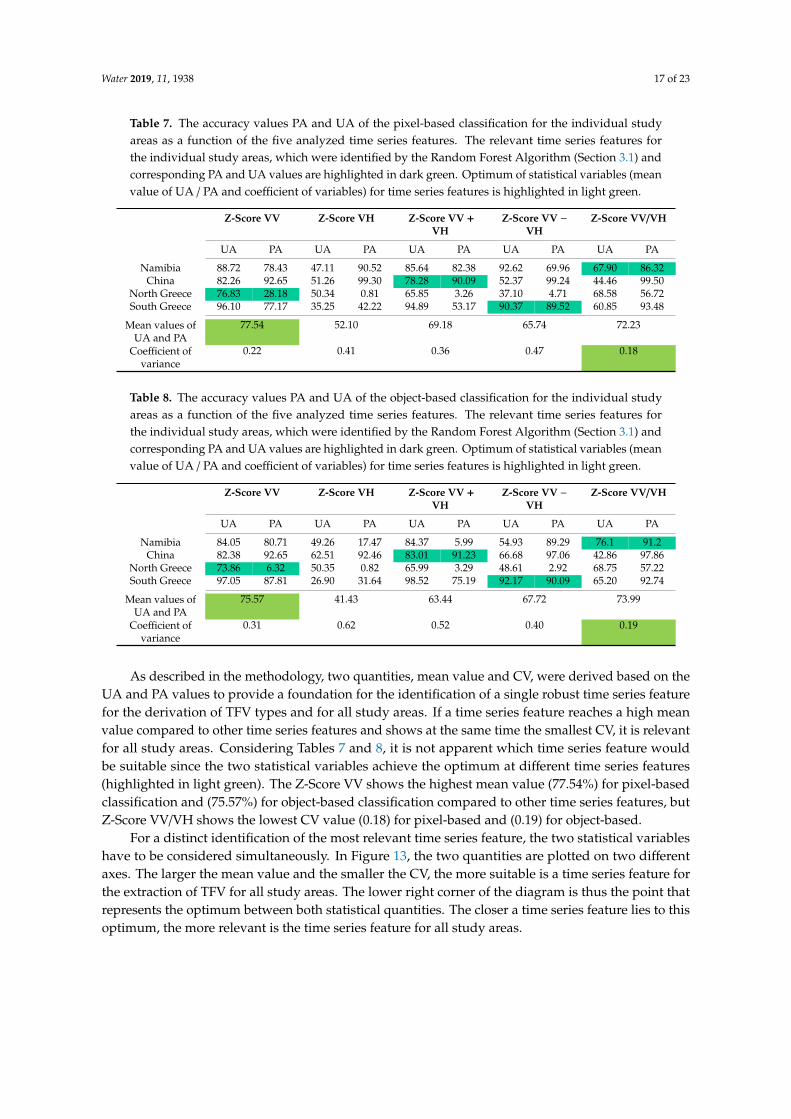
Water 2019, 11, 1938 17 of 23
Table 7. The accuracy values PA and UA of the pixel-based classification for the individual study
areas as a function of the five analyzed time series features. The relevant time series features for
the individual study areas, which were identified by the Random Forest Algorithm (Section 3.1) and
corresponding PA and UA values are highlighted in dark green. Optimum of statistical variables (mean
value of UA / PA and coefficient of variables) for time series features is highlighted in light green.
Z-Score VV Z-Score VH Z-Score VV +VH
Z-Score VV −VH
Z-Score VV/VH
UA PA UA PA UA PA UA PA UA PA
Namibia 88.72 78.43 47.11 90.52 85.64 82.38 92.62 69.96 67.90 86.32China 82.26 92.65 51.26 99.30 78.28 90.09 52.37 99.24 44.46 99.50
North Greece 76.83 28.18 50.34 0.81 65.85 3.26 37.10 4.71 68.58 56.72South Greece 96.10 77.17 35.25 42.22 94.89 53.17 90.37 89.52 60.85 93.48
Mean values ofUA and PA
77.54 52.10 69.18 65.74 72.23
Coefficient ofvariance
0.22 0.41 0.36 0.47 0.18
Table 8. The accuracy values PA and UA of the object-based classification for the individual study
areas as a function of the five analyzed time series features. The relevant time series features for
the individual study areas, which were identified by the Random Forest Algorithm (Section 3.1) and
corresponding PA and UA values are highlighted in dark green. Optimum of statistical variables (mean
value of UA / PA and coefficient of variables) for time series features is highlighted in light green.
Z-Score VV Z-Score VH Z-Score VV +VH
Z-Score VV −VH
Z-Score VV/VH
UA PA UA PA UA PA UA PA UA PA
Namibia 84.05 80.71 49.26 17.47 84.37 5.99 54.93 89.29 76.1 91.2China 82.38 92.65 62.51 92.46 83.01 91.23 66.68 97.06 42.86 97.86
North Greece 73.86 6.32 50.35 0.82 65.99 3.29 48.61 2.92 68.75 57.22South Greece 97.05 87.81 26.90 31.64 98.52 75.19 92.17 90.09 65.20 92.74
Mean values ofUA and PA
75.57 41.43 63.44 67.72 73.99
Coefficient ofvariance
0.31 0.62 0.52 0.40 0.19
As described in the methodology, two quantities, mean value and CV, were derived based on the
UA and PA values to provide a foundation for the identification of a single robust time series feature
for the derivation of TFV types and for all study areas. If a time series feature reaches a high mean
value compared to other time series features and shows at the same time the smallest CV, it is relevant
for all study areas. Considering Tables 7 and 8, it is not apparent which time series feature would
be suitable since the two statistical variables achieve the optimum at different time series features
(highlighted in light green). The Z-Score VV shows the highest mean value (77.54%) for pixel-based
classification and (75.57%) for object-based classification compared to other time series features, but
Z-Score VV/VH shows the lowest CV value (0.18) for pixel-based and (0.19) for object-based.
For a distinct identification of the most relevant time series feature, the two statistical variables
have to be considered simultaneously. In Figure 13, the two quantities are plotted on two different
axes. The larger the mean value and the smaller the CV, the more suitable is a time series feature for
the extraction of TFV for all study areas. The lower right corner of the diagram is thus the point that
represents the optimum between both statistical quantities. The closer a time series feature lies to this
optimum, the more relevant is the time series feature for all study areas.
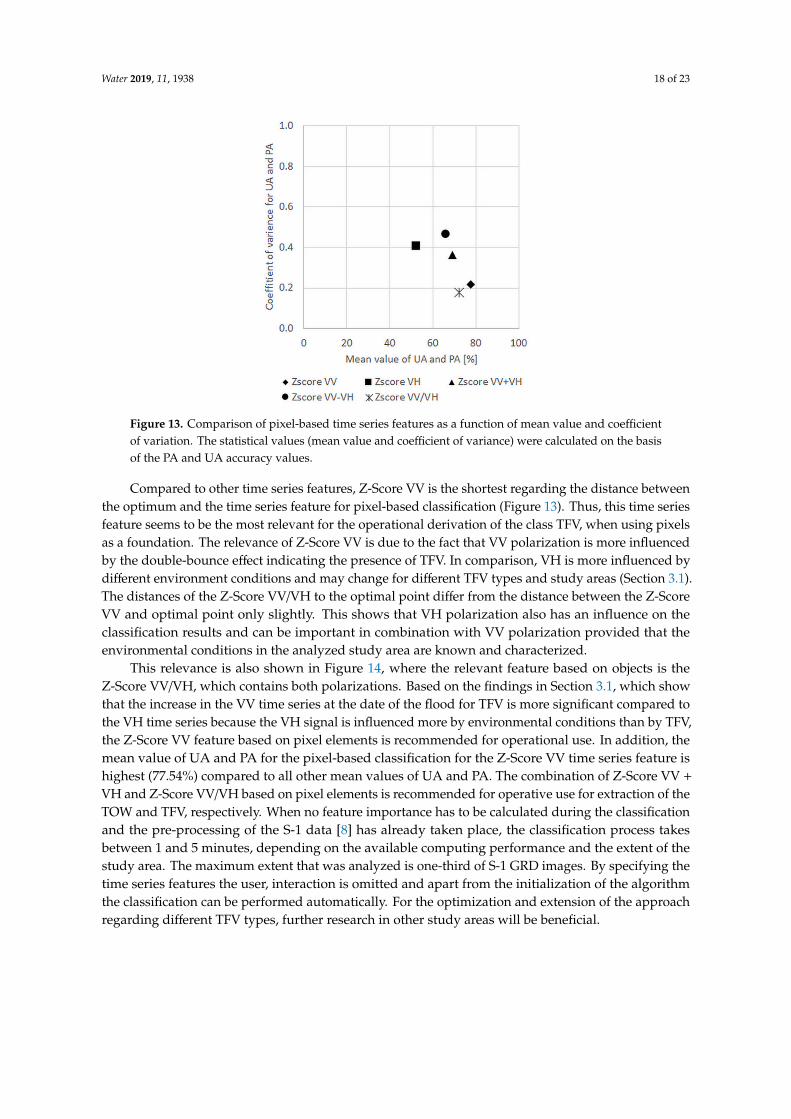
Water 2019, 11, 1938 18 of 23Water , x FOR PEER REVIEW 18 of
Figure 13. Comparison of pixel-based time series features as a function of mean value and
coefficient of variation. The statistical values (mean value and coefficient of variance) were
calculated on the basis of the PA and UA accuracy values.
Compared to other time series features Z-Score VV is the shortest regarding the distance
between the optimum and the time series feature for pixel-b sed classific tion (Figure 13). Thus,
this time series feature seems to be the most relev nt for the oper tion l deriv tion of the cl ss
TFV, when using pixels as found tion. The relevance of Z-Score VV is due to the f ct th t VV
polari tion is more influenced by the double-bounce effect indic ting the presence of TFV. In
comparison, VH is more influenced by different environment conditions and may change for
different TFV types and study are s (Section 3.1). The distances of the Z-Score VV/VH to the
optim l point differ from the distance between the Z-Score VV and optim l point only slightly
This shows that VH pol ri tion lso h s an influence on the classification results and can be
important in combination with VV pol riz tion provided that the environmental conditions in
the analy ed study are are known and characterized
This relevance is also shown in Figure 1 where the relevant fe ture based on objects is the
Z-Score VV/VH, which contains both polari tions. Based on the findings in Section which
show th t the incre se in the VV time series t the d te of the flood for TFV is more significant
compared to the VH time series because the VH signal is influenced more by environmental
conditions th n by TFV the Z-Score VV fe ture based on pixel elements is recommended for
operation l use. In addition, the mean value of UA and PA for the pixel-b sed classific tion for
the Z-Score VV time series feature is highest (77.54%) compared to all other mean values of UA
and PA. The combination of Z-Score VV VH and Z-Score VV/VH b sed on pixel elements is
recommended for operative use for extraction of the TOW and TFV, respectively. When no
fe ture import nce h s to be c lcul ted during the classific tion and the pre-processing of the S-
1 d ta [ ] h s already taken place, the classific tion process takes between and minutes,
depending on the available computing perform nce and the extent of the study are The
maximum extent that was analyzed is one-third of S- GRD images By specifying the time series
features the user, interaction is omitted and apart from the initi li tion of the lgorithm the
classific tion can be performed autom tically. For the optimi tion and extension of the
approach reg rding different TFV types, further research in other study areas will be beneficial.
Figure 13. Comparison of pixel-based time series features as a function of mean value and coefficient
of variation. The statistical values (mean value and coefficient of variance) were calculated on the basis
of the PA and UA accuracy values.
Compared to other time series features, Z-Score VV is the shortest regarding the distance between
the optimum and the time series feature for pixel-based classification (Figure 13). Thus, this time series
feature seems to be the most relevant for the operational derivation of the class TFV, when using pixels
as a foundation. The relevance of Z-Score VV is due to the fact that VV polarization is more influenced
by the double-bounce effect indicating the presence of TFV. In comparison, VH is more influenced by
different environment conditions and may change for different TFV types and study areas (Section 3.1).
The distances of the Z-Score VV/VH to the optimal point differ from the distance between the Z-Score
VV and optimal point only slightly. This shows that VH polarization also has an influence on the
classification results and can be important in combination with VV polarization provided that the
environmental conditions in the analyzed study area are known and characterized.
This relevance is also shown in Figure 14, where the relevant feature based on objects is the
Z-Score VV/VH, which contains both polarizations. Based on the findings in Section 3.1, which show
that the increase in the VV time series at the date of the flood for TFV is more significant compared to
the VH time series because the VH signal is influenced more by environmental conditions than by TFV,
the Z-Score VV feature based on pixel elements is recommended for operational use. In addition, the
mean value of UA and PA for the pixel-based classification for the Z-Score VV time series feature is
highest (77.54%) compared to all other mean values of UA and PA. The combination of Z-Score VV +
VH and Z-Score VV/VH based on pixel elements is recommended for operative use for extraction of the
TOW and TFV, respectively. When no feature importance has to be calculated during the classification
and the pre-processing of the S-1 data [8] has already taken place, the classification process takes
between 1 and 5 minutes, depending on the available computing performance and the extent of the
study area. The maximum extent that was analyzed is one-third of S-1 GRD images. By specifying the
time series features the user, interaction is omitted and apart from the initialization of the algorithm
the classification can be performed automatically. For the optimization and extension of the approach
regarding different TFV types, further research in other study areas will be beneficial.

Water 2019, 11, 1938 19 of 23Water , x FOR PEER REVIEW 19 of
Figure 14. Comparison of object-based time series features as function of mean value and coefficient
of variation. The statistical v lues (mean v lue and coefficient of variance) were calculated on the
basis of the PA and UA ccuracy values
4. Conclusion
The results of the study areas in northern and southern Greece/Turkey and in China show the
potential of the method presented in Tsygansk y et al [ ] using S- time series d t to extract the
total flood extent considering both temporary open w ter (TOW) and temporary flooded vegetation
(TFV). In p rticular, different types of TFV were analy ed. The individual flood extent w s
determined by time series features, which represent the characteristics of both classes.
This study confirms the results of the study of Tsyg nskaya et l [8], showing that the Z-Score
VV+VH, which was derived based on the characteristics mentioned above, is the most relev nt time
series feature for the extraction of the TO reas in all study areas. For the deriv tion of TFV three
different time series fe tures were determined by the algorithm for individu l study areas. This c n
be explained by the complex structure of the veget tion, the v rious an ly ed veget tion types, and
the dependency of the TFV on environmental conditions (e.g vegetation type soil moisture
topography) which differ in ll study reas Nevertheless, in the results for all study are s OA values
reached between 8 % and 87%, which were slightly higher even compared to the results in [8]. For
the study are in northern Greece, the TFV are s could only p rtially be derived based on the C-band
data due to the presence of forested vegetation, which reduces the penetration of the SAR signal. In
both other study are s TFV in high grassland/reed was successfully classified
The potenti l of the time series approach for transferability as prerequisite for operation l use
was analyzed by comparing time series features with respect to their suitability for the deriv tion of
TFV for all study areas simultaneously. For the comp rison, statistical qu ntities were derived from
the classific tion accuracies PA and UA of the TFV. For TFV, Z-Score VV, or Z-Score VV/VH appear
to be the most relev nt time series fe ture for pixel-based and object-based classification, respectively.
Nevertheless, Z-Score VV is recommended for operation l use based on pixel elements for the
extraction of TFV as this allows improved differenti tion to non-flood d tes due to the more
significant increase in the VV time series for TFV at the date of the flood compared to the VH time
series. The Z-Score VV + VH is recommended for the extraction of TOW surfaces, because of the
unanimity regarding the feature importance c lcul tion for all study areas (Section 3.1). Since the
time series features have been defined and no feature importance needs to be c lculated, the user
inter ction is reduced to the initiali tion of the classific tion process and the computation time
decreases.
Figure 14. Comparison of object-based time series features as a function of mean value and coefficient
of variation. The statistical values (mean value and coefficient of variance) were calculated on the basis
of the PA and UA accuracy values.
4. Conclusions
The results of the study areas in northern and southern Greece/Turkey and in China show the
potential of the method presented in Tsyganskaya et al., [8] using S-1 time series data to extract the
total flood extent considering both temporary open water (TOW) and temporary flooded vegetation
(TFV). In particular, different types of TFV were analyzed. The individual flood extent was determined
by time series features, which represent the characteristics of both classes.
This study confirms the results of the study of Tsyganskaya et al., [8], showing that the Z-Score
VV+VH, which was derived based on the characteristics mentioned above, is the most relevant time
series feature for the extraction of the TOW areas in all study areas. For the derivation of TFV, three
different time series features were determined by the algorithm for individual study areas. This can be
explained by the complex structure of the vegetation, the various analyzed vegetation types, and the
dependency of the TFV on environmental conditions (e.g., vegetation type, soil moisture, topography),
which differ in all study areas. Nevertheless, in the results for all study areas OA values reached
between 80% and 87%, which were slightly higher even compared to the results in [8]. For the study
area in northern Greece, the TFV areas could only partially be derived based on the C-band data due to
the presence of forested vegetation, which reduces the penetration of the SAR signal. In both other
study areas, TFV in high grassland/reed was successfully classified.
The potential of the time series approach for transferability as a prerequisite for operational use
was analyzed by comparing time series features with respect to their suitability for the derivation
of TFV for all study areas simultaneously. For the comparison, statistical quantities were derived
from the classification accuracies PA and UA of the TFV. For TFV, Z-Score VV, or Z-Score VV/VH
appear to be the most relevant time series feature for pixel-based and object-based classification,
respectively. Nevertheless, Z-Score VV is recommended for operational use based on pixel elements
for the extraction of TFV as this allows improved differentiation to non-flood dates due to the more
significant increase in the VV time series for TFV at the date of the flood compared to the VH time
series. The Z-Score VV + VH is recommended for the extraction of TOW surfaces, because of the
unanimity regarding the feature importance calculation for all study areas (Section 3.1). Since the time
series features have been defined and no feature importance needs to be calculated, the user interaction
is reduced to the initialization of the classification process and the computation time decreases.

Water 2019, 11, 1938 20 of 23
Overall, the approach can be used for irregularly occurring flood events, as well as for irregularly
acquired S-1 images. It is flexible for individual applications depending on the vegetation and takes
account of the seasonal changes by the use of multitemporal data. The presented SAR time series
approach lays the cornerstone for automatic flood detection on a global scale, allowing the detection of
the entire flood extent by supplementing the TOW with TFV areas.
Author Contributions: The concept of this study was developed by V.T., P.M. and S.M., while V.T. was responsiblefor the implementation, which included the preparation of data, generation and validation of flood classificationmaps, and methodological comparison of relevant features and their discussion.
Funding: This work is funded by the Federal Ministry for Economic Affairs and Energy (BMWi), grant number50 EE1338.
Acknowledgments: The WorldView-2 imagery was kindly provided by European Space Imaging Ltd. (EUSI).The RapidEye imagery was kindly provided by Planet Labs Inc.
Conflicts of Interest: The authors declare no conflict of interest.
References
1. The International Disaster-Emergency Events Database (EMDAT). OFDA/CRED International Disaster Database;
Université catholique de Louvain: Brussels, Belgium, 2019; Available online: https://www.emdat.be (accessed
on 1 August 2019).
2. Centre for Research on the Epidemiology of Disasters (CRED); The United Nations Office for Disaster Risk
Reduction (UNISDR). 2018 Review of Disaster Events. 2019. Available online: https://www.emdat.be/
publications (accessed on 31 August 2019).
3. Klemas, V. Remote Sensing of Floods and Flood-Prone Areas: An Overview. J. Coast. Res. 2014, 31, 1005–1013.
[CrossRef]
4. Cazals, C.; Rapinel, S.; Frison, P.-L.; Bonis, A.; Mercier, G.; Mallet, C.; Corgne, S.; Rudant, J.-P. Mapping and
Characterization of Hydrological Dynamics in a Coastal Marsh Using High Temporal Resolution Sentinel-1A
Images. Remote Sens. 2016, 8, 570. [CrossRef]
5. Martinis, S.; Rieke, C. Backscatter Analysis Using Multi-Temporal and Multi-Frequency SAR Data in the
Context of Flood Mapping at River Saale, Germany. Remote Sens. 2015, 7, 7732–7752. [CrossRef]
6. Pulvirenti, L.; Pierdicca, N.; Chini, M. Analysis of Cosmo-SkyMed observations of the 2008 flood in Myanmar.
Ital. J. Remote Sens. 2010, 42, 79–90. [CrossRef]
7. Brisco, B.; Shelat, Y.; Murnaghan, K.; Montgomery, J.; Fuss, C.; Olthof, I.; Hopkinson, C.; Deschamps, A.;
Poncos, V. Evaluation of C-Band SAR for Identification of Flooded Vegetation in Emergency Response
Products. Can. J. Remote Sens. 2019. [CrossRef]
8. Tsyganskaya, V.; Martinis, S.; Marzahn, P.; Ludwig, R. Detection of Temporary Flooded Vegetation Using
Sentinel-1 Time Series Data. Remote Sens. 2018, 10, 1286. [CrossRef]
9. Moser, L.; Schmitt, A.; Wendleder, A. Automated Wetland Delineation from Multi-Frequency and
Multi-Polarized SAR Images in High Temporal and Spatial Resolution. ISPRS Ann. Photogramm. Remote
Sens. Spat. Inf. Sci. 2016, 3, 57–64. [CrossRef]
10. Pulvirenti, L.; Pierdicca, N.; Chini, M.; Guerriero, L. Monitoring Flood Evolution in Vegetated Areas Using
COSMO-SkyMed Data: The Tuscany 2009 Case Study. IEEE J. Sel. Top. Appl. Earth Obs. Remote Sens. 2012, 6,
1807–1816. [CrossRef]
11. Betbeder, J.; Rapinel, S.; Corpetti, T.; Pottier, E.; Corgne, S.; Hubert-Moy, L. Multitemporal Classification of
TerraSAR-X Data for Wetland Vegetation Mapping. J. Appl. Remote Sens. 2014, 8, 83648. [CrossRef]
12. Chapman, B.; McDonald, K.; Shimada, M.; Rosenqvist, A.; Schroeder, R.; Hess, L. Mapping Regional
Inundation with Spaceborne L-Band SAR. Remote Sens. 2015, 7, 5440–5470. [CrossRef]
13. Evans, T.L.; Costa, M.; Tomas, W.M.; Camilo, A.R. Large-Scale Habitat Mapping of the Brazilian Pantanal
Wetland. A synthetic aperture radar approach. Remote Sens. Environ. 2014, 155, 89–108. [CrossRef]
14. Hess, L. Dual-Season Mapping of Wetland Inundation and Vegetation for the Central Amazon Basin. Remote
Sens. Environ. 2003, 87, 404–428. [CrossRef]

Water 2019, 11, 1938 21 of 23
15. Lang, M.W.; Kasischke, E.S.; Prince, S.D.; Pittman, K.W. Assessment of C-band synthetic aperture radar data
for mapping and monitoring Coastal Plain forested wetlands in the Mid-Atlantic Region, USA. Remote Sens.
Environ. 2008, 112, 4120–4130. [CrossRef]
16. Chini, M.; Papastergios, A.; Pulvirenti, L.; Pierdicca, N.; Matgen, P.; Parcharidis, I. SAR coherence and
polarimetric information for improving flood mapping. In Proceedings of the 2016 IEEE International
Geoscience & Remote Sensing Symposium, Beijing, China, 10–15 July 2016; pp. 7577–7580.
17. Morandeira, N.; Grings, F.; Facchinetti, C.; Kandus, P. Mapping Plant Functional Types in Floodplain
Wetlands. An Analysis of C-Band Polarimetric SAR Data from RADARSAT-2. Remote Sens. 2016, 8, 174.
[CrossRef]
18. Touzi, R.; Deschamps, A.; Rother, G. Wetland Characterization using Polarimetric RADARSAT-2 Capability.
Can. J. Remote Sens. 2007, 33, S56–S67. [CrossRef]
19. Pulvirenti, L.; Chini, M.; Pierdicca, N.; Boni, G. Use of SAR Data for Detecting Floodwater in Urban and
Agricultural Areas: The Role of the Interferometric Coherence. IEEE Trans. Geosci. Remote Sens. 2016, 54,
1532–1544. [CrossRef]
20. Baghdadi, N.; Bernier, M.; Gauthier, R.; Neeson, I. Evaluation of C-band SAR Data for Wetlands Mapping.
Int. J. Remote Sens. 2001, 22, 71–88. [CrossRef]
21. Gallant, A.; Kaya, S.; White, L.; Brisco, B.; Roth, M.; Sadinski, W.; Rover, J. Detecting Emergence, Growth,
and Senescence of Wetland Vegetation with Polarimetric Synthetic Aperture Radar (SAR) Data. Water 2014,
6, 694–722. [CrossRef]
22. White, L.; Brisco, B.; Pregitzer, M.; Tedford, B.; Boychuk, L. RADARSAT-2 Beam Mode Selection for Surface
Water and Flooded Vegetation Mapping. Can. J. Remote Sens. 2014, 40, 135–151.
23. Brisco, B.; Schmitt, A.; Murnaghan, K.; Kaya, S.; Roth, A. SAR Polarimetric Change Detection for Flooded
Vegetation. Int. J. Digit. Earth 2011, 6, 103–114. [CrossRef]
24. De Grandi, G.F.; Mayaux, P.; Malingreau, J.P.; Rosenqvist, A.; Saatchi, S.; Simard, M. New Perspectives on
Global Ecosystems from Wide-Area Radar Mosaics. Flooded forest mapping in the tropics. Int. J. Remote
Sens. 2010, 21, 1235–1249. [CrossRef]
25. Dabboor, M.; White, L.; Brisco, B.; Charbonneau, F. Change Detection with Compact Polarimetric SAR for
Monitoring Wetlands. Can. J. Remote Sens. 2015, 41, 408–417. [CrossRef]
26. Zhao, L.; Yang, J.; Li, P.; Zhang, L. Seasonal Inundation Monitoring and Vegetation Pattern Mapping of the
Erguna Floodplain by Means of a RADARSAT-2 Fully Polarimetric Time Series. Remote Sens. Environ. 2014,
152, 426–440. [CrossRef]
27. Koch, M.; Schmid, T.; Reyes, M.; Gumuzzio, J. Evaluating Full Polarimetric C- and L-Band Data for Mapping
Wetland Conditions in a Semi-Arid Environment in Central Spain. IEEE J. Sel. Top. Appl. Earth Obs. Remote
Sens. 2012, 5, 1033–1044. [CrossRef]
28. Lee, J.-S.; Pottier, E. Polarimetric Radar Imaging: From Basics to Applicationsvol; CRC Press: Boca Raton, FL,
USA, 2009; p. 142.
29. Tsyganskaya, V.; Martinis, S.; Marzahn, P.; Ludwig, R. SAR-based Detection of Flooded Vegetation–A Review
of Characteristics and Approaches. Int. J. Remote Sens. 2018, 39, 2255–2293. [CrossRef]
30. Chini, M.; Pulvirenti, L.; Pierdicca, N. Analysis and Interpretation of the COSMO-SkyMed Observations of
the 2011 Japan Tsunami. IEEE Geosci. Remote Sens. Lett. 2012, 9, 467–471. [CrossRef]
31. Long, S.; Fatoyinbo, T.E.; Policelli, F. Flood Extent Mapping for Namibia using Change Detection and
Thresholding with SAR. Environ. Res. Lett. 2014, 9, 035002. [CrossRef]
32. Voormansik, K.; Praks, J.; Antropov, O.; Jagomagi, J.; Zalite, K. Flood Mapping with TerraSAR-X in Forested
Regions in Estonia. IEEE J. Sel. Top. Appl. Earth Obs. Remote Sens. 2014, 7, 562–577. [CrossRef]
33. Horritt, M.S.; Mason, D.C.; Luckman, A.J. Flood Boundary Delineation from Synthetic Aperture Radar
Imagery Using a Statistical Active Contour Model. Int. J. Remote Sens. 2001, 22, 2489–2507. [CrossRef]
34. Martinis, S.; Twele, A. A Hierarchical Spatio-Temporal Markov Model for Improved Flood Mapping Using
Multi-Temporal X-Band SAR Data. Remote Sens. 2010, 2, 2240–2258. [CrossRef]
35. Chen, Y.; He, X.; Wang, J.; Xiao, R. The Influence of Polarimetric Parameters and an Object-Based Approach
on Land Cover Classification in Coastal Wetlands. Remote Sens. 2014, 6, 12575–12592. [CrossRef]
36. Plank, S.; Jüssi, M.; Martinis, S.; Twele, A. Mapping of Flooded Vegetation by Means of Polarimetric Sentinel-1
and ALOS-2/PALSAR-2 imagery. Int. J. Remote Sens. 2017, 38, 3831–3850. [CrossRef]

Water 2019, 11, 1938 22 of 23
37. Karszenbaum, H.; Kandus, P.; Martinez, J.M.; Le Toan, T.; Tiffenberg, J.; Parmuchi, G. Radarsat SAR
Backscattering Characteristics of the Parana River Delta Wetland, Argentina; ESA Publication: Auckland,
New Zealand, 2000.
38. Pierdicca, N.; Chini, M.; Pulvirenti, L.; Macina, F. Integrating Physical and Topographic Information into a
Fuzzy Scheme to Map Flooded Area by SAR. Sensors 2008, 8, 4151–4164. [CrossRef] [PubMed]
39. Pulvirenti, L.; Pierdicca, N.; Chini, M.; Guerriero, L. An Algorithm for Operational Flood Mapping from
Synthetic Aperture Radar (SAR) Data using Fuzzy Logic. Nat. Hazards Earth Syst. Sci. 2011, 2, 529–540.
[CrossRef]
40. Bouvet, A.; Le Toan, T. Use of ENVISAT/ASAR wide-swath data for timely rice fields mapping in the Mekong
River Delta. Remote Sens. Environ. 2011, 115, 1090–1101. [CrossRef]
41. Martinez, J.; Le Toan, T. Mapping of Flood Dynamics and Spatial Distribution of Vegetation in the Amazon
Floodplain using Multitemporal SAR Data. Remote Sens. Environ. 2007, 108, 209–223. [CrossRef]
42. Hess, L.L.; Melack, J.M.; Affonso, A.G.; Barbosa, C.; Gastil-Buhl, M.; Novo, E.M.L.M. Wetlands of the
Lowland Amazon Basin. Extent, Vegetative Cover, and Dual-season Inundated Area as Mapped with JERS-1
Synthetic Aperture Radar. Wetlands 2015, 35, 745–756. [CrossRef]
43. Schlaffer, S.; Chini, M.; Dettmering, D.; Wagner, W. Mapping Wetlands in Zambia Using Seasonal Backscatter
Signatures Derived from ENVISAT ASAR Time Series. Remote Sens. 2016, 8, 402. [CrossRef]
44. Ferreira-Ferreira, J.; Silva, T.S.F.; Streher, A.S.; Affonso, A.G.; de Almeida Furtado, L.F.; Forsberg, B.R.; de
Moraes Novo, E.M.L. Combining ALOS/PALSAR derived vegetation structure and inundation patterns to
characterize major vegetation types in the Mamirau? Sustainable Development Reserve, Central Amazon
floodplain, Brazil. Wetlands Ecol. Manag. 2015, 23, 41–59. [CrossRef]
45. Lee, H.; Yuan, T.; Jung, H.C.; Beighley, E. Mapping wetland water depths over the central Congo Basin
using PALSAR ScanSAR, Envisat altimetry, and MODIS VCF data. Remote Sens. Environ. 2015, 159, 70–79.
[CrossRef]
46. Li, J.; Chen, W. A rule-based method for mapping Canada’s wetlands using optical, radar and DEM data.
Int. J. Remote Sens. 2005, 22, 5051–5069. [CrossRef]
47. Marti-Cardona, B.; Dolz-Ripolles, J.; Lopez-Martinez, C. Wetland inundation monitoring by the synergistic
use of ENVISAT/ASAR imagery and ancilliary spatial data. Remote Sens. Environ. 2013, 139, 171–184.
[CrossRef]
48. Bourgeau-Chavez, L.; Lee, Y.; Battaglia, M.; Endres, S.; Laubach, Z.; Scarbrough, K. Identification of Woodland
Vernal Pools with Seasonal Change PALSAR Data for Habitat Conservation. Remote Sens. 2016, 8, 490.
[CrossRef]
49. Zhang, M.; Li, Z.; Tian, B.; Zhou, J.; Zeng, J. A Method for Monitoring Hydrological Conditions Beneath
Herbaceous Wetlands Using Multi-temporal ALOS PALSAR Coherence Data. Int. Arch. Photogramm. Remote
Sens. Spat. Inf. Sci. 2015, 6, 221–226. [CrossRef]
50. Evans, T.L.; Costa, M. Landcover classification of the Lower Nhecolândia subregion of the Brazilian Pantanal
Wetlands using ALOS/PALSAR, RADARSAT-2 and ENVISAT/ASAR imagery. Remote Sens. Environ. 2013,
128, 118–137. [CrossRef]
51. Grings, F.M.; Ferrazzoli, P.; Karszenbaum, H.; Salvia, M.; Kandus, P.; Jacobo-Berlles, J.C.; Perna, P. Model
investigation about the potential of C band SAR in herbaceous wetlands flood monitoring. Int. J. Remote
Sens. 2008, 29, 5361–5372. [CrossRef]
52. Lang, M.W.; Kasischke, E.S. Using C-Band Synthetic Aperture Radar Data to Monitor Forested Wetland
Hydrology in Maryland’s Coastal Plain, USA. IEEE Trans. Geosci. Remote Sens. 2008, 46, 535–546. [CrossRef]
53. Farr, T.G.; Rosen, P.A.; Caro, E.; Crippen, R.; Duren, R.; Hensley, S.; Kobrick, M.; Paller, M.; Rodriguez, E.;
Roth, L.; et al. The Shuttle Radar Topography Mission. Rev. Geophys. 2007, 45, 1485. [CrossRef]
54. Esch, T.; Taubenböck, H.; Roth, A.; Heldens, W.; Felbier, A.; Thiel, M.; Schmidt, M.; Müller, A.; Dech, S.
TanDEM-X Mission—New Perspectives for the Inventory and Monitoring of Global Settlement Patterns.
J. Appl. Remote Sens. 2012, 6, 061702. [CrossRef]
55. Rennó, C.D.; Nobre, A.D.; Cuartas, L.A.; Soares, J.V.; Hodnett, M.G.; Tomasella, J.; Waterloo, M.J. HAND,
a New Terrain Descriptor Using SRTM-DEM: Mapping terra-firme rainforest environments in Amazonia.
Remote Sens. Environ. 2008, 112, 3469–3481. [CrossRef]
56. Twele, A.; Cao, W.; Plank, S.; Martinis, S. Sentinel-1-based Flood Mapping: A fully Automated Processing
Chain. Int. J. Remote Sens. 2016, 37, 2990–3004. [CrossRef]

Water 2019, 11, 1938 23 of 23
57. Richards, J.A. Remote Sensing Digital Image Analysis; Springer: Berlin, Germany, 2013.
58. Lewis, F.M.; Henderson, A.J. Principles and Applications of Imaging Radar: Manual of Remote Sensingvol; Wiley:
New York, NY, USA, 1998; Volume 2.
59. Marti-Cardona, B.; Lopez-Martinez, C.; Dolz-Ripolles, J.; Bladè-Castellet, E. ASAR Polarimetric, Multi-Incidence
Angle and Multitemporal Characterization of Doñana Wetlands for Flood Extent Monitoring. Remote Sens.
Environ. 2010, 114, 2802–2815. [CrossRef]
60. Hess, L.L.; Melack, J.M.; Simonett, D.S. Radar Detection of Flooding Beneath the Forest Canopy: A review.
Int. J. Remote Sens. 1990, 11, 1313–1325. [CrossRef]
61. Sang, H.; Zhang, J.; Lin, H.; Zhai, L. Multi-Polarization ASAR Backscattering from Herbaceous Wetlands in
Poyang Lake Region, China. Remote Sens. 2014, 6, 4621–4646. [CrossRef]
62. Woodhouse, I.H. Introduction to Microwave Remote Sensing; CRC Press Taylor & Francis: Boca Raton, FL,
USA, 2006.
63. Yu, Y.; Saatchi, S. Sensitivity of L-Band SAR Backscatter to Aboveground Biomass of Global Forests. Remote
Sens. 2016, 8, 522. [CrossRef]
64. Hu, J.-Y.; Xie, Y.-H.; Tang, Y.; Li, F.; Zou, Y.-A. Changes of Vegetation Distribution in the East Dongting Lake
After the Operation of the Three Gorges Dam, China. Front. Plant Sci. 2018, 9, 582. [CrossRef] [PubMed]
65. Ulaby, F.T.; Long, D.G. Microwave Radar and Radiometric Remote Sensing; Artech House: Norwood,
Switzerland, 2015.
66. Bousbih, S.; Zribi, M.; Lili-Chabaane, Z.; Baghdadi, N.; El Hajj, M.; Gao, Q.; Mougenot, B. Potential of
Sentinel-1 Radar Data for the Assessment of Soil and Cereal Cover Parameters. Sensors 2017, 17, 2617.
[CrossRef]
67. Kasischke, E.S.; Smith, K.B.; Bourgeau-Chavez, L.L.; Romanowicz, E.A.; Brunzell, S.; Richardson, C.J. Effects
of Seasonal Hydrologic Patterns in South Florida Wetlands on Radar Backscatter Measured from ERS-2 SAR
Imagery. Remote Sens. Environ. 2003, 88, 423–441. [CrossRef]
68. Kwoun, O.; Lu, Z. Multi-temporal RADARSAT-1 and ERS Backscattering Signatures of Coastal Wetlands in
Southeastern Louisiana. Photogramm. Eng. Remote Sens. 2009, 75, 607–617. [CrossRef]
© 2019 by the authors. Licensee MDPI, Basel, Switzerland. This article is an open access
article distributed under the terms and conditions of the Creative Commons Attribution
(CC BY) license (http://creativecommons.org/licenses/by/4.0/).

5 Conclusion and outlook
120
5 Conclusion and outlook
This thesis focuses on the extraction of TFV areas for improved flood detection. As a foundation
the new generation of dual polarized C-Band satellites, such as the dual polarized S-1
constellation, with high revisit frequencies is applied. The increased availability of SAR imagery
and the use of C-band data provide a foundation for frequent and accurate large-scale flood
monitoring. Furthermore, the possibility of detecting and extracting flooded areas even under
the vegetation is growing. The major goal of this thesis is to develop a SAR times series-based
approach for the extraction of TFV and improved and transferable flood extent derivation using
a new generation of temporally and spatially high-resolution C-band SAR satellite data. The
publications present the steps performed, the challenges emerging from this as well as the final
results and their critical discussion. The key findings of this work are summarized in the
following conclusion along with the research questions presented in Section 1.3.
Research question 1: Does the comparison of the state of the art of the method provide an
identification of the trends regarding the SAR-based classification algorithms for the extraction of
TFV?
The comparison of the state-of-the-art method revealed some inconsistencies in the application
of classification algorithms for the extraction of TFV. It can be explained by the wide variety of
the applied data, which often depends on the individual task, but is mostly limited by its
availability. A large variety of different classification techniques were applied in the investigated
studies, ranging from simple threshold approaches to more complex algorithms such as machine
learning. Single image approaches are still preferred and mostly applied in combination with
additional data, such as optical or elevation information, to describe TFV and other ground cover
types (Tsyganskaya et al. 2018b). Significantly fewer studies apply change detection techniques,
which requires manual intervention for the selection of an image acquired under dry conditions.
The selection of an image with dry conditions for a change detection approach is crucial because
it has an impact on the differentiability to an image indicating flood conditions and thus whether
the selected image provides a suitable foundation for flood detection.
Although the comparison of the state of the art of the methods in Tsyganskaya et al. (2018b)
shows a low application of studies with multi-date or time series SAR data, the use of such data
is promising, because these data include the information about the seasonal changes of the
backscatter signal regarding the vegetation. SAR time series data provide the opportunity to
distinguish seasonal fluctuations from flood-related outliers over the given timeframe. The use
of multitemporal SAR data in combination with the increasing availability of data, short revisit
times and systematic data acquisition by satellite missions, such as Sentinel-1, paves the way for
the application of SAR time series approaches.
Overall, the overview of the state of the art in relation to the data sets and algorithms available
in the future for the extraction of TFV showed a methodological trend towards a SAR time series
approach. The comparably low use of SAR time series data and only few existing SAR time series
approaches for the detection of TFV show the potential need for research in this area. Continuing
efforts in the analysis of long-term profiles will increase understanding about the seasonal and
annual variability and enable the development of potentially transferable and operationally

5 Conclusion and outlook
121
usable approaches for the extraction of TFV and for the improved flood detection (Section 4.2
and 4.3).
Research question 2: Are the multitemporal characteristics and patterns of the SAR time series
data suitable for identifying flood-related classes (TOW and TFV)?
The analysis of dual-polarized C-band time series data revealed specific multitemporal
characteristics and patterns (decrease and increase of backscatter values during the flood
period), which are indicative of flood related classes, such as temporary open water (TOW) and
temporary flooded vegetation (TFV). The multi-temporal behavior of the flood-related classes
has been analyzed for the two single polarizations (VV, VH) and their ratio VV/VH. A significant
decrease of the backscatter values for TOW could be identified for both polarizations on the
analyzed time period during the flood event. The ratio of these two polarizations shows no
change at the analyzed date of the flood event, which indicates a simultaneous and similar
change in both polarizations during the flood event. On the contrary, TFV is characterized by an
increase in the backscatter values on the analyzed flood date in VV polarization (Tsyganskaya
et al. 2018a). This increase can be explained by the double- or multi-bounce interactions
between the specular water surface and the vertical structures of the vegetation (Moser et al.
2016, Pulvirenti et al. 2011b, Pulvirenti et al. 2012). Compared to VV polarization, VH
polarization shows a decrease of the backscatter value for TFV. Due to the depolarizing property
of VH polarization, the double-bounce effect cannot be detected and the increase in
backscattering values is not expected in VH (Henderson and Lewis 1998, Marti-Cardona et al.
2010, Martinis and Rieke 2015). The backscatter value of the polarization ratio increases at the
time of flood, because of the aforementioned different behavior between VV and VH
(Tsyganskaya et al. 2018a).
To ensure that the decrease or increase of the backscatter signal is not related to phenological
or other influences, but rather corresponds to the flood-related changes, the multi-time
behavior of the NDVI and NDWI ratios, derived from optical images, was included in the analysis.
The use of characteristics and patterns allows for the integration of seasonal changes and thus
the identification of the variation of the backscatter values for the non-flooded condition. The
consideration of this information leads to improved differentiability between the backscatter
values on the flood date and the backscatter values acquired under dry conditions.
Research question 3: Do the operational dual-polarized SAR systems have the potential to
provide time series features for the derivation of flood related classes (TOW and TVF)?
Based on multitemporal characteristics and patterns, time series features were determined
using VV, VH and their combinations. To ensure the comparability of the changes for each image
element and thus the independency of the different phenological developments of the
vegetation or other local environmental influences, the normalization of backscatter values over
the time series for each image element was implemented. For this purpose, the time series
features were developed using each of the polarizations (VV, VH) and their combinations
(VV/VH, VV-VH, VV+VV) individually (Tsyganskaya et al. 2018a). Considering the backscatter
values on the flood date and the mean value and standard deviation of the backscatter values
from the non-flood dates, the generation of the time series features was performed by Z-
transform for each image element. When calculating the time series features, this irregularity of

5 Conclusion and outlook
122
the data, such as gaps, is not necessary, assuming the decrease or increase during the flood time
is present.
The time series features were generated for four independent study areas. In order to reduce
the redundant information and thus the application complexity, time series features were
identified for each individual study area regarding their informational relevance for the
identification of flood-related classes. The identification was implemented by applying the
Random Forest Algorithm based on the study area-related training data. With this method,
relevant time series features for the extraction of flood-related classes (TOW and TFV) could be
identified using dual-polarized SAR data.
For TOW, a single time series feature based on the polarization combination VV+VH was
independently identified for each study area. However, different time series features for TFV
were identified for different study areas containing the relevant information for differentiation
in to other classes. The time series features based on the polarization ratio VV/VH, polarization
combination VV-VH, polarization VV and polarization combination VV+VH were identified for
the study areas Namibia, Southern Greece/Turkey, Northern Greece/Turkey and China,
respectively. This can be attributed to the complexity of the TFV vegetation and the strong
influence of the environmental conditions (vegetation types, water level, topography
(Tsyganskaya et al. 2018b) in each of the analyzed study areas having a strong influence on the
radar signal (Tsyganskaya et al. 2019).
Research question 4: Are dual-polarized Sentinel-1 time series data suitable for the
development of a robust classification approach for TFV extraction and improved flood detection?
Utilizing the time series features with the highest contribution for TOW and TFV for each of the
study areas, a supervised hierarchical threshold-based method was applied to the derivation of
the flood extent. The approach developed here was used to map large-scale flood events that
occurred in Namibia, at the border between Greece and Turkey and in China containing TFV
areas. The results indicate a reliable classification with an overall accuracy between of 75.0%
and 84.3% for a pixel-based and 80.5% and 87.3 % for an object-based approach and refer to
the flood extent assessment for the individual study areas with individual time series features
(Tsyganskaya et al. 2018a, Tsyganskaya et al. 2019). In addition, it was demonstrated that the
inclusion of TFV enhances the extraction of an entire flood extent by 27.0%. In addition, the
Kappa coefficient increased from 0.24 to 0.69. Overall, the classification results show that the
dual-polarized Sentinel-1 time series approach allows for a reliable extraction of the TFV area
and thus improved flood detection.
Since the approach developed here is based on the information about the increase and decrease
of backscatter values observed in the time series during the flood period, it is essential that the
number of images capturing flood conditions does not exceed the number images capturing non-
flood conditions. Periodically occurring events within an investigated period can also reduce the
intensity of the changes during the flood event. This may affect the differentiability, especially
between classes TFV and dry land, as the increase in time series data for TFV is not as
pronounced as the decrease for TOW. Furthermore, the use of a time series with at least one
vegetation cycle is recommended, as the statistical range of the backscatter values of the
vegetation stages is detected and thus sufficiently represented (Tsyganskaya et al. 2018a).
Nevertheless, the application is particularly suitable for the derivation of flood extent in relation
to extreme events, since the SAR time series approach is based on the indirect identification of
outliers.

5 Conclusion and outlook
123
The robustness of the time series approach is achieved by integrating a variety of ancillary
information, such as the distribution of permanent water and urban areas, as well as
information about the topography. On the one hand, this information allows for the preventive
avoidance of confusion between permanent water surfaces and TOW areas, while on the other
hand the prevention of water-lookalikes, such as shadows in mountainous areas. In addition, the
identification of urban areas helps to prevent lookalikes to TFV, since they are characterized by
strong double-bounce and multiple scattering effects. Since the focus of the study is on the
derivation of TFV areas and a high probability of confusion of backscatter values between
flooded urban areas and TFV exists, and the derivation of floodplains in urban areas is a highly
complex issue, these areas are excluded in the methodology. Nevertheless, flood mapping in
urban areas is of great importance, as most fatalities and economic losses occur during floods in
urban areas and should be addressed in an independent research project in the future.
Research question 5: Can the SAR time series approach be transferred to different study areas
and vegetation types using a single time series feature for the extraction of TFV and thus be applied
operationally?
In order to answer this research question, a comparison of the time series features based on
statistical values was carried out for all study areas. This method is applied to the transferability
analysis of the SAR times series approach, allowing for the identification of a single time series
feature, which can be used for the derivation of the TFV types for all study areas simultaneously.
Thereby, the potential of the SAR time series approach for operational use was demonstrated.
The analysis is carried out based on accuracy values, obtained by multiple runs of the SAR time
series approach with each of the time series features for the study areas in Namibia, in
Greece/Turkey and in China containing different vegetation types, such as high grassland and
forested areas. The visualization and quantification of the time series features comparison
demonstrates that Z-Score VV + VH and Z-Score VV are recommended for the operational use
for the derivation of the TOW and TFV for analyzed study areas, respectively. Because no feature
importance has to be calculated during the classification process, the calculation time decreases
significantly. In addition, the user interaction is reduced to the initialization of the classification
process, since the time series features have already been defined.
With the upcoming new spaceborne SAR sensor operating at L-band, such as TanDEM-L
(German Aerospace Center 2017), new opportunities for the synergetic use of C-band und L-
band data will arise. In combination with the short revisit time of TanDEM-L, the proposed time
series approach could be initially transferred and adapted to the L-band data. Since the SAR
signal in the C- and L-band has different penetration depths into vegetation crowns, better
results for the derivation of the TFV in forest areas, as already observed in previous studies
based on other L-band SAR satellite data (Hess et al. 1990) using TanDEM-L data, can be
expected.
The achievements of this thesis provide a pathway for the future flood monitoring with the focus
on TFV providing an enhanced derivation of flood extent from S-1 time series C-band data
worldwide. It has been shown that the flood extent can be extracted more precisely due to the
new component the TFV.

Reference
124
Reference
Ansari, A. A.; and S. S. Gill. 2014. 'Eutrophication'. Causes, Consequences and Control
Dordrecht: Springer Netherlands.
Arnhold, T. 2008. 'Vegetation hardly affected by extreme flood events'. First publication on the
impacts on flora and fauna of the Elbe flood of 2002. Hg. v. Helmholtz Centre for
Environmental Research (UFZ). Available online at:
https://www.ufz.de/index.php?en=35643).
Bähr, H.-P., and T. Vögtle. (Hg.). 1998. 'Digitale Bildverarbeitung'. Anwendung in
Photogrammetrie, Kartographie und Fernerkundung 3. Ed. Heidelberg: Wichmann.
Bamler, R., and B. Schättler. 1993. 'SAR data acquisition and image formation'. In: SAR
geocoding: data and systems. 53–102.
Bayanudin, A. A., and R. H. Jatmiko. 2016. 'Orthorectification of Sentinel-1 SAR (Synthetic
Aperture Radar) Data in Some Parts of South-eastern Sulawesi Using Sentinel-1 Toolbox'.
In: IOP Conference Series: Earth and Environmental Science. 47.
Bayer, T., and R. Winter. 1990. 'Correction of relief effects in SAR-images of vegetated areas'.
In: 10th Annual International Symposium on Geoscience and Remote Sensing. College Park,
Maryland, USA: IEEE. 2215–2218.
Bhatta, B. 2011. 'Remote sensing and GIS'. 2. Ed. New Delhi, India: Oxford University Press.
Bourgeau-Chavez, L. L., E. S. Kasischke, and K. Smith. 1997. 'Using satellite radar imagery to
monitor flood conditions in wetland ecoystems of southern Florida'. In: Proc. SPIE 2959,
Remote Sensing of Vegetation and Sea. Taormina, Italy. 139–148.
Bronstert, A. 2003. 'Floods and Climate Change'. Interactions and Impacts In: Risk Analysis. 23
(3). 545–557.
Ciszewski, D., and T. M. Grygar. 2016. 'A Review of Flood-Related Storage and Remobilization
of Heavy Metal Pollutants in River Systems'. In: Water, air, and soil pollution. 227 (7). 239.
Copernicus. 2018. 'What is Copernicus?'. Available online at: http://copernicus.eu/. (Accessed:
28.10.2018).
CRED, and UNISDR. 2019. '2018 Review of Disaster Events'. Available online at:
https://www.emdat.be/publications).
Curlander, J. C., and R. N. MacDonough. 1991. 'Synthetic aperture radar'. Systems and signal
processing New York, NY: Wiley (A Wiley Interscience publication).
Damm, C. 2013. 'Ecological restoration and dike relocation on the river Elbe, Germany'.
Dobson, C. M., F. T. Ulaby, and L. E. Pierce. 1995. 'Land-cover classification and estimation of
terrain attributes using synthetic aperture radar'. In: Remote Sensing of Environment. 51 (1).
199–214.
EMDAT. 2019. 'OFDA/CRED International Disaster Database, Université catholique de Louvain – Brussels – Belgium'. Available online at: https://www.emdat.be/. (Accessed: 01.08.2019).
Reference
125
ESA. 2018a. 'Copernicus Open Access Hub'. Available online at:
https://scihub.copernicus.eu/dhus/#/home. (Accessed: 28.10.2018).
ESA. 2018b. 'Sentinel-1'. Available online at:
https://sentinel.esa.int/web/sentinel/missions/sentinel-1. (Accessed: 28.10.2018).
FAO. 2011. 'Global food losses and food waste – Extent, causes and prevention.'. Rome.
Frost, V. S., J. A. Stiles, K. S. Shanmugan, and J. C. Holtzman. 1982. 'A Model for Radar Images
and Its Application to Adaptive Digital Filtering of Multiplicative Noise'. In: IEEE
Transactions on Pattern Analysis and Machine Intelligence. PAMI-4 (2). 157–166.
Garssen, A. G., A. Baattrup-Pedersen, T. Riis, B. M. Raven, C. C. Hoffman, J. T. A. Verhoeven, and
M. B. Soons. 2017. 'Effects of increased flooding on riparian vegetation'. Field experiments
simulating climate change along five European lowland streams In: Global change biology.
23 (8). 3052–3063.
Gergel, S. E., M. D. Dixon, and M. G. Turner. 2002. 'Consequences of human-altered floods'.
Levees, floods, and floodplain forests along the wisconsin river In: Ecological Applications.
12 (6). 1755–1770.
German Aerospace Center. 2017. 'Tandem-L'. Satellite Mission Proposal for Monitoring
Dynamic Processes on the Earth s Surface Available online at: www.dlr.de/hr/en/Portaldata/32/Resources/dokumente/tdml/Tandem-
L_Brochure_2017-05.pdf. (Accessed: 27.08.2017).
Hafeez, F., N. Zafar, R. Nazir, H. M. R. Javeed, M. Rizwan, S. A. A. Faridullah et al. 2019.
'Assessment of flood-induced changes in soil heavy metal and nutrient status in Rajanpur,
Pakistan'. In: Environmental monitoring and assessment. 191 (4). 234.
Hein, A. 2004. 'Processing of SAR Data'. Fundamentals, Signal Processing, Interferometry
Berlin, Heidelberg s.l.: Springer Berlin Heidelberg (Signals and Communication
Technology).
Henderson, F. M., and A. J. Lewis. (Hg.). 1998. 'Principles and Applications of Imaging Radar'.
New York: J. Wiley (2).
Hess, L. L., J. M. Melack, and D. S. Simonett. 1990. 'Radar Detection of Flooding Beneath the
Forest Canopy'. A review In: International Journal of Remote Sensing. 11 (7). 1313–1325.
IPPC. 2012. 'Managing the Risks of Extreme Events and Disasters to Advance Climate Change
Adaptation'. Unter Mitarbeit von Field, C.B., V. Barros, T.F. Stocker, D. Qin, D.J. Dokken, K.L.
Ebi, M.D. Mastrandrea, K.J. Mach, G.-K. Plattner, S.K. Allen, M. Tignor, and P.M. Midgley (ED.)
Cambridge: Cambridge University Press.
IPPC. 2013. 'The Physical Science Basis. Contribution of Working Group I to the Fifth
Assessment Report of the Intergovernmental Panel on Climate Change'. Unter Mitarbeit von
Stocker, T.F., D. Qin, G.-K. Plattner, M. Tignor, S.K. Allen, J. Boschung, A. Nauels, Y. Xia, V. Bex
and P.M. Midgley Cambridge New York: Cambridge University Press.
Junk, Wolfgang J. (Hg.). 1997. 'The Central Amazon Floodplain'. Ecology of a Pulsing System
Berlin, Heidelberg: Springer Berlin Heidelberg (Ecological Studies, Analysis and Synthesis,
126).

Reference
126
Kasischke, E. S., and L. L. Bourgeau-Chavez. 1997. 'Monitoring South Florida Wetlands Using
ERS-1 SAR Imagery'. In: Photogrammetric Engineering & Remote Sensing. 63. 281–291.
Kiage, L. M., N. D. Walker, S. Balasubramanian, A. Babin, and J. Barras. 2005. 'Applications of
Radarsat?'. Synthetic Aperture Radar Imagery to Assess Hurricane-Related Flooding of
Coastal Louisiana In: International Journal of Remote Sensing. 26 (24). 5359–5380.
Klausing, H., and W. Holpp. 2010. 'Radar mit realer und synthetischer Apertur'. Konzeption
und Realisierung München: Oldenbourg Wissenschaftsverlag (Naturwissenschaft und
Technik II 6-2010).
Klimo, E., and H. Hager. (Hg.). 2001. 'The floodplain forests in Europe'. Current situation and
perspectives Leiden: Brill (European Forest Institute research report, 10).
Kryspin-Watson, J., S. Dharmavaram, Z. Stanton-Geddes, and B. Chia. 2017. 'Land use planning
for urban flood risk management'. : Global Facility for Disaster Reduction and Recovery. Kundzewicz, Z. W., I. Pińskwar, and G. R. Brakenridge. . 'Changes in river flood hazard in
Europe'. A review In: Hydrology Research. 49 (2). 294–302.
Lee, J.-S. 1981. 'Refined filtering of image noise using local statistics'. In: Computer Graphics and
Image Processing. 15 (4). 380–389.
Lee, J.-S., and E. Pottier. 2009. 'Polarimetric Radar Imaging'. From basics to applications Boca
Raton: CRC Press (142).
Lewis, A. J., F. M. Henderson, and D. Holcomb. 1998. 'Radar Fundamentals: The Geoscience
Perspective'. In: F. M. Henderson und A. J. Lewis (Hg.): Principles and Applications of Imaging
Radar. New York: J. Wiley (2). 131–181.
Lillesand, T. M.; Kiefer, R. W.; Chipman, J. W. 2008. 'Remote sensing and image interpretation'.
6. ed. Hoboken, NJ: Wiley.
Lillesand, T. M., R. W. Kiefer, and J. W. Chipman. 2015. 'Remote sensing and image
interpretation'. Seventh edition Hoboken, NJ: Wiley.
Long, S., T. E. Fatoyinbo, and F. Policelli. 2014. 'Flood Extent Mapping for Namibia using
Change Detection and Thresholding with SAR'. In: Environmental Research Letters. 9 (3). 1–9.
Machar, I., H. Hager, V. Pechanec, J. Kulhavy, and J. Mindas. 2019. 'Floodplain Forests—Key
Forest Ecosystems for Maintaining and Sustainable Management of Water Resources in
Alluvial Landscape.'. In: Zelenakova M., Fialová J., Negm A. (Hg.): Assessment and Protection
of Water Resources in the Czech Republic. Cham: Springer Water. Springer.
Marti-Cardona, B., C. Lopez-Martinez, J. Dolz-Ripolles, and E. Bladè-Castellet. 2010. 'ASAR
Polarimetric, Multi-Incidence Angle and Multitemporal Characterization of Doñana
Wetlands for Flood Extent Monitoring'. In: Remote Sensing of Environment. 114 (11). 2802–2815.
Martinez, J., and T. Le Toan. 2007. 'Mapping of Flood Dynamics and Spatial Distribution of
Vegetation in the Amazon Floodplain using Multitemporal SAR Data'. In: Remote Sensing of
Environment. 108. 209–223.
Martinis, S., J. Kersten, and A. Twele. 2015. 'A fully automated TerraSAR-X based flood service'.
In: ISPRS Journal of Photogrammetry and Remote Sensing. 104. 203–212.
Reference
127
Martinis, S., and C. Rieke. 2015. 'Backscatter Analysis Using Multi-Temporal and Multi-
Frequency SAR Data in the Context of Flood Mapping at River Saale, Germany'. In: Remote
Sensing. 7 (6). 7732–7752.
Moreira, A., P. Prats-Iraola, M. Younis, G. Krieger, I. Hajnsek, and K. P. Papathanassiou. 2013. 'A
Tutorial on Synthetic Aperture Radar'. In: IEEE Geoscience and Remote Sensing Magazine. 1
(1). 6–43.
Moser, L., A. Schmitt, and A. Wendleder. 2016. 'Automated Wetland Delineation From Multi-
Frequency and Multi-Polarized SAR Images in High Temporal and Spatial Resolution'. In:
ISPRS Annals of Photogrammetry, Remote Sensing and Spatial Information Sciences. III-8. 57–64.
Mouginis, P. 2017. 'Introduction to Radar Remote Sensing.'. Available online at:
http://satftp.soest.hawaii.edu/space/hawaii/vfts/kilauea/radar_ex/page2.html. (Accessed:
28.10.2018).
Natura 2000. 2019. 'Auenwald Plötzkau (SPA0017)'. Available online at:
https://www.natura2000-
lsa.de/natura_2000/front_content.php?idart=355&idcat=33&lang=1&pn_note=checked.
OECD. 2017. 'Diffuse Pollution, Degraded Waters: Emerging Policy Solutions'. OECD Studies on
Water Paris: OECD Publishing.
Pierdicca, N., M. Chini, L. Pulvirenti, and F. Macina. 2008. 'Integrating Physical and Topographic
Information Into a Fuzzy Scheme to Map Flooded Area by SAR'. In: Sensors. 8 (7). 4151–4164.
Pulvirenti, L., M. Chini, N. Pierdicca, and G. Boni. 2016. 'Use of SAR Data for Detecting
Floodwater in Urban and Agricultural Areas: The Role of the Interferometric Coherence'. In:
IEEE Transactions on Geoscience and Remote Sensing. 54 (3). 1532–1544.
Pulvirenti, L., M. Chini, N. Pierdicca, L. Guerriero, and P. Ferrazzoli. 2011a. 'Flood Monitoring
using Multi-Temporal COSMO-SkyMed Data'. Image segmentation and signature
interpretation In: Remote Sensing of Environment. 115 (4). 990–1002.
Pulvirenti, L., N. Pierdicca, and M. Chini. 2010. 'Analysis of Cosmo-SkyMed observations of the
2008 flood in Myanmar'. In: Italian Journal of Remote Sensing. 79–90.
Pulvirenti, L., N. Pierdicca, M. Chini, and L. Guerriero. 2011b. 'An Algorithm for Operational
Flood Mapping from Synthetic Aperture Radar (SAR) Data using Fuzzy Logic'. In: Natural
Hazards and Earth System Science. 11 (2). 529–540.
Pulvirenti, L., N. Pierdicca, M. Chini, and L. Guerriero. 2012. 'Monitoring Flood Evolution in
Vegetated Areas Using COSMO-SkyMed Data'. The Tuscany 2009 Case Study In: IEEE Journal
of Selected Topics in Applied Earth Observations and Remote Sensing. 6 (4). 1807–1816.
Raney, R. K. 1998. 'Radar Fundamentals: Technical Perspective.'. In: F. M. Henderson und A. J.
Lewis (Hg.): Principles and Applications of Imaging Radar, Bd. 2. New York: J. Wiley (2). 9–130.
Rao, K. K., S. K. Patwardhan, A. Kulkarni, K. Kamala, S. S. Sabade, and K. K. Kumar. 2014.
'Projected changes in mean and extreme precipitation indices over India using PRECIS'. In:
Global and Planetary Change. 113. 77–90.

Reference
128
Richards, J. A. 2009. 'Remote Sensing with Imaging Radar'. Berlin, Heidelberg: Springer-Verlag
Berlin Heidelberg (Signals and Communication Technology).
Ritchie, H., and M. Roser. 2019. 'Natural Disasters'. Available online at: OurWorldInData.org.
Schädler, G., P. Berg, D. Düthmann, H. Feldmann, J. Ihringer, H. Kunstmann et al. 2012. 'Flood
Hazards in a Changing Climate'. Projekt report: Center for Disaster Management and Risk
Reduction Technology (CEDIM).
Schlaffer, S., M. Chini, D. Dettmering, and W. Wagner. 2016. 'Mapping Wetlands in Zambia
Using Seasonal Backscatter Signatures Derived from ENVISAT ASAR Time Series'. In:
Remote Sensing. 8 (5).
Stefanidis, S., and D. Stathis. 2013. 'Assessment of flood hazard based on natural and
anthropogenic factors using analytic hierarchy process (AHP)'. In: Natural Hazards. 68 (2).
569–585.
Thistlethwaite, J., A. Minano, J. A. Blake, D. Henstra, and D. Scott. 2018. 'Application of
re/insurance models to estimate increases in flood risk due to climate change'. In:
Geoenvironmental Disasters. 5 (1). 158.
Townsend, P. A. 2001. 'Mapping Seasonal Flooding in Forested Wetlands Using Multi-
Temporal Radarsat SAR'. In: Photogrammetric Engineering & Remmote Sensing. 67. 857–864.
Townsend, P. A. 2002. 'Relationships between Forest Structure and the Detection of Flood
Inundation in Forested Wetlands using C-band SAR'. In: International Journal of Remote
Sensing. 23 (3). 443–460.
Tsyganskaya, V., S. Martinis, P. Marzahn, and R. Ludwig. 2018a. 'Detection of Temporary
Flooded Vegetation Using Sentinel-1 Time Series Data'. In: Remote Sensing. 10 (8). 1286.
Tsyganskaya, V., S. Martinis, P. Marzahn, and R. Ludwig. 2018b. 'SAR-based Detection of
Flooded Vegetation – A Review of Characteristics and Approaches'. In: International Journal
of Remote Sensing. 39 (8). 2255–2293.
Tsyganskaya, V., Sandro Martinis, and Philip Marzahn. 2019. 'Flood Monitoring in Vegetated
areas Using Multitemporal Sentinel-1 data: Impact of time series features'. In: Water.
submitted
Tully, K., K. Gedan, R. Epanchin-Niell, A. Strong, E. S. Bernhardt, T. BenDor et al. 2019. 'The
Invisible Flood'. The Chemistry, Ecology, and Social Implications of Coastal Saltwater
Intrusion In: BioScience. 69 (5). 368–378.
Ulaby, F. T., and D. G. Long. 2015. 'Microwave Radar and Radiometric Remote Sensing'.
Norwood: Artech House.
UNISDR. 2019. '2018 Review of Disaster Events'. Available online at:
https://www.cred.be/2018-review-disaster-events.
Vormoor, K., D. Lawrence, M. Heistermann, and A. Bronstert. 2015. 'Climate change impacts on
the seasonality and generation processes of floods – projections and uncertainties
for catchments with mixed snowmelt/rainfall regimes'. In: Hydrology and Earth System
Sciences. 19 (2). 913–931.

Reference
129
Wang, Y., L. L. Hess, S. Filoso, and J. M. Melack. 1995. 'Understanding the radar backscattering
from flooded and nonflooded Amazonian forests'. Results from canopy backscatter
modeling In: Remote Sensing of Environment. 54 (3). 324–332.
Woodhouse, I. H. 2006. 'Introduction to Microwave Remote Sensing'. Boca Raton, Fla.: CRC
Press Taylor & Francis.
Zhao, L., J. Yang, P. Li, and L. Zhang. 2014. 'Seasonal Inundation Monitoring and Vegetation
Pattern Mapping of the Erguna Floodplain by Means of a RADARSAT-2 Fully Polarimetric
Time Series'. In: Remote Sensing of Environment. 152. 426–440.
Zischg, A. P., P. Hofer, M. Mosimann, V. Röthlisberger, J. A. Ramirez, M. Keiler, and R.
Weingartner. 2018. 'Flood risk (d)evolution'. Disentangling key drivers of flood risk change
with a retro-model experiment In: The Science of the total environment. 639. 195–207.