Nutrient Dynamics in Flooded Wetlands. I:Model Development

M. M. Hantush, A.M.ASCE1; L. Kalin, Ph.D., A.M.ASCE2; S. Isik, Ph.D.3; and A. Yucekaya4

Abstract: Wetlands are rich ecosystems recognized for ameliorating floods, improving water quality, and providing other ecosystem ben-efits. This part of a two-paper series presents a relatively detailed process-based model for nitrogen and phosphorus retention, cycling, andremoval in flooded wetlands. The model captures salient features of nutrient dynamics and accounts for complex interactions among variousphysical, biogeochemical, and physiological processes. The model simulates oxygen dynamics and the impact of oxidizing and reducingconditions on nitrogen transformation and removal, and approximates phosphorus precipitation and releases into soluble forms under aerobicand anaerobic conditions, respectively. Nitrogen loss pathways of volatilization and denitrification are explicitly accounted for on a physicalbasis. Processes in surface water and the bottom-active soil layer are described by a system of coupled ordinary differential equations. Afinite-difference numerical scheme is implemented to solve the coupled system of ordinary differential equations for various multiphaseconstituents’ concentrations in the water column and wetland soil. The numerical solution algorithm is verified against analytical solutionsobtained for simplified transport and fate scenarios. Quantitative global sensitivity analysis revealed consistent model performance withrespect to critical parameters and dominant nutrient processes. A hypothetical phosphorus loading scenario shows that the model is capableof capturing the phenomenon of phosphorus precipitation and release under oxic and anoxic conditions, respectively. DOI: 10.1061/(ASCE)HE.1943-5584.0000741. © 2013 American Society of Civil Engineers.

CE Database subject headings:Wetlands; Nitrogen; Phosphorus; Sediment; Nitrification; Denitrification; Ammonia; Oxygen demand;Floods; Nutrients.

Author keywords: Wetlands; Model; Nitrogen; Phosphorus; Sediment; Nitrification; Denitrification; Ammonium; Aerobic; Anaerobic;Sediment oxygen demand; Ammonia volatilization; Diffusion.

Introduction

Wetland ecosystems are transitions between dry lands and aquaticecosystems which are recognized for their hydrologic, ecological,and economic values (Hammer 1989; Mitsch and Gosselink 2000).Wetlands act as natural purifiers and are known for improving thewater quality of industrial waste discharge and urban storm andagricultural runoff. They receive, hold, and recycle nutrients con-tinually washed from urban and agricultural areas. Wetlands pro-vide habitats that support biota and diverse wildlife, and amelioratefloods and recharge aquifers, allowing stored groundwater to sus-tain base flow in streams during dry periods. They also protectshores against the erosive power of sea waves (Hammer 1989).

Proper management of wetlands and optimizing their hydro-ecological benefits require a quantitative understanding of how

these systems function and how they respond to anthropogenic dis-turbances and alternative management plans (e.g., Brown 1988).Ecological models are useful tools for understanding wetland func-tion and structure, testing hypotheses, and making predictions fordecision making.

Wetland processes modeling is fairly recent and a nascent re-search area (e.g., Mitsch et al. 1988; Min et al. 2011; Walkerand Kadleck 2011, on reviews of mechanistic biogeochemical wet-land models). Complexities of wetland models describing primaryproductivity and water quality function vary from the underlyingecosystem addressed by the model to the mathematical system inthe model describing a specific wetland ecosystem. Earlier mod-els included empirical relationships relating wetland productivityand biomass growth to hydrology and nutrient inputs (e.g., Bodkinet al. 1972; Mitsch et al. 1988; Odum 1979; Brown 1981; Phipps1979; Pearlstein et al. 1985), then evolved into simple process-based models with apparent net settling rate or first-order ratereaction/decay (Reed et al. 1988; Watson et al. 1989; Kadlec 1989;Walker 1995; Raghunathan et al. 2001). An improved tier ofmechanistic, process-based wetland nutrient and organic carbonmodels have been developed that account for mass exchange be-tween standing water and wetland soil or biomass compartment[Logofet and Alexandrov 1988; Kadlec and Hammer 1988; Mitschand Reeder 1991; Water Quality Institute 1992 (MIKE 11 WET);Kadlec 1997; Wang et al. 2009; Paudel et al. 2010]. Among these,the models by Kadlec (1997) and Kadlec and Hammer (1988) arespatially distributed nutrient and biomass models. Paudel andJawitz (2012) showed that wetland phosphorus model performanceimproves significantly by accounting for interactive exchangesbetween overlying water and wetland soil; however, a proposedcoefficient of effectiveness and Akaike’s information criterion

1Senior Scientist, Land Remediation and Pollution Control Division,National Risk Management Research Laboratory, Office of Researchand Development, U.S. EPA, 26 W. Martin Luther King Dr., Cincinnati,OH 45268 (corresponding author). E-mail: hantush.mohamed@epa.gov

2Associate Professor, School of Forestry and Wildlife Sciences, AuburnUniv., 602 Duncan Dr., Auburn, AL 36849.

3Postdoctoral Fellow, School of Forestry and Wildlife Sciences, AuburnUniv., 602 Duncan Dr., Auburn, AL 36849.

4Assistant Professor, Industrial Engineering, Kadir Has Univ., Cibali,Istanbul 34083, Turkey.

Note. This manuscript was submitted on March 8, 2012; approved onNovember 5, 2012; published online on November 7, 2012. Discussionperiod open until May 1, 2014; separate discussions must be submittedfor individual papers. This paper is part of the Journal of Hydrologic En-gineering, Vol. 18, No. 12, December 1, 2013. © ASCE, ISSN 1084-0699/2013/12-1709-1723/$25.00.

JOURNAL OF HYDROLOGIC ENGINEERING © ASCE / DECEMBER 2013 / 1709

J. Hydrol. Eng. 2013.18:1709-1723.

Dow

nloa

ded

from

asc

elib

rary

.org

by

Aub

urn

Uni

vers

ity o

n 02

/19/

14. C

opyr

ight

ASC

E. F

or p

erso

nal u

se o

nly;

all

righ

ts r

eser

ved.

showed modest improvement with increased model complexity.More complex wetland models that involve a large number of si-mulated state variables and parameters included those developed byJørgensen et al. (1988) for fate and transport of nitrogen and phos-phorus in three-dimensional variably saturated wetland systems,and the detailed but highly parameterized nutrient models byBrown (1988), Van der Peijl and Verhoeven (1999), and Wang andMitsch (2000). Computationally intensive, highly nonlinear flow,heat transfer, and Monod-kinetics models have also been used tosimulate waste treatment in constructed wetlands, such as the Con-structed Wetlands 2 Dimensional (CW2D) model (Langergraber2001) and the Constructed Wetland Model Number 1 (CWM1)(Langergraber et al. 2009).

Microbial denitrification of nitrate to gaseous forms of nitrogenunder anaerobic conditions and their subsequent release to theatmosphere remain one of the more significant ways in which nitro-gen is lost from wetland systems (Mitsch and Gosselink 2000).Nitrate introduced with the influent or produced by nitrificationis ultimately removed in the anaerobic soil zone typically situatedbelow a thin layer of oxidized soil (a few millimeters to centimetersthick) at the soil surface (e.g., Mitsch and Gosselink 2000). Theoxidized soil layer exerts a geochemical control wherein oxidationreactions regulate nitrate production in the process of nitrificationwhich prevents ammonium from further building up in the under-lying anaerobic zone.

Ammonia volatilization to the atmosphere is generally less sig-nificant, but an important nitrogen loss pathway, especially forpH values greater than 8 (Reddy and Patrick 1984), and it increaseswith ammonium concentrations in the water column and windspeed (Reddy and Delaune 2008). Up to 70% of nitrogen fertilizersapplied to rice paddies can be lost through ammonia volatilization(Reddy and Delaune 2008; Buresh et al. 2008). Linking oxidationand reduction reactions in wetland soils to oxygen dynamics andaerobic-anaerobic wetland soil conditions, and ammonia volatiliza-tion to physical and geochemical factors would improve both pre-dictive capability and explanatory depth of existing wetland modelsto simulate nitrogen transformation and removal. Moreover, suchenhancement allows the coupling of oxygen dynamics to precipi-tation of phosphorus and removal from solution phase under aero-bic condition and subsequent release in dissolved form under lowoxygen conditions (e.g., Mitsch and Gosselink 2000; Di Toro2001). The objective of this paper is to improve the dynamics ofnutrient retention, removal, and cycling in flooded wetlands anddevelop a computationally simple nutrient wetland model giventhe details of processes being modeled. The model is unique ina sense that it (1) simulates with relative ease the dynamics of thethickness of the soil surface aerobic layer and nitrogen transforma-tion and removal on the basis of oxygen dynamics in the wetlandsystem; (2) accounts for ammonia volatilization losses as a functionof physicochemical parameters; and (3) simulates approximatelythe phenomenon of phosphorus precipitation under oxidized con-ditions and release into solution under anoxic conditions.

This manuscript formulates and quantitatively examines thewetland nutrient model. In Paper II (Kalin et al. 2013), the modelis applied to a restored treatment wetland to evaluate nutrient re-moval and examine its ability to capture the key nutrient dynamicsat the study site. In the following sections, the conceptual model isdescribed, and the mathematical model is presented. Model param-eters are presented or derived in terms of climate and environmentalparameters. The numerical solver is presented and verified by com-parison with analytical solutions, and quantitative global sensitivityanalysis is conducted to examine model consistency. A scenarioapplication is carried out to illustrate model capability to simulatethe phenomenon of orthophosphate precipitation and release and

the dependence of this phenomenon on oxygen concentrationvariations and local flow conditions. The manuscript ends with asummary and conclusions.

Model Development

Conceptual Model

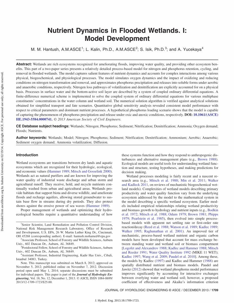
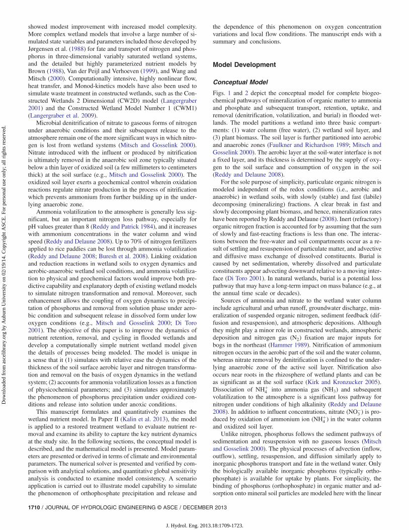
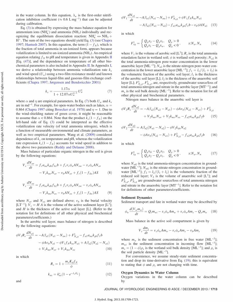
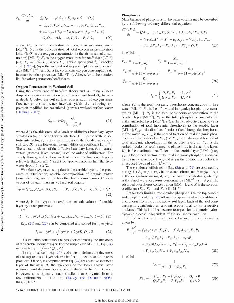
Figs. 1 and 2 depict the conceptual model for complete biogeo-chemical pathways of mineralization of organic matter to ammoniaand phosphate and subsequent transport, retention, uptake, andremoval (denitrification, volatilization, and burial) in flooded wet-lands. The model partitions a wetland into three basic compart-ments: (1) water column (free water), (2) wetland soil layer, and(3) plant biomass. The soil layer is further partitioned into aerobicand anaerobic zones (Faulkner and Richardson 1989; Mitsch andGosselink 2000). The aerobic layer at the soil-water interface is nota fixed layer, and its thickness is determined by the supply of oxy-gen to the soil surface and consumption of oxygen in the soil(Reddy and Delaune 2008).

For the sole purpose of simplicity, particulate organic nitrogen ismodeled independent of the redox conditions (i.e., aerobic andanaerobic) in wetland soils, with slowly (stable) and fast (labile)decomposing (mineralizing) fractions. A clear break in fast andslowly decomposing plant biomass, and hence, mineralization rateshave been reported by Reddy and Delaune (2008). Inert (refractory)organic nitrogen fraction is accounted for by assuming that the sumof slowly and fast-reacting fractions is less than one. The interac-tions between the free-water and soil compartments occur as a re-sult of settling and resuspension of particulate matter, and advectiveand diffusive mass exchange of dissolved constituents. Burial iscaused by net sedimentation, whereby dissolved and particulateconstituents appear advecting downward relative to a moving inter-face (Di Toro 2001). In natural wetlands, burial is a potential losspathway that may have a long-term impact on mass balance (e.g., atthe annual time scale or decades).

Sources of ammonia and nitrate to the wetland water columninclude agricultural and urban runoff, groundwater discharge, min-eralization of suspended organic nitrogen, sediment feedback (dif-fusion and resuspension), and atmospheric depositions. Althoughthey might play a minor role in constructed wetlands, atmosphericdeposition and nitrogen gas (N2) fixation are major inputs forbogs in the northeast (Hammer 1989). Nitrification of ammoniumnitrogen occurs in the aerobic part of the soil and the water column,whereas nitrate removal by denitrification is confined to the under-lying anaerobic zone of the active soil layer. Nitrification alsooccurs near roots in the rhizosphere of wetland plants and can beas significant as at the soil surface (Kirk and Kronzucker 2005).Dissociation of NHþ

4 into ammonia gas (NH3) and subsequentvolatilization to the atmosphere is a significant loss pathway fornitrogen under conditions of high alkalinity (Reddy and Delaune2008). In addition to influent concentrations, nitrate (NO−

3 ) is pro-duced by oxidation of ammonium ion (NHþ

4 ) in the water columnand oxidized soil layer.

Unlike nitrogen, phosphorus follows the sediment pathways ofsedimentation and resuspension with no gaseous losses (Mitschand Gosselink 2000). The physical processes of advection (inflow,outflow), settling, resuspension, and diffusion similarly apply toinorganic phosphorus transport and fate in the wetland water. Onlythe biologically available inorganic phosphorus (typically ortho-phosphate) is available for uptake by plants. For simplicity, thebinding of phosphorus (orthophosphate) in organic matter and ad-sorption onto mineral soil particles are modeled here with the linear

1710 / JOURNAL OF HYDROLOGIC ENGINEERING © ASCE / DECEMBER 2013

J. Hydrol. Eng. 2013.18:1709-1723.

Dow

nloa

ded

from

asc

elib

rary

.org

by

Aub

urn

Uni

vers

ity o

n 02

/19/

14. C

opyr

ight

ASC

E. F

or p

erso

nal u

se o

nly;

all

righ

ts r

eser

ved.

Fig. 2. Phosphorus processes in wetlands: water column, aerobic soil layer, and lower reduced soil layer

Fig. 1. Nitrogen processes in wetlands: water column, aerobic soil layer, and reduced lower soil layer

JOURNAL OF HYDROLOGIC ENGINEERING © ASCE / DECEMBER 2013 / 1711

J. Hydrol. Eng. 2013.18:1709-1723.

Dow

nloa

ded

from

asc

elib

rary

.org

by

Aub

urn

Uni

vers

ity o

n 02

/19/

14. C

opyr

ight

ASC

E. F

or p

erso

nal u

se o

nly;

all

righ

ts r

eser

ved.

adsorption isotherm. Imported phosphorus (runoff, sediment,groundwater) and decomposition of organic matter are primarysources of inorganic phosphorus in wetland soil and water. Exclud-ing plant harvesting, burial is about the only mechanism for theremoval of phosphorus in wetlands.

As discussed above, the removal of dissolved orthophosphatefrom solution occurs under oxidized soil conditions, whereby phos-phorus bonds with precipitating iron hydroxide and separates fromsolution. When oxygen levels drop, the iron hydroxides are reducedto soluble ferrous iron, which leads to an associated release ofdissolved phosphorus into the sediment pore waters where it is freefor transport into the overlying water (e.g., Mitsch and Gosselink2000; Di Toro 2001).

Although the primary objective of the wetland model is nutrientcycling, productivity is modeled using a generic mass balance forfree-floating algae and rooted plants with relatively simple growthand death processes. Major underlying assumptions of the wetlandmodel are as follows: (1) concentrations of various constituents areuniform (i.e., complete mixing) in each compartment or layer;(2) first-order reaction rates occur (mineralization, nitrification, de-nitrification, etc.); (3) abundant dissolved organic carbon (DOC) ispresent in soil; (4) the aerobic layer is aggregate (i.e., effectivelayer) of the oxidizing soil surface and the rhizosphere; (5) phos-phorus precipitation and release could be approximated by anoxygen-dependent linear adsorption coefficient; and (6) nitrogenfixation and assimilation into microbial biomass are accounted forin the organic pool. The consequence of unlimited DOC supply inthe third of the above assumptions is that denitrification wouldnot be limited by DOC. If the supply of DOC is limited, a morerigorous approach would require the coupling of nitrate and DOCdynamics, e.g., with Monod kinetics describing the rate of denitri-fication. Assumption (6) follows from neglecting microbial growthand decay as a separate compartment; i.e., nitrogen fixed by or as-similated into microbial biomass is at equilibrium with the amountreleased to the organic pool. Extension of the model to multiplecells arranged in series along the main flow direction is straightfor-ward for applications involving spatially variable data.

Wetland Model Equations

Figs. 1 and 2 depict various transport mechanisms and loss path-ways for nitrogenous species and phosphorus in both free-waterand sediment compartments in a typical flooded wetland system.These are accounted for in the mass balance ordinary differentialequations that are presented below. First, we start with the hydro-logic model.

Water FlowSurface flow routing in a wetland system can be described using asimple flow continuity equation:

ϕwdVw

dt¼ Qi þQg −Qo − AET þ Aip ð1Þ

where Vw is the water volume of wetland surface water [L3]; A isthe wetland surface area [L2]; Qi is the volumetric inflow rate[L3T−1]; Qg is groundwater discharge (negative for infiltration)[L3T−1]; Qo is wetland discharge (outflow) rate [L3T−1]; ip is pre-cipitation rate [LT−1]; ET is evapotranspiration rate [L3T−1L−2];and ϕw is effective porosity of wetland surface water (since biomassoccupies part of the submerged wetland volume). ET accountsfor the wetland evapotranspiration rate [L3T−1L−2] which is thesum of plant transpiration (Tr) and surface evaporation (Ev),ET ¼ Tr þ Ev. Although Tr is derived by plant uptake in the soilroot zone, it is accounted for in the ET term to maintain appropriate

mass balance for the entire wetland system (free water and soil).By lumping plant transpiration rate into the surface reservoir flowbalance, flow balance for the overall wetland system is maintainedbut without the need to compute Tr.

The outflow-depth relationship (rating-curve) of the form Qo ¼ρhε, where h ¼ ϕwVw=A, can be used to route flow out of thewetland for a given inflow event, Qi. The specific case of ε ¼ 1corresponds to a linear-reservoir model.

NitrogenMass balance of nitrogen constituents in the water column is de-scribed by the following ordinary differential equations:

ϕwdðVwNowÞ

dt¼ QiNowi þ anakdaaþ anakdbfbwb

− ϕwVwkmwNow − vsϕwANow

þ vrϕwAðNor þ NosÞ −QoNow þ AfSwS ð2Þ

ϕwdðVwNawÞ

dt¼ QiNawi þ ipANap − ϕwVwfNknwNaw

þ βa1AðNa1 − NawÞ þ FwNag

− kvϕwAð1 − fNÞNaw þ ϕwVwkmwNow

−QoNaw − fawanakgaaþ Aqa ð3Þ

ϕwdðVwNnwÞ

dt¼ QiNnwi þ ipANnp þ ϕwVwfNknwNaw

þ βn1AðNn1 − NnwÞ þ FwNng

− fnwanakgaa

−QoNnw þ Aqn ð4Þin which

knw ¼ k�nwð1 − e−λwOwÞ ð5Þ

Fwxg ¼

�Qgx1; Qg > 0

Qgxw; Qg < 0; x∶Na;Nn ð6Þ

where Now is particulate organic nitrogen concentration in freewater [ML−3]; Naw ¼ ½NHþ

4 � þ ½NH3� is total ammonia-nitrogenconcentration in free water [ML−3]; Nnw is nitrate-nitrogen concen-tration in free water [ML−3]; Ow is oxygen concentration in freewater [ML−3]; a is mass of free floating plant [M Chl a]; b is massof rooted plants [M Chl a]; Nowi, Nawi, and Nnwi, respectively, areconcentrations of organic nitrogen, total ammonia nitrogen, and ni-trate nitrogen in incoming inflow [ML−3]; Na1 and Nn1, respec-tively, are pore-water concentrations of total ammonia nitrogenand nitrate nitrogen in oxygenated top soil layer (aerobic layerin Figs. 1 and 2) [ML−3]; Nor is concentration of rapidly mineral-izing organic nitrogen in wetland soil [ML−3]; Nos is the concen-tration of slowly mineralizing organic nitrogen in wetland soil[ML−3]; Nap and Nnp, respectively, are concentrations of total am-monia nitrogen and nitrate nitrogen in precipitation [ML−3]; qa andqn, respectively, are dry depositional rates of total ammonia nitro-gen and nitrate [ML−2T−1]; vs is effective settling velocity [LT−1];vr is resuspension rate [LT−1]; S is rate of nitrogen fixation bymicroorganisms [ML−2T−1]; Fw

Nagand Fw

Nng, respectively, are

groundwater source/loss for total ammonia nitrogen and nitrate ni-trogen [MT−1]; and fN is the fraction of total ammonia in ionizedform. All other related physical, biochemical, reaction, and physio-logical parameters are defined in the notation list.

Eq. (5), proposed first by Brown and Barnwell (1987), latercited by Chapra (1997), limits the nitrification rate to oxygen levels

1712 / JOURNAL OF HYDROLOGIC ENGINEERING © ASCE / DECEMBER 2013

J. Hydrol. Eng. 2013.18:1709-1723.

Dow

nloa

ded

from

asc

elib

rary

.org

by

Aub

urn

Uni

vers

ity o

n 02

/19/

14. C

opyr

ight

ASC

E. F

or p

erso

nal u

se o

nly;

all

righ

ts r

eser

ved.

in the water column. In this equation, λw is the first-order nitrifi-cation inhibition coefficient (≈ 0.6 Lmg−1) that can be adjustedduring calibration.

Eq. (3) is obtained by expressing the mass balance equation forammonium ions (NHþ

4 ) and ammonia (NH3) individually and rec-ognizing the equilibrium dissociation reaction: NHþ

4 ↔ NH3 þHþ. The sum of the two equations should yield Eq. (3) (see Chapra1997; Hantush 2007). In this equation, the term (1 − fN), which isthe fraction of total ammonia in un-ionized form, appears becausevolatilization is limited to un-ionized ammonia (NH3). An empiricalequation relating fN to pH and temperature is given in Appendix II[Eq. (47)], and the dependence on temperature of all other bio-chemical parameters is also included in Appendix II. In Appendix I,we derive a relationship between ammonia volatilization rate kvand wind speed (Uw) using a two-film resistance model and knownrelationships between liquid-film and gaseous-film exchange coef-ficients (Chapra 1997; Jørgensen and Bendoricchio 2001):

kv ¼1.17α

1þ 12.07αUη−1w

Uηw ð7Þ

where α and η are empirical parameters. In Eq. (7) both Uw and kvare in md−1. For example, for open-water bodies such as lakes, α ¼0.864 (Chapra 1997 citing Broecker et al. 1978) and η ¼ 1. Due tothe wind-shielding nature of green cover, it might be reasonableto assume that α < 0.864. Note that the product kvð1 − fNÞ on theleft-hand side of Eq. (3) could be interpreted as the effectivevolatilization rate velocity (of total ammonia nitrogen), which isa function of measurable environmental and climate parameters, aswell as two empirical parameters. Wang et al. (2009) considereddependence of kv on temperature and pH, whereas the volatilizationrate expression kvð1 − fNÞ accounts for wind speed in addition tothe above two parameters (Reddy and Delaune 2008).

Mass balance of particulate organic nitrogen in the soil is givenby the following equations:

VsdNor

dt¼ franakdbfbsbþ frvsϕwANow − vrϕwANor

− VskmrNor − vbANor þ frð1 − fSwÞAS ð8Þ

VsdNos

dt¼ fsanakdbfbsbþ fsvsϕwANow − vrϕwANos

− VskmsNos − vbANos þ fsð1 − fSwÞAS ð9Þ

where Nor and Nos are defined above; vb is the burial velocity[LT−1]; Vs ¼ H A is the volume of the active sediment layer [L3];and H is the thickness of the active soil layer [L]. (Refer to thenotation list for definitions of all other physical and biochemicalparameters/coefficients.)

In the aerobic soil layer, mass balance of nitrogen is describedby the following equations:

ϕV1RsdNa1

dt¼ −Aβa1ðNa1 − NawÞ þ F1

Nag− fa1anakgbf1b

− ϕAvbNa1 − ϕV1fNknsNa1 þ Aβa2ðNa2 − Na1Þþ V1kmrNor þ V1kmsNos ð10Þ

in which

Rs ¼ 1þmsKdfNϕ

ð11Þ

kns ¼ k�nsð1 − e−λsOwÞ ð12Þand

ϕV1

dNn1

dt¼−Aβn1ðNn1−NnwÞþF1

NngþϕV1fNknsNa1

−Aβn2ðNn1−Nn2Þ−fn1anakgbf1b−vbϕANn1 ð13Þ

in which

F1xg ¼

�Qgx2 −Qgx1; Qg > 0

Qgx1 −Qgxw; Qg < 0; x∶Na;Nn ð14Þ

where V1 is the volume of aerobic soil [L3]; Rs is the total ammoniaretardation factor in wetland soil; ϕ is wetland soil porosity; Na2 isthe total ammonia-nitrogen pore-water concentration in the loweranaerobic layer [ML−3]; Nn2 is the nitrate-nitrogen pore-water con-centration in the lower anaerobic layer [ML−3]; f1 ¼ l1=ðl1 þ l2Þ isthe volumetric fraction of the aerobic soil layer; l1 is the thicknessof the aerobic soil layer [L]; l2 is the thickness of the anaerobic soillayer [L]; F1

Nag, F1

Nng, are, respectively, groundwater source/loss of

total ammonia nitrogen and nitrate in the aerobic layer [MT−1]; andms is the soil bulk density [ML−3]. Refer to the notation list for allother physical and biochemical parameters.

Nitrogen mass balance in the anaerobic soil layer is

ϕV2RsdNa2

dt¼ −Aβa2ðNa2 − Na1Þ − ϕAvbðNa2 − Na1Þ þ F2

Nag

þ V2kmrNor þ V2kmsNos − fa2anakgbf2b ð15Þ

ϕV2

dNn2

dt¼ Aβn2ðNn1 − Nn2Þ − ϕV2kdnNn2

− ϕAvbðNn2 − Nn1Þ þ F2Nng

− fn2anakgbf2b ð16Þ

in which

F2xg ¼

�QgxG −Qgx2; Qg > 0

Qgx2 −Qgx1; Qg < 0; x∶Na;Nn ð17Þ

where NaG is the total ammonia-nitrogen concentration in ground-water [ML−3]; NnG is the nitrate-nitrogen concentration in ground-water [ML−3]; f2 ¼ l2=ðl1 þ l2Þ is the volumetric fraction of thereduced soil layer; V2 is the volume of anaerobic soil [L3]; andF2Nag

, F2Nng

are groundwater source/loss of total ammonia nitrogenand nitrate in the anaerobic layer [MT−1]. Refer to the notation listfor definitions of other parameters/coefficients.

Sediment DynamicsSediment transport and fate in wetland water may be described by

ϕwdðVwmwÞ

dt¼ Qimwi − vsϕwAmw þ vrϕwAms −Qomw ð18Þ

Mass balance in the active soil compartment is given by

Vsdms

dt¼ vsϕwAmw − vrϕwAms − vbAms ð19Þ

where mw is the sediment concentration in free water [ML−3];mwi is the sediment concentration in incoming flow [ML−3];ms ¼ ð1 − ϕÞρs is the wetland soil bulk density [ML−3]; and ρs isthe soil particle density [ML−3].

For convenience, we assume steady-state sediment concentra-tion and drop its time-derivative from Eq. (19); this is equivalentto stating that ϕ and ρs are not changing with time.

Oxygen Dynamics in Water ColumnOxygen variations in the water column can be describedby

JOURNAL OF HYDROLOGIC ENGINEERING © ASCE / DECEMBER 2013 / 1713

J. Hydrol. Eng. 2013.18:1709-1723.

Dow

nloa

ded

from

asc

elib

rary

.org

by

Aub

urn

Uni

vers

ity o

n 02

/19/

14. C

opyr

ight

ASC

E. F

or p

erso

nal u

se o

nly;

all

righ

ts r

eser

ved.

ϕwdðVwOwÞ

dt¼ QiOwi þ ipAOp þ KoϕwAðO� −OwÞ− ron;mϕwVwkmwNow − ron;nϕwVwfNknwNaw

þ aocrc;chlfðkgb − kdbÞfbwbþ ðkga − kdaÞag−QoOw − ASO − ϕwVwSw − ETAOw ð20Þ

where Owi is the concentration of oxygen in incoming water[ML−3]; Op is the concentration of total oxygen in precipitation[ML−3]; O� is the oxygen concentration in the air (assumed at sat-uration) [ML−3]; Ko is the oxygen mass-transfer coefficient [LT−1][e.g., Ko ¼ 0.864 Uw, where Uw is wind speed (md−1), Broeckeret al. (1978)]; SO is the wetland soil oxygen depletion rate per unitarea [ML−2T−1]; and Sw is the volumetric oxygen consumption ratein water by other processes [ML−3T−1]. Also, refer to the notationlist for other parameters/coefficients.

Oxygen Penetration in Wetland SoilUsing the equivalence of two-film theory and assuming a lineardrop of oxygen concentration from the ambient level Ow to zeroat depth l1 below the soil surface, conservation of oxygen massflux across the soil-water interface yields the following ex-pression modified for constricted (porous) wetland surface water(Hantush 2007):

SO ¼ ϕτD�o

Ow

l1 þ ϕτϕwτw

δð21Þ

where δ is the thickness of a laminar (diffusive) boundary layersituated on top of the soil-water interface [L]; τ is the wetland soiltortuosity factor; τw is effective tortuosity of the flooded area abovesoil; and D�

o is the free-water oxygen diffusion coefficient [L2T−1].The typical thickness of the diffusive boundary layer, δ, in naturalwaters (streams, lakes, oceans) is of the order of millimeters. Forslowly flowing and shallow wetland waters, the boundary layer isrelatively thicker, and δ might be approximated as half the free-water depth, δ ≈ h=2.

We relate oxygen consumption in the aerobic layer to the proc-esses of nitrification, aerobic decomposition of organic matter(mineralization), and allow for other but unknown sinks. Conser-vation of oxygen mass in wetland soil requires

SO ¼ l1ron;nϕfNknsðOwÞNa1 þ l1ron;mðkmsNos þ kmrNorÞ þ l1Ssð22Þ

where Ss is the oxygen removal rate per unit volume of aerobiclayer by other processes.

Let

Ω ¼ ron;nϕfNknsðOwÞNa1 þ ron;mðkmsNos þ kmrNorÞ þ Ss ð23ÞEqs. (21) and (22) can be combined and solved for l1 to yield

l1 ¼ −ϕτδ þffiffiffiffiffiffiffiffiffiffiffiffiffiffiffiffiffiffiffiffiffiffiffiffiffiffiffiffiffiffiffiffiffiffiffiffiffiffiffiffiffiffiffiffiffiðϕτδÞ2 þ 2ϕτD�

oOw=Ωq

ð24Þ

This equation constitutes the basis for estimating the thicknessof the aerobic sediment layer. For the simple case of δ ¼ 0, Eq. (24)reduces to l1 ¼

ffiffiffiffiffiffiffiffiffiffiffiffiffiffiffiffiffiffiffiffiffiffiffiffiffiffi2ϕτD�

oOw=Ωp

.The significance of Eq. (24) is obvious; it defines the thickness

of the top oxic soil layer where nitrification occurs and nitrate isproduced. Once l1 is computed from Eq. (24) for an active sedimentlayer of thickness H, the thickness of the lower anoxic layerwherein denitrification occurs would therefore be l2 ¼ H − l1.However, l1 is typically much smaller than l2 (varies from afew millimeters to 1–2 cm) (Reddy and Delaune 2008),thus, l2 ≈ H.

PhosphorusMass balance of phosphorus in the water column may be describedby the following ordinary differential equation:

dðVwPwÞdt

¼ QiPwi − vsFswmwϕwAPw þ f1vrϕwAFssmsP1

þ f2vrϕwAfssmsP2 − apakgaaþ VwapnkmwNow

þ βp1AðFdsP1 − FdwPwÞ þ FwPg −QoPw ð25Þ

in which

Fdw ¼ 1

1þ Kwmw; Fsw ¼ Kw

1þ Kwmw;

Fds ¼1

ϕþ ð1 − ϕÞρsKs1; Fss ¼

Ks1

ϕþ ð1 − ϕÞρsKs1;

fss ¼Ks2

ϕþ ð1 − ϕÞρsKs2ð26Þ

FwPg ¼

�QgFdsP1; Qg > 0

QgFdwPw; Qg < 0ð27Þ

where Pw is the total inorganic phosphorus concentration in freewater [ML−3]; Pwi is the inflow total inorganic phosphorus concen-tration [ML−3]; P1 is the total phosphorus concentration in theaerobic layer [ML−3]; P2 is the total phosphorus concentrationin the anaerobic layer [ML−3]; Fw

Pg is the net advective groundwatercontribution of total inorganic phosphorus to the aerobic layer[MT−1]; Fd;w is the dissolved fraction of total inorganic phosphorusin free water; mw Fs;w is the sorbed fraction of total inorganic phos-phorus in free water (1 − Fd;w); ϕ Fd;s is the dissolved fraction oftotal inorganic phosphorus in the aerobic layer; ms Fs;s is thesorbed fraction of total inorganic phosphorus in the aerobic layer;Ks1 is the distribution coefficient in the aerobic layer [L3M−1]; msfs;s is the sorbed fraction of the total inorganic phosphorus concen-tration in the anaerobic layer; and Ks2 is the distribution coefficientin reduced wetland soil [L3M−1].

The sorption coefficients in Eqs. (26) and (29) are obtained bynoting that Pw ¼ pþmws in the water column and P ¼ ϕpþmssin the soil (volume averaged, i.e., residence concentration), where pis the dissolved phosphorus concentration [ML−3]; s ¼ Kp is theadsorbed phosphorus concentration [MM−1]; and K is the sorptioncoefficient (Kw, Ks1, and Ks2) [L3M−1].

Rather than limiting resuspended phosphorus to the top aerobicsoil compartment, Eq. (25) allows resuspension of sediment-boundphosphorus from the entire active soil layer. Each of the soil com-partments contributes an amount proportional to its respectivethickness. This is intuitive because resuspension is a purely hydro-dynamic process independent of the soil redox condition.

In the aerobic soil layer, mass balance of phosphorus isgiven by:

V1

dP1

dt¼ f1ϕwAvsmwFswPw − f1ϕwAvrmsFssP1

− βp1AðFdsP1 − FdwPwÞ − vbAP1

þ βp2AðfdsP2 − FdsP1Þ þ F1Pg − apakgbf1b

þ V1apnkmrNor þ V1apnkmsNos ð28Þin which

fds ¼1

ϕþ ð1 − ϕÞρsKs2ð29Þ

F1Pg ¼

�QgfdsP2 −QgFdsP1; Qg > 0

QgFdsP1 −QgFdwPw; Qg < 0ð30Þ

1714 / JOURNAL OF HYDROLOGIC ENGINEERING © ASCE / DECEMBER 2013

J. Hydrol. Eng. 2013.18:1709-1723.

Dow

nloa

ded

from

asc

elib

rary

.org

by

Aub

urn

Uni

vers

ity o

n 02

/19/

14. C

opyr

ight

ASC

E. F

or p

erso

nal u

se o

nly;

all

righ

ts r

eser

ved.

where F1Pg is the net advective groundwater contribution of total

phosphorus to the aerobic layer [MT−1]; and ϕ fd;s is the dissolvedfraction of total phosphorus concentration in the anaerobicsoil layer.

Mass balance of phosphorus in the anaerobic layer is given by

V2

dP2

dt¼ f2ϕwAvsmwFswPw − f2ϕwAvrmsfssP2

þ V2apnkmrNor þ V2apnkmsNos − vbAðP2 − P1Þ− βp2AðfdsP2 − FdsP1Þ þ F2

Pg − apakgbf2b ð31Þwhere

F2Pg ¼

�QgPg −QgfdsP2; Qg > 0

QgfdsP2 −QgFdsP1; Qg < 0ð32Þ

Similarly, the preceding equations assumed that the aerobic andanaerobic soil compartments receive sediment-bound phosphorusdepositional fluxes in proportion to their respective thicknesses[first terms on the right-hand side of Eqs. (28) and (31)].

Phosphorus Adsorption and PrecipitationWe account in an approximate fashion for the aggregate effect ofsorption onto precipitated iron hydroxide under aerobic conditionsand release into solution when anoxic conditions prevail with a pro-posed functional relationship. The precipitation of phosphorus andrelease into aqueous phase could be accounted for by artificiallyincreasing or decreasing the distribution coefficient according tooxygen levels in the bulk water. Thus, we relate the sorption ratein the aerobic layer to the oxygen level in the overlying water bysuggesting the following functional relationship:

Ks1 ¼ Ksa þ KsbOw

O� ; Ow ≤ O�

Ks1 ¼ Ksa þ Ksb; Ow > O� ð33Þwhere Ksa accounts for partitioning to phosphorus sorption sites[L3M−1]; and Ksb accounts for association with the iron hydroxideprecipitate [L3M−1]. This relationship predicts Ks1 ¼ Ksa whenOw ¼ 0, whereas Ks1 ¼ Ksa þ Ksb when Ow ¼ O�. Ks1 could bethought of as an effective distribution coefficient, wherein Ksb istreated as a calibration parameter. In general, the oxygen concen-tration threshold value in Eq. (33), O�, might be selected smallerthan the oxygen saturation concentration.

A more general extension to Eq. (33) is Ks1 ¼ KsaþKsbð1 − e−cOwÞ, which for cOw ≪ 1 can be approximated asKs1 ¼KsaþKsbf1− ½1− ð−cOwÞ−OðcOwÞ2�g≅KsaþKsbcOw. Notethe similarity with Eq. (33) with c ¼ ðO�Þ−1.Primary Productivity ModelWe use a simple mass balance model for plant biomass growth anddeath (e.g., Thoman and Mueller 1987; Chapra 1997), and separatefree-floating plant biomass (e.g., phytoplankton) from rootedaquatic plants and those attached to the sediment mat (e.g., benthicalgae). As indicated earlier, microbial biomass growth and deathare not modeled, and nutrients assimilated are assumed to be re-leased instantly to the organic matter pool. A more rigorous ap-proach, of course, is to model this process with nitrogen andphosphorus assimilated (immobilization and nitrogen fixation) intoa separate microbial biomass compartment and with subsequent re-leases upon death/excretion.

We present a simple model for productivity in which thedaily growth rate is related to daily solar radiation and the annualgrowth rate of plants. The MIKE 11 WET model uses a similarconcept but with plant uptake rather than growth rate-solar radia-tion relationship.

The equation governing rooted/benthic plant growth/death is

dbdt

¼ kgbb − kdbb ð34Þ

in which

kgbðiÞ ¼R0ðiÞR̄0

k̄gb; R̄0 ¼1

365

X365i¼1

R0ðiÞ ð35aÞ

and from Iqba (1983)

R0ðiÞ ¼ 30r0ðiÞ�ωTdðiÞ2

sinψðiÞ sin λ

þ cosψðiÞ cos λ sin�ωTdðiÞ2

��

r0ðiÞ ¼ 1þ 0.033 cos

�2πi365

�

ψðiÞ ¼ sin−1�0.4 sin

�2π365

ði − 82Þ��

TdðiÞ ¼2cos−1ð− tanψðiÞ tanðΛÞÞ

ωð35bÞ

where kgb is the growth rate parameter of rooted plants [T−1]; kdb isthe death rate of rooted plants [T−1]; k̄gb is the mean daily growthrate of rooted plants [d−1]; R0ðiÞ is solar radiation on day i; rðiÞ isearth’s eccentricity correction factor for day i; TdðiÞ is the total daylength on day i; i is the day number of the year; Λ is latitude inradians; and ω is angular velocity of earth (15°=h, or π=12 rad=h).

Floating plants growth/death are described by this equation

dadt

¼ kgaa − kdaa −�

Qo

ϕwVw

�a ð36Þ

in which

kgaðiÞ ¼R0ðiÞR̄0

k̄ga ð37Þ

where kga is the growth rate parameter of a floating plant [T−1]; kdbis the death rate of a floating plant [T−1]; and k̄ga is the mean dailyplant growth rate for a floating plant [d−1] (calibration parameter).The third term on the right-hand side accounts for the hydrologicexport of floating biomass.

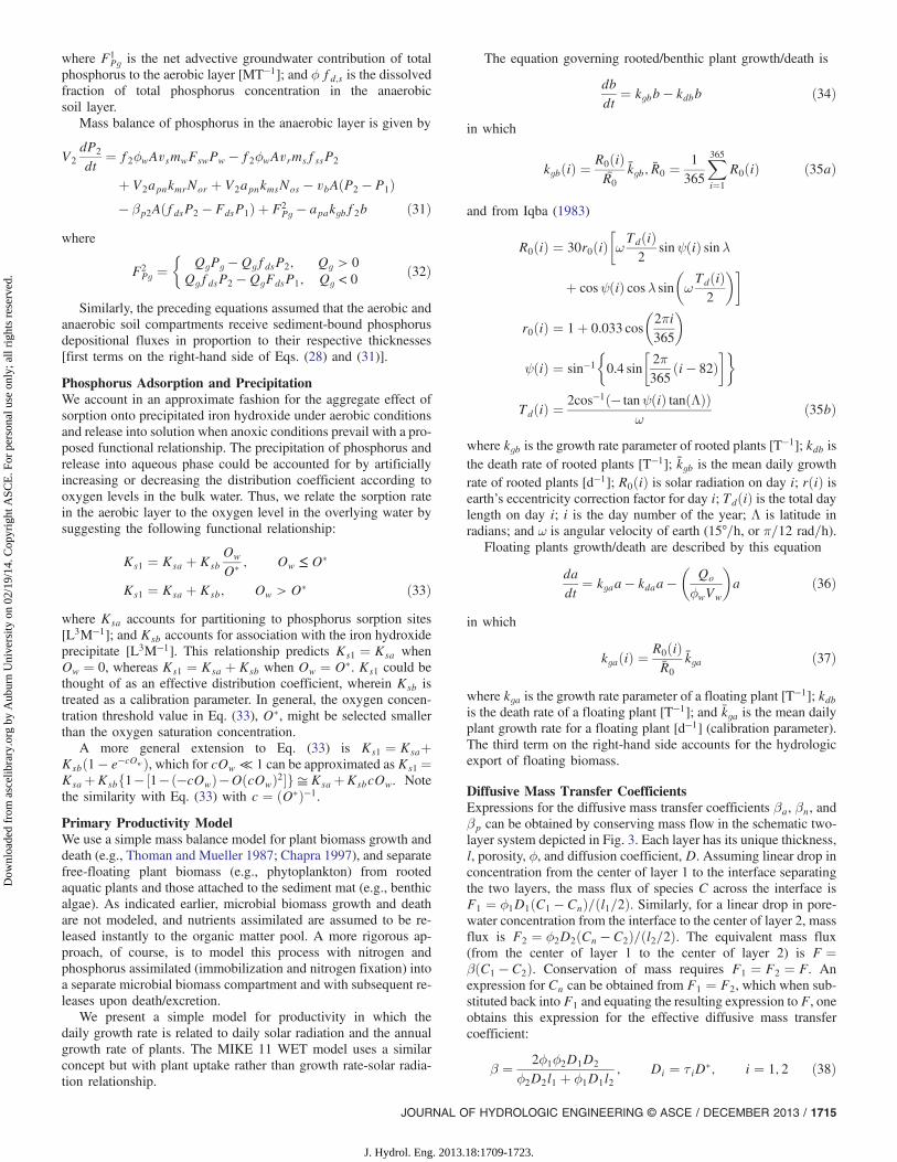
Diffusive Mass Transfer CoefficientsExpressions for the diffusive mass transfer coefficients βa, βn, andβp can be obtained by conserving mass flow in the schematic two-layer system depicted in Fig. 3. Each layer has its unique thickness,l, porosity, ϕ, and diffusion coefficient, D. Assuming linear drop inconcentration from the center of layer 1 to the interface separatingthe two layers, the mass flux of species C across the interface isF1 ¼ ϕ1D1ðC1 − CnÞ=ðl1=2Þ. Similarly, for a linear drop in pore-water concentration from the interface to the center of layer 2, massflux is F2 ¼ ϕ2D2ðCn − C2Þ=ðl2=2Þ. The equivalent mass flux(from the center of layer 1 to the center of layer 2) is F ¼βðC1 − C2Þ. Conservation of mass requires F1 ¼ F2 ¼ F. Anexpression for Cn can be obtained from F1 ¼ F2, which when sub-stituted back into F1 and equating the resulting expression to F, oneobtains this expression for the effective diffusive mass transfercoefficient:

β ¼ 2ϕ1ϕ2D1D2

ϕ2D2l1 þ ϕ1D1l2; Di ¼ τ iD�; i ¼ 1; 2 ð38Þ

JOURNAL OF HYDROLOGIC ENGINEERING © ASCE / DECEMBER 2013 / 1715

J. Hydrol. Eng. 2013.18:1709-1723.

Dow

nloa

ded

from

asc

elib

rary

.org

by

Aub

urn

Uni

vers

ity o

n 02

/19/

14. C

opyr

ight

ASC

E. F

or p

erso

nal u

se o

nly;

all

righ

ts r

eser

ved.

where D� is the free-water diffusion coefficient [L2T−1], and τ i istortuosity of layer i. For example, nitrate diffusive mass transferfrom the water column (ϕw, h, D�

n) to the aerobic soil layer (ϕ,l1, Dn) is βn1 ¼ 2ϕwϕτD�

n=ðϕτhþ ϕwl1Þ, where Dn and D�n, re-

spectively, are nitrate soil and free-water diffusion coefficient[L2T−1]; and τ as defined above is the wetland soil tortuosity factor.Due to plant biomass and other debris obstructing flow, ϕw is gen-erally less than 1 but expected to be larger than typical soil porosity.

Eq. (38) assumes linear variation of concentration betweenlayers; however, for highly nonlinear concentration profiles, adjust-ment of β might be needed to compensate for potential errors.

Numerical Scheme Verification

Numerical integration was performed using an explicit schemewith forward-difference approximation of the time derivatives.The first-order ordinary differential equation (ODE) of each depen-dent variable C (constituent concentration or mass) in a particularcompartment is cast in the form dC=dtþ μC ¼ F, where F de-notes all sources and sinks including coupling terms (i.e., constitu-ent variables coupled to C); and μ is the net sum of all constants/coefficients in the ODE multiplied by C. The time derivative isexpressed using the forward-difference approximation dC=dt ≈½CðtþΔtÞ − CðtÞ�=Δt, with the second term on the left-handside in the above ODE involving variable C approximated asμðtþΔtÞCðtþΔtÞ. F is approximated with its value at the begin-ning of the time step, i.e., FðtÞ. Although the numerical schemerequires relatively small time increments Δt, it is essentially anexplicit scheme, and the solution is straightforward and does notrequire solving a coupled system of equations.

The developed code was numerically verified using analyt-ical solutions for simplified cases. Maple software [version 11(Maplesoft, Waterloo, ON, Canada)] was used to obtain the analyti-cal solutions. Simplifications were kept to a minimum in this pro-cess, i.e., the most complete sets of differential equations that haveanalytical solutions were used (available upon request). The modelwas run over a 2-year simulation time period using input data givenin Tables 1–3 and mean parameter/coefficient values with priordistributions given in Table 4. The data in Tables 1–3 are obtainedfrom a study on a restored treatment wetland (Jordan et al. 2003)described in Paper II. Table 4 lists model parameters, minima,maxima, and their prior distributions partly obtained from liter-ature (related references are in Table 4 footnote) and partlyexpert judgment. The equations obtained by analytical solutionsthrough Maple were too lengthy and are not shown here to con-serve space. The time stepΔt for the simulation was 1 day over the2 years with the analytical solutions. The selected numerical inte-gration time step isΔt ¼ 0.01 day, but results were written at 1-day

intervals for comparison purposes. The parameters were kept fixedfor both numeric and analytic equations.

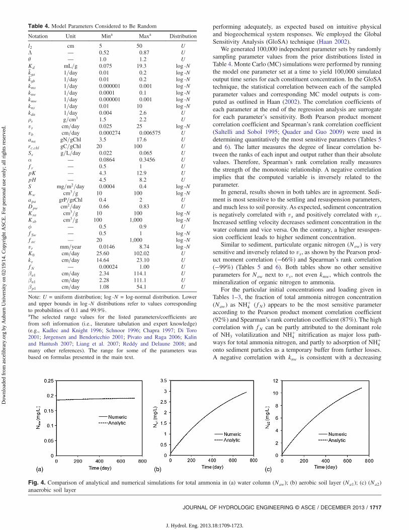
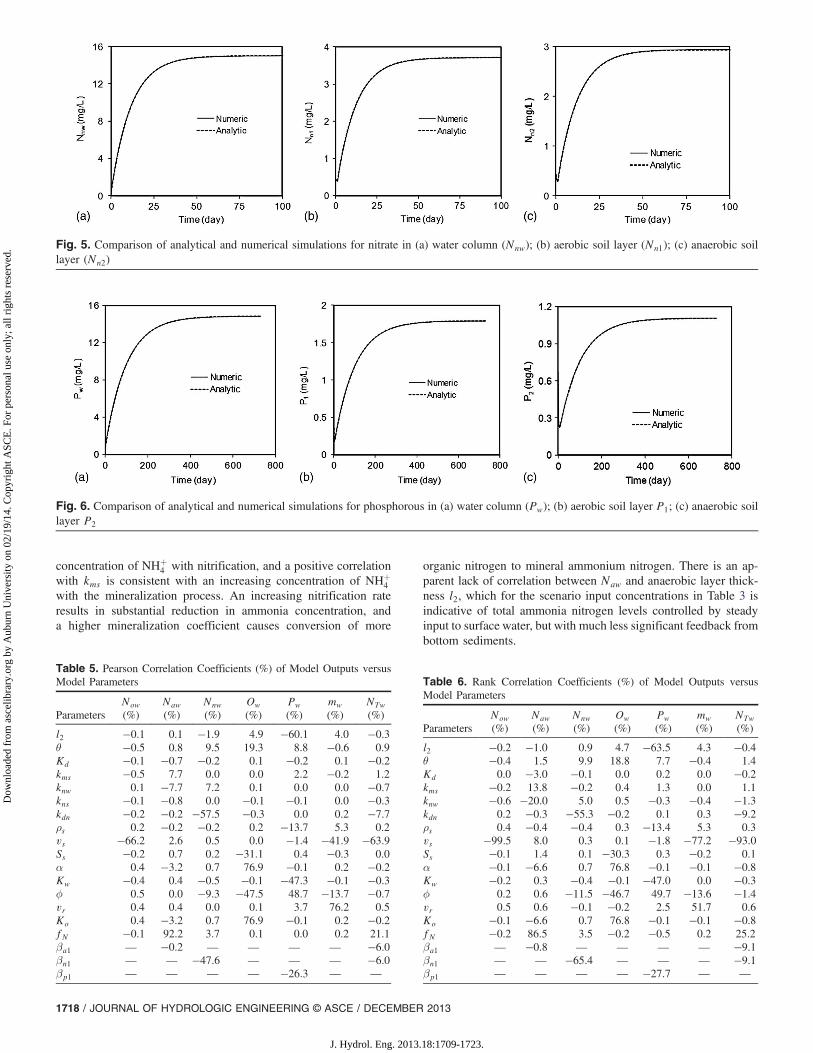
Figs. 4–6 show almost perfect matches between analyticalsolutions and finite-difference solutions for organic nitrogen, totalammonia nitrogen, nitrate, and phosphorus in the water columnand wetland soil. Differences between numerical and analyticalsolutions were indistinguishable in both oxidized and reducedsoil layers for nitrate, total ammonia nitrogen, and phosphorus.Although not shown in figures, differences were negligible fororganic nitrogen concentrations and free-floating and rooted plantbiomass.

Sensitivity Analysis

In this section, we conducted a sensitivity analysis by perturbing allparameters and examined whether or not the mathematical model is

Fig. 3. Two porous cells and concept of effective diffusion parameter

Table 1. Initial Concentrations (mg=L)

Parameter Value

Now 1.80Nor 0.91Nos 0.14a 0.04b 0.05mw 36.0Naw 0.26Na1 0.09Na2 0.16Pw 0.80P1 0.35P2 0.67Nnw 0.40Nn1 0.45Nn2 0.43ms 0.30Ow 6.0

Table 2. Hydrologic Variables

Parameter Value

Qi (m3=day) 194.02Qo (m3=day) 191.76Vw (m3) 2,409A (m2) 7,809ip (cm=day) 0.303ET (cm=day) 0.332l1 (cm) 0.01l2 (m) 0.275

Table 3. Input Concentrations (mg=L)

Parameter Value

Nowi 1.23Nnwi 0.18Nawi 0.12Pwi 0.31Owi 6.011mwi 149.85a� 0.50n� 0.5NnG 0.056NaG 0.038PwG 0.01

1716 / JOURNAL OF HYDROLOGIC ENGINEERING © ASCE / DECEMBER 2013

J. Hydrol. Eng. 2013.18:1709-1723.

Dow

nloa

ded

from

asc

elib

rary

.org

by

Aub

urn

Uni

vers

ity o

n 02

/19/

14. C

opyr

ight

ASC

E. F

or p

erso

nal u

se o

nly;

all

righ

ts r

eser

ved.

performing adequately, as expected based on intuitive physicaland biogeochemical system responses. We employed the GlobalSensitivity Analysis (GloSA) technique (Haan 2002).

We generated 100,000 independent parameter sets by randomlysampling parameter values from the prior distributions listed inTable 4. Monte Carlo (MC) simulations were performed by runningthe model one parameter set at a time to yield 100,000 simulatedoutput time series for each constituent concentration. In the GloSAtechnique, the statistical correlation between each of the sampledparameter values and corresponding MC model outputs is com-puted as outlined in Haan (2002). The correlation coefficients ofeach parameter at the end of the regression analysis are surrogatefor each parameter’s sensitivity. Both Pearson product momentcorrelation coefficient and Spearman’s rank correlation coefficient(Saltelli and Sobol 1995; Quader and Guo 2009) were used indetermining quantitatively the most sensitive parameters (Tables 5and 6). The latter measures the degree of linear correlation be-tween the ranks of each input and output rather than their absolutevalues. Therefore, Spearman’s rank correlation really measuresthe strength of the monotonic relationship. A negative correlationimplies that the computed variable is inversely related to theparameter.

In general, results shown in both tables are in agreement. Sedi-ment is most sensitive to the settling and resuspension parameters,and much less to soil porosity. As expected, sediment concentrationis negatively correlated with vs and positively correlated with vr.Increased settling velocity decreases sediment concentration in thewater column and vice versa. On the contrary, a higher resuspen-sion coefficient leads to higher sediment concentration.

Similar to sediment, particulate organic nitrogen (Now) is verysensitive and inversely related to vs, as shown by the Pearson prod-uct moment correlation (−66%) and Spearman’s rank correlation(−99%) (Tables 5 and 6). Both tables show no other sensitiveparameters for Now next to vs, not even kmw, which controls themineralization of organic nitrogen to ammonia.

For the particular initial concentrations and loading given inTables 1–3, the fraction of total ammonia nitrogen concentration(Naw) as NHþ

4 (fN) appears to be the most sensitive parameteraccording to the Pearson product moment correlation coefficient(92%) and Spearman’s rank correlation coefficient (87%). The highcorrelation with fN can be partly attributed to the dominant roleof NH3 volatilization and NHþ

4 nitrification as major loss path-ways for total ammonia nitrogen, and partly to adsorption of NHþ

4

onto sediment particles as a temporary buffer from further losses.A negative correlation with knw is consistent with a decreasing

Table 4. Model Parameters Considered to Be Random

Notation Unit Mina Maxa Distribution

l2 cm 5 50 UΛ — 0.52 0.87 Uθ — 1.0 1.2 UKd mL=g 0.075 19.3 log -Nk̄ga 1=day 0.01 0.2 log -Nk̄gb 1=day 0.01 0.2 log -Nkms 1=day 0.000001 0.001 log -Nknw 1=day 0.0001 0.1 log -Nkmw 1=day 0.000001 0.001 log -Nkns 1=day 0.01 10 log -Nkdn 1=day 0.004 2.6 Uρs g=cm3 1.5 2.2 Uvs cm=day 0.025 25 log -Nvb cm=day 0.000274 0.006575 Uana gN=gChl 3.5 17.6 Urc;chl gC=gChl 20 100 USs g=L=day 0.022 0.065 Uα — 0.0864 0.3456 Ufr — 0.5 1 UpK — 4.3 12.9 UpH — 4.5 8.2 US mg=m2=day 0.0004 0.4 log -NKw cm3=g 10 100 log -Napa grP=grChl 0.4 2 UDpw cm2=day 0.66 0.83 UKsa cm3=g 10 100 log -NKsb cm3=g 100 1,000 log -Nϕ — 0.5 0.9 UfSw — 0.5 1 log -Nfac — 20 1,000 log -Nvr mm=year 0.0146 8.74 log -NK0 cm=day 25.60 102.02 Ukv cm=day 14.64 23.10 UfN — 0.00024 1.00 Uβa1 cm=day 2.34 114.1 Uβn1 cm=day 2.28 111.1 Uβp1 cm=day 1.08 54.1 U

Note: U = uniform distribution; log -N = log-normal distribution. Lowerand upper bounds in log -N distributions refer to values correspondingto probabilities of 0.1 and 99.9%.aThe selected range values for the listed parameters/coefficients arefrom soft information (i.e., literature tabulation and expert knowledge)(e.g., Kadlec and Knight 1996; Schnoor 1996; Chapra 1997; Di Toro2001; Jørgensen and Bendoricchio 2001; Pivato and Raga 2006; Kalinand Hantush 2007; Liang et al. 2007; Reddy and Delaune 2008; andmany other references). The range for some of the parameters wasbased on formulas presented in the main text.

Fig. 4. Comparison of analytical and numerical simulations for total ammonia in (a) water column (Naw); (b) aerobic soil layer (Na1); (c) (Na2)anaerobic soil layer

JOURNAL OF HYDROLOGIC ENGINEERING © ASCE / DECEMBER 2013 / 1717

J. Hydrol. Eng. 2013.18:1709-1723.

Dow

nloa

ded

from

asc

elib

rary

.org

by

Aub

urn

Uni

vers

ity o

n 02

/19/

14. C

opyr

ight

ASC

E. F

or p

erso

nal u

se o

nly;

all

righ

ts r

eser

ved.

concentration of NHþ4 with nitrification, and a positive correlation

with kms is consistent with an increasing concentration of NHþ4

with the mineralization process. An increasing nitrification rateresults in substantial reduction in ammonia concentration, anda higher mineralization coefficient causes conversion of more

organic nitrogen to mineral ammonium nitrogen. There is an ap-parent lack of correlation between Naw and anaerobic layer thick-ness l2, which for the scenario input concentrations in Table 3 isindicative of total ammonia nitrogen levels controlled by steadyinput to surface water, but with much less significant feedback frombottom sediments.

Fig. 5. Comparison of analytical and numerical simulations for nitrate in (a) water column (Nnw); (b) aerobic soil layer (Nn1); (c) anaerobic soillayer (Nn2)

Fig. 6. Comparison of analytical and numerical simulations for phosphorous in (a) water column (Pw); (b) aerobic soil layer P1; (c) anaerobic soillayer P2

Table 5. Pearson Correlation Coefficients (%) of Model Outputs versusModel Parameters

ParametersNow(%)

Naw(%)

Nnw(%)

Ow(%)

Pw(%)

mw(%)

NTw(%)

l2 −0.1 0.1 −1.9 4.9 −60.1 4.0 −0.3θ −0.5 0.8 9.5 19.3 8.8 −0.6 0.9Kd −0.1 −0.7 −0.2 0.1 −0.2 0.1 −0.2kms −0.5 7.7 0.0 0.0 2.2 −0.2 1.2knw 0.1 −7.7 7.2 0.1 0.0 0.0 −0.7kns −0.1 −0.8 0.0 −0.1 −0.1 0.0 −0.3kdn −0.2 −0.2 −57.5 −0.3 0.0 0.2 −7.7ρs 0.2 −0.2 −0.2 0.2 −13.7 5.3 0.2vs −66.2 2.6 0.5 0.0 −1.4 −41.9 −63.9Ss −0.2 0.7 0.2 −31.1 0.4 −0.3 0.0α 0.4 −3.2 0.7 76.9 −0.1 0.2 −0.2Kw −0.4 0.4 −0.5 −0.1 −47.3 −0.1 −0.3ϕ 0.5 0.0 −9.3 −47.5 48.7 −13.7 −0.7vr 0.4 0.4 0.0 0.1 3.7 76.2 0.5Ko 0.4 −3.2 0.7 76.9 −0.1 0.2 −0.2fN −0.1 92.2 3.7 0.1 0.0 0.2 21.1βa1 — −0.2 — — — — −6.0βn1 — — −47.6 — — — −6.0βp1 — — — — −26.3 — —

Table 6. Rank Correlation Coefficients (%) of Model Outputs versusModel Parameters

ParametersNow(%)

Naw(%)

Nnw(%)

Ow(%)

Pw(%)

mw(%)

NTw(%)

l2 −0.2 −1.0 0.9 4.7 −63.5 4.3 −0.4θ −0.4 1.5 9.9 18.8 7.7 −0.4 1.4Kd 0.0 −3.0 −0.1 0.0 0.2 0.0 −0.2kms −0.2 13.8 −0.2 0.4 1.3 0.0 1.1knw −0.6 −20.0 5.0 0.5 −0.3 −0.4 −1.3kdn 0.2 −0.3 −55.3 −0.2 0.1 0.3 −9.2ρs 0.4 −0.4 −0.4 0.3 −13.4 5.3 0.3vs −99.5 8.0 0.3 0.1 −1.8 −77.2 −93.0Ss −0.1 1.4 0.1 −30.3 0.3 −0.2 0.1α −0.1 −6.6 0.7 76.8 −0.1 −0.1 −0.8Kw −0.2 0.3 −0.4 −0.1 −47.0 0.0 −0.3ϕ 0.2 0.6 −11.5 −46.7 49.7 −13.6 −1.4vr 0.5 0.6 −0.1 −0.2 2.5 51.7 0.6Ko −0.1 −6.6 0.7 76.8 −0.1 −0.1 −0.8fN −0.2 86.5 3.5 −0.2 −0.5 0.2 25.2βa1 — −0.8 — — — — −9.1βn1 — — −65.4 — — — −9.1βp1 — — — — −27.7 — —

1718 / JOURNAL OF HYDROLOGIC ENGINEERING © ASCE / DECEMBER 2013

J. Hydrol. Eng. 2013.18:1709-1723.

Dow

nloa

ded

from

asc

elib

rary

.org

by

Aub

urn

Uni

vers

ity o

n 02

/19/

14. C

opyr

ight

ASC

E. F

or p

erso

nal u

se o

nly;

all

righ

ts r

eser

ved.

The relatively high negative correlations in both Pearson andSpearman rank correlations of nitrate concentrations (Nnw) withthe denitrification rate (kdn) and diffusive mass transfer coefficient(βn1) are indicative of a strong decreasing trend with both param-eters. Albeit smaller, the positive 7.2% correlation with knw reflectsa monotonically increasing nitrate concentration with nitrification.As expected, higher denitrification rates reduce nitrate under re-duced conditions in the soil, whereas higher nitrification rates in-crease the nitrate amount under aerobic conditions. The decrease ofNnw with βn1 is attributed to diffusive transport caused by concen-tration gradient from higher nitrate concentrations in the watercolumn to lower concentrations in bottom soil, wherein nitrateis removed by denitrification under reduced condition. Althoughthe anaerobic layer is where denitrification occurs, its thicknessl2 had a marginal impact on Nnw. As discussed above, external in-put seems to dominate sediment feedback in the given simulationscenario.

The last column in Tables 5 and 6 shows that total nitrogen con-centration NTw is most sensitive to and negatively correlated withthe settling velocity vs. Both this correlation and the smaller one (inabsolute value) with denitrification rate kdn accentuate the role ofsettling into bottom sediments and denitrification therein as sinksfor total nitrogen in the water column. At time scale of this exampleapplication, the model was not sensitive to burial velocity. How-ever, it remains inconclusive whether or not burial is a long-termloss pathway.

Both Pearson and Spearman’s rank correlations for totalphosphorus (Pw) show large negative correlations with l2 and Kw

and high positive correlation with ϕ. This shows that for the givensimulation scenario, settling and sorption onto soil particles is aremoval process for total phosphorus in the water column. Positivecorrelations with kms and vr are consistent with mineralizationin bottom sediment and resuspension mechanism as sources fortotal phosphorus in the water column. Negative correlations alsoreveal significant inverse relationships between Pw and diffusiverate transfer coefficient (βp1) and sediment particle density (ρs).

The negative correlations of dissolved oxygen in the watercolumn (Ow) with Ss and φ in Tables 5 and 6 are expected becausethe increased oxygen removal rate in the sediment layer and largersediment porosity lead to reduced oxygen levels in the water col-umn. The large positive correlation with oxygen mass transfer rate(KO) is also anticipated since Ow increases with the oxygen aera-tion rate.

The sensitivity analysis carried above points toward internalmathematics of the wetland model that are consistent with whatis expected from various physical and biochemical processes. How-ever, the order of parameter sensitivities is generally site-specificand might vary to some extent from one site to another, as param-eters are surrogates of underlying physical and biogeochemicalprocesses that can dominate under varying wetland conditions.

Phosphorus Precipitation/Release

In this section we attempted to simulate precipitation and releasephenomena described above. The effect of oxygen level on phos-phorus dynamics was simulated using Eq. (28). This relationshipassumes maximum phosphorus adsorption when the water columnis saturated with oxygen. The sorption coefficient decreases lin-early when oxygen levels drop, thus resulting in more phosphorusin solution. In other words, Ks1 ¼ Ksa when Ow ¼ 0 and Ks1 ¼Ksa þ Ksb when Ow ¼ O�.

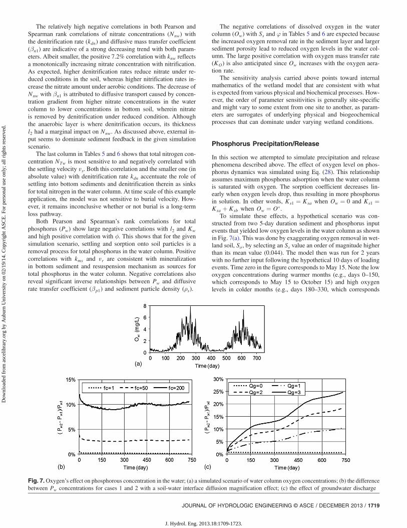
To simulate these effects, a hypothetical scenario was con-structed from two 5-day duration sediment and phosphorus inputevents that yielded low oxygen levels in the water column as shownin Fig. 7(a). This was done by exaggerating oxygen removal in wet-land soil, So, by selecting an Ss value an order of magnitude higherthan its mean value (0.044). The model then was run for 2 yearswith no further input following the hypothetical 10 days of loadingevents. Time zero in the figure corresponds to May 15. Note the lowoxygen concentrations during warmer months (e.g., days 0–150,which corresponds to May 15 to October 15) and high oxygenlevels in colder months (e.g., days 180–330, which corresponds

Fig. 7.Oxygen’s effect on phosphorous concentration in the water; (a) a simulated scenario of water column oxygen concentrations; (b) the differencebetween Pw concentrations for cases 1 and 2 with a soil-water interface diffusion magnification effect; (c) the effect of groundwater discharge

JOURNAL OF HYDROLOGIC ENGINEERING © ASCE / DECEMBER 2013 / 1719

J. Hydrol. Eng. 2013.18:1709-1723.

Dow

nloa

ded

from

asc

elib

rary

.org

by

Aub

urn

Uni

vers

ity o

n 02

/19/

14. C

opyr

ight

ASC

E. F

or p

erso

nal u

se o

nly;

all

righ

ts r

eser

ved.

to mid-December to mid-April). Two cases were considered. In thefirst case, the model was run ignoring the oxygen effect on phos-phorus sorption onto sediment particles. In other words, Ks1 wasassumed at its maximum Ksa þ Ksb all the time regardless of varia-tion in oxygen. In the second case, the model was run consideringvariation of Ks1 with Ow using Eq. (28). If the model is capable ofcapturing the phenomenon described above, then we should expectto see higher phosphorus concentrations with case 2.

Figs. 7(b and c), respectively, show the differences in simulatedphosphorus concentrations under different values of diffusion mag-nification factor fac and varying groundwater discharge rates Qg.Phosphorus diffusion across the soil-water interface is magnifiedby multiplying the free-water diffusion coefficient by fac to sim-ulate the effect of wind-induced turbulence and bioturbation. Itis clearly seen that simulations with case 2 generated higher dis-solved phosphorus concentrations in the water column. Consider-ing molecular diffusion only (without turbulence/bioturbation andgroundwater discharge) showed marginal differences between thetwo cases. If the diffusion coefficient increases by an order of mag-nitude or more, one can observe significant differences between thetwo scenarios [Fig. 7(b)]. Simulated dissolved phosphorus concen-trations in the water column are greater for the second scenario withperiodic decrease and increase in the computed concentrationscoinciding, respectively, with periods of high and low dissolvedoxygen [compare Fig. 7(a) with Fig. 7(b)]. The smallest differenceis around the 250th day, on which day the oxygen concentration ishighest. The peaks are at around the 75th and 450th days and at theend of the simulation, which all coincide with low oxygen levels.

This behavior is either dampened or accentuated by the mode ofgroundwater and surface water interactions. Higher groundwaterdischarge rates (m=d) (effluent wetlands) magnify the difference[Fig. 7(c)]. Although not shown in a figure, infiltration (i.e., influentwetlands) diminishes the mechanism of phosphorus release duringlow oxygen periods by countering the effect of upward diffusivemigration to the water column. Worth noting also is that the slopeof the relative differences between the two scenarios is steeperduring the periods of low oxygen (e.g., days 0–150) than duringperiods with higher oxygen levels (e.g., days 180–330), asFig. 7(c) shows.

Summary and Conclusions

Wetlands are recognized for controlling floods and providing waterquality and ecological benefits. In this part of a two-paper series,using basic physical and biochemical principles, a process-basedmathematical model has been developed using conservation ofmass to simulate nutrient retention, cycling, and removal in floodedwetlands. Specifically, transport and fate of organic and inorganicnitrogenous and phosphorus constituents in the water column andwetland soil are emphasized. The role of primary productivity onnutrient cycling is accounted for in an aggregate manner, but with-out a plant diversity component and shading and growth relation-ship. The novel aspect of this development, however, is the modelability to simulate with relative ease oxygen dynamics in the wet-land system and the formation of a thin, oxidized surface layer thatexerts geochemical control on nitrogen and phosphorus cyclingat the soil-water interface. The model accounts for nitrogen lossby ammonia volatilization as a function of environmental factorsand a newly derived volatilization rate transfer coefficient. The pro-cess of precipitation of insoluble phosphate under aerobic condi-tions and release into solution under anoxic conditions was alsomodeled by proposing a functional relationship between sorptioncoefficient and oxygen concentration.

The coupled system of ordinary differential equations is solvedusing the finite-difference method. Comparison with analytical so-lutions of specific scenarios revealed the adequacy of the numericalscheme. Global sensitivity analysis revealed the order of parametersensitivities that is generally anticipated and consistent with thewetland sediment and nutrient loading scenario application.

Application to a hypothetical phosphorus loading scenarioillustrated the conditions where the wetland model was capableof capturing the phenomenon of orthophosphate precipitationunder aerobic conditions and releases into solution under anoxicconditions.

The limitations of this model nonetheless should be recognizedfrom the underlying assumptions, and further improvements arewarranted. The most notable areas of additions include unsaturatedconditions, transverse-lateral interactions with stagnant zones, ex-tension to carbon cycling, and coupling of dissolved organic carbonto nitrogen transformation. Other areas needing improvement in-clude adding microbial-communities dynamics and improving theprimary productivity component. The model, however, is robust,and spatial variability along the main flow direction can be ac-counted for in a straightforward fashion. The wetland nutrientmodel is a potential tool for the design and management of con-structed and natural wetlands.

Appendix I. Ammonia Volatilization Mass TransferVelocity

From Whitman’s two-film resistance model, one can show that nettransfer velocity of any gas across the air-water interface is given by(Chapra 1997)

kv ¼ KlHe

He þ RGTaðKg=KlÞðmd−1Þ ð39Þ

where Kl = mass-transfer velocity in the liquid laminar layer(m d−1); Kg = mass transfer velocity in the gaseous laminar layer(m d−1); He = Henry’s constant (1.37 × 10−5 atmm3 mole−1 at20°C for NH3); RG = universal gas constant (8.206 × 10−5 atmm3

(K−1mole−1); and Ta = absolute temperature (K).The liquid-film and gaseous-film exchange can be calculated as

a function of molecular weight and the corresponding coefficientsfor oxygen and water vapor (Jørgensen and Bendoricchio 2001)

Kl ¼ Kl;O2

�32

M

�0.25

ð40Þ

and

Kg ¼ Kl;H2O

�18

M

�0.25

ð41Þ

where Kl;O2= liquid-film exchange coefficient for oxygen; and

Kl;H2O = gaseous-film exchange coefficient for water vapor. Thegas-film coefficient for water can be approximated by (e.g., Chapra1997; Jørgensen and Bendoricchio 2001)

Kl;H2O ¼ 168Uw ð42Þwhere Uw = wind speed (m s−1); and Kl;H2O is in units (m d−1).We assume the following power relationship relating liquid-filmmass transfer coefficient to wind speed:

Kl;O2¼ αUη

w ð43Þwhere α and η are empirical parameters. Combining (43) and (42)with (41) and (42) and substituting into (39) yields

1720 / JOURNAL OF HYDROLOGIC ENGINEERING © ASCE / DECEMBER 2013

J. Hydrol. Eng. 2013.18:1709-1723.

Dow

nloa

ded

from

asc

elib

rary

.org

by

Aub

urn

Uni

vers

ity o

n 02

/19/

14. C

opyr

ight

ASC

E. F

or p

erso

nal u

se o

nly;

all

righ

ts r

eser

ved.

kv ¼1.17α

1þ 12.07αUη−1w

Uηw ð44Þ

Appendix II. Temperature-Dependent Coefficients

In general, reaction rates and physiological parameters vary withtemperature in natural water environments. Assuming temperaturevariations over narrow ranges (e.g., 0 to 35°C), the Arrhenius equa-tion could be used to derive this parameter-temperature formula(e.g., Schnoor 1996):

kT ¼ k20θT−20 ð45Þwhere T = temperature expressed in °C; θ = constant temperaturecoefficient greater than 1.0 and usually within the range 1.0 to 1.10;and k20 = rate constant at the reference temperature 20°C. For ex-ample, Chapra (1997) recommended θ ≅ 1.024 for oxygen mass-transfer coefficient, KO.

This temperature variation formula might be applicable to reac-tion-related and plant-related rate parameters kda, kdb, kmw, kmr,kms, knw, kga, kgb, kns, and kdn. We also extend Eq. (45) to describetemperature variation of nitrogen fixation, S, and soil oxygen con-sumption rate parameters, Sw and Ss.

The dependence of oxygen saturation, O�, on temperaturemay be described by the following relationship (Chapra 1997;refer to Jørgensen and Bendoricchio 2001, on modification forchlorination):

O� ¼ exp

�−139.34411þ 1.575701 × 105

Ta− 6.642308 × 107

T2a

þ 1.2438 × 1010

T3a

− 8.621949 × 1011

T4a

�ð46Þ

where O� = saturation concentration of dissolved oxygen in freshwater at 1 atm (mgL−1); and Ta ¼ T þ 273.15 is absolute temper-ature in °K. Chapra (1997) provides a correction to this equation forsalinity and pressure effects.

The fraction of total ammonia in ionized form, fN , is related toboth temperature and pH using a relationship originally proposedby Emerson et al. (1975):

fN ¼ 10−pH10−pH þ expð−2.3026pKÞ ; pK ¼

�c1 þ

c2Ta

�ð47Þ

where c1 and c2 (≈ 0.09018 and 2729.92, respectively, Emersonet al. 1975) might be treated as calibration parameters.

Boudreau (1997) provides these temperature-dependent free-water diffusion coefficients in units of (cm2d−1) for oxygen, D�

o,ammonium ion (D�

a), and nitrate (D�n):

D�o ¼ 0.864

�0.2604þ 0.006383

Tμ

�ð48Þ

D�a ¼ 0.0864ð9.5þ 0.413TÞ ð49Þ

D�n ¼ 0.0864ð9.5þ 0.388TÞ ð50Þ

and an average equation for inorganic phosphorus (PO3−4 , HPO2−

4 ,H2PO−

4 ) free-water diffusion coefficient (D�p) in units of (cm2d−1)

takes the form

D�p ¼ 0.0864ð3.3þ 0.181TÞ ð51Þ

where T is in °C [°K in (48)]; and μ = dynamic viscosity of waterin centipoises (10−2 g cm−1s−1). A relationship relating μ in

centipoises to T in (°C) can be obtained by fitting μ to T valuesreported by Chapra (1997):

μ ¼ 0.5e−0.0762T þ 1.3e−0.0177T ð52ÞA more general relationship relating μ to temperature, salinity,

and pressure developed by Matthaus (as cited by Boudreau 1997)could also be used.

Acknowledgments

The U.S. Environmental Protection Agency through its Officeof Research and Development partially funded and collaboratedin the research described here under contract (EP08C000066) withAuburn University, School of Forestry and Wildlife Sciences. It hasnot been subject to the Agency review and therefore does notnecessarily reflect the views of the Agency, and no official endorse-ment should be inferred.

Notation

The following symbols are used in this paper:ana = gram of nitrogen per gram of chlorophyll-a in plant/algae;aoc = gram of oxygen produced per gram of organic carbon

synthesized (= 2.67);apa = gram of phosphorus per gram of chlorophyll-a;apn = phosphorus-to-nitrogen mass ratio produced by

mineralization of particulate organic matter (POM)(= 1.389);

faw = fraction of mineral nitrogen plant uptake as ammonia-Nin free water;

fa1 = fraction of mineral nitrogen plant uptake as ammonia-Nin the soil aerobic layer;

fa2 = fraction of mineral nitrogen plant uptake as ammonia-Nin the soil anaerobic layer;

fbs = fraction of rooted plant biomass below soil-waterinterface (within soil layer);

fbw = fraction of rooted plant biomass above soil-waterinterface;

fN = fraction of total ammonia nitrogen (½NHþ4 � þ ½NH3�) as

NHþ4 ;

fnw = fraction of mineral nitrogen plant uptake as nitrate-N infree water;

fn1 = fraction of mineral nitrogen plant uptake as nitrate-N inthe aerobic layer;

fn2 = fraction of mineral nitrogen plant uptake as nitrate-N inthe anaerobic layer;

fr = fraction of rapidly mineralizing particulate organicmatter;

fSw = fraction of nitrogen fixation in water;fs = fraction of slowly mineralizing particulate organic matter;f1 = volumetric fraction of the active soil layer that is aerobic;f2 = volumetric fraction of the active soil layer that is

anaerobic;Kd = ammonium ion distribution coefficient [L3M−1];Ko = oxygen reaeration mass-transfer velocity [LT−1];kda = death rate of free-floating plants [T−1];kdb = death rate of benthic and rooted plants [T−1];kdn = denitrification rate in anaerobic soil layer [T−1];kga = growth rate of free-floating plant [T−1];kgb = growth rate of benthic and rooted plant [T−1];kmr = first-order rapid mineralization rate in wetland soil [T−1];kms = first-order slow mineralization rate in wetland soil [T−1];

JOURNAL OF HYDROLOGIC ENGINEERING © ASCE / DECEMBER 2013 / 1721

J. Hydrol. Eng. 2013.18:1709-1723.

Dow

nloa

ded

from

asc

elib

rary

.org

by

Aub

urn

Uni

vers

ity o

n 02

/19/

14. C

opyr

ight

ASC

E. F

or p

erso

nal u

se o

nly;

all

righ

ts r

eser

ved.

kmw = first-order mineralization rate in wetland free water [T−1];kns = first-order nitrification rate in aerobic soil layer [T−1];knw = first-order nitrification rate in wetland free water [T−1];k�nw = maximum first-order nitrification rate in wetland free

water [T−1];k�s = maximum first-order nitrification rate in wetland soil

[T−1];kv = volatilization mass transfer velocity [LT−1];

rc;chl = carbon mass ration in chlorophyll a;ron;m = gram of oxygen consumed per gram of organic nitrogen

mineralized (= 15.29);ron;n = gram of oxygen consumed per gram of total ammonium

nitrogen nitrified (= 4.57);α, η = empirical parameters in Eq. (7) for ammonia liquid-film

transfer velocity;βa1,βn1

= diffusive mass-transfer rates, respectively, of totalammonia nitrogen and nitrate between wetland water andaerobic soil layer [LT−1];

βa2,βn2

= diffusive mass-transfer rates, respectively, of totalammonia nitrogen and nitrate between aerobic andanaerobic soil layers [LT−1];

βp1 = diffusive mass-transfer rate of dissolved phosphorusbetween wetland water and aerobic soil layer [LT−1];

βp2 = diffusive mass-transfer rate of dissolved phosphorusbetween aerobic and anaerobic soil layers [LT−1]; and

λs, λw = empirical coefficients in the relationships limitingnitrification, respectively, in soil and free water to oxygenconcentration in wetland water.

References

Bodkin, D. B., Janak, J. F., and Wallis, J. R. (1972). “Some ecologicalconsequences of a computer model of forest growth.” J. Ecol., 60(3),849–872.

Boudreau, B. P. (1997). Diagenetic models and their implementation:Modeling transport and reactions in aquatic sediments, Springer,Berlin, Heidelberg, 414.

Broecker, H. C., Petermann, J., and Siems, W. (1978). “The influence ofwind on CO2 exchange in a wind-wave tunnel.” J. Marine Res., 36(4),595–610.

Brown, L. C., and Barnwell, T. O., Jr. (1987). “The enhanced stream waterquality models QUAL2E and QUAL2E-UNCAS: Documentation andUser Manual.” Report EPA/600/3-87/007, U.S. Environmental Protec-tion Agency, Athens, GA.

Brown, M. T. (1988). “A simulation model of hydrology and nutrient dy-namics in wetlands.” Comput. Environ. Urban Syst., 12(4), 221–237.

Brown, S. L. (1981). “A comparison of the structure, primary productivity,and transpiration of cypress ecosystems in Florida.” Ecol. Monogr.,51(4), 403–427.

Buresh, R. J., Reddy, K. R., and van Kessel, C. (2008). “Nitrogen trans-formations in submerged soils.” Agronomy, 49, 401–436.

Chapra, S. C. (1997). Surface water-quality modeling, McGraw-Hill,New York.

Di Toro, D. M. (2001). Sediment flux modeling, Wiley, New York.Emerson, K., Russo, R. C., Lund, R. E., and Thurston, R. V. (1975). “Aque-

ous ammonia equilibrium calculations: Effect of pH and temperature.”J. Fish. Res. Board. Can., 32(12), 2379–2383.

Faulkner, S. P., and Richardson, C. J. (1989). “Physical and chemicalcharacteristics of fresh-water wetland soils.” In Constructed wetlandsfor wastewater treatment, municipal, industrial and agricultural,D. A. Hammer, ed., Lewis Publishers, Boca Raton, FL, 41–72.

Haan, C. T. (2002). Statistical methods in hydrology, 2nd Ed., Iowa StatePress.

Hammer, D. A. (1989). “Wetland ecosystems: Natural water purifiers?”Constructed wetlands for wastewater treatment, municipal, industrialand agricultural, D. A. Hammer, ed., Lewis Publishers, Boca Raton,FL, 5–19.

Hantush, M. M. (2007). “Modeling nitrogen-carbon cycling and oxygenconsumption in bottom sediments.” Adv. Water Resour., 30(1), 59–79.

Iqba, M. (1983). An introduction to solar radiation, Academic Press,New York.

Jordan, T. E., Whigham, D. F., Hofmockel, K. H., and Pittek, M. A. (2003).“Nutrient and sediment removal by a restored wetland receiving agri-cultural runoff.” J. Environ. Qual., 32, 1534–1547.

Jørgensen, S. E., and Bendoricchio, G. (2001). Fundamentals of ecologicalmodeling, 3rd Ed., Elsevier, New York.

Jørgensen, S. E., Hoffman, C. C., and Mitsch, W. J. (1988). “Modelingnutrient retention by Reedswamp and wet meadow in Denmark.” Wet-land modeling, W. J. Mitsch, M. Straškraba, and S. E. Jørgensen, eds.,Elsevier, New York, 133–152.

Kadlec, R. H. (1989). “Decomposition in wastewater wetlands.” Con-structed wetlands for wastewater treatment, municipal, industrial andagricultural, D. A. Hammer, ed., Lewis Publishers, Boca Raton, FL,459–468.

Kadlec, R. H. (1997). “An autobiotic wetland phosphorus model.” Ecol.Eng., 8(2), 145–172.

Kadlec, R. H., and Hammer, D. A. (1988). “Modeling nutrient behavior inwetlands.” Ecol. Modell., 40(1), 37–66.

Kadlec, R. H., and Knight, R. L. (1996). “Treatment Wetlands, LewisPublishers, 459.

Kalin, L., and Hantush, M. M. (1996). “Predictive uncertainty and param-eter sensitivity of a sediment-flux model: Nitrogen flux and sedimentoxygen demand”, World Environment and Water Resources Congress:Restoring Our Natural Habitat, Tampa, May 15–19.

Kalin, L., Hantush, M. M., Isik, S., Yucekaya, A., and Jordan, T. (2013).“Nutrient dynamics in flooded wetlands. II: Model application.” J. Hy-drol. Eng., 10.1061/(ASCE)HE.1943-5584.0000750, 1724–1738.

Kirk, G. J. D., and Kronzucker, H. J. (2005). “The potential for nitrificationand nitrate uptake in the rhizosphere of wetland plants: A modelingstudy.” Ann. Bot., 96(4), 639–646.

Langergraber, G. (2001). “Development of a simulation tool for subsurfaceflow constructed wetlands.” Wiener Mitteilungen 169, Vienna, Austria,P. 207.

Langergraber, G., Rousseau, D. P. L., Garcia, J., and Mena, J. (2009).“CWM1: A general model to describe biokinetic processes insubsurface flow constructed wetlands.” Water Sci. Technol., 59(9),1687–1697.

Liang, X. Q., et al. (2007). “Modeling transport and fate of nitrogen fromurea applied to a near-trench paddy field.” Environ. Pollut., 150(3),13–320.

Logofet, D. O., and Alexandrov, G. A. (1988). “Interference betweenmosses and trees in the framework of a dynamic model of carbonand nitrogen cycling in a mesotrophic bog ecosystem.” Wetland mod-eling, W. J. Mitsch, M. Straškraba, and S. E. Jørgensen, eds., Elsevier,New York, 55–66.

Min, J.-H., Paudel, R., and Yawitz, J. W. (2011). “Mechanistic biogeo-chemical model applications for Everglades restoration: A review ofcase studies and suggestions for future modeling needs.” Crit. Rev. Env.Sci. Technol., 41(S1), 489–516.

Mitsch, W., Straškraba, M., and Jørgensen, S. E. (1988). “Wetlandmodeling—An introduction and overview.” Wetland modeling, W. J.Mitsch, M. Straškraba, and S. E. Jørgensen, eds., Elsevier, New York,1–8.

Mitsch, W. J., and Gosselink, J. G. (2000). Wetland, Wiley, New York.Mitsch, W. J., and Reeder, B. C. (1991). “Modeling nutrient retention of a

freshwater coastal wetland: Estimating the roles of primary productiv-ity, resuspension and hydrology.” Ecol. Modell., 54(3–4), 151–187.

Odum, E. P. (1979). “Ecological importance of the riparian zone.”Strategies for protection and management of floodplain wetlandsand other riparian ecosystems, R. R. Johnson and J. F. McCormick,eds., Forest Service General Technical Report WO-12, Washington,DC, 2–4.

Paudel, R., and Jawitz, J. W. (2012). “Does increased model complexityimprove description of phosphorus dynamics in a large treatmentwetland?” Ecol. Eng., 42, 283–294.

1722 / JOURNAL OF HYDROLOGIC ENGINEERING © ASCE / DECEMBER 2013

J. Hydrol. Eng. 2013.18:1709-1723.

Dow

nloa

ded

from

asc

elib

rary

.org

by

Aub

urn

Uni

vers

ity o

n 02

/19/

14. C

opyr

ight

ASC

E. F

or p

erso

nal u

se o

nly;

all

righ

ts r

eser

ved.

Paudel, R., Min, J.-H., and Jawitz, J. W. (2010). “Management scenarioevaluation for a large treatment wetland using a spatio-temporal phos-phorus transport and cycling model.” Ecol. Eng., 36(12), 1627–1638.

Pearlstein, L., McKellar, H., and Kitchens, W. (1985). “Modelling theimpact of a river diversion on bottomland forest communities in theSantee River floodplain, South Carolina.” Ecol. Modell., 29(1–4),283–302.

Phipps, R. L. (1979). “Simulation of wetlands forest vegetation dynamics.”Ecol. Modell., 7(4), 257–288.

Pivato, A., and Raga, R. (2006). “Tests for the evaluation of ammoniumattenuation in MSW landfill leachate by adsorption into bentonite ina landfill liner.” Waste Manage., 26(2), 123–132.

Quader, A., and Guo, Y. (2009). “Relative importance of hydrologicaland sediment-transport characteristics affecting effective discharge ofsmall urban streams in southern Ontario.” J. Hydrol. Eng., 10.1061/(ASCE)HE.1943-5584.0000042, 698–710.

Raghunathan, R., et al. (2001). “Exploring the dynamics and fate of totalphosphorus in the Florida Everglades using a calibrated mass balancemodel.” Ecol. Modell., 142(3), 247–259.

Reddy, K. A., and Delaune, R. D. (2008). Biogeochemistry of wetlands:Science and applications, CRC Press, Boca Raton, FL.

Reddy, K. R., and Patrick, W. H. (1984). “Nitrogen transformations andloss in flooded soils and sediments.” Crit. Rev. Environ. Control, 13(4),273–309.

Reed, S. C., Middlebrooks, F. J., and Crites, R. W. (1988). Natural systemsfor waste management and treatment, McGraw-Hill, New York.

Saltelli, A., and Sobol, I. M. (1995). “About the use of rank transformationin sensitivity analysis of model output.” Reliab. Eng. Syst. Saf., 50(3),225–239.

Schnoor, J. L. (1996). Environmental modeling: Fate and transport ofpollutants in water, air, and soil, Wiley, New York.

Thoman, R. V., and Mueller, J. A. (1987). Principles of surface waterquality modeling and control, HarperCollins, London.

Van der Peijl, M. J., and Verhoeven, J. T. A. (1999). “A model of carbon,nitrogen and phosphorus dynamics and their interactions in rivermarginal wetlands.” Ecol. Modell., 118(2–3), 95–130.

Walker, W. W. (1995). “Design basis for Everglades stormwater treatmentareas.” Water Res. Bullet., 31, 671–685.

Walker, W. W., and Kadlec, R. H. (2011). “Modeling phosphorus dynamicsin Everglades wetlands and stormwater treatment areas.” Crit. Rev. Env.Sci. Technol., 41(S1), 430–446.

Wang, N., and Mitsch, W. J. (2000). “A detailed ecosystem model of phos-phorus dynamics in created riparian wetlands.” Ecol. Modell., 126(2–3),101–130.

Wang, Y., et al. (2009). “A simulation model of nitrogen transformation inreed constructed wetlands.” Desalination, 235(1–3), 93–101.

Water Quality Institute (VKI). (1992). MIKE 11 WET, short description,VKI, Hørsholm, Denmark.

Watson, J. T., Reed, S. C., Kadlec, R. H., Knight, R. L., and Whitehouse,A. E. (1989). “Performance expectations and loading rates for con-structed wetlands.” Constructed wetlands for wastewater treatment,municipal, industrial and agricultural, D. A. Hammer, ed., LewisPublishers, Boca Raton, FL, 319–351.

JOURNAL OF HYDROLOGIC ENGINEERING © ASCE / DECEMBER 2013 / 1723

J. Hydrol. Eng. 2013.18:1709-1723.

Dow

nloa

ded

from

asc

elib

rary

.org

by

Aub

urn

Uni

vers

ity o

n 02

/19/

14. C

opyr

ight

ASC

E. F

or p

erso

nal u

se o

nly;

all

righ

ts r

eser

ved.