detection of additive outliers in seasonal time series
TRANSCRIPT
School of Economics and Management Aarhus University
Bartholins Allé 10, Building 1322, DK-8000 Aarhus C Denmark
CREATES Research Paper 2009-40
Detection of additive outliers in seasonal time series
Niels Haldrup, Antonio Montañés and Andreu Sansó
Detection of additive outliers in seasonal time
series
Niels Haldrup∗
Aarhus University and CREATESAntonio Montañés∗∗
University of Zaragoza
Andreu Sansó∗∗∗
University of The Balearic Islands
14 September 2009
Abstract
The detection and location of additive outliers in integrated variableshas attracted much attention recently because such outliers tend to affectunit root inference among other things. Most of these procedures havebeen developed for non-seasonal processes. However, the presence of sea-sonality in the form of seasonally varying means and variances affect theproperties of outlier detection procedures, and hence appropriate adjust-ments of existing methods are needed for seasonal data. In this paper wesuggest modifications of tests proposed by Shin et al. (1996) and Perronand Rodriguez (2003) to deal with data sampled at a seasonal frequencyand the size and power properties are discussed. We also show that thepresence of periodic heteroscedasticity will inflate the size of the tests andhence will tend to identify an excessive number of outliers. A modifiedPerron-Rodriguez test which allows periodically varying variances is sug-gested and it is shown to have excellent properties in terms of both powerand size.
K�������: Additive outliers, outlier detection, integrated processes, peri-odic heteroscedasticity, seasonality.JEL C�������������: C12, C2, C22,
∗CREATES, School of Economics and Management, Aarhus University, Building 1322,DK-8000 Aarhus C, Denmark. E-mail: [email protected]. ∗∗Department of Eco-nomic Analysis, University of Zaragoza, Gran Via 2, 50005 Zaragoza, Spain. E-mail:[email protected].∗∗∗Department of Applied Economics University of The BalearicIslands, Ctra. Valldemossa km 7.5, 07122, Spain. E-mail: [email protected]. Niels Hal-drup acknowledges financial support from the Danish National Research Foundation and theDanish Social Sciences Research Council. Andreu Sansó acknowledges the financial supportfrom Ministerio de Ciencia e Innovacion under grant ECO 2008-05215/ECON.
1
1 Introduction
Franses and Haldrup (1994), and Shin et al. (1996), (for non-seasonal timeseries), and Haldrup et al. (2005), (for seasonal data), show that the presenceof additive outliers (AO) affects the limiting distribution of Dickey-Fuller typetests which tend to overreject the unit root null hypothesis in this case. Theintuition behind these results is that the AOs introduce an MA-type autocor-relation component which distorts the size of the tests. As a consequence, it isnecessary to check for the presence of outliers prior to testing for unit roots andsubsequently to modify the unit root testing procedure. With respect to thefirst step, i.e. the testing for the presence of outliers in I(1) variables, Shin et al.(1996), Vogelsang (1999), and Perron and Rodriguez (2003) have proposed testsbased on iterative procedures. See however, Haldrup and Sanso (2008) regard-ing some caveats of the Vogelsang tests. Concerning the second aspect, i.e. thecorrection for the outliers when testing for unit roots, this has been consideredby Franses and Haldrup (1994), Haldrup et al. (2005), Shin et al. (1996) andVogelsang (1999). One of the suggestions of the last author is to use modifiedPhillips-Perron (1988) tests, see Perron and Ng (1996). These tests were orig-inally designed to deal with dependent errors but also turn out to successfullydeal with dynamics generated from outliers. Franses and Haldrup proposed toextend the auxiliary regression by including dummy variables to control for theAOs whilst Shin et al. (1996) suggested to consider the observation affectedby AOs as a missing observation and replace this by its expected value underthe hypothesis of a unit root. These procedures necessarily have to identify thelocation of outliers.
In this paper we will be concerned with the first step, i.e. the outlier detec-tion problem for both stationary and non-stationary integrated processes. Mostoutlier detection procedures assume non seasonal data. However, the presence ofseasonality in the form of seasonally varying means and variances easily interferewith outlying observations and hence affects the properties of outlier detectionprocedures when there is strong seasonality in the data. It is also importantto consider how to deal with outlying observations in order not to affect theseasonal periodicity and the autocorrelation structure of the data. Thereforeappropriate adjustments of existing methods are needed for seasonal data. Inthis paper we suggest modifications of tests proposed by Shin et al. (1996) andPerron and Rodriguez (2003) to deal with the seasonal case. It turns out thatespecially the observations in the beginning and the end of a sample need to begiven a particular treatment. The modified version of the Perron-Rodriguez testappears to perform the best in terms of both power and size. One particularform of seasonality concerns the possibility of periodically varying variances,see also Burridge and Wallis (1990), Burridge and Taylor (2001), and Franses(1996). Periodic heteroscedasticity appears to generate inflated size distortionwith respect to the identification of additive outliers and hence too many out-liers are likely to be identified. Fortunately a simple (further) modification ofthe Perron-Rodriguez test statistic can be easily constructed to alleviate theseproblems.
2
In section 2 we review the tests proposed by Perron and Rodriguez (2003)and Shin et al. (1996), and we extend their tests in different ways to allowdata observed at a seasonal frequency. Also we suggest a modification of thePerron Rodriguez test that allows for periodically varying variances. In section3 the new tests are compared in a Monte Carlo experiment and we concludein general that the extensions of the Perron-Rodriguez test perform excellently.However, when periodic heteroscedasticity is present the extensions of the testto allow for this feature will be necessary to control size. The modified Shin etal. tests are generally found to perform poorly. Section 4 presents an empiricalapplication before we conclude.
2 Testing for additive outliers in integrated timeseries
Consider the univariate seasonal process generated by
yt = yt−s + ut, (1)
where ut is a general I(0) process and s indicates the number of observationsper year. For example, ut can be a linear process of the form ut = ϕ(L)et with
ϕ(L) =∞∑
i=0
ϕiLi
∞∑
i=0
i2ϕ2i <∞.
Additive outliers can be introduced in different ways. For instance, theobserved variable may read
zt = µt + yt + δπt (2)
where µt collects the deterministic terms (e.g. a constant, trend, and seasonaldummy variables) and δπt is the additive outlier. πt is a Bernouilli-type variableindependent of ut, such that P (πt = 1) = P (πt = −1) = p/2, P (πt = 0) = 1−p,0 ≤ p < 1 and δ is the (fixed) magnitude of outliers. The size of outliers may alsobe considered to be stochastic. Alternatively, the location of additive outliersmay be assumed fixed, e.g. like δjπ
jt where δj is the magnitude of outlier j with
fixed location πjt = 1 for t = Tj and πjt = 0 otherwise. Accordingly, zt is an
integrated process subject to AOs. We will consider simple procedures to detectoutliers in integrated processes and suggest their modification to accomodateseasonal data. For the sake of simplicity of the exposition we initially assumethat µt = 0.
2.1 The Shin- Sarker-Lee (1996) test
The test due to Shin et al. (1996) (SSL hereafter) tests the null hypothesisδ = 0 in equation (2), and is given by,
τSSL = supTao
∣∣tSSL (Tao)∣∣
3
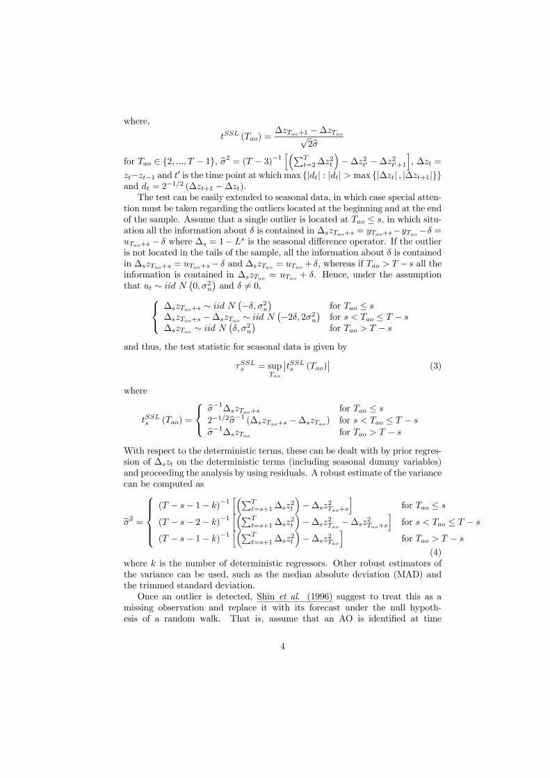
where,
tSSL (Tao) =∆zTao+1 −∆zTao√
2σ
for Tao ∈ {2, ..., T − 1}, σ2 = (T − 3)−1[(∑T
t=2∆z2t
)−∆z2t′ −∆z2t′+1
], ∆zt =
zt−zt−1 and t′ is the time point at whichmax {|dt| : |dt| > max {|∆zt| , |∆zt+1|}}and dt = 2
−1/2 (∆zt+1 −∆zt).The test can be easily extended to seasonal data, in which case special atten-
tion must be taken regarding the outliers located at the beginning and at the endof the sample. Assume that a single outlier is located at Tao ≤ s, in which situ-ation all the information about δ is contained in ∆szTao+s = yTao+s−yTao−δ =uTao+s − δ where ∆s = 1−Ls is the seasonal difference operator. If the outlieris not located in the tails of the sample, all the information about δ is containedin ∆szTao+s = uTao+s− δ and ∆szTao = uTao + δ, whereas if Tao > T − s all theinformation is contained in ∆szTao = uTao + δ. Hence, under the assumptionthat ut ∼ iid N
(0, σ2u
)and δ = 0,
∆szTao+s ∼ iid N
(−δ, σ2u
)for Tao ≤ s
∆szTao+s −∆szTao ∼ iid N(−2δ, 2σ2u
)for s < Tao ≤ T − s
∆szTao ∼ iid N(δ, σ2u
)for Tao > T − s
and thus, the test statistic for seasonal data is given by
τSSLs = supTao
∣∣tSSLs (Tao)∣∣ (3)
where
tSSLs (Tao) =
σ−1∆szTao+s for Tao ≤ s2−1/2σ−1 (∆szTao+s −∆szTao) for s < Tao ≤ T − sσ−1∆szTao for Tao > T − s
With respect to the deterministic terms, these can be dealt with by prior regres-sion of ∆szt on the deterministic terms (including seasonal dummy variables)and proceeding the analysis by using residuals. A robust estimate of the variancecan be computed as
σ2 =
(T − s− 1− k)−1[(∑T
t=s+1∆sz2t
)−∆sz2Tao+s
]for Tao ≤ s
(T − s− 2− k)−1[(∑T
t=s+1∆sz2t
)−∆sz2Tao −∆sz2Tao+s
]for s < Tao ≤ T − s
(T − s− 1− k)−1[(∑T
t=s+1∆sz2t
)−∆sz2Tao
]for Tao > T − s
(4)where k is the number of deterministic regressors. Other robust estimators ofthe variance can be used, such as the median absolute deviation (MAD) andthe trimmed standard deviation.
Once an outlier is detected, Shin et al. (1996) suggest to treat this as amissing observation and replace it with its forecast under the null hypoth-esis of a random walk. That is, assume that an AO is identified at time
4
Tao, then the contaminated observation zTao has to be replaced by: zTao =E (zTao | zTao−1, zTao−2, ...) = zTao−s. Next, the new series with the correctedobservation must be checked for the presence of new outliers and the corre-sponding observations replaced by its forecast. The iterative procedure stopswhen no additional outlier is detected.
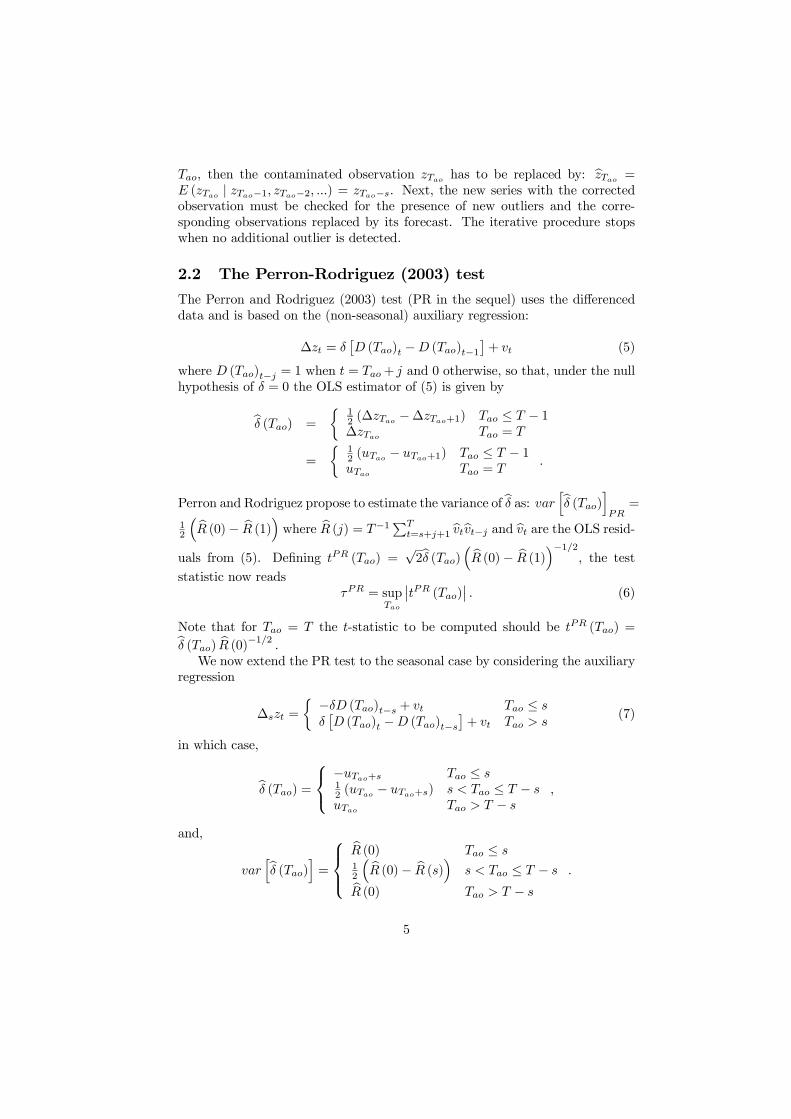
2.2 The Perron-Rodriguez (2003) test
The Perron and Rodriguez (2003) test (PR in the sequel) uses the differenceddata and is based on the (non-seasonal) auxiliary regression:
∆zt = δ[D (Tao)t −D (Tao)t−1
]+ vt (5)
where D (Tao)t−j = 1 when t = Tao+ j and 0 otherwise, so that, under the nullhypothesis of δ = 0 the OLS estimator of (5) is given by
δ (Tao) =
{12 (∆zTao −∆zTao+1) Tao ≤ T − 1∆zTao Tao = T
=
{12 (uTao − uTao+1) Tao ≤ T − 1uTao Tao = T
.
Perron and Rodriguez propose to estimate the variance of δ as: var[δ (Tao)
]PR
=
12
(R (0)− R (1)
)where R (j) = T−1
∑Tt=s+j+1 vtvt−j and vt are the OLS resid-
uals from (5). Defining tPR (Tao) =√2δ (Tao)
(R (0)− R (1)
)−1/2, the test
statistic now readsτPR = sup
Tao
∣∣tPR (Tao)∣∣ . (6)
Note that for Tao = T the t-statistic to be computed should be tPR (Tao) =
δ (Tao) R (0)−1/2 .
We now extend the PR test to the seasonal case by considering the auxiliaryregression
∆szt =
{−δD (Tao)t−s + vt Tao ≤ sδ[D (Tao)t −D (Tao)t−s
]+ vt Tao > s
(7)
in which case,
δ (Tao) =
−uTao+s Tao ≤ s12 (uTao − uTao+s) s < Tao ≤ T − suTao Tao > T − s
,
and,
var[δ (Tao)
]=
R (0) Tao ≤ s12
(R (0)− R (s)
)s < Tao ≤ T − s
R (0) Tao > T − s.
5
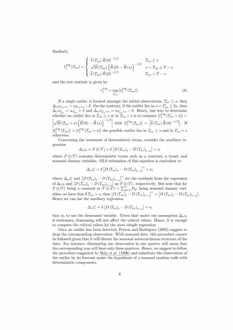
Similarly,
tPRs (Tao) =
δ (Tao) R (0)−1/2 Tao ≤ s
√2δ (Tao)
(R (0)− R (s)
)−1/2s < Tao ≤ T − s
δ (Tao) R (0)−1/2 Tao > T − s
and the test statistic is given by
τPRs = supTao
∣∣tPRs (Tao)∣∣ . (8)
If a single outlier is located amongst the initial observations, Tao ≤ s, then∆szTao+s = uTao+s−δ. On the contrary, if the outlier lies in s < T ′ao ≤ 2s, then∆szT ′
ao= uT ′
ao+ δ and ∆szT ′
ao+s = uT ′
ao+s − δ. Hence, one way to determine
whether an outlier lies in Tao ≤ s or in Tao + s is to compare∣∣tPRs (Tao + s)
∣∣ =∣∣∣∣√2δ (Tao + s)
(R (0)− R (s)
)−1/2∣∣∣∣ with∣∣tPRs (Tao)
∣∣ =∣∣∣δ (Tao) R (0)−1/2
∣∣∣. If∣∣tPRs (Tao)
∣∣ >∣∣tPRs (Tao + s)
∣∣ the possible outlier lies in Tao ≤ s and in Tao + sotherwise.
Concerning the treatment of deterministic terms, consider the auxiliary re-gression
∆szt = F (t/T ) + δ[D (Tao)t −D (Tao)t−s
]+ vt
where F (t/T ) contains deterministic terms such as a constant, a trend, andseasonal dummy variables. OLS estimation of this equation is equivalent to
∆sz∗
t = δ[D (Tao)t −D (Tao)t−s
]∗+ vt
where ∆sz∗
t and[D (Tao)t −D (Tao)t−s
]∗are the residuals from the regression
of ∆szt and[D (Tao)t −D (Tao)t−s
]on F (t/T ) , respectively. But note that for
F (t/T ) being a constant or F (t/T ) =∑sq=1Dqt being seasonal dummy vari-
ables, we have that if Tao > s, then[D (Tao)t −D (Tao)t−s
]∗=[D (Tao)t −D (Tao)t−s
].
Hence we can use the auxiliary regression
∆sz∗
t = δ[D (Tao)t −D (Tao)t−s
]+ vt
that is, to use the demeaned variable. Given that under our assumption ∆sztis stationary, demeaning will not affect the critical values. Hence, it is enoughto compute the critical values for the most simple regression.
Once an outlier has been detected, Perron and Rodriguez (2003) suggest todrop the corresponding observation. With seasonal data, this procedure cannotbe followed given that it will distort the seasonal autocorrelation structure of thedata. For instance, eliminating one observation in one quarter will mean thatthe corresponding year will have only three quarters. Hence, we suggest to followthe procedure suggested by Shin et al. (1996) and substitute the observation ofthe outlier by its forecast under the hypothesis of a seasonal random walk withdeterministic components.
6
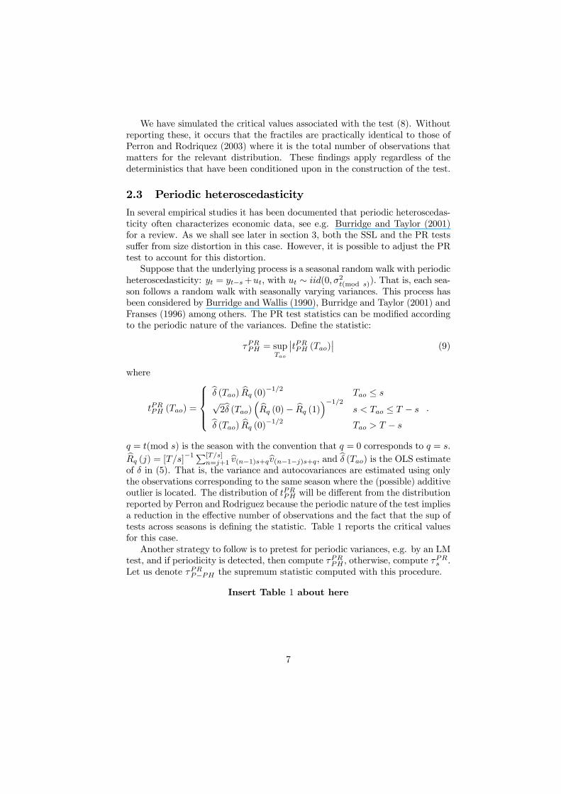
We have simulated the critical values associated with the test (8). Withoutreporting these, it occurs that the fractiles are practically identical to those ofPerron and Rodriquez (2003) where it is the total number of observations thatmatters for the relevant distribution. These findings apply regardless of thedeterministics that have been conditioned upon in the construction of the test.
2.3 Periodic heteroscedasticity
In several empirical studies it has been documented that periodic heteroscedas-ticity often characterizes economic data, see e.g. Burridge and Taylor (2001)for a review. As we shall see later in section 3, both the SSL and the PR testssuffer from size distortion in this case. However, it is possible to adjust the PRtest to account for this distortion.
Suppose that the underlying process is a seasonal random walk with periodicheteroscedasticity: yt = yt−s+ut, with ut ∼ iid(0, σ2t(mod s)). That is, each sea-son follows a random walk with seasonally varying variances. This process hasbeen considered by Burridge and Wallis (1990), Burridge and Taylor (2001) andFranses (1996) among others. The PR test statistics can be modified accordingto the periodic nature of the variances. Define the statistic:
τPRPH = supTao
∣∣tPRPH (Tao)∣∣ (9)
where
tPRPH (Tao) =
δ (Tao) Rq (0)−1/2 Tao ≤ s
√2δ (Tao)
(Rq (0)− Rq (1)
)−1/2s < Tao ≤ T − s
δ (Tao) Rq (0)−1/2 Tao > T − s
.
q = t(mod s) is the season with the convention that q = 0 corresponds to q = s.
Rq (j) = [T/s]−1∑[T/s]
n=j+1 v(n−1)s+qv(n−1−j)s+q, and δ (Tao) is the OLS estimateof δ in (5). That is, the variance and autocovariances are estimated using onlythe observations corresponding to the same season where the (possible) additiveoutlier is located. The distribution of tPRPH will be different from the distributionreported by Perron and Rodriguez because the periodic nature of the test impliesa reduction in the effective number of observations and the fact that the sup oftests across seasons is defining the statistic. Table 1 reports the critical valuesfor this case.
Another strategy to follow is to pretest for periodic variances, e.g. by an LMtest, and if periodicity is detected, then compute τPRPH , otherwise, compute τ
PRs .
Let us denote τPRP−PH the supremum statistic computed with this procedure.
Insert Table 1 about here
7
3 Monte Carlo Experiments
In this section we study the finite sample performance of the outlier detectiontests presented above, i.e. the τSSLz and τPRs tests and the tests accounting forperiodic variances, τPRPH and τPRP−PH .
The Monte Carlo experiment conducted here is similar to that of Perronand Rodriguez (2003) for the non-seasonal case. The data generating process(DGP) is given by:
zt =m∑
j=1
δjπjt + yt (10)
(1− L4
)dyt = vt
vt = ρvt−4 + εt + θεt−4
εt ∼ iid N (0, 1)
Hence the series zt is following a seasonal ARIMA4 possibly contaminatedwith m = 4 additive outliers and with fixed locations Tj (i.e. π
jt = 1 for t = Tj
and πjt = 0 otherwise) where j = 1, 2, 3, 4. The j′th outlier has magnitude δj .
Note that when δj = 0 for all j then no additive outliers are present, i.e. the caseof interest in analyzing the size of the tests. To analyze powers we have chosenan experimental design where δj = {5, 3, 2, 2} and Tj = {30, 55, 77, 100}. Hence,the first outlier is expected to be more easily detected than the subsequent threeoutliers. Note also that the last two outliers may be difficult to detect giventhat these have a magnitude of only two standard errors. The sample size inthe experiments is T = 120 corresponding to 30 years of quarterly data. Wehave also considered T = 200 and a design with different values of δj and thelocation of outliers. In particular, we have considered experiments where thelocation of outliers is either in the beginning or in the end of the sample size.To economize the space, these results are not reported here, but are availablefrom the authors upon request. However, we do comment on the conclusionsfollowing these extended experiments. In this set up, the size and power can beanalyzed under different assumptions about the dynamics describing vt whichfollows a seasonal ARMA4(1,1) model. We separate AR and MA dynamics andsimulate the cases θ = {−.8,−.4, 0, .4, .8} and ρ = {−.8,−.4, .4, .8}. Note thatby choice of d in (10) we have a non-stationary seasonal process for d = 1 or astationary process for d = 0.
Sizes and powers are reported in Table 2 and 3. In both tables Panel A andB correspond to non-stationary seasonal processes with MA and AR dynamics,respectively, and Panel C corresponds to a stationary seasonal process with ARdynamics.
First, we focus on sizes, Table 2. It is remarkable, that in all cases wherevt exhibits autocorrelation the τ
SLLs test is seriously size distorted which makes
the test useless in practice. For positive autocorrelation the test is very conser-vative whereas for negative autocorrelation it is heavily over sized. Also for the
8

stationary case the τSLLs test will be heavily over sized implied by differencingwhen constructing the test and the implied negative autocorrelation induced.
Insert Table 2 about here
The Perron and Rodriguez based tests appear to have almost the correct sizefor both stationary and non-stationary processes. One exception is the τPRPH testin the non-stationary case when strong positive autocorrelation is present in vt.In this case the test is slightly conservative.
Next, turn to the powers reported in Table 3. Given the poor size of theτSLLs test, we do not comment on powers or size-adjusted powers for this case.In detecting the first outlier, all the three Perron and Rodriguez tests performvery similarly and show good power in the case of non-stationary seasonality,see Panels A and B.. The tests loose some power, however, in the case withnegative autocorrelation. But overall power seems fine. Turning to the secondoutlier, results are equally similar but obviously detection of the second out-lier is less powerful mainly because the magnitude of this outlier is somewhatsmaller, i.e. 3 standard deviations instead of 5. Also in this case negative au-tocorrelation decreases power. Essentially the outlier is hidden by the negativeautocorrelation pattern and clearly this is most apparent as the magnitude ofthe outlier becomes smaller. This general pattern extends to outlier detectionof outlier 3 and 4 with the modification, however, that the τPRs test has betterpower than the equivalent tests correcting for periodic heteroscedasticity.
In the stationary case, Panel C, the rejection probabilites for the three PRtests are again similar. The performance in detecting the first outlier is generallyfine but deteriorating w.r.t. the subsequent outliers following the same line ofarguments as given above. However, when ρ becomes small the overdifferencingimplied by the construction of the tests again induces negative autocorrelationwhich will hidden the outliers in a similar fashion as discussed in relation topanels A and B.
In the previous simulations the data generating mechanism assumed out-liers to be located centrally amongst the observations. Simulation results notreported here but available upon request seem to indicate that in general out-liers at the very end of the sample yield test powers similar to those reportedhere. However, for outliers in the beginning of the sample some loss of power isdetected.
Table 4 presents results for a data generating process with periodic het-eroscedasticity, which has also been considered by Burridge and Taylor (2001).The data generating mechanism corresponds to (10) with d = 1 and θ = ρ =
δj = 0, j = 1, 2, 3, 4, but with εt ∼ iid N(0, σ2t(mod s)
)with the convention
that σ0 = σ4. Hence zt follows a seasonal random walk with variances de-pending upon the season. As it is clear from Table 4 the τPRs test is seriouslydistorted in this case (as is the τSSLs test). However, it can be seen that boththe tests correcting for heteroscedasticity perform nicely in terms size and henceis generally recommendable when periodic heteroscedasticity is suspected.
9
Insert Table 3 about hereInsert Table 4 about here
4 Empirical applications
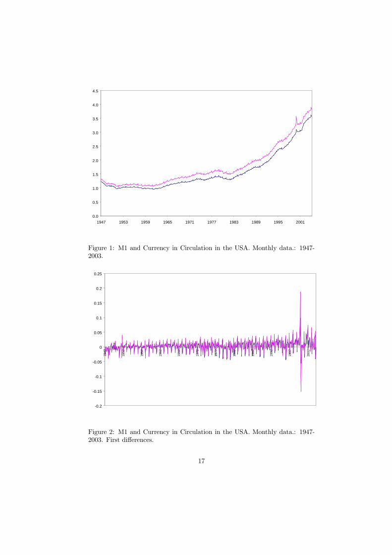
In order to illustrate the performance of the procedures for outlier detection,we have applied the tests to the analysis of US money demand. To that end,we have selected the most liquid definition of money demand, considering boththe currency component of the US money stock, measured by M1, as well as thecurrency in circulation in the US economy. We will refer to these as CCM1 andCC, respectively. The variables have been made real by using the US consumerprice index as deflator. The monthly data covers the period 1947:1-2004:2 andthe data are from the Board of Governors of the Federal Reserve System (seehttp://www.forecasts.org/data ).
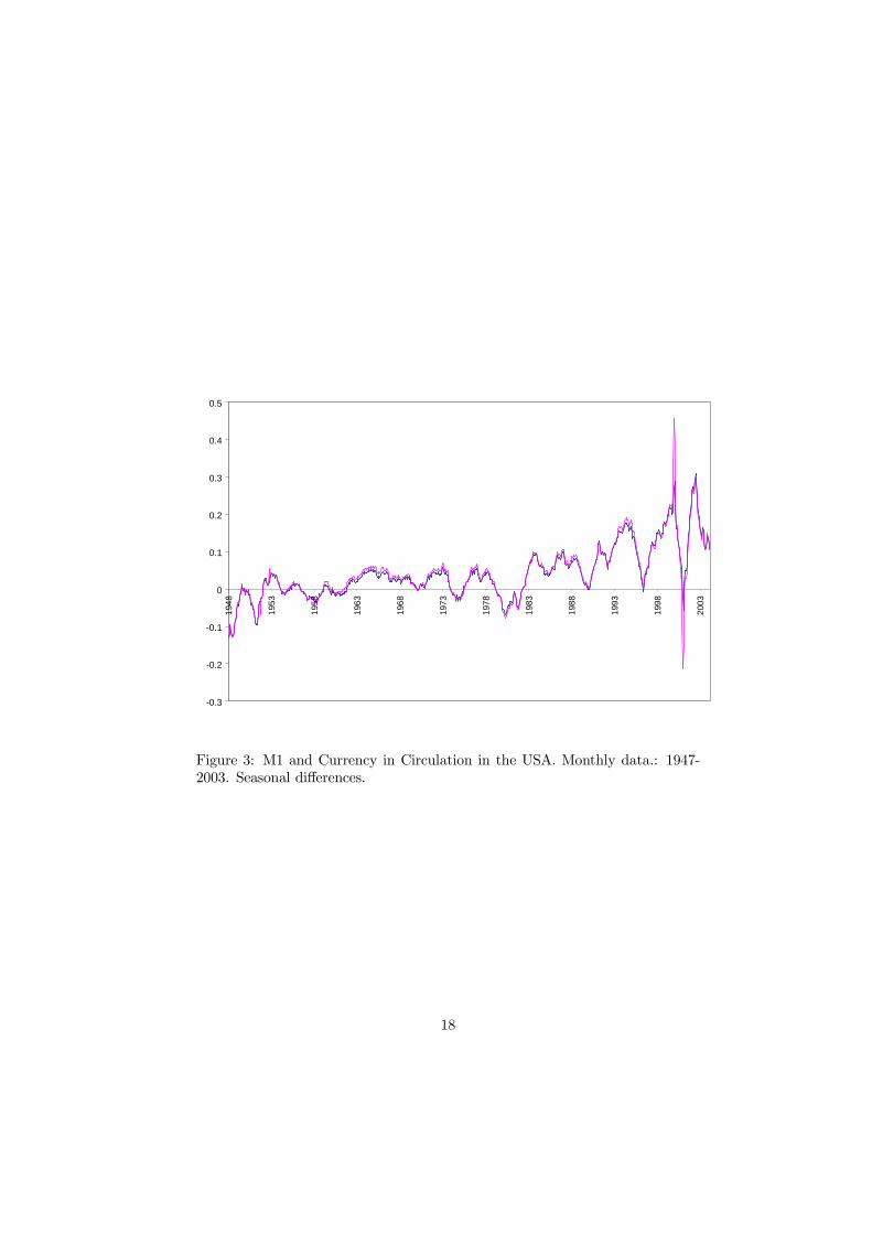
Figures 1-3 display the variables and their first regular and first seasonaldifferences, respectively. These figures show that the variables exhibit similarbehavior. Also, the series do not seem stationary, they exhibit a clear seasonalcomponent and finally, they take values abnormally high in some periods. Moreprecisely, we can relate these abnormal behaviour to the end of 1999 and thefirst half of 2001 episodes. Thus, it will be interestsing to see whether we canidentify these as being outliers using the various tests.
Table 5 reports the values of the τPRPH , and τPRs tests. Formal F-tests for
non-periodic heteroscedasticity could not be rejected and hence the results forτPRPH and τPRs are expected to be similar. For the currency component of theUS money stock, CCM1, it can be seen that the τPRPH and τPRs tests imply thepresence of 4 additive outliers (identically dated). Two of the outliers are clearlyassociated with the Y2K-effect: December 1999, and January 2000.
Insert Table 5 about here
The results of the currency in circulation, CC, are rather similar, althoughslight modifications exist. First, we observe that the τPRPH statistic detects theexistence of 6 outliers whilst the τPRs tests identifies 5 outliers. The tests gen-erally agree about the four outliers from November 1999 through January 2000.In fact, the τPRPH test suggests the outlier episode to start in October 1999. TheFebruary 2002 outlier is common to all tests (as for CCM1) as are the June2001 observation associated with the τPRPH and τPRs tests.
Insert Figure 1 about hereInsert Figure 2 about hereInsert Figure 3 about here
5 Conclusions
The presence of outlying observations in seasonal time can seriously affect in-ference and hence robust detection of outliers and their location is of utmost
10
importance. Seasonal time series appear to be especially problematic when de-tecting outliers because both the means and variances are likely to be seasonallyvarying. In this paper we show how existing procedures for outlier detection fornon-seasonal data can be modified when analyzing seasonally unadjusted data.In particular, we shown how tests originally suggested by Perron and Rodriguez(2003) can be modified to the seasonal case and we demonstrate that size andpower generally will be excellent in most cases. Periodic heteroscedasticity isgenerally a problem concerning the size of the tests, but we show how appro-priately calculated estimates of the periodic variances and a correction of thetest statistic will alleviate these problems. In practice, pretesting for periodicheteroscedasticity is recommended as an integral part of the outlier detectionprocedure.
References
[1] Burridge, P. and K.F. Wallis (1990). Seasonal adjustment and Kalmanfiltering: extension to periodic variances. Journal of Forecasting, 9, 109-118.
[2] Burridge, P. and A.M.R. Taylor (2001). On regression based tests for sea-sonal unit roots in the presence of periodic heteroscedasticity. Journal ofEconometrics, 104, 91-117.
[3] Franses, P. H. (1996). Periodicity and Stochastic Trends in Economic TimeSeries. Oxford University Press.
[4] Franses, P. H., and N. Haldrup, (1994). The effects of additive outliers ontests for unit roots and cointegration. Journal of Business and EconomicStatistics, 12, 471-478.
[5] Haldrup, N., A. Montañés and A. Sansó (2005). Measurement errors andoutliers in seasonal unit root testing. Journal of Econometrics, 127, 103-128
[6] Haldrup, N., A. Sansó (2008). A note on the Vogelsang test for additiveoutliers. Statistics and Probability Letters, 78, 296-306.
[7] Perron, P., and S. Ng, (1996). Useful modifications to unit root tests withdependent errors and their local asymptotic properties. Review of EconomicStudies, 63, 435–465.
[8] Perron, P. and G. Rodriguez (2003): Searching for additive outliers innonstationay time series. Journal of Time Series Analysis, 24, 193-220.
[9] Phillips, P. C. B. and P. Perron, (1988). Testing for a unit root in timeseries regression. Biometrika, 75, 335-346.
[10] Shin, D.W., S. Sarkar and J.H. Lee (1996). Unit root tests for time serieswith outliers. Statistics & Probability Letters, 30, 189-197.
11

[11] Vogelsang, T. J., (1999). Two simple procedures for testing for a unit rootwhen there are additive outliers. Journal of Time Series Analysis, 20, 237-52.
12
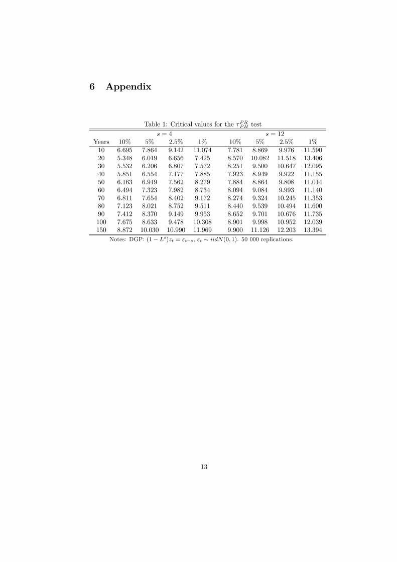
6 Appendix
Table 1: Critical values for the τPRPH test
s = 4 s = 12Years 10% 5% 2.5% 1% 10% 5% 2.5% 1%10 6.695 7.864 9.142 11.074 7.781 8.869 9.976 11.59020 5.348 6.019 6.656 7.425 8.570 10.082 11.518 13.40630 5.532 6.206 6.807 7.572 8.251 9.500 10.647 12.09540 5.851 6.554 7.177 7.885 7.923 8.949 9.922 11.15550 6.163 6.919 7.562 8.279 7.884 8.864 9.808 11.01460 6.494 7.323 7.982 8.734 8.094 9.084 9.993 11.14070 6.811 7.654 8.402 9.172 8.274 9.324 10.245 11.35380 7.123 8.021 8.752 9.511 8.440 9.539 10.494 11.60090 7.412 8.370 9.149 9.953 8.652 9.701 10.676 11.735100 7.675 8.633 9.478 10.308 8.901 9.998 10.952 12.039150 8.872 10.030 10.990 11.969 9.900 11.126 12.203 13.394
Notes: DGP: (1− Ls)zt = εt−s, εt ∼ iidN(0, 1). 50 000 replications.
13
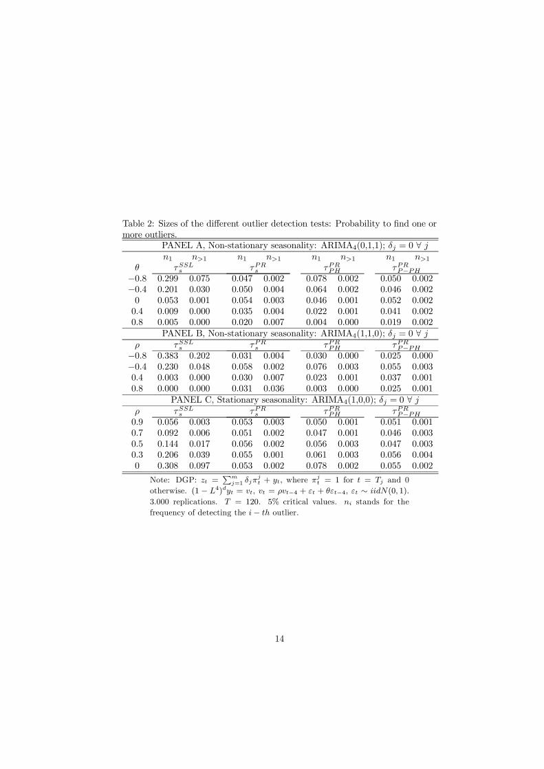
Table 2: Sizes of the different outlier detection tests: Probability to find one ormore outliers.
PANEL A, Non-stationary seasonality: ARIMA4(0,1,1); δj = 0 ∀ jn1 n>1 n1 n>1 n1 n>1 n1 n>1
θ τSSLs τPRs τPRPH τPRP−PH−0.8 0.299 0.075 0.047 0.002 0.078 0.002 0.050 0.002−0.4 0.201 0.030 0.050 0.004 0.064 0.002 0.046 0.0020 0.053 0.001 0.054 0.003 0.046 0.001 0.052 0.0020.4 0.009 0.000 0.035 0.004 0.022 0.001 0.041 0.0020.8 0.005 0.000 0.020 0.007 0.004 0.000 0.019 0.002
PANEL B, Non-stationary seasonality: ARIMA4(1,1,0); δj = 0 ∀ jρ τSSLs τPRs τPRPH τPRP−PH
−0.8 0.383 0.202 0.031 0.004 0.030 0.000 0.025 0.000−0.4 0.230 0.048 0.058 0.002 0.076 0.003 0.055 0.0030.4 0.003 0.000 0.030 0.007 0.023 0.001 0.037 0.0010.8 0.000 0.000 0.031 0.036 0.003 0.000 0.025 0.001
PANEL C, Stationary seasonality: ARIMA4(1,0,0); δj = 0 ∀ jρ τSSLs τPRs τPRPH τPRP−PH0.9 0.056 0.003 0.053 0.003 0.050 0.001 0.051 0.0010.7 0.092 0.006 0.051 0.002 0.047 0.001 0.046 0.0030.5 0.144 0.017 0.056 0.002 0.056 0.003 0.047 0.0030.3 0.206 0.039 0.055 0.001 0.061 0.003 0.056 0.0040 0.308 0.097 0.053 0.002 0.078 0.002 0.055 0.002
Note: DGP: zt =∑m
j=1 δjπjt + yt, where π
jt = 1 for t = Tj and 0
otherwise. (1 − L4)dyt = vt, vt = ρvt−4 + εt + θεt−4, εt ∼ iidN(0, 1).
3.000 replications. T = 120. 5% critical values. ni stands for the
frequency of detecting the i− th outlier.
14
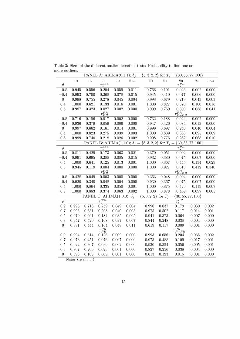
Table 3: Sizes of the different outlier detection tests: Probability to find one ormore outliers.
PANEL A: ARIMA(0,1,1); δj = {5, 3, 2, 2} for Tj = {30, 55, 77, 100}n1 n2 n3 n4 n>4 n1 n2 n3 n4 n>4
θ τSSLs τPRs−0.8 0.945 0.556 0.204 0.059 0.011 0.766 0.191 0.026 0.002 0.000−0.4 0.993 0.700 0.268 0.078 0.015 0.945 0.410 0.077 0.006 0.0000 0.998 0.755 0.278 0.045 0.004 0.998 0.679 0.219 0.043 0.0030.4 1.000 0.621 0.133 0.016 0.001 1.000 0.827 0.370 0.100 0.0160.8 0.987 0.323 0.027 0.002 0.000 0.999 0.769 0.309 0.088 0.041
τPRPH τPRP−PH−0.8 0.716 0.156 0.017 0.002 0.000 0.732 0.188 0.024 0.002 0.000−0.4 0.936 0.379 0.059 0.006 0.000 0.947 0.426 0.084 0.013 0.0000 0.997 0.662 0.161 0.014 0.001 0.999 0.697 0.240 0.040 0.0040.4 1.000 0.823 0.275 0.039 0.003 1.000 0.839 0.368 0.095 0.0090.8 0.999 0.740 0.218 0.026 0.002 0.998 0.775 0.282 0.068 0.010
PANEL B: ARIMA(1,1,0); δj = {5, 3, 2, 2} for Tj = {30, 55, 77, 100}ρ τSSLs τPRs
−0.8 0.811 0.429 0.173 0.063 0.021 0.370 0.051 0.002 0.000 0.000−0.4 0.991 0.695 0.288 0.085 0.015 0.932 0.380 0.075 0.007 0.0000.4 1.000 0.641 0.125 0.013 0.001 1.000 0.867 0.445 0.134 0.0290.8 0.945 0.119 0.004 0.000 0.000 1.000 0.927 0.618 0.412 0.340
τPRPH τPRP−PH−0.8 0.428 0.049 0.003 0.000 0.000 0.363 0.048 0.004 0.000 0.000−0.4 0.920 0.340 0.048 0.004 0.000 0.930 0.367 0.075 0.007 0.0000.4 1.000 0.864 0.335 0.050 0.001 1.000 0.875 0.429 0.119 0.0070.8 1.000 0.883 0.374 0.063 0.002 1.000 0.878 0.408 0.097 0.005
PANEL C: ARIMA(1,0,0); δj = {5, 3, 2, 2} for Tj = {30, 55, 77, 100}ρ τSSLs τPRs0.9 0.998 0.718 0.259 0.049 0.004 0.996 0.637 0.179 0.030 0.0020.7 0.995 0.651 0.208 0.040 0.005 0.975 0.502 0.117 0.014 0.0010.5 0.979 0.601 0.184 0.035 0.005 0.941 0.373 0.064 0.007 0.0000.3 0.957 0.520 0.168 0.037 0.007 0.844 0.248 0.038 0.004 0.0000 0.881 0.444 0.164 0.048 0.011 0.619 0.117 0.009 0.001 0.000
τPRPH τPRP−PH0.9 0.994 0.614 0.126 0.009 0.000 0.993 0.656 0.204 0.035 0.0020.7 0.973 0.451 0.076 0.007 0.000 0.973 0.488 0.109 0.017 0.0010.5 0.922 0.307 0.039 0.002 0.000 0.930 0.354 0.056 0.005 0.0010.3 0.807 0.209 0.023 0.001 0.000 0.827 0.256 0.038 0.004 0.0000 0.595 0.108 0.009 0.001 0.000 0.613 0.123 0.015 0.001 0.000
Note: See table 2.
15
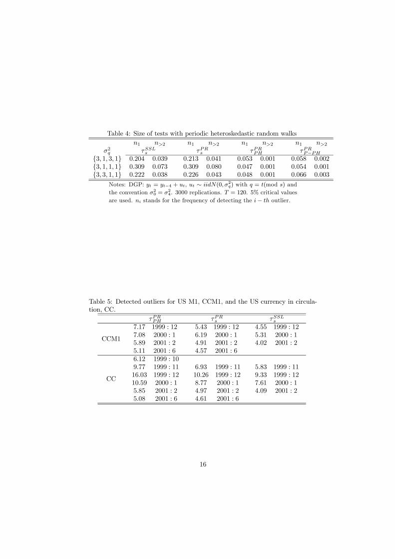
Table 4: Size of tests with periodic heteroskedastic random walks
n1 n>2 n1 n>2 n1 n>2 n1 n>2σ2q τSSLs τPRs τPRPH τPRP−PH
{3, 1, 3, 1} 0.204 0.039 0.213 0.041 0.053 0.001 0.058 0.002{3, 1, 1, 1} 0.309 0.073 0.309 0.080 0.047 0.001 0.054 0.001{3, 3, 1, 1} 0.222 0.038 0.226 0.043 0.048 0.001 0.066 0.003
Notes: DGP: yt = yt−4 + ut, ut ∼ iidN(0, σ2
q) with q = t(mod s) and
the convention σ20 = σ2
4. 3000 replications. T = 120. 5% critical values
are used. ni stands for the frequency of detecting the i− th outlier.
Table 5: Detected outliers for US M1, CCM1, and the US currency in circula-tion, CC.
τPRPH τPRs τSSLs
CCM1
7.17 1999 : 127.08 2000 : 15.89 2001 : 25.11 2001 : 6
5.43 1999 : 126.19 2000 : 14.91 2001 : 24.57 2001 : 6
4.55 1999 : 125.31 2000 : 14.02 2001 : 2
CC
6.12 1999 : 109.77 1999 : 1116.03 1999 : 1210.59 2000 : 15.85 2001 : 25.08 2001 : 6
6.93 1999 : 1110.26 1999 : 128.77 2000 : 14.97 2001 : 24.61 2001 : 6
5.83 1999 : 119.33 1999 : 127.61 2000 : 14.09 2001 : 2
16
0.0
0.5
1.0
1.5
2.0
2.5
3.0
3.5
4.0
4.5
1947 1953 1959 1965 1971 1977 1983 1989 1995 2001
Figure 1: M1 and Currency in Circulation in the USA. Monthly data.: 1947-2003.
-0.2
-0.15
-0.1
-0.05
0
0.05
0.1
0.15
0.2
0.25
1947
1952
1957
1962
1967
1972
1977
1982
1987
1992
1997
2002
Figure 2: M1 and Currency in Circulation in the USA. Monthly data.: 1947-2003. First differences.
17
-0.3
-0.2
-0.1
0
0.1
0.2
0.3
0.4
0.5
1948
1953
1958
1963
1968
1973
1978
1983
1988
1993
1998
2003
Figure 3: M1 and Currency in Circulation in the USA. Monthly data.: 1947-2003. Seasonal differences.
18

Research Papers 2009
2009-27: Kim Christensen, Roel Oomen and Mark Podolskij: Realised Quantile-
Based Estimation of the Integrated Variance
2009-28: Takamitsu Kurita, Heino Bohn Nielsen and Anders Rahbek: An I(2) Cointegration Model with Piecewise Linear Trends: Likelihood Analysis and Application
2009-29: Martin M. Andreasen: Stochastic Volatility and DSGE Models
2009-30: Eduardo Rossi and Paolo Santucci de Magistris: Long Memory and Tail dependence in Trading Volume and Volatility
2009-31: Eduardo Rossi and Paolo Santucci de Magistris: A No Arbitrage Fractional Cointegration Analysis Of The Range Based Volatility
2009-32: Alessandro Palandri: The Effects of Interest Rate Movements on Assets’ Conditional Second Moments
2009-33: Peter Christoffersen, Redouane Elkamhi, Bruno Feunou and Kris Jacobs: Option Valuation with Conditional Heteroskedasticity and Non-Normality
2009-34: Peter Christoffersen, Steven Heston and Kris Jacobs: The Shape and Term Structure of the Index Option Smirk: Why Multifactor Stochastic Volatility Models Work so Well
2009-35: Peter Christoffersen, Jeremy Berkowitz and Denis Pelletier: Evaluating Value-at-Risk Models with Desk-Level Data
2009-36: Tom Engsted and Thomas Q. Pedersen: The dividend-price ratio does predict dividend growth: International evidence
2009-37: Michael Jansson and Morten Ørregaard Nielsen: Nearly Efficient Likelihood Ratio Tests of the Unit Root Hypothesis
2009-38: Frank S. Nielsen: Local Whittle estimation of multivariate fractionally integrated processes
2009-39: Borus Jungbacker, Siem Jan Koopman and Michel van der Wel: Dynamic Factor Models with Smooth Loadings for Analyzing the Term Structure of Interest Rates
2009-40: Niels Haldrup, Antonio Montañés and Andreu Sansó: Detection of additive outliers in seasonal time series