design of empirical propagation models supported in the log

*Author for correspondence

Indian Journal of Science and Technology, Vol 11(22), DOI: 10.17485/ijst/2018/v11i22/122149, June 2018ISSN (Print) : 0974-6846

ISSN (Online) : 0974-5645

Design of Empirical Propagation Models Supported in the Log-Normal Shadowing Model for the 2.4 GHz

and 5 GHz Bands under Indoor EnvironmentsF. Juan Carlos Vesga1*, H. Martha Fabiola Contreras1 and B. Jose Antonio Vesga2

1Escuela de Ciencias Basicas Tecnologia e Ingenieria (ECBTI), Universidad Nacional Abierta y a Distancia; Carrera 27 Nro. 40-43. Bucaramanga, Colombia; [email protected], [email protected]

2Facultad de Ingenieria, Corporacion Universitaria de Ciencia y Desarrollo; Cra. 12 #37-14. Bucaramanga, Colombia; [email protected]

Keywords: Channels Allocation, Efficiency, Optimization, Performance, SINR, WLAN

AbstractObjectives: The growing demand of Wireless connectivity supported in the 802.11 standard has caused a high demand of wireless networks by the users, due to the benefits of mobility and low-cost implementation. Such networks have been used in common places such as houses, offices, schools among others. The objective of this article is to propose an empiric propagation model, supported in the Log-Normal-Shadowing Path Loss model for 2.4 GHz and 5 GHz bands in Indoor environments, compatible with University campus building. Methods/Statistical Analysis: A scenario of a six-storey building on a university campus was proposed, with dimensions of 60 m long, 34 m wide and 24 m high. Additionally, such building has 24 Access Points (AP) distributed in such a way that allow network to serve connectivity to its students. In order to establish the expressions that describe the Log-Normal-Shadowing Path Loss propagation model, an experimental design of factorial mixed type was considered involving three factors: frequency band (2.4 GHz or 5 GHz), condition of the media (Free space or with obstacles) and the distance between the receiver and the AP. The experiment aims to assess how each factor influences on the Received Signal Strength Indicator RSSI. Topic Significance: The proposed model will be used to run analysis of radio propagation in indoor environments using institutional educational buildings and holding a capacity of carrying out prediction processes of RSSI, in the 2.4 GHz and 5 GHz bands. Findings: Based on obtained results, it was possible to evidence that the established models allow predicting the behavior the reception power and signal damping, with a level of confidence of 95%. Additionally, it was possible to verify, in the 5 GHZ band, the damping levels are bigger that those in 2.4 GHz band. Such aspect holds great importance when it comes to perform design processes of Wireless networks. Applications/Improvements: In future research papers, it would be significantly important to establish the expression for outdoor environments, supported in the Shadowing Path model.

1. IntroductionDuring the last years, the demand of wireless networks by users has grown due to the benefits of mobility and low-cost implementation. Within the range of wireless networks, it is possible to locate the WLAN (Wireless Local Area Network), which have been used in common area s such as

homes, offices, schools among others. These kinds of net-works are mainly formed by the use of aggregating devices called Access Point (AP), which allow users to connect wirelessly to the network, performing the same job that a switch in a wired network. However, despite that APs allow to establish connections wirelessly, the distance the AP user must be is quite reduced (inferior to 100 m), due to the

10.17485/ijst

Indian Journal of Science and TechnologyVol 11 (22) | June 2018 | www.indjst.org 2

Design of Empirical Propagation Models Supported in the Log-Normal Shadowing Model for the 2.4 GHz and 5 GHz Bands under Indoor Environments

power of the transmission signal and the obstacles found by the signal in the environment in order to reach the user1.

Due to the interest on wireless communication both in indoor and outdoor environments, it is impor-tant to predict the behavior of signal radio-propaga-tion, product of the reflection, refraction, absorption and dispersion, which can mainly affect the coverage and performance of networks2. In3 the most important propagation models in terms of WLAN are described. Through those models it is possible to estimate the losses and the scope in the coverage, both conditions of the cannel when it comes to carry out a transmission process in both outdoor and indoor environments. Among the propagation models, it is possible to find: Log-Distance, ITU-R propagation model, COST 231 Keenan and Motley´s model, COST 231 Multi-Wall model, and the list goes on.

In face to this situation, one question arises: Is it pos-sible to establish a propagation model that allows esti-mating the power levels that the user can receive on a specific place, in function of the frequency band, the distance towards the AP and the environment character-istics, empirically for indoor environments? In view of the above, the following paper seeks to establish a propa-gation model, supported in the empirical model Log-Normal – Shadowing Path Loss, that allows to predict the power levels of attenuation, in function of the frequency bands of 2.4 GHz and 5 GHz, the distance between the receiver and the AP and the conditions of environment (free space or with obstacles) in order to provide solutions to the proposed problem and that can serve as a founda-tion for future research related to the design of wireless network in building.

2. Propagation ModelsThe signal emitted by an antenna can experience multi-ple transformations during its path into the receiver. The path between the transmitter and the receiver can vary in several ways due to the presence of obstacles, aspect that makes it difficult to predict the received signal in a determined spot. The propagation models have tradition-ally been focused on the received signal, as well as the power variation in the spatial proximity of a given place4. A model can be defined as the simplified representation of the reality by means of the cluster of restrictions or hypotheses.

The models can be classified according to the preci-sion and the method used to analyze the environment variables. In view of the above, the models can be clas-sified as:

• Mathematic models.• Statistical or empirical models.• Theoretical models.• Deterministic models.• Stochastic models.• Black box models.

2.1 Mathematical Models Those models are based on mathematical procedures that describe the behavior of the modeled phenomenon. They depend on the complexity of the mathematical expres-sions that were considered during the analysis process and on the number of input parameters that are required. In most of the cases, a high level of computational com-plexity is required in order to generate the desired results, which makes them little attractive.

2.2 Empiric or Statistical ModelsIt uses the statistical extrapolation from the sampling campaigns of the phenomenon object of study. The main advantage of this type of models is that the own influences of the environment in its cluster are implicitly taken into account, with no need to be considered independently. The results depend on the precision of the conducted measures, as well as the similarity between the analysis and reference environments.

2.3 Theoretical ModelsThey are based on the fundamental principles of the media that is attempted to be modeled. Those models can be applied in different environments without being affected in its precision. In practice, the implementation of theoretical models requires huge data bases of charac-teristics related to the environment, which makes it not to viable for its implementation. Additionally, the algo-rithms considered for the analysis require, as mathemati-cal models, a very high computational complexity.

2.4 Deterministic Model In this type of models, the results of the simulation do not have any distribution of probability and are values that

www.indjst.org

Indian Journal of Science and Technology 3Vol 11 (22) | June 2018 | www.indjst.org

F. Juan Carlos Vesga, H. Martha Fabiola Contreras and B. Jose Antonio Vesga

depend only on the simulation conditions (input). The results will produce the same output with the same input. In the particular case of the propagation models, those models are supported in Maxwell´s equations in order to the predict several characteristics of propagation. Despite some inaccurate results, the model implementation requires algorithms demanding a high computational power.

2.5 Stochastic ModelsThose are models whose results have a probability distri-bution. The very same input doesn´t have to produce the same results, in diverse model simulations.

2.6 Black Box ModelThose are models in which not only the phenomenon input and output are reproduced, without caring about what happens within.

In the particular case, the model of propagation can be classified according to the coverage zone in two types: Indoor y Outdoor.

3. Outdoor Models of Propagation5

The Outdoor models can be divided in: Model of prop-agation in big zones (macrocells) and in small zones (Microcells). Tables 1-3 show the cell classification for urban environments, the most common outdoor models of propagation and the classification of the cells for urban environments and the classification of the most recom-mended models in function of the type of cell, respec-tively.

4. Indoor Models of Propagation6

Indoor models of propagation differ from the outdoor mainly in two aspects:

• The covered distances are way much smaller.• The environment conditions, taking into account that

in indoor environments, the amount of obstacles pre-sented is higher.

Table 1. Classification of urban environmentDistance of reference Type of cell Ratio of the cell Typical position of the antenna1 Km Small Macrocell 0,5 a 3 Km Outdoors (e of media level of roofs)100 m Microcell 100 a 500 m Outdoors (under the media level of roofs)1 m Peak cell Hasta 100 m Indoors and outdoors under the maximum level of roofs

Table 2. Classification of the models of propagations for outdoors

Empirical Semi empirical DeterministicModel Hata Model Egli Model FriisModel Okamura Model Walfisch Model of two raysModel in laws of power Model Ikegami Model Longley Rice Model of diffraction by thing objects

Table 3. Classification of models of propagations for outdoors in function of the type of cellMacrocells Microcells• Bullinngton• Okumura• ITU (CCIR)• Hata• Ericsson 1999• Lee• Cost – 231 – Walfisch-Ikegami• Ann• Among others

• Models of two rays• Models based on UTD (Uniform Theory of Diffraction)• Theory of multiple images• Model of Lee

www.indjst.org



In processes of designing wireless networks, it is very important to get to know the results on coverage predic-tion of an Access Point, which can be provided by a model of propagation, enabling with it the following:

• To predict the coverage area of an Access Point (AP).• To plan the location of the cells in such a way that the

levels of interference between AP neighbors can be decreased.

For the development of the following paper, the use of empirical models has been considered. Such models are based on in the statistical extrapolation of results starting from measures made on a known environment. Additionally, those models are considered to be very computationally efficient and its use in Indoor envi-ronments is highly recommended. As follows, a brief description of the most used empiric models is carried out.

4.1 Model of Propagation of Free Space7

In free space, the power radiated by an omni directional antenna is spread through the surface of a sphere. The surface area of a sphere of d radius is given by:

( )=2 2 4Area π d

The model of free space is used to predict the power of signal when the transmitter and receptor are at line of sight. This model is highly used in system of satellite or microwave communications.

Like the most of models to large scale, the model of propagation in free space predicts that the received power wanes in terms of the distance between the transmitter and receptor, where the value corresponding to the signal power is given by the equation of Friis:

( )( )

=π

2

2 2

ë

4t t y

r

PG GP d

d L

Where:

Pr(d): Received power which is function of the separa-tion between the transmitter and receptor.

Pt: Power of transmission.

Gt: Gain of the transmitting antenna.

Gy: Gain of the Receiving antenna.

λ: Length of wave of the signal frequency in meters.

d: Distance of separation between the transmitter and receiver in meters.

L: Losses of the system due to factors external to the propagation.

The gain of the antenna is given by:

( )π=

λ

2

2

4 AeG

2πλ = =

c

c cf w

Where:

Ae: Effective Aperture.

c: Light speed in m/seg.

f: Frequency of the carrier in Hertz.

wc: Frequency of the carrier in rad/seg.

Gt y Gr: Are dimensionless.

When L=1 is considered that the system will not consid-ered losses due to external factors to the propagation.

The path losses represent the attenuation of signal as a positive amount in dB according to the following expres-sion:

2

2 210log 10 (4 )

t yt

r

G G APPL logP d

= = −

π

When the gain of the antennas is excluded and consider-ing that such antennas have gains of value L, the resulting expression for path losses would be:

2

2 210 (4 ) t rPL log P P

d λ

= − = π−

Friis´s equation shows that the power of received signal damps according to the square of distance, which implies that such power wanes 20 dB/decade.

When the power received to a reference distance (d0) is known, the equation can be adjusted to estimate the power to a further distance. In view of the above, the power of reception could be represented as follows:

( ) ( ) = +

0

0

20r rdP d P d logd

www.indjst.org



Similarly, the expression of path losses would be given by:

( ) ( ) = +

0

0

20L LdP d P d logd

Friis´s equation is only valid to predict Pr for values in which d is found within the region known as Far-field of the Transmitting antenna. This region is defined as the distance beyond df which is related to the dimension of higher number opening of the transmitting antenna y and with the carrier.

The distance of Fraunhofer is given by:

=λ

22f

Dd

D: Higher Physical dimension of the antenna. Additionally, the following expression must be complied:

>> >>λ f fd D y d

4.2 Log-Normal Shadowing Path Loss Model (Shadowing Attenuation)8 Most parts of the empirical models are based on this model, which is used a lot for indoor environments. The expression that describes the path loss for this model is the following:

( ) ( ) σ

= + γ +

0

0

10L LdP d P d log Xd

γ :Attenuation coefficient for path.

PL (d0): Loss to the distance of reference d0.

Xσ: Typical deviation.

“γ” is a variable related to the path losses, which depends on the environment. Table 4 shows the typical values of γ for different environments.

Xσ: is a random variable expressed in dB, which expresses a typical deviation σ in dB.

This model allows estimating the losses of propagation in a practical manner and also offers as main advantage the inclusion of all factors that influence the propagation. Additionally, the model allows carrying out calibration processes when considering empirical elements in the estimation of all parameters.

Table 4. Typical values of γ for different environments

EnvironmentsBuildings – With line of sight 1,6 to 2Buildings – Without line of sight 2 to 4Buildings – Without line of sight and with a separation from 1 to 3 floors 4 to 6

4.3 Model of Path Loss based on COST-2319

It is an indoor model of propagation used in UMTS (Universal Mobile Telecommunications System). The model is defined as follows:

( )( ) +

− + = + + +∑

21

i i

nb

nL FS C w w fP L L k L n L

LFS: Loss of free space between transmitter and receiver.

LC: Constant of loss (Value by default 37 dB).

iwk : Number of walls type i penetrated.

n: Number of penetrated stories.

iwL : Loss due to the wall type i.

Lf: Loss between adjacent stories.

b: Empirical parameter.

The model COST 231 takes into account both the open space loss and the losses by obstacles. Table 5 shows the mean values of factors.

Table 5. Media values of factors

Parameter Description Factor [dB]

fL

Floors (typical structure) Concrete tiles. Typical thickness lower than 30 cm

18,3

1wL Fine Interior walls, plasters. Walls with many holes (Windows) 3,4

2wL Interior walls: Concrete, brick, with very few number of holes. 6,9

4.4 Models based on the Number of Walls and Stories (Simplified) – Model Multi–Wall10

The model uses the following expression:

( )+= + +1 20logL f f w wP L r n a n a

www.indjst.org



r: Distance in meters in straight line between trans-mitter and the receiver

L1: Loss of reference with r = 1 m

af: Attenuation for each story that is crossed by

aw: Attenuation for each wall that is crossed by

nf: Number of grounds/soils that is crossed by…

nw: Number of walls that are crossed by…

4.5 Linear Mode Path Attenuation11

This model is suggested when the transmitter and the receiver are in the same floor. This model arises from an adjustment of the Path Loss model in free space

FSLP plus a linear factor obtained experimentally. The mathematical expression that describes this model is the following:

( ) = +FSL LP d P ad

a: Coefficientof linear attenuation. In the case of offices, the value can be considered of 0,47 dB/m.

d: Distance between the transmitter and receiver.

FSLP : Path Loss in free space.

( ) ( ) = = +

0

0

20FSL L L

dP P d P d logd

This model is simpler than the Log-Normal Shadowing Path Loss model and doesn’t take into account the vanish-ing effects. Additionally, it is susceptible of being specific for an environment given that the value of a is unique for each site.

4.6 Dual–lope Model9

This model was developed by Feverstein and Beyer. The model comes up due to the phenomenon that was observed in the attenuation model by shadowing, which behaves in two different ways (Close distances and far distances). In view of the above, the model proposes the following expressions:

( ) π = − λ 1 1 0410

DSLdP d n log a

( ) ( ) = +

2 1210

DS DSL L BRBR

dP d n log P dd

dBR: Rupture distance between the two models (taken empirically).

λ: Wavelength.

n1: Exponent of Path Loss before 1)(

DSBR Ld P .

n2: Exponent of Path Loss before 2)(

DSBR Ld P .

a0: Difference between DSL FSP PLy to the distance of 1

meter.

Another of the improvements to the attenuation model considered the losses in walls and ground. The math-ematical expression to describe the adjusted model is the following:

( ) ( ) ( ) ( ) σ= =

= + + + + ∑ ∑0

0 1 1

10Q P

L f q pq i

dP d L d nlog FAF WAF Xd

FAF: Attenuation by floors

WAF: Atenuation by walls

4.7 Model ITU-R12

This model is used to describe the path losses in buildings and is given by:

( ) ( )= + γ + −20 10 28TOTAL fL logf log d L n

γ : Coefficient of power loss (Table 6).

Lf: Loss by penetration (Table 7).

n: Number of floors

Table 6. Coefficients of power loss and for loss of transmitter indoors

Frequency Residential building

Office building

Commercial building

900 MHz - 33 201,8 to 2,4 GHz 28 30 225 GHz - 31 -

Table 7. Loss by penetration on the ground Lf (dB) where n: Numbers of floors penetrated for para n ≥ 1

Frequency Residential building

Office building

Commercial building

900 MHz -9 (1 floor)19 (2 floor)24 (3 floor)

-

1,8 to 2,4 GHz 4n ( )+ −15 4 1n ( )+ +6 3 1n

5 GHz - 16 (1 floor) -

www.indjst.org



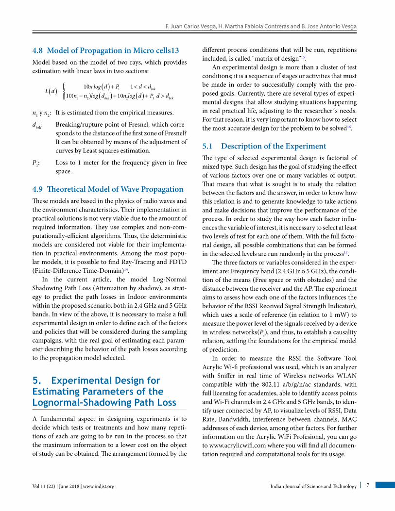
4.8 Model of Propagation in Micro cells13Model based on the model of two rays, which provides estimation with linear laws in two sections:

( ) ( )( ) ( )

+ < <= − + + >

1 1

1 2 2 1

10 1 10( ) 10

brk

brk brk

n log d P d dL d

n n log d n log d P d d

n1 y n2: It is estimated from the empirical measures.

dbrk: Breaking/rupture point of Fresnel, which corre-sponds to the distance of the first zone of Fresnel? It can be obtained by means of the adjustment of curves by Least squares estimation.

P1: Loss to 1 meter for the frequency given in free space.

4.9 Theoretical Model of Wave PropagationThese models are based in the physics of radio waves and the environment characteristics. Their implementation in practical solutions is not very viable due to the amount of required information. They use complex and non-com-putationally-efficient algorithms. Thus, the deterministic models are considered not viable for their implementa-tion in practical environments. Among the most popu-lar models, it is possible to find Ray-Tracing and FDTD (Finite-Difference Time-Domain)14.

In the current article, the model Log-Normal Shadowing Path Loss (Attenuation by shadow), as strat-egy to predict the path losses in Indoor environments within the proposed scenario, both in 2.4 GHz and 5 GHz bands. In view of the above, it is necessary to make a full experimental design in order to define each of the factors and policies that will be considered during the sampling campaigns, with the real goal of estimating each param-eter describing the behavior of the path losses according to the propagation model selected.

5. Experimental Design for Estimating Parameters of the Lognormal-Shadowing Path Loss

A fundamental aspect in designing experiments is to decide which tests or treatments and how many repeti-tions of each are going to be run in the process so that the maximum information to a lower cost on the object of study can be obtained. The arrangement formed by the

different process conditions that will be run, repetitions included, is called “matrix of design”15.

An experimental design is more than a cluster of test conditions; it is a sequence of stages or activities that must be made in order to successfully comply with the pro-posed goals. Currently, there are several types of experi-mental designs that allow studying situations happening in real practical life, adjusting to the researcher´s needs. For that reason, it is very important to know how to select the most accurate design for the problem to be solved16.

5.1 Description of the ExperimentThe type of selected experimental design is factorial of mixed type. Such design has the goal of studying the effect of various factors over one or many variables of output. That means that what is sought is to study the relation between the factors and the answer, in order to know how this relation is and to generate knowledge to take actions and make decisions that improve the performance of the process. In order to study the way how each factor influ-ences the variable of interest, it is necessary to select at least two levels of test for each one of them. With the full facto-rial design, all possible combinations that can be formed in the selected levels are run randomly in the process17.

The three factors or variables considered in the exper-iment are: Frequency band (2.4 GHz o 5 GHz), the condi-tion of the means (Free space or with obstacles) and the distance between the receiver and the AP. The experiment aims to assess how each one of the factors influences the behavior of the RSSI Received Signal Strength Indicator), which uses a scale of reference (in relation to 1 mW) to measure the power level of the signals received by a device in wireless networks(Pr), and thus, to establish a causality relation, settling the foundations for the empirical model of prediction.

In order to measure the RSSI the Software Tool Acrylic Wi-fi professional was used, which is an analyzer with Sniffer in real time of Wireless networks WLAN compatible with the 802.11 a/b/g/n/ac standards, with full licensing for academies, able to identify access points and Wi-Fi channels in 2.4 GHz and 5 GHz bands, to iden-tify user connected by AP, to visualize levels of RSSI, Data Rate, Bandwidth, interference between channels, MAC addresses of each device, among other factors. For further information on the Acrylic WiFi Profesional, you can go to www.acrylicwifi.com where you will find all documen-tation required and computational tools for its usage.

www.indjst.org

http://www.acrylicwifi.com



In order to estimate the number of samples to take beforehand, the software tool XLSTAT was used, which allows to define the number of samples required by means the analysis of means for two independent samples sup-ported in the t-Student test, with a minimal power of 80%, a size of effect of 60% in order to establish meaning-ful differences between the variable object of study and a level of confidence of 95%. The results are the following:

Software tool: XLSTAT

Tests: t-Student test

Alternative hypothesis: Means 1 ≠ Means 2

Interpretation of the test: Hypothesis:

• H0: The difference between the means is equal to 0.• Ha: The difference between the means is different

from 0.

According to the results obtained in Table 8, in function to the given parameters, for an Alfa of 0,05 and a size of effect of 60%, the size of the sample that is the minimum required to obtain a power of 80% is that of 45 observa-tions in total. Additionally, the risk of not rejecting the null hypothesis H= when it is false (error type 2) is that of β = 0,2.

Table 8. Estimation of the minimal number of samples beforehand for the development of the experimentParameters ResultsPower 0,800Alfa 0,05Size of effect 0,6Size of sample 1 45Size of sample 2 2 45

Adjusted Power ( )−1 β 0,804

5.2 Results of the ExperimentTable 9 displays the matrix of design of the experiment in RSSI mediation, which consolidates in an organized fashion the results obtained during the sampling cam-paign, according to the factors and levels established in the experimental design.

During the sampling campaigns, a total number of 50 samples were considered. Such number corresponds

to a level higher than the established in the analysis beforehand for the minimal estimation of the number of required samples. In view of the above, an ex post analy-sis was carried out in order to estimate the power of the definitive test and the confidence of the obtained results. The obtained results are the following:

Ex post analysis analysis to estimate the level of confi-dence and power of the results obtained experimentally

Software tool: XLSTAT

Tests: T tests by means of the analysis of means for two independent samples

Alternative hypothesis: Media 1 ≠ Media 2

Interpretation of the test:Hypothesis:

• H0: The difference between the means is equal to 0.• Ha: the difference between the means is different from 0.

According to the results obtained in Table 10, in function of the given parameters, for an alfa of 0,05, a size of the effect of 60% and a number of samples of 50, the analysis showed that the obtained data present a power of the test of 84.4% with a confidence level of 95%. Additionally, the risk of not rejecting the null hypothesis H0 when it is false (error type 2) is that of β = 0,156.

5.3 Validity of the Results Obtained ExperimentallyThe validity of the results obtained in any of the variance analysis remains subject to the fact that the assumptions of Normality, Constant variance (equal variance of the treatments) and Independence are complied. That is, the answer (Y) should have a normal distribution, with the same variance in each treatment and the measurements must be independent. Those assumptions about (Y) are translated into assumptions about the term error (ε) in the different models15.

It is very common to use the residual plots in order to test the assumptions of the model, as if the assumptions are complied, the residual can be seen as random sample of normal distribution with means 0 0 and constant vari-ance. It is very important to verify the compliance of the assumptions, since if not complied; some of them can have a negative impact on the conclusions. The analysis for each of the assumptions is carried out as follows:

www.indjst.org



Table 9. Matrix of design in the experiment for the RSSIFree space With obstacles

Frequency [MHz] Frequency [MHz]2,4 GHz 5 GHz 2,4 GHz 5 GHz

Distance [m] RSSI [dBm] Distance [m] RSSI [dBm] Distance [m] RSSI [dBm] Distance [m] RSSI [dBm]

1

-23

1

-29

7

-43

5

-60-24 -31 -42 -60-24 -31 -43 -60-28 -31 -46 -60-23 -30 -54 -55

5

-29

5

-36

27

-72

27

-82-29 -37 -70 -82-31 -36 -65 -82-54 -37 -72 -82-33 -34 -71 -82

10

-39

10

-40

19,2

-60

17,14

-63-42 -41 -60 -62-41 -41 -57 -63-43 -41 -60 -63-37 -42 -60 -61

20

-52

20

-65

15,58

-61

6,86

-64-50 -65 -54 -64-48 -66 -55 -64-51 -65 -62 -64-50 -62 -56 -63

40

-65

40

-71

6,86

-49

35

-87-59 -72 -50 -85-60 -72 -49 -85-61 -72 -49 -85-59 -68 -53 -86

Table 10. Estimation of the level of confidence and power of the obtained resultsParameters ResultsSize of sample 1 50Size of sample 2 50Alfa 0,05Size of the effect 0,6Beta (β) 0,156Power (1-β) 0,844

5.3.1 Assumption of Normality

A procedure to verify the assumptions of normality of the residuals is to plot the residuals in a normal probability plot, which is included in most of the statistical programs. This plot X-Y type has the scales in such a way that if the residuals follow a normal distribution, they tend to be aligned in a straight line when being plotted; if such thing does not occur, it can be concluded that the assumption of normality is not correct.1

www.indjst.org



In order to evidence the compliance of the assump-tion of Normality, the residual values of RSSI for a sce-nario with obstacles in 2.4 GHz Band is presented as an example. Such example in Figure 1 shows the compliance of the assumption of Normality of the residual, due to the fact that the values obtained are adjusted on the straight line.

Figure 1. Residual values of RSSI in scenarios with obstacles in 2.4 GHz band.

5.3.2 Assumption of Constant Variance18

A way to verify the assumption of constant variance (or to verify that the treatments have the same variance) is plot-ting the estimated values against the residuals ε( ˆ )ij ijY vs . Generally, ijY goes in the X axis X (horizontal) and the residuals in the vertical axis. If the points of the residual plot against the estimated value are distributed randomly in a horizontal band, with no clear or robust pattern, then it is certain that the assumption the treatments have equal variance is complied. On the other hand, if those points are distributed with a clear and robust pattern, for instance in the shape of a bugle or funnel, then, it can be said that the assumption of constant variance is not complied. In particular, the narrow part of the funnel indicates that in those estimated levels for the response variable. A lower variability is expected. For that reason, it is important to analyze if those values help to minimize or maximize the wanted result.

In order to evidence the compliance of the assump-tions of Variance, the residual values vs. estimated values for RSSI in free space in 5 GHz B and are presented as an example in Figure 2. Such figure shows the compliance of the assumption of constant Variance of the residuals, due to the values obtained reflect no pattern known as bugle or funnel.

Figure 2. Residual values vs. estimated values for RSSI in the free space in 5 GHz band.

5.3.3 Assumption of Independence16

The assumption of Independence in the residual can be verified if the order in which data was taken against the corresponding residual is plotted. Thus, when plotting in the horizontal axis, order of data taking and vertical axis (residuals), a tendency towards the non-random pattern is clearly defined; so, it shows that there is a correlation between the errors and this the assumption of indepen-dence is not complied.

If the behavior of the points is random within the horizontal band, it considered then that the assumption is not complied. The violation of this assumption generally indicates deficiencies in planning, executing experiment. This could also mean that the principle of randomization was not correctly applied or that when experiment was carried out, other factors, altering the response and not being taking into account, came out.

Figure 3 shows the relation between the residual val-ues and the order in which data were acquired experi-mentally. It also shows the compliance of the assumption

Figure 3. Residual according to the order of data acquisition for the RSSI in the 2.4 GHz band in free space.

www.indjst.org



of Independence where the residual values are distributed randomizing on the horizontal axis. It is very important to mention that, in each case, in both 2.4 GHz and 5 GHz bands, the compliance of the three assumptions was veri-fied in order to guarantee the optimal development and the validation of the obtained data.

5.4 Estimation of Parameters of the Log-Normal Shadowing Model for Predicting RSSIIn many practical situations there are independent vari-ables that are believed to influence or relate with a variable of response Y and hence, it will be necessary to take them into account if you want to predict or have a better under-standing of the behavior of Y, where KXXX ,...,, 21 will be the independent variables and Y will be the variable of response by means of a multiple regression model with k independent variable.

Most of the computational systems specialized in sta-tistics include procedures to perform regression analysis both simple and multiple and include techniques of vari-able selection. Excel includes a cluster of specialized func-tions within a Office complement called “ Data Analysis”, which allows to select the range of cells where the depen-dent variable datum (y) is found, and the independent variable data ( KXXX ,...,, 21 ). This tool allows to esti-mate diverse parameters of the regression models such as: Residual analysis, adjusted regression slope, regres-sion coefficient, typical errors, statistical errors, variance analysis of the regression model, limits of confidence, among other important aspects under the desired level of confidence, which for that particular case, was established using a percentage of confidence of 95%, in order to allow latter adjustments without affecting the degree of confi-dence of the established regression.

5.5 Quality of the Adjustment in the Regression Model19

The coefficient of determination(R2) is defined as the percentage of variation of the dependent variable. It is a descriptive measure that works to assess the degree of adjustment of the model according to the input data, due to the fact that it allows measuring the predictive capacity of the adjusted model. The mathematical expression used to estimate the coefficient of determination is the follow-ing:

( )( )

2

2 12

1

ˆn

iR in

yy ii

y ySCRS y y

=

=

−= =

−

∑∑

Where:ˆiy : Estimated Values

iy : Values obtained experimentally

y : Average value of the data obtained experimentally

n: Size of the sample

Coefficient of multiple correlation (R). The coefficient of multiple correlation in the context of the analysis of the regression, establishes a measure corresponding to the degree of dependent variable Y and the cluster of inde-pendent variables ( KXXX ,...,, 21 ). It corresponds to the square root of the coefficient of determination 2R .= 2R R

In general, in order to speak about the satisfactory adjustment of a model, it is necessary that both the coeffi-cient of determination ( 2R ) and the coefficient of multi-ple correlation (R) have values higher than 0,7. A value of

<2 0,3R will indicate that there is no correlation between variable. A value of 1, 0will correspond to a perfect cor-relation.

Standard error of estimation20: The standard error of esti-mation corresponds to a measurement over the quality of the adjustment of the model, which is a estimation of the standard deviation of the error. Its value will be lower as the model is better adjusted. The expression that allows estimating this parameter for a model of multiple regres-sions is the following:

( )2

1

1 ˆ2

ˆn

i ii

y yn =

σ = −− ∑

Means of the absolute error (mea)20: It corresponds to a different way to measure the quality of the adjustment of the regression model, which provides the means of the absolute value of the residuals. Thecan be seen as a mea-surement to spot how much the model fails in average when doing the estimation of the variable of response. IT is clear that the better the adjustment is, the smaller the residuals will be and thus, the value of will be smaller too:

=ε

= ∑ 1

n

iimean

www.indjst.org



Based on the obtained results for the standard esti-mation error and the means of the absolute error, given the scale of measurement of the variable of response (Throughput), these present a relatively small magnitude, which is very favorable within the behavior presented by the model of prediction suggested for the estimation of the Throughput in PLC networks. Each of the values estimated under the use of Excel, corresponding to the coefficient of regression, coefficient of determination, coefficients of multiple correlation, standard error of esti-mation and means of absolute error; for the logarithmic regression model proposed for the prediction of the RSSI, for which the factors γ and σ

dBX will be extracted for the

expression corresponding to the model pf propagation ( ) LP d .

Parameters of Regression in 2.4 GHz Band in Free Space: Based on the values obtained in Tables 11 and 12the equation that describes the model for estimating the power of reception RSSI in 2.4 GHz band in free space is given by:

( ) ( )=− − 10 23.95 22.16RSSI d dBm Log d

Figure 4 shows the slope corresponding to the power of reception in function to the distance according to the expression resulting for RSSI (d). In such figure, it can be seen that the slope is adjusted to the values obtained experimentally and that the quality of adjustment statis-tics registered in Table 11 for a model reflect a value of the coefficient of (R²) of 0,84 and a coefficient of multiple cor-relation (R) is that of 0,916, which are values higher than 0,7. Additionally, the model of regression obtained quite reduced values corresponding to standard error and the absolute media/mean error of 5,54 and 3,91 respectively. This result granted a higher level of confidence for the proposed model of propagation in 2.4 GHz in free space.

As a result of the obtained expression for the model of RSSI, the equation of the model of propagation for the 2.4 GHz band in free space is:

( ) ( ) σ= + + 10 49.95 22.16dBLP d dB Log d X

Where:

• The losses to distance of reference PL(d0) = 49.95 dB.• Coefficient of loss by trajectory γ = 2.2.• Typical deviation σ = 5.54dB

dBX .

Table 11. Parameters of quality in the adjustment of the equation in 2.4 GHz band – free spaceStatistics ValueR² 0,840R 0,916SEC 707,911MEC 30,779

σ 5,548

mea 3,91

Table 12. Coefficients of the model of prediction RSSI in 2.4 GHz band – free spaceCoefficient Value Standard errorβ1 -22,165 2,018β0 -23,95 2,163

Figure 4. Power of reception in function of distance for the 2,4 GHz - free space.

Parameters of Regression in the 2.4 GHz Band in Environment with Obstacles: Based on the values obtained in Tables 13 and 14the equation that describes the model for the estimation of power of reception RSSI in 2.4 GHz band for an environment with obstacles is given by:

( ) ( )10 22,89 32,98RSSI d dBm Log d=− −

Figure 5 shows the slope corresponding to the power of reception in function to the distance according to the expression resulting for RSSI (d). In it, it is possible to observe that the slope is adjusted to the values obtained experimentally and that the quality of the adjustment registered in Table 13 for the proposed model reflect a value in the coefficient of determination (R²) of 0,718 and

www.indjst.org



a coefficient of multiple correlation (R) is that of 0,847, which are values higher than a 0,7. Additionally, the model of regression obtained values quite reduced cor-responding to the standard error of estimation and the absolute mean/media error of 4,67 and 3,84 respectively, making sure with this result a higher level of confidence for the model of propagation proposed in 2.4 GHz band oriented to environment with obstacles.

As a result of the expression obtained for the model of RSSI, the equation of the model of propagation for the 2.4 GHz band for an environment with obstacles is:

( ) ( )10 48,89 32,98dBLP d dB Log d Xσ= + +

Where:

• The losses to distance of reference PL(d0) = 48,89 dB.• Coefficient of loss by trajectory γ = 3,29• Typical deviation σ = 4,67

dBX dB.

Table 13. Statistics of quality of the adjustment in the 2.4 GHz band – environment with obstaclesStatistics ValueR² 0,718R 0,847SEC 611,329MEC 21,833

σ 4,673

mea 3,84

Table 14. Coefficients of the model of prediction RSSI in 2.4 GHz – environment with obstaclesCoefficient Value Standard errorβ1 -32,98 3,909β0 -22,89 4,472

Parameters of regression in 5 GHz band in free space: Based on the values obtained in Tables 15 and 16the equa-tion that describes the model for estimating the power of reception RSSI in 5 GHz band in free space is given by::

( ) ( )=− − 10 26,87 26,65 RSSI d dBm Log d

Figure 6 shows the slope corresponding to the Power or reception in function to the distance according to the expression resulting for RSSI (d). In such figure, one can observe that the slope is adjusted to the values obtained

experimentally and that the quality of the adjustment reg-istered in Table 15 for the model proposed reflects a value of the coefficient of determination (R²) of 0,818 and a coefficient of multiple relation (R) is 0,905, which are val-ues higher than 0,7. Additionally, the model of regression got values quite reduced corresponding to the standard error of estimation and the absolute mean/media error of 7,19 and 6,56 respectively, making sure with this result a higher level of confidence for the model of propagation proposed in 5 GHz band in free space.

As a result of the expression obtained for the RSSI model, the equation of the propagation model for the 5 GHz band in free space is:

( ) ( )10 51,87 26,65dBLP d dB Log d Xσ= + +

Where:

• The losses to distance of reference PL(d0) = 51,87 dB.• Coefficient of loss by trajectory γ = 2,6.• Typical deviation σ = 7,195

dBX dB.

Table 15. Quality of the adjustment in 5 GHz band – free spaceStatistics ValueR² 0,818R 0,905SEC 1190,657MEC 51,768

σ 7,195

mea 6,56

Figure 5. Power of reception in function for the 2,4 GHz band - environment with obstacles.

www.indjst.org



Table 16. Coefficient of the model of prediction RSSI in 5 GHz band– free spaceCoefficient Value Standard errorβ1 -26,650 2,617β0 -26,87 2,806

Figure 6. Power of reception in function to the distance for 5 GHz band – free space.

Parameters of regression in GHz band in envi-ronment with obstaclesBased on the value obtained in Tables 17 and 18the equa-tion that describes the model for estimating the power of reception RSSI in 5 GHz band for an environment with obstacles is given by:

( ) ( )=− − 10 41,29 29,07RSSI d dBm Log d

Figure 7 shows the slope corresponding to the power of reception in function to the distance according to the result-ing expression for RSSI (d). In such figure, one can observe that the slope is adjusted to the values obtained experimen-tally and that the quality of the adjustment registered in Table 17 for the model proposed reflects a value of the deter-mination coefficient (R²) of 0,75 and a coefficient of mul-tiple correlation (R) is that of 0,869, which are values higher than 0,7. Additionally, the model of regression obtained val-ues quite reduced corresponding to the standard error of estimation and to the absolute means error of 5,69 and 2,85 respectively, making sure with this result a higher level of confidence for the model of propagation proposed in 5 GHz band oriented to environment with obstacles.

As a result, to the expression obtained for the model of RSSI, the equation of the model of propagation for 5 GHz band for an environment with obstacles is:

( ) ( ) σ= + + 10 66,29 29,07dBLP d dB Log d X

Where:

• The losses to distance of reference PL(d0) = 66,29 dB• Coefficient of losses by trajectory γ = 2,9• Typical deviation σ = 5,697

dBX dB

Figures 8 and 9 show the slopes corresponding to the resulting expressions for the models Log-Normal path loss shadowing for the 2.4 GHz and 5 GHz bands, in which it is possible to observe highest levels of shadowing for environments with obstacles in comparison to free space, as the distance between the receiver and the AP increases in coherence with the theory. Additionally, it can be seen a value almost constant in the existing relation between slope for environment with obstacles and the slope for free space, in both 2.4 GHz and 5 GHz bands, which may suggest the existence of a linear correlation between both environments of propagation.

Figures 10 and 11 show the slopes corresponding to the power of reception expressed in dBm for environ-ments with obstacles or free space for 2.4 GHz and 5 GHz bands, which reflect the phenomenon mentioned before in relation to the expressions established for each case adjusted to the shadowing propagation model. In such expressions, it can be seen a higher attenuation of the power received for environments with obstacles

Table 17. Statistics for the quality of the adjustment in 5 GHz band – environment with obstaclesStatistics ValueR² 0,755R 0,869SEC 746,462MEC 32,455

σ 5,697

mea 2,85

Table 18. Coefficients of the model of prediction RSSI in 5 GHz band – environment with obstaclesCoefficient Value Standard error

1â -29,070 3,456

0â -41,29 4,131

www.indjst.org



as the distance of separation between the receiver and the AP increases. Additionally, higher levels of attenu-ation for the 5 GHz band in relation to the 2.4 GHz band can be observed. Such fact suggests that, despite the fact that the 5 GHz band offers the users bigger

bandwidth features according to the configuration of available channels, it displays a bigger number of limi-tations as far as the areas of coverage compared to the ones of 2.4 GHz bands, aspect that will be validated in next chapter.

Figure 7. Power of reception in function to the distance for the 5 GHz band - environment with obstacles.

Figure 8. Log-normal path loss shadowing 2.4 GHz band.

www.indjst.org



Figure 9. Log-normal path loss shadowing 5 GHz band.

Figure 10. Power of reception in 2.4 GHz band.

www.indjst.org



6. ConclusionThe use of statistical models to establish a model of propa-gation in indoor environments has been considered as an excellent strategy within the designing processes in Wireless networks, due to its easy implementation and implicit consideration of environment conditions, with-out having to run detailed analysis of each scenario inde-pendently. In view of the mentioned before and according to the results obtained, the use of the model Log-Normal Shadowing Path Loss was considered as a strategy to pre-dict the losses by trajectory, in indoor environments within the proposed scenario, in both 2.4 GHz and 5 GHz bands. The obtained model allows estimating the power of recep-tion and the signal attenuation, in function to the band of frequency, the distance between the receiver and the AP and the environment conditions, whether being a line of sight or with obstacles. In order to estimate the values of the coefficients that are part of the model, an experimental design of mixed factorial type, complying with the vari-ance assumptions, linearity and Independence, validat-ing the data obtained experimentally and establishing the

expressions of adjustments for each case, supported in a logarithmic regression model, with a level of confidence of 95%, a power of the test of 84.4% and a risk of not rejecting the null hypothesis when is false (error type 2) of β = 0,156.

7. References1. Rajesh A, Pragathi G, Shankar T. Investigation of an

improved adaptive power saving technique for IEEE 802.11ac Systems. Indian Journal of Science and Technology. 2016; 9(37):1–7.

2. Ibhaze AE, Imoize AL, Ajose SO, John SN, Ndujiuba CU, Idachaba FE. An empirical propagation model for path loss prediction at 2100 MHz in a Dense Urban Environment. Indian Journal of Science and Technology. 2017; 10(5):1–9.

3. Yeong SY, Al-Salihy W, Wan TC. Indoor WLAN monitoring and planning using empirical and theoretical propagation models. IEEE Second International Conference on Network Applications, Protocols and Services; 2010. p. 165–9.

4. Basha Pathan H, Varma PS, Rajesh KS. QoS performance of IEEE 802.11 in MAC and PHY layer using enhanced OAR algorithm. Indian Journal of Science and Technology. 2017; 10(9):1–9.

Figure 11. Power of reception in 5 GHz band.

www.indjst.org



5. Zvanovec S, Pechac P, Klepal M. Wireless LAN networks design: Site survey or propagation modeling? Radio Engineering. 2003; 12(4):1–8.

6. Zarkovic J, Stojkovic P, Neskovic N. 3D statistical propa-gation model for indoor WLAN radio coverage. IEEE 19thTelecommunications Forum (TELFOR); 2011. p. 461–4.

7. Sangolli SV, Jayavignesh T. TCP throughput measurement and comparison of IEEE 802.11 legacy, IEEE 802.11n and IEEE 802.11ac Standards. Indian Journal of Science and Technology. 2015; 8(20):1–8.

8. Desimone R, Brito BM, Baston J. Model of indoor signal propagation using log-normal shadowing. IEEE Long Island Systems, Applications and Technology; 2015. p. 1–4.

9. Solahuddin YF, Mardeni R. Indoor empirical path loss prediction model for 2.4 GHz 802.11n network. IEEE International Conference on Control System, Computing and Engineering; 2011. p. 12–7.

10. Li L, Ibdah Y, Ding Y, Eghbali H, Muhaidat SH, Ma X. Indoor multi-wall path loss model at 1.93 GHz. IEEE MILCOM 2013-2013 Military Communications Conference; 2013. p. 1233–7.

11. Chrysikos T, Georgopoulos G, Kotsopoulos S. Attenuation over distance for indoor propagation topologies at 2.4 GHz. IEEE Symposium on Computers and Communications (ISCC); 2011. p. 329–34.

12. Chrysikos T, Georgopoulos G, Kotsopoulos S. Wireless channel characterization for a home indoor propagation

topology at 2.4 GHz. IEEE Wireless Telecommunications Symposium (WTS); 2011. p. 1–10.

13. Andrade CB, Hoefel RF, Cheung KW. IEEE 802. 11 WLANS: A comparison on indoor coverage models. Canadian Conference on Electrical and Computer Engineering; 2010. p. 1–10.

14. Kuntal A, Karmakar P, Chakraborty S. Optimization technique based localization in IEEE 802.11 WLAN. International Conference on Recent Advances and Innovations in Engineering; 2014. p. 1–5.

15. Salazar JC, Zapata AB. Analisis y diseno de experimentos aplicados a estudios de simulacion analysis and design of experiments applied to simulation studies. 2009; 76(159):249–57.

16. Del Ca-izo Lopez JF, Lopez Martín D, Lledo Garcia E GBP. Dise-o de modelos experimentalesen investigación quirúr-gica. Actas Urologicas Espa-olas. 2008; 32(1):27–40.

17. Ravindranath NS, Singh I, Prasad A, Rao VS. Performance Evaluation of IEEE 802.11ac and 802.11n using NS3. Indian Journal of Science and Technology. 2016; 9(26):1–9.

18. Diaz Cadavid A. Diseno Estadistico de Experimentos. 2nd Ed. Editorial Universidad de Antioquia. 2009. p. 1–286.

19. Gonzaalez Manteiga MT, Peerez de Vargas A. Estadística Aplicada Una Visioon Instrumental. Ediciones Diaz de Santos; 2010.

20. Rodriiguez FJ, Pierdant Rodríguez AI, Rodriiguez Jimeenez EC. Estadiistica Aplicada. II, Estadiistica En Administracioon Para La Toma de Decisiones; 2014. p. 1–34.

www.indjst.org

design of empirical propagation models supported in the log

Documents